Hybrid 3D Mass Spring System for Soft Tissue Simulation
161
HAL Id: tel-01761851 https://tel.archives-ouvertes.fr/tel-01761851v1 Submitted on 9 Apr 2018 (v1), last revised 24 Apr 2018 (v2) HAL is a multi-disciplinary open access archive for the deposit and dissemination of sci- entific research documents, whether they are pub- lished or not. The documents may come from teaching and research institutions in France or abroad, or from public or private research centers. L’archive ouverte pluridisciplinaire HAL, est destinée au dépôt et à la diffusion de documents scientifiques de niveau recherche, publiés ou non, émanant des établissements d’enseignement et de recherche français ou étrangers, des laboratoires publics ou privés. Hybrid 3D Mass Spring System for Soft Tissue Simulation Karolina Golec To cite this version: Karolina Golec. Hybrid 3D Mass Spring System for Soft Tissue Simulation. Modeling and Simulation. Universite Lyon 1, 2018. English. tel-01761851v1
-
Upload
khangminh22 -
Category
Documents
-
view
2 -
download
0
Transcript of Hybrid 3D Mass Spring System for Soft Tissue Simulation
HAL Id: tel-01761851https://tel.archives-ouvertes.fr/tel-01761851v1
Submitted on 9 Apr 2018 (v1), last revised 24 Apr 2018 (v2)
HAL is a multi-disciplinary open accessarchive for the deposit and dissemination of sci-entific research documents, whether they are pub-lished or not. The documents may come fromteaching and research institutions in France orabroad, or from public or private research centers.
L’archive ouverte pluridisciplinaire HAL, estdestinée au dépôt et à la diffusion de documentsscientifiques de niveau recherche, publiés ou non,émanant des établissements d’enseignement et derecherche français ou étrangers, des laboratoirespublics ou privés.
Hybrid 3D Mass Spring System for Soft TissueSimulationKarolina Golec
To cite this version:Karolina Golec. Hybrid 3D Mass Spring System for Soft Tissue Simulation. Modeling and Simulation.Universite Lyon 1, 2018. English. tel-01761851v1
THÉSE DE DOCTORAT DE L’UNIVERSITÉ DE LYONopérée au sein de
L’UNIVERSITÉ CLAUDE BERNARD LYON 1
École Doctorale ED 512InfoMaths
Spécialité de doctorat: InformatiqueDiscipline: Modélisation et simulation
Soutenue publiquement le 19/01/2018, par:Karolina GOLEC
Hybrid 3D Mass Spring System for SoftTissue Simulation
Devant le jury composé de:
Maud MARCHAL, Maître de Conférences HDR INSA Rennes, IRISAYohan PAYAN, Directeur de Recherche CNRS, TIMC-IMAGLaurence CHÈZE, Professeure UCBL, LBMCSébastien LAPORTE, Professeur ENSAM, IBHGCPhilippe MESEURE, Professeur UP, XLIMGuillaume DAMIAND, Chargé de Recherche HDR CNRS, LIRISFlorence ZARA, Maître de Conférences UCBL, LIRISStéphane NICOLLE, Maître de Conférences UCBL, LBMCJean-François PALIERNE, Chargé de Recherche CNRS, Lab. Physique,
ENS de Lyon
RapporteureRapporteur
ExaminatriceExaminateurExaminateur
Directeur de thèseCo-directrice de thèseCo-directeur de thèse
Invité
April 9, 2018

“You will never feel truly satisfied by work until you are satisfied by life.”
Heather Schuck, The Working Mom Manifesto
Resumé
La nécessité de simulations de tissus mous, tels que les organes internes, se pose avec leprogrès des domaines scientifiques et médicaux. Le but de ma thèse est de développer unnouveau modèle générique, topologique et physique, pour simuler les organes humains.Un tel modèle doit être facile à utiliser, doit pouvoir effectuer des simulations en tempsréel avec un niveau de précision permettant l’utilisation à des fins médicales.
Cette thèse explore de nouvelles méthodes de simulation et propose des améliora-tions pour la modélisation de corps déformables. Les méthodes proposées visent à pou-voir effectuer des simulations rapides, robustes et fournissant des résultats physiquementprécis. L’intérêt principal de nos solutions réside dans la simulation de tissus mous élas-tiques à petites et grandes déformations à des fins médicales. Nous montrons que pourles méthodes existantes, la précision pour simuler librement des corps déformables ne vapas de pair avec la performance en temps de calcul. De plus, pour atteindre l’objectif desimulation rapide, de nombreuses approches déplacent certains calculs dans une étape depré-traitement, ce qui entraîne l’impossibilité d’effectuer des opérations de modificationtopologiques au cours de la simulation comme la découpe ou le raffinement.
Dans cette thèse, le cadre utilisé pour les simulations s’appelle TopoSim. Il est conçupour simuler des matériaux à l’aide de systèmes masses-ressorts (MSS) avec des paramètresd’entrée spécifiques. En utilisant un MSS, qui est connu pour sa simplicité et sa capac-ité à effectuer des simulations temps réel, nous présentons plusieurs améliorations baséphysiques pour contrôler les fonctionnalités globales du MSS qui jouent un rôle clé dansla simulation de tissus réels.
La première partie de ce travail de thèse vise à reproduire une expérience réelle desimulation physique qui a étudié le comportement du tissu porcin à l’aide d’un rhéomètrerotatif. Son objectif était de modéliser un corps viscoélastique non linéaire. À partir del’ensemble des données acquises, les auteurs de l’expérience ont dérivé une loi de com-portement visco-élastique qui a ensuite été utilisée afin de la comparer avec nos résultatsde simulation. Nous définissons une formulation des forces viscoélastiques non linéairesinspirée de la loi de comportement physique. La force elle-même introduit une non-linéarité dans le système car elle dépend fortement de l’amplitude de l’allongement duressort et de trois paramètres spécifiques à chaque type de tissu.
La seconde partie de la thèse présente notre travail sur les forces de correction de vol-ume permettant de modéliser correctement les changements volumétriques dans un MSS.Ces forces assurent un comportement isotrope des solides élastiques et un comportementcorrect du volume quelquesoit la valeur du coefficient de Poisson utilisé. La méthodenécessite de résoudre deux problèmes: l’instabilité provoquant des plis et les contraintesde Cauchy. Nos solutions à ces limitations impliquent deux étapes. La première consisteà utiliser trois types de ressorts dans un maillage entièrement hexaédrique: les arêtes,les faces diagonales et les diagonales internes. Les raideurs des ressorts dans le systèmeont été formulées pour obéir aux lois mécaniques de base. La deuxième étape consisteà ajouter des forces de correction linéaires calculées en fonction du changement de vol-ume et des paramètres mécaniques du tissu simulé, à savoir le coefficient de Poisson et lemodule de Young.
La troisième partie concerne les aspects de création d’un maillage précis et léger. C’esten effet un des éléments les plus importants lorsqu’il s’agit de simulations de corps réels.Dans ce chapitre, nous présentons une introduction à la mise en œuvre de maillagesd’éléments mixtes construits avec les éléments 3D suivants: tétraèdres, prismes, pyra-mides et hexaèdres. Le maillage mixte nous permet d’obtenir un niveau de détail plusprécis tout en diminuant le nombre d’éléments à utiliser. Une telle structure nécessite

une formulation correcte des raideurs des ressorts pour chaque élément, pour produireune méthode physiquement réaliste. Notre cadre générique peut être étendu au mail-lages mixtes en se basant sur les mêmes lois que la structure entièrement hexaédrique.Le modèle mixte devra ensuite être comparé aux maillages validés existants ainsi qu’auxsolutions FEM.
Les systèmes masses-ressorts sont connus pour être simples et faciles à utiliser, maisils nécessitent une base physique solide pour être utilisés dans le cadre de simulationsphysiques précises. D’un autre côté, l’environnement médical cherche constamment àpousser les méthodes dans le sens de la simulation en temps réel d’objets déformablesdétaillés. Les méthodes présentées dans ce travail nous permettent de contrôler globale-ment la non-linéarité et le volume d’un système masses-ressorts, et améliorent égalementsa précision. De plus, la mise en œuvre de maillage mixtes facilitera des simulations pré-cises avec des performances en temps réel en diminuant le nombre d’éléments requis.
Abstract
The need for simulations of soft tissues, like internal organs, arises with the progress ofthe scientific and medical environments. The goal of my PhD is to develop a novel generictopological and physical model to simulate human organs. Such a model shall be easy touse, perform the simulations in the real time and which accuracy will allow usage for themedical purposes.
This thesis explores novel simulation methods and improvement approaches for mod-eling deformable bodies. The methods aim at fast and robust simulations with physicallyaccurate results. The main interest lies in simulating elastic soft tissues at small and largestrains for medical purposes. We show however, that in the existing methods the accu-racy to freely simulate deformable bodies and the real-time performance do not go handin hand. Additionally, to reach the goal of simulating fast, many of the approaches movethe necessary calculations to pre-computational part of the simulation, which results ininability to perform topological operations like cutting or refining.
The framework used for simulations in this thesis is called TopoSim and it is designedto simulate materials using Mass Spring Systems (MSS) with particular input parameters.Using Mass-Spring System, which is known for its simplicity and ability to perform fastsimulations, we present several physically-based improvements to control global featuresof MSS which play the key role in simulation of real bodies.
First part of the thesis present work, which aim is to reproduce a real experiment. Theexperiment studied the behavior of porcine tissue using a rotational rheometer. Its objec-tive was to model non-linear visco-elastic body. From the set of acquired data the authorsof the experiment derived a visco-elastic constitutive law which was then used to com-pare with our simulation results. We define a non-linear visco-elastic force formulationinspired by the constitutive law. The force itself introduces non-linearity in the systemas it strongly depends on the magnitude of the spring elongation and three parametersspecific for each type of tissue.
Next part presents work on volume correction forces to correctly model the volumetricchanges in MSS. It ensures isotropic behavior of elastic solids and correct volume behaviorbased on a free modification of Poisson’s ratio. The method requires us to solve twoproblems: wrinkle instability and Cauchy’s constraints. Our solutions to the presentedlimitations of MSS involve thus two steps. The first step is to use three types of springs inan all-hexahedral mesh: edge, face-diagonal and inner-diagonal ones. The stiffnesses ofthe springs in the system were formulated to obey the basic mechanical laws. Next stepinvolved adding the corrections to computed linear forces based on the change of volumeand given mechanical parameters of the simulated tissue, namely the Poisson ratio andYoung modulus.
Creating a detailed and lightweight mesh structure is one of the most important ele-ments when dealing with simulations of real bodies. Therefore the last chapter presentsan introduction to implementation of mixed-element meshes built of the following 3D el-ements: tetrahedra, prisms, pyramids and hexahedra. The mixed-element mesh allowsus to obtain the desired level of detail of a mesh and use the minimal required num-ber of elements in the same time. Such a structure requires a correct formulation of thestiffnesses for particular springs to be integrated as a physically plausible method intoour framework. We talk about the solution basis: it shall be based on the same laws asour all-hexahedral structure. The model built of different types of elements shall be thencompared to the already existing validated meshes as well as FEM solutions.
Mass Spring Systems are known to be simple and easy to use, however they requirestrong physical basis to be considered suitable for accurate simulations. On the other

hand the medical environment constantly encourages research in the direction of real-timesimulation of real, deformable bodies. The presented methods allow us to globally controlthe non-linearity and volume of a locally-focused Mass Spring System and improve itsprecision. Additionally, the mixed-element mesh implementation will facilitate accuratesimulations with real-time performance on a minimal required number of elements.

Acknowldgements
For three years I have worked hard to obtain the PhD title. If it’s been a success, it mostdefinitely wasn’t solely for my work alone. I cannot count the times I asked for help oradvice and, sure enough, received more than I ever hoped for: friendship, understanding,support. As every scientist shall back my words if asked - we are merely people withideas, but it is the bright insight, countless discussions and unique views presented byothers that make our work possible.
On this note I would like to thank my irreplaceable team of supervisors. Guillaumefor offering me help when I could see no further options, for not throwing me out of hisroom when I took a peak there for the thousandth time, for showing me how many thingscan be ’templated’. Florence, true master of all articles and bibliography, for sharing herenormous resources and broad knowledge with me. Stéphane, for the practical, ’handson’ aspect of our work, the one which drew me most to this topic. Jean-Francois for hisstunning ideas, mathematical reasoning and unwavering certainty, all used to introduceus to the mechanical understanding of our work. Working with each of you was purepleasure, even when it was hard work!
I would like to thank my lab-friends for all the time spent together. For the cakes,cookies and only a bit of coffee. I wish to see you all every time I come to visit! I couldn’tforesee meeting people who became such an important part of my life: Abdou, Ewelina,Patrycja, each of you holds a special place in my heart. Amandine, thank you for beingwith me ever since we just had each other. Ania, Becia - for not closing the book on me,even when we saw each other only so often.
The agreement of the personal and professional aspects of life is of a great importanceto me. I believe that nobody should be forced to give up one in favor of the other. Ibelieve it so much so that the biggest achievement of the last three years of my life isnot only the successful defense of my doctoral thesis, but also marrying the love of mylife and becoming a mother. That said, I would like to thank Damian for his unabatedsupport of my (even most crazy) ideas and for making my dreams come true. My parentsfor their incredible encouragement, which lasted even if you knew we’d see each otheronly twice a year. Thank you for the bond we have, the one no one with their right mindcan understand.
I wish to thank everyone who I have met on my journey, for being part of it.

Contents
Resumé
Abstract
1 Introduction 1
2 Simulation of Deformable Objects 92.1 Deformable Objects in Biomechanics . . . . . . . . . . . . . . . . . . . . . . . 9
2.1.1 Physical Parameters of Soft Tissues . . . . . . . . . . . . . . . . . . . . 92.1.2 Application of Soft Tissue Modeling . . . . . . . . . . . . . . . . . . . 11
MSS-Based Surgery Simulation . . . . . . . . . . . . . . . . . . . . . . 11FEM-Based Methods . . . . . . . . . . . . . . . . . . . . . . . . . . . . 11Other Techniques . . . . . . . . . . . . . . . . . . . . . . . . . . . . . . 12
2.2 Basic Notions of Mechanics . . . . . . . . . . . . . . . . . . . . . . . . . . . . 122.2.1 Simulation Loop . . . . . . . . . . . . . . . . . . . . . . . . . . . . . . 122.2.2 Continuum Mechanics . . . . . . . . . . . . . . . . . . . . . . . . . . . 132.2.3 Integration Schemes . . . . . . . . . . . . . . . . . . . . . . . . . . . . 14
Explicit Euler Scheme . . . . . . . . . . . . . . . . . . . . . . . . . . . 15Semi-implicit Euler Scheme . . . . . . . . . . . . . . . . . . . . . . . . 15Implicit Euler Scheme . . . . . . . . . . . . . . . . . . . . . . . . . . . 15Verlet Integration . . . . . . . . . . . . . . . . . . . . . . . . . . . . . . 16Shortly on Stability . . . . . . . . . . . . . . . . . . . . . . . . . . . . . 17Conclusions . . . . . . . . . . . . . . . . . . . . . . . . . . . . . . . . . 19
2.3 Existing Simulation Methods . . . . . . . . . . . . . . . . . . . . . . . . . . . 202.3.1 Finite Element Method . . . . . . . . . . . . . . . . . . . . . . . . . . . 20
Application . . . . . . . . . . . . . . . . . . . . . . . . . . . . . . . . . 20FEM Derivation . . . . . . . . . . . . . . . . . . . . . . . . . . . . . . . 21Extended Finite Element Method . . . . . . . . . . . . . . . . . . . . . 22Co-rotational Finite Element Method . . . . . . . . . . . . . . . . . . 22Mass-Tensor Model . . . . . . . . . . . . . . . . . . . . . . . . . . . . . 23
2.3.2 Position Based Dynamics . . . . . . . . . . . . . . . . . . . . . . . . . 24General Algorithm . . . . . . . . . . . . . . . . . . . . . . . . . . . . . 24Stabilization Step . . . . . . . . . . . . . . . . . . . . . . . . . . . . . . 25Projection of the Constraint Functions - the Solver . . . . . . . . . . . 25Stiffness and Damping . . . . . . . . . . . . . . . . . . . . . . . . . . . 26Deformable Body Improvements . . . . . . . . . . . . . . . . . . . . . 27Conclusions . . . . . . . . . . . . . . . . . . . . . . . . . . . . . . . . . 28
2.3.3 Meshless Deformations . . . . . . . . . . . . . . . . . . . . . . . . . . 28Shape Matching Function . . . . . . . . . . . . . . . . . . . . . . . . . 28Linear and Quadratic Terms . . . . . . . . . . . . . . . . . . . . . . . . 29Improved Explicit-Based Integration . . . . . . . . . . . . . . . . . . . 30Method Extensions . . . . . . . . . . . . . . . . . . . . . . . . . . . . . 30
2.3.4 Summary . . . . . . . . . . . . . . . . . . . . . . . . . . . . . . . . . . 312.4 Conclusions . . . . . . . . . . . . . . . . . . . . . . . . . . . . . . . . . . . . . 33
3 Mass Spring System (MSS) 353.1 Classical MSS . . . . . . . . . . . . . . . . . . . . . . . . . . . . . . . . . . . . 363.2 MSS Instabilities and Natural Limitations . . . . . . . . . . . . . . . . . . . . 36
3.2.1 Natural Limitation of the Poisson Ratio . . . . . . . . . . . . . . . . . 36Linear Assumption . . . . . . . . . . . . . . . . . . . . . . . . . . . . . 36Cubic Symmetry . . . . . . . . . . . . . . . . . . . . . . . . . . . . . . 37Isotropic Assumption . . . . . . . . . . . . . . . . . . . . . . . . . . . 37
3.2.2 Natural Wrinkle and Buckling Instability of the MSS . . . . . . . . . 383.3 Types of Lattice . . . . . . . . . . . . . . . . . . . . . . . . . . . . . . . . . . . 41
3.3.1 Classical Meshes . . . . . . . . . . . . . . . . . . . . . . . . . . . . . . 413.3.2 3D Surface Mesh . . . . . . . . . . . . . . . . . . . . . . . . . . . . . . 423.3.3 Mixed-Element Mesh . . . . . . . . . . . . . . . . . . . . . . . . . . . 43
3.4 Identification of the Physical Parameters . . . . . . . . . . . . . . . . . . . . . 443.4.1 Masses . . . . . . . . . . . . . . . . . . . . . . . . . . . . . . . . . . . . 443.4.2 Damping . . . . . . . . . . . . . . . . . . . . . . . . . . . . . . . . . . . 443.4.3 Stiffness . . . . . . . . . . . . . . . . . . . . . . . . . . . . . . . . . . . 45
Data Driven Parameter Identification . . . . . . . . . . . . . . . . . . 45Analytical Solutions . . . . . . . . . . . . . . . . . . . . . . . . . . . . 46
3.5 MSS Constraints . . . . . . . . . . . . . . . . . . . . . . . . . . . . . . . . . . . 513.5.1 Volume change . . . . . . . . . . . . . . . . . . . . . . . . . . . . . . . 513.5.2 Other Constraints . . . . . . . . . . . . . . . . . . . . . . . . . . . . . . 52
3.6 Non-linear Behavior . . . . . . . . . . . . . . . . . . . . . . . . . . . . . . . . 54Natural MSS Non-linearity . . . . . . . . . . . . . . . . . . . . . . . . 54Additional Forces . . . . . . . . . . . . . . . . . . . . . . . . . . . . . . 55Non-linear Stiffness Formulations . . . . . . . . . . . . . . . . . . . . 55Non-linear Parametrization . . . . . . . . . . . . . . . . . . . . . . . . 55Constraints . . . . . . . . . . . . . . . . . . . . . . . . . . . . . . . . . 55
3.7 Topological modifications . . . . . . . . . . . . . . . . . . . . . . . . . . . . . 563.8 Presentation of Our Framework (TopoSim) Suitable for MSS . . . . . . . . . 57
3.8.1 The Topological Data Structure . . . . . . . . . . . . . . . . . . . . . . 57Graph . . . . . . . . . . . . . . . . . . . . . . . . . . . . . . . . . . . . 57Combinatorial Map . . . . . . . . . . . . . . . . . . . . . . . . . . . . . 58
3.8.2 The 3D LCC+MSS Model . . . . . . . . . . . . . . . . . . . . . . . . . 59Physical Parameters and Topology . . . . . . . . . . . . . . . . . . . . 59Data Structures . . . . . . . . . . . . . . . . . . . . . . . . . . . . . . . 60Improvement of the LCC+MSS Data Structure . . . . . . . . . . . . . 60Computation of the Force . . . . . . . . . . . . . . . . . . . . . . . . . 62
3.8.3 Structure of Our Model in TopoSim Framework . . . . . . . . . . . . 633.9 Conclusions . . . . . . . . . . . . . . . . . . . . . . . . . . . . . . . . . . . . . 66
4 Linear and Non-linear Behavior of Biological Soft Tissues 674.1 The Experimentally Obtained Constitutive Law . . . . . . . . . . . . . . . . 67
4.1.1 Real Tissues Experimental Setup . . . . . . . . . . . . . . . . . . . . . 674.1.2 Strain-Hardening Bi-Power Law . . . . . . . . . . . . . . . . . . . . . 68
4.2 Integration of the Constitutive Law in MSS . . . . . . . . . . . . . . . . . . . 714.3 Implementation of the Non-Linear MSS Force in TopoSim . . . . . . . . . . 724.4 Results of Simulations Using Non-linear Force Formulation . . . . . . . . . 72
4.4.1 Comparison of Linear and Non-Linear Formulations . . . . . . . . . 734.5 Discussion . . . . . . . . . . . . . . . . . . . . . . . . . . . . . . . . . . . . . . 77
5 Improvement of MSS for stable simulation with any Poisson’s Ratio 795.1 Definition of the Spring Stiffness . . . . . . . . . . . . . . . . . . . . . . . . . 80
General Case . . . . . . . . . . . . . . . . . . . . . . . . . . . . . . . . 81Our 3D Cubical MSS’s Element . . . . . . . . . . . . . . . . . . . . . . 81
5.2 Definition of the Volume Correction Forces . . . . . . . . . . . . . . . . . . . 855.2.1 Energy of Volume Variation . . . . . . . . . . . . . . . . . . . . . . . . 855.2.2 Approximation of the Current Volume . . . . . . . . . . . . . . . . . . 855.2.3 Formulation of the Correction Forces . . . . . . . . . . . . . . . . . . 865.2.4 Definition of κ. . . . . . . . . . . . . . . . . . . . . . . . . . . . . . . . 86
5.3 Assembly of Cubical MSS Elements . . . . . . . . . . . . . . . . . . . . . . . 895.4 Implementation of Our Hybrid MSS in TopoSim . . . . . . . . . . . . . . . . 89
5.4.1 Face-Diagonal Springs . . . . . . . . . . . . . . . . . . . . . . . . . . . . 905.4.2 Force Corrections . . . . . . . . . . . . . . . . . . . . . . . . . . . . . . 90
5.5 Expected Mechanical Behavior . . . . . . . . . . . . . . . . . . . . . . . . . . 945.6 Our Hybrid MSS Experimental Results . . . . . . . . . . . . . . . . . . . . . . 95
5.6.1 Experimental Setup . . . . . . . . . . . . . . . . . . . . . . . . . . . . . 95Five Basic Deformations . . . . . . . . . . . . . . . . . . . . . . . . . . 95
5.6.2 Results of the Experiments Using Different Models . . . . . . . . . . 97Compression . . . . . . . . . . . . . . . . . . . . . . . . . . . . . . . . 97Tension . . . . . . . . . . . . . . . . . . . . . . . . . . . . . . . . . . . . 100Shearing . . . . . . . . . . . . . . . . . . . . . . . . . . . . . . . . . . . 102Torsion . . . . . . . . . . . . . . . . . . . . . . . . . . . . . . . . . . . . 103Beam bending . . . . . . . . . . . . . . . . . . . . . . . . . . . . . . . . 105
5.7 Performance Study . . . . . . . . . . . . . . . . . . . . . . . . . . . . . . . . . 1085.7.1 Performance Results . . . . . . . . . . . . . . . . . . . . . . . . . . . . 1095.7.2 Results of Our Parallel Simulations . . . . . . . . . . . . . . . . . . . . 110
5.8 Summary of the Results of the Experiments . . . . . . . . . . . . . . . . . . . 1135.9 Conclusions . . . . . . . . . . . . . . . . . . . . . . . . . . . . . . . . . . . . . 113
6 Mixed-Element Mesh for Mass-Spring System 1156.1 Mesh Structure and Shape Subdivision for MSS . . . . . . . . . . . . . . . . . 115
Hexahedron Subdivision . . . . . . . . . . . . . . . . . . . . . . . . . 1166.1.1 Joining Mesh Elements . . . . . . . . . . . . . . . . . . . . . . . . . . . 1196.1.2 Parameter Acquisition . . . . . . . . . . . . . . . . . . . . . . . . . . . 120
Mass . . . . . . . . . . . . . . . . . . . . . . . . . . . . . . . . . . . . . 120Volume . . . . . . . . . . . . . . . . . . . . . . . . . . . . . . . . . . . . 121Spring Stiffness . . . . . . . . . . . . . . . . . . . . . . . . . . . . . . . 121
6.2 Mixed-Element Mesh Implementation . . . . . . . . . . . . . . . . . . . . . . 1226.3 Conclusions . . . . . . . . . . . . . . . . . . . . . . . . . . . . . . . . . . . . . 123
7 Conclusions and Perspectives 125
Bibliography 129

List of Figures
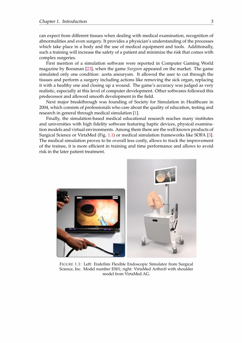
1.1 Left: EndoSim Flexible Endoscopic Simulator from Surgical Science, Inc.Model number ES01; right: VirtaMed ArthroS with shoulder model fromVirtaMed AG. . . . . . . . . . . . . . . . . . . . . . . . . . . . . . . . . . . . . 3
2.1 Relationship curves relative to longitudinal strain for (a) lateral strain, (b),Poisson’s ratio, (c) longitudinal strain and (d) tensile modulus [168]. . . . . 10
2.2 The stability regions for backward (left) and forward (right) Euler schemes;the colored regions indicate the stability. . . . . . . . . . . . . . . . . . . . . . 18
2.3 The stability region for semi-implicit Euler scheme; the colored region in-dicates the stability. . . . . . . . . . . . . . . . . . . . . . . . . . . . . . . . . . 18
2.4 From left to right: a non-moving particle at time t = 0 being at a wrongposition, which would be fixed at time t = 1, but with a resulting velocitypropagating to the next step t = 2 [104]. . . . . . . . . . . . . . . . . . . . . . 25
2.5 Two triangles undergoing a bending deformation [116]. . . . . . . . . . . . . 272.6 Cloth character simulated under pressure using PBD [116]. . . . . . . . . . . 282.7 A duck model squeezed by a heavy object and recovered after the big de-
formation [115]. . . . . . . . . . . . . . . . . . . . . . . . . . . . . . . . . . . . 29
3.1 A MSS composed of 5 particles (notedA,B,C,D,E) connected by 4 springswith stiffness constant k and rest length l. Green points represent the restpositions of particles A, B and C. . . . . . . . . . . . . . . . . . . . . . . . . . 39
3.2 Curve: normalized vertical force as a function of extension ζ accordingto Eq. (3.18). Dashed arrows: trajectory under progressive compression.Buckling occurs for −1/2 < ζ < 1/2. . . . . . . . . . . . . . . . . . . . . . . . 40
3.3 2D MSS: (a) triangular and (b) quadrangular with blue face diagonal springs. 413.4 Two types of 3D MSS meshes. . . . . . . . . . . . . . . . . . . . . . . . . . . . 413.5 Structured (left) and unstructured (right) 2D triangular mesh [71]. . . . . . . 423.6 Sphere-surface (left) and skull-surface (right) meshes [137]. . . . . . . . . . . 423.7 A 3D surface mesh with normal to the surface Ni and spring of length li
connecting the node pi with a central point ci. . . . . . . . . . . . . . . . . . 433.8 (left) A conformal mesh; (right) A non-conformal mesh. . . . . . . . . . . . . 433.9 Linear elastic material simulated with an equilateral triangular mesh. From
left to right: stretching, compressing and shearing experiments. MSS isdepicted in red and corresponding FEM in black [99]. . . . . . . . . . . . . . 49
3.10 Linear elastic material simulated with a tetrahedral mesh. From left toright: stretching, compressing and shearing experiments. MSS is depictedin red and corresponding FEM in black [99]. . . . . . . . . . . . . . . . . . . 50
3.11 Linear elastic material simulated with hexahedral mesh [119]. . . . . . . . . 503.12 A stress-time relationship for different types of materials at loading be-
tween t1 and t2 and a static strain at t > t2 [136]. . . . . . . . . . . . . . . . . 54
3.13 Cutting with necessary update of the spring extremities. (a) The bold seg-ments represent the inner springs wrongly attached to particle v1 after thecutting. (b) The same springs updated after a post-processing step. . . . . . 57
3.14 2-map: space subdivision (left) and c-map structure consisting of darts andβi links (right). . . . . . . . . . . . . . . . . . . . . . . . . . . . . . . . . . . . . 58
3.15 Three possible configuration of springs in a cubical element: (a) face-diagonalsprings, (b) inner-diagonal springs, (c) face-diagonal and (d) inner-diagonalsprings. . . . . . . . . . . . . . . . . . . . . . . . . . . . . . . . . . . . . . . . . 60
3.16 (a) Two adjacent cubes described by a 3-map. Each cube has 6× 4 darts. (b)LCC+MSS underlying structure of the same cubes: particles and springsassociated to i-cells and inner particles associated to an object. . . . . . . . . 61
3.17 Convention used to store darts of a hexahedron composed of points Xi
with i ∈ 0, . . . , 7. fj = dart[j][0] with j ∈ 0, . . . , 5 correspondingto first darts of each face (the bolded arrows). . . . . . . . . . . . . . . . . . . 61
3.18 UML class diagram of TopoSim basic simulation components. . . . . . . . . 63
4.1 A Bohlin C-VOR rotational rheometer (left) with parallel plate configura-tion (right). . . . . . . . . . . . . . . . . . . . . . . . . . . . . . . . . . . . . . . 68
4.2 Torsional deformation (left) understood as local shearing (right). . . . . . . . 684.3 Analytical bi-power law of liver for three different strain rates dγ/dt in log
scale for big deformation in stress-strain. . . . . . . . . . . . . . . . . . . . . 704.4 Stress-strain curve of kidney deformation obtained by the MSS with the
linear formulation of forces, using three different strain rates dγ/dt, in com-parison to the theoretical linear bi-power law (Eq. 4.3). . . . . . . . . . . . . 74
4.5 Stress-time curve of kidney deformation obtained by the MSS with the lin-ear formulation of forces, using three different strain rates dγ/dt, in com-parison to the theoretical linear bi-power law (Eq. 4.3). . . . . . . . . . . . . 74
4.6 Non-linear MSS simulation of kidney at three different strain rates in com-parison with analytical curve. . . . . . . . . . . . . . . . . . . . . . . . . . . . 75
4.7 Non-linear MSS simulation of liver at three different strain rates in compar-ison with analytical curve. . . . . . . . . . . . . . . . . . . . . . . . . . . . . . 75
4.8 Non-linear MSS simulation of spleen at three different strain rates in com-parison with analytical curve. . . . . . . . . . . . . . . . . . . . . . . . . . . . 76
5.1 Wrinkle instability occurring at the base of a beam under gravity. . . . . . . 795.2 A 3D cubical MSS element composed of 12 edge springs, 12 face diagonal
springs and 4 inner diagonal springs. . . . . . . . . . . . . . . . . . . . . . . . 805.3 Comparison of MSS-CF beam under gravity experiments using different
values of A parameter: A = 0.01, 0.01, 1, 10, 100. E = 2 MPa, ν = 0.3,g = −10. . . . . . . . . . . . . . . . . . . . . . . . . . . . . . . . . . . . . . . . 84
5.4 The κ coefficient depicted as a function of the ratio κ/E in terms of thePoisson ratio ν. . . . . . . . . . . . . . . . . . . . . . . . . . . . . . . . . . . . 89
5.5 UML diagram of the algorithm to apply force corrections. . . . . . . . . . . . 925.6 UML class diagram of the TopoSim basic simulation components after adding
the face-diagonal springs and the force corrections. Newly added elementsare marked in green and the modified functions in blue. . . . . . . . . . . . . 93
5.7 Correct elastic behavior of a square MSS element (top left) under tension(top right) and compression (bottom) loads. . . . . . . . . . . . . . . . . . . . 94
5.8 Five types of body deformation for a model validation. . . . . . . . . . . . . 95
5.9 Compression experiment comparison between MSS-Baudet, MSS-nFD, MSS-CF and FEM at a big (20 %) deformation with different Poisson’s ratios. . . 99
5.10 Tension experiment comparison between MSS-Baudet, MSS-nFD, MSS-CFand FEM with big (20 %) deformation. . . . . . . . . . . . . . . . . . . . . . . 101
5.11 Alignment of cross-sectional view on points in a shearing experiment withbig (20 %) deformation at different Poisson’s ratios, E = 10,000; compari-son between MSS-CF and FEM. . . . . . . . . . . . . . . . . . . . . . . . . . . 102
5.12 Shearing experiment with big (20 %) deformation at different Poisson’s ra-tios, E = 10,000; comparison between MSS-CF and FEM. . . . . . . . . . . . 102
5.13 Alignment of cross-sectional view on points in a torsion experiment withbig (20 %) deformation at different Poisson’s ratios, E = 10,000; compari-son between MSS-CF and FEM. . . . . . . . . . . . . . . . . . . . . . . . . . . 103
5.14 Torsion experiment with big (20 %) deformation at different Poisson’s ra-tios, E = 10,000; comparison between MSS-CF and FEM. . . . . . . . . . . . 104
5.15 Beam under gravity: (a) MSS-Baudet, (b) MSS-nFD, (c) MSS-CF.E = 2 MPa,ν = 0.25, g = −10. . . . . . . . . . . . . . . . . . . . . . . . . . . . . . . . . . . 105
5.16 Beam under gravity: MSS-Baudet and MSS-nFD in comparison with ana-lytical result. E = 10 MPa, ν = 0.25, g = −10. . . . . . . . . . . . . . . . . . . 106
5.17 Beam under gravity: MSS-Baudet and MSS-nFD in comparison with ana-lytical result. E = 2 MPa, ν = 0.25, g = −10. . . . . . . . . . . . . . . . . . . 106
5.18 Beam under gravity comparison between MSS-CF, MSS-nFD and the ana-lytical solution. E = 10 MPa, ν = 0.25, g = −10. . . . . . . . . . . . . . . . . 107
5.19 Beam under gravity comparison between MSS-CF, MSS-nFD and the ana-lytical solution. E = 2 MPa, ν = 0.25, g = −10. . . . . . . . . . . . . . . . . . 107
5.20 Real time performance of 1,000 iterations versus the number of mesh ele-ments (volumes) with CPU-software configuration I for the compressionexperiment and the simulation methods: MSS-nFD, MSS-FD, MSS-CF. . . . 109
5.21 Real time execution of 300,000 iterations versus the number of mesh ele-ments (volumes) on the CPU-software configuration I for the beam undergravity experiment and the three simulation methods: MSS-nFD, MSS-FD,MSS-CF. . . . . . . . . . . . . . . . . . . . . . . . . . . . . . . . . . . . . . . . 110
5.22 The tu/tr ratio versus the number of mesh volumes on the CPU-softwareconfiguration I - 8 threads. . . . . . . . . . . . . . . . . . . . . . . . . . . . . . 111
5.23 The tu/tr ratio versus the number of mesh volumes of the MSS-nFD methodon the CPU-software configuration II. . . . . . . . . . . . . . . . . . . . . . . 111
5.24 The tu/tr ratio versus the number of mesh volumes of the MSS-FD methodon the CPU-software configuration II. . . . . . . . . . . . . . . . . . . . . . . 112
5.25 The tu/tr ratio versus the number of mesh volumes of the MSS-CF methodon the CPU-software configuration II. . . . . . . . . . . . . . . . . . . . . . . 112
6.1 Basic MSS elements: (a) tetrahedron, (b) prism, (c) pyramid and (d) hexahe-dron. The rectangular faces are supported by face-diagonal springs (drawnin red); hexahedron is additionally supported with use of inner diagonalsprings (drawn in green). . . . . . . . . . . . . . . . . . . . . . . . . . . . . . 116
6.2 Hexahedron subdivision into (a) six tetrahedra or (b) twelve tetrahedra. . . 1176.3 Hexahedron subdivision into 5 tetrahedra. . . . . . . . . . . . . . . . . . . . 1176.4 Hexahedron subdivision into two prisms. . . . . . . . . . . . . . . . . . . . . 1186.5 Prism subdivision into (b) three tetrahedra or (b) six tetrahedra. . . . . . . . 1186.6 Hexahedron subdivision into six pyramids. . . . . . . . . . . . . . . . . . . . 1196.7 Pyramid subdivision into two tetrahedra. . . . . . . . . . . . . . . . . . . . . 119

6.8 Possible sewing scenarios. . . . . . . . . . . . . . . . . . . . . . . . . . . . . . 120

Dedicated to my Mother who believes in me no matter what. . .

1
Chapter 1
Introduction
Motivation - Soft Tissue Modeling for Biomedical Simulation
Nowadays the need for simulation, so modeling real-life events and phenomena, ariseswith development of many scientific branches. Being able to predict particular events orbehaviors (like weather or interactions between bodies) under known circumstances is avaluable asset in treatment of many problems. It strongly affects the decision-making pro-cess and makes a huge impact on one’s actions. Among many types of physical simulationwe can distinguish simulation of gases, liquids, clothes, rigid and deformable bodies. Themain interest of this thesis lies in simulation of deformable solids. Deformable objectslike soft bodies and, in particular, soft tissues like internal organs are modeled to improvepatient treatment and study nature of the human body.
Now, let us introduce different aspects of the physical simulation depending on thefield-type point of view: biomedical simulation in computer graphics and biomechanics.
Biomechanical Simulation in Computer Graphics
As many authors like to remind, the pioneers in the field of simulation in computer graph-ics are Demetri Terzopoulos, John Platt and Kurt Fleischer, who in late 80’s presented firstdeformable models [150, 149].
The application vary from offline to real-time simulations to model visually and phys-ically accurate models of liquids, rigid and deformable bodies. As the field includes sucha vast number of areas in which it can be used, we can choose and pick from various typesof simulations including cloth animation, fluid simulation, rigid objects and soft tissue be-havior under interactions with other objects. To study this field in depth it is useful to beequipped in the knowledge of the basic elasticity theory and continuum mechanics. Thefields using these types of simulation the most are of course gaming and movie industry.Therefore the most important features from the computer graphics point of view are: timeperformance, visual accuracy and lightweight solutions.
There are several approaches to simulate realistic objects in real time, like learning al-gorithms or random function generators, but the one we focus on is a simplified physical-mathematical solution. This approach gained great popularity. Usually methods likeMass-Spring System or Position Based Dynamics are used to model even complex ob-jects. They are said to be physically inaccurate, but produce real-time simulations usingsimplified physical laws, mathematical models and many approximations.
2 Chapter 1. Introduction
Biomedical Simulation in Biomechanics
Unlike computer graphics, the biomedical and especially biomechanical community val-ues the accuracy of the simulation and its robustness. Therefore, to create complex sys-tems for simulation, most of the researchers use Finite Element Model (FEM) and its vari-ations. FEM is used to solve the equations responsible for body’s mechanical behavior.These simulations may take very long time, but are known to be reliable when it comesto the solution. The biggest interest includes simulation of deformable bodies meaningmostly soft tissues, which can be used for medical training and virtual surgeries. An earlysurvey on the difficulties in creating realistic models for medical simulation of soft tissueswas written by Delingette in 1998 [45], to which we direct a curious reader.
The biomechanical simulation field involves several pioneers especially worth men-tioning. First of all there are Carley Ward and Robert Thompson, who in 1975 introduceda detailed Finite Element model of a brain [158]. They based the model on fewer as-sumptions while keeping it detailed enough for future brain simulations and the studyof brain dynamics. Then, there are Cover et al. who in their paper from 1993 [36] talkedabout gall-bladder model for surgical simulation and their methodology which addressesissues of graphical models for surgery simulation in general. Shortly after that, in 1995,Bro-Nielsen presented an active cubes approach used to model deformations of humantissue in response to bone movements [26]. We cannot forget also about the ever-activeStéphane Cotin, who in 1996 was among first to introduce us to the virtual surgery envi-ronment and application of tissue modeling in the biomedical context [35].
To find out about the mechanical properties of the modeled tissues, the physical be-havior of the tissue needs to be studied in depth. Usually to obtain information aboutthe simulated tissue it is necessary to perform numerous experiments on real tissues likehuman or animal organs. The tests include treatment in different types of loads: com-pression, traction, torsion, etc. Specially designed devices measure necessary parametersto obtain different curves (e.g. stress-strain), which depict the behavior of studied tissue.From those it is possible to derive constitutive laws [82, 124, 32, 94, 172, 126] which thencan be used for example by Finite Element simulators.
Since 1967 Fung studied in depth the elastic behavior of soft tissues [62] and the me-chanical properties of real bodies. The complexity of soft tissues includes many proper-ties, which he studied by mechanical experiments [59]. These experiments have provenmany biological tissues to manifest properties like incompressibility (or behavior veryclose to incompressible) [161], anisotropy [59], visco-elasticity and non-linearity [46, 61,59]. From Fung we also know that these bodies exhibit non-linear behavior when theyundergo large deformations [59].
According to the application, a good approximation of the soft tissues behavior isobtained by making some assumptions such as isotropy [100], elasticity [145, 29] andhomogeneity [75].
Medical simulation from early 80’s to this day
Since the possibility of simulation appeared on the horizon, the medical environmentgot also interested in it. More specifically, a solution for a gap in the training process ofthe health professionals was discovered. Since early beginning of medicine the study wasfirst only theoretical, to then pass to the practical approach as an assistant or an intern andfinally, to become self sufficient physician on an independent job. This learning approachinvolves major risk for potential patients, therefore this is where the medical simulationcomes in view. It allows an accurate study of real bodied and what kinds of behavior one
Chapter 1. Introduction 3
can expect from different tissues when dealing with medical examination, recognition ofabnormalities and even surgery. It provides a physician’s understanding of the processeswhich take place in a body and the use of medical equipment and tools. Additionally,such a training will increase the safety of a patient and minimize the risk that comes withcomplex surgeries.
First mention of a simulation software were reported in Computer Gaming Worldmagazine by Boosman [23], when the game Surgeon appeared on the market. The gamesimulated only one condition: aorta aneurysm. It allowed the user to cut through thetissues and perform a surgery including actions like removing the sick organ, replacingit with a healthy one and closing up a wound. The game’s accuracy was judged as veryrealistic, especially at this level of computer development. Other softwares followed thispredecessor and allowed smooth development in the field.
Next major breakthrough was founding of Society for Simulation in Healthcare in2004, which consists of professionals who care about the quality of education, testing andresearch in general through medical simulation [1].
Finally, the simulation-based medical educational research reaches many institutesand universities with high fidelity software featuring haptic devices, physical examina-tion models and virtual environments. Among them there are the well known products ofSurgical Science or VirtaMed (Fig. 1.1) or medical simulation frameworks like SOFA [3].The medical simulation proves to be overall less costly, allows to track the improvementof the trainee, it is more efficient in training and time performance and allows to avoidrisk in the later patient treatment.
FIGURE 1.1: Left: EndoSim Flexible Endoscopic Simulator from SurgicalScience, Inc. Model number ES01; right: VirtaMed ArthroS with shoulder
model from VirtaMed AG.
4 Chapter 1. Introduction
Problem Statement and Aim of the Thesis
In the presented context soft tissue simulation became a huge field of interest in thebiomedical environment as it provides reliable information about tissue behavior andallows to create complex models of human intestines involving many different organsat the same time. The challenge in fast soft tissue simulation is to faithfully representthe simulated tissues and their non-linear behavior at large deformations. Additionally,global behavior of real organs, like volume changes, is hard to control. There are manysimulation methods, all of them with their advantages and limitations, which we presentin the following chapter. The choice of a simulation method also poses many questions- the aimed simulation must be looked at from all the different angles: type of simulatedmaterial, stability, time performance, computational capabilities, level of detail and useof small or large time steps. The created framework could then be integrated as a part oflarger simulation environment with use of haptic devices.
Our interest lies in a real-time biomedical simulation, where simplified deformationmodels are used. We are also interested in parallelization approaches on both CPU andGPU and possible pre-computations. Fast and accurate simulation shall then be used tosimulate real organs for medical surgery simulation. The existing approaches present lim-ited possibilities when it comes to type of simulated tissues and behaviors they represent.Usually there are three main issues we meet:
• use of simplified laws which do not succeed at modeling deformable bodies withenough accuracy for medical purposes;
• use of complex formulas which fail at real-time simulation;
• use of computation acceleration technique based on moving possibly biggest num-ber of calculations to pre-computational phase of a simulation, which prevents useof topological modifications in an ongoing simulation.
Our work aims at creating a framework capable of performing simulations of de-formable bodies like real organs in real time. The goal of this thesis concerns thus theimplementation of a new biomedical model of soft tissues suitable for interactive simu-lations and allowing simulations of organ movements. For that purpose we decided toimprove a locally-oriented Mass Spring System to accurately model real organs at largestrains and control the volume of the simulated tissue. We have chosen Mass-Spring Sys-tem as the simulation method because of its simplicity, ease of use and implement newsolutions and fast performance. However, due to natural limitations of this modelingtechnique we have decided to introduce some improvement to reach our goal. The firsttask aimed at simulating small (linear) or large (non-linear) deformations without spec-ifying which of them a body undergoes. Non-linearity is one of main characteristics ofreal bodies at large deformations. Since MSS is a locally-oriented technique with so calledCauchy limitation, our second task included controlling global feature: volume of a de-formed tissue defined with compressibility constraint. The third task aims at expandingthe variety of mesh types which our MSS is able to use. The new type of mesh involvesmixed-elements: hexahedra, tetrahedra, prisms and pyramids.
Chapter 1. Introduction 5
Contributions
In this thesis we have investigated various methods which deal with the challenge of softtissue simulation, especially in the context of medical application. In our work we focuson aspects like genericity, accuracy and physically-based inspiration. Our methods aresimple to use and implement, same as the Mass-Spring System itself. They improve theMSS and broaden the possibilities to use it for fast, stable and controllable simulation.
The major contributions of this thesis are:
• Non-linear force formulation for simulation of real organs inspired by a consti-tutive law. This method aims at reproducing a real experiment used to formulatea bi-power constitutive law. The new formulation of force allows us to control theshape of a stress-time curve at different strain rates when deforming a visco-elasticbody.
• Physically-based formulation of stiffness for all-hexahedral mesh. We present aphysically-based derivation of the stiffness parameters for three types of springsin an all-hexahedral MSS mesh. The formulation is independent of the type ofdeformation the simulated body undergoes and it stabilizes MSS to avoid a natu-ral wrinkle and buckling phenomena. The formulation considers elastic, homoge-neous, isotropic tissues.
• New volume correcting force based on the Poisson ratio. This contribution allowsus to control the volumetric changes in MSS depending on the compressibility rateparameter called Poisson’s ratio (ν). It aims at dealing with natural MSS limitationwhich restricts the physically correct 3D MSS to such with ν = 1/4. Additionalforce terms computed at every time step when a volume change occurs correct theresultant error at ν 6= 1/4 and allow to use values of this parameter characteristic ofnatural materials: ν ∈ [0; 0.5[.
• Introduction to formulation of mixed-element mesh for Mass-Spring Systems.We propose to formulate the physical and topological structure for a MSS mixed-element mesh. Such a structure consists of four basic 3D shapes: commonly usedtetrahedra and hexahedra and joint-elements used to connect them - pyramids andprisms.
Organization of the Thesis
The thesis outline is the following:
• Chapter 2 presents the overview on the past research done in the field of physicalsimulation and modeling deformable bodies, also for medical purposes. We ana-lyze a general simulation loop with existing time integration methods as well as thesimulation techniques and how they are improved to successfully model behaviorof elastic solids.
• Chapter 3 describes in detail Mass-Spring Model. It includes detailed informationon simulation loop, MSS limitations and instabilities and types of mesh used forsimulation. In further part we talk about different methods to obtain the physicalMSS parameters and constraints used to control various MSS features. We discussthe non-linearity of MSS and possible topological modifications. Finally we present
6 Chapter 1. Introduction
our framework used for MSS simulations and the initial implementation of the sim-ulation method.
• Chapter 4 introduces our novel approach used for simulation of real organs up to100% strains. The simulation is as fast as the original MSS and is able to control theshape of the output stress-time curve at different strain rates. The method repro-duces the shape of a visco-elastic body deformation thanks to minimal number oftissue parameters.
• In Chapter 5 we present an improvement of the MSS which provides two main fea-tures: a solution to avoid wrinkle and buckling instability as well as volume correct-ing forces. Such an approach provides us with a stable, physically-based MSS ableto control the global volumetric changes of a simulated body based on a compress-ibility parameter. It successfully controls the volume of absolutely compressible toincompressible soft elastic, homogeneous, isotropic bodies.
• Chapter 6 proposes a mixed-element mesh structure and its parametrization forMSS. This type of a lattice would allow a faster simulation while providing detailedmesh with a minimal number of used elements.
• Finally, Chapter 7 concludes the thesis by summarizing the research results anddiscussing the future possibilities and directions of the next steps.
Collaboration and Publications
This work was supported by the LABEX PRIMES (ANR-11-LABX-0063) of Université deLyon, within the program "Investissements d’Avenir" (ANR-11-IDEX-0007) operated bythe French National Research Agency (ANR).
This thesis allowed a collaboration between Computer Science Laboratory for ImageProcessing and Information Systems (Laboratoire d’InfoRmatique en Image et Systèmesd’information - LIRIS) and The Biomechanics and Impact Mechanics Laboratory (Labora-toire de Biomécanique et Mécanique des Chocs - LBMC) of which representatives are Flo-rence Zara, Guillaume Damiand (LIRIS) and Stéphane Nicolle (LBMC). The collaborationwas also extended to Physic laboratory of ENS (École Normale Superieure) representedby Jean-François Palierne.
The topic of this thesis is ’Hybrid 3D Mass Spring System for Soft Tissue Simulation’,which expands capabilities of the simple Mass Spring System to model complex behaviorsof deformable bodies. This thesis introduces improvements of the simulation techniqueto deal with its natural limitations.
Our publications involve the following articles published in conference proceedingsor submitted for review in journals:
• Karolina Golec, Matthieu Coquet, Florence Zara, Guillaume Damiand. ’Improve-ment of a Topological-Physical Model to manage different physical simulations’,23rd International Conference in Central Europe on Computer Graphics, Visualiza-tion and Computer Vision 2015, Jun 2015, Plzen, Czech Republic. pp.25−34, WSCGFull papers proceedings;
Chapter 1. Introduction 7
• Karolina Golec, Florence Zara, Stéphane Nicolle, Jean-François Palierne, GuillaumeDamiand. ’New Mass Spring System formulation to model the behavior of soft tis-sues’, 22nd European Society of Biomechanics Congress (ESB 2016), Jul 2016, Lyon,France;
• Karolina Golec, Jean-François Palierne, Florence Zara, Stéphane Nicolle, GuillaumeDamiand. ’Hybrid 3D Mass-Spring System to simulate isotropic materials’, Work InProgress Session, VRIPHYS 2017: 13th Workshop on Virtual Reality Interaction andPhysical Simulation 2017;
• Karolina Golec, Jean-François Palierne, Florence Zara, Stéphane Nicolle, GuillaumeDamiand. ’Hybrid 3D Mass-Spring System for simulation of isotropic materialswith any Poisson’s ratio’, under review in The Visual Computer International Jour-nal of Computer Graphics.

9
Chapter 2
Simulation of Deformable Objects
In this chapter we introduce previously employed physically based models in the topic ofsoft tissue modeling for biomedical simulations. We describe the general context of softtissue simulation in biomechanics, research in the direction of various techniques and theacquisition of tissue parameters. Then, we remind the basic notions of mechanics includ-ing continuum mechanics and commonly used time integration schemes. We finish thechapter by introducing three main simulation methods, their advantages and weaknesses.
2.1 Deformable Objects in Biomechanics
Soft bodies are known for several types of behavior which define them: they are incom-pressible, visco-elastic, their stress-strain relationship depends strongly on the type oftissue and conditions of the physical experiments [60]. The knowledge about mechani-cal behavior of human body is crucial in various fields like crash-testing, biomedicine orsport simulations. Identification of mechanical properties of different tissues allows usto know the stresses acting within them during an impact as well as compute the hapticforces used in virtual surgeries.
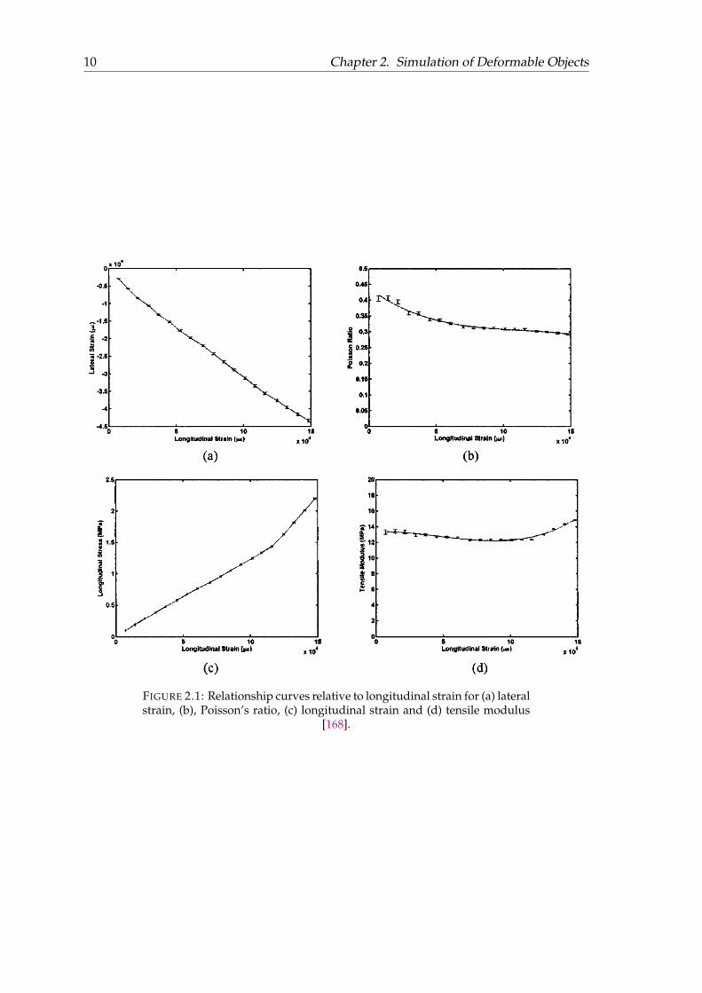
Deformable objects can also be defined in terms of linear and non-linear stress-strainrelationship, meaning that their behavior is linear if the body undergoes a small deforma-tion and strongly non-linear if the body is deformed above the linear limit. Soft tissuescan be studied under different angles. An example of several relationships is depictedin Fig. 2.1, where the curves are plotted for a mono-axial tensile experiment of cartilagetissue [168].
2.1.1 Physical Parameters of Soft Tissues
Study of mechanical behavior of human organs is a crucial task in simulation because ofthe severity of a potential trauma [166, 117], meaning extensive bleeding and the fact, thatthey play the key role in the functioning of human body. The topic is frequently discussedin the context of surgical simulation as well as accidentology and automotive safety. Rightafter the brain tissue [108, 109, 125, 74, 154] the kidney and liver [98, 118, 139, 142, 120, 90]are reported most often in terms of their mechanical behavior, followed by the spleen inthe same kind of identification [146, 138, 87].
The acquisition of the mechanical properties of abdominal organs is useful especiallywhen applying or developing constitutive laws for FEM simulations. Several existingsolutions for this type of organ simulation in automotive safety are described by Nicolleet al. [123] including, but not limited to: Ford model from Ford Motor Company [53],Humos model from the HUMOS European Consortium [155] or THUMS model fromToyota Motor Corporation and Toyota Central R&D [143].
10 Chapter 2. Simulation of Deformable Objects
FIGURE 2.1: Relationship curves relative to longitudinal strain for (a) lateralstrain, (b), Poisson’s ratio, (c) longitudinal strain and (d) tensile modulus
[168].
2.1. Deformable Objects in Biomechanics 11
Additionally, in the context of medical simulation, we know that to be able to simulatethe behavior of soft bodies accurately on haptic devices it is crucial to know the necessarylevel of accuracy of a simulation. Study of Batteau et al. shows that the perception ofhaptic feedback varies greatly, even among the specialists [11]. In their experiments theyfound out that the standard deviation of such a perception is within 8%. Moreover, Misraet al. have shown that the non-linearity of a tissue deformation highly exceeds the humanperception threshold for force discrimination in some tissues and thus has to be taken intoaccount in surgery simulation [111].
2.1.2 Application of Soft Tissue Modeling
The application of the soft tissue modeling can vary as well: we can distinguish modelsused purely for a full surgery simulation or surgery-guidance systems, which are usedintraoperatively i.e. during an ongoing surgery. A survey on particular type of modeling:real time deformable models for surgery simulation, was written in 2005 by Meier et al.[106]. The authors gathered many simulation techniques available for modeling elasticobjects in real time, dividing them, however, into two categories: interactive or realistic.Another survey, this time in the topic of computer-aided surgery, was written by Frisoli etal. [57]. The authors discuss two main aspects of this kind of simulation: the technologicaland realistic simulation challenges. We direct a curious reader to these articles for moredetails. Now let us review several contributions made in these areas.
Keeve et al. studied the behavior of MSS and FEM for craniofacial surgery simulation[86]. This application took into account the complexity of human tissue, which in this casewas constructed of 3 layers with different properties, and the underlying bone structure,which plays the most important role in the postoperative result to be simulated. Bothsimulation methods turned out to allow a correct prediction of the impact of the appliedchanges, even though the MSS was known to be not as accurate as FEM, especially FEMin its expanded form including visco-elasticity and long-term relaxation of the tissue.
MSS-Based Surgery Simulation
A method created for real-time micro-surgery simulation of blood vessels was presentedby Brown et al. [28]. The Mass-Spring System based method favors the visual rather thannumerical accuracy and is focused on local deformations only, but this early applicationof MSS in virtual surgery was one of the first to take into account the properties of realtissue such as visco-elasticity, non-linearity, non-homogeneity and anisotropy insteadof their respective simplifications.
An intraoperative update of the surgery guidance using ultrasound segmentationcombined with MSS was presented by Dagon et al. [39]. Their simulation system wasbuilt of two elements: update of the positions of simulated liver tissue and its vessels; anda simple elastic deformation system used to model organ deformations, so the updatedmesh. The idea was first developed on Matlab software and the accuracy was not takeninto account at this point yet, since all the parameters of MSS were adjusted manually.
FEM-Based Methods
Niroomandi et al. put up with several challenges of simulation of deformable bodies,like non-linear behavior or real time execution, using Proper Orthogonal Decomposition(POD) technique [130]. Their experiments have shown good alignment with the completemodel results. However, the method limits the simulation to very few degrees of freedom
12 Chapter 2. Simulation of Deformable Objects
and suffers from buckling phenomenon (we discuss the buckling instability in Ch. 3.2.2),which causes an error up to 30% in large deformations. Additionally the method re-quires a lot of pre-computations which may potentially cause difficulties in a simulationof topological modifications. Nevertheless, the authors propose several methods for sim-ulation of deformable bodies including a Proper Generalized Decomposition (PGD) forsimulation of non-linear hyper-elastic solids and soft tissues [37, 128] or reduced ordermodeling with X-FEM [129].
A deformable model for virtual-reality based simulations of Choi et al. was built onan idea of a deformation understood as a localized force transmittal process [31]. Theiralgorithm is thus based on a breadth-first search with an adjustable depth and uses simu-lated annealing process with linear static FEM reference data.
Other Techniques
Virtual surgery training system, which used a meshless technique and a method of finitespheres combined, was presented by De et al. [44]. The demonstrated real time simulationhave assumed behavior of linear elastic tissue and aimed at the speed of the simulationrather than anything else.
As we have shown, in the medical simulation of deformable bodies there are vari-ous forms of application of the developed methods. The field of virtual surgery intro-duces many types of behavior into the surgery room with computer-aided proceduresand virtual reality training programs. Since human tissues manifest very different typesof behavior and physical properties, the simulation capabilities have to be adjustable andprecise to meet the today’s requirements for a good surgery simulation method.
2.2 Basic Notions of Mechanics
In this section we present the basic notions of mechanics and continuum mechanics tointroduce the methods used by different simulation models in a dynamic simulation.
2.2.1 Simulation Loop
In this context we need to use the Newton’s second law of motion, which writes:
a m = f(v, x, t), (2.1)
where a is the acceleration, m the mass, v the velocity and x the position of an object attime t. f is a general function dependent on the physical model. It is defined by v, x andt parameters. Then, an integration scheme of a choice is used to evaluate the velocitiesv using accelerations a and then calculate the resulting positions x from the previouslyobtained velocities. This is usually broken down into a general simulation loop, wherethe following components are integrated:
a =
∑f(v, x, t)m
,
v =
∫a dt,
x =
∫v dt.
(2.2)
2.2. Basic Notions of Mechanics 13
This can be written down in a form of a system of first order differential equations.At the end, a chosen integration method needs to solve a system of ordinary differentialequations (ODEs) of a form:
vn = f(vn, xn, tn)xn = x0
(2.3)
taking into account the positions xn and velocities vn at time tn for unknown set ofdiscrete values n ∈ 1, ..., N, where n marks the consecutive time steps and N is thenumber of simulation steps.
2.2.2 Continuum Mechanics
Now, we present some basic notions about the continuum mechanics, which have to becovered to present the simulation methods.
From the Newtonian dynamics and Eq. (2.1) we can transform the second law of mo-tion to a continuum mechanics manner, where the partial differential equation (PDE) ofan elastic, continuous material is given by the Cauchy momentum equation:
ρx = ∇ · σ + Fext. (2.4)
Here ρ is the body density and Fext are the external forces acting on it. In this contextthe global forces F are usually computed as a derivative of the system’s energy over adisplacement vector u:
F = −∂W∂u
. (2.5)
Knowing that we use the linear algebra and calculus to describe deformations on con-tinuous or discretized objects, we can describe a deformation Φ as a displacement field ap-plied to an undeformed body Ω ∈ R3. Then, when a part of the body at a location X ∈ Ωis moved to a new location x ∈ Ω′ in deformed state Ω′, we can define the displacementvector field as u = x − X. To measure the deformation there exists a deformation tensor,which allows us to quantify it: Green Lagrange tensor. There are several choices as forhow to compute the elastic infinitesimal Green-Lagrange strain tensor εGL, which in thesimplest (1D) case is a ratio of the change of the length divided by the initial length. TheHooke’s law gives us the relationship between εGL and the stress σ. It also gives us thethe fourth-rank elasticity tensor C, so that next we can choose the appropriate ε:
σ = C : ε ; σij = Cijkl εkl, for i, j, k, l = x, y, z. (2.6)
The Green-Lagrange strain tensor is then defined by:
εGL = (∇X +∇u)T(∇X +∇u). (2.7)
The linearized Green-Lagrange strain tensor εL ∈ R3×3, which is valid only for smallstrains, is defined as follows:
εL =1
2
(∇u + (∇u)T
). (2.8)
Another solution is to use Green’s non-linear strain tensor εN ∈ R3×3 defined as:
14 Chapter 2. Simulation of Deformable Objects
εN =1
2(∇u + (∇u)T + (∇u)T∇u). (2.9)
In both cases ∇u is a 3 × 3 displacement gradient tensor (spatial variation of the dis-placement field), where the x, y, z indices indicate the differentiation over the u, v, wcomponents of u:
∇u =
ux uy uzvx vy vzwx wy wz
. (2.10)
Having the previously introduced displacement vector field u, Lamé parameters (µ =E
2(1+ν) , λ = Eν(1+ν)(1−2ν) ) and the linear Green - St. Venant strain tensor (Eq. (2.8)) it is
possible to compute the linear elastic energy Wl for homogeneous isotropic materials, i.e.Hooke’s law:
Wl =λ
2(Tr(εL))2 + µ Tr(ε2
L). (2.11)
Let us focus on the linearized tensor and its linear elastic energy from Eq. (2.11) first. Itis can take the following form, modeled by the Hooke’s law, which shows that the linearelastic energy of a deformable elastic object is a quadratic function of the displacementvector [135]:
Wl =λ
2(∇ · u)2 + µ||∇u||2 − µ
2||rot(u)||2, (2.12)
where ∇ · σ is the divergence of the stress tensor σ. the stress tensor derives from thestrain energy function given by Eq. (2.11) in the linear elasticity theory. The non-lineardeformations will then be defined by non-linear energy Wnl which corresponds to the St.Venant Kirchhoff model - extension of the linear elastic model to non-linear deformations.Wnl, defined with the non-linear Green tensor (see Eq. (2.9)), becomes a polynomial of 4th
order:
Wnl =λ
2(Tr(εN ))2 + µ Tr(ε2
N )
=λ
2
(∇ · u +
1
2||∇u||2
)2
+ µ||∇u||2 − µ
2||rot(u)||2
+ µ(Tr(∇uT (∇uT∇u))
)+µ
4||∇uT∇u||2
(2.13)
2.2.3 Integration Schemes
Let us continue the detailed mechanical introduction by the most popular first order in-tegration schemes, which are a base of a dynamic simulation and allow us to predict thebehavior of a body at a particular time step. We also present one second order integrationmethod called Verlet integration scheme. In real time simulation one needs to carefullychoose the integration method to use. Since the simulations are largely dependent on thetime step the most crucial criteria are stability and simplicity. The scheme has to allow useof large number of elements, fairly big time step and a fast solving method.
2.2. Basic Notions of Mechanics 15
Explicit Euler Scheme
Explicit Euler method, called also Forward Euler, is the simplest of the presented methods.It is also straight-forward in computation. It computes the information about the nexttime step explicitly with the following formula:
vn+1 = vn + ∆t f(xn, tn)xn+1 = xn + ∆t vn
(2.14)
where ∆t = tn+1 − tn. The method is said to be ’blindly’ iterating into the futureand not taking into account the changing derivatives, while its implicit sibling computesthe output values as a part of the current step equation, therefore solving the systeminstead. The advantage of the Forward Euler scheme is that only the function f needs tobe evaluated at a time step.
Semi-implicit Euler Scheme
This method has many names including symplectic Euler, semi-implicit, semi-explicit Eu-ler as the most common ones. As a symplectic integrator it gives better results than stan-dard Euler method. The differential equations in this scheme take the following form:
vn+1 = vn + ∆t f(xn, tn)xn+1 = xn + ∆t vn+1
(2.15)
The first noticeable difference between this and the explicit Euler is in the xn+1 equa-tion, which here takes vn+1 in parameter, unlike the forward scheme, which simply usesvn. Another difference lays in the integration method. It turns out that the symplectic in-tegrator almost conserves the energy of the system, which for the same case solved usingstandard Euler - increases steadily. One can easily draw a conclusion, that the accuracy ofa system which conserves the energy is far better. However, both of those schemes needto use small time steps for stability, even though the computations at each time step arenot complex.
Implicit Euler Scheme
As the name indicates, the implicit Euler scheme (called also backward Euler) involvessolving the implicitly given unknowns. This means that the system of equations, nowdefined by ∆x = xn+1 − xn and ∆v = vn+1 − vn becomes:
∆v = ∆t M−1 f(vn+1, xn+1, tn)∆x = ∆t vn+1
(2.16)
where M−1 is the global mass matrix and function f usually defined with Taylor ex-pansion [6] as:
f(vn+1, xn+1, tn) = (fn +∂f∂x
∆x +∂f∂v
∆v). (2.17)
In this equation we can already note important components: ∂F∂x is the so called Jaco-
bian in terms of positions and ∂F∂v is the Jacobian in terms of velocities. Now, knowing that
∆x = ∆t(vn + ∆v) and M−1 is a diagonal matrix, we can transform equation (2.17) into:
(M−∆t∂f∂v−∆t2
∂f∂x
)∆v = ∆t(fn + ∆t∂f∂x
vn). (2.18)
16 Chapter 2. Simulation of Deformable Objects
This system can be now evaluated as a matrix - vector system A∆v = b, with ∆v asthe vector of unknown velocity values. Solving it allows simple computation of velocitiesand subsequent positions of the point masses. Such a system can be solved using differentfactorization methods, like the most common LU factorization, or approximation one - asconjugate gradient [6].
Verlet Integration
Verlet integration is a second order integration method, which uses central difference ap-proximation to the second derivative:
∆2xn∆t2
=xn+1−xn
∆t − xn−xn−1
∆t
∆t=
xn+1 − 2xn + xn−1
∆t2= an = A(xn). (2.19)
Such a representation allows us to compute the system of equations without velocitiesof the following form:
xn+1 = 2xn − xn−1 + an∆t2
an = A(xn).(2.20)
However we can approximate the velocities v at step n + 12 , so in the middle of time-
step interval. To do it we need to establish the velocities at time-steps n + 1 and n − 1using Taylor expansion:
vn+1 = vn + ∆t an +∆t2
2x(3)n +
∆t3
6x(4)n +
∆t4
24x(5)n +O(∆t5), (2.21)
vn−1 = vn −∆t an +∆t2
2x(3)n −
∆t3
6x(4)n +
∆t4
24x(5)n +O(∆t5). (2.22)
Then, the difference of these terms equals:
vn+1 − vn−1 = 2∆t an +∆t3
3x4n +O(∆t5), (2.23)
which after derivation gives us the following formula for vn+1:
vn+1 = vn−1 + 2∆t an +O(∆t3). (2.24)
Thanks to this computation we can directly find the initially searched approximationof velocity:
vn+ 12
= vn− 12
+ ∆t an. (2.25)
Using the computation of velocities we can easily find the positions:
xn+1 = xn + ∆t vn+ 12. (2.26)
It corresponds to the following:
vn− 12
= (xn − xn−1)/∆t. (2.27)
2.2. Basic Notions of Mechanics 17
Shortly on Stability
Evaluation of the stability of every integration method facilitates the choice of appropriatescheme for particular simulation purpose. There exist several methods to compute thestability of a numerical integration scheme. In case of the first order schemes we canstudy a linear test equation
x(t) = Γx(t), (2.28)
where Γ ∈ C is a parameter mimicking the eigenvalues of linear systems of differentialequations, we test the stability by verifying if
real(Γ) ≤ 0. (2.29)
We know that the exact solution of Eq. 2.28 decays exponentially with time [68], mean-ing:
limt→∞ x(t) = 0. (2.30)
Now, the verification is based on the same evaluation of a numerical solution un, sowhen
limn→∞ un = 0. (2.31)
Explicit Euler. We can evaluate the forward Euler scheme with the linear test equation:
un+1 = un + ∆t Γ un (2.32)
which gives us
un+1 = (1 + ∆t Γ)n+1 u0. (2.33)
In this case the solution is stable if |1 + ∆t Γ| ≤ 1.
Implicit Euler. Now, let us define the linear test equation in the backward Euler schemeas:
un+1 = un + ∆t Γ un+1 (2.34)
which yields
un+1 =
(1
1−∆t Γ
)n+1
u0. (2.35)
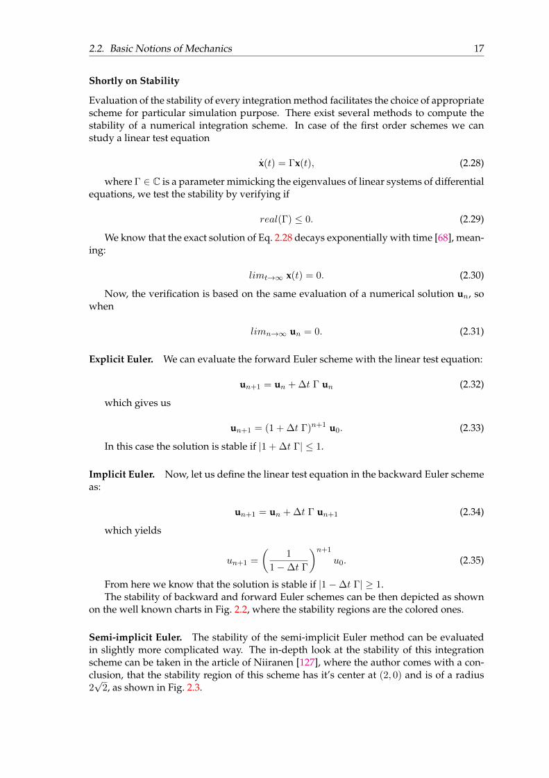
From here we know that the solution is stable if |1−∆t Γ| ≥ 1.The stability of backward and forward Euler schemes can be then depicted as shown
on the well known charts in Fig. 2.2, where the stability regions are the colored ones.
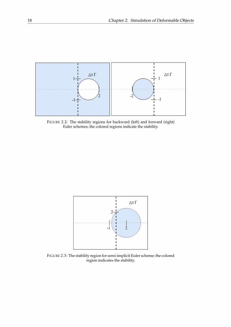
Semi-implicit Euler. The stability of the semi-implicit Euler method can be evaluatedin slightly more complicated way. The in-depth look at the stability of this integrationscheme can be taken in the article of Niiranen [127], where the author comes with a con-clusion, that the stability region of this scheme has it’s center at (2, 0) and is of a radius2√
2, as shown in Fig. 2.3.
18 Chapter 2. Simulation of Deformable Objects
FIGURE 2.2: The stability regions for backward (left) and forward (right)Euler schemes; the colored regions indicate the stability.
FIGURE 2.3: The stability region for semi-implicit Euler scheme; the coloredregion indicates the stability.
2.2. Basic Notions of Mechanics 19
Verlet Integration Scheme. While in the forward Euler integration scheme a velocity iscalculated by dividing it by the time step in consecutive steps (which causes a change ofposition, but also increases the error at every time step), the Verlet approach uses differentmethod. In fact the Verlet integration assumes the time step to be constant and computesthe velocity as the change in position by multiplying by the ∆t. Thanks to this calculationdifference the Verlet scheme is much more precise than the explicit Euler method.
Conclusions
There exist numerous more integration methods among which we have presented theones which are used most frequently. In the literature there are available some improve-ments to the integration schemes to ameliorate the quality of simulation of deformabletissues [147, 162], also based on parallelization techniques [89]. The differences betweenthe presented time integration methods focus on the stability and the size of the time stepused for simulation. In general we can sum up the implicit integration scheme as uncon-ditionally stable, which allows the use of time step of large size [6, 10], and the explicit asone suitable for use of small time steps only. The number of iterations is linearly depen-dent on the size of the time step, which has great influence on the calculation time. Thesemi-implicit time integration has a much better stability than its explicit counterpart andallows usage of small time steps.
20 Chapter 2. Simulation of Deformable Objects
2.3 Existing Simulation Methods
In the previous section we have covered the basis of mechanics and described the sim-ulation loop used to calculate the movement of an object with a carefully chosen timestep. Such a simulation loop is based on the computation of forces and depends on aphysical model chosen for a simulation. We also presented several commonly used inte-gration schemes for a dynamic simulation. Now we can continue by presentation of themost known simulation techniques, which use the notions presented before. Note that tochoose the appropriate simulation method one needs to look from the point of view of thesimulated body and the chosen conditions.
Simulation of deformable bodies is a broad field which covers topics from vector cal-culus, through topology and constraints acquisition until types of modeled behaviors. Agreat survey on the different types of models was written by Nealen et al. in 2006 [121]and earlier, in 1997 also by Gibson and Mirtich [65]. As the authors of the first survey[121] pointed out, the following subdivision of the methods can be made:
1. Lagrangian Particle Methods - this field can be divided into two parts: mesh basedand mesh free methods. The first one is represented by Mass-Spring Systems andother continuum mechanics based methods, while the second one describes meth-ods like Smoothed Particle Hydrodynamics (SPH) and other loosely coupled parti-cle systems. In these methods, the models consist of particles with varying locations.
2. Eulerian particle methods - used mostly for gases, liquids and melting objects, witha statistical approach to solve the disperse phase. The particles are computed as adensity in particular volume and treated as stationary points.
In this section we focus on three most commonly used simulation methods: FiniteElement Method, Position Based Dynamics and Meshless Deformations.
2.3.1 Finite Element Method
The Finite Element Method (FEM), also referred to as Finite Element Analysis (FEA), de-scribed in detail in a book of K.J. Bathe [9], is the most popular choice for simulation in theexact sciences and medical environment. It computes approximations of real solutions topartial differential equations (PDE’s), called basis functions. In FEM simulation we viewsimulated bodies as continuous volumes discretized into a sum of basis functions andsolve the PDE’s, which gives outstanding precision in the results. Thanks to this, FEMis used to simulate not only deformable bodies, but also airflow, heat transfer, magneticflux, fluids, turbulences and many others. In general, the FEM problem is usually brokedown into set of equations describing the properties of a body, boundary/initial condi-tions and particular body properties, such as elasticity, viscosity, etc. Then the system canbe solved using the principle of minimization of the energy to obtain a static solution inan equilibrium position. The other possibility is to use dynamic simulation loop with oneof the integration schemes presented in Ch. 2.2.
Application
One of good examples of application of the Finite Element Method is SOFA framework[3], where FEM is used for a dynamic medical simulation of various deformable objectsincluding soft tissues.
2.3. Existing Simulation Methods 21
As we already mentioned in Ch. 1, it was Terzopoulos et al. who first introducedsimulation of elastic deformable models [150]. The FEM discretization method was firstused in their paper to obtain set of partial differential equations (PDE’s) of motion to besolved further on.
The usage of FEM to simulate deformable bodies was perfected by the authors overthe years. In 1996 FEM was used by Bro-Nielsen and Cotin [27] in their 3D real-timesimulation of deformable solids. They discussed three methods of solving the problem ofreal-time simulation with topological modifications using FEM. The authors focused onthe speed of simulation without regard to the pre-calculation time or the accuracy of thesimulation though.
In the same year, Cotin et al. presented virtual environment for surgery simulation,which used FEM as the basis [35]. The model was based on the elasticity theory andcomputed force feedback within the sample in real-time, however it was not simulatingdynamical behavior.
Even more practical use of FEM for medical purposes was presented by Azar et al. in2001 [5]. The FEM was used to simulate non-linear material properties of breast tissue todetect the position of a tumor after compression. Thanks to the predictions calculated bythe method it was possible to detect the position of the tumor with 5 mm accuracy anduse it for more accurate insertion of a needle in the actual procedure.
Simplifications and Improvements for Fast Simulation. In 1999 Berkley et al. pre-sented one of the first simplified FEM methods designated for real-time simulation ofanatomical structures [17]. The method was based on the preprocessing and optimizationof the FEM mathematics and yielded only the essential simulation information.
In 2001 Wu et al. presented an adaptive non-linear FEM for simulation of deformablebodies improved by a global diagonal mass matrix for faster computations [163]. Classicalnon-linear FEM methods are known to be slow and the fast FEM simulations are based onapproximations and lack standard FEM’s accuracy. Wu et al. decided to use an improvednon-linear method, which allows real-time computations. It used adaptive meshing toallow faster computations and keep the desired level of detail in the same time.
Many more authors attempted solving issues of real-time performance and accuracyin FEM to allow fast and precise simulation of deformable bodies and especially soft tis-sues. One can read more about mixed solutions with use of Finite Element and FiniteVolume [43], FEM for large elasto-plastic deformations [77] and dynamic deformable sim-ulation using FEM and modal analysis [8]. As we discuss later on in this chapter, the FEMmethod is most eagerly used for medical simulation of soft tissues and surgery planning,but still leaving room for many improvements.
FEM Derivation
Considering the use of FEM in the field of deformable body simulation, we have to knowthat the whole domain is divided into sub-domains (finite elements), for which the ele-mentary problem is solved. The approximation of the solution is computed for the givenmesh nodes and interpolated to the whole domain. Then after solving the problem foreach sub-domain and gathering the solutions one can get the global solution itself. Wealready know, that the PDE of an elastic material is defined by Eq. (2.4). Next step is todefine the spatially continuous function x(t) ∈ Ω as a set of discrete locations xi(t) (withi ∈ 1, ..., N and N being the number of nodes):
22 Chapter 2. Simulation of Deformable Objects
x(t) =∑i
xi(t)bi. (2.36)
bi are fixed binary nodal basis functions, or shape functions, meaning that they areequal to 1 at node i and 0 at other nodes. The general formula for a dynamic deformationof a mesh can be described as:
M x(t) + D x(t) + K x(t) = Fext, (2.37)
where the M, D and K are respectively global mass, damping and stiffness matrices.
Extended Finite Element Method
One of the most important FEM improvements is called XFEM. The XFEM, as presentedfor the first time by Belytschko et al. [13], is an eXtended Finite Element Method usedfor stable interactive simulation of deformable tissues. Unlike the classical FEM, XFEMmethod allows us to model cracks in the mesh without additional need for remeshing(or only with the minimal remeshing procedure) or re-computations connected with theboundary conditions. For the purpose of correct cracks modeling the so called enrichmentfunctions are introduced into the XFEM system. Considering a crack, the neighboring jnodes of the crack are ’enriched’, therefore the basic Eq. (2.36) is extended to the form:
x(t) =∑i
xi(t)bi +∑j
bjΨjaj , (2.38)
where Φ is the enrichment function and a is the set of nodal degrees of freedom andi, j ∈ 1, ..., N.
Even though the original purpose of XFEM was to be used on cracks and fractures onrigid surfaces [113, 148], it was lately adapted to model cutting in deformable objects [81,97, 80, 85]. However the modeling of very curved surfaces requires use of a refined mesh[2].
Co-rotational Finite Element Method
Geometrically non-linear structures can be currently modeled with use of three Lagrangiankinematic descriptions: (i) Total Lagrangian, (ii) Updated Lagrangian and (iii) Co-rotational.The latter one is broadly used in medical simulators these days, therefore we shall take acloser look at it.
The a priori assumption of the co-rotational FEM is that displacements and rotations maybe arbitrarily large, but deformations must be small. As the description follows the body as itmoves, we can decompose the motion-tracking into two components - the base and theco-rotated configuration. While the base configuration serves as the origin of the body dis-placements, the purpose of the co-rotational one is to track the rigid body motion, wherethe associate coordinate system follows the body like a ghost. Then, all the deformationscan be measured with respect to the co-rotated body configuration. In an element’s localrotated frame the calculation of the forces applied by a deformed element to its samplingpoint is done using the following formula:
f = RTK(Rx− x0), (2.39)
2.3. Existing Simulation Methods 23
where K and R are the global stiffness and rotation matrices respectively, x and x0 arethe current and initial positions of the point.
The co-rotational FEM was first introduced by Wempner [159] and Belytschko andGlaum [14], as presented in the article of Nour-Omid and Rankin from 1991 [131]. Themain idea is to compute the matrix R. Since the initial assumption of the co-rotationalmethod poses a great limitation, the idea of multiple frames has been proposed by Veubeke[42]. Several other methods include use of eigenvectors and eigenvalues [114, 78, 54].
Admittedly, this method has significant superiority over the classical FEM, thanks towhich it can easily be used in biomedical simulators. The CR layer works like a filter tomodel the deformations efficiently. However the main assumption limits the use of co-rotational FEM to only small deformations (assuming them to be smaller than 1%) and itdoes not involve interconnecting deformable and rigid elements.
Mass-Tensor Model
Another way of discretizing the equations of continuum mechanics is called Mass-Tensor(MT) or Tensor-Mass model. In Computer Graphics it was introduced by Cotin et al. [34,33] and Picinbono et al. [135]. The method is based on another technique of discretizationof the continuum mechanics equations.
The MT model is defined in two forms: small deformations (under 10%) are de-fined with the linearized Green-Lagrange tensor and the corresponding linear energy(see Eq. (2.12)) and big deformations (> 10%) with Green’s non-linear strain tensor usedto compute non-linear energy (Eq. (2.13)). Next step is to compute the forces (using theaforementioned energies expressed with Finite Element Method) with Eq. (2.5). Then,for each 3D mesh element every force component has to be split into two parts. Thus,the force Ftp of a particle p of an element t ∈ Np (where Np is the number of volumes)of a mesh is a sum of the forces produced by the movement of the particle up and theforces coming from movements of its neighbors uj (j 6= p). Therefore, for a single forcecomponent corresponding to a linear elastic case 2
∑j Bpjuj we have the following MT
force:
Ftp = Btppup +∑j 6=pBtpjuj , (2.40)
where Bt is a (3×3) local symmetric matrix of a linear elastic model dependent on thebasic mesh element used, otherwise called local stiffness tensor. Now, to create the globaltensors we need simply to sum up all the local tensors on the existing vertices and edges:
Bpp =∑t∈Np
Btpp, (2.41)
Bpj =∑t∈Npj
Btpj , (2.42)
where Npj is the number of edges in the mesh. The other force components derivedfrom the FEM formulation are responsible for the stiffness tensors of vertices, edges, 2Dand 3D elements. The forces computed this way are used to update the positions of ver-tices from Eq. (2.37).
The MT model was used in real-tissue modeling like the methods presented by [142],and more recently by [93].
24 Chapter 2. Simulation of Deformable Objects
The most important limitation of the linear model is that it is not rotationally invari-ant. That can cause further issues with the reference frame when global rotations areapplied and even bigger issues with the change of volume when only local rotations takeplace. MT is known to be not as slow as FEM itself thanks to the precomputed stresstensors when the mesh file is loaded, but it is also not as fast as the particle-based meth-ods because of its computational complexity. Additionally, if the tensor functions are notconstant, the computation time might increase even more.
2.3.2 Position Based Dynamics
The Position Based Dynamics (PBD) method of Matthias Müller was described first in hisarticle [115] as a no-name approach and then introduced under its current name two yearslater [116]. In the field of rigid and deformable body simulation, Bender et al. publisheda state of the art report describing the large part of PBD methods of simulation [15]. Dif-ferent constraint functions are used to simulate various types of materials and particularbehaviors in PBD. Müller et al. [115] used rigid shape-matching constraint functions forrigid body simulation, which then were improved by Macklin et al. [104], coupled withan improvement of the simulation loop and stabilization step.
For a discretized object consisting of set of particles, the PBD, as the name alreadyindicates, works directly with positions of those particles instead of their forces. Addi-tionally the method is straight-forward and easy to use, especially in the gaming context.In the first attempts of introducing the PBD, Verlet integration scheme was willingly usedby many authors, but only Müller introduced and elaborated on the whole idea.
Due to the similarities of Position-Based Dynamics approach to Mass Spring System(described in Ch. 3) as particle-based methods we want to elaborate on the PBD simula-tion method to point out and clarify differences between them.
General Algorithm
The most important role in Müller’s PBD play the so called constraint functions Cj :R3M → R (not to be confused with C, Cijkl, the fourth-rank elasticity tensor), where M isthe number of constraints in the system and j ∈ 1, ...,M. The first type of the constraintfunction is called equality. As the name suggests it is satisfied if equality Cj(x1, ..., xN ) = 0,where N is the number of particles, is satisfied as well. The second type, called inequalityis satisfied if Cj(x1, ..., xN ) ≥ 0. The general algorithm of PBD consists of the followingsteps:
• initialization of the particle’s variables (positions x, velocities v and masses m);
• initialization/estimation of the new location for each particle (using explicit Eulerintegration scheme) according to the forces;
• iterative solving of the system by projecting the constraints Cj over the estimatedpositions (the projection is done using Gauss-Seidel method);
• moving the vertices to computed and corrected positions, updating the velocities.
This algorithm is indeed also based on the Verlet approach, but takes also from themodification of the current positions instead of storing the velocities as the difference be-tween the positions from the current and previous step. Additionally it is interesting tonote, that the iterative part of the algorithm makes it hard to define PBD as implicit orexplicit. As the authors point out, the method will behave more like an explicit scheme
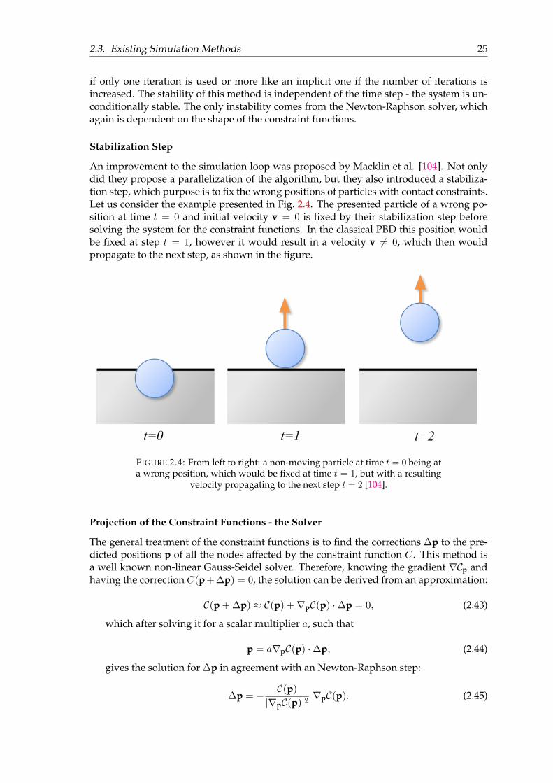
2.3. Existing Simulation Methods 25
if only one iteration is used or more like an implicit one if the number of iterations isincreased. The stability of this method is independent of the time step - the system is un-conditionally stable. The only instability comes from the Newton-Raphson solver, whichagain is dependent on the shape of the constraint functions.
Stabilization Step
An improvement to the simulation loop was proposed by Macklin et al. [104]. Not onlydid they propose a parallelization of the algorithm, but they also introduced a stabiliza-tion step, which purpose is to fix the wrong positions of particles with contact constraints.Let us consider the example presented in Fig. 2.4. The presented particle of a wrong po-sition at time t = 0 and initial velocity v = 0 is fixed by their stabilization step beforesolving the system for the constraint functions. In the classical PBD this position wouldbe fixed at step t = 1, however it would result in a velocity v 6= 0, which then wouldpropagate to the next step, as shown in the figure.
FIGURE 2.4: From left to right: a non-moving particle at time t = 0 being ata wrong position, which would be fixed at time t = 1, but with a resulting
velocity propagating to the next step t = 2 [104].
Projection of the Constraint Functions - the Solver
The general treatment of the constraint functions is to find the corrections ∆p to the pre-dicted positions p of all the nodes affected by the constraint function C. This method isa well known non-linear Gauss-Seidel solver. Therefore, knowing the gradient ∇Cp andhaving the correction C(p + ∆p) = 0, the solution can be derived from an approximation:
C(p + ∆p) ≈ C(p) +∇pC(p) ·∆p = 0, (2.43)
which after solving it for a scalar multiplier a, such that
p = a∇pC(p) ·∆p, (2.44)
gives the solution for ∆p in agreement with an Newton-Raphson step:
∆p = − C(p)
|∇pC(p)|2∇pC(p). (2.45)
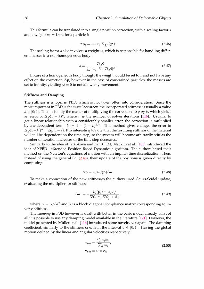
26 Chapter 2. Simulation of Deformable Objects
This formula can be translated into a single position correction, with a scaling factor sand a weight wi = 1/mi for a particle i:
∆pi = −s wi ∇piC(p). (2.46)
The scaling factor s also involves a weight w, which is responsible for handling differ-ent masses in a non-homogeneous body:
s =C(p)∑
j wj |∇pjC(p)|2. (2.47)
In case of a homogeneous body though, the weight would be set to 1 and not have anyeffect on the correction ∆p, however in the case of constrained particles, the masses areset to infinity, yielding w = 0 to not allow any movement.
Stiffness and Damping
The stiffness is a topic in PBD, which is not taken often into consideration. Since themost important in PBD is the visual accuracy, the incorporated stiffness is usually a valuek ∈ [0; 1]. Then it is only the matter of multiplying the corrections ∆p by k, which yieldsan error of ∆p(1 − k)n, where n is the number of solver iterations [116]. Usually, toget a linear relationship with a considerably smaller error, the correction is multipliedby a k-dependent term: k′ = 1 − (1 − k)1/n. This method gives changes the error to∆p(1−k′)n = ∆p(1−k). It is interesting to note, that the resulting stiffness of the materialwill still be dependent on the time step, so the system will become arbitrarily stiff as thenumber of iteration increases or the time step decreases.
Similarly to the idea of Jerábková and her XFEM, Macklin et al. [103] introduced theidea of XPBD - eXtended Position-Based Dynamics algorithm. The authors based theirmethod on the Newton’s equations of motion with an implicit time discretization. Then,instead of using the general Eq. (2.46), their update of the positions is given directly bycomputing:
∆p = wi∇C(p)∆a. (2.48)
To make a connection of the new stiffnesses the authors used Gauss-Seidel update,evaluating the multiplier for stiffness:
∆aj = −Cj(pi)− αjaij∇Cj wj ∇CTj + αj
, (2.49)
where α = α/∆t2 and α is a block diagonal compliance matrix corresponding to in-verse stiffness.
The damping in PBD however is dealt with better in the basic model already. First ofall it is possible to use any damping model available in the literature [121]. However, themodel presented by Müller et al. [116] introduced some novelty yet again. The dampingcoefficient, similarly to the stiffness one, is in the interval d ∈ [0; 1]. Having the globalmotion defined by the linear and angular velocities respectively:
vlin =
∑i vimi∑imi
,
vrot = ω × ri,(2.50)
2.3. Existing Simulation Methods 27
we can compute the deviation of the velocity ∆vi = vlin + vrot − vi. Finally, thedamping coefficient can be used to damp these deviations, giving the final velocity vi =vi + d∆vi.
Deformable Body Improvements
Since we are interested in the deformable body behavior we present several constraint func-tions which control such body properties.
Stretch and Bend Control. A first good example is a constraint function introduced tocontrol the stretching and bending of the material:
Cstretch(p1,p2) = |p1 − p2| − l0, (2.51)
Cbend(p1,p2,p3,p4) = acos
((p2 − p1)× (p3 − p1)
|(p2 − p1)× (p3 − p1)|·
(p2 − p1)× (p4 − p1)
|(p2 − p1)× (p4 − p1)|
)− ϕ0.
(2.52)In these equations l0 is the initial length of an edge and ϕ0 is the initial dihedral angle
between two triangles (p1, p2, p3 and p1, p4, p2) taken into account, as depicted in Fig. 2.5.
FIGURE 2.5: Two triangles undergoing a bending deformation [116].
In case of cloth simulation one can use a constraint function for cloth balloon (insteadof a volumetric mesh) to model a 3D object. Here the ti1, ti2 and ti3 indices stand for thevertices belonging to a triangle i:
C(p1, ...,pN ) =
(ntriangles∑i=1
(pti1 × pti2) · pti3
)− kpV0, (2.53)
where kp is the pressure constant and V0 is the initial volume of a balloon.
Volume Control. Another interesting behavior, which can be modeled with PBD, thistime using a full 3D object built of tetrahedra, is volume conservation. The constraintfunction in case of tetrahedral meshes to conserve volume takes the form of the differenceof the current and initial volume:
C(p1,p2,p3,p4) =1
6(p2,1 × p3,1) · p4,1 − V0. (2.54)
An example of Position-Based simulation on a cloth balloon mesh under pressure isshown in Fig. 2.6. The method uses the stretch, bend and volume constraint functionspresented above.
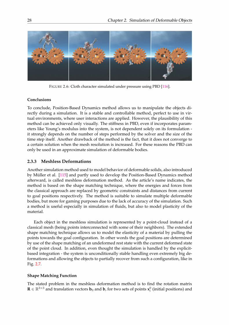
28 Chapter 2. Simulation of Deformable Objects
FIGURE 2.6: Cloth character simulated under pressure using PBD [116].
Conclusions
To conclude, Position-Based Dynamics method allows us to manipulate the objects di-rectly during a simulation. It is a stable and controllable method, perfect to use in vir-tual environments, where user interactions are applied. However, the plausibility of thismethod can be achieved only visually. The stiffness in PBD, even if incorporates param-eters like Young’s modulus into the system, is not dependent solely on its formulation -it strongly depends on the number of steps performed by the solver and the size of thetime step itself. Another drawback of the method is the fact, that it does not converge toa certain solution when the mesh resolution is increased. For these reasons the PBD canonly be used in an approximate simulation of deformable bodies.
2.3.3 Meshless Deformations
Another simulation method used to model behavior of deformable solids, also introducedby Müller et al. [115] and partly used to develop the Position-Based Dynamics methodafterward, is called meshless deformation method. As the article’s name indicates, themethod is based on the shape matching technique, where the energies and forces fromthe classical approach are replaced by geometric constraints and distances from currentto goal positions respectively. The method is suitable to simulate multiple deformablebodies, but more for gaming purposes due to the lack of accuracy of the simulation. Sucha method is useful especially in simulation of fluids, but also to model plasticity of thematerial.
Each object in the meshless simulation is represented by a point-cloud instead of aclassical mesh (being points interconnected with some of their neighbors). The extendedshape matching technique allows us to model the elasticity of a material by pulling thepoints towards the goal configuration. In other words the goal positions are determinedby use of the shape matching of an undeformed rest state with the current deformed stateof the point cloud. In addition, even thought the simulation is handled by the explicit-based integration - the system is unconditionally stable handling even extremely big de-formations and allowing the objects to partially recover from such a configuration, like inFig. 2.7.
Shape Matching Function
The stated problem in the meshless deformation method is to find the rotation matrixR ∈ R3×3 and translation vectors b0 and b, for two sets of points x0
i (initial positions) and
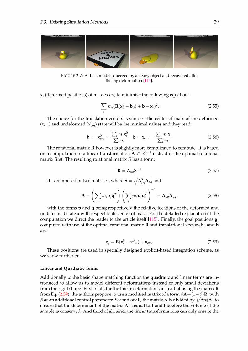
2.3. Existing Simulation Methods 29
FIGURE 2.7: A duck model squeezed by a heavy object and recovered afterthe big deformation [115].
xi (deformed positions) of masses mi, to minimize the following equation:∑i
mi(R(x0i − b0) + b− xi)2. (2.55)
The choice for the translation vectors is simple - the center of mass of the deformed(xcm) and undeformed (x0
cm) state will be the minimal values and they read:
b0 = x0cm =
∑imix0
i∑imi
, b = xcm =
∑imixi∑imi
(2.56)
The rotational matrix R however is slightly more complicated to compute. It is basedon a computation of a linear transformation A ∈ R3×3 instead of the optimal rotationalmatrix first. The resulting rotational matrix R has a form:
R = ApqS−1 (2.57)
It is composed of two matrices, where S =√
ATpqApq and
A =
(∑i
mipiqTi
)(∑i
miqiqTi
)−1
= ApqAqq, (2.58)
with the terms p and q being respectively the relative locations of the deformed andundeformed state x with respect to its center of mass. For the detailed explanation of thecomputation we direct the reader to the article itself [115]. Finally, the goal positions gicomputed with use of the optimal rotational matrix R and translational vectors b0 and bare:
gi = R(x0i − x0
cm) + xcm. (2.59)
These positions are used in specially designed explicit-based integration scheme, aswe show further on.
Linear and Quadratic Terms
Additionally to the basic shape matching function the quadratic and linear terms are in-troduced to allow us to model different deformations instead of only small deviationsfrom the rigid shape. First of all, for the linear deformations instead of using the matrix Rfrom Eq. (2.59), the authors propose to use a modified matrix of a form βA+(1−β)R, withβ as an additional control parameter. Second of all, the matrix A is divided by 3
√det(A) to
ensure that the determinant of the matrix A is equal to 1 and therefore the volume of thesample is conserved. And third of all, since the linear transformations can only ensure the
30 Chapter 2. Simulation of Deformable Objects
correct behavior in shear and stretch deformations, the quadratic deformations are intro-duced in the model as well to simulate twist and bending. Similarly to the method of theshape matching function presented above, the authors define a quadratic transformation,this time of a form:
gi = [AQM]qi. (2.60)
They introduce the following quadratic vectors and matrices of respective sizes:
gi ∈ R3,
q = [qx, qy, qz, q2x, q
2y , q
2z , qxqy, qyqz, qzqx] ∈ R9,
A, Q, M ∈ R3×3,
A = [AQM] ∈ R3×9
R = [R 0 0] ∈ R3×9.
(2.61)
The matrix A is holding the information for the linear deformation, matrix Q thequadratic terms and matrix M - mixed terms. The solution of minimization term
∑imi(Aqi−
pi)2 is the optimal quadratic transformation matrix:
A =
(∑i
mipiqTi
)(∑i
miqiqTi
)−1
= ApqAqq. (2.62)
Adequately to the linear case, the goal shape is computed with the term βA+(1−β)R.
Improved Explicit-Based Integration
As we introduced the basic integration methods in Ch. 2.2, we can directly introduce theintegration proposed by Müller et al. [115] as a modification of the semi-implicit scheme(Ch. 2.2.3) with an additional term added to the vn+1:vn+1 = vn + ∆t F(xn, tn) + k
gn − xn∆t
xn+1 = xn + ∆t vn+1
(2.63)
This model uses the knowledge of the goal positions gn to not overshoot the calcula-tions. Similarly to the PBD method, the stiffness term k ∈ [0; 1]. The function F here hasthe following form: F(xn, tn) = Fext/m, where Fext are the external forces.
Method Extensions
The meshless deformation method was further improved by Henriques et al. [69]. Firstof all they show the problem of volume preservation without additional area-preservingmethod. In fact the volume preservation causes the body to abnormally grow face-wise ata big deformation, for example like pushing a cube into a wall. The authors suggest thenseveral area-preserving methods to fix this problem, including their three improved ideasbased on:
1. scaling the face back to a particular size if the area exceeds some predefined thresh-old;
2. constrain the magnitude of A matrix when the predefined threshold is reached.There are two sub-solutions proposed:
2.3. Existing Simulation Methods 31
• more complex approach with use of the rotation matrix R and a coefficient γderived from the quadratic term;
• simpler approach with the γ parameter simply defined as the predefined thresh-old divided by the Frobenius norm of matrix A.
As an additional visual effect the authors suggest a use of ’soft’ treatment of thesemethods. As constraining the deformation at a threshold causes the object to rapidly stopdeforming, they introduced gradual treatment of the area preservation methods. Hen-riques et al. improve their method once again presenting it in their short paper [70] fi-nally stating that the most promising approach is to limit the deformation by increasingthe rigidity of the object. Additionally they use a weighting function, which is preventingdiscontinuities in the point cloud.
Other meshless simulation methods used for deformable solids and thin-shells, sim-ulating fractures and elastic deformations include work of Guo et al. [67], and for thesurgical simulation there are also several meshless methods built on the Element FreeGalerkin (EFG) method [72, 73, 83].
2.3.4 Summary
Regardless such an extensive variety of the simulation methods we still have a lot to workon: each of the methods is suitable only for particular application and it differs dependingon the type of material (cloth, soft tissue, solid, liquid), deformation (plastic, elastic, linear,etc.), purpose (surgery, real-time, interactive simulation) and many different parametersto be used. Table 2.1 presents a small summary of each method usage purpose, its mainadvantages and limitations.
Finite Element Method is the most accurate of all the presented simulation techniquesand gives a perfect standpoint for any comparisons. Using appropriate constitutive lawswe can obtain results, which do not leave room for errors in comparison with experimentsperformed on real tissues. However, the biggest drawback of this approach is the time ofexecution of a dynamic simulation. It is frequently made up for with massive precompu-tations to mitigate the workload. Such approaches may use parallelization techniques toimprove the time of the execution. Another problem arises when one wants to performtopological modifications during an ongoing simulation - this forces the classical FEM torecompute boundary conditions for the new topology (necessity of re-doing all the pre-computations), which again increases the computation time. Also, as we have discussed,any real-time FEM improvements usually simplify the constitutive laws, which has a di-rect impact on the method’s accuracy.
Position Based Dynamics offers real time simulation opportunities of deformable bod-ies and proves to be useful in computer graphics thanks to its simplicity, stability, control-lability and easy application of the constraint functions. However, we need to take intoaccount that this method is relatively new and only recent work start to show usabilityof PBD in simulation of deformable objects, where accuracy plays any role as one of therequirements. Main issue of PBD in the context of real tissue simulation is thus the fact,that it is based on the probability and not actual physical laws. This fact makes PBD moresuitable for general use in virtual environments, but not simulations which require strongphysical basis of the continuum mechanics.
The efficient and unconditionally stable meshless deformations provide many oppor-tunities for interactive simulation without the need of precomputations. Again, as in thecase of PBD simulation method, the meshless deformations are not physically motivated,
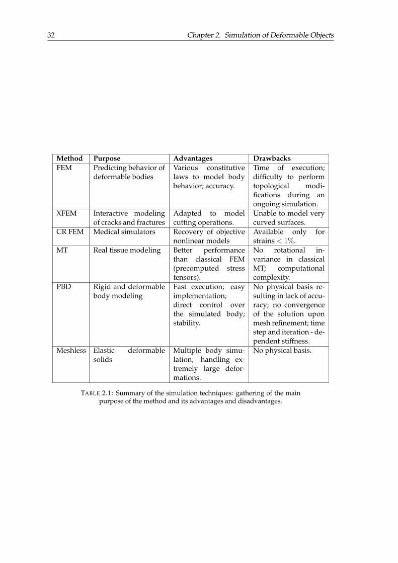
32 Chapter 2. Simulation of Deformable Objects
Method Purpose Advantages DrawbacksFEM Predicting behavior of
deformable bodiesVarious constitutivelaws to model bodybehavior; accuracy.
Time of execution;difficulty to performtopological modi-fications during anongoing simulation.
XFEM Interactive modelingof cracks and fractures
Adapted to modelcutting operations.
Unable to model verycurved surfaces.
CR FEM Medical simulators Recovery of objectivenonlinear models
Available only forstrains < 1%.
MT Real tissue modeling Better performancethan classical FEM(precomputed stresstensors).
No rotational in-variance in classicalMT; computationalcomplexity.
PBD Rigid and deformablebody modeling
Fast execution; easyimplementation;direct control overthe simulated body;stability.
No physical basis re-sulting in lack of accu-racy; no convergenceof the solution uponmesh refinement; timestep and iteration - de-pendent stiffness.
Meshless Elastic deformablesolids
Multiple body simu-lation; handling ex-tremely large defor-mations.
No physical basis.
TABLE 2.1: Summary of the simulation techniques: gathering of the mainpurpose of the method and its advantages and disadvantages.
2.4. Conclusions 33
so the use of this technique is limited mainly to the gaming environment.
There are more and more methods being more flexible and adjustable, but a fullygeneric method, which allows real-time simulation and offers accuracy of modeling com-plex materials, still doesn’t exist. For the reasons mentioned above we decided to turn ourattention to yet another simulation technique with interesting development and applica-tion history: Mass-Spring System (MSS). In the process of studying the MSS simulationtechnique we chose to use FEM as an accurate method to compare our proposed contri-butions with alongside with any available analytical, physically-based results. In the nextchapter we present in detail the MSS method and the related research.
2.4 Conclusions
In this chapter we introduced the basic notions of the mechanics including the continuummechanics and well known integration schemes, which built a basis for understandingthe existing simulation techniques. The pros and cons of these integration schemes makeit easier to meet requirements of a simulation, where the stability and size of a time stepplay the biggest role.
After that we have presented the most known simulation methods used to modeldeformable bodies in general and we have discussed their application in the computergraphics field. Among them we want to highlight the FEM method as one used mostcommonly for medical simulation where the accuracy and application of variety of phys-ical laws in form of constitutive functions are the most important.
We have also shown that in the topic of deformable body simulation there are variousways to deal with the problems posed by the physical parameters of soft tissues. Theexisting techniques are adapted for specific use by every research work to create a widerange on simulation methods to choose from, each being able to model different types ofbehavior, material and phenomena.
In the next chapter we want to look closer at Mass-Spring System - our simulationmethod chosen to deal with the real time simulation of soft tissues. We present in detailwhat MSS challenges us with and how it can be used to serve our purpose of applicationto medical simulation best.

35
Chapter 3
Mass Spring System (MSS)
Mass Spring System (MSS) is a fairly simple and intuitive model, incorporating our knowl-edge about physical laws based on the continuum mechanics into uncomplicated systemof point-masses interconnected by springs. It discretizes complex shapes into sets of par-ticles connected together by a set of springs. The behavior of MSS is then evaluated asinteractions between the particles modeled by the springs. Then a simulation loop (pre-sented in Ch. 2.2) is used to find new positions of the particles due to the springs’ andexternal forces. The relation of the acceleration of point-masses to the reacting springforces is used for this purpose. The local deformations of springs result then in the globaldeformation of the object.
Despite some limitations of the model coming usually from its simplicity (which wediscuss in this section further on), MSS are widely used in computer graphics for sim-ulation of clothes [25, 76] or deformable solids [151, 156]. Indeed, the MSS is easy toimplement, provides simple calculations and easily incorporates any topological modi-fications. MSS is also eagerly used for simulation of soft tissues and has been adaptedlately for virtual surgery simulation as a real-time performing model.
Due to all the interests, in this chapter we present the detailed structure of classicalMSS. We give the formulation of the interaction forces, which comes from the deforma-tion of springs, and is evaluated by the classical simulation loop based on the Newtoniandynamics. Then we discuss the natural MSS limitations and instabilities. We continue bypresenting different types of lattice and topologies used for simulation. We discuss howto correctly construct a MSS using particles and springs of particular properties. Fur-ther on we talk about the methods for acquisition of MSS parameters like mass, stiffnessand damping. We follow by the topic of constraining MSS behavior e.g. ensuring cor-rect volume behavior or volume conservation. In the next sections we talk about MSSnon-linearity and topological modifications of MSS lattice. At the end, we present ourframework for MSS simulation suitable for topological modifications during simulation:its structure, some improvements and implementation details.
36 Chapter 3. Mass Spring System (MSS)
3.1 Classical MSS
To use a classical MSS to simulate the elastic behavior of a soft body, we first have todiscretize it in a set of particles pi, with i ∈ N, of mass mi, which are connected to oneanother by springs of a stiffness constant k and initial length l0. Then the deformation ofthe springs gives us the deformation of the object. The length of a spring at an elongationδ is then noted l = l0 + δ. Knowing this, we can define the energy of a spring deformationas:
Wspring(δ) =1
2k(l − l0)2 =
1
2kδ2 (3.1)
and the force due to this deformation as:
Fspring(δ) = −∂Wspring(δ)
∂δ= −k(l0 − l) = −kδ (3.2)
In case of a single spring connecting particles pi and pj , when a damping d is incor-porated into the MSS, the force of a deformed spring with stiffness kij is then redefinedto:
Fij(δ) = −kijδ − d(vj − vi), (3.3)
with vi and vj being relatively the velocities of particles pi, pj .
3.2 MSS Instabilities and Natural Limitations
In this part we present the limitations and natural instabilities of MSS. We present theinstances in which they occur and discuss the existing methods used to deal with them.To do that we focus on a MSS formed by a lattice of cubical elements. Each cubical ele-ment is composed of 8 particles placed at the vertices. Then Baudet and Zhao [12, 170]have suggested to link these particles together with springs placed on the 12 edges of anelement and by springs placed on the 4 inner diagonals of an element.
3.2.1 Natural Limitation of the Poisson Ratio
Let us consider a material with V0 and V being respectively its initial and current volume.
Linear Assumption
Due to the use of linear springs, the mechanical behavior of the material is linear andfollows Hooke’s law with a linear relationship [96] between the stress σ applied on thematerial and resulting strain ε with the relation defined in Sec. 2.3 Eq. (2.6). For smalldeformations, we can use the linearized strain tensor of Green-Lagrange (Eq. (2.8)). Fur-thermore, the stress tensor σ represents the quantity conjugate to the deformation ε in thesense that, when ε varies by dε, the change of energy per unit volume is dW = σij dεij .Therefore the expression of the tensor stress is also given by:
σij =∂W
∂εij. (3.4)
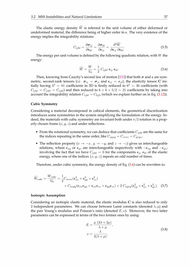
3.2. MSS Instabilities and Natural Limitations 37
The elastic energy density W is referred to the unit volume of either deformed orundeformed material, the difference being of higher order in ε. The very existence of theenergy implies the integrability relations:
Cijkl =∂σij∂εkl
=∂σkl∂εij
=∂2W
∂εij ∂εkl. (3.5)
The energy per unit volume is defined by the following quadratic relation, withW theenergy:
W =W
V0=
1
2Cijkl εij εkl. (3.6)
Then, knowing from Cauchy’s second law of motion [153] that both σ and ε are sym-metric, second-rank tensors (i.e. σij = σji and εij = εji), the elasticity tensor C ini-tially having 34 = 81 coefficients in 3D is firstly reduced to 62 = 36 coefficients (withCijkl = Cjikl = Cijlk) and then reduced to 6 + 6 × 5/2 = 21 coefficients by taking intoaccount the integrability relation Cijkl = Ckjli (which we explain further on in Eq. (3.12)).
Cubic Symmetry
Considering a material decomposed in cubical elements, the geometrical discretizationintroduces some symmetries in the system simplifying the formulation of the energy. In-deed, the materials with cubic symmetry are invariant both under π/2 rotation in a prop-erly chosen frame (x, y, z) and under reflections.
• From the rotational symmetry, we can deduce that coefficients Cijkl are the same forthe indices repeating in the same order, like Cxyxy = Cxzxz = Cyzyz .
• The reflection property (x → −x, y → −y, and z → −z) gives us interchangeablerelations, where εxy or εyz are interchangeable respectively with −εxy and −εyz ;involving the fact that we have Cijkl = 0 for the components εij εkl of the elasticenergy, where one of the indices x, y, z repeats an odd number of times.
Therefore, under cubic symmetry, the energy density of Eq. (3.6) can be rewritten to:
Wcube =Wcube
V0=
1
2Cxxxx(ε2
xx + ε2yy + ε2
zz)
+ Cxxyy(εxxεyy + εxxεzz + εyyεzz) + 2 Cxyxy(ε2xy + ε2
xz + ε2yz). (3.7)
Isotropic Assumption
Considering an isotropic elastic material, the elastic modulus C is also reduced to only2 independent parameters. We can choose between Lamé constants (denoted λ, µ) andthe pair Young’s modulus and Poisson’s ratio (denoted E, ν). Moreover, the two latterparameters can be expressed in terms of the two former ones by using:
E =µ (3λ+ 2µ)
λ+ µ,
ν =λ
2(λ+ µ).
(3.8)
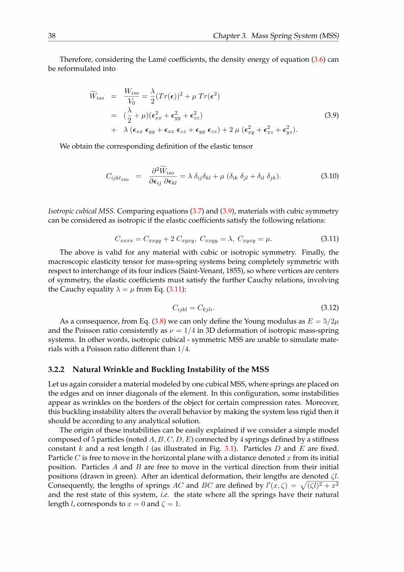
38 Chapter 3. Mass Spring System (MSS)
Therefore, considering the Lamé coefficients, the density energy of equation (3.6) canbe reformulated into
Wiso =Wiso
V0=λ
2(Tr(ε))2 + µ Tr(ε2)
= (λ
2+ µ)(ε2
xx + ε2yy + ε2
zz) (3.9)
+ λ (εxx εyy + εxx εzz + εyy εzz) + 2 µ (ε2xy + ε2
xz + ε2yz).
We obtain the corresponding definition of the elastic tensor
Cijkliso =∂2Wiso
∂εij ∂εkl= λ δijδkl + µ (δik δjl + δil δjk). (3.10)
Isotropic cubical MSS. Comparing equations (3.7) and (3.9), materials with cubic symmetrycan be considered as isotropic if the elastic coefficients satisfy the following relations:
Cxxxx = Cxxyy + 2 Cxyxy, Cxxyy = λ, Cxyxy = µ. (3.11)
The above is valid for any material with cubic or isotropic symmetry. Finally, themacroscopic elasticity tensor for mass-spring systems being completely symmetric withrespect to interchange of its four indices (Saint-Venant, 1855), so where vertices are centersof symmetry, the elastic coefficients must satisfy the further Cauchy relations, involvingthe Cauchy equality λ = µ from Eq. (3.11):
Cijkl = Ckjli. (3.12)
As a consequence, from Eq. (3.8) we can only define the Young modulus as E = 5/2µand the Poisson ratio consistently as ν = 1/4 in 3D deformation of isotropic mass-springsystems. In other words, isotropic cubical - symmetric MSS are unable to simulate mate-rials with a Poisson ratio different than 1/4.
3.2.2 Natural Wrinkle and Buckling Instability of the MSS
Let us again consider a material modeled by one cubical MSS, where springs are placed onthe edges and on inner diagonals of the element. In this configuration, some instabilitiesappear as wrinkles on the borders of the object for certain compression rates. Moreover,this buckling instability alters the overall behavior by making the system less rigid then itshould be according to any analytical solution.
The origin of these instabilities can be easily explained if we consider a simple modelcomposed of 5 particles (notedA,B,C,D,E) connected by 4 springs defined by a stiffnessconstant k and a rest length l (as illustrated in Fig. 3.1). Particles D and E are fixed.Particle C is free to move in the horizontal plane with a distance denoted x from its initialposition. Particles A and B are free to move in the vertical direction from their initialpositions (drawn in green). After an identical deformation, their lengths are denoted ζl.Consequently, the lengths of springs AC and BC are defined by l′(x, ζ) =
√(ζl)2 + x2
and the rest state of this system, i.e. the state where all the springs have their naturallength l, corresponds to x = 0 and ζ = 1.
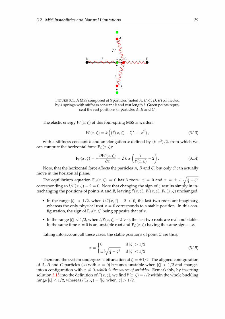
3.2. MSS Instabilities and Natural Limitations 39
FIGURE 3.1: A MSS composed of 5 particles (notedA,B,C,D,E) connectedby 4 springs with stiffness constant k and rest length l. Green points repre-
sent the rest positions of particles A, B and C.
The elastic energy W (x, ζ) of this four-spring MSS is written:
W (x, ζ) = k((l′(x, ζ)− l
)2+ x2
), (3.13)
with a stiffness constant k and an elongation x defined by (k x2)/2, from which wecan compute the horizontal force FC(x, ζ):
FC(x, ζ) = −∂W (x, ζ)
∂x= 2 k x
(l
l′(x, ζ)− 2
). (3.14)
Note, that the horizontal force affects the particles A, B and C, but only C can actuallymove in the horizontal plane.
The equilibrium equation FC(x, ζ) = 0 has 3 roots: x = 0 and x = ± l√
14 − ζ2
corresponding to l/l′(x, ζ) − 2 = 0. Note that changing the sign of ζ results simply in in-terchanging the positions of points A and B, leaving l′(x, ζ), W (x, ζ), FC(x, ζ) unchanged.
• In the range |ζ| > 1/2, when l/l′(x, ζ) − 2 < 0, the last two roots are imaginary,whereas the only physical root x = 0 corresponds to a stable position. In this con-figuration, the sign of FC(x, ζ) being opposite that of x.
• In the range |ζ| < 1/2, when l/l′(x, ζ)− 2 > 0, the last two roots are real and stable.In the same time x = 0 is an unstable root and FC(x, ζ) having the same sign as x.
Taking into account all these cases, the stable positions of point C are thus:
x =
0 if |ζ| > 1/2
±l√
14 − ζ2 if |ζ| < 1/2
(3.15)
Therefore the system undergoes a bifurcation at ζ = ±1/2. The aligned configurationof A, B and C particles (so with x = 0) becomes unstable when |ζ| < 1/2 and changesinto a configuration with x 6= 0, which is the source of wrinkles. Remarkably, by insertingsolution 3.15 into the definition of l′(x, ζ), we find l′(x, ζ) = l/2 within the whole bucklingrange |ζ| < 1/2, whereas l′(x, ζ) = l|ζ|when |ζ| > 1/2.
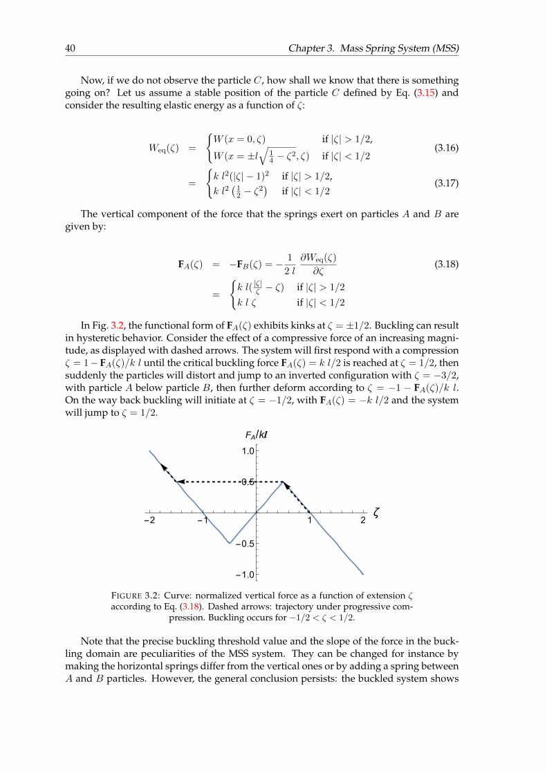
40 Chapter 3. Mass Spring System (MSS)
Now, if we do not observe the particle C, how shall we know that there is somethinggoing on? Let us assume a stable position of the particle C defined by Eq. (3.15) andconsider the resulting elastic energy as a function of ζ:
Weq(ζ) =
W (x = 0, ζ) if |ζ| > 1/2,
W (x = ±l√
14 − ζ2, ζ) if |ζ| < 1/2
(3.16)
=
k l2(|ζ| − 1)2 if |ζ| > 1/2,k l2
(12 − ζ
2)
if |ζ| < 1/2(3.17)
The vertical component of the force that the springs exert on particles A and B aregiven by:
FA(ζ) = −FB(ζ) = − 1
2 l
∂Weq(ζ)
∂ζ(3.18)
=
k l( |ζ|ζ − ζ) if |ζ| > 1/2
k l ζ if |ζ| < 1/2
In Fig. 3.2, the functional form of FA(ζ) exhibits kinks at ζ = ±1/2. Buckling can resultin hysteretic behavior. Consider the effect of a compressive force of an increasing magni-tude, as displayed with dashed arrows. The system will first respond with a compressionζ = 1− FA(ζ)/k l until the critical buckling force FA(ζ) = k l/2 is reached at ζ = 1/2, thensuddenly the particles will distort and jump to an inverted configuration with ζ = −3/2,with particle A below particle B, then further deform according to ζ = −1 − FA(ζ)/k l.On the way back buckling will initiate at ζ = −1/2, with FA(ζ) = −k l/2 and the systemwill jump to ζ = 1/2.
-2 -1 1 2ζ
-1.0
-0.5
0.5
1.0
FA/kl
FIGURE 3.2: Curve: normalized vertical force as a function of extension ζaccording to Eq. (3.18). Dashed arrows: trajectory under progressive com-
pression. Buckling occurs for −1/2 < ζ < 1/2.
Note that the precise buckling threshold value and the slope of the force in the buck-ling domain are peculiarities of the MSS system. They can be changed for instance bymaking the horizontal springs differ from the vertical ones or by adding a spring betweenA and B particles. However, the general conclusion persists: the buckled system shows
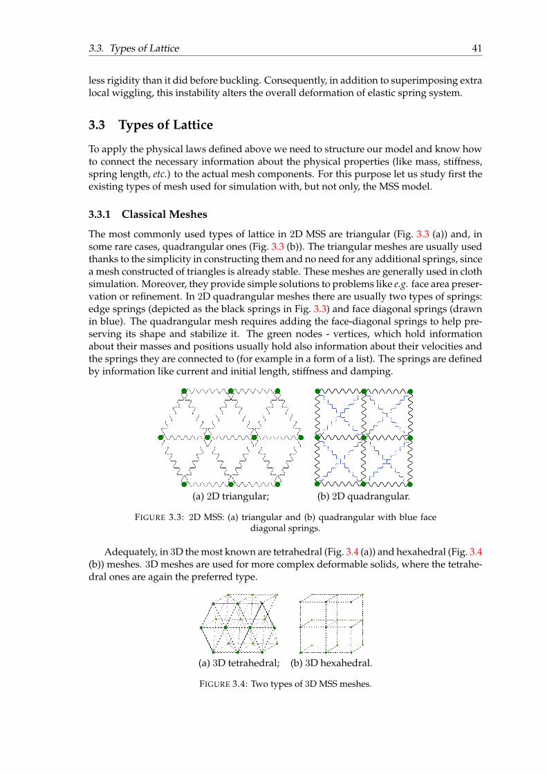
3.3. Types of Lattice 41
less rigidity than it did before buckling. Consequently, in addition to superimposing extralocal wiggling, this instability alters the overall deformation of elastic spring system.
3.3 Types of Lattice
To apply the physical laws defined above we need to structure our model and know howto connect the necessary information about the physical properties (like mass, stiffness,spring length, etc.) to the actual mesh components. For this purpose let us study first theexisting types of mesh used for simulation with, but not only, the MSS model.
3.3.1 Classical Meshes
The most commonly used types of lattice in 2D MSS are triangular (Fig. 3.3 (a)) and, insome rare cases, quadrangular ones (Fig. 3.3 (b)). The triangular meshes are usually usedthanks to the simplicity in constructing them and no need for any additional springs, sincea mesh constructed of triangles is already stable. These meshes are generally used in clothsimulation. Moreover, they provide simple solutions to problems like e.g. face area preser-vation or refinement. In 2D quadrangular meshes there are usually two types of springs:edge springs (depicted as the black springs in Fig. 3.3) and face diagonal springs (drawnin blue). The quadrangular mesh requires adding the face-diagonal springs to help pre-serving its shape and stabilize it. The green nodes - vertices, which hold informationabout their masses and positions usually hold also information about their velocities andthe springs they are connected to (for example in a form of a list). The springs are definedby information like current and initial length, stiffness and damping.
(a) 2D triangular; (b) 2D quadrangular.
FIGURE 3.3: 2D MSS: (a) triangular and (b) quadrangular with blue facediagonal springs.
Adequately, in 3D the most known are tetrahedral (Fig. 3.4 (a)) and hexahedral (Fig. 3.4(b)) meshes. 3D meshes are used for more complex deformable solids, where the tetrahe-dral ones are again the preferred type.
(a) 3D tetrahedral; (b) 3D hexahedral.
FIGURE 3.4: Two types of 3D MSS meshes.
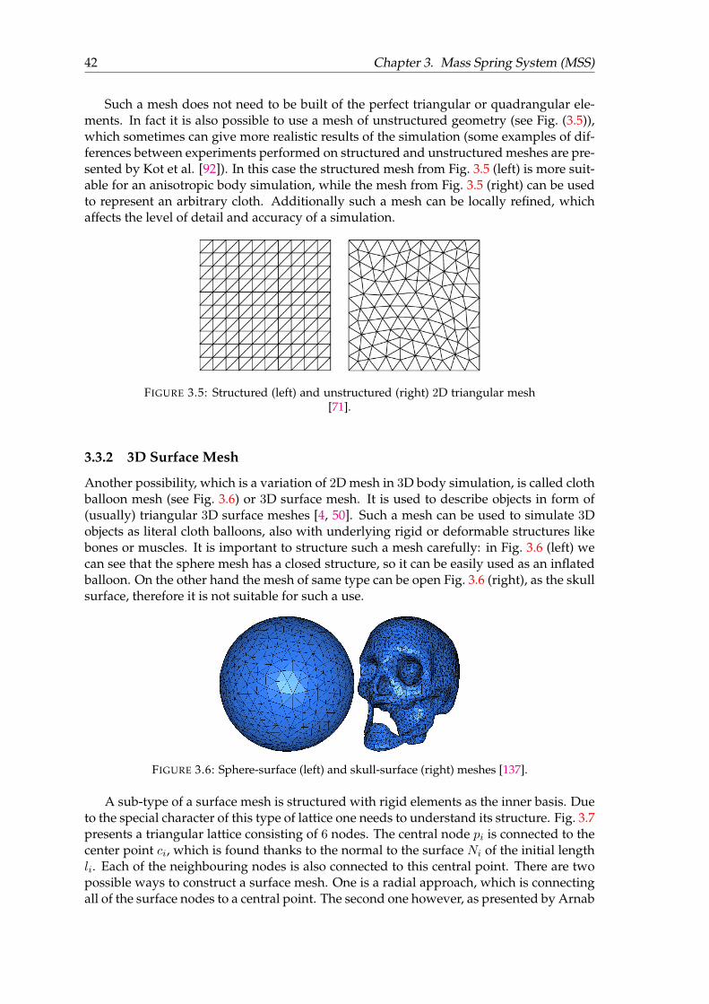
42 Chapter 3. Mass Spring System (MSS)
Such a mesh does not need to be built of the perfect triangular or quadrangular ele-ments. In fact it is also possible to use a mesh of unstructured geometry (see Fig. (3.5)),which sometimes can give more realistic results of the simulation (some examples of dif-ferences between experiments performed on structured and unstructured meshes are pre-sented by Kot et al. [92]). In this case the structured mesh from Fig. 3.5 (left) is more suit-able for an anisotropic body simulation, while the mesh from Fig. 3.5 (right) can be usedto represent an arbitrary cloth. Additionally such a mesh can be locally refined, whichaffects the level of detail and accuracy of a simulation.
FIGURE 3.5: Structured (left) and unstructured (right) 2D triangular mesh[71].
3.3.2 3D Surface Mesh
Another possibility, which is a variation of 2D mesh in 3D body simulation, is called clothballoon mesh (see Fig. 3.6) or 3D surface mesh. It is used to describe objects in form of(usually) triangular 3D surface meshes [4, 50]. Such a mesh can be used to simulate 3Dobjects as literal cloth balloons, also with underlying rigid or deformable structures likebones or muscles. It is important to structure such a mesh carefully: in Fig. 3.6 (left) wecan see that the sphere mesh has a closed structure, so it can be easily used as an inflatedballoon. On the other hand the mesh of same type can be open Fig. 3.6 (right), as the skullsurface, therefore it is not suitable for such a use.
FIGURE 3.6: Sphere-surface (left) and skull-surface (right) meshes [137].
A sub-type of a surface mesh is structured with rigid elements as the inner basis. Dueto the special character of this type of lattice one needs to understand its structure. Fig. 3.7presents a triangular lattice consisting of 6 nodes. The central node pi is connected to thecenter point ci, which is found thanks to the normal to the surface Ni of the initial lengthli. Each of the neighbouring nodes is also connected to this central point. There are twopossible ways to construct a surface mesh. One is a radial approach, which is connectingall of the surface nodes to a central point. The second one however, as presented by Arnab
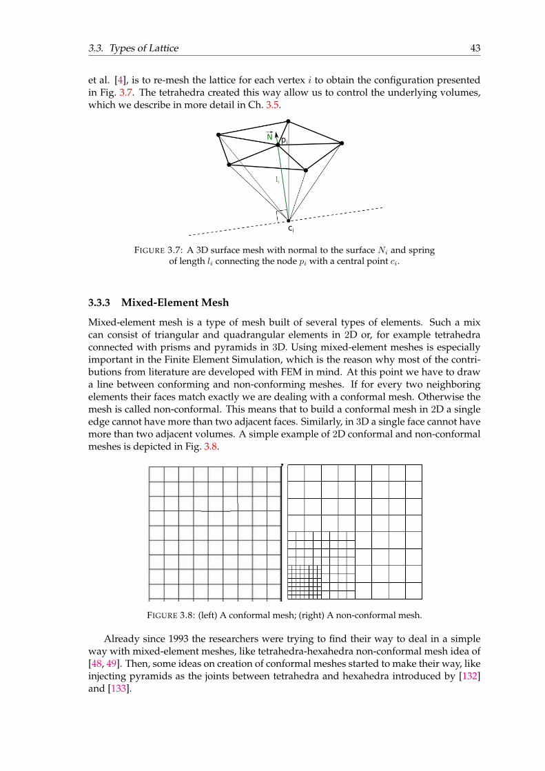
3.3. Types of Lattice 43
et al. [4], is to re-mesh the lattice for each vertex i to obtain the configuration presentedin Fig. 3.7. The tetrahedra created this way allow us to control the underlying volumes,which we describe in more detail in Ch. 3.5.
FIGURE 3.7: A 3D surface mesh with normal to the surface Ni and springof length li connecting the node pi with a central point ci.
3.3.3 Mixed-Element Mesh
Mixed-element mesh is a type of mesh built of several types of elements. Such a mixcan consist of triangular and quadrangular elements in 2D or, for example tetrahedraconnected with prisms and pyramids in 3D. Using mixed-element meshes is especiallyimportant in the Finite Element Simulation, which is the reason why most of the contri-butions from literature are developed with FEM in mind. At this point we have to drawa line between conforming and non-conforming meshes. If for every two neighboringelements their faces match exactly we are dealing with a conformal mesh. Otherwise themesh is called non-conformal. This means that to build a conformal mesh in 2D a singleedge cannot have more than two adjacent faces. Similarly, in 3D a single face cannot havemore than two adjacent volumes. A simple example of 2D conformal and non-conformalmeshes is depicted in Fig. 3.8.
FIGURE 3.8: (left) A conformal mesh; (right) A non-conformal mesh.
Already since 1993 the researchers were trying to find their way to deal in a simpleway with mixed-element meshes, like tetrahedra-hexahedra non-conformal mesh idea of[48, 49]. Then, some ideas on creation of conformal meshes started to make their way, likeinjecting pyramids as the joints between tetrahedra and hexahedra introduced by [132]and [133].
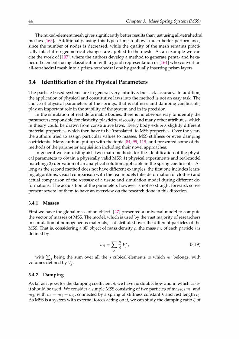
44 Chapter 3. Mass Spring System (MSS)
The mixed-element mesh gives significantly better results than just using all-tetrahedralmeshes [165]. Additionally, using this type of mesh allows much better performance,since the number of nodes is decreased, while the quality of the mesh remains practi-cally intact if no geometrical changes are applied to the mesh. As an example we cancite the work of [107], where the authors develop a method to generate penta- and hexa-hedral elements using classification with a graph representation or [164] who convert anall-tetrahedral mesh into a prism-tetrahedral one by gradually inserting prism layers.
3.4 Identification of the Physical Parameters
The particle-based systems are in general very intuitive, but lack accuracy. In addition,the application of physical and constitutive laws into the method is not an easy task. Thechoice of physical parameters of the springs, that is stiffness and damping coefficients,play an important role in the stability of the system and in its precision.
In the simulation of real deformable bodies, there is no obvious way to identify theparameters responsible for elasticity, plasticity, viscosity and many other attributes, whichin theory could be drawn from constitutive laws. Every body exhibits slightly differentmaterial properties, which then have to be ’translated’ to MSS properties. Over the yearsthe authors tried to assign particular values to masses, MSS stiffness or even dampingcoefficients. Many authors put up with the topic [84, 99, 119] and presented some of themethods of the parameter acquisition including their novel approaches.
In general we can distinguish two main methods for the identification of the physi-cal parameters to obtain a physically valid MSS: 1) physical experiments and real-modelmatching; 2) derivation of an analytical solution applicable in the spring coefficients. Aslong as the second method does not have different examples, the first one includes learn-ing algorithms, visual comparison with the real models (like deformation of clothes) andactual comparison of the response of a tissue and simulation model during different de-formations. The acquisition of the parameters however is not so straight forward, so wepresent several of them to have an overview on the research done in this direction.
3.4.1 Masses
First we have the global mass of an object. [47] presented a universal model to computethe vector of masses of MSS. The model, which is used by the vast majority of researchersin simulation of homogeneous materials, is distributed over the different particles of theMSS. That is, considering a 3D object of mass density ρ, the mass mi of each particle i isdefined by
mi =∑j
ρ
8V cj , (3.19)
with∑
j being the sum over all the j cubical elements to which mi belongs, withvolumes defined by V c
j .
3.4.2 Damping
As far as it goes for the damping coefficient d, we have no doubts how and in which casesit should be used. We consider a simple MSS consisting of two particles of masses m1 andm2, with m = m1 + m2, connected by a spring of stiffness constant k and rest length l0.As MSS is a system with external forces acting on it, we can study the damping ratio ζ of
3.4. Identification of the Physical Parameters 45
complex oscillations within the springs [22]. In that regard MSS can be undamped (ζ = 0)or damped in one of the three following ways:
• underdamped - the system is decaying exponentially with oscillation at time t of a
form exp(i√
km(1− ζ2)t), where ζ < 1 and i =
√−1; in this case we have: 0 < ζ < 1;
• overdamped - the system is decaying exponentially with no oscillation, with ζ > 1;
• critically damped - the system goes to its equilibrium state as fast as possible with-out any oscillations. Such a behavior is possible when ζ = 1, with the correspondingcritical damping coefficient d = 2
√km
Usually it is the critical damping used in the MSS to avoid unnecessary oscillationsand naturally damp the system as fast as possible. However it can be also adjusted (byscaling it with use of the spring length l0) to handle the same amplitude of oscillations fordifferent mesh resolutions [134, 167]:
d = 2
√k(m1 +m2)
l0. (3.20)
3.4.3 Stiffness
To obtain the stiffness for a simulation of deformable bodies there are generally two ap-proaches: data driven parameter identification and analytical solution based on physicalbody properties or a constitutive law. Let us present several methods used for this pur-pose.
Data Driven Parameter Identification
The data-driven approach is to adjust the spring parameters according to some previouslyacquired set of physical or theoretical data. These information can be, and very often are,taken from visual aids, like videos of body deformation. Having such sets of the goal datait is easier to adjust the MSS accordingly and find the optimal parameters. This methodwas eagerly used by Louchet et al., who introduced visual comparison combined withevolutionary genetic strategy [101]. The goal was to model isotropic, homogeneous cloth,which consisted of 6 types of springs, each described by 3 parameters, but simplified to 5parameters for the fabrics: spring stiffness, elongation rate, and 3 pairs of natural lengths.
A genetic algorithm was used by Joukhadar et al., who tried to determine the physicalparameters such as viscosity, elasticity or plasticity to describe the object for a dynamicsimulation [84]. The MSS used by the authors is built of tetrahedral 3D mesh.
Bianchi et al. in turn used genetic algorithm to teach their MSS the correct behavior byassigning correct stiffness value to the springs [20, 19]. First article was focused on the 2Dmodel, but the second one extended the method to 3D. The reference model was linearelastic Finite Element Method. The model was supposed to learn the correct behavior tosimulate soft tissues as a linear elastic material. What is interesting, the authors shownthat the parameter distribution in MSS has to be non-homogeneous to model this type ofbody.
In the cloth simulation, Bhat et al. presented a method to obtain the parameters ofdifferent fabrics (like linen, satin or knit) based on some video samples [18]. A simulatedannealing method was used to compare the simulation and video data and to optimizethe triangular 2D MSS by studying the folds of the material.
46 Chapter 3. Mass Spring System (MSS)
Previously mentioned Deussen et al. used a theoretical elastic model as a basis for thecomparison and parameter identification [47]. Again, an optimized simulated annealingis used to obtain elastic parameters of the MSS. Instead of obtaining the parameters di-rectly, the behavior of MSS is being optimized over time to obtain the best results of thesimulation.
Da Silva et al. presented a method based on the data-driven strategy comparing themodel’s acceleration to have similar behavior of the MSS and the reference model [144].The derivation of the parameters is divided into several elements: solving the optimiza-tion to compute the stiffness parameters, compute the masses and the damping.
San-Vincente et al. studied the cubical MSS with 3 types of springs (edge, inner andface diagonal) and based their parametrization approach on a tensile test and a non-linearmaterial model [141]. On top of the derived model they decided to add an objectivefunction to optimize the model’s parameters but fitting the curve with respect to somereference data, therefore obtaining particular stiffness values for particular experimentcases. They used Neo-Hookean, Mooney-Rivlin, Yeoh, and Ogden models, usually usedto model non-linear behavior of rubber-like materials or soft tissues.
Data driven approach is generally well optimized for a particular type of body in a pre-defined simulation environment and under specific circumstances. Such a setup largelylimits the possibilities of simulation, especially if anything shall change in the modeledenvironment. Unless we want to be limited to such a narrow use of the simulation tool,we need to reach for more generic method which takes into account the physically-basedanalytical behavior.
Analytical Solutions
Since the soft bodies have particular properties, like elasticity, viscosity, etc., some authorsdecided to derive the parameters of MSS from the theoretical laws governing these bodyproperties. Some of them are based on theoretical laws, some use simplified approxi-mations and some draw inspiration directly from the Finite Element approach. Let uspresent the existing methods in a form of a table (Tab. 3.1) and a corresponding list whichdescribes the presented approaches. The table structure allows us to verify the exact for-mulas, types of simulated tissue and the physical basis on which these were derived. Inthe second column we listed the authors of the related articles, then the formulations ofstiffness followed by the properties of the simulated material. In the last column we notethe type of derivation the presented formulas are based on.
1. One of the first attempts in MSS parametrization was done by Wilhelms and VanGelder [160]. The elastic membrane model which they used divided the structure ofMSS into two components: skin MSS and underlying structures MSS (bones - rigidMSS; muscles - deformable MSS). The stiffness k of a skin spring, which belongs totwo neighbouring triangles was defined with their respective surface areas A1 andA2. The second type of springs was used to connect the skin and the virtual anchorand its stiffness was denoted ka. Its rest length was l0 = 0, but its stiffness, whichwas summed over the i incident triangles, was also multiplied by a proportionalityconstant coefficient c to allow ’sliding’ of the skin mesh on the bones and muscles.
2. A year after that Gelder et al. decided to derive an approximation of the stiffnessbased on the geometry of a mesh [64]. Their formulation evolves around the elastic-ity law and incorporates Young’s modulus E and Poisson’s ratio ν into the model.
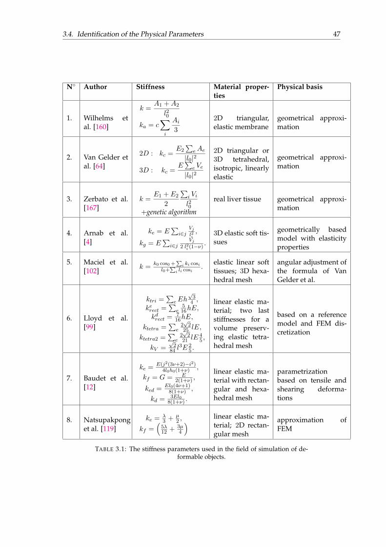
3.4. Identification of the Physical Parameters 47
N Author Stiffness Material proper-ties
Physical basis
1. Wilhelms etal. [160]
k =A1 +A2
l20
ka = c∑i
Ai3
2D triangular,elastic membrane
geometrical approxi-mation
2. Van Gelder etal. [64]
2D : kc =E2∑
eAe|l0|2
3D : kc =E∑
e Ve|l0|2
2D triangular or3D tetrahedral,isotropic, linearlyelastic
geometrical approxi-mation
3. Zerbato et al.[167]
k =E1 + E2
2
∑i Vil20
+genetic algorithm
real liver tissue geometrical approxi-mation
4. Arnab et al.[4]
ke = E∑
i∈jVjl2i,
kg = E∑
i∈jVj
2 l2i (1−ν).
3D elastic soft tis-sues
geometrically basedmodel with elasticityproperties
5. Maciel et al.[102]
k =k0 cos0 +
∑i ki cosi
l0+∑
i li cosi.
elastic linear softtissues; 3D hexa-hedral mesh
angular adjustment ofthe formula of VanGelder et al.
6. Lloyd et al.[99]
ktri =∑
eEh√
34 ,
kerect =∑
e516hE,
kdrect = 716hE,
ktetra =∑
e2√
225 lE,
ktetra2 =∑
e2√
221 lE
45 ,
kV =√
284 l
3E 25 .
linear elastic ma-terial; two laststiffnesses for avolume preserv-ing elastic tetra-hedral mesh
based on a referencemodel and FEM dis-cretization
7. Baudet et al.[12]
ke = E(j2(3ν+2)−i2)4l0h0(1+ν) ,
kf = G = E2(1+ν) ,
ked = El0(4ν+1)8(1+ν) ,
kd = 3El08(1+ν) .
linear elastic ma-terial with rectan-gular and hexa-hedral mesh
parametrizationbased on tensile andshearing deforma-tions
8. Natsupakponget al. [119]
ke = λ3 + µ
2 ,
kf =(
5λ12 + 3µ
4
) linear elastic ma-terial; 2D rectan-gular mesh
approximation ofFEM
TABLE 3.1: The stiffness parameters used in the field of simulation of de-formable objects.
48 Chapter 3. Mass Spring System (MSS)
The formula presented in Tab. 3.1 is a simplified version of a more expansive form,which states for a spring c:
kc =
(E2
1 + ν
)Ae|lc|2
+
(E2ν
1− ν2
)|la|2 + |lb|2 − |lc|2
8Ae. (3.21)
In this equation E2 = Eh is a parameter defined with Young’s modulus multipliedby the thickness h of a material; Ae is the area of a triangle adjacent to the springc, with a and b being the two other springs and la, lb, lc their relative lengths. Thisformulation is a general one, which can be used for triangles of any type. Howeverin their experiments the authors used ν = 0, which simplifies this equation. Theydecided to use the simple form, since they did not see any significant impact on thesimulation when ν = 1/4 was used. The results are studied only visually, so theaccuracy of this formulation was not established.
The work of Wilhelms and Van Gelder was used also by several other authors [167,4, 112]. Mollemans et al. decided to use MSS for maxillofacial surgery purposeswhere their model consists of bone and tissue nodes called respectively joint andfree points. Unlike the free points, the joint points provided an actual connectionbetween the soft tissue part and the bone structure, so they were not allowed tochange their positions.
3. The method of Zerbato et al. does not really fall into the method derived from an-alytical solution, since they used a genetic algorithm to adjust the MSS parameters,however they did use a slightly modified stiffness formula of Van Gelder et al. [64]to model their 3D tetrahedral MSS as a starting point to the simulation. In the for-mula presented in Tab. 3.1 E1 and E2 are the Young moduli of the two vertices thespring connects and Vi are the volumes of i tetrahedra incident to the spring. Aswe can see, E is simply replaced by the average of E1 and E2 terms. The differencebetween simulated and theoretical E was relatively big (about 9.49%), however themax. absolute error along different axes was measured to be of a 4 ·10−4 magnitude.
4. Arnab and Raja used a surface mesh with two stiffnesses: ke based on the linearelasticity law (Young’s modulus) and kg based on the shear modulus (G, depen-dent on the Young modulus and Poisson ratio). The formula is based on nodesi ∈ 1, ..., N (with N being the number of vertices) belonging to a triangular ele-ment j ∈ 1, ...,M (where M is the number of triangles in the surface mesh).
5. An analytical expression for stiffness of cubical meshes was introduced by Macielet al. [102]. They focused on the elastic linear behavior of a simplified MSS calledmolecular model. Their MSS mesh is built of round masses (molecules) intercon-nected by edge springs and face-diagonal springs. The computation of the springstiffness was based on the uniaxial tensile test and it depends on the angular con-figuration of the springs. The stiffness was defined for i ∈ [1; N ], where N is thenumber of connections sharing an extremity with spring k0, and cosi, which is thecosine function of the angle between spring 0 and spring i. It was based of VanGelder’s formula [64], but with the angular adjustment.
6. Lloyd et al. discussed about the previously developed approaches to identify theMSS parameters and introduced their own, more accurate and reference based methodfor symmetric triangular, rectangular and tetrahedral meshes [99]. They focused on
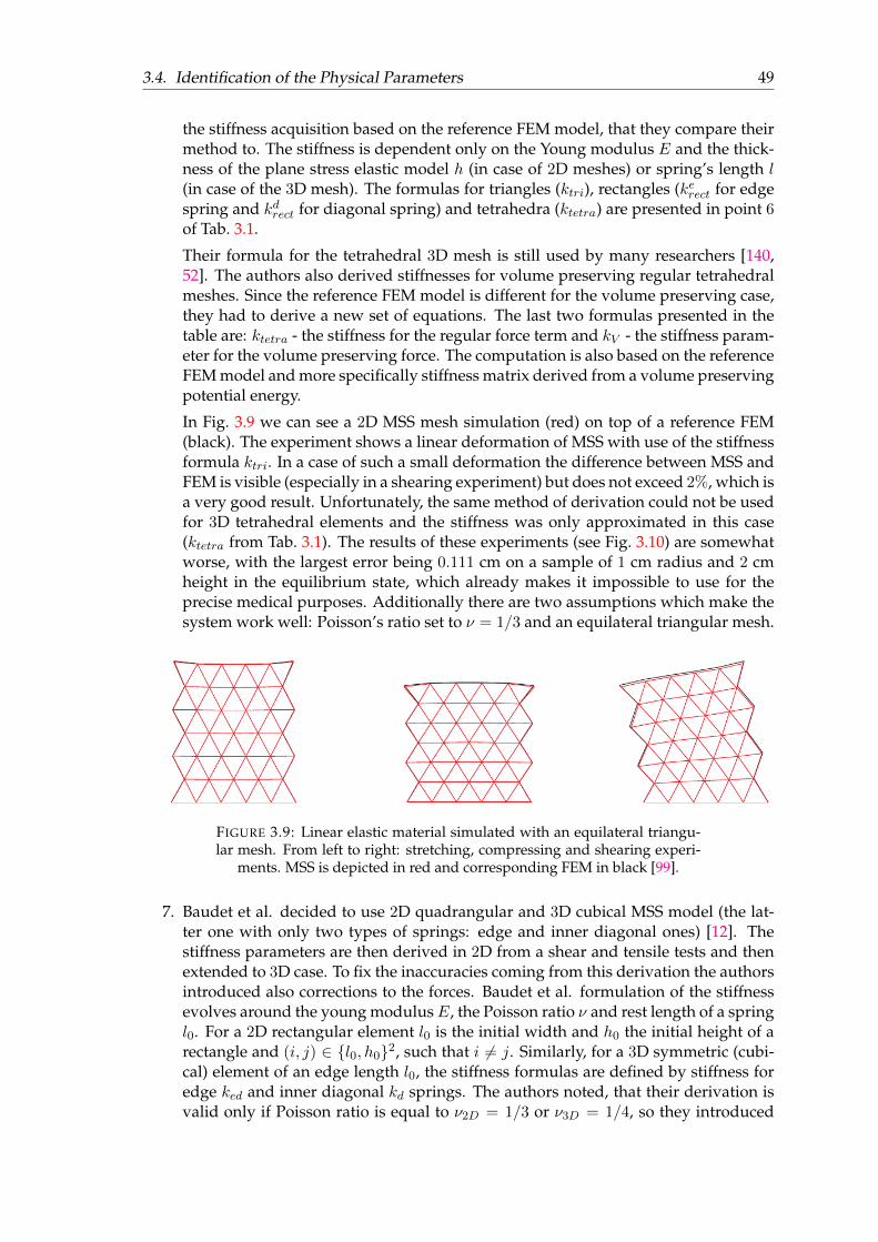
3.4. Identification of the Physical Parameters 49
the stiffness acquisition based on the reference FEM model, that they compare theirmethod to. The stiffness is dependent only on the Young modulus E and the thick-ness of the plane stress elastic model h (in case of 2D meshes) or spring’s length l(in case of the 3D mesh). The formulas for triangles (ktri), rectangles (kerect for edgespring and kdrect for diagonal spring) and tetrahedra (ktetra) are presented in point 6of Tab. 3.1.
Their formula for the tetrahedral 3D mesh is still used by many researchers [140,52]. The authors also derived stiffnesses for volume preserving regular tetrahedralmeshes. Since the reference FEM model is different for the volume preserving case,they had to derive a new set of equations. The last two formulas presented in thetable are: ktetra - the stiffness for the regular force term and kV - the stiffness param-eter for the volume preserving force. The computation is also based on the referenceFEM model and more specifically stiffness matrix derived from a volume preservingpotential energy.
In Fig. 3.9 we can see a 2D MSS mesh simulation (red) on top of a reference FEM(black). The experiment shows a linear deformation of MSS with use of the stiffnessformula ktri. In a case of such a small deformation the difference between MSS andFEM is visible (especially in a shearing experiment) but does not exceed 2%, which isa very good result. Unfortunately, the same method of derivation could not be usedfor 3D tetrahedral elements and the stiffness was only approximated in this case(ktetra from Tab. 3.1). The results of these experiments (see Fig. 3.10) are somewhatworse, with the largest error being 0.111 cm on a sample of 1 cm radius and 2 cmheight in the equilibrium state, which already makes it impossible to use for theprecise medical purposes. Additionally there are two assumptions which make thesystem work well: Poisson’s ratio set to ν = 1/3 and an equilateral triangular mesh.
FIGURE 3.9: Linear elastic material simulated with an equilateral triangu-lar mesh. From left to right: stretching, compressing and shearing experi-
ments. MSS is depicted in red and corresponding FEM in black [99].
7. Baudet et al. decided to use 2D quadrangular and 3D cubical MSS model (the lat-ter one with only two types of springs: edge and inner diagonal ones) [12]. Thestiffness parameters are then derived in 2D from a shear and tensile tests and thenextended to 3D case. To fix the inaccuracies coming from this derivation the authorsintroduced also corrections to the forces. Baudet et al. formulation of the stiffnessevolves around the young modulusE, the Poisson ratio ν and rest length of a springl0. For a 2D rectangular element l0 is the initial width and h0 the initial height of arectangle and (i, j) ∈ l0, h02, such that i 6= j. Similarly, for a 3D symmetric (cubi-cal) element of an edge length l0, the stiffness formulas are defined by stiffness foredge ked and inner diagonal kd springs. The authors noted, that their derivation isvalid only if Poisson ratio is equal to ν2D = 1/3 or ν3D = 1/4, so they introduced
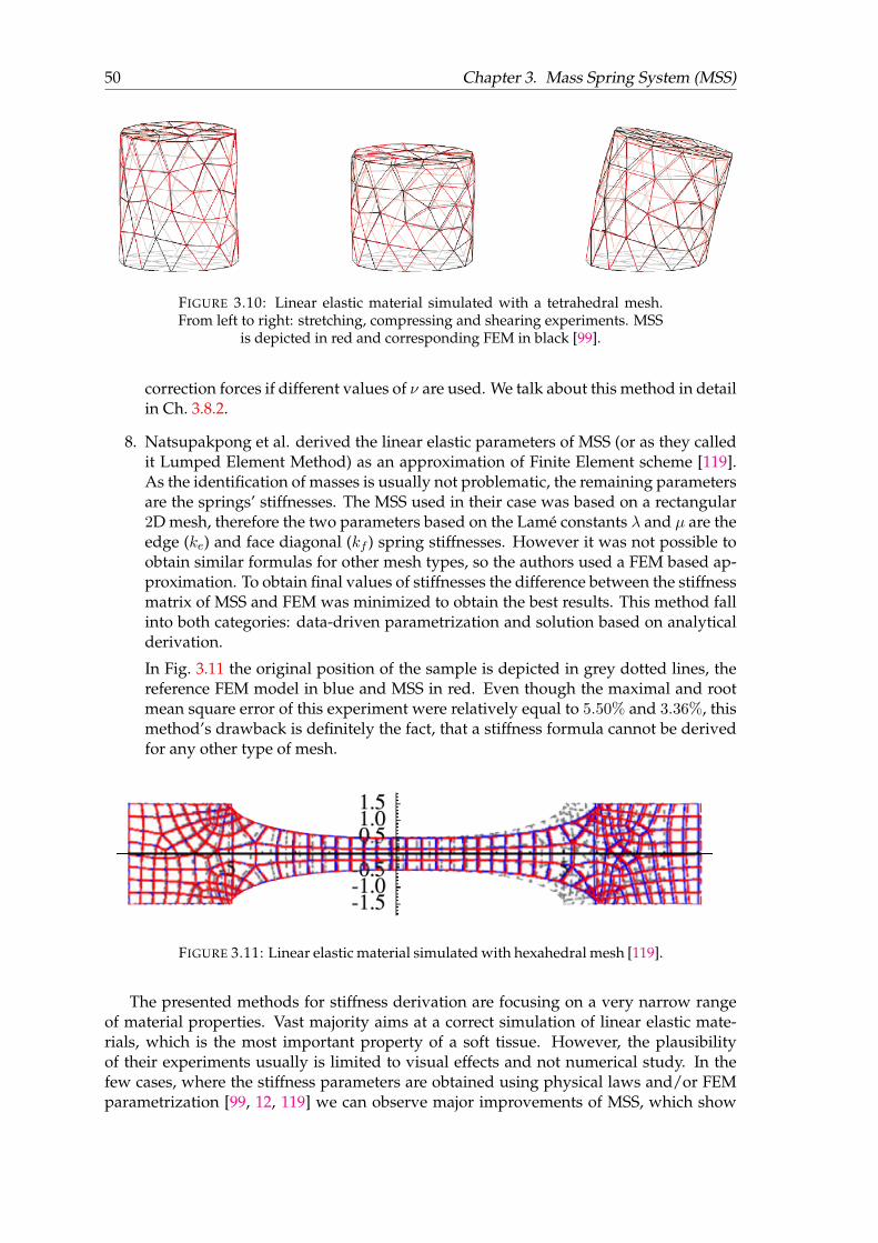
50 Chapter 3. Mass Spring System (MSS)
FIGURE 3.10: Linear elastic material simulated with a tetrahedral mesh.From left to right: stretching, compressing and shearing experiments. MSS
is depicted in red and corresponding FEM in black [99].
correction forces if different values of ν are used. We talk about this method in detailin Ch. 3.8.2.
8. Natsupakpong et al. derived the linear elastic parameters of MSS (or as they calledit Lumped Element Method) as an approximation of Finite Element scheme [119].As the identification of masses is usually not problematic, the remaining parametersare the springs’ stiffnesses. The MSS used in their case was based on a rectangular2D mesh, therefore the two parameters based on the Lamé constants λ and µ are theedge (ke) and face diagonal (kf ) spring stiffnesses. However it was not possible toobtain similar formulas for other mesh types, so the authors used a FEM based ap-proximation. To obtain final values of stiffnesses the difference between the stiffnessmatrix of MSS and FEM was minimized to obtain the best results. This method fallinto both categories: data-driven parametrization and solution based on analyticalderivation.
In Fig. 3.11 the original position of the sample is depicted in grey dotted lines, thereference FEM model in blue and MSS in red. Even though the maximal and rootmean square error of this experiment were relatively equal to 5.50% and 3.36%, thismethod’s drawback is definitely the fact, that a stiffness formula cannot be derivedfor any other type of mesh.
FIGURE 3.11: Linear elastic material simulated with hexahedral mesh [119].
The presented methods for stiffness derivation are focusing on a very narrow rangeof material properties. Vast majority aims at a correct simulation of linear elastic mate-rials, which is the most important property of a soft tissue. However, the plausibilityof their experiments usually is limited to visual effects and not numerical study. In thefew cases, where the stiffness parameters are obtained using physical laws and/or FEMparametrization [99, 12, 119] we can observe major improvements of MSS, which show
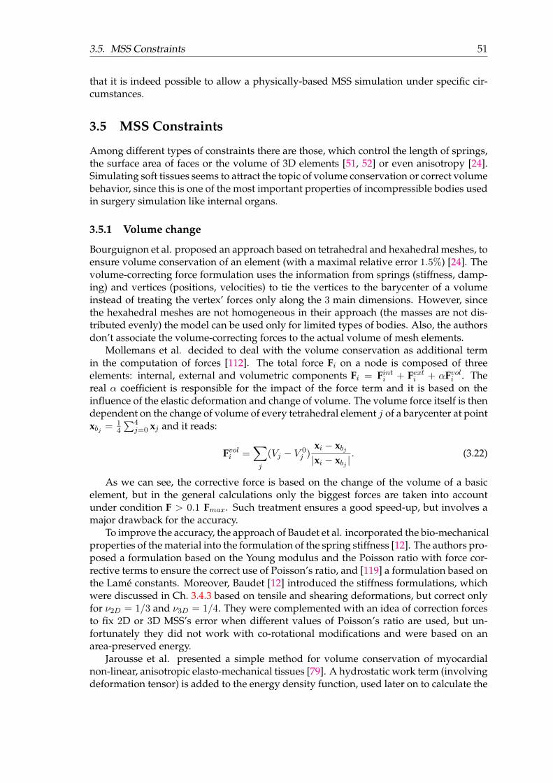
3.5. MSS Constraints 51
that it is indeed possible to allow a physically-based MSS simulation under specific cir-cumstances.
3.5 MSS Constraints
Among different types of constraints there are those, which control the length of springs,the surface area of faces or the volume of 3D elements [51, 52] or even anisotropy [24].Simulating soft tissues seems to attract the topic of volume conservation or correct volumebehavior, since this is one of the most important properties of incompressible bodies usedin surgery simulation like internal organs.
3.5.1 Volume change
Bourguignon et al. proposed an approach based on tetrahedral and hexahedral meshes, toensure volume conservation of an element (with a maximal relative error 1.5%) [24]. Thevolume-correcting force formulation uses the information from springs (stiffness, damp-ing) and vertices (positions, velocities) to tie the vertices to the barycenter of a volumeinstead of treating the vertex’ forces only along the 3 main dimensions. However, sincethe hexahedral meshes are not homogeneous in their approach (the masses are not dis-tributed evenly) the model can be used only for limited types of bodies. Also, the authorsdon’t associate the volume-correcting forces to the actual volume of mesh elements.
Mollemans et al. decided to deal with the volume conservation as additional termin the computation of forces [112]. The total force Fi on a node is composed of threeelements: internal, external and volumetric components Fi = Finti + Fexti + αFvoli . Thereal α coefficient is responsible for the impact of the force term and it is based on theinfluence of the elastic deformation and change of volume. The volume force itself is thendependent on the change of volume of every tetrahedral element j of a barycenter at pointxbj = 1
4
∑4j=0 xj and it reads:
Fvoli =∑j
(Vj − V 0j )
xi − xbj|xi − xbj |
. (3.22)
As we can see, the corrective force is based on the change of the volume of a basicelement, but in the general calculations only the biggest forces are taken into accountunder condition F > 0.1 Fmax. Such treatment ensures a good speed-up, but involves amajor drawback for the accuracy.
To improve the accuracy, the approach of Baudet et al. incorporated the bio-mechanicalproperties of the material into the formulation of the spring stiffness [12]. The authors pro-posed a formulation based on the Young modulus and the Poisson ratio with force cor-rective terms to ensure the correct use of Poisson’s ratio, and [119] a formulation based onthe Lamé constants. Moreover, Baudet [12] introduced the stiffness formulations, whichwere discussed in Ch. 3.4.3 based on tensile and shearing deformations, but correct onlyfor ν2D = 1/3 and ν3D = 1/4. They were complemented with an idea of correction forcesto fix 2D or 3D MSS’s error when different values of Poisson’s ratio are used, but un-fortunately they did not work with co-rotational modifications and were based on anarea-preserved energy.
Jarousse et al. presented a simple method for volume conservation of myocardialnon-linear, anisotropic elasto-mechanical tissues [79]. A hydrostatic work term (involvingdeformation tensor) is added to the energy density function, used later on to calculate the
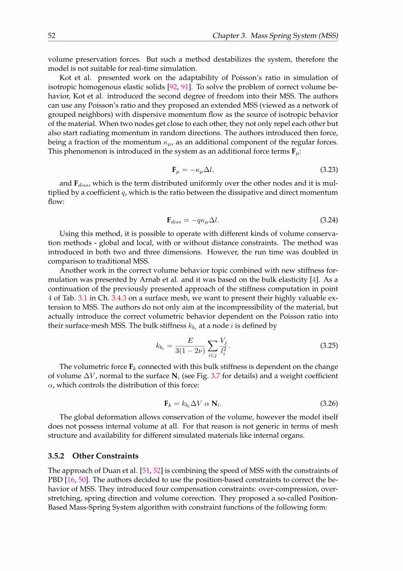
52 Chapter 3. Mass Spring System (MSS)
volume preservation forces. But such a method destabilizes the system, therefore themodel is not suitable for real-time simulation.
Kot et al. presented work on the adaptability of Poisson’s ratio in simulation ofisotropic homogenous elastic solids [92, 91]. To solve the problem of correct volume be-havior, Kot et al. introduced the second degree of freedom into their MSS. The authorscan use any Poisson’s ratio and they proposed an extended MSS (viewed as a network ofgrouped neighbors) with dispersive momentum flow as the source of isotropic behaviorof the material. When two nodes get close to each other, they not only repel each other butalso start radiating momentum in random directions. The authors introduced then force,being a fraction of the momentum κµ, as an additional component of the regular forces.This phenomenon is introduced in the system as an additional force terms Fµ:
Fµ = −κµ∆l, (3.23)
and Fdiss, which is the term distributed uniformly over the other nodes and it is mul-tiplied by a coefficient q, which is the ratio between the dissipative and direct momentumflow:
Fdiss = −qκµ∆l. (3.24)
Using this method, it is possible to operate with different kinds of volume conserva-tion methods - global and local, with or without distance constraints. The method wasintroduced in both two and three dimensions. However, the run time was doubled incomparison to traditional MSS.
Another work in the correct volume behavior topic combined with new stiffness for-mulation was presented by Arnab et al. and it was based on the bulk elasticity [4]. As acontinuation of the previously presented approach of the stiffness computation in point4 of Tab. 3.1 in Ch. 3.4.3 on a surface mesh, we want to present their highly valuable ex-tension to MSS. The authors do not only aim at the incompressibility of the material, butactually introduce the correct volumetric behavior dependent on the Poisson ratio intotheir surface-mesh MSS. The bulk stiffness kbi at a node i is defined by
kbi =E
3(1− 2ν)
∑i∈j
Vjl2i. (3.25)
The volumetric force Fk connected with this bulk stiffness is dependent on the changeof volume ∆V , normal to the surface Ni (see Fig. 3.7 for details) and a weight coefficientα, which controls the distribution of this force:
Fk = kbi∆V α Ni. (3.26)
The global deformation allows conservation of the volume, however the model itselfdoes not possess internal volume at all. For that reason is not generic in terms of meshstructure and availability for different simulated materials like internal organs.
3.5.2 Other Constraints
The approach of Duan et al. [51, 52] is combining the speed of MSS with the constraints ofPBD [16, 50]. The authors decided to use the position-based constraints to correct the be-havior of MSS. They introduced four compensation constraints: over-compression, over-stretching, spring direction and volume correction. They proposed a so-called Position-Based Mass-Spring System algorithm with constraint functions of the following form:
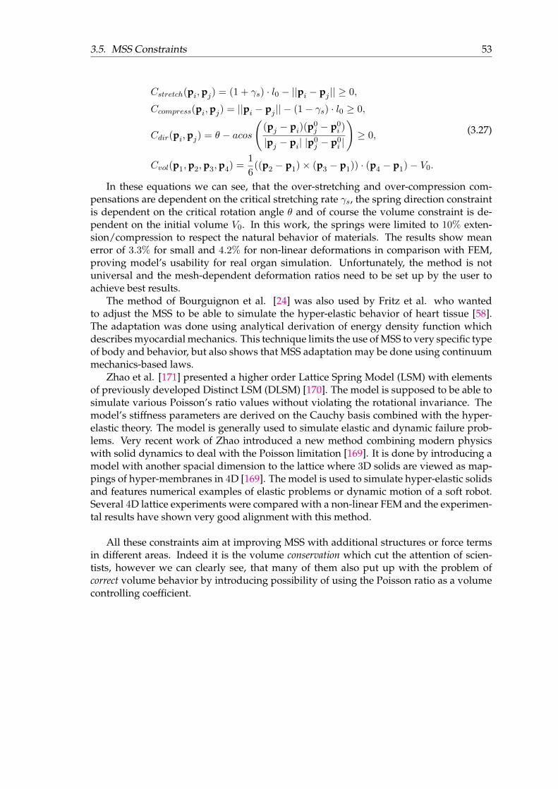
3.5. MSS Constraints 53
Cstretch(pi,pj) = (1 + γs) · l0 − ||pi − pj || ≥ 0,
Ccompress(pi,pj) = ||pi − pj || − (1− γs) · l0 ≥ 0,
Cdir(pi,pj) = θ − acos
((pj − pi)(p0
j − p0i )
|pj − pi| |p0j − p0
i |
)≥ 0,
Cvol(p1,p2,p3,p4) =1
6((p2 − p1)× (p3 − p1)) · (p4 − p1)− V0.
(3.27)
In these equations we can see, that the over-stretching and over-compression com-pensations are dependent on the critical stretching rate γs, the spring direction constraintis dependent on the critical rotation angle θ and of course the volume constraint is de-pendent on the initial volume V0. In this work, the springs were limited to 10% exten-sion/compression to respect the natural behavior of materials. The results show meanerror of 3.3% for small and 4.2% for non-linear deformations in comparison with FEM,proving model’s usability for real organ simulation. Unfortunately, the method is notuniversal and the mesh-dependent deformation ratios need to be set up by the user toachieve best results.
The method of Bourguignon et al. [24] was also used by Fritz et al. who wantedto adjust the MSS to be able to simulate the hyper-elastic behavior of heart tissue [58].The adaptation was done using analytical derivation of energy density function whichdescribes myocardial mechanics. This technique limits the use of MSS to very specific typeof body and behavior, but also shows that MSS adaptation may be done using continuummechanics-based laws.
Zhao et al. [171] presented a higher order Lattice Spring Model (LSM) with elementsof previously developed Distinct LSM (DLSM) [170]. The model is supposed to be able tosimulate various Poisson’s ratio values without violating the rotational invariance. Themodel’s stiffness parameters are derived on the Cauchy basis combined with the hyper-elastic theory. The model is generally used to simulate elastic and dynamic failure prob-lems. Very recent work of Zhao introduced a new method combining modern physicswith solid dynamics to deal with the Poisson limitation [169]. It is done by introducing amodel with another spacial dimension to the lattice where 3D solids are viewed as map-pings of hyper-membranes in 4D [169]. The model is used to simulate hyper-elastic solidsand features numerical examples of elastic problems or dynamic motion of a soft robot.Several 4D lattice experiments were compared with a non-linear FEM and the experimen-tal results have shown very good alignment with this method.
All these constraints aim at improving MSS with additional structures or force termsin different areas. Indeed it is the volume conservation which cut the attention of scien-tists, however we can clearly see, that many of them also put up with the problem ofcorrect volume behavior by introducing possibility of using the Poisson ratio as a volumecontrolling coefficient.
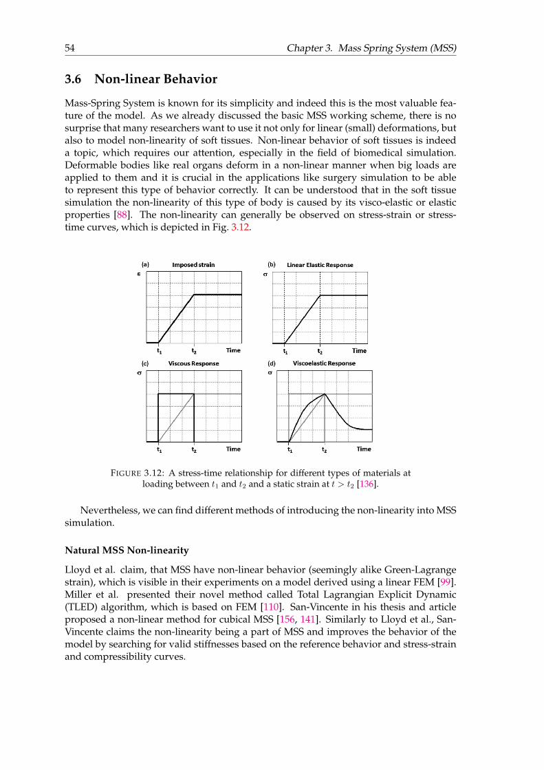
54 Chapter 3. Mass Spring System (MSS)
3.6 Non-linear Behavior
Mass-Spring System is known for its simplicity and indeed this is the most valuable fea-ture of the model. As we already discussed the basic MSS working scheme, there is nosurprise that many researchers want to use it not only for linear (small) deformations, butalso to model non-linearity of soft tissues. Non-linear behavior of soft tissues is indeeda topic, which requires our attention, especially in the field of biomedical simulation.Deformable bodies like real organs deform in a non-linear manner when big loads areapplied to them and it is crucial in the applications like surgery simulation to be ableto represent this type of behavior correctly. It can be understood that in the soft tissuesimulation the non-linearity of this type of body is caused by its visco-elastic or elasticproperties [88]. The non-linearity can generally be observed on stress-strain or stress-time curves, which is depicted in Fig. 3.12.
FIGURE 3.12: A stress-time relationship for different types of materials atloading between t1 and t2 and a static strain at t > t2 [136].
Nevertheless, we can find different methods of introducing the non-linearity into MSSsimulation.
Natural MSS Non-linearity
Lloyd et al. claim, that MSS have non-linear behavior (seemingly alike Green-Lagrangestrain), which is visible in their experiments on a model derived using a linear FEM [99].Miller et al. presented their novel method called Total Lagrangian Explicit Dynamic(TLED) algorithm, which is based on FEM [110]. San-Vincente in his thesis and articleproposed a non-linear method for cubical MSS [156, 141]. Similarly to Lloyd et al., San-Vincente claims the non-linearity being a part of MSS and improves the behavior of themodel by searching for valid stiffnesses based on the reference behavior and stress-strainand compressibility curves.
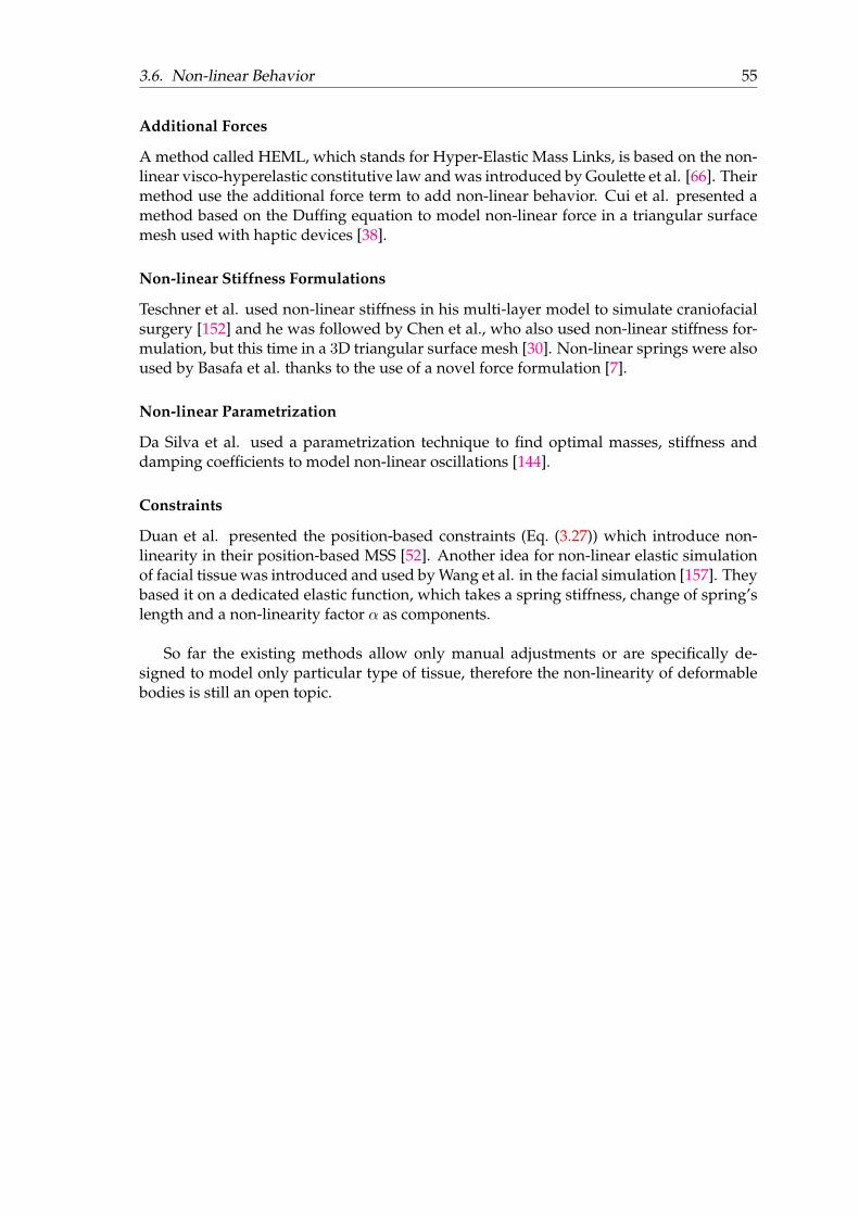
3.6. Non-linear Behavior 55
Additional Forces
A method called HEML, which stands for Hyper-Elastic Mass Links, is based on the non-linear visco-hyperelastic constitutive law and was introduced by Goulette et al. [66]. Theirmethod use the additional force term to add non-linear behavior. Cui et al. presented amethod based on the Duffing equation to model non-linear force in a triangular surfacemesh used with haptic devices [38].
Non-linear Stiffness Formulations
Teschner et al. used non-linear stiffness in his multi-layer model to simulate craniofacialsurgery [152] and he was followed by Chen et al., who also used non-linear stiffness for-mulation, but this time in a 3D triangular surface mesh [30]. Non-linear springs were alsoused by Basafa et al. thanks to the use of a novel force formulation [7].
Non-linear Parametrization
Da Silva et al. used a parametrization technique to find optimal masses, stiffness anddamping coefficients to model non-linear oscillations [144].
Constraints
Duan et al. presented the position-based constraints (Eq. (3.27)) which introduce non-linearity in their position-based MSS [52]. Another idea for non-linear elastic simulationof facial tissue was introduced and used by Wang et al. in the facial simulation [157]. Theybased it on a dedicated elastic function, which takes a spring stiffness, change of spring’slength and a non-linearity factor α as components.
So far the existing methods allow only manual adjustments or are specifically de-signed to model only particular type of tissue, therefore the non-linearity of deformablebodies is still an open topic.

56 Chapter 3. Mass Spring System (MSS)
3.7 Topological modifications
The topological modifications are invaluable part of surgery simulation. Indeed, in virtualsurgery it is crucial to be able to cut or pierce the tissue, therefore models with possibil-ity of real-time cutting are much more valuable as virtual reality tools than those whichneed some pre-computations after applying topological changes. These modificationsmay include tearing, refinement and de-refinement techniques, but here we focus on thecutting and piercing in particular. Note, that the most popular meshes when it comes totopological modifications are triangular and tetrahedral - these elements are simplest tosubdivide into more triangular shaped elements, therefore possible refinement techniquesare easily applied in comparison to e.g. hexahedral meshes, which pose a huge problemof T-junctions.
Paloc et al. presented a multi-resolution MSS working on tetrahedral meshes [134].The method is able to handle haptic feedback and uses change of the resolution dependenton the distance from the body. Authors use dynamic update of the mass, stiffness anddamping coefficients to simulate a MSS with high visual resolution.
Starting the topological cutting topic from an article of Cotin et al. from 2000, whointroduced one of the first models for surgery simulation including topological modifi-cations and even force feedback [33], we can already see how long time ago the need forsuch a simulation was recognized. The authors used computation and constant updateof local tensors to know when to remove a tetrahedron at which the cutting takes place.However, this method requires the tetrahedra at the cutting place to be relatively smalland it is possible that more than only the cut element will be removed from the mesh.Additionally to cutting, the local tensors and stresses are computed to verify if the tissueis not torn - if they exceed a given limit - tetrahedra are automatically removed.
Bielser et al. presented a cutting technique based on a pre-defined cutting scenariosfor triangles, which was extended to tetrahedra [21]. Such a method limits the number ofpossibilities when it comes to cutting, but the method allows fairly fast recognition of thecut patterns and does not allow unexpected instabilities to tamper with the model.
Ganovelli et al. used a Multiresolution Triangulation (exceptionaly in this section re-ferred to as MT) method for decomposition of their tetrahedral mesh [63]. The mesh isgenerally composed of segments with particular borders, so an update of a segment withuse of MT will exchange such a segment with a new one (refined or simplified, accordingto the need), but with the same border. After discovering a collision of the mesh with ascalpel, the intersecting segment is modified to not have any intersections with the tooland then the MT algorithm is applied to update the mesh.
Flechon et al. used combinatorial maps and LCC+MSS layer (see Ch. 3.8.2 for details)to facilitate all the topological operations including cutting and adaptive refinement [56].The method works well during an ongoing simulation while allowing operations likecutting in the same time.
As we can see, the topological modifications are handled well in MSS in the literature.It is another advantage of using MSS for surgical simulation in virtual environments,where user is able to modify the tissue according to the needs.
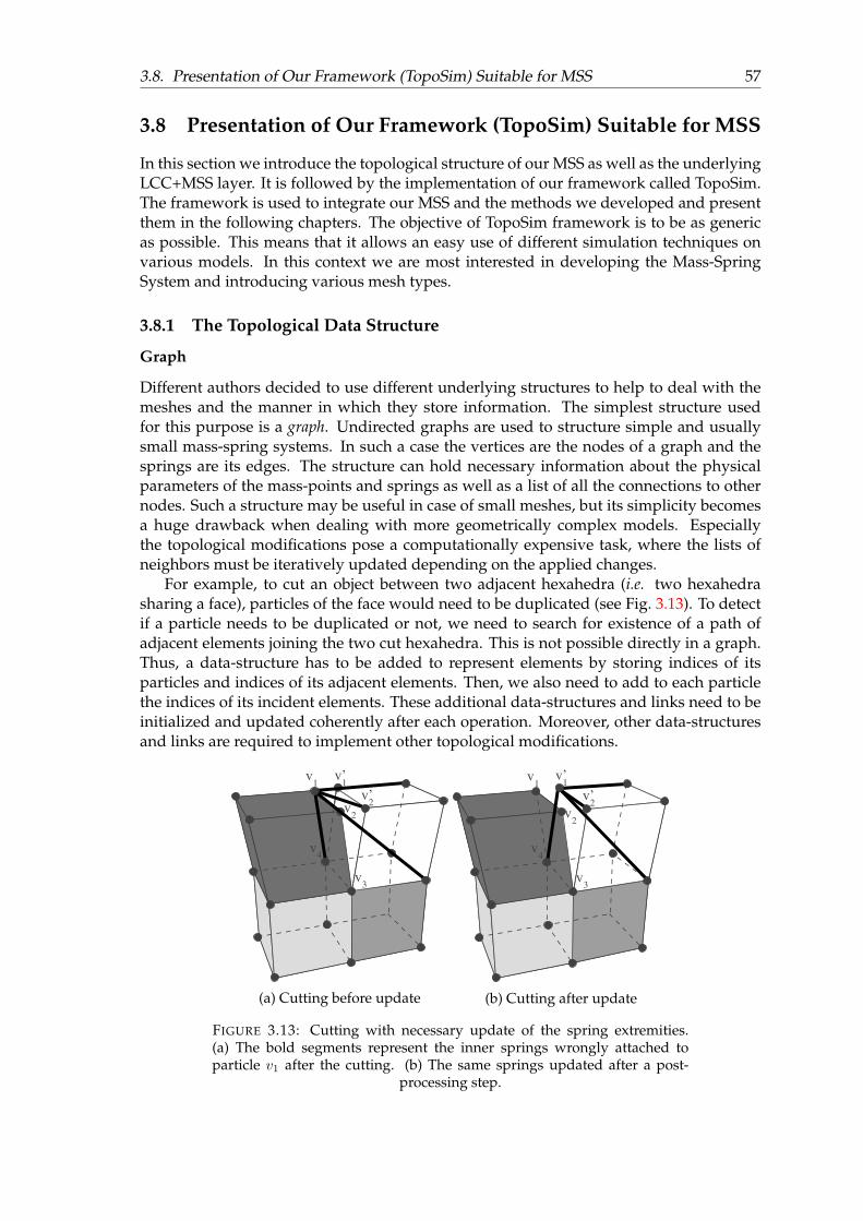
3.8. Presentation of Our Framework (TopoSim) Suitable for MSS 57
3.8 Presentation of Our Framework (TopoSim) Suitable for MSS
In this section we introduce the topological structure of our MSS as well as the underlyingLCC+MSS layer. It is followed by the implementation of our framework called TopoSim.The framework is used to integrate our MSS and the methods we developed and presentthem in the following chapters. The objective of TopoSim framework is to be as genericas possible. This means that it allows an easy use of different simulation techniques onvarious models. In this context we are most interested in developing the Mass-SpringSystem and introducing various mesh types.
3.8.1 The Topological Data Structure
Graph
Different authors decided to use different underlying structures to help to deal with themeshes and the manner in which they store information. The simplest structure usedfor this purpose is a graph. Undirected graphs are used to structure simple and usuallysmall mass-spring systems. In such a case the vertices are the nodes of a graph and thesprings are its edges. The structure can hold necessary information about the physicalparameters of the mass-points and springs as well as a list of all the connections to othernodes. Such a structure may be useful in case of small meshes, but its simplicity becomesa huge drawback when dealing with more geometrically complex models. Especiallythe topological modifications pose a computationally expensive task, where the lists ofneighbors must be iteratively updated depending on the applied changes.
For example, to cut an object between two adjacent hexahedra (i.e. two hexahedrasharing a face), particles of the face would need to be duplicated (see Fig. 3.13). To detectif a particle needs to be duplicated or not, we need to search for existence of a path ofadjacent elements joining the two cut hexahedra. This is not possible directly in a graph.Thus, a data-structure has to be added to represent elements by storing indices of itsparticles and indices of its adjacent elements. Then, we also need to add to each particlethe indices of its incident elements. These additional data-structures and links need to beinitialized and updated coherently after each operation. Moreover, other data-structuresand links are required to implement other topological modifications.
v3
v4
v1
v’1
v2
v’2
(a) Cutting before update
v3
v4
v1
v’2
v2
v’1
(b) Cutting after update
FIGURE 3.13: Cutting with necessary update of the spring extremities.(a) The bold segments represent the inner springs wrongly attached toparticle v1 after the cutting. (b) The same springs updated after a post-
processing step.
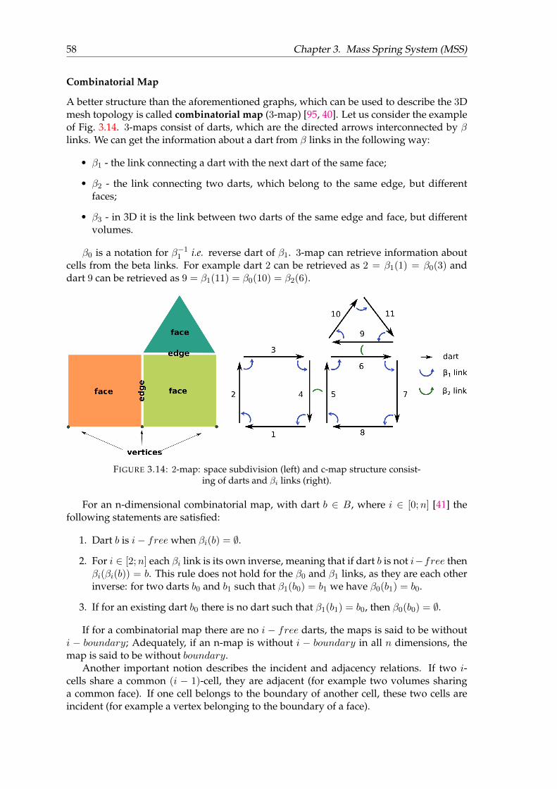
58 Chapter 3. Mass Spring System (MSS)
Combinatorial Map
A better structure than the aforementioned graphs, which can be used to describe the 3Dmesh topology is called combinatorial map (3-map) [95, 40]. Let us consider the exampleof Fig. 3.14. 3-maps consist of darts, which are the directed arrows interconnected by βlinks. We can get the information about a dart from β links in the following way:
• β1 - the link connecting a dart with the next dart of the same face;
• β2 - the link connecting two darts, which belong to the same edge, but differentfaces;
• β3 - in 3D it is the link between two darts of the same edge and face, but differentvolumes.
β0 is a notation for β−11 i.e. reverse dart of β1. 3-map can retrieve information about
cells from the beta links. For example dart 2 can be retrieved as 2 = β1(1) = β0(3) anddart 9 can be retrieved as 9 = β1(11) = β0(10) = β2(6).
FIGURE 3.14: 2-map: space subdivision (left) and c-map structure consist-ing of darts and βi links (right).
For an n-dimensional combinatorial map, with dart b ∈ B, where i ∈ [0;n] [41] thefollowing statements are satisfied:
1. Dart b is i− free when βi(b) = ∅.
2. For i ∈ [2;n] each βi link is its own inverse, meaning that if dart b is not i−free thenβi(βi(b)) = b. This rule does not hold for the β0 and β1 links, as they are each otherinverse: for two darts b0 and b1 such that β1(b0) = b1 we have β0(b1) = b0.
3. If for an existing dart b0 there is no dart such that β1(b1) = b0, then β0(b0) = ∅.
If for a combinatorial map there are no i − free darts, the maps is said to be withouti − boundary; Adequately, if an n-map is without i − boundary in all n dimensions, themap is said to be without boundary.
Another important notion describes the incident and adjacency relations. If two i-cells share a common (i − 1)-cell, they are adjacent (for example two volumes sharinga common face). If one cell belongs to the boundary of another cell, these two cells areincident (for example a vertex belonging to the boundary of a face).
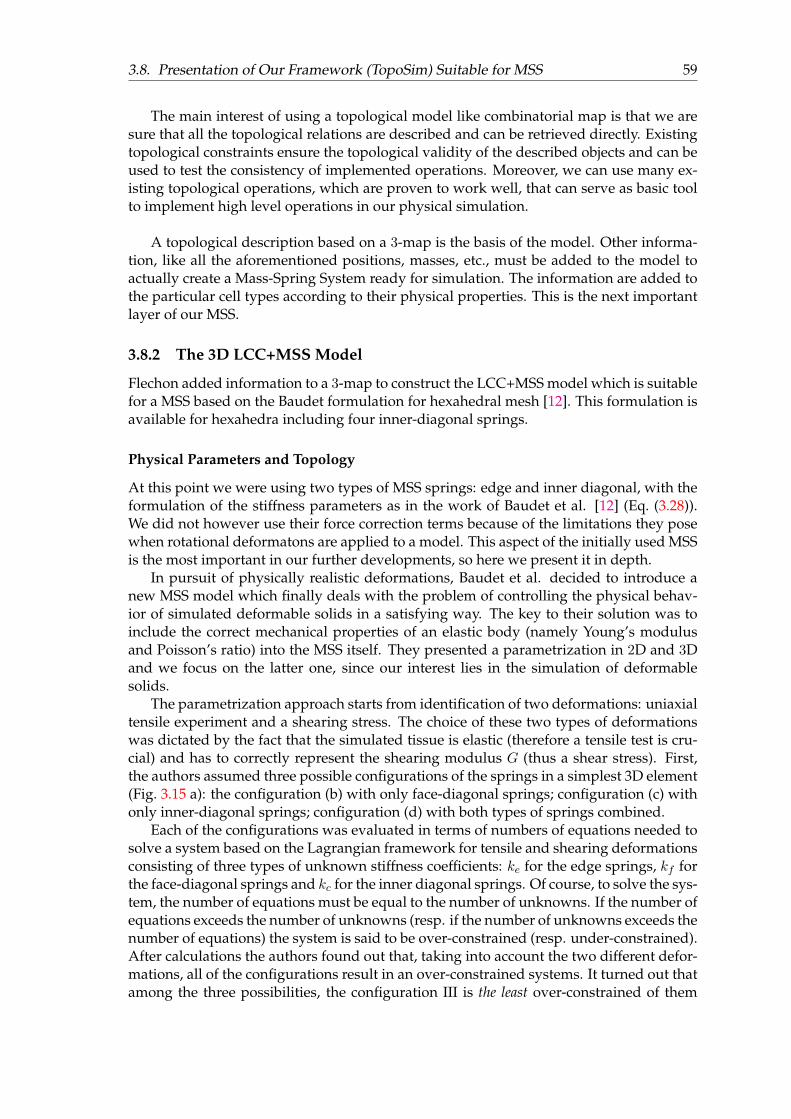
3.8. Presentation of Our Framework (TopoSim) Suitable for MSS 59
The main interest of using a topological model like combinatorial map is that we aresure that all the topological relations are described and can be retrieved directly. Existingtopological constraints ensure the topological validity of the described objects and can beused to test the consistency of implemented operations. Moreover, we can use many ex-isting topological operations, which are proven to work well, that can serve as basic toolto implement high level operations in our physical simulation.
A topological description based on a 3-map is the basis of the model. Other informa-tion, like all the aforementioned positions, masses, etc., must be added to the model toactually create a Mass-Spring System ready for simulation. The information are added tothe particular cell types according to their physical properties. This is the next importantlayer of our MSS.
3.8.2 The 3D LCC+MSS Model
Flechon added information to a 3-map to construct the LCC+MSS model which is suitablefor a MSS based on the Baudet formulation for hexahedral mesh [12]. This formulation isavailable for hexahedra including four inner-diagonal springs.
Physical Parameters and Topology
At this point we were using two types of MSS springs: edge and inner diagonal, with theformulation of the stiffness parameters as in the work of Baudet et al. [12] (Eq. (3.28)).We did not however use their force correction terms because of the limitations they posewhen rotational deformatons are applied to a model. This aspect of the initially used MSSis the most important in our further developments, so here we present it in depth.
In pursuit of physically realistic deformations, Baudet et al. decided to introduce anew MSS model which finally deals with the problem of controlling the physical behav-ior of simulated deformable solids in a satisfying way. The key to their solution was toinclude the correct mechanical properties of an elastic body (namely Young’s modulusand Poisson’s ratio) into the MSS itself. They presented a parametrization in 2D and 3Dand we focus on the latter one, since our interest lies in the simulation of deformablesolids.
The parametrization approach starts from identification of two deformations: uniaxialtensile experiment and a shearing stress. The choice of these two types of deformationswas dictated by the fact that the simulated tissue is elastic (therefore a tensile test is cru-cial) and has to correctly represent the shearing modulus G (thus a shear stress). First,the authors assumed three possible configurations of the springs in a simplest 3D element(Fig. 3.15 a): the configuration (b) with only face-diagonal springs; configuration (c) withonly inner-diagonal springs; configuration (d) with both types of springs combined.
Each of the configurations was evaluated in terms of numbers of equations needed tosolve a system based on the Lagrangian framework for tensile and shearing deformationsconsisting of three types of unknown stiffness coefficients: ke for the edge springs, kf forthe face-diagonal springs and kc for the inner diagonal springs. Of course, to solve the sys-tem, the number of equations must be equal to the number of unknowns. If the number ofequations exceeds the number of unknowns (resp. if the number of unknowns exceeds thenumber of equations) the system is said to be over-constrained (resp. under-constrained).After calculations the authors found out that, taking into account the two different defor-mations, all of the configurations result in an over-constrained systems. It turned out thatamong the three possibilities, the configuration III is the least over-constrained of them
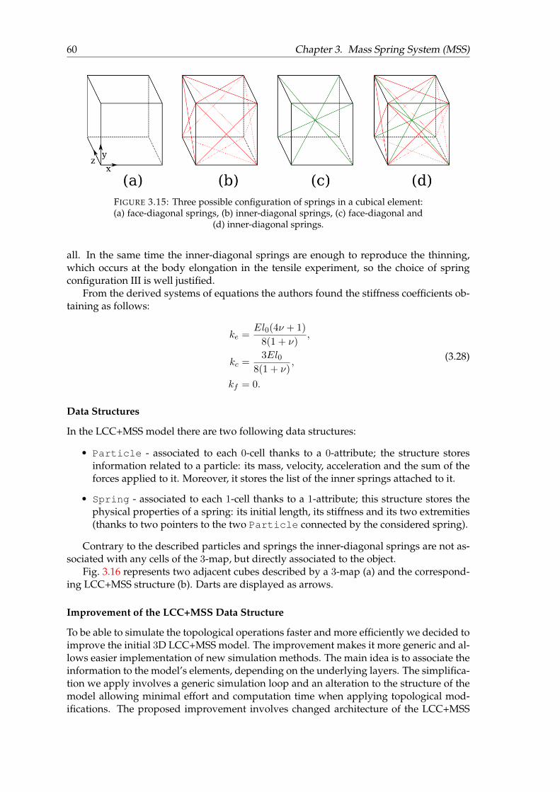
60 Chapter 3. Mass Spring System (MSS)
FIGURE 3.15: Three possible configuration of springs in a cubical element:(a) face-diagonal springs, (b) inner-diagonal springs, (c) face-diagonal and
(d) inner-diagonal springs.
all. In the same time the inner-diagonal springs are enough to reproduce the thinning,which occurs at the body elongation in the tensile experiment, so the choice of springconfiguration III is well justified.
From the derived systems of equations the authors found the stiffness coefficients ob-taining as follows:
ke =El0(4ν + 1)
8(1 + ν),
kc =3El0
8(1 + ν),
kf = 0.
(3.28)
Data Structures
In the LCC+MSS model there are two following data structures:
• Particle - associated to each 0-cell thanks to a 0-attribute; the structure storesinformation related to a particle: its mass, velocity, acceleration and the sum of theforces applied to it. Moreover, it stores the list of the inner springs attached to it.
• Spring - associated to each 1-cell thanks to a 1-attribute; this structure stores thephysical properties of a spring: its initial length, its stiffness and its two extremities(thanks to two pointers to the two Particle connected by the considered spring).
Contrary to the described particles and springs the inner-diagonal springs are not as-sociated with any cells of the 3-map, but directly associated to the object.
Fig. 3.16 represents two adjacent cubes described by a 3-map (a) and the correspond-ing LCC+MSS structure (b). Darts are displayed as arrows.
Improvement of the LCC+MSS Data Structure
To be able to simulate the topological operations faster and more efficiently we decided toimprove the initial 3D LCC+MSS model. The improvement makes it more generic and al-lows easier implementation of new simulation methods. The main idea is to associate theinformation to the model’s elements, depending on the underlying layers. The simplifica-tion we apply involves a generic simulation loop and an alteration to the structure of themodel allowing minimal effort and computation time when applying topological mod-ifications. The proposed improvement involves changed architecture of the LCC+MSS
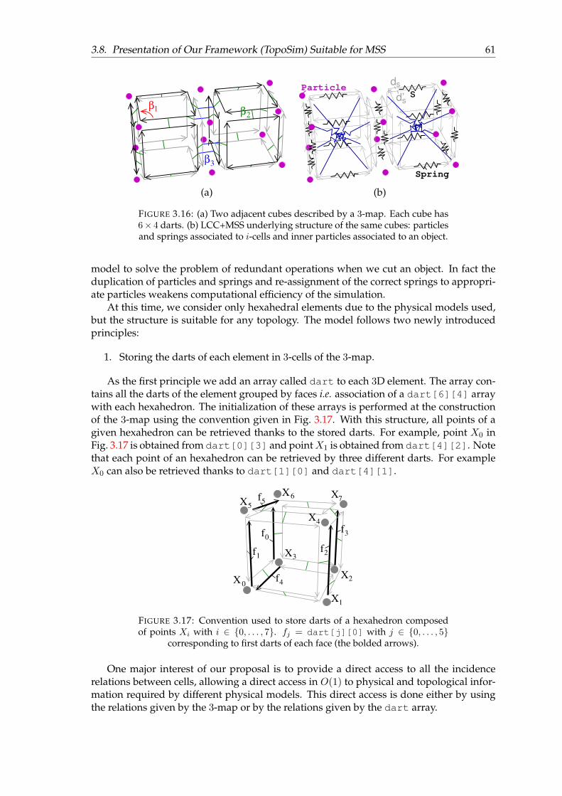
3.8. Presentation of Our Framework (TopoSim) Suitable for MSS 61
3β
2β1β
Spring
s
ds
d’s
Particle
(a) (b)
FIGURE 3.16: (a) Two adjacent cubes described by a 3-map. Each cube has6× 4 darts. (b) LCC+MSS underlying structure of the same cubes: particlesand springs associated to i-cells and inner particles associated to an object.
model to solve the problem of redundant operations when we cut an object. In fact theduplication of particles and springs and re-assignment of the correct springs to appropri-ate particles weakens computational efficiency of the simulation.
At this time, we consider only hexahedral elements due to the physical models used,but the structure is suitable for any topology. The model follows two newly introducedprinciples:
1. Storing the darts of each element in 3-cells of the 3-map.
As the first principle we add an array called dart to each 3D element. The array con-tains all the darts of the element grouped by faces i.e. association of a dart[6][4] arraywith each hexahedron. The initialization of these arrays is performed at the constructionof the 3-map using the convention given in Fig. 3.17. With this structure, all points of agiven hexahedron can be retrieved thanks to the stored darts. For example, point X0 inFig. 3.17 is obtained from dart[0][3] and pointX1 is obtained from dart[4][2]. Notethat each point of an hexahedron can be retrieved by three different darts. For exampleX0 can also be retrieved thanks to dart[1][0] and dart[4][1].
f5
f3
f2f
1
f40
X
5X
7X
2X
1X
3X
f0
6X
4X
FIGURE 3.17: Convention used to store darts of a hexahedron composedof points Xi with i ∈ 0, . . . , 7. fj = dart[j][0] with j ∈ 0, . . . , 5
corresponding to first darts of each face (the bolded arrows).
One major interest of our proposal is to provide a direct access to all the incidencerelations between cells, allowing a direct access in O(1) to physical and topological infor-mation required by different physical models. This direct access is done either by usingthe relations given by the 3-map or by the relations given by the dart array.
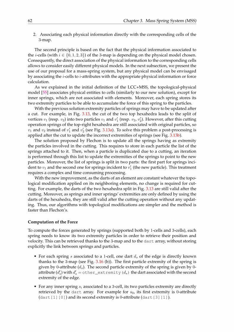
62 Chapter 3. Mass Spring System (MSS)
2. Associating each physical information directly with the corresponding cells of the3-map.
The second principle is based on the fact that the physical information associated tothe i-cells (with i ∈ 0, 1, 2, 3) of the 3-map is depending on the physical model chosen.Consequently, the direct association of the physical information to the corresponding cellsallows to consider easily different physical models. In the next subsection, we present theuse of our proposal for a mass-spring system, but any physical model can be envisagedby associating the i-cells to i-attributes with the appropriate physical information or forcecalculation.
As we explained in the initial definition of the LCC+MSS, the topological-physicalmodel [55] associates physical entities to cells (similarly to our new solution), except forinner springs, which are not associated with elements. Moreover, each spring stores itstwo extremity particles to be able to accumulate the force of this spring to the particles.
With the previous solution extremity particles of springs may have to be updated aftera cut. For example, in Fig. 3.13, the cut of the two top hexahedra leads to the split ofvertices v1 (resp. v2) into two particles v1 and v′1 (resp. v2, v′2). However, after this cuttingoperation springs of the top-right hexahedra are still associated with original particles, sov1 and v2 instead of v′1 and v′2 (see Fig. 3.13a). To solve this problem a post-processing isapplied after the cut to update the incorrect extremities of springs (see Fig. 3.13b).
The solution proposed by Flechon is to update all the springs having as extremitythe particles involved in the cutting. This requires to store in each particle the list of thesprings attached to it. Then, when a particle is duplicated due to a cutting, an iterationis performed through this list to update the extremities of the springs to point to the newparticles. Moreover, the list of springs is split in two parts: the first part for springs inci-dent to v1 and the second one for springs incident to v′1 (the new particle). This treatmentrequires a complex and time consuming processing.
With the new improvement, as the darts of an element are constant whatever the topo-logical modification applied on its neighboring elements, no change is required for cut-ting. For example, the darts of the two hexahedra split in Fig. 3.13 are still valid after thecutting. Moreover, as springs and inner springs’ extremities are only defined by using thedarts of the hexahedra, they are still valid after the cutting operation without any updat-ing. Thus, our algorithms with topological modifications are simpler and the method isfaster than Flechon’s.
Computation of the Force
To compute the forces generated by springs (supported both by 1-cells and 3-cells), eachspring needs to know its two extremity particles in order to retrieve their position andvelocity. This can be retrieved thanks to the 3-map and to the dart array, without storingexplicitly the link between springs and particles.
• For each spring s associated to a 1-cell, one dart ds of the edge is directly knownthanks to the 3-map (see Fig. 3.16 (b)). The first particle extremity of the spring isgiven by 0-attribute (ds). The second particle extremity of the spring is given by 0-attribute (d′s) with d′s = other_extremity(ds) the dart associated with the secondextremity of the edge.
• For any inner spring si associated to a 3-cell, its two particles extremity are directlyretrieved by the dart array. For example for s0, its first extremity is 0-attribute(dart[1][0]) and its second extremity is 0-attribute (dart[3][1]).
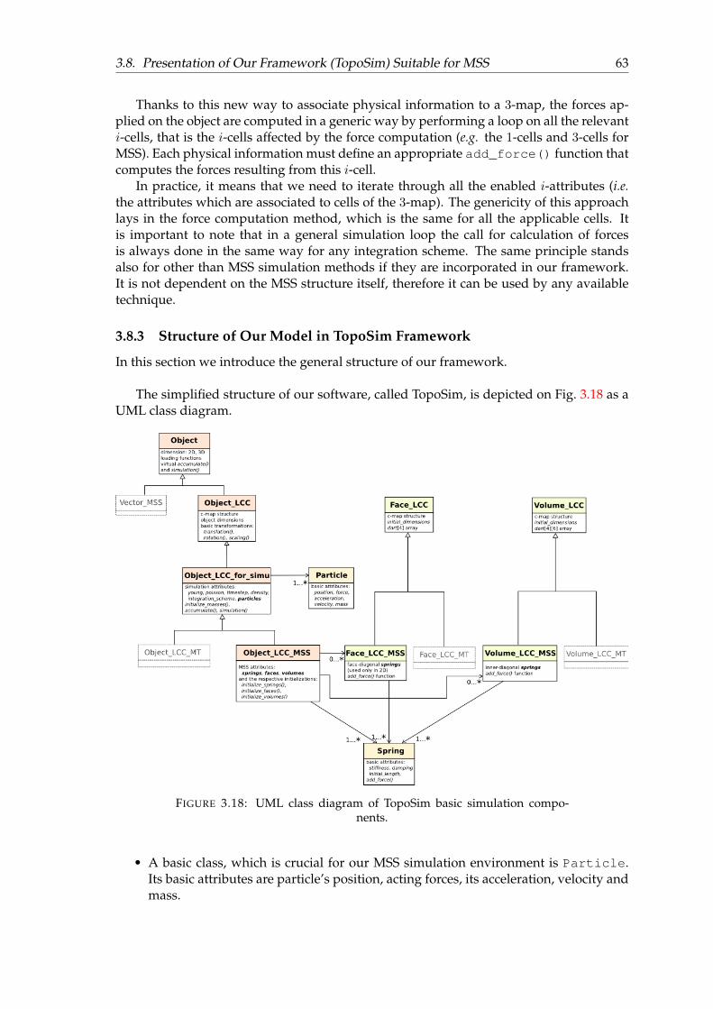
3.8. Presentation of Our Framework (TopoSim) Suitable for MSS 63
Thanks to this new way to associate physical information to a 3-map, the forces ap-plied on the object are computed in a generic way by performing a loop on all the relevanti-cells, that is the i-cells affected by the force computation (e.g. the 1-cells and 3-cells forMSS). Each physical information must define an appropriate add_force() function thatcomputes the forces resulting from this i-cell.
In practice, it means that we need to iterate through all the enabled i-attributes (i.e.the attributes which are associated to cells of the 3-map). The genericity of this approachlays in the force computation method, which is the same for all the applicable cells. Itis important to note that in a general simulation loop the call for calculation of forcesis always done in the same way for any integration scheme. The same principle standsalso for other than MSS simulation methods if they are incorporated in our framework.It is not dependent on the MSS structure itself, therefore it can be used by any availabletechnique.
3.8.3 Structure of Our Model in TopoSim Framework
In this section we introduce the general structure of our framework.
The simplified structure of our software, called TopoSim, is depicted on Fig. 3.18 as aUML class diagram.
FIGURE 3.18: UML class diagram of TopoSim basic simulation compo-nents.
• A basic class, which is crucial for our MSS simulation environment is Particle.Its basic attributes are particle’s position, acting forces, its acceleration, velocity andmass.
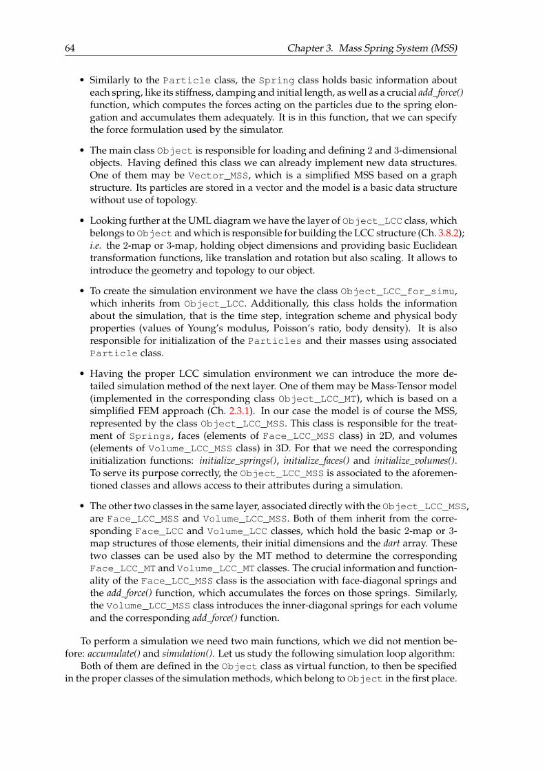
64 Chapter 3. Mass Spring System (MSS)
• Similarly to the Particle class, the Spring class holds basic information abouteach spring, like its stiffness, damping and initial length, as well as a crucial add_force()function, which computes the forces acting on the particles due to the spring elon-gation and accumulates them adequately. It is in this function, that we can specifythe force formulation used by the simulator.
• The main class Object is responsible for loading and defining 2 and 3-dimensionalobjects. Having defined this class we can already implement new data structures.One of them may be Vector_MSS, which is a simplified MSS based on a graphstructure. Its particles are stored in a vector and the model is a basic data structurewithout use of topology.
• Looking further at the UML diagram we have the layer of Object_LCC class, whichbelongs to Object and which is responsible for building the LCC structure (Ch. 3.8.2);i.e. the 2-map or 3-map, holding object dimensions and providing basic Euclideantransformation functions, like translation and rotation but also scaling. It allows tointroduce the geometry and topology to our object.
• To create the simulation environment we have the class Object_LCC_for_simu,which inherits from Object_LCC. Additionally, this class holds the informationabout the simulation, that is the time step, integration scheme and physical bodyproperties (values of Young’s modulus, Poisson’s ratio, body density). It is alsoresponsible for initialization of the Particles and their masses using associatedParticle class.
• Having the proper LCC simulation environment we can introduce the more de-tailed simulation method of the next layer. One of them may be Mass-Tensor model(implemented in the corresponding class Object_LCC_MT), which is based on asimplified FEM approach (Ch. 2.3.1). In our case the model is of course the MSS,represented by the class Object_LCC_MSS. This class is responsible for the treat-ment of Springs, faces (elements of Face_LCC_MSS class) in 2D, and volumes(elements of Volume_LCC_MSS class) in 3D. For that we need the correspondinginitialization functions: initialize_springs(), initialize_faces() and initialize_volumes().To serve its purpose correctly, the Object_LCC_MSS is associated to the aforemen-tioned classes and allows access to their attributes during a simulation.
• The other two classes in the same layer, associated directly with the Object_LCC_MSS,are Face_LCC_MSS and Volume_LCC_MSS. Both of them inherit from the corre-sponding Face_LCC and Volume_LCC classes, which hold the basic 2-map or 3-map structures of those elements, their initial dimensions and the dart array. Thesetwo classes can be used also by the MT method to determine the correspondingFace_LCC_MT and Volume_LCC_MT classes. The crucial information and function-ality of the Face_LCC_MSS class is the association with face-diagonal springs andthe add_force() function, which accumulates the forces on those springs. Similarly,the Volume_LCC_MSS class introduces the inner-diagonal springs for each volumeand the corresponding add_force() function.
To perform a simulation we need two main functions, which we did not mention be-fore: accumulate() and simulation(). Let us study the following simulation loop algorithm:
Both of them are defined in the Object class as virtual function, to then be specifiedin the proper classes of the simulation methods, which belong to Object in the first place.
3.8. Presentation of Our Framework (TopoSim) Suitable for MSS 65
Algorithm 1: TopoSim simulation loop algorithm
forall Objects doAccumulate
forall Particles j doaccumulate external forces: Fj ← Fext;
forall Springs i docompute forces Fi;accumulate forces on the extremity particles:Fp1 ← +Fi;Fp2 ← −Fi;
Simulationforall Particles j do
compute the new positions xj using an integration scheme given Fj
Thus, in the case of MSS method to run the simulation we need to first call the accumu-late() function on all the existing objects of Object_LCC_for_simu class. This functioniterates through all the existing springs and computes and accumulates the forces on allthe particles belonging to those springs. Then, the second step is the simulation() function(also run on all the Object_LCC_for_simu objects) which is responsible for updatingthe positions of all the particles using specified integration scheme and depending on thepreviously accumulated forces. Both functions are parallelized using Intel® TBB libraryalgorithms, which largely improves the performance of the simulations. The function ac-cumulate() is parallelized on particles and then springs and adequately, the function simu-late() is parallelized on the particles.
Thanks to this particular architecture we are able to easily add and adjust the simu-lation methods, chose among different integration schemes and introduce new function-alities. The approach we chose is generic and simple to understand, which facilitates theworkflow for any user and developer. In this section we have explained the topologicalstructure and implementation of our framework in detail. It allows easy implementationof new solutions, straight-forward adjustment of simulation methods to the topologicalstructure and generic force accumulation loop. Naturally, the computation of the accel-eration of the object and its integration in order to obtain the velocity and position is thesame for all physical objects who are based on the Newtonian dynamics.
66 Chapter 3. Mass Spring System (MSS)
3.9 Conclusions
This chapter has presented the Mass Spring System in its fullest form. Knowing thecapabilities and limitations of this simulation technique we are able to verify the mostimportant contributions which need to be made to reach our goal: be able to simulatedeformable bodies - real tissues - with speed and accuracy. We know that it is crucialto define and deal with the MSS instabilities and limitations: Cauchy’s limitation, MSSwrinkles and buckling phenomenon. Researchers constantly work on improvements ofthis method seeing a potential laying in this simple yet capable simulation technique.Looking at the existing MSS methods one may draw a conclusion that an advantage ofusing FEM instead would be the possibility of applying different physical laws in formof constitutive functions and precise boundary conditions to the model. Nevertheless,this better description of the mechanical behavior in case of FEM is counterbalanced bythe advantages of mass-spring models, namely the fast computation and the effortlesstopological modifications in real-time without additional pre-computation (which is stillnecessary when using FEM). Indeed, it is possible to simulate complex behavior with MSSwithout resigning from the real-time capabilities of this modeling technique.
We have also presented the topology characteristics used for MSS (and other) simu-lations. The additional MSS+LCC layer which improves boosts the MSS capabilities wasdescribed in detail thanks to the previous work of Fléchon et al. and introduction of ourimprovement. Additionally we have covered the topic of the initial implementation of oursolution, which makes a generic basis for the contributions which are to be introduced.
In next chapters we present our methods to solve several MSS limitations and in-troduce correct global behavior. We will show that it is possible to be able to simulateelastic deformable solids in an adjustable manner, which does not require complex pre-computations. In our work we focus on the correct MSS behavior and controllability ofthe system. In the same time we introduce physically-based methods for MSS simula-tions with use of constitutive law and continuum mechanics. Using appropriate physicalparameters should be the main focus of a correct physically based simulation.
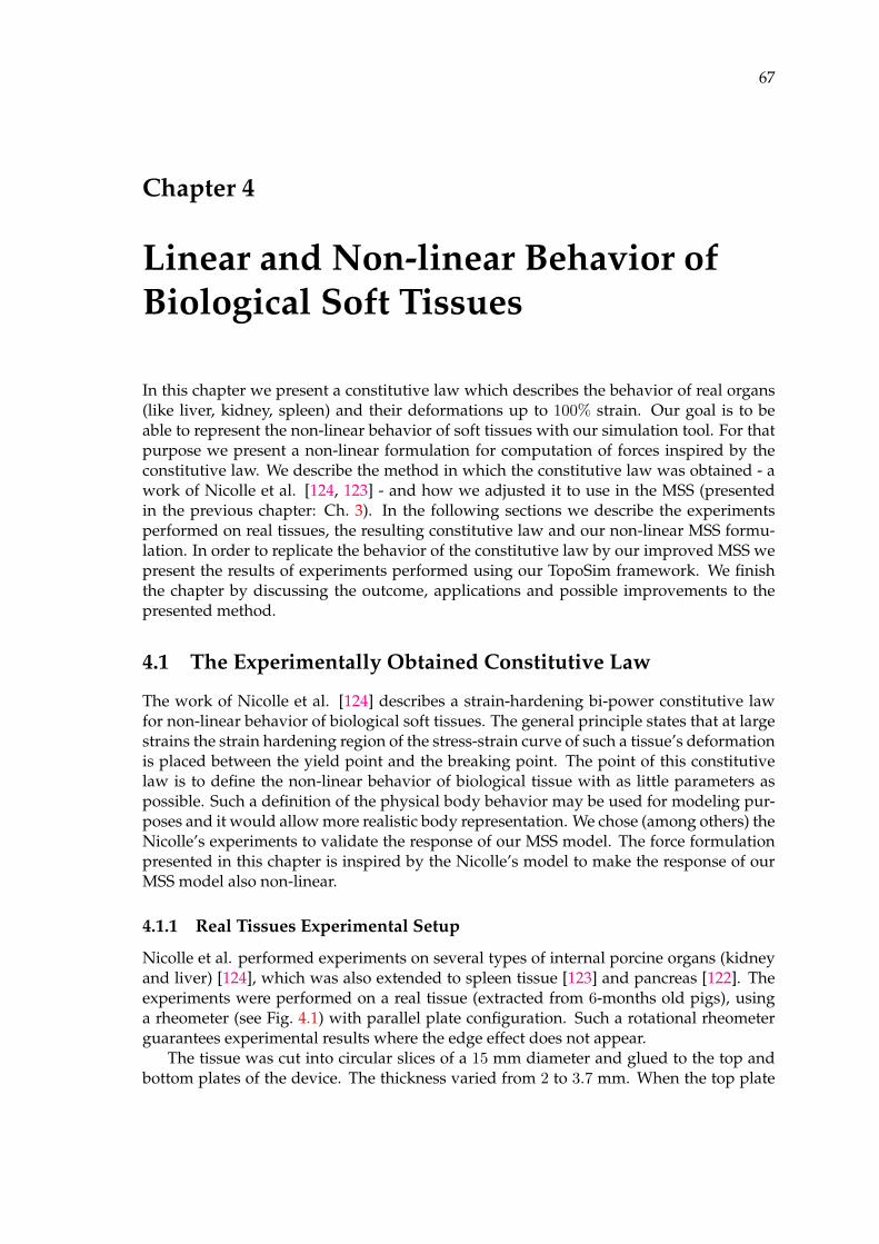
67
Chapter 4
Linear and Non-linear Behavior ofBiological Soft Tissues
In this chapter we present a constitutive law which describes the behavior of real organs(like liver, kidney, spleen) and their deformations up to 100% strain. Our goal is to beable to represent the non-linear behavior of soft tissues with our simulation tool. For thatpurpose we present a non-linear formulation for computation of forces inspired by theconstitutive law. We describe the method in which the constitutive law was obtained - awork of Nicolle et al. [124, 123] - and how we adjusted it to use in the MSS (presentedin the previous chapter: Ch. 3). In the following sections we describe the experimentsperformed on real tissues, the resulting constitutive law and our non-linear MSS formu-lation. In order to replicate the behavior of the constitutive law by our improved MSS wepresent the results of experiments performed using our TopoSim framework. We finishthe chapter by discussing the outcome, applications and possible improvements to thepresented method.
4.1 The Experimentally Obtained Constitutive Law
The work of Nicolle et al. [124] describes a strain-hardening bi-power constitutive lawfor non-linear behavior of biological soft tissues. The general principle states that at largestrains the strain hardening region of the stress-strain curve of such a tissue’s deformationis placed between the yield point and the breaking point. The point of this constitutivelaw is to define the non-linear behavior of biological tissue with as little parameters aspossible. Such a definition of the physical body behavior may be used for modeling pur-poses and it would allow more realistic body representation. We chose (among others) theNicolle’s experiments to validate the response of our MSS model. The force formulationpresented in this chapter is inspired by the Nicolle’s model to make the response of ourMSS model also non-linear.
4.1.1 Real Tissues Experimental Setup
Nicolle et al. performed experiments on several types of internal porcine organs (kidneyand liver) [124], which was also extended to spleen tissue [123] and pancreas [122]. Theexperiments were performed on a real tissue (extracted from 6-months old pigs), usinga rheometer (see Fig. 4.1) with parallel plate configuration. Such a rotational rheometerguarantees experimental results where the edge effect does not appear.
The tissue was cut into circular slices of a 15 mm diameter and glued to the top andbottom plates of the device. The thickness varied from 2 to 3.7 mm. When the top plate
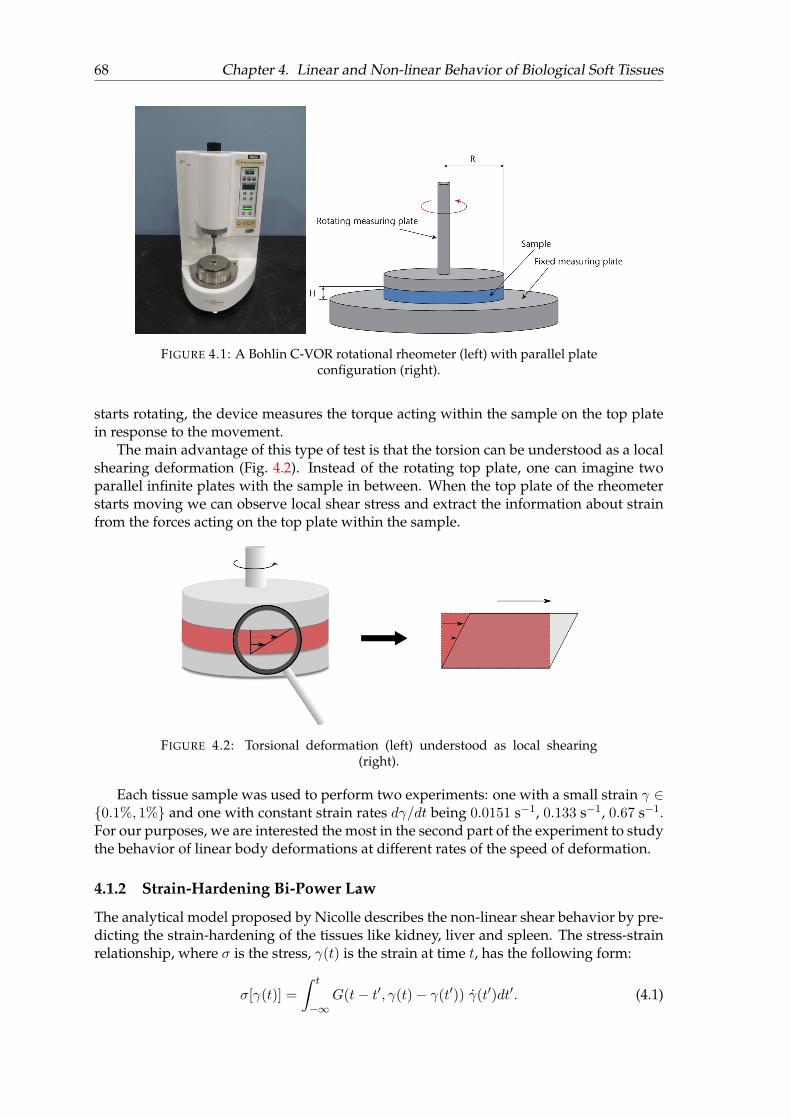
68 Chapter 4. Linear and Non-linear Behavior of Biological Soft Tissues
FIGURE 4.1: A Bohlin C-VOR rotational rheometer (left) with parallel plateconfiguration (right).
starts rotating, the device measures the torque acting within the sample on the top platein response to the movement.
The main advantage of this type of test is that the torsion can be understood as a localshearing deformation (Fig. 4.2). Instead of the rotating top plate, one can imagine twoparallel infinite plates with the sample in between. When the top plate of the rheometerstarts moving we can observe local shear stress and extract the information about strainfrom the forces acting on the top plate within the sample.
FIGURE 4.2: Torsional deformation (left) understood as local shearing(right).
Each tissue sample was used to perform two experiments: one with a small strain γ ∈0.1%, 1% and one with constant strain rates dγ/dt being 0.0151 s−1, 0.133 s−1, 0.67 s−1.For our purposes, we are interested the most in the second part of the experiment to studythe behavior of linear body deformations at different rates of the speed of deformation.
4.1.2 Strain-Hardening Bi-Power Law
The analytical model proposed by Nicolle describes the non-linear shear behavior by pre-dicting the strain-hardening of the tissues like kidney, liver and spleen. The stress-strainrelationship, where σ is the stress, γ(t) is the strain at time t, has the following form:
σ[γ(t)] =
∫ t
−∞G(t− t′, γ(t)− γ(t′)) γ(t′)dt′. (4.1)
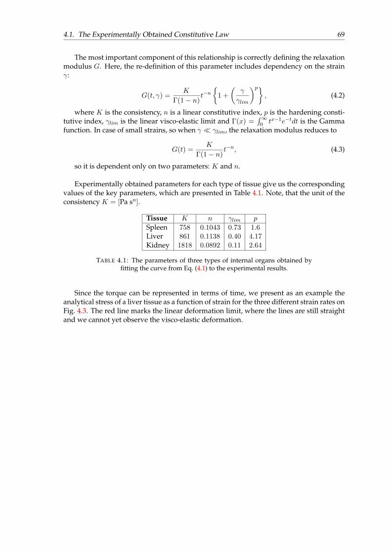
4.1. The Experimentally Obtained Constitutive Law 69
The most important component of this relationship is correctly defining the relaxationmodulus G. Here, the re-definition of this parameter includes dependency on the strainγ:
G(t, γ) =K
Γ(1− n)t−n
1 +
(γ
γlim
)p, (4.2)
where K is the consistency, n is a linear constitutive index, p is the hardening consti-tutive index, γlim is the linear visco-elastic limit and Γ(x) =
∫∞0 tx−1e−tdt is the Gamma
function. In case of small strains, so when γ γlim, the relaxation modulus reduces to
G(t) =K
Γ(1− n)t−n, (4.3)
so it is dependent only on two parameters: K and n.
Experimentally obtained parameters for each type of tissue give us the correspondingvalues of the key parameters, which are presented in Table 4.1. Note, that the unit of theconsistency K = [Pa sn].
Tissue K n γlim p
Spleen 758 0.1043 0.73 1.6Liver 861 0.1138 0.40 4.17Kidney 1818 0.0892 0.11 2.64
TABLE 4.1: The parameters of three types of internal organs obtained byfitting the curve from Eq. (4.1) to the experimental results.
Since the torque can be represented in terms of time, we present as an example theanalytical stress of a liver tissue as a function of strain for the three different strain rates onFig. 4.3. The red line marks the linear deformation limit, where the lines are still straightand we cannot yet observe the visco-elastic deformation.
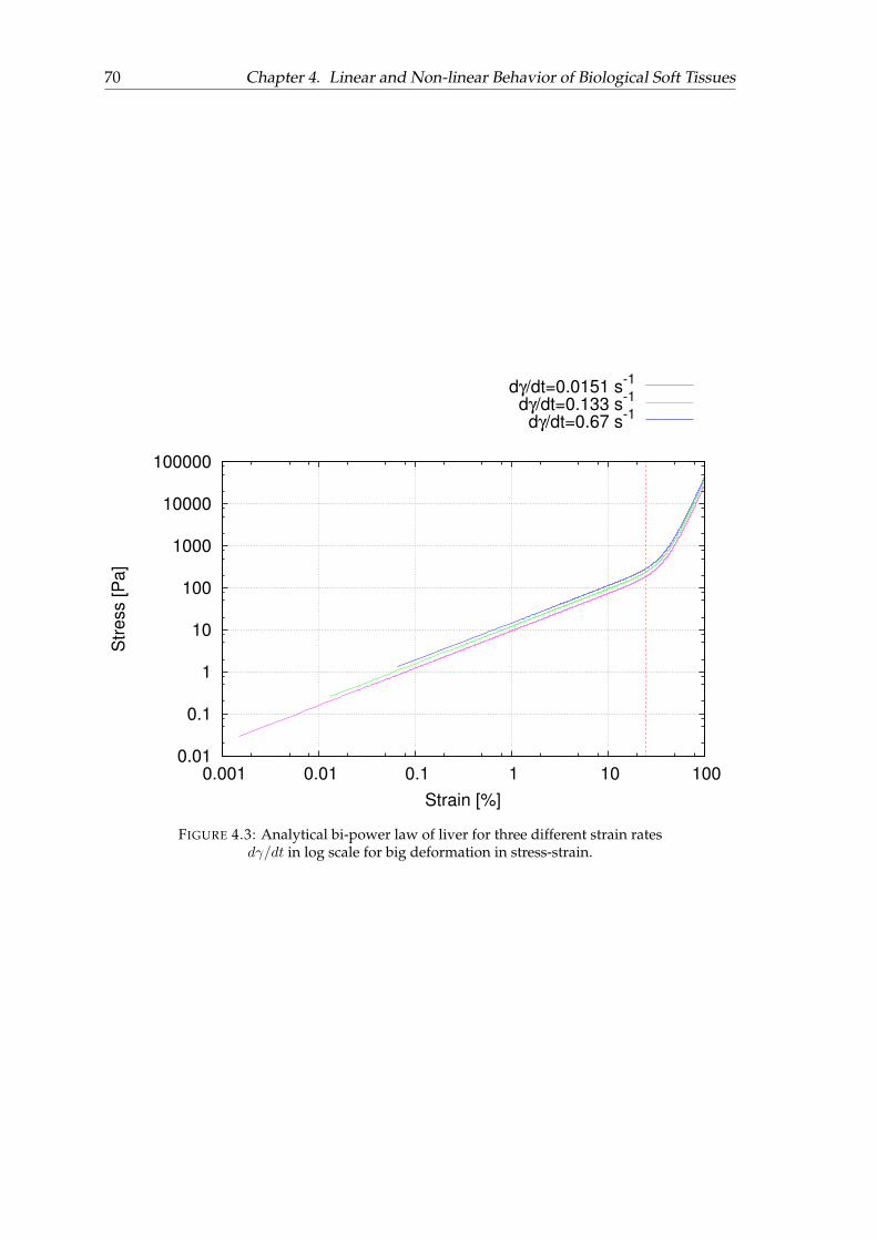
70 Chapter 4. Linear and Non-linear Behavior of Biological Soft Tissues
0.01
0.1
1
10
100
1000
10000
100000
0.001 0.01 0.1 1 10 100
Str
ess [P
a]
Strain [%]
dγ/dt=0.0151 s-1
dγ/dt=0.133 s-1
dγ/dt=0.67 s-1
FIGURE 4.3: Analytical bi-power law of liver for three different strain ratesdγ/dt in log scale for big deformation in stress-strain.
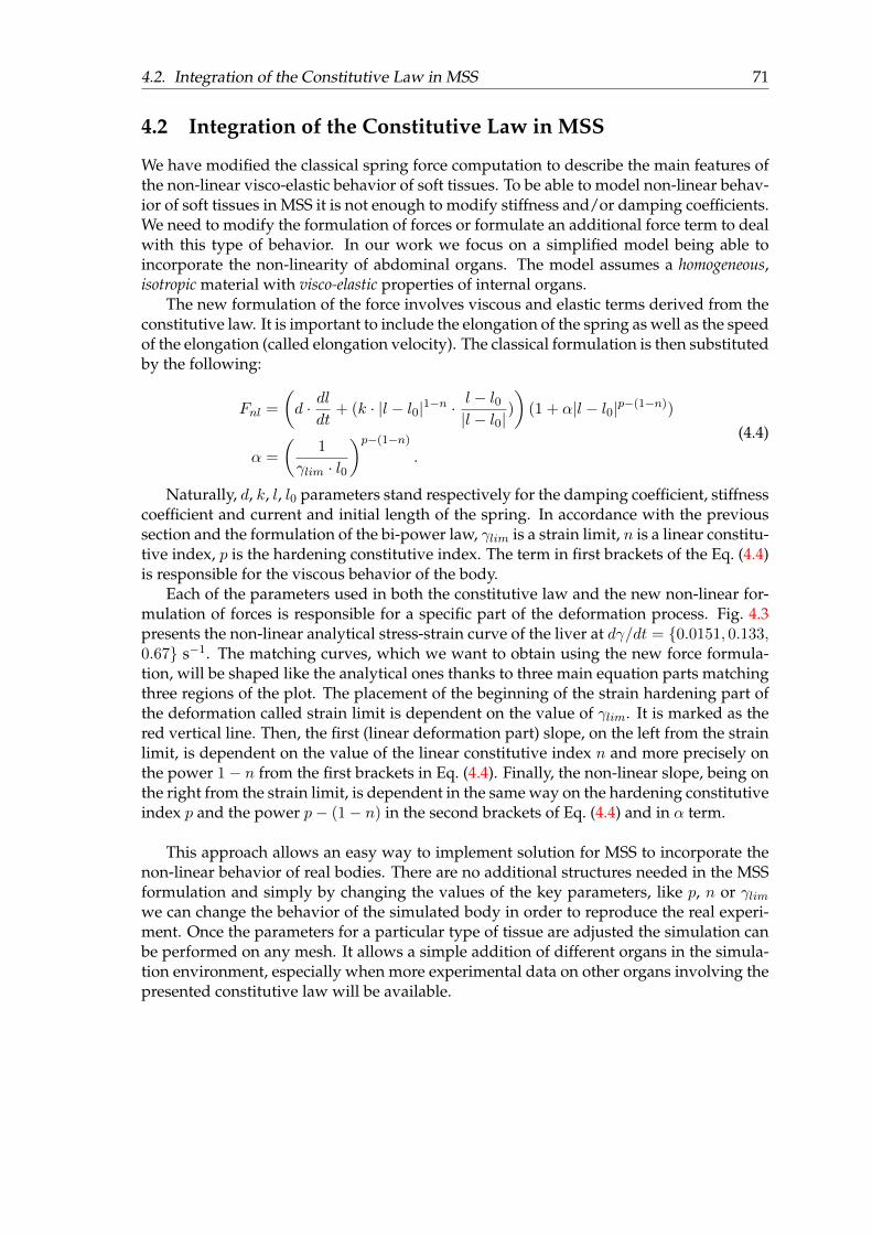
4.2. Integration of the Constitutive Law in MSS 71
4.2 Integration of the Constitutive Law in MSS
We have modified the classical spring force computation to describe the main features ofthe non-linear visco-elastic behavior of soft tissues. To be able to model non-linear behav-ior of soft tissues in MSS it is not enough to modify stiffness and/or damping coefficients.We need to modify the formulation of forces or formulate an additional force term to dealwith this type of behavior. In our work we focus on a simplified model being able toincorporate the non-linearity of abdominal organs. The model assumes a homogeneous,isotropic material with visco-elastic properties of internal organs.
The new formulation of the force involves viscous and elastic terms derived from theconstitutive law. It is important to include the elongation of the spring as well as the speedof the elongation (called elongation velocity). The classical formulation is then substitutedby the following:
Fnl =
(d · dl
dt+ (k · |l − l0|1−n ·
l − l0|l − l0|
)
)(1 + α|l − l0|p−(1−n))
α =
(1
γlim · l0
)p−(1−n)
.
(4.4)
Naturally, d, k, l, l0 parameters stand respectively for the damping coefficient, stiffnesscoefficient and current and initial length of the spring. In accordance with the previoussection and the formulation of the bi-power law, γlim is a strain limit, n is a linear constitu-tive index, p is the hardening constitutive index. The term in first brackets of the Eq. (4.4)is responsible for the viscous behavior of the body.
Each of the parameters used in both the constitutive law and the new non-linear for-mulation of forces is responsible for a specific part of the deformation process. Fig. 4.3presents the non-linear analytical stress-strain curve of the liver at dγ/dt = 0.0151, 0.133,0.67 s−1. The matching curves, which we want to obtain using the new force formula-tion, will be shaped like the analytical ones thanks to three main equation parts matchingthree regions of the plot. The placement of the beginning of the strain hardening part ofthe deformation called strain limit is dependent on the value of γlim. It is marked as thered vertical line. Then, the first (linear deformation part) slope, on the left from the strainlimit, is dependent on the value of the linear constitutive index n and more precisely onthe power 1− n from the first brackets in Eq. (4.4). Finally, the non-linear slope, being onthe right from the strain limit, is dependent in the same way on the hardening constitutiveindex p and the power p− (1− n) in the second brackets of Eq. (4.4) and in α term.
This approach allows an easy way to implement solution for MSS to incorporate thenon-linear behavior of real bodies. There are no additional structures needed in the MSSformulation and simply by changing the values of the key parameters, like p, n or γlimwe can change the behavior of the simulated body in order to reproduce the real experi-ment. Once the parameters for a particular type of tissue are adjusted the simulation canbe performed on any mesh. It allows a simple addition of different organs in the simula-tion environment, especially when more experimental data on other organs involving thepresented constitutive law will be available.
72 Chapter 4. Linear and Non-linear Behavior of Biological Soft Tissues
4.3 Implementation of the Non-Linear MSS Force in TopoSim
As we saw in Ch. 3, the force formulation applies to all of the springs of MSS by theadd_force function in the Spring class. To modify the formulation of the forces it simplyrequires one to change the formula used in this function to a new one, which uses alreadyavailable parameters, like the spring elongation dl, initial spring length l0, the elonga-tion velocity dl/ dt, spring’s stiffness k, spring damping d, etc. The three new parametersused by our non-linear force formulation (see Eq. (4.4)) have to be additionally definedas the add_force function arguments to easily change them depending on the type of thebody. They will include the linear constitutive index n, hardening constitutive index pand visco-elastic strain limit γlim. From now on they are treated as the simulation in-put parameters alongside Young’s modulus, Poisson’s ratio, time step, body density andintegration method. The implementation of the new formulation of force is very easy.Additionally, the simplicity of adjustments allows us to use this formulation for differenttypes of tissues and reproduce various simulations.
4.4 Results of Simulations Using Non-linear Force Formulation
Let us start the presentation of our simulations’ results from the linear and non-linear for-mulation of forces. We begin by verifying the linear approach, followed by the results ofnon-linear force formulation applied to simulate real tissues.
The simulation’s objective is to measure the shear stress of the deformed material. Itis done by constraining the bottom layer of the sample and applying a constant velocity(based on the strain rate dγ/dt) to the top layer. When the deformation occurs, we measurethe shear stress response of the top layer to the applied deformation at every time-step.
The classical formulation of force in MSS (see Eq. (3.3), page 36) provides very littlepossibilities to control the stress-strain curve. The main source of the tissue’s behavior isthen the formulation of spring stiffness, which in our initial implementation incorporatesthe Young modulus and Poisson ratio as the physical parameters in the MSS. Using it wecan try to simulate the linear (small, under the strain limit) deformations, but, as we showin this section, it is not sufficient and requires a use of a force formulation, which takesinto account the particular behavior of selected tissue.
The mesh used for these simulations is in a shape of a cube consisting of 10× 10× 10hexahedral elements of a total size 5 × 5 × 5 cm. The other parameters setup includedensity ρ = 1000 kg/m3 and the gravity g = 0 m/s2. Time step of the simulation was setto dt = 0.001 s. The topological aspect of the simulation is equivalent to the one describedfurther on, in the Sec. 5.3. The parameters used for the linear simulation are limited to theYoung modulus E = 1000 Pa and Poisson ratio ν = 0.499 (indicating incompressibility ofthe simulated body and describing only elasticity of a material), which are in the rangesusually describing soft materials like internal organs. From this simulation we expectonly an approximately correct result in comparison with the analytical solution.
The non-linear simulation works well with the parameters E, n and p chosen accord-ing to Tab. 4.1 from Ch. 4.1.2. The consistency K is used as a reference point to assignYoung’s modulus to the simulation input parameters. The only parameter which needsto be adjusted manually to fit the simulation to the analytical model is the strain limitγlim, which for our non-linear MSS we denoted γlim_mss. Strain limit is responsible forthe part of the curve, which marks the start of the non-linear behavior. The reason for theadjustment of the strain limit and such an approximation of the Young modulus is simple
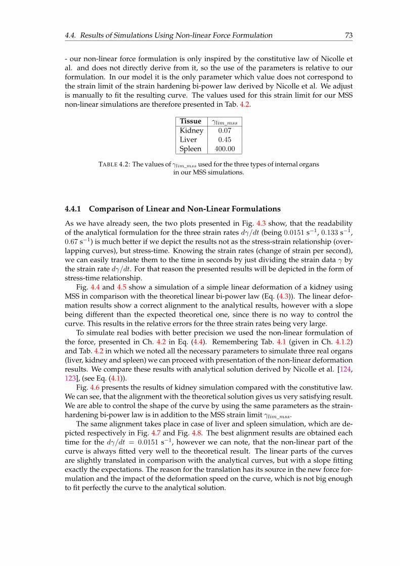
4.4. Results of Simulations Using Non-linear Force Formulation 73
- our non-linear force formulation is only inspired by the constitutive law of Nicolle etal. and does not directly derive from it, so the use of the parameters is relative to ourformulation. In our model it is the only parameter which value does not correspond tothe strain limit of the strain hardening bi-power law derived by Nicolle et al. We adjustis manually to fit the resulting curve. The values used for this strain limit for our MSSnon-linear simulations are therefore presented in Tab. 4.2.
Tissue γlim_mssKidney 0.07Liver 0.45Spleen 400.00
TABLE 4.2: The values of γlim_mss used for the three types of internal organsin our MSS simulations.
4.4.1 Comparison of Linear and Non-Linear Formulations
As we have already seen, the two plots presented in Fig. 4.3 show, that the readabilityof the analytical formulation for the three strain rates dγ/dt (being 0.0151 s−1, 0.133 s−1,0.67 s−1) is much better if we depict the results not as the stress-strain relationship (over-lapping curves), but stress-time. Knowing the strain rates (change of strain per second),we can easily translate them to the time in seconds by just dividing the strain data γ bythe strain rate dγ/dt. For that reason the presented results will be depicted in the form ofstress-time relationship.
Fig. 4.4 and 4.5 show a simulation of a simple linear deformation of a kidney usingMSS in comparison with the theoretical linear bi-power law (Eq. (4.3)). The linear defor-mation results show a correct alignment to the analytical results, however with a slopebeing different than the expected theoretical one, since there is no way to control thecurve. This results in the relative errors for the three strain rates being very large.
To simulate real bodies with better precision we used the non-linear formulation ofthe force, presented in Ch. 4.2 in Eq. (4.4). Remembering Tab. 4.1 (given in Ch. 4.1.2)and Tab. 4.2 in which we noted all the necessary parameters to simulate three real organs(liver, kidney and spleen) we can proceed with presentation of the non-linear deformationresults. We compare these results with analytical solution derived by Nicolle et al. [124,123], (see Eq. (4.1)).
Fig. 4.6 presents the results of kidney simulation compared with the constitutive law.We can see, that the alignment with the theoretical solution gives us very satisfying result.We are able to control the shape of the curve by using the same parameters as the strain-hardening bi-power law is in addition to the MSS strain limit γlim_mss.
The same alignment takes place in case of liver and spleen simulation, which are de-picted respectively in Fig. 4.7 and Fig. 4.8. The best alignment results are obtained eachtime for the dγ/dt = 0.0151 s−1, however we can note, that the non-linear part of thecurve is always fitted very well to the theoretical result. The linear parts of the curvesare slightly translated in comparison with the analytical curves, but with a slope fittingexactly the expectations. The reason for the translation has its source in the new force for-mulation and the impact of the deformation speed on the curve, which is not big enoughto fit perfectly the curve to the analytical solution.
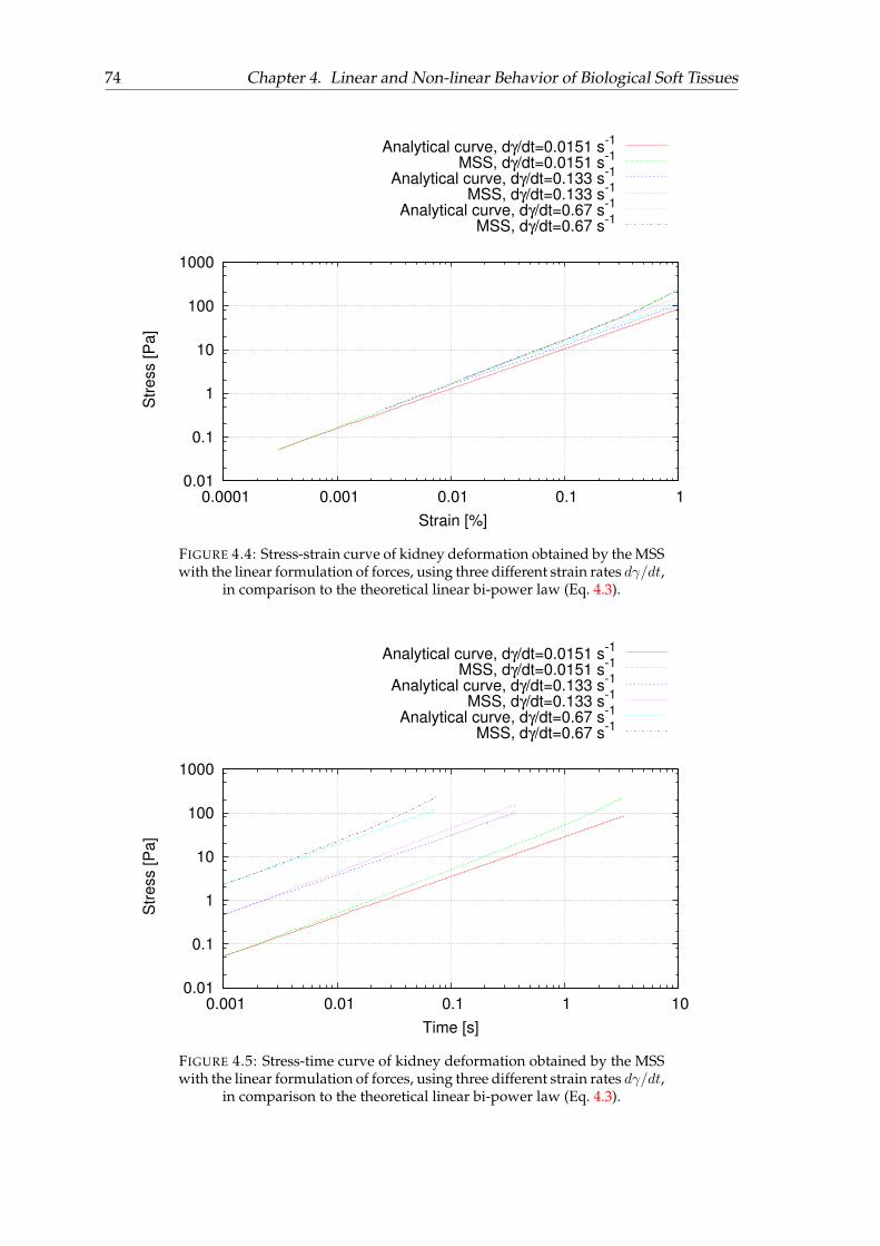
74 Chapter 4. Linear and Non-linear Behavior of Biological Soft Tissues
0.01
0.1
1
10
100
1000
0.0001 0.001 0.01 0.1 1
Str
ess [P
a]
Strain [%]
Analytical curve, dγ/dt=0.0151 s-1
MSS, dγ/dt=0.0151 s-1
Analytical curve, dγ/dt=0.133 s-1
MSS, dγ/dt=0.133 s-1
Analytical curve, dγ/dt=0.67 s-1
MSS, dγ/dt=0.67 s-1
FIGURE 4.4: Stress-strain curve of kidney deformation obtained by the MSSwith the linear formulation of forces, using three different strain rates dγ/dt,
in comparison to the theoretical linear bi-power law (Eq. 4.3).
0.01
0.1
1
10
100
1000
0.001 0.01 0.1 1 10
Str
ess [P
a]
Time [s]
Analytical curve, dγ/dt=0.0151 s-1
MSS, dγ/dt=0.0151 s-1
Analytical curve, dγ/dt=0.133 s-1
MSS, dγ/dt=0.133 s-1
Analytical curve, dγ/dt=0.67 s-1
MSS, dγ/dt=0.67 s-1
FIGURE 4.5: Stress-time curve of kidney deformation obtained by the MSSwith the linear formulation of forces, using three different strain rates dγ/dt,
in comparison to the theoretical linear bi-power law (Eq. 4.3).
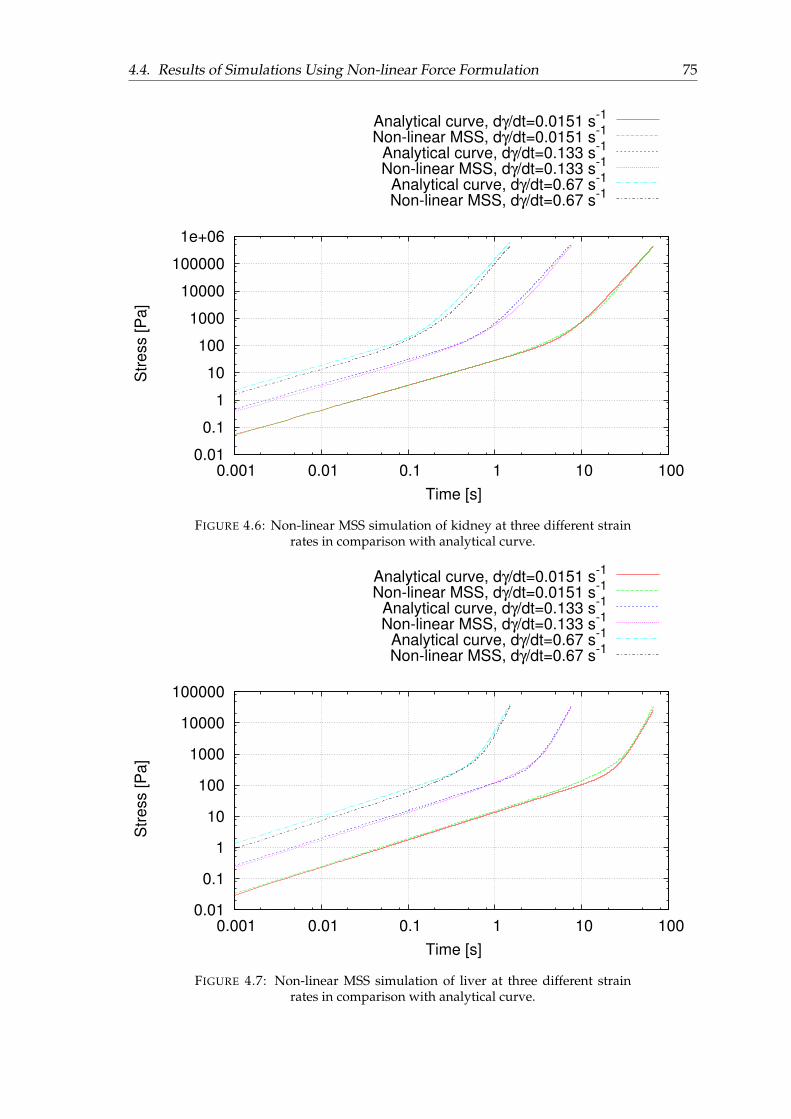
4.4. Results of Simulations Using Non-linear Force Formulation 75
0.01
0.1
1
10
100
1000
10000
100000
1e+06
0.001 0.01 0.1 1 10 100
Str
ess [P
a]
Time [s]
Analytical curve, dγ/dt=0.0151 s-1
Non-linear MSS, dγ/dt=0.0151 s-1
Analytical curve, dγ/dt=0.133 s-1
Non-linear MSS, dγ/dt=0.133 s-1
Analytical curve, dγ/dt=0.67 s-1
Non-linear MSS, dγ/dt=0.67 s-1
FIGURE 4.6: Non-linear MSS simulation of kidney at three different strainrates in comparison with analytical curve.
0.01
0.1
1
10
100
1000
10000
100000
0.001 0.01 0.1 1 10 100
Str
ess [P
a]
Time [s]
Analytical curve, dγ/dt=0.0151 s-1
Non-linear MSS, dγ/dt=0.0151 s-1
Analytical curve, dγ/dt=0.133 s-1
Non-linear MSS, dγ/dt=0.133 s-1
Analytical curve, dγ/dt=0.67 s-1
Non-linear MSS, dγ/dt=0.67 s-1
FIGURE 4.7: Non-linear MSS simulation of liver at three different strainrates in comparison with analytical curve.
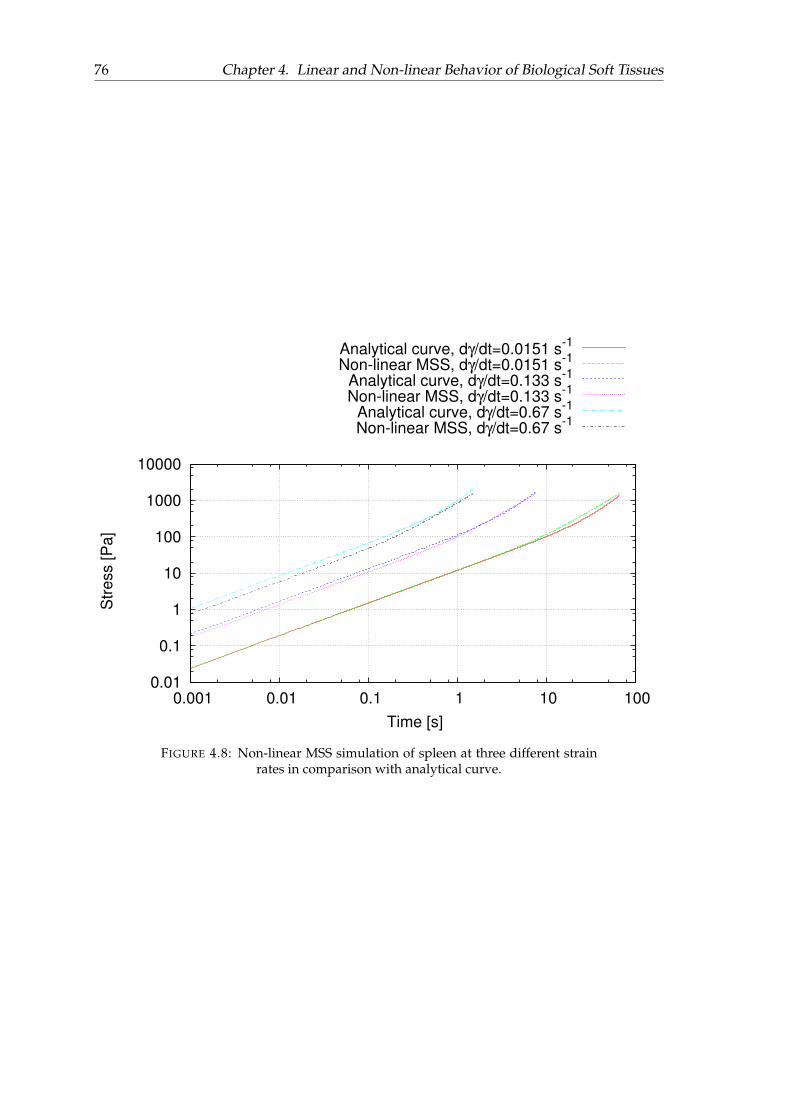
76 Chapter 4. Linear and Non-linear Behavior of Biological Soft Tissues
0.01
0.1
1
10
100
1000
10000
0.001 0.01 0.1 1 10 100
Str
ess [P
a]
Time [s]
Analytical curve, dγ/dt=0.0151 s-1
Non-linear MSS, dγ/dt=0.0151 s-1
Analytical curve, dγ/dt=0.133 s-1
Non-linear MSS, dγ/dt=0.133 s-1
Analytical curve, dγ/dt=0.67 s-1
Non-linear MSS, dγ/dt=0.67 s-1
FIGURE 4.8: Non-linear MSS simulation of spleen at three different strainrates in comparison with analytical curve.
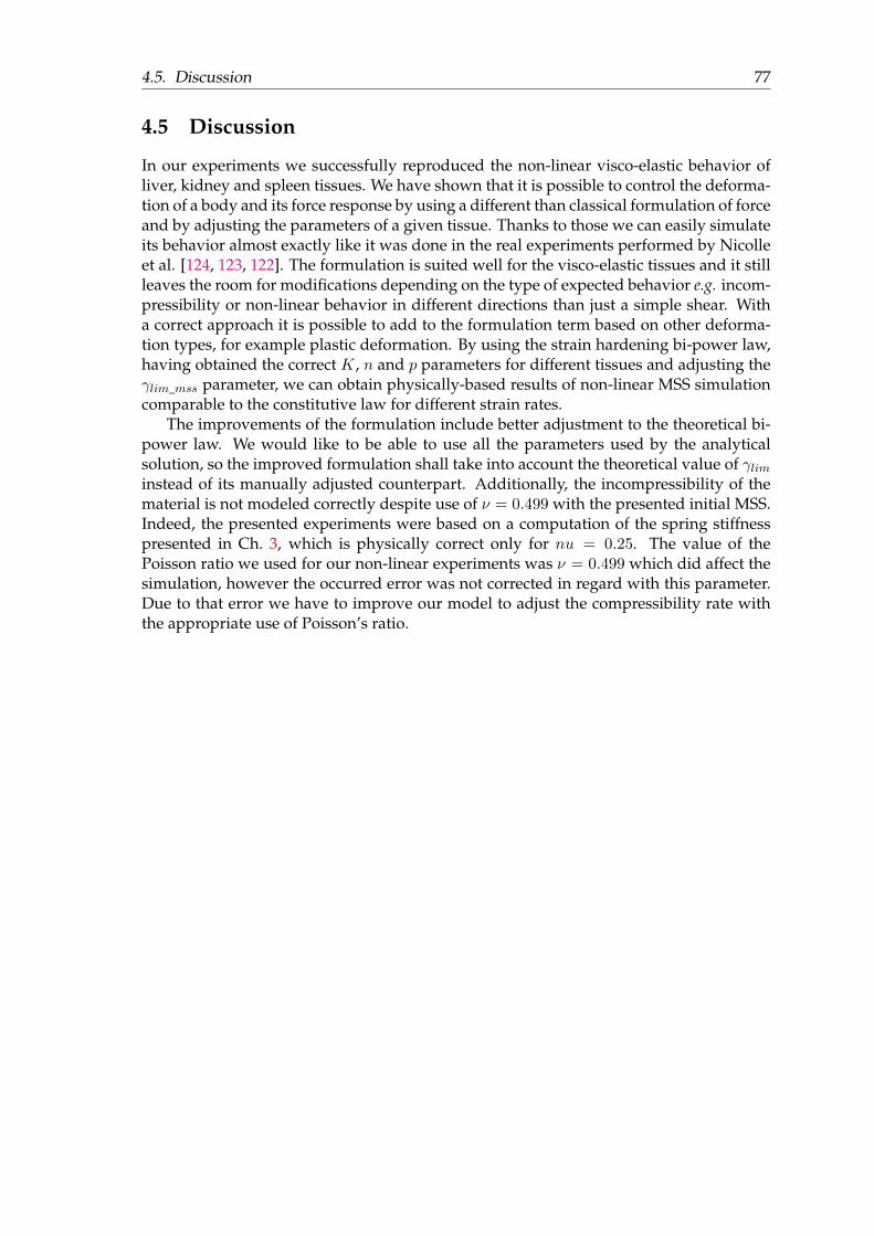
4.5. Discussion 77
4.5 Discussion
In our experiments we successfully reproduced the non-linear visco-elastic behavior ofliver, kidney and spleen tissues. We have shown that it is possible to control the deforma-tion of a body and its force response by using a different than classical formulation of forceand by adjusting the parameters of a given tissue. Thanks to those we can easily simulateits behavior almost exactly like it was done in the real experiments performed by Nicolleet al. [124, 123, 122]. The formulation is suited well for the visco-elastic tissues and it stillleaves the room for modifications depending on the type of expected behavior e.g. incom-pressibility or non-linear behavior in different directions than just a simple shear. Witha correct approach it is possible to add to the formulation term based on other deforma-tion types, for example plastic deformation. By using the strain hardening bi-power law,having obtained the correct K, n and p parameters for different tissues and adjusting theγlim_mss parameter, we can obtain physically-based results of non-linear MSS simulationcomparable to the constitutive law for different strain rates.
The improvements of the formulation include better adjustment to the theoretical bi-power law. We would like to be able to use all the parameters used by the analyticalsolution, so the improved formulation shall take into account the theoretical value of γliminstead of its manually adjusted counterpart. Additionally, the incompressibility of thematerial is not modeled correctly despite use of ν = 0.499 with the presented initial MSS.Indeed, the presented experiments were based on a computation of the spring stiffnesspresented in Ch. 3, which is physically correct only for nu = 0.25. The value of thePoisson ratio we used for our non-linear experiments was ν = 0.499 which did affect thesimulation, however the occurred error was not corrected in regard with this parameter.Due to that error we have to improve our model to adjust the compressibility rate withthe appropriate use of Poisson’s ratio.

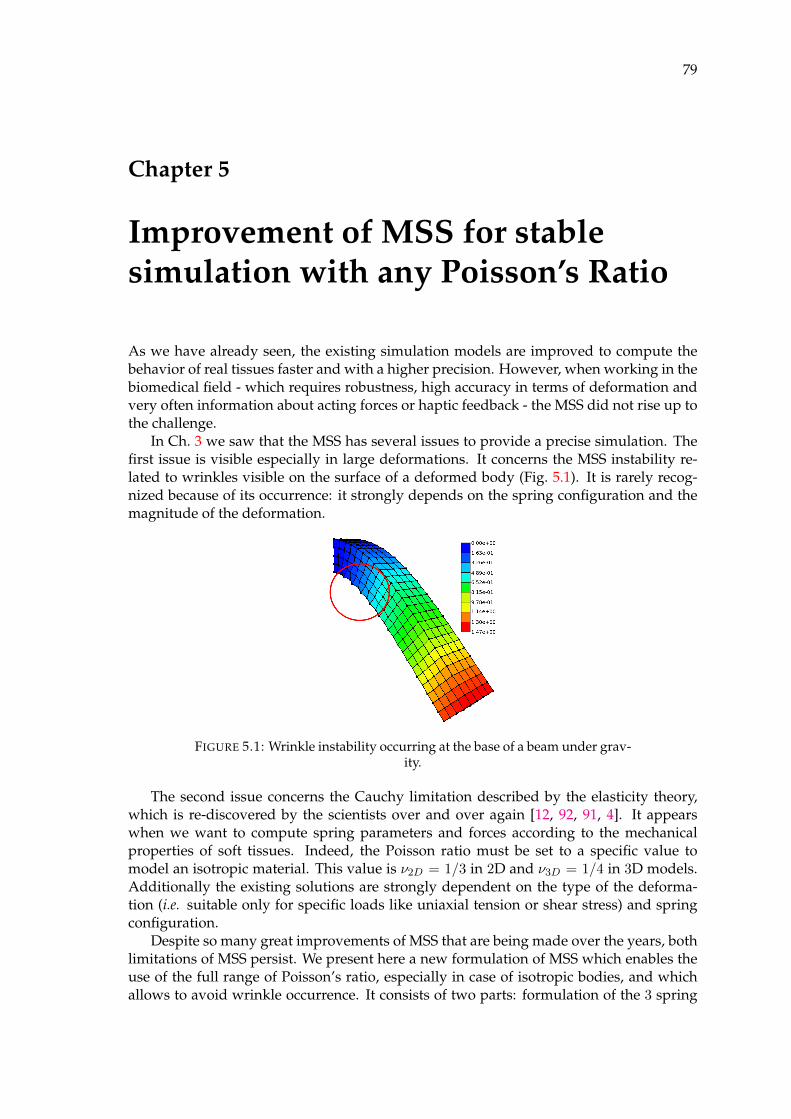
79
Chapter 5
Improvement of MSS for stablesimulation with any Poisson’s Ratio
As we have already seen, the existing simulation models are improved to compute thebehavior of real tissues faster and with a higher precision. However, when working in thebiomedical field - which requires robustness, high accuracy in terms of deformation andvery often information about acting forces or haptic feedback - the MSS did not rise up tothe challenge.
In Ch. 3 we saw that the MSS has several issues to provide a precise simulation. Thefirst issue is visible especially in large deformations. It concerns the MSS instability re-lated to wrinkles visible on the surface of a deformed body (Fig. 5.1). It is rarely recog-nized because of its occurrence: it strongly depends on the spring configuration and themagnitude of the deformation.
FIGURE 5.1: Wrinkle instability occurring at the base of a beam under grav-ity.
The second issue concerns the Cauchy limitation described by the elasticity theory,which is re-discovered by the scientists over and over again [12, 92, 91, 4]. It appearswhen we want to compute spring parameters and forces according to the mechanicalproperties of soft tissues. Indeed, the Poisson ratio must be set to a specific value tomodel an isotropic material. This value is ν2D = 1/3 in 2D and ν3D = 1/4 in 3D models.Additionally the existing solutions are strongly dependent on the type of the deforma-tion (i.e. suitable only for specific loads like uniaxial tension or shear stress) and springconfiguration.
Despite so many great improvements of MSS that are being made over the years, bothlimitations of MSS persist. We present here a new formulation of MSS which enables theuse of the full range of Poisson’s ratio, especially in case of isotropic bodies, and whichallows to avoid wrinkle occurrence. It consists of two parts: formulation of the 3 spring
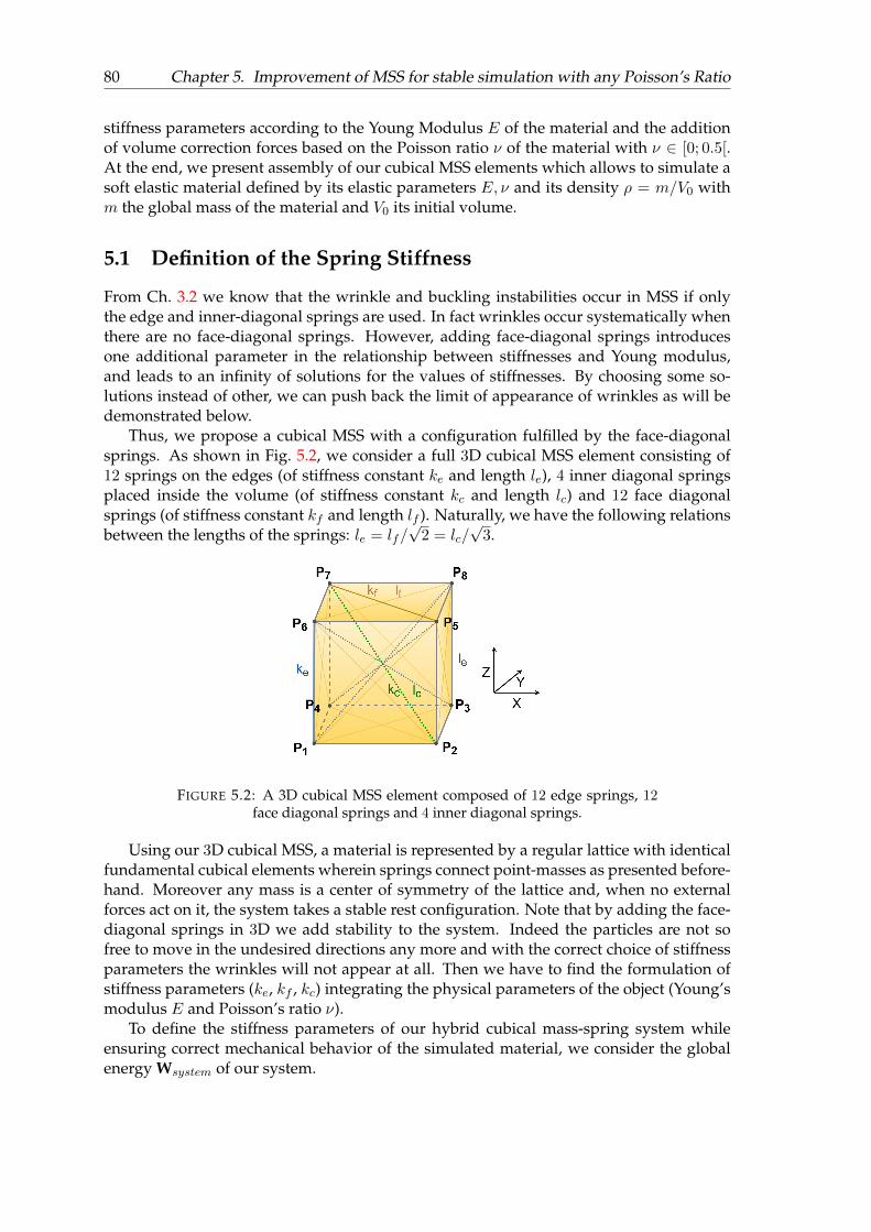
80 Chapter 5. Improvement of MSS for stable simulation with any Poisson’s Ratio
stiffness parameters according to the Young Modulus E of the material and the additionof volume correction forces based on the Poisson ratio ν of the material with ν ∈ [0; 0.5[.At the end, we present assembly of our cubical MSS elements which allows to simulate asoft elastic material defined by its elastic parameters E, ν and its density ρ = m/V0 withm the global mass of the material and V0 its initial volume.
5.1 Definition of the Spring Stiffness
From Ch. 3.2 we know that the wrinkle and buckling instabilities occur in MSS if onlythe edge and inner-diagonal springs are used. In fact wrinkles occur systematically whenthere are no face-diagonal springs. However, adding face-diagonal springs introducesone additional parameter in the relationship between stiffnesses and Young modulus,and leads to an infinity of solutions for the values of stiffnesses. By choosing some so-lutions instead of other, we can push back the limit of appearance of wrinkles as will bedemonstrated below.
Thus, we propose a cubical MSS with a configuration fulfilled by the face-diagonalsprings. As shown in Fig. 5.2, we consider a full 3D cubical MSS element consisting of12 springs on the edges (of stiffness constant ke and length le), 4 inner diagonal springsplaced inside the volume (of stiffness constant kc and length lc) and 12 face diagonalsprings (of stiffness constant kf and length lf ). Naturally, we have the following relationsbetween the lengths of the springs: le = lf/
√2 = lc/
√3.
FIGURE 5.2: A 3D cubical MSS element composed of 12 edge springs, 12face diagonal springs and 4 inner diagonal springs.
Using our 3D cubical MSS, a material is represented by a regular lattice with identicalfundamental cubical elements wherein springs connect point-masses as presented before-hand. Moreover any mass is a center of symmetry of the lattice and, when no externalforces act on it, the system takes a stable rest configuration. Note that by adding the face-diagonal springs in 3D we add stability to the system. Indeed the particles are not sofree to move in the undesired directions any more and with the correct choice of stiffnessparameters the wrinkles will not appear at all. Then we have to find the formulation ofstiffness parameters (ke, kf , kc) integrating the physical parameters of the object (Young’smodulus E and Poisson’s ratio ν).
To define the stiffness parameters of our hybrid cubical mass-spring system whileensuring correct mechanical behavior of the simulated material, we consider the globalenergy Wsystem of our system.
5.1. Definition of the Spring Stiffness 81
In the following, we first present the formulation of the stiffness constants ke, kc, kf ofthe springs coming from the energy Wsprings (defined by Eq. (3.1), page 37).
General Case
Let us first consider a MSS constructed using identical springs defined by a stiffness con-stant k and rest length l. We introduce r and r′ of respective lengths l and l′ as the exten-sion vectors of the springs at rest and in a deformed state.
Let us apply a homogeneous deformation to the lattice of this MSS, whereby point Xis displaced to x = X + u. The displacement is described by ui = xi −Xi = ∂ui/∂Xj Xj ,with i, j = x, y, z, where the displacement gradient ∂ui/∂Xj = ∇uij is small with respectto unity. By the assumption that any mass point is the center of symmetry for all springsconnected to it, any spring is connected to identical springs, all with the same vector raligned through the entire lattice, the spring vector too varies by a displacement δ = ∇u·rand its length varies by δ = l′− l =
√(r +∇uT · r)2− l. At first order included in∇u, we
have:
δ =√
(r + (∇u)T · r)2 =1
2l∇iujrirj (5.1)
To the same precision, the elastic energy of the spring (Eq. (3.1), page 36) can be writ-ten:
Wspring(δ) =1
2∇iuj ∇kul
k
l2ri rj rk rl. (5.2)
Using the linearized strain tensor of Green-Lagrange, we have to keep in mind that thetotal elastic energy density of a fundamental cell defined in Eq. (3.6) (page 37), is obtainedby summing over all springs α of the cell (being a unit cube), with:
Cijkl =1
V
∑α∈cell
k
l2rα i rα j rαk rα l, (5.3)
where rα i is the i-th cartesian component of vector rα. We perform a summation overi to l being implied, whereas summation over α identifying the springs is explicitly stated.
Our 3D Cubical MSS’s Element
Now let us consider one cubical element of our MSS which is composed of 12 edge springs(ke, le), 12 face diagonal springs (kf , lf ) and 4 inner diagonal springs (kf , lf ) as illustratedin Fig. 5.2 and which lays in the middle of an infinite lattice of the same cubical elements.
• Four of the edge springs are parallel to any of the axes directions, but each spring be-longs to four adjacent cells, resulting into only one edge spring (ke, le) to be countedin each direction. These are represented by the following vectors of identical lengthequal to le:
r1 = (le, 0, 0)T , r2 = (0, le, 0)T , r3 = (0, 0, le)T . (5.4)
• The four inner diagonal springs are represented by the following vectors of identicallength lc =
√3 le:
82 Chapter 5. Improvement of MSS for stable simulation with any Poisson’s Ratio
r4 = (le, le, le)T , r5 = (le, le,−le)T ,
r6 = (le,−le, le)T , r7 = (−le, le, le)T .(5.5)
• There are two identical vectors appearing on two opposite faces of the cell, but sinceeach face belongs to two adjacent cells, one must count once each of the followingvectors of identical length lf =
√2 le:
r8 = (le, le, 0)T , r9 = (le,−le, 0)T , r10 = (0, le, le)T ,
r11 = (0, le,−le)T , r12 = (le, 0, le)T , r13 = (le, 0,−le)T .
(5.6)
Considering these assumptions, Eq. (5.3) for an element of our MSS becomes:
Cijkl = l−3e
(3∑
α=1
l−2e ke rα i rα j rαk rα l +
7∑α=4
l−2c kc rα i rα j rαk rα l
+13∑α=8
l−2f kf rα i rα j rαk rα l
)
= l−5e
(ke
3∑α=1
rα i rα j rαk rα l
+ 13 kc
7∑α=4
rα i rα j rαk rα l + 12 kf
13∑α=8
rα i rα j rαk rα l
).
(5.7)
From this equation, we directly obtain:
Cxxxx = l−5e
(ke
3∑α=1
(rαx)4 + 13 kc
7∑α=4
(rαx)4 + 12 kf
13∑α=8
(rαx)4
)(5.8)
= l−1e
(ke +
4
3kc + 2 kf
),
Cxxyy = l−5e
(ke
3∑α=1
(rαxrαy)2 + 1
3 kc
7∑α=4
(rαxrαy)2 + 1
2 kf
13∑α=8
(rαxrαy)2
)(5.9)
= l−1e
(4
3kc + kf
)Then, we have to satisfy Eq. (3.11) which give the relation between the elastic coeffi-
cients for an isotropic material modeled by a cubical MSS. Cauchy relation Cxxyy = Cxyxyis automatically satisfied, as expected for a system of springs. Thus, let us remember thatwe have:
Cxxxx = Cxxyy + 2 Cxyxy,
Cxxyy = Cxyxy = λ = µ(5.10)
leading to:
5.1. Definition of the Spring Stiffness 83
ke =8
3kc + kf ,
λ = µ =
(4
3kc + kf
)l−1e .
(5.11)
Consequently, to compute a formula for each stiffness coefficient ke, kf , kc we still needone more dependency. For this purpose we decided that there exists a relation kf/kc = Athat will serve as a degree of freedom stabilizing the critical movements of the particles.After the computations, we get the following formulas for the stiffness constants, remem-bering that Cauchy equality forces us to use ν = 1/4 (involving λ = µ = 2/5 E):
kfkc
= A
kc =3 µ le
3A+ 4=
3 E le10 + 7.5 A
=3 E lc√
3 (10 + 7.5 A)
kf =3 µ le
3 + 4/A=
3 E le7.5 + 10/A
=3 E lf√
2 (7.5 + 10/A)
ke = kf +8
3kc =
3 E le7.5 + 10/A
+8 E le
10 + 7.5 A
(5.12)
Assuming a case in whichA = 0 the term kf = 0, which means that we do not considersprings on the diagonals of the faces. Similarly, assuming A → ∞ would mean that theterms kc and 1/A will go to 0. In this case, we would have:
kfkc→∞ ; kc → 0 ;
kf = ke =3 E le
7.5=
3 E lf
7.5√
2.
(5.13)
To sum up, considering one cubical element of the lattice, we obtain the formulationsof the stiffness constants for the 3 kinds of springs involved in our MSS. These formula-tions are defined for any value of Young’s modulus E and obeying the Cauchy restrictionν = 1/4. It corresponds to the ratio kf/kc established according to the geometrical mod-eling of the material. In our experiments presented in Ch. 5.6 we have verified the impactof the value of A and we found out that a variation of A ∈ [0.01; 100] does not impactthe simulation in a noticeable way. The most visible impact that the parameter has on thesimulation took place in the beam under gravity simulation case (see Fig. 5.3). Of course itis worth to note that extreme values of A: A = 0 or A→∞ result in using only two typesof springs instead of all three. Nevertheless, by introducing A in our MSS we introducea new degree of freedom which permits to better control the instability of our simulationmethod.
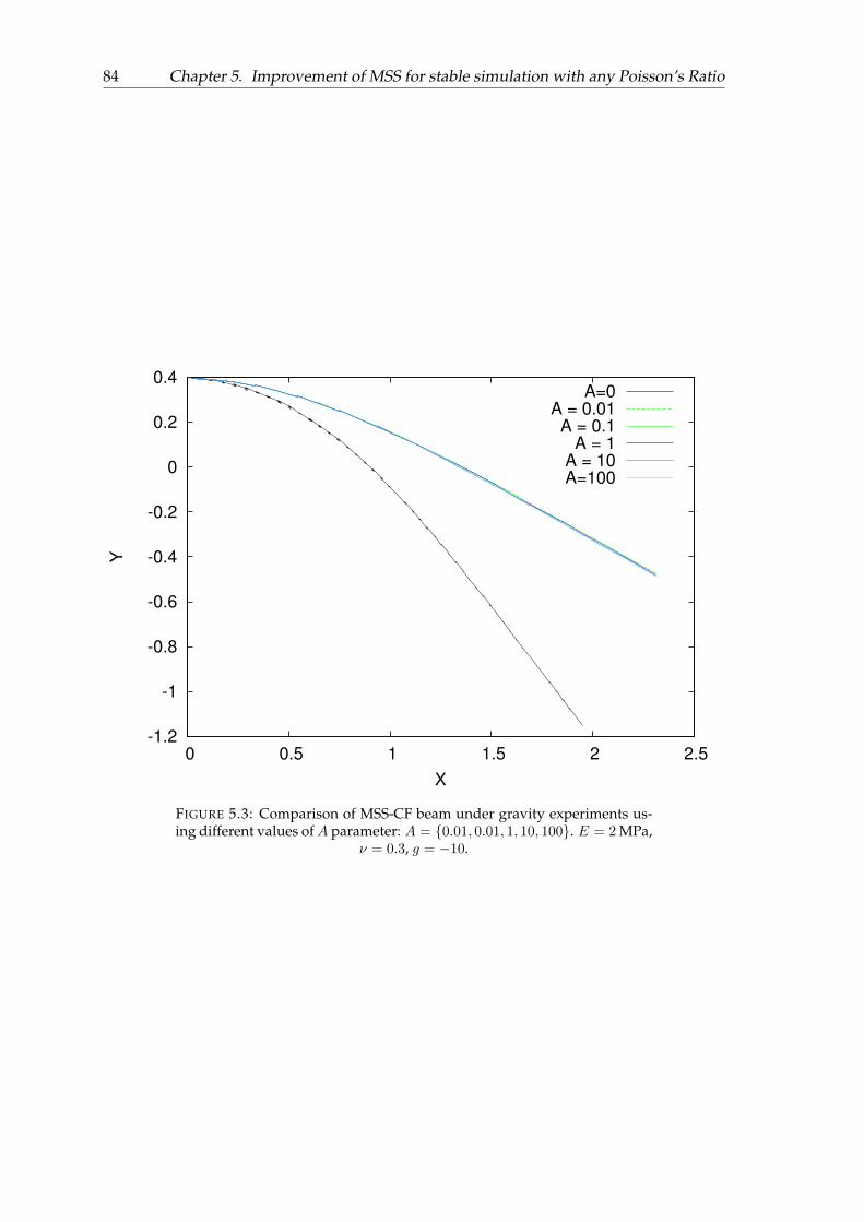
84 Chapter 5. Improvement of MSS for stable simulation with any Poisson’s Ratio
-1.2
-1
-0.8
-0.6
-0.4
-0.2
0
0.2
0.4
0 0.5 1 1.5 2 2.5
Y
X
A=0
A = 0.01
A = 0.1
A = 1
A = 10
A=100
FIGURE 5.3: Comparison of MSS-CF beam under gravity experiments us-ing different values ofA parameter: A = 0.01, 0.01, 1, 10, 100. E = 2 MPa,
ν = 0.3, g = −10.
5.2. Definition of the Volume Correction Forces 85
5.2 Definition of the Volume Correction Forces
The second contribution of this chapter is finding a solution to escape the Cauchy limi-tation (imposing a Poisson ratio fixed to 1/4) using a cubical MSS to simulate isotropicelastic material. As a solution we propose to add another type of forces - called correctionforces - as an addition to the existing linear spring forces. At the end of each time step ofthe simulation loop the forces applied on each particle of our hybrid MSS correspond tothe sum of the classical spring forces and the correction forces.
A similar idea was already proposed by [12], but our formulation ensures the use ofany Poisson’s ratio thanks to quadratic formulation of the correction forces. This meansthat we increase the degree of the formulation of forces of our system. Moreover, theseadditional forces will enable to control the volume variation of the material while consid-ering its compressibility property (Poisson’s ratio). These forces will ensure the correctvolumetric behavior of the body without affecting the global shape of the deformation.
5.2.1 Energy of Volume Variation
To formulate these correction forces, we consider the energy due to the volume variationof the material during its deformation. To achieve this, let us consider a cubical element cof our system. We note its current volume V c and its initial volume V c
0 . The coefficient κof the material is linked to the volume variation and will be defined later on. The energyof our element c due to this variation is then defined by:
W cvol =
1
2κ
(V c − V c0 )2
V0, (5.14)
with the corresponding energy density:
W cvol =
W cvol
V c0
=1
2κ
(V c − V c
0
V c0
)2
(5.15)
and the following differential dW cvol = · · · dV c of the energy:
δW cvol = κ
V c − V c0
V0δV c. (5.16)
From the energy density we can deduce the corresponding correction force that wehave to apply on each particle of the element in order to control its volume variation.Thus, considering a particle Pi residing in a position Pi, its correction force is defined by:
FPi = −∂W c
vol
∂Pi= −κ V
c − V c0
V0
∂V c
∂Pi. (5.17)
Consequently, to compute this force, we need: (i) to estimate the volume V c of theelement and its gradient ∂V c/∂Pi according to each particle Pi, all during the simulationloop; (ii) to express the coefficient κ with E and ν.
5.2.2 Approximation of the Current Volume
As illustrated in Fig. 5.2, we consider a cubical element composed of 8 particles notedPi for i ∈ 1, ..., 8. After some deformations this element is no more a cube, but itis slightly distorted. We can compute three vectors X,Y,Z to describe a mean value ofthe cube’s edges in Cartesian directions. These vectors are computed by the followingintuitive formulas:
86 Chapter 5. Improvement of MSS for stable simulation with any Poisson’s Ratio
X =
1
4(−−→P1P2 +
−−→P4P3 +
−−→P6P5 +
−−→P7P8)
Y =1
4(−−→P2P3 +
−−→P1P4 +
−−→P5P8 +
−−→P6P7)
Z =1
4(−−→P1P6 +
−−→P3P8 +
−−→P2P5 +
−−→P4P7).
(5.18)
Then, considering a linear deformation of the volume, instead of a complex and timeconsuming computation of splitting each hexahedron into tetrahedra, we can get an ap-proximation of the current volume V c using these 3 vectors with:
V c = X · (Y× Z) = Y · (Z× X) = Z · (X× Y). (5.19)
5.2.3 Formulation of the Correction Forces
Now we can express the formulation of the correction forces for each particle Pi of acubical element with i ∈ [1, 8]. Considering Eq. (5.17) and computing the volume gradient∂V c/∂Pi according to Eq. (5.19), we obtain the following formulas:
FP1 = −κ (V c − V c0 )
4 V0(−(Y× Z)− (Z× X)− (X× Y)) ,
FP2 = −κ (V c − V c0 )
4 V0((Y× Z)− (Z× X)− (X× Y)) ,
FP3 = −κ (V c − V c0 )
4 V0((Y× Z) + (Z× X)− (X× Y)) ,
FP4 = −κ (V c − V c0 )
4 V0(−(Y× Z) + (Z× X)− (X× Y)) ,
FP5 = −κ (V c − V c0 )
4 V0((Y× Z)− (Z× X) + (X× Y)) ,
FP6 = −κ (V c − V c0 )
4 V0(−(Y× Z)− (Z× X) + (X× Y)) ,
FP7 = −κ (V c − V c0 )
4 V0(−(Y× Z) + (Z× X) + (X× Y)) ,
FP8 = −κ (V c − V c0 )
4 V0((Y× Z) + (Z× X) + (X× Y)) ,
(5.20)
with the logical relations:
FP1 = −FP8 , FP2 = −FP7 , FP3 = −FP6 , FP4 = −FP5 . (5.21)
5.2.4 Definition of κ.
To compute all the necessary equations, we have to express the coefficient κ accordingto the actual material properties: Poisson ratio ν and the Young modulus E. Keep inmind that V0 and V correspond respectively to the initial and current volume of the entiremodel. Moreover, if we consider ε as the linearized strain tensor of Green-Lagrange, weknow that Tr(ε) corresponds to the volume variation of the material during the simula-tion with Tr(ε) = (V − V0)/V0.
Then the energy density of our hybrid MSS with correction forces is defined by:
Wsystem =Wsystem
V0=Wsprings
V0+Wvol
V0= Wsprings + Wvol. (5.22)
5.2. Definition of the Volume Correction Forces 87
First let us focus on the energy due to the springs by only considering the 3D MSSwithout correction forces. Simulating an isotropic elastic material we know from Eq. (3.9)and the Cauchy equality that its elastic energy density is:
Wsprings =µ
2(Tr(ε))2 + µ Tr(ε2). (5.23)
Then, if we focus on the energy density at a volume variation, we can note fromEq. (5.15) and the expression of Tr(ε) that we have:
Wvol =1
2κ (Tr(ε))2. (5.24)
At the end, considering our complete hybrid MSS with the correction forces and re-calling that (V − V0)/V0 = Tr(ε), its energy density is defined by:
Wsystem = Wsprings + Wvol
=1
2(µ+ κ) (Tr(ε))2 + µ Tr(ε2)
(5.25)
The corresponding stress tensor is then defined by:
σij =∂Wsystem
∂εij= (µ+ κ) δij εkk + 2 µ εij . (5.26)
Now, let us consider an uniaxial strain experiment performed on our isotropic, elasticmaterial. This experiment is characterized by σ11 = σ22 = σ33 = 0 and σij = 0 for(i, j) 6= (1, 1). Thus, we obtain the following expressions for the stress tensor components:
σ11 = (3µ+ κ) ε11 + (µ+ κ)(ε22 + ε33)σ22 = (3µ+ κ) ε22 + (µ+ κ)(ε11 + ε33) = 0σ33 = (3µ+ κ) ε33 + (µ+ κ)(ε11 + ε22) = 0σij = σji = 2µ εij , i 6= j.
(5.27)
From these we can deduce that ε22 = ε33. Consequently, the previous expressions canbe reformulated:
σ11 = (3µ+ κ) ε11 + 2 (µ+ κ) ε22
σ22 = σ33 = (µ+ κ) ε11 + 2 (2µ+ κ) ε22 = 0σij = σji = 2µ εij , i 6= j.
(5.28)
Using Eq. (5.27) will result in:
σ11 =µ (5 µ+ 3 κ)
2 µ+ κε11, (5.29)
and from Eq. (5.28) we obtain:
ε22 = − µ+ κ
2 (2µ+ κ)ε11 = ε33, (5.30)
Then, knowing that the Poisson ratio and the Young modulus are defined for this typeof body by ν = −ε22/ε11 and E = σ11/ε11, we have:
88 Chapter 5. Improvement of MSS for stable simulation with any Poisson’s Ratio
ν =µ+ κ
2 (2µ+ κ), (5.31)
E =µ (5 µ+ 3 κ)
2 µ+ κ. (5.32)
By inverting these relationships, we obtain:
µ =κ(2 ν − 1)
1− 4 ν, (5.33)
κ =µ(5µ− 2E)
(E − 3µ)(5.34)
finally leading to the following relations:
µ =E
2 (1 + ν), (5.35)
κ =1
2
E (4ν − 1)
(1 + ν)(1− 2ν)= K − 5
3µ. (5.36)
If we observe the formulation of the coefficient κ (Eq. (5.36)) depicted in Fig. 5.4 as afunction of the Poisson ratio κ/E (ν), we note the following:
• for ν = 1/4 the κ coefficient is equal to 0 leading to Wvol = 0, since we do not needcorrection force for this kind of material (as the 3D cubical MSS naturally modeledit);
• for ν → 1/2, the κ coefficient moves toward the infinity, as infinite forces have to beapplied to preserve the volume of the incompressible material;
• for ν = 0, κ = −12 E. Thus, in the compression experiment we can observe no
dilatation in the transverse direction and the change of the volume is equal to thedisplacement of the top face of the fully compressible material;
• although all known materials are characterized by ν ≥ 0, the stability limits of ν are−1 ≤ ν ≤ 1/2.
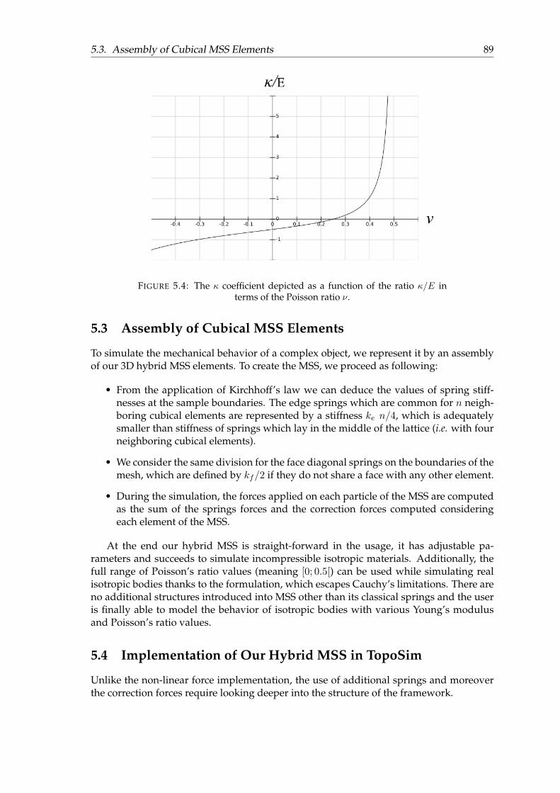
5.3. Assembly of Cubical MSS Elements 89
FIGURE 5.4: The κ coefficient depicted as a function of the ratio κ/E interms of the Poisson ratio ν.
5.3 Assembly of Cubical MSS Elements
To simulate the mechanical behavior of a complex object, we represent it by an assemblyof our 3D hybrid MSS elements. To create the MSS, we proceed as following:
• From the application of Kirchhoff’s law we can deduce the values of spring stiff-nesses at the sample boundaries. The edge springs which are common for n neigh-boring cubical elements are represented by a stiffness ke n/4, which is adequatelysmaller than stiffness of springs which lay in the middle of the lattice (i.e. with fourneighboring cubical elements).
• We consider the same division for the face diagonal springs on the boundaries of themesh, which are defined by kf/2 if they do not share a face with any other element.
• During the simulation, the forces applied on each particle of the MSS are computedas the sum of the springs forces and the correction forces computed consideringeach element of the MSS.
At the end our hybrid MSS is straight-forward in the usage, it has adjustable pa-rameters and succeeds to simulate incompressible isotropic materials. Additionally, thefull range of Poisson’s ratio values (meaning [0; 0.5[) can be used while simulating realisotropic bodies thanks to the formulation, which escapes Cauchy’s limitations. There areno additional structures introduced into MSS other than its classical springs and the useris finally able to model the behavior of isotropic bodies with various Young’s modulusand Poisson’s ratio values.
5.4 Implementation of Our Hybrid MSS in TopoSim
Unlike the non-linear force implementation, the use of additional springs and moreoverthe correction forces require looking deeper into the structure of the framework.
90 Chapter 5. Improvement of MSS for stable simulation with any Poisson’s Ratio
5.4.1 Face-Diagonal Springs
Let us start by adding the face-diagonal spring to the existing MSS. From Fig. 3.18 (page63) we know that in 2D models the face-diagonal springs are attributes of the 2-cells (ob-jects of Face_LCC_MSS class) and in 3D the inner-diagonal springs are the attributes of3-cells (objects of Volume_LCC_MSS class). Since our face-diagonal springs will be usedonly in 3D, we need to add them to the MSS structure in the correct corresponding classes.This will be done in three simple steps:
• Add 12 face-diagonal springs to each volume;
• Add initialization of those springs to assign correct stiffness values;
• Include the force computation in the add_force function for the new springs for theglobal accumulation loop.
Let us now verify these steps starting from the bottom layer of LCC_MSS from Fig. 5.6:
• The starting point is to add the face-diagonal springs as the attributes alongsidethe inner-diagonal springs. To do that we created separate structures and meth-ods to assign, modify and get information about those particular springs in theVolume_LCC_MSS class. It is very important to know the spring extremities (par-ticles they are connecting) and to be consistent when it comes to the order of num-bering the springs - it will be crucial information to accumulate the forces on theparticles further on.
• Then, to initialize the correct stiffness we needed to add proper code with the newstiffness formulation to the initialize_springs function in the Object_LCC_MSS class,which includes the face-diagonal springs of 3D elements.
• The last step is to modify the add_force function to include the new springs in theglobal force accumulation loop. As the accumulate function is called globally on thewhole MSS from the Object_LCC_for_simu class, we just need to modify thecontents of the local add_force function of the Volume_LCC_MSS and compute theforces of the face-diagonal springs the same way as we already do for the inner-diagonal springs of each volume.
5.4.2 Force Corrections
The next method to be implemented in our framework is to apply the correction forces.Let us take a look at the procedure of applying the force corrections properly in the fol-lowing steps:
• Add volume attribute to the 3-cells information; add its initialization;
• Add global correction forces loop;
– For all volumes compute the current volume;
– For all particles of the volume accumulate the correction forces according toEq. (5.17).
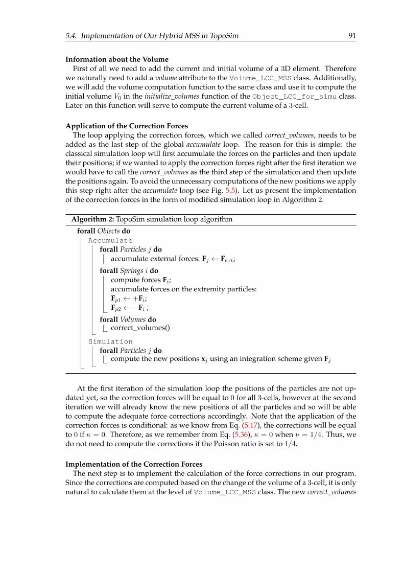
5.4. Implementation of Our Hybrid MSS in TopoSim 91
Information about the VolumeFirst of all we need to add the current and initial volume of a 3D element. Therefore
we naturally need to add a volume attribute to the Volume_LCC_MSS class. Additionally,we will add the volume computation function to the same class and use it to compute theinitial volume V0 in the initialize_volumes function of the Object_LCC_for_simu class.Later on this function will serve to compute the current volume of a 3-cell.
Application of the Correction ForcesThe loop applying the correction forces, which we called correct_volumes, needs to be
added as the last step of the global accumulate loop. The reason for this is simple: theclassical simulation loop will first accumulate the forces on the particles and then updatetheir positions; if we wanted to apply the correction forces right after the first iteration wewould have to call the correct_volumes as the third step of the simulation and then updatethe positions again. To avoid the unnecessary computations of the new positions we applythis step right after the accumulate loop (see Fig. 5.5). Let us present the implementationof the correction forces in the form of modified simulation loop in Algorithm 2.
Algorithm 2: TopoSim simulation loop algorithm
forall Objects doAccumulate
forall Particles j doaccumulate external forces: Fj ← Fext;
forall Springs i docompute forces Fi;accumulate forces on the extremity particles:Fp1 ← +Fi;Fp2 ← −Fi ;
forall Volumes docorrect_volumes()
Simulationforall Particles j do
compute the new positions xj using an integration scheme given Fj
At the first iteration of the simulation loop the positions of the particles are not up-dated yet, so the correction forces will be equal to 0 for all 3-cells, however at the seconditeration we will already know the new positions of all the particles and so will be ableto compute the adequate force corrections accordingly. Note that the application of thecorrection forces is conditional: as we know from Eq. (5.17), the corrections will be equalto 0 if κ = 0. Therefore, as we remember from Eq. (5.36), κ = 0 when ν = 1/4. Thus, wedo not need to compute the corrections if the Poisson ratio is set to 1/4.
Implementation of the Correction ForcesThe next step is to implement the calculation of the force corrections in our program.
Since the corrections are computed based on the change of the volume of a 3-cell, it is onlynatural to calculate them at the level of Volume_LCC_MSS class. The new correct_volumes
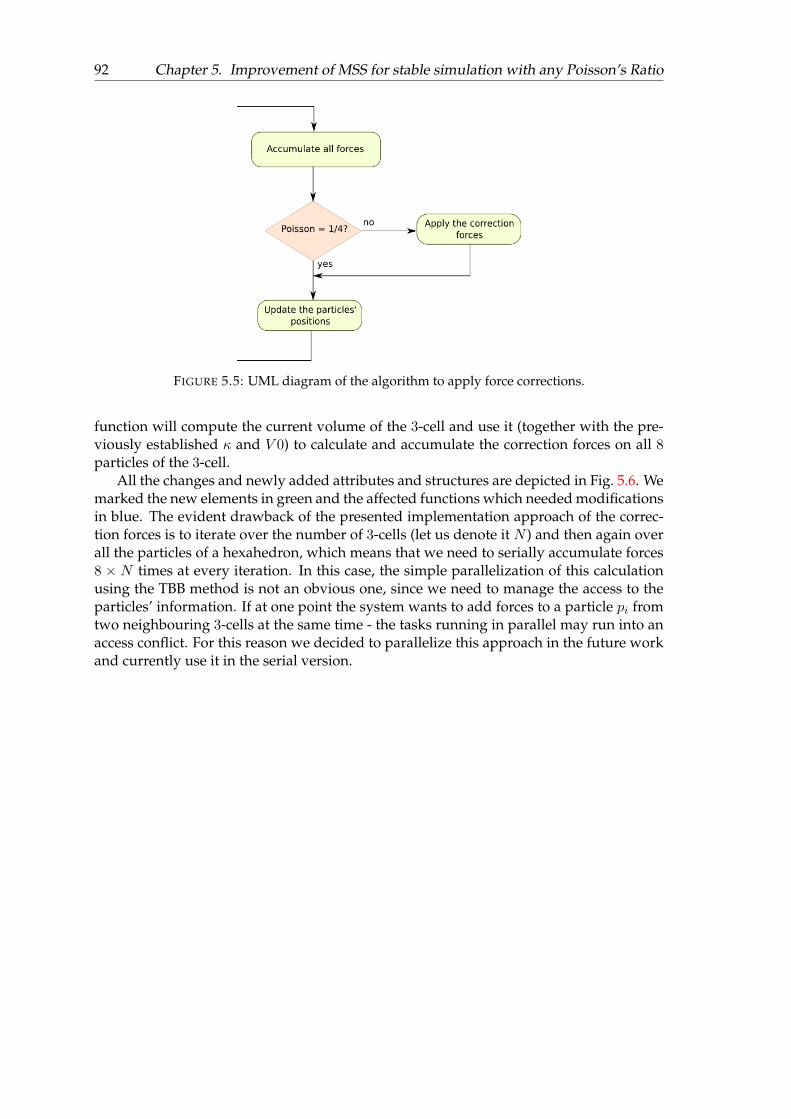
92 Chapter 5. Improvement of MSS for stable simulation with any Poisson’s Ratio
FIGURE 5.5: UML diagram of the algorithm to apply force corrections.
function will compute the current volume of the 3-cell and use it (together with the pre-viously established κ and V 0) to calculate and accumulate the correction forces on all 8particles of the 3-cell.
All the changes and newly added attributes and structures are depicted in Fig. 5.6. Wemarked the new elements in green and the affected functions which needed modificationsin blue. The evident drawback of the presented implementation approach of the correc-tion forces is to iterate over the number of 3-cells (let us denote it N ) and then again overall the particles of a hexahedron, which means that we need to serially accumulate forces8 × N times at every iteration. In this case, the simple parallelization of this calculationusing the TBB method is not an obvious one, since we need to manage the access to theparticles’ information. If at one point the system wants to add forces to a particle pi fromtwo neighbouring 3-cells at the same time - the tasks running in parallel may run into anaccess conflict. For this reason we decided to parallelize this approach in the future workand currently use it in the serial version.
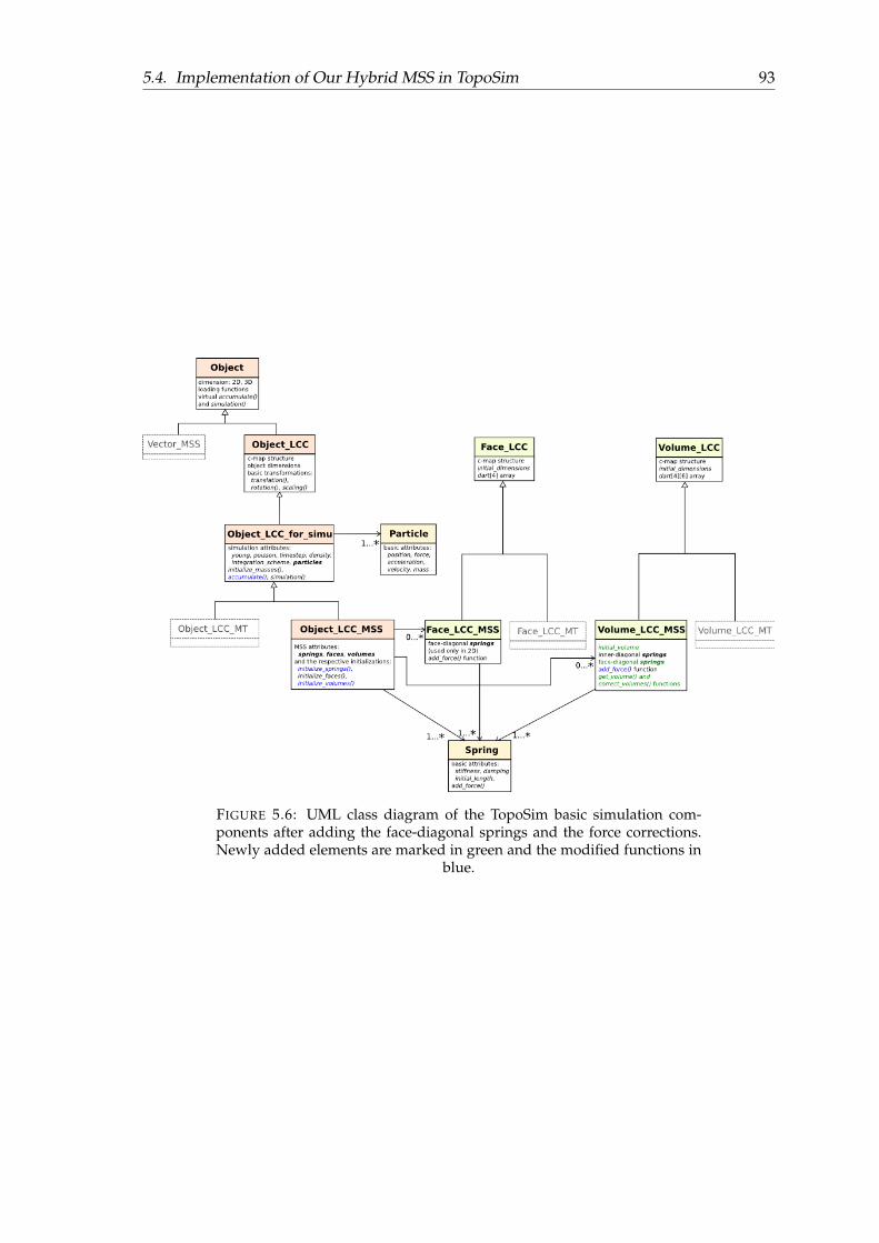
5.4. Implementation of Our Hybrid MSS in TopoSim 93
FIGURE 5.6: UML class diagram of the TopoSim basic simulation com-ponents after adding the face-diagonal springs and the force corrections.Newly added elements are marked in green and the modified functions in
blue.
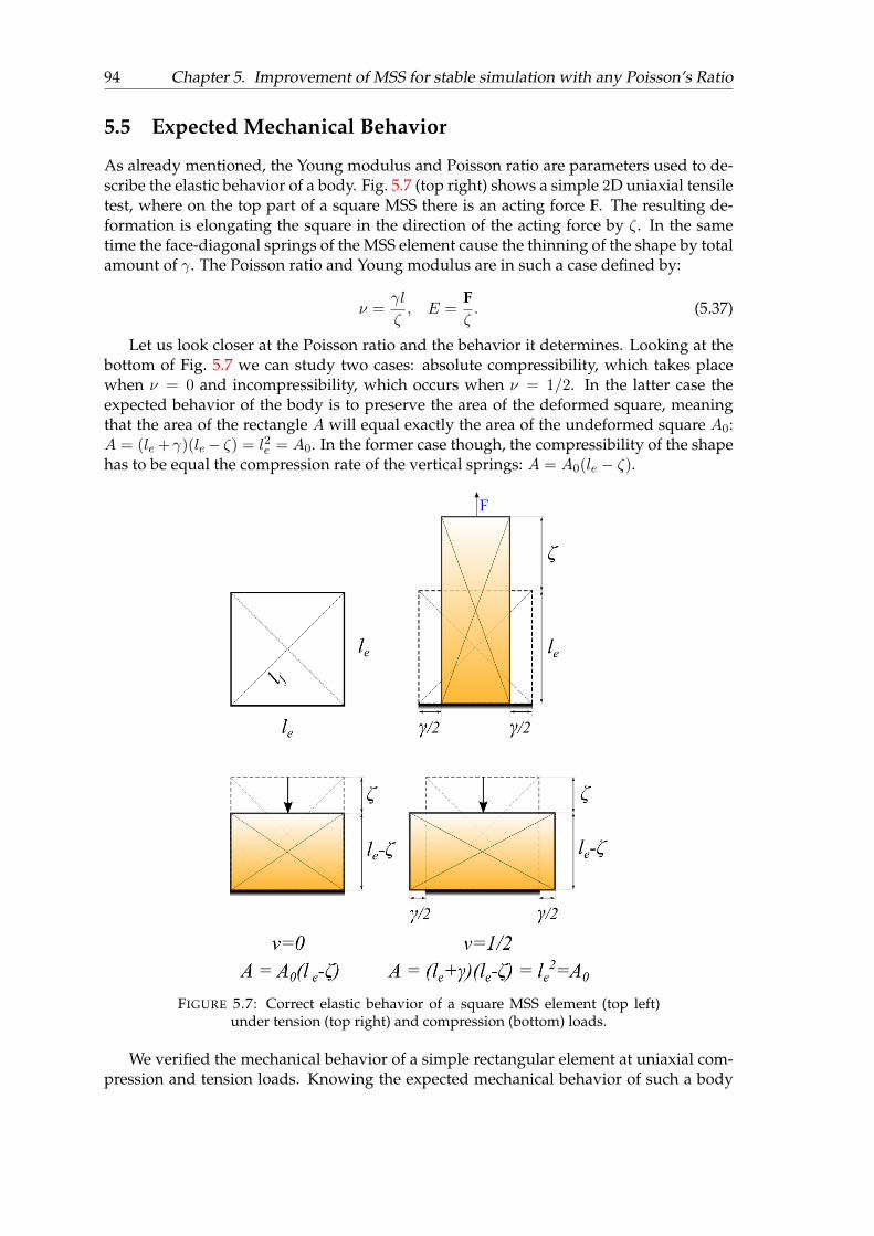
94 Chapter 5. Improvement of MSS for stable simulation with any Poisson’s Ratio
5.5 Expected Mechanical Behavior
As already mentioned, the Young modulus and Poisson ratio are parameters used to de-scribe the elastic behavior of a body. Fig. 5.7 (top right) shows a simple 2D uniaxial tensiletest, where on the top part of a square MSS there is an acting force F. The resulting de-formation is elongating the square in the direction of the acting force by ζ. In the sametime the face-diagonal springs of the MSS element cause the thinning of the shape by totalamount of γ. The Poisson ratio and Young modulus are in such a case defined by:
ν =γl
ζ, E =
Fζ. (5.37)
Let us look closer at the Poisson ratio and the behavior it determines. Looking at thebottom of Fig. 5.7 we can study two cases: absolute compressibility, which takes placewhen ν = 0 and incompressibility, which occurs when ν = 1/2. In the latter case theexpected behavior of the body is to preserve the area of the deformed square, meaningthat the area of the rectangle A will equal exactly the area of the undeformed square A0:A = (le + γ)(le− ζ) = l2e = A0. In the former case though, the compressibility of the shapehas to be equal the compression rate of the vertical springs: A = A0(le − ζ).
FIGURE 5.7: Correct elastic behavior of a square MSS element (top left)under tension (top right) and compression (bottom) loads.
We verified the mechanical behavior of a simple rectangular element at uniaxial com-pression and tension loads. Knowing the expected mechanical behavior of such a body
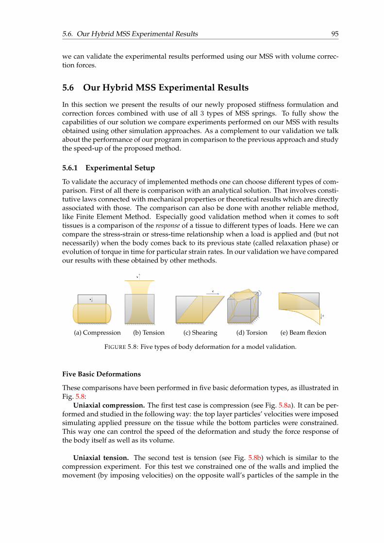
5.6. Our Hybrid MSS Experimental Results 95
we can validate the experimental results performed using our MSS with volume correc-tion forces.
5.6 Our Hybrid MSS Experimental Results
In this section we present the results of our newly proposed stiffness formulation andcorrection forces combined with use of all 3 types of MSS springs. To fully show thecapabilities of our solution we compare experiments performed on our MSS with resultsobtained using other simulation approaches. As a complement to our validation we talkabout the performance of our program in comparison to the previous approach and studythe speed-up of the proposed method.
5.6.1 Experimental Setup
To validate the accuracy of implemented methods one can choose different types of com-parison. First of all there is comparison with an analytical solution. That involves consti-tutive laws connected with mechanical properties or theoretical results which are directlyassociated with those. The comparison can also be done with another reliable method,like Finite Element Method. Especially good validation method when it comes to softtissues is a comparison of the response of a tissue to different types of loads. Here we cancompare the stress-strain or stress-time relationship when a load is applied and (but notnecessarily) when the body comes back to its previous state (called relaxation phase) orevolution of torque in time for particular strain rates. In our validation we have comparedour results with these obtained by other methods.
(a) Compression (b) Tension (c) Shearing (d) Torsion (e) Beam flexion
FIGURE 5.8: Five types of body deformation for a model validation.
Five Basic Deformations
These comparisons have been performed in five basic deformation types, as illustrated inFig. 5.8:
Uniaxial compression. The first test case is compression (see Fig. 5.8a). It can be per-formed and studied in the following way: the top layer particles’ velocities were imposedsimulating applied pressure on the tissue while the bottom particles were constrained.This way one can control the speed of the deformation and study the force response ofthe body itself as well as its volume.
Uniaxial tension. The second test is tension (see Fig. 5.8b) which is similar to thecompression experiment. For this test we constrained one of the walls and implied themovement (by imposing velocities) on the opposite wall’s particles of the sample in the
96 Chapter 5. Improvement of MSS for stable simulation with any Poisson’s Ratio
perpendicular direction. During the deformation we studied the force response and vol-ume change.
Shearing. The third deformation, depicted in Fig. 5.8c is shearing. Usually such anexperiment is performed on a body which is stretched up to certain stresses or/and upto failure. We perform this experiment by constraining the bottom layer of the tissue andimplying a change of the positions of the parallel layer at a constant speed - strain rate.As the comparable output of such an experiment one can use the stress-strain relationship.
Torsion. The fourth experiment with which it is possible to validate a model is torsion(see Fig. 5.8d). To perform this experiment, we rotated sample’s top layer at a constantspeed while the parallel bottom layer of the sample was constrained. The studied param-eter in such experiment was torque.
Beam flexion. The last experiment is beam bending. For this test, a long beam wasattached with its smallest face to an imaginary wall and then it was exposed to the gravity(see Fig. 5.8e).
Having such an experimental setup we are sure to cover vast majority of the possiblescenarios of body deformations, which are usually a combination of the presented basicloads. Additionally, with available theoretical values and expected body behavior we cansuccessfully verify our solution.
In this context we compared our results with the following methods:
• The Mass-Spring System (denoted MSS-Baudet) with the stiffness formulation pro-posed by Baudet [12] and defined in Ch. 3, using only two types of springs: edgeand inner-diagonal;
• Our Mass-Spring System with the stiffness formulation defined in Eq. (5.1), usingthe correction forces, but with the parameter A set to 0 in order to simulate no face-diagonal springs (denoted MSS-nFD);
• Our Mass-Spring System with all springs and correction forces which is the fullformulation presented in Ch. 5.1 (denoted MSS-CF);
• The Finite Element Method using LS-Dyna software (denoted FEM). These experi-ments are performed on LS-Dyna version 971dR4 (LSCT, Livermore, CA, USA) us-ing the linear elastic material law of Hooke, fully integrated selective reduced solidelements and implicit numerical integration scheme.
Now let us present the details of each experiment from its technical point of view. Thepresented tests were performed using the following principles, assumptions and meshes:
• In all the instances (except of the beam bending experiment which is examined inthe equilibrium state under gravity), we fixed the time-step to 0.001 s and the totalnumber of iteration steps to 10,000 (i.e. 10 s), without applying gravity force. Defor-mations were limited to 5% and 20% to verify the behavior of the simulated tissueat both small and big loads.
• For the correction forces expressed in Eq. (5.17), we used the compression moduluscomputed by Eq. (5.36), where ν 6= 1/2. Note that in case of ν = 1/4 these correctionforces are equal to 0, i.e. the MSS naturally models this case.
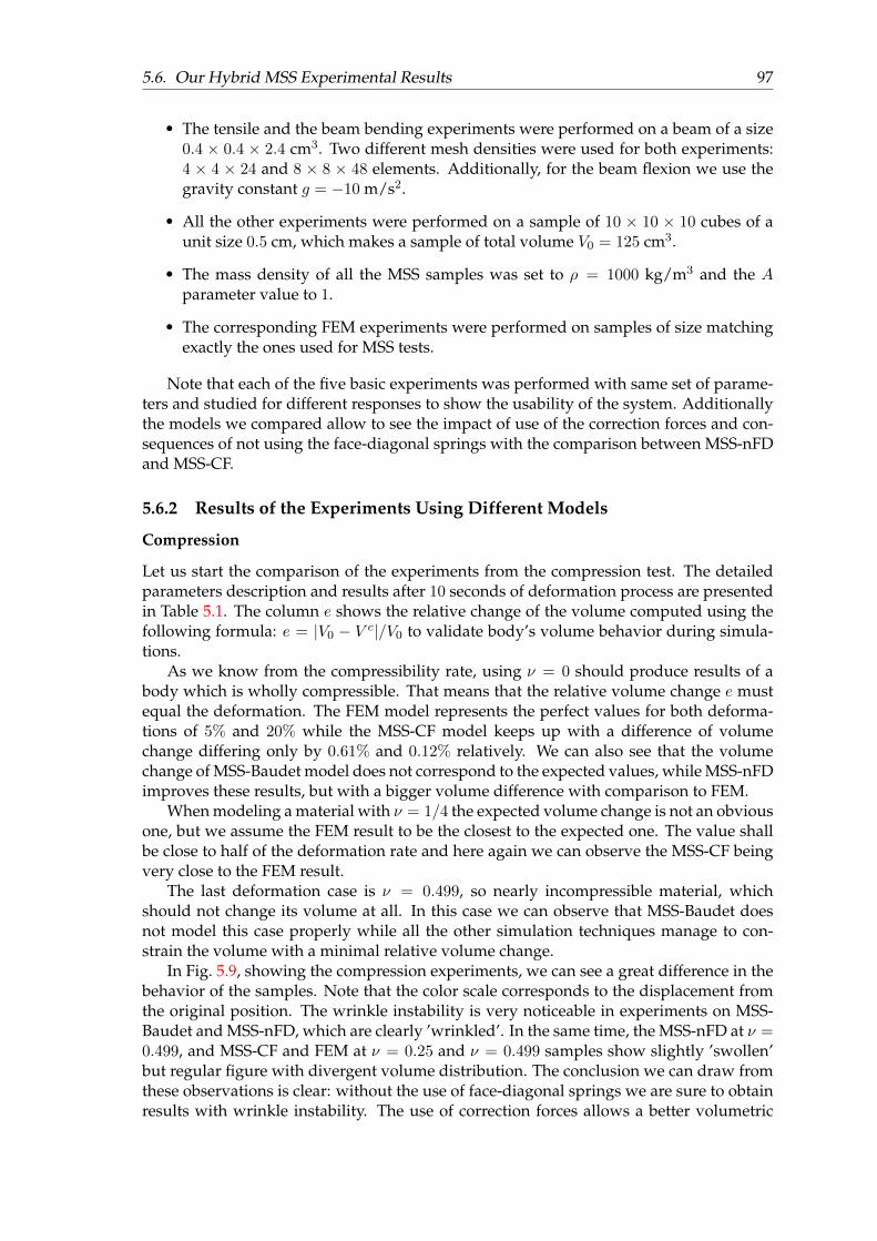
5.6. Our Hybrid MSS Experimental Results 97
• The tensile and the beam bending experiments were performed on a beam of a size0.4 × 0.4 × 2.4 cm3. Two different mesh densities were used for both experiments:4 × 4 × 24 and 8 × 8 × 48 elements. Additionally, for the beam flexion we use thegravity constant g = −10 m/s2.
• All the other experiments were performed on a sample of 10 × 10 × 10 cubes of aunit size 0.5 cm, which makes a sample of total volume V0 = 125 cm3.
• The mass density of all the MSS samples was set to ρ = 1000 kg/m3 and the Aparameter value to 1.
• The corresponding FEM experiments were performed on samples of size matchingexactly the ones used for MSS tests.
Note that each of the five basic experiments was performed with same set of parame-ters and studied for different responses to show the usability of the system. Additionallythe models we compared allow to see the impact of use of the correction forces and con-sequences of not using the face-diagonal springs with the comparison between MSS-nFDand MSS-CF.
5.6.2 Results of the Experiments Using Different Models
Compression
Let us start the comparison of the experiments from the compression test. The detailedparameters description and results after 10 seconds of deformation process are presentedin Table 5.1. The column e shows the relative change of the volume computed using thefollowing formula: e = |V0 − V c|/V0 to validate body’s volume behavior during simula-tions.
As we know from the compressibility rate, using ν = 0 should produce results of abody which is wholly compressible. That means that the relative volume change e mustequal the deformation. The FEM model represents the perfect values for both deforma-tions of 5% and 20% while the MSS-CF model keeps up with a difference of volumechange differing only by 0.61% and 0.12% relatively. We can also see that the volumechange of MSS-Baudet model does not correspond to the expected values, while MSS-nFDimproves these results, but with a bigger volume difference with comparison to FEM.
When modeling a material with ν = 1/4 the expected volume change is not an obviousone, but we assume the FEM result to be the closest to the expected one. The value shallbe close to half of the deformation rate and here again we can observe the MSS-CF beingvery close to the FEM result.
The last deformation case is ν = 0.499, so nearly incompressible material, whichshould not change its volume at all. In this case we can observe that MSS-Baudet doesnot model this case properly while all the other simulation techniques manage to con-strain the volume with a minimal relative volume change.
In Fig. 5.9, showing the compression experiments, we can see a great difference in thebehavior of the samples. Note that the color scale corresponds to the displacement fromthe original position. The wrinkle instability is very noticeable in experiments on MSS-Baudet and MSS-nFD, which are clearly ’wrinkled’. In the same time, the MSS-nFD at ν =0.499, and MSS-CF and FEM at ν = 0.25 and ν = 0.499 samples show slightly ’swollen’but regular figure with divergent volume distribution. The conclusion we can draw fromthese observations is clear: without the use of face-diagonal springs we are sure to obtainresults with wrinkle instability. The use of correction forces allows a better volumetric
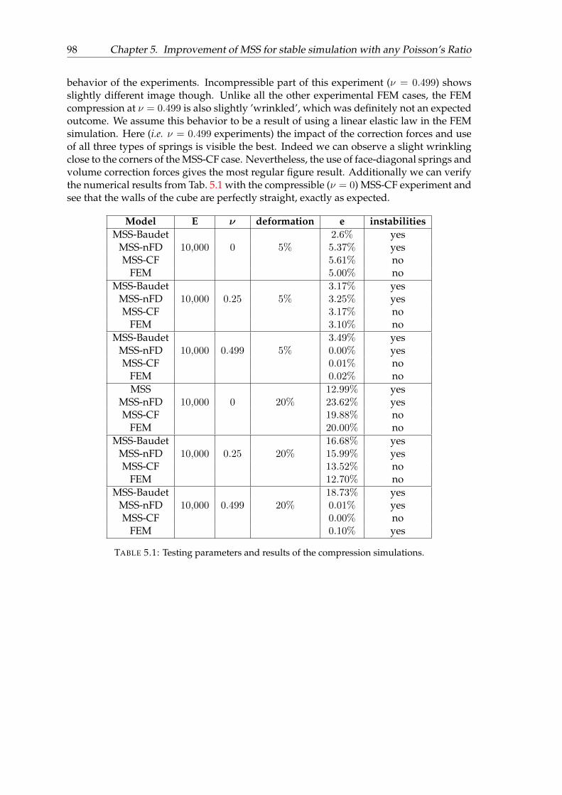
98 Chapter 5. Improvement of MSS for stable simulation with any Poisson’s Ratio
behavior of the experiments. Incompressible part of this experiment (ν = 0.499) showsslightly different image though. Unlike all the other experimental FEM cases, the FEMcompression at ν = 0.499 is also slightly ’wrinkled’, which was definitely not an expectedoutcome. We assume this behavior to be a result of using a linear elastic law in the FEMsimulation. Here (i.e. ν = 0.499 experiments) the impact of the correction forces and useof all three types of springs is visible the best. Indeed we can observe a slight wrinklingclose to the corners of the MSS-CF case. Nevertheless, the use of face-diagonal springs andvolume correction forces gives the most regular figure result. Additionally we can verifythe numerical results from Tab. 5.1 with the compressible (ν = 0) MSS-CF experiment andsee that the walls of the cube are perfectly straight, exactly as expected.
Model E ν deformation e instabilitiesMSS-Baudet 2.6% yes
MSS-nFD 10,000 0 5% 5.37% yesMSS-CF 5.61% no
FEM 5.00% noMSS-Baudet 3.17% yes
MSS-nFD 10,000 0.25 5% 3.25% yesMSS-CF 3.17% no
FEM 3.10% noMSS-Baudet 3.49% yes
MSS-nFD 10,000 0.499 5% 0.00% yesMSS-CF 0.01% no
FEM 0.02% noMSS 12.99% yes
MSS-nFD 10,000 0 20% 23.62% yesMSS-CF 19.88% no
FEM 20.00% noMSS-Baudet 16.68% yes
MSS-nFD 10,000 0.25 20% 15.99% yesMSS-CF 13.52% no
FEM 12.70% noMSS-Baudet 18.73% yes
MSS-nFD 10,000 0.499 20% 0.01% yesMSS-CF 0.00% no
FEM 0.10% yes
TABLE 5.1: Testing parameters and results of the compression simulations.
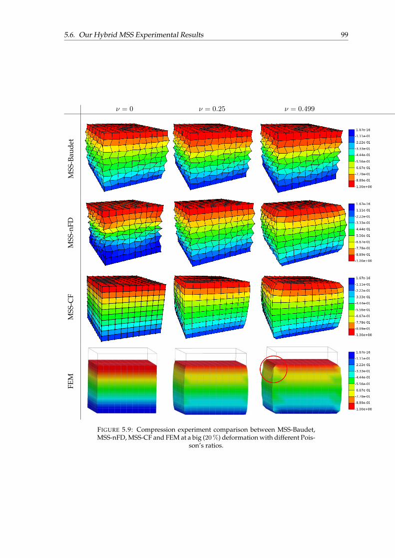
5.6. Our Hybrid MSS Experimental Results 99
ν = 0 ν = 0.25 ν = 0.499
MSS
-Bau
det
MSS
-nFD
MSS
-CF
FEM
FIGURE 5.9: Compression experiment comparison between MSS-Baudet,MSS-nFD, MSS-CF and FEM at a big (20 %) deformation with different Pois-
son’s ratios.
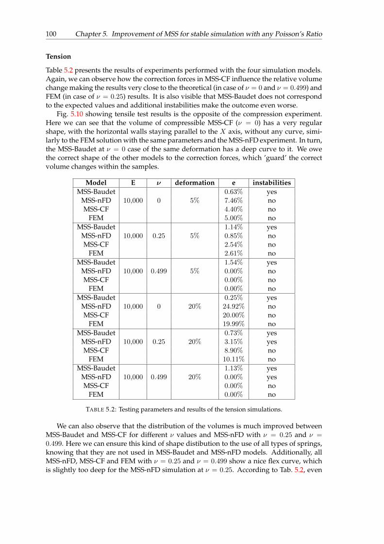
100 Chapter 5. Improvement of MSS for stable simulation with any Poisson’s Ratio
Tension
Table 5.2 presents the results of experiments performed with the four simulation models.Again, we can observe how the correction forces in MSS-CF influence the relative volumechange making the results very close to the theoretical (in case of ν = 0 and ν = 0.499) andFEM (in case of ν = 0.25) results. It is also visible that MSS-Baudet does not correspondto the expected values and additional instabilities make the outcome even worse.
Fig. 5.10 showing tensile test results is the opposite of the compression experiment.Here we can see that the volume of compressible MSS-CF (ν = 0) has a very regularshape, with the horizontal walls staying parallel to the X axis, without any curve, simi-larly to the FEM solution with the same parameters and the MSS-nFD experiment. In turn,the MSS-Baudet at ν = 0 case of the same deformation has a deep curve to it. We owethe correct shape of the other models to the correction forces, which ’guard’ the correctvolume changes within the samples.
Model E ν deformation e instabilitiesMSS-Baudet 0.63% yes
MSS-nFD 10,000 0 5% 7.46% noMSS-CF 4.40% no
FEM 5.00% noMSS-Baudet 1.14% yes
MSS-nFD 10,000 0.25 5% 0.85% noMSS-CF 2.54% no
FEM 2.61% noMSS-Baudet 1.54% yes
MSS-nFD 10,000 0.499 5% 0.00% noMSS-CF 0.00% no
FEM 0.00% noMSS-Baudet 0.25% yes
MSS-nFD 10,000 0 20% 24.92% noMSS-CF 20.00% no
FEM 19.99% noMSS-Baudet 0.73% yes
MSS-nFD 10,000 0.25 20% 3.15% yesMSS-CF 8.90% no
FEM 10.11% noMSS-Baudet 1.13% yes
MSS-nFD 10,000 0.499 20% 0.00% yesMSS-CF 0.00% no
FEM 0.00% no
TABLE 5.2: Testing parameters and results of the tension simulations.
We can also observe that the distribution of the volumes is much improved betweenMSS-Baudet and MSS-CF for different ν values and MSS-nFD with ν = 0.25 and ν =0.499. Here we can ensure this kind of shape distibution to the use of all types of springs,knowing that they are not used in MSS-Baudet and MSS-nFD models. Additionally, allMSS-nFD, MSS-CF and FEM with ν = 0.25 and ν = 0.499 show a nice flex curve, whichis slightly too deep for the MSS-nFD simulation at ν = 0.25. According to Tab. 5.2, even
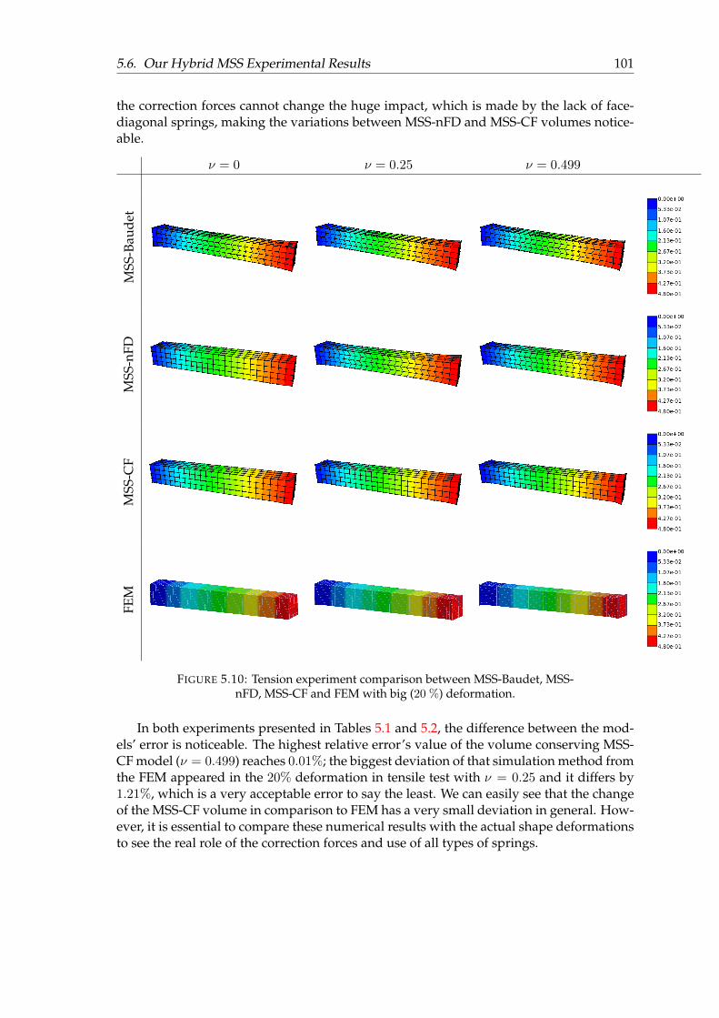
5.6. Our Hybrid MSS Experimental Results 101
the correction forces cannot change the huge impact, which is made by the lack of face-diagonal springs, making the variations between MSS-nFD and MSS-CF volumes notice-able.
ν = 0 ν = 0.25 ν = 0.499
MSS
-Bau
det
MSS
-nFD
MSS
-CF
FEM
FIGURE 5.10: Tension experiment comparison between MSS-Baudet, MSS-nFD, MSS-CF and FEM with big (20 %) deformation.
In both experiments presented in Tables 5.1 and 5.2, the difference between the mod-els’ error is noticeable. The highest relative error’s value of the volume conserving MSS-CF model (ν = 0.499) reaches 0.01%; the biggest deviation of that simulation method fromthe FEM appeared in the 20% deformation in tensile test with ν = 0.25 and it differs by1.21%, which is a very acceptable error to say the least. We can easily see that the changeof the MSS-CF volume in comparison to FEM has a very small deviation in general. How-ever, it is essential to compare these numerical results with the actual shape deformationsto see the real role of the correction forces and use of all types of springs.
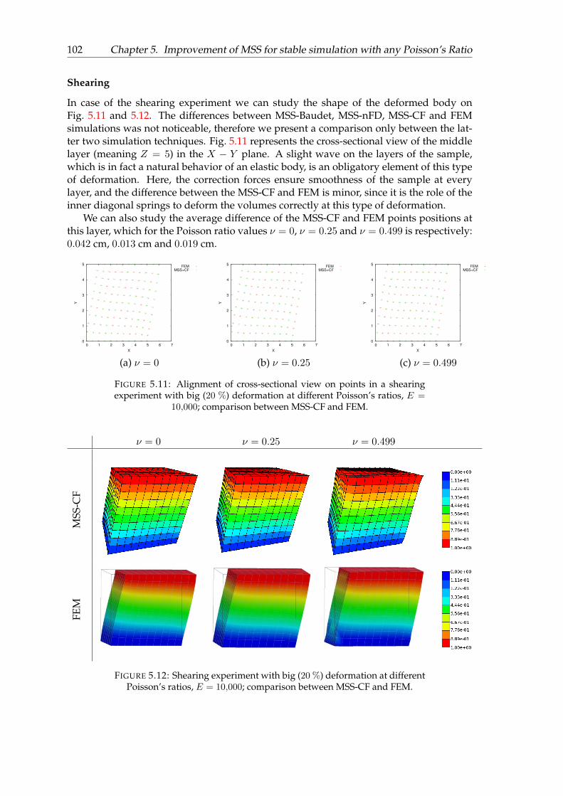
102 Chapter 5. Improvement of MSS for stable simulation with any Poisson’s Ratio
Shearing
In case of the shearing experiment we can study the shape of the deformed body onFig. 5.11 and 5.12. The differences between MSS-Baudet, MSS-nFD, MSS-CF and FEMsimulations was not noticeable, therefore we present a comparison only between the lat-ter two simulation techniques. Fig. 5.11 represents the cross-sectional view of the middlelayer (meaning Z = 5) in the X − Y plane. A slight wave on the layers of the sample,which is in fact a natural behavior of an elastic body, is an obligatory element of this typeof deformation. Here, the correction forces ensure smoothness of the sample at everylayer, and the difference between the MSS-CF and FEM is minor, since it is the role of theinner diagonal springs to deform the volumes correctly at this type of deformation.
We can also study the average difference of the MSS-CF and FEM points positions atthis layer, which for the Poisson ratio values ν = 0, ν = 0.25 and ν = 0.499 is respectively:0.042 cm, 0.013 cm and 0.019 cm.
0
1
2
3
4
5
0 1 2 3 4 5 6 7
Y
X
FEM
MSS+CF
0
1
2
3
4
5
0 1 2 3 4 5 6 7
Y
X
FEM
MSS+CF
0
1
2
3
4
5
0 1 2 3 4 5 6 7
Y
X
FEM
MSS+CF
(a) ν = 0 (b) ν = 0.25 (c) ν = 0.499
FIGURE 5.11: Alignment of cross-sectional view on points in a shearingexperiment with big (20 %) deformation at different Poisson’s ratios, E =
10,000; comparison between MSS-CF and FEM.
ν = 0 ν = 0.25 ν = 0.499
MSS
-CF
FEM
FIGURE 5.12: Shearing experiment with big (20 %) deformation at differentPoisson’s ratios, E = 10,000; comparison between MSS-CF and FEM.
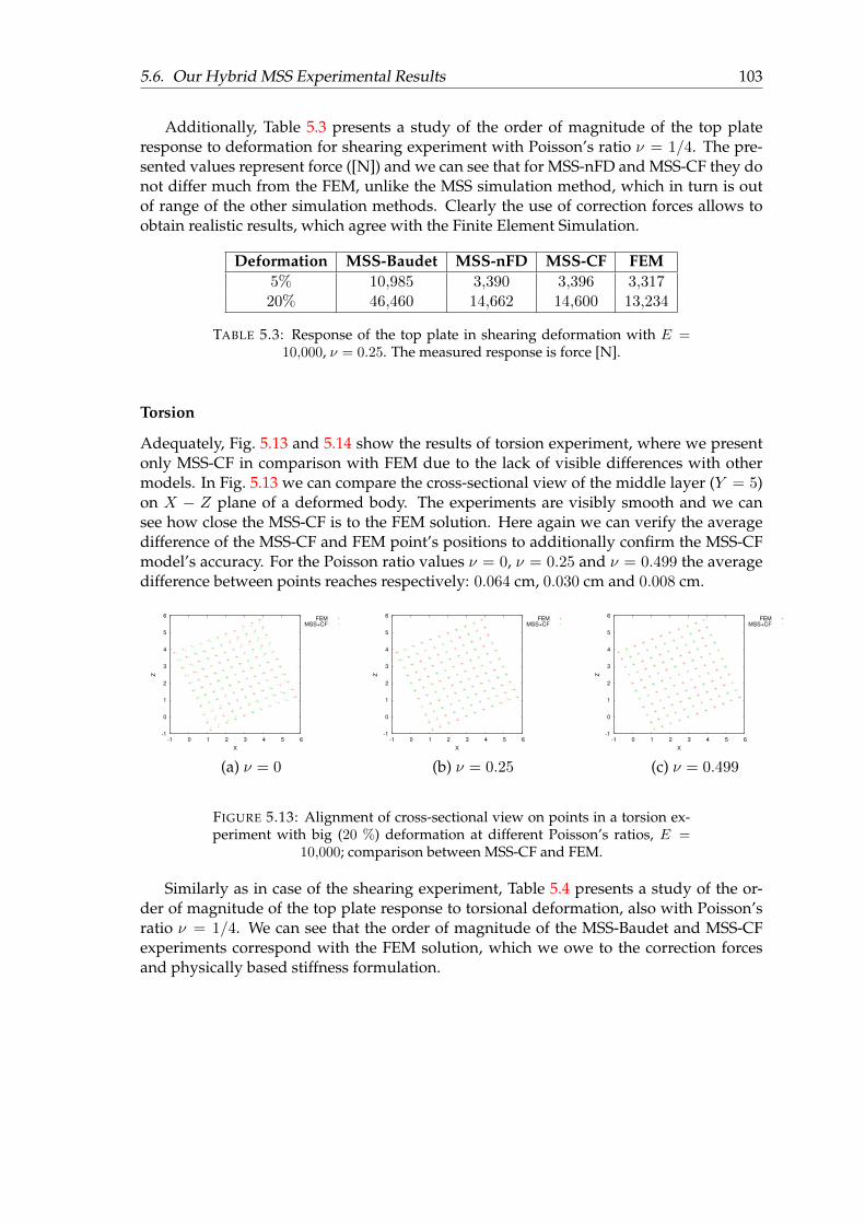
5.6. Our Hybrid MSS Experimental Results 103
Additionally, Table 5.3 presents a study of the order of magnitude of the top plateresponse to deformation for shearing experiment with Poisson’s ratio ν = 1/4. The pre-sented values represent force ([N]) and we can see that for MSS-nFD and MSS-CF they donot differ much from the FEM, unlike the MSS simulation method, which in turn is outof range of the other simulation methods. Clearly the use of correction forces allows toobtain realistic results, which agree with the Finite Element Simulation.
Deformation MSS-Baudet MSS-nFD MSS-CF FEM5% 10,985 3,390 3,396 3,31720% 46,460 14,662 14,600 13,234
TABLE 5.3: Response of the top plate in shearing deformation with E =10,000, ν = 0.25. The measured response is force [N].
Torsion
Adequately, Fig. 5.13 and 5.14 show the results of torsion experiment, where we presentonly MSS-CF in comparison with FEM due to the lack of visible differences with othermodels. In Fig. 5.13 we can compare the cross-sectional view of the middle layer (Y = 5)on X − Z plane of a deformed body. The experiments are visibly smooth and we cansee how close the MSS-CF is to the FEM solution. Here again we can verify the averagedifference of the MSS-CF and FEM point’s positions to additionally confirm the MSS-CFmodel’s accuracy. For the Poisson ratio values ν = 0, ν = 0.25 and ν = 0.499 the averagedifference between points reaches respectively: 0.064 cm, 0.030 cm and 0.008 cm.
-1
0
1
2
3
4
5
6
-1 0 1 2 3 4 5 6
Z
X
FEM
MSS+CF
-1
0
1
2
3
4
5
6
-1 0 1 2 3 4 5 6
Z
X
FEM
MSS+CF
-1
0
1
2
3
4
5
6
-1 0 1 2 3 4 5 6
Z
X
FEM
MSS+CF
(a) ν = 0 (b) ν = 0.25 (c) ν = 0.499
FIGURE 5.13: Alignment of cross-sectional view on points in a torsion ex-periment with big (20 %) deformation at different Poisson’s ratios, E =
10,000; comparison between MSS-CF and FEM.
Similarly as in case of the shearing experiment, Table 5.4 presents a study of the or-der of magnitude of the top plate response to torsional deformation, also with Poisson’sratio ν = 1/4. We can see that the order of magnitude of the MSS-Baudet and MSS-CFexperiments correspond with the FEM solution, which we owe to the correction forcesand physically based stiffness formulation.
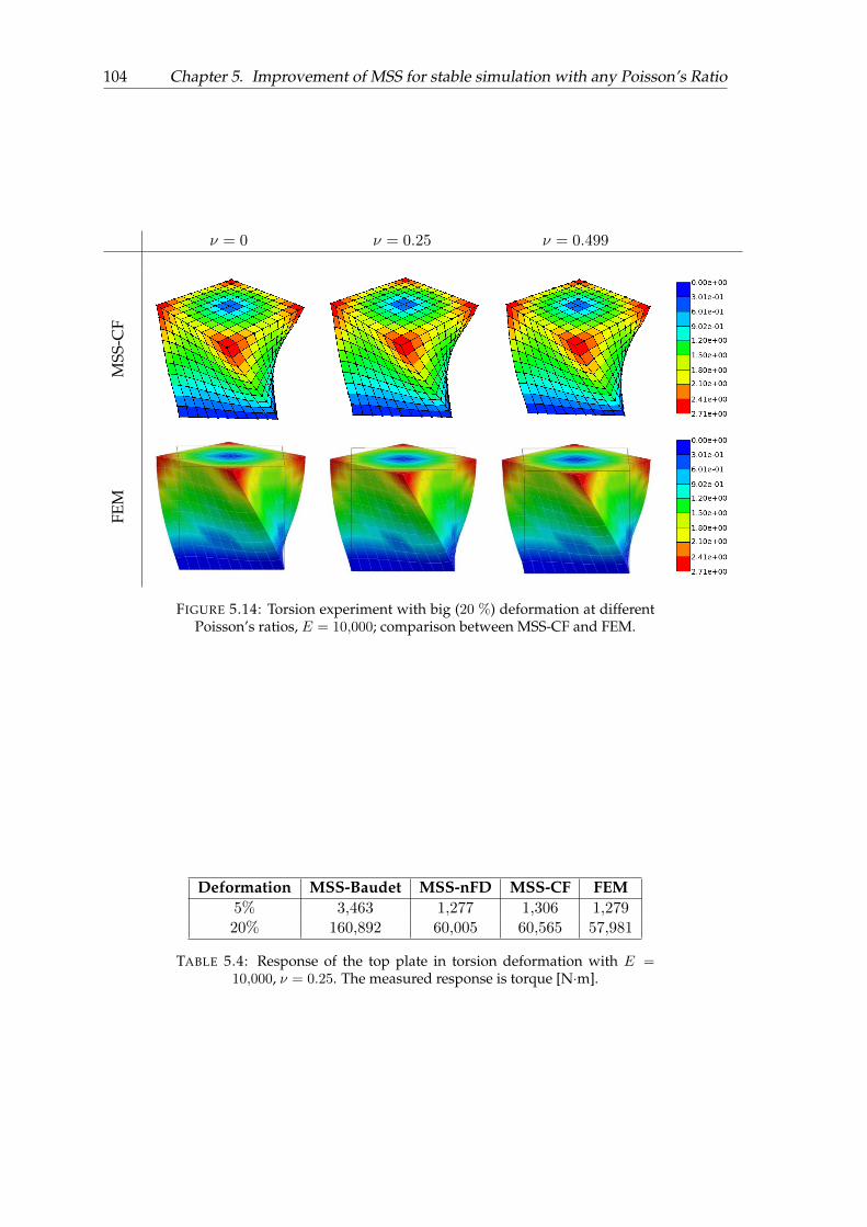
104 Chapter 5. Improvement of MSS for stable simulation with any Poisson’s Ratio
ν = 0 ν = 0.25 ν = 0.499
MSS
-CF
FEM
FIGURE 5.14: Torsion experiment with big (20 %) deformation at differentPoisson’s ratios, E = 10,000; comparison between MSS-CF and FEM.
Deformation MSS-Baudet MSS-nFD MSS-CF FEM5% 3,463 1,277 1,306 1,27920% 160,892 60,005 60,565 57,981
TABLE 5.4: Response of the top plate in torsion deformation with E =10,000, ν = 0.25. The measured response is torque [N·m].
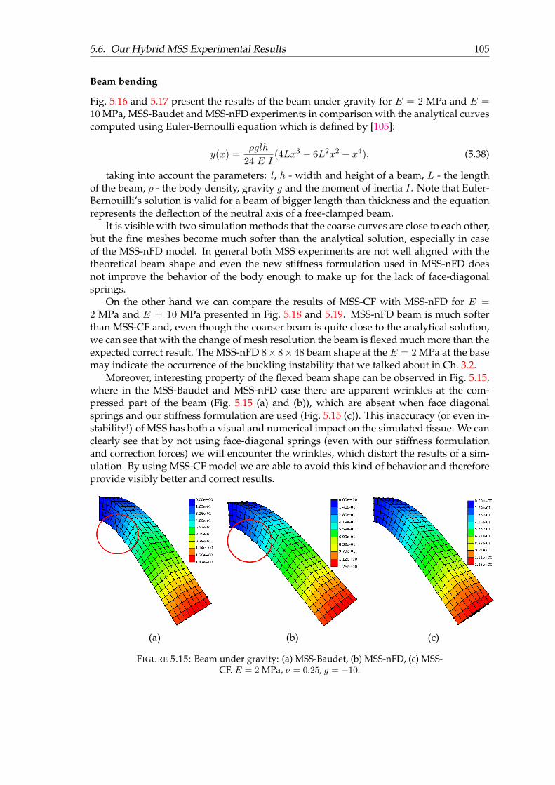
5.6. Our Hybrid MSS Experimental Results 105
Beam bending
Fig. 5.16 and 5.17 present the results of the beam under gravity for E = 2 MPa and E =10 MPa, MSS-Baudet and MSS-nFD experiments in comparison with the analytical curvescomputed using Euler-Bernoulli equation which is defined by [105]:
y(x) =ρglh
24 E I(4Lx3 − 6L2x2 − x4), (5.38)
taking into account the parameters: l, h - width and height of a beam, L - the lengthof the beam, ρ - the body density, gravity g and the moment of inertia I . Note that Euler-Bernouilli’s solution is valid for a beam of bigger length than thickness and the equationrepresents the deflection of the neutral axis of a free-clamped beam.
It is visible with two simulation methods that the coarse curves are close to each other,but the fine meshes become much softer than the analytical solution, especially in caseof the MSS-nFD model. In general both MSS experiments are not well aligned with thetheoretical beam shape and even the new stiffness formulation used in MSS-nFD doesnot improve the behavior of the body enough to make up for the lack of face-diagonalsprings.
On the other hand we can compare the results of MSS-CF with MSS-nFD for E =2 MPa and E = 10 MPa presented in Fig. 5.18 and 5.19. MSS-nFD beam is much softerthan MSS-CF and, even though the coarser beam is quite close to the analytical solution,we can see that with the change of mesh resolution the beam is flexed much more than theexpected correct result. The MSS-nFD 8× 8× 48 beam shape at the E = 2 MPa at the basemay indicate the occurrence of the buckling instability that we talked about in Ch. 3.2.
Moreover, interesting property of the flexed beam shape can be observed in Fig. 5.15,where in the MSS-Baudet and MSS-nFD case there are apparent wrinkles at the com-pressed part of the beam (Fig. 5.15 (a) and (b)), which are absent when face diagonalsprings and our stiffness formulation are used (Fig. 5.15 (c)). This inaccuracy (or even in-stability!) of MSS has both a visual and numerical impact on the simulated tissue. We canclearly see that by not using face-diagonal springs (even with our stiffness formulationand correction forces) we will encounter the wrinkles, which distort the results of a sim-ulation. By using MSS-CF model we are able to avoid this kind of behavior and thereforeprovide visibly better and correct results.
(a) (b) (c)
FIGURE 5.15: Beam under gravity: (a) MSS-Baudet, (b) MSS-nFD, (c) MSS-CF. E = 2 MPa, ν = 0.25, g = −10.
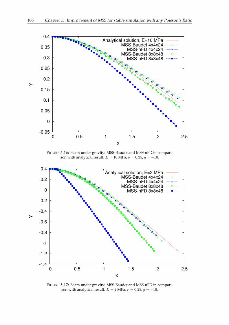
106 Chapter 5. Improvement of MSS for stable simulation with any Poisson’s Ratio
-0.05
0
0.05
0.1
0.15
0.2
0.25
0.3
0.35
0.4
0 0.5 1 1.5 2 2.5
Y
X
Analytical solution, E=10 MPaMSS-Baudet 4x4x24
MSS-nFD 4x4x24MSS-Baudet 8x8x48
MSS-nFD 8x8x48
FIGURE 5.16: Beam under gravity: MSS-Baudet and MSS-nFD in compari-son with analytical result. E = 10 MPa, ν = 0.25, g = −10.
-1.4
-1.2
-1
-0.8
-0.6
-0.4
-0.2
0
0.2
0.4
0 0.5 1 1.5 2 2.5
Y
X
Analytical solution, E=2 MPaMSS-Baudet 4x4x24
MSS-nFD 4x4x24MSS-Baudet 8x8x48
MSS-nFD 8x8x48
FIGURE 5.17: Beam under gravity: MSS-Baudet and MSS-nFD in compari-son with analytical result. E = 2 MPa, ν = 0.25, g = −10.
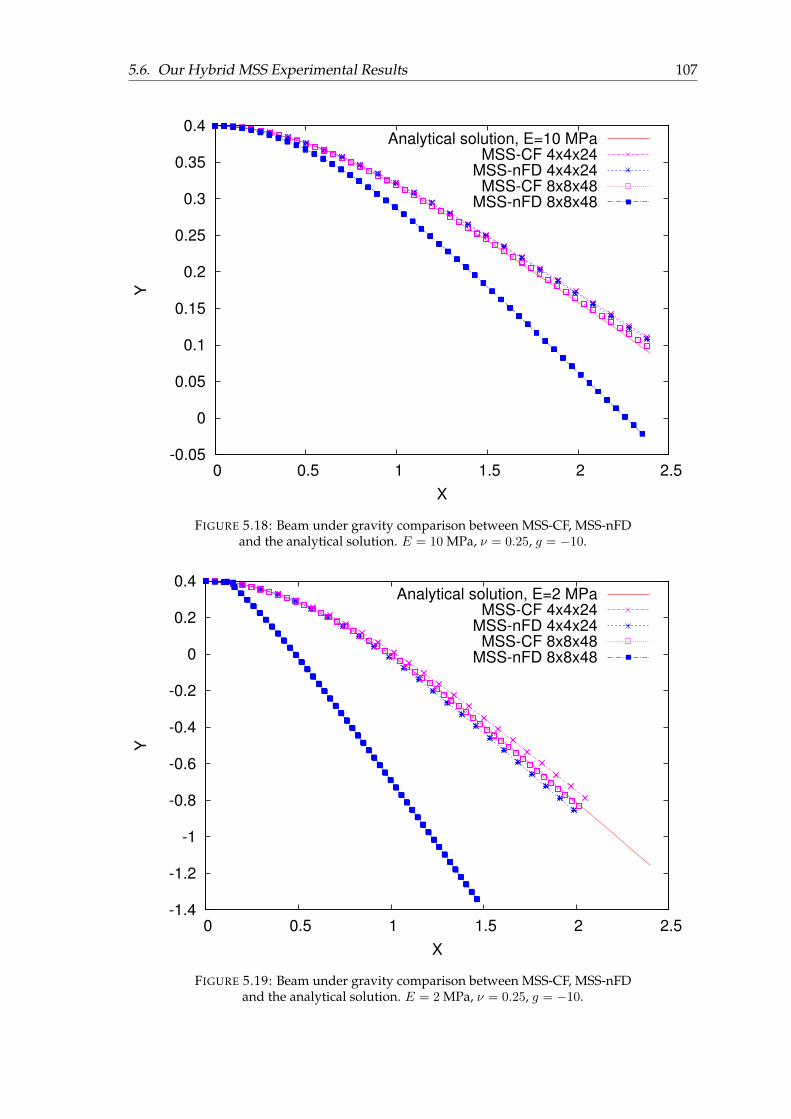
5.6. Our Hybrid MSS Experimental Results 107
-0.05
0
0.05
0.1
0.15
0.2
0.25
0.3
0.35
0.4
0 0.5 1 1.5 2 2.5
Y
X
Analytical solution, E=10 MPaMSS-CF 4x4x24
MSS-nFD 4x4x24MSS-CF 8x8x48
MSS-nFD 8x8x48
FIGURE 5.18: Beam under gravity comparison between MSS-CF, MSS-nFDand the analytical solution. E = 10 MPa, ν = 0.25, g = −10.
-1.4
-1.2
-1
-0.8
-0.6
-0.4
-0.2
0
0.2
0.4
0 0.5 1 1.5 2 2.5
Y
X
Analytical solution, E=2 MPaMSS-CF 4x4x24
MSS-nFD 4x4x24MSS-CF 8x8x48
MSS-nFD 8x8x48
FIGURE 5.19: Beam under gravity comparison between MSS-CF, MSS-nFDand the analytical solution. E = 2 MPa, ν = 0.25, g = −10.
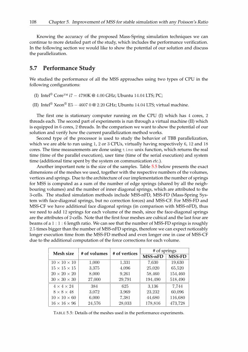
108 Chapter 5. Improvement of MSS for stable simulation with any Poisson’s Ratio
Knowing the accuracy of the proposed Mass-Spring simulation techniques we cancontinue to more detailed part of the study, which includes the performance verification.In the following section we would like to show the potential of our solution and discussthe parallelization.
5.7 Performance Study
We studied the performance of all the MSS approaches using two types of CPU in thefollowing configurations:
(I) Intel® Core™ i7− 4790K @ 4.00 GHz; Ubuntu 14.04 LTS; PC;
(II) Intel® Xeon® E5− 4607 0 @ 2.20 GHz; Ubuntu 14.04 LTS; virtual machine.
The first one is stationary computer running on the CPU (I) which has 4 cores, 2threads each. The second part of experiments is run through a virtual machine (II) whichis equipped in 6 cores, 2 threads. In the comparison we want to show the potential of oursolution and verify how the current parallelization method works.
Second type of the processor is used to study the behavior of TBB parallelization,which we are able to run using 1, 2 or 3 CPUs, virtually having respectively 6, 12 and 18cores. The time measurements are done using time unix function, which returns the realtime (time of the parallel execution), user time (time of the serial execution) and systemtime (additional time spent by the system on communication etc.).
Another important note is the size of the samples. Table 5.5 below presents the exactdimensions of the meshes we used, together with the respective numbers of the volumes,vertices and springs. Due to the architecture of our implementation the number of springsfor MSS is computed as a sum of the number of edge springs (shared by all the neigh-bouring volumes) and the number of inner diagonal springs, which are attributed to the3-cells. The studied simulation methods include MSS-nFD, MSS-FD (Mass-Spring Sys-tem with face-diagonal springs, but no correction forces) and MSS-CF. For MSS-FD andMSS-CF we have additional face diagonal springs (in comparison with MSS-nFD), thuswe need to add 12 springs for each volume of the mesh, since the face-diagonal springsare the attributes of 2-cells. Note that the first four meshes are cubical and the last four arebeams of a 1 : 1 : 6 length ratio. We can see that the number of MSS-FD springs is roughly2.5 times bigger than the number of MSS-nFD springs, therefore we can expect noticeablylonger execution time from the MSS-FD method and even longer one in case of MSS-CFdue to the additional computation of the force corrections for each volume.
Mesh size # of volumes # of vertices# of springs
MSS-nFD MSS-FD10× 10× 10 1,000 1,331 7,630 19,63015× 15× 15 3,375 4,096 25,020 65,52020× 20× 20 8,000 9,261 58,460 154,46030× 30× 30 27,000 29,791 194,490 518,490
4× 4× 24 384 625 3,136 7,7448× 8× 48 3,072 3,969 23,232 60,096
10× 10× 60 6,000 7,381 44,680 116,68016× 16× 96 24,576 28,033 178,816 473,728
TABLE 5.5: Details of the meshes used in the performance experiments.
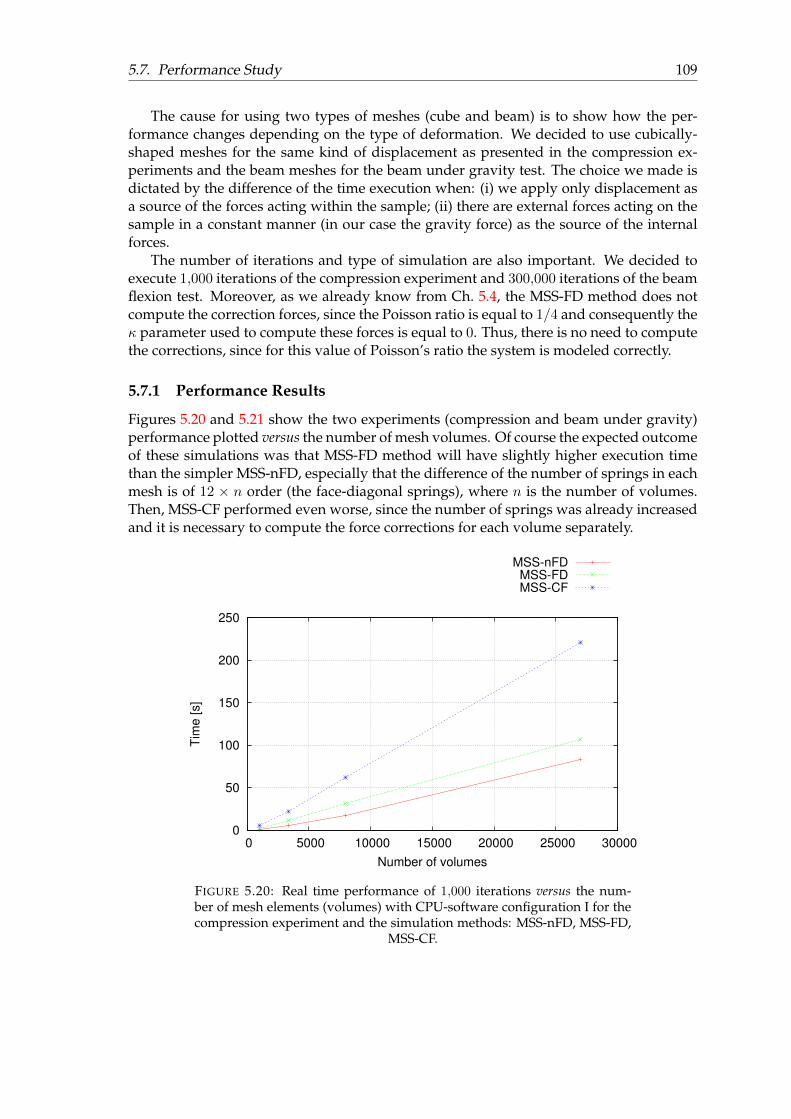
5.7. Performance Study 109
The cause for using two types of meshes (cube and beam) is to show how the per-formance changes depending on the type of deformation. We decided to use cubically-shaped meshes for the same kind of displacement as presented in the compression ex-periments and the beam meshes for the beam under gravity test. The choice we made isdictated by the difference of the time execution when: (i) we apply only displacement asa source of the forces acting within the sample; (ii) there are external forces acting on thesample in a constant manner (in our case the gravity force) as the source of the internalforces.
The number of iterations and type of simulation are also important. We decided toexecute 1,000 iterations of the compression experiment and 300,000 iterations of the beamflexion test. Moreover, as we already know from Ch. 5.4, the MSS-FD method does notcompute the correction forces, since the Poisson ratio is equal to 1/4 and consequently theκ parameter used to compute these forces is equal to 0. Thus, there is no need to computethe corrections, since for this value of Poisson’s ratio the system is modeled correctly.
5.7.1 Performance Results
Figures 5.20 and 5.21 show the two experiments (compression and beam under gravity)performance plotted versus the number of mesh volumes. Of course the expected outcomeof these simulations was that MSS-FD method will have slightly higher execution timethan the simpler MSS-nFD, especially that the difference of the number of springs in eachmesh is of 12 × n order (the face-diagonal springs), where n is the number of volumes.Then, MSS-CF performed even worse, since the number of springs was already increasedand it is necessary to compute the force corrections for each volume separately.
0
50
100
150
200
250
0 5000 10000 15000 20000 25000 30000
Tim
e [s]
Number of volumes
MSS-nFDMSS-FDMSS-CF
FIGURE 5.20: Real time performance of 1,000 iterations versus the num-ber of mesh elements (volumes) with CPU-software configuration I for thecompression experiment and the simulation methods: MSS-nFD, MSS-FD,
MSS-CF.
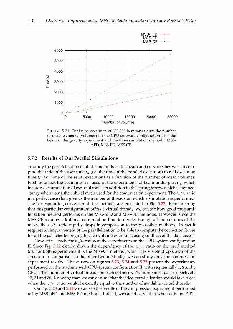
110 Chapter 5. Improvement of MSS for stable simulation with any Poisson’s Ratio
0
1000
2000
3000
4000
5000
6000
0 5000 10000 15000 20000 25000
Tim
e [s]
Number of volumes
MSS-nFDMSS-FDMSS-CF
FIGURE 5.21: Real time execution of 300,000 iterations versus the numberof mesh elements (volumes) on the CPU-software configuration I for thebeam under gravity experiment and the three simulation methods: MSS-
nFD, MSS-FD, MSS-CF.
5.7.2 Results of Our Parallel Simulations
To study the parallelization of all the methods on the beam and cube meshes we can com-pute the ratio of the user time tu (i.e. the time of the parallel execution) to real executiontime tr (i.e. time of the serial execution) as a function of the number of mesh volumes.First, note that the beam mesh is used in the experiments of beam under gravity, whichincludes accumulation of external forces in addition to the spring forces, which is not nec-essary when using the cubical mesh used for the compression experiment. The tu/tr ratioin a perfect case shall give us the number of threads on which a simulation is performed.The corresponding curves for all the methods are presented in Fig. 5.22. Rememberingthat this particular configuration offers 8 virtual threads, we can see how good the paral-lelization method performs on the MSS-nFD and MSS-FD methods. However, since theMSS-CF requires additional computation time to iterate through all the volumes of themesh, the tu/tr ratio rapidly drops in comparison to the two other methods. In fact itrequires an improvement of the parallelization to be able to compute the correction forcesfor all the particles belonging to each volume without causing conflicts of the data access.
Now, let us study the tu/tr ratios of the experiments on the CPU-system configurationII. Since Fig. 5.22 clearly shown the dependency of the tu/tr ratio on the used method(i.e. for both experiments it is the MSS-CF method, which has visible drop down of thespeedup in comparison to the other two methods), we can study only the compressionexperiment results. The curves on figures 5.23, 5.24 and 5.25 present the experimentsperformed on the machine with CPU-system configuration II, with sequentially 1, 2 and 3CPUs. The number of virtual threads on each of those CPU numbers equals respectively12, 24 and 36. Knowing that, we can assume that the ideal parallelization would take placewhen the tu/tr ratio would be exactly equal to the number of available virtual threads.
On Fig. 5.23 and 5.24 we can see the results of the compression experiment performedusing MSS-nFD and MSS-FD methods. Indeed, we can observe that when only one CPU
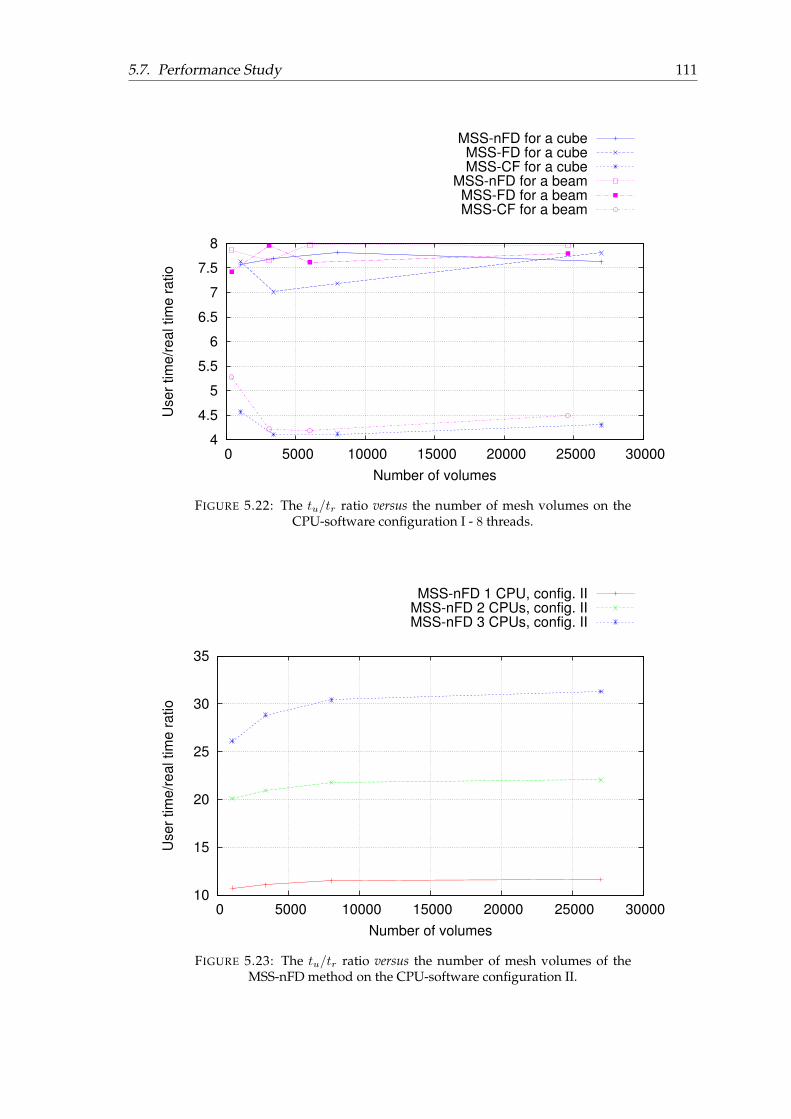
5.7. Performance Study 111
4
4.5
5
5.5
6
6.5
7
7.5
8
0 5000 10000 15000 20000 25000 30000
User
tim
e/r
eal tim
e r
atio
Number of volumes
MSS-nFD for a cube
MSS-FD for a cube
MSS-CF for a cube
MSS-nFD for a beam
MSS-FD for a beam
MSS-CF for a beam
FIGURE 5.22: The tu/tr ratio versus the number of mesh volumes on theCPU-software configuration I - 8 threads.
10
15
20
25
30
35
0 5000 10000 15000 20000 25000 30000
User
tim
e/r
eal tim
e r
atio
Number of volumes
MSS-nFD 1 CPU, config. IIMSS-nFD 2 CPUs, config. IIMSS-nFD 3 CPUs, config. II
FIGURE 5.23: The tu/tr ratio versus the number of mesh volumes of theMSS-nFD method on the CPU-software configuration II.
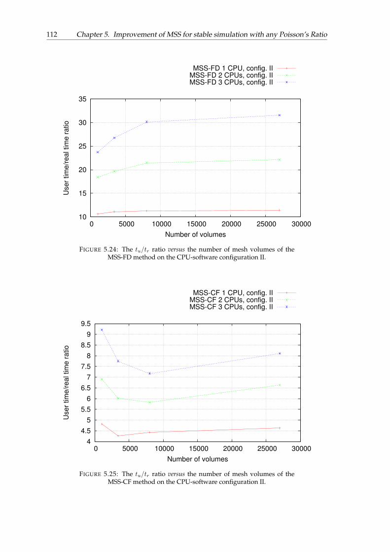
112 Chapter 5. Improvement of MSS for stable simulation with any Poisson’s Ratio
10
15
20
25
30
35
0 5000 10000 15000 20000 25000 30000
User
tim
e/r
eal tim
e r
atio
Number of volumes
MSS-FD 1 CPU, config. IIMSS-FD 2 CPUs, config. IIMSS-FD 3 CPUs, config. II
FIGURE 5.24: The tu/tr ratio versus the number of mesh volumes of theMSS-FD method on the CPU-software configuration II.
4
4.5
5
5.5
6
6.5
7
7.5
8
8.5
9
9.5
0 5000 10000 15000 20000 25000 30000
User
tim
e/r
eal tim
e r
atio
Number of volumes
MSS-CF 1 CPU, config. IIMSS-CF 2 CPUs, config. IIMSS-CF 3 CPUs, config. II
FIGURE 5.25: The tu/tr ratio versus the number of mesh volumes of theMSS-CF method on the CPU-software configuration II.
5.8. Summary of the Results of the Experiments 113
(12 virtual threads) is used the tu/tr ratio is the most advantageous in both cases. We ob-tained very good ratios also when two CPUs are used, but with the three CPUs we can seethat the capabilities of the machines are not fully used. The third figure (Fig. 5.25) showsthe results of the MSS-CF simulations and the first noticeable difference in comparisonwith the other simulation methods is the shape of the curves. Since the vast majority ofthe computation time is spent on the correction forces, the curve automatically becomesdependent on the number of volumes and rapidly drops when this number increases.We can see that the parallelization is the most advantageous for a smaller mesh and thenevens out when the mesh becomes bigger than ∼ 8,000 volumes due to the side and cor-rection forces computations which are not parallelized.
5.8 Summary of the Results of the Experiments
To sum up, we have seen that the use of correction forces and all types of springs inMass-Spring Systems plays a huge role in the body behavior and the shape of resultingdeformations. Our aim is to propose a generic model, working regardless of the externalforces and any topological modifications which a sample may undergo. The presentedexperimental results show that MSS-CF creates natural deformations of shapes, exactly asexpected by the physical laws. Additionally, the numerical results indicate that it is pos-sible to create an MSS model, which ensures the correct compressibility rate in a samplethroughout all volumes (so at the local level) and not just as an average result (globally).These results encourage the use of mass-spring systems for simulation of real tissues,showing that the MSS-CF simulation is equally worth the attention from the point of viewof accuracy and performance as the Finite Element Method. Even though we verified thatthe proposed MSS-CF method is able to perform a simulation slower than the presentedMSS-nFD approach, we are sure to simulate deformations faster than the available FEMmethods can. Additionally, we have shown that there is still room for the improvementof the performance of the MSS-CF approach, especially when iterating over the 3-cells ofthe mesh to calculate the correction forces.
5.9 Conclusions
In this chapter we introduced improvements to the classical MSS used to simulate isotropic,elastic tissues. The proposed contributions include dealing with the wrinkle instabilityand introducing physically-based stiffness formulations for all the used types of springs.The extension of the MSS to use all the real values of Poisson’s ratio, namely the correc-tion forces, is our final and major contribution. Working on cubical-symmetrical meshes,we have shown the effect of face-diagonal springs on the simulation; presented the newstiffness computation, which incorporates the mechanical information about a body intothe model; and shown how to locally correct volumes in order to keep the simulationphysically correct with adequate Poisson’s ratio.
The proposed solutions offer stable, physically-justified basis with a simple implemen-tation and many possibilities to improve and modify it. The easily adjustable parametersallow to successfully simulate compressible and incompressible isotropic materials (pre-sented ν = 0.499) with a minimal error. The solution is suitable for real-time applications(the mean performance of 10 second compression simulation of MSS-CF on a sample of1,000 elements on 8-thread processor is 5.579 s and the beam flexion of a 384 elementmesh lasting 300 seconds can be simulated within 74.149 s on the same CPU), however

114 Chapter 5. Improvement of MSS for stable simulation with any Poisson’s Ratio
the additional computation of the volume and correction forces on every element obvi-ously worsens the performance. It is possible to improve the computation time using TBBor consider other parallelization methods. What is more, the method has many conditionsimposed on the model, which makes it complicated to adapt to other mesh structures.
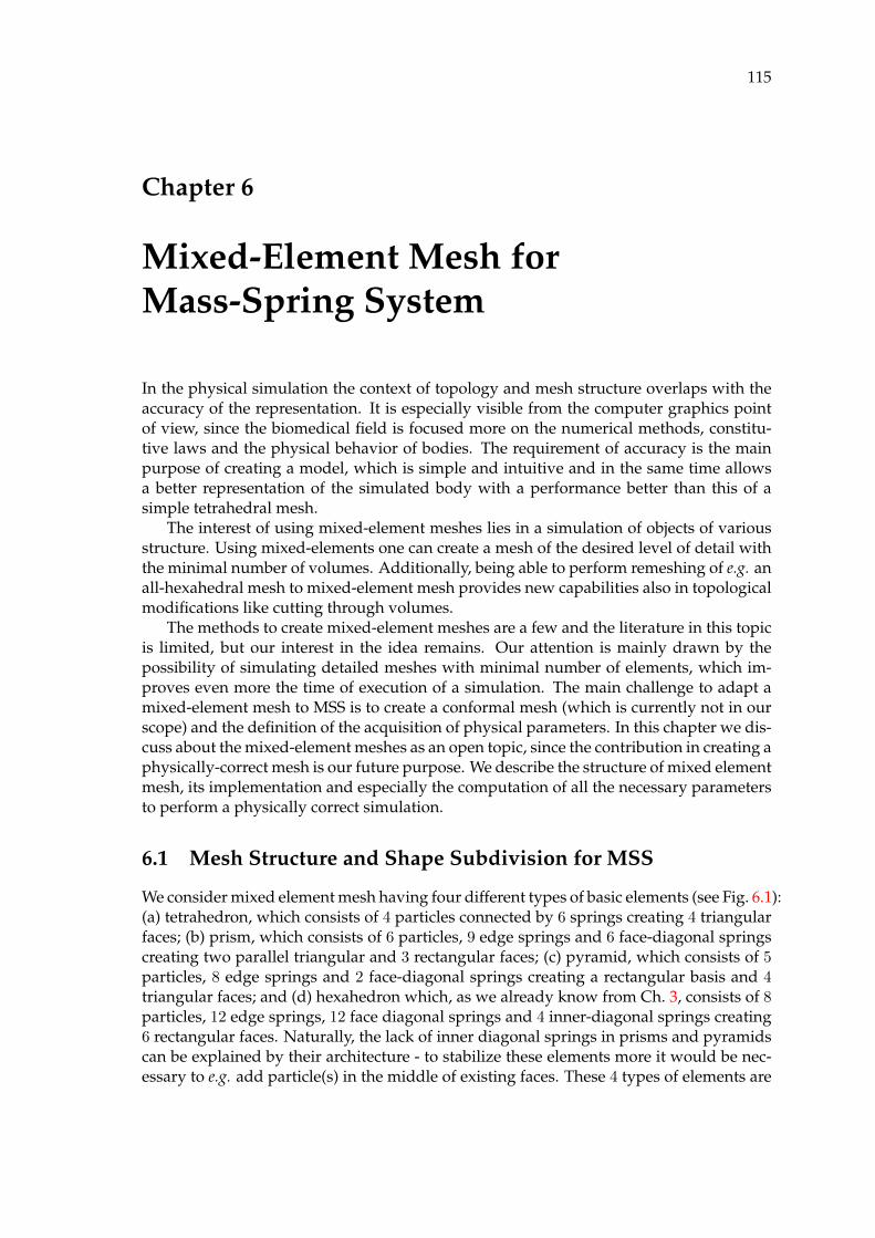
115
Chapter 6
Mixed-Element Mesh forMass-Spring System
In the physical simulation the context of topology and mesh structure overlaps with theaccuracy of the representation. It is especially visible from the computer graphics pointof view, since the biomedical field is focused more on the numerical methods, constitu-tive laws and the physical behavior of bodies. The requirement of accuracy is the mainpurpose of creating a model, which is simple and intuitive and in the same time allowsa better representation of the simulated body with a performance better than this of asimple tetrahedral mesh.
The interest of using mixed-element meshes lies in a simulation of objects of variousstructure. Using mixed-elements one can create a mesh of the desired level of detail withthe minimal number of volumes. Additionally, being able to perform remeshing of e.g. anall-hexahedral mesh to mixed-element mesh provides new capabilities also in topologicalmodifications like cutting through volumes.
The methods to create mixed-element meshes are a few and the literature in this topicis limited, but our interest in the idea remains. Our attention is mainly drawn by thepossibility of simulating detailed meshes with minimal number of elements, which im-proves even more the time of execution of a simulation. The main challenge to adapt amixed-element mesh to MSS is to create a conformal mesh (which is currently not in ourscope) and the definition of the acquisition of physical parameters. In this chapter we dis-cuss about the mixed-element meshes as an open topic, since the contribution in creating aphysically-correct mesh is our future purpose. We describe the structure of mixed elementmesh, its implementation and especially the computation of all the necessary parametersto perform a physically correct simulation.
6.1 Mesh Structure and Shape Subdivision for MSS
We consider mixed element mesh having four different types of basic elements (see Fig. 6.1):(a) tetrahedron, which consists of 4 particles connected by 6 springs creating 4 triangularfaces; (b) prism, which consists of 6 particles, 9 edge springs and 6 face-diagonal springscreating two parallel triangular and 3 rectangular faces; (c) pyramid, which consists of 5particles, 8 edge springs and 2 face-diagonal springs creating a rectangular basis and 4triangular faces; and (d) hexahedron which, as we already know from Ch. 3, consists of 8particles, 12 edge springs, 12 face diagonal springs and 4 inner-diagonal springs creating6 rectangular faces. Naturally, the lack of inner diagonal springs in prisms and pyramidscan be explained by their architecture - to stabilize these elements more it would be nec-essary to e.g. add particle(s) in the middle of existing faces. These 4 types of elements are
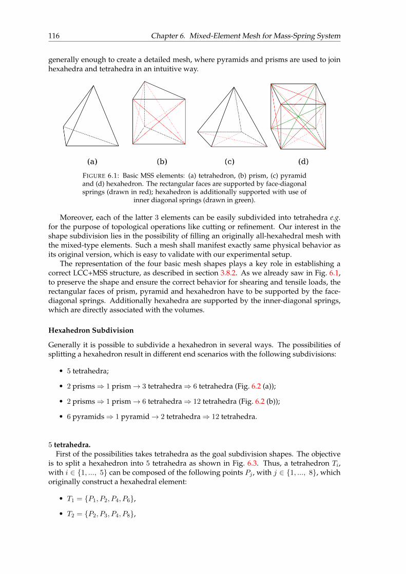
116 Chapter 6. Mixed-Element Mesh for Mass-Spring System
generally enough to create a detailed mesh, where pyramids and prisms are used to joinhexahedra and tetrahedra in an intuitive way.
FIGURE 6.1: Basic MSS elements: (a) tetrahedron, (b) prism, (c) pyramidand (d) hexahedron. The rectangular faces are supported by face-diagonalsprings (drawn in red); hexahedron is additionally supported with use of
inner diagonal springs (drawn in green).
Moreover, each of the latter 3 elements can be easily subdivided into tetrahedra e.g.for the purpose of topological operations like cutting or refinement. Our interest in theshape subdivision lies in the possibility of filling an originally all-hexahedral mesh withthe mixed-type elements. Such a mesh shall manifest exactly same physical behavior asits original version, which is easy to validate with our experimental setup.
The representation of the four basic mesh shapes plays a key role in establishing acorrect LCC+MSS structure, as described in section 3.8.2. As we already saw in Fig. 6.1,to preserve the shape and ensure the correct behavior for shearing and tensile loads, therectangular faces of prism, pyramid and hexahedron have to be supported by the face-diagonal springs. Additionally hexahedra are supported by the inner-diagonal springs,which are directly associated with the volumes.
Hexahedron Subdivision
Generally it is possible to subdivide a hexahedron in several ways. The possibilities ofsplitting a hexahedron result in different end scenarios with the following subdivisions:
• 5 tetrahedra;
• 2 prisms⇒ 1 prism→ 3 tetrahedra⇒ 6 tetrahedra (Fig. 6.2 (a));
• 2 prisms⇒ 1 prism→ 6 tetrahedra⇒ 12 tetrahedra (Fig. 6.2 (b));
• 6 pyramids⇒ 1 pyramid→ 2 tetrahedra⇒ 12 tetrahedra.
5 tetrahedra.First of the possibilities takes tetrahedra as the goal subdivision shapes. The objective
is to split a hexahedron into 5 tetrahedra as shown in Fig. 6.3. Thus, a tetrahedron Ti,with i ∈ 1, ..., 5 can be composed of the following points Pj , with j ∈ 1, ..., 8, whichoriginally construct a hexahedral element:
• T1 = P1, P2, P4, P6,
• T2 = P2, P3, P4, P8,
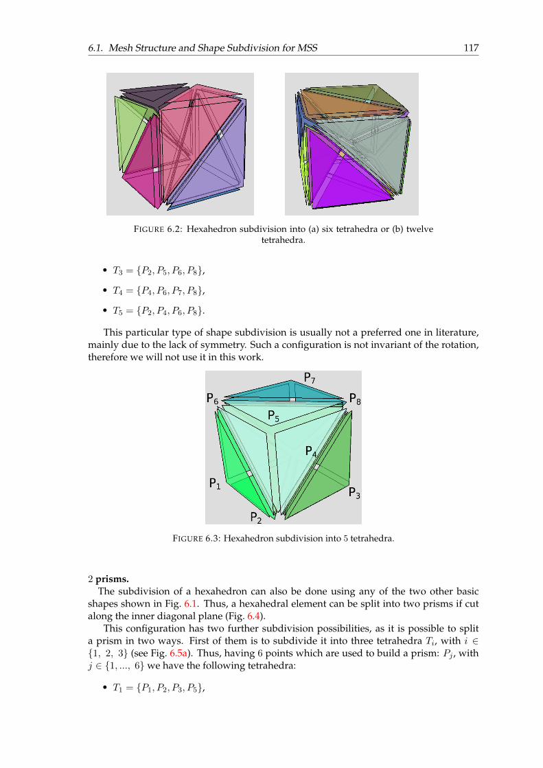
6.1. Mesh Structure and Shape Subdivision for MSS 117
FIGURE 6.2: Hexahedron subdivision into (a) six tetrahedra or (b) twelvetetrahedra.
• T3 = P2, P5, P6, P8,
• T4 = P4, P6, P7, P8,
• T5 = P2, P4, P6, P8.
This particular type of shape subdivision is usually not a preferred one in literature,mainly due to the lack of symmetry. Such a configuration is not invariant of the rotation,therefore we will not use it in this work.
FIGURE 6.3: Hexahedron subdivision into 5 tetrahedra.
2 prisms.The subdivision of a hexahedron can also be done using any of the two other basic
shapes shown in Fig. 6.1. Thus, a hexahedral element can be split into two prisms if cutalong the inner diagonal plane (Fig. 6.4).
This configuration has two further subdivision possibilities, as it is possible to splita prism in two ways. First of them is to subdivide it into three tetrahedra Ti, with i ∈1, 2, 3 (see Fig. 6.5a). Thus, having 6 points which are used to build a prism: Pj , withj ∈ 1, ..., 6we have the following tetrahedra:
• T1 = P1, P2, P3, P5,
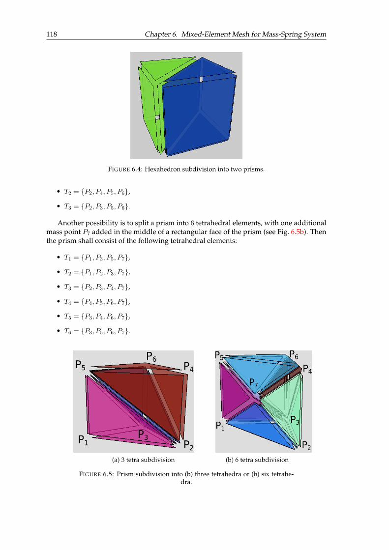
118 Chapter 6. Mixed-Element Mesh for Mass-Spring System
FIGURE 6.4: Hexahedron subdivision into two prisms.
• T2 = P2, P4, P5, P6,
• T3 = P2, P3, P5, P6.
Another possibility is to split a prism into 6 tetrahedral elements, with one additionalmass point P7 added in the middle of a rectangular face of the prism (see Fig. 6.5b). Thenthe prism shall consist of the following tetrahedral elements:
• T1 = P1, P3, P5, P7,
• T2 = P1, P2, P3, P7,
• T3 = P2, P3, P4, P7,
• T4 = P4, P5, P6, P7,
• T5 = P3, P4, P6, P7,
• T6 = P3, P5, P6, P7.
(a) 3 tetra subdivision (b) 6 tetra subdivision
FIGURE 6.5: Prism subdivision into (b) three tetrahedra or (b) six tetrahe-dra.
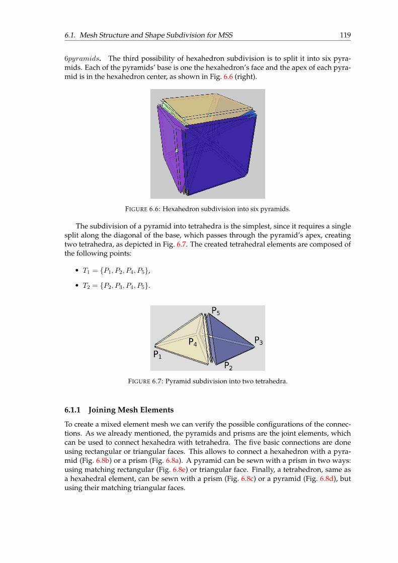
6.1. Mesh Structure and Shape Subdivision for MSS 119
6pyramids. The third possibility of hexahedron subdivision is to split it into six pyra-mids. Each of the pyramids’ base is one the hexahedron’s face and the apex of each pyra-mid is in the hexahedron center, as shown in Fig. 6.6 (right).
FIGURE 6.6: Hexahedron subdivision into six pyramids.
The subdivision of a pyramid into tetrahedra is the simplest, since it requires a singlesplit along the diagonal of the base, which passes through the pyramid’s apex, creatingtwo tetrahedra, as depicted in Fig. 6.7. The created tetrahedral elements are composed ofthe following points:
• T1 = P1, P2, P4, P5,
• T2 = P2, P3, P4, P5.
FIGURE 6.7: Pyramid subdivision into two tetrahedra.
6.1.1 Joining Mesh Elements
To create a mixed element mesh we can verify the possible configurations of the connec-tions. As we already mentioned, the pyramids and prisms are the joint elements, whichcan be used to connect hexahedra with tetrahedra. The five basic connections are doneusing rectangular or triangular faces. This allows to connect a hexahedron with a pyra-mid (Fig. 6.8b) or a prism (Fig. 6.8a). A pyramid can be sewn with a prism in two ways:using matching rectangular (Fig. 6.8e) or triangular face. Finally, a tetrahedron, same asa hexahedral element, can be sewn with a prism (Fig. 6.8c) or a pyramid (Fig. 6.8d), butusing their matching triangular faces.
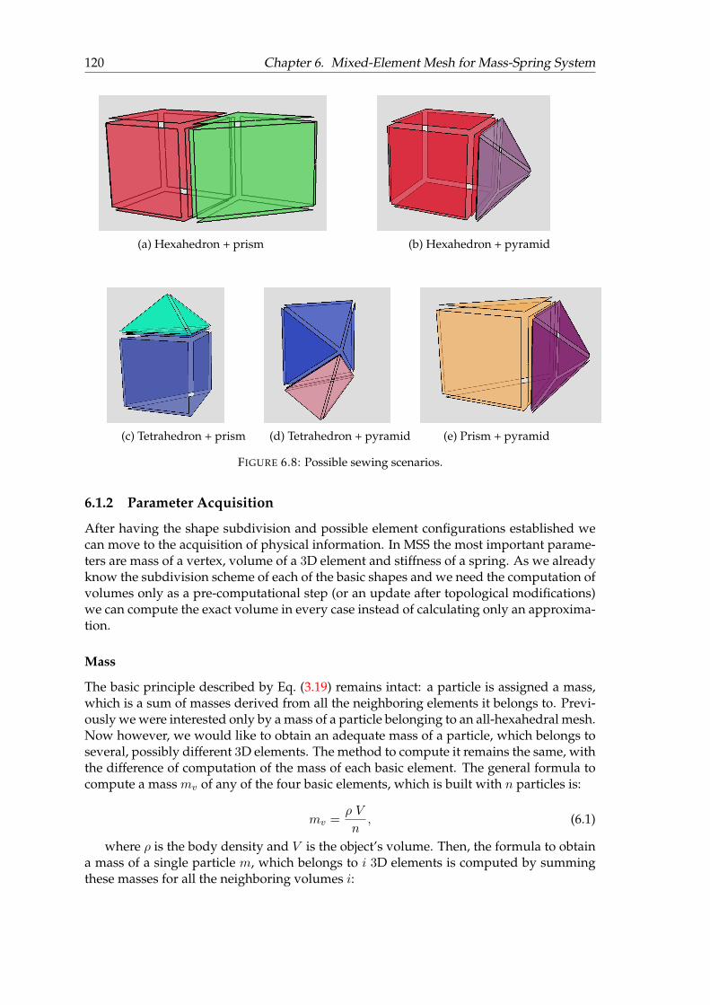
120 Chapter 6. Mixed-Element Mesh for Mass-Spring System
(a) Hexahedron + prism (b) Hexahedron + pyramid
(c) Tetrahedron + prism (d) Tetrahedron + pyramid (e) Prism + pyramid
FIGURE 6.8: Possible sewing scenarios.
6.1.2 Parameter Acquisition
After having the shape subdivision and possible element configurations established wecan move to the acquisition of physical information. In MSS the most important parame-ters are mass of a vertex, volume of a 3D element and stiffness of a spring. As we alreadyknow the subdivision scheme of each of the basic shapes and we need the computation ofvolumes only as a pre-computational step (or an update after topological modifications)we can compute the exact volume in every case instead of calculating only an approxima-tion.
Mass
The basic principle described by Eq. (3.19) remains intact: a particle is assigned a mass,which is a sum of masses derived from all the neighboring elements it belongs to. Previ-ously we were interested only by a mass of a particle belonging to an all-hexahedral mesh.Now however, we would like to obtain an adequate mass of a particle, which belongs toseveral, possibly different 3D elements. The method to compute it remains the same, withthe difference of computation of the mass of each basic element. The general formula tocompute a mass mv of any of the four basic elements, which is built with n particles is:
mv =ρ V
n, (6.1)
where ρ is the body density and V is the object’s volume. Then, the formula to obtaina mass of a single particle m, which belongs to i 3D elements is computed by summingthese masses for all the neighboring volumes i:
6.1. Mesh Structure and Shape Subdivision for MSS 121
m =∑i
miv. (6.2)
This generalization allows us to be generic and focus only on the computation of vol-umes of the 3D objects.
Volume
The computation of a volume of a 3D element is important not only to establish the massof each particle of a MSS, but also as a potential tool to introduce volume correction forcesinto a mixed-element mesh MSS.
Tetrahedron. A volume of a regular tetrahedron is classically computed using the sim-ple equation, which uses the length of tetrahedron’s arm lt: V = l3t /(6
√2). However in
our case, which aims at a generic treatment of the shapes, it has to be computed by ageneral formula, which is independent of the tetrahedron’s arms’ lengths:
Vtetra =1
3AbaseH, (6.3)
where Abase is the area of the base of a tetrahedron, meaning any of the face triangles,and H is the height of the tetrahedron measured from this base.
Other basic shapes. Using the formula of tetrahedron volume computation Vtetra wecan simply establish the volumes of all the other basic shapes using the previously pre-sented subdivision. Therefore, with a prism consisting of 3 tetrahedra, a pyramid consist-ing of 2 tetrahedra and a hexahedron consisting of 6 tetrahedra we have:
Vprism =3∑i=1
V itetra (6.4)
Vpyramid =
2∑i=1
V itetra (6.5)
Vhexa =
6∑i=1
V itetra (6.6)
Using this method we can easily compute the initial or updated volumes of the 3Dshapes and use them to correctly compute the masses of the points they belong to. Inthe same time we are sure that the computation is generic i.e. each of the shapes after adeformation can still be subdivided into tetrahedra in the same way as the initial figure,so the computation is not affected by the shapes’ geometry.
Spring Stiffness
The full discussion about the literature in the topic of obtaining stiffness for springs inMSS was undertaken in Ch. 3.4.3. From there we already know the variety of the meth-ods used to compute or approximate this parameter. Because of its importance and theinfluence on the behavior of the simulated tissue we have presented our own idea in thismatter in Ch. 5.1 for all-hexahedral symmetric isotropic meshes.
122 Chapter 6. Mixed-Element Mesh for Mass-Spring System
The mixed-element mesh is a much greater challenge though, since the variety of theshapes and our will to approach the topic with genericity do not allow us to use just anyformulation. Additionally, since the mixed-element meshes were by now mainly used forFEM simulations, the computation of the spring stiffness was simply not needed. To fillin the gap in this topic we decided to approach the problem in a similar way as we havein Ch. 5.1 for the cubical elements. The full derivation of the stiffnesses of the mixed-element meshes is in our future work plan, but we want to stress out that it is the last stepto obtain a full definition of this architecture for MSS. We aim at a formulation which takesinto account the physical body parameters (defined by Young’s modulus and Poisson’sratio), which involves the use of the face-diagonal and inner-diagonal springs and whichallows simulation of real tissues with the same accuracy as our current model defined inthe previously presented contributions. Adapting the mixed-element mesh to the idea ofcorrection forces (see Ch. 5.2) is also one of our main goals.
6.2 Mixed-Element Mesh Implementation
Our work on the mixed-element meshes features the introduction of new basic shapesand their initialization (except of the spring stiffness parameters). We present the imple-mentation details of the mixed-element mesh in TopoSim framework below.
To implement the mixed-element mesh shapes we need to add basic shapes to thelowest level of our implementation i.e. 3-map part (see Fig. 3.18). Since we are dealingwith the 3-map elements we can work directly with the Volume_LCC class. All the basicshapes need to initialized in this class based on their c-maps. We can easily distinguishthem by the number of vertices they are built with.
The next step is to associate the face-diagonal springs of a pyramid and a prism tothe 3-cells, which means, that we need to look into the Volume_LCC_MSS class. Herewe had implemented and associated the additional springs and introduced all the small’get’ functions, which are used to differentiate between basic shapes and allow to use thegeneric functions (like the add_force function) without any adaptations. To do that weneed to mind the distinction between different types of basic elements, since every one ofthem has a different number of face-diagonal (and inner diagonal in case of a hexahedron)springs. The list below presents the number of vertices and face-diagonal springs, whichwe need to take into account:
• tetrahedron - 4 vertices - 0 face-diagonal springs;
• pyramid - 5 vertices - 2 face-diagonal springs;
• prism - 6 vertices - 6 face-diagonal springs;
• hexahedron - 8 vertices - 12 face-diagonal springs.
The ’get’ functions will then return the appropriate shape type, number of vertices,number of face-diagonal springs and the spring extremities.
The last function to be modified is the initialization of masses in the Object_LCC_MSSclass: initialize_masses. As we have already explained in Ch. 6.1.2, the masses are com-puted thanks to a generic formulation, which uses the volume V of a 3-cell as one of thecomponents. This means that we need to modify the initialization function to computethe exact volumes of our basic shapes using the previously defined shape subdivision intotetrahedra. Then, the function will return the resulting volume as a sum of the volumesof all the tetrahedra which compose particular basic shape.
6.3. Conclusions 123
6.3 Conclusions
Having a full mixed-element mesh formulation we will be able to simulate various realmaterials with a new level of accuracy. Additionally, the presented implementation, es-pecially the most low-level part, which is building the LCC structure, can be used bydifferent simulation techniques, being not only MSS but also MT or even FEM. Finally,it will be possible to perform a physically correct simulation with a mixed-element meshusing Mass-Spring System, which, to our knowledge, is not yet possible.
We have already verified that mixed-element meshes work well in our frameworkwith the presented computation of mass and assigned fixed spring stiffness parameters.When the physically-based spring stiffness computation will be correctly derived, thiscontribution will open new door to research in the direction of mixed-element meshesused for MSS and hopefully will draw attention of researchers to work more on this topicnot only from the point of view of FEM, but also other simulation methods.

125
Chapter 7
Conclusions and Perspectives
Context of the Thesis Subject
Modeling and simulation of behavior of deformable bodies, especially soft tissues, wasthe general subject of this thesis. Our first goal was to integrate the physical laws basedon real experiments into our framework to model behavior of real bodies. The second,more general goal was to find a balance between the speed of calculations and precision.Because of our assumptions and objectives we have chosen to use Mass-Spring System,which, unlike continuous models, allows simple and fast calculations. However, due toits natural limitations and instabilities we had to improve this simulation technique to beable to reach our goals.
Contributions
In this thesis, we proposed several novel approaches to deal with MSS limitations andimprove its accuracy in simulating real tissues. They are suitable for modeling elasticdeformable bodies at small and large strains while controlling key behaviors specified bythe physical body parameters.
• In the first part we presented a non-linear force formulation for the springs inter-actions, which is easily adaptable for simulation of real tissues at small and largedeformations. It has proven to control the shape of the stress-time curve up to 100%strain with only 4 parameters. The method has the advantage of being easy to imple-ment and reformulate if needed. Nonetheless, the formula needs an improvementto fit the curves based on the presented bi-power constitutive law and better adjustto the speed of body deformation.
• The second part of the thesis described physically based formulation of stiffnesscomputation complemented with force corrections to allow use of full range ofthe Poisson ratio. This contribution deals well with global volumetric changes ina locally-oriented MSS. As we have presented in the experimental validation part,our hybrid approach is able to simulate the bodies from absolutely compressible(ν = 0) to nearly incompressible (ν = 0.499). Additionally, the presented formu-lation of stiffness parameters for three types op springs in an all-hexahedral meshis not restricted to specific deformation types. The improvements stabilize the MSSand deal well with the natural MSS limitations and instabilities. The method needshowever to be parallelized, since the time of execution of the hybrid model largelyexceeds our target. What is more, the presented stiffness formulation works onlyfor all-hexahedral meshes, mainly due to the assumption of isotropy we made.
126 Chapter 7. Conclusions and Perspectives
• In the last part we have also presented the preliminary work concerning mixed-element mesh and its implementation. Our idea is to be able to create a mesh ofa complex structure with minimal number of elements to allow fast and physicallyaccurate simulation. We have successfully created and implemented the topologi-cal structure of this lattice. The mixed-element MSS mesh has also a good basis forthe future implementation of volume correction forces thanks to the element sub-division. However, our work on the derivation of the stiffness parameters requirescomplex computations and a thorough validation, especially for the joint elements:pyramids and prisms.
We have implemented all of the above contributions in our framework - TopoSim.The methods are introduced in the framework to simulate the desired behaviors withrobustness, speed and efficiency. We took into account the computational cost as well asthe memory usage. The volume correction forces are adaptable to other physically-basedsimulation methods. Similarly, the mixed-element mesh structure can be easily extendedto any modeling technique thanks to the presented choice of its topological structure.
Discussion
All the presented experimental results aim at a correct simulation of chosen body features,which we have validated in the previous chapters. Nonetheless, there are several partic-ular features which can be discussed when it comes to this validation. Let us sum up thefollowing characteristics of a successful physical simulation of deformable bodies:
• Accuracy. Non-linear formulation of forces presented in Chapter 4 controls well theshape of the curve, lining up with the analytical results. However the magnitudeof each curve should strongly depend on the speed of deformation (strain rate),so the method still needs improvement in this matter. Additionally the methodneeds proper validation in various deformation scenarios e.g. compression or tor-sion, since the only validation we proposed by now is in shearing. On the otherhand, the hybrid 3D improvement of MSS presented in Chapter 5 proves to be asaccurate as a Finite Element Method in simulating elastic bodies. It has proven to ac-curately model the volumetric behavior of soft tissues under various deformationsup to 20% strain, which is very satisfying for a linear deformation model.
• Speed. The non-linear force formulation is a simple solution to introduce non-linearity into MSS and it performs equally as the linear approach. Thus, the speedof simulation is naturally the same as for the linear MSS and was not studied in de-tail. The hybrid MSS however lacks parallelization in the computation of correctionterms and therefore doubles the time of simulation execution.
• Genericity. All of the presented approaches were carefully evaluated to be as genericas our framework used for simulations. The non-linear force formulation can modelany real organ with parameters defined with the bi-power constitutive law. In thesame time, the hybrid MSS is not limited by the type of deformation to model. In-deed, this improvement can be used on any mesh element, since the formulationitself takes into account the volume change and physical body parameters, but notthe mesh geometry.
• Stability. We have solved the problem of natural MSS wrinkle and buckling insta-bilities by using three types of springs in all-hexahedral meshes with the presentedformulation of stiffness parameters.
Chapter 7. Conclusions and Perspectives 127
The results of our experiments convince us that working on MSS structure can be fast,easy and, what is most important, give physically correct results. Another undeniableadvantage of Mass-Spring System is the possibility to perform interactive simulations,thanks to the underlying LCC structure, which is not possible with the commonly usedclassical FEM. Despite the drawbacks of the chosen approaches we have shown that thechoice of the simulation method in the biomedicine can be expanded to MSS, which pro-vides new possibilities in the physical simulation field thanks to our improvements.
Future work
The MSS simulation method has been largely omitted in the field of medical modeling dueto its lack of accuracy and supposed inability to introduce physically-based behaviors ordeformable bodies. However our work have proven that MSS is still a plausible solutionto model real organs fast and precisely. Nonetheless, there still remains a lot to work onin the future.
The first task we ought to focus on is the physically-based formulation of stiffnessparameters for the elements of a mixed-type mesh. This work will significantly improvethe performance of our simulations thanks to use of smaller number of mesh elementswhile keeping the same level of detail. To do that we want to follow the derivation methodpresented on hexahedral elements, however the simplifications done for hexahedra arenot possible on other 3D elements e.g. due to the symmetry. Naturally, the mixed-typemesh formulation can easily be extended by our volume correction forces to control thevolumetric changes with use of any natural value of the Poisson ratio.
Our method for simulating non-linear deformations with specially designed force for-mulation is able to control the shape of the curve, however lacks in accuracy to model thecorrect magnitude of deformation. We aim at improving the existing formulation to matchthe constitutive law at different strain rates, which currently is the biggest drawback ofour formulation. Additionally we want to be able to model the behavior of various bodies(performing verification of different deformations) using all the parameters which definea body in case of the bi-power law.
The most interesting step to work on will be our hybrid MSS extension to model largedeformations. In fact the volume correction forces are supposedly suitable for large de-formations, which needs a thorough validation with suitable, improved formulation ofnon-linear computation of forces. The combination of the two methods shall prove MSSto accurately model non-linear deformations of real tissues with possibility of adjustingtheir compressibility. Such a formulation would be useful in combination with hapticdevices to model real organs in real time with the possibility of topological modifications.
The remaining task will involve many experiments done on different types of ele-ments and model geometries to verify how to model real behavior of soft tissues best.Additionally we will need to compare a dynamic FEM and MSS simulations to verify thestability, accuracy and performance of the two approaches. Once we establish that, weget a simulation environment which will allow us to model different types of behaviorof various tissues while being able to perform topological modifications during a simu-lation. We take into account possible modifications to be done to ensure the stability ofphysical models when changing the mesh topology.

129
Bibliography
[1] About Society for Simulation in Healthcare. 2017. URL: http://www.ssih.org/About-SSH (visited on 05/16/2017).
[2] Awais Ahmed. “Extended finite element method (XFEM)-modeling arbitrary dis-continuities and failure analysis”. In: Research degree thesis (2009).
[3] Jérémie Allard, Stéphane Cotin, François Faure, Pierre-Jean Bensoussan, FrançoisPoyer, Christian Duriez, Hervé Delingette, and Laurent Grisoni. “SOFA - an OpenSource Framework for Medical Simulation”. In: MMVR 15 - Medicine Meets Vir-tual Reality. Vol. 125. Studies in Health Technology and Informatics. Palm Beach,United States: IOP Press, Feb. 2007, pp. 13–18.
[4] S. Arnab and V. Raja. “Chapter 4: Simulating a Deformable Object Using a SurfaceMass Spring System”. In: 2008 3rd International Conference on Geometric Modelingand Imaging. July 2008, pp. 21–26. DOI: 10.1109/GMAI.2008.24.
[5] Fred S. Azar, Dimitris N. Metaxas, and Mitchell D. Schnall. “A Deformable FiniteElement Model of the Breast for Predicting Mechanical Deformations under Exter-nal Perturbations”. In: Academic Radiology 8.10 (2001), pp. 965 –975. ISSN: 1076-6332.DOI: https://doi.org/10.1016/S1076-6332(03)80640-2.
[6] David Baraff and Andrew Witkin. “Large Steps in Cloth Simulation”. In: Proceed-ings of the 25th Annual Conference on Computer Graphics and Interactive Techniques.SIGGRAPH ’98. New York, NY, USA: ACM, 1998, pp. 43–54. ISBN: 0-89791-999-8.DOI: 10.1145/280814.280821.
[7] Ehsan Basafa, Farzam Farahmand, and Gholamreza Vossoughi. “A non-linear mass-spring model for more realistic and efficient simulation of soft tissues surgery”. In:Studies in health technology and informatics 132 (2008), p. 23.
[8] Cagatay Basdogan. “Real-time simulation of dynamically deformable finite ele-ment models using modal analysis and spectral lanczos decomposition methods”.In: (2000).
[9] K.J. Bathe. Finite Element Procedures in Engineering Analysis. Prentice Hall, New Jer-sey, 1982.
[10] Klaus-Jürgen Bathe. “Conserving energy and momentum in nonlinear dynamics:a simple implicit time integration scheme”. In: Computers & structures 85.7 (2007),pp. 437–445.
[11] Lukas M. Batteau, Alan Liu, J. B. Antoine Maintz, Yogendra Bhasin, and Mark W.Bowyer. “A Study on the Perception of Haptics in Surgical Simulation”. In: MedicalSimulation: International Symposium, ISMS 2004, Cambridge, MA, USA, June 17-18,2004. Proceedings. Ed. by Stéphane Cotin and Dimitris Metaxas. Berlin, Heidelberg:Springer Berlin Heidelberg, 2004, pp. 185–192. ISBN: 978-3-540-25968-8. DOI: 10.1007/978-3-540-25968-8_21.
130 BIBLIOGRAPHY
[12] V. Baudet, M. Beuve, F. Jaillet, B. Shariat, and F. Zara. “Integrating Tensile Param-eters in Hexahedral Mass-Spring System for Simulation”. In: WSCG’2009. 2009.ISBN: 9788086943930.
[13] T. Belytschko and T. Black. “Elastic crack growth in finite elements with mini-mal remeshing”. In: International Journal for Numerical Methods in Engineering 45.5(1999), pp. 601–620. ISSN: 1097-0207. DOI: 10.1002/(SICI)1097-0207(19990620)45:5<601::AID-NME598>3.0.CO;2-S.
[14] Ted Belytschko and Lawrence W. Glaum. “Applications of higher order corota-tional stretch theories to nonlinear finite element analysis”. In: Computers & Struc-tures 10.1 (1979), pp. 175 –182. ISSN: 0045-7949. DOI: https://doi.org/10.1016/0045-7949(79)90085-3.
[15] Jan Bender, Matthias Müller, Miguel A. Otaduy, and Matthias Teschner. “Position-based Methods for the Simulation of Solid Objects in Computer Graphics”. In:EUROGRAPHICS 2013 State of the Art Reports. Girona, Spain: Eurographics Asso-ciation, 2013.
[16] Jan Bender, Matthias Müller, Miguel A. Otaduy, and Matthias Teschner. “Position-based Methods for the Simulation of Solid Objects in Computer Graphics”. In:EUROGRAPHICS 2013 State of the Art Reports. Girona, Spain: Eurographics Asso-ciation, 2013.
[17] J. Berkley, S. Weghorst, H. Gladstone, G. Raugi, D. Berg, and M. Ganter. “Bandedmatrix approach to Finite Element modelling for soft tissue simulation”. In: VirtualReality 4.3 (Sept. 1999), pp. 203–212. ISSN: 1434-9957. DOI: 10.1007/BF01418156.
[18] Kiran S. Bhat, Christopher D. Twigg, Jessica K. Hodgins, Pradeep K. Khosla, Zo-ran Popovic, and Steven M. Seitz. “Estimating Cloth Simulation Parameters fromVideo”. In: Proceedings of the 2003 ACM SIGGRAPH/Eurographics Symposium onComputer Animation. SCA ’03. San Diego, California: Eurographics Association,2003, pp. 37–51. ISBN: 1-58113-659-5.
[19] G. Bianchi, B. Solenthaler, G. Székely, and M. Harders. “Simultaneous Topologyand Stiffness Identification for Mass-Spring Models based on FEM Reference De-formations”. In: MICCAI 2004. Vol. 2. Springer, Nov. 2004, pp. 293–301.
[20] Gérald Bianchi, Matthias Harders, and Gábor Székely. “Mesh Topology Identifica-tion for Mass-Spring Models”. In: Medical Image Computing and Computer-AssistedIntervention - MICCAI 2003: 6th International Conference, Montréal, Canada, November15-18, 2003. Proceedings. Ed. by Randy E. Ellis and Terry M. Peters. Berlin, Heidel-berg: Springer Berlin Heidelberg, 2003, pp. 50–58. ISBN: 978-3-540-39899-8. DOI:10.1007/978-3-540-39899-8_7.
[21] D. Bielser and M. H. Gross. “Interactive simulation of surgical cuts”. In: Proceedingsthe Eighth Pacific Conference on Computer Graphics and Applications. 2000, pp. 116–442. DOI: 10.1109/PCCGA.2000.883933.
[22] Richard Evelyn Donohue Bishop and DC Johnson. The Mechanics of Vibration. Cam-bridge University Press, 1979.
[23] F. Boosman. “Macintosh Windows”. In: Computer Gaming World 32 (Nov. 1986),pp. 15, 32.
[24] David Bourguignon and Marie-Paule Cani. “Controlling Anisotropy in Mass-SpringSystems”. In: Computer Animation and Simulation 2000: Proceedings of the Eurograph-ics Workshop in Interlaken, Switzerland, August 21–22, 2000. Vienna: Springer Vienna,2000, pp. 113–123. ISBN: 978-3-7091-6344-3.
BIBLIOGRAPHY 131
[25] R. Bridson, R. Fedkiw, and J. Anderson. “Robust Treatment of Collisions, Contactand Friction for Cloth Animation”. In: ACM Trans. Graph. 21.3 (July 2002), pp. 594–603. ISSN: 0730-0301.
[26] Morten Bro-Nielsen. “Modelling Elasticity in Solids Using Active Cubes — Appli-cation to Simulated Operations”. In: Computer Vision, Virtual Reality and Roboticsin Medicine: First International Conference, CVRMed ’95, Nice, France, April 3–6, 1995Proceedings. Ed. by Nicholas Ayache. Berlin, Heidelberg: Springer Berlin Heidel-berg, 1995, pp. 535–541. ISBN: 978-3-540-49197-2. DOI: 10.1007/978-3-540-49197-2_70.
[27] Morten Bro-Nielsen and Stephane Cotin. “Real-time Volumetric Deformable Mod-els for Surgery Simulation using Finite Elements and Condensation”. In: ComputerGraphics Forum 15.3 (1996), pp. 57–66. ISSN: 1467-8659. DOI: 10.1111/1467-8659.1530057.
[28] Joel Brown, Stephen Sorkin, Jean-Claude Latombe, Kevin Montgomery, and MichaelStephanides. “Algorithmic tools for real-time microsurgery simulation”. In: Medi-cal image analysis 6.3 (2002), pp. 289–300.
[29] David T. Chen and David Zeltzer. “Pump It Up: Computer Animation of a Biome-chanically Based Model of Muscle Using the Finite Element Method”. In: Proceed-ings of the 19th Annual Conference on Computer Graphics and Interactive Techniques.SIGGRAPH ’92. New York, NY, USA: ACM, 1992, pp. 89–98. ISBN: 0-89791-479-1.DOI: 10.1145/133994.134016.
[30] F. Chen, L. Gu, P. Huang, J. Zhang, and J. Xu. “Soft Tissue Modeling using Non-linear Mass Spring and Simplified Medial Representation”. In: 2007 29th AnnualInternational Conference of the IEEE Engineering in Medicine and Biology Society. Aug.2007, pp. 5083–5086.
[31] Kup-Sze Choi, Hanqiu Sun, and Pheng-Ann Heng. “An efficient and scalable de-formable model for virtual reality-based medical applications”. In: Artificial Intelli-gence in Medicine 32.1 (2004). Atificial Intelligence in Medicine in China, pp. 51 –69.ISSN: 0933-3657. DOI: https://doi.org/10.1016/j.artmed.2004.01.013.
[32] Gerard M Cooney, Kevin M Moerman, Michael Takaza, Des C Winter, and CiaranK Simms. “Uniaxial and biaxial mechanical properties of porcine linea alba.” In:Journal of the mechanical behavior of biomedical materials 41C (Oct. 2014), pp. 68–82.ISSN: 1878-0180. DOI: 10.1016/j.jmbbm.2014.09.026.
[33] S. Cotin, H. Delingette, and N. Ayache. “A Hybrid Elastic Model allowing Real-Time Cutting, Deformations and Force-Feedback for Surgery Training and Sim-ulation”. Anglais. In: Visual Computer 16.8 (2000), pp. 437–452. DOI: 10.1007/PL00007215.
[34] S. Cotin, H. Delingette, and N. Ayache. “Real-time elastic deformations of soft tis-sues for surgery simulation”. In: IEEE Transactions on Visualization and ComputerGraphics 5.1 (1999), pp. 62–73.
[35] Stéphane Cotin, Hervé Delingette, and Nicholas Ayache. “Real time volumetric de-formable models for surgery simulation”. In: Visualization in Biomedical Computing:4th International Conference, VBC’96 Hamburg, Germamy, September 22–25, 1996 Pro-ceedings. Ed. by Karl Heinz Höhne and Ron Kikinis. Berlin, Heidelberg: SpringerBerlin Heidelberg, 1996, pp. 535–540. ISBN: 978-3-540-70739-4. DOI: 10.1007/BFb0046995.
132 BIBLIOGRAPHY
[36] S. A. Cover, N. F. Ezquerra, J. F. O’Brien, R. Rowe, T. Gadacz, and E. Palm. “Inter-actively deformable models for surgery simulation”. In: IEEE Computer Graphicsand Applications 13.6 (Nov. 1993), pp. 68–75. ISSN: 0272-1716. DOI: 10.1109/38.252559.
[37] Elias Cueto, Siamak Niroomandi, David Gonzalez, Iciar Alfaro, Felipe Bordeu,Adrien Leygue, and Francisco Chinesta. “Real Time Simulation of Non-LinearSolids by PGD Techniques”. In: Material Forming ESAFORM 2012. Vol. 504. KeyEngineering Materials. Trans Tech Publications, Apr. 2012, pp. 467–472. DOI: 10.4028/www.scientific.net/KEM.504-506.467.
[38] Tong Cui, Aiguo Song, and Juan Wu. “Simulation of a mass-spring model forglobal deformation”. In: Frontiers of Electrical and Electronic Engineering in China4.1 (2009), pp. 78–82. ISSN: 1673-3584. DOI: 10.1007/s11460-009-0001-6.
[39] Benoît Dagon, Charles Baur, and Vincent Bettschart. “Real-time update of 3D de-formable models for computer aided liver surgery”. In: Pattern Recognition, 2008.ICPR 2008. 19th International Conference on. IEEE. 2008, pp. 1–4.
[40] G. Damiand and P. Lienhardt. Combinatorial Maps: Efficient Data Structures for Com-puter Graphics and Image Processing. A K Peters/CRC Press, Sept. 2014.
[41] Guillaume Damiand. “Combinatorial Maps”. In: CGAL User and Reference Man-ual. 4.10. CGAL Editorial Board, 2017. URL: http://doc.cgal.org/4.10/Manual/packages.html#PkgCombinatorialMapsSummary.
[42] B Fraeijs De Veubeke. “The dynamics of flexible bodies”. In: International Journal ofEngineering Science 14.10 (1976), pp. 895–913.
[43] G. Debunne, M. Desbrun, M. P. Cani, and A. Barr. “Adaptive simulation of softbodies in real-time”. In: Proceedings Computer Animation 2000. 2000, pp. 15–20. DOI:10.1109/CA.2000.889022.
[44] S DeŁ, J Kim, and MA Srinivasan. “Virtual surgery simulation using a collocation-based method of finite spheres”. In: (2001).
[45] H. Delingette. “Toward realistic soft-tissue modeling in medical simulation”. In:Proceedings of the IEEE 86.3 (Mar. 1998), pp. 512–523. ISSN: 0018-9219. DOI: 10.1109/5.662876.
[46] Hilmi Demiray. “A note on the elasticity of soft biological tissues”. In: Journal ofBiomechanics 5.3 (1972), pp. 309 –311. ISSN: 0021-9290. DOI: http://dx.doi.org/10.1016/0021-9290(72)90047-4.
[47] Oliver Deussen, Leif Kobbelt, and Peter Tücke. “Using Simulated Annealing toObtain Good Nodal Approximations of Deformable Bodies”. In: Computer Ani-mation and Simulation ’95: Proceedings of the Eurographics Workshop in Maastricht,The Netherlands, September 2–3, 1995. Ed. by Demetri Terzopoulos and Daniel Thal-mann. Vienna: Springer Vienna, 1995, pp. 30–43. ISBN: 978-3-7091-9435-5. DOI: 10.1007/978-3-7091-9435-5_3.
[48] Donald L. Dewhirst and Peter M. Grinsell. “Joining Tetrahedra to Hexahedra”. In:MSC 1993 World Users’ Conference Proceedings. Arlington, Virginia, May 1993.
[49] Donald L. Dewhirst, Sreedhar Vangavolu, and Harley Wattrick. “The Combinationof Hexahedral and Tetrahedral Meshing Algorithms”. In: 4th International MeshingRoundtable. Sandia National Laboratories, Oct. 1995, pp. 291–304.
BIBLIOGRAPHY 133
[50] R. Diziol, J. Bender, and D. Bayer. “Robust Real-time Deformation of Incompress-ible Surface Meshes”. In: Proceedings of the 2011 ACM SIGGRAPH/Eurographics Sym-posium on Computer Animation. SCA ’11. Vancouver, British Columbia, Canada:ACM, 2011, pp. 237–246. ISBN: 978-1-4503-0923-3.
[51] Y. Duan, W. Huang, H. Chang, K. K. Toe, T. Yang, J. Zhou, J. Liu, S. K. Teo, C. W.Lim, Y. Su, C. K. Chui, and S. Chang. “Synchronous simulation for deformationof liver and gallbladder with stretch and compression compensation”. In: 201335th Annual International Conference of the IEEE Engineering in Medicine and BiologySociety (EMBC). July 2013, pp. 4941–4944. DOI: 10.1109/EMBC.2013.6610656.
[52] Y. Duan, W. Huang, H. Chang, W. Chen, J. Zhou, S. K. Teo, Y. Su, C. Chui, andS. Chang. “Volume Preserved Mass-spring Model with Novel Constraints for SoftTissue Deformation.” In: IEEE journal of biomedical and health informatics 2194.c (Nov.2014), pp. 1–12. ISSN: 2168-2208. DOI: 10.1109/JBHI.2014.2370059.
[53] Raed E El-Jawahri, Tony R Laituri, Jesse S Ruan, Stephen W Rouhana, and SaeedD Barbat. “Development and validation of age-dependent FE human models of amid-sized male thorax”. In: Stapp car crash journal 54 (2010), p. 407.
[54] Olaf Etzmuß, Michael Keckeisen, and Wolfgang Straßer. “A fast finite element so-lution for cloth modelling”. In: Computer Graphics and Applications, 2003. Proceed-ings. 11th Pacific Conference on. IEEE. 2003, pp. 244–251.
[55] E. Flechon, F. Zara, G. Damiand, and F. Jaillet. “A generic topological frameworkfor physical simulation”. en. In: WSCG’2013. June 2013, pp. 104–113. ISBN: 978-80-86943-74-9.
[56] E. Flechon, F. Zara, G. Damiand, and F. Jaillet. “A unified topological-physicalmodel for adaptive refinement ”. en. In: VRIPHYS’2014. Sept. 2014, pp. 39–48. DOI:10.2312/vriphys.20141222.
[57] A Frisoli, LF Borelli, C Stasi, M Bellini, C Bianchi, E Ruffaldi, G Di Pietro, andM Bergamasco. “Simulation of real-time deformable soft tissues for computer as-sisted surgery”. In: The International Journal of Medical Robotics and Computer As-sisted Surgery 1.1 (2004), pp. 107–113.
[58] Thomas Fritz, Oussama Jarrousse, and Olaf Dössel. “Adapting a Mass-Spring sys-tem to energy density function describing myocardial mechanics”. In: 4th Euro-pean Conference of the International Federation for Medical and Biological Engineering:ECIFMBE 2008 23–27 November 2008 Antwerp, Belgium. Ed. by Jos Vander Sloten,Pascal Verdonck, Marc Nyssen, and Jens Haueisen. Berlin, Heidelberg: SpringerBerlin Heidelberg, 2009, pp. 2003–2006. ISBN: 978-3-540-89208-3. DOI: 10.1007/978-3-540-89208-3_477.
[59] YC Fung. “Biomechanics: mechanical properties of living tissues”. In: (1981).
[60] Y.C. Fung. Biomechanics: Mechanical Properties of Living Tissues. Biomechanics. SpringerNew York, 1993. ISBN: 9780387979472.
[61] YC Fung. “Biorheology of soft tissues”. In: Biorheology 10.2 (1973), pp. 139–155.
[62] YC Fung. “Elasticity of soft tissues in simple elongation”. In: American Journal ofPhysiology–Legacy Content 213.6 (1967), pp. 1532–1544.
[63] Fabio Ganovelli, Paolo Cignoni, Claudio Montani, and Roberto Scopigno. “A Mul-tiresolution Model for Soft Objects Supporting Interactive Cuts and Lacerations”.In: Computer Graphics Forum 19.3 (2000), pp. 271–281. ISSN: 1467-8659. DOI: 10.1111/1467-8659.00419.
134 BIBLIOGRAPHY
[64] Allen Van Gelder. “Approximate Simulation of Elastic Membranes by Triangu-lated Spring Meshes”. In: Journal of Graphics Tools 3.2 (1998), pp. 21–41. DOI: 10.1080/10867651.1998.10487490.
[65] Sarah F F Gibson and Brian Mirtich. “A Survey of Deformable Modeling in Com-puter Graphics”. In: Mitsubishi Electric Information Technology Center America (Nov.1997).
[66] François Goulette and Zhuo-Wei Chen. “Fast computation of soft tissue deforma-tions in real-time simulation with Hyper-Elastic Mass Links”. In: Computer Methodsin Applied Mechanics and Engineering 295 (2015), pp. 18 –38. ISSN: 0045-7825. DOI:http://dx.doi.org/10.1016/j.cma.2015.06.015.
[67] XiaoHu Guo and Hong Qin. “Meshless methods for physics-based modeling andsimulation of deformable models”. In: Science in China Series F: Information Sciences52.3 (2009), pp. 401–417. ISSN: 1862-2836. DOI: 10.1007/s11432-009-0069-x.
[68] Michael Hauth, Olaf Etzmuss, and Wolfgang Strasser. “Analysis of numerical meth-ods for the simulation of deformable models”. In: The Visual Computer 19.7 (Dec.2003), pp. 581–600. ISSN: 1432-2315. DOI: 10.1007/s00371-003-0206-2.
[69] A. Henriques and B. Wünsche. “Improved Meshless Deformation Techniques forReal-Time Interactive Collaborative Environments”. In: GRAPP ’07. Barcelona, Spain,2007, pp. 154–161.
[70] Alex Henriques, Burkhard Wünsche, and Stefan Marks. “An investigation of mesh-less deformation for fast soft tissue simulation in virtual surgery applications”. In:(2007).
[71] H.R. Hiester, M.D. Piggott, P.E. Farrell, and P.A. Allison. “Assessment of spuriousmixing in adaptive mesh simulations of the two-dimensional lock-exchange”. In:Ocean Modelling 73.Supplement C (2014), pp. 30 –44. ISSN: 1463-5003. DOI: https://doi.org/10.1016/j.ocemod.2013.10.003.
[72] Ashley Horton, Adam Wittek, and Karol Miller. “Towards Meshless Methods forSurgical Simulation”. In: Computational Biomechanics for Medicine. Ed. by Karol Millerand Dimos Poulikakos. Copenhagen, Denmark. Vol. 1. MICCAI, 2006, pp. 34–42.ISBN: 10.
[73] Ashley Horton, Adam Wittek, Grand Roman Joldes, and Karol Miller. “A meshlessTotal Lagrangian explicit dynamics algorithm for surgical simulation”. In: Interna-tional Journal for Numerical Methods in Biomedical Engineering 26.8 (2010), pp. 977–998. ISSN: 2040-7947. DOI: 10.1002/cnm.1374.
[74] M Hrapko, JA Van Dommelen, GW Peters, and JS Wismans. “The influence of testconditions on characterization of the mechanical properties of brain tissue”. In:Journal of Biomechanical Engineering 130.3 (2008), p. 031003.
[75] J.D. Humphrey and F.C. Yin. “A new constitutive formulation for characterizingthe mechanical behavior of soft tissues”. In: Biophysical Journal 52.4 (1987), pp. 563–570. ISSN: 0006-3495. DOI: http://dx.doi.org/10.1016/S0006-3495(87)83245-9.
[76] Xavier Provot Institut and Xavier Provot. “Deformation Constraints in a Mass-Spring Model to Describe Rigid Cloth Behavior”. In: In Graphics Interface. 1996,pp. 147–154.
BIBLIOGRAPHY 135
[77] G. Irving, J. Teran, and R. Fedkiw. “Invertible Finite Elements for Robust Simula-tion of Large Deformation”. In: Proceedings of the 2004 ACM SIGGRAPH/EurographicsSymposium on Computer Animation. SCA ’04. Grenoble, France: Eurographics Asso-ciation, 2004, pp. 131–140. ISBN: 3-905673-14-2. DOI: 10.1145/1028523.1028541.
[78] Geoffrey Irving, Joseph Teran, and Ronald Fedkiw. “Invertible finite elements forrobust simulation of large deformation”. In: Proceedings of the 2004 ACM SIGGRAPH/Eurographicssymposium on Computer animation. Eurographics Association. 2004, pp. 131–140.
[79] O. Jarrousse, T. Fritz, and O. Dössel. “Implicit Time Integration in a VolumetricMass-Spring System for Modeling Myocardial Elastomechanics”. In: World Congresson Medical Physics and Biomedical Engineering, September 7 - 12, 2009, Munich, Ger-many: Vol. 25/4 Image Processing, Biosignal Processing, Modelling and Simulation, Biome-chanics. Berlin, Heidelberg: Springer Berlin Heidelberg, 2010, pp. 876–879. ISBN:978-3-642-03882-2.
[80] Lenka Jerábková and Torsten Kuhlen. “Stable cutting of deformable objects in vir-tual environments using XFEM”. In: IEEE Computer Graphics and Applications 29.2(2009), pp. 61–71.
[81] L. Jerábková, J. Jerábek, R. Chudoba, and T. Kuhlen. “Stable Interactive Cutting ofDeformable Objects”. In: Vriphys: 3rd Workshop in Virtual Realitiy, Interactions, andPhysical Simulation. Ed. by Cesar Mendoza and Isabel Navazo. The EurographicsAssociation, 2006. ISBN: 3-905673-61-4. DOI: 10.2312/PE/vriphys/vriphys06/125-126.
[82] M. Farshadb J.G. Snedekera, M. Barbezatb, P. Niederera, F.R. Schmidlinc. “Strainenergy density as a rupture criterion for the kidney: impact tests on porcine organs,finite element simulation, and a baseline comparison between human and porcinetissues”. In: Journal of Biomechanics 38 (2005), pp. 993–1001.
[83] Xia Jin, Grand Roman Joldes, Karol Miller, King H. Yang, and Adam Wittek. “Mesh-less algorithm for soft tissue cutting in surgical simulation”. In: Computer Methodsin Biomechanics and Biomedical Engineering 17.7 (2014). PMID: 22974246, pp. 800–811. DOI: 10.1080/10255842.2012.716829.
[84] A. Joukhadar, F. Garat, and C. Laugier. “Parameter identification for dynamic sim-ulation”. In: Proceedings of International Conference on Robotics and Automation. Vol. 3.Apr. 1997, 1928–1933 vol.3. DOI: 10.1109/ROBOT.1997.619070.
[85] Peter Kaufmann, Sebastian Martin, Mario Botsch, Eitan Grinspun, and MarkusGross. “Enrichment Textures for Detailed Cutting of Shells”. In: ACM Trans. Graph.28.3 (July 2009), 50:1–50:10. ISSN: 0730-0301. DOI: 10.1145/1531326.1531356.
[86] E. Keeve and R. Kikinis. “Deformable modeling of facial tissue”. In: Proceedings ofthe First Joint BMES/EMBS Conference. 1999 IEEE Engineering in Medicine and Biology21st Annual Conference and the 1999 Annual Fall Meeting of the Biomedical EngineeringSociety (Cat. N. Vol. 1. 1999, p. 502. DOI: 10.1109/IEMBS.1999.802580.
[87] Andrew R. Kemper, Anthony C. Santago, Joel D. Stitzel, Jessica L. Sparks, andStefan M. Duma. “Biomechanical response of human spleen in tensile loading”.In: Journal of Biomechanics 45.2 (2012), pp. 348 –355. ISSN: 0021-9290. DOI: http://dx.doi.org/10.1016/j.jbiomech.2011.10.022.
136 BIBLIOGRAPHY
[88] M. Keshavarz and A. Mojra. “Dynamic modeling of breast tissue with applica-tion of model reference adaptive system identification technique based on clinicalrobot-assisted palpation”. In: Journal of the Mechanical Behavior of Biomedical Mate-rials 51 (2015), pp. 269 –278. ISSN: 1751-6161. DOI: http://dx.doi.org/10.1016/j.jmbbm.2015.07.017.
[89] Junggon Kim and Nancy S Pollard. “Fast simulation of skeleton-driven deformablebody characters”. In: ACM Transactions on Graphics (TOG) 30.5 (2011), p. 121.
[90] Dieter Klatt, Christian Friedrich, Yasmin Korth, Robert Vogt, Jürgen Braun, andIngolf Sack. “Viscoelastic properties of liver measured by oscillatory rheometryand multifrequency magnetic resonance elastography”. In: Biorheology 47.2 (2010),pp. 133–141.
[91] M. Kot and H. Nagahashi. “Second Degree of Freedom of Elastic Objects - Ad-justable Poisson’s Ratio for Mass Spring Models”. In: GRAPP 2015 - Proceedings,Berlin, Germany, 11-14 March, 2015. SciTePress, 2015, pp. 138–142. ISBN: 978-989-758-087-1. DOI: http://dx.doi.org/10.5220/0005303601380142.
[92] M. Kot, H. Nagahashi, and P. Szymczak. “Elastic moduli of simple mass springmodels”. In: The Visual Computer (Sept. 2014). ISSN: 0178-2789. DOI: 10.1007/s00371-014-1015-5.
[93] Yoram Lanir and Ravi Namani. “Reliability of structure tensors in representingsoft tissues structure”. In: Journal of the Mechanical Behavior of Biomedical Materials46 (2015), pp. 222 –228. ISSN: 1751-6161. DOI: http://dx.doi.org/10.1016/j.jmbbm.2015.02.012.
[94] Donghua Liao, Lene Hee, Puk Sandager, Niels Uldbjerg, and Hans Gregersen.“Identification of biomechanical properties in vivo in human uterine cervix.” In:Journal of the mechanical behavior of biomedical materials 39 (Nov. 2014), pp. 27–37.ISSN: 1878-0180. DOI: 10.1016/j.jmbbm.2014.07.005.
[95] P. Lienhardt. “N-Dimensional Generalized Combinatorial Maps and Cellular Quasi-Manifolds”. In: Int. J. Comput. Geometry Appl. 4.3 (1994), pp. 275–324.
[96] E.M. Lifshitz, A.M. Kosevich, and L.P. Pitaevskii. “Theory of Elasticity (Third Edi-tion)”. In: Third Edition. Oxford: Butterworth-Heinemann, 1986. ISBN: 978-0-08-057069-3.
[97] Alex Lindblad and George Turkiyyah. “A Physically-based Framework for Real-time Haptic Cutting and Interaction with 3D Continuum Models”. In: Proceedingsof the 2007 ACM Symposium on Solid and Physical Modeling. SPM ’07. New York, NY,USA: ACM, 2007, pp. 421–429. ISBN: 978-1-59593-666-0. DOI: 10.1145/1236246.1236307.
[98] Zizhen Liu and Lynne Bilston. “On the viscoelastic character of liver tissue: exper-iments and modelling of the linear behaviour”. In: Biorheology 37.3 (2000), pp. 191–201.
[99] B. A. Lloyd, G. Székely, and M. Harders. “Identification of spring parameters fordeformable object simulation”. In: IEEE Transactions on Visualization and ComputerGraphics 13.1 (2007), pp. 1081–1093. ISSN: 10772626. DOI: 10.1109/TVCG.2007.1055.
BIBLIOGRAPHY 137
[100] E. G. Loboa, T. A. L. Wren, G. S. Beaupré, and D. R. Carter. “Mechanobiology ofsoft skeletal tissue differentiation—a computational approach of a fiber-reinforcedporoelastic model based on homogeneous and isotropic simplifications”. In: Biome-chanics and Modeling in Mechanobiology 2.2 (Nov. 2003), pp. 83–96. ISSN: 1617-7940.DOI: 10.1007/s10237-003-0030-7.
[101] Jean Louchet, Xavier Provot, and David Crochemore. “Evolutionary identificationof cloth animation models”. In: Computer Animation and Simulation ’95: Proceed-ings of the Eurographics Workshop in Maastricht, The Netherlands, September 2–3, 1995.Ed. by Demetri Terzopoulos and Daniel Thalmann. Vienna: Springer Vienna, 1995,pp. 44–54. ISBN: 978-3-7091-9435-5. DOI: 10.1007/978-3-7091-9435-5_4.
[102] Anderson Maciel, Ronan Boulic, and Daniel Thalmann. “Deformable Tissue Pa-rameterized by Properties of Real Biological Tissue”. In: Surgery Simulation and SoftTissue Modeling: International Symposium, IS4TM 2003 Juan-Les-Pins, France, June 12–13, 2003, Proceedings. Ed. by Nicholas Ayache and Hervé Delingette. Berlin, Hei-delberg: Springer Berlin Heidelberg, 2003, pp. 74–87. ISBN: 978-3-540-45015-3. DOI:10.1007/3-540-45015-7_8.
[103] Miles Macklin, Matthias Müller, and Nuttapong Chentanez. “XPBD: Position-basedSimulation of Compliant Constrained Dynamics”. In: Proceedings of the 9th Interna-tional Conference on Motion in Games. MIG ’16. San Francisco, USA: ACM, 2016,pp. 49–54. ISBN: 978-1-4503-4592-7. DOI: 10.1145/2994258.2994272.
[104] Miles Macklin, Matthias Müller, Nuttapong Chentanez, and Tae-Yong Kim. “Uni-fied Particle Physics for Real-Time Applications”. In: ACM Transactions on Graphics(TOG) 33.4 (2014), p. 104.
[105] Maud Marchal. “Soft tissue modeling for computer assisted medical interven-tions”. Theses. Université Joseph-Fourier - Grenoble I, Dec. 2006.
[106] U. Meier, O. López, C. Monserrat, M.C. Juan, and M. Alcañiz. “Real-time de-formable models for surgery simulation: a survey”. In: Computer Methods and Pro-grams in Biomedicine 77.3 (2005), pp. 183 –197. ISSN: 0169-2607. DOI: https://doi.org/10.1016/j.cmpb.2004.11.002.
[107] Sia Meshkat and Dafna Talmor. “Generating a mixed mesh of hexahedra, pentahe-dra and tetrahedra from an underlying tetrahedral mesh”. In: International Journalfor Numerical Methods in Engineering 49.1-2 (2000), pp. 17–30. ISSN: 1097-0207. DOI:10.1002/1097-0207(20000910/20)49:1/2<17::AID-NME920>3.0.CO;2-U.
[108] Karol Miller and Kiyoyuki Chinzei. “Constitutive modelling of brain tissue: exper-iment and theory”. In: Journal of biomechanics 30.11 (1997), pp. 1115–1121.
[109] Karol Miller, Kiyoyuki Chinzei, Girma Orssengo, and Piotr Bednarz. “Mechani-cal properties of brain tissue in-vivo: experiment and computer simulation”. In:Journal of biomechanics 33.11 (2000), pp. 1369–1376.
[110] Karol Miller, Grand Joldes, Dane Lance, and Adam Wittek. “Total Lagrangian ex-plicit dynamics finite element algorithm for computing soft tissue deformation”.In: Communications in Numerical Methods in Engineering 23.2 (2007), pp. 121–134.ISSN: 1099-0887. DOI: 10.1002/cnm.887.
[111] Sarthak Misra, KT Ramesh, and Allison M Okamura. “Modelling of non-linearelastic tissues for surgical simulation”. In: Computer methods in biomechanics andbiomedical engineering 13.6 (2010), pp. 811–818.
138 BIBLIOGRAPHY
[112] Wouter Mollemans, Filip Schutyser, Johan Van Cleynenbreugel, and Paul Suetens.“Tetrahedral Mass Spring Model for Fast Soft Tissue Deformation”. In: SurgerySimulation and Soft Tissue Modeling: International Symposium, IS4TM 2003 Juan-Les-Pins, France, June 12–13, 2003, Proceedings. Berlin, Heidelberg: Springer Berlin Hei-delberg, 2003, pp. 145–154. ISBN: 978-3-540-45015-3.
[113] Nicolas Moës, John Dolbow, and Ted Belytschko. “A finite element method forcrack growth without remeshing”. In: International Journal for Numerical Methodsin Engineering 46.1 (1999), pp. 131–150. ISSN: 1097-0207. DOI: 10.1002/(SICI)1097-0207(19990910)46:1<131::AID-NME726>3.0.CO;2-J.
[114] Matthias Müller and Markus Gross. “Interactive virtual materials”. In: Proceedingsof Graphics Interface 2004. Canadian Human-Computer Communications Society.2004, pp. 239–246.
[115] Matthias Müller, Bruno Heidelberger, Matthias Teschner, and Markus Gross. “Mesh-less Deformations Based on Shape Matching”. In: ACM SIGGRAPH 2005 Papers.SIGGRAPH ’05. Los Angeles, California: ACM, 2005, pp. 471–478. DOI: 10.1145/1186822.1073216.
[116] Matthias Müller, Bruno Heidelberger, Marcus Hennix, and John Ratcliff. “PositionBased Dynamics”. In: J. Vis. Comun. Image Represent. 18.2 (Apr. 2007), pp. 109–118.ISSN: 1047-3203. DOI: 10.1016/j.jvcir.2007.01.005.
[117] Ahmed Nasim and Jerome Vernick. “Management of liver trauma in adults”. In:vol. 4. Jan. 2011, pp. 114–9. DOI: 10.4103/0974-2700.76846.
[118] Simin Nasseri, Lynne E Bilston, and Nhan Phan-Thien. “Viscoelastic properties ofpig kidney in shear, experimental results and modelling”. In: Rheologica acta 41.1(2002), pp. 180–192.
[119] Suriya Natsupakpong and M. Cenk Çavusoglu. “Determination of elasticity pa-rameters in lumped element (mass-spring) models of deformable objects”. In: Graph-ical Models 72.6 (2010), pp. 61–73. ISSN: 1524-0703. DOI: http://dx.doi.org/10.1016/j.gmod.2010.10.001.
[120] Alessandro Nava, Edoardo Mazza, M Furrer, Peter Villiger, and WH Reinhart. “Invivo mechanical characterization of human liver”. In: Medical image analysis 12.2(2008), pp. 203–216.
[121] A. Nealen, M. Müller, R. Keiser, E. Boxerman, and M. Carlson. “Physically BasedDeformable Models in Computer Graphics”. In: Computer Graphics Forum 25.4 (Dec.2006), pp. 809–836. ISSN: 0167-7055.
[122] S. Nicolle, L. Noguer, and J.-F. Palierne. “Shear mechanical properties of the porcinepancreas: Experiment and analytical modelling”. In: Journal of the Mechanical Behav-ior of Biomedical Materials 26.Supplement C (2013), pp. 90 –97. ISSN: 1751-6161. DOI:https://doi.org/10.1016/j.jmbbm.2013.05.029.
[123] S. Nicolle, L. Noguer, and J. F. Palierne. “Shear mechanical properties of the spleen:Experiment and analytical modelling”. In: Journal of the Mechanical Behavior of Biomed-ical Materials 9 (May 2012), pp. 130–136. ISSN: 1878-0180. DOI: 10 . 1016 / j .jmbbm.2012.02.005.
[124] S Nicolle, P Vezin, and J-F Palierne. “A strain-hardening bi-power law for the non-linear behaviour of biological soft tissues.” In: Journal of biomechanics 43.5 (Mar.2010), pp. 927–32. ISSN: 1873-2380. DOI: 10.1016/j.jbiomech.2009.11.002.
BIBLIOGRAPHY 139
[125] Stéphane Nicolle, Mourad Lounis, and Rémy Willinger. “Shear properties of braintissue over a frequency range relevant for automotive impact situations: new ex-perimental results”. In: Stapp Car Crash Journal 48 (2004), p. 239.
[126] Stéphane Nicolle, Johanna Decorps, Bérengère Fromy, and J-F Palierne. “New regimein the mechanical behavior of skin: strain-softening occurring before strain-hardening”.In: Journal of the mechanical behavior of biomedical materials 69 (2017), pp. 98–106.
[127] Jouko Niiranen. “Fast and accurate symmetric euler algorithm for electromechan-ical simulations”. In: IMACS 1 (1999), pp. 71–78.
[128] S. Niroomandi, D. González, I. Alfaro, F. Bordeu, A. Leygue, E. Cueto, and F.Chinesta. “Real-time simulation of biological soft tissues: a PGD approach”. In:International Journal for Numerical Methods in Biomedical Engineering 29.5 (2013),pp. 586–600. ISSN: 2040-7947. DOI: 10.1002/cnm.2544.
[129] S. Niroomandi, I. Alfaro, D. González, E. Cueto, and F. Chinesta. “Real-time simu-lation of surgery by reduced-order modeling and X-FEM techniques”. In: Interna-tional Journal for Numerical Methods in Biomedical Engineering 28.5 (2012), pp. 574–588. ISSN: 2040-7947. DOI: 10.1002/cnm.1491.
[130] Siamak Niroomandi, Icíar Alfaro, Elías Cueto, and Francisco Chinesta. “Real-timedeformable models of non-linear tissues by model reduction techniques”. In: Com-puter methods and programs in biomedicine 91.3 (2008), pp. 223–231.
[131] B. Nour-Omid and C.C. Rankin. “Finite rotation analysis and consistent lineariza-tion using projectors”. In: Computer Methods in Applied Mechanics and Engineering93.3 (1991), pp. 353 –384. ISSN: 0045-7825. DOI: https://doi.org/10.1016/0045-7825(91)90248-5.
[132] Steven J Owen, Scott A Canann, and Sunil Saigal. “Pyramid elements for maintain-ing tetrahedra to hexahedra conformability”. In: ASME Applied Mechanics Division-Publications-AMD 220 (1997), pp. 123–130.
[133] Steven J Owen and Sunil Saigal. “Formation of pyramid elements for hexahedra totetrahedra transitions”. In: Computer Methods in Applied Mechanics and Engineering190.34 (2001), pp. 4505 –4518. ISSN: 0045-7825. DOI: http://dx.doi.org/10.1016/S0045-7825(00)00330-3.
[134] Celine Paloc, Fernando Bello, Richard I. Kitney, and Ara Darzi. “Online Multireso-lution Volumetric Mass Spring Model for Real Time Soft Tissue Deformation”. In:Medical Image Computing and Computer-Assisted Intervention — MICCAI 2002: 5th In-ternational Conference Tokyo, Japan, September 25–28, 2002 Proceedings, Part II. Ed. byTakeyoshi Dohi and Ron Kikinis. Berlin, Heidelberg: Springer Berlin Heidelberg,2002, pp. 219–226. ISBN: 978-3-540-45787-9. DOI: 10.1007/3-540-45787-9_28.
[135] G. Picinbono, H. Delingette, and N. Ayache. “Real-Time Large Displacement Elas-ticity for Surgery Simulation: Non-linear Tensor-Mass Model”. In: Proceedings ofMICCAI’00. London, UK: Springer-Verlag, 2000, pp. 643–652. ISBN: 978-3-540-40899-4. DOI: 10.1007/978-3-540-40899-4_66.
[136] Alessandro Protti, Emiliano Votta, and Luciano Gattinoni. “Which is the most im-portant strain in the pathogenesis of ventilator-induced lung injury: dynamic orstatic?” In: Current Opinion in Critical Care 20 (1 Feb. 2014), pp. 33–38. DOI: 10.1097/MCC.0000000000000047.
[137] Laurent Rineau and Mariette Yvinec. “3D Surface Mesh Generation”. In: CGALUser and Reference Manual. 4.10.1. CGAL Editorial Board, 2017. URL: http://doc.cgal.org/4.10.1/Manual/packages.html#PkgSurfaceMesher3Summary.
140 BIBLIOGRAPHY
[138] Jacob Rosen, Jeffrey D Brown, Smita De, Mika Sinanan, and Blake Hannaford.“Biomechanical properties of abdominal organs in vivo and postmortem undercompression loads”. In: Journal of biomechanical engineering 130.2 (2008), p. 021020.
[139] Ichiro Sakuma, Yosuke Nishimura, Chee Chui, Etsuko Kobayashi, Hiroshi Inada,Xian Chen, and Toshiaki Hisada. “In vitro measurement of mechanical propertiesof liver tissue under compression and elongation using a new test piece holdingmethod with surgical glue”. In: Surgery Simulation and Soft Tissue Modeling (2003),pp. 1003–1003.
[140] Alessandro Sala, Giuseppe Turini, Mauro Ferrari, Franco Mosca, and Vincenzo Fer-rari. “Integration of biomechanical parameters in tetrahedral mass-spring modelsfor virtual surgery simulation”. In: Proceedings of the Annual International Conferenceof the IEEE Engineering in Medicine and Biology Society, EMBS. 2011, pp. 4550–4554.
[141] Gaizka San-Vicente, Iker Aguinaga, and Juan Tomas Celigueta. “Cubical Mass-Spring Model Design Based on a Tensile Deformation Test and Nonlinear Mate-rial Model”. In: IEEE Transactions on Visualization and Computer Graphics 18.2 (Feb.2012), pp. 228–241. ISSN: 1077-2626. DOI: 10.1109/TVCG.2011.32.
[142] J.-M. Schwartz, M. Denninger, D. Rancourt, C. Moisan, and D. Laurendeau. “Mod-elling liver tissue properties using a non-linear visco-elastic model for surgerysimulation.” In: Medical image analysis 9 (2005), pp. 103–112. ISSN: 13618415. DOI:10.1016/j.media.2004.11.002.
[143] Kenji Shigeta, Yuichi Kitagawa, and Tsuyoshi Yasuki. “Development of next gen-eration human FE model capable of organ injury prediction”. In: Proceedings of the21st Annual Enhanced Safety of Vehicles (2009).
[144] Josildo Pereira da Silva, Gilson A. Giraldi, and Antônio L. Apolinário Jr. “A newoptimization approach for mass-spring models parameterization”. In: GraphicalModels 81 (2015), pp. 1 –17. ISSN: 1524-0703. DOI: http://dx.doi.org/10.1016/j.gmod.2015.07.001.
[145] Thomas H. Speeter. “Three-dimensional Finite Element Analysis of Elastic Con-tinua for Tactile Sensing”. In: The International Journal of Robotics Research 11.1 (1992),pp. 1–19. DOI: 10.1177/027836499201100101.
[146] J. Stingl, V. Báca, P. Cech, J. Kovanda, H. Kovandová, V. Mandys, J. Rejmontová,and B. Sosna. “Morphology and some biomechanical properties of human liverand spleen”. In: Surgical and Radiologic Anatomy 24.5 (Dec. 2002), pp. 285–289. ISSN:1279-8517. DOI: 10.1007/s00276-002-0054-1.
[147] J. Su, R. Sheth, and R. Fedkiw. “Energy Conservation for the Simulation of De-formable Bodies”. In: IEEE Transactions on Visualization and Computer Graphics 19.2(Feb. 2013), pp. 189–200. ISSN: 1077-2626. DOI: 10.1109/TVCG.2012.132.
[148] N. Sukumar, N. Moës, B. Moran, and T. Belytschko. “Extended finite element methodfor three-dimensional crack modelling”. In: International Journal for Numerical Meth-ods in Engineering 48.11 (2000), pp. 1549–1570. ISSN: 1097-0207. DOI: 10.1002/1097-0207(20000820)48:11<1549::AID-NME955>3.0.CO;2-A.
[149] D. Terzopoulos and A. Witkin. “Physically based models with rigid and deformablecomponents”. In: IEEE Computer Graphics and Applications 8.6 (1988), pp. 41–51.
[150] D. Terzopoulos, J. Platt, A. Barr, and K. Fleischer. “Elastically deformable models”.In: SIGGRAPH. 1987, pp. 205–214.
BIBLIOGRAPHY 141
[151] M. Teschner, B. Heidelberger, M. Muller, and M. Gross. “A versatile and robustmodel for geometrically complex deformable solids”. In: Proceedings Computer Graph-ics International. June 2004, pp. 312–319. DOI: 10.1109/CGI.2004.1309227.
[152] Matthias Teschner, Sabine Girod, and Bernd Girod. “Direct Computation of Non-linear Soft-Tissue Deformation”. In: VMV. 2000.
[153] C. Truesdell. A First Course in Rational Continuum Mechanics, Vol 1: General Concepts.2nd ed. corr., rev. and augmented. Boston, Mass. : Academic Press, 1991.
[154] JAW Van Dommelen, TPJ Van der Sande, M Hrapko, and GWM Peters. “Mechani-cal properties of brain tissue by indentation: interregional variation”. In: Journal ofthe mechanical behavior of biomedical materials 3.2 (2010), pp. 158–166.
[155] Philippe Vezin and Jean Pierre Verriest. “Development of a set of numerical humanmodels for safety”. In: The 19th International ESV Conference. 2005, pp. 05–0163.
[156] G. San Vincente-Otamendi. “Designing deformable models of soft tissue for vir-tual surgery planning and simulation using the Mass-Spring Model”. PhD thesis.Universidad de Navarra, 2011.
[157] W. Wang, X. Yan, Y. Xie, J. Qin, W. M. Pang, and P. A. Heng. “A Physically-BasedModeling and Simulation Framework for Facial Animation”. In: 2009 Fifth Inter-national Conference on Image and Graphics. Sept. 2009, pp. 521–526. DOI: 10.1109/ICIG.2009.26.
[158] Carley Conrad Ward and Robert B. Thompson. “The Development of a DetailedFinite Element Brain Model”. In: AE Technical Paper. SAE International, Feb. 1975.DOI: 10.4271/751163.
[159] Gerald Wempner. “Finite elements, finite rotations and small strains of flexibleshells”. In: International Journal of Solids and Structures 5.2 (1969), pp. 117 –153. ISSN:0020-7683. DOI: https://doi.org/10.1016/0020-7683(69)90025-0.
[160] Jane Wilhelms and Allen Van Gelder. “Anatomically Based Modeling”. In: Proceed-ings of the 24th Annual Conference on Computer Graphics and Interactive Techniques.SIGGRAPH ’97. New York, NY, USA: ACM Press/Addison-Wesley PublishingCo., 1997, pp. 173–180. ISBN: 0-89791-896-7. DOI: 10.1145/258734.258833.
[161] Han-Chin Wu and Ren-Feng Yao. “Mechanical behavior of the human annulus fi-brosus”. In: Journal of Biomechanics 9.1 (1976), pp. 1 –7. ISSN: 0021-9290. DOI: http://dx.doi.org/10.1016/0021-9290(76)90132-9.
[162] Xiaofeng Wu. “Reduced Deformable Body Simulation with Richer Dynamics”.PhD thesis. The Ohio State University, 2016.
[163] Xunlei Wu, Michael S. Downes, Tolga Goktekin, and Frank Tendick. “AdaptiveNonlinear Finite Elements for Deformable Body Simulation Using Dynamic Pro-gressive Meshes”. In: Computer Graphics Forum 20.3 (2001), pp. 349–358. ISSN: 1467-8659. DOI: 10.1111/1467-8659.00527.
[164] Soji Yamakawa and Kenji Shimada. “Converting a tetrahedral mesh to a prism–tetrahedralhybrid mesh for FEM accuracy and efficiency”. In: International Journal for Numeri-cal Methods in Engineering 80.1 (2009), pp. 74–102. ISSN: 1097-0207. DOI: 10.1002/nme.2634.
[165] Soji Yamakawa and Kenji Shimada. “Fully-automated hex-dominant mesh genera-tion with directionality control via packing rectangular solid cells”. In: InternationalJournal for Numerical Methods in Engineering 57.15 (2003), pp. 2099–2129. ISSN: 1097-0207. DOI: 10.1002/nme.754.
142 BIBLIOGRAPHY
[166] Narayan Yoganandan, Frank Pintar, Thomas Gennarelli, and Matthew Maltese.“Patterns of Abdominal Injuries in Frontal and Side Impacts”. In: Annual Proceed-ings / Association for the Advancement of Automotive Medicine. Vol. 44. 2000, pp. 17–36.
[167] D. Zerbato, S. Galvan, and P. Fiorini. “Calibration of mass spring models for or-gan simulations”. In: 2007 IEEE/RSJ International Conference on Intelligent Robotsand Systems. Oct. 2007, pp. 370–375. DOI: 10.1109/IROS.2007.4399289.
[168] Jun Zhang, Guan-chang Jin, Li-Bo Meng, Longhui Jian, Aiyuan Wang, and ShibiLu. “Strain and mechanical behavior measurements of soft tissues with digitalspeckle method”. In: Journal of Biomedical Optics 10 (2005), pp. 10 –10 –7. DOI:10.1117/1.1895185.
[169] Gao-Feng Zhao. “Developing a four-dimensional lattice spring model for mechan-ical responses of solids”. In: Computer Methods in Applied Mechanics and Engineering315 (2017), pp. 881–895.
[170] Gao-Feng Zhao, Jiannong Fang, and Jian Zhao. “A 3D distinct lattice spring modelfor elasticity and dynamic failure”. In: International Journal for Numerical and Ana-lytical Methods in Geomechanics 35.8 (2011), pp. 859–885. ISSN: 1096-9853. DOI: 10.1002/nag.930.
[171] Shuan-Feng Zhao and Gao-Feng Zhao. “Implementation of a high order latticespring model for elasticity”. In: International Journal of Solids and Structures 49.18(2012), pp. 2568–2581.
[172] Boran Zhou, Alexander Rachev, and Tarek Shazly. “The biaxial active mechanicalproperties of the porcine primary renal artery”. In: Journal of the Mechanical Behaviorof Biomedical Materials 48 (2015), pp. 28 –37. ISSN: 1751-6161. DOI: http://dx.doi.org/10.1016/j.jmbbm.2015.04.004.