HTL Self-energies in Hot and Dense QCD - Helda
74
Master’s Thesis Theoretical Physics HTL Self-energies in Hot and Dense QCD Kaapo Seppänen November 1, 2021 Supervisor(s): Aleksi Vuorinen Risto Paatelainen Examiner(s): Aleksi Vuorinen Risto Paatelainen University of Helsinki Faculty of Science PL 64 (Gustaf Hällströmin katu 2a) 00014 Helsingin yliopisto
-
Upload
khangminh22 -
Category
Documents
-
view
4 -
download
0
Transcript of HTL Self-energies in Hot and Dense QCD - Helda
Master’s ThesisTheoretical Physics
HTL Self-energies in Hot and Dense QCD
Kaapo Seppänen
November 1, 2021
Supervisor(s): Aleksi VuorinenRisto Paatelainen
Examiner(s): Aleksi VuorinenRisto Paatelainen
University of HelsinkiFaculty of Science
PL 64 (Gustaf Hällströmin katu 2a)00014 Helsingin yliopisto
Faculty of ScienceMaster’s Programme in Theoretical andComputational Methods, Theoretical Physics
Kaapo Seppänen
HTL Self-energies in Hot and Dense QCD
Master’s Thesis November 1, 2021 70
quantum chromodynamics, thermal field theory, real-time formalism, perturbation theory
We determine the leading thermal contributions to various self-energies in finite-temperature and-density quantum chromodynamics (QCD). The so-called hard thermal loop (HTL) self-energiesare calculated for the quark and gluon fields at one-loop order and for the photon field at two-looporder using the real-time formulation of thermal field theory. In-medium screening effects arising atlong wavelengths necessitate the reorganization of perturbative series of thermodynamic quantities.Our results may be directly applied in a reorganization called the HTL resummation, which appliesan effective theory for the long-wavelength modes in the medium. The photonic result provides apartial next-to-leading order correction to the current leading-order result and can be later extendedto pure QCD with the techniques we develop.
The thesis is organized as follows. First, by considering a complex scalar field, we review the mainaspects of the equilibrium real-time formalism to build a solid foundation for our thermal fieldtheoretic calculations. Then, these concepts are generalized to QCD, and the properties of the QCDself-energies are thoroughly studied. We discuss the long-wavelength collective behavior of thermalQCD and introduce the HTL theory, outlining also the main motivations for our calculations. Theexplicit computations of self-energies are presented in extensive detail to highlight the computationaltechniques we employ.
HELSINGIN YLIOPISTO — HELSINGFORS UNIVERSITET — UNIVERSITY OF HELSINKITiedekunta — Fakultet — Faculty Koulutusohjelma — Utbildningsprogram — Degree programme
Tekijä — Författare — Author
Työn nimi — Arbetets titel — Title
Työn laji — Arbetets art — Level Aika — Datum — Month and year Sivumäärä — Sidantal — Number of pages
Tiivistelmä — Referat — Abstract
Avainsanat — Nyckelord — Keywords
Säilytyspaikka — Förvaringsställe — Where deposited
Muita tietoja — Övriga uppgifter — Additional information
Contents
1 Introduction 1
2 Thermal Field Theory 42.1 In-medium expectation value . . . . . . . . . . . . . . . . . . . . . . . 42.2 Thermodynamic equilibrium . . . . . . . . . . . . . . . . . . . . . . . 62.3 Correlators . . . . . . . . . . . . . . . . . . . . . . . . . . . . . . . . 102.4 Perturbative expansion . . . . . . . . . . . . . . . . . . . . . . . . . . 142.5 Self-energies in r/a basis . . . . . . . . . . . . . . . . . . . . . . . . . 20
3 Quantum Chromodynamics 223.1 Fundamentals of QCD . . . . . . . . . . . . . . . . . . . . . . . . . . 23
3.1.1 Pure Yang–Mills theory . . . . . . . . . . . . . . . . . . . . . 233.1.2 QCD Lagrangian . . . . . . . . . . . . . . . . . . . . . . . . . 233.1.3 Gauge fixing and ghosts . . . . . . . . . . . . . . . . . . . . . 24
3.2 Thermal QCD . . . . . . . . . . . . . . . . . . . . . . . . . . . . . . . 263.2.1 r/a basis Feynman rules for QCD . . . . . . . . . . . . . . . . 263.2.2 QCD self-energies . . . . . . . . . . . . . . . . . . . . . . . . . 303.2.3 IR problems and HTL resummation . . . . . . . . . . . . . . . 34
4 Calculation of Self-energies 374.1 One-loop gluon self-energy . . . . . . . . . . . . . . . . . . . . . . . . 384.2 One-loop quark self-energy . . . . . . . . . . . . . . . . . . . . . . . . 454.3 Two-loop photon self-energy in QCD medium . . . . . . . . . . . . . 47
5 Conclusions 58
A Notation and Conventions 59
B Complex Time Translation 60
C Contour Integration 61
D Radial Integrals 63
E Angular Integrals 64
F r/a Assignments 66
ii

Bibliography 68
1. Introduction
Quantum chromodynamics (QCD) is the established description of the strong inter-action, one of the four fundamental interactions in Nature. The elementary particlesthat feel the strong force are called quarks and gluons. Quarks are fermionic “matterparticles”, and gluons are bosonic “force particles” that mediate the strong interac-tion. At low energies (. 400 MeV), or equivalently at large distances, the interactionstrength is so high that gluons confine quarks together to form hadrons, such as pro-tons, neutrons and different mesons. Due to confinement, quarks and gluons cannotbe observed as individual particles at these energies. Apart from lattice simulations,QCD has not been solved explicitly for the hadronic phase, where the interactionstrength is large and physics nonperturbative. Instead, the physics of hadrons relieson effective theories such as the chiral perturbation theory.
As one moves to higher energies (& 400 MeV), or shorter distances, the inter-action strength becomes weaker, so that hadrons deconfine into almost freely prop-agating quarks and gluons. This essential property of QCD is known as asymptoticfreedom. At very high energy scales, where individual quarks and gluons becomethe relevant degrees of freedom and the interactions are weak enough, QCD is welldescribed by perturbation theory. In this Thesis, we focus on those scales and usethe methods of perturbative QCD (pQCD). Furthermore, we consider an extendedsystem of particles consisting of a large collection of quarks and gluons.
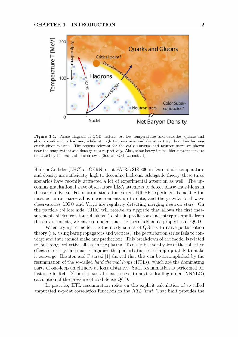
Many extended physical systems consisting of quarks and gluons are in ther-modynamic equilibrium. In such systems, the high energy scales needed for decon-finement are provided by high temperature and/or density. To illustrate the differentphases of QCD at various temperatures and densities, one may draw a phase dia-gram as seen in Fig. 1.1. As indicated by the diagram, the low-energy hadronicphase “melts” into a quark–gluon plasma (QGP) phase, when the temperature anddensity are raised above a critical value. At zero temperature and high density, thecorresponding phase is called quark matter. There exist other more exotic phases,such as ones with superconducting properties, but we do not consider them in thisThesis. Rather, we assume high temperature and high density system is composedQGP.
Also written on the phase diagram, there are three physical situations rele-vant for deconfined matter: (i) In the early universe, between the electroweak phasetransition and the confinement transition, temperature was high enough to formQGP. (ii) Inside compact stars, such as in the cores of neutron stars, densities maybe high enough to form quark matter. (iii) In relativistic heavy ion collisions, forinstance at the Relativistic Heavy Ion Collider (RHIC) in Brookhaven, at the Large
1
CHAPTER 1. INTRODUCTION 2
Figure 1.1: Phase diagram of QCD matter. At low temperatures and densities, quarks andgluons confine into hadrons, while at high temperatures and densities they deconfine formingquark–gluon plasma. The regions relevant for the early universe and neutron stars are shownnear the temperature and density axes respectively. Also, some heavy ion collider experiments areindicated by the red and blue arrows. (Source: GSI Darmstadt)
Hadron Collider (LHC) at CERN, or at FAIR’s SIS 300 in Darmstadt, temperatureand density are sufficiently high to deconfine hadrons. Alongside theory, these threescenarios have recently attracted a lot of experimental attention as well. The up-coming gravitational wave observatory LISA attempts to detect phase transitions inthe early universe. For neutron stars, the current NICER experiment is making themost accurate mass–radius measurements up to date, and the gravitational waveobservatories LIGO and Virgo are regularly detecting merging neutron stars. Onthe particle collider side, RHIC will receive an upgrade that allows the first mea-surements of electron–ion collisions. To obtain predictions and interpret results fromthese experiments, we have to understand the thermodynamic properties of QCD.
When trying to model the thermodynamics of QGP with naive perturbationtheory (i.e. using bare propagators and vertices), the perturbation series fails to con-verge and thus cannot make any predictions. This breakdown of the model is relatedto long-range collective effects in the plasma. To describe the physics of the collectiveeffects correctly, one must reorganize the perturbation series appropriately to makeit converge. Braaten and Pisarski [1] showed that this can be accomplished by theresummation of the so-called hard thermal loops (HTLs), which are the dominatingparts of one-loop amplitudes at long distances. Such resummation is performed forinstance in Ref. [2] in the partial next-to-next-to-next-to-leading-order (NNNLO)calculation of the pressure of cold dense QCD.
In practice, HTL resummation relies on the explicit calculation of so-calledamputated n-point correlation functions in the HTL limit. That limit provides the
CHAPTER 1. INTRODUCTION 3
leading thermal contribution to a correlation function. In this Thesis, we concentrateon the n = 2 case, namely, we compute self-energies. Specifically, we calculate theleading-order (LO) quark and gluon self-energies in the HTL limit, which serve asbasic building blocks in the HTL resummation. The LO HTL theory has been exten-sively used in the literature but recently many high-order perturbative computationshave reached a point, where one has to extend the HTLs to the next-to-leading-order(NLO). For example, the completion of the aforementioned NNNLO pressure cal-culation requires the two-loop gluon self-energy in the HTL limit at finite density[2]. To pave the way towards the gluonic two-loop computation, we calculate theslightly simpler counterpart for the photon from quantum electrodynamics (QED)at finite temperature and density. The extension of HTL theory to NLO has beendone before in some specific cases at finite temperature and zero density [3, 4, 5, 6].However, NLO HTLs that account for finite density effects have remained largelyuntouched prior to this work. We provide some interesting and physically relevantresults that show the effects of finite density to the two-loop photon self-energy. Inthe process, we lay out the tools for extending the calculation to the two-loop gluonself-energy.
This Thesis is divided into five chapters. In Chapter 2, we introduce thetheoretical framework for calculating correlation functions in the presence of a hotand dense medium. Chapter 3 is devoted to explain us the properties of QCD andhow they are affected by the medium. After these chapters, we have collected all themachinery needed to compute QCD self-energies in the HTL limit. In Chapter 4,we employ the machinery to calculate the previously mentioned one- and two-loopself-energies, providing all the technical details along the way. Finally, Chapter 5concludes the Thesis with final remarks and the future implications of this work.The notations and conventions are listed in Appendix A.
2. Thermal Field Theory
To perform calculations of self-energies of various particles propagating in a weaklyinteracting plasma, we require a systematic quantum field theory (QFT) descrip-tion that accounts for medium effects consistently. Such description for a thermalmedium is provided by the framework of thermal field theory (TFT). In this Chap-ter, we introduce a particular formulation of TFT, namely the real-time formalism,that supplies the basic tools for our QCD self-energy calculations in Chapter 4. Here,we focus on a single complex scalar field and generalize to QCD later in Chapter 3.
The overall structure of our derivation follows the one found in Ref. [7]. Atfirst, we write a general path integral expression for an expectation value of someoperator in the presence of a medium in Sec. 2.1, specializing to thermodynamicequilibrium in Sec. 2.2. In Sec. 2.3, we introduce various two-point correlationfunctions that are important in TFT calculations. Secs. 2.4 and 2.5 are devoted toperturbation theory, an essential tool for producing numbers from a weakly coupledtheory. Further, the concept of self-energy is introduced as a powerful tool to or-ganize the perturbative series. More detailed derivations can be found in standardtextbooks, such as [8, 9]. A curious reader might find the review articles in Refs.[10, 11, 12] interesting.
2.1 In-medium expectation valueLet O be a (composite) operator local in time. In the Heisenberg picture, its timeevolution from time t0 to t1 is governed by the time translation operator U ,
O(t1) = U(t0, t1)O(t0)U(t1, t0) = eiH(t1−t0)O(t0)e−iH(t1−t0) , (2.1)
where H is the Hamiltonian of the theory in question. We assume H to be time-independent at this point. The spatial arguments and all possible additional indicesare suppressed in favor of a clean notation.
Next, our goal is to compute the expectation value of O when our systemconsists of a medium described by a complete set of states |i〉. In contrast tovacuum field theory, where expectation values only account for quantum mechanicalfluctuations and are computed for a pure vacuum state |0〉, the presence of a mediumrequires us to consider statistical fluctuations in the medium as well. To this end,the in-medium expectation value is given by a weighted sum of expectation values
4
CHAPTER 2. THERMAL FIELD THEORY 5
with respect to the states of the medium,
〈O(t0)〉 ≡∑i
pi(t0) 〈i|O|i〉 , (2.2)
where pi(t0) is the probability of |i〉 at time t0. By defining a density operator as
ρ(t0) ≡∑i
pi(t0) |i〉 〈i| , (2.3)
the expectation value can be written as a trace over the Hilbert space,
〈O(t0)〉 = Tr ρ(t0)O(t0) . (2.4)
The density operator is normalized to Tr ρ = 1 as the probabilities pi must add upto one.
In order to evaluate the expectation value of some operator at a later timet1 > t0, we need to obtain the form of the density operator at that time. Again,for this, we employ the time translation operator, ρ(t1) = U(t1, t0)ρ(t0)U(t0, t1) (seedifference to Eq. (2.1)). The expectation value at the time t1 now takes the form
〈O(t1)〉 = Tr ρ(t1)O(t1) = TrU(t1, t0)ρ(t0)U(t0, t1)O(t1) . (2.5)
Considering a scalar field φ, we expand the trace in the field basis |φi〉 by insertingcomplete sets of eigenstates 1 = ∑
i |φi〉 〈φi| between the operators
〈O(t1)〉 =∑i
〈φi|U(t1, t0)ρ(t0)U(t0, t1)O(t1)|φi〉
=∑i,j,k,l
〈φi|U(t1, t0)|φj〉 ρjk 〈φk|U(t0, t1)|φl〉Oli , (2.6)
where ρjk ≡ 〈φj|ρ(t0)|φk〉 are the elements of the density matrix in the field basis.Analogously, Oli ≡ 〈φl|O(t1)|φi〉 are the matrix elements of the operator O.
For the matrix elements of the time evolution operators, we employ the usualFeynman–Matthews–Salam path integral formula [13, 14],1
〈φi|U(t1, t0)|φj〉 = 〈φi|e−iH(t1−t0)|φj〉 =∫ φ1(t1)=φi
φ1(t0)=φjDφ1(t)eiS[φ1] , (2.7)
〈φk|U(t0, t1)|φl〉 = 〈φk|e−iH(t0−t1)|φl〉 =∫ φ2(t1)=φl
φ2(t0)=φkDφ2(t)e−iS[φ2] , (2.8)
where S[φ] =∫ t1t0
dt L(φ(t), φ(t)) is the action functional given by the Lagrangian,L =
∫d3xL, related to the Hamiltonian through a Legendre transformation, and L is
the Lagrangian density. The former equation describes the transition amplitude as-sociated with the field configuration φj evolving into φi. The “forward-propagating”field interpolating between these configurations is denoted by φ1. By taking the
1Although the intermediate step assumes a time-independent Hamiltonian, the path-integralrepresentation covers a general case with time-dependence.
CHAPTER 2. THERMAL FIELD THEORY 6
Hermitian conjugate of this relation we obtain the latter one, which describes theamplitude for φl evolving backward into φk. In the path-integral, the “backward-propagating” field interpolating between φl and φk is denoted by φ2. Insertion ofboth relations into Eq. (2.6) gives
〈O(t1)〉 =∑i,j,k,l
∫ φ1(t1)=φi
φ1(t0)=φjDφ1(t)
∫ φ2(t1)=φl
φ2(t0)=φkDφ2(t)eiS[φ1]−iS[φ2]ρjkOli . (2.9)
As a reminder, the Latin indices i, j, k and l are associated with the field configu-rations corresponding to the field basis states |φi〉 , . . . , |φl〉, and the labels 1 and 2refer to the forward and backward evolving fields.
Thus, considering a density operator ρ that we know at time t0, we can repre-sent the thermal expectation value of O at later time t1 as path integrals, essentiallydoubling the field content of the theory φ → {φ1, φ2}. This formal procedure, in-herent in all real-time formulations of thermal field theories, is commonly known asdoubling the degrees of freedom. The doubling complicates calculations, especiallyat high orders in perturbation theory, but is necessary for correct results.
Eq. (2.9) allows us to compute expectation values with respect to a generalnon-equilibrium density operator, serving as a basis for the so-called closed timepath formalism [15, 16]. Next, and for the rest of this Thesis, we concentrate on aspecial case where our system is in equilibrium, fixing the density operator to havea specific form.
2.2 Thermodynamic equilibriumMany interesting physical systems are in thermal equilibrium, meaning that the tem-perature T within the system is spatially and temporally constant. If, in addition,the system possesses conserved global charges Qi (usually stemming from globalU(1) symmetries), and the associated chemical potentials µi are constant as well,the system is said to be in thermodynamic equilibrium. In that case, the possiblestates of the system are represented by the grand canonical ensemble for which thedensity operator takes the form
ρeq = 1Ze−β(H−µiQi) , Z = Tr e−β(H−µiQi) , (2.10)
in the rest frame of the system. Here β = 1/T is the inverse of the temperatureT , Qi are the operators corresponding to the conserved charges, and Z is the grandcanonical partition function, which normalizes the density operator such that 〈1〉 =1. There is an implicit summation over the repeated index i.
The (grand) canonical partition function is the most essential function in ther-modynamics since it contains all the information needed to obtain the macroscopicthermodynamic properties of a specific system from its microscopic description.Once the explicit form of the partition function is obtained, one can determineevery other thermodynamic quantity. For instance, in the thermodynamic limit
CHAPTER 2. THERMAL FIELD THEORY 7
(V →∞), pressure, particle number, entropy, and energy are given by
P = ∂(T lnZ)∂V
,
Qi = ∂(T lnZ)∂µi
,
S = ∂(T lnZ)∂T
,
E = −PV + TS + µiQi ,
(2.11)
respectively. Here V denotes the volume of the system. In this Thesis, we use theterms “finite chemical potential” and “finite (particle number) density” interchange-ably.2 The former is a useful quantity in theoretical calculations, whereas the latterhas more physical significance. These quantities are related to each other throughthe second equation above.
To calculate thermal expectation values using Eq. (2.9), we require an ex-pression for the density matrix element. Thereby, let us look more closely at theequilibrium density operator and write it as
ρeq = 1Ze−i(H−µiQi)(−iβ) ≡ 1
Ze−iK((t0−iβ)−t0) , (2.12)
where we have defined K ≡ H − µiQi and inserted the initial time t0 for futureconvenience. Since, by definition, the conserved charge operators commute with theHamiltonian, [H, Qi] = 0, as well as with each other, [Qi, Qj] = 0, we can treatK as an effective Hamiltonian. Comparing the density operator in Eq. (2.12) tothe time translation operator in Eq. (2.1) shows a great deal of similarity betweenthem. Formally, we can consider ρeq as a time translation operator in imaginarytime, evolving states from t0 to t0− iβ. In Appendix B, we take a closer look at thegeneralization of time translation to complex times.
The formal similarity allows us to represent the density matrix element (ρeq)jkin Eq. (2.9) as a path integral. We denote the interpolating field between configura-tions φk and φj with φE, motivating the choice of the subscript E soon. Analogouslyto the transition amplitude across real time in Eq. (2.7), the density matrix elementmay be expressed as
(ρeq)jk = 1Z〈φj|e−iK((t0−iβ)−t0)|φk〉 = 1
Z
∫ φE(t0−iβ)=±φj
φE(t0)=φkDφE eiS[φE ] , (2.13)
where the integration is carried over the field configurations defined on a verticaltime path starting from t0 and ending to t0 − iβ. The sign of the upper bound ±φjwill be explained in a moment. Here the action is written as a complex contourintegral,
S =∫ t0−iβ
t0dt (L+ µiQi) =
∫ −iβ0
dt (L+ µiQi) , (2.14)
2In this context, the term “finite” means “having a positive (or negative) numerical value”.

CHAPTER 2. THERMAL FIELD THEORY 8
where we shifted the integration variable by t0. The corresponding shift in theintegrand has been left implicit. Since the time variable is now purely imaginary,we rename it as τ = it, bringing the action to the form
S = −i∫ β
0dτ (L(t→ −iτ) + µiQi) ≡ i
∫ β
0dτ (LE − µiQi) ≡ iSE , (2.15)
where we defined the Euclidean action, SE =∫ β
0 dτ(LE − µiQi), with the EuclideanLagrangian, LE = −L(t → −iτ). Hence, we write the density matrix element interms of the Euclidean quantities as
(ρeq)jk = 1Z
∫ φE(t0−iβ)=±φj
φE(t0)=φkDφE e−SE [φE ] . (2.16)
At boundary t = t0 − iβ, the field is fixed to configuration ±φj. The upper sign isvalid for bosonic fields obeying a periodic boundary condition, and the lower one isfor fermionic fields with an antiperiodic boundary condition. We should note thatthe sign of configuration φj is just an overall phase factor and thus not observable.Hence the physical states the two configurations describe are indeed the same. Adetailed derivation of the (anti)periodic boundary conditions is found, for instance,in Ref. [17].
Analogously, we obtain a path integral representation for the partition functionby tracing the density matrix,
Z =∫φE(t0)=±φE(t0−iβ)
DφE e−SE [φE ] . (2.17)
Let us return to the thermal expectation value (2.9) now that we have expressedeverything as path integrals. The matrix element of the operator O simplifies byassuming it is composed only of the field operators φ, containing no conjugate mo-menta, so that Oli = 〈φl|O[φ]|φi〉 = O[φi]δli. Therefore, inserting Eq. (2.16) intoEq. (2.9) gives
〈O(t1)〉 = 1Z
∑i,j,k,l
∫ φE(t0−iβ)=±φj
φE(t0)=φkDφE e−SE [φE ]
∫ φ1(t1)=φi
φ1(t0)=φjDφ1
×∫ φ2(t1)=φl
φ2(t0)=φkDφ2 e
iS[φ1]−iS[φ2]Oli
= 1Z
∫DφE e−SE [φE ]
∫Dφ1Dφ2 e
iS[φ1]−iS[φ2]O[φ1(t1)] , (2.18)
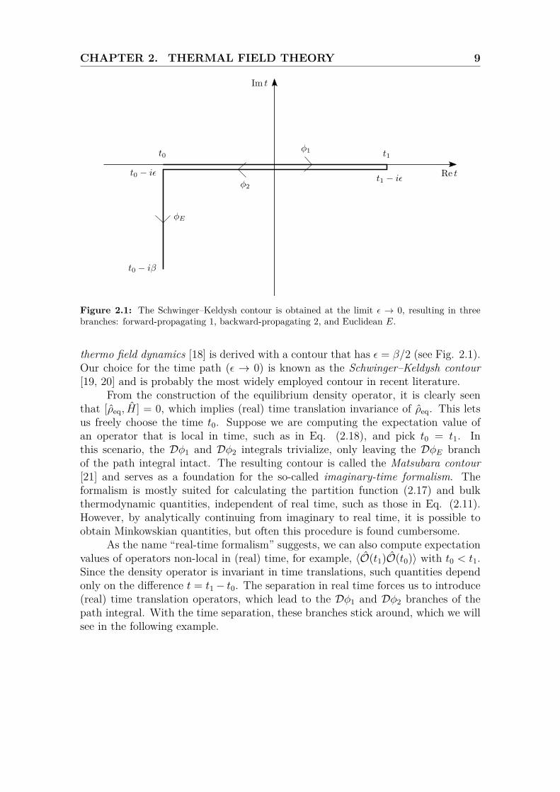
where φ2(t1) = φ1(t1), φ2(t0) = φE(t0) and φ1(t0) = ±φE(t0 − iβ) forming a con-nected time path in the complex plane (see Fig. 2.1). As discussed in AppendixB, the result ends up being independent of the time path as long as it runs from t0to t0 − iβ and has a non-increasing imaginary part. Additionally, it obviously hasto include time t1 and other possible time arguments appearing in the expectationvalue. Due to this freedom, the literature shows various choices for the time pathapplied in different formulations of thermal field theories. For example, the so-called
CHAPTER 2. THERMAL FIELD THEORY 9
Figure 2.1: The Schwinger–Keldysh contour is obtained at the limit ε → 0, resulting in threebranches: forward-propagating 1, backward-propagating 2, and Euclidean E.
thermo field dynamics [18] is derived with a contour that has ε = β/2 (see Fig. 2.1).Our choice for the time path (ε → 0) is known as the Schwinger–Keldysh contour[19, 20] and is probably the most widely employed contour in recent literature.
From the construction of the equilibrium density operator, it is clearly seenthat [ρeq, H] = 0, which implies (real) time translation invariance of ρeq. This letsus freely choose the time t0. Suppose we are computing the expectation value ofan operator that is local in time, such as in Eq. (2.18), and pick t0 = t1. Inthis scenario, the Dφ1 and Dφ2 integrals trivialize, only leaving the DφE branchof the path integral intact. The resulting contour is called the Matsubara contour[21] and serves as a foundation for the so-called imaginary-time formalism. Theformalism is mostly suited for calculating the partition function (2.17) and bulkthermodynamic quantities, independent of real time, such as those in Eq. (2.11).However, by analytically continuing from imaginary to real time, it is possible toobtain Minkowskian quantities, but often this procedure is found cumbersome.
As the name “real-time formalism” suggests, we can also compute expectationvalues of operators non-local in (real) time, for example, 〈O(t1)O(t0)〉 with t0 < t1.Since the density operator is invariant in time translations, such quantities dependonly on the difference t = t1− t0. The separation in real time forces us to introduce(real) time translation operators, which lead to the Dφ1 and Dφ2 branches of thepath integral. With the time separation, these branches stick around, which we willsee in the following example.

CHAPTER 2. THERMAL FIELD THEORY 10
Example: forward Wightman function
The so-called forward Wightman function D> is an expectation value of two fieldoperators with a particular ordering. This correlation function is properly introducedin the next Section. In the following, the field operators are evaluated at φ(0)(previously at φ(t1)), so we have φkl ≡ 〈φk|φ(0)|φl〉 = φkδkl,
D>(t) ≡ 〈φ(t)φ(0)〉 = Tr ρeqU(0, t)φ(0)U(t, 0)φ(0)
= 1Z
∑i,j,k,l,m
∫ φE(−iβ)=±φi
φE(0)=φjDφE e−SE [φE ]
∫ φ1(t)=φl
φ1(0)=φmDφ1 e
iS[φ1]
×∫ φ2(t)=φk
φ2(0)=φjDφ2 e
−iS[φ2]φklφmi
= 1Z
∑i,j,k
∫ φE(−iβ)=±φi
φE(0)=φjDφE e−SE [φE ]
∫ φ1(t)=φk
φ1(0)=φiDφ1 e
iS[φ1]
×∫ φ2(t)=φk
φ2(0)=φjDφ2 e
−iS[φ2]φ2(t)φ1(0)
= 1Z
∫DφE e−SE [φE ]
∫Dφ1Dφ2 e
iS[φ1]−iS[φ2]φ2(t)φ1(0) , (2.19)
where φ1(0) = ±φE(−iβ), φ2(t) = φ1(t) and φ2(0) = φE(0), i.e. the time contour isconnected.
2.3 CorrelatorsMany observables can be reduced to structures containing various correlation func-tions (or just correlators), which are defined as expectation values of elementaryor composite field operators having a particular ordering. For instance, in vacuumQFT, the LSZ reduction formula relates the scattering amplitudes for asymptoticstates to products of time-ordered correlators. Different from the vacuum case, inmedium one cannot separate asymptotic states in faraway past and future usingthe LSZ formula due to the statistical fluctuations introduced by the medium notpreserving those states. Consequently, time-ordering does not have a significant rolein medium, rather many different correlators with various operator orderings comeinto play.
Here, we introduce several two-point correlators that measure correlation andcausation in the medium. In the following, φ denotes a generic bosonic field andψ a generic fermionic field, ˆψ being the corresponding conjugate field. Subscriptsα and β contain all the otherwise suppressed indices, including spatial coordinates.The time coordinates are written out explicitly, being relevant for different operator
CHAPTER 2. THERMAL FIELD THEORY 11
orderings. The forward and backward Wightman functions are then defined as
D>αβ(t1, t0) =
⟨φα(t1)φβ(t0)
⟩, (2.20)
D<αβ(t1, t0) =
⟨φβ(t0)φα(t1)
⟩, (2.21)
S>αβ(t1, t0) =⟨ψα(t1) ˆψβ(t0)
⟩, (2.22)
S<αβ(t1, t0) = −⟨ ˆψβ(t0)ψα(t1)
⟩, (2.23)
where 〈. . . 〉 is the expectation value defined in Eq. (2.4). They measure the physicalcorrelation in the fields between the times t0 and t1. In order to measure causation,we define the retarded and advanced correlators,
DRαβ(t1, t0) = θ(t1 − t0)ρBαβ(t1, t0) , (2.24)
DAαβ(t1, t0) = −θ(t0 − t1)ρBαβ(t1, t0) , (2.25)SRαβ(t1, t0) = θ(t1 − t0)ρFαβ(t1, t0) , (2.26)SAαβ(t1, t0) = −θ(t0 − t1)ρFαβ(t1, t0) , (2.27)
which are expressed in terms of the bosonic and fermionic spectral functions,3
ρBαβ(t1, t0) =⟨[φα(t1), φβ(t0)]
⟩, (2.28)
ρFαβ(t1, t0) =⟨{ψα(t1), ˆψβ(t0)}
⟩, (2.29)
respectively. Here [ · , · ] denotes a commutator and { · , · } an anti-commutator.Because of the step function, the Fourier transform of the retarded (advanced) cor-relator is an analytic function of the momentum coordinate conjugate to time in theupper (lower) half of the complex plane, which is found to be a convenient property.Finally, the time- and anti-time-ordered correlators read
DTαβ(t1, t0) = θ(t1 − t0)D>
αβ(t1, t0) + θ(t0 − t1)D<αβ(t1, t0) , (2.30)
DTαβ(t1, t0) = θ(t0 − t1)D>
αβ(t1, t0) + θ(t1 − t0)D<αβ(t1, t0) , (2.31)
with analogous relations to fermions.The correlation functions have useful symmetry properties. By employing the
cyclicity of the trace and the Hermiticity of the density operator, the forward andbackward Wightman functions can be shown to satisfy(
D>/<αβ (t1, t0)
)∗= D
>/<βα (t0, t1) . (2.32)
With the definitions (2.24)–(2.25), a direct consequence is that the causal correlatorsfulfil (
DRαβ(t1, t0)
)∗= −DA
βα(t0, t1) . (2.33)Analogous relations apply for fermionic fields as well, modulo possible sign differ-ences stemming from anti-commutation.
3The density matrix is also denoted by ρ but it is clear from context which one we refer to.
CHAPTER 2. THERMAL FIELD THEORY 12
The definitions of the five correlation functions for bosons, and respectivelyfor fermions, allow us to write the relations
ρBαβ(t1, t0) = DRαβ(t1, t0)−DA
αβ(t1, t0) = D>αβ(t1, t0)−D<
αβ(t1, t0) , (2.34)ρFαβ(t1, t0) = SRαβ(t1, t0)− SAαβ(t1, t0) = S>αβ(t1, t0)− S<αβ(t1, t0) . (2.35)
In an out-of-equilibrium situation, with a general density operator ρ, two of the fivecorrelation functions are independent since the retarded and advanced correlatorsare defined in terms of the spectral function, which in turn is constructed out of theforward and backward Wightman functions. However, in the special case of thermalequilibrium, we will derive additional relations, thereby reducing the number ofindependent correlators to one.
Correlators in thermal equilibriumIn a thermal medium described by the grand canonical density operator, the two-point correlation functions depend only on the difference t ≡ t1 − t0 rather thantheir arguments separately, as discussed in the previous Section. Hence, we employthe notation Dj(t) = Dj(t, 0), where j labels the type of the correlator. As we arefocusing on QCD, we assign a chemical potential only to fermions in the following.Further, we suppress the index labeling possible multiple chemical potentials.
The form of the equilibrium density operator allows us to derive a relationbetween the forward and backward Wightman functions. By using the cyclicity ofthe trace and considering exp(−βH) as a time translation operator in imaginarytime, we write
D>αβ(t) =
⟨φα(t)φβ(0)
⟩= Tr ρeqφα(t)φβ(0) = 1
ZTr e−βH φα(t)φβ(0)
= 1Z
Tr φβ(0)e−βH φα(t) = 1Z
Tr e−βH φβ(0)e−βH φα(t)eβH
= Tr ρeqφβ(0)φα(t+ iβ) =⟨φβ(0)φα(t+ iβ)
⟩= D<
αβ(t+ iβ) . (2.36)
For fermionic fields, we take similar steps, additionally taking the chemical potentialand the corresponding conserved charge operator Q into account. As a reminder,K = H − µQ and [H, Q] = 0. Thus,
S>αβ(t) = 1Z
Tr e−βKψα(t) ˆψβ(0) = 1Z
Tr e−βK ˆψβ(0)e−βKψα(t)eβK
= Tr ρeqˆψβ(0)eβµQe−βHψα(t)eβHe−βµQ
= Tr ρeqˆψβ(0)eβµQψα(t+ iβ)e−βµQ . (2.37)
Next, we wish to commute the first exponent with the conserved charge over thefield operator on its right side. We assume the validity of the commutation relation
CHAPTER 2. THERMAL FIELD THEORY 13
[ψ(t), Q] = ψ(t) [8], yielding
S>αβ(t) = Tr ρeqˆψβ(0)ψα(t+ iβ)eβµ(Q−1)e−βµQ
= e−βµTr ρeqˆψβ(0)ψα(t+ iβ)
= −e−βµS<αβ(t+ iβ) . (2.38)
The relations in Eqs. (2.36) and (2.38) are the so-called Kubo–Martin–Schwinger(KMS) relations [22, 23], which relate the forward and backward Wightman func-tions to each other in thermal equilibrium. In a more general context, these relationsare a consequence of the fluctuation-dissipation theorem.
From the perspective of practical calculations, the KMS relations take espe-cially convenient forms in the momentum space.4 We begin by inserting completesets of energy eigenstates, 1 = ∑
n |n〉 〈n|, into the trace and integrating over t. Forthe bosonic forward Wightman function we obtain the Fourier transform
D>αβ(ω) ≡
∫dt eiωtD>
αβ(t) = 1Z
∑m,n
∫dt eiωtTr
[e−βH φα(t)φβ(0)
]= 1Z
∑m,n
∫dt eiωtTr
[e(−β+it)H |m〉 〈m| φα(0)e−itH |n〉 〈n| φβ(0)
]= 1Z
∑m,n
∫dt e−βEmei(ω+Em−En)t 〈m|φα(0)|n〉 〈n|φβ(0)|m〉
= 1Z
∑m,n
e−βEm2πδ(ω + Em − En) 〈m|φα(0)|n〉 〈n|φβ(0)|m〉 , (2.39)
and for the backward Wightman function, additionally using the cyclicity of thetrace, we have
D<αβ(ω) ≡
∫dt eiωtD<
αβ(t) = 1Z
∑m,n
∫dt eiωtTr
[e−βH φβ(0)φα(t)
]= 1Z
∑m,n
∫dt eiωtTr
[e(−β−it)H |n〉 〈n| φβ(0)eitH |m〉 〈m| φα(0)
]= 1Z
∑m,n
∫dt e−βEnei(ω+Em−En)t 〈m|φα(0)|n〉 〈n|φβ(0)|m〉
= 1Z
∑m,n
e−βEn2πδ(ω + Em − En) 〈m|φα(0)|n〉 〈n|φβ(0)|m〉
= 1Z
∑m,n
e−β(Em+ω)2πδ(ω + Em − En) 〈m|φα(0)|n〉 〈n|φβ(0)|m〉
= e−βωD>αβ(ω) , (2.40)
where we have substituted En = Em + ω, owing to the Dirac delta function. Thus,we get the momentum space KMS relation for bosonic fields,
D>αβ(ω) = eβωD<
αβ(ω) . (2.41)4To simplify the notation, the correlators and their Fourier transforms are recognized through
their arguments. This applies to the rest of the Thesis.
CHAPTER 2. THERMAL FIELD THEORY 14
For the fermionic Wightman function, the derivation is similar to the bosoniccase. Again, the only change is the finite chemical potential and the correspondingconserved charge operator. Analogously to the derivation of Eq. (2.38), we needto commute the charge operator over the field operator yielding an extra factor ofexp(−βµ). With this exception in mind, we arrive to the fermionic momentum spaceKMS relation,
S>αβ(ω) = −eβ(ω−µ)S<αβ(ω) . (2.42)With Eqs. (2.34) and (2.35), and the momentum space KMS relations, we are
able to write
(1 + nB(ω))ρBαβ(ω) = D>αβ(ω) , (2.43)
nB(ω)ρBαβ(ω) = D<αβ(ω) , (2.44)
(1− nF (ω − µ))ρFαβ(ω) = S>αβ(ω) , (2.45)−nF (ω − µ)ρFαβ(ω) = S<αβ(ω) , (2.46)
where the distribution functions for bosons and fermions have emerged, nB/F (ω) =(eβω ∓ 1)−1, respectively. In thermal equilibrium, it appears that the number ofindependent correlators has reduced to one since the KMS relation allows us toexpress every correlator in terms of the spectral function.
The Fourier transformations of Eqs. (2.32)–(2.33) state that the momentumspace forward and backward Wightman functions are Hermitian matrices,(
D>/<αβ (ω)
)∗= D
>/<βα (ω) . (2.47)
For the causal correlators, we obtain an anti-Hermiticity relation,(DRαβ(ω)
)∗= −DA
βα(ω) . (2.48)
2.4 Perturbative expansionA common way of defining a quantum field theory is to introduce a generating func-tional in terms of path integrals, including external sources conjugate to the classicalfields. All the n-point correlation functions (or Green’s functions) can be solved fromthe generating functional by taking derivatives with respect to the sources. The ob-servables of the theory can then be expressed in terms of the correlation functions.Thus, if one can write a closed-form expression for the generating functional, onehas solved the theory completely.
The generating functional is obtained by generalizing the previously derivedfield-doubled path integral, Eq. (2.18), by introducing source functions Ji(x) conju-gate to the fields φi(x), i = 1, 2,
Z[J1, J2] =∫DφE e−SE [φE ]
∫Dφ1Dφ2e
iS[φ1]−iS[φ2]+i∫
d4x (J1(x)φ1(x)+J2(x)φ2(x)) .
(2.49)
CHAPTER 2. THERMAL FIELD THEORY 15
Here we have explicitly written the spatial dependence of the source functions andcorresponding fields for clarity. The time contour is the standard Schwinger-Keldyshcontour introduced in Sec. 2.2, where we have formally taken t0 → −∞ and t1 →∞.The possibility of introducing a source for the Euclidean part of the path integral isomitted due to the interest in real time correlation functions.
By setting the sources to zero in Eq. (2.49), one obtains the partition function,Z = Z[0, 0]. As discussed at the end of Sec. 2.2, the Dφ1 and Dφ2 branches of thepath integral trivialize, leaving us only with the Euclidean branch given by thepartition function (2.17).
To generate n-point functions from Eq. (2.49), we need to define a functionalderivative with respect to the two sources. Naturally, the derivative is defined as
δJi(x)δJj(y) = δijδ
4(x− y) . (2.50)
Now, by taking derivatives of the generating functional, one ends up with thermalaverages of combinations of φ1 and φ2 fields at different spacetime points,
〈φi1(x1)φi2(x2) . . . φin(xn)〉 = 1Z
δ
iδJi1(x1)δ
iδJi2(x2) . . .δ
iδJin(xn)Z[J1, J2]∣∣∣∣∣J1=J2=0
,
(2.51)where i1, i2, . . . , in = 1, 2 and, by abuse of notation, 〈. . . 〉 denotes the thermalaverage in the sense of the Schwinger-Keldysh path integral,
〈. . . 〉 ≡ 1Z
∫DφE e−SE [φE ]
∫Dφ1Dφ2e
iS[φ1]−iS[φ2](. . . ) . (2.52)
Performing manipulations like Eq. (2.19), one can identify various thermal corre-lation functions with path integral expressions such as on the left-hand side of Eq.(2.51).
The doubling of the field content renders the structure of real-time formalismmore complicated than that of imaginary-time formalism or vacuum QFTs. As Eq.(2.51) suggests, the 2-point correlation function, or propagator, is now a 2×2 matrix,
Dij(t) = 〈φi(t)φj(0)〉 = 1Z
δ
iδJi(t)δ
iδJj(0)Z[J1, J2]∣∣∣∣∣J1=J2=0
, (2.53)
where the spatial dependence is again suppressed for clarity. The computation inEq. (2.19) shows a connection between the 21-component of the propagator matrixand the forward Wightman function. Similarly, the other components can be asso-ciated with various correlation functions introduced in Sec. 2.3. The 12-componentidentifies to the backward Wightman function, and as the diagonal entries, we havethe time- and anti-time-ordered correlators,
D(t) =(〈φ1(t)φ1(0)〉 〈φ1(t)φ2(0)〉〈φ2(t)φ1(0)〉 〈φ2(t)φ2(0)〉
)=(DT (t) D<(t)D>(t) DT (t)
). (2.54)
To compute correlation functions explicitly using Eq. (2.51), we need a closed-form expression for the generating functional. To this end, the action has to be
CHAPTER 2. THERMAL FIELD THEORY 16
quadratic in fields so that the resulting path integral is Gaussian, allowing one tocompute it explicitly. Therefore, we separate the quadratic (free) part of the actionS0 from the interaction part SI. For the Euclidean sector, these are denoted by SE,0and SE,I, respectively. Since the interacting part of the theory, in general, cannot besolved exactly, we need to employ an approximation scheme, namely the perturbativeexpansion. The interaction part of the action is typically proportional to a couplingconstant g that characterizes the strength of the interaction. By assuming weakinteractions, g � 1, the exponents with the interaction parts may be expanded asTaylor series around the free theory, g = 0, to obtain the perturbative expansion,
Z[J1, J2] =∫DφE e−SE,0[φE ]
∞∑n=0
(−1)nn! SnE,I[φE]
×∫Dφ1Dφ2 e
iS0[φ1]−iS0[φ2]+i∫
d4x (J1(x)φ1(x)+J2(x)φ2(x))
×∞∑n=0
in
n! (SI[φ1]− SI[φ2])n ,
(2.55)
where each term in the series is now a path integral in the solvable free theory.The leading term in Eq. (2.55) gives the free generating functional Z0, which
as a Gaussian integral, has an exact solution,
Z0[J1, J2] = N1 exp{−1
2
∫d4x
∫d4y Ji(x)Dij
0 (x− y)Jj(y)}, (2.56)
where Dij0 can be identified with the propagator matrix of the free theory. It is
obtained by explicitly computing the Gaussian integral for a given free action andis related to the inverse of the associated matrix.5 The Euclidean part of the freepath integral factorized out into the multiplicative constant factor N1 due to theboundary conditions imposed on the path integral [24].6 The solved Z0 depends ontemperature and chemical potential through Dij
0 , whose elements are related to eachother via the KMS relation. By taking derivatives of Z0 with respect to the sourcesaccording to Eq. (2.51), one expresses n-point functions in the free theory as sumsof products of free propagators. This is known as Wick’s theorem.
The full generating functional can now be expressed in terms of the solved freecounterpart. Equivalent to Eq. (2.55), we write
Z[J1, J2] = N2 exp{i∫
d4x
(LI
[δ
iδJ1(x)
]− LI
[δ
iδJ2(x)
])}Z0[J1, J2] , (2.57)
where LI is the interaction part of the Lagrangian, and N2 is a factor containing N1and the interactions of the Euclidean sector. It cancels out when dividing by Z inEq. (2.51). Expanding the exponent in the above expression and plugging it intoEq. (2.51) reproduces the perturbative series for the n-point correlation functionwith the standard Feynman rules.
5Alternatively, and perhaps most conveniently, Dij0 is continued analytically from the Euclidean
propagator computed in imaginary-time formalism [8].6In general, the factorization requires the time arguments of the correlation functions to be
real and finite. Also, one has to use the so-called η-regularized δ-functions in the propagators, asdiscussed in Sec. 3.2.1.
CHAPTER 2. THERMAL FIELD THEORY 17
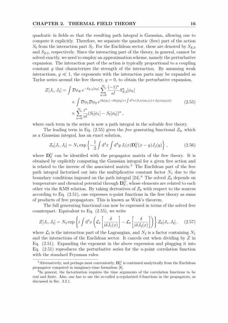
Figure 2.2: Graphical representation of the vertices of the φ4 theory in the 1/2 basis. Note theminus sign associated with the type 2 vertex.
The vertices are given by the interaction part of the action, SI[φ1] − SI[φ2],in Eq. (2.55). The fields φ1 and φ2 do not mix there, so the vertices will have theusual vacuum field theory form, with every connection point in the vertex havingeither an index 1 or 2. Additionally, the minus sign in front of the interaction partinvolving the field φ2 is transferred to the vertices with indices 2. As an example,the φ4 theory would include the vertices shown in Fig. 2.2. In diagrams, the twokinds of vertices can be connected to each other with the off-diagonal elements inthe propagator matrix (2.54).
r/a basisMany practical calculations, including the ones carried out in this Thesis, turn outto be convenient to perform in another field basis defined in terms of the averageand difference of the fields φ1 and φ2,
φr ≡12(φ1 + φ2) , φa ≡ φ1 − φ2 , (2.58)
respectively. From now on, we shall exclusively use the r/a basis (also known as theKeldysh basis) so let us study how the perturbative expansion is carried out in thisbasis.
The propagator matrix in the r/a basis can also be expressed in terms of thecorrelation functions introduced in Sec. 2.3. Using the definition of the field basisand the identifications made in Eq. (2.54), allow us to write
D(t) =(〈φr(t)φr(0)〉 〈φr(t)φa(0)〉〈φa(t)φr(0)〉 〈φa(t)φa(0)〉
)=(Drr(t) DR(t)DA(t) 0
), (2.59)
where we have defined the symmetric propagator, as Drr ≡ 12(D> + D<). The
off-diagonal entries are the retarded and advanced correlators. The aa-componentidentifies to zero due to the definitions of the different correlation functions.
As pointed out in Sec. 2.3, the retarded and advanced correlators measurecausation forward and backward in time, respectively. This leads to an intuitivediagrammatic representation of the perturbative expansion [25], where the prop-agators are denoted by arrows that indicate the flow of causation. The retardedpropagator is represented by an arrow from time 0 to t, and the advanced one by
CHAPTER 2. THERMAL FIELD THEORY 18
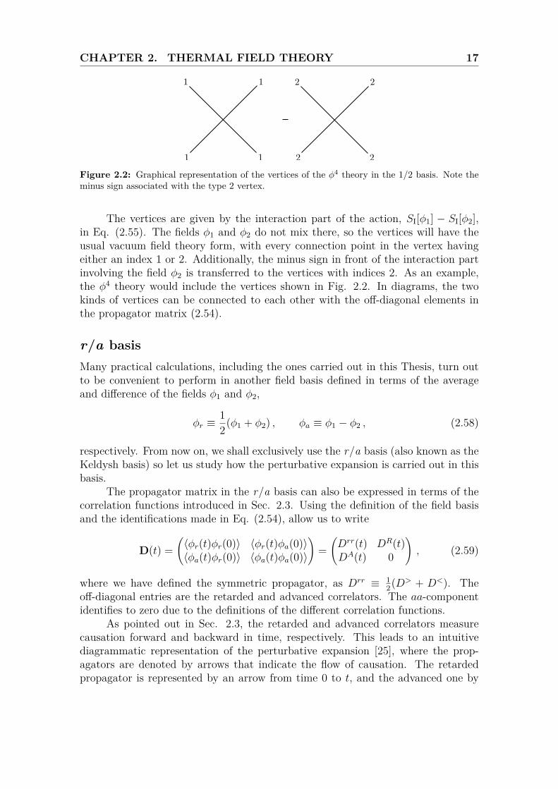
Figure 2.3: r/a basis momentum space free propagators represented graphically as arrows de-scribing the flow of causality [25]. The cut represents the source of the flow originating fromfluctuations in the past. When used in diagrams, the arrows are not usually drawn explicitly inthe rr-propagators.
an arrow from t to 0. The free propagators in momentum space are depicted in Fig.2.3.
The symmetric propagator is defined as the average of the forward and back-ward Wightman functions, which measure correlation in the fields at different times.The correlation is due to quantum or statistical fluctuations in the past, originatingfrom the density matrix at the time when the system was initialized as ρ(t0). Hence,the symmetric propagator is denoted by two outgoing arrows separated by a cut.The cut can be thought of as a source for the flow of causation, essentially tracingback to the initial density matrix ρ(t0).
Unlike the 1/2 basis, φr and φa fields mix in the interaction part of the actionSI. Therefore, the vertices include both r and a indices. For example, interactionterms like λ3
3! φ3 and λ4
4! φ4 become
SI[φ1]− SI[φ2] = SI
[φr + 1
2φa]− SI
[φr −
12φa
]= λ3
2! φaφ2r + 1
22λ3
3! φ3a + λ4
3! φaφ3r + 1
22λ4
3! φ3aφr . (2.60)
The normalization of the fields was chosen such that the correct symmetry factorsappear in the interaction terms. In terms with more than one φa field, an extrafactor of 1
2 is associated with each additional φa field. Furthermore, we notice thatterms with an even number of φa fields vanish identically due to the opposite signsof the vertices with indices 1 and 2 in the 1/2 basis. For a graphical representationof the vertices corresponding to the terms in Eq. (2.60), see Fig. 2.4.
One of the many convenient properties of the r/a basis representation is its di-rect connection to causality. As the propagators carry a flow of causation, any closedloop of causation, formed by retarded or advanced propagators only, would violatecausality, and should not exist (see Fig. 2.5). However, it turns out that this kind ofdiagrams integrate to zero, and can be safely disregarded when drawing different r/aassignments. This is due to the momentum space retarded (advanced) propagatorsbeing analytic functions of energy in the upper (lower) half of the complex plane,so the integration contour can be deformed to infinity.
CHAPTER 2. THERMAL FIELD THEORY 19
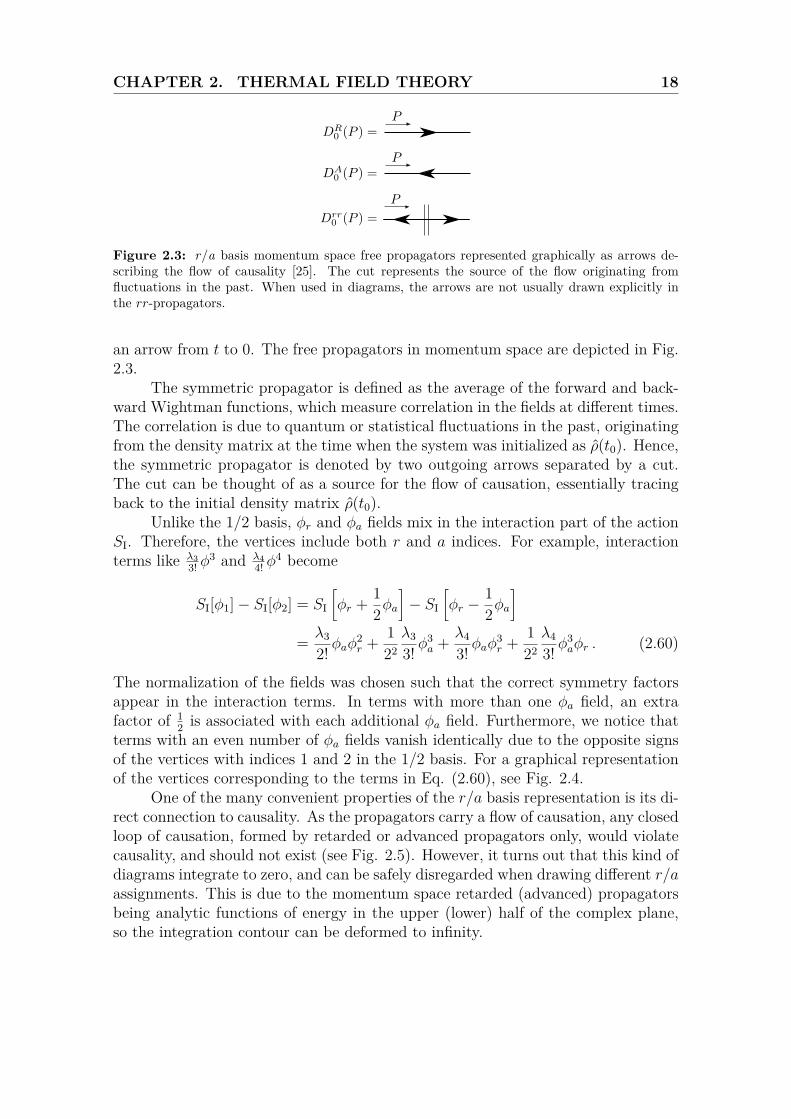
Figure 2.4: In r/a basis, the vertices mix r and a indices, and extra factors, such as the 14 in
the diagrams above, occur in vertices with many a indices. Both φ3 and φ4 vertices have two r/aassignments.
Figure 2.5: An example of a diagram that contains a closed loop of causation. The properties ofthe causal propagators guarantee that this kind of diagrams vanish identically.
Equilibrium
In thermal equilibrium, the whole propagator matrix is determined by one of thepropagators through the KMS relations derived in Sec. 2.3. For example, in mo-mentum space, the symmetric propagators for bosons and fermions turn out to beproportional to the spectral function,
Drr =(1
2 + nB(p0)) (
DR −DA), (2.61)
Srr =(1
2 − nF (p0 − µ)) (
SR − SA). (2.62)
Hence, DR determines the whole propagator matrix as DA results from DR by achange of arguments. As discussed in Sec. 3.2.1, the free DR is independent of Tand µ, and therefore all thermal dependence is contained in Drr alone inside thedistribution functions. This is yet another advantageous feature of the r/a basisrepresentation.
CHAPTER 2. THERMAL FIELD THEORY 20
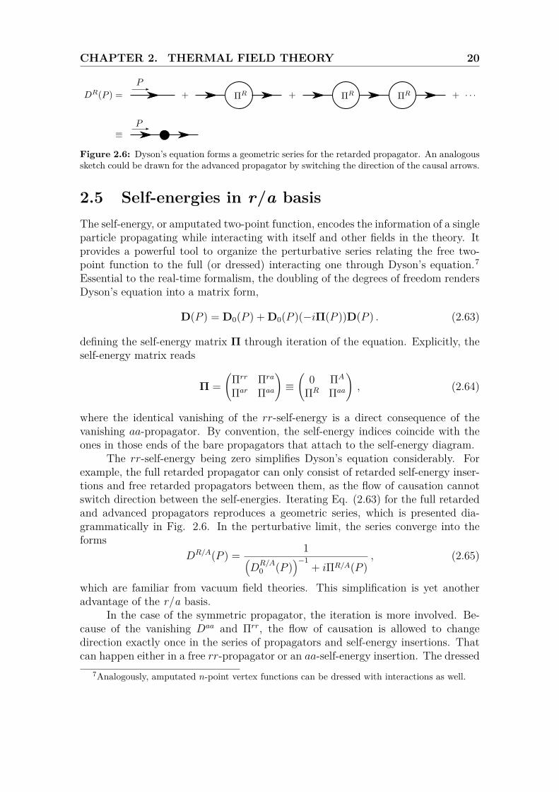
Figure 2.6: Dyson’s equation forms a geometric series for the retarded propagator. An analogoussketch could be drawn for the advanced propagator by switching the direction of the causal arrows.
2.5 Self-energies in r/a basisThe self-energy, or amputated two-point function, encodes the information of a singleparticle propagating while interacting with itself and other fields in the theory. Itprovides a powerful tool to organize the perturbative series relating the free two-point function to the full (or dressed) interacting one through Dyson’s equation.7Essential to the real-time formalism, the doubling of the degrees of freedom rendersDyson’s equation into a matrix form,
D(P ) = D0(P ) + D0(P )(−iΠ(P ))D(P ) . (2.63)
defining the self-energy matrix Π through iteration of the equation. Explicitly, theself-energy matrix reads
Π =(
Πrr Πra
Πar Πaa
)≡(
0 ΠA
ΠR Πaa
), (2.64)
where the identical vanishing of the rr-self-energy is a direct consequence of thevanishing aa-propagator. By convention, the self-energy indices coincide with theones in those ends of the bare propagators that attach to the self-energy diagram.
The rr-self-energy being zero simplifies Dyson’s equation considerably. Forexample, the full retarded propagator can only consist of retarded self-energy inser-tions and free retarded propagators between them, as the flow of causation cannotswitch direction between the self-energies. Iterating Eq. (2.63) for the full retardedand advanced propagators reproduces a geometric series, which is presented dia-grammatically in Fig. 2.6. In the perturbative limit, the series converge into theforms
DR/A(P ) = 1(DR/A0 (P )
)−1+ iΠR/A(P )
, (2.65)
which are familiar from vacuum field theories. This simplification is yet anotheradvantage of the r/a basis.
In the case of the symmetric propagator, the iteration is more involved. Be-cause of the vanishing Daa and Πrr, the flow of causation is allowed to changedirection exactly once in the series of propagators and self-energy insertions. Thatcan happen either in a free rr-propagator or an aa-self-energy insertion. The dressed
7Analogously, amputated n-point vertex functions can be dressed with interactions as well.
CHAPTER 2. THERMAL FIELD THEORY 21
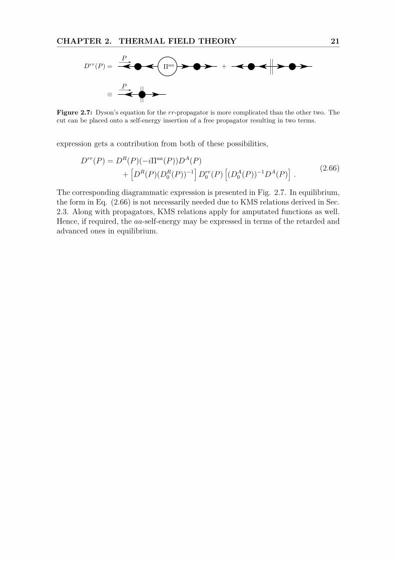
Figure 2.7: Dyson’s equation for the rr-propagator is more complicated than the other two. Thecut can be placed onto a self-energy insertion of a free propagator resulting in two terms.
expression gets a contribution from both of these possibilities,
Drr(P ) = DR(P )(−iΠaa(P ))DA(P )+[DR(P )(DR
0 (P ))−1]Drr
0 (P )[(DA
0 (P ))−1DA(P )].
(2.66)
The corresponding diagrammatic expression is presented in Fig. 2.7. In equilibrium,the form in Eq. (2.66) is not necessarily needed due to KMS relations derived in Sec.2.3. Along with propagators, KMS relations apply for amputated functions as well.Hence, if required, the aa-self-energy may be expressed in terms of the retarded andadvanced ones in equilibrium.
3. Quantum Chromodynamics
Quantum chromodynamics, or QCD, is the theory of strong interactions betweenmassless spin-1 force-carrying bosons called gluons and massive spin-1
2 fermionscalled quarks. These elementary particles constitute hadrons, such as protons, neu-trons and pions, and hence make up the majority of the visible matter in the universe.To make self-energy calculations of quarks and gluons applicable, and to justify theuse of perturbative methods introduced in the previous Chapter, the coupling con-stant of QCD, g, should be small. However, at low energy scales, g is large (hencethe name strong interaction), making quarks and gluons confine into hadrons, andinvalidating the use of perturbation theory. But thanks to the running of the cou-pling dictated by the QCD beta function, the coupling constant depends on theenergy scale at which one probes it. In QCD, as one moves to higher energies, gbecomes smaller, making hadrons deconfine into almost freely propagating quarksand gluons at some critical scale.1 This property, known as asymptotic freedom,validates the use of perturbative methods at high energies, in our case at high tem-peratures and/or densities. In fact, at high densities, perturbation theory currentlyserves as the only first-principles method to produce quantitative and reliable pre-dictions from QCD, due to failure of lattice QCD with its infamous sign problem(see e.g. Ref. [26]).
This Chapter is divided into two Sections. Sec. 3.1 is devoted to motivatingthe structure of the QCD Lagrangian, which is essential in perturbative calcula-tions, without focusing on the effects of finite temperature or density. A similar ormore elaborate derivation can be found in any standard QFT textbook, such as Ref.[27]. Sec. 3.2 studies QCD in the presence of a medium at equilibrium, that is, atfinite temperature and chemical potential. The r/a Feynman rules and self-energiesbrought up in Chapter 2 are generalized to QCD. Additionally, a certain conver-gence problem with perturbation series, raised by finite temperature and density, isdiscussed, and a solution is presented, serving as a motivation to the calculations inChapter 4.
1In a thermal medium formed by QGP, collective effects also become important as quarks andgluons manifest as long-wavelength quasi-particle excitations. These effects modify perturbationtheory, as discussed in Sec. 3.2.3.
22
CHAPTER 3. QUANTUM CHROMODYNAMICS 23
3.1 Fundamentals of QCD
3.1.1 Pure Yang–Mills theoryQCD is a non-Abelian gauge field theory, meaning that it is constructed with a prin-ciple of invariance under local gauge transformations of the non-Abelian symmetrygroup SU(3). First, we consider QCD without quarks, i.e. pure Yang–Mills theory,which describes the dynamics of a non-Abelian gauge field, i.e. the gluon field. TheLagrangian for a non-Abelian gauge field is
LYM = −14F
aµνF aµν , (3.1)
where F aµν is the field strength tensor with the vector gauge field Aaµ, given by
F aµν = ∂µA
aν −Dacν Acµ = ∂µA
aν − ∂νAaµ + gfabcAbµA
cν . (3.2)
We introduced the covariant derivative in the adjoint representation, defined asDacµ ≡ ∂µδ
ac + gfabcAbµ . (3.3)Here g is the strong coupling constant and fabc are the structure constants of SU(Nc).The adjoint color indices a, b, c range from 1 to N2
c − 1. For QCD, Nc = 3. Thespacetime indices range from 0 to D − 1 in D-dimensional spacetime.
3.1.2 QCD LagrangianThe QCD Lagrangian is generalized from the pure Yang–Mills Lagrangian (3.1) byadding Nf flavors of quark and anti-quark spinor fields, ψif and ψif , of color i, flavorf , and mass mf to it. Here, and in the following, the Latin indices i, j, k, ... denotethe fundamental color indices, which range from 1 to Nc. The QCD Lagrangianthen reads
LQCD = ψ(i /D −m)ψ + LYM ≡Nf∑f=1
ψif (iγµDijµ −mf1δ
ij)ψjf + LYM , (3.4)
where /D ≡ γµDµ and Dijµ = ∂µδij − igAaµT
aij is the covariant derivative in the
fundamental representation. The T a are Nc × Nc Hermitian matrices generatingthe Lie group SU(Nc) and forming a Lie algebra [T a, T b] = ifabcT c. By convention,they are normalized as Tr[T aT b] = TF δ
ab. TF is the index of the fundamentalrepresentation, and is given by TF = 1
2 . With our convention for the spacetimemetric, the γ-matrices satisfy the algebra {γµ, γν} = −2gµν .
The principle leading the construction of the QCD Lagrangian is invarianceunder local gauge transformations. Parametrized by smooth functions θa(x), thetransformation matrices are generated by exponentiating elements of the Lie algebra,U = exp(igθaT a) ∈ SU(Nc). By standard jargon, gauge fields transform in theadjoint representation and fermion fields in the fundamental representation, i.e.
Aµ ≡ AaµTa → UAµU
−1 + i
gU∂µU
−1 , (3.5)
ψ → Uψ , (3.6)
CHAPTER 3. QUANTUM CHROMODYNAMICS 24
leaving Eq. (3.4) invariant, which one can straightforwardly verify. Infinitesimalversions of the gauge transformations read
Aaµ → Aaµ +Dacµ θc +O(θ2) , (3.7)ψ → (1 + igθaT a)ψ +O(θ2) . (3.8)
To quantize the field theory given by Eq. (3.4), we should derive a functionalintegral from which we can calculate ensemble averages of some field operators.Skipping a detailed derivation, we just plug the QCD Lagrangian into the functionalintegral in Eq. (2.49), which we obtained for the complex scalar field. The resultingfunctional integral could be applied directly to perturbative calculations, but as itturns out, there are some subtleties in the perturbative series of QCD, which weshall consider next.
3.1.3 Gauge fixing and ghostsHaving established the Lagrangian for QCD (3.4), we could in principle write downthe weak-coupling expansion in the form of Eq. (2.55) and perform perturbativecalculations by computing correlation functions. However, when trying to solve thefree theory, as in Eq. (2.56), one encounters a non-invertible matrix in the quadraticpart of the gauge field action and therefore fails to write down an unambiguouspropagator matrix for the gauge fields. A standard way around this road block isprovided by the Faddeev-Popov procedure [28], which fixes the gauge and producessome new fields. The main steps will be described in the following.
The functional integral for QCD is written as
ZQCD =∫DAψψ eiSQCD[A,ψ,ψ] , (3.9)
where the time path is understood as a full Schwinger–Keldysh contour. We essen-tially compactified the notation of Eq. (2.49) by leaving the doubling of the fieldsimplicit. The problem of non-invertible matrix stems from the fact that (3.9) isbadly defined, as we are redundantly integrating over the gauge orbits, which corre-spond to physically equivalent gauge field configurations. To compute the functionalintegral and make the quadratic gauge field part of SQCD invertible, we have to fac-tor out the redundancy from the integral and in that way constrain the remainingpart to the space of physically non-equivalent field configurations.
Let G(A) = 0 be a gauge fixing condition, which ideally has a unique solutionfor A.2 To fix the gauge in the functional integral (3.9), a Dirac delta function,δ(G(Aθ)), is inserted to it in the form of
1 =∫Dθδ
(G(Aθ)
)det
(δG(Aθ)δθ
). (3.10)
The Jacobian determinant originates from the change of integration variables fromG(Aθ) to the function θ that parametrizes the gauge transformations. Aθ is the
2If this not the case, we encounter the so-called Gribov ambiguity.
CHAPTER 3. QUANTUM CHROMODYNAMICS 25
gauge transformed field given by Eq. (3.5). For the sake of readability, the colorand Lorentz indices are kept suppressed.
Next, we perform a simple change of integration variables from A to Aθ. Thechange is effortless, since the gauge invariance of QCD action allows us to writeSQCD[A] = SQCD[Aθ], and if G is linear in A, δG(Aθ)/δθ is independent of θ. Further,it can be shown that the measure is invariant, DA = DAθ. Finally, renamingAθ → A yields
ZQCD =[∫Dθ] ∫DAψψ δ (G(A)) det
(δG(Aθ)δθ
)eiSQCD[A,ψ,ψ] , (3.11)
where the integration over the gauge orbits is factored out in the first brackets, justas we wished. It evaluates to an (infinite) constant, which cancels in observablequantities, and thus can be discarded safely. The domain of the remaining integralconsists of gauge fixed, physically inequivalent field configurations.
Although we removed the infinite gauge redundancy from the functional in-tegral and thus removed our problem, Eq. (3.11) still contains the δ-function andJacobian determinant, making little use for it in practical perturbative calculations.To utilize our existing machinery for perturbation theory, we cast the δ-function anddeterminant into terms in an effective action, and therefore into Feynman rules.
First, we deal with the δ-function by inserting a multiplicative constant∫Df exp(− i
2ξ∫X f
2) into Eq. (3.11).∫X denotes integration over spacetime co-
ordinates X. The function f depends on X, and ξ is an arbitrary parameter. Sincethe partition function is independent of the choice of gauge, the function G can beshifted by f inside the δ-function, yielding δ(G(A) − f). Performing the integralover f is now straightforward, resulting in
ZQCD =∫DAψψ det
(δG(Aθ)δθ
)exp
(iSQCD[A, ψ, ψ]− i
2ξ
∫XG(A)2
). (3.12)
Next, for the determinant we employ a well known formula for a general linearoperator O,
detO =∫Dcc exp
(−i∫XcOc
), (3.13)
which casts it into a functional integral over a pair of Grassmannian fields c and c.The resulting form for ZQCD resembles the original one (3.9), additionally havingtwo extra terms in the action and a new set of anticommuting fields.
For practical purposes, we choose the gauge fixing function as G ≡ −∂µAaµ,specifying the family of covariant gauges, parametrized by ξ. By using the infinites-imal form of the gauge transformation (3.7) to compute δG(Aθ)/δθ, we end up with
ZQCD =∫DAψψcc exp
(iSQCD[A, ψ, ψ]− i
2ξ
∫X
(∂µAaµ)2 − i∫X∂µcaDabµ cb
),
(3.14)from which we read off the gauge-fixed QCD Lagrangian,
Leff = LQCD −12ξ (∂µAaµ)2 − ∂µca∂µca − gfabc∂µcaAbµcc , (3.15)
CHAPTER 3. QUANTUM CHROMODYNAMICS 26
where the covariant derivative is explicitly written out using Eq. (3.3).We acquired a completely gauge-fixed partition function for QCD that inte-
grates only over physically inequivalent field configurations. The quadratic part ofthe resulting effective action is indeed invertible, making propagators well-defined,and by adding sources to the fields in Eq. (3.14), they can be worked out accordingto Eq. (2.53) to conduct perturbative calculations. In other words, one can read offthe Feynman rules from Eq. (3.15) and start calculating perturbative corrections todifferent quantities.
As a by-product, we got a pair of auxiliary fields c and c, called Faddeev-Popov ghosts. Despite their Grassmannian (i.e. anticommuting) nature, they satisfyperiodic boundary conditions and obey bosonic statistics, since they originate fromthe bosonic operator δG/δθ. This mismatch violates the spin-statistics theorem,and thus the quanta of ghost fields cannot be physical particles. Instead, they areinterpreted as “negative” degrees of freedom that cancel the unphysical longitudinaland temporal gluons out from observables. They must be periodic in order toneutralize periodic gluons.
3.2 Thermal QCDUntil this point, we have not considered the effects of a thermal medium to QCD. Todo so, we assume a medium in equilibrium at high temperature and density, so thatperturbation theory is applicable. For simplicity, we take the chiral limit, i.e. set thequark masses to zero. In many physical applications at high temperatures and/orchemical potentials, quark masses become negligible. Either some of the masses aretiny compared to the characteristic scales of a particular problem, or they are hugemaking the corresponding quarks “inactive” by integrating them out.
3.2.1 r/a basis Feynman rules for QCDTo conduct perturbative calculations in thermal QCD, we need to generalize the r/aFeynman rules derived in Chapter 2 to the fields in QCD. We write the Feynmanrules in momentum space by Fourier transforming the ones in real space, yieldingmomentum-preserving δ-functions, which we omit to write explicitly. Thus, oneshould remember to use momentum conservation in vertices and propagators. Also,we suppress any r/a indices in the vertex rules we write here.
Perturbation series for observables in QCD are constructed with the principlesconsidered in Sec. 2.4. Instead of a single scalar field, we now have multiple fields:gluons Aaµ, ghosts ca and ca, and quarks ψif and ψif , whose dynamics are governed bythe gauge-fixed QCD Lagrangian (3.15). The propagators are obtained by taking thequadratic part of Leff corresponding to a given field and computing the associatedGaussian integral. An alternative way is to consider the Euclidean propagators,obtained by inverting the matrices appearing in the quadratic Euclidean action,and analytically continue to the retarded propagators [8]. The remaining elementsof the propagator matrix are then given by the relations introduced previously.

CHAPTER 3. QUANTUM CHROMODYNAMICS 27
The vertex rules are directly read off from the interaction part of Leff , keeping thedoubling rules in mind. Next, we will simply write down the QCD Feynman rulesin the r/a basis without going into any more details of deriving them.
The QCD propagators are more complex compared to the ones in scalar fieldtheory, involving spacetime, color, flavor and spin indices. However, they share thesame basic structure, so let us first consider the free part of a scalar field theory forthe sake of simplicity. Further, we drop the subscript 0 from the free propagatorsfrom now on and rely on the context when differentiating them from the dressedones. Now, the retarded and advanced scalar propagators are identical to the onesin vacuum and are given by
∆R/A(P ) = −iP 2 ∓ iηp0 , (3.16)
which are indeed related to each other through Eq. (2.48). Here η is an infinitesimalpositive number. The symmetric propagators for bosons and fermions differ fromeach other and are obtained from the KMS relation by using Eqs. (2.61) and (2.62),respectively. For those, we need the free spectral function
∆d(P ) ≡ ∆R −∆A = 2π sgn(p0)δ(P 2) = π
p
(δ(p− p0)− δ(p+ p0)
), (3.17)
for which we employed the Sokhotski–Plemelj formula
1∆± iη = P
( 1∆
)∓ iπδ(∆) , (3.18)
where P is the Cauchy principal value. Hence, the symmetric propagators are writtenas
∆rrB (P ) =
(12 + nB(p0)
)∆d(P ) , ∆rr
F (P ) =(1
2 − nF (p0 − µ))
∆d(P ) , (3.19)
for bosons and fermions respectively. We recall that the bosonic and fermionicdistribution functions read nB/F (p0) = (eβp0 ∓ 1)−1.
The δ-function in Eq. (3.17) should be understood as a regularized one, keepingη finite until the end of a calculation. In other words, rr-propagators should bewritten in terms of the retarded and advanced ones. Otherwise one might run intoill-defined quantities, such as P(1/P 2)δ(P 2). This is definitely the case in the two-loop calculation in Chapter 4. After the δ-functions are treated properly to avoidmathematical pathologies, rr-propagators set loop momenta on shell with spatialmomenta distributed according to either bosonic or fermionic distribution function.This is just a manifestation of the interpretation of rr-cut sourcing a flow of causalityfrom the equilibrium density matrix.

CHAPTER 3. QUANTUM CHROMODYNAMICS 28
Gluons
The propagators corresponding to gluons Aaµ have color and spacetime indices andare now expressed in terms of the scalar propagators as
GR/Aµν (P ) =
[gµν − (1− ξ) PµPν
P 2 ∓ iηp0
]∆R/A(P )
= gµν∆R/A(P )− i(1− ξ)PµPν(∆R/A(P )
)2, (3.20)
andGrrµν(P ) = gµν∆rr
B (P )− i(1− ξ)PµPν(1
2 + nB(p0))
∆d2(P ) , (3.21)
where ξ is the gauge-fixing parameter in covariant gauges. The propagators containan implicit Kronecker delta δab over the adjoint color indices. Here we introduceda shorthand notation for the difference of the squares of retarded and advancedpropagators,
∆d2 ≡ (∆R)2 − (∆A)2 . (3.22)
The interaction part of the Yang-Mills Lagrangian carries purely gluonic three-and four-point interaction vertices given by
iV abcµνρ(P,Q,R) = gfabc
[(Q−R)µgνρ + (R− P )νgρµ + (P −Q)ρgµν
]
= ,(3.23)
and
iV abcdµνρσ = −ig2
[fabef cde(gµρgνσ − gµσgνρ)
+ facefdbe(gµσgρν − gµνgρσ)+ fadef bce(gµνgσρ − gµρgσν)
]
= ,
(3.24)
respectively.
CHAPTER 3. QUANTUM CHROMODYNAMICS 29
Ghosts
As the gauge-fixed Lagrangian (3.15) suggests, the ghost propagators, correspondingto the fields ca and ca, are identical to the scalar ones with an additional delta overthe adjoint color indices, which we again suppress for a clean notation,
GR/A(P ) = ∆R/A(P ) , Grr(P ) = ∆rrB (P ) . (3.25)
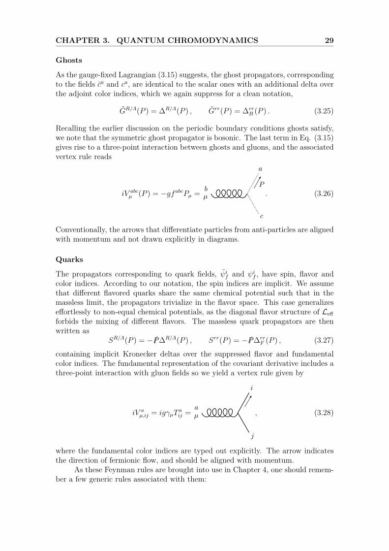
Recalling the earlier discussion on the periodic boundary conditions ghosts satisfy,we note that the symmetric ghost propagator is bosonic. The last term in Eq. (3.15)gives rise to a three-point interaction between ghosts and gluons, and the associatedvertex rule reads
iV abcµ (P ) = −gfabcPµ = . (3.26)
Conventionally, the arrows that differentiate particles from anti-particles are alignedwith momentum and not drawn explicitly in diagrams.
Quarks
The propagators corresponding to quark fields, ψif and ψif , have spin, flavor andcolor indices. According to our notation, the spin indices are implicit. We assumethat different flavored quarks share the same chemical potential such that in themassless limit, the propagators trivialize in the flavor space. This case generalizeseffortlessly to non-equal chemical potentials, as the diagonal flavor structure of Leffforbids the mixing of different flavors. The massless quark propagators are thenwritten as
SR/A(P ) = −/P∆R/A(P ) , Srr(P ) = −/P∆rrF (P ) , (3.27)
containing implicit Kronecker deltas over the suppressed flavor and fundamentalcolor indices. The fundamental representation of the covariant derivative includes athree-point interaction with gluon fields so we yield a vertex rule given by
iV aµ,ij = igγµT
aij = , (3.28)
where the fundamental color indices are typed out explicitly. The arrow indicatesthe direction of fermionic flow, and should be aligned with momentum.
As these Feynman rules are brought into use in Chapter 4, one should remem-ber a few generic rules associated with them:
CHAPTER 3. QUANTUM CHROMODYNAMICS 30
• Momentum is conserved at vertices and in propagators.
• In each loop, the associated momentum is integrated over and discrete indicesare traced over.
• For each loop formed by a Grassmannian field, an additional minus sign isinserted.
• Each diagram is multiplied by a suitable symmetry factor, which counts thenumber of topologically equivalent forms of the same diagram.
3.2.2 QCD self-energiesCompared to the case of a complex scalar field, the fields in QCD, and therefore theirself-energies, possess a more complicated structure involving Lorentz (i.e. spacetime)indices. The introduction of a thermal medium breaks the spacetime symmetry,making thermal QCD self-energies manifestly richer in structure compared to thesymmetric vacuum counterparts. By using general symmetry arguments, we shallnow derive convenient bases for QCD self-energies that incorporate the availablespacetime symmetry, ultimately reducing our workload later when we actually cal-culate them. In the following, the quark and gluon self-energies contain an implicitKronecker delta over appropriate color indices, similar to the propagators.
Gluon self-energy Πµν
Given that the gluon is a vector particle, its self-energy is a symmetric tensor of ranktwo, Πµν . The form of the self-energy tensor3 is further constrained by requiringgauge invariance of various QCD Green’s functions resulting in the Slavnov–Tayloridentities [29, 30] (non-Abelian generalization of Ward–Takahashi identities). Forexample, the full retarded gluon propagator satisfies the following identity [31],
KµKνGRµν(K) = −iξ , (3.29)
which constraints the self-energy tensor through the Dyson equation (2.63).Considering the case of vacuum, the only available tensor structures for Πµν
are gµν and KµKν , owing to Lorentz symmetry. The application of Eq. (3.29) inthat case requires the self-energy to be transverse to its momentum,
KµΠµν(K) = 0 . (3.30)
Hence, the vacuum self-energy may be written as
Πµν(K) =(gµν −
KµKν
K2
)Π(K2) ≡ Pµν(K)Π(K2) , (3.31)
where P is a projector transverse to its argument, satisfying the usual propertyPµλPλν = Pµν (idempotent), and Π(K2) is a Lorentz scalar.
3Also known as polarization tensor.

CHAPTER 3. QUANTUM CHROMODYNAMICS 31
Introducing a thermal medium breaks the Lorentz symmetry by specifyinga special frame of reference, the rest frame of the thermal bath. In that frame,the remaining symmetry is associated with spatial rotations, and the velocity ofthe medium has the form nµ = (1,0). Consequently, the tensor basis for the self-energy extends to four different tensors: gµν , KµKν , nµnν and nµKν +Kµnν . Whenconsidering the transversality properties of the self-energy, it is convenient to definea vector nµ(K) = Pµν(K)nν , and choose the tensor basis as linear combinations ofthe above tensors,
PTµν = Pµν − PL
µν = δiµδjν
(gij −
kikjk2
), (3.32)
PLµν = nµnν
n2 , (3.33)
PCµν = 1
k(nµKν +Kµnν) , (3.34)
PDµν = KµKν
K2 . (3.35)
One may check that PT, PL and PD are idempotent and mutually orthogonal. Onthe other hand, PC satisfies the relations
PCµλPCλ
ν = −PLµν − PD
µν , (3.36)PTµλPCλ
ν = 0 , (3.37)
PLµλPCλ
ν = nµKν
k, (3.38)
PDµλPCλ
ν = Kµnνk
, (3.39)
i.e. it is not idempotent and only orthogonal to PT. Further, it is easy to showthat the projectors PT and PL are transverse to K. PT is additionally transverse tothe spatial momentum k. PC satisfies the weaker property KµKνPC
µν = 0 and PD
projects longitudinally with respect to K.By using the above projectors, the gluon self-energy decomposes as
Πµν = PTµνΠT + PL
µνΠL + PCµνΠC + PD
µνΠD (3.40)
in the rest frame of the thermal medium. The components depend now separatelyon k0 and k as a result of the broken Lorentz symmetry. By employing the aboveproperties of the projectors, one can project out the individual components from thefull tensor,
ΠT = 1d− 1P
TµνΠµν , ΠL = PL
µνΠµν ,
ΠC = −12P
CµνΠµν , ΠD = PD
µνΠµν .
(3.41)
The full gluon propagator can be obtained by inserting the self-energy matrix(3.40) and free propagators from the previous Section into the Dyson equation (2.63).
CHAPTER 3. QUANTUM CHROMODYNAMICS 32
For instance, the full retarded propagator is given by Eq. (2.65) and admits adecomposition in terms of the four projectors,
GRµν = PT
µν∆RT + PL
µν∆RL + PC
µν∆RC + PD
µν∆RD , (3.42)
where
∆RT = −i
K2 + ΠRT, (3.43)
∆RL = −i
K2 + ΠRL + ξ(ΠRC)2
K2+ξΠRD
, (3.44)
∆RC = − ξΠR
CK2 + ξΠR
D∆R
L , (3.45)
∆RD = ξ(K2 + ΠR
L )K2 + ξΠR
D∆R
L . (3.46)
For notational simplicity, we have absorbed the iη from the free propagator into k0,i.e. we need to substitute k0 → k0 + iη. Similar expressions can be derived for therest of the full propagators by utilizing the form of the retarded propagator. Theadvanced propagator is given by replacing k0 +iη with k0−iη and the rr-propagatoris obtained from the KMS-condition in the case of equilibrium.
Imposing the Slavnov–Taylor identity (3.29) on the gluon propagator (3.42)yields a non-linear relation between the self-energy components,
ΠRD(K2 + ΠR
L ) = −(ΠRC)2 , (3.47)
also simplifying the last three of the propagator components to
∆RL = −i(K
2 + ξΠRD)
K2(K2 + ΠRL ) , (3.48)
∆RC = iξΠR
CK2(K2 + ΠR
L ) , (3.49)
∆RD = − iξ
K2 . (3.50)
Thus, the longitudinal component ∆RD does not receive self-energy corrections being
determined by the bare propagator alone. As opposed to the vacuum case, theSlavnov–Taylor identity does not require a transverse gluon self-energy, so generallyKµΠµν 6= 0 in a thermal medium.
At the one-loop level, we will show that ΠRC = 0 in Feynman gauge (ξ = 1).4
Then, Eq. (3.47) gives ΠRD = 0, and the self-energy becomes fully transverse.5,6
4In other covariant gauges ΠRC 6= 0 even at one-loop order [32, 33, 34].
5In the so-called hard thermal loop (HTL) approximation this is true (at least at one-loop order)in every gauge due to HTLs satisfying Abelian Ward identities [1, 35].
6This holds to all loop orders, e.g., in temporal gauges [36].
CHAPTER 3. QUANTUM CHROMODYNAMICS 33
In practical calculations, one may conveniently express the two remaining non-zerocomponents using the 00-component Π00 and trace Πµ
µ of the self-energy
ΠT = 1d− 1
(Πµµ + K2
k2 Π00
), (3.51)
ΠL = −K2
k2 Π00 , (3.52)
as we do in the next Chapter when calculating the one-loop self-energy.In vacuum, the gluon remains massless at all orders in perturbation theory,
i.e. the full propagator has a pole always at K2 = 0 [27]. In the thermal case,however, the breaking of the Lorentz symmetry allows gluons to have a thermalmass. Indeed, the thermal gluon propagator has two poles,7 one at K2 = −ΠR
T andanother at K2 = −ΠR
L , making the self-energy components act as effective gluonmasses, since, in medium, Πµν 6= 0 as K → 0. Later we will calculate the leading-order thermal mass to be at the scale of gT at finite temperature or gµ at finitedensity. The generation of this mass can be interpreted as collective effects in theplasma of quarks and gluons, as we will discuss in a moment.
Quark self-energy Σ
Quarks are spinor fields so the corresponding self-energy Σ is a matrix acting onspinors, i.e. a linear combination of γ-matrices. In the Lorentz symmetric vacuum,Σ must be a linear combination of 1 and /K. This symmetry breaks again in thethermal setting, leaving us with a spatial rotational symmetry in the rest frame ofthe medium. In other words, the structure /K splits into γ0k0 and γiki ≡ γ · k.Therefore, the thermal quark self-energy has the general form
Σ(K) = γ0Σ0(k0, k) + γ · kΣs(k0, k) + [γ0,γ · k]Σc(k0, k) + 1Σm(k0, k) . (3.53)
At the one-loop level, the expression simplifies as the commutator term Σc gets nocontributions, as we will explicitly show in the next chapter. The Σm term is a masscorrection, proportional to the quark mass. In the chiral limit, where quarks aremassless, this term vanishes as well, allowing us to rewrite the self-energy as
γ0 Σ(K) = Λ+k Σ+(k0, k)− Λ−k Σ−(k0, k) , (3.54)
where Σ± ≡ Σs ± Σ0, and Λ±k is a projector to states with positive (negative)chirality-to-helicity ratio,8 given by
Λ±k ≡12(1± γ0γ · k
). (3.55)
As orthogonal projection operators, they satisfy the properties
Λ±Λ± = Λ± , Λ±Λ∓ = 0 , Λ+ + Λ− = 1 . (3.56)7The locations of these poles are gauge invariant [37].8Or equivalently to positive (negative) energy states.
CHAPTER 3. QUANTUM CHROMODYNAMICS 34
The basis defined by Λ± is later referred as the helicity basis.Again, the full propagator is given by the Dyson equation by utilizing the free
quark propagators from the previous Section and the self-energy (3.54). Consideringthe retarded full propagator, we arrive to
SR(K)γ0 =iΛ+
kk0 − k − ΣR
++
iΛ−kk0 + k + ΣR
−, (3.57)
where k0 is understood as k0 + iη. In equilibrium, the other propagators are conve-niently derived from this one, analogously to the gluon case.
The vacuum theory is chirally invariant only when quarks are massless. Al-though quarks acquire a thermal mass at the same scale as gluons after introducinga thermal medium, the chiral symmetry stays intact (at least at one-loop order).This is easily seen from the fact that the self-energy Σ and the full propagator Sstill anti-commute with γ5.
3.2.3 IR problems and HTL resummationAnyone working with QFTs at zero temperature and density is familiar with theemergence of divergences in such theories. These divergences are classified accord-ing to the scales they appear in. Those found at long distances (or small momenta)are called infrared (IR) divergences, and conversely at short distances (or large mo-menta) one deals with ultraviolet (UV) divergences. In order to obtain sensibleresults, all divergent parts must vanish in any observable quantity. This is achievedwith the carefully designed machinery of renormalization, where the fields and pa-rameters of the theory are redefined such that divergences cancel order-by-order inperturbation theory resulting in finite observables.
In a thermal setting, naive perturbative expansions of physical quantities suf-fer from divergences that depend on temperature and density. As in the vacuumcase, their cancellation is required for the theory to make sense, so we employ renor-malization. After doing that, UV divergences have disappeared at all perturbativeorders but we are left with uncanceled IR divergences even at low order. This in-dicates that our thermal theory breaks down in the IR, and thus has to be curedof the remaining divergences to make predictions. Before introducing a remedy, wegive some physical insight to the origin of these IR divergences.
Typically, the most IR sensitive degrees of freedom in thermal field theoriesare associated with massless bosons. They have no mass to “protect” them in theIR, and the bosonic distribution function diverges at zero momentum, giving hintsof the IR sensitivity of such particles. In QCD, gluons carry these characteristicsand are the main source of the bad IR behaviour. Bearing the theme of the thesisin mind, we will focus our attention only to QCD from now on.
At high energies, the degrees of freedom in QCD are quarks and gluons. Theyform a plasma, in which individual particles appear in the hard energy scale Λh,where Λh = f(T, µ): their average energy is ∼ Λh and the average distance betweentwo neighbouring particles is ∼ Λ−1
h . The function f satisfies f(T, 0) = T andf(0, µ) = µ. Another scale of interest ends up being the soft scale gΛh, rising from
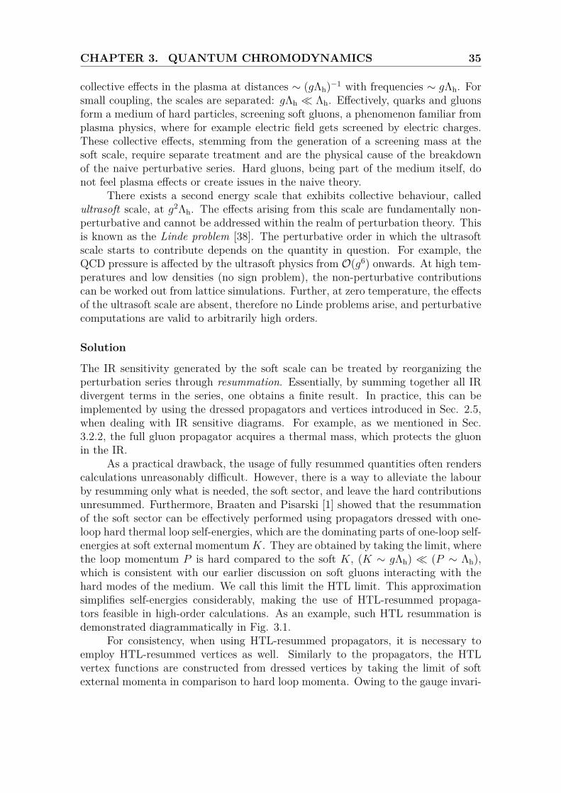
CHAPTER 3. QUANTUM CHROMODYNAMICS 35
collective effects in the plasma at distances ∼ (gΛh)−1 with frequencies ∼ gΛh. Forsmall coupling, the scales are separated: gΛh � Λh. Effectively, quarks and gluonsform a medium of hard particles, screening soft gluons, a phenomenon familiar fromplasma physics, where for example electric field gets screened by electric charges.These collective effects, stemming from the generation of a screening mass at thesoft scale, require separate treatment and are the physical cause of the breakdownof the naive perturbative series. Hard gluons, being part of the medium itself, donot feel plasma effects or create issues in the naive theory.
There exists a second energy scale that exhibits collective behaviour, calledultrasoft scale, at g2Λh. The effects arising from this scale are fundamentally non-perturbative and cannot be addressed within the realm of perturbation theory. Thisis known as the Linde problem [38]. The perturbative order in which the ultrasoftscale starts to contribute depends on the quantity in question. For example, theQCD pressure is affected by the ultrasoft physics from O(g6) onwards. At high tem-peratures and low densities (no sign problem), the non-perturbative contributionscan be worked out from lattice simulations. Further, at zero temperature, the effectsof the ultrasoft scale are absent, therefore no Linde problems arise, and perturbativecomputations are valid to arbitrarily high orders.
Solution
The IR sensitivity generated by the soft scale can be treated by reorganizing theperturbation series through resummation. Essentially, by summing together all IRdivergent terms in the series, one obtains a finite result. In practice, this can beimplemented by using the dressed propagators and vertices introduced in Sec. 2.5,when dealing with IR sensitive diagrams. For example, as we mentioned in Sec.3.2.2, the full gluon propagator acquires a thermal mass, which protects the gluonin the IR.
As a practical drawback, the usage of fully resummed quantities often renderscalculations unreasonably difficult. However, there is a way to alleviate the labourby resumming only what is needed, the soft sector, and leave the hard contributionsunresummed. Furthermore, Braaten and Pisarski [1] showed that the resummationof the soft sector can be effectively performed using propagators dressed with one-loop hard thermal loop self-energies, which are the dominating parts of one-loop self-energies at soft external momentumK. They are obtained by taking the limit, wherethe loop momentum P is hard compared to the soft K, (K ∼ gΛh) � (P ∼ Λh),which is consistent with our earlier discussion on soft gluons interacting with thehard modes of the medium. We call this limit the HTL limit. This approximationsimplifies self-energies considerably, making the use of HTL-resummed propaga-tors feasible in high-order calculations. As an example, such HTL resummation isdemonstrated diagrammatically in Fig. 3.1.
For consistency, when using HTL-resummed propagators, it is necessary toemploy HTL-resummed vertices as well. Similarly to the propagators, the HTLvertex functions are constructed from dressed vertices by taking the limit of softexternal momenta in comparison to hard loop momenta. Owing to the gauge invari-
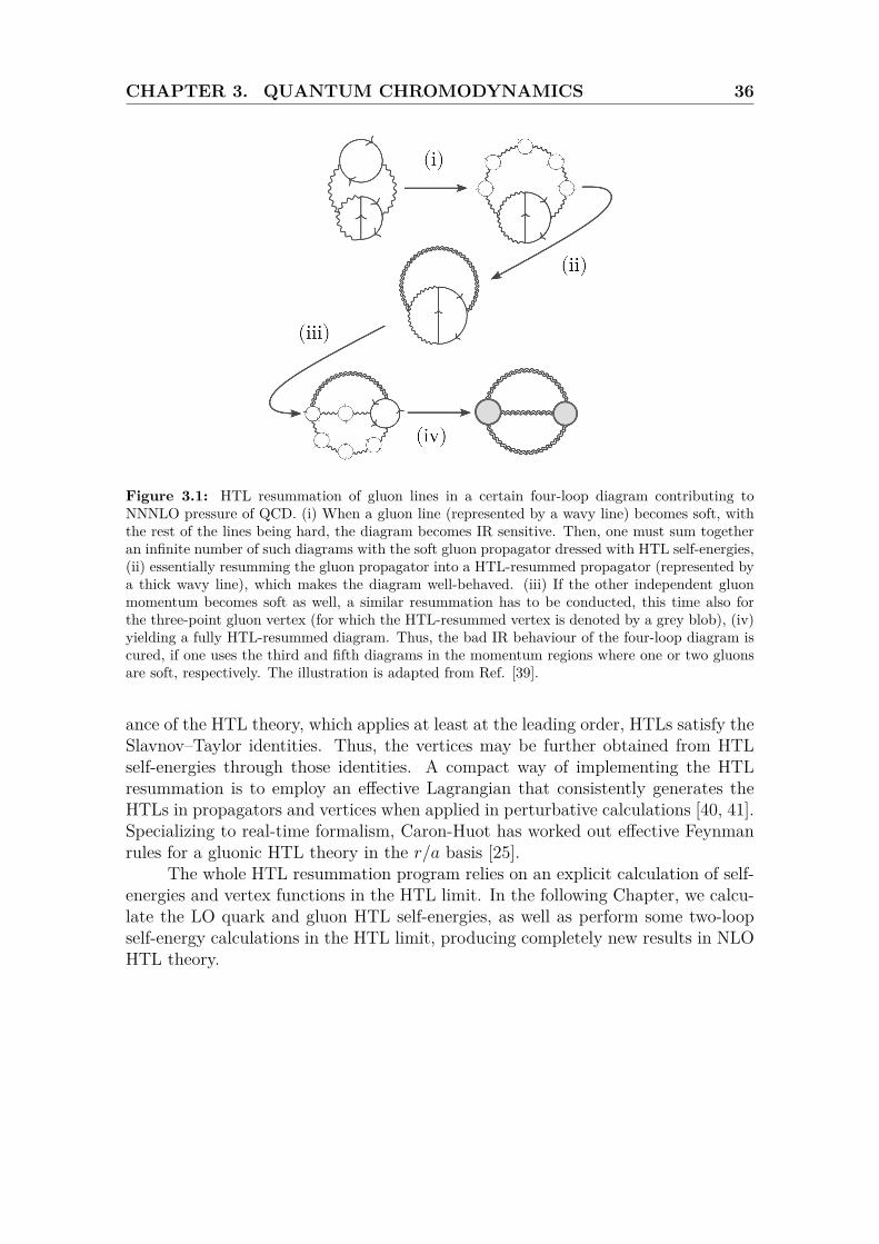
CHAPTER 3. QUANTUM CHROMODYNAMICS 36
Figure 3.1: HTL resummation of gluon lines in a certain four-loop diagram contributing toNNNLO pressure of QCD. (i) When a gluon line (represented by a wavy line) becomes soft, withthe rest of the lines being hard, the diagram becomes IR sensitive. Then, one must sum togetheran infinite number of such diagrams with the soft gluon propagator dressed with HTL self-energies,(ii) essentially resumming the gluon propagator into a HTL-resummed propagator (represented bya thick wavy line), which makes the diagram well-behaved. (iii) If the other independent gluonmomentum becomes soft as well, a similar resummation has to be conducted, this time also forthe three-point gluon vertex (for which the HTL-resummed vertex is denoted by a grey blob), (iv)yielding a fully HTL-resummed diagram. Thus, the bad IR behaviour of the four-loop diagram iscured, if one uses the third and fifth diagrams in the momentum regions where one or two gluonsare soft, respectively. The illustration is adapted from Ref. [39].
ance of the HTL theory, which applies at least at the leading order, HTLs satisfy theSlavnov–Taylor identities. Thus, the vertices may be further obtained from HTLself-energies through those identities. A compact way of implementing the HTLresummation is to employ an effective Lagrangian that consistently generates theHTLs in propagators and vertices when applied in perturbative calculations [40, 41].Specializing to real-time formalism, Caron-Huot has worked out effective Feynmanrules for a gluonic HTL theory in the r/a basis [25].
The whole HTL resummation program relies on an explicit calculation of self-energies and vertex functions in the HTL limit. In the following Chapter, we calcu-late the LO quark and gluon HTL self-energies, as well as perform some two-loopself-energy calculations in the HTL limit, producing completely new results in NLOHTL theory.
4. Calculation of Self-energies
We are finally ready to perform some explicit calculations of QCD (and photon) self-energies in a hot and dense medium. In this Chapter, using the powerful machineryof real-time formalism in the r/a basis, we compute quark, gluon and photon self-energies explicitly in the HTL limit. As a warm-up exercise, and an introductionto the technical details of such calculations, the quark and gluon self-energies areworked out at one-loop order. These simpler computations prepare us to tackle themore complicated problem of two-loop photon self-energy allowing us to extend theexisting HTL theory to the next perturbative order.
As mentioned in the previous Chapters, in equilibrium, we only need to obtaina single self-energy component from the self-energy matrix, the rest following fromthe KMS relation. We choose to compute retarded self-energies. The computationsare most conveniently performed in the Feynman gauge (ξ = 1). Furthermore, weassume the chiral limit with massless quarks, and only a single quark flavor withchemical potential µ.
We wish to obtain HTL limits of self-energies by expanding in small externalmomentumK compared to the hard scale Λh. Therefore, it is sensible to extract onlythe T and µ dependent parts (thermal parts) of the small K expansions as they havean external scale Λh, which K can be compared with. The other parts, independentof T and µ, are consistently omitted in our calculations. They contribute to thevacuum parts of the self-energies and are well-known to high loop orders in thecurrent literature.
To regularize any divergences we might encounter in integrals of D = 4 space-time dimensions, we employ dimensional regularization by writing the integrationmeasure in D = 4 + 2ε dimensions as∫
P≡∫ dDP
(2π)D =∫ ∞−∞
dp0
2π
∫p, (4.1)
where ε > 0. Here, the spatial d = D−1 dimensional integration measure is writtenin spherical coordinates as [8]
∫p≡ (Λ2) 3−d
2
∫ ddp(2π)d = 4(Λ2) 3−d
2
(4π) d+12 Γ
(d−1
2
) ∫ ∞0
dp pd−1∫ 1
−1dz(1− z2) d−3
2 , (4.2)
where Λ is the renormalization scale parameter and z = k · p parametrizes an anglewith respect to some external vector k.
37
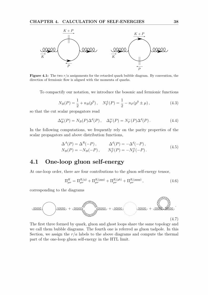
CHAPTER 4. CALCULATION OF SELF-ENERGIES 38
Figure 4.1: The two r/a assignments for the retarded quark bubble diagram. By convention, thedirection of fermionic flow is aligned with the momenta of quarks.
To compactify our notation, we introduce the bosonic and fermionic functions
NB(P ) = 12 + nB(p0) , N±F (P ) = 1
2 − nF (p0 ± µ) , (4.3)
so that the cut scalar propagators read
∆rrB (P ) = NB(P )∆d(P ) , ∆rr
F (P ) = N−F (P )∆d(P ) . (4.4)
In the following computations, we frequently rely on the parity properties of thescalar propagators and above distribution functions,
∆A(P ) = ∆R(−P ) , ∆d(P ) = −∆d(−P ) ,NB(P ) = −NB(−P ) , N±F (P ) = −N∓F (−P ) .
(4.5)
4.1 One-loop gluon self-energyAt one-loop order, there are four contributions to the gluon self-energy tensor,
ΠRµν = ΠR,(q)
µν + ΠR,(ggg)µν + ΠR,(gh)
µν + ΠR,(gggg)µν , (4.6)
corresponding to the diagrams
.
(4.7)The first three formed by quark, gluon and ghost loops share the same topology andwe call them bubble diagrams. The fourth one is referred as gluon tadpole. In thisSection, we assign the r/a labels to the above diagrams and compute the thermalpart of the one-loop gluon self-energy in the HTL limit.
CHAPTER 4. CALCULATION OF SELF-ENERGIES 39
Quark bubble
There are two ways to draw the r/a arrows to a retarded bubble diagram as shownin Fig. 4.1. The application of the Feynman rules to the assignments yields
−iΠR,(q)µν (K) = −
∫P
{Tr[(iV aµ,ij
)SA(P )
(iV bν,ji
)Srr(K + P )
]+ Tr
[(iV aµ,ij
)Srr(P )
(iV bν,ji
)SR(K + P )
] }= −
∫PF (q)µν (K,P )
{∆A(P )∆rr
F (K + P ) + ∆rrF (P )∆R(K + P )
}, (4.8)
where the extra minus in front is required since quarks are anti-commuting (orGrassmannian) fields. For clarity, the numerator algebra is contained in F (q)
µν , andit simplifies to
F (q)µν (K,P ) = Tr
[(iV aµ,ij
)/P(iV bν,ji
)( /K + /P )
]= −g2TF δ
abTr[γµ /Pγν( /K + /P )
]= −4g2TF δ
ab(2PµPν +KµPν + PµKν −
(P 2 +K · P
)gµν
), (4.9)
where the last line follows from the γ-matrix identity
Tr [γµγνγργσ] = 4 (gµσgνρ − gµρgνσ + gµνgρσ) . (4.10)
The color factor is given by T aijTbji = TF δ
ab, with TF = 12 being the index of the
fundamental representation of SU(Nc).Next, we should bring Eq. (4.8) into a form where the δ-functions and distri-
bution functions in rr-propagators depend only on the loop momentum P , so thatthe distribution functions become independent of the angle between k and p makingthe angular integral easier to handle. To this end, we shift the loop momentum inthe first term by P → −K − P . The numerator is invariant under this change ofvariables due to the cyclicity of the trace and the symmetry under µ↔ ν. Hence,
−iΠR,(q)µν (K) = −
∫PF (q)µν
{N−F (P ) +N+
F (P )}
∆R(K + P )∆d(P ) , (4.11)
where we utilized the parity properties of the propagators and distribution functionswe introduced in Eq. (4.5).
CHAPTER 4. CALCULATION OF SELF-ENERGIES 40
Gluon bubble
The gluon bubble acquires the same r/a labels as the quark loop, so the Feynmanrules give
−iΠR,(ggg)µν (K) = 1
2
∫P
{(iV acdµρλ(−K,−P,K + P )
)GρσA (P )
×(iV bcdνσγ(K,P,−K − P )
)Gγλrr (K + P )
+(iV acdµρλ(−K,−P,K + P )
)Gρσrr (P )
×(iV bcdνσγ(K,P,−K − P )
)GγλR (K + P )
}= 1
2
∫PF (ggg)µν (K,P )
{∆A(P )∆rr
B (K + P ) + ∆rrB (P )∆R(K + P )
},
(4.12)
where the overall factor of 12 is a symmetry factor due to gluons being their own
antiparticles. The structure constants satisfy facdf bcd = CAδab simplifying the nu-
merator to
F (ggg)µν (K,P ) =
(iV acdµρλ(−K,−P,K + P )
)gρσ
(iV bcdνσγ(K,P,−K − P )
)gγλ
= −g2CAδab((D − 6)KµKν + (2D − 3)(2PµPν +KµPν + PµKν)
+(5K2 + 2K · P + 2P 2
)gµν
).
(4.13)
Here CA is the quadratic Casimir of the adjoint representation of SU(Nc) and isgiven by CA = Nc. In the above, the factor of D originates from the trace of ametric tensor, gµµ = D. Just like previously, the first term of Eq. (4.12) is shiftedby P → −K − P leaving the numerator invariant and giving
−iΠR,(ggg)µν (K) =
∫PF (ggg)µν NB(P )∆R(K + P )∆d(P ) . (4.14)
Ghost bubble
The third bubble diagram contains a ghost loop and since ghosts are anti-commutingjust like quarks, we have an overall minus sign multiplying the expression
−iΠR,(gh)µν (K) = −
∫P
{(iV dacµ (K + P )
)GA(P )
(iV cbdν (P )
)Grr(K + P )
+(iV dacµ (K + P )
)Grr(P )
(iV cbdν (P )
)GR(K + P )
}= −
∫PF (gh)µν (K,P )
{∆A(P )∆rr
B (K + P ) + ∆rrB (P )∆R(K + P )
},
(4.15)where the numerator algebra yields
F (gh)µν (K,P ) =
(iV dacµ (K + P )
) (iV cbdν (P )
)= −g2CAδ
ab (PµPν +KµPν) . (4.16)
CHAPTER 4. CALCULATION OF SELF-ENERGIES 41
In this case, only the diagonal elements (µ = ν) of F (gh)µν , which end up being the
only ones we need, are left invariant under the shift P → −K − P . Due to thissimplification, we may write
−iΠR,(gh)µν (K) = −2
∫PF (gh)µν NB(P )∆R(K + P )∆d(P ) , (4.17)
which again applies only for the diagonal elements.
Gluon tadpole
A retarded tadpole diagram contains a single propagator, which must have an rr-label. In this case, the rr-propagator already depends only on P making any shiftsunnecessary. Hence we simply write
−iΠR,(gggg)µν (K) = 1
2
∫P
(iV abccµνρσ
)Gρσrr (P )
= 12
∫PF (gggg)µν (K,P )NB(P )∆d(P ) , (4.18)
where the overall 12 is again a symmetry factor. The numerator simplifies to
F (gggg)µν (K,P ) =
(iV abccµνρσ
)gρσ
= −2ig2CAδab(D − 1)gµν . (4.19)
All contributions together
Summing the four contributions in Eqs. (4.11), (4.14), (4.17) and (4.18) togethergives
−iΠRµν(K) = −iΠR,(q)
µν (K)− iΠR,(ggg)µν (K)− iΠR,(gh)
µν (K)− iΠR,(gggg)µν (K)
= 12
∫P
∆d(P ){− 2F (q)
µν
{N−F (P ) +N+
F (P )}
∆R(K + P )
+ 2(F (ggg)µν − 2F (gh)
µν
)NB(P )∆R(K + P )
+ F (gggg)µν NB(P )
}.
(4.20)
We could compute every component of the tensor ΠRµν individually, but instead we
reduce our workload by exploiting the symmetry provided by the Slavnov–Taylor-identity (3.29). In Sec. 3.2.2 we argued that if ΠR
C = 0, the self-energy tensorbecomes fully transverse, KµΠR
µν = 0, and has only two independent components.The ΠR
C component is projected out from the full tensor (4.20) by using Eq. (3.41),yielding
ΠRC(K) = 2g2δab
∫P
∆d(P ){CA(D − 1)NB(P ) + 2TF (N−F (P ) +N+
F (P ))}
× 1k
(p0 − k0K · P
K2
),
(4.21)
CHAPTER 4. CALCULATION OF SELF-ENERGIES 42
where the loop momentum has been set on-shell P 2 = 0 due to the δ-function in ∆d.Indeed, Eq. (4.21) vanishes1 since the integrand is an odd function of P . The twoindependent non-vanishing components are then given by the spatially transverseand longitudinal ones in Eqs. (3.51) and (3.52). For those, we must figure out thetrace (ΠR)µµ and 00-component ΠR
00 of the self-energy.
Trace
Contracting the metric tensor with the numerators in Eqs. (4.9), (4.13), (4.16) and(4.19) gives
(F (q))µµ = 4g2TF (D − 2)K · P , (4.22)(F (ggg))µµ = −6g2CA(D − 1)
(K2 +K · P
), (4.23)
(F (gh))µµ = −g2CAK · P , (4.24)(F (gggg))µµ = −2ig2CA(D − 1)D , (4.25)
where again the spectral function ∆d sets P is on-shell, P 2 = 0. The Kroneckerdelta δab over the adjoint indices has been suppressed and it stays suppressed fromnow on. We plug the above numerators into Eq. (4.20) and write the ∆R propagatorout explicitly,
(ΠR)µµ(K) = g2∫P
∆d(P ){− 4TF (D − 2)
{N−F (P ) +N+
F (P )} K · P
2K · P +K2
+ CANB(P )(
(D − 2)2 − (3D − 2)K2
2K · P +K2
)}.
(4.26)
To avoid clutter, the iη from the retarded propagator has been absorbed into k0
since we can write (K + P )2 − iη(k0 + p0) = (K + P )2|k0→k0+iη for small η. Hence,later on, we should remember that the 0-component of the external momentum hasa small imaginary part and replace k0 with k0 + iη in our expressions.
In the HTL limit, we are interested in the behaviour of the self-energy whenthe external momentum is soft, i.e. K � Λh. A convenient shortcut for extractingthe limit is to expand for K � p in the integrand. Strictly speaking, we should firstintegrate over p0 properly, but since ∆d is proportional to δ(p0 − p) − δ(p0 + p), ithas already been done implicitly by the δ-functions. Before expanding, we shouldtherefore set P 2 = 0 to obtain the correct expansion. Hence, we can directly expandEq. (4.26) for small K and pick out the leading terms, yielding
(ΠR)µµ(K) = g2∫P
∆d(P ){− 2TF (D − 2)
{N−F (P ) +N+
F (P )}
+ CANB(P )(D − 2)2}.
(4.27)
1Since we only want to extract the leading HTL contribution, and we know that leading orderHTLs are transverse and gauge independent, we are not really required to show the vanishing ofΠR
C . In any case, we see that the exact one-loop gluon self-energy is transverse in Feynman gauge.
CHAPTER 4. CALCULATION OF SELF-ENERGIES 43
In general, expressions gain more symmetry in the HTL limit, which is the reasonwe have taken the limit before integrating explicitly. In our case, the expression inthe curly brackets in Eq. (4.27) is odd in P so we can carry out the p0-integral byemploying the formula ∫
P∆d(P )f(p0) =
∫p
f(p)p
, (4.28)
where f is an odd function of P (∆d is odd making the integrand even). The aboveformula is a straight consequence of the definition of ∆d in Eq. (3.17). Integratingover p0 then gives
(ΠR)µµ(K) = g2∫
p
1p
{− 2TF (D − 2)
{N−F (p) +N+
F (p)}
+ CANB(p)(D − 2)2},
(4.29)
where N±F (p) is understood as N±F (P )|p0→p.Next, we proceed to integrate over the spatial momentum. We regulate the
spatial integrals by dimensional regularization but one encounters no divergences inEq. (4.29). Hence, we may set d = 3 simplifying the integration measure given byEq. (4.2) to ∫
p=∫ d3p
(2π)3 = 14π2
∫ ∞0
dp p2∫ 1
−1dz , (4.30)
and bringing Eq. (4.29) into
(ΠR)µµ(K) = 4g2 14π2
∫ ∞0
dp p{− TF
{N−F (p) +N+
F (p)}
+CANB(p)}∫ 1
−1dz . (4.31)
The angular part integrates trivially to 2, and for the radial integrals, we apply theresults from Appendix D,
(ΠR)µµ(K) = g2{
(TF + CA)T2
3 + TFµ2
π2
}≡ m2
E . (4.32)
Here we defined mE as the Debye mass at finite temperature and density.
00-component
Next, we repeat the above steps for the 00-component, the second independentcomponent of the self-energy. Picking out the 00-component from the numeratorsin Eqs. (4.9), (4.13), (4.16) and (4.19) gives
F(q)00 = −4g2TF
(2(p0)2 + 2k0p0 +K · P
), (4.33)
F(ggg)00 = −g2CA
((D − 6)(k0)2 + 2(2D − 3)
((p0)2 + k0p0
)−(5K2 + 2K · P
)),
(4.34)
F(gh)00 = −g2CA
((p0)2 + k0p0
), (4.35)
F(gggg)00 = 2ig2CA(D − 1) , (4.36)

CHAPTER 4. CALCULATION OF SELF-ENERGIES 44
and inserting them into Eq. (4.20) leads to
ΠR00(K) = g2
∫P
∆d(P ){
4TF{N−F (P ) +N+
F (P )} 2(p0)2 + 2k0p0 +K · P
2K · P +K2
− CANB(P )(D − 6)k2 + 2(D − 2) (2(p0)2 + 2k0p0 +K · P )2K · P +K2
}.
(4.37)
The HTL limit is obtained by expanding in small K,
ΠR00(K) = g2
∫P
∆d(P ){
2TF{N−F (P ) +N+
F (P )}− CA(D − 2)NB(P )
}
×(
1 + 2k0p0
K · P− K2(p0)2
(K · P )2 + 2(p0)2
K · P
).
(4.38)
The last term in the round brackets behaves parametrically as O(1/K) and leadsthe small K expansion. However, the term vanishes due to symmetry since thecorresponding integrand is an odd function of P . The remaining terms becomeleading, and since their integrands are even, we can use Eq. (4.28) to integrate overp0,
ΠR00(K) = g2
∫p
1p
{2TF
{N−F (p) +N+
F (p)}− CA(D − 2)NB(p)
}
×(
1 + 2k0
v ·K− K2
(v ·K)2
),
(4.39)
where v ≡ (1, p) so that v ·K = −k0 + kz.Again, the integrals in Eq. (4.39) are finite allowing us to set d = 3 and write
the integration measure as in Eq. (4.30),
ΠR00(K) = 2g2 1
4π2
∫ ∞0
dp p{TF
{N−F (p) +N+
F (p)}− CANB(p)
}
×∫ 1
−1dz(
1 + 2k0
v ·K− K2
(v ·K)2
).
(4.40)
The radial and angular integrals have factorized, and the former is identical to theradial integral in Eq. (4.31), and for the latter, we consult Appendix E, leading usto
ΠR00(K) = −m2
E
(1− k0L(K)
), (4.41)
whereL(K) ≡ 1
2k log k0 + k
k0 − k. (4.42)
Finally, we express the self-energy tensor in the basis of spatially transverseand longitudinal projectors, for which the corresponding components are given by

CHAPTER 4. CALCULATION OF SELF-ENERGIES 45
Figure 4.2: The two r/a assignments for the retarded one-loop quark self-energy. The directionof fermionic flow is aligned with the momenta of quarks.
Eqs. (3.51) and (3.52),
ΠRT(K) = m2
E2
[(k0)2
k2 + k0
2k
(1− (k0)2
k2
)log k
0 + k + iη
k0 − k + iη
], (4.43)
ΠRL (K) = m2
E
(1− (k0)2
k2
)[1− k0
2k log k0 + k + iη
k0 − k + iη
], (4.44)
where we have explicitly written the function L and the iη-prescription we sup-pressed earlier.
Characteristic to a small K expansion, the radial and angular integrals havefactorized, the former leading to a factor of m2
E, containing the information aboutT and µ, and the latter to a kinematic part depending only on the ratio k0/k. Aswe already brought up in Chapter 3, this explicit leading order calculation showsthat the gluon develops a thermal mass on the soft scale gΛh. The physics at thesoft scale, provided by Eqs. (4.43) and (4.44), include Debye screening, plasmaoscillations and Landau damping [8], which can be interpreted as collective effectsin the plasma of quarks and gluons.
4.2 One-loop quark self-energyOnly one diagram contributes to the quark self-energy at one-loop order. It has thetopology of a bubble diagram so the r/a assignments shown in Fig. 4.2 are familiarfrom the previous calculation. We start by applying the Feynman rules to the twoassignments,
−iΣR(K) =∫P
{(iV aµ,ik
)SR(K + P )
(iV aν,kj
)Gµνrr (P )
+(iV aµ,ik
)Srr(K + P )
(iV aν,kj
)GµνA (P )
}=∫PF (K,P )
{∆R(K + P )∆rr
B (P ) + ∆rrF (K + P )∆A(P )
}. (4.45)
CHAPTER 4. CALCULATION OF SELF-ENERGIES 46
The numerator is denoted by F and simplifies to
F (K,P ) =(iV aµ,ik
)(− /K − /P )
(iV aν,kj
)gµν
= g2CF δijγµ( /K + /P )γµ
= g2CF δij(D − 2)( /K + /P ) , (4.46)
where we employed the well-known γ-matrix identity, γµγνγµ = (D − 2)γν . Thecolor algebra has been solved with the formula (T aT a)ij = CF δij for the generatorsin the fundamental representation. The quadratic Casimir for the fundamentalrepresentation is given by CF = (N2
c − 1)/(2Nc). From now on, the Kronecker deltaδij over the fundamental indices is suppressed to avoid clutter.
Handling of the integrals in Eq. (4.45) simplifies if we shift the second termby P → −K − P , so that the δ-function and distribution function in ∆rr
F dependonly on the loop momentum P . This time, the numerator is affected by the shift,and we get
−iΣR(K) =∫P
{F (K,P )NB(P ) + F (K,−K − P )N+
F (P )}
∆R(K + P )∆d(P ) ,(4.47)
where we employed the parity properties of the propagators and distribution func-tions given by Eq. (4.5). Writing out the numerator and retarded propagatorexplicitly now gives
ΣR(K) = g2CF (D − 2)∫P
∆d(P ){NB(P )( /K + /P )
2K · P +K2 − N+F (P )/P
2K · P +K2
}, (4.48)
where the δ-function in ∆d sets the loop momentum on-shell P 2 = 0. The retardedprescription iη has been absorbed into k0 such that we need to substitute k0 → k0+iηin the final result.
Analogously to the case of gluon self-energy, we expand for small K at thispoint to extract the HTL limit. The correct limit is obtained even before integratingexplicitly over p0 since we have set P 2 = 0 by implicit p0-integration. The leadingterm in the small K expansion is
ΣR(K) = g2
2 CF (D − 2)∫P
∆d(P ){NB(P )−N+
F (P )} /P
K · P, (4.49)
which can be brought into a more symmetric form by symmetrizing the integrandwith the formula ∫
Pf(P ) = 1
2
∫P
(f(P ) + f(−P )) , (4.50)
for some function f . If there were any terms that would vanish by symmetry uponintegration, the symmetrization step would get rid of those terms early on. Addi-tionally, it makes the integrand an even function of P allowing us to integrate overp0 with Eq. (4.28). Applying the symmetrization formula to Eq. (4.49) yields
ΣR(K) = g2
4 CF (D − 2)∫P
∆d(P ){
2NB(P )−N−F (P )−N+F (P )
} /P
K · P, (4.51)
CHAPTER 4. CALCULATION OF SELF-ENERGIES 47
for which the p0-integral gives
ΣR(K) = g2
4 CF (D − 2)∫
p
1p
{2NB(p)−N−F (p)−N+
F (p)} /v
v ·K. (4.52)
As a reminder, v = (1, p) so that v ·K = −k0 + kz.Also in the case of quark self-energy, the spatial integral is finite when d = 3.
Writing the integration measure as in Eq. (4.30) leads to
ΣR(K) = g2
2 CF1
4π2
∫ ∞0
dp p{
2NB(p)−N−F (p)−N+F (p)
} ∫ 1
−1dz /v
v ·K, (4.53)
where the radial integral, carrying the information about T and µ, has factorizedfrom the angular integral, which purely contains the kinematics. Using the resultsfor radial and angular integrals in Appendices D and E, respectively, we find
ΣR(K) = m2q
{γ0L(K) + γ · k
k
(1− k0L(K)
)}, (4.54)
where we have defined the thermal mass of the quarks,
m2q = g2CF
8
(T 2 + µ2
π2
). (4.55)
The function L is written out in Eq. (4.42).The self-energy in Eq. (4.54) is now precisely in the form of Eq. (3.53), as we
have anticipated. The commutator term indeed vanishes at one-loop level, and noexplicit mass terms have appeared in the chiral limit. Hence, we may express theself-energy in the helicity basis (3.54), for which the positive and negative energycomponents become
ΣR±(k0, k) =
m2q
k
{1− k0 ∓ k
2k log k0 + k + iη
k0 − k + iη
}, (4.56)
where we have explicitly written the function L and the previously suppressed smallimaginary part of k0. Similarly to the gluon case, the quark has acquired a thermalmass at the soft scale stemming from the radial integral. The angular integral leadsto the kinematic part dependent on the external momentum K.
4.3 Two-loop photon self-energy in QCD mediumHaving carried out the LO computations of the HTL self-energies, a natural sequel isto move to the NLO. At the NLO, there are many different contributions to the self-energies depending on the number of soft internal lines in the diagrams, as discussedbelow Fig 3.1. We choose to study the situation in which only the external lines aresoft, leaving every internal line hard.
Furthermore, if the external lines are gluonic, the quantity we are interested inis the HTL limit of the two-loop gluon self-energy. However, at the two-loop order,
CHAPTER 4. CALCULATION OF SELF-ENERGIES 48
the number of different diagrams contributing to gluon self-energy grows up to a fewdozen, and performing the full calculation exceeds the scope of this Thesis. A lesscomplicated but still physically relevant scenario would be to replace the externalgluon with a photon, a counterpart for the gluon from quantum electrodynamics.The photon has a significantly simpler structure compared to that of the gluon,as it only interacts with quarks via electromagnetic interaction described by theinteraction vertex
iVµ = ieQeγµ = , (4.57)
where e is the QED coupling constant, analogous to g, and Qe denotes the electriccharge of the quark. Color indices are absent in the vertex rule since photons donot feel the strong interaction. As we replace the external line to be photonic, weare actually calculating the retarded two-loop self-energy of a photon in a mediumformed by quarks and gluons, which we denote by ΠR
QED. Due to the simplicity ofthe QED vertex, there are only three diagrams contributing at the two-loop order,which we call the cat’s eye, watermelon 1 and watermelon 2,
(ΠRQED)µν = (ΠR
cat)µν + (ΠRmelon1)µν + (ΠR
melon2)µν , (4.58)
and are represented by the graphs2
,
(4.59)respectively. The second watermelon diagram seems at a first glance identical to thefirst watermelon, with just the quarks flowing in the opposite directions. They evengive the same results at µ = 0. However, finite µ breaks this symmetry betweenthe different directions of the quark flow, and one has to compute those diagramsseparately.
The tensorial structure of the photon self-energy is also simpler compared tothe gluonic one. The QED version of the Slavnov–Taylor identity (3.29), namely theWard–Takahashi identity (given for example in Ref. [31]), restricts the self-energyto be four-dimensionally transverse. Therefore, it can be written directly in termsof the transverse and longitudinal components, (ΠR
QED)T and (ΠRQED)L, for which we
only need to calculate the trace (ΠRQED)µµ and the 00-component (ΠR
QED)00.At the two-loop level, the integrals contain products of two distribution func-
tions. These products can be manipulated with the following relation,
N±F (P1)N∓F (P2) +N∓F (P2)NB(P3) +NB(P3)N±F (P1) + 1 = 0 , (4.60)2Conventionally, the direction of the fermionic flow is aligned with the momentum assignments.
CHAPTER 4. CALCULATION OF SELF-ENERGIES 49
where the momenta satisfy P1 +P2 +P3 = 0. As we are only interested in extractingthe thermal parts of the self-energy, we persistently ignore the last term on the LHSof the above relation.
Before commencing with the two-loop calculation, let us recap the two mainsteps we took in the one-loop calculations. First, we assign the r/a arrows to thethree diagrams and shift the loop momenta in the individual diagrams so that the cutpropagators depend only on single momentum. Second, we sum the contributionstogether, consider either the trace or 00-component, and compute the resultingintegrals in the HTL limit. Keeping these steps as our guideline, let us begin.
Cat’s eye diagram
Applying the Feynman rules to the cat’s eye diagram without writing any specificr/a assignments yields
−∫P
∫Q
Tr[(iVµ
)Sp(P )
(iV aρ,ij
)Sq(PQ)
(iVν
)Sr(KPQ)
(iV aσ,ji
)Ss(KP )
]Gρσt (Q) ,
(4.61)where the indices pqrst are replaced with appropriate r/a labels. In favour of savingspace, we have compactified the notation by suppressing plus signs in the argumentsof propagators: KPQ = K + P + Q, etc. The minus sign in front originates fromthe fermion loop present in the diagram. The application of the r/a basis Feynmanrules to the above expression yields the following assignments (see Appendix F fora graphical representation),
−i(ΠRcat)µν(K) = −
∫P
∫QFCµν(K,P,Q)
×{
∆R(P )∆rrB (Q)∆rr
F (PQ)∆R(KP )∆R(KPQ)+∆A(P )∆rr
B (Q)∆A(PQ)∆A(KP )∆rrF (KPQ)
+∆A(P )∆rrB (Q)∆A(PQ)∆rr
F (KP )∆R(KPQ)+∆rr
F (P )∆rrB (Q)∆A(PQ)∆R(KP )∆R(KPQ)
+∆rrF (P )∆R(Q)∆rr
F (PQ)∆R(KP )∆R(KPQ)+∆A(P )∆R(Q)∆rr
F (PQ)∆rrF (KP )∆R(KPQ)
+∆A(P )∆A(Q)∆A(PQ)∆rrF (KP )∆rr
F (KPQ)+∆rr
F (P )∆A(Q)∆A(PQ)∆R(KP )∆rrF (KPQ)
}.
(4.62)
We have only included assignments with thermal contributions and dropped allpurely vacuum terms, i.e. those not containing any rr-propagators. Additionally,assignments with closed loops of retarded or advanced propagators have been dis-regarded since they integrate to zero as discussed in Chapter 2. The numeratoralgebra simplifies to
FCµν = Tr
[(iVµ
)/P(iV aρ,ij
)(/P + /Q)
(iVν
)( /K + /P + /Q)
(iV aσ,ji
)( /K + /P )
]gρσ
= e2g2Q2eCFNcTr
[γµ /Pγ
ρ(/P + /Q)γν( /K + /P + /Q)γρ( /K + /P )], (4.63)
CHAPTER 4. CALCULATION OF SELF-ENERGIES 50
where T aijT aji = CFNc. The Dirac trace can be computed inD-dimensions by employ-ing well-known γ-matrix identities analogous to Eq. (4.10). The resulting expressionis rather lengthy and we choose not to write it down explicitly. As the trace and00-component end up being the only components we need, we may utilize the factthat the diagonal elements (µ = ν) of FC
µν are invariant under the following changesof integration variables
(1) P → −K − P −Q , (4.64)(2) P → −K − P , Q→ −Q . (4.65)
Next, our goal is to bring Eq. (4.62) into a form where the ∆d functionsand distribution functions depend only on single momenta making the integrationmanageable. This turns out to be significantly more complicated compared to theone-loop case, but fortunately the relation between the distribution functions (4.60)helps us. That relation, together with the variable changes (1) and (2) lets ussimplify Eq. (4.62) to
−i(ΠRcat)µν(K) = −
∫P
∫QFCµν(K,P,Q)∆d(P )∆R(K + P )
×{
2NB(Q)[N−F (P ) +N+
F (P )]
∆R(K + P +Q)
×(∆d(P +Q)∆p(Q) + ∆d(Q)∆p(P +Q)
)+[N−F (P )N−F (K + P +Q) +N+
F (P )N+F (K + P +Q)
]×∆A(Q)∆A(P +Q)∆d(K + P +Q)
},
(4.66)
where we utilized the parity properties of functions listed in Eq. (4.5), and adoptedthe notation ∆p ≡ 1
2(∆R + ∆A). By introducing another two changes of variables,
(3) Q→ −K − P −Q , (4.67)(4) Q→ Q− P , (4.68)
and making use of Eq. (4.60) again, we bring Eq. (4.66) into
−i(ΠRcat)µν(K) = −
∫P
∫Q
∆d(P )∆d(Q)
×{
∆R(K + P )∆p(P +Q)∆R(K + P +Q)
× 2NB(Q)[N−F (P ) +N+
F (P )]FCµν
+∆R(K + P )∆R(K +Q)∆R(K + P +Q)×[N−F (P )N+
F (Q) +N+F (P )N−F (Q)
]FC(3)µν
+∆R(K + P )∆p(P −Q)∆R(K +Q)
×[N−F (P )N−F (Q) +N+
F (P )N+F (Q)
]FC(4)µν
},
(4.69)
where the variable changes (3) and (4) have not left the numerator FCµν invariant,
and we have denoted the results of those changes by FC(i)µν .
CHAPTER 4. CALCULATION OF SELF-ENERGIES 51
Watermelon diagram 1
The Feynman rules applied to the watermelon diagram 1 give
−∫P
∫Q
Tr[(iVµ
)Sp(P )
(iVν
)Sq(KP )
(iV aρ,ij
)Sr(KPQ)
(iV aσ,ji
)Ss(KP )
]Gρσt (Q) ,
(4.70)to which we assign the r/a labels as
−i(ΠRmelon1)µν(K) = −
∫P
∫QFM1µν (K,P,Q)
×{
∆rrF (P )∆rr
B (Q)∆R(KP )∆R(KP )∆R(KPQ)+∆A(P )∆rr
B (Q)∆rrF (KP )∆R(KP )∆R(KPQ)
+∆A(P )∆rrB (Q)∆rr
F (KP )∆A(KP )∆A(KPQ)+∆A(P )∆rr
B (Q)∆R(KP )∆A(KP )∆rrF (KPQ)
+∆rrF (P )∆A(Q)∆R(KP )∆R(KP )∆rr
F (KPQ)+∆A(P )∆A(Q)∆rr
F (KP )∆R(KP )∆rrF (KPQ)
+∆A(P )∆R(Q)∆rrF (KP )∆A(KP )∆rr
F (KPQ)}.
(4.71)
Again, contributions independent of distribution functions or containing closedcausality loops have been neglected. The numerator reads
FM1µν = Tr
[(iVµ
)/P(iVν
)( /K + /P )
(iV aρ,ij
)( /K + /P + /Q)
(iV aσ,ji
)( /K + /P )
]gρσ
= e2g2Q2eCFNcTr
[γµ /Pγν( /K + /P )γρ( /K + /P + /Q)γρ( /K + /P )
]. (4.72)
Eq. (4.71) contains so-called pinch singularities, which are realized as retarded andadvanced propagators with the same momentum arguments multiplying each other,i.e. ∆R(KP )∆A(KP ). They arise when a 0-component integration contour getssqueezed between two poles, which approach a point on the contour from oppositesides of the contour. In this case, a pole from a retarded and another from anadvanced propagator pinch the contour when taking the limit η → 0. Fortunately,these ill-defined terms cancel each other, when using Eq. (4.60) to simplify Eq.(4.71), leaving us with
−i(ΠRmelon1)µν(K) = −
∫P
∫QFM1µν (K,P,Q)
×{
∆rrF (P )∆R(KP )2
[∆A(Q)∆rr
F (KPQ) + ∆rrB (Q)∆R(KPQ)
]+ ∆A(P )∆rr
B (Q)N−F (KP )[∆R(KP )2∆R(KPQ)−∆A(KP )2∆A(KPQ)
]+ ∆A(P )∆rr
F (KPQ)N−F (KP )[∆A(Q)∆R(KP )2 −∆R(Q)∆A(KP )2
] }.
(4.73)
In some terms, we have lost an rr-propagator whose δ-function makes a 0-componentintegral trivial. It turns out to be convenient to write those terms in terms of thedifference ∆d
2 ≡ (∆R)2 − (∆A)2, which resembles the spectral function ∆d except
CHAPTER 4. CALCULATION OF SELF-ENERGIES 52
the retarded and advanced propagators are squared. The main motivation behinddefining ∆d
2 is that an integral over ∆d2 can be carried out with the help of the
following prescription,∫ ∞−∞
dp0
2π ∆d2(P )f(p0)→ i
∫ ∞−∞
dp0
2π ∆d(P ) ddp0
f(p0)2p0 , (4.74)
which effectively reduces it to an integral over ∆d. Eq. (4.74) follows directly fromthe residue theorem, as elaborated in Appendix C. Now, we wish to replace (∆A)2
with −∆d2 + (∆R)2 in Eq. (4.73), yielding
−i(ΠRmelon1)µν(K) = −
∫P
∫QFM1µν (K,P,Q)
×{
∆rrF (P )∆R(KP )2
[∆A(Q)∆rr
F (KPQ) + ∆rrB (Q)∆R(KPQ)
]+ ∆A(P )∆d
2(KP )N−F (KP )[∆R(Q)∆rr
F (KPQ) + ∆rrB (Q)∆A(KPQ)
]+ ∆A(P )∆R(KP )2∆rr
B (Q)∆rrF (KPQ)
},
(4.75)
where on the last line we have used Eq. (4.60) to simplify out. What we haveachieved at this point, is that Eq. (4.75) is free of pinch singularities and its everyterm is written in terms of δ-functions that trivialize the 0-component integrals.
As before, our next goal is to make changes of variables to our expression suchthat ∆d, ∆d
2 and distribution functions depend only on single loop momenta. Byintroducing an additional variable change,
(5) P → −K − P , Q→ P +Q , (4.76)
and performing the necessary changes we arrive to
−i(ΠRmelon1)µν(K) = −
∫P
∫Q
∆d(Q)
×{
∆R(K + P )2∆R(K + P +Q)∆d(P )N−F (P )[NB(Q)FM1
µν +N+F (Q)FM1(3)
µν
]+ ∆R(K + P )∆R(P +Q)∆d
2(P )N+F (P )
[NB(Q)FM1(2)
µν +N−F (Q)FM1(5)µν
]+ ∆R(K + P +Q)∆A(P +Q)2∆d(P )N+
F (P )NB(Q)FM1(1)µν
}.
(4.77)
In this case, the changes of variables have not left the numerator FM1µν invariant.
Watermelon diagram 2
For the second watermelon diagram, applying the Feynman rules gives
−∫P
∫Q
Tr[(iVµ
)Sp(P )
(iV aρ,ij
)Sq(PQ)
(iV aσ,ji
)Sr(P )
(iVν
)Ss(KP )
]Gρσt (Q) . (4.78)
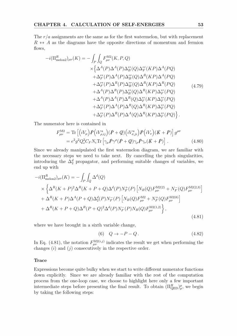
CHAPTER 4. CALCULATION OF SELF-ENERGIES 53
The r/a assignments are the same as for the first watermelon, but with replacementR ↔ A as the diagrams have the opposite directions of momentum and fermionflows,
−i(ΠRmelon2)µν(K) = −
∫P
∫QFM2µν (K,P,Q)
×{
∆A(P )∆A(P )∆rrB (Q)∆rr
F (KP )∆A(PQ)+∆rr
F (P )∆A(P )∆rrB (Q)∆R(KP )∆A(PQ)
+∆rrF (P )∆R(P )∆rr
B (Q)∆R(KP )∆R(PQ)+∆A(P )∆R(P )∆rr
B (Q)∆R(KP )∆rrF (PQ)
+∆A(P )∆A(P )∆R(Q)∆rrF (KP )∆rr
F (PQ)+∆rr
F (P )∆A(P )∆R(Q)∆R(KP )∆rrF (PQ)
+∆rrF (P )∆R(P )∆A(Q)∆R(KP )∆rr
F (PQ)}.
(4.79)
The numerator here is contained in
FM2µν = Tr
[(iVµ
)/P(iV aρ,ij
)(/P + /Q)
(iV aσ,ji
)/P(iVν
)( /K + /P )
]gρσ
= e2g2Q2eCFNcTr
[γµ /Pγ
ρ(/P + /Q)γρ /Pγν( /K + /P )]. (4.80)
Since we already manipulated the first watermelon diagram, we are familiar withthe necessary steps we need to take next. By cancelling the pinch singularities,introducing the ∆d
2 propagator, and performing suitable changes of variables, weend up with
−i(ΠRmelon2)µν(K) = −
∫P
∫Q
∆d(Q)
×{
∆R(K + P )2∆R(K + P +Q)∆d(P )N+F (P )
[NB(Q)FM2(2)
µν +N−F (Q)FM2(2,3)µν
]+ ∆R(K + P )∆A(P +Q)∆d
2(P )N−F (P )[NB(Q)FM2
µν +N+F (Q)FM2(6)
µν
]+ ∆R(K + P +Q)∆R(P +Q)2∆d(P )N−F (P )NB(Q)FM2(1,2)
µν
},
(4.81)where we have brought in a sixth variable change,
(6) Q→ −P −Q . (4.82)
In Eq. (4.81), the notation FM2(i,j)µν indicates the result we get when performing the
changes (i) and (j) consecutively in the respective order.
Trace
Expressions become quite bulky when we start to write different numerator functionsdown explicitly. Since we are already familiar with the rest of the computationprocess from the one-loop case, we choose to highlight here only a few importantintermediate steps before presenting the final result. To obtain (ΠR
QED)µµ, we beginby taking the following steps:
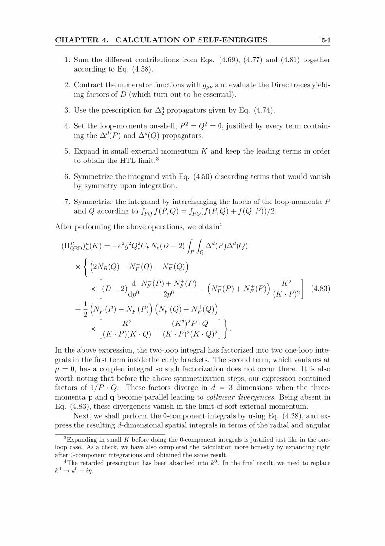
CHAPTER 4. CALCULATION OF SELF-ENERGIES 54
1. Sum the different contributions from Eqs. (4.69), (4.77) and (4.81) togetheraccording to Eq. (4.58).
2. Contract the numerator functions with gµν and evaluate the Dirac traces yield-ing factors of D (which turn out to be essential).
3. Use the prescription for ∆d2 propagators given by Eq. (4.74).
4. Set the loop-momenta on-shell, P 2 = Q2 = 0, justified by every term contain-ing the ∆d(P ) and ∆d(Q) propagators.
5. Expand in small external momentum K and keep the leading terms in orderto obtain the HTL limit.3
6. Symmetrize the integrand with Eq. (4.50) discarding terms that would vanishby symmetry upon integration.
7. Symmetrize the integrand by interchanging the labels of the loop-momenta Pand Q according to
∫PQ f(P,Q) =
∫PQ(f(P,Q) + f(Q,P ))/2.
After performing the above operations, we obtain4
(ΠRQED)µµ(K) = −e2g2Q2
eCFNc(D − 2)∫P
∫Q
∆d(P )∆d(Q)
×{(
2NB(Q)−N−F (Q)−N+F (Q)
)×[(D − 2) d
dp0N−F (P ) +N+
F (P )2p0 −
(N−F (P ) +N+
F (P )) K2
(K · P )2
]
+ 12(N−F (P )−N+
F (P )) (N−F (Q)−N+
F (Q))
×[
K2
(K · P )(K ·Q) −(K2)2P ·Q
(K · P )2(K ·Q)2
]}.
(4.83)
In the above expression, the two-loop integral has factorized into two one-loop inte-grals in the first term inside the curly brackets. The second term, which vanishes atµ = 0, has a coupled integral so such factorization does not occur there. It is alsoworth noting that before the above symmetrization steps, our expression containedfactors of 1/P · Q. These factors diverge in d = 3 dimensions when the three-momenta p and q become parallel leading to collinear divergences. Being absent inEq. (4.83), these divergences vanish in the limit of soft external momentum.
Next, we shall perform the 0-component integrals by using Eq. (4.28), and ex-press the resulting d-dimensional spatial integrals in terms of the radial and angular
3Expanding in small K before doing the 0-component integrals is justified just like in the one-loop case. As a check, we have also completed the calculation more honestly by expanding rightafter 0-component integrations and obtained the same result.
4The retarded prescription has been absorbed into k0. In the final result, we need to replacek0 → k0 + iη.
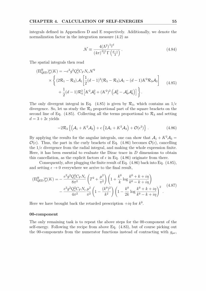
CHAPTER 4. CALCULATION OF SELF-ENERGIES 55
integrals defined in Appendices D and E respectively. Additionally, we denote thenormalization factor in the integration measure (4.2) as
N ≡ 4(Λ2) 3−d2
(4π) d+12 Γ
(d−1
2
) . (4.84)
The spatial integrals then read
(ΠRQED)µµ(K) = −e2g2Q2
eCFNcN 2
×{
(2R1 −R2)A1
[12(d− 1)2(R5 −R3)A1 − (d− 1)K2R3A3
]
+ 12(d− 1)R2
4
[K2A2
2 + (K2)2(A2
3 −Ai6Ai6)]}
.
(4.85)
The only divergent integral in Eq. (4.85) is given by R3, which contains an 1/εdivergence. So, let us study the R3 proportional part of the square brackets on thesecond line of Eq. (4.85). Collecting all the terms proportional to R3 and settingd = 3 + 2ε yields
−2R3{(A1 +K2A3
)+ ε
(2A1 +K2A3
)+O(ε2)
}. (4.86)
By applying the results for the angular integrals, one can show that A1 + K2A3 =O(ε). Thus, the part in the curly brackets of Eq. (4.86) becomes O(ε), cancellingthe 1/ε divergence from the radial integral, and making the whole expression finite.Here, it has been essential to evaluate the Dirac trace in D dimensions to obtainthis cancellation, as the explicit factors of ε in Eq. (4.86) originate from there.
Consequently, after plugging the finite result of Eq. (4.86) back into Eq. (4.85),and setting ε→ 0 everywhere we arrive to the final result,
(ΠRQED)µµ(K) =− e2g2Q2
eCFNc
8π2
(T 2 + µ2
π2
)(1 + k0
klog k
0 + k + iη
k0 − k + iη
)
− e2g2Q2eCFNc
4π2µ2
π2
(1− (k0)2
k2
)(1− k0
2k log k0 + k + iη
k0 − k + iη
)2
.
(4.87)
Here we have brought back the retarded prescription +iη for k0.
00-component
The only remaining task is to repeat the above steps for the 00-component of theself-energy. Following the recipe from above Eq. (4.83), but of course picking outthe 00-components from the numerator functions instead of contracting with gµν ,
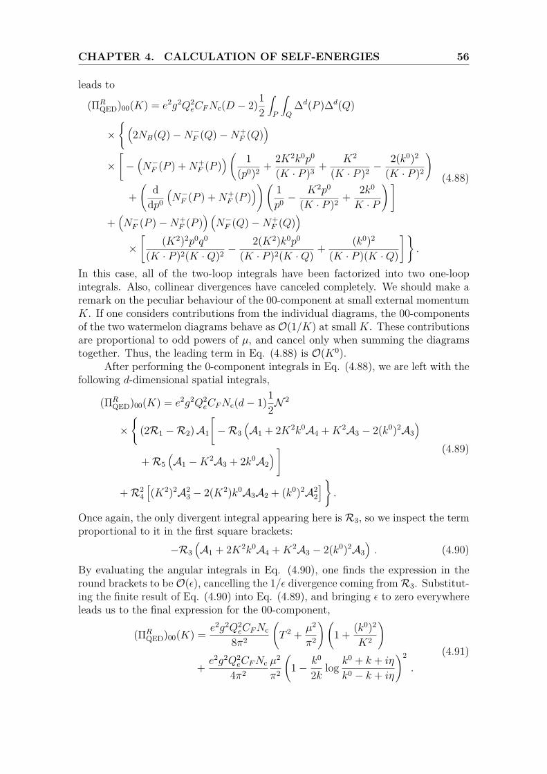
CHAPTER 4. CALCULATION OF SELF-ENERGIES 56
leads to
(ΠRQED)00(K) = e2g2Q2
eCFNc(D − 2)12
∫P
∫Q
∆d(P )∆d(Q)
×{(
2NB(Q)−N−F (Q)−N+F (Q)
)×[−(N−F (P ) +N+
F (P ))( 1
(p0)2 + 2K2k0p0
(K · P )3 + K2
(K · P )2 −2(k0)2
(K · P )2
)
+(
ddp0
(N−F (P ) +N+
F (P )))( 1
p0 −K2p0
(K · P )2 + 2k0
K · P
)]+(N−F (P )−N+
F (P )) (N−F (Q)−N+
F (Q))
×[
(K2)2p0q0
(K · P )2(K ·Q)2 −2(K2)k0p0
(K · P )2(K ·Q) + (k0)2
(K · P )(K ·Q)
]}.
(4.88)
In this case, all of the two-loop integrals have been factorized into two one-loopintegrals. Also, collinear divergences have canceled completely. We should make aremark on the peculiar behaviour of the 00-component at small external momentumK. If one considers contributions from the individual diagrams, the 00-componentsof the two watermelon diagrams behave as O(1/K) at small K. These contributionsare proportional to odd powers of µ, and cancel only when summing the diagramstogether. Thus, the leading term in Eq. (4.88) is O(K0).
After performing the 0-component integrals in Eq. (4.88), we are left with thefollowing d-dimensional spatial integrals,
(ΠRQED)00(K) = e2g2Q2
eCFNc(d− 1)12N
2
×{
(2R1 −R2)A1
[−R3
(A1 + 2K2k0A4 +K2A3 − 2(k0)2A3
)+R5
(A1 −K2A3 + 2k0A2
) ]
+R24
[(K2)2A2
3 − 2(K2)k0A3A2 + (k0)2A22
] }.
(4.89)
Once again, the only divergent integral appearing here is R3, so we inspect the termproportional to it in the first square brackets:
−R3(A1 + 2K2k0A4 +K2A3 − 2(k0)2A3
). (4.90)
By evaluating the angular integrals in Eq. (4.90), one finds the expression in theround brackets to be O(ε), cancelling the 1/ε divergence coming fromR3. Substitut-ing the finite result of Eq. (4.90) into Eq. (4.89), and bringing ε to zero everywhereleads us to the final expression for the 00-component,
(ΠRQED)00(K) = e2g2Q2
eCFNc
8π2
(T 2 + µ2
π2
)(1 + (k0)2
K2
)
+ e2g2Q2eCFNc
4π2µ2
π2
(1− k0
2k log k0 + k + iη
k0 − k + iη
)2
.
(4.91)
CHAPTER 4. CALCULATION OF SELF-ENERGIES 57
From this result, one obtains the NLO correction to the photon Debye mass (asdefined in Ref. [17]),
limk→0
(ΠRQED)00(k0 = 0,k) = e2g2Q2
eCFNc
8π2
(T 2 + 3µ2
π2
), (4.92)
which extends the result in Ref. [17] to finite µ.The transverse and longitudinal components from Eqs. (3.51) and (3.52) read
(ΠRQED)T(K) =− e2g2Q2
eCFNc
8π2
(T 2 + µ2
π2
)k0
2k log k0 + k + iη
k0 − k + iη, (4.93)
(ΠRQED)L(K) =− e2g2Q2
eCFNc
8π2
(T 2 + µ2
π2
)
− e2g2Q2eCFNc
4π2µ2
π2
(1− (k0)2
k2
)(1− k0
2k log k0 + k + iη
k0 − k + iη
)2
.
(4.94)
The limit µ = 0 of Eqs. (4.93) and (4.94) agrees with the results by Carignano etal. [6]. They have computed the same quantity for vanishing chemical potential,letting the internal line to be a photon. The result with the internal gluon replacedby a photon can be obtained by the replacement g2Q2
eCFNc → e2, since the internalgluon line only provides an overall color factor. Our result shows that at the two-loop order the finite chemical potential does not only modify the “mass factor” byT 2 → T 2 +µ2/π2 as in the one-loop case, but introduces a completely new kinematicstructure to the longitudinal component that is proportional to µ2/π2 and includesa square of a logarithm.
5. Conclusions
In this Thesis, we have calculated thermal parts of QCD (and QED) self-energies inthe HTL limit at finite temperature and chemical potential, specifically for the quarkand gluon at one-loop order and for the photon at two-loop order. The latter pro-vides a NLO extension to the current HTL theory at finite density. Along the way,we reviewed the essential tools and techniques necessary for such self-energy calcu-lations, further serving as a preparation to a forthcoming two-loop gluon self-energycomputation. Particularly, after the Introduction in Chapter 1, we introduced thereal-time formulation of perturbative thermal field theory, including the conceptof self-energy in Chapter 2. These ideas were generalized to QCD in Chapter 3,where we also discussed the role of HTLs as an effective description of soft physicsin thermal QCD. HTL theory supplied the primary motivation for our self-energycalculations that we presented in detail in Chapter 4.
The main result of this Thesis, the two-loop photon self-energy in the HTLlimit at finite temperature and density, can be directly applied in determining phys-ical quantities. For example, by solving the poles of the HTL-resummed propagatorgiven by the dispersion relations
K2 + ΠRT/L(K) = 0 , (5.1)
one obtains the NLO correction to the plasma frequency of soft photons in theQCD medium. For that, other possible NLO contributions should be checked for.One results from power corrections, which are given by expanding the one-loopphoton self-energy to the NLO for small external momenta. Another possibilityis that some of the internal lines of the two-loop diagrams become soft and requireresummation (as discussed below Fig. 3.1). However, by power counting arguments,these HTL-resummed diagrams do not contribute at the NLO level [42]. Thus,the only pieces missing from the NLO result are the power corrections, which arefairly straightforward to compute given the tools we have developed. The dispersionrelation and other physical applications will be further studied in future publications.
The long-term goal of the research related to this Thesis is to complete thecalculation of the NNNLO pressure of cold dense QCD, yielding a new perturbativecorrection to the equation of state of cold quark matter. The perturbative resultwould help us gain insight into the extreme physics in the cores of neutron stars.The next step towards that is to extend our photonic result to the two-loop gluonself-energy in the HTL limit.
58
A. Notation and Conventions
We work in D spacetime dimensions and d = D − 1 spatial dimensions with theMinkowskian metric
gµν = diag(−1,+1, ...,+1) . (A.1)With the “mostly plus” metric, the Clifford algebra reads{
γµ, γν}
= −2gµν . (A.2)
Four-vectors are denoted by upper case letters and the magnitudes of spatial vectorswith lower case letters,
P ≡ (p0,p) , p ≡ |p| , (A.3)where the individual spatial components are pi, i = 1, ..., d. The integration measureis defined as ∫
P≡∫ dDP
(2π)D =∫ ∞−∞
dp0
2π
∫p, (A.4)
and the spatial part is ∫p≡ (Λ2) 3−d
2
∫ ddp(2π)d , (A.5)
where Λ is the renormalization scale parameter. Momentum integrations are regu-lated by letting the spacetime dimension be D = 4 + 2ε, where ε > 0.
We apply the Latin letters i, j, k, ... for fundamental color indices as well as forthe components of spatial vectors. The difference between the two is understoodfrom the context. The Latin letters a, b, c, ... are reserved for adjoint color indicesand the Greek letters µ, ν, ρ, ... for spacetime indices. Repeated indices are alwayssummed over.
Throughout the Thesis, we use the natural units, where the reduced Planckconstant ~, the speed of light c, and the Boltzmann constant kB have been set tounity.
Finally, we should highlight the sign convention we employ for self-energies.The self-energies are defined as i times the appropriate Feynman diagram.
59
B. Complex Time Translation
In Chapter 2, we defined the time translation operator as
U(t1, t0) = e−iH(t1−t0) , (B.1)
evolving operators from time t0 to t1 in the Heisenberg picture. Here we assume thatthe Hamiltonian of the system H is time-independent. By relaxing the assumptionof the reality of t1 and t0, we can analytically continue Eq. (B.1) to describe complextime translation,
U(z1, z0) = e−iH(z1−z0) , (B.2)where z0 and z1 are complex-valued. To check if Eq. (B.2) is well-defined, wewrite its matrix element in the field basis |φi〉 and insert a complete set of energyeigenstates to obtain the spectral representation,
〈φi|e−iH(z1−z0)|φj〉 =∑n
e−iEn(z1−z0) 〈φi|n〉 〈n|φj〉 . (B.3)
For this sum to converge, we must require Im(z1−z0) ≤ 0 since energies are positive.Given a general complex time path z = γ(u) connecting z0 to z1, where u
is real and monotonically increasing, we may decompose U(z1, z0) as a product ofinfinitesimal time translation operators along the path γ. Each of the infinitesimaloperators must then correspond to time translation with a non-increasing imaginarypart according to the convergence of its spectral representation. Hence, Im(γ(u))has to be a non-increasing function of u for U(z1, z0) to be well-defined. As usual,we may write the matrix element of U(z1, z0) as a path integral,
〈φi|e−iH(z1−z0)|φj〉 =∫ φ(z1)=φi
φ(z0)=φjDφ(z)eiS[φ] , (B.4)
where the integration is performed over the field configurations defined on the com-plex path γ. The path integral representation in Eq. (B.4) is, in fact, independentof the choice of γ [43], as long as it has a non-increasing imaginary part, starts fromz0 and ends to z1. As we are interested in representing the matrix element of thegrand canonical density operator as a path integral, we end up taking z0 = t0 andz1 = t0 − iβ, t0 being real, and choosing γ to be vertical. This time path obviouslysatisfies our requirements.
60
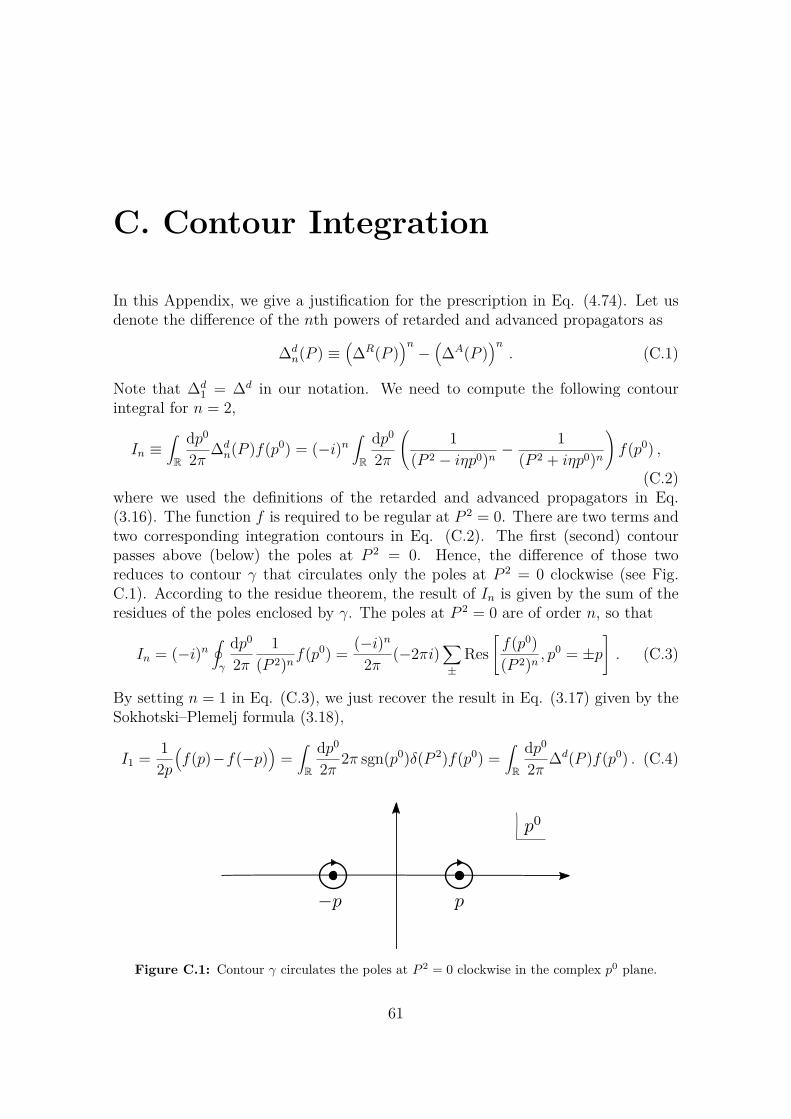
C. Contour Integration
In this Appendix, we give a justification for the prescription in Eq. (4.74). Let usdenote the difference of the nth powers of retarded and advanced propagators as
∆dn(P ) ≡
(∆R(P )
)n−(∆A(P )
)n. (C.1)
Note that ∆d1 = ∆d in our notation. We need to compute the following contour
integral for n = 2,
In ≡∫R
dp0
2π ∆dn(P )f(p0) = (−i)n
∫R
dp0
2π
(1
(P 2 − iηp0)n −1
(P 2 + iηp0)n
)f(p0) ,
(C.2)where we used the definitions of the retarded and advanced propagators in Eq.(3.16). The function f is required to be regular at P 2 = 0. There are two terms andtwo corresponding integration contours in Eq. (C.2). The first (second) contourpasses above (below) the poles at P 2 = 0. Hence, the difference of those tworeduces to contour γ that circulates only the poles at P 2 = 0 clockwise (see Fig.C.1). According to the residue theorem, the result of In is given by the sum of theresidues of the poles enclosed by γ. The poles at P 2 = 0 are of order n, so that
In = (−i)n∮γ
dp0
2π1
(P 2)nf(p0) = (−i)n2π (−2πi)
∑±
Res[f(p0)(P 2)n , p
0 = ±p]. (C.3)
By setting n = 1 in Eq. (C.3), we just recover the result in Eq. (3.17) given by theSokhotski–Plemelj formula (3.18),
I1 = 12p(f(p)−f(−p)
)=∫R
dp0
2π 2π sgn(p0)δ(P 2)f(p0) =∫R
dp0
2π ∆d(P )f(p0) . (C.4)
Figure C.1: Contour γ circulates the poles at P 2 = 0 clockwise in the complex p0 plane.
61
APPENDIX C. CONTOUR INTEGRATION 62
The case of n = 2 gives us the desired result,
I2 = − 2i(2p)3
(f(p)− f(−p)
)+ i
(2p)2
(f ′(p) + f ′(−p)
)= i
∫R
dp0
2π ∆d(P ) ddp0
f(p0)2p0 , (C.5)
where we have obtained the final line by using the δ-function representation of ∆d
given by Eq. (3.17).
D. Radial Integrals
Here we list some results for radial integrals over the distribution functions definedin the beginning of Chapter 4. To save space, we denote the radial part of theintegration measure in d = 3 + 2ε spatial dimensions (see Eq. (4.2)) as∫
p≡∫ ∞
0dp pd−1 . (D.1)
The results for integrals over the bosonic and fermionic distribution functions maybe written in terms of polylogarithm as follows∫
ppαNB(p) = T d+αΓ(d+ α)Lid+α (1) , (D.2)∫
ppαN±F (p) = T d+αΓ(d+ α)Lid+α
(−e∓
µT
), (D.3)
for some parameter α. Scale-free parts of the integrands have been discarded as theyvanish in dimensional regularization. By integrating by parts, we obtain results forthe derivatives of the distribution functions,∫
ppα
ddpNB(p) = −T d+α−1Γ(d+ α)Lid+α−1 (1) , (D.4)∫
ppα
ddpN
±F (p) = −T d+α−1Γ(d+ α)Lid+α−1
(−e∓
µT
). (D.5)
For our calculations in Chapter 4, we need the leading terms of the small ε expansionsfor various combinations of the above integrals for particular values of α,
R1 ≡∫p
1pNB(p) = π2T 2
6 +O(ε) , (D.6)
R2 ≡∫p
1p
(N−F (p) +N+
F (p))
= −π2T 2 + 3µ2
6 +O(ε) , (D.7)
R3 ≡∫p
1p3
(N−F (p) +N+
F (p))
= − 12ε +O(ε0) , (D.8)
R4 ≡∫p
1p2
(N−F (p)−N+
F (p))
= −µ+O(ε) (D.9)
R5 ≡∫p
1p2
ddp(N−F (p) +N+
F (p))
= 1 +O(ε) . (D.10)
63
E. Angular Integrals
This Appendix is reserved for the results of some angular integrals appearing in ourcalculations. In d = 3 + 2ε spatial dimensions, the angular piece of the integrationmeasure in Eq. (4.2) may be written as∫
z≡∫ 1
−1dz (1− z2) d−3
2 , (E.1)
where z = k · p parametrizes an angle between an external velocity k and loopvelocity p. According to our conventions, the “direction” of the on-shell loop four-momentum P is denoted by v = (1, p), so that v ·K = −k0 + kz for the externalfour-momentum K. In the HTL limit, we often encounter integrals of the type
∫z
1(v ·K)α =
Γ(
12
)Γ(
12(d− 1)
)Γ(d2
) (−k0)−α2F1
(α
2 ,1 + α
2 ; d2; k2
(k0)2
), (E.2)
for some parameter α. The result has been written in terms of the hypergeometricfunction. Another useful integral is∫z
vi
(v ·K)α = ki∫z
z
(v ·K)α
= αki
2k0
Γ(
12
)Γ(
12(d− 1)
)Γ(
2+d2
) (−k0)−α2F1
(1 + α
2 ,2 + α
2 ; 2 + d
2 ; k2
(k0)2
),
(E.3)
where we have exploited rotational symmetry on the first line. By denoting
L(K) ≡ 12k log k
0 + k
k0 − k, (E.4)
64
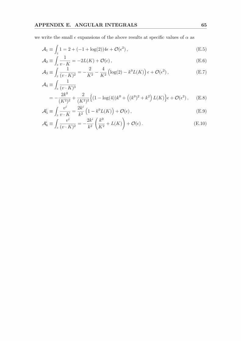
APPENDIX E. ANGULAR INTEGRALS 65
we write the small ε expansions of the above results at specific values of α as
A1 ≡∫z
1 = 2 + (−1 + log(2))4ε+O(ε2) , (E.5)
A2 ≡∫z
1v ·K
= −2L(K) +O(ε) , (E.6)
A3 ≡∫z
1(v ·K)2 = − 2
K2 −4K2
(log(2)− k0L(K)
)ε+O(ε2) , (E.7)
A4 ≡∫z
1(v ·K)3
= − 2k0
(K2)2 + 2(K2)2
{(1− log(4))k0 +
((k0)2 + k2
)L(K)
}ε+O(ε2) , (E.8)
Ai5 ≡∫z
vi
v ·K= 2ki
k2
(1− k0L(K)
)+O(ε) , (E.9)
Ai6 ≡∫z
vi
(v ·K)2 = −2kik2
(k0
K2 + L(K))
+O(ε) . (E.10)
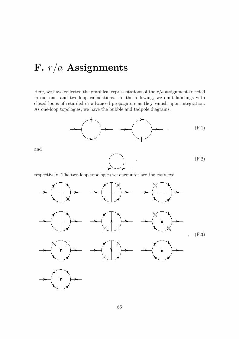
F. r/a Assignments
Here, we have collected the graphical representations of the r/a assignments neededin our one- and two-loop calculations. In the following, we omit labelings withclosed loops of retarded or advanced propagators as they vanish upon integration.As one-loop topologies, we have the bubble and tadpole diagrams,
, (F.1)
and
, (F.2)
respectively. The two-loop topologies we encounter are the cat’s eye
, (F.3)
66
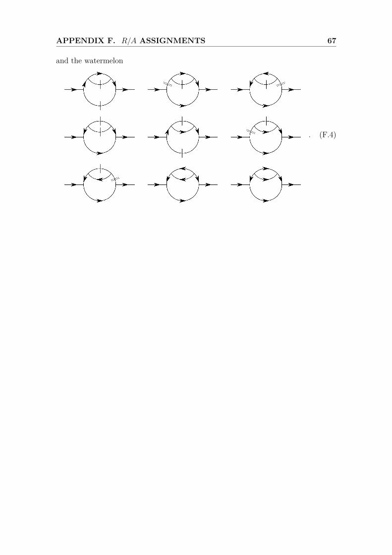
APPENDIX F. R/A ASSIGNMENTS 67
and the watermelon
. (F.4)
Bibliography
[1] Eric Braaten and Robert D. Pisarski. Soft amplitudes in hot gauge theories: Ageneral analysis. Nuclear Physics B, 337(3):569–634, 1990.
[2] Tyler Gorda, Aleksi Kurkela, Risto Paatelainen, Saga Säppi, and Aleksi Vuori-nen. Cold quark matter at nnnlo: soft contributions, 2021.
[3] Hermann Schulz. Gluon plasma frequency — the next-to-leading order term.Nuclear Physics B, 413(1):353–395, 1994.
[4] P. Aurenche, F. Gelis, H. Zaraket, and R. Kobes. Two-loop compton andannihilation processes in thermal qcd. Phys. Rev. D, 60:076002, Aug 1999.
[5] Emil Mottola and Zsolt Szép. Systematics of high temperature perturbationtheory: The two-loop electron self-energy in qed. Phys. Rev. D, 81:025014, Jan2010.
[6] Stefano Carignano, Margaret E. Carrington, and Joan Soto. The htl lagrangianat nlo: The photon case. Physics Letters B, 801:135193, 2020.
[7] Jacopo Ghiglieri, Aleksi Kurkela, Michael Strickland, and Aleksi Vuorinen. Per-turbative thermal qcd: Formalism and applications. Physics Reports, 880:1–73,2020. Perturbative Thermal QCD: Formalism and Applications.
[8] Mikko Laine and Aleksi Vuorinen. Basics of Thermal Field Theory: A Tutorialon Perturbative Computations. Lecture Notes in Physics. Springer InternationalPublishing AG, Switzerland, 2016.
[9] Michel Le Bellac. Thermal Field Theory. Cambridge Monographs on Mathe-matical Physics. Cambridge University Press, 1996.
[10] N.P. Landsman and Ch.G. van Weert. Real- and imaginary-time field theoryat finite temperature and density. Physics Reports, 145(3):141–249, 1987.
[11] Jean-Paul Blaizot and Edmond Iancu. The quark–gluon plasma: collectivedynamics and hard thermal loops. Physics Reports, 359(5):355–528, 2002.
[12] U Kraemmer and A Rebhan. Advances in perturbative thermal field theory.Reports on Progress in Physics, 67(3):351–431, feb 2004.
68
BIBLIOGRAPHY 69
[13] Richard P. Feynman and Albert R. Hibbs. Quantum mechanics and path inte-grals. McGraw-Hill, New York, 1965. ID: 987995.
[14] P. T. Matthews and A. Salam. Propagators of quantized field. Il Nuovo Cimento(1955-1965), 2(1):120–134, Jul 1955.
[15] Kuang chao Chou, Zhao bin Su, Bai lin Hao, and Lu Yu. Equilibrium andnonequilibrium formalisms made unified. Physics Reports, 118(1):1–131, 1985.
[16] E. Calzetta and B. L. Hu. Nonequilibrium quantum fields: Closed-time-path ef-fective action, wigner function, and boltzmann equation. Phys. Rev. D, 37:2878–2900, May 1988.
[17] Joseph I. Kapusta and Charles Gale. Finite-Temperature Field Theory: Prin-ciples and Applications. Cambridge Monographs on Mathematical Physics.Cambridge University Press, 2 edition, 2006.
[18] H. Umezawa, H. Matsumoto, and M. Tachiki. Thermo field dynamics andcondensed states. North-Holland Pub. Co. ; Sole distributors for the U.S.A.and Canada, Elsevier Science Pub. Co., Amsterdam; New York; New York,N.Y., 1982. ID: 8114603.
[19] Julian Schwinger. Brownian motion of a quantum oscillator. Journal of Math-ematical Physics, 2(3):407–432, 1961.
[20] L.V. Keldysh. Diagram technique for nonequilibrium processes. Zh. Eksp. Teor.Fiz., 47:1515–1527, 1964.
[21] Takeo Matsubara. A New Approach to Quantum-Statistical Mechanics.Progress of Theoretical Physics, 14(4):351–378, 10 1955.
[22] Ryogo Kubo. Statistical-mechanical theory of irreversible processes. 1. generaltheory and simple applications to magnetic and conduction problems. Journalof the Physical Society of Japan, 12(6):570–586, 1957.
[23] Paul C. Martin and Julian Schwinger. Theory of many-particle systems. 1.Phys. Rev., 115:1342–1373, Sep 1959.
[24] T. S. Evans and A. C. Pearson. Reexamination of the path-ordered approachto real time thermal field theory. Phys. Rev. D, 52:4652–4659, Oct 1995.
[25] Simon Caron-Huot. Hard thermal loops in the real-time formalism. Journal ofHigh Energy Physics, 2009(04):004–004, Apr 2009.
[26] Philippe de Forcrand. Simulating QCD at finite density. PoS, LAT2009:010,2009.
[27] Michael E. Peskin and Daniel V. Schroeder. An Introduction to quantum fieldtheory. Addison-Wesley, Reading, USA, 1995.
BIBLIOGRAPHY 70
[28] L.D. Faddeev and V.N. Popov. Feynman diagrams for the yang-mills field.Physics Letters B, 25(1):29–30, 1967.
[29] A. A. Slavnov. Ward identities in gauge theories. Theoretical and MathematicalPhysics, 10(2):99–104, Feb 1972.
[30] J.C. Taylor. Ward identities and charge renormalization of the yang-mills field.Nuclear Physics B, 33(2):436–444, 1971.
[31] H.Arthur Weldon. Structure of the gluon propagator at finite temperature.Annals of Physics, 271(1):141–156, 1999.
[32] David J. Gross, Robert D. Pisarski, and Laurence G. Yaffe. Qcd and instantonsat finite temperature. Rev. Mod. Phys., 53:43–80, Jan 1981.
[33] K Kajantie and J Kapusta. Behaviour of gluons at high temperature. Annalsof Physics, 160(2):477–513, 1985.
[34] R. Kobes, G. Kunstatter, and K. W. Mak. Linear response of the hot qcdplasma from the gluon propagator. Zeitschrift für Physik C Particles and Fields,45(1):129–140, Mar 1989.
[35] J. Frenkel and J.C. Taylor. High-temperature limit of thermal qcd. NuclearPhysics B, 334(1):199–216, 1990.
[36] F. T. Brandt, J. Frenkel, and F. R. Machado. Finite temperature gluon self-energy in a class of temporal gauges. Phys. Rev. D, 61:125014, May 2000.
[37] R. Kobes, G. Kunstatter, and A. Rebhan. Gauge dependence identities andtheir application at finite temperature. Nuclear Physics B, 355(1):1–37, 1991.
[38] A.D. Linde. Infrared problem in the thermodynamics of the yang-mills gas.Physics Letters B, 96(3):289–292, 1980.
[39] Tyler Gorda, Aleksi Kurkela, Risto Paatelainen, Saga Säppi, and Aleksi Vuori-nen. Soft interactions in cold quark matter, 2021.
[40] Eric Braaten and Robert D. Pisarski. Simple effective lagrangian for hardthermal loops. Phys. Rev. D, 45:R1827–R1830, Mar 1992.
[41] J.C. Taylor and S.M.H. Wong. The effective action of hard thermal loops inqcd. Nuclear Physics B, 346(1):115–128, 1990.
[42] A. Mirza and M. E. Carrington. Thermal field theory at next-to-leading orderin the hard thermal loop expansion. Phys. Rev. D, 87:065008, Mar 2013.
[43] David W. McLaughlin. Complex time, contour independent path integrals, andbarrier penetration. Journal of Mathematical Physics, 13(8):1099–1108, 1972.