How Xenopus laevis embryos replicate reliably: Investigating the random-completion problem

How Xenopus laevis embryos replicate reliably: Investigating the random-completion problem

Scott Cheng-Hsin Yang (楊正炘�* and John BechhoeferDepartment of Physics, Simon Fraser University, Burnaby, British Columbia, Canada V5A 1S6

�Received 12 June 2008; published 27 October 2008�

DNA synthesis in Xenopus frog embryos initiates stochastically in time at many sites �origins� along thechromosome. Stochastic initiation implies fluctuations in the time to complete and may lead to cell death ifreplication takes longer than the cell cycle time ��25 min�. Surprisingly, although the typical replication timeis about 20 min, in vivo experiments show that replication fails to complete only about 1 in 300 times. How isreplication timing accurately controlled despite the stochasticity? Biologists have proposed two solutions tothis “random-completion problem.” The first solution uses randomly located origins but increases their rate ofinitiation as S phase proceeds, while the second uses regularly spaced origins. In this paper, we investigate therandom-completion problem using a type of model first developed to describe the kinetics of first-order phasetransitions. Using methods from the field of extreme-value statistics, we derive the distribution of replication-completion times for a finite genome. We then argue that the biologists’ first solution to the problem is not onlyconsistent with experiment but also nearly optimizes the use of replicative proteins. We also show that spatialregularity in origin placement does not alter significantly the distribution of replication times and, thus, is notneeded for the control of replication timing.

DOI: 10.1103/PhysRevE.78.041917 PACS number�s�: 87.15.A�, 87.14.G�, 87.17.Ee, 87.15.Ya

I. INTRODUCTION

DNA replication is an important yet complicated processthat requires not only accurate and efficient DNA synthesisbut also genome-wide coordination among replicative pro-teins �1�. In a time that can be as short as a few minutes, allof a cell’s O�109� bases of DNA must be replicated once andonly once �2,3�. Unfaithful and uncontrolled replication ofthe genome—for example, misreplication, partial replication,and rereplication—can lead to chromosomal instability thatactivates programmed cell death or oncogenes �4,5�. Overthe past few decades, significant advances have been made inidentifying the molecular basis of DNA repair and rereplica-tion prevention �3,6�. On the other hand, it is only in the lastfew years that large amounts of data on the genome-widecoordination have become available. In particular, a tech-nique called molecular combing has been used to examinethe replication state of large fractions of the genome by con-trolled stretching of fluorescently labeled replicated and un-replicated regions onto a substrate �7,8�.

Many of the molecular-combing experiments have beendone on embryos of the South African clawed frog Xenopuslaevis �9–11�. The detailed kinetics of replication revealed aparticularly interesting scenario where stochastic effects playan important role in the DNA replication process �9,12�. Inprevious work, we mapped the stochastic replication processonto a one-dimensional nucleation-and-growth process andmodeled the detailed kinetics of replication seen inmolecular-combing experiments �11,13,14�. In a recent Let-ter, we extended the model to quantitatively address a gen-eralized version of the “random-completion problem,” whichasks how cells can accurately control the replication comple-tion time despite the stochasticity �15�. Here, we give fulldetails about those calculations and go further, to investigate

the idea that cells regulate the replication process in order tominimize their use of cell “resources” and to explore theeffects of spatial regularity on the placement of origins.

A. DNA replication in eukaryotic cells

DNA replication is a two-step process �3�. First, potentialorigins—sites where DNA synthesis may start—are “li-censed” across the genome. For somatic cells, licensing oc-curs in the G1 phase of the cell cycle; for embryos, whoseabbreviated cell cycles lack the G1 and G2 phases, this oc-curs late in the mitosis �M� phase. The process of licensinginvolves the formation of prereplicative complexes �pre-RCs� of proteins. Each complex is first formed through thebinding of a single group of six proteins, known as the originrecognition complex �ORC�, to the DNA. Each ORC, withthe help of two additional proteins �Cdc6 and Cdt1�, thenrecruits 20–40 copies of minichromosome maintenance�MCM� 2-7 hexamer rings onto the chromosome �3�. Afterlicensing, the second step, DNA synthesis, starts in the syn-thesis �S� phase. The synthesis begins with the initiation of apotential origin—two of the MCM2-7 rings—triggered bythe association of cyclin-dependent kinases �3�. Once an ori-gin is initiated, the pre-RC disassembles, and two helicases,probably the MCM2-7 rings, move bidirectionally outwardfrom the origin to unwind the double-stranded DNA, form-ing two symmetrically propagating replication forks. Poly-merases are recruited behind the forks to synthesize DNA onthe single-stranded DNA. When two replication forks travel-ing in opposite directions meet, the helicases disassemble,and the two growing strands of newly synthesized DNA arejoined together by DNA ligases. This process is referred to asa coalescence. In eukaryotic cells, the processes of origininitiation, fork progression, and domain coalescence takeplace at multiple sites throughout S phase until the wholegenome is replicated. Rereplication is prevented because pre-RCs are “nonrecyclable” in S phase. When potential origins*[email protected]

PHYSICAL REVIEW E 78, 041917 �2008�

Selected for a Viewpoint in Physics

1539-3755/2008/78�4�/041917�15� ©2008 The American Physical Society041917-1

http://dx.doi.org/10.1103/PhysRevE.78.041917

http://link.aps.org/viewpoint-for/10.1103/PhysRevE.78.041917

initiate or are passively replicated by other replication forks,pre-RCs disassemble and are inhibited from reassembling onthe DNA throughout the current S phase, thereby preventingreinitiation and rereplication �3�.

B. The random-completion problem

Replication in Xenopus embryos is interesting because theprocess is stochastic yet the replication completion times aretightly controlled. After fertilization, a Xenopus embryo un-dergoes 12 rounds of synchronous, uninterrupted, and abbre-viated cell cycles �lacking G1 and G2 phases�, whose dura-tions are strictly controlled by biochemical processes that areindependent of replication �4,16�. In contrast to the case ofmost somatic cells, these embryonic cells lack an efficientS /M checkpoint to delay entrance into mitosis for unusuallyslow replication �17�. Nonetheless, in each embryonic cellcycle, roughly 3�109 base pairs of DNA are replicated in a20-min S phase followed by a 5-min mitosis phase at 23 °C�18,19�. If replication is not completed before the end ofmitosis, the cell suffers a “mitotic catastrophe” where thechromosomes break, eventually leading to cell death�4,20,21�. �See Sec. III A for more discussion.� In replicatingthe lengthy genome, O�106� potential origins are licensed,without sequence specificity, and initiated stochasticallythroughout S phase �11,12,22–24�. One might expect thisspatiotemporal stochasticity to lead to large fluctuations inreplication times, which would result in frequent mitotic ca-tastrophes. However, experiments imply that such cata-strophic events for Xenopus embryos happen only once inabout 300 instances �see Sec. III A�. This means that, despitethe stochasticity in licensing and initiations, Xenopus em-bryos tightly control the duration of S phase, in order to meetthe 25-min “deadline” imposed by the cell-cycle duration.

Laskey was the first to ask whether non-sequence-specificlicensing might lead to incomplete replication �25�. Specifi-cally, he assumed that origins in embryonic cells initiate atthe start of S phase. He then noted that if the origins werelicensed at random, they would have an exponential distribu-tion of separations. With the estimates of the average inter-origin spacing and fork velocity known at that time, onewould expect a few large gaps. The extra time needed toreplicate the gaps would then imply a replication time largerthan the known duration of S phase. Even though some de-tails have changed, biologists still have such a paradox inmind when they refer to the random-completion problem�18�.

In older references in replication �e.g., �26��, it was as-sumed implicitly that the potential origins are associatedwith ORCs. The estimated number of ORCs per nucleus inXenopus embryos is about 3.5�105 �1 ORC per 8 kilobase-pairs� �22�. Positioning these ORCs randomly on the genome�non-sequence-specificity assumption�, one indeed findsmany gaps that cannot be replicated in time �12,18�. How-ever, more recent experiments revealed that initiations coin-cide with the MCM2-7 rings and that each ORC loads 20-40copies of MCM2-7 �23,24�. Using a pair of MCM rings as apotential origin, one then expects about �5.3�1.7��106 po-tential origins per nucleus �1.9�0.6 potential origins/kb�.

With such a high density of potential origins, there is negli-gible chance of having a gap that is too large to replicatewhen licensed randomly �see Sec. III B�. Although a largeexcess of potential origins can resolve the issue, the actualdistribution of these origins is not known. There is evidencethat potential origins can cluster together, effectively reduc-ing the average density �18�. In addition, experiments alsoshowed that potential origins initiate throughout S phase in astochastic manner �11�.

Over the years, biologists have proposed two qualitativescenarios to address this random-completion paradox. Thefirst scenario, the “regular-spacing model,” incorporatesmechanisms that regularize the placement of potential ori-gins despite the nonsequence specificity to suppress largeinterorigin gaps �16�. The second scenario, the “origin-redundancy model,” uses a large excess of randomly licensedpotential origins and initiates them with increasing probabil-ity throughout S phase �11,16,27�. Experimentally, the ob-served replication kinetics in Xenopus are compatible withthe origin-redundancy model, but there is also evidence forlimited regularity in the origin spacings �18,28,29�.

In this paper, we shall reformulate the random-completionproblem in a more general way. In particular, we investigatenot only the possibility of replication completion, but alsothe probability of completion �fluctuations in completiontime�. We generalize both scenarios to incorporate time-dependent origin initiation rates using a stochastic model andMonte Carlo simulations. We then investigate how cells con-trol the replication time despite the non-sequence-specificplacement and stochastic initiation of potential origins. Aswe shall see, the fluctuations in the replication times can bereduced arbitrarily if one allows an unrestricted number ofinitiations. As an extreme example, having an infinite num-ber of initiations at time t* implies that replication will al-ways finish at t*. Thus, an even more general formulation ofthe random-completion problem is to ask how reliability intiming control can be achieved with a reasonable or “opti-mal” use of resources in the cell. Of course, the terms “rea-sonable,” “optimal,” and “resources” must be carefully de-fined.

In the following section, we review and extend the previ-ously developed model of replication to derive the distribu-tion of replication times �13,14�. The results will show howreplication timing can be controlled despite the stochasticity.In Sec. III, we use the extended model to extract replicationparameters from in vivo and in vitro experiments. In Sec. IV,we compare the extracted in vivo “replication strategy” withthe strategy that optimizes the consumption of replicationforks. In Sec. V, we explore the effect of spatial ordering onthe replication time via a variant of the regular-spacingmodel. We summarize our findings in Sec. VI.

II. MODELING REPLICATION COMPLETION

In previous work, we developed a stochastic model ofDNA replication �13,14� that was inspired by theKolmogorov-Johnson-Mehl-Avrami �KJMA� theory ofphase-change kinetics �30–35�. The KJMA model capturesthree aspects of phase transformation: nucleation of the

SCOTT CHENG-HSIN YANG AND JOHN BECHHOEFER PHYSICAL REVIEW E 78, 041917 �2008�

041917-2

transformed phase, growth of the nucleated domains, andcoalescence of impinging domains. Making a formal analogybetween phase transformations and DNA replication, wemap the kinetics of the DNA replication onto a one-dimensional KJMA model with three corresponding ele-ments: initiation of potential origins, growth of replicateddomains, and coalescence of replicated domains. Note thatour use of a phase-transformation model implicitly incorpo-rates the observation that, ordinarily, rereplication is pre-vented.

Since we neglect any stochasticity in the movement ofreplication forks, the stochastic element of the model liesentirely in the placement and initiation of origins �36�. Thelicensing and initiations can be viewed as a two-dimensionalstochastic process with a spatial dimension whose range cor-responds to the genome and a temporal dimension whoserange corresponds to S phase. There is good evidence thatthe positions of the potential origins in Xenopus embryos arealmost—but not completely—random �12,18,29�. In this sec-tion, we assume the spatial positions of the potential originsto be uniformly distributed across the genome for ease ofcalculation. We discuss the implications of origin regularityin Sec. V. The temporal program of stochastic initiation timesis governed by an initiation function I�t�, defined as the rateof initiation per unreplicated length per time. In writingdown the initiation rate as a simple function of time, we areimplicitly averaging over any spatial variation and neglectingcorrelations in neighboring initiations. The I�t� deduced froma previously analyzed in vitro experiment on Xenopus im-plies that the initiation rate increases throughout S phase�11�. In order to explore analytically a family of initiationfunctions that includes such a form, we investigate the dis-tribution of replication completion times associated withI�t�= Intn, with In a constant. We also examine an alternative�-function form, where all potential origins initiate at thestart of S phase, as one might expect this to be the bestscenario for accurate control of replication time. �In the earlyliterature on DNA replication, biologists assumed this sce-nario to be true �25�.�

Figure 1 shows schematically the initiations and subse-quent development of replicated domains discussed earlier.

After initiation, a replicated domain grows bidirectionallyoutward from the origin. The growth stops when domainsmeet and coalescence but proceeds elsewhere. Multiple do-mains grow and coalesce throughout S phase until the entiregenome is duplicated. We shall assume, for simplicity, thatthe replication fork velocity is constant. Since variations infork velocity have been observed, a constant velocity shouldbe interpreted as averaging over the course of S phase�37,38�. We discuss the effect of varying fork velocities inmore detail in Sec. III B.

Our model results in a deterministic growth pattern oncethe initiations are set. Figure 1 illustrates such deterministicgrowth and shows that, except at the edges, there is a one-to-one mapping between the initiations and the coalescences.It follows that every distribution of initiations �i�t� deter-mines an associated distribution of coalescences �c�t�. Sincethe completion of replication is marked by the last coales-cence, the problem of determining the time needed to repli-cate a genome of finite length is equivalent to that of deter-mining the distribution of times at which the last coalescenceoccurs. We refer to this distribution as the “end-time” distri-bution �e�t�. Below, we derive an analytical approximationto the end-time distribution function for arbitrary I�t�. Thisanalytical result will allow us to investigate how licensingand initiation programs affect the timing of replicationcompletion.

In addition to analytic results, we also carried out exten-sive numerical simulations of DNA replication. The simula-tion algorithm used is a modified version of the previouslydeveloped “phantom-nuclei algorithm” �13�. The phantom-nuclei algorithm includes three main routines: the first deter-mines the random-licensing positions and the origins’ sto-chastic initiation times via Monte Carlo methods �39�; thesecond implements the deterministic growth; and the thirdeliminates passively replicated origins. Once potential ori-gins are licensed, the algorithm can calculate the state of thegenome at any time step without computing intermediatetime steps. We modified our earlier code to generate end-time distributions using the bisection method to search forthe first t at which the replication fraction f becomes 1 �40�.All programming was done using IGOR PRO v. 6.01 �41�.

A. The end-time distribution

In previous work, we showed that for an infinitely longgenome the fraction f of the genome that has replicated attime t is given by �13�

f�t� = 1 − e−2vh�t�, �1�

where v is the fork velocity �assumed constant�, h�t�=�0

t g�t��dt�, and g�t�=�0t I�t��dt�. Equation �1� predicts that

an infinite time is needed to fully duplicate the genome;however, since all real genomes are finite in length, they canbe fully replicated in a finite amount of time. During thecourse of replication, as long as the number of replicateddomains is much greater than 1, the infinite-genome model isreasonably accurate. However, since the number of domainsis small at the beginning and end of replication �f →0 andf →1�, we expect discrepancies in those regimes. In particu-

FIG. 1. Schematic of the DNA replication model. A horizontalslice in the figure represents the state of the genome at a fixed time.The lighter �darker� gray represents unreplicated �replicated� re-gions. Open circles denote initiated origins, while filled circles de-note coalescences. The dark dotted line cuts across the last coales-cence, which marks the completion of replication. The slope of thelines connecting the adjacent open and filled circles gives the in-verse of the fork velocity.

HOW XENOPUS LAEVIS EMBRYOS REPLICATE… PHYSICAL REVIEW E 78, 041917 �2008�

041917-3

lar, to calculate the finite replication time expected in a finitegenome, we need to extend our previous model.

We begin by introducing the hole distribution nh�x , t�=g2�t�exp�−g�t�x−2vh�t��, which describes the number of“holes” of size x per unit length at time t �13�. A hole is thebiologists’ term for an unreplicated domain surrounded byreplicated domains. Since a coalescence corresponds to ahole of zero length, we define the coalescence distribution�c�t��nh�0, t�. Normalizing by imposing the condition�0

��c�t�dt=1, we find

�c�t� =2vL

Nog2�t�e−2vh�t�, �2�

where L is the genome length and No the expected totalnumber of initiations. Note that No is also the total number ofcoalescences because of the one-to-one mapping discussed inthe previous section. One can calculate No via

No = L�0

�

I�t��1 − f�t��dt = L�0

�

I�t�e−2vh�t�dt , �3�

where the factor �1− f�t�� arises because initiations can occuronly in unreplicated regions. The integrand in Eq. �3� dividedby No is the initiation distribution �i�t�dt, which correspondsto the number of initiations between time t and t+dt.

Given the initiation distribution, we picture the initiationsas sampling No times from �i�t�. This implies that No inde-pendent coalescence times are sampled from �c�t�. The rep-lication completion time, finite on a finite genome, can thenbe associated with the largest value of the No coalescencetimes, and the end-time distribution is the distribution ofthese largest values obtained from multiple sets of samplingfrom �c�t�. At this point, we apply extreme-value theory�EVT� to calculate the end-time distribution. EVT is a well-established statistical theory for determining the distribu-tional properties of the minimum and maximum values of aset of samples drawn from an underlying “parent” distribu-tion �42,43�. The properties of interest include the expectedvalue, fluctuations around the mean, frequency of occur-rence, etc. EVT plays a key role in the insurance industry,where, for example, the “100-year-flood” problem asks forthe expected maximum water level over 100 years �44�. Inphysics, EVT has attracted increasing interest and been ap-plied to analyze crack avalanches in self-organized material�45�, degree distribution in scale-free networks �46�, andmany other problems.

EVT is powerful because of its universality. The key theo-rem in EVT states that the distribution of the extremes of anindependent and identically distributed random variabletends to one of three types of extreme value distributions, theGumbel, Frechet, and Weibull distributions, depending onlyon the shape of the tail of the underlying distribution. Theuniversality of the extreme-value distribution with respect tothe underlying distribution is similar to that of the better-known central limit theorem �47�. For an underlying distri-bution with an unbounded tail that decays exponentially orfaster, the distribution of the extremes tends to a Gumbeldistribution. Such is the case of Xenopus since the underly-ing distribution, the coalescence distribution �c�t�, is ap-

proximately proportional to e−�4, where � is a dimensionless

time �48,49�. The other initiation functions we consider alsolead to the Gumbel distribution.

The Gumbel distribution,

�x� =1

exp�− x − e−x�, x =

t − t*

, �4�

depends on only two parameters, t* and �42,43,50�. Theformer is a “location” parameter that gives the mode of thedistribution. The latter is a “scale” parameter proportional tothe standard deviation. We follow standard procedures to ob-tain t* and as functions of the initiation rate and the forkvelocity �42,50�. The main step is to recognize that the cu-mulative end-time distribution �e�t�, which has a Gumbelform, is equal to the product of No cumulative coalescencedistributions, each resulting from the same initiation distri-bution �i�t�. In other words, the probability that No coales-cences occur at or before time t is equivalent to the probabil-ity that the last of them occurred at or before time t, which isalso the probability that the replication will finish at or be-fore time t. For our case, we find that the mode t* is deter-mined implicitly by

No�1 − �c�t*�� = 1 �5�

and �1 / �No�c�t*��. In Eq. �5�, �c�t� is the cumulativedistribution of �c�t�; thus, �1−�c�t�� is the probability that acoalescence would occur at or after time t. Equation �5� thenimplies that, given a total of No coalescences, t* is the timeafter which the expected number of coalescences is 1, andtherefore the typical end time. The Gumbel form of the end-time distribution is one of our main results, as it allows quan-titative comparison between the fluctuations of completiontimes resulting from different initiation functions.

Below, we derive the end-time distribution for a power-law initiation function In�t�= Intn �where n�−1� and a�-function initiation function I��t�= I��t�. In the power-lawcase, h�t�� tn+2, while for the �-function case, h�t�� t. FromEq. �2�, both initiation forms give rise to coalescence distri-butions that decay exponentially or faster, and thus bothforms will lead to an end-time distribution of the Gumbelform. Using these initiation functions, we see that the coa-lescence distribution given by Eq. �2� is completely deter-mined by three parameters: the fork velocity v, the initiationstrength given by the prefactor In or I�, and the initiationform determined by n or ��t�. The relationship between thesethree parameters and the two Gumbel parameters revealshow different “initiation strategies” affect the completiontime.

We write the cumulative distribution �c�t� of the coales-cences as 1−�t

��c�t��dt�. Then, using integration by parts,we obtain

�t

�

�c�t��dt� =L

Nog�t�e−2vh�t� −

L

No�

t

�

I�t��e−2vh�t��dt�.

�6�

Substituting Eq. �6� into Eq. �5�, we obtain a transcendentalequation


041917-4

2vh�t*� = ln��1 − �Lg�t*��, =�t*

� I�t�e−2vh�t�dt

g�t*�e−2vh�t*� , �7�

that relates the initiation parameters to t*. For the width, Eqs.�2� and �7� give

=1 −

2vg�t*�, �8�

indicating that the width of the end-time distribution isinversely proportional to g�t*�. Since g�t� is the integral ofI�t�, and since LI�t�dt is the number of initiations in the giventime interval, Lg�t*� is the number of origins that would haveinitiated during S phase if there were no passive replication.In other words, g�t*� is the lower bound on the average num-ber of potential origins per length �“average” here is over anensemble of genomes�. It is the lower bound because thepotential origins that would have fired with a longer S phaseare not counted. At the end of Sec. III B, we compare theinferred in vivo bound on potential origin density with theexperimental estimate.

In practice, given experimentally observed quantities suchas v, t*, and L, we solve Eqs. �7� and �8� numerically todetermine the initiation prefactor �I� or In� and the width fordifferent initiation forms ��t� or tn�. Nevertheless, an ana-lytical approximation of Eqs. �7� and �8� is possible, as thefactor is often small. For instance, in the power-law I�t�case, we introduce a function ��t�=be−at that decays moreslowly than �i�t�. Then, imposing ��t*�=�i�t*� so that ��t��i�t� for t� t*, we find to be at most O�10−2�. Neglect-ing , we then obtain the analytical approximations

In ��n + 1��n + 2�

2vt*n+2 ln�L�n + 2�2vt*n+2 , �9�

�n + 1

2vInt*n+1 �10�

that show the explicit relationship between the initiation pa-rameters and the Gumbel parameters.

In summary, given a realistic initiation function I�t� andfork velocity v, we have shown that the distribution functionof replication end time tends toward a Gumbel form. Wehave also shown how the replication parameters relate to thelocation and scale Gumbel parameters analytically.

B. Replication timing control

As a first step toward understanding the solutions to therandom-completion problem, we consider the end-time dis-tributions produced by different initiation functions. Fromthese results and the theory developed, we infer two heuristicprinciples for controlling the end-time distribution: the firstnarrows the width, while the second adjusts the mode. Wefirst explore how the width depends on the initiation form��t� and tn� by simulating the replication process while con-straining the typical replication time and fork velocity tomatch the values inferred from in vitro experiments: t*=38 min and v=0.6 kb /min. �As we discuss in Sec. III, rep-

lication in vitro is slower than in vivo.� The genome length Lis 3.07�106 kb throughout the paper �51�. The prefactors I�and In are then calculated using Eq. �7�.

The result shown in Fig. 2�a� is perhaps counterintuitive:initiating all origins in the beginning of S phase, which cor-responds to a �-function I�t�, gives rise to the broadest dis-tribution. Initiating origins throughout S phase narrows theend-time distribution. The narrowing is more pronounced asthe power-law exponent n increases. These observations canbe explained by Eq. �8�, which states that the width is in-versely proportional to the average density of potential ori-gins. The physical interpretation is that having fewer poten-tial origin sites leads to more variation in the spacingbetween potential origins. This in turn induces fluctuations inthe largest spacings between initiated origins, which widensthe end-time distribution. In this light, Fig. 2�a� shows thatwhen t* is fixed, the �-function case uses the fewest potentialorigins and thus produces the widest distribution. In contrast,a large power-law exponent n implies the use of many po-tential origins and thus produces a narrow distribution. Insummary, the first heuristic principle is that the end-timedistribution can be narrowed arbitrarily by increasing thenumber of potential origins in the system.

FIG. 2. �Color online� �a� End-time distribution with fixed modet*=38 min. Markers are the results of the Monte Carlo simulations.Each distribution is estimated from 3000 end times. The “� func-tion” corresponds to initiating all potential origins simultaneously att=0 min. The n=0,1 ,2 cases correspond to constant, linearly in-creasing, and quadratically increasing initiation rates, respectively.Solid lines are Gumbel distributions with t* and calculated ac-cording to Eqs. �7� and �8�. There are no fit parameters. �b� Initia-tion distribution �i�t� for n=0,1 ,2. Parameter values correspond tothose in �a�. Error bars are smaller than marker size. Solid lines arecalculated from Eq. �3�. Again, there are no fit parameters.


041917-5

The second principle is that, given an excess of potentialorigins, cells can initiate origins progressively throughout Sphase instead of all at once to lower the consumption ofresources while still controlling the typical replication time.In S phase, initiation factors and polymerases are recyclableproteins; i.e., they can be reused once they are liberated fromthe DNA �52�. Progressive initiation then allows a copy ofthe replicative protein to be used multiple times. Comparedwith initiating all origins at once, this strategy requires fewercopies of replicative proteins and thus saves resources. Thisnotion of minimizing the required replication resources isfurther discussed in Sec. IV.

Figure 2�b� shows that increasing the exponent n resultsin the “holding back” of more and more initiations until laterin S phase. Comparing this with Fig. 2�a�, one finds thatholding back initiations corresponds to narrowing the end-time distribution. Although many potential origins are pas-sively replicated and thus never initiate, the timing of repli-cation can still be accurately controlled, as initiations nowoccur in the “needed places.” Since the probability of initia-tion inside a hole is proportional to the size of the hole, theheld-back initiations are more likely to occur in large holes.This filling mechanism is made efficient by increasing I�t�toward the end of S phase so that any remaining large holesare increasingly likely to be covered.

One subtle point of the origin-redundancy scenario is that,although the potential origins are licensed at random, thespacings between initiated origins form a distribution i�s�with a nonzero mode that contrasts with the exponential dis-tribution of spacings between potential origins. An exampleof the i�s� is shown later in Sec. V. In earlier literature,before experiments showed that initiations can take placethroughout S phase, biologists believed that all potential ori-gins initiate at the start of S phase. In this �-function case,the distribution of the interpotential-origin spacing is thesame as that of the spacing between fired origins �interoriginspacing�. However, with an increasing I�t�, a peak will arisein i�s� because closely spaced potential origins are notlikely to all initiate but be passively replicated by a nearbyinitiation. This passive replication effect suppresses the like-lihood of having small interorigin spacings and thus creates anonzero mode in the spacing distribution. One should becareful not to confuse the two distributions.

In conclusion, we have shown that a large excess of po-tential origins suppresses fluctuations in the size ofinterpotential-origin gaps while the strategy of holding backinitiations allows control of the typical replication time.These control mechanisms are also “open loop” in that theydo not require any information about the replication state ofthe cell. In the next section, we review what is known ex-perimentally about DNA replication in Xenopus embryos, inlight of the analysis we have just presented.

III. ANALYSIS OF REPLICATION EXPERIMENTS

In the previous section, we showed that, given an initia-tion function and a fork velocity, one can find the associatedend-time distribution using EVT. In this section, we reviewwhat is known experimentally about these quantities in Xe-

nopus embryos. There have been two classes of experiments:in vivo, where limited work has been done �4,20,21�, and invitro, where rather more detailed studies have been per-formed on cell-free extracts �9–11,18�. Typically, embryoreplication in vivo takes about 20 min of the �abbreviated�25-min cell cycle �16,19�. As we discuss below, in vivo ex-periments imply that replication “failure”—incomplete repli-cation by the end of the cell cycle—is very unlikely, occur-ring only once in about 300 instances. The in vitroexperiments on cell-free extracts give more detailed informa-tion about the replication process, including an estimate ofthe in vitro initiation function Ivitro�t�. However, the typicalreplication time in vitro is about 38 min, not 20 min, and it isnot obvious how one can apply the results learned from thein vitro experiments to the living system. Below, we proposea way to transform Ivitro�t� into an estimate of the in vivoinitiation function Ivivo�t� that satisfies the failure probabilityof the in vivo system.

A. The in vivo experiments

A low replication-failure rate is remarkable because Xe-nopus embryos lack an efficient S/M checkpoint to delay cellcycle progression when replication is incomplete �16�. Ifchromosomes separate before replication is complete, cellssuffer “mitotic catastrophe,” which leads to apoptosis �20�.Thus, a low failure rate in embryonic cells implies that rep-lication timing is precisely controlled by the initiation func-tion and fork velocity. Mathematically, we can test whetheran initiation function is realistic by calculating the rate ofmitotic catastrophe F it implies. To evaluate F, we firstchoose a time t** at which mitotic catastrophe occurs if rep-lication is not fully completed. Then,

F �t**

�

�e�t�dt = 1 − �e�t**� . �11�

As a first step in estimating F, we identify t** with thecell cycle time ��25 min� �19�. Our identification is justifiedby observations that imply that replication can continuethroughout mitosis, if needed �20�. Thus, even if the bulk ofreplication is completed before entering mitosis, small partsof the genome may continue to replicate, essentially until thecell totally divides. However, if while the cell is dividingunreplicated regions of the chromosome segregate, mitoticcatastrophe would cause the two daughter cells to inheritfragmented chromosomes.

Having identified t**, we estimate F using data from anexperiment on DNA damage in embryos �4,21�. In �4�,Hensey and Gautier found that cells with massive DNA dam-age �induced by radiation� will continue to divide throughten generations. Then, at the onset of gastrulation, whichoccurs between the 10th and 11th cleavages, an embryo trig-gers a developmental checkpoint that activates programmedcell death. The role of cell death is to eliminate abnormalcells before entering the next phase of development, wherethe embryo’s morphology is constructed via cell migration.In Hensey and Gautier’s study, abnormal cells were detectedusing terminal deoxynucleotidyl transferase-mediated dUTPNick end labeling �TUNEL� staining, a technique for detect-


041917-6

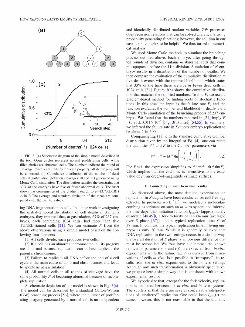
ing DNA fragmentation in cells. In a later work investigatingthe spatial-temporal distribution of cell deaths in Xenopusembryos, they reported that, at gastrulation, 67% of 237 em-bryos, each containing 1024 cells, had more than fiveTUNEL-stained cells �21�. We can estimate F from theabove observations using a simple model based on the fol-lowing four elements.

�1� All cells divide; each produces two cells.�2� If a cell has an abnormal chromosome, all its progeny

are abnormal because replication can at best duplicate theparent’s chromosome.

�3� Failure to replicate all DNA before the end of a cellcycle is the main cause of abnormal chromosomes and leadsto apoptosis at gastrulation.

�4� All normal cells in all rounds of cleavage have thesame probability F of becoming abnormal because of incom-plete replication.

A schematic depiction of our model is shown in Fig. 3�a�.The model can be described by a standard Galton-Watson�GW� branching process �53�, where the number of prolifer-ating progeny generated by a normal cell is an independent

and identically distributed random variable. GW processesobey recursion relations that can be solved analytically usingprobability generating functions; however, the solution in ourcase is too complex to be helpful. We thus turned to numeri-cal analysis.

We used Monte Carlo methods to simulate the branchingprocess outlined above. Each embryo, after going throughten rounds of division, contains m abnormal cells that com-mit apoptosis before the 11th division. Simulation of N em-bryos results in a distribution of the number of deaths. Wethen compare the evaluation of the cumulative distribution atfive death events with the reported likelihood, which statesthat 33% of the time there are five or fewer dead cells in1024 cells �21�. Figure 3�b� shows the cumulative distribu-tion that matches the reported numbers. To find F, we used agradient-based method for finding roots of stochastic func-tions. In this case, the input is the failure rate F, and thefunction evaluates the number and likelihood of deaths via aMonte Carlo simulation of the branching process of 237 em-bryos. We found that the numbers reported in �21� imply F= �3.73�0.01��10−3 �Fig. 3�b� inset� �54,55�. In summary,we inferred the failure rate in Xenopus embryo replication tobe about 1 in 300.

Comparing Eq. �11� with the standard cumulative Gumbeldistribution given by the integral of Eq. �4�, one can relatethe quantities t** and F to the Gumbel parameters via

t** = t* − �t*�ln�ln� 1

1 − F� . �12�

For F�1, the expression simplifies to t**� t*−�t*�ln�F�,which implies that the end time is insensitive to the exactvalue of F: an order-of-magnitude estimate suffices.

B. Connecting in vitro to in vivo results

As discussed above, the most detailed experiments onreplication in Xenopus have been conducted on cell-free eggextracts. In previous work �11�, we modeled a molecular-combing experiment on such an in vitro system and inferredthe time-dependent initiation function Ivitro�t� �approximatelyquadratic �48,49��, a fork velocity of 0.6 kb /min �averagedover S phase �37��, and a typical replication time t* of38 min. In contrast, the typical replication time in living em-bryos is only 20 min. While it is generally believed thatDNA replication in the two settings occurs in a similar way,the overall duration of S phase is an obvious difference thatmust be reconciled. We thus have a dilemma: the knownreplication parameters, v and I�t�, are extracted from in vitroexperiments while the failure rate F is derived from obser-vations of cells in vivo. Is it possible to “transpose” the re-sults from the in vitro experiments to the in vivo setting?Although any such transformation is obviously speculative,we propose here a simple way that is consistent with knownexperimental results.

We hypothesize that, except for the fork velocity, replica-tion is unaltered between the in vitro and in vivo systems.The subtlety is that there are several conceivable interpreta-tions of “unaltered” replication. One could keep Ivitro�t� thesame; however, this is not reasonable in that the dramatic

FIG. 3. �a� Schematic diagram of the simple model described inthe text. Open circles represent normal proliferating cells, whilefilled circles are abnormal cells. The numbers indicate the round ofcleavage. Once a cell fails to replicate properly, all its progeny willbe abnormal. �b� Cumulative distribution of the number of deadcells at gastrulation �between cleavages 10 and 11� generated usingMonte Carlo simulation. The distribution satisfies the constraint that33% of the embryos have five or fewer abnormal cells. The insetshows the convergence of the gradient search to F= �3.73�0.01��10−3. The average and standard deviation of the mean are com-puted over the last 40 values.


041917-7

increase in Ivitro�t�, at t�17.4 min, would be moved from themidpoint of replication to the end �11�. Alternatively, onecould express the initiation function in terms of the fractionof replication, i.e., I= I�f�, and preserve this function. In thiscase, one would need a fork velocity of about 2.2 kb /min toproduce the extracted in vivo failure rate. Although this is areasonable fork speed in systems such as the Drosophila em-bryo, it is about twice the maximum fork speed observed inXenopus embryonic replication in vitro �37�. The third pos-sibility is to preserve the maximum number of simulta-neously active replication forks. Intuitively, this is plausibleas each replication fork implies the existence of a large set ofassociated proteins. The maximum fork density then givesthe minimum number of copies of each protein set required.Thus, we are in effect assuming that the numbers of replica-tive proteins remains the same in both cases.

The simplest way to preserve fork usage is to rescale thedensity of forks active at time t,

nf�t� =1

2v

df

dt= g�t�e−2vh�t�, �13�

linearly in time so that

nfvivo� t

tscale = nf

vitro� t

tvitro* , �14�

where tvitro* �38 min and tscale is chosen so that t**=25 min

and F= �3.73�0.01��10−3. We found that the in vitro forkusage is preserved by using the rescaling Ivivo�t / tscale� 2Ivitro�t / t

vitro* � and v=1.030�0.001 kb /min �Fig. 4�. The

error on v is the consequence of the uncertainty in F.Using the transformed Ivivo�t�, we estimate from gvivo�t*�

the lower bound of the potential origin density to be 1.2potential origins/kb �PO/kb�. This lower bound is consistentwith the experimentally estimated average density of1.9�0.6 PO /kb mentioned in Sec. I B. Given this density

�1.2 PO /kb�, by applying Eqs. �4� and �5�, we then find thatthe largest interpotential-origin gap resulting from randomlicensing is typically 15 kb, and that the probability Pg ofhaving a gap that is inherently too large to replicate, i.e.,larger than 2vt**�50 kb, is less than O�10−16�, which ismuch smaller than the failure rate �F�O�10−3�� 56�.

The velocity we infer also has a significant interpretation.In a recent experiment, Marheineke and Hyrien found thatthe fork velocity in vitro is not constant but decreases lin-early from about 1.1 to 0.3 kb /min at the end of S phase�37�. The decrease in fork velocity suggests that in vitro rep-lication progressively depletes rate-limiting factors �e.g.,dNTP� throughout S phase. We suggest that our extracted v�1 kb /min means that in vivo systems are able to maintainthe concentration of rate-limiting factors, perhaps by regulat-ing their transport across the nuclear membrane �57,58�, tomaintain a roughly constant fork velocity throughout Sphase. In summary, by preserving the rescaled version of thein vitro fork usage rate, we have transformed Ivitro�t� into anIvivo�t� that results in reasonable replication parameters andreproduces the in vivo failure rate.

IV. OPTIMIZING FORK ACTIVITY

The random-completion problem mentioned in Sec. I canbe quantitatively recast into a problem of searching for aninitiation function that produces the in vivo failure rate con-straint in Eq. �11�. In Fig. 5�a�, we show that any initiationform with the proper prefactor can satisfy the constraint onthe integral of the end-time distribution, including the trans-formed in vivo initiation function. Can we then understandwhy Xenopus embryos adopt the roughly quadratic I�t� andnot some other function of time?

To explore this question, we calculate for the differentcases of I�t� the maximum number of simultaneously activeforks. Figure 5�b� shows that initiation of all origins at thestart of S phase �setting I�t� ��t�� requires a higher maxi-mum than a modestly increasing I�t�. At the other extreme, atoo rapidly increasing I�t� �high exponent n� also requiresmany copies of replicative machinery because the bulk ofreplication is delayed and needs many forks close to the endof S phase to finish the replication on time. Thus, intuitively,one expects that an intermediate I�t� that increases through-out S phase—but not too much—would minimize the use ofreplicative proteins. Figure 5�b� hints that the in vivo initia-tion function derived from in vitro experiments may be closeto such an optimal I�t�, as the number of resources requiredby Ivivo�t� is close to the minimum of the power-law case.

The three resources modeled explicitly are potential ori-gins, initiation factors, and replication forks. It is not imme-diately clear which replication resources should be opti-mized. In general, the metabolic costs of expressing genesand making proteins are assumed to be non-rate-limiting fac-tors. On the other hand, it is plausible that the cell minimizesthe “complexity” of the replication process, minimizing to-pological problems caused by simultaneously active replica-tion forks, and thus minimizing the chance of unfaithful rep-lication. Thus, in our optimization analysis, we ignore themetabolic costs of having a large number of potential origins

FIG. 4. Density of simultaneously active replication forksthroughout S phase, nf�t�. The dotted curve corresponds to the invitro fork usage while the solid curve is the rescaled fork usage thatsatisfies the constraints t**=25 min and F=0.003 73. The rescalednf�t� is generated using Ivivo�t / t

vivo* � 2Ivitro�t / t

vitro* � and v

=1.030 kb /min.


041917-8

and propose that the maximum number of simultaneouslyactive forks is minimized. Above, we argued that the maxi-mum of nf�t� gives the minimum number of copies of theproteins required for DNA synthesis. Moreover, since theunwinding and synthesis of DNA at the forks create torsionalstress on the chromosomes, minimizing the number of activeforks would minimize the complexity of the chromosometopology, which may help maintain replication fidelity �59�.For these reasons, the maximum number of active forks is aplausible limiting factor that causes replication to proceedthe way it does. Below, we calculate the optimal I�t� andcompare it with Ivivo�t�.

The number of forks active at time t is given by nf�t�=2g�t�exp�−2vh�t��. One can find the I�t� that optimizes themaximum of nf�t� by minimizing

nmax�I�t�� = limp→�

��0

t**

nf�I�t��pdt1/p

. �15�

This is a common analytic method to optimize the maximumof a function �60�. The trick is to analytically calculate the

Euler-Lagrange equations for finite p and then take the limitp→�, where the contribution of the maximum dominatesthe integrand. The associated Euler-Lagrange equation is

h�t� = 2vh2�t� , �16�

where we recall that h�t�= I�t� and h�t�=g�t�. Note that Eq.�16� is independent of p, suggesting that the optimal nf�t�does not have a peak. Solving Eq. �16� subject to the bound-ary condition that the replication fraction be 0 at t=0 �i.e.,h�0�=0� and 1 at t= t**, we obtain

Iopt�t� =1

2vt**��t� +

1

t**

1

�1 − t/t**�2 . �17�

Inserting the result from Eq. �17� into Eq. �13�, one sees thatnf�t�=1 /vt** indeed is constant throughout S phase and isabout three times smaller than the maximum number of si-multaneously active forks in vivo �Fig. 6�c��. This optimalsolution, like Ivivo�t�, increases slowly at first, then growsrapidly toward the end of S phase �Fig. 6�b��. However, thisinitiation function is unphysical, as the diverging initiationprobability at t→ t** implies an infinite number of initiationsat the end of S phase. In effect, a constant fork density im-plies that, when the protein complexes associated with twocoalescing forks are liberated, they instantly find and attachto unreplicated parts of the chromosome. It also implies thatat the end of S phase all the replication forks would be activeon a vanishingly small length of unreplicated genome. Bothimplications are unrealistic.

To find a more realistic solution, we tamed the behavior ofthe initiation rate for t→ t** by adding a constraint. A naturalconstraint to impose is that the failure rate in vivo be satis-fied. The infinite initiations at t= t** implied by Eq. �17�means that the replication always finishes exactly at t** andthe failure rate is zero. Therefore, having a nonzero failurerate would force the number of initiations to be finite. Thisconstraint is also consistent with the idea that the replicationprocess is shaped by the evolutionary pressure of survival.The new optimization quantity is then

J�I�t�� = max�nf�I�t�� + ��F�I�t�� − Fvivo� , �18�

where the first term is the maximum of the fork density, andthe second term is a penalty function that increases J for F�Fvivo. The strength of the penalty is set by the Lagrangemultiplier �. The time associated with F is t**=25 minthroughout this section.

Substituting Eq. �15� into the first term of Eq. �18� andapplying the method of variational calculus, we obtained anintegro-differential equation that turns out to be stiff math-ematically and thus difficult to solve. The difficulty in ana-lytic methods is that the gradient of Eq. �15� is highly non-linear and that F depends on t*, which is not readilyexpressible in terms of the basic replication parameters I�t�and v. For these reasons, we turned to a gradient-free nu-merical method called finite difference stochastic approxima-tion �FDSA� �55�. Although this search method is used forstochastic functions �as the name suggests�, the method isjust as suitable for deterministic functions. The basic conceptis that the gradient of a function, which encodes the steepest-

FIG. 5. �Color online� �a� Replication end-time distribution witht** fixed to be 25 min and F=0.003 73. Similar to Fig. 2�a�, thewidth decreases with an increase in the exponent n. �b� Typicalmaximum number of simultaneously active forks. The curve is ob-tained by extracting the maximum value of nf�t� for different expo-nents n.


041917-9

decent direction toward a local minimum, can be approxi-mated by a finite difference of the function. The advantage ofthis method is that we can replace the complicated evaluationof the variation �J�I�t�� by the easily calculable differenceJ�I+�I�−J�I−�I�.

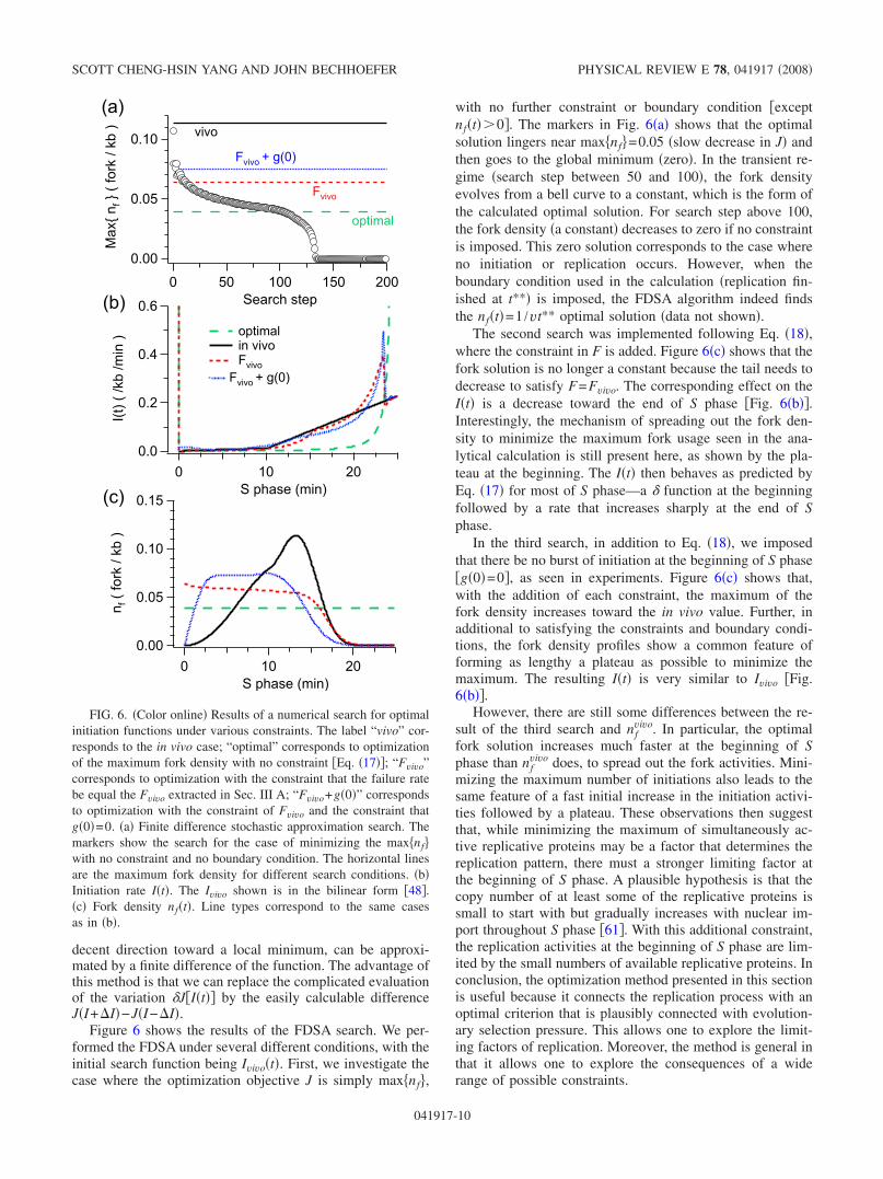
Figure 6 shows the results of the FDSA search. We per-formed the FDSA under several different conditions, with theinitial search function being Ivivo�t�. First, we investigate thecase where the optimization objective J is simply max�nf�,

with no further constraint or boundary condition �exceptnf�t��0�. The markers in Fig. 6�a� shows that the optimalsolution lingers near max�nf�=0.05 �slow decrease in J� andthen goes to the global minimum �zero�. In the transient re-gime �search step between 50 and 100�, the fork densityevolves from a bell curve to a constant, which is the form ofthe calculated optimal solution. For search step above 100,the fork density �a constant� decreases to zero if no constraintis imposed. This zero solution corresponds to the case whereno initiation or replication occurs. However, when theboundary condition used in the calculation �replication fin-ished at t**� is imposed, the FDSA algorithm indeed findsthe nf�t�=1 /vt** optimal solution �data not shown�.

The second search was implemented following Eq. �18�,where the constraint in F is added. Figure 6�c� shows that thefork solution is no longer a constant because the tail needs todecrease to satisfy F=Fvivo. The corresponding effect on theI�t� is a decrease toward the end of S phase �Fig. 6�b��.Interestingly, the mechanism of spreading out the fork den-sity to minimize the maximum fork usage seen in the ana-lytical calculation is still present here, as shown by the pla-teau at the beginning. The I�t� then behaves as predicted byEq. �17� for most of S phase—a � function at the beginningfollowed by a rate that increases sharply at the end of Sphase.

In the third search, in addition to Eq. �18�, we imposedthat there be no burst of initiation at the beginning of S phase�g�0�=0�, as seen in experiments. Figure 6�c� shows that,with the addition of each constraint, the maximum of thefork density increases toward the in vivo value. Further, inadditional to satisfying the constraints and boundary condi-tions, the fork density profiles show a common feature offorming as lengthy a plateau as possible to minimize themaximum. The resulting I�t� is very similar to Ivivo �Fig.6�b��.

However, there are still some differences between the re-sult of the third search and nf

vivo. In particular, the optimalfork solution increases much faster at the beginning of Sphase than nf

vivo does, to spread out the fork activities. Mini-mizing the maximum number of initiations also leads to thesame feature of a fast initial increase in the initiation activi-ties followed by a plateau. These observations then suggestthat, while minimizing the maximum of simultaneously ac-tive replicative proteins may be a factor that determines thereplication pattern, there must a stronger limiting factor atthe beginning of S phase. A plausible hypothesis is that thecopy number of at least some of the replicative proteins issmall to start with but gradually increases with nuclear im-port throughout S phase �61�. With this additional constraint,the replication activities at the beginning of S phase are lim-ited by the small numbers of available replicative proteins. Inconclusion, the optimization method presented in this sectionis useful because it connects the replication process with anoptimal criterion that is plausibly connected with evolution-ary selection pressure. This allows one to explore the limit-ing factors of replication. Moreover, the method is general inthat it allows one to explore the consequences of a widerange of possible constraints.

FIG. 6. �Color online� Results of a numerical search for optimalinitiation functions under various constraints. The label “vivo” cor-responds to the in vivo case; “optimal” corresponds to optimizationof the maximum fork density with no constraint �Eq. �17��; “Fvivo”corresponds to optimization with the constraint that the failure ratebe equal the Fvivo extracted in Sec. III A; “Fvivo+g�0�” correspondsto optimization with the constraint of Fvivo and the constraint thatg�0�=0. �a� Finite difference stochastic approximation search. Themarkers show the search for the case of minimizing the max�nf�with no constraint and no boundary condition. The horizontal linesare the maximum fork density for different search conditions. �b�Initiation rate I�t�. The Ivivo shown is in the bilinear form �48�.�c� Fork density nf�t�. Line types correspond to the same casesas in �b�.


041917-10

V. THE LATTICE-GENOME MODEL: FROM RANDOMTO PERIODIC LICENSING

Until now, we have assumed a spatially random distribu-tion of potential origins. In this section, we explore the im-plications of spatial ordering among the potential origins onthe end-time distribution. We have two motivations. First, an“obvious” method for obtaining a narrow end-time distribu-tion is to space the potential origins periodically and initiatethem all at once. However, such an arrangement would notbe robust, as the failure of just one origin to initiate woulddouble the replication time. Still, the situation is less clear ifinitiations are spread out in time, as the role of spatial regu-larity in controlling interorigin spacing would be blurred bythe temporal randomness.

Our second motivation is that there is experimental evi-dence that origins are not positioned completely at random.A completely random positioning implies that the distribu-tion of gaps between potential origins is exponential, result-ing in many small interpotential-origin spacings. However, inan experiment of plasmid replication in Xenopus egg ex-tracts, Lucas et al. found no interorigin gap smaller than 2 kb�29�. In a previous analysis, we also observed that, assumingrandom licensing, one expects more small interorigin gaps��8 kb� and fewer medium gaps �8–16 kb� than were ex-perimentally observed �14�. Second, experiments have sug-gested a qualitative tendency for origins to fire in groups, orclusters �18�. These findings collectively imply that there issome spatial regularity in the Xenopus system, perhapsthrough a “lateral inhibition” of licensing potential originstoo closely together. Our goal is to find an “ordering thresh-old,” at which point the resulting end-time distribution startsto deviate from the random-licensing case.

To investigate spatial ordering, we change the continuousgenome to a “lattice genome” with variable lattice spacingdl. Potential origins can be licensed only on the lattice sites.For dl→0, the lattice genome becomes continuous, and themodel recovers the random-licensing case. As dl increases,the lattice genome has fewer available sites for licensing po-tential origins, and the fraction of licensed sites increases. Inthis scenario, the spacing between initiated origins take ondiscrete values—multiples of dl. One can imagine that a fur-ther increase in dl would eventually lead to a critical dl,where every lattice site would have a potential origin. Thisscenario corresponds to an array of periodically licensed ori-gins, which leads to a periodic array of initiated origins withspacing dl. Thus, by increasing a single parameter dl, we cancontinuously interpolate from complete randomness to per-fect periodicity.

In order to compare regularized licensing to random li-censing, we impose that while the potential origins may bedistributed along the genome differently, the total initiationprobability across the genome is conserved. We then write

I�x,t� = dlI�t��n=0

L/dl

��x − ndl� , �19�

where x is the position along the genome. This equationshows that, as the number of lattice sites L /dl is reduced viaan increase in dl, the initiation probability for each site is

enhanced, resulting in more efficient potential origins. Thisimplies a trade-off between the “quantity” and “efficiency”of potential origins.

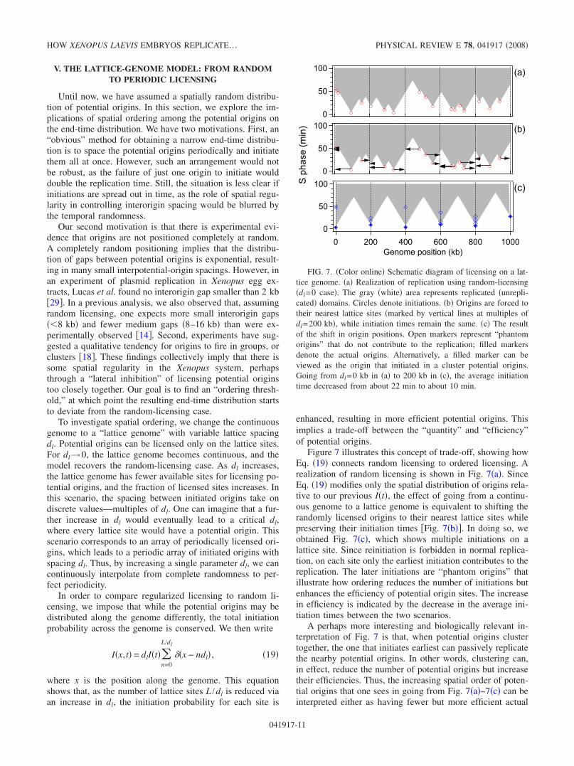
Figure 7 illustrates this concept of trade-off, showing howEq. �19� connects random licensing to ordered licensing. Arealization of random licensing is shown in Fig. 7�a�. SinceEq. �19� modifies only the spatial distribution of origins rela-tive to our previous I�t�, the effect of going from a continu-ous genome to a lattice genome is equivalent to shifting therandomly licensed origins to their nearest lattice sites whilepreserving their initiation times �Fig. 7�b��. In doing so, weobtained Fig. 7�c�, which shows multiple initiations on alattice site. Since reinitiation is forbidden in normal replica-tion, on each site only the earliest initiation contributes to thereplication. The later initiations are “phantom origins” thatillustrate how ordering reduces the number of initiations butenhances the efficiency of potential origin sites. The increasein efficiency is indicated by the decrease in the average ini-tiation times between the two scenarios.

A perhaps more interesting and biologically relevant in-terpretation of Fig. 7 is that, when potential origins clustertogether, the one that initiates earliest can passively replicatethe nearby potential origins. In other words, clustering can,in effect, reduce the number of potential origins but increasetheir efficiencies. Thus, the increasing spatial order of poten-tial origins that one sees in going from Fig. 7�a�–7�c� can beinterpreted either as having fewer but more efficient actual

FIG. 7. �Color online� Schematic diagram of licensing on a lat-tice genome. �a� Realization of replication using random-licensing�dl=0 case�. The gray �white� area represents replicated �unrepli-cated� domains. Circles denote initiations. �b� Origins are forced totheir nearest lattice sites �marked by vertical lines at multiples ofdl=200 kb�, while initiation times remain the same. �c� The resultof the shift in origin positions. Open markers represent “phantomorigins” that do not contribute to the replication; filled markersdenote the actual origins. Alternatively, a filled marker can beviewed as the origin that initiated in a cluster potential origins.Going from dl=0 kb in �a� to 200 kb in �c�, the average initiationtime decreased from about 22 min to about 10 min.


041917-11

potential origins or as indicating clustering, which leads tofewer but more efficient effective potential origins.

Having outlined the rules for licensing, we now introducetwo quantities, “periodicity” P and dinter, that will be usefulin later discussions of how dl alters the end-time distribution.We first look at i�s�, the distribution of the spacing betweeninitiated origins, where s is the interorigin spacing. Figure8�a� shows two i�s�’s: the continuous one corresponds torandom licensing, while the discrete one corresponds to set-ting dl to 2 kb. The two distributions are different because ofthe discretization effect of the lattice genome: origins canhave separations that are only multiples of dl. As dl in-creases, one expects a dominant spacing to appear in thesystem. We characterize this ordering effect by defining theperiodicity P, the probability at the mode of the discreteinterorigin-spacing distribution. As an example, the dl=2 kb distribution shown in Fig. 8�a� has P=0.23, indicating

that 23% of the spacings have the same value. In the fullyperiodic case, the probability at the mode is 1, as all thespacings have the same value: the system is then 100% pe-riodic �P=1�. For dl→0, P should be interpreted as themode of i�s� times a vanishingly small �s � dl�. Thus, P→0 in the small-�s limit, as there will be no interoriginspacings sharing the same size.

In interpolating from random licensing to periodic licens-ing, one expects that the average interorigin spacing davgwould change from being dl independent to being linearlydependent on dl. Indeed, from Fig. 8�b�, which shows davg asa function of dl, we can label two asymptotes and therebyidentify two regimes. We first introduce dinter to be the aver-age interorigin spacing of the dl=0 kb case. For dl→0, wesee that davg asymptotically approaches dinter. In contrast, forlarge dl �when all lattice sites are occupied�, we see davgapproaching the asymptote davg=dl. The intersection of thetwo asymptotes is precisely at dl=dinter. We therefore identifytwo regimes, with regime I being dl�dinter and regime IIbeing dl�dinter. Physically, the weak dl dependence in re-gime I suggests that the system is spatially random, whereasthe asymptotically linear behavior in regime II indicates thatthe system is becoming periodic.

The length scale dinter encodes the two factors that deter-mine the distribution of interorigin spacings. The first factoris the passive replication of closely positioned potential ori-gins, which suppresses the likelihood of having small inter-origin spacings. The second factor is based on the low prob-ability of randomly licensing two faraway origins, whichreduces the probability of having large interorigin gaps. Bothof these effects can be seen in Fig. 8�a�.

When dl exceeds dinter, the typical spacing between poten-tial origins � dl� exceeds the typical range of passive repli-cation and approaches the typical largest spacing of therandom-licensing case. This means that potential origins arenot likely to be passively replicated or positioned farther thandl apart �note that the next smallest spacing 2dl is quitelarge�. The inset in Fig. 8�b�, which shows the periodicity Pas a function of dl, strengthens this notion that for dl�dinter,the system enters a nearly periodic regime where P has satu-rated.

Our main result is Fig. 9, which shows how the end-timedistribution changes with increasing dl. The initiation func-tion used in the simulation is the power-law approximationof the Ivivo�t� found in Sec. III B, transformed using Eq. �19�.The fork velocity and failure rate used are as extracted inSec. III. There are again two distinct regimes separated bythe ordering threshold dinter�6.5 kb. Below the threshold�regime I�, the end-time distribution is nearly independent ofdl. Above the threshold �regime II�, the mode shifts to theright. The width is unaltered.

To understand the changes in going from regime I to re-gime II, we note that in Eq. �5�, t* depends on the number ofinitiations No. On average, No is unaffected when the numberof lattice sites available is in excess �

No

L/dl�1�. This means

that t* starts to change only when dl=L /No which is pre-cisely dinter. In regime II, the minimum time to replicate thesmallest gap between potential origins, dl /v, becomes sig-nificant compared to the temporal randomness resulting from

FIG. 8. �Color online� �a� Distribution of spacings between ini-tiated origins, i�s�, for the dl=0 and 2 kb cases �2 kb is chosen tomimic the minimal spacing between origins reported in �29��. Theinitiation rate and fork velocity are those obtained in Sec. III B. Themean of the continuous distribution �dl=0 kb case� is marked dinter

and is �6.5 kb. The mode of the discrete distribution �dl=2 kbcase� is marked by �. The probability P at the mode �0.23 in thiscase� is defined to be the periodicity, a measure of ordering in thesystem. �b� Average interorigin spacing davg as a function of dl.There is a gradual transition from regime I to regime II. In regimeI �dl�dinter�, davg is asymptotically independent of dl for dl→0. Inregime II �dl�dinter�, dav is asymptotically linearly proportional todl. Inset shows the periodicity P as a function of dl.


041917-12

stochastic initiation. In effect, t*�dl /v+ tav, where tav is theaverage initiation time. We tested numerically that the meanand standard deviation of the initiation times both decreasesigmoidally, for dl /dinter�3. Thus, for the range of dl shownin Fig. 9, one expects t*�dl in regime II, while the widthshould be unaltered.

In Xenopus embryos, the inhibition zone observed in plas-mid replication corresponds to dl�2 kb �dashed line in Fig.9� �29�. The value is well below the ordering threshold ofdinter�6.5 kb, suggesting that the experimentally observedspatial ordering plays a minor role in solving the random-completion problem in embryonic replication.

VI. CONCLUSION

In this paper, we have extended the stochastic nucleation-and-growth model of DNA replication to describe not onlythe kinetics of the bulk of replication but also the statistics ofreplication quantities at the end of replication. Using themodel, we have quantitatively addressed a generalized ver-sion of the random-completion problem, which asks how sto-chastic licensing and initiation lead to the tight control ofreplication end times observed in systems such as Xenopusembryos. In particular, we applied our model to investigateand compare the two solutions proposed by biologists—theregular-spacing model �RSM� and the origin-redundancymodel �ORM�.

First, we found that the ORM, which utilizes purely ran-dom licensing, can still accurately control the replicationtime. With this approach, the fluctuation of the end times issuppressed by licensing a large excess of potential origins,while the typical end time is adjusted by increasing the ini-tiation rate toward late S phase. Then, we analyzed the effectof spatial ordering in the RSM using a lattice genome. Our

results show that �1� incorporating regularity leads to a trade-off: the large number of potential origins in the ORM iseffectively replaced by fewer but more efficient ones in theRSM and that �2� under the condition that the initiation rateacross the genome is preserved, the two models produce thesame end-time distribution until an ordering threshold isreached. We show that the experimentally observed orderingeffect of lateral inhibition in Xenopus is well below the or-dering threshold.

These results are particularly enlightening when consider-ing clustering as a mechanism that transforms the ORM intothe RSM. As mentioned in Sec. V, clustering spontaneouslyleads to an effective trade-off between quantity and effi-ciency of potential origins, while satisfying the condition ofpreserving the initiation rate. This means that the intrinsicreason that the RSM and the ORM produce the same end-time distribution is not the spatial distribution of potentialorigins but the high density of potential origins. Thus, weargue that the key factors in resolving the random-completion problem, at least in the Xenopus case, are thelicensing of a large excess of potential origins and an in-creasing initiation rate—and not an ordered spatial distribu-tion of origins. To say it in a different way, the analysis inSec. V implies that the end-time distribution due to a randomordering of potential origins will be unaltered if those samepotential origins are positioned more regularly �e.g., in or-dered clusters�, as long as the clustering is small enough. Theamount of clustering needed to alter the end-time distributionfar exceeds the experimentally observed amounts.

We have also found the optimal I�t� that minimizes themaximum number of simultaneously active forks. Like theobserved in vitro initiation function, it increases throughout Sphase except for the end. Further pursuit of the optimizationproblem with more detailed model may reveal the rate-limiting factors in replication, which have not been identifiedto date. Further, an open issue not addressed by our model isthe observation that there is a weak correlation in the initia-tions of neighboring origins �18�. To model this effect, onecan introduce correlations in licensing, initiation, and forkprogression based on localization of replication foci �62�,chromatin structures �28�, or some other mechanisms. We donot expect that correlations will modify the scenario we havepresented here significantly, as the most significant effect ofcorrelations, an increase in spatial ordering, would not beimportant even at exclusion-zone sizes that are much largerthan observed �e.g., 10 kb�.

Among the various cases of replication programs, replica-tion in bacteria is the most well understood—DNA synthesisstarts at a single, sequence-specific genome site and proceedsto completion �63�. With this case, the genome-wide regula-tion of the replication process is deterministic and strictlygoverned by biochemical effects. In this work, we modeled avery different type of replication program, where both thelicensing and initiation timings are strongly influenced bystochastic effects. This type of stochastic replication strategyis usually present in embryos, especially those that developoutside the parent’s body, for rapid development of the em-bryos. We showed how stochastic effects ensure the fast andreliable replication needed for rapid development.

In between these two special cases lie all other replicationprograms, where the licensing mechanisms are more compli-

FIG. 9. �Color online� Evolution of the end-time distributionwith increasing spatial ordering due to increasing dl. Each horizon-tal profile is an end-time distribution. In regime I, the end-timedistribution does not change appreciably; in regime II, the modeshifts to the right. The ordering threshold is at dl=dinter�6.5 kb.The dashed line shows the dl=2 kb end-time distribution, whichcorresponds to the lateral inhibition ordering observed experimen-tally �29�.


041917-13

cated than simple sequence targeting or a Poisson process�64�. These include replication in nonembryonic �somatic�cells, in simple organisms such as yeast, and in cancer cellswhere abnormal replication such as rereplication can occur�5,65,66�. For instance, replication experiments done onfission-yeast cells show that, while there is an excess numberof potential origins as in embryonic replication, the positionsof the origins are associated with a sequence asymmetry ofthe genome instead of being completely sequence indepen-dent �67�. The experiments also show that different originshave different efficiencies, suggesting that initiation timingsare not entirely stochastic. In future work, we shall modify

our model to study such systems, which may lead to a fullerunderstanding of how replication is regulated by the genomeorganization and by DNA replication strategies that are theoutcome of evolution.

ACKNOWLEDGMENTS

We thank Nick Rhind and Michel Gauthier for helpfuldiscussions and a thorough reading of the manuscript. Wethank Olivier Hyrien for informing us of unpublished resultsand data. This work was funded by NSERC �Canada� and byHFSP.

�1� J. Herrick and A. Bensimon, Chromosoma 117, 243 �2008�.�2� J. F. Diffley, Genes Dev. 10, 2819 �1996�.�3� E. E. Arias and J. C. Walter, Genes Dev. 21, 497 �2007�.�4� C. Hensey and J. Gautier, Mech. Dev. 69, 183 �1997�.�5� R. D. Micco et al., Nature �London� 444, 638 �2006�.�6� A. Sancar, L. A. Lindsey-Boltz, K. Ünsal Kaçmaz, and S.

Linn, Annu. Rev. Biochem. 73, 39 �2004�.�7� A. Bensimon, A. Simon, A. Chiffaudel, V. Croquette, F.

Heslot, and D. Bensimon, Science 265, 2096 �1994�.�8� J. Herrick and A. Bensimon, Biochimie 81, 859 �1999�.�9� J. Herrick, P. Stanislawski, O. Hyrien, and A. Bensimon, J.

Mol. Biol. 300, 1133 �2000�.�10� K. Marheineke and O. Hyrien, J. Biol. Chem. 276, 17092

�2001�.�11� J. Herrick, S. Jun, J. Bechhoefer, and A. Bensimon, J. Mol.

Biol. 320, 741 �2002�.�12� O. Hyrien and M. Méchali, EMBO J. 12, 4511 �1993�.�13� S. Jun, H. Zhang, and J. Bechhoefer, Phys. Rev. E 71, 011908

�2005�.�14� S. Jun and J. Bechhoefer, Phys. Rev. E 71, 011909 �2005�.�15� J. Bechhoefer and B. Marshall, Phys. Rev. Lett. 98, 098105

�2007�.�16� O. Hyrien, K. Marheineke, and A. Goldar, BioEssays 25, 116

�2003�.�17� D. Kimelman, M. Kirschner, and T. Scherson, Cell 48, 399

�1987�.�18� J. J. Blow, P. J. Gillespie, D. Francis, and D. A. Jackson, J.

Cell Biol. 152, 15 �2001�.�19� The duration of the embryonic cell cycle depends on tempera-

ture. For this paper, we take the cell cycle time to be 25 min at23 °C �61�. A typical duration of S phase used is �20 min�16,18�. Longer times �25 min for S phase and 30 min for thecell cycle� have been observed at 20 °C �61�.

�20� T. A. Prokhorova, K. Mowrer, C. H. Gilbert, and J. C. Walter,Proc. Natl. Acad. Sci. U.S.A. 100, 13241 �2003�.

�21� C. Hensey and J. Gautier, Dev. Biol. 203, 36 �1998�.�22� J. Walter and J. W. Newport, Science 275, 993 �1997�.�23� M. C. Edwards, A. V. Tutter, C. Cvetic, C. H. Gilbert, T. A.

Prokhorova, and J. C. Walter, J. Biol. Chem. 277, 33049�2002�.

�24� K. J. Harvey and J. Newport, Mol. Cell. Biol. 23, 6769 �2003�.�25� R. A. Laskey, J. Embryol. Exp. Morphol. 89, 285 �1985�.�26� P. Romanowski, M. A. Madine, A. Rowles, J. J. Blow, and R.

A. Laskey, Curr. Biol. 6, 1416 �1996�.�27� N. Rhind, Nat. Cell Biol. 8, 1313 �2006�.�28� S. Jun, J. Herrick, A. Bensimon, and J. Bechhoefer, Prog. Cell

Cycle Res. 3, 223 �2004�.�29� I. Lucas, M. Chevrier-Miller, J. M. Sogo, and O. Hyrien, J.

Mol. Biol. 296, 769 �2000�.�30� A. N. Kolmogorov, Bull. Acad. Sci. USSR, Phys. Ser. �Engl.

Transl.� 1, 335 �1937�.�31� W. A. Johnson and F. L. Mehl, Trans. AIME 135, 416 �1939�.�32� M. Avrami, J. Chem. Phys. 7, 1103 �1939�; 8, 212 �1940�; 9,

177 �1941�.�33� K. Sekimoto, Physica A 125, 261 �1984�; 135, 328 �1986�.�34� K. Sekimoto, Int. J. Mod. Phys. B 5, 1843 �1991�.�35� E. Ben-Naim and P. L. Krapivsky, Phys. Rev. E 54, 3562

�1996�.�36� It is known that when DNA polymerases introduce copying

errors in the process of synthesizing nucleotides, replicationforks stall to repair the mispairing �63�. These fork stalls occurstochastically in time. Thus, in our model, a constant fork ve-locity is a mean-field approximation of the time-varying forkvelocities and the fork-to-fork variation in progression speed.

�37� K. Marheineke and O. Hyrien, J. Biol. Chem. 279, 28071�2004�. To test whether replacing the observed decreasing forkvelocity with its average is a valid approximation, we simu-lated the two cases with a modified version of the phantom-nuclei algorithm discussed in Sec. II. We found that the tails ofthe coalescence distributions for the two cases agree to �1%,indicating that the two cases also have similar end-time distri-butions.

�38� C. Conti, B. Saccà, J. Herrick, C. Lalou, Y. Pommier, and A.Bensimon, Mol. Biol. Cell 18, 3059 �2007�.

�39� W. Krauth, Statistical Mechanics: Algorithms and Computa-tions �Oxford University Press, Oxford, 2006�.

�40� W. H. Press, S. A. Teukolsky, V. William T, and B. P. Flannery,Numerical Recipes: The Art of Scientific Computing, 3rd ed.�Cambridge University Press, New York, 2007�.

�41� Computer code IGOR PRO �Wavemetrics Inc., 2008�, URLhttp://www.wavemetrics.com/

�42� E. J. Gumbel, Statistics of Extremes �Columbia UniversityPress, New York, 1958�.

�43� S. Kotz and S. Nadarajah, Extreme Value Distributions �Impe-rial College Press, London, 2000�.

�44� R.-D. Reiss and M. Thomas, Statistical Analysis of Extreme


041917-14

Values, 2nd ed. �Birkhauser-Verlag, Basel, 2001�.�45� G. Caldarelli, F. D. Di Tolla, and A. Petri, Phys. Rev. Lett. 77,

2503 �1996�.�46� A. A. Moreira, J. S. Andrade, and L. A. Nunes Amaral, Phys.

Rev. Lett. 89, 268703 �2002�.�47� H. Tijms, Understanding Probability: Chance Rules in Every-

day Life �Cambridge University Press, Cambridge, NY, 2004�.�48� The original inference of the in vitro data was fitted using a

bilinear function �11�. Using the transformation in Sec. III totranspose the bi-linear Ivitro, we obtained a scaled bilinear Ivivo.For ease of calculation, in parts of the paper, we approximateboth bilinear functions with power-law functions. Both initia-tion functions are approximately quadratic �Ivitro t2.62 andIvivo t2.45�.

�49� Ivitro is approximately quadratic except for a decrease �I�t�→0� toward the end of S phase �11�. Since the errors on thedecreasing part of the data are large, we neglected the decreasein our previous work �13,15�. However, a recent repeat of theoriginal experiment has shown that the decrease is not an arti-fact of poor statistics but represents a real feature of the repli-cation process �61�. Thus, we examined how the decrease inI�t� affects the end-time distribution. We found that with thedecrease the mode of the distribution was delayed by �3%and the width increased by 15%. These quantities approxi-mately translate into an S phase that is prolonged by�0.5 min. This difference is small compared to the overallduration of S phase �20 min�.

�50� J. P. Sethna, Statistical Mechanics: Entropy, Order Param-eters, and Complexity �Oxford University Press, Oxford,2006�. The derivation of the Gumbel distribution appears, athttp://pages.physics.cornell.edu/sethna/StatMech/NewExercises.pdf.

�51� C. H. Thiébaud and M. Fischberg, Chromosoma 59, 253�1977�.

�52� S. P. Bell and A. Dutta, Annu. Rev. Biochem. 71, 333 �2002�.

�53� M. Kimmel and D. E. Axelrod, Branching Processes in Biol-ogy �Springer, New York, 2002�.

�54� In �15�, we estimated a failure rate F�10−4 using a simplemodel that neglected the complications due to the branchingprocess. Since t** depends on the logarithm of F from Eq.�12�, the factor of 30 between the two estimates of F resultsonly in a roughly 1-min shift in the t** of the end-time distri-bution and does not alter the qualitative conclusion of the pre-vious work.

�55� J. C. Spall, Introduction to Stochastic Search and Optimization�J. Wiley, Hoboken, NJ, 2003�.

�56� Using the in vitro fork velocity �v=0.6 kb /min�, we find Pg

=O�10−9�. Thus, whether our assumption that vvivo�vvitro istrue or not, we always expect Pg�F.

�57� J. D. Moore, J. Yang, R. Truant, and S. Kornbluth, J. Cell Biol.144, 213 �1999�.

�58� V. Q. Nguyen, C. Co, K. Irie, and J. J. Lib, Curr. Biol. 10, 195�2000�.

�59� L. Postow, N. J. Crisona, B. J. Peter, C. D. Hardy, and N. R.Cozzarelli, Proc. Natl. Acad. Sci. U.S.A. 98, 8219 �2001�.

�60� S. Skogestad and I. Postlethwaite, Multivariable FeedbackControl, 2nd ed. �John Wiley, Chichester, 2005�.

�61� O. Hyrien �private communication�.�62� P. Meister, A. Taddei, A. Ponti, G. Baldacci, and S. M. Gasser,

EMBO J. 26, 1315 �2007�.�63� H. Lodish, A. Berk, C. A. Kaiser, M. Krieger, M. P. Scott, A.

Bretscher, H. Ploegh, and P. Matsudairu, Molecular Cell Biol-ogy, 6th ed. �W. H. Freeman and Company, New York, 2008�.

�64� D. M. Gilbert, Science 294, 96 �2001�.�65� M. Anglana, F. Apiou, A. Bensimon, and M. Debatisse, Cell

114, 385 �2003�.�66� P. K. Patel, B. Arcangioli, S. P. Baker, A. Bensimon, and N.

Rhind, Mol. Biol. Cell 17, 308 �2006�.�67� C. Heichinger, C. J. Penkett, J. Bähler, and P. Nurse, EMBO J.

25, 5171 �2006�.


041917-15

How Xenopus laevis embryos replicate reliably: Investigating the random-completion problem

Documents

Transcript of How Xenopus laevis embryos replicate reliably: Investigating the random-completion problem