MARINE ECOLOGY PROGRESS SERIESMar Ecol Prog Ser

Vol. 350: 223–234, 2007doi: 10.3354/meps07190

Published November 22

INTRODUCTION

Estimates of organism abundance are fundamental formarine ecology, but particularly difficult in many circum-stances that preclude the intensive use of trawl sam-pling, or acoustic survey, e.g. abyssal systems and areassuch as reefs, where trawls cannot run or would damagethe sea floor unacceptably. Priede & Merrett (1998)recommended the deployment of autonomous landerplatforms equipped with bait and camera systems as arelatively low-cost and low-impact alternative. In earlywork, Priede et al. (1990) successfully fitted an empiricalcurve to the time series of scavenger numbers present ata bait on the sea floor; this was later used to estimate (theassumed constant) staying time at bait (Henriques et al.2002). Additionally, Priede & Merrett (1996) found anempirical relationship λ ∝ τ1

–2, between the time to firstfish arrival, τ1, and environmental fish density, λ, deter-mined independently by trawling. Following these dis-

coveries, interpretation of statistics other than first arrivaltime had not succeeded in predicting organism abun-dance (Priede & Merrett 1998), and thus has not beenconsidered further.

More recent emphasis has been placed on usingmechanistic models of the arrival process (Priede &Bagley 2000, Bailey & Priede 2002, Collins et al. 2002).These models make assumptions about foraging be-haviour and the spatial distribution of scavengers, aswell as the prevailing current, swimming speeds andodour plume development (linear extension and diffu-sive spread). The models fall into 2 main categories—those assuming actively searching foragers (usuallyfish) and those, following earlier work by Sainte-Marie& Hargrave (1987), assuming that scavengers pas-sively wait for signs of food arriving on a spreadingplume. In reality there is a continuum between these 2extremes depending on the speed of searching relativeto passive diffusion. For passive scavengers, a descrip-

© Inter-Research 2007 · www.int-res.com*Email: k.farnsworth@qub.ac.uk

How to estimate scavenger fish abundance usingbaited camera data

K. D. Farnsworth1,*, U. H. Thygesen2, S. Ditlevsen3, N. J. King4

1School of Biological Science, Queens University Belfast, 97 Lisburn Road, Belfast BT9 7BL, UK2Danmarks Fiskeriundersøgelser Afd. for Havfiskeri, Charlottenlund Slot, 2920 Charlottenlund, Denmark

3Biostatistisk Afdeling, Københavns Universitet, Øster Farimagsgade 5, Opgang B, Postboks 2099, 1014 Copenhagen, Denmark4Oceanlab, University of Aberdeen, Main Street, Newburgh, Aberdeenshire AB41 6AA, UK

ABSTRACT: Baited cameras are often used for abundance estimation wherever alternative tech-niques are precluded, e.g. in abyssal systems and areas such as reefs. This method has thus far usedmodels of the arrival process that are deterministic and, therefore, permit no estimate of precision.Furthermore, errors due to multiple counting of fish and missing those not seen by the camera haverestricted the technique to using only the time of first arrival, leaving a lot of data redundant. Here,we reformulate the arrival process using a stochastic model, which allows the precision of abundanceestimates to be quantified. Assuming a non-gregarious, cross-current-scavenging fish, we show thatprediction of abundance from first arrival time is extremely uncertain. Using example data, we showthat simple regression-based prediction from the initial (rising) slope of numbers at the bait givesgood precision, accepting certain assumptions. The most precise abundance estimates were obtainedby including the declining phase of the time series, using a simple model of departures, and takingaccount of scavengers beyond the camera’s view, using a hidden Markov model.

KEY WORDS: Deep sea · Coryphaenoides · Lander · Hidden Markov model · Population · Wildlifecensus

Resale or republication not permitted without written consent of the publisher

OPENPEN ACCESSCCESS

Mar Ecol Prog Ser 350: 223–234, 2007

tion of the plume is most important, but the crux ofmodels with active scavengers is accurate representa-tion of their search strategy in relation to the current(Bailey & Priede 2002). There is good evidence thatswimming in an approximately orthogonal direction tothe current is optimal (Dusenbery 1989, Vabo et al.2004) and is commonly displayed by scavengers(Priede et al. 1991, Bailey & Priede 2002). Conse-quently, Bailey & Priede (2002) derived a deterministicmodel of arrival rate for cross-current scavengers andshowed it was able to predict first arrival times, thoughthey found this measure was relatively insensitive toabundance above about 100 ind. km–2.

Biologists with time series data collected from baitedcamera deployments are still faced with the question ofhow to make the most effective and justifiable use of thedata in estimating organism abundance. This is not byany means a simple question, as it depends on arrivaland departure statistics, scavenger behaviour through-out the feeding cycle, and the limitations of the equip-ment used. The aim of the present work was to provideguidelines for estimating abundance from baited cameradata, specifically for fish scavengers that actively search,rather than sit and wait, for odour plumes. We shall firstbuild a conceptual model of the processes determiningnumbers of fish seen at the bait. Then we will assess 3indirect measures of abundance using these counts, inorder of increasing use of the data. Each measure will bedemonstrated using example data taken from obser-vations of Coryphaenoides armatus in the NazaréCanyon, west of Portugal (King 2006). The importantattributes of each method will be illustrated, showing itsstrengths and weaknesses; in particular, we shall showhow the precision of the techniques increases as moreinformation is used. The ecological time scale to whichour analysis applies is that of the time series of cameraobservations in a single deployment.

CONCEPTUAL MODEL

The number of fish attending the bait results froma balance between arrivals and departures (Sainte-Marie & Hargrave 1987). The arrival rate depends onthe number that are attracted to the bait, which is deter-mined by the abundance of scavenger fish able to de-tect the plume, and the proportion of them that respondby swimming to the bait. We note here that the pres-ence of competitors and predators near the bait canaffect the bait’s attractiveness (see Lapointe & Saint-Marie 1992), but such effects are separate from themain estimation problem and we do not deal with themfurther. Hence, we assume that fish that can detect thebait will attend it. Even with this assumption, assessingcounts at the bait is complicated by the fact that fish

may arrive at the bait, circle it, perhaps exiting the cam-era view and may repeatedly return to the bait beforefinally leaving the area around the bait (bait zone) alto-gether (Collins et al. 1999). These behaviours poten-tially undermine efforts to estimate abundance (Yau etal. 2001), but a common response has been to averageobserved numbers of fish over several replications ofbait deployment; for example, Priede et al. (1994) tookthe maximum mean number observed per block of 15image frames as a best estimate of true numbers. Wehope to improve on such heuristics. To facilitate refer-ence to calculations, the symbols used and their rangeshave been collated in Table 1.

Arrival rate is stochastically related to populationdensity. Departure rate depends on the number of fishpresent at the bait and the fish behaviour (determiningresidence time), and the observable fraction dependson both movements local to the bait and the visualscope of the camera. These processes are brought to-gether in the conceptual model (Fig. 1), in which n(t) isthe expected (mean) number of fish that have been at-tracted to the bait, but are not in the view of the cameraand m(t) is the expected number that are photo-graphed. Thus, in our model, fish are attracted to thebait zone at a stochastic rate ρa(t) and switch betweenthis state and the ‘in camera’ state at rate ζ, finally de-parting the bait zone at a stochastic rate of ρd(t) (Fig. 1).

We make a simplifying assumption that the switch-ing rate between in-camera and out-of-camera states issymmetrical (individual fish in the region are equallylikely to become apparent as become obscure) and istherefore ζ[n(t) – m(t)]. Conservation of numbers (fishare neither created nor destroyed here) ensures thatafter a time T:

(1)

and inspection of flow rates yields the following pair ofdifferential equations:

(2)

(3)

The resulting time series of numbers at the bait has thefollowing general features: a delay phase before the firstarrival, a growth phase during which the arrival rate ex-ceeds the departure rate, and a decay phase in which de-partures exceed arrivals and, hence, a maximum in num-bers when the arrival rate equals the departure rate(these features are shown in Bailey & Priede 2002, theirFig. 3). Superimposed on this gross pattern, the time se-ries shows random rises and falls due to movements inand out of the field of view, as well as the stochasticity ofarrival and departure processes. The above equationsserve to explain the processes involved, but they are con-

ddm t

tn t m t

( )[ ( ) ( )]= −ζ

ddn t

tt m t n ta d

( )( , ) ( ) ( ) ( )= + − +ρ λ ζ ρ ζ

n T m T t t ta d

T( ) ( ) [ ( , ) ( )]+ = −∫ ρ λ ρ d

0

224

Farnsworth et al.: Scavenger fish abundance estimation

tinuous approximations. Next, we de-velop stochastic models that explicitlycount individuals because the num-bers involved are small.

MODELS OF FISH ARRIVAL RATES

Two models will be considered:the first assumes that fish swim withconstant velocity across the current(geometric model) and the secondallows for random direction switch-ing (diffusion model). The modelsgive different predictions on howthe number of arriving fish increaseswith time; empirical estimation of thisrate will later be used to select themodel which best fits a time series offish arrivals.

Geometric model of fish arrivals.We assume a constant velocity watercurrent, with fish searching ortho-gonally (cross-current) for odourplumes. Given that fish searchingspeed is likely to be much greaterthan the odour diffusion rate (seeYen et al. 1998, Webster & Weiss-burg 2001), diffusive spreading hasa negligible effect on arrival times.This greatly simplifies the problemby reducing the plume to a 1-dimen-sional target extending in space atthe same rate (and in the same direc-tion) as the current.

We use a coordinate system withthe bait as the origin, with thepositive y-direction defined by thecurrent direction as it flows withconstant speed u. Fish move perpen-dicularly to the current (the x-axis)at a constant speed w; on average,half of them move in the positive x-direction and the other half move inthe negative x-direction. Once theyencounter the plume, they swim upit at a speed v over the substrate byswimming faster than the opposingcurrent. We also assume that fish actindependently of one another, areequivalent in all respects, swim withconstant velocity (except wherestated) and that there is only 1attractant (these fish cannot be dis-tracted).

225

Table 1. Symbols and their definitions, the quantities in the model, the dimensions, their range and the values used here

Description Units Range Typical

A(t) Area from which fish will reach the bait in m2 A ≥ 0 –time t

α(t) A constant gathering speed terms in the m2 s–2 α > 0 –stochastic model

D Diffusion coefficient of fish l2 s–1 D > 0 0.01c

J Flux of fish fish l–2 s–1 J > 0 –λ Mean density of scavengers in the environ- fish m–2 λ ≥ 0 10–4

ment Λ Constant in an empirical model of number fish s–ϕ Λ ≥ 0 –

of fish observedγ Shape parameter of the Weibull distributiona – γ > 0 –β Scale parameter of the Weibull distributionb – β > 0 –ϕ Non-linear regression scaling constant – ϕ > 0 1 < ϕ < 3q Quintile of a statistical distribution – – –m(t) Expected number of fish in camera view fish m(t) ≥ 0 –m(t) Observed number of fish in camera view fish m(t) ≥ 0 –n(t) Expected number of fish hidden from the fish n(t) ≥ 0 –

cameran(t) Hypothetically ‘observed’ number of hidden fish n(t) ≥ 0 –

fishN (t) Expected number of fish arrived after time t fish N (t) ≥ 0 –μ Expected rate of reorientation in foraging fish s–1 μ ≥ 0 10–3

p Observable fraction of fish in the bait zone – 0 < p < 1 –ρa(t) Rate of arrival of fish at the bait zone s–1 ρa > 0 –ρd(t) Rate of departure of fish at the bait zone s–1 ρd ≥ 0 –T A finite time after deployment of the baited s T > 0 –

cameraτ1 Time of arrival of first fish s τ1 > 0 103

τ* Time when observed number of fish becomes s τ* > 0 103

maximumu Speed of the current m s–1 u > 0 0.05v Fish swimming speed against the current m s–1 v > 0 0.05

(upstream)w Fish searching speed perpendicular to the m s–1 w > 0 0.05

currentx (t) Total number of fish in the bait zone fish x (t) > 0 –~z Estimate of parameter controlling rate of fish s–2 – –

change of ρd(t)ζ Switching rate in and out of camera view s–1 ζ ≥ 0 –aAs β increases, the PDF of the distribution lowers and spreads (see Johnson et al.1994)

bAs γ increases, the PDF of the distribution becomes more symmetrical (Johnsonet al. 1994)

cUnsupported by published data

Out of camera view

In camera view

Arrival ratem( t )n( t )

ρd( t )

ρa(λ,t )

Departure ratefrom the bait area

Switching

ζ

Fig. 1. Poisson processes of the ‘bait zone’ governing the number of fish seen by thecamera at time t: ρa is the true arrival rate, ζ is the rate of switching in and out

of view of the camera and ρd is the true departure rate

Mar Ecol Prog Ser 350: 223–234, 2007

At time 0 the bait is placed at coordinates (0,0). Attime t, � [0,T ], the bait can be detected in the set {(x,y):x = 0, 0 ≤ y ≤ ut } —this defines the plume as a lineextending in the y-direction at a constant rate u. Sincefish can swim both left and right across the current, weassume half of them do each, and, since the system issymmetrical about the plume’s axis, we can simplify byconsidering only 1 side (halving the swept area), andassuming 1 swimming direction (doubling the fishinterceptions), cancelling factors of 2, this is equivalentto the complete system. A fish starting at position (x,y),x ≥ 0, y ≥ 0, swimming to the left (direction –x), canreach the plume at time x/w and the bait at time x/w +y/v. Thus, for the fish to arrive at the bait, the followingmust be true: x/w + y/v ≤ T or y ≤ vT – vx/w. Since thefish crosses the line x = 0 at time x/w, it will only detectthe bait plume if x/w ≥ y/u or y ≤ ux/w. Therefore,between time 0 and time T the fish arriving at the baitmust have been in the following triangular region attime 0:

{(x,y ): x ≥ 0, y ≥ 0, y ≤ vT – vx/w, y ≤ ux/w }

which we call the ‘swept area’ A(T ). Fig. 2 illustratesthe geometry of this argument, and Fig. 3 shows howthe 3 boundaries defining the swept area are used tocalculate its size for a given value of T:

(4)

defining a constant α.If the initial configuration of fish in the plane is a

Poisson process with intensity λ (meaning a random2-dimensional distribution of mean density λ), then the

number of fish expected to have arrived at time t isPoisson distributed with an expected value (denotedby E[Nt]:

E[Nt] = λαt2 (5)

Correspondingly, the time of arrival of each fish,marked on a time line, is a Poisson process of intensity:

(6)

Assuming continuous linear growth of the plume,this intensity will grow linearly in time. Ultimately, theplume will be diluted below the detection threshold ofsearching fish, from this point the quadratic scalingwould be replaced by a linear extrapolation giving aconstant arrival rate. However, for simplicity weassume that at least until the first fish arrives, theplume is not truncated. Since Lokkeborg et al. (1995)found sablefish Anoplopoma fimbria to be able todetect food odour plumes over 1000s of metres andsince dispersion is likely to be small over this scale(Zimmer-Faust et al. 1995), we expect the assumptionto be reasonable over the time scale of several 10s ofhours, which is typical of bait deployments.

Diffusion model of fish arrivals. Relaxing the as-sumption that fish swim with constant velocity forever,we allow them to occasionally turn in the oppositedirection during cross-current foraging. We call thisbehaviour ‘reorientation’ and assume that it occurs atindependently random times, thus constituting a Pois-son process for the individual fish. We denote theexpected rate of reorientation as μ and assume it to beconstant.

When the time since deployment of the bait is muchshorter than 1/μ, we do not need to take reorientationsinto account, but, when it is much larger, the move-ment of the fish can be approximated with Brownian

λ ddAtA T

uvTu v

wTuvwT

u vT( )

( ) ( )=

+=

+=1

2 2

22α

226

w

w

uFish nearer the plume axis than this line will passbefore the plume reaches their y-ordinate

Plume axis

Fish further from the plume axis than this line will not reach the bait by time T

Bait x

y

Fig. 2. Explanation of ‘swept area’ A(T) for fish swimmingright to left searching for a plume. Those within the shadedtriangle will meet the plume and swim to the bait all withintime T. If they are too near the plume axis, they will swim pastit before the plume extends to their y-ordinate; if they are toofar from the plume axis, they will not reach it in time to have

swum to the bait before the deadline of T seconds

x

y, d

irect

ion

of t

he c

urre

nt

Bait wT

vT

(wT,uT )

[vwT/(u+v),uvT/(u+v)]

y = ux/w

y = vT − vx/wA(T )

w : swimming velocity cross currentv : swimming velocity upstreamu: velocity of current

Fig. 3. Calculation of swept area: fish swim past the plumeaxis if y > ux/w and fail to reach the bait in time T if y > vT –vx/w. These 2 inequalities, along with the positive y rule: y > 0,define the swept area triangle—the solutions to their corre-sponding equations give us the triangle’s dimensions, and

hence, the area

Farnsworth et al.: Scavenger fish abundance estimation

motion (Okubo 1980), characterised by an equivalentdiffusivity, D = w 2μ (since with orthogonal searching,this is effectively a 1-dimensional system).

In this diffusive model, we can estimate the flux offish to the bait by first considering the diffusion prob-lem C

·= D∇2C with the absorbing boundary C (0,t ) = 0,

far field C (∞,t ) = C∞ and initial condition C (x,0) = C∞.In this partial differential equation system, used todefine diffusion, C represents the concentration of par-ticles (in our case fish) and D can be interpreted as therate at which they spread from a point (∇ is the Deloperator—representing multi-dimensional differentia-tion). The solution of this system is well known (e.g.Okubo 1980):

C(x,t) = C∞erf[x/(212222Dt)] (7)

(in which erf[z] is the ‘error function’, familiar in math-ematical physics—it is twice the integral of the Gauss-ian distribution with 0 mean and variance 1⁄2, from zeroto z). From the solution, we find the flux to the originfrom the positive half axis:

J(t) = D∇C (0,t ) = C∞12222D/πt22222222222 (8)

which again follows textbook mathematics.Now we apply this basic result to the present problem:for a fish to arrive at the bait at time t, it must have hadan initial y-coordinate such that y/u + y/v ≤ t, since firstthe plume must reach distance y, and the fish needstime to reach the bait after encountering the plume.It must have arrived at the plume a time interval t – y/u – y/v after the plume reached an extension of y.Integrating over all such y, we find the instantaneousflux of fish to the bait at time t:

(9)

This shows that the flux to the bait scales with 12t,which is the expected scaling for a diffusive process.Eq. (9) can be interpreted in terms of a ‘swept area’,analogous to the A(t) we had before. It states that theexpected number of fish arriving at the bait no laterthan t is the expected number of fish contained withina parabolic region defined by the speed constants(v,u,w) and D. The area of this parabolic region scalesas t12t.

Distribution of first arrival times. First arrival timesare the standard measure for estimating abundanceusing deterministic models (following Priede & Bagley2000). Here, we derive the stochastic equivalent and,from this, determine the theoretical precision of abun-dance estimates based on first arrival time, assumingthat the camera accurately records the true arrival timeof the first fish. The following analysis applies for boththe geometric and diffusion models, and more gener-ally.

We use the stochastic variable n(t) to describe theobserved number of fish at time t, which is Poisson dis-tributed with expectation E[n(t)] = n(t) = λA(t), so n(t)denotes a sort of ‘average’ number we expect to see attime t. Let τ1 be the time of arrival of the first fish. Thiswill occur after time t only if n(t) = 0, and from thedefinition of the Poisson distribution the probability ofthis is:

P(τ1 > t) = P[n(t) = 0] = exp[–λA(t)] (10)

We find the probability density function (PDF) of τ1 bydifferentiating with respect to time:

P (τ1�[t,t + dt])�dt = λ(dA/dt) exp[–λA(t)] (11)

If we now let A(t) = αt γ (allowing for the geometric,diffusion, and more general models of arrivals), thenEq. (11) gives the PDF:

P (τ1) = γ αλτ1γ–1exp(–λατ1

γ) (12)

We recognise this density of τ1 to be that of a Weibulldistribution (which is the subject of Chapter 21 inJohnson et al. 1994), with a shape parameter of γ andscale parameter β = 1�(λα)1/γ.

Note that in the geometric model described above,A(t) is quadratic in time (assuming the plume does nottruncate), so γ = 2, but using the more flexible diffusionmodel, the scaling is with 12t, giving the value of γ = 3⁄2in Eq. (12).

We need to estimate the Weibull scale parameter βas it provides the means for estimating λ from τ1 viaEq. (12). Irrespective of the shape parameter (so forany model of arrivals founded on the assumption of aPoisson distribution of fish in the environment), themaximum-likelihood estimator for β is β = τ1 (Johnsonet al. 1994, p. 656), so the variance of the estimator isequal to the variance of the first arrival time, which isknown from the properties of the Weibull distribution:

(13)

where Γ(z) is the Gamma function (a generalisation ofthe factorial).

We will now determine the precision of estimatingfish abundance (λ) from first arrival times, irrespectiveof the precise model used for the arrival process.

Assuming α is known (i.e. the speeds of fish and cur-rent), we obtain an estimator for λ, using the definitionof the scale parameter above:

(14)

In this, βγ is distributed as τ1γ which is an exponential

distribution with mean β (Johnson et al. 1994). αλ mustbe distributed the same as 1�βγ, which is the reciprocalof an exponential distribution, the mean of which is β.

ˆˆλ

αβ γ= 1

V V[ ˆ ] [ ] [ ( )]β τ β γ= = +12 1 2Γ

λ π21

0

1 1t u vD

/( / / )/

+

∫ 12222 //

dy tvu

v uD

t y u=

+− −12 12222

1222222224λ π

yy v/22222

227

Mar Ecol Prog Ser 350: 223–234, 2007

The exponential distribution is a special case of aGamma distribution, having a shape parameter a = 1.A classic result is that if any variable X follows aGamma distribution with any shape parameter a, thenits reciprocal Y = 1/X follows an inverse Gamma distri-bution with shape parameter a. Unfortunately, it is alsowell known that the inverse Gamma distribution hav-ing shape parameter a = 1 has no finite expectation(implying that it cannot be predicted). Strictly, E[Y] < ∞if a > 1, so our case is right at the limit of expectationsexisting. Because V[Y ] < ∞, only if a > 2, the presentproblem is deep within the range having infinite vari-ance, so no sample of τ1 can yield an estimate λ withnon-zero certainty. In practice, the initial disturbingeffect of the lander arriving on the bottom makes theassumption of Poisson arrivals invalid for a short timefrom the start, where an immediate visit from a fish ispractically ruled out. This ‘smoothes’ the extreme con-clusion of the statistical theory somewhat. Exceptingthe initial ‘disturbance transient’, the assumed Poissondistribution is readily justified as being the standardnull model (minimum assumptions) for any randomdistribution in space. Thus, using well-known andlong-established probability theory, we have shownthat for a range of reasonable arrival models, assumingfish do not show social interactions and are not dis-tracted from the bait, then the time of first arrival is avery poor predictor of their abundance.

REGRESSION MODEL

Using the rising phase of the time series. Next weexamine a regression on the rising phase of the timeseries to estimate arrival rate and thereby abundance.

For practical purposes, we define the rising phase asthe region from t = 0 to the time of arrival of the fishcausing the maximum number to be observed together(which we label as τ*). The start of the time series ischosen because fish are potentially arriving from t = 0.The time when numbers reach maximum will not usu-ally be the exact end of the rising phase, because thetrend in expected numbers is superimposed with sto-chastic variation. However, since the distribution of theresulting error is approximately symmetric about theexpected number-maximum, the observed maximumis close to an unbiased estimator.

The analysis assumes that observations are indepen-dent and that departure rate is zero during the risingphase (ρd = 0 in t = 0, τ*) and that all fish attractedto the bait are seen; hence, arrivals are measured bymt = m(t) (see Fig. 1; error of these assumptions willunderestimate abundance).

Non-linear regression, describing the model mt =Λt ϕ, accommodates both the geometric cross-current

forager (where Λ = λα and ϕ = 2) and the diffusionapproximation (where Λ = vu——v+u 4λ12222D/π and ϕ = 3⁄2), butalso permits a purely empirical estimate of Λ and ϕ,for which we have no theoretical explanation (it mayinvolve complicating factors such as turbulence ofthe plume). This empirical fit should be included todemonstrate the plausibility (or otherwise) of the the-oretically justifiable options. Thus, we have 3 regres-sion models to compare (linear in the parameter inthe first 2 cases and non-linear in the last case), sum-marised below.

Model 1: E[mt] = Λt2 : linear geometryModel 2: E[mt] = Λt 3/2 : diffusion limit in fish behaviourModel 3: E[mt] = Λt ϕ : empirical model

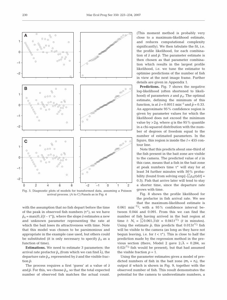
Regression predictions. Here, we show the methodin use on examplary data taken from observations ofCoryphaenoides armatus in the Nazaré Canyon, westof Portugal (King 2006). Normal regression assumesthat errors are approximately normally distributedwith zero mean and equal variances. Inspection of theresiduals (using residual and normal quantile plots,Fig. 4) for the examplary data does not support thisassumption, especially as the variance can be seenincreasing with fitted values.

Conversely, our theoretical models of arrival assumethat mt is Poisson distributed—chosen as it is a neutralmodel (zero information) for the spatial distribution offish. To test this, we transformed the data prior toregression. Assuming that mt follows a Poisson distrib-ution with mean value λt ϕ, then 122mt + 122222(mt +1)22 willapproximate a normal distribution (especially for smallvalues of λt ϕ, as here), with an approximate meanvalue of 21222λt ϕ and unit variance (Freeman & Tukey1950).

The normal quantile plots on transformed data (Fig. 5)provide statistical justification for these Poisson as-sumptions. Fitting the transformed models gave theresults provided in Table 2.

The fitting of these models to the data is shown inFig. 6, which indicates that both Models 2 and 3 havebeen very successful, the deviance values (Table 2)confirm this. It is impossible to distinguish Models 2and 3 in the fitting of plots, because the empirical fitfor ϕ (Model 3) gave an estimate very close to 3⁄2, which

228

Table 2. Results from regression models, assuming 122mt + 12222mt +122 normally distributed around twice the square root ofthe estimated mean. Deviance is the residual sum of squares

212Λ SE(212Λ) ϕ SE(ϕ) Deviance

Model 1 0.10577 0.00272 – – 32.23Model 2 0.28474 0.00613 – – 22.85Model 3 0.29025 0.06177 1.4902 0.1084 22.84

Farnsworth et al.: Scavenger fish abundance estimation

was the value assumed in Model 2. The residual plots(Fig. 5) support these conclusions, showing goodcompliance with the statistical assumptions. On thisbasis, we select Model 2 (the diffusive swimmingfish), with transformation of Poisson distributed data,as the best model for the rising phase of the time series.Using the test data, we obtain a value for Λ of 0.02027(95% confidence intervals: 0.01859 and 0.02202). Thiscan be translated into a 95% confidence interval for λ(the fish abundance) using a suitable estimate of D inΛ = vu——v+u 4λ12222D/π. The dependence on an unknown para-meter D is a nuisance, which we will see again in thenext section. There is a clear need for estimatingit from observations of the behaviour of relevant fishspecies.

This method is easy to implement:Models 1 and 2 are simply linear regres-sions. Model 3 is non-linear in the ϕ para-meter, adding a slight complication, but itis still simple to implement with standardstatistical software.

HIDDEN MARKOV MODEL

Using the whole time series. The maxi-mum use of information theoreticallyyields the highest achievable precision. Inthis section we will show how the wholetime series can be analysed, using a modelof departures from the bait of fish bothseen and unseen by the camera.

Referring to Fig. 1, we regard n(t) ashidden and the ρ and ζ terms as para-meters that can be estimated using thestatistical technique of a hidden Markovmodel (HMM) (Cappé et al. 2005)—nowcommonly used in automatic speechrecognition. With this method, the systemrepresented by Fig. 1 is assumed to bea 2-state Markov process (mt, nt), withparameters estimated from mt (again,using the non-italic font to denote ob-served counts). The ‘hidden state’ is thenumber of fish at the bait, but outsidethe camera view (nt).

We make the simplifying assumptionthat fish move among visible and hiddenstates between camera shots, so the ob-served mt at each time step is a samplefrom a binomial distribution with numberparameter xt = nt + mt and some constantprobability parameter p. This p corre-sponds to the visible fraction of the fish atthe bait.

Since the diffusive model of arrivals (Eq. 9) was thebest supported by regression in the previous section, itis chosen to represent arrivals here, so we assumeρa(λ,t) = ~ρa12t (note tilde notation for empirically esti-mated parameters). We aim to estimate the prefactor~ρa, to derive from it a fish abundance estimate

~λ using

Eq. (9). Now a model for departures is needed. The mean

flux away from the bait zone at time t is proportional tothe number of fish present at t. To take account of thebehaviour of fish towards a depleting bait, we definethe departure rate ρd as follows. The probability of anyfish leaving in a short time interval t to t + h is set to ρdh(approximated to first order in h), which we assume tobe a linear function of time. However, we continue

229

0 2 4 6 8 10 12 −2 −1 0 1 2

4

0

–4

4

0

–4

4

0

–4

A

ssssssss

ss

s

s

sssss

s

ss

s

s

s

s

s

ss

ss

s

s

s

s

s

s

s

s

ss

s

s

ss

ss

s

s

s

sssssssss

ss

s

s

sssss

s

ss

s

s

s

s

s

ss

ss

s

s

s

s

s

s

s

s

ss

s

s

ss

ss

s

s

s

B

sssssssss

ss

s

s

sssss

s

ss

s

s

s

s

s

ss

ss

s

s

s

s

s

s

s

s

ss

s

s

ss

ss

s

s

sssssssss

ss

s

s

sssss

s

ss

s

s

s

s

s

ss

ss

s

s

s

s

s

s

s

s

ss

s

s

ss

ss

s

s

s

C

sssssssss

ss

s

s

sssss

s

ss

s

s

s

s

s

ss

ss

s

s

s

s

s

s

s

s

ss

s

s

s

s

s

s

s

s

s

s

s

ss

ss

s

s

sssssssss

ss

s

s

sssss

s

ss

s

s

s

s

s

ss

ss

s

s

s

ss

ss

s

s

s

Fig. 4. Diagnostic plots of models for untransformed data. (A) Model 1, (B)Model 2 and (C) Model 3. Left column: residuals against fitted values for the 3models. Right column: quantile plots (empirical quantiles of residuals againstquantiles of the standard normal distribution), reference lines pass through

the first and third quartiles

Mar Ecol Prog Ser 350: 223–234, 2007

with the assumption that no fish depart before the timeof the peak in observed fish numbers (τ*), so we havel~ρd = max(0, ~z [t – τ*]), where the slope ~z estimates a newand unknown parameter representing the rate atwhich the bait loses its attractiveness with time. Notethat this model was chosen to be parsimonious andappropriate in the example case used, but others couldbe substituted (it is only necessary to specify ~ρd as afunction of time).

Estimations. We need to estimate 3 parameters: thearrival rate prefactor ~ρa (from which we can find

~λ), the

departure rate ~ρd, represented by ~z and the visible frac-tion ~p.

The process requires a first ‘guess’ at a value of ~zand ~p. For this, we choose ~ρa, so that the total expectednumber of observed fish matches the actual count.

(This moment method is probably veryclose to a maximum-likelihood estimate,and reduces computational complexitysignificantly). We then tabulate the fit, i.e.the profile likelihood, for each combina-tion of ~z and ~p. The parameter estimate isthen chosen as that parameter combina-tion which results in the largest profilelikelihood, i.e. we tune the estimator tooptimise predictions of the number of fishin view at the next image frame. Furtherdetails are given in Appendix 1.

Predictions. Fig. 7 shows the negativelog-likelihood (often shortened to likeli-hood) of parameters z and ρd. The optimalestimate, defining the minimum of thisfunction, is at z = 0.0011 min–2 and p = 0.33.An approximate 95% confidence region isgiven by parameter values for which thelikelihood does not exceed the minimumvalue by >2q, where q is the 95% quantilein a chi-squared distribution with the num-ber of degrees of freedom equal to thenumber of estimated parameters. In thefigure, this region is inside the l = 455 con-tour line.

Note that this predicts about one-third ofthe fish present in the bait zone are visibleto the camera. The predicted value of z inthis case, means that a fish in the bait zoneat peak numbers time τ* will stay for atleast 34 further minutes with 50% proba-bility (found from solving exp[–∫T

0 ρd(t)dt] =0.5). Fish that arrive later will tend to staya shorter time, since the departure rategrows with time.

Fig. 8 shows the profile likelihood forthe prefactor in fish arrival rate. We seethat the maximum-likelihood estimate is

0.061 min–3�2, with a 95% confidence interval be-tween 0.044 and 0.091. From this we can find thenumber of fish having arrived in the bait region attime t: Nt = ∫T

0 0.06112t dt = 0.041t 3�2 (t in minutes).Using the estimate ~p, this predicts that 0.013t 3�2 fishwill be visible to the camera (as long as they have notbegun leaving, i.e. for t < τ*). This is close to half theprediction made by the regression method in the pre-vious section (there, Model 2 gave 212Λ = 0.284, so0.02t 3�2 fish would be present), but that had assumedthe visible fraction p = 1.

Using the parameter estimates gives a model of pre-dicted numbers of fish in the bait zone (mt + nt), theoutput if which is shown in Fig. 9, together with theobserved number of fish. This result demonstrates thepotential for the camera to underestimate numbers, a

230

A

●●●●●●●●

●

●

●

●

●

●

●●●●

●

●

●

●

●

●

●

●

●●

●

●

●

●

●

●

●

●

●

●

●●

●

●

●●

●●

●

●

●

●●

●●

●●

●●

●

●

●

●

●

●

●●

●●

●

●

●

●

●

●

●

●

●●

●

●

●

●

●

●

●

●

●

●

●●

●

●

●●

●●

●

●

●

B

●

●

●●

●●

●●

●

●

●

●

●

●

●●●●

●

●

●

●

●

●

●

●

●●

●

●

●

●

●

●

●

●

●

●

●

●

●

●

●●

●●

●

●

●

●

●

●●

●●

●●

●

●

●

●

●

●

●●

●●

●

●

●

●

●

●

●

●

●●

●

●

●

●

●

●

●

●

●

●

●

●

●

●

●●

●●

●

●

●

C

●

●

●●

●●

●●

●

●

●

●

●

●

●●●●

●

●

●

●

●

●

●

●

●●

●

●

●

●

●

●

●

●

●

●

●

●

●

●

●●

●●

●

●

●

0 2 4 6 8

●

●

●●

●●

●●

●

●

●

●

●

●

●●

●●

●

●

●

●

●

●

●

●

●●

●

●

●

●

●

●

●

●

●

●

●

●

●

●

●●

●●

●

●

●

−2 −1 0 1 2

1

0

–1

–2

1

0

–1

–2

1

0

–1

–2

Fig. 5. Diagnostic plots of models for transformed data, assuming a Poisson arrival process. (A to C) Panels as in Fig. 4

Farnsworth et al.: Scavenger fish abundance estimation

phenomenon now empirically confirmed by Jamiesonet al. (2006) (though with a different lander to that usedin generating the test data). Some may be surprised atthe closeness with which the HMM model follows thedata. The explanation is that the HMM is not a simple3-parameter model (as often encountered in basic sta-tistics), but a Markov model, which at each time stepuses the whole time series along with the 3 parametersin a constantly updating calculation of expected num-bers in the next photoframe. The fact that it follows thedata consistently suggests that the parameter esti-mates are good.

DISCUSSION

Having examined 3 different methods for estimatingabundance from fish counts at a bait, we are in a posi-tion to make recommendations for studies with cross-current foraging fish in reasonably stable currents. Thefirst of these may be very surprising for biologists whohave relied on first arrival times for their estimates.This measure was found to have a theoretically infinitevariance and, in practice, to make a very poor estima-tor, as long as we can assume that fish do not sociallyinteract, or become distracted from the bait. This find-ing is independent of the specific model of fish arrivalsused, as it is a consequence of assuming a random dis-tribution of fish in the environment. The weakness offirst arrival time as a predictor had been obscured bythe use of deterministic models, which did not allowuncertainty to be quantified. Despite several reports ofcorrelations between τ1 and independently measuredabundance (e.g. Sainte-Marie & Hargrave 1987), thereis no support from statistical theory for using firstarrival times.

Conversely, a regression on the rising phase of thetime series (the period until maximum numbers areexpected), assuming Poisson distribution of residualsand a diffusive scaling of arrival rate, gave a precisemeasure of abundance with the test data. This methodis theoretically sound and simple to use, so we recom-mend it for circumstances where its assumptions arefound to hold. These assumptions are specifically thatfish behave independently, are distributed at randomin the environment, and that all fish arriving at the baitare seen upon arrival. Further, that fish do not leave

231

0 10 20 30 40 50 60 70

15

10

5

0

Time in photoframes

Num

ber

of f

ish

in c

amer

a vi

ew

Fig. 6. Regression models. Circles: observed data; dashedline: Model 1; dotted line: Model 2; dot-dashed line:Model 3—all using transformed data. Note that Models 2

and 3 are indistinguishable at the scale plotted

Slope z of departure rate ρd( t ) (min−2)

Frac

tion

p o

f vis

ible

ind

ivid

uals

+

0.6

0.5

0.4

0.3

0.2

0.0000 0.0005 0.0010 0.0015 0.0020 0.0025

Fig. 7. Contour plot of the negative log-likelihood function forestimating departure rate slope z and observable fraction p

0.02 0.04 0.06 0.08 0.10 0.12 0.14

Arrival rate prefactor ~ρa (min–3/2)

Pro

file

likel

ihoo

d

462

460

458

456

454

452

Fig. 8. Profile negative log-likelihood for estimating thearrival rate prefactor ~ρa. The 95% confidence interval is

indicated where the curve crosses the dashed line

Mar Ecol Prog Ser 350: 223–234, 2007

the bait until after maximum numbers are observed,that the plume does not change greatly in directionduring the rising phase, and that the usual assump-tions for regression hold.

The more flexible method of HMM is recommendedfor its smaller set of assumptions, though it incurs a costin complexity and additional parameters to be esti-mated. The assumptions of the HMM method are thatfish are distributed randomly in the environment, actindependently (including at the bait) and that theplume does not change greatly in direction during thetime series (though the method could be adapted tocope with violations of the latter 2 assumptions). Wewish to emphasise that it is very important to deter-mine if the assumptions of any method are met prior touse.

In our example, for models of both the regressionand HMM methods, we introduced a new parameterD, defined as fish searching diffusivity. Estimates of Dshould be sought if this simple and flexible model is tobe used. D has the form of swimming speed squared,divided by the frequency of changing direction whilstsearching for plumes: D = w 2/μ. Search speeds (w) areoften known, but new effort is needed to estimate turn-ing frequencies (μ) from observations of fish behaviour.Abundance estimates are sensitive to 1222D, which ismuch less than their sensitivity to swimming speed, so,given a reasonable estimate of a fish’s turning fre-quency μ, a working estimate of D is attainable. It ispossible to interpret D more broadly as an empiricalparameter that depends in part on non-linear exten-sion of the plume, non-ideal swimming strategies ofthe fish and other factors that ‘spoil’ the theoreticalideals of the geometric model. However, a calibration

based on independent abundance estimates(e.g. from trawls) would be necessary to esti-mate D, following this interpretation.

The regression and, in our example (thoughnot necessarily or generally), the HMMmethod assumed that departure rate from thebait is zero until the maximum number of fishis seen (τ*). Strictly, this is not likely, partlybecause of randomness in fish behaviour andpartly because the maximum should appearwhen the departure rate exceeds the arrivalrate, which by definition is greater than zero.The resulting bias underestimates abundancein the regression method. It is therefore veryimportant to ensure that this assumption is areasonable approximation (i.e. that the maxi-mum occurs at a time after deployment that isless than the expected staying time of a fish).The HMM method is less affected by this biasfrom the rising phase, because the iterativefitting can compensate using the remainder

of the time series. If there is a long rising phase, werecommend the HMM method with some simpledeparture model designed to reflect the researchers’beliefs about departures. In other words, the HMMmethod should be customised to the particular case forwhich it is to be used.

Practical application of the regression method is sim-ple, using most statistical software packages. Time actsas the independent variable in a univariate non-linearregression for number of fish observed in each cameraexposure (as in the described Model 2). The interceptshould be set as zero (no fish at time zero), leaving theslope to be estimated, giving Λ (as in Model 2), whichenables λ to be found from the various velocity esti-mates. We illustrated diagnostic plots to check that theassumptions of this method support its use; we espe-cially recommend residual and quantile plots for this.Practical use of the HMM method requires some pro-gramming, for example, in a statistical or mathematicspackage—details are provided in the Appendix.

The problem caused by fish attracted to the appara-tus, but not photographed on the bait (Collins et al.1999) is well known and has been demonstrated byJamieson et al. (2006, admittedly using a design oflander that is not usual for abundance estimation). TheHMM method estimates the size of the resulting biassimultaneously while estimating arrival and departurerates. In the example shown, the HMM method esti-mated an arrival rate close to half that of the regressionmethod when using the same model of arrivals overthe same section of the time series. Independent mea-sures of the ‘hidden fraction’ of fish would be hard toobtain, unless cameras were set to observe the landersystem.

232

0 100 200 300Time t (min)

No.

of i

ndiv

idua

ls

Mean ind. at baitEstimated ind. at baitMean ind. in visionObserved count

30

25

20

15

10

5

0

Fig. 9. Examplary data (counted individuals in each photo) with hiddenMarkov model (HMM)-fitted estimates. HMM with full knowledge of ob-servations (–––––); model based on parameter estimates with the mean ofobserved count (––––); model of observed (visible) fish only, based on

mean observed count (– –)

Farnsworth et al.: Scavenger fish abundance estimation

The HMM method requires a model of departures aswell as arrivals. Priede & Merrett (1998) fitted an em-pirical curve to the estimated staying time (which de-termines departure rate) using the time of maximumnumber of fish (τ*) minus the first arrival time (τ1), thusassuming staying time to be constant. However, baitdepletion and scavenger competition mitigate againstthis assumption, especially for long time series. In prin-ciple, we could understand both effects in terms of opti-mal foraging theory, as suggested by Priede & Merrett(1998), who showed that staying time (as they definedit) declined with fish abundance (independently deter-mined with trawls). However, using the marginal valuetheorem (Charnov 1976), suggested by this result, re-quires a model for competition and satiation, leading toconsiderable complications and introducing new para-meters. For the present purpose, we suggest the parsi-monious, single-parameter model in which the proba-bility of departing in a small time interval increases at aconstant rate with elapsed time. The gradual increasein departure probability that we hypothesise is mostlikely related to bait depletion, which can be estimatedfrom the photographs. This could set limits (at least)on the z parameter of ρd, so even crude estimates ofbait depletion rate could be useful in using the HMMmodel. Clearly, there are opportunities to improve onthis, but each development of sophistication needs tobe justified by quantity and quality of data available.

Broadening the discussion, our overall model of fishbehaviour can be extended in a number of ways to ad-dress specific biological issues. For example, speciesthat show either gregarious or food-swarming behav-iour could be represented by alternative statisticalmodels of dispersion (the Poisson model being a null-hypothesis), and allowing for autocorrelation in thetime series in the regression technique could probablyaccommodate most of these effects. Territoriality can betaken into account by truncating the arrival rate after atime representing territory size, and this approach canalso be used to allow for rival attractants (e.g. naturalfood falls) in the environment. Changes in currentvelocity over measurement time are often observed inthe deep sea and are almost inevitable (due to tides) inshallower seas. The result is a more complicated plumeshape and perhaps changes in fish swimming veloci-ties. To take account of this, our model could be treatedas a piecewise fit to the number of observed fish, usingdifferent current parameters over different sections.More sophisticated modelling of the plume will allow amore precise description of how arrival rate depends onabundance, but not necessarily more precise abun-dance estimates, since additional parameters reducestatistical power. As stated earlier, it is possible toinclude plume spreading in the diffusivity parameter Dof fish searching behaviour.

Acknowledgements. We thank D. M. Bailey for his very help-ful suggestions and J. E. Beyer for facilitating the UK–Danishcollaboration.

LITERATURE CITED

Bailey D, Priede I (2002) Predicting fish behaviour in responseto abyssal food falls. Mar Biol 141:831–840

Cappé O, Moulines E, Rydén T (2005) Inference in hiddenMarkov models. Springer-Verlag, Heidelberg

Charnov E (1976) Optimal foraging: the marginal valuetheorem. Theor Popul Biol 9:129–136

Collins M, Yau C, Nolan C, Bagley P, Priede I (1999) Be-havioural observations on the scavenging fauna of thePatagonian slope. J Mar Biol Assoc UK 79:963–970

Collins M, Yau C, Guilfoyle F, Bagley P, Everson I, Priede I,Agnew D (2002) Assessment of stone crab (Lithodidae)density on the South Georgia slope using baited videocameras. ICES J Mar Sci 59:370–379

Dusenbery D (1989) Optimal search direction for an animalflying or swimming in a wind or current. J Chem Ecol15:2511–2519

Freeman M, Tukey J (1950) Transformations related to theangular and the square root. Ann Math Stat 21:607–611

Henriques C, Priede I, Bagley P (2002) Baited camera ob-servations of deep-sea demersal fishes of the NortheastAtlantic Ocean at 15–28° N off West Africa. Mar Biol 141:307–314

Jamieson A, Bailey D, Wagner H, Bagley P, Priede I (2006)Behavioural responses to structures on the seafloorby the deep-sea fish Coryphaenoides armatus: implica-tions for the use of baited landers. Deep-Sea Res I 53:1157–1166

Johnson N, Kotz S, Balakrishnan N (1994) Continuous uni-variate distributions, Vol 1, 2nd edn. Wiley-Interscience,New York

King N (2006) Deep-sea ichthyofauna of contrasting loca-tions: mid-Atlantic Ridge, Nazare Canyon (North AtlanticOcean) and Crozet Plateau (Southern Indian Ocean), withspecial reference to the abyssal grenadier, Coryphaeno-ides (Nematonurus) armatus (Hector, 1875). PhD disserta-tion, University of Aberdeen

Lapointe V, Sainte-Marie B (1992) Currents, predators, andthe aggregation of the gastropod Buccinum undatumaround bait. Mar Ecol Prog Ser 85:245–257

Lokkeborg S, Olla B, Pearson W, Davis M (1995) Behavioralresponses of sablefish, Anoplopoma fimbria, to bait odor.J Fish Biol 46:142–155

Okubo A (1980) Diffusion and ecological problems: mathe-matical models. Springer-Verlag, Heidelburg

Priede I, Bagley P (2000) In situ studies on deep-sea demersalfishes using autonomous unmanned lander platforms.Oceanogr Mar Biol Annu Rev 38:357–392

Priede I, Merrett N (1996) Community studies. 2. Estimationof abundance of abyssal demersal fishes: a comparison ofdata from trawls and baited cameras. J Fish Biol Suppl A49:207–216

Priede I, Merrett N (1998) The relationship between numbersof fish attracted to baited cameras and population density:studies on demersal grenadiers Coryphaenoides (Nema-tonurus) armatus in the abyssal NE Atlantic Ocean. FishRes 36:133–137

Priede I, Smith K, Armstrong J (1990) Foraging behavior ofabyssal grenadier fish—inferences from acoustic taggingand tracking in the North Pacific Ocean. Deep-Sea Res37:81–101

233

Mar Ecol Prog Ser 350: 223–234, 2007

Priede I, Bagley P, Armstrong J, Smith K, Merrett N (1991)Direct measurement of active dispersal of food-falls bydeep-sea demersal fishes. Nature 351:647–649

Priede I, Bagley P, Smith A, Creasey S, Merrett N (1994) Scav-enging deep demersal fishes of the Porcupine Seabight,Northeast Atlantic—observations by baited camera, trapand trawl. J Mar Biol Assoc UK 74:481–498

Sainte-Marie B, Hargrave B (1987) Estimation of scavengerabundance and distance of attraction to bait. Mar Biol94:431–443

Vabo R, Huse G, Ferno A, Jorgensen T, Lokkeborg S, SkaretG (2004) Simulating search behaviour of fish towards bait.ICES J Mar Sci 61:1224–1232

Webster D, Weissburg M (2001) Chemosensory guidancecues in a turbulent chemical odor plume. Limnol Oceanogr46:1034–1047

Yau C, Collins M, Bagley P, Everson I, Nolan C, Priede I(2001) Estimating the abundance of Patagonian toothfishDissostichus eleginoides using baited cameras: a prelimi-nary study. Fish Res 51:403–412

Yen J, Weissburg M, Doall M (1998) The fluid physics of sig-nal perception by mate-tracking copepods. Philos Trans RSoc B 353:787–804

Zimmer-Faust R, Finelli C, Pentcheff N, Wethey D (1995)Odor plumes and animal navigation in turbulent water-flow—a field study. Biol Bull (Woods Hole) 188:111–116

234

Appendix 1. Implementing the HMM technique

The hidden Markov model (HMM) method is imple-mented through an HMM filter. In the following, we brieflydescribe how this filter is constructed, so that those familiarwith modelling can replicate the technique. In-depth treat-ments of the theory of HMMs are found in Cappé et al.(2005). The filter first aims to estimate the total number offish, xt = nt + mt, in which xt is a stochastic variable that maytake integer values between 0 and a sufficiently largebound K on the total number of fish at the bait.

The filter needs the transition probabilities of xt. Assumethat xt = i and consider xt+h, where h is a fixed short timeinterval. If a fish has arrived, then xt+h = i + 1; the probabil-ity of this is gi(i + 1)(t) = h × ρa(t). If a fish has departed, thenxt+h = i – 1; the probability of this is gi(i – 1)(t) = i × h × ρd(t).Alternatively, nothing has happened; the probability of thisis gii(t) = 1 – gi(i – 1)(t) – gi(i + 1)(t). These are valid approxima-tions when h is small compared to ρa(t), ρd(t) and the rate ofchange of these functions. Typical camera sampling times of30 to 120 s (in our example it was h = 90 s) will give sufficientresolution in most practical cases.

The predictive filter consists of Φ(t), a (row) vector, the ithentry Φi(t) of which is the probability that xt = i, given allobservations strictly prior to t. Similarly, the row vector ψ(t)has entries ψi(t) being the probability that xt = i, given allobservations no later than t. The ‘data update’ transformsΦ(t) to ψ(t) by taking the observation mt = mt into account:

(A1)

Here, l (t) = ΣiP{mt = mt |xt = i } is a normalization ensuringthat Σiψi(t) = 1. These probabilities are computed using theassumption that, conditional on xt = i, mt is binomially dis-tributed with number parameter i and probability para-meter p:

(A2)

The time update projects ψ(t) forward in time to obtain aprediction Φ(t + h):

(A3)

The time update and the data update are iterated for-wards in time; the initial condition is ψ0(0) = 1 and ψi(0) = 0for i ≠ 0. At the end of the iteration, we evaluate the likeli-hood function L( ~z, ~p) = ∏tl(t). Recall that ~ρa is estimated by amoment method rather than with the likelihood method.The likelihood function is optimized numerically. For esti-mated parameters, we ‘smooth’ to obtain probability vectorsπ(t), with π i(t) denoting the probability that xt = i, given allobservations. This smoothing is an iteration backwards intime:

(A4)

with terminal condition π(T) = ψ(T).

π ψπ

i i ijj i

ij

j

t t g tt h

t h( ) ( ) ( )

( )

( )=

++= −

+

∑1

1

Φ

Φ j i iji j

j

t h t g t( ) ( ) ( )+ == −

+

∑ ψ1

1

P m x ii

p pt t tt

it t= ={ } = ⎛⎝⎜

⎞⎠⎟ − −m

mm m� ( )1

ψ ii

t t ttt

l tm x i( )

( )( )

= = ={ }ΦP m �

Editorial responsibility: Howard Browman (Associate Editor-in-Chief), Storebø, Norway

Submitted: November 30, 2006; Accepted: July 27, 2007Proofs received from author(s): November 2, 2007