Critical Path Stability Region: A Single-Time Estimate Approach

��

Copyright © 2014, IGI Global. Copying or distributing in print or electronic forms without written permission of IGI Global is prohibited.

&KDSWHU��

DOI: 10.4018/978-1-4666-4856-2.ch003

&ULWLFDO�3DWK�6WDELOLW\�5HJLRQ�$�6LQJOH�7LPH�(VWLPDWH�$SSURDFK

$%675$&7

Models transform the managerial inputs into useful information for managerial decision. The Project Evaluation and Review Technique (PERT) is the most widely used model for project management. However, it requires three estimates for the duration of each activity as its input. This uncertainty in the input requirement makes the Critical Path (CP) unstable, causing major difficulties for the manager. A linear programming formulation of the project network is proposed in this chapter for determining a CP based on making one estimate for the duration of each activity. Upon finding the CP, Sensitivity Analysis (SA) of Data Perturbation (DP) is performed using the constraints of the dual problem. This largest DP set of uncertainties provides the manager with a tool to deal with the simultaneous, indepen-dent, or dependent changes of the input estimates that preserves the current CP. The application of DP results to enhance the traditional approach to PERT is presented. The proposed procedure is easy to understand, easy to implement, and provides useful information for the manager. A numerical example illustrates the process.

Hossein ArshamUniversity of Baltimore, USA

Veena AdlakhaUniversity of Baltimore, USA

��

&ULWLFDO�3DWK�6WDELOLW\�5HJLRQ�

��,1752'8&7,21

Project management is one of the fastest growing career fields in business education today. Most of the growth in this field is in the business sectors, where there are widespread reports about most projects being late, many over budget, and all too often do not satisfy design specifications. This paper is about business project management, although the principles apply to projects in any field. When proposing a new business system, the project manager will be confronted with many questions from top management, in particular “How much will it cost? And “When will it be done?” As many project managers know, these two questions are difficult to answer correctly.

A project involves getting a new, complex activity accomplished. Generally projects de-signed to accomplish something for the company undertaking them. Because projects involve new activities, they typically involve high levels of uncertainty and risk. It is very difficult to predict what problems are going to occur in business system development.

Projects are systems consisting of inter-related parts working together to accomplish project objectives. There are a number of im-portant roles within business systems projects. Project managers have to balance technical understanding with the ability to motivate diverse groups of people (the project team) brought together on a temporary basis. Projects are collections of activities. If one activity is late, other activities are delayed. If an activity is ahead of schedule, workers tend to slow down to meet the original completion date. Business systems projects have many similarities to ge-neric projects. They consist of activities, each with durations, predecessor relationships, and resource requirements. They involve high levels of uncertainty and often suffer from time and cost overruns, while rarely experiencing time

and cost underruns. However, business systems projects are different from generic projects in some aspects. While each project is unique, there are usually numerous replications of business systems project types. Most are served by a standard methodology, with the need to iden-tify user requirements, followed by design of a system, production of the system, testing of the system, training and implementation, and, ultimately, maintenance of the system. These steps are not always in serial; there are often many loops back to prior stages.

Defining project success in itself is difficult. There are many views of what makes a project successful. Successful implementation has been found to require mastery of the technical aspects of systems, along with understanding key organizational and behavioral dynamics. There has been a great deal of research into business systems project failure. Failure can occur when design objectives are not met. The difference between successful and failed busi-ness systems projects often lies in planning and implementation. A great deal of research has been performed to identify factors that lead to project success. These factors include planning, user involvement, and good communication. Additional factors that are reported as important in business systems project success repeatedly include top management support and clear statement of project objectives.

Business systems project management can involve a wide variety of tasks. Typical busi-ness systems project types include maintenance work, conversion projects, and new systems implementation. Maintenance projects are by far the most common type of business systems project. They can arise from need to fix errors or to add enhancements to some system, or to involve major enhancements. Conversion projects involve changing an existing system. New systems development involves different management characteristics by type of system.

��


Business systems projects have high levels of uncertainty. The size of the project is usually not well understood until systems analysis has been completed. Most of the unexpected delay in these projects occurs during the latter stages of testing. Almost one third of the time used in typical projects is required for the planning phase, and coding typically consisted of one-sixth of the project. Coding is the most predict-able portion of the project. The last half of the project is testing – one-quarter for component testing and one-quarter for system testing. The activity most difficult to predict was testing. Project managers currently use the critical path method (CPM) and/or project evaluation and review technique (PERT) in order to provide a planning and control structure for projects. CPM helps managers understand the relation-ships among project activities. Key personnel and other resources can be allocated to activi-ties on the critical path. These activities can be closely monitored to avoid completion delays.

CPM identifies the sequence of activities that will have the longest completion time of the entire project. PERT extends CPM’s scope to deal with uncertainties inherent in any project. Project activity network models ranked above all other quantitative decision making tools in terms of the percentage of business firms who used them. Although these techniques are widely used in practice and have provided economic benefit to their users, they are not problem-free. Problems derive from the nature of the underlying statistical assumptions, the potential for high computational expense, and from the assumption that factors determining activity duration are essentially probabilistic rather than determined by managerial action.

��&ULWLTXH�RI�&30�3(57

In this section examines the scope and limitations of CPM/PERT. The most widely used CPM/PERT

algorithm is based on the following assumptions and procedure:

• Activity Duration: Rarely (if ever) known with certainty; the CPM asks the manager for three time estimates. Three time esti-mates are determined (by guesses, etc.) for each activity: ƕ a: An optimistic completion time. ƕ m: A most likely completion time

(this is what we will use in this paper). ƕ b: A pessimistic completion time.

• Activity Approximations: ƕ An approximation for the distribution

of an activity’s completion time is a BETA distribution

ƕ An approximation for the mean completion time for an activity is a weighted average (1/6, 4/6, 1/6) of the three time estimates is (a +4m +b)/6

ƕ An approximation for the standard deviation for the completion time for an activity is its range/6 or (b – a)/6

ƕ The variance of an activity’s comple-tion time is the square of the standard deviation = [(b – a)/6] 2

• Project Assumptions:1. The distribution of the project comple-

tion time is determined by the critical path using the mean activity completion times

2. The activity completion times are Independent.

3. There are enough activities (at least 30, to make sure) on the critical path so that the central limit can be used to determine the distribution, mean, variance and standard deviation of the project

• Project Distribution: Given the above as-sumptions, this means: ƕ The project completion time distribu-

tion is normal.

��


ƕ The mean (expected) completion time, µ, of the project is the sum of the expected completion times along the critical path.

ƕ The variance of the completion time, σ2, of the project is the sum of the variance in completion times along the critical path.

ƕ The standard deviation of the com-pletion time, σ, of the project is the square root of the variance of the completion time of the project.

The probability of completing by a certain date t, can now be found by finding the P(X < t) from a normal distribution with mean µ and standard deviation σ.

The critical path method requires three time estimates from the manager for each activity in the project. In a dialog with this author, a manager said that it is difficult enough to offer one estimate for the duration of one activity. By asking for three estimates for each activity in the project, more uncertainty is introduced. It makes sense to ask the manager for one good estimate.

An alternative to the CPM/PERT is a stochastic activity network (Adlakha and Arsham, 1992). This approach assumes that the same project is to be performed repeatedly, and there is full knowledge of the time distribution function to be used in Monte-Carlo simulation experiments to approximate the expected CPM/PERT duration. This approach suffers from even more severe practical pitfalls, in addition to being computa-tionally expensive.

The validity of the above assumptions has been a long-standing question (Kallo, 1996; Kambu-rowski, 1997; Keefer and Verdini, 1993; Kuklan, 1993). The solution based on inaccurate inputs result in the incorrect designation of the CPM/PERT, and the accuracy of the results decreases in relation to increased project complexity (Na-kashima, 1999).

While Hasan and Gould (2001) support the sense-making activity of managers, more than half a century after the debut of CPM and PERT, they still are requiring complex user input. While mod-ern decision support systems for project manage-ment are more sophisticated and comprehensive than CPM/PERT, they show insufficient progress in dealing with uncertainties (Trietsch and Baker, 2012). Czuchra (1999) presents recommendations on optimizing budget spending for software imple-mentation and testing. Yaghoubi, Noori, Azaron and Tavakkoli-Moghaddam (2011) consider dy-namic PERT networks where activity durations are unrealistically independent random variables with exponential distributions. Mouhoub, Benho-cine, and Belouadah (2011) propose to reduce the number of dummy activities as much as possible, but the result is even more complex. Herrerı´as-Velasco, Herrerı´as-Pleguezuelo, and René van Dorp (2011), being aware of the difficulties with the interpretation of the parameters of the beta distribution, suggest an alternative to the PERT variance expression regarding the constant PERT variance assumption. Martín, García, Pérez, and Sánchez Granero (2012), propose a two-sided power and the generalized biparabolic distribu-tions as an alternative to the mixture of the uniform and the beta distributions to the beta distribution in PERT methodology. Yakhchali (2012) expands the work of Nasution (1994) while addressing the problem of determining the degree of possible and necessary criticality of activities, as well as determining paths in networks that have fuzzy activity durations.

D’Aquila (1993) recommends simultaneous use of CPM/PERT. Mehrotra, Chai, and Pillutla (1996) suggest approximating the moments of the job completion. Banerjee and Paul (2008) use multivariate statistical tools analysis to measure the error in the classical PERT method of estimating mean project completion time when correlation is ignored. Premachandra (2001) yet provides approximations for the mean and the variance of

��


activity based on “pessimistic”, “optimistic” and “most likely” time estimates to get away from the beta distribution assumption.

Even ordinary sensitivity analysis is rarely performed in activity network projects, because the existing CPM/PERT algorithms do not con-tain enough information to perform the calcula-tions necessary for this simplest form of Data Perturbation Analysis (DPA). To the best of our knowledge NETSOLVE is the only software avail-able capable of dealing with ordinary sensitivity analysis for CPM (Jarvis and Shier, 1990; Phillips and Garcia-Diaz, 1990). The existing stochastic PERT software packages require a separate run for each scenario if any parameters are changed (Higgs, 1995; Lewis, 2007).

The probabilistic nature in both PERT models assumes random factors (e.g., bad luck, good luck) are present and does not allow for any managerially planned point of view to deal with uncertainty. In other words, much of the variability for activity duration may result from management decisions, rather than from random acts of nature.

��$Q�$OWHUQDWLYH�&RPSXWDWLRQDO�$SSURDFK

This chapter discusses a non-statistical approach, referred to as Data Perturbation Analysis (DPA), to calculate a variety of activity duration uncertain-ties. DPA deals with a collection of managerial questions related to uncontrollable environmental factors in project estimation tasks. The underlying mathematics of the DPA is a linear program based formulation. This approach provides:

1. An assessment and analysis of the stability of the critical path(s) under uncertainty;

2. Monitoring of the admissible range of activ-ity durations that preserve the current CP; and

3. Disclosure of the useful limits on simultane-ous, dependent departures from the activity

duration estimates to determine maximum “crashing” of critical activity durations, the maximum “slippage” for non-critical activity durations; and the impacts of such departures on the entire project completion time.

These benefits allow the manager more lever-age in allocating project resources. Knowing the stability of the critical path(s) under uncertainty allows the manager to perceive a range of timing changes before a new path of activities is critical. Monitoring the admissible range of activity dura-tions that preserve the current CP aids in deter-mining how resources should be applied among the activities to expedite the completion of the project and to smooth out workloads. Disclosure of information about departure times for critical and non-critical activities allows the manager to anticipate the consequences of slippage wherever it might occur in the project and to pre-determine back-up strategies.

This chapter develops a simplex-type solution algorithm to find the CP. The algorithm is easy to use and does not introduce any slack or surplus variables (as in the dual simplex method), or any artificial variables (Arsham, 1997a, 1997b); therefore it is computationally practical and stable to implement. A unified approach is presented to cover all aspects of the sensitivity analysis.

The remainder of this chapter is divided into five parts. First, based on one estimate for the duration of each activity, the CP is obtained by a linear program formulation and an efficient solu-tion algorithm. This is followed by an illustrated numerical example. In the next section we discuss how the data manipulation leading to the CP provides the necessary information for the Data Perturbation Analysis (DPA) that provides the largest sensitivity region,. This is followed by the parametric analysis, which includes the ordinary sensitivity analysis and the so-called 100% rule. Then the tolerance analysis is developed and, as its by-products, we obtain the individual and sym-

��


metric tolerance analysis together with a discussion of some potential applications. The last section is devoted to concluding remarks. Throughout the paper the emphasis is on constructive procedures, proofs and a small numerical example since these lead directly to an efficient computer program for implementation. Furthermore, this algorithm facilitates PDA, including structural changes in the nominal project network.

��/,1($5�352*5$0�)2508/$7,21�:,7+�$�1(:�62/87,21�7(&+1,48(

Suppose that in a given project activity network, there are m nodes, n arcs (i.e. activities) and an estimated duration, tij, associated with each arc (i, j) in the network. Without loss of generality, it is assumed that the activities durations are continu-ous. The beginning node of an arc corresponds to the start of the associated activity and the end node to its completion. To find the CP, define the binary variables Xij, where Xij = 1, if the activity (i, j) is on the CP, and Xij = 0 otherwise. The length of the path is the sum of the durations of the activi-ties on the path. Formally, the CP problem is to find the longest path from node 1 to node m, i.e.

Maximize t Xij ijj

m

i

m

==∑∑��

subject to:

X jj

m

��

�==∑ (1)

− + ===∑∑ X Xij kik

m

j

m

11

0

for i ≠ 1 or m

X jmj

m

==∑ 11

,

where the sums are taken over existing arcs in the network, and all variable are non-negative. The first and the last constraints are imposed to start (node 1) and complete the project (node m) by critical activities, respectively; while the other constraints provide that if any node is arrived at by a critical activity, then it must be left by a criti-cal activity. Note that the integrality conditions (i.e., Xij=0 or 1) are changed to Xij ≥ 0 since it is known that the optimal solution to these types of LP problems satisfy these conditions. Note also that one of these m constraints is redundant; e.g. the first constraint is the sum of all other constraints.

7KH�&ULWLFDO�3DWK�)LQGHU

The following notation is used in the new algo-rithm:

• BVS: Basic Variable Set• GJP: Gauss-Jordan Pivoting• PR: Pivot Row (Row to be assigned to the

variable to come in BVS)• PC: Pivot Column (Column associated

with variable to come in BVS)• PE: Pivot Element• OR: Open Row. A row not yet assigned to

a variable. Labeled (?).• (?): Label for a row that is not yet assigned

a variable (Open Row)• RHS: Right Hand Side• C/R: Column Ratio, RHS/PE• R/R: Row Ratio, Last row/PR• OP: Optimality Phase• FE: Feasibility Phase

��


The algorithm consists of preliminaries for setting up the initialization followed by three main phases: Basic Variable Set Augmentation, Optimality, and Feasibility. The Basic Variable Set Augmentation Phase develops a basic vari-able set (BVS) which may or may not be feasible. Unlike simplex and dual simplex, this approach starts with an incomplete BVS initially, and then variables are brought into the basis one by one. This strategy pushes towards an optimal solution. Since some solutions generated may be infeasible, the next step, if needed, pulls the solution back to feasibility. The Optimality Phase satisfies the optimality condition, and the Feasibility Phase obtains a feasible and optimal basis. All phases use the Gauss-Jordan pivoting (GJP) transforma-tion used in the standard simplex and dual simplex algorithms (Arsham, 2005). The proposed scheme is as follows:

Step 1. Set Up: The initial tableau may be empty, partially empty, or contain a full basic vari-able set (BVS).

Step 2. Push: Fill-up the BVS completely by pushing it toward the optimal vertex.

Step 3. Push Further: If the BVS is complete, but the optimality condition is not satisfied, then push further until this condition is satisfied; i.e., a primal simplex approach.

Step 4. Pull: If the BVS is complete, and the op-timality condition is satisfied but infeasible, then pull back to the optimal vertex; i.e., a dual simplex approach.

Not all project networks must go through the Push Further and Pull sequence of steps, as shown in the numerical example. In essence, this approach generates a tableau containing all the information we need to perform all parts of DPA.

The large number of equality constraints, with zero value as their right-hand-side, raises concern for primal (pivotal) degeneracy that may cause pivotal cycling. In the proposed solution algorithm,

the BVS Augmentation Phase does not replace any BVs, and the Feasibility Phase uses the dual simplex rule, therefore, there is no pivotal degen-eracy in these two phases. However, degeneracy (cycling) may occur in the Optimality Phase after the BVS Augmentation Phase and the Feasibility Phase are completed. This strategy reduces the possibility of any cycling. In the case of cycling in the Optimality Phase, this could be treated us-ing the simple and effective anti-cycling rule for simplex method. Out of the many problems solved by this algorithm, no cycling was encountered.

It is common in applications of CPM/PERT to have side-constraints in the nominal model. Network-based approaches to problems with side constraints require an extensive revision of the original solution algorithms to handle even one side-constraint. Additional difficulties arise from multiple side-constraints. In the proposed algo-rithm, when the optimal solution without the side constraints does not satisfy some or all of the side constraints, the “most” violated constraint can be brought into the final tableau by performing the “catch-up” operation using the dual simplex rule. After doing so, the Feasibility Phase can be used to generate the updated final tableau. To ensure the integrality of the solution appropriate cutting planes can be introduced, if needed.

As part of PA, there is also interest in any structural changes to the nominal project network. There appear to be only a few references that deal with adding an arc to the network, and furthermore, updating the optimal solution requires solving a large number of sub-problems. The dual problem is used to determine whether the new arc changes the CP and if so, the new network is re-optimized. A distinction between basic and non-basic deleted arcs is made. If the deleted arc is a non-basic variable, then the solution remains unchanged. However, if the deleted arc is a basic variable, then the proposed algorithm replaces the deleted variable with a currently non-basic variable by using the optimality phase.

��


6HW�8S

Identify the largest tij value for the starting and finishing arcs. Subtract these largest values from the starting and finishing arcs activities respec-tively. Eliminate the first or the last constraint, whichever has the largest number of activities. Break any ties arbitrarily. Set up the initial simplex tableau without adding any artificial variables, and then start Phase I.

3KDVH�,��3XVK�3KDVH

1.0 Push Phase Termination Test IF (?) Label exists, there are Open Rows. THEN continue the BV Iteration. OTHERWISE BVS is complete, start Push

Further Phase (Step 2.0).1.1 PE Selection PC: Select the Largest tij and any ties as

candidate column(s). PR: Select OPEN ROWS as candidate rows. PE: Select the candidate row and column with

the smallest non-negative C/R. Arbitrarily break ties. If no non-negative C/R choose the C/R with the smallest absolute value. If the pivot element is zero, select the next best tij.

1.2 BVS Augmentation1. Perform GJP.2. Replace the (?) row label with the vari-

able name.3. Remove PC from the Tableau.

Continue Push Iteration (Loop back to 1.0)

3KDVH�,,��3XVK�)XUWKHU�3KDVH

2.0 Push Further Termination Test IF any tij is positive, THEN continue the OP

Iteration, OTHERWISE OP is complete, start Pull

Phase Phase (Step 3.0).

2.1 PE Selection PC: Select the Largest tij and any ties as

candidate column(s). PR: Select the candidate row and column

with the largest positive C/R. Arbitrarily break ties.

If no positive C/R choose the C/R with the smallest absolute value. If the pivot element is zero, select the next best tij.

2.2 Push Further Iteration1. Save PC outside the tableau.2. Perform GJP.3. Exchange PC and PR labels.4. Replace the new PC with old PC with

all elements multiplied by -1 except the PE.

Continue Push Further Iteration Loop back to 2.0.

3KDVH�,,,��3XOO�3KDVH

3.0 Pull Phase Iteration Termination Test IF RHS is non-negative, THEN Tableau is Optimal. Interpret the

results. OTHERWISE continue Pull Phase Iteration

(Step 3.1)3.1 PE Selection PR: row with the most negative RHS. Tie Breaker arbitrary PC: column with a negative element in the

PR. Tie Breaker: column with the smallest tij. Further Tie Breaker arbitrary.3.2 Pull Phase Transformation

1. Save PC outside the tableau.2. Perform usual GJP.3. Exchange PC and PR Labels.4. Replace the new PC with old PC saved

in (a). Continue Pull Phase Iteration (Loop back

to 3.0)

��


The final tableau generated by this algorithm con-tains all of the information needed to perform the DPA. There is also additional useful information in the final tableau; e.g., the absolute value of the last row in the final tableau provides the slack times for the non-critical activities. Such information is useful to project managers because it indicates how much flexibility exists in scheduling various activities without affecting succeeding activities. Clearly, the critical activities have slack time equal to zero. However, the reverse statement is not necessarily true; an activity can have slack-time equal to zero while being non-critical. This can happen whenever there are multiple critical paths. In this case the sensitivity analysis is not valid.

Theorem 1: The critical path is invariant under time reduction operations introduced in set-up phase.

Proof: The proof follows from the fact that mul-tiplying the first and the last constraints by their maximum duration of starting and ending activities, respectively, and then subtracting from the objective function is equivalent to subtracting a constant from the objective function.

In real-life situations, it is common to have a few side-constraints or some structural changes, such as deletion or addition of an arc. The final tableau may be updated after incorporating the side-constraint or the structural changes and then apply the Pull Phase if needed. The violation of the total unimodularity does not affect the solu-tion procedure. If the solution is not integral, then cutting planes may be introduced to ensure an integral optimal solution.

The proposed algorithm operates in the space of the original variables and has a geometric in-terpretation of its strategic process. The simplex method is a vertex-searching method. It starts at the origin that is far away from the optimal solution. It then moves along the intersection of the boundary hyper-planes of the constraints, hopping from one

vertex to the neighboring vertex, until an optimal vertex is reached in two phases. It requires adding artificial variables since it lacks feasibility at the origin. In the first phase, starting at the origin, the simplex hops from one vertex to the next vertex to reach a feasible one. Upon reaching a feasible vertex; i.e., upon removal of all artificial variables from the basis, the simplex moves along the edge of the feasible region to reach an optimal vertex, improving the objective value in the process. Hence, the first phase of simplex method tries to reach feasibility, and the second phase of simplex method strives for optimality. The simplex works in the space of n+(m-1) dimensions, leading to m-1artificial variables, where m is the number of nodes and n is the number of arcs.

In contrast, the proposed algorithm strives to create a full basic variable set (BVS); i.e., the intersection of m-1 constraint hyper-planes that provides a vertex. The initialization phase pro-vides the starting segment of a few intersecting hyper-planes and yields an initial BVS with some open rows. The algorithmic strategic process is to arrive at the feasible part of the boundary of the feasible region. In the Push Phase, the algorithm pushes towards an optimal vertex, unlike the simplex, which only strives for a feasible vertex. Occupying an open row means arriving on the face of the hyper-plane of that constraint. Any successive iteration in the Push Phase augments the BVS by including another hyper-plane in the current intersection. By restricting incoming variables to open rows only, this phase ensures movement in the space of intersection of hyper-planes selected in the initialization phase only until another hyper-plane is hit. Recall that no replacement of variables is done in this phase. By every algorithm’s iteration the dimensionality of the working table is reduced until the BVS is filled, indicating a vertex. This phase is free from pivotal degeneracy. The selection of an incoming variable having the largest tij, pushes toward an optimal vertex. As a result, the next phase starts with a vertex.

��


At the end of the Push-Further phase the BVS is complete, indicating a vertex which is in the neighborhood of an optimal vertex. If feasible, this is an optimal solution. If this basic solution is not feasible, it indicates that the push has been excessive. Note that, in contrast to the first phase of the simplex, this infeasible vertex is on the other side of the optimal vertex. Like the dual simplex, now the Pull Phase moves from vertex to vertex to retrieve feasibility while maintaining optimality; it is free from pivotal degeneracy since it removes any negative; non- zero, RHS elements. The space of the algorithm is m-1 dimensions in the Push Phase and n dimensions in the Push Further and Pull Phases, m-1 being the number of constraints and n the number of arcs.

Theorem 2: The Push and Pull Phases are free from pivotal degeneracy that may cause cycling.

Proof: As it is known, whenever a RHS element is zero in any simplex tableau (except the final tableau), the subsequent iteration may be pivotal degenerate when applying the ordinary simplex method, which may cause cycling. In the Push phase, we do not replace any variables. Rather, we expand the basic variable set (BVS) by bringing in new variables to the open rows marked with “ ? ”. The Pull Phase uses the customary dual simplex rule to determine what variable goes out. This phase is also free from pivotal degeneracy since its aim is to replace any negative, non- zero RHS entries.

Theorem 3: The solution algorithm terminates successfully in a finite number of iterations.

Proof: The algorithm consists of the Set-up Phase to generate an initial tableau that contains some basic variables, followed by three phases. The Push Phase is a BVS augmenta-tion process that develops a basic solution, which may or may not be feasible. The Push Further Phase aims to satisfy the optimal-ity condition. If the BVS is not feasible, the Pull Phase is activated to obtain a feasible

optimal solution. All phases use the usual GJP, but differ in the method used to select the pivot element. The Push Phase uses modified simplex column selection criteria to enter one variable at a time into an open row, rather than replacing a variable, while moving towards a vertex that is “close” to the optimal vertex. This strategy pushes to-ward an optimal solution, which may result in pushing too far into non-feasibility. The Pull Phase, if needed, pulls back to a feasible solution that is optimal.

The theoretical basis for the proposed algo-rithm rests largely upon the total unimodularity of the constraints coefficient matrix and it remains unimodal under the GJP operations. By the LP formulation, optimality is attained when all tijs in the last row of a tableau are non-positive and the algorithm terminates successfully. The cur-rent algorithm starts with some non-positive tijs. Removing the redundant constraint turns a column into a unit vector identifying a basic variable for the set-up phase.

Since we are adding (not replacing) variables to the BVS in the Initialization and Push Phases, deletion of basic columns is permissible. This reduces the complexity significantly and results in a smaller tableau. In the Pull Phase, if an RHS is negative, there exists at least one element of -1 in that row. If this were not the case, an inconsistent constraint would exist, which is impossible. In this phase, the reduced pivoting rule produces the same results as the usual pivoting with a smaller tableau. The proof follows from the well-known reduced pivoting rule in GJP.

The proposed algorithm converges successfully since the path through the Push, Push-Further and Pull Phases does not contain any loops. Therefore, it suffices to show that each phase of the algorithm terminates successfully. The Set-up Phase uses the structure of the problem to fill-up the BVS as much as possible without requiring GJP iterations. The Push Phase constructs a complete BVS. The

��


number of iterations is finite since the size of the BVS is finite. Push-Further Phase uses the usual simplex rule. At the end of this phase, a basic solution exists that may not be feasible. The Pull Phase terminates successfully by the well-known theory of dual simplex.

��$1�,//8675$7,9(�180(5,&$/�(;$03/(

This section illustrates this new algorithm by walking through the project as shown in Figure 1. The LP formulation of this project network is:

Maximize 9X12 + 6X13 + 0X23 + 7X34 + 8X35 + 10X45 + 12X56

Subject to:

X12 +X13 = 1,

X12 - X23 = 0,

X13 + X23 - X34 - X35 = 0,

X34 - X45 = 0,

X35 + X45 - X56 = 0,

X56 = 1, and all Xij ≥ 0.

3KDVH�,��6HW�8S�3KDVH

Subtract the largest duration of starting and ending activities (which are 9 and 12) from the starting and ending activity durations. Eliminate the first constraint. The reduced problem is

Maximize -3X13 + 7X34 + 8X35 + 10X45

Subject to

X12 - X23 = 0,

X13 + X23 - X34 - X35 = 0,

X34 - X45 = 0,

X35 + X45 - X56 = 0,

Figure 1. An illustrative numerical example

��


X56 = 1,

and all Xij ≥ 0.

Refer to Table 1 for the initial tableau, and Tables 2, 3, 4, 5, and 6 for the consequence tableaux.

End of Push Iteration

3KDVH�,,��3XVK�)XUWKHU

2.0 Push Further Iteration Termination Test All tij are non-positive therefore end of OP

Iteration

Table 1. Tentative initial simplex tableau

Node Var X12 X13 X23 X34 X35 X45 X56 RHS2 ? 1 -1 03 ? 1 1 -1 -1 04 ? 1 -1 05 ? 1 1 -1 06 ? 1 1

tij 0 -3 0 7 8 10 0 -21

Table 2. First tableau

Node Var X13 X23 X34 X35 X45 X56 RHS2 X12 -1 03 ? 1 1 -1 -1 04 ? 1 -1 05 ? 1 [1] -1 06 ? 1 1

tij -3 0 7 8 10 0 -21

Note that the non-zero pivot element is enclosed by [ ].

Table 3. Second tableau

Node Var X13 X23 X34 X35 X56 RHS2 X12 -1 03 ? 1 1 -1 -1 04 ? 1 1 -1 05 X45 1 -1 06 ? [1] 1

tij -3 0 7 -2 10 -21

��


3KDVH�,,,��3XOO�3KDVH

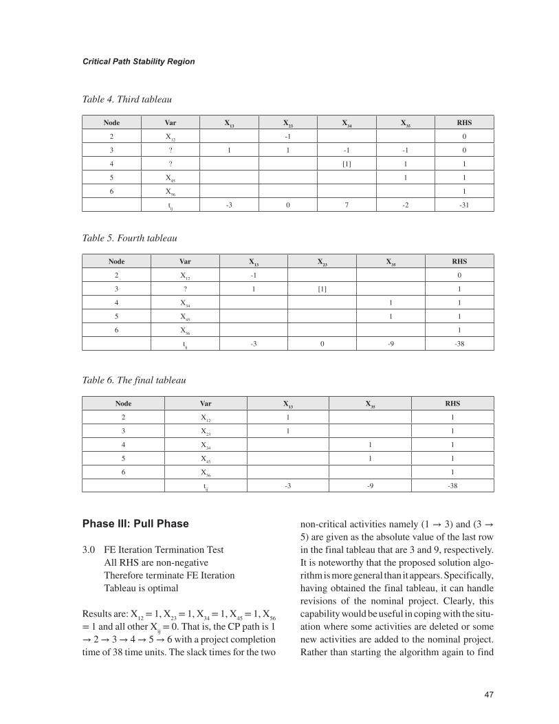
3.0 FE Iteration Termination Test All RHS are non-negative Therefore terminate FE Iteration Tableau is optimal

Results are: X12 = 1, X23 = 1, X34 = 1, X45 = 1, X56 = 1 and all other Xij = 0. That is, the CP path is 1 → 2 → 3 → 4 → 5 → 6 with a project completion time of 38 time units. The slack times for the two

non-critical activities namely (1 → 3) and (3 → 5) are given as the absolute value of the last row in the final tableau that are 3 and 9, respectively. It is noteworthy that the proposed solution algo-rithm is more general than it appears. Specifically, having obtained the final tableau, it can handle revisions of the nominal project. Clearly, this capability would be useful in coping with the situ-ation where some activities are deleted or some new activities are added to the nominal project. Rather than starting the algorithm again to find

Table 4. Third tableau

Node Var X13 X23 X34 X35 RHS2 X12 -1 03 ? 1 1 -1 -1 04 ? [1] 1 15 X45 1 16 X56 1

tij -3 0 7 -2 -31

Table 5. Fourth tableau

Node Var X13 X23 X35 RHS2 X12 -1 03 ? 1 [1] 14 X34 1 15 X45 1 16 X56 1

tij -3 0 -9 -38

Table 6. The final tableau

Node Var X13 X35 RHS2 X12 1 13 X23 1 14 X34 1 15 X45 1 16 X56 1

tij -3 -9 -38

��


the CP, the current final tableau can be updated. Moreover, if one is interested in finding all critical paths, or counting (which is combinatorial) the number of CPs, the last row in the final tableau provides the necessary information. If any tij = 0, then there might be multiple critical paths. By bringing any Xij with tij = 0 into the BVS, a new CP may be generated. Clearly, in such a case, the DPA results are valid for the current CP and may not withhold for the others.

��'$7$�3(5785%$7,21�$1$/<6,6

Given the outcome of a linear program formulation and calculation for the set of project activities, a series of analyses can provide valuable informa-tion. These uncertainty ranges can be obtained by performing the following different types of Data Perturbation Analysis (DPA) depending on the nature of the uncertainty: perturbation analysis; tolerance analysis; individual symmetric tolerance analysis; symmetric tolerance analysis; paramet-ric sensitivity analysis; and ordinary sensitivity analysis.

��&RQVWUXFWLRQ�RI�3HUWXUEDWLRQ�$QDO\VLV�6HW

Simultaneous and independent changes in the estimated activity durations in either direction (over or under estimation) for each activity that will maintain the current CP. This provides the largest set of perturbations. Inclusion of all actual activ-ity durations in this set preserves the current CP.

As we notice earlier, the LP formulation of this project network can be written as an LP, called the primal problem:

Maximize 9X12 + 6X13 + 0X23 + 7X34 + 8X35 + 10X45 + 12X56

Subject to:

X12 +X13 = 1,

-X12 + X23 = 0,

-X13 - X23 + X34 + X35 = 0,

-X34 + X45 = 0,

-X35 - X45 + X56 = 0,

-X56 = -1,

and all Xij ≥ 0.

The Dual Problem is:

Minimize U1 - U6

Subject to:

U1 – U2 ≥ 9 The Dual Constraint Related to Critical Activity X12 = 1

U1 – U3 ≥ 6 The Dual Constraint Related to Non-critical Activity X13 = 1

U2 – U3 ≥ 0 The Dual Constraint Related to Critical Activity, X23 = 1

U3 – U4 ≥ 7 The Dual Constraint Related to Critical Activity, X34 = 1

U3 – U5 ≥ 8 The Dual Constraint Related to Non-critical Activity X35 = 1



Uj’s are unrestricted

��


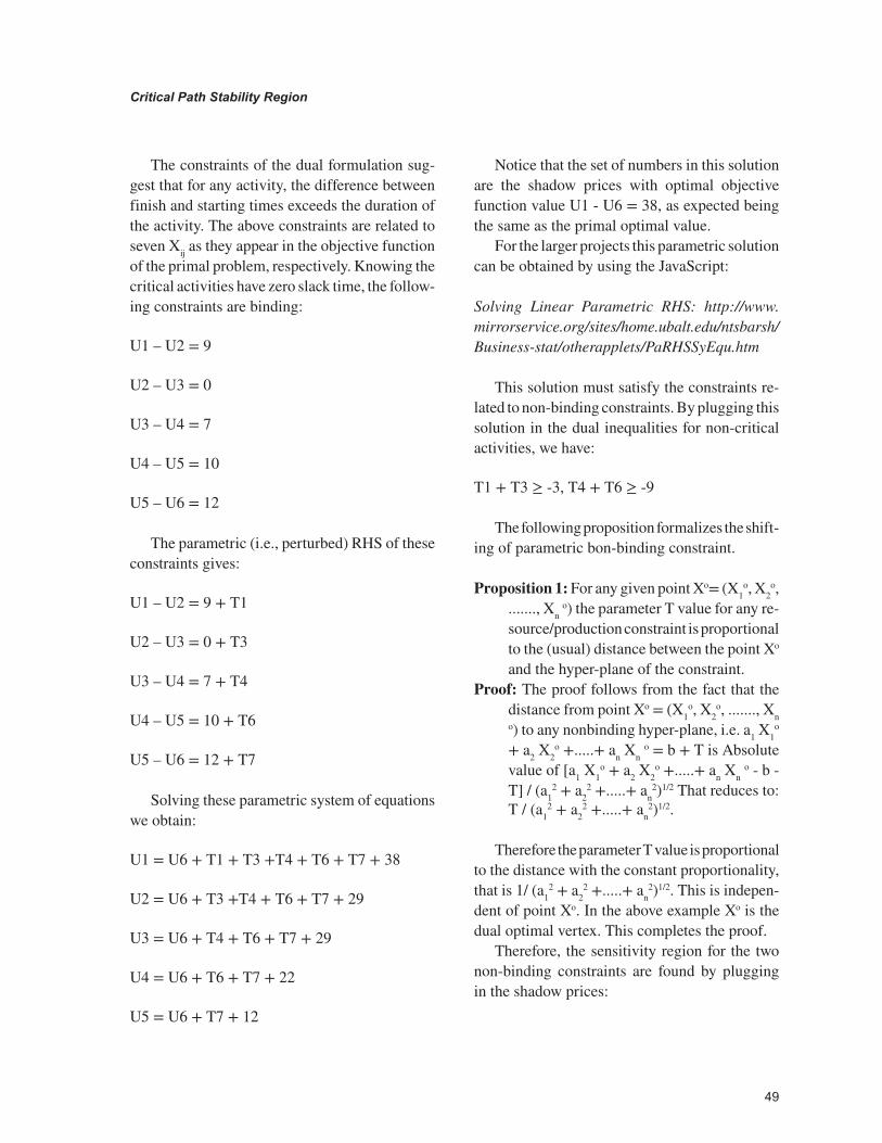
The constraints of the dual formulation sug-gest that for any activity, the difference between finish and starting times exceeds the duration of the activity. The above constraints are related to seven Xij as they appear in the objective function of the primal problem, respectively. Knowing the critical activities have zero slack time, the follow-ing constraints are binding:

U1 – U2 = 9

U2 – U3 = 0

U3 – U4 = 7

U4 – U5 = 10

U5 – U6 = 12

The parametric (i.e., perturbed) RHS of these constraints gives:

U1 – U2 = 9 + T1

U2 – U3 = 0 + T3

U3 – U4 = 7 + T4

U4 – U5 = 10 + T6

U5 – U6 = 12 + T7

Solving these parametric system of equations we obtain:

U1 = U6 + T1 + T3 +T4 + T6 + T7 + 38

U2 = U6 + T3 +T4 + T6 + T7 + 29

U3 = U6 + T4 + T6 + T7 + 29

U4 = U6 + T6 + T7 + 22

U5 = U6 + T7 + 12

Notice that the set of numbers in this solution are the shadow prices with optimal objective function value U1 - U6 = 38, as expected being the same as the primal optimal value.

For the larger projects this parametric solution can be obtained by using the JavaScript:

Solving Linear Parametric RHS: http://www.mirrorservice.org/sites/home.ubalt.edu/ntsbarsh/Business-stat/otherapplets/PaRHSSyEqu.htm

This solution must satisfy the constraints re-lated to non-binding constraints. By plugging this solution in the dual inequalities for non-critical activities, we have:

T1 + T3 ≥ -3, T4 + T6 ≥ -9

The following proposition formalizes the shift-ing of parametric bon-binding constraint.

Proposition 1: For any given point Xo= (X1o, X2

o, ......., Xn o) the parameter T value for any re-source/production constraint is proportional to the (usual) distance between the point Xo and the hyper-plane of the constraint.

Proof: The proof follows from the fact that the distance from point Xo = (X1

o, X2o, ......., Xn

o) to any nonbinding hyper-plane, i.e. a1 X1o

+ a2 X2o +.....+ an Xn o = b + T is Absolute

value of [a1 X1o + a2 X2

o +.....+ an Xn o - b - T] / (a1

2 + a22 +.....+ an

2)1/2 That reduces to: T / (a1

2 + a22 +.....+ an

2)1/2.

Therefore the parameter T value is proportional to the distance with the constant proportionality, that is 1/ (a1

2 + a22 +.....+ an

2)1/2. This is indepen-dent of point Xo. In the above example Xo is the dual optimal vertex. This completes the proof.

Therefore, the sensitivity region for the two non-binding constraints are found by plugging in the shadow prices:

��


U1 – U3 ≥ 6 + T2, 38 - 29 ≥ 6 + T2, T2 ≤ 3

U3 – U5 ≥ 8 + T5, 29 -12 ≥ 8 + T5, T5 ≤ 9

Putting all together, i.e., the union of all sen-sitivity regions, we obtain the largest sensitivity region for the duration of all activities:

S = { Tj, j=1, 2, 3, 4, 5, 6, 7 | T1 ≥ -9, T2 ≥ -6, T3 = 0, T4 ≥ -7, T5 ≥ -8, T6 ≥ -10,

T7 ≥ -12, T1 + T3 ≥ -3, T2 ≤ 3, T4 + T6 ≥ -9, T5 ≤ 9}

Notice that Data Perturbation set S in convex and non-empty since it contains the origin, i.e. when all Tj = 0. Perturbation is said to be CP preserving, if the perturbed model has the same CP as the nominal project. Clearly, the DPA are concerned with CP preserving as outlined in the Introduction. This set could be used to check whether a given numerical perturbed activity durations has any impact on the current CP.

The following presents different types of popular sensitivity analysis for non-degenerate problems. For treatment of degeneracy see Lin and Wen (2003), Arsham (2007), Lin (2010), and Lin (2011)

��3DUDPHWULF�DQG�2UGLQDU\�6HQVLWLYLW\�$QDO\VLV

Parametric analysis is of particular interest when-ever there are some kinds of dependency among the activity durations. This dependency is very common in project activity networks. This analysis can be considered as simultaneous changes in a given direction. Define a perturbation vector P specifying a perturbed direction of the activity durations. Introducing a scalar parameter a ≥ 0, it is required to find out how far the direction of P can be moved while still maintaining the current CP.

In our numerical example let us assume the activity duration times [9, 6, 0, 7, 8, 10, 12] are perturbed along the dependent vector P = (0, 0, -1, 3, 1, -2, -1). To find scalar parameter a, sub-stitute for vector a P = (0, 0, -a, 3a, a, -2a, -a) in the critical region

S = { Tj, j=1, 2, 3, 4, 5, 6, 7 | T1 ≥ -9, T2 ≥ -6, T3 = 0, T4 ≥ -7, T5 ≥ -8, T6 ≥ -10, T7 ≥ -12, T1 + T3 ≥ -3, T2 ≤ 3, T4 + T6 ≥ -9, T5 ≤ 9}

Now all terms are converted in terms of pa-rameter a. The smallest positive value for a in 3.

Therefore the current CP remains critical for any perturbation aP, where 0 ≤ a ≤ 3.

��2UGLQDU\�6HQVLWLYLW\�$QDO\VLV

In this sub-section interest is in finding the range for any particular activity duration, holding all other activity durations unchanged. Clearly, the ordinary sensitivity is a special case of parametric analysis where it is required to find the extent of the move in positive and negative directions of any one of the axes in the n-parametric space tij. Here, P is a unit row vector or is negative depending on whether an upper or a lower limit is required. The ordinary sensitivity analysis is summarized in Table 7. Alternatively, to find the allowable uncertainty Ti for any particular activity duration time i, set all other T = 0 in perturbation set S. The results are summarized in Table 7.

Table 7. One change at a time sensitivity limits

Lower Limit Upper LimitT1 -3 MT2 -6 3T3 0 0T4 -7 MT5 -8 9T6 -9 MT7 -12 M

��


The above analysis deals with one duration-uncertainty at-a-time analysis. Suppose we want to find the simultaneous allowable changes all activity durations, in such a case one may apply what is known as the 100% rule.

��7KH��5XOH

The 100% rule states that simultaneous increase (decrease) changes is allowed as long as the sum of the percentages of the change divided by the corresponding maximum increase (decrease) al-lowable change in the range of ordinary sensitivity analysis for each coefficient does not exceed 100%.

Therefore, base on this rule, the CP will be preserved if

T2 / 3 + T5 / 9 ≤ 1,

where the two denominators are the allowable increases from the sensitivity analysis for t13 and t35 respectively. That is, as long as this inequality holds, the current CP remains unchanged. Clearly, this condition is sufficient but not necessary. Similarly, the application of the 100% rule for decreasing some activity duration provides:

T1 / (-3) + T2 / (-6) + T4 / (-7) + T5 / (-8) + T6 / (-9) + T7 / (-12) ≤ 1,

with a similar interpretation.As mentioned earlier the Data Perturbation

Set, S, is useful to check for any numerically known values of durations if current CP remains critical. However the algebra becomes messy if one tries to find, for example, what is the largest percentage change for all activities to maintain the current CP? Arsham (1990) provides detailed treatments of this and other useful sensitivity analyses with numerical examples including the followings.

��7ROHUDQFH�$QDO\VLV

Simultaneous and independent changes ex-pressed as the maximum allowable percent-age of the estimated activity duration in either direction (over or under estimation) for each activity that will maintain the current CP. Such an analysis is useful whenever the uncertainties in the estimated activity durations can be ex-pressed as some percentages of their estimated values. Here, the lower and upper uncertainty limits to maintain the current CP, i.e. error in both directions: over and under estimation for all activities must be found. Let B denotes the matrix in the body of the final tableau, then matrix A denotes the row-wise augmented matrix B, constructed by pending an identity matrix I of order k as its last k rows where k is the number of non-critical activities in the final tableau. That is, A = [B | I]T, where the superscript T means transpose. Denote τ j =C.A.j where Aj is the absolute value of the jth column of A, in the body of the final tableau, and T is the estimated activity duration time vector. From now on, the critical and non-critical activities must be differentiated.

D��7ROHUDQFH�/LPLWV�IRU�&ULWLFDO�$FWLYLWLHV

For any critical activity duration, i.e., for any tsk, the upper tolerance limit is unbounded. However, the lower tolerance limit for t’sk is:

tsk- = max {tsk [(lower sensitivity limit)j / τ j], and

the lower limit from the sensitivity analysis},

where the max is over all j such that the (t’sk row and the jth column) element of A is positive.

In the numerical example, the augmented matrix A is shown in Table 8 and C = (9, 0, 7, 10, 12, 6, 8). The element of matrix τ = C.A, are τ1 = 15 and τ2 = 25.

��


For example, the lower tolerance limit for the activity duration t’12 can be found as follows:

t’12- = max {9(-3)/15, 9(-9)/25, -3}= -9/5

E��7ROHUDQFH�/LPLWV�IRU�1RQ�&ULWLFDO�$FWLYLWLHV

For any non-critical activity duration, i.e., for any t’sk, the lower tolerance limit is the ordinary sensitivity limit, and its upper limit for t’sk is:

t’sk+ = min {tsk [(Tn*)j /- τ j], and the upper limit

from the sensitivity analysis},

where the min is over all j such that the (t’sk row and the jth column) element of A is positive. For example, the upper tolerance limit for the activity duration t13 is:

t’13+ = min{6 (-3) / -15, 6(-9)/-25, 3}=6/5.

The tolerance limits of all activity duration for the numerical example are shown in Table 9.

The symmetric tolerance limits reflect the maximum allowable equal percentage error in both directions (over and under estimations) that hold simultaneously over all activity durations. Clearly, the symmetric tolerance range is a subset of the tolerance range. From Table 3, it is clear that the symmetric tolerance limit for the nu-merical example is 20%.

��$SSOLFDWLRQ�WR�(QKDQFH�WKH�7UDGLWLRQDO�3(57�$SSURDFK

The modeler asks the manager to express the dura-tion of uncertainty for each activity by a percent change in either direction. Clearly, there might be different percentage for different activities, thus many scenarios, however, suppose the uncertainty is at most 20% in either direction for all activities. This makes sense to have equal uncertainty since larger durations will have larger uncertainty range. In this case; by setting lower and upper limits of individual symmetric tolerance analysis (ISA) as the largest lower bound for optimistic and the smallest upper bound for pessimistic estimates respectively. The data shown in Table 10 pertain to the network of Figure 1.

Table 8. Matrix A as a tool for tolerance analysis

t’13 t’35

A =

t’12 1 0t’23 1 0t’34 0 1t’45 0 1t’56 0 0t’13 1 0t’35 0 1

Table 9. Tolerance limits for all durations

Lower Limit Upper Limitt’12 -9/5 (20%) Mt’13 -6 (100%) 6/5 (20%)t’23 0 0t’34 -63/25 (36%) Mt’35 -8 (100%) 72/25 (36%)t’45 -18/5 (36%) Mt’56 -12 (100%) M

��


Suppose the optimistic time, most likely time, and pessimistic time for each activity are accept-able to the members of the project team. Note that since the pessimistic time and the optimistic time are symmetrical with regard to the most likely time, the mean completion time ET is equal to the most likely time for each activity.

Note that in an AOA convention, a node rep-resents both the end of an activity and the start of another. It is sometimes useful to present the network in Activity-on-node (AON) convention

to distinguish between the early finish time for the predecessor and the early start time for successor. Another advantage of an AON convention is that it does not need dummy activities. Figure 2 pres-ents the network of Figure 1 in AON convention.

The following steps are required in developing and solving a network:

1. Identify each activity to be done in the project.2. Determine the sequence of activities and

construct a network reflecting the prece-

Table 10. Data for Figure 1

Notation Activity Optimistic Time aMost Likely Time

m Pessimistic Time b te = (a+4m+b)/61→3 A 4.8 6 7.2 61→2 B 7.2 9 10.8 92→3 Dummy Activity3→4 D 5.6 7 8.4 73→5 C 6.4 8 9.6 84→5 E 8 10 12 105→6 F 9.6 12 14.4 12

The optimistic time (a) is the amount of time that an activity will take if everything goes well. The probability that the activity will take less than this amount of time is 0.01.

The pessimistic time (b) is the amount of time that an activity will take if everything goes poorly. The probability that the activity will exceed this duration is 0.01.

The most likely time (m) is the time that the estimator thinks an activity will probably take. The activity could be performed many times under the same conditions (no learning), this is the time that would occur most often.

Figure 2. Network in Activity-on-node (AON) convention

��


dence relationships. The network consists of nodes and arrows. In a CPM network, nodes represent activities and arrows denote precedence relationships only.

3. Four values are calculated for each activity: ƕ Earliest Start, ES: earliest time an

activity can start based on completion of all predecessor activities

ƕ Latest Start, LS: latest time an activ-ity can start and still achieve its latest finish time

ƕ Earliest Finish, EF: earliest time an activity can be completed given that it starts at its earliest start time

ƕ Latest Finish, LF: latest time an ac-tivity can be completed if its succes-sor activities are to begin by a set time and/or if the project is to be complet-ed by a set time.

Forward and backward passes are needed for the calculation of early start, early finish, late start, and late finish times for activities. This information in turn can be used to identify the critical path, slack times and project completion time.

The slack time for each activity is defined as either LS - ES or LF - EF. The slack time is the amount of time by which the start of a given event may be delayed without delaying the completion of the project. The critical path is the longest se-

quence of connected activities through the network and is defined as the path with zero slack time.

The management significance of the critical path is that it constrains the completion date of the project since it is the longest path of activity times from the start to the end of the network. As a result, activities on the critical path should be intensively managed to avoid slippage. Other activities, not on the critical path, can be allowed to slip somewhat, up to their amount of slack, without affecting the project completion date. Table 11 provides the ES, EF, LS, LF and slack for all activities for the network in Figure 2.

Note that there are four paths with total length of time as indicated below:

1. A→C→F, total time = 262. A→D→E→F, total time = 353. B→C→F, total time = 294. B→D→ E→F, total time = 38

The critical path is B→D→ E→F, the longest path and the project completion time is 38. Note that EF and LF are equal for activities on the critical path providing slacks for all activities as 0. So you cannot delay these activities.

Table 11. Calculation of Figure 2 network

Activity Time ES EF LS LF SlackA 6 0 6 3 9 3B 9 0 9 0 9 0C 8 9 17 18 26 9D 7 9 16 9 16 0E 10 16 26 16 26 0F 12 26 38 26 38 0

��


��)XUWKHU�$SSOLFDWLRQ�RI�WKH�'3$�5HVXOWV�IRU�WKH�0DQDJHUV

Table 12 summarizes some parts of our findings from analysis applied to the numerical example, using the sensitivity region:

S = { Tj, j=1, 2, 3, 4, 5, 6, 7 | T1 ≥ -9, T2 ≥ -6, T3 = 0, T4 ≥ -7, T5 ≥ -8, T6 ≥ -10, T7 ≥ -12, T1 + T3 ≥ -3, T2 ≤ 3, T4 + T6 ≥ -9, T5 ≤ 9}

As always, care must be taken when rounding the DPA limits. Clearly the upper limit and lower limit must be rounded down and up, respec-tively.

Since project managers are concerned with the stability of the CP under uncertainty of the estimated durations, the output information from our various DPA should be of interest to project managers. As long as the actual activity dura-tions remain within these intervals, the current CP remains critical. Some specific implications from these results for the project manager are that they provide means for discussion and analysis by the project team members as to how to consider modifying the project prior to its implementa-tion. The results given in Table 7 help the project manager to assess, analyze, monitor, and manage all phases of a project; i.e. planning, scheduling,

and controlling. When the issues caused by the inherent uncertainty in any project are considered, there are other benefits to be gained by using the proposed DPA approach; e.g., it provides vari-ous ranges of uncertainty with the lower limits as the maximum “crashing” for critical activity durations and the upper limits as the maximum “slippage” for non-critical activity durations and their impacts on the entire project completion time. These results could be helpful in some large projects, e.g., if certain activities could be moved into certain intervals or be divisible into smaller sub-activities and “tucked in” at several locations.

The proposed approach can also provide a rich modeling environment for strategic management of complex projects using Monte-Carlo simulation experiments. In this treatment, a priori duration distribution function may be selected for each activity with the support range produced by the tolerance analysis. Clearly, in the case of complete lack of knowledge uniform distribution function could be used.

Throughout the DPA it has been assumed that duration of all activities are continuous. Clearly, whenever some activity durations are required to be discrete, then this admissibility condition must be added to all parts of DPA. The discussion of DPA did not include other important managerial issues, such as time-cost-performance tradeoff, including

Table 12. Ranges for the Ordinary Sensitivity Analysis (OSA), Tolerance Analysis (TA), Individual Sym-metric Tolerance Analysis (IST), and Symmetric Tolerance Analysis (STA) with Critical Activities in Bold

Crash Durations Duration Slippage DurationsSA TA IST STA STA IST TA SA

t12 6 7.2 7.2 7.2 9 10.8 10.8 M Mt13 0 0 4.8 4.8 6 7.2 7.2 7.2 9t23 0 0 0 0 0 0 0 0 0t34 0 4.48 4.48 5.6 7 8.4 9.52 M Mt35 0 0 5.12 6.4 8 9.6 10.88 10.88 17t45 1 6.4 6.4 8 10 12 13.6 M Mt56 0 0 0 9.6 12 14.4 24 M M

��


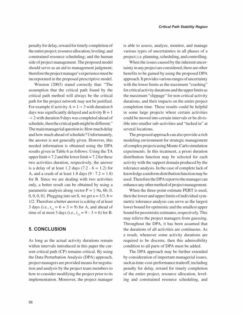
penalty for delay, reward for timely completion of the entire project; resource allocation; leveling; and constrained resource scheduling; and the human side of project management. The proposed model should serve as an aid to management judgment; therefore the project manager’s experience must be incorporated in the proposed prescriptive model.

Winston (2003) stated correctly that: “The assumption that the critical path found by the critical path method will always be the critical path for the project network may not be justified. For example if activity A = 1→ 3 with duration 6 days was significantly delayed and activity B = 1 → 2 with duration 9 days was completed ahead of schedule, then the critical path might be different.” The main managerial question is: How much delay and how much ahead of schedule? Unfortunately, the answer is not generally given. However, this needed information is obtained using the DPA results given in Table 6 as follows: Using the TA upper limit = 7.2 and the lower limit = 7.2 for these two activities duration, respectively, the answer is a delay of at least 1.2 days (7.2 - 6 = 1.2) for A, and a crash of at least 1.8 days (9 - 7.2 = 1.8) for B. Since we are dealing with two activities only, a better result can be obtained by using a parametric analysis along vector P = {-9a, 6b, 0, 0, 0, 0, 0}. Plugging into set S, we get a = 1/3, b = 1/2. Therefore a better answer is a delay of at least 3 days (i.e., t13 = 6 + 3 = 9) for A, and ahead of time of at most 3 days (i.e., t12 = 9 – 3 = 6) for B.

��&21&/86,21

As long as the actual activity durations remain within intervals introduced in this paper the cur-rent critical path (CP) remains critical. By using the Data Perturbation Analysis (DPA) approach, project managers are provided means for negotia-tion and analysis by the project team members to how to consider modifying the project prior to its implementation. Moreover, the project manager

is able to assess, analyze, monitor, and manage various types of uncertainties in all phases of a project; i.e. planning, scheduling, and controlling.

When the issues caused by the inherent uncer-tainty in any project are considered, there are other benefits to be gained by using the proposed DPA approach. It provides various ranges of uncertainty with the lower limits as the maximum “crashing” for critical activity durations and the upper limits as the maximum “slippage” for non-critical activity durations, and their impacts on the entire project completion time. These results could be helpful in some large projects where certain activities could be moved into certain intervals or be divis-ible into smaller sub-activities and “tucked in” at several locations.

The proposed approach can also provide a rich modeling environment for strategic management of complex projects using Monte-Carlo simulation experiments. In this treatment, a priori duration distribution function may be selected for each activity with the support domain produced by the tolerance analysis. In the case of complete lack of knowledge a uniform distribution function may be used. Therefore the DPA report to the manager can enhance any other method of project management.

When the three-point estimate PERT is used, then the lower and upper limits of individual sym-metric tolerance analysis can serve as the largest lower bound for optimistic and the smallest upper bound for pessimistic estimates, respectively. This may relieve the project managers from guessing. Throughout the DPA, it has been assumed that the durations of all activities are continuous. As a result, whenever some activity durations are required to be discrete, then this admissibility condition to all parts of DPA must be added.

The DPA approach may be further extended by consideration of important managerial issues, such as time-cost-performance tradeoff, including penalty for delay, reward for timely completion of the entire project, resource allocation, level-ing and constrained resource scheduling, and

��


the human side of project management. Clearly, the proposed model in this paper should serve as an aid to, rather than substitute for, manage-ment judgment. Therefore, the project manager’s experience must be incorporated in the proposed prescriptive model. The proposed approach has the advantage of being computationally practical, easy for a project manager to understand, and provides useful practical information.

$&.12:/('*(0(17

We are most appreciative to reviewers for their comments and useful suggestions on an earlier version.

��


5()(5(1&(6

Adlakha, V., & Arsham, H. (1992). A simulation technique for estimation in perturbed stochastic activity networks. Simulation, 58(2), 258–267. doi:10.1177/003754979205800406

Arsham, H. (1990). Perturbation analysis of gen-eral LP models: A unified approach to sensitivity, parametric, tolerance, and more-for-less analysis. Mathematical and Computer Modelling, 13(8), 79–102. doi:10.1016/0895-7177(90)90073-V

Arsham, H. (1997a). Initialization of the sim-plex algorithm: An artificial-free approach. SIAM Review, 39(5), 736–744. doi:10.1137/S0036144596304722

Arsham, H. (1997b). Affine geometric method for linear programs. Journal of Scientific Computing, 12(3), 289–303. doi:10.1023/A:1025601511684

Arsham, H. (2005). A computer implementation of the push-and-pull algorithm and its computational comparison with LP simplex method. Applied Mathematics and Computation, 170(1), 36–63. doi:10.1016/j.amc.2004.10.078

Arsham, H. (2007). Construction of the largest sensitivity region for general linear programs. Applied Mathematics and Computation, 189(2), 1435–1447. doi:10.1016/j.amc.2006.12.020

Banerjee, A., & Paul, A. (2008). On path cor-relation and PERT bias. European Journal of Operational Research, 189(3), 1208–1216. doi:10.1016/j.ejor.2007.01.061

Cassone, D. (2010). A process to build new product development cycle time predictive models combin-ing fuzzy set theory and probability theory. Inter-national Journal of Applied Decision Sciences, 3(2), 168–183. doi:10.1504/IJADS.2010.034838

Czuchra, W. (1999). Optimizing budget spendings for software implementation and testing. Com-puters & Operations Research, 26(7), 731–747. doi:10.1016/S0305-0548(98)00086-0

D’Aquila, N. (1993). Facilitating in-service programs through PERT/CPM: Simultaneous use of these tools can assist nurses in organizing workshops. Nursing Management, 24(2), 92–98. PMID:8265089

Gido, J., & Clements, J. (2011). Successful proj-ect management with Microsoft. New York, NY: South-Western College Pub.

Hasan, H., & Gould, E. (2001). Support for the sense-making activity of managers. Decision Support Systems, 1(31), 71–86. doi:10.1016/S0167-9236(00)00120-2

Herrerı’as-Velasco, J., Herrerı’as-Pleguezuelo, R., & René van Dorp, J. (2011). Revisiting the PERT mean and variance. European Journal of Opera-tional Research, 210(2), 448–451. doi:10.1016/j.ejor.2010.08.014

Higgs, S. (1995). Software roundup: Project management for windows. Byte, 20, 185–186.

Hoffer, J., Valacich, J., & George, J. (2011). Es-sentials of systems analysis and design. Englewood Cliffs, NJ: Prentice Hall.

Jarvis, J., & Shier, D. (1990). Netsolve: Interactive software for network optimization. Operations Re-search Letters, 9(3), 275–282. doi:10.1016/0167-6377(90)90073-E

Kallo, G. (1996). The reliability of critical path method (CPM) techniques in the analysis and evaluation of delay claims. Coastal Engineering, 38(1), 35–39.

Kamburowski, J. (1997). New validations of PERT times. Omega, 25(3), 323–328. doi:10.1016/S0305-0483(97)00002-9

Keefer, D., & Verdini, W. (1993). Better estima-tion of PERT activity time parameters. Manage-ment Science, 39(6), 1086–1091. doi:10.1287/mnsc.39.9.1086

��


Keramati, A., Dardick, G., Mojir, N., & Banan, B. (2009). Application of latent moderated structuring (LMS) to rank the effects of interven-ing variables on the IT and firm performance relationship. International Journal of Applied Decision Sciences, 2(2), 167–188. doi:10.1504/IJADS.2009.026551

Kerzner, H. (2009). Project management: A systems approach to planning, scheduling, and controlling. New York, NY: Wiley.

Kuklan, H. (1993). Effective project manage-ment: An expanded network approach. Journal of Systems Management, 44(1), 12–16.

Lewis, J. (2007). Mastering project management: Applying advanced concepts to systems thinking, control & evaluation, resource allocation. New York: McGraw-Hill.

Lin, C.-J. (2010). Computing shadow prices/costs of degenerate LP problems with reduced simplex tables. Expert Systems with Applications, 37(8), 5848–5855. doi:10.1016/j.eswa.2010.02.021

Lin, C.-J. (2011). A labeling algorithm for the sen-sitivity ranges of the assignment problem. Applied Mathematical Modelling, 35(10), 4852–4864. doi:10.1016/j.apm.2011.03.045

Lin, C.-J., & Wen, U.-P. (2003). Sensitivity analysis of the optimal assignment. European Journal of Operational Research, 149(1), 35–46. doi:10.1016/S0377-2217(02)00439-3

Martín, M., García, C., Pérez, J., & Sánchez Granero, M. (2012). An alternative for robust estimation in project management. European Jour-nal of Operational Research, 220(2), 443–451. doi:10.1016/j.ejor.2012.01.058

Mehrotra, K., Chai, J., & Pillutla, S. (1996). A study of approximating the moments of the job completion time in PERT networks. Journal of Operations Management, 14(3), 277–289. doi:10.1016/0272-6963(96)00002-2

Meredith, J., & Mantel, S. Jr. (2008). Project management: A managerial approach. New York, NY: Wiley.

Mouhoub, N., Benhocine, A., & Belouadah, H. (2011). A new method for constructing a minimal PERT network. Applied Mathematical Modelling, 35(9), 4575–4588. doi:10.1016/j.apm.2011.03.031

Nasution, S. (1994). Fuzzy critical path method. IEEE Transactions on Systems, Man, and Cy-bernetics, 24(1), 48–51. doi:10.1109/21.259685

Nicholas, J., & Steyn, H. (2008). Project manage-ment for business, engineering, and technology. New York, NY: Butterworth-Heinemann.

Phillips, D., & Garcia-Diaz, A. (1990). Funda-mental of network analysis. Englewood Cliffs, NJ: Prentice-Hall.

Pirdashti, M., Mohammadi, M., Rahimpour, F., & Kennedy, D. (2008). An AHP-Delphi multi-criteria location planning model with application to whey protein production facility decisions. In-ternational Journal of Applied Decision Sciences, 1(2), 245–259. doi:10.1504/IJADS.2008.020326

Premachandra, I. (2001). An approximation of the activity duration distribution in PERT. Com-puters & Operations Research, 28(5), 443–452. doi:10.1016/S0305-0548(99)00129-X

Satzinger, J., Jackson, J., & Burd, S. (2011). Sys-tems analysis and design in a changing world. New York, NY: Course Technology.

Shipley, M., & Olson, D. (2008). Interval-valued evidence sets from simulated product competi-tiveness: A Bulgarian winery decision. Inter-national Journal of Applied Decision Sciences, 1(4), 397–417. doi:10.1504/IJADS.2008.022977

Trietsch, D., & Baker, K. (2012). PERT 21: Fitting PERT/CPM for use in the 21st century. Interna-tional Journal of Project Management, 30(4), 490–502. doi:10.1016/j.ijproman.2011.09.004

��


Valacich, J., George, J., & Hoffer, J. (2001). Es-sentials of systems analysis and design. Englewood Cliffs, NJ: Prentice Hall.

Winston, W. (2003). Operations research: Ap-plications and algorithms. Boston, MA: PWS-KENT Pub. Co.

Wu, S., & Wu, M. (1994). Systems analysis and design. New York: West Publishing Company.

Yaghoubi, S., Noori, S., Azaron, A., & Tavakkoli-Moghaddam, R. (2011). Resource allocation in dynamic PERT networks with finite capac-ity. European Journal of Operational Research, 215(3), 670–678.

Yakhchali, S. (2012). A path enumeration ap-proach for the analysis of critical activities in fuzzy networks. Information Sciences, 204, 23–35. doi:10.1016/j.ins.2012.01.025

Critical Path Stability Region: A Single-Time Estimate Approach

Documents

Transcript of Critical Path Stability Region: A Single-Time Estimate Approach