How Recent History Affects Perception: The Normative Approach and Its Heuristic Approximation
10
How Recent History Affects Perception: The Normative Approach and Its Heuristic Approximation Ofri Raviv 1 *, Merav Ahissar 1,2 , Yonatan Loewenstein 1,3 1 The Edmond & Lily Safra Center for Brain Sciences, Interdisciplinary Center for Neural Computation, Hebrew University, Jerusalem, Israel, 2 Departments of Psychology and Cognitive Sciences, Hebrew University, Jerusalem, Israel, 3 Departments of Neurobiology and Cognitive Sciences and the Center for the Study of Rationality, Hebrew University, Jerusalem, Israel Abstract There is accumulating evidence that prior knowledge about expectations plays an important role in perception. The Bayesian framework is the standard computational approach to explain how prior knowledge about the distribution of expected stimuli is incorporated with noisy observations in order to improve performance. However, it is unclear what information about the prior distribution is acquired by the perceptual system over short periods of time and how this information is utilized in the process of perceptual decision making. Here we address this question using a simple two-tone discrimination task. We find that the ‘‘contraction bias’’, in which small magnitudes are overestimated and large magnitudes are underestimated, dominates the pattern of responses of human participants. This contraction bias is consistent with the Bayesian hypothesis in which the true prior information is available to the decision-maker. However, a trial-by-trial analysis of the pattern of responses reveals that the contribution of most recent trials to performance is overweighted compared with the predictions of a standard Bayesian model. Moreover, we study participants’ performance in a-typical distributions of stimuli and demonstrate substantial deviations from the ideal Bayesian detector, suggesting that the brain utilizes a heuristic approximation of the Bayesian inference. We propose a biologically plausible model, in which decision in the two- tone discrimination task is based on a comparison between the second tone and an exponentially-decaying average of the first tone and past tones. We show that this model accounts for both the contraction bias and the deviations from the ideal Bayesian detector hypothesis. These findings demonstrate the power of Bayesian-like heuristics in the brain, as well as their limitations in their failure to fully adapt to novel environments. Citation: Raviv O, Ahissar M, Loewenstein Y (2012) How Recent History Affects Perception: The Normative Approach and Its Heuristic Approximation. PLoS Comput Biol 8(10): e1002731. doi:10.1371/journal.pcbi.1002731 Editor: Robert Sekuler, Brandeis, United States of America Received April 17, 2012; Accepted August 21, 2012; Published October 25, 2012 Copyright: ß 2012 Raviv et al. This is an open-access article distributed under the terms of the Creative Commons Attribution License, which permits unrestricted use, distribution, and reproduction in any medium, provided the original author and source are credited. Funding: This research was supported by grants from the National Institute for Psychobiology in Israel - founded by The Charles E. Smith Family, from the Israel Science Foundation (grants No. 868/08 and 616/11), and from the Gatsby Charitable Foundation. The funders had no role in study design, data collection and analysis, decision to publish, or preparation of the manuscript. Competing Interests: The authors have declared that no competing interests exist. * E-mail: [email protected] Introduction Perception is a complex cognitive process, in which noisy signals are extracted from the environment and interpreted. It is generally believed that perceptual resolution is limited by internal noise that constrains our ability to differentiate physically similar stimuli. The magnitude of this internal noise is typically estimated using the 2- alternative forced choice (2AFC) paradigm, which was introduced to eliminate participants’ perceptual and response biases [1,2]. In this paradigm, a participant is presented with two temporally- separated stimuli that differ along a physical dimension and is instructed to compare them. The common assumption is that the probability of a correct response is determined by the physical difference between the two stimuli, relative to the level of internal noise. Performance is typically characterized by the threshold of discrimination, referred to as the Just Noticeable Difference (JND). Thus, the JND is a measure of the level of internal noise such that the higher the JND, the higher the inferred internal noise. However, the idea that there is a one-to-one correspondence between the JND and the internal noise is inconsistent with theoretical considerations which postulate that participants’ performance can be improved by taking into account expectations about the stimuli in the process of perception or decision-making. If the internal representation of a stimulus was uncertain, the prior expectations should bias the participant against unlikely stimuli. The larger the uncertainty, the larger the contribution of these prior expectations should be. The Bayesian theory of inference describes how expectations regarding the probability distribution of stimuli should be combined with the noisy representations of these stimuli in order to optimize performance [3]. In fact, expectations, formalized as prior distribution of stimuli used in the experiment, have been shown to bias participants’ responses in a way that is consistent with the Bayesian framework (reviewed in [4]). In particular, responses in the 2AFC paradigm have been shown to be biased by prior expectations: when the magnitudes of the two stimuli are small relative to the distribution of stimuli used in the experiment, participants tend to respond that the 1 st stimulus was larger, whereas they tend to respond that the 2 nd stimulus was larger when the magnitudes of the two stimuli are relatively large [5–7]. In a previous study we have shown that this bias, known as the ‘‘contraction bias’’, can be understood in the Bayesian framework: following the presentation of the two stimuli, the participant combines her noisy representations of the two stimuli with the prior distribution of the stimuli to form two PLOS Computational Biology | www.ploscompbiol.org 1 October 2012 | Volume 8 | Issue 10 | e1002731
Transcript of How Recent History Affects Perception: The Normative Approach and Its Heuristic Approximation
How Recent History Affects Perception: The NormativeApproach and Its Heuristic ApproximationOfri Raviv1*, Merav Ahissar1,2, Yonatan Loewenstein1,3
1 The Edmond & Lily Safra Center for Brain Sciences, Interdisciplinary Center for Neural Computation, Hebrew University, Jerusalem, Israel, 2 Departments of Psychology
and Cognitive Sciences, Hebrew University, Jerusalem, Israel, 3 Departments of Neurobiology and Cognitive Sciences and the Center for the Study of Rationality, Hebrew
University, Jerusalem, Israel
Abstract
There is accumulating evidence that prior knowledge about expectations plays an important role in perception. TheBayesian framework is the standard computational approach to explain how prior knowledge about the distribution ofexpected stimuli is incorporated with noisy observations in order to improve performance. However, it is unclear whatinformation about the prior distribution is acquired by the perceptual system over short periods of time and how thisinformation is utilized in the process of perceptual decision making. Here we address this question using a simple two-tonediscrimination task. We find that the ‘‘contraction bias’’, in which small magnitudes are overestimated and large magnitudesare underestimated, dominates the pattern of responses of human participants. This contraction bias is consistent with theBayesian hypothesis in which the true prior information is available to the decision-maker. However, a trial-by-trial analysisof the pattern of responses reveals that the contribution of most recent trials to performance is overweighted comparedwith the predictions of a standard Bayesian model. Moreover, we study participants’ performance in a-typical distributionsof stimuli and demonstrate substantial deviations from the ideal Bayesian detector, suggesting that the brain utilizes aheuristic approximation of the Bayesian inference. We propose a biologically plausible model, in which decision in the two-tone discrimination task is based on a comparison between the second tone and an exponentially-decaying average of thefirst tone and past tones. We show that this model accounts for both the contraction bias and the deviations from the idealBayesian detector hypothesis. These findings demonstrate the power of Bayesian-like heuristics in the brain, as well as theirlimitations in their failure to fully adapt to novel environments.
Citation: Raviv O, Ahissar M, Loewenstein Y (2012) How Recent History Affects Perception: The Normative Approach and Its Heuristic Approximation. PLoSComput Biol 8(10): e1002731. doi:10.1371/journal.pcbi.1002731
Editor: Robert Sekuler, Brandeis, United States of America
Received April 17, 2012; Accepted August 21, 2012; Published October 25, 2012
Copyright: � 2012 Raviv et al. This is an open-access article distributed under the terms of the Creative Commons Attribution License, which permitsunrestricted use, distribution, and reproduction in any medium, provided the original author and source are credited.
Funding: This research was supported by grants from the National Institute for Psychobiology in Israel - founded by The Charles E. Smith Family, from the IsraelScience Foundation (grants No. 868/08 and 616/11), and from the Gatsby Charitable Foundation. The funders had no role in study design, data collection andanalysis, decision to publish, or preparation of the manuscript.
Competing Interests: The authors have declared that no competing interests exist.
* E-mail: [email protected]
Introduction
Perception is a complex cognitive process, in which noisy signals
are extracted from the environment and interpreted. It is generally
believed that perceptual resolution is limited by internal noise that
constrains our ability to differentiate physically similar stimuli. The
magnitude of this internal noise is typically estimated using the 2-
alternative forced choice (2AFC) paradigm, which was introduced
to eliminate participants’ perceptual and response biases [1,2]. In
this paradigm, a participant is presented with two temporally-
separated stimuli that differ along a physical dimension and is
instructed to compare them. The common assumption is that the
probability of a correct response is determined by the physical
difference between the two stimuli, relative to the level of internal
noise. Performance is typically characterized by the threshold of
discrimination, referred to as the Just Noticeable Difference (JND).
Thus, the JND is a measure of the level of internal noise such that
the higher the JND, the higher the inferred internal noise.
However, the idea that there is a one-to-one correspondence
between the JND and the internal noise is inconsistent with
theoretical considerations which postulate that participants’
performance can be improved by taking into account expectations
about the stimuli in the process of perception or decision-making.
If the internal representation of a stimulus was uncertain, the prior
expectations should bias the participant against unlikely stimuli.
The larger the uncertainty, the larger the contribution of these
prior expectations should be. The Bayesian theory of inference
describes how expectations regarding the probability distribution
of stimuli should be combined with the noisy representations of
these stimuli in order to optimize performance [3].
In fact, expectations, formalized as prior distribution of stimuli
used in the experiment, have been shown to bias participants’
responses in a way that is consistent with the Bayesian framework
(reviewed in [4]). In particular, responses in the 2AFC paradigm
have been shown to be biased by prior expectations: when the
magnitudes of the two stimuli are small relative to the distribution
of stimuli used in the experiment, participants tend to respond that
the 1st stimulus was larger, whereas they tend to respond that the
2nd stimulus was larger when the magnitudes of the two stimuli are
relatively large [5–7]. In a previous study we have shown that this
bias, known as the ‘‘contraction bias’’, can be understood in the
Bayesian framework: following the presentation of the two stimuli,
the participant combines her noisy representations of the two
stimuli with the prior distribution of the stimuli to form two
PLOS Computational Biology | www.ploscompbiol.org 1 October 2012 | Volume 8 | Issue 10 | e1002731
posterior distributions. Rather than comparing the two noisy
representations of the stimuli, the participant is assumed to
compare the two posteriors in order to maximize the probability of
a correct response. The contribution of the prior distribution to
the two posteriors is not equal. The larger the level of noise in the
representation of the stimulus, the larger is the contribution of the
prior distribution to the posterior. The level of noise in the
representation of the magnitude of the 1st stimulus is larger than
the level of noise in the representation of the magnitude of the 2nd
stimulus because of the noise associated with the encoding and
maintenance of the 1st stimulus in memory [8,9]. As a result, the
posterior distribution of the 1st stimulus is biased more by the prior
distribution than the posterior distribution of the 2nd stimulus. If
the prior distribution is unimodal, both posteriors are contracted
towards the median of the prior distribution. Because the posterior
of the 1st stimulus is contracted more than the posterior of the 2nd
stimulus, participants’ responses are biased towards overestimating
the 1st stimulus when it is relatively small and underestimating it
when it is relatively large [7].
One limitation of the Bayesian model is that it relies heavily on
the assumption that the prior distribution of stimuli is known to the
observer. While this assumption may be plausible in very long
experiments comprising a large number of trials (e.g. thousands in
[10]) or in experiments utilizing natural tasks (e.g., reading, [11]),
it is unclear how Bayesian inference can take place if participants
have less experience in the task.
In this paper we study participants’ pattern of responses in a
2AFC tone discrimination task in relatively short experiments
consisting of tens of trials. We report a substantial contraction bias
that persists even when it hampers performance due to a-typical
statistics. We show that participants’ pattern of behavior is
consistent with an ‘‘implicit memory’’ model, in which the
representation of previous stimuli is a single scalar that continu-
ously updates with examples. Thus, this model can be viewed as a
simple implementation of the Bayesian model that provides a
better account of participants’ perceptual decision making.
Results
The contraction biasWe measured the performance of our participants in the random
2AFC paradigm (Materials and Methods, Fig. 1), in which subjects
compared the frequencies of two sequentially presented tones drawn
from a broad frequency range. Averaged across the population of
participants, the JND was 13.6%60.7% (SEM), which is higher
than typically reported in the literature ([12,13]). The relatively high
value of the JND, which is likely to result from the lack of experience
of the participants and the fact that no reference was used, is
comparable with previous studies using the random frequency
paradigm, with short stimuli and untrained participants [14,15].
As predicted by the contraction bias, the JND did not capture
the full pattern of participants’ responses. This is depicted in
Fig. 2A. The coordinates of each dot in Fig. 2A correspond to the
frequencies of the 1st and 2nd tones in a trial, referred to as f1 and
f2. Blue and red dots denote trials, in which the participant’s
response was correct and incorrect, respectively. The closer the
dots are to the diagonal, the smaller is the difference in the
frequencies of the two tones. Therefore naively, one would expect
that the probability of a trial to be incorrect (red dot) would be
highest near the diagonal. Moreover, if the probability of a correct
response as a function of log(f1){log(f2) is symmetrical around 0,
as implicitly assumed when measuring the JND, then the pattern
of red and blue dots is expected to be symmetrical around the
diagonal. In contrast, we found that the pattern of incorrect
responses is highly non-symmetrical. Participants tended to err
more when both frequencies were high and f1wf2 and when both
frequencies were low and f1vf2. To quantify this asymmetry, we
considered separately two regions: the Bias+ region corresponds to
trials in two sections of this plane (yellow in Fig. 2A): in the first
section are trials in which the frequencies of both stimuli are above
the median (1000 Hz) and the frequency of the 1st tone is lower
than that of the 2nd tone. In the second section are trials in which
the frequencies of both stimuli are below the median frequency and
the frequency of the 1st tone is higher than that of the 2nd tone.
Similarly, The Bias2 region (gray in Fig. 2A) corresponded to
trials in which the frequencies of both stimuli are above the median
(1000 Hz) and the frequency of the 1st tone is higher than that of the
2nd tone and trials in which the frequencies of both stimuli are
below the median frequency and the frequency of the 1st tone is
lower than that of the 2nd tone. Participants’ rate of success differed
greatly between the Bias+ and Bias2 regions. Participants were
typically successful when either the two tones were low
(,1000 Hz) and the 2nd tone was lower (lower left yellow region,
88.2%60.5% correct responses, mean 6 SEM) or when the two
tones were high (.1000 Hz) and the 2nd tone was higher (upper
yellow region, 88.4%60.6% correct responses). On the other
hand, performance was relatively poor either when the two tones
were low and the 1st tone was lower (lower left gray region,
63.2%60.8% correct responses) or when the two tones were high
and the 1st tone was higher (upper gray region, 61.8%60.8%
correct responses). These effects were highly significant in each of
the two quadrants (p,1026, Monte Carlo Permutation test). The
differential level of proficiency in the yellow and gray regions
indicates a substantial contraction bias, in line with that bias
described in previous studies [6,7]: when the frequency of the 1st
tone was relatively low, participants tended to overestimate it
(leading to successful performance when the 1st tone was higher).
The opposite was true when the frequency of the 1st tone was
relatively high (leading to successful performance when the 1st tone
was lower). The differential level of proficiency in the yellow and
gray regions is evident not only in the response pattern of the
population of participants but also in the response pattern in
individual blocks (Fig. S1A–C). Moreover, it was evident for all
levels of proficiency in the task (Fig. S1D).
To further illustrate the contraction bias, we constructed a two-
dimensional histogram of participants’ performance by binning
the f1|f2 space of Fig. 2A and computing the fraction of correct
responses in each bin (Fig. 2B, grayscale). The non-symmetrical
distribution of the shades of gray of the squares around the diagonal
Author Summary
In this paper we study how history affects perceptionusing an auditory delayed comparison task, in whichhuman participants repeatedly compare the frequencies oftwo, temporally-separated pure tones. We demonstratethat the history of the experiment has a substantial effecton participants’ performance: when both tones are highrelative to past stimuli, people tend to report that the 2nd
tone was higher, and when they are relatively low, theytend to report that the 1st tone was higher. Interestingly,only the most recent trials bias performance, which can beinterpreted as if the participants assume that the statisticsof stimuli in the experiment is highly volatile. Moreover,this bias persists even in settings, in which it is detrimentalto performance. These results demonstrate the abilities, aswell as limitations, of the cognitive system when incorpo-rating expectations in perception.
How Recent History Affects Perception
PLOS Computational Biology | www.ploscompbiol.org 2 October 2012 | Volume 8 | Issue 10 | e1002731
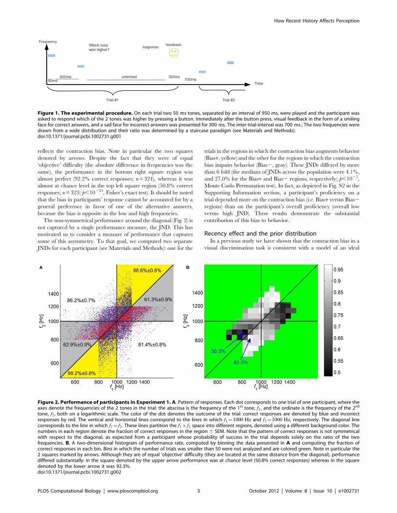
reflects the contraction bias. Note in particular the two squares
denoted by arrows. Despite the fact that they were of equal
‘objective’ difficulty (the absolute difference in frequencies was the
same), the performance in the bottom right square region was
almost perfect (92.2% correct responses; n = 324), whereas it was
almost at chance level in the top left square region (50.8% correct
responses; n = 323; p,10233, Fisher’s exact test). It should be noted
that the bias in participants’ response cannot be accounted for by a
general preference in favor of one of the alternative answers,
because the bias is opposite in the low and high frequencies.
The non-symmetrical performance around the diagonal (Fig. 2) is
not captured by a single performance measure, the JND. This has
motivated us to consider a measure of performance that captures
some of this asymmetry. To that goal, we computed two separate
JNDs for each participant (see Materials and Methods): one for the
trials in the regions in which the contraction bias augments behavior
(Bias+, yellow) and the other for the regions in which the contraction
bias impairs behavior (Bias2, gray). These JNDs differed by more
than 6 fold (the medians of JNDs across the population were 4.1%,
and 27.0% for the Bias+ and Bias2 regions, respectively; p,1025,
Monte Carlo Permutation test). In fact, as depicted in Fig. S2 in the
Supporting Information section, a participant’s proficiency on a
trial depended more on the contraction bias (i.e. Bias+ versus Bias2
regions) than on the participant’s overall proficiency (overall low
versus high JND). These results demonstrate the substantial
contribution of this bias to behavior.
Recency effect and the prior distributionIn a previous study we have shown that the contraction bias in a
visual discrimination task is consistent with a model of an ideal
Figure 1. The experimental procedure. On each trial two 50 ms tones, separated by an interval of 950 ms, were played and the participant wasasked to respond which of the 2 tones was higher by pressing a button. Immediately after the button press, visual feedback in the form of a smilingface for correct answers, and a sad face for incorrect answers was presented for 300 ms. The inter-trial-interval was 700 ms.; The two frequencies weredrawn from a wide distribution and their ratio was determined by a staircase paradigm (see Materials and Methods).doi:10.1371/journal.pcbi.1002731.g001
Figure 2. Performance of participants in Experiment 1. A. Pattern of responses. Each dot corresponds to one trial of one participant, where theaxes denote the frequencies of the 2 tones in the trial: the abscissa is the frequency of the 1st tone, f1 , and the ordinate is the frequency of the 2nd
tone, f2 , both on a logarithmic scale. The color of the dot denotes the outcome of the trial: correct responses are denoted by blue and incorrectresponses by red. The vertical and horizontal lines correspond to the lines in which f1~1000 Hz and f2~1000 Hz, respectively. The diagonal linecorresponds to the line in which f1~f2. These lines partition the f1|f2 space into different regions, denoted using a different background color. Thenumbers in each region denote the fraction of correct responses in the region 6 SEM. Note that the pattern of correct responses is not symmetricalwith respect to the diagonal, as expected from a participant whose probability of success in the trial depends solely on the ratio of the twofrequencies. B. A two-dimensional histogram of performance rate, computed by binning the data presented in A and computing the fraction ofcorrect responses in each bin. Bins in which the number of trials was smaller than 50 were not analyzed and are colored green. Note in particular the2 squares marked by arrows. Although they are of equal ‘objective’ difficulty (they are located at the same distance from the diagonal), performancediffered substantially: in the square denoted by the upper arrow performance was at chance level (50.8% correct responses) whereas in the squaredenoted by the lower arrow it was 92.3%.doi:10.1371/journal.pcbi.1002731.g002
How Recent History Affects Perception
PLOS Computational Biology | www.ploscompbiol.org 3 October 2012 | Volume 8 | Issue 10 | e1002731
detector that utilizes Bayes’ rule to incorporate the prior
distribution with the sensed stimuli in order to optimize
performance [7]. In agreement with that study, such a Bayesian
model, with 2 free parameters that correspond to the noise in the
internal representation of each of the two stimuli, can qualitatively
account for the observed contraction in the two-tone discrimina-
tion task (see Fig. S3 in the Supporting Information section).
However, it should be noted that the Bayesian model relies on
the assumption that the prior distribution of stimuli is known to the
observer, which seems unreasonable in our experiment, which
consisted of merely tens of trials. Therefore, it is not clear how the
history of trials experienced by the participants in the experiment
contributes to the bias. To address this question, we considered the
contribution of individual trials to the bias. Because the statistics of
stimuli in our experiment are stationary, all past trials are equally
informative about the prior distribution. Therefore, normative
considerations that incorporate an assumption of stationarity
imply that the effect of past trials on participants’ choices will be
independent of the number of trials elapsed between these trials
and the choice. By contrast, previous studies have reported that
participants’ responses are influenced to a greater degree by recent
stimuli, which is known as the recency effect [16–21]. In addition,
the activity of neurons in the primary auditory cortex has been
shown to contain information about both current and previous
stimuli [22]. To test for recency in our dataset, we fitted a linear
non-linear model that relates the response in each trial to a linear
combination of present and past stimuli according to the following
equation:
AA(t)~W(XT
t~0(wt
1 log(f1(t{t)){wt2 log(f2(t{t)))zw? log(�ff )) ð1Þ
where AA(t) is the probability that the model would report that the
frequency of the 1st tone was higher than that of the 2nd tone in
trial t; W is the normal cumulative distribution function such that
W(x)~
ðx
-?
dtffiffiffiffiffiffi2pp e
{t2
2 ; wti ,t[f0::Tg,i[f1,2g and w? are parame-
ters, f1(t) and f2(t) are the frequencies of the 1st and 2nd tone,
respectively, in trial t and �ff is the geometric mean of the
frequencies of all stimuli in the experiment until trial t.
To gain insights into the behavior of the model (Eq. (1)) we
consider the simple case in which w01~w0
2~ww0 and
wtw0i ~w?~0. In this case, Eq. (1) becomes
AA(t)~W(w(log(f1(t)){log(f2(t)))), which corresponds to a model
participant that is indifferent to the history of the experiment and
its choices depend solely on the ratio of the frequencies of the two
tones and the internal noise. The value of w denotes the level of
internal noise of the model participant. If w is very small, wvv1then independently of the frequencies of the stimuli, f1(t) and f2(t),
AA(t)&W(0)~0:5, and the model participant responds at random.
In contrast, if w is very large, www1 then
AA(t)&H(log(f1(t)){log(f2(t))) where H(x) is the Heaviside step
function such that H(x)~1 for xw0 and H(x)~0 for xv0. In
other words, if w is very large the model participant always
answers correctly. The larger the value of w, the smaller the JND
of the model participant. The values of the parameters wtw0i
determine the contribution of past stimuli to perception, where the
value of wti determines the contribution of the ith stimulus
presented t trials ago and the value of w? determines the
contribution of the average frequency of past stimuli to perception.
If all past stimuli contribute equally to perception, as expected
from normative participants who assume that the distribution of
stimuli is stationary then we expect wti ~0 and w?
=0. In contrast,
if the participant assumes that the statistics of the experiment is
non-stationary then we expect the most recent trials to have a
stronger effect on behavior, resulting in wti whose magnitude
decreases as the value of t increases.
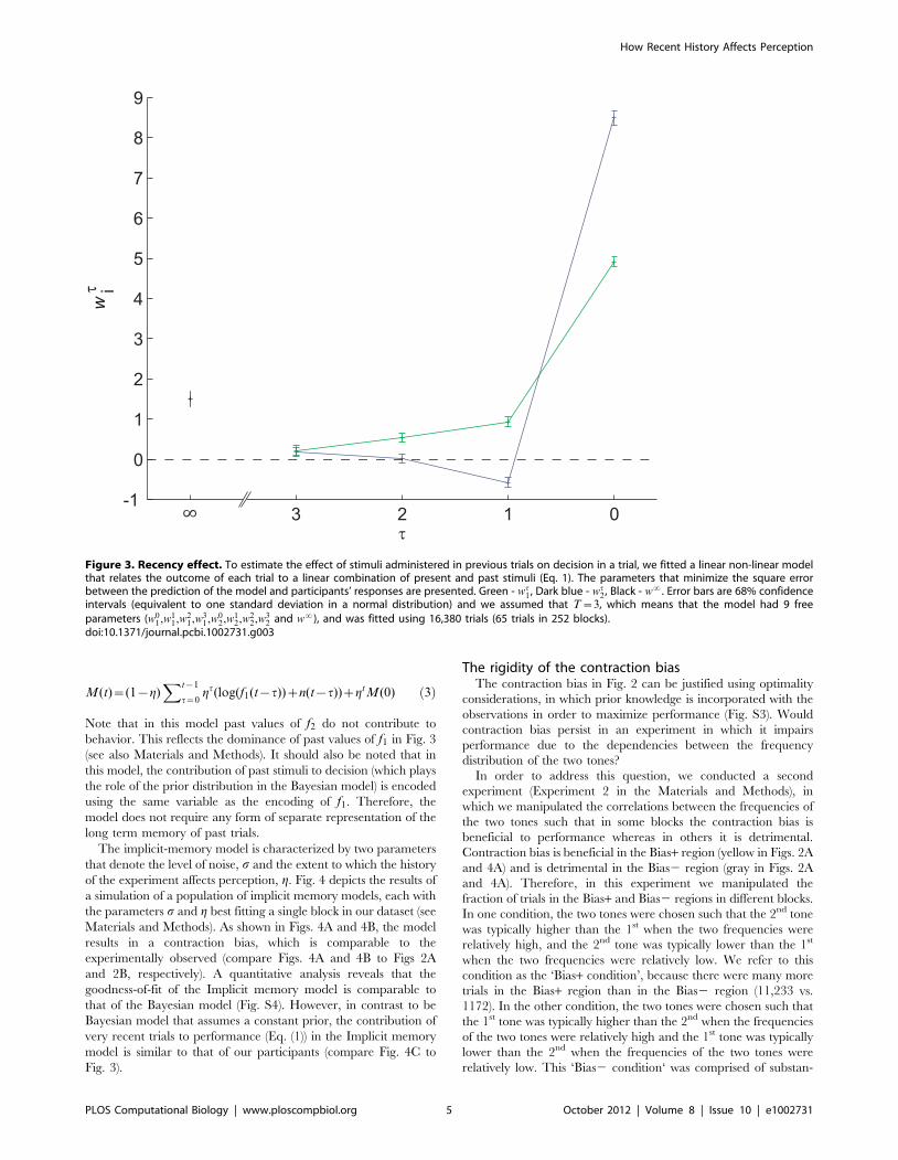
Assuming that T~3, we analyzed the sequence of frequencies
and decisions of our participants. We found the values of the
parameters wt1 (Fig. 3, green), wt
2 (dark blue) and w? (black) that
minimize the mean square error (MSE), the mean square distance
of the vector of probabilities, AA(t) from the vector of choices, A(t)such that A(t)~1 if the participant responded that the frequency
of the 1st tone was higher than the frequency of the 2nd tone in trial
t and A(t)~0 otherwise. Note that the values of w01 and w0
2 in
Fig. 3 are larger than the values of all other coefficients, wtw0i . This
result reflects the simple fact that the tones presented in a trial
influence the decision in that trial more than tones presented in
previous trials. The recency effect is manifested in the non-zero
coefficients of wtw0i (see Materials and Methods). As depicted in
Fig. 3, the contribution of past trials to choice diminishes within
several trials. This result is consistent with other findings of rapid
perceptual learning [23,24] (but see also [25]) and demonstrates
that at least some aspects of the prior distribution are estimated
using a small number of the most recent trials. It should also be
noted that the contribution of past stimuli to decision is dominated
by past values of f1 and not past values of f2 (Fig. 3. See also
Materials and Methods).
The implicit-memory modelThe recency effect described in the previous section is difficult to
reconcile with a Bayesian inference model that takes into account
the stationary statistics of the experiment. This finding has
motivated us to consider the possibility that the contraction bias
described in Fig. 2 emerges from simpler cognitive processes that
do not require an explicit representation of the prior distribution.
In this section we present a simple model that accounts for the
contraction bias and the recency effect, which does not explicitly
keep track of the prior distribution of stimuli presented in the
experiment.
In our model, the memory trace of past stimuli is a single scalar
M (rather than the full prior distribution). In response to the
presentation of f1, the participant updates the value of M such that
M is a linear combination of the past value of M with the present
stimulus, corrupted by sensory and encoding noise. Formally, the
value of M in trial tz1, is given by
M(tz1)~(1{g)(log(f1(t))zn(t))zgM(t) ð2Þ
where g is the weight given to the memory and n(t) is the noise
associated with the encoding of f1. We assume that this noise is
Gaussian with variance s2 and is uncorrelated across trials:
Sn(t):n(t0)T~s2dt,t0 , where dt,t0 is the Kronecker delta function,
dt,t0~1 if t~t0 and dt,t0~0 if t=t0.
A decision in a trial in this model depends on the relative values
of f2 and M. If Mwf2, the model responds that ‘‘f1wf2’’.
Otherwise it responds that ‘‘f1vf2’’. In this model we assume that
the noise is restricted to the representation of f1. The reason for
ignoring noise in the representation of f2 is that noise in f2 is
mathematically equivalent to a larger magnitude noise in f1 when
considering decision in a given trial.
It is easy to show that in this model, M(t) is an exponentially
weighted sum of the current and past stimuli and their respective
encoding noises:
How Recent History Affects Perception
PLOS Computational Biology | www.ploscompbiol.org 4 October 2012 | Volume 8 | Issue 10 | e1002731
M(t)~(1{g)Xt{1
t~0gt(log(f1(t{t))zn(t{t))zgtM(0) ð3Þ
Note that in this model past values of f2 do not contribute to
behavior. This reflects the dominance of past values of f1 in Fig. 3
(see also Materials and Methods). It should also be noted that in
this model, the contribution of past stimuli to decision (which plays
the role of the prior distribution in the Bayesian model) is encoded
using the same variable as the encoding of f1. Therefore, the
model does not require any form of separate representation of the
long term memory of past trials.
The implicit-memory model is characterized by two parameters
that denote the level of noise, s and the extent to which the history
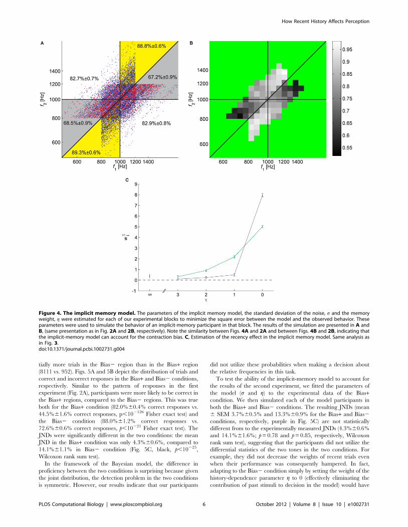
of the experiment affects perception, g. Fig. 4 depicts the results of
a simulation of a population of implicit memory models, each with
the parameters s and g best fitting a single block in our dataset (see
Materials and Methods). As shown in Figs. 4A and 4B, the model
results in a contraction bias, which is comparable to the
experimentally observed (compare Figs. 4A and 4B to Figs 2A
and 2B, respectively). A quantitative analysis reveals that the
goodness-of-fit of the Implicit memory model is comparable to
that of the Bayesian model (Fig. S4). However, in contrast to be
Bayesian model that assumes a constant prior, the contribution of
very recent trials to performance (Eq. (1)) in the Implicit memory
model is similar to that of our participants (compare Fig. 4C to
Fig. 3).
The rigidity of the contraction biasThe contraction bias in Fig. 2 can be justified using optimality
considerations, in which prior knowledge is incorporated with the
observations in order to maximize performance (Fig. S3). Would
contraction bias persist in an experiment in which it impairs
performance due to the dependencies between the frequency
distribution of the two tones?
In order to address this question, we conducted a second
experiment (Experiment 2 in the Materials and Methods), in
which we manipulated the correlations between the frequencies of
the two tones such that in some blocks the contraction bias is
beneficial to performance whereas in others it is detrimental.
Contraction bias is beneficial in the Bias+ region (yellow in Figs. 2A
and 4A) and is detrimental in the Bias2 region (gray in Figs. 2A
and 4A). Therefore, in this experiment we manipulated the
fraction of trials in the Bias+ and Bias2 regions in different blocks.
In one condition, the two tones were chosen such that the 2nd tone
was typically higher than the 1st when the two frequencies were
relatively high, and the 2nd tone was typically lower than the 1st
when the two frequencies were relatively low. We refer to this
condition as the ‘Bias+ condition’, because there were many more
trials in the Bias+ region than in the Bias2 region (11,233 vs.
1172). In the other condition, the two tones were chosen such that
the 1st tone was typically higher than the 2nd when the frequencies
of the two tones were relatively high and the 1st tone was typically
lower than the 2nd when the frequencies of the two tones were
relatively low. This ‘Bias2 condition‘ was comprised of substan-
Figure 3. Recency effect. To estimate the effect of stimuli administered in previous trials on decision in a trial, we fitted a linear non-linear modelthat relates the outcome of each trial to a linear combination of present and past stimuli (Eq. 1). The parameters that minimize the square errorbetween the prediction of the model and participants’ responses are presented. Green - wt
1 , Dark blue - wt2 , Black - w?. Error bars are 68% confidence
intervals (equivalent to one standard deviation in a normal distribution) and we assumed that T~3, which means that the model had 9 freeparameters (w0
1,w11,w2
1,w31,w0
2,w12,w2
2,w32 and w?), and was fitted using 16,380 trials (65 trials in 252 blocks).
doi:10.1371/journal.pcbi.1002731.g003
How Recent History Affects Perception
PLOS Computational Biology | www.ploscompbiol.org 5 October 2012 | Volume 8 | Issue 10 | e1002731
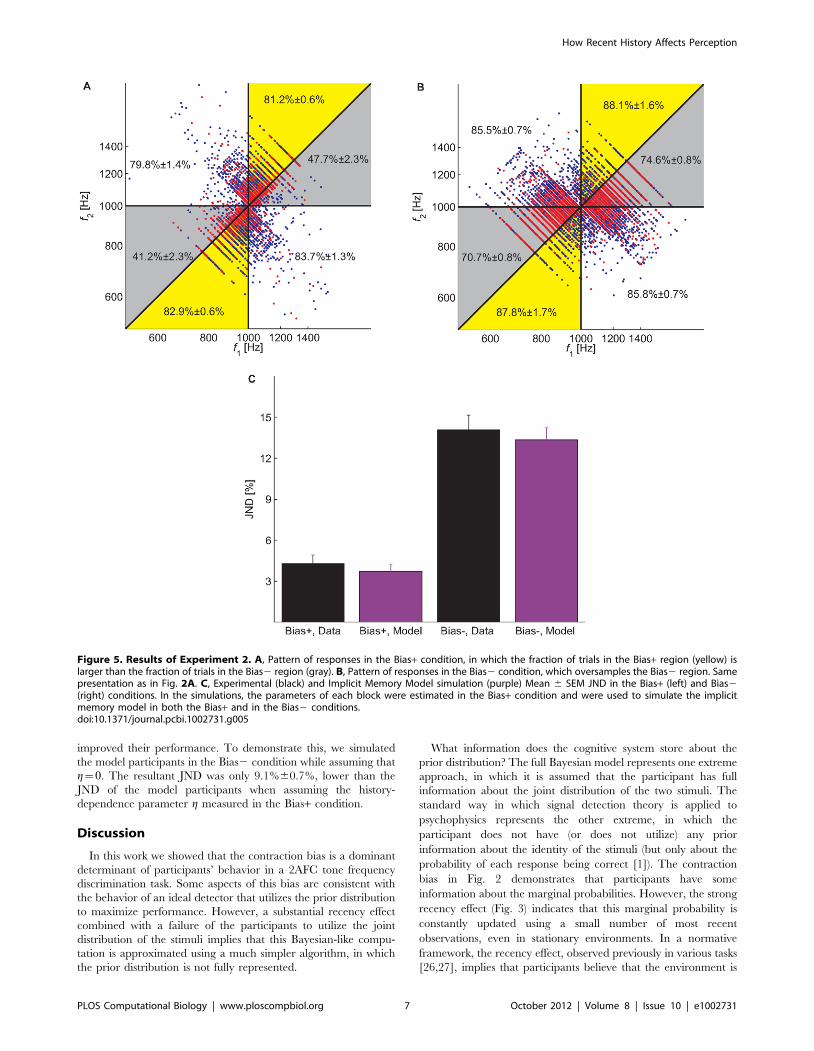
tially more trials in the Bias2 region than in the Bias+ region
(8111 vs. 952). Figs. 5A and 5B depict the distribution of trials and
correct and incorrect responses in the Bias+ and Bias2 conditions,
respectively. Similar to the pattern of responses in the first
experiment (Fig. 2A), participants were more likely to be correct in
the Bias+ regions, compared to the Bias2 regions. This was true
both for the Bias+ condition (82.0%60.4% correct responses vs.
44.5%61.6% correct responses, p,102126 Fisher exact test) and
the Bias2 condition (88.0%61.2% correct responses vs.
72.6%60.6% correct responses, p,10221 Fisher exact test). The
JNDs were significantly different in the two conditions: the mean
JND in the Bias+ condition was only 4.3%60.6%, compared to
14.1%61.1% in Bias2 condition (Fig. 5C, black, p,10225,
Wilcoxon rank sum test).
In the framework of the Bayesian model, the difference in
proficiency between the two conditions is surprising because given
the joint distribution, the detection problem in the two conditions
is symmetric. However, our results indicate that our participants
did not utilize these probabilities when making a decision about
the relative frequencies in this task.
To test the ability of the implicit-memory model to account for
the results of the second experiment, we fitted the parameters of
the model (s and g) to the experimental data of the Bias+condition. We then simulated each of the model participants in
both the Bias+ and Bias2 conditions. The resulting JNDs (mean
6 SEM 3.7%60.5% and 13.3%60.9% for the Bias+ and Bias2
conditions, respectively, purple in Fig. 5C) are not statistically
different from to the experimentally measured JNDs (4.3%60.6%
and 14.1%61.6%; p = 0.78 and p = 0.85, respectively, Wilcoxon
rank sum test), suggesting that the participants did not utilize the
differential statistics of the two tones in the two conditions. For
example, they did not decrease the weights of recent trials even
when their performance was consequently hampered. In fact,
adapting to the Bias2 condition simply by setting the weight of the
history-dependence parameter g to 0 (effectively eliminating the
contribution of past stimuli to decision in the model) would have
Figure 4. The implicit memory model. The parameters of the implicit memory model, the standard deviation of the noise, s and the memoryweight, g were estimated for each of our experimental blocks to minimize the square error between the model and the observed behavior. Theseparameters were used to simulate the behavior of an implicit-memory participant in that block. The results of the simulation are presented in A andB, (same presentation as in Fig. 2A and 2B, respectively). Note the similarity between Figs. 4A and 2A and between Figs. 4B and 2B, indicating thatthe implicit-memory model can account for the contraction bias. C, Estimation of the recency effect in the implicit memory model. Same analysis asin Fig. 3.doi:10.1371/journal.pcbi.1002731.g004
How Recent History Affects Perception
PLOS Computational Biology | www.ploscompbiol.org 6 October 2012 | Volume 8 | Issue 10 | e1002731
improved their performance. To demonstrate this, we simulated
the model participants in the Bias2 condition while assuming that
g~0. The resultant JND was only 9.1%60.7%, lower than the
JND of the model participants when assuming the history-
dependence parameter g measured in the Bias+ condition.
Discussion
In this work we showed that the contraction bias is a dominant
determinant of participants’ behavior in a 2AFC tone frequency
discrimination task. Some aspects of this bias are consistent with
the behavior of an ideal detector that utilizes the prior distribution
to maximize performance. However, a substantial recency effect
combined with a failure of the participants to utilize the joint
distribution of the stimuli implies that this Bayesian-like compu-
tation is approximated using a much simpler algorithm, in which
the prior distribution is not fully represented.
What information does the cognitive system store about the
prior distribution? The full Bayesian model represents one extreme
approach, in which it is assumed that the participant has full
information about the joint distribution of the two stimuli. The
standard way in which signal detection theory is applied to
psychophysics represents the other extreme, in which the
participant does not have (or does not utilize) any prior
information about the identity of the stimuli (but only about the
probability of each response being correct [1]). The contraction
bias in Fig. 2 demonstrates that participants have some
information about the marginal probabilities. However, the strong
recency effect (Fig. 3) indicates that this marginal probability is
constantly updated using a small number of most recent
observations, even in stationary environments. In a normative
framework, the recency effect, observed previously in various tasks
[26,27], implies that participants believe that the environment is
Figure 5. Results of Experiment 2. A, Pattern of responses in the Bias+ condition, in which the fraction of trials in the Bias+ region (yellow) islarger than the fraction of trials in the Bias2 region (gray). B, Pattern of responses in the Bias2 condition, which oversamples the Bias2 region. Samepresentation as in Fig. 2A. C, Experimental (black) and Implicit Memory Model simulation (purple) Mean 6 SEM JND in the Bias+ (left) and Bias2(right) conditions. In the simulations, the parameters of each block were estimated in the Bias+ condition and were used to simulate the implicitmemory model in both the Bias+ and in the Bias2 conditions.doi:10.1371/journal.pcbi.1002731.g005
How Recent History Affects Perception
PLOS Computational Biology | www.ploscompbiol.org 7 October 2012 | Volume 8 | Issue 10 | e1002731
highly volatile and as a result only the very recent history is
informative about future stimuli.
The results of experiment 2 (Fig. 5) indicate that participants are
either unable to compute the joint distribution or unable to utilize
it, at least within a single experimental block of 80 trials. The
implicit memory model can be viewed as a minimal modification
of the standard approach of applying signal detection theory to
perception in the direction of the full Bayesian model. Here,
participants represent the prior distribution of the stimuli with a
single scalar, which is an estimate of the mean of the marginal of
the prior distribution. Nevertheless this implicit model captures
many aspects of the behavioral results. Further studies are needed
to determine whether, and to what extent other moments of the
prior distributions are learned and utilized in the 2AFC
discrimination task, especially under longer exposure to distribu-
tion statistics.
Several studies have shown that the magnitude of the contribu-
tion of the prior distribution to perception on a given trial depends
on the level of internal noise [10,28]. In particular in the framework
of the 2AFC task, increasing the delay between the 1st and 2nd
stimuli [29,30] or introducing a distracting task between them [7]
enhances the contraction bias. These results are consistent with the
Bayesian approach. How can these results be accounted for in the
framework of the implicit memory model? One possibility is to
assume that the relative contribution of the prior in the simplified
online rule of Eq. (2) is affected by perceptual noise. However, it
should be noted that at least in one case, the level of noise was
determined after the encoding of the 1st stimulus [7]. The
dependence of g on the level of noise can be accounted for in the
framework of the implicit memory model if we assume that the
computation of M(t), which incorporates the prior knowledge with
the response to the 1st stimulus, is carried out simultaneously by
several neurons, or populations of neurons, which are characterized
by different values of g [22,31,32]. At the time of the decision, the
magnitude of the noise determines which populations of neurons
will be the most informative with respect to the 1st stimulus. If the
level of noise is high, the populations of neurons that are more
affected by past trials (for whom the value of g is large) will dominate
perception, resulting in a substantial contraction bias. Otherwise the
populations that are less affected by past trials will dominate
perception, resulting in a small contraction bias.
Almost 40 years ago, Tversky and Kahneman characterized
irrational decision making and reasoning and concluded that
‘‘people rely on a limited number of heuristic principles which
reduce the complex tasks … to simpler judgmental operations. In
general, these heuristics are quite useful, but sometimes they lead
to severe and systematic errors’’ [33]. Our study extends these
results to the domain of implicit perceptual judgments.
Materials and Methods
Ethics StatementThe research was approved by the department ethics commit-
tee, and all participants signed consent forms.
Experiment 1150 participants (mean age 2463.1 years) engaged in a 2AFC
high/low pure tone frequency discrimination task, after signing
consent forms. 18 participants were excluded due to poor
performance on a hearing test or because they did not complete
the full schedule. Each participant performed 2 blocks of 80 trials.
Each trial consisted of two 50 ms pure tones, with 10 ms linear rise
time, and 10 ms linear fall time, separated by 950 ms. Immedi-
ately after the 2nd stimulus was played, the text ‘Which tone was
higher?’ appeared on screen, and the participant responded by
clicking one of two on-screen buttons using a computer mouse,
with no time constraint. Visual feedback of a smiling face or a sad
face was presented for 300 ms after correct and incorrect
responses, respectively. After a pause of 700 ms the next trial
began (Fig. 1). All stimuli were presented binaurally through
Sennheiser HD-265 linear headphones using a TDT System III
signal generator (Tucker Davis Technologies) controlled by in-
house software in a sound attenuated room in the laboratory.
Tone intensity was 65 dB SPL. Both the 1st and the 2nd
frequencies in each trial were drawn from a wide distribution
according to the following procedure: a frequency f was drawn
from a uniform distribution between 800 Hz and 1200 Hz.
Another frequency, either f zDf or f {Df was drawn with a
probability 0.5, where Df was controlled by an adaptive 3-down 1-
up staircase, in which the initial difference between the stimuli in
each block was 20% and was bounded from below by 0.1%. The
step size decreased every four reversals, from 4.5% to 2% to 1% to
0.5% to 0.1%. One of the two frequencies was randomly selected
as f1 and the other frequency was selected as f2. This schedule is
expected to converge to a Df for which the participant answers
correctly in 79.4% of the trials ([34]; Fig. 2A, dots). Blocks that did
not converge to at least 65% correct responses in the last 40 trials
were excluded from the analysis (12 of 264 blocks). The JND was
calculated as the average difference between the stimuli frequen-
cies in the last 6 reversals. As a result of the adaptive staircase
schedule, the ratios between the frequencies of the two stimuli
tended to decrease in the first trials of the block. On average, after
15 trials this ratio stabilized and therefore the first 15 trials of each
block were excluded from the analysis.
Estimating the JND in Bias+ and Bias2 regionsTo estimate the JND in a Bias+ or Bias2 region of a block, we
fitted a cumulative normal distribution function psychometric
curve that relates the response in each trial AA to the difference in
the logarithm of the 1st and 2nd frequencies:
AA~Wlog(f1){log(f2)
s
� �where W is the normal cumulative
distribution function, such that W(x)~
ðx
-?
dtffiffiffiffiffiffi2pp e{t2
2 . The value of
the parameter s was chosen as to minimize the square difference
between the vector predictions AA and the vector of choices A such
that A~1 on trials in which the participant responded ‘‘f1wf2’’
and A~0 otherwise. Assuming that the cumulative normal
distribution function reflects the probability of responding
‘‘f1wf2’’, the corresponding value of the JND is the difference in
the natural logarithms of f1 and f2 such that the probability of a
correct response is the asymptotic performance level in our
staircase paradigm, 0.794. Therefore, JND~s:W{1(0:794).
Statistical methodsTo test for differences in performance between different regions,
we used a Monte Carlo permutation test in which the identities of
f1 and f2 in a trial were randomly shuffled. We used 106
permutations, and in all cases the experimentally observed
differences were larger than the differences observed in all
permutations, resulting in p,1026.
To test for differences in the JNDs between different regions, we
used a Monte Carlo permutation test in which the identities of f1
and f2 in a trial were randomly shuffled. We estimated the JND of
these simulated results using the same process as described for the
data, and estimated the median JND+ and median JND- for the
whole population. We used 105 permutations and the experimen-
How Recent History Affects Perception
PLOS Computational Biology | www.ploscompbiol.org 8 October 2012 | Volume 8 | Issue 10 | e1002731
tally observed difference was larger than the difference observed in
all permutations, resulting in p,1025.
In order to verify the contribution of the parameters wti for
t[½1,2,3�; i[½1,2� to the linear-non-linear model (Eq. 1), we
compared several models using a cross validation test: the
parameters of the different models were estimated using all blocks
but one, and these parameters were used in order to compute the
MSE for that block. The MSE of the model was computed by
repeating this procedure for all blocks in the experiment and
averaging the resultant MSE.
We considered three models: (1) a naıve model with no
history dependence: AA1(t)~W w01 log(f1(t)){w0
2 log(f2(t))� �
;
(2) a model with a global history term,
AA2(t)~W w01 log(f1(t)){w0
2 log(f2(t))zw? log(�ff )� �
; (3) the
full model with an explicit history dependence of
three previous trials, and a global term,
AA3(t)~WP3
t~0 (wt1 log(f1(t{t)){wt
2 log(f2(t{t)))zw?�ff� �
.
The resultant MSEs are MSE(AA1)~0:187+0:002;
MSE(AA2)~0:172+0:003; MSE(AA3)~0:169+0:003. We
found that MSE(AA3) is significantly smaller than MSE(AA1)
and MSE(AA2) (p~5:8:10{22 and p~1:10{10 respectively,
Wilcoxon signed rank test).
In order to verify that the contribution of past trials is
dominated by values of f1, we compared two additional models,
using the same analysis as above: (4) a model in which
the recent history is represented by f1 only:
AA4(t)~WP3
t~0 wt1 log(f1(t{t)){w0
2 log(f2(t))zw?�ff� �
; (5) a
model in which the recent history is represented by f2 only:
AA5(t)~W w01 log(f1(t)){
P3t~0 wt
2 log(f2(t{t))zw?�ff� �
. The re-
sultant MSEs are MSE(AA4)~0:169+0:003 and
MSE(AA5)~0:170+0:003. While MSE(AA4) is not statistically
different from MSE(AA3) (p~0:58), MSE(AA5) is significantly higher
(p~0:018) indicating that the model with only coefficients corre-
sponding to the contribution of f1 is as predictive as the full model.
Experiment 2Experiment 2 was similar to experiment 1, except for the joint
distribution of f1 and f2: in each trial, a frequency f was chosen
such that the natural logarithm of f , measured in Hz, was drawn
from a normal distribution with mean 6.908 (corresponding to
1000 Hz), and standard deviation 0.115. In all trials, the mean of
f1 and f2 (in the logarithmic domain) was f . Another frequency,
either f zDf or f {Df (in the logarithmic domain) was drawn
with a probability 0.5, where Df was controlled by an adaptive 3-
down 1-up staircase schedule. In contrast to Experiment 1, the
order of frequencies was biased and depended on f . In trials in which
f w1000, f2 was chosen to be larger than f1 with a probability q. In
contrast, in trials in which f v1000, f2 was chosen to be larger
than f1 with a probability 1{q. We studied two conditions: in one
condition, which we refer to as ‘‘Bias+’’, q~0:9. In the second
condition, referred to as ‘‘Bias2’’, q~0:1. 60 participants (mean
age 23.863.3 years) that did not participate in experiment 1
performed 6 interleaved blocks of Bias+ and Bias2 conditions,
with the order counterbalanced across participants. Similar to
experiment 1, each block consisted of 80 trials.
Fitting implicit memory model parametersRewriting Eq. (3), M(t)~S(t)zN(t) where
S(t)~(1{g)Pt{1
t~0 gt log(f1(t{t)) is a ‘‘signal’’ term that de-
pends on previous trials and N(t)~(1{g)Pt{1
t~0 gtn(t{t) is a
‘‘noise’’ term. The probability of responding ‘‘f1wf2’’ response is
thus given by AA(t)~WS(t){f2(t)
~ss
� �, where W is the normal
cumulative distribution function, and ~ss is the standard deviation of
N(t). Because we excluded the first 15 trials from our analysis, we
assumed that Var(N)~(1{g)2P?t~0 g2ts2~
1{g
1zgs2. We fitted
the pair (s,g) to the remaining 65 trials of each block to minimize
the square error between the predictions of the model AA(t) and the
actual responses, A(t).
Supporting Information
Figure S1 Performance of participants in Experiment 1as a function of the JND. A–C, Three representative blocks
demonstrating contraction bias in single blocks. The three blocks
correspond to the 15th, 50th and 85th percentile of the JNDs,
respectively, Same presentation as in Fig. 2A. The fraction in each
region corresponds to the number of correct responses in that
region divided by the total number of trials there. D, Contraction
bias as a function of the JND. The blocks were divided to 10
groups of approximately equal number of blocks (25–26 blocks).
For each group, we report the fraction of correct responses 6
SEM in the Bias+ (yellow) and Bias2 (gray) regions. The
horizontal lines correspond to the ranges of JNDs in each group.
(EPS)
Figure S2 Cumulative distribution of JNDs. Blue and red
denote the cumulative distribution of JNDs of good and poor
performers, respectively, as measured in the Bias+ (solid lines), and
Bias2 regions (dashed lines). Good/poor performers are defined as
participants whose overall JND, measured for all trials, was below/
above the median JND. As expected, good performers were better
than poor performers even when considering the Bias+ and Bias2
regions separately (solid blue line is above solid red line and dashed
blue line is above dashed red line). As predicted from the contraction
bias, performance in the Bias+ region was higher than in the Bias2
region (solid blue line is above dashed blue line and solid red line is
above dashed red line). Note that poor performers in the Bias+regions (solid red line) performed better than good performers in the
Bias2 regions (dashed blue line). This indicates that the region is
more informative about performance in a trial than whether the
participant belongs to the group of good or poor performers.
(EPS)
Figure S3 The Bayesian model. The parameters of the
Bayesian model, the standard deviations of the noise in the
representation of the two stimuli, s1 and s2 were estimated for
each of our experimental blocks to minimize the square error
between the model and the observed behavior (see ‘Fitting the
Bayesian model parameters’ in the Supporting Information
section). These parameters were used to simulate the behavior of
a Bayesian-model participant in that block. The results of the
simulation of the Bayesian models in all blocks are presented in Aand B. In the same presentation as in Figs. 2A and 2B. Note the
similarity between Fig. S3A and Fig. 2A and between Fig. S3Band Fig. 2B, demonstrating that the Bayesian model can account
for the contraction bias observed in the experiment.
(TIF)
Figure S4 Goodness of fit of the Bayesian and Implicitmemory models in Experiment 1. Each dot corresponds to
the MSE of the Bayesian model as a function of the MSE of the
Implicit memory model in a single block. In 55% (138/252) of the
blocks the Bayesian model outperformed the Implicit Memory
How Recent History Affects Perception
PLOS Computational Biology | www.ploscompbiol.org 9 October 2012 | Volume 8 | Issue 10 | e1002731
model but the difference is not statistically significant (p = 0.07,
Wicoxson signed rank test).
(EPS)
Text S1 Fitting the Bayesian model parameters. Assumptions
and implementation details for the Bayesian model fitted to the data.
(PDF)
Author Contributions
Conceived and designed the experiments: OR MA YL. Performed the
experiments: OR MA. Analyzed the data: OR MA YL. Wrote the paper:
OR MA YL.
References
1. Green DM, Swets JA (1966) Signal detection theory and psychophysics. Wiley.
455 p.
2. Macmillan NA, Creelman CD (2005) Detection theory: a user’s guide.
Cambridge University Press.
3. Knill DC, Richards W (1996) Perception as Bayesian Inference. In: Knill DC,
Richards W, editors. Cambridge University Press.
4. Kording K (2007) Decision theory: what ‘‘should’’ the nervous system do?
Science 318: 606–610.
5. Berliner JE, Durlach NI, Braida LD (1977) Intensity perception. VII. Further
data on roving-level discrimination and the resolution and bias edge effects.
J Acoust Soc Am 61: 1577–1585.
6. Preuschhof C, Schubert T, Villringer A, Heekeren HR (2010) Prior Information
biases stimulus representations during vibrotactile decision making. J Cognitive
Neurosci 22: 875–887.
7. Ashourian P, Loewenstein Y (2011) Bayesian inference underlies the contraction
bias in delayed comparison tasks. PLoS ONE 6: e19551.
8. Bull AR, Cuddy LL (1972) Recognition memory for pitch of fixed and roving
stimulus tones. Atten Percept Psychophys 11: 105–109.
9. Wickelgren WA (1969) Associative strength theory of recognition memory for
pitch. J Math Psychol 6: 13–61.
10. Kording KP, Wolpert DM (2004) Bayesian integration in sensorimotor learning.
Nature 427: 244–247.
11. Norris D (2006) The Bayesian reader: explaining word recognition as an optimal
Bayesian decision process. Psychol Rev 113: 327–357.
12. Wier CC, Jesteadt W, Green DM (1977) Frequency discrimination as a function
of frequency and sensation level. J Acoust Soc Am 61: 178–184.
13. Dai H, Micheyl C (2011) Psychometric functions for pure-tone frequency
discrimination. J Acoust Soc Am 130: 263–272.
14. Ahissar M, Lubin Y, Putter-Katz H, Banai K (2006) Dyslexia and the failure to
form a perceptual anchor. Nat Neurosci 9: 1558–1564.
15. Nahum M, Daikhin L, Lubin Y, Cohen Y, Ahissar M (2010) From comparison
to classification: a cortical tool for boosting perception. J Neurosci 30: 1128–
1136.
16. Holland MK, Lockhead GR (1968) Sequential effects in absolute judgments of
loudness. Percept Psychophys 3: 409–414.
17. Jesteadt W, Luce RD, Green DM (1977) Sequential effects in judgments of
loudness. J Exp Psychol Hum Percept Perform 3: 92–104.
18. Purks SR, Callahan DJ, Braida LD, Durlach NI (1980) Intensity perception. X.Effect of preceding stimulus on identification performance. J Acoust Soc Am 67:
634–637.
19. Treisman M, Williams TC (1984) A theory of criterion setting with anapplication to sequential dependencies. Psychol Rev 91:68–11.
20. Baird JC (1997) Sensation and judgment: complementarity theory ofpsychophysics. Mahwah, N.J.: Lawrence Erlbaum Associates.
21. Stewart N, Brown GDA (2004) Sequence effects in the categorization of tonesvarying in frequency. J Exp Psychol Learn 30: 416–430.
22. Ulanovsky N, Las L, Farkas D, Nelken I (2004) Multiple time scales of
adaptation in auditory cortex neurons. J Neurosci 24: 10440–10453.23. Agus TR, Thorpe SJ, Pressnitzer D (2010) Rapid Formation of Robust Auditory
Memories: Insights from Noise. Neuron 66: 610–618.24. Chalk M, Seitz AR, Series P (2010) Rapidly learned stimulus expectations alter
perception of motion. J Vis 10: 1–18.
25. Chopin A, Mamassian P (2012) Predictive properties of visual adaptation. CurrBiol 22: 622–626.
26. Neiman T, Loewenstein Y (2011) Reinforcement learning in professionalbasketball players. Nat Commun 2: 569.
27. Summerfield C, Behrens TE, Koechlin E (2011) Perceptual Classification in aRapidly Changing Environment. Neuron 71: 725–736.
28. Trommershauser J, Gepshtein S, Maloney LT, Landy MS, Banks MS (2005)
Optimal compensation for changes in task-relevant movement variability.J Neurosci 25: 7169–7178.
29. Berliner JE, Durlach NI (1973) Intensity perception. IV. Resolution in roving-level discrimination. J Acoust Soc Am 53: 1270–1287.
30. Hanks TD, Mazurek ME, Kiani R, Hopp E, Shadlen MN (2011) Elapsed
decision time affects the weighting of prior probability in a perceptual decisiontask. J Neurosci 31: 6339–6352.
31. Jun JK, Miller P, Hernandez A, Zainos A, Lemus L, et al. (2010) Heterogenouspopulation coding of a short-term memory and decision task. J Neurosci 30:
916–929.32. Bernacchia A, Seo H, Lee D, Wang X-J (2011) A reservoir of time constants for
memory traces in cortical neurons. Nat Neurosci 14: 366–372.
33. Tversky A, Kahneman D (1974) Judgment under Uncertainty: Heuristics andBiases. Science 185: 1124–1131.
34. Levitt H (1971) Transformed up-down methods in psychoacoustics. J Acoust SocAm 49: 467–477.
How Recent History Affects Perception
PLOS Computational Biology | www.ploscompbiol.org 10 October 2012 | Volume 8 | Issue 10 | e1002731