How Good Is Crude MDL for Solving the Bias-VarianceDilemma? An Empirical Investigation Based on BayesianNetworksNicandro Cruz-Ramırez1*, Hector Gabriel Acosta-Mesa1, Efren Mezura-Montes1, Alejandro Guerra-

Hernandez1, Guillermo de Jesus Hoyos-Rivera1, Rocıo Erandi Barrientos-Martınez1, Karina Gutierrez-

Fragoso2, Luis Alonso Nava-Fernandez3, Patricia Gonzalez-Gaspar1, Elva Marıa Novoa-del-Toro1,

Vicente Josue Aguilera-Rueda1, Marıa Yaneli Ameca-Alducin1

1 Facultad de Fısica e Inteligencia Artificial, Universidad Veracruzana, Xalapa, Veracruz, Mexico, 2 Centro de Investigaciones Biomedicas, Universidad Veracruzana, Xalapa,

Veracruz, Mexico, 3 Centro de Alta Tecnologıa de Educacion a Distancia UNAM, Tlaxcala, Tlaxcala, Mexico

Abstract

The bias-variance dilemma is a well-known and important problem in Machine Learning. It basically relates thegeneralization capability (goodness of fit) of a learning method to its corresponding complexity. When we have enoughdata at hand, it is possible to use these data in such a way so as to minimize overfitting (the risk of selecting a complexmodel that generalizes poorly). Unfortunately, there are many situations where we simply do not have this required amountof data. Thus, we need to find methods capable of efficiently exploiting the available data while avoiding overfitting.Different metrics have been proposed to achieve this goal: the Minimum Description Length principle (MDL), Akaike’sInformation Criterion (AIC) and Bayesian Information Criterion (BIC), among others. In this paper, we focus on crude MDLand empirically evaluate its performance in selecting models with a good balance between goodness of fit and complexity:the so-called bias-variance dilemma, decomposition or tradeoff. Although the graphical interaction between thesedimensions (bias and variance) is ubiquitous in the Machine Learning literature, few works present experimental evidence torecover such interaction. In our experiments, we argue that the resulting graphs allow us to gain insights that are difficult tounveil otherwise: that crude MDL naturally selects balanced models in terms of bias-variance, which not necessarily need bethe gold-standard ones. We carry out these experiments using a specific model: a Bayesian network. In spite of thesemotivating results, we also should not overlook three other components that may significantly affect the final modelselection: the search procedure, the noise rate and the sample size.

Citation: Cruz-Ramırez N, Acosta-Mesa HG, Mezura-Montes E, Guerra-Hernandez A, Hoyos-Rivera GdJ, et al. (2014) How Good Is Crude MDL for Solving the Bias-Variance Dilemma? An Empirical Investigation Based on Bayesian Networks. PLoS ONE 9(3): e92866. doi:10.1371/journal.pone.0092866

Editor: Raya Khanin, Memorial Sloan Kettering Cancer Center, United States of America

Received October 23, 2013; Accepted February 27, 2014; Published March 26, 2014

Copyright: � 2014 Cruz-Ramırez et al. This is an open-access article distributed under the terms of the Creative Commons Attribution License, which permitsunrestricted use, distribution, and reproduction in any medium, provided the original author and source are credited.

Funding: The first author thanks PROMEP (Programa de Mejoramiento del Profesorado), project number PROMEP/103.5/06/0585, for the economic supportgiven for this research. The funders had no role in study design, data collection and analysis, decision to publish, or preparation of the manuscript.

Competing Interests: The authors have declared that no competing interests exist.

* E-mail: ncruz@uv.mx

Introduction

It is often assumed, when collecting data of a phenomenon

under investigation, that some underlying process is the respon-

sible for the production of these data. A common approach for

knowing more about this process is to build a model, from such

data, that closely and reliably represents it. Once we have this

model, it is potentially possible to discover the laws and principles

governing the phenomenon under study and, therefore, gain a

deeper understanding. Many researchers have pursued this task

with very good and promising results [1–7]. However, a very

important question arises when carrying out this task: how to

choose such a model, if there are many of them, that best captures

the features of the underlying process? The answer to this question

has been guided by the criterion known as Occam’s razor (also

called parsimony): the model that fits the data in the simplest way

is the best one [1,7–10]. This issue is very well known under the

name of model selection [2,3,7,8,10–13]. The balance between

goodness of fit and complexity of a model is also known as the

bias-variance dilemma, decomposition or tradeoff [14–16].

In a nutshell, the philosophy behind model selection is to choose

only one model among all possible models; this single model is

treated as the ‘‘good’’ one and used as if it were the correct model

[13]. But how can we measure the goodness of fit and complexity

of the models in order to decide whether they are good or not?

Different metrics have been proposed and widely accepted for this

purpose: the minimum description length (MDL), the Akaike’s

Information Criterion (AIC) and the Bayesian Information

Criterion (BIC), among others [1–3,8,10,13]. These metrics were

designed for efficiently exploiting the data at hand while balancing

bias and variance. In the context of Bayesian networks (BNs),

having these measures at hand, the most intuitive and secure way

to know which network is the best (in terms of this interaction) is to

construct every possible structure and test each one. Some

researchers [13,17–20] consider the best network as the gold-

standard one; i.e., the BN that generated the data. In contrast,

PLOS ONE | www.plosone.org 1 March 2014 | Volume 9 | Issue 3 | e92866

some others [1–3,5] consider that the best BN is that with the

optimal balance between goodness of fit and complexity (which is

not necessarily the gold-standard BN). Unfortunately, being sure

that we choose the optimal-balanced BN is not, in general,

feasible: Robinson [21] has shown that finding the most probable

Bayesian network structure has an exponential complexity on the

number of variables (Equation 1).

f (n)~Xn

i~1

({1)iz1 n

i

� �(2i(n{i))f (n{i) ð1Þ

Where n is the number of nodes (variables) in the BN. If, for

instance, we consider two variables, i.e., n = 2, then the number of

possible structures is 3. If n = 3, the number of structures is 25; for

n = 5, the number of networks is now 29, 281 and for n = 10, the

number of networks is about 4.261018. In order to partially solve

this complex problem, much work has been carried out on

heuristic methods, namely methods that use a certain kind of

reliable criterion to avoid exhaustive enumeration [9,13,22–32].

Despite this important limitation, we can evaluate the perfor-

mance of these metrics in an ideal environment as well as in a

realistic one. Our experiments consider each possible structure

with n = 4; i.e., 543 different networks, in combination with

different probability distributions and sample sizes, plotting the

resulting bias-variance interaction given by crude MDL. We use

the term ‘‘crude’’ in the sense of Grunwald’s [2]: the two-part

version of MDL (Equation 3), where the term ‘‘crude’’ implies that

code lengths for a specific model are not optimal (for more details

on this, see [2]). In contrast, Equation 4 shows a refined version of

MDL: it basically says that the complexity of a model does not

only depend on the number of parameters but also on its

functional form. Such functional form is taken into account by the

third term of this equation. Since we are focusing on crude MDL,

we do not give here details about refined MDL. Once again, the

reader is referred to [2] for a comprehensive review. We chose to

explore the crude version as this is source of contradictory results:

some researchers consider that crude MDL has been specifically

designed for finding the gold-standard network [13,17–20],

whereas others claim that, although MDL has been designed for

recovering a network with a good bias-variance tradeoff (which

not necessarily need be the gold-standard one), this crude version

of MDL is not complete; thus, it will not work as expected [1–3,5].

Our results suggest that crude MDL tends not to find the gold-

standard network as the one with the minimum score but a

network that optimally balances accuracy and complexity (thus

recovering the ubiquitous bias-variance interaction). By accuracy

we do not mean classification accuracy but the computation of the

corresponding log likelihood of the data given a BN structure (see

first term of Equation 3). By complexity we mean the second term

of equation 3, which, in our case, is proportional to the number of

arcs of the BN structure (see also Equation 3a). In terms of MDL,

the lower the score a BN yields, the better. Moreover, we identify

that this metric is not the only responsible for the final selection of

the model but a combination of different dimensions: the noise

rate, the search procedure and the sample size.

In this work, we graphically characterize the performance of

crude MDL in model selection. It is important to emphasize that,

although the MDL criterion and its different versions and

extensions have been widely studied in the context of Bayesian

networks (see Section ‘Related work’), none of these works, to the

best of our knowledge, has graphically presented its corresponding

empirical performance in terms of the interaction between

accuracy and complexity. Thus, this is our main contribution:

the illustration of the graphical performance of crude MDL for BN

model selection, which allows us to more easily visualize its

properties and gain more insights about it.

The remainder of the paper is organized as follows. In Section

‘Bayesian networks’, we provide a definition for Bayesian networks

as well as the background of a specific problem we are focused on

here: learning BN structures from data. In Section ‘The problems’,

we explicitly mention the problem we are dealing with: the

performance of crude MDL for model selection in the context of

BN. In Section ‘Related work’, we describe some related work that

studies the behavior of crude MDL in model selection. In Section

‘Material and Methods’, we present the materials and methods

used in our analyses. In Section ‘Experimental methodology and

results’, we explain the methodology of the experiments carried

out and present the results. In Section ‘Discussion’, we discuss such

results and finally, in Section ‘Conclusion and future work’, we

conclude the paper and propose some directions for future work.

Bayesian NetworksA Bayesian network (BN) [9,29] is a graphical model that

represents relationships of probabilistic nature among variables of

interest (Figure 1). Such networks consist of a qualitative part

(structural model), which provides a visual representation of the

interactions amid variables, and a quantitative part (set of local

probability distributions), which permits probabilistic inference

and numerically measures the impact of a variable or sets of

variables on others. Both the qualitative and quantitative parts

determine a unique joint probability distribution over the variables

in a specific problem [9,29,33] (Equation 2). In other words, a

Bayesian network is a directed acyclic graph consisting of [11]:

a. nodes, which represent random variables; arcs, which

represent probabilistic relationships among these variables

and

b. for each node, there exists a local probability distribution

attached to it, which depends on the state of its parents.

An important concept within the framework of Bayesian

networks is that of conditional independence [9,29]. This concept

refers to the case where every instantiation of a specific variable (or

a set of variables) leaves other two variables independent each

other. In the case of Figure 1, once we know variable X2, variables

X1 and X3 become conditionally independent. The corresponding

local probability distributions are P(X1), P(X2|X1) and P(X3|X2).

In sum, one of the great advantages of BNs is that they allow the

representation of a joint probability distribution in a compact and

economical way by making extensive use of conditional indepen-

dence, as shown in Equation 2:

P(X1,X2,:::,Xn)~ Pn

i~1P(Xi DPa(Xi)) ð2Þ

where P(X1, X2, …, Xn) represents the joint probability of variablesFigure 1. A simple Bayesian network.doi:10.1371/journal.pone.0092866.g001

MDL Bias-Variance Dilemma

PLOS ONE | www.plosone.org 2 March 2014 | Volume 9 | Issue 3 | e92866

X1, X2, …, Xn; Pa(Xi) represents the set of parent nodes of Xi; i.e.,

nodes with arcs pointing to Xi and P(Xi|Pa(Xi)) represents the

conditional probability of Xi given its parents. Thus, Equation 2

shows how to recover a joint probability distribution from a

product of local conditional probability distributions.

Learning Bayesian Network Structures From DataThe qualitative and quantitative nature of Bayesian networks

determines basically what Friedman and Goldszmidt [33] call the

learning problem, which comprises a number of combinations of

the following sub-problems:

N Structure learning

N Parameter learning

N Probability propagation

N Determination of missing values (also known as missing data)

N Discovery of hidden or latent variables

Since this paper focuses on the performance of MDL in the

determination of the structure of a BN from data, it is only the first

problem of the above list that will have further elaboration here.

The reader is referred to [34] for an extensive literature review on

all the above sub-problems.

Structure learning is the part of the learning problem that has to

do with finding the topology of the BN; i.e., the construction of a

graph that shows the dependence/independence relationships

among the variables involved in the problem under study [33,34].

Basically, there are three different ways for determining the

topology of a BN: the manual or traditional approach [35], the

automatic or learning approach [9,30], in which the work

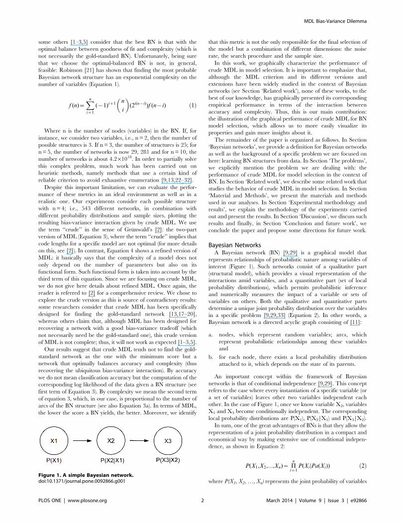
Figure 2. The first term of MDL.doi:10.1371/journal.pone.0092866.g002

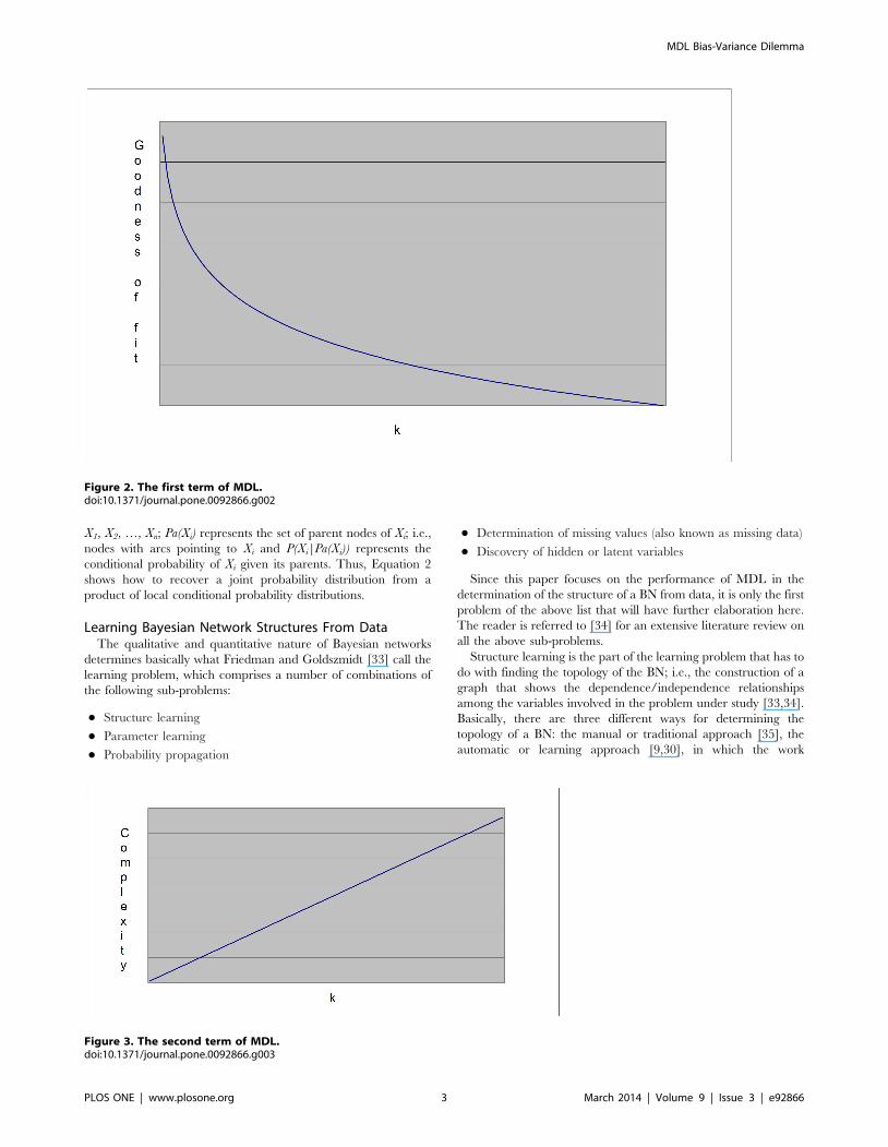
Figure 3. The second term of MDL.doi:10.1371/journal.pone.0092866.g003

MDL Bias-Variance Dilemma

PLOS ONE | www.plosone.org 3 March 2014 | Volume 9 | Issue 3 | e92866

presented in this paper is inspired, and the Bayesian approach,

which can be seen as a combination of the previous two [13].

Friedman and Goldszmidt [33], Chickering [36], Heckerman

[13,26] and Buntine [34] give a very good and detailed account of

this structure-learning problem within the automatic approach in

Bayesian networks. The motivation for this approach is basically to

solve the problem of the manual extraction of human experts’

knowledge found in the traditional approach. We can do this by

using the data at hand collected from the phenomenon under

investigation and pass them on to a learning algorithm in order for

it to automatically determine the structure of a BN that closely

represents such a phenomenon. Since the problem of finding the

best BN is NP-complete [34,36] (Equation 1), the use of heuristic

methods is compulsory.

Generally speaking, there are two different kinds of heuristic

methods for constructing the structure of a Bayesian network from

data: constraint-based and search and scoring based algorithms

[9,11,23,29,30,33,36]. We focus here on the latter. The philoso-

phy of the search and scoring methodology has the two following

typical characteristics:

N a measure (score) to evaluate how well the data fit with the

proposed Bayesian network structure (goodness of fit) and

N a searching engine that seeks a structure that maximizes

(minimizes) this score.

For the first step, there are a number of different scoring metrics

such as the Bayesian Dirichlet scoring function (BD), the cross-

validation criterion (CV), the Bayesian Information Criterion

(BIC), the Minimum Description Length (MDL), the Minimum

Message Length (MML) and the Akaike’s Information Criterion

(AIC) [13,22,23,34,36]. For the second step, we can use well-

known and classic search algorithms such as greedy-hill climbing,

best-first search and simulated annealing [13,22,36,37]. Such

procedures act by applying different operators, which in the

framework of Bayesian networks are:

N the addition of a directed arc

N the reversal of an arc

N the deletion of an arc

In each step, the search algorithm may try every allowed

operator and score to create each resulting graph; it then chooses

the BN structure that has more potential to succeed, i.e., the one

having the highest (lowest) score. In order for the search

procedures to work, we need to provide them with an initial

BN. There are typically three different search-space initializations:

an empty graph, a complete graph or a random graph. The

search-space initialization chosen determines which operators can

be firstly used and applied.

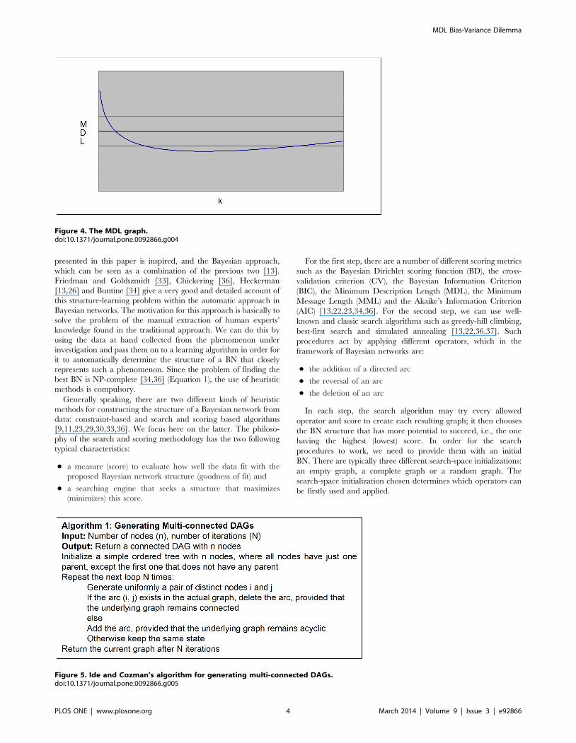
Figure 4. The MDL graph.doi:10.1371/journal.pone.0092866.g004

Figure 5. Ide and Cozman’s algorithm for generating multi-connected DAGs.doi:10.1371/journal.pone.0092866.g005

MDL Bias-Variance Dilemma

PLOS ONE | www.plosone.org 4 March 2014 | Volume 9 | Issue 3 | e92866

In sum, search and scoring algorithms are a widely used option

for learning the structure of a Bayesian network from data; many

of them have used MDL as a score metric with good results [17–

20,24]. However, as we shall see in the next section, we find some

problems that at first sight seem to do with the definition of the

MDL metric itself. Also, we find different works that are

inconsistent each other with respect to their findings regarding

the performance of MDL as a metric for model selection. In the

following sections, we present these inconsistencies.

The ProblemsLet us first consider the traditional or crude definition of MDL

(Equation 3) [2,13]:

MDL~{ log P(DDH)zk

2log n ð3Þ

where D is the data, H represents the parameters of the model, k is

the dimension of the model (number of free parameters) and n is

the sample size. The parameters H of our specific model are the

corresponding local probability distributions for each node in the

network. Such distributions are determined by the structure of the

BN (for a clear example, see [34]). The way to compute k (the

dimension of the model) is given in Equation 3a.

k~Xm

i~1

qi(ri{1) ð3aÞ

where m is the number of variables, qi is the number of possible

configurations of the parents of variable Xi and ri is the number of

values of that variable. For details on how to compute Equation 3

in the context of BN, the reader is referred to [34]. The first term

of this equation measures the accuracy (log likelihood) of the

model (Figure 2); i.e., how well it fits the data, whereas the second

term measures the complexity (Figure 3): such a term punishes

models more heavily as they get more complex. In our case, the

complexity of a BN is, in general, proportional to the number of

arcs (given by k in Equation 3a) [17]. In theory, metrics that

incorporate these two terms can identify models with a good

balance between accuracy and complexity (Figure 4).

Regarding the first term of MDL (Figure 2), Grunwald [2,3]

notes an important analogy between codes and probability

distributions: a large probability means a small code and vice

versa. To be clearer about this, a probability of 1 will produce a

code of length 0 and a probability approaching 0 will produce a

code of length approaching ‘. In order to build the graph in

Figure 2, we just compute the first term of Equation 3 by giving

probability values in the range (0–1].

In this figure, the X-axis represents k (Equation 3a), which, in

general, is proportional to the number of arcs in a BN. The Y-axis

is –log P(D|H) (the accuracy term), which is the log likelihood of

the data given the parameters of the model. Since the log

likelihood is used as the accuracy term, such a term is better as it

approaches zero. As can be seen, while a BN becomes more

complex (in terms of k), its accuracy gets better (i.e., the log

likelihood approaches zero). Unfortunately, such a situation is not

desirable since the resulting model will, in general, overfit unseen

data. This behavior is similar to that when only the training set is

used for both the construction of a model and the test of this model

[16]. By definition, MDL has been explicitly designed for finding

models with a good tradeoff between accuracy and complexity [1–

3,5]. Unfortunately, the first term alone does not achieve this goal.

That is why we need a second term: a term that punishes the

complexity of a model (Figure 3). In order to build the graph in

this figure, we just compute the second term of Equation 3 by

giving complexity values in the arbitrary range [0–1].

Figure 6. Algorithm for randomly generating conditional probability distributions.doi:10.1371/journal.pone.0092866.g006

Figure 7. Algorithm for randomly generating raw sample data.doi:10.1371/journal.pone.0092866.g007

MDL Bias-Variance Dilemma

PLOS ONE | www.plosone.org 5 March 2014 | Volume 9 | Issue 3 | e92866

The X-axis represents k too, while the Y-axis represents the

complexity. Hence, the second term punishes complex models

more heavily than it does to simpler models. This term is used for

compensating the training error. If we only take into account such

a term, we do not get well-balanced BNs either since this term

alone will always choose the simplest one (in our case, the empty

BN structure – the network with no arcs). Therefore, MDL puts

these two terms together in order to find models with a good

balance between accuracy and complexity (Figure 4) [17]. In order

to build the graph in this figure, we now compute the interaction

between accuracy and complexity, where we manually assign

small values of k to large code lengths and vice versa, as MDL

dictates.

It is important to notice that this graph is also the ubiquitous

bias-variance decomposition [16]. On the X-axis, k is again

plotted. On the Y-axis, the MDL score is now plotted. In the case

of MDL values, the lower, the better. As the model gets more

complex, the MDL gets better up to a certain point. If we continue

increasing the complexity of the model beyond this point, the

MDL score, instead of improving, gets worse. It is precisely in this

lowest point where we can find the best-balanced model in terms

of accuracy and complexity (bias-variance). However, this ideal

procedure does not easily tell us how difficult would be, in general,

to reconstruct such a graph with a specific model in mind. To

appreciate this situation in our context, we need to see again

Equation 1. In other words, an exhaustive analysis of all possible

BN is, in general, not feasible. But we can carry out such an

analysis with a limited number of nodes (say, up to 4 or 5) so that

we can assess the performance of MDL in model selection. One of

our contributions is to clearly describe the procedure to achieve

the reconstruction of the bias-variance tradeoff within this limited

setting. To the best of our knowledge, no other paper shows this

procedure in the context of BN. In doing so, we can observe the

graphical performance of MDL, which allows us to gain insights

about this metric. Although we have to bear in mind that the

experiments are carried out using such a limited setting, we will see

that these experiments are enough to show the mentioned

performance and generalize to situations where we may have

more than 5 nodes.

As we will see with more detail in the next section, there is a

discrepancy on the MDL formulation itself. Some authors claim

that the crude version of MDL is able to recover the gold-standard

BN as the one with the minimum MDL, while others claim that

this version is incomplete and does not work as expected. For

instance, Grunwald and other researchers [1,5] claim that model

selection procedures incorporating Equation 3 will tend to choose

complex models instead of simpler ones. Thus, from these

contradictory results, we have two more contributions: a) our

results suggest that crude MDL produces well-balanced models (in

terms of bias-variance) and that these models do not necessarily

coincide with the gold-standard BN, and b) as a corollary, these

findings imply that there is nothing wrong with the crude version.

Authors who consider that crude definition of MDL is

incomplete, propose a refined version (Equation 4) [2,3,5]:

MDL~{ log P(DDH)zk

2log

n

2pz log

ð ffiffiffiffiffiffiffiffiffiffiffiffiDI(H)D

pdHzo(1) ð4Þ

where |I(H)| is the determinant of the Fisher information matrix

I(H) and the constant term o(1) approaches 0 as n (the sample size)

approaches ‘. Roughly speaking, this formula says that the

complexity of a model does not only depend on the number of

parameters but also on its functional form. Such functional form is

taken into account by the third term of Equation 4. Since we are

considering the crude version of MDL for our experiments

(Equation 3), we do not give here details of this term. The

interested reader might like to see [2]. We leave as a future work

the comparison between the crude version and the refined one.

Related WorkRecall, from Sections ‘Introduction’ and ‘The problems’, that

some researchers consider crude MDL as a metric specifically

designed for finding the gold-standard BN structure [13,17–20],

whereas others claim that, although MDL has been designed for

recovering a network (not necessarily the gold-standard network)

with a good bias-variance tradeoff, this crude version of MDL is

not complete; thus, it will not work as expected [1–3,5]. Most of

the most representative works dealing with the construction of BN

structures from data fall in the first situation (the recovery of the

gold-standard BN structure) [17–20,34]. There are much fewer

works dealing with the second situation: the study of crude MDL

as a good metric for selecting BN structures from data with a good

bias-variance tradeoff [24,38,39,40–70]. In fact, these works

explicitly mention the accuracy dimension but hardly the

complexity dimension: they only show the accuracy performance

of classifiers but seldom show the BN structures of such classifiers.

In this paper, we concentrate on plotting the resulting structures

and comparing the one chosen by MDL against the gold-standard

network. It is important to mention that some works [24,38,39]

Figure 8. Expansion and evaluation algorithm.doi:10.1371/journal.pone.0092866.g008

Figure 9. Gold-standard Network.doi:10.1371/journal.pone.0092866.g009

MDL Bias-Variance Dilemma

PLOS ONE | www.plosone.org 6 March 2014 | Volume 9 | Issue 3 | e92866

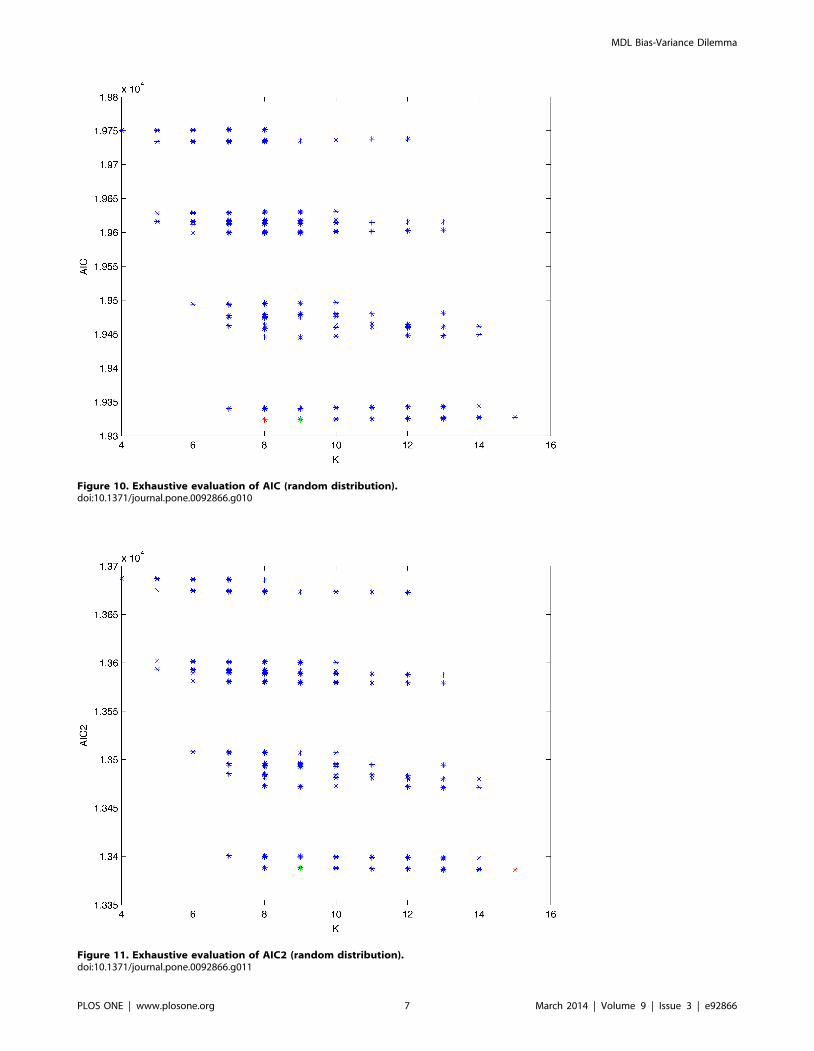
Figure 10. Exhaustive evaluation of AIC (random distribution).doi:10.1371/journal.pone.0092866.g010

Figure 11. Exhaustive evaluation of AIC2 (random distribution).doi:10.1371/journal.pone.0092866.g011

MDL Bias-Variance Dilemma

PLOS ONE | www.plosone.org 7 March 2014 | Volume 9 | Issue 3 | e92866

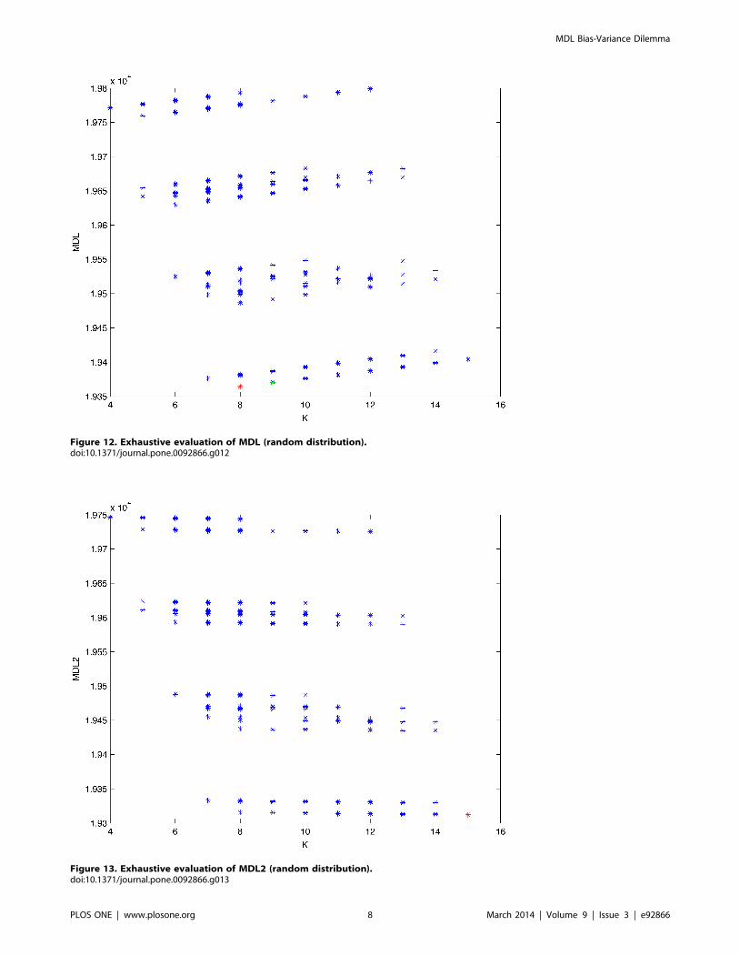
Figure 12. Exhaustive evaluation of MDL (random distribution).doi:10.1371/journal.pone.0092866.g012

Figure 13. Exhaustive evaluation of MDL2 (random distribution).doi:10.1371/journal.pone.0092866.g013

MDL Bias-Variance Dilemma

PLOS ONE | www.plosone.org 8 March 2014 | Volume 9 | Issue 3 | e92866

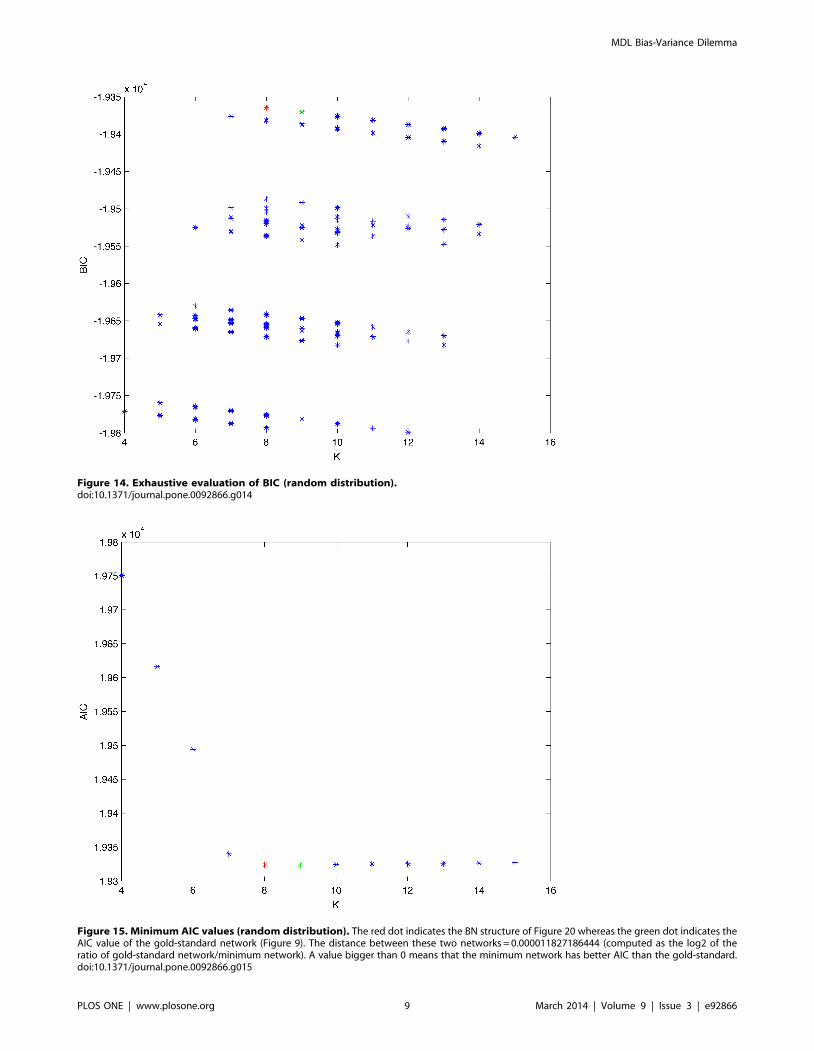
Figure 14. Exhaustive evaluation of BIC (random distribution).doi:10.1371/journal.pone.0092866.g014

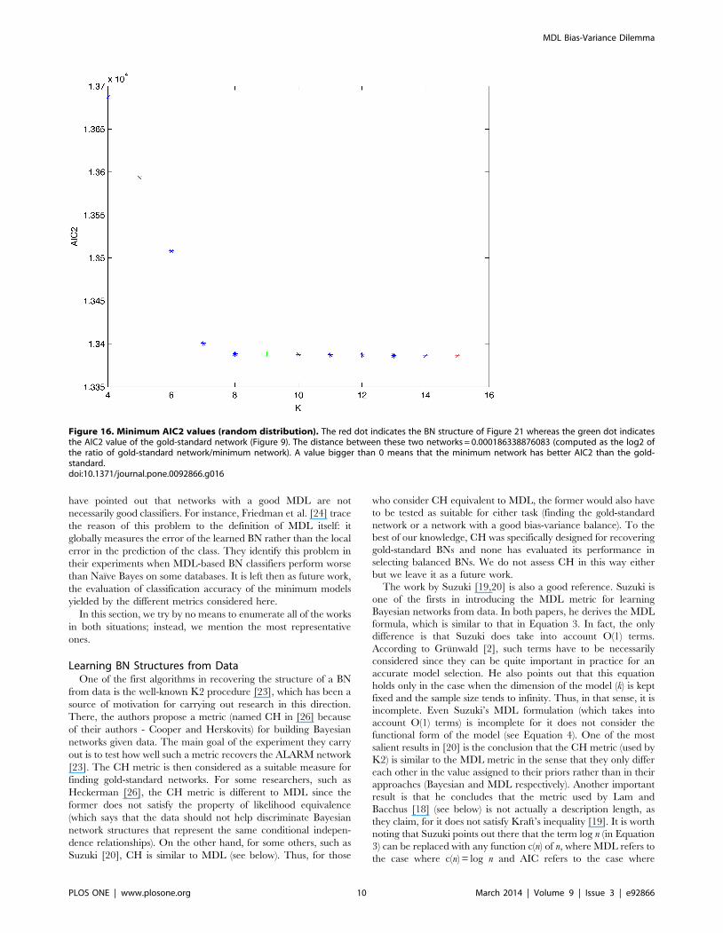
Figure 15. Minimum AIC values (random distribution). The red dot indicates the BN structure of Figure 20 whereas the green dot indicates theAIC value of the gold-standard network (Figure 9). The distance between these two networks = 0.000011827186444 (computed as the log2 of theratio of gold-standard network/minimum network). A value bigger than 0 means that the minimum network has better AIC than the gold-standard.doi:10.1371/journal.pone.0092866.g015

MDL Bias-Variance Dilemma

PLOS ONE | www.plosone.org 9 March 2014 | Volume 9 | Issue 3 | e92866

have pointed out that networks with a good MDL are not

necessarily good classifiers. For instance, Friedman et al. [24] trace

the reason of this problem to the definition of MDL itself: it

globally measures the error of the learned BN rather than the local

error in the prediction of the class. They identify this problem in

their experiments when MDL-based BN classifiers perform worse

than Naıve Bayes on some databases. It is left then as future work,

the evaluation of classification accuracy of the minimum models

yielded by the different metrics considered here.

In this section, we try by no means to enumerate all of the works

in both situations; instead, we mention the most representative

ones.

Learning BN Structures from DataOne of the first algorithms in recovering the structure of a BN

from data is the well-known K2 procedure [23], which has been a

source of motivation for carrying out research in this direction.

There, the authors propose a metric (named CH in [26] because

of their authors - Cooper and Herskovits) for building Bayesian

networks given data. The main goal of the experiment they carry

out is to test how well such a metric recovers the ALARM network

[23]. The CH metric is then considered as a suitable measure for

finding gold-standard networks. For some researchers, such as

Heckerman [26], the CH metric is different to MDL since the

former does not satisfy the property of likelihood equivalence

(which says that the data should not help discriminate Bayesian

network structures that represent the same conditional indepen-

dence relationships). On the other hand, for some others, such as

Suzuki [20], CH is similar to MDL (see below). Thus, for those

who consider CH equivalent to MDL, the former would also have

to be tested as suitable for either task (finding the gold-standard

network or a network with a good bias-variance balance). To the

best of our knowledge, CH was specifically designed for recovering

gold-standard BNs and none has evaluated its performance in

selecting balanced BNs. We do not assess CH in this way either

but we leave it as a future work.

The work by Suzuki [19,20] is also a good reference. Suzuki is

one of the firsts in introducing the MDL metric for learning

Bayesian networks from data. In both papers, he derives the MDL

formula, which is similar to that in Equation 3. In fact, the only

difference is that Suzuki does take into account O(1) terms.

According to Grunwald [2], such terms have to be necessarily

considered since they can be quite important in practice for an

accurate model selection. He also points out that this equation

holds only in the case when the dimension of the model (k) is kept

fixed and the sample size tends to infinity. Thus, in that sense, it is

incomplete. Even Suzuki’s MDL formulation (which takes into

account O(1) terms) is incomplete for it does not consider the

functional form of the model (see Equation 4). One of the most

salient results in [20] is the conclusion that the CH metric (used by

K2) is similar to the MDL metric in the sense that they only differ

each other in the value assigned to their priors rather than in their

approaches (Bayesian and MDL respectively). Another important

result is that he concludes that the metric used by Lam and

Bacchus [18] (see below) is not actually a description length, as

they claim, for it does not satisfy Kraft’s inequality [19]. It is worth

noting that Suzuki points out there that the term log n (in Equation

3) can be replaced with any function c(n) of n, where MDL refers to

the case where c(n) = log n and AIC refers to the case where

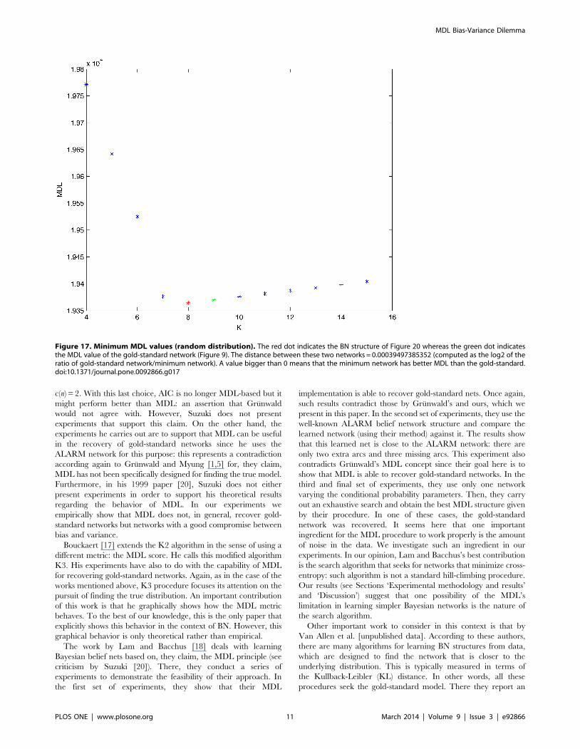
Figure 16. Minimum AIC2 values (random distribution). The red dot indicates the BN structure of Figure 21 whereas the green dot indicatesthe AIC2 value of the gold-standard network (Figure 9). The distance between these two networks = 0.000186338876083 (computed as the log2 ofthe ratio of gold-standard network/minimum network). A value bigger than 0 means that the minimum network has better AIC2 than the gold-standard.doi:10.1371/journal.pone.0092866.g016

MDL Bias-Variance Dilemma

PLOS ONE | www.plosone.org 10 March 2014 | Volume 9 | Issue 3 | e92866

c(n) = 2. With this last choice, AIC is no longer MDL-based but it

might perform better than MDL: an assertion that Grunwald

would not agree with. However, Suzuki does not present

experiments that support this claim. On the other hand, the

experiments he carries out are to support that MDL can be useful

in the recovery of gold-standard networks since he uses the

ALARM network for this purpose: this represents a contradiction

according again to Grunwald and Myung [1,5] for, they claim,

MDL has not been specifically designed for finding the true model.

Furthermore, in his 1999 paper [20], Suzuki does not either

present experiments in order to support his theoretical results

regarding the behavior of MDL. In our experiments we

empirically show that MDL does not, in general, recover gold-

standard networks but networks with a good compromise between

bias and variance.

Bouckaert [17] extends the K2 algorithm in the sense of using a

different metric: the MDL score. He calls this modified algorithm

K3. His experiments have also to do with the capability of MDL

for recovering gold-standard networks. Again, as in the case of the

works mentioned above, K3 procedure focuses its attention on the

pursuit of finding the true distribution. An important contribution

of this work is that he graphically shows how the MDL metric

behaves. To the best of our knowledge, this is the only paper that

explicitly shows this behavior in the context of BN. However, this

graphical behavior is only theoretical rather than empirical.

The work by Lam and Bacchus [18] deals with learning

Bayesian belief nets based on, they claim, the MDL principle (see

criticism by Suzuki [20]). There, they conduct a series of

experiments to demonstrate the feasibility of their approach. In

the first set of experiments, they show that their MDL

implementation is able to recover gold-standard nets. Once again,

such results contradict those by Grunwald’s and ours, which we

present in this paper. In the second set of experiments, they use the

well-known ALARM belief network structure and compare the

learned network (using their method) against it. The results show

that this learned net is close to the ALARM network: there are

only two extra arcs and three missing arcs. This experiment also

contradicts Grunwald’s MDL concept since their goal here is to

show that MDL is able to recover gold-standard networks. In the

third and final set of experiments, they use only one network

varying the conditional probability parameters. Then, they carry

out an exhaustive search and obtain the best MDL structure given

by their procedure. In one of these cases, the gold-standard

network was recovered. It seems here that one important

ingredient for the MDL procedure to work properly is the amount

of noise in the data. We investigate such an ingredient in our

experiments. In our opinion, Lam and Bacchus’s best contribution

is the search algorithm that seeks for networks that minimize cross-

entropy: such algorithm is not a standard hill-climbing procedure.

Our results (see Sections ‘Experimental methodology and results’

and ‘Discussion’) suggest that one possibility of the MDL’s

limitation in learning simpler Bayesian networks is the nature of

the search algorithm.

Other important work to consider in this context is that by

Van Allen et al. [unpublished data]. According to these authors,

there are many algorithms for learning BN structures from data,

which are designed to find the network that is closer to the

underlying distribution. This is typically measured in terms of

the Kullback-Leibler (KL) distance. In other words, all these

procedures seek the gold-standard model. There they report an

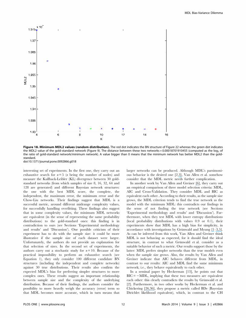
Figure 17. Minimum MDL values (random distribution). The red dot indicates the BN structure of Figure 20 whereas the green dot indicatesthe MDL value of the gold-standard network (Figure 9). The distance between these two networks = 0.00039497385352 (computed as the log2 of theratio of gold-standard network/minimum network). A value bigger than 0 means that the minimum network has better MDL than the gold-standard.doi:10.1371/journal.pone.0092866.g017

MDL Bias-Variance Dilemma

PLOS ONE | www.plosone.org 11 March 2014 | Volume 9 | Issue 3 | e92866

interesting set of experiments. In the first one, they carry out an

exhaustive search for n = 5 (n being the number of nodes) and

measure the Kullback-Leibler (KL) divergence between 30 gold-

standard networks (from which samples of size 8, 16, 32, 64 and

128 are generated) and different Bayesian network structures:

the one with the best MDL score, the complete, the

independent, the maximum error, the minimum error and the

Chow-Liu networks. Their findings suggest that MDL is a

successful metric, around different midrange complexity values,

for successfully handling overfitting. These findings also suggest

that in some complexity values, the minimum MDL networks

are equivalent (in the sense of representing the same probability

distributions) to the gold-standard ones: this finding is in

contradiction to ours (see Sections ‘Experimental methodology

and results’ and ‘Discussion’). One possible criticism of their

experiment has to do with the sample size: it could be more

illustrative if the sample size of each dataset were larger.

Unfortunately, the authors do not provide an explanation for

that selection of sizes. In the second set of experiments, the

authors carry out a stochastic study for n = 10. Because of the

practical impossibility to perform an exhaustive search (see

Equation 1), they only consider 100 different candidate BN

structures (including the independent and complete networks)

against 30 true distributions. Their results also confirm the

expected MDL’s bias for preferring simpler structures to more

complex ones. These results suggest an important relationship

between sample size and the complexity of the underlying

distribution. Because of their findings, the authors consider the

possibility to more heavily weigh the accuracy (error) term so

that MDL becomes more accurate, which in turn means that

larger networks can be produced. Although MDL’s parsimoni-

ous behavior is the desired one [2,3], Van Allen et al. somehow

consider that the MDL metric needs further complication.

In another work by Van Allen and Greiner [6], they carry out

an empirical comparison of three model selection criteria: MDL,

AIC and Cross-Validation. They consider MDL and BIC as

equivalent each other. According to their results, as the sample size

grows, the MDL criterion tends to find the true network as the

model with the minimum MDL: this contradicts our findings in

the sense of not finding the true network (see Sections

‘Experimental methodology and results’ and ‘Discussion’). Fur-

thermore, when they test MDL with lower entropy distributions

(local probability distributions with values 0.9 or 0.1), their

experiments show that MDL has a high bias for simplicity, in

accordance with investigations by Grunwald and Myung [1–3,5].

As can be inferred from this work, Van Allen and Greiner think

MDL is not behaving as expected, for it should find the ideal

structure, in contrast to what Grunwald et al. consider as a

suitable behavior of such a metric. Our results support those by the

latter: MDL prefers simpler networks than the true models even

when the sample size grows. Also, the results by Van Allen and

Greiner indicate that AIC behaves different from MDL, in

contrast to our results: AIC and MDL find the same minimum

network; i.e., they behave equivalently to each other.

In a seminal paper by Heckerman [13], he points out that

BIC = 2MDL, implying that these two measures are equivalent

each other: this clearly contradicts the results by Grunwald et al.

[2]. Furthermore, in two other works by Heckerman et al. and

Chickering [26,36], they propose a metric called BDe (Bayesian

Dirichlet likelihood equivalent), which, in contrast to the CH

Figure 18. Minimum MDL2 values (random distribution). The red dot indicates the BN structure of Figure 22 whereas the green dot indicatesthe MDL2 value of the gold-standard network (Figure 9). The distance between these two networks = 0.00018701910455 (computed as the log2 ofthe ratio of gold-standard network/minimum network). A value bigger than 0 means that the minimum network has better MDL2 than the gold-standard.doi:10.1371/journal.pone.0092866.g018

MDL Bias-Variance Dilemma

PLOS ONE | www.plosone.org 12 March 2014 | Volume 9 | Issue 3 | e92866

metric, considers that data cannot help discriminate Bayesian

networks where the same conditional independence assertions

hold (likelihood equivalence). This is also the case of MDL:

structures with the same set of conditional independence relations

receive the same MDL score. These researchers carry out

experiments to show that the BDe metric is able to recover

gold-standard networks. From these results, and the likelihood-

equivalence between BDe and MDL, we can infer that MDL is

also able to recover these gold-standard nets. Once again, this

result is in contradiction to Grunwald’s [1–3] and ours. On the

other hand, Heckerman et al. mention two important points: 1)

not only is the metric relevant for getting good results but also the

search method and 2) the sample size has a significant effect on the

results.

Regarding the limitation of traditional MDL for classification

purposes, Friedman and Goldszmidt come up with an alternative

MDL definition that is known as local structures [71]. They

redefine this traditional MDL metric incorporating and exploiting

the notion of a feature called CSI (context-specific independence).

In principle, such local models perform better as classifiers than

their global counterparts. However, this last approach tends to

produce more complex networks (in terms of the number of arcs),

which, according to Grunwald, do not reflect the very nature of

MDL: the production of models that well balance accuracy and

complexity.

It is also important to mention the work by Kearns et al. [4].

They present a beautiful theoretical and experimental comparison

of three model selection methods: Vapnik’s Guaranteed Risk

Minimization, Minimum Description Length and Cross-Valida-

tion. They carry out such a comparison using a particular model,

called the intervals model selection problem, which is a rare case

where training error minimization is possible. In contrast,

procedures such as backpropagation neural networks [37,72],

whose heuristics have unknown properties, cannot achieve

training error minimization. Their most significant findings have

to do with the impossibility of always reducing the generalization

error by diminishing the training error: this implies that there is no

universal relation between these two types of error leading to

either the undercoding or overcoding of data by penalty-based

procedures, such as MDL, BIC or AIC. Their experimental results

give us a clue for considering more than just the metric for

obtaining balanced models: a) the sample size and b) the amount

of noise in the data.

To close this section, it is important to recall the distinction

that Grunwald and some other researchers emphasize regarding

crude and refined MDL [1,5]. For these researchers crude

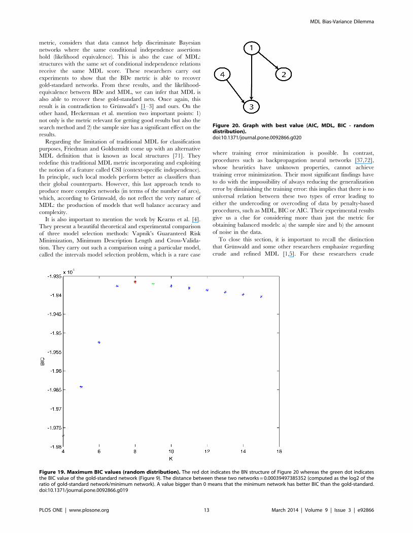
Figure 19. Maximum BIC values (random distribution). The red dot indicates the BN structure of Figure 20 whereas the green dot indicatesthe BIC value of the gold-standard network (Figure 9). The distance between these two networks = 0.00039497385352 (computed as the log2 of theratio of gold-standard network/minimum network). A value bigger than 0 means that the minimum network has better BIC than the gold-standard.doi:10.1371/journal.pone.0092866.g019

Figure 20. Graph with best value (AIC, MDL, BIC - randomdistribution).doi:10.1371/journal.pone.0092866.g020

MDL Bias-Variance Dilemma

PLOS ONE | www.plosone.org 13 March 2014 | Volume 9 | Issue 3 | e92866

MDL is not complete; hence, it cannot produce well-balanced

models. This assertion also applies to metrics such as AIC and

BIC since they do not either take into account the functional

form of the model (see Equation 4). On the other hand, there

are some works, which regard BIC and MDL as equivalent

[16,40,73–84]. In this paper, we also assess the performance of

AIC and BIC to recover the bias-variance tradeoff. Our results

suggest that, under certain circumstances, these metrics behave

similarly to crude MDL.

Learning BN Classifiers from DataSome investigations have used MDL-like metrics for building

BN classifiers from data [24,38,39,40–70]. They partially charac-

terize the bias-variance dilemma: their results have mainly to do

with the classification performance but little to do with the

structure of those classifiers. Here, we mention some of those well-

known works.

A classic and pioneer work is that by Chow and Liu [41]. There,

they approximate discrete probability distributions using depen-

dence trees, which are applied to recognize (classify) hand-printed

numerals. Although the method for building such trees does not

strictly use an MDL-like metric but mutual information, the latter

can be identified as an important part of the former. These

dependence trees can be considered as a special case of a BN.

Friedman and Goldszmidt [42] present an algorithm, based on

MDL, which discretize continuous attributes while learning BN

classifiers. In fact, they only show accuracy results but do not show

the structure of such classifiers.

Another reference work is that by Friedman et al. [24]. There,

they compare the classification performance among different

classifiers: Naıve Bayes, TAN (tree augmented Naıve Bayes), C4.5

and unrestricted Bayesian networks. This last type of classifiers is

built using as a scoring function the MDL metric (using the same

definition as in Equation 3). Although Bayesian networks are more

powerful than the Naıve Bayes classifier, in the sense of more

richly representing the dependences among attributes, the former

perform worse on some datasets from the UCI repository [http://

www.ics.uci.edu/,mlearn/MLRepository.html] than the latter,

in terms of classification accuracy. Friedman et al. trace the reason

of this problem to the definition of MDL itself: it globally measures

the error of the learned BN rather than the local error in the

prediction of the class. In other words, a Bayesian network with a

good MDL score does not necessarily represent a good classifier.

Unfortunately, the experiments they present in their paper are not

specifically designed to prove whether MDL is good at finding the

gold-standard networks. However, we can infer so from the text:

‘‘…with probability equal to one the learned distribution

converges to the underlying distribution as the number of samples

grows’’ [24]. This contradicts our experimental findings. In other

words, our findings show that MDL does not in general recover

the true distribution (represented by the gold-standard net) even

when the sample size grows.

Cheng and Greiner [43] compare different BN classifiers:

Naıve Bayes, Tree Augmented Naıve Bayes (TAN), BN

Augmented Naıve Bayes (BAN) and General BN (GBN).

TAN, BAN and GBN all use conditional independence tests

(based on mutual information and conditional mutual informa-

tion) to build their respective structure. It can be inferred from

this work that such structures, combined with data, are used for

classification purposes. However, these structures are not

explicitly shown in this paper making it virtually impossible to

measure their corresponding complexity (in terms of the number

of arcs). Once again, as in the case of Chow and Liu’s work

[41], these tests are not exactly MDL-based but can be

identified as an important part of this metric.

Grossman and Domingos [38] propose a method for learning

BN classifiers based on the maximization of conditional likelihood

instead of the optimization of the data likelihood. Although the

results are encouraging, the resulting structures are not presented

either. If those structures were presented, that would give us the

opportunity of grasping the interaction between bias and variance.

Unfortunately, this is not the case.

Drugan and Wiering [75] introduce a modified version of

MDL, called MDL-FS (Minimum Description Length for Feature

Selection) for learning BN classifiers from data. However, we

cannot measure the bias-variance tradeoff since the results these

authors present are only in terms of classification accuracy. This

same situation happens in Acid et al. [40] and Kelner and Lerner

[39].

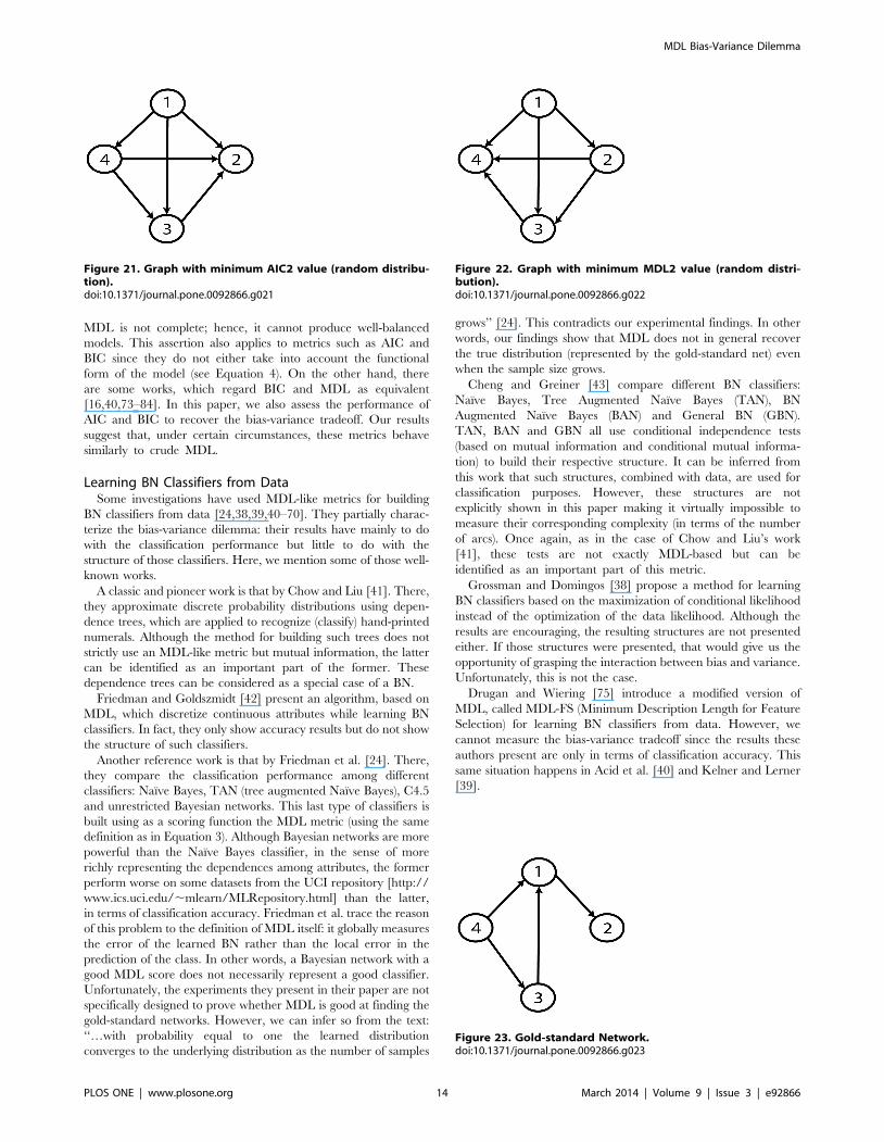
Figure 21. Graph with minimum AIC2 value (random distribu-tion).doi:10.1371/journal.pone.0092866.g021

Figure 22. Graph with minimum MDL2 value (random distri-bution).doi:10.1371/journal.pone.0092866.g022

Figure 23. Gold-standard Network.doi:10.1371/journal.pone.0092866.g023

MDL Bias-Variance Dilemma

PLOS ONE | www.plosone.org 14 March 2014 | Volume 9 | Issue 3 | e92866

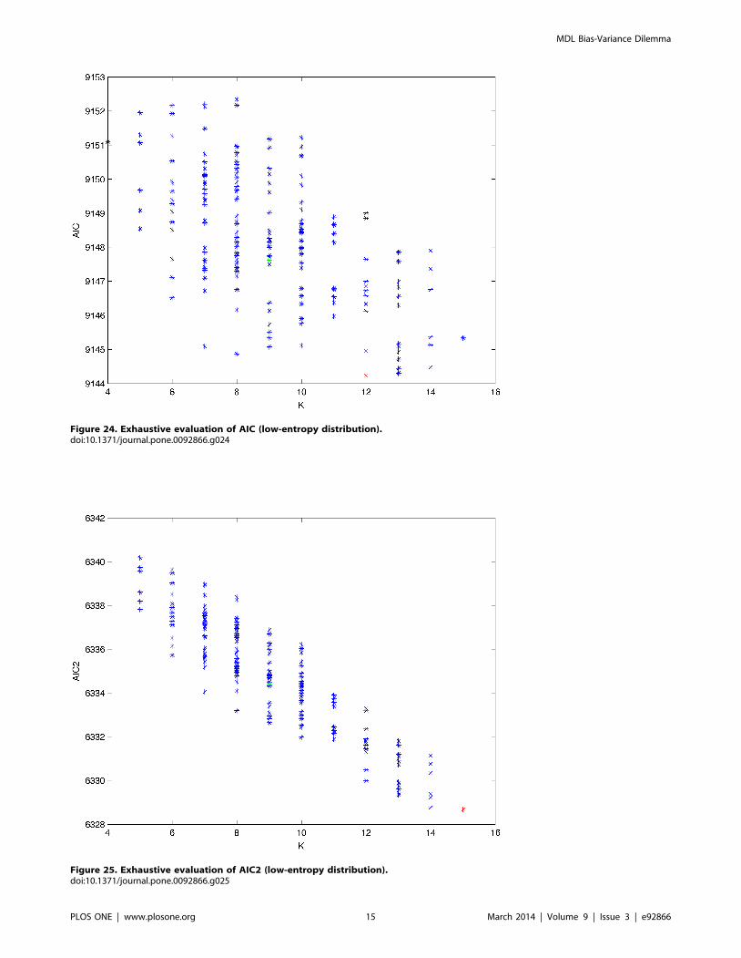
Figure 24. Exhaustive evaluation of AIC (low-entropy distribution).doi:10.1371/journal.pone.0092866.g024

Figure 25. Exhaustive evaluation of AIC2 (low-entropy distribution).doi:10.1371/journal.pone.0092866.g025

MDL Bias-Variance Dilemma

PLOS ONE | www.plosone.org 15 March 2014 | Volume 9 | Issue 3 | e92866

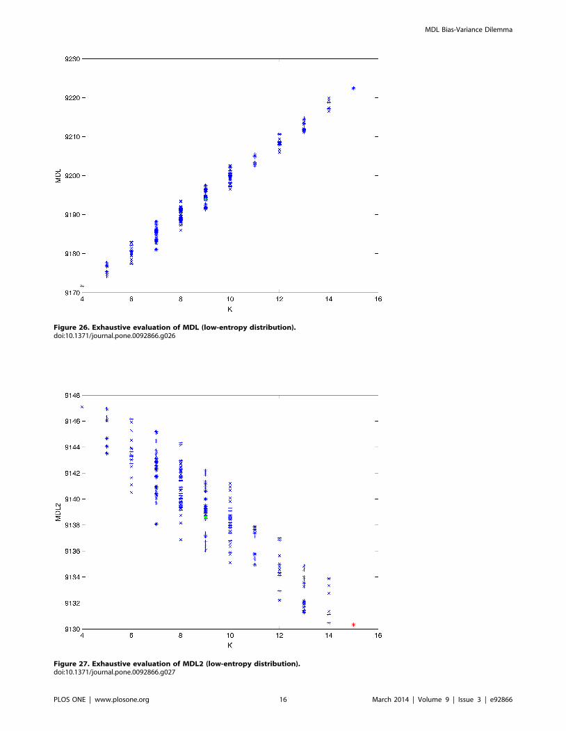
Figure 26. Exhaustive evaluation of MDL (low-entropy distribution).doi:10.1371/journal.pone.0092866.g026

Figure 27. Exhaustive evaluation of MDL2 (low-entropy distribution).doi:10.1371/journal.pone.0092866.g027

MDL Bias-Variance Dilemma

PLOS ONE | www.plosone.org 16 March 2014 | Volume 9 | Issue 3 | e92866

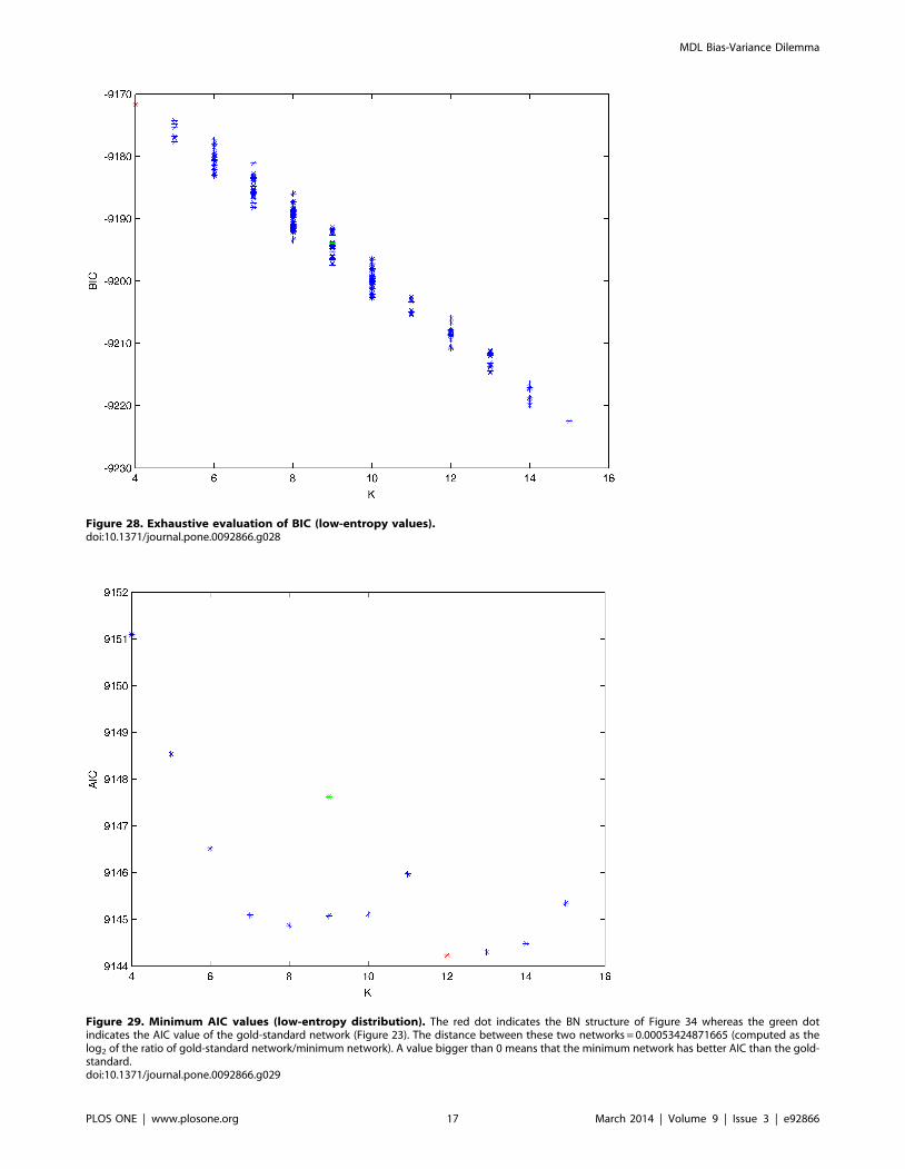
Figure 28. Exhaustive evaluation of BIC (low-entropy values).doi:10.1371/journal.pone.0092866.g028

Figure 29. Minimum AIC values (low-entropy distribution). The red dot indicates the BN structure of Figure 34 whereas the green dotindicates the AIC value of the gold-standard network (Figure 23). The distance between these two networks = 0.00053424871665 (computed as thelog2 of the ratio of gold-standard network/minimum network). A value bigger than 0 means that the minimum network has better AIC than the gold-standard.doi:10.1371/journal.pone.0092866.g029

MDL Bias-Variance Dilemma

PLOS ONE | www.plosone.org 17 March 2014 | Volume 9 | Issue 3 | e92866

Materials and Methods

DatasetsFor the tests carried out in this work, we generated databases

from random 4-node gold-standard Bayesian networks with

various sample sizes. All the random variables considered in these

experiments are binary: this choice does not produce any

significant qualitative impact on the results; rather, it makes the

computation and analyses easier [6]. The use of simulated datasets

is a common practice to evaluate the performance of heuristic

algorithms that recover the structure of a BN from data

[34,36,85]. Also, synthetic data from gold-standard BN give us

the flexibility of plotting learning curves over different combina-

tions of probability distributions and sample sizes (see cf. [4]). The

only difference in our experiments is that we are carrying out an

exhaustive search among all possible network structures (for n = 4)

and using these simulated datasets to assess the potential of

different metrics (including MDL) for recovering models that well

balance accuracy and complexity. The methods used for

generating the datasets from a specific BN structure, a specific

probability distribution and a determined sample size are

presented in the next section.

Algorithm for Generating Directed Acyclic GraphsIn order to generate a database, we firstly need to propose a

specific structure from which such a database is created (in

combination with a specific joint probability distribution and a

sample size). We decided to use the procedure by Ide and Cozman

[86], which allows to generate uniformly distributed DAGs. The

pseudo-code of such a procedure, called algorithm 1, is given in

figure 5. Note that line 01 of algorithm 1 initializes a simple

ordered tree, which we achieve by using a pseudo-random number

generator called ran3 [87]. It is important to mention that,

although some generators can satisfy most of applications, they are

not recommended as reliable random number procedures. This is

because they do not either fulfill some statistical tests for

randomness or cannot be used in long sequences. Since the

generator we use in our experiments is based more on a

subtractive method than a linear congruential one, it offers

specific desirable features that the others do not: portability, low

correlation in successive runs and independence on the computer

arithmetic. This same procedure is used for carrying out step 03 of

algorithm 1 as well. The interested reader might like to see the C

code of procedure ran3 in [87].

Generation of Conditional Probability DistributionsOnce we have a DAG, we randomly generate the correspond-

ing conditional probability distributions from such a DAG using

procedure ran3 as well. The pseudo-code of this random

conditional probability distribution generator, which we call

algorithm 2, is given in figure 6.

Generation of Raw Sample DataGiven a DAG and its corresponding set of local conditional

probability distributions, we generate a random data sample

according to algorithm 3 (see figure 7).

Construction of BAYESIAN NetworksSince the goal of the present study is to assess the performance

of MDL (among some other metrics) in model selection; i.e., to

check whether these metrics can recover the gold-standard

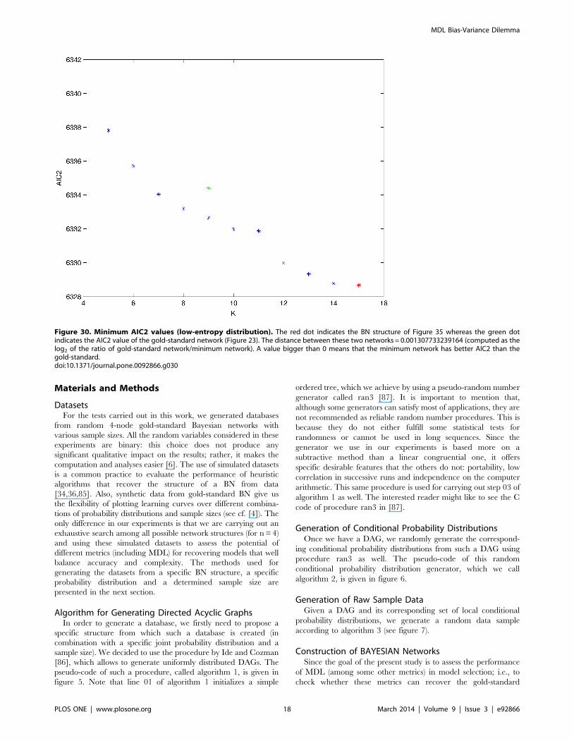
Figure 30. Minimum AIC2 values (low-entropy distribution). The red dot indicates the BN structure of Figure 35 whereas the green dotindicates the AIC2 value of the gold-standard network (Figure 23). The distance between these two networks = 0.001307733239164 (computed as thelog2 of the ratio of gold-standard network/minimum network). A value bigger than 0 means that the minimum network has better AIC2 than thegold-standard.doi:10.1371/journal.pone.0092866.g030

MDL Bias-Variance Dilemma

PLOS ONE | www.plosone.org 18 March 2014 | Volume 9 | Issue 3 | e92866

Bayesian networks or whether they can come up with a balanced

model (in terms of accuracy and complexity) that is not necessarily

the gold-standard one, we need to exhaustively build all the

possible network structures given a number of nodes. Recall that

one of our goals is to characterize the behavior of AIC and BIC,

since some works [13,73,88] consider them equivalent to crude

MDL while others regard them different [1–3,5]. For the analyses

presented here, the number of nodes is 4, which produces 543

different Bayesian network structures (see equation 1). Our

procedure that exhaustively builds all possible networks, called

algorithm 4, is given in figure 8.

Regarding the implementation of the metrics tested here, we

wrote procedures for crude MDL (Equation 3) and one of its

variants (Equation 7) as well as procedures for AIC (Equations 5

and 6) and BIC (Equation 8). We included in our experiments

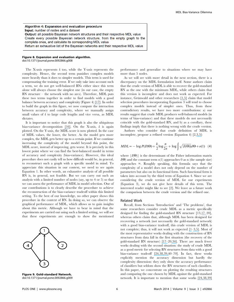
alternative formulations of AIC and MDL (called here AIC2 and

MDL2) suggested by Van Allen and Greiner [6] (Equations 6 and

7 respectively), in order to assess their performance. The

justification Van Allen and Greiner provide for these alternative

formulations of MDL and AIC is, for the former, that they

normalize everything by 1/n (where n is the sample size) so as to

compare such criterion across different sample sizes; and for the

latter, they simply carry out a conversion from nats to bits by using

log e.

AIC~{log P(DDH)zk ð5Þ

AIC2~{log P(DDH)zk

nlog e ð6Þ

MDL2~{log P(DDH)zk

2nlog n ð7Þ

BIC~log P(DDH){k

2log n ð8Þ

For all these equations, D is the data, H represents the

parameters of the model, k is the dimension of the model (number

of free parameters), n is the sample size, e is the base of the natural

logarithm and log e is simply a conversion from nats to bits [6].

Experimental Methodology and Results

In this section, we describe the experimental methodology and

show the results of two different experiments. In Section

‘Discussion’, we discuss those results.

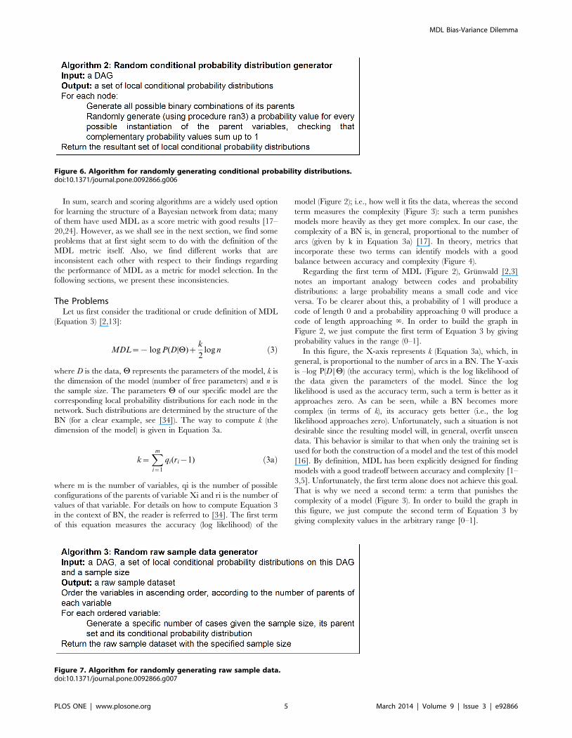
Experiment 1From a random gold-standard Bayesian network structure

(Figure 9) and a random probability distribution, we generate 3

datasets (1000, 3000 and 5000 cases) using algorithms 1, 2 and 3

(Figures 5, 6 and 7 respectively). Then, we run algorithm 4 (Figure 8)

in order to compute, for every possible BN structure, its

corresponding metric value (MDL, AIC and BIC – see Equations

3 and 5–8). Finally, we plot these values (see Figures 10–14). The

main goals of this experiment are, on the one hand, to check

whether the traditional definition of the MDL metric (Equation 3) is

enough for producing well-balanced models (in terms of complexity

and accuracy) and, on the other hand, to check if such a metric is

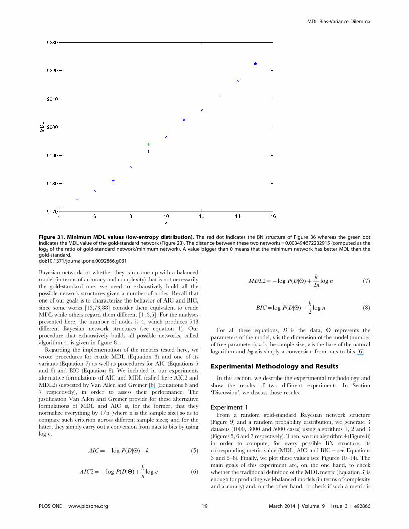
Figure 31. Minimum MDL values (low-entropy distribution). The red dot indicates the BN structure of Figure 36 whereas the green dotindicates the MDL value of the gold-standard network (Figure 23). The distance between these two networks = 0.003494672232915 (computed as thelog2 of the ratio of gold-standard network/minimum network). A value bigger than 0 means that the minimum network has better MDL than thegold-standard.doi:10.1371/journal.pone.0092866.g031

MDL Bias-Variance Dilemma

PLOS ONE | www.plosone.org 19 March 2014 | Volume 9 | Issue 3 | e92866

able to recover gold-standard models. Recall that some researchers

(see Section ‘Introduction’) point out that the crude MDL is not

complete so it should not be possible for it to come up with well-

balanced models. If that is the case, other metrics such as AIC and

BIC should not select well-balanced models either. That is why we

also plot the values for AIC, BIC and a modified version of MDL as

well [2,6,88]. Furthermore, regarding the second goal, other

researchers claim that MDL can recover gold-standard models

while others say that this metric is not specifically designed for this

task. Our experiments with different sample sizes aim to check the

influence of this dimension on the MDL metric itself. Here, we only

show the results with 5000 cases since these are representative for all

the chosen sample sizes. These results are presented in Figures 9–22.

Figure 9 shows the gold-standard BN structure from which, together

with a random probability distribution, the corresponding dataset is

generated. Figures 10–14 show the exhaustive evaluation (blue dots)

of all BN structures with the corresponding metric (AIC, AIC2,

MDL, MDL2 and BIC respectively). Figures 15–19 plot only those

BN structures with the minimum values for each metric and each k.

Figure 20 shows the network with the minimum value for AIC,

MDL and BIC, Figure 21 shows the network with the minimum

value for AIC2 and Figure 22 shows the MDL2 minimum network.

Experiment 2From a random gold-standard Bayesian network structure

(Figure 23) and a low-entropy probability distribution [6], we

generate 3 datasets (1000, 3000 and 5000 cases) using algorithms

1, 2 and 3 (Figures 5, 6 and 7 respectively). According to Van

Allen [6], changing the parameters to be high or low (0.9 or 0.1)

tends to produce low-entropy distributions, which in turn make

data have more potential to be compressed. Here, we only show

experiments with distribution p = 0.1 since such a distribution is

representative of different low-entropy probability distributions

(0.2, 0.3, etc.). Then, we run algorithm 4 (Figure 8) in order to

compute, for every possible BN structure, its corresponding metric

value (MDL, AIC and BIC – see Equations 3 and 5–8). Finally, we

plot these values (see Figures 24–28). The main goal of this

experiment is to check whether the noise rate present in the data of

Experiment 1 affects the behavior of MDL in the sense of its

expected curve (Figure 4). As in Experiment 1, we evaluate the

performance of the metrics in Equations 3 and 5–8. Our

experiments with different sample sizes aim to check the influence

of this dimension on the MDL metric itself. Here, we only show

the results with 5000 cases since these are representative for all the

chosen sample sizes. These results are presented in Figures 23–36.

Figure 23 shows the gold-standard BN structure from which,

together with a random probability distribution, the corresponding

dataset is generated. Figures 24–28 show the exhaustive evaluation

of all BN structures with the corresponding metric (AIC, AIC2,

MDL, MDL2 and BIC respectively). Figure 29–33 plot only those

BN structures with the minimum values for each metric and each

k. Figure 34 shows the network with the minimum value for AIC;

Figure 35 shows the network with the minimum value for AIC2

and MDL2 and Figure 36 shows the network with the minimum

value for MDL and BIC.

Discussion

Experiment 1The main goals of this experiment were, given randomly

generated datasets with different sample sizes, a) to check whether

the traditional definition of the MDL metric (Equation 3) was

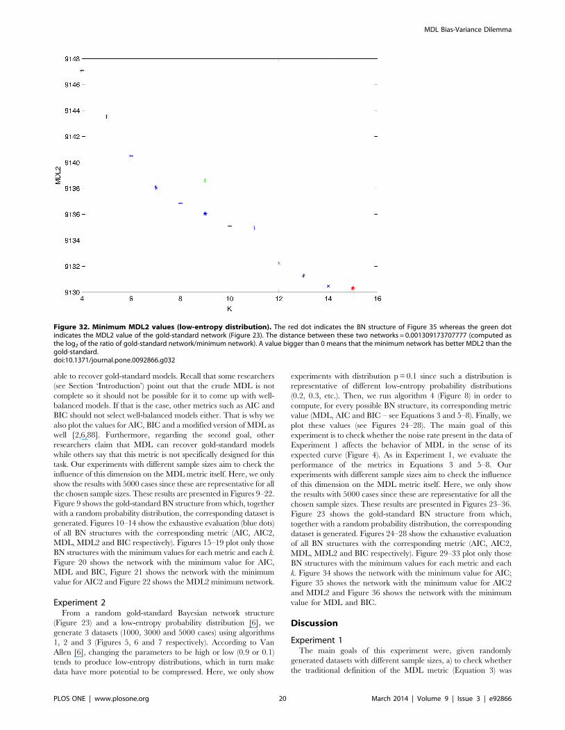
Figure 32. Minimum MDL2 values (low-entropy distribution). The red dot indicates the BN structure of Figure 35 whereas the green dotindicates the MDL2 value of the gold-standard network (Figure 23). The distance between these two networks = 0.001309173707777 (computed asthe log2 of the ratio of gold-standard network/minimum network). A value bigger than 0 means that the minimum network has better MDL2 than thegold-standard.doi:10.1371/journal.pone.0092866.g032

MDL Bias-Variance Dilemma

PLOS ONE | www.plosone.org 20 March 2014 | Volume 9 | Issue 3 | e92866

enough for producing well-balanced models (in terms of complex-

ity and accuracy), and b) to check if such a metric was able to

recover gold-standard models. To better understand the way we

present the results, we give here a brief explanation on each of the

figures corresponding to Experiment 1. Figure 9 presents the gold-

standard network from which, together with a random probability

distribution, we generate the data. Figures 10–14 show an

exhaustive evaluation of each possible BN structure given by

AIC, AIC2, MDL, MDL2 and BIC respectively. We plot in these

figures the dimension of the model (k – X-axis) vs. the metric (Y-

axis). Dots represent BN structures. Since equivalent networks

have, according to these metrics, the same value, there may be

more than one in each dot; i.e., dots may overlap. A red dot in

each of these figures represent the network with the best metric; a

green dot represents the gold-standard network so that we can

visually measure the distance between these two networks.

Figures 15–19 plot the minimum values of each of these metrics

for every possible value for k. In fact, these figures are the result of

extracting, from Figures 10–14, only the corresponding minimum

values. Figure 20 shows the BN structure with the best value for

AIC, MDL and BIC; Figure 21 shows the BN structure with the

best value for AIC2 and Figure 22 shows the network with the best

MDL2 value.

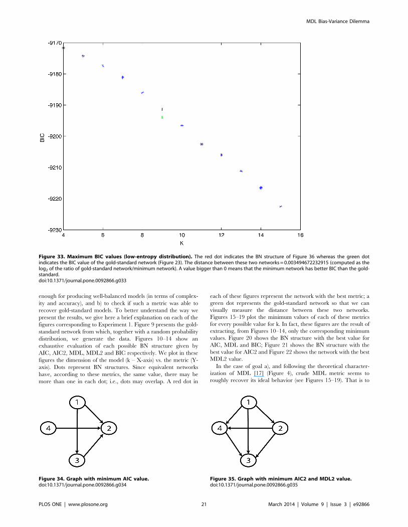
In the case of goal a), and following the theoretical character-

ization of MDL [17] (Figure 4), crude MDL metric seems to

roughly recover its ideal behavior (see Figures 15–19). That is to

Figure 33. Maximum BIC values (low-entropy distribution). The red dot indicates the BN structure of Figure 36 whereas the green dotindicates the BIC value of the gold-standard network (Figure 23). The distance between these two networks = 0.003494672232915 (computed as thelog2 of the ratio of gold-standard network/minimum network). A value bigger than 0 means that the minimum network has better BIC than the gold-standard.doi:10.1371/journal.pone.0092866.g033

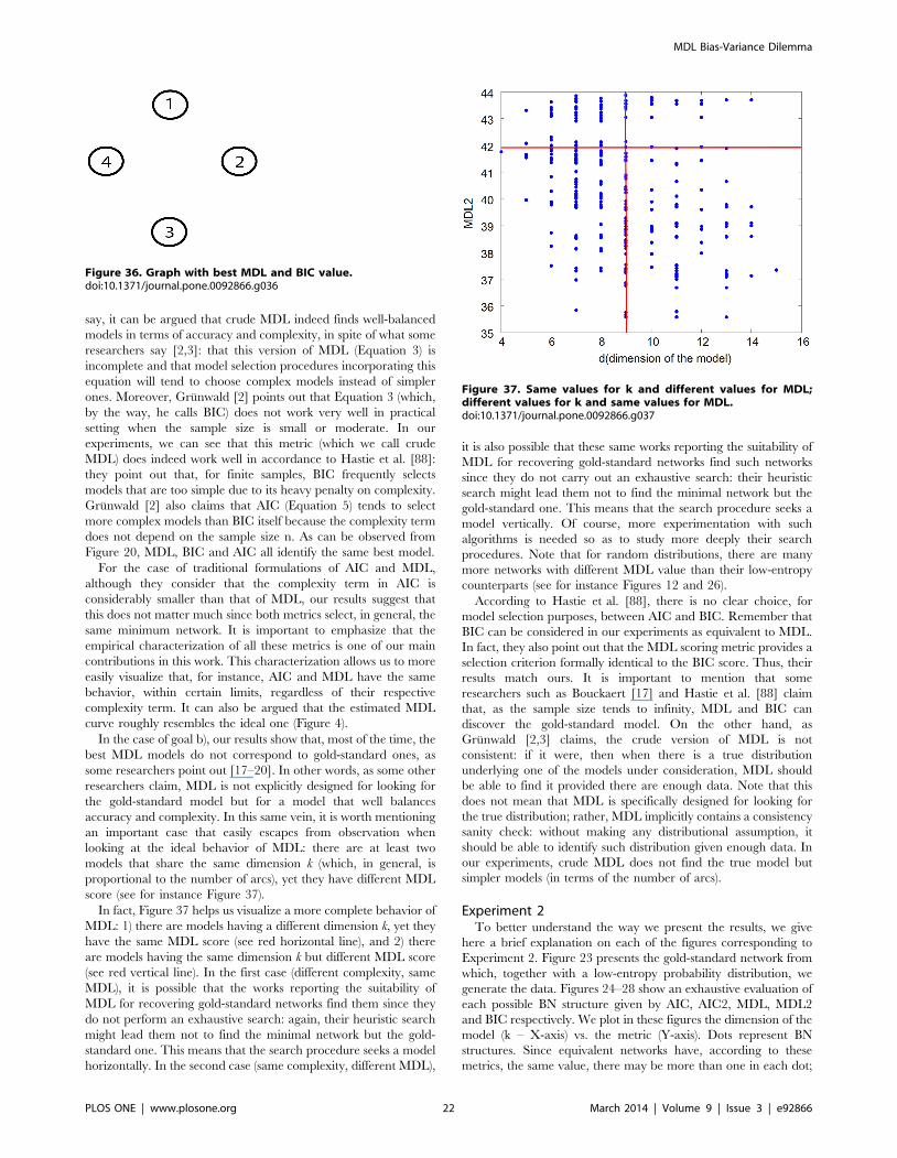
Figure 34. Graph with minimum AIC value.doi:10.1371/journal.pone.0092866.g034

Figure 35. Graph with minimum AIC2 and MDL2 value.doi:10.1371/journal.pone.0092866.g035

MDL Bias-Variance Dilemma

PLOS ONE | www.plosone.org 21 March 2014 | Volume 9 | Issue 3 | e92866

say, it can be argued that crude MDL indeed finds well-balanced

models in terms of accuracy and complexity, in spite of what some

researchers say [2,3]: that this version of MDL (Equation 3) is

incomplete and that model selection procedures incorporating this

equation will tend to choose complex models instead of simpler

ones. Moreover, Grunwald [2] points out that Equation 3 (which,

by the way, he calls BIC) does not work very well in practical

setting when the sample size is small or moderate. In our

experiments, we can see that this metric (which we call crude

MDL) does indeed work well in accordance to Hastie et al. [88]:

they point out that, for finite samples, BIC frequently selects

models that are too simple due to its heavy penalty on complexity.

Grunwald [2] also claims that AIC (Equation 5) tends to select

more complex models than BIC itself because the complexity term

does not depend on the sample size n. As can be observed from

Figure 20, MDL, BIC and AIC all identify the same best model.

For the case of traditional formulations of AIC and MDL,

although they consider that the complexity term in AIC is

considerably smaller than that of MDL, our results suggest that

this does not matter much since both metrics select, in general, the

same minimum network. It is important to emphasize that the

empirical characterization of all these metrics is one of our main

contributions in this work. This characterization allows us to more

easily visualize that, for instance, AIC and MDL have the same

behavior, within certain limits, regardless of their respective

complexity term. It can also be argued that the estimated MDL

curve roughly resembles the ideal one (Figure 4).

In the case of goal b), our results show that, most of the time, the

best MDL models do not correspond to gold-standard ones, as

some researchers point out [17–20]. In other words, as some other

researchers claim, MDL is not explicitly designed for looking for

the gold-standard model but for a model that well balances

accuracy and complexity. In this same vein, it is worth mentioning

an important case that easily escapes from observation when

looking at the ideal behavior of MDL: there are at least two

models that share the same dimension k (which, in general, is

proportional to the number of arcs), yet they have different MDL

score (see for instance Figure 37).

In fact, Figure 37 helps us visualize a more complete behavior of

MDL: 1) there are models having a different dimension k, yet they

have the same MDL score (see red horizontal line), and 2) there

are models having the same dimension k but different MDL score

(see red vertical line). In the first case (different complexity, same

MDL), it is possible that the works reporting the suitability of

MDL for recovering gold-standard networks find them since they

do not perform an exhaustive search: again, their heuristic search

might lead them not to find the minimal network but the gold-

standard one. This means that the search procedure seeks a model

horizontally. In the second case (same complexity, different MDL),

it is also possible that these same works reporting the suitability of

MDL for recovering gold-standard networks find such networks

since they do not carry out an exhaustive search: their heuristic

search might lead them not to find the minimal network but the

gold-standard one. This means that the search procedure seeks a

model vertically. Of course, more experimentation with such

algorithms is needed so as to study more deeply their search

procedures. Note that for random distributions, there are many

more networks with different MDL value than their low-entropy

counterparts (see for instance Figures 12 and 26).

According to Hastie et al. [88], there is no clear choice, for

model selection purposes, between AIC and BIC. Remember that

BIC can be considered in our experiments as equivalent to MDL.

In fact, they also point out that the MDL scoring metric provides a

selection criterion formally identical to the BIC score. Thus, their

results match ours. It is important to mention that some

researchers such as Bouckaert [17] and Hastie et al. [88] claim

that, as the sample size tends to infinity, MDL and BIC can

discover the gold-standard model. On the other hand, as

Grunwald [2,3] claims, the crude version of MDL is not

consistent: if it were, then when there is a true distribution

underlying one of the models under consideration, MDL should

be able to find it provided there are enough data. Note that this

does not mean that MDL is specifically designed for looking for

the true distribution; rather, MDL implicitly contains a consistency

sanity check: without making any distributional assumption, it

should be able to identify such distribution given enough data. In

our experiments, crude MDL does not find the true model but

simpler models (in terms of the number of arcs).

Experiment 2To better understand the way we present the results, we give

here a brief explanation on each of the figures corresponding to

Experiment 2. Figure 23 presents the gold-standard network from

which, together with a low-entropy probability distribution, we

generate the data. Figures 24–28 show an exhaustive evaluation of

each possible BN structure given by AIC, AIC2, MDL, MDL2

and BIC respectively. We plot in these figures the dimension of the

model (k – X-axis) vs. the metric (Y-axis). Dots represent BN

structures. Since equivalent networks have, according to these

metrics, the same value, there may be more than one in each dot;

Figure 36. Graph with best MDL and BIC value.doi:10.1371/journal.pone.0092866.g036

Figure 37. Same values for k and different values for MDL;different values for k and same values for MDL.doi:10.1371/journal.pone.0092866.g037

MDL Bias-Variance Dilemma

PLOS ONE | www.plosone.org 22 March 2014 | Volume 9 | Issue 3 | e92866

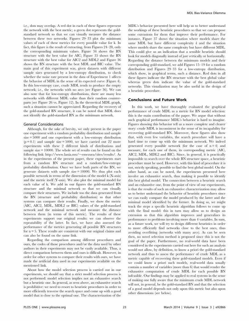
i.e., dots may overlap. A red dot in each of these figures represent

the network with the best metric; a green dot represents the gold-

standard network so that we can visually measure the distance

between these two networks. Figures 29–33 plot the minimum

values of each of these metrics for every possible value for k. In

fact, this figure is the result of extracting, from Figures 24–28, only

the corresponding minimum values. Figure 34 shows the BN

structure with the best value for AIC; Figure 35 shows the BN

structure with the best value for AIC2 and MDL2 and Figure 36

shows the BN structure with the best MDL and BIC value. The

main goal of this experiment was, given datasets with different

sample sizes generated by a low-entropy distribution, to check

whether the noise rate present in the data of Experiment 1 affects

the behavior of MDL in the sense of its expected curve (Figure 4).

In this low-entropy case, crude MDL tends to produce the empty

network; i.e., the networks with no arcs (see Figure 36). We can

also note that for low-entropy distributions, there are many less

networks with different MDL value than their random counter-

parts (see Figure 26 vs. Figure 12). In the theoretical MDL graph,

such a situation cannot be appreciated. Regarding the recovery of

the gold-standard BN structure, it can be noted that MDL does

not identify the gold-standard BN as the minimum network.

General ConsiderationsAlthough, for the sake of brevity, we only present in the paper

one experiment with a random probability distribution and sample

size = 5000 and one experiment with a low-entropy distribution

(p = 0.1) and sample size = 5000, we have carried out 22 more

experiments with these 2 different kinds of distributions and

sample size = 10000. The whole set of results can be found on the

following link: http://www.lania.mx/,emezura/sites/results/. As

in the experiments of the present paper, these experiments start

from a random BN structure and a random/low-entropy

probability distribution. Once we have both parts of the BN, we

generate datasets with sample size = 10000. We thus plot each

possible network in terms of the dimension of the model k (X-axis)

and the metric itself (Y-axis). We also plot the minimal model for

each value of k. We add in our figures the gold-standard BN

structure and the minimal network so that we can visually

compare their structures. We include too the data generated from

the BN (structure and probability distribution) so that other

systems can compare their results. Finally, we show the metric

(AIC, AIC2, MDL, MDL2 or BIC) values of the gold-standard

network and the minimal network and measure the distance

between them (in terms of this metric). The results of these

experiments support our original results: we can observe the

repeatability of the latter. In fact, we have also assessed the

performance of the metrics generating all possible BN structures

for n = 5. These results are consistent with our original claims and

can also be found on the same link.

Regarding the comparison among different procedures and

ours, the codes of those procedures and/or the data used by other

authors in their experiments may not be easily available. Thus, a

direct comparison between them and ours is difficult. However, in

order for other systems to compare their results with ours, we have

made the artificial data used in our experiments available on the

mentioned link.

About how the model selection process is carried out in our

experiments, we should say that a strict model selection process is

not performed: model selection implies not an exhaustive search

but a heuristic one. In general, as seen above, an exhaustive search

is prohibitive: we need to resort to heuristic procedures in order to

more efficiently traverse the search space and come up with a good

model that is close to the optimal one. The characterization of the

MDL’s behavior presented here will help us to better understand

the workings of these heuristic procedures so that we can propose

some extensions for them that improve their performance. For

instance, Figure 37 shows the situation where models share the

same MDL but have different complexity k and the situation

where models share the same complexity but have different MDL.

This could give us an indication that a sensible heuristic should

look for models diagonally instead of just vertically or horizontally.

Regarding the distance between the minimum models and their

corresponding gold-standard, we add Figures 15–19 for a random

distribution and Figures 29–33 for a low-entropy distribution,

which show, in graphical terms, such a distance. Red dots in all

these figures indicate the BN structure with the best global value

whereas green dots indicate the value of the gold-standard

networks. This visualization may be also useful in the design of

a heuristic procedure.

Conclusions and Future Work

In this work, we have thoroughly evaluated the graphical

performance of crude MDL as a metric for BN model selection:

this is the main contribution of the paper. We argue that without

such graphical performance MDL’s behavior is hard to imagine.

Figures showing this behavior tell us a more complete and clearer

story: crude MDL is inconsistent in the sense of its incapability for

recovering gold-standard BN. Moreover, these figures also show

that, with even few variables, the search procedure will have a

hard time to come up with the minimum network. We indeed

generated every possible network (for the case of n = 4) and

measure, for each one of them, its corresponding metric (AIC,

AIC2, MDL, MDL2 and BIC). Since, in general, it is practically

impossible to search over the whole BN structure space, a heuristic

procedure must be used. However, with this kind of procedure it is

not, strictly speaking, possible to find the best global model. On the

other hand, as can be noted, the experiments presented here

involve an exhaustive search, thus making it possible to identify

this best global model. The connection between a heuristic search

and an exhaustive one, from the point of view of our experiments,

is that the results of such an exhaustive characterization may allow

us to better understand the behavior of heuristic procedures since

we can easily compare the model produced by the latter and the

minimal model identified by the former. In doing so, we might

track the steps a specific heuristic algorithm follows to come up

with the final model: this in turn may allow us to design an

extension so that this algorithm improves and generalizes its

performance to problems involving more than 4 variables. In sum,

as a future work, we will try to design different heuristics in order

to more efficiently find networks close to the best ones, thus

avoiding overfitting (networks with many arcs). As can be seen

then, no novel selection method is proposed since this is not the

goal of the paper. Furthermore, no real-world data have been

considered in the experiments carried out here for such an analysis

would not allow, by definition, to know a priori the gold-standard

network and thus to assess the performance of crude MDL as a

metric capable of recovering these gold-standard models. Even if

we could know a priori such models, real-world data usually

contain a number of variables (more than 6) that would render the

exhaustive computation of crude MDL for each possible BN

infeasible. Our findings may be applied to real systems in the sense

of making one fully aware that the minimum crude MDL network

will not, in general, be the gold-standard BN and that the selection

of a good model depends not only upon this metric but also upon

other dimensions (see below).

MDL Bias-Variance Dilemma

PLOS ONE | www.plosone.org 23 March 2014 | Volume 9 | Issue 3 | e92866

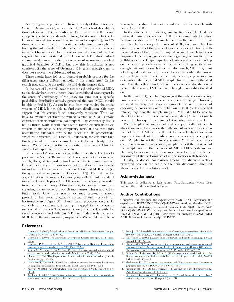
According to the previous results in the study of this metric (see

Section ‘Related work’), we can identify 2 schools of thought: 1)

those who claim that the traditional formulation of MDL is not

complete and hence needs to be refined, for it cannot select well-

balanced models (in terms of accuracy and complexity); and 2)

those who claim that this traditional definition is enough for

finding the gold-standard model, which in our case is a Bayesian

network. Our results can be situated somewhat in the middle: they

suggest that the traditional formulation of MDL does indeed

choose well-balanced models (in the sense of recovering the ideal

graphical behavior of MDL) but that this formulation is not

consistent (in the sense of Grunwald [2]): given enough data, it

does not recover the gold-standard model.

These results have led us to detect 4 probable sources for the

differences among different schools: 1) the metric itself, 2) the

search procedure, 3) the noise rate and 4) the sample size.

In the case of 1), we still have to test the refined version of MDL

to check whether it works better than its traditional counterpart in

the sense of consistency: if we know for sure that a specific

probability distribution actually generated the data, MDL should

be able to find it [2]. As can be seen from our results, the crude

version of MDL is not able to find such distribution: this may

suggest that this version is not completely consistent. Thus, we

have to evaluate whether the refined version of MDL is more

consistent than its traditional counterpart. This consistency test is

left as future work. Recall that such a metric extends its crude

version in the sense of the complexity term: it also takes into

account the functional form of the model (i.e., its geometrical/

structural properties) [2]. From this extension, we can infer that

this functional form more accurately reflects the complexity of the

model. We propose then the incorporation of Equation 4 for the

same set of experiments presented here.

In the case of 2), our results suggest that, since the related works

presented in Section ‘Related work’ do not carry out an exhaustive

search, the gold-standard network often reflects a good tradeoff

between accuracy and complexity but this does not necessarily

mean that such a network is the one with the best MDL score (in

the graphical sense given by Bouckaert [17]). Thus, it can be

argued that the responsible for coming up with this gold-standard

model is the search procedure. Of course, it is necessary, in order

to reduce the uncertainty of this assertion, to carry out more tests

regarding the nature of the search mechanism. This is also left as

future work. Given our results, we may propose a search

procedure that works diagonally instead of only vertically or

horizontally (see Figure 37). If our search procedure only seeks

vertically or horizontally, it can get trapped in the problems

mentioned in Section ‘Discussion’: it may find models with the

same complexity and different MDL or models with the same

MDL but different complexity respectively. We would like to have

a search procedure that looks simultaneously for models with

better k and MDL.

In the case of 3), the investigation by Kearns et al. [4] shows

that while more noise is added, MDL needs more data to reduce

its generalization error. Although their results have to do more

with the classification performance of MDL, they are related to

ours in the sense of the power of this metric for selecting a well-

balanced model that, it can be argued, is useful for classification

purposes. Their finding gives us a clue regarding the possibility of a

well-balanced model (perhaps the gold-standard one - depending

on the search procedure) to be recovered as long as there are

enough data and not much noise. In other words, MDL might not

select a good model in the presence of noise, even when the sample

size is large. Our results show that, when using a random

distribution, the recovered MDL graph closely resembles the ideal

one. On the other hand, when a low-entropy distribution is

present, the recovered MDL curve only slightly resembles the ideal

one.

In the case of 4), our findings suggest that when a sample size

limit is reached, the results do not considerably change. However,

we need to carry out more experimentation in the sense of

checking the consistency of the definition of MDL (both crude and

refined) regarding the sample size; i.e., MDL should be able to

identify the true distribution given enough data [2] and not much

noise [4]. This experimentation is left as future work as well.

We also plan to implement and compare different search

algorithms in order to assess the influence of such a dimension in

the behavior of MDL. Recall that the search algorithm is an

important ingredient for finding simpler models over complex

ones. We plan to plot the refined version of MDL and to check its

consistency as well. Furthermore, we plan to test the influence of

the sample size in the behavior of MDL. Other tests we are

planning to carry out as a future work have to do with a deeper

assessment of the performance of all the metrics with 6 nodes.

Finally, a deeper comparison among the different metrics

presented here (in the sense of the four dimensions discussed

above) is also left as a future work.

Acknowledgments

This paper is dedicated to Luis Alonso Nava-Fernandez (whose ideas

inspired this work) who died last year.

Author Contributions

Conceived and designed the experiments: NCR LANF. Performed the

experiments: REBM KGF PGG VJAR MYAA. Analyzed the data: NCR

KGF. Contributed reagents/materials/analysis tools: NCR REBM KGF

PGG VJAR MYAA. Wrote the paper: NCR. Gave ideas for experiments:

HGAM EMM AGH GDJHR. Gave ideas for analysis: HGAM EMM

AGH. Formatted the manuscript: EMNDT.

References

1. Grunwald P (2000) Model selection based on Minimum Description Length.J Math Psychol 44 (1): 133–152.

2. Grunwald P (2007) The Minimum Description Length principle. MIT Press.703 p.

3. Grunwald P, Myung IJ, Pitt MA, eds. (2005) Advances in Minimum DescriptionLength: theory and applications. MIT Press. 452 p.

4. Kearns M, Mansour Y, Ng AY, Ron D (1997), An experimental and theoreticalcomparison of model selection methods. Mach Learn 27 (1): 7–50.

5. Myung IJ (2000) The importance of complexity in model selection. J MathPsychol 44 (1): 190–204.

6. Van Allen T, Greiner R (2000) Model selection criteria for learning belief nets:an empirical comparison. Proc Int Conf Mach Learn 17: 1047–1054.

7. Zucchini W (2000) An introduction to model selection. J Math Psychol 44 (1):

41–61.

8. Bozdogan H (2000) Akaike’s information criterion and recent developments in

information complexity. J Math Psychol 44 (1): 62–91.

9. Pearl J (1988) Probabilistic reasoning in intelligent systems: networks of plausible

inference. San Mateo, California: Morgan Kaufmann. 552 p.

10. Wasserman L (2000) Bayesian model selection and model averaging. J Math

Psychol 44 (1): 92–107.

11. Cooper GF (1999) An overview of the representation and discovery of causal

relationships using Bayesian networks. In: Glymour C and Cooper GF, editors.Computation, causation & discovery. AAAI Press/MIT Press. 3–62.

12. Geiger D, Heckerman D, Meek C (1998) Asymptotic model selection fordirected networks with hidden variables. Learning in graphical models, NATO

ASI series 89: 461–477.

13. Heckerman D (1998) A tutorial on learning with Bayesian networks. Learning in

graphical models, NATO ASI series 89: 301–354.

14. Friedman JH (1997) On bias, variance, 0/1-loss, and the curse of dimensionality.

Data Min Knowl Discov 1 (1): 55–77.

15. Geman S, Bienenstock E, Doursat R (1992) Neural Networks and the bias/

variance dilemma. Neural Comput 4 (1): 1–58.

MDL Bias-Variance Dilemma

PLOS ONE | www.plosone.org 24 March 2014 | Volume 9 | Issue 3 | e92866

16. Hastie T, Tibshirani R, Friedman J (2001) The elements of statistical learning.

New York: Springer. 533 p.

17. Bouckaert RR (1993) Probabilistic network construction using the Minimum

Description Length principle. In: Clarke M, Kruse R and Moral S, editors.Symbolic and quantitative approaches to reasoning and uncertainty. Springer-

Verlag. 41–48.

18. Lam W, Bacchus F (1994) Learning Bayesian belief networks: an approachbased on the MDL principle. Comput Intell 10 (3): 269–293.

19. Suzuki J (1996) Learning Bayesian belief networks based on the Minimum

Description Length principle: an efficient algorithm using the B & B technique.

Proc Int Conf Mach Learn 13: 462–470.

20. Suzuki J (1999) Learning Bayesian belief networks based on the MinimumDescription Length Principle: basic properties. IEICE transactions on

fundamentals of electronics, communications and computer science E82-A(10): 2237–2245.

21. Robinson RW (1977) Counting unlabeled acyclic digraphs. Combinatorial

mathematics V, Lecture notes in mathematics 622: 28–43.

22. Chickering DM, Heckerman D, Meek C (1997) A Bayesian approach to learning

Bayesian networks with local structure. Uncertain Artif Intell 13: 80–89.

23. Cooper GF, Herskovits E (1992) A Bayesian method for the induction ofprobabilistic networks from data. Mach Learn 9: 309–347.

24. Friedman N, Geiger D, Goldszmidt M (1997) Bayesian network classifiers. Mach

Learn 29 (2–3): 131–163.

25. Glymour C, Cooper GF, eds. (1999) Computation, causation & discovery. AAAIPress/MIT Press. 552 p.

26. Heckerman D, Geiger D, Chickering DM (1995) Learning Bayesian networks:

the combination of knowledge and statistical data. Mach Learn 20 (3): 197–243.

27. Jordan MI, ed. (1998) Learning in graphical models. Dordecht, The Nether-

lands: Kluwer Academic Publishers. 634 p.

28. Neapolitan RE (1990) Probabilistic reasoning in expert systems: theory andalgorithms. New York: John Wiley & Sons, Inc. 433 p.

29. Pearl J (2000) Causality: models, reasoning and inference. New York:

Cambridge University Press. 384 p.

30. Spirtes P, Glymour C, Scheines R (1993) Causation, prediction and search. NewYork: Springer-Verlag. 526 p.

31. Spirtes P, Meek C (1995) Learning Bayesian networks with discrete variables

from data. KDD 1: 294–299.

32. Whittaker J (1990) Graphical Models in Applied Mathematical Multivariate

Statistics. New York: John Wiley & Sons. 448 p.

33. Friedman N, Goldszmidt M (1998) Learning Bayesian networks from data. ProcConf AAAI Artif Intell 15.

34. Buntine W (1996) A guide to the literature on learning probabilistic networks

from data. IEEE Trans Knowl Data Eng 8 (2): 195–210.

35. Diez FJ, Mira J, Iturralde E, Zubillaga S (1997) DIAVAL, a Bayesian expertsystem for echocardiography. Artif Intell Med 10 (1): 59–73.

36. Chickering DM (1996) Learning Bayesian Networks is NP-Complete. Learning

from data, Lecture notes in statistics 112: 121–130.

37. Russell S, Norvig P (2002) Artificial intelligence: a modern approach. Prentice

Hall. 1179 p.

38. Grossman D, Domingos P (2004) Learning Bayesian network classifiers bymaximizing conditional likelihood. Proc Int Conf Mach Learn 21: 46.

39. Kelner R, Lerner B (2012) Learning Bayesian network classifiers by risk

minimization. Int J Approx Reason 53: 248–272.

40. Acid S, de Campos LM, Fernandez M (2013) Score-based methods for learningMarkov boundaries by searching in constrained spaces. Data Min Knowl Discov

26 (1): 174–212.

41. Chow CK, Liu CN (1968) Approximating discrete probability distributions with

dependence trees. IEEE Trans Inf Theory 14 (3): 462–467.

42. Friedman N, Goldszmidt M (1996) Discretizing continuous attributes whilelearning Bayesian networks. Proc Int Conf Mach Learn 13: 157–165.

43. Cheng J, Greiner R (1999) Comparing Bayesian network classifiers. Uncertain

Artif Intell 15: 101–108.

44. Kontkanen P, Silander T, Myllymaki P, Tirri H (1999) On supervised selectionof Bayesian networks. Uncertain Artif Intell 15: 334–342.

45. Kontkanen P, Myllymaki P, Silander T, Tirri H, Grunwald P (2000). On

predictive distributions and Bayesian networks. Stat Comput 10 (1): 39–54.

46. Kleiner A, Sharp B (2000) A new algorithm for learning Bayesian classifiers from

data. Artificial Intelligence and Soft Computing: 191–197.

47. Clarke EJ, Barton BA (2000) Entropy and MDL discretization of continuousvariables for Bayesian belief networks. International Journal of Intelligent

Systems 15 (1): 61–92.

48. Madden MG (2002) A new Bayesian network structure for classification tasks.Artificial intelligence and cognitive science, Lecture notes in computer science

2464: 203–208.

49. Wong ML, Lee SY, Leung KS (2002) A hybrid data mining approach to

discover Bayesian networks using evolutionary programming. GECCO 2: 214–222.

50. Wong ML, Lee SY, Leung KS (2002) A hybrid approach to discover Bayesian

networks from databases using evolutionary programming. Proc IEEE Int ConfData Min 2002: 498–505.

51. Madden M (2003) The performance of Bayesian network classifiers constructed

using different techniques. Proceedings of European conference on machinelearning, workshop on probabilistic graphical models for classification 14: 59–70.

52. Santos E, Hussein A (2004) Case-based Bayesian network classifiers. FLAIRSconference 2004: 538–543.

53. Roos R, Wettig H, Grunwald P, Myllynaki P, Tirri H (2005) On discriminative

Bayesian network classifiers and logistic regression. Mach Learn 59 (3): 267–296.

54. Castillo G, Gama J (2005) Bias management of Bayesian network classifiers.

Discovery science, Lecture notes in computer science 3735: 70–83.

55. Jing Y, Pavlovic V, Rehg JM (2005) Efficient discriminative learning of Bayesiannetwork classifier via boosted augmented naive Bayes. Proc Int Conf Mach

Learn 22: 369–376.

56. Langseth H, Nielsen TD (2006) Classification using hierarchical naıve Bayes

models. Mach Learn 63 (2): 135–159.

57. Su J, Zhang H (2006) Full Bayesian network classifiers. Proc Int Conf MachLearn 23: 897–904.

58. O’Donnell RT, Allison L, Korb KB (2006) Learning hybrid Bayesian networks

by MML. Advances in artificial intelligence, Lecture notes in computer science

4304: 192–203.

59. Yehezkel R, Lerner B (2006) Bayesian network structure learning by recursiveautonomy identification. Structural, syntactic, and statistical pattern recognition,

Lecture notes in computer science 4109: 154–162.

60. Carvalho AM, Oliveira AL, Sagot MF (2007) Efficient learning of Bayesian

network classifiers: an extension to the TAN classifier. Advances in artificialintelligence, Lecture notes in computer science 4830: 16–25.

61. Boulle M (2007) Compression-based averaging of selective naive Bayes

classifiers. J Mach Learn Res 8: 1659–1685.

62. Francois OCH (2008) Efficient Bayesian network learning using EM or pairwise

deletion. European Workshop on Probabilistic Graphical Models 4: 121–128.

63. Jing Y, Pavlovic V, Rehg JM (2008) Boosted Bayesian network classifiers. MachLearn 73 (2): 155–184.

64. Madden MG (2009) On the classification performance of TAN and general

Bayesian networks. Knowledge-Based Systems 22 (7): 489–495.

65. Silander T, Roos T, Myllymaki P (2010) Learning locally minimax optimal

Bayesian networks. Int J Approx Reason 51 (5): 544–557.

66. Drugan MM, Wiering MA (2010) Feature selection for Bayesian networkclassifiers using the MDL-FS score. Int J Approx Reason 51 (6): 695–717.

67. Lee N, Kim JM (2010) Conversion of categorical variables into numericalvariables via Bayesian network classifiers for binary classifications. Comput Stat

Data Anal 54 (5): 1247–1265.

68. Flores MJ, Nicholson AE, Brunskill A, Korb KB, Mascaro S (2011)Incorporating expert knowledge when learning Bayesian network structure: a

medical case study. Artif Intell Med 53 (3): 181–204.

69. Flores MJ, Gamez JA, Martınez AM (2011) Handling numeric attributes when

comparing Bayesian network classifiers: does the discretization method matter?Applied Intelligence 34 (3): 372–385.

70. Larranaga P, Karshenas H, Bielza C, Santana R (2013) A review on

evolutionary algorithms in Bayesian network learning and inference tasks.

Information Sciences 233: 109–125.

71. Friedman N, Goldszmidt M (1998) Learning Bayesian networks with localstructure. Learning in graphical models, NATO ASI series 89: 421–459.

72. Quinlan JR (1986) Induction of decision trees. Mach Learn 1: 81–106.

73. Neapolitan RE (2004) Learning Bayesian networks. New Jersey: Pearson-Prentice Hall. 674 p.

74. Isozaki T (2012) Learning causal Bayesian networks using minimum free energy

principle. New Generation Computing 30 (1): 17–52.

75. Drugan MM, Wiering MA (2010) Feature selection for Bayesian network

classifiers using the MDL-FS score. Int J Approx Reason 51 (6): 695–717.

76. Lee N, Kim JM (2010) Conversion of categorical variables into numericalvariables via Bayesian network classifiers for binary classifications. Comput Stat

Data Anal 54 (5): 1247–1265.

77. Alonso-Barba JI, delaOssa L, Puerta JM (2011) Structural learning of Bayesian

networks using local algorithms based on the space of orderings. Soft Computing15 (10): 1881–1895.

78. Freno A, Trentin E (2011) Hybrid random fields: a scalable approach to

structure and parameter learning in probabilistic graphical models. Berlin,Germany: Springer Berlin-Heidelberg. 207 p.

79. Lima CF, Lobo FG, Pelikan M, Goldberg DE (2011) Model accuracy in theBayesian optimization algorithm. Soft Computing 15 (7): 1351–1371.

80. Liu Y, Han JDJ (2010) Application of Bayesian networks on large-scale

biological data. Front Biol (Beijing) 5 (2): 98–104.

81. de Campos CP, Zeng Z, Ji Q (2009) Structure learning of Bayesian networks

using constraints. Proc Int Conf Mach Learn 26: 113–120.

82. Yang Y, Webb G, Korb K, Ting KM (2007) Classifying under computationalresource constraints: anytime classification using probabilistic estimators. Mach

Learn 69 (1): 35–53.

83. Sahin F, Tillett J, Raghuveer R, Rao T (2004) An evolutionary algorithmic

approach to learning a Bayesian network from complete data. Proc. SPIE 5433,Data Mining and Knowledge Discovery: Theory, Tools, and Technology VI:

88–99.

84. de Campos LM (2006) A scoring function for learning Bayesian networks basedon mutual information and conditional independence tests. J Mach Learn Res 7:

2149–2187.

85. Cheng J, Greiner R, Kelly J, Bell D, Liu W (2002) Learning Bayesian networks

from data: an information theory based approach. Artif Intell 137: 43–90.

86. Ide JS, Cozman FG (2002) Random generation of Bayesian networks. Advancesin artificial intelligence, Lecture notes in computer science 2507: 366–376.

MDL Bias-Variance Dilemma

PLOS ONE | www.plosone.org 25 March 2014 | Volume 9 | Issue 3 | e92866

87. Press WH, Flannery BP, Teukolsky SA, Vetterling WT (1999) Numerical recipes

in C: the art of scientific computing. New York: Cambridge University Press.

994 p.

88. Hastie T, Tibshirani R, Friedman J (2001) The elements of statistical learning.

New York: Springer. 533 p.89. Friedman N, Yakhini Z (1996) On the sample complexity of learning Bayesian

networks. Uncertain Artif Intell 12: 274–282.

MDL Bias-Variance Dilemma

PLOS ONE | www.plosone.org 26 March 2014 | Volume 9 | Issue 3 | e92866