arX

iv:1

010.

1397

v1 [

stat

.AP]

7 O

ct 2

010

The Annals of Applied Statistics

2010, Vol. 4, No. 1, 299–319DOI: 10.1214/09-AOAS289c© Institute of Mathematical Statistics, 2010

AN MDL APPROACH TO THE CLIMATE SEGMENTATION

PROBLEM1

By QiQi Lu, Robert Lund and Thomas C. M. Lee

Mississippi State University, Clemson University, and Colorado State

University and Chinese University of Hong Kong

This paper proposes an information theory approach to estimatethe number of changepoints and their locations in a climatic time se-ries. A model is introduced that has an unknown number of change-points and allows for series autocorrelations, periodic dynamics, anda mean shift at each changepoint time. An objective function gaugingthe number of changepoints and their locations, based on a minimumdescription length (MDL) information criterion, is derived. A geneticalgorithm is then developed to optimize the objective function. Themethods are applied in the analysis of a century of monthly temper-atures from Tuscaloosa, Alabama.

1. Introduction. Changes in station instrumentation, location, or ob-server can often induce artificial discontinuities into climatic time series.For example, United States temperature recording stations average aboutsix station relocation and instrumentation changes over a century of oper-ation [Mitchell (1953)]. Many of these changepoint times are documentedin station histories; however, other changepoint times are unknown for avariety of reasons. Even when a changepoint time is known, one may stillquestion whether the change instills a mean shift in series observations. Thispaper proposes an information based approach to the multiple changepointidentification (segmentation) problem.

Our methods are specifically tailored to climatic time series in that theyallow for periodicities and autocorrelations. Multiple changepoint detectionprocedures have been studied under the assumption that the series is drivenby independent and identically distributed errors [Braun and Muller (1998),

Received December 2008; revised September 2009.1Supported by NSF Grants DMS-07-07037 and DMS-09-05570 and Hong Kong Re-

search Grant Council Grant CERG 401507.Key words and phrases. Changepoints, genetic algorithm, level shifts, minimum de-

scription length, periodic autoregression, time series.

This is an electronic reprint of the original article published by theInstitute of Mathematical Statistics in The Annals of Applied Statistics,2010, Vol. 4, No. 1, 299–319. This reprint differs from the original in paginationand typographic detail.

1

2 Q. LU, R. LUND AND T. C. M. LEE

Caussinus and Mestre (2004), Menne and Williams (2005)]. This is unrealis-tic in climate settings where observations display moderate to strong serialautocorrelation. Ignoring autocorrelations can drastically alter changepointinferences, as positive autocorrelation can be easily mistaken for mean shifts[see Berkes et al. (2006) and Lund et al. (2007)]. Multiple changepoint meth-ods for time series data represent a very active area of current research[Davis, Lee, and Rodriguez-Yam (2006), Fearnhead (2006)]. Series recordeddaily or monthly also display periodic dynamics. Our methods allow for sea-sonality by employing a time series regression model with periodic features.In short, this paper develops a multiple changepoint segmenter that appliesto a variety of realistic climate series.

The rest of this paper is organized as follows. Section 2 introduces thetime series regression model that underlies our work. Section 3 develops anobjective function for the model. The objective function is a penalized like-lihood whose penalty is based on the minimum description length (MDL)principle. This modifies Caussinus’ and Mestre’s (2004) model to allow forautocorrelation, seasonal effects, and also changes their likelihood penaltyto an MDL-based penalty. Each segment of our model is allowed to havea distinct mean, but the autocovariance structure of each segment is con-strained to be the same. Section 4 presents a genetic-type algorithm capableof optimizing the objective function to obtain estimates of the changepointnumbers, locations, and the time series regression parameters. Section 5presents a short simulation study for feel. Section 6 applies the methods toa century of monthly temperatures from Tuscaloosa, Alabama and Section7 concludes with comments.

2. Model description. The object under study is a time series {Xt} gov-erned by periodic errors and multiple level shifts. The period of the series isT and is assumed known. The series observation during season ν, 1≤ ν ≤ T ,of the (n+1)st cycle is denoted by XnT+ν . The time-homogeneous and pe-riodic notation {Xt} and {XnT+ν} are used interchangeably, the latter toemphasize seasonality. We index the first data cycle with n= 0 so that thefirst observation is indexed by unity. For simplicity, we take d complete cy-cles of observations; specifically, the observed data are ordered asX1, . . . ,XN

and d=N/T is assumed a natural number.The model driving our work is a simple linear regression in a periodic

environment:

XnT+ν = µν + α(nT + ν) + δnT+ν + εnT+ν .(2.1)

In (2.1) α is a linear trend parameter that is assumed time homogeneousfor simplicity; µν is the season ν location parameter (a detrended mean in

MDL CLIMATE SEGMENTATION 3

the absence of changepoints). The errors {εt} have zero mean and are aperiodically stationary series with period T in that

Cov(εt, εs) = Cov(εt+T , εs+T )(2.2)

for all integers t and s. Many climatic series have periodic second momentsin the sense of (2.2). For a sample of size N with m<N changepoints, theordered times of the changepoints are denoted by 1< τ1 < τ2 < · · ·< τm ≤N .The number of changepoints and the changepoint times are considered un-known. There are m+1 different segments (regimes) during the observationrecord. At each changepoint time, our model allows for a mean shift in theobservations. Such a structure is described by

δt =

∆1, 1≤ t < τ1,∆2, τ1 ≤ t < τ2,...

...∆m+1, τm ≤ t < N + 1.

For parameter identifiability, we take ∆1 = 0; otherwise, the ∆i’s and µν ’swould become confounded. For a fixed N , the mean component E[XnT+ν ] in(2.1) depends on the T +1+m parameters µ1, . . . , µT , α, and ∆2, . . . ,∆m+1.Generalizations of (2.1) are mentioned in Section 3 when we derive MDLcodelengths.

To describe the time series component {εnT+ν}, we use a causal periodicautoregression of order p [PAR(p)]. Such errors are the unique (in meansquare) solution to the periodic linear difference equation

εnT+ν =

p∑

k=1

φk(ν)εnT+ν−k +ZnT+ν .(2.3)

Here, {Zt} is zero mean periodic white noise with variance σ2(ν) duringseason ν. Solutions to (2.3) are indeed periodic with period T in the senseof (2.2). PAR models are dense in the set of short memory periodic timeseries and parsimoniously describe many such series; explicit expressions formany time series quantities are available for PARs.

In many applications, reference series are available. A reference series isa series of the same genre as the series to be studied (the target series) thatserves to aid changepoint identification. For example, with the Tuscaloosatemperatures examined later, series from nearby Greensboro AL, Selma AL,and Aberdeen MS are available over the same period of record. By con-structing a target minus reference difference series, mean shifts induced bychangepoints are sometimes illuminated. When the reference series is highlypositively correlated with the target series, the target minus reference se-ries will have smaller autocorrelations than the target series at all lags (this

4 Q. LU, R. LUND AND T. C. M. LEE

happens when the target and reference series have the same periodic autoco-variance structure and the correlation between these two series exceeds 1/2at all times). Also, the linear trend assumption is typically more plausiblefor target minus reference differences than the target series, as long-memoryand other nonlinear features can be eliminated in the subtraction. More-over, the seasonal mean cycle is frequently reduced or altogether eliminatedin target minus reference series. Drawbacks with reference series lie withadditional undocumented changepoints that the reference series may intro-duce. Algorithms aimed at resolving which series among target and multiplereferences is responsible for any found changepoints are now available [seeMenne and Williams (2005, 2009)], but these works do not consider seasonalfeatures or autocorrelated errors.

Note that the difference of two series governed by (2.1) again lies in (2.1).Hence, in the next three sections we simply consider a single series satisfy-ing (2.1). Reference series will return in Section 6.

The parameters in the model will become important later. The PAR(p)model, including the T white noise variance parameters, has (p+1)T auto-covariance parameters. For a fixed m, there are also the changepoint timesτ1, . . . , τm and the mean shifts ∆2, . . . ,∆m+1. Finally, a trend component αand the seasonal means µ1, . . . , µT are present. Hence, given p and m, thereare 2m+1+(p+2)T model parameters. Given p and m, we will need to es-timate τ1, . . . , τm, ∆2, . . . ,∆m+1, µ1, . . . , µT , α, and all PAR(p) parameters.Developing and optimizing an objective function for this purpose will be thesubject of our next two sections.

Before leaving the model description, we make a comment. The modelstudied here allows for process changes at the changepoint times in the formof level shifts. This is reasonable in climate cases [Vincent (1998), Menne andWilliams (2005), Lund et al. (2007)]. In other applications such as speechrecognition and finance, it may be more realistic to keep mean process levelsfixed and allow the time series parameters to change at each changepointtime [see Inclan and Tiao (1994), Chen and Gupta (1997), Davis, Lee, andRodriguez-Yam (2006)].

3. An MDL objective function. To fit the above model, estimates of thechangepoint numbers and locations, as well as the model parameters, areneeded. Since different changepoint numbers refer to models with a differentnumber of parameters, the model dimension will also need to be estimated.This is a model selection problem. Popular approaches to model selectionproblems include AIC (Akaike Information Criterion), BIC (Bayesian Infor-mation Criterion), cross-validation type methods, and MDL methods. Forproblems that involve the detection of regime changes, MDL methods oftenprovide superior empirical results [e.g., Lee (2000, 2002), Davis, Lee, andRodriguez-Yam (2006)]. This superiority is likely due to the fact that both

MDL CLIMATE SEGMENTATION 5

AIC and BIC place the same penalty on all parameters, regardless of thenature of the parameter (e.g., mean shift magnitudes and changepoint timesreceive the same penalty). On the other hand, MDL methods can situation-ally tailor penalties for parameters of different natures, thereby accountingfor whether the parameter is real or integer-valued.

The MDL principle was developed by Rissanen (1989, 2007) as a generalmethod for solving model selection problems. It has roots in coding andinformation theories. In brief, MDL defines the best fitting model as theone that enables the best compression of the data; for the current problem,the data are the observed {Xt}. There exist several versions of MDL; theso-called two-part MDL is used here. For introductory MDL material, seeHansen and Yu (2001) and Lee (2001).

The rest of this section develops a two-part MDL objective function forfitting a good model. The main idea behind the two-part MDL is describedas follows. First, the data {Xt} is decomposed into two parts, the fittedcandidate model and its corresponding residuals. MDL methods then cal-culate the total codelength (i.e., the amount of computer memory) requiredfor storing both parts as a sum of the codelength of the two parts. Finally,MDL methods define the best fitting model as one that produces a min-imal codelength. Intuition behind MDL methods lies with why minimumcodelength models are also good statistical models. Essentially, it is thatboth good compression and good statistical models are capable of capturingregularities in the data.

To proceed, let CL(z) denote the codelength of the object z. Also write

a candidate fitted model as M and its residuals as {εt}. The codelength isadditive in that

CL({Xt}) = CL(M) +CL({εt}).(3.1)

The term CL(M) in (3.1) can be viewed as a model complexity term, whileCL({εt}) can be viewed as a data fidelity term. Our next task is to obtain acomputable expression for CL({Xt}) that can be minimized. We begin with

the calculation of CL(M).An important result of Rissanen (1989) is that the maximum likelihood

estimate of a real-valued parameter computed from a series of N observa-tions (N is large) can be effectively encoded with log2(N)/2 bits. The trendparameter α hence requires log2(N)/2 bits to encode. The seasonal meanparameters µν are effectively estimated via seasonal sample means, eachof which contributes log2(d)/2 bits to the codelength. Given values of thechangepoint times τ1, . . . , τm, the mean shift parameter ∆j can be estimatedwith data from the jth segment only. Hence, ∆j requires log2(τj − τj−1)/2bits to encode for 2 ≤ j ≤m+ 1 (τm+1 =N + 1 is taken as a convention).

6 Q. LU, R. LUND AND T. C. M. LEE

Hence, the portion of the codelength from mean parameters in the timeseries regression (i.e., α,{µν}

Tν=1, and {∆j}

m+1j=2 ) is

log2(N)

2+

T log2(d)

2+

1

2

m+1∑

j=2

log2(τj − τj−1).(3.2)

The PAR(p) time series parameters [φk(ν) for 1 ≤ k ≤ p; 1 ≤ ν ≤ T andσ2(ν) for 1≤ ν ≤ T ] are also real valued. Because {εt} is a zero mean pro-cess, we need only consider the zero mean version of this model. In this case,the PAR parameters can be estimated in an efficient manner via seasonalversions of the Yule–Walker equations [see Pagano (1978)]. The necessaryequations for this task are presented in Shao and Lund (2004). Yule–WalkerPAR parameter estimators are asymptotically most efficient [Pagano (1978)];in fact, these estimators are the likelihood estimators except for the edge-effects (i.e., the likelihood is conditional on the first p observations). TheYule–Walker estimators can be computed from the sample autocovariancesγν(h) over the lags h = 0, . . . , p. The lag h sample autocovariance at sea-

son ν is defined as γν(h) = d−1∑d−1

n=0 εnT+νεnT+ν−h, where εt is taken aszero should a t≤ 0 be encountered in the summation. Observe that γν(0) isa function of d series observations for each fixed ν. Moreover, γν(h) is es-sentially computed from 2d observations. Hence, the total codelength fromPAR(p) parameters is

T log2(d)

2+

pT log2(2d)

2.(3.3)

The parameters τ1, . . . , τm are integers and must be treated as such. Ar-guing as in Davis, Lee, and Rodriguez-Yam (2006), an integer parameterbounded by Q takes log2(Q) bits to encode. Since the τj ’s are ordered, wehave τj < τj+1. This differs from Davis, Lee, and Rodriguez-Yam (2006)in that we do not loosely bound τj − τj−1 by N for each j. In short, thecodelength induced by the changepoint times that we use is

m∑

j=2

log2(τj) + log2(N).(3.4)

Finally, the model orders p and m contribute

log2(p) + log2(m)(3.5)

bits to the codelength. While m is bounded by N , typical values of m aresignificantly smaller than N and a penalty of log2(N) would be too muchfor m changepoints.

MDL CLIMATE SEGMENTATION 7

Adding (3.2)–(3.5) gives

CL(M) =3

2log2(N) + T log2(d) +

1

2

m+1∑

j=2

log2(τj − τj−1)

(3.6)

+pT log2(2d)

2+

m∑

j=2

log2(τj) + log2(m) + log2(p).

Moving to CL({εt}), a fundamental result of Rissanen (1989) is that thisquantity equals the negative logarithm (base 2) of the likelihood of the

fitted model M. For the present problem, this conditional likelihood canbe calculated as follows. A Gaussian joint density of observations from themodel, denoted by L, takes the classical innovations form modified to allowfor series periodicities and level shifts at the changepoint times:

L= (2π)−N/2

(

N∏

t=1

vt

)

−1/2

exp

[

−1

2

N∑

t=1

(Xt − Xt)2

vt

]

.(3.7)

Here, Xt = P (Xt|X1, . . . ,Xt−1,1) is the best one-step-ahead predictor ofXt from linear combinations of a constant and X1, . . . ,Xt−1. Also, vt =E[(Xt − Xt)

2] is the mean squared error (unconditional) of the one-step-ahead predictor.

The one-step-ahead prediction equations and mean squared errors for thePAR(p) setup are easily expressed:

XnT+ν =E[XnT+ν ] +

p∑

k=1

φk(ν)(XnT+ν−k −E[XnT+ν−k]), nT + ν > p,

where E[XnT+ν ] = µν +α(nT +ν)+ δnT+ν is the mean function. Computing

Xt and vt for t≤ p is done as in Shao and Lund (2004). Taking a negativelogarithm in (3.7) gives

CL({εt}) =N

2log2(2π) +

1

2

N∑

t=1

log2(vt) +1

2log2(e)

N∑

t=1

(Xt − Xt)2

vt.(3.8)

Substituting (3.6) and (3.8) into (3.1), we arrive at the following approx-imation:

CL({Xt}) = log2(e)

[

3

2ln(N) + T ln(d) +

1

2

m+1∑

j=2

ln(τj − τj−1) +pT ln(2d)

2

+m∑

j=2

ln(τj) + ln(m) + ln(p) +N

2ln(2π)

8 Q. LU, R. LUND AND T. C. M. LEE

+1

2

N∑

t=1

ln(vt) +1

2

N∑

t=1

(Xt − Xt)2

vt

]

.

Because N , d, and T are constant, our objective function for the model M,denoted by MDL(M), can be taken as

MDL(M) =1

2

m+1∑

j=2

ln(τj − τj−1) +pT ln(2d)

2+

m∑

j=2

ln(τj)

(3.9)

+ ln(m) + ln(p) +1

2

N∑

t=1

ln(vt) +1

2

N∑

t=1

(Xt − Xt)2

vt.

MDLs for variants of the model in (2.1) are worth mentioning. Should onealso allow the trend to change with each regime, the codelength becomes,after appropriate modification of (3.2),

MDL(M) =

m+1∑

j=1

ln(τj − τj−1)− ln(τ1 − 1)/2 +pT ln(2d)

2+

m∑

j=2

ln(τj)

+ ln(m) + ln(p) +1

2

N∑

t=1

ln(vt) +1

2

N∑

t=1

(Xt − Xt)2

vt,

where τ0 = 1 is taken as a convention. If the seasonal location parametersµν are consolidated to a single µ, then an appropriate MDL (this assumesa single trend parameter) is

MDL(M) =1

2

m+1∑

j=1

ln(τj − τj−1) +pT ln(2d)

2+

m∑

j=2

ln(τj)

(3.10)

+ ln(m) + ln(p) +1

2

N∑

t=1

ln(vt) +1

2

N∑

t=1

(Xt − Xt)2

vt,

which is (3.9) expect for the 2−1 ln(τ1 − τ0) term added in the first summa-tion. MDLs for models where the structural form of the regression changessegment by segment are harder to quantify, but also have climate ramifica-tions and are currently being investigated.

By an MDL model, we refer to a model M that minimizes a MDLscore over the class of models being considered. Practical minimization ofMDL(M) over all admissible models is not a trivial task, which brings usto our next section.

MDL CLIMATE SEGMENTATION 9

4. Optimizing the objective function. First, suppose that we know p andm and the changepoint times τ1, . . . , τm. Then computation of MDL(M)proceeds as follows. Computation of the model codelength given the param-eters is straightforward. For computation of the likelihood contribution tothe codelength, write (2.1) in the general linear models form

~X =D~β + ~ε.(4.1)

In (4.1), ~β = (µ1, . . . , µT , α,∆2, . . . ,∆m+1)′, ~X = (X1, . . . ,XN )′, ~ε= (ε1, . . . ,

εN )′, and D is the N × (T +1+m) design matrix

D = [S|C|R],

where S is an N × T dimensional seasonal indicator matrix (all entries arezero except St,ν = 1 if t= ℓT + ν for some ℓ ∈ {0, . . . , d− 1}), C is an N × 1vector with Ct = t, and R is an N ×m dimensional matrix with all zeroentries except Rt,j = 1 when time t, 1≤ t≤N , is observed during regime jfor 2≤ j ≤m+1.

We first estimate ~β with ordinary least squares methods. From the esti-mated ~β, residuals of this model fit are next computed. From these resid-uals and a PAR order parameter p, estimates of φk(ν) for 1 ≤ ν ≤ T and1≤ k ≤ p and σ2(ν) for 1≤ ν ≤ T are constructed via seasonal Yule–Walkermoment estimation methods. With estimates of the φk(ν)’s and σ2(ν)’s,one can return to (4.1) and compute generalized weighted least squares es-

timators of ~β. New residuals are computed and the process is iterated ina Cochrane–Orcutt fashion [see Cochrane and Orcutt (1949)] until conver-

gence is achieved. The process gives jointly optimal estimators of ~β and theφk(ν)’s and σ2(ν)’s. Typically, only several iterations are needed.

The above enables us to quickly compute a codelength for fixed values ofp, m, and τ1, . . . , τm. However, not counting different values of p, there are2N different configurations of m and τ1, . . . , τm that must be considered. Inother words, the parameter space has a huge cardinality. To optimize thecodelength over this parameter space, we now introduce a genetic algorithm.

A genetic algorithm (GA) is a stochastic search that can be applied toa variety of combinatorial optimization problems [Goldberg (1989), Davis(1991), Reeves (1993)]. The basic principles of GAs were first developed byHolland (1975) and are designed to mimic the genetic process of naturalselection and evolution. GAs start with an initial population of individuals,each representing a possible solution to the given problem. Each individ-ual or chromosome in the population is evaluated to determine how well itscores with respect to the objective function. Highly fit individuals are morelikely to be selected as parents for reproduction. In a crossover procedure,the offspring (children) share some characteristics of the parents. Mutation

is often applied after crossover to introduce random changes to the current

10 Q. LU, R. LUND AND T. C. M. LEE

population with a small probability. Mutation increases population diversity.The offspring are used to construct a new generation by either a generationalapproach (replacing the whole population) or a steady-state approach (re-placing a few of the less fit individuals). This process is repeated until anindividual is found that roughly optimizes the objective function.

The GA used in this study is described as follows.Chromosome representation: The first step in designing a GA is to create

a suitable chromosome representation for the problem. Here, any individual(model) can be described as a set of parameters: the number of changepointsm, the order of the PAR model p, and the changepoint locations τ1, . . . , τm.Once these parameters are fixed, the regression parameters in the model(2.1) can be estimated using the methods described above. Hence, the chro-mosome, denoted by u = (m,p, τ1, . . . , τm), is an integer vector of lengthm + 2. The lengths of the chromosomes in the population depend on thenumber of changepoints. A minimum number of observations in each regimeis set to mℓT to ensure that reasonable mean shift estimates are obtained inall segments. Here, mℓ is the minimum number of cycles between adjacentchangepoints. Our work will take mℓ = 1 (no changepoints within a year formonthly data). Also, we impose the upper bound pmax for the order of thePAR(p) model; pmax = 3 is used in the forthcoming simulation study andexamples.

Initial population generation: For each individual, the PAR order p isfirst randomly selected with equal probabilities from the set {0,1,2,3}. Thechangepoint numbers m and locations are then independently simulated asfollows. There is a probability pb, essentially representing the probabilitythat any admissible time is selected as a changepoint. Since there can be nochangepoint before time t = 1 +mℓT , we first examine time t = 1 +mℓT ,flipping a coin with heads probability pb. If the flip is heads, t= 1 +mℓTis declared to be the first changepoint (τ1 = 1 +mℓT ) and attention shiftsto the next possible changepoint time, which is time 1 + 2mℓT . But if theflip is tails, t= 1+mℓT is not chosen as a changepoint and we move to thenext location at t= 1+mℓT +1, independently flipping the coin again. Theprocess is continued in a similar manner until the last admissible changepointtime at t=N −mℓT is exceeded. The population size np = 30 is used in thisstudy and pb is set to be 0.06d (six changepoints over a century).

Crossover : Pairs of parent chromosomes, representing mother and father,are randomly selected from the initial population or current population by alinear ranking/selection method. That is, a selection probability is assignedto an individual that is proportional to the individual’s rank in optimizingthe objective function. The least fit individual is assigned the rank 0 andthe most fit individual is assigned the rank np−1. A crossover procedure, asexplained in the paragraph below, is then applied to the parents to produce

MDL CLIMATE SEGMENTATION 11

offspring for the next generation. The probability that any two parents havechildren, denoted by pc, is set to pc = 1−mℓ/d.

In our GA implementation, only one pair of parent chromosomes is chosenfrom the current generation and one child is produced by “mixing” two par-ent chromosomes with a uniform crossover. This works as follows. The child’sPAR order p is either the mother’s or the father’s PAR order, with both be-ing equally likely. The child’s changepoint locations are randomly selectedusing all admissible changepoint locations from both mother and father. Forexample, for N = 1200, T = 12, and mℓ = 1, suppose the mother’s chro-mosome has 3 changepoints at the times t = 200,320,600 and the father’schromosome has 4 changepoints at the times t= 205,300,710,850. First, allchangepoints from mother and father are mixed together and sorted fromsmallest to largest, yielding the string (200,205,300,320,600,710, 850). Weselect the first changepoint of the child at t= 200 with probability 0.5. Ift= 200 is selected as a changepoint, then we discard the changepoint t= 205(it would violate segmentation spacing requirements) and move to the nextcandidate changepoint at t= 300, again doing a fifty-fifty selection/inclusionrandomization. If t= 200 is not chosen as one of the child’s changepoints, wemove to the next changepoint at t= 205 with the same fifty-fifty selectioncriterion. The child’s m is simply the number of retained changepoints.

Mutation: Mutation is applied to the child after crossover with a constantprobability pm. The probability pm is typically low; we use pm = 0.05 in thefollowing examples. The PAR order p for the new chromosome produced bymutation is equal to the child’s p with a probability of 0.5. Then change-point locations can either take on the corresponding changepoints from thechild’s or be a new set randomly selected from the parameter space. Muta-tion ensures that no solution in the admissible parameter space has a zeroprobability of being examined.

New generation: The steady-state replacement method with a duplicationcheck as suggested by Davis (1991) is applied here to form a new generation.One advantage of the steady-state approach over the generational approachis that it typically finds better solutions faster. In our implementation of thesteady-state approach, only one individual is replaced in the current gener-ation by a child after crossover and/or mutation. This allows parents andoffsprings to live concurrently, which is true for long-lived species [Beasley,Bull, and Martin (1993)]. If the child is already present in the current gen-eration, this child will be discarded and another child must be produced bythe selection-crossover-mutation process. The duplication check is appliedto all new children until a child is found that is not present in the currentgeneration. In this way, duplicate solutions and premature convergence aresignificantly avoided.

Migration: Migrations act to speed up convergence of the GA and can beimplemented via a parallel scheme [Davis (1991), Alba and Troya (1999)].

12 Q. LU, R. LUND AND T. C. M. LEE

Migration also reduces the probability of premature convergence. The pop-ulation is divided into several different sub-populations (islands). Highly fitindividuals periodically migrate between the islands. The island model GAis controlled by several parameters, such as the number of islands NI , thefrequency of migration Mi, the number of migrants Mn, and the methodused to select which individuals migrate. The migration policy used here isas follow. After every Mi generations, the least fit individual on island j,j = 1, . . . ,NI , is replaced by the best individual on island i, which is ran-domly selected among all other islands (j 6= i). Therefore, each island sendsand receives individuals from different islands throughout the duration ofthe search process. Here, we set NI = 40, Mi = 5, and Mn = 1.

Convergence and stopping criteria: We follow the criterion of Davis, Lee,and Rodriguez-Yam (2006) to declare convergence and terminate the GA.If the overall best individual at the end of each migration does not changefor Mc consecutive migrations, then the GA is deemed to have converged tothis best individual. Additionally, if the total number of migrations exceedsa predetermined maximum number M∗, then the search process is termi-nated and the best individual in the M∗th migration is taken as the optimalsolution to the given problem. The parameters Mc and M∗ are taken as 10and 25 in the study, respectively.

5. A simulation study. This section investigates the accuracy of theabove methods via simulation. This study is designed to correspond to thesimulation study in Caussinus and Mestre (2004). Elaborating, we will sim-ulate a thousand series and apply our methods to each series. Each seriescontains a century (d = 100) of monthly data (T = 12) with six (m = 6)changepoints. This corresponds to the average number of changepoints overa century of operation reported in Mitchell (1953). The changepoint meanshifts in every series occur at the times τ1 = 240, τ2 = 480, τ3 = 600, τ4 = 840,τ5 = 900, and τ6 = 1020. The error terms {εt} are simulated as a Gaussianfirst order periodic autoregression (p= 1) with parameters φ1(ν) and σ2(ν)as specified in Table 1; the seasonal means µν are also listed in Table 1and are in degrees Celsius. These values are those that were estimated for50 years of monthly temperatures from Longmire, Washington, which wasstudied in Lund et al. (2007). The trend parameter α was set to zero in allsimulations.

The magnitude of the mean shifts ∆2, . . . ,∆7 are critical. Big mean shiftsmake changepoints easier to detect. To facilitate interpretability, we use acommon mean shift magnitude ∆> 0 at all changepoint times. For instance,if the current regime has mean level c (trend and seasonal effects are assumedzero here), the next regime will have mean c+∆ or c−∆, with a fifty-fiftychance of shifting up or down at each changepoint time. It follows that∆= |∆j −∆j−1| for j = 2, . . . ,7.

MDL CLIMATE SEGMENTATION 13

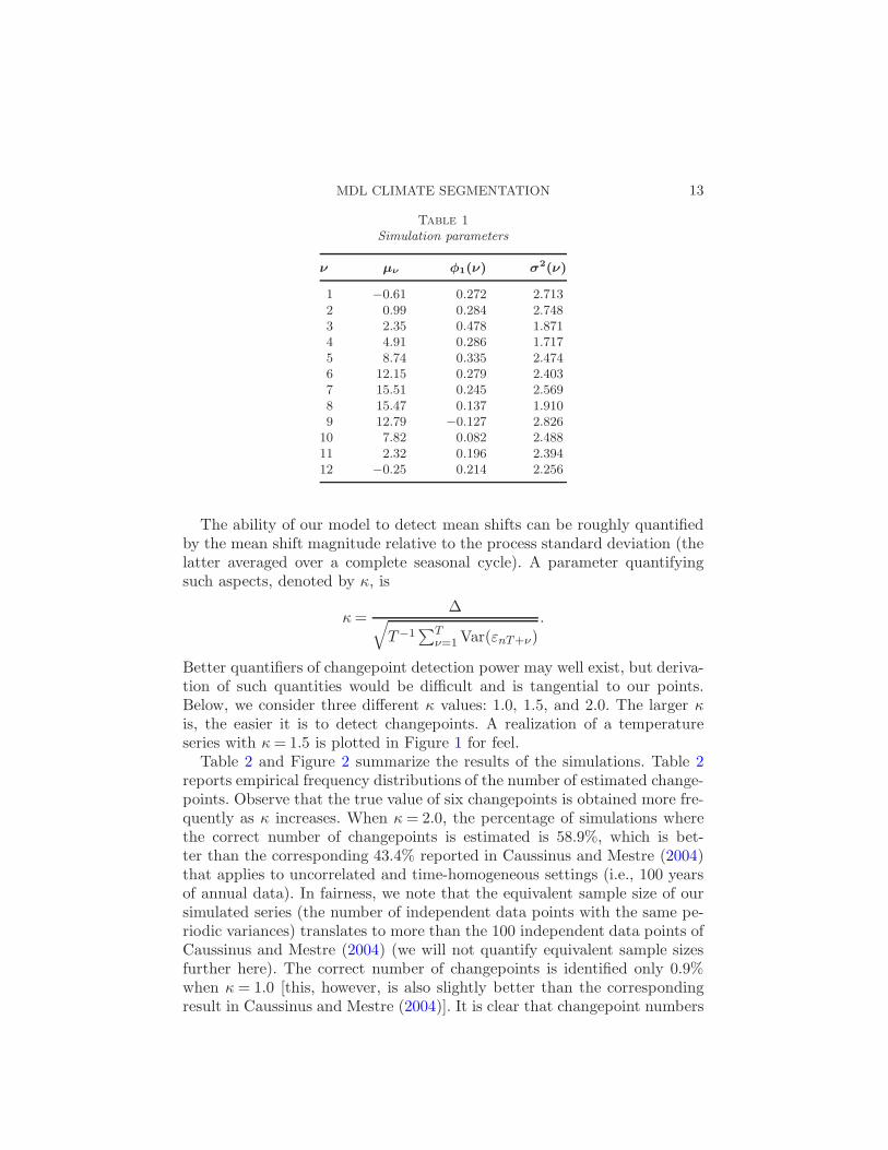
Table 1

Simulation parameters

ν µν φ1(ν) σ2(ν)

1 −0.61 0.272 2.7132 0.99 0.284 2.7483 2.35 0.478 1.8714 4.91 0.286 1.7175 8.74 0.335 2.4746 12.15 0.279 2.4037 15.51 0.245 2.5698 15.47 0.137 1.9109 12.79 −0.127 2.826

10 7.82 0.082 2.48811 2.32 0.196 2.39412 −0.25 0.214 2.256

The ability of our model to detect mean shifts can be roughly quantifiedby the mean shift magnitude relative to the process standard deviation (thelatter averaged over a complete seasonal cycle). A parameter quantifyingsuch aspects, denoted by κ, is

κ=∆

√

T−1∑T

ν=1Var(εnT+ν).

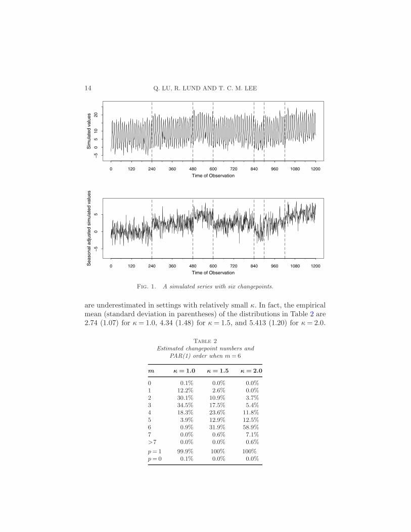
Better quantifiers of changepoint detection power may well exist, but deriva-tion of such quantities would be difficult and is tangential to our points.Below, we consider three different κ values: 1.0, 1.5, and 2.0. The larger κis, the easier it is to detect changepoints. A realization of a temperatureseries with κ= 1.5 is plotted in Figure 1 for feel.

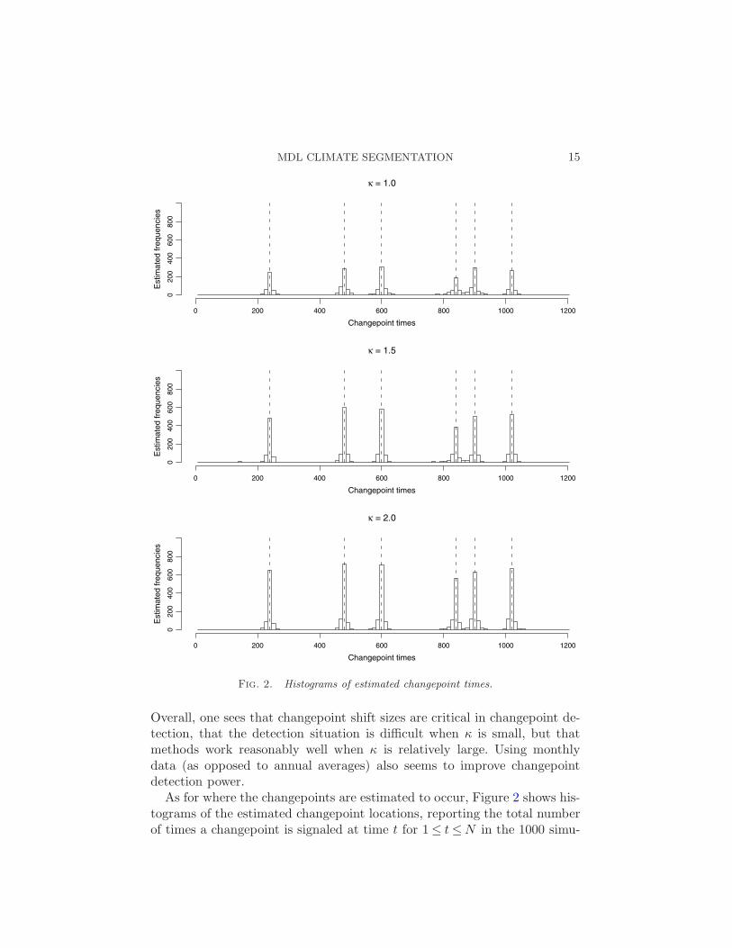
Table 2 and Figure 2 summarize the results of the simulations. Table 2reports empirical frequency distributions of the number of estimated change-points. Observe that the true value of six changepoints is obtained more fre-quently as κ increases. When κ= 2.0, the percentage of simulations wherethe correct number of changepoints is estimated is 58.9%, which is bet-ter than the corresponding 43.4% reported in Caussinus and Mestre (2004)that applies to uncorrelated and time-homogeneous settings (i.e., 100 yearsof annual data). In fairness, we note that the equivalent sample size of oursimulated series (the number of independent data points with the same pe-riodic variances) translates to more than the 100 independent data points ofCaussinus and Mestre (2004) (we will not quantify equivalent sample sizesfurther here). The correct number of changepoints is identified only 0.9%when κ= 1.0 [this, however, is also slightly better than the correspondingresult in Caussinus and Mestre (2004)]. It is clear that changepoint numbers

14 Q. LU, R. LUND AND T. C. M. LEE

Fig. 1. A simulated series with six changepoints.

are underestimated in settings with relatively small κ. In fact, the empiricalmean (standard deviation in parentheses) of the distributions in Table 2 are2.74 (1.07) for κ= 1.0, 4.34 (1.48) for κ= 1.5, and 5.413 (1.20) for κ= 2.0.

Table 2

Estimated changepoint numbers andPAR(1) order when m= 6

m κ= 1.0 κ= 1.5 κ= 2.0

0 0.1% 0.0% 0.0%1 12.2% 2.6% 0.0%2 30.1% 10.9% 3.7%3 34.5% 17.5% 5.4%4 18.3% 23.6% 11.8%5 3.9% 12.9% 12.5%6 0.9% 31.9% 58.9%7 0.0% 0.6% 7.1%>7 0.0% 0.0% 0.6%

p= 1 99.9% 100% 100%p= 0 0.1% 0.0% 0.0%

MDL CLIMATE SEGMENTATION 15

Fig. 2. Histograms of estimated changepoint times.

Overall, one sees that changepoint shift sizes are critical in changepoint de-tection, that the detection situation is difficult when κ is small, but thatmethods work reasonably well when κ is relatively large. Using monthlydata (as opposed to annual averages) also seems to improve changepointdetection power.

As for where the changepoints are estimated to occur, Figure 2 shows his-tograms of the estimated changepoint locations, reporting the total numberof times a changepoint is signaled at time t for 1≤ t≤N in the 1000 simu-

16 Q. LU, R. LUND AND T. C. M. LEE

lations. Observe that the histograms have modes around the actual change-point times. It is also evident that the changepoints at times 840 and 900were the most difficult to detect, a feature attributed to the close proximityof the times of these two changepoints (with the fifty-fifty up/down meanshift randomization employed, the sign of these two mean shifts differ withprobability 1/2, in which case their detection is relatively more difficult).

Note that the correct autoregressive order p = 1 was obtained virtuallyall of the time. Hence, the time series model selection component seems tobe working well. As changing the trend parameter did not appreciably affectresults, we will not report separate tables with nonzero trends.

We now compare the MDL penalty more closely with the Caussinus–Lyazrhi penalty used in Caussinus and Mestre (2004). The Caussinus–Lyazrhipenalty is larger than AIC or BIC penalties, but does not penalize parame-ters in the mean function or consider autocorrelation aspects. To make thiscomparison, 1000 series of length 100 were simulated with six changepointsalways occurring at the times 20, 40, 50, 70, 75, and 85. The mean shiftsize parameter κ was changed to the parameter a in Caussinus and Mestre(2004) to mimic their simulations. The errors in the model were assumed tobe Gaussian and independent. Note that the level of changepoint activityrelative to the sample size has increased 12-fold from the previous simula-tions. Table 3 below lists estimates of the relative frequencies of changepointsfound by the genetic algorithm with an MDL penalty when µν is held con-stant with ν. No trends were considered in this setup nor was tuning of thegenetic algorithm (varying its mutation probabilities, etc.) considered in de-tail. The frequency distributions in Table 3 are approximately the same asthose in Caussinus and Mestre (2004), perhaps slightly worse, in all cases.For this sample size and level of changepoint activity, an MDL penalty seemsto perform about the same as the Caussinus–Lyazrhi penalty. Of course, wereiterate that some gains are made by considering monthly data in lieu ofannual averages.

Table 3

Estimated number of changepoints for n= 100

m a= 1.0 a= 2.0 a = 3.0

0 6.2% 0.1% 0.0%1 29.5% 0.3% 0.0%2 32.5% 4.2% 0.0%3 22.8% 5.4% 0.0%4 7.4% 35.3% 7.7%5 1.5% 33.0% 4.4%6 0.1% 20.9% 81.7%7 0.0% 0.8% 6.1%>7 0.0% 0.0% 0.1%

MDL CLIMATE SEGMENTATION 17

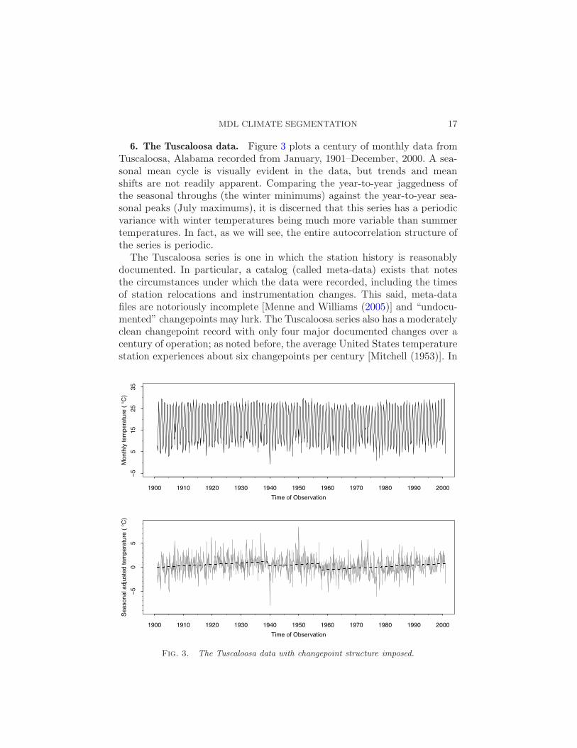
6. The Tuscaloosa data. Figure 3 plots a century of monthly data fromTuscaloosa, Alabama recorded from January, 1901–December, 2000. A sea-sonal mean cycle is visually evident in the data, but trends and meanshifts are not readily apparent. Comparing the year-to-year jaggedness ofthe seasonal throughs (the winter minimums) against the year-to-year sea-sonal peaks (July maximums), it is discerned that this series has a periodicvariance with winter temperatures being much more variable than summertemperatures. In fact, as we will see, the entire autocorrelation structure ofthe series is periodic.

The Tuscaloosa series is one in which the station history is reasonablydocumented. In particular, a catalog (called meta-data) exists that notesthe circumstances under which the data were recorded, including the timesof station relocations and instrumentation changes. This said, meta-datafiles are notoriously incomplete [Menne and Williams (2005)] and “undocu-mented” changepoints may lurk. The Tuscaloosa series also has a moderatelyclean changepoint record with only four major documented changes over acentury of operation; as noted before, the average United States temperaturestation experiences about six changepoints per century [Mitchell (1953)]. In

Fig. 3. The Tuscaloosa data with changepoint structure imposed.

18 Q. LU, R. LUND AND T. C. M. LEE

short, the Tuscaloosa is a good “proving ground” series for changepointmethods.

Level shifts in temperature series are arguably the most important factorin assessing temperature trends [see Lu and Lund (2007)]. It has been arguedin climate settings that the manner in which changepoints are handled maybe the most critical factor in the global warming debate. Supporting this,temperature insurance treaties on Wall Street are based solely on stationlocation and gauge properties, while ignoring long-term trends altogether.

Our methods were applied to the Tuscaloosa data. A reference series wasconstructed by averaging three neighboring series located at Selma, AL,Greensboro, AL, and Aberdeen, MS over the century of record. We workwith one reference series that averages three neighboring series to expeditethe discourse; methods that analyze all

(

42

)

pairs of stations are discussed inMenne and Williams (2005, 2009).

First, we examine the Tuscaloosa series without a reference. The fittedMDL model has two changepoints at times 460 (April, 1939) and 679 (July,1957). The mean function induced by these two changepoints, less the sea-sonal cycle but including the trend, is plotted against the data in Figure 3.The mean shift magnitudes of the 1939 and 1957 changepoints, in degreesCelsius, are both negative: ∆2 =−0.94± 0.20 and ∆3 =−2.33± 0.30. Theestimated trend parameter is α = 0.00258 ± 0.00039. The standard errorswere estimated from the fitted time series regression model with generalizedweighted least squares techniques. The estimated order of the PAR modelis p = 1; a consequence of this is that the autocovariance structure in theerrors of the fitted models is indeed periodic.

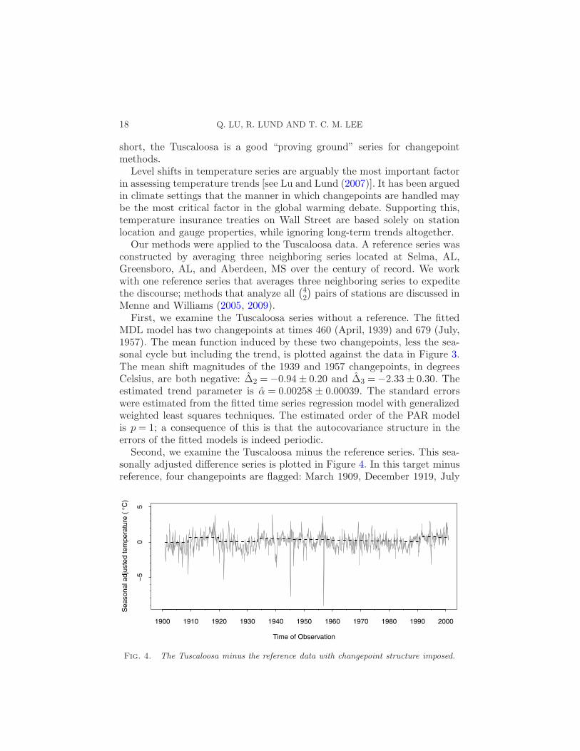
Second, we examine the Tuscaloosa minus the reference series. This sea-sonally adjusted difference series is plotted in Figure 4. In this target minusreference, four changepoints are flagged: March 1909, December 1919, July

Fig. 4. The Tuscaloosa minus the reference data with changepoint structure imposed.

MDL CLIMATE SEGMENTATION 19

1933, and August 1990. The estimates of the ∆i’s are ∆2 = 0.76 ± 0.11,∆3 = 0.26± 0.11, ∆4 = 0.77± 0.13, and ∆5 = 1.47± 0.19. Note that a meanshift with the small magnitude of 0.26 has been flagged. The trend estimateis α = −0.00066 ± 0.00015 and the selected order of the autoregression isp = 1. Observe that the fitted order of the autoregression did not reducefrom that for the raw series; that is, periodic autocorrelation still existsin the target minus reference series. Also, the trend for the target minusreference series appears to be significantly negative. We comment that thetwo large negative values occurring in the 1940s and the 1950s appear tobe decimal typos in the raw data; that is, the monthly average tempera-ture for Tuscaloosa was entered as ten degrees too small. We make thisclaim after examining additional reference series from various cities close toTuscaloosa. Whereas the series in this database have been quality checkedto some degree, errors like this may still exist. We reran the analysis aboveafter replacing these two values by (1) their estimated seasonal means µν

and (2) what we believe are the correct values, that is, adding 10 degreesto both outliers. In both cases, four changepoints with similar magnitudesand times to the ones above are found. The 1957 changepoint flagged in thetarget series has not been flagged in any version of the target minus differ-ence series. The 1909 changepoint is possibly attributed to a changepointin the reference series: Greensboro reports a time of observation change in1906 and Aberdeen reports a station relocation in 1915.

The meta-data show four changepoints in this series: the first was a sta-tion relocation in November of 1921, the second was a station relocation inMarch of 1939, the third was a station relocation during June of 1956 andan accompanying instrumentation change in November of 1956 (we regardthis as one changepoint), and the fourth is a station relocation and instru-mentation change in May of 1987. The reference series analysis seems tohave correctly identified three of these four changepoints (we are liberallyincluding the 1933 flagged changepoint time as correctly identifying the 1939changepoint), missing the 1956 changepoint and adding a 1909 changepoint.The raw target series analysis misses the 1921 and 1987 changepoints, butfinds the 1956 changepoint; also, the estimated time of the 1939 changepointis much closer to its true value than that for the reference analysis. Over-all, it seems that the reference analysis is superior to simple target seriesanalysis, but that one can learn something with both analyses.

We caution the reader that trends in some monthly temperature series,especially when the series is aggregated over a large geographic region, maynot be well described by a linear regression component. As noted by Hand-cock and Wallis (1994), trends at localized series are more likely to be ade-quately described with a simple linear structure. As a final diagnostic check,residuals from the model fits were computed. Figure 5 shows the sample au-tocorrelation of the residuals for the target series over the first 60 lags. The

20 Q. LU, R. LUND AND T. C. M. LEE

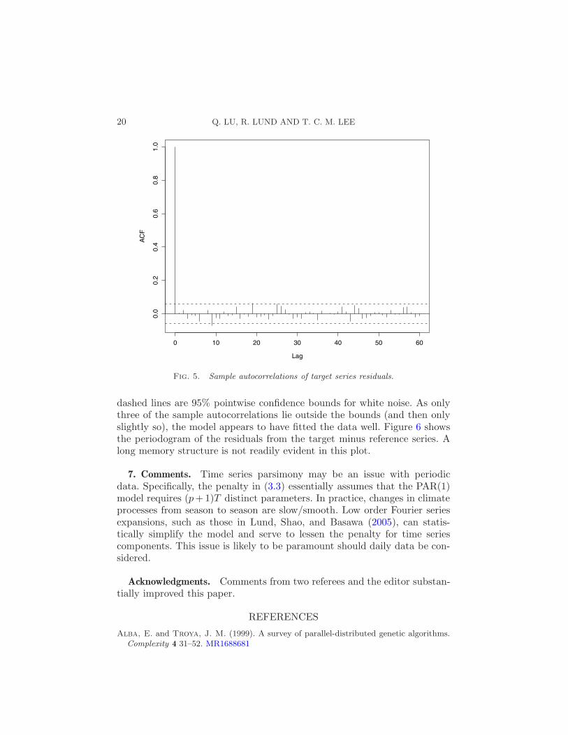
Fig. 5. Sample autocorrelations of target series residuals.

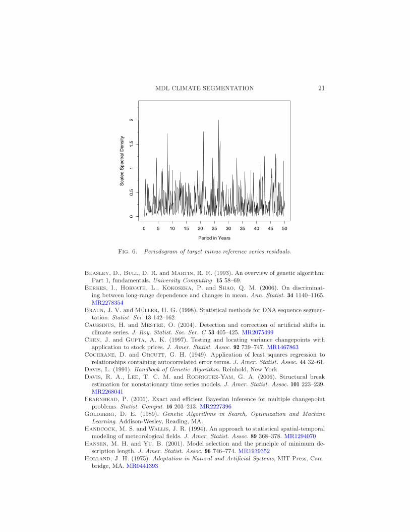
dashed lines are 95% pointwise confidence bounds for white noise. As onlythree of the sample autocorrelations lie outside the bounds (and then onlyslightly so), the model appears to have fitted the data well. Figure 6 showsthe periodogram of the residuals from the target minus reference series. Along memory structure is not readily evident in this plot.

7. Comments. Time series parsimony may be an issue with periodicdata. Specifically, the penalty in (3.3) essentially assumes that the PAR(1)model requires (p+1)T distinct parameters. In practice, changes in climateprocesses from season to season are slow/smooth. Low order Fourier seriesexpansions, such as those in Lund, Shao, and Basawa (2005), can statis-tically simplify the model and serve to lessen the penalty for time seriescomponents. This issue is likely to be paramount should daily data be con-sidered.

Acknowledgments. Comments from two referees and the editor substan-tially improved this paper.

REFERENCES

Alba, E. and Troya, J. M. (1999). A survey of parallel-distributed genetic algorithms.Complexity 4 31–52. MR1688681

MDL CLIMATE SEGMENTATION 21

Fig. 6. Periodogram of target minus reference series residuals.

Beasley, D., Bull, D. R. and Martin, R. R. (1993). An overview of genetic algorithm:Part 1, fundamentals. University Computing 15 58–69.

Berkes, I., Horvath, L., Kokoszka, P. and Shao, Q. M. (2006). On discriminat-ing between long-range dependence and changes in mean. Ann. Statist. 34 1140–1165.MR2278354

Braun, J. V. and Muller, H. G. (1998). Statistical methods for DNA sequence segmen-tation. Statist. Sci. 13 142–162.

Caussinus, H. and Mestre, O. (2004). Detection and correction of artificial shifts inclimate series. J. Roy. Statist. Soc. Ser. C 53 405–425. MR2075499

Chen, J. and Gupta, A. K. (1997). Testing and locating variance changepoints withapplication to stock prices. J. Amer. Statist. Assoc. 92 739–747. MR1467863

Cochrane, D. and Orcutt, G. H. (1949). Application of least squares regression torelationships containing autocorrelated error terms. J. Amer. Statist. Assoc. 44 32–61.

Davis, L. (1991). Handbook of Genetic Algorithm. Reinhold, New York.Davis, R. A., Lee, T. C. M. and Rodriguez-Yam, G. A. (2006). Structural break

estimation for nonstationary time series models. J. Amer. Statist. Assoc. 101 223–239.MR2268041

Fearnhead, P. (2006). Exact and efficient Bayesian inference for multiple changepointproblems. Statist. Comput. 16 203–213. MR2227396

Goldberg, D. E. (1989). Genetic Algorithms in Search, Optimization and MachineLearning. Addison-Wesley, Reading, MA.

Handcock, M. S. and Wallis, J. R. (1994). An approach to statistical spatial-temporalmodeling of meteorological fields. J. Amer. Statist. Assoc. 89 368–378. MR1294070

Hansen, M. H. and Yu, B. (2001). Model selection and the principle of minimum de-scription length. J. Amer. Statist. Assoc. 96 746–774. MR1939352

Holland, J. H. (1975). Adaptation in Natural and Artificial Systems, MIT Press, Cam-bridge, MA. MR0441393

22 Q. LU, R. LUND AND T. C. M. LEE

Inclan, C. and Tiao, G. C. (1994). Use of cumulative sums of squares for retrospective

detection of changes of variance. J. Amer. Statist. Assoc. 89 913–923. MR1294735

Lee, T. C. M. (2000). A minimum description length based image segmentation pro-

cedure, and its comparison with a cross-validation based segmentation procedure. J.

Amer. Statist. Assoc. 95 259–270. MR1803154

Lee, T. C. M. (2001). An introduction to coding theory and the two-part minimum

description length principle. International Statistical Review 69 169–183.

Lee, T. C. M. (2002). Automatic smoothing for discontinuous regression functions.

Statist. Sinica 12 823–842. MR1929966

Lu, Q. and Lund, R. B. (2007). Simple linear regression with multiple level shifts. Canad.

J. Statist. 37 447–458. MR2396030

Lund, R. B., Shao, Q. and Basawa, I. V. (2005). Parsimonious periodic time series

modeling. Aust. N. Z. J. Statist. 48 33–47. MR2234777

Lund, R. B., Wang, X. L., Lu, Q., Reeves, J., Gallagher, C. and Feng, Y. (2007).

Changepoint detection in periodic and autocorrelated time series. Journal of Climate

20 5178–5190.

Mitchell, J. M., Jr. (1953). On the causes of instrumentally observed secular temper-

ature trends. Journal of Applied Meteorology 10 244–261.

Menne, J. M. andWilliams, C. N., Jr. (2005). Detection of undocumented changepoints

using multiple test statistics and composite reference series. Journal of Climate 18 4271–

4286.

Menne, J. M. and Williams, C. N., Jr. (2009). Homogenization of temperature series

via pairwise comparisons. Journal of Climate 22 1700–1717.

Pagano, M. (1978). On periodic and multiple autoregressions. Ann. Statist. 6 1310–1317.

MR0523765

Reeves, C. (1993). Modern Heuristic Techniques for Combinatorial Problems. Wiley, New

York. MR1230642

Rissanen, J. (1989). Stochastic Complexity in Statistical Inquiry. World Scientific, Singa-

pore. MR1082556

Rissanen, J. (2007). Information and Complexity in Statistical Modeling, Springer, New

York. MR2287233

Shao, Q. and Lund, R. B. (2004). Computation and characterization of autocorrelations

and partial autocorrelations in periodic ARMA models. J. Time Ser. Anal. 25 359–372.

MR2062679

Vincent, L. A. (1998). A technique for the identification of inhomogeneities in Canadian

temperature series. Journal of Climate 11 1094–1104.

Q. Lu

Department of Mathematics and Statistics

Mississippi State University

Mississippi State, Mississippi 39762

USA

E-mail: qlu@math.msstate.edu

R. Lund

Department of Mathematical Sciences

Clemson University

Clemson, South Carolina 29634-0975

USA

E-mail: lund@clemson.edu

MDL CLIMATE SEGMENTATION 23

T. C. M. Lee

Department of Statistics

Colorado State University

Fort Collins, Colorado 80523

USA

and

Department of Statistics

Chinese University of Hong Kong

Shatin, Hong Kong

E-mail: tlee@sta.cuhk.edu.hk