House dust mites and their genetic systems - CentAUR

House dust mites and their genetic

systems

Thesis submitted for the degree of

Doctor of Philosophy

School of Biological Sciences

Kirsten M. Farncombe

July 2018

1

Declaration

Declaration:

I confirm that this is my own work and the use of all material from other sources has been

properly and fully acknowledged

Kirsten M. Farncombe

2

Table of Contents

Declaration................................................................................................................................ 1

Abstract ..................................................................................................................................... 8

Acknowledgements .................................................................................................................. 9

Chapter 1: Knowledge and Applications of House Dust Mites ......................................... 11

1.1 Ecology of House Dust Mites .................................................................................. 12

1.1.1 Mites in the home: ............................................................................................. 12

1.1.2 Life cycle: .......................................................................................................... 12

1.1.3 Humans in the home: ......................................................................................... 13

1.1.4 Pets in the home: ................................................................................................ 13

1.1.5 Colonisation of mites: ........................................................................................ 14

1.2 Taxonomy of Mites .................................................................................................. 16

1.2.1 Accuracy: ........................................................................................................... 16

1.2.2 The Acariformes: ............................................................................................... 16

1.2.3 The Parasitiformes: ............................................................................................ 18

1.2.4 Published mite genomes: ................................................................................... 20

1.3 Relevance of Mites ................................................................................................... 23

1.3.1 Medical importance: .......................................................................................... 23

1.3.2 Economic importance: ....................................................................................... 24

1.3.3 Forensic importance: .......................................................................................... 25

1.4 Various Genetic Systems in Mites.......................................................................... 26

1.4.1 Diploidy: ............................................................................................................ 26

1.4.2 Thelytoky: .......................................................................................................... 26

1.4.3 Arrhenotoky: ...................................................................................................... 27

1.4.4 Pseudo-arrhenotoky: .......................................................................................... 28

1.5 Population Genetic Structure in Mites: ................................................................ 30

1.5.1 Fragmented habitats: .......................................................................................... 30

1.5.2 Tetraynchus urticae population structure: ......................................................... 31

Chapter 2: Compiling a Database of House Dust Mites and Geographic Location ........ 32

2.1 Introduction ............................................................................................................. 32

2.2 Materials and Methods ........................................................................................... 33

2.2.1 Collection of published research:....................................................................... 33

2.2.2 Publication parameters: ...................................................................................... 34

3

2.3 Results and Discussion ............................................................................................ 35

2.3.1 Database from the literature: .............................................................................. 35

2.3.2 Assessing completeness of the database: ........................................................... 38

2.3.3 Limitations of the dataset and how they have been mitigated: .......................... 46

a. Number of studies: .......................................................................................................................... 46

b. External variants: ............................................................................................................................ 47

c. Collection methods: ........................................................................................................................ 47

d. Publication bias: .............................................................................................................................. 48

2.3.4 Applications of the database: ............................................................................. 49

2.4 Conclusions .............................................................................................................. 54

Chapter 3: Biogeographical Distribution of House Dust Mites ......................................... 56

3.1 Introduction ............................................................................................................. 56



3.3.1 Distribution by biogeographical region: ............................................................ 58

3.3.2 Distribution by country: ..................................................................................... 58

3.3.3 Latitudinal diversity gradient: ............................................................................ 60

3.3.4 Pleistocene glaciation: ....................................................................................... 61

a. Hypothesis: ..................................................................................................................................... 61

b. Select species supporting this hypothesis: ...................................................................................... 63

c. Issues with this hypothesis: ............................................................................................................. 63

3.3.5 Niche conservatism: ........................................................................................... 64

a. Hypothesis: ..................................................................................................................................... 64



3.3.6 Tropical conservatism hypothesis: ..................................................................... 66

a. Hypothesis: ..................................................................................................................................... 66



3.3.7 Time and area hypothesis (Time-for-speciation effect): .................................... 71

a. Hypothesis: ..................................................................................................................................... 71



3.3.8 Species-energy hypothesis: ................................................................................ 73

a. Hypothesis: ..................................................................................................................................... 73



4

3.3.9 House dust mites and the latitudinal diversity gradient: .................................... 77

a. Most likely hypotheses: .................................................................................................................. 77

b. House dust mites and the latitudinal diversity gradient: ................................................................. 78

3.4 Conclusions .............................................................................................................. 83

Chapter 4: Method Development and Optimisation of Dermatophagoides farinae

Extraction Protocols .............................................................................................................. 84

4.1 Introduction ............................................................................................................. 84

4.1.1 Mite samples and sequences: ............................................................................. 85

4.1.2 Previous extraction techniques: ......................................................................... 85


4.2.1 Mite culturing: ................................................................................................... 87

4.2.2 Morphological identification: ............................................................................ 88

4.2.3 Preparation of mites: .......................................................................................... 88

a. Surface cleaning: ............................................................................................................................ 88

b. Mite maceration: ............................................................................................................................. 90

4.2.4 DNA extraction: ................................................................................................. 90

a. Qiagen kit extraction protocol: ....................................................................................................... 90

b. Alternative DNA extraction protocols: ........................................................................................... 92


4.3.1 Species identification: ........................................................................................ 97

4.3.2 Mould growth: ................................................................................................... 99

4.3.3 Qiagen extraction protocol:.............................................................................. 100

4.3.4 Dead mite extraction protocols: ....................................................................... 101

4.3.5 Presence of contaminants:................................................................................ 104

4.4 Conclusions ............................................................................................................ 106

Chapter 5: Population Genetic Structure of Dermatophagoides farinae Mites .............. 107

5.1 Introduction ........................................................................................................... 107

5.1.1 Molecular techniques: ...................................................................................... 107

5.1.2 PCR of mitochondrial regions: ........................................................................ 107

5.1.3 Amplified fragment length polymorphisms: .................................................... 108

5.1.4 Microsatellite loci: ........................................................................................... 109

5.1.5 Nucleotide diversity in mites: .......................................................................... 109

5.1.6 Amplification of Dermatophagoides farinae mites: ........................................ 110

5.2 Materials and Methods ......................................................................................... 111

5.2.1 Primer design: .................................................................................................. 111

5

5.2.2 General PCR parameters: ................................................................................. 115

5.2.3 Mitochondrial CO1: ......................................................................................... 115

5.2.4 Nuclear EF1a: .................................................................................................. 115

5.2.5 Two non-coding regions: ................................................................................. 116

5.2.6 DNA purification and sequencing: .................................................................. 116

5.3 Results and Discussion .......................................................................................... 118

5.3.1 Mitochondrial CO1: ......................................................................................... 118

5.3.2 Nuclear EF1a: .................................................................................................. 120

5.3.3 Two non-coding regions: ................................................................................. 121

5.3.4 Bioinformatics analysis:................................................................................... 123

5.3.5 Dermatophagoides farinae CO1 barcoding: .................................................... 123

a. CO1 sequence alignment: ............................................................................................................. 123

b. DNA barcoding: ............................................................................................................................ 125

c. Phylogeny ..................................................................................................................................... 126

5.3.6 Cryptic species: ................................................................................................ 128

a. Identification of cryptic species: ................................................................................................... 128

b. Cryptic species in mites: ............................................................................................................... 128

5.3.7 Amplification protocol: .................................................................................... 129

5.4 Conclusions ............................................................................................................ 131

Chapter 6: Exploring Costs and Benefits of Different Mating Systems ......................... 132

6.1 Introduction ........................................................................................................... 132

6.1.1 Experimentation in yeasts: ............................................................................... 135

a. The use of Saccharomyces cerevisiae:.......................................................................................... 135

b. Yeast mating-type switching: ....................................................................................................... 136

6.1.2 Reproductive strategies in algae: ..................................................................... 139

6.1.3 Prevalence of diploidy: .................................................................................... 140

a. Increased beneficial mutations: ..................................................................................................... 140

b. Two copies of genes: .................................................................................................................... 141

c. Masking deleterious mutations: .................................................................................................... 141

6.1.4 Prevalence of haploidy – fewer mutations: ...................................................... 142

6.1.5 Why be both haploid and diploid: .................................................................... 142

a. Advantageous balance: ................................................................................................................. 142

b. Rates of adaptation: ...................................................................................................................... 143

c. Maternal and paternal selection levels: ......................................................................................... 145

6.1.6 Alternative theories regarding ploidy influence: ............................................. 146

a. Non-genetic factors: ...................................................................................................................... 146

6

b. Contradiction to Cavalier-Smith’s hypothesis: ............................................................................. 147

c. Nutrient-sparing hypothesis: ......................................................................................................... 147

d. Contradiction to Lewis’s hypothesis: ............................................................................................ 148

6.1.7 Haplodiploidy is expected to show adaptive evolution: .................................. 149


6.2.1 Developing Perl: .............................................................................................. 151

6.2.2 Altering parameters – selection coefficient: .................................................... 154

6.2.3 Altering parameters – sex ratio: ....................................................................... 154


6.3.1 Varying selection with five mating systems over time: ................................... 155

6.3.2 Varying selection: ............................................................................................ 157

6.3.3 Varying sex ratio with beneficial mutations: ................................................... 163

6.3.4 Varying sex ratio with deleterious mutations: ................................................. 166

6.3.5 Differences between models: ........................................................................... 169

6.4 Conclusions ............................................................................................................ 171

Chapter 7: Haplodiploid and Diploid Direct Competition .............................................. 173

7.1 Introduction ........................................................................................................... 173

7.1.1 Evolutionary stable strategy:............................................................................ 173

a. Concept: ........................................................................................................................................ 173

b. Evolutionary invasion analysis: .................................................................................................... 174

c. Example – hawk/dove: .................................................................................................................. 175

d. Example – sex ratio: ..................................................................................................................... 176

7.1.2 Evolution of haplodiploidy: ............................................................................. 177

7.1.3 Advantages for haplodiploid males: ................................................................ 180

a. Maternal transmission advantage: ................................................................................................. 180

b. Maternal sex ratio control: ............................................................................................................ 180

c. Female reproductive assurance: .................................................................................................... 180

7.1.4 Difficulties of transitioning to male haploidy: ................................................. 181

a. Exposure of deleterious alleles: .................................................................................................... 181

b. Parthenogenesis and dosage compensation: ................................................................................. 182

7.1.5 Paternal genome elimination as an intermediate step: ..................................... 182

a. Definition: ..................................................................................................................................... 182

b. Endosymbionts in arthropods: ...................................................................................................... 183

c. Hypothesis one for paternal genome elimination evolution: ........................................................ 184

d. Hypothesis two for paternal genome elimination evolution: ........................................................ 185

7.1.6 Competition model: ......................................................................................... 187

7


7.2.1 Competition parameters: .................................................................................. 188

7.2.2 Maternally transmitted element: ...................................................................... 188

7.2.3 Initial diversity: ................................................................................................ 189


7.3.1 Comparing element prevalence without initial diversity: ................................ 191

7.3.2 Comparing element prevalence with initial diversity of 0.01: ......................... 191

7.3.3 Comparing element prevalence with initial diversity of 0.1: ........................... 193

7.3.4 Comparing element prevalence at selection extremes: .................................... 198

7.3.5 Future work: ..................................................................................................... 200

a. Sex ratios: ..................................................................................................................................... 200

b. Altering mutations: ....................................................................................................................... 201

7.4 Conclusions ............................................................................................................ 202

Chapter 8: General Discussion of House Dust Mites and Genetic Systems ................... 204

8.1 Mites are understudied: ........................................................................................ 204

8.2 Main focuses of mite research: ............................................................................. 205

a. Economic: ..................................................................................................................................... 205

b. Medical: ........................................................................................................................................ 205

c. Forensic: ....................................................................................................................................... 206

8.3 Summary of findings: ........................................................................................... 207

a. Biogeography of mites (Chapters 2 & 3): ..................................................................................... 207

b. Dermatophagoides farinae genetic system (Chapters 4 & 5): ...................................................... 207

c. Mating system simulations (Chapters 6 & 7):............................................................................... 207

8.4 Proposals for future work – Biogeography and genetic system: ...................... 209

a. Latitudinal diversity gradient and cryptic species: ........................................................................ 209

b. Nuclear genome research: ............................................................................................................. 210

8.5 Proposals for future work – Genetic system and mating system:..................... 212

a. Advancement of genetic markers: ................................................................................................ 212

b. Alternative transmission routes: ................................................................................................... 212

c. Genetic markers and modelling genome elimination: .................................................................. 213

8.6 Concluding remarks: ............................................................................................ 215

Appendix 1: Regions, Country and References of House Dust Mites ............................. 217

Appendix 2: Perl Mating System Scripts ........................................................................... 221

References ............................................................................................................................. 245

8

Abstract

Despite their medical implications and widespread distribution, there is limited knowledge of

house dust mites. I assessed their biogeographical distribution, examined the genetic system of

one of the most common species of house dust mite, Dermatophagoides farinae, and modelled

different mating systems of mites, with the aim of improving understanding. This included

assembling a database of house dust mite diversity, and identifying the most successful

protocols for molecular work, which will save researchers time and provide a solid base for

future studies. The creation of a house dust mite fauna database through published resources

provided a worldwide distribution of all mites collected from homes. This may prove useful in

future, particularly by allergists who are focusing on eradicating these mites for the benefit of

human health. In addition, this identified the possibility of a latitudinal diversity gradient in

house dust mites. Assessing D. farinae mitochondrial and nuclear genome regions through

PCR and sequencing has illustrated dissimilarity between populations. This suggested that D.

farinae may have been previously misidentified and the examined populations actually

represent more than one species. This gives a basis for further analysis with an increased

number of populations from a variety of locations. Finally, modelling and comparing different

mating systems which may be found in mites, illustrate that despite the benefits of being

haplodiploid, it is difficult to transition to this system from diploidy. This indicates that

cytoplasmically inherited maternally-transmitted haplodiploidy is not favoured in diploid

populations, forming part of the reason why many species are still in the ancestral diploid state.

9

Acknowledgements

I would first like to thank my incredible supervisor Louise Johnson for her endless support and

unwavering confidence in my skills as a researcher. I cannot express how much I appreciate

her accepting me as a PhD student halfway through my studies. Her kindness, knowledge, and

assistance were exactly what I needed at such a low point in my life. I could not have completed

my PhD without her.

I am indebted to Rob Jackson for providing the use of his lab when I had nowhere else to go.

Both Rob and his students were incredibly welcoming, helpful, and positive about my research.

I am thrilled to have met such a wonderful group of people and amazing friends (Kris,

Shyamali, Mojgan, Mahira, Luke, Oliver, Glyn, and Mateo). I have so many incredible

memories filled with lots of food, drinking, and laughter. Special mention to Mahdi, and

Princess Lexi for some fab parties!

Thanks to the coffee time group for helping me meet new people and giving me something to

look forwards to during the second year of my PhD. I also want to thank the acarology lab PhD

students in Suite 8 (Naila, Lyna, Jess, Robin, Jas, and Edhah) for help with mite extraction

techniques, preparation for my first-ever conference, and one very unforgettable trip to

Valencia. We bonded over continuous, endless, and unnecessary PhD difficulties, but this

common ground formed some long-lasting friendships. I will never forget the night of “Donald

where’s your troosers”!

I also had the experience of moving up to the Lyle building fourth floor. I think I can safely

say this office is a special environment that I will likely never come across again in the rest of

my working career. They are a group of dysfunctional, wildly inappropriate, and entertaining

10

people. So thank you to Mark, Andrew, Chris, Jo, Ciara, Manabu, and George for making every

single day during the last year of my PhD memorable. Special thanks goes to Andrew for

modelling my haplodiploid and diploid simulations and helping create a phylogeny, and to my

favourite rugby friend for all our early-morning gossips, and a great night of wine-stealing and

way too much wine-drinking at Pop Group.

Thanks to Tom Oliver for his assistance with a crash course in RStudio to examine mite species

richness. I would not have been able to learn this program in time without your help! Thank

you to Sean, the best former housemate and friend a girl could ever have asked for. Thank you

for all the late nights watching Sons of Anarchy, introducing me to COD and GTA, never

letting my food go to waste, and for being an absolute boss at Excel.

Many thanks to my surrogate family in England for the well-needed weekend breaks from PhD

work, “home-cooked” meals, and an endless supply of wine. I am very appreciative of how

generous and welcoming you have been to me. Lots of love to John, Joanne, Joe, Odin, and the

entire extended Wincott family.

Finally, I am forever grateful to my incredible family. Thank you for your generous financial

and emotional support, daily phone calls, funny emails, cards at every occasion (with the

exception of my forgotten birthday card), and for loving me even at times when you probably

did not like me very much. I know even if I fall you will always be there to catch me. I would

not be where I am today without your endless support. Love always to my Mum, Dad, and

Auntie Lise. And of course, a special thank you to Ben. We found each other when it was

needed the most, and I look forwards to better things than PhD life with you.

11

Chapter 1: Knowledge and Applications of House Dust Mites

The Acari are an underrepresented taxonomic group with a limited amount of knowledge

regarding taxonomy, sequence data, and genetic information (Weeks et al., 2000). Mites are

very small, there is incomplete knowledge regarding their distribution, and similar species are

often confused and misidentified (O'Connor, 2009, Braig & Perotti, 2009, Perotti et al., 2009).

This dissertation will begin by broadly discussing some of the more widely-studied mites, as

well as some of their known applications and implications to humans (Chapter 1).

Subsequently, focus will be narrowed specifically to the house dust mites (HDMs) and their

presence worldwide in the published literature (Chapters 2 and 3), with a particular focus on

the American house dust mite, Dermatophagoides farinae and molecular techniques (Chapters

4 and 5). Finally, computer simulations of some of the different genetic systems which are

present in mites will be examined (Chapters 6 and 7), before future directions for this research

are outlined (Chapter 8).

Chapter 1 will firstly provide a basic introduction regarding house dust mites, before outlining

the taxonomy of mites, including a description of species which have been sequenced thus far.

The importance of mites for economic, medical, and forensic purposes will be described, as

well as discussing a variety of mating systems which have been identified in different species

of mites.

12

1.1 Ecology of House Dust Mites

1.1.1 Mites in the home:

House dust mites are micro-arthropods, which feed on shed skin scales and other organic debris

collected from house dust (Arlian & Platts-Mills, 2001). The small size of mites enables them

to exist in many microhabitats, therefore species and number of mites can vary between

different sampled locations within a home (Frost et al., 2010). The composition of mite fauna

in any given location is influenced by many factors including temperature, altitude, light, and

relative air humidity (van Bronswijk, 1981). Temperate climates are more likely to have one

dominant species collected from a single dust sample, whereas tropical climates have a

minimum of three predominant species (Colloff, 2009). Dermatophagoides farinae,

Dermatophagoides pteronyssinus, and Euroglyphus maynei comprise 90% of mite fauna in a

home (Blythe et al., 1974), and their ability to survive in different climates and

microenvironments mean they may not be collected from the same location within the home

(Crowther et al., 2000).

1.1.2 Life cycle:

There are five distinct life stages of pyroglyphid mites: egg, larva, protonymph, tritonymph,

and adult (van Bronswijk & Sinha, 1971). D. farinae mites prefer a higher temperature than

some other species of HDMs (van Bronswijk & Sinha, 1971). This species dehydrates after

death and can comprise up to 80% of the mite population in household mattresses (Crowther

et al., 2000). Due to an extended post egg period, D. farinae females are able to live longer

than D. pteronyssinus (100 v 31 days) (Crowther et al., 2000, Arlian & Dippold, 1996).

Laboratory experiments have demonstrated that these mites are capable of multiple matings;

although the second batch of fertilized eggs are smaller and have a shorter reproductive period

13

(18 days v. 34 days) (Alexander et al., 2002). D. farinae mites have high survival when reared

at continuous 75% RH for ten weeks (Arlian et al., 1999).

1.1.3 Humans in the home:

Humans have the largest effect on mite fauna, as they are responsible for controlling different

factors in the home (ventilation, temperature, humidity, and furnishings) (van Bronswijk,

1981). General household activities by the inhabitants of a house (ie cleaning or making the

bed), has an impact on the dust structure and competition between mite species (Cunnington &

Gregory, 1968, Takaoka et al., 1977a). In addition, mites are transferred between locations in

the home with the assistance of the inhabitants (Colloff, 2009, Perotti & Braig, 2009), and the

dead skin cells shed from humans act as a food source for HDMs (van Bronswijk, 1981).

Although space and predation is often a limiting factor with population size, it is most likely

that the food supply of dead skin shed by a person per day contributes most to the size of HDM

populations within their natural environment (Crowther et al., 2000).

1.1.4 Pets in the home:

The domestication of animals also had an impact on mite fauna, with Cheyletiella a common

parasitic presence in cats, dogs and rabbits (Dobrosavljevic et al., 2007). Feather mites may be

brought in by birds, and lizards and snakes are commonly associated with mites from the

families Pterygosomatidae and Omentolaelapidae (Frost et al., 2010). Demodicidae in the hair

follicle of humans, as well as dogs, cats, gerbils, and hamsters illustrate harmonious coexisting

between species (Frost et al., 2010). Homes with a dog were found to have a higher incidence

rate of Blomia tropicalis, Cheyletus sp., and Gohieria fusca (Baqueiro et al., 2006). Finally,

homes with predominately indoors pets are correlated with an increased quantity of animal

dander, which leads to higher mite density due to increased food sources (Binotti et al., 2005).

14

1.1.5 Colonisation of mites:

HDMs are collected from a variety of microenvironments within the home, often being

transferred indoors on pets, humans, furniture, stored food products and commercial pet foods.

Mites continue to disperse around the home, most frequently by passive transport on human

clothing (Tovey et al., 1995). Tovey et al. (1995) examined living mites and mite allergen

levels from individuals in Sydney, Australia with high quantities of mite allergens identified

on all items of clothing. Mites were isolated from a sub-sampling of 8 of 15 items of clothing,

with woollen clothing harbouring the most mites and allergen levels due to infrequent washing

(Tovey et al., 1995). Another study used marked D. farinae mites stained with Sudan Red 7B

dye and acetone to examine dispersal within a two-story house (Mollet & Robinson, 1996).

Approximately 1850 marked mites were released on a downstairs sofa and left overnight. The

following day two young children sat on the sofa for three hours, and then their clothes were

removed and 51 live marked mites were recovered, as well as unmarked mites. Upholstered

surfaces in the house were sampled 10 days later with both marked and unmarked mites

collected in small numbers, illustrating their active dispersal around the house (Mollet &

Robinson, 1996).

As mites are transferred between locations on individuals’ clothing, there is the potential for

mites which normally reside in barns or in farm storage locations to be brought into

farmhouses. For example, mites were collected from 86.4% of 121 farms across five regions

in Germany, with a total of 49 different species identified (Franz et al., 1997). Furthermore, 12

species of mites were identified from stored hay on barn floors of 30 farms in the Swedish

island of Gotland (Böstrom et al., 1997), and 70 species of mites were collected from grain

storages, handling areas, and stock rearing facilities from 31 Scottish farms (Jeffrey, 1976).

15

Mites may also be dispersed within the home via stored food products, illustrated by an

investigation into the levels of mite-contaminated food imported through southern California

ports (Olsen, 1983). This included 35 types of food from 12 different countries, with 212

positive samples contaminated by 22 mite species. Living mites or surviving eggs which hatch

after the product was sold and taken into the home, would then be able to disperse (Olsen,

1983). Under laboratory settings, D. farinae and Glycyphagus domesticus can survive at

varying levels when 41 different types of common cereals, cereal product + human food, and

animal food were provided as a food source (Sinha & Paul, 1972). Further research illustrated

that storage mites easily contaminate unopened commercial dry dog food from manufacturing

factories, representing an additional manner mites contaminate the home (Brazis et al., 2008).

Human habitation is often necessary for the presence of HDMs, exemplified by the lack of

mites collected from newly built, uninhabited homes in Europe (van Bronswijk, 1981). Only

one of 26 sampled houses in Ohio, USA did not contain HDMs, as it had been constructed less

than two months prior and had all new furniture and carpeting (Arlian et al., 1982). Additional

studies in The Netherlands identified mites on the floors of homes almost immediately after

humans occupy a house (van Bronswijk, 1974). However almost all mites were dead and

collected in small numbers, indicating they were transferred into the new home on clothing and

furniture from their previous location (van Bronswijk, 1974). Living mites were only collected

from floors of homes in The Netherlands and Japan after humans had occupied the beds and

furniture for at least one week (van Bronswijk, 1974, Miyamoto & Ouchi, 1976). Very few

mites were found in homes in Colorado, USA; however, houses containing furniture imported

from California, Texas, Tennessee and Germany had a higher mite population due to more

humid climates (Moyer et al., 1985). Mite population densities then decreased over the next

two years until the normal mite density of Colorado homes was reached (Moyer et al., 1985).

16

1.2 Taxonomy of Mites

1.2.1 Accuracy:

Many difficulties arise with accurate taxonomic classification of mites, due to outdated and

differing nomenclature. Although certain aspects of taxonomy appears to be consistent among

acarologists (Kingdom: Animalia, Phylum: Arthropoda, Class: Arachnida, and Subclass: Acari

(or Acarina)), ordinal / subordinal classification is not consistent between mite species (Colloff,

1998). There is limited fossil evidence of terrestrial Arthropoda due to their small size and lack

of a large exoskeleton, however there are some estimations of species divergence (Krantz &

Walter, 2009). Despite these discrepancies, there are two distinct taxa within the Acari:

Acariformes and Parasitiformes (Krantz & Walter, 2009).

1.2.2 The Acariformes:

Modern-day descendants of the Acariformes feed on fungi, algae, and organic soil debris, and

likely invaded land through the soil pores of the littoral zone (Krantz & Walter, 2009). The

Acariformes are subcategorised into the Trombidiformes and Sarcoptiformes, however

inconsistent taxonomy results in them being listed as either an order or suborder (Colloff, 1998,

Krantz & Walter, 2009). Furthermore, four main groups have been identified within this order:

Astigmata, Endeostigmata, Oribatida (Cryptostigmata), and Trombidiformes (Prostigmata)

(Krantz & Walter, 2009). The limited fossilisation record has made accurate paleontological

dating difficult, however it is likely that the Trombidiformes, Endeostigmata, and Oribatida

originated much earlier (410-415 MYA) than the Astigmata (370 MYA) (Dabert et al., 2010).

No further details are given to the divergence of these suborders on TimeTree, besides an

estimated time of 494 MYA (Kumar et al., 2017). Figure 1.1 illustrates the taxonomic tree of

members of the Acariformes with published genomes on NCBI GenBank (2017).

17

Figure 1.1. Taxonomic tree with published genomes on GenBank (2017) of the nine species of Acariformes (Krantz & Walter, 2009, Proctor,

1998). This includes the true members of HDMs, the Pyroglyphidae, which will be the focus in later Chapters. The estimated divergence between

D. farinae and D. pteronyssinus was noted to be 35 MYA (Dabert et al., 2010).

Acari Subclass

Superorder

Order

Suborder

Superfamily

Family

Genus

Species

Parasitiformes Acariformes

Trombidiformes Sarcoptiformes

Prostigmata

Tetranychoide

a

Tetranychida

e

Tetranychu

s

T. urticae

Astigmatina Oribatida

Psoroptoide

a

Pyroglyphoide

a

Sarcoptida

e

Sarcoptes

S. scabiei

Pyroglyphidae

Dermatophagoides

Euroglyphus

D.

pteronyssinus

D. farinae

E.

maynei

Phthiracaroide

a Hyopchthonioide

a

Crotonioda

e

Achipterioidea

Phthiracarida

e Hypochthoniidae Camisiidae

Achipteriidae

Steganacarus Hypochthonius

Platynothrus

Achipteri

a

S.

magnus

H.

rufulus P.

peltifer

A.

coleoptrata

18

1.2.3 The Parasitiformes:

In contrast, the Parasitiformes were likely predators in the surface of the littoral zone (Krantz

& Walter, 2009). The Parasitiformes include the families Mesostigmata, Holothyrida, and

Ixodida (ticks) (Hughes, 1976). The fossil record does not date as far back for the

Parasitiformes (Krantz & Walter, 2009), and according to TimeTree (Kumar et al., 2017) these

two orders diverged an estimated 494 MYA (Jeyaprakash & Hoy, 2009, Dabert et al., 2010).

Figure 1.2 illustrates the taxonomic tree of members of the Parasitiformes with published

genomes on NCBI GenBank (2017). Kingdom (Animalia), Phylum (Arthropoda), and Class

(Arachnida) were not included in either figure. Additionally, unlike the Acariformes, there are

no suborders in the Parasitiformes.

19

Figure 1.2. Taxonomic tree with published genomes on GenBank (2017) of six species of Parisitiformes (Krantz & Walter, 2009, Walter, 1996).

This group includes the ticks, and less common inhabitants of house dust, therefore there is less focus on these species in future Chapters.

Superorder

Order

Suborder

Superfamily

Family

Genus

Species

Acariformes Parasitiformes

Ixodida

Ixodoidea

T.

mercedesae

Rhipicephalu

s

Ixodes

Ixodidae

Mesostigmat

a

R. microplus I. ricinus I. scapularis

Galendromus

Phytoseiidae

(Subfamily:

Typhlodrominae)

Dermanyssoidea Ascoidea

Varroa Tropilaelaps

G. occidentalis

Varroidae Laelapidae

V. destructor

Acari Subclass

20

1.2.4 Published mite genomes:

There are 15 Acari genomes (mites and ticks) which have been sequenced and assembled on

NCBI GenBank (2017). Further information for sequences is provided in Table 1.1, and each

species is briefly described below.

The two-spotted spider mite, Tetranychus urticae will be discussed later in further detail, as it

is the most economically important species of spider mites worldwide (Krantz & Walter, 2009).

Galendromus occidentalis, known as the western predatory mite, is commonly collected from

spider mites. Nomenclature for this species is inconsistent, and may also be listed as a species

of Typhlodromus or Metaseiulus. Sarcoptes scabiei (human scabies mite) is a burrowing

ectoparasite found underneath the skin surface in small numbers (fewer than 100 mites per

host). In susceptible individuals, red patches and intense itching occurs at the site of mite entry.

S. scabiei can be transmitted by humans to domesticated animals, which can then be transmitted

by direct contact to wild animals (Krantz & Walter, 2009).

Achipteria coleoptrata is particularly common in European forest soils, with other members of

the species common in temperate soil, litter, mosses and liverworts (Krantz & Walter, 2009).

Hypochthonius rufulus is also distributed in forests and peatlands in the Nearctic and Palearctic

regions (Marshall et al., 1987). It is acidophilous (VanStraalen & Verhoef, 1997), intolerant of

heat and drought extremes (Siepel, 1996), and feeds on fungi (Maraun et al., 1998).

Platynothrus peltifer is an asexual species (Heethoff et al., 2007) which inhabits forest soil and

litter, mosses, peatlands, various freshwater habitats, and benthic habitats (Schatz & Gerecke,

1996). It is relatively heat and drought tolerant (Siepel, 1996), and has been widely used in

ecotoxicological studies (Krantz & Walter, 2009). Steganacarus magnus is a decomposer,

particularly in coniferous forests, and contributes to respiratory metabolism in oribatid

21

communities (Luxton, 1981). It is also drought tolerant and able to survive heat extremes

(Siepel, 1996).

Tropilaelaps mercedesae is an ectoparasite of honey bees (Apis spp.) (Forsgren et al., 2009).

Similarly, Varroa destructor is collected from the nests of social insects, where it acts as a

hematophagous ectoparasite, and is considered to pose a threat to international beekeeping

(Krantz & Walter, 2009). The overabundance of mites on these bees results in reduced weight,

along with abnormal body and wing development (DeJong et al., 1982).

There are nearly 700 species in the Ixodidae (hard ticks), most of which are invertebrate pests

transmitting diseases with little specificity for a particular host (Krantz & Walter, 2009). The

genus Ixodes parasitize burrow / den-inhabiting mammals, with two common species I. ricinus

and I. scapularis acting as vectors for the spirochete that transmits Lyme disease in North

America, and western Europe, respectively (Krantz & Walter, 2009). In addition, I. scapularis

also carries the viruses which cause louping-ill, Crimean-Congo haemorrhagic fever, tick-

borne encephalitis, and Q fever (Keirans et al., 1999). Similarly, Rhipicephalus microplus is a

large subgenus of highly economically important ticks which assist in the transmission of cattle

fever (Krantz & Walter, 2009).

Over time, D. farinae, D. pteronyssinus, and E. maynei have adapted to be the dominant house

dust mites in many areas worldwide, as well as acting as a primary allergen source through

their shed exoskeleton and faeces (Krantz & Walter, 2009). These mites, as true species of

HDMs, will be discussed in later Chapters.

22

Table 1.1. Description of 15 Acari genomes (mite and ticks) which have been assembled on NCBI GenBank. D. farinae will be the focus of later

research in this dissertation. Along with D. pteronyssinus and E. maynei it is one of the main species of HDM collected worldwide.

Species Order Classification

GenBank

Accession Submitter Date

Sarcoptes scabiei Acariformes (Sarcoptiformes: Astigmatina) GCA_000828355 Wright State University 10/02/2015

Dermatophagoides

farinae Acariformes (Sarcoptiformes: Astigmatina) GCA_000767015

The Chinese University of Hong

Kong 15/10/2014

GCA_002085665 University of Southern Mississippi 11/04/2017

Dermatophagoides

pteronyssinus Acariformes (Sarcoptiformes: Astigmatina) GCA_001901225 Maynooth University 21/06/2017

Euroglyphus maynei Acariformes (Sarcoptiformes: Astigmatina) GCA_002135145 Wright State University 12/05/2017

Achipteria coleoptrata Acariformes (Sarcoptiformes: Oribatida) GCA_000988765 University of Lausanne 06/05/2015

Hypochthonius rufulus Acariformes (Sarcoptiformes: Oribatida) GCA_000988845 University of Lausanne 06/05/2015

Platynothrus peltifer Acariformes (Sarcoptiformes: Oribatida) GCA_000988905 University of Lausanne 06/05/2015

Steganacarus magnus Acariformes (Sarcoptiformes: Oribatida) GCA_000988885 University of Lausanne 06/05/2015

Tetranychus urticae Acariformes (Trombidiformes: Prostigmata) GCA_000239435 DOE Joint Genome Institute 20/12/2011

Ixodes ricinus Parasitiformes (Ixodida) GCA_000973045 Luxembourg Institute of Health 24/08/2016

Ixodes scapularis Parasitiformes (Ixodida) GCA_000208615 Ixodes scapularis Genome Project 18/04/2008

Rhipicephalus

microplus Parasitiformes (Ixodida) GCA_000181235 USDA-ARS 08/07/2012

GCA_002176555 Centre for Comparative Genomics 08/06/2017

Galendromus

occidentalis Parasitiformes (Mesostigmata) GCA_000255335 Baylor College of Medicine 27/03/2012

Tropilaelaps

mercedesae Parasitiformes (Mesostigmata) GCA_002081605

Xi'an Jiaotong-Liverpool

University 06/04/2017

Varroa destructor Parasitiformes (Mesostigmata) GCA_000181155

Varroa Genome Sequencing

Consortium 09/05/2017

23

1.3 Relevance of Mites

1.3.1 Medical importance:

There has been a lot of research into HDM fauna due to their adverse effect on human health,

as associations can cause chronic diseases including asthma, rhinitis, atopic dermatitis, and

conjunctivitis (Colloff et al., 1992). Biochemical composition, sequence homology, and

molecular weight has assisted with classifying groups of mites (Arlian & Platts-Mills, 2001).

The development of expressed sequence tags (ESTs) for common HDM species by

identification of isoallergens (cDNA clones that have slightly differing amino acid sequences

from known allergens) has assisted with identifying mite allergens (Angus et al., 2004).

There is no consensus between microenvironments in the home and factors contributing to the

mite allergen concentrations. For example, in the city of Chiang Mai in Thailand, mattresses

had higher levels of allergen dust than living room floors (Trakultivakorn & Krudtong, 2004).

Mattress age, family size, dampness, and mold growth had no effect on allergen concentration,

however the type of mattress and presence of a rug in the living room were associated with a

concentration increase (Trakultivakorn & Krudtong, 2004). In comparison, analysis of atopic

sensitization of children in Stockholm, Sweden, showed a correlation between mite

sensitization and house dampness (Nordvall et al., 1988). Also, mite allergens tend to differ

between geographic locations due to favoured climatic conditions of mites (Ferrándiz et al.,

1996). In Cuba, positive skin reactions are particularly prevalent with B. tropicalis and

Dermatophagoides siboney, with lower levels of sensitization to other common species of

HDM which are less less inclined to thrive in such hot conditions (Ferrándiz et al., 1996).

24

Techniques to eradicate mite allergens within the home involve diminishing the live mite

populations, as well as decreasing human exposure to mites and their allergens (Arlian & Platts-

Mills, 2001). This involves reducing indoor humidity, using mattress and pillow encasements,

conducting weekly washing of bedding materials using hot water (55oC or higher), replacing

carpets, curtains and upholstery, frequent vacuuming of carpets, and freezing soft toys (Arlian

& Platts-Mills, 2001).

1.3.2 Economic importance:

Many insects and arthropods, including certain species of mites, are crop pests with economic

importance. The increase in world food supplies caused by the “green revolution” comes at an

ecological, environmental, and socioeconomic cost (Dhaliwal et al., 2010). The improved use

of dwarf varieties of crops, as well as increased agrochemicals and irrigation have contributed

to the rise of minor crop pests to the stage where they are now major pests. However there is

limited quantitative data encompassing the wide variety of pests, which is detrimental to crop

protection aims (Dhaliwal et al., 2010).

Phytophagous mites, particularly Tetranychidae (spider mites), Tenuipalpidae (false spider

mites), Tarsonemidae (tarsonemid mites), and Eriophyidae (gall and rust mites) are a major

threat to the production of food, feed and fibre (Van Leeuwen et al., 2010a, Van Leeuwen et

al., 2010b). Mites attack by direct feeding, or transmission of plant pathogens and viruses to

host plants representing major crops such as vegetables, fruits, corn, soybeans, and cotton (Van

Leeuwen et al., 2010a, Van Leeuwen et al., 2010b). As an example, the green mite

Mononychellus tanajoa and the two-spotted spider mite T. urticae have both been reported on

the plant Cassava (Manihot esculenta) (Bellotti & Vanschoonhoven, 1978). Cassava is a plant

cultivated in developing countries which acts as a major energy source of 300-500 million

25

people. Due to the amount of damage they cause through necroses in stems, leaves, and possible

plant death, these mites can decrease crop yield by 46% in Uganda (Nyiira, 1975), 15-20% in

Venezuela, and 20-53% in Colombia (Bellotti & Vanschoonhoven, 1978).

In addition, the spider mites are able to develop resistance to modern insecticide (Whalon et

al., 2014). To contradict some of these issues, members of the predatory mite family

Laelaptidae, can be introduced to control the phytophagous mites which are depleting crop

supplies (Evans, 1952). A 2008 review on phytophagous mite data illustrated that almost 80%

of acaricides are spent on spider mite control (€400 million) (Van Leeuwen et al., 2015). Three-

quarters of these acaricides are sprayed on fruits and vegetables. Acaricides are continuously

being developed for specific pests with new modes of action and different chemistries to try to

circumvent resistance to insecticides (Van Leeuwen et al., 2015).

1.3.3 Forensic importance:

Various arthropods, including mites, have previously been used by forensic entomologists to

estimate post-mortem interval (Goff, 1989). The first documented case of mites being used in

this manner was the examination of a mummified body in 1878 (Perotti, 2009). Insects such as

blowflies, fleshflies, and beetles are commonly used in forensic investigations, but the absence

of these insects poses a grave problem for the forensic entomologist (Perotti et al., 2009). Due

to the small size of mites, they are present in a variety of microenvironments within a home

(Amendt et al., 2010), and their size and light weight contribute to them unknowingly being

transferred to various locations by humans, animals and corpses (Perotti & Braig, 2009). As

such, DNA from mites could potentially be used as trace evidence, by performing population

genetic analysis to link a mite (and person) to their original location (Perotti & Braig, 2009).

26

1.4 Various Genetic Systems in Mites

1.4.1 Diploidy:

There is a wide range of mating systems in mites, which makes them useful for studying genetic

systems. Detailed reviews of methods of different modes of reproduction in various members

of the Acari can be found in Oliver (1977) and Oliver (1971). Table 1.2 provides a list of four

different mating systems and some mite species and families which reproduce using this

system.

As previously outlined, Parasitiformes and Acariformes are the two distinct taxa within the

Acari (Krantz & Walter, 2009, Wrensch et al., 1994). In both orders, the ancestral mode of

reproduction was diploidy, without separate sex chromosomes (Wrensch et al., 1994). This

ancestral method was retained in certain members of the Acari, including members of the

Ixodida (ticks), Mesostigmata, Oribatida, Astigmata, and Parasitengona. However, some of

these species also reproduce by other methods to become haplodiploid (females are diploid,

males are haploid). In many instances, distinct sex chromosomes have evolved with mostly XO

or XY males (Wrensch et al., 1994). Diploidy reproduction is exemplified by similar levels of

heterozygosity in males and females (Palmer & Norton, 1992).

1.4.2 Thelytoky:

There are two other main methods of reproduction for mites: thelytoky and arrhenotoky.

Thelytokous parthenogenesis results in unfertilized eggs developing into diploid females

(Goudie & Oldroyd, 2014, Pearcy et al., 2004). This mating system is exemplified by reduced

genetic diversity and skewed sex ratios in mite species (Palmer & Norton, 1992). Thelytokous

mites have varying levels of genetic variation between populations, and the genomes in a

27

population may have been inherited as a unit. This may have been caused by only one incident

of thelytoky in the past, or differences in the length of time since becoming asexual (Palmer &

Norton, 1992, Helle et al., 1980, Welbourn et al., 2003). Thelytoky can arise through genetic

means, or is endosymbiont induced, often through Cardinium or Wolbachia bacteria (Groot &

Breeuwer, 2006, Cruickshank & Thomas, 1999). Thelytoky is present in all suborders of mites,

apart from Notostigmata and Tetrastigmata (due to limited data), but it is not considered the

major reproductive mechanism in mite families (Oliver, 1971). In approximately 300 species

of the genus Brevipalpus, both thelytokous and arrhenotokous mechanisms are present (Weeks

et al., 2001).

1.4.3 Arrhenotoky:

In comparison, arrhenotokous reproduction is a form of parthenogenesis in which fertilized

eggs develop into diploid females, whereas unfertilized eggs develop into haploid males

(Goudie & Oldroyd, 2014). The term arrhenotoky has been used interchangeably in literature

with haplodiploidy or pseudo-arrhenotoky, however these are distinct occurrences and can

occur independently (Cruickshank & Thomas, 1999). This is a common method of

reproduction in the Acari (Helle et al., 1978).

However, there are no reported instances of arrhenotoky in any species of tick or oribatid mites

(Oliver, 1971). In the oribatid mites, it has been theorised that both sexual and parthenogenetic

species undergo a meiotic process (Wrensch et al., 1994). Parthenogenic lineages likely arose

through occasional sexual lineages, and did not diversify (Maraun et al., 2003). The larger

differences in age between four closely related parthenogenetic species compared to the age

between four closely related sexual species provides support that some parthenogenetic oribatid

28

mite species may radiate slower than the sexual species, and are “ancient asexuals” (Maraun et

al., 2003).

1.4.4 Pseudo-arrhenotoky:

Pseudo-arrhenotoky results from diploid males expelling the paternal genome or retaining it in

somatic cells, which leads to haplodiploidy in the individuals (Cruickshank & Thomas, 1999,

Wrensch et al., 1994). As in arrhenotokous reproduction, females have twice as many copies

of genes as males (Hedrick & Parker, 1997). This has an influence on allelic frequencies,

mutation rates, and recombination rates (Hedrick & Parker, 1997).

Haplodiploidy will be discussed in greater detail in Chapter 6. In general, haplodiploids are not

as affected by inbreeding depression (reduction in offspring fitness from inbred parents,

compared to offspring from unrelated parents) as diploid species (Tien et al., 2015). In outbred

populations which suddenly experience inbreeding, homozygosity is increased, which leads to

unfavourable genetic material being expressed (Henter, 2003). Unfavourable recessive

deleterious mutations are masked in heterozygous females, but will be immediately exposed

and removed in haploid males (Werren, 1993). Consequently, it is likely that traits which are

expressed and subject to selection in males have a reduction in inbreeding depression.

Additionally, the lower ploidy level in haplodiploids may also result in an overall lower

“effective” mutation rate and reduced unfavourable genetic material (genetic load), even in

traits which are only expressed in females (Werren, 1993).

29

Table 1.2. Different mating systems identified in mites, and some species which are known to reproduce in this manner.

Mating System Mite Species/ Family Additional Information Reference

Diploidy Heminothrus gibba Sexual (Oliver, 1977)

Acarids XO sex determination system with the

exception of Rhizoglyphus echinopus (no

sex chromosomes)

(Oliver, 1977)

Thelytoky Desmonomata (Palmer & Norton,

1992)

Eylais rimosa and Eylais setosa Two chromosomes (Moss et al., 1968)

Tetranyccopsis horridus 2n=4 (Helle & Bolland,

1967)

Lorryia formosa (Hernandes et al 2006)

Brevipalpus californicus and Brevipalpus obovatus (Helle et al., 1980)

Brevipalpus phoenicis Due to endosymbiotic bacterium feminizing

haploid genetic males, both male and female

parthenogens are haploid

(Weeks et al., 2001)

Arrhenotoky Mesostigmata, Macrochelidae, Dermanyssidae,

Macronyssidae and Phytoseiidae

Astigmata, Prostigmata, Cheyletoidea and

Tetranychoidea

Harpyrhynchus novoplumaris n=2; 2n=4

Ornithonyssus bacoti and Ophionyssus natricis n=8; 2n=16 and n=9; 2n=18

Rattus assimilis and Anoetus laboratorium n=7; 2n=14 and n=4; 2n=8

12 species of Tetranychidae (exception

Tetranycopsis horridus which is a diploid species

which undergoes thelytokous parthenogenesis)

Male n=2-7, female 2n=double the

corresponding haploid male

Haplodiploidy Otopheidomenidae (including Dicrocheles

phalaenodectes and Hemipteroseius wormersleyi)

(Treat, 1965)

Phytoseiidae (including Amblyseius cucmeris,

Phytoseiulus persimilis, Typhlodromus

occidentalis and Typhlodromus pyri)

(Treat, 1965, Hoy,

1979)

30

1.5 Population Genetic Structure in Mites:

1.5.1 Fragmented habitats:

As genes are exchanged between populations, allele frequencies are homogenised and

geographical isolation can result in closer populations being more genetically similar than

distant populations (Balloux & Goudet, 2002). This results in a population genetic structure.

Small isolated populations are particularly affected by genetic drift if deleterious mutations

become fixed in the population (Balloux & Goudet, 2002). Mite diversity and population

structure may be affected by habitat fragmentation (Gibbs & Stanton, 2001). For example,

phoretic mites in temperature forests attach to carrion beetles (Silphidae) and are transported

to decomposing carcasses, where they disembark and reproduce. Although the mite loads on

beetles in both fragmented and contiguous forests were comparable, mite variance increased in

fragmented sites. The reasoning behind these differences remain unknown, however it was not

due to changes in the composition of beetle communities (Gibbs & Stanton, 2001).

Additionally, the presence of fragmented habitats may lead to patchy food distribution, where

the presence of food in discontinuous patches would prevent mite populations at each source

from interbreeding with mites from other populations. In species such as copepods

(Arthropoda: Crustacea), movement between isolated food sources is influenced by the length

of time they can survive without food with no significant physiological affect (Dagg, 1977).

Although a patch is theoretically noted as a well-defined area where food is uniformly

distributed with no food between patches, there is a possibility of non-patchy habitats (Arditi

& Dacorogna, 1988). In these cases, animals could travel and feed whist moving across their

environment (Arditi & Dacorogna, 1988). Therefore, mite populations could either move from

31

isolated food patches allowing the populations to mix, or the mites could remain in isolated

microenvironments, creating geographically isolated and distinct populations.

1.5.2 Tetraynchus urticae population structure:

Microsatellites have been used to examine T. urticae population genetic structure. The

population structure of T. urticae may be influenced by host plant as well as geographical

distances between populations (Sauné et al., 2015). Multiple populations of this species

illustrate heterozygote deficiency leading to deviations from Hardy-Weinberg Equilibrium

(HWE) (Carbonnelle et al., 2007, Sun et al., 2012, Sauné et al., 2015). Mites tend to have a

higher heterozygote deficiency due to distribution in isolated patches at the beginning of the

season, compared to later in the season following complete panmixia (Carbonnelle et al., 2007).

Inbreeding may influence genetic variation (Carbonnelle et al., 2007), and low genetic diversity

within each population of T. urticae is likely caused by the effects of genetic drift over time

(Sun et al., 2012).

In China, T. urticae populations of both the native red mites and invasive green mites displayed

deviations from HWE (Sun et al., 2012). Genetic diversity was higher in the red mites,

potentially due to a founder effect reducing genetic diversity in the green mites. Additionally,

diversity was inversely correlated with latitude, possibly due to a higher mutation rate in

southern populations (Sun et al., 2012). Compared to other species, T. urticae has low level

microsatellite polymorphism, potentially because it is an invasive species which underwent a

bottleneck during invasion (Zhang et al., 2016).

As previously stated, the next two Chapters will focus on the worldwide distribution of HDMs,

through the creation of a database from published resources.

32

Chapter 2: Compiling a Database of House Dust Mites and

Geographic Location

2.1 Introduction

The original definition of house dust mites (HDMs), by Arlian and Platts-Mills (2001)

encompassed only mites belonging to the Acarine, and family Pyroglyphidae, however over

time this definition has widened to include other families of mites such as the Acaridae,

Glycyphagidae, Cheyletidae, and Oribatid (Colloff, 2009). Despite the numerous mites

collected from house dust, the majority are likely contaminants introduced into an indoor

environment on plants, animals, soil, or humans (van Bronswijk, 1981). The natural habitat of

HDMs are locations where they feed on fungi, organic material, and bacteria (Klimov &

O'Connor, 2013). Over time, mites have phoretically associated with birds and mammals

(Colloff, 2009). Through this relationship, mites could be mechanically transferred by these

hosts to increase their diversification, eventually becoming contaminants within the home

(Colloff, 2009).

As outlined in the previous chapter, the majority of research into mite fauna has been focused

on the medical and economic implications of these species; however, there is not a recent

comprehensive report of all indoors HDM fauna worldwide. As such, a database of HDM fauna

worldwide based on all accessible published resources was created. From this, species diversity

between countries and biogeographical regions were compared to assess the completeness of

the database. In addition a variety of factors were examined in countries with high levels of

research as applications of the HDM database.

33

2.2 Materials and Methods

2.2.1 Collection of published research:

Examination of all published journal articles from 1950 to the beginning of 2017 available in

the United Kingdom containing relevant information of the global distribution and abundance

of HDMs identified 347 publications on HDMs. This involved online searches using Web of

Science, Google Scholar, EThOs, ProQuest Dissertations & Theses Global, and Summon2.0.

Searches were conducted systematically by decade, and involved the terms: “house dust

mite*”, “Dermatophagoides”, “Euroglyphus”, “Blomia”, “worldwide”, “distribution”, and

“abundance”. The following exclusion terms were also employed to reduce the number of non-

relevant publications: “allerg*”, “asthma”, “rhinitis”, and “skin prick test”. Subsequently,

interlibrary loans, archives in the University of Reading collection, as well as the resources

available at the University College of London library were used to acquire publications that

were not available online or through the University of Reading journal subscription catalogue.

Publications were separated by country, and then biogeographical realm (Figure 2.1) (Olson et

al., 2001).

Figure 2.1. Map of the generalised biogeographical realms of the world. HDM fauna was

categorised within the Afrotropical, Australasian, Indo-Malay, Nearctic, Neotropical, and

Palearctic East and West regions.

34

2.2.2 Publication parameters:

To consolidate the number of publications included in the review to a manageable level, some

parameters were enacted. Only mites which were collected from a location people were living

(ie sleeping and eating on a regular basis) were included. This comprised houses, flats,

university dormitories, and farmhouses. Studies which examined mite fauna in other indoor

locations, including but not limited to, hospitals, schools, day care centres, bakeries, research

laboratories, libraries, and offices, were not included. However, mites collected from hospital

staff clothing, or other clothing were encompassed in this study. Although it is highly likely

that mites would be transferred on people between locations, studies from outdoor or

agricultural locations were not included. This involved locations such as passenger trains, hire

cars, grocery stores involving stored food, and farming environments / agricultural areas.

Furthermore, this review excluded mites which were collected and identified following an

allergic reaction, anaphylactic shock or from human sputum following ingestion. Finally, only

mite species which were morphologically identified, rather than DNA identified, were

included. As such, publications which identified the mite species by only a positive skin prick

test for the allergen, (ie positive reaction for the Der p 1 allergen being indicative of D.

pteronyssinus) were not counted. The rationale for only including morphologically identified

mites was that these mites were undeniably present in the house at the time of collection. A

positive skin prick test is indicative of an allergic reaction to a particular mite species. While

this suggests the presence of that species, I did not believe it was conclusive evidence of that

mite in the examined home, as exposure to the allergenic mites could occur in other locations

outside of the home.

35

2.3 Results and Discussion

2.3.1 Database from the literature:

A database of HDM fauna from the literature was published with the University of Reading’s

Data Repository, the Research Data Archive (http://dx.doi.org/10.17864/1947.145)

(Farncombe, 2018). The HDM fauna database was compiled in Microsoft Excel and contains

two tables with 347 articles and 531 species. It is important to note that some publications

examined multiple countries within the same article. Therefore although 347 publications were

collected, there are a total of 363 study numbers in the database, as the mite fauna for each

country was individually recorded.

Each species name is linked by ID number to the publication source. All taxon names were

analysed to account for spelling errors and language barriers, however misidentification may

still have inadvertently occurred. For all mite fauna, if the publication was listed with “sp.” or

“spp.”, it was changed to the genus name for consistency and to consolidate the number of

species. Unidentified samples are listed as “other”. Geographical information is also recorded,

both by biogeographical region and country level. Comments regarding the study, including

year of study (if given), housing, socioeconomic factors, presence of pets, and state / province,

were noted.

Figure 2.2 illustrates the countries where studies of HDM fauna have been conducted, with

each biogeographical region represented by a different colour. Some judgement calls were

made which resulted in slight variations from Figure 2.1 (ie biogeographical realm of Algeria),

and China is an intermediate colour due to being classified as part of both the Indo-Malay and

Palearctic East regions.

36

Figure 2.2. Coloured-coded illustration of where research into HDM fauna has occurred.

Coloured biogeographical regions as follows: Afrotropical; Australasian; Indo-Malay;

Nearctic; Neotropical; Palearctic East; and Palearctic West.

Table 2.2, provided in Appendix 1, illustrates the biogeographical region, country of collection,

and reference(s) for all publications. The number of times each species was identified out of

363 publications was calculated. Figure 2.3 illustrates the 37 most common HDM species,

collected from a minimum of 5% of publications. The most frequently collected species

worldwide were D. pteronyssinus (298 – 82.1%), followed by D. fariane (235 – 64.7%), E.

maynei (155 – 42.7%), and Tyrophagus putrescentiae (132 – 24.9%).

37

Figure 2.3. Number of times HDMs were collected (out of 363 studies) noted on the top of the bars, along with the percentage of each species out

of all publications. Information is only provided for species identified in at least 5% of publications.

298

235

155 13298 92 88

83 70 69 66 63 60 60 5849 49 47 44 43 42 34 32 29 29 27 26 26 25 23 21 21 20 19 19 18

99

0%

10%

20%

30%

40%

50%

60%

70%

80%

90%

Per

cen

tage

HDM Species

HDM Species Collected from a Minimum of 5% of Publications

38

The other 494 species not included in Figure 2.3 were found at a frequency of less than 5%,

with 368 of those species collected at a frequency of less than 1%. The natural habitat for many

of these rarely identified species is not in homes or house dust (van Bronswijk, 1981). As such,

these species would not be considered true HDMs, and have instead been inadvertently

transferred indoors on plants, animals, soil, or humans (van Bronswijk, 1981). For example,

members of the suborder Oribatida inhabit the soil-litter system, and are frequently collected

from temperate forests (Krantz & Walter, 2009). Mites from the order Mesostigmata have

highly varied habitats, including soil, litter, rotting wood, compost, manure, carrion, nests, and

house dust. In addition, the order Trombidiformes has 38 recognised superfamilies, which are

highly diverse and occupy a wide variety of habitats (Krantz & Walter, 2009). Therefore, many

mites are well known to occupy natural habitats which do not readily include a home

environment, indicating that they are contaminants within the house.

2.3.2 Assessing completeness of the database:

Randomised accumulation curves were created to determine if there is a minimum number of

publications, above which no new species of HDMs will be collected from a country. If a

country was sampled at regular intervals, the total number of species would slowly accumulate

and plateau over time as it starts to approach the true number of species for that area. However,

if there was a very thorough survey conducted at the beginning, followed by less thorough

surveys from that point onwards, then the curve may falsely appear to plateau. In this instance,

there would still be many species to find even if the curves indicate all species have been

collected. Taking replicates of randomised accumulation curves should help distinguish

between these two situations. If all the randomised curves plateau (including the original and

all replicates), then it is likely the true species count for that country is being approached.

Initially, there will be a high number of species identified, and then as either the area of the

39

study decreases or time progresses, the accumulation of the species will decline as only rarer

species are collected and an asymptote is reached (Ugland et al., 2003). As the order in which

new species are added to a species-accumulation curve will have an effect on the curve, the

data was randomised after the initial examination, to prevent the bias which would have

occurred had the information been organised chronologically by year (Ugland et al., 2003).

The curves of the 13 countries with the highest level of research (greater than 10 publications)

were created as follows:

1) The database matrix illustrated the presence / absence of each species from every

study. Studies were arranged chronologically by increasing year of publication.

2) It was determined when the species was first identified across all studies (“new

species”) in the examined country.

3) The number of “new species” were summed with the addition of each study.

4) A graph illustrated by study in order of increasing year the number of “new species”

(blue bars). The number of “new species” were summed over each study (solid

green line).

5) Then the studies were randomised (no longer categorised by year), by assigning a

number from 1 to x, where x was the total number of publications from that country.

6) Excel arbitrarily generated a number between 0 and 1 which was randomly ranked.

These numbers corresponded to the study ID numbers from the database and

enabled the studies to be reordered without prejudice.

7) The matrix information illustrating the presence / absence of each species per study

was rearranged based on the newly randomised study order.

8) As before, it was determined when the species was first identified across all studies

(“new species”) in the examined country.

40

9) This provided the number of “new species” per study, and again, the number of

“new species” were summed with the addition of each study.

10) 10 iterations were performed, providing 10 randomised replicates of the sum of

number of new species.

11) Results were graphed, illustrating only the sum of number of species (dotted orange

lines). Study ID is provided along the x-axis. This corresponds to the study ID given

in the database, and is shown with increasing publication year.

12) All steps were repeated independently for all 13 countries which had greater than

10 publications.

A total of 13 countries with a minimum of 10 publications were individually examined:

Australia, Brazil, China, Denmark, Egypt, India, Japan, Poland, Spain, The Netherlands,

Turkey, United Kingdom, and the United States of America, with the results plotted in Figure

2.4. I did not want to examine countries with only a few publications, as I knew they may not

be accurate for the number of different species due to the low amount of research. Based on

the information available, I decided to use 10 as the threshold value as above this value there

was almost an incremental step-wise pattern of number of publications. Below 10, the next

closest number of publications was seven and there were multiple countries for each of the

values. From these graphs, it should be clear whether the number of studies which have been

conducted in each country is enough to have collected all available species of HDM, or whether

more research is necessary to identify the total number of HDM species.

41

A B

C D

42

E F

43

G H

I J

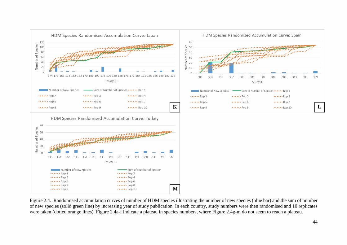
44

Figure 2.4. Randomised accumulation curves of number of HDM species illustrating the number of new species (blue bar) and the sum of number

of new species (solid green line) by increasing year of study publication. In each country, study numbers were then randomised and 10 replicates

were taken (dotted orange lines). Figure 2.4a-f indicate a plateau in species numbers, where Figure 2.4g-m do not seem to reach a plateau.

K L

M

45

Out of the 13 examined countries, there are six countries that do appear to reach a plateau in the

number of species after the original sampling and 10 replicates (Figure 2.4a-f). The curves for

China are all increasing at a gradual rate, suggesting that all studies have identified equivalent

number of HDM species. A plateau seems to have been reached around 80 species. India seems to

be levelling at around 150 species, as is Poland at around 70 species, the Netherlands at around 40

species, the UK around 60 species, and the USA around 50 species. This provides support that all

HDM species have been identified in these countries, and further sampling and publications would

not identify any additional species.

In comparison, Australia, Brazil, Denmark, Egypt, Japan, Spain, and Turkey do not appear to reach

a plateau with regards to the number of new species (Figure 2.4g-m). There is still an increase with

the number of new species following the original sampling, as well as the 10 randomised replicates.

When the number of species is still rising after all publications, it is indicative that not all HDM

species have been collected from these countries. There are some possible explanations for not

identifying all HDM fauna. For example, collection methods may have improved over time, and

perhaps more recent research looks more intensively into all mite fauna within a home, rather than

only searching for one family of mites. As acarologists increase their knowledge of mite fauna,

they may be becoming more adept at identifying different species of mites, particularly those

which are less common. Increased knowledge into HDM taxonomy means that if mites can be

characterised by their species name, instead of by their family name or “unidentified”, the number

of new species collected from a country would increase. In addition, these countries may simply

have not been sampled thoroughly enough, or research may not have encompassed the entire

country in different geographical locations.

46

This does, however, make it difficult to determine a threshold number of publications, above which

no new species of HDM would be collected. In countries where minimal research has been

conducted (ie one or two studies), it is reasonable to assume that more research is required to

identify all HDM fauna. Nevertheless, Figure 2.4g-m indicates that despite a minimum of 10

publications, there are still some unidentified species from seven of 13 countries. Upon examining

the six countries which identified all HDM species (Figure 2.4a-f), apart from the Netherlands, the

plateau began around 13 publications (China, Poland and the UK). However, in India 16

publications were needed, and the USA needed 19 studies for mite fauna to begin to plateau. This

suggests that 10 publications was too low a value to identify all mite fauna within a country, and

a minimum of 15 publications may be more accurate to determine HDM fauna. Therefore, there

likely remains more HDM fauna to be identified outside of this database.

2.3.3 Limitations of the dataset and how they have been mitigated:

a. Number of studies:

Although a comprehensive database of current HDM fauna worldwide was generated from

publications, there are a variety of issues associated with examining mite fauna in this manner.

Firstly, there is a large discrepancy in the number of studies conducted within one region or

country. There are a variety of factors which may have an influence on the amount of research in

a single country, including the level of research funding available. Despite HDMs correlation with

allergens, there may be more significant research for funding to go towards in certain countries,

negating the need for extensive HDM research. Issues regarding the number of publications has

been addressed in Section 2.3.2.

47

b. External variants:

Consequently, many studies from one country at a variety of locations are necessary to provide an

accurate representation of the mite fauna. Certain species of mites are more prevalent at specific

temperatures, relative humidity, and altitudes. There are many geographical differences between

regions in a single country, for example rural vs. urban, inland vs. coastal, and low vs. high altitude.

Additionally, differences exist with types of housing including age of house, material, number of

occupants, length of occupation, furnishings, and a variety of socioeconomic factors. As such,

HDM fauna can vary between these conditions and therefore a broad number of studies would

need to be carried out in each country.

Additionally, there are variations with seaonality, length of sampling time, and whether additional

factors such as presence of pets, temperature, relative humidity, and housing conditions were

recorded and considered. Some publications may also have only been searching for specific type

of mite (ie tarsonemid, storage mites, Dermatophagoides spp.). Therefore, even if other mites were

present they may have only be listed as “unidentified” or completely excluded from the results.

Following from this, there may also be an issue of misidentification. This is particularly relevant

with older publications before more accurate keys had been produced, as some species are

morphologically quite similar and it is easy to mistake one sister species for another.

c. Collection methods:

Another issue surrounds the inconsistency in collection methods between the individual

publications. Different techniques may be used for collecting the mites (ie hoovering, brushing, or

shaking) which may affect the total number of mites, as well as increasing the chances of a certain

48

species not being identified. House dust contains detritus material from clothing, furniture, shed

skin, pet dander, and other household items, of which can widely vary between homes creating

inconsistencies with mite retrieval (Spieksma & Spieksma-Boezeman, 1967). Most often, a 5g

portion of dust is used to isolate mites, however samples containing a higher amount of sand will

contain less dust than samples with little or no sand. This will influence the number of mites

identified in a sample. Afterwards, the dust is sieved, with the size of sieve influencing collection

of all possible mites from the dust. Mites may also be missed by untrained scientists searching

through the remaining dust particles after treatment (Spieksma & Spieksma-Boezeman, 1967).

However, my analysis focused solely on the presence of a species of mite, rather on the number of

each mite species or their density or abundance. This was due to inconsistencies in publications

regarding density of mites in g/dust or specific number of mite species. Therefore, issues with

collection methods influencing the mite fauna in this database are not of a great concern.

d. Publication bias:

One of the main issues associated with this report is a bias towards English-written publications.

The online searches may not have encompassed research into HDM fauna from certain countries,

possibly due to the journal the research was published in, or the language it was written. As some

of the online searches were conducted using the Latin nomenclature for common HDM species,

this problem would have been reduced. Some information or articles may also be overlooked due

to poor translation, as often the abstract or summary is given in English but not the reminder of

the publication.

49

This became even more difficult with the overall lack of accessibility of primary research articles

citing HDM fauna. Older publications were not readily available in libraries. Additionally,

publications were often in lesser-known or lower impact journals that did not have an ongoing

subscription. Some research was only listed as personal communication, and often the results of a

doctoral thesis was cited, but due to country or language, the published version was not accessible.

In a few instances, a review study of the mite fauna had previously been published for a country.

A pertinent example would be when 101 publications were created into a review paper of mite

fauna in Brazil (Binotti et al., 2001a). For this report, this work was cited as one publication in the

database, unless the primary journal article was available and was then referenced as a separate

entity in the database. However, the majority of publications were not available from the UK, and

could possibly only be accessed at a Brazilian institute in their native Portuguese. As such, the

number of publications from Brazil may be much higher than the database indicates. However,

although the number of publications would not be accurate, the different HDM species which were

collected from Brazil will be correctly recorded in the database.

2.3.4 Applications of the database:

Applications for the HDM database were examined using RStudio (2015c). A table was created

which identified the 13 countries with the highest number of publications and the total number of

species collected from these publications. This did not identify whether the species was a “new”

species, but was a cumulative count across all publications from each country. A second table

identified different factors which I thought may contribute to species richness in a country. These

two tables were merged, and log graphs were created of species richness based on country and the

50

pertinent factor. Originally a Poisson model was used, however the data was overdispersed

(residual deviance divided by degree of freedom was too high). Therefore a QuasiPossion model

was used, with an ANOVA F test.

All data was taken from World Bank (online), with information regarding air travel, GDP, rural

population, and urban population (2018). Air transport was recorded as the recoded registered

carrier departures (2016) in millions, with the number of HDM species collected from the

corresponding country. As HDMs are transferred on clothing, pets and furniture, countries with a

higher level of air transport would have higher species richness, as mites would be easily

transported from one country to another. GDP was measured as current US$ (2016) in millions,

and countries with a higher GDP may be representative of a more affluent country and therefore

HDM species richness may be lower and more controlled.

Similarly, rural and urban populations (2016) were recorded, and it is possible that a higher level

of urbanization would lead to a lower level of HDM species richness. Countries with high rural

populations may not be as prosperous, and levels of cleanliness may be lower which contribute to

more mites. In addition, rural areas have higher farming, and although this was not examined in

the scope of this database, there are mites transferred from farming equipment into farmhouses.

This would increase the number of HDM species collected from that country. Socioeconomic

factors and housing characteristics may also affect population density and number of HDMs.

Newer houses in good condition identified mites 19% of the time, compared to 40% of the time in

poorly constructed single story homes in Turkey (Acican et al., 1993). Mite numbers are also

increased by heating using stoves compared to houses with central heating, regardless of whether

51

the house is made from stone or wood (Stenius & Cunnington, 1972). Mite growth and survival is

favoured in carpets (Sharma et al., 2011) and older homes, often due to structural cracks and older

furniture (Heikal, 2015, Saleh et al., 2013). More HDMs are also collected from damp homes, due

to higher relative humidity (Acican et al., 1993, Heikal, 2015). Statistical results are presented in

Table 2.1, and log species richness graphs are provided in Figure 2.5.

Table 2.1. Summary table of species richness based on country and relevant factor which may

contribute to HDM fauna (air travel, GDP, rural population, and urban population). Information

was taken for a maximum of 13 countries (depending on whether information was provided in

World Bank for that location). A QuasiPoisson model with an ANOVA F test was performed.

Df Deviance Resid. Df Resid. Dev F Pr(>F)

NULL 203 1825.5

Air travel 1 108.13 202 1717.3 12.504 0.0005090

Country 10 272.38 192 1445 3.1498 0.0009366

NULL 217 1915.1

GDP 1 40.55 216 1874.5 4.892 0.02809

Country 11 392.23 205 1482.3 4.3021 8.915e-06

NULL 217 1915.1

Rural population 1 75.22 216 1839.8 9.0756 0.002917

Country 11 357.56 205 1482.3 3.9217 3.589e-05

NULL 217 1915.1

Urban population 1 43.04 216 1872 5.1924 0.02372

Country 11 389.74 205 1482.3 4.2748 9.854e-06

52

Figure 2.5. HDM species richness in 13 countries with high numbers of publications, and the correlation with air travel, GDP, rural

population, and urban population. Each vertical set of dots represents data from a single country regarding the number of species

collected within that publication.

53

Each factor was examined on its own as well as in conjunction with country to determine

whether this had an impact on statistical significance. Results from Table 2.1 show that for air

travel results were highly significant in both instances (P<0.001), for GDP results were

significant on its own (P<0.01) and highly significant when examined with country (P<0.001),

for rural populations results were significant on its own (P<0.01) and highly significant when

examined with country (P<0.001), and for urban population results were significant on its own

(P<0.01) and highly significant when examined with country (P<0.001). This indicates HDM

species richness is affected both by the number of publications in a country identifying species

richness, as well as external factors. As such, when species richness is examined it is necessary

to take into account that while HDM fauna varies between countries, this is not the only

contributing factor to the species composition per country. It should, however, be noted that

data was only provided on World Bank for the year 2016, whereas publications varied from

the 1950s to 2017. In addition, the cumulative number of mite species collected from each

country was examined; therefore, there is a high degree of overlap of a single species, and it is

not representative of the number of different species within a country.

54

2.4 Conclusions

In total, 347 publications of HDM fauna spanning seven biogeographical regions and 65

countries, identified 531 different HDM species. This encompasses seven countries from the

Afrotropical region, three countries from Australasia, 8 countries from the Indo-Malay region,

three Nearctic countries, 12 countries from the Neotropics, four countries from the Palearctic

East region, and 27 countries from the Palearctic West region. Country was a significant factor

with regards to the number of HDM species, however the addition of more countries to the

database is necessary to establish whether additional factors, such as level of air travel, GDP,

rural and urban populations also contribute to number of species. D. pteronyssinus, D. farinae¸

E. maynei, and T. putrescentiae were shown to be the most cosmopolitan and abundant species

of HDM. Due to availability, D. farinae will be used in future research to examine distribution,

as well as population genetic differences (see Chapters 4 and 5).

The aim of this database was to assist future researchers by saving time, money, and effort

when analysing HDM fauna. In future, the database could be expanded as more research is

accumulated, and studies which were inadvertently overlooked could be added. This database

of HDM fauna can be referred to for medical research for HDM mite allergens to identify the

most common species collected within the home in a specific country or generalised

biogeographical region. Focus could then be directed towards the most abundant species in the

attempt to eradicate mites from homes to assist with asthma, allergies and rhinitis. In addition,

other factors influencing mite fauna could also be more easily examined with the application

of this database. Preliminary research regarding air travel, GDP, and size of rural and urbans

populations was conducted, however, there are other factors which may be of interest to other

researchers. This includes poverty levels, agriculture, literacy rates, and climatic indicators, to

name a few. As mites have such a negative economic impact on agriculture, it may be useful

55

to explore whether the transfer of HDMs, and the species of mites collected for homes, have a

greater impact than originally believed. This could assist with biological control methods to

reduce crop exposure to these “pests”. Levels of education could also be correlated with

abundance of HDMs. Increased knowledge regarding mite eradication for allergy and asthma

suffers could be of use in this instance.

One application of the database is addressed in the next chapter, regarding the concept of a

latitudinal diversity gradient, different methods by which this gradient has arisen, and whether

there is any correlation between HDMs and a higher level of taxa diversity in tropical climates

when compared to temperate regions at higher latitudes. In conclusion, HDMs are found

worldwide to varying degrees, and have a medical, economic and forensic importance, as well

as having an effect on lives in unknown ways. Therefore, there are many ways in which the

data consolidated within this database could be used for future research.

56

Chapter 3: Biogeographical Distribution of House Dust Mites

3.1 Introduction

Following the creation of the HDM database in Chapter 2, I will further illustrate distribution

of HDMs by country and species. This will be expanded upon to discuss the concept of a

latitudinal diversity gradient (LDG). This theory states that most taxonomic species have higher

levels of diversity in the tropics, compared to temperate zones at a higher latitude. A previous

study has been conducted on oribatid mites and their relationship to a LDG (Maraun et al.,

2007). Oribatid mites mainly live underground in the soil, where they act as decomposers, by

feeding on dead organic material, fungi, and small animals. Examination of 22 islands and 33

mainland geographical areas illustrated that while oribatid mite species richness increased with

decreasing latitude, this pattern only continued to warm temperate sites and did not reach

tropical locations. There is little known about below-ground taxa and the presence of a LDG.

The authors proposed two factors which may contribute to the non-linear pattern they identified

in oribatid mites. They believe oribatid mites are generalists with regards to habitat and feeding.

They do not have a strong relationship to plant or fungal diversity, therefore there would not

be a correlation between plant diversity and mite diversity increasing towards the tropics. In

addition, there are minimal differences between the physio-chemical composition of litter in

temperate and tropical sites. Food resources are similar for the mites and therefore it is unlikely

they would adapt to specific local niches (Maraun et al., 2007).

In this chapter, I will outline some possible explanations for a LDG, and as another application

of the HDM database, examine the most highly-published countries identified in the previous

chapter. If HDMs were to follow a LDG, there would be greater species diversity in tropical

compared to temperate climates.

57


Two methods were performed to examine whether HDMs follow a latitudinal diversity gradient

(LDG). For both methods, latitude was determined on google for a specific region or city (if

provided), for a maximum of three locations per study. If mites were collected from more than

three locations, the mid-point latitude of the country was used for simplicity. If no region or

city was noted in the publication, again the mid-point of the country was used. The average

(absolute values, without including the distance north or south) was then taken.

In the first method, a graph of the 13 countries which had a minimum of 10 publications (see

Chapter 2) was created in Excel to compare the number of species and the latitudinal distance

from the equator. “New species” were plotted for each country, thereby only the number of

different species were examined.

In the second method, the 13 countries were examined in RStudio (2015c), and again the

number of species and latitudinal distance from equator was determined. This method differed

from the first as this method was a cumulative count of number of species across all

publications from each country. Therefore, this does not show the number of different species

per country, but rather the total number of species which were collected across all publications

in each of the 13 countries. Originally a Poisson model was used, however the data was

overdispersed (residual deviance divided by degree of freedom was too high). Therefore a

QuasiPossion model was used, with an ANOVA F test.

58


3.3.1 Distribution by biogeographical region:

The number of different HDM species in each biogeographical region was graphed in Figure

3.1. The highest number of species were collected from the Palearctic West region (265),

followed by the Neotropical (207) and the Indo-Malay (204). Overall these three regions are

highly researched (see database), which would increase the odds of collecting more species

and provide more opportunities to identify new mite fauna.

Figure 3.1. Number of HDM species collected from seven biogeographical regions in 363

publications. The highest number of species were collected from the Palearctic West, and the

fewest from the Afrotropical region.

3.3.2 Distribution by country:

Two heat maps were generated of HDM fauna using data from the country of mite collection

(not the country researchers were based). The first was of the number of publications on HDM

fauna per country (Figure 3.2), and the second was of species counts from each country (Figure

3.3). Darker shades either indicate a higher number of publications or a higher number of HDM

species within that country. The United States of America had the highest number of

23

48

204

58

207180

265

0

50

100

150

200

250

300

Afrotropical Australasian Indo-Malay Nearctic Neotropical Palearctic East PalearcticWest

Nu

mb

er

of

HD

M S

pe

cie

s

Biogeographical Region

Number of HDM Species per Biogeographical Region

59

publications (28), followed by Japan (22), Poland (21), and India (20). India had the highest

number of species (153), followed by Japan (112) and Brazil (99).

Figure 3.2. Distribution HDM fauna in each studied country based on the number of

publications. The highest number of publications were conducted in the USA (28), with a

gradient to only a single publication from 16 countries.

Figure 3.3. Distribution of number of different HDM species collected from each country

where there was published research into HDM fauna. The highest number of species were

collected from India, Japan, and Brazil.

60

Next, the 10 countries with the most diverse HDM fauna were graphed in Figure 3.4. Species

counts were often highest in countries where the most sampling has been conducted. This

suggests that greater sampling effort may be at least partly responsible for the apparent higher

species diversity. In addition, many of these countries are in tropical locations, which suggests

a LDG in HDMs.

Figure 3.4. The ten countries with the highest number of HDM species, as identified from 363

publications in the HDM fauna database.

3.3.3 Latitudinal diversity gradient:

The new database of mite diversity that I have complied can be used to investigate global

patterns of mite biodiversity. As an application for this database, I chose to examine whether

HDM fauna follows a LDG. The existence of a LDG can be traced back millions of years,

however the mechanism behind this gradient or the reasoning behind why it occurs has not yet

been established (Mittelbach et al., 2007). Early explanations for the LDG proposed by Darwin

(1859) and Wallace (1878) focused on geographical differences, where temperate regions have

a harsh climate for adaption, whereas in tropical regions biotic interactions are enough for

adaptation (Mittelbach et al., 2007). There is an overwhelming amount of literature on different

153

11299

85 8372 69

63 62 62

0

20

40

60

80

100

120

140

160

180

India Japan Brazil China Colombia Korea Poland UnitedKingdom

Malaysia Turkey

Nu

mb

er

of

HD

M S

pe

cie

s

Country

Countries with the Highest Number of HDM Species

61

hypotheses for a LDG, and given time constraints, it is not possible to review every theory.

Over time, many theories have been proposed, altered, rejected, and combined with other

theories. As a result, one single theory has not been accepted as correct. See the following for

reviews of some of the theories (Currie, 1991, Schemske & Mittelbach, 2017, Rohde, 1992,

Pianka, 1966, Willig & Presley, 2018, Mittelbach et al., 2007, Willig et al., 2003).

One of the main issues surrounding the concept of a LDG besides the number of theories, is

that often only one species, or a small related group, has been used to assess the hypothesis

(Hillebrand, 2004). This is based on simple correlations between diversity and species richness,

and the main focus is often on vertebrate taxa and higher plants. Additionally, there is a bias

towards studies being conducted in the Americas (Hillebrand, 2004). Theories centre around

one of three possibilities: ecological, evolutionary, and historical (Mittelbach et al., 2007).

Ecological hypotheses examine the mechanisms of how species coexist and diversity is

maintained, evolutionary hypotheses observe diversification rates, and historical hypotheses

focus on how long tropical environments have existed (Mittelbach et al., 2007). Some of the

possible explanations for the existence of a LDG will be outlined below.

3.3.4 Pleistocene glaciation:

a. Hypothesis:

Over the last 700 000 years, major ice ages have been interspersed with short warm interglacial

periods (such as the one currently experienced) (Hewitt, 1996). Climatic oscillations would not

have been consistent worldwide, as features such as distance from the equator, ocean position

and currents, continental mass and mountain ranges would have variable consequences

(Hewitt, 1996). Pleistocene glaciation is a historical hypothesis centering around past

glaciations that created an inhabitable environment for organisms in North America and

62

Eurasia (Brown, 2014). There was a stronger impact of glaciation on the larger amounts of

landmass distributed at higher latitude, in comparison to lower (tropical) latitudes (Lomolino

et al., 2009) (as referenced in Wilson & Veraguth, 2010). For example, species in European

continental areas were very affected by oceans, deserts, and mountains that acted as barriers to

create inhospitable environments during glacial periods (Hewitt, 1996). While these high

latitudes were covered with ice, tropical regions were not as affected (Hewitt, 2004).

Pleistocene fossil records illustrate most taxa responded in an independent manner to the

changing climate (Graham et al., 1996). Species tended to move south during cooling periods

and north during warming periods, where genome mixing may occur (Hewitt, 1996). Species

adapted to these large demographic changes, resulting in some populations going extinct,

bottlenecks and founder events reducing allelic and overall genetic diversity, and mutations

may be lost or spread by selection through populations (Hewitt, 2004). Hybrid zones were

formed by the expansion of species from their refugia (Hewitt, 1996). These zones may have

protected the integrity of two different genomes until the next glaciation cooling occurred when

there would be a decrease in the number of species to its refugia (Hewitt, 1996). In the tropics,

conditions were colder and more arid, reducing rain forests and spreading deserts and savannah

(Hewitt, 2000). Temperate species could adapt further south than “cold-hardy” species (Hewitt,

2004).

63

b. Select species supporting this hypothesis:

Table 3.1. Some select species which were outlined in the published literature to provide

support to the Pleistocene glaciation hypothesis. Molecular markers dated when phylogenetic

events occurred, which illustrates differences in species age between tropical and high-latitude

(more glaciated) regions.

Species Method Reasoning Reference

Microtus

longicaudus

mt cytB Similarities in Northern subclades due to

recent recolonization

(Conroy &

Cook, 2000)

Deeper among-clade branch lengths near

glacial areas due to long periods of

isolation

Syngnathus

typhle

mtDNA,

nDNA,

microsatellites

Northern and Eastern European

populations had reduced level of genetic

variation; recolonization after LGM

(Wilson &

Veraguth,

2010)

Central populations were highly diverse;

phylogenetic structure dates to before

LGM

Southern Atlantic populations had

moderate levels of genetic variation;

divergences occurred in the middle of

the last glacial cycle

Chorthippus

parallelus

nDNA,

mtDNA, rDNA

Illustrated five major geographical

regions

(Hewitt, 1996)

Genetic variation was higher in Southern

than Northern populations

Nearctic and

Palearctic

freshwater /

anadromous

fish

mtDNA Tree topologies deeper for non-glaciated

(Southern) species compared to

Northern species

(Bernatchez &

Wilson, 1998)

Phylogeny very similar among Southern

species whereas glaciated species show

decreased consistencies

c. Issues with this hypothesis:

The advancement of molecular methods has allowed for DNA sequencing to be used to date

phylogenetic events (Hewitt, 1996). Regions in the D-loop of mtDNA can be useful in

distinguishing between mutations due to these hypervariable regions (Hewitt, 2000). Molecular

data using DNA similarities can illustrate from which refugia certain genomes appeared, along

with their relation to present-day distribution (Hewitt, 2000). This method, comparative

phylogeography, can also be applied to illustrate previous discrepancies between genetic and

64

phylotypic variation (Bernatchez & Wilson, 1998). Although this is a particularly useful

method to illustrate species diversity, there is a large amount of error connected with estimating

time based on DNA sequence divergence (Hewitt, 1996). Additionally, there are differences in

dating between nuclear and mitochondrial DNA results due to the stochastic natures of the

coalescent process (Wilson & Veraguth, 2010). This is particularly problematic as much

research relies solely on the mitochondrial results; as such a multi-locus data set is necessary

to accurately date species divergence (Wilson & Veraguth, 2010).

3.3.5 Niche conservatism:

a. Hypothesis:

Niche conservatism is an ecological hypothesis, where tropical species are more specialised

due to adaptations to biotic and abiotic factors, leading to finely distributed resources (Brown,

2014). It is anticipated that every niche will have particular biotic and abiotic factors crucial to

survival, and individuals and populations are not expected to survive outside of their niche

(Wiens et al., 2010). Niche conservatism may occur within species, therefore phylogenetic tests

are not necessarily the most informative or appropriate. There is no universal test for niche

conservatism, and different tests may apply in different contexts (Wiens et al., 2010).

The niche conservatism hypothesis is influenced by the historical climate change which

occurred during the Pleistocene glaciation (Andam et al., 2016). As previously outlined,

glaciation events prevented speciation at higher latitudes; instead the current species collected

from high latitudes are derived from species expanding upwards from lower latitudes (Andam

et al., 2016). When early colonizers arrive at higher latitudes, they impose barriers to prevent

late-dispersers from entering their habitats (Waters et al., 2013) (in Andam et al., 2016).

Subsequently, the high latitude populations adapt to their new surroundings over time. They

65

then put further barriers in place to prevent latitudinal movement across climate zones. This

creates specific niches for different species (Waters et al., 2013) (in Andam et al., 2016).



support to the niche conservatism hypothesis. This theory centers on dispersion rates limiting

diversity at higher latitudes, as well as contributing factors from the Pleistocene glaciation.


Streptomyces

bacteria

Isolation and

characterisati

on of 924

strains

Limitations in dispersal distance despite

the potential for long-range dispersal

through desiccation-resistant spores

(Andam et al.,

2016)

Taxon composition varied between the

different sites

Amazonian

birds

Phylogenetics

of 739 species

Ecological speciation is the driving force

behind their diversity

(Salisbury et

al., 2012)

Desmognathus

and Plethodon

mtDNA Niche conservatism promotes allopatric

isolation (isolation of biological

populations of the same species) and

speciation

(Kozak &

Wiens, 2006)

Vicariance events (evolutionary

conservatism in climatic tolerances)

resulted in allopatric sister lineages

Two of eight pairs of allopatric sister

taxa do not support this hypothesis

(strong divergence in climatic niche

area)

Small climatic gradients resulted in

highly fragmented populations between

mountainous ecosystems and lowlands

Due to their small size and dispersal tendencies, Streptomyces bacteria across North American

soils may be most relevant to a potential LDG in HDMs. As Streptomyces species form

desiccation-resistant spores that can be carried in the wind, it provides an opportunity to test

whether limitations in dispersal has a strong effect on terrestrial microbial diversity (Andam et

al., 2016). Examination of physiologically similar strains of these bacteria from geographically

different yet ecologically similar habitats illustrated a LDG. There were limitations in dispersal

and genetic drift resulting in regional diversification of Streptomyces, providing support to the

66

niche conservatism hypothesis. There is a bias towards the tropics with regards to niches

categorised by dispersal constraints. Consequently, these areas were colonized following

glacial retreat by species expansion from lower latitudes (Andam et al., 2016). These tropical

niches decrease dispersal across barriers, resulting in an increase in geographic speciation

diversification and a LDG (Salisbury et al., 2012).


See Peterson (2011) for a full review of issues surrounding the ecological niche conservatism

hypothesis, including problems such as over-interpretation of niche models. Methodologies

widely vary, and “niche” can be defined very simply to result in a high level of conservatism

(Peterson, 2011).

A similar theory to niche conservatism is the physiological tolerance hypothesis (Currie et al.,

2004). This hypothesis states that species exist in the regions they have adapted to, therefore

species richness is limited by the number of species which can inhabit these areas. The authors

agree that while climatic tolerances do limit species dispersal, there still remain many areas

that a species could tolerate the climatic conditions, but have not dispersed to. As such, this

hypothesis was rejected on those grounds (Currie et al., 2004).

3.3.6 Tropical conservatism hypothesis:

a. Hypothesis:

To build upon the niche conservatism hypothesis, three ideas were combined: high species

richness originated in the tropics and expanded outwards to more temperate zones, extant

clades from the tropics existed because there was a greater geographic extent, and many species

67

and clades are well-designed for tropical locations and would not be able to adapt to colder

climates (Wiens & Donoghue, 2004). The tropical conservatism hypothesis assumes a

relationship between how long a species has been in an area and how many species are currently

present. It states that high species diversity will be in regions with warm temperature and high

rainfall, and there will be differences in relative ages and diversities between clades in

temperate and tropical locations. Cold climates and niche conservatism prevent tropical species

and clades from invading more temperate locations (Wiens & Donoghue, 2004). There should

be few transitions between tropical and temperate habitats due to the conservation of

environmental tolerances (Kerkhoff et al., 2014).

The tropical conservatism hypothesis is not mutually exclusive; instead it forms a nested

hierarchy with the diversification rates hypothesis and the “out of tropics” model (Kerkhoff et

al., 2014). In the diversification rates hypothesis, a tropical origin for many lineages is highly

likely as these environments are older and more wide-spread than temperate regions

(Mittelbach et al., 2007). Palaeontological studies provide support that net diversification rates

are higher in tropical climates, and species are more likely to have originated in the tropics and

then diversified outwards (“out of tropics” model). Phylogenies can also be used to examine

diversification rates through sister clades. Sister clades are of equal ages, therefore any

differences between species diversity will be because of diversification rates. Although this

method has proved accurate in some instances, sister taxa tend to retain ancestral traits, making

latitudinal comparisons difficult (Mittelbach et al., 2007).

68



support to the tropical conservatism hypothesis. This theory centers on high species diversity

in regions with warm temperature and high rainfall, as well as differences in relative ages and

diversities between clades in temperate and tropical locations.


New World

woody

angiosperms

Phylogeny of 12 500

species and a fossil-

calibrated supertree

Lower phylogenetic diversity in

temperate regions

(Kerkhoff et al.,

2014)

Temperate and semi-temperate

species were clustered and

nested within ancient tropical

lineages

Evolutionary transitions from

tropical to temperate

environments were very rare

North

American

butterflies

Mapping species

richness and

phylogenies to

subfamily level

Mean root distances (number of

nodes separating butterfly’s

subfamily from base of

phylogenetic tree) decrease to

the south

(Hawkins &

DeVries, 2009)

More derived clades found in

Northern regions, and species in

basal subfamilies are in the

South

Winter cold tolerance is main

factor explaining why some

groups can permanently inhabit

temperate region

Vertebrate

clades

Phylogeny of 12 101

species (ray-finned fish,

amphibians, turtles,

squamates, mammals

and birds in

North/South America

Families that evolved in the

tropics illustrate strong niche

conservatism and many

lineages cannot expand into

temperate regions (contribute

little to temperate biodiversity)

(Smith et al.,

2012)

Terrestrial families with

temperate origins can inhabit

both Northerly and Southerly

habitats (contribute strongly to

tropical biodiversity)

Ants Online datasets and

phylogenies

In temperate zones ant lineages

are more phylogenetically

clustered

(Economo et al.,

2018)

Diversification rates are similar

between temperate and tropical

regions

69

In addition, clades including modern cycads, palms, figs, onychophorans, caecilians,

crocodiles, parrots, trogons, and primates are widely distributed in tropical regions, but have

not successfully entered temperate zones (Wiens & Donoghue, 2004). This again provides

support that niche conservatism reduces the degree of dispersal. However, this hypothesis has

not yet been fully developed, therefore more empirical studies need to be conducted (Wiens &

Donoghue, 2004).


Some data has refuted a LDG under the tropical conservatism hypothesis. For example, grasses

(Poaceae) have old lineages and have been able to adapt to a variety of environmental

conditions, including arid and cold climates (Visser et al., 2014). This was supported by

distribution data for 11,086 species of grasses which illustrated highest species richness at mid-

latitudes and only significantly decreased at northern latitudes above 50o. Continental patterns

were also visible, with species diversity significantly higher in South America and Australasia.

However, not all grass lineages have high number of species in cooler latitudes, and adaptation

to temperate climates occurs slowly, if at all. Therefore these dispersion events from tropical

locations happened recently (Visser et al., 2014).

The tropical conservatism hypothesis was also contradicted by the New World snake tribe

Lampropeltini (Pyron & Burbrink, 2009). Results showed an inverse LDG, where biodiversity

in temperate regions were caused by early colonisers and a longer amount of time for speciation

(Pyron & Burbrink, 2009). A futher review of 111 phylogenetic studies of birds, mammals,

insects and flowering plants mapped the latitudinal ranges of all taxa to determine which

hypotheses contributed to the LDG (Jansson et al., 2013). Diversification rates did not differ

between sister lineages in tropical and temperate locations. As the tropical conservatism

70

hypothesis focuses on fewer clades being collected from higher-latitude regions, this

hypothesis was not supported. Instead, the phylogenies illustrated that species originated in the

tropics and then travelled outwards into temperate zones (“out-of-tropics” hypothesis) (Jansson

et al., 2013).

Additionally, a phylogenetic analysis of Old World frogs (Ranidae) depicted a tropical origin

in Africa and Asia before spreading to other geographical areas (Wiens et al., 2009). When

diversification rates were examined, either rates were similar between tropical and temperate

areas, or the level of diversification was higher in temperate clades than tropical in clades. It is

possible that temperate regions have higher diversification simply because the clades are

younger than those in tropical zones; however, exclusion of the oldest and youngest clades still

provided similar results. This illustrates that historical biogeography needs to be included when

assessing LDG hypotheses (Wiens et al., 2009).

A LDG cannot be fully explained simply by the longer existence of tropical environments

compared to temperate habitats (Mittelbach et al., 2007). Therefore, it is essential to understand

why tropical habitats diversity at a faster rate. The seven mechanisms postulated to explain a

LDG due to diversification rates are outlined in Table 3.4. It has been suggested that the tropical

conservatism hypothesis would be better explained by the combinational effects of the niche

conservation hypothesis (discussed in Section 3.3.3) and the time-for-speciation hypothesis

(discussed next in Section 3.3.5) (Wiens et al., 2006).

71

Table 3.4. Description of seven mechanisms to explain latitudinal variation in diversification

rates. For a complete description of mechanisms, see Mittelbach et al., (2007).

Mechanism Description Reference

Genetic drift Rapid speciation in the tropics is due to low average

population density leading to greater genetic drift

(Fedorov, 1966)

Climate change Resulted from change in Earth’s orbit and rotational

axis (Milkankovitch cycles) which is greater at high

latitudes and favours species with high dispersal

potential (habitat range could change to follow

favourable conditions)

(Dynesius &

Jansson, 2000)

Mechanisms of

speciation

Unknown at present whether this differs at varying

latitudes

(Mittelbach et al.,

2007)

Geographical

area

As geographical area increases in size, speciation

rates are higher and extinction rates are lower,

resulting in differences between tropical and

temperate diversification rates

(Terborgh, 1973)

Physiological

tolerances and

dispersal

limitation

There is a reduction in physiological tolerances and

limited dispersal abilities in species through

unfavourable climatic regions, such as that in

lowland tropical habitats due to small temperature

ranges (compared to higher latitude temperate zones)

(Janzen, 1967)

Evolutionary

speed

Biodiversity is highest at the equator as a result of

kinetic effects of environmental temperature on rates

of biological processes (higher speciation due to

increases in genetic divergence caused by mutation

rates and generation times)

(Rohde, 1992)

Biotic

interactions

Biotic interactions are stronger in tropical regions

compared to temperate zones leading to an increase

in species richness

(Fischer, 1960,

Dobzhansky,

1950)

3.3.7 Time and area hypothesis (Time-for-speciation effect):

a. Hypothesis:

The time and area hypothesis states that species have been amassed for a longer period of time

in tropical regions versus temperate regions (“time-for-speciation-effect”) (Mittelbach et al.,

2007). This hypothesis focuses on both the Pleistocene glaciations, which affected temperate

regions more than tropical equatorial areas, as well as how tropical regions were distributed

during the early Cenozoic period. During this period, warmer temperatures meant tropical flora

covered a large area outside of tropical latitudes. These mild temperatures were followed by a

cooling period, and glacial-interglacial cycles which had a more pronounced effect on species

72

in higher latitudes (Mittelbach et al., 2007). Ultimately, speciation causes species richness;

however little research has examined the amount of time it takes for speciation to occur

(Stephens & Wiens, 2003).



support to the time and area (time-for-speciation) hypothesis. This theory states that the tropical

regions have had longer to accumulate species; therefore diversity will be increased in

comparison to newer inhabitants at higher latitudes.


Current

tree

species

Paleogeographic

reconstruction of

biomes

Positive correlations between current tree

diversity and area-time periods since Eocene,

Oligocene, and Miocene

(Fine &

Ree,

2006)

High tropical diversity due to larger biomes

compared to temperate biomes which lead to

increased speciation / lower extinction rates

New

World

leaf-

nosed

bats

nDNA, mtDNA,

RNA

Higher rate of sequence divergence at the edges,

versus the central equator with average relative

tax age decreasing with increasing distance

from the equator

(Stevens,

2006)

Tropical location likely resulted in more time

for species richness to occur

Hylid

frogs

Phylogenetic

analysis,

ancestral area

reconstruction,

molecular dating

methods, and

ecological niche

modelling

Illustrated species-rich clades of hylids had a

tropical origin with radiation outwards to

temperate regions at a more recent date

(Wiens et

al., 2006)

Strong correlation between richness in an area

and time when the region was first colonised

(regardless of geographic location)

Emydid

turtles

Molecular and

morphological

divergences;

phylogenies

High species richness in Eastern North America

compared to other continental habitats

(Stephens

& Wiens,

2003)

Reduced species richness in regions bordering

eastern North America likely due to more recent

colonisation

Despite equivalent local species richness, higher

levels of regional species richness in Southeast

compared to Northeast (North America)

73


One of the major issues with this hypothesis is that there is an assumption that rates of

speciation and extinction are similar between all regions and lineages (Stephens & Wiens,

2003). This is often untrue, as rates can greatly vary over time, space, and between taxa. While

the time-for-speciation hypothesis seems to successfully explain patterns of species richness at

large spatial scales, with correlations between regions and the length of time species inhabited

this area, its effect is indirect and reduced at a smaller scale. At these smaller spatial scales, the

time-for-speciation effect creates species richness patterns through local ecological processes

such as extinction, competition, adaption, and predation (Stephens & Wiens, 2003).

Currie et al. (2004) analysed three data sets and two speciation rates hypotheses (evolutionary

rates and biotic interactions), where speciation is predicted to vary with climate due to

differences in evolutionary rates or biotic interactions (Currie et al., 2004). In the “evolutionary

rates” hypothesis, higher mean temperatures result in shorter generation times, increased

mutation rates, and an increase in physiological processes. This will lead to faster rates of

selection and higher speciation rates. In the “biotic interactions” hypothesis, differences in the

importance of biotic factors between regions will result in differences in speciation rates.

However, there is little data to examine either of these hypotheses accurately and thoroughly

at this point in time (Currie et al., 2004).

3.3.8 Species-energy hypothesis:

a. Hypothesis:

The other class of ecological hypotheses involves level of productivity (Brown, 2014). The

tropics are an area of high productivity; therefore, this region can sustain more individuals

among more species. Since temperature and seasonality is at a maximum in tropical climates,

74

the level of resources is higher, maintaining stable populations and increasing biodiversity. In

comparison, the freezing-cold poles and dry deserts have limited life forms due to inhospitable

environments. Net primary production (NPP) is limited by both temperature and water in

terrestrial habitats, and by nutrients and solar radiation in marine habitats. Consequently, there

are limitations on the total amount of resources available, biomass, as well as the number of

individuals which can survive in a single location. A fixed NPP means that either a high

biomass with few large organisms, or a low biomass with lots of small organisms can be

sustained in an ecosystem. As NPP is temperature dependant, a latitudinal gradient exists for

productivity level (Brown, 2014).

In this hypothesis, the increase in species diversity in the tropics is caused by faster

evolutionary speed – a result of shorter generation times, faster mutation rates, and increased

selection at higher temperatures (Brown, 2014, Rohde, 1992). However, species diversity

increases with temperature at a faster rate than the number of individuals and NPP. As a result,

productivity is not enough to fully explain the LDG, and instead the direct effects of kinetics

are influential on the LDG. In the tropics, increased temperatures lead to higher metabolic rates,

ecological dynamics and coevolutionary processes, which all act to main a high level of

biodiversity (Brown, 2014).

A model was developed which included temperature in the “energetic-equivalence rule”, which

states that individual metabolic rates increase with body size (Allen et al., 2002). Body

metabolic rates within an individual vary with body size and temperature, therefore the addition

of biochemical kinetics of metabolism provides another component to test species diversity.

Terrestrial, freshwater, and marine taxa examined across latitudinal gradients in North America

and elevation in Costa Rica, all supported an increase in species diversity with environmental

75

temperature. Biochemical kinetics influence metabolism, and metabolic rates direct an

individuals’, and populations’ resource requirements. Higher temperatures increase the rate of

biochemical reactions controlling speciation, thereby increasing species diversity (Allen et al.,

2002). To expand upon this theory, Brown (2014) used theoretical and simulation models to

create a pattern of beta diversity, where biotic factors prevent species from dispersing into other

niches (Brown, 2014). Rates of diversity are therefore increased, whereas rates of dispersal are

decreased. A combination of higher rates of evolution and higher rates of Red Queen

coevolution have resulted in increased biotic interactions. In turn, “the Red Queen runs faster

when she is hot” leads to higher species diversity in tropical climates (Brown, 2014).



support to the species-energy hypothesis. This theory centers on higher biodiversity due to

more species acquiring resources which will maintain stable populations in areas of high

productivity.


Coral reefs Published diversity at

single or multiple sites

Diversity best predicted by mean

annual ocean temperature and regional

coral biomass

(Fraser &

Currie,

1996)

Suggests regional coral richness is

limited by available energy

Atlantic

salmon, brown

trout and sea

trout

Data sets and ANCOVA

to estimate relationship

between log(population

density) and log(mean

body weight)

Negative relationship between

log(population density) and log(mean

body weight) suggests competition for

energy resources

(Bohlin et

al., 1994)

Fish metabolic rate is proportional to

(body weight)0.9 and total energy flow

is constant within a population but

varies among populations and within

sites in a population

Extant

continental and

continental

island birds

Distribution maps, and

simulations of random

dynamics of species

ranges

Species richness is highest at the

tropics, with peaks in major mountain

chains

(Davies et

al., 2007)

High-resolution (1o equivalent) models,

most important components for bird

species richness is temperature and

topographical variability

76


To expand on the species-energy hypothesis, Evans et al. (2005) proposed nine mechanisms to

explain positive species-energy relationships at a macro-scale: sampling, increased population

size, dynamic equilibrium, niche position, niche breadth, more tropic levels, consumer

pressure, range limitation, and diversification rate. Each of the outlined mechanisms overlap

with at least one prediction of another mechanism (Evans et al., 2005). The authors note that

the most relevant mechanisms are increased population size, niche position, and diversification

rate. These mechanisms will not be further discussed in this dissertation, however more detail

can be found in their publication. Testing the macro-scale species-energy hypothesis is

currently a difficult task. The relationships are broad and general, and no single mechanism has

been identified to explain the cause of this hypothesis, in part due to little research testing all

concepts. The overlap between predictions has been ignored in some previous studies,

detracting from the contribution each mechanism may make on positive species-energy (Evans

et al., 2005).

Finally, extant evidence does not support the species-energy hypothesis, where variation in

species richness is due to total number of species in the area (Currie et al., 2004). Climate has

an influence on net primary productivity (NPP), and the NPP limits individuals per area.

Additionally, the changes in organism density due to latitude or productivity are very small,

and therefore cannot solely explain the observed changes in species diversity (Currie et al.,

2004).

77

3.3.9 House dust mites and the latitudinal diversity gradient:

a. Most likely hypotheses:

There have been many hypotheses to explain a general LDG across species, and data suggests

this arose from a combination of these proposed hypotheses. Research into swallowtail

biodiversity found evidence for the diversification rates hypothesis, illustrating two different

rates between temperate and tropical species of similar age (Condamine et al., 2012). These

diversification rates were highly influenced by glacial climatic rates between tropical and

temperate clades. Additionally, plant shifts helped to promote diversification of swallowtails.

In extant populations, tropical biodiversity does not necessary come from a tropical clade, and

there have been multiple dispersals outwards from the tropics. The conclusions of this study

used a multidisciplinary approach, and outlines that ecological and evolutionary theories and

their corresponding evidence need to be combined for an enhanced understanding of the LDG

(Condamine et al., 2012).

It seems likely that glaciation events leading to climatic oscillations, as well as physical barriers

such as oceans, deserts, and mountains had a greater impact on high latitude species. Following

the warming periods, species than had to radiate outwards from the tropics to recolonize the

temperate zones (Pleistocene glaciation hypothesis). As such, species have been amassed for a

longer period of time in tropical regions versus temperate regions (Time and area hypothesis).

Species richness is higher in the tropics, extant clades in this area existed due to greater

geographic extent, and species are less able to adapt to colder climates (Tropical conservatism

hypothesis). The interaction between biotic and abiotic factors made specific habitats adaptable

to organisms. This also prevented some organisms which are better adapted to colder climates

from moving farther south, and vice versa (Niche conservatism hypothesis). Additionally, there

is higher speciation in the tropics due to increases in genetic divergence caused by mutation

78

rates and generation times. This increase in kinetic energy contributes to high species

biodiversity (Species-energy hypothesis). A combination of many factors and overlapping

theories, often reliant on the validity of a previous theory, are required to explain the LDG.

b. House dust mites and the latitudinal diversity gradient:

To establish whether HDMs follow the LGD hypothesis, the 13 countries with a minimum of

10 publications (refer back to Chapter 2, Figure 2.4) were first plotted in Excel to compare the

number of species and the latitudinal distance from the equator (Figure 3.5).

Figure 3.5. Comparison between latitudinal distance and number of HDM species for 13

countries. If mites follow the LDG, there should be a downward linear trend. As distance

increases from the equator, number of species should decrease.

Next, the same data was analysed in RStudio (again refer to Chapter 2, Section 2.3.4), however

as previously stated, this did not examine the number of different species per country, but

instead a total HDM species count. Results are given in Table 3.7 and Figure 3.6, and illustrate

that latitude itself is not significant with regards to HDM species richness. However, species

richness is highly statistically significant (P<0.001) when latitude and country are examined in

0

20

40

60

80

100

120

140

160

18 23 28 33 38 43 48 53 58

Nu

mb

er o

f Sp

ecie

s

Latitudinal Distance from Equator

Correlation Between Distance from Equator and Number of Species

Brazil India Egypt China

Australia Japan USA Turkey

Spain Poland The Netherlands UK

Denmark

79

conjunction. This illustrates that multiple factors can have an impact on species richness, and

there is the possibility that a LDG exists for HDMs. As in the previous chapter, country is a

highly significant factor when examining a LDG. This could, however, be due to the locations

where the countries with high levels of research being performed. This could inadvertently lead

to a country bias suggesting a LDG. To establish whether this is true, more countries would

need to be included in this examination, as these 13 countries only suggest that a gradient may

exist. If more countries were included, it would become clearer whether a LDG for HDMs

exist.

Table 3.7. Summary table of species richness based on country and distance from latitude.

Information was taken for 13 countries, and a QuasiPoisson model with an ANOVA F test was

performed.

Df Deviance Resid. Df Resid. Dev F Pr(>F)

NULL 217 1915.1

Latitude (study) 1 23.99 216 1819.1 2.8755 0.09146

Country 12 421.67 204 1469.4 4.2116 6.326e-06

Figure 3.6. HDM species richness in 13 countries, arranged alphabetically, and the correlation

with latitudinal distance. The latitudinal distance was determined for each individual study (if

given), not the overall country latitude.

80

One final analysis was performed to examine the existence of a LDG in HDMs. Two countries

with contrasting latitudes, Brazil and Poland, were compared. These countries had a high

number of publications, and different locations within the country were often noted in the

original publication. Therefore exact latitudes per study could be determined, and the

corresponding number of species was graphed (Figures 3.7 and 3.8). This illustrated that in

tropical locations such as Brazil, there is not necessary a LDG for HDMs; however, in higher

latitudes locations such as Poland, there is the potential that HDMs follow this trend. Again,

more research in mite fauna at a variety of latitudes and countries would help assess the validity

of a possible gradient.

Figure 3.7. Comparison between latitudinal distance and number of HDM species for Brazil.

If mites follow the LDG, there should be a downward linear trend, with increasing distance

from the equator depicting decreasing number of species. This trend is not seen for Brazil.

0

10

20

30

40

50

60

70

0 5 10 15 20 25 30

Nu

mb

er o

f Sp

ecie

s

Latitude

Correlation Between Number of Species and Latitude in Brazil

81

Figure 3.8. Comparison between latitudinal distance and number of HDM species for Poland.

If mites follow the LDG, there should be a downward linear trend, with increasing distance

from the equator depicting decreasing number of species. This trend is seen for Poland.

It should be noted that my research has examined mites which have been collected from indoor

locations. Although these mites may be transferred on humans, pets, or other entities outside,

they are not exclusively found outdoors, and for the true HDMs, the outdoors is not their natural

habitat. Other research for LDG examines species collected from the wild, therefore HDMs

may not follow the same patterns or support the same hypotheses.

With regards to the LDG theories, Pleistocene glaciation likely does not explain mite

biodiversity. Mites have very specific temperature and humidity requirements; therefore I find

it unlikely that they survived within tropical regions and then recolonized outwards to

temperate zones following the last major ice age. I find it most likely that HDMs follow a niche

conservatism hypothesis. Each species has specific requirements for their survival. The niche

conservatism hypothesis states that every niche will have particular biotic and abiotic factors

crucial to survival, and individuals and populations are not expected to survive outside of their

niche (Wiens et al., 2010).

0

5

10

15

20

25

30

35

40

45

50 50.5 51 51.5 52 52.5 53 53.5 54 54.5 55

Nu

mb

er o

f Sp

ecie

s

Latitude

Correlation Between Number of Species and Latitude in Poland

82

As outlined in previous chapters, the natural habitat of HDMs are locations where they feed on

fungi, organic material, and bacteria (Klimov & O'Connor, 2013). Over time, mites have

phoretically associated with birds and mammals (Colloff, 2009). As such, their relationship

with other organisms is likely a contributing factor to their diversity, and it is possible that

movement by other taxa would have relocated mites from tropical to higher latitudes. They

could have then adjusted their requirements to survive in a specific location, resulting in their

survival in house dust.

83

3.4 Conclusions

There has been a lot of research on HDM fauna published worldwide. All accessible resources

were consolidated into a HDM fauna database, encompassing 65 countries from seven

biogeographical regions. As an application for the database, the concept of a LDG was

examined for HDMs. It is commonly known and accepted that there is a higher number of

species in tropical areas, with lowered species diversity in higher latitude (temperate) regions.

Although there are many hypotheses, there is no concrete conclusion as to how or why this

gradient occurred.

The 13 most thoroughly researched countries with greater than 10 publications were examined

using two different methods to determine whether there was a correlation between number of

mite species and latitudinal distance from the equator. The results given in Section 3.3.9b

suggests that a LDG may exist for HDMs when taking into account both study latitude and the

country, with the correlation to species richness. However for this to be conclusively

determined, more countries at a wider variety of latitudes would need to be included.

84

Chapter 4: Method Development and Optimisation of

Dermatophagoides farinae Extraction Protocols

4.1 Introduction

The American house dust mite Dermatophagoides farinae (Hughes 1961) (D. culinae De Leon,

1963) was identified as one of the most common species of house dust mite (HDM) worldwide

(Chapter 2), therefore it was chosen for further population-level analysis. As with many mite

species, knowledge regarding the species population genetic structure is lacking (see Chapter

1). As molecular and population genetics techniques can provide clues to the natural history of

under-examined species (Johnson et al., 2004, Hashimoto et al., 2016, Barraclough et al., 2007,

Cesari et al., 2009, Faurby et al., 2011, Fontaneto et al., 2007, Gladyshev & Arkhipova, 2010),

I aimed to identify genetic differences between populations of the same species using a variety

of molecular markers.

One of the main problems with molecular techniques in mites is the low amount of DNA

extracted from a single individual (Li et al., 2010a). To provide a context of the low quantities

of DNA from mites, the genome size of D. farinae has been estimated to be 53.5Mb (Chan et

al., 2015), whereas the genome size of a human is approximately 3000Mb (Morton, 1991). It

is commonly stated that 50ng of human DNA is required as PCR template; therefore

approximately 1ng of high quality mite DNA would be needed as PCR template. As it is often

necessary to only have DNA from a single mite sample, combining mites to increase DNA

yield is not often an option (Li et al., 2010b). Even if mites are from the same population, they

potentially have diverse genotypes. In addition, there could be accidental contamination of

another mite species, which would provide inaccurate molecular results for the species of

interest (Li et al., 2010b). This chapter will discuss three different extraction protocols which

85

were optimised for three European populations of D. farinae mites, prior to their use as PCR

template in Chapter 5.

4.1.1 Mite samples and sequences:

I obtained three European populations of D. farinae, and combined information from these

with mitochondrial and nuclear sequences available from GenBank (Table 4.1).

Table 4.1. Summary of D. farinae mite populations, including country of origin and GenBank

accession numbers, where applicable. This includes D. farinae samples which were provided

for analysis, as well as information obtained from online populations.

ID Country of

Origin

Provider / Identifier Accession

Number

Reference

DF Poland Crop Research

Institute (Prague,

Czech Republic) /

Krysztof Solarz

N/A (Erban &

Hubert, 2015)

VI Unknown

European

Victor Iraola (Spain) N/A N/A

BH The

Netherlands

Barbara Hart

(France) / Marianne

van Bronswijck

N/A N/A

Online CO1

USA

USA Klimov & O’Connor

(Michigan, USA)

GQ465336

(Klimov &

O'Connor,

2009)

Online

EF1a USA

USA Klimov & O’Connor

(Michigan, USA)

JQ000856 (Klimov &

O'Connor,

2009)

Online

genome

China

China Chan et al (China) GCA_000767015.1

(KN266307)

(KN266725)

(Chan et al.,

2015)

Online CO1

China

China Yang, Cai & Cheng

(Shanghai, China)

HQ287786 (Yang et al.,

2011)

Online CO1

Thailand

Thailand Phumee et al

(Bangkok, Thailand)

HQ823622 (Insung et al.,

2015)

4.1.2 Previous extraction techniques:

The first step was to develop and optimise an extraction protocol for this species of mites. To

better identify genetic differences between individual mites and to account for accidental

86

contamination with a different species, single mite extractions were performed when possible.

Extraction techniques successfully used for D. farinae in the previous publications above are

shown in Table 4.2; most of these involve modifications to commercially available genomic

DNA extraction kits.

Table 4.2. Comparison of extraction techniques previously used for D. farinae mites. There is

a minimal amount of information regarding the most successful extraction protocols for HDMs.

Extraction

Technique

Manufacturer Modifications Number of

Mites

Reference

Extraction

kit, tissue

lysis protocol

Qiagen, GmbH,

Hilden,

Germany

N/A Not

provided

(Chan et al.,

2015)

Invisorb

SpinTissue

Mini Kit

STRATEC

Molecular

GmbH,

Germany

N/A Not

provided

(Insung et

al., 2015)

QIAamp

DNA Micro

Qiagen Mite crushed in drop of

buffer ATL prior to step 1;

pro K added but not mixed;

incubation time 24hr; no

carrier RNA added; DNA

eluted in 30µL buffer AE

Single mites (Klimov &

O'Connor,

2009)

87


4.2.1 Mite culturing:

Live mites were provided in T-25 cell culture flasks with filter caps. The flasks were placed in

plastic containers, filled with damp blue roll and table salt (Figure 4.1). To prevent mites from

escaping their enclosure and potentially contaminating other colonies, Vaseline was used to

coat the rim of the plastic container and aluminium foil prevented exposure to light. The

colonies were reared on refrigerated broken pieces of dry dog food (Pedigree Vital Protection,

for adult dogs with chicken), and placed in a closed desk drawer. D. farinae mites have

previously been identified in dogmeal and yeast in Manchester and on biscuit meal, as well as

in house dust (Hughes, 1976). Additionally, they have been cultured in Gainesburger dogfood

at room temperature and 75% RH (Hughes, 1976).

Figure 4.1. The mite culturing method used in the Acarology lab at the University of Reading

for sustaining D. farinae mite colonies. Flasks were kept isolated from other mite colonies to

prevent accidental contamination.

88

4.2.2 Morphological identification:

Dead mites (from The Netherlands and an unknown European origin; see Table 4.1) had

already been identified to species level in other acarology laboratories. However, as the live D.

farinae mite colonies were reared in a lab which also housed other live mite species, there was

a possibility of contamination by other colonies. To visually confirm the species of live mites,

a morphological identification was conducted by permanently mounting them on glass slides

following the method outlined by Krantz et al. (2009) (p. 90-92). Individual mites were left in

70% ethanol for one hour before being transferred into tubes pre-filled with 75% lactic acid

(Krantz & Walter, 2009). After one hour the tubes were centrifuged and the liquid was carefully

removed. The mites were rehydrated with 70% ethanol for one hour, and placed on a glass

slide. A drop of Hoyer’s mounting medium was added, and a coverslip was carefully placed.

Hoyer’s medium is an aqueous solution composed of distilled water, gum Arabic, chloral

hydrate and glyercin. It is chosen due to ease of use and good optical properties. The coverslip

edges were sealed using Glyptal, an insulating paint which provides a flexible and effective

barrier against water, necessary when working with the hygroscopic properties of Hoyer’s

medium (Krantz & Walter, 2009). Slides were viewed under a phase contrast microscope using

immersion oil. Hughes’ (1976) key for adult Pyroglyphidae was used as a reference to make

an accurate identification.

4.2.3 Preparation of mites:

a. Surface cleaning:

When mites are removed from the cell culture flasks, many contaminants such as food, fungi,

mould, bacteria, and dead mites are also transferred. Therefore, it is necessary to surface clean

the mites to remove these contaminants and to ensure only one mite is being examined prior to

DNA extraction. Many modifications (Table 4.3) were made to the original surface cleaning

89

protocol provided by the Acarology lab at the University of Reading. This was performed in

an attempt to elute the highest concentration of DNA possible from a single mite, in

combination with modifications made to the DNA extraction protocol. All techniques requiring

the visualisation of mites were performed under a stereo-microscope.

Table 4.3. Comparison between the original protocol for mite surface cleaning and the final

protocol following optimisation. Additional modifications were made in between the two

outlined protocols, in the attempt to increase D. farinae DNA yield.

Step Original Protocol Surface Cleaning Final Protocol Surface Cleaning

1 Isolate mites under the microscope using

a metal loop to transfer to a wash glass

Place mites in wash glass

2 Transfer mites to 1.5mL tube Add 1000μL STE+Tween-20

3 Add 1000μL STE+Tween-20 and place

into a sonic bath for 280s

Transfer using pipette to new wash glass

4 Pipet wash out avoiding mites Repeat steps 2 and 3



Add 1000μL nfH2O

6 Pipet wash out avoiding mites Transfer using pipette to tubes pre-filled

with 45μL Buffer ATL



Macerate mites using pestle and begin

extraction protocol

8 Pipet wash out avoiding mites

9 Add 1000μL nfH2O and place into a

sonic bath for 60s

10 Pipet wash out avoiding mites

11 Repeat steps 9 and 10

12 Macerate mites against side of tube and

begin extraction protocol

During D. farinae surface cleaning, the watch glass of living mites was originally placed in a

sonic bath to agitate the solution and remove contaminants. Although contaminants were easily

detached from the mites, DNA concentration was negatively affected, particularly as an

extended sonic bath killed the mites. Therefore, this process was removed from the final

protocol. In addition, the surface cleaning technique involved more washes with both detergent

and nuclease-free H2O, but ultimately experimentation determined that the DNA quantities

90

following extraction were optimal with fewer washes. When possible, live mite samples were

used, as once an organism dies and the decay process begins, DNA will degrade.

b. Mite maceration:

Three methods of mite maceration were attempted: a pipette tip in an Eppendorf tube, a glass

rod in a wash glass, and a pestle in an Eppendorf tube. This was conducted to determine which

method was most successful at crushing the exoskeleton, thereby allowing the lysing agents to

work best. Ultimately the pestle was easiest to use and proved most effective. The number of

mites being macerated varied per extraction from one to 42, to establish if more mites resulted

in high DNA concentration. Not only did this not have a significant effect on DNA quantity,

pooling the mites would also have created an issue with identifying mite populations in future,

due to the inability to separate homozygotes and heterozygotes.

4.2.4 DNA extraction:

a. Qiagen kit extraction protocol:

The first DNA extraction method followed that of the Qiagen DNeasy Purification of Total

DNA from Animal Tissues (Spin-Column Protocol) (Hilden, Germany, Cat. No. 69504) along

with modifications which were suggested by the Acarology lab at the University of Reading as

having previously proved successful with mites. Although this technique was successful with

living mites, the dead mites (VI and BH populations) had been previously frozen which may

have influenced exoskeleton hydration by possibly making it tougher, and lowering DNA

quantity. Maceration with a pestle combined with the Qiagen kit and extended incubation time

may not have been forceful enough for the dead mites to successfully disintegrate. The

91

extraction techniques for the Qiagen kit are detailed in Table 4.4, illustrating modifications

from the original Qiagen protocol.

Table 4.4. Comparison between the original protocol for DNA extraction using a Qiagen kit

and the final protocol following optimisation.

Step Original Protocol Qiagen Extraction Final Protocol Qiagen Extraction

1 Place single mite in a 1.5mL microcentrifuge

tube. Add 180μL Buffer ATL

Place single mite in a 1.5mL microcentrifuge

tube filled with 45μL Buffer ATL

2 Add 20μL proteinase K. Mix thoroughly by

vortexing, and incubate at 56oC overnight until

the tissue is completely lysed

Macerate mite using pestle. Add 45μL Buffer

ATL and 20μL proteinase K. Mix thoroughly

by vortexing, and incubate at 56oC overnight

3 Vortex for 15s. Add 200μL Buffer AL to the

sample, and mix thoroughly by vortexing. Then

add 200μL ethanol (96-100%), and mix again

thoroughly by vortexing

Add 90μL Buffer ATL and 20μL proteinase

K. Mix thoroughly by vortexing, and

incubate at 56oC overnight

4 Pipet the mixture from step 3 (including any

precipitate) into the DNeasy Mini spin column

placed in a 2mL collection tube (provided).

Centrifuge at 8000rpm for 1min. Discard flow-

through and collection tube

Repeat step 3

5 Place the DNeasy Mini spin column in a new

2mL collection tube (provided), add 500μL

Buffer AW1, and centrifuge for 1min at

8000rpm. Discard flow through and collection

tube

Vortex for 15s. Add 300μL Buffer AL to the

sample, and mix thoroughly by vortexing.

Then add 300μL ethanol (96-100%), and mix

again thoroughly by vortexing

6 Place the DNeasy Mini spin column in a new

2mL collection tube (provided), add 500μL

Buffer AW2, and centrifuge for 3min at

13000rpm to dry the DNeasy membrane.

Discard flow through and collection tube

Pipet the mixture into the DNeasy Mini spin

column placed in a 2mL collection tube.

Centrifuge at 8000rpm for 1min. Discard

flow-through and collection tube

7 Place the DNeasy Mini spin column in a clean

1.5mL microcentrifuge tube, and pipet 200μL

Buffer AE directly onto the DNeasy membrane.

Incubate at room temperature for 1min, and then

centrifuge for 1min at 8000rpm to elute

Place the DNeasy Mini spin column in a new

2mL collection tube, add 500μL Buffer

AW1, and centrifuge for 1min at 8000rpm.

Discard flow through and collection tube

8 For maximum DNA yield, repeat elution once as

described in step 7

Place the DNeasy Mini spin column in a new

2mL collection tube, add 500μL Buffer

AW2, and centrifuge for 3min at 13000rpm

to dry the DNeasy membrane. Discard flow

through and collection tube. Leave tube open

to air dry for 10min

9 Place the DNeasy Mini spin column in a

clean 1.5mL microcentrifuge tube, and pipet

40μL Buffer AE directly onto the DNeasy

membrane. Incubate at room temperature for

5min, and then centrifuge for 1min at

8000rpm to elute

10 Repeat step 9

92

A variety of factors, some of which had previously been applied to obtain DNA from small

mite specimens, were also altered to increase DNA yield during Qiagen extractions. This

included the quantity of reagents, the length of incubation, the temperature of the elution buffer,

and the incubation period of the elution buffer. The incubation period was extended from one

to three hours, to two days, and then later to four days. Often a gelatinous layer formed in the

lysate, and to prevent obstructing the spin columns, the tubes were thoroughly vortexed daily.

In addition, quantities of buffer ATL and proteinase K were added daily until the gelatine no

longer formed. Due to the small size of mites and therefore the low quantity of DNA, only

80μL of Buffer AE was eluted in two steps, instead of the recommended 200μL. A lower

volume was eluted to concentrate the DNA within the buffer, and was performed in two steps

to prevent the DNA from sticking to the spin column. However, all these changes did not have

a significant impact on DNA concentration (refer to Table 4.6).

b. Alternative DNA extraction protocols:

After the Qiagen extraction protocol proved insufficient to successfully extract DNA from dead

mites, I modified the technique for DNA extraction from two protocols: the first from stem

bark (Novaes et al., 2009), and the other from mature tree leaves (Lefort & Douglas, 1999).

Table 4.5 depicts these other two protocols, with both altered for a smaller starting material

and did not involve the use of liquid nitrogen to grind the sample. For the stem bark protocol,

the “pellet” was only washed once with cold 70% ethanol, and RNase A was not added.

Modifications from the original mature tree leaf protocol also include drying the “pellet” at

37oC, and no RNase digestion or column purification.

93

Table 4.5. Details of the stem bark, and mature tree leaves DNA extraction protocols. These

protocols were used to increase DNA yield from dead mites, as the Qiagen protocol was unable

to extract any DNA from these D. farinae samples.

Step Protocol for Stem Bark of

Leguminosae Trees Extraction

Protocol for Mature Leaves of

Hardwood Trees Extraction

1 Add 100μL of a CTAB extraction buffer

(10mL = 0.2g CTAB + 2.8mL NaCl

(5M) + 1mL Tris-HCl (1M, pH 7.5) +

0.4mL EDTA (0.5M, pH 8) + 0.2g PVP

+ nfH2O to total) and stir on heat until

fully dissolved

Add 100μL of CTAB buffer (20mL =

1000μL Tris-HCl (1M, pH 8) + 800μL

EDTA (0.5M, pH 8) + 2.8mL NaCl (5M)

+ 1.6mL LiCl (5M) + 0.2g CTAB + 0.2g

PVP + 0.4g SDS) and 1μL of

mercaptoethanol

2 Add 2μL of 2% 2-mercaptoethanol, 2μL

of Proteinase K (200mg/mL), and 3.5μL

of 20% SDS (w/v). Vortex

Vortex 5sec and incubate at 65oC for

15mins with vortexing

3 Incubate for 60min at 60oC. Vortex every

15mins.

Add 50μL of cholorform/isoamyl alcohol

(24:1) and invert for 5mins

4 Cool tubes to room temperature. Centrifuge at 13000rpm for 5mins

5 Add 60μL of chloroform/isoamyl alcohol

(24:1) and homogenize by gentle

inversion for 5mins

Transfer aqueous phase to a new 1.5mL

tube and centrifuge for 1min at

13000rpm

6 Centrifuge at 13000rpm for 15mins.

Transfer supernatant to new 1.5mL tubes

Transfer supernatant to a new 1.5mL

tube. Add equal volume of cold

isopropanol and swirl gently

7 Add 14μL of 10% CTAB (w/v) and 28μL

NaCl (5M) and homogenize by gentle

inversion

Centrifuge at 13000rpm for 5mins.

Discard supernatant

8 Repeat steps 5 and 6 Wash with 100μL of 70% ethanol and

centrifuge for 1min at 13000rpm

9 Precipitate DNA by adding 1 volume

cold isopropanol. Incubate overnight at

-20oC

Remove ethanol and dry pellet at 37oC on

heat block

10 Centrifuge for 10mins at 13000rpm to

pellet the DNA. Discard supernatant

Resuspend in 50μL of TE buffer

11 Wash the pellet with 50μL of cold 70%

ethanol (v/v), mix, and centrifuge

13000rpm for 5mins. Discard

supernatant.

12 Dry at 37oC on heat block.

13 Resuspend in 15μL of TE buffer and

vortex

Table 4.6 outlines modifications to the washing and extraction technique using the

Qiagen kit. In addition, spectrophotometer readings are given for DF mites, and one instance

of VI mites.

94

Table 4.6. Yield of DNA protocol development using a Qiagen kit protocol. Modifications to the technique, to increase DNA concentration, are

given numerically beside the sample name. Unless otherwise stated, the modification is then used from this point onwards. All buffer quantities

are given in µL, and incubation is in days. Numbers in parenthesis indicate how many consecutive days this volume was added. Quantities of

Buffers AW1 and AW2 were not included as the volume was consistent at 500µL each. An asterisk (*) besides the sample name denotes negative

values. Single mite extractions did not give high DNA yields.

Sample # Mites Buffer ATL ProK Incubation Buffer AL Ethanol Buffer AE Yield ng A260 A260/280

DF1 20 45(x2) 5(x2) 1(x2) 100 100 50(x2) 315 0.064 1.905

DF2 20 45(x2) 5(x2) 1(x2) 100 100 100(x2) 390 0.039 1.425

DF3 20 90 10 2 100 100 50(x2) 155 0.031 1.275

DF4 20 90 10 2 100 100 100(x2) 140 0.015 1.065

DF5 20 90 10 1 100 100 50(x2) 230 0.046 2.020

DF6 20 90 10 1 100 100 100(x2) 540 0.054 1.560

DF7/DF8 (1) 20+ 45(x2) 5(x2) 1(x2) 100 100 25(x2) 69 0.028 1.838

DF9-DF12 (2) 20+ 90(x2) 5(x2) 1(x2) 200 200 25(x2) 105.5 0.042 1.794

DF13/DF15 10 180 20 2 200 200 25(x2) 250 0.101 1.878

DF14 10 90(x2) 10(x2) 1(x2) 200 200 25(x2) 232.5 0.093 1.680

DF16 8 180 20 2 200 200 25(x2) 255 0.102 1.590

DF17 (3) 10 180 10(x2) 1(x2) 200 200 25(x2) 88.5 0.035 1.157

DF18/DF19 (3) 10 360 20(x2) 1(x2) 200 200 25(x2) 136 0.055 1.302

DF20 (3) 20+ 360 20(x2) 1(x2) 200 200 25(x2) 216.5 0.086 1.430

DF21 (4) 11 180 20(x2) 1(x2) 200 200 25(x2) 134.5 0.054 3.280

DF22* 12 180 10(x2) 1(x2) 200 200 25(x2) -3.5 -0.001 0.040

DF23 1 180 20 2 200 200 50+25 78.75 0.022 1.405

DF24 3 180 20 2 200 200 50+25 134.25 0.035 0.910

DF25 5 180 20 2 200 200 50+25 48.75 0.013 0.687

DF26 1 360 40 2 400 400 50+25 75 0.020 0.785

DF27 3 360 40 2 400 400 50+25 132 0.032 1.205

DF28 5 360 40 2 400 400 50+25 183 0.049 1.505

DF29 1 90(x2) 10+10 1(x2) 100 100 50+25 122.25 0.033 1.525

DF30 (5) 1 180 20 2 200 200 25(x2) 78 0.032 0.755

DF31 3 180 20 2 200 200 25(x2) 103 0.041 0.770

DF32 5 180 20 2 200 200 25(x2) 32.5 0.014 0.635

DF33/DF35 1 90(x2) 10(x2) 1(x2) 200 200 25(x2) 120.5 0.048 0.873

DF34 3 90(x2) 10(x2) 1(x2) 200 200 25(x2) 193 0.077 0.910

95

DF36* 1 90(x2) 10(x2) 1(x2) 200 200 25(x2) -24.5 -0.010 -0.660

DF37 3 90(x2) 10(x2) 1(x2) 200 200 25(x2) 23 0.009 0.280

DF38 5 90(x2) 10(x2) 1(x2) 200 200 25(x2) 52 0.021 0.280

DF39* 4 180(x2) 20(x2) 1(x2) 200 200 25(x2) -3 -0.001 -0.040

DF40/DF41 1 90(x2) 10(x2) 1(x2) 200 200 25(x2) 90 0.036 2.080

DF42/DF43 1 180 20 2 200 200 25(x2) 77.5 0.031 2.070

DF44-DF50 2 90(x2) 10(x2) 1(x2) 200 200 25(x2) 126.5 0.051 1.443

DF51-DF56 (6) 2 90(x2) 10(x2) 1(x2) 200 200 25(x2) 73 0.029 1.931

DF57 1 90(x2) 10(x2) 1(x2) 200 200 25(x2) 50 0.021 1.220

DF58-DF64 (7) 2 90(x2) 10(x2) 1(x2) 200 200 25(x2) 53 0.021 1.543

DF65 3 90(x2) 10(x2) 1(x2) 200 200 25(x2) 110 0.044 1.510

DF66-DF73 (8) 2 90(x2) 10(x2) 1(x2) 200 200 25(x2) 159.5 0.064 1.606

DF74* 40 180+90(x4) 20+10(x3) 1(x4) 500 500 25(x4) 90 0.018 -1.395

DF75* 1 90(x5) 10(x4) 1(x4) 500 500 25(x4) 251 0.045 -5.750

DF76* 1 180+90(x4) 20+10(x3) 1(x4) 500 500 25(x4) -80 -0.016 0.980

DF77*(9) 1 180+90(x4) 20+10(x3) 1(x4) 500 500 25(x4) 88 0.018 -7.165

DF78 (9) 8 140+70+50 15+10(x2) 1+2 285 285 75(x2) 817.5 N/A 0.403

DF79 (10) 8 140+70+50 15+10(x2) 1+2 285 285 75(x2) 837 N/A 0.290

DF80 82 180+90(x2) 20+10(x2) 1(x3) 400 400 25(x4) 464 0.093 2.620

DF81 4 90(x3) 10(x3) 1(x3) 300 300 40(x2) 107.2 0.027 1.015

DF82-DF100 2 90(x3) 10(x3) 1(x3) 300 300 40(x2) 112 0.029 0.000

DF101 2 90(x3) 10(x3) 1(x3) 300 300 40(x2) 234.4 0.059 2.100

DF102-DF104 (11) 1 90(x3) 10(x3) 1(x3) 300 300 40(x2) 189.6 0.047 5.807

DF105 2 90(x3) 10(x3) 1(x3) 300 300 40(x2) 416 0.104 2.060

DF106* 3 90(x3) 10(x3) 1(x3) 300 300 40(x2) 33.6 0.008 -0.460

DF115-DF140 1 90(x3) 10(x3) 1(x3) 300 300 40(x2) 197.6 0.049 1.315

V1141-V1144 (12) 1 90(x3) 10(x3) 1(x3) 300 300 40(x2) 316 0.410 1.833

DF145-DF155 (13) 1 90(x3) 10(x3) 1(x3) 300 300 40(x2) 332 0.444 1.747

96

(1) Wash 1x (1.5mL tube), 1x (wash glass), 3x (1.5mL tube); buffer AE left 10 mins before

elution

(2) Wash 2x (wash glass), 3x (1.5mL tube)

(3) Buffer AE heated this time only

(4) Nuclease free water used for washes

(5) Wash 5x (wash glass); tubes air dry 10 mins after wash

(6) All washes done in same glass

(7) First wash 180s in STE

(8) First wash 90s STE this time only

(9) No sonic bath this time; wash 2x (STE+Tween, 2x (nfH2O)

(10) First wash 90s STE

(11) Wash 2x (STE+Tween), 1x (nfH2O); no sonic bath

(12) New pestle each extraction; dead mites this time; wash STE+TritonX

(13) Wash with STE+TritonX this time

DNA was quantified on a DeNovix DS-11FX+, or a NanoDrop Lite spectrophotometer. Both

machines work by measuring nucleic acid concentration at 260nm, purity using the 260/280

ratio, and purified protein concentration at 280nm (2015b, 2016). Ideal readings are A260 at

0.1-1.0, and A260/280 at 1.8-2.0. This illustrates the effect of surface cleaning and Qiagen

extraction modifications on D. farinae concentrations and quality. If the same technique was

used for multiple mite samples, an average was taken of the readings, and these values were

included in the above table. Maceration was as follows: DF1-DF12 used a pipette tip, DF36-

DF39 used a glass rod, and DF13-DF35 / DF40-DF155 used a pestle in a tube. Yield ng/μL

was calculated as concentration in ng/μL multiplied by total elution volume (buffer AE).

Negative DNA concentrations, or spectrophotometer ratios indicates the presence of

contaminants on the machine or in the sample which prevented an accurate reading.

97


4.3.1 Species identification:

Due to the presence of other living mite colonies in the Acarology lab there was a possibility

of contamination. Therefore, a morphological examination was conducted to identify the

species of mite that was being analysed from the living colony of mites which originated from

Poland. It was particularly necessary to confirm that the species was D. farinae and not the

closely related sister species, D. pteonyssinus (the European HDM). The following image of a

mite from this colony, was taken under a Leica stereo-microscope with attached camera (Figure

4.2). Furthermore, the image of the mite used for morphological species identification is

provided in Figure 4.3.

Figure 4.2. D. farinae mites on fabric taken under a stereo-microscope (photo courtesy of M.

Hani). These mites were obtained from a colony originally from Poland before being cultured

in the Acarology lab at the University of Reading.

98

Figure 4.3. An image taken of a mite from a lab colony at the University of Reading under a

phase contrast microscope, identified the species as D. farinae using Hughes’ (1976) key for

adult Pyroglyphidae as a reference.

The mite was identified as a female, due to the lack of a hysterosomal shield, as well as two

short setae which replace the vestigial suckers found on tarsus IV of the male (Hughes, 1976).

There were two pairs of long setae projecting from the posterior margin of the body, and setae

sc e were much longer than sc i, indicating a Dermatophagoidinae mite (Hughes, 1976). Next,

the cuticle between the d2 and d3 setae was examined (Hughes, 1976). In D. pteronyssinus

female mites, the cuticle is longitudinally striated, whereas in D. farinae female mites, the

cuticle is transversely striated (Hughes, 1976). Upon examination of the mite in question, it

was apparent the cuticle which covers the dorsal region of the idiosoma was striated

99

transversely, indicating a D. farinae female (Hughes, 1976). To finally confirm this mite was

D. farinae, the length of the legs were examined (Hughes, 1976). In D. pteronyssinus mites the

legs are almost equal in length and width, and this was not true for the mite being identified

(Hughes, 1976). In the examined mite, legs I and II were the same length and width, and legs

IV were longer than legs III on the tarsus (leg segments) (Hughes, 1976). This is consistent

with a D. farinae mite (Hughes, 1976).

4.3.2 Mould growth:

During mite rearing, the dog food supplied for the living D. farinae mites in the cell culture

flasks had an accumulation of mould. Both HDMs and fungi are affected by relative humidity

(van Bronswijk, 1981), and the increase in relative humidity in damp dwellings promotes

fungal growth (van der Lustgraaf, 1978). If the fungal growth is too high, mites which are

susceptible, such as the Pyroglyphidae (including D. farinae) will decline over time (van der

Lustgraaf, 1978). If contamination were to occur in D. farinae colonies, other families such as

the Acaridae and Glycyphagidae may outcompete these Pyroglyphidae mites (van Bronswijk,

1981).

An ideal habitat for mite growth was created by the warm temperature in the lab (approximately

25oC), combined with the moisture from the wet blue roll. Not only did this lead to an issue

with mite survival, mould may have been extracted alongside the mite DNA, which hindered

DNA quantity and risks contamination for PCR. I attempted to rectify the high humidity by

reducing the amount of water on the blue roll, which appeared to prevent such rapid mould

growth. Following this, the colonies were relocated to a less humid location. However, even

after removal of the mouldy food, spores still remained in the cell culture flasks. There appears

to be a trade-off between high moisture content increasing mite growth, which is preferable,

100

and this higher moisture also increasing mould growth, which is detrimental to the survival of

the mites. Although the effects this has on further applications is currently unknown, it is

possible that mould acted as a contaminant and had a negative impact on quality and quantity

of D. farinae DNA. This would have had a negative effect on DNA extractions and the

subsequent PCR experiments.

4.3.3 Qiagen extraction protocol:

Readings on the spectrophotometer (see Table 4.6), regardless of which machine was used,

often provided inconsistent results. This occurred whether the repetitions were taken minutes

or days apart. I believed that this was initially due to potential protein residues which had been

improperly removed from the machine. However, previous research showed that when the

A260/280 ratio was examined over a range of DNA / protein mixtures, there did not seem to

be a strong negative effect with the addition of protein until the percentage was approximately

75% (Held, 2001). Therefore, there would need to be a very high concentration of proteins for

these results to be seen, which is unlikely.

Due to the nature of the mite sample having a low quantity of DNA, samples needed to be

thoroughly mixed through vortexing, and then repeat-pipetted prior to taking a reading.

Otherwise the D. farinae DNA may not have been taken up by the pipette, and instead the

reading was of the elution buffer and any contaminants. This may have contributed to low /

negative concentration readings. Factors affecting readings include: the wavelength accuracy

between instruments, concentration, types of protein present, and very small differences in

wavelength around 280nm (Held, 2001). The machine was always carefully cleaned with

nuclease-free H2O prior to use, in an attempt to prevent contamination with these delicate

samples. Although heating samples was not attempted, reports state that heating samples to

101

37oC for at least 30 minutes, and then thoroughly mixing can ensure that the DNA is completely

in solution (2011). In general, optimisation of cleaning and extraction protocols increased DNA

quantity. Ineffective maceration may have affected DNA quantity, as could potential variations

in individual mite genetic structure. Factors such as genome structure, breeding system, type

of reproduction, and differences in ploidy may influence the mite genetic system (Melters et

al., 2012). However, there has been minimal research into the number of chromosomes in mites

(Oliver & Nelson, 1967), with very little known about the genetic composition of D. farinae.

4.3.4 Dead mite extraction protocols:

As previously stated, the Qiagen extraction protocol was only successful with living mites (DF

population), however with low DNA concentrations for single mite extraction. Therefore, two

other extraction techniques were modified for dead D. farinae mites (VI and BH). The first

protocol, using a stem bark protocol with minor modifications for mites did work for all three

populations, however there were few replicates from each population. This is despite

spectrophotometer readings indicating the presence of DNA. In addition, when the technique

was attempted a second time, no samples successfully amplified. This was likely caused either

by DNA sample decay, due to the mites having been placed in tubes with nuclease-free H2O

weeks prior, or by possible errors during the extraction technique where trace amounts of

chloroform/isoamyl alcohol were accidentally transferred. From the stem bark protocol there

was a 50% success rate with DF mites, a 17% success rate with BH mites, and a 33% success

rate with VI mites (2/4, 1/6, and 2/6 respectively) during PCR amplification (Table 4.7). I

wanted a minimum of two replicates per D. farinae population to examine genetic differences.

As such, another technique modified from mature tree leaves was conducted. This technique

could be completed in a shorter amount of time, and followed similar steps to the stem bark

102

protocol, however with the addition of lithium chloride. This was the most successful, although

it was still not 100% effective. This protocol had a 75% success rate with DF mites, a 100%

success rate with BH mites, and a 50% success rate with VI mites (3/4, 4/4, and 2/4

respectively) during PCR amplification (Table 4.7). It is possible that these three extraction

techniques were all successful, however varied genetic composition of the mites prevented

primer binding. As such, PCR amplification was not 100% effective. An alternative solution

was postulated that the mature tree leaf protocol was more successful with D. farinae

extractions, as the addition of lithium chloride quickly softens cell walls (Hong et al., 1992).

This may be necessary when working with the hard exoskeleton of mites.

103

Table 4.7. DNA quantification on a spectrophotometer following stem bark tree, and mature

tree leaves DNA extraction protocols. A single mite was used for each extraction. The sample

denoted with an * had a negative DNA concentration, and did not amplify during PCR. It is

possible that this sample was highly contaminated and there was no DNA present.

Sample Technique A260 A260/280 Yield (ng)

DF1 Stem bark 0.630 1.180 294

DF2 Stem bark 0.720 1.190 442.5

BH1* Stem bark 0.050 -0.100 -147

BH2 Stem bark 0.640 1.260 556.5

BH3 Stem bark 0.870 1.280 1023

VI1 Stem bark 0.400 2.150 178.5

VI2 Stem bark 0.880 1.250 1057.5

VI3 Stem bark 0.790 1.220 1140

DF3 Stem bark 0.570 1.330 1117.5

DF4 Stem bark 0.500 1.570 1525.5

BH4 Stem bark 0.150 3.980 127.5

BH5 Stem bark 0.330 2.780 415.5

BH6 Stem bark 0.270 2.890 522

VI4 Stem bark 0.660 1.390 1419

VI5 Stem bark 0.540 1.300 354

VI6 Stem bark 0.790 1.300 1135.5

DF5 Mature tree leaf 0.350 3.220 530




BH7 Mature tree leaf 0.560 1.660 520




VI7 Mature tree leaf 0.350 2.480 505




The above results of the mature tree leaf protocol were successful, and these DF, VI and BH

specimens could be used as PCR template for further molecular analysis. The results of the

PCR reactions of these three populations, along with comparisons to available online sequences

(see Table 4.1) are presented in Chapter 5.

104

4.3.5 Presence of contaminants:

Despite the eventual success of the DNA extraction techniques, the samples seemed to be

plagued with contaminants. The A260 and 260/280 readings, which indicate purity of nucleic

acid samples, were consistently outside of the normal frame of 0.1-1.0 and a minimum reading

of 1.8, respectively. These readings were originally designed to act as a measure of the amount

of protein contamination in a DNA sample of interest (2011). However there are additional

factors besides excess protein, which could contribute to inaccurate A260 and 260/280

readings. For example, a pH which is too low or too high resulting in destabilisation of the

double-stranded DNA structure and thereby influencing absorption, very slight differences

between the 260nm and 280nm absorbance values due to very dilute samples which leads to

inaccurate ratio calculations, or contamination by proteins, phenols, RNA and other substances

which absorb near 280nm and affect the ratio reading (2011). In addition, in mollusc taxa, DNA

extraction and PCR amplification is problematic due to the presence of polysaccharides in

tissues and mucus (Jaksch et al., 2016). This could inhibit PCR polymerase activity and prevent

samples from accurately amplifying (Jaksch et al., 2016). Extraction techniques were compared

for RAPD using phenol-chloroform, CTAB, or Chelex 100 illustrating a higher success rate

with a double phenol-chloroform extraction (Mikhailova & Johannesson, 1998).

The presence of contaminants was highlighted through the chromatograph images that were

provided on the spectrophotometer. Instead of appearing as a discernible peak as anticipated,

DNA extracted from D. farinae mites resulted in chromatographs that often appeared as either

a jagged flat-line across the bottom of the graph near the x-axis, an extremely jagged line at the

top of the y-axis that rapidly fell to a straight line near the x-axis, or a graph which did not have

the expected peak (Figure 4.4a and b).

105

Figure 4.4. DNA quantification on a spectrophotometer following PCR purification. The black

lines represent the reading of a D. farinae sample, whereas the red lines illustrate an ideal

reading.

A

B

106

4.4 Conclusions

Following DNA extraction using three different D. farinae extraction protocols (Qiagen kit,

stem bark, and mature tree leaves), low concentrations of DNA were obtained. However, it is

highly likely that the samples are contaminated. No extraction protocol had a 100% success

rate, and a large amount of time was spent attempting new techniques and optimising existing

protocols to get the highest quantity DNA possible. The mature tree leaf extraction protocol

was the most successful, particularly compared to the Qiagen kit. This may be due to the tree

bark and mature tree leaf protocols being developed to break through harder material. The

Qiagen kit may have been unable to penetrate the hard mite exoskeleton, despite maceration

and an extended incubation period.

Due to the limited knowledge about this species, it was unknown at this point whether genetic

differences between populations and individual mites may have contributed to the lack of

amplification. Although D. farinae mites have proven to be a very difficult species to work

with on a molecular level, the best extraction technique for this species was determined. This

can be useful for researchers in future to save time and effort on D. farinae DNA extraction.

However, the low DNA yield suggests that PCR amplification of multi-copy target sequences

may be more successful than amplification of single-copy target sequences. This DNA is used

a PCR template to provide a basis for analysis of genetic differences between three European

populations of D. farinae mites (Chapter 5).

107

Chapter 5: Population Genetic Structure of Dermatophagoides

farinae Mites

5.1 Introduction

5.1.1 Molecular techniques:

Many methods have been used to examine population structure in different mite species. This

includes protein electrophoresis (allozymes), amplification of DNA (PCR), random amplified

polymorphic DNA (RAPD), restriction fragment length polymorphism (RFLP),

microsatellites, direct amplification of length polymorphism (DALP), amplified fragment

length polymorphism (AFLP), and DNA sequencing (Navajas & Fenton, 2000). However,

some of these techniques are considered outdated, and have more limitations that others

(Navajas & Fenton, 2000). A main consideration is that methods need to be adapted to

overcome the issues of low level DNA from a single mite. Due to the low DNA yield from

single mite extractions, multi-copy target sequences may be more successful for PCR.

5.1.2 PCR of mitochondrial regions:

PCR based techniques require a small amount of DNA template, therefore it can be successful

with only a single mite (Thet-Em et al., 2012). To reduce cost and labour, primers can be

custom-labelled with a dye allowing multiple primer sets to be combined together in a single

reaction (multiplex-PCR) (Culley et al., 2013). The internal transcribed spacer 2 (ITS2) region

of nuclear ribosomal DNA was used to successfully distinguish between populations of D.

pteronyssinus, D. farinae, and B. tropicalis from Thailand (Thet-Em et al., 2012), as well as

spider mites (Ben-David et al., 2007). Nested PCR, where generic primers are first used,

followed by a second PCR using species specific primers to amplify the region of interest is

108

useful for small quantities of template DNA to prevent non-target DNA sequences from being

amplified and to avoid contamination (Li et al., 2010a, Li et al., 2010b). This has successfully

been implemented for ribosomal DNA from single bulb mites (Li et al., 2010a), as well as the

28S ribosomal DNA of single false spider mites (Li et al., 2010b). However, it should be noted

that ribosomal DNA is multi-copy, therefore this technique may not be successful with single-

copy target sequences. In addition, although there is no annotated genome for bulb mites, the

length of a single Rhizoglyphus robini mite is approximately 600-940μm (2015a), whereas the

length of a D. farinae mite is approximately 420 μm (Denmark & Cromroy, 1998). As such,

techniques which may be successful on the larger bulb mites may not work with the smaller

samples and lower quantities of DNA from D. farinae mites.

5.1.3 Amplified fragment length polymorphisms:

Amplified fragment length polymorphisms (AFLP) is a process which involves first digesting

genomic DNA with restriction enzymes before ligating adapters to the fragments (Vos et al.,

1995). This is followed by two amplifications using primers with minimal selective nucleotides

(Vos et al., 1995). This technique does not require large quantities of DNA, can assess an

unlimited number of loci, and generic primers can be used eliminating the need for previous

sequence knowledge (Weeks et al., 2000). However, AFLP results in largely dominant multiple

markers. This makes accurately assessing certain genotypes in diploid or polyploid organisms

difficult (Weeks et al., 2000). Heterozygotes cannot be separated from homozygotes, therefore

allele frequencies cannot accurately be determined (Lynch & Milligan, 1994). This method has

been successfully used to assess genetic diversity and population structure in the phytophagous

mite species T. urticae and B. phoenicis (Weeks et al., 2000).

109

5.1.4 Microsatellite loci:

Microsatellites are tandem repeats of 1-6bp, evenly distributed though the genome at many

diverse loci, and are highly variable with regards to the number of repeats in different

individuals (Kantartzi, 2013). In general, mutations in these regions are due to replication

slippage or recombination. These markers have a polymorphic tendency, even between closely

related lineages, with co-dominance providing discrimination between homozygotes and

heterozygotes (Kantartzi, 2013). Despite the many positive attributes of using microsatellite

loci, null alleles are common due to high mutation rate in the microsatellite flanking region

affecting primer binding (Sun et al., 2012), preferential amplification of short alleles, and

slippage during DNA replication (Chapuis & Estoup, 2007).

5.1.5 Nucleotide diversity in mites:

Currently, the Acari is one of the most poorly represented orders with regards to the range of

CO1 diversity data published in GenBank (Arabi et al., 2012). A 7.2% within species diversity

rate was identified in Tetranychidae mites collected from Europe and North America (Ros &

Breeuwer, 2007), and CO1 nucleotide diversity rates ranged from 5% in T. urticae, 1.9% in T.

turkestani (Navajas et al., 1994a), and 0-2.1% in Mononychellus progresivus (Navajas et al.,

1994b). Furthermore, two morphologically similar species collected from vines in France and

Italy were identified as the same species (Typhlodromus exhilarates); however there were very

low differences in the CO1 region (0.9%) (Tixier et al., 2006). Mites collected from vines less

than 200m apart in France had a divergence rate of 3%, which classified these these populations

as two different species (T. exhilarates and Typhlodromus phialatus) (Tixier et al., 2006).

However, the CO1 region cannot always discriminate between populations. Only slight

differences were seen between the red and green forms of T. urticae following sequencing of

110

the mitochondrial genome (Chen et al., 2014). The overall finding of low evolutionary

divergence was not enough evidence to classify one of the T. urticae forms as a new species of

mite (Chen et al., 2014). In addition, divergence in the CO1 region in six astigmatid mites (D.

farinae, D. pteronyssinus, Aleuroglyphus ovatus, B. tropicalis, E. maynei, and T. putrescentiae)

found that distance between species was much higher than within species (Yang et al., 2011).

When these sequences were compared to online GenBank sequences, the CO1 region could

not be used to discriminate between geographical populations (Yang et al., 2011).

5.1.6 Amplification of Dermatophagoides farinae mites:

Primers were designed for the CO1 region of the mitochondrial genome (high copy number;

mitochondrial), elongation factor 1 alpha protein (EF1a) (single copy number; coding; nuclear),

and non-coding regions of the published genome scaffolds, which were expected to show

higher genetic variation (single copy number; non-coding; nuclear) (Kopp & Barmina, 2005).

The mitochondrial genome undergoes rapid evolution, therefore illustrating genetic divergence

between different populations of the same species (Bowles et al., 1993). As the CO1 gene is

essential, universal, and present in high copies per cell, it seemed likely this region would easily

amplify in all D. farinae samples, from all three populations. This gene is typically highly

conserved between members of the same species (Evans et al., 2007, Yang et al., 2011, Kopp

& Barmina, 2005), although there may be single nucleotide differences within individuals

(Rubinoff et al., 2006). However, the EF1a and non-coding regions of the genome were more

likely to show population differences compared to the CO1 region. The transfer of HDMs

between locations on humans, pets, furnishings, and in plant soil (van Bronswijk, 1981) could

result in panmictic populations, where random mating with other members of the same species

leads to increased recombination. However, as the lab mites are isolated and potentially inbred,

the same population differences may not be seen as in the wild.

111


5.2.1 Primer design:

Primers were designed using the online computer program Primer3 Plus (Untergasser et al.,

2007). The forwards and reverse primers were examined for self-binding (hairpins) using the

online program provided by IDT, as well as binding to each other (primer-dimer) using the

online program provided by Thermo Scientific. Primers which bound to themselves at four or

more sites were eliminated, as were primers which displayed any primer-dimer to avoid further

complications.

Primer sequences were examined using NCBI BLAST (nBLAST and tBLASTx), on nucleotide

collection database and whole-genome shotgun contigs for D. fariane (2017). This ensured

species-specificity, particularly in view of the danger of contamination by human, alternative

mite species, or fungal DNA. All primer sequences for CO1, EF1a and non-coding regions,

along with primer conditions are detailed below in Table 5.1. Figures 5.1a – d illustrate primer

positions in the D. farinae genome.

112

Table 5.1. Primer sequences and conditions for all reactions involving CO1, EF1a and non-coding regions of D. farinae. Three primers were

designed for the CO1 region, four primers for EF1a, and four primers for non-coding regions of the genome. The sequence, length, melting

temperature, GC content, and position in the D. farinae genome are provided.

Primer Name Primer Sequence Length (bp) Tm (oC)

GC Content

(%) D. farinae BLAST Position

160F AGTTGTCTCAGCCTGGTGAT 20 57.3 50 CO1 152-171

1020R ACCACCCAACATAGTAGCCA 20 57.3 50 CO1 1023-1004

HCO2198 TAAACTTCAGGGTGACCAAAAAATCA 26 58.5 34.6 CO1 764-742

05-0812-001 L1 AACCCGTGAACATGCTTTGC 20 57.3 50 EF1a 225-244

05-0812-001 R1 CATTATCGCCAGGGACAGCT 20 59.4 55 EF1a 751-732

05-0812-001 L4 ACCACCGAACCACCATTCTC 20 59.4 55 EF1a 298-317

05-0812-001 R4 CACCAGCCACATAACCACGA 20 59.4 55 EF1a 811-792

Scaffold 551 L1 GTGGACTATGAATGTGCACGA 21 57.9 47.6 Non-coding region 2950-2970

Scaffold 551 R1 GTGTGTGGTGTGTATGTGTTCG 22 60.3 50 Non-coding region 3531-3510

Scaffold 101 L1 GGCGGTGGTAAGAGTGTTGA 20 59.4 55 Non-coding region 12632-12651

Scaffold 101 R1 GCGAGCAAGCAAGCAACAAA 20 57.3 50 Non-coding region 13148-13129

113

1 taatgcgaaa gagtttaagc ctcttagatt tttattaaaa ttggacgatg attaatatcc

61 acaaatcata aagatattgc tactttgtat tttgtttttg gggtgtgatc tggtatgttg

121 gggactaggt ttagaagact aattcgttta gagttgtctc agcctggtga tttttctatg

181 gattttgatt actataactc tgttgtaaca gctcatgctt ttattataat tttttttatg

241 gttatgccta tcatgatagg gggttttggt aatttattgg tgccacttat aattggggct

301 actgatatgg cctaccctcg tttaaataat atgaggtttt gattattacc cccatctttg

361 tctcttcttg ttagctctgc ggtggttggt tctggtgttg gtactggatg aactgtttac

421 ccccccttgt ctaatggtat ctttcactct ggtcctgcag ttgattttgg tattcttagt

481 ttacatattg caggtgtttc ttctatttta ggtgctatta attttattgt tactattatt

541 aacataaagg ttgaaggtat agggtgatct agtgttcctt tgtttgtttg atctgttttt

601 attacttcct ttttgttagc cttttctctt ccagtcttgg cggcagcttt gactatattg

661 ttgaccgatc gtaattttaa ttctactttt tttgatcctg tgggaggagg tgaccctatt

721 ttgtatcaac atttgttttg gttttttggt caccctgagg tttatatctt gattttgcca

781 ggatttggta ttattgccca tactgtgagg ttttatagta ataaagttga gccttttggc

841 tctttaggga tgatttatgc tatagtgtct attgctgtgc ttggatttat tgtttgagct

901 catcatatat ttacagtggg tttagatatt gatactcgtg cttattttac ttctgctact

961 ataattattg ctgttcccac tggtgtaaaa gtttttaggt ggttggctac tatgttgggt

1021 ggtaaacttg attttagtcc ttcttttttg tggtctatag ggtttgtttt tctctttact

1081 gttggtggtt taactggggt tattttgtct aactcttctt tagatgttag tttacatgac

1141 acgtactatg ttgttgctca ttttcattat gtattgtcga taggtgctgt gtttgctatt

1201 atggcgggaa ttactcattg atttcctgct atttataata ttcctatgaa cccttatttc

1261 ttaaaaggtc aattttgggt gatattttta ggggttaatt taactttctt tcctcagcat

1321 tttttaggat taaatggtat accacgtcgt tattgtgact atcctgatgg ttttacgtat

1381 tggaatactg taagtagttt agggagattg gttactgtta tatctattgt tttctttgtt

1441 tttattattt gagagggtgt aaggagaggc cgagttgtaa atcagtatac ttctaatcta

1501 actacttcgg agttttttta tgactctcct tccccctccc acaactaatg tgtagacgct

1561 tg

Figure 5.1a. Binding positions of CO1 mitochondrial primers, with primer 160F highlighted in

yellow, 1020R highlighted in blue, and HCO2198 highlighted in green. Expected amplicon

sizes were 160F / 1020R 872bp, and 160F / HCO2198 612bp. GenBank accession GQ465336.

Refer to Table 5.1 for additional information.

1 tgggttttgg ataaactaaa agctgaacgt gaacgtggta ttaccattga tatcactttg

61 tggaaattcg aaacaccaaa atattacgta actgttattg atgctcctgg tcacagagat

121 ttcatcaaaa acatgattac tggtacttct caagccgatg tggctgtttt gattgtcgct

181 gctggtactg gtgaatttga agctggtatc tcgaaaaacg gtcaaacccg tgaacatgct

241 ttgcttgcct atactttggg tgtcaaacaa ttgattgttg gtgtaaacaa aatggacacc

301 accgaaccac cattctctca agctcgtttc gaagaaatcc aaaaggaagt gtctgcctat

361 gtaaaaaaga ttggttataa tccggctacc gtcgcttttg tcccaatctc tggctggaac

421 ggtgacaaca tgttggaccc atcaaccaac atgacctggt ttaaaggatg gtcgattgaa

481 cgaaaaggac aaaaattcga aggcaaaact ttgttgcaag ctttggatgc ccaagaacca

541 ccaactcgtc caactgacaa accacttcga ttgccattgc aagatgtgta caagattggt

601 ggtattggta ccgtgcccgt tggtcgtgtt gaaactggtg ttttgaaacc aggttgtgtc

661 gttacttttg ctccagctgg tattaccact gaagttaaat ctgtcgaaat gcaccatgaa

721 gccttgcaag aagctgtccc tggcgataat gttggtttca atgtcaagaa cgtttccgtc

781 aaggaattgc gtcgtggtta tgtggctggt gatagcaaag ataatcctcc aaagggatgt

841 gaagaattca ctgcccaggt cattgtattg aatcatccag gccaaatctc caatggatac

901 actccagtgt tggattgcca cacagctcac attgcttgca aattcaagga aatcaaggaa

961 aaatgtgacc gtcgttcagg aaaaaaattg gaagatatgc ccaaatcaat caaatcaggt

1021 gatgccgcca ttatcgattt ggcgccaacc aaa

Figure 5.1b. Binding positions of nuclear EF1a primers, with primer sets L1 / R4 highlighted

in yellow, and L4 / R1 highlighted in blue. Expected amplicon sizes were L1 / R4 586bp, and

L4 / R1 453bp. GenBank accession EU152829. Refer to Table 5.1 for additional information.

114

2341 tcatcatcac atcatcataa gaatacaagc acaaatctat tacagactat cggcactggt

2401 gtggtaagtg taaataaaat gtatacatac acatacacat tttacattac aatatatcga

2461 tttacattat ttacatatat tgaatatata atcttcatct attcagattt gttttataca

2521 aattcaaatc tttaaaacaa aaaaaaatat cacatatgga tttgatcgct aagtcaataa

2581 actttttttt tctttttttt gttttgtttt ctattcattt tcttccaatt catagcaaca

2641 actattcaaa tgaatgatgt tcctgaaaca aaactggtcc atatacatag atttatcatg

2701 aagaaaaaaa attcatgata ttcaatcttc acttgaacat acatcaatct gagataacga

2761 aaaaaaaaga aaaaagaaaa atcattcttt tttttcgtca tcgtaacaaa aatctacatt

2821 tatgtccacg ttcaacacaa acgcacacac acacacattt tatgcaaaat tctccaaaaa

2881 aagaaagaaa aaaagaaatt tgaccaaaga attgacaaaa aagtattatt attatttgaa

2941 ccatttaaag tggactatga atgtgcacga tcaaacatct ttatcagcaa atgaaaaaaa

3001 aagaaaaaga aatatggcat gatatttgga cattttttcg gtacaatgat atgaacgata

3061 aataaaatga aactcaatga tgaattttca aacgtgatat tcaacatgat catcatttat

3121 atatgaagcc atatcatgtc ataatgttca gttttcattc attgaaaaac atgaaaccaa

3181 aacataatta cttaatcatc atatatatat tgattataaa tttctatttc gaaagccgag

3241 ccaatcaatc aatatatttt cgattgatac attttaataa ctactaacct tcatacacac

3301 acataaatac acttttatgc caaaaaaaaa acattaaacc actcaatcaa catgaaattt

3361 tcttttcaca tttcggctca ctaaaacgat atagaacgat tatatttgta ccgagattga

3421 tgagatagtg ttcaccaaaa aaaaaattgc tcattcaaat taatattatt tccaataatt

3481 taatccaaat tatcaattta tcaatcaatc gaacacatac acaccacaca cacacacaat

3541 cacaagttat tcaatggatg attttttttc tttcttgttc tttttttttc ttctctcaca

3601 aattcatttg caacaacaaa aatcactaaa aaggttatcc acatttaaca tttcattcat

3661 cacattttac gtaatttaag tgttttcaaa atgaatattt ttttaattgt tatcgctatt

3721 tatttgttaa tccgtttatt gatgatcata attatttgat tgatttattt cgatttttct

Figure 5.1c. Binding positions for non-coding scaffold primers 551, with primer sets L1 / R1

highlighted in yellow. Expected amplicon sizes were L1 / R1 582bp. GenBank accession

KN266726. Refer to Table 5.1 for additional information.

12181 tgttccagaa cgatttttat ttatttgttt gtgtttgcta tgcgaacaac aacaacaaca

12241 acaacaacaa caaaacaaca caacatcatc agtatcgggc cgtcgtcgta caataagtta

12301 atttagaatt attaccatcc catccaatat tcttgttcta ttcgacaaca ttagacatca

12361 acgataaaag aacaaattaa tctaatctaa tagtaatggc aatactcttg ttgtcttctt

12421 gtctattttg acacattttt ttccaaacgg ttatctattt taatttaatt tctctgtata

12481 tgagtataag ggtagatgga aaacgaaaca acaacaaagt cgatgatcat ctttttgagc

12541 gtgaattaaa ttttttaagt ttttcatcat tcaaaaacat taatttgaaa aaaattgtgg

12601 tttccttaca cactttggtc tctagtgaac aggcggtggt aagagtgttg aaatttcacc

12661 gtgatcgatg gttttaaagt tttgaatcag ctacattata aaacacaaga tgacagccat

12721 accaatatgg aatatggtac caccagacat cgtgtgtata taaaaataaa aaacataaat

12781 tgaaatgaca gacaaaaaaa gaactattca ttcttggtca atctatgtat cataccagcg

12841 acaaacaaat cacacacaca cacaaacaca aggcaatggg caaacatttc gtttggatga

12901 atctttgaat ctacctacct tctggaatat atatagacat acctgatgca ttatttatta

12961 tcatacaccc gaattttggt cgaccaatag ttatatgttg ttgttggtga ataaagtaat

13021 ttcattgctg cctgccagct tgcctacctc aaacatggtc gatccattct gttttttttt

13081 tgtttttttt ttttggtatt tagatcccgc tggatttgct gtcgactttt tgttgcttgc

13141 ttgctcgcag gtttctcttt catctttttc tttcagaatg aattccggtt ctcattcatt

13201 catttctatt cttgacaatt tgtatttgaa tgccatcact tttcgaatga tgatgatgat

13261 gatgatgaac accaatggtt gtgtttatca atttgacatc tacacaaata catcagcaat

13321 acctacacaa accgaattcg aatgataatg acgatgacga tgacgatgat gatgaaaaaa

13381 gaggcagcct accgaatgaa atgttttaaa ttattaataa tcatatatat caagatggaa

Figure 5.1d. Binding positions for non-coding scaffold primers 101, with primer sets L1 / R1

highlighted in yellow. Expected amplicon sizes were L1 / R1 517bp. GenBank accession

KN266307. Refer to Table 5.1 for additional information.

115

5.2.2 General PCR parameters:

Unless otherwise stated, the following PCR parameters, thermal cycler settings, and gel

electrophoresis conditions were used in all experiments. DNA for DF, VI and BH populations

were extracted using a stem bark or mature tree leaves protocol, with the positive control (DF

population) extracted using a Qiagen protocol (refer to Table 4.7). Each 25μL reaction

contained: 12.5μL Go Taq Green Master Mix (Promega); 8.5μL nuclease-free H2O; 3μL DNA;

0.5μL forwards primer (10μM); and 0.5μL reverse primer (10μM). Thermal cycler conditions

were as follows: heat lid to 110oC; 95oC for 10mins; 30 cycles of 95oC for 45sec, 54oC for

45sec, 72oC for 90sec; hold at 72oC for 10mins; hold at 4oC for infinity. Samples were run on

a 1.2% gel using gel red dye for visualisation for 45mins at 90 volts and 400 amps before

visualising on a Syngene G: Box gel doc system.

5.2.3 Mitochondrial CO1:

Semi-nested PCRs were performed, with the first reaction using primers 160F and 1020R, and

the second reaction using primers 160F and the universal mitochondrial primer HCO2198,

which illustrated a few single nucleotide polymorphisms to the online D. farinae sequence. The

PCR product from the first semi-nested PCR was diluted 1:800 with nuclease-free H2O, and

3μL of the diluted product was used as the DNA template for the second semi-nested PCR.

Thermal cycler conditions for the second PCR were as detailed above, with modifications to

the annealing temperature as follows: 30 cycles of 95oC for 45sec, 52oC for 45sec, 72oC for

90sec.

5.2.4 Nuclear EF1a:

Only DNA samples which had previously amplified during the CO1 reactions were used for

EF1a nested PCRs. Samples which did not amplify for mitochondrial sequences were not likely

116

to have a high enough concentration of nuclear DNA, and were therefore omitted. The first part

of the nested PCR used primers L1 and R4, and the second part of the nested PCR used primers

L4 and R1. The PCR product from the first nested PCR was diluted 1:800 with nuclease-free

H2O, and 3μL of the diluted product was used as the DNA template for the second nested PCR.

5.2.5 Two non-coding regions:

Primer set one (551 L1 / 551 R1) was designed to amplify a non-coding sequence of

approximately 550bp in the published scaffold number 551 given online. Primer set two (101

L1 / 101 R1) was designed to amplify a non-coding sequence of approximately 500bp in the

published scaffold number 101 given online. These regions were selected after determining in

NCBI that they were not coding regions in other species which may accidentally amplify

(specifically mites, bacteria, and human). Thermal cycler conditions differed from previous

reactions, with parameters as follows: heat lid to 110oC; 95oC for 10mins; 40 cycles of 95oC

for 45sec, 54oC for 45sec, 72oC for 90sec; hold at 72oC for 10mins; hold at 4oC for infinity.

5.2.6 DNA purification and sequencing:

PCR purification was performed using QIAquick PCR purification kit protocol by Qiagen,

following manufacturer’s instructions (Hilden, Germany, Cat. No. 28104). After purification,

DNA samples were quantified on a spectrophotometer, and sent for sequencing using Eurofins

Genomics Mix2Seq, as per manufacturer’s instructions (Ebersberg, Germany). Templates

consisted of 15μL purified DNA, 2μL of primer (10μM) with nuclease-free H2O to a total

volume of 17μL.

Sequences were analysed using Geneious v6.1.8 (http://www.geneious.com) (Kearse et al.,

2012), and sequences with unclear nucleotides were eliminated. Ends were trimmed based on

117

the clarity of the nucleotide bases, the reverse complement was taken of the right primer

sequence, and a consensus was taken between the forwards and reverse primers for each

sample. Only samples which had a clear reading of both the forwards and reverse primers were

used in the final analysis along with any corresponding online sequences.

The aligned sequences were exported into DnaSP v5.10.01 for further analysis of nucleotide

diversity (Librado & Rozas, 2010). Polymorphisms were highlighted and compared with the

chromatographs (Geneious) to make a judgement call on the nucleotide in question, and

sequences were amended if necessary. Number of polymorphisms (S), nucleotide diversity (π),

θ (per site) from Eta, and Tajima’s D were calculated for the CO1 region only, as there were

not enough sequences for analysis of the other regions.

A phylogeny of the D. farinae mitochondrial CO1 region was created of 20 sequences,

combining the aforementationed aligned sequences from three lab populations, online CO1

regions from Thailand, USA, and Canada, as well as the two other main species of HDMs (D.

pteronyssinus and E. maynei), and two outgroups (Acarus siro and Tyrophagus putrescentiae).

The tree was inferred using an MCMC method implemented in BayesPhylogenies (Pagel &

Meade, 2004). The model GTR model with gamma rate heterogeneity was selected using a

stepping stone sample (Yang, 1994). Three independent analyses were run to check for

convergence, and the chains were run for 11 000 000 iterations, with first 100 000 used for

burn in. All chains converged to the sample place. The chain was sampled every 10 000

iterations to reduce auto correlation to 0.025. The final sample constisited of 1000 trees.

118


5.3.1 Mitochondrial CO1:

Semi-nested PCRs were performed for the mitochondrial CO1 region using primers

160F/1020R and 160F/HCO2198 following a stem bark extraction protocol (refer to Table 4.7).

Figure 5.2. Semi-nested PCR of mitochondrial CO1 in D. farinae illustrated an observed

fragment size of approximately 1200bp and 800bp, respectively, with amplification of samples

DF1, DF2, BH2, VI2, and the positive control DF151.



VI3, and the positive control DF151.

119

To obtain enough replicates per D. farinae population to examine genetic differences, another

semi-nested PCR was performed for the mitochondrial CO1 region following a mature tree leaf

extraction protocol (refer to Table 4.7).



DF6, DF7, DF8, BH7, BH8, BH9, BH10, VI9, VI10, and the positive control DF151.

As there were varying levels of intensity with this semi-nested PCR (see Figure 5.4), sample

VI10 was replicated for the second part of the semi-nested PCR using 6μL of PCR product.

This was to ensure that this was not a result of contamination and there was a significant amount

of DNA for this sample, which was confirmed in Figure 5.5.

120

Figure 5.5. Semi-nested PCR part 2 of mitochondrial CO1 in D. farinae illustrated an observed

fragment size of approximately 800bp for sample VI10 and the positive control, with higher

intensity than previously reported.

5.3.2 Nuclear EF1a:

The nuclear EF1a region was amplified using a nested PCR with primers L1/R4 and L4/R1.

Only some of the samples which had previously amplified were included (DF6, DF7, DF8,

BH7, BH8, BH9, BH10, VI9, and VI10). Samples which did not amplify mitochondrial

sequences likely did not have a high enough concentration of nuclear DNA. However, despite

the high rate of success of the CO1 amplification, only samples from the DF population showed

any amplification during PCR with EF1a primers. No samples from the BH and VI populations

amplified (Figure 5.6).

121

Figure 5.6. Nested PCR of nuclear EF1a in D. farinae illustrated an observed fragment size of

approximately 800bp and 500bp, respectively, with amplification of DF7, DF8, and the

positive control DF151. Despite previous CO1 amplification, only samples from one of the

three populations amplified.

5.3.3 Two non-coding regions:

Primers were designed for two non-coding regions of the online published scaffold sequences:

551 L1 / 551 R1, and 101 L1 / 101 R1. These samples were amplified during a single PCR

reaction, however once again only samples from the DF population amplified (Figure 5.7).

122

Figure 5.7. PCR of two non-coding regions (551 and 101) in D. farinae illustrated an observed

fragment size of approximately 800bp and 500bp, respectively. Amplification was observed in

the positive control DF151 for region 551, and for DF7 and DF151 for region 101. Only

samples from one of three populations amplified.

Although all three populations had samples which amplified for the CO1 region, only mites

from the DF population amplified for the EF1a region as well as for the primers designed from

the online non-coding scaffold regions. It is possible that the PCR failure may have been caused

by differences between the populations which affected the ability for the primers to bind

successfully. If the DF sequences were more closely related to the online mite sequence from

which the primers were designed, the primers would accurately bind and amplify. However, if

the VI and BH populations were more diverged and there were nucleotide polymorphisms, then

the primers may have been unable to bind and amplify the region of interest.

123

5.3.4 Bioinformatics analysis:

To further test this possibility, all amplified PCR products were purified, sequenced, and

visualised using the bioinformatics software program Geneious v6.1.8, which allowed

alignment between the PCR amplicons and the corresponding online GenBank genome

sequence(s). For the CO1 region, the following sequences were aligned: online CO1 Thailand,

online CO1 China, online CO1 USA, DF1, DF2, DF6, DF7, DF8, DF9, DF151, BH2, BH9,

BH10, VI9, and VI10. For the EF1a region, the following three sequences were aligned: online

EF1a USA, DF7, and DF8. Only three sequences were aligned for the 101 scaffold region:

online genome China, DF151, and DF7.

5.3.5 Dermatophagoides farinae CO1 barcoding:

a. CO1 sequence alignment:

A gene tree for five populations (Thailand, USA, Poland, The Netherlands, and unknown

European) with 15 sequences from D. farinae CO1 region was created (Figure 5.8). Identical

sequences are grouped together, and branch lengths are labelled with the number of nucleotide

changes. The online CO1 China sequence (GenBank accession HQ287786) (Yang et al., 2011)

was omitted due to an inability to align with the other sequences. This sequence was very short

(377bp), and may therefore lack the necessary consensus with the other sequences. There was

95% similarity to the online CO1 USA sequence (GenBank accession GQ465336) (refer back

to Table 4.1) (Klimov & O'Connor, 2009). At 95% similarity, the sequences should have able

to align, so there may be a contaminant included in the sequencing, or that this CO1 sequence

has been misidentified and is not a D. farinae mite, but instead a closely related species.

124

Figure 5.8. Gene tree of nucleotide changes (given in the brackets) in the CO1 gene in 15

sequences from five populations of D. farinae. The tree follows the protocol used in PopART,

where only the alignments with all nucleotides (511bp) present over the 15 sequences were

included (French et al., 2013). Different colours represent the different populations (online,

DF, VI, and BH).

In my analysis of the alignments in DnaSP, estimated genetic variation assessed by the degree

of polymorphisms within a population were provided as follows: nucleotide diversity π =

0.01633; θ from Eta = 0.01502; and Tajima’s D = 0.36451 (P>0.10, not significant). These

values and Figure 5.8 were supported by an analysis using PopART (http://popart.otago.ac.nz)

(French et al., 2013). The number of nucleotide differences at a given site between two DNA

sequences (π), and the number of sites where there is a polymorphism (θ), are compared

(Moriyama & Powell, 1996). Tajima’s D is a measurement of the difference between the two

values (Moriyama & Powell, 1996). The majority of changes occurred between sequences from

the BH population (The Netherlands), and all other aligned CO1 sequences.

125

b. DNA barcoding:

The three sequences from the BH population have 24 nucleotide changes out of 606 from the

consensus sequence (3.96%). The standard sequence threshold value for barcoding is 10x the

mean intraspecific variation (Hebert et al., 2004). Through the examination of North American

bird species, an average intraspecific variation of 0.27% was determined, and by applying the

10x principle, a 2.7% threshold for the CO1 gene was established. Therefore, this value of

3.96% is considered larger than would be expected as a measure for intraspecific variation at

the CO1 gene.

Although this threshold is useful as a screening technique, it would not be effective on species

with short evolutionary histories and recent hybridization (Hebert et al., 2004). It is highly

unlikely that a single CO1 barcoding threshold could be applicable across all species, including

new animals and geographical locations. However, if a new genomics database were to be

developed alongside advancement of CO1 profiling, a comprehensive CO1 database could be

designed as a global bioidentification system for animals. This would assist with issues

regarding morphological identification to categorise species by recognising sister species,

identifying all life stages, quantifying intraspecies diversity, and by making taxonomic

decisions objective (Hebert et al., 2003).

DNA barcoding of CO1 regions may provide an indication that despite morphological

identifications, distinct populations are actually members of the same species (Hebert et al.,

2004). However, if the CO1 sequences are highly divergent, this could be an indication of

hidden species diversity (Hebert et al., 2004). As the CO1 sequence divergence was higher than

the 2.7% threshold, barcoding scientists would consider the BH population to be an entirely

different species than D. farinae. This could mean that D. farinae mite populations are much

126

more highly diverse than originally thought, or that samples from this population had been

contaminated or misidentified. Therefore, the amplified sequences for samples BH2, BH9 and

BH10 were run through the NCBI nucleotide database to establish the top sequence match. All

three sequences gave a 99% match to unpublished D. farinae sequences from a different CO1

region from China (Zhao et al., 2016).

c. Phylogeny

A phylogeny of 16 D. farinae CO1 sequences, as well as one sequence each from D.

pteronyssinus, E. maynei, A. siro and T. putrescentiae was created to illustrate the divergence

between D. farinae populations (Refer back to Section 5.2.6). All samples taken during

laboratory analysis were included, however, it is noted that some sequences are identical and

therefore cannot be completely resolved in the phylogeny. Figure 5.9 used A. siro and T.

putrescentiae as outgroups, as these are commonly identified storage mites, as well as the two

other common species of HDMs. This phylogeny supports the high divergence of the BH

population identified in the gene tree provided in Figure 5.8, as well as the 3.96% DNA

barcoding score. Therefore, it is likely that this population is a cryptic species and has been

misidentified.

127

Figure 5.9. Phylogeny of relatedness of the CO1 gene in 16 sequences from six populations of D. farinae (DF, VI, BH, online Canada, online

USA, online Thailand). The tree includes four sequences, one each from D. pteronyssinus, E. maynei, A. siro and T. putrescentiae. This phylogeny

illustrates that the BH population has likely been misidentified in previous research and is a cryptic species.

128

5.3.6 Cryptic species:

a. Identification of cryptic species:

It is not uncommon for a molecular technique to identify cryptic species – species which had

previously been morphologically identified as the same species (Rubinoff & Sperling, 2004).

Principal component analyses (PCAs) are often employed to confirm the separation of two

species, and allow visualisation of dispersal between individuals within a group (Deunff et al.,

2004). Size and shape variables can be examined through PCA to separate one cryptic species

into formal identification of two species (Klimov et al., 2004). Identifying cryptic species is

not only important for taxonomy, but also to assist with understanding speciation, biodiversity,

phylogeography, evolutionary theory, and ecological interactions (Skoracka et al., 2012).

b. Cryptic species in mites:

Within the Acari, cryptic species have been identified in the following species: Spinturnix

bechsteini (parasitic mite) (Deunff et al., 2004), Cheletophytes venator and Cheletophytes

torridae (mites associated with two species of large African carpenter bees) (Klimov et al.,

2006), Cordylochernes scorpioides (neotropical pseudoscorpion) (Wilcox et al., 1997),

Typhlodromus phialatus and Typhlodromus exhilarates (highly morphologically similar)

(Tixier et al., 2006), Aceria tosichella (wheat curl mite) (Skoracka et al., 2012, Szydło et al.,

2015), Glaucalges tytonis (feather mite) (Dabert et al., 2008), and Sancassania salasi and

Sancassania ochoai (Klimov et al., 2004).

It is often necessary to distinguish between mites for successful implantation of biological

control, however this can be a very difficult task when there are such small morphological

differences between species (Tixier et al., 2006). If slight morphological differences go

129

undetected, particularly if all populations from various geographic locations morphologically

overlapped, then multiple species can be considered a single species for many years (ie A.

tosicella) (Skoracka et al., 2012). Morphological features may not have had a chance to evolve

if lineage separation is very recent (Skoracka et al., 2012).

More cryptic species may be identified in future once more research has been conducted into

the hosts’ isolation which promotes the appearance of new species (Deunff et al., 2004). To

successfully differentiate cryptic species, such as in multi-host feather mite species, both

morphological and DNA barcoding analyses are necessary, and assist in speeding up the

process (Dabert et al., 2008). As illustrated by A. tosicella, speciation is not always reflected

by a clear morphological change, and often examination of mitochondrial and nuclear markers

between populations is necessary to suggest the presence of a cryptic species with genetically

separated lineages (Skoracka et al., 2012).

Compared to sequences from other populations, there was a high level of nucleotide diversity

in the BH populations. Although these sequences aligned with unpublished D. farinae results

from China (GenBank accession KX211990), these populations may be a cryptic species that

has been misidentified in the Chinese and BH population. Further morphological and molecular

research would be necessary to confirm.

5.3.7 Amplification protocol:

When CO1 semi-nested primers were designed for D. farinae samples, the first amplification

involved two designed primers, whereas the second amplification introduced the reverse

universal mitochondrial primer HCO2198 (Folmer et al., 1994). These three primers did not

exhibit self-complementation, binding to each other, or amplification of other species besides

130

D. farinae when assessed in NCBI. However, if the sequences in Table 5.1 and Figure 5.1a are

compared, the HCO2198 primer does not demonstrate 100% sequence similarity with the

online CO1 region which was used to design the other primers. Although this does not explain

the high level of variation between the CO1 sequences from the BH population and the other

populations, it may explain why not all samples amplified during PCR. If there were mutations

at additional nucleotides in the primer binding site of some D. farinae mites, the combination

of this and the full lack of complementarity, the HCO2198 may have been unable to bind. As

such, the sample would not have amplified.

With regards to the nuclear regions (EF1a and non-coding regions), only DF mite samples

amplified during PCR, and there was no amplification from the BH or VI populations. This is

despite earlier amplification with mitochondrial primers. As primers were designed from the

online sequences, there is a possibility that these sequences were a closer match to the DF

population than the other two populations. If the BH and VI populations were highly diverged

from the online sequences, the primers would not have been able to bind and there would have

been no amplification of these D. farinae samples. Additionally, D. farinae could be more than

one species – morphologically similar and therefore misidentified by previous scientists. As

such, the nuclear primers may not have been specific enough to amplify for these samples,

since it was a different species.

131

5.4 Conclusions

The results from Chapter 5 confirm that due to the low DNA yield obtained from D. farinae

extractions in Chapter 4, PCR amplification of multi-copy target sequences (CO1

mitochondrial) was more successful than amplification of single-copy target sequences (EF1a

and non-coding regions). Analysis of the mitochondrial CO1 gene in D. farinae illustrated a

high level of diversity between 15 sequences from five populations of European, North

American, and Asian origins. There was 3.8% diversity between the BH population (The

Netherlands) and the other populations, with a high level of intraspecific mitochondrial DNA

divergence indicating that a cryptic species may exist. Previous results in other mite species

support the possibility that samples of D. farinae have been misidentified in the past and are

two separate species.

The CO1 universal primer (HCO2198) did not illustrate 100% sequence similarity with the

examined D. farinae sequence. Therefore, primers should be developed from the published

genome, and universal primers discarded to ensure high levels of amplification. Further

research would need to be conducted into mitochondrial and nuclear genes involving more D.

farinae populations worldwide would be necessary to corroborate these preliminary findings.

132

Chapter 6: Exploring Costs and Benefits of Different Mating

Systems

6.1 Introduction

The previous chapters have illustrated that there are still deficits in our knowledge of mites.

There is very little information available regarding the genetic systems of a lot of species,

however it has been shown that mites have a wide variety of reproductive mechanisms (refer

to Chapter 1, Section 1.4, and Table 1.2). As such, mites are an important taxon to act as a

model for mating system evolution. One of the main focuses of my research in Chapters 6 and

7 is to examine haplodiploidy, a known mating system in mites.

This chapter seeks to enhance knowledge of genetic systems by examining different ploidy

systems. Between organisms, ploidy level varies from haploid (one chromosome set), diploid

(two chromosome sets) and polyploid (more than two sets of chromosomes) (Gerstein & Otto,

2009) (Figure 6.1). Models are useful because they mimic the individual in question, however,

the researcher is able to set parameters to control different factors that they would not be able

to control for in the wild. The system is easily manipulable, and it is easy to determine whether

a certain aspect is the most important. As this is a theoretical approach, it can provide support

to prior experimental results, or suggest a new theory which can be explored in the lab. Much

of the previous research into haplodiploidy in mites has focused on the spider mite, T. urticae.

This research has shown that in the haplodiploid spider mite, sex ratio is controlled by each sex

to their own advantage; this often occurs by manipulating egg size in females, as larger eggs

will have an increased chance of fertilization (Macke et al., 2012, Macke et al., 2014). In

addition, the host plant on which the population evolved had an effect on sex ratio, with females

on cucumber plants producing a higher proportion of males when compared to females on

133

tomato plants (Marinosci et al., 2015). Spider mites are able to adapt to different host plants,

and their long-term evolution on one type of plant does not prevent them from adapting to a

different environment (Magalhães et al., 2007).

In Chapter 6, firstly, some organisms with interesting and different mating systems

(Saccharomyces cerevisiae, and Ulva) will be examined, before discussing mating systems

commonly identified in mites (diploidy and haplodiploidy). It is necessary to examine the

advantages and disadvantages of being a haploid or a diploid individual first, to understand

what benefits and detriments would be encountered by being a haplodiploid. Although this is

sufficient to explain the existence of an individual in one state or another, some alternative

theories regarding ploidy influence will be explored. Finally, through computer simulations,

different models will be tested to expand our understanding of the consequences of

evolutionary factors, such as selection and mutation, on a variety of mating systems.

Ultimately, high divergence from the ancestor over time is positive for the individual if a

mutation is beneficial, however it is bad for the individual if a mutation is deleterious.

134

CLONAL DIPLOID DIPLOID POLYPLOID

2N 2N 2N 2N

2N 2N N N + N N 2N 2N

(self-fertilization)

2N 2N 2N 2N 2N 4N (tetraploid)

CLONAL HAPLOID HAPLODIPLOID (FEMALES) HAPLODIPLOID (MALES) HAPLONTY

N 2N N 2N N N

N N N N + N N N N N N

(2N zygote)

(fertilization) (no fertilization)

N N N N 2N N N N

Figure 6.1. Schematic of five mating systems. Representatives of haploids include bacteria, some fungi, some protists, and moss, whereas most

vertebrates, ferns, and seed plants are diploid (Gerstein & Otto, 2009). Polyploidy is less common in animals, but identified quite often in a variety

of plant species (Gerstein & Otto, 2009). Mites are known to reproduce through diploidy, thelytoky, arrhenotoky, and haplodiploidy (see Table

1.2); therefore, this represents some different systems explaining the usefulness of mites as model organisms for mating system evolution.

135

6.1.1 Experimentation in yeasts:

a. The use of Saccharomyces cerevisiae:

The model organism, Saccharomyces cerevisiae, is advantageous in ploidy research, and

therefore can be used to empirically measure differences in ploidy. The primary state of S.

cerevisiae is diploid, meaning it differs from the many other yeast species which are haploid,

such as Kluyveromyces lactis, Saccharomyces pombe, and the methylotrophic yeasts (obtain

carbon and energy for growth solely from methanol) (Dujon, 2010). Although some organisms

are haplontic (life cycle is haploid with a brief diploid zygote phase), S. cerevisiae is diplontic,

meaning all life cycle stages with the exception of gametes are diploid (Hanson & Wolfe,

2017). Figure 6.2 illustrates the life cycle of S. cerevisiae.

Figure 6.2. Life cycle of haploid and diploid mating types of S. cerevisiae, with cells in either

the a, α, or a/α form (Hanson & Wolfe, 2017).

136

b. Yeast mating-type switching:

In S. cerevisiae, cells come in one of three forms: a, α, and a/α, and differ in DNA content at

the MAT locus which specifies cell type (Hanson & Wolfe, 2017). In most organisms’ cell type

is irreversible, however mating (cell)-type switching can occur between the haploid states (a

and α) by changing genotype at the MAT locus from MATa to MATα, and vice versa. This

process is tightly regulated to ensure switching occurs only when the outcome will be

successful mating (Hanson & Wolfe, 2017), and is a rapid process, occurring within a single

cell division (Haber, 2012). This process (homothallism) means that the subsequent mating

with the opposite type allows for self-diploidization. The MATa/MATα diploids are non-

mating, and provide the yeast with advantages such as meiosis, and spore formation in

nutritionally poor environments (Haber, 2012). All three types of S. cerevisiae cells divide

mitotically under favourable environmental conditions (Hanson & Wolfe, 2017). Unlike some

other species, nutrient availability has no influence, and the haploid species undergoes both

mating and mating-type switching even in nutrient-rich environments (Hanson & Wolfe,

2017).

c. Exposure of Saccharomyces cerevisiae to varying environments:

S. cerevisiae ploidy is able to shift to suit the environment for immediate fitness increases;

however ideal environments for each ploidy levels have yet to be discovered (Gerstein & Otto,

2009). Haploids and tetraploids are prone to evolve to be diploids (Gerstein et al., 2006, Mable

& Otto, 2001). This is potentially due to S. cerevisiae haploids and tetraploids trying to revert

back to their typically diploid state, or diploidy simply happens to be the most stable state for

this yeast species (Mable & Otto, 2001). Table 6.1 provides some examples of how haploid,

diploid, and tetraploid S. cerevisiae adapt to varying environments.

137

Table 6.1. Adaptation of different mating systems in a variety of S. cerevisiae strains provides a summary of how changing environments can

result in different mating system successes.

States Conditions Mating System Success Additional Comments Reference

Isogenic

haploids, and

diploids

Carbon-limited

chemostat

environment

Adaptive rate of change

1.6x higher in diploids

(Paquin &

Adams, 1983)

Two strains:

haploids,

diploids, and

tetraploids

DNA-damaging

agent ethane methyl

sulphonate (EMS)

Reduction in haploid

population size compared

to diploid and tetraploid

populations

Inability of haploids to mask deleterious mutations (Mable & Otto,

2001)

Equal growth reduction

rates between diploids

and tetraploids

Higher ploidy may not have a significant impact on a cells

ability to mask deleterious mutations

Similar increase in

growth rate between

haploids and diploids

Potentially caused by severely deleterious mutations

immediately eliminated in haploids, but there is a delay in

the removal of mildly deleterious mutations

Results may have been influenced by toxic effects of EMS

reducing fitness (instead of direct mutations), as well as

changes towards diploidy making it difficult to determine

to what degree growth and masking were dependent on the

original ploidy

Haploids, and

diploids

Large population size Haploids adapt faster than

diploids

10 populations over 2000 generations (Zeyl et al.,

2003)

Small population size Diploids adapt faster than

haploids

Haploids, and

diploids

Antifungal drug

fluconazole (high

concentrations)

Haploids adapt faster than

diploids

Recessive mutations in ERG3 causing resistance to be

favoured

(Anderson et al.,

2004)

Antifungal drug

fluconazole (low

concentrations)

Diploids adapt faster than

haploids

Mutations in PDR1 and PDR3 genes (regulate transporters

that confer resistance to fluconazole)

138

Genes are favoured at low concentrations, therefore

mutations quickly become fixed in the population

Isogenic

haploids,

diploids, and

tetraploids

Salt-stressed media

(long-term study)

Haploids converge to

diploids

1766 asexual generations (Gerstein et al.,

2006)

Unstressed media Tetraploids converge to

diploids

Haploids,

diploids, and

tetraploids

YPD (yeast extract

peptone dextrose) +

salt


diploids or tetraploids

(Gerstein &

Otto, 2009)

Diploids spread through

haploid populations faster

than normal under

standard YPD conditions

Haploids, and

diploids

YPD / YPD + salt

(short-term study)


diploids

7 environments for 200 generations

Results true for all seven environments, with three

significant

(Gerstein et al.,

2011)

139

6.1.2 Reproductive strategies in algae:

Species of the sea lettuce, Ulva, reproduces similarly to S. cerevisiae, by alternating haploid

and diploid cycles of reproduction (haplodiplonic) (Wichard et al., 2015). Diploid sporophytes

arise from the fusion of two cells which mate with the opposite type, and haploid cells originate

from meiotically-formed haploid cells or unmated biflagellated gametes (Wichard et al., 2015).

In mosses, the haploid stage is significantly larger than the diploid stage, whereas in ferns, the

reverse is true (Bell, 1997). The life cycle of Ulva as a representation of plant and algae

reproduction is given in Figure 6.3.

Figure 6.3. Life cycle of the sea lettuce, Ulva, illustrating alternating haploid and diploid cycles

(2013). This provides an example of an uncommon mating system.

A 1:1 sex ratio is most common in algae, however if this is not the case, female gameotophytes

are more frequent (De Wreede & Kinger, 1988). The biphasic life history can either be

isomorphic (Ulva), where the sporophyte and gametophyte are similar in appearance, or

heteromorphic (kelps), where either the sporophyte or gametophyte can be larger. A triphasic

140

life history also exists for the red algae, where there is an additional diploid spore-producing

phase. As in S. cerevisiae, diploidy is the dominant state of algae. Although parthenogenesis

frequently occurs with members of the algae in laboratory culture, further study in wild

populations is necessary (De Wreede & Kinger, 1988).

6.1.3 Prevalence of diploidy:

a. Increased beneficial mutations:

There is a bias towards diploidy in many organisms, with nearly all metazoan taxa undergoing

somatic development in this state (Mable & Otto, 1998). It has been hypothesized that diploids

evolve at a faster rate than haploids due to having twice as many alleles, which also makes

diploids more likely to carry a new beneficial mutation. However, this does not necessarily

mean beneficial mutations will evolve at a faster rate than in haploids (Mable & Otto, 1998).

The rate at which a population adapts to a new environment is dependent on the rate of fixation

of beneficial mutations (Gerstein et al., 2011). In diploids, there may be slower adaptive

evolutionary increase if fitness benefits are masked by the alternative allele (Mable & Otto,

1998). There is an assumption that advantageous mutations are dominant or semi-dominant

(therefore expressed in the heterozygous state), whereas deleterious mutations are recessive

(Paquin & Adams, 1983). As such, if the beneficial mutation is dominant and genetic mixing

is frequent, diploidy will be favoured over haploidy (Mable & Otto, 1998). But if the mutation

is rare, it will be lost more easily from the diploid population (Mable & Otto, 1998, Orr & Otto,

1994).

141

b. Two copies of genes:

Diploids have the ability to expand their genome at a faster rate than haploids due to insertion

of both new and old genes simultaneously (Lewis & Wolpert, 1979). For a new beneficial gene

to be created, the present gene must first be mutated; however it is often necessary for the

original gene to remain to carry out its current function. In diploids, there is a “spare copy” of

any given gene automatically present, whereas in haploids, there is only one copy of the gene;

therefore duplication must occur prior to mutation. In the diploid genome, new beneficial

mutations can be taken to fixation, as well as being integrated and sexually recombined to add

diversity and preserve this state (Lewis & Wolpert, 1979). Ultimately, in a sexual population,

multiple beneficial mutations can be incorporated into an individual genome at the same time

through recombination; whereas in an asexual population, multiple mutations can only be

added sequentially once the first mutation has occurred (Crow & Kimura, 1965).

c. Masking deleterious mutations:

The overwhelming advantage to being a sexual diploid is masking of deleterious mutations

within a genome (Mable & Otto, 1998). Deleterious mutant alleles are rare within a population;

therefore it is unlikely for a diploid to possess two mutant alleles at the same locus. In contrast,

haploids will express every allele at a locus and only one mutant copy is required for a decrease

in fitness. Deleterious mutations persist longer in a diploid population, compared to the

immediate exposure and removal in haploids. Consequently, genetic variation is higher in

diploid populations (Mable & Otto, 1998). Increased genetic variation would be advantageous

to diploids if these deleterious recessive mutations were to abruptly become beneficial in a

novel environment, resulting in quicker adaptation to the changing environment (Otto &

Gerstein, 2008).

142

6.1.4 Prevalence of haploidy – fewer mutations:

When deleterious mutations are introduced, the mean fitness of a population depends mainly

on the genome-wide deleterious mutation rate and not on the selective disadvantage of the

mutations (Haldane, 1937). These deleterious mutations must then be removed by selection.

Mutations are “masked” for a period of time in diploids and polyploids, and therefore they are

present in the population for more generations and reach higher frequencies before being

eliminated (Haldane, 1937). In haploids, deleterious mutations are immediately exposed and

removed, therefore those individuals that survive are of a higher fitness and carry fewer

mutations than a diploid (Mable & Otto, 1998). Any offspring will subsequently have fewer

mutations and higher fitness, with selection efficiently removing any future deleterious

mutations (Mable & Otto, 1998).

6.1.5 Why be both haploid and diploid:

a. Advantageous balance:

Although both extended haploid and extended diploid phases should be favoured under certain

conditions, individuals tend to favour either diplonty or haplonty (Mable & Otto, 1998).

Changes in ploidy level, such as alternating between haploid and diploids phases in higher

plants, may be brought on by environmental changes (Ewing, 1977). Often generations are

unequal and the organism exists in one state for most of the time, but undergoes reproduction

in the other phase. When selection acts at both haploid and diploid phases of development, the

retention of variability in the population can differ. The occurrence of a single diploid phase

within a mainly haploid organism helps maintain a heterozygous advantage and frequency-

dependent selection in the population. In contrast, this equilibrium could not be maintained

over time in only haploid populations (Ewing, 1977).

143

In some instances, both phases are maintained (haplodiploidy) (see Figure 6.3). Therefore,

even though haplodiploidy may seem like an unusual system, many organisms have both

haploid and diploid stages. The amount of time spent in each stage is variable, but this indicates

that perhaps the system is not as strange as it initially appears. This provides the organism with

two different methods of dispersing genetic material, increases exploitation of resources, and

sex occurs half as often (useful in conditions where costs of sex are high) (Mable & Otto, 1998).

Generally, diploids will have higher fitness if the only form of evolutionary change is mutation,

whereas haploids will have the advantage if selection is the only evolutionary force (Otto &

Gerstein, 2008). This is based on both beneficial and deleterious mutations being immediately

expressed in haploids, so selection can “see” fitness effects of mutations more easily.

Deleterious mutations are immediately removed and reach lower equilibrium frequencies, and

beneficial mutations easily spread through the population (Otto & Gerstein, 2008).

b. Rates of adaptation:

The rate of adaptation is influenced by both the time it takes for mutations to appear, as well

as how long it takes for the mutation to be fixed at a high frequency in a population due to

directional selection (Orr & Otto, 1994). Although diploids have increased fitness due to double

the number of alleles to be beneficially mutated, they will only profit if mutations are dominant

(and disadvantageous if recessive), and there is no effect to the rate of adaptation if mutations

are additive (genes do not interact and their effect is the sum of each mutation) (Zeyl et al.,

2003, Manuel Pérez-Pérez et al., 2009, Orr & Otto, 1994). In the presence of recessive

mutations, haploids will respond more efficiently to selection (Orr & Otto, 1994). The rate of

fixation of adaptive mutations is dependent on population size, therefore producing the larger

diploid cells may come at an increased cost (Paquin & Adams, 1983). The effects of mutations

on three different mating systems is given in Table 6.2.

144

Table 6.2. Comparison of beneficial and deleterious mutations, as well as the expected rate of adaptation in haploid and diploid populations, based

on previous publications, as well as the predicted outcomes with haplodiploid populations.

Haploid Diploid Predicted Haplodiploid

Beneficial

Mutations

Half as many alleles as diploids Twice as many alleles, therefore twice as

many chances for beneficial mutations

Would increase twice as quickly in

females (diploid) compared to males

(haploid)

Any gene must first be mutated prior

to duplication to keep original

function

Spare copy of gene means new beneficial

mutations inserted rapidly into genome

Retention of variability in environments

due to having two different states

Deleterious

Mutations

Immediately expressed and

removed

Masked, therefore persist longer in the

population

Deleterious mutations immediately

exposed and removed in the male

haploids, increasing fitness

Individuals that survive have higher

fitness and carry fewer mutations, as

will offspring

Advantageous in an individual but inherited

by offspring and accumulation is ultimately

disadvantageous

Increased genetic variation could be useful if

deleterious mutations became beneficial in

novel environment

Rate of

Adaptation

Faster in large populations (Zeyl et

al., 2003)

Fixed more often (Paquin & Adams, 1983) If mutations dominant, diploids have

increased fitness

Faster in short term yeast studies

(Gerstein et al., 2011)

Faster in long term yeast studies (Gerstein et

al., 2006)

If mutations recessive, haploids respond

better to selection

145

c. Maternal and paternal selection levels:

In sexually reproducing organisms, both a haploid (postmeiotic) and diploid (postsyngamy)

phase exist, however selection does not necessarily occur in both phases (Otto et al., 2015).

Instead diploid parents can modify the level of selection during the haploid phase to suit their

needs. In the models designed by Otto et al. (2015), the organism is assumed to be mainly

diploid, with genes in the diploid parent affecting the gametic phenotype and evolving the

strength of selection in the haploid phase. Fathers evolve competitive sperm to mask mutations

in the haploid gametes, thereby acting to reduce the exposure of their gametes to haploid

selection prior to fertilization. In contrast, maternal control occurs after fertilization, with

haploid selection strengthened by the corresponding genes. If mutations which are positively-

selected for in the haploid phase are negatively-selected in the diploid phase, fitness will be

decreased in the diploid offspring. As such, females have evolved a high level of gametic

selection to counterbalance the occurrence of deleterious mutations (Otto et al., 2015).

It would be expected that in mammals, egg cells are carefully shielded from selection to

increase the chances of normal embryonic development and survival. However, research has

illustrated that there are a large number of reproductive proteins that show evidence of

evolution by positive Darwinian selection (Swanson et al., 2003). As egg coat proteins are

subject to positive selection, it was questioned by Swanson et al. (2003), whether sperm

receptors would also have to change to allow continued compatibility. This analysis could not

identify the selective pressures, but did illustrate that the areas subjected to positive selection

were in sperm-egg-binding domains (Swanson et al., 2003). This indicated that there was a

selective force related to male-female interaction (fertilization). If selection contributed to rapid

evolution resulting in a mismatch between the egg-sperm-binding proteins, infertility would

146

occur, a dire consequence of a positive selection arms race between egg and sperm (Swanson

et al., 2003).

6.1.6 Alternative theories regarding ploidy influence:

There have been some alternative theories postulated to explain discrepancies between haploids

and diploids. To be thorough to this report, a few hypotheses will be described below, however

the research outlined in the previous sections are deemed sufficient to explain the advantages

and disadvantages of haploidy, diploidy, and haplodiploidy.

a. Non-genetic factors:

Cavalier-Smith (1978) hypothesized that non-genetic factors, particularly cell size, contribute

to differences in ploidy number. Organisms with a larger body size are strongly K-selected and

will be multicellular, whereas organisms which are strongly r-selected are unicellular. The

varying degrees of r- and K-selection leads to ploidy disparities. Additionally, DNA has both

structural and genetic purposes, and non-transcribed DNA determines the size of the nucleus,

and therefore the size of the cell. Varying levels in haploid DNA content (DNA C-value)

respond to selection, which creates variability in cellular and organismic properties. Organisms

with low C-values are small celled and reproduce quickly, whereas organisms with high C-

values have large cells and grow slowly. Due to the double volume difference between diploid

nuclei/cells compared to haploid cells, when large size is selectively advantageous the life cycle

will be diploid, and when small size is advantageous the life cycle will be haploid (Cavalier-

Smith, 1978).

147

b. Contradiction to Cavalier-Smith’s hypothesis:

Lewis (1985) disputed this theory, with one of the main issues the assumption that all simple

organisms which are haploid have been strongly r-selected. In actuality, some simple

organisms are diploid which violates this principle (Lewis, 1985). I agree with this notion, as

there will be instances where haploid genomes have double the volume, meaning the cell will

be larger. This large cell size does not necessarily mean it will be diploid. Likewise, some

smaller and simpler organisms with reduced cell sizes can be diploid. There is some evidence

from plants that evolution to higher ploidy number results in an enlarged cell size (Ranney,

2006). Fruit from tetraploid apples may be twice as large as the fruit from diploid apples;

however, this increased size also results in watery and misshapen fruit (Ranney, 2006). Plants

cells have the ability to change their shape while maintaining their volume, therefore in some

instances the previous would not happen and cell structure would hold (Kondorosi et al., 2000).

Advances over the past forty years have likely made this hypothesis less applicable than when

it was first suggested.

c. Nutrient-sparing hypothesis:

In the nutrient-sparing hypothesis, haploidy is advantageous based on nutrition rather than

genetics, under specific conditions (Lewis, 1985). The retention of haploidy is due to three

factors: the relationship between DNA, cell size and mitotic cycle; how selection pressures

affect cell size when numerous cells are present; and differences in selection pressures when

obtaining nutrients and consuming energy at the same time. If elements such as nitrogen and

phosphorus can be accounted for in DNA, there is a reduction in the total element inventory

for a fixed cell size. Haploids have a reduced DNA inventory to help with nutrient intake, and

due to size differences between haploids and diploids, the nutrient-sparing effect in the former

148

can save 25-50% of any nutrient. The mixture of ploidy levels found in the algae and fungi is

consistent with this hypothesis (Lewis, 1985).

This concept was studied by examining whether species with a large genome size and/or high

ploidy level are limited by the availability of nitrogen and phosphorus (Guignard et al., 2016).

Genome size widely varies in plants, a factor which influences nutrient demands, and

consequently the ability to grow and thrive in a variety of environments. As such, larger

genomes may have an increased cost due to the requirements of nitrogen and phosphorus for

nucleic acids. Genome size was larger in nutrient rich environments with both nitrogen and

phosphorus, whereas on control plots with only nitrogen or only phosphorus added, genome

size was significantly smaller. This supported the hypothesis that genome sizes are costly when

there is limited nitrogen and phosphorus nutrient availability. The authors suggest that these

two nutrients are linked with an organisms DNA requirements (Guignard et al., 2016).

d. Contradiction to Lewis’s hypothesis:

The small size of haploid cells results in a higher surface area to volume ratio, as well as half

the energetic costs of DNA replication compared to diploids (Mable, 2001). As such, haploidy

is advantageous in nutrient poor conditions, and it could be expected that diploids grow better

in nutrient rich conditions. However, experiments indicated that haploids performed better than

diploids in nutrient rich conditions, and diploids and haploids performed similarly in nutrient-

poor conditions. Tetraploids demonstrated poor results all around in comparison to the other

ploidy states, and at higher temperatures, haploid cell size and growth rates increased. Despite

previous experiments these results do not support the nutrient-sparing hypothesis (Mable,

2001).

149

6.1.7 Haplodiploidy is expected to show adaptive evolution:

As previously demonstrated in S. cerevisiae, haploid, tetraploid, and diploid yeast all tried to

maintain life as diploids, indicating that this may be the most stable state, or there is a natural

inclination of organisms to try to retain this ancestral form (Mable & Otto, 2001). In addition,

mutations do not introduce enough variation into a population, and the process of meiosis

(haplonty or diploidy) resulting in a certain level of recombination may be a requirement for

development and survival. There are, however, “ancient asexuals”, which have survived over

extended periods of time without sex and recombination (Schaefer et al., 2006). For example,

there are no known males in the bdelloid rotifers, therefore their mating system was determined

to be fully asexual reproduction by thelytoky (Pouchkina-Stantcheva et al., 2007). However,

see the following for evidence of how this species also uptakes bacterial DNA from the

environment (Gladyshev et al., 2008). The lack of sexual recombination makes environmental

adaptation difficult, as genetic diversity can only arise through mutations. It was determined

that in the rotifers, two LEA proteins, involved in desiccation, diverged in function. One protein

maintained its original purpose, whereas the other does not, but can assist with membrane

integrity during drying. This provides an example of how asexual reproduction could lead to

genetic diversity (Pouchkina-Stantcheva et al., 2007). A commonly deployed test to examine

the long-term absence of recombination is the “Meselson effect”, which assumes that in a

diploid the two allelic copies at a locus will diverge over time as mutations are independently

accumulated (Welch & Meselson, 2000). Nevertheless the presence of the Meselson effect is

not conclusive of long-term absence of recombination, as low rates of sexual reproduction

mimic this effect – something which has also been seen in the bdelloid rotifers (Ceplitis, 2003,

Boschetti et al., 2012, Boschetti et al., 2011).

150

Due to the exposure and removal of deleterious mutations resulting in increased fitness in

offspring, haploid individuals have an advantage over diploids. The masking effects in diploids

permit deleterious mutations to travel through the population and reduce fitness in future

generations, as well as reducing the impact of beneficial mutations. However, diploids thrive

from beneficial mutations and having two copies of a gene, suggesting why most organisms

are still in this ancestral state. As such, haplodiploidy incurs the advantages of both systems,

and therefore has better adaptive evolution compared to individuals which are only diploid.

This concept was explored in the models discussed in the remainder of the chapter.

151


6.2.1 Developing Perl:

The programming language Perl 5 (Schwartz et al., 2017) was used to simulate populations

using the following mating systems: haplodiploidy, diploidy, haploidy with recombination,

clonal haploid, and clonal diploid (Figure 6.1). A haploid is represented by a string of numbers

depicting the accumulative mutations at loci. Diploid individuals have two haploid genomes

and can therefore be heterozygous or homozygous for mutations at a particular locus. They are

therefore represented by two strings of numbers depicting the accumulative mutations at loci.

The number of males and females are set at the beginning and numbers remain constant across

generations.

Males are made through a spermatogenesis subroutine, and females are made through an

oogenesis subroutine. Mutations are introduced at spermatogenesis and oogenesis, and only

non-lethal mutations are considered. New individuals are made by choosing parents from the

previous generation, and checking their fitness. Selection is imposed at mate choice. Fitness is

checked for all individuals by comparing against the fittest male / female in the population.

The fitness effect of mutations are influenced by dominance, where fully dominant mutations

in their heterozygous state (01) are equivalent to the effect of a mutant homozygote (11), and

fully recessive mutations are equivalent to the effect of a wild type homozygote (00).

Dominance degree meant that the absolute fitness of an individual will depend on sex, so fitness

relative to others of the same sex is used to decide chances of mating success. If the individual

is fit enough, it is allowed to mate. If the individual is not fit enough, it is discarded and a new

individual is selected. New individuals are created until the predetermined population size and

sex ratio is reached. Through the generations, the accumulation of mutations are monitored, as

152

these are fixed or lost from the population. Full programs are provided in Appendix 2, Figures

6.10 – 6.14.

The model is stochastic with the following parameters that could be altered (not all are

applicable in every mating system): number of genes, census population size, sex ratio

(illustrating the proportion of males in the population), number of generations, mutation rate,

selection coefficient, and degree of dominance. The number of genes was kept constant at 20

genes, which mutated at a rate of µ = 10-3. In the wild, there would be higher number of genes

and a lower mutation rate of approximately 10-6 (Bürger & Bagheri, 2008, Lynch, 2010, Lynch,

2011). Matings are modelled between individuals with specific genotypes, with mutations

occurring in particular genes to allow for future iterations of the model to include inbreeding.

There are separate sexes and a directly manipulable sex ratio, which is imposed on the

population, rather than being allowed to evolve.

Three different degrees of dominance (complete dominance (0), co-dominant (0.5), or

complete recessiveness (1)) were tested at each stage, at different population sizes and number

of generations. Analysis of average dominance across studies conducted in the past forty years

(at time of publication) illustrated an average dominance value of 0.27 (confidence interval

[0.18, 0.36]) (Manna et al., 2011). In addition, the selection coefficient of new mutations varied

from strongly recessive (0.8) to strongly beneficial (1.2), inclusive, representing the fitness

disadvantage given to the individual. The simulations were performed to measure the

accumulation of mutations, both beneficial and deleterious, over time, and compare this

between mating systems. Focus was on altering one of two parameters: sex ratio or selection

coefficient. Figure 6.4 provides a representation of how the program is designed for a

haplodiploid population.

153

Figure 6.4. Representation of Perl program for a haplodiploid population. Other programs

follow a similar format, however with differences in the number of genes and the involvement

of male reproduction.

Set up initial population with no mutations

Subroutine: Spermatogenesis Subroutine: Oogenesis

Make males (1x genes)

Fitness low

Repeat until

population size & sex

ratio accurate

Fitness high

Make females (2x genes)

Fitness high

Make each generation

Start with no females

Pick random female &

random male

Check fitness

Fitness low

Repeat until


ratio accurate

Fitness high

Make male

Fitness high

Make female

Fitness low

Repeat until


ratio accurate

Fitness low

Repeat until


ratio accurate

Start with no males

Pick random female

Check fitness

Make males Make females

Reset for next generation

Make next generation

Repeat until generation complete

at accurate population size

Repeat until specified number of generations completed

Report divergence and fitness of

each individual

154

6.2.2 Altering parameters – selection coefficient:

The first set of simulations were performed with a changing selection coefficient between 0.3

– 1.8, while keeping the sex ratio constant at 1:1 (0.5). The selection coefficient is

representative of fitness, with a value of 0.8 incurring a 20% fitness disadvantage. When

mutations are beneficial, it is useful for the mutation to be accumulated within the population;

however, when mutations are deleterious the population which is able to eliminate or maintain

the mutation at low frequencies will best survive. Although a wide range of selection

coefficients were examined, few mutations in a population that are not neutral are advantageous

(Eyre-Walker & Keightley, 2007). The majority of mutations are lost within a population due

to random genetic drift, however an advantageous mutation which is strongly selected for is

less likely to be lost (Eyre-Walker & Keightley, 2007). Because of the rarity of advantageous

mutations, it is uncommon for a selection coefficient to be measured at 1.2 or larger in a natural

population. These experiments were conducted with changes to the degree of dominance,

number of generations, and population size.

6.2.3 Altering parameters – sex ratio:

In the second set of simulations, the sex ratio was changed incrementally between 0.1 – 0.9,

while selection was kept constant with either beneficial (greater than one), or deleterious (less

than one) mutations. When mutations are strongly deleterious (ie selection parameter set to

0.8), mutations will quickly be lost from the population over a small number of generations

(100). Therefore, the selection parameter was increased to midly deleterious mutations, while

changing population sizes and number of generations to establish the optimal conditions to

show accumulation of deleterious mutations across different mating systems.

155


6.3.1 Varying selection with five mating systems over time:

In the first set of simulations, five different mating systems were examined to determine how

each population reacted to both beneficial and slightly deleterious mutations. Summary given

in Table 6.3.

Table 6.3. Five different mating systems, description of their genetics, and the abbreviated

name they will be referred to for the simulations. Diploids can also be referred to in literature

as diplodiploids, as both males and females are diploid; therefore the abbreviated name in the

simulations follows this longer name for consistency with other model names.

Mating System Description Model Name

Haplodiploid Diploid females produced by fertilization; haploid

males developed from unfertilized eggs

HD

Diploid (diplodiploid) Diploid females and males developed from

fertilized eggs

DD

Haplonty Haploid individuals with a brief diploid

recombination phase

H-R

Clonal haploids All individuals are considered haploid females,

with offspring identical to parent

H-C

Clonal diploids All individuals are considered diploid females,

with offspring identical to parent

H-D

Three replicates were taken for each mating system, for 100 generations in a population size of

100 individuals. Selection was modelled for completely dominant, slightly deleterious (0.95),

and strongly beneficial (1.2) mutations, at a 1:1 sex ratio (0.5). It should be noted that in the

clonal haploid mating system model, there is neither a sex ratio nor a dominance value. In

addition, although there is a dominance level in the clonal diploid mating system model, all

individuals in the population are considered to be female, eliminating the possibility of a sex

ratio. The average divergence is depicted on the y-axis of all graphs, representing how quickly

the mutation spreads through the population. When the mutation is beneficial, high divergence

is advantageous, whereas if the mutation is deleterious, low divergence is advantageous.

Results are provided in Figure 6.5.

156

Figure 6.5. The average divergence from ancestor is depicted for five mating systems (HD,

DD, H-R, H-C, and D-C), in a population of 100 individuals for 100 generations. There was a

1:1 sex ratio, and dominant mutations. Selection is measured with coefficients less than one

(0.95) indicating deleterious mutations, and greater than one (1.2) representing beneficial

mutations. A higher average divergence is best when mutations are beneficial, and a lower

average divergence is best when mutations are deleterious. As a result, HD populations

performed best.

HD DD H-R H-C D-C

0

0.2

0.4

0.6

0.8

1

1.2

1.4

0 20 40 60 80 100Ave

rage

Div

erge

nce

fro

m

An

cest

or

Generations

HD v H-C Beneficial Mutations

0

0.2

0.4

0.6

0.8

1

1.2

1.4

0 20 40 60 80 100Ave

rage

Div

erge

nce

fro

m

An

cest

or

Generations

H-R v H-C Beneficial Mutations

0

0.2

0.4

0.6

0.8

1

1.2

1.4

0 20 40 60 80 100

Ave

rage

Div

erge

nce

fro

m

An

cest

or

Generations

DD v D-C Beneficial Mutations

0

0.02

0.04

0.06

0.08

0.1

0.12

0.14

0 20 40 60 80 100

Ave

rage

Div

erge

nce

fro

m

An

cest

or

Generations

HD v H-C Deleterious Mutations

0

0.02

0.04

0.06

0.08

0.1

0.12

0.14

0 20 40 60 80 100Ave

rage

Div

erge

nce

fro

m

An

cest

or

Generations

H-R v H-C Deleterious Mutations

0

0.02

0.04

0.06

0.08

0.1

0.12

0.14

0 20 40 60 80 100Ave

rage

Div

erge

nce

fro

m

An

cest

or

Generations

DD v D-C Deleterious Mutations

157

As illustrated by Figure 6.5, dominant strongly beneficial mutations are rapidly accumulated

in haplodiploids when compared to the other four mating systems. This is represented by a

higher divergence from ancestor value (approximately 1.3, compared to the next highest value

of approximately 0.8). As the mutations are beneficial, the individual wants to acquire more

mutations, so this is positive for the haplodiploid mating system. In comparison, dominant

deleterious mutations were maintained at a low equilibrium in haplodiploid, diploid, haplonty,

and clonal haploids. However, clonal diploids accumulated deleterious mutations

(approximately 0.1, compared to the lower values of approximately 0.02). Clonal diploid

populations are influenced by the Meselson effect, where two alleles in an asexual diploid

individual evolve over time to become different from one another (Welch & Meselson, 2000).

This indicates how necessary a recombination phase is for the divergence and fixation of

mutations in a population. The inability to add recombination into the clonal systems means

beneficial mutations do not reach a high level of fixation, and deleterious mutations quickly

spread through the population. This again provides support for the haplodiploidy mating system

providing a fitness advantage, due to low accumulation of deleterious mutations.

6.3.2 Varying selection:

In the second set of selection simulations, five replicates were taken for the five aforementioned

mating systems (haplodiploid, diploid, haplony, clonal haploids, and clonal diploids) over 100

generations in a population size of 100 individuals. Selection was modelled at 0.05 increments

between strongly deleterious (0.8) and strongly beneficial (1.2) mutations. These mutations

were fully dominant, and a 1:1 sex ratio (0.5) was applied (Figure 6.6). As before, the average

divergence is depicted on the y-axis of all graphs, representing how quickly the mutation

spreads through the population.

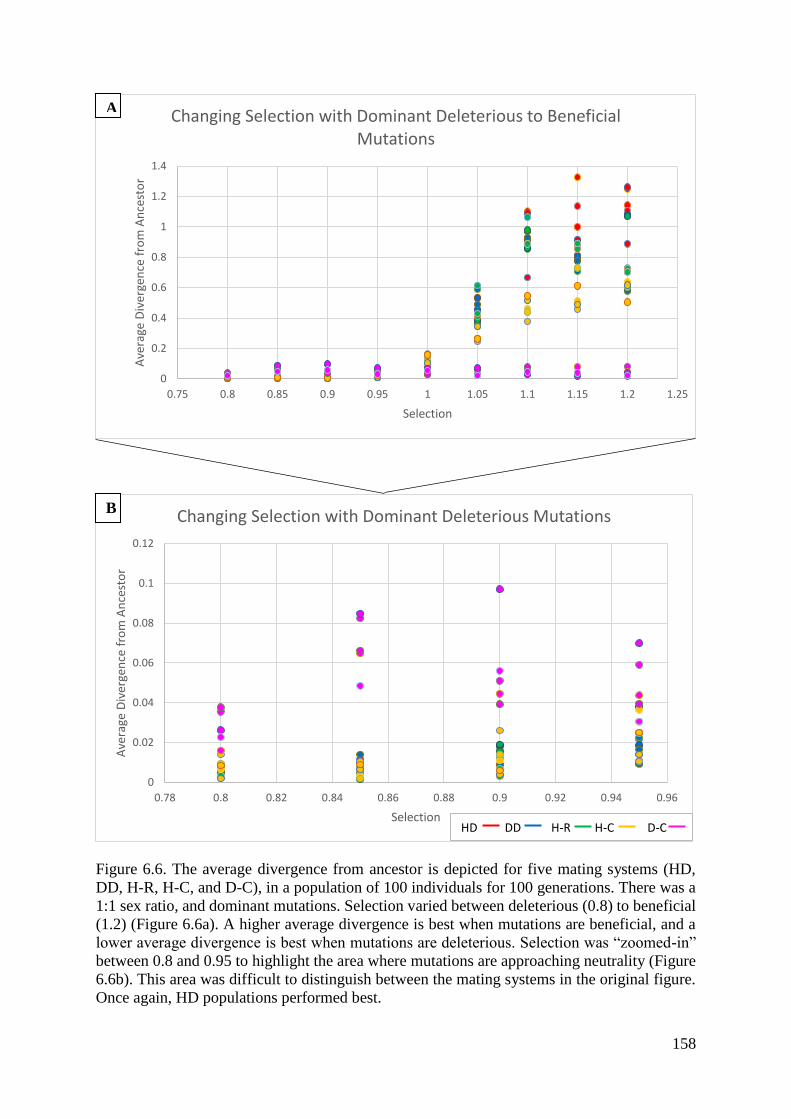
158

Figure 6.6. The average divergence from ancestor is depicted for five mating systems (HD,

DD, H-R, H-C, and D-C), in a population of 100 individuals for 100 generations. There was a

1:1 sex ratio, and dominant mutations. Selection varied between deleterious (0.8) to beneficial

(1.2) (Figure 6.6a). A higher average divergence is best when mutations are beneficial, and a

lower average divergence is best when mutations are deleterious. Selection was “zoomed-in”

between 0.8 and 0.95 to highlight the area where mutations are approaching neutrality (Figure

6.6b). This area was difficult to distinguish between the mating systems in the original figure.

Once again, HD populations performed best.

0

0.2

0.4

0.6

0.8

1

1.2

1.4

0.75 0.8 0.85 0.9 0.95 1 1.05 1.1 1.15 1.2 1.25

Ave

rage

Div

erge

nce

fro

m A

nce

sto

r

Selection

Changing Selection with Dominant Deleterious to Beneficial Mutations

0

0.02

0.04

0.06

0.08

0.1

0.12

0.78 0.8 0.82 0.84 0.86 0.88 0.9 0.92 0.94 0.96

Ave

rage

Div

erge

nce

fro

m A

nce

sto

r

Selection

Changing Selection with Dominant Deleterious Mutations

HD DD H-R H-C D-C

A

B

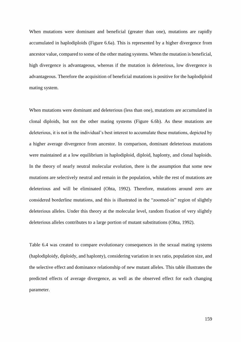
159

When mutations were dominant and beneficial (greater than one), mutations are rapidly

accumulated in haplodiploids (Figure 6.6a). This is represented by a higher divergence from

ancestor value, compared to some of the other mating systems. When the mutation is beneficial,

high divergence is advantageous, whereas if the mutation is deleterious, low divergence is

advantageous. Therefore the acquisition of beneficial mutations is positive for the haplodiploid

mating system.

When mutations were dominant and deleterious (less than one), mutations are accumulated in

clonal diploids, but not the other mating systems (Figure 6.6b). As these mutations are

deleterious, it is not in the individual’s best interest to accumulate these mutations, depicted by

a higher average divergence from ancestor. In comparison, dominant deleterious mutations

were maintained at a low equilibrium in haplodiploid, diploid, haplonty, and clonal haploids.

In the theory of nearly neutral molecular evolution, there is the assumption that some new

mutations are selectively neutral and remain in the population, while the rest of mutations are

deleterious and will be eliminated (Ohta, 1992). Therefore, mutations around zero are

considered borderline mutations, and this is illustrated in the “zoomed-in” region of slightly

deleterious alleles. Under this theory at the molecular level, random fixation of very slightly

deleterious alleles contributes to a large portion of mutant substitutions (Ohta, 1992).

Table 6.4 was created to compare evolutionary consequences in the sexual mating systems

(haplodiploidy, diploidy, and haplonty), considering variation in sex ratio, population size, and

the selective effect and dominance relationship of new mutant alleles. This table illustrates the

predicted effects of average divergence, as well as the observed effect for each changing

parameter.

160

Table 6.4. Expected and observed outcomes on average divergence from ancestor in haploidiploid (HD), diploid (DD), and haploid with

recombination (H-R) mating systems. Refer back to Table 6.2 for further descriptions of haploid, diploid, and haplodiploid mating systems with

the addition of beneficial and deleterious mutations. Refer to Figures 6.5 – 6.8 for a graph of the observed effect on average divergence, however,

not all results are included as figures.

Parameter Expected Effect on Average Divergence Observed Effect on Average Divergence

Population size increased Would increase with beneficial mutations and

decrease with deleterious mutations

As expected

Changes in sex ratio;

beneficial mutations;

dominant

Highest in H-R, followed by HD, and lowest

divergence in DD

Highest in HD, much lower for H-R and DD (which had the

lowest divergence)

At high female sex ratio (0.1), effect on HD

would be less compared to high male sex ratio

(0.9)

Sex ratio was higher in HD when more equivalent, and lower in

skewed sex ratios


strongly deleterious

mutations; dominant

Highest in DD, lowest in H-R Not clearly differentiated


beneficial mutations; co-

dominant

Divergence would be half as high compared to

beneficial mutations that were dominant

As expected

Pattern same as beneficial dominant – Highest

in H-R, lowest in DD

Not clearly differentiated, but appears to follow the expected

pattern



mutations; co-dominant

Divergence would be twice as high compared to

deleterious mutations that were dominant

As expected

Pattern same as deleterious dominant – Highest

in DD, lowest in H-R

As expected


beneficial mutations;

recessive

Highest divergence in H-R, lowest divergence in

DD

H-R and HD display equally high divergence, with DD

divergence substantially lower



mutations; recessive

Highest in DD, lowest in H-R As expected

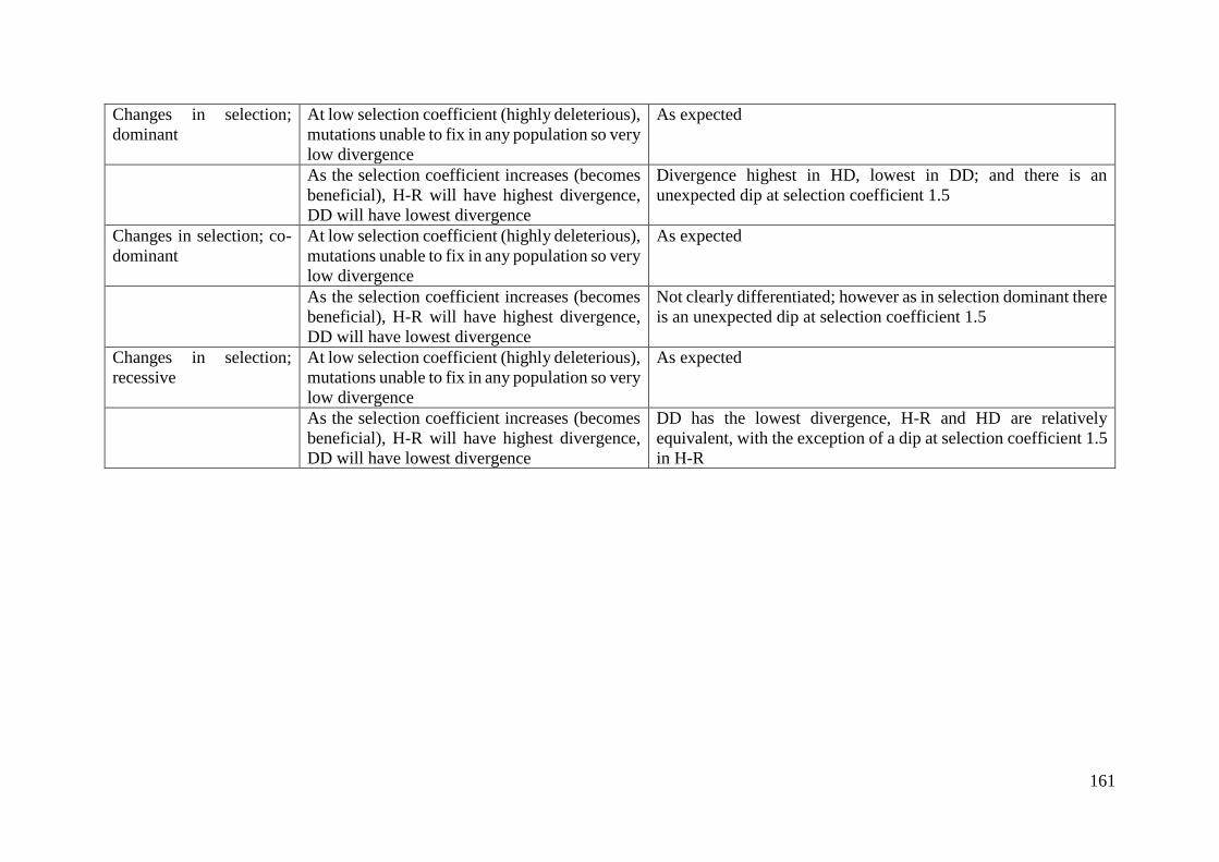
161

Changes in selection;

dominant

At low selection coefficient (highly deleterious),

mutations unable to fix in any population so very

low divergence

As expected

As the selection coefficient increases (becomes

beneficial), H-R will have highest divergence,

DD will have lowest divergence

Divergence highest in HD, lowest in DD; and there is an

unexpected dip at selection coefficient 1.5

Changes in selection; co-

dominant



low divergence

As expected




Not clearly differentiated; however as in selection dominant there

is an unexpected dip at selection coefficient 1.5

Changes in selection;

recessive



low divergence

As expected




DD has the lowest divergence, H-R and HD are relatively

equivalent, with the exception of a dip at selection coefficient 1.5

in H-R

162

Simulations were performed for dominant, co-dominant and recessive mutations, with

selection varying from very deleterious (0.3) to very beneficial (1.8). Five replicates were taken

for haplodiploid, diploid, and haplonty mating systems. Sex ratio was 1:1, and population size

was 10 000 individuals over 100 generations (results not shown). It was anticipated that very

deleterious mutations would not accumulate in the population in any of these three mating

systems, and instead be maintained at low equilibrium frequencies. This was true for

haplodiploid, diploid and haplonty mating systems, with dominant, co-dominant and recessive

deleterious mutations.

However, it was expected that when mutations are beneficial, they would accumulate and

spread through the population. It was anticipated that haplonty individuals would diverge at

the fastest rate with beneficial mutations, as there is only one copy of every allele. Therefore

immediate expression will lead to an increased fitness of the individual and its offspring.

Unexpectedly, the haplodiploid mating system performed better than haplonty when the

mutations were dominant, and relatively equivalently when the mutations were co-dominant

and recessive. This is likely due to the extra copies of genes in haplodiploid individuals

compared to haplonty providing more opportunities for beneficial mutations. In comparison,

diploid individuals had to lowest divergence when beneficial mutations. This is likely a

consequence of having two copies of each allele meaning only half as many mutations are

passed on to the offspring, when compared to the haplonty mating system.

Taken together with the results presented in Figure 6.5 and 6.6, haplodiploidy is best at

accumulating beneficial mutations and eliminating deleterious mutations at all dominance

levels when there is an equal 1:1 sex ratio. Therefore, this was further explored with varying

sex ratios to establish if this holds true in other situations.

163

6.3.3 Varying sex ratio with beneficial mutations:

In the first set of sex ratio simulations, five replicates were taken for haplodiploid, diploid, and

haplonty mating systems. This was performed for dominant, co-dominant and recessive

mutations, with sex ratio varying between highly female biased (0.1) to highly male biased

(0.9). Selection was beneficial (1.2), and population size was 10 000 individuals over 100

generations (Figure 6.7).

Many preliminary simulations were performed with varied selection coefficients, number of

generations, and population sizes (data not shown). There was little difference with number of

generations, therefore 100 generations was selected for consistency. In addition, a similar

pattern was observed for smaller-sized populations as for those with 10 000 individuals,

however average divergence from ancestor became larger with increasing population size.

Mutations spread more quickly when there is a larger number of individuals in a population,

therefore divergence will be increased.

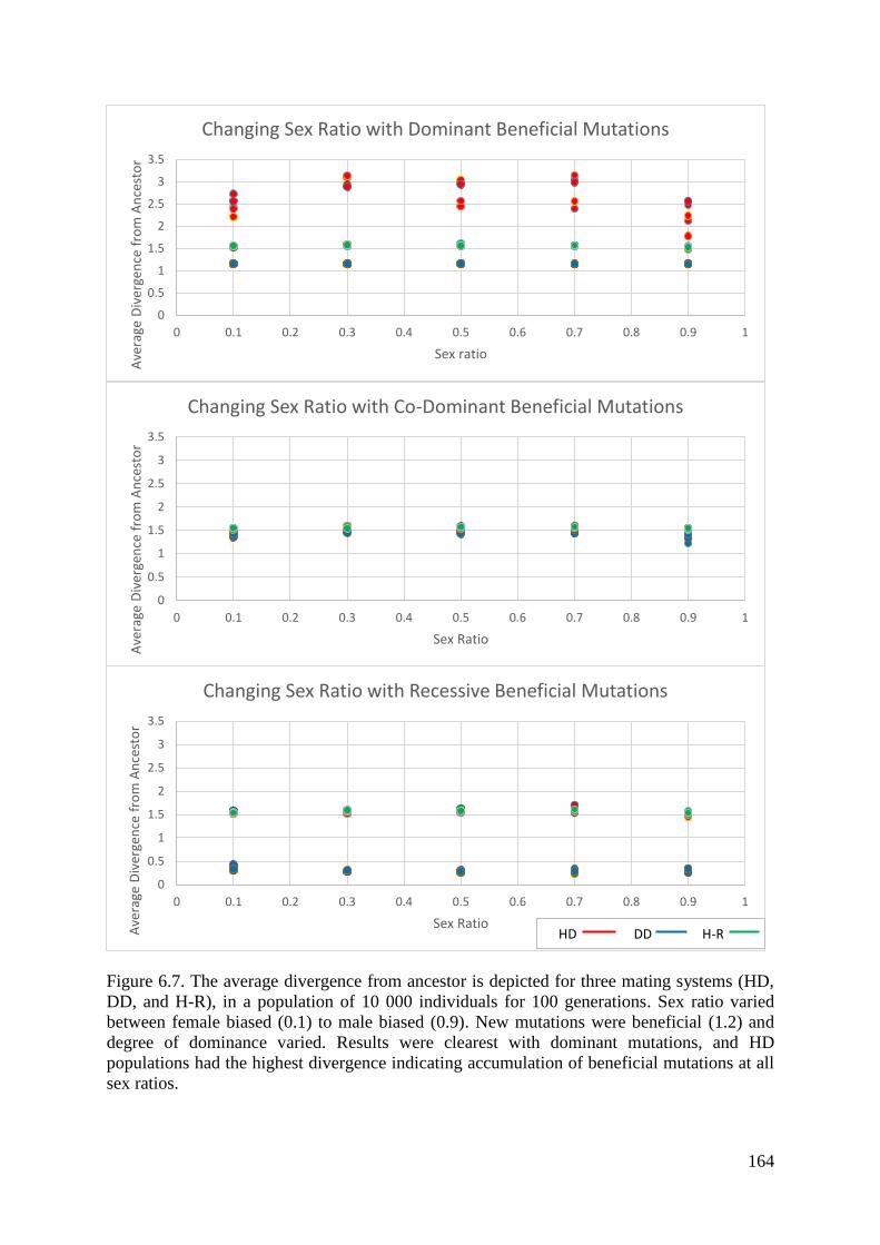
164

Figure 6.7. The average divergence from ancestor is depicted for three mating systems (HD,

DD, and H-R), in a population of 10 000 individuals for 100 generations. Sex ratio varied

between female biased (0.1) to male biased (0.9). New mutations were beneficial (1.2) and

degree of dominance varied. Results were clearest with dominant mutations, and HD

populations had the highest divergence indicating accumulation of beneficial mutations at all

sex ratios.

0

0.5

1

1.5

2

2.5

3

3.5

0 0.1 0.2 0.3 0.4 0.5 0.6 0.7 0.8 0.9 1

Ave

rage

Div

erge

nce

fro

m A

nce

sto

r

Sex ratio

Changing Sex Ratio with Dominant Beneficial Mutations

0

0.5

1

1.5

2

2.5

3

3.5

0 0.1 0.2 0.3 0.4 0.5 0.6 0.7 0.8 0.9 1

Ave

rage

Div

erge

nce

fro

m A

nce

sto

r

Sex Ratio

Changing Sex Ratio with Co-Dominant Beneficial Mutations

0

0.5

1

1.5

2

2.5

3

3.5

0 0.1 0.2 0.3 0.4 0.5 0.6 0.7 0.8 0.9 1

Ave

rage

Div

erge

nce

fro

m A

nce

sto

r

Sex Ratio

Changing Sex Ratio with Recessive Beneficial Mutations

HD DD H-R

165

As in Section 6.3.2, it was expected that haplonty populations would have the highest

divergence from ancestor when exposed to recessive beneficial mutations. As previously

described, there is only one copy of each allele in haploids; therefore a beneficial mutation

would be immediately expressed and rapidly passed from parent to offspring. In comparison,

in a haplodiploid population, the recessive beneficial mutation would only be immediately

exposed in males but not females, and could be stochastically lost while still at very low

frequency. The masking effects in a diploid population means only half as many mutations will

be passed on to the offspring; therefore divergence from ancestor will be lower. I anticipated

that sex ratios would have an effect on the level of divergence, with haplodiploid divergence

higher when sex ratio was male-biased, and lower when female-biased. When mutations are

recessive, the abundance of haploid males in the population will allow the beneficial mutations

to be passed through the generations at a high frequency.

When mutations were beneficial and co-dominant, it was difficult to distinguish between the

three mating systems (Figure 6.7). In both dominant and recessive simulations, the diploid

mating system had the lowest divergence from ancestor, as expected. Results were clearest

with dominant beneficial mutations, and showed that haplodiploids have the highest divergence

at all sex ratios (between approximately 2.5 to 3, compared to haplonty at 1.5). This result was

unexpected, as it was predicted haplonty would faster accumulate dominant beneficial

mutations. This is explained by the presence of extra copies of the genes in the haplodiploid

population compared to haptonty, which provides more opportunities for beneficial mutations.

Average divergence was equivalent between haplodiploids and haplonty when exposed to

beneficial recessive mutations. This indicates that haplodiploids are best at accumulating

beneficial mutations compared to haplonty and diploids. Refer back to Table 6.4.

166

6.3.4 Varying sex ratio with deleterious mutations:

In the second set of sex ratio simulations, five replicates were taken for haplodiploid, diploid,

and haplonty mating systems. This was performed for dominant, co-dominant and recessive

mutations, with sex ratio varying between highly female biased (0.1) to highly male biased

(0.9) in a population size of 10 000 individuals over 100 generations (Figure 6.8). As previously

stated, preliminary simulations were performed with varied selection coefficients, number of

generations, and population sizes (data not shown). It was established that for deleterious

mutations, a selection coefficient of 0.95 best distinguished the level of divergence for the three

mating systems. This mutation rate could be considered biologically applicable in wild

populations.

167

Figure 6.8. The average divergence from ancestor is depicted for three mating systems (HD,

DD, and H-R), in a population of 10 000 individuals for 100 generations. Sex ratio varied

between female biased (0.1) to male biased (0.9). New mutations were deleterious (0.95) and

degree of dominance varied. Results were clearest with recessive mutations, and DD

accumulated deleterious mutations, represented by high divergence. In comparison, HD had a

low level of accumulation of deleterious mutations at all sex ratios, however this value was

higher than in the H-R populations, which accumulated the fewest deleterious mutations.

0

0.02

0.04

0.06

0.08

0.1

0.12

0 0.1 0.2 0.3 0.4 0.5 0.6 0.7 0.8 0.9 1

Ave

rage

Div

erge

nce

fro

m A

nce

sto

r

Sex Ratio

Changing Sex Ratio with Dominant Deleterious Mutations

0

0.02

0.04

0.06

0.08

0.1

0.12

0 0.1 0.2 0.3 0.4 0.5 0.6 0.7 0.8 0.9 1

Ave

rage

Div

erge

nce

fro

m A

nce

sto

r

Sex Ratio

Changing Sex Ratio with Co-Dominant Delterious Mutations

0

0.02

0.04

0.06

0.08

0.1

0.12

0 0.1 0.2 0.3 0.4 0.5 0.6 0.7 0.8 0.9 1

Ave

rage

Div

erge

nce

fro

m A

nce

sto

r

Sex Ratio

Changing Sex Ratio with Recessive Deleterious Mutations

HD DD H-R

168

As in Section 6.3.2, it was expected that in the presence of deleterious mutations, diploids

would have the highest divergence from ancestor, and haplonty would have the lowest

divergence. In a large population, deleterious mutations will be masked in diploids due to

“duplicated” alleles, and these mutations will be passed to offspring and will persist in the

population. However in haplodiploid and haplonty populations, deleterious mutations will be

expressed and removed. Members of those populations that survive will have a higher fitness

to pass onto their offspring. As such, the divergence will be less, especially in haplonty as

removal will occur for both males and females, whereas in haplodiploids only males are haploid

and benefit from expression.

The level of divergence was not clearly defined in dominant deleterious mutations. However,

exposure to co-dominant and recessive deleterious mutations, illustrated higher divergence in

diploid populations, as expected. Diploids are able to mask deleterious mutations, therefore the

individual can survive and pass down the deleterious mutation to their offspring. The mutations

are not purged at a high rate and therefore remain in the population at low frequencies.

Consequently, the mutation persists for a longer period of time and becomes more diverged.

Results were clearest with recessive deleterious mutations in Figure 6.8. Diploids accumulated

deleterious mutations at a faster frequency (approximately 0.09), whereas haplodiploids and

haplonty accumulated deleterious mutations at a lower rate (approximately 0.05 and 0.02,

respectively), across all sex ratios. The haplonty population had the lowest divergence due to

the immediate expression and removal of deleterious mutations in all individuals, whereas

haplodiploids had an intermediate effect. This is due to deleterious mutations being exposed

and removed in the males, but masked and transmitted through the populations by the females.

Refer back to Table 6.4.

169

6.3.5 Differences between models:

To test the consistency of the above results, two models were designed with the same

information, but differed slightly in the way fitness was simulated. Three replicates were taken

for a population size of 100 individuals over 1000 generations, with an equal 1:1 sex ratio.

Selection was modelled at slightly beneficial (1.05) and very slightly deleterious (0.999).

Mutations were either fully dominant or fully recessive. The first model used the Perl program

designed in this chapter and provided in Appendix 2, and the second model used the

programming language C. Figure 6.9 compares haplodiploids and diploids under identical

parameters with the following pattern in both: haplodiploids were better able to accumulate

beneficial mutations when compared to diploids, and that the opposite was true regarding

deleterious mutations. The average divergence from ancestor was marginally higher for the C

program, which I expect is due to slight differences in how the program was coded.

170

Dominant Recessive

Figure 6.9. The average divergence from ancestor is depicted for two mating systems (HD and

DD), in a population of 100 individuals for 1000 generations. There was a 1:1 sex ratio, and

mutations were modelled as (a) dominant and slightly beneficial, (b) dominant and slightly

deleterious, (c) recessive and slightly beneficial, and (d) recessive and slightly deleterious. Two

programs, Perl and C, were compared. Under all conditions and both programs, haplodiploids

were better able to accumulate beneficial mutations, and eliminate deleterious mutations

compared to diploids.

0

1

2

3

4

5

6

7

8

9

10

0 200 400 600 800 1000

Ave

rage

Div

erge

nce

fro

m A

nce

sto

r

Generations

Beneficial Mutations

0

0.2

0.4

0.6

0.8

1

1.2

1.4

1.6

0 200 400 600 800 1000

Ave

rage

Div

erge

nce

fro

m A

nce

sto

r

Generations

Delterious Mutations

0

0.2

0.4

0.6

0.8

1

1.2

1.4

1.6

0 200 400 600 800 1000

Ave

rage

Div

erge

nce

fro

m A

nce

sto

r

Generations

Deleterious Mutations

0

1

2

3

4

5

6

7

8

9

10

0 200 400 600 800 1000

Ave

rage

Div

erge

nce

fro

m A

nce

sto

r

Generations

Beneficial Mutations

HD: Perl HD: C DD: Perl DD:

C

A

B

C

D

171

6.4 Conclusions

This chapter explored the rates of accumulation of beneficial and deleterious mutations and

simulated populations. Five mating systems (haploidploidy, diploidy, haplonty, clonal haploid

and clonal diploid populations) were examined at varying selection coefficients – from strongly

deleterious to strongly beneficial mutations. The y-axis in Figures 6.5-6.8 illustrate the average

divergence from ancestor. When mutations are beneficial, a high divergence is advantageous,

whereas when mutations are deleterious, a low divergence is optimal. For beneficial mutations,

all populations accumulate mutations, however in a population size of 100 individuals over 100

generations and an equal sex ratio, haplodiploid individuals were most adept at accumulating

beneficial mutations and keeping deleterious mutations at a low frequency within the

population. In comparison, when mutations were deleterious, few mating systems are

accumulate these mutations. Deleterious mutations are quickly exposed and removed from the

population in haploid males, increasing fitness of the survivors and their offspring. In

comparison, diploids mask recessive deleterious mutations due to having “duplicated” copies

of alleles. As such, these deleterious mutations are kept in the population. Due to a lack of

recombination, clonal populations were unable to accumulate beneficial mutations but had a

higher frequency of deleterious mutations.

Varying sex ratios from strongly female-biased to strongly male-biased were examined with

deleterious and beneficial mutations at differing levels of dominance across three mating

systems (haplodiploid, diploid, and haplonty). When mutations were beneficial, haplodiploids

had a higher divergence from ancestor, indicating the accumulation of mutations. However,

when mutations were deleterious, diploids accumulated these mutations, which would have a

negative impact on their survival. In comparison deleterious mutations remained at a low

frequency in haplodiploids, and an even lower frequency in haplonty populations. Haplodiploid

172

males are able to expose and remove the deleterious mutations, whereas both males and females

can expose and remove deleterious mutations in haplonty populations.

In the next chapter, these results will be expanded to include haplodiploid and diploid mating

systems within one population. The population will begin as diploid, however the introduction

of a cytoplasmic maternally-transmitted element into the population will turn males who inherit

this element from their mothers, haploid. This will be performed to have a direct competition

between these two mating systems to assess whether haplodiploidy shows more adaptive

evolution compared to diploidy. Based on the results from this chapter, it is expected that the

element will spread through the population and after a chosen number of generations, the

majority of the population will have changed from diploidy to haplodiploidy.

173

Chapter 7: Haplodiploid and Diploid Direct Competition

7.1 Introduction

Previous results (see Chapter 6) illustrated the advantages of haplodiploidy using Perl

simulations due to the immediate exposure and removal of deleterious mutations as well as

faster accumulation of adaptive mutations compared to other genetic systems. However,

although haplodiploidy may be advantageous for the individual to evolve to this mating system

for survival, it may not readily spread through the population. In fact, the strategy most likely

to evolve is the one with the most evolutionary stable strategy (ESS). In this chapter I will

explain the concept of an ESS, followed by the evolution of haplodiploidy. This will further

discuss previous notions from Chapter 6 regarding the advantages and disadvantages of

haploidiploidy, as well as outlining mechanisms which can turn an individual haplodiploid.

Finally, a model will be used to directly compete diploids and haplodiploids in the same

program to determine whether haplodiploidy will spread through a diploid population.

7.1.1 Evolutionary stable strategy:

a. Concept:

John Maynard Smith (1974) expanded upon previous ideas and research (Maynard Smith &

Price, 1973, Geist, 1966, Hamilton, 1967, MacArthur, 1965) to propose the concept of an

evolutionary stable strategy (ESS). This work was first carried out with regards to animal

conflicts, however the underlying ideas have been applied to many other evolutionary

phenomena, such as the Prisoner’s dilemma (Lindgren, 1992), the social sciences (Axelrod,

1984), and game theory (Maynard Smith, 1992b). This concept is solely dependent on

individual advantage and is not impacted by interactions with nature. When the best strategy

174

for an individual is reliant on the behaviour of others, ultimately the strategy that they adopt

will be an ESS (Maynard Smith, 1992a).

b. Evolutionary invasion analysis:

One of the main issues when modelling genetic systems is the level of genetics explicitly

included within that model. Optimality arguments are used in an attempt to predict evolution,

on the basis that a particular trait will be maximized over time (Otto & Day, 2007). These are

a measure of fitness, normally assessed though either population growth rate or the basic

reproduction number (Mylius & Diekmann, 1995). In a steady state, both these values can be

considered maximal. One refers to the environment, determined by the resident; whereas the

other refers to the type of invader in a population (and the maximum is determined with respect

to this value). Fitness measure is reliant on the way density dependence acts, and when

examining life-history traits, population growth is limited by this density dependence (Mylius

& Diekmann, 1995). However, even if something is beneficial for the individual, it does not

necessarily mean that it will evolve in the population.

Many hypotheses, including some game-theoretic models are based on principles of

evolutionary invasion analysis, but do not overtly outline the genetic model upon which they

are based (Otto & Day, 2007). Genetic and ecological details such as number of individuals or

genes can be ignored in place of observing social interactions of the requisite species. One type

of evolutionary invasion analysis, adaptive dynamics, attempts to elucidate evolutionary forces

with a focus on explicit mathematical framework and mutational steps. Evolution is considered

a mutation-limited process, where there is an equilibrium in the population when only a single

allele remains. Introduction of a new allele through mutation either replaces the current allele,

175

with a new equilibrium reached, or is lost. This process continually repeats itself, and adaptive

dynamics provides a clear stochastic model of this process (Otto & Day, 2007).

c. Example – hawk/dove:

Conflict situations result in strategies where an individual can cause serious injuries to another,

or strategies where injury is impossible and the winner is the individual who is able to fight the

longest (Maynard Smith & Price, 1973). A common example of an ESS-based evolutionary

model is given in Table 7.1, where it was asked: what selection strategy is best for the

individual? It should be noted that this is a simplified model, and the “best” outcomes, in terms

of optimal average outcome for the population as a whole, is not necessarily best for an

individual and therefore may not be one that evolves (Maynard Smith & Price, 1973).

Table 7.1. Average pay-offs using computer simulations of five strategies (Maynard Smith &

Price, 1973). Green illustrates ESS, yellow is almost an ESS, and red is not an ESS. Only

“Retaliator” is an ESS, with “Prober-Retaliator” almost an ESS. In the other strategies, the pay-

off for the opponent is not highest for the corresponding contestant. Evolution will occur to

comprise mainly these two strategies, with the other three kept at low frequencies in the

population by mutation.

Contestant

receiving

the pay-off

Opponent

Mouse Hawk Bully Retaliator Prober-

Retaliator

Mouse 29 19.5 19.5 29 17.2

Hawk 80 -19.5 74.6 -18.1 -18.9

Bully 80 4.9 41.5 11.9 11.2

Retaliator 29 -22.3 57.1 29 23.1

Prober-

Retaliator

56.7 -20.1 59.4 26.9 21.9

Under natural selection, if most members of a population adopt the ESS, no invading “mutant”

strategy would have a higher reproductive fitness (Maynard Smith & Price, 1973). A payoff

may be a direct or indirect measure of fitness, and even if the fitness of a population may be

maximised under certain conditions, the strategy will not be considered a competitive optimum

176

or ESS if a mutant strategy can invade (Parker & Maynard Smith, 1990). An ESS may be either

a pure or mixed strategy; a mixed strategy is defined as adopting a “pure” strategy based on

preassigned probabilities (Maynard Smith, 1974). Therefore a stable population may be

genetically polymorphic (different frequencies of individuals adopting different pure

strategies), or monomorphic (behaviour of individuals is appropriately random) (Maynard

Smith, 1974). Overall, the ESS is to adopt a strategy that does not cause serious injury, but to

escalate to serious injury if your opponent does (Maynard Smith & Price, 1973). However,

there are some instances where an optimal ESS is not generated (Parker & Maynard Smith,

1990).

d. Example – sex ratio:

An important application of ESS thinking is the evolution of the sex ratio (Maynard Smith,

1992a). In most species there are an equal number of males and females, and equal sex ratios

tend to evolve. One option seeks to explain this by evolving the sex ratio to maximize the

number of encounters between individuals of the opposite sex. This is a “group selection”

argument, and was proposed as an adaptive explanation for the prevalence of 1:1 sex ratios as

optimal (Maynard Smith, 1992a). However, equal sex ratios are not best from an “optimise the

population” perspective (ie fig wasps) (Cook et al., 2017). If group selection was strong and

groups tended to “win” an ESS, then few males would be needed to successfully sustain the

population. There would be an unequal sex ratio, therefore, optimisation at the population level

is not necessary.

The second option taken from Fisher (and the one Maynard Smith deems correct) assumes

genes can influence the sex ratio by favouring the number of offspring produced by one

individual carrying the genes (Maynard Smith, 1992a). In a female biased population,

177

production of sons will lead to more grandchildren, with the opposite being true of daughters

in a male-biased population. If there are equal numbers of males and females, offspring of both

sexes are equally important making a 1:1 sex ratio the “evolutionary stable strategy”. There

may also be different costs associated with the production of sons or daughters (Maynard

Smith, 1992a). Sex ratio theory based on ESS and Fisherian assumptions has been rigorously

tested, and can generally explain sex ratios in nature very well (Frank, 1990).

7.1.2 Evolution of haplodiploidy:

There are many different mechanisms through which haplodiploidy may have evolved (Table

7.2). See (Blackmon et al., 2015) for a current theory of how haplodiploidy evolved due to

genetic conflicts, as well as authors who have considered different theories for haplodiploidy

evolution. Two of the most common methods to generate haplodiploids are arrhenotoky

(unfertilized eggs develop into males), and pseudo-arrhenotoky (males develop from fertilized

eggs but become haploid after paternal genome inactivation or elimination) (Sabelis &

Nagelkerke, 1988). Although in both systems males are effectively haploid and only the

maternal genome is passed down to their offspring (Sabelis & Nagelkerke, 1988), these two

processes differ as arrhenotokous males are completely haploid throughout development,

whereas pseudo-arrhenotokous males begin development as diploid, but lose their paternal

genome and their genes are not passed down to offspring (Normark, 2004).

178

Table 7.2. Four hypotheses for the evolution and maintenance of haplodiploidy (Normark,

2004). Sex ratio control illuminates why haplodiploidy may occur, and the other three

hypotheses describe the mechanisms behind how the process of haplodiploidy may occur.

Hypothesis Description References

Sex ratio control There is maternal control over sex-ratio in

haplodiploidy which leads to female-biased sex

ratios

(Hamilton, 1967,

Borgia, 1980)

Haplodiploid individual has the advantage

Maternal transmission

advantage

Females have a transmission-genetic advantage

if they can produce viable sons without the

requirement of a male parent

(Brown, 1964,

Hartl & Brown,

1970, Smith,

2000, Bull, 1979)

Most successful mechanism

Haplodiploid individual has the advantage

Deleterious mutation

clearance

Selection during the haploid phase is most

effective at removing deleterious mutations

(Smith, 2000,

Goldstein, 1994)

Haplodiploid population has the advantage

Feminizing

endosymbionts

Endosymbionts are transmitted maternally and

eliminate the paternal genome; only the

maternal genes are passed to offspring,

resulting in a female-biased sex ratio

Primary reference

not found, but see

(Normark, 2004)

Endosymbiont has the advantage but not the

haplodiploid host

Previous models of mating system evolution often compare different mating systems, in

particular haploidy with diploidy, to identify the duration an individual remains in each phase

due to the advantages of being either haploid or diploid for a prolonged period of time (Jenkins

& Kirkpatrick, 1995). Theoretical studies which examined effects of deleterious mutations

displayed different outcomes (Jenkins & Kirkpatrick, 1995). In a population which includes

genome-wide mutations and selection, if there is no interbreeding between haploids and

diploids, then diploidy is favoured when epistasis is strong between loci (Kondrashov & Crow,

1991). However, diploidy can be evolved without epistasis, and diploid systems can be

favoured over haploid systems under “reasonable assumptions” of dominance and

recombination (Perrot et al., 1991, Kondrashov & Crow, 1991, Bengtsson, 1992, Otto &

Goldstein, 1992). The development of a two-locus model provided a basis for interbreeding

between haploid and diploid individuals (Perrot et al., 1991). Diploid invasion was dependent

on how deleterious the mutation was, and diploids only invaded when dominance degree of

179

each deleterious mutation was less than ½ (Perrot et al., 1991). A companion study (Jenkins &

Kirkpatrick, 1994) referenced in Jenkins & Kirkpatrick (1995), developed a single locus model

where lengths of haploid and diploid phases could be varied. It was determined that haploidy

evolves when there is complete linkage, mutations are strongly deleterious, or mutations are

partially dominant (Jenkins & Kirkpatrick, 1994).

Furthermore, evolution of life cycles were examined in a model that included mutation and

selection in an interbreeding population (Jenkins & Kirkpatrick, 1995). The length of time

spent in haploid and diploid phases can evolve, with a single genetic locus controlling the

amount of time spent in each phase. Selection acts on deleterious mutations and results in the

evolving life cycle. The number of deleterious mutations controls mortality rate of the

individual. There are epistatic interactions between mutations and fitness is multiplicative

across loci. Results of this genome-wide analysis again showed that the diploid phase in

increased under biologically reasonable assumptions, regardless of the presence or absence of

epistasis. In comparison, the haploid phase is favoured when mutations are highly deleterious

or partially dominant. This supports the evolution of life cycles in the above models which

examined interbreeding populations and selection on mutations at single-loci (Jenkins &

Kirkpatrick, 1995). Therefore, to expand upon these concepts and examine mating systems

from a different angle, I created a simulation model where two strategies (diploid and

haplodiploid) could be competed directly (Section 7.2). The following sections discuss

advantages of male haploidy that can be incorporated into these models, as well as difficulties

of male haploidy, something which is not normally included in models.

180

7.1.3 Advantages for haplodiploid males:

a. Maternal transmission advantage:

In haplodiploid males, only the maternal genome is transmitted; therefore the maternal genes

will occur twice as often in the gametes of haploid sons when compared to the gametes of

diploid sons (Bull, 1979). This two-fold representation of maternal genes confers a selective

advantage on females for the selection of haploid males when compared to biparental diploid

sons. This provides higher identity-by-descent between a grandmother and her grandchild, an

advantage which may compensate for the potentially lower fitness of the haploid male

offspring. Once haploid males are established, selection must be towards mutations in maternal

genes that produce haploid sons and against paternal genes attempting to restore diploid sons

(Bull, 1979).

b. Maternal sex ratio control:

As previously discussed, there is an increased ability for haplodiploid individuals to control

sex ratio (Sabelis & Nagelkerke, 1988). In mites, the Phytoseiidae are pseudo-arrhenotokous,

where haploid males arise from fertilized eggs. However, the paternal genome is eliminated by

an unknown underlying maternal control mechanism that distinguishes between the paternal

and maternal genomes, prior to inactivation and elimination of the paternal genome (Sabelis &

Nagelkerke, 1988).

c. Female reproductive assurance:

A final advantage of male haploidy is reproductive assurance for females in instances where a

sexually compatible partner cannot be easily obtained (Gates & Nason, 2012). In figs (genus

Ficus, family Moraceae), there is a mutualistically beneficial relationship with species-specific

181

pollinating fig wasps. Although Ficus is very diverse with greater than 750 species, individual

species are found at low population densities. Consequently, dispersal between the fig and

wasps is quite difficult. This can further be exemplified in many plants, as a requirement for

survival is some sexual reproduction via outcrossing through the movement of pollen (often by

an animal from one plant to another). Many of these plants, however, are self-compatible and

can undergo selfing as well as outcrossing. Selfing increases gene transmission and provides

reproductive assurance by eliminating the need of a “mate” for sexual reproduction (Gates &

Nason, 2012). This is a similar process in haplodiploidy: since females can produce males from

unfertilized eggs, if there is a lack of mates there is a shift towards reproduction in this manner

so that the population is still able to survive and thrive.

7.1.4 Difficulties of transitioning to male haploidy:

a. Exposure of deleterious alleles:

Ultimately the evolution of the haplodiploidy mating system is dependent on overcoming

issues with development of haploid males (Borgia, 1980). The process of haploid male

spermatogenesis is highly restrictive, which has likely limited the evolution towards

haplodiploidy (Whiting, 1945, Hartl & Brown, 1970). It is necessary for diploids to have a low

level of deleterious mutations, otherwise there would be issues with haploid survival (Whiting,

1945, Hartl & Brown, 1970). Inbreeding assists haplodiploidy through purging deleterious

mutations which results in a reduced mutational load, as well as reducing the effectiveness of

recombination (Smith, 2000). Diploid individuals carry recessive lethal mutations, and if these

genes are passed to an unfertilized haploid egg, there is incomplete parthenogenesis and

mortality (Whiting, 1945, Hartl & Brown, 1970).

182

b. Parthenogenesis and dosage compensation:

In a normal diploid population, genes favouring parthenogenesis will spread through the

population (Whiting, 1945, Hartl & Brown, 1970). However, in most diploid species there are

mechanisms like dosage compensation which act as a barrier to parthenogenesis.

Parthenogenesis results in a reduced number of chromosomes in haploid males (Whiting, 1945,

Hartl & Brown, 1970). Due to the imbalance between two large gene rich X chromosomes in

females, and only one X chromosome and one small, gene poor Y chromosome in males,

individuals have evolved processes to equalise gene expression (dosage compensation)

(Brockdorff & Turner, 2015, Kaiser & Bachtrog, 2010). For a haplodiploid male to develop,

dosage compensation mechanisms must be overcome (Whiting, 1945, Hartl & Brown, 1970).

Haplodiploidy may take away some of these barriers, as females are able to make males without

a father. Genes favouring parthenogenesis are likely to be transmitted in genetic systems where

the initial viability of many eggs is poor (Normark, 2006), and may particularly occur in

haplodiploids due to the two-fold increase in relatedness of mothers to their haploid offspring

(Brown, 1964). However, it should be noted that full parthenogenesis is considered an

evolutionary dead-end (Maynard Smith, 1978), as referenced in (Lynch & Gabriel, 1983). Due

to the two-fold cost of sex in haplodiploidy, population size would be increased fastest by

cloning (Maynard Smith, 1992a). However, males are still being made at a higher frequency in

haplodiploidy, something which would not occur so readily in cloning. As such, adaptive

evolution will favour haplodiploidy over asexual mating systems (Maynard Smith, 1992a).

7.1.5 Paternal genome elimination as an intermediate step:

a. Definition:

Haplodiploidy most often occurs through arrhenotokous reproduction, where unfertilized eggs

develop into haploid males and fertilized eggs develop into diploid females (Normark, 2004).

183

However, a haplodiploid mating system can also be created through paternal genome

elimination (PGE; pseudo-arrhenotoky) (Normark, 2004). PGE is frequent in arthropods, and

often occurs by infection with endosymbionts (ie Wolbachia) (Cordaux et al., 2011). In groups

of arthropods, PGE occurs less often than haplodiploidy (Yokogawa & Yahara, 2009). As such

it was suggested that PGE acts as a transitionary step towards haplodiploidy, a theory which

has not yet been explicitly tested (Schrader & Hughes-Schrader, 1931), or that that PGE may

evolve into arrhenotoky which would eliminate the need for males and any paternal

contribution (Normark, 2004).

b. Endosymbionts in arthropods:

Endosymbionts are a factor which have been known to manipulate host reproduction affecting

mating systems in arthropods (Cordaux et al., 2011). For example, the common endosymbiont

Wolbachia infects arthropods and causes PGE in the infested individual (Cordaux et al., 2011).

Although nuclear volumes are consistent between males and females in organisms, there is a

large size discrepancy in cytoplasmic volume (Normark & Ross, 2014). Due to the egg having

a much greater cytoplasmic volume compared to sperm, often including elements with their

own genome, cytoplasmic genomes are transmitted via females. As a result, unlike in the

nucleus, there is no direct fitness on the cytoplasmic elements in males. Consequently, male

fitness is often sacrificed for female fitness in one of four ways: cytoplasmic incompatibility,

male-killing, feminization of genetic males, and parthenogenesis induction (Normark & Ross,

2014) (Table 7.3).

184

Table 7.3. Wolbachia is the only known endosymbiont to induce all four types of reproductive

manipulation leading to haploid males following initial development as diploids (Cordaux et

al., 2011). Each type of reproductive manipulation leading to male haploidy is described in

detail.

Reproductive

Manipulation

Process Description

Cytoplasmic

incompatibility

Favours infected

female

reproduction

Causes sterility due to sperm and egg incompatibility

during mating between an infected and uninfected

individual

Maternally inherited endosymbionts are transmitted

Male-killing Distorts sex ratio Male offspring death leads to highly female-biased

sex ratio

Differs from feminization and PI as death occurs in

the (male) sex that does not vertically transmit

endosymbionts

Feminization Distorts sex ratio Converts genetic males into phenotypic functional

females, which leads to a highly female-biased sex

ratio

Mechanism largely unknown, however possible that

interactions between endosymbionts with different

molecular pathways create populations in which all

Wolbachia infected individuals develop a female

phenotype, and non-carriers develop as males

Parthenogenesis

induction

Distorts sex ratio Converts non-transmitting (genetic) haploid males

into transmitting (genetic) diploid females, through

chromosomal doubling in unfertilized eggs

Infected females can then produce endosymbiont-

transmitting female offspring without the use of males

during sexual reproduction, promoting asexual

daughter development (highly female-biased sex

ratio)

c. Hypothesis one for paternal genome elimination evolution:

There is a high risk for male haploids to revert to diploidy if there are mutations transmitted

through sperm which prevent PGE (Bull, 1979). As such, inheritance of genes controlling PGE

from the mother may lead to the evolution of male haploidy (Bull, 1979). An XX-XO sex

determination system may be able to evolve into a maternally controlled sex ratio system,

allowing for PGE evolution (Haig, 1993). This XX-XO sex determination system is found in

nature in species such as nematodes, where sperm with an X chromosome produce daughters,

and without an X chromosome produce sons (Haag, 2005). X-linked genes favour higher

185

proportion of X-bearing sperm in males when compared to autosomal genes. If there is meiotic

drive on the X chromosome in XO males, autosomal genes may evolve to exploit this system

to be included in X-bearing sperm. This high level of X-bearing sperm leads to a highly biased

female sex ratio, and an overall evolution to eliminate the paternal genome (haplodiploidy)

(Haig, 1993).

d. Hypothesis two for paternal genome elimination evolution:

The second hypothesis involves the invasion of a maternally transmitted endosymbiont which

turns diploid male zygotes into haploids (Haig, 1993) (Table 7.4). Normark’s original model

is based off Hamilton’s (1993) observation that haplodiploid ancestors were commonly

infected by symbionts. This hypothesis combines the maternal transmission advantage along

with the association to maternal endosymbionts (Normark, 2004). Engelstädter and Hurst

(2006) expanded upon Normark’s model to examine the conditions which allow male

haplodizers to invade the population. They found issues with the original model, namely it is

never beneficial to be a male-killer when viability for haploid males is low, as the skewed

female-biased sex ratio would reduce the fitness of infected females (Engelstädter & Hurst,

2006). Additionally, haploid male fertility must be high to generate conditions in which male-

killers are beneficial for host females, which is unlikely in an initial population (Engelstädter

& Hurst, 2006). Although Normark’s model plus their expansions is plausible, evolution acting

on both the bacteria and the host is necessary to drive haplodiploidy evolution by male-killers

(Engelstädter & Hurst, 2006). Kuijper & Pen (2010) demonstrated that the assumptions made

in the previous models would not lead to the persistence of haplodiploidy. Eventually the

survival of haploidized males will select for maximal levels of haploid male viability and

reallocate resources from infected hosts. This decreases the fitness benefits of infected hosts,

as such, the endosymbiont is likely to be purged due to genetic drift (Kuijper & Pen, 2010).

186

Table 7.4. Models for the origin and adaptation of haplodiploidy providing further support for

hypothesis two of the evolution of PGE through the invasion of a maternally transmitted endosymbiont

turning diploid male zygotes haploid.

Model Mechanism Outcome

(Normark,

2004)

Cytoplasmic maternally transmitted

element (male hapolidizer) that kills

males by haploidizing them

immediately after fertilization (reacts

against the genome of incoming male-

determining sperm (Ych))

Small number of haploid males survive,

and the elimination of the paternal genome

provides an advantage to the maternal host

(increased transmission of her genome

through haploid males)

Provides an opportunity for the male-

killing endosymbionts to become fixed in

the population, which in turn may increase

haploid male viability and result in a PGE

genetic system

(Engelstädter

& Hurst,

2006)

As before, but includes circumstances

allowing maternally transmitted

male-killing bacteria to invade and

thrive in a population, alters the

associated cost of the death of sons

due to the higher female sex ratio, and

the unequal gene transmission

through offspring infected and

uninfected females

As before, meaning a haplodiploid mating

system may be favoured in the population

(Úbeda &

Normark,

2006)

Analyze co-evolution between male

haploidizers and its host by including

variable transmission of male

haplodizers and variable survivorship

of haploidized males

Invasion of male haplodizers leads to

selective pressures on bacterial

transmission and host survivorship;

regardless of whether gene control is

cytoplasmic or nuclear, male haplodizers

either become fixed or go extinct

Selection on cytoplasmic genes increase

their own transmission but decrease male

host survivorship; selection on nuclear

genes may increase or decrease bacterial

transmission, but increase host

survivorship

PGE originates once selection acts to

maintain male haplodizer transmission and

host survivorship, keeping the population at

this equilibrium

(Kuijper &

Pen, 2010)

As before, with two proposed

mechanisms through which male-

killing endosymbionts can drive the

evolution of haplodiploidy: spatially-

structured populations which are

highly inbreed, or a mutualistic

relationship between endosymbionts

and their hosts

It is nearly impossible for the haplodizing

endosymbiont (and haplodizing males) to

stably persist in a population longer than 20

000 to 30 000 generations when

transmission is controlled by either the host

or the endosymbiont

187

7.1.6 Competition model:

To further explore haplodiploidy and diploidy, I created a simulation model which allowed for

direct competition between the two mating systems. I was interested in exploring that given

the advantages incurred by haplodiploids (see Chapter 6), will this mating system be able to

evolve from diploidy. The two programs were modelled as similarly as possible, with both

males and females beginning development as a diploid. The only difference was the

introduction of a maternally transmitted element causing haploidploidy in diploid males if they

inherited the element to create competition between the two mating systems. Since

haplodiploidy favours the mothers, as outlined in Section 7.1.3, the element was modelled as a

maternally transmitted cytoplasmic element.

The aim of this model was to determine whether haplodiploidy is a better mating system to

evolve, as it has proven to be an efficient system for removal of deleterious mutations and

accumulating beneficial mutations. From this, the model could be examined through many

generations to determine whether haplodiploidy is carried and converts all members of the

population to this genetic mating system, or whether haplodiploidy is lost after a few

generations and the population remains diploid.

188


7.2.1 Competition parameters:

As before, Perl 5 (Schwartz et al., 2017) was used to directly compare haplodiploidy and

diploidy, within the same population. As in Chapter 6, number of genes was kept constant at

20, and mutation rate was kept constant at 0.001 throughout all simulations. There was a 1:1

sex ratio (0.5), in a population size of 100 individuals, and the simulation was run for 100

generations. Selection and dominance varied between simulations. These simulations differed

from those presented in Chapter 6 in that some females initially carried a maternally transmitted

element inducing haplodiploidy. The complete program is provided in Appendix 2, Figure 7.5.

7.2.2 Maternally transmitted element:

As outlined in the introduction, there are a variety of potential mechanisms which can be used

to convert diploid males into haploid males. For these simulations, it was decided that the most

straightforward way to model the two mating system competition was for individuals to begin

as diploid, and introduce a maternally-transmitted element which caused male haploidy. The

element had an initial starting rate in the population which illustrated the number of individuals,

both male and female, who carried the element. All females, regardless of whether they carried

the element or not would be diploid and remain in this state throughout all matings and

generations. Diploid females who did not carry the element would mate with diploid males and

produce diploid offspring (male and female). However, diploid females who carried the

element would mate with diploid males and produce haploid sons; this amounts to paternal

genome elimination. Haploid males are able to mate, and transmit their entire genome to

offspring. Note that the reproductive assurance advantage of haplodiploid therefore does not

apply, as the females must still find a suitable fit male for mating. The prevalence of this

189

element, determining the frequency at which it was transmitted through the population could

be measured over a set number of generations. See Figure 7.1 for an illustration of how the

competition Perl program was designed.

The maternally transmitted element causing paternal genome elimination was introduced at a

starting rate of either 0.1, 0.5, or 0.9. If the mutation was completely neutral, due to genetic

drift it would be expected that the element would be fixed 10% of the time, 50% of the time,

or fixed 90% of the time, respectively. Strong variations from these values would indicate

whether haplodiploidy or diploidy was favoured in the population, as the rate of loss or gain of

the element would not be due to random chance (drift).

7.2.3 Initial diversity:

Following the first set of simulations (see Section 7.3.1), an initial diversity parameter for

standing genetic diversity was included in the simulations. This represented the percentage of

alleles that were initially mutated within the population prior to mating, and illustrates another

difference between the competition parameters and those from Chapter 6. Without an initial

diversity, there are no recessive deleterious alleles in the population to begin with.

Haplodiploidy will expose and remove these alleles over a period of time as they accumulate

in the population, however there would be no immediate initial effect. By introducing an initial

diversity, females may already have deleterious alleles to be passed on to her sons, which would

be a disadvantage to these males. Therefore, the initial diversity was included in the simulations

to better resemble a transition from an initial diploid state with some standing genetic diversity

to haplodiploidy.

190

Figure 7.1. Design of Perl for a diploid population which turns some males haploid through the

introduction of a maternally transmitted paternal genome elimination element. Rate of gain /

loss of the element illustrates whether haplodiploidy or diploidy becomes the dominant genetic

system. Compare with Figure 6.4 (haplodiploid mating system).

Set up initial diploid population with a set level of standing genetic variation

Subroutine: Spermatogenesis Subroutine: Oogenesis

Make males (2x genes)

Fitness low

Repeat for population

size & sex ratio

Fitness high

Make females (2x genes)

Fitness high

Make each generation

Start with no females


random male

Check fitness

Fitness low


size & sex ratio

Fitness high

Female does not

have element

Make diploid male

Fitness high

Make diploid

female or male

(may / may not

have element)

Fitness low


size & sex ratio

Fitness low


size & sex ratio

Start with no males


random male

Check fitness

Make males Make females

Reset for next generation

Make next generation

Repeat until generation complete (accurate population size)

Repeat until number of generations completed

Report element prevalence of

each individual

Maternally transmitted

element leads to paternal

genome elimination

Fitness high

Female has element

Make haploid male

191


7.3.1 Comparing element prevalence without initial diversity:

In the first set of simulations, three replicates were taken for dominant, co-dominant, and

recessive mutations with varying selection rates (refer to Section 7.2.1 for full conditions). This

was examined for a starting element rate of 0.1, 0.5, and 0.9 (results not shown). These results

illustrated that at a starting element rate of 0.1, the maternally transmitted element causing PGE

never reached fixation. It would be expected that at this starting rate, the element would fix

10% of the time. It was decided to introduce a standing initial diversity rate so some members

of the population may already have deleterious alleles to be inherited by their offspring. I could

select the percentage of alleles that were initially mutated within the population prior to mating

and accelerate the mutation rate to increase chances of haplodiploidy. Without an initial

diversity, there is no immediate consequence of recessive deleterious alleles in the population.

This better resembles the transition from an initial diploid state with some standing genetic

diversity to haplodiploidy.

7.3.2 Comparing element prevalence with initial diversity of 0.01:

In the second set of simulations, 10 replicates were taken for dominant, co-dominant, and

recessive strongly deleterious mutations (0.8) (refer to Section 7.2.1 for full conditions). The

choice of strongly deleterious mutations was used as this value will likely not be found in

nature, and would be a clear indication of whether haploid males becomes fixed in the

population. If this did not occur at such an extreme, it is unlikely that the results will be clear

around neutrality, where mutations are more likely to occur in the wild. Simulations were

performed for a starting element rate of 0.1, 0.5, and 0.9. It was expected that if only genetic

drift was acting on neutral mutations (selection coefficient 1.0), mutations would fix at 10%

192

(for starting element rate 0.1), 50% (for starting element rate 0.5), and 90% (for starting element

rate 0.9). Standing genetic diversity was initially set at a low value of 0.01; this illustrated that

1% of alleles in the original population will mutated prior to mating. Results are provided in

Table 7.4.

Table 7.4. Expected and observed rates of fixation of the maternally-transmitted cytoplasmic

element in 10 replicates for deleterious mutations (0.8) over 100 generations in a population

size of 100. Starting element rate varied at 0.1, 0.5, 0.9, with an initial standing diversity rate

of 0.01. Fixation rate is what would be expected for neutral mutations under genetic drift.

Conditions Expected Fixation

Rate

Observed Fixation

Rate

Dominant; Starting element rate 0.1 1/10 1/10



Co-dominant; Starting element rate 0.1 1/10 1/10



Recessive; Starting element rate 0.1 1/10 0/10



Following results from Chapter 6, it was anticipated that the element would spread through the

population and evolve the population from diploidy to haplodiploidy. The largest discrepancy

was for dominant mutations at 0.9 starting element rate, which illustrated fixation of 70%

instead of 90%. This is not a significant difference, but may suggest a slight element

disadvantage, since it is fixing at a lower rate than expected. However, the effect may have

been too subtle to be seen with this number of replicates or this amount of standing genetic

variation. To further explore this possibility, a third set of simulations were performed with an

initial standing genetic diversity of 0.1, instead of 0.01.

193

7.3.3 Comparing element prevalence with initial diversity of 0.1:

The third set of simulations were repeated as in Section 7.3.2, however the initial standing

diversity rate was set to a high value of 0.1. This means that 10% of alleles in the original

population will already be mutated prior to mating. At this high diversity it is best to have a

haplodiploid mating system as the strongly deleterious mutations will be exposed and removed

due to the haploid nature of the males. As before, 10 replicates were taken for dominant, co-

dominant, and recessive mutations which were strongly deleterious (0.8) with a starting

element rate was 0.1, 0.5, and 0.9. All other parameters were as previously outlined. Results of

this set of simulations are provided in Figures 7.2-7.4.

194

Figure 7.2. Element prevalence after 10 replicates with dominant, strongly deleterious (0.8)

mutations over 100 generations in a population size of 100 individuals. Starting element rate

was 0.1, 0.5, or 0.9, and the standing diversity rate was 0.1 (10% of alleles in the original

population will already be mutated prior to mating). Fixation rates were not significantly

different from initial frequencies in any simulation, suggesting that drift alone is responsible

for determining the fate of the element.

0

20

40

60

80

100

0 10 20 30 40 50 60 70 80 90 100

Elem

ent

Pre

vale

nce

Generations

Dominant Mutations with a Starting Element Rate of 0.1

0

20

40

60

80

100

0 10 20 30 40 50 60 70 80 90 100

Elem

ent

Pre

vale

nce

Generations


0

20

40

60

80

100

0 10 20 30 40 50 60 70 80 90 100

Elem

ent

Pre

vale

nce

Generations


195

Figure 7.3. Element prevalence after 10 replicates with co-dominant, strongly deleterious






0

20

40

60

80

100

0 10 20 30 40 50 60 70 80 90 100

Elem

ent

Pre

vale

nce

Generations

Co-Dominant Mutations with a Starting Element Rate of 0.1

0

20

40

60

80

100

0 10 20 30 40 50 60 70 80 90 100

Elem

ent

Pre

vale

nce

Generations


0

20

40

60

80

100

0 10 20 30 40 50 60 70 80 90 100

Elem

ent

Pre

vale

nce

Generations


196

Figure 7.4. Element prevalence after 10 replicates with recessive, strongly deleterious






0

20

40

60

80

100

0 10 20 30 40 50 60 70 80 90 100

Elem

ent

Pre

vale

nce

Generations

Recessive Mutations with a Starting Element Rate of 0.1

0

20

40

60

80

100

0 10 20 30 40 50 60 70 80 90 100

Elem

ent

Pre

vale

nce

Generations


0

20

40

60

80

100

0 10 20 30 40 50 60 70 80 90 100

Elem

ent

Pre

vale

nce

Generations


197

In general, Figures 7.2 to 7.4 illustrated levels of fixation for starting element rates of 0.1, 0.5,

and 0.9 which would be expected for neutral mutations under genetic drift (fixation at 10%,

50%, and 90% of the time, respectively). A total of 50 replicates were taken (results not shown),

and discussed in Table 7.5 to establish whether the results were statistically significant.

Table 7.5. Summary table of 50 replicates, including the results from Figures 7.2-7.4

illustrating the rate of fixation for deleterious mutations (0.8) over 100 generations in a

population size of 100 individuals. Starting element rate varied at 0.1, 0.5, 0.9, with an initial

standing diversity rate of 0.1.


Rate

Observed Fixation

Rate

Statistical

Significance

Dominant; Selection 0.8;

Starting element rate 0.1

5/50 Fixed: 2/48

Lost: 46/48

0.9597 / 0.1289



25/50 Fixed: 20/43

Lost: 23/43

0.7608



45/50 Fixed: 47/49

Lost: 2/49

0.1200 / 0.9631

Co-dominant; Selection 0.8;


5/50 Fixed: 3/46

Lost: 43/46

0.8516 / 0.3119



25/50 Fixed: 20/40

Lost: 20/40

1.0000



45/50 Fixed: 37/46

Lost: 9/46

0.9860 / 0.0364

Recessive; Selection 0.8;


5/50 Fixed: 5/48

Lost: 43/48

0.5314 / 0.6531



25/50 Fixed: 23/41

Lost: 18/41

0.5327



45/50 Fixed: 42/47

Lost: 5/47

0.6714 / 0.5122

Statistical significance was determined for the number of times the element was fixed in the

population, using the sign and binomial two-tailed P test for a starting element rate of 0.5

(online), excluding polymorphic data. This is the chance of observing either “x” or more

successes, or “y” or fewer successes in “z” trials. When the starting element rate was 0.1 or

0.9, two values were provided: the chance of observing “x” or more successes / chance of

observing “y” or fewer successes in “z” trials. The only result which was statistically significant

(p<0.05) was for co-dominant deleterious mutations with a starting rate of 0.9 (p=0.0364). This

198

states that the chance of observing 37 or fewer successes out of 46 trials under these conditions

is not likely, and therefore there may be an element advantage. Due to the number of replicates

and conditions examined, it is reasonable to have one positive result simply by chance. In the

other instances, the lower than expected fixation rates may suggest an element disadvantage,

however these results are not statistically significant. If the element was favoured which would

convert more males to haploids, mutations would be fixed at higher rates higher than what is

expected under genetic drift.

7.3.4 Comparing element prevalence at selection extremes:

One final set of simulations were performed to confirm the previous results that the maternally

transmitted element which converts diploid males into haploids, is not being favoured as

originally expected. For these experiments, strongly deleterious (0.8) and strongly beneficial

(1.2) mutations, at the three dominance levels, were modelled with a population size of 100,

and over 100 generations. Standing diversity rate was kept at 0.1 (as in Section 7.3.3). Element

prevalence was only examining for a starting element rate of 0.5. A total of 50 replicates were

taken to determine statistical signficance, and all other parameters remained the same. Results

are not graphed, but presented in Table 7.6.

199

Table 7.6. Summary table of results for 50 replicates, excluding polymorphic data, illustrating

the rate of fixation for deleterious mutations (0.8) and beneficial mutations (1.2) over 100

generations in a population size of 100. Starting element rate was 0.5, and the standing diversity

rate was 0.1.


Rate

Observed Fixation

Rate

Statistical

Significance

Dominant; Selection 0.8 25/50 Fixed: 23/43

Lost: 20/43

0.7608

Co-dominant; Selection 0.8 25/50 Fixed: 20/43

Lost: 23/43

0.7608

Recessive; Selection 0.8 25/50 Fixed: 13/40

Lost: 27/40

0.0385

Dominant; Selection 1.2 25/50 Fixed: 14/39

Lost: 15/39

0.1081

Co-dominant; Selection 1.2 25/50 Fixed: 20/41

Lost: 21/41

1.0000

Recessive; Selection 1.2 25/50 Fixed: 22/45

Lost: 23/45

1.0000

As before, statistical significance was determined for the number of times the element was

fixed in the population, using the sign and binomial two-tailed P test for a starting element rate

of 0.5 (online), excluding polymorphic data. This is the chance of observing either “x” or more

successes, or “y” or fewer successes in “z” trials. The only condition which was statistically

significant (p<0.05) was for recessive deleterious mutations (p=0.0385). As before, due to the

number of replicates and conditions examined, it is reasonable to have one positive result

simply by chance. In all other instances, the element does not fix at the expected rates and it is

possible these results are what would be expected under genetic drift. This is surprising given

the previous results from Chapter 6, as well as previous research elucidating the benefits of

haplodiploidy over diploidy. Therefore, while haplodiploidy may provide a population-level

advantage, in this model it does not confer a gene-level or an individual-level advantage that

would allow haplodiploidy to successfully invade a population.

As haplodiploid mating systems expose and remove deleterious mutations at a fast rate

compared to diploids, overall fitness over time is increased (Mable & Otto, 1998), it would be

200

expected that the element would be fixed at a higher frequency. This would lead to an overall

benefit with haplodiploidy compared to diploidy over many generations. Particularly for

beneficial mutations, it would be anticipated that the element would be fixed at a higher

frequency, as higher divergence for haplodiploids was seen in Chapter 6 simulations,

illustrating the assets of this mating system. Some of the reasons why the element may be

declining in frequently may be due to diploids having a higher fitness than haploids if mutations

are advantageous. Haploids may have more exposed deleterious alleles, when compared to

diploids in a mixed population. In addition, selfing (discussed in Section 7.1.3) provides the

same reproductive assurance as haplodiploidy, however it is easy to model aneuploid selfing

invading a population. Haplodiploidy is the equivalent to selfing, although it does not invade

nearly as easily in the model discussed in this chapter. This may possibly be due to a lack of

inbreeding in the diploid / haplodiploid competition model, and provides an opportunity for

further research with the addition of an inbreeding coefficient.

7.3.5 Future work:

One of the main caveats of modelling is that many direct assumptions regarding the system

will be made, and these will influence the results. Therefore, future work could be performed

with different parameters to compare haplodiploid and diploid mating systems (a few of which

are outlined below).

a. Sex ratios:

Following the addition of a maternally transmitted element, sex ratios were kept equal (1:1);

as the population most likely to evolve is the one that adopts the most evolutionary stable

strategy, and equal sex ratios tend to evolve (Maynard Smith, 1992). However a biased sex

ratio may be favoured in certain situations, as there are different costs associated with the

201

production of either sons or daughters (Maynard Smith, 1992). Changing the sex ratio would

likely have an impact on whether diploidy remained as the prevailing mating system within the

model, or whether haplodiploidy would become the dominant system as more males were

converted to haploidy. I would expect that for a highly female-biased sex ratio, there would be

a greater chance for the diploid females to carry the element causing paternal genome loss.

Therefore, males would quickly gain the element and go from being diploid to haploid. In

comparison, if there was a male-biased sex ratio, transmission rates of the element would be

lower due to the smaller proportion of females. It would be more likely that the element would

be lost or be maintained at low rates within the population.

b. Altering mutations:

Mutations were always assumed to all be beneficial or all be deleterious. Future research could

have various selection coefficients, where some mutations could be beneficial and others could

be deleterious. In comparison, a system with some mutations acting favourably, others acting

unfavourably, and some acting neutrally and therefore having no effect on an organism is more

realistic of an actual system. Therefore, the influence of the mutations would then depend on

which was the predominant type of mutation, therefore the outcome would be on a case-by-

case basis. However, based on the results of Chapter 7, diploidy still prevailed as the main

mating system as the introduction of the element did not convert a large proportion of males to

haploidy. This was regardless of whether mutations were beneficial or deleterious. Therefore,

there may be a small effect of having different types of mutations within one system. It was

also assumed that mutations acted independently of each other. This could be expanded upon

so that mutations could have an additive effect or act in conjunction with one another. This

may be more realistic of real-world mutations, with mutations combining together to have an

effect on the individual.

202

7.4 Conclusions

In conclusion, the results of the haplodiploid and diploid competition were not as originally

anticipated. Despite the results of Chapter 6, as well as previous literature describing the

benefits of haplodiploidy compared to other mating systems (Mable & Otto, 1998, Otto &

Gerstein, 2008, Orr & Otto, 1994), the introduction of a maternally transmitted element which

turned diploid males into haploid males did not survive in the population to a great extent. The

levels which were seen for this element are the equivalent as to what would be expected for

neutral mutations being acted on by genetic drift.

Despite haplodiploidy being the most advantageous mating system for the population or

species, introducing it is either neutral or subtly disadvantageous at the individual-level. These

results illustrate that in spite of the evidence that haplodiploidy exposes and removes

deleterious mutations more efficiently than diploids, as well as accumulates beneficial

mutations at a faster rate, it is a very difficult process to initially overcome the barrier between

diploidy and haplodiploidy. Once an individual is haplodiploid, it is able to thrive at high rates,

however the actual process of becoming haplodiploid is difficult. This explains why so many

current mating systems are diploid – organisms have been unable to convert to haplodiploidy

despite the advantages of this mating system. As such, it may be beneficial to be haplodiploid

as a species, but not advantageous at the individual level.

In this model, if the female had the element, she did not require a mate, providing her with

reproductive assurance, and she would produce haploid males. Females always presented as

diploid, but males would present as haploid if they inherited the element from their mother

which eliminated their paternal genome. These haploid males, provided they were fit enough,

could mate in the next generation with diploid females. This raises the question of why

203

reproductive assurance fails to confer an advantage to the haplodiploid. We anticipate that

although the element provides an advantage to the individual female through reproductive

assurance, as the element is maternally-transmitted, her infected sons can mate but will not

transmit the element to their offspring. This provides an explanation for why haplodiploidy did

not out-evolve the diploid population, as there is no advantage of the element in haploid males.

Further exploration into this model is necessary to confirm these findings and expand upon the

results.

204

Chapter 8: General Discussion of House Dust Mites and Genetic

Systems

8.1 Mites are understudied:

Over the course of my research over the past three years into mite fauna, it has become very

obvious that the Acari are an understudied taxa at all levels – from the molecular to the

biogeographic. Numbers of terrestrial arthropods, insects, and beetles have been estimated

based on the percentage distribution of the world’s vascular plant species (402, 500) illustrated

7 million arthropods species, 5.5 million insect species, and 1.5 million beetle species (Stork,

2018). In comparison, there are 93 000 Acari DNA sequences in the GenBank database

(Dabert, 2006), however there are only 15 mite and tick genomes published on NCBI GenBank

(see Chapter 1) (2017).

A main issue regarding accurate classification of mites arises with taxonomy, largely due to

inconsistent nomenclature. Although some taxonomy classifications are trustworthy, the

existence of ordinal / subordinal classification is not reliable between mite species (Colloff,

1998). Some other main issues surrounding mites involve their small size, incomplete

knowledge regarding distribution, and confusion and misidentification between similar species

(O'Connor, 2009, Braig & Perotti, 2009, Perotti et al., 2009). Specialist knowledge is often

required to accurately identify and distinguish between species of mites. However, mites are a

promising taxon for investigating questions in mating system evolution, and act as an emerging

model system for life history evolution.

205

8.2 Main focuses of mite research:

a. Economic:

The majority of research into mites has been from agricultural (economic) and medical

perspectives. Although there is an interest in mite species by taxonomists and some

evolutionary biologists, there is minimal collaborative research between these fields. For

example, much research has centered on the Phytophagous mites, particularly members of the

Tetranychidae (spider mites). These species are crop pests and able to develop resistance to

modern insecticide (Whalon et al., 2014). In addition, their genetic system is better studied,

with many species undergoing arrhenotokous reproduction (Helle & Bolland, 1967). Detailed

reviews of mating systems in the Acari can be found in the following references (Oliver, 1971,

Oliver, 1977). In comparison to the Tetranychidae and some other mite species, little is known

about the mating system for the HDMs.

b. Medical:

In addition, mites are considered highly relevant due to their medical importance as allergens.

For some reviews on HDM allergens see the following references (van Bronswijk & Sinha,

1971, Gøtzsche & Johansen, 2008, Thomas, 2010). Focus has been placed on reducing HDM

exposure by allergists and scientists worldwide. A study in the Netherlands illustrated that

HDM allergen concentrations was higher with increasing age of the home, higher number of

people, absence of floor insulation, carpets, older mattresses, natural ventilation (continuous

mechanical ventilation decreases mite concentration), dampness in homes, and higher relative

humidity (Van Strien et al., 1994). As such, reducing indoor humidity, using mattress and

pillow encasements, weekly washing of bedding materials using hot water (55oC or higher),

206

replacing carpets, curtains and upholstery, frequent vacuuming of carpets, and freezing soft

toys may decrease mite allergen levels (Arlian & Platts-Mills, 2001).

As outlined above, connections have been made between house dust mites and allergens, as

there are many known factors which increase mite prevalence in the home. Although

information regarding mite allergens was not included in the database, in future this could be

expanded upon to potentially increase the number of countries and the number of species.

However, it should be noted that the most common species of mites are allergen tested;

therefore the less common species which are contaminants within the home would likely not

be identified within an allergen study.

c. Forensic:

Arthropods, including mites, have been applied to forensic investigations to estimate post-

mortem interval (Goff, 1989). Due to their small size and light weight, they are easily

transferred between locations by humans, animals, and corpses (Perotti & Braig, 2009a).

Therefore, microsatellite mite DNA could be used for population genetic analysis to link a

single mite back to its original colony, and identify whether a crime has been committed in a

different location than originally thought (Perotti et al., 2009a). Microsatellites are highly

variable in the number of repeats between individuals and therefore allow for discrimination

between populations (Kantartzi, 2013). Although mites have the potential to be used for corpse

movement analysis, full molecular and taxonomic understanding of the species is required.

This already poses a problem with using other organisms for similar aspects of forensic

entomology, such as the use of blowflies (Amendt et al., 2004, Amendt et al., 2011). Due to

the limited knowledge of mites, more attention and progress needs to be completed before

mites can regularly be applied in forensic investigations.

207

8.3 Summary of findings:

a. Biogeography of mites (Chapters 2 & 3):

To increase the deficient knowledge of HDM fauna, a database of HDM fauna from the

literature (1950 to the beginning of 2017) was published with the University of Reading

(http://dx.doi.org/10.17864/1947.145) (Farncombe, 2018). The main application of this

database was to determine whether a latitudinal diversity gradient (LDG) could be established

for HDM fauna. Although the concept of a LDG is well-known, the mechanism behind the

gradient or why it exists has not been conclusively determined (Mittelbach et al., 2007). Results

suggest that a LDG for HDMs may exist, with country being a highly significant factor.

b. Dermatophagoides farinae genetic system (Chapters 4 & 5):

DNA was extracted and optimised from three European populations of D. farinae mites, before

primers were designed for the CO1 mitochondrial region, the EF1a nuclear region, and two

non-coding regions of the nuclear genome. A gene tree of 15 sequences depicting single

nucleotide polymorphisms in the CO1 region showed high divergence in one population. It is

possible that this population was misidentified as D. farinae and is a cryptic species. It is not

uncommon for a molecular technique to identify cryptic species which previously had been

morphologically identified as the same species (Rubinoff & Sperling, 2004).

c. Mating system simulations (Chapters 6 & 7):

Different mating systems in mites were modelled and compared using Perl 5 under a variety of

conditions. The success of a mating system was recorded as the average divergence from

ancestor over time. Preliminary results showed haplodiploidy as the most successful mating

system by rapidly accumulating beneficial mutations (high divergence), and removing

208

deleterious mutations (low divergence). This model was expanded with all individuals (males

and females) in the population beginning development as diploids, however the introduction

of a maternally transmitted element which caused paternal genome loss converted males with

the element into haploids. Haplodiploidy did not invade the population as anticipated,

indicating that although this mating system is most beneficial for a population, it is not the best

system for an individual. The individual is unable to overcome the diploid state to successfully

convert to and maintain a haplodiploid state.

It is evident that a main priority for the future of mite research is an overall increase of research

into HDM fauna in order to expand the database, as well as to explore genetic differences

between populations from a variety of locations worldwide.

209

8.4 Proposals for future work – Biogeography and genetic system:

a. Latitudinal diversity gradient and cryptic species:

Firstly, a common theme with HDMs is that more research, particularly in tropical locations,

is necessary for an accurate understanding of HDM fauna. Although it is clear that a LDG

exists for many species, with an increase in different species in the tropics compared to

temperate locations, it would be interesting to explore this further with HDMs. One of the

contributing factors which may influence whether a LDG exists for HDMs is the possibility of

cryptic species.

Although there is such a higher proportion of species in the tropics (approximately two-thirds

of all described species), the majority of research into cryptic species have been conducted on

temperate organisms (Bickford et al., 2007). As such, further research needs to be performed

in tropical rainforests. These species-rich habitats may have unknown high levels of cryptic

species (Bickford et al., 2007). However, analysis of the Zoological Record database from 1978

to 2006 for cryptic species in relation to number of described species showed an equal

distribution among major metazoan taxa and across biogeographical regions when corrected

for species richness and study intensity (Pfenninger & Schwenk, 2007). Therefore, this

indicates that the number of cryptic species does not increase in tropical locations (Pfenninger

& Schwenk, 2007), however no definitive conclusion has been established. Since HDMs have

been understudied, particularly in tropical locations, is it very likely that cryptic species for the

mites do exist in these regions, something which would have an effect on the presence of a

LDG.

My preliminary CO1 mitochondrial results indicate the possibility of a cryptic species in D.

farinae. The CO1 mitochondrial region has been used as a DNA barcode to successfully

210

distinguish between species of tropical Lepidoptera, with 97.9% of 521 examined species

having distinctive CO1 barcodes (Hajibabaei et al., 2006). Therefore, this marker has the

potential to be successfully used for mites to identify cryptic species, however more

populations of D. farinae would need to be examined.

The Acari is one of the most underrepresented orders with regards to the range of CO1 diversity

data published in GenBank (Arabi et al., 2012). One of the major issues with the molecular

work I conducted was the lack of D. farinae populations available to me. I contacted multiple

groups worldwide by email to try to expand my number of populations, however the majority

did not respond, or were unable to provide any colonies for me. I also attempted to find my

own colonies through hoover dust from my house, however despite many attempts no mites

were found. As a result, I had a very small sample size, and future work would require a better

representation of D. farinae populations worldwide.

b. Nuclear genome research:

Furthermore, for a more accurate illustration of the D. farinae genome, more research into

nuclear regions would need to be conducted. Due to time constraints, I was unable to explore

different nuclear genes across populations to establish whether amplification would have

occurred with diverse primers or at different locations in the genome. Little is known about the

molecular diversity of HDMs, including D. farinae, therefore any information gained may be

able to assist with future research. Advancements in molecular techniques, as well as their

increased use, can be helpful with the biogeography of this species. DNA sequencing can be

used to date phylogenetic events (Hewitt, 1996), and comparative phylogeography has the

ability to examine discrepancies between genetic and phylotypic variation (Bernatchez &

Wilson, 1998). Molecular datasets have been used to create phylogenies of Old World frogs

211

(Wiens et al., 2009), Hylid frogs (Wiens et al., 2006), and Emydid turtles (Stephens & Wiens,

2003), to name a few. If molecular techniques could be used to identify mite species based on

mitochondrial and nuclear genes, it may be possible to create a fully inclusive phylogenetic

tree of HDM fauna. Once a tree was created, it could then be used to determine locations of

mite species, as well as determining when diversification happened and whether these rates

were higher near the equator. This would provide support for the LDG for HDMs.

212

8.5 Proposals for future work – Genetic system and mating system:

a. Advancement of genetic markers:

The advancement of new molecular techniques continually assists in discovering more about a

species which could not have been determined without the new technologies. For example,

examination of allozymes in eusocial Hymenoptera illustrated that diploid insects have higher

heterozygosity than haplodiploid insects, possibly due to smaller effective population size,

higher inbreeding, and lower mutation rate in haplodiploids (Hedrick & Parker, 1997).

However, the advancement of microsatellite loci illustrates increased variability than what is

seen in allozyme loci, due to the higher mutation rate of microsatellites (Hedrick & Parker,

1997). As such, issues which are prevalent with certain genetic markers may be overcome with

new markers. This can only help acarologists, due to such limited knowledge of the species. In

future, techniques such as next generation sequencing and environmental DNA studies may

help identify different mutations in HDMs, and this increase in knowledge of the mite nuclear

genome could help detect inbreeding and haplodiploidy in a variety of species.

b. Alternative transmission routes:

I only modelled a maternally-transmitted route for the element resulting in PGE. However, this

is not the only mode of transmission which would result in the production of haploid males,

and it would be interesting to model different transmission routes. Other forms of genome

elimination often involve hybridisation events (Beukeboom & Vrijenhoek, 1998, Burt &

Trivers, 2006). In these instances, a genome is temporarily “borrowed” from a related species,

and expressed in somatic tissues, before being eliminated from the germline. This form of

parthenogenesis is clonal, all-female descent, however, requires the use of a “sperm-donor”. In

another form of genome elimination, androgenesis, the maternal genome is eliminated and

213

zygotes only inherit sperm-contributing genes. This mode of reproduction has been identified

in two species of ant, four species of clam, and one species of cypress tree. The evolution of

androgenesis differs: in ants it has evolved from haplodiploidy, whereas in clams and cypress

it has evolved from hermaphroditism (Beukeboom & Vrijenhoek, 1998, Burt & Trivers, 2006).

c. Genetic markers and modelling genome elimination:

Within the Acari, embryonic PGE occurs in the Phytoseiidae and Otopheidomenidae

(Mesostigmata) (Nagelkerke & Sabelis, 1998, Gardner & Ross, 2014). Although studies have

been conducted on the effect of Cardinium and Wolbachia bacteria in Phytoseiidae mites

(Sourassou et al., 2014) and Tetranychidae mites (Ros et al., 2012), it is possible that there are

other unidentified endosymbionts causing PGE in different mite species. As genome

elimination provides a two-fold transmission advantage, it is a mystery as to why more species

do not adopt this mode of inheritance (Gardner & Ross, 2014).

A mathematical kin selection model was developed for the citrus mealybug, Planococcus citri,

an organism which undergoes PGE (Gardner & Ross, 2014). This model examined how the

degree of inbreeding, mode of sex determination, genomic location, pattern of gene expression,

and paternal origin of the lost genome had an influence on the alleles involved in PGE. A

diploid population with random mating is assumed, and genome elimination may be autosomal,

on sex chromosomes, maternally-activated, or paternally-activated. Genome elimination in the

heterogametic sex would result in a biased offspring sex ratio, towards males if genome

elimination is maternal, and vice versa. Results illustrated that although there is a transmission

advantage for some genes, other genes are disadvantaged from reduced transmission.

Inbreeding encourages PGE in the heterogametic sex which can result in death of the

population under female heterogamety. However, extinction of the population does not occur

214

under male heterogamety, due to the effect of sex ratio selection. This provides an explanation

for the pattern of PGE in inbred heterogametic males. It should be noted that this is most

common under XO than XY inheritance; the Y chromosome potentially inhibits the actions of

PGE in males (Gardner & Ross, 2014).

There has been minimal research into the presence of endosymbionts in HDMs, including D.

farinae (Hubert et al., 2012, Kopecký et al., 2013), therefore further knowledge regarding mite

genetic system may lead to identification of additional endosymbionts causing PGE. Additional

work into nuclear markers in D. farinae could possibly identify haplodizing endosymbionts

resulting in PGE in this species.

215

8.6 Concluding remarks:

My research aimed to address some of the deficits in knowledge of house dust mite fauna. This

was conducted through the assembly of a database of HDM publications worldwide, as well as

examining the mitochondrial and nuclear regions of one of the most widespread species of

HDM, D. farinae. In addition, a variety of mating systems found among different species of

mites were examined through computer based modelling. This was performed to try to explain

the prevalence of diploidy in the majority of taxa, even though haplodiploidy has been shown

to be the most efficient system at gaining beneficial mutations and removing deleterious

mutations.

Any future applications require more information to accurately depict HDM fauna across the

globe. However, this data provides a solid starting point for additional research, and contributes

to the currently limited understanding of house dust mites and their genetic systems. As

previous discussed, a lot of research has been conducted into Tetranychidae mites due to their

economic impact, and it would be useful to examine D. farinae, D. pteronyssinus and E. maynei

in more detail as the main species of HDMs. Although there are published genomes for those

three species, little is known of their genetic system or mating system. As these three mites

have such a large impact on allergens negatively impacting human health, it is surprising how

little information is known about these species. If more nuclear genome markers were

identified, additional information could be provided regarding their mating system. This could

possibly result in the development of a biological control, which could be sprayed in homes

and affect mite DNA to reduce their development and survival, and help eradicate them.

Focus should first be placed on discovering more about genetic structure and mating systems

of the main HDM species, prior to expanding outwards for a larger picture focus on worldwide

216

biodiversity. It is likely that many mite species are not true HDMs, and therefore they are not

as likely to survive outside their natural habitat. Therefore they may have less of an impact on

human health. I think the database is a good starting point for mite biodiversity which can be

expanded upon in future. Therefore researchers in each country can determine which species

are most prevalent and redirect their research efforts towards these species. This can help with

household allergen prevention, and potential future forensic uses of mites. There is currently a

huge deficit of research which would need to be filled for mites to be used in forensic

applications. Genetic information, such as microsatellite markers, would need to be identified

in many mite populations to establish which loci are the most variable between populations.

Only if this could be accomplished, would it then be possible to link a single mite with its

original population, and therefore linking a corpse or object with its original location as trace

evidence.

In conclusion, given mites are an understudied system, any information is a step forwards.

There are many avenues to explore, using my research involving a solid HDM database,

molecular protocols which are most likely to be successful, and computer modelling of

interesting genetic systems in mites. While there is still much to learn, my research has

enhanced the limited knowledge of HDMs.

217

Appendix 1: Regions, Country and References of House Dust

Mites

Table 2.2. Biogeographical region, countries and references illustrating the 347 studies

collected to generate the mite fauna database. More detailed information can be found in the

online database (Farncombe, 2018).

Biogeographical

Region

Country Reference

Afrotropical Algeria (Abed-Benamara et al., 1983)

Afrotropical Kenya (Gitoho & Rees, 1971)

Afrotropical Mali (Rijckaert et al., 1981)

Afrotropical Mauritius (Guerin et al., 1992)

Afrotropical Nigeria (Somorin et al., 1978, Warrell et al., 1975)

Afrotropical South Africa (Ordman, 1971, Sinclair et al., 2010)

Afrotropical Zambia (Buchanan & Jones, 1972, Buchanan & Jones, 1974,

Mwase & Baker, 2006)

Australasian Australia (Colloff et al., 1991, Domrow, 1970, Green &

Woolcock, 1978, Green et al., 1986, Morgan et al.,

1974, Mulvey, 1973, Tovey et al., 1975, Tovey et al.,

2000, Wallace & Vogelnest, 2010, Couper et al.,

1998)

Australasian New Zealand (Abbott et al., 1981, Andrews et al., 1995, Cornere,

1971, Cornere, 1972, Ingham & Ingham, 1976, Martin

et al., 1997, Pike & Wickens, 2008)

Australasian Papua New

Guinea

(Anderson & Cunningham, 1974, Green & Woolcock,

1978, Green et al., 1982)

Indo-Malay Brunei (Woodcock & Cunnington, 1980)

Indo-Malay China (Chen et al., 2008, Lai, 1988, Rao et al., 2006, Wang

et al., 2009, Yu et al., 2015)

Indo-Malay Hong Kong (Gabriel et al., 1982)

Indo-Malay India (Chaudhury et al., 2013, Dar & Gupta, 1979, Gill &

Kaur, 2014, Gupta & Roy, 1975, Kannan et al., 1996,

Maurya & Jamil, 1982, Modak, 1991, Modak & Saha,

2002, Modak et al., 1991, Modak et al., 2004, Nath et

al., 1974, Nayar et al., 1974, Podder et al., 2006,

Podder et al., 2009a, Podder et al., 2009b, Podder et

al., 2010, Krishna Rao et al., 1973, Saha, 1997,

Sharma et al., 2011, Tripathi & Parikh, 1983)

Indo-Malay Indonesia (Baratawidjaja et al., 1998, Fain et al., 1969),

Malaysia (Fain & Nadchatram, 1980, Ho, 1986, Ho &

Nadchatram, 1984, Ho & Nadchatram, 1985, Mariana

et al., 2000, Nadchatram, 2005, Rueda, 1985)

Indo-Malay Philippines (Catanghal & Paller, 2012, de las Llagas et al., 2005)

Indo-Malay Singapore (Fain et al., 1969, Fain & Feinberg, 1970, Chew et al.,

1999, Kuo et al., 1999, Neo et al., 1984)

Indo-Malay Thailand (Malainual et al., 1995, Wongsathuaythong &

Lakshana, 1972)

218

Nearctic Canada (Fain, 1966, Murray & Zuk, 1979)

Nearctic Mexico (Fernández-Duro et al., 2013, Fernández-Duro et al.,

2012, Servin & Tejas, 1991)

Nearctic United States

of America

(Arlian et al., 1982, Arlian et al., 1992, Aylesworth &

Baldridge, 1985, Babe et al., 1995, Carpenter et al.,

1985, De Leon, 1961, De Leon, 1962, Fernández-

Caldas et al., 1990, Furumizo, 1975, Hannaway &

Roundy, 1997, Haramoto, 1961, King et al., 1989,

Klein et al., 1986, Lang & Mulla, 1977, Lang &

Mulla, 1978a, Lang & Mulla, 1978b, Massey et al.,

2010, Moyer et al., 1985, Mulla et al., 1975,

Nadchatram et al., 1981, Nelson & Fernandez-Caldas,

1995, Randall et al., 2003, Sharp & Haramoto, 1970,

Smith et al., 1985, Vyszenski-Moher et al., 1986,

Wharton, 1970, Woodford et al., 1978, Yoshikawa &

Bennett, 1979)

Neotropical Brazil (Baqueiro et al., 2006, Binotti et al., 2001a, Binotti et

al., 2001b, Binotti et al., 2005, Binotti et al., 2003, da

Silva et al., 2005, de Oliveira et al., 1999, de Oliveira

et al., 2003, Campos et al., 2010, Demite et al., 2007,

Ezequiel et al., 2001, Fain, 1967, Galvāo & Guitton,

1986, Medeiros et al., 2002, Nascimento et al., 2017,

Rijckaert et al., 1981, Terra et al., 2004)

Neotropical Barbados (Pearson & Cunnington, 1973)

Neotropical Chile (Artigas & Casanueva, 1983, Franjola & Malonnek,

1995, Franjola & Rosinelli, 1999, Muñoz et al., 1986,

Rosas & Casanueva, 1991)

Neotropical Colombia (Charlet et al., 1977b, Charlet et al., 1977c, Charlet et

al., 1977a, Charlet et al., 1978, Navarro et al., 2008,

Sánchez-Medina & Zarante, 1996, Fernández-Caldas

et al., 1993)

Neotropical Costa Rica (Vargas & Mairena, 1991, Vargas & Smiley, 1994),

Cuba (Cao Lopez & Estruch Fajardo, 1981, Cuervo et

al., 1983, Dusbábek et al., 1982, Estruch Fajardo et

al., 1980)

Neotropical Ecuador (Valdivieso et al., 2006, Valdivieso et al., 2009)

Neotropical Martinique (Marin et al., 2006)

Neotropical Panama (Miranda et al., 2002)

Neotropical Peru (Caceres & Fain, 1977, Croce et al., 2000, Villanueva

et al., 2003)

Neotropical Puerto Rico (Montealegre et al., 1997)

Neotropical Suriname (Fain & Van Bronswijk, 1973, Fain et al., 1974)

Neotropical Venezuela (Hurtado & Parini, 1987)

Palearctic East China (Cai & Wen, 1989, Cui et al., 2004, Jiang et al., 2009,

Li et al., 2005b, Shen & Li, 2008, Sun et al., 2013,

Sun et al., 2014, Tao & Li, 2006, Wang et al., 2007,

Wu et al., 2008, Zhao et al., 2009, Zhu & Zhuge,

2007)

219

Palearctic East Japan (Fain et al., 1974, Ishii et al., 1979, Komatsu et al.,

1996, Li et al., 2005a, Oshima, 1967, Oshima, 1970,

Sakaki & Suto, 1995a, Sakaki & Suto, 1995b, Suto et

al., 1992b, Suto et al., 1992a, Suto et al., 1993,

Takaoka et al., 1977a, Takaoka et al., 1977b, Takaoka

& Okada, 1984, Takeda et al., 1995, Takeda et al.,

1997, Takeda et al., 1998, Takeda et al., 2000, Toma

et al., 1993, Toma et al., 1998, Yatani et al., 1984,

Miyamoto & Ouchi, 1976)

Palearctic East Korea (Cho, 1980, Cho & Houh, 1977, Kang & Chu, 1975,

Lee & Cho, 1984, Paik et al., 1992, Ree et al., 1997)

Palearctic East Taiwan (Chang & Hsieh, 1989, Oshima, 1970, Sun & Lue,

2000, Tsai et al., 1998)

Palearctic West Belgium (Fain et al., 1980, Fain, 1966, de Saint Georges-

Gridelet & Lebrun, 1973, de Saint Georges-Gridelet,

1975)

Palearctic West Croatia (Macan et al., 2003)

Palearctic West Czech

Republic

(Dusbábek, 1975, Dusbábek, 1995, Samšiňák et al.,

1972, Samšiňák et al., 1978, Vobrázková et al., 1979)

Palearctic West Denmark (Alani & Haarløv, 1972, Andersen, 1985, Haarløv &

Alani, 1970, Hallas & Korsgaard, 1983, Hallas &

Korsgaard, 1997, Harving et al., 1993, Korsgaard &

Harving, 2005, Korsgaard & Hallas, 1979, Korsgaard,

1979, Korsgaard, 1983, Mosbech et al., 1988,

Porsbjerg et al., 2002, Sidenius et al., 2002a, Sidenius

et al., 2002b)

Palearctic West Egypt (Gamal-Eddin et al., 1982, El-Shazly et al., 2006, El-

Sherbiny et al., 2010, Kenawy et al., 2012, Frankland

& El-Hefny, 1971, Heikal, 2015, Koraiem & Fahmy,

1999, Morsy et al., 1994, Rezk et al., 1996, Sadaka et

al., 2000, Saleh et al., 2013, Saleh et al., 1985, Yassin

& Rifaat, 1997)

Palearctic West Finland (Stenius & Cunnington, 1972)

Palearctic West France (Guy et al., 1972, Lascaud, 1978, Pauli et al., 1997,

Penaud et al., 1972)

Palearctic West Germany (van Bronswijk & Jorde, 1975, Rijckaert et al., 1981)

Palearctic West Greenland (Korsgaard & Hallas, 1979, Porsbjerg et al., 2002)

Palearctic West Hungary (Halmai & Szócska, 1983, Halmai, 1984, Sebes et al.,

1973)

Palearctic West Iceland (Guðmundsson et al., 2008, Hallas et al., 2004)

Palearctic West Iran (Amoli & Cunnington, 1977, Hagli et al., 2003,

Sepasgasarian & Mumcuoglu, 1979, Soltani et al.,

2011)

Palearctic West Ireland (Clarke et al., 2016)

Palearctic West Israel (Fain et al., 1980, Feldman-Muhsam et al., 1985,

Kivity et al., 1993, Mumcuoglu et al., 1999,

Spieksma, 1973)

220

Palearctic West Italy (Bigliocchi & Maroli, 1995, Castagnoli et al., 1983,

Fain, 1966, Maroli & Mari, 1995, Noferi et al., 1974,

Ottoboni et al., 1979, Ottoboni et al., 1983)

Palearctic West Kazakhstan (Jagofarov & Galikeev, 1987)

Palearctic West Lithuania (Dautartiené, 2001)

Palearctic West Norway (Aas & Mehl, 1996, Dotterud et al., 1995, Mehl, 1998,

Nafstad et al., 1998)

Palearctic West Poland (Aloszko et al., 2004, Henszel et al., 2009, Henszel et

al., 2010b, Henszel et al., 2010a, Kosik-Bogacka et

al., 2012, Kosik-Bogacka et al., 2010, Horak, 1987,

Horak et al., 1996, Piontek et al., 2011, Racewicz,

2001, Solarz et al., 2007, Solarz, 1996, Solarz, 1997,

Solarz, 1998, Solarz, 2000a, Solarz, 2000b, Solarz,

2001, Solarz, 2006, Solarz, 2009, Solarz, 2010,

Solarz, 2011)

Palearctic West Russia (Petrova & Zheltikova, 2000, Pletnev & Dmitrieva,

1977, Zheltikova et al., 2007, Zheltikova et al., 1994)

Palearctic West Saudi Arabia (Al-Frayh et al., 1997, Al-Nasser, 2011)

Palearctic West Spain (Agratorres et al., 1999, Blasco Sabio et al., 1975,

Blasco Sabio & Portus Vinyeta, 1973, Boquete et al.,

2006, García Abujeta et al., 1992, Gómez et al., 1981,

López-Rico et al., 2000, Pagán et al., 2012, Portus &

Soledad Gomez, 1976, García Robaina et al., 1996,

Sanchez-Covisa et al., 1999, Sastre et al., 2002)

Palearctic West Sweden (Turos, 1979, Warner et al., 1999, Wickman et al.,

1993)

Palearctic West Switzerland (Fain et al., 1980, Mumcuoglu, 1977, Spieksma et al.,

1971)

Palearctic West The

Netherlands

(van Bronswijk et al., 1971, van Bronswijk, 1973, de

Boer, 1990, de Boer, 2003, Fain, 1966, van der

Lustgraaf, 1978, Rijckaert et al., 1981, Spieksma &

Spieksma-Boezeman, 1967, Spieksma, 1971, van der

Hoeven et al., 1992, Voorhorst et al., 1967,

Wassenaar, 1988, van Bronswijk, 1974)

Palearctic West Turkey (Acican et al., 1993, Akdemir & Gürdal, 2005,

Akdemir & Soyucen, 2009, Atambay et al., 2006,

Aycan et al., 2007, Ciftci et al., 2006, Aykut et al.,

2013b, Aykut et al., 2013a, Zeytun et al., 2015,

Gülegen et al., 2005, Kalpaklıoǧlu et al., 1997,

Kalpaklıoǧlu et al., 2004, Kilinçarslan, 2012,

Rijckaert et al., 1981, Zeytun et al., 2016)

Palearctic West United

Kingdom

(Baker & Swan, 2013, Blythe et al., 1975, Blythe et

al., 1974, Brown & Filer, 1968, Carswell et al., 1982,

Colloff, 1987, Colloff, 1988, Cunnington & Gregory,

1968, Cuthbert et al., 1979, Gabriel et al., 1982, Hart

& Whitehead, 1990, Rao et al., 1975, Sesay &

Dobson, 1972, Thind & Clarke, 2001, Walshaw &

Evans, 1987, Wraith et al., 1979)

221

Appendix 2: Perl Mating System Scripts

#!/usr/bin/perl

print ("Haplodiploid evolution simulator\n");

#1. Parameters you can change:

$genes = 20; #change this to 20,000 later! Set low to begin with, for speed

$popsize = 100; #note this is census population size, not effective population size

$sexratio = 0.9; #proportion males

$generations = 100; #duration of simulation

$mutationrate = 0.001; #too high, change to something plausible later eg 0.000001

$selection = 0.8; #1 for neutral, 0 for lethal, less than 1 for deleterious, more than 1 for beneficial

$recessive = 0; #0 is fully dominant, 1 is fully recessive

#2. The filename includes a long random number so you don't accidentally overwrite something you

need

$random= int(rand(1000000));

open (OUTFILE, ">haplodiploid5_$random.txt") || die "can't open outfile";

print OUTFILE "Conditions: $genes genes; population size $popsize; sex ratio $sexratio; generations

$generations; mutation rate $mutationrate; selection $selection; recessivity $recessive\n";

#3. These are useful numbers in the program but they depend on the parameters previously put in

$dominant = (1-$recessive);

$males = int($sexratio * $popsize);

$females = ($popsize - $males);

#4. First set up initial population. A male is represented as a string of numbers, a female as two strings

of the same length

for($m= 0; $m<$males; $m++) { #for each individual

for ($g=0; $g<($genes); $g++) {

$mgenome{$m, $g} = 0;

} $malefitnesses[$m] = 1;

}

for($f= 0; $f<2*$females; $f++) { #for each individual

for ($g=0; $g<($genes); $g++) {

$fgenome{$f, $g} = 0;

} $femalefitnesses[$f] = 1;

}

$fittestmale = &max(@malefitnesses);

$fittestfemale = &max(@femalefitnesses);

print OUTFILE "Initial setup: fittest male has fitness $fittestmale and fittest female has fitness

$fittestfemale\n";

print ("\nInitial setup: fittest male has fitness $fittestmale and fittest female has fitness

$fittestfemale\n");

#5. Here we start the evolutionary process: make each generation and monitor it

EVOLVE: for ($gen=0; $gen<$generations; $gen++) {

222

print "Doing generation $gen of $generations\n";

# print OUTFILE ("$gen\t");

#6. Build the next generation: first make males

$m=0;

while ($m<$males) { #starting with no males

$rf = int (rand($females));

if ($femalefitnesses[$rf]>rand($fittestfemale)){

@egg=&Oogenesis;

$fitness=1;

for ($g=0; $g<($genes); $g++) {

$newmales{$m, $g} = $egg[$g];

$fitness*= ($selection ** $egg[$g]);

} $newmalefitnesses[$m] = $fitness;

$m++;

}

}

#7 then make females - slightly more complicated as they need a sperm too

$f=0;

while ($f<$females) { #starting with no females

$rm = int(rand($males));

$rf= int(rand($females));

if (($femalefitnesses[$rf] > rand($fittestfemale))&&($malefitnesses[$rm]>rand($fittestmale))) {

$h=($f+$females);

@egg = &Oogenesis;

@sperm = &Spermatogenesis;

$fitness=1;

for ($g=0; $g<($genes); $g++) {

$newfemales{$f, $g} = $egg[$g];

$newfemales{$h, $g} = $sperm[$g];

if ($egg[$g] eq $sperm[$g]) {

$fitness *= ($selection ** $egg[$g]);

} else { $power = ($recessive* &min($egg[$g], $sperm[$g]) + $dominant * &max($egg[$g],

$sperm[$g]));

$fitness *= $selection ** $power;

}

} $newfemalefitnesses[$f] = $fitness;

$f++;

}

}

#8. Now reset everything ready for the next generation

%mgenome = %newmales;

%fgenome = %newfemales;

@malefitnesses = @newmalefitnesses;

@femalefitnesses = @newfemalefitnesses;


$fittestfemale = &max (@femalefitnesses);

print "generation $gen ended, fittest male now $fittestmale, fittest female now $fittestfemale\n";

print OUTFILE "At generation $gen\n MALE GENOMES:\n";

223

for ($m=0; $m<($males); $m++) {

print OUTFILE "male $m genome:\t";

for ($g=0; $g<($genes); $g++) {

print OUTFILE "$newmales{$m, $g} ";

} print OUTFILE "\n";

} print OUTFILE " FEMALE GENOMES:\n";

for ($f=0; $f<($females); $f++) {

print OUTFILE "female $f genome:\t";

for ($g=0; $g<($genes); $g++) {

print OUTFILE "$newfemales{$f, $g} ";


} } #ends a generation

#9. Reports back on screen

$changes = 0;

print "Final results are generation $gen\n MALE GENOMES:\n";

for ($m=0; $m<($males); $m++) {

print "male $m genome:\t";

for ($g=0; $g<($genes); $g++) {

print "$newmales{$m, $g} ";

$changes += ($newmales{$m, $g});

} print "\n";

} print " FEMALE GENOMES:\n";

for ($f=0; $f<($females*2); $f++) {

print "female $f genome:\t";

for ($g=0; $g<($genes); $g++) {

print "$newfemales{$f, $g} ";

$changes += ($newfemales{$f, $g});

} print "\n";

} $sites = ($popsize + $females) * $genes;

$divergence = $changes/$sites;

print "Average divergence from ancestor is $divergence\n";

print OUTFILE "Average divergence from ancestor after $generations generations is $divergence\n";

close OUTFILE;

#6. Subroutines

sub Oogenesis {

$chrom_two = ($females + $rf); #the mother's other chromosome

for ($g=0; $g<($genes); $g++) {

if (rand(1) <0.5){

@egg[$g] = $fgenome{$rf, $g};

} else { @egg[$g] = $fgenome{$chrom_two, $g};

} if (rand(1)<$mutationrate) {

print "mutation! in oogenesis at locus $g\n";

@egg[$g]++;

224

}

} @return=@egg;

}

sub Spermatogenesis {

for ($g=0; $g<($genes); $g++) {

@sperm[$g] = $mgenome{$rm, $g};

if (rand(1)<$mutationrate) {

print "mutation! in spermatogenesis at locus $g\n";

@sperm[$g]++;

}

} @return=@sperm;

}

sub max {

@array = @_;

$number = @array -1;

@list = sort(@array);

$highest = $list[$number];

}

sub min {

@array = @_;


$lowest = $list[0];

}

Figure 6.10. Perl haplodiploid mating system script. See Chapter 6 for applications.

225

#!/usr/bin/perl

print ("Diplodiploid evolution simulator\n");










need


open (OUTFILE, ">diplodiploid5_$random.txt") || die "can't open outfile";







#4. First set up initial population. A male is represented as a string of numbers, a female as two strings

of the same length

for($m= 0; $m<2*$males; $m++) { #for each individual

for ($g=0; $g<($genes); $g++) {



}

for($f= 0; $f<2*$females; $f++) { #for each individual

for ($g=0; $g<($genes); $g++) {



}




$fittestfemale\n";


$fittestfemale\n");






226

$m=0;





$j=($m+$males);

@egg = &Oogenesis;


$fitness=1;

for ($g=0; $g<($genes); $g++) {


$newmales{$j, $g} = $sperm[$g];




$sperm[$g]));


}


$m++;

}

}

#7 then make females

$f=0;





$h=($f+$females);

@egg = &Oogenesis;


$fitness=1;

for ($g=0; $g<($genes); $g++) {






$sperm[$g]));


}


$f++;

}

}





227






for ($m=0; $m<($males*2); $m++) {


for ($g=0; $g<($genes); $g++) {




for ($f=0; $f<($females*2); $f++) {


for ($g=0; $g<($genes); $g++) {





$changes = 0;


for ($m=0; $m<($males*2); $m++) {


for ($g=0; $g<($genes); $g++) {



} print "\n";


for ($f=0; $f<($females*2); $f++) {


for ($g=0; $g<($genes); $g++) {



} print "\n";

} $sites = $popsize * $genes * 2;




close OUTFILE;

#6. Subroutines

sub Oogenesis {


for ($g=0; $g<($genes); $g++) {

if (rand(1) <0.5){


228




@egg[$g]++;

}

} @return=@egg;

}


$chrom_two = ($males + $rm); #the father's other chromosome

for ($g=0; $g<($genes); $g++) {

if (rand(1) <0.5){


} else { @sperm[$g] = $mgenome{$chrom_two, $g};



@sperm[$g]++;

}

} @return=@sperm;

}

sub max {

@array = @_;




}

sub min {

@array = @_;


$lowest = $list[0];

}

Figure 6.11. Perl diploid mating system script. See Chapter 6 for applications.

229

#!/usr/bin/perl

print ("Recombinant haploid evolution simulator\n");










need


open (OUTFILE, ">haplorecomb_$random.txt") || die "can't open outfile";







#4. First set up initial population. Each male or female is represented as a single array of numbers


for ($g=0; $g<($genes); $g++) {



}

for($f= 0; $f<$females; $f++) { #for each individual

for ($g=0; $g<($genes); $g++) {



}




$fittestfemale\n";


$fittestfemale\n");






$m=0;

230





for ($g=0; $g<($genes); $g++) {

if (rand(1) <0.5){

$newmales{$m, $g} = $fgenome{$rf, $g};

} else { $newmales{$m, $g} = $mgenome{$rm, $g};


print "mutation! at locus $g\n";

$newmales{$m, $g}++;

}

} $fitness=1;

for ($g=0; $g<($genes); $g++) {

$fitness *= ($selection ** $newmales{$m, $g});


$m++;

}

}

#7 then make females

$f=0;





for ($g=0; $g<($genes); $g++) {

if (rand(1) <0.5){

$newfemales{$f, $g} = $fgenome{$rf, $g};

} else { $newfemales{$f, $g} = $mgenome{$rm, $g};



$newfemales{$f, $g}++;

}

} $fitness=1;

for ($g=0; $g<($genes); $g++) {

$fitness *= ($selection ** $newfemales{$f, $g});


$f++;

}

}






231





for ($m=0; $m<($males); $m++) {


for ($g=0; $g<($genes); $g++) {




for ($f=0; $f<($females); $f++) {


for ($g=0; $g<($genes); $g++) {





$changes = 0;


for ($m=0; $m<($males); $m++) {


for ($g=0; $g<($genes); $g++) {



} print "\n";


for ($f=0; $f<($females); $f++) {


for ($g=0; $g<($genes); $g++) {



} print "\n";

} $sites = $popsize * $genes;




close OUTFILE;

#6. Subroutines

sub max {

@array = @_;




232

}

sub min {

@array = @_;


$lowest = $list[0];

}

Figure 6.12. Perl haptony mating system script. See Chapter 6 for applications.

233

#!/usr/bin/perl

print ("Clonal haploid evolution simulator\n");








need


open (OUTFILE, ">haploclonal_$random.txt") || die "can't open outfile";

print OUTFILE "Conditions: $genes genes; population size $popsize; generations $generations;

mutation rate $mutationrate; selection $selection\n";


$females = $popsize;

$sites = $popsize * $genes;

#4. First set up initial population. Each female is represented as a single array of numbers


for ($g=0; $g<($genes); $g++) {



}


print OUTFILE "Initial setup: fittest female has fitness $fittestfemale\n";

print ("\nInitial setup: fittest female has fitness $fittestfemale\n");





#7 Make the next generation females

$f=0;



if ($femalefitnesses[$rf] > rand($fittestfemale)){

for ($g=0; $g<($genes); $g++) {


if (rand(1)<$mutationrate){



}

} $fitness=1;

for ($g=0; $g<($genes); $g++) {

$fitness *= ($selection ** $newfemales{$f, $g});

}

234

$newfemalefitnesses[$f] = $fitness;

$f++;

}

}





print "generation $gen ended, fittest female now $fittestfemale\n";

#print OUTFILE "At generation $gen\n FEMALE GENOMES:\n";

# for ($f=0; $f<($females); $f++) {

# print OUTFILE "female $f genome:\t";

# for ($g=0; $g<($genes); $g++) {

# print OUTFILE "$newfemales{$f, $g} ";

# }

# print OUTFILE "\n";

# }

#ends a generation


$changes = 0;

print "Final results are generation $gen\n FEMALE GENOMES:\n";

for ($f=0; $f<($females); $f++) {


for ($g=0; $g<($genes); $g++) {



} print "\n";

} print OUTFILE "$divergence\n";

}


$changes = 0;


for ($f=0; $f<($females); $f++) {


for ($g=0; $g<($genes); $g++) {



} print "\n";

}



close OUTFILE;

#6. Subroutines

sub max {

@array = @_;


235



}

sub min {

@array = @_;


$lowest = $list[0];

}

Figure 6.13. Perl clonal haploid mating system script. See Chapter 6 for applications.

236

#!/usr/bin/perl

print ("Clonal diploid evolution simulator\n");









need


open (OUTFILE, ">diploclonal_$random.txt") || die "can't open outfile";

print OUTFILE "Conditions: $genes genes; population size $popsize, mutation rate $mutationrate,

selection coefficient $selection\n";



$females = $popsize;

$sites = $popsize * $genes*2;

#4. First set up initial population. Each female is represented as a single array of numbers

for($f= 0; $f<$females*2; $f++) { #for each individual

for ($g=0; $g<($genes); $g++) {



}


print OUTFILE "Initial setup: fittest female has fitness $fittestfemale\n";

print ("\nInitial setup: fittest female has fitness $fittestfemale\n");





#7 Make the next generation females

$f=0;


$h = $f+$females;


$rh=$rf+$females;

if ($femalefitnesses[$rf] > rand($fittestfemale)){

for ($g=0; $g<($genes); $g++) {



print "mutation! Genome $f at locus $g\n";

237


} $newfemales{$h, $g} = $fgenome{$rh, $g};


print "mutation! Genome $f at locus $g\n";

$newfemales{$f, $h}++;

}

} $fitness=1;

for ($g=0; $g<($genes); $g++) {

$power = ($recessive* &min($f[$g], $h[$g]) + $dominant * &max($f[$g], $g[$g]));



$f++;

}

}





$fittestfemale1 = &max (@femalefitnesses1);


$changes = 0;


for ($f=0; $f<($females*2); $f++) {

$h = $f+$females;


for ($g=0; $g<($genes); $g++) {



} print "\n";

# print "female $f genome 2:\t";

# for ($g1=0; $g1<($genes); $g1++) {

# print "$newfemales1{$h, $g1} ";

# $changes1 += ($newfemales1{$h, $g1});

# }

# print "\n";

} print OUTFILE "$divergence\n";

}




close OUTFILE;

238

#6. Subroutines

sub max {

@array = @_;




}

sub min {

@array = @_;


$lowest = $list[0];

}

Figure 6.14. Perl clonal diploid mating system script. See Chapter 6 for applications.

239

#!/usr/bin/perl

print ("Simulates competing haplodiploids and diploids, difference encoded by cytplasmic

element\n");


$genes = 20; #Set low to begin with, for speed





$diversity = 0.01;

$selection = 1; #1 for neutral, 0 for lethal, less than 1 for deleterious, more than 1 for beneficial


$elstart = 0.9; #proportion with the element to begin with


need


open (OUTFILE, ">haplodiploid5_$random.txt") || die "can't open outfile";


$generations; mutation rate $mutationrate; element diversity $diversity; selection $selection;

recessivity $recessive; element start $elstart\n";





#4. First set up initial population as diploids. A male is represented as a string of numbers, a female as

two strings of the same length


if (rand(1)<$elstart) {

$melement[$m] = 1;

$prevalence++;

for ($g=0; $g<($genes); $g++) {

if (rand(1)<$diversity) {


} else { $mgenome{$m, $g} = 0;}

}

}

else { $melement[$m] = 0;

$n = $m+$males;

for ($g=0; $g<($genes); $g++) {



} else { $mgenome{$m, $g} = 0;}


$mgenome{$n, $g} = 1;

} else { $mgenome{$n, $g} = 0;}

}

}

240

$malefitnesses[$m] = 1;

} #Some males and some females have have the element; the $melement list is used as a tag for

whether the male is haploid or diploid.


$h = $f+$females;

for ($g=0; $g<($genes); $g++) {



} else { $fgenome{$f, $g} = 0;

} if (rand(1)<$diversity) {

$fgenome{$h, $g} = 1;

} else { $fgenome{$h, $g} = 0;

}


if (rand(1)<$elstart) {

$felement[$f] = 1;

$prevalence++;

}

else { $felement[$f] = 0;

}

} $fittestmale = &max(@malefitnesses);


print "Initial setup, fittest male now $fittestmale, fittest female now $fittestfemale\n";

print OUTFILE "Initial setup, fittest male now $fittestmale, fittest female now $fittestfemale\n";

print "At generation $gen\n MALE GENOMES:\n"; #print out whole genome!

for ($m=0; $m<($males*2); $m++) {


for ($g=0; $g<($genes); $g++) {

print "$mgenome{$m, $g} ";

} print "\n";


for ($f=0; $f<($females*2); $f++) {


for ($g=0; $g<($genes); $g++) {

print "$fgenome{$f, $g} ";

} print "\n";

}


$fittestfemale\n";

print OUTFILE "Element prevalence: $prevalence of $popsize individuals have the element.\n";

241


$fittestfemale\n");

print "Element prevalence: $prevalence of $popsize individuals have the element.\n";





$prevalence = 0;


$m=0;


$n = $m+$males;

$rf = int (rand($females)); #choose a mother

if ($femalefitnesses[$rf]>rand($fittestfemale)){

@egg = &Oogenesis;

if ($felement[$rf] eq 0) {

$newmelement[$m] = 0;

$rm = int(rand($males)); #choose a male here; you can make HD with or without reproductive

assurance by tweaking this bit

if ($malefitnesses[$rm]>rand($fittestmale)){ #think carefully: in this simulation the diploids may

have more extreme fitness than the haploids

@sperm = &Spermatogenesis; #need to tweak subroutine; this will differ between mhaploid and

diploid males

$fitness = 1;

for ($g=0; $g<($genes); $g++) {


$newmales{$n, $g} = $sperm[$g]; #makes a diploid




$sperm[$g]));


}


$m++;

} } else { #still with our fitness-checked female, but what if she has the element

$newmelement[$m] = 1;

$fitness=1;

for ($g=0; $g<($genes); $g++) {

$newmales{$m, $g} = $egg[$g]; #makes a haploid male

$fitness*= ($selection ** $egg[$g]);


$m++;

$prevalence++;

}

} } #see if that works...

242

#7 then make females - similar to before, only the element has been introduced, maternally

transmitted

$f=0;





$h=($f+$females);

@egg = &Oogenesis;


$fitness=1;

for ($g=0; $g<($genes); $g++) {






$sperm[$g]));


}

} $newfelement[$f] = $felement[$rf];

$prevalence += $newfelement[$f];

$newfemalefitnesses[$f] = $fitness;

$f++;

}

}




@melement = @newmelement;

@felement = @newfelement;





print "generation $gen ended, fittest male now $fittestmale, fittest female now $fittestfemale\n

Element prevalence: $prevalence of $popsize individuals have the element.\n";

print OUTFILE"generation $gen ended, fittest male now $fittestmale, fittest female now

$fittestfemale\n

Element prevalence: $prevalence of $popsize individuals have the element.\n";

#print OUTFILE "At generation $gen\n MALE GENOMES:\n"; #print out whole genome!

for ($m=0; $m<($males*2); $m++) {

#print OUTFILE "male $m genome:\t";

for ($g=0; $g<($genes); $g++) {

#print OUTFILE "$newmales{$m, $g} ";

} #print OUTFILE "\n";

} #print OUTFILE " FEMALE GENOMES:\n";

for ($f=0; $f<($females*2); $f++) {

#print OUTFILE "female $f genome:\t";

243

for ($g=0; $g<($genes); $g++) {

#print OUTFILE "$newfemales{$f, $g} ";

} #print OUTFILE "\n";



$changes = 0;


for ($m=0; $m<($males*2); $m++) {


for ($g=0; $g<($genes); $g++) {



} print "\n";


for ($f=0; $f<($females*2); $f++) {


for ($g=0; $g<($genes); $g++) {



} print "\n";

} $sites = ($popsize + $females) * $genes;




close OUTFILE;

#6. Subroutines

sub Oogenesis {


for ($g=0; $g<($genes); $g++) {

if (rand(1) <0.5){





@egg[$g]++;

}

} @return=@egg;

}


if ($melement[$rm] eq 0) { #diploid male

$chrom_two = ($males + $rm); #the male's other chromosome

for ($g=0; $g<($genes); $g++) {

if (rand(1) <0.5){

244


} else { @sperm[$g] = $mgenome{$chrom_two, $g};



@sperm[$g]++;

}

} } else { #haploid male with element

for ($g=0; $g<($genes); $g++) {


if (rand(1)<$mutationrate) {


@sperm[$g]++;

}

}

} @return=@sperm;

}

sub max {

@array = @_;




}

sub min {

@array = @_;


$lowest = $list[0];

}

Figure 7.5. Perl diploid with cytoplasmically inherited maternally-transmitted causing

haplodiploidy mating system script. See Chapter 7 for applications.

245

References

(2011) Understanding and measuring variations in DNA sample quality. (Technology, O. G.,

ed.). pp.

(2013) Ulva. In: Knowledge Class Blog, (University, D. o. B. P. S., ed.). pp.,

https://knowledgeclass.blogspot.co.uk/2013/01/ulva.html.

(2015a) Bulb mite Rhizoglyphus robini. (Services, B., ed.). pp., Loxton, Australia.

(2015b) NanoDrop Lite Spectrophotometer. (ThermoFisher, ed.). pp. Thermo Fisher Scientific

Inc., United Kingdom.

(2015c) RStudio: Integrated development for R. (Team, R., ed.). pp. RStudio Inc., Boston, MA.

(2016) DS-11 FX and DS-11 FX+ spectrophotometer / fluorometer. (DeNovix, ed.). pp.

DeNovix Inc., United Kingdom.

(2017) Database resources of the national center for biotechnology information. In: Nucleic

Acids Research, (Coordinators, N. R., ed.). pp. Database issue.

(2018) World Bank Group [online]. (WorldBank, ed.). pp., http://www.worldbank.org.

Aas, K. & Mehl, R. 1996. Påvisning og kvantitering av husstøvmidd [Detection and

quantification of household applicances] [in Mehl 1998]. Allergi i Praksis 1: 37-40.

Abbott, J., Cameron, J. & Taylor, B. 1981. House dust mite counts in different types of

mattresses, sheepskins and carpets, and a comparison of brushing and vacuuming

collection methods. Clinical Allergy 11: 589-595.

Abed-Benamara, M., Fain, A. & Abed, L. 1983. Note préliminare sur la faune acarologique

des poussières de matelas D'Alger [A preliminary account on acarological fauna from

mattress dust in Alger] [In French]. Acarologia 24: 79-83.

Acican, T., Gürbüz, L., Emekci, M., Misirligil, Z., Mungan, D. & Demierl, Y. S. 1993. House

dust mites in Ankara. Doga - Turkish Journal of Medical Sciences 17: 167-175.

Agratorres, J. M., Pereira-Lorenzo, A. & Fernandez-Fernandez, I. 1999. Population dynamics

of house dust mites (Acari: Pyroglyphidae) in Santiago de Compostela (Galicia, Spain).

Acarologia 40: 59-63.

Akdemir, C. & Gürdal, H. 2005. Kütahya'da ev tozu akarları [House dust mite in Kutahya,

Turkey] [In Turkish]. Türkiye Parazitoloji Dergisi 29: 110-115.

Akdemir, C. & Soyucen, E. 2009. Sensitization of children to storage mites in Kutahya, Turkey.

Korean Journal of Parasitology 47: 387-391.

246

Al-Frayh, A. S., Hasnain, S. M., Gad-El-Rab, M. O., Schwartz, B., Al-Mobairek, K. & Al-

Sedairy, S. T. 1997. House dust mite allergens in Saudi Arabia: Regional variations and

immune response [Abstract]. Annals of Saudi Medicine 17: 156-160.

Al-Nasser, A. S. 2011. Quantitative survey of stored products mites infesting wheat flour in

Jeddah Governorate. Journal of Entomology and Nematology 3: 78-84.

Alani, M. V. & Haarløv, N. 1972. The house dust mite: A possible source of allergen in the

environment of patients with atopic dermatitis. Journal of the National Medical

Association 64: 302-304.

Alexander, A., Fall, N. & Arlian, L. G. 2002. Mating and fecundity of Dermatophagoides

farinae. Experimental and Applied Acarology 26: 79-86.

Allen, A. P., Brown, J. H. & Gillooly, J. F. 2002. Global biodiversity, biochemical kinetics,

and the energetic-equivalence rule. Science 297: 1545-1548.

Aloszko, A., Mincewicz, G., Kurowski, W. & Wasilewska, E. 2004. Obecność roztoczy kurzu

domowego w mieszkaniach chorych na całoroczny alergiczny nieżyt nosa na terenie

Trójmiasta [The presence of dust mites in the houses of patients with perennial allergic

rhinitis in Trójmiasto] [In Polish]. Alergia Astma Immunologia 9: 33-38.

Amendt, J., Goff, M. L., Campobasso, C. P. & Grassberger, M. 2010. Current concepts in

forensic entomology. Springer London.

Amendt, J., Krettek, R. & Zehner, R. 2004. Forensic entomolgy. Naturwissenschaften 91: 51-

65.

Amendt, J., Richards, C. S., Campobasso, C. P., Zehner, R. & Hall, M. J. R. 2011. Forensic

entomology: Applications and limitations. Forensic Science Medicine and Pathology

7: 379-392.

Amoli, K. & Cunnington, A. M. 1977. House dust mites in Iran. Clinical Allergy 7: 93-101.

Andam, C. P., Doroghazi, J. R., Campbell, A. N., Kelly, P. J., Choudoir, M. J. & Buckley, D.

H. 2016. A latitudinal diversity gradient in terrestrial bacteria of the genus

Streptomyces. American Society for Microbiology (mBio) 7: 1-9.

Andersen, A. 1985. Microfungi in beds and their relation to house dust mites. Grana 24: 55-

59.

Anderson, H. R. & Cunningham, A. M. 1974. House dust mites in the highlands of Papua New

Guinea. Papua New Guinea Medical Journal 17: 304-308.

Anderson, J. B., Sirjusingh, C. & Ricker, N. 2004. Haploidy, diploidy and evolution of

antifungal drug resistance in Saccharomyces cerevisiae. Genetics 168: 1915-1923.

Andrews, J. R. H., Crane, J., Phillips, L. & Robertson, B. 1995. House dust mites, asthma and

skin prick testing in a group of Wairoa school children. New Zealand Entomologist 18:

71-75.

247

Angus, A. C., Ong, S. T. & Chew, F. T. 2004. Sequence tag catalogs of dust mite-expressed

genomes: Utility in allergen and acarologic studies. American Journal of

Pharmacogenomics 4: 357-369.

Arabi, J., Judson, M. L. I., Deharveng, L., Lourenco, W. R., Cruaud, C. & Hassanin, A. 2012.

Nucleotide composition of CO1 sequences in Chelicerata (Arthropoda): Detecting new

mitogenomic rearrangements. Journal of Molecular Evolution 74: 81-95.

Arditi, R. & Dacorogna, B. 1988. Optimal foraging on arbitrary food distributions and the

definition of habitat patches. American Naturalist 131: 837-846.

Arlian, L. G., Bernstein, D., Bernstein, I. L., Friedman, S., Grant, A., Lieberman, P., Lopez,

M., Metzger, J., Plattsmills, T., Schatz, M., Spector, S., Wasserman, S. I. & Zeiger, R.

S. 1992. Prevalence of dust mites in the homes of people with asthma living in eight

different geographic areas of the United States. Journal of Allergy and Clinical

Immunology 90: 292-300.

Arlian, L. G., Bernstein, I. L. & Gallagher, J. S. 1982. The prevalence of house dust mites,

Dermatophagoides spp., and associated environmental conditions in homes in Ohio.

Journal of Allergy and Clinical Immunology 69: 527-532.

Arlian, L. G. & Dippold, J. S. 1996. Development and fecundity of Dermatophagoides farinae

(Acari: Pyroglyphidae). Journal of Medical Entomology 33: 257-260.

Arlian, L. G., Neal, J. S. & Vyszenski-Moher, D. L. 1999. Reducing relative humidity to

control the house dust mite Dermatophagoides farinae. Journal of Allergy and Clinical


Arlian, L. G. & Platts-Mills, T. A. E. 2001. The biology of dust mites and the remediation of

mite allergens in allergic disease. Journal of Allergy and Clinical Immunology 107:

S406-S413.

Artigas, J. N. & Casanueva, M. E. 1983. House dust mites from Chile (Acari) [Abstract].

Gayana Zoologia: 5-104.

Atambay, M., Aycan, Ö. M. & Daldal, N. 2006. Malatya'da ev tozu akar faunası [House dust

mite fauna in Malatya] [In Turkish]. Türkiye Parazitolojii Dergisi 30: 205-208.

Axelrod, R. 1984. The evolution of cooperation. Basic Books, New York.

Aycan, Ö. M., Atambay, M. & Daldal, Ü. N. 2007. Ev tozu akarlarının görülme durumunun

sosyal deǧişkenler açısından incelenmesi [Investigation of house dust mite incidence

according to social factors] [In Turkish]. Türkiye Parazitoloji Dergisi 31: 219-224.

Aykut, M., Erman, Ö. K. & Doǧan, S. 2013a. Diyarbakır'da ev, otel ve öǧrenci yurtlarında ev

tozu akarlarının görülme durumu [Prevalence of house dust mites in houses, hotels and

student dormitories of Diyarbakır province] [In Turkish]. Dicle Üniversitesi Fen

Bilimleri Enstitüsü Dergisi 2: 41-47.

248

Aykut, M., Erman, Ö. K. & Doǧan, S. 2013b. Seasonal changes of house dust mite population

in Bitlis and Muş provinces of Turkey. Türkiye Parazitoloji Dergisi 37: 113-117.

Aylesworth, R. & Baldridge, D. 1985. Feather pillow dermatitis caused by an unusual mite,

Dermatophagoides scheremetewskyi. Journal of the American Academy of

Dermatology 13: 680-681.

Babe, K. S., Arlian, L. G., Confer, P. D. & Kim, R. 1995. House dust mite (Dermatophagoides

farinae and Dermatophagoides pteronyssinus) prevalence in the rooms and hallways of

a tertiary care hospital. Journal of Allergy and Clinical Immunology 95: 801-805.

Baker, A. S. & Swan, M. C. 2013. A puzzling domestic infestation of the storage mite

Tyrophagus longior. Journal of Stored Products Research 54: 64-66.

Balloux, F. & Goudet, J. 2002. Statistical properties of population differentiation estimators

under stepwise mutation in a finite island model. Molecular Ecology 11: 771-783.

Baqueiro, T., Carvalho, F. M., Rios, C. F., dos Santos, N. M., Alcântara-Neves, N. & Medical

Student, G. 2006. Dust mite species and allergen concentrations in beds of individuals

belonging to different urban socioeconomic groups in Brazil. Journal of Asthma 43:

101-105.

Baratawidjaja, I. R., Baratawidjaja, P. P., Darwis, A., Yi, F. C., Chew, F. T., Lee, B. W. &

Baratawidjaja, K. G. 1998. Mites in Jakarta homes. Allergy 53: 1226-1227.

Barraclough, T. G., Fontaneto, D., Ricci, C. & Herniou, E. A. 2007. Evidence for inefficient

selection against deleterious mutations in cytochrome oxidase I of asexual bdelloid

rotifers. Molecular Biology and Evolution 24: 1952-1962.

Bell, G. 1997. The evolution of the life cycle of brown seaweeds. Biological Journal of the

Linnean Society 60: 21-38.

Bellotti, A. & Vanschoonhoven, A. 1978. Mite and insect pests of cassava. Annual Review of

Entomology 23: 39-67.

Ben-David, T., Melamed, S., Gerson, U. & Morin, S. 2007. ITS2 sequences as barcodes for

identifying and analyzing spider mites (Acari: Tetranychidae). Experimental and

Applied Acarology 41: 169-181.

Bengtsson, B. O. 1992. Deleterious mutations and the origin of the meiotic ploidy cycle.

Genetics 131: 741-744.

Bernatchez, L. & Wilson, C. C. 1998. Comparative phylogeography of Nearctic and Palearctic

fishes. Molecular Ecology 7: 431-452.

Beukeboom, L. W. & Vrijenhoek, R. C. 1998. Evolutionary genetics and ecology of sperm-

dependent parthenogenesis. Journal of Evolutionary Biology 11: 755-782.

249

Bickford, D., Lohman, D. J., Sodhi, N. S., Ng, P. K. L., Meier, R., Winker, K., Ingram, K. K.

& Das, I. 2007. Cryptic species as a window on diversity and conservation. Trends in

Ecology & Evolution 22: 148-155.

Bigliocchi, F. & Maroli, M. 1995. Distribution and abundance of house dust mites (Acarina:

Pyroglyphidae) in Rome, Italy. Aerobiologia 11: 35-40.

Binotti, R. S., Muniz, J. R. O., Paschoal, I. A., do Prado, A. P. & Oliveira, C. H. 2001a. House

dust mites in Brazil - An annotated bibliography. Memorias Do Instituto Oswaldo Cruz

96: 1177-1184.

Binotti, R. S., Oliveira, C. H., Muniz, J. R. O. & Prado, A. P. 2001b. The acarine fauna in dust

samples from domestic pantries in Southern Brazil. Annals of Tropical Medicine and

Parasitology 95: 539-541.

Binotti, R. S., Oliveira, C. H., Santos, J. C., Binotti, C. S., Muniz, J. R. O. & Prado, A. P. 2005.

Survey of acarine fauna in dust samplings of curtains in the city of Campinas, Brazil.

Brazilian Journal of Biology 65: 25-28.

Binotti, R. S., Santos, J. C., Oliveira, C. H., Condino-Neto, A. & Prado, A. P. 2003.

Characterization of mites in sofa dust samples from homes in Campinas, Southeast

Brazil. Revista de Ciências Médicas 12: 327-330.

Blackmon, H., Hardy, N. B. & Ross, L. 2015. The evolutionary dynamics of haplodiploidy:

Genome architecture and haploid viability. Evolution 69: 2971-2978.

Blasco Sabio, C., Gállego Berenguer, J. & Portús Vinyeta, M. 1975. Estudio de la acarofauna

del polvo doméstico de Barcelona y poblaciones circundantes [Study of the acarofauna

of the domestic dust of Barcelona and surrounding populations] [In Spanish].

Allergologia et Immunopathologia 3: 403-418.

Blasco Sabio, C. & Portus Vinyeta, M. 1973. Presence in Europe of Malayoglyphus carmelitus,

Spieksma, 1973 (Pyroglyphidae: Sarcoptiformes) [Abstract]. Revista Ibérica de

Parasitologia 33: 649-652.

Blythe, M. E., Alubaydi, F., Williams, J. D. & Smith, J. M. 1975. Study of dust mites in three

Birmingham hospitals. British Medical Journal 1: 62-64.

Blythe, M. E., Williams, J. D. & Smith, J. M. 1974. Distribution of pyroglyphid mites in

Birmingham with particular reference to Euroglyphus maynei. Clinical Allergy 4: 25-

33.

Bohlin, T., Dellefors, C., Faremo, U. & Johlander, A. 1994. The energetic equivalence

hypothesis and the relation between population-density and body-size in stream-living

salmonids. The American Naturalist 143: 478-493.

Boquete, M., Iraola, V., Fernández-Caldas, E., Arenas Villaroel, L., Carballada, F. J., González

de la Cuesta, C., López-Rico, M. R., Núñez, O., R., Parra, A., Soto-Mera, M. T., Varela,

S. & Vidal, C. 2006. House dust mite species and allergen levels in Galicia, Spain: A

250

cross-sectional, multicenter, comparative study. Journal of Investigational Allergology

and Clinical Immunology 16: 169-176.

Borgia, G. 1980. Evolution of haplodiploidy: Models for inbred and outbred systems.

Theoretical Population Biology 17: 103-128.

Boschetti, C., Carr, A., Crisp, A., Eyres, I., Wang-Koh, Y., Lubzens, E., Barraclough, T. G.,

Micklem, G. & Tunnacliffe, A. 2012. Biochemical diversification through foreign gene

expression in bdelloid rotifers. PLOS Genetics 8: 1-12.

Boschetti, C., Pouchkina-Stantcheva, N., Hoffmann, P. & Tunnacliffe, A. 2011. Foreign genes

and novel hydrophilic protein genes participate in the desiccation response of the

bdelloid rotifer Adineta ricciae. Journal of Experimental Biology 214: 59-68.

Böstrom, S., Johansson, E., Härfast, B., Lundqvist, L., Bäckman, I., Von Rosen, E. & van

Hage-Hamsten, M. 1997. Characterization of the mite fauna (Acari) in Swedish barn

dust. International Journal of Acarology 23: 127-132.

Bowles, J., Hope, M., Tiu, W. U., Liu, X. S. & McManus, D. P. 1993. Nuclear and

mitochondrial genetic markers highly conserved between Chinese and Philippine

Schistosoma japonicum. Acta Tropica 55: 217-229.

Braig, H. R. & Perotti, M. A. 2009. Carcases and mites. Experimental and Applied Acarology

49: 45-84.

Brazis, P., Serra, M., Sellés, A., Dethioux, F., Biourge, V. & Puigdemont, A. 2008. Evaluation

of storage mite contamination of commercial dry dog food. Veterinary Dermatology

19: 209-214.

Brockdorff, N. & Turner, B. M. 2015. Dosage compensation in mammals. Cold Spring Harbor

Perspectives in Biology 7: 1-25.

Brown, H. M. & Filer, J. L. 1968. Role of mites in allergy to house dust. British Medical

Journal 3: 646-647.

Brown, J. H. 2014. Why are there so many species in the tropics? Journal of Biogeography 41:

8-22.

Brown, S. W. 1964. Automatic frequency response in the evolution of male haploidy and other

coccid chromosome systems. Genetics 49: 797-817.

Buchanan, D. J. & Jones, I. G. 1972. Allergy to house dust mites in the tropics. British Medical

Journal 3: 764.

Buchanan, D. J. & Jones, I. G. 1974. Mites and house dust mite allergy in bronchial asthma in

Northern Zambia Postgraduate Medical Journal 50: 680-682.

Bull, J. J. 1979. An advantage for the evolution of male haploidy and systems with similar

genetic transmission. Heredity 43: 361-381.

251

Bürger, R. & Bagheri, H. C. (2008) Dominance and its evolution. In: Encyclopedia of Ecology,

(Jørgensen, S. E. & Fath, B. D., eds.). pp. 945-952. Elsevier, Oxford.

Burt, A. & Trivers, R. 2006. Genes in conflict. Harvard University Press, Cambridge.

Caceres, I. & Fain, A. 1977. Notes sur la faune acarologique des poussieres de maisons du

Perou [Notes on the acarological fauna of the dust of houses of Peru] [In French].

Bulletin and Annales de la Societe Royale Belge d'Entomologie 114: 301-303.

Cai, L. & Wen, T. H. 1989. Faunal survey and seasonal prevalence of house dust mites in the

urban area of Shanghai [In Chinese]. Acta Entomologica Sinica 9: 225-229.

Campos, A. G., Liporaci, T. d. P. C. & Terra, S. A. 2010. Identificação de ácaros da poeira

domiciliar de Ituverava-sp [Identification of household dust mites of Ituverava-sp] [In

Portuguese]. Nucleus 7: 170-180.

Cao Lopez, J. & Estruch Fajardo, I. 1981. Estudio preliminar de la acarofauna del polvo

doméstico del área metropolitana de Ciudad de La Habana [Preliminary study of the

acarofauna of domestic dust of the metropolitan area of Havana City] [In Spanish].

Revista Cubana de Higiene y Epidemiología 19: 237-243.

Carbonnelle, S., Hance, T., Migeon, A., Baret, P., Cros-Arteil, S. & Navajas, M. 2007.

Microsatellite markers reveal spatial genetic structure of Tetranychus urticae (Acari:

Tetranychidae) populations along a latitudinal gradient in Europe. Experimental and


Carpenter, G. B., Win, G. H., Furumizo, R. T., Massey, D. G. & Ortiz, A. A. 1985. Air

conditioning and house dust mite. Journal of Allergy and Clinical Immunology 75: 121-

121.

Carswell, F., Robinson, D. W., Oliver, J., Clark, J., Robinson, P. & Wadsworth, J. 1982. House

dust mites in Bristol. Clinical Allergy 12: 533-545.

Castagnoli, M., Liguori, M. & Nannelli, R. (1983) Gli acari della polvere delle case in Italia

[The dust mites of houses in Italy] [In Italian]. In: XIII Congresso Nazionale Italiano

di Entomologia. pp. 577-582. Sestriere, Torino.

Catanghal, R. A. M. & Paller, V. G. V. 2012. Mite fauna and mite antigen detection in house

dust found in residential areas in Los Baños, Laguna, Philippines. Southeast Asian

Journal of Tropical Medicine and Public Health 43: 1114-1121.

Cavalier-Smith, T. 1978. Nuclear volume control by nucleoskeletal DNA, selection for cell-

volume and cell-growth rate, and solution of DNA C-value paradox. Journal of Cell

Science 34: 247-278.

Ceplitis, A. 2003. Coalescence times and the Meselson effect in asexual eukaryotes. Genetical

Research 82: 183-190.

252

Cesari, M., Bertolani, R., Rebecchi, L. & Guidetti, R. 2009. DNA barcoding in Tardigrada:

The first case study on Macrobiotus macrocalix Bertolani & Rebecchi 1993

(Eutardigrada, Macrobiotidae). Molecular Ecology Resources 9: 699-706.

Chan, T.-F., Ji, K.-M., Yim, A. K.-Y., Liu, X.-Y., Zhou, J.-W., Li, R.-Q., Yang, K. Y., Li, J.,

Li, M., Law, P. T.-W., Wu, Y.-L., Cai, Z.-L., Qin, H., Bao, Y., Leung, R. K.-K., Ng, P.

K.-S., Zou, J., Zhong, X.-J., Ran, P.-X., Zhong, N.-S., Liu, Z.-G. & Tsui, S. K.-W.

2015. The draft genome, transcriptome, and microbiome of Dermatophagoides farinae

reveal a broad spectrum of dust mite allergens. Journal of Allergy and Clinical


Chang, Y. C. & Hsieh, K. H. 1989. The study of house dust mites in Taiwan [Abstract]. Annals

of Allergy 62: 101-106.

Chapuis, M. P. & Estoup, A. 2007. Microsatellite null alleles and estimation of population

differentiation. Molecular Biology and Evolution 24: 621-631.

Charlet, L. D., Mulla, M. S. & Sánchez-Medina, M. 1977a. Domestic acari of Colombia:

Abundance of European house dust mite, Dermatophagoides pteronyssinus (Acari:

Pyroglyphidae), in homes in Bogota. Journal of Medical Entomology 13: 709-712.

Charlet, L. D., Mulla, M. S. & Sánchez-Medina, M. 1977b. Domestic acari of Columbia:

Acaridae, glycyphagidae and cryptostigmata recovered from house dust. International

Journal of Acarology 3: 55-64.

Charlet, L. D., Mulla, M. S. & Sánchez-Medina, M. 1977c. Domestic acarina of Colombia:

Occurrence and distribution of acari in house dust. Acarologia 19: 302-317.

Charlet, L. D., Mulla, M. S. & Sánchez-Medina, M. 1978. Domestic acari of Colombia:

Population trends of house dust mites (Acari: Pyroglyphidae) in homes in Bogota,

Colombia. International Journal of Acarology 4: 23-31.

Chaudhury, S., Gupta, S. K. & Saha, G. K. 2013. Synanthropic mites of Kolkata, India: An

ecological appraisal. Proceedings of the Zoological Society (Calcutta) 66: 56-63.

Chen, D. S., Jin, P. Y., Zhang, K. J., Ding, X. L., Yang, S. X., Ju, J. F., Zhao, J. Y. & Hong, X.

Y. 2014. The complete mitochondrial genomes of six species of Tetranychus provide

insights into the phylogeny and evolution of spider mites. PLOS One 9: 1-11.

Chen, G. J., Lu, Q. & Pang, L. P. 2008. Investigation of house dust mite fauna in school

dormitory in Guangzhou City [In Chinese]. Journal of Environment and Health 25:

229-231.

Chew, F. T., Zhang, L., Ho, T. M. & Lee, B. W. 1999. House dust mite fauna of tropical

Singapore. Clinical and Experimental Allergy 29: 201-206.

Cho, B. K. 1980. Studies on house dust mites in Korea: Part 1. taxonomy. The Journal of

Catholic Medical College 33: 407-421.

253

Cho, B. K. & Houh, W. 1977. The mite fauna of Korean house dust part 1 [In Korean]. Korean

Journal of Dermatology 15: 133-137.

Ciftci, I. H., Cetinkaya, Z., Atambay, M., Kiyildi, N., Aycan, O. M. & Daldal, N. 2006. House

dust mite fauna in western Anatolia, Turkey. Korean Journal of Parasitology 44: 259-

264.

Clarke, D., Dix, E., Liddy, S., Gormally, M. & Byrne, M. 2016. The influence of household

pets on the composition and quantity of allergenic mite fauna within Irish homes: A

preliminary investigation. Medical and Veterinary Entomology 30: 21-30.

Colloff, M. J. 1987. Mites from house dust in Glasgow Medical and Veterinary Entomology 1:

163-168.

Colloff, M. J. 1988. Mite ecology and microclimate in my bed. III. Methods to detect mites and

mite allergens. The UCB Institute of Allergy Brussels.

Colloff, M. J. 1998. Taxonomy and identification of dust mites. Allergy 53: 7-12.

Colloff, M. J. 2009. Dust mites. Springer Science + Business Media B. V., The Netherlands.

Colloff, M. J., Ayres, J., Carswell, F., Howarth, P. H., Merrett, T. G., Mitchell, E. B., Walshaw,

M. J., Warner, J. O., Warner, J. A. & Woodcock, A. A. 1992. The control of allergens

of dust mites and domestic mites: A position paper. Clinical and Experimental Allergy

22: 1-28.

Colloff, M. J., Stewart, G. A. & Thompson, P. J. 1991. House dust acarofauna and Der p I

equivalent in Australia: The relative importance of Dermatophagoides pteronyssinus

and Euroglyphus maynei. Clinical and Experimental Allergy 21: 225-230.

Condamine, F. L., Sperling, F. A. H., Wahlberg, N., Rasplus, J.-Y. & Kergoat, G. J. 2012.

What causes latitudinal gradients in species diversity? Evolutionary processes and

ecological constraints on swallowtail biodiversity. Ecology Letters 15: 267-277.

Conroy, C. J. & Cook, J. A. 2000. Phylogeography of a post-glacial colonizer: Microtus

longicaudus (Rodentia: Muridae). Molecular Ecology 9: 165-175.

Cook, J. M., Reuter, C., Moore, J. C. & West, S. A. 2017. Molecular markers reveal

reproductive strategies of non-pollinating fig wasps. Ecological Entomology 42: 689-

696.

Cordaux, R., Bouchon, D. & Grève, P. 2011. The impact of endosymbionts on the evolution of

host sex-determination mechanisms. Trends in Genetics 27: 332-341.

Cornere, B. M. 1971. The incidence of house dust mites in Auckland. New Zealand Journal of

Medical Laboratory Technology 25: 7-9.

Cornere, B. M. 1972. House dust mites: A national survey. New Zealand Medical Journal 76:

270-271.

254

Couper, D., Ponsonby, A. L. & Dwyer, T. 1998. Determinants of dust mite allergen

concentrations in infant bedrooms in Tasmania. Clinical and Experimental Allergy 28:

715-723.

Croce, M., Costa-Manso, E., Baggio, D. & Croce, J. 2000. House dust mites in the city of Lima,

Peru [Abstract]. Journal of Investigational Allergology & Clinical Immunology 10:

286-288.

Crow, J. F. & Kimura, M. 1965. Evolution in sexual and asexual populations. American

Naturalist 99: 439-450.

Crowther, D., Horwood, J., Baker, N., Thomson, D., Pretlove, S., Ridley, I. & Oreszczyn, T.

(2000) House dust mites and the built environment: A literature review. In: EPSRC

Project A Hygrothermal Model for Predicting House Dust Mite Response to

Environmental Conditions in Dwellings. pp.

Cruickshank, R. H. & Thomas, R. H. 1999. Evolution of haplodiploidy in Dermanyssine mites

(Acari: Mesostigmata). Evolution 53: 1796-1803.

Cuervo, N., Dusbabek, F., de la Cruz, J. & Abreu, R. 1983. Los ácaros (Acarina:

Pyroglyphidae, Cheyletidae, Saproglyphidae y Glycyphagidae) de los polvos

domésticos en Cuba [Acarids (Acarina: Pyroglyphidae, Cheyletidae, Saproglyphidae

and Glycyphagidae) of house dust in Cuba] [In Spanish]. Revista Cubana de Medicina

Tropical 35: 83-103.

Cui, Y. B., Li, C. P. & Yang, Q. G. 2004. Investigation of mites breeding in student dormitories

[In Chinese]. Journal of Environment and Health 21: 240-241.

Culley, T. M., Stamper, T. I., Stokes, R. L., Brzyski, J. R., Hardiman, N. A., Klooster, M. R.

& Merritt, B. J. 2013. An efficient technique for primer development and application

that integrates fluorescent labeling and multiplex PCR. Applications in plant sciences

1.

Cunnington, A. M. & Gregory, P. H. 1968. Mites in bedroom air. Nature 217: 1271-1272.

Currie, D. J. 1991. Energy and large-scale patterns of animal- and plant-species richness.

American Naturalist 137: 27-49.

Currie, D. J., Mittelbach, G. G., Cornell, H. V., Field, R., Guégan, J. F., Hawkins, B. A.,

Kaufman, D. M., Kerr, J. T., Oberdorff, T., O'Brien, E. & Turner, J. R. G. 2004.

Predictions and tests of climate-based hypotheses of broad-scale variation in taxonomic

richness. Ecology Letters 7: 1121-1134.

Cuthbert, O. D., Brostoff, J., Wraith, D. G. & Brighton, W. D. 1979. 'Barn allergy': Asthma

and rhinitis due to storage mites. Clinical Allergy 9: 229-236.

da Silva, D. R., Binotti, R. S., da Silva, C. M., de Oliveira, C. H., Condino-Neto, A. & de

Capitani, E. M. 2005. Mites in dust samples from mattress surfaces from single beds or

cribs in the south Brazilian city of Londrina. Pediatric Allergy and Immunology 16:

132-136.

255

Dabert, J., Ehrnsberger, R. & Dabert, M. 2008. Glaucalges tytonis sp. n. (Analgoidea,

Xolalgidae) from the barn owl Tyto alba (Strigiformes, Tytonidae): Compiling

morphology with DNA barcode data for taxon descriptions in mites (Acari). Zootaxa

1719: 41-52.

Dabert, M. 2006. DNA markers in the phylogenetics of the Acari. Biological Letters 43: 97-

107.

Dabert, M., Witalinski, W., Kazmierski, A., Olszanowski, Z. & Dabert, J. 2010. Molecular

phylogeny of acariform mites (Acari: Arachnida): Strong conflict between

phylogenetic signal and long-branch attraction artifacts. Molecular Phylogenetics and

Evolution 56: 222-241.

Dagg, M. 1977. Some effects of patchy food environments on copepods. Limnology and

Oceanography 22: 99-107.

Dar, N. & Gupta, V. 1979. Studies on the house dust mites of India and their role in causation

of bronchial asthma and allergic rhinitis Part 1. The mites. Oriental Insects 13: 261-

298.

Dautartiené, A. 2001. Seasonal changes in house dust mites. Ejologija (Vilnius) 2: 3-7.

Davies, R. G., Orme, C. D. L., Storch, D., Olson, V. A., Thomas, G. H., Ross, S. G., Ding, T.-

S., Rasmussen, P. C., Bennett, P. M., Owens, I. P. F., Blackburn, T. M. & Gaston, K.

J. 2007. Topography, energy and the global distribution of bird species richness.

Proceedings of the Royal Society B-Biological Sciences 274: 1189-1197.

de Boer, R. 1990. The control of house dust mite allergens in rugs. Journal of Allergy and

Clinical Immunology 86: 808-814.

de Boer, R. 2003. The effect of sub-floor heating on house dust-mite populations on floors and

in furniture. Experimental and Applied Acarology 29: 315-330.

de las Llagas, L. A., Mistica, M. S. & Bertuso, A. G. 2005. House dust mites collected from

houses of persons with respiratory allergies [Abstract]. Philippine Entomologist 19:

193-200.

De Leon, D. 1961. A new Dermatophagoides: It prevents the rising of self-rising flour

(Acarina: Epidermoptidae). The Florida Entomologist 46: 247-250.

De Leon, D. 1962. Three new genera and seven new species of Cheyletids (Acarina:

Cheyletidae). The Florida Entomologist 45: 129-137.

de Oliveira, C. H., Binotti, R. S., Muniz, J. R. O., de Pinho, A. J., do Prado, Â. P. & Lazzarini,

S. 1999. Fauna acarina da poeira de colchões na cidade de Campinas - SP [House dust

mites in mattresses in the city of Campinas - SP] [In Portuguese]. Revista Brasileira de

Alergia e Imunopatologia 22: 188-197.

256

de Oliveira, C. H., Binotti, R. S., Muniz, J. R. O., dos Santos, J. C., do Prado, A. P. & de Pinho,

A. J. 2003. Comparison of house dust mites found on different mattress surfaces. Annals

of Allergy Asthma and Immunology 91: 559-562.

de Saint Georges-Gridelet, D. 1975. Techniques d'extraction applicables a l'étude écologique

des acariens des poussières de maison. Comparison qualitative et quantitative de divers

types de poussières [Extraction techniques applicable to the ecological study of house

dust mites. Qualitative and quantitative comparison of various types of dust] [In

French]. Acarologia (Paris) 17: 693-708.

de Saint Georges-Gridelet, D. & Lebrun, P. 1973. Contribution a l'étude écologique des

acariens des poussières de maisons [Contribution to the ecological study of house dust

mites] [In French]. Acarologia (Paris) 15: 461-476.

De Wreede, R. E. & Kinger, T. 1988. Chapter 13. Reproductive strategies in algae. Oxford

University Press, Oxford.

DeJong, D., Morse, R. A. & Eickwort, G. C. 1982. Mite pests of honey bees. Annual Review

of Entomology 27: 229-252.

Demite, P. R., Isa, L. S. & Fazzio Feres, R. J. 2007. House dust mites in São José Do Rio Preto,

state of São Paulo, Brazil. Biociȇncias (Porto Alegre) 15: 154-156.

Denmark, H. A. & Cromroy, H. L. (1998) Featured creatures: House dust mites. (Sciences, I.

o. F. a. A., ed.). pp. University of Florida, Florida.

Deunff, J., Walter, G., Bellido, A. & Volleth, M. 2004. Description of a cryptic species,

Spinturnix bechsteini n. sp. (Acari: Mesostigmata: Spinturnicidae), parasite of Myotis

bechsteinii (Kuhl, 1817) (Chiroptera: Vespertilionidae) by using ecoethology of host

bats and statistical methods. Journal of Medical Entomology 41: 826-832.

Dhaliwal, G. S., Jindal, V. & Dhawan, A. K. 2010. Insect pest problems and crop losses:

Changing trends. Indian Journal of Ecology 37: 1-7.

Dobrosavljevic, D. D., Popovic, N. D. & Radovanovic, S. S. 2007. Systemic manifestations of

Cheyletiella infestation in man. International Journal of Dermatology 46: 397-399.

Dobzhansky, T. 1950. Evolution in the tropics. American Scientist 38: 209-221.

Domrow, R. 1970. Seasonal variation in numbers of house dust mite in Brisbane. Medical

Journal of Australia 2: 1248-1250.

Dotterud, L. K., Korsgaard, J. & Falk, E. S. 1995. House dust mite content in mattresses in

relation to residential characteristics and symptoms in atopic and nonatopic children

living in Northern Norway. Allergy 50: 788-793.

Dujon, B. 2010. Yeast evolutionary genomics. Nature Reviews Genetics 11: 512-524.

257

Dusbábek, F. 1975. Population structure and dynamics of the house dust mite

Dermatophagoides farinae (Acarina: Pyroglyphidae) in Czechoslovakia. Folia

Parasitologica (Praha) 22: 219-231.

Dusbábek, F. 1995. Present state of research on house dust mites (Pyroglyphidae) in the Czech

Republic. Wiadomości Parazytologiczne 41: 337-342.

Dusbábek, F., Cuervo, N. & Delacruz, J. 1982. Dermatophagoides siboney sp. n. (Acarina:

Pyroglyphidae): A new house dust mite from Cuba. Acarologia 23: 55-62.

Dynesius, M. & Jansson, R. 2000. Evolutionary consequences of changes in species'

geographical distributions driven by Milankovitch climate oscillations. Proceedings of

the National Academy of Sciences of the United States of America 97: 9115-9120.

Economo, E. P., Narula, N., Friedman, N. R., Weiser, M. D. & Guénard, B. 2018.

Macroecology and macroevolution of the latitudinal diversity gradient in ants. Nature

Communications 9: 1-8.

El-Shazly, A. M., El-Beshbishi, S. N., Azab, M. S., El-Nahas, H. A., Soliman, M. E., Fouad,

M. A. H. & Monib, M. E.-S. M. M. 2006. Present situation of house dust mites in

Dakahlia Governorate, Egypt [Abstract]. Journal of the Egyptian Society of


El-Sherbiny, G. T., El-Sherbini, E. T., Saled, N. M. K., Haridy, F. M. & Morsy, A. T. A. 2010.

A study on the prevalence of house dust mites in Al-Arish city, North Sinai

Governorate, Egypt. Journal of the Egyptian Society of Parasitology 40: 57-70.

Engelstädter, J. & Hurst, G. D. D. 2006. Can maternally transmitted endosymbionts facilitate

the evolution of haplodiploidy? Journal of Evolutionary Biology 19: 194-202.

Erban, T. & Hubert, J. 2015. Two-dimensional gel proteomic analysis of Dermatophagoides

farinae feces. Experimental and Applied Acarology 65: 73-87.

Estruch Fajardo, I., Mesa Despaigne, A. & Cao Lopez, J. 1980. Estudio preliminar de la

acarofauna del polvo doméstico de la ciudad de Santiago de Cuba [Preliminary study

of the acarofauna of the domestic dust of the city of Santiago de Cuba] [In Spanish].

Revista Cubana de Higiene y Epidemiología 18: 288-296.

Evans, G. O. 1952. On a new predatory mite of economic importance. Bulletin of

Entomological Research 43: 397-401.

Evans, J. D., Pettis, J. S. & Smith, I. B. 2007. A diagnostic genetic test for the honey bee

tracheal mite, Acarapis woodi. Journal of Apicultural Research 46: 195-197.

Evans, K. L., Warren, P. H. & Gaston, K. J. 2005. Species-energy relationships at the

macroecological scale: A review of the mechanisms. Biological Reviews 80: 1-25.

Ewing, E. P. 1977. Selection at the haploid and diploid phases: Cyclical variation. Genetics 87:

195-207.

258

Eyre-Walker, A. & Keightley, P. D. 2007. The distribution of fitness effects of new mutations.

Nature Reviews Genetics 8: 610-618.

Ezequiel, O. S., Gazeta, G. S., Amorim, M. & Serra-Freire, N. M. 2001. Evaluation of the

acarofauna of the domiciliary ecosystem in Juiz de Fora, State of Minas Gerais, Brazil.

Memórias do Instituto Oswaldo Cruz 96: 911-916.

Fain, A. 1966. Nouvelle description de Dermatophagoides pteronyssinus (Trouessart, 1897):

Importance de cet acarien en pathologie humaine (Psoroptidae: Sarcoptiformes) [New

description of Dermatophagoides pteronyssinus (Trouessart, 1897): Importance of this

mite in human pathology (Psoroptidae: Sarcoptiformes)] [In French]. Acarologia 8:

302-327.

Fain, A. 1967. Deux nouvelles èspeces de Dermatophagoidinae rattachement de cette sous-

famille aux Pyroglyphidae (Sarcoptiformes) [Two new species of Dermatophagoidinae

attached this subfamily to Pyroglyphidae (Sarcoptiformes)] [In French]. Acarologia 9:

870-881.

Fain, A., Cunnington, A. M. & Spieksma, F. T. M. 1969. Malayoglyphus intermedius new

genus new species a new mite from house dust in Singapore and Djakarta

(Pyroglyphidae: Sarcoptiformes). Acarologia (Paris) 11: 121-126.

Fain, A. & Feinberg, J. G. 1970. Un nouvel acarien provenant des poussières d'une maison à

Singapour (Sarcoptiformes: Pyroglyphidae) [A new mite taken in dust from a house in

Singapore (Sarcoptiformes: Pyroglyphidae)] [In French]. Acarologia (Paris) 12: 164-

167.

Fain, A., Feldmanmuhsam, B. & Mumcuoglu, Y. 1980. Cheyletus tenuipilis (n.sp.) (Acari:

Cheyletidae), nouvel acarien des poussieres de maisons en Europe occidentale et en

Israel [Cheyletus tenuipilis (n.sp.) (Acari: Cheyletidae), new dust mite of houses in

Western Europe and Israel] [In French]. Bulletin et Annales de la Societe Royale Belge

d'Entomologie 116: 35-44.

Fain, A. & Nadchatram, M. 1980. New house dust mites from Malaysia 1. Two new species of

Austroglycyphagus (Fain & Lowry, 1974) (Astigmata: Glycyphagidae) [Abstract].

International Journal of Acarology 6: 1-8.

Fain, A., Oshima, S. & Van Bronswijk, J. E. M. H. 1974. Hirstia domicola sp. n. from house

dust in Japan and Surinam (Acarina: Sarcoptiformes, Pyroglyphidae). Japanese

Journal of Sanitary Zoology 25: 197-203.

Fain, A. & Van Bronswijk, J. E. M. H. 1973. On a species of Dermatophagoides (D.

neotropicalis) from house dust producing both normal and heteromorphic males

(Sarcoptiformes: Pyroglyphidae). Acarologia (Paris) 15: 181-187.

Farncombe, K. M. (2018) Biogeographical distribution of house dust mites: Database from the

literature. In: Dataset, (Reading, U. o., ed.). pp.

259

Faurby, S., Jørgensen, A., Kristensen, R. M. & Funch, P. 2011. Phylogeography of North

Atlantic intertidal tardigrades: Refugia, cryptic speciation and the history of the Mid-

Atlantic Islands. Journal of Biogeography 38: 1613-1624.

Fedorov, A. A. 1966. The structure of tropical rain forest and speciation in the humid tropics.

Journal of Ecology 54: 1-11.

Feldman-Muhsam, B., Mumcuoglu, Y. & Osterovich, T. 1985. A survey of house dust mites

(Acari: Pyroglyphidae and Cheyletidae) in Israel. Journal of Medical Entomology 22:

663-669.

Fernández-Caldas, E., Fox, R. W., Bucholtz, G. A., Trudeau, W. L., Ledford, D. K. & Lockey,

R. F. 1990. House dust mite allergy in Florida: Mite survey in households of mite-

sensitive individuals in Tampa, Florida Allergy Proceedings 11: 263-267.

Fernández-Caldas, E., Puerta, L., Mercado, D., Lockey, R. F. & Caraballo, L. R. 1993. Mite

fauna, Der p I, Der f I and Blomia tropicalis allergen levels in a tropical environment.

Clinical and Experimental Allergy 23: 292-297.

Fernández-Duro, B. I., Cuervo-Pineda, N., Rodríguez-Alvízar, J. A., Celio-Murillo, R., Juárez-

Anaya, D. & Pérez-Ortiz, T. M. 2013. Identification of house dust mite fauna from

allergic patients' mattress in six Mexican states [In Spanish] [Abstract]. Revista Alergia

Mexico 60: 87-92.

Fernández-Duro, B. I., Cuervo-Pineda, N., Rodríguez-Alvizar, J. A., Celio-Murillo, R., Pérez-

Ortiz, T. M. & Juárez-Anaya, D. 2012. House dust mite fauna and its relationship to

allergen skin tests in six Mexican states [Abstract]. World Allergy Organization 401.

Ferrándiz, R., Casas, R. & Dreborg, S. 1996. Sensitization to Dermatophagoides siboney,

Blomia tropicalis, and other domestic mites in asthmatic patients. Allergy 51: 501-505.

Fine, P. V. A. & Ree, R. H. 2006. Evidence for a time-integrated species-area effect on the

latitudinal gradient in tree diversity. The American Naturalist 168: 796-804.

Fischer, A. G. 1960. Latitudinal variations in organic diversity. Evolution 14: 64-81.

Folmer, O., Black, M., Hoeh, W., Lutz, R. & Vrijenhoek, R. 1994. DNA primers for

amplification of mitochondrial cytochrome c oxidase subunit I from diverse metazoan

invertebrates. Molecular Marine Biology and Biotechnology 3: 294-299.

Fontaneto, D., Herniou, E. A., Boschetti, C., Caprioli, M., Melone, G., Ricci, C. & Barraclough,

T. G. 2007. Independently evolving species in asexual bdelloid rotifers. PLOS Biology

5: 914-921.

Forsgren, E., de Miranda, J. R., Isaksson, M., Wei, S. & Fries, I. 2009. Deformed wing virus

associated with Tropilaelaps mercedesae infesting European honey bees (Apis

mellifera). Experimental and Applied Acarology 47: 87-97.

260

Franjola, R. & Malonnek, M. 1995. Acaros del polvo de habitaciones de la ciudad de Valdiva,

Chile [House dust mites in the city of Valdivia, Chile] [In Spanish]. Boletin Chileno de

Parasitologia 50: 16-20.

Franjola, R. & Rosinelli, D. 1999. Acaros del polvo de habitaciones enla ciudad de Punta

Arenas, Chile [House dust mites in Punta Arenas city, Chile] [In Spanish]. Boletín

Chileno de Parasitología 54: 82-88.

Frank, S. A. 1990. Sex allocation theory for birds and mammals. Annual Review of Ecology

Evolution and Systematics 21: 13-55.

Frankland, A. W. & El-Hefny, A. 1971. House dust and mites as causes of inhalant allergic

problems in the United Arab Republic. Clinical Allergy 1: 257-260.

Franz, J. T., Masuch, G., Müsken, H. & Bergmann, K. C. 1997. Mite fauna of German farms.

Allergy 52: 1233-1237.

Fraser, R. H. & Currie, D. J. 1996. The species richness-energy hypothesis in a system where

historical factors are thought to prevail: Coral reefs. The American Naturalist 148: 138-

159.

French, N., Yu, S., Biggs, P., Holland, B., Fearnhead, P., Binney, B., Fox, A., Grove-White,

D., Leigh, J. W., Miller, W., Muellner, P. & Carter, P. 2013. Evolution of

Campylobacter species in New Zealand. Horizon Scientific Press, Norfolk.

Frost, C. L., Braig, H. R., Amendt, J. & Perotti, M. A. 2010. Indoor arthropods of forensic

importance: Insects associated with indoor decomposition and mites as indoor

markers.

Furumizo, R. T. 1975. Geographical distribution of house dust mites (Acarina: Pyroglyphidae)

in California. Vector Views 22: 89-95.

Gabriel, M., Cunnington, A. M., Allan, W. G. L., Pickering, C. A. C. & Weaith, D. G. 1982.

Mite allergy in Hong Kong. Clinical Allergy 12: 157-171.

Galvāo, A. B. & Guitton, N. 1986. Dermatophagoides deanei sp. n., nova éspecie de ácaro

piroglifídeo encontrada no Brasil, em poeira domiciliar [Dermatophagoides deanei new

species of Pyroglyphid mite from house dust in Brazil] [In Portuguese]. Memorias do

Instituto Oswaldo Cruz 81: 241-244.

Gamal-Eddin, F. M., Tayel, S. E., Abou-Senaa, F. M. & Shehata, K. K. 1982. Present status

and ecology of house dust mites in Egypt as approaches to environmental control of

mites and preparation of specific diagnostic antigen before resort to any desensitizing

vaccine [Abstract]. Journal of the Egyptian Society of Parasitology 12: 253-282.

García Abujeta, J. L., Duque, S., Iriarte, P., Fernández, L., Rodriguesz, F., Jiménez, I., Martín-

Gil, D. & Jerez, J. 1992. Estudio de la acarofauna del polvo doméstico en Cantabria

[Study of the acarofauna of the domestic dust in Cantabria] [In Spanish]. Revista

Española de Alergología e Inmunología Clínica 7: 132.

261

García Robaina, J. C., Torre Morín, F., G., B. M. C., Antolín Arias, J., Pérez Santos, C. &

Sánchez Covisa, A. 1996. House dust mites and Der p1 in Tenerife (Canary Islands,

Spain): The relative importance of other non Dermatophagoides spp. mites.

Allergologia et Immunopathologia 24: 135-138.

Gardner, A. & Ross, L. 2014. Mating ecology explains patterns of genome elimination.

Ecology Letters 17: 1602-1612.

Gates, D. J. & Nason, J. D. 2012. Flowering asynchrony and mating system effects on

reproductive assurance and mutualism persistence in fragmented fig-fig wasp

populations. American Journal of Botany 99: 757-768.

Geist, V. 1966. The evolution of horn-like organs. Behaviour 27: 175-214.

Gerstein, A. C., Chun, H. J. E., Grant, A. & Otto, S. P. 2006. Genomic convergence toward

diploidy in Saccharomyces cerevisiae. PLOS Genetics 2: 1396-1401.

Gerstein, A. C., Cleathero, L. A., Mandegar, M. A. & Otto, S. P. 2011. Haploids adapt faster

than diploids across a range of environments. Journal of Evolutionary Biology 24: 531-

540.

Gerstein, A. C. & Otto, S. P. 2009. Ploidy and the causes of genomic evolution. Journal of

Heredity 100: 571-581.

Gibbs, J. P. & Stanton, E. J. 2001. Habitat fragmentation and arthropod community change:

Carrion beetles, phoretic mites, and flies. Ecological Applications 11: 79-85.

Gill, N. K. & Kaur, H. 2014. A study on the occurrence, prevalence and species composition

of mite fauna in human dwellings of Patiala City, Punjab (India). Indian Journal of

Scientific Research 8: 91-97.

Gitoho, F. & Rees, P. 1971. High altitude and house dust mites. British Medical Journal 3:

475.

Gladyshev, E. A. & Arkhipova, I. R. 2010. Genome structure of bdelloid rotifers: Shaped by

asexuality or desiccation? Journal of Heredity 101: S85-S93.

Gladyshev, E. A., Meselson, M. & Arkhipova, I. R. 2008. Massive horizontal gene transfer in

bdelloid rotifers. Science 320: 1210-1213.

Goff, M. L. 1989. Gamasid mites as potential indicators of postmortem interval. Oxford &

IBH Publishing, New Delhi.

Goldstein, D. B. 1994. Deleterious mutations and the evolution of male haploidy. American


Gómez, M. S., Portus, M. & Gallego, J. 1981. Factores que influyen en la composición de la

fauna de ácaros del polvo domestico. IV. Altitud [Factors that influence the

composition of the domestic dust mite fauna. IV. Altitude] [In Spanish]. Allergologia

et Immunopathologia 9: 123-130.

262

Gøtzsche, P. C. & Johansen, H. K. 2008. House dust mite control measures for asthma:

Systematic review. Allergy 63: 646-659.

Goudie, F. & Oldroyd, B. P. 2014. Thelytoky in the honey bee. Apidologie 45: 306-326.

Graham, R. W., Lundelius, E. L., Graham, M. A., Schroeder, E. K., Toomey, R. S., Anderson,

E., Barnosky, A. D., Burns, J. A., Churcher, C. S., Grayson, D. K., Guthrie, R. D.,

Harington, C. R., Jefferson, G. T., Martin, L. D., McDonald, H. G., Morlan, R. E.,

Semken, H. A., Webb, S. D., Werdelin, L. & Wilson, M. C. 1996. Spatial response of

mammals to late Quaternary environmental fluctuations. Science 272: 1601-1606.

Green, W., Woolcock, A. J. & Dowse, G. 1982. House dust mites in blankets and houses in the

highlands of Papua New Guinea [Abstract]. Papua New Guinea Medical Journal 25:

219-222.

Green, W. F. & Woolcock, A. J. 1978. Tyrophagus putrescentiae: An allergenically important

mite. Clinical Allergy 8: 135-144.

Green, W. F., Woolcock, A. J., Stuckey, M., Sedgwick, C. & Leeder, S. R. 1986. House dust

mites and skin tests in different Australian localities. Australian and New Zealand

Journal of Medicine 16: 639-643.

Groot, T. V. M. & Breeuwer, J. A. J. 2006. Cardinium symbionts induce haploid thelytoky in

most clones of three closely related Brevipalpus species. Experimental and Applied

Acarology 39: 257-271.

Guðmundsson, G., Sigurðarson, S. P., Tómasson, K., Gíslason, D. & Hallas, T. E. 2008.

Maurar í húsryki á íslenskum bóndabæjum [House dust mites at Icelandic farms] [In

Icelandic]. Læknabladid 94: 723-727.

Guerin, B., Levy, D. A., Lemao, J., Leynadier, F., Baligadoo, G., Fain, A. & Dry, J. 1992. The

house dust mite Dermatophagoides pteronyssinus is the most important allergen on the

island of Mauritius. Clinical and Experimental Allergy 22: 533-539.

Guignard, M. S., Nichols, R. A., Knell, R. J., Macdonald, A., Romila, C.-A., Trimmer, M.,

Leitch, I. J. & Leitch, A. R. 2016. Genome size and ploidy influence angiosperm

species' biomass under nitrogen and phosphorus limitation. New Phytologist 210: 1195-

1206.

Gülegen, E., Gırışgın, O., Kütükoğlu, F., Gırışgın, A. O. & Coşkun, S. Z. 2005. Bursa evlerinde

bulunan ev tozu akar türleri [Mite species found in house dust in houses in Bursa] [In

Turkish]. Türkiye Parazitoloji Dergisi 29: 185-187.

Gupta, S. K. & Roy, R. K. D. 1975. Occurrence of house dust mites in West Bengal. Newsletter

- Zoological Survey of India 1: 48-50.

Guy, Y., Rioux, J. A., Guin, J. J. & Rousset, G. 1972. La faune acarologique de la poussière de

maison. Résultats d'une enquête en Languedoc-Roussillon [The acarological fauna of

house dust. Results of a survey in Languedoc-Roussillon] [In French]. Bulletin de la

Société de Pathologie Exotique 65: 472-481.

263

Haag, E. S. 2005. The evolution of nematode sex determination: C. elegans as a reference point

for comparative biology. WormBook: The online review of C. elegans biology.

Haarløv, N. & Alani, M. 1970. House dust mites Dermatophagoides pteronyssinus,

Dermatophagoides farinae, Euroglyphus maynei in Denmark (Acarina). Entomologica

Scandinavica 1: 301-306.

Haber, J. E. 2012. Mating-type genes and MAT switching in Saccharomyces cerevisiae.

Genetics 191: 33-64.

Hagli, F., Sharif, M., Ësmaeli, R., Rafinejad, J. & Parsi, B. 2003. Identification of different

species of mites in dust, collected from residents of Sari township in 1999-2000

[Abstract]. Journal of Mazandaran University of Medical Sciences 13: 54-58.

Haig, D. 1993. The evolution of unusual chromosomal systems in coccoids: Extraordinary sex

ratios revisited. Journal of Evolutionary Biology 6: 69-77.

Hajibabaei, M., Janzen, D. H., Burns, J. M., Hallwachs, W. & Hebert, P. D. N. 2006. DNA

barcodes distinguish species of tropical Lepidoptera. Proceedings of the National

Academy of Sciences of the United States of America 103: 968-971.

Haldane, J. B. S. 1937. The effect of variation on fitness. The American Naturalist 71: 337-

349.

Hallas, T. E., Gislason, D., Björnsdottir, U. S., Jörundsdottir, K. B., Janson, C., Luczynska, C.

M. & Gislason, T. 2004. Sensitization to house dust mites in Reykjavik, Iceland, in the

absence of domestic exposure to mites. Allergy 59: 515-519.

Hallas, T. E. & Korsgaard, J. 1983. Annual fluctuations of mites and fungi in Danish house

dust: An example. Allergologia et Immunopathologia 11: 195-200.

Hallas, T. E. & Korsgaard, J. 1997. Systematic variations in the appearance of house dust mites

(Dermatophagoides spp.), house mites (Glycyphagus domesticus) and of Tarsonemus

sp. in dust samples from dwellings. Journal of Allergy and Clinical Immunology 12:

173-177.

Halmai, Z. 1984. Changes in the composition of house dust mite fauna in Hungary.

Parasitologia Hungarica 17: 59-70.

Halmai, Z. & Szócska, M. 1983. The correlation between the allergic tests with house dust

extracts and the mite content of the house dust samples. Parasitologia Hungarica 16:

111-117.

Hamilton, W. D. 1967. Extraordinary sex ratios: A sex-ratio theory for sex linkage and

inbreeding has new implications in cytogenetics and entomology. Science 156: 477-

488.

Hannaway, P. J. & Roundy, C. 1997. Distribution of Dermatophagoides spp., D. farinae and

D. pteronyssinus, antigen in homes of patients with asthma in eastern Massachusetts.

Allergy and Asthma Proceedings 18: 177-180.

264

Hanson, S. J. & Wolfe, K. H. 2017. An evolutionary perspective on yeast mating-type

switching. Genetics 206: 9-32.

Haramoto, F. H. (1961) New Hawaiian mite records. In: Proceedings - Hawaiian

Entomological Society, Vol. 17. pp. 320-321.

Hart, B. J. & Whitehead, L. 1990. Ecology of house dust mites in Oxfordshire. Clinical and

Experimental Allergy 20: 203-209.

Hartl, D. L. & Brown, S. W. 1970. The origin of male haploid genetic systems and their

expected sex ratio. Theoretical Population Biology 1: 165-190.

Harving, H., Korsgaard, J. & Dahl, R. 1993. House dust mites and associated environmental

conditions in Danish homes. Allergy 48: 106-109.

Hashimoto, T., Horikawa, D. D., Saito, Y., Kuwahara, H., Kozuka-Hata, H., Shin, T. I.,

Minakuchi, Y., Ohishi, K., Motoyama, A., Aizu, T., Enomoto, A., Kondo, K., Tanaka,

S., Hara, Y., Koshikawa, S., Sagara, H., Miura, T., Yokobori, S. I., Miyagawa, K.,

Suzuki, Y., Kubo, T., Oyama, M., Kohara, Y., Fujiyama, A., Arakawa, K., Katayama,

T., Toyoda, A. & Kunieda, T. 2016. Extremotolerant tardigrade genome and improved

radiotolerance of human cultured cells by tardigrade-unique protein. Nature

Communications 7: 1-14.

Hawkins, B. A. & DeVries, P. J. 2009. Tropical niche conservatism and the species richness

gradient of North American butterflies. Journal of Biogeography 36: 1698-1711.

Hebert, P. D. N., Cywinska, A., Ball, S. L. & DeWaard, J. R. 2003. Biological identifications

through DNA barcodes. Proceedings of the Royal Society (London) 270: 313-321.

Hebert, P. D. N., Stoeckle, M. Y., Zemlak, T. S. & Francis, C. M. 2004. Identification of birds

through DNA barcodes. PLOS Biology 2: 1657-1663.

Hedrick, P. W. & Parker, J. D. (1997) Evolutionary genetics and genetic variation of

haplodiploids and X-linked genes. In: Annual Review of Ecology and Systematics, Vol.

28 (Fautin, D. G., ed.). pp. 55-83 Annual Review of Ecology and Systematics.

Heethoff, M., Domes, K., Laumann, M., Maraun, M., Norton, R. A. & Scheu, S. 2007. High

genetic divergences indicate ancient separation of parthenogenetic lineages of the

oribatid mite Platynothrus peltifer (Acari: Oribatida). Journal of Evolutionary Biology

20: 392-402.

Heikal, H. M. 2015. House dust mites: Studies on the occurrence, identification and control in

rural houses of Shebin El-Kom locality, Egypt. African Entomology 23: 451-457.

Held, P. G. (2001) Nucleic acid purity assessment using A260/A280 ratios. In: BioTek

Application Note. pp., USA.

Helle, W. & Bolland, H. R. 1967. Karyotypes and sex-determination in spider mites

(Tetranychidae). Genetics 38: 43-53.

265

Helle, W., Bolland, H. R. & Heitmans, W. R. B. 1980. Chromosomes and types of

parthenogenesis in the false spider mites (Acari: Tenuipalpidae). Genetica 54: 45-50.

Helle, W., Bolland, H. R., Vanarendonk, R., Deboer, R., Schulten, G. G. M. & Russell, V. M.

1978. Genetic evidence for biparental males in haplodiploid predator mites (Acarina:

Phytoseiidae). Genetica 49: 165-171.

Henszel, L., Kalisińska, E., Kosik-Bogacka, D. I. & Kuźna-Grygiel, W. 2009. Warunki

mieszkaniowe a akarofauna kurzu pochodzącego z budynków mieszkalnych północno-

zachodniej Polski [Living conditions and the acarofauna of dust collected from the

apartments in North-West Poland] [In Polish]. Alergia Astma Immunologia 14: 252-

258.

Henszel, Ł., Kalisińska, E., Kosik-Bogacka, D. I. & Kuźna-Grygiel, W. 2010a. Akarologiczna

analiza faunistyczna i statystyczna kurzu pochodzącego z różnych pomieszczeń

mieszkań północnozachodniej Polski [Acarological faunistic and statistical analysis of

dust from various compartments of human dwellings in North-Western Poland] [In

Polish]. Wiadomości Parazytologiczne 56: 51-57.

Henszel, Ł., Kalisińska, E., Kosik-Bogacka, D. I. & Kuźna-Grygiel, W. 2010b. Mites in dust

samples collected from sleeping places in apartments. Polish Journal of Environmental

Studies 19: 723-730.

Henter, H. J. 2003. Inbreeding depression and haplodiploidy: Experimental measures in a

parasitoid and comparisons across diploid and haplodiploid insect taxa. Evolution 57:

1793-1803.

Hewitt, G. 2000. The genetic legacy of the Quaternary ice ages. Nature 405: 907-913.

Hewitt, G. M. 1996. Some genetic consequences of ice ages, and their role in divergence and

speciation. Biological Journal of the Linnean Society 58: 247-276.

Hewitt, G. M. 2004. Genetic consequences of climatic oscillations in the Quaternary.

Philosophical Transactions of the Royal Society of London Series B-Biological

Sciences 359: 183-195.

Hillebrand, H. 2004. On the generality of the latitudinal diversity gradient. The American


Ho, T. M. 1986. Pyroglyphid mites found in house dust in Peninsular Malaysia [Abstract].

Tropical Biomedicine 3: 89-93.

Ho, T. M. & Nadchatram, M. 1984. Distribution of house dust mites in a new settlement scheme

in Jengka, Pahang, Malaysia. Tropical Biomedicine 1: 49-53.

Ho, T. M. & Nadchatram, M. 1985. Distribution of Dermatophagoides pteronyssinus

(Astigmata: Pyroglyphidae) in Cameron Highlands, Malaysia. Tropical Biomedicine 2:

54-58.

266

Hong, Y. K., Coury, D. A., Polnefuller, M. & Gibor, A. 1992. Lithium chloride extraction of

DNA from the seaweed Porphyra perforatoa (Rhodophyta). Journal of Phycology 28:

717-720.

Horak, B. 1987. Preliminary study on the concentration and species composition of bacteria,

fungi and mites in samples of house dust from Silesia (Poland). Allergologia et

Immunopathologia 15: 161-166.

Horak, B., Dutkiewicz, J. & Solarz, K. 1996. Microflora and acarofauna of bed dust from

homes in Upper Silesia, Poland. Annals of Allergy Asthma and Immunology 76: 41-50.

Hoy, M. A. 1979. Parahaploidy of the arrhenotokous predator, Metaseiulus occidentalis

(Acarina: Phytoseiidae) demonstrated by X-irradiation of males. Entomologia

Experimentalis Et Applicata 26: 97-104.

Hubert, J., Kopecký, J., Perotti, M. A., Nesvorná, M., Braig, H. R., Ságová-Marečková, M.,

Macovei, L. & Zurek, L. 2012. Detection and identification of species-specific bacteria

associated with synanthropic mites. Microbial Ecology 63: 919-928.

Hughes, A. M. 1976. The mites of stored food and houses. Her Majesty' Stationary Office,

London.

Hurtado, I. & Parini, M. 1987. House dust mites in Caracas, Venezuela [Abstract]. Annals of

Allergy 59: 128-130.

Ingham, P. E. & Ingham, D. M. 1976. House dust mites and infant use sheepskins. Medical

Journal of Australia 1: 302-304.

Insung, A., Ruangsomboon, S., Phumee, A. & Siriyasatien, P. 2015. Discrimination between

house dust mite Dermatophagoides pteronyssinus and D. farinae by polymerase chain

reaction-restriction fragment length polymorphism (PCR-RFLP). Chulalongkorn

Medical Journal 59: 241-251.

Ishii, A., Takaoka, M., Ichinoe, M., Kabasawa, Y. & Ouchi, T. 1979. Mite fauna and fungal

flora in house dust from homes of asthmatic children. Allergy 34: 379-387.

Jagofarov, F. F. & Galikeev, K. L. 1987. HEКOTOPƄIE ДAHHƄIE IIO ЗКOЛOГИИ

КЛEЩEЙ ДOMAIIIHEЙ IIƄЛИ B УCЛOBИЯX ГOPOДA CEMИIIAЛATИHCКA

[Some data on ecology of house dust mites under conditions of Semipalatinsk city] [In

Russian]. Parazitologiya 21: 148-151.

Jaksch, K., Eschner, A., Rintelen, T. V. & Haring, E. 2016. DNA analysis of molluscs from a

museum wet collection: A comparison of different extraction methods. BMC Research

Notes 9: 348-359.

Jansson, R., Rodríguez-Castañeda, G. & Harding, L. E. 2013. What can multiple phylogenies

say about the latitudinal diversity gradient? A new look at the tropical conservatism,

out of the tropics, and diversification rate hypotheses. Evolution 67: 1741-1755.

267

Janzen, D. H. 1967. Why mountain passes are higher in the tropics. The American Naturalist

101: 233-249.

Jeffrey, I. G. 1976. Survey of mite fauna of Scottish farms. Journal of Stored Products

Research 12: 149-156.

Jenkins, C. D. & Kirkpatrick, M. (1994) Deleterious mutation and ecological selection in the

evolution of life cycles. In: The evolution of haploid-diploid life cycles, Vol. 25

(Kirkpatrick, M., ed.). pp. 53-68. Lectures on Mathematics in the Life Sciences,

Providence, R. I.

Jenkins, C. D. & Kirkpatrick, M. 1995. Deleterious mutation and the evolution of genetic life

cycles. Evolution 49: 512-520.

Jeyaprakash, A. & Hoy, M. A. 2009. First divergence time estimate of spiders, scorpions, mites

and ticks (subphylum: Chelicerata) inferred from mitochondrial phylogeny.

Experimental and Applied Acarology 47: 1-18.

Jiang, Q. F., Jiao, R. H., Chen, X. X. & He, X. 2009. House dust mites in Hengyang City and

their pathogenicity [In Chinese]. Journal of Pathogen Biology 4: 370-371.

Johnson, L. J., Koufopanou, V., Goddard, M. R., Hetherington, R., Schafer, S. M. & Burt, A.

2004. Population genetics of the wild yeast Saccharomyces paradoxus. Genetics 166:

43-52.

Kaiser, V. B. & Bachtrog, D. (2010) Evolution of sex chromosomes in insects. In: Annual

Review of Genetics, Vol. 44 (Campbell, A., Lichten, M. & Schupbach, G., eds.). pp.

91-112 Annual Review of Genetics.

Kalpaklıoǧlu, A. F., Emekçi, M., Ferizli, A. & Mısırlıgıl, Z. 1997. House dust mite fauna in

Turkey [Abstract]. Journal of Investigational Allergology & Clinical Immunology 7:

578-582.

Kalpaklıoǧlu, A. F., Emekçi, M., Ferizli, A. & Mısırlıgıl, Z. 2004. A survey of acarofauna in

Turkey: Comparison of seven different geographic regions. Allergy and Asthma

Proceedings 25: 185-190.

Kang, S. Y. & Chu, J. K. 1975. Studies on the dust mite (Tarsonemus) in Korea [In Korean].

Journal of the Korean Medical Association 18: 1081-1089.

Kannan, I., Rajendran, P., Slelvarani, P. & Thyagarajan, S. P. 1996. A survey of house dust

mites in Madras (India) in relation to mite density, seasonal variation and niche

[Abstract]. Biomedicine 16: 58-62.

Kantartzi, S. K. 2013. Microsatellites: Methods and protocols. Springer Protocols: Humana

Press, London.

Kearse, M., Moir, R., Wilson, A., Stone-Havas, S., Cheung, M., Sturrock, S., Buxton, S.,

Cooper, A., Markowitz, S., Duran, C., Thierer, T., Ashton, B., Mentjies, P. &

Drummond, A. 2012. Geneious Basic: An integrated and extendable desktop software

268

platform for the organization and analysis of sequence data. Bioinformatics 28: 1647-

1649.

Keirans, J. E., Needham, G. R. & Oliver J. H., J. 1999. The Ixodes (Ixodes) ricinus complex

worldwide: Diagnosis of the species in the complex, hosts and distribution. Acarology

IX 2: 341-347.

Kenawy, M. A., Awad, A. A., El-Shafei, A. M., Helmi, N., Abdel-Hamid, Y. M. & El-Zohery,

Y. Z. A. 2012. House dust mites associated with the asthmatic patients in some houses

of Cairo, A.R. Egypt. Egyptian Academic Journal of Biological Sciences 4: 1-5.

Kerkhoff, A. J., Moriarty, P. E. & Weiser, M. D. 2014. The latitudinal species richness gradient

in New World woody angiosperms is consistent with the tropical conservatism

hypothesis. Proceedings of the National Academy of Sciences of the United States of

America 111: 8125-8130.

Kilinçarslan, L. E. (2012) Kayseri'de ev tozu akarlarinin yayilişi [Distribution of house dust

mites in Kayseri] [In Turkish]. In: Paraxitoloji Anabilim Dali Yüksek Lisans Tezi. pp.

26-51. Ankara Üniversitesi.

King, M. J., Betts, L. S. & Sonenshine, D. E. 1989. House dust mites in naval ships, military

barracks, and homes in the Hampton roads area of Virginia. Military Medicine 154:

467-473.

Kivity, S., Solomon, A., Soferman, R., Schwarz, Y., Mumcuoglu, K. Y. & Topilsky, M. 1993.

Mite asthma in childhood: A study of the relationship between exposure to house dust

mites and disease activity Journal of Allergy and Clinical Immunology 91: 844-849.

Klein, B. S., Rogers, M. F., Patrican, L. A., White, M. C., Burgdorfer, W., Schell, W. L.,

Kochel, R. L., Marchette, N. J., McPherson, J. T., Nelson, D. B., Yolken, R. H.,

Wortmann, D. & Davis, J. P. 1986. Kawasaki syndomre: A controlled study of an

outbreak in Wisconsin. American Journal of Epidemiology 124: 306-316.

Klimov, P. B., Bochkov, A. V. & O'Connor, B. M. 2006. Host specificity and multivariate

diagnostics of cryptic species in predacious cheyletid mites of the genus Cheletophyes

(Acari: Cheyletidae) associated with large carpenter bees. Biological Journal of the

Linnean Society 87: 45-58.

Klimov, P. B., Lekveishvili, M., Dowling, A. P. G. & O'Connor, B. M. 2004. Multivariate

analysis of morphological variation in two cryptic species of Sancassania (Acari:

Acaridae) from Costa Rica. Annals of the Entomological Society of America 97: 322-

345.

Klimov, P. B. & O'Connor, B. 2013. Is permanent parasitism reversible? Critical evidence from

early evolution of house dust mites. Systematic Biology 62: 411-423.

Klimov, P. B. & O'Connor, B. M. 2009. Improved tRNA prediction in the American house

dust mite reveals widespread occurrence of extremely short minimal tRNAs in

acariform mites. BMC Genomics 10: 1-19.

269

Komatsu, Y., Makiya, K. & Takaoka, M. 1996. Seasonal change in abundance of house dust

mites, especially of Talsonemus in Kitakyushu City [In Japanese] [Abstract]. The Japan

Society of Medical Entomology and Zoology 226: 59.

Kondorosi, E., Roudier, F. & Gendreau, E. 2000. Plant cell-size control: Growing by ploidy?

Current Opinion in Plant Biology 3: 488-492.

Kondrashov, A. S. & Crow, J. F. 1991. Haploidy or diploidy: Which is better? Nature 351:

314-315.

Kopecký, J., Perotti, M. A., Nesvorná, M., Erban, T. & Hubert, J. 2013. Cardinium

endosymbionts are widespread in synanthropic mite species (Acari: Astigmata).

Journal of Invertebrate Pathology 112: 20-23.

Kopp, A. & Barmina, O. 2005. Evolutionary history of the Drosophila bipectinata species

complex. Genetical Research (Cambridge) 85: 23-46.

Koraiem, M. K. Y. & Fahmy, I. A. 1999. Studies on house dust mites in great Cairo, Egypt

[Abstract]. Journal of the Egyptian Society of Parasitology 29: 131-138.

Korsgaard, J. 1979. Husstøvmider og husstøvallergi [House dust mites and house dust allergy]

[In Danish]. Ugeskrift for Læger 141: 892-897.

Korsgaard, J. 1983. House dust mites and absolute indoor humidity. Allergy 38: 85-92.

Korsgaard, J. & Hallas, T. E. 1979. Tarsonemid mites in Danish house dust. Allergy 34: 225-

232.

Korsgaard, J. & Harving, H. 2005. House dust mites and summer cottages. Allergy 60: 1200-

1203.

Kosik-Bogacka, D. I., Kalisinska, E., Henszel, L. & Kuzna-Grygiel, W. 2012. Seasonal

dynamics of house dust mites in dust samples collected from sleeping places in North-

Western Poland. Zoonoses and Public Health 59: 8-15.

Kosik-Bogacka, D. I., Kalisińska, E., Henszel, Ł. & Kuźna-Grygiel, W. 2010. Acarological

characteristics of dust originating from urban and rural houses in Northwestern Poland.

Polish Journal of Environmental Studies 19: 1239-1247.

Kozak, K. H. & Wiens, J. J. 2006. Does niche conservatism promote speciation? A case study

in North American salamanders. Evolution 60: 2604-2621.

Krantz, G. W. & Walter, D. E. 2009. A manual of acarology, 3rd ed. Texas Tech University

Press, Lubbock, Texas.

Krishna Rao, N. S., Khuddus, C. A. & Channabasavanna, G. P. 1973. Pyroglyphid mites in

man and his surroundings. Short Scientific Notes 42: 33.

270

Kuijper, B. & Pen, I. 2010. The evolution of haplodiploidy by male-killing endosymbionts:

Importance of population structure and endosymbiont mutualisms. Journal of

Evolutionary Biology 23: 40-52.

Kumar, S., Stecher, G., Suleski, M. & Hedges, S. B. 2017. TimeTree: A resource for timelines,

timetrees, and divergence times. Molecular Biology and Evolution 34: 1812-1819.

Kuo, I. C., Yi, F. C., Cheong, N., Shek, L. P. C., Chew, F. T., Lee, B. W. & Chua, K. Y. 1999.

Sensitization to Blomia tropicalis and Dermatophagoides pteronyssinus: A

comparative study between Singapore and Taiwan. Asian Pacific Journal of Allergy

and Immunology 17: 179-188.

Lai, N. 1988. Study of mite allergy in the Guangzhou area [In Chinese]. Academic Journal of

the First Medical College of PLA 22: 347-349.

Lang, J. D. & Mulla, M. S. 1977. Distribution and abundance of house dust mites

Dermatophagoides spp. in different climatic zones of Southern California USA

[Abstract]. Environmental Entomology 6: 213-216.

Lang, J. D. & Mulla, M. S. 1978a. Seasonal dynamics of house dust mites, Dermatophagoides

spp. (Acarina : Pyroglyphidae) in homes in Southern California. Environmental

Entomology 7: 281-286.

Lang, J. D. & Mulla, M. S. 1978b. Spatial distribution and abundance of house dust mites,

Dermatophagoides spp., (Acarina Pyroglyphidae) in homes in Southern California.

Environmental Entomology 7: 121-127.

Lascaud, D. 1978. Ecological study of pyroglyphides mites in house dust in the Grenoble area.

A qualitative approach and incidence of various parameters: Seasons, altitude,

temperature and relative dampness in their multiplication [Abstract]. Annales de

Parasitologie Humaine et Comparee 53: 675-695.

Lee, W. K. & Cho, B. K. 1984. An ecological study on the house dust mite [In Korean]. The

Korean Journal of Dermatology 22: 286-294.

Lefort, F. & Douglas, G. C. 1999. An efficient micro-method of DNA isolation from mature

leaves of four hardwood tree species Acer, Fraxinus, Prunus and Quercus. Annals of

Forest Science 56: 259-263.

Lewis, J. & Wolpert, L. 1979. Diploidy, evolution and sex. Journal of Theoretical Biology 78:

425-438.

Lewis, W. M. J. 1985. Nutrient scarcity as an evolutionary cause of haploidy. American


Li, C. P., He, J., Jiang, J. J. & Wang, H. Y. 2005a. Composition and diversity of acaroid mite

community in different environments in Huainan City [in Chinese]. Chinese Journal of

Parasitology & Parasitic Diseases 23: 460-462.

271

Li, C. P., Wang, H. Y., Jiang, J. J. & He, J. 2005b. Composition and diversity of acaroid mite

community in house ecosystem of Huainan area [In Chinese]. Chinese Journal of

Ecology 24: 1534-1536.

Li, H. Y., Hua, T. & Yeh, W. B. 2010a. Amplification of single bulb mites by nested PCR:

Species-specific primers to detect Rhizoglyphus robini and R. setosus (Acari:

Acaridae). Journal of Asia-Pacific Entomology 13: 267-271.

Li, H. Y., Hua, T. & Yeh, W. B. 2010b. DNA amplification of single false spider mites (Acari:

Tenuipalpidae) by nested PCR. Formosan Entomologist 30: 103-110.

Librado, P. & Rozas, J. 2010. DnaSP v5: A software for comprehensive analysis of DNA

polymorphism data. Bioinformatics 25: 1451-1452.

Lindgren, K. 1992. Evolutionary phenomena in simple dynamics. Addison−Wesley.

Lomolino, M. V., Riddle, B. R. & Brown, J. H. 2009. Biogeography, 3rd ed. Sinauer

Associates, Inc, Sunderland, Massachusetts.

López-Rico, R., Sánchez-Covisa, A., Janeiro, J. M., Álvarez, M. G., Carballas, C. & Argüelles,

A. 2000. Prevalencia de ácaros en el domicilio de pacientes alérgicos en el área sanitaria

de La Coruña [Prevalence of mites in the home of allergic patients in the sanitary area

of La Coruña] [In Spanish]. Journal of Allergy and Clinical Immunology 15: 115.

Luxton, M. 1981. Studies on the oribatid mites of a danish beech wood soil IV: Developmental

biology [Abstract only]. Pedobiologia 21: 312-340.

Lynch, M. 2010. Evolution of the mutation rate. Trends in Genetics 26: 345-352.

Lynch, M. 2011. The lower bound to the evolution of mutation rates. Genome Biology and

Evolution 3: 1107-1118.

Lynch, M. & Gabriel, W. 1983. Phenotypic evolution and parthenogenesis. American


Lynch, M. & Milligan, B. G. 1994. Analysis of population genetic structure with RAPD

markers. Molecular Ecology 3: 91-99.

Mable, B. K. 2001. Ploidy evolution in the yeast Saccharomyces cerevisiae: A test of the

nutrient limitation hypothesis. Journal of Evolutionary Biology 14: 157-170.

Mable, B. K. & Otto, S. P. 1998. The evolution of life cycles with haploid and diploid phases.

BioEssays 20: 453-462.

Mable, B. K. & Otto, S. P. 2001. Masking and purging mutations following EMS treatment in

haploid, diploid and tetraploid yeast (Saccharomyces cerevisiae). Genetics Research

77: 9-26.

272

Macan, J., Kanceljak, B., Plavec, D. & Milković-Kraus, S. 2003. Differences in mite fauna

between the continental and Mediterranean climates of Croatia: Microscopy and

Dustscreen(TM) test findings. Allergy 58: 780-783.

MacArthur, R. H. 1965. Ecological consequences of natural selection. Blaisdell, New York.

Macke, E., Magalhães, S., Bach, F. & Olivieri, I. 2012. Sex-ratio adjustment in response to

local mate competition is achieved through an alteration of egg size in a haplodiploid

spider mite. Proceedings of the Royal Society B-Biological Sciences 279: 4634-4642.

Macke, E., Olivieri, I. & Magalhães, S. 2014. Local mate competition mediates sexual conflict

over sex ratio in a haplodiploid spider mite. Current Biology 24: 2850-2854.

Magalhães, S., Fayard, J., Janssen, A., Carbonell, D. & Olivieri, I. 2007. Adaptation in a spider

mite population after long-term evolution on a single host plant. Journal of

Evolutionary Biology 20: 2016-2027.

Malainual, N., Vichyanond, P. & Phan-Urai, P. 1995. House dust mite fauna in Thailand.


Manna, F., Martin, G. & Lenormand, T. 2011. Fitness landscapes: An alternative theory for the

dominance of mutation. Genetics 189: 923-937.

Manuel Pérez-Pérez, J., Candela, H. & Micol, J. L. 2009. Understanding synergy in genetic

interactions. Trends in Genetics 25: 368-376.

Maraun, M., Heethoff, M., Scheu, S., Norton, R. A., Weigmann, G. & Thomas, R. H. 2003.

Radiation in sexual and parthenogenetic oribatid mites (Oribatida, Acari) as indicated

by genetic divergence of closely related species. Experimental and Applied Acarology

29: 265-277.

Maraun, M., Migge, S., Schaefer, M. & Scheu, S. 1998. Selection of microfungal food by six

oribatid mite species (Oribatida: Acari) from two different beech forests. Pedobiologia

42: 232-240.

Maraun, M., Schatz, H. & Scheu, S. 2007. Awesome or ordinary? Global diversity patterns of

oribatid mites. Ecography 30: 209-216.

Mariana, A., Ho, T. M., Sofian-Azirun, M. & Wong, A. L. 2000. House dust mite fauna in the

Klang Valley, Malaysia. The Southeast Asian Journal of Tropical Medicine and Public

Health 31: 712-721.

Marin, S. L., Iraola, V., Merle, S. & Fernández-Caldas, E. 2006. Êtude de la faune acarologique

des matelas de i'île de la Martinique [Study of house dust mites in mattresses of

Martinique] [In French]. Revue Française d'Allergologie et d'Immunologie Clinique

46: 62-67.

Marinosci, C., Magalhães, S., Macke, E., Navajas, M., Carbonell, D., Devaux, C. & Olivieri,

I. 2015. Effects of host plant on life-history traits in the polyphagous spider mite

Tetranychus urticae. Ecology and Evolution 5: 3151-3158.

273

Maroli, M. & Mari, A. 1995. L'allergia agli acari della polvere domestica: Un problema di

sanità pubblica [Allergy to domestic dust mites: A public health problem] [In Italian].

Annali dell'Istituto superiore di sanita 31: 343-350.

Marshall, V. G., Reeves, R. M. & Norton, R. A. (1987) Catalog of the Oribatida (Acari) of

continental United States and Canada. In: Memoirs of the Entomological Society of

Canada, Vol. 119. pp. 1-418.

Martin, I. R., Henwood, J. L., Wilson, F., Koning, M. M., Pike, A. J., Smith, S. & Town, G. I.

1997. House dust mite and cat allergen levels in domestic dwellings in Christchurch.

New Zealand Medical Journal 110: 229-231.

Massey, D. G., Hope, B. E. & Furumizo, R. T. 2010. Subtropical acarien profile by topography,

seasons and change of house furnishings: 80's blueprint to the future. Hawaii Medical

Journal 69: 89-92.

Maurya, K. R. & Jamil, Z. 1982. Distribution of the Cryptostigmatid, Mesostigmatid and

Prostigmatid mites (Acarina) in the houses of Northeastern and Northern India.

Biological Memoirs 7: 131-138.

Maynard Smith, J. 1974. The theory of games and the evolution of animal conflicts. Journal of

Theoretical Biology 47: 209-221.

Maynard Smith, J. 1978. The evolution of sex. Cambridge University Press, Cambridge.

Maynard Smith, J. (1992a) Evolution and the theory of games. In: Did Darwin get it right?

Essays on games, sex, and evolution. pp. 202-215. Clays Ltd., London.

Maynard Smith, J. 1992b. Games, sex and evolution. Clays Ltd., London.

Maynard Smith, J. & Price, G. R. 1973. The logic of animal conflict. Nature 246: 15-18.

Medeiros, M., Figueiredo, J. P., Almeida, M. C., Atta, A. M., Taketomi, E. A., Silva, D. A. O.,

Terra, S. A., Amorim, W. W., Pinho, R. S., Araujo, M. I. & Carvalho, E. M. 2002.

Association between mite allergen (Der p1, Der f1, Blo t5) levels and microscopic

identification of mites or skin prick test results in asthmatic subjects. International

Archives of Allergy and Immunology 129: 237-241.

Mehl, R. 1998. Occurrence of mites in Norway and the rest of Scandinavia. Allergy 53: 28-35.

Melters, D. P., Paliulis, L. V., Korf, I. F. & Chan, S. W. L. 2012. Holocentric chromosomes:

Convergent evolution, meiotic adaptations, and genomic analysis. Chromosome

Research 20: 579-593.

Mikhailova, N. & Johannesson, K. 1998. A comparison of different protocols for RAPD

analysis of Littorina. Hydrobiologia 378: 33-42.

Miranda, R. J., Quintero, D. A. & Almanza, A. 2002. House dust mites from urban and rural

houses on the lowland Pacific slopes of Panama. Systematic & Applied Acarology 7:

23-30.

274

Mittelbach, G. G., Schemske, D. W., Cornell, H. V., Allen, A. P., Brown, J. M., Bush, M. B.,

Harrison, S. P., Hurlbert, A. H., Knowlton, N., Lessios, H. A., McCain, C. M., McCune,

A. R., McDade, L. A., McPeek, M. A., Near, T. J., Price, T. D., Ricklefs, R. E., Roy,

K., Sax, D. F., Schluter, D., Sobel, J. M. & Turelli, M. 2007. Evolution and the

latitudinal diversity gradient: Speciation, extinction and biogeography. Ecology Letters

10: 315-331.

Miyamoto, J. & Ouchi, T. 1976. Ecological studies of house dust mites: Seasonal changes in

mite populations in house dust in Japan [In Japanese]. The Japan Society of Medical

Entomology and Zoology 27: 251-259.

Modak, A. (1991) Taxonomic studies of house dust mite fauna of West Bengal with reference

to the biology and ecology of Dermatophagoides pteronyssinus. Chapter 1: Mite fauna

of human and animal habitations. pp. 5-47.

Modak, A. & Saha, G. K. 2002. Effect of certain socio-ecological factors on the population

density of house dust mites in mattress-dust of asthmatic patients of Calcutta, India.

Aerobiologia 18: 239-244.

Modak, A., Saha, G. K., Tandon, N. & Gupta, S. K. 1991. Dust mite fauna in homes of

bronchial asthma patients: A comparative study of 3 zones of West Bengal (India).

ENTOMON 16: 115-120.

Modak, A., Saha, G. K., Tandon, N. & Gupta, S. K. 2004. Faunal diversity and habitat

preference of house dust mites in West Bengal in relation to nasobronchial allergic

disorders. Zoological Survey of India Recruitment 102: 137-146.

Mollet, J. A. & Robinson, W. H. 1996. Dispersal of American house dust mites (Acari :

Pyroglyphidae) in a residence. Journal of Medical Entomology 33: 844-847.

Montealegre, F., Sepulveda, A., Bayona, M., Quiñones, C. & Fernández-Caldas, E. 1997.

Identification of the domestic mite fauna of Puerto Rico [Abstract]. Puerto Rico Health

Sciences Journal 16: 109-116.

Morgan, F. D., Hopkins, D., Morgan, B. J., Johnston, M. & Ford, R. M. 1974. House dust mite

in Adelaide, South Australia. Medical Journal of Australia 2: 224-225.

Moriyama, E. N. & Powell, J. R. 1996. Intraspecific nuclear DNA variation in Drosophila.

Molecular Biology and Evolution 13: 261-277.

Morsy, T. A., Zohdi, H. W., Abdalla, K. F., El Fakahani, A. F., Ibrahim, A. A. & Khalil, H. T.

1994. Isolation of three species of mites from house dust of atopic dermatitis patients

in Qualyobia Governorate, Egypt [Abstract]. Journal of the Egyptian Society of


Morton, N. E. 1991. Parameters of the human genome Proceedings of the National Academy

of Sciences of the United States of America 88: 7474-7476.

Mosbech, H., Korsgaard, J. & Lind, P. 1988. Control of house dust mites by electrical heating

blankets. Journal of Allergy and Clinical Immunology 81: 706-710.

275

Moss, W. W., Oliver, J. H., Jr. & Nelson, B. C. 1968. Karyotypes and developmental stages of

Harpyrhynchus novoplumaris sp. n. (Acari: Cheyletoidea: Harpyrhynchidae), a parasite

of North American birds. The Journal of Parasitology 54: 377-392.

Moyer, D. B., Nelson, H. S. & Arlian, L. G. 1985. House dust mites in Colorado [Abstract].

Annals of Allergy 55: 680-682.

Mulla, M. S., Harkrider, J. R., Galant, S. P. & Amin, L. 1975. Some house-dust control

measures and abundance of Dermatophagoides mites in Southern California (Acari :

Pyroglyphidae) [Abstract]. Journal of Medical Entomology 12: 5-9.

Mulvey, P. M. 1973. House dust mite in the baby's environment. Medical Journal of Australia

1: 1120-1120.

Mumcuoglu, K. Y., Gat, Z., Horowitz, T., Miller, J., Bar-Tana, R., Ben-Zvi, A. & Naparstek,

Y. 1999. Abundance of house dust mites in relation to climate in contrasting agricultural

settlements in Israel. Medical and Veterinary Entomology 13: 252-258.

Mumcuoglu, Y. 1977. House dust mites in Switzerland. III. Allergenic properties of the mites.

Acta Allergologica 32: 333-349.

Muñoz, V., Reyes, H., Fuentes, E. & Vicherat, L. 1986. Acaros del polvo de habitaciones,

especies comprobadas en Santiago de Chile, 1980-1985 [Species dust mites proven in

Santiago Chile, 1980-1985] [In Spanish]. Parasitología al Día 10: 64-65.

Murray, A. B. & Zuk, P. 1979. Seasonal variation in a population of house dust mites in a North

American city. Journal of Allergy and Clinical Immunology 64: 266-269.

Mwase, E. T. & Baker, A. S. 2006. An annotated checklist of mites (Arachnida: Acari) of

Zambia. Zootaxa 1106: 1-24.

Mylius, S. D. & Diekmann, O. 1995. On evolutionarily stable life histories, optimization and

the need to be specific about density dependence. OIKOS 74: 218-224.

Nadchatram, M. 2005. House dust mites, our intimate associates. Tropical Biomedicine 22: 23-

37.

Nadchatram, M., Fournier, G., Gordon, B. L. & Massey, D. G. 1981. House dust mites in

Hawaii. Annals of Allergy 46: 197-200.

Nafstad, P., Øie, L., Mehl, R., Gaarder, P. I., Lødrup-Carlsen, K. C., Botten, G., Magnus, P. &

Jaakkola, J. J. K. 1998. Residential dampness problems and symptoms and signs of

bronchial obstruction in young Norwegian children. American Journal of Respiratory

and Critical Care Medicine 157: 410-414.

Nagelkerke, C. J. & Sabelis, M. W. 1998. Precise control of sex allocation in pseudo-

arrhenotokous phytoseiid mites. Journal of Evolutionary Biology 11: 649-684.

Nascimento, J. M., Reis-Avila, G., Dutra, M. S., Silva, D. E., de Castro, L. C. & Ferla, N. J.

2017. Seasonal and environmental variations in community structure of house dust

276

mites (Acari) in subtropical southern Brazil. International Journal of Acarology 43: 86-

90.

Nath, P., Gupta, R. & Jameel, Z. 1974. Mite fauna in the house dust of bronchial asthma

patients. Indian Journal of Medical Research 62: 1140-1145.

Navajas, M. & Fenton, B. 2000. The application of molecular markers in the study of diversity

in acarology: A review. Experimental and Applied Acarology 24: 751-774.

Navajas, M., Fournier, D., Gutierrez, J., Lagnel, J. & Boursot, P. (1994a) Evolution of

mitochondrial cytochrome oxidase subunit 1 sequences, morphological and life history

traits in Tetranychidae. pp., Molecular Biology and Evolution.

Navajas, M., Gutierrez, J., Bonato, O., Bolland, H. R. & Mapangoudivassa, S. 1994b.

Intraspecific diversity of the cassava green mite Mononycellus progresivus (Acari:

Tetranychidae) using comparisons of mitochondrial and nuclear ribosomal DNA

sequences and cross-breeding. Experimental & Applied Acarology 18: 351-360.

Navarro, J. M., Mendoza Meza, D. L. & Bermúdez, D. M. 2008. Identificación de ácaros del

polvo casero en colchones y almohadas de niños alérgicos de Santa Marta, Colombia

[Identification of home dust mites in mattresses and pillows of allergic children from

Santa Marta, Colombia] [In Spanish]. Revista de la Facultad de Ciencias de la Salud

5: 24-31.

Nayar, E., Lal, M. & Dasgupta, A. 1974. Prevalence of mite Dermatophagoides pteronyssinus

and its association with house dust allergy [Abstract]. Indian Journal of Medical

Research 62: 11-14.

Nelson, H. S. & Fernandez-Caldas, E. 1995. Prevalence of house dust mites in the Rocky

Mountain states. Annals of Allergy Asthma & Immunology 75: 337-339.

Neo, Y. M., Lok, C. K. & Nadchatram, M. (1984) The mite fauna of house dust in Singapore

with laboratory studies on the life history of Austroglyphus malaysiensis (Fain &

Nadchatram) [Abstract]. In: Department of Zoology. pp. National University of

Singapore.

Noferi, A., Serino, W., Sacerdoti, G. & Blythe, M. E. 1974. Survey on concentration and type

of house dust mites (HDM) in dusts of specifically sensitized people in Naples.

Preliminary data. Folia Allergologica et Immunologica Clinica 21: 466-469.

Nordvall, S. L., Eriksson, M., Rylander, E. & Schwartz, B. 1988. Sensitization of children in

the Stockholm area to house dust mites. Acta Paediatrica Scandinavica 77: 716-720.

Normark, B. B. 2004. Haplodiploidy as an outcome of coevolution between male-killing

cytoplasmic elements and their hosts. Evolution 58: 790-798.

Normark, B. B. 2006. Perspective: Maternal kin groups and the origins of asymmetric genetic

systems: Genomic imprinting, haplodiploidy, and parthenogenesis. Evolution 60: 631-

642.

277

Normark, B. B. & Ross, L. 2014. Genetic conflict, kin and the origins of novel genetic systems.

Philosophical Transactions of the Royal Society Biological Sciences 369: 1-10.

Novaes, R. M. L., Rodrigues, J. G. & Lovato, M. B. 2009. An efficient protocol for tissue

sampling and DNA isolation from the stem bark of Leguminosae trees. Genetics and

Molecular Research 8: 86-96.

Nyiira, Z. M. (1975) Advances in research on the economic significance of the green cassava

mite (Mononychellus tanajoa) in Uganda. In: Proceedings of an interdisciplinary

workshop: The international exchange and testing of cassava germ plasm in Africa,

(Terry, E. R. & MacIntyre, R., eds.). pp. 27-29. IITA, lbadan, Nigeria.

O'Connor, B. M. 2009. Astigmatid mites (Acari: Sarcoptiformes) of forensic interest.


Ohta, T. (1992) The nearly neutral theory of molecular evolution. In: Annual Review of Ecology

and Systematics, Vol. 23 (Fautin, D. G., ed.). pp. 263-286 Annual Review of Ecology

and Systematics.

Oliver, J. H., Jr. 1971. Parthenogenesis in mites and ticks (Arachnida: Acari). American

Zoologist 11: 283-299.

Oliver, J. H., Jr. 1977. Cytogenetics of mites and ticks. Annual Review of Entomology 22: 407-

429.

Oliver, J. H., Jr. & Nelson, B. C. 1967. Mite chromosomes: An exceptionally small number.

Nature 214: 809-809.

Olsen, A. R. 1983. Food contaminating mites from imported foods entering the USA through

Southern California. International Journal of Acarology 9: 189-194.

Olson, D. M., Dinerstein, E., Wikramanayake, E. D., Burgess, N. D., Powell, G. V. N.,

Underwood, E. C., D'Amico, J. A., Itoua, I., Strand, H. E., Morrison, J. C., Loucks, C.

J., Allnutt, T. F., Ricketts, T. H., Kura, Y., Lamoreux, J. F., Wettengel, W. W., Hedao,

P. & Kassem, K. R. 2001. Terrestrial ecoregions of the worlds: A new map of life on

Earth. Bioscience 51: 933-938.

Ordman, D. 1971. The incidence of "climate asthma" in South Africa: Its relation to the

distribution of mites. South African Medical Journal 45: 739-743.

Orr, H. A. & Otto, S. P. 1994. Does diploidy increase the rate of adaptation? Genetics 136:

1475-1480.

Oshima, S. 1967. Studies on the genus Dermatophagoides (Psoroptidae: Acarina) as floor-

mites, with special reference to the medical importance. The Japan Society of Medical


Oshima, S. 1970. Studies on the mite fauna of the house dust of Japan and Taiwan with special

reference to house dust allergy. Japanese Journal of Sanitary Zoology 21: 1-17.

278

Otto, S. P. & Day, T. 2007. A biologist's guide to mathematical modeling in ecology and

evolution. Princeton University Press, New Jersey.

Otto, S. P. & Gerstein, A. C. 2008. The evolution of haploidy and diploidy. Current Biology

18: R1121-R1124.

Otto, S. P. & Goldstein, D. B. 1992. Recombination and the evolution of diploidy. Genetics

131: 745-751.

Otto, S. P., Scott, M. F. & Immler, S. 2015. Evolution of haploid selection in predominantly

diploid organisms. Proceedings of the National Academy of Sciences of the United

States of America 112: 15952-15957.

Ottoboni, F., Falagiani, P., Lorenzini, E., Più, G., Carluccio, A. & Centanni, S. 1983. Gli acari

domestici in Sardegna [Domestic acari in Sardinia] [In Italian]. Bollettino Dell Istituto

Sieroterapico Milanese 62: 362-369.

Ottoboni, F., Falagiani, P., Morlacchi, C. & Centanni, G. 1979. Indagine sugli acari delle

polveri di casa [Survey on house dust mites] [In Italian]. Folia Allergologica et

Immunologica Clinica 26: 427-428.

Pagán, J. A., Huertas, A. J., Iraola, V., Pinto, H., Martínez, R., Ramírez, M., Martos, M. D. &

Carnés, J. 2012. Mite exposure in a Spanish Mediterranean region. Allergologia et

Immunopathologia (Madrid) 40: 92-99.

Pagel, M. & Meade, A. 2004. A phylogenetic mixture model for detecting pattern-

heterogeneity in gene sequence or character-state data. Systematic Biology 53: 571-581.

Paik, Y. H., Takaoka, M., Matsuoka, H. & Ishii, A. 1992. Mite fauna and mite antigen in house

dust from houses in Seoul, Korea. Japanese Journal of Sanitary Zoology 43: 29-35.

Palmer, S. C. & Norton, R. A. 1992. Genetic diversity in thelytokous oribatid mites (Acari;

Acariformes: Desmonomata). Biochemical Systematics and Ecology 20: 219-231.

Paquin, C. & Adams, J. 1983. Frequency of fixation of adaptive mutations is higher in evolving

diploid than haploid yeast populations. Nature 302: 495-500.

Parker, G. A. & Maynard Smith, J. 1990. Optimality theory in evolutionary biology. Nature

348: 27-33.

Pauli, G., di Blay, F., Bessot, J. C., Ott, M. & Gries, P. 1997. The role of mattress bases in the

mite infestation of dwellings. Journal of Allergy and Clinical Immunology 99: 261-263.

Pearcy, M., Aron, S., Doums, C. & Keller, L. 2004. Conditional use of sex and parthenogenesis

for worker and queen production in ants. Science 306: 1780-1783.

Pearson, R. S. B. & Cunnington, A. M. 1973. The importance of mites in house dust sensitivity

in Barbadian asthmatics. Clinical Allergy 3: 299-306.

279

Penaud, A., Nourrit, J., Autran, P., Timon-David, P. & Nicoli, R. M. 1972. Données actuelles

sur les acariens Pyroglyphides des poussières de maison [Current data on house dust

Pyroglyphides] [In French]. Annales de Parasitologie (Paris) 47: 631-662.

Perotti, M. A. 2009. Mégnin re-analysed: The case of the newborn baby girl, Paris, 1878.


Perotti, M. A. & Braig, H. R. 2009. Phoretic mites associated with animal and human

decomposition. Experimental and Applied Acarology 49: 85-124.

Perotti, M. A., Goff, M. L., Baker, A. S., Turner, B. D. & Braig, H. R. 2009. Forensic

acarology: An introduction. Experimental and Applied Acarology 49: 3-13.

Perrot, V., Richerd, S. & Valéro, M. 1991. Transition from haploidy to diploidy. Nature 351:

315-317.

Peterson, A. T. 2011. Ecological niche conservatism: A time-structured review of evidence.

Journal of Biogeography 38: 817-827.

Petrova, A. D. & Zheltikova, T. M. 2000. МНОГОЈІЕТНЯЯ ДИНАМИКА И

СТРУКТУРНАЯ ОРГАНИЗАЦИЯ АКАРОКОМПЈІЕКСА (Acariformes:

Astigmamta) ДОМАІІІНЕЙ ІІЬІЈІИ В г. МОСКВЕ [Long-term dynamics and

structure of house dust mite community in Moscow (Acariformes: Astigmata)] ]In

Russian]. Zoologicheskiĭ Zhurnal 79: 1402-1408.

Pfenninger, M. & Schwenk, K. 2007. Cryptic animal species are homogeneously distributed

among taxa and biogeographical regions. BMC Evolutionary Biology 7: 121-126.

Pianka, E. R. 1966. Latitudinal gradients in species diversity: A review of concepts. The

American Naturalist 100: 33-46.

Pike, A. J. & Wickens, K. 2008. The house dust mite and storage mite fauna of New Zealand

dwellings. New Zealand Entomologist 31: 17-22.

Piontek, M., Łuszcyńska, K. & Solarz, K. 2011. The occurrence of mites (Acari) on walls

infested with moulds in dwelling houses. Civil and Environmental Engineering Reports

66: 163-172.

Pletnev, B. D. & Dmitrieva, N. P. 1977. Acarofauna in domestic dust in patients wtih atopic

dermatitis. Vestnik Dermatologii i Venerologii: 32-36.

Podder, S., Gupta, S. K. & Saha, G. K. 2006. Description of a new species of Grallacheles De

Leon (Acari: Cheyletidae) from floor dust in India [Abstract]. ENTOMON 31: 333-338.

Podder, S., Gupta, S. K. & Saha, G. K. 2009a. Description of two new species of dust mites

from Kolkata, India. Proceedings of the Zoological Society (Calcutta) 62: 45-49.

Podder, S., Gupta, S. K. & Saha, G. K. 2009b. Seasonal prevalence of allergenic mites in house

dust of Kolkata Metropolis, India. Aerobiologia 25: 39-47.

280

Podder, S., Gupta, S. K. & Saha, G. K. 2010. House dust mites in relation to different habitat

conditions of Kolkata Metropolis, India. Acarina 18: 91-95.

Porsbjerg, C., Linstow, M. L., Nepper-Christensen, S. C., Rasmussen, A., Korsgaard, J., Nolte,

H. & Backer, V. 2002. Allergen sensitization and allergen exposure in Greenlander

Inuit residing in Denmark and Greenland. Respiratory Medicine 96: 736-744.

Portus, M. & Soledad Gomez, M. 1976. Variaciones cuali y cuantitativas de la fauna de ácaros

del polvo doméstico en diversas localidades Catalanas [Qualitative and quantitative

variations of the domestic dust mite fauna in several Catalan localities] [In Spanish].

Circular Farmacéutica 34: 547-551.

Pouchkina-Stantcheva, N. N., McGee, B. M., Boschetti, C., Tolleter, D., Chakrabortee, S.,

Popova, A. V., Meersman, F., Macherel, D., Hincha, D. K. & Tunnacliffe, A. 2007.

Functional divergence of former alleles in an ancient asexual invertebrate. Science 318:

268-271.

Proctor, H. (1998) Acariformes: The "mite-like" mites (version 9). pp.,

http://tolweb.org/Acariformes/2563/1998.08.09 in The Tree of Life Web Project,

http://tolweb.org/.

Pyron, R. A. & Burbrink, F. T. 2009. Can the tropical conservatism hypothesis explain

temperate species richness patterns? An inverse latitudinal biodiversity gradient in the

New World snake tribe Lampropeltini. Global Ecology and Biogeography 18: 406-415.

Racewicz, M. 2001. House dust mites (Acari: Pyroglyphidae) in the cities of Gdańsk and

Gdynia (Northern Poland). Annals of Agricultural and Environmental Medicine 8: 33-

38.

Randall, A., Hillier, A., Cole, L. K., Kwochka, K. W., Needham, G. & Wassom, D. L. 2003.

Quantitation of house dust mites and house dust mite allergens in the microenvironment

of dogs. American Journal of Veterinary Research 64: 1301-1309.

Ranney, T. G. (2006) Polyploidy: From evolution to new plant development. In: Combined

Proceedings International Plant Propagators Society, Vol. 46. pp. 137-142.

Rao, L. Y., Lin, Y.-Z. & Wang, Y. C. 2006. Study on the breeding situations of dust mites in

the college dormitories in Haikou city [Abstract]. Journal of Hainan Medical College

12: 124-127.

Rao, V. R. M., Dean, B. V., Seaton, A. & Williams, D. A. 1975. A comparison of mite

populations in mattress dust from hospital and from private houses in Cardiff, Wales.

Clinical Allergy 5: 209-215.

Ree, H. I., Jeon, S. H., Lee, I. Y., Hong, C. S. & Lee, D. K. 1997. Fauna and geographical

distribution of house dust mites in Korea. Korean Journal of Parasitology 35: 9-17.

Rezk, H. A., Abd-El-Hamod, M. M. & Abd-El-Latif, M. A. 1996. House dust mites in

Alexandria region, Egypt. Alexandria Journal of Agricultural Research 41: 209-216.

http://tolweb.org/Acariformes/2563/1998.08.09

http://tolweb.org/

281

Rijckaert, G., Vanbronswijk, J. & Linskens, H. F. 1981. House dust community (fungi, mites)

in different climatic regions. Oecologia 48: 183-185.

Rohde, K. 1992. Latitudinal gradients in species diversity: The search for the primary cause.

Oikos 65: 514-527.

Ros, V. I. D. & Breeuwer, J. A. J. 2007. Spider mite (Acari: Tetranychidae) mitochondrial CO1

phylogeny reviewed: Host plant relationships. phylogeography, reproductive parasites

and barcoding. Experimental & Applied Acarology 42: 239-262.

Ros, V. I. D., Fleming, V. M., Feil, E. J. & Breeuwer, J. A. J. 2012. Diversity and recombination

in Wolbachia and Cardinium from Bryobia spider mites. BMC Microbiology 12: 1-15.

Rosas, M. A. & Casanueva, M. E. 1991. House dust mites Acarus farris (Oudemans 1905)

redescription of a new record for Chile (Acari: Acaridae) [Abstract]. Gayana Zoologia

55: 213-226.

Rubinoff, D., Cameron, S. & Will, K. 2006. A genomic perspective on the shortcomings of

mitochondrial DNA for "barcoding" identification. Journal of Heredity 97: 581-594.

Rubinoff, D. & Sperling, F. A. H. 2004. Mitochondrial DNA sequence, morphology and

ecology yield contrasting conservation implications for two threatened buckmoths

(Hemileuca: Saturniidae). Biological Conservation 118: 341-351.

Rueda, L. M. 1985. House dust mites (Acari) in Malaysia. Philippine Entomologist 6: 428-434.

Sabelis, M. W. & Nagelkerke, C. J. 1988. Evolution of pseduo-arrhenotoky. Experimental &


Sadaka, H. A., Allam, S. R., Rezk, H. A., Abo-El-Nazar, S. Y. & Shola, A. Y. 2000. Isolation

of dust mites from houses of Egyptian allergic patients and induction of experimental

sensitivity by Dermatophagoides pteronyssinus. Journal of the Egyptian Society of


Saha, G. K. 1997. House dust mite sensitivity among rural and urban asthmatics of West

Bengal, India: A comparison. Aerobiologia 13: 269-273.

Sakaki, I. & Suto, C. 1995a. Cluster analysis of domestic mites and housing conditions in

wooden houses in Nagoya, Japan [In Japanese]. Japanese Journal of Sanitary Zoology

46: 41-48.

Sakaki, I. & Suto, C. 1995b. Multiple regression analysis of housing conditions associated with

the prevalence of domestic mites in concrete-built apartments in Nagoya, Japan [In

Japanse]. The Japan Society of Medical Entomology and Zoology 46: 367-380.

Saleh, A. M. A., Ali, H. A. E.-R., Ahmed, S. A. M., Mohammad, N. M. & Morsy, T. A. 2013.

The effect of an intervention program in nurses' knowledge and performance regarding

management of house dust mites in a military hospital. Journal of the Egyptian Society

of Parasitology 43: 821-840.

282

Saleh, S. M., El-Helaly, M. S. & El-Gayar 1985. Survey on stored product mites of Alexandria

(Egypt). Acarologia 26: 87-93.

Salisbury, C. L., Seddon, N., Cooney, C. R. & Tobias, J. A. 2012. The latitudinal gradient in

dispersal constraints: Ecological specialisation drives diversification in tropical birds.

Ecology Letters 15: 847-855.

Samšiňák, K., Dusbabek, F. & Vobrázková, E. 1972. Note on the house dust mites in

Czechoslovakia. Folia Parasitologica (Praha) 19: 383-384.

Samšiňák, K., Vobrázková, E. & Špičák, V. 1978. Investigations on the fauna of beds in flats,

children's sanatoria and old age homes. Folia Parasitologica (Praha) 25: 157-163.

Sanchez-Covisa, A., Rodriguez-Rodriguez, J. A., de la Torre, F. & Garcia-Robaina, J. C. 1999.

Faune d'acariens de la poussière domestique dans l'ile de Tenerife [Mite fauna of house

dust of the island of Tenerife] [In Spanish]. Acarologia 40: 55-58.

Sánchez-Medina, M. & Zarante, I. 1996. Dust mites at high altitude in a tropical climate.

Journal of Allergy and Clinical Immunology 97: 1167-1168.

Sastre, J., Iraola, V., Figueredo, E., Tornero, P. & Fernandez-Caldas, E. 2002. Mites in Madrid.

Allergy (Copenhagen) 57: 58-59.

Sauné, L., Auger, P., Migeon, A., Longueville, J.-E., Fellous, S. & Navajas, M. 2015. Isolation,

characterization and PCR multiplexing of microsatellite loci for a mite crop pest,

Tetranychus urticae (Acari: Tetranychidae). BMC Research Notes 8: 247-250.

Schaefer, I., Domes, K., Heethoff, M., Schneider, K., Schön, I., Norton, R. A., Scheu, S. &

Maraun, M. 2006. No evidence for the 'Meselson effect' in parthenogenetic oribatid

mites (Oribatida, Acari). Journal of Evolutionary Biology 19: 184-193.

Schatz, H. & Gerecke, R. 1996. Hornmilben aus quellen und quellbächen im Nationalpark

Berchtesgaden (Oberbayern) und in den Südlichen Alpen (Trentino-Alto Adige)

[Horn mites from springs and springbrooks in the Berchtesgaden National Park

(Bavarian Alps, Germany) and in the Southern Alps (Trentino-Alto Adige, Italy):

(Acari: Oribatida) [In German]. Berichte des Naturwissenschaftlich-Medizinischen

Vereins in Innsbruck 83: 121-134.

Schemske, D. W. & Mittelbach, G. G. 2017. "Latitudinal gradients in species diversity":

Reflections on Pianka's 1966 article and a look forward. American Naturalist 189: 599-

603.

Schrader, F. & Hughes-Schrader, S. 1931. Haploidy in metazoa. The Quarterly Review of

Biology 6: 411-438.

Schwartz, R. L., Foy, B. D. & Phoenix, T. 2017. Learning Perl, 7th ed. O'Reilly Meida, Inc.,

United States of America.

283

Sebes, T., Szócska, M., Halmai, Z. & Kiss-Tóth, E. 1973. Atkavizsgálatok házipor-allergiás

asthmás gyermekeken [Computer tests on house-allergic asthmatic children] [In

Hungarian]. Tuberkulózis és Tüdőbetegségek 26: 257-260.

Sepasgasarian, H. & Mumcuoglu, Y. 1979. Faunistische und ökologische studien der

hausstaubmilben in Iran [Faunal and ecological studies of mites in Iran] [In

Luxembourgish]. International Journal of Acarology 5: 131-138.

Servin, R. & Tejas, A. 1991. Presencia de Dermatophagoides en Baja California sur, Mexico

[Presence of Dermatophagoides (Acarida, Pyroglyphidae) in Baja California South,

Mexico] [in Spanish]. Southwestern Entomologist 16: 156-161.

Sesay, H. R. & Dobson, R. M. 1972. Studies on the mite fauna of house dust in Scotland with

special reference to that of bedding. Acarologia (Paris) 14: 384-392.

Sharma, D., Dutta, B. K. & Singh, A. B. 2011. Dust mites population in indoor houses of

suspected allergic patients of South Assam, India. International Scholarly Research

Network Allergy 2011: 576849-576853.

Sharp, J. L. & Haramoto, F. H. 1970. Dermatophagoides pteronyssinus (Trouessart) and other

Acarina in house dust in Hawaii. Proceedings of the Hawaiian Entomological Society

20: 583-589.

Shen, J. & Li, C. P. 2008. Composition and diversity of acaroid mite community in houses in

Huaibei area [In Chinese]. Journal of Environment and Health 25: 622-623.

Sidenius, K. E., Hallas, T. E., Brygge, T., Poulsen, L. K. & Mosbech, H. 2002a. House dust

mites and their allergens at selected locations in the homes of house dust mite allergic

patients. Clinical and Experimental Allergy 32: 1299-1304.

Sidenius, K. E., Hallas, T. E., Poulsen, L. K. & Mosbech, H. 2002b. House dust mites and their

allergens in Danish mattresses: Results from a population-based study. Annals of

Agricultural and Environmental Medicine 9: 33-39.

Siepel, H. 1996. The importance of unpredictable and short-term environmental extremes for

biodiversity in oribatid mites. Biodiversity Letters 3: 26-34.

Sinclair, W., Coetzee, L. & Joubert, G. 2010. House dust mite species in Bloemfontein, South

Africa. South African Medical Journal 100: 164-167.

Sinha, R. N. & Paul, T. C. 1972. Survival and multiplication of two stored-product mites on

cereals and processed foods. Journal of Economic Entomology 65: 1301-1303.

Skoracka, A., Kuczyński, L., de Mendonça, R. S., Dabert, M., Szydło, W., Knihinicki, D.,

Truol, G. & Navia, D. 2012. Cryptic species within the wheat curl mite Aceria

tosichella (Keifer) (Acari: Eriophyoidea), revealed by mitochondrial, nuclear and

morphometric data. Invertebrate Systematics 26: 417-433.

284

Smith, B. T., Bryson, R. W., Jr., Houston, D. D. & Klicka, J. 2012. An asymmetry in niche

conservatism contributes to the latitudinal species diversity gradient in New World

vertebrates. Ecology Letters 15: 1318-1325.

Smith, N. G. C. 2000. The evolution of haplodiploidy under inbreeding. Heredity 84: 186-192.

Smith, T. F., Kelly, L. B., Heymann, P. W., Wilkins, S. R. & Plattsmills, T. A. E. 1985. Natural

exposure and serum antibodies to house dust mite of mite-allergic children with asthma

in Atlanta. Journal of Allergy and Clinical Immunology 76: 782-788.

Solarz, K. 1996. The actual data on the occurrence of pyroglyphid mites in Poland (Astigmata:

Psoroptidia: Pyroglyphidae) [Abstract]. Parassitologia 38.

Solarz, K. 1997. Seasonal dynamics of house dust mite populations in bed/mattress dust from

two dwellings in Sosnowiec (Upper Silesia, Poland): An attempt to assess exposure.

Annals of Agricultural and Environmental Medicine 4: 253-261.

Solarz, K. 1998. The allergenic acarofauna of house dust from dwellings, hospitals, libraries

and institutes in Upper Silesia (Poland). Annals of Agricultural and Environmental

Medicine 5: 73-85.

Solarz, K. 2000a. Annual fluctuations in the number of the developmental stages of

Dermatophagoides spp. (Astigmata: Pyroglyphidae) in the Upper Silesia Region,

Poland. International Journal of Acarology 26: 371-377.

Solarz, K. 2000b. Some species of mites (Acari) from house dust in Upper Silesia (Poland).

Acta Zoologica Cracoviensia 43: 241-259.

Solarz, K. 2001. Risk of exposure to house dust pyroglyphid mites in Poland. Annals of

Agricultural and Environmental Medicine 8: 11-24.

Solarz, K. 2006. Allergenic mites in habitats associated with man. Biological Letters 43: 299-

306.

Solarz, K. 2009. Indoor mites and forensic acarology. Experimental and Applied Acarology

49: 135-142.

Solarz, K. 2010. Temporal changes in the composition of house dust mite fauna in Poland. Acta

Zoologica Cracoviensia 53: 39-64.

Solarz, K. (2011) House dust mites, other domestic mites and forensic medicine In: Forensic

Medicine - From Old Problems to New Challenges, ((Ed.), P. D. N. V., ed.). pp. 327-

358.

Solarz, K., Senezuk, L., Maniurka, H., Cichecka, E. & Peszke, M. 2007. Comparisons of the

allergenic mite prevalence in dwellings and certain outdoor environments of the Upper

Silesia (Southwest Poland). International Journal of Hygiene and Environmental

Health 210: 715-724.

285

Soltani, A., Azizi, K., Saleh, V. & Dabaghmanesh, T. 2011. The fauna and distribution of house

dust mites in residential homes of Bandar Abbas District, Southern Iran. Experimental

and Applied Acarology 54: 269-276.

Somorin, A. O., Hunponu-Wusu, O. O., Mumcuoglu, Y. & Heiner, D. C. 1978. Mite allergens

in Nigerians: Studies on house dust mites in houses of allergic patients in Lagos. Irish

Journal of Medical Science 147: 26-30.

Sourassou, N. F., Hanna, R., Breeuwer, J. A. J., Negloh, K., de Moraes, G. J. & Sabelis, M. W.

2014. The endosymbionts Wolbachia and Cardinium and their effects in three

populations of the predatory mite Neoseiulus paspalivorus. Experimental and Applied


Spieksma, F. T., Zuidema, P. & Leupen, M. J. 1971. High altitude and house dust mites. British

Medical Journal 1: 82-84.

Spieksma, F. T. M. (1971) Ecological distribution of house dust mites in Europe In:

Proceedings of the 3rd International Congress of Acarology. pp. 551-556. Prague.

Spieksma, F. T. M. 1973. Malayoglyphus carmelitus n. sp., a new mite from dust from a house

on Mount Carmel (Pyroglyphidae: Sarcoptiformes). Acarologia (Paris) 15: 171-180.

Spieksma, F. T. M. & Spieksma-Boezeman, M. I. A. 1967. The mite fauna of house dust with

particular reference to the house dust mite Dermatophagoides pteronyssinus

(Trouessart, 1897) (Psoroptidae: Sarcoptiformes). Acarologia 9: 226-241.

Stenius, B. & Cunnington, A. M. 1972. House dust mites and respiratory allergy: A qualitative

survey of species occurring in Finnish house dust. Scandinavian Journal of Respiratory

Diseases 53: 338-348.

Stephens, P. R. & Wiens, J. J. 2003. Explaining species richness from continents to

communities: The time-for-speciation effect in emydid turtles. The American Naturalist

161: 112-128.

Stevens, R. D. 2006. Historical processes enhance patterns of diversity along latitudinal

gradients. Proceedings of the Royal Society B-Biological Sciences 273: 2283-2289.

Stork, N. E. 2018. How many species of insects and other terrestrial arthropods are there on

earth? Annual Review of Entomology 63: 31-45.

Sun, H. L. & Lue, K. H. 2000. Household distribution of house dust mite in central Taiwan.

Journal of Microbiology Immunology and Infection 33: 233-236.

Sun, J. L., Shen, L., Chen, J., Yu, J. M. & Yin, J. 2013. Species diversity of house dust mites

in Beijing, China. Journal of Medical Entomology 50: 31-36.

Sun, J. L., Shen, L., Chen, J., Yu, J. M. & Yin, J. 2014. Mite and booklouse fauna from

vacuumed dust samples from Beijing. Allergy Asthma & Immunology Research 6: 257-

262.

286

Sun, J. T., Lian, C., Navajas, M. & Hong, X. Y. 2012. Microsatellites reveal a strong

subdivision of genetic structure in Chinese populations of the mite Tetranychus urticae

Koch (Acari: Tetranychidae). BMC Genetics 13: 8-20.

Suto, C., Sakaki, I., Itoh, H. & Mitibata, M. 1992a. Influence of floor levels on the prevalence

of house dust mites in apartments in Nagoya, Japan [In Japanese]. The Japan Society

of Medical Entomology and Zoology 43: 307-318.

Suto, C., Sakaki, I., Itoh, H. & Mitibata, M. 1992b. Studies on the ecology of house dust mites

in wooden houses in Nagoya, with special reference to the influence of room ratios on

the prevalence of mites and allergy [In Japanese]. The Japan Society of Medical


Suto, C., Sakaki, I., Itoh, H. & Mitibata, M. 1993. Influence of types of rooms and flooring on

the prevalence of house dust mites, Dermatophagoides farinae and D. pteronyssinus

(Acari: Pyroglyphidae), in houses in Nagoya, Japan [In Japanese]. The Japan Society


Swanson, W. J., Nielsen, R. & Yang, Q. F. 2003. Pervasive adaptive evolution in mammalian

fertilization proteins. Molecular Biology and Evolution 20: 18-20.

Szydło, W., Hein, G., Denizhan, E. & Skoracka, A. 2015. Exceptionally high levels of genetic

diversity in wheat curl mite (Acari: Eriophyidae) populations from Turkey. Journal of

Economic Entomology 108: 2030-2039.

Takaoka, M., Ishii, A., Kabasawa, Y. & Ouchi, T. 1977a. Mite fauna in house dust of asthmatic

children and their immunologic reactions to the mite extract [In Japanese]. The Japan

Society of Medical Entomology and Zoology 28: 355-361.

Takaoka, M., Ishii, A., Kabasawa, Y. & Ouchi, T. 1977b. Mite fauna in house dusts collected

from the residence of asthmatic children [In Japanese]. The Japan Society of Medical


Takaoka, M. & Okada, S. 1984. Ecological studies on the house dust mites in Saitama

Prefecture Japan: Seasonal occurrences of the pyroglyphid mites in house dusts in 1981

to 1982 [In Japanese]. The Japan Society of Medical Entomology and Zoology 35: 129-

137.

Takeda, F., Toma, T. & Miyagi, I. 1998. House dust mites from bedroom floors in Okinawa

Prefecture, Japan. Journal of the Acarological Society of Japan 7: 127-133.

Takeda, F., Toma, T. & Miyagi, I. 2000. Mite number collected from house dust by several

collection methods [In Japanese]. The Japan Society of Medical Entomology and

Zoology 51: 243-247.

Takeda, F., Toma, T., Miyagi, I. & Kishimoto, M. 1995. Comparison of isolation rates of

tarsonemid mites in house dust between two mesh-size sieves. Japanese Journal of

Sanitary Zoology 46: 145-149.

287

Takeda, F., Toma, T., Miyagi, I., Kishimoto, M., Uza, M. & Ozasa, Y. 1997. Reduction of

mites in bedding in Okinawa Prefecture, Japan [In Japanese]. Medical Entomology and

Zoology 48: 243-249.

Tao, L. & Li, C. 2006. Community structure and diversity of acaroid mite in South Anhui

Province [In Chinese]. Chinese Journal of Ecology 25: 667-670.

Terborgh, J. 1973. On the notion of favourableness in plant ecology. The American Naturalist

107: 481-501.

Terra, S. A., Silva, D. A. O., Sopelete, M. C., Mendes, J., Sung, S. J. & Taketomi, E. A. 2004.

Mite allergen levels and acarologic analysis in house dust samples in Uberaba, Brazil.

Journal of Investigational Allergology and Clinical Immunology 14: 232-237.

Thet-Em, T., Tungtrongchitr, A., Tiewcharoen, S. & Malainual, N. 2012. Multiplex PCR for

identifying common dust mites species (Dermatophagoides pteronyssinus,

Dermatophagoides farinae and Blomia tropicalis). Asian Pacific Journal of Allergy


Thind, B. B. & Clarke, P. G. 2001. The occurrence of mites in cereal-based foods destined for

human consumption and possible consequences of infestation. Experimental and


Thomas, W. R. 2010. Geography of house dust mite allergens. Asian Pacific Journal of Allergy


Tien, N. S. H., Sabelis, M. W. & Egas, M. 2015. Inbreeding depression and purging in a

halplodiploid: Gender-related effects. Heredity 114: 327-332.

Tixier, M. S., Kreiter, S., Barbar, Z., Ragusa, S. & Cheval, B. 2006. Status of two cryptic

species, Typhlodromus exhilaratus (Ragusa) and Typhlodromus phialatus (Athias-

Henriot) (Acari: Phytoseiidae): Consequences for taxonomy. Zoologica Scripta 35:

115-122.

Toma, T., Miyagi, I., Kishimoto, M., Nagama, T. & Tamanaha, I. 1993. Fauna and seasonal

appearances of mites in house dusts collected from the residences including asthmatic

children in Okinawa Prefecture, Ryukyu Archipelago [In Japanese]. The Japan Society


Toma, T., Miyagi, I., Takeda, F., Kishimoto, R. & Ahagon, A. 1998. Mite fauna and abundance

in dust collected from bedding and bedrooms in Okinawa, Japan. The Japan Society of

Medical Entomology and Zoology 49: 309-319.

Tovey, E. R., Guinan, J. E. & Vandenberg, R. A. 1975. Mite populations in Sydney household

bedding with particular reference to nursery sheepskins. Medical Journal of Australia

2: 770-772.

Tovey, E. R., Mahmic, A. & McDonald, L. G. 1995. Clothing - An important source of mite

allergen exposure. Journal of Allergy and Clinical Immunology 96: 999-1001.

288

Tovey, E. R., McDonald, L. G., Peat, J. K. & Marks, G. B. 2000. Domestic mite species and

Der p1 allergen levels in nine locations in Australia [Abstract]. Allergy & Clinical

Immunology International 12: 226-231.

Trakultivakorn, M. & Krudtong, S. 2004. House dust mite allergen levels in Chiang Mai

homes. Asian Pacific Journal of Allergy and Immunology 22: 1-6.

Treat, A. E. 1965. Sex-distinctive chromain and the frequency of males in the moth ear mite.

Journal of the New York Entomological Society 73: 12-18.

Tripathi, D. M. & Parikh, K. M. 1983. Mite fauna and other allergens present in the house dust

in Bombay. Lung India 1: 147-151.

Tsai, J. J., Wu, H. H., Shen, H. D., Hsu, E. L. & Wang, S. R. 1998. Sensitization to Blomia

tropicalis among asthmatic patients in Taiwan. International Archives of Allergy and


Turos, M. 1979. Mites in house dust in the Stockholm area. Allergy 34: 11-18.

Úbeda, F. & Normark, B. B. 2006. Male killers and the origins of paternal genome elimination.

Theoretical Population Biology 70: 511-526.

Ugland, K. I., Gray, J. S. & Ellingsen, K. E. 2003. The species-accumulation curve and

estimation of species richness. Journal of Animal Ecology 72: 888-897.

Untergasser, A., Nijveen, H., Rao, X., Bisseling, T., Geurts, R. & Leunissen, J. A. M. 2007.

Primer3 Plus: An enhanced web interface to Primer3. Nucleic Acids Research 35: W71-

W74.

Valdivieso, R., Iraola, V., Estupiñán, M. & Fernandez-Caldas, E. 2006. Sensitization and

exposure to house dust and storage mites in high-altitude areas of Ecuador. Annals of

Allergy Asthma & Immunology 97: 532-538.

Valdivieso, R., Iraola, V. & Pinto, H. 2009. Presence of domestic mites at an extremely high

altitude (4800 m) in Andean Ecuador. Journal of Investigational Allergology and

Clinical Immunology 19: 323-324.

van Bronswijk, J. E. M. H. 1973. Dermatophagoides pteronyssinus (Trouessart, 1897) in

mattress and floor dust in a temperate climate (Acari: Pyroglyphidae). Journal of

Medical Entomology 10: 63-70.

van Bronswijk, J. E. M. H. 1974. Colonisation and its prevention on house floors and in

mattresses with Dermatophagoides pteronyssinus (Acari: Sarcoptiformes) in a center

for asthmatic children. Entomologia Experimentalis et Applicata 17: 199-203.

van Bronswijk, J. E. M. H. 1981. House dust biology (for allergists, acarologists and

mycologists). NIB Publishers, Zoelmond.

van Bronswijk, J. E. M. H. & Jorde, W. 1975. Mites and allergenic activity in house dust on

Heligoland. Acta Allergologica 30: 209-215.

289

van Bronswijk, J. E. M. H., Schoonen, J. M. C. P., Berlie, M. A. F. & Lukoschus, F. S. 1971.

On the abundance of Dermatophagoides pteronyssinus (Trouessart, 1897)

(Pyroglyphidae: Acarina) in house dust. Researches on Population Ecology 13: 67-79.

van Bronswijk, J. E. M. H. & Sinha, R. N. 1971. Pyroglyphid mites (Acari) and house dust

allergy. Journal of Allergy 47: 31-52.

van der Hoeven, W. A. D., de Boer, R. & Bruin, J. 1992. The colonization of new houses by

house dust mites (Acari: Pyroglyphidae). Experimental and Applied Acarology 16: 75-

84.

van der Lustgraaf, B. 1978. Seasonal abundance of xerophilic fungi and house dust mites

(Acarida: Pyroglyphidae) in mattress dust. Oecologia 36: 81-91.

Van Leeuwen, T., Tirry, L., Yamamoto, A., Nauen, R. & Dermauw, W. 2015. The economic

importance of acaricides in the control of phytophagous mites and an update on recent

acaricide mode of action research. Pesticide Biochemistry and Physiology 121: 12-21.

Van Leeuwen, T., Vontas, J., Tsagkarakou, A., Dermauw, W. & Tirry, L. 2010a. Acaricide

resistance mechanisms in the two-spotted spider mite Tetranychus urticae and other

important Acari: A review. Insect Biochemistry and Molecular Biology 40: 563-572.

Van Leeuwen, T., Witters, J., Nauen, R., Duso, C. & Tirry, L. 2010b. The control of eriophyoid

mites: State of the art and future challenges. Experimental and Applied Acarology 51:

205-224.

Van Strien, R. T., Verhoeff, A. P., Brunekreef, B. & Van Wijnen, J. H. 1994. Mite antigen in

house dust: Relationship with different housing characteristics in the Netherlands.


VanStraalen, N. M. & Verhoef, H. A. 1997. The development of a bioindicator system for soil

acidity based on arthropod pH preferences. Journal of Applied Ecology 34: 217-232.

Vargas, M. V. & Mairena, H. A. 1991. House dust mites from the metropolitan areas of San

José Costa Rica. International Journal of Acarology 17: 141-144.

Vargas, M. V. & Smiley, R. L. 1994. A new species of Hughesiella (Acari: Astigmata:

Pyroglyphidae) from Costa Rica. International Journal of Acarology 20: 123-131.

Villanueva, E., Wong, P. A., Yengle, M. A., Yoshida, I., Ysmodes, Y., Vílchez, F., Yoshioka,

D., Yamunaqué, P. & Yana, E. 2003. Prevalencia de ácaros del polvo en habitaciones

de la Comunidad "7 de Octubre" de El Agustino, Lima. Octubre 2002 [Prevalence of

dust mites in rooms of the "7 de Octubre" Community of El Agustino, Lima] [In

Spanish]. Revista Peruana de Epidemiología 11.

Visser, V., Clayton, W. D., Simpson, D. A., Freckleton, R. P. & Osborne, C. P. 2014.

Mechanisms driving an unusual latitudinal diversity gradient for grasses. Global

Ecology and Biogeography 23: 61-75.

290

Vobrázková, E., Samšiňák, K. & Špičák, V. 1979. Allergogenous mites (Acari: Pyroglyphidae)

in private recreation houses. Folia Parasitologica (Praha) 26: 343-349.

Voorhorst, R., Spieksma, F. T. M., Varekamp, H., Leupen, M. J. & Lyklema, A. W. 1967. The

house dust mite (Dermatophagoides pteronyssinus) and the allergens it produces:

Identity with the house dust allergen. Allergy 39: 325-339.

Vos, P., Hogers, R., Bleeker, M., Reijans, M., Vandelee, T., Hornes, M., Frijters, A., Pot, J.,

Peleman, J., Kuiper, M. & Zabeau, M. 1995. AFLP - A new technique for DNA-

fingerprinting. Nucleic Acids Research 23: 4407-4414.

Vyszenski-Moher, D. L., Arlian, L. G., Bernstein, I. L. & Gallagher, J. S. 1986. Prevalence of

house dust mites in nursing-homes in Southwest Ohio. Journal of Allergy and Clinical


Wallace, J. C. & Vogelnest, L. J. 2010. Evaluation of the presence of house dust mites in horse

rugs. Veterinary Dermatology 21: 602-607.

Walshaw, M. J. & Evans, C. C. 1987. The effect of seasonal and domestic factors on the

distribution of Euroglyphus maynei in the homes of Dermatophagoides pteronyssinus

allergic patients. Clinical Allergy 17: 7-14.

Walter, D. E. (1996) Parasitiformes: Holothyrans, ticks and mesostigmatic mites (version 13).

pp., http://tolweb.org/Parasitiformes/2566/1996.12.13 in The Tree of Life Web Project,

http://tolweb.org/.

Wang, B., Wu, J., Liu, Z. G., Ran, P. X., Gao, Q., Luo, C. H. & Ai, M. 2009. Mites in mattress

dust and relevant environmental factors in student dormitories in Shenzhen [In

Chinese]. Chinese Journal of Parasitology & Parasitic Diseases 27: 89-93.

Wang, X. C., Guo, D. M. & Shi, W. B. 2007. Seasonal distribution and breeding conditions of

Acaroid mites [Abstract]. Journal of Environment and Health 24: 696-698.

Warner, A., Boström, S., Möller, C. & Kjellman, N. I. M. 1999. Mite fauna in the home and

sensitivity to house dust and storage mites. Allergy 54: 681-690.

Warrell, D. A., Fawcett, I. W., Harrison, B. D. W., Agamah, A. J., Ibu, J. O., Pope, H. M. &

Maberly, D. J. 1975. Bronchial-asthma in Nigerian Savanna region: A clinical and

laboratory study of 106 patients with a review of literature on asthma in tropics.

Quarterly Journal of Medicine 44: 325-347.

Wassenaar, D. P. J. 1988. Effectiveness of vacuum cleaning and wet cleaning in reducing house

dust mites, fungi and mite allergen in a cotton carpet: A case study. Experimental &


Waters, J. M., Fraser, C. I. & Hewitt, G. M. 2013. Founder takes all: Density-dependent

processes structure biodversity. Trends in Ecology & Evolution 28: 78-85.

Weeks, A. R., Marec, F. & Breeuwer, J. A. J. 2001. A mite species that consists entirely of

haploid females. Science 292: 2479-2482.

http://tolweb.org/Parasitiformes/2566/1996.12.13

http://tolweb.org/

291

Weeks, A. R., Van Opijnen, T. & Breeuwer, J. A. J. 2000. AFLP fingerprinting for assessing

intraspecific variation and genome mapping in mites. Experimental and Applied


Welbourn, W. C., Ochoa, R., Kane, E. C. & Erbe, E. F. 2003. Morphological observations on

Brevipalpus phoenicis (Acari: Tenuipalpidae) including comparisons with B.

californicus and B. obovatus. Experimental and Applied Acarology 30: 107-133.

Welch, D. M. & Meselson, M. 2000. Evidence for the evolution of bdelloid rotifers without

sexual reproduction or genetic exchange. Science 288: 1211-1215.

Werren, J. H. 1993. The evolution of inbreeding in a haplodiploid organism. University of

Chicago Press, Chicago, IL.

Whalon, M. E., Mota-Sanchez, R. M., Hollingworth, R. M. & Duynslager, L. (2014)

Arthropods resistant to pesticides database (ARPD). pp.,

https://www.pesticideresistance.org/.

Wharton, G. W. 1970. Mites and commerical extracts of house dust. Science 167: 1382-1383.

Whiting, P. W. 1945. The evolution of male haploidy. The Quarterly Review of Biology 20:

231-260.

Wichard, T., Charrier, B., Mineur, F., Bothwell, J. H., De Clerck, O. & Coates, J. C. 2015. The

green seaweed Ulva: A model system to study morphogenesis. Frontiers in Plant

Science 6: 1-8.

Wickman, M., Nordvall, S. L., Pershagen, G., Korsgaard, J. & Johansen, N. 1993. Sensitization

to domestic mites in a cold temperate region. American Review of Respiratory Disease

148: 58-62.

Wiens, J. J., Ackerly, D. D., Allen, A. P., Anacker, B. L., Buckley, L. B., Cornell, H. V.,

Damschen, E. I., Davies, T. J., Grytnes, J.-A., Harrison, S. P., Hawkins, B. A., Holt, R.

D., McCain, C. M. & Stephens, P. R. 2010. Niche conservatism as an emerging

principle in ecology and conservation biology. Ecology Letters 13: 1310-1324.

Wiens, J. J. & Donoghue, M. J. 2004. Historical biogeography, ecology and species richness.

Trends in Ecology & Evolution 19: 639-644.

Wiens, J. J., Graham, C. H., Moen, D. S., Smith, S. A. & Reeder, T. W. 2006. Evolutionary

and ecological causes of the latitudinal diversity gradient in hylid frogs: Treefrog trees

unearth the roots of high tropical diversity. The American Naturalist 168: 579-596.

Wiens, J. J., Sukumaran, J., Pyron, R. A. & Brown, R. M. 2009. Evolutionary and

biogeographic origins of high tropical diversity in old world frogs (Ranidae). Evolution

63: 1217-1231.

Wilcox, T. P., Hugg, L., Zeh, J. A. & Zeh, D. W. 1997. Mitochondrial DNA sequencing reveals

extreme genetic differentiation in a cryptic species complex of neotropical

pseudoscorpions. Molecular Phylogenetics and Evolution 7: 208-216.

https://www.pesticideresistance.org/

292

Willig, M. R., Kaufman, D. M. & Stevens, R. D. 2003. Latitudinal gradients of biodiversity:

Pattern, process, scale, and synthesis. Annual Review of Ecology Evolution and

Systematics 34: 273-309.

Willig, M. R. & Presley, S. J. (2018) Latitudinal gradients of biodiversity: Theory and

empirical patterns. In: Encyclopedia of the Anthopocene. pp. 13-20.

Wilson, A. B. & Veraguth, I. E. 2010. The impact of Pleistocene glaciation across the range of

a widespread European coastal species. Molecular Ecology 19: 4535-4553.

Wongsathuaythong, S. & Lakshana, P. 1972. House dust mite survey in Bangkok and other

provinces in Thailand. Journal of the Medical Association of Thailand 55: 272-286.

Woodcock, A. A. & Cunnington, A. M. 1980. The allergenic importance of house dust and

storage mites in asthmatics in Brunei, S.E. Asia Clinical Allergy 10: 609-615.

Woodford, P. J., Arlian, L. G., Bernstein, I. L., Johnson, C. L. & Gallagher, J. S. 1978.

Population dynamics of Dermatophagoides spp. in Southwest Ohio USA homes.

Recent Advances in Acarology 2: 197-204.

Wraith, D. G., Cunnington, A. M. & Seymour, W. M. 1979. Role and allergenic importance of

storage mites in house dust and other environments. Clinical Allergy 9: 545-561.

Wrensch, D. L., Kethley, J. B. & Norton, R. A. 1994. Cytogenetics of holokinetic chromosomes

and inverted meiosis: Keys to the evolutionary success of mites, with generalizations

on eukaryotes. Chapman and Hall, New York.

Wu, Z.-Y., Luo, J., Xu, X. & Fan, Q.-H. 2008. Investigation on mites in houses from Fujian

area [In Chinese]. Chinese Journal of Vector Biology and Control 19: 446-450.

Yang, B., Cai, J. & Cheng, X. 2011. Identification of astigmatid mites using ITS2 and COI

regions. Parasitology Research 108: 497-503.

Yang, Z. H. 1994. Maximum likelihood phylogenetic estimation from DNA sequences with

variable rates over sites: Approximate methods. Journal of Molecular Evolution 39:

306-314.

Yassin, M. K. & Rifaat, M. M. A. 1997. Distribution and abundance of house dust mites,

Dermatophagoides spp., in different ecological localities in Esna City, Kena

Governorate, Egypt [Abstract]. Journal of the Egyptian Society of Parasitology 27:

431-437.

Yatani, T., Ishii, A. & Furusho, K. 1984. Mite fauna in house dusts collected from homes of

children with Kawasaki disease (MCLS) in Kyushu [In Japanese]. The Japan Society


Yokogawa, T. & Yahara, T. 2009. Mitochondrial phylogeny certified PGL (Paternal Genome

Loss) is of single origin and haplodiploidy sensu stricto (arrhenotoky) did not evolve

from PGL in the scale insects (Hemiptera: Coccoidea). Genes & Genetic Systems 84:

57-66.

293

Yoshikawa, M. & Bennett, P. H. 1979. House dust mites in Columbus, Ohio. Ohio Journal of

Science 79: 280-282.

Yu, J. M., Luo, Q. H., Sun, J. L., Shi, C. L., Yin, J., Zhou, Y. L., Tang, R., Zhang, H., Yu, Z.

& Chen, M. 2015. Diversity of house dust mite species in Xishuangbanna Dai, a tropical

rainforest region in Southwest China. BioMed Research International 2015: 421716-

421721.

Zeyl, C., Vanderford, T. & Carter, M. 2003. An evolutionary advantage of haploidy in large

yeast populations. Science 299: 555-558.

Zeytun, E., Doǧan, S., Aykut, M., Özçiçek, F., Ünver, E. & Özçiçek, A. 2015. House dust mites

in Erzinean province. Türkiye Parazitoloji Dergisi 39: 124-130.

Zeytun, E., Doǧan, S., Özçiçek, F., Ünver, E. & Dilkaraoǧlu, S. 2016. Comparison of living

and bedrooms in terms of house dust mites in the province of Erzincan, Turkey. Journal

of Medical Entomology 53: 26-30.

Zhang, J., Sun, J. T., Jin, P. Y. & Hong, X. Y. 2016. Development of microsatellite markers

for six Tetranychus species by transfer from Tetranychus urticae genome.


Zhao, J. H., Tao, L., Liu, X. Y. & Li, C. P. 2009. Investigation of acaroid mites in houses of

Anhui Province [In Chinese]. Journal of Pathogen Biology 4: 679-681.

Zhao, Y. E., Cheng, J., Hu, L. & Yang, Y. J. (2016) The study of molecular classification and

identification, phylogenetic relationship and DNA barcode in acaroid mites. pp.

Department of Pathogen Biology and Immunology, School of Basic Medical Sciences,

China.

Zheltikova, T. M., Manzhos, M. V., Antropova, A. B., Mitereva, D. Y., Arkhipova, N. V. &

Petrova-Nikitina, A. D. 2007. Domestic dust mites in the dwellings of Penza [In

Russian]. Meditsinskaya Parazitologiya i Parazitarnye Bolezni: 44-48.

Zheltikova, T. M., Ovsyannikova, I. G., Gervazieva, V. B., Plattsmills, T. A. E., Chapman, M.

D., Petrovanikitina, A. D. & Stepanova, G. N. 1994. Comparative detection of mite

allergens in house dust of homes in Moscow by enzyme-linked immunosorbent assay

and acarologic analysis. Allergy 49: 816-819.

Zhu, W.-C. & Zhuge, H.-X. 2007. Investigation on Acarid mites breeding in dwellings [In

Chinese]. Journal of Environment and Health 24: 210-212.

House dust mites and their genetic systems - CentAUR

Documents

Transcript of House dust mites and their genetic systems - CentAUR