Honey Bee Population Decline in Michigan: Causes, Consequences, and Responses to Protect the...
124
The Michigan Journal of Public Affairs ~ Volume 11 | Spring 2014 ~ Gerald R. Ford School of Public Policy University of Michigan, Ann Arbor mjpa.umich.edu
Transcript of Honey Bee Population Decline in Michigan: Causes, Consequences, and Responses to Protect the...

The Michigan Journal
of Public Affairs
~
Volume 11 | Spring 2014
~
Gerald R. Ford School of Public Policy
University of Michigan, Ann Arbor
mjpa.umich.edu

Michigan Journal of Public Affairs 2014 Editorial Staff
Editors-in-Chief
Matthew Schwab Katherine Wen
Managing Editor
Michael Dobias
Senior Editors
Jarron Bowman Steven Nelson
Submissions Editor
Ahmed Alawami
Web Editor
Jacob Ignatoski
Associate Editors
Lauren Burdette Jessica Compton
Brian Gileczek Samina Hossain
Jacob Ignatoski Prabhdeep Kehal
Conor McKay

Table of Contents
Honey Bee Population Decline in Michigan: Causes, Consequences, and Responses to
Protect the State’s Agriculture and Food System
Michael Bianco, Jenny Cooper, and Michelle Fournier ............................................................... 4
Red Dirt, Red Alert: How Oklahoma State Energy Policy Harms National Security
Charles Dickerson ................................................................................................................. 27
Agency Politicization and the Implementation of Executive Order 13514
Aaron Ray ............................................................................................................................ 40
Disorganization and Network Institution: A Possible Source of Economic Downturn
Endrizal Ridwan .................................................................................................................. 50
Big Ag Talks Going Green: Public Opinion Research on Large Scale Farmer Attitudes
and Activities on Conservation Practices on Illinois Farms
Betsy Riley ............................................................................................................................ 65
Street-Level Bureaucrats Shirking to Success: An Application of Principal-Agent
Theory to the Implementation of Florida’s Third Grade Retention Policy
Rachel White ........................................................................................................................ 81
State Charter Law and Charter School Outcomes
Audrye Wong ...................................................................................................................... 103

Honey Bee Population Decline in Michigan | 4
Michigan Journal of Public Affairs Volume 11, Spring 2014 | mjpa.umich.edu
Gerald R. Ford School of Public Policy at the University of Michigan
One
Honey Bee Population Decline in Michigan: Causes,
Consequences, and Responses to Protect the State’s Agriculture
and Food System
Michael Bianco, Jenny Cooper, and Michelle Fournier
Abstract
Michigan’s current level of food production and its agricultural economy are in jeopardy due
to drastic honey bee population declines across the state over the past seven years. This problem
should be a priority for policy makers; honey bee losses affect almost everyone in the state because
over a third of the food we consume is pollinated by bees. The causes of honey bee population
decline are multiple and interconnected. A growing body of research shows that the principal factors
involved are parasites and pathogens, environmental stressors, and monocrop farming, widespread
use of pesticides, and industrial beekeeping practices within the paradigm of conventional industrial
agriculture. In addition to individual stressors, there are synergetic interactions between some
stressors that increase the vulnerability of managed honey bee colonies.
Many of Michigan’s agricultural products—such as soybeans, dry beans, apples, blueberries,
cherries, cucumbers, and other produce—depend on honey bee pollination to produce a good crop.
Michigan is a state that relies heavily on pollination services to maintain its agricultural production,
but it has been hard hit by honey bee population declines. Honey bee losses of more than 30%
annually have been reported by Michigan beekeepers over the past few years, with the 2013/2014
winter poised to be even worse. Honey bee population declines in Michigan will likely not improve,
and could continue to worsen, unless the problem is addressed by policy makers and other
stakeholders in a substantive way. Because the problem involves many different causal factors and
actors spanning agricultural production and consumption, potential solutions are also complex.
There are various local-level mitigation measures that beekeepers, farmers, and the general public
can implement, such as improving communication with beekeepers about pesticide application,
reducing or eliminating the use of insecticides, and improving the area of habitat for bee-friendly
forage. Initiatives to connect and support Michigan beekeepers using sustainable practices are also
promising. But on their own, local steps are likely not enough to stem honey bee population
declines; higher-level institutional approaches are also needed. A combination of facilitated dialogue
among key Michigan stakeholders, legislation, and litigation originating at the state or national level
could provide the additional impetus needed to rein in and reverse honey bee colony losses in the
state. This paper provides recommendations for effectively implementing a multi-stakeholder
dialogue process, and proposes modifications to legislation targeted at improving honey bee
populations nationally.

Honey Bee Population Decline in Michigan | 5
Michigan Journal of Public Affairs Volume 11, Spring 2014 | mjpa.umich.edu
Gerald R. Ford School of Public Policy at the University of Michigan
Mike Bianco received his BA in Interdisciplinary arts from Alfred University, an MA in Curatorial Practice from
the California College of the Arts, and is currently completing an MFA in Art & Design at the Penny W. Stamps
School of Art and Design at the University of Michigan. He was one of the first members of the University of
Michigan’s Dow Sustainability Fellowship, and is the only fellow to date to represent Art & Design. His work is
invested in issues of “Social Sculpture” and focuses on issues of politics, environment, sustainability, and community
activism. Most recently, he received a Planet Blue Student Innovation Fund grant to put honeybees on roofs at the
University of Michigan.
Jenny Cooper is an MS/MBA (2015) student at the University of Michigan Erb Institute, a partnership between
the School of Natural Resources & Environment and the Ross School of Business. Her work focuses on climate
mitigation and adaptation, and the intersecting roles of the private and public sectors in those processes. She conducted
the research and writing for this article as part of the 2013 - 2014 University of Michigan Dow Sustainability
Fellows Program.
Michelle Fournier, MS, is an independent researcher whose work focuses on livelihood vulnerability and adaptation to
climate change among rural communities in the northern Bolivian Amazon. She carried out the research for this
article while a student at the University of Michigan's School of Natural Resources and Environment, with support
from the Dow Sustainability Fellowship.

Honey Bee Population Decline in Michigan | 6
Michigan Journal of Public Affairs Volume 11, Spring 2014 | mjpa.umich.edu
Gerald R. Ford School of Public Policy at the University of Michigan
“The way humanity manages or mismanages its nature-based assets, including pollinators, will in part define our
collective future in the 21st century. The fact is that of the 100 crop species that provide 90 per cent of the world's
food, over 70 are pollinated by bees. Human beings have fabricated the illusion that in the 21st century they have the
technological prowess to be independent of nature. Bees underline the reality that we are more, not less, dependent on
nature's services in a world of close to seven billion people.”
-- Achim Steiner, UN Under-Secretary-General and UNEP Executive Director, 2011
The Road to Honey Bee Population Decline in Michigan
If you travel to the northern end of Michigan’s famed highway M-22, you will find yourself in the
pinky finger of the Michigan mitten, the Leelanau Peninsula. Leelanau is a rolling landscape of
apples, pears, cherries, and grapes. Dotted among the orchards are fields of corn and soy, and
patches of young woods. At first glance, the environment of the Leelanau Peninsula might appear to
be an agricultural paradise. But where the asphalt turns into rough dirt at the dead end of the
peninsula, you will find a bee yard strewn with discarded barrels of corn syrup and stacks of
beehives from dead honey bee colonies. The bee yard belongs to Mr. Adams (name changed to
protect confidentiality), a beekeeper who has kept honey bees almost his entire life. With nearly
10,000 hives, Mr. Adams maintains one of the largest commercial beekeeping operations in the state.
He would be the first to acknowledge that his business, and the orchards that surround his bee yard,
are endangered.
During the mid-1990s, Mr. Adams lost approximately 80 percent of his colonies to a
tracheal mite epidemic. However, he, like the majority of other beekeepers who reported major
losses, recovered his honey bee populations quickly as a result of a national tracheal mite mitigation
campaign. In contrast to the brief dip in honey bee populations of the 1990s, Mr. Adams and
beekeepers in many other countries have now been experiencing consistent heavy colony losses
since 2005, which they say are unprecedented in severity and mystery.
Heading southeast across Michigan as the crow flies from the cherry capital of the world,
Traverse City, toward the research and education hub of Ann Arbor, the path is flanked by some of
the most important actors in the complex problem of honey bee population decline. At the
beginning of the trip, one is surrounded by farms cultivating some of the nation’s most robust crops
of apples, blueberries, and cherries, all dependent on pollination services. Next along the path is
Midland, home of Dow Chemical Company, a Fortune 50 corporation and one of the world’s
largest producers of pesticides. Then comes Lansing, Michigan’s capital and home to the state
Department of Agriculture and Michigan State University, a top agricultural research institution. All
along the way, commercial and hobby beekeepers abound. In sum, Michigan exemplifies the
diversity of actors invested in protecting food production and dealing with the crisis of honey bee
population decline on a local, state, and national level.
This paper represents a one-year investigation into the complex causes and consequences of
the current honey bee population decline, and potential responses that key stakeholders in Michigan
can adopt to mitigate the problem. The investigation consisted of a literature review as well as
author participation in various beekeeping conferences and meetings. Conversations with beekeepers
Honey Bee Population Decline in Michigan | 7
Michigan Journal of Public Affairs Volume 11, Spring 2014 | mjpa.umich.edu
Gerald R. Ford School of Public Policy at the University of Michigan
in Michigan and other states, as well as other key stakeholders, also helped guide our research and
recommendations.
We begin the paper by outlining the state of honey bee population declines nationally and in
Michigan. The second section describes some of the consequences of these declines for Michigan’s
agricultural production and economy. The third section summarizes the various factors that likely
contribute to current honey bee population declines. In the fourth section we briefly identify local
mitigation techniques that can be (and are being) implemented by farmers and beekeepers in
Michigan. In the fifth section we present recommendations for combating honey bee population
decline at the state and national level.
Honey Bee Population Decline
Honey bees (Apis mellifera) are currently in a state of rapid decline in many places around the world.
Since 2005, colony collapse disorder (CCD) and other causes of honey bee mortality have resulted
in the loss of about 30 percent of all managed honey bee colonies in the United States annually,
about twice the expected mortality rate (Smith et al. 2014; VanEngelsdorp et al. 2012). CCD is
characterized by the mysterious disappearance of honey bees from their hive, except for the queen
and brood, without evidence of a hive invader or dead bees remaining in the hive (Smith et al. 2014).
However, while CCD has been one of the most visible and perplexing manifestations of honey bee
losses over the past nine years, particularly in the United States, it appears to be a relatively minor
component of a much broader decline in managed honey bee populations and health. As some
researchers have pointed out, “we must be careful to not synonymize CCD with all honey bee
losses” (Williams et al. 2010). In this paper we consider honey bee population declines in general,
including from colony collapse disorder and other causes.
Statistics regarding the magnitude of honey bee colony losses are shocking. The Bee
Informed Partnership, coordinated by the International Bee Research Association, began conducting
an annual survey in 2006 of thousands of beekeepers across the United States about colony
mortality rates and perceived causes of mortality (VanEngelsdorp et al. 2012). In total surveyed
beekeepers have hundreds of thousands of honey bee colonies. Even with a net purchase of tens of
thousands of colonies each year among those surveyed, the average honey bee colony losses over
the last seven years are about 30 percent per year, roughly double the expected rate (see Table
1)..Beekeepers consider acceptable colony losses to be around 13 percent, and researchers consider a
normal (before the advent of CCD) annual mortality rate to be about 15 percent (Rucker et al.
2011).

Honey Bee Population Decline in Michigan | 8
Michigan Journal of Public Affairs Volume 11, Spring 2014 | mjpa.umich.edu
Gerald R. Ford School of Public Policy at the University of Michigan
Table 1. Total estimated losses of managed honey bee colonies in the United States, 2006-2013.
Winter season Estimated percent of total colony losses in the U.S.
2006/2007 32%
2007/2008 36%
2008/2009 29%
2009/2010 34%
2010/2011 30%
2011/2012 22%
2012/2013 31%
Source: VanEngelsdorp et al. 2012; Bee Informed Partnership 2013
In Michigan, beekeepers reported a loss of 34.8 percent of the total colonies in the state in
2011/2012 (VanEngelsdorp et al. 2012). While official statewide numbers have yet to be released
for colony losses over the winter of 2013/2014, there is reason to believe that this winter caused
high mortality among Michigan colonies, with some small-scale beekeepers reporting losses of up to
90% of their colonies (SEMBA 2014). A 2014 USDA report states that “the harsh winter has taken
a toll on bees across [Michigan]. In the Southeast, 70 beekeepers were surveyed and reported severe
losses: in September 2013, 581 hives were reported alive and by March 2014, only 256 hives had
survived, or a 56% loss…. Similar statistics have been reported in other regions of the state” (USDA
National Honey Report 2014).
In spite of growing scientific and public awareness of these massive honey bee die-offs,
efforts to date have been unable to substantively address the crisis. The dearth of collaboration and
coordination to assess the challenges and propose solutions among policy makers and the scientific,
corporate, farming, and beekeeping communities has presented a major barrier to comprehensively
combating honey bee losses. A lack of broad consensus among key stakeholders regarding the
causes of honey bee population decline also presents formidable obstacles to action. However, there
is an extensive and growing body of research on the issue, with enough evidence to begin drawing
conclusions and taking action based on the results of existing studies.
Consequences of Honey Bee Population Decline in Michigan
The crisis of honey bee population decline merits a swift and serious response from policy makers
and other actors in Michigan and nationally. This is principally because of the strong reliance of a
large proportion of agricultural production on pollination by honey bees and wild pollinators. Out
of the 115 most important food crops globally, 87 (or 75 percent) depend on pollination by animals,
such as honey bees, for the production of the fruit, vegetable or seeds (Klein et al. 2007). In terms
of the quantity of global food production, about 35 percent of the food we eat requires pollinators
(Klein et al. 2007). Honey bees pollinate almost all of the fruits, vegetables, and nuts grown in the
United States. Thus, honey bee population decline is emerging as a significant threat to food
production in the United States and many other countries (Potts et al. 2010).
In Michigan, the sharp decline in survivorship and health of honey bee colonies is a problem
because many crops require the pollination services provided by managed honey bees. These crops

Honey Bee Population Decline in Michigan | 9
Michigan Journal of Public Affairs Volume 11, Spring 2014 | mjpa.umich.edu
Gerald R. Ford School of Public Policy at the University of Michigan
generate significant income for producers and contribute to Michigan’s food system and the cultural
identity of the state. The agriculture and food industry in Michigan contributes over $90 billion
annually to the state’s economy, with the largest growth sector coming from farming (MI
Department of Agriculture and Rural Development 2013). Michigan stands ninth in the nation in
honey production (USDA National Honey Report 2014). Fruit and tree nut production in the state
was worth an average of $344 million annually over the years 2008-2012, with the potential value
being even higher (in 2007 these crops were worth close to $420 million) (National Agricultural
Statistics Service 2013). Vegetable production generated an average of $249 million from 2008 to
2012 (National Agricultural Statistics Service 2013). In addition, some of these crops have
significance for the cultural identity of Michigan and also contribute to tourism revenues, such as
from the National Cherry Festival held in Traverse City.
Apples, blueberries, cherries, cucumbers, dry beans, peaches, pears, plums, soybeans, and
squash are all produced in Michigan. All of these either require animal pollination—mostly honey
bees and wild pollinators—to produce, or the yield is significantly greater and of higher quality with
animal pollination (Klein et al 2007). Estimations have not yet been made as to how much crop
production and value has likely been lost in Michigan as a result of the decline in honey bee
availability for crop pollination in recent years. But given the critical importance of pollination for
the successful fruiting of so many crops produced in the state, we can expect further impacts of
honey bee decline on the agricultural sector if the crisis is not rapidly mitigated. As just one
example, the USDA’s National Agricultural Statistics Service reported that in Michigan, usually the
largest producer of tart cherries in the United States, “the majority of growers lost all of their
harvestable crop” in 2012 because of atypical weather and the fact that “pollination conditions were
poor.” The combined factors resulted in a drop from 157.5 million pounds of tart cherries
harvested in 2011 to an estimated 5.5 million pounds in 2012 (National Agricultural Statistics
Service 2012).
In addition, with such high honey bee mortality rates, Michigan farmers face elevated and
increasing costs of commercial pollination services. According to a local commercial beekeeper, the
current price was $65 to $75 per hive in Michigan in the 2013 season. In California, where there is
now an extreme shortage of honey bees owing to heavy losses, growers pay $145 - $165 per hive—
more than triple the average cost before the emergence of CCD in 2005 (Olliver 2012).
Causal Factors
Research to date has identified several factors that are likely contributing to honey bee
declines, and it is evident that the cumulative negative impacts of multiple stressors create lethal
conditions for honey bees (Doublet et al. in press; Potts et al. 2010; Smith et al. 2014). Scientists and
beekeepers have identified various causal factors which can be divided into three main categories:
parasites and pathogens; environmental stressors; and conventional industrial agriculture. But rather
than focus on individual stressors, it is critical to consider factors contributing to the current
extremely high rates of honey bee mortality as an interconnected web of causality (Figure 1).

Honey Bee Population Decline in Michigan | 10
Michigan Journal of Public Affairs Volume 11, Spring 2014 | mjpa.umich.edu
Gerald R. Ford School of Public Policy at the University of Michigan
Figure 1. Web of causality for the current decline in honey bee populations across the United States.

Honey Bee Population Decline in Michigan | 11
Michigan Journal of Public Affairs Volume 11, Spring 2014 | mjpa.umich.edu
Gerald R. Ford School of Public Policy at the University of Michigan
Parasites and Pathogens
Parasites and pathogens are considered by many to be principal actors in the high losses of bees that
are occurring in many countries in the northern hemisphere (Dainat et al. 2012; Smith et al. 2014).
In particular, the parasitic mite Varroa destructor has received much of the blame for honey bee
colony failures, especially because of its ability to serve as a vector for bee viruses (Martin et al.
2012). Three viruses in particular have been associated with heavy losses of honey bees during the
winter: deformed wing virus, acute bee paralysis virus, and Israeli acute bee paralysis virus (Dainat et
al. 2012). Other important viruses that can weaken or kill honey bees include Kashmir bee virus,
black queen cell virus, chronic paralysis virus, and sacbrood virus (Chen and Siede 2007). Very
recently, tobacco ringspot virus has also been posited by one group of researchers as a significant
causal factor in honey bee weakening and winter colony collapse (Li et al. 2014). Nosema, a type of
microscopic parasitic fungus, has also been identified as a potential agent contributing to honey bee
losses, though its role remains unclear (Chen et al. 2008). These pathogens and parasites represent a
small portion of the many viruses, fungi, bacteria, and arthropods that endanger the health of
managed honey bee colonies. As Figure 1 illustrates, many of the pathogens and parasites that affect
honey bees also interact synergetically with other factors which have deleterious effects on colony
health and survivorship.
Environmental Stressors
Like all organisms, honey bees are affected by aspects of the environment in which they live.
Changes in this environment such as extreme weather events and shifts in the global climate regime,
may directly influence honey bee behavior and physiology, potentially “giv[ing] rise to new
competitive relationships among species and races [of honey bees], as well as among their parasites
and pathogens” (LeConte and Navajas 2008). While beekeepers cannot control the climate (except
by transporting their bees south out of Michigan in the winter, which some commercial beekeepers
do), it needs to be taken into consideration, especially the potential for harsh weather to exacerbate
other challenges to colony health.
The area of habitat that can provide “bee-friendly” forage, both for managed honey bees
and wild pollinators, has also greatly decreased from historical levels. Bee-friendly habitat includes
areas of vegetation with diverse flowering species, including melliferous trees and native vegetation
that provide ample shelter, nectar, and pollen-producing sources on a constant blooming cycle
throughout the months bees are active. Unlike many wild pollinators, managed honey bees can do
well in disturbed and fragmented habitats, but they still require sufficient food sources in these areas
(Potts et al. 2010). In addition, pesticide drift into areas where bees forage may be a concern, though
little is known about the extent of this problem (Pettis et al. 2013). The effects of pesticides are
discussed below in the context of agriculture, but it should also be mentioned that use of
neonicotinoids on gardens and lawns also negatively affect honey bees and other pollinators
(Hopwood et al. 2012; Larson et al. 2013).
Conventional Industrial Agriculture: Monocrop Farming
Conventional large-scale agriculture in the United States today typically includes a suite of practices
such as planting large areas with a single crop species, or monocropping; application of chemical
fertilizers, pesticides, and herbicides (depending on the type of crop and variety); and the use of

Honey Bee Population Decline in Michigan | 12
Michigan Journal of Public Affairs Volume 11, Spring 2014 | mjpa.umich.edu
Gerald R. Ford School of Public Policy at the University of Michigan
commercial pollination services for crops that rely on honey bee pollination. Monocropping to some
extent necessitates the use of agrochemicals and industrial-scale beekeeping to provide pollination
services. But on their own, large monocultures also pose a problem for the health and stability of
honey bee populations as well as other pollinators. Monocultures have replaced large areas of native
vegetation in some regions of the United States, including much of Michigan. Some researchers
have suggested that poor bee nutrition resulting from foraging primarily on large monocultures is an
important factor in honey bee losses (Johnson et al. 2010). Bee-pollinated monocultures provide an
abundance of plants producing nectar and pollen for food, but only of one type and only for a brief
period of time (Decourtye et al. 2010). Having access to a diversity of pollen sources at any given
time may be an important missing link to maintain honey bee colony health.
Conventional Industrial Agriculture: Pesticides
An increasing number of studies have found that particular pesticides play a central role in the
current high rates of honey bee mortality. Honey bees are exposed to pesticides and other chemicals
commonly used in agriculture via numerous pathways including direct exposure, exposure through
the pollen and nectar of plants treated with systemic pesticides, and exposure through the food that
beekeepers feed to bees (pesticide residues in high fructose corn syrup).
Neonicotinoids are a type of systemic insecticide that act as a neurotoxin to honey bees and
other insects. The neonicotinoid class of insecticides is the most widely used pesticide in the United
States and internationally, and is increasingly being implicated in the decline of honey bee
populations, despite a paucity of large-scale field studies (Blacquiere et al 2012). The neonicotinoid
class of insecticides includes acetamiprid, clothianidin, dinotefuran, imidacloprid, thiamethoxam,
and others, manufactured under many different trade names in the United States, mainly by Bayer
CropScience and Syngenta. A growing number of studies are finding that “at field realistic doses,
neonicotinoids cause a wide range of adverse sublethal effects in honey bee and bumble bee
colonies, affecting colony performance through impairment of foraging success, brood and larval
development, memory and learning, damage to the central nervous system, susceptibility to diseases,
[and] hive hygiene” (Van der Sluijs et al. 2013). Researchers recently concluded that initially sub-
lethal exposure of honey bees to thiamethoxam later causes high mortality owing to homing failure
(Henry et al. 2012). Another study found “convincing evidence that exposure to sub-lethal levels of
imidacloprid in HFCS causes honey bees to exhibit symptoms consistent to CCD 23 weeks post
imidacloprid dosing” (Lu et al. 2012).
Citing evidence from a growing number of studies, the European Union tightly restricted
the use of three types of neonicotinoids (clothianidin, imidacloprid, and thiamethoxam) in 2013,
although Bayer CropScience and Syngenta have sued to overturn the ban (U.S. EPA 2013). The U.S.
Environmental Protection Agency (EPA) does not currently ban or severely restrict the use of
neonicotinoid pesticides, although, “based on currently available data, the EPA's scientific
conclusions are similar to those expressed in the [European Food Safety Authority’s] report with
regard to the potential for acute effects and uncertainty about chronic risk” (U.S. EPA 2013).
A new type of systemic insecticide about which many beekeepers and public stakeholders
have expressed concern are sulfoximines. Sulfoxaflor is so far the only pesticide synthesized in this
class and it is produced exclusively by Dow AgroSciences. Sulfoxaflor is acutely toxic to honey bees,
but it has a very short half-life in the environment, which purportedly reduces the risk to bees

Honey Bee Population Decline in Michigan | 13
Michigan Journal of Public Affairs Volume 11, Spring 2014 | mjpa.umich.edu
Gerald R. Ford School of Public Policy at the University of Michigan
(Brinkmeyer, Juberg and Kramer 2013). Because it has only recently gained EPA approval (Federal
Register 2013), few independent studies have been published about its effects on pollinators. The
National Honey Bee Advisory Board, national beekeeping organizations, and individual beekeepers
filed an appeal to the EPA in 2013 to rescind the approval of sulfoxaflor on the grounds that it has
not yet been proven safe (Earthjustice 2013). More extensive and field-realistic testing is needed on
the effects of sulfoxaflor and other systemic insecticides on honey bees, including impacts on colony
overwintering success.
Conventional Industrial Agriculture: Industrial Beekeeping
There are several stressors resulting from current conventional beekeeping practices that likely
contribute to the weakening of honey bee colonies and colony losses. Industrial-scale beekeeping
practices are likely the biggest contributor, but conventional small-scale beekeeping practices can
also be detrimental. Long-distance transportation of bees to provide pollination services likely
causes stress to transported colonies, though there is little information to date about the effects of
transportation per se on honey bees. More importantly, transportation of honey bee colonies for
pollination and long-distance shipment of bees to form new colonies provide an opportunity for the
spread of parasites and pathogens such as Nosema (Klee et al. 2007).
Prolonged exposure to moisture in the hive poses a threat to honey bees. Many small-scale
beekeepers are debating whether the current industry standard Langstroth hive design, which has
been used since the nineteenth century, provides adequate ventilation of moisture in winter
conditions. Other research suggests that current honeycomb foundation patterns are set to a
diameter conducive to Varroa mite infestation, and that the reduction of cell size (small-cell combs)
may be a viable option for combating mites (Piccirillo and De Jong 2003). Therefore, while current
commercial hive designs may be conducive to large-scale pollination services, the design may be a
factor endangering honey bee populations. As a result, some small-scale beekeepers are looking to
alternative hive designs, such as the top bar hive, that allow bees to dictate their own cell diameter as
a means to combating Varroa mite infestations (Piccirillo and De Jong 2003).
Commercial beekeepers also typically rely on high fructose corn syrup (HFCS) to feed their
bees in the absence of adequate nectar sources and during transportation. Current research suggests
that the use of HFCS may be dangerous to honey bee digestion because it may form a toxic
compound under typical temperature conditions (LeBlanc et al. 2009). Additionally, conventional
beekeeping practices often utilize miticides and antibiotics to treat infections and infestations in
honey bee hives. At least one research group has found that while the application of miticides is
generally effective at controlling Varroa mite infestations, the miticide itself appears to increase
honey bees’ susceptibility to viruses (Locke et al. 2011). Furthermore, small-scale beekeepers are
beginning to question whether miticides are beginning to produce miticide-resistant Varroa (SEMBA
2014).
Some research has shown that a lack of genetic diversity among honey bee populations
significantly lowers the probability of colony survivorship (Potts et al. 2010; Tarpy et al. 2013). Many
beekeepers have expressed concern over the lack of genetic diversity among managed honey bee
populations in the United States, and are concerned with the possible risks associated with a small
honey bee gene pool. The United States Department of Agriculture has begun to take the positive
step of importing Russian honey bees (Apis mellifera cerana) which are more resistant to Varroa mites.

Honey Bee Population Decline in Michigan | 14
Michigan Journal of Public Affairs Volume 11, Spring 2014 | mjpa.umich.edu
Gerald R. Ford School of Public Policy at the University of Michigan
However, further research is needed to assess the potential for increasing the diversity of the
national honey bee gene pool by importing heritage breeds of Eastern and Western European bees
including subspecies Apis mellifera mellifera, Apis mellifera carnica, and Apis mellifera ligustica.
Synergetic Effects
Further complicating the picture, some of the multiple factors that are likely contributing to honey
bee losses also interact synergetically with one another: the combined effect is greater than the sum
of the deleterious impacts of individual factors (also known as additive interaction). For example,
researchers have demonstrated that exposure to field-realistic sub-lethal doses of neonicotinoid
pesticides may weaken bees’ immune systems, making them more vulnerable to pathogens and
parasites such as Nosema and bee viruses (Di Prisco et al. 2013; Doublet et al. in press). Other
researchers have found that the combinations of different insecticides and fungicides to which
honey bees are exposed during foraging in agricultural fields and surrounding areas can have sub-
lethal negative effects on the bees, including increased probability of Nosema infection (Pettis et al.
2013). The susceptibility of honey bees to pathogens and parasites is also likely influenced by
climate. For example, particularly harsh winters seem to produce greater colony losses. However,
much more research is needed to better understand the interactions between different factors that
are likely contributing to the widespread decline in managed honey bee populations.
Local Steps to Mitigate Honey Bee Population Decline in Michigan
Considering the complex web of causality contributing to steep losses of honey bees in Michigan
and across the United States, it is probable that multiple actors are contributing to the problem
either directly or indirectly. In addition, it is clear that honey bee population declines are having
negative effects on both large- and small-scale farmers, commercial and hobby beekeepers, the food
processing industry, consumers of Michigan produce, and many others. To address the
interconnected factors contributing to honey bee population decline, a multifaceted and coordinated
response from a variety of stakeholders is required. We need to address honey bee population
declines both on the ground—in farm fields and bee yards across Michigan—and at the level of
local, state, and national institutions.
There are many strategies that farmers, beekeepers, and the general public can implement to
reduce the number and intensity of stressors on honey bees, leading to healthier and more resilient
colonies and a reduction in the incidence of hive mortality. These strategies promote the
development of agricultural and ornamental (lawn and garden) environments that are more
conducive to honey bees and native pollinators. A “bee-friendly” environment may have the
following characteristics:
Contains significant areas of habitat with diverse food sources throughout the months that
bees are active, including melliferous species of trees and native vegetation (those with
flowers that contain nectar and pollen accessible to honey bees).
Provides an adequate supply of clean water.
Reduces or eliminates the use of pesticides and other agrochemicals, with an emphasis on
eliminating systemic pesticide exposure.

Honey Bee Population Decline in Michigan | 15
Michigan Journal of Public Affairs Volume 11, Spring 2014 | mjpa.umich.edu
Gerald R. Ford School of Public Policy at the University of Michigan
Strategies for farmers to promote bee-friendly environments include the following:
Planting or allowing growth of native vegetation, including cropland margins, that provides a
diverse range of food sources for honey bees.
Reducing monocropping in favor of a more diversified planting scheme (intercropping),
which could include the use of melliferous cover crops.
Reducing or eliminating the application of pesticides, particularly systemic insecticides, and
avoiding pesticide drift onto field margins and other native vegetation.
Communicating with beekeepers within a six-mile radius of pesticide application sites to
ensure that honey bees are kept away from fields during and after application (the duration
of time depends on the type of insecticide), and treating crops long before blooming occurs
to reduce the number of pollinators in the vicinity and provide time for the chemicals to
break down.
Incorporating beekeeping as an integral part of agricultural practices.
Some of these changes, such as improving communication between farmers and
neighboring beekeepers, can be implemented relatively easily and are already occurring in some
cases. Other changes, such as increasing the area of bee-friendly habitat and reducing the use of
insecticides, require a fundamental shift in how conventional agricultural commodities are produced.
But one doesn’t need to look very far to find examples of Michigan farmers that are implementing
viable solutions to protect local honey bee populations. One such farmer is Jim Koan, owner of
Almar Orchards, an organic apple farm and cider brewery. Almar Orchards features a variety of
melliferous crops maintained by agroecological methods that promote integrated pest management
and a bee-friendly landscape. Almar Orchards demonstrates that a bee-friendly farm can adequately
satisfy the triple bottom line of social, environmental, and economic sustainability, while producing
high-value agricultural products.
In addition to farming practices, some small-scale beekeepers are passionately pursuing
sustainable practices with the goal of stabilizing honey bee populations in Michigan. One such
beekeeper is Dr. Therese McCarthy, a veterinarian in southeast Michigan who began beekeeping
four years ago. Dr. McCarthy has committed herself and her resources to fighting honeybee
population declines. She is also a treatment-free beekeeper, rejecting the use of miticides, antibiotics,
and sugar/HFCS feeding, and is a model for small-scale beekeepers committed to good practices.
She keeps extensive journals for each colony to monitor conditions of the hive in relation to
conditions in the environment. She regularly checks her bees and monitors for potential parasites
and pathogens. In addition, she communicates with the farmer next door and locks her bees in the
hive when she knows the fields around her are going to be sprayed with pesticides.
However, the emergence of better beekeeping practices such as Dr. McCarthy’s has so far
been slow and isolated. This is largely due to a lack of organization and communication among first-
tier stakeholders. In response to this deficit, Dr. Meghan Millbrath, a beekeeper and researcher at
Michigan State University, founded the Northern Bee Network (NBN) in 2014. The NBN is “an
organization designed to support beekeepers in the Northern States by promoting collaboration
between beekeepers and by providing resources for more sustainable beekeeping” (Northern Bee
Network 2014). Its objectives include “improving the stock of locally adapted northern bees,
providing an interface to connect Northern beekeepers, providing resources for sustainable apiary

Honey Bee Population Decline in Michigan | 16
Michigan Journal of Public Affairs Volume 11, Spring 2014 | mjpa.umich.edu
Gerald R. Ford School of Public Policy at the University of Michigan
expansion, [and] increasing access to local bees” (Northern Bee Network 2014). The project, which
exists largely as a website, hosts a directory of beekeepers who sell honey bee drones and queens,
and are willing to mentor new beekeepers. The NBN also seeks to facilitate a queen/drone exchange
to promote genetic diversity and to facilitate bulk purchases of queens to strengthen desired genetic
traits. The Network also provides a forum for clubs to list their information and events, thus
allowing beekeepers in Michigan to communicate with each other and to build community.
However, the NBN is largely a labor of love and is dependent on both Dr. Millbrath’s volunteered
time and resources.
The efforts of individuals such as Jim Koan, Dr. Therese McCarthy, and Dr. Meghan
Millbrath have yet to be supported at the state level. However, encouraging and providing resources
to expand the implementation of sustainable bee-friendly practices on the ground and supporting
incipient organizations like the Northern Bee Network are very proactive and feasible steps the state
government could take to protect Michigan’s agriculture and food systems.
Institutional Approaches to Mitigate Honey Bee Population Decline in
Michigan
To reduce the threat of continued honey bee population decline, we must pursue synergetic
solutions at multiple levels of decision making. Stepping back from local mitigation strategies to a
state- and national-level perspective, we have identified three avenues to protect Michigan’s food
production from continued honey bee population decline: facilitated multi-stakeholder discussion,
legislation, and litigation.
These three paths are not mutually exclusive and should not be pursued in isolation. Rather,
these actions are interrelated and, if pursued without open communication among stakeholders, they
could prove counterproductive to effectively mitigating honey bee population decline. For example,
in the absence of attempted open dialogue, the path of litigation could result in inhibited
information sharing and communication. Communication is critical to resolving the interwoven set
of challenges associated with honey bee population decline. Similarly, legislation in the absence of
open dialogue and stakeholder engagement can produce policy that fails to comprehensively address
the challenges of honey bee population decline. Finally, open dialogue can arguably only go so far; in
the absence of policy changes—whether governmental or organizational—discussion can have
limited impact.
Facilitated Multi-Stakeholder Discussion
Taking into consideration these interconnections and the dearth of inter-sectoral collaboration on
this issue, our recommendation is to create an inclusive, facilitated set of discussions among key
stakeholders. Stakeholders should represent expertise in diverse areas related to pollinators, honey
bee population decline, and the food system. This stakeholder engagement process could start in
Michigan, but could also serve as a model for similar processes regionally and nationally.
There are many models for stakeholder engagement. However, given the diversity of key
actors impacted by honey bee population declines in Michigan, it is critical to design a stakeholder
engagement process that builds trust, transparency, and communication, and facilitates collaborative
and effective solutions. Valuable lessons can be drawn from three examples of multi-stakeholder

Honey Bee Population Decline in Michigan | 17
Michigan Journal of Public Affairs Volume 11, Spring 2014 | mjpa.umich.edu
Gerald R. Ford School of Public Policy at the University of Michigan
engagement processes: Sustainable Harvest, a U.S.-based coffee importer founded in 1997; the
Pebble Mine in Bristol Bay, Alaska; and the Dow Chemical Company’s partnership with People for
the Ethical Treatment of Animals (PETA).
Sustainable Harvest is a certified B Corporation, purchasing coffee from 84 producer
organizations in Latin America and Africa. Their work supports nearly 200,000 farmers. This
company, which has experienced rapid growth over the past decade, has been remarkably successful
in tackling sustainability challenges through hosting annual “Let’s Talk Coffee” gatherings, a series
of events aimed at facilitating international, inter-sectoral, intra-supply chain collaboration
(Sustainable Harvest 2013). “Let’s Talk Coffee” involves key actors in the coffee supply chain, as
well as experts in related subjects, in a multi-day conference aimed at relationship building and
“cultivating a community of trust” (Sustainable Harvest 2013). The conference includes workshops,
lectures, communal meals, and time for informal interactions and collaboration. Attendees include
both small and large coffee producers and roasters, corporate executives from large-scale coffee
buyers/sellers (e.g. Walmart), politicians, agronomists, climate scientists, and many others (Sinclair
2012). All of the participants’ work and lives are intertwined with the coffee business in the fields,
markets, and laboratories. Sustainable Harvest provides an innovative, scalable model that could
inspire multi-stakeholder discussion to mitigate honey bee population decline in Michigan.
Additional lessons can be drawn from stakeholder engagement experiences with the Pebble
Mine in Bristol Bay, Alaska and the Dow Chemical Company’s partnership with PETA. While both
of these cases have lengthy histories and warrant further study, there are two highly applicable
lessons to the challenge of mitigating honey bee population declines in Michigan. First, productive,
lasting partnerships, common ground, and collaboration can be cultivated between entities with
seemingly divergent objectives. The Dow Chemical Company and PETA have starkly different
missions; one is a leading chemical and plastics company, the other an international non-
governmental organization dedicated to animal rights. However, the two have found some common
ground and formed a strong partnership through a lengthy process that included shareholder
petitions followed by open dialogue (Gregory Bond 2013).
Second, a neutral third party should convene the discussion series as well as choose the
facilitator to mediate the process. Pebble Limited Partnership (PLP)—a large company that
proposed a copper mine near Bristol Bay, Alaska—hired a policy resolution group to review the
copper mine proposal and convene a stakeholder dialogue about mining in the area. However, key
stakeholders in the process saw PLP’s efforts as not being made in good faith and not helping to
build trust (Reynolds 2012). This example shows that effective stakeholder dialogue around
contentious problems is best when convened by a third party and when that third party selects the
facilitators, as opposed to a party with vested interests facilitating the dialogue.
Weaving these lessons from Sustainable Harvest, Pebble Mine, and the Dow/PETA
partnership together, an effective multi-stakeholder discussion series could be designed to find
solutions to mitigate honey bee population decline in Michigan. A consortium of universities around
Michigan, such as the University of Michigan, Michigan State, Michigan Tech, Central Michigan, and
Wayne State, could serve as a convening body and provide or help select facilitators. The organizers
of these discussions could pursue Federal and state government funding opportunities and reach
out to Michigan-based foundations that may be invested in the issue. The multi-stakeholder
discussion could include participants from the government, the private sector, NGOs, and research

Honey Bee Population Decline in Michigan | 18
Michigan Journal of Public Affairs Volume 11, Spring 2014 | mjpa.umich.edu
Gerald R. Ford School of Public Policy at the University of Michigan
universities, representing a diverse array of fields including, but not limited to: agriculture (industrial,
small-scale, organic); apiculture (commercial and non-commercial, treatment-free and conventional);
entomology; toxicology; agricultural chemical production and sales; ecology and biology (including
entomological neuroscience and neurology); law; and local, state, and federal policy (including
legislators, EPA, and the Michigan Department of Environmental Quality).
The objective of the discussion series would be to share cutting-edge research findings and
best practices in a manner that enables and expedites constructive, scalable approaches to mitigating
honey bee population decline and ensuring the viability and health of honey bee populations in
perpetuity. This type of multi-stakeholder discussion series could take many forms, but looking to
lessons learned from similar processes yields recommendations that the discussions should be
convened by a neutral third party;
facilitated by a neutral third party agreed upon by both public and private sector participants
with objectives and timeline agreed upon by all parties;
conducted using Chatham House rules (or similar to ensure candid participation from
stakeholders);
located in an environment and setting that facilitates both formal and informal interactions,
community, and group cohesion (e.g., around communal meals, collaborative
projects/activities).
Legislation and Litigation
Facilitated multi-stakeholder dialogue has the potential to catalyze trust and collaboration across
sectors to develop strategies to mitigate honey bee population decline. However, in concert with
discussions, the need for legislation or litigation may arise. Legislation and litigation have the
potential to be collaborative, but if done in the absence of efforts to engage in constructive dialogue
may be seen as divisive and antagonistic. Given the scale of the challenge of pollinator decline both
in Michigan and the United States, there is a dire need for policy change via state and federal
legislation on the issue, as well as shifts in the internal policies of major stakeholders that impact
pollinators, such as commercial beekeepers, large-scale farmers, and agrochemical companies.
Legislation is currently pending in the U.S. House of Representatives that aims to, at least in
part, address some potential causes of honey bee population decline. The legislation, titled “Save
America’s Pollinators Act of 2013” (H.R. 2692), is sponsored by Michigan Representative John
Conyers, Jr. It directs the EPA Administrator to suspend the registration of neonicotinoids until it is
scientifically proven that such pesticides do not “cause unreasonable adverse effects on pollinators,
including honey bees.” H.R. 2692 also calls on the EPA Administrator to conduct a series of
additional studies regarding the impacts of neonicotinoids on pollinators. As of April 2014, the bill
has bipartisan support and 57 co-sponsors. It was referred to the House Subcommittee on
Horticulture, Research, Biotechnology, and Foreign Agriculture in July 2013 (Library of Congress
2013).
The introduction of H.R. 2692 demonstrates that the issue of honey bee population decline
is of national importance. As the legislation goes through the process of committee mark-up, it
would greatly benefit from additional stakeholder input. To be more comprehensively effective, the
scope of the legislation should be broadened from only addressing the “nitro group of

Honey Bee Population Decline in Michigan | 19
Michigan Journal of Public Affairs Volume 11, Spring 2014 | mjpa.umich.edu
Gerald R. Ford School of Public Policy at the University of Michigan
neonicotinoid insecticides” to incorporate “all systemic insecticides, including the nitro group of
neonicotinoid insecticides and sulfoximines.”
Successful enactment of much tighter protections of honey bees and other pollinators at the
national level would probably be more effective at mitigating honey bee population decline than
state-level legislation, in part because of the long interstate distances over which honey bees are
transported. However, given that federal-level action seems unlikely in the short term, Michigan’s
policy makers should take immediate action to protect the state’s food production and agricultural
economy by promulgating legislation similar to the “Save America’s Pollinators Act of 2013.” Like
national policy, state legislation should be developed as a collaboration among beekeepers, farmers,
scientists, economists, agrochemical companies, environmental advocacy groups, and legislators.
Such collaboration would not only strengthen the efficacy of pollinator legislation, but also prevent
the promulgation of policies that threaten pollinator health.
Conclusion
The causes of honey bee population decline are multiple and interconnected. A growing body of
research shows that the principal factors involved are parasites and pathogens such as Varroa mites
and bee viruses; environmental stressors like loss of foraging habitat; and monocrop farming,
widespread use of pesticides, and industrial beekeeping practices within the paradigm of
conventional industrial agriculture. Synergetic interactions between some stressors reinforce the web
of causality leading to honey bee population declines. For example, sublethal exposure to
neonicotinoid insecticides has been shown to increase honey bees’ susceptibility to bee viruses.
These various interacting stressors increase the vulnerability of managed honey bee colonies in the
United States and many other countries, and jeopardize the yields of pollinator-dependent crops.
Michigan is a state that both relies heavily on pollination services to maintain its agricultural
production and has been hard hit by honey bee population declines over the past few years. Many of
Michigan’s agricultural products—such as soybeans, dry beans, apples, blueberries, cherries,
cucumbers, and other produce—depend on honey bee pollination to produce a good crop. It is
particularly concerning that honey bee losses of more than 30% annually have been reported by
Michigan beekeepers over the past few years, with the 2013/2014 winter poised to be even worse.
Honey bee population declines in Michigan will likely not improve, and could continue to worsen,
unless the problem is addressed by policy makers and other stakeholders in a substantive way.
Because the problem involves many different causal factors and actors spanning agricultural
production and consumption, potential solutions are also complex. No silver bullets are evident.
There are various local-level mitigation measures that beekeepers, farmers, and the general public
can implement, such as improving communication with beekeepers about pesticide application,
reducing or eliminating the use of neonicotinoid insecticides, and improving the area of habitat for
bee-friendly forage. Initiatives to connect and support Michigan beekeepers using sustainable
practices such as the Northern Bee Network are also promising. But as important as they are, these
local steps are likely not enough to stem honey bee population declines because the problem
transcends the local level. Higher-level institutional approaches are also needed. A combination of
facilitated dialogue among key Michigan stakeholders, legislation, and litigation originating at the
state or national level could provide the additional impetus needed to rein in and reverse honey bee

Honey Bee Population Decline in Michigan | 20
Michigan Journal of Public Affairs Volume 11, Spring 2014 | mjpa.umich.edu
Gerald R. Ford School of Public Policy at the University of Michigan
colony losses in the state. In addition to further identifying the causes and impacts of honey bee
population decline, facilitated multi-stakeholder dialogue and collaboration could prove critical to
exploring and implementing solutions to this wicked problem.
The reality is that honey bee population decline affects almost everyone in Michigan; we all
buy food that was pollinated by honey bees. Michigan’s current level of food production and its
agricultural economy are clearly in jeopardy unless honey bee populations are stabilized. This
problem should be a priority for policy makers in Lansing and Washington, D.C. alike.
Honey Bee Population Decline in Michigan | 21
Michigan Journal of Public Affairs Volume 11, Spring 2014 | mjpa.umich.edu
Gerald R. Ford School of Public Policy at the University of Michigan
References
Barrett, Bruce. 2001. Integrated Pest Management: Insect and Mite Pests of Apples. Columbia, MO: MU
Extension, University of Missouri-Columbia.
Blacquiere, T., G. Smagghe, C. van Gestel, and V. Mommaerts. 2012. “Neonicotinoids in bees: a review on concentrations, side-effects and risk assessment.” Ecotoxicology 21:973-92.
Boswell, Evelyn. 2013. “Honey Bee Investigator Awarded Major Fellowship.” MSU News Service, October 8. Accessed April 20, 2014. http://www.montana.edu/news/12202/honey-bee-investigator-awarded-major-fellowship.
Chen, Y. and R. Siede. 2007. “Honey bee viruses.” Advances in Virus Research 70:33-80. Chen, Y., J. Evans, I.B. Smith, and J. Pettis. 2008. “Nosema ceranae is a long-present and wide-spread
microsporidian infection of the European honey bee (Apis mellifera) in the US.” Journal of Invertebrate Pathology 97:186-8.
Dainat, B., J. Evans, Y.P. Chen, L. Gauthier, and P. Neumann. 2012. “Predictive markers of honey
bee colony collapse.” PLoS ONE 7:e32151. doi:10.1371/journal.pone.0032151. Decourtye, A., E. Mader, and N. Desneux. 2010. “Landscape enhancement of floral resources for
honey bees in agro-ecosystems.” Apidologie 41:264-77. Di Prisco, G., C. Cavaliere, D. Annoscia, P. Varricchio, E. Caprio, F. Nazzi, G. Gargiulo, , and F.
Pennacchioa. 2013. “Neonicotinoid clothianidin adversely affects insect immunity and promotes replication of a viral pathogen in honey bees.” Proceedings of the National Academy of Sciences 110:18466–71.
Doublet, V., M. Labarussias, J. de Miranda, R. Moritz, and R. Paxton. 2014. In press. “Bees under
stress: sublethal doses of a neonicotinoid pesticide and pathogens interact to elevate honey bee mortality across the life cycle.” Environmental Microbiology. doi:10.1111/1462-2920.12426
Dow AgroSciences. 2010. “Dow AgroSciences Submits Dossier for New Sap-Feeding Insecticide: CLOSER and TRANSFORM to be Global Trade Names for Sulfoxaflor.” Accessed April 20, 2014. http://www.dowagro.com/newsroom/corporate/2010/20101102d.htm.
Dow AgroSciences. 2013. “Specimen Label: Closer SC Insecticide.” Specimen Label Revised May 07, 2013. http://msdssearch.dow.com/PublishedLiteratureDAS/dh_08d1/ 0901b803808d1281.pdf?filepath=pdfs/noreg/010-02281.pdf&fromPage=GetDoc.
Earthjustice. 2013. “Beekeeping industry sues EPA for approval of bee-killing pesticide.”. Accessed April 20, 2014. http://earthjustice.org/news/press/2013/beekeeping-industry-sues-epa-for-approval-of-bee-killing-pesticide.
GovTrack.us. 2014. “H.R. 2692: Saving America's Pollinators Act of 2013.” Accessed March 6,
2014. https://www.govtrack.us/congress/bills/113/hr2692.

Honey Bee Population Decline in Michigan | 22
Michigan Journal of Public Affairs Volume 11, Spring 2014 | mjpa.umich.edu
Gerald R. Ford School of Public Policy at the University of Michigan
Gross, M. 2013. “EU ban puts spotlight on complex effects of neonicotinoids.” Current Biology 23:R462-4.
Gurr, G. H. 1998. “Habitat Manipulation and Natural Enemy Efficiency: Implications for the
Control of Pests.” In Conservation Biological Control, edited by P. A. Barbosa, 155-184. San Diego, CA: Academic Press.
Henry, M., M. Beguin, F. Requier, O. Rollin, J. Odoux, P. Aupinel, J. Aptel, S. Tchamitchian, and A. Decourtye. 2012. “A common pesticide decreases foraging success and survival in honey bees.” Science 336:348-50.
Hopwood, J., M. Vaughan, M. Shepherd, D. Biddinger, E. Mader, S. Hoffman Black, and C.
Mazzacano. 2012. “Are Neonicotinoids Killing Bees? A Review of Research into the Effects of Neonicotinoid Insecticides on Bees, with Recommendations for Action.” The Xerces Society for Invertebrate Conservation.
Johnson, R., M. Ellis, C. Mullin, and M. Frazier. 2010. “Pesticides and honey bee toxicity–USA.”
Apidologie 41:312-31. Klee, J., A. Besana, E. Genersch, S. Gisder, A. Nanetti, D. Quyet Tam, T. Xuan Chinh et al. 2007.
“Widespread dispersal of the microsporidian Nosema ceranae, an emergent pathogen of the western honey bee, Apis mellifera.” Journal of Invertebrate Pathology 96:1-10.
Klein, A.M., B. Vaissiere, J. Cane, I. Steffan-Dewenter, S. Cunningham, C. Kremen, and T.
Tscharntke. 2007. “Importance of pollinators in changing landscapes for world crops.” Proceedings of the Royal Society B: Biological Sciences 274:303-13.
Landis, D. A., S. D. Wratten, and G. M. Gurr. 2000. “Habitat Management to Conserve Natural
Enemies of Arthropod Pests in Agriculture.” Annual Reviews of Entomology 45:175–201.
Larson, J., C. Redmond, and D. Potter. 2013. “Assessing insecticide hazard to bumble bees foraging on flowering weeds in treated lawns.” PloS one 8:e66375.
LeBlanc, B., G. Eggleston, D. Sammataro, C. Cornett, R. Dufault, T. Deeby, and E. St. Cyr. 2009.
“Formation of Hydroxymethylfurfural in Domestic High-Fructose Corn Syrup and Its Toxicity to the Honey Bee (Apis mellifera).” Journal of Agricultural and Food Chemistry 57:7369-76.
Le Conte, Y., and M. Navajas. 2008. “Climate change: impact on honey bee populations and
diseases.” Revue Scientifique et Technique (International Office of Epizootics) 27:499-510. Li, J., R. Cornman, J. Evans, J. Pettis, Y. Zhao, C. Murphy, W. Peng, J. Wu, M. Hamilton, H.
Boncristiani Jr., L. Zhou, J. Hammond, Y. Chen. 2014. “Systemic spread and propagation of a plant-pathogenic virus in European honeybees.” Apis mellifera. mBio 5:e00898-13. doi:10.1128/mBio.00898-13.
Library of Congress. 2014. “Bill Text 113th Congress (2013-2014) H.R.2692 IH.” Accessed April
20, 2014. http://thomas.loc.gov/cgi-bin/query/z?c113:H.R.2692:.

Honey Bee Population Decline in Michigan | 23
Michigan Journal of Public Affairs Volume 11, Spring 2014 | mjpa.umich.edu
Gerald R. Ford School of Public Policy at the University of Michigan
Locke, B., E. Forsgren, I. Fries, and J. de Miranda. 2012. “Acaricide treatment affects viral dynamics in Varroa destructor-infested honey bee colonies via both host physiology and mite control.” Applied and Environmental Microbiology 78:227-35.
Lu, C., K. Warchol, and R. Callahan. 2012. “In situ replication of honey bee colony collapse
disorder.” Bulletin of Insectology 65:99-106. Martin, S., A. Highfield, L. Brettell, E. Villalobos, G. Budge, M. Powell, S. Nikaido, and C. Schroeder.
2012. “Global honey bee viral landscape altered by a parasitic mite.” Science 336:1304-1306. Michigan Department of Agriculture and Rural Development. 2014. Facts About Michigan Agriculture.
Accessed April 20, 2014. http://www.michigan.gov/mdard/0,4610,7-125-1572-7775--,00.html.
Miles, C., J. Roozen, and J. King. 2014. Pest Management in Western WA Cherry Orchards. Mount Vernon, WA: Washington State University Extension Office, 2012. Accessed April 20, 2014. http://extension.wsu.edu/maritimefruit/Documents/CherryPests.pdf.
National Agricultural Statistics Service of the United States Department of Agriculture. 2009. “Michigan Agricultural Statistics 2008-2009.” Accessed April 20, 2014. http://www.nass.usda.gov/Statistics_by_State/Michigan/Publications/Annual_Statistical_Bulletin/stats09/statspdf.html.
National Agricultural Statistics Service of the United States Department of Agriculture. 2013.
“Michigan Agricultural Statistics 2012-2013.” Accessed April 20, 2014. http://www.nass.usda.gov/Statistics_by_State/Michigan/Publications/Annual_Statistical_Bulletin/stats13/statspdf.html.
National Agricultural Statistics Service of the United States Department of Agriculture. 2012.
“Press release: Washington and US sweet cherry production higher.” June 28. Accessed April 20, 2014. http://www.nass.usda.gov/Statistics_by_State/Washington/Publications/ Current_News_Release/swtchery.pdf.
National Agricultural Statistics Service. 2011. “Annual Statistical Bulletin: Statistics 2011: Fruit.” Accessed April 20, 2014. http://www.nass.usda.gov/Statistics_by_State/Michigan/ Publications/Annual_Statistical_Bulletin/stats11/fruit.txt.
National Agricultural Statistics Service. 2013. “Statistics by State: Michigan: Publications.” Accessed April 20, 2014. http://www.nass.usda.gov/Statistics_by_State/Michigan/Publications/ Annual_Statistical_Bulletin/stats13/fruit.txt.
Northern Bee Network website. 2014. Accessed April 20, 2014. http://northernbeenetwork.com/. Olliver, R. 2012. “2012 Almond Pollination Update.” Accessed April 20, 2014.
http://scientificbeekeeping.com/2012-almond-pollination-update/. Pettis, J., E. Lichtenberg, M. Andree, J. Stitzinger, and R. Rose. 2013. “Crop pollination exposes
honey bees to pesticides which alters their susceptibility to the gut pathogen Nosema ceranae.” PloS one 8:e70182.

Honey Bee Population Decline in Michigan | 24
Michigan Journal of Public Affairs Volume 11, Spring 2014 | mjpa.umich.edu
Gerald R. Ford School of Public Policy at the University of Michigan
Pettis, J., D. vanEnglesdorp, J. Johnson, and G. Dively. 2012. “Pesticide exposure in honey bees results in increased levels of the gut pathogen Nosema.” Naturwissenschaften 99:153-8.
Piccirillo, G. and D. De Jong. 2003. “The influence of brood comb cell size on the reproductive
behavior of the ectoparasitic mite Varroa destructor in Africanized honey bee colonies.” Genetics and Molecular Research 2:36-42.
Potts, S., J. Biesmeijer, C. Kremen, P. Neumann, O. Schweiger, and W. Kunin. 2010. “Global
pollinator declines: trends, impacts and drivers.” Trends in Ecology and Evolution 25:345-53. Rabesandratana, T. 2013. “European Commission Wants to Restrict Potentially Bee-Harming
Pesticides.” Science Insider. January 21. Accessed April 20, 2014. http://news.sciencemag.org/ environment/2013/01/european-commission-wants-restrict-potentially-bee-harming-pesticides.
Reynolds, Joel. 2012. “Independence or Co-Dependence: The Keystone Center and the Pebble Mine.” Switchboard Blog, Natural Resources Defense Counsel. September 25. Accessed April 20, 2014. http://switchboard.nrdc.org/blogs/jreynolds/independence_or_co-dependence.html.
Rucker, R., W. Thurman and M. Burgett. 2011. “Colony collapse and the economic implications of
bee disease.” February 25. Runk, D. 2010. “Invasive Knapweed Extermination Efforts Worry Beekeepers.” Huffington Post:
Green. December 20. Accessed April 20, 2014. http://www.huffingtonpost.com/2010/12/21/efforts-to-kill-invasive-_n_799096.html.
Sinclair, L. 2012. “Let’s Talk Coffee: 5 Takeaways.” Sprudge.com. October 9. Accessed April 20, 2014. http://sprudge.com/lets-talk-lets-talk-coffee-5-takeaways-from-a-marvelous-event.html.
Smith, K., E. Loh, M. Rostal, C. Zambrana-Torrelio, L. Mendiola, and P. Daszak. 2014. “Pathogens,
pests, and economics: drivers of honey bee colony declines and losses.” EcoHealth 10:434-45. Sumner, Daniel A., and H. Boriss. 2006. “Bee-conomics and the Leap in Pollination Fees.”
Agricultural and Resource Economics Update, 9:9-11. University of California, Giannini Foundation of Agricultural Economics. Accessed April 20, 2014. http://aic.ucdavis.edu/research/bee-conomics-1.pdf.
Tarpy, D., D. vanEngelsdorp, and J. Pettis. 2013. “Genetic diversity affects colony survivorship in
commercial honey bee colonies.” Naturwissenschaften 100 (2013): 723–728. United Nations Environment Programme. 2011. “Bees Under Bombardment: Report shows
multiple factors behind pollinator losses. From Chemicals to Air Pollution, New UNEP Report Points to Multiple Factors Behind Pollinator Losses.” March 10. Accessed April 20, 2014. http://www.unep.org/Documents.Multilingual/ Default.Print.asp?DocumentID=664&ArticleID=6923.
United States Department of Agriculture. 2014. “National honey report.” April 14. Accessed April 20, 2014. http://www.ams.usda.gov/mnreports/fvmhoney.pdf.

Honey Bee Population Decline in Michigan | 25
Michigan Journal of Public Affairs Volume 11, Spring 2014 | mjpa.umich.edu
Gerald R. Ford School of Public Policy at the University of Michigan
United States Environmental Protection Agency. 2013. “Colony Collapse Disorder: European Bans on Neonicotinoid Pesticides.” August 15. Accessed April 20, 2014. http://www.epa.gov/pesticides/about/intheworks/ccd-european-ban.html.
Van der Sluijs, N. Simon-Delso, D. Goulson, L. Maxim, J. Bonmatin, and L. Belzunces. 2013.
“Neonicotinoids, bee disorders and the sustainability of pollinator services.” Current Opinion in Environmental Sustainability 5:293-305.
VanEnglesdorp, D., D. Caron, J. Hayes, R. Underwood, M. Henson, K. Rennich, A. Spleen, M.
Andree, R. Snyder, K. Lee, K. Roccasecca, M. Wilson, J. Wilkes, E. Lengerich, J. Pettis. 2012. “A national survey of managed honey bee 2010-11 winter colony losses in the USA: results from the Bee Informed Partnership.” Journal of Apicultural Research 51:115-24.
VanEngelsdorp, D., N. Steinhauer, K. Rennich, J. Pettis, E. Lengerich, D. Tarpy, K. S. Delaplane, A.
M. Spleen, J. T. Wilkes, R. Rose, K. Lee, M. Wilson, J. Skinner, and D. M. Caron. 2013. “Winter Loss Survey 2012-2013: Preliminary Results.” Bee Informed Partnership, May 2. Accessed April 20, 2014. http://beeinformed.org/2013/05/winter-loss-survey-2012-2013/.
Williams, G., D. Tarpy, D. vanEngelsdorp, M. Chauzat, D. Cox-Foster,K. S. Delaplane, P. Neumann,
J. S. Pettis, R. E. L. Rogers and D. Shutler. 2010. “Colony Collapse Disorder in Context.” Bioessays 32:845-6.

Honey Bee Population Decline in Michigan | 26
Michigan Journal of Public Affairs Volume 11, Spring 2014 | mjpa.umich.edu
Gerald R. Ford School of Public Policy at the University of Michigan
Acknowledgements
The authors would like to extend thanks to the Dow Sustainability Fellowship program at the
University of Michigan for facilitating and financially supporting this project. We thank our Dow
Sustainability Fellowship teammate Betsy Riley for her contributions to the research and writing
process. We are grateful to the many beekeepers, farmers, researchers, and corporate leaders who
shared their expertise and experiences with us, including the following people and organizations:
Bret Adee; Parker Anderson; Almar Orchards, Jim Koan and family; Bliss Honeybees; Ray
Brinkmeyer; Andy Buchsbaum; Neil C. Hawkins; Daland Juberg; Ben Kobren; Vince Kramer; Greg
Loarie; Therese McCarthy; Michigan State University Leelanau County extension; Kat Nesbit; Dave
Nesky; Lynn Royce; Tom Seeley; and the Union Nationale de l’Apiculture Française.

Red Dirt, Red Alert | 27
Michigan Journal of Public Affairs Volume 11, Spring 2014 | mjpa.umich.edu
Gerald R. Ford School of Public Policy at the University of Michigan
Two
Red Dirt, Red Alert: How Oklahoma State Energy Policy Harms
National Security
Charles Dickerson
Abstract
In 2008, the Defense Science Board released a report that found multiple points of vulnerability in
the U.S. electrical grid, which include cascading power outages caused by accidental overload, severe
weather, and sabotage. Despite its frailty, domestic military installations derive nearly all of their
electricity from the commercial grid. By conducting an analysis of pertinent government and private-
sector reports, this paper argues that the state of Oklahoma can have a substantial effect on
installation energy security by changing its utility regulation and renewable energy policies. Because
of its inadequate renewable energy policy and critical military installations, Oklahoma provides a
telling example of how individual states can affect both national and international security. This
paper finds that renewable energy sources are uniquely suited to provide energy security to military
bases.
Charles Dickerson is a political science student at the University of Central Oklahoma. His research interests include
defense and strategic studies.

Red Dirt, Red Alert | 28
Michigan Journal of Public Affairs Volume 11, Spring 2014 | mjpa.umich.edu
Gerald R. Ford School of Public Policy at the University of Michigan
Introduction
In 2008, the Defense Science Board (DSB) released a report, More Fight, Less Fuel, that found
multiple points of vulnerability in the commercial electrical grid. These include cascading power
outages from accidental overload; severe weather; and acts of sabotage such as a cyber-attack,
electro-magnetic pulse (EMP), and terrorist attacks on critical infrastructure. Castillo (2012) provides
reasons why on-site solar photovoltaic (PV), which converts sunlight into electricity, could
potentially shield U.S. military installations from the devastating effects of a prolonged black-out.
Unfortunately, neither the DSB nor Castillo (2012) discuss the role individual states could play to
ensure energy security for the Department of Defense (DOD).
The literature on DOD energy security in Oklahoma is sparse. Nesse et al. (2011) examines
the possibilities for alternative energy sources at Fort Sill. However, this report only focuses on one
of Oklahoma’s five military installations, barely mentions the role of state energy policy, and does
not approach renewable energy as a tool to provide energy security. At the time of this writing
(October 2013), I could not find any scholarly articles discussing how Oklahoma’s renewable energy
policy can help or hinder DOD’s energy security goals.
Through a thorough analysis of DOD, private sector, and various think-tank reports, this
paper outlines a theoretical basis to support the claim that the State of Oklahoma can have a
significant effect on national and state security by making changes to its utility regulation and
renewable energy policies. This paper argues that the State of Oklahoma should reform its
renewable energy policy to protect U.S. military installations.
In order to support my contention that renewable energy technology can contribute to
installation energy security, I make three fundamental assumptions. First, DOD will harden any on-
site wind or solar PV systems against cyber or EMP attacks. Second, the Nesse et al. (2011) report’s
claims of the viability of on-site renewable resources for Fort Sill are applicable to the entire State of
Oklahoma. Third, DOD will attempt to integrate on-site renewable energy if project economics
improve.
The Impact of Grid Disruption on Oklahoma’s Military Installations
The Grid: Scope and Future
The electrical grid is a marvel of modern engineering, and has been called the “supreme engineering
achievement of the 20th century” by the National Academy of Engineering (MIT 2011, 1). The grid
consists of about 6 million miles of transmission and distribution lines, which are owned by over
3,000 different public, private, and cooperative institutions. This complex system provides power to
around 145 million users, such as homes, factories, and offices (MIT 2011, 1).
However, the state of the electrical grid is rapidly deteriorating, as evidenced by the steadily
rising rate of grid outages. Amin analyzes the total number of power outages of 100 Megawatts or
more during consecutive five-year periods from 2000-2009, and finds that:
Adjusting for a 2 percent per year increase in load to 2000 levels, these outages
reflect a trend. First, there were 147 outages of 100 megawatts or more during 2000-
Red Dirt, Red Alert | 29
Michigan Journal of Public Affairs Volume 11, Spring 2014 | mjpa.umich.edu
Gerald R. Ford School of Public Policy at the University of Michigan
2004; such outages increased to 230 during 2005-2009. Second, assuming the same 2
percent annual demand growth, the number of U.S. power outages affecting 50,000
or more consumers increased from 140 during 2000-2004 to 303 during 2005-2009
(Amin 2011).
The grid is also increasingly vulnerable to both natural and intentional disruptions. These
vulnerabilities do not stem from a lack of energy, as the United States has large reserves of critical
energy resources, such as coal and natural gas. Rather, the problem stems from the frailty of the grid
itself, and its susceptibility to acts of sabotage (Defense Science Board 2008, 11; Sameras and Willis
2013, xi). The DSB (2008) isolated four scenarios for grid collapse. First, overload, which makes
power lines sag and overheat, can create cascading power outages. Second, natural disasters, such as
tornados and hurricanes, may severely impact the grid. Third, and potentially most damaging, are
targeted terrorist attacks using physical, cyber, or EMP weapons that can disable the grid for
months. Fourth, interruption of fuel supplies from natural, terrorist, or economic forces can disrupt
electrical generation.
The 2003 Northeastern power outage is a particularly instructive example of electrical grid
weakness. This outage caused a loss of power to over 50 million customers in both the Unites States
and Canada. Moreover, over 500 power generation facilities were taken off-line, including 22 nuclear
power stations (MIT 2011, 36; Defense Science Board 2008, 54). The task force sent to investigate
this incident found that the blackout originated from an Ohio utility’s failure to distance a power line
from a nearby tree. Simply put, 50 million people lost power for up to two weeks because of an
untrimmed tree branch. What is most surprising, however, is that precautionary load-protection
measures were primarily to blame for the grid’s failure. Differences in load (electrical demand) and
supply can severely damage the electrical infrastructure. This suggests that seemingly small failures
can have a cascading effect on the entire system. (MIT 2011).
DOD has a massive domestic presence. It occupies more than 300,000 structures with a
combined building space of 2.2 billion square feet, three times Wal-Mart’s total retail and support
space. (Robyn 2012; “Department of Defense Annual” 2011; Sameras and Willis 2013; Marqusee
2012). Furthermore, DOD installations use immense amounts of power. In fact, DOD alone
consumes more energy than Nigeria, which has a population of 140 million (Castillo 2012, 2).
Facility energy needs represent about 25 percent of this usage, while the rest is for operational needs.
However, this balance is likely to shift with the recent and continuing drawdowns in Iraq and
Afghanistan (Robyn 2010). Even with a relatively low share of total DOD energy use, facility energy
costs DOD nearly $4 billion annually. (Kleber 2009; Department of Defense Annual” 2011; Robyn
2010).
Despite the grid’s frailty, the U.S. military’s domestic installations are almost entirely
dependent on it, with about 99 percent of all power used by DOD coming from the grid (Defense
Science Board 2008; Sameras and Willis 2013; Aimone 2012). There are few methods to provide
external electrical support to military installations, and the military only retains enough mobile
energy capability to sustain a few large bases at any one time. Even worse, many units responsible
for this task are located too far away or are too small to provide adequate support to domestic
installations (BENS 2012). This means many installations must rely on power produced on-site.

Red Dirt, Red Alert | 30
Michigan Journal of Public Affairs Volume 11, Spring 2014 | mjpa.umich.edu
Gerald R. Ford School of Public Policy at the University of Michigan
Some on-site power capability exists on nearly all military installations. However, this energy
comes from diesel generators, which were not built for long-term operation. As such, most bases
typically keep enough fuel for only three days of operation (Broekhoven et al. 2013). Additionally,
there are numerous problems associated with reliance on diesel generators. First, these generators
usually provide power to individual buildings, and therefore cannot be re-tasked to feed power to
mission-critical loads. This lack of energy management means some large installations can have over
one hundred generators not well-integrated with other sources of power (Broekhoven et al. 2013;
Defense Science Board 2008). Second, diesel generators require increasingly more maintenance as
they are used, which implies that bases may have to temporarily power down for major repairs
(Castillo 2012, 27). While an operational lapse may have been acceptable when these generators were
first installed, this system is not feasible for modern military operations that require real-time
support from domestic military installations. Third, diesel generators have proven vulnerable to
cyber-attacks, as evidenced by a Department of Homeland Security test that caused a generator to
self-destruct (Castillo 2012). Finally, the same factors that can destroy the electrical grid can also
disrupt the transportation of petroleum. This suggests it would be difficult to resupply generators
after their stored fuel supplies are exhausted (Defense Science Board 2008).
The Importance of Domestic Installations
Domestic bases, regardless of geographic location, are critical to U.S. military activities at home and
abroad. This is because advanced technologies have fundamentally shifted the role of domestic
installations from training and deploying forces, to providing real-time support and intelligence to
U.S. forces. For example, predator drone missions in Afghanistan are frequently piloted from bases
in Nevada (Robyn 2010, 3; Aimone 2012, 3). Furthermore, domestic bases often provide critical
command and control and strategic deterrence functions (Defense Science Board 2008; Sameras and
Willis 2013).
Oklahoma has two Army and three Air Force installations, which fill vital military roles.
Altus Air Force Base (AFB), located in Southwest Oklahoma, hosts the 97th Air Mobility Wing,
which commands the only heavy mobility and air fueling school in the U.S. Air Force (USAF). Altus
also hosts the HQ Air Mobility Command Detachment 2 that certifies the performance of air
training simulators. Fort Sill, in Southwest Oklahoma, is one of five army basic combat training sites
– as well as the Army’s premier field artillery training school. In Southeast Oklahoma, McAlester
Army Ammunition Plant produces and stores conventional ammunition and missiles. Tinker AFB,
located in Central Oklahoma, is a critical installation hosting several specialized units. Finally, Vance
AFB, in Northwest Oklahoma, hosts the 71st Training Wing (Oklahoma Department of Commerce
2011).
Tinker AFB is arguably Oklahoma’s most strategically important military installation because
it hosts the Navy’s Strategic Communications Wing ONE, which is responsible for the maintenance
and support of the E-6B Mercury aircraft fleet (Office of Economic Adjustment 2013; Oklahoma
Department of Commence 2011). These aircraft are tasked with allowing the President and Secretary
of Defense to communicate with strategic nuclear forces, including bombers, missile silos, and
nuclear submarines (Office of Economic Adjustment 2013; ACOG 2008). Presently, Strategic

Red Dirt, Red Alert | 31
Michigan Journal of Public Affairs Volume 11, Spring 2014 | mjpa.umich.edu
Gerald R. Ford School of Public Policy at the University of Michigan
Communications Wing ONE is the only one of its kind under the control of the Department of the
Navy (ACOG 2008, I-4). Tinker was originally chosen by the Navy because its location, near the
center of the continental U.S., ensured the E-6B aircraft could survive a nuclear attack. After such
an attack, these aircraft are to provide communication capability to surviving U.S. nuclear forces
(Schill 1995, 7). Unfortunately, the E-6B might be unable to take-off after a devastating attack on
the electrical grid, since airfield communications, lighting, and approach systems require power to
function (Sameras and Willis 2013, 21).
As a result of electrical grid vulnerability, Tinker, and other bases that hold similar strategic
importance, may appear to be extremely vulnerable targets to an enemy. Further, during tense
relations, a rival state could decide that a cyber or EMP attack on the electrical grid could entirely
prevent a nuclear response, which would make the idea of a nuclear first-strike seem like a viable
course of action. While this scenario is unlikely, state policy makers should be aware of the strategic
role that their installations play, and the possible consequences of leaving those bases unprotected.
The strategic importance of these military installations depends primarily on how long the
United States can maintain military readiness without their individual contributions. These bases also
provide security in the form of available disaster relief to their local communities. In the aftermath
of Hurricane Katrina, military bases played three critical roles: as bases of operation for relief and
rescue missions, as command and control stations for various national resources, and as providers of
skilled personnel to aid in rescue efforts. Oklahoma’s military installations have undertaken similar
operations. During both the 2013 Moore tornado and a 1999 tornado outbreak, Tinker AFB
provided substantial relief aid (O’Brien 2013). And amid an ice storm in 2007, Tinker aided
Oklahomans whose homes had lost power and heat (ACOG 2008, II-10). Furthermore, these bases
would be required to ensure the well-being of civilians in the aftermath of a terrorist attack. But
without a stable supply of electrical power, military bases will be unable to fulfill their disaster relief
obligations (Defense Science Board 2008, 53). These obligations will become even more important
as climate change increases the likelihood of natural disasters (President’s Council of Economic
Advisors 2013).
The Potential for Additional Installation Energy Security from On-Site Renewable Energy
Sources
Considering the vulnerability of the commercial electrical grid, along with the unreliability of diesel
generators and, to a lesser extent, natural gas generation, renewable energy sources appear best
suited to provide energy security. Renewable energies offer a massive advantage over other
conventional fuel sources. Namely, unlike diesel and natural gas, neither sunlight nor wind have to
be trucked or pipelined to an installation, suggesting that only renewable energy can truly be
considered on-site generation. Further, to provide critical support to deployed forces, military
installations must be self-sustainable for months (BENS 2012). In the event of a catastrophic
disruption to the electrical grid, conventional fuels will not be able to provide steady, high-quality
power. Renewable energy sources, along with an advanced micro-grid system, can provide sustained
power to critical military loads (Castillo 2012; “Department of Defense Annual” 2011). There are
challenges associated with integrating renewable energy generation with a micro-grid. However,

Red Dirt, Red Alert | 32
Michigan Journal of Public Affairs Volume 11, Spring 2014 | mjpa.umich.edu
Gerald R. Ford School of Public Policy at the University of Michigan
current technologies and technical understanding should prevent these issues from inhibiting the
effectiveness of on-site renewable energy (BENS 2012).
Renewable energy potential, such as sunlight and wind, must be adequate before renewable
energy technologies can be considered feasible. In a report describing renewable energy project
economics at Fort Sill, Nesse et al (2011) found that Oklahoma has moderate solar and moderate-
high wind potential. However, DOD’s Annual Energy Management Report (2011) found that the
availability of renewable energy sources was not the primary inhibitor of renewable energy
development. Rather, factors such as permitting, mission execution, and land ownership were the
cause of limited renewable development.
Renewable Energy: Challenges and Potential
This paper focuses on the two most common renewable energy technologies, solar PV and wind.
Solar PV seems the most viable technology for a number of reasons (Castillo 2012). First, there are
numerous examples of the effectiveness of solar PV. Nellis AFB installed a 14-megawatt solar PV
array that provides a quarter of its energy needs, reduces its CO2 emissions by 24,000 tons, and
saves $1 billion annually (Robyn 2010, 6). Santa Rita Jail, the fifth largest in the United States,
installed a 1.2- megawatt rooftop solar array that coupled with other technologies, saves the jail up
to $20,000 per year and helps provide uninterrupted power. The Sendai Project in Japan was
designed to test a micro-grids ability to control a complex electrical system. The Sendai micro-grid,
augmented with a 25-kilowatt solar array, survived a two-day blackout caused by the 2011 Japan
earthquake (Marney et al. 2012, 66).
A second advantage of solar is that during heat waves, which place tremendous stress on the
grid, sunlight is abundant. As a result, solar PV would become much more effective and be able to
reinforce grid stability In fact, the 2003 Northeastern blackout, caused in-part by a heat wave, would
not have spread so far if the commercial grid had a moderate amount of solar PV generation (Perez
et al. 2011). Third, solar PV technologies have a relatively long life-span. A properly maintained solar
array will still produce about 60 percent of its initial rating after 50 years of operation (Perez et al.
2011). However, the promise of solar PV is reduced by its largest, and most obvious, flaw. It cannot
produce electricity at night, which along with a lack of high-quality batteries, will undermine its
contribution to installation energy security (Sadler et al. 2008, xx).
Wind power also has potential. Unfortunately, wind power has several serious problems that
make it a sub-par choice. The wind power industry is not as mature as solar PV, since the solar
industry has gained much experience on the residential level. Wind also has high up-front capital
costs. Furthermore, siting large-scale wind farms is difficult because of environmental, military, and
local concerns. The most daunting obstacle to the effectiveness of wind projects is the turbine’s
spinning blades. Wind turbines can severely disrupt radar tracking systems, since the spinning blades
have a larger radar signature than a Boeing 747. While several agencies are attempting to find
solutions to this problem, at present, wind technologies do not seem viable as an option to provide
energy security to military installations (Scholtes 2013; Robyn 2010).
There is also a question of whether an on-site renewable system should be owned and
operated by the military or the private sector. BENS (2012) finds that private sector ownership

Red Dirt, Red Alert | 33
Michigan Journal of Public Affairs Volume 11, Spring 2014 | mjpa.umich.edu
Gerald R. Ford School of Public Policy at the University of Michigan
offers the better option. The first reason is because energy production is not currently a military
competency. This implies that DOD does not have the expertise to manage renewable energy
systems, especially large-scale systems (Broekhoven et al. 2013). Second, since DOD faces
uncertainty in funding, it is unlikely to budget for developing electrical infrastructure without help
from private sector financing (McAlister 2011; Nesse et al. 2011). Moreover, there seems to be a
positive correlation between the presence of private industry and the quality of military electrical
systems (BENS 2012, 30). Despite the promise of private ownership, BENS (2012, 29) has
postulated that the private sector may not be able to function in many localities, such as Oklahoma,
because of regulatory and siting concerns.
Resolving Barriers to the Deployment of On-Site Renewable Energy
Technologies in Oklahoma
How PPAs Can Solve Cost Concerns
There are two main cost impediments to the introduction of on-site solar PV or wind power on U.S.
military installations in Oklahoma. First, high up-front capital costs make it difficult for the Defense
Department to afford on-site solar PV or wind projects, since these project may require hundreds of
millions of dollars just to install (McAlister 2011, 9). Second, Oklahoma’s electricity prices are far
below the national average. In 2010, Oklahoma’s average electricity price was 7.59 cents per
Kilowatt hour (Kwh), compared to the national rate of 9.83 cent per Kwh (EIA 2012). These price
trends have held relatively constant, with Oklahoma’s July 2013 average retail price at 8.38 cents per
Kwh compared to the national average retail price of 10.71 cents per Kwh (EIA 2013). Low
electricity prices undermine the economic basis for renewable energy, since wind and solar PV are
more costly than conventional fuels (Nesse et al. 2011, 6). Indeed, the Navy has stated it will only
purchase renewable energy if it is competitive with other conventional sources of power
(“Department of Defense Annual” 2011).
These barriers can be broken with the help of innovative financing mechanisms, such as a
third-party power purchase agreement (PPA). A third-party PPA includes a customer, system owner,
and utility. The system owner installs, operates, and maintains the on-site renewable energy system,
usually solar PV. The customer (i.e., a military installation), purchases power by Kwh from the
system owner, and may purchase additional power from a local utility if needed. Alternatively, if the
system owner generates more power than the customer requires, it can be sold to the utility. Lastly,
the system owner also gets to keep any federal or state incentives payments (Cory, Caravan, and
Koenig 2009).
PPAs are attractive to DOD for a number of reasons. First, PPAs require little or no upfront
capital from DOD, since the system owner is responsible for installation. Second, DOD pays a
lower price for energy because the system owner passes down savings earned through government
incentives, such as the Production Tax Credit (PTC), a refund for each Kwh the power producer
generates. Third, the costs of power are more stable and predictable, since PPAs are usually long-
term contracts. Fourth, DOD does not have to deal with system design and permitting. Fifth, since
DOD does not maintain or operate the system, it can focus on its primary operations (Cory,
Red Dirt, Red Alert | 34
Michigan Journal of Public Affairs Volume 11, Spring 2014 | mjpa.umich.edu
Gerald R. Ford School of Public Policy at the University of Michigan
Caravan, and Koenig 2009). Taken together, these advantages can dramatically reduce costs, and
may make $100 million projects viable (Scholtes 2013, 64; McAlister 2011; Nesse et al. 2011). For
example, White Sands Missile Range in New Mexico saves nearly $1 million annually through its
twenty-five year solar PV PPA (Scholtes 2013, 80).
Unfortunately, third-party PPAs are impractical in Oklahoma (DsireSolar 2013). This
impracticality derives from the Oklahoma Corporation Commission Code, Okla. Stat. tit. 17, §151
(2013):
The term "public utility" as used in Sections 151 through 155 of this title, shall be
taken to mean and include every corporation, association, company, individuals, their
trustees, lessees, or receivers, successors or assigns, except as hereinafter provided,
and except cities, towns, or other bodies politic, that now or hereafter may own,
operate, or manage any plant or equipment, or any part thereof, directly or indirectly,
for public use, or may supply any commodity to be furnished to the public.
(a) For the conveyance of gas by pipeline.
(b) For the production, transmission, delivery or furnishing of heat or light with gas.
(c) For the production, transmission, delivery or furnishing electric current for light,
heat or power.
(d) For the transportation, delivery or furnishing of water for domestic purposes or
for power…
While this regulation does not explicitly restrict the use of third-party PPAs, it does not
distinguish between a system owner engaged in a PPA and a traditional utility. Therefore, a system
owner is subject to a flood of administrative and regulatory restrictions, which may undermine
profitability, and, as a result, partnership potential. (Scholtes 2013; McAlister 2011).
However, it remains unclear whether DOD is subject to state utility laws. United States
Code 10 sec 2922a states that “...the Secretary of a military department may enter into contracts for
periods up to 30 years for the provision and operation of energy production facilities on real
property under the Secretary’s jurisdiction or on private property and the purchase of energy
produced from such facilities...” Still, the law does not clarify how to resolve state barriers to PPA
adoption (McAlister 2011). DOD would probably be able to fend off legal challenges from the State
of Oklahoma, but this legal uncertainty will likely dissuade private groups from participating in PPAs
(Scholtes 2013).
Oklahoma’s Renewable Failure
Other than the restriction of PPAs, there is no single cause of Oklahoma’s scant renewable energy
economy. A 2003 Union of Concerned Scientists report, which graded states based on renewable
energy generation, placed Oklahoma in the “hall of shame” because its renewable generation was
paltry, despite adequate wind and solar potential. A number of political factors seem to contribute to
Oklahoma’s reluctance to support local renewable energy development. Wiener and Koontz (2010,
641-643), who conducted a qualitative analysis by interviewing prominent state employees,
environmental advocates, and wind turbine installers, found that Oklahoma’s political culture
strongly supports oil and gas development, mainly because it was responsible for the state’s early

Red Dirt, Red Alert | 35
Michigan Journal of Public Affairs Volume 11, Spring 2014 | mjpa.umich.edu
Gerald R. Ford School of Public Policy at the University of Michigan
economic activity. As a result, the oil and natural gas lobby consistently undermines environmental
and renewable interests. It is also possible that, even if the power of oil and gas interest is overstated,
the very perception of such influence may discourage a supportive renewable energy agenda from
coalescing. Further, Oklahoma is a politically conservative state, which evidenced by strong
Republican majorities in both the state’s House of Representatives and Senate. As a consequence of
this conservative ideology, Oklahoma’s citizenry strongly supports free-market principals, is ‘very
suspicious of change, especially if it is coming from the government’, and is apathetic to
environmental degradation.
Unfortunately, the level of state support and the strength of incentives are major factors in
determining DOD renewable energy project economics (BENS 2012; Nesse et al. 2011). This is not
likely to change as states take the lead in alternative energy (Williamson and Sayer 2012). This shift,
from a federally led to state led renewable agenda, is likely to continue for many reasons. First, state
governments have begun to associate renewable energy with long-term economic growth. Second,
many states perceive that climate change may be responsible for violent storms and other natural
disasters, and this perception may lead them to conclude that supporting renewable energy
technologies is a necessary cost (Rabe 2008). Third, at 16 percent, renewable energy’s share of
federal R&D funding is low (Rosenberg 2009). Last, a comprehensive federal policy regarding
renewable energy is not likely to appear in the near future (Rabe 2008). This suggests that if
Oklahoma’s military bases are to be secure, then the state must foster an energy environment
conducive to their security.
A small, but potentially productive, step Oklahoma could take is strengthening its Renewable
Portfolio Standard (RPS), which is a mandate requiring utilities to derive a certain percentage of their
electrical load from specified renewables by a specified date (Rabe 2008). Though, there is some
doubt as to whether an RPS is an effective policy tool. An empirical study on RPS effectiveness
found that while they do not usually succeed in increasing the share of renewable energy production
compared to conventional fuel sources, they do increase total renewable energy production (Carley
2009). Regardless, a mandate requiring an increase in renewable energy generation, along with
financing schemes like the PPA, may drive more private entities to seek to develop on-site solar PV
or wind.
Oklahoma currently has a voluntary goal, enacted by the legislature in 2010, of achieving 15
percent of electrical generation from renewable sources by 2015 (Brunette 2011; DsireSolar 2013).
There are multiple problems with this goal. It is only voluntary and is to expire in 2015, so it is not
clear whether Oklahoma will replace it with similar or more stringent requirements. Additionally,
efficiency improvements can count toward up to a quarter of the 15 percent goal, which means the
actual renewable energy generation target is just 11.25 percent (Nesse et al. 2011, A-4).
Conclusion
The U.S. electrical grid is a marvel of modern science and engineering. Unfortunately, the grid is
falling into disrepair, and a large and prolonged power outage would nearly collapse U.S. military
capability by disabling domestic military installations (Defense Science Board 2008). This paper

Red Dirt, Red Alert | 36
Michigan Journal of Public Affairs Volume 11, Spring 2014 | mjpa.umich.edu
Gerald R. Ford School of Public Policy at the University of Michigan
advocates solar photovoltaic (PV) as the most versatile and effective technology to achieve energy
security.
There are two main cost impediments to the introduction of on-site solar PV on U.S.
military installations in Oklahoma: high up-front capital costs and electricity prices far below the
national average in Oklahoma. Since DOD is facing a period of austerity, these low electricity prices
effectively undermine the economic basis for renewable energy (Nesse et al. 2011). A third party
PPA is the best way to mitigate the challenges associated with high costs. Unfortunately, third-party
PPAs are impractical in Oklahoma due to regulatory measures.
Furthermore, the level of state support and the strength of incentives are major factors in
determining DOD renewable energy project economics (BENS 2012; Nesse et al. 2011). A small,
but potentially productive step Oklahoma could take is to strengthen its Renewable Portfolio
Standard (RPS), which mandates that utilities derive a certain percentage of their electrical load from
specified renewables by a set date (Rabe 2008).
The commercial electrical grid, along with other energy infrastructure, will be a vulnerable
target for the foreseeable future. Unless the federal government creates a national renewable energy
policy, states will have to encourage a private sector environment conducive to profitable renewable
development and innovative financing mechanisms, such as the PPA. While the State of Oklahoma
alone will not alone decide the security of the United States, it can take can positive steps to ensure
both regional and national security.

Red Dirt, Red Alert | 37
Michigan Journal of Public Affairs Volume 11, Spring 2014 | mjpa.umich.edu
Gerald R. Ford School of Public Policy at the University of Michigan
References
Aimone, Michael. 2012. Statement to the House, Subcommittee on CyberSecurity, Infrastructure
Protection, and Security Technologies. http://homeland.house.gov/sites/
homeland.house.gov/files/Testimony%20-%20McClelland.pdf.
Amin, Massoud. 2011. “U.S. Electrical Grid Gets Less Reliable as Outages Increase and R&D
Decreases.” University Of Minnesota: 2050 Initiative. http://tli.umn.edu/blog/security-technology/u-s-electrical-grid-gets-less-reliable-as-outages-increase-and-rd-decreases/.
Association of Central Oklahoma Governments. 2008. “Defending Oklahoma’s Future: Tinker
AFB.” September. http://www.okc.gov/planning/documents/jlus%20final%20report.pdf. Broekhoven, Scott Van, Nicholas Judson, James Galvin, and Jeffrey Marqusee. 2013. “Leading the
Charge.” IEEE Power & Energy Magazine 11, no. 4. Brunette, Cassandra. 2011. “Commons and Commodity Paradigms: Analysis of the Conflicts Arising
from Renewable Energy & Wildlife Policies in the U.S.” University of Delaware: Wildlife Policy Program. http://ag.udel.edu/enwc/faculty/Williams/ Cassie%20Brunette%20MEEP%20Analytical%20Paper.pdf.
Business Executives for National Security. 2012. “Power the Fight: Capturing Smart Microgrid
Potential for DoD Installation Energy Security.” www.bens.org/document.doc?id=187. Carley, Sanya. 2009. “State renewable energy electricity policies: An empirical evaluation of
effectiveness.” Energy Policy 37:3071-81. Castillo, Ariel S. 2012. “Determination of Solar Energy Transition Potential of Large Organizations:
An Application to Department of Defense Facilities and Non-Tactical Vehicles.” PhD diss., George Washington University, School of Engineering and Applied Science. http://gradworks.umi.com/3481180.pdf.
Cory, Karlynn, Brendan Canavan, and Ronald Koenig. 2009. “Power Purchase Agreement Check
for State and Local Governments.” National Renewable Energy Laboratory. http://www.nrel.gov/docs/fy10osti/46668.pdf.
Defense Science Board Task Force on DoD Energy Strategy. 2008. “More Fight – Less Fuel.”
Office of the Under Secretary of Defense for Acquisition, Technology, and Logistics. www.acq.osd.mil/dsb/reports/ADA477619.pdf.
Deyette, Jeff, Steve Clemmer, and Deborah Donovan. 2003. “Plugging In Renewable Energy.”
Union of Concerned Scientists. http://www.ucsusa.org/assets/documents/clean_energy/ plugging_in_renewable_energy.pdf.
DsireSolar. 2013. “3rd Party Solar PV Power Purchase Agreements (PPAs).” U.S. Department of
Energy (accessed September 27 2013). http://www.indianadg.net/wpcontent/uploads/ 2013/06/DSIREUSA_3rd_Party_PPA_map.pdf.

Red Dirt, Red Alert | 38
Michigan Journal of Public Affairs Volume 11, Spring 2014 | mjpa.umich.edu
Gerald R. Ford School of Public Policy at the University of Michigan
DsireSolar. 2013. “Oklahoma Incentives/Policies for Solar.” U.S. Department of Energy (accessed September 27 2013). http://www.dsireusa.org/solar/incentives/ allsummaries.cfm?State=OK&SolarPortal=1&&re=1&ee=1.
Kleber, Drexel. 2009. “The US Department of Defense: Valuing Energy Security.” June 18. Journal of
Energy Security 3, no. 3. http://ensec.org/index.php?option=com_content&view=article&id=196:the-us-department-of-defense-valuing-energy-security&catid=96:content&Itemid=345
Marney, Chris, Nan Zhou, Min Qu, and John Romankiewicz. 2012. “International Microgrid
Assessment: Governance, Incentives, and Experience (IMAGINE).” China Energy Group: Environmental Energy Technologies Division, Lawrence Berkeley National Laboratory. http://eetd.lbl.gov/sites/all/files/publications/lbl-5914e-imagine-microgridsjune-2012.pdf.
Marqusee, Jeffrey. 2012. “Energy Innovation at the Department of Defense Assessing the
Opportunities.” Arizona State University: Consortium for Science, Policy and Outcomes and Clean Air Task Force. http://bipartisanpolicy.org/sites/default/files/Energy%20Innovation%20at%20DoD.pdf.
McAllister, Keith. 2011. “Barriers to Military Installations Utilizing Distributed Generation from
Renewable: Third Party Power Purchase Agreements”. North Carolina State University: Southeast Clean Energy Application Center. http://www.southeastcleanenergy.org/ resources/reports/SERAC_3rd_Party_PPA_Whitepaper_%20110518.
Nesse, RK, BK Boyd, JR Hand, JA Horner, AC Orrel, BJ Russo, MR Wiemar. 2011. “Renewable
Energy Opportunities at Fort Sill, Oklahoma.” U.S. Department of Energy. http://www.pnl.gov/main/publications/external/technical_reports/pnnl-20222.pdf.
O’Brien, Brandice J. 2013. “Team Tinker flies into action, aids in Moore tornado rescue, relief
effort.” Tinker Public Affairs, May 22. http://www.tinker.af.mil/news/story.asp?id=123349717.
Office of Economic Adjustment, U.S. Department of Defense. 2013. “Tinker Air Force Base,
Oklahoma.” Last modified May 31. http://www.oea.gov/project-highlights/compatible-use/tinker-air-force-base,-oklahoma.
Office of the Deputy Under Secretary of Defense (Installations and Environment). 2011.
“Department of Defense Annual Energy Management Report Fiscal Year 2010.” July. http://www.acq.osd.mil/ie/energy/DoD_AEMR_FY2010__July_2011%5B1%5D%5B1%5D.pdf.
Oklahoma Department of Commerce. 2011 “Oklahoma’s Five Military Installations: An Economic
Impact Report.” http://www.okstatechamber.com/sites/www.okstatechamber.com/ additional/21stCentury/MilitaryImpactStudy_Report_FINAL.pdf.
Perez, Richard, Ken Zeweibel, and Thomas E. Hoff. 2011. “Solar power generation in the US: Too expensive, or a bargain?” Energy Policy 39:7290–97. doi:10.1016/j.enpol.2011.08.052.
Red Dirt, Red Alert | 39
Michigan Journal of Public Affairs Volume 11, Spring 2014 | mjpa.umich.edu
Gerald R. Ford School of Public Policy at the University of Michigan
President’s Council of Economic Advisors and U.S. Department of Energy’s Office of Electricity Delivery and Energy Reliability. 2013. “Economic Benefits of Increasing Electric Grid Resilience to Weather Outages.”
Rabe, Barry G. 2008. “States on Steroids: The Intergovernmental Odyssey of American Climate
Policy.” Review of Policy Research 25:105-28. Robyn, Dorothy. 2010. “Statement of Deputy Under Secretary of Defense for Installations and
Environment.” House Armed Services Committee: Subcommittee on Readiness. February 24. http://www.acq.osd.mil/ie/download/robyn_testimony022410.pdf.
Robyn, Dorothy. 2012. “Statement before the Subcommittee on Readiness.” House Armed Services
Committee: Subcommittee on Readiness. March 29. http://www.acq.osd.mil/ie/download/robyn_testimony_hasc%20mar292012.pdf.
Rosenberg, Ronald H. 2009. “Harmonious Federalism in Support of National Energy Goals:
Increased Wind Renewable Energy.” North Dakota Law Review 85:781-823. http://web.law.und.edu/lawreview/issues/web_assets/pdf/85/85-4/85NDLR781.pdf.
Sadler, Michael, Chris Marnay, Afsal Siddiqui, Judy Lai, Brian Coffey, Hirohisa Aki. 2008. “Effect of
Heat and Electricity Storage and Reliability on Microgrid Viability: A Study of Commercial Buildings in California and New York States.” Ernest Orlando Lawrence Berkeley National Laboratory: Environmental Energy Technologies Division. December. www.science.smith.edu/~jcardell/Readings/uGrid/micro-Grid/uGridReliability BldgsCal&NY.pdf.
Sameras, Constantine and Henry H. Willis. 2013. “Capabilities-Based Planning for Energy Security
at Department of Defense Installations.” Rand Corporation. Schill, Dan M. 1995. “The Navy Comes to Tinker Air Force Base.” Tinker Public Affairs. Scholtes, Jeremy S. 2013. “On Point for the Nation: Army and Renewable Energy.” Energy Law
Journal 34:55-110. MIT (Massachusetts Institute of Technology). 2011. “The Future of the Electric Grid.” Cambridge:
MIT. https://mitei.mit.edu/system/files/Electric_Grid_Full_Report.pdf. U.S. Energy Information Administration. 2012. “State Electricity Profiles.” January 30. http://www.eia.gov/electricity/state/. U.S. Energy Information Administration. 2013. “Electric Power Monthly.” February.
http://www.eia.gov/electricity/monthly/epm_table_grapher.cfm?t=epmt_5_6_a. Wiener, Joshua G., and Tomas M. Koontz. 2010. “Shifting Winds: Explaining Variation in State
Policies to Promote Small-Scale Wind Energy.” Policy Studies Journal 38:629-651. Williamson, Jeremiah I. and Matthias L. Sayer. 2012. “Federalism in State Renewable Policy.” Natural Resources and Environment 27:1-5.

Agency Politicization | 40
Michigan Journal of Public Affairs Volume 11, Spring 2014 | mjpa.umich.edu
Gerald R. Ford School of Public Policy at the University of Michigan
Three
Agency Politicization and the Implementation of Executive Order
13514
Aaron Ray
Abstract
Federal agencies are responsible for implementing policies created by the United States Congress
and the president. However, a tension exists between an agency’s independence and its
responsiveness to the preferences of elected officials. Berry and Gersen (2010) argue that the more
political appointees there are in control of an agency, the more influence political principals have
over that agency. The implementation of a presidential requirement that agencies engage in climate
change adaptation planning allows for a test of this hypothesis. This paper uses the variation in
implementation of this requirement across agencies to test factors which may explain that variation.
Results of this analysis indicate that the degree of agency politicization is a significant predictor of
responsiveness to the president’s preferences.
Aaron D. Ray, MPP, is an institute associate at the Georgetown Climate Center. He carried out the research for this
article as a PhD candidate at American University's School of Public Affairs. His research interests focus on
environmental politics and policy, specifically the politics of climate change adaptation policy in the United States.

Agency Politicization | 41
Michigan Journal of Public Affairs Volume 11, Spring 2014 | mjpa.umich.edu
Gerald R. Ford School of Public Policy at the University of Michigan
Background
President Barack Obama took office in 2009 promising to make addressing climate change a
national priority. Although the administration has achieved little progress legislatively on the issue, it
has used executive orders to begin the process of reducing emissions and adapting to the impacts of
climate change.
President Obama issued Executive Order (EO) 13514, “Federal Leadership in
Environmental, Energy, and Economic Performance,” on October 5, 2009. EO 13514 mandates
that a number of measures be taken to reduce greenhouse gas (GHG) emissions by the federal
government. In addition to these climate change mitigation efforts, the EO includes measures to
promote adaptation to climate change impacts.1 Section 16 of the EO requires federal agencies2 to
participate in the Interagency Climate Change Adaptation Task Force (ICCATF) and develop
policies to reinforce the strategy being developed by the ICCATF. The EO also directs the Council
on Environmental Quality (CEQ) Chair to oversee the development of a progress report and make
additional recommendations to promote adaptation by the federal government. Since the signing of
the EO, CEQ and the ICCATF have produced two progress reports on climate change adaptation –
one in 2010 and another in 2011.
CEQ and ICCATF have also released a set of instructions to guide agencies in developing
and implementing coordinated climate change adaptation plans in accordance with provisions of the
EO (CEQ, “Instructions,” 2011). Adaptation plans are meant to enable agencies to evaluate the risks
that climate change presents to agency missions and operations. The CEQ Chair monitors agency
compliance with these instructions through the Office of the Federal Environmental Executive
(OFEE). The instructions require each agency to take the following steps:
Establish an agency climate change adaptation plan.
Increase agency understanding of how the climate is changing.
Apply understanding of climate change to agency mission and operations.
Develop, prioritize, and implement actions.
Evaluate and learn.
Given the difficulty the Obama administration has had moving comprehensive climate
change legislation through Congress, the implementation of the adaptation provisions of the EO
represents an attempt to pursue climate change policy through non-legislative avenues. This involves
three related efforts. First, the administration has designated the relevant organ (CEQ) within the
Executive Office of the President (EOP) to oversee implementation of the EO. Second, the
administration tasked an existing interagency body, the ICCATF, with developing policy and
recommendations for CEQ and federal agencies. Third, the administration has used its authority
over federal agencies to mandate implementation of the recommendations of the ICCATF and
CEQ.
While the EO instructs agencies to comply with the mandates of the ICCATF and CEQ,
agencies vary in responsiveness to these instructions. For example, of 76 federal agencies identified
by scholars, only 35 submitted adaptation plans. This variation presents an opportunity to test
theories from the literature on policy implementation and agency responsiveness. This paper uses

Agency Politicization | 42
Michigan Journal of Public Affairs Volume 11, Spring 2014 | mjpa.umich.edu
Gerald R. Ford School of Public Policy at the University of Michigan
early data on the progress of agencies in drafting climate change adaptation plans to test
explanations of agency responsiveness to executive orders.
Theory
An extensive literature exists exploring the role of federal agencies in implementing policy. Theory
and practice suggest that a tension exists between the independence of an agency and its
responsiveness to the preferences of elected officials. Calvert et al. (1989) developed a model in
which agencies exercise considerable bureaucratic discretion in implementation while policy choice
reflects the preferences of elected officials. The model attempts to capture policy implementation as
a dynamic and multi-stage game. This game includes the appointment stage, in which the legislature
or executive creates the set of choices available to bureaucrats. It also includes mechanisms of
continuous control, both active and latent, such as budgeting and oversight powers available both to
the legislature and to the executive. Executive orders represent one mechanism by which the
executive exerts control over federal agencies.
Another mechanism through which the legislature and executive exercise control over
agencies is the politicization of agencies in the appointment stage, in this case measured as a ratio of
political appointees to career staff. Berry and Gersen (2010) find that the more political appointees
there are in control of an agency, the more influence political principals have over that agency.
Presidents have actively increased the number of appointees over time as a means to increase their
control over executive agencies. Figure 1 illustrates this increase in the politicization of federal
agencies since 1960.
Figure 1. Politicization of the bureaucracy (data from Lewis, 2005).
0
0.02
0.04
0.06
0.08
0.1
0.12
0.14
1960 1964 1968 1972 1976 1980 1984 1988 1992 1996 2000 2004
SH
AR
E O
F T
OT
AL
YEAR
Politically Appointed Federal Employees as Share of Total1960-2004
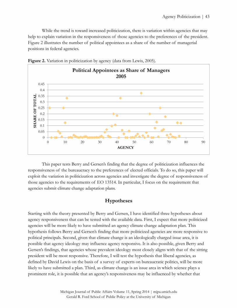
Agency Politicization | 43
Michigan Journal of Public Affairs Volume 11, Spring 2014 | mjpa.umich.edu
Gerald R. Ford School of Public Policy at the University of Michigan
While the trend is toward increased politicization, there is variation within agencies that may
help to explain variation in the responsiveness of those agencies to the preferences of the president.
Figure 2 illustrates the number of political appointees as a share of the number of managerial
positions in federal agencies.
Figure 2. Variation in politicization by agency (data from Lewis, 2005).
This paper tests Berry and Gersen’s finding that the degree of politicization influences the
responsiveness of the bureaucracy to the preferences of elected officials. To do so, this paper will
exploit the variation in politicization across agencies and investigate the degree of responsiveness of
those agencies to the requirements of EO 13514. In particular, I focus on the requirement that
agencies submit climate change adaptation plans.
Hypotheses
Starting with the theory presented by Berry and Gersen, I have identified three hypotheses about
agency responsiveness that can be tested with the available data. First, I expect that more politicized
agencies will be more likely to have submitted an agency climate change adaptation plan. This
hypothesis follows Berry and Gersen’s finding that more politicized agencies are more responsive to
political principals. Second, given that climate change is an ideologically charged issue area, it is
possible that agency ideology may influence agency responsive. It is also possible, given Berry and
Gersen’s findings, that agencies whose prevalent ideology most closely aligns with that of the sitting
president will be most responsive. Therefore, I will test the hypothesis that liberal agencies, as
defined by David Lewis on the basis of a survey of experts on bureaucratic politics, will be more
likely to have submitted a plan. Third, as climate change is an issue area in which science plays a
prominent role, it is possible that an agency’s responsiveness may be influenced by whether that
0
0.05
0.1
0.15
0.2
0.25
0.3
0.35
0.4
0.45
0 10 20 30 40 50 60 70 80 90
SH
AR
E O
F T
OT
AL
AGENCY
Political Appointees as Share of Managers2005

Agency Politicization | 44
Michigan Journal of Public Affairs Volume 11, Spring 2014 | mjpa.umich.edu
Gerald R. Ford School of Public Policy at the University of Michigan
agency’s mission revolves around science. The third hypothesis, then, is that science-oriented
agencies will be more likely to have submitted a plan. I will discuss the operationalization of these
hypotheses in the next section.
Model and Data
The model described below is used to test the influence of the relevant theoretical variables on the
submission of agency climate change adaptation plans in response to EO 13514 and the subsequent
implementation instructions developed by the ICCATF and CEQ. The dependent variable of
interest is the submission status of an agency adaptation plan in 2012. The instructions required
agencies to develop initial adaptation plans as part of the Strategic Sustainability Performance Plans
submitted to the Office of Management and Budget (OMB) in 2012. On February 7, 2013, 35
federal agencies released their climate change adaptation plans (CEQ 2013).
The independent variables of interest include a number of agency characteristics. These data
were collected from the website of David Lewis, professor of Political Science at Vanderbilt
University. The most recent data available from Professor Lewis are from 2005. This dataset includes
76 federal agencies.3 Table 1 lists the independent variables included in the data set and descriptive
statistics.
Table 1. Independent variables.
Variable Name Description Mean Minimum Maximum Standard Deviation
apt Number of Senate-confirmed appointees 5.07 0 31 5.94
year Year oldest unit created 1940 1789 1993 54.7
science 1=identified by Lewis as science agency 0.185 0 1 0.356
regulat 1=identified by Lewis as regulatory agency 0.294 0 1 0.435
totalemp Number of employees 24,343 10 235,846 53,176
manage Number of managers 2,731 2 24,389 5,841
ideo Measure of agency ideological preferences;
1=liberal, 1=conservative
-0.010 -0.929 0.962 0.550
pol Measure of politicization; number of
appointees as fraction of managers
0.068 0 1 0.140
Agency Politicization | 45
Michigan Journal of Public Affairs Volume 11, Spring 2014 | mjpa.umich.edu
Gerald R. Ford School of Public Policy at the University of Michigan
The independent variables described in Table 1 include both the theoretically relevant
variables and controls for other agency characteristics. The three theoretically relevant independent
variables are pol, ideo, and science.
The variable that measures the degree of politicization (pol) is a measure designed by Lewis
in which the number of senate-confirmed political appointees in an agency are divided by the
number of managerial positions in that agency. This measure creates a ratio of political appointees
to management level staff in each agency, which can be used as a proxy for the influence of political
principals on the agency. The first hypothesis outlined above predicts that a higher degree of
politicization (i.e., a higher ratio) will correlate with a greater likelihood of plan submission. The
variable that measures agency ideology (ideo) was constructed by Lewis after a survey of experts in
bureaucratic politics. Lewis surveyed 39 top experts from academia, journalism, and think tanks and
asked them to rate the ideology of government agencies. The higher the value of this measure, the
more liberal the agency. The second hypothesis then predicts that higher values of this measure will
correlate with a greater likelihood of plan submission. The third variable (science) is a dichotomous
indicator with a value of one if the agency was identified by Lewis as having a mission that is closely
aligned with scientific processes or outcomes (See Appendix 1 for a list of science-oriented
agencies). Lewis identified agencies as science-oriented by utilizing data from three National
Academy of Science reports on presidential appointments to leadership positions in science. The
third hypothesis suggests that being identified as a science agency will correlate with a greater
likelihood of plan submission.
Of the 76 agencies for which data were available, 294 submitted agency adaptation plans to
OMB in 2012. The analytical model in this paper uses logistic regression to test the effect of the
independent variables identified in Table 1 on the likelihood that an agency submitted a plan. The
model5 is expressed as:
Yplan = B0 + B1pol +B2ideo + B3totalemp +B4regulat +B5science +B6age
Results
Table 2 presents results, in the form of odds ratios, from a logistic regression of the submission of
an agency adaptation plan on various agency characteristics. The results indicate that of the factors
included in the model, only agency politicization has a significant (p=0.032) effect on the likelihood
of plan submission. Controlling for the other factors included in the model, a one unit increase in
politicization increases the odds of submission by 0.986 times. Thus, an agency that is completely
made up of political appointees would be nearly 100% more likely to submit a plan than one
without any political appointees. While this is a small substantive effect, as the mean level of
politicization among agencies in the sample is only 6%, it is the only statistically significant effect in
the model. This result is consistent with the theory tested by Berry and Gersen that politicized
agencies are more responsive to the preferences of elected officials. In this case, more politicized
agencies were more likely to comply with the provisions of EO 13514 and the associated
instructions.

Agency Politicization | 46
Michigan Journal of Public Affairs Volume 11, Spring 2014 | mjpa.umich.edu
Gerald R. Ford School of Public Policy at the University of Michigan
Table 2. Results of logistic regression.
Variable Name Log Odds Ratio (Std. Error)
pol 0.986**
(0.007)
ideo 1.043
(0.583)
totalemp 0.999
(7.08)
regulat 0.924
(0.621)
science 2.436
(1.959)
age 1.012
(0.008)
N=74
Log likelihood=-39.7
Pseudo R2=0.198
*** p<0.01; ** p<0.05; * p<0.10
These results provide some preliminary support for the first hypothesis, that agency
politicization increases responsiveness. The results do not support either of the second two
hypotheses. Based on these data and model specification, the factors of agency ideology and having
a science-related mission do not increase the likelihood of plan submission. However, as discussed
below, there are limitations in the data that require some caution in interpreting these results.
Discussion
These findings provide empirical confirmation for the theory and observations of Berry and
Gersen. They also suggest that in the arena of environmental policy generally, and climate
adaptation in particular, policy making by executive order involves limitations in terms of agency
responsiveness. These findings provide further explanation for the trend toward politicization of
executive agencies. If presidents want to make policy through executive orders, there is evidence to
suggest that their interests are served by politicizing executive agencies in order to increase the
likelihood that their instructions will be followed. As predicted by Berry and Gersen, presidents’
ability to exert control over agencies is strengthened by appointing a higher percentage of political
staff in those agencies.
There are a number of limitations to this preliminary finding that present opportunities for
further research. The limitations presented by the availability of data are clear. First, the Lewis data
were only available up to 2005. Having data from more recent years would likely improve the
theoretical link between agency characteristics and policy outcomes. Using the 2005 data requires the
assumption that the level of politicization and ideological orientations of agencies has remained
stable since 2005. This assumption is a significant limitation and stands to be tested if more recent

Agency Politicization | 47
Michigan Journal of Public Affairs Volume 11, Spring 2014 | mjpa.umich.edu
Gerald R. Ford School of Public Policy at the University of Michigan
data can be obtained. Second, the budget information was not available even in the 2005 data.
Having information on agency budgets would allow the model to be refined and alleviate justifiable
concerns about omitted variable bias. Third, the construction of the dependent variable as a
dichotomous one, indicating submission of plan, may not capture variation in the quality and
comprehensiveness of the plans or the effort devoted to their creation. Collecting data from each
agency on how many people were involved in the plan development, what resources were devoted to
the process, and the how close the process was to the agency leadership would allow for a more
nuanced analysis of agency responsiveness.
In spite of these limitations, this research provides additional evidence to support the view
that the politicization of federal agencies may increase the power presidents exert over the
bureaucracy. The trend towards politicization seems to increase the responsiveness of the
bureaucracy to the president, but potentially reduces agency independence. The potential link
between agency independence and responsiveness to the executive will remain an issue requiring
thoughtful consideration by scholars, politicians, and voters alike.
1 The United Nations Environment Program (UNEP) defines mitigation as “efforts to reduce or prevent
emissions of greenhouse gases.” UNEP defines adaptation policy as measures to “reduce vulnerabilities and
build resilience to the impacts of climate change.” See United Nations Environment Program. 2 Throughout this paper, “agency” and “agencies” are used to refer to all federal executive units. 3 Of the 76 agencies included in the dataset from 2005, 74 remained in 2013 and were included in the
regression analysis. 4 Of the 35 agencies that submitted plans, only 29 were represented it the data set constructed using Lewis’
data. 5 The following modifications were made to the model: 1) apt and manage were not included as they are
components of pol; 2) age was calculated as the difference between the year the agency was started and 2013.

Agency Politicization | 48
Michigan Journal of Public Affairs Volume 11, Spring 2014 | mjpa.umich.edu
Gerald R. Ford School of Public Policy at the University of Michigan
References
Berry, Christopher R., and Jacob E. Gersen. 2010. “Agency Spending and Political Control of the
Bureaucracy.” Working Paper, Harris School of Public Policy Studies.
Calvert, Randall, Matthew D. McCubbins, and Barry R. Weingast. 1989. “A theory of political
control and agency discretion.” American Journal of Political Science 33:588-611. Council on Environmental Quality (CEQ). 2010. “Progress Report of the Interagency Climate
Change Adaptation Task Force: Recommended Actions in Support of a National Climate Change Adaptation Strategy.” October 5. http://www.whitehouse.gov/sites/default/files/ microsites/ceq/Interagency-Climate-Change-Adaptation-Progress-Report.pdf.
Council on Environmental Quality. 2011. “Federal Actions for a Climate Resilient Nation: Progress Report of the Interagency Climate Change Adaptation Task Force.” October 28. http://www.whitehouse.gov/ sites/default/files/microsites/ceq/2011_adaptation_progress_report.pdf.
Council on Environmental Quality. 2011. “Instructions for Implementing Climate Change Adaptation Planning in Accordance with Executive Order 13514.” March 4. http://www.whitehouse.gov/sites/default/files/microsites/ceq/ adaptation_final_implementing_instructions_3_3.pdf.
Council on Environmental Quality. 2013. “Obama Administration Releases Federal Agency Strategic Sustainability Performance Plans.” February 7. http://www.whitehouse.gov/administration/ eop/ceq/Press_Releases/February_07_2013.
Deland, M. 1982. “The Council on Environmental Quality: An enviable record in jeopardy.” Environmental Science & Technology 16:52117-27.
Exec. Order No. 13,514, 74 F.R. 52117 (October 8, 2009). http://www.gpo.gov/fdsys/pkg/CFR-
2010-title3-vol1/pdf/CFR-2010-title3-vol1-eo13514.pdf. FedCenter.gov. “EO 13514.” Accessed 2012. http://www.fedcenter.gov/programs/eo13514/. Harris, R. 1981. “Demise of CEQ.” Environmental Science & Technology 15:485. Lewis, D. 2005. “Presidents and the politicization of the United States Federal Government, 1988-
2004.” Paper presented at the annual meeting of the American Political Science Association, Washington, District of Columbia, August 31-September 3. http://www.dartmouth.edu/~govt/docs/Lewis.pdf
Train, R. 1971. “CEQ: Environmental voice at the top.” Environmental Science & Technology 5:1075-
1075. United Nations Environment Program. 2013. “Climate Change.”
http://www.unep.org/climatechange/.

Agency Politicization | 49
Michigan Journal of Public Affairs Volume 11, Spring 2014 | mjpa.umich.edu
Gerald R. Ford School of Public Policy at the University of Michigan
Appendix 1. Science Agencies, as defined by David Lewis
Consumer Product Safety Commission
Council of Economic Advisers
Council on Environmental Quality/Office of Environmental Quality
Department of Agriculture
Department of Commerce
Department of Defense
Department of Energy
Department of Health and Human Services
Department of Homeland Security
Department of Interior
Department of Justice
Department of Labor
Department of Transportation
Environmental Protection Agency
National Aeronautics and Space Administration
National Science Foundation
National Transportation Safety Board
Nuclear Regulatory Commission
Office of Science and Technology Policy
U.S. Agency for International Development

Disorganization and Network Institution | 50
Michigan Journal of Public Affairs Volume 11, Spring 2014 | mjpa.umich.edu
Gerald R. Ford School of Public Policy at the University of Michigan
Four
Disorganization and Network Institution: A Possible Source of
Economic Downturn
Endrizal Ridwan
Abstract
This article considers the roles of networks on investment decisions to explain the existence of a
possible economic downturn during a transition period from a dictatorship towards a democracy. A
supplier is willing to invest in a state production only if there are enough other suppliers taking part
such that the return on investment is at least equal to their private alternatives. The suppliers build
knowledge of others' private alternatives through a communication network. The investment model
presented here shows that a decision to invest not only depends upon knowledge about others, but
also, more importantly, understanding of others' knowledge. When networks fail to fully disseminate
knowledge, investment decisions are suboptimal. These suboptimal decisions consequently lead to a
decline in output in the early stage of market decentralization as the state loses power to force
suppliers into joining state production.
Endrizal Ridwan is currently pursuing a PhD in Economics at Indiana University Bloomington. He previously
received a BA in Economics from Andalas University Indonesia and MA in Economics from the Australian
National University. His research focuses on the roles of social network and institution on entrepreneurships,
microfinance and economic development.

Disorganization and Network Institution | 51
Michigan Journal of Public Affairs Volume 11, Spring 2014 | mjpa.umich.edu
Gerald R. Ford School of Public Policy at the University of Michigan
Introduction
The fundamental economic problems in all societies are questions of what is to be produced, how
to efficiently allocate resources, and how to distribute the production. These decisions can be made
at the hand of a single dictator, which may be called a central planner, or a centralized government;
these decisions can also be decentralized to all individuals of economic agents through some market
mechanism. For instance, a decision to produce pencils, whether to use machines in the process of
production and how to distribute its value among resource owners can be made by one entity, a
dictator. This nation is under a regime of a dictatorship. In other situations, society as a whole can
also make such decisions through a market mechanism; instead of force, markets work voluntarily to
guide the decision-making process. When pencils are more valuable as indicated by an increase in
their price, the society will voluntarily allocate their resources to produce pencils without being
forced to do so. In this governance structure, the nation is under a regime of a decentralized market.
Sometimes, political situations, such as a coup or revolution, may change the economic regime from
a dictatorship to fully decentralized market. This typical regime change, as widely accepted by the
neoclassical theorists, is expected to boost economic output.
However, changing economic regimes from a state where there is powerful government
intervention to a state where there is strong market decentralization does not guarantee an increase
in economic output. In fact, historical case studies show that output has a tendency to fall
immediately after the collapse of a dictatorship and continue to decline during the transition from
the centralized government to a decentralized governance structure (Blanchard and Kremer 1997,
Brenton, Gros, and Vanadille 1997, and Duflo and Senik-Leygonie 1997). For example, most
countries of the former Soviet Union experienced a large decline in output after the collapse of the
Soviet Union. Their output was less than half of its pre-decentralization period (Blanchard and
Kremer 1997). Despite a myriad of economic distortions during centralized planning and under
dictatorships, the movement towards competitive, decentralized markets failed to increase output,
contrary to common expectations.
This type of decline in output is an interesting puzzle for neoclassical theory because
decentralized transactions between suppliers and buyers do not instantly boost economic growth.
The existing literature has tried to explain the economic reasons behind this downturn. The
explanations for these temporary output declines vary, ranging from changing the reporting
incentives, the need to restructure enterprises and redeploy assets, to the increase in uncertainty that
affects investment. Blanchard and Kremer (1997), for instance, argue that the economic downturn is
due to the presence of incomplete contracts and asymmetric information. During the regime of
dictatorships in the Soviet Union, the central government had the power to force each supplier to
participate in state owned firms. The characteristics of the state firms’ production processes were
complex; they involved many stages of production starting from planning and designing to
delivering the final product. The firms were served highly specified functions, in which the suppliers
were almost perfect complements to each other, i.e. each supplier had its own specific roles in the
production processes that was difficult to be substituted by other suppliers.
Disorganization and Network Institution | 52
Michigan Journal of Public Affairs Volume 11, Spring 2014 | mjpa.umich.edu
Gerald R. Ford School of Public Policy at the University of Michigan
This specific relationship among suppliers opened an opportunity for each supplier to
bargain for a higher wage for its services immediately after the regime of dictatorship collapsed.
This bargaining mostly resulted in inefficiency due to asymmetric information in which some
relevant information was hidden from each supplier. Moreover, the complexity in production stages
resulted in incomplete contracts because it was difficult to accurately state all the production steps in
the contracts from beginning to the end. Thus, both incomplete contract and inefficient bargaining
caused a drop in national output shortly after the end of the dictatorship. The output loss may be
even larger if more parties were involved in the complex set of specific relations, increasing the cost
of disorganization.
One limitation of many existing theories, including Blanchard and Kremer (1997), is that
they put too little attention on the communication relationship among individual suppliers when
analyzing bargaining outcomes. Most of the existing literature uses models of non-cooperative game
theories. That is, by assuming no communication among agents, the models predict the outcome of
non-cooperative bargaining. In reality, however, some parties communicate to each other or rely on
their prior existing communication network when deciding which strategic actions to take.1
Therefore, I believe that the outcomes of bargaining are also influenced by the presence of
communication network among those suppliers.
This paper proposes an alternative explanation of the reduction in output during transition
by introducing the role of networks. This explanation will complement other studies using
asymmetric information to explain the possible dramatic fall in output. I first modify the Blanchard
and Kremer (1997) model on how specificity and complexity may create coordination failure
between a state firm and its suppliers. I then transfer this coordination game into a type of collective
action game by linking the supplier's private opportunities to the number of participants in the state
firm. Finally, I borrow Chwe’s (1999) style of network analysis on collective action problems to
explain how a fall in output may result from the network structures among the suppliers.
Section 2 presents the model of an economy with one state firm and several suppliers. The
suppliers are strategically rational and also take into account that the others are completely rational.
Section 3 analyzes the equilibrium outcome for various institutions and shows that none of these
institutions would produce efficient investments. Section 4 discusses the model’s implications for a
solution to coordination problems, and possible extensions to a more sophisticated and realistic
network structures. The model has implications for countries in a transition period from a strong
government power into more market-dominant or democratic structure, such as Turkey, Libya, or
Egypt. The message is that the transition cannot be done radically if countries are attempting to
maintain pre-transition levels of output. Section 5 draws conclusions that a better network
relationship among suppliers is necessary to solve coordination problems and achieve the most
efficient economic outcome during a transition period from a more centralized government regime
to a more market-oriented regime.

Disorganization and Network Institution | 53
Michigan Journal of Public Affairs Volume 11, Spring 2014 | mjpa.umich.edu
Gerald R. Ford School of Public Policy at the University of Michigan
The Model
The economy consists of only one state firm and several private firms. Both types of firms use
intermediate capital inputs from 𝑛 + 1 number of suppliers; the suppliers outnumber the private firms. We assume that profit-maximizing private firms have monopoly power, which allows them to offer take-it-or-leave-it rent to the suppliers. Hence, the suppliers will get paid their private
thresholds if they decide to supply their intermediate inputs in the forms of capital, 𝑘, to private firms.2
The state firm
The state firm operates on an increasing return to scale with an 𝑌 = 𝐴𝑘𝛼 type of production
function where ≥ 1 . This type of economic scale is common for the state firm since the state
usually is a natural monopolist for publicly crucial output such as electricity, telecommunication, and
mining. Instead of being constant, however, we assume that the technology coefficient, 𝐴, increases
with capital 𝑘. We can think of k as smart capital, which has positive externalities. In other words,
this capital is more productive when it interacts with other forms of capital.3 Specifically, for this
model 𝐴(𝑘) = 𝑘 so that the technology coefficient is just the units of capital. Hence, the state firm’s
effective production function would be
𝑦 = 𝑘1+𝛼 (1)
We further assume for the purpose of the model that 𝛼 = 1, so that the effective
production function is
𝑦 = 𝑘2 (2)
In addition, the state firm is not a profit-maximizing firm, but a welfare-maximizing firm. It
operates under zero-profit conditions and ensures the equality of income among its suppliers. We
can also think of suppliers as workers, where the state firm aims to distribute its output equally to its
workers. To ensure equality, the state firm pays rent, 𝑟, to supplier 𝑖 according to the firm's average
product. With the above effective production function, as in (2), the rent is
𝑟𝑖 =𝑦
𝑘= 𝑘 ∀𝑖 (3)
Equation (3) reads the state firm as paying rents to every supplier equal to the units of
capital used in production. Note here that only the quantity of capital matters, not the quality.
Suppose, for instance, that two suppliers each supply one unit of capital to the state firm. Each
capital supplied is not necessarily equal in quality. With two units of capital, the state firm’s output is
four units. The return on capital from the state firm to both suppliers is, therefore, 𝑟𝑖 =4
2= 2 units,
although each supplier supplies only one unit of capital. Of course, this does not mean that every
supplier will join the state firm since they may have sufficiently high opportunity costs, which are
alternatives from private firms. Consider, as an example, the case of public transportation, such as
city buses. In some developing countries, the public transportation company is owned and
controlled by state enterprises. However, these individual buses can be owned privately by
community members or suppliers. Since the state firm controls the bus fare, the rent payment to the
bus suppliers is based on the quantity of buses, not the quality. Each bus may have a different seat

Disorganization and Network Institution | 54
Michigan Journal of Public Affairs Volume 11, Spring 2014 | mjpa.umich.edu
Gerald R. Ford School of Public Policy at the University of Michigan
capacity and a unique bundle of other accessories, but each gets paid equally. If the bus were hired
by a private enterprise, the payment would be based on its quality.
The suppliers
There are 𝑛 + 1 suppliers to decide whether to engage in the state firm production or to accept
take-it-or-leave-it rent from private firms. Each supplier has one unit of capital. The capital differs in
quality, which is indicated by different threshold levels 𝑐𝑖 ∈ (2, … , 𝑛 + 2).4 As mentioned above,
the private firms will pay each supplier exactly the supplier’s threshold in regards to the supplier’s
product quality. The suppliers then compare these private alternatives to the rents earned from the
state firm. However, each supplier must decide simultaneously whether or not to participate in the
state firm’s production without knowing the actions of other suppliers.
The decision of any particular supplier 𝑖 is obvious. That is, to join (𝑗) the state firm if 𝑟𝑖 ≥
𝑐𝑖; or stay (𝑠) and take the private opportunities at 𝑐𝑖. Notice, due to the specific production
function in (2) and the value of private alternatives, the supplier decisions to join the state firm
depend upon how many other suppliers would join the state production. This specific relation is the
critical feature of this model. For example, supplier A with threshold of 𝑐 = 2 would join the state
firm only if accompanied by at least one other supplier. To see this, suppose that only supplier A
joined the state firm. This supplier then gets rent equal to one, which is lower than its threshold. If,
instead, two other suppliers join, supplier A gets rent equal to three, which is strictly higher than its
threshold. Moreover, a supplier with a threshold of 𝑛 + 1, which is equal to the number of
suppliers, would prefer to join only if everyone else does. Meanwhile, a supplier with threshold of
𝑛 + 2 would never join the state firm. Thus, we can formulate the profit of supplier 𝑖 given its own
threshold and everyone else’s actions 𝑎 = (𝑎1, … , 𝑎𝑁) as follows:
𝜋𝑖 (𝑐𝑖, 𝑎𝑖 , … , 𝑎𝑁) = {𝑐𝑖 , 𝑖𝑓 𝑎𝑖 = 𝑠
𝑟𝑖 = 𝑘, 𝑖𝑓 𝑎𝑖 = 𝑗 𝑎𝑛𝑑 #ℎ{𝑠.𝑡. 𝑎ℎ=𝑗}=𝑘 (4)
This profit equation (4) simply states that the supplier’s profit (𝜋) would be its private value,
𝑐, if it stays and takes an offer from a private firm. Otherwise, when it joins the state firm, the profit
would be 𝑟 = 𝑘, where 𝑘 is the total number of suppliers that take part in the state production.
Thus, the suppliers’ decision simply depends on whether ex-ante 𝑟𝑖 ≥ 𝑐𝑖. The only problem for the
supplier, then, is to accurately predict the value of 𝑟. In the following section, I describe how the
supplier uses knowledge from networks to predict 𝑟𝑖.
Network
Suppliers use a network to communicate their thresholds and to gain knowledge of others. Since the
decision under this type of network is voluntary, a commitment is not necessary. Even if there is a
commitment, no penalties are levied for deviances. Following Chwe (1999), I define network → as a
binary relation over 𝑛 suppliers, where 𝑔 → 𝑖 means that supplier 𝑔 communicates to supplier 𝑖. I
define the neighborhood of 𝑖 as every supplier who communicates to 𝑖. I also assume that supplier

Disorganization and Network Institution | 55
Michigan Journal of Public Affairs Volume 11, Spring 2014 | mjpa.umich.edu
Gerald R. Ford School of Public Policy at the University of Michigan
𝑖 knows the thresholds of everyone in its neighborhood. Furthermore, supplier 𝑖 knows all network
relations among members in its neighborhood, i.e., whether the neighborhood members
communicate with each other.
Succinctly, for supplier 𝑖, let 𝐵(𝑖) = {𝑔 ∈ 𝑁: 𝑔 → 𝑖} be its neighborhood, where 𝑖 ∈ 𝐵(𝑖)
and for all 𝑝, 𝑞 ∈ 𝐵(𝑖), supplier 𝑖 knows whether 𝑝 → 𝑞. Take 4 suppliers as an example: supplier
1, 2, 3 and 4. Supplier 2 and 3 communicate to supplier 1 but supplier 4 does not communicate back.
However, supplier 4 communicates to supplier 2. Then, we write 𝐵(1) = {2,3} and 𝐵(2) = {1,4}.
In other words, supplier 2 and 3 are in the neighborhood of supplier 1 since both supplier 2 and 3
communicate with supplier 1. Moreover, supplier 1 also knows whether supplier 2 and 3
communicate with each other. Supplier 4 is not in the neighborhood of supplier 1, but it is in the
neighborhood of supplier 2 for the same reason. Supplier 2 knows whether or not supplier 1 and 4
communicate each other.
Finally, since the suppliers’ decisions depend upon the decisions of other suppliers joining
the state firm, it is sufficient to model this situation as a collective action problem in which all player
have to collectively take the same action in order to get the best outcome. If any players deviate
from that action, it would cost all players since more costs are born to those who cooperate. Thus,
everyone is reluctant to cooperate unless everyone confidently knows that everyone else will
cooperate. Thus, the best outcome may not be achieved if players are uncoordinated. We will see
how network structures play important roles in disseminating knowledge and predicting actions
taken by others. In particular, networks have the potential to solve coordination problems among
suppliers.
Equilibrium
Equilibrium under central planning and perfect decentralization
Before looking at the role of networks, let us analyze the outcomes of the economy under central
planning and perfect decentralization with uncertainty. First, note that the best outcome of the
economy is when there is no uncertainty and every supplier is free to choose its trading partners. In
this environment, every supplier knows the other suppliers’ thresholds due to perfect information.
As mentioned above, there are 𝑛 + 1 available suppliers in the economy and suppose that 𝑘 of them
voluntarily join the state firm where 𝑘 ≤ 𝑛 + 1. The value of 𝑘 is endogenous, not predetermined,
depending on the suppliers’ decisions. Consequently, a supplier with threshold of 𝑐𝑖 ∈ {2, … , 𝑘}
would join the state firm when 𝑘 suppliers join. The supplier with threshold 𝑐 = 𝑘 + 1 or more
would be better off staying (not joining); this supplier would take the rent offered by the private
firms since the maximum rent the state firm can provide is only 𝑘, but the private firm will pay
according to its threshold of 𝑘 + 1. However, this option may not be available in an imperfect
information environment.
In a fully centralized economy or dictatorship, the central planner or dictator has full power
to force all suppliers to engage in state production for the purpose of advancing state interests. In
this case, 𝑘 = 𝑛 + 1 since all suppliers are forced to join the state firm, where 𝑘 is the number of
Disorganization and Network Institution | 56
Michigan Journal of Public Affairs Volume 11, Spring 2014 | mjpa.umich.edu
Gerald R. Ford School of Public Policy at the University of Michigan
firms that join the state firm. The supplier with threshold 𝑐 = 𝑛 + 2 has no option but to join the
state firm. Unfortunately, this forced participation creates distortion in the economy because it
makes suppliers with threshold 𝑛 + 2 or more worse off, as the state firm will pay only 𝑛 + 1, which
is equal to the number of total suppliers. If this supplier had been given the choice of joining the
private firms and not the state firm, it would have been paid its threshold of 𝑛 + 2. The degree of
distortion is much larger when the upper limit of private thresholds is higher than 𝑛 + 2. Hence, the
outcome of central planning is suboptimal.
Under full market decentralization, all 𝑛 + 1 suppliers are free to invest in the state
production or in the private firms. The existence of asymmetric information among suppliers and
between suppliers and private firms causes suboptimal investment decisions. The market may even
collapse. In this case, an adverse selection problem may exist since the suppliers’ thresholds are
private information unknown to other suppliers and firms. What the firms and suppliers may know
is the distribution of the suppliers’ thresholds. For example, if we assume that each supplier has
equal probability of having a certain threshold, then a uniform distribution would be appropriate to
use. When the thresholds are uniformly distributed on the interval [2, 𝑛 + 2] the private firms will
offer all suppliers the same rent, which is the expected value of the thresholds level, 𝑛/2. Thus, a
supplier will join the private production if its threshold is no higher than 𝑛/2. Those whose
thresholds are higher than 𝑛/2 will leave the market. They will not join the state production because
they have high thresholds and need to coordinate prior to investing. This adverse selection
phenomenon is familiar in economics and is known as a lemon problem, where the low quality
suppliers drive out the good quality suppliers from the market (Akerlof 1970). Knowing that only
low quality suppliers are available to trade, the private firms may lower the offered rent, causing
more suppliers to leave the market. Thus, the market may collapse.5 In short, asymmetric
information among suppliers makes it hard to coordinate and asymmetric information between
suppliers and firms triggers adverse selection causing the market to collapse.
We have seen that both central planning and perfect decentralization fail to produce optimal
decisions. Communication networks, as we will see, may solve the coordination problems and
eliminate the adverse selection problem associated with asymmetric information. However, we shall
see that mere certainty about other suppliers’ thresholds is not sufficient to induce suppliers to
participate in the state firm. More important to this decision is whether one firm knows about the
other firms' decisions.
Equilibrium under networks
A supplier is assumed to be rational and takes into account that other suppliers are also rational.
Their rational decisions depend on their knowledge acquired from networks. This knowledge
determines the supplier’s ability to distinguish between states of the world – the set of all possible
outcomes. If a supplier cannot distinguish between several states of the world, it must take the same
action in all of them. Take for example that there are only two suppliers: 𝑖 = (1,2) and three
possible threshold levels 𝑐𝑖 = (1,2,3). Hence, there are nine possible states of the world
{1,1; 1,2; 1,3; 2,1; 2,2; 2,3; 3,1; 3,2; 3,3}, where 2,3 means supplier 1 has threshold 2 and supplier 2

Disorganization and Network Institution | 57
Michigan Journal of Public Affairs Volume 11, Spring 2014 | mjpa.umich.edu
Gerald R. Ford School of Public Policy at the University of Michigan
has threshold 3. The rest of this section will present how each supplier distinguishes each state of
the world through a communication network. Three network structures are discussed: null network,
full network, and incomplete network.
Figure 1. Null network (no communication).
Supplier 1's partition
Supplier 2's partition
1,1 1,2 1,3
1,1 1,2 1,3
2,1 2,2 2,3
2,1 2,2 2,3
3,1 3,2 3,3
3,1 3,2 3,3
Supplier 1's actions
Supplier 2's actions
j j j
j s s
s s s
j s s
s s s
j s s
Figure 1 presents a null network in which supplier 1 does not communicate to supplier 2 and
supplier 2 does not communicate to supplier 1. Hence, supplier 1 knows its own threshold, but does
not know supplier 2’s threshold. The best supplier 1 can do is realize that supplier 2’s threshold is
either 1, 2, or 3, but supplier 1 cannot be sure. The same situation also applies to supplier 2.
Therefore, supplier 1's knowledge can be represented by the partition set {1,1;1,2;1,3}, {2,1;2,2;2,3},
and {3,1;3,2;3,3}. Similarly, supplier 2's knowledge is represented by {1,1;2,1;3,1}, {1,2;2,2;3,2}, and
{1,3;2,3;3,3}. Each partition, {.}, means that the owner of the partition cannot distinguish between
its contents; therefore, the owner has to take the same action when facing any content within the
partition.
Let us consider supplier 1. It chooses whether to join (j) or stay (s) given a state of the world.
If it has a threshold of one, it will surely join the state firm. If instead it has a threshold of three, it
will never join the state firm, regardless of the threshold of supplier 2. How about if it has a
threshold of two? In this case, it ideally joins if the state is (2,1) or (2,2) and stays if the state is (2,3).
However, since it cannot distinguish between these three states, it has to take the same action. If it
decides to stay, the state could be (2,1). But if it decides to join, the state could be (2,3) and the other
supplier will not join. Thus, the number of suppliers joining the state firm would be lower than its
threshold. If the latter happens, (2,3), I assume that supplier 1 suffers a large cost from joining the
state firm and its profit is then lower than its threshold.6
An analogy for the situation above is as follows. Imagine two community members Adam
and Eve who each wants to decide whether to volunteer for community work, which requires a total
of two hours. If only one shows up, he or she will work for two hours and, if both show up, each
will work for 1 hour. Each member may not be available to volunteer at all, or may be available for
one hour or two hours, but neither of them knows the other’s availability with certainty. In this case,
Adam will show up if he has a free time of two hours and will not show up if he has no free time,
regardless of Eve’s decision. Eve will make a similar decision. The problem arises if Adam is only

Disorganization and Network Institution | 58
Michigan Journal of Public Affairs Volume 11, Spring 2014 | mjpa.umich.edu
Gerald R. Ford School of Public Policy at the University of Michigan
available for one hour. Should he volunteer? His decision depends on his knowledge of Eve’s
availability. Since he does not communicate with Eve, he is not sure whether she will show up or
not. Therefore, to minimize loss, Adam will stay home when he has only one hour of free time and
does not know Eve’s threshold.
Back to the supplier-state firm case above, supplier 1 joins only if it knows for certain that
supplier 2 will join. Hence, in this example, if supplier 1 has a threshold of two, it stays in all three
states: (2,1), (2,2), and (2,3). Supplier 2 takes similar actions. It joins only if it has a threshold of one
and stays if it has a threshold of two or three. Their set of actions is depicted in Figure 1. The
coordination problem here is when they have threshold of (2,2). Social efficiency requires that they
both join the state firm but their knowledge gaps prevent them from doing so. Thus, the outcome
of the null network is inefficient. In general, each supplier joins only if it knows with certainty that a
sufficient number of the other suppliers will join the state firm
Figure 2. Full network (complete communication).
Supplier 1's partition
Supplier 2's partition
1,1 1,2 1,3
1,1 1,2 1,3
2,1 2,2 2,3
2,1 2,2 2,3
3,1 3,2 3,3
3,1 3,2 3,3
Supplier 1's actions
Supplier 2's actions
j j j
j j s
j j s
j j s
s s s
j s s
Figure 2 depicts a full network or complete communication. Here, supplier 1 communicates to
supplier 2 and vise versa. Both suppliers know each other's threshold and can distinguish among all
states of the world. The difference between figure 1 and figure 2 is best seen when supplier 1 has a
threshold of two. In a null network, it stays in state (2,1); (2,2); and (2,3) because it cannot
distinguish between the three states. Now, supplier 1 can distinguish between these three states and
can take different actions in regards to each of them. Supplier 1 will definitely join in state (2,1)
because it knows with certainty that supplier 2 has a threshold of one and hence will also join. In
contrast, supplier 1 stays in state (2,3) because it knows that supplier 2 has a threshold of three and
will also stay. Supplier 2 has a similar case in which it will join at state (1,2) and stay at state (3,2).
What if the state is (2,2)? In this case, there would be two equilibria: one point where both
suppliers join and the other point where neither chooses to join. In this model, whenever there is
this kind of indeterminacy, I assume that the equilibrium is one point where both choose to join. In
other words, when each supplier with a threshold of two discovers the other also has a threshold of
two, I assume they both join the state firm.
No coordination problem arises when the threshold is (2,2). Both suppliers join the state
firm. That is because each supplier knows the other’s threshold and each knows that it has mutual

Disorganization and Network Institution | 59
Michigan Journal of Public Affairs Volume 11, Spring 2014 | mjpa.umich.edu
Gerald R. Ford School of Public Policy at the University of Michigan
knowledge of each other’s threshold. Networks here materialize the gains from participation and
hence solve the coordination problem
Figure 3. Incomplete network (partial communication).
Supplier 1's partition
Supplier 2's partition
1,1 1,2 1,3
1,1 1,2 1,3
2,1 2,2 2,3
2,1 2,2 2,3
3,1 3,2 3,3
3,1 3,2 3,3
Supplier 1's actions
Supplier 2's actions
j j j
j s s
j j s
j s s
s s s
j s s
After establishing the difference between the null and complete network, let us consider the
incomplete network presented in Figure 3. Here, supplier 2 communicates with supplier 1, but
supplier 1 does not communicate back to supplier 2. In this case, only supplier 1 has full knowledge
of the exact state of the world. An interesting question here is whether supplier 1 chooses to join
the state firm when it knows the exact state of the world is (2,2). The answer depends upon its
expectation about supplier 2's decision. To join, supplier 1 has to make sure that supplier 2 also
joins. However, it knows that supplier 2 cannot distinguish between the states of the world, and
therefore it predicts that supplier 2 stays. From supplier 2's point of view, the state of the world
could be (3,2). This indeterminacy would predict that supplier 2 chooses to stay and hence, supplier
1 will also stay. In short, under the incomplete network, both suppliers stay at state (2,2) because one
supplier knows that the other supplier does not know for certain whether its counterpart will join
the state firm. Thus, the coordination problem still exists and gains from participation cannot be
materialized.
It is easy to extend the model to 𝑛 players, which is simply a matter of writing down all
states of the world. The point here is that knowing the state of the world per se is not sufficient for a supplier
to join the state firm. It is more important to know what others know, and also to know that others
know what we know (common knowledge), in order to solve the coordination problem.
Discussion and Extension
Chwe (1999) defines transition as moving "from plan and plan institution to market and market
institutions.” In this paper, this means moving from involuntary participation under the central
planning (dictatorship) towards voluntary participation under networks (market decentralization).
This transition may harm a nation’s total economic production or output despite a common belief
that market decentralization boosts economic growth. The main problem with voluntary
participation under market decentralization is the existence of asymmetric information. Since

Disorganization and Network Institution | 60
Michigan Journal of Public Affairs Volume 11, Spring 2014 | mjpa.umich.edu
Gerald R. Ford School of Public Policy at the University of Michigan
voluntary participation involves coordination, asymmetric information may inhibit the ability of
economic agents to coordinate and to collectively take the preferred actions. This inability
contributes to suboptimal investment decisions and hence suboptimal outcomes. During a transition
period, after a regime change from a dictatorship towards democracy, economic agents such as
laborers, capital owners, and entrepreneurs may not yet be ready to coordinate with each other due
to limited knowledge of required information. The example below shows that a country can
experience a sharp decline in output during a transition from dictatorship towards decentralization.
Suppose that there are two electrical power companies: one is state-owned and the other is
private-owned. These companies require several electrical components, each supplied by an
individual private supplier. Each supplier has its respective marginal cost of production. The lower
its marginal cost, the higher the quality of the components. Thus, each supplier has its own
threshold for a minimum rent at which the supplier is willing to sell its components. The thresholds
are measured by units of capital equivalent. Suppose there are five suppliers with thresholds of one,
two, two, nine, and nine units of capital, respectively. Here, I allow the upper limit of private
thresholds to be sufficiently high to indicate the more advanced private sectors. Each supplier can
provide its components to the state firm or to a private firm. The state firm has production function
as in (2) and distributes the output equally to the suppliers. The private firm produces output equal
to the sum of suppliers’ thresholds and pays each supplier equal to their thresholds.
Under central governance or dictatorship, everyone is forced to engage in state production.
The private firm does not exist in such regime. With a production function of the state firm of 𝑦 =
𝑘2 as defined earlier in (2), the total production of those five suppliers is 25 units. Every supplier
then has capital income of five units since the state firm divides its value of output equally. Notice
that two suppliers with a threshold of nine are worse off because their incomes are below their
thresholds (incomes of five versus incomes of nine). Meanwhile, the other three suppliers are better
off.
Under a regime of market decentralization with a network, the national output may be
higher or lower than that under the central planner. This paper’s purpose is to show that the output
may be lower. If the network is empty, or there is a null network where there is no communication
among the suppliers, only supplier 1 will voluntarily join the state firm while the other suppliers take
their private alternatives from the private firm. Hence, the total output and income produced in the
economy would be 1 + 2 + 2 + 9 + 9 = 23 units, which is lower than that under the central
planner. Under full networks or complete communication, three suppliers with thresholds of one,
two, and two join the state firm while two suppliers with a threshold of nine join the private firm
and take their private alternatives, delivering total output or total income of 3 + 3 + 3 + 9 + 9 =
27 units, which is higher than that under the central planner. Finally, if the network is incomplete,
the outcome will depend on the network’s structure, i.e., who communicates to whom. When
networks are incomplete, lower income is more likely to occur, but when networks are fully
developed, higher income will be more probable.
There are two conditions that can make output fall after the collapse of dictatorship: imperfect
network communication and rapid growth in private industries. Rapid growth in private sector industries,
indicated by relatively high productivity or low marginal cost, gives suppliers more opportunities to

Disorganization and Network Institution | 61
Michigan Journal of Public Affairs Volume 11, Spring 2014 | mjpa.umich.edu
Gerald R. Ford School of Public Policy at the University of Michigan
earn higher rents. Those opportunities are disseminated through a communication network. Hence,
when information is well disseminated and the private sectors are relatively well developed, the
economic distortions caused by central planning are relatively larger. However, if the network to
disseminate information is ill developed and private sectors are still primitive, central planning or
dictatorship provides a better solution to coordination problems.
This model is applicable to current political transitions and can be seen as a warning to
countries that are now at the early stage of democracy such as Turkey, Libya, Egypt, Afghanistan,
and Syria, among others. One could expect that their economic output would fall shortly after the
collapse of the dictatorship or powerful central government. The main reason is the communication
networks, which transmit relevant information, may not be feasible and may take some time to
develop. Along with a fear of political instabilities, business owners need an economic adjustment
period from the former forced participation by the central government to the voluntary
participation under market institution. During this adjustment period, output is predicted to fall.
Moreover, if the transition periods run radically instead of gradually, the fall in output would be
even worse.
By the example above, this paper is able to show the importance of network development
during a transition period from a centralized governance structure to a decentralized governance
structure. Nevertheless, the model presented has some shortcomings in that it only deals with a
simple network model that relies on an increasing return to scale in state production. In reality,
networks are more complex and sophisticated. The assumption of increasing returns to scale is
plausible under monopoly but too restricted for a competitive market economy. In a competitive
market literature, firms are commonly assumed to have a technology of constant return to scale.
Therefore, one possible extension of this paper’s model would be to develop more sophisticated
communication network models. These would allow for an exploration of the value of each
economic agent in a network; in other words, the contribution each player makes in a network to
disseminate information can be analyzed. Thus we can detect who the key players are and what their
roles are in their respective strategic positions (Ballester, Calvo-Armengol, and Zenou, 2006). For
example, in a star communication network, one can analyze the central player, the gains and costs of
being at the center of the network and its roles in transmitting information.
Another possible extension of this paper is to allow for a more flexible production function
in both public and private sectors. This relaxation would allow the production function to reflect
different market structures such as monopoly, oligopoly, and perfect competition. Given market
structures, a more flexible production function would also allow us to encompass firms with
stronger network interactions. For example, in industrial organization literature, networks among
suppliers play a crucial role when the market is oligopolistic rather than when it is monopolistic, as
the suppliers use the network as a barrier to entry. Therefore, using a more flexible production
function and a more sophisticated network, one should be able to better explain the decline in
output during governance transitions.
Disorganization and Network Institution | 62
Michigan Journal of Public Affairs Volume 11, Spring 2014 | mjpa.umich.edu
Gerald R. Ford School of Public Policy at the University of Michigan
Conclusion
This paper provides a theory for why changing institutions from dictatorship towards democracy
does not necessarily improve economic performance. The theory is based on the argument that
suppliers need to be able to predict their partner’s knowledge in order to voluntarily invest in state
production. During dictatorship, no voluntary decisions are necessary since all agents are forced to
work for state production. Once this central government loses its power to compel actions, the
availability of information plays a crucial role in mitigating coordination problems among suppliers.
Unfortunately, no immediate set of institutions exists that can disseminate knowledge to society. As
suppliers are heterogeneous and some information is hidden from other suppliers, investment
decisions produce an inefficient outcome. Only when communication networks among suppliers are
well developed can the hidden information be revealed and transferred through the network. These
knowledge dissemination structures are necessary to reach the optimal economic decision.
We have seen various equilibrium scenarios. Under full centralization, all suppliers are forced
to participate in state production leading to suboptimal investment for higher threshold suppliers.
Under complete market decentralization, imperfect information may cause the entire market to
collapse due to adverse selection problems. Under a communication network, output depends
crucially on how the network has developed. When networks fail to produce common knowledge,
investment decisions are also not optimal, even if there is no uncertainty about the other players’
information. In all these scenarios, investment decisions are suboptimal and coordination problems
exist as long as information is not fully transmitted.
Common knowledge is therefore a key to solve the coordination problems. Once every
supplier knows each other and they have a mutual understanding of each other, investment
decisions can be optimal. However, it takes some time to build this common knowledge. In the
meantime, lack of communication causes output to fall. Moreover, output may continuously fall at
the beginning of a transition period but start to recover once networks are developed and
information is well disseminated. This prediction therefore can be seen as an early warning to
countries which are now at the beginning of their transition periods. Those countries should let the
transition process proceed gradually instead of radically to foster the development of networks
among economic agents.
1 The literature on networks has been fast growing since the last decade. Readers may refer to Jackson (2008)
for an excellent survey. 2 An example for the existence of these three firms in reality is seen in any electronic products. Apple for
example uses many components produced by several independence firms. This component-producing firms
are called suppliers in this paper. 3 It is relatively easy to show the externalities in terms of skilled labor. It can be argued that a smart worker is
more productive when he or she collaborates with other smart workers than with less skilled workers. 4 We set the thresholds as integer just to simplify the analysis in the following sections and we restrict the
upper limit to just to make sure that there are suppliers that are always better off taking their private
alternatives even when all n suppliers are forced to engage in the state firm. As stated above, if n suppliers

Disorganization and Network Institution | 63
Michigan Journal of Public Affairs Volume 11, Spring 2014 | mjpa.umich.edu
Gerald R. Ford School of Public Policy at the University of Michigan
join the state firm, they each will get return of n units regardless their thresholds. The higher the upper limit,
then, shows the larger economic distortions caused by the state firm. We will relax this assumption in later
discussion to compare the outcomes under different institutions. 5 The analysis is independent on the distribution of threshold. The uniform distribution is just used as an
example. 6 In case of workers, we can assume that the worker gets very large negative disutility when the number of
people joining the state firm is less than his or her threshold.

Disorganization and Network Institution | 64
Michigan Journal of Public Affairs Volume 11, Spring 2014 | mjpa.umich.edu
Gerald R. Ford School of Public Policy at the University of Michigan
References Akerlof, George A. 1970. “The Market for “Lemons”: Quality Uncertainty and the Market
Mechanism.” The Quarterly Journal of Economics 84:488-500. Ballester, Coralio, Antoni Calvo-Armengol, and Yves Zenou. 2006. “Who's Who in Networks.
Wanted: The Key Player.” Econometrica 74:1403-17. Blanchard, Olivier, and Michael Kremer. 1997. “Disorganization.” The Quarterly Journal of Economics
112:1091-126. Brenton, Paul, Daniel Gros, and Guy Vanadille. 1997. “Output decline and recovery in the transition
economies: causes and social consequences.” Economics of Transition 5:113-30. Chwe, Michael Suk-Young. 1999. “Structure and Strategy in Collective Action.” The American Journal
of Sociology 105:128-56. Duflo, Esther, and Claudia Senik-Leygonie. 1997. “Industrial restructuring in Russia: early reactions
from firms to the shock of liberalization.” Economics of Transition 5:45-62. Jackson, Matthew O. 2008. Social and Economic Networks. Princeton: Princeton University Press.
Big Ag Talks Going Green | 65
Michigan Journal of Public Affairs Volume 11, Spring 2014 | mjpa.umich.edu
Gerald R. Ford School of Public Policy at the University of Michigan
Five
Big Ag Talks Going Green: Public Opinion Research on Large
Scale Farmer Attitudes and Activities on Conservation Practices
on Illinois Farms
Betsy Riley
Abstract
This research looks at farmers’ opinions toward conservation measures, specifically those related to
the environmental movement. Two versions of a mail survey, altered slightly to determine language
preferences, were distributed to a randomly selected group of Illinois farmers. Participants were
asked whether they agree with certain statements about environmental management. Results of the
study suggest that farmers are sensitive to word choice such as “sustainable,” which is traditionally
associated with the environmental movement. Additional differences were found due to
demographic preferences, such as political affiliation. Farmers also demonstrated an awareness of
scientific vocabulary and concepts, seeing no difference between the terms “global warming” and
“climate change,” and preferring terms such as “ecosystem” to equivalent layman terminology.
Results indicate that conservationists working with farmers should strongly consider word choice
and issue framing.
Betsy Riley, MS, MPP, is a University Distinguished Fellow studying for her PhD global fisheries policy under Dr.
William Taylor in the Department of Fisheries and the Center for Systems Integration and Sustainability at
Michigan State University. She received a Master's in Public Policy at the Gerald R. Ford School of Public Policy
and a Master's of Science in Natural Resource Communications at the School of Natural Resources and the
Environment, both at the University of Michigan, where this research was completed. She received her BA in Social
Psychology, with a minor in Environmental Studies at Wellesley College. Her research interests include fisheries
management and political decision making.

Big Ag Talks Going Green | 66
Michigan Journal of Public Affairs Volume 11, Spring 2014 | mjpa.umich.edu
Gerald R. Ford School of Public Policy at the University of Michigan
Introduction
While a great deal of research has been done regarding general public opinion towards American
agricultural practices, comparatively little research directly explores farmer opinions. Most existing
research concerns scientific advancements like biofuels, GMOs, and organic farming (Rossi 2011,
Guehlstorf 2008, Duram 2000). The research presented here is an overview of the currently
available public opinion research as it relates to large scale, industrial farmers and their attitudes and
opinions toward environmentalism and water quality conservation initiatives. This review will
address the main research findings, focusing on farmers’ perspectives of economic incentives,
environmental stewardship and policy, along with noted demographic trends.
Economic Incentives
Economic incentives for farming are frequently assumed to be a determining factor for
implementation of conservation initiatives (Heilman and D.S. Yakowitz 1997), and some research
supports this. Federal funding programs have been shown to jumpstart conservation practices,
though little is known about farmer attitudes toward the initiatives (Trout, Francis, and Jr. 2005), and
such conservation efforts may begin and end with the availability of funding. A study on Michigan
farmers found that subsidies alone could not account for farmer motivations to engage in
conservation practices (Ryan, Erickson, and DeYoung 2003).
While economic incentives are a high priority for farmers, and necessary to stay in business,
there are instances that suggest that these are not the sole motivation for enactment of such
measures. Ahnstrom et al.’s review found farms with higher incomes used more pesticides than low-
income farms although high-income farms were also more likely to enroll in more conservation
programs (Ahnstrom et al. 2009). This finding suggests that motivations besides income could
account for conservation efforts.
Environmental Stewardship
There is a great deal of agricultural marketing that portrays the American farmer as a steward of her
or his environment (Hanson 2001). Some research supports this idea, though it is often more
complex than a simple desire to be a good steward of the land. One hypothesis on farmers’ values
for their land looks at understanding farmers within their social network, by theorizing that farmers
are more likely to engage in conservation work if they believe it will impress their neighbors. Ryan et
al. (2003) showed that Michigan farmers were more likely to join conservation programs that
emphasized tidy conservation management practices, rather than the less kept wildlife habitats,
leading the researchers to speculate that the physical appearance of their land was an important
component in farmer decision making (Ryan, Erickson, and DeYoung 2003). A small scale interview
project found that when farmers were posed with questions about environmental stewardship, they
frequently pointed out neighbors who failed to engage in such initiatives (Yakatan 2008). Should
further research find similar phenomena in Midwestern farmers, this could have significant
implications for the sort of conservation practices that are most likely to appeal to farmers,
particularly those conservation practices which are visually appealing.

Big Ag Talks Going Green | 67
Michigan Journal of Public Affairs Volume 11, Spring 2014 | mjpa.umich.edu
Gerald R. Ford School of Public Policy at the University of Michigan
Research on Midwest farmers indicates that should the appropriate conservation strategies
be developed, agricultural producers do not require a great deal of convincing that they are
worthwhile. Around 94 percent of survey respondents agreed that water quality in Kansas needed to
be protected, in a 2007 survey of 136 Kansas agricultural producers, and few disagreed with the
statement that Kansas waters were polluted (Smith, Peterson, and Leatherman 2007). A study of
Michigan farmers found that farmers rated soil conservation extremely highly (average of 4.41 on a
five point scale) and believe that it makes economic sense for their farms (Ryan, Erickson, and
DeYoung 2003). When asked about hypoxia (oxygen depletion caused by fertilizers) in the Gulf of
Mexico, farmers in a small-scale interview study emphasized that they do everything they can to
prevent run-off, since it does not make economic sense for them to waste fertilizer (Yakatan 2008).
Policy
Some themes have been found regarding farmer support for general types of policies. Interviews
with Midwestern farmers along the Mississippi River from Iowa, Illinois, Missouri, Arkansas, and
Indiana, found support for the “free market with a safety net” mentality towards subsidies, with
displeasure over the bureaucracy farmers must go through to get such subsidies (Yakatan 2008).
“Being over-regulated” was cited by 80 percent of ranchers in one California survey as one of the
most likely reasons they would quit ranching (Liffman, Huntsinger, and Forero 2000).
Of the 15 farmers that were interviewed in the Mississippi research project, few expressed
support of President Obama, but the majority appreciated his increased funding for ethanol
production (Yakatan 2008), indicating that these farmers would be unlikely to support reductions in
economic incentives for this production.
Some research shows a general distrust of conservationists, with a Michigan based study
finding 56 percent of farmers refusing to have their land surveyed for fear of being subjected to
regulations, with responders specifically stating a mistrust of government regulators and
conservation biologists (Brook, Zint, and DeYoung 2003). In the study of Mississippi farmers, the
interviewer describes “viscerally negative reactions” towards environmentalists and conservation
initiatives (Yakatan 2008). A survey of Kansas farmers found that slightly over half of producers
believed that environmental legislation in general is unfair to agricultural producers (Featherstone
and Goodwin 1993).
Farmer Demographics and Values
Research has indicated that willingness to engage in conservation practices depends on some general
demographics. Although the majority of this research was done prior to 2005 and exact percentages
may have changed, the general trends served as part of the basis for this research. The difficulty in
finding recent research emphasizes the need for updated work in the area.
Farm Size. New York farmers were shown to favor the use of conservation practices if they
owned smaller farms, rather than larger farms (Buttel and G.W. Gillespie 1988). However, further
research on Kansas farmers showed an anomaly in the trend of smaller farms using more
conservation practices if the larger farms also had larger households. Researchers speculated that
perhaps farmers feel more attachment to land if they see it being passed on to their children

Big Ag Talks Going Green | 68
Michigan Journal of Public Affairs Volume 11, Spring 2014 | mjpa.umich.edu
Gerald R. Ford School of Public Policy at the University of Michigan
(assuming larger households means a higher likelihood of an heir) (Featherstone and Goodwin
1993). An alternative explanation is that these larger families have more hands to do work around
the farm, making conservation practices more affordable.
Family Tradition. A similar, family emphasis was strongly observed in British farmers, with
the desire to look after the farm for future generations being rated more highly than any other value
in explaining their farming practices. In addition, farmers living on old, family farms were more
likely to adopt conservation measures than relative newcomers to the field (Wilson 1996). This same
factor was found to be the highest rated reason for joining nature conservancies in a study of
Michigan farmers (Ryan, Erickson, and DeYoung 2003). Although not statistically significant, a
similar study in North Dakota revealed that all farmers surveyed using conservation practices
believed that they would be farming in the future, as compared to 92 percent of conventional
farmers and 95.8 percent of mixed-type farmers (Jacobsen, et al. 1991).
Age. Younger farmers were more likely than older farmers to engage in conservation
activities. Results were shown across the United States, with farmers in Kansas (Featherstone and
Goodwin 1993), North Dakota (Jacobsen, et al. 1991), and Iowa (Bultena and P. Nowak 1981).
Education. Farmers with more education are more likely to adopt new technologies or join
conservation efforts (Gould, Saupe, and Klemme 1989).
A General Note about the Reliability of Available Research
All research contained in this report is based on peer reviewed reports, and/or information from
research organizations. However, much of the data is becoming increasingly outdated. Prior to 2005,
U.S. agricultural policies had created a farming culture that is significantly different than the culture
today. Market prices for corn were kept extremely low due to large subsidies being granted to
farmers. Because of these low corn prices, farmers were forced to produce as much corn as possible
in order to get some return on investment, forcing many small farmers to expand or sell their farms.
In 2005, new policies such as the New Renewable Fuel Standard, which encouraged using corn for
ethanol, dramatically increased demand for corn, raising corn prices. Farmers were suddenly
incentivized to continue producing as much corn as possible, changing their motivations from a
desire to simply stay in business to a desire to make a large profit. An acre of land set aside for
conservation, even with the existence of economic incentives for sustainability initiatives, was
suddenly much more costly to farmers than it had been before the 2005 fuel standards were passed.
It is likely that with this change in farmer motivation, farmer attitudes and opinions will
change as well. Much of the public opinion research available was done prior to 2005 and may no
longer reflect farmer opinion. In addition, research done on farmers outside of the United States,
who were not subject to changing subsidies and requirements, may be equally unreflective of
Mississippi River Basin farmers. This underscores the need for current research on this
demographic.
Big Ag Talks Going Green | 69
Michigan Journal of Public Affairs Volume 11, Spring 2014 | mjpa.umich.edu
Gerald R. Ford School of Public Policy at the University of Michigan
Methodology
Bluestem Communications (formally Biodiversity Project), an environmental outreach organization
based in Chicago, is the nonprofit organization that instigated this research. The organization
recently completed similar research with the general public, looking at what values people generally
hold with regards to the Mississippi River, in the hopes that an outreach campaign geared towards
meeting public interests would be more effective than a campaign geared to meet the needs of a
subset of environmentalists.
This first round of research was not complete, however, due to a lack of farmer input.
Frequently cited by environmentalists as being responsible for the bulk of what is currently creating
the Dead Zone or oxygen depletion in the Gulf of Mexico, farmers are an indispensable part of
both the problem and the solution. In the present study, the original Bluestem Communications
survey was modified from a telephone survey to a paper survey with questions that pertained
directly to farmers, to determine why farmers make the conservation choices they do and how they
value the land and waterways.
300 addresses were randomly selected to receive a paper copy of the survey from a list of
600 farmers in the Illinois region who participated in the Conservation Stewardship Program, which
was obtained from an environmental organization that was part of Bluestem Communications’s
Mississippi River Network. Of these, 102 surveys were returned either fully or partially completed,
with two returned as incorrect addresses. This was a response rate of 34 percent, a high response
rate for mail surveys, especially for a general population with no incentives and no follow.1 The
information was collected by a University of Michigan graduate student, in association with
Bluestem Communications and their Mississippi River Network.
The variables in the dataset include a listing of conservation activities and basic
demographics, as well as a set of responses meant to measure certain viewpoints with regards to the
environment. These include questions about agreement with certain statements and environmental
arguments, as well as their support for potential conservation initiatives, and how threatening they
perceive certain activities to be to the Mississippi River.
Data was collected in six parts: 1.) Conservation information, 2.) Reasons for conservation
choices, 3.) Opinions about the Mississippi River, 4.) Beliefs about possible threats to the Mississippi
River, 5.) Support for proposed corrective measures with regards to Mississippi River maintenance,
and 6.) Judgments about reasons for valuing the river in a particular way. All data was collected using
Likert scales, with the exception of demographic information and the conservation choices section,
which was collected using a binomial, yes or no, system.
The data was collected using two different surveys, called Survey A (46 percent of
respondents) and Survey B (54 percent of respondents). While these surveys had many of the same
questions, 20 of 63 questions were altered slightly to determine if the use of certain language affects
farmer agreement with environmental sentiments. With one exception (discussed in results), there
was no statistical difference between the responses to identical questions between the surveys.
1 For comparison works, see up (Kaplowitz, Hadlock, and Levine 2004), (Cobanoglu, Warde, and Moreo 2001), (Greenlaw and Brown-Welty 2009), (Church 1993), (Kephart and Bressler 1958)
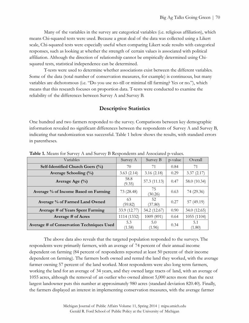
Big Ag Talks Going Green | 70
Michigan Journal of Public Affairs Volume 11, Spring 2014 | mjpa.umich.edu
Gerald R. Ford School of Public Policy at the University of Michigan
Many of the variables in the survey are categorical variables (i.e. religious affiliation), which
means Chi-squared tests were used. Because a great deal of the data was collected using a Likert
scale, Chi-squared tests were especially useful when comparing Likert scale results with categorical
responses, such as looking at whether the strength of certain values is associated with political
affiliation. Although the direction of relationship cannot be empirically determined using Chi-
squared tests, statistical independence can be determined.
T-tests were used to determine whether associations exist between the different variables.
Some of the data (total number of conservation measures, for example) is continuous, but many
variables are dichotomous (i.e. “Do you use no-till or minimal till farming? Yes or no.”), which
means that this research focuses on proportion data. T-tests were conducted to examine the
reliability of the differences between Survey A and Survey B.
Descriptive Statistics
One hundred and two farmers responded to the survey. Comparisons between key demographic
information revealed no significant differences between the respondents of Survey A and Survey B,
indicating that randomization was successful. Table 1 below shows the results, with standard errors
in parentheses.
Table 1. Means for Survey A and Survey B Respondents and Associated p-values.
Variables Survey A Survey B p-value Overall
Self-Identified Church Goers (%) 70 71 0.84 71
Average Schooling (%) 3.63 (2.14) 3.16 (2.18) 0.29 3.37 (2.17)
Average Age (%) 58.8
(9.35) 57.3 (11.13) 0.47 58.0 (10.34)
Average % of Income Based on Farming 73 (28.48) 75
(30.26) 0.63 74 (29.36)
Average % of Farmed Land Owned 63
(59.82) 52
(37.80) 0.27 57 (49.19)
Average # of Years Spent Farming 33.9 (12.77) 34.2 (12.67) 0.90 34.0 (12.65)
Average # of Acres 1114 (1332) 1009 (891) 0.64 1055 (1104)
Average # of Conservation Techniques Used 5.3
(1.58) 5.0
(1.96) 0.34
5.1 (1.80)
The above data also reveals that the targeted population responded to the surveys. The
respondents were primarily farmers, with an average of 74 percent of their annual income
dependent on farming (84 percent of respondents reported at least 50 percent of their income
dependent on farming). The farmers both owned and rented the land they worked, with the average
farmer owning 57 percent of the land worked. Most respondents were also long term farmers,
working the land for an average of 34 years, and they owned large tracts of land, with an average of
1055 acres, although the removal of an outlier who owned almost 5,000 acres more than the next
largest landowner puts this number at approximately 980 acres (standard deviation 820.40). Finally,
the farmers displayed an interest in implementing conservation measures, with the average farmer

Big Ag Talks Going Green | 71
Michigan Journal of Public Affairs Volume 11, Spring 2014 | mjpa.umich.edu
Gerald R. Ford School of Public Policy at the University of Michigan
having at least five conservation techniques employed on her or his land at the time the survey was
taken.
Based on available data, the demographic data collected closely resembles the national
average data in areas like age and differs in a few key characteristics. The USDA’s 2012 Census of
Agriculture reported the average age of Illinois farmers to be 57.8 (versus the study’s finding of
57.99), and found that 82 percent of farmers had been farming for 10 years or more. The key
difference is farm size: the average Illinois farmer farms 359 acres—significantly smaller than the
survey average, whether determined with or without the outlier (US Department of Agriculture
2014). Because the survey creators were hoping to gather information on large scale farmers, this
difference provides evidence that the target population was reached.
Many demographics measured in the questionnaire are not measured through government
surveys (such as religious practices and schooling). Other traditional demographic variables, such as
sex and race, were not collected, although this would be a very interesting extension of this work. In
this instance, the small sample size would make it difficult to identify statistically significant
differences between these demographics (which are not evenly represented in the United States large
scale farming community), and with limited space, other demographic information was determined
to be more important.
Data Analysis
Conservation Practices
Ninety-nine percent of farmers report using some sort of conservation practices, with a mean of
five conservation practices overall. The most popular practice is No Till/Minimal Till farming,
which provides not only conservation benefits in terms of water and soil retention, but also
provides gains in time and labor costs from a business perspective, making it an obvious choice for
many farmers. Crop rotation is also extremely popular, as it allows productive use of the land for
agriculture, while also providing some environmental benefits. The least popular method of
conservation is wetland restoration, which takes up a great deal of space and has few obvious
economic benefits for the farmer, despite requiring a great deal of restoration work. Strip-cropping
is almost equally unpopular, as the practice requires alternating different types of crops on the same
land, making harvesting more difficult.

Big Ag Talks Going Green | 72
Michigan Journal of Public Affairs Volume 11, Spring 2014 | mjpa.umich.edu
Gerald R. Ford School of Public Policy at the University of Michigan
Table 2. Percent of Farmers Using Conservation Practices.
Conservation Practice Percentage of Farmers Using
Any Conservation Practices 99
No Till/Minimal Till 90
Crop Rotation 86
Waterways 81
Buffer Strips 59
Field Borders 43
Cover Crops 39
Terracing 32
Strip-cropping 14
Wetland Restoration 13
Of the demographic characteristics measures, two displayed significant relationships, as
determined through standard regression, although both were relatively small effects. Age and
conservation use were positively correlated (p = 0.043). Each decade of farming experience is
associated with an increase of 0.3 conservation practices used. In addition, another positive
correlation was found for conservation use and farming-based income (p = 0.002). Each 10 percent
increase in farming-based income is associated with an increase of 0.2 conservation practices used.
There was no significant relationship between conservation usage and farm size, owning versus
renting, frequency of church attendance, or schooling.
Additional analyses were conducted to determine whether demographic information played
a role in total conservation measures used. A chi-squared test was run to look at the correlation
between political affiliation and the total number of conservation measures used. The variable for
“total conservation measures used” was broken down into two categories, “Few conservation
measures used”, denoted as five practices or less, and “Many conservation measures used”, denoted
as six practices or more. Political affiliation included Republicans, Democrats, and Independents.
The results are displayed on Table 3 below.
Table 3. Total Implemented Conservation Practices by Political Affiliation.
Political Affiliation 0-5 6+ Total
Democrat 9 0 9
Independent 9 13 22
Republican 33 25 58
Total 51 38 89
The chi-squared test revealed that the association between party affiliation and conservation
practices is significant (p=0.0104). This result was confirmed using the Fisher’s Exact Test for small
sample size (with the category of “Independent” removed in order to achieve the two-by-two matrix

Big Ag Talks Going Green | 73
Michigan Journal of Public Affairs Volume 11, Spring 2014 | mjpa.umich.edu
Gerald R. Ford School of Public Policy at the University of Michigan
required for the test), which found the same p-value as the chi-squared test in a one-tailed variation,
and a value of 0.021 in a two-tailed test, both significant values.
Conservation Measures: Farmer Decision Making
This analysis raised questions as to why farmers belonging to one political affiliation chose to
implement specific conservation measures over those belonging to another. An analysis was run
with a breakdown of responses by political party, as shown in Table 4 below.
Table 4. Percentage of farmers who responded with “Agree” to the following statements.
Measured Values Political Affiliation
“Participation in conservation initiatives…” Democrat Independent Republican Overall
Benefits me economically (All) 33 86 83 79
Puts me at a competitive disadvantage relative to other farmers in the area, who aren’t implementing these measures. (All)
0 9 5 6
Is important because other farmers will look poorly on my farm if I don’t participate. (All)
0 0 5 3
Helps to maintain the quality of my land and soils, so that I can use the land for longer. ( Survey A)
100 100 100 100
Improves the health of my farmland, so I can use it more sustainably. (Survey B)
75 82 89 86
Helps clean up local waterways. (Survey A) 40* 82* 68* 68
Helps clean up the Mississippi River. (Survey B) 50 45 58 55
Is part of my responsibility as a farmer. (Survey A)
100 100 91 95
Makes me a good steward of the environment. (Survey B)
100 100 100 100
*Although these appear very different, the small sample sizes for each survey prevented a significant finding.
From this data, only the first question on economic benefits displayed a significant
difference, as determined by a chi-squared test (p = 0.0021) and corroborated by the Fischer's Exact
Test (p = 0.0025), which indicates an interaction effect of this measure and political affiliation. While
a large majority of both Republicans and Independents believed conservations measures have
economic benefits, the majority of Democrats did not. The small sample size brings the significance
into question, but party affiliation as it relates to conservation activities could be an area of further
research, to try to understand if and why Democrats specifically are less likely to believe in the
economic benefits of conservation.
Of note is that farmers were the least likely to agree with the idea that conservation
measures put farmers at a competitive disadvantage (six percent) or believed that other farmers
would disapprove if they chose not to implement conservation measures (three percent). As to this
last question, further study may be warranted, as this finding contradicts previous research. Because
this survey looked at conscious attitudes, however, it is possible that farmers do not notice the effect

Big Ag Talks Going Green | 74
Michigan Journal of Public Affairs Volume 11, Spring 2014 | mjpa.umich.edu
Gerald R. Ford School of Public Policy at the University of Michigan
of social pressures. The lack of subtlety of this question may have overshadowed underlying social
forces.
Analysis of Differences Between Survey A and Survey B
In the survey, several questions were asked of only one half of the survey respondents, for two
reasons: 1) to see if there were differences in reaction to slight variations in framing and 2) because
the survey was short, and we needed to get as much information out of it as possible. For this
reason, some comparisons between Survey A and Survey B make quite a lot of sense. In other
instances, the comparison is less appropriate. For the purpose of this paper, only the questions
posed differently between the surveys are analyzed.
Interchangeable Terminology
From a communication standpoint, understanding when word choice does not make a difference is
just as important as understanding when it does. For this reason, a brief review of non-significant
findings has been included.
In terms of language used, farmers did not readily differentiate between the terms "global
warming" and "climate change," "state" and "region," or "cultural" versus "historical." In addition,
farmers showed no difference in opinion when the term "steward" was used or not used, when a
divine "God" was invoked versus not invoked, when the Mississippi was mentioned specifically
rather than “waterways” generally, nor the mention of specific flooding events as opposed to general
flooding.
Interestingly, the farmers showed equal concern for protecting wetlands as a form of flood
control as they did as a form of wildlife habitat. This question was posed to determine farmer
opinion changed towards wetlands when they considered it a detriment to themselves (flooding their
land) versus a non-human, non-personal entity (wildlife). The farmer’s unchanging concern for
wetlands was demonstrated twice in the data, whether framing the issue of wetland destruction as a
threat, or wetland protection as a benefit. In neither instance was the end concern shown by farmers
statistically different, regardless of framing. This lack of opinion change with regards to human and
nonhuman benefits was also echoed in the lack of a significant difference found between wanting to
protect land beside rivers from development, versus protecting it for human use and enjoyment.
In order to increase sample size in the full analysis, the following non-significant variables
have been combined into their respective single variables for the purpose of the full analysis:
climate change and global warming
historical and cultural
region and state
"God" mentioned versus not mentioned
specific flooding events versus general ones

Big Ag Talks Going Green | 75
Michigan Journal of Public Affairs Volume 11, Spring 2014 | mjpa.umich.edu
Gerald R. Ford School of Public Policy at the University of Michigan
Non-Interchangeable Terminology
In several instances, farmers responded significantly differently to different phrasings. Farmers were
more likely to agree with a statement that the Mississippi is "polluted," rather than "full of trash,"
for instance. This could be related to a sense that "trash" is a visible substance, whereas "pollution"
can combine with the water to make it unsafe for human and ecosystem health without very visible
signs of trash. In terms of curtailing non-visible pollution like fertilizer runoff, this distinction may
be highly salient.
In addition, farmers who received Survey A unanimously agreed that conservation
“improved the quality of their land,” which allowed them to use it longer. However, there was less
agreement as to whether these same activities resulted in “improved land health and sustainable
use.” These statements, which are arguably the same, received different reactions, indicating that
farmers may respond more favorably to statements that do not directly use the words
"sustainability" and/or "health."
Interestingly, farmers were more likely to agree that the Mississippi River is a "living
ecosystem" rather than "full of life." This difference was chosen as two potential wordings for
outreach materials, one representing a more scientific approach (the word “ecosystem”) to river
management and the other representing a more layperson language. The farmer response to the
word “ecosystem” shows a familiarity with the more technical language used to describe natural
environments, signaling that it might be useful to engage with farmers on a more technical level
when it comes to river management. The difference in the survey results here could be because
farmers were reminded in this survey that the Mississippi River is polluted, and were reluctant to say
that it is "full of life" but did not have the same qualm about thinking about the river as an
ecosystem. Whatever the reason, the difference is significant.
Farmers also responded differently to two different framings regarding restoration initiatives.
One survey simply asked how much farmers were likely to support an “increase [in] public funding
to clean up and restore the Mississippi.” The second survey used exactly the same language, but with
the phrase “supported by an increase in taxes” at the end. Farmers were less likely to support the
statement if taxes were identified as the funding mechanism.
A difference was found between the views that the Mississippi is a “place of scenic beauty”
rather than a “place to relax,” with farmers rating "place of scenic beauty" more highly. One
explanation for why farmer opinion seems to be slanted towards "scenic beauty" could be that
farmers are more accustomed to seeing the river as a place to look at, but not necessarily interact
with, as the phrase "a place to relax" implies.
There was one question which bordered on significance that should be mentioned. Farmers
seemed to agree more to the statement that the Mississippi River is "vulnerable" than it being
"threatened." This is an interesting differentiation, since "threatened" implies outside, aggressive
forces, while "vulnerable" does not. It is possible that farmers are uncomfortable with the idea that
the Mississippi River is being "threatened" as farmers themselves are often accused of doing harm
to it. It is possible that "vulnerable" is more harmless, whereas "threatened" inspires defensive
reactions. No variables with significant differences were aggregated.

Big Ag Talks Going Green | 76
Michigan Journal of Public Affairs Volume 11, Spring 2014 | mjpa.umich.edu
Gerald R. Ford School of Public Policy at the University of Michigan
Farmer as Residents of the Mississippi River Region
With one exception, there were no statistical differences between the surveys, indicating that in
general, there were no serious interaction effects as a result of the slightly different wording. This
one exception was farmer feelings about their own residency status with regards to the Mississippi
River region.
The question posed was “I consider myself a resident of the Mississippi River region” with
the options “Strongly Agree” to “Strongly Disagree” (1-5). Those who responded to Survey A were
statistically more likely to consider themselves resident than those who responded to Survey B (p =
0.0015). It is possible that the assortment of questions in survey A vs. survey B may have inspired
differences of thought around residency. It should be noted that there were no differences between
the surveys on measures such as total conservation measures and it was confirmed through a
regression that no linear relationship exists between the implementation of conservation measures
and feelings about residency status. An association was uncovered between feelings of residency
status and feelings of responsibility towards maintaining the Mississippi, although the link is tenuous
due to an insufficient number of farmers rating this measure as unimportant to create an effective
chi-squared test, even when numbers were combined to make larger categories. While of theoretical
interest, this finding is of limited importance since neither measure correlates with increased use of
conservation measures.
Limitations
While a random selection of all farmers would have been better than a random sample of farmers
who are already associated with an environmental organization, this data was chosen for two
reasons:
1. Farmer contact information is, quite understandably, private. An organization of some kind
was required in order to gain access to farmer addresses.
2. The use of an environmental organization to gather this data had the potential to skew the
data in favor of farmers that have already shown an interest in the environmental movement.
However, analysis of survey respondent demographics indicated a wide range of responses,
from those implementing one conservation measure to those implementing ten, and a wide
range of environmental perspectives. Indeed, far more Republicans responded to the survey
than Democrats, who are conventionally seen as more environmentally minded. While it is
always possible that a population skew occurred, as well as potential for a nonresponse bias,
the data analysis makes this unlikely.
The most obvious drawback of the data is that only 102 observations are available for
analysis. Although the return rate for surveys was high, this may make it difficult to find more subtle
difference between populations. The data collection was a relatively low budget operation and only
300 surveys were sent out initially. Further research in this area should focus on collecting
information with more participants, to ensure that small effects (which are implied by the several
instances in which effects approaching significance are found) are properly accounted for.

Big Ag Talks Going Green | 77
Michigan Journal of Public Affairs Volume 11, Spring 2014 | mjpa.umich.edu
Gerald R. Ford School of Public Policy at the University of Michigan
In addition, it should be made clear that the population is sampled from the Illinois region
only. While Illinois is a big player in agricultural states and is traditionally considered to have a typical
Midwestern culture, personal judgment (and hopefully further research) will need to determine
whether the state is representative of the Midwest region or the country as a whole.
Discussion
Language
The analysis offers interesting insight into the values and thought processes of farmers. Many of the
reasons that farmers put forth for why they make the decisions that they do are remarkably
consistent with environmentalist thinking, despite not using environmentalist terminology. In some
instances, use of classic environmentalist words such as “sustainability” seem to have reduced
support for the idea (85 percent approval) while the concept itself, expressed as an issue of longevity
and land quality, was unanimously accepted (100 percent approval).
The appreciation of the word “vulnerable” instead of “threatened” may be another example
of farmers being extremely conscious of where they stand with regard to the Mississippi River’s
health. This research seems to indicate that the tension that exists between the two groups, farmers
and environmentalists, has spilled over into the language used to communicate ideas and concepts or
vice versa.
In other instances, language seemed to play a much smaller role. Farmers overall had no
change in response when the word environmental “steward” was used or omitted. Nor were farmers
interested in “global warming” versus “climate change.” It seems likely that the subtle distinction
between these terms and the concepts that they respectively represent may not be of great
importance to farmers, whereas terminology frequently used by environmentalists, such as
“sustainability,” or that seems to assign blame, such as “threatened,” may be seen as more
meaningful.
Demographics
Often the demographic results raised more questions than it provided answers. Although the chi-
squared tests are slightly suspect due to the limited number of Democrats in the subject pool, the
statistically significant findings raise questions about what a large dataset might reveal given further
study. As it stands, the data implies that Democratic farmers in Illinois engage in less conservation
activities than Republicans or Independents, and that they are less likely than these other political
affiliations to believe that such engagement in these measures will benefit them economically. These
findings are counter to current intuition on the subject, but if true, would indicate a necessary
change in communication patterns towards farmers, with more emphasis on environmental
measures as sound business decisions and targeting Democratic farmers. More research with larger
subject pools should be conducted before final conclusions are made.

Big Ag Talks Going Green | 78
Michigan Journal of Public Affairs Volume 11, Spring 2014 | mjpa.umich.edu
Gerald R. Ford School of Public Policy at the University of Michigan
Conclusion
In a great deal of conversations about American farming practices, large scale farmers are
characterized as being uncommitted to conservation reform. Farmers who use conventional
methods, as opposed to organic farming, are considered less environmentally conscious than those
who do. This research provides evidence that when working with farmers directly, a strong
commitment to sustainable land management is revealed as well as many values that mirror those of
environmentalists. There is also a degree of sensitivity to words that take on an accusing tone, such
as “threatened” instead of “vulnerable.” This suggests that the historic tensions between farmers
and conservationists may have left an impact on farmer perception of river ecosystems, which
should be acknowledged when working with the industry.
This research provides strong evidence that negative environmental perceptions about large
scale farmers are not only wrong, but harmful to the cause of conservation. The farmers surveyed
were reluctant to say that they engaged in conservation measures in order to use the land “more
sustainably,” but they unanimously agreed that they wanted to use their land in a way that maintained
the quality and longevity of the land and soil. These are arguably the same thing, and yet an
environmentalist hoping to work with farmers to improve conservation could unintentionally
alienate an audience through word choice. In the same conversation, environmentalists may feel a
farmer is disagreeing with them if the farmer were to respond negatively to the word, even though
the farmer may agree with sustainability in principle. Avoiding this sort of misunderstanding could
help farmers and environmentalists be allies in their work. Farmers express a strong interest in
implementing conservation measures that fit with their land, as well as an appreciation for
sustainability that mirrors the views of environmentalists.
One of the most interesting findings of the research is the prevalence of farmers who see
conservation work as a good business decision. Future research should look into why farmers see
conservation practices as a business investment—and why some farmers do not. The difference
between the business realities of daily farm work and the large scale implications of sustainable
farming are often considered to be incompatible, but this work suggests that many farmers, who
have been successfully running their farming business for an average of 34 years, have been able to
strike a balance between the two. This is extremely valuable knowledge in the work towards more
sustainable large scale farming and an area that requires a great deal more study and understanding.
Finally, it should also be noted that farm culture in America is changing. The farm size of
the survey participants may seem large to those more used to urban gardens or community farms,
but the reality is that a great deal of these “large” farms are being bought out by even larger farm
owners, who then rent out the land to actual farmers and receive government price supports.
Unfortunately, the predictions that this survey can make about the effects of this large scale farm
“buy out” are limited. This survey included mainly farmers who worked the land personally, a very
different demographic than a detached business owner. While this study found no significant
relationship between farm size and use of conservation measures, this relationship may change
when farm size increases drastically. More research should be done to determine what impact this
large-scale buy out is having on conservation practices on Midwest farms.
Big Ag Talks Going Green | 79
Michigan Journal of Public Affairs Volume 11, Spring 2014 | mjpa.umich.edu
Gerald R. Ford School of Public Policy at the University of Michigan
References
Ahnstrom, J., Hockert, J., Bergea, H., Francis, C., Skelton, P., & Hallgren, L. 2009. “Farmers and
Nature Conservation: What is Known about Attitudes, Contect Factors and Actions
Affecting Conservation?” Renewable Agriculture and Food Systems 24: 38-47.
Brook, A., Zint, M., & DeYoung, R. 2003. “ Landowners' Responses to an Endangered Species Act
Listing and Implications for Encouraging Conservation.” Conservation Biology 17 no.6: 1638-1649.
Bultena, G., & P. Nowak, E. H. 1981. “Farmers' Attitudes towards Land Use Planning.” Journal of
Soil and Water Conservation 36: 37-41. Buttel, F., & G.W. Gillespie, J. 1988. “Preferences for Crop Production Practices among
Conventional and Alternative Farmers.” American Journal of Alternative Agriculture 3: 11-17. Church, A. H. 1993. “Estimating the Effect of Incentives on Mail Survey Response Rates: A Meta-
Analysis.” The Public Opinion Quarterly 57 no. 1: 62-79. Cobanoglu, C., Warde, B., & Moreo, P. J. 2001. “A comparison of mail, fax and web-based survey
methods.” International Journal of Market Research 43 no. 4: 441-452. Duram, L. M. 2000. “Agents' Perceptions of Structure: How Illinois Organic Farmers View Political,
Economic, Social, and Ecological Factors.” Agriculture and Human Values 17: 35-48. Featherstone, M., & Goodwin, B. 1993. “Factors Influencing a Farmer's Decision to Invest in Long-
Term Conservation Improvements.” Land Economics 69 no. 1: 79. Gould, W., Saupe, W., & Klemme, R. 1989. “Conservation Tillage: The Role of Farm and Operator
Characteristics and Perception of Soil Erosion.” Land Economics 65: 167-181. Greenlaw, C., & Brown-Welty, S. 2009. “A Comparison of Web-Based and Paper-Based Survey
Methods: Testing Assumptions of Survey Mode and Response Cost.” Evaluation Review 33 no. 5: 464-480.
Guehlstorf, N. 2008. “Understanding the Scope of Farmer Perceptions of Risk: Considering Farmer
Opinions on the Use of Genetically Modified (GM) Crops as a Stakeholder Voice in Policy.” Journal of Agriculture Environmental Ethics 21: 541-558.
Hanson, J. 2001. “A Phenomenological Case for the Family Farmer as an Environmental Steward.”
Great Plains Research 11: 347-360. Heilman, P., & D.S. Yakowitz, L. L. 1997. “Targeting Farms to Improve Water Quality.” Applied
Mathematics and Computation 83: 173-194.

Big Ag Talks Going Green | 80
Michigan Journal of Public Affairs Volume 11, Spring 2014 | mjpa.umich.edu
Gerald R. Ford School of Public Policy at the University of Michigan
Jacobsen, R., Toungs, G., Goreham, G., Watt, D., Dahl, B., Sell, R., et al. 1991. “Report No. 271: Selected Characteristics of North Dakota Farm Families Engaged in Sustainable Agricultural Practices. ” Fargo, ND: Department of Agricultural Economics, North Dakota State University.
Kaplowitz, M. D., Hadlock, T. D., & Levine, R. 2004. “A Comparison of Web and Mail Survey
Response Rates.” The Public Opinion Quarterly 68 no. 1: 94-101. Kephart, W. M., & Bressler, M. 1958. “Increasing the Responses to Mail Questionnaires: A Research
Study.” Public Opinion Quarterly 22: 123-132. Liffman, R., Huntsinger, L., & Forero, L. 2000. “To Ranch or Not to Ranch: Home on the Urban
Range?” Journal of Range Management 53: 362-370. Pyysiainen, J. 2010. “Co-Constructing a Virtuous Ingroup Attitude? Evaluation of New Business
Activities in a Group Interview of Farmers.” Text & Talk 30 no. 6: 701-721. Rossi, A. 2011. “Hope and Skepticism: Farmer and Local Community Views on the Socio-
Economic Benefits of Agricultural Bioenergy.” Biomass and Bioenergy 35: 1418-1428. Ryan, R., Erickson, D., & DeYoung, R. 2003. “Farmers' Motivations for Adopting Conservation
Practices along Riparian Zones in a Mid-Western Agricultural Watershed.” Journal of Environmental Planning and Management 46 no. 1: 19-37.
Smith, C., Peterson, J., & Leatherman, J. 2007. “Attitudes of Great Plains Producers about Best
Management Practices, Conservation Programs, and Water Quality.” Journal of Soil and Water Conservation 62 no.5: 97A-105A.
Trout, S., Francis, C., & Jr., J. B. 2005. “Impacts of the North-Central Region SARE Grants, 1988-
2002.” Journal of Sustainable Agriculture 27: 117-137. US Department of Agriculture. Feb. 2014. 2012 Census of Agriculture: Preliminary Report, US and
State Data. Wilson, G. 1996. “Farmer Environmental Attitudes and EAS Participation.” Geoforum 27: 119. Yakatan, N. 2008. Midwest Farmer Interviews: A Snapshot of Opinions about Agriculture and the
Environment. Retrieved from Farms, Food and Fuel.org: http://www.farmsfoodandfuel.org/system/files/Midwest%20Farmer%20Interviews%20-%20Executive%20Summary_0.pdf

State Charter Law and Charter School Outcomes | 81
Michigan Journal of Public Affairs Volume 11, Spring 2014 | mjpa.umich.edu
Gerald R. Ford School of Public Policy at the University of Michigan
Six
Street-Level Bureaucrats Shirking to Success: An Application of
Principal-Agent Theory to the Implementation of Florida’s Third
Grade Retention Policy
Rachel White
Abstract
Policymakers have aimed to increase early reading skills for decades, yet in recent years state
governments have placed particular emphasis on the mastery of reading proficiency by the third
grade – a pivotal year in a child’s education since it is typically when students shift from learning to
read to reading to learn (Hernandez 2011). Research provides mixed results as to whether retaining
students based on the results of a state standardized test will benefit the student in the long run.
This study utilizes principal-agent theory and street-level bureaucracy theory to better understand
the ways in which school district teachers and administrators, as street-level bureaucrats, respond to
a state-mandated test-based third grade retention policy in Florida. While both policymakers and
practitioners may have the same end goal – to increase third grade reading proficiency rates –
evidence from regression analyses suggest that street-level bureaucrats use their informational
advantage to pursue means other than retention to achieve this end. For example, street-level
bureaucrats may be able to shirk around the policy by providing students with exemptions from the
state-mandated policy. Thus, while it appears as though a certain percent of students are proficient
on the third grade reading exam, these statistics may distort the actual scenario and our
understanding of the policy effects. By providing more students with good cause exemptions, these
students’ FCAT scores are not included in the interpretation of the increase in third grade reading
proficiency levels.
Rachel S. White is a doctoral student and Dean’s Scholar in the education policy program at Michigan State
University College of Education. Her research interests include issues of education policy implementation, education
governance structures, the historical trends of education policymaking and implementation, and the economics of
education policy implementation.

State Charter Law and Charter School Outcomes | 82
Michigan Journal of Public Affairs Volume 11, Spring 2014 | mjpa.umich.edu
Gerald R. Ford School of Public Policy at the University of Michigan
Introduction
In the American federal system, which divides elements of sovereignty between the central
government and the states, the Tenth Amendment of the Constitution grants state governments full
reign over their respective public education systems. However, governmental entities at every level
of the American federalist system partake in the pursuit of achieving state and national education
goals. The federalist structure of American government allows multiple layers of government to
engage in public education policymaking. Unlike most other nations, the United States does not
operate a national education system, and the federal government has historically taken a relatively
decentralized approach to education policymaking. Schools in the United States have been, and
remain, overwhelmingly a state and local responsibility.
Each government’s level of influence over education policy has historically been a reflection
of its funding contribution. According to the U.S. Department of Education, about 90 percent of
the annual expenditures of education at all levels come from state, local, and private sources and just
10 percent from the federal government. As states governments have taken on a greater role in the
funding of public schools, they have also taken on a greater role in education policymaking.
Similarly, the increase in the share of education spending from the federal government has increased
from less than 5 percent in the 1980s to 13 percent in 2010 (NCES 2013), and has coincided with an
increasing focus on education policymaking at the federal level. Since the distribution of reports
such as A Nation at Risk (National Commission on Excellence in Education 1983), Why Johnny Can’t
Read (Flesch 1955), and Why Johnny Still Can’t Read (Flesch 1981), the federal government has taken
an active role in increasing reading proficiency. For example, the federal government enacted a
federal mandate requiring states to set targets for student performance consistent with national
objectives around reading proficiency. The NCLB Act (2002) provided the federal government with
a way to monitor adherence to the policy by requiring each state education agency to submit a
regular “adequate yearly progress” report to the United States Department of Education.
Under the auspices of the federal government’s NCLB provision, state governments and
state education agencies require local education agencies (LEAs, i.e., school districts) to set targets
for their own performance consistent with progress toward the goals determined on the state level.
Similar to the federal-state monitoring process, most states require LEAs to submit a report to the
state department of education with data documenting progress toward the state goals. Likewise, to
be in compliance with federal and state law, local school district governing boards require school
administrators and teachers to set targets for student performance and report progress towards
these goals to the local education agency.
This paper will focus on the relationships between state and local education agencies during
the implementation of education policy. While state governments typically treat each LEA as a single
organization that must set targets for their own performance consistent with progress towards state
objectives, they also treat each LEA as a self-managing entity, allowing school administrators and
teachers to choose the processes and methods by which they will strive to reach district and, hence,
state and national education objectives. These two arms of the education policy body – state
government and local education agencies – can thus be perceived as a principal-agent relationship in

State Charter Law and Charter School Outcomes | 83
Michigan Journal of Public Affairs Volume 11, Spring 2014 | mjpa.umich.edu
Gerald R. Ford School of Public Policy at the University of Michigan
which the principal (i.e., state government) designs a contract with various incentive structures to
facilitate control of the agent (i.e., LEAs), even when the agents may have different objectives and
more information than the principal.
In this research study, I will apply principal-agent theory to the development and
implementation of a Florida policy that mandates school districts to retain any third grade student
who does not achieve “proficiency” on the annual third grade standardized reading exam. I will
analyze Florida’s reading proficiency and retention data as well as data around student good-cause
exemptions, and consider the relationship between the state government’s decision to implement a
test-based grade retention policy and the decisions of school administrators and teachers around
promotion and retention. I will then discuss the implications that state-mandated test-based
retention policies may have on the decisions of administrators and teachers, who can be understood
to be street-level bureaucrats, to include or exclude students in state standardized tests.
Review of Research on Reading Proficiency, Retention, and Student Success
Researchers and education practitioners alike have long recognized the importance of mastering
reading by the end of third grade. This year is seen as a pivotal point in a child’s education since it is
typically when students shift from learning to read to reading to learn (Hernandez 2011). Hernandez
(2011) found that students who did not read proficiently by third grade were four times more likely
to drop out of school than proficient readers. Lloyd (1978), too, found this result – that third-grade
reading achievement was a strong predictor of student success – more than three decades ago. Lloyd
(1978) also found, however, that retention in any of the first three grades is also a strong predictor
of later school dropout.
Third Grade Reading Proficiency as a National Movement
While policy reforms have aimed to increase early reading skills for decades, the most recent
nationwide effort – the No Child Left Behind Act of 2001 (NCLB 2002) – required states to test
reading skills annually for all students beginning in third grade. The NCLB (2002) Act fully
implemented President Bush’s “Reading First” initiative, underlying the President’s “unequivocal
commitment to ensuring that every child can read by the end of third grade” (U.S. Department of
Education 2002). This emphasis on third grade reading proficiency has continued into the current
presidential administration; President Obama reiterated the importance of child literacy in his
“Putting Reading First” blueprint for revising the Elementary and Secondary Education Act (ESEA,
known in its most recent form as NCLB) when it was being considered for reauthorization (U.S.
Department of Education 2010).
Significant national attention has been placed on third grade reading proficiency as a signal
of future academic access, compelling the federal government to address this issue through
education legislation. States and some local school districts have also recognized the urgency to
increase third graders’ reading proficiency levels. In fact, several states and some school districts
have enacted policies requiring that third grade students who fail to demonstrate basic reading
proficiency on the end-of-grade assessment be retained. Similar policies are under debate in

State Charter Law and Charter School Outcomes | 84
Michigan Journal of Public Affairs Volume 11, Spring 2014 | mjpa.umich.edu
Gerald R. Ford School of Public Policy at the University of Michigan
numerous state legislatures across the nation. While such policies have focused on reading
proficiency, enacting mandatory third grade retention policies renewed a different longstanding
debate: the consequences of retention on student achievement.
Return to the Retention Debate
Grade retention can be used with K-12 students who struggle in school. In today’s test-based
accountability environment, the term “struggle” often correlates with those students who have not
met a state test performance standard. The intended objective of retaining a struggling student is to
ensure the student learns the skills and knowledge necessary for success at the next grade level
(Krier 2013). Policies of social promotion, on the other hand, allow struggling students to move on
to the next grade level with their same-age peers.
Research around student retention and social promotion policies provide mixed results.
Proponents of mandatory student retention policies often cite research that shows socially
promoted students struggle academically in later grades. Although studies have found a slight gain in
academic achievement directly after completing a retention year, the majority did not find long-term
positive academic benefits (Moser, West and Hughes 2012; Schwerdt and West 2013; Roderick and
Nagaoka 2005).
Opponents of student retention policies argue that grade retention produces more harm
than good and that the benefits of keeping students with their age group outweigh the costs (Krier
2013). For instance, when it comes to motivation to learn and succeed – another strong indicator of
success in both academic and professional life – numerous studies have found that retention has a
negative effect on students (Pierson and Connell 1992). Retained students were found to have lower
emotional health, self-esteem, academic self-concept, and homework completion than socially
promoted students (Jimerson, Carlson, Rotert, Egeland and Sourfe 1997; Martin 2011). Moreover,
elementary school students ranked academic retention as one of the top five most stressful things
that could happen to them, just behind losing a parent, parental fighting, getting lost, and being
caught stealing (Jimerson, Anderson and Whipple 2005).
State Policy Decisions to Increase Student Literacy
Given the conflicting lines of research around retention and reading proficiency, it seems incredibly
challenging to conceive a policy solution to address the one-third of American third graders who are
not proficient in the subject of reading, according to the National Assessment of Educational
Progress (U.S. Department of Education 2013).1 While policymakers are aware that third grade
students not proficient in reading are at a greater risk for academic struggles in later grades, they also
know that retained students are much more likely to drop out of school than those who are socially
promoted. So, what decisions have policymakers made thus far?
A total of 32 states and the District of Columbia have enacted policies aimed at improving
third grade reading proficiency (Rose 2012). Moreover, 14 states and the District of Columbia have
recently enacted policies requiring that students who do not demonstrate basic reading proficiency at
the end of third grade be retained and provided with remedial services (Rose 2012). Seven additional
states require such students to be retained unless the student participates in an intervention, such as

State Charter Law and Charter School Outcomes | 85
Michigan Journal of Public Affairs Volume 11, Spring 2014 | mjpa.umich.edu
Gerald R. Ford School of Public Policy at the University of Michigan
mandatory summer school before starting fourth grade (Rose 2012). While some states (such as
Florida and Ohio) have had laws in place for years that require no student be promoted without
reaching the level of proficient on the state standardized third grade reading assessment, others
(such as Indiana and North Carolina) implemented such policies within the last three years. In many
other states (such as Iowa and Michigan), policy discussions around third grade test-based retention
rates are occurring in state legislatures at this very moment.
Case Study: Test-Based Third Grade Retention Policy in Florida
Retention Policy
Florida has one of the oldest and most frequently cited models of a strict third grade retention
policy (Rose and Schimke 2012). Beginning in the 2002-03 school year, Florida legislative statute
mandated retention of students whose reading deficiency was not remediated by the end of third
grade, as demonstrated by scoring at Level 2 or higher on the third grade statewide reading
assessment (Florida K-20 Education Code 2002). Florida was also one of the first states to include
“good cause exemptions” by which students may be exempt from the mandatory retention policy.
Good cause exemptions identified in the 2002 Florida K-20 Education Code include:
1. Limited English Proficient students who have had less than two years of instruction in an
English for Speakers of Other Languages program;
2. Students with disabilities whose individual education plan (IEP) indicates that participation
in the statewide assessment program is not appropriate;
3. Students who demonstrate an acceptable level of performance on an alternative
standardized reading assessment approved by the State Board of Education;
4. Students who demonstrate, through a student portfolio, that the student is reading on grade
level as evidenced by demonstration of mastery of the Sunshine State Standards in reading
equal to at least a Level 2 performance on the Florida Comprehensive Assessment Test
(FCAT);
5. Students with disabilities who participate in the FCAT and who have an IEP or a Section
504 plan that reflects that the student has received the intensive remediation in reading (as
required in statute) for more than 2 years but still demonstrate a deficiency in reading and
who were previously retained in kindergarten, first or second grade; and
6. Students who have received intensive remediating for two or more years but still
demonstrate a deficiency in reading and who were previously retained for two years before
entering third grade.
Two years after the law went into effect, the Florida Department of Education promulgated
rules around the use of alternative standardized reading assessment and student portfolios for good
cause promotion. The rules specify that students who score at Level 1 on the grade three reading
FCAT may be promoted to grade four if the student scores at or above the 51st percentile on the
grade three Norm Referenced Test portion of the reading FCAT or above the 51st percentile on a

State Charter Law and Charter School Outcomes | 86
Michigan Journal of Public Affairs Volume 11, Spring 2014 | mjpa.umich.edu
Gerald R. Ford School of Public Policy at the University of Michigan
parallel form of the SAT-9 alternative assessment. Moreover, good cause promotion under the
student portfolio exemption requires evidence, collected by the student’s teacher that shows an
accurate picture of the student’s ability and only includes student work that is independently
produced in the classroom. The student portfolio must include evidence that the benchmarks
assessed by the grade three reading FCAT are met, which includes multiple choice items and
passages that are approximately 60 percent literary text and 40 percent information text, and that are
between 100 and 700 words with an average of 350 words. Finally, for each Sunshine State Standard
Benchmark for Language Arts assessed on the grade three reading FCAT, the teacher must collect at
least five examples of mastery as demonstrated by a grade of “C” or above (Alternative
Standardized Reading Assessment 2004).
The Florida Department of Education (FDE) administrative rule was amended twice more
in 2008. The first set of amendments permitted the use of the SAT-10 as an alternative reading
assessment and reduced the required student score percentile on any of the alternative reading
assessments from the 51st to the 45th percentile. The second set of amendments allowed teachers to
administer the SAT-9 or SAT-10 to a student two times, as compared to the previous rule that only
allowed the student one try to achieve a proficient score on the SAT-9 or SAT-10 (Alternative
Standardized Reading Assessment 2004, as amended in 2008).
One year later, in 2009, the rule underwent major reconstruction. Rather than limit the
alternative standardized reading assessment to just the SAT-9 and SAT-10, the FDE permitted
school districts to submit requests for approval of alternative standardized reading assessment that
met certain criteria determined by FDE. Once an assessment was approved by FDE, it was also
approved for statewide use. Moreover, the FDE was required to approve the percentile passing score
for each approved alternative standardized reading assessment based on an analysis of Florida
student achievement results (Alternative Standardized Reading Assessment 2004, as amended in
2009).
The latest FDE rule change occurred in 2011. The change removed the SAT-9 as an
acceptable alternative assessment, increased the average number of words required in the passages
included in a student portfolio from 350 to 500 words, decreased the number of examples of
mastery included in a student’s collection of evidence from five to three examples, and changed the
definition of “mastery” for student portfolio work from a grade of “C” or above to a grade of 70
percent or above (Alternative Standardized Reading Assessment 2004, as amended in 2011).
Intervention Policy
Under the first iteration of the Florida test-based third grade retention legislation, school districts
were only required to provide a retained student with supplemental instructional services and
supports. In early 2004, however, the legislation was amended to include suggested interventions,
including, but not limited to: small group instruction; reduced teacher-student ratios; more frequent
progress monitoring; tutoring or mentoring; transition classes containing both third and fourth grade
students; extended school day, week or year; and/or summer reading camps (Florida K-20
Education Code 2002, as amended in 2004). The 2004 amendments also required school districts to:
(1) implement a policy for midyear promotion of any retained student who can demonstrate that he
State Charter Law and Charter School Outcomes | 87
Michigan Journal of Public Affairs Volume 11, Spring 2014 | mjpa.umich.edu
Gerald R. Ford School of Public Policy at the University of Michigan
or she is ready to be promoted to fourth grade; (2) provide retained students with a higher-
performing teacher; and (3) provide parents of retained students with either supplemental tutoring
options, a “Read at Home” plan outlined in a parental contract, or a mentor/tutor with specialized
reading training (Florida K-20 Education Code 2002, as amended in 2004).
No amendments were made to the third grade test-based retention statute of the Florida K-
20 Education Code between 2005 and 2012. In 2013, the legislature amended the statute to require
school districts to provide retained third grade students with a school district summer reading camp
(Florida K-20 Education Code 2002, as amended in 2013).
Policy Effects
In the 2002-03 school year, the first year of implementation, the number of third graders retained
jumped from 3.3 percent (6,435 students) to 14.4 percent (27,713 students). The number of Florida
students retained in third grade has fallen steadily over the last nine years, reaching 7.3 percent
(15,098 students) in 2012 (Florida Department of Education Bureau of Education Information and
Accountability Services). Schwerdt and West (2013) contend that this steady decline is primarily due
to an increase in the number of students meeting the promotion standard, level 3 on the third grade
FCAT reading assessment.
Theoretical Framework: Street-Level Bureaucrats and Principal-Agent Theory
In this study, I utilize two theories to develop a hypothesis about the relationship between state
government and school district administrators and teachers in the implementation of the Florida
test-based third grade retention policy: street-level bureaucracy theory and principal-agent theory.
Lipsky’s (1969) theory of street-level bureaucracy identifies street-level bureaucrats as people
employed by the government who are constantly called upon to interact with citizens in the regular
course of their jobs; have significant independence in job decision-making; and potentially have
extensive impact on the lives of their clients. Moreover, street-level bureaucrats’ work experiences
are relatively strongly affected by three conditions: relative unavailability of resources, both personal
and organizational; regular challenges to bureaucrats’ authority; and ambiguous, contradictory, and in
some ways unattainable, role expectations (Lipsky 1969). Public school administrators and teachers
are often referred to as street-level bureaucrats because they are employed by the school district and
their work environment closely emulates that which is described by Lipsky (1969).
Principal-agent theory focuses on the dynamic process of interaction between principals and
agents. Economists developed principal-agent theory in the 1960s and early 1970s in an effort to
describe the so-called agency problem that occurs when cooperating parties have different goals and
divisions of labor (e.g. Jensen and Meckling 1976; Ross 1973). The theory attempted to describe the
relationship between a work-delegating party (the principal) and a work-performing party (the agent)
using the metaphor of a contract (Jensen and Meckling 1976).
From an economic perspective, principal-agent theory is concerned with two dilemmas that
occur in agency relationships: conflicting desires or goals of the principal and agent and oversight
costs for the principal to verify what the agent is actually doing (Eisenhardt 1989). Given these two
State Charter Law and Charter School Outcomes | 88
Michigan Journal of Public Affairs Volume 11, Spring 2014 | mjpa.umich.edu
Gerald R. Ford School of Public Policy at the University of Michigan
dilemmas, the focus of the theory is on determining the most efficient contract governing the
principal-agent relationship given assumptions about people (e.g., self-interest, bounded rationality,
risk aversion), organizations (e.g., goal conflict among members), and information (e.g.
commodification of information) (Eisenhardt 1989).
Applying Principal-Agent Theory to Education Policymakers and Street-Level Bureaucrats
In the 1980s, Terry Moe (1984; 1987) extended the principal-agent framework to relationships where
a contract is implied rather than executed, particularly in the public sector context. Moreover, Matt
McCubbins and colleagues (1987) adopted a distinct political approach to the goal conflict and
information asymmetry dilemmas of principal-agent theory arguing “a system of rewards and
punishments is unlikely to be a completely effective solution to the control problem” due to “the
cost of monitoring, limitations in the range of rewards and punishments, and for the most
meaningful forms of rewards and punishments, the cost to the principals of implementing them”
(McCubbins et al. 1987, 251).
By the 1990s, the politically oriented principal-agent theory framework was expanded again,
allowing for one to view public funding of government agencies as a “contract” (e.g., Boston 1991;
Downs and Rocke 1994). Under this condition, an executive can be viewed as an agent of the
public; while the public may be unable to monitor each and every action taken by the chief
executive, they can readily monitor the success or failure of his decisions and take action (i.e., vote to
remove or reelect) based upon the perceived success or failure of the chief executive’s policy
(Downs and Rocke 1994).
Both the 1980s and 1990s principal-agent theory applications to political science can be
applied to the American education policy arena. Moe’s (1984; 1987) conception of an implied
contract can be applied to state government and LEAs. The state government, as the principal,
needs certain tasks carried out, such as ensuring all third grade students achieve proficiency on the
state standardized reading assessment. Because the state government lacks the time and expertise to
personally carry out this task, it delegates the task to LEAs. Therefore, the state government enters
into a contract with the LEAs in which the state government will allocate taxpayer dollars to pay for
the cost of educating each student and, in return, the LEAs must provide education services to
children that will ostensibly increase student reading proficiency levels.
At the heart of this principal-agent relationship is the question of how the state government
can design the contract with various incentive structures to facilitate control of the LEAs when: (a)
the objectives of the state government and LEA diverge, such as when street-level bureaucrats at the
school district level see a different means – other than mandatory retention – to reach the end goal
of all third graders reading proficiently; and (b) the LEA has an informational advantage over the
state government. From this informational advantage, two dilemmas arise: adverse selection and
moral hazard. For example, when the state government devolves much of the responsibility for
educating students to the LEAs and when the school district level educators (i.e., school
administrators and teachers) are embodiments of street-level bureaucrats, the LEA has a
comparative advantage that stems from the information and expertise possessed by the street-level
bureaucrats. In this situation, the problem of adverse selection arises if the state government is not

State Charter Law and Charter School Outcomes | 89
Michigan Journal of Public Affairs Volume 11, Spring 2014 | mjpa.umich.edu
Gerald R. Ford School of Public Policy at the University of Michigan
fully informed about the abilities of the school district level educators. Moreover, the problem of
moral hazard arises when the contract between the principal and agent has been agreed to and the
agent, realizing the principal’s lack of information, pursues the agent’s own objectives at the expense
of the principal’s interests.
In the next section, I will return to the Florida test-based third grade retention policy and
utilize the theoretical frameworks of street level bureaucracy and principal-agent relationships to
hypothesize how the enactment and implementation of the policy may be impacted by the
aforementioned dilemmas that occur in principal-agent relationships.
Hypothesis
Drawing upon the previous discussion of principal-agent theory and street-level bureaucracy theory,
I conjecture that the implementation of Florida’s third grade test-based retention policy will lead
street-level bureaucrats to (a) shirk in response to goal conflict and (b) define student interests in
ways different from those of the state government and subsequently impose their own view of
student interest due to the dilemma of asymmetric information.
Therefore, I hypothesize that because of agent shirking and the dilemma of asymmetric
information, a positive change (in this case, a decrease) in the percentage of third grade students not
proficient on the FCAT reading assessment will be associated with a positive change (in this case, an
increase) in the percentage of students receiving good cause exemptions from the FCAT reading
assessment.
Data and Methods
To test my hypothesis, I use data publicly provided by the Florida Department of Education. My
rationale for including only data from Florida is based upon data availability and the policy
implementation timeframe. Florida provides public access to school district level longitudinal data
with data available at the grade level by year. Furthermore, no other states have had a test-based
third grade retention policy in place for more than two years. Therefore, data from Florida allows for
a longitudinal study of student achievement, retention, and good cause exemption after the test-
based third grade retention policy was enacted. Appendix 1 outlines the sources of the data used in
this study.
I conduct simple descriptive analyses to examine trends in third grade student reading
proficiency levels, third grade retention rates, and third grade good cause exemption rates. I also
conduct bivariate regression analyses to understand how the implementation of the Florida test-
based third grade retention policy impacted the percent of third grade students proficient on the
third grade reading assessment. In the analysis, I also consider school district-level factors to
examine whether changes in student proficiency rates are significantly related to school district-level
characteristics such as a change in the percent of students receiving a good cause exemption; student
population, stability, and demographics; and teacher expertise, education level, and salary.

State Charter Law and Charter School Outcomes | 90
Michigan Journal of Public Affairs Volume 11, Spring 2014 | mjpa.umich.edu
Gerald R. Ford School of Public Policy at the University of Michigan
Further, to understand the relationship between the change in the percentage of third grade
students proficient on the FCAT reading assessment and the school district-level variables, I apply a
production function that starts with the following general education production function: the change
in the percent of third grade students proficient on the third grade reading assessment in school
district j between 2002-2003 and 2010-2011 is a function of school district-level student
characteristics, StudChar, school district-level teacher characteristics, TeachChar; and the change in the
percentage of students receiving good cause exemptions from the FCAT reading assessment at the
school district level, %Exempt.
SchChange%Profj = f (StudCharj, TeachCharj, %Exemptj) (1)
From this production function, model 2 was developed. The log of school district
enrollment, school district average level of teacher experience, and school district average teacher
salary were used to improve model fit. Descriptions of the variables in model 2 are provided in
Appendix 1.
SchChange%Profj = α + β1 log(SchEnroll) + β2SchStabil + β3Sch%White +
β4Sch%ELL + β5Sch%FRPL + β6Sch%SWD + +β7Teach%AdvDeg + β8lo g(TeachAvgSal) +
β9lo g(TeachAvgExp) + β10SchChange%Exempt + ε (2)
Analysis and Discussion
Student Reading Proficiency and Retention
To understand whether the implementation of the Florida test-based third grade retention policy
had an effect on student reading proficiency levels and student retention rates, I conducted an
analysis of the trends of the third grade proficiency and retention rates before and after the policy
was implemented.
The blue trend line in Figure 1 shows that the percent of students testing not proficient in
reading decreased the first three years after the retention policy was enacted, as determined by the
statewide assessment. This decrease was followed by a sharp increase in the percentage of students
designated not proficient in reading. This dramatic shift occurred in the two school years following
the FDE’s promulgation of rules around the alternative standardized reading assessment and use of
student portfolios for good cause promotion. This also marked the year that the Florida legislature
amended the law to require school districts to: (1) implement a policy for midyear promotion of any
retained student who can demonstrate that he or she is ready to be promoted to fourth grade; (2)
provide retained students with a higher-performing teacher; and (3) provide parents of retained
students with either supplemental tutoring options, a “Read at Home” plan outlined in a parental
contract, or a mentor/tutor with specialized reading training. Since the 2007-08 school year, the
percent of third grade students testing not proficient in reading has remained relatively steady at
between 16 and 18 percent.

State Charter Law and Charter School Outcomes | 91
Michigan Journal of Public Affairs Volume 11, Spring 2014 | mjpa.umich.edu
Gerald R. Ford School of Public Policy at the University of Michigan
The red trend line in Figure 1 also shows that after the enactment of the retention policy, the
percent of retained third graders more than tripled, from less than four percent to more than 14
percent. After the initial spike, however, the percent of retained third graders steadily declined for
the next three years. Third grade student retention has remained at about seven percent since the
2007-08 school year.
Finally, the gap between the percentage of third grade students retained and the percentage
of third grade students testing not proficient in reading as seen in Figure 1 narrowed after the
enactment of the test-based third grade retention policy. Since the initial year of implementation, the
difference between these two factors has remained relatively stable between 10 and 11 percent. A
visible punctuation occurred during 2005-06 school year, which marks the year when both FDE and
Florida legislature made substantial changes to the test-based third grade retention policy.
Figure 2 compares the distributions of school districts’ percent of third graders who were
not proficient in reading and the percent of non-promotions for each year after the implementation
of the Florida retention policy. From this figure, two takeaways are evident: first, there is a stark shift
between the distribution of the percent of third graders who are not proficient in reading and the
distribution of the percent of third graders who are not promoted; second, the gap between these
two distributions has widened over the last ten years.
Figure 1. Comparison of Percent of Third Grade Students in Florida Not Proficient on FCAT and
Percent of Third Grade Students in Florida Retained in Third Grade, 2001-02 School Year to 2011-
12 School Year.

State Charter Law and Charter School Outcomes | 92
Michigan Journal of Public Affairs Volume 11, Spring 2014 | mjpa.umich.edu
Gerald R. Ford School of Public Policy at the University of Michigan
Figure 2. Comparison of Distribution of School Districts’ Percent of Third Grade Students Not
Proficient on FCAT and Percent of Third Grade Students in Florida Retained, 2001-02 School Year
to 2011-12.
Reading Proficiency, Retention, Good Cause Exemption, and School District Level Factors
Table 1 presents the bivariate linear regression analyses with change in percent of third grade
students proficient on the third grade reading FCAT as the dependent variable. Two significant
relationships emerged from these bivariate analyses: first is a positive relationship between the
change in percent of proficient students and the change in percent of students retained; second is a
positive relationship between the change in percent of proficient students and the change in percent
of students who receive a good cause exemption. The change in percent of proficient students and

State Charter Law and Charter School Outcomes | 93
Michigan Journal of Public Affairs Volume 11, Spring 2014 | mjpa.umich.edu
Gerald R. Ford School of Public Policy at the University of Michigan
change in percent of students who receive a good cause exemption were highly correlated and the
analysis estimates that a one percent decrease in the percentage of third grade students scoring at
Level 1 on the FCAT is associated with a 72.9 unit increase in the school district’s percent of
students receiving a good cause exemption. For example, if a school district were to decrease the
percentage of third grade students scoring at Level 1 on the FCAT by 5 percent between 2003-04
and 2010-11 and the percent of students receiving a good cause exemption in 2003-04 was 4
percent, the bivariate linear regression estimates that the percent of students receiving a good cause
exemption in 2010-11 would increase by 2.9 percent (72.9 percent of 4 percent) to 6.9 percent.
Table 1. Bivariate linear regression results with dependent variable, SchChange%Prof.
Explanatory Variable 𝜷 coefficient 𝑹𝟐 Adjusted 𝑹𝟐
P-Value Ho (5%)
Rejected?
School District level Students Characteristics
Log(SchEnroll) 0.005 0.004 -0.012 0.628 No
SchStabil -0.125 0.004 -0.012 0.632 No
Sch%White 0.046 0.035 0.02 0.128 No
Sch%ELL -0.15 0.037 0.022 0.118 No
Sch%FRPL -0.064 0.026 0.011 0.196 No
SCh%SWD 0.295 0.035 0.02 0.13 No
SchChange%Retain 0.374 0.079 0.065 0.021 Yes
SchChange%Exempt 0.729 0.261 0.249 0.000 Yes
School District level Teacher Characteristics
Log(TeachAvgExp) 0.065 0.007 -0.008 0.501 No
Log(TeachAvgSal) -0.093 0.004 -0.011 0.607 No
Teach%AdvDeg 0.071 0.018 0.003 0.275 No
Table 2 presents an analysis using a relative change ordinary least squares regression model
with change in percent of third grade students proficient on the third grade FCAT reading
assessment as the dependent variable. The model in table 2 allows for an examination of the factors
associated with a school district’s decrease in the percent of third grade students performing below
proficient on the FCAT reading assessment. Results from this analysis indicate that there is a
significant, positive relationship between the change in the percent of students scoring at a level 1
on the FCAT reading assessment and the change in percent of third grade students receiving a good
cause exemption. Holding all other school-level variables constant, a one unit increase in a school
district’s change in percent of students scoring at level 1 on the FCAT reading assessment is
associated with a 39.5 unit increase in the school district’s change in percent of third grade students
receiving a good cause exemption. That is, a large decrease in the percent of students scoring non-
proficient on the reading assessment is associated with a large increase in the percent of students
receiving good cause exemptions. Using the same example above, if a school district were to
decrease the percentage of third grade students scoring at level 1 on the FCAT by 5 percent
between 2003-04 and 2010-11 and the percent of students receiving a good cause exemption in
2003-04 was 4 percent, the full model difference regression estimates that the 2010-11 percent of

State Charter Law and Charter School Outcomes | 94
Michigan Journal of Public Affairs Volume 11, Spring 2014 | mjpa.umich.edu
Gerald R. Ford School of Public Policy at the University of Michigan
students receiving a good cause exemption would increase from 1.6 percent (39.5 percent of 4
percent) to 5.6 percent.
Results from this analysis also indicate that there is a significant, positive relationship
between the change in the percent of students scoring at a level 1 on the FCAT reading assessment
and the change in percent of third grade students with disabilities. That is, a decrease in the percent
of students scoring non-proficient on the reading assessment is associated with an increase in the
percent of students identified as a student with a disability within the school district. While these
results do not suggest that such an increase in the percent of students with a disability within a
school district could cause the decrease in the percent change of students proficient on the FCAT
assessment, they do suggest that school districts that experience an increase in the percent of
students with a disability may also experience a decrease in the percent of students not proficient on
the test. One possible explanation for this is that the students with disabilities may be exempt from
taking the FCAT assessment and, instead, take an alternative assessment or complete a reading
portfolio; thus, the scores that these students would have received on the FCAT reading assessment
are not taken into account.
Table 2. Full model differenced regression results with dependent variable, SchChange%Prof.
Independent Variable Coefficient (Standard Error)
Intercept 0.431(0.984)
School District level Student Characteristics
Log(SchEnroll) 0.018(0.015)
SchStabil 0.02(0.275)
Sch%White 0.035(0.043)
Sch%ELL 0.009(0.136)
Sch%FRPL -0.034(0.063)
SCh%SWD 0.505(0.203)**
SchChange%Exempt 0.764(0.16)***
School District level Teacher Characteristics
Log(TeachAvgExp) 0.005(0.089)
Log(TeachAvgSal) -0.147(0.206)
Teach%AdvDeg -0.02(0.064)
𝑅2 0.387
Adjusted 𝑅2 0.278
Sample Size 67
°p<.10, *p<.05, **p<.01, ***p<.001.

State Charter Law and Charter School Outcomes | 95
Michigan Journal of Public Affairs Volume 11, Spring 2014 | mjpa.umich.edu
Gerald R. Ford School of Public Policy at the University of Michigan
Shirking Student Success?
These analyses provide evidence that student proficiency levels increased and student retention
levels decreased after the initial enactment of the Florida test-based third grade retention policy.
This offers some evidence that the policy was successful and that school districts have emphasized
the importance of increasing the number of students who are proficient in reading by the end of
third grade.
However, my analyses also support the hypothesis that school districts that experienced a
positive change (i.e., a decrease) in the percentage of non-proficient students on the FCAT reading
assessment also experienced a positive change (i.e., an increase) in the percentage of students
receiving good cause promotions. Since the Florida law provides teachers and, ultimately, school
administrators with the authority to decide which students receive a good cause exemption, these
results suggest that street-level bureaucrats take advantage of the asymmetric information dilemma
in the principal-agent relationship. The results indicate that perhaps one of the reasons a school
district experienced a decrease in the percent of students scoring at level 1 on the FCAT reading
assessment is because school administrators and teachers provided more students with good cause
exemptions (e.g., determining that the student will take an alternative assessment or the teacher will
complete a reading portfolio for the student). School district bureaucrats may do this for a variety of
reasons. For example, they may provide more students with good cause exemptions so that certain
students who may put the school district at risk for lower FCAT scores will, instead, take the
alternative assessment or complete a reading portfolio. Alternatively, street-level bureaucrats may not
agree with the objectives of the state government’s mandated policy and, instead, believe that social
promotion is best for their students; therefore, the bureaucrats may provide more students with
good cause exemptions so that they can be promoted with the rest of their grade level cohort.
At the heart of this principal-agent relationship is the question of how the state government
can design a contract with LEAs to increase third grade reading proficiency levels when the
objectives of the state government and LEAs may diverge and when the LEA has an informational
advantage over the state government. These two dilemmas are deeply intertwined in the
development and implementation of any test-based third grade retention policy. The state
government realizes it is being held accountable by the public to do something about the large number
of third graders with dismal reading proficiency levels. In Florida, the state government responded
to this call for action by implementing a test-based third grade student retention policy. While this
study does not provide insight into how the Florida policymakers came to the final conclusion to
enact a policy mandating retention of a third grader who does not score proficient on the state
standardized reading assessment, the findings of this study indicate that street-level bureaucrats and
policymakers may diverge in how to reach the end goal of increasing third grade reading proficiency.
The LEAs’ comparative advantage stemming from the information (e.g., student-specific
circumstances) and expertise (e.g., research-based reading intervention strategies) possessed by the
street-level bureaucrats may have led to agent shirking to provide more students with good cause
exemptions.

State Charter Law and Charter School Outcomes | 96
Michigan Journal of Public Affairs Volume 11, Spring 2014 | mjpa.umich.edu
Gerald R. Ford School of Public Policy at the University of Michigan
Conclusion
In the case of Florida, policymakers enacted a test-based third grade retention policy with hopes of
increasing third grade reading proficiency levels (as measured by standardized reading assessments)
and, in the long term, student academic success. However, the results of this study suggest that
street-level bureaucrats in school districts may shirk around the mandatory third grade retention
policy, leading to an increasing number of students receiving good cause exemptions and, therefore,
removing low-achieving students from the population whose scores are considered in the measure
of third grade reading proficiency. The removal of certain students from taking the third grade
FCAT reading assessment could overestimate the percentage of third grade students who are
proficient in reading when the measure used by policymakers to monitor this education policy’s
success is the percent of students scoring at the proficient level on the third grade FCAT reading
assessment. Furthermore, providing more students with good cause exemptions could exacerbate
information asymmetry between the policymakers and street-level bureaucrats in the school districts
since policymakers have provided relatively open-ended descriptions of the elements required in two
of the most often used good cause exemptions: alternative assessments and student portfolios.
School districts are now allowed to submit a request for approval of any alternative
standardized reading assessment to the Florida Department of Education. While FDE does require
that the alternative assessments meet certain criteria, this may make it more difficult for the state to
monitor whether students are reaching the perceived level of reading proficiency as measured by the
state standardized assessment by the end of third grade. Similarly vague descriptions are given
around the good cause exemption of a student reading portfolio. Florida Department of Education
rules require just three examples of mastery included in a student’s reading portfolio that are graded
by the classroom teacher. Letting school districts complete such reading portfolios for their students
may, again, make it more difficult for the state to monitor whether students are reaching the
perceived level of reading proficiency by the end of third grade.
Policymakers are aware that students who are not proficient on a third grade reading
assessment are at greater risk to struggle in later grades and drop out of school. They also know that
students who are retained are much more likely to drop out of school than those who are socially
promoted. In developing policy to increase third grade reading proficiency, policymakers across the
United States are currently considering whether they want to prioritize reading proficiency at the
expense of the potential negative effects of student retention. This study provides an examination
of how street-level bureaucrats at the school district level in a principal-agent relationship with state
government responded to a state’s prioritization of reading proficiency over retention. It should be
noted that the results by no means suggest that shirking by street-level bureaucrats is wrong; it may
in fact be best for local administrators to make decisions about the students with whom they are in
close contact. What this study does show, however, is that principal-agent theory and street level
bureaucracy theory can help explain why ground-level results may deviate from initial policy goals.
When the principal-agent relationship between government and LEAs includes a street-level
bureaucrat as an agent, it seems that, despite their best efforts to control the agents, agents as street
level bureaucrats take into account their context and use their expertise and in-depth knowledge of

State Charter Law and Charter School Outcomes | 97
Michigan Journal of Public Affairs Volume 11, Spring 2014 | mjpa.umich.edu
Gerald R. Ford School of Public Policy at the University of Michigan
the students in the on-the-ground implementation of the policy. Further research with student-level
data is needed to understand whether the school street-level bureaucrats’ decisions to provide more
students with good cause exemptions in fact positively effects academic achievement in subsequent
years.
Although the results drawn from this case study can tell us a great deal about the trends in
third grade student retention and reading proficiency after the implementation of a mandatory test-
based third grade retention policy, they cannot be generalized to other states with different reading
assessments, different student populations, and different social, political, and economical
environments. Once more longitudinal data is available, additional research of other states that have
implemented test-based third grade student retention policies will be necessary to inform further
case study work on the subject. Furthermore, findings from this research could be strengthened with
qualitative research aimed at understanding the ways in which street-level bureaucrats interpret and
implement test-based retention policies.

State Charter Law and Charter School Outcomes | 98
Michigan Journal of Public Affairs Volume 11, Spring 2014 | mjpa.umich.edu
Gerald R. Ford School of Public Policy at the University of Michigan
References
Alexander, K.L., Entwisle, D.R., & Duaber, S.L. 2003. On the Success of Failure: A Reassessment of the
Effects of Retention in the Primary Grades. Cambridge, England: Cambridge University Press.
Alternative Standardized Reading Assessment and Use of Student Portfolio for Good Cause
Promotion. § 6A-1.094221. Boston, J. 1991. “The Theoretical Underpinnings of Public Sector Structuring in New Zealand.” In
Reshaping the state: New Zealand’s bureaucratic revolution, edited by J. Boston, J. Martin, J. Pallot and P. Walsh, 1-26. Auckland: Oxford University Press.
Downs, G.W. and Rocke, D.M. 1994. “Conflict, Agency, and Gambling for Resurrection: The
Principal-Agent Problem Goes to War.” American Journal of Political Science 38: 362-380. Eisenhardt, K.M. 1989. “Agency Theory: An Assessment and Review.” Academy of Management Review
14: 57-74. Ferris, J.M. 1992. “School-Based Decision Making: A Principal Agent Perspective.” Educational
Evaluation and Policy Analysis 14: 333-346. Fiester, L. 2010. Early Warning Confirmed: A Research Update on Third-Grade Reading. Baltimore, MD:
The Annie E. Casey Foundation. Florida Department of Education Bureau of Education Information and Accountability Services.
“Non-Promotions in Florida’s Public Schools.” http://www.fldoe.org/eias/eiaspubs/archives.asp
Florida Education Code § 20.15, 1008.25 Stat. 5 (2002). Hernandez, D.J. 2011. Double Jeopardy: How Third-Grade Reading Skills and Poverty Influence High School
Graduation. Albany, NY: Annie E Casey Foundation and the Center for Demographic Analysis, University of Albany, State University of New York.
Jensen, M. and Meckling, W. 1976. Theory of the Firm: Managerial Behavior, Agency Costs, and
Ownership Structure. Journal of Financial Economics 3: 305-360. Jimerson, S.R., Anderson, G., and Whipple, A. 2002. “Winning the Battle and Losing the War:
Examining the Relation Between Grade Retention and Dropping Out of High School.” Psychology in the Schools 39: 441-457.
Jimerson, S.R., Carlson, E., Rotert, M., Egeland, B., and Sourfe, L.A. 1997. “A Prospective,
Longitudinal Study of the Correlates and Consequences of Early Grade Retention.” Journal of School Psychology 35: 3-25.
Flesch, R. (1955). Why Johnny Can’t Read. New York, NY: Harper & Row Publishers Inc.
State Charter Law and Charter School Outcomes | 99
Michigan Journal of Public Affairs Volume 11, Spring 2014 | mjpa.umich.edu
Gerald R. Ford School of Public Policy at the University of Michigan
Flesch, R. (1981). “Why Johnny Still Can’t Read.” New York, NY: Harper Collins. Krier, J. 2013. “Grade Retention in Elementary Schools: Policies, Practices, Results, and Proposed
New Directions.” UCLA Center on Mental Health in Schools Information Resource. Lipsky, M. 1969. “Toward a Theory on Street-Level Bureaucracy.” Paper presented at the 1977
annual meeting of the American Political Science Association, New York, New York. Lloyd, D.M. 1978. “Prediction of School Failure from Third-Grade Data.” Educational and
Psychological Measurement 38: 1193-1200. Martin, A.J. 2011. “Holding Back and Holding On: Grade Retention and Students’ Non-Academic
and Academic Outcomes.” British Educational Research Journal 37: 739-763. McCubbins, M.D., Noll, R.G. and Weingast, B.R. 1987. “Administrative Procedures as Instruments
of Political Control.” Journal of Law Economics Organization 3: 243-277. Moe, T.M. 1984. “The New Economics of Organization.” American Journal of Political Science 28: 739-
777. −−. 1987. “An Assessment of the Positive Theory of Congressional Dominance.” Legislative Studies
Quarterly 12: 475-520. Moser, S.E., West, S.G., and Hughes, J.N. 2012. “Trajectories of Math and Reading Achievement in
Low Achieving Children in Elementary School: Effects of Early and Later Retention in Grade.” Journal of Educational Psychology 104: 603-621.
Munsen, L. 2010. Early Reading Proficiency. New York, NY: Annenberg Institute for School Reform at
Brown University. National Center for Education Statistics [NCES] (2013). Revenues and Expenditures for Public Elementary
and Secondary School Districts: School Year 2009-10. Washington, D.C.: U.S. Department of Education.
National Commission on Excellence in Education. (1983). “A Nation at Risk: The Imperative for
School Reform.” Washington, DC: Author. No Child Left Behind (NCLB) Act of 2001, Pub. L. No. 107-110 (2002). Pierson, L.H. and Connell, J.P. 1992. “Effect of Grade Retention on Self-System Processes, School
Engagement, and Academic Performance.” Journal of Educational Psychology 84: 300-307. Roderick, M. and Nagaoka, J. 2005. “Retention Under Chicago’s High-Stakes Testing Program:
Helpful, Harmful, or Harmless?” Educational Evaluation and Policy Analysis 27: 309-340. Rose, S. 2012. Third Grade Reading Policies. Denver, CO: Education Commission of the States.

State Charter Law and Charter School Outcomes | 100
Michigan Journal of Public Affairs Volume 11, Spring 2014 | mjpa.umich.edu
Gerald R. Ford School of Public Policy at the University of Michigan
Rose, S. and Schimke, K. 2012. Third Grade Literacy Policies: Identification, Intervention, Retention. Denver, CO: Education Commission of the States.
Ross, S. 1973. “The Economic Theory of Agency: The Principal’s Problem.” American Economic
Review 63: 135-151. Schwerdt, G. and West, M.R. 2013. The Effects of Test-Based Retention on Student Outcomes Over Time:
Regression Discontinuity Evidence from Florida. Harvard Program on Education Policy and Governance Working Paper Series (No. 12-09). Cambridge, MA: Harvard Kennedy School.
U.S. Department of Education. 2002. “The No Child Left Behind Act of 2001.”
http://www2.ed.gov/nclb/overview/intro/execsumm.html −−. 2010. “ESEA Reauthorization: A Blueprint for Reform.”
http://www2.ed.gov/policy/elsec/leg/blueprint/complete-education.pdf −−. 2011. “Mapping state proficiency standards onto the NAEP scales: Variation and change in
state standards for reading and mathematics, 2005-2009.” http://nces.ed.gov/nationsreportcard/pdf/studies/2011458.pdf
−−. 2013. “National Assessment of Educational Progress, Reading Assessment.” Washington, DC:
U.S. Department of Education, Institute of Education Sciences, National Center for Education Statistics.
Waterman, R.W. and Meier, K.J. 1998. “Principal-Agent Models: An Expansion?” Journal of Public
Administration Research and Theory 2: 173-202.
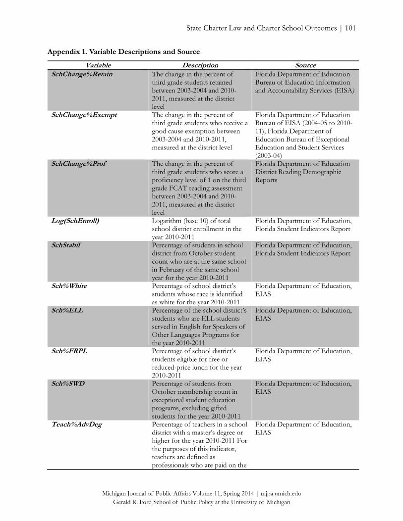
State Charter Law and Charter School Outcomes | 101
Michigan Journal of Public Affairs Volume 11, Spring 2014 | mjpa.umich.edu
Gerald R. Ford School of Public Policy at the University of Michigan
Appendix 1. Variable Descriptions and Source
Variable Description Source SchChange%Retain The change in the percent of
third grade students retained between 2003-2004 and 2010-2011, measured at the district level
Florida Department of Education Bureau of Education Information and Accountability Services (EISA)
SchChange%Exempt The change in the percent of third grade students who receive a good cause exemption between 2003-2004 and 2010-2011, measured at the district level
Florida Department of Education Bureau of EISA (2004-05 to 2010-11); Florida Department of Education Bureau of Exceptional Education and Student Services (2003-04)
SchChange%Prof The change in the percent of third grade students who score a proficiency level of 1 on the third grade FCAT reading assessment between 2003-2004 and 2010-2011, measured at the district level
Florida Department of Education District Reading Demographic Reports
Log(SchEnroll) Logarithm (base 10) of total school district enrollment in the year 2010-2011
Florida Department of Education, Florida Student Indicators Report
SchStabil Percentage of students in school district from October student count who are at the same school in February of the same school year for the year 2010-2011
Florida Department of Education, Florida Student Indicators Report
Sch%White Percentage of school district’s students whose race is identified as white for the year 2010-2011
Florida Department of Education, EIAS
Sch%ELL Percentage of the school district’s students who are ELL students served in English for Speakers of Other Languages Programs for the year 2010-2011
Florida Department of Education, EIAS
Sch%FRPL Percentage of school district’s students eligible for free or reduced-price lunch for the year 2010-2011
Florida Department of Education, EIAS
Sch%SWD Percentage of students from October membership count in exceptional student education programs, excluding gifted students for the year 2010-2011
Florida Department of Education, EIAS
Teach%AdvDeg Percentage of teachers in a school district with a master’s degree or higher for the year 2010-2011 For the purposes of this indicator, teachers are defined as professionals who are paid on the
Florida Department of Education, EIAS

State Charter Law and Charter School Outcomes | 102
Michigan Journal of Public Affairs Volume 11, Spring 2014 | mjpa.umich.edu
Gerald R. Ford School of Public Policy at the University of Michigan
instructional salary schedule negotiated by a Florida school district.
Log(TeachAvgSal) Logarithm (base 10) of average salary for all teachers within a school district for the year 2010-2011 For the purposes of this indicator, teachers are defined as professionals who are paid on the instructional salary schedule negotiated by a Florida school district.
Florida Department of Education, EIAS
Log(TeachAvgExp) Logarithm (base 10) of average number of years of teaching experience for all teachers within a school district for the year 2010-2011. Both in-state and out-of-state experience is counted.
Florida Department of Education, EIAS
Note: ANOVA analyses were conducted to test the hypothesis that means of the following variables are equal
across school years between 2001-02 and 2010-11, the year in which the most recent data was available:
Log(SchEnroll), SchStabil, Sch%White, Sch%ELL, Sch%FRPL, Sch%SWD, Teach%AdvDeg, TeachAvgSal,
and TeachAvg Exp. The ANOVA results indicated that there was no significant difference in any of the
variables across school years. Therefore, I chose to include the most recent data in my analyses.
State Charter Law and Charter School Outcomes | 103
Michigan Journal of Public Affairs Volume 11, Spring 2014 | mjpa.umich.edu
Gerald R. Ford School of Public Policy at the University of Michigan
Seven
State Charter Law and Charter School Outcomes
Audrye Wong
Abstract
Despite federal initiatives encouraging the expansion of charter schools, there remains a limited
understanding of the empirical relationship between state charter school laws and charter
performance. In this study, I categorize state legislation across three dimensions – permissibility,
autonomy, and accountability – and investigate each dimension’s statistical relationship with the
number of schools as well as NAEP performance. Results suggest that a state’s legal environment
may play a large and significant role in charter school students’ academic outcomes. Permissibility
and autonomy are associated with a greater number of charter schools, while higher accountability
standards may restrict and reverse growth. Although greater autonomy has some positive correlation
with academic outcomes, the negative correlations of increased permissibility and increased
accountability with student outcomes are greater in magnitude. These findings suggest that
policymakers may want to consider tightening permissive charter laws and overhauling current
accountability frameworks while encouraging a reasonable degree of autonomy. Furthermore,
expanding charter school programs through permissive laws may adversely affect academic
outcomes. Accountability standards seem to restrict charter school growth without necessarily
improving student performance.
Audrye Wong received her bachelor’s degree in public and international affairs at Princeton University and is starting
a PhD in Security Studies at Princeton’s Woodrow Wilson School in fall 2014. She was recently a Junior Fellow at
the Carnegie Endowment for International Peace.
State Charter Law and Charter School Outcomes | 104
Michigan Journal of Public Affairs Volume 11, Spring 2014 | mjpa.umich.edu
Gerald R. Ford School of Public Policy at the University of Michigan
Introduction
Background
Since 1991, when the first charter school law was passed in Minnesota, charter schools have been a
growing feature of the U.S. education landscape. In the 2009-10 academic year, there were over
4,900 charter schools nationwide, serving more than 1.6 million students (Chen 2011). Charter
schools were conceived as a means of revolutionizing public education through both competition
and choice by introducing greater competition in quality with traditional public schools, and
boosting student achievement along with parent satisfaction (Stillings 2005). Charter schools can be
set up by parents, teachers, community organizations, or other groups, and are governed by a
legislative contract with an authorizing body, such as the state or local school board. Such contracts,
which are periodically reviewed after a certain number of years, are meant to articulate performance
guidelines and hence maintain a certain degree of accountability.
Charter schools occupy an intermediary space between traditional public and private schools.
Like public schools, they receive state tax dollars and are generally open enrollment. Charter schools
also adopt features of private schools such as greater autonomy from regulations, increased
operational and curriculum flexibility, expanded choice by parents and students, and a diminished
teacher union presence (Miron and Nelson 2002; McNeal and Dotterweich 2007).
Because policymakers must try to manage the tension between local-level flexibility and
macro-level accountability (Shober et al. 2006), and between private choice and public standards,
charter school policy has inevitably become controversial. Detractors argue that the per-pupil
funding redirected to charter schools has drained much-needed resources from public school
districts without producing tangible success. Charter performance has been mixed and, despite some
successful case studies, performance tends to be lower than that of traditional public schools (U.S.
Department of Education 2006; CREDO 2009). A U.S. Department of Education study (2006)
found that charter school students had, on average, lower mean reading and mathematics scores on
the National Assessment of Educational Progress (NAEP) than students in traditional public
schools. A 2009 study by Stanford University’s Center for Research on Education Outcomes
(CREDO) found significant state-by-state differences in charter school performance. A more recent
CREDO 2013 study found some performance improvements but with high unevenness in quality
between states and across schools.
Despite inconsistent results, the federal government is actively supporting charter school
initiatives. The No Child Left Behind (NCLB) Act of 2001 included $300 million of federal funding
for charter schools. The Obama administration has also put considerable emphasis on expanding
charter schools nationwide. For example, Race to the Top is a recent initiative seeking to spur local-
level reform and innovation in education policies. In order to qualify for Race to the Top funding,
states’ applications must include initiatives for charter schools. Given such federal support, it
becomes even more critical to evaluate the factors behind the successes and shortcomings of charter
schools.
Each state implements its own set of charter laws. Because of such variation across states,
legislation has considerable implications on the creation and operation of charter schools in

State Charter Law and Charter School Outcomes | 105
Michigan Journal of Public Affairs Volume 11, Spring 2014 | mjpa.umich.edu
Gerald R. Ford School of Public Policy at the University of Michigan
different states. Miron and Nelson (2002) describe legislation as creating “an opportunity space in
which charter schools may experiment.” The authors highlight choice, deregulation, and
accountability as broad structural variables that can act through legislation to influence school and
student outcomes (Miron and Nelson 2002). Yet, there remains a limited understanding of the
relationship between state charter school laws and student academic performance, especially one
that is empirically based and at the national level.
This is in part because of the blanket ratings and classification of state charter laws that are
widely used. For example, letter grades A through E and classifications such as “strong” or “weak”
are subsumed into charter school policy discourse as a standard proxy for quality of charter
legislation (Wong and Shen 2006). A “strong” law supporting the expansion of charter schools does
not necessarily translate into quality outcomes and suggests a bias toward charter reform. Moreover,
such ratings do not adequately capture different dimensions of state legislation that can have
opposite effects on charter school presence and performance. Additionally, the complicated nature
of charter school politics involves competing interests of multiple actors, such as education
departments, traditional public schools, teacher unions, local politicians, parents, and citizens of
various ideological stripes. This has given rise to legislative and regulatory “layering” (Wong 1999) in
which laws are usually far from homogeneous. Wong and Shen (2006) have not only found variation
across states but also variation in the degree of permissibility across provisions within a single state’s
law.
To better understand charter school legislation as it relates to charter school outcomes, my
study decomposes state legislation into different clusters of provisions based on legal dimensions of
permissibility, autonomy, and accountability. Wong and Shen (2006) describe a consensus that
“evaluation of charter schools is not about, ‘Are charter schools working?’ but rather, ‘What makes
some charters work and others falter?’” A better understanding and evaluation of the effects of
charter school legislation is particularly relevant for pinpointing the circumstances that make charters
effective and those that do not. This has crucial implications for the design and direction of existing
and future charter law.
Literature Review
Through statistical analysis of clustered charter law provisions, Witte et al. (2003) concluded,
“unexpected[ly],” that “increasing flexibility in creating and running charter schools is correlated
with increasingly stringent state requirements for accountability of charter schools.” Subsequently,
Wong and Shen (2006) highlighted the importance of studying links between charter law and charter
outcomes and included a significant effort to kick-start the creation of a charter legislation database
for the purposes of policy analysis. They described in detail a systematic procedure of coding state
legislation, with the emphasis on individual provisions that were operationalized as objective,
dichotomous variables for easy use in empirical work. While the authors outlined four broad
categories of provisions (authorizing process; personnel policy flexibility; operation; and
accountability, standards, and expectations), they only analyzed the link between these provisions
and selected state-level factors, such as starting teacher salaries, size of state school system, and

State Charter Law and Charter School Outcomes | 106
Michigan Journal of Public Affairs Volume 11, Spring 2014 | mjpa.umich.edu
Gerald R. Ford School of Public Policy at the University of Michigan
Democratic Party strength, leaving unanswered the question of the relationship between charter law
provisions and student academic outcomes.
Such a relationship with student outcomes was specifically examined in a 2007 conference
paper by Watral, looking at fall-to-spring achievement gains in Northwest Education Assessment
test scores for schools in that region. Watral (2007) found that guaranteed funding for charters had
positive and significant effects on student achievement. Additionally, collective bargaining
exemptions and automatic waivers produced significant negative effects. Watral (2006) concluded
that there is no strong support for the impact of autonomy and flexibility on student achievement,
despite the arguments of advocates. However, Watral’s analysis was based on Center for Education
Reform (CER) rankings, which may potentially reflect the bias of this pro-charter advocacy group.
A CREDO (2009) analysis found significant variation in charter school performance across
16 selected states (including the District of Columbia), and demonstrated a link between legislation
and academic outcomes. These states, which had education department partnerships with Stanford,
represented over 50 percent of K-12 students in the United States and over 70 percent of the
country’s charter school students. In particular, charter schools in states with either enrollment caps
or multiple authorizers demonstrated significantly lower student growth in academic learning
compared to traditional public schools. At the same time, states that provided an avenue for appeals
on applications or renewals showed small but significant gains in learning. While the study’s strength
lies in its methodological selection of “twinned” students for comparison in charter versus
traditional public schools, it also relies on value-added analysis using state test scores. This limits the
ability to evaluate charter school performance between states as a function of legislation, since
different test measures would potentially have varied parameters and standards of student
achievement.
To take into account differences in education quality, the CREDO (2009) study also mapped
charter school effects by state against the state’s average performance on the 2007 National
Assessment for Education Progress (NAEP). The study finds that charters were more positively
associated with student performance gains in states with lower overall academic performance.
Nonetheless, there remains an absence of research on a nationwide scale using national-level
assessments as a common basis for comparison of legislation.
Methods and Data
Data and Methodology
Legal variables are based on individual state laws as reported in a 2004 study by CER. While the
CER is admittedly a pro-charter organization, I only use the legal analysis and explanation provided
for relevant individual provisions, in order to avoid any potential bias from CER’s rankings of the
state laws. I also refer to actual legal texts, legal databases and existing literature.1 Charter school
numbers by state were obtained from the National Alliance for Public Charter Schools (NAPCS)
database and NAEP test scores were provided online by the National Center for Education Statistics
(NCES) Data Explorer. There were fewer observations for charter NAEP scores, as some states did
not meet NCES reporting requirements in some years; missing data were left out of subsequent

State Charter Law and Charter School Outcomes | 107
Michigan Journal of Public Affairs Volume 11, Spring 2014 | mjpa.umich.edu
Gerald R. Ford School of Public Policy at the University of Michigan
regression analyses. Data on poverty status and population size at the state level came from the
Current Population Survey (CPS) Annual Social and Economic Supplement (U.S. Census Bureau).
The above data were collected for four time points: 2005, 2007, 2009, and 2011. Because CPS data
for 2011 were not yet available, 2010 figures were used instead. This is unlikely to significantly affect
results since the relative change within a year would likely be limited. State government and citizen
ideology scores are based on the most updated, commonly used measures by William Berry et al.
(2010), using a scale of 0 to 100, with 100 being the most liberal.
I use state legislation in three dimensions: permissibility, autonomy, and accountability.
Although previous studies code for a general “flexibility” dimension that encompasses the openness
of authorization processes and freedom from general regulation, such a dimension actually
encompasses both the ease of establishing and the freedom of operating charter schools. Thus, to
better understand such factors, I chose to code more specific dimensions: permissibility, the legal
ease of obtaining legal approval and setting up a charter school, and autonomy, the flexibility and
freedom from usual district and state education regulations once a charter has been established. The
third dimension, accountability, captures the public accountability and external monitoring standards
imposed on charter schools.
Each legal dimension consists of several legal variables coded individually along a scale. I
combine the variables’ scores to give each state three overall scores – one per dimension. Table 1
shows the breakdown of legal variables for each of the three dimensions. Instead of coding the
entire body of legislation, I identify the legal variables after a thorough review of proposed model
laws and the academic literature. Variables were coded on a scale of one to five, with a higher score
indicating a greater level of permissibility, autonomy, or accountability. The overall dimension score
for a state is equal to the sum of its individual variable scores. Because autonomy encompassed
many individual variables, states’ overall scores in that dimension were scaled down proportionally to
give the same maximum score of 15 as the other two dimensions.2 Appendix 1 further elaborates on
how these variables are defined.
Table 1. Breakdown of legal variables for each legal dimension.
Dimension Legal Variable
Permissibility
No cap on the number of schools; if there is one, 90% of the cap is not reached
Number and nature of authorizers
Involvement of for-profit organizations
Autonomy
Automatic exemptions from most district and state regulations
Waiver of teacher certification requirements
Legal and operational autonomy
Fiscal autonomy
Guaranteed funding sources
Accountability
Defined academic and operational performance expectations
Submission of annual performance reports to higher bodies
Periodic formal evaluation of state charter school program

State Charter Law and Charter School Outcomes | 108
Michigan Journal of Public Affairs Volume 11, Spring 2014 | mjpa.umich.edu
Gerald R. Ford School of Public Policy at the University of Michigan
I study two main outcomes: the number of charter schools in each state and the academic
performance of charter schools by state. I investigate the relationship between state charter law and
each outcome using ordinary least squares (OLS) regression. To measure student performance, I use
state-level mean charter scores from the National Assessment for Education Progress (NAEP)
reading and writing tests for grades four and eight, starting from 2005, the first year a breakdown of
scores according to charter and traditional public schools is available. I examine scores at four time
points: 2005, 2007, 2009, and 2011.
While forty states and the District of Columbia passed charter laws by 2004, only 21 states
are used because of the availability of NAEP charter school data. This approach assumes that state
charter laws remained constant after 2004, which is not likely to be the case. Therefore, I presume
that revisions would likely not be a determining factor of academic performance or school numbers.
State legislative changes could primarily affect new charter schools, a relatively small proportion
compared to the existing numbers, or would be phased in slowly to give current schools time to
adjust their practices and hence taking legal effect after the studied time frame. Such laws also tend
to produce effects observable only after a time lag. For example, more stringent accountability
requirements may only lead to improved test scores after a few years, or may only be imposed during
charter renewal. This is admittedly a potential weakness that will have to be addressed in future
studies.
I use OLS regression models to understand how differences in charter law structure relate to
point increases or decreases in NAEP test scores. Model 1 accounts for the number of charter
schools by state (N) and Model 2 uses charter NAEP scores (T). The two equations follow:
Model 1
N = α1 + βperm1Lperm + βauto1Lauto + βacc1Lacc + λ1Pops + ω1Povs + ϕ1Lt + φ1Lr +θ1Igov + ς1Iciti + ε1
Model 2
T = α2 + βperm2Lperm + βauto2Lauto + βacc2Lacc + γ2Tp + λ2Pops + ω2Povs + ϕ2Lt + φ2Lr + ε2
Variables Lperm, Lauto and Lacc represent state permissibility, autonomy, and accountability scores,
respectively. These are the main explanatory variables of interest. Constants are represented by α1
and α2 and ε1 and ε2 are error terms. Additional control variables include: state population (Pops);
state poverty rate (Povs); time since the charter law first took effect (Lt); and, time since the last legal
revision (Lr). I also include two other controls in Model 1: measures of government (Igov) and citizen
(Iciti) ideological leanings.
In Model 2, I incorporate the mean state-level NAEP scores for traditional public schools,
Tp, as a covariate to take into account exogenous performance variations and education standards
between the various states. By controlling for the mean performance of non-charter public school
students in the same state, any remaining gaps in charter academic achievement across states as
measured by βc may more accurately be attributed to differences in state laws.
I also control for additional state-level factors that may influence charter law design as well
as school numbers or performance. First, I use the percentage of the population under the poverty
State Charter Law and Charter School Outcomes | 109
Michigan Journal of Public Affairs Volume 11, Spring 2014 | mjpa.umich.edu
Gerald R. Ford School of Public Policy at the University of Michigan
line by state, Povs, as a proxy for the quality of the education system as a function of state resources.
To the extent that charter schools are seen as a vehicle of school choice and a solution to increase
the quality of traditional public schools through a competitive effect, states with more limited
resources could be inclined to encourage the expansion of charter school programs by designing
more permissive charter laws that grant greater autonomy without demanding high levels of
accountability. To factor in large demographic disparities across the United States that affect the
absolute number of charter schools per state, I include state population numbers (Pops) as a control.
Larger states may also face greater demographic variation which may make it harder for states to
implement or monitor higher education standards. Therefore, such difficulty may lead to variability
in academic performance.
The two OLS models also factor in the number of years since a state’s charter school law
was first implemented and last revised. A combination of both variables could capture the potential
time lag from any legal changes. The variable Lt refers to the age of the state charter law and is
calculated by subtracting the year when the law was first implemented in that state from 2004 (the
year for which state laws were coded). Lr is defined as the difference between the year in which the
NAEP test was administered and the year of the most recent substantive revision to state law (until
2004). This information was obtained from prior research done by Shober et al. (2006). Additionally
use the 2004 CER report for revisions after 2002 that were not included in the Shober et al. (2006)
study.
Laws that were passed earlier would give charter schools more time to open and gain
operational experience and this would plausibly facilitate improved academic performance. At the
same time, legal amendments would likely occur over the years to meet changing needs, depending
on whether the original law was regarded as too strict or too lax. Research has shown that state laws
have often been revised to increase flexibility and decrease accountability requirements (Shober et al.
2006). Alternatively, amendments may tighten accountability standards because of experience from
failed charter experiments or negative political or popular sentiment. For instance, a recent law
proposed by the pro-charter National Alliance for Public Charter Schools (NAPCS) gave more
attention to accountability and monitoring requirements.
Model 1 incorporates two variables on state government (Igov) and citizen ideology (Iciti). Both
variables are measured on a scale from 0 for the most conservative to 100 for the most liberal.
Those with conservative leanings traditionally favor school choice and expansion of charter school
programs. Therefore, I expect that states with a lower score will implement laws making it easier for
charter schools to open.
Citizen ideology may also be related to state government ideology in that people tend to vote
for political representatives with similar ideological leanings. Thus, ideology could influence charter
school numbers directly through broader support or opposition at the grassroots level to the
opening or closing of schools and indirectly, acting through the intermediary of state charter law.
However, this is not included in Model 2 as it is less likely to be significant in terms of student
academic performance. Finally, each state is weighted equally regardless of overall or charter student
population size. This is because charter laws are developed by individual states and this study is
focused on state-level comparisons rather than national aggregate effects.

State Charter Law and Charter School Outcomes | 110
Michigan Journal of Public Affairs Volume 11, Spring 2014 | mjpa.umich.edu
Gerald R. Ford School of Public Policy at the University of Michigan
Findings
Descriptive Results
This section presents a summary of the data used and descriptive trends of the two outcomes:
number of charter schools and student academic outcomes. Figure 1 shows the geographic coding
of state scores with darker regions reflecting higher scores. There is no clear pattern in the degree of
autonomy but permissive laws and lower accountability standards tend to be prevalent in the West.
Figure 1. Permissibility, accountability, and autonomy ratings by state.
Figure 2 contains three box plots presenting the spread of scores for each legal dimension.
State laws show greater variation in autonomy and accountability. The mean level of permissibility,
9.52, is slightly higher than those of the other dimensions. For accountability in particular, states that
score below the median are more likely to have far less stringent standards than the average, as
shown by the relatively large distance between the median and lower quartile lines. Although there is
a large range of autonomy scores, most states are clustered around the median score of 9.
State Charter Law and Charter School Outcomes | 111
Michigan Journal of Public Affairs Volume 11, Spring 2014 | mjpa.umich.edu
Gerald R. Ford School of Public Policy at the University of Michigan
Figure 2. Spread of scores for each legal dimension.
The box plots in Figure 3 show the range in the number of charter schools for different
states. Overall, states saw an expansion of charter schools over the years, although numbers varied
greatly across states (which may also be a function of population size). While most states have fewer
than 200 charter schools each, states with more schools than the median greatly exceed this median
figure, indicating a positively skewed distribution. The dots that appear from 2007 onwards
represent California as an outlier state.
Figure 3. Range in the number of charter schools for different states.
Mean state-level NAEP scores for charter and traditional public schools are almost the same
and the mean ratio of charter to public school scores is very close to one (Table 2). However, the
longer left tail of the histogram in Figure 4 suggests that charters that perform worse have a larger

State Charter Law and Charter School Outcomes | 112
Michigan Journal of Public Affairs Volume 11, Spring 2014 | mjpa.umich.edu
Gerald R. Ford School of Public Policy at the University of Michigan
achievement gap relative to traditional public schools in the same state and those that did better than
state public schools produce relatively smaller improvement.
Table 2. Descriptive statistics of state laws.
Variable Obs. Mean Std. Dev. Min. Max.
Permissibility of state law 36 9.52 2.54 5 14
Autonomy of state law 36 8.91 3.09 .6 14.4
Accountability of state law 36 8.00 3.19 3 14
No. of charter schools in state (sum of the obs. across all 4 years) 36 168.96 176.26 3 917
2005 4 144.76 147.57 3 498
2007 4 158.14 159.64 7 627
2009 4 176.86 179.32 8 748
2011 4 196.10 210.85 9 917
Charter NAEP scores 46 248.08 26.42 88 311
Traditional Public School NAEP scores 36 249.10 24.99 90 299
Ratio of Charter NAEP scores to public school NAEP scores 46 .997 0.05 .84 1.11
Year state law was implemented 36 1994.91 2.09 991 1999
Year of latest revision to state law 36 2001 1.85 996 2003
Time in years between law implementation and 2004 36 9.10 2.09 5 13
Time in years between last revision of law and when test was taken 36 7.00 2.91 2 15
Citizen ideology rating by state 20 52.41 14.52 0.3 85.3
State government ideology rating 20 47.82 13.21 5.9 67.7
Figure 4. Distribution of charter-to-public NAEP score ratios.
The linear relationships of the three legal dimensions are plotted in Figure 5. Permissive
state laws have a strong negative correlation with relative student achievement and, perhaps
unexpectedly, laws that demand greater accountability also have a negative correlation with charters’

State Charter Law and Charter School Outcomes | 113
Michigan Journal of Public Affairs Volume 11, Spring 2014 | mjpa.umich.edu
Gerald R. Ford School of Public Policy at the University of Michigan
performance compared to traditional public schools. The degree of legislative autonomy has only a
very small negative association with relative student achievement.
Figure 5. Ratio of charter to public NAEP scores against state law.
Regression Results
Based on my regressions, the influence of all three legal dimensions remained large and statistically
significant even after adjusting for multiple controls. This demonstrates that legal environment may
still have a major influence on the eventual number of operating charters (a joint F-test of all three
dimensions provides a test statistic of F(3, 310) = 102.02 and a p-value of 0.0000).
I also test the three legal parameters of permissibility, autonomy, and accountability for
correlation. The correlation coefficients are between 0.1 and 0.4 suggesting that individual analysis
of each parameter (as well as in tandem) may be significant in predicting my outcome variables.
Table 3 presents the results for the number of charter schools (Model 1) and Table 4 shows the
results for charter NAEP scores (Model 2).

State Charter Law and Charter School Outcomes | 114
Michigan Journal of Public Affairs Volume 11, Spring 2014 | mjpa.umich.edu
Gerald R. Ford School of Public Policy at the University of Michigan
Table 3. Impact of the legal environment on the number of charter schools in each state (Model 1).
Table 4. Impact of the legal environment on charter NAEP performance in each state (Model 2).
Model 1: Number of charter schools in state
Without controlling for other state factors, laws granting higher permissibility and autonomy
significantly relate to a greater number of charter schools, while accountability is associated with
fewer charter schools. Adding control variables reduces the apparent influence of permissive laws.
Table 3.1 Impact of the legal environment on the number of charter schools in each state (Model 1)
VARIABLES (1) (2) (3) (4) (5) (6) (7) (8) (9)
Permissive 26.64*** 22.21*** 13.02*** 15.60*** 11.00*** 11.07*** 7.135***
(3.504) (3.662) (2.024) (2.103) (2.056) (1.997) (1.934)
Autonomous 17.49*** 12.71*** 12.58*** 10.37*** 12.75*** 12.75*** 19.26***
(2.967) (3.077) (1.678) (1.749) (1.659) (1.611) (1.734)
Accountable -1.740 -7.027** -12.69*** -12.39*** -13.67*** -13.73*** -16.97***
(3.023) (2.809) (1.545) (1.518) (1.423) (1.382) (1.354)
State population (in 100,000s) 1.577*** 1.524*** 1.484*** 1.380*** 1.266***
(0.0563) (0.0570) (0.0533) (0.0565) (0.0573)
State poverty rate 5.736*** 6.612*** 9.685*** 12.52***
(1.533) (1.431) (1.544) (1.636)
Age of law in 2004 16.38*** 18.61*** 22.99***
(2.260) (2.248) (2.333)
Time since last legal revision -7.770*** -5.945***
(1.700) (1.701)
Government ideology -0.510
(0.414)
Citizen ideology -0.615
(0.392)
Constant -84.73** 13.03 185.3*** -89.94** -78.15*** -158.2*** -280.9*** -279.4*** -285.3***
(34.53) (27.99) (29.94) (41.15) (22.45) (30.71) (33.20) (32.24) (33.70)
Observations 336 336 336 336 336 336 336 336 320
R-squared 0.148 0.094 0.001 0.195 0.761 0.771 0.803 0.814 0.844
Standard errors in parentheses
*** p<0.01, ** p<0.05, * p<0.1
Table 3.2 Impact of the legal environment on charter NAEP performance in each state (Model 2)
VARIABLES (1) (2) (3) (4) (5) (6) (7) (8) (9)
Permissive -0.839 -0.619 -1.902*** -1.798*** -1.986*** -2.391*** -2.401***
(0.688) (0.734) (0.317) (0.318) (0.341) (0.367) (0.365)
Autonomous -0.601 -0.421 0.599** 0.560** 0.714*** 0.869*** 0.901***
(0.525) (0.558) (0.241) (0.240) (0.261) (0.263) (0.262)
Accountable -0.383 -0.243 -1.197*** -1.150*** -1.112*** -0.998*** -0.971***
(0.593) (0.602) (0.260) (0.259) (0.259) (0.259) (0.258)
Public school NAEP scores 0.975*** 0.974*** 0.969*** 0.972*** 0.969***
(0.0297) (0.0295) (0.0296) (0.0292) (0.0291)
State population (in 100,000s) -0.0164** -0.0134* -0.0173** -0.00953
(0.00760) (0.00784) (0.00785) (0.00875)
State poverty rate -0.358 -0.292 -0.506*
(0.239) (0.237) (0.260)
Age of law in 2004 1.203*** 1.070**
(0.432) (0.435)
Time since last legal revision 0.530*
(0.272)
Constant 256.3*** 253.7*** 251.7*** 260.4*** 29.73*** 30.46*** 36.35*** 25.42*** 25.34***
(6.942) (5.179) (5.842) (8.730) (7.967) (7.914) (8.824) (9.546) (9.491)
Observations 246 246 246 246 246 246 246 246 246
R-squared 0.006 0.005 0.002 0.009 0.819 0.822 0.824 0.829 0.832
Standard errors in parentheses
*** p<0.01, ** p<0.05, * p<0.1

State Charter Law and Charter School Outcomes | 115
Michigan Journal of Public Affairs Volume 11, Spring 2014 | mjpa.umich.edu
Gerald R. Ford School of Public Policy at the University of Michigan
As seen in Model 1, every point increase in permissibility of state law relates to seven more charter
schools. In contrast, granting greater legislative autonomy has a larger positive correlation, while
enhancing accountability requirements has a strong negative correlation. Each unit increase in the
degree of legal autonomy is associated with an increase of over 19 charter schools, but the same
increase in legal accountability correlates with almost 17 fewer charter schools.
Permissive laws – the lack of caps, having multiple authorizers, and allowing for-profit
organizations – relate to an increase in charter schools. This suggests that permissive laws do make it
easier or provide incentives for charters to be set up. Comparing states with high (score greater than
10) versus low permissibility (score less than 9), more permissive laws are associated with a faster
rate of increase in the number of schools over time (Figure 6).
Figure 6. Effect of permissibility on the number of charter schools over time.
In terms of autonomy, fewer regulations, guaranteed funding, and more charter control over
teacher certification and operational matters also appear to provide incentives to set up and maintain
operation of charter schools. Freedom plausibly encourages innovation and hence more charter
proposals. However, accountability standards in terms of performance expectations and monitoring
requirements greatly limit growth, either by enforcing closures of schools or by reducing the
incentive to open a school in the first place. A more daunting monitoring environment could deter
potential applicants.
Model 2: Academic achievement of charter schools on NAEP tests
There is no significant correlation between charter school performance and any of the three legal
parameters in the model without the covariate of traditional public school performance on NAEP.
However, the corresponding coefficients are large and highly significant when mean scores of
traditional public schools in the same state are considered. This underscores the large overall
variability in academic achievement between states that could obscure any potential performance
trends.

State Charter Law and Charter School Outcomes | 116
Michigan Journal of Public Affairs Volume 11, Spring 2014 | mjpa.umich.edu
Gerald R. Ford School of Public Policy at the University of Michigan
Without adding any other variables, permissibility and accountability have a negative
influence on charter academic achievement, whereas autonomy has a slight positive effect. After
controlling for other state-level variables, the model suggests greater negative influence of more
permissive laws, and greater positive influence of greater legislative autonomy, alongside a smaller
negative effect of accountability requirements. As shown in Table 3, a one-unit increase in the level
of permissibility relates to a 2.4 point decrease on the NAEP. Increasing the degree of legal
autonomy by one point correlates with a 0.9-point increase in NAEP score, while a similar increase
in accountability is linked with a decrease of 0.97 points on the NAEP. A joint F-test of all three
legal dimensions provides a test statistic of F(3,237) = 22.57 and a corresponding p-value of 0.0000.
This further confirms the high significance of the overall legal environment and suggests good
model fit.
Discussion
The regression results suggest potentially adverse implications for greater permissiveness in charter
legislation. Charter school students in states with no caps on growth, multiple non-governmental
authorizers, or laws that allow the involvement of for-profit organizations are far more likely to
perform worse on NAEP tests. An unlimited number of possible charters would reduce authorizer
oversight and incentive in screening for high-quality charter applications. At the same time,
authorizers such as private non-profits or higher education institutions may have less stringent
standards compared to state or local school boards who may be more demanding or even skeptical
of charters because charters directly affect the operations of their public schools. The availability of
multiple authorizers makes the approval process easier as applicants can work outside the usual
governmental bodies to find an authorizer with less rigorous standards. Finally, for-profits could well
have differing priorities when operating schools (charter or non-charter) and may be inclined to
maximize revenue at the expense of quality, which in turn affects the academic learning
opportunities of students.
The results do provide some empirical support to charter school advocates calling for
increased operational and legal freedom, whether in terms of automatic exemptions from standard
regulations, guaranteed funding, or even waivers of teacher certification requirements. This would be
a means of spurring educational innovation and enhancing student outcomes without having to
worry as much about fulfilling bureaucratic across-the-board regulations. States that have given more
space for charter schools to operate and experiment appear to have attained higher NAEP scores. It
is also plausible that increased autonomy could have even larger impacts if a broader definition of
student outcomes was used to take into account specialized programs in music, art, language, or
gifted education not usually captured in standardized reading and math tests. At the same time, it
should be noted that this positive autonomy effect remains smaller than the size of the strongly
negative permissibility factor. The different impacts of legislative permissiveness and autonomy
underlines the potentially opposing effects of what is commonly called flexibility at different stages
of charter school implementation (setting up versus operating the school).

State Charter Law and Charter School Outcomes | 117
Michigan Journal of Public Affairs Volume 11, Spring 2014 | mjpa.umich.edu
Gerald R. Ford School of Public Policy at the University of Michigan
Interestingly, greater accountability is associated with significantly lower test scores in charter
schools (although the influence was less pronounced than with permissive laws). This influence was
reduced in size but remained significant even after controlling for population, poverty, and law age.
A possible reason could be omitted variable bias. Introducing a dummy variable that grouped states
by census region, I also run a modified regression model (Table 5) with just the accountability
parameter and eliminate state poverty and population controls to minimize collinearity. The
accountability coefficient, however, remains negative. This could simply be because states with
poorly performing charters have implemented accountability requirements as a remedial response
with time lag limiting the influence of these more recent legal revisions.
Table 5. Impact of legal accountability on charter NAEP performance.
Variables (1) (2)
Accountable -0.421* -0.439*
(0.238) (0.238)
Public school NAEP scores 0.996*** 0.996***
(0.0241) (0.0241)
Age of law in 2004
0.406
(0.354)
Midwest region -5.184* -6.037*
(3.005) (3.093)
South region 11.23*** 11.26***
(2.864) (2.862)
West region 17.67*** 16.95***
(3.036) (3.098)
Constant -5.794 -8.816
(7.362) (7.814)
Observations 246 246
R-squared 0.882 0.883
Standard errors in parentheses
*** p<0.01, ** p<0.05, * p<0.1
On the other hand, the results provide strong indication that existing accountability
mechanisms are failing and suggest important implications for the improvement of charter school
legislation and policy. For example, authorizers may not rigorously enforce accountability
requirements prescribed by the law, and schools have little incentive to respond to such standards,
especially when legal language is vague and permits are flexible. Furthermore, the illusion of having
stringent accountability standards might lead to a perverse effect of laxer action in practice;
monitoring bodies may be inclined to grant schools’ requests for continued operation under
supposedly consistent monitoring.
State Charter Law and Charter School Outcomes | 118
Michigan Journal of Public Affairs Volume 11, Spring 2014 | mjpa.umich.edu
Gerald R. Ford School of Public Policy at the University of Michigan
The coded variables for the accountability dimension also focused on reporting and
monitoring requirements with no explicit link to upholding said accountability standards even if
such performance standards may have been defined in the charter contract. Submission of annual
performance reports or even state-level evaluation of the charter school program may not
necessarily lead to rapid corrective action on poorly performing charters. State laws have largely been
silent on requirements for sanctions, probation, or closure of failing charters. It may take years to
complete follow-up action, given the possibility of an appeals process and schools may be allowed
some time for self-improvement before stricter action is taken by authorizers or boards of
education. In addition, the influence of interest groups and political pressure muddies the entire
process. Thus, within the limited time period for which charter school NAEP scores are available,
we may not be able to clearly determine the impacts of accountability requirements.
Moreover, the “ideal” definition of accountability standards has yet to be adequately
captured in existing charter legislation across the country. Authorizers play an important role in
upholding accountability, not just in granting “permissibility” during the initial stages of setting up a
charter. Accountability standards should also encompass greater monitoring and intervention
powers for authorizers, as well as specific reporting and performance mandates for authorizing
bodies. This would provide important incentives for authorizers to maintain a quality portfolio of
charter schools.
Several studies have found that authorizers face difficulties imposing accountability
standards and implementing sanctions because of unclear laws, financial and logistical limitations,
political pressure, and adverse impacts on reputation (Finnigan et al. 2004). However, such specific
requirements are not traditionally emphasized in legal texts and public discourse. Only in recent
years has this aspect started to receive more attention. Therefore, the true influence of
accountability standards cannot yet be determined from data currently available for this study. This
presents a broader challenge in evaluating the association of accountability standards across states.
Future long-term studies will hopefully be better positioned for conclusive analyses.
Finally, methodological limitations may contribute to the negative association between
accountability and charter school performance. The sample of states with charter school data
available in NAEP is limited and not necessarily representative of the true population distribution
of accountability scores. This limits conclusive interpretations of current results. For instance,
several Northeastern states are not included in this study. Yet, the Northeast region tends to have
higher accountability standards compared to the West and Midwest. The lack of a geographic region
control variable in the model may also contribute to bias.
Conclusion
According to my analysis, states’ legal environments significantly shape the growth of charter school
programs as well as charter academic performance. Different aspects of the law are working in
varying directions. Permissibility and autonomy favor a greater number of charter schools while
accountability restricts and reverses growth. In addition, although greater autonomy has some

State Charter Law and Charter School Outcomes | 119
Michigan Journal of Public Affairs Volume 11, Spring 2014 | mjpa.umich.edu
Gerald R. Ford School of Public Policy at the University of Michigan
positive association with student academic outcomes, it tends to be outweighed by the negative
relationship between these outcomes and permissibility and accountability.
The results of this study suggest that different dimensions of charter laws may have
conflicting influences on the expansion and quality of charter schools. It is thus important for
policymakers to evaluate legislation at a finer level, by dimensions or even by individual provisions.
Otherwise, legal policy may impede progress towards effective understanding and management of
charter school programs. Charter school advocates consistently favor permissibility, autonomy, and,
increasingly, accountability. However, this study indicates that blanket support for all three
dimensions is detrimental to charter academic performance. While encouraging a reasonable degree
of autonomy, policymakers need to tighten permissive laws and overhaul currently inadequate
accountability frameworks. Just as with traditional public schools or any other system, charter
schools (and charter laws) are not simply “good” or “bad.” Meaningful discourse needs to consider
which aspects of policy and legislation are constructive and which ones are not. States that have
implemented permissive laws as a means of expanding charter school programs tend to struggle
with poor academic outcomes in these schools. On the other hand, accountability standards seem to
be restricting growth without necessarily improving student performance. Given the relatively weak
influence of autonomy, there is no clear-cut formula or combination of parameters that facilitate
charter performance alongside growth. Thus, the best strategy in designing charter school law may
be to first focus on ensuring academic quality through accountability reform and establishing
adequate standards in a smaller group of schools prior to engaging in a state-wide expansion of
charter schools. It would certainly be harder to belatedly rein in growth and enforce higher
accountability standards on a large, heterogeneous, and poorly-regulated pool of schools.
Charter schools are a relatively recent initiative with mixed research results and there remains
a paucity of reliable data. This study is limited by the number of years and states for which NAEP
data for charters were available. This study also does not incorporate changes in state legislation after
2004, as governments respond to the growing interest (positive and negative) in charter schools.
Nonetheless, this study provides groundwork for subsequent studies using more comprehensive
coded legislation and larger datasets.
Future research might code state charter laws over time, especially after 2004, to analyze the
dynamic influence of changes in permissibility, autonomy, or accountability. Research could also
look into how various dimensions of charter school law correlate with variability in school
performance within states. The legal environment may have varying influence on schools in rural,
urban, or suburban settings, for instance, or depending on whether the charter school is virtual,
newly set-up, or converted from a public or private school. It would thus be interesting to explore
the legislative effects at the school or district level within a state.
1 This included: the Education Commission of the States’ State Policies for Charter Schools Database, the Law, accessed Feb 23, 2012 at http://www.ecs.org/html/IssueSection.asp?issueid=20ands= What+States+Are+Doing; Librarian’s Society of Washington DC Legislative Database, Wong and Shen (2006), Watral (2007), accessed Mar 18, 2012 at http://www.llsdc.org/state-leg/

State Charter Law and Charter School Outcomes | 120
Michigan Journal of Public Affairs Volume 11, Spring 2014 | mjpa.umich.edu
Gerald R. Ford School of Public Policy at the University of Michigan
2 The summed score for permissibility as well as accountability, each consisting of three variables, was 15. Autonomy, which had five variables, had a total score of 25 – this was then adjusted to a 15-point scale, to facilitate easy comparison of dimension scores.

State Charter Law and Charter School Outcomes | 121
Michigan Journal of Public Affairs Volume 11, Spring 2014 | mjpa.umich.edu
Gerald R. Ford School of Public Policy at the University of Michigan
References
Berry, William D., Richard C. Fording, Evan J. Ringquist, Russell L. Hanson and Carl Klarner. 2010.
Measuring Citizen and Government Ideology in the American States: A Re-Appraisal. State
Politics and Policy Quarterly 10(2): 117-135.
The Center for Education Reform. 2004. Charter School Laws Across the States 2004: Ranking Scorecard
and Legislative Profiles. Washignton, DC: The Center for Education Reform. Center for Research on Education Outcomes. 2009. Multiple Choice: Charter School Performance in 16
States. Palo Alto, CA: Stanford University, center for Research on Education Outcomes. Chen, Chen-Su. 2011. Numbers and Types of Public Elementary and Secondary Schools from the Common Core
of Data: School Year 2009-10 – First Look. Washington, DC: U.S. Department of Education, National Center for Education Statistics.
McNeal, Ramona and Lisa Dotterweich. 2007. Legislative Activities on Charter Schools: The Beginning of
Policy Change? New York, NY: Columbia University, National Center for the Study of Privatization in Education.
National Alliance for Public Charter Schools. 2012. Measuring Up to the Model: A Ranking of State
Charter School Laws, Third Edition. Washington, DC: National Alliance for Public Charter Schools.
Shober, Arnold F., Paul Manna and John F. Witte. 2006. Flexibility Meets Accountability: State
Charter School Laws and Their Influence on the Formation of Charter Schools in the United States. The Policy Studies Journal 34(4): 563-587.
Finnigan, Kara, Nancy Adelman, Lee Anderson, Lynyonne Cotton, Mary Beth Donnelly and Tiffany
Price. 2004. Evaluation of the Public Charter Schools Program: Final Report. Washington, DC: U.S. Department of Education.
Stillings, Cara. 2005. Charter Schools and the No Child Left Behind: Sacrificing Autonomy for
Accountability. Journal of Education, 186(2): 51-70. Watral, Caroline. “Differences that Make a Difference: An Examination of the Relationship between
Charter Law ‘Strength’ and Student Achievement.” Presentation at the Annual Meeting of the American Educational Research Association, Chicago, IL, April 9-13, 2007.
Witte, John F., Shober, Arnold F., and Manna, Paul. “Analyzing State Charter School Laws and Their
Influence on the Formation of Charter Schools in the United States.” Presentation at the Annual Meeting of the American Political Science Association, Philadelphia, PA, August 28-31, 2003.

State Charter Law and Charter School Outcomes | 122
Michigan Journal of Public Affairs Volume 11, Spring 2014 | mjpa.umich.edu
Gerald R. Ford School of Public Policy at the University of Michigan
Wong, Kenneth K., and Francis X. Shen, “Charter Law and Charter Outcomes: Re-Examining the Charter School Marketplace.” Presentation at the National Conference on Charter School Research, Nashville, TN, September 29, 2006.
U.S. Department of Education. 2000. The State of Charter Schools, Fourth-Year Report.
Washington, DC: U.S. Department of Education.

State Charter Law and Charter School Outcomes | 123
Michigan Journal of Public Affairs Volume 11, Spring 2014 | mjpa.umich.edu
Gerald R. Ford School of Public Policy at the University of Michigan
Appendix 1. Definition of coded legal variables
Dimension Legal Variable Definition/Examples
Permissibility
No cap on the
number of schools;
if there is one, 90%
of the cap is not
reached
A cap limits the number of charter schools in a state, either through an
absolute total or a cap on new schools per year e.g. in California, 550
schools were allowed in 2004, with the cap increased by 100 every year.
Sometimes the cap can vary by the type of authorizing body, or by the type
of charter (e.g. Florida imposed no limits on charters converted from
existing public schools, but the number of new start-ups was limited by
district size).
Number and nature
of authorizers
A state could designate the local or state school board of education as the
sole authorizing body, or create a specialized statewide charter review
board (as in Colorado). Alternatively, a more permissive state law could
permit multiple authorizers, including higher education universities, non-
profits, or other private organizations. At times, eligible authorizers may
depend on the type or location of the proposed charter school. For
example, in Wisconsin, charters in Milwaukee can be authorized by the
local board, the city of Milwaukee, or the two universities; however, local
school boards are the only legal authorizers outside of Milwaukee.
Involvement of for-
profit organizations
For-profit organizations can either directly operate charter schools (i.e.
granted an approved charter), or indirectly be contracted for management
and operational services. Statutory silence sometimes occurs, when a state’s
law does not explicitly permit or disallow the involvement of for-profits.
Autonomy
Automatic
exemptions from
most district and
state regulations
Quite often, in the spirit of the original charter school concept, states
automatically provide blanket waivers from most of the usual state and
district education laws, regulations or policies, apart from those of health
or safety for example. In some states, state- and district-level regulations
are treated differently, or exemptions have to be negotiated on a case-by-
case basis (e.g. in New Mexico).
Waiver of teacher
certification
requirements
Teachers employed at charter schools in certain states may be exempted
from the standard certification requirements for traditional public schools.
Such waivers could also be for up to a certain percentage of teachers, or
allow alternative levels of certification (e.g. Ohio), or depend on the type
of teacher (e.g. Texas waives all requirements except for bilingual and
special education teachers).
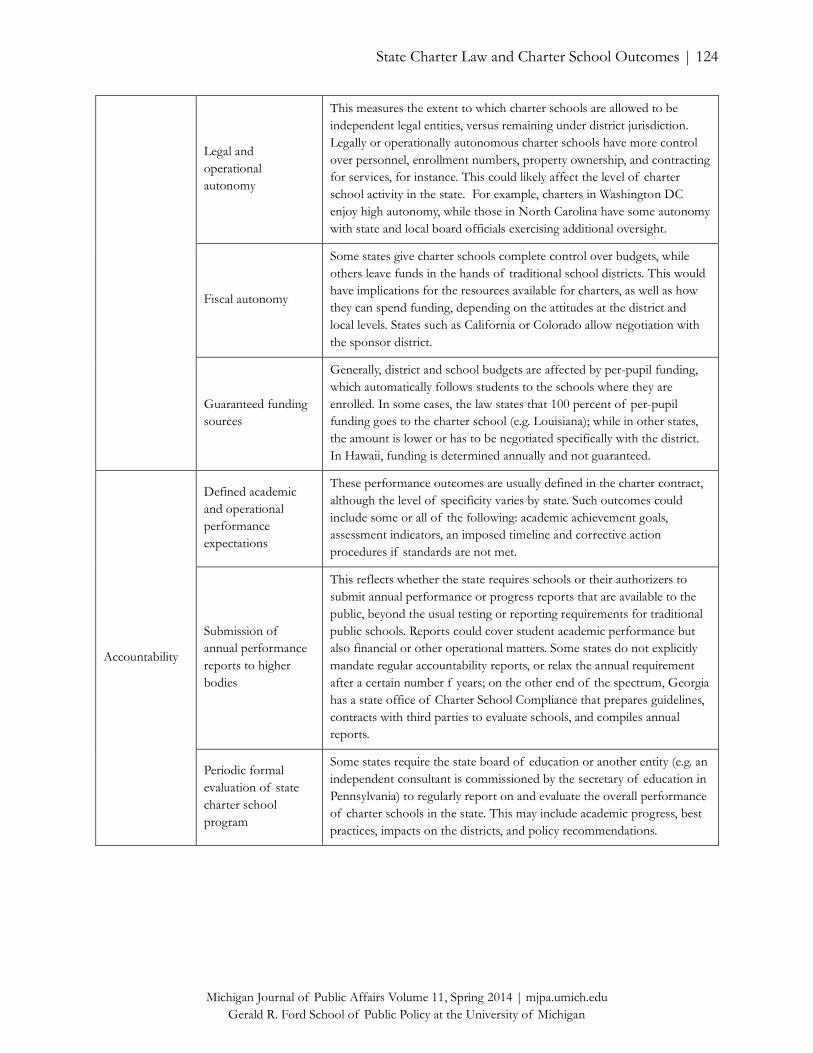
State Charter Law and Charter School Outcomes | 124
Michigan Journal of Public Affairs Volume 11, Spring 2014 | mjpa.umich.edu
Gerald R. Ford School of Public Policy at the University of Michigan
Legal and
operational
autonomy
This measures the extent to which charter schools are allowed to be
independent legal entities, versus remaining under district jurisdiction.
Legally or operationally autonomous charter schools have more control
over personnel, enrollment numbers, property ownership, and contracting
for services, for instance. This could likely affect the level of charter
school activity in the state. For example, charters in Washington DC
enjoy high autonomy, while those in North Carolina have some autonomy
with state and local board officials exercising additional oversight.
Fiscal autonomy
Some states give charter schools complete control over budgets, while
others leave funds in the hands of traditional school districts. This would
have implications for the resources available for charters, as well as how
they can spend funding, depending on the attitudes at the district and
local levels. States such as California or Colorado allow negotiation with
the sponsor district.
Guaranteed funding
sources
Generally, district and school budgets are affected by per-pupil funding,
which automatically follows students to the schools where they are
enrolled. In some cases, the law states that 100 percent of per-pupil
funding goes to the charter school (e.g. Louisiana); while in other states,
the amount is lower or has to be negotiated specifically with the district.
In Hawaii, funding is determined annually and not guaranteed.
Accountability
Defined academic
and operational
performance
expectations
These performance outcomes are usually defined in the charter contract,
although the level of specificity varies by state. Such outcomes could
include some or all of the following: academic achievement goals,
assessment indicators, an imposed timeline and corrective action
procedures if standards are not met.
Submission of
annual performance
reports to higher
bodies
This reflects whether the state requires schools or their authorizers to
submit annual performance or progress reports that are available to the
public, beyond the usual testing or reporting requirements for traditional
public schools. Reports could cover student academic performance but
also financial or other operational matters. Some states do not explicitly
mandate regular accountability reports, or relax the annual requirement
after a certain number f years; on the other end of the spectrum, Georgia
has a state office of Charter School Compliance that prepares guidelines,
contracts with third parties to evaluate schools, and compiles annual
reports.
Periodic formal
evaluation of state
charter school
program
Some states require the state board of education or another entity (e.g. an
independent consultant is commissioned by the secretary of education in
Pennsylvania) to regularly report on and evaluate the overall performance
of charter schools in the state. This may include academic progress, best
practices, impacts on the districts, and policy recommendations.