Electronic copy available at: http://ssrn.com/abstract=1711653

Home Away From Home:

Economic Relevance and Local Investors∗

Gennaro Bernile, University of Miami

Alok Kumar, University of Miami

Johan Sulaeman, Southern Methodist University

March 25, 2012

Abstract – We identify states that are economically relevant for a firm through textual analysis

of the firm’s annual financial (10-K) reports and show that institutional investors overweight

firms with strong local economic presence and generate superior returns from those investments.

This evidence of local over-weighting and superior local performance in economically relevant

regions are stronger than those around corporate headquarters, even when those regions are far

from the headquarters location. Our results are stronger among more sophisticated institutions

and for firms that have speculative features or are harder-to-value. Overall, we demonstrate

that economic relevance rather than physical presence has a stronger impact on institutional

preferences for local stocks and their local informational advantage.

∗Please address all correspondence to Alok Kumar, Department of Finance, School of Busi-ness Administration, 514 Jenkins Building, University of Miami, Coral Gables, FL 33124;Phone: 305-284-1882; email: akumar@miami.edu. Gennaro Bernile can be reached at 305-284-6690 or gbernile@bus.miami.edu. Johan Sulaeman can be reached at 214-768-8284 orsulaeman@mail.cox.smu.edu. We thank an anonymous referee, Brad Barber, Josh Coval, DougEmery, Robin Greenwood, Michael Halling, Zoran Ivkovich, George Korniotis, Kelvin Law, TobyMoskowitz, Jeremy Page, Bill Schwert (the editor), Sophie Shive, Kumar Venkataraman, ScottYonker, and seminar participants at the 2011 FEA Meetings, 2012 AFA Meetings, SouthernMethodist University and University of Miami for helpful comments and valuable suggestions.We are responsible for all remaining errors and omissions.

Electronic copy available at: http://ssrn.com/abstract=1711653

Home Away From Home:Economic Relevance and Local Investors

Abstract – We identify states that are economically relevant for a firm through textual analysis

of the firm’s annual financial (10-K) reports and show that institutional investors overweight

firms with strong local economic presence and generate superior returns from those investments.

This evidence of local over-weighting and superior local performance in economically relevant

regions are stronger than those around corporate headquarters, even when those regions are far

from the headquarters location. Our results are stronger among more sophisticated institutions

and for firms that have speculative features or are harder-to-value. Overall, we demonstrate

that economic relevance rather than physical presence has a stronger impact on institutional

preferences for local stocks and their local informational advantage.

Electronic copy available at: http://ssrn.com/abstract=1711653

I. Introduction

The recent local bias literature has shown that institutional investors around corporate head-

quarters overweight local firms and earn higher returns from those investments.1 Most of these

studies use corporate headquarters to identify firm location.2 However, although the typical

U.S. publicly traded firm has physical presence in only a few locations, it has economic presence

in nine U.S. states (median is six) and often in several international locations. Further, the

economically relevant regions of a typical firm are often located far away from its corporate

headquarters. On average, the economically relevant states are about 1,000 miles away from the

headquarters location.3

The finance literature recognizes the importance of economic location of a firm. However,

for simplicity, the recent local bias literature uses the headquarters location to proxy for firm

location.4 In this paper, we use a firm’s physical location of corporate headquarters and its

economic presence in other U.S. regions to define its geographical location. Using this multi-

dimensional firm location measure, we study the investment behavior of institutional investors

during the 1996 to 2008 period.5 We first examine whether, compared to local preferences

of institutions around corporate headquarters, institutional investors in economically relevant

regions exhibit a stronger preference for firms with local economic presence.

Next, we identify which investor, firm, and local factors influence the overweighting of local

stocks. The main objective of this analysis is to investigate whether there are systematic differ-

ences in the local clientele characteristics of investors in headquarters and economically relevant

states. We also want to examine whether the local ownership levels are higher for stocks with

certain characteristics.

Last, we investigate whether institutional investors in economically relevant regions are able

to exploit local information more effectively than institutions around corporate headquarters,

1We do not use the term “local bias” to strictly imply that the local stock preference is “irrational”. The“bias” towards local investments could be induced by a familiarity bias or may arise from informational reasons.

2For example, see Coval and Moskowitz (1999, 2001), Huberman (2001), Ivkovic and Weisbenner (2005),Loughran and Schultz (2005), Pirinsky and Wang (2006), Hong, Kubik, and Stein (2008), Baik, Kang, and Kim(2010), and Seasholes and Zhu (2010).

3These firm location statistics are based on our new firm location data described later. The mean of 1,000miles is obtained after excluding international locations.

4One exception is the study of Swedish investors by Massa and Simonov (2006). In addition to distance tocorporate headquarters, they use the distance to the closest branch or subsidiary to define “local”. However, theirproximity measures based on headquarters and subsidiary locations are strongly correlated, while our measuresof physical and economic proximity are distinct.

5Although our focus is on the investment behavior of institutional investors, in the Internet Appendix, weuse a shorter sample period covering the 1993 to 1996 period and compare the local ownership patterns ofinstitutional and retail investors.

1

especially if those stocks have speculative features or are harder-to-value.

There are several reasons why the local bias mechanisms around firm headquarters and in

economically relevant regions could differ. If a firm’s headquarters location is the primary source

of value-relevant information, investors around corporate headquarters may earn superior returns

from their local investments. And in contrast, investors away from corporate headquarters may

hold stocks that have local economic presence but would not necessarily earn superior returns

from those local investments. In this scenario, their local stock preference would reflect a

familiarity bias.

However, it is also likely that useful “soft” information about future profitability and per-

formance of a firm is geographically distributed and resides away from firm headquarters. In a

recent study, Giroud (2010) demonstrates that information asymmetry between firm headquar-

ters and plant locations decreases when airline routes are introduced between headquarters and

plant locations. If this information asymmetry is economically significant, investors around these

non-headquarters locations may have better information and may acquire the information faster

than investors around firm headquarters. Consequently, investors away from firm headquarters

may exhibit a preference for stocks that have local economic presence and those investors on av-

erage may have superior value-relevant information about local firms than investors around firm

headquarters. In this scenario, investors in economically relevant states would overweight local

stocks due to an informational advantage and earn higher returns from those local investments.

For example, the Boeing Company is headquartered in Chicago but most of its operations

are around Seattle. Due to their potentially greater ability to observe manufacturing and oper-

ations, it is likely that investors in the state of Washington have better information about the

overall financial health of Boeing than investors in Illinois. Similarly, Whole Foods Market is

headquartered in Austin, but investors in other states in which Whole Foods Market has large

number of stores and significant economic presence (e.g., Massachusetts, Florida, Colorado) may

have the same or even greater degree of awareness about Whole Foods Market than investors

in Texas. Another example is Xerox Corporation, which is perceived by many as a Rochester

company due to its major operations there but the firm is headquartered in Stamford, Con-

necticut. It is possible that investors around the operations of Xerox in Rochester, New York

possess better short-term information about Xerox than investors in Connecticut.

In addition to differences in information environments, the investor clientele characteristics

could differ between firm headquarters and other regions in which the firm has an economic

presence. The local investor clientele at headquarters location may be relatively less sophisti-

cated than local investors in economically relevant regions. Specifically, being aware of a firm

2

with local economic presence may require a higher level of sophistication than identifying a firm

that merely has a physical local presence.6 Consequently, a more sophisticated clientele may

emerge in non-headquarters locations where firms have economic rather than physical presence.

Those local investors away from headquarters locations may be able to earn higher risk-adjusted

returns from their local investments.

In contrast, investors around headquarters may exhibit greater awareness about a firm merely

because that firm has a local physical presence. Those investors need not possess superior

information about local firms. In this scenario, short-term demand shifts of local investors

would contain less information about future returns of local firms.

To test our conjectures, we identify U.S. states that are economically relevant for a firm

through a textual analysis of its annual financial (10-K) reports. This economic relevance

measure of a U.S. state for a given firm is based on the citation share of the state in the firm’s

annual financial reports. The citation share of a firm-state pair is defined as the number of times

the U.S. state is cited in the relevant sections of the firm’s annual financial statement divided

by the total number of citations of all U.S. locations. Thus, a firm can be present in multiple

locations within the U.S. and we are also able to quantify the strength of a firm’s presence

in each of the states in the U.S. This multi-dimensional location measure allows us to better

identify the geographical regions in which value-relevant information about a firm is likely to be

produced.

According to the citation-based location measure, in many instances, a firm’s headquarters

state is not its most economically relevant region. We find that in about 37 percent of cases,

another state is at least as economically relevant as the headquarters state. And in 29 percent of

cases, there is at least one other state that is economically more relevant than the headquarters

state.7 The average citation share of the most economically-relevant state away from firm

headquarters is large (= 0.244), although it is lower than the average citation share of 0.383 for

the headquarters state. These citation share statistics indicate that many firms have significant

economic presence and visibility even in non-headquarters states, which could induce investors

in those states to overweight firms with local economic presence.

In our main empirical tests, we estimate the local ownership levels and local informational

advantage of institutional investors during the 1996 to 2008 sample period. We compare the

6This argument has limitations and does not apply to all types of firms. For example, firms with retail outletsmay be familiar even to investors located far away from corporate headquarters location.

7For example, Connecticut is never the most relevant state for Xerox Corporation even though it is head-quartered in Stamford, Connecticut. Similarly, Washington continues to be Boeing’s most economically relevantstate even after the relocation of its headquarters to Chicago.

3

local ownership and performance levels of investors around headquarters and those located in

economically relevant states. Similar to several previous local bias studies, we perform the

analysis at both the institution- and the firm-level.

Our results indicate that investors allocate disproportionately large fractions of their port-

folios to firms for which the investor’s state is economically relevant. For example, a typical

institution around corporate headquarters overweights local firms by 1.78%, while the mean

institutional local bias for economically relevant firms is 4.70%, which is 2.92% higher than the

mean local bias for locally headquartered firms. Similarly, the average excess local ownership

is 6.17 percent in non-headquarters states with high economic relevance, only 0.99 percent in

low economic relevance states, and significantly negative in states that are not mentioned in the

annual reports. The average excess local ownership in high economic relevance states remain

high even when the economically relevant state is far from the firm headquarters.

Even in headquarters states, the average excess local ownership is strongly dependent upon

the degree of economic relevance. The average excess local ownership is 14.58 percent in head-

quarters states with high economic relevance but only 3.02 percent in less economically relevant

headquarters states. And when the headquarters state is not economically relevant for a firm,

there is no local bias as institutions located within the state under-weight local stocks by an

average of 1.81%. Overall, the institution-level and firm-level local ownership estimates portray

a consistent picture and suggest that economic relevance affects local ownership levels more than

physical proximity.

To investigate whether there are differences in the underlying mechanisms that induce high

levels of local ownership around headquarters and in economically relevant states, we identify

the characteristics of regions in which local ownership levels are high. We also identify the stock

attributes that are associated with higher levels of local ownership. The goal of this analysis is

to examine whether institutional local bias is stronger in regions where local investors are more

sophisticated and local stocks have greater information asymmetry or are harder-to-value.

Our results indicate that local ownership levels are high in conservative Republican states as

well as regions with low population density, and these effects are more pronounced in headquar-

ters states. Further, the local ownership levels around headquarters are higher in states with

lower education levels, while the excess local ownership levels in economically relevant states

exhibit an opposite pattern. Examining the impact of firm attributes on local ownership levels,

we find that local investors exhibit a stronger propensity to overweight smaller and younger

firms, recent losers, value stocks, and firms that have higher volatility. Taken together, the lo-

cal ownership regression estimates indicate that the local institutional clientele in economically

4

relevant states is likely to be more sophisticated.

To examine whether sophisticated investors in economically relevant states are able to exploit

their potential local informational advantage more effectively, we compare the degree of infor-

mational advantage of investors around firm headquarters and economically relevant regions.

We find that, irrespective of the performance measure, institutions in economically relevant re-

gions outperform nonlocal investors and investors around corporate headquarters by 1-2% on

an annualized basis.

The results are similar when we perform firm-level tests to account for potential cross-

sectional dependence in institutional performance. When we measure the performance of local

ownership sorted portfolios, consistent with the recent evidence in Baik, Kang, and Kim (2010),

we find that firms with higher local ownership levels earn higher risk-adjusted returns and

the local ownership-performance relation is strong in headquarters states. However, when we

measure the performance of portfolios sorted on quarterly changes in local ownership levels, we

find that changes in local ownership levels of firms in economically relevant states have a greater

ability to predict the returns of local firms in the following quarter.

Even when changes in ownership levels in headquarters states are low or negative, increases

in ownership levels in economically relevant states are associated with higher local returns in

the next quarter. When the quarterly demand shifts are high in both headquarters states and

economically relevant states, their impact on next quarter returns is the strongest. These effects

are especially pronounced among the types of stocks that have strong local investor clienteles in

economically relevant states (i.e., low priced and high volatility firms, lottery-type stocks). The

annualized risk-adjusted performance differentials are economically significant and range from

two percent to about eight percent for smaller firms.

These empirical findings make several important contributions to the local bias literature. A

recurring criticism of local bias studies is that firm headquarters may not capture the location of a

firm. Our study overcomes this criticism. We use a multi-dimensional measure of geographical

location of a firm based on both economic and physical local presence. To our knowledge,

this is the first paper that uses a broader measure of firm location to quantify the local stock

preferences and informational advantage of institutional investors. In a related study, Garcıa

and Norli (2012) use citation shares to obtain geographic dispersion levels of firms and show

that more dispersed firms earn lower returns. But they do not study investors’ local bias around

headquarters and economically relevant regions, which is the main focus of our study.

We use the citation-based firm location measure to document the key result that institutional

investors need not be located near a firm’s headquarters to exhibit a preference for local stocks

5

and possess local informational advantage. The aggregate excess ownership levels of investors

that are local to firms but are located away from firm headquarters are more than the excess

ownership levels of investors in headquarters states. Our estimates of higher local ownership

levels compared to the estimates reported in previous local bias studies further highlights the

importance of local investors for asset pricing. In particular, our findings suggest that the impact

of local investors on the asset prices of local stocks may be considerably stronger than reported

in recent studies (e.g., Hong, Kubik, and Stein (2008), Korniotis and Kumar (2011)).

We also demonstrate that, compared to institutions around corporate headquarter, investors

in economically relevant states have better short-term information about local firms, especially

if those firms have speculative features or are harder-to-value. This evidence is consistent with

Giroud (2010) who finds that useful information about a firm may be located away from firm

headquarters.8 These performance results extend the recent evidence of superior local informa-

tion among a large sample of institutional investors reported in Baik, Kang, and Kim (2010).

Similar to their study, we find that local institutions have superior information about local firms.

However, we show that unlike institutions around corporate headquarters, institutions located

in regions where firms have economic presence possess superior information about local firms.

The rest of the paper is organized as follows. In the next section, we summarize the main

data sources and explain the citation-based measure of firm location. We present our main

empirical results in Sections III, IV, and V. We conclude in Section VI with a brief discussion.

The Appendix provides additional information about the construction of citation-based firm

location measure and reports additional results.

II. Data Sources and Summary Statistics

In this section, we summarize our main data sources. Table I provides a brief description of the

main variables used in the empirical analysis.

II.A. Citation-Based Firm Location Data

Our first main data source is the annual financial reports stored on the Electronic Data Gath-

ering, Analysis, and Retrieval system (EDGAR) of U.S. Securities and Exchange Commission

(SEC). All U.S.-based companies are required to file Form 10-K with the SEC. This is a stan-

dardized form with a fixed structure and a pre-determined number of sections. It contains

8We are not suggesting that firms intentionally choose to pick headquarters locations in regions with unso-phisticated investors. While the choice of the headquarters location is an important corporate decision, in thecurrent context it is more likely that a relatively less sophisticated investor clientele emerges around headquarterswhile more sophisticated clienteles develop in regions where firms have economic presence.

6

details about a firm’s organizational structure, executive compensation, competition, and regu-

latory issues. For our purposes, more importantly, the form contains information about a firm’s

physical assets, including factories, warehouses, and sales offices. In addition, the form contains

a comprehensive summary of a company’s performance and operations, including information

about changes in firm’s operations during a certain year.

We use a computer-based parsing method to count the number of times references to 50

U.S. states and Washington D.C. appear in annual 10-K filings stored on EDGAR.9 The sample

period is from 1996 to 2008. For each annual filing, we count the occurrence of geographic

locations in sections “Item 1: Business”, “Item 2: Properties”, “Item 6: Consolidated Financial

Data”, and “Item 7: Management’s Discussion and Analysis.” These citation counts provide a

measure of the geographic locations of a firm’s economic interests. This includes information

about a firm’s plant and store locations, office spaces, acquisition activities, and other means

through which a firm can have an economic presence in a state.

Specifically, we compute the citation share of each state in the firm’s annual financial reports.

The citation share of a firm-state pair is defined as the number of times a U.S. state is cited in

the relevant sections of the annual financial statement of a firm divided by the total number of

citations of all U.S. locations. Internet Appendix A provides a brief summary of the information

contained in these four sections of the annual financial reports, while Appendix B provides

excerpts from a few actual 10-K forms filed during the 1996 to 2008 sample period.

Table II provides the summary of the citation share estimates. We find that a typical U.S.

firm has economic presence in nine U.S. states (median is six).10 The average citation share

is 0.205 (median is 0.167) and, as expected, the headquarters states have a higher citation

share (mean = 0.383, median = 0.333). The average citation share of the most economically-

relevant state away from headquarters is also economically significant (= 0.244). These citation

share statistics suggest that many firms are likely to have economic presence and visibility

even in non-headquarters states. These economically relevant states are often located far from

its headquarters. Even though we exclude international locations, the states with economic

presence are on average about 1,000 miles away from the headquarters location.

Although the economic presence of a firm across the U.S. states can vary over time, it is

9Our parsing algorithm would miss instances where the 10-K report mentions the city but not the state. Wewould also be unable to capture cases in which the 10-K reports use state abbreviations. Manual inspection of afew randomly chosen 10-K reports indicates that both cases are rare. Further, there is no reason to believe thatcertain types of firms or firms located in certain states are more likely to abbreviate states or mention only citynames in their reports. Thus, the citation share estimates may be downward biased but the relative rankings offirms would not be affected systematic bias due to these exclusions.

10We present the histogram of this distribution in Figure A.1 of the Internet Appendix.

7

unlikely to change significantly from year-to-year. Consistent with this expectation, we find

that the citation share estimates are quite persistent. In about two-third of cases, the most

economically-relevant state in a certain year is one of the top three economically-relevant states

in each of the past three years. And in more than 90% of cases, the most economically-relevant

state in a certain year is one of the top three economically-relevant states at least once in the

past three years.

II.B. Other Data Sources

Our second main data set is the quarterly common stock holdings of 13(f) institutions compiled

by Thomson Reuters. The sample period is from 1996 to 2008. We identify the institutional

location (zip code) using the Nelson’s Directory of Investment Managers and by searching the

SEC documents and web sites of institutional managers.

In addition to these main data sources, we use several other standard data sets. We obtain

price, volume, return, and industry membership data from the Center for Research on Security

Prices (CRSP). The firm headquarters location data are from the CRSP-Compustat merged

(CCM) file. We obtain monthly time series of the market (RMRF), size (SMB), value (HML),

and momentum (UMD) factors from Kenneth French’s web site.11 We obtain the performance

benchmarks for computing characteristic-adjusted stock returns from Russell Wermers’ web

site.12 The quarterly data on state economic activity index are from Korniotis and Kumar

(2011). The index is defined as the equal weighted average of the standardized values of state

income growth, state housing collateral (Lustig and van Nieuwerburgh (2005, 2010)), and the

negative value of standardized relative state unemployment.

To match the citation-based firm location data with CRSP and Compustat, we use the

Central Index Key (CIK). All entities registered with the SEC are uniquely identified by CIK.

Specifically, we use the firm CIK and link file from the CRSP-Compustat Merged database

to match the annual citation-based location data with data on stock returns and various firm

characteristics.

We use state-level Presidential elections data to identify the political preferences of all U.S.

states.13 We obtain additional state-level demographic characteristics from the U.S. Census

Bureau. Specifically, we consider state population density and the state education level (the

proportion of state population above age 25 that has completed a bachelor’s degree or higher) in

our local ownership regressions. Further, using the religious adherence data from the “Churches

11The web site is http://mba.tuck.dartmouth.edu/pages/faculty/ken.french/data library.html.12The web site is http://www.smith.umd.edu/faculty/rwermers/ftpsite/Dgtw/coverpage.htm.13The election data are obtained from David Leip’s web site: www.uselectionatlas.org.

8

and Church Membership” files available through the American Religion Data Archive (ARDA),

we compute the proportion of Catholics (CATH) and the proportion of Protestants in a state

(PROT). Using the two religion variables, we define the Catholic-Protestant ratio (CPRATIO)

to capture the relative proportions of Catholics and Protestants in a state. We also measure the

overall religiosity of all U.S. states.

Table I provides a brief definition of all variables. Table II provides the summary statistics

for the firm-level economic relevance measure, while Table III report those statistics for other

key variables used in the empirical analysis.

III. Economic Presence and Local Ownership

We begin our main empirical analysis by quantifying the local ownership levels in headquarters

states and in states that are economically relevant for a firm. Our main objective is to assess

the extent to which investors display a preference for investing in firms that have an economic

presence in their state even when the investor is located far away from the firm’s headquarters

location. We provide estimates of local stock preferences of institutions using both institutional-

level and firm-level measures.

III.A. Institutional-Level Local Bias Estimates

Similar to previous local bias studies (e.g., Coval and Moskowitz (2001), Ivkovic and Weisbenner

(2005)), we use the following equation to measure the local bias of institution i around firm

headquarters:

HQ Local Biasi = Weight allocated to firms with headquarters in the state

− Market portfolio weight of firms headquartered in the state. (1)

Here, “weight allocated to firms with headquarters in the state” is the dollar value of the

institutional holdings in firms that are headquartered in the state in which institution i is

located divided by the total dollar value of all of holdings of institution i. The second term is

the benchmark weight and is defined as the total market value of firms headquartered in the

state in which institution i is located divided by the aggregate market value of all firms in the

market portfolio. If institution i follows the prescriptions of the traditional portfolio theory and

holds the well-diversified market portfolio, the HQ local bias measure would be zero.

A similar measure of institutional “local” bias can be defined with respect to firms that

have economic rather than physical presence in the state in which an institution is located.

9

Specifically, the local bias of institution i for firms with local economic presence is defined as:

ER Local Biasi = Weight allocated to firms with economic presence in the state

− Weight of economically relevant firms in the market portfolio. (2)

In this equation, “weight allocated to firms with economic presence in the state” is the dollar

value of the institutional holdings in firms that have strong economic presence in the state in

which institution i is located divided by the total dollar value of all of holdings of institution i.

We define the set of firms with strong economic presence as those for which the state is one of

the top five most economically relevant states based on the citation share scores. If institution

i follows the prescriptions of the traditional portfolio theory, the weight allocated to firms with

economic presence in the state would be the same as the weight of those firms in the market

portfolio, and the ER local bias measure would be zero.

Table IV reports the mean HQ and ER local bias estimates for all institutions (Panel A) and

various subgroups of institutions (Panels B to E). Consistent with the prior evidence, we find

that institutional investors exhibit a stronger preference for firms that have headquarters in the

state where the institution is located. The mean HQ local bias is 1.78%. More interestingly, we

find that the institutional local bias is stronger if the state in which the institution is located is

one of the top five economically relevant state for the firm. The mean ER local bias is 4.70%,

which is 2.92% higher than the mean HQ bias.

The strong institutional preference for firms with local economic presence is not restricted

to economically relevant states that are close to corporate headquarters. In fact, the evidence

in Panel A indicates that ER local bias is stronger in economically relevant states that are far

away from headquarters state. The ER−HQ local bias differentials are 1.29%, 2.88%, and 4.17%

for close, medium-distance, and far away ER states, respectively.

When we decompose the total ER bias based on the magnitude of economic relevance, we

find that the local bias for first, second, third, fourth, and fifth most economically relevant

firms are 1.84%, 0.96%, 0.84%, 0.60%, and 0.46%, respectively. The value-weighted estimates

exhibit a similar monotonically declining trend.14 This evidence indicates that the extent of

institutional local bias is strongly dependent upon the strength of local economic relevance of

firms.

When we use the size of the institutional portfolio to weight the institution-level local bias

14Using the value-weighted measures, the local bias for first, second, third, fourth, and fifth most economicallyrelevant firms are 1.50%, 0.83%, 0.78%, 0.59%, and 0.63%, respectively.

10

measures, we find that the HQ local bias measure is weakly negative (= −0.61%). This evidence

indicates that large institutions do not exhibit a stronger preference for locally headquartered

firms. However, they do exhibit a stronger preference for firms with local economic presence as

the mean ER local bias is positive (= 4.32%) and significantly higher than the mean HQ local

bias estimate.

To ensure that our results are not concentrated in any particular geographical region, we

compute the mean institutional local bias estimate for each U.S. state. These results are reported

in Appendix Table A.I. We find that institutional local bias in economically relevant states is

larger in magnitude than HQ local bias in 31 states.

We find similar results when we examine the excess local holdings of institutional subsamples

based on the institution type, trading frequency, portfolio size, and the number of stocks in the

portfolio. In particular, motivated by the evidence of heterogeneity in the informational advan-

tage across institutional types presented in Baik, Kang, and Kim (2010), we examine whether

local stock preferences in economically relevant states vary across institutional categories.

We use two methods to identify institutional types. Bushee (1998) distinguishes institutional

investors by the levels and changes of their past holdings into three different categories: quasi-

indexers, transient (i.e., short-term investors), and dedicated (i.e., long-term, non-indexers).

Another approach to categorize institutional investors is by examining their 13(f) institutional

types. Specifically, we consider investment advisers (including investment companies and inde-

pendent investment advisers), banks (including bank trusts), and other institutions (including

pension funds and university endowments).

In all instances, with the exception of dedicated investors, the ER local bias is significantly

higher than the HQ local bias. Further, while the local HQ bias estimates are weaker for large

institutional investors or those with large number of stocks in their portfolios, the ER−HQ bias

differential is significantly positive in those cases. These differences are also stronger when we

examine the value-weighted institution-level local bias estimates.

III.B. Firm-Level Excess Local Ownership Estimates

To provide an alternative perspective on the local stock preferences of institutional investors,

we report firm-level local ownership estimates. This aggregated measure avoids several pitfalls

associated with portfolio-level analysis highlighted in Seasholes and Zhu (2010). In particular,

the firm-level measure allows us to effectively account for potential cross-sectional dependence

in the performance of institutional portfolios.

Similar to the institution-level analysis, we estimate the abnormal local ownership level of

11

each firm in the headquarters state as well as in economically relevant states. Our measure

is similar to the firm-level local ownership measures used in previous studies (e.g., Coval and

Moskowitz (1999), Baik, Kang, and Kim (2010), Korniotis and Kumar (2011)). Specifically, we

measure the quarterly local institutional ownership for each firm-state pair as the ratio of the

number of firm shares held by institutions located within the state and the total institutional

ownership in the firm at the end of that quarter.

We also calculate the percentage weight of local institutions in the aggregate institutional

portfolio, which provides a benchmark for comparison. The aggregate portfolio weight represents

the expected level of ownership by local institutions when they follow the prescriptions of the

traditional portfolio theory and do not exhibit an abnormal preference for firms with physical

or economic presence in their state. The expected local ownership measure also accounts for

the non-uniform geographical distribution of institutions across the U.S. It is higher for regions

with greater concentration of institutional investors.

Using the two measures, we define each firm-state pair’s excess local institutional ownership

level as the difference between the quarterly local institutional ownership level of that firm-state

pair and the percentage weight of the state’s institutional investors in the aggregate institutional

portfolio:

Excess State-j Ownershipi =Ownership of state-j institutions in firm i

Total institutional ownership in firm i

−Value of portfolios of institutions located in state j

Value of the aggregate institutional portfolio(3)

For each firm, we compute the average excess state ownership levels for headquarters states

as well as five of its economically relevant (ER) states. For many firms, the HQ state is also

economically most relevant. To better distinguish between the effects of physical and economic

presence on local ownership levels and performance, we only consider ER states after excluding

the HQ state.

We aggregate the firm-level excess state ownership estimates to obtain state-level ownership

levels. For each state, we compute the excess HQ-state ownership and obtain estimates of excess

ERk-state ownership levels (k = 1, . . . , 5).15 Specifically, we compute the excess HQ-state own-

ership for a given state using the equal-weighted average of the firm-level excess state ownership

measures of firms whose headquarters are located in that state. Similarly, to compute the excess

ERk-state ownership for a given state, we aggregate the firm-level excess state ownership esti-

15For brevity, we consider only the five most economically relevant states. This choice is motivated by themedian number of economically relevant states, which is six.

12

mates of all firms for which the state is the kth most economically relevant states. For example,

the excess ER1-state ownership for a certain state is the equal-weighted average of firm-level

excess state ownership levels of firms for which that state is economically most relevant.

The firm-level local ownership estimates are reported in Table V. Panel A reports the average

excess state ownership levels for HQ and non-HQ states. We further sort HQ states using their

economic relevance, as captured by the citation share scores. We also sort non-HQ states using

economic relevance and distance from firm headquarters. Consistent with the institution-level

local bias estimates, we find that, the average excess local ownership in the HQ state is 4.86

percent and it varies significantly with economic relevance. The excess HQ-state ownership

increases monotonically with the citation share of the HQ state (see the “HQ State” column

in Panel A). The average excess HQ-state ownership levels for high economic relevance (i.e.,

citation share above 0.50) and low economic relevance (i.e., citation share below 0.05) HQ states

are 14.58 and 3.02 percent, respectively.

For firms whose HQ states are not mentioned in the 10-K reports (i.e., the citation share is

zero), the average excess local HQ ownership is negative (= −1.81 percent). This evidence indi-

cates that economic presence is an important determinant of high local institutional ownership

levels. Institutional investors do not overweight locally headquartered firms if those firms have

no economic presence in their respective HQ states.

To further quantify the relation between economic relevance and ownership, we examine the

ownership patterns in non-HQ states. We find that in non-HQ states the excess local ownership

level is also a monotonically increasing function of the state’s economic relevance for the firm

(see the second column of Panel A). The average excess local ownership levels for the most

and the least economically relevant non-HQ states are 6.17 and 0.99 percent, respectively. And

similar to the evidence in HQ states, the average excess local ownership level is negative in states

that are not mentioned in the 10-K reports (i.e., the citation share is zero).

For robustness, we use an alternative method to create economic relevance based firm-state

categories. This method does not use pre-defined citation share cutoffs. Rather, for each firm, we

rank all non-HQ states based on their citation share scores and identify its five most economically

relevant states. We designate the top five states as ER1, ER2, . . . ER5. We report the average

excess local ownership for these states in “All Non-HQ” column of Table V, Panel B. The results

are consistent with the evidence in Panel A. The excess local ownership is a monotonically

increasing function of the state’s economic relevance for the firm.

We find that these results are not driven by geographical concentration of firms and insti-

tutions in certain dominant states such as California and New York. Firms are economically

13

present throughout the U.S. and the citation share estimates of firms in economically relevant

states are comparable to the citation share estimates of firms headquartered in those states.

Figure 1 shows that the average proportion of economically relevant firms in a state is 0.660

(median is 0.667), while the average ER to HQ citation share ratio is 0.658 (median is 0.573).

These estimates are based on data for the year 2008 but the results are qualitatively similar in

other years.

To further ensure that our results are not concentrated in any particular geographical region,

Appendix Table A.II reports the mean state-level excess institutional ownership of firms whose

headquarters are located in the state. We also list the most economically relevant state and

provide local ownership estimates when the state is one of the five most economically relevant

states. Even in large states such as California and New York, local ownership levels for firms

with economic presence are comparable to the local ownership levels for firms with physical

presence in those states. And in several states, economic presence affects local ownership more

than the physical presence of firm headquarters.16

Figure 2 summarizes the mean local state-level ownership levels for the HQ state and ER

states. To highlight the importance of economic relevance, we report the mean local ownership

levels for ER1, ER2, ER3, ER4, and ER5 states separately. As expected, the level of excess

ownership declines as the economic relevance of a state declines. However, investors in even the

fifth most economically relevant state overweight local firms by an average of 1.32 percent. The

average local ownership in the five most economically relevant states is 8.73 percent, which is

considerably higher than the headquarters state average of 5.02 percent. These results are very

similar when we focus only on the subsample of states with highest institutional ownership levels.

Overall, the state-level local ownership estimates indicate that the institutional preference for

firms with local economic presence is not concentrated in any particular geographical region of

the U.S.

III.C. Distance From HQ, Economic Relevance, and Local Ownership

In the next set of tests, we examine whether the distance between headquarters location and

economically relevant states affect the local institutional ownership patterns. If the observed

impact of economic relevance on local ownership is concentrated in states that are closer to HQ

16To address the potential concern that our citation measure captures the economic relevance of a region ratherthan a state, we compare the state-level excess holdings of cited and non-cited states located in the same Censusregion or division. The results of this supplemental analysis are reported in Internet Appendix Table A.IV. Theevidence indicates that states with explicit citations are associated with larger local excess holdings than statesin the same Census region/division that are not cited explicitly in firms’ 10-K filings.

14

states, the high local ownership levels in economically relevant states may simply reflect the

proximity of economically relevant states to corporate headquarters.

We double-sort firm-state pairs based on the degree of economic relevance and distance from

headquarters and measure the mean excess local ownership levels. These results are reported in

the last four columns of Table V, Panels A and B. We find that local ownership levels are high

even when an economically relevant state is very far from the headquarters state. For example,

the results in Panel A indicate that the average excess local ownership is 5.97% for economically

relevant states that are close to the headquarters state (i.e., less than 500 kilometers away).

And the average local ownership level is higher (= 6.92%) for economically relevant states that

are located far from the headquarters state (i.e., at least 2,000 kilometers away).17

Even when we use an alternative method to create economic relevance based firm-state cat-

egories (see Panel B), we find that local ownership is a monotonically increasing function of the

state’s economic relevance, irrespective of the distance between firm headquarters and econom-

ically relevant states. These double sorting results indicate that the relation between economic

relevance and local institutional ownership does not merely reflect the physical proximity be-

tween economically relevant states and firm headquarters. Overall, economic presence rather

than physical proximity is a stronger determinant of local institutional ownership.

III.D. Firm Attributes, Economic Relevance, and Local Ownership

In this section, we examine whether firm attributes determine the impact of economic or physical

local presence on institutional ownership. We consider three firm attributes: size, age, and

geographic dispersion. These results are reported in Table V, Panel C. We find that local

ownership levels are higher for smaller firms, both in HQ and non-HQ economically relevant

states. However, in all three size-based categories, local ownership decreases monotonically with

economic relevance. Examining the firm age-based categories, we find that local ownership levels

are higher for younger firms, but again, we find a monotonic relation between local ownership

and economic relevance within each firm age category.

To ensure that our results are not driven by geographically dispersed firms that are present

in almost every state, we examine the level of excess local ownership in geographical dispersion

based subsamples. In particular, we examine the local ownership patterns in subsamples of

firms for which the number of states mentioned in the 10-K reports are below and above the

median number of states. We find stronger excess local ownership levels at both HQ and

17Our results are not very sensitive to the distance and economic relevance cutoffs. The results are qualitativelysimilar when we use other cutoffs to define these categories.

15

economically relevant locations for firms that are less dispersed geographically. And yet again, in

both subsamples, we find a monotonic relation between local ownership and economic relevance.

This evidence indicates that the observed local ownership patterns are not driven by firms

that are present in most states and are not really local to any particular set of investors. Overall,

the firm attributes based subsample results indicate that while firm attributes influence local

ownership patterns, economic relevance has an additional impact on local institutional ownership

levels.

IV. Determinants of Local Ownership

Our next battery of tests focuses on identifying the characteristics of regions and stocks that

are associated with stronger local clienteles. The goal of this analysis is to investigate whether

there are systematic differences in the local clientele characteristics of investors in headquarters

and economically relevant states. We also want to examine whether the local ownership levels

are higher when stocks are more difficult to value. For this exercise, we use several proxies for

investor sophistication (e.g., local education level, local religiosity, etc.) and the difficulty in

stock valuation (e.g., idiosyncratic volatility, firm size, etc.).

IV.A. Baseline Estimates

We estimate a set of Fama and MacBeth (1973) style regressions in which the dependent variable

is the local ownership of a given firm in a certain state (LocalOwni,j). It is defined as firm j’s

total share ownership of institutional investors located in state i as a fraction of the aggregate

institutional ownership in firm j. Among the independent variables, our primary focus is on

the following two location-based indicator variables: HQ state dummy for the headquarters

state and ER1−5 state dummy for the top five most economically relevant states excluding the

headquarters state. We also interact the two indicator variables with various state characteristics

and stock attributes to measure their incremental effects on local stock ownership. We include

state fixed effects in each quarterly cross-sectional regression to account for the expected level

of state ownership based on the size of a state’s institutional investor base in that quarter.

We report the time-series average of the coefficient estimates from quarterly cross-sectional

regressions in Table VI, where the t-statistics are calculated using the time series of these

coefficient estimates. In Model (1), we include only the two location indicator variables. The

first indicator variable is the HQ state dummy, which is set to one for firm-state pair when the

state is the firm’s headquarter location. The second indicator variable is the ER1−5 dummy,

16

which is defined using the economic relevance rank of a state for a given firm-year. This indicator

variable is set to one for a firm-state pair when the state has one of the five highest citation

shares for that firm-year.

Consistent with our sorting results, we find strong evidence of excess local ownership among

investors in both the headquarters states and economically relevant non-headquarters states.

Specifically, institutions in headquarters state overweight local firms by 7.1 percent, while the

average excess local ownership of institutions in the top five economically relevant states is 1.6

percent.

We also estimate the local ownership baseline regressions separately for subsamples based

on firm size. Small, medium, and large stock categories contain stocks in the bottom, middle,

and top terciles defined on the basis of the market capitalization measure. In these regressions,

instead of using one dummy variable for the five most economically relevant states, we use five

distinct dummies for those five states. The local ownership regression estimates for subsamples

based on firm size are summarized in Figure 3.

We find that the coefficient estimate is highest for the HQ state indicator variable. Examin-

ing the estimates of the five state economic relevance indicator variables, we find that across all

size groups the coefficient estimates decline monotonically as the degree of economic relevance

decreases. In addition, we find that the local ownership levels vary inversely with firm size,

independent of the location type (HQ or ER) and state economic relevance rank. This evidence

shows that the link between economic relevance of a firm’s location and local investors’ propen-

sity to hold disproportionately large fractions of the firm’s stocks is not exclusively a “small firm

phenomenon”. Both the strength of a firm’s presence as well as its size independently affect the

level of local ownership.

IV.B. Role of Investor Sophistication

In Model (2) of Table 5, we interact the local indicator variables with each state’s average educa-

tion level. Since education does not vary within state-quarter, we do not include the education

variable itself in the regression. We use the level of education as a proxy for overall investor

sophistication as the level of education would be correlated with local or investor attributes that

affect investor sophistication. But we do not assume that institutions in more educated regions

would be more educated.

The negative coefficient estimate of the HQ × Education interaction term suggests that local

bias in the HQ state is stronger among states with lower education levels. In contrast, the local

bias in economically relevant states is positively correlated with the state’s education level. The

17

opposite signs of these interaction estimates suggest that the underlying mechanisms that induce

high local ownership around headquarters and in economically relevant states may be different.

For robustness, we provide another perspective on the relation between education and local

ownership. We sort states into quartiles based on the level of education in the state and compute

the average excess local ownership for the four state quartiles separately for headquarters states

and economically most relevant states. The results are reported in Figure 4. The evidence

indicates that the average excess local ownership around headquarters decreases with educa-

tion but the average excess local ownership levels in economically most relevant states exhibits

an opposite pattern. This evidence further supports the conjecture that investors in economi-

cally relevant states are likely to be more sophisticated than local investors around corporate

headquarters.

IV.C. Impact of State Attributes

To further examine the underlying mechanisms that induce higher levels of local ownerships, we

introduce additional state characteristics in local ownership regression specification. In Model

(3), we include interactions between location indicators and the ratio of Catholic adherents to

Protestant adherents in a state (CPRATIO). This specification is motivated by the evidence

in Kumar, Page, and Spalt (2011), who demonstrate that investors in high CPRATIO regions

have a higher tendency to invest in lottery-type stocks.18 It is likely that investors’ gambling

propensity is stronger among local stocks because investors perceive them as being less risky. The

regression estimates indicate that investors in high CPRATIO regions have a higher tendency to

invest in local firms, particularly for firms with local economic presence. This evidence indicates

that investors’ speculative tendencies influence their local stock preferences.

In Model (4), we include additional state characteristics, including state religiosity, political

orientation, population density, and state economic activity index, as defined in Korniotis and

Kumar (2011). The religiosity and political orientation measures are designed to capture the

level of local conservatism, which is likely to influence institutional investors’ propensity to hold

local stocks. Our premise is that conservatism would be positively correlated with local stock

preferences of institutional investors.

The estimates from this extended specification indicate that local ownership levels are high

in Republican states as well as regions with low population density, and these effects are more

pronounced in headquarters states. Further, once we account for these state attributes, local

18Motivated by the salient features of state lotteries (low price, low negative expected return, and risky as wellas skewed payoff) and the theoretical framework of Barberis and Huang (2008), Kumar (2009) defines stocksthat have low prices, high idiosyncratic volatility, and high idiosyncratic skewness as lottery-type stocks.

18

economic conditions do not have a significant impact on the local stock preferences of local

institutions. In this extended specification, we also find that institutional investors in high

CPRATIO regions no longer have a greater tendency to invest in firms with local headquarters,

but the local ownership levels remain high in economically relevant states with high CPRATIO.19

IV.D. Impact of Firm Attributes

In the next set of tests, we identify firms that are more difficult to value and examine the impact

of firm attributes on local ownership levels. We are particularly interested in identifying firms

that may be less visible and/or harder-to-value because familiarity- or information-driven local

bias should be most pronounced among these firms. Further, the effects of these characteristics

on local ownership could vary across location types (i.e., HQ vs ER) if investor clienteles are

indeed different, as our earlier evidence indicates.

Harder-to-value are typically younger, have highly volatile prices, and have lottery-type

features (e.g., Zhang (2006), Jiang, Lee, and Zhang (2005)). Models (5) and (6) include the

interactions of local indicator variables with these firm characteristics. We find that local in-

vestors exhibit a stronger propensity to overweight younger firms, firms with higher volatility,

and stocks with lottery features. Interestingly, the preference for harder-to-value firms and

stocks with lottery features, which are likely to have higher information asymmetry, is stronger

in economically relevant states. In Model (7), we include other firm characteristics, including

firm size, market-to-book equity ratio, past return, return skewness, and stock price. We find

that local investors also exhibit a stronger propensity to invest in smaller firms, value stocks,

and recent losers.20

Overall, the results from our local ownership regressions indicate that local institutional

clientele is likely to be sophisticated as they invest in local stocks that are more difficult to value.

In addition, the coefficient estimates of the interactions with state-level education suggest that

local investors in economically relevant states may be more sophisticated than local investors in

headquarters states.21

19We also estimate the full model without these variables and report the estimates in Table A.V of the InternetAppendix. Our inferences for the other variables remain very similar.

20For robustness, we estimate the full model on the subsample of large firms and geographically dispersedfirms. We report the estimates in Table A.V of the Internet Appendix. We find very similar results across thesesubsamples.

21Motivated by the evidence of heterogeneity in informational advantage across institutional types (Baik,Kang, and Kim (2010)), we also examine whether local stock preferences in economically relevant states varyacross institutional categories. We use both the Bushee (1998) classification and the 13(f) institutional types.We find that the evidence of local stock preference is quantitatively similar across all different types of insti-tutional investors. Thus, local stock preferences in economically relevant regions do not vary significantly withinstitutional type.

19

V. Local Ownership and Local Performance

Our analysis so far provides evidence of institutional local bias at the headquarters location

and in economically relevant states, where institutional preference for firms with local economic

presence is stronger than their preference for locally headquartered firms. Further, the local in-

stitutional clienteles in economically relevant states are likely to be relatively more sophisticated.

In this section, we examine whether those sophisticated investors have an informational advan-

tage that they are able exploit to earn superior returns from their local investments. Specifically,

we compare the performance of portfolios sorted by local ownership and trading levels at both

the headquarters location and in economically relevant states.

Our analysis is partially motivated by the emerging evidence in the recent finance literature,

which suggests that useful “soft” information about future profitability and performance of a firm

may be geographically distributed and could reside away from firm headquarters. Specifically,

Giroud (2010) shows that information asymmetry between firm headquarters and plant locations

decreases when airline routes are introduced between headquarters and plant locations. In

a similar manner, useful information about a firm’s future performance may reside at non-

headquarters locations where a firm has economic presence.

Further, due to their relatively higher sophistication, investors around these non-headquarters

locations may have better local information and/or a greater ability to interpret this informa-

tion than investors around firm headquarters. Those institutions may also be able acquire local

information faster than institutions located around corporate headquarters.

V.A. Demand Shift Correlations

Before presenting the performance results, we examine the correlation between the demand

shifts of institutional investors at the HQ and ER locations. If the two groups of investors

are responding to different information signals or if they are interpreting the same information

signals differently, their trades are less likely to be correlated. In contrast, if their information

sources and sophistication levels are similar, their trades would be strongly positively correlated.

We find that the trading correlation between local demand shifts at HQ and various ER

locations is essentially zero. The average cross-sectional correlations vary between −0.013 and

0.003 but none of these estimates is statistically different from zero. Examining the correlations

among the demand shifts from various economically relevant states (ER1, ER2, . . . ER5), we find

that these estimates are also very low and statistically indistinguishable from zero.

The lack of strong positive correlation between demand shifts at HQ and ER locations is

20

consistent with the conjecture that the mechanisms driving the local bias around HQ and ER

locations are different. In the remaining part of this section, we compare the performance levels

of HQ and ER investors to provide stronger and more direct evidence to support this conjecture.

V.B. Institution-Level Local Performance Estimates

In the first set of returns-based tests, we examine the local informational advantage of institu-

tions by comparing the performance of institutions in headquarters (HQ) states and economically

relevant (ER) states. We also compare the performance levels of institutions at HQ and ER

locations with the performance of nonlocal institutions. To get better insights into the source

of institutional local information, we measure institutional performance using both portfolio

holdings and quarterly changes in institutional holdings.

We start by separating each institution’s portfolio into three sub-portfolios:

• Local HQ portfolio, which comprises of stocks in the institutional portfolio whose head-

quarters are located in the investor’s state;

• Local ER1−5 portfolio, which comprises of stocks for which the investor’s state is one of

the five most economically relevant state for the firm but the firm is not headquartered in

the institution’s state; and

• Non-Local portfolio, which contains all other positions in the institutional portfolio.

We then use the Daniel, Grinblatt, Titman, and Wermers (1997) method to calculate the

monthly characteristic-adjusted returns of each investor’s local and non-local portfolios. We

compute the average of portfolio returns across all institutions each month, and then report the

time-series averages of those monthly averages. To obtain the monthly performance estimates,

we value-weight the institutional performance measures using the total dollar value of the in-

stitution’s holdings at the beginning of the quarter. For robustness, we also report the alphas

from the four-factor model.

Table VII, Panel A reports the average performance of local and non-local holdings of institu-

tional investors. We find that the average characteristic-adjusted returns or the alpha estimates

are positive for all three portfolios, but significantly so for only the Local ER1−5 portfolio (see

Columns (2) and (3), first three rows). In the last three rows, we report the performance dif-

ferentials among these portfolios. These performance differentials indicate that institutional

investors’ Local ER1−5 holdings outperform the other two portfolios by a significant margin.

21

Specifically, the evidence in Column (3) indicates that Local ER1−5 holdings outperform non-

local holdings by 15.3 basis points per month, which translates into an annual characteristic-

adjusted out-performance of about 1.84%. In contrast, Local HQ holdings outperform non-local

holdings only by 5.5 basis points per month or about 0.66% annually (t-statistic = 1.21) on a

characteristic-adjusted basis.22 The four-factor alpha estimates reported in Column (2) portray

a similar picture.

These comparisons suggest that institutions at ER locations have better local informa-

tion than institutions at HQ locations. When we directly compare the performance of local

institutions at HQ and ER locations, we find that Local ER1−5 holdings outperform Local

HQ holdings by 8.9 basis points per month, which translates into an annual characteristic-

adjusted out-performance of about 1.04% (t-statistic = 2.54). The performance differential is

0.143 × 12 = 1.72% when we use the risk-adjusted performance measure. These performance

differentials are not very large but this evidence is consistent with our conjecture that investors

in economically relevant states are relatively more sophisticated and earn higher returns on their

local investments.

In Columns (4) to (9) of Panel A, we report the portfolio performance estimates and per-

formance differentials for subsamples of institutional investors sorted by their type and their

trading characteristic as categorized by Bushee (1998). We find that the superior performance

of Local ER1−5 portfolio in the aggregate sample is driven by two (non-exclusive) investor types:

investment companies and advisors as identified in the 13(f) filings and institutions categorized

as transient investors using the Bushee (1998) classification method. In particular, the Local

ER1−5 holdings of institutions identified as investment companies and advisors outperform their

Local HQ holdings by 14.9 basis points per month, which translates into an annual characteristic-

adjusted out-performance of about 1.79% (t-statistic = 3.26).

To gain additional insights into the local informational advantage of institutional investors,

we measure the performance impact of “trading” activities of institutional investors in local

and non-local stocks. Given the quarterly structure of institutional investors’ holdings data,

we cannot measure their trading activities directly. Instead, we use the changes in portfolio

holdings between two quarterly snapshots to identify “trading”. Specifically, we estimate trading

performance as the difference in the monthly characteristics-adjusted returns of the holdings

snapshot at the end of the preceding quarter minus the holdings snapshot at the beginning of

the preceding quarter. This performance differential captures the incremental performance that

22This evidence suggests that the superior performance of local HQ portfolios documented for the mutual fundsample during the 1975-1994 period (Coval and Moskowitz (2001)) does not extend to the broader institutionalinvestor sample and our sample period.

22

is due to trades executed during a quarter.

Table VII, Panel B reports the average performance of local and non-local trading by insti-

tutional investors. Similar to the holdings-based analysis, we divide each institutional portfolio

into Local HQ, Local ER1−5, and Non-Local sub-portfolios and obtain the performance estimates

of each of these three components. Consistent with the holdings-based performance results, we

find that the average characteristic-adjusted “trading” returns are positive for all three portfo-

lios (see Column (3), first three rows), but significantly so only for the Local ER1−5 portfolio

(14.2 basis points per month or about 1.70% annually; t-statistic = 2.20).

Examining the performance differences between the local and non-local portfolios, we find

that trading in Local HQ stocks does not outperform trading in Non-Local stocks. However,

institutional investors’ trading in Local ER1−5 stocks outperform their trading in both Non-

Local and Local HQ stocks. The performance differentials are 9.6 and 10.5 basis points per

month and both estimates are statistically significant. The t-statistics for these two estimates

are 3.68 and 3.57, respectively. When we break-down the trading-based performance estimates

by institution type (see Columns (4) to (9)), we again find that the superior performance in

Local ER1−5 stocks is concentrated among investment companies and advisors and transient

investors.

Overall, these holdings- and trading-based institutional-level performance results are consis-

tent with our key conjecture, which posits that institutional investors in economically relevant

regions would have better information about firms with strong local presence than investors

around corporate headquarters and non-local regions.

V.C. Performance of Local Ownership Sorted Portfolios

In the next set of tests, we examine the performance of firm-level local ownership and trading

portfolios. These tests allow us to further quantity the local informational advantage of insti-

tutions around headquarters and in economically relevant states. Specifically, we compare the

future performance of location-based portfolios constructed using institutional investors’ portfo-

lio holdings as well as quarterly changes in their holdings. A key advantage of this portfolio-based

approach is that it is not sensitive to potential cross-sectional correlations in the performance

of institutional portfolios. Thus, we are able to avoid one of the main pitfalls common in local

bias studies, as identified in Seasholes and Zhu (2010).

In these tests, we aggregate the positions of each state’s institutional investors in each firm

into a firm-state level observation of state holdings. These firm-state holdings are then normal-

ized by the aggregate holdings of all institutional shareholders of the firm. To account for the

23

variation in the size of institutional investor population across states, we calculate the abnormal

level of firm-state holdings by subtracting the expected level of holdings for the firm-state pair.

The expected measure is the share of the state’s institutional investors in the aggregate portfolio

of institutional investors.

We form the first set of level-based portfolios by sorting stocks into quintiles using the

excess local ownership of investors located in the firm’s headquarters state. The second set of

level-based portfolios are defined using the excess local ownership of investors located in non-

headquarters states that are economically relevant for the firm. This analysis is similar in spirit

to the method used in Baik, Kang, and Kim (2010). However, to account for the variation in

the size of local institutional investor population across states, we use excess local ownership

levels of local institutions instead of their raw local holdings.

In addition to the level-based portfolios, we create two sets of change-based portfolios by cal-

culating the percentage change in the normalized firm-state holdings. The first set of portfolios is

formed by sorting stocks into quintiles using the change in the holdings of institutional investors

located in a firm’s headquarters state. The second set of portfolios is formed by sorting stocks

using ownership changes of investors located in non-headquarters states that are economically

relevant for a firm.

The performance of local ownership sorted portfolios are reported in Table VIII. Specifically,

we report the average return of each quintile portfolio in the quarter immediately following the

quarter in which we measure the excess local ownership levels and local ownership changes. Panel

A reports the average return of level-based quintile portfolios, while Panel B reports the average

return of change-based portfolios. For brevity, we only report the performance estimates using

characteristic-adjusted returns, but our results are very similar when we use raw or risk-adjusted

returns. The characteristic-adjusted stock return computed using the Daniel, Grinblatt, Titman,

and Wermers (1997) method is the raw stock return minus the return of a firm size, book-to-

market, and past return matched benchmark portfolio. The risk-adjusted performance measure

is the alpha from a four-factor model that contains the market, size, value, and momentum

factors.

Consistent with the findings in Baik, Kang, and Kim (2010), we find that the abnormal

level of local holdings by investors in the headquarters state is positively related to future

stock returns. The equal-weighted average characteristic-adjusted quarterly return of stocks

in the highest quintile of abnormal local HQ holdings is about 1.02 percent higher (t-statistic

= 2.67) than the average return of stocks in the lowest quintile of abnormal local HQ holdings.

However, this result weakens considerably when we use value-weighted returns. The quarterly

24

return differential shrinks to 0.48 percent (t-statistic = 0.60).

We find a similar but weaker pattern when we examine the level-based quintile portfolios

sorted on the abnormal level of local holdings of investors located in non-headquarters states

that are economically relevant for the firm (i.e., ER locations). The differences in characteristic-

adjusted returns are positive but statistically weak.

When we examine change-based portfolios, however, the positive correlation between local

ownership changes and local stock returns becomes considerably stronger in economically most

relevant states but weaker in headquarters states. Specifically, the average return of stocks in the

highest change in local ownership in top non-HQ states (i.e., ∆LocalOwn) quintile is 0.78 percent

higher (t-statistic = 2.75) than the average return of stocks in the lowest ∆LocalOwn quintile.

This difference remains significant when we use value-weighted portfolios. In contrast, among

headquarters states, the difference between the highest and the lowest ∆LocalOwn quintiles is

smaller (0.01 to 0.11 percent) and statistically insignificant. The t-statistics range from 0.02 to

0.49.

Since our sorting results exhibit a non-monotonic pattern, we also use the Patton and Tim-

mermann (2010) test to examine whether we can reject the null of identical returns across the

quintiles or weakly declining trend in quintile returns. The p-values from these tests are reported

in both panels of Table VIII. We find that the null of no increasing trend cannot be rejected for

the HQ states. However, for the ER states, we are able to reject the null for holdings as well as

trading based portfolios, except for the value-weighted returns in Panel A where the p-value is

0.15.

Taken together, our performance estimates from univariate sorts indicate that local owner-

ship levels and changes in local ownerships at HQ and ER locations are related to the future

performance of local stocks, but the relation is weak. In the next set of tests, we examine whether

the ownership patterns at HQ and ER locations jointly contain better information about future

returns of local stocks.

V.D. Performance of Double-Sorted Portfolios

For these performance tests, we construct double-sorted portfolios and directly compare the

relative informational advantage of local investors in the headquarters state and economically

relevant non-HQ states. We perform independent sorts using changes in the holdings of local

investors in headquarters states and five most economically relevant states. We assign each

stock to one of the following four portfolios: Low HQ-Low ER (LL), High HQ-Low ER (HL),

Low HQ-High ER (LH), and High HQ-High ER (HH).

25

Table IX reports the average subsequent quarter average returns of stocks in each of these

four portfolios. Again, for brevity, we only report the performance estimates using characteristic-

adjusted returns. The table also reports the performance differences for each column and each

row. The diagonal differential (i.e., HH−LL) is reported in Figure 5. We find that stocks

with relatively high demand from local investors located in both the headquarters state and

most economically relevant states earn the highest returns. In addition, only the HH portfolio

earns significantly positive abnormal returns. The characteristic-adjusted quarterly return of

this portfolio is 0.51 percent (t-statistic = 2.30).

Consistent with the notion that proximity to ER locations are more likely to be information-

based, we also find that local investors’ demand shifts in most economically relevant states

are more significantly related to future returns than those in HQ states. Moving down along

each column (i.e., from low ER to high ER portfolio) is associated with relatively more positive

average stock returns than moving right within each row (i.e., from low HQ to high HQ portfolio).

For example, the quarterly characteristic-adjusted return is 0.81 percent (t-statistic = 2.04) for

the HH−HL portfolio but only 0.20 percent (t-statistic = 0.65) for the HH−LH portfolio. The

diagonal difference is 0.65 percent with a t-statistic of 1.80 (see Figure 5).

Overall, the performance estimates of double-sorted portfolios indicate that changes in hold-

ings of investors in economically relevant states are more informative about future returns than

the demand shifts of investors in headquarters states.

V.E. Firm Attributes and Performance of Double-Sorted Portfolios

To further characterize the local informational advantage of investors in economically most rele-

vant states over investors in headquarters states, we examine whether the previously documented

performance differences are a function of firm attributes. We focus on firm attributes that are

associated with strong local investor clienteles (i.e., low priced, high volatility, and lottery-type

stocks). If local investors overweight local stocks due to an informational advantage, they should

display particularly superior performance among these stocks with greater information asym-

metry. Further, if local bias in economically relevant regions is associated with higher levels

of investor sophistication, this evidence of superior performance should be stronger in those

regions.

We examine the relative information advantage of local ER investors for market capitalization

and distance based subsamples. The distance based subsamples are formed using the mean

distance between the HQ state and the five most economically relevant states for the firm. We

report the performance estimates for size- and distance-based subsamples in Table IX. For small

26

firms, we find that local investors in ER states possess better information than local investors in

the HQ state. In particular, irrespective of the demand shifts of HQ investors, small stocks that

experience high demand from investors in ER states outperform small stocks that experience low

demand from these investors by about 0.80 percent per quarter. The corresponding performance

differentials for local investors in the headquarters state is about 0.40 percent and statistically

insignificant.

In the large firm subsample, we find that the future local returns are high when the de-

mand shifts of investors in economically most relevant states are high. In particular, the quar-

terly characteristic-adjusted returns for the LH−LL and HH−HL portfolios are 0.35 percent

(t-statistic = 1.07) and 0.64 percent (t-statistic = 1.89), respectively. In addition, the HH−LL

performance is still significantly positive for this subsample: 0.49 percent per quarter (t-statistic

= 1.85). Further, the results reported in Figure 5 indicate that the average HH−LL performance

differential declines with firm size.

The distance-based subsample results also reported in Table IX and Figure 5 indicate that

informational advantage of ER investors is not concentrated in ER states that are close to HQ

states. In fact, the performance differences increase with the mean HQ-ER state distance. For

example, the HH−LL performance differences for the low, medium, and high distance subsam-

ples are 0.12, 0.79, and 1.12 percent, respectively. Similarly, the LH−LL and HH−HL portfolio

performance increases with distance.

V.F. Performance Regression Estimates

To account for the effects of firm characteristics on stock returns more directly, we estimate

Fama and MacBeth (1973) style regressions in which the dependent variable is the subsequent

quarter characteristic-adjusted stock return computed using the Daniel, Grinblatt, Titman,

and Wermers (1997) method. We account for the effects of other stock characteristics (e.g.,

idiosyncratic skewness, idiosyncratic volatility, and turnover) that are known to be correlated

with future stock return by including these stock characteristics as independent variables in the

performance regressions.

For ease of interpretation, the structure of this regression analysis mimics the structure of

the double sorting analysis presented in Table IX. In particular, we assign three independent

indicator variables that correspond to the portfolios in our double sorts: High HQ-Low ER

(HL), Low HQ-High ER (LH), and High HQ-High ER (HH). Since we do not include an indicator

variable for the Low HQ-Low ER (LL) portfolio, the intercept estimate corresponds to the excess

return of this portfolio. Further, the estimates of the three indicator variables corresponds to

27

the incremental excess return of each of the corresponding portfolios relative to the LL portfolio.

To set the stage, Model (1) in Table X reports the performance regression estimates when

only the three indicator variables are the independent variables. Consistent with the sorting

results in Table IX, we find that stocks with high demand from local investors in both the

headquarters state and the economically relevant non-HQ states (HH) experience the highest

stock return in the subsequent quarter.

Next, we examine whether the impact of local demand shifts on future returns of local

stocks is higher for stock categories that have strong local investor clienteles and/or exhibit

greater information asymmetry. Specifically, we consider small stocks, value firms, low-return

stocks, low priced and high volatility firms, young firms, and lottery-type stocks categories.

Following Kumar (2009), lottery type stocks have low prices, high idiosyncratic volatility, and

high idiosyncratic skewness. We examine each of these stock attributes separately by including

an indicator variable for each of these attributes (identified as “Char”) and interacting it with

the local demand indicator variables (LH, HL, and HH).

We report the results from these tests in Columns (2) to (8) of Table X. The coefficient

estimates of interactions between each stock attribute and local demand measures that corre-

spond to high demand by investors in the five most economically relevant non-HQ states (LH

and HH) are always positive. Further, the coefficient estimates of interactions with LH and

HH are statistically significant in six out of seven regression models, respectively. In contrast,

the coefficient estimates of interactions with the remaining local demand measure (i.e., HL)

that corresponds to high demand by investors in the headquarters state but low demand by

investors in economically relevant non-HQ states are negative in six out of seven models and

never statistically significant.

To examine whether the economic relevance-performance varies with distance between HQ-

ER states, we use distance as an additional firm attribute and re-estimate the performance

regression. Specifically, we set the “Char” indicator variable to one for firms that are in the

highest tercile of mean HQ-ER distance. The results reported in Column (9) of Table X are

similar to the evidence from other firm attribute interactions. The coefficient estimates of

“High Dist” interactions with LH and HH are significantly positive, which indicate that the

performance differentials are higher when the mean HQ-ER distance distance is high.

These performance results are consistent with the conjecture that institutional investors

in economically relevant states rather than headquarters states have superior access to value-

relevant information about local firms, especially within the subsample of stocks with strong

local institutional clienteles. These are also high information asymmetry stocks with speculative

28

features that are harder-to-value (e.g., younger and higher volatility firms). Our findings are

also consistent with the conjecture that the local bias of institutional investors in economically

relevant states is more likely to be driven by local informational advantage. In contrast, the

local bias of investors around corporate headquarters have weaker short-term information, which

suggests that their local bias is more likely to be induced by familiarity.

VI. Summary and Conclusion

This study uses a multi-dimensional measure of firm location to estimate the local bias and

local informational advantage of U.S. institutional investors. Our measure of firm location is

based on economic and physical presence rather than mere headquarters location. We identify

economically relevant states for a firm through a textual analysis of its annual financial reports.

Specifically, the economic relevance measure of a firm-state pair is the citation share of a state

in the firm’s annual financial reports. This citation-based firm location measure allows a firm

to be present in multiple locations within the U.S. Thus, our location measure overcomes the

recurring criticism of local bias studies that firm headquarters location is unlikely to capture

the true geographical location of that firm.

Using the citation-based firm location measure, we examine whether investors away from

headquarters location exhibit a stronger preference for firms with local economic presence. We

also investigate whether investors in economically relevant states earn higher returns on their

local investments as compared to investors around corporate headquarters. Our results indicate

that institutional investors overweight firms with local economic presence more than they over-

weight firms with local headquarters. In addition, institutions earn higher returns from their

investment in firms with local economic presence than their investments in locally headquar-

tered companies. These patterns exist even when economically relevant regions are far from the

headquarters location. Further, our results are stronger among more sophisticated institutions

and for firms that have speculative features or are harder-to-value.

Overall, we demonstrate that economic relevance rather than physical presence has a stronger

impact on institutional preferences for local stocks and their local informational advantage. This

evidence is consistent with the recent findings in Giroud (2010) and indicates that important

sources of information about a firm may be located far away from its headquarters.

Future studies could further improve our estimates of local ownership and local informational

advantage. Like publicly traded firms, institutional investors may also have presence in multiple

locations beyond their headquarters locations. It would be useful to examine whether the

29

evidence of institutional local bias becomes stronger with this multi-dimensional measure of

institutional location. Further, like previous local bias studies, our paper takes the physical and

economic locations of a firm as given. In future work, it would be interesting to examine how

firms choose their headquarters location and states in which they have economic presence.

More broadly, our findings change the debate in the local bias and related literatures in a

significant manner. Given the evidence in our paper, any paper that exploits local attributes

around firm location in its empirical analysis may find it useful to consider the local economic

environments in all regions where the firm has economic or physical presence.23 For example,

Hilary and Hui (2009) and Kumar, Page, and Spalt (2011) show that local culture as captured

by the local religious environment around corporate headquarters affects the corporate policies

of local firms. It is likely that the local environments around corporate headquarters and other

regions where a firm is economically present have better ability to explain managerial decisions.

References

Baik, Bok, Jun-Koo Kang, and Jin-Mo Kim, 2010, Local institutional investors, information

asymmetries, and equity returns, Journal of Financial Economics 97, 81–106.

Barberis, Nicholas, and Ming Huang, 2008, Stocks as lotteries: The implications of probability

weighting for security prices, American Economic Review 98, 2066–2100.

Bushee, Brian J., 1998, The influence of institutional investors on myopic R&D investment

behavior, Accounting Review 73, 305–333.

Coval, Joshua D., and Tobias J. Moskowitz, 1999, Home bias at home: Local equity preference

in domestic portfolios, Journal of Finance 54, 2045–2073.

, 2001, The geography of investment: Informed trading and asset prices, Journal of

Political Economy 109, 811–841.

Daniel, Kent D., Mark Grinblatt, Sheridan Titman, and Russell Wermers, 1997, Measuring

mutual fund performance with characteristic-based benchmarks, Journal of Finance 52, 1035–

1058.

23Of course, in several instances the local economic environment around headquarters is likely to be moreimportant. But the local environments in economically relevant regions are likely to matter too and which ofthe two effects is more important is an empirical issue.

30

Fama, Eugene F., and James D. MacBeth, 1973, Risk, return, and equilibrium: Empirical tests,

Journal of Political Economy 81, 607–636.

Garcıa, Diego, and Oyvind Norli, 2012, Geographic dispersion and stock returns, Journal of

Financial Economics Forthcoming.

Giroud, Xavier, 2010, Soft information and investment: Evidence from plant-level data, Working

Paper (November); Available at SSRN: http://ssrn.com/abstract=1699154.

Hilary, Gilles, and Kai Wai Hui, 2009, Does religion matter in corporate decision making in

America?, Journal of Financial Economics 93, 455–473.

Hong, Harrison, Jeffrey D. Kubik, and Jeremy C. Stein, 2008, The only game in town: Stock-

price consequences of local bias, Journal of Financial Economics 90, 20–37.

Huberman, Gur, 2001, Familiarity breeds investment, Review of Financial Studies 14, 659–680.

Ivkovic, Zoran, and Scott Weisbenner, 2005, Local does as local is: Information content of the

geography of individual investors’ common stock investments, Journal of Finance 60, 267–306.

Jiang, Guohua, Charles M.C. Lee, and Yi Zhang, 2005, Information uncertainty and expected

returns, Review of Accounting Studies 10, 185–221.

Korniotis, George M., and Alok Kumar, 2011, State-level business cycles and local return pre-

dictability, Working Paper (November); Available at http://ssrn.com/abstract=1094560.

Kumar, Alok, 2009, Who gambles in the stock market?, Journal of Finance 64, 1889–1933.

, Jeremy Page, and Oliver Spalt, 2011, Religious beliefs, gambling attitudes, and financial

market outcomes, Journal of Financial Economics 102, 671–708.

Loughran, Timothy, and Paul H. Schultz, 2005, Liquidity: Urban versus rural firms, Journal of

Financial Economics 78, 341–374.

Lustig, Hanno, and Stijn van Nieuwerburgh, 2005, Housing collateral, consumption insurance,

and risk premia: An empirical perspective, Journal of Finance 60, 1167–1219.

, 2010, How much does household collateral constrain regional risk sharing?, Review of

Economic Dynamics 13, 265–294.

31

Massa, Massimo, and Andrei Simonov, 2006, Hedging, familiarity and portfolio choice, Review

of Financial Studies 19, 633–685.

Newey, Whitney K., and Kenneth D. West, 1987, A simple, positive semi-definite heteroskedas-

ticity and auto-correlation consistent variance-covariance matrix, Econometrica 55, 703–708.

Patton, Andrew J., and Allan Timmermann, 2010, Monotonicity in asset returns: New tests

with applications to the term structure, the CAPM and portfolio sorts, Journal of Financial

Economics 98, 605–625.

Pirinsky, Christo, and Qinghai Wang, 2006, Does corporate headquarters location matter for

stock returns?, Journal of Finance 61, 1991–2015.

Seasholes, Mark S., and Ning Zhu, 2010, Individual investors and local bias, Journal of Finance

65, 1987–2010.

Zhang, X. Frank, 2006, Information uncertainty and stock returns, Journal of Finance 61, 105–

136.

32

Table I

Variable Definitions

This table provides a brief description of all variables used in the empirical analysis.

Panel A: Citation-Based Variables

Variable Definition and Source

Citation Share The number of times a U.S. location is cited in the relevant sections ofthe annual financial statement divided by the total number of citations ofall U.S. locations. Source: Securities and Exchange Commission (SEC)10-K filings.

States Cited The number of U.S. states cited at least once in the relevant sections ofthe annual financial statement. Source: SEC 10-K filings.

Citation Concentration The sum of squared citation shares divided by the square of the sum ofcitation shares. Source: SEC 10-K filings.

Panel B: Ownership and Distance Variables

HQ State The U.S. state or the District of Columbia in which the firm headquarters

are located. Source: Compustat and Compact Disclosure.

Distance From HQ The distance in miles between the relevant U.S. state’s centroid and the

HQ location. Source: Computed.

ERk State Excess Ownershipi,t State excess ownership of firm i’s kth most economically relevant non-HQ

state.

ER1−5 States The five most economically relevant non-HQ state for a firm. Source:

SEC 10-K filings.

State Ownershipi,s,t State-level ownership of firm i, calculated as institutional ownership

share of investors in state s as proportion of the total institutional own-

ership in firm i. Source: Thomson Reuters.

State Excess Ownershipi,s,t State ownershipi,s,t minus the average state ownership of state s over all

firms in quarter t. Source: Thomson Reuters.

HQ State Excess Ownershipi,t State excess ownership of firm i’s HQ state.

HQ State Demandi,t The percentage change in the State Ownership of firm i’s HQ state.

ERk State Excess Ownershipi,t State excess ownership of firm i’s kth most economically relevant state.

ERk State Demandi,t The percentage change in the state ownership of firm i’s kth most eco-

nomically relevant non-HQ state.

33

Table I (Continued)

Variable Definitions

Panel C: Stock Characteristics

Variable Definition and Source

Raw Stock Return Quarterly stock return. Source: Center for Research on Security Prices

(CRSP).

Characteristic-Adjusted Return Quarterly stock return adjusted for size, market-to-book, and momen-

tum as defined in Daniel, Grinblatt, Titman, and Wermers (1997).

Source: Professor Russell Wermers’ web site.

Firm Size Stock price multiplied by the number of shares outstanding. Source:CRSP.

Past Six-Month Return Stock return over the past six months. Source: CRSP.

Market-to-Book Ratio Market equity plus book assets minus book equity divided by book as-

sets. Source: Compustat and CRSP.

Stock Price Stock price at the beginning of the quarter. Source: CRSP.

Monthly Turnover Monthly stock trading volume divided by shares outstanding. Source:

CRSP.

Idiosyncratic Volatility Volatility of residuals of annual market-model regressions of monthly

stock returns. Source: CRSP.

Idiosyncratic Skewness Skewness of residuals of annual market-model regressions. Source:

CRSP.

Panel D: State Attributes

Democratic (Republican) The percentage of the state’s registered voters that voted for the pres-

idential candidate from the Democratic (Republican) party in the last

election. Source: US Election Atlas.

Catholic-Protestant Ratio The ratio of Catholic adherents to Protestant adherents in a state.

Source: Association of Religion Data Archives (ARDA).

Religiosity The fraction of religious adherents in a state. Source: ARDA.

Education The fraction of college graduates in a state. Source: US Census.

Population Density A state’s population divided by its land area. Source: US Census.

State Economic Activity Index A state’s macroeconomic indicator as defined in Korniotis and Kumar

(2011). The index is defined as the equal weighted average of the stan-

dardized values of state income growth, state housing collateral (Lustig

and van Nieuwerburgh (2005, 2010)), and the negative value of stan-

dardized relative state unemployment.

34

Table II

Summary Statistics: Firm-Level Economic Relevance Measures

This table reports the summary statistics for firm-level economic relevance and distance measures. The

sample consists of 50,731 firm-year observations between 1996 and 2008. Economic relevance is based

on the citation share in a firm’s annual financial reports. The set of All States contains U.S. states

that are cited at least once in the relevant sections of the annual financial statement. HQ States refer

to the U.S. state or the District of Columbia in which the firm headquarters are located. Top States

refer to the U.S. location with the highest number of citations in a given firm-year. The Top Non-HQ

State is the economically most relevant state (or ER1 state) for the firm and refers to the U.S. location

that is not the firm HQ state but has the highest number of citations in a given firm-year. The Top 5

Non-HQ States are the five economically most relevant states (or ER1−5 states) for the firm and refers

to the U.S. locations that are not the firm HQ state but have the five highest number of citations in a

given firm-year. Additional details about the variables are available in Table I. We report the statistics

for the pooled data used in the panel regressions.

Percentile

Variable Mean Std Dev 1st 5th 25th Median 75th 95th 99th N

All States

States Cited 9.10 8.30 1 2 4 6 11 27 44 50,731

Citation Share 0.205 0.176 0.023 0.037 0.091 0.167 0.250 0.500 1 50,731

Citation Conc. 0.335 0.228 0.036 0.069 0.164 0.278 0.447 0.830 1 50,731

Distance From HQ 886 454 45 144 593 837 1,146 1,713 1,926 50,731

HQ States

Citation Share 0.383 0.264 0 0.030 0.167 0.333 0.559 0.896 1 50,731

Top States

Citation Share 0.454 0.229 0.083 0.140 0.276 0.417 0.600 0.909 1 50,731

Top Non-HQ States

Citation Share 0.244 0.153 0.028 0.064 0.136 0.208 0.316 0.533 0.756 49,588

Distance From HQ 1,095 826 28 198 475 922 1,664 2,509 2,659 49,588

Top 5 Non-HQ States

Citation Share 0.330 0.202 0.056 0.122 0.227 0.272 0.392 0.611 0.786 49,588

Distance From HQ 1,083 647 50 166 574 1, 017 1,449 2,409 2,582 49,588

35

Table III

Summary Statistics: Other Main Variables

This table reports the summary statistics for the main variables used in the empirical analysis. State

Ownership is the state level ownership, calculated as the state’s institutional investors’ share in total

institutional ownership. Characteristic-adjusted return is the quarterly stock return adjusted for size,

market-to-book, and momentum as defined in Daniel, Grinblatt, Titman, and Wermers (1997). Market

Cap is the stock price multiplied by the number of shares outstanding. M/B is the market-to-book

equity ratio. Turnover is trading volume divided by shares outstanding. Idiosyncratic Volatility and

Idiosyncratic Skewness are calculated from residuals of annual market-model regressions of monthly

stock returns. Democratic (Republican) is the percentage of the state’s registered voters that vote

for the presidential candidate from the Democratic (Republican) party in the last election. Catholic-

Protestant Ratio is the ratio of Catholic adherents to Protestant adherents in the state, Religious

Population is the fraction of religious adherents in the state, Education is the fraction of college

graduates in the state, Population Density is the state’s population divided by its land area. State

Economic Activity Index is a state’s macroeconomic indicator defined in Korniotis and Kumar (2011).

HQ Excess Ownership is the State Ownership of a firm’s HQ state minus that state’s average State

Ownership. ER Excess Ownership is the State Holdings of a firm’s most economically relevant state

minus that state’s average State Ownership. HQ State Demand is the percentage change in the State

Ownership of a firm’s HQ state. ER State Demand is the percentage change in the State Ownership of

a firm’s most economically relevant state. HQ State refers to the U.S. state or the District of Columbia

in which the firm headquarters are located. ER1−5 States are the five economically most relevant

states for a firm and refer to the U.S. locations that are not the firm HQ state but have the five highest

numbers of citations in a given firm-year. Additional details about the variables are available in Table

I. The sample period is from 1996 to 2008. All statistics reported are pooled statistics for the panel

data.

36

Percentile

Variable Mean Std Dev 1st 5th 25th Median 75th 95th 99th

Dependent Variables

State Ownership 0.019 0.070 0 0 0 0 0.002 0.110 0.362

Quarterly Raw Return 0.024 0.333 −0.658 −0.417 −0.124 0.010 0.135 0.473 1.133

Quarterly Char-Adj Return 0.002 0.294 −0.591 −0.364 −0.130 −0.016 0.100 0.400 0.920

Firm Characteristics

Firm Size (in $b) 1.64 0.985 0.018 0.006 0.036 0.136 0.579 5.44 28.16

M/B Ratio 4.980 89.96 0.020 0.280 1.03 1.78 3.22 10.07 31.31

Past Six-Month Ret 0.077 0.557 −0.791 −0.552 −0.172 0.026 0.222 0.819 1.93

Stock Price 25.96 795.55 0.443 1.30 5.62 12.90 23.69 50.87 85.49

Monthly Turnover 1.31 8.22 0.028 0.087 0.303 0.665 1.43 3.96 7.99

Idio Volatility 9.59 8.71 0 1.50 4.44 7.54 12.32 23.74 40.11

Idio Skewness 0.148 0.736 −1.62 −1.03 −0.330 0.134 0.609 1.40 1.99

State Characteristics

Prop Democratic 0.457 0.097 0.260 0.303 0.401 0.456 0.509 0.595 0.852

Prop Republican 0.456 0.108 0.093 0.306 0.385 0.456 0.525 0.625 0.689

Cath-Prot Ratio 0.892 1.04 0.019 0.026 0.295 0.516 1.16 2.96 5.06

Prop Religious 0.528 0.130 0.302 0.328 0.422 0.530 0.638 0.741 0.820

Education 23.218 4.71 14.30 16.46 20.02 22.50 26.10 31.40 39.10

Population Density 359.21 1297.92 1.10 6.21 40.25 88.83 205.30 995.67 9311.45

State Econ Act Index 0.000 0.559 −1.23 −0.861 −0.358 −0.018 0.322 0.911 1.66

Firm-State Characteristics

HQ Excess Ownership 0.058 0.182 −0.234 −0.111 −0.017 −0.001 0.067 0.464 0.835

ER1−5 Excess Ownership 0.102 0.218 −0.245 −0.162 −0.031 0.003 0.092 0.501 0.803

HQ State Demand 8.20 507.18 −1.000 −0.859 −0.176 −0.006 0.184 2.21 21.01

ER1−5 State Demand 6.52 492.67 −0.982 −0.765 −0.149 0 0.169 2.04 18.26

37

Table IV

Economic Relevance and Institution-Level Local Bias Estimates

This table presents institution-level local bias estimates for the full sample of institutions and various

subsets of institutions. For each institutional investor’s portfolio, we divide the holdings into three

mutually exclusive categories: (i) Local HQ: firms headquartered in the investor’s state, (ii) Local

ER1−5: firms for which the investor’s state is in the top five of citation share, but the firms are not

headquartered in the institution’s state, and (iii) Non-Local: the rest of the holdings. We report the

mean local bias, i.e., the mean excess portfolio weight (the raw weight minus the portfolio weight in the

“market portfolio” for locally headquartered firms as well as firms with local economic presence. ER

state refers to the five most economically relevant states (ER1 to ER5). ER1 has the highest economic

relevance for the firm, while ER5 has the fifth highest economic relevance. Economic relevance is based

on the citation share in a firm’s annual financial reports. Citation share is equal to the number of

times a U.S. location is cited in the relevant sections of the annual official statement divided by the

total number of citations to U.S. locations. We report the equal-weighted and dollar-weighted averages

across institutions. The dollar-weighted averages use the size of the institutional portfolios to weight the

institutional-level local bias observations. Panel A reports the local bias estimates for the full sample

and subsamples based on the mean distance between the HQ state and the top five ER states. The

rest of the table reports the local bias estimates for various subsamples of institutional investors based

on 13(f) institutional types (Panel B), trading type as defined in Bushee (1998) (Panel C), portfolio

size quintile (Panel D), and the number of stocks in the portfolio (Panel E). Additional details about

the variables are available in Table I. The sample period is from 1996 to 2008.

38

Panel A: All Institutions

Equal-Weighted Value-Weighted

Prop Total HQ ER ER−HQ HQ ER ER−HQ

(1) (2) (3) (4) (5) (6) (7)

Local Bias, Full Sample 100.00 1.78 4.70 2.92 −0.61 4.32 4.93

Local Bias, Close ER States 36.42 2.03 3.32 1.29 −0.38 3.30 3.68

Local Bias, Medium-Distance ER States 37.03 1.69 4.57 2.88 −0.50 4.69 5.19

Local Bias, Far Away ER States 26.55 1.57 5.74 4.17 −0.93 5.22 6.15

Panel B: Institution Type Subsamples

Investment Companies and Advisors 55.49 1.66 4.74 3.08 −0.48 4.38 4.86

Pension and Endowment Funds 6.91 0.24 4.36 4.12 −1.52 4.76 6.28

Banks and Insurance Firms 35.70 2.18 4.92 2.74 −0.74 4.18 4.92

Panel C: Institution Type Subsamples (Second Method)

Transient 17.72 2.83 5.28 2.45 −1.08 4.88 5.96

Dedicated 15.33 4.96 4.92 −0.04 −0.22 4.72 4.94

Quasi-Indexers 66.09 0.48 4.08 3.60 −0.57 4.08 4.65

Panel D: Institution Subsamples Based on Portfolio Size

Smallest Portfolios 0.43 2.51 4.21 1.70 2.55 4.96 2.41

Q2 1.07 2.69 4.94 2.25 3.42 5.02 1.60

Q3 2.26 1.98 4.81 2.83 2.53 5.12 2.59

Q4 6.32 1.13 4.71 3.58 1.75 4.94 3.19

Largest Portfolios 89.92 0.17 4.58 4.41 −0.91 4.25 5.20

Panel E: Institution Subsamples Based on Number of Stocks in the Portfolio

≤100 Stocks 9.27 1.26 3.82 2.56 −0.14 5.62 5.76

101-250 11.18 2.49 5.00 2.51 1.33 4.97 3.64

251-500 11.72 1.99 5.28 3.29 0.69 4.33 3.64

501-1000 18.22 2.31 4.58 2.27 1.31 3.36 2.05

1001-2000 22.30 0.83 3.73 2.90 −1.26 4.50 5.76

>2000 27.32 0.36 2.54 2.18 −2.19 3.47 5.66

39

Table V

Economic Relevance and Firm-Level Local Ownership Estimates

This table reports the average excess firm-level local institutional ownership as a function of the eco-

nomic relevance of the investors’ state in the firm and the distance between the investor’s state and

the firm’s headquarters state. Economic relevance is based on the citation share in a firm’s annual

financial reports. Citation share is equal to the number of times a U.S. location is cited in the relevant

sections of the annual financial statement divided by the total number of citations of all U.S. locations.

Distance From HQ is the distance between the relevant U.S. state centroid and the HQ location. HQ

State refers to the U.S. state or the District of Columbia in which the firm headquarters are located.

Panel A reports the excess state-level ownership as a function of distance from the firm’s HQ state

and the state’s economic relevance. Panel B reports the excess state-level ownership as a function of

distance from HQ state and the state’s economic relevance ranks within each firm-year (i.e., ER1, ER2,

etc.) ERk State is the kth economically most relevant state for a firm and refers to the U.S. state that

is not the firm HQ state but has the kth highest number of citations in a given firm-year. Panel C

reports the excess state-level ownership as a function of firm characteristics and the state’s economic

relevance ranks within each firm-year. The firm characteristics are firm size, firm age, and the number

of U.S. states cited at least once in the relevant sections of the annual financial statement. Additional

details about the variables are available in Table I. The sample period is from 1996 to 2008.

Panel A: Economic Relevance and Excess Local Ownership

Distance from HQ (in km)

Economic Relevance HQ State All Non-HQ <500 500-1000 1000-2000 2000-5000

All States 4.86 −0.97 −1.09 −0.93 −0.85 −1.19

Above 0.50 (High) 14.58 6.17 5.97 5.28 7.22 6.92

0.20 to 0.50 8.35 5.28 4.88 3.90 5.11 7.79

0.10 to 0.20 5.46 3.40 3.03 2.15 3.53 5.71

0.05 to 0.10 4.07 2.02 1.76 1.22 2.17 3.44

Below 0.05 (Low) 3.02 0.99 0.99 0.60 1.06 1.72

Zero −1.81 −1.20 −1.48 −1.08 −1.00 −1.50

Panel B: Economic Relevance Rank and Excess Local Ownership

Distance from HQ (in km)

Economic Relevance All Non-HQ <500 500-1000 1000-2000 2000-5000

Highest (ER1) 5.18 4.91 4.06 5.45 6.40

Second (ER2) 2.60 2.32 1.79 2.70 3.88

Third (ER3) 1.13 0.91 0.91 1.04 2.01

Fourth or Fifth (ER4, ER5) 0.58 0.57 0.39 0.62 0.95

Zero −1.15 −1.39 −1.03 −0.97 −1.46

40

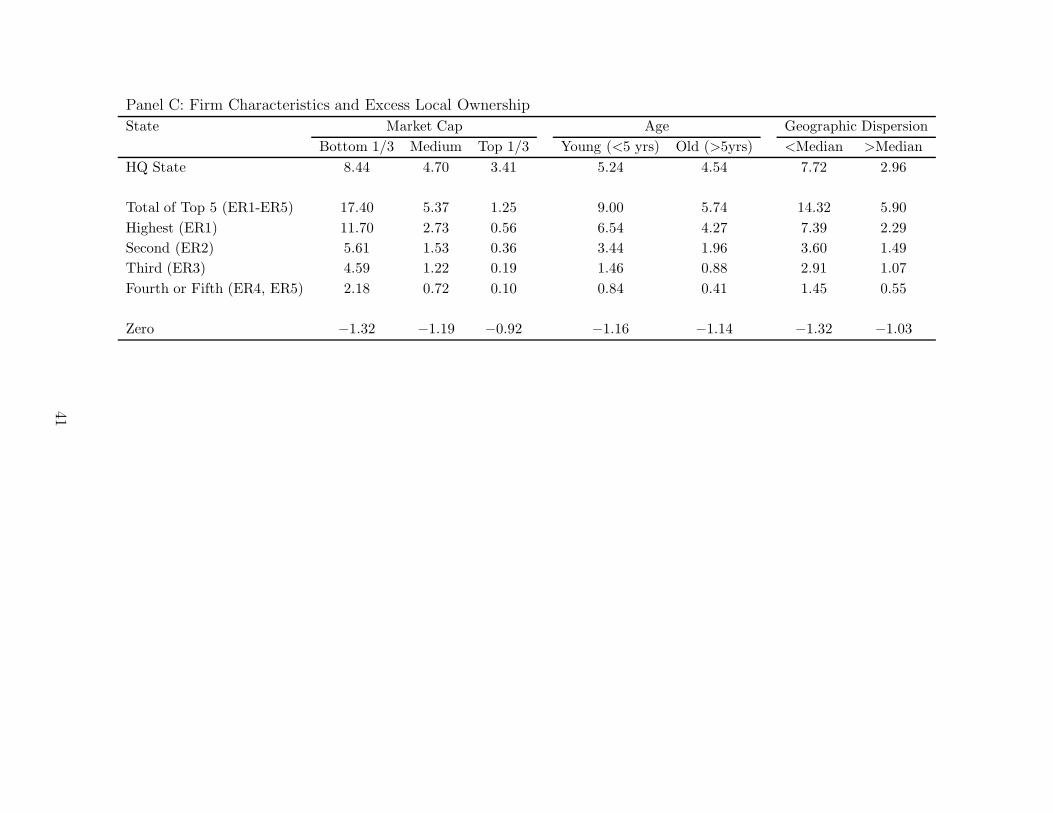
Panel C: Firm Characteristics and Excess Local Ownership

State Market Cap Age Geographic Dispersion

Bottom 1/3 Medium Top 1/3 Young (<5 yrs) Old (>5yrs) <Median >Median

HQ State 8.44 4.70 3.41 5.24 4.54 7.72 2.96

Total of Top 5 (ER1-ER5) 17.40 5.37 1.25 9.00 5.74 14.32 5.90

Highest (ER1) 11.70 2.73 0.56 6.54 4.27 7.39 2.29

Second (ER2) 5.61 1.53 0.36 3.44 1.96 3.60 1.49

Third (ER3) 4.59 1.22 0.19 1.46 0.88 2.91 1.07

Fourth or Fifth (ER4, ER5) 2.18 0.72 0.10 0.84 0.41 1.45 0.55

Zero −1.32 −1.19 −0.92 −1.16 −1.14 −1.32 −1.03

41

Table VI

Local Ownership Regression Estimates

This table reports the parameter estimates from Fama and MacBeth (1973) style regressions. The

dependent variable is a state’s institutional investors’ share in a firm’s total institutional ownership.

The independent variables include an indicator variable for a firm’s HQ state (HQ), an indicator

variable for a firm’s top five most economically relevant non-HQ states (ER1−5), state characteristics,

firm characteristics, and industry indicators. The state characteristics include: (i) Education: the

fraction of college graduates in a state; (ii) CPRATIO: the ratio of Catholic adherents to Protestant

adherents in a state; (iii) Religiosity: the fraction of religious adherents in a state; (iv) Republican:

an indicator variable that is set to one for states that picked the Republican presidential candidate

in the last election, (v) Population Density: state population divided by its land area, and (vi) State

Econ Index: state economic activity index as defined in Korniotis and Kumar (2011). The set of firm

characteristics includes market capitalization (Firm Size), market-to-book ratio (M/B), stock returns

in the past six months (Past Return), an indicator for public firms that are five years old or younger

(Young), idiosyncratic volatility, idiosyncratic skewness, stock price, and an indicator variable for firms

that are in the top third of volatility, the top third of skewness, and the top third of price (Lottery

Stock). Each of these characteristics (with the exception of the indicator variables) is standardized

such that it has a mean of zero and a standard deviation of one. Each quarterly regression also includes

fixed effects for each U.S. state and the District of Columbia. The t-statistics reported in parentheses

are adjusted using the Newey and West (1987) correction for heteroscedasticity and serial correlation.

Additional details about the variables are available in Table I. The sample period is from 1996 to 2008.

42

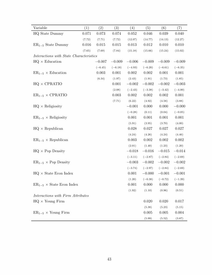
Variable (1) (2) (3) (4) (5) (6) (7)

HQ State Dummy 0.071 0.073 0.074 0.052 0.046 0.039 0.040

(7.72) (7.71) (7.72) (12.07) (14.77) (14.13) (12.27)

ER1−5 State Dummy 0.016 0.015 0.015 0.013 0.012 0.010 0.010

(7.65) (7.69) (7.84) (15.18) (15.66) (15.24) (15.02)

Interactions with State Characteristics

HQ × Education −0.007 −0.009 −0.006 −0.009 −0.009 −0.009

(−6.45) (−6.18) (−4.93) (−6.20) (−6.61) (−6.35)

ER1−5 × Education 0.003 0.001 0.002 0.002 0.001 0.001

(6.34) (1.97) (2.43) (1.91) (1.73) (1.85)

HQ × CPRATIO 0.001 −0.002 −0.002 −0.002 −0.003

(2.08) (−2.43) (−3.38) (−3.42) (−4.00)

ER1−5 × CPRATIO 0.003 0.002 0.002 0.002 0.001

(7.71) (6.22) (4.92) (4.58) (3.88)

HQ × Religiosity −0.001 0.000 0.000 −0.000

(−0.28) (0.11) (0.04) (−0.05)

ER1−5 × Religiosity 0.001 0.001 0.001 0.001

(5.91) (3.95) (3.70) (4.00)

HQ × Republican 0.028 0.027 0.027 0.027

(4.24) (4.26) (4.24) (4.46)

ER1−5 × Republican 0.003 0.002 0.002 0.002

(2.01) (1.40) (1.23) (1.20)

HQ × Pop Density −0.018 −0.016 −0.015 −0.014

(−3.11) (−2.87) (−2.84) (−2.69)

ER1−5 × Pop Density −0.003 −0.002 −0.002 −0.002

(−3.74) (−2.97) (−2.84) (−2.69)

HQ × State Econ Index 0.001 −0.000 −0.001 −0.001

(1.20) (−0.38) (−0.72) (−1.39)

ER1−5 × State Econ Index 0.001 0.000 0.000 0.000

(1.92) (1.10) (0.96) (0.51)

Interactions with Firm Attributes

HQ × Young Firm 0.020 0.020 0.017

(5.38) (5.23) (5.15)

ER1−5 × Young Firm 0.005 0.005 0.004

(5.99) (5.52) (3.87)

43

Variable (1) (2) (3) (4) (5) (6) (7)

Interactions with Firm Attributes

HQ × Idio Vol 0.008 0.003 0.004

(3.13) (1.30) (1.69)

ER1−5 × Idio Vol 0.006 0.004 0.005

(12.65) (8.50) (8.35)

HQ × Lottery Stock 0.026 0.024

(4.29) (3.55)

ER1−5 × Lottery Stock 0.012 0.012

(4.83) (5.27)

HQ × Firm Size −0.008

(−11.44)

ER1−5 × Firm Size −0.002

(−5.30)

HQ × M/B Ratio −0.001

(−1.92)

ER1−5 × M/B Ratio −0.001

(−0.97)

HQ × Past Return −0.004

(−4.24)

ER1−5 × Past Return −0.003

(−4.97)

HQ × Idio Skew 0.001

(0.84)

ER1−5 × Idio Skew −0.001

(−5.38)

HQ × Price 0.000

(1.66)

ER1−5 × Price −0.001

(−4.06)

Estimates of all firm attributes and state characteristics are suppressed.

State FE Yes Yes Yes Yes Yes Yes Yes

Average N 181,386 181,386 181,386 181,386 181,386 181,386 181,386

Average Adjusted R2 0.499 0.499 0.500 0.500 0.506 0.507 0.510

44

Table VII

Local Bias and Portfolio Performance: Institution-Level Analysis

This table reports the average performance of institutional investors’ local and non-local holdings. For

each institution with non-zero portfolio weight in local stocks, we calculate the monthly characteristics-adjusted returns of its local and non-local portfolios, as well as the performance differential between

the local and non-local sub-portfolios. We examine two types of local portfolios: (i) Local HQ: firmsheadquartered in the investor’s state, and (ii) Local ER1−5: firms for which the investor’s state is in thetop five of citation share, but the firm is not headquartered in the institution’s state. The Non-Local

portfolio component contains the rest of the holdings. The portfolio returns are obtained using theDaniel, Grinblatt, Titman, and Wermers (1997) method. The risk-adjusted performance measure is

the alpha from a four-factor model that contains the market, size, value, and momentum factors. Wecompute the average values of portfolio estimates across all institutions each month, and then report

the time-series averages of those monthly averages. The monthly averaging across institutions is value-weighted by the total dollar value of the institution’s holdings at the beginning of the quarter. The

t-statistics reported in parentheses below the performance estimates are adjusted for autocorrelationand heteroscedasticity following Newey and West (1987). Columns (1) to (3) report results using the

full sample of institutions. In Columns (4) to (6), we consider the following types of 13(f) institutions:(i) Column 4: investment companies and advisors, (ii) Column 5: pension and endowment funds,and (iii) Column (6): banks and insurance firms. In Columns (7) to (9), we consider the Bushee

(1998) institutional type subsamples: (i) Column 6: transient institutions, (ii) Column 7: dedicatedinstitutions, and (iii) Column 9: quasi-indexers. Panel A reports holdings-based performance and Panel

B reports the trading-based performance. Trading performance is defined as the difference in monthlyreturns of the holdings snapshot at the end of the preceding quarter minus the holdings snapshot at

the beginning of the preceding quarter. Additional details about the variables are available in Table I.The sample period is from 1996 to 2008.

45

Panel A: Holdings-Based Performance Estimates

All All All InvAdv PenEnd Banks Tran Ded QInd

Raw Alpha Cadj Cadj Cadj Cadj Cadj Cadj Cadj

(1) (2) (3) (4) (5) (6) (7) (8) (9)

Non-Local 1.059 0.092 0.088 0.101 0.061 0.071 0.083 0.137 0.079

(2.74) (1.08) (1.14) (1.22) (0.90) (0.98) (0.74) (1.71) (1.11)

Local HQ 1.139 0.175 0.142 0.149 0.149 0.124 0.018 0.304 0.146

(2.93) (1.55) (1.48) (1.17) (2.27) (1.44) (0.12) (1.69) (1.58)

Local ER1−5 1.273 0.318 0.242 0.311 0.114 0.143 0.317 0.312 0.204

(3.00) (3.02) (3.48) (3.14) (1.49) (1.84) (2.46) (3.22) (3.55)

Loc HQ 0.082 0.083 0.055 0.050 0.087 0.054 −0.062 0.175 0.067

− NL (1.55) (1.73) (1.21) (0.67) (1.53) (0.87) (−0.52) (1.16) (1.61)

Loc ER1−5 0.214 0.226 0.153 0.209 0.053 0.072 0.233 0.177 0.124

− NL (3.18) (3.24) (3.99) (4.04) (0.62) (1.30) (4.60) (1.97) (4.05)

Loc ER1−5 0.130 0.143 0.089 0.149 −0.031 0.018 0.286 −0.026 0.053

− Loc HQ (1.80) (2.66) (2.54) (3.26) (−0.44) (0.28) (2.96) (−0.25) (1.22)

Panel B: Trading-Based Performance Estimates

All All All InvAdv PenEnd Banks Tran Ded QInd

Raw Alpha Cadj Cadj Cadj Cadj Cadj Cadj Cadj

(1) (2) (3) (4) (5) (6) (7) (8) (9)

Non-Local 0.089 0.022 0.046 0.071 0.054 0.031 0.100 0.055 0.035

(1.20) (0.24) (0.91) (0.85) (0.73) (0.34) (0.82) (0.36) (0.49)

Local HQ 0.082 0.034 0.037 0.031 0.055 0.054 0.045 0.109 0.024

(1.20) (0.53) (0.77) (0.23) (0.46) (0.23) (0.34) (0.81) (0.33)

Local ER1−5 0.167 0.145 0.142 0.206 0.114 0.072 0.296 0.130 0.119

(1.93) (2.03) (2.20) (2.89) (0.96) (0.64) (2.45) (0.85) (1.20)

Loc HQ −0.007 0.012 −0.009 −0.040 0.001 0.023 −0.054 0.054 −0.011

− NL (−0.25) (0.19) (−0.40) (−0.35) (0.01) (0.18) (−0.52) (0.56) (0.09)

Loc ER1−5 0.078 0.123 0.096 0.135 0.060 0.041 0.197 0.075 0.085

− NL (2.51) (3.01) (3.68) (2.01) (1.14) (0.53) (1.96) (0.85) (0.99)

Loc ER1−5 0.085 0.111 0.105 0.175 0.059 0.018 0.251 0.021 0.095

− Loc HQ (2.36) (2.98) (3.57) (2.45) (1.34) (0.17) (3.43) (0.12) (1.02)

46

Table VIII

Local Ownership and Stock Returns: Univariate Sorts

Panel A reports the average quarterly returns of stocks sorted on state-level excess local ownership.

State-level excess local ownership is defined as the share of local institutional ownership in a stock

minus the share of local institutional ownership in the aggregate market portfolio. Panel B reports the

average quarterly returns of quintile portfolios sorted on the change in local ownership. The change in

local ownership is defined as the change in the holdings of local investors in the preceding quarters. We

report the equal- and value-weighted averages of characteristic-adjusted returns of quarterly quintile

portfolios sorted on the abnormal level of local holdings or “trading” at the end of the preceding

quarter. We report the performance estimates for the headquarters state (HQ) as well as the five most

economically relevant states (ER1−5) excluding the HQ state. Economic relevance is based on the

citation share in a firm’s annual financial reports. Citation share is equal to the number of times a U.S.

location is cited in the relevant sections of the annual official statement divided by the total number

of citations to U.S. locations. The t-statistics reported in parentheses are based on Newey and West

(1987) standard errors that account for heteroscedasticity and serial correlation. We also report the

p-values from the Patton and Timmermann (2010) test of monotonicity. The test examines the null of

identical returns across the quintiles or weakly declining trend in quintile returns. Additional details

about the variables are available in Table I. The sample period is from 1996 to 2008.

47

Panel A: Local Ownership Sorted Portfolios

HQ State ER1−5 States

LocalOwn Quintile EW VW EW VW

Low LocalOwn 0.15 0.26 −0.08 −0.07

Q2 −0.15 0.13 0.07 −0.17

Q3 0.13 −0.06 0.02 −0.11

Q4 0.52 0.51 0.14 0.16

High LocalOwn 1.17 0.74 0.21 0.24

High−Low LocalOwn 1.02 0.48 0.29 0.31

(2.67) (0.60) (1.24) (1.59)

Monotonicity Test p-value 0.397 0.527 0.017 0.150

Panel B: Change in Local Ownership Sorted Portfolios

HQ State ER1−5 States

∆LocalOwn Quintile EW VW EW VW

Low ∆LocalOwn 0.26 −0.40 −0.23 −0.33

Q2 0.27 −0.12 −0.08 −0.06

Q3 0.06 −0.01 −0.14 0.03

Q4 0.50 0.33 0.23 0.21

High ∆LocalOwn 0.37 −0.39 0.54 0.33

High−Low ∆LocalOwn 0.11 0.01 0.78 0.66

(0.49) (0.02) (2.75) (2.62)

Monotonicity Test p-value 0.340 0.820 0.075 0.001

48

Table IX

Local Ownership and Stock Returns: Double Sorts

This table reports the average quarterly returns of stocks sorted independently on change in holdings oflocal investors in headquarters states and local investors in economically relevant states. We report the

equal-weighted averages of characteristic-adjusted returns of quarterly 2 × 2 portfolios independentlysorted on two measures of change in the holdings of local investors in the preceding quarters. The first

measure is the change in the holdings of investors located in the same state as the firm’s headquarters(HQ). The second measure is the change in the holdings of investors located in the firm’s economically

relevant states (ER). HQ State refers to the U.S. state or the District of Columbia in which the firmheadquarters are located. ER States are the five economically most relevant states for a firm excludingthe HQ state. Economic relevance is based on the citation share in a firm’s annual financial reports.

Citation share is equal to the number of times a U.S. location is cited in the relevant sections of theannual official statement divided by the total number of citations to U.S. locations. We report the

performance estimates for the full sample of firms as well as for size- and distance-based subsamples.The distance based subsamples are based on the average distance between the HQ state and the

top five ER states. The t-statistics reported in parentheses are adjusted using the Newey and West(1987) correction for heteroskedasticity and serial correlation. Additional details about the variables

are available in Table I. The sample period is from 1996 to 2008.

49

∆LocalOwn in HQ State ∆LocalOwn in HQ State

∆LocalOwn in ER State Low High High−Low Low High High−Low

All Firms

Low −0.140 −0.300 −0.160

(−0.21) (−0.75) (−0.29)

High 0.310 0.510 0.200

(1.43) (2.30) (0.65)

High−Low 0.450 0.810

(1.53) (2.04)

Small Firms Close ER States

Low −0.180 0.170 0.340 −0.070 0.120 0.190

(−0.27) (0.48) (0.88) (−0.14) (0.34) (0.42)

High 0.610 1.030 0.410 0.160 0.050 −0.110

(1.28) (2.00) (0.65) (0.35) (0.12) (−0.25)

High−Low 0.790 0.860 0.220 −0.070

(1.46) (1.84) (0.48) (−0.10)

Mid-Sized Firms Medium-Distance

Low −0.090 −0.400 −0.310 −0.150 −0.130 0.020

(−0.26) (−1.44) (−0.90) (−0.33) (−0.31) (0.05)

High 0.600 0.500 −0.090 0.390 0.640 0.250

(1.87) (1.61) (−0.33) (0.94) (1.82) (−0.33)

High−Low 0.690 0.910 0.540 0.770

(2.19) (2.01) (1.23) (2.12)

Large Firms Far ER States

Low −0.110 −0.260 −0.150 −0.390 −0.210 0.180

(−0.48) (−0.72) (−0.42) (−0.92) (−0.38) (−0.42)

High 0.240 0.380 0.130 0.590 0.730 0.140

(1.02) (1.40) (0.41) (1.43) (2.18) (0.41)

High−Low 0.350 0.640 0.980 0.940

(1.07) (1.89) (2.11) (2.36)

50

Table X

Firm Attributes and Local Informational Advantage:Fama-MacBeth Regression Estimates

This table reports the parameter estimates from Fama and MacBeth (1973) style regressions in which

the dependent variable is characteristic-adjusted return computed using the Daniel, Grinblatt, Titman,

and Wermers (1997) method. The set of independent variables includes: Low HQ-High ER, which is

an indicator variable that takes the value of one if the firm experiences a below-median change in local

HQ investors’ holdings but an above-median change in local ER investors’ holdings, and zero otherwise;

High HQ-Low ER, which is an indicator variable that takes the value of one if the firm experiences an

above-median change in local HQ investors’ holdings but a below-median change in local ER investors’

holdings, and zero otherwise; High HQ-High ER, which is an indicator variable that takes the value of

one if the firm experiences above-median changes in both local HQ investors’ holdings and local ER

investors’, and zero otherwise. In each of Models (2) to (8), we also include an indicator variable for

the following firm and state characteristics: small firm (one if the firm is in the bottom third of market

capitalization in CRSP), value firm (one if the firm is in the bottom third of M/B ratio), low return

(one if the firm’s previous six-month return is in the bottom third), high volatility (one if the firm is

in the top third of idiosyncratic volatility), low price (one if the firm’s stock price is in the bottom

third), young firm (one if the firm has been in CRSP for five years or less), and lottery-Catholic (one

if the firm’s ER states have above-median Catholic-to-Protestant ratio and the firm is in the top third

of volatility, the top third of skewness, or the bottom third of price). These indicator variables are

identified as “Char”. In Column (9), we set the “Char” indicator variable to one for firms that are in the

highest tercile of mean HQ-ER distance. Each regression also includes (lagged) idiosyncratic skewness,

idiosyncratic volatility, and turnover variables as additional control variables. HQ State refers to the

U.S. state or the District of Columbia in which the firm headquarters are located. ER States are the

five most economically relevant non-HQ states for a firm. Economic relevance is based on the citation

share in a firm’s annual financial reports. The parameter estimates are reported in percentages, and

the t-statistics reported in parentheses are adjusted using the Newey and West (1987) correction for

heteroscedasticity and serial correlation. Additional details about the variables are available in Table

I. The sample period is from 1996 to 2008.

51

Char: Char: Char: Char: Char: Char: Char: Char:

Baseline Small Value Low High Low Young Lott + Far

Firm Firm Return Vol Price Firm High ER

Cath

(1) (2) (3) (4) (5) (6) (7) (8) (9)

Intercept 0.042 0.081 0.105 0.232 0.203 0.312 0.224 0.285 −0.060

(0.20) (0.56) (0.52) (1.78) (0.93) (1.72) (1.23) (1.42) (−0.29)

Low HQ-High ER 0.362 0.123 0.156 −0.004 −0.213 0.072 −0.423 −0.379 0.107

(1.64) (1.48) (0.84) (−0.02) (−1.87) (0.14) (−1.98) (−2.27) (0.41)

High HQ-Low ER −0.023 −0.047 −0.147 −0.135 −0.137 −0.126 −0.219 −0.092 −0.174

(−0.09) (−0.26) (−0.82) (−0.76) (−0.63) (−0.72) (−1.25) (−0.51) (−0.38)

High HQ-High ER 0.473 0.016 −0.092 0.225 −0.492 −0.613 −0.382 −0.215 −0.064

(2.03) (0.07) (−0.42) (1.32) (−2.04) (−1.23) (−0.97) (−0.42) (−0.12)

Firm Characteristic 0.390 −0.547 −1.012 0.072 −0.247 −0.498 −0.072 1.105

(Char) (0.59) (−1.51) (−4.32) (0.15) (−0.18) (−1.08) (−0.12) (1.58)

Low HQ-High ER 0.328 0.732 1.145 0.988 1.512 1.234 1.005 0.850

× Char (0.67) (1.72) (4.78) (2.89) (2.75) (1.90) (2.16) (1.85)

High HQ-Low ER −0.245 −0.211 0.324 −0.042 −0.173 −0.157 −0.326 −0.366

× Char (−0.12) (−0.75) (1.04) (−0.12) (−0.54) (−0.59) (−0.83) (−0.45)

High HQ-High ER 0.923 1.576 0.523 1.452 1.758 1.452 1.905 1.411

× Char (2.15) (2.39) (0.65) (2.38) (2.34) (1.95) (3.49) (2.37)

Skewness 0.002 0.002 0.007 0.009 −0.003 −0.004 −0.008 −0.013 0.005

(0.05) (0.03) (−0.08) (0.12) (−0.05) (−0.09) (−0.13) (−0.24) (0.05)

Volatility 0.027 0.029 0.023 0.039 −0.143 −0.145 0.104 0.031 −0.027

(0.09) (0.11) (0.09) (0.21) (−0.81) (−0.65) (0.39) (0.11) (−0.12)

Turnover −0.219 −0.223 −0.215 −0.220 −0.221 −0.084 −0.192 −0.218 −0.246

(−0.89) (−0.98) (−1.01) (−0.95) (−0.97) (−0.47) (−0.82) (−1.04) (−1.18)

Average N 1,952 1,952 1,946 1,947 1,947 1,947 1,952 1,947 1,952

Average Adj. R2 0.03 0.03 0.03 0.03 0.03 0.03 0.04 0.04 0.04

52

AK AL AR AZ CA CO CT DE FL GA HI IA ID IL IN KS KY LA MA MD ME MI MN MO MS MT NC ND NE NH NJ NM NV NY OH OK OR PA RI SC SD TN TX UT VA VT WA WI WVWY0

0.1

0.2

0.3

0.4

0.5

0.6

0.7

0.8

0.9

1

Pro

p o

f E

R F

irm

s in

200

8

State

Panel A: Geographical Distribution of Firms

AK AL AR AZ CA CO CT DE FL GA HI IA ID IL IN KS KY LA MA MD ME MI MN MO MS MT NC ND NE NH NJ NM NV NY OH OK OR PA RI SC SD TN TX UT VA VT WA WI WVWY0

0.2

0.4

0.6

0.8

1

1.2

1.4

1.6

1.8

2

ER

/HQ

Cit

ati

on S

hare

Rati

o

State

Panel B: State−Level Citation Share

Figure 1. Geographical distribution of economically relevant firms. This figure shows the

geographical distribution of economically relevant firms and their citation shares relative to headquar-

tered firms. The estimates are for the year 2008 only. For each state, we report the proportion of

all firms in the state that are economically most relevant (Panel A) and the average ER/HQ citation

share ratio. HQ refers to the location of firm headquarters and ER refers to the location of the most

economically relevant state for a firm. Economic relevance is based on the citation share in a firm’s

annual financial reports. Citation share is equal to the number of times a U.S. location is cited in

the relevant sections of the annual official statement divided by the total number of citations to U.S.

locations.

53

HQ ER1 ER2 ER3 ER4 ER50

1

2

3

4

5

6A

ver

age

Exce

ss L

oca

l O

wner

ship

Location

All States

States with High Insti. Presence

Figure 2. Local ownership in regions with physical and economic presence. This figure

presents the average excess portfolio weight assigned to stocks with local physical presence (HQ) or

economic presence (ER1, ER2, . . ., ER5). HQ refers to the location of firm headquarters and ER1-ER5

refers to five most economically relevant regions. ER1 has the highest economic relevance for the firm,

while ER5 has the fifth highest economic relevance. Economic relevance is based on the citation share

in a firm’s annual financial reports. Citation share is equal to the number of times a U.S. location is

cited in the relevant sections of the annual official statement divided by the total number of citations to

U.S. locations. The excess weights are computed for each state and then we obtain an equal-weighted

average of those excess weights. The ten states with the highest average institutional ownership levels

are identified as the high institutional presence states. The state-level institutional ownership for a

firm is the ratio of the total ownership of investors located within the state and the total institutional

ownership in the firm. The mean state-level institutional ownership is the equal-weighted average of

the state-level institutional ownership of all firms located within the state. The sample period is from

1996 to 2008.

54

HQ ER1 ER2 ER3 ER4 ER50

0.02

0.04

0.06

0.08

0.1

0.12

0.14

0.16

0.18

0.2

Coeff

icie

nt

Est

imate

Location

All Firms

Small−Cap

Mid−Cap

Large−Cap

Figure 3. Local ownership estimates for size-sorted categories. This figure reports the coef-

ficient estimates of location indicator variables in local ownership regressions. The caption of Table

VI provides details about the ownership regressions. The regressions are estimated separately for size-

based subsamples. Small, medium, and large stock categories contain stocks in the bottom, middle,

and top third groups defined on the basis of the market capitalization measure. HQ refers to the loca-

tion of firm headquarters and ER1-ER5 refers to five most economically relevant regions. ER1 has the

highest economic relevance for the firm, while ER5 has the fifth highest economic relevance. Economic

relevance is based on the citation share in a firm’s annual financial reports. The sample period is from

1996 to 2008.

55

Low Q2 Q3 High0

1

2

3

4

5

6

7

Exce

ss S

tate

Ow

ner

ship

State−Level Education

Headquarters State

Economically Relevant State

Figure 4. State-level education level and excess local ownership. This figure reports the

average excess local ownership for states with varying education levels. State education is the fraction

of college graduates in the state. The excess local ownership is the difference between actual and

expected levels of ownership in a state. The expected level of state ownership is defined as the total

value of a state’s institutional ownership as a fraction of the total firm ownership by all institutional

investors. The actual level of state ownership is a state’s institutional investors’ holdings in each local

stock divided by that stock’s aggregate institutional ownership. The sample period is from 1996 to

2008.

56

All Firms Small Mid−Sized Large Close ER Medium Far ER0

0.2

0.4

0.6

0.8

1

1.2

1.4

Quart

erl

y P

erf

orm

an

ce D

iffe

ren

tial

Firm Subsample

1.80

2.15

2.07

1.85

0.23

1.99

2.34

Figure 5. HH−LL performance differential for double-sorted portfolios. This figure reports

the equal-weighted characteristic-adjusted performance estimates for portfolios defined using local own-

ership changes in headquarters states and economically relevant states. HH portfolio contains stocks

with high local ownership change in headquarters state and five most economically relevant states. LL

portfolio contains stocks with low local ownership change in headquarters state as well as the econom-

ically most relevant state. HH−LL portfolio captures the difference in the performance of these two

portfolios. We report the performance estimates of the HH−LL portfolio for the full sample of firms

as well as for size- and distance-based subsamples. The distance based subsamples are based on the

average distance between the HQ state and the top five ER states. The t-statistics for the performance

estimates are reported at the top of the bars. The sample period is from 1996 to 2008.

57

Home Away From Home:

Economic Relevance and Local Investors

(Internet Appendix)

This Appendix provides additional information about the construction of citation-based firm

location measure and reports additional results.

A Information Content of Items 1, 2, 6, and 7

The federal securities laws require companies issuing publicly traded securities to disclose in-

formation on an ongoing basis. Notably, Section 13 or 15(d) of the Securities Exchange Act of

1934 (‘the Act’) requires companies with more than $10 million in assets whose securities are

held by more than 500 owners to file an annual report (Form 10-K) providing a comprehensive

overview of the company’s business and financial condition. A 10-K must be filed within 90

days after the end of the fiscal year covered by the report. This form contains information such

as company history, organizational structure, executive compensation, equity, subsidiaries, and

audited financial statements, among other information. Regulation S-K outlines the reporting

requirements for various SEC filings used by public companies, including Form 10-K. Although

this standardized form contains four parts and 15 schedules, for the purpose of our analysis, we

focus on Items 1, 2, 6, and 7.

In particular, Section 229.101 of Regulation S-K requires that Item 1 in Form 10-K sum-

marizes the general development of the business of the filing company, its subsidiaries and any

predecessor(s) during the prior five years. Specifically, this item provides the following infor-

mation: (i) the year in which the registrant was organized and its form of organization; (ii)

the nature and results of any bankruptcy, receivership or similar proceedings with respect to

the registered company or any of its significant subsidiaries; (iii) the nature and results of any

other material reclassification, merger or consolidation of the company or any of its significant

subsidiaries; (iv) the acquisition or disposition of any material amount of assets otherwise than

in the ordinary course of business; and (v) any material changes in the mode of conducting the

business.

The business description is expected to include all material information about the company’s

(i) principal products or services and their markets; (i) distribution methods; (iii) competitive

1

position in the industry and methods of competition; (iv) sources and availability of raw ma-

terials, and principal suppliers; (v) dependence on major customers; (vi) patents, trademarks,

licenses, franchises, concessions, royalty agreements, or labor contracts; (vii) need for any govern-

ment approval of principal products or services; (viii) effect of existing or probable regulations;

(ix) research and development activities; and (x) number of employees.

Item 2 of Form 10-K, pursuant to Section 229.102, lists the location and general charac-

ter of the principal plants, mines, and other materially important physical properties of the

company and its subsidiaries. In principle, this item should include any information that will

inform investors as to the suitability, adequacy, productive capacity and extent of utilization of

the facilities by the company, although a detailed description of the physical characteristics of

individual properties is not required.

Section 229.301 requires for Item 6 of Form 10-K to supply in a convenient and readable

format selected financial data that highlight certain significant trends in the company’s financial

condition and operating performance. Subject to appropriate variation due to the nature of the

business, the following items are expected to be included: (i) net sales or operating revenues;

(ii) income (loss) from continuing operations; (iii) income (loss) from continuing operations per

common share; (iv)total assets; (v) long-term obligations and redeemable preferred stock (in-

cluding long-term debt, capital leases, and redeemable preferred stock); and (vi) cash dividends

declared per common share.

Finally, pursuant to section 229.303, Item 7 of the annual report includes the management’s

discussion and analysis (MD&A) of the company’s financial condition and results of operations.

The purpose of MD&A is to provide readers with information that may help their understanding

of the financial data included in the annual report. This section is intended to meet three broad

objectives: (i) provide a narrative explanation of a company’s financial statements that enables

investors to see the company through the eyes of management; (ii) enhance the overall financial

disclosure and provide the context within which financial information should be analyzed; and

(iii) provide information about the quality and potential variability a company’s earnings and

cash flow, so that investors may assess the extent to which past performance is indicative of

future performance.

Specifically, the MD&A is expected to identify current trends, deficiencies, and commit-

ments, and highlight any expected changes pertaining to the company’s liquidity and capital

resources. Moreover, it should identify unusual events or significant economic changes that ma-

2

terially affected the reported operating results, and describe any known trends or uncertainties

that have had or are expected to have a favorable or unfavorable impact on the company’s op-

erations. Finally, the discussion should provide explicit information regarding off-balance sheet

arrangements that have or are likely to have an effect on the company’s financial performance.

B Excerpts from Items 1, 2, 6, and 7

Following are some representative examples of excerpts from Form 10-K filed during the 1996 to

2008 period and available on the SEC’s EDGAR system. Specifically, we report those passages

appearing in Items 1, 2, 6, or 7 of the annual report that make any explicit reference to one of

the 50 U.S. states or the District of Columbia. For ease of presentation, the referenced locations

are underlined.

Example 1: RELM WIRELESS CORPORATION

CIK 0000002186, Form 10-K filed on 2008-03-05

Item 1 - Business

. . . Our principal executive offices are located at 7100 Technology Drive, West Melbourne, Florida

32904. . . In June 2007, one of our dealers was awarded a contract to be the exclusive supplier of

BK Radio-brand P-25 digital portable radios and accessories to the West Virginia Division of

Forestry. . .In May 2007, the California Department of Forestry (CDF) extended its contract with

our authorized RELM BK Radio dealer. . . In May 2007, we received a certificate of award for a

contract to be a supplier of two-way radio communications equipment to the state government

of North Carolina. . .As of December 31, 2007, we had 101 full-time employees, most of whom

are located at our West Melbourne, Florida facility. . .

Item 2 - Properties

. . .We lease approximately 54,000 square feet of industrial space at 7100 Technology Drive in

West Melbourne, Florida. . .We also lease 8,100 square feet of office space in Lawrence, Kansas,

to accommodate a segment of our engineering team. . ..

Item 7 - MD&A

. . .We lease approximately 54,000 square feet of industrial space at 7100 Technology Drive in

West Melbourne, Florida. . .We also lease 8,100 square feet of office space in Lawrence, Kansas,

3

to accommodate a segment of our engineering team. . ..

Example 2: LEHMAN T H & CO INC

CIK 0000721647, Form 10-KSB filed on 2001-06-29

Item 1 - Business

. . . Effective October 27, 1989, the Company acquired all of the outstanding stock of Self Powered

Lighting, Inc. a New York corporation with offices in Elmsford, New York (“SPL”) from an

entity affiliated with two of the Company’s directors. . . Presently, the company has one client,

which operates a specialty clinic in the Los Angeles, California area. . . effective February 1,

1993, the Company purchased Healthcare Professional Billing Corp. (HPB), in Broomfield,

Colorado. . .

Item 2 - Properties

. . . The Company presently has an administrative sharing arrangement which, among other

things, provides use of other office facilities in Houston, Texas. MedFin Management Corpora-

tion leases office space in Burbank, California under an operating lease. . .

Example 3: ELECTRONIC TELE COMMUNICATIONS INC

CIK 0000773547, Form 10-K405 filed on 1997-03-27

Item 1 - Business

. . . Electronic Tele-Communications, Inc. is a Wisconsin corporation, incorporated in 1980. . .

ETC has executive offices, manufacturing, engineering, technical services, marketing, and a

regional sales office in Waukesha, Wisconsin. In addition, engineering, technical services, and

corporate sales staff are located in Atlanta, Georgia, and technical services, repair services, and

a regional sales office are located in Pleasanton, California. . . A staff of degreed meteorologists,

using state-of-the-art information services and equipment, update weather forecasts at least four

times daily from ETC’s weather center in Atlanta, Georgia. . . The Company’s corporate sales

staff and a regional sales office are located in Atlanta, Georgia. The Company’s marketing staff

are headquartered in Waukesha, Wisconsin. In addition regional sales offices are located in

Waukesha, Wisconsin and Pleasanton, California, and five sales representatives are at various

other locations in the United States. . .

4

Item 2 - Properties

. . . The Company’s executive offices, manufacturing and engineering facilities, technical services,

marketing, and a regional sales office are located at 1915 MacArthur Road, Waukesha, Wisconsin

53188. . . The Company leases 87,300 square feet in seven buildings located in Atlanta, Georgia. . .

The Company leases 12,277 square feet at 6689 Owens Drive, Suite B, Pleasanton, California

94588. . . The Company believes that its equipment and facilities at its California location are

modern, well maintained, and adequate for its anticipated needs. . .

Example 4: BOEING CO

CIK 0000012927, Form 10-K filed on 1997-03-10

Item 2 - Properties

The locations and floor areas of the Company’s principal operating properties at January 1, 1997,

are indicated in the following table. . . United States: Seattle, Washington; Wichita, Kansas;

Greater Los Angeles area; Philadelphia, Pennsylvania; Portland, Oregon; Palmdale, California;

Huntsville, Alabama; Oakridge, Tennessee; Sunnyvale, California; Spokane, Washington; Corinth

& Irving, Texas; Duluth, Georgia; Vienna, Virginia; Chicago, Illinois; Glasgow, Montana;

Tulsa, Oklahoma. . . With the exception of the Glasgow Industrial Airport located in Glasgow,

Montana, which is Company-owned, runways and taxiways used by the Company are located

on airport properties owned by others and are used by the Company jointly with others. . .

Example 5: XEROX CORP

CIK 0000108772, Form 10-K filed on 1999-03-22

Item 2 - Properties

. . . The domestic facilities are located in California, New York and Oklahoma. . . The Company

also has four principal research facilities; two are owned facilities in New York and Canada, and

two are leased facilities in California and France. . . The Company’s Corporate Headquarters

facility, located in Connecticut, is leased. . . A training facility, located in Virginia, is owned by

the Company. . .

5

C Local Ownership of Retail Investors

Our empirical investigation in the main text has focused on the local holdings of institutional

investors. In particular, the evidence in Section II.A. indicates that a large component of firm

ownership can be attributed to institutional investors located in economically relevant states.

In this section, we examine whether retail investors exhibit similar local ownership patterns.

First, to better interpret the results obtained using institutional portfolios, we examine local

retail ownership patterns around firm headquarters and in economically relevant states. To

estimate retail ownership, we use the portfolio holdings of a large sample of retail investors

at a large U.S. discount brokerage house. Consistent with previous studies (e.g., Ivkovic and

Weisbenner (2005), Seasholes and Zhu (2010)), we find strong local retail concentration in

headquarters states. The average excess local retail ownership of 15.67% around headquarters is

considerably higher than the average excess local institutional ownership of 7.60%. Further, the

total local ownership levels of retail and institutional investors are comparable (≈ 20%) when

we consider the five most economically relevant states together with the headquarters states.

However, the local ownership of retail investors is concentrated mainly around firm headquarters.

In economically relevant regions, retail investors exhibit weak or insignificant local bias.

Thus, while institutional investors’ local stock preferences largely depend upon firms’ eco-

nomic presence, retail investors’ local preferences are almost exclusively centered on locally

headquartered firms. This evidence provides further support to the notion that the sophistica-

tion levels of local investors in headquarters and economically relevant states differ.

While ideally we would like to directly compare the local ownership patterns of retail and

institutional investors, our analysis is limited by the availability of retail investors data, which

are only available for the 1991 to 1996 period.1 Further, although the locations of economically

relevant regions are available from 1993, they are reliable only from 1996 onwards.2 Due to these

data constraints, we are able to compare the local ownership levels of retail and institutional

investors for only the 1993 to 1996 subperiod. The incomplete location data and the relatively

short sample period for retail data prevent us from meaningfully comparing the local performance

of retail and institutional investors.3

1Additional information about the brokerage data set is available in Barber and Odean (2000).2Since the SEC did not require all firms to electronically file their 10-K forms until 1996, the sample

of firms for which we can identify their economic locations is limited during most of the 1993 to 1996 pe-riod. Additional information about the implementation of electronic filing requirements can be found athttp://www.sec.gov/edgar/aboutedgar.htm.

3See Ivkovic and Weisbenner (2005) and Seasholes and Zhu (2010) for a more detailed analysis of the local

6

We start by estimating each firm’s local retail ownership levels in the headquarters state

and economically relevant states. Specifically, the quarterly local retail ownership measure for

a firm-state pair is the ratio of the number of firm shares held by retail investors located within

the state and the total retail share ownership of brokerage investors at the end of the quarter.

Similar to the institutional investor analysis, we use the equal-weighted average of these firm-

level local retail ownership measures of firms that are headquartered or have economic presence

in the state to obtain the local ownership level of a U.S. state.

Table A.III is the analog of Table A.II for retail investors. In this table, we report the average

excess retail ownership levels for headquarters states and the most economically relevant state

that is not a firm’s headquarters state. To provide a benchmark for comparison, we report

the percentage weight of local retail investors in the aggregate retail portfolio. This measure

represents the expected level of ownership by local retail investors if they did not exhibit an

abnormal preference for firms with physical or economic presence in their state compared to

non-local retail investors.

The evidence shows that the retail investors in headquarters state overweight local firms

by an average of 15.67 percent, which is considerably higher than the average excess local

ownership of local institutional investors during the same period (= 7.60 percent). In contrast,

the average local excess retail ownership in the five most economically relevant non-headquarters

state is only 2.71 percent, which is lower than the corresponding estimate for local institutional

investors (= 12.43 percent). The contrast between headquarters state and economically relevant

non-headquarters state is even more vivid among states such as California, New York, Texas,

and Illinois that have strong retail presence. For example, local retail investors in California

where 30.46 percent of our retail sample is located overweight firms headquartered in California

by 19.09 percent. However, these investors underweight firms with strong economic presence,

but not headquartered in California by an average of −31.29 percent.

To further highlight the relative absence of retail investors’ local bias in economically relevant

non-headquarters states, Figure A.2 provides a graphical summary of the average excess local

ownership levels of both retail and institutional investors in headquarters states and in other

economically relevant states. Similar to the evidence from the 1996 to 2008 sample period

(see Figure 2), the excess local ownership of institutional investors during the 1993 to 1996

period declines slowly as a state’s citation share rank declines. For example, the average excess

performance of the retail investors in our sample.

7

ownership of institutional investors in the second most economically relevant non-headquarters

state is 2.40 percent and in the fifth most economically relevant state, the overweight is still

relatively similar (= 2.21 percent). In contrast, the excess retail ownership level declines very

quickly as a state’s economic relevance weakens. Specifically, local retail investors in the second

most economically relevant state overweight local firms by an average of 0.50 percent, while

local retail investors in the fifth most economically relevant state exhibit no local bias.

This figure also illustrates a significant difference between the type of local bias of retail

and institutional investors. While the aggregate excess local ownership of retail investors (18.12

percent) and institutional investors (20.45 percent) are similar, retail investors’ local bias is

concentrated mostly in headquarters states (15.67 percent) while institutional investors’ local

bias is more dispersed across headquarters and economically relevant states.

We contrast the difference between the local biases of retail and institutional investors further

by computing the correlation between their local bias estimates. In particular, we calculate

the correlation between the firm-level excess ownership levels of local retail and institutional

investors in the headquarters state. We find that the average correlation is significantly positive

(= 0.123, p-value < 0.0001). In contrast, we find that this correlation estimate in the most

economically relevant non-headquarters state is not significantly different from zero (average

correlation = −0.003, p-value = 0.556). These correlation estimates suggest that unlike the local

biases in economically relevant non-headquarters states that are more likely to be information

based, the local biases of retail and institutional investors in the headquarters state may be

driven by a common familiarity-based factor.

Overall, the results in this section highlight the difference between the local ownership pat-

terns of retail and institutional investors. The local retail ownership is more concentrated

among firms that are locally headquartered, while economic relevance is more important for

institutional investors. We also document a significantly positive correlation between the excess

ownership levels of local retail and institutional investors around headquarters location, but not

in economically relevant non-headquarters states. The evidence in this section is also consistent

with our earlier conclusion that local ownership patterns around headquarters are more likely

to be familiarity based, while the local bias in economically relevant states are more likely to

be information based. If retail investors are on average less sophisticated than institutional

investors, we would expect to find higher retail concentration around headquarters and greater

institutional presence in economically relevant regions. This is precisely the pattern we observe.

8

References

Barber, Brad M., and Terrance Odean, 2000, Trading is hazardous to your wealth: The common

stock investment performance of individual investors, Journal of Finance 55, 773–806.

Fama, Eugene F., and James D. MacBeth, 1973, Risk, return, and equilibrium: Empirical tests,

Journal of Political Economy 81, 607–636.

Ivkovic, Zoran, and Scott Weisbenner, 2005, Local does as local is: Information content of the

geography of individual investors’ common stock investments, Journal of Finance 60, 267–306.

Korniotis, George M., and Alok Kumar, 2011, State-level business cycles and local return pre-

dictability, Working Paper (November); Available at http://ssrn.com/abstract=1094560.

Newey, Whitney K., and Kenneth D. West, 1987, A simple, positive semi-definite heteroskedas-

ticity and auto-correlation consistent variance-covariance matrix, Econometrica 55, 703–708.

Seasholes, Mark S., and Ning Zhu, 2010, Individual investors and local bias, Journal of Finance

65, 1987–2010.

9

Table A.I

Institution-Level Local HQ and ER Bias: Mean State Estimates

This table reports the state-level local bias estimates of institutional investors. For each institutional

investor’s portfolio, we divide the holdings into three mutually exclusive categories: (i) Local HQ: firms

headquartered in the investor’s state, (ii) Local ER1−5: firms for which the investor’s state is in the top

five of citation share, but the firm is not headquartered in the institution’s state, and (iii) Non-Local:

the rest of the holdings. We report the mean portfolio weight for locally headquartered firms as well

as firms with local economic presence. ER state refers to the five most economically relevant states

(ER1 to ER5). Additional details about the variables are available in Table I. The sample period is

from 1996 to 2008.

State Exp HQ ER ER−HQ State Exp HQ ER ER−HQ

AL 0.13% 19.24% 3.16% −16.08% MT 0.04% 0.45% 2.63% 2.18%

AK 0.02% 0.00% 1.61% 1.61% NE 0.71% 0.36% 4.60% 4.25%

AZ 0.31% −0.05% 14.68% 14.73% NV 0.24% 0.11% 3.97% 3.86%

AR 0.15% 16.98% 2.63% −14.35% NH 1.01% 0.04% 1.54% 1.50%

CA 12.17% 2.02% 0.63% −1.40% NJ 1.71% 5.00% 2.64% −2.36%

CO 2.58% 0.39% 5.06% 4.66% NM 0.05% 0.00% 2.77% 2.77%

CT 1.91% 1.35% 4.01% 2.66% NY 31.57% −7.16% 6.58% 13.73%

DE 0.42% 11.58% 7.42% −4.16% NC 3.61% 4.22% 3.14% −1.09%

DC 0.06% 5.31% 6.17% 0.86% ND 0.00% 1.99% 2.22% 0.23%

FL 0.92% 1.16% 15.53% 14.37% OH 2.26% 8.31% 4.08% −4.22%

GA 1.16% 4.77% 3.82% −0.96% OK 0.14% 1.02% 1.60% 0.58%

HI 0.05% 10.85% 2.18% −8.67% OR 0.17% 2.08% 6.02% 3.94%

ID 0.01% 14.16% 3.13% −11.02% PA 5.01% 2.65% 2.44% −0.21%

IL 5.24% 3.66% −0.54% −4.20% RI 0.08% 1.54% 4.27% 2.73%

IN 0.35% 59.78% −1.37% −61.14% SC 0.07% 1.73% 5.70% 3.98%

IA 0.03% 10.47% 5.53% −4.94% SD 0.00% 0.91% 1.00% 0.10%

KS 0.36% 0.23% 7.03% 6.80% TN 0.25% 6.49% 4.53% −1.96%

KY 0.21% 4.38% 4.49% 0.11% TX 3.29% 1.44% 7.80% 6.36%

LA 0.03% 5.56% 8.03% 2.47% UT 0.05% 8.17% 2.24% −5.93%

ME 1.91% 0.05% 1.71% 1.66% VT 0.01% 3.25% 4.14% 0.89%

MD 1.85% 1.10% 3.82% 2.73% VA 0.40% 5.43% 5.89% 0.46%

MA 14.83% 0.86% 4.44% 3.58% WA 0.69% 2.09% 4.19% 2.10%

MI 0.77% 8.39% 3.73% −4.66% WV 0.03% 10.50% 4.28% −6.22%

MN 0.85% 11.70% 3.61% −8.09% WI 1.16% 4.54% 5.06% 0.52%

MS 0.02% 20.22% 10.13% −10.09% WY 0.11% 0.00% 4.13% 4.13%

MO 1.04% 2.51% 2.83% 0.31%

10

Table A.II

Excess Local Ownership in Headquarters and Economically Relevant States:Institutional Investors

This table reports institutional investors’ excess local share ownership. Local Bias is the average state-

level excess local ownership, which is calculated as the fraction of the firm’s institutional ownership that

is local (i.e., located in that state) minus the local fraction of aggregate institutional ownership. The

local bias measures are computed for each firm within the state and then we obtain the equal-weighted

average across all firms in a state. The time-series average of all state-level averages are reported in

the table. We report the averages when a state is the headquarters state (HQ) or one of the five most

economically relevant non-HQ states (ER1 to ER5) for the firm. For the latter measure, we calculate

the average value for each ER ranking (ER1, ER2, . . . ER5) separately, and then sum those values for

each state. We also report the most frequent ER1 state (and the frequency, in parentheses) for firms

with headquarters located in each state. The sample period is from 1996 to 2008.

Local Bias Most Frequent Local Bias Most Frequent

State HQ ER ER1 State (%) State HQ ER ER1 State (%)

AL 5.69 5.35 TX (14.97%) MT 3.61 2.44 CA (38.12%)

AK 0.05 4.11 WA (74.80%) NE 3.06 25.11 CA (20.00%)

AZ 1.71 4.10 CA (36.22%) NV 5.62 6.81 CA (47.99%)

AR 3.95 3.22 TX (29.26%) NH 0.94 4.16 MA (32.37%)

CA 8.62 24.44 NY (27.45%) NJ 3.44 8.46 NY (47.27%)

CO 1.59 1.36 CA (34.91%) NM −0.04 1.17 CA (44.53%)

CT 4.32 19.20 NY (38.13%) NY 2.58 6.93 CA (28.73%)

DE 4.32 6.10 PA (26.53%) NC 7.01 9.02 NY (21.41%)

DC 0.93 1.56 WA (48.31%) ND 0.67 0.42 MN (41.26%)

FL 3.76 11.35 NY (31.32%) OH 7.80 4.81 CA (17.56%)

GA 3.67 4.83 CA (19.85%) OK 4.96 1.31 TX (42.56%)

HI 10.75 0.56 CA (78.08%) OR 4.93 13.70 CA (37.11%)

ID 1.80 2.86 CA (27.18%) PA 5.46 2.34 NY (25.89%)

IL 3.51 4.43 CA (22.79%) RI 2.32 11.21 MA (35.02%)

IN 10.74 3.39 CA (21.52%) SC 7.96 8.15 NC (28.44%)

IA 3.30 8.75 CA (22.01%) SD 1.43 1.21 MN (25.85%)

KS 3.43 7.18 CA (18.41%) TN 3.91 11.35 CA (15.63%)

KY 7.80 4.47 OH (16.67%) TX 1.82 0.41 CA (28.61%)

LA 3.48 4.33 TX (37.36%) UT 3.09 5.30 CA (47.89%)

ME 7.33 8.56 NY (43.37%) VT 6.25 4.59 NY (41.64%)

MD 4.74 10.43 NY (21.49%) VA 8.15 14.57 NY (19.59%)

MA 1.37 −2.82 CA (32.96%) WA 4.31 6.20 CA (41.36%)

MI 5.56 4.11 CA (22.22%) WV 28.71 22.34 VA (33.09%)

MN 11.61 17.07 CA (29.74%) WI 11.76 26.24 IL (18.38%)

MS 7.90 1.37 TX (27.69%) WY −0.12 11.89 CA (63.54%)

MO 4.57 18.57 CA (19.46%)

11

Table A.III

Excess Local Ownership in Headquarters and Economically Relevant States:Retail Investors

This table reports retail investors’ excess local share ownership. Local Bias is the average state-level

excess local ownership, which is calculated as the fraction of the firm’s institutional ownership that

is local (i.e., located in that state) minus the local fraction of aggregate institutional ownership. The

local bias measures are computed for each firm within the state and then we obtain the equal-weighted

average across all firms in a state. The time-series average of all state-level averages are reported in

the table. We report the averages when a state is the headquarters state (HQ) or one of the five most

economically relevant non-HQ states (ER1 to ER5) for the firm. For the latter measure, we calculate

the average value for each ER ranking (ER1, ER2, . . . ER5) separately, and then sum those values for

each state. We also report the most frequent ER1 state (and the frequency, in parentheses) for firms

with headquarters located in each state. The sample period is from 1993 to 1996.

Local Bias Most Frequent Local Bias Most Frequent

State HQ ER ER1 State (%) State HQ ER ER1 State (%)

AL 14.97 7.77 FL (16.80%) MT 5.02 3.16 CA (66.20%)

AK 33.42 1.20 WA (90.32%) NE 16.15 −0.29 CO (20.97%)

AZ 16.56 0.16 CA (35.06%) NV 15.28 −2.21 CA (69.25%)

AR 14.82 1.93 TX (33.39%) NH 12.64 2.84 MA (48.02%)

CA 19.09 −31.29 NY (22.36%) NJ 14.07 5.88 NY (40.27%)

CO 10.96 1.92 CA (37.64%) NM 8.10 1.34 CA (56.79%)

CT 10.59 1.02 NY (32.05%) NY 10.14 0.84 CA (25.56%)

DE 7.30 −0.39 OH (18.07%) NC 11.37 0.88 NY (29.51%)

DC 0.56 0.00 WA (39.62%) ND 6.37 1.15 MT (81.03%)

FL 14.89 5.68 NY (31.67%) OH 14.54 2.29 CA (15.73%)

GA 16.02 6.41 CA (18.29%) OK 32.25 3.93 TX (38.76%)

HI 64.84 18.16 CA (57.09%) OR 18.78 1.53 CA (34.40%)

ID 7.88 12.71 CA (25.79%) PA 12.72 1.80 NY (21.36%)

IL 17.53 2.95 CA (22.92%) RI 11.22 1.75 MA (42.10%)

IN 14.80 3.53 CA (30.53%) SC 15.17 0.11 CA (28.19%)

IA 4.69 1.91 CA (27.46%) SD 5.26 0.45 NE (79.31%)

KS 11.39 9.92 CA (36.46%) TN 25.54 6.83 TX (24.64%)

KY 9.00 2.70 CA (21.41%) TX 13.78 −4.80 CA (32.90%)

LA 15.38 −0.63 TX (45.30%) UT 25.79 14.94 CA (54.16%)

ME 2.65 0.58 CA (26.40%) VT 1.16 −0.21 NY (50.96%)

MD 18.08 10.55 CA (26.71%) VA 15.36 7.07 CA (22.58%)

MA 11.11 5.40 CA (36.97%) WA 39.05 −0.05 CA (41.68%)

MI 16.05 3.21 CA (29.21%) WV 19.60 2.01 OH (34.43%)

MN 32.19 10.14 CA (27.03%) WI 25.99 8.28 IL (23.51%)

MS 21.69 −0.42 CA (32.84%) WY −0.08 −0.07 FL (100.00%)

MO 17.40 3.79 CA (20.63%)

12

Table A.IV

Excess Local Institutional Ownership in Economically Relevant States andNeighboring States

This table reports institutional investors’ excess local share ownership. The Local Bias measure is

identical to that used in Tables A.II and A.III. In addition to each state’s local bias, we calculate

the average local bias of states in the same Census region/division as the state cited in Form 10-

K. Census regions and divisions are listed at http://www.census.gov/geo/www/reg_div.txt. The

sample period is from 1996 to 2008.

Local Bias Local Bias

Same Same Same Same

Census Census Census Census

ER Division Region ER Division Region

(From (Non ER; (Non ER; (From (Non ER; (Non ER;

State Table A.II) Non HQ) Non HQ) State Table A.II) Non HQ) Non HQ)

AL 5.35 −0.25 −2.01 MT 2.44 −1.27 −1.73

AK 4.11 −0.95 −0.83 NE 25.11 −1.08 −2.92

AZ 4.10 −1.15 −1.33 NV 6.81 −1.34 −1.53

AR 3.22 −1.38 −2.44 NH 4.16 −6.70 −10.75

CA 24.44 −0.33 −1.14 NJ 8.46 −21.16 −11.43

CO 1.36 −0.50 −1.06 NM 1.17 −0.92 −1.42

CT 19.20 −8.60 −10.66 NY 6.93 −9.72 −9.61

DE 6.10 −4.10 −2.56 NC 9.02 −2.03 −1.62

DC 1.56 −0.54 −2.77 ND 0.42 −0.42 −1.32

FL 11.35 −2.89 −1.88 OH 4.81 −4.43 −2.50

GA 4.83 −2.85 −1.87 OK 1.31 −0.81 −2.16

HI 0.56 −0.01 −0.76 OR 13.70 −1.06 −1.30

ID 2.86 −0.54 −0.45 PA 2.34 −16.51 −11.32

IL 4.43 −3.39 −2.19 RI 11.21 −4.87 −6.72

IN 3.39 −4.49 −2.36 SC 8.15 −2.71 −1.62

IA 8.75 −0.89 −2.17 SD 1.21 −0.57 −2.21

KS 7.18 −1.34 −2.77 TN 11.35 −0.36 −2.17

KY 4.47 −0.49 −2.32 TX 0.41 −0.30 −1.94

LA 4.33 −0.54 −2.27 UT 5.30 −1.33 −1.59

ME 8.56 −6.81 −8.72 VT 4.59 −7.10 −7.18

MD 10.43 −2.87 −1.97 VA 14.57 −3.00 −1.96

MA −2.82 −3.30 −8.21 WA 6.20 −3.09 −2.10

MI 4.11 −5.05 −2.65 WV 22.34 −3.77 −2.21

MN 17.07 −1.26 −2.99 WI 26.24 −5.18 −2.68

MS 1.37 −0.61 −2.20 WY 11.89 −0.94 −1.70

MO 18.57 −1.14 −2.77

13

Table A.V

Fama-MacBeth Regression Estimates: Subsample Estimates

This table reports the parameter estimates from Fama and MacBeth (1973) style regressions. The

dependent variable is a state’s institutional investors’ share in a firm’s total institutional ownership.

The dependent variable is a state’s institutional investors’ share in a firm’s total institutional ownership.

The independent variables include an indicator variable for a firm’s HQ state (HQ), an indicator

variable for a firm’s top five most economically relevant non-HQ states (ER1−5), state characteristics,

firm characteristics, and industry indicators. The state characteristics include: (i) Education: the

fraction of college graduates in a state; (ii) CPRATIO: the ratio of Catholic adherents to Protestant

adherents in a state; (iii) Religiosity: the fraction of religious adherents in a state; (iv) Republican:

an indicator variable that is set to one for states that picked the Republican presidential candidate

in the last election, (v) Population Density: state population divided by its land area, and (vi) State

Econ Index: state economic activity index as defined in Korniotis and Kumar (2011). The set of firm

characteristics includes market capitalization (Firm Size), market-to-book ratio (M/B), stock returns

in the past six months (Past Return), an indicator for public firms that are five years old or younger

(Young), idiosyncratic volatility, idiosyncratic skewness, stock price, and an indicator variable for firms

that are in the top third of volatility, the top third of skewness, and the top third of price (Lottery

Stock). Each of these characteristics (with the exception of the indicator variables) is standardized

such that it has a mean of zero and a standard deviation of one. Each quarterly regression also includes

fixed effects for each U.S. state and the District of Columbia. In specification (1), we exclude religion

and a few other related variables from the specification. In specification (2), we only consider firms

that cite six states or more in their 10-K’s. In specification (3), we consider firms that are above the

median firm size. The t-statistics reported in parentheses are adjusted using the Newey and West

(1987) correction for heteroscedasticity and serial correlation. Additional details about the variables

are available in Table I. The sample period is from 1996 to 2008.

Variable (1) (2) (3)

Minus Rel, etc. >Median N States >Median Size

HQ State Dummy 0.060 0.023 0.032

(7.95) (12.32) (5.91)

ER1−5 State Dummy 0.011 0.005 0.005

(7.88) (8.91) (6.98)

Interactions with State Characteristics

HQ × Education −0.011 −0.006 −0.012

(−6.32) (−7.16) (−3.98)

ER1−5 × Education 0.002 0.000 0.000

(4.68) (0.02) (0.42)

HQ × CPRATIO 0.001 0.002

(1.86) (3.58)

ER1−5 × CPRATIO 0.000 0.000

(1.57) (0.75)

HQ × Religiosity −0.002 −0.005

(−3.75) (−3.89)

ER1−5 × Religiosity 0.001 0.001

(2.52) (2.64)

14

Variable (1) (2) (3)

Minus Rel, etc. >Median N States >Median Size

Interactions with State Characteristics

HQ × Republican 0.008 0.007

(5.25) (5.33)

ER1−5 × Republican −0.000 −0.000

(−0.37) (−1.02)

HQ × Pop Density −0.004 −0.002

(−3.76) (−1.49)

ER1−5 × Pop Density −0.000 −0.000

(−0.71) (−1.08)

HQ × State Econ Index −0.001 −0.001 −0.002

(−0.50) (−2.78) (−5.14)

ER1−5 × State Econ Index 0.000 −0.000 −0.000

(0.20) (−0.92) (−1.76)

Interactions with Firm Attributes

HQ × Young Firm 0.017 −0.003 −0.005

(5.25) (−2.05) (−2.82)

ER1−5 × Young Firm 0.004 −0.001 0.000

(3.83) (−1.91) (0.33)

HQ × Idio Vol 0.005 −0.002 −0.002

(1.71) (−1.43) (−1.43)

ER1−5 × Idio Vol 0.005 0.002 0.002

(8.52) (7.95) (6.65)

HQ × Lottery Stock 0.024 0.000 0.001

(3.54) (0.20) (0.66)

ER1−5 × Lottery Stock 0.012 0.001 0.002

(5.29) (0.45) (2.96)

HQ × Firm Size −0.008 −0.003 −0.004

(−11.02) (−4.55) (−4.39)

ER1−5 × Firm Size −0.002 −0.001 −0.001

(−4.89) (−2.75) (−2.47)

HQ × M/B Ratio −0.001 −0.001 0.001

(−1.76) (−1.07) (1.11)

ER1−5 × M/B Ratio −0.001 −0.001 0.001

(−0.90) (−1.05) (0.80)

HQ × Past Return −0.005 0.000 −0.000

(−4.38) (0.18) (−0.17)

ER1−5 × Past Return −0.003 −0.001 −0.001

(−4.98) (−5.05) (−4.05)

HQ × Idio Skew 0.001 −0.001 −0.000

(0.87) (−3.30) (−0.37)

ER1−5 × Idio Skew 0.005 −0.000 −0.000

(8.52) (−1.59) (−1.26)

HQ × Price −0.000 0.000 0.000

(−0.06) (2.20) (2.78)

ER1−5 × Price −0.001 −0.001 −0.001

(−4.91) (−3.31) (−3.38)

Estimates of all firm attributes and state characteristics are suppressed.

State-Quarter FE Yes Yes Yes

Average N 181,386 100,913 94,754

Average Adjusted R2 0.509 0.692 0.682

15

0 5 10 15 20 25 30 35 40 45 500

2

4

6

8

10

12

Perc

enta

ge o

f F

irm

−Y

ear

Obse

rvati

ons

Number of States Cited in Form 10−K

Figure A.1. Citation share histogram. This figure presents the distribution of the number of

states cited in Items 1, 2, 6, and 7 of Form 10-K. The sample period is from 1996 to 2008.

16

HQ ER1 ER2 ER3 ER4 ER50

2

4

6

8

10

12

14

16

18

Avera

ge E

xcess

Local

Ow

ners

hip

Location

Retail Investors

Institutional Investors

Figure A.2. Local retail ownership in regions with physical and economic presence. This

figure presents the average excess local retail ownership levels of stocks with local physical presence

(HQ) or economic presence (ER1, ER2, ER3, ER4, and ER5). For comparison, we also plot the average

excess local ownership levels of institutional investors. HQ refers to the location of firm headquarters

and ER1-ER5 refers to economically relevant regions. ER1 has the highest economic relevance for the

firm, while ER5 has the fifth highest economic relevance. Economic relevance is based on the citation

share in a firm’s annual financial reports. Citation share is equal to the number times a U.S. location is

cited in the relevant sections of the annual official statement divided by the total number of citations to

U.S. locations. The excess weights are computed for each state and then we obtain an equal-weighted

average of those excess weights. The sample period is from 1993 to 1996.

17