ISSN 1471-0498

DEPARTMENT OF ECONOMICS

DISCUSSION PAPER SERIES

MULTI-PRODUCT FIRMS AT HOME AND AWAY: COST- VERSUS QUALITY-BASED COMPETENCE

Carsten Eckel, Leonardo Iacovone, Beata Javorcik and J. Peter Neary

Number 522 December 2010

Manor Road Building, Oxford OX1 3UQ

MULTI-PRODUCT FIRMS AT HOME AND AWAY:

COST- VERSUS QUALITY-BASED COMPETENCE�

Carsten Eckely

University of Munich

Leonardo Iacovonez

The World Bank

Beata Javorcikx

University of Oxford and CEPR

J. Peter Neary{

University of Oxford and CEPR

December 17, 2010

Abstract

We develop a new model of multi-product �rms which invest to improve both the quality

of their individual products and of their brand. Because of �exible manufacturing, products

closer to �rms�core competence have lower costs, so they produce more of them, and also

have higher incentives to invest in their quality. These two e¤ects have opposite implications

for the pro�le of prices. Mexican data provide robust con�rmation of the model�s key

prediction: �rms in di¤erentiated-good sectors exhibit quality-based competence (prices fall

with distance from core competence), but export sales of �rms in non-di¤erentiated-good

sectors exhibit the opposite.

Keywords: Flexible manufacturing, multi-product �rms, quality competition.

JEL Classi�cation: F12

�We are grateful to Gerardo Leyva and Abigail Duran for granting us access to INEGI data at the o¢ cesof INEGI in Aguascalientes subject to the commitment of complying with the con�dentiality requirements setby Mexican law. We also thank Matilde Bombardini, Banu Demir, Swati Dhingra, Amit Khandelwal, SebastianKrautheim, Kalina Manova, Monika Mrázová, Frédéric Robert-Nicoud, Paul Segerstrom, Dan Tre�er, JonathanVogel, and participants at various conferences and seminars for valuable comments. Carsten Eckel thanks theGerman Science Foundation (DFG grant number EC 216/4-1) for research support. The �ndings, interpretationsand conclusions expressed in this paper are entirely those of the authors and do not necessarily represent theviews of any institutions with which they are or have been a¢ liated.

yDepartment of Economics, Ludwig-Maximilians-Universität München, Ludwigstr. 28, D-80539 München;e-mail: carsten.eckel@lrz.uni-muenchen.de.

zThe World Bank, 1818 H Street, NW, Washington, D.C., 20433, USA; e-mail: liacovone@worldbank.org.xDepartment of Economics, University of Oxford, Manor Road Building, Oxford, OX1 3UQ, U.K.; e-mail:

beata.javorcik@economics.ox.ac.uk.{Department of Economics, University of Oxford, Manor Road Building, Oxford, OX1 3UQ, U.K.; e-mail:

peter.neary@economics.ox.ac.uk. (Corresponding author)

1 Introduction

What makes a successful exporting �rm? This question has attracted much interest from

policy makers, keen to design e¤ective export promotion programs, and from academics, keen

to understand the implications of globalization for economic growth. Two answers have been

proposed. The �rst focuses on �rm productivity. Studies by Clerides, Lach and Tybout (1998)

and Bernard and Jensen (1999), among others, have found that �rms self select into export

markets on the basis of their successful performance at home. This evidence inspired the

theoretical work by Melitz (2003) where only the most productive �rms �nd it worthwhile to

cover the extra costs of exporting. The second answer focuses on product quality. A growing

body of work has provided evidence that successful exporters charge higher prices on average,

suggesting that quality matters.1

This study integrates these two views and shows both theoretically and empirically that �rms

may choose to compete on the basis of either cost or quality depending on the characteristics of

the products they sell and the markets in which they operate.2 Unlike other studies which have

compared the behaviour of di¤erent �rms, and emphasized the between-�rm extensive margin,

we focus on the portfolio of products sold by multi-product �rms, and highlight what Eckel and

Neary (2010) call the �intra-�rm extensive margin.�Our theoretical innovation is to construct a

model of multi-product �rms in which the quality of goods is determined endogenously by �rms�

pro�t-maximizing decisions. Because of �exible manufacturing, products closer to a �rm�s core

competence have lower costs. As a result, they produce more of those products, but they also

have higher margins on them, and therefore higher incentives to invest in their quality. These

two e¤ects have opposite implications for the pro�le of prices and, depending on which e¤ect

dominates, the model implies one of two possible con�gurations which we call �cost-based�and

�quality-based� competence, respectively. The former corresponds to the case where a �rm�s

core products are sold at lower prices, in order to induce consumers to buy more of them. In

the words of Jack Cohen, founder of the UK supermarket chain Tesco, �rms �pile �em high and

1A large and growing literature includes Antoniades (2009), Baldwin and Harrigan (2007), Crozet, Head andMayer (2009), Hallak and Schott (2010), Hallak and Sivadasan (2009), Iacovone and Javorcik (2007), Johnson(2010), Khandelwal (2009), Kneller and Yu (2008), Kugler and Verhoogen (2008), Mandel (2009), Manova andZhang (2009), and Verhoogen (2008).

2Hallak and Sivadasan (2009) also integrate the productivity and quality approaches in a model of internationaltrade by assuming two sources of exogenous �rm heterogeneity: productivity and �caliber�, the latter being theability to produce quality using fewer �xed inputs. Provided exporting requires attaining minimum quality levels,their model explains the empirical fact that �rm size is not monotonically related to export status, and predictsthat, conditional on size, exporters sell products of higher quality and at higher prices. However, they con�neattention to single-product �rms.

2

sell �em cheap�. As a result, the pro�le of prices across a �rm�s products is inversely correlated

with its pro�le of sales. By contrast, quality-based competence corresponds to the case where

the dominant e¤ect comes from �rms� investing more in enhancing the quality of their core

products. As a result, these products command quality premia, and so the pro�le of prices

across a �rm�s products is positively correlated with its pro�le of sales.

Our model not only allows for di¤erent pro�les of prices but also makes predictions about

which kinds of goods should exhibit which pro�le. In particular, it predicts that a higher level

of product di¤erentiation encourages �rms to invest relatively more in the quality of individual

varieties than in the quality of their overall brand. As a result, quality-based competence

should be more in evidence in sectors where products are more di¤erentiated. We test this

prediction using a rich Mexican data set already used by Iacovone and Javorcik (2007, 2010).

Most previous empirical studies of multi-product �rms at plant level have been constrained to

use data on export sales only, or to combine export and production data at di¤erent levels of

disaggregation.3 By contrast, a unique characteristic of our data is that it provides consistently

disaggregated information on both the home and export sales of all goods produced by a large

representative sample of manufacturing establishments.4 As we show, the Mexican data provide

robust con�rmation of the model�s key prediction: comparing price pro�les with sales pro�les, we

�nd that �rms in di¤erentiated-good sectors exhibit quality-based competence to a much greater

extent than �rms in non-di¤erentiated-good sectors, both at home and abroad. The contrast

is particularly striking in export markets, where Mexican producers in non-di¤erentiated-good

sectors engage in cost- rather than quality-based competence. Our results are robust to focusing

attention on a variety of subsamples, including only those products sold both at home and

abroad, only those plants which sell on the home market and also select into exporting, and

only single-plant �rms.

Our paper builds on and extends the existing literature on multi-product �rms in inter-

national trade. While there already existed a large literature on multi-product �rms in the

theory of industrial organization, our model is one of a number of recent trade models which is

3Examples of the �rst approach include Arkolakis and Muendler (2009), Berthou and Fontagné (2009), Eaton,Eslava, Kugler and Tybout (2008), and Mayer, Melitz and Ottaviano (2010). Examples of the second includeBernard, Redding and Schott (2006), and Goldberg, Khandelwal, Pavcnik and Topalova (2010a, 2010b). Baldwinand Gu (2005) use compatible data on production and exports by Canadian plants, but implement a theoreticalframework which imposes symmetry between a �rm�s products, an issue which we discuss in more detail below.

4While our data set is unique in providing information at the same level of disaggregation on both homeand export sales, we cannot distinguish between di¤erent export destinations. Fortunately, this problem is notso severe in the case of Mexico, since the U.S. is by far the dominant market for most Mexican manufacturingexports.

3

more applicable to the kinds of large-scale �rm-level data sets which are increasingly becoming

available.5 Within this latter tradition, existing models impose one or other pro�le of a �rm�s

prices by assumption. One class of models assumes that products are symmetric on both the

demand and supply sides, with the motivation for producing a range of products coming from

economies of scope. As a result, all products sell in the same amount and at the same price.6 A

di¤erent approach, pioneered by Bernard, Redding and Schott (2006, 2010), emphasizes asym-

metries between products on the demand side. Before they decide to enter, �rms draw their

overall level of productivity and also a set of product-market-speci�c demand shocks. The latter

determine the �rm�s scale and scope of sales in di¤erent markets, and imply that its price and

output pro�les are always positively correlated. By contrast, Eckel and Neary (2010) develop a

model that emphasizes asymmetries between products on the cost side and implies that price

and output pro�les are always negatively correlated.7 The present paper integrates the demand

and cost approaches by assuming that costs determine the pro�le of investment in quality across

di¤erent varieties, and develops a model which is more in line with recent work on models of

heterogeneous �rms that engage in process and product R&D: see, for example, Bustos (2010)

and Lileeva and Tre�er (2010) on single-product �rms, and Dhingra (2010) on multi-product

�rms. It is even more closely related to those papers which allow for endogenous investment in

quality, such as Antoniades (2009), including the view that quality is really perceived quality,

which may be market-speci�c, so investment in quality includes spending on marketing as in

Arkolakis (2007). All this work has so far focused on single-product �rms only.

This brief review of the literature on multi-product �rms highlights our main interest: how

the theoretical models di¤er in the way they model the demand for and the decision to sup-

ply multiple products. The models also di¤er in other ways which are of less interest in the

present application. One type of di¤erence is in the assumptions made about market structure.

In particular, most recent models assume that markets can be characterized by monopolistic

competition, in which �rms produce a large number of products but are themselves in�nitesi-

5Most models of multi-product �rms in industrial organization make one or more assumption which makesthem harder to apply to large �rm-level data sets. In particular, they typically assume that products are verticallybut not horizontally di¤erentiated; and/or that the number of products produced by a �rm is �xed, so the keyquestion of interest is where in quality space it will choose to locate; and/or that the number of products producedis relatively small. For examples from a large literature, see Brander and Eaton (1984), Klemperer (1992), andJohnson and Myatt (2003). Baldwin and Ottaviano (2001) apply this kind of model in a trade context.

6See, for example, Allanson and Montagna (2005), Feenstra and Ma (2009), Nocke and Yeaple (2006), andDhingra (2009).

7Arkolakis and Muendler (2009) and Mayer, Melitz and Ottaviano (2010) apply this approach toheterogeneous-�rm models of monopolistic competition with CES and quadratic preferences, respectively.

4

mal relative to the size of the overall market.8 By contrast, Eckel and Neary (2010) assume in

their core model that markets are oligopolistic. In this paper, we know little about the market

environment facing individual �rms: we do not know with which other Mexican plants in the

sample they compete directly, and we have no information at all on their foreign competitors.

Hence we prefer to remain agnostic on this issue, where possible deriving predictions which

will hold at the level of individual �rms irrespective of the market structure in which they

operate. A further dimension of di¤erence concerns the level of analysis, whether partial or

general equilibrium. Some of the trade theory papers, including Eckel and Neary (2010), high-

light general-equilibrium adjustments working through factor markets as an important channel

of transmission of external shocks. However, with the data set we use, it is not possible to

ascertain how factor prices are a¤ected by general-equilibrium adjustments to changes in trade

policy. Hence, we concentrate on testing implications of the model in partial equilibrium.

Section 2 of the paper presents the model and shows how di¤erences in technology, tastes and

market characteristics determine whether a multi-product �rm exhibits cost-based or quality-

based competence. Section 3 describes the data and explores the extent to which they con�rm

our theoretical predictions. The Appendix shows how the results of Section 2 extend to a

Cournot oligopolistic market with heterogeneous �rms, and also presents some additional ro-

bustness checks on the empirical �ndings.

2 The Model

As already explained, the paper extends the �exible-manufacturing model of Eckel and Neary

(2010) to allow for the interaction of quality and cost di¤erences between the varieties pro-

duced by a multi-product �rm. To simplify ideas and notation, we focus in the text on a single

monopoly �rm, but, as we show in the Appendix, all the results extend to a heterogeneous-�rms

industry in which �rms engage in Cournot competition. Section 2.1 introduces our speci�ca-

tion of preferences, while Section 2.2 reviews the earlier model, which allowed for cost-based

competence only, showing how a �rm chooses its product range, its total sales, and their dis-

tribution across varieties in a single market. Section 2.3 explores the additional complications

which quality-based competence introduce and derives our main theoretical result, and Section

2.4 considers the model�s comparative statics properties.

8This is true, for example, of all the theoretical models cited in the preceding paragraph, including Section5.1 of Eckel and Neary (2010).

5

2.1 Preferences for Quantity and Quality

Consider a single market, in which each one of L consumers maximizes a quadratic sub-utility

function de�ned over the consumption and quality levels of a set ~ of di¤erentiated products:

u = u1 + �u2 (1)

u1 = a0Q� 1

2b

�(1� e)

Zi2~

q (i)2 di+ eQ2�, Q �

Zi2~

q (i) di

u2 =

Zi2~

q (i) ~z (i) di

Utility is additive in a component that depends only on quantities consumed, u1, and one that

depends on the interaction of quantity and quality, u2. The �rst component is a standard

quadratic function, where q (i) denotes the consumption of a single variety and Q denotes

total consumption. The parameter e is an inverse measure of product di¤erentiation, assumed

to lie strictly between zero and one (which correspond to the extreme cases of independent

demands and perfect substitutes respectively). The second component shows that additional

utility accrues from consuming goods of higher quality, where ~z (i) is the perceived quality level

of an individual variety. We defer until Section 2.3 a detailed consideration of how the quality

levels ~z (i) are determined.

As discussed in the introduction, we remain agnostic in the paper about whether this sub-

utility function is embedded in a general or partial equilibrium model: our analysis is compatible

with both approaches. All we need assume is that the marginal utility of income can be set

equal to one. This is ensured if the sub-utility function (1) is part of a quasi-linear upper tier

utility function, with all income e¤ects concentrated on the �numéraire�good. Alternatively, as

in Eckel and Neary (2010), (1) can be one of a mass of sub-utility functions without an outside

good, with the marginal utility of income set equal to unity by choice of numéraire.

Maximization of (1) subject to the budget constraintRi2~ p (i) q (i) di = I (where I is indi-

vidual income) generates linear demand functions for the typical consumer. These individual

demand functions can then be aggregated over all L identical consumers in the market. Impos-

ing market-clearing, so sales volume x (i) equal total demand Lq (i), gives the market inverse

6

demand functions faced by the monopoly �rm:

p (i) = a (i)� ~b [(1� e)x (i) + eX] , i 2 (2)

~b � b

LX �

Zi2

x (i) di a (i) = a0 + �~z (i)

Here p (i) is the price that consumers are willing to pay for an extra unit of variety i. This

depends negatively on a weighted average of x (i), the sales of that variety, and X, the total

volume of all varieties produced and consumed in the market. Note that X is de�ned over the

set of goods actually consumed, , which is a proper subset of the exogenous set of potential

products ~, � ~. We will show below how is determined. Finally, the demand price also

depends positively, through the intercept a (i), on the perceived quality of the individual variety,

~z (i).

2.2 Cost-Based Competence

Consider next the technology and behaviour of the �rm in a single market, which is segmented

from the other markets in which the �rm operates. The �rm�s objective is to maximize pro�ts

by choosing both the scale and scope of production, as well as choosing how much to invest in

enhancing the quality of individual varieties and of its overall brand. We begin by abstracting

from the quality dimension in this sub-section, and recapping the results of Eckel and Neary

(2010) for the case where the �rm�s competence derives from di¤erences between varieties in

production costs only. This is most easily done by setting � equal to zero in equation (1), so

utility does not depend on quality. Though it is convenient to make explicit the variety-speci�c

intercepts a (i) in all equations, we do not consider the implications of di¤erences between them

until the next sub-section.

With no investment in quality, the �rm�s problem is to maximize its operating pro�ts only:

� =

Zi2

[p (i)� c (i)� t]x (i) di (3)

Here t is a uniform trade cost payable by the �rm on all the varieties it sells. The marginal cost

function c (i) embodies an assumption which Eckel and Neary (2010) identify as a key aspect

of �exible manufacturing: marginal costs di¤er between varieties and rise as the �rm moves

away from its �core competence�variety, the one with lowest marginal cost.9 More precisely,

9We assume that production costs are independent of the market served. Mayer, Melitz and Ottaviano (2009)

7

the �rm�s marginal cost of production for variety i is independent of the amount produced of

that variety, is lowest for the core-competence variety indexed �0�, and rises monotonically as

the �rm moves away from its core competence: c0 (i) > 0. With uniform trade costs included,

this is shown by the upward-sloping locus c (i) + t in Figure 1.10

To derive the �rm�s behaviour, we �rst consider the optimal choice of output for each variety

produced, i.e., for all i in the set . In choosing the output of each variety, the �rm must take

account of its e¤ect on the demand for all the varieties it produces, through the demand functions

(2).11 The �rst-order conditions with respect to x (i) are:

@�

@x (i)= [p (i)� c (i)� t]� ~b [(1� e)x (i) + eX] = 0, i 2 (4)

These imply that the net price-cost margin for each variety, p (i) � c (i) � t, equals ~b times a

weighted average of the output of that variety and of total output, where the weights depend on

the degree of product substitutability. The presence of total output in this expression re�ects

the �cannibalization e¤ect�: an increase in the output of one variety will, from the demand

function (2), reduce its sales of all varieties. Taking this into account induces the �rm to reduce

its sales relative to an otherwise identical multi-divisional �rm where decisions on the output of

each variety were taken independently.12 Combining the �rst-order conditions with the demand

function (2) we can solve for the output of each variety as a function of its own cost and of the

�rm�s total output:

x (i) =a (i)� c (i)� t� 2~beX

2~b (1� e)i 2 (5)

With a (i) independent of i, the outputs of di¤erent varieties are unambiguously ranked from

larger to smaller by their distance from the �rm�s core competence. Hence the problem of

add an exogenous market-speci�c adaptation cost function which augments the production costs c (i). Withexisting data sets, this is observationally equivalent to exogenous market-speci�c taste shifts a (i), as in Bernard,Redding and Schott (2006).10Figures 1 to 2 are drawn under the assumption that the cost function c (i) is linear in i. Though a convenient

special case, this assumption is not needed for any of the results.11Strictly speaking, the �rm is choosing the whole output schedule fx (i)g, which is a calculus of variations

problem. However, it is helpful to think of it instead as choosing the output of each variety, one at a time. The �rst-order condition is: @�

@x(i)= [p (i)� c (i)� t] �

Ri02

@p(i)@x(i0)x (i

0) di0 = 0. Bearing in mind that X =Ri02 x (i

0) di0,

the e¤ect of a small change in the output of variety i on prices (2) can be written as: @p(i)@x(i0) = �~be when i 6= i

0,

and @p(i)@x(i0) = �~b = �~b [(1� e) + e] when i = i

0. Substituting gives equation (4).12Each division of such a �rm would independently set p(i) � c(i) � t equal to ~bx(i). In doing so, it would

forego the gains from internalizing the externality which higher output of one variety imposes on the �rm byreducing the demand for all other varieties. Such a myopic �rm would also be indistinguishable from a set ofsingle-product �rms which happened to have the same pro�le of marginal costs. (Thanks to Jonathan Vogel forthe latter point.)

8

choosing the set of products to produce, , reduces to the problem of choosing the product

range, which we denote by �. From Eckel and Neary (2010), the �rst-order condition for choice

of � is that the output of the marginal variety is exactly zero: x (�) = 0. Hence the pro�le of

outputs is as shown by the downward-sloping locus x (i) in Figure 1. Finally, since demands

are symmetric when a (i) = a0, the prices which will induce this pattern of demand must be

increasing in i. To induce consumers who, ceteris paribus, are indi¤erent between varieties to

buy more of those closest to its core competence, the �rm must �pile �em high and sell �em

cheap�. This is con�rmed when we substitute for outputs x(i) from (5) into the �rst-order

condition (4) to obtain the pro�t-maximizing pro�le of prices:

p (i) =1

2[a (i) + c (i) + t] (6)

Thus prices increase with costs, though less rapidly, implying that the �rm�s mark-up is lower

on non-core varieties. However, it makes a strictly positive mark-up on all varieties: because of

the cannibalization e¤ect, it would not be pro�t-maximizing to set price equal to marginal cost

on the marginal variety x(�).13 All this is illustrated in Figure 1.

2.3 Quality-Based Competence

Consider next the case where consumers care about quality as well as quantity, so � in the

utility function (1) is positive. Consumers therefore perceive a quality premium ~z (i) attaching

to each variety, which we assume can be decomposed as follows:

~z (i) = (1� e) z (i) + e �Z (7)

Here z (i) is the variety-speci�c component of quality, and �Z is the quality of the �rm�s brand as

a whole. Note that �Z is not equal toRi2~ z (i) di, the aggregate of individual varieties�quality.

Here too, product di¤erentiation matters. If varieties are close to independent in demand (so e

is close to zero), then the consumer perceives little bene�t from a higher quality brand in itself.

By contrast, if varieties are close substitutes (so e is close to one), then the consumer attaches

more importance to the quality of the brand as a whole than to that of individual varieties. In

general, the perceived quality of each individual variety is a weighted average of the variety-

13The price-cost margin on the marginal variety is p(�)� c(�)� t = ~beX > 0, using (4) and the fact that x(�)is zero. For a multi-divisional �rm which ignored the cannibalization e¤ect, it would be zero.

9

speci�c quality component and that of the �rm�s brand as a whole, where the weights are 1� e

and e respectively.14

Next, we need to specify how the components of quality are determined. It would be

possible to assume that the perceived qualities of di¤erent varieties and of the �rm�s brand vary

exogenously, perhaps determined by a random process as in Bernard et al. (2010). However,

this would be hard to reconcile with the assumption of �exible manufacturing, where a �rm�s

products are ranked by their distance from its core competence. We assume instead that, in

the absence of investment in quality, consumers are indi¤erent between all varieties. However,

the �rm can invest to enhance the perceived quality of each of its individual varieties, as well

as the perceived quality of its overall brand.15 As we will see, this generates a rich framework

where di¤erences between varieties are ultimately determined by costs, but where the pro�les

of outputs and prices may exhibit what we call �quality-based competence� if investment in

quality is su¢ ciently e¤ective.

To allow for explicit solutions, we assume that the costs of and returns to investment take

simple functional forms. With k (i) denoting the �rm�s investment in the quality of variety i,

we assume that the cost incurred is linear in k (i), equal to k (i), while the bene�ts come in

the form of higher quality, though at a diminishing rate: z (i) = 2�k (i)0:5. Similarly, investment

in the quality of the brand incurs costs of � �K and raises brand quality at a diminishing rate:

�Z = 2� �K0:5. Total �rm pro�ts in the market are thus given by:

� =

Zi2

[fp (i)� c (i)� tgx (i)� k (i)] di� � �K (8)

The �rst-order conditions for scale and scope are as before. The new feature is the �rm�s optimal

choice of investment in quality, which is determined by the following �rst-order conditions:

(i) k (i)0:5 = � (1� e) �x (i) , i 2 [0; �] and (ii) � �K0:5 = �e�X (9)

The �rst equation shows that the �rm will invest in the quality of variety i up to the point where

the marginal cost of investment equals its marginal return. The latter is increasing in �, the

weight that consumers attach to quality as a whole, and in �, the e¤ectiveness of investment

14The linear speci�cation of (7) simpli�es the derivations but is not essential. All our results go throughqualitatively provided only that ~z (i) is less responsive to z (i) and more responsive to �Z the higher is e.15Brand-speci�c investment ranges from neon signs on skyscrapers to sponsorship of sports and cultural events;

variety-speci�c investment includes setting up and maintaining websites with detailed speci�cations of individualvarieties, as well as renting more or less prominent shelf space in stores to showcase them.

10

in raising quality. However, it is decreasing in the substitution parameter e: as goods become

less di¤erentiated the incentive to invest in the quality of an individual variety falls. Exactly

analogous considerations determine the optimal level of investment in the �rm�s brand, with one

key di¤erence: for given total output this is increasing rather than decreasing in the substitution

parameter e. The more consumers view the �rm�s varieties as close substitutes, the greater the

pay-o¤ to investing in the brand.

The relationship between the di¤erent components of investment is highlighted by comparing

total investment in the quality of individual varieties, K �R �0 k (i) di, with investment in brand

quality �K:K�K=

�1� ee

�

�

�

�2� where: � �

R �0 x (i)

2 di

X2(10)

Not surprisingly, investment in varieties is higher than in the overall brand the more e¤ective

it is (the higher is � relative to �) and the less expensive it is (the lower is relative to �).

It is also higher the less substitutable are di¤erent varieties (the lower is e). In addition, it is

also higher the greater is �, which Eckel and Neary (2010) de�ne as an ex post measure of the

�exibility of technology of a multi-product �rm. Intuitively, the more �exible is its technology

the more the �rm wants to di¤erentiate its marketing spending across di¤erent varieties; by

contrast, if � is low, the distribution of outputs across varieties is more even and the �rm will

tend to focus on promoting its brand as a whole.

Consider next the implications of investment in quality for the pattern of the �rm�s sales

across varieties. The �rst-order condition (9)-(i) shows that the �rm will invest more in a variety

with greater sales volume. The latter is endogenous of course, but combining this and (9)-(ii)

with the expression for outputs in (5) allows us to write the output of each variety as a function

of exogenous variables and of total sales only:

x (i) =a0 � c (i)� t� 2(~b� ��e)eX2[~b� � (1� e)] (1� e)

, i 2 [0; �] � � �2�2

�� � �2�2

�(11)

Here, � and �� are composite parameters which we can call, following Leahy and Neary (1997),

the �marginal e¤ectiveness of investment�in the quality of individual varieties and of the �rm�s

brand respectively.16 So, for example, � is higher the more consumers value quality (the higher

16Similar parameter combinations appear in many models in trade and industrial organization where investmentin process innovation or in quality enhancement takes a linear-quadratic form. See for example, d�Aspremontand Jacquemin (1988) and, in the literature on heterogeneous �rms and trade, Antoniades (2009), Bustos (2010),and Dhingra (2009).

11

is �), the more e¤ective is investment in quality (the higher is �), and the less costly it is (the

lower is ). Note that � and �� cannot be too high: both ~b � � (1� e) and ~b � ��e must be

positive from the second-order conditions for optimal choice of outputs and investment. To see

the implications of (11) more clearly, evaluate it at i = � and use the fact that the output of the

marginal variety is zero, x (�) = 0. The output of each variety can then be expressed in terms

of the di¤erence between its own cost and that of the marginal variety:

x (i) =c (�)� c (i)

2[~b� � (1� e)] (1� e), i 2 [0; �] (12)

This con�rms that the pro�le of outputs across varieties is the inverse of the pro�le of costs:

outputs fall monotonically as the �rm moves further away from its core competence. Moreover,

it shows that the output pro�le is steeper the higher is �. The greater the marginal e¢ ciency

of investment in the quality of individual varieties, the more a �rm faces a di¤erential incentive

to invest in the quality of its most e¢ cient varieties, those closer to its core competence, since

they have the highest mark-ups in the absence of investment.

Equation (12) shows that investment in quality increases the variance of outputs but does

not change their qualitative pro�le. By contrast, it can reverse the slope of the �rm�s price

pro�le. To see this, substitute from the expression for output (12) into the �rst-order condition

(4) to solve for the equilibrium prices:

p (i) =~b� 2� (1� e)2[~b� � (1� e)]

c (i) +~b

2[~b� � (1� e)]c (�) + t+~beX, i 2 [0; �] (13)

The coe¢ cient of c (i) in this expression gives one of our key results. Recalling that the denom-

inator must be positive from the second-order conditions, the slope of the price pro�le depends

on the sign of the numerator ~b� 2� (1� e). When the direct e¤ect of an increase in i, working

through a higher production cost, dominates, the numerator is positive, and the price pro�le

exhibits �cost-based competence�: varieties closer to the �rm�s core competence must sell at a

lower price to induce consumers to purchase more of them. The extreme case of this is where

investment in the quality of individual varieties is totally ine¤ective, so � is zero and the coef-

�cient of c (i) in (13) reduces to one half as in the last sub-section. By contrast, if the indirect

e¤ect of an increase in i, working through a higher value of a (i), is su¢ ciently strong, so the

�rm invests disproportionately in the quality of products closer to its core competence, then it

charges higher prices for them, and the price pro�le slopes downwards, as illustrated in Figure

12

2. We call this case one of �quality-based competence�. Summarizing:

Proposition 1 The pro�le of prices across varieties increases with their distance from the

�rm�s core competence if ~b > 2� (1� e), whereas it decreases with the distance if ~b < 2� (1� e) <

2~b.

Proposition 1 gives the necessary and su¢ cient condition for each outcome, but for com-

pleteness and because we will draw on them in the empirical section, it is useful to spell out its

implications:

Corollary 1 Quality-based competence, the case where prices of di¤erent varieties are positively

correlated with sales, is more likely to dominate: (i) when investment in quality is more e¤ective,

so � is larger; (ii) when market size L is larger, so ~b is smaller; and (iii) when products are

more di¤erentiated, so e is smaller.

This result has been derived for the case of a single monopoly �rm, but it is independent

of the extent of competition which the �rm faces. We show formally in the Appendix that

it continues to hold in a heterogeneous-�rms Cournot oligopoly market, but the intuition is

straightforward. With all goods symmetrically di¤erentiated, �rms compete against each other

only at the level of total output, not at the level of individual varieties. Changes in the extent

of competition a¤ect the scale and scope of production as well as the level of investment in

quality, but do not in�uence the pro�le of prices across products.

It should be noted that our distinction between cost- and quality-based competence is an ex

post one, based on the observable correlation between the slopes of the price and sales pro�les.

In a fundamental sense, a �rm�s core competence in our model is always based on production

costs, since these determine the �rm�s incentives to invest in improving the quality of di¤erent

varieties. It is also possible to consider how the �rm�s �full marginal costs�, i.e., its marginal

production cost plus the average cost of investing in the quality of each variety, varies as it

moves away from its core competence. Combining the �rst-order condition for investment with

the expression for output in (12), the average cost of investing in the quality of each variety can

be shown to equal:

k (i)

x (i)=

� (1� e)2[~b� � (1� e)]

[c (�)� c (i)] , i 2 [0; �] (14)

13

Hence the full marginal cost equals:

c (i) + k (i)

x (i)=2~b� 3� (1� e)2[~b� � (1� e)]

c (i) +� (1� e)

2[~b� � (1� e)]c (�) , i 2 [0; �] (15)

Combining this with Proposition 1, we can conclude that neither marginal production costs nor

full marginal costs predict the pro�le of prices across varieties. There are three cases:

(i) If cost-based competence dominates, so � (1� e) < 12~b, then both prices and full marginal

costs rise with i.

(ii) If quality-based competence dominates, but mildly, so 12~b < � (1� e) < 2

3~b, then prices

fall with i but full marginal costs rise with i.

(iii) If quality-based competence strongly dominates, so 23~b < � (1� e) < ~b, then both prices

and full marginal costs fall with i.

Note that in case (ii), both measures of cost rise with i, despite which prices fall with i.

However, the mark-up over full marginal cost, � (i), is always decreasing in i, and takes a

particularly simple form:

� (i) � p (i)��c (i) +

k (i)

x (i)

�=1

2[c (�)� c (i)] + t+~beX, i 2 [0; �] (16)

This is independent of � and �� for given X and �. Hence the relative contribution of di¤erent

varieties to total pro�ts is independent of the e¤ectiveness of investment in quality: � (i) �

� (i0) = �12 [c (i)� c (i

0)].

2.4 Comparative Statics

The predictions of the model for the shape of the �rm�s equilibrium price pro�le given in

Proposition 1 are the ones that we take to the data in the next section. It is also of interest to

explore the comparative statics properties of the model. Here we note the e¤ects of exogenous

shocks on the scale and scope of a single monopoly �rm, while in the Appendix we show that

our results generalize to the case of a group of �rms engaged in Cournot competition.

With a continuum of �rst-order conditions for both outputs and investment levels, it might

seem di¢ cult to derive the comparative statics of the equilibrium. However, we can follow the

approach used in Eckel and Neary (2010) to express the equilibrium in terms of two equations

14

which depend on total output X and �rm scope � only. First, evaluate equation (11) at the

marginal variety i = �, recalling that x (�) equals zero. This yields one equation in X and �:

c (�) = a0 � t� 2�~b� ��e

�eX (17)

Next, consider the alternative expression for individual outputs, equation (12), and integrate it

over i to obtain a second equation:

X =

R �0 [c (�)� c (i)] di

2[~b� � (1� e)] (1� e)(18)

These two equations can now be solved for X and � and the result for X plugged back into

equation (11) to solve for the outputs of individual varieties. Table 1 gives the implications

for the e¤ects on �rm behaviour of increases in the marginal e¤ectiveness of either kind of

investment, in market access costs, and in market size.

Increase in: �� � t L

X + + � +

x (0) + + � +

� + � � +=�

Table 1: Comparative Statics Responses

An increase in the marginal e¤ectiveness of investment in brand quality, ��, is neutral across

varieties, and so it leads the �rm to expand in both size and scope. By contrast, an increase

in the marginal e¤ectiveness of investment in the quality of individual varieties, �, accentuates

the incentive to focus on the �rm�s core competence. Hence it leads to what Eckel and Neary

(2010) call a �leaner and meaner� response: a rise in total output but a fall in scope. As for

an increase in market access costs t, this induces a contraction in both scale and scope. The

only ambiguity in the table is the e¤ect of an increase in market size L on scope. While the

�rm always sells more in total in a larger market, this may or may not come with an increase

in scope. The outcome depends on the relative e¤ectiveness of the two kinds of investment and

on the degree of substitutability in demand between varieties:

d�

dL/ ��e� � (1� e) (19)

15

Thus, more varieties are sold in a larger market, the less products are di¤erentiated (the higher

is e), and the more e¤ective is investment in brand quality relative to investment in the quality

of individual varieties (the higher is �� relative to �).

All these results are proved in the Appendix in the general case with heterogeneous multi-

product �rms, both home and foreign-based, engaging in oligopolistic competition. We show

there that the results continue to hold without quali�cation, except for the e¤ects of market

size. An increase in market size raises the output of all �rms if they are identical. However,

with heterogeneous �rms, the outcome exhibits a �superstar �rms�tendency as in Neary (2010).

Firms with above average total output Xj and output per variety Xj=�j tend to grow faster

with market size, while those below average grow more slowly or may even su¤er falls in output

as they are squeezed by larger more pro�table �rms. As a result, the size distribution of �rms

becomes more dispersed. This tendency is not peculiar to markets with multi-product �rms,

but is a general feature of Cournot competition between heterogeneous �rms that invest in R&D

or quality. As we show in the Appendix, even when goods are homogeneous (e = 1), so �rms

are single-product, an increase in market size still implies the �superstar �rms� result. Only

when �j = ��j = 0, so there is no investment, does an increase in market size leave the initial

distribution of output across �rms unchanged: d lnXjd lnL = 1 and d ln �jd lnL = 0 for all j and for all e,

0 � e � 1.

3 Empirics

Our theoretical model makes a number of novel predictions about the behaviour of multi-product

�rms. One of these in particular is unique to our model, has both theoretical and policy interest,

and lends itself to empirical testing with our data. This is the prediction from Corollary 1 that

the pro�le of prices across the di¤erent goods produced by a multi-product �rm is more likely

to be positively correlated with the corresponding pro�le of outputs, thus exhibiting what we

have called quality-based competence, when products are more di¤erentiated. In the remainder

of the paper we subject this prediction to empirical testing. We �rst describe the data and

document the pro�les of sales across �rms�products which it exhibits; then we explain how we

operationalize the prediction about price pro�les; subsequent sub-sections present the results of

testing it and consider various robustness checks.

16

3.1 The Data

We begin by reviewing the data set.17 A unique characteristic of our data is the availability

of plant-product level information on the value and the quantity of sales for both domestic and

export markets. Our data source is the Encuesta Industrial Mensual (EIM) administered by

the Instituto Nacional de Estadística Geografía e Informática (INEGI) in Mexico. The EIM is

a monthly survey conducted to monitor short-term trends and dynamics in the manufacturing

sector. As we are not primarily interested in short-term �uctuations, we aggregate the monthly

EIM data into annual observations. The survey covers about 85% of Mexican industrial out-

put, with the exception of �maquiladoras.�18 It includes information on 3,183 unique products

produced by over 6,000 plants.19 Plants are asked to report both values and quantities of total

production, total sales, and export sales for each product produced, making the data set par-

ticularly valuable for our purposes. Note that the unit of observation is the plant rather than

the �rm: we return to this issue in our robustness checks below.

Products in the survey are grouped into 205 clases, or activity classes, corresponding to the

6-digit level CMAP (Mexican System of Classi�cation for Productive Activities) classi�cation.

Each clase contains a list of possible products, which was developed in 1993 and remained

unchanged during the entire period under observation. The classi�cation of products is similar

in level of detail to the 6-digit international Harmonized System classi�cation, though with

di¤erences that re�ect special features of the structure of Mexican industrial production.20

Table 2 shows that the number of plants in the sample varies from 6,291 in 1994 to 4,424 in

2004. Between 1,579 and 2,137 plants were engaged in exporting.21 The decline in the number

of establishments during the period under analysis is due to exit.22 In this paper, we refer to

17For a more complete account, see Iacovone and Javorcik (2007).18Maquiladoras are mostly foreign-owned plants located close to the U.S. border, almost exclusively engaged

in assembling imported inputs for export.19The classi�cation system has a total of 4,085 potential products. However, this includes headings entitled

"Other unspeci�ed products" and "Other non-generic products" in each clase. Excluding the latter, 3,183 is thenumber of products actually produced at some point in the sample period. For comparison, the US productiondata at the �ve-digit SIC code level used by Bernard, Redding and Schott (2010) contain approximately 1,800product codes, while the US export data used by Bernard, Redding and Schott (2006) contain approximately8,000 product codes, though these include agricultural products and raw materials as well as manufactures.20For instance, the clase of Distilled Alcoholic Beverages (identi�ed by the CMAP code 313014) lists 13 prod-

ucts: gin, vodka, whisky, other distilled alcoholic beverages, co¤ee liqueurs, �habanero� liqueurs, �rompope�,prepared cocktails, hydroalcoholic extract, and other alcoholic beverages prepared from either agave, brandy,rum, or table wine. However, it does not include tequila, which is included, along with six other related products,in a separate clase, Produccion de Tequila y Mezcal (identi�ed by the CMAP code 313011).21We exclude a very small number of plant-year observations (23 in total) which reported positive exports but

no production: see Table 2.22Plants that exited after 1994 were not systematically replaced in our sample. This does not bias our results,

as our main focus is on within-year rather than panel features of the data.

17

each plant-product combination as a product variety. The number of varieties sold ranges from

19,154 in 1994 to 12,887 in 2004, while the number of varieties exported rose from 2,844 in 1994

to 3,118 in 2004, reaching a peak of 4,193 in 1998.

3.2 Sales Pro�les

As a �rst step in exploring the properties of the data through the lens of our theoretical model,

we considered the patterns of sales across the varieties produced by di¤erent plants in our

sample. (Details are given in a background paper: Eckel, Iacovone, Javorcik and Neary (2009).)

The results were unsurprising. In particular, the data show that exporting plants are larger,

and that larger plants produce more products. The vast majority of plants sell more products

at home, and most exported products are also sold at home. Finally, the pro�le of sales across

products is highly non-uniform, with a broadly similar ranking of products by sales in the

home and foreign markets. These patterns are consistent with the model presented in Section

2. They are also broadly in line with the empirical patterns found in other recent studies of

multi-product �rms.23

3.3 Empirical Strategy

Consider next the theoretical prediction which is unique to our model: if and only if bL <

2�(1 � e), then quality-based competence should prevail, so prices fall with distance from a

�rm�s core competence, or, equivalently, prices and sales values are positively correlated across

a �rm�s products. In our theoretical section we showed that this holds for a single �rm or (as

shown in the Appendix) for a group of �rms competing against each other in an oligopolistic

market. Given our large data set, it is natural to explore how this prediction fares when we

consider di¤erent values of the exogenous variables, �, L and e. Unfortunately, we cannot

observe the marginal e¤ectiveness of investment �, which is itself a composite of parameters

representing the costs and bene�ts to the �rm of investment in product quality. As for market

size L, the condition for quality-based competence states that it is more likely to hold the

larger the market. However, we should be careful of interpreting this too literally: since we

do not have data on sales in individual export markets, we cannot take for granted that the

23See, for example, the studies of Bernard, Redding and Schott (2010) and Goldberg, Khandelwal, Pavcnikand Topalova (2010), who look at home production by multi-product �rms in the U.S. and India respectively;and of Arkolakis and Muendler (2009), Bernard, Redding and Schott (2006), Berthou and Fontagné (2009), andMayer, Melitz and Ottaviano (2010), who apply models of multi-product �rms similar to ours to data sets forBrazil, Chile, the U.S. and France.

18

rest of the world is a larger market than the domestic Mexican market. This will be true for

some �rms but not for others, depending on the foreign customers they target and on their

past history of investment in marketing and product quality. This leaves only the degree of

product di¤erentiation e. Fortunately, thanks to Rauch (1999), we have good information on

which goods are more di¤erentiated. Hence we can test the implication of the model that more

di¤erentiated products are more likely to exhibit a quality-based price pro�le.

How do we operationalize testing this prediction? The �rst issue to be addressed is how to

measure the distance of each product from the �rm�s core competence. In our theoretical model,

with all goods symmetrically and horizontally di¤erentiated from each other, it was natural to

look at products ranked by sales volume. This can be thought of as measuring volumes in terms

of the true units of measurement in which all goods can be compared. However, when we come

to apply the model to real data we do not observe sales volumes in terms of these underlying

units of measurement. Fortunately, we can still operationalize the model by focusing on the

pro�les of sales value rather then volume: s(i) = p(i)x(i). As i rises, so we consider products

further from the �rm�s core competence, output de�nitely falls but price may rise or fall as we

have seen. However, as we show in the Appendix, Section 5.2, the output e¤ect must dominate.

Hence sales value, like sales volume, unambiguously falls as the �rm moves away from its core

competence, and so can be used as an empirical proxy for the distance of a product from the

�rm�s core competence.

A related issue we need to address is �prices relative to what?� In the theoretical model,

all goods are symmetrically di¤erentiated and so, as with outputs, their prices are directly

comparable. By contrast, with real-world data, we have to compare the price of each good

with the average price of an appropriate set of comparator goods. The strategy we adopt is

the following. Prices are measured throughout by unit values, equal to sales value divided by

sales quantity. For each product i, let Ji denote the number of plants that produce a variety

of that product. We measure the relative price of each variety as its own price relative to the

average price of all varieties of the same product. More precisely, in all the regressions below,

the dependent variable is the log of the unit value of product i from plant j at time t, relative

to the weighted average unit value of all Ji varieties of product i produced in or exported from

Mexico at time t. We call this the price premium:

19

ln Price Premiumijt � lnUnit V alueijtPJi

j=1 !ijtUnit V alueijt(20)

Note that we are comparing the price of a particular variety of each product with di¤erent

varieties of the same good, which in all cases are produced in di¤erent plants. The weights !ijt

are either 1=Ji or shares in domestic sales or exports; in practice this choice makes very little

di¤erence to the results.

Given our price premia, we relate them to the ranking of products produced or exported

by the same plant. Thus our measure of how close a product is to its plant�s core competence

relies on observable production or export data, not on unobservable cost data. In all the tables

below, the estimating equation is then:

ln Price Premiumijt = �0 +

RXr=1

�rDrijt +X + "ijt (21)

where Drijt is a dummy variable, which equals one if product i is ranked r in the production or

exports of plant j in year t, and zero otherwise; X is a vector of plant �xed e¤ects; and "ijt is

a stochastic error term. We present results for a range of values of the number of products R,

trading o¤ the improvement in the �ne detail of the price pro�le which we are able to estimate

against the loss of degrees of freedom as we exclude more plants which produce or export only

a small number of products.

Finally, as already mentioned, we wish to use estimates of (21) to test the prediction of

Proposition 1 that a higher degree of product di¤erentiation should make �rms more likely to

exhibit a price pro�le that re�ects quality-based rather than cost-based competence. To imple-

ment this test, we need independent observations on the degree of product di¤erentiation, and

for this purpose we make use of the classi�cation developed by Rauch (1999). He grouped goods

by the Standard International Trade Classi�cation (SITC), Revision 2, four-digit classi�cation

into three categories, �di¤erentiated,��traded on organized exchanges�or �reference priced.�

We combine the latter two into a catch-all �non-di¤erentiated�category, and follow many au-

thors in adopting the so-called �liberal� classi�cation, which maximizes the number of goods

classi�ed as non-di¤erentiated. To implement this classi�cation with our Mexican data, we had

to make a concordance between the clases in our data and the SITC system. Fortunately, this

was possible without too much arbitrariness.24 We are thus able to explore how the relationship

24Examples of di¤erentiated clases include: 311901: Produccion de chocolate y golosinas a partir de cocoa o

20

between the price and sales pro�les of multi-product �rms varies with the degree of product

di¤erentiation.

3.4 Results for Price Pro�les at Home and Away

Table 3 gives the results of estimating equation (21) over di¤erent subsets of the data on all

plant/product/year observations for which the plant in question sells at least two products. Each

column gives the results of regressing the corresponding price premium on plant �xed e¤ects and

on a dummy variable for the highest selling product.25 Thus, in the �rst equation, the coe¢ cient

0.042 gives the estimated price premium on the top-selling product relative to the average price

premium on the excluded category of all products ranked second or lower in production. This

coe¢ cient is highly signi�cant, indicating that, on average, the highest-selling product from each

plant commands a price premium of 4.3%.26 This provides overwhelming evidence of quality-

based competence, in the sense in which we have used the term in our theoretical model. The

positive and highly signi�cant coe¢ cient implies that the product which is closest to a plant�s

core competence sells for a higher price on average than products lower down the ranking. The

fourth equation in the table shows that export sales exhibit a similar pattern on average, with

the coe¢ cient on the dummy variable for the top-selling equal to 0.038 and highly signi�cant.

The most interesting feature of the table is the pattern of the estimated coe¢ cients when we

disaggregate by type of product and by destination. Looking �rst at the second and third equa-

tions, both di¤erentiated and non-di¤erentiated products sold at home exhibit the same pattern

of quality-based competition. However, the coe¢ cient for di¤erentiated products is signi�cantly

greater than that for non-di¤erentiated ones, exactly as our theory predicts.27 This di¤erence

between the two categories of products is repeated but to an even more striking extent in the

chocolate (Production of chocolate and candy from cocoa or chocolate); 323003: Produccion de maletas, bolsasde mano y similares (Production of suitcases, handbags and similar); and 322005: Confeccion de camisas (Ready-to-wear shirts). Examples of non-di¤erentiated ones include: 311201: Pasteurizacion de leche (Pasteurizationof milk); 311404: Produccion de harina de trigo (Production of wheat �our); and 341021: Produccion de papel(Production of paper).25Except where otherwise stated, in this and all subsequent tables, ***, **, and * denote coe¢ cients that are

signi�cant at the 1%, 5%, and 10% levels, respectively; all regressions have plant �xed e¤ects; and �gures inparentheses are standard errors which are clustered by plant-year.26The estimated di¤erence between the natural logarithm of the price premium for the top product and that

for all other products in the �rst equation is 0.042, implying a di¤erence in the levels of 4.289%.27The di¤erence between the coe¢ cients 0.048 and 0.033 in the second and third equations is signi�cant at

the 10% level, while the corresponding di¤erences in Tables 4 to 7 below are considerably more signi�cant. Analternative way of presenting the results is in terms of a single equation for all 128,493 observations, with adummy variable for the top-selling product and a second for top-selling products that are di¤erentiated. Forhome sales in Table 3, this estimated equation is: lnPrice Premium = �0 + 0:033D

1 + 0:015D1d, where thestandard error of the second coe¢ cient is 0.008. This alternative format makes it easier to see the di¤erencebetween the coe¢ cients, but obscures their levels.

21

export market, as the �fth and sixth equations show. The coe¢ cient for di¤erentiated exports

is 0.081, implying an even higher price premium for the top-selling product in this category. By

contrast, the coe¢ cient for non-di¤erentiated exports is �0:031, implying that these products

exhibit cost-based rather than quality-based competence. (The coe¢ cient is signi�cantly di¤er-

ent from zero at the 5% level, and signi�cantly lower than that on di¤erentiated exports at the

1% level.)

It is worth summarizing the empirical �ndings from Table 3, since the same pattern is

repeated, and is nearly always statistically signi�cant, in the vast majority of the equations,

estimated for di¤erent groupings of the data, given below:

�̂DX

r > �̂DH

r > �̂NH

r > 0 > �̂NX

r (22)

(Here �̂DX

1 is the estimated coe¢ cient of the dummy variable for the top-selling di¤erentiated

product in the export market, etc.; the product rank r equals one in Table 3, and takes other

values in later tables.) As already noted, this con�guration strongly con�rms the predictions

of our model for the degree of product di¤erentiation. Firms producing more di¤erentiated

products face stronger incentives to enhance their perceived quality, so the extent of quality-

based competition is greater for these products. Less consistent with our model is the e¤ect

of market size, although, as already discussed, this prediction is not as clear-cut, since the

identi�cation of L, the relevant market size, with raw population is problematic. In any case,

our results show a systematic tendency for the coe¢ cient on di¤erentiated products to be higher

abroad than at home, whereas this pattern is reversed for non-di¤erentiated products.

So far we have only considered the coe¢ cient of the dummy variable for a �rm�s top-selling

product. Tables 4 to 7 extend the analysis to observations in which the same plant sold at

least three, four or �ve products in the one year. In each equation the residual category is all

products with ranks lower than the lowest-ranking dummy variable included. For example, in

the �nal equation, the four coe¢ cients give the estimated price premia on the top four products

relative to the average price premium on the excluded category of all products ranked �fth or

lower in production. In these tables, there is some loss of degrees of freedom as we consider

plants selling more products, but nevertheless the results are qualitatively identical to those in

Table 3. In addition, they show for plants selling more than two products how the pattern of

dummy-variable coe¢ cients varies as we move away from the core competence product.

22

Tables 4 and 5 con�rm that the pattern of quality-based competition which Table 3 showed

for plants selling two or more products on the home market also applies to plants selling up to

�ve or more. For di¤erentiated products, Table 4 shows that the implied price premium for the

top product ranges from 4.9% when all plants producing two or more products are included, to

10.0% when only those producing �ve or more are included. In Table 5 the corresponding �gures

are 3.4% and 4.8%, showing once again that non-di¤erentiated products exhibit signi�cantly

less quality-based competition than di¤erentiated ones.28 Of even greater interest is that, in

the second, third and fourth equations, there is clear evidence that the pro�le of prices falls

with a product�s rank. Not only is each coe¢ cient of the dummy variables for second- and

lower-ranking products in these equations signi�cantly di¤erent from zero, almost all of them

are also signi�cantly smaller than the coe¢ cient above them in the table. We can thus conclude

that there is strong evidence that prices fall with a product�s distance from a plant�s core

competence, so the price and production pro�les are negatively correlated, implying that on

average the �rms in our sample compete on the basis of quality-based competence on the home

market.

Tables 6 and 7 show that export sales behave even more di¤erently depending on the degree

of product di¤erentiation. Consider �rst Table 6, which shows that exports of products in

di¤erentiated sectors exhibit the same price pro�le away as they do at home. The evidence for

a monotonically decreasing pro�le is less strong in the case of plants producing �ve or more

products, although this may be due to the smaller number of observations in this sub-sample,

and in any case the top three products command a signi�cant price premium over products

ranked �fth or lower. Moreover, the quantitative magnitude of the e¤ects is much higher than

in Table 4: the implied price premium for the top product ranges from 8.4% when all plants

producing two or more products are included, to 16.1% when only those producing �ve or more

are included.

By contrast, Table 7 tells a very di¤erent story for exports of non-di¤erentiated products.

Not a single coe¢ cient in this table is signi�cantly positive, most are negative, and all the

coe¢ cients of the dummy variable for the top product are signi�cantly negative at the 5% level.

Unlike Tables 4, 5 and 6, this provides strong evidence against quality-based competence, and

clear evidence in favour of cost-based competence for exports of non-di¤erentiated products.

Though not as overwhelmingly signi�cant as the results for di¤erentiated products, the results

28As before, these premia are given by the antilogs of the corresponding entries in Tables 4 and 5.

23

imply that the two groups of products behave very di¤erently, and exactly in the way predicted

by Proposition 1. For di¤erentiated exports, prices fall with their distance from the plant�s core

competence, suggesting that Mexican exporters in these sectors compete on the basis of quality.

By contrast, for non-di¤erentiated exports, prices rise with their distance from the plant�s core

competence, suggesting that competition in such sectors is on the basis of cost rather than

quality, exactly as our theory suggests.

Overall, these four tables con�rm that the coe¢ cient pattern summarized in equation (22)

continues to hold when we consider plants that sell up to �ve or more products.

3.5 Robustness Checks

A possible concern with the results so far is that the sample sizes are very di¤erent in di¤erent

tables, with more products produced for the home market than for exports. This is perfectly

consistent with our model which predicts that higher costs of accessing a foreign market will

reduce the range of products sold there. Nevertheless it might suggest a concern that the

regularities we have found in our data re�ect behaviour very di¤erent from that predicted by

our model; for example, that plants sell di¤erent products in the home and foreign markets,

or that plants which select into exporting are very di¤erent from those that sell only on the

home market. To address these concerns we reestimate our price pro�le equations �rst for those

products that are sold on both markets, and next for the home sales of exporting plants.

Tables 8 and 9 address the issue of di¤erent sample sizes directly by reestimating the equa-

tions for only those observations on products that are both exported and sold at home. The two

tables present results for plants selling two or more and �ve or more products respectively. It

can be seen that the conclusions drawn from the earlier tables survive this robustness check. All

signi�cant coe¢ cients in the �rst �ve columns in both tables are positive, whereas the signi�cant

coe¢ cient in the sixth column, the regression equation for non-di¤erentiated exports, is nega-

tive. It is true that the evidence for quality-based competence by plants in non-di¤erentiated

sectors is weaker, with no signi�cant coe¢ cients in the third equation in Table 9. However,

in Table 8 the coe¢ cient of the dummy variable on the top product when all observations on

plants producing two or more products are included remains signi�cant and positive. We can

conclude that the evidence from this smaller sample is less overwhelmingly in support of di¤er-

ent behaviour by non-di¤erentiated product plants at home and away; but that the evidence for

a di¤erence between behavior by plants in di¤erentiated and non-di¤erentiated sectors remains

24

very strong, especially in export markets.

Table 10 addresses the question of whether plants that select into exporting behave di¤er-

ently on the home market. It gives results for home sales by export plants in both di¤erentiated

and non-di¤erentiated clases, and it is clear that the two behave very similarly to the corre-

sponding samples of all plants selling on the home market, as in Tables 4 and 5. Once again, all

home sales exhibit quality-based competence, with those of di¤erentiated products signi�cantly

more so. Bearing in mind that the plants in Table 10 are identical to those whose exporting

behaviour is shown in Tables 6 and 7, our earlier conclusions are reinforced. Exporting plants

in both di¤erentiated and non-di¤erentiated sectors exhibit quality-based competence in the

home market, though the latter less strongly, so the very di¤erent behaviour of exporters in

non-di¤erentiated sectors shown in Table 7 does not re�ect any di¤erential selection process of

plants into exporting.

A di¤erent robustness check addresses the concern that our theory was developed for multi-

product �rms, whereas our data consist of observations on multi-product plants. Treating

plants as the unit of observation risks ignoring the interdependence of decision-making within

multi-plant �rms. To deal with this problem empirically we would ideally like to have data

on the ownership patterns of plants in all years. Unfortunately, we can only identify which

plants were owned by the same �rm in the penultimate year of our sample, 2003. We therefore

adopt the following strategy. We retain in the sample only those plants which were single-plant

�rms in 2003, and consider their sales and price pro�les in all years. This risks including some

observations on plants which did not correspond to single-plant �rms either in 2004 because

of mergers and acquisitions, or in years prior to 2003 because of divestitures. However, the

number of such cases is likely to be small, and this strategy seems preferable to losing many

more degrees of freedom by focusing on single-plant �rms in 2003 only.29

Tables 11 and 12 give the results of this robustness check, for single-plant �rms selling at

least two and at least �ve products respectively. The evidence for quality-based competence

remains overwhelming for both categories of home sales and for di¤erentiated exports. The

pro�le of the sales-rank dummies is not always monotonically decreasing, and de�nitely not

signi�cantly so. However, all coe¢ cients are signi�cant at the 1% level, implying that products

closer to the core sell for higher prices than the non-core products in the default category of each

equation. As for exports of non-di¤erentiated products, the evidence for cost-based competence

29Results for 2003 alone have similar coe¢ cients to those reported here, but with larger standard errors.

25

is much less strong than in earlier tables. At the same time, with all coe¢ cients insigni�cant,

there is no evidence for quality-based competence either. We can conclude that our earlier

results are reasonably robust to excluding plants owned by multi-plant �rms in 2003.

A related concern is that our model is more applicable to Mexican-owned �rms than foreign-

owned ones. At least for sales in their export markets, and even in their home market too, we

would expect the decisions of foreign-owned Mexican plants to be taken as part of the global

operations of their parent multinational companies rather than on a stand-alone basis. It seems

appropriate therefore to check that the results hold when foreign-owned plants are excluded.

Tables 13 and 14 con�rm that this is the case. All coe¢ cients of the dummy variable for the

top-selling product are signi�cant and �t the pattern summarized in equation (22).

Finally, it is desirable to check that the results for price pro�les which we have uncovered

do not re�ect features peculiar to only some years in our sample. (The Mexican economy was

subjected to a number of major shocks during the early years of our data, including the coming

into force of NAFTA in January 1994 and the peso devaluation of December 1994.) Table 15

gives the results of estimating the price pro�le for plants selling two or more products in each

year for each of the four disaggregated categories we have considered so far. Sample sizes are

now much smaller of course, especially for export markets, so not all coe¢ cients are signi�cant.

Nonetheless, the pattern of coe¢ cients is very much in line with that found already. In eight of

the eleven years, it conforms exactly to that given in equation (22), and in the remaining three

years there is only one departure from that pattern: in 1995, non-di¤erentiated exports exhibit

quality-based competence, though less strongly than any other category; in 1996, di¤erentiated

sales exhibit quality-based competence more strongly in the home market than the export

market; and in 2004, di¤erentiated products exhibit slightly though not signi�cantly less quality-

based competence in the home market than non-di¤erentiated ones. It is tempting to propose

ad hoc rationalizations for these departures from the norm: the improved competitiveness of

Mexican exports following the peso crisis might explain the departures from the general pattern

in 1995 and 1996, for example. However, it is probably better to attribute them merely to the

relatively small samples available for each year, and to conclude that the patterns for individual

years are not substantially out of line with those found in the sample as a whole.

26

4 Conclusion

This paper has developed a new model of multi-product production in which �rms invest to

improve the quality of their products as well as the quality of their overall brand. It is thus the

�rst to integrate two important strands of recent work on the behaviour of �rms in international

markets. On the one hand, the growing evidence that many �rms, and especially most large

exporters, are multi-product, has inspired theoretical and empirical work which focuses on the

�intra-�rm extensive margin�, changes in the range of products produced by �rms, distinct

from the inter-�rm extensive margin which has attracted so much attention in the literature

on heterogeneous single-product �rms. On the other hand, an increasing number of authors

have suggested that successful �rms in international markets compete on the basis of superior

quality rather than superior productivity. Our model integrates these two strands in a tractable

framework. Crucially, it endogenises both the choice of product range and the choice of quality,

or more speci�cally, the choice of investment in quality, thus allowing a range of issues to be

explored which have so far been little studied.

The model has interesting implications for the manner in which �rms compete in inter-

national markets. In particular, it throws light on the question of whether productivity or

quality is the key to successful export performance, and suggests a way of reconciling these two

views. Because of �exible manufacturing, �rms produce more of products closer to their core

competence. They also have incentives to invest more in the quality of those goods. These

two e¤ects have opposite implications for the pro�le of prices. On the one hand, to the extent

that consumers view all products as symmetrically di¤erentiated substitutes for each other,

�rms can only sell more of their core products by charging lower prices for them. Hence, the

direct e¤ect of lower production costs for core products is that �rms �pile �em high and sell

�em cheap,� implying that the pro�les of prices and sales should be negatively correlated, an

outcome we call �cost-based competence�. On the other hand, �rms face stronger incentives

to invest in raising the perceived quality of their core products, since these are the products

with the highest mark-ups. Even though investment in the quality of an individual product is

subject to diminishing returns, this implies that �rms will invest more in the quality of their

core products, so raising the price which consumers are willing to pay for them. This indirect

e¤ect of lower production costs for core products implies that the pro�les of prices and sales

should be positively correlated, an outcome we call �quality-based competence�. We show that

27

both these outcomes are possible in our model, and that which of them prevails depends on a

number of exogenous factors. In particular, the greater the degree of product di¤erentiation,

the more the �rm faces di¤erential incentives to invest in the quality of di¤erent products, and

so the more likely is the indirect e¤ect to dominate, giving rise to quality-based competence.

This last prediction is the one we explore empirically, drawing on a unique data set on

Mexican plants already used by Iacovone and Javorcik (2007, 2010). A great advantage of this

data set is that it gives detailed information on both home and foreign sales at the same level

of disaggregation, allowing us to test theoretical predictions about their relative pro�les. Our

�ndings show that a two-way distinction is crucial: between home sales and exports on the one

hand, and between di¤erentiated and non-di¤erentiated products on the other. In the domestic

market, we �nd that both di¤erentiated and non-di¤erentiated products exhibit quality-based

competence, with prices falling as sales value falls. However, this pattern is signi�cantly more

pronounced for di¤erentiated products, exactly as our theory predicts. The same holds true in

the export market, where the di¤erence in price behaviour between the two groups of products is

considerably greater: plants in di¤erentiated-product sectors exhibit quality-based competence

in export markets, but those in non-di¤erentiated-good sectors exhibit cost-based competence,

with core-competence products selling for signi�cantly lower prices on average. These results

turn out to be robust to a slew of alternative ways of grouping our data. We �nd very similar

results whether we consider all products or only those which are sold in both home and foreign

markets; and whether we consider all plants active in either market or only those active in

both. They also hold when we consider only the sub-sample of single-plant �rms: con�rmation

that our theory, which was developed for �rms, helps in understanding behaviour at plant

level too. Finally, the patterns we have found hold in all years in our eleven-year sample, and

are particularly in evidence for home-owned as opposed to foreign-owned �rms. We can thus

conclude that, for this data set, quality-based competence is dominant for �rms in di¤erentiated-

good sectors, but not for the export sales of �rms in non-di¤erentiated-good sectors.

While a full consideration of the costs and bene�ts of di¤erent export promotion strategies

is beyond the scope of this paper, our results have interesting implications for the design of

such policies. In particular, our �nding that exporters from a middle-income country such as

Mexico compete in foreign markets on either cost or quality suggests that export promotion

e¤orts should focus on improving perceived product quality in di¤erentiated-good sectors and on

helping producers to lower production costs in non-di¤erentiated-good sectors. The former type

28

of intervention can take the form of marketing campaigns to stress the advantages of national

products, or reductions in the costs of quality certi�cations (e.g. ISO 9000 or 14000) to improve

the producer�s image. The latter type of intervention can focus on stimulating investment in

cost-saving technologies and worker training.

Our �ndings also have broader implications for the nature of competition in international

markets. Our data set shows that within-�rm product heterogeneity is not just a rich-country

phenomenon, but is also important in at least one middle-income country. Moreover, the evi-

dence we present suggests that only �rms in di¤erentiated-product sectors compete in export

markets on quality. This has a key implication for understanding how �rms compete successfully

abroad. While previous studies have shown that all exporters have a productivity premium, our

results suggest that those in di¤erentiated-product sectors have a quality premium too, whereas

those producing non-di¤erentiated goods behave di¤erently at home and away, competing less

on quality and more on price in their export markets.

29

5 Appendix

5.1 Cournot Competition with Heterogeneous Firms

The model in the text considered a single monopoly �rm only, whose goal is to maximize the

operating pro�ts from all the products it sells in a market. Here we show that the results on

sales and price pro�les derived in the text also hold for a �rm engaged in Cournot competition,

that takes as given the outputs of other �rms. We also derive the comparative statics e¤ects

on such a �rm of changes in the marginal e¤ectiveness of both types of investment, in market

size, and in market access costs.

To simplify notation, we consider a world of two countries only. We focus on the foreign

market, in which we assume there is a �xed number of �rms, �m, of which m are from the home

country and m� from the foreign country, each with the �exible manufacturing technology

considered in the text. We let M , M� and �M denote the sets of �rms in the home and foreign

countries and in the world, respectively. We allow for arbitrary di¤erences between �rms in

their cost functions, with the cost function of �rm j denoted by: cj (i) ; j = 1; :::; �m. The

utility function is unchanged from equation (1) in the text, since, in the absence of investment

in quality, consumers do not value di¤erently the goods produced by di¤erent �rms. Hence the

demand function is the same as (2), except that total consumption is now Y =P

j2 �MXj .

Consider the behaviour of an individual �rm. The presence of competitor �rms does not

a¤ect the �rst-order condition for the output of each variety in equation (4): each �rm continues

to equate the price-cost margin of each variety to ~b times a weighted average of that variety�s

output and of its total output. Combining this with the demand function, the expression for

outputs, equation (5), must be replaced by:

xj (i) =aj (i)� cj (i)� tj � ~beXj � ~beY

2~b (1� e)i 2 j ; j 2 �M (23)

where j = f0; :::; �jg is the set of goods sold by �rm j, and, as in the monopoly case, the sales of

each marginal product are zero: xj (�j) = 0. Note that we write the tari¤ with �rm subscripts:

tj = t for all home exporting �rms j 2 M , and tj = 0 for all foreign import-competing �rms

j 2 M�. As for the �rst-order conditions for investment in quality, they continue to be given

30

by (9).30 Substituting these into aj (i) and proceeding as in the text gives, instead of (12):

xj (i) =cj (�j)� cj (i)

2[~b� �j (1� e)] (1� e); i 2 [0; �j ] ; j 2 �M (24)

This in turn leads to an equation for prices just like equation (13) in the text. Hence Proposition

1 is una¤ected: the key condition for the pro�le of a �rm�s prices to rise with distance from its

core competence continues to be ~b > �j (1� e), independent of the number of �rms m and m�.

Consider next the comparative statics of an initial equilibrium. We seek a set of �m equations,

one per �rm, which relate changes in the total output of each �rm, Xj , to changes in exogenous

variables � =��j ; ��j ; L; t

�. For simplicity we con�ne attention to the e¤ects of a change in the

relative e¤ectiveness of investment for only one �rm j, assumed to be an exporter based in the

home country. To eliminate the individual varieties xj (i), integrate (24) to get:

Xj =�j (�j)

2[~b� �j (1� e)] (1� e); �j (�j) �

Z �j

0[cj (�j)� cj (i)] di; j 2 �M (25)

To obtain a second equation linking Xj and �j , evaluate (23) at i = �j to obtain:

cj (�j) = aj (�j)� tj � ~beXj � ~beY = a0j � tj ��~b� 2��je

�eXj � ~beY j 2 �M (26)

Finally, total market sales Y can be eliminated by recalling that it equals the sales of all �m

�rms.

To proceed, �rst totally di¤erentiate (25) and (26):

dXj =1

2[~b� �j (1� e)] (1� e)

"�jc

0j (�j) d�j + 2

~b

L(1� e)XjdL+ 2 (1� e)2Xjd�j

#(27)

c0j (�j) d�j = �dtj ��~b� 2��je

�edXj � ~bedY �

~b

LeXjdL+ 2e

2Xjd��j (28)

Combining these and eliminating �j gives a single equation for each �rm, which is the total

di¤erential of its reaction function in fXjg space:

A�1j dXj +~bedY = d�j (29)

30For simplicity, we abstract from strategic investment by �rms. So, we focus only on the open-loop case wheredecisions on sales, product scope, and investment are taken simultaneously.

31

where:

A�1j � 1

�j

h2n~b� �j (1� e)

o(1� e) +

�~b� 2��je

�e�j

i(30)

and

d�j � �dtj +~b

L

�2 (1� e) Xj

�j+ e (Xj + Y )

�dL+

2

�j(1� e)2Xjd�j + 2e2Xjd��j (31)

d�j is a composite term summarizing the exogenous shocks to �rm j�s reaction function. Solving

these �m reaction functions (29) allows us to derive the comparative statics e¤ects of changes in

the exogenous variables.

To solve the equations in (29), we follow Dixit (1986). Multiply (29) by Aj , sum the reaction

functions over all �m �rms, and collect terms to solve for total output Y :

dY =

Pj0 Aj0d�j0

1 + ~bePj0 Aj0

(32)

Next, substitute into (29) to solve for the change in the output of an individual �rm:

dXj = Ajd�j �Aj~bePj0 Aj0d�j0

1 + ~bePj0 Aj0

=Aj

1 + ~bePj0 Aj0

24d�j +~beXj0

Aj0�d�j � d�j0

�35 (33)

Thus any exogenous shock a¤ects the output of �rm j directly by shifting its own reaction

function, and also indirectly to the extent that it shifts di¤erentially the reaction functions of

all other �rms. We can now consider the e¤ects of di¤erent shocks in turn.

5.1.1 E¤ects of Tari¤s

When the foreign tari¤ increases, we have: d�j = �dt; j 2 M and d�j = 0; j 2 M�. Hence

from (33) the e¤ect of a foreign tari¤ on the output of a foreign import-competing �rm is:

dXj = Aj~bePj02M Aj0

1 + ~bePj0 Aj0

dt > 0; j 2M� (34)

This implies that a reduction in foreign trade barriers (dt < 0) lowers the output of all foreign

�rms, since it exposes them to more competition. Similarly, the change in the total output of

32

a home exporting �rm is:

dXj = �Aj1 + ~be

Pj02M� Aj0

1 + ~bePj0 Aj0

dt < 0; j 2M (35)

Hence a reduction in foreign trade barriers raises the export sales of all home �rms. From (25),

each �rm�s output and scope move together for given L and �j , and so the e¤ects of a tari¤ on

�j are qualitatively the same as its e¤ects on the corresponding Xj .

5.1.2 E¤ects of the Marginal E¤ectiveness of Brand-Enhancing Investment

In this case we have d�j0 = 2e2Xjd��j ; j

0 = j and d�j0 = 0; j0 6= j. Hence from (33):

dXj = 2e2Aj

1 + ~bePj0 6=j Aj0

1 + ~bePj0 Aj0

Xjd��j > 0 (36)

As for �rm j�s scope, it follows immediately from (25) that it too must rise.

5.1.3 E¤ects of the Marginal E¤ectiveness of Variety-Enhancing Investment

In this case we have d�j0 =2�j(1� e)2Xjd�j ; j0 = j and d�j0 = 0; j0 6= j. Hence from (33):

dXj = 2 (1� e)2Aj�j

1 + ~bePj0 6=j Aj

1 + ~bePj0 Aj0

Xjd�j > 0 (37)

It also follows immediately that the output of all other �rms must fall. As for the implications

for scope, substituting dXj into (27) yields:

d�j =

"2n~b� �j (1� e)

o(1� e) Aj

�j

1 + ~bePj0 6=j Aj

1 + ~bePj0 Aj0

� 1#2 (1� e)2Xj�jc0j (�j)

d�j (38)

Substituting for Aj�j from (30), this becomes:

d�j = �

241� 2n~b� �j (1� e)

o(1� e)

2n~b� �j (1� e)

o(1� e) +

�~b� 2��je

�e�j

1 + ~bePj0 6=j Aj

1 + ~bePj0 Aj0

35 2 (1� e)2Xj�jc0j (�j)

d�j

(39)

Both the fractions in parentheses are less than one, so the whole expression must be negative.

Hence product scope must fall for all �rms in this case. The �rm enjoying more e¤ective

investment adopts a �leaner and meaner�pro�le, while all other �rms face tougher competition

33

and so cut back on both scale and scope.

5.1.4 E¤ects of Market Size

All �rms are directly a¤ected by this shock and the outcome turns out to depend a lot on the

degree of asymmetry between them. Substituting for dL from (31) into (33) gives:

dXjd lnL

=~bAj

1 + ~be�j0Aj0

��2 (1� e) Xj

�j+ e (Xj + Y )

�+~be�j0Aj0

�2 (1� e)

�Xj�j� Xj

0

�j0

�+ e

�Xj �Xj0

���(40)

The second set of terms inside the square brackets on the right-hand side exhibits the "superstar

�rms" tendency discussed in the text: �rms with total sales Xj or sales per varietyXj�jabove the

industry average tend to grow by more, and conversely for �rms below average. In the special

case where goods are homogeneous (e = 1), so �rms are single-product, equation (40) becomes:

dXjd lnL =

Aj1+~b�j0Aj0

hXj + Y +~b�j0Aj0

�Xj �Xj0

�i~b, with A�1j = ~b � 2��j . Though simpler than

(40), this still implies the �superstar �rms�result. A di¤erent special case is where all �rms are

identical, in which case the e¤ect on output is:

d lnX

d lnL=

f2 (1� e) + ( �m+ 1) e�g~b2n~b� � (1� e)

o(1� e) +

n( �m+ 1)~b� 2��e

oe�

(41)

This is greater than one provided either � or �� is strictly positive, so �rms engage in either

or both type of investment. Finally, when �rms are heterogeneous but do not invest, because

�j = ��j = 0, equation (40) reduces tod lnXjd lnL = 1.

Turning to the e¤ect on scope, equation (28) can be rewritten to give:

d ln �jd lnL

=1

Ej

"d lnXjd lnL

�~b

~b� �j (1� e)

#(42)

where Ej ��j�

0j(�j)

�j(�j)=

�2jc0j(�j)

�j(�j)is the elasticity of cost savings from �exible manufacturing,

as in Eckel and Neary (2010), p. 201. Even for superstar �rms, scope may fall, and a high

e¤ectiveness of investment in individual varieties, �j , tends to encourage this outcome. When

�j = ��j = 0, so �rms do not invest, scope is independent of market size, d ln �jd lnL = 0, as noted

in Eckel and Neary (2010), Proposition 13. As for the case where �rms are symmetric, (42)

34

reduces to:

d ln �

d lnL=~be�

E

2��e� ( �m+ 1) � (1� e)h2n~b� � (1� e)

o(1� e) +

n( �m+ 1)~b� 2��e

oe�in~b� � (1� e)

o (43)

Clearly, a higher e¤ectiveness of investment in brand quality encourages an expansion of scope,

and a higher e¤ectiveness of investment in the quality of individual varieties encourages a

reduction, with increased competition from more rival �rms tending to accentuate the latter.

With only one �rm, the numerator is proportional to ��e � � (1� e), the case discussed in the

text.

5.2 Sales Value and Distance from Core Competence

To show that the pro�le of sales value falls with distance from core competence, totally di¤er-

entiate the equation de�ning s(i):

ds(i)

di= p(i)

dx(i)

di+ x(i)

dp(i)

di(44)

The derivative of p (i) with respect to i can be found by di¤erentiating the �rst-order condition

(4). Substituting this and collecting terms gives:

ds(i)

di=hp(i) + ~b (1� e)x(i)

i dx(i)di

+ x(i)dc(i)

di(45)

Next, substituting for both output x (i) itself and its derivative with respect to i from equation

(5) gives:

ds(i)

di=

1

2~b (1� e)

�np(i) + ~b (1� e)x(i)

o da(i)di

�nc (i) + t+~beX

o dc(i)di

�(46)

Since c (i) rises with i and a (i) is either independent of i or falls with it, it follows that sales

value must fall with distance from the �rm�s core competence.

35

References

[1] Allanson, Paul and Catia Montagna (2005): �Multiproduct Firms and Market Structure:

An Explorative Application to the Product Life Cycle,�International Journal of Industrial

Organization, 23, 587-597.

[2] Antoniades, Alexis (2009): �Heterogeneous Firms, Quality, and Trade,�mimeo., Columbia

University.

[3] Arkolakis, Costas (2009): �Market Penetration Costs and the New Consumers Margin in

International Trade,�mimeo., Yale University.

[4] Arkolakis, Costas and Marc-Andreas Muendler (2009): �The Extensive Margin of Exporting

Goods: A Firm-Level Analysis,�mimeo., Yale University.

[5] Baldwin, John and Wulong Gu (2005): �The Impact of Trade on Plant Scale, Production-

Run Length and Diversi�cation,�mimeo., Statistics Canada.

[6] Baldwin, Richard E. and James Harrigan (2007): �Zeros, Quality and Space: Trade Theory

and Trade Evidence,�NBER Working Paper No. 13214.

[7] Baldwin, Richard E. and Gianmarco I.P. Ottaviano (2001): �Multiproduct Multinationals

and Reciprocal FDI Dumping,�Journal of International Economics, 54, 429-448.

[8] Bernard, Andrew B. and J. Bradford Jensen (1999): �Exceptional Exporter Performance:

Cause, E¤ect, or Both?,�Journal of International Economics, 47, 1-25.

[9] Bernard, Andrew B., Stephen J. Redding and Peter K. Schott (2006): �Multi-Product

Firms and Trade Liberalization,�NBER Working Paper No. 12782, Cambridge, Mass.

[10] Bernard, Andrew B., Stephen J. Redding and Peter K. Schott (2010): �Multiple-Product

Firms and Product Switching,�American Economic Review, 100, 70�97.

[11] Berthou, Antoine and Lionel Fontagné (2009): �How do Multi-Product Exporters React to

a Change in Trade Costs?,�mimeo., CEPII.

[12] Brander, James A. and Jonathan Eaton (1984): �Product Line Rivalry,�American Eco-

nomic Review, 74, 323-334.

36

[13] Bustos, Paula (2010): �Trade Liberalization, Exports and Technology Upgrading: Evidence

on the Impact of MERCOSUR on Argentinean Firms,�forthcoming in American Economic

Review.

[14] Clerides, Sofronis K., Saul Lach and James R. Tybout (1998): �Is Learning by Exporting

Important? Micro-Dynamic Evidence from Colombia, Mexico and Morocco,�Quarterly

Journal of Economics, 903-947.

[15] Crozet, Matthieu, Keith Head and Thierry Mayer (2009): �Quality Sorting and Trade:

Firm-Level Evidence for French Wine,�CEPR Discussion Paper No. 7295.

[16] d�Aspremont, Claude and Alexis Jacquemin (1988): �Cooperative and Noncooperative

R&D in Duopoly with Spillovers,�American Economic Review, 78, 1133-1137.

[17] Dhingra, Swati (2009): �Trading awayWide Brands for Cheap Brands,�mimeo., University

of Wisconsin-Madison.

[18] Dixit, Avinash (1986): �Comparative Statics for Oligopoly,� International Economic Re-

view, 27, 107-122.

[19] Eaton, Jonathan, Marcela Eslava, Maurice Kugler and James R. Tybout (2008): �Export

Dynamics in Colombia: Firm-Level Evidence,� in E. Helpman, D. Marin and T. Verdier,

eds., The Organization of Firms in a Global Economy, Cambridge, Mass.: Harvard Uni-

versity Press, 231-272.

[20] Eckel, Carsten and J. Peter Neary (2010): �Multi-Product Firms and Flexible Manufac-

turing in the Global Economy,�Review of Economic Studies, 77, 188-217.

[21] Eckel, Carsten, Leonardo Iacovone, Beata Javorcik and J. Peter Neary (2009): �Multi-

Product Firms at Home and Away,�Working Paper, University of Oxford.

[22] Feenstra, Robert C. and Hong Ma (2008): �Optimal Choice of Product Scope for Multi-

product Firms under Monopolistic Competition,�in E. Helpman, D. Marin and T. Verdier,

eds., The Organization of Firms in a Global Economy, Cambridge, Mass.: Harvard Uni-

versity Press, 173-199.

[23] Goldberg, Pinelopi K., Amit Khandelwal, Nina Pavcnik and Petia Topalova (2010a):

�Multi-Product Firms and Product Turnover in the Developing World: Evidence from

India,�forthcoming in Review of Economics and Statistics.

37

[24] Goldberg, Pinelopi K., Amit Khandelwal, Nina Pavcnik and Petia Topalova (2010b): �Im-

ported Intermediate Inputs and Domestic Product Growth: Evidence from India,� forth-

coming in Quarterly Journal of Economics.

[25] Hallak, Juan Carlos and Peter Schott (2010): �Estimating Cross-Country Di¤erences in

Product Quality,�forthcoming in Quarterly Journal of Economics.

[26] Hallak, Juan Carlos and Jagadeesh Sivadasan (2009): �Firms�Exporting Behavior under

Quality Constraints,�International Policy Center Working Paper No. 88.

[27] Iacovone, Leonardo and Beata S. Javorcik (2007): �Getting Ready: Preparation for Ex-

porting,�mimeo.

[28] Iacovone, Leonardo and Beata S. Javorcik (2010): �Multi-Product Exporters: Product

Churning, Uncertainty and Export Discoveries,�Economic Journal, 120, 481-499.

[29] Johnson, Robert C. (2010): �Trade and Prices with Heterogeneous Firms,�mimeo., Dart-

mouth College.

[30] Johnson, Justin P. and David P. Myatt (2003): �Multiproduct Quality Competition: Fight-

ing Brands and Product Line Pruning,�American Economic Review, 93, 748-774.

[31] Ju, Jiandong (2003): �Oligopolistic Competition, Technology Innovation, and Multiproduct

Firms,�Review of International Economics, 11, 346-359..

[32] Khandelwal, Amit (2010): �The Long and Short (of) Quality Ladders,� forthcoming in

Review of Economic Studies.

[33] Klemperer, Paul (1992): �Equilibrium Product Lines: Competing Head-to-Head may be

Less Competitive,�American Economic Review, 82, 740-755.

[34] Kneller, Richard and Zhihong Yu (2008): �Quality Selection, Chinese Exports and Theories

of Heterogeneous Firm Trade,�Discussion Paper, University of Nottingham.

[35] Kugler, Maurice and Eric Verhoogen (2008): �The Quality-Complementarity Hypothesis:

Theory and Evidence from Colombia,�NBER Working Paper No. 14418.

[36] Leahy, Dermot and J. Peter Neary (1997): �Public Policy Towards R&D in Oligopolistic

Industries,�American Economic Review, 87, 642-662.

38

[37] Lileeva, Alla and Daniel Tre�er (2010): �Improved Access to Foreign Markets Raises Plant-

Level Productivity ... for some Plants,�forthcoming in Quarterly Journal of Economics.

[38] Mandel, Benjamin R. (2009): �Heterogeneous Firms and Import Quality: Evidence from

Transaction-Level Prices,�Federal Reserve Board International Finance Discussion Paper

No. 991.

[39] Manova, Kalina B. and Zhiwei Zhang (2009): �Quality Heterogeneity across Firms and

Export Destinations,�mimeo., Stanford University

[40] Mayer, Thierry, Marc J. Melitz and Gianmarco Ottaviano (2010): �Market Size, Com-

petition, and the Product Mix of Exporters,�Working Paper No. 202, National Bank of

Belgium.

[41] Melitz, Marc J. (2003): �The Impact of Trade on Intra-Industry Reallocations and Aggre-

gate Industry Productivity,�Econometrica, 71, 1695-1725.

[42] Neary, J. Peter (2010): �Two and a Half Theories of Trade,�The World Economy, 33,

1-19.

[43] Nocke, Volker and Stephen Yeaple (2006): �Globalization and Endogenous Firm Scope,�

NBER Working Paper No. 12322, Cambridge, Mass.

[44] Rauch, James E. (1999): �Networks versus Markets in International Trade,� Journal of

International Economics, 48, 7-35.

[45] Verhoogen, Eric (2008): �Trade, Quality Upgrading and Wage Inequality in the Mexican

Manufacturing Sector,�Quarterly Journal of Economics, 123, 489-530.

39

)(ix)0(x

0a

tc )0(

tic )()(ip

)0(p

a

tc )0(

“Core Competence”

i

Figure 1: Profiles of Outputs, Prices and Costs with Cost-Based Competence

)(ix)0(x

0a )(ia

tc )0(

tic )()(ip)0(p

a )(ia

tc )0(

“Core Competence”

i

Figure 2: Profiles of Outputs, Prices and Costs with Quality-Based Competence

Number of plants Number of products

Year Total Owned by Other Exporters Produced Exported

MPFs1 Total Adjusted2

1994 6,291 1,259 5,032 1,582 1,579 19,154 2,8441995 6,011 1,245 4,766 1,844 1,842 18,568 3,4061996 5,747 1,256 4,491 2,024 2,023 17,662 3,8811997 5,538 1,256 4,282 2,138 2,137 16,938 4,0921998 5,380 1,268 4,112 2,095 2,094 16,419 4,1931999 5,230 1,279 3,951 1,951 1,950 15,885 3,8892000 5,100 1,280 3,820 1,901 1,899 15,279 3,7372001 4,927 1,258 3,669 1,770 1,766 14,714 3,5092002 4,765 1,237 3,528 1,686 1,684 14,182 3,3212003 4,603 1,193 3,410 1,678 1,675 13,507 3,2822004 4,424 1,159 3,265 1,602 1,599 12,887 3,118

Total 58,016 13,690 44,326 20,271 20,248 175,195 39,272

Table 2: Number of Plants and Products

(1) MPFs: Multi-plant firms; information on the number of plants owned by a single firm is available for 2003 only.(2) The adjusted data exclude plants not reporting production in the year in question.

Market: Home Export

Varieties: All Diff. Non-Diff. All Diff. Non-Diff.

Top Product: 0.042(0.004)

∗∗∗ 0.048(0.006)

∗∗∗ 0.033(0.005)

∗∗∗ 0.038(0.008)

∗∗∗ 0.081(0.012)

∗∗∗ −0.031(0.010)

∗∗

r2 0.441 0.447 0.381 0.365 0.378 0.303N 128, 493 81, 708 46, 785 23, 227 14, 975 8, 252

Table 3: Price Profiles for All Plants Selling Two or More Products

Plants with: 2+ products 3+ products 4+ products 5+ products

Top Product: 0.048(0.006)

∗∗∗ 0.069(0.007)

∗∗∗ 0.088(0.008)

∗∗∗ 0.095(0.009)

∗∗∗

Top 2nd: 0.050(0.007)

∗∗∗ 0.072(0.008)

∗∗∗ 0.087(0.009)

∗∗∗

Top 3rd: 0.057(0.008)

∗∗∗ 0.080(0.009)

∗∗∗

Top 4th: 0.057(0.009)

∗∗∗

r2 0.447 0.423 0.421 0.425N 81, 708 71, 932 61, 520 52, 251

Table 4: Price Profiles at Home: Differentiated Products

42

Plants with: 2+ products 3+ products 4+ products 5+ products

Top Product: 0.033(0.005)

∗∗∗ 0.029(0.006)

∗∗∗ 0.025(0.007)

∗∗∗ 0.047(0.009)

∗∗∗

Top 2nd: 0.014(0.006)

∗∗ 0.025(0.007)

∗∗∗ 0.041(0.009)

∗∗∗

Top 3rd: 0.030(0.007)

∗∗∗ 0.029(0.009)

∗∗

Top 4th: 0.041(0.009)

∗∗∗

r2 0.381 0.347 0.326 0.313N 46, 785 38, 436 30, 634 23, 557

Table 5: Price Profiles at Home: Non-Differentiated Products

Plants with: 2+ products 3+ products 4+ products 5+ products

Top Product: 0.081(0.012)

∗∗∗ 0.128(0.015)

∗∗∗ 0.139(0.019)

∗∗∗ 0.149(0.024)

∗∗∗

Top 2nd: 0.072(0.015)

∗∗∗ 0.115(0.020)

∗∗∗ 0.145(0.025)

∗∗∗

Top 3rd: 0.107(0.020)

∗∗∗ 0.151(0.025)

∗∗∗

Top 4th: 0.041(0.024)

∗

r2 0.378 0.348 0.341 0.349N 14, 975 11, 528 8, 812 6, 720

Table 6: Price Profiles Away: Differentiated Products

Plants with: 2+ products 3+ products 4+ products 5+ products

Top Product: −0.031(0.010)

∗∗ −0.033(0.014)

∗∗ −0.053(0.019)

∗∗ −0.075(0.027)

∗∗

Top 2nd: 0.003(0.014)

0.006(0.019)

−0.016(0.027)

Top 3rd: 0.010(0.019)

−0.024(0.027)

Top 4th: −0.012(0.027)

r2 0.303 0.251 0.191 0.187N 8, 252 5, 738 3, 847 2, 550

Table 7: Price Profiles Away: Non-Differentiated Products

43

Market: Home Export

Varieties: All Diff. Non-Diff. All Diff. Non-Diff.

Top Product: 0.045(0.009)

∗∗∗ 0.056(0.013)

∗∗∗ 0.027(0.013)

∗∗ 0.037(0.009)

∗∗∗ 0.079(0.012)

∗∗∗ −0.033(0.010)

∗∗

r2 0.412 0.421 0.376 0.350 0.361 0.292N 20, 646 13, 382 7, 264 20, 646 13, 382 7, 264

Table 8: Price Profiles for Products both Exported and Sold at Home:Plants with Two or More Products

Market: Home Export

Varieties: All Diff. Non-Diff. All Diff. Non-Diff.

Top Product: 0.112(0.022)

∗∗∗ 0.162(0.027)

∗∗∗ −0.036(0.039)

0.092(0.021)

∗∗∗ 0.173(0.040)

∗∗∗ −0.070(0.014)

∗∗∗

Top 2nd: 0.099(0.022)

∗∗∗ 0.148(0.027)

∗∗∗ −0.048(0.039)

0.119(0.022)

∗∗∗ 0.108(0.027)

∗∗ −0.016(0.027)

Top 3rd: 0.092(0.022)

∗∗ 0.130(0.027)

∗∗∗ −0.024(0.039)

0.108(0.022)

∗∗∗ 0.102(0.040)

∗∗ −0.024(0.027)

Top 4th: 0.022(0.022)

0.040(0.027)

−0.039(0.039)

0.038∗(0.021)

0.005(0.040)

−0.012(0.027)

r2 0.321 0.337 0.265 0.329 0.400 0.380N 7, 636 5, 679 1, 957 7, 636 5, 679 1, 957

Table 9: Price Profiles for Products both Exported and Sold at Home:Plants with Five or More Products

Varieties: Differentiated Non-Differentiated

# Prods.: 2+ 3+ 4+ 5+ 2+ 3+ 4+ 5+

Top Prod.: 0.039(0.009)

∗∗∗ 0.054(0.010)

∗∗∗ 0.086(0.012)

∗∗∗ 0.095(0.014)

∗∗∗ 0.039(0.008)

∗∗∗ 0.034(0.010)

∗∗ 0.032(0.014)

∗∗ 0.052(0.018)

∗∗

Top 2nd: 0.052(0.010)

∗∗∗ 0.075(0.012)

∗∗∗ 0.100(0.014)

∗∗∗ 0.026(0.011)

∗∗ 0.040(0.014)

∗∗ 0.058(0.018)

∗∗

Top 3rd: 0.079(0.012)

∗∗∗ 0.105(0.014)

∗∗∗ 0.035(0.014)

∗∗ 0.020(0.018)

Top 4th: 0.089(0.014)

∗∗∗ 0.035(0.018)

∗

r2 0.423 0.400 0.391 0.392 0.348 0.322 0.300 0.280N 39, 718 34, 538 29, 502 24, 893 21, 697 17, 136 13, 189 9, 621

Table 10: Price Profiles for Home Sales of Exporting Plants

44

Market: Home Export

Varieties: All Diff. Non-Diff. All Diff. Non-Diff.

Top Product: 0.049(0.005)

∗∗∗ 0.057(0.007)

∗∗∗ 0.035(0.006)

∗∗∗ 0.050(0.011)

∗∗∗ 0.086(0.014)

∗∗∗ −0.013(0.014)

r2 0.439 0.444 0.389 0.384 0.401 0.306N 95, 881 64, 720 31, 161 14, 690 9, 896 4, 794

Table 11: Price Profiles for Single-Plant Firms with Two or More Products

Market: Home Export

Varieties: All Diff. Non-Diff. All Diff. Non-Diff.

Top Product: 0.093(0.008)

∗∗∗ 0.102(0.011)

∗∗∗ 0.071(0.012)

∗∗∗ 0.121(0.025)

∗∗∗ 0.146(0.031)

∗∗∗ 0.035(0.036)

Top 2nd: 0.083(0.008)

∗∗∗ 0.091(0.010)

∗∗∗ 0.062(0.012)

∗∗∗ 0.160(0.025)

∗∗∗ 0.205(0.031)

∗∗∗ 0.028(0.036)

Top 3rd: 0.081(0.008)

∗∗∗ 0.087(0.010)

∗∗∗ 0.065(0.012)

∗∗∗ 0.126(0.025)

∗∗∗ 0.176(0.032)

∗∗∗ −0.021(0.037)

Top 4th: 0.066(0.008)

∗∗∗ 0.067(0.010)

∗∗∗ 0.062(0.012)

∗∗∗ 0.055(0.025)

∗∗ 0.053(0.031)

∗ 0.042(0.037)

r2 0.403 0.413 0.318 0.343 0.359 0.203N 57, 579 41, 576 16, 003 5, 600 4, 229 1, 371

Table 12: Price Profiles for Single-Plant Firms with Five or More Products

Market: Home Export

Varieties: All Diff. Non-Diff. All Diff. Non-Diff.

Top Product: 0.046(0.005)

∗∗∗ 0.055(0.007)

∗∗∗ 0.033(0.005)

∗∗∗ 0.024(0.010)

∗∗ 0.062(0.015)

∗∗∗ −0.028∗∗(0.013)

r2 0.442 0.448 0.392 0.369 0.395 0.292N 92, 895 57, 481 35, 414 12, 939 7, 661 5, 278

Table 13: Price Profiles for Domestically Owned Plants with Two or More Products

Market: Home Export

Varieties: All Diff. Non-Diff. All Diff. Non-Diff.

Top Product: 0.087(0.008)

∗∗∗ 0.108(0.011)

∗∗∗ 0.045(0.010)

∗∗∗ 0.056(0.026)

∗∗ 0.103(0.034)

∗∗ −0.035(0.037)

Top 2nd: 0.076(0.008)

∗∗∗ 0.088(0.011)

∗∗∗ 0.035(0.010)

∗∗∗ 0.073(0.026)

∗∗ 0.123(0.035)

∗∗∗ −0.023(0.038)

Top 3rd: 0.063(0.008)

∗∗∗ 0.077(0.011)

∗∗∗ 0.035(0.010)

∗∗∗ 0.087(0.026)

∗∗∗ 0.144(0.035)

∗∗∗ −0.022(0.037)

Top 4th: 0.049(0.008)

∗∗∗ 0.056(0.011)

∗∗∗ 0.032(0.011)

∗∗ 0.045(0.026)

∗ 0.075(0.034)

∗∗ −0.016(0.038)

r2 0.411 0.420 0.334 0.299 0.325 0.200N 54, 140 36, 187 17, 953 4, 556 3, 016 1, 540

Table 14: Price Profiles for Domestically Owned Plants with Five or More Products

45

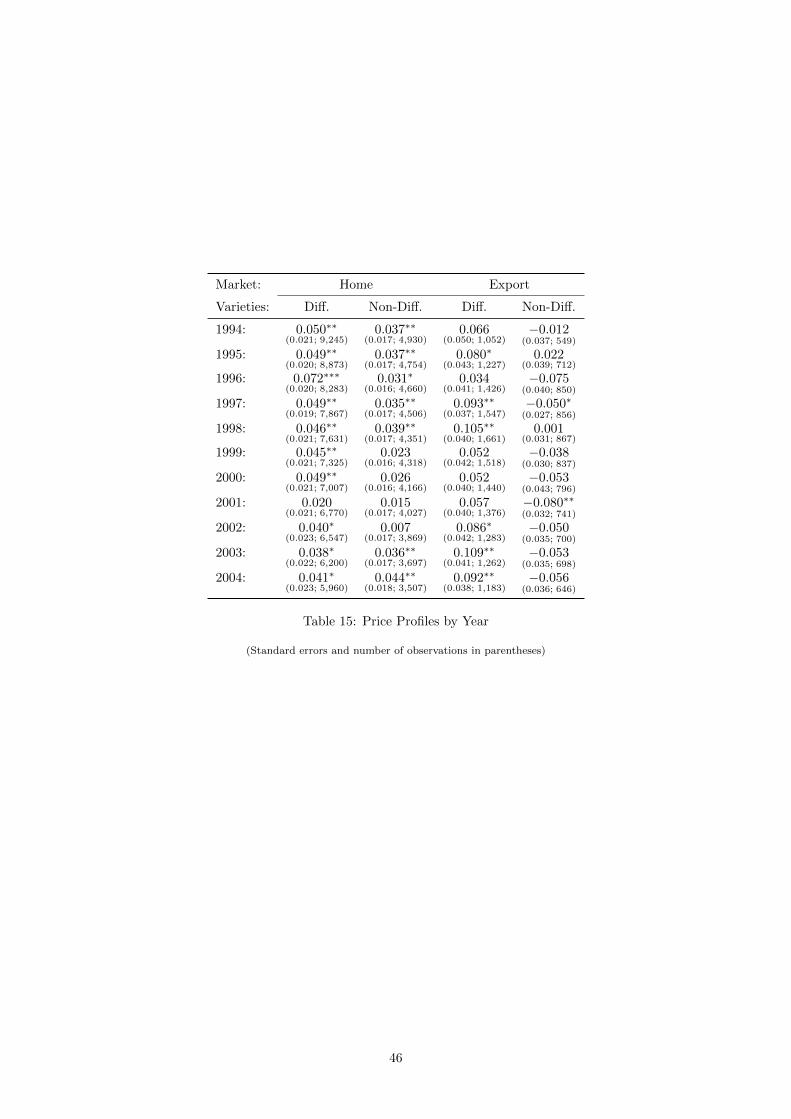
Market: Home Export

Varieties: Diff. Non-Diff. Diff. Non-Diff.

1994: 0.050∗∗(0.021; 9,245)

0.037∗∗(0.017; 4,930)

0.066(0.050; 1,052)

−0.012(0.037; 549)

1995: 0.049∗∗(0.020; 8,873)

0.037∗∗(0.017; 4,754)

0.080∗(0.043; 1,227)

0.022(0.039; 712)

1996: 0.072∗∗∗(0.020; 8,283)

0.031∗(0.016; 4,660)

0.034(0.041; 1,426)

−0.075(0.040; 850)

1997: 0.049∗∗(0.019; 7,867)

0.035∗∗(0.017; 4,506)

0.093∗∗(0.037; 1,547)

−0.050∗(0.027; 856)

1998: 0.046∗∗(0.021; 7,631)

0.039∗∗(0.017; 4,351)

0.105∗∗(0.040; 1,661)

0.001(0.031; 867)

1999: 0.045∗∗(0.021; 7,325)

0.023(0.016; 4,318)

0.052(0.042; 1,518)

−0.038(0.030; 837)

2000: 0.049∗∗(0.021; 7,007)

0.026(0.016; 4,166)

0.052(0.040; 1,440)

−0.053(0.043; 796)

2001: 0.020(0.021; 6,770)

0.015(0.017; 4,027)

0.057(0.040; 1,376)

−0.080∗∗(0.032; 741)

2002: 0.040∗(0.023; 6,547)

0.007(0.017; 3,869)

0.086∗(0.042; 1,283)

−0.050(0.035; 700)

2003: 0.038∗(0.022; 6,200)

0.036∗∗(0.017; 3,697)

0.109∗∗(0.041; 1,262)

−0.053(0.035; 698)

2004: 0.041∗(0.023; 5,960)

0.044∗∗(0.018; 3,507)

0.092∗∗(0.038; 1,183)

−0.056(0.036; 646)

Table 15: Price Profiles by Year

(Standard errors and number of observations in parentheses)

46