Hitting and Trapping Times on Branched Structures

Elena Agliari,1 Fabio Sartori,2 Luca Cattivelli,3 and Davide Cassi2

1Dipartimento di Fisica, Sapienza Universita di Roma2Dipartimento di Fisica e Scienze della Terra, I-43124 Parma, Italy

3SNS Scuola Normale Superiore, Pisa, Italy

In this work we consider a simple random walk embedded in a generic branched structure and wefind a close-form formula to calculate the hitting time H (i, f) between two arbitrary nodes i and j.We then use this formula to obtain the set of hitting times {H (i, f)} for combs and their expectationvalues, namely the mean-first passage time (MFPTf ), where the average is performed over the initialnode while the final node f is given, and the global mean-first passage time (GMFPT), where theaverage is performed over both the initial and the final node. Finally, we discuss applications in thecontext of reaction-diffusion problems.

PACS numbers:

I. INTRODUCTION

Random walks (RWs) on inhomogeneous structureshave been first introduced to describe anomalous diffu-sion [1], but they actually constitute a convenient modelfor many real phenomena, ranging from soft matter (e.g.gels and biological structures [2]), to condensed matter(e.g., fractures [3] and light scattering [4]).

Here we will focus on the so-called “branched struc-tures”, namely graphs V obtained by attaching to eachvertex j of a base graph G0 a different graph Gj calledfiber (see Fig. 1). Branched strucutres were used todescribe the energy transfer in polymers [5], the trans-port of calcium in spiny dendrites [6–8], the excitation ofnano-antennas [9], the anomalous diffusion in real struc-ture with similar topology [1, 10–15]. In particular, wewill consider a specific class of branched structures calledcombs, namely graphs where the base graph as well thefiber ones are linear chains, in such a way that Gj is siteindependent and equivalent to Z (see Fig. 2).

Diffusion on combs has been shown to display manypeculiar features ultimately stemming from their highlyinhomogenous topology (see e.g.,[16–19]). Now, most ofthe previous results have been proven in the thermody-namic limit, namely for structures of infinite size, whilereal systems are intrinsically finite. In this work we aim

Figure 1: Example of branched structure V obtained by join-ing to each point j of a graph G0 called base (leftmost panel)a graph Gj called fiber (middle panel).

Figure 2: Examples of 2-dimensional comb, where the back-bone is endowed with reflecting boundary conditions (upperpanel) or periodic boundary conditions (lower panel). Thesize of the backbone is referred to as 2L+ 1, while the lengthof teeth Ly is taken to be uniform and scaling linearly withL, namely Ly = αL. For instance, in the upper panel L = 7and αL = 5.

to investigate the problem of diffusion in finite comb lat-tices and we will especially focus on first-passage quan-tities such as the hitting time H (i, f) from i to f (i.e.the mean time for a random walker to first reach site fstarting from i), the mean first-passage time MFPTf tof (i.e., the mean time needed to first reach the vertex f ,averaged over the starting site), and the global mean-firstpassage time GMFPT (i.e., the mean time to go from arandom vertex to a second random vertex).

These quantities have been extensively studied in thepast, also due to the number of different applications inseveral research areas: pharmacokinetics [20], reaction-diffusion processes [21], excitation transport in photosys-tems [22], target search processes [23], disease spreading[24] and many other physical problems [25–33].

arX

iv:1

412.

5883

v1 [

cond

-mat

.sta

t-m

ech]

18

Dec

201

4

2

In this work we calculate the above mentioned quan-tities for (d-dimensional) combs using the resistancemethod: the original graph V is mapped into a resis-tance network by replacing any link (a, b) between twoadjacent nodes a and b with a unitary resistance R [34].Then, we use Tetali’s formula [35] to calculate the exactvalue of the hitting time between i and f as

H (i, f) = mRi,f +1

2

∑z∈V

g (z) {Rf,z −Ri,z} , (1)

where m is the number of links in the graph, g(z) isthe coordination number of the vertex z, and Ra,b is theeffective resistance between the vertices a and b.

II. HITTING TIME OF BRANCHEDSTRUCTURES

In this section we will use Eq.(1) to calculate the valueof the hitting time for generic branched structures (seeFig. 1).

When the starting point i and the ending point f be-long to different fibers, we can divide vertices of V intothree disjoint subsets, referred to as I,F and B respec-tively (see Fig. 3): V = I∪F∪B. More precisely, the sub-set I contains all vertices belonging to the fiber-graphGi = (I,Li), the sub-set F contains all vertices belong-ing to the fiber-graph Gf = (F ,Lf ) and finally the sub-set B contains all vertices belonging to the fiber-graphsGk = (Kk,Lk) with k 6= (i, f), formally B =

⋃k 6=i,f Kk,

where Lj is the adjacency matrix of the fiber graph Gj .

Figure 3: Schematization of the decomposition used in Eq.(2): where vertices of V are V = I ∪ F ∪ B. Notice that thewhole set of fiber graphs {Gj} also includes the set of nodesmaking up the base graph because the joining nodes, alsocalled “roots”, are shared.

This procedure allows us to write the sum in (1) as:∑z∈V

g (z) (Rf,z −Ri,z) =∑z∈I

g (z) (Rf,z −Ri,z) +

+∑z∈F

g (z) (Rf,z −Ri,z) +

+∑z∈B

g (z) (Rf,z −Ri,z) . (2)

namely we distinguish the case where z is in the samefiber graph as i (z ∈ I), z is in the same fiber graph asf (z ∈ F), and z is in a fiber graph which neither i nor

f belong to (z ∈ B). In the following we will call rootri the vertex shared by the base graph G0 and the fibergraph Gi.

In general, when two vertices i and f belong to differentfiber-graphs, we can write the effective resistance Ri,fbetween these point as a sum of three resistances in series:

Ri,f = Ri,ri +Rri,rf +Rf,rf . (3)

Now, recalling Eq. (2), we can notice that when z ∈ Bwe can use Eq. (3), for both Ri,z and Rz,f , while whenz ∈ I or z ∈ F , we can use Eq. (3) only for Ri,z or forRi,z, respectively.

In fact, suppose we consider a linear chain as a fibergraph Gi: when z and i belong to the same fiber graph theeffective resistance according to Eq. (2) would be |yi| +|yz|, being yi and yf the coordinates of i and f along therelated theeth, while the correct estimte is |yi−yf |, whichrecovers the former only when the signs are different.

Exploiting this remark, the three sums appearing inEq. (3) can be written as:

∑z∈B

g (z) (Rf,z −Ri,z) =∑z∈B

g (z){Rrf ,rz −Rri,rz +

+ Rf,rf −Ri,ri},∑

z∈Ig (z) (Rf,z −Ri,z) =

∑z∈I

g (z){Rf,rf +Rrf ,rz +

+ R (z, rz)−Ri,z} ,∑z∈F

g (z) (Rf,z −Ri,z) =∑z∈F

g (z) {Rf,z −Ri,ri +

− Rri,rz −Rz,rz} .

Then, after some algebraic manipulations we find that

H (i, f) = mRri,rf +1

2

∑z∈V

g (z)(Rrf ,rz −Rri,rz

)+ (4)

+2 (m−mf )R (f, rf ) +Hi (i, ri) +Hf (rf , f) ,

where mk is the number of links in the sub-graph Gk, andHk (a, b) the mean time for a walker to go from a to b,(a, b ∈ G0), without ever exiting out from the fiber G0.

We have obtained a summation similar to that withwhich we began, but now resistances are considered be-tween points of the base-graph. This allows us to fac-torize the difference

(Rrf ,rz −Rri,rz

), by splitting the

summation over z ∈ V into the summation over everyvertex of all fiber-graphs:∑z∈V

g (z)(Rrf ,rz −Rri,rz

)=∑k∈G0

∑z∈Gk

g (z)(Rrf ,rz −Rri,rz

).

Previously we noticed that the difference of resistancesdepends only on the fiber graph, so we can factorize it:

3

∑z∈V

g (z)(Rrf ,rz −Rri,rz

)=

=∑k∈G0

(Rrf ,rk −Rri,rk

) ∑z∈Gk

g (z)

=∑k∈G0

(Rrf ,rk −Rri,rk

)2mk.

Finally, merging the previous results we get

H (i, f) = Hi (i, ri) +∑k∈G0

mk

(Rrf ,rk −Rrk,ri

)+

+ Hf (rf , f) + 2 (m−mf )R (f, rf )

+ mRri,rf . (5)

Of course, this formula recovers the Tetali one (1) whenall the branched graphs Gi are composed only of a singlevertex (the one that is shared with G0, i.e. the root ri).The details of the fibers only enter in the summationterm, and the only important things about these graphsare the position on the base graph and the number oflinks mk, neither the topology nor the number of verticesof these fiber graphs affect H (i, f).

A. Particular Cases:

There are special cases where the formula in Eq. (5)can be significantly simplified. In particular when theratio between the coordination number g(k) of any vertexk belonging to the base graph and the number of links mk

in the k−th subgraph is independent of k. This allowsus to write mk = γg(k), being γ a constat value whichis the same for every vertex of the base graph G0. Then,the summation in Eq. (5) becomes:

∑k∈G0

mk

(Rrf ,rz −Rri,rz

)= 2γ

[H0 (ri, rf )−m0Rrf ,ri

],

(6)and, using this result, Eq. (5) becomes:

H (i, f) = HI (i, ri) + 2γH0 (ri, rf ) +HF (rf , f) + (7)

+2 (m−mf )R (f, rf ) + (m− 2γm0)Rri,rf ,

where HI (a, b) and HF (a, b) represent the mean timetaken by a walker to first go from a node a to a node b(being a, b ∈ I and a, b ∈ F respectively) without evereciting out of I and F respectively; analogously H0 (a, b)represent the mean time to first reach b starting from a(being a, b ∈ G0) and moving only on the base graph. Inthis case the mean time to go from i to f can be expressedby a sum of three hitting times, and some constant value.

Another interesting case appears when the position ofthe root of the starting vertex ri and the root of theending one rf displays a symmetry such that

H (ri, rf ) = H (rf , ri) (8)

Figure 4: Example of a Sierpinsku gasket of genereation 3fibrated with linear chains with 5 vertices.

in this particular case Eq. (5) becomes

H(i, f) = Hi (i, ri) +Hf (rf , f) +

+ 2 (m−mf )R (f, rf ) +mRri,rf . (9)

This formula allows us to calculate the hitting times forany ”symmetric structure” (according to Eq. (8)), like aSierpinski fibrated with linear chains, (see Fig 4).

Let us consider a Sierpinski gasket of generation n andas fibers linear chains with L vertices. The total numberof vertices in the base-graph is [36] |V |(n)0 = 3(3n+1)

2 and

the total number of links is [36] m(n)0 = 3n+1. For in-

stance let us try to evaluate the mean time to first reachthe node f belonging to a tooth stemming from a cor-ner, starting from a node i belonging to a tooth stemmingfrom another corner (see Fig 4). Neri et al. in [37] showed

that Rri,rf = 2·5n3n+1 . Using Eq. (9) it is straightforward

to show that H (i, f) reads as

HMax = 3L2 +

(1 +

L

2

)(3n+1 + 2 · 5n

)+

(5

3

)nL.

B. Bidimensional Combs

Bidimensional combs are branched structures wherethe base-graph G0 is a monodimensional graph, like alinear chain or a ring, usually called backbone, and fibergraphs are linear chains usually called teeth, see Fig. 2.Here, we consider two different cases according to thethe boundary conditions applied to the backbone: we

4

call “Bidimensional Open Combs” those combs whosebackbone is a linear chain, and “Bidimensional ClosedCombs” those whose backbone is a ring; teeth are alwaystaken as open (i.e. reflecting at boundaries).

As shown in Fig. 2, the size of the backbone is 2L+ 1,and each linear chain departing from the backbone countsαL vertices, in such a way that α measures the degree ofinhomogeneity along the two directions (e.g., when α = 1the comb is square).

Using Eq. (5) we are now able to calculate the valueof H (i, f) for those graphs.

In the following, exploiting the fact that combs areembedded in 2−dimensional lattices, the position of thearbitrary point k will be denoted as (xk, yk) where xkindicates the projection of k on the backbone, and yk itslength along the related tooth. Let us start with opencombs for which we apply Eq. (5), with some algebra weget 1:

H (i, f) = mRi,f +(y2f − y2i

)+ (2αL+ 1)

(x2f − x2i

)+

+ (|y2| − |y1|)(L24α+ 2L

), (10)

where the resistance between two generic points a =(xa, ya) and b = (xb, yb) for open combs is

Ra,b = δxa,xb|ya−yb|+(1− δxa,xb

) (|xa − xb|+ |ya|+ |yb|) .

From this equation we can extract important infor-mation, for example the mean time to cross the wholebackbone and the mean time to “climb” a tooth. Thesequantities are, respectively,

H (−L, 0→ L, 0) = L3 (8α) + L2 (4 + 4α) ,

and

H ({0, 0} → {0, αL}) = L3(8α2

)+ L2

(4α+ 3α2

).

Using Eq. (5) we can also calculate the Hitting Timefor closed combs, H

2 (i, f), where we used the apex toemphasize that this quantity is reffered to a closed comb2:

H2 (i, f) = mR

if+(|yf | − |yi|)[4αL2 + 2L+ 1

]+(y2f − y2i

),

(11)

1 What we really find from Eq. (5) is H (i, f) −2L (1 + α+ 2αL)

[−1 + |yi|+ |yf | − |yi − yf |

]δxi,xf . This

difference is due to the hypotesis that xi 6= xf , namely thestarting point and the final point belong to different fibergraphs. If we use Eq. (7) instead of Eq. (5), we introduce anadditional error of

(xi − xf

) (xi + xf

)due the different value

of g (x, 0) between x = ±L, where g (±L, 0) = 3, and x 6= ±L,where g (x, 0) = 4.

2 Once again what we really find using Eq. (5) is H2 (i, f) −

(1 + 2L) (1 + 2αL)[|yi|+ |yf | − |yi − yf |

]δxi,xf . This differ-

ence is due to the hypotesis that xi 6= xf . This time if we useEq. (7) instead of Eq. (5), we do not introduce any additionalerror.

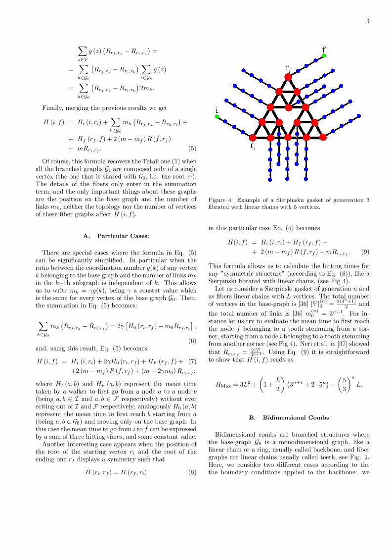
Figure 5: Example of a 3-dimensional comb. Vertices whichbelong to the first generation are green, those which belongto the second are lilac, and those which belong to the tird arered.

where the resistance between two generic points a =(xa, ya) and b = (xb, yb) for close combs is

Ra,b = δxa,xb

|ya − yb|+ (1− δxa,xb)×

×

(|xa − xb|+ |ya|+ |yb| −

(xa − xb)2

2L+ 1

).

From Eq. (11) we can extract the time needed to crosshalf backbone as

H2 ({0, 0} → {L, 0}) = L3 (6α) + L2 (3 + 2α) + L,

and the time to climb a thoot as

H2 ({0, 0} → {0, αL}) = L3

(8α2

)+L2

(4α+ 3α2

)+L (2α) .

We can notice that the leading order of the mean timeneeded to cross the backbone is proportional to α (con-sistent with results in [31]) and the leading order of themean time to climb a tooth is proportional to α2.

C. d-dimensional Open Combs

We define d-dimensional open combs recursively asdone in [38](see also Fig 5):

• a 1−dimensional open comb is a linear chain;

• a 2−dimensional open comb is a branched graph Gwhose base graph is a linear chain and whose fibergraphs are linear chain;

• . . .

• a d−dimensional open comb is a branched graph Gwhose base graph is a (d − 1)−dimensional combsand whose fibers are linear chains.

As shown in Sec. II B, a finite 2-dimensional comb canbe defined by fixing two parameters: the length of thebackbone L and the ratio α between the length of a tooth

5

and the length of the backbone, in such a way that thethermodynamic limit L → ∞ is well defined. Now, tofix a d−dimensional comb we introduce d parameters:(L,α2, . . . , αd), being αi the ratio between the length ofthe tooth in the i-th direction (i.e. added at the i−thiteration) and the length of the backbone: αi = Li

L .We label every vertices with d coordinates and call

i = (x1, . . . , xd) and f = (y1, . . . , yd), where the firstcoordinate labels the vertices on the base graph and ittakes value from−L to L, the second one goes from−α2Lto α2L and labels the base of the fiber graphs, the thirdone goes from −α3L to α3L and so on.

We define H(d) (i, f), the Hitting Time from i to fin a d−dimensional comb and we will use Eq. (5) tocalculate its leading order. Using Tetali’s equation it isstraightforward to observe that H(d) (i, f) ∼ O

(Ld+1

).

In fact, the first term of the right hand side in Eq. (1) ismdRi,f and one can see that in the d−dimensional combthe number of links md is

md ∼

(Ld2d

d∏k=2

αk

), (12)

while the maximum value of R is

R = 2L

(1 +

d∑k=2

αk

)+ 1,

thus, the leading order of this first term is Ld+1. Also thesecond term in the right hand side of the Eq. (1), that is12

∑z∈V g (z) (Rf,k −Rk,i), where g (z) ≤ 2d = O

(L0),

V = O(Ld)

and R = O (L), is order Ld+1.Using this observation we can simplify Eq. (5), in fact

Hi, Hf and mdR (f, rf ) are O(Ld). So the leading order

of Eq. (5) is given only by

H (i, f) ∼ 1

2

L∑k=0

{|k − y1| − |k − x1|}mk +

+ 2mdR (f, rf ) +mdRri,rf . (13)

We have just pointed out that md ∼(Ld2d−1

∏dk=2 αk

),

where mk is the number of links in the fiber-graphs start-ing from the node k, and its leading value is mk ∼(Ld−12d−1

∏dk=2 αk

), so

H (i, f)(d) ∼

(Ld−12d−2

d∏k=2

αk

)(y21 − x21

)+

+

(Ld2d

d∏k=2

αk

)|x1 − y1|+ 2

d∑j=2

|yj |

.By introducing the normalized coordinates ξi = yi

αiL,

and ηi = xi

αiL(posing conventionally α1 = 1), we can

express the leading value of H(d) (i, f):

H(−→η ,−→ξ ) ∼ Ld+12d−2

d∏i=2

αi × (14)

×

[(ξ21 − η21

)+ 4|ξ1 − η1|+ 8

d∑k=2

αkξk

].

We can use Eq. (14) to calculate the mean time to cross

the backbone going from η =(−1,~0

)to ξ =

(+1,~0

), as

H(d)({−1,~0

}→{

1,~0})∼ Ld+12d+1

d∏i=2

αi,

and its maximum value going from η =(−1,~1

)to ξ =(

1,~1)

:

H(d)({−1,~1

}→{

+1,~1})∼ Ld+12d+1

d∏i=2

αi

[1 +

d∑k=2

αk

].

III. TRAPPING TIMES

In this section, we will analyze some average quanti-ties, in particular we introduce the mean first-passagetime defined by MFPTf = Ei [H (i, f)] and the GlobalMean First Passage Time, defined by GMFPT =Ei [Ef [H (i, f)]]. The first quantity rapresents the meantime to reach a fixed reaction node placed in f , startingfrom a random one. The second one is the mean timeto reach a random vertex starting from another randomone.

A. MFPTf

The MFPTf was introduced by Montroll for regulargraphs [22] to describe the excitation transfer on a pho-tosintetic complex. Later this quantities was extended forirregular graph, see [27, 31, 39–43]. Once we know everyvalue of H (i, f) we can calculate exactly this quantityusing MFPTf = 1

V

∑i∈V H (i, f), where V is the volume

of the graph V.

1. Bidimensional Open Combs

Knowing the values of H (i, f) for every couple of nodes(i, f) (see Eq.10), it is straightforward to calculate thevalue of MFPTf = 1

V

∑i∈V H (i, f), where V is the vol-

ume of the graph V. To achieve this results it is conve-nient to split Eq. (10) in three parts:

H (i, f) = {mRif}+{

(2αL+ 1)(x2f − x2i

)}+

+{(y2f − y2i

)+ (|yf | − |yi|)

(L24α+ 2L

)}= (A) + (B) + (C) ,

6

and calculate these separately. The first contribution,Ei [A], can be written as

Ei [A] =

L∑xi=−L

L∑yi=−αL

m [δxi,xf |yi − yf | +

+ (1− δxi,xf ) (|xi − xf |+ |yi|+ |yf |)] ,

and after the summation on xi it becomes:

Ei [A] =m

V

αL∑yi=−αL

[|yi − yf |+[+2L

(|yi|+ |yf |+ x2f + L+ L2

)],

and finally

Ei [A] = y2fm

V+ |yf |

[mV

(2αL+ 1) 2L]

+

+x2f

[mV

(2αL+ 1)]

+m

V[αL (αL+ 1) +

+L (L+ 1) (2αL+ 1) + 2αL2 (αL+ 1)].

Performing similar calculation the second contribution,Ei [B], can be written as

Ei [B] =∑xi,yi

[(2αL+ 1)

(x2f − x2i

)]= (2αL+ 1)x2f −

1

3L (L+ 1) (2αL+ 1) ;

and the third contribution, Ei [C], becomes:

Ei [C] = |yf |2L (2αL+ 1)− y2f − αL(

1

3+ 2L

).

Merging these three contributions we find the exact valueof MFPTf :

MFPT(xf ,yf ) = (15)(1 +

m

V

) [y2f + x2f (2αL+ 1) |yf |

(4αL2 + 2L

)]+

+ |yf |(4αL2 + 2L

)]+

1

3 (1 + 2L) (1 + 2αL)×

×[16α2L5 + L4

(16α+ 24α2 + 8α3

)+

−L (1 + α) + L23 (1 + α)L3(4 + 18α+ 14α2 + 4α3

)].

The position of the trap affects only the contribute inthe first square braket. Therefore, MFPT(xf ,yf ) can bewritten as the sum of two terms, the former depends onthe final vertex, and the latter depends only on L and αand is exactly the value of MFPT(0,0):

MFPT(xf ,yf ) (L,α) = φ (xf , yf ) + MFPT(0,0). (16)

We have numerically tested this result for three positionsof the trap (xf , yf ) and for several values of L and α, as

shown in Figs. (6, 7 and 8). In each of those figures thevalue of (xf , yf ) is fixed and we changed the value of Land α. The values of (xf , yf ) are respectively (0, 0),(L, 0)and (L,αL), L takes values from 8 and 256, and α goesfrom 1/32 to 128.

0 20 40 60 80 100 120 1400.99

0.995

1

1.005

1.01

1.015

MFPT(0,0)

L

Sim

ul./Theor.

−4 −3 −2 −1 0 1 2 3 4 50.99

0.995

1

1.005

1.01

1.015

MFPT(0,0)

log(α)Sim

ul./Theor.

Figure 6: Numerical check of the theoretical predictions ofEq. (15) for (xf , yf ) = (0, 0). In both figures the results of thesimulations are divided by the theoretical value of MFPT(0,0).

20 40 60 80 100 120

0.985

0.99

0.995

1

1.005

1.01

MFPT(0,αL)

L

Sim

ul./Theor.

−4 −2 0 2 40.98

0.985

0.99

0.995

1

1.005

1.01

MFPT(0,αL)

log(α)

Sim

ul./Theor.

Figure 7: Numerical check of the theoretical predictionsof Eq. (15) for (xf , yf ) = (0, αL). In both figures the re-sults of the simulations are divided by the theoretical valueof MFPT(0,αL).

7

0 20 40 60 80 100 120 1400.99

0.995

1

1.005

1.01

1.015

L

Sim

ul./Theor.

MFPT(L,αL)

−4 −2 0 2 4 60.99

0.995

1

1.005

1.01

1.015

log(α)

Sim

ul./Theor.

MFPT(L,αL)

Figure 8: Numerical check of the theoretical predictionsof Eq. (15) for (xf , yf ) = (L,αL). In both figures the re-sults of the simulations are divided by the theoretical valueof MFPT(L,αL).

The asymptotic behaviour of MFPTf is

MFPTf (L,α) ∼ L3

{4α

[1

3+( xL

)2]+ 8α

∣∣∣ yL

∣∣∣}(17)

∼ 4

3αL3,

where the last relation holds as long as both x and y arefinite. The dependence on L3 is consistent with previousasymptotic results [19, 31].

2. Bidimensional Close Combs

Analogous argoments can be applied to calculate theexact value of the Mean First Passage Time for closecombs, and we call this quantity MFPT

f . We skiplengthy passages and provide straightforwardly the finalresult:

MFPT(xf ,yf )

=[|yf |

(1 + 4L+ 8L2α

)+ 2y2f

]+

1

3 + 6αL×

×[L (2− α) + L2

(2 + 8α+ 3α2

)+

+ L34α(2 + 2α+ α2

)+ L4

(8α2

)]. (18)

Of course, MFPTf does not depend on xf , due to the

periodic condition on the x axis. Moreover, as done inEq. (16) we can distinuish two contribution highlightingthe dependance of the trap position (height) as

MFPT(xf ,yf )

(L,α) = φ (yf ) + MFPT(0).

Figure 9: Numerical check of the theoretical predictions ofEq. (18) for (yf ) = (0). In both figures the results of thesimulations are divided by the theoretical value of MFPT

(0).

Figure 10: Numerical check of the theoretical predictions ofEq. (18) for (yf ) = (αL). In both figures the results of thesimulations are divided by the theoretical value of MFPT

(αL).

The asimptotic behaviour reads as:

MFPTf (L,α) ∼ L3

{4

3α+ 8α

y

L

}. (19)

∼ 4

3αL3,

where the last relation holds as longs y is finite.

8

We have numerically tested this result for two valuesof yf and for several values of L and α, as shown in Figs.(9 and 10). In each of those figures the value of yf isfixed and we changed the value of L and α. The valuesof yf are respectively 0 and αL, L takes values from 8and 256, and α goes from 1/32 to 128.

B. GMFPT

We define the Global Mean First Passage Time,GMFPT, as the mean Hitting Time averaged on startingand on ending points:

GMFPT = Ei,f [H (i, f)] ;

=1

V 2

∑i∈V

∑f∈V

H (i, f)

GMFPT depends qualitatively on the topological prop-erties of the underlying structure and this has beenproven from different perspectives. For instance, it is wellknown that GMFPT is related with the Kirchhoff index[44], K = Ei,f [Ri,f ] (in fact, from Chandra’s formulaH (i, f) + H (f, i) = 2mRi,f [45] it follows straightfor-wardly that GMFPT = m〈R〉).

Moreover, Benichou et al. [46] found a very generalasymptotic expression reading as:

GMFPTB ∼

V dw < dfV log (V ) dw = dfV dw/df dw > df

(20)

where dw is the walk dimension and df is the fractaldimension. Their definition of global mean first passagetime, is slightly different from ours: theirs is averagedover links,

GMFPTB =1

m

∑i,f∈V

H (i, f) g (i) g (f)

(m− g (f))

while ours is averaged over vertices:

GMFPT =1

V 2

∑i,f∈V

H (i, f) .

Despite this different definitions they showed (via nu-merically simulation) that these lead to the same asymp-totics. Now, for comb lattice the walk dimension dwis not unique [47] and Einstein’s relation d dw = 2dfdoes not hold directly and one could therefore calculateGMFPT in a more ”pedestrian” way. Now, we report theexact value of GMFP for the combs structures outlinedabove, and compare their asymptotic behaviors with Eq.(20).

1. Bidimensional Open Combs

To calculate the GMFPT for open combs, we startfrom Eq. (15). We recall that MFPTf can be written

as the sum two terms, the former depends on the finalvertex, and the latter is exactly the value of MFPT(0,0),in a such way that in order to obtain the exact value ofGMFPT we have to average only on the former; namely

GMFPT = E [f (xf , yf )] + MFPT(0,0). (21)

and after some algebra we find:

GMFPT =

L∑xf=−L

αL∑yf=−αL

MFPTf = (22)

=1

3 (1 + 2L) (1 + 2Lα)

[8L2

(1 + 2α+ α2

)+

+8L3(1 + 8α+ 8α2 + α3

)+

8L4(4α+ 15α2 + 5α3

)+ 16L5α2 (2 + 3α)

],

whose leading order is:

GMFPT (L,α) ∼ L3

(8

3α+ 4α2

). (23)

0 20 40 60 80 100 120 1400.98

0.985

0.99

0.995

1

1.005

1.01

1.015

1.02

GMFPT

L

Sim

ul./Theor.

−3 −2 −1 0 1 2 3 4 50.97

0.98

0.99

1

1.01

1.02

GMFPT

log(α)

Sim

ul./Theor.

Figure 11: Numerical check of the theoretical predictions ofEq. (22). In both figures the results of the simulations aredivided by the theoretical value of GMFPT.

We have numerically tested this result for many valuesof L and α, as shown in Fig. 11. In this figure we changedthe value of L from 8 to 256 and α from 1

32 to 128.

2. Bidimensional Close Combs

We now apply analogous arguments to calculate theexact value of the global mean first passage time forclose combs, hereafter referred to as GMFPT; averag-ing MFPT

f over f we find the exact value of GMFPT

9

as

GMFPT (L,α) =2

3[L (1 + 2α) + (24)

+L2(1 + 8α+ 2α2

)+ L3

(2α+ 6α2

)]whose leading order is:

GMFPT (L,α) ∼ L3

(4

3α+ 4α2

). (25)

We have numerically tested this result for many valuesof L and α, as shown in Fig. 12. In this figure we changedthe value of L from 8 and 256 and α from 1

32 and 128.

Figure 12: Numerical check of the theoretical predictions ofEq. (24). In both figures the results of the simulations aredivided by the theoretical value of GMFPT.

Once again we can notice that the coefficient of α2

is the same in both combs, but the coefficient of α1 isnot. For both GMFPT and GMFPT the leading order∼ L3 is larger than the behaviour expected from a more

homogeneous structure with analogous dimensions (δ =3/2 and df = 2). This underlines once more the peculiarbehaviour of combs.

IV. PREY-PREDATOR RELATIONS

In this section we frame the previous results within achemical-kinetics perspective. Imagine having two reac-tants, say A (static) and B (dynamic). If we are allowedto choose the position of A, but we have no control onB (namely we can not fix its starting point), which willdiffuse freely thorought the lattice, we can choose for

the static reactant the place which minimize the reac-tion time. In fact, this is just the node f that minimizeMFPTf .

As shown in Sec. [III A 1)] and in Sec. [III B 2], theMFPT for both open and close combs can be writtenas MFPTf = φ (f) + const. In both combs previouslyanalyzed we found that φ (f) ≥ 0 for every final vertexf . In particular, in open combs φ (f) = 0 when f =(0, 0), and in close ones it is zero when f = (i, 0); themaximum value of MFPTf arises when the value of φ (f)is maximized, this occurs for f = (±L,±αL) for opencombs and f = (i,±αL) for close ones. Of course, forclose combs there is no dependence on the x coordinatedue to the periodic condition on the x axis.

Now, if we can not control the position of A, but thisis stochastic, which is the typical time τf = MFPTf forthe reaction to occur? In particular, the reaction willbe considered “slow” if τf > GMFPT and “fast” if τf <GMFPT. We characterize the boundary between the tworegimes finding those vertices f for which GMFPT =MFPTf . We will obtain this results in the limits of L→∞ by imposing the asimptotic equality between Eq. (17)and (23), and between Eq. (19) and (25). Recallingthat f = (xf , yf ) we will looking for the functional formyf (xf , L, α) such that GMFPT ∼ MFPTxf ,yf .

A. GMFPT vs MFPTf in Open Combs

Let us consider the leading value of GMFPT andMFPTf from, Eqs. (17) and (23):{

GMFPT (L,α) ∼ L3(83α+ 4α2

)MFPTf (L,α) ∼ L3

{4α[13 +X2

]+ 8α2|Y |

},

where we normalized the coordinates as X = x/L andY = y/αL. Now vertices f for which MFPTf = GMFPTare those whose coordinates fulfill the following equality:(

8

3α+ 4α2

)=

[4α

(1

3+X2

)+ 8α2|Y |

].

Solving for Y we find

|Y | =(

1

2+

1

6α

)− X2

2α.

It is interesting to note that the fraction of vertices forwhich the reaction is slow, Fslow, or fast, Ffast, are ex-actly the same for every value of α. This is obtainedintegrating the value of Y :

Fslow =

1∫0

|Y (X,α) |dX =1

2.

The phase diagram is shown in Fig. 13. As we can see,varying the value of α there are three possible scenarios:when α is sufficently small there are some teeth totally

10

X

Yα = 1/3

−1 −0.5 0 0.5 1

−1

0

1

X

Y

α = 1/2

−1 −0.5 0 0.5 1

−1

0

1

X

Y

α = 2/3

−1 −0.5 0 0.5 1

−1

0

1

X

Y

α = 1

−1 −0.5 0 0.5 1

−1

0

1

Figure 13: Phase diagram of MFPT(Y )−GMFPT; those ver-tices where MFPT(Y ) > GMFPT are colored red, and thosewhere MFPT(Y ) < GMFPT are green

composed by ”fast” vertices (like in α = 13 ), when α

is large enough there are no teeth that are completely”fast” or ”slow” (like in α = 2

3 and in α = 1), and anintermediate case where there exist some teeth entirelycomposed by ”slow” vertices but no one that is totallycomposed by ”fast” vertices (like in α = 1

2 );

• the first case happens when |Y | ≥ 1 for X = 0.This means that |Y | =

(12 + 1

6α

)≥ 1, and solving

in α we find

α ≤ 1

3;

• the second case happens when |Y | ≥ 0 for X = 1.This means that |Y | =

(12 + 1

6α

)− 1

2α ≥ 0, andsolving in α we find

α ≥ 2

3;

• the last case happens in the intermediate case:

2

3> α >

1

3.

B. GMFPT vs MFPTf in Close Combs

Let us consider the leading terms of GMFPT andMFPTf , Eqs. (19) and (25){

GMFPT (L,α) ∼ L3(43α+ 4α2

)MFPT

f (L,α) ∼ L3{

43α+ 8α2|Y |

},

X

Y

α = 1/2

−1 −0.5 0 0.5 1

−1

0

1

X

Y

α = 10

−1 −0.5 0 0.5 1

−1

0

1

Figure 14: Phase diagram of MFPT(Y ) − GMFPT; those

vertices where MFPT(Y ) > GMFPT are colored red, andthose where MFPT(Y ) < GMFPT are colored green

the set of vertices f for which MFPTf ∼ GMFPT arethose whose coordinates fulfill the following equality:

(4

3α+ 4α2

)=

{4

3α+ 8α2|Y |

}.

Solving for Y we find

|Y | = 1

2.

This means that the location of nodes f such thatGMFPT = MFPTf , does not depend neither on X (andthis is obvious due to the periodic boundary condition)nor on α. Therefore, if the target is placed sufficientlyfar from the backbone (i.e. at least at half the height of athoot) the reaction turns out to be slow. Once again thefraction of vertices giving rise to slow and fast reactionsis the same. The phase diagram is shown in Fig. 14.

V. CONCLUSIONS AND FUTUREPERSPECTIVES

In this work we found an useful formula, (5), to calcu-late the exact value of the hitting time, that is an alter-native form of Tetali’s equation. This formula is partic-ularly useful when the graph has ramifications. In par-ticular we have calculated explicitly the value of H (i, f)for the bidimensional combs and its leading value for thed−dimensional ones.

We then used these results to calculate the MFPTf andthe GMFP for 2-dimensional combs, observing that theleading value is composed by two terms, one proportionalto αL3, and the other one to α2L3, being α the ratiobetween the size of the backbone and of the teeth.

As for the GMFPT we noticed that its asymptotic be-haviour does not directly depends on its fractal and spec-tral dimension (as for homogeneous lattices and fractals)and we calculated it exactly. Finally we discussed our re-sults in the context of reaction-kinetics. Infact the MFPTcan be seen as the mean time taken by a mobile reac-tant A to reach a static reactant B, when the startingpoint of the mobile reactant is not known. Interestinglythe typical time for the reaction to occur can be eitherlarger (slow reaction) or smaller (fast reaction) than theGMFPT, and we outlined the set of trap locations forwhich these regimes are recovered.

11

[1] Havlin, Shlomo, and Daniel Ben-Avraham. ”Diffusion indisordered media.” Advances in Physics 36.6 (1987): 695-798.

[2] Berg, Howard C., ed. Random walks in biology. PrincetonUniversity Press, 1993.

[3] Vicsek, Tamas. Fractal growth phenomena. Vol. 4. Sin-gapore: World scientific, 1989.

[4] Maret, G., and P. E. Wolf. ”Multiple light scattering fromdisordered media. The effect of Brownian motion of scat-terers.” Zeitschrift fur Physik B Condensed Matter 65.4(1987): 409-413.

[5] Casassa, E. F., Berry, G. C. (1966). Angular distribu-tion of intensity of Rayleigh scattering from comblikebranched molecules. Journal of Polymer Science Part A-2: Polymer Physics, 4 (6), 881-897.

[6] Santamaria, Fidel, et al. ”Anomalous diffusion in Purk-inje cell dendrites caused by spines.” Neuron 52.4 (2006):635-648.

[7] Yuste, Rafael. ”Dendritic spines and distributed cir-cuits.” Neuron 71.5 (2011): 772-781.

[8] Nimchinsky, Esther A., Bernardo L. Sabatini, and KarelSvoboda. ”Structure and function of dendritic spines.”Annual review of physiology 64.1 (2002): 313-353.

[9] Chu, L. C. Y., D. Guha, and Y. M. M. Antar. ”Comb-shaped circularly polarised dielectric resonator antenna.”Electronics Letters 42.14 (2006): 785-787.

[10] Havlin, Shlomo, James E. Kiefer, and George H. Weiss.”Anomalous diffusion on a random comblike structure.”Physical Review A 36.3 (1987): 1403.

[11] Weiss, George H., and Shlomo Havlin. ”Use of comb-likemodels to mimic anomalous diffusion on fractal struc-tures.” Philosophical Magazine Part B 56.6 (1987): 941-947.

[12] Thiriet, M. (2013). Tissue Functioning and Remodel-ing in the Circulatory and Ventilatory Systems (Vol. 5).Springer.

[13] Welte, M. A. (2004). Bidirectional transport along mi-crotubules. Current Biology, 14 (13), R525-R537.

[14] Arkhincheev, V. E., Kunnen, E., Baklanov, M. R. (2011).Active species in porous media: Random walk and cap-ture in traps. Microelectronic Engineering, 88 (5),694-696.

[15] Arkhincheev, V. E., Baklanov, M. R., Yumozapova, N.Y. (2013, June). The Diffusion Mechanism of PolymerTransfer Through Nanopores. In Strategic Technology(IFOST), 2013 8th International Forum on (Vol. 1, pp.61-64). IEEE.

[16] Bertacchi, Lanchier, Zucca. ”Contact and voter processeson the infinite percolation cluster as models of host-symbiont interactions.” The Annals of applied probabil-ity 21.4 (2011): 1215-1252.

[17] Krishnapur, Manjunath, and Yuval Peres. ”Recurrentgraphs where two independent random walks collidefinitely often.” Electron. Comm. Probab 9 (2004): 72-81.

[18] Campari, Riccardo, and Davide Cassi. ”Random colli-sions on branched networks: How simultaneous diffusionprevents encounters in inhomogeneous structures.” Phys-ical Review E 86.2 (2012): 021110.

[19] Agliari, Elena, Alexander Blumen, and Davide Cassi.”Slow encounters of particle pairs in branched struc-

tures.” Physical Review E 89.5 (2014): 052147.[20] Veng-Pedersen, Peter. ”Mean time parameters in phar-

macokinetics.” Clinical pharmacokinetics 17.5 (1989):345-366.

[21] Szabo, Attila, Klaus Schulten, and Zan Schulten. ”Firstpassage time approach to diffusion controlled reactions.”The Journal of Chemical Physics 72.8 (1980): 4350-4357.

[22] Montroll, Elliott W. ”Random Walks on Lattices. III.Calculation of First-Passage Times with Application toExciton Trapping on Photosynthetic Units.” Journal ofMathematical Physics 10.4 (1969): 753-765.

[23] Fauchald, Per, and Torkild Tveraa. ”Using first-passagetime in the analysis of area-restricted search and habitatselection.” Ecology 84.2 (2003): 282-288.

[24] Lloyd, Alun L., and Robert M. May. ”How viruses spreadamong computers and people.” Science 292.5520 (2001):1316-1317.

[25] Lin, Yuan, and Zhongzhi Zhang. ”Controlling the effi-ciency of trapping in a scale-free small-world network.”Scientific reports 4 (2014).

[26] Lin, Yuan, and Zhongzhi Zhang. ”Mean first-passagetime for maximal-entropy random walks in complex net-works.” Scientific reports 4 (2014).

[27] Condamin, S., et al. ”First-passage times in complexscale-invariant media.” Nature 450.7166 (2007): 77-80.

[28] Condamin, S., O. Benichou, and M. Moreau. ”First-passage times for random walks in bounded domains.”Physical review letters 95.26 (2005): 260601.

[29] Meyer, B., Agliari, E., Benichou, O., Voiturez, R. ”Ex-act calculations of first-passage quantities on recursivenetworks.” Phys. Rev. E 50, 026113 (2012).

[30] Agliari, E. ”Exact mean first-passage time on the T-graph.” Phys. Rev. E 77, 011128 (2008).

[31] Redner, Sidney. A guide to first-passage processes. Cam-bridge University Press, 2001.

[32] Metzler, G. Oshanin, and S. Redner. First-Passage Phe-nomena and Their Applications. WSPC, 2014.

[33] Agliari, E., et al. ”Autocatalytic reaction on low-dimensional substrates.” Theoretical Chemistry Ac-counts 118.5-6 (2007): 855-862.

[34] Doyle, Peter G., and J. Laurie Snell. ”Random walks andelectric networks.” AMC 10 (1984): 12.

[35] Tetali, Prasad. ”Random walks and the effective resis-tance of networks.” Journal of Theoretical Probability4.1 (1991): 101-109.

[36] Chang, Shu-Chiuan, and Lung-Chi Chen. ”Number ofconnected spanning subgraphs on the Sierpinski gasket.”arXiv preprint arXiv:0806.0701 (2008)

[37] Burioni, R., D. Cassi, and F. M. Neri. ”Electrical circuitson mesoscopic Sierpinski gaskets.” Journal of Physics A:Mathematical and General 37.37 (2004): 8823.

[38] Cassi, D., and S. Regina. ”Random walks on d-dimensional comb lattices.” Modern Physics Letters B6.22 (1992): 1397-1403.

[39] Kahng, B., and S. Redner. ”Scaling of the first-passagetime and the survival probability on exact and quasi-exact self-similar structures.” Journal of Physics A:Mathematical and General 22.7 (1989): 887.

[40] Matan, Ofer, and Shlomo Havlin. ”Mean first-passagetime on loopless aggregates.” Physical Review A 40.11(1989): 6573.

12

[41] Kozak, John J., and V. Balakrishnan. ”Analytic expres-sion for the mean time to absorption for a random walkeron the Sierpinski gasket.” Physical Review E 65.2 (2002):021105.

[42] Baronchelli, Andrea, and Vittorio Loreto. ”Ring struc-tures and mean first passage time in networks.” PhysicalReview E 73.2 (2006): 026103.

[43] Van den Broeck, C. ”Renormalization of first-passagetimes for random walks on deterministic fractals.” Phys-ical Review A 40.12 (1989): 7334.

[44] Klein, Douglas J., and M. Randic. ”Resistance distance.”Journal of Mathematical Chemistry 12.1 (1993): 81-95.

[45] Chandra, Ashok K., et al. ”The electrical resistance of agraph captures its commute and cover times.” Computa-tional Complexity 6.4 (1996): 312-340.

[46] Tejedor, V., O. Benichou, and R. Voituriez. ”Globalmean first-passage times of random walks on complexnetworks.” Physical Review E 80.6 (2009): 065104.

[47] Bertacchi, Daniela, and Fabio Zucca. ”Uniform asymp-totic estimates of transition probabilities on combs.”Journal of the Australian Mathematical Society 75.03(2003): 325-354.