Highly parallelizable route planner based on cellular automata algorithms

by P. N. Stiles I. S. Glickstein

An overview Is presented of our work on a highly parallelizable route planner that efficiently finds an optimal route between two points; both serial and massively parallel Implementations are described. We compare the advantages and disadvantages of the associated search algorithm relative to other search algorithms, and conclude with a discussion of future extensions and related applications.

Introduction Route planning addresses the question of how "best" to go from point A to point B. Solutions are important for routing and scheduling manned and unmanned air, land, and sea vehicles. The best route may be the one that is fastest, safest, cheapest, or smoothest, or it may be the one that covers the largest search area. It usually is one that optimizes some combination of these factors. The famous traveling salesman problem is NP-complete; i.e..

there is no known polynomial time algorithm for inding an optimal solution. The shortest-path route-planning problem has polynomial complexity which is not as bad, but still poses a challenge for today's computers operating on real-time applications. This overview covers various aspects of the route-planning problem and focuses on algorithms we have developed and associated insights we have gained over the past eight years.

Route-planning example Consider the pilot of a medical rescue helicopter on a stormy night who needs to plan a route from a hospital to the scene of an accident. The pilot wants to avoid the worst areas of the storm but also must arrive quickly to save the patient. There is likely to be a conflict between a safer route that avoids the worst of the storm but takes longer, and a short, direct route that is faster but more dangerous. The pilot also wants to avoid flying near radio towers, transmission lines, and developed areas with tall buildings, since the reduced visibility makes them

•Cow^Wit 1994 by International Business Machines Corporation. Copying in printed fonn for private use is pennilted without payment o( royalty provided that (I) each reproduction is done widioat alteration and (2) SheJcmmal reference and IBM copyright notice are inctoded on the first page. The title and abstract, but no other portions, of this paper may be copied or distributed royalty ftee without tather permission by computer-based and other inforniation.service systems. Permission to republish any other

portion of this paper must be obtained from the Editor. 167

IBM J. RES. DEVEUaP. VOL. 38 NO. 2 MARCH 1994 P. N. STILES AND I. S. GLICKSTEIN

A c c i d e n t

168

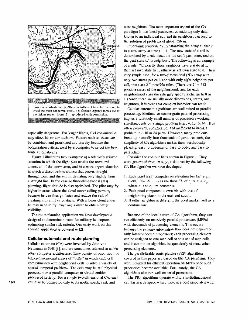
Two rescue situations: (a) There is sufficient time for tlie route to avoid the most dangerous areas, (b) Greater urgency forces use of the rislcier route. From [1], reproduced with permission.

especially dangerous. For longer flights, fuel consumption may affect his or her decision. Factors such as these can be combined and prioritized and thereby become the optimization criteria used by a computer to select the best route automatically.

Figure 1 illustrates two examples: a) a relatively relaxed situation in which the flight plan avoids the town and almost all of the storm area, and b) a more urgent situation in which a direct path is chosen that passes straight through town and the storm, deviating only slightly from a straight line. In the case of three-dimensional (3D) planning, flight altitude is also optimized. The pilot may fly higher in areas where the cloud cover ceiling permits, because he can thus go faster and reduce the risk of crashing into a hill or obstacle. With a lower cloud cover he may need to fly lower and slower to obtain better visibility.

The route-planning application we have developed is designed to determine a route for military helicopters optimizing similar risk criteria. Our early work on this specific application is covered in [2].

Cellular automata and route planning Cellular automata (CA) were invented by John von Neumann in 1948 [3], and are sometimes referred to as his other computer architecture. They consist of one-, two-, or higher-dimensional arrays of "cells" in which each cell communicates with neighboring cells to solve a variety of spatial-temporal problems. The cells may be real physical processors in a parallel computer or virtual entities processed serially. For a simple two-dimensional CA, each cell may be connected only to its north, south, east, and

west neighbors. The most important aspect of the CA paradigm is that local processes, considering only data known to an individual cell and its neighbors, can lead to the solution of problems of global extent.

Processing proceeds by transforming the array at time t to a new array at time t + I. The new state of a cell is determined by a rule based on the cell's past state, and on the past state of its neighbors. The following is an example of a rule: "If exactly three neighbors have a state of 1, then set own state to 1, otherwise set own state to 0." In a very simple case, for a two-dimensional (2D) array with only two states per cell, and with only eight neighbors per cell, there are 2 ' possible rules. (There are 2' = 512 possible states of the neighborhood, and for each neighborhood state the rule may specify a change to 0 or 1.) Since there are usually more dimensions, states, and neighbors, it is clear that complex behavior can result.

Cellular automata algorithms are well suited to parallel processing. Medium- or coarse-grain parallel processing implies a relatively small number of processors working simultaneously on a single problem (e.g., 4, 10, or 64). It is often awkward, complicated, and inefficient to break a problem into 10 or 64 parts. However, many problems break up naturally into thousands of parts. As such, the simplicify of CA algorithms makes them aesthetically pleasing, easy to understand, easy to code, and easy to parallelize.

Consider the contour lines shown in Figure 1. They were generated from an x, y, z data set by the following CA-like algorithm we have developed:

1. Each pixel (cell) computes its elevation bin EB (e.g., 0-99, 100-199, • • •) as the floor FLoic^ x z + c^, where Cj and Cj are constants.

2. Each pixel compares its own bin with that of neighboring pixels to the east and south.

3. If either neighbor is different, the pixel marks itself as a contour line.

Because of the local nature of CA algorithms, they can run efficiently on massively parallel processors (MPPs) with thousands of processing elements. This occurs because the primary information flow does not depend on fully interconnected processors; each processing element can be assigned to one map cell or to a set of map cells, and it can run an algorithm independently of most other processing elements.

The parallelizable route planner (PRP) algorithms covered in this paper are based on this CA paradigm. They were designed for efficient operation on MPPs once such processors became available. Fortunately, the CA algorithms also run well on serial processors.

The PRP algorithms operate within a multidimensional cellular search space where there is a cost associated with

p. N. STILES AND I. S. GLICKSTEIN IBM J. RES. DEVELOP. VOL. 38 NO. 2 MARCH 1994

travel through each cell. (A 2D cell is a small square area, a 3D cell is a small volume, and a 4D cell is a small volume at some instant in time.) This cost is a single positive integer that represents a nonlinear weighted combination of many different factors such as distance, fuel consumed, and risks encountered. The "best" route is defined to be the lowest-cost route, where the route cost is simply the summation of map costs for all cells traversed. The quality of the solution is determined by the accuracy with which the map costs model the real world and reflect the user's priorities and constraints.

On a relatively small 2D map that contains only 15 x 15 map cells, there are over eight billion distinct routes from one corner to the other (assuming a limitation that the motion is constrained to one of three directions—e.g., for the start location at the top left to a goal at bottom right, the motion would be limited to right, down, or right/down). A more realistic map with 1000 x 1000 cells and eight directions of travel therefore has an extremely large number of paths. Additionally, in 3D planning there are 26 possible directions. Better route-planning solutions are obtained when other factors such as time, speed, and fuel are considered. This paper primarily presents the 2D case, which is relatively easy to explain and conceptualize.

Parallelizable Route Planner (PRP) algorithms This section discusses the serial implementation of the PRP algorithms we have developed. The parallel implementation is discussed in the MPP implementation section. Parallelizable route-planner algorithms determine the lowest-cost path from point A (the start) to point B (the goal), using the stages 1) cost estimation, 2) ellipse or corridor constraints, 3) search, 4) digital indiscrimination.

• Cost estimation Cost estimation is a domain-dependent function that establishes the "cost" or grid value for each cell. For example, the cost to traverse a cell through the middle of a town might be ten times higher than the cost to traverse a cell outside the town. Taken together, the set of cost values are referred to as the map cost {MC) array. A significant amount of time and knowledge is required to develop an effective, relevant set of factors and their relative weightings.

• Ellipse or corridor constraints Ellipse or corridor constraints can be applied to the search to improve the processing performance and reduce memory requirements. An ellipse, with foci at the start and goal and a major axis of length d, applies when the path is constrained to be no greater than d. A corridor can be defined by a human user as a width along with a series of points marking the center of the corridor. A corridor

constraint can also be generated by an automated process such as the quadtree search described later.

• Search The optimizing search algorithm of the PRP has two elements: cost minimization and path generation. Cost minimization uses the map cost array as input and generates a best cost {BC) array as output. At completion of cost minimization, each cell in the BC array contains the cost of the cheapest path from that cell to the goal. Path generation uses the BC array as input and produces the optimal path coordinates from the start to the goal.

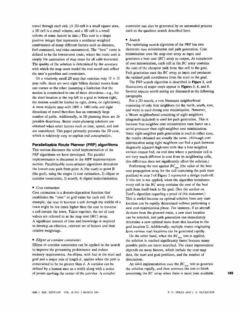
The PRP search algorithm is described in Figure 2, and illustrations of major steps appear in Figures 3, 4, and 5. Several aspects worth noting are discussed in the following paragraphs.

For a 2D search, a von Neumann neighborhood consisting of only four neighbors (to the north, south, east, and west) is used during cost minimization. However, a Moore neighborhood consisting of eight neighbors (diagonals included) is used for path generation. This is because four-neighbor cost minimization runs faster on a serial processor than eight-neighbor cost minimization. Since eight-neighbor path generation is used in either case, the results obtained are usually the same. (Although cost minimization using eight neighbors can find a path between diagonally adjacent high-cost cells that a four-neighbor version cannot find, on real data where a particular cell is not very much different in cost from its neighboring cells, this difference does not significantly affect the solution.)

Performing the test against 5Q^^, (the value of the best cost propagation array for the cell containing the path start position) in step 3 of Figure 2 represents a design trade-off. If this test is not applied, when the algorithm terminates every cell in the BC array contains the cost of the best path from itself back to the goal. (See the section on Ford's algorithm regarding a proof of this statement.) This is useful because an optimal solution from any start location can be rapidly determined without performing a new cost-minimization phase. For instance, if an aircraft deviates from the planned route, a new start location can be selected, and path generation can immediately determine a new optimal route from that location to the goal location G. Additionally, multiple routes originating from various start locations can be generated rapidly.

On the other hand, when the BC^^^^ test is applied, the solution is reached significantly faster because many possible paths are never searched. The exact improvement depends on many factors, which include the cost map data, the start and goal positions, and the number of dimensions.

An ideal implementation uses the BC^^^^ test to generate the solution rapidly, and then removes the test to finish processing the BC array when there is more time available. 169

IBM J. RES. DEVELOP. VOL. 38 NO. 2 MARCH 1994 P. N. STILES AND I. S. GLICKSTEIN

1. Initialization Set all BC,. = <» (maximum integer)

Except edge/ellipse/corridor map cells BC^ = 0 All MF. = false TODO list empty

2. Compute initial path from goal to start (Figure 3) If corridor mode, first path is corridor center; else straight line 5C , = 0 BC. along line = sum of map costs along line from goal to / MF. along line = true Each cell / along line added to TODO list

3. Cost minimization: loop until TODO list is empty (Figure 4) Select and remove top cell i from TODO list and set MF. = false For each neighbor; of i (four neighbors for 2D)

cost = BC. + MC. if cost < BCj and cost < BC^^

BCj = cost iijifF. = false add; to TODO list and set MF. = true

4. Path generation (Figure 5) Set BCi = 00 for edge/ellipse/corridor cells First path cell = start cell Loop until goal reached

Examine BC value of each nearest neighbor (eight neighbors for 2D) Select next path cell as cell with lowest BC value

Notation BC. is the ith element of best-cost propagation anay BC (e.g., BC^^ = value

of BC at the path start position). MC. is the ith element of map-cost array MC. MF. is the ith element of mail-flag array MF, which indicates that a cell is on the TODO list.

TODO list is a Ust of cells that can potential^ update their neighbors.

PRP scdivh digoiithm i2L> SOILII impleiTiLMitiiliiin)

170

The BC array is originally initialized to oo (maximum integer). Under some circumstances it does not require complete reinitialization, and the processing will then converge sooner. For example, if map costs are reduced, the BC array can be left unaltered. The cells that had their map costs changed must be added to the TODO list and have their mail flags set. Then the algorithm begins at step 3 shown in Figure 2 and will run to completion faster than

if the BC array had been fully reinitialized. (Unfortunately, the same is not true when the map costs increase. In that case, the BC array must be fully reinitialized.)

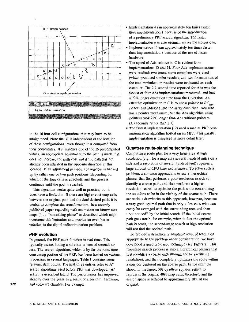
• Digital indiscrimination When regions of map costs are equal, a grid-based algorithm is incapable of recognizing the difference between any two paths of the type shown in Figure 6.

p. N. STILES AND I. S. GLICKSTEIN raM J. RES. DEVELOP. VOL. 38 NO. 2 MARCH 1994

1 ,•••••

,.••••' C50

1 , . - '

.•• •' o o

1 0 4

1 / '

, ••• O O

1 / ' '

/ oo

1 ...•••'

,••• o o

1 /

, • o o

1 ,.••••

, • • • • 1 0 3

100,." '

,••'' ° °

1 ,.••••'

1 .•••••'

,••••' o o :

1 0 O / - • '

,•••'• O O

1 ,•••'

, - • • • 1 0 2

1 0 0 ,.••••'

,.-•'" O O

1 ,.-•'•'

,.••'• o o

1.••••' '

/ 0 0

10Q/-'''

,•••'' o o

J/ /101

,••••• o o

I,---'" ,.•••• o o

1 ,•••••'

_,••••' o o

loq..--:'"' ,•••••' o o

loo-/'''

y - " ' 1 0 0

1 0 0 ,.•••''

/'"' oo

1 / _,••••'' o o

1 .y ,••••'" ' O O

1 /'' ./ oo

1 G 0

1 y ,.•••'' o o

1 _/

,••••' c x )

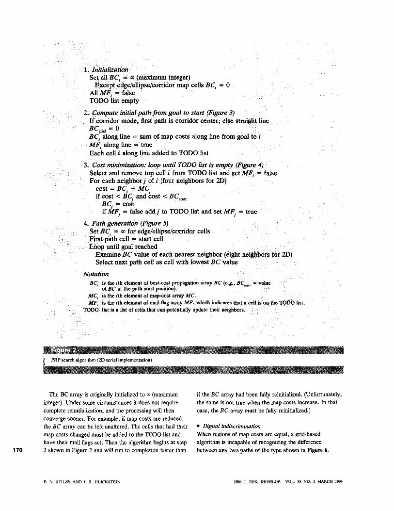
Figure 3 Initialized, and straight-line path computed. The map-cost array values (AfC() are indicated by the upper left number in each cell; most cells cost 1, but there is a u-shaped high-cost region where cells cost 100. Best-cost values (BC) am indicated by the lower right number in each cell; all are set very large except along a line from start to goal. BC^^^ = 104. As indicated by checkmarks, six cells ate on the TODO list.

y^'^m^^^M^^^:^-

They both "cost" the same amount, but there may still be reasons to prefer one over the others. Sometimes these equally low-cost paths are designated as geodesies. As shown in the example, the path that more closely approximates a straight line between start and goal is often better than other equal-cost paths. This is because when this route is traversed, algorithms (such as an aircraft guidance algorithm) can remove the stair-stepping and thus reduce the distance and maneuvering required to follow the route. Improving the resolution to any arbitrary level of detail does not help differentiate the paths, nor does the use of alternate grids such as a hexagonal grid.

We have developed a solution to the digital indiscrimination problem based on the idea of straightening small portions of the path to transform a potentially less desirable path into a more desirable path. The method is to identify four-cell confiprations and adjust them to a straighter configuration when doing so does not increase the cost of the optimal path. One such four-cell configuration is identified in Figure 6 by the cells labeled 1 through 4. The path is adjusted to go through the cell above cell 2, rather than through cell 2. The algorithm proceeds by sliding a four-cell window along the original path from start to goal. A weighted geometric function F is computed using the x and y coordinates of the four cells in the window:

1 ,.•••••'

,.•-•• o o

1 ,.•••••'

.• • ' 0 0

1 0 4

1 ..••••'

, •• O O

1 ,.•••••'

, • • ' o o

1 ,.•••'•'

, .•• ' o o

1 ,••••••

,•••' 0 0

1 ,••••

..••'io3

100 , . • • • • • '

,.•••• o o

1 ,.-•'' ,•••'' 0 0

1 ,.•••••

..•-••' o o

lop,.-'' ,.•••' 0 0

1 ,•••' ,-i '02

1 0 0 ,.••••'

,.•••• 0 0

1 ,•••••'

,-•••'' 0 0

! , . • • • • '

..••••• 0 0

lOQ.-''

/ ' 0 0

1 ,•••••

..-••••'101

loq..---''' / oo

,-•••' 0 0

1 .••••••'"

,.••••' 0 0 ^

lOO..--'

..••••' o o

looy ''

..•••loo

1 0 0 ..•••••'

,••••' o o

1 / • •

,.•••' o o

1 ,-••••''

,.••••'' 0 0

,.••••' 1

1 G 0

. V ,.-•••• 1

1 ,.••••'

/ • ' o o

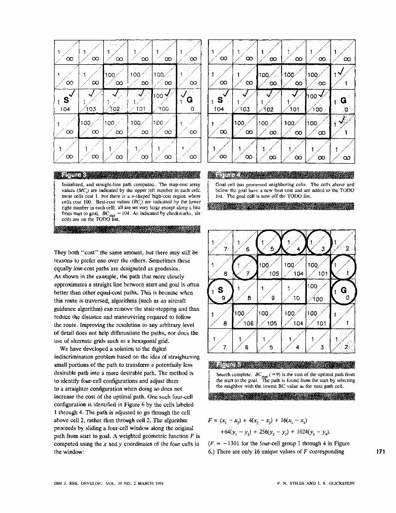
j Goal cell has processed neighboring cells. The cells above and I below the goal have a new best cost and are added to the TODO I list. The goal cell is now off the TODO list.

I Search complete. flCj^^, ( = 9) is the cost of the optimal path from I the start to the goal. "ITie path is found firom the start by selecting , the neighbor with the lowest BC value as the next path cell.

F = (x^ - Xj) + 4(^2 - Xj) + 16( :3 - x^}

+64(y, - y,) + 2S6(y, ~ y,) + 1024{> 3 - y^.

(F = -1301 for the four-cell group 1 through 4 in Figure 6.) There are only 16 unique values off corresponding 171

IBM J. RES. DEVELOP. VOL. 38 NO. 2 MARCH 1994 P. N. STILES AND I. S. GUCKSTEIN

X = Desired solution

\

s-X

0 0 0

x

0

\ \

0

V H

x

'o ")

y

<

\

A X

^0

0

G1

«

/ O = Another equal-cost solution

DI' . ' I IJ I iriJ]M.Min]n iiinn

172

to the 16 four-cell configurations that may have to be straightened. Note that F is independent of the location of these configurations, even though it is computed from their coordinates. If F matches one of the 16 precomputed values, an appropriate adjustment to the path is made if it does not increase the path cost and if the path has not already been adjusted in the opposite direction at this location. If an adjustment is made, the window is backed up by either one or two path positions (depending on which of the four cells is affected), and the process continues until the goal is reached.

This algorithm works quite well in practice, but it does have a limitation. If there are higher-cost map cells between the original path and the final desired path, it is unable to complete the transformation. In a recently published paper regarding path estimation on binary cost maps [4], a "smoothing phase" is described which might overcome this limitation and provide an even better solution to the digital indiscrimination problem.

PRP evolution In general, the PRP must function in real time. This typically means finding a solution in tens of seconds or less. The search algorithm, which is by far the most time-consuming portion of the PRP, has been hosted on various processors in several languages. Table 1 contains some relevant data points. The first three entries refer to A* search algorithms used before PRP was developed. (A* search is described later.) The performance has improved steadily over the years as a result of algorithm, hardware, and software changes. For example,

• Implementation 4 ran approximately ten times faster than implementation 1 because of the introduction of a preliminary PRP search algorithm. The faster implementation was also optimal, unlike the slower one.

• Implementation 11 ran approximately ten times faster than implementation 8 because of the use of faster hardware.

• The speed of Ada relative to C is evident from implementations 13 and 14. Four Ada implementations were studied: two brand-name compilers were used (which produced similar results), and two formulations of the cost-minimization routine were evaluated on each compiler. The 2.7-second time reported for Ada was the fastest of four Ada implementations measured, and had a 70% longer execution time than the C version. An effective optimization in C is to use a pointer to BC^^^, rather than indexing into the array each time. Ada also has a pointer mechanism, but the Ada algorithm using pointers took 22% longer than Ada without pointers (3.3 seconds rather than 2.7).

• The fastest implementation (12) used a mature PRP cost-minimization algorithm hosted on an MPP. This parallel implementation is discussed in more detail later.

Quadtree route-planning technique Computing a route plan for a very large area at high resolution (e.g., for a map area several hundred miles on a side and a resolution of several hundred feet) requires a large amount of CPU time and memory. To solve such a problem, a common approach is to use a hierarchical planner that first performs a poor-resolution search to identify a coarse path, and then performs a higher-resolution search to optimize the path while constraining the solutions to be in the vicinity of the coarse path. There are serious drawbacks to this approach, however, because a very good optimal path that is only a few cells wide can easily be averaged with the surrounding area and then "not noticed" by the initial search. If the initial coarse path goes north, for example, when in fact the optimal path is south, the second-stage search at high resolution will not find the optimal path.

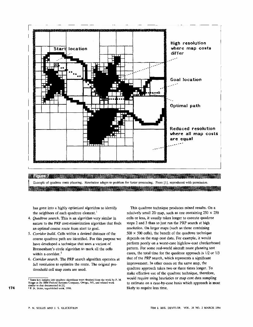
To provide a dynamically adaptable level of resolution appropriate to the problem under consideration, we have developed a quadtree-based technique (see Figure 7). This two-stage search process is also a hierarchical planner that first identifies a coarse path (though not by sacrificing resolution), and then completely optimizes the route within a corridor centered on the coarse path. In the example shown in the figure, 502 quadtree squares suffice to represent the original 4096 map cells; therefore, and the search space is reduced to approximately 10% of the original.

p . N. STILES AND I. S. GLICKSTEIN IBM J. RES. DEVELOP. VOL. 38 NO. 2 MARCH 1994

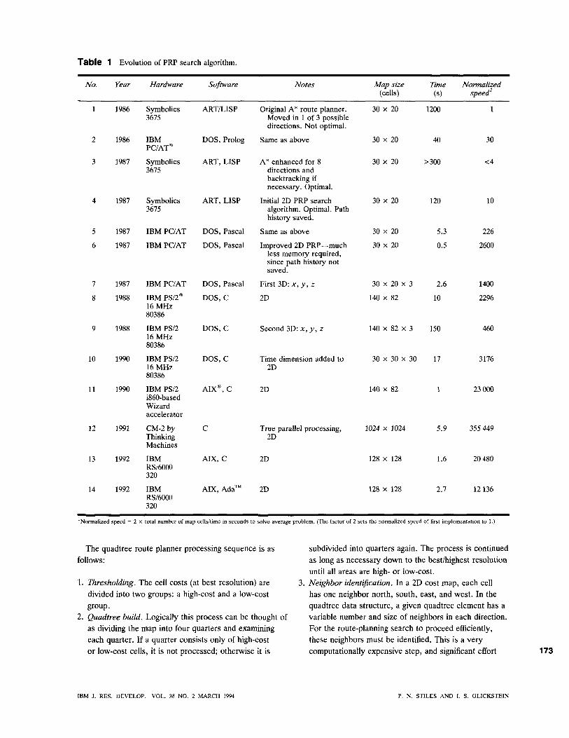
Table 1 Evolution of PRP search algorithm.

No. Year Hardware Software Notes Map size Time Normalized (cells) (s) speed'

1 1986 Symbolics ART/LISP Original A* route planner. 30 x 20 3675

1986 IBM PC/AT®

Moved in 1 of 3 possible directions. Not optimal.

DOS, Prolog Same as above

3 1987 Symbolics ART, LISP A* enhanced for 8 3675 directions and

backtracking if necessary. Optimal.

4 1987 Symbolics ART, LISP Initial 2D PRP search 3675 algorithm. Optimal. Path

history saved.

5 1987 IBM PC/AT DOS, Pascal Same as above

6 1987 IBM PC/AT DOS, Pascal Improved 2D PRP—much less memory required, since path history not saved.

7 1987 IBM PC/AT DOS, Pascal First 3D: x, y, z

8 1988 IBM PS/2* DOS, C 2D 16 MHz 80386

9 1988 IBM PS/2 DOS, C 16 MHz 80386

10 1990 IBM PS/2 DOS, C 16 MHz 80386

11 1990 IBM PS/2 AIX®, C i860-based Wizard accelerator

12 1991 CM-2by C Thinking Machines

13 1992 IBM RS/6000 320

14 1992 IBM RS/6000 320

Second 3D: x, y, z

Time dimension added to 2D

2D

AIX, C

AIX, Ada" '

2D

2D

30 X 20

30 X 20

30 X 20

30 X 20

30 X 20

1200

40

>300

120

140 X 82

True parallel processing, 1024 x 1024 2D

128 X 128

128 X 128

5.3

0.5

30 X 20 X 3 2.6

140 X 82 10

140 X 82 X 3 150

30 X 30 X 30 17

30

<4

10

226

2600

1400

2296

460

3176

23 000

5.9 355 449

1.6

2.7

20 480

12136

Normalized speed = 2 x total number of map cells/time in seconds to solve average problem. (The factor of 2 sets the normalized speed of first implementation to 1.)

The quadtree route planner processing sequence is as follows:

1. Thresholding. The cell costs (at best resolution) are divided into two groups: a high-cost and a low-cost group.

2. Quadtree build. Logically this process can be thought of as dividing the map into four quarters and examining each quarter. If a quarter consists only of high-cost or low-cost cells, it is not processed; otherwise it is

subdivided into quarters again. The process is continued as long as necessary down to the best/highest resolution until all areas are high- or low-cost.

3. Neighbor identification. In a 2D cost map, each cell has one neighbor north, south, east, and west. In the quadtree data structure, a given quadtree element has a variable number and size of neighbors in each direction. For the route-planning search to proceed efficiently, these neighbors must be identified. This is a very computationally expensive step, and significant effort 173

IBM J, RES. DEVELOP. VOL. 38 NO. 2 MARCH 1994 P. N. STILES AND I. S, GLICKSTEIN

Star t location

^ • H H ^ ^

1 • • • • • l

U m • • • •

•

•

1 1

. 1 • • •

> • • •

• « litt

a

•

• • • • •

aaaa a a a a a

aa

• • • • aa • aa a a a a

a a

•s 7) a • D D D

• •

• • . . .

•••aa

a a a •

a a

H •. .• •

aa aa

aa

• a I S « i

• - " ' '

..-

• 1 1

• • l i (aa ia

High resolution where map costs differ

Goal location

Optimal path

Reduced resolution where all map costs are equal

Example of quadtree route planning. Resolution adapts to problem for faster processing. From [1], reproduced with permission

has gone into a highly optimized algorithm to identify the neighbors of each quadtree element.*

4. Quadtree search. This is an algorithm very similar in nature to the PRP cost-minimization algorithm that finds an optimal coarse route from start to goal.

5. Corridor build. Cells within a desired distance of the coarse quadtree path are identified. For this purpose we have developed a technique that uses a variant of Bressenham's circle algorithm to mark all the cells within a corridor.^

6. Corridor search. The PRP search algorithm operates at full resolution to optimize the route. The original pre-threshold cell map costs are used.

174

' Some key insights into quatJtree algorithms were obtained from the work by P. M. Kogge at the IBM Federal Systems Company, Owego, NY, and related work similar to that documented in [5]. 2 P. N. Stiles, unpublished work, 1990.

This quadtree technique produces mixed results. On a relatively small 2D map, such as one containing 250 x 250 cells or less, it usually takes longer to execute quadtree steps 2 and 3 than to just run the PRP search at high resolution. On larger maps (such as those containing 500 X 500 cells), the benefit of the quadtree technique depends on the map cost data. For example, it would perform poorly on a worst-case high/low-cost checkerboard pattern. For some real-world aircraft route planning test cases, the total time for the quadtree approach is 1/2 or 1/3 that of the PRP search, which represents a significant improvement. In other cases on the same map, the quadtree approach takes two or three times longer. To make effective use of the quadtree technique, therefore, would require using heuristics or map cost data sampling to estimate on a case-by-case basis which approach is most likely to require less time.

p. N. STILES AND I. S, GLICKSTEIN IBM J. RES. DEVELOP. VOL. 38 NO. 2 MARCH 1994

Comparison with ottier aigorithms Many search and optimization techniques can be apphed to the route-planning problem. Some are quite similar to the search algorithm of the PRP, while others are entirely different. This section primarily discusses alternative techniques that include a spectrum of interesting, efficient, or widely used algorithms. Some experienced readers may find little to recommend some of these techniques for the route-planning problem—^particularly simulated annealing and genetic algorithms. They are included here, however, because we devoted a considerable amount of time to investigating the use of these techniques, and would like to point others in potentially more useful directions.

• Dynamic programming In [6], the following graph notation is introduced:

3

1

120

100

80

60

40

20

n

1

Curve of 0(n'*) /

/

/

/ Curve of 0(n) ,* ,-*

,''' __j.-''^^^^Measured —_-SX^---:ZZ^^^^—B— performance

50 100 150 200 250 300 350 400

Map cells along one axis (n)

• A graph G(F, E) is a structure which consists of a set of vertices V = {p^, v^, • • •} and a set of edges E = {Cj, Cj, • • •}; each edge e is incident to the elements of an unordered pair of vertices {«, v).

• /(e) is the length of edge e. • A(v) is the label of a vertex v assigned by a shortest-path

algorithm. • r is a set of temporarily assigned vertices. • 5 is the start vertex. • g is the goal vertex.'

For the route-planning problem under consideration, the graph is assumed to be finite and undirected, and all edges are assumed to be of nonnegative length.

Dynamic programming, as typified by Dijkstra's shortest-path algorithm, is similar to the PRP search algorithm. Dijkstra's shortest-path algorithm is expressed in [6] as

1. K(s) *- 0 and for all v -^ s, k{v) <- oo. l.T-^V. 3. Let M be a vertex in T for which A(M) is minimum. 4. If M = g, stop. 5. For every edge u ^' v,\iv ET and \{v) > X(u) +

lie), then \{v) •*- A(«) + 1(e). 6. r «- r - {M} and go to step 3.

With a little thought, it is clear that this algorithm will determine an optimal path, because the search proceeds by expanding the lowest-cost vertices first, and optimal wavefronts are generated that work their way out through the search space; an optimal decision at each step produces a globally optimal solution. Unlike the PRP search algorithm, with which each map cell (vertex) may

3 In [6] use is made of s and / to represent the start and goal vertices, respectively; here they are designated as s and g.

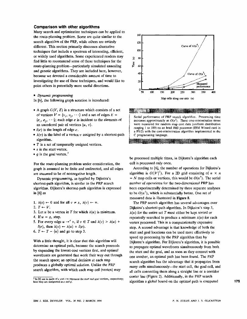
Serial performance of PRP search algorithm. Processing time increases approximately as 0(«'). These cost-minimization times were measured for random map cost data (uniform distribution ranging 1 to 100) on an Intel i860 processor (IBM Wizard card in a PS/2) with the cost-minimization algorithm implemented in the C programming language.

be processed multiple times, in Dijkstra's algorithm each cell is processed only once.

According to [6], the number of operations for Dijkstra's algorithm is 0(|K|^). For a 2D grid consisting of w x n = N map cells or vertices, this would be 0{n*). The serial number of operations for the two-dimensional PRP has been experimentally determined by three separate analyses to be O(n'), which is substantially better. One set of measured data is illustrated in Figure 8.

The PRP search algorithm has several advantages over Dijkstra's shortest-path algorithm. In Dijkstra's step 3, A(M) for the entire set T must either be kept sorted or repeatedly searched to produce a minimum A(M) for each vertex processed. This is a computationally expensive step. A second advantage is that knowledge of both the start and goal locations can be used more effectively to speed up processing by the PRP algorithm than by Dijkstra's algorithm. For Dijkstra's algorithm, it is possible to propagate optimal wavefronts simultaneously from both the start and the goal, and as soon as they connect with one another, an optimal path has been found. The PRP search algorithm has the advantage that it propagates from many cells simultaneously—the start cell, the goal cell, and all cells connecting them along a straight line or a corridor center line (Figure 2). Additionally, in the PRP search algorithm a global bound on the optimal path is computed 175

IBM J. RES. DEVELOP. VOL. 38 NO. 2 MARCH 1994 P. N. STILES AND I. S. GLICKSTEIN

176

at the beginning and applied to limit the search on an ongoing basis; there is no obvious way to make this improvement to Dijkstra's algorithm.

We have implemented Dijkstra's algorithm, and in real-world test cases the PRP search algorithm ran 20 to 25 times faster. For unusual data sets where the optimal path is very complex, such as a spiral maze, Dijkstra's algorithm can be faster. A related characteristic of the PRP search algorithm is that the processing time is highly dependent on the data.

The PRP search algorithm also exhibits a useful "best-so-far" characteristic not shared by Dijkstra's shortest-path algorithm. It begins with a straight-line path from start to goal and therefore has a solution available immediately. As time proceeds, better and better solutions become available until inally, at termination, the globally optimal solution is produced. If processing must be terminated early to meet a real-time deadline, path generation can be executed at any time to generate the best path discovered at that point in time.

With regard to implementation on an MPP, the minimum A(u) step in Dijkstra's algorithm presents a very serious disadvantage. For the algorithm to proceed, all of the labels A{M) must be compared against one another, or kept in a sorted list, in order for the minimum choice to be processed next. With 1000 or 10 000 processors in the MPP, this becomes an untenable communications or shared-memory problem. In contrast, the local and potentially random processing nature of vertices in the PRP search algorithm permits multiple processors to proceed independently of one another as long as they can share information about the cells on the edge of the area they are each processing (i.e., if processor i operates on a square area of map, and processor j operates on an adjacent square area, they must both be able to access a single common column of map-cost and best-cost array values where they Join).

• Ford's algorithm In [6], Ford's shortest-path algorithm, which finds the distance of all the vertices from a given vertex s, is characterized as

1. A(s) «- 0 and for every v -^ s, k{v) «- ». 2. As long as there is an edge u ^^ v such that A(ii) >

k{u) -f- /(e), replace \{v) with A(M) + /(e).

This 35-year-old algorithm was noticed and pointed out to the authors several years after the PRP search algorithm was developed. It is a concise generalized expression of the cost-minimization element of the PRP search algorithm and captures the most crucial, unique, and unintuitive aspect of this algorithm—that even though the vertices can be processed in any order (even random), the algorithm

will indeed terminate having produced the lowest-cost distance from every vertex to the start (or goal) vertex. (A proof of this statement is provided in [6].) The path can be generated directly from \{v) without having saved any other information during the search. This was a pleasant and unexpected realization during development of the PRP, because earlier efforts had stored path history in memory or left pointers for path generation. (The path-generation phase is not discussed in [6].) Ford's algorithm is shown to be 0(|£| |F|), and as is the case with Dijkstra's algorithm, this is equivalent to 0{N^) or 0(«*) for a 2D grid.

There are many ways to implement Ford's statement "as long as there is an edge." The technique developed for the PRP and presented in Figure 2 performed significantly faster than earlier approaches utilizing geometric sweeps to iteratively process the vertices. The current PRP method initially focuses processing along the straight line which connects the start and the goal, and thereafter processes changed cells on a first-come, first-served basis.

As indicated previously, the PRP cost-minimization algorithm takes advantage of the knowledge of both endpoints (start and goal) rather than just the one used in Ford's algorithm, producing a much faster solution.

* A* search The term A* designates an optimal best-first search technique that, like Dijkstra's shortest-path algorithm, is used quite extensively. (Two examples may be found in [7] and [8].) The A* algorithm explores the search space by computing a cost function for each possible next position, and then selecting the lowest-cost position to add to the path and from which to generate more possible positions. All paths in the search space are explicitly represented using pointers from each position back to the previous position from which it was derived.

The cost function is

c, - ac., -I- ec, .B '

where ac is the actual cost from start to an intermediate position /, and ec^^ is the estimated cost from / to the goal. If the actual cost from position / to the goal is greater than or equal to the estimate (ec.J of this cost, the solution is guaranteed to be optimal. The accuracy of the estimate will affect the speed of the solution and the amount of memory needed.

Having implemented several versions of A*, and having witnessed the performance of other implementations, we have found that this algorithm is generally unsatisfactory for route planning because the time and/or memory requirements are often excessive. One reason for this is the explicit path representation. Another is evident in a situation such as when the goal is surrounded by a high-

P. N. STILES AND 1, S. OLICKSTEIN IBM 3. RES. DEVELOP. VOL. 38 NO. 2 MARCH 1994

cost region. In this case the algorithm expands the search space almost everywhere else first, and eventually consumes all available memory.

However, an advantage of the explicit path representation of A* is that the algorithm can readily factor in constraints that are dependent on the path encountered thus far. For example, the cost associated with traversing three connected cells may be higher than the cost of traversing the same three cells spread out across the map (e.g., a pilot encountering three separate ten-second episodes of lost visibility may have a safer route than one with a single thirty-second loss).

We have developed a modified version of A* (not necessarily optimal, but faster) to impose aircraft turn-rate limiting constraints." This algorithm can replace the path-generation element of the PRP search algorithm. It executes after PRP cost minimization and uses the best cost value at each cell as a very good lower bound estimate ec.^. Though it often performs quite well, it is not entirely reliable, since in some cases it runs out of memory for reasons already discussed.

For an MPP implementation, A* has the same disadvantage as Dijkstra's algorithm—a global collection of possible next positions must be available to all processors so that the best (lowest-cost) can be expanded for the next stage.

* Potential field methods Another route-planning technique utilizes artificial potential fields that "repel" the path from obstacles and high-cost regions, and "attract" the path to the goal and to desirable regions [9]. The potential field affects the entire path simultaneously (not just one position), and uses optimization techniques to alter the path so that it passes through an accumulated minimum potential. In contrast to the previous algorithms discussed, this technique does not guarantee an optimal global solution upon algorithm termination. Although various methods are used to reduce this problem, the solution may be trapped in a local field minimum. (Local minima may also cause difficulties for several of the algorithms discussed subsequently. An example would be a northern route that passes through a low-cost valley in a high-cost region. The optimal route may be farther south, but the solution can converge to the northern route, having gotten "stuck" in the low-cost valley. This happens because most routes near the northern route are poorer, and the algorithm can accept a locally optimal solution even though it is not globally optimal.) In some applications this may be an acceptable trade-off, since this technique is purported to be much faster than more thorough graph-searching algorithms.

* p. N. Stiles, unpublished work, 1990.

% Simulated annealing Simulated annealing [10,11] is a relatively general optimization technique that can be parallelized and applied to problems with a complex search space to provide an approximate, though not necessarily optimal, solution. Simulated annealing seeks to minimize an objective function (e.g., path cost) by utilizing stochastic processes. It selects a feasible initial solution and then iteratively 1) produces random perturbations of the previous solution to generate a new possible solution, and 2) decides whether or not to accept the new solution. The new solution is always accepted if it is better than the previous solution, and it is sometimes accepted if it is worse. A "temperature" value is initially set high and is decreased at each iteration. If the new solution is worse, it is accepted with probability e^'^^''', where A£ = E^^ -previous' new ^ ^^^ valuc of the objcctivc function for the

new solution (for example, the cost of traversing a path described by the current route solution) and E . is

•^ ' previous

the value of the objective function for the previous solution.

The authors are not familiar with any papers specifically detailing the use and results of simulated annealing for route planning, although it has been suggested for such use. The nature of the route-planning search space is such that small perturbations of the path produce very different solution costs, which again leads to problems with local minima. For a search space with this characteristic, a simulated annealing algorithm would have difficulty converging to a good solution.

Unlike the PRP search algorithm, which focuses processing along the straight-Une path between start and goal and then only to map cells that have changed, simulated annealing is essentially a random undirected process, and is even likely to waste processing by repeatedly exploring the same solutions.

For applications that are so large they are computationally intractable for an optimal search strategy like that of the PRP search algorithm, simulated annealing may be a good alternative. Otherwise, it appears to be less well suited than some of the other alternatives discussed.

* Genetic algorithms Genetic algorithm (GA) search is a very intriguing idea that was invented by John Holland in 1975 and is thoroughly explored in [12] by Goldberg. He classifies traditional search algorithms as

% Calculus-based: gradient or hill-climbing search algorithms.

% Enumerative: dynamic programming (and the PRP search algorithm).

% Random: simulated annealing. 177

B M J. RES. DEVELOP. VOL. 38 NO. 2 MARCH 1994 P. N. STILES AND I. S. GLICKSTEIN

178

Holland states that a unique strength of genetic algorithms is that there is a structured, yet randomized, information exchange. Genetic algorithm search applies to large, complex problems that cannot be solved by enumerative methods, and situations in which any good solution, as opposed to the best solution, will suffice. It also applies to complex search spaces that would violate continuity or derivative constraints usually imposed by calculus-based algorithms. Since the route-planning problem search space can be highly nonlinear, such calculus-based search techniques are seldom, if ever, attempted.

The GA algorithms use search strings that are coded solutions. For route planning, a string could represent a path from A to B. A population of many simultaneous search strings is used, and since they are modeled after biological evolution, they evolve over time in such a way that the "fittest" tend to survive. (A low-cost path is more fit to survive than a high-cost path.) Three primary operators used are reproduction, crossover, and mutation. Reproduction selects pairs of search strings that will survive into the next generation after undergoing crossover. It favors those with the best "payoff' (lowest cost), but even low-payoif strings can survive with some probability. This process tends to keep the best substrings in the search population. For route planning, the substrings could be path segments. Crossover operates on each pair of strings selected by reproduction and exchanges randomly selected substrinp between them. Mutation guards against premature loss of good substrings by occasionally generating new substrings that are patched into the search strings or replace existing portions.

We have spent considerable time developing a genetic algorithm route planner, but results to date have been very disappointing. The paths tend to become complex and loop back on themselves, and the search population often converges to a ptxjr solution even when a good solution is close by. Perhaps with more effort a method could be found to constrain the crossover process so that loops would not form; and perhaps with better mutation or a different algorithm formulation the search would usually converge to a good solution. However, Goldberg admits that genetic algorithms do not work well on a problem with a "deceptive needle-in-haystack" search space—where the best solution is surrounded by bad solutions. As explained above, the route-planning problem under investigation often has this property.

% Neural networks Huse has presented a locally connected, fixed-weight neural network paradigm [13] that finds "optimal/ near-optimal" paths. The world is represented by a grid, and each {x, y) location is represented by a unique node

of the neural network. Interconnection weights are fixed values ranging from zero to less than one, and are based upon the ease of movement from one neuron to its respective north, south, east, and west neighbors (e.g., a good road = 0.9 and a lake = 0). The output value of the goal node is initialized and maintained at IttX). The outputs of nodes with connection weight = 0 are initialized to 0. The outputs of all other neurons are initialized to 1. For the processing stage, the output value of each neuron is updated as follows:

Neuron output •- max(Nj.N„, S S , E^E„, W^W ),

where N = north, S = south, E = east, W = west, c = connection weight, and o = output value.

All of the neurons are updated simultaneously in this manner until the output levels are stable. Then, beginning at the start, the path is selected by choosing the highest neighboring node for the next position. This algorithm is essentially the same as a parallel implementation of Ford's algorithm and also the NASA invention discussed below. Unlike the PRP search algorithm, it does not make use of the speedup possible by knowledge of both the start and goal.

Huse also states that the solution is not optimal because there can be competing nodes with the same output value, in which case the path selection is purely arbitrary. This is the digital indiscrimination problem, and no solution is offered in [13].

Another neural network implementation has been presented by Welker and Barhorst [14]. Constraint-satisfaction neural networks were investigated. Of the three types of models analyzed, a Boltzmann machine model worked the best. This Boltzmann machine neural network technique is very similar in nature to simulated annealing; most of the comments in that section (e.g., the tendency to become trapped in a local energy minimum) are applicable here. Additionally, the functional operation of the algorithm depends on some simplifying assumptions that would probably be violated in a real-world application. For example, since the path must flow continuously in one direction from start to goal, a path which temporarily heads in the wrong direction to avoid a high-cost region is not permitted.

% Dedicated hardware A unique and interesting approach to the route-planning problem has been presented by Carroll [15]. He has described an integrated circuit designed in the late 1970s that used a fine-grained parallel processor architecture to perform the computationally expensive portion of a maze-solving algorithm. Travel through the maze in different directions is represented by continuously variable weights incorporated as analog parameters affecting interprocessor communication of digital data. Using analog VLSI, the

p. N. STILES AND I. S. OLICKSTEIN IBM J. RES. DEVELOP. VOL. 38 NO. 2 MARCH 1994

traversal cost is represented via capacitance discharge rates that directly/physically control the speed of wavefront propagation firom cell to cell. The first path to reach the goal in real time is thus the lowest-cost path.

Unlike many maze-solving algorithms that incorporate only binary traversal costs, this circuit has at least three different traversal costs: low, medium, and high. The dynamic range required for the map costs depends on the application. If the route planner is used for robot obstacle avoidance where a cell is either occupied or empty, a one-bit dynamic range may suffice. H the route planner primarily optimizes fuel consumption but also avoids very high-cost regions, a much larger dynamic range may be necessary. The PRP route planner uses a 16-bit integer for the map cost value that provides a fairly good dynamic range. Some map regions can be "really bad" (e.g., 1000 times worse than normal), yet if the path is forced to go through them, the smaller variations in map cost are still factored into the solution.

A NASA technical brief [16] describes a patent application for a "Processor [that] Would Find Best Paths on Map." This invention is essentially a hardware implementation of Ford's shortest-path algorithm. A cost would be assigned to each map cell, and each cell would be represented by a microprocessor (which could be analog or partly analog.) The cost could be stored as the voltage on a capacitor. One microprocessor would be designated as the start (or goal), and would send out a constant maximum signal to its nearest neighbors. Each other processor would take whichever of the signals from its nearest neighbors was the maximum one, scale it down according to the cost assigned to that map cell, and transmit the resulting signal to its nearest neighbors.

Additionally, several companies (including Lockheed/Sanders and FMC) have built dedicated hardware route planners. From the limited information available, they appear to be custom-desiped accelerators used to solve dynamic programming algorithms.

Though some of these hardware approaches are certainly interesting and clever, it is probably not practical or affordable in most cases to desip and build a piece of dedicated hardware to solve a single type of problem, especially if a generic MPP algorithm can do the job just as well.

Massively parallel processor (MPP) implementation The cellular automata concept has been discussed (in the section following the Introduction) and a rationale has been provided indicating that it is very well suited to fine-grain parallel processor implementation. For route planning, if each map cell had its own processor, the PRP cost-minimization step could be simply

lOOp

10

1 :

0.1

0.01

«=256.A'=65536

' I ' I I • I n lull 10 100 1000

M ^ cells alofl one axis («)

, . , . . . ; ^ :•,•=.

10 000

•::<:?^;-v:.v-

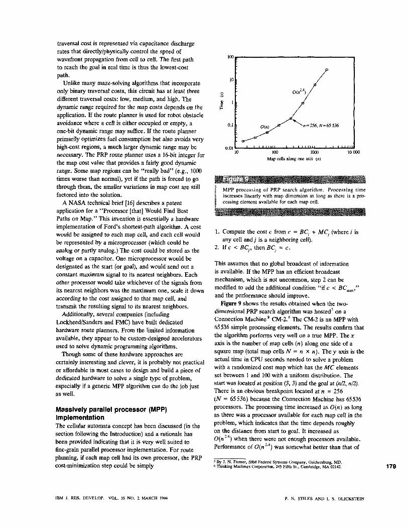
MPP processing of PRP search algorithm. Processing time increases linearly with map dimension as long as there is a pro-cessing element available for each map cell.

1. Compute the cost c from c = J9C, -l- MCj (where i is any cell and/ is a neighboring cell).

2. Ifc < JSC. thenflC = c.

This assumes that no global broadcast of information is available. If the MPP has an efficient broadcast mechanism, which is not uncommon, step 2 can be modified to add the additional condition "if c < BC. .,"

start'

and the performance should improve. Figure 9 shows the results obtained when the two-

dimensional PRP search algorithm was hosted' on a Connection Machine* CM-2.' The CM-2 is an MPP with 65536 simple processing elements. The results confirm that the algorithm performs very well on a true MPP. The x axis is the number of map cells (n) along one side of a square map (total map cells N = n x n). They axis is the actual time in CPU seconds needed to solve a problem with a randomized cost map which has the MC elements set between 1 and 100 with a uniform distribution. The start was located at position (3, 3) and the goal at (n/2, nff). There is an obvious breakpoint located at rt = 256 (N = 65536) because the Connection Machine has 65536 processors. The processing time increased as 0{n) as long as there was a processor available for each map cell in the problem, which indicates that the time depends roughly on the distance from start to goal. It increased as 0{n ^") when there were not enough processors available. Performance of 0(n^'*) was somewhat better than that of

' By J. N. Femer, IBM Federal Systems Company, Gaithersburg, MD. <• Thinking Machines Corporation, 245 Fiftli St., Cambridge, MA 02142. 179

mM J. RES. DEVEIXJP. VOL. 38 NO. 2 MARCH 1994 P. N. STILES AND I. S. GLICKSTEIN

the serial algorithm, which increases as 0{n ) because the number of processors on the MPP constitutes a large portion of the number of map cells.

An interesting observation was made pertaining to the number of neighbors processed. In the serial PRP implementation, the cost minimization runs significantly faster if four neighbors are considered rather than eight. On the Connection Machine, better performance was obtained when cost minimization considered eight neighbors. This is because, using such a machine, the information spreads out faster and causes idle processors to function sooner. For the same reason, the initialization step that immediately sets a path from start to goal also improves processor efficiency. Other optimizations are possible on the MPP, such as initializing all map cells with a simple Manhattan distance path.

Equally promising parallel speedup results were obtained in a small study' that hosted the PRP search algorithm on a simulator for a new MPP computer (designated as Execube) being developed at IBM Owego.

Extensions and related applications Current work in the area of route planning is primarily focused on explicitly including time and speed in the optimization. The route planner described here assumed a fixed-cost map for the duration of the problem. But what if the storm front in the original example were to be moving? At a faster speed, the helicopter might get through before the storm moved in. A preliminary JC, y, t search algorithm has been developed to deal with such possibilities, but more work remains to be done.

In addition to the route-planning application, the authors have developed a CA approach to situation assessment which correlates evidence from multiple sources to help locate objects of interest in space and time. It also predicts the likely future locations of those objects. Evidence of an object's location propagates from cell to cell on the basis of terrain, context of the situation, and characteristics of the object. Early work has been presented in [17].

Other CA-like applications reported in the literature include image processing, classification, target detection, and signal processing. It takes a different approach to solve problems in a massively parallel manner, and Norman Margolus of MIT provides motivation to do so [18]. He states that cellular automata constitute an important general approach to massively parallel computation. The uniform arrays of simple processors used by the CA approach are a good match for the capabilities of parallel digital hardware. Taking advantage of the locality and scalability provided by CA, extremely high-performance MPPs can be built. Margolus states, "It is the possibility of making efficient use of this level of

180 ' By M. C. Dapp, IBM Federal Systems Company, Owego, NY.

performance which can be made available only in a CA format which makes it so important to discover what computations of practical interest can be cast into this mold."

Summary Our work on an efficient cellular automata parallelizable route planner has been described. The details of the PRP optimal search algorithm were presented; its performance was analyzed relative to other search and optimization techniques, and was shown to provide advantages over those techniques.

Various supporting and related algorithms were also described, including a quadtree algorithm for reducing the search space of a large map area, and a contour hne algorithm which illustrates the simplicity and efficiency of cellular automata.

As massively parallel processors become more prevalent, the benefits obtained by using cellular automata techniques for route planning and other applications should become more apparent.

Acknowledgments The following individuals have contributed in various ways to portions of the work described in this paper: Dr. WiUiam Camp, Michael Dapp, Steve Felter, Jack Fenner, Maurice Hutton, Jim King, Dr. Peter Kogge, Greg Olsen, Mark Robinson, David Sieber, and Ron Vienneau. Michael Benesh and David Thompson from ENSCO Inc. also contributed. Additionally, the authors wish to thank Frank Kilmer, David Simkins, Ron Vienneau, and several manuscript reviewers for their suggested improvements to this manuscript.

PC/AT, PS/2, and AIX are registered trademarks, and Ada is a trademark, of International Business Machines Corporation.

Connection Machine is a registered trademark of Thinking Machines Corporation.

References 1. I. S. Glickstein and P. N. Stiles, "Application of AI

Technology to Time-Critical Functions," AIAAIIEEE Digital Avionics Systems Conference (Paper No. AIAA-88-4030), 1988.

2. P. N. Stiles and I. S. Glickstein, "Route Planning," Proceedings of AIAAIIEEE Tenth Digital Avionics System Conference (IEEE Catalog No. 91CH3030-4), 1991, pp. 420-425.

3. F. F. Soulie and Y. Robert, Automata Networks and Computer Science: Theory and Applications, F. F. Soulie, Y. Robert, and M. Tchuente, Eds., Princeton University Press, Princeton, NJ, 1987, p. xi.

4. P. Tzionas, Ph. Tsalides, and A. Thanailakis, "Cellular Automata Based Minimum Cost Path Estimation on Binary Maps," Electron. Lett. 28, No. 17, 1653-1654 (1992).

5. J. V. Oldfleld, R. D. Williams, N. E. Wiseman, and M. R. Brule, "Content-Addressable Memories for Quadtree-

P. N. STILES AND I. S. GLICKSTEIN IBM J. RES. DEVELOP. VOL. 38 NO. 2 MARCH 1994

Based Images," Technical Report No. 8802, Syracuse University CASE Center, Syracuse, NY, 1988.

6. S. Even, Graph Algorithms, Computer Science Press Inc., Potomac, MD, 1979.

7. G. J. Grevera and A. Meystel, "Searching tor an Optimal Path Through Pasadena," Proceedings of the Third International Symposium on Intelligent Control, IEEE Catalog No. 0-8186-2012-9/89/0000/0308, 1988, pp. 308-319.

8. Z. Cvetanovic and C. Nofsinger, "Parallel Astar Search on Message-Passing Architectures" (IEEE Publication No. 0073-1129/90/0000/0082), 1990, pp. 82-90.

9. C. W. Warren, "A Technique for Autonomous Underwater Vehicle Route Planning," IEEE J. Oceanic Eng. 15, No. 3, 199-204 (1990).

10. D. R. Greening, "A Taxonomy of Parallel Simulated Annealing Techniques," Research Report RC-14884 (No. 66639), IBM Thomas J. Watson Research Center, Yorktown Heights, NY, 1989.

11. S. Kirkpatrick, Jr., C. D. Gelatt, and M. P. Vecchi, "Optimization by Simulated Annealing," Science 220, No. 4598, 671-680 (1983).

12. D. E. Goldberg, Genetic Algorithms in Search, Optimization, and Machine Learning (ISBN 0-201-15767-5), Addison-Wesley Publishing Co, Inc., Reading, MA, 1989.

13. S. M. Huse, "Path Analysis Using a Predator-Prey Neural Network Paradigm," Proceedings of the 3rd International Conference on Industrial and Engineering (ACM Publication No. 089791-372-8/90/0007/1054), 1990, pp. 1054-1062.

14. K. B. Welker and J. F. Barhorst, "Analysis of Constraint Satisfaction Neural Nets for Route Planning," Proceedings of the AIAAIIEEE Tenth Digital Avionics System Conference (IEEE Catalog No. 91CH3030-4), 1991, pp. 454-459.

15. C. R. Carroll, "A Neural Processor for Maze Solving," m Analog VLSI Implementations of Neural Systems, C. Mead and M. I. Ismail, Eds., Kluwer Academic Press, Norwell, MA, 1989, pp. 1-26.

16. Technical Brief NPO-17716, NASA Jet Propulsion Laboratory, Pasadena, CA, May 1990.

17. I. S. Glickstein and P. N. Stiles, "Situation Assessment Using Cellular Automata Paradigm," IEEE Aerospace & Electron. Syst. Magazine 1, No. 1, 32-37 (1992).

18. N. Margolus, "Cellular Automata Machines: A New Environment for Modeling," Proceedings of the 1988 Rochester Fourth Conference, 1988, pp. 12-21.

Peter N. Stiles IBM Federal Systems Company, Route 17C, Owego, New York 13827 (STILES at OWGVM6, stiles@vnet.ibm.com). Mr. Stiles is an Advisory Engineer in the Flight Systems Engineering Department. He joined IBM in 1979 after receiving a B.S. degree in physics from the State University of New York at Binghamton. In 1987 he received an M.S. degree in electrical engineering from Syracuse University. He is currently working on the Rotorcraft Pilot's Associate program. For several years prior to that he was principal investigator of an Independent Research and Development (IR&D) project, exploring automated situation assessment and mission planning capabilities via the application of massive parallelism. Mr. Stiles received an IBM Outstanding Technical Achievement Award for cognitive decision aiding innovation related to the IR&D. He previously worked on a variety of avionics programs in areas including advanced cockpit controls and displays, voice recognition, radar data processing and targeting, ASW acoustic signal processing. Global Positioning System, and data link applications.

Ira S. Glickstein IBM Federal Systems Company, Route 17C, Owego, New York 13827 (IRA at OWGVM6, ira@vnet.ibm.com). Mr. Glickstein is a Senior Engineer in the Avionics Business Development Department at the Owego facility. He received his B.E.E. degree from City College of New York in 1961 and his professional engineering license (New York) in 1965. He joined IBM in 1965 and was lead engineer on a number of systems engineering projects and principal investigator on IR&D projects in the areas of advanced visionics, artificial intelligence, and object database management systems. Mr. Glickstein received IBM Outstanding Contribution Awards for "Weighted Checksum Routine to Restore Altered Bits" and "Systems Engineering Performance," and an IBM Outstanding Innovation Award for "Technical Proposal and Personal Computer Display Simulation." In 1990 he received an M.S. in system science and in 1992 a Certificate of Advanced Technical Studies in natural and artificial biosystems from the Watson School, Binghamton University, State University of New York, where he is currently pursuing his Ph.D.

Received March 18, 1993; accepted for publication November 10, 1993

181

IBM J. RES. DEVELOP. VOL. 38 NO. 2 MARCH 1994 P. N. STILES AND I. S. GLICKSTEIN