High-level Integrated Design Environment for dependability (HIDE

____ Deliverable 4 ___________________________________________ 27439 - HIDE ____

1

Deliverable 4: Transformation Assessment

Assessment of Analysis andTransformation Techniques

Esprit Project 27439 - HIDE

High-level IntegratedDesignEnvironment forDependability

A. Bondavalli, M. Dal Cin, E. Giusti, D. Latella, I. Majzik, M. Massink, I. Mura

Friedrich-Alexander-Universität Erlangen-Nürnberg (FAU)

Consorzio Pisa Ricerche - Pisa Dependable Computing Centre (PDCC)

Technical University of Budapest (TUB)

HIDE/D4/FAU/1/v1.1

____ 27439 - HIDE ____________________________________________ Deliverable 4 ____

2

Contents

1. Qualitative Assessment of the Transformation fromStructural UML Diagrams to Timed Petri Nets

2. Qualitative and Quantitative Assessment of the Transformationfrom Dynamic UML Diagrams to Stochastic Petri Nets

3. Qualitative Assessment of the Translatation fromStatechart Diagrams to Kripke Structures

4. Quantitative Assessment of the TranslatationStatechart Diagrams to Kripke Structures

_______ 27439 _ HIDE _____________________ Deliverable 4 _______________________

1

Qualitative Assessment of the Transformation fromStructural UML Diagrams to Timed Petri Nets

Andrea Bondavalli CNUCE/CNR and PDCC

Majzik Istvan TUB

Ivan Mura University of Pisa and PDCC

Introduction

Though all the transformation procedure has been worked out, a prototype implementation is

not available yet. Moreover no example of applying the transformation is available. Actually

this transformation targets large systems and has the primary task to provide a modelling

framework in which detailed behavioral models can be added as information becomes available

and the need for such precision arise. It was out of the scope of the first phase of HIDE to

provide such large UML specifications to exercise the transformations. This activity, which

will provid feed-backs to improve and optimise (from a quantitative viewpoint) the

transformation is part of the second phase of the project. Thus, at this stage, we are far from

being able to provide a real quantitative assessment of the transformation. However some

remarks related to the size of the resulting models and to a comparison with hand-made models

for the same systems is given.

1. Adherence to UML diagrams

The basic input for the transformation from UML to timed Petri net models is represented by

the standard structural UML diagrams, that is use cases, classes, objects and deployment

diagrams.

Since the UML specification does not cover the aspects related to the dependability of the

system, these input diagrams are enriched to allow the designer to provide the parameters

needed for the definition of the dependability models.

Essentially two types of extensions are necessary: one for identifying redundancy and the other

for defining the dependability parameters. The facilities to introduce such extensions are found

in the standard UML language itself. They are:

Tagged values.

Constraints.

Stereotypes.


2

Comments.

The number of parameters needed for the definition of the models is kept as low as possible.

Default values are provided to be used whenever an explicit assignment is not performed. Also,

a library of pre-defined classical fault-tolerance schemes is provided, defined by using the

UML notation. On the other hand, no particular restrictions are imposed to the UML designer,

apart from the controlled introduction of the redundancy into the diagrams. Therefore, we can

affirm that the transformation does maintain completely the adherance to UML diagrams.

2. Semantic truthfulness of the transformation

The transformation procedure starts from the UML structural diagrams, and proceeds towards

Petri net models. It is important to point out that not only the set of UML diagrams that forms

the input of our transformation do not have a formal semantics, but also the specification this

set provides might be incomplete or ambiguous.

Therefore, before discussing about the semantic truthfulness of the transformation, we must

observe that a formal proof of correctness of the transformation itself can not be given because

the original UML models do not possess a formal precise semantics. On the other side, a Petri

net model does have a semantic. Thus, what we have done with the first step of the

transformation has been to fix fault, propagation and repair processes in a more precise way so

that the intermediate model resulting from the UML diagrams becomes a proper input for the

definition of a timed Petri net dependability model.

Then a first step of the transformation is defined, which builds the intermediate model by

performing an abstraction from the plethora of structural UML diagrams. The Intermediate

model identifies:

1) a set of elements, which form a subset of all the entities contained in the UML

specification

2) a set of relations among elements, which specifies (as far as possible with the information

provided by structural diagrams) the way elements interacts.

In the intermediate model, each element is assigned an internal failure/repair process, which

originates the so-called basic events. Each relation specifies a way for the propagation of basic

events from one element to the other, thus defining a set of new events, called derived events.

In the end, the failure of the system will be one of this derived events.

Starting from the Intermediate model, a second step of the transformation generates a timed

Petri net model, as follows:

1) for each element, define the basic subnets modelling the local failure/repait processes of

the element

2) for each relation, define the failure/repair propagation subnets modelling the generation of

the derived events


3

3. Availability of a complete description of the transformation

The transformation has been specified in a precise and unhambiguous way. The algorithmic

description of some steps of model generation have been provided. The computational

complexity of the transformation algorithms is linear in the size of the overall number of UML

diagrams composing the specification of the system.

4. Availability and performance figures of a prototype implementation

Though all the transformation procedure has been worked out, a prototype implementation is

not available yet. Moreover no examples of applying the transformation are available. Actually

this transformation targets large systems and has the primary task to provide a modelling

framework in which detailed behavioral models can be added as information become available

and the need for such precision arise. It was out of the scope of the first phase of HIDE to

provide such large UML specifications to exercise the transformations. This activity, which

will provid feed-backs to improve and optimise (from a quantitative viewpoit) the

transformation is part of the second phase of the project.

5. Number of modelling elements wrt. the number of modelling elements of theoriginal UML models

The following statement appears as one of the quantitative assessment targets: “The number of

modelling elements produced by the transformation is of the same order of magnitude as the

number of modelling elements of the original UML models”.

Despite the lack of an implementation, some arguments to support this statement can already be

given. We separately consider the two steps of the transformation.

The generation of the Intermediate model is an abstraction step from the UML specification,

therefore the intermediate model size is no bigger than that of the UML specification. At most,

the set of nodes of the intermediate model can in a one-to-one correspondence with the set of

UML entities. However, since behavioural diagrams and composite UML entities (apart

stereotypes for fault-tolerance schemes) does not have a correspondent in the intermediate

model, the number of nodes is in general less than the number of UML entities. Similarly, the

number of relations in the intermediate model is a subset of the relations among UML entities

which appear in the UML diagrams.

Notice that the fault-trees associated from the FTS nodes of the intermediate model are in fact a

concise representation of the behaviour of the controller of the fault-tolerance scheme itself.

This representation can be obtained from the UML statechart of the controller, with the

algorithmic procedure given in Deliverable 2. The size of the fault-tree is of course proportional

to the size of the controller’s statechart.

The generation of the timed Petri net produces a model with a number of modelling elements

proportional to those of the elements of the intermediate model. Of course, we are here just


4

considering the case when no refined submodels obtained with the other HIDE transformations

are included into the final dependability model.

In particular, for each node of the intermediate model, the basic subnets are generated, which

for a type of node other than FTS and SYS contain:

- a number of places ranging from 3 to 6;

- a number of transitions ranging from 4 to 8;

- a number of input/output arcs ranging from 3 to 10.

These basic subnets are linked by a set of input/output arcs whose number is between 3 and 6.

Each FTS type of node and the SYS node turn out in a subnet that only contains 2 places.

For each of the U relations of the intermediate model, a failure propagation subnet is generated,

which contains:

- 3 places

- 4 immediate transitions

- 7 input/output arcs

4 input/output arcs are added to the model to link the failure propagation subnet to the basic

subnets previoulsy defined, and from 4 to 8 input/output arcs are added to constrain the repair.

For each of the C relations, a failure and a repair subnet are generated, which correspond to the

fault-tree expressing the logic of the associated fault-tolerance scheme. The size of these

propagation subnets (places and transitions) is proportional to the number of of elements

(intermediate events and gates) of the fault-tree.

The failure propagation subnet thus generated is linked with 1 input and 1 output arc to each of

the elements involved in the C relation, and so does the repair propagation subnet. Last, a set of

input/output arcs is added to link between them the failure and repair propagation subnets.

These arcs are in number proportional to the size of the fault-tree.

Therefore, the size of final dependability Petri net model is proportional to the size of the

intermediate model, whose size is in turns less or equal to that of the UML specification.

6. Efficiency of the analysis of the automatically generated models.

The second target of the quantitative assessment is expressed in the Project Plan as: “For a

selected set of examples, the efficiency of the analysis of the automatically generated models is

within an order of magnitude of the efficiency of corresponding hand-made models.”

Since the transformation has not been implemented yet, the considerations that follow focus on

the size of the Resulting Petri Net allowing to draw expected differences in the cost of the

analysis performed using the transformation wrt. that of using hand-made models.


5

The size of the automatically generated model is minimal with respect to the basic events, in a

sense no more concise timed Petri net model can be used to represent the considered

failure/repair scenario.

A hand-made model could save on the modelling elements involved in the propagation

processes (failure/repair), at the expenses of the modularity. Therefore, timed Petri net built by

the transformation results in marking processes whose state space can be bigger than those

underlying hand-made models. However, note that no timed transitions are introduced by the

propagation subnets, and this implies that all the additional states found in the marking process

contribute only to vanishing markings.

Thus, the definition of the reduced reachability graph for a hand-made model can be less

expensive than for the a timed Petri net model generated by the transformation. On the other

hand, the computational complexity to numerically solve the stochastic process represented by

the reduced reachability graph does not differ for a hand-made and automatically generated

model.

Qualitative and Quantitative Assessment of the Trans-formation from Dynamic UML Diagrams to StochasticPetri Nets

Mario Dal Cin FAU- IMMD3

1 Qualitative Assessment

The qualitative criteria for the assessment of the transformations as defined in the ProjectProgramme of the HIDE contract are:

QL1) Adherence to the UML-modeling techniques

QL2) Semantic truthfulness

QL3) Availability of the formal definition of the translations

We assess these criteria as follows.

QL1) Adherence to the UML-modeling techniquesThe dynamic aspects of an UML-model are captured in interaction diagrams (SequenceDiagrams), Statecharts and Activity Diagrams. We referred to the realization of this aspectby these diagrams as the Dynamic Model. We developed transformations for all of thesediagrams.

With regard to Statecharts, however, we only considered a subclass which we felt is mostappropriate for modeling embedded systems [3, 4, 7] and which has a well definedsemantics. 'An embedded system is a software-intensive collection of hardware thatinterfaces with the physical world. Embedded systems involve software that controlsdevices such as motors, actuators and displays and, in turn, is controlled by external stimulisuch as sensor input, movement, and temperature changes' [3]. An example of a model ofsuch an embedded system is provided by our demonstrator.

We introduced no new modeling element. So, adherence to the UML-modeling techniquesis guaranteed.

QL2) Semantic truthfulnessIt was our concern to preserve the semantics of the UML-constructs. This led us to make afew restrictions with regard to the modeling power of some of these constructs. Theserestrictions, however, are not essential. Thus the generated Petri nets exhibit the same

2

semantics as their UML-counterparts. When turning to Stochastic Petri nets we enhancedtheir semantics in a straightforward manner so that the resulting Generalized StochasticPetri nets [1] specify Semi-Markov-Processes.

QL3) Availability of the formal definition of the translationsThe translation of the Dynamic Model to Stochastic Perti nets is given informally but in anrigorous way.

Concerning Sequence Diagrams, Graubmann et. al. [8] indicated how to transformsequence diagrams into Petri nets, specifically into labeled occurrence nets. They provideformal specifications for transformation rules for basic sequence diagram constructs andcover also structural concepts like co-regions and sub-diagrams. When defining ourtransformation we followed their approach.

Activity Diagrams can be viewed as a combination of Statecharts and Petri nets. Hence, thetransformation of activity diagrams to Generalized Stochastic Petri nets is straightforward.

Concerning Statecharts, we defined in an rigorous way the subclass of Guarded Statecharts[5] such that their translation to Petri nets also became straightforward. Here we employedsome modeling constructs for Petri nets which are supported by the evaluation toolPANDA [2]. These constructs can be translated to standard constructs albeit in a somewhatlaborious way.

Thus, the criteria QL1, OL3 and QL2 can be considered as being satisfied by thetransformations.

2 Quantitative Assessment

The quantitative criteria for the assessment of the transformations as defined in the ProjectProgramme are:

QL4) Number of modeling elements with respect to the number of modeling elements ofthe original UML models.

QL5) Availability and performance figures of a prototype implementation.

The translation starts from the UML-dynamic diagrams. These diagrams are exported fromthe UML-modeling environment and deposited in a database. The first step of thetranslation is to access this database and to generate a Petri net specific database. This Petrinet specific database can then be accessed by the evaluation tools. Hence, it provides anopen interface for evaluation tools based on Petri nets. We employed PANDA as ourevaluation tool. Thus, the second step of the translation is to generate PANDA readablefiles.

3

QL4) Number of modeling elements with respect to the number of modeling elements ofthe original UML models.The number of elements of the Petri net models is the same as the number of modelingelements of the original UML-models. States are transformed to places and arcs totransitions; guards of UML-Statecharts (i.e., of Guarded Statecharts) become guards ofPetri net transitions. Therefor, it goes without saying that 'the complexity of theautomatically generated models is within an order of magnitude of the complexity ofcorresponding hand-made models'.

Concerning again the Statecharts we provided a means to model, for example, sensor andactuator faults by state perturbations. This gives us the possibility to inject fault during theevaluation of the model. With this possibility the number of modeling elements doubles atmost.

QL5) Availability and performance figures of a prototype implementation.A prototype implementation based on the Production Cell example is available. Thisexample is of manageable size albeit not a trivial one. It has been widely used as abenchmark for modeling and verification techniques. Our model example contains a fullsuit of UML-models: the requirement models (use case and sequence diagram), the objectmodel, the package model, the deployment model and last but not least the dynamic model.The dynamic model has been transformed to a Kripke Structure for formal verification andto a Generalized Stochastic Petri Net for quantitative evaluation. The usefulness of formalverification was clearly demonstrated, since by formal verification we detected in shorttime, for example, several dead-locks in the original version of the model.

The dynamic model of the production cell contains 11 Statecharts with altogether 84concurrent states and 95 concurrent state transitions. The Cartesian product of theindividual state spaces has 265.072 Millions states of which are 375 544 reachable. Hence,problems when evaluating the model were expected.

Nevertheless, we were able to evaluate the Statechart model and we performed severalevaluation runs. The main problem is not posed by the evaluation times but by the hugesize of the reachability graph of the obtained Stochastic Petri Net. We were, therefore,forced to use the supercomputer (Convex Exemplar) of our University. Fortunately, ourevaluation tool made it very easy to map the job onto a parallel machine [2]. Using thesupercomputer considerably larger models can be analyzed.

On the other hand, the sequence diagrams of our example are quite simple and, hence,posed no problem for their evaluation. Based on the sequence diagrams, we computedperformance figures such as cumulative distribution functions for the time to process ametal blank.

These evaluation experiments provided us with very useful experience and insight whendealing with and evaluating relatively large UML-models.

4

References

[1] M. Ajmone Marsan, G. Balbo, G. Conte, Performance Models of MultiprocessorSystems, The MIT Press 1986

[2] S. Allmaier, S. Dalibor: PANDA -- Petri net ANalysis and Design Assistant, ToolsDescriptions, 9th Int. Conference on Modeling Techniques and Tools for ComputerPerformance Evaluation, St. Malo, 1997

[3] G. Booch, J. Rumbauch, I. Jacobson, The Unified Modeling Language User Guide,Addison Wesseley, 1998

[4] D. Harel, M. Politi. Modeling Reactive systems with Statecharts, McGraw Hill, 1998

[5] Deliverable 1 Specification of the Modeling Techniques

[6] Deliverable 5 Demonstrator

[7] Deliverable 6. Specification of the Pilot Application

[8] P. Graubmann, E. Rudolph, J. Gabrowski., Towards a Petri Net based semanticsdefinition for message sequence charts, Siemens AG ZFE, Technical Report

Qualitative assessment of the translation from

Statechart Diagrams to Kripke StructuresD. Latella - CPR PDCC and CNR Ist. CNUCE

I. Majzik - TUB

M. Massink - CNR Ist. CNUCE

The qualitative criteria for the assessment of the translation are those de�ned in theProject Programme of the HIDE contract. They are listed below:

QL1) Adherence to the UML-modeling techniques

QL2) Semantic truthfulness

QL3) Availability of the formal de�nition of the translation

The translation from statechart diagrams to Kripke Structures satis�es the requirements set

by the above criteria:

QL1) Being statechart diagrams a notation de�ned within the UML, and being their transla-tion into Kripke Structures a way for providing such a notation with a formal operationalsemantics, adherence to the UML-modeling techniques is guaranteed.

So the requirements of criterion QL1 are satis�ed.

QL2) The formal proofs of some interesting properties of extended hierarchical automataand their semantic model, including the correctness of such a model with respect to theinformal de�nition of statechart diagrams of the UML, show that the translation issound from a semantical point of view. The proofs are given below.

This provides evidence for the ful�llment of QL2.

QL3) The complete formal de�nition of the translation from Extended Hierarchical Automatato Kripke Structures (i.e. the operational semantics of Extended Hierarchical Automata

) can be found in [1] and in Deliverable 2 of Task 1.2 of the HIDE Project.

The translation from statechart diagrams to Extended Hierarchical Automata is given

informally but in a rigorous way.

So also QL3 is ful�lled.

The fully detailed proofs of the propositions and the main theorem stated in the Deliverable 2of Task 1.2 are given below. The reader is referred to Deliverable 2 of Task 1.2 for all relevant

de�nitions.In the sequel we will implicitly make reference to a generic extended hierarchical automa-

ton H = (F;E; �). Moreover we let A 2 F; C 2 ConfH; E 2 (�E); P 2 2(T H) be respectivelya generic automaton, a con�guration, an environment and a set of transitions.

Lemma 1 For A;A0; �A; �A0 2 F , s 2 S H, the following holds: (i) A0 2 A A implies A A0 �A A, S A0 � S A, and T A0 � T A. (ii) A;A0 2 (�s); A 6= A0; �A 2 (A A); �A0 2 (A A0) implies

A �A \ A �A0 = S �A \ S �A0 = T �A \ T �A0 = ;. (iii) s 2 (S A) implies 91A0 2 (A A): s 2 �A0 .

Proof We prove only (i) since (ii) and (iii) are simple consequences of the de�nitions of

Extended Hierarchical Automata, A ;S ; T r.We �rst prove A0 2 A A implies A A0 � A A, by induction on the tree structure of F . Infact we can de�ne a relation on F such that X is related Y i� X 2 ��Y and take its re exiveand transitive closure. This way, we get a well-founded partial order, since antisymmetry is a

consequence of property (iii) in the de�nition of extended hierarchical automata. The bottomelements are those X such that ��X = ;.

Base case:Trivial.

Induction step:If A0 2 ��A then A A0 � A A easily follows from the de�nition of A . Suppose then thereexists A00 such that A0 2 A A00 and A00 2 ��A.

A00 2 ��A ^ A0 2 A A00

) fInduction Hypothesis(A A00 strictly smaller than A A0)g

A00 2 ��A ^ A A0 � A A00

) fde�nition of A g

A A00 � A A ^ A A0 � A A00

) fSet Theoryg

A A0 � A A

The proof for S A0 � S A whenever A0 2 A A follows:

S A0

= fde�nition of S gSA002A A0 �A00

� fA A0 � A A (see above); Set TheorygSA002A A �A00

= fde�nition of S g

S A

The proof for T is similar to that for S .

2

Lemma 2 For A;A0 2 F , s 2 �A, s0 2 �A0 the following holds: s0 2 S (�s) ) A0 2 (A A).

Proof

s0 2 S (�s)

) fde�nition of imageg

9 �A 2 �s: s0 2 (S �A)

) fLemma 1 (iii)g

9 �A 2 �s: 91 �A0 2 A �A: s0 2 � �A0

) fs0 2 �A0 and state sets of di�erent automata disjoint implies A0 = �A0g

9 �A 2 �s: A0 2 (A �A)

) f �A 2 �s) �A 2 (A A); Lemma 1 (i)g

9 �A 2 �s: A0 2 (A �A) ^ (A �A) � (A A)

) fLogicsg

A0 2 (A A) 2

Proposition 1 Relation � is a partial order.

Proof Transitivity easily follows from Lemmata 1 and 2, antisymmetry follows from property

(iii) of �. 2

Lemma 3 For s; s0; �s 2 (S H) the following holds: (s � �s) ^ (s0 � �s) ) (s � s0) _ (s0 � s)

Proof Suppose w.l.g. there is no s00 such that s � s00 � �s or s0 � s00 � �s and assume s 6= s0.

(s � �s) ^ (s0 � �s)

) fde�nition of �;S ;A g

9A 2 F: �s 2 �A ^ A 2 (� s) \ (� s0)

) fde�nition of extended hierarchical automaton (ii)g

FALSE 2

Lemma 4 For all A;A0 2 F and all s 2 �A, s0 2 �A0 the following holds: s � s0 )

(S A) \ (S A0) 6= ;

Proof The assert trivially holds for s = s0.

s � s0

) fde�nition of �g

s0 2 S (�s)

) fLemma 2g

A0 2 A A

) fLemma 1 (i)g

(S A0) � (S A)

) fs0A0 2 (S A0)g

(S A0) \ (S A) 6= ; 2

Lemma 5 For all s; s0 2 S H the following holds: s jj s0 ) s 6� s0

Proof

(s jj s0) ^ (s � s0)

) fde�nition of jjg

(9�s 2 (S H); A;A0 2 (��s): A 6= A0 ^ s 2 S A ^ s0 2 S A0) ^ (s � s0)

) fLemma 1 (ii)g

(9A;A0 2 F: s 2 S A ^ s0 2 S A0 ^ S A \ S A0 = ;) ^ (s � s0)

) fLemma 1 (iii)g

(9A;A0 2 F: 91 �A 2 (A A); �A0 2 (A A0): s 2 � �A ^ s0 2 � �A0 ^ S A \ S A0 = ;) ^ (s � s0)

) fLemma 1 (i)g

(9A;A0; �A; �A0 2 F:

(S �A) � (S A)^(S �A0) � (S A0)^s 2 � �A^s0 2 � �A0^S A\S A0 = ;)^(s � s0)

) fSet Theoryg

(9 �A; �A0 2 F: s 2 � �A ^ s0 2 � �A0 ^ S �A \ S �A0 = ;) ^ (s � s0)

) fLemma 4g

(9 �A; �A0 2 F: S �A \ S �A0 = ; ^ S �A \ S �A0 6= ;

) fLogicsg

FALSE 2

Lemma 6 For S; S0 � S H sets of pairwise orthogonal states S �s S0 ^ S0 �s S implies

S = S0.

Proof We show S � S0, the proof for S0 � S being similar.

s 2 S

) fde�nition of �s; S �s S0g

9s0 2 S0: s � s0

) fde�nition of �s; S0 �s Sg

9s0 2 S0: s � s0 ^ 9s00 2 S: s0 � s00

) fTransitivity of �g

s � s00

) fLemma 5; s; s00 2 Sg

s = s00

) fs � s0 � s00; s = s00g

s = s0

) fs0 2 S0g

s 2 S0 2

Lemma 7 For t; t0 2 (T H) the following holds: (SRC t) jj (SRC t0) implies :(t#t0).

Proof

(SRC t) jj (SRC t0)

) fCommutativity of jj follows directly from its de�nitiong

(SRC t) jj (SRC t0) ^ (SRC t0) jj (SRC t)

) fLemma 5g

(SRC t) 6� (SRC t0) ^ (SRC t0) 6� (SRC t)

) fLogicsg

:((SRC t) � (SRC t0) _ (SRC t0) � (SRC t))

) fde�nition of #g

:(t#t0) 2

Lemma 8 For t; t0 2 (T H) the following holds: (SRC t) jj (SRC t0) implies �t 6v �t0.

Proof

(SRC t) jj (SRC t0) ^ �t v �t0

) fLemma 7; (SRC t) jj (SRC t0) implies t 6= t0g

:(t#t0) ^ t 6= t0 ^ �t v �t0

) fde�nition of Priority Schemag

:(t#t0) ^ t#t0

) fLogicsg

FALSE 2

Proposition 2 (PWO;�s; f) is a priority schema.

Proof It follows directly from the de�nition of �s and from Lemma 6 that (PWO;�s) isa partial order. Moreover the co-domain of f is PWO since for any t (ORIG t) is pairwise

orthogonal by de�nition. We show that 8t; t0 2 (T H): (ft �s ft0) ^ t 6= t0 ) t#t0:

ft �s ft0

) fde�nition of fg

ORIG t �s ORIG t0

) fde�nition of �sg

8s 2 ORIG t: 9s0 2 ORIG t0: s � s0

) f8x 2 ORIG y: SRC y � xg

8s 2 ORIG t: 9s0 2 ORIG t0: s � s0 ^ SRC t � s ^ SRC t0 � s0

) fLogicsg

9s 2 ORIG t; s0 2 ORIG t0: s � s0 ^ SRC t � s ^ SRC t0 � s0

) f� transitiveg

9s0 2 (S H): SRC t � s0 ^ SRC t0 � s0

) fLemma 3g

(SRC t � SRC t0) _ (SRC t0 � SRC t)

) fde�nition of #g

t#t0 2

Proposition 3 For A 2 F and A0 2 �A �A: C 2 ConfA ^ C \ �A0 6= ; ) C \ S A0 2 ConfA0

Proof The assert easily follows from the de�nitions. 2

The following proofs are carried out by induction either on the length of the derivation

for proving A " P :: (C; E)L�! (C 0; E 0) [3] or on the structure of the subset of F a�ected by

C. With respect to structural induction, let FC be the set fA 2 F j C \ �A 6= ;g. It is easy to

de�ne a relation on FC such that X is related Y i� s 2 C \ �Y and X 2 (�Y s). Notice thatsince C is a con�guration, for each A in FC there is a unique state s 2 �A \ C. The transitiveand re exive closure of such a relation is a well-founded partial order, since antisymmetry isa consequence of property (iii) in the de�nition of extended hierarchical automata. and the

bottom elements are those X such that ��X = ; [2].In the sequel we shall often abbreviate

[A02

�Ss2�A

(�As)

� : : :

with the more compact (although not strictly type-correct)SA02(��A)

: : :.

Proposition 4 For all L 2 2(T H); C 0; E 0 the following holds:

A " P :: (C; E)L�! (C 0; E 0)) ((C 0 2 ConfA) ^ (E 0 2 (�E))).

Proof By induction on the length d of the derivation for A " P :: (C; E)L�! (C 0; E 0).

Base case (d = 1):If the derivation has length 1, then only the Progress Rule or the Stuttering Rule could havebeen applied. In both cases the assert follows directly from the consequent of the rule.

Induction step (d > 1):In this case the Composition Rule must have been applied in the last step of the deriva-tion. Each Cj belongs to a step-transition which is proven by a sub-derivation of length

strictly less than d, so, by the Induction Hypothesis, it is a con�guration of Aj ; consequentlyfsg [

Snj=1 Cj 2 ConfA. 2

Lemma 9 For all L 2 2(T H); t 2 L the following holds:

A " P :: (C; E)L�!)6 9t0 2 P: �t < �t0

Proof By induction on the length d of the derivation for A " P :: (C; E)L�! (C 0; E 0).

Base case (d = 1):If the derivation has length 1, then only the Progress Rule or the Stuttering Rule could havebeen applied. In the second case the assert follows trivially since L = ;. In the �rst case the

assert follows from (2) of the Progress Rule.Induction step (d > 1):In this case the Composition Rule must have been applied in the last step of the derivation.IfSnj=1Lj = ; then the assert follows trivially. Suppose then that

Snj=1Lj 6= ;, and, w.l.g.,

let t 2 Lj with Aj " P0 :: (C; E)

Lj�! (Cj; Ej), according to (3) of the Composition Rule. The

following steps prove the assert:

t 2 Lj ^ Aj " P0 :: (C; E)

Lj�! (Cj; Ej)

) fInduction Hypothesisg

6 9t0 2 P [ LEA C E: �t < �t0

) fSet Theoryg

6 9t0 2 P: �t < �t0 2

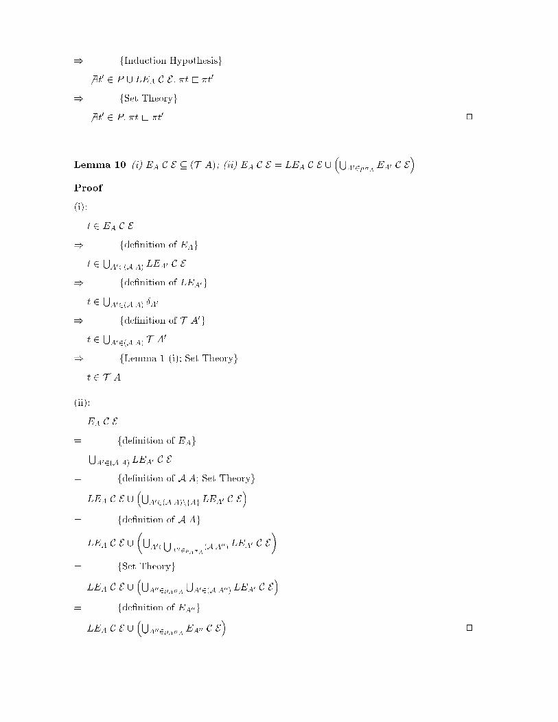
Lemma 10 (i) EA C E � (T A); (ii) EA C E = LEA C E [�S

A02��AEA0 C E

�

Proof

(i):

t 2 EA C E

) fde�nition of EAg

t 2SA02(A A) LEA0 C E

) fde�nition of LEA0g

t 2SA02(A A) �A0

) fde�nition of T A0g

t 2SA02(A A) T A0

) fLemma 1 (i); Set Theoryg

t 2 T A

(ii):

EA C E

= fde�nition of EAgSA02(A A) LEA0 C E

= fde�nition of A A; Set Theoryg

LEA C E [�S

A02(A A)nfAgLEA0 C E�

= fde�nition of A Ag

LEA C E [

�SA02S

A002�A�A(A A00) LEA0 C E

�

= fSet Theoryg

LEA C E [�S

A002�A�A

SA02(A A00) LEA0 C E

�

= fde�nition of EA00g

LEA C E [�S

A002�A�A EA00 C E�

2

Lemma 11 For s 2 C \ �A and Aj 2 �As the following holds: EAjC E = (EA C E) \ (T Aj)

Proof

Part 1 - EAjC E � (EA C E) \ T Aj .

t 2 EAjC E

) fLemma 10 (i); Set Theoryg

t 2 (EAjC E) \ (T Aj)

) fde�nition of EAjg

t 2�S

A02(A Aj) LEA0 C E�\ (T Aj)

) fLemma 1 (i)g

t 2�S

A02(A A) LEA0 C E�\ (T Aj)


t 2 (EA C E) \ (T Aj)

Part 2 - (EA C E) \ T Aj � EAjC E.

t 2 (EA C E) \ T Aj


t 2�S

A02(A A) LEA0 C E�\ (T Aj)

) fde�nition of A A;Set Theoryg

t 2�LEA C E [

�SA02(A Aj)

LEA0 C E�[�S

A02S

A002(�A�AnfAjg)(A A00) LEA0 C E��\(T Aj)

) f�A \ T Aj = ; ) (LEA C E) \ T Aj = ;g

t 2��S

A02(A Aj)LEA0 C E

�[�S

A02S

A002(�A�AnfAjg)(A A00) LEA0 C E��

\ (T Aj)

) fLemmata 10 and 1 (ii) imply (LEA0 C E) \ (T Aj) = ; for A0 2 (A A00) withA00 2 (�A�A n fAjg) g

t 2�S

A02(A Aj) LEA0 C E�\ (T Aj)

) fLemmata 10 and 1 (i) and A0 2 (A Aj) imply (LEA0 C E) \ (T Aj) = LEA0 C Eg

t 2SA02(A Aj) LEA0 C E

) fde�nition of EAjg

t 2 EAjC E 2

Remark 1 An obvious consequence of the above lemma is that EAjC E � EA C E

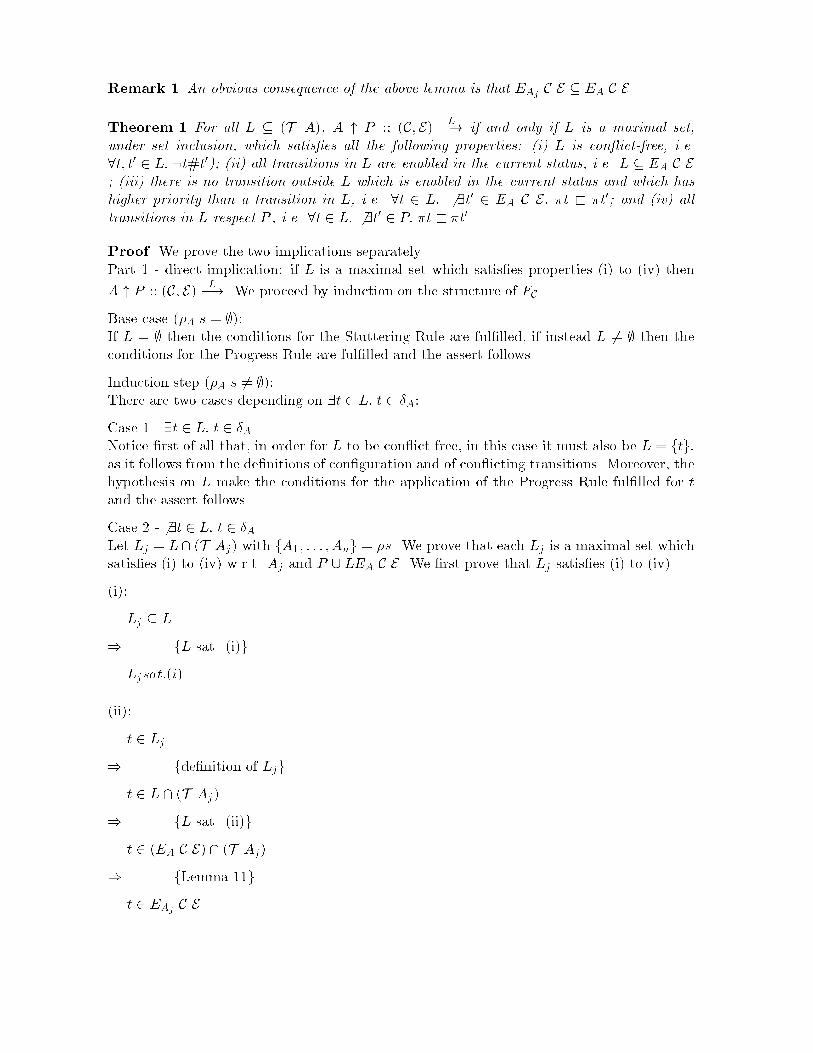
Theorem 1 For all L � (T A), A " P :: (C; E)L�! if and only if L is a maximal set,

under set inclusion, which satis�es all the following properties: (i) L is con ict-free, i.e.

8t; t0 2 L: :t#t0); (ii) all transitions in L are enabled in the current status, i.e. L � EA C E; (iii) there is no transition outside L which is enabled in the current status and which has

higher priority than a transition in L, i.e. 8t 2 L: 6 9t0 2 EA C E: �t < �t0; and (iv) all

transitions in L respect P , i.e. 8t 2 L: 6 9t0 2 P: �t < �t0

Proof We prove the two implications separately.

Part 1 - direct implication: if L is a maximal set which satis�es properties (i) to (iv) then

A " P :: (C; E)L�!. We proceed by induction on the structure of FC.

Base case (�A s = ;):If L = ; then the conditions for the Stuttering Rule are ful�lled, if instead L 6= ; then theconditions for the Progress Rule are ful�lled and the assert follows.

Induction step (�A s 6= ;):There are two cases depending on 9t 2 L: t 2 �A:

Case 1 - 9t 2 L: t 2 �ANotice �rst of all that, in order for L to be con ict free, in this case it must also be L = ftg,as it follows from the de�nitions of con�guration and of con icting transitions. Moreover, thehypothesis on L make the conditions for the application of the Progress Rule ful�lled for tand the assert follows.

Case 2 - 6 9t 2 L: t 2 �ALet Lj = L\ (T Aj) with fA1; : : : ; Ang = �s. We prove that each Lj is a maximal set whichsatis�es (i) to (iv) w.r.t. Aj and P [ LEA C E. We �rst prove that Lj satis�es (i) to (iv).

(i):

Lj � L

) fL sat. (i)g

Ljsat:(i)

(ii):

t 2 Lj

) fde�nition of Ljg

t 2 L \ (T Aj)

) fL sat. (ii)g

t 2 (EA C E) \ (T Aj)

) fLemma 11g

t 2 EAjC E

(iii) By contradiction:

t 2 Lj ^ t0 2 EAj

C E ^ �t < �t0

) fLj � L and Remark 1g

t 2 L ^ t0 2 EA C E ^ �t < �t0

) fL sat. (iii) w.r.t Ag

FALSE

(iv) By contradiction:

Suppose t 2 Lj ^ t0 2 (P [ LEA C E) ^ �t < �t0. Either t0 2 P or t0 2 LEA C E:

Case 1 - t0 2 P

t 2 Lj ^ t0 2 P ^ �t < �t0

) fLj � Lg

t 2 L ^ t0 2 P ^ �t < �t0

) fL sat. (iv) w.r.t Pg

FALSE

Case 2 - t0 2 LEA C Et 2 Lj ^ t

0 2 LEA C E ^ �t < �t0

) fLj � Lg

t 2 L ^ t0 2 LEA C E ^ �t < �t0

) fLemma 10 (ii)g

t 2 L ^ t0 2 EA C E ^ �t < �t0

) fL sat. (iii) w.r.t Ag

FALSE

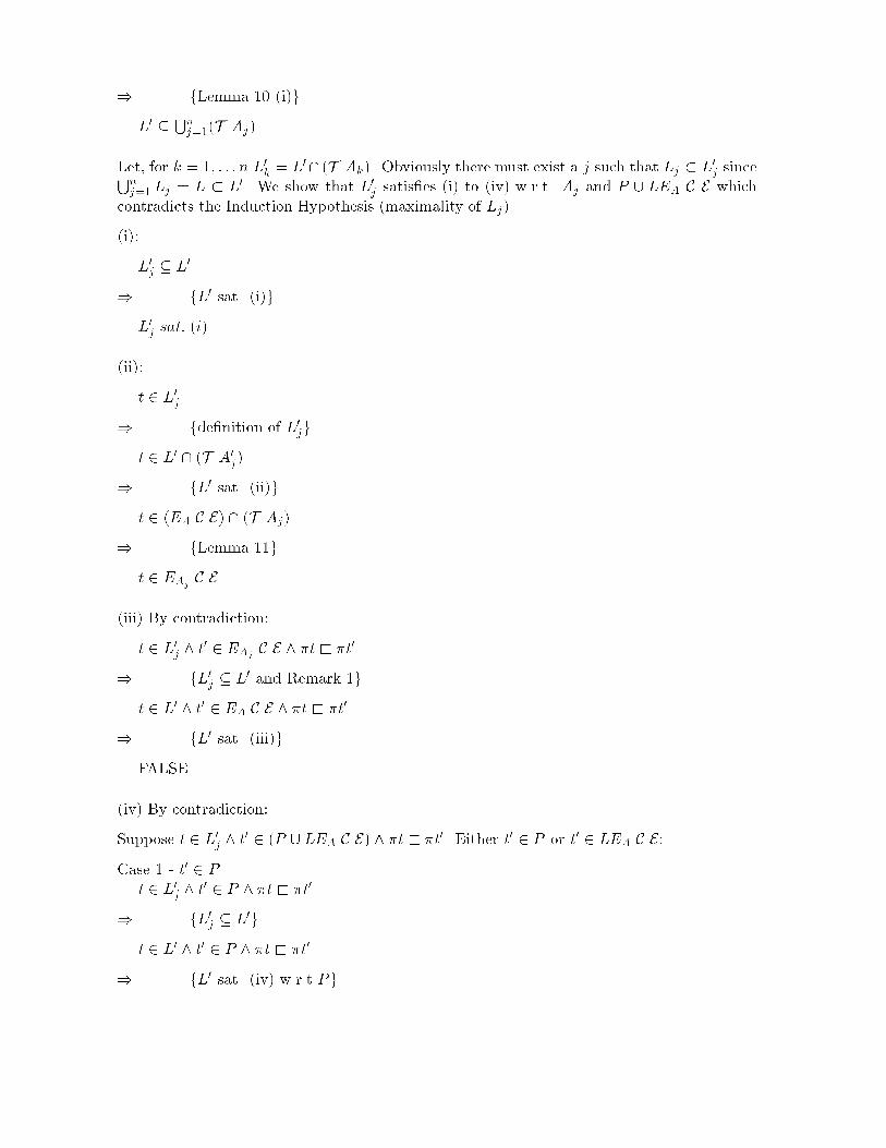
Now we prove that Lj is maximal. We proceed again by contradiction. Suppose thereexists L0

j such that Lj � L0j and L0

j satis�es (i) to (iv) w.r.t. Aj and P [ LEA C E. Let

L0 = L0j [

Sk=nk=1;k 6=j Lk. Clearly L � L0 and in the following we show that L0 would satisfy (i)

to (iv) w.r.t. A and P .

(i):

TRUE

) fL0j sat. (ii) w.r.t. Aj;Lemma 10 (i)g

L0j � (T Aj)

) fComposition Rule; de�nition of T ; jj; Lemma 7g

8t 2 L0j; t

0 2 Lk: :(t#t0)

) fde�nition of L0; L0j and Lk sat. (i)g

L0sat:(i)

(ii):

L0 � EA C E since L0j sat. (ii) w.r.t. Aj and Lemma 10 (ii) applies; moreover

Sk 6=j Lk � L

and L sat. (i) w.r.t. A.

(iii):

First notice that

1. 8t 2 Lk: 6 9t0 2 EA C E: �t < �t0 for k 6= j since Lk � L which sat. (iii) w.r.t. A.

2. 8t 2 L0j : 6 9t

0 2 EAjC E: �t < �t0 since L0

j sat. (iii) w.r.t.Aj

3. 8t 2 L0j : 6 9t

0 2 EAkC E: �t < �t0 for k 6= j because of Lemma 8

4. 8t 2 L0j : 6 9t

0 2 LEA C E: �t < �t0 since L0j sat. (iv) w.r.t. P [ LEA C E.

Points (1) to (4) above, together with Lemma 10 (ii) prove that L0 satis�es (iii) w.r.t. A.

(iv):

8t 2 L0: 6 9t0 2 P: �t < �t0 since L sat. (iv) w.r.t. P and L0j sat. (iv) w.r.t. P [ LEA C E.

All the above shows that L0 would satisfy (i) to (iv) w.r.t. A and P and L � L0 which wouldcontradict the hypothesis on L.

So, by the Induction HypothesisVnj=1Aj " P [ LEA C E :: (C; E)

Lj�! (Cj; Ej). Moreover,

ifSnj=1Lj = ; then L = ; which, by hypothesis on L implies in turn 8t 2 LEA C E: 9t0 2

P: �t < �t0. This means that the Composition Rule can be applied and the assert is proven.

Part 2 - reverse implication: if A " P :: (C; E)L�! then L is a maximal set which satis-

�es properties (i) to (iv). We proceed by induction on the length d of the derivation for

A " P :: (C; E)L�! (C 0; E 0).

Base case (d = 1):

If the derivation has length 1, then only the Progress Rule or the Stuttering Rule could havebeen applied. In both cases the assert follows directly from the conditions of the rules.Induction step (d > 1):In this case the Composition Rule must have been applied in the last step of the derivation.

By the Induction Hypothesis, every Lj satis�es (i) to (iv) w.r.t. Aj and P [ LEA C E. Weshow that L =

Snj=1Lj is a maximal set which satis�es (i) to (iv) w.r.t. A and P .

We �rst show that L satis�es (i) to (iv) w.r.t. A and P .

(i): L sat. (i) since each Lj sat. (i) by Induction Hypothesis and for i 6= j if t 2 Li and

t0 2 Lj , then :(t#t0) because of (SRC t jj SRC t0) and Lemma 7.

(ii):

TRUE

) fLj sat. (ii) w.r.t. AjgVnj=1Lj � EAj

C E

) fRemark 1; L =Snj=1Ljg

L � EA C E

(iii)By contradiction:

Suppose w.l.g. t 2 Lj and t0 2 EA C E with �t < �t0. By Lemma 10 (ii) either t0 2 LEA C Eor t0 2 EAk

C E for some k such that Ak 2 �s.

Case 1 - t0 2 LEA C E

t 2 L ^ t0 2 LEA C E ^ �t < �t0

) fComposition Ruleg

t 2 Lj ^ t0 2 LEA C E ^ Aj " P [ LEA C E :: (C; E)

Lj�! ^�t < �t0

) fLemma 9g

FALSE

Case 2 - t0 2 EAkC E for some k such that Ak 2 �s.

Notice �rst that it cannot be k = j since Lj is con ict free and �t < �t0 implies t#t0 by

de�nition of priority schema. On the other hand, it cannot be k 6= j since �t < �t0 wouldviolate Lemma 8.


t 2 L ^ t0 2 P ^ �t < �t0

) fComposition Rule and Set Theoryg

9Lj: t 2 Lj ^ t0 2 P [ LEA C E ^ �t < �t0

) fLj sat. (iv) w.r.t. P [ LEA C Eg

FALSE

Now we prove that L is maximal. We proceed again by contradiction. Suppose there ex-ists L0 such that L � L0 and L0 satis�es (i) to (iv) w.r.t. A and P . First observe thatL0 �

Snj=1(T Aj) in fact:

TRUE

) fL � L0, L0 sat. (i), and L0 sat. (ii)g

L0 \ (LEA C E) = ; ^ L0 � EA C E

) fLemma 10 (ii)g

L0 �Snj=1EAj

C E

) fLemma 10 (i)g

L0 �Snj=1(T Aj)

Let, for k = 1; : : : n L0k = L0\ (T Ak). Obviously there must exist a j such that Lj � L0

j sinceSnj=1Lj = L � L0. We show that L0

j satis�es (i) to (iv) w.r.t. Aj and P [ LEA C E which

contradicts the Induction Hypothesis (maximality of Lj).

(i):

L0j � L0

) fL0 sat. (i)g

L0j sat: (i)

(ii):

t 2 L0j

) fde�nition of L0jg

t 2 L0 \ (T A0j)

) fL0 sat. (ii)g

t 2 (EA C E) \ (T Aj)

) fLemma 11g

t 2 EAjC E

(iii) By contradiction:

t 2 L0j ^ t

0 2 EAjC E ^ �t < �t0

) fL0j � L0 and Remark 1g

t 2 L0 ^ t0 2 EA C E ^ �t < �t0

) fL0 sat. (iii)g

FALSE


Suppose t 2 L0j ^ t

0 2 (P [ LEA C E) ^ �t < �t0. Either t0 2 P or t0 2 LEA C E:

Case 1 - t0 2 P

t 2 L0j ^ t

0 2 P ^ �t < �t0

) fL0j � L0g

t 2 L0 ^ t0 2 P ^ �t < �t0

) fL0 sat. (iv) w.r.t Pg

FALSE

Case 2 - t0 2 LEA C Et 2 L0

j ^ t0 2 LEA C E ^ �t < �t0

) fL0j � L0g

t 2 L ^ t0 2 LEA C E ^ �t < �t0

) fLemma 10 (ii)g

t 2 L0 ^ t0 2 EA C E ^ �t < �t0

) fL0 sat. (iii) w.r.t Ag

FALSE

So L is maximal. 2

References

[1] D. Latella, M. Massink, and I. Majzik. A Simpli�ed Formal Semantics for a Subset ofUML Statechart Diagrams. Technical Report HIDE/T1.2/PDCC/5/v1, ESPRIT Projectn. 27439 - High-Level Integrated Design Environemnt for Dependability HIDE, 1998.Available in the HIDE Project Public Repository (https://asterix.mit.bme.hu:998/).

[2] Z. Manna, S. Ness, and J. Vuillemin. Inductive methods for proving properties of pro-grams. Communications of the ACM, 16(8), 1973.

[3] R. Milner. Communication and Concurrency. Series in Computer Science. Prentice Hall,1989.

Quantitative assessment of the translation from

Statechart Diagrams to Kripke StructuresE. Giusti - CPR PDCC

D. Latella - CPR PDCC and CNR Ist. CNUCE

M. Massink - CNR Ist. CNUCE

1 Rationale

During the �rst phase of the HIDE Project the formal de�nition of the translation from UMLstatechart diagrams to Kripke Structures have beed fully developed (see Deliverable 2) and

its correctness has been formally proven (see Deliverable 4).

Such a de�nition is to be considered as a speci�cation for the translation itself, to whichany implementation of such a translation needs to conform.

No implementation of the translation has been developed during the �rst phase of HIDEfor which a conformance proof is available.

So no de�nite quantitative assessment which refers to implementation issues, like memoryusage or execution time can be done at this stage of development of the work.

The major consideration which can be done at this moment is that the translation from

statechart diagrams to Kripke Structures is a way for providing a formal semantics for UMLstatechart diagrams within the HIDE environment. The de�nition of the semantics is a neces-

sary pre-requisite for any formal veri�cation activity and the formal de�nition of the possiblebehaviours (i.e. the semantics) is the minimal information one needs for understanding the

statechart diagram.

2 Outline of an Extended Hierarchical Automata to PROMELA

translation

At a more concrete level, it is worth mentioning that there is work ongoing in PDCC for im-plementing a translation from Extended Hierarchical Automata to the PROMELA language[1]. The implementation is still in progress. The implementation language we chose is ML,due to its sound mathematical basis which hopefully will help in developing a conformance

proof.PROMELA is the modeling language of the SPIN model-checker, which is a widely used

tool specially due to the various state compression and e�ciency enhancement techniques itincludes.

The main idea of our implementation e�ort is to translate an extended hierarchical au-tomaton into a PROMELA model which, when executed by SPIN, generates as statespaceessentially the Kripke Structure which is the semantic model, via our operational semantics,

of the extended hierarchical automaton.

Experiments with classical statecharts [2] show that the translation is feasible and theresults, in terms of memory usage and execution time, are encouraging.

The above facts bring us to formulate a strong conjecture that a PROMELA representationof extended hierarchical automata, as we are de�ning it can be a very e�cient one.

We conclude this section showing what would be the result of applying the PROMELAtranslation to the extended hierarchical automaton of Fig. 1

s1 s2t3

t2

t1

s3

t8

s8 s9

t4

t6

s6 s7t7 t9

A0

A2A1

t5

Figure 1: Example of an Extended Hierarchical Automaton

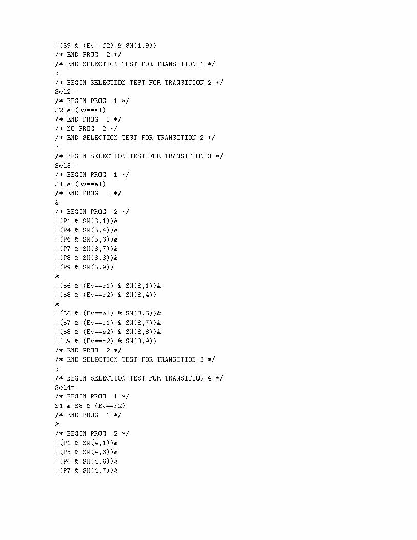
The code is given below. There is a distinct boolean variable Sn for each state sn.Moreover, set P (see deliverable 2) is represented by its characteristic function coded as 9boolean variables, one per each transition. Variable Pn is referred to transition tn. Transitiontn is �red i� the corresponding variable Firen evaluates to 1. The program essentially marks

those transitions which are enabled and respect the priority constraints. This labeling ismade via variables Seln. On the basis of those transition which are enabled and whichrespect priority (i.e. those tn such that Seln is 1) and using the PROMELA non-deterministicconstruct, the transitions to be �red are selected (i.e. their corresponding variable Firen is

set to 1). The fact that transition i has lower priority than transition j is coded via functionSM, i.e SM(i,j) evaluates to 1. Otherwise SM(i,j) evaluates to 0. Finally, no parallelism isused in the PROMELA model since, given the absence of synchronization and the fact that

there is no particular order in which parallel automata have to be considered, such parallelismwould only result in an increase of the state space.

Finally, for the sake of simplicity and limited to the present example, we have chosen torepresent the event queue as an integer. This is because we know, a priori, that the queue

will never contain more than one item in this example.In the actual code below, the comments often refer to the speci�c premisses of the opera-

tional semantics rules (e.g. PROG. 1 is condition (1) of the progress rule).

bit S1, S2, S3, S6, S7, S8, S9;

bit P1, P2, P3, P4, P5, P6, P7, P8, P9;

bit Sel1, Sel2, Sel3, Sel4, Sel5, Sel6, Sel7, Sel8, Sel9;

bit Fire1, Fire2, Fire3, Fire4, Fire5, Fire6, Fire7, Fire8, Fire9;

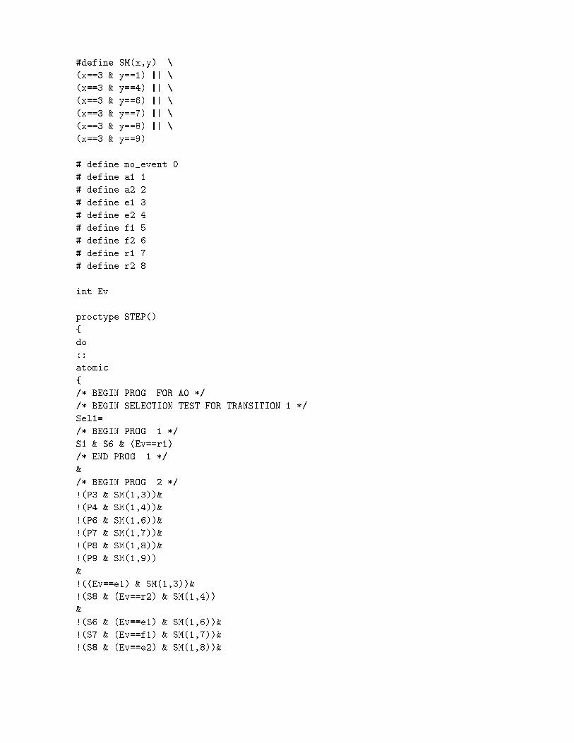
#define SM(x,y) \

(x==3 & y==1) || \

(x==3 & y==4) || \

(x==3 & y==6) || \

(x==3 & y==7) || \

(x==3 & y==8) || \

(x==3 & y==9)

# define no_event 0

# define a1 1

# define a2 2

# define e1 3

# define e2 4

# define f1 5

# define f2 6

# define r1 7

# define r2 8

int Ev

proctype STEP()

{

do

::

atomic

{

/* BEGIN PROG. FOR A0 */

/* BEGIN SELECTION TEST FOR TRANSITION 1 */

Sel1=

/* BEGIN PROG. 1 */

S1 & S6 & (Ev==r1)

/* END PROG. 1 */

&

/* BEGIN PROG. 2 */

!(P3 & SM(1,3))&

!(P4 & SM(1,4))&

!(P6 & SM(1,6))&

!(P7 & SM(1,7))&

!(P8 & SM(1,8))&

!(P9 & SM(1,9))

&

!((Ev==e1) & SM(1,3))&

!(S8 & (Ev==r2) & SM(1,4))

&

!(S6 & (Ev==e1) & SM(1,6))&

!(S7 & (Ev==f1) & SM(1,7))&

!(S8 & (Ev==e2) & SM(1,8))&

!(S9 & (Ev==f2) & SM(1,9))

/* END PROG. 2 */

/* END SELECTION TEST FOR TRANSITION 1 */

;


Sel2=

/* BEGIN PROG. 1 */

S2 & (Ev==a1)

/* END PROG. 1 */

/* NO PROG. 2 */


;


Sel3=

/* BEGIN PROG. 1 */

S1 & (Ev==e1)

/* END PROG. 1 */

&

/* BEGIN PROG. 2 */

!(P1 & SM(3,1))&

!(P4 & SM(3,4))&

!(P6 & SM(3,6))&

!(P7 & SM(3,7))&

!(P8 & SM(3,8))&

!(P9 & SM(3,9))

&

!(S6 & (Ev==r1) & SM(3,1))&

!(S8 & (Ev==r2) & SM(3,4))

&

!(S6 & (Ev==e1) & SM(3,6))&

!(S7 & (Ev==f1) & SM(3,7))&

!(S8 & (Ev==e2) & SM(3,8))&

!(S9 & (Ev==f2) & SM(3,9))

/* END PROG. 2 */


;


Sel4=

/* BEGIN PROG. 1 */

S1 & S8 & (Ev==r2)

/* END PROG. 1 */

&

/* BEGIN PROG. 2 */

!(P1 & SM(4,1))&

!(P3 & SM(4,3))&

!(P6 & SM(4,6))&

!(P7 & SM(4,7))&

!(P8 & SM(4,8))&

!(P9 & SM(4,9))

&

!(S6 & (Ev==r1) & SM(4,1))&

!((Ev==e1) & SM(4,3))

&

!(S6 & (Ev==e1) & SM(4,6))&

!(S7 & (Ev==f1) & SM(4,7))&

!(S8 & (Ev==e2) & SM(4,8))&

!(S9 & (Ev==f2) & SM(4,9))

/* END PROG. 2 */


;


Sel5=

/* BEGIN PROG. 1 */

S3 & (Ev==a2)

/* END PROG. 1 */

/* NO PROG. 2 */


/* END PROG. FOR A0 */

;

/* BEGIN COM. FOR A0 */

/* BEGIN UPDATING P WITH ACTIVE TRANSITIONS OF A0 */

P1= S1 & S6 & (Ev==r1);

P2= S2 & (Ev==a1);

P3= S1 & (Ev==e1);

P4= S1 & S8 & (Ev==r2);

P5= S3 & (Ev==a2)

/* END UPDATING P WITH ACTIVE TRANSITIONS OF A0 */

;



Sel6=

/* BEGIN PROG. 1 */

S6 & (Ev==e1)

/* END PROG. 1 */

&

/* BEGIN PROG. 2 */

!(P1 & SM(6,1))&

!(P3 & SM(6,3))&

!(P4 & SM(6,4))

/* END PROG. 2 */


;


Sel7=

/* BEGIN PROG. 1 */

S7 & (Ev==f1)

/* END PROG. 1 */

&

/* BEGIN PROG. 2 */

!(P1 & SM(7,1))&

!(P3 & SM(7,3))&

!(P4 & SM(7,4))

/* END PROG. 2 */



;



Sel8=

/* BEGIN PROG. 1 */

S8 & (Ev==e2)

/* END PROG. 1 */

&

/* BEGIN PROG. 2 */

!(P1 & SM(8,1))&

!(P3 & SM(8,3))&

!(P4 & SM(8,4))

/* END PROG. 2 */


;


Sel9=

/* BEGIN PROG. 1 */

S9 & (Ev==f2)

/* END PROG. 1 */

&

/* BEGIN PROG. 2 */

!(P1 & SM(9,1))&

!(P3 & SM(9,3))&

!(P4 & SM(9,4))

/* END PROG. 2 */



;

/* BEGIN SELECTING TRANSITIONS TO FIRE */

if

::Sel1->Fire1=1

::Sel2->Fire2=1

::Sel3->Fire3=1

::Sel4->Fire4=1

::Sel5->Fire5=1

::(Sel6||Sel7||Sel8||Sel9)->

if

::Sel6->Fire6=1

::Sel7->Fire7=1

::else->skip

fi;

if

::Sel8->Fire8=1

::Sel9->Fire9=1

::else->skip

fi

::else->skip

fi

/* END SELECTING TRANSITIONS TO FIRE */

;

/* BEGIN FIRING SELECTED TRANSITIONS */

if ::Fire1->S1=0;S2=1;S3=0;S6=0;S7=0;S8=0;S9=0;Ev=a1 ::else->skip fi;

if ::Fire2->S1=1;S2=0;S3=0;S6=1;S7=0;S8=1;S9=0;Ev=r2 ::else->skip fi;

if ::Fire3->S1=0;S2=1;S3=0;S6=0;S7=0;S8=0;S9=0;Ev=no_event ::else->skip fi;

if ::Fire4->S1=0;S2=0;S3=1;S6=0;S7=0;S8=0;S9=0;Ev=a2 ::else->skip fi;

if ::Fire5->S1=1;S2=0;S3=0;S6=1;S7=0;S8=0;S9=1;Ev=e1 ::else->skip fi;

if ::Fire6->S6=0;S7=1;Ev=f1 ::else->skip fi;

if ::Fire7->S6=1;S7=0;Ev=r1 ::else->skip fi;

if ::Fire8->S8=0;S9=1;Ev=e1 ::else->skip fi;

if ::Fire9->S8=1;S9=0;Ev=no_event ::else->skip fi

/* END FIRING SELECTED TRANSITIONS */

;

/* BEGIN CLEANING-UP AUXILIARY STRUCTURES */

P1=0;P2=0;P3=0;P4=0;P5=0;P6=0;P7=0;P8=0;P9=0;

Sel1=0;Sel2=0;Sel3=0;Sel4=0;Sel5=0;Sel6=0;Sel7=0;Sel8=0;Sel9=0;

Fire1=0;Fire2=0;Fire3=0;Fire4=0;Fire5=0;Fire6=0;Fire7=0;Fire8=0;Fire9=0

/* END CLEANING-UP AUXILIARY STRUCTURES */

}

od

}

init

{

/* BEGIN SETTING INITIAL CONFIGURATION */

S1=1;S2=0;S3=0;S6=1;S7=0;S8=1;S9=0;

/* END SETTING INITIAL CONFIGURATION */

Ev=e2;

atomic{run STEP()}

}

References

[1] G Holzmann. The model checker SPIN. IEEE Transactions on Software Engineering,23(5):279{295, 1997.

[2] E. Mikk, Y. Lakhnech, and M. Siegel. Hierarchical automata as model for statecharts.

In R. Shyamasundar and K. Euda, editors, Third Asian Computing Science Conference.

Advances in Computing Sience - ASIAN'97, volume 1345 of Lecture Notes in Computer

Science, pages 181{196. Springer-Verlag, 1997.

High-level Integrated Design Environment for dependability (HIDE

Documents

Transcript of High-level Integrated Design Environment for dependability (HIDE