Personal use of the material in this paper is permitted. However, permission toreprint or republish this material for advertising or promotional purposes or forcreating new works for resale or redistribution, or to reuse any copyrightedcomponent of this work in other works must be obtained from the authors of thispaper.

This paper has appeared in the proceedings of DCCA-7 - 7th IFIP Int.Conference on Dependable Computing for Critical Applications, San Jose, CA,USA, IEEE Computer Society Press, pp 299-318, 1999

Dependability Modeling and Evaluation ofPhased Mission Systems: a DSPN Approach

I. Mura1, A. Bondavalli2, X. Zang3 and K. S. Trivedi31 Department of Information Engineering, University of Pisa, Italy

{mura@rep1.iei.pi.cnr.it}2 CNUCE/CNR, Pisa, Italy {a.bondavalli@cnuce.cnr.it}

3 CACC, Department of Electronic Engineering, Duke University, Durham NC{xzang, kst @ee.duke.edu}

AbstractIn this paper we focus on the analytical modeling for the dependabil-ity evaluation of phased-mission systems. Because of their dynamicbehavior, phased-mission systems offer challenges in modeling. Wepropose the modeling and evaluation of phased-mission systemsdependability through the Deterministic and Stochastic Petri Nets(DSPN). The DSPN approach to the phased-mission systems offersmany advantages, concerning both the modeling and the solution.The DSPN model of the mission can be a very concise one, and itcan be efficiently solved for the dependability evaluation purposes.The solution procedure is supported by the existence of an analyticalsolution for the transient probabilities of the marking processunderlying the DSPN model. This analytical solution can be fullyautomated. We show how the DSPN models capabilities are able todeal with various peculiar features of phased-mission systems,including those systems where the next phase to be performed canbe chosen at the time the preceding phase ends.

1 Introduction

Many of the systems devoted to the control and management of critical activitieshave to perform a series of tasks that must be accomplished in sequence. Their op-erational life consists of a sequence of non-overlapping periods, called phases.These systems are often called phased-mission systems, abbreviated as PMS here-after. Both the system behavior and the conditions of the environment in which thesystem is embedded may vary from phase to phase. These changes may be due todifferent tasks to be performed within each phase, or different stresses the system is

Mura, Bondavalli, Zang, Trivedi

subject to, as well as different dependability requirements and failure scenarios. Inorder to accomplish its mission the system needs to change its configuration overtime, to adopt the most suitable one with respect to the performance and depend-ability requirements of the phase being currently executed. Many examples of PMScan be found in various application domains. For instance, systems for the aided-guide of aircrafts, whose mission-time is divided into several phases such as take-off, cruise, landing, with completely different requirements. Other systems alternatebetween operational and maintenance phases (e.g., nuclear power plants), or havemissions with multiple goals such as a spacecraft meant for scientific research.

In this paper we focus on the analytical modeling for the dependability evaluationof PMS. We propose the modeling and evaluation of phased-mission systems de-pendability through Deterministic and Stochastic Petri Nets (DSPN). The class ofDSPN models allows timed transitions with exponentially distributed firing times,immediate transitions, and includes deterministic transitions as well. Moreover, theDSPNs allow a very concise modeling of even quite complex systems, through theuse of guards on transitions, timed transition priorities, halting conditions, rewardrates, etc. Due to their high expressiveness, DSPNs are able to cope with the dy-namic structure of the phased mission systems. The DSPN approach to the phased-mission systems offers many advantages, concerning both the modeling and thesolution. PMS are modeled with a single DSPN model representing the whole mis-sion. This single-model approach enables us to deal with dependencies amongphases caused by the sharing of architectural components. Moreover, the model ofthe mission can be a very concise one. The single DSPN model can be efficientlysolved for dependability evaluation purposes. The solution procedure is supportedby the existence of an analytical solution for the transient probabilities of themarking process underlying the DSPN model [8]. This solution only requires theseparate solution of each single phase, and can be fully automated.

The main contribution of this paper lies in the proposal of the DSPN modelingapproach for PMS. In this respect, it offers a suitable means for a systematic for-mulation and solution of PMS models, and for their sensitivity analysis. We showhow well DSPN can represent the typical features of PMS that have been taken intoaccount by the previous proposals appeared in the literature. We also point out thatDSPNs models of PMS can naturally deal with the connections between solution ofdifferent phases, which has been only treated in an ad hoc manner in earlier ap-proaches. Moreover, the DSPN formulation easily lends itself to automation andallows additional features of PMS to be modeled, features which are usually notconsidered in literature. For instance, we consider in this paper the state-dependentselection of the next phase to be executed. The exploitation of the full DSPN model-ing power to include more and more features of PMS promises to be a fruitful in-vestigation and is the subject of our on-going work.

The paper is organized as follows. Section 2 presents the class of PMS we willbe dealing with. That section gives a retrospective on the different Markov chain-based models that have appeared in literature, and explains at an high abstractionlevel the DSPN approach in the modeling of PMS. In Section 3 we briefly intro-duce the mathematical background underlying the analytical solution of the DSPNmodels. Section 4 shows how the DSPN capabilities are able to deal with the vari-ous peculiar features of PMS, through the modeling of an imaginary though realis-tic example of a space application. Three different models are considered, whichprogressively include more and more features of PMS in a still concise, readableand easy-to-define DSPN model. In Section 5 the general theory of DSPN is spe-cialized to PMS modeling, and an analytical solution is given for the transient prob-abilities of the marking process. Section 6 explains the automation procedure of the

Dependability Modeling and Evaluation of PMS: a DSPN Approach

DSPN model solution, and presents the results of an evaluation aimed at assessingthe probability of completing the mission for the example of space application.

Finally, our concluding remarks are given in Section 7, where we summarise ournew approach discussing its advantages and limitations, and how we intend to ad-dress them in our future work.

2 PMS problem viewed as a DSPN

As we already pointed out, systems showing a phased behavior offer challengesin dependability modeling and evaluation. The architectural components the systemutilizes during a phase are in general used in other subsequent phases, thus adding aset of dependencies among the models of different phases. Moreover, the phasechanges very often reflect the occurrence of particular events that do not depend onthe system state itself, but are rather triggered by time-out exceptions, or are pre-planned for the entire system life-time.

All these characteristics of PMS call for powerful modeling tools, able to captureand concisely represent these peculiar features. PMS have been widely investigated.Starting from the early studies [6, 24], which assumed fairly simple phasedependencies of system components, many works have been proposed which re-sort to Fault-Tree models [7, 11, 17, 23] (only for non-repairable systems) and toMarkov chain models [2, 3, 5, 10, 16, 21, 22]. A different approach based on theSAN (Stochastic Activity Networks) modeling is adopted in [4], a study closelyrelated to our investigation. To better understand the novelty of our approach, in thefollowing we first give a brief review of the related studies that have appeared in theliterature. Then, we propose the DSPN approach, in order to compare the main ad-vantages and drawbacks of all the presented methods with respect to the new one.

2.1 Literature survey

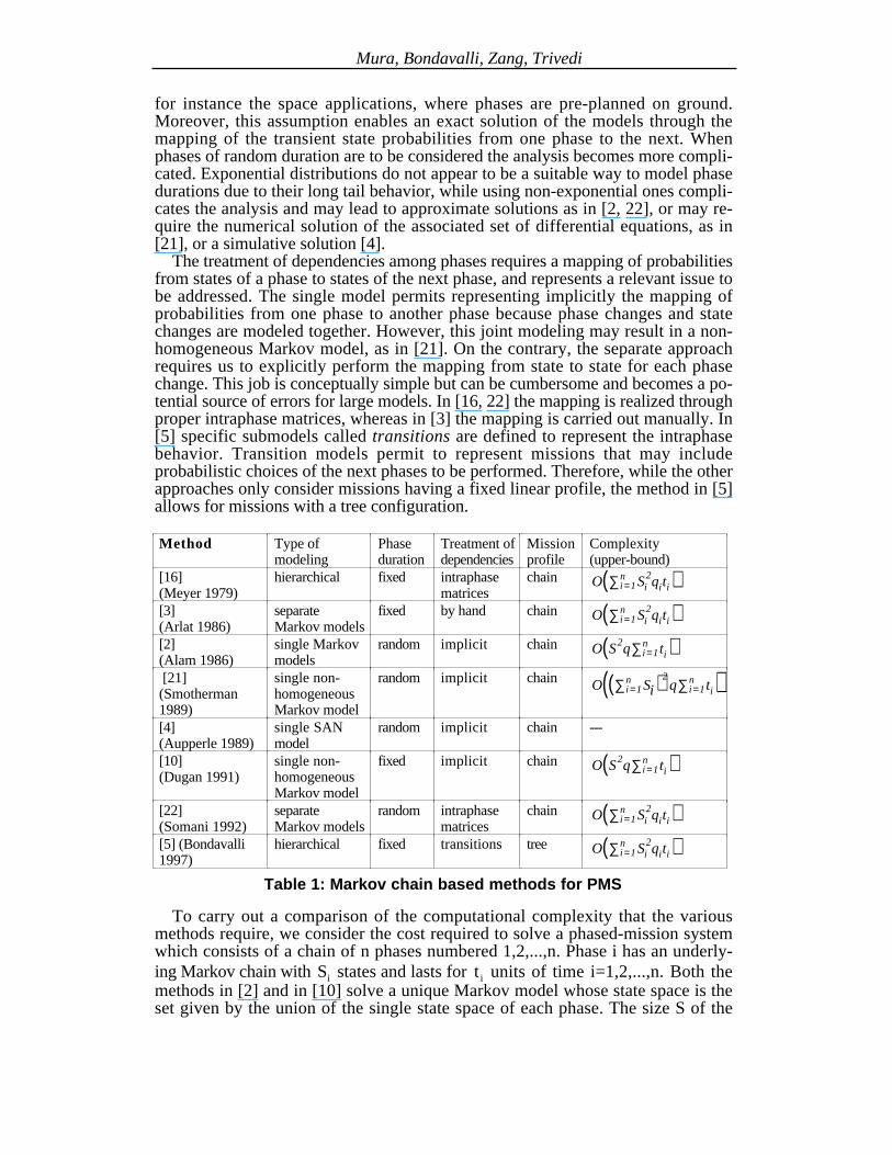
In this section we present and compare the Markov chain-based approaches [2,3, 5, 10, 16, 21, 22] and the one based on SAN in [4] for the dependability model-ing and analysis of PMS. The most relevant aspects of the comparison are summa-rized in Table 1.

A key point that impacts most of the other aspects is represented by the sin-gle/separate modeling of the phases: it affects the reusability/flexibility of previouslybuilt models, the modeling of dependencies among phases and the complexity ofthe solution steps. The single model approaches [2, 4, 10, 21] suffer from a lack ofreusability: a new model needs to be built if the behavior of the system in any phaseis changed or if the phase order is changed. However, this task is considerablysimpler for the SAN model of PMS than for the Markov chain based approaches.As an advantage, the single-model approach allows the exploitation of similaritiesamong phases to obtain a compact model in which all the phases are properlyembedded as in [2, 4, 10]. Conversely, the separate modeling of each phase [3, 22]allows the reuse of previously built models of the phases. Moreover, it is easier tocharacterize the differences among phases, in terms of different failure rates anddifferent configuration requirements. The hierarchical approaches in [5, 16] try tocombine the advantages of the single and separate modeling to keep phase modelssmall and easy-to-define and at the same time to provide different levels ofabstraction at which the mission can be described and analyzed.

The duration of phases is assumed to be fixed and known in advance in [3, 5,10, 16]. This assumption seems to hold for a wide range of application of PMS, as

Mura, Bondavalli, Zang, Trivedi

for instance the space applications, where phases are pre-planned on ground.Moreover, this assumption enables an exact solution of the models through themapping of the transient state probabilities from one phase to the next. Whenphases of random duration are to be considered the analysis becomes more compli-cated. Exponential distributions do not appear to be a suitable way to model phasedurations due to their long tail behavior, while using non-exponential ones compli-cates the analysis and may lead to approximate solutions as in [2, 22], or may re-quire the numerical solution of the associated set of differential equations, as in[21], or a simulative solution [4].

The treatment of dependencies among phases requires a mapping of probabilitiesfrom states of a phase to states of the next phase, and represents a relevant issue tobe addressed. The single model permits representing implicitly the mapping ofprobabilities from one phase to another phase because phase changes and statechanges are modeled together. However, this joint modeling may result in a non-homogeneous Markov model, as in [21]. On the contrary, the separate approachrequires us to explicitly perform the mapping from state to state for each phasechange. This job is conceptually simple but can be cumbersome and becomes a po-tential source of errors for large models. In [16, 22] the mapping is realized throughproper intraphase matrices, whereas in [3] the mapping is carried out manually. In[5] specific submodels called transitions are defined to represent the intraphasebehavior. Transition models permit to represent missions that may includeprobabilistic choices of the next phases to be performed. Therefore, while the otherapproaches only consider missions having a fixed linear profile, the method in [5]allows for missions with a tree configuration.

Method Type ofmodeling

Phaseduration

Treatment ofdependencies

Missionprofile

Complexity(upper-bound)

[16](Meyer 1979)

hierarchical fixed intraphasematrices

chain O Si2qitii=1

n∑( )[3](Arlat 1986)

separateMarkov models

fixed by hand chain O Si2qitii=1

n∑( )[2](Alam 1986)

single Markovmodels

random implicit chain O S2q tii=1n∑( )

[21](Smotherman1989)

single non-homogeneousMarkov model

random implicit chain O Sii=1n∑( )2

q tii=1n∑( )

[4](Aupperle 1989)

single SANmodel

random implicit chain ---

[10](Dugan 1991)

single non-homogeneousMarkov model

fixed implicit chain O S2q tii=1n∑( )

[22](Somani 1992)

separateMarkov models

random intraphasematrices

chain O Si2qitii=1

n∑( )[5] (Bondavalli1997)

hierarchical fixed transitions tree O Si2qitii=1

n∑( )Table 1: Markov chain based methods for PMS

To carry out a comparison of the computational complexity that the variousmethods require, we consider the cost required to solve a phased-mission systemwhich consists of a chain of n phases numbered 1,2,...,n. Phase i has an underly-ing Markov chain with Si states and lasts for t i units of time i=1,2,...,n. Both themethods in [2] and in [10] solve a unique Markov model whose state space is theset given by the union of the single state space of each phase. The size S of the

Dependability Modeling and Evaluation of PMS: a DSPN Approach

unified state space is at least maxi =1,2,K ,n Si , and can be at most Sii =1

n∑ . The singleMarkov chain is solved n times for n phases. If the uniformization method [19] isused to evaluate the transient probability vector, the overall complexity of the

solution is S2q t ii =1

n∑ , where q is defined as the maximum module entry of thegenerator matrix of the whole Markov model. The method of Smotherman andZemoudeh [21] requires the solution of a set of nS differential equations. Theauthors also adopt a Runge-Kutta solution algorithm, at a cost that can be bounded

by O ( Sii =1

n∑ )2q t ii =1

n∑( ), where q is defined as above. The complexity of the

solution for the method in [4] can not be compared to the others listed in Table 1,because the SAN model is to be solved by simulation. Therefore, the computationalcost is affected by a number of factors, as the width of the confidence intervals, themethod used for the statistical analysis, etc. The methods in [5, 16], as well as allthose that adopt the separate modeling approach [3, 22], require a number of op-

erations which is dominated by O( Si2qii =1

n∑ t i ), where qi is the maximum moduleentry of the Markov chain generator matrix of phase i. This computational com-plexity grows linearly with the number of phases. Therefore, the methods that useseparate solution of the phase models are, in general, more efficient than the onesthat use a combined model. Note that all the computational cost reported here are tobe intended as upper-bounds. In fact, often the matrices obtained are quite sparse,thus allowing cheaper solution techniques [19].

2.2 The DSPN approach

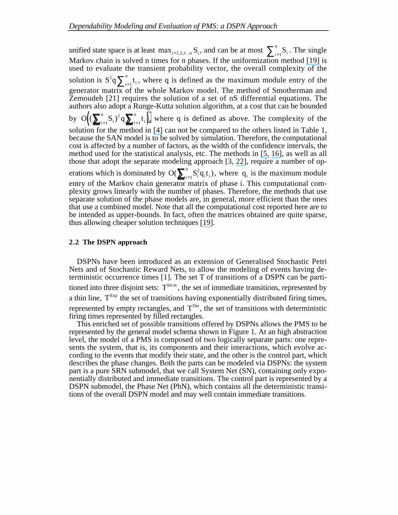
DSPNs have been introduced as an extension of Generalised Stochastic PetriNets and of Stochastic Reward Nets, to allow the modeling of events having de-terministic occurrence times [1]. The set T of transitions of a DSPN can be parti-tioned into three disjoint sets: T Im m , the set of immediate transitions, represented bya thin line, TExp the set of transitions having exponentially distributed firing times,represented by empty rectangles, and TDet, the set of transitions with deterministicfiring times represented by filled rectangles.

This enriched set of possible transitions offered by DSPNs allows the PMS to berepresented by the general model schema shown in Figure 1. At an high abstractionlevel, the model of a PMS is composed of two logically separate parts: one repre-sents the system, that is, its components and their interactions, which evolve ac-cording to the events that modify their state, and the other is the control part, whichdescribes the phase changes. Both the parts can be modeled via DSPNs: the systempart is a pure SRN submodel, that we call System Net (SN), containing only expo-nentially distributed and immediate transitions. The control part is represented by aDSPN submodel, the Phase Net (PhN), which contains all the deterministic transi-tions of the overall DSPN model and may well contain immediate transitions.

Mura, Bondavalli, Zang, Trivedi

Phase 1 Phase 2 Phase 3 StopOk Down

t_fail

Rep

p 1-pτ1 τ2 τ3

Figure 1: DSPN model of a PMS

A token in a place of the PhN model represents a phase being executed, and thefiring of a deterministic transition models a phase change. The sequence of phasesends with a token in END place, which represents the end of the mission. The SNmodel describing the evolution of the underlying system is governed by the PhN:the SN's evolution may depend on the marking of the PhN thus representing thephase-dependent behavior of the system. According to the SRN modeling rules,this phase dependent behavior is modeled by proper marking dependent predicateswhich modify transition rates, enabling conditions, reward rates, etc., of the overallDSPN. As we will detail in the following, the two nets can interact in variousways, and this allows the modeling of different features of PMS mentioned above.Any structure of the two nets can be considered: in particular, the PhN is not limitedto have a linear structure.

The same structure of the model of a PMS can be found in the paper of Aupperleet al. in [4]. They used the METASAN [20] modeling tool, based on StochasticActivity Networks, to represent both the PhN and the SN. In the SAN language,transitions are called activities. SANs allow for general distributions of activity du-ration, for marking dependent firing rates, and for guards on the enabling condi-tions of activities. Hence, SANs and DSPNs share many of the modeling features,and the work in [4] contains many interesting elements for the modeling of complexPMS. Here, we intend to apply the potentialities of DSPNs to investigate how thevarious aspects of PMS can be modeled. Moreover, we exploit the MRGP theory toprovide an analytical solution technique for the DSPN model of PMS, and for itssensitivity analysis. The possibility of such analytical solution was not available atthe time the work in [4] was proposed, and it represents a considerable step to-wards the definition of a systematic solution method for PMS. To guarantee theanalytical tractability of the DSPN, the only constraint to be imposed on the modelis the following one (although this assumption has been relaxed in some recentwork [15, 18]):

Assumption 1: at most one transition belonging to TDet is enabled in each ofthe possible markings of the DSPN.

This condition is obviously satisfied for the DSPN model of a PMS provided thatthe only deterministic activities modeled are the phase durations. In this case, thereis only one (and exactly one) deterministic transition enabled, which corresponds tothe current phase of the system, and an elegant analytical solution can be given forthe transient marking probabilities.

3 Solution of PMS via DSPN

In this section we briefly present the mathematical background underlying theanalysis of a generic DSPN model. The general theory for the analysis will be tai-lored to the PMS problem in a subsequent section. A complete exposition of theDSPN solution approach for the general case can be found in [8, 12].

Dependability Modeling and Evaluation of PMS: a DSPN Approach

Let M t( ) denote the marking of the DSPN at time t . The analysis relies on thestudy of the piecewise-constant, right-continuous, continuous-time stochasticmarking-process M t t( ), >{ }0 , underlying the DSPN model, formed by thechanges of tangible markings over time. Note that, due to the existence of determin-istic transitions, this stochastic process is neither a Markov chain, nor a semi-Markov process. To deal with such stochastic process, we resort to the theory ofMarkov Regenerative Processes (MRGP). First we recall the definition of Markovrenewal sequence.

Definition 1: Let S be a discrete state space. A sequence of bivariate randomvariables ( , ),Y T nn n ≥{

�}0 is called a Markov renewal sequence if:

1) T0 0= , T Tn n+ ≥1 Tn ∈ ℜ +; Y Sn ∈ n ≥ 0

2) ∀ ≥ = − ≤ = =+ + − −n ob Y j T T x Y i T Y T Y Tn n n n n n n0 1 1 1 1 0 0,Pr [ , , , , , , , ]K

Pr [ , ]

Pr [ , ] ( ),

ob Y j T T x Y i

ob Y j T T x Y i k xn n n n

n n n i j

+ +

+ +

= − ≤ = == = − ≤ = =

1 1

1 1 0

The matrix K(x) = k i , j (x) is referred as the kernel of the Markov renewal se-quence. The definition of MRGP is based on Markov renewal sequences [14].

Definition 2: A stochastic process Z t t( ), ≥{ }0 is called a MRGP if there

exists a Markov renewal sequence ( , ),Y T nn n ≥{�

}0 of random variables such

that all the conditional finite distributions of Z T t tn( ),+ ≥{�

}0 given

Z u u T Y in n( ), ,0 ≤ ≤ ={�

} are the same as those of Z t t( ), ≥{ }0 givenY i0 = .

It is possible to show [8] that, if Assumption 1) holds, the marking processM t t( ), >{ }0 of a DSPN is an MRGP. For this aim, we first define a suitable re-

newal sequence, as follows. Let S denote the set of tangible markings of the reach-ability graph of the DSPN, which is exactly the state space of the marking process

M t t( ), >{ }0 . Let T0 0= , and consider the sequence T nn, ≥{�

}0 of time instantsrecursively defined. Suppose m S∈ is the marking such that m M Tn= +( ) . If m isan absorbing marking, then set Tn+ = ∞1 . If no deterministic transitions are en-abled in marking m, define Tn+1 as the first time after Tn that a marking changeoccurs. If one deterministic transition is enabled in marking m, define Tn+1 to bethe time when such transition fires or is disabled. Now, define the sequence

Y nn, ≥{�

}0 as Y M Tn n= +( ), ∀ ≥n 0. It can be proved that the so defined bivari-

ate sequence ( , ),Y T nn n ≥{�

}0 embedded in the marking-process {M(t), t>0} of theDSPN model is a Markov renewal sequence, according to Definition 1. Moreover,it is easy to show that the stochastic behavior of the marking process from time Tn

onwards M T t tn( ),+ ≥{�

}0 depends only on Y in = , and this implies that:

M T t t M u u T Y i M T t t Y in n ndist

n ndist

( ), ( ), , ( ),+ ≥ ≤ ≤ ={ } = + ≥ ={ } =0 0 0

M T t t Y in( ),+ ≥ ={� }0 0

Mura, Bondavalli, Zang, Trivedi

where =dist�

denotes equality in distribution, and this proves that {M(t), t>0} is an

MRGP. Let V t v ti j( ) ( ),= be the matrix defined as follows:

v t ob M t j M Y i i j Si j, ( ) Pr [ ( ) ( ) ], ,= = = = ∈0 0 To obtain matrix V(t), which describes the transient behavior of the stochastic

process underlying the DSPN, an analytical method has been proposed in [8], andhere we briefly recall that. For the sake of conciseness, denote with K*V(t) thematrix whose element i,j is defined as follows:

k v t dk t v t ui j i h h j

t

h S∗ = −∫∑

∈, , ,( ) ( ) ( )

0that is K*V(t) is the matrix of functions of t whose generic element is obtained withthe row by column convolution of the kernel matrix K(t) and matrix V(t), ratherthan with the usual multiplication operator. According to the MRGP theory [14],the transition matrix V(t) can be obtained by solving the following generalizedMarkov renewal equation:

V t E t K V t( ) ( ) ( )= + ∗ (1)

where E t e ti j( ) ( ),= is called the local kernel matrix, and is formally defined as

e t ob M t j T t Y ii j, ( ) Pr [ ( ) , ]= = > =1 0 . Solving Equation (1) to obtain matrix V(t)for a general MRGP may require the use of numerical algorithms or of Laplace-Stiltjes transform. However, as we shall see in the following, the solution ofEquation (1) in the case of an MRGP underlying a DSPN model for a PMS can begreatly simplified, and matrix V(t) can be obtained exactly in the time domain at alimited computational cost.

4 Applications

In this section we investigate the modeling capabilities of the DSPNs, to under-stand what features of PMS can be represented by the high-level model in Figure 1.Different PMS characteristics will be modeled by enriching step by step the DSPNmodel with new interaction capabilities between the PhN and the SN. As an exam-ple, throughout the rest of the paper we will be considering a typical example ofPMS: a phased-mission of an ideal space application.

4.1 Case 1: phase-dependent behavior of the SN

Consider a space application whose mission alternates operational phases asLaunch, Planet, Scientific Obsevations 1 and Scientific Obsevations 2 withHibernation phases, typically entered to maintain a low level of activity during peri-ods of navigation. Operational phases have stringent dependability requirements,hence the system employs a set of n redundant identical processors. Processors failand are repaired independently from each other. Processors fail with phase-depen-dent rates: the failure rate during hibernation phases is less than the failure rateduring operational phases. The repair strategy is based on the nature of faults affect-ing the space-probe. Indeed, since most of the faults are of transient nature, it ispossible that after a random period of time a faulty processor becomes availableagain. Moreover, it is also possible to reload parts of the software from ground, to

Dependability Modeling and Evaluation of PMS: a DSPN Approach

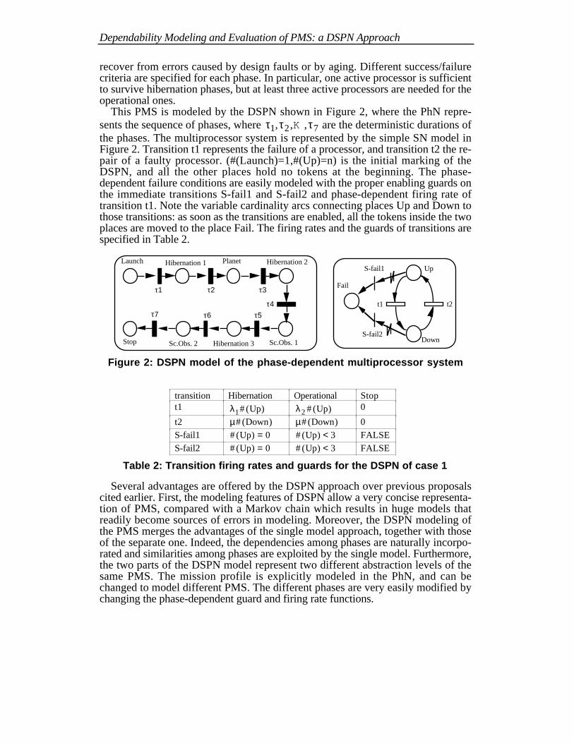
recover from errors caused by design faults or by aging. Different success/failurecriteria are specified for each phase. In particular, one active processor is sufficientto survive hibernation phases, but at least three active processors are needed for theoperational ones.

This PMS is modeled by the DSPN shown in Figure 2, where the PhN repre-sents the sequence of phases, where τ τ τ1 2 7, , ,K are the deterministic durations ofthe phases. The multiprocessor system is represented by the simple SN model inFigure 2. Transition t1 represents the failure of a processor, and transition t2 the re-pair of a faulty processor. (#(Launch)=1,#(Up)=n) is the initial marking of theDSPN, and all the other places hold no tokens at the beginning. The phase-dependent failure conditions are easily modeled with the proper enabling guards onthe immediate transitions S-fail1 and S-fail2 and phase-dependent firing rate oftransition t1. Note the variable cardinality arcs connecting places Up and Down tothose transitions: as soon as the transitions are enabled, all the tokens inside the twoplaces are moved to the place Fail. The firing rates and the guards of transitions arespecified in Table 2.

Up

Down

Fail

S-fail1

S-fail2

t2t1

Launch Hibernation 1

Sc.Obs. 1

Hibernation 2

Stop

τ1 τ2

τ4τ6τ7

Sc.Obs. 2

Planet

τ3

τ5

Hibernation 3

Figure 2: DSPN model of the phase-dependent multiprocessor system

transition Hibernation Operational Stopt1 λ1#( )Up λ2#( )Up 0

t2 µ#( )Down µ#( )Down 0

S-fail1 #( )Up = 0 #( )Up < 3 FALSE

S-fail2 #( )Up = 0 #( )Up < 3 FALSE

Table 2: Transition firing rates and guards for the DSPN of case 1

Several advantages are offered by the DSPN approach over previous proposalscited earlier. First, the modeling features of DSPN allow a very concise representa-tion of PMS, compared with a Markov chain which results in huge models thatreadily become sources of errors in modeling. Moreover, the DSPN modeling ofthe PMS merges the advantages of the single model approach, together with thoseof the separate one. Indeed, the dependencies among phases are naturally incorpo-rated and similarities among phases are exploited by the single model. Furthermore,the two parts of the DSPN model represent two different abstraction levels of thesame PMS. The mission profile is explicitly modeled in the PhN, and can bechanged to model different PMS. The different phases are very easily modified bychanging the phase-dependent guard and firing rate functions.

Mura, Bondavalli, Zang, Trivedi

4.2 Case 2: phase-triggered reconfigurations of the SN

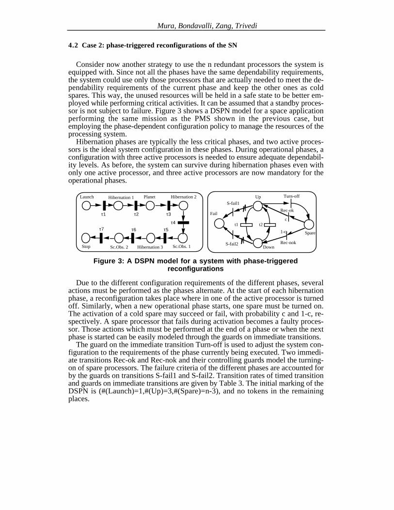
Consider now another strategy to use the n redundant processors the system isequipped with. Since not all the phases have the same dependability requirements,the system could use only those processors that are actually needed to meet the de-pendability requirements of the current phase and keep the other ones as coldspares. This way, the unused resources will be held in a safe state to be better em-ployed while performing critical activities. It can be assumed that a standby proces-sor is not subject to failure. Figure 3 shows a DSPN model for a space applicationperforming the same mission as the PMS shown in the previous case, butemploying the phase-dependent configuration policy to manage the resources of theprocessing system.

Hibernation phases are typically the less critical phases, and two active proces-sors is the ideal system configuration in these phases. During operational phases, aconfiguration with three active processors is needed to ensure adequate dependabil-ity levels. As before, the system can survive during hibernation phases even withonly one active processor, and three active processors are now mandatory for theoperational phases.

Launch Hibernation 1

Sc.Obs. 1

Hibernation 2

Stop

τ1 τ2

τ4τ6τ7

Sc.Obs. 2

Planet

τ3

τ5

Hibernation 3

Up

Down

Fail

S-fail1

S-fail2

t2t1

Spare

Turn-off

Rec-nok

Rec-ok

c

1-c

Figure 3: A DSPN model for a system with phase-triggeredreconfigurations

Due to the different configuration requirements of the different phases, severalactions must be performed as the phases alternate. At the start of each hibernationphase, a reconfiguration takes place where in one of the active processor is turnedoff. Similarly, when a new operational phase starts, one spare must be turned on.The activation of a cold spare may succeed or fail, with probability c and 1-c, re-spectively. A spare processor that fails during activation becomes a faulty proces-sor. Those actions which must be performed at the end of a phase or when the nextphase is started can be easily modeled through the guards on immediate transitions.

The guard on the immediate transition Turn-off is used to adjust the system con-figuration to the requirements of the phase currently being executed. Two immedi-ate transitions Rec-ok and Rec-nok and their controlling guards model the turning-on of spare processors. The failure criteria of the different phases are accounted forby the guards on transitions S-fail1 and S-fail2. Transition rates of timed transitionand guards on immediate transitions are given by Table 3. The initial marking of theDSPN is (#(Launch)=1,#(Up)=3,#(Spare)=n-3), and no tokens in the remainingplaces.

Dependability Modeling and Evaluation of PMS: a DSPN Approach

transition Hibernation Operational Stopt1 λ1#( )Up λ2#( )Up 0

t2 µ#( )Down µ#( )Down 0

S-fail1 #( ) #( )Up Spare+ = 0 #( ) #( )Up Spare+ < 3 FALSE

S-fail2 #( ) #( )Up Spare+ = 0 #( ) #( )Up Spare+ < 3 FALSE

Turn-off #( )Up ≥ 3 #( )Up ≥ 4 FALSE

Rec-ok #( )Up ≤ 1 #( )Up ≥ 2 FALSE

Rec-nok #( )Up ≤ 1 #( )Up ≥ 2 FALSE

Table 3: Transition firing rates and guards for the DSPN of Figure 3

It is worthwhile observing that phase-triggered reconfigurations would compli-cate the treatment of dependencies among phases and the mapping that it involves.Indeed, consider a change from phase i to phase j. In any marking of phase i manyimmediate transitions (reconfigurations) can be triggered as phase j starts, leading todifferent initial markings in the new phase. All those events should be accounted forby the mapping of state probability vector, which must be done at the level of theunderlying marking process, and hence can be a laborious job for large models. Allthe separate modeling methods cited in the previous section basically deal with thisissue in this tedious manner. The single model approaches in [2, 4, 10, 21] solvethe dependencies problem with an implicit mapping which is embedded in themodel. For our single DSPN model approach, the modeling of the mappingbecomes extremely easy, in that it uses the high expressivity of the SRN paradigm.

4.3 Case 3: mission profile depending on SN marking

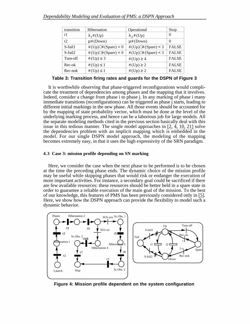
Here, we consider the case when the next phase to be performed is to be chosenat the time the preceding phase ends. The dynamic choice of the mission profilemay be useful while skipping phases that would risk or endanger the execution ofmore important activities. For instance, a secondary goal could be sacrificed if thereare few available resources: these resources should be better held in a spare state inorder to guarantee a reliable execution of the main goal of the mission. To the bestof our knowledge, this features of PMS has been previously considered only in [5].Here, we show how the DSPN approach can provide the flexibility to model such adynamic behavior.

Up

Down

Fail

S-fail1

S-fail2

t2t1

Spare

Turn-off

Rec-nok

Rec-ok

c

1-c

Hibernation 1

Hibernation 4

Stop

τ2 τ5

τ5+τ6

τ7

τ4

τ7

Hibernation 3

SO1-yes

SO1-no

Launch

τ1

Sc.Obs. 1Hibernation 2

τ6

Planet

τ3

Sc.Obs. 2

Sc.Obs. 2

Figure 4: Mission profile dependent on the system configuration

Mura, Bondavalli, Zang, Trivedi

Figure 4 shows the DSPN model for this case. We assume that the secondarygoal, the Scientific Obsevations 1, is to be skipped if the system has less then 4non-failed processors. If we do not consider the place Stop, the PhN net shows atree structure.

transition Hibernation Operational Stopt1 λ1#( )Up λ2#( )Up 0

t2 µ#( )Down µ#( )Down 0

S-fail1 #( ) #( )Up Spare+ = 0 #( ) #( )Up Spare+ < 3 FALSE

S-fail2 #( ) #( )Up Spare+ = 0 #( ) #( )Up Spare+ < 3 FALSE

Turn-off #( )Up ≥ 3 #( )Up ≥ 4 FALSE

Rec-ok #( )Up ≤ 1 #( )Up ≥ 2 FALSE

Rec-nok #( )Up ≤ 1 #( )Up ≥ 2 FALSE

SO1-yes #( ) #( )Up Spare+ ≥ 4

SO1-no #( ) #( )Up Spare+ ≤ 3

Table 4: Transition firing rates and guards for the DSPN of Figure 4

The system-dependent mission profile is easily modeled with the two immediatetransitions SO1-yes and SO1-no, whose enabling conditions depend on the mark-ing of the SN. Table 4 gives all the transition firing rates of timed transitions andthe guards of immediate transitions.

5 Analytical solution

DSPN models of PMS have two properties that allow us to simplify the generalexpression (1) of the transient probability matrix of an MRGP:

Property 1: each of the regeneration points Tn , n≥0 is chosen as the firingtime of a transition having deterministic firing duration.

Property 2: in every non-absorbing marking of the DSPN, there is always onedeterministic transition enabled.

We first tailor the general theory introduced in Section 3 to the case when thePhN has a linear structure, as in cases 1 and 2 of the preceding section, and then weaddress the more general case (as in case 3) when the PhN has a tree structure.

5.1 Linear PhN

Let S denote the state space of the marking process of a DSPN for a PMS havinga PhN with linear structure. Let 1,2,...,n be the ordered sequence of phases

performed through the mission. Let t iDet be the deterministic transition having fir-

ing time τ i which models the time the PMS spends in phase i, i=1,2,...,n, re-spectively.

For any marking rm of the DSPN state space S, let D m( )

r denote the determinis-

tic transition which is enabled in marking rm. Consider the subsets Si of S defined

as follows:

S m S D m t i ni i

Det= ∈ ={ } =r rK( ) , , , , 1 2

Dependability Modeling and Evaluation of PMS: a DSPN Approach

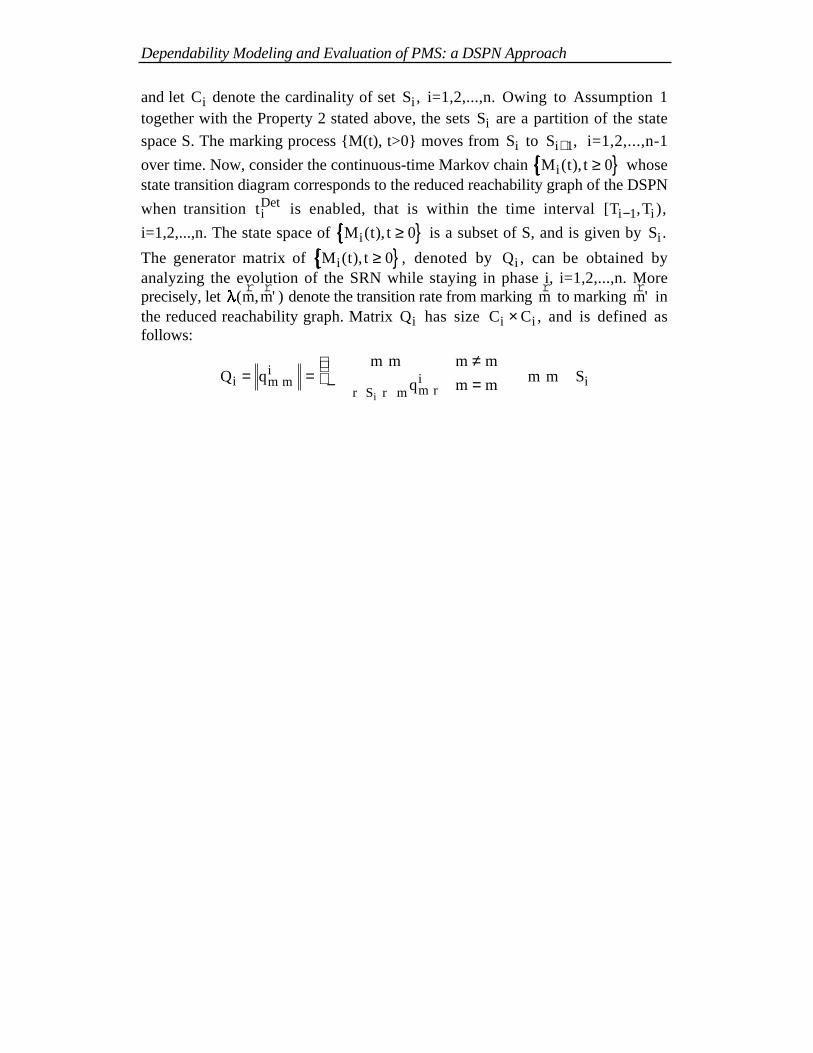
and let Ci denote the cardinality of set Si , i=1,2,...,n. Owing to Assumption 1together with the Property 2 stated above, the sets Si are a partition of the state

space S. The marking process {M(t), t>0} moves from Si to Si+1, i=1,2,...,n-1

over time. Now, consider the continuous-time Markov chain M t ti ( ), ≥{� }0 whosestate transition diagram corresponds to the reduced reachability graph of the DSPN

when transition t iDet is enabled, that is within the time interval [ , )T Ti i−1 ,

i=1,2,...,n. The state space of M t ti ( ), ≥{� }0 is a subset of S, and is given by Si .

The generator matrix of M t ti ( ), ≥{� }0 , denoted by Qi , can be obtained byanalyzing the evolution of the SRN while staying in phase i, i=1,2,...,n. Moreprecisely, let λ� ( , ' )

r rm m denote the transition rate from marking

rm to marking

rm' in

the reduced reachability graph. Matrix Qi has size C Ci i× , and is defined asfollows:

Q qm m m m

q m m m m Si m mi

m ri

r S r mi

i

= =≠

− =

î∈

∈ ≠∑r r

r rr r r

r r r r

r rr r

, ',,

( , ' ) '

' , 'λ

,

Between the regeneration points Ti−1 and Ti , i=1,2,...,n, the evolution of theMRGP underlying the DSPN follows that of the simple continuous-time Markovchain M t ti ( ), ≥{� }0 . Therefore, for any t T Ti i∈ −[ , )1 , the transient probability ma-

trix can be obtained through the exponential of the matrix Qi .Let us define the following branching-probability matrices which account for the

state changes as the deterministic transitions fire. Let ∆ i , i=1,2,...,n-1 be thematrix defined as follows:

∆ i m m

ii i i iob Y m M T m m S m S= = = − = ∈ ∈ +δr r r r r r

, ' Pr [ ' ( ) ], , ' 1

The branching-probability matrix ∆ i has dimension C Ci i× +1 , i=1,2,...,n-1.These matrices can be automatically obtained when the reachability graph is gener-ated.

According to the partition Si , i=1,2,...,n of the state space S, the matrices K(t)

and E(t) can be written in block form K t K ti j( ) ( ),= and E t E ti j( ) ( ),= . The

block matrices K ti j, ( ) and E ti j, ( ), i,j=1,2,...,n have size C Ci j× . We emphasizethat subscript i and j now denote the phase being executed and not individualmarkings of the DSPN. Thus K ti j, ( ) and E ti j, ( ) are submatrices of K(t) and E t( ) ,respectively. They are defined as follows:

K te u t i n j i

i j

Qi i

i i

, ( )( ) ,= − ≤ ≤ − = +

î

τ τ∆ 1 1 1

0

otherwise

E te u t j i

i j

Q ti

i

, ( )( ( ))= − − =

î1

0

τ

otherwisewhere u t i( )− τ is the delayed unit step function defined as u(t)=0 if t i< τ andu(t)=1 if t i≥ τ , i=1,2,...,n. Let us observe that function u t i( )− τ is the cumulativedistribution of the deterministic firing time of transition i, for i=1,2,...,n. Matrices

Mura, Bondavalli, Zang, Trivedi

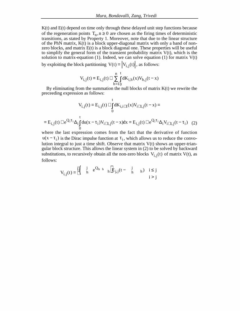
K(t) and E(t) depend on time only through these delayed unit step functions becauseof the regeneration points T nn, ≥ 0 are chosen as the firing times of deterministictransitions, as stated by Property 1. Moreover, note that due to the linear structureof the PhN matrix, K(t) is a block upper-diagonal matrix with only a band of non-zero blocks, and matrix E(t) is a block diagonal one. These properties will be usefulto simplify the general form of the transient probability matrix V(t), which is thesolution to matrix-equation (1). Indeed, we can solve equation (1) for matrix V(t)

by exploiting the block partitioning V t V ti j( ) ( ),= , as follows:

V t E t dK x V t xi j i j i h h j

t

h

n

, , , ,( ) ( ) ( ) ( )= + −∫∑= 01

By eliminating from the summation the null blocks of matrix K(t) we rewrite thepreceeding expression as follows:

V t E t dK x V t xi j i j i i i j

t

, , , ,( ) ( ) ( ) ( )= + − =+ +∫ 1 10

= + − − = + −+ +∫E t e du x V t x dx E t e V ti jQ

i i i j

t

i jQ

i i j ii i i i

, , , ,( ) ( ) ( ) ( ) ( )τ ττ τ∆ ∆10

1 (2)

where the last expression comes from the fact that the derivative of functionu x i( )− τ is the Dirac impulse function at τ i , which allows us to reduce the convo-lution integral to just a time shift. Observe that matrix V(t) shows an upper-trian-gular block structure. This allows the linear system in (2) to be solved by backwardsubstitutions, to recursively obtain all the non-zero blocks V ti j, ( ) of matrix V(t), asfollows:

V t e E t i j

i ji j

Qhj

h j j hhjh h

,,( ) ( )= ( ) − ≤

>

î=−

=−∏ ∑τ τ1

111

0

∆ (3)

where the product over an empty set is intended to be the identity matrix.It is worthwhile observing that evaluating the formula given in (3) to obtain the

transient state probability matrix only requires us to derive matrices eQ th ,h=1,2,...,j and ∆h , h=1,2,...,j-1. The solution of the single DSPN model isreduced to the cheaper problem of deriving the transient probability matrices of a setof homogeneous, time-continuous Markov chains whose state spaces are propersubsets of the whole state space of the marking process. Therefore, Equation (3)provides a highly effective way of solving the single DSPN model of a PMS with alinearly structured mission.

5.2 Tree-like PhN

Now, consider the case when the next phase to be performed can be chosen atthe time the current phase ends, as in case 3 of Section 4. The PhN exhibits a tree-structure, with all the leaves of the tree linked to the place Stop. The solution ofequation (1) is quite similar to the previous case, but it requires a little bit more no-

tation. As before, let 1,2,...,n be the set of phases and t t tDet DetnDet

1 2, , ,K be thecorresponding deterministic transitions. Let f(i) denote the forward phases of phase

Dependability Modeling and Evaluation of PMS: a DSPN Approach

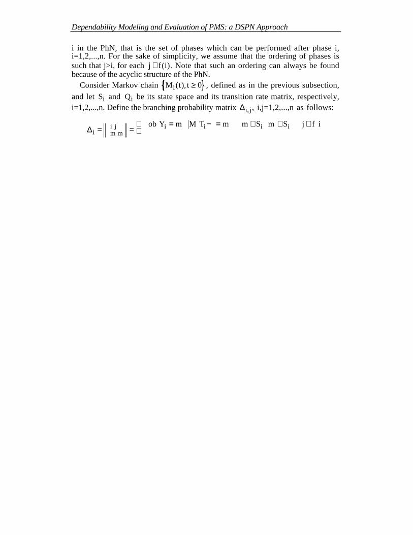
i in the PhN, that is the set of phases which can be performed after phase i,i=1,2,...,n. For the sake of simplicity, we assume that the ordering of phases issuch that j>i, for each j

�f i∈ ( ). Note that such an ordering can always be found

because of the acyclic structure of the PhN.Consider Markov chain M t ti ( ), ≥{� }0 , defined as in the previous subsection,

and let Si and Qi be its state space and its transition rate matrix, respectively,i=1,2,...,n. Define the branching probability matrix ∆ i j, , i,j=1,2,...,n as follows:

∆ i m m

i j i i i iob Y m M T m m S m S j f i= =

= − = ∈ ∈ ∈î

+δr r

r r r r

, ', Pr [ ' ( ) ] , ' , ( )

otherwise1

0According to the partition Si , i=1,2,...,n of the state space S, matrix K(t) can be

written in block form as K t K ti j( ) ( ),= . Each block K ti j, ( ) has size C Ci j× and

is defined as follows:

K t e u t i j ni j

Qi j i

i i, ,( ) ( ), , , , ,= − =τ τ∆ 1 2 K

Note that matrix E(t) which accounts for the local evolution of the MRGP whilewithin a phase remains unchanged. The tree-structure of the PhN still results in ablock upper-diagonal form of matrix K(t), but in this case more non-zero blocksmay appear in each row of the block matrix. Equation (1) can be rewritten as fol-lows:

V t E t dK x V t xi j i j i h h j

t

h

n

, , , ,( ) ( ) ( ) ( )= + − =∫∑= 01

= + − − =∫∑∈

E t e du x V t x dxi jQ

i h i h j

t

h f i

i i, , ,

( )( ) ( ) ( )τ τ∆

0

= + −∈∑E t e V ti j

Qi h h j i

h f i

i i, , ,

( )( ) ( )τ τ∆ (4)

The linear system in (4) can be solved by backward substitutions and a solutioncan be provided as follows by exploiting the acyclic structure of the PhN. Considerthe unique path p(i,j) linking phase i to phase j according to the tree-structure of thePhN. This path is a set of phases p i j p p pr( , ) , , ,= { }1 2 K , where p i1 = , p jr = andp f ph h+ ∈1 ( ), h=1,2,...,r-1. Matrix V ti j, ( ) is then given by the following formula:

V t e E t p i ji j

Qhr

p p j j phrph ph

h h h,, ,( ) ( ) ( , )=

− ≠ ∅

î=−

=−∏ ∑+

τ τ11

11

1

0

∆otherwise

(5)

Formula (5) gives an operative way to evaluate the transient probability matrix ofthe DSPN model through the separate analysis of the various alternative pathswhich compose the mission. The preceding formula (3) can be derived as a particu-lar case of (5).

Mura, Bondavalli, Zang, Trivedi

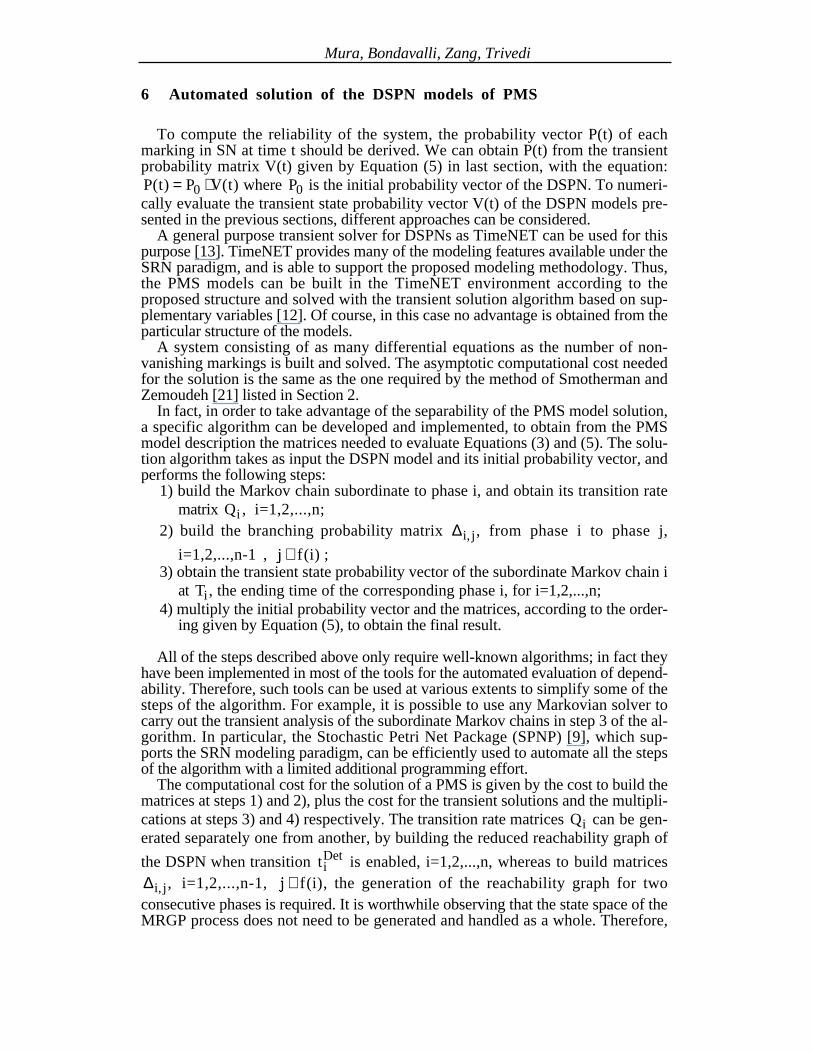
6 Automated solution of the DSPN models of PMS

To compute the reliability of the system, the probability vector P(t) of eachmarking in SN at time t should be derived. We can obtain P(t) from the transientprobability matrix V(t) given by Equation (5) in last section, with the equation:P t P V t( ) ( )= ⋅0 where P0 is the initial probability vector of the DSPN. To numeri-cally evaluate the transient state probability vector V(t) of the DSPN models pre-sented in the previous sections, different approaches can be considered.

A general purpose transient solver for DSPNs as TimeNET can be used for thispurpose [13]. TimeNET provides many of the modeling features available under theSRN paradigm, and is able to support the proposed modeling methodology. Thus,the PMS models can be built in the TimeNET environment according to theproposed structure and solved with the transient solution algorithm based on sup-plementary variables [12]. Of course, in this case no advantage is obtained from theparticular structure of the models.

A system consisting of as many differential equations as the number of non-vanishing markings is built and solved. The asymptotic computational cost neededfor the solution is the same as the one required by the method of Smotherman andZemoudeh [21] listed in Section 2.

In fact, in order to take advantage of the separability of the PMS model solution,a specific algorithm can be developed and implemented, to obtain from the PMSmodel description the matrices needed to evaluate Equations (3) and (5). The solu-tion algorithm takes as input the DSPN model and its initial probability vector, andperforms the following steps:

1) build the Markov chain subordinate to phase i, and obtain its transition ratematrix Qi , i=1,2,...,n;

2) build the branching probability matrix ∆ i j, , from phase i to phase j,

i=1,2,...,n-1 , j�

f i∈ ( ) ;3) obtain the transient state probability vector of the subordinate Markov chain i

at Ti , the ending time of the corresponding phase i, for i=1,2,...,n;4) multiply the initial probability vector and the matrices, according to the order-

ing given by Equation (5), to obtain the final result.

All of the steps described above only require well-known algorithms; in fact theyhave been implemented in most of the tools for the automated evaluation of depend-ability. Therefore, such tools can be used at various extents to simplify some of thesteps of the algorithm. For example, it is possible to use any Markovian solver tocarry out the transient analysis of the subordinate Markov chains in step 3 of the al-gorithm. In particular, the Stochastic Petri Net Package (SPNP) [9], which sup-ports the SRN modeling paradigm, can be efficiently used to automate all the stepsof the algorithm with a limited additional programming effort.

The computational cost for the solution of a PMS is given by the cost to build thematrices at steps 1) and 2), plus the cost for the transient solutions and the multipli-cations at steps 3) and 4) respectively. The transition rate matrices Qi can be gen-erated separately one from another, by building the reduced reachability graph of

the DSPN when transition t iDet is enabled, i=1,2,...,n, whereas to build matrices

∆ i j, , i=1,2,...,n-1, j�

f i∈ ( ), the generation of the reachability graph for twoconsecutive phases is required. It is worthwhile observing that the state space of theMRGP process does not need to be generated and handled as a whole. Therefore,

Dependability Modeling and Evaluation of PMS: a DSPN Approach

the overall computational cost of the algorithm sketched above is dominated by theoperations at the steps 3) and 4), which require the same cost as the one for theseparate approaches listed in Section 2. Thus, with our single model approach weare able to deal with all the scenarios of PMS that have been analytically treated inthe literature, at a cost which is comparable with that of the cheapest ones. The is-sues posed by the phased-behaviour of PMS are completely solved by our method,whose applicability is only limited by the size of the biggest Petri net model whichcan be handled by the automated tool.

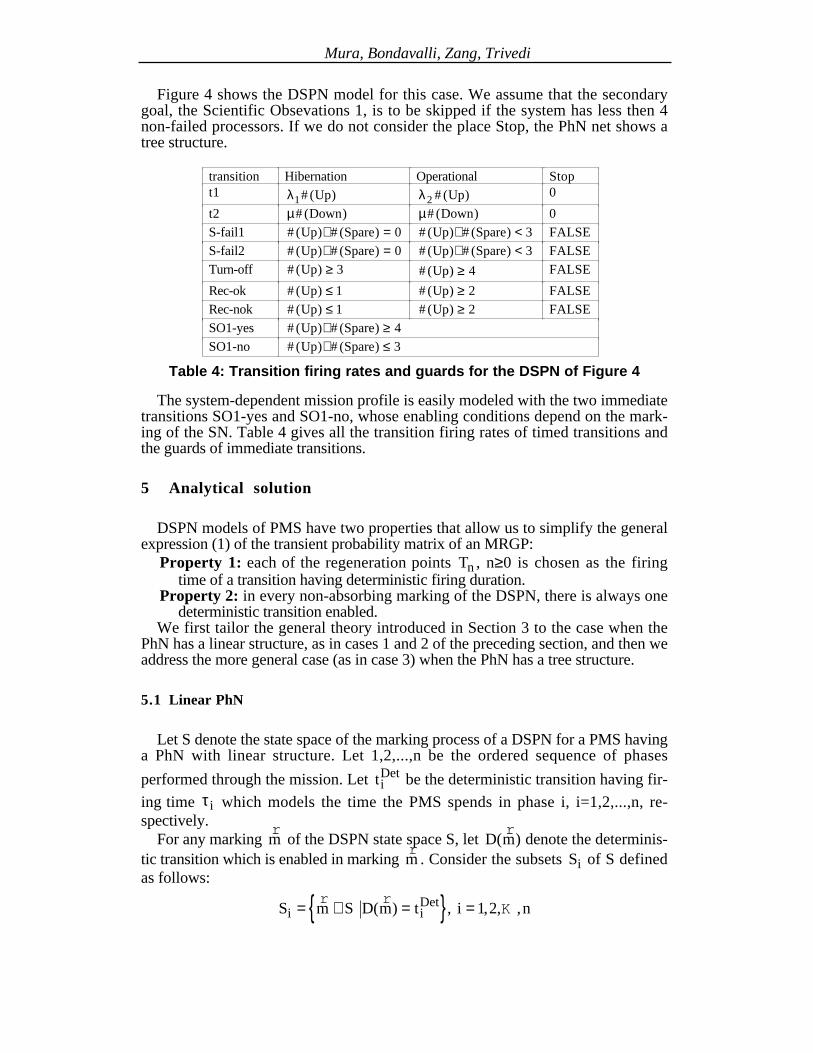
We show now a set of experimental evaluations for the application example givenin subsection 4.3, assuming the system has 4 nodes, obtained by directlyimplementing the four steps of the algorithm listed above. We evaluate the proba-bility that the system succesfully completes its mission, that is the reliability of thePMS at the end of the mission time, varying the values of the relevant system pa-rameters, that is the failure rate λ, the repair rate µ and the probability of successfulspare insertion c.

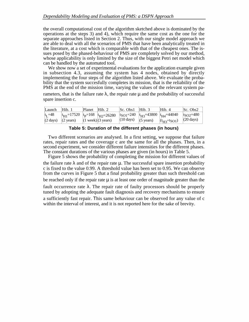
Launch Hib. 1 Planet Hib. 2 Sc. Obs1 Hib. 3 Hib. 4 Sc. Obs2tL=48

(2 days)

tH1=17520

(2 years)

tP=168

(1 week)

tH2=26280(3 years)

tSO1=240(10 days)

tH3=43800

(5 years)

tH4=44040

(tH3+tSO1)

tSO2=480(20 days)

Table 5: Duration of the different phases (in hours)

Two different scenarios are analysed. In a first setting, we suppose that failurerates, repair rates and the coverage c are the same for all the phases. Then, in asecond experiment, we consider different failure intensities for the different phases.The constant durations of the various phases are given (in hours) in Table 5.

Figure 5 shows the probability of completing the mission for different values ofthe failure rate λ and of the repair rate µ. The successful spare insertion probabilityc is fixed to the value 0.99. A threshold value has been set to 0.95. We can observefrom the curves in Figure 5 that a final probability greater than such threshold canbe reached only if the repair rate µ is at least one order of magnitude greater than the

fault occurrence rate λ. The repair rate of faulty processors should be properlytuned by adopting the adequate fault diagnosis and recovery mechanisms to ensurea sufficiently fast repair. Τhis same behaviour can be observed for any value of cwithin the interval of interest, and it is not reported here for the sake of brevity.

Mura, Bondavalli, Zang, Trivedi

0.85

0.875

0.9

0.925

0.95

0.975

1

1.00E-07 1.00E-06 1.00E-05 1.00E-04 1.00E-03

µ=10Ε−2µ=10Ε−3µ=10Ε−4µ=10Ε−5

λ

p(Mission completion)

Figure 5: Probability of completing the mission for different values offault and repair rates

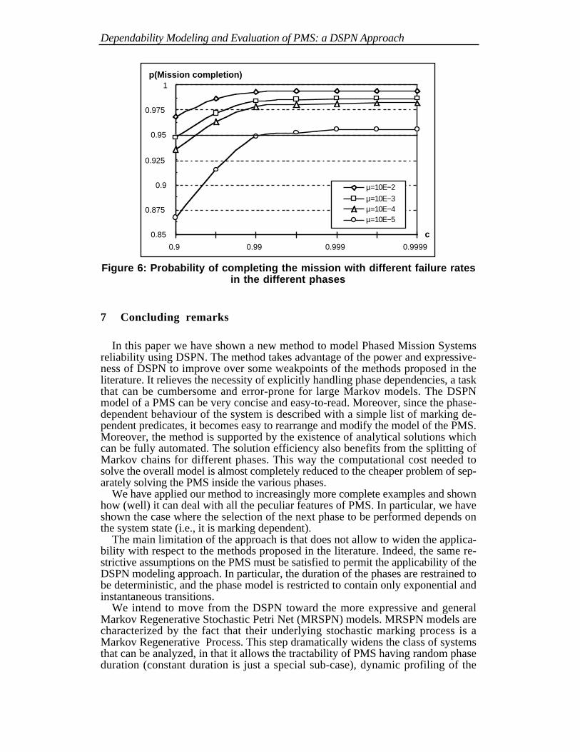
In our second evaluation we consider different failure rates in the differentphases. Changes of the processor failure rates are due to increased environmentalstresses. Thus during the most stressing phase (Scientific Observations 2) the sys-tem is subject to an higher fault rate, while during the Hibernation phases a lowerfault rate is assumed. Values assigned to the failure rate λ in the different phases aregiven in Table 6.

Launch Hibernation Planet Sc. Obs1 Sc. Obs.2

λ =10-5 λ =10-6 λ =10-5 λ =10-5 λ =10-4

Table 6: Fault occurrence rates in the different phases

Figure 6 shows the results of this evaluation for different values of the spare in-sertion probability c and the repair rate µ. The Figure shows that the probability ofcompleting the mission improves rather quickly for low values of c (for any valueof µ). In fact, passing from 0.9 to 0.99 it reaches acceptable values for three of thefour curves. The probability of completing the mission becomes less sensitive tovariations of c in the right part of the figure: passing from 0.99 to 0.9999 veryslight variations can be observed.

Dependability Modeling and Evaluation of PMS: a DSPN Approach

0.85

0.875

0.9

0.925

0.95

0.975

1

0.9 0.99 0.999 0.9999

µ=10Ε−2µ=10Ε−3µ=10Ε−4µ=10Ε−5

c

p(Mission completion)

Figure 6: Probability of completing the mission with different failure ratesin the different phases

7 Concluding remarks

In this paper we have shown a new method to model Phased Mission Systemsreliability using DSPN. The method takes advantage of the power and expressive-ness of DSPN to improve over some weakpoints of the methods proposed in theliterature. It relieves the necessity of explicitly handling phase dependencies, a taskthat can be cumbersome and error-prone for large Markov models. The DSPNmodel of a PMS can be very concise and easy-to-read. Moreover, since the phase-dependent behaviour of the system is described with a simple list of marking de-pendent predicates, it becomes easy to rearrange and modify the model of the PMS.Moreover, the method is supported by the existence of analytical solutions whichcan be fully automated. The solution efficiency also benefits from the splitting ofMarkov chains for different phases. This way the computational cost needed tosolve the overall model is almost completely reduced to the cheaper problem of sep-arately solving the PMS inside the various phases.

We have applied our method to increasingly more complete examples and shownhow (well) it can deal with all the peculiar features of PMS. In particular, we haveshown the case where the selection of the next phase to be performed depends onthe system state (i.e., it is marking dependent).

The main limitation of the approach is that does not allow to widen the applica-bility with respect to the methods proposed in the literature. Indeed, the same re-strictive assumptions on the PMS must be satisfied to permit the applicability of theDSPN modeling approach. In particular, the duration of the phases are restrained tobe deterministic, and the phase model is restricted to contain only exponential andinstantaneous transitions.

We intend to move from the DSPN toward the more expressive and generalMarkov Regenerative Stochastic Petri Net (MRSPN) models. MRSPN models arecharacterized by the fact that their underlying stochastic marking process is aMarkov Regenerative Process. This step dramatically widens the class of systemsthat can be analyzed, in that it allows the tractability of PMS having random phaseduration (constant duration is just a special sub-case), dynamic profiling of the

Mura, Bondavalli, Zang, Trivedi

mission and the modeling of multiple concurrent non-exponential activities.Actually, the class of DSPN is merely a subset of MRSPN. We intend to exploitthe peculiar characteristics of PMS to tailor the general transient analysis method forMRGP [8], to obtain computationally efficient solution algorithms for MRSPNmodels of PMS. Moreover, the existence of an analytic solution for the transientprobability distribution of the MRGP also allows us to perform the sensitivity anal-ysis of PMS, a topic that has not yet been addressed in the literature.

Acknowedgments

This research was supported in part by the NC-ACTS under an enhancementproject to the Center for Advanced Computing and Communications in DukeUniversity, and in part by the European Commission in the framework of ESPRITProject 20716 GUARDS — Generic Upgradable Architecture for Real-TimeDependable Systems. GUARDS is carried out by a consortium consisting of:Technicatome (France), Ansaldo Segnalamento Ferrovario (Italy), Matra MarconiSpace (France), Intecs Sistemi (Italy), Siemens AG Osterreich PSE (Austria),LAAS-CNRS (France), Pisa Dependable Computing Centre (Italy) and theUniversity of York (UK).

References

[1] M. Ajmone Marsan and G. Chiola, “On Petri nets with deterministic and exponentiallydistributed firing times,” in “Lecture Notes in Computer Science 266”, Ed., Springer-Verlag,1987, pp. 132-145.

[2] M. Alam and U. M. Al-Saggaf, “Quantitative Reliability Evaluation of Reparaible Phased-Mission Systems Using Markov Approach,” IEEE Transactions on Reliability, Vol. R-35,pp. 498-503, 1986.

[3] J. Arlat, T. Eliasson, K. Kanoun, D. Noyes, D. Powell and J. Torin, “Evaluation of Fault-Tolerant Data Handling Systems for Spacecraft: Measures, Techniques and ExampleApplications,” LAAS-CNRS November 1986.

[4] B.E. Aupperle, J.F. Meyer and L. Wei, “Evaluation of fault-tolerant systems with non-homogeneous workloads,” in Proc. 19th IEEE Fault Tolerant Computing Symposium(FTCS-19), 1989, pp. 159-166.

[5] A. Bondavalli, I. Mura and M. Nelli, “Analytical Modelling and Evaluation of Phased-Mission Systems for Space Applications,” in Proc. IEEE High Assurance SystemEngineering Workshop (HASE’97), Bethesda Maryland, USA, 1997, pp. 85 - 91.

[6] J.L. Bricker, “A unified method for analizing mission reliability for fault tolerant computersystems,” IEEE Trans. on Reliability, Vol. R-22, 1973.

[7] G. R. Burdick, J. B. Fussell, D. M. Rasmuson and J. R. Wilson, “Phased Mission Analysis:A review of New Developments and An Application,” IEEE Transactions on Reliability,Vol. R-26, pp. 43-49, 1977.

[8] H. Choi, V.G. Kulkarni and K.S. Trivedi, “Transient analysis of deterministic and stochasticPetri nets.,” in Proc. 14th International Conference on Application and Theory of Petri Nets,Chicago Illinois, USA, 1993, pp. 166-185.

[9] G. Ciardo, J. Muppala and K.S. Trivedi, “Spnp: Stochastic Petri net package.,” in Proc.International Conference on Petri Nets and Performance Models, Kyoto, Japan, 1989.

[10] J. B. Dugan, “Automated Analysis of Phased-Mission Reliability,” IEEE Transaction onReliability, Vol. 40, pp. 45-52, 1991.

[11] J.D. Esary and H. Ziehms, “Reliability analysis of phased missions.,” in “Reliability andfault tree analysis”, Ed., SIAM Philadelphia, 1975, pp. 213--236.

Dependability Modeling and Evaluation of PMS: a DSPN Approach

[12] R. German, “Transient analysis of deterministic and stochastic Petri nets by method ofsupplementary variables.,” in Proc. MASCOTS ‘95, Durham, NC, 1995.

[13] R. German, C. Kelling, A. Zimmermann and G. Hommel, “TimeNET: a toolkit forevaluating non-Markovian stochastic Petri nets.,” Performance Evaluation, Vol. 24, pp.1995.

[14] V.G. Kulkarni, “Modeling and analysis of stochastic systems,” Chapman-Hall, 1995.[15] C. Lindemann, “Performance modeling using DSPNexpress,” in Proc. Tool Descriptions of

PNPM’97, Saint-Malo, France, 1997.[16] J.F. Meyer, D.G. Furchgott and L.T. Wu, “Performability Evaluation of the SIFT

Computer,” in Proc. IEEE FTCS’79 Fault-Tolerant Computing Symposium, June20-22,Madison, Wisconsin, USA, 1979, pp. 43-50.

[17] A. Pedar and V. V. S. Sarma, “Phased-Mission Analysis for Evaluating the Effectiveness ofAerospace Computing-Systems,” IEEE Transactions on Reliability, Vol. R-30, pp. 429-437,1981.

[18] A. Puliafito, M. Scarpa and K.S. Trivedi, “Petri nets with k simultaneously enabledgenerally distributed timed transitions,” Performance Evaluation, 1997.

[19] A. Reibman and K.S. Trivedi, “Numerical transient analysis of Markov models,” Computersand Operation Research, Vol. 15, pp. 19-36, 1988.

[20] W.H. Sanders and J.F. Meyer, “METASAN: a performability evaluation tool based onstochastic activity networks,” in Proc. ACM-IEEE Comp. Soc. 1986 Fall Joint Comp.Conf., Dallas TX, 1986, pp. 807--816.

[21] M. Smotherman and K. Zemoudeh, “A Non-Homogeneous Markov Model for Phased-Mission Reliability Analysis,” IEEE Transactions on Reliability, Vol. 38, pp. 585-590,1989.

[22] A. K. Somani, J. A. Ritcey and S. H. L. Au, “Computationally-Efficent Phased-MissionReliability Analysis for Systems with Variable Configurations,” IEEE Transactions onReliability, Vol. 41, pp. 504-511, 1992.

[23] A. K. Somani and K. S. Trivedi, “Phased-Mission Systems Using Boolean AlgebraicMethods,” Performance Evaluation Review, Vol. pp. 98-107, 1994.

[24] H.S. Winokur and L.J. Goldstein, “Analysis of mission oriented systems,” IEEE Trans. onReliability, Vol. R-18, pp. 144-148, 1969.