Hierarchical Large-scale Volume Representation with3�

2 Subdivision and Trivariate B-spline Wavelets

Lars Linsen � Jevan T. Gray � Valerio Pascucci† Mark A. Duchaineau† Bernd Hamann �Kenneth I. Joy �

� Center for Image Processing and Integrated Computing † Center for Applied Scientific ComputingUniversity of California, Davis‡ Lawrence Livermore National Laboratory

���������� ��

Multiresolution methods provide a means for representing data atmultiple levels of detail. They are typically based on a hierarchicaldata organization scheme and update rules needed for data valuecomputation. We use a data organization that is based on what wecall n

�2 subdivision. The main advantage of n

�2 subdivision, com-

pared to quadtree (n � 2) or octree (n � 3) organizations, is that thenumber of vertices is only doubled in each subdivision step insteadof multiplied by a factor of four or eight, respectively. To updatedata values we use n-variate B-spline wavelets, which yield betterapproximations for each level of detail. We develop a lifting schemefor n � 2 and n � 3 based on the n

�2-subdivision scheme. We ob-

tain narrow masks that provide a basis for out-of-core techniquesas well as view-dependent visualization and adaptive, localized re-finement.

CR Categories: I.3.5 [Computer Graphics]: Computational Ge-ometry and Object Modeling Project—; J [Computer Applications]:Physical Sciences and Engineering—Life and Medical Science

Keywords: hierarchical volume modeling, subdivision, B-splinewavelets, lifting, multiresolution modeling, data approximation

� ��� �������� ������ �

Multiresolution schemes are used in computer graphics mainly forediting and rendering curves and surfaces at multiple levels of reso-lution. While most existing schemes could, in principle, be general-ized for higher-dimensional data, only a few have been extended todata (or functions) defined over three- or even higher-dimensionaldomains. The combined subdivision-wavelet scheme we are de-scribing in this paper is driven by the need to represent trivariatedata (or functions) at multiple resolution levels for scientific visu-alization.

Representing volume data hierarchically is important in the con-text of “volume modeling” and visualizing volume data, e.g., scalaror vector fields defined over volumetric domains. Visualizing in-herently trivariate phenomena often requires one to apply renderingoperations to volumetric data - examples being volume slicing viaa cutting plane, isosurface extraction through marching-cubes-likealgorithms, and ray casting. The multiresolution approximation ap-proach we describe in this paper provides an elegant means of hi-erarchically organizing volume data, and we can use the resulting

�llinsen@ucdavis.edu, grayj,hamann,joy ! @cs.ucdavis.edu

† pascucci1,duchaineau1 ! @llnl.gov‡http://graphics.cs.ucdavis.edu

hierarchy to apply to its various levels volume data visualizationmethods.

We combine n�

2 subdivision with n-variate B-spline wavelets forn-dimensional multiresolution data representation. Multiresolutionschemes have been studied extensively over the past decade. A sur-vey of the main multiresolution approaches, considering also topo-logical constraints, is given by Kobbelt in [11]. These approachescan, for example, be used for a multiresolution representation ofisosurfaces. However, when considering (bio-)medical imagingdata, for instance, we must be able to switch quickly between iso-surfaces corresponding to different isovalues, and when consider-ing, for example, numerically simulated time-dependent hydrody-namics data, we even have to deal with isosurfaces changing overtime. It is undesirable to store every single isosurface for all pos-sibly important isovalues at different resolutions and load themduring visualization. Instead, we devise a multiresolution volumedata representation. We first develop a bivariate B-spline waveletscheme for

�2 subdivision and then generalize it to a trivariate B-

spline wavelet scheme for 3�

2 subdivision. We have applied ourtechniques to bivariate as well as volumetric data.

For large-scale multiresolution representation, one should useregular rather than irregular data structures, since grid connectiv-ity is implicit and data access simple for regular data. To overcomeregular data structures’ disadvantage of coarse granularity, we havedeveloped the n

�2-subdivision scheme we discuss in Section 3. Ev-

ery n�

2-subdivision step only doubles the number of vertices, whichis a factor of n

�2 in each of the n dimensions.

When using a wavelet scheme, the data value at a vertex p is up-dated when changing the level of detail, and thus the value varieswith varying level of detail. On a coarse level, the value repre-sents the value at p itself as well as an average value of a certainregion around p. This approach leads to better approximationson coarser levels. Wavelets based on the n

�2-subdivision scheme

unfortunately have the disadvantage of creating over- and under-shoots. For example, for isosurface extraction (n � 3) this charac-teristic can cause creation of isosurfaces (or isosurface components)that vanish when increasing the resolution. Therefore, we use n-variate B-spline wavelets and adjust them to the n

�2-subdivision

scheme.

B-spline wavelets have the property that they do not only influ-ence the neighbors of a vertex p. Thus, when using out-of-coretechniques to operate on or visualize large-scale data, a lot of datamust be loaded from external memory with low I/O-performance.Furthermore, the adaptivity for view-dependent refinement tech-niques is restricted. Lifting schemes with narrow filters can be usedto overcome this problem. We review and generalize the liftingscheme from [3] in Section 4. In Sections 5 and 7, we develop asimilar lifting scheme for the n

�2-subdivision scheme for n � 2 and

n � 3. We provide results in Sections 6 and 8.

� ����� � � � ��� � �

Multiresolution volume representation is based on a three-dimensional hierarchical data organization of irregular or regulartype. Irregular data structures, see [4, 8, 7], use non-uniform refine-ment steps, which makes them highly adaptive. On the other hand,grid information must be stored and data access is not straight-forward. Especially for large-scale data, additional memory re-quirements and memory organization needs are a major disadvan-tage of irregular structures.

Concerning regular data organizations, octrees, see [14, 18, 22,25, 32]; and sometimes tetrahedral grids are used, see [18]. Forregular structures grid connectivity is implicit and data is easilyand quickly accessed. However, the refinement steps have to con-form to the topological constraints, which makes regular structuresless adaptive. To overcome this disadvantage, we use the 3

�2-

subdivision scheme, a regular data organization supporting finergranularity. While, for example, an octree refinement step doublesthe number of vertices in every dimension, which leads to a fac-tor of eight, a 3

�2-subdivision step only doubles the overall number

of vertices. Therefore, 3�

2 subdivision will, in general, require lessvertices than octrees to satisfy specified image quality error bounds.Since finer granularity leads to higher adaptivity this fact still holdswhen using adaptive refinement techniques.

The splitting step of the n�

2-subdivision scheme goes back to Co-hen and Daubechies [5] for n � 2 and Maubach [16] for arbitraryn. It can be described by using triangular as well as quadrilateralmeshes (n � 2) or their counterparts for higher dimensions. In thefollowing, we will consider the quadrilateral case and its general-ization.

The refinement step of the approaches described in [6, 20, 33]is a longest-edge bisection applied to tetrahedral meshes. This stepis equivalent to the splitting step of the 3

�2-subdivision scheme.

However, these approaches do not represent a full subdivisionscheme, since the averaging step is missing. Thus, these schemesare restricted to structured-rectilinear grids, where eight cuboidsshare a common vertex, and the cuboids have the same size. The3�

2-subdivision scheme also applies to structured-curvilinear grids,where hexahedra of arbitrary shape (but with linear edges) are usedinstead of cuboids. The scheme could even handle extraordinaryvertices.

Recently, Velho and Zorin [30] introduced�

2-subdivision sur-faces (n � 2) by adding an averaging step. They showed that theproduced surfaces are C4-continuous at regular and C1-continuousat extraordinary vertices. (For an introduction to subdivision meth-ods, we refer to [31].)

The main advantage of wavelet schemes is the fact that they pro-vide a means to generate best approximations in a multiresolutionhierarchy. Stollnitz et al. [26] described how to generate waveletsfor subdivision schemes. However, n

�2-subdivision wavelets can

lead to over- and undershoots, see Figure 7(b), which are especiallydisturbing when extracting isosurfaces from different levels of ap-proximation. They can even cause topological changes of isosur-faces when changing the level of resolution. Therefore, we have de-cided to generate B-spline wavelets for the n

�2-subdivision scheme,

which are known to produce good approximations. (For an intro-duction to B-spline techniques, we refer to [23].)

The computation of wavelet coefficients at a certain vertex forwavelets with good approximation quality like B-spline waveletsis not limited to using only adjacent vertices. Localization, how-ever, is strongly desirable when we want to apply the waveletscheme to adaptive refinement and to out-of-core visualization tech-niques. Lifting schemes as introduced by Sweldens [27] decomposewavelet computations into several steps, but they assert narrow fil-ters, see Figure 6. Bertram et al. [2, 3] defined a lifting schemefor one- and two-dimensional B-spline wavelets using a quadtree

organization of the vertices.Wavelets for general dilation matrices go back to Riemenschnei-

der and Shen [24] who used a box-spline approach. Kovacevic andVetterli [13] and, more recently, Uytterhoeven [29] and Kovacevicand Sweldens [12] developed lifting schemes that can be applied ton�

2-subdivision data structures. Uytterhoeven [29] only addressedthe two-dimensional case. In [12], the filters that produce good ap-proximations are not narrow enough for our purposes. On the otherhand, the update rule for the narrow filters in [12] is the identity,which does not support the creation of good approximations.

Another main difference between our approach and the non-separable filters used in [29] and [12] is the update rule. For exam-ple, we update the vertices in a 3

�2-subdivision scheme by apply-

ing first the three-, then the two-, and finally the one-dimensionalupdate rules. This approach automatically includes the boundarycases, which are not sufficiently addressed in [29] and [12]. More-over, the generalization to arbitrary dimension n is straight-forward.

� ��� n�

2 � � � � � ��� ��� ��� � � �������

We first describe the case n � 2. For a�

2-subdivision step of aquadrilateral Q, we compute its centroid c, and connect c to all fourvertices of Q. The “old” edges of the mesh are removed (exceptfor the edges determining the mesh/domain boundary). Figure 1illustrates four

�2-subdivision steps.

cQ

Figure 1:�

2 subdivision.

The mask used for the computation of the centroid c is given inFigure 2(a). Figure 2(b) shows the mask of the averaging step ac-cording to [30]. A

�2-subdivision step is executed by first applying

the mask shown in Figure 2(a), which inserts the new vertices, andthen (after the topological mesh modifications) applying the maskshown in Figure 2(b), which repositions the old vertices.

(a)14

14

14

14 (b)

12

18

18

18

18

Figure 2: Masks of�

2-subdivision step: (a) inserting centroid; (b)repositioning old vertices.

This subdivision scheme for quadrilaterals is analogous to the�3-subdivision scheme of Kobbelt [10] for triangles. Therefore,

we call it�

2 subdivision.We now generalize the subdivision scheme to n

�2 subdivision for

arbitrary dimension n. The splitting step is executed by insertingthe centroid and adjusting vertex connectivity. The averaging stepapplies to every old vertex v the update rule

v � αv ��� 1 � α � w �where w is the centroid of the adjacent new vertices.

We are especially interested in the case n � 3. Little research hasbeen done to date concerning three-dimensional (volumetric) sub-division. One example is the work described in [15]. The literaturecurrently provides no analysis of averaging steps for dimensions

larger than two. Thus, at present, we cannot provide a solution forthe choice of α used in the update rule. Some investigations aboutapplying the update rule in arbitrary dimensions were made by Pas-cucci in [19].

When applying the 3�

2-subdivision scheme to large volumet-ric data sets, we usually deal with structured-rectilinear grids,especially when considering imaging data sets. For structured-rectilinear grids, the update rule does not change the position of thevertices regardless of the specific α value, but it only affects the val-ues at the vertices. In Section 6, we show that the

�2-subdivision

wavelets are not appropriate for our purposes, and we replace themby B-spline wavelets. Therefore, we do not need to choose a valuefor α .

In Figure 3, three 3�

2-subdivision steps are shown. In each step,the centroids of the polyhedral shapes are inserted, and the connec-tivity is adjusted. Three kinds of polyhedral shapes arise. They areshown in Figure 4.

In the first step, each cuboid (first picture of Figure 3 / thirdpicture of Figure 4) is subdivided by inserting the cuboid’s cen-troid and connecting the centroid to all old vertices (second pictureof Figure 3). In the second step, each octahedron (first picture ofFigure 4) is subdivided by inserting the octahedron’s centroid andconnecting the centroid to all old vertices, while all old edges, ex-cept the (red) edges inserted in the last subdivision step, are deleted(third picture of Figure 3). In the third step, each octahedron withsplit faces (second picture of Figure 4) is subdivided by inserting itscentroid and connecting the centroid to all old vertices, except the(red) vertices inserted in the next-to-the-last subdivision step, whileall old edges, except the edges between the (red) vertices insertedin the next-to-the-last subdivision step and the (green) vertices in-serted in the last step, are deleted (fourth picture of Figure 3).

The three subdivision steps can also be described in the follow-ing way: The first step inserts the centroid of the cuboid, the secondstep inserts the centers of the faces of the original cuboid, and thethird step inserts the midpoints of the edges of the original cuboid.Three 3

�2-subdivision steps produce the same result as one octree

refinement step. Hence, for multiresolution purposes, we obtaina much finer granularity through 3

�2 subdivision. We can thus

approximate much more closely a required level of mesh-elementsize. Therefore, it is likely that one must render much less data toobtain a desired image / visualization quality.

� � ����� � ��� � � ��� � � � ����� � � ������� ��� � ����� �

In this section, we review and define masks for the one-dimensionallifting scheme of [2] and generalize them to the two- and three-dimensional cases. In the following sections, we will adjust thetwo-dimensional lifting scheme to

�2 subdivision and the three-

dimensional lifting scheme to 3�

2 subdivision.The one-dimensional B-spline wavelet lifting scheme makes use

of two operations that are defined by the following two masks,called s-lift and w-lift:

s-lift � a � b � : a b a � (1)

w-lift � a � b � : a b a �� (2)

The s-lift mask is applied to the old vertices (black) and their newneighbors (blue), whereas the w-lift mask is applied to the new ver-tices (blue) and their neighbors (black), see Figure 5(a). For a de-tailed derivation of the lifting scheme that we use as a basis for thispaper, as well as for its analysis (smoothness, stability, approxima-tion order, and zero moments), we refer to [1].

Using the s-lift and w-lift masks, a linear B-spline wavelet en-

(a) (b)

���

���� ������ ��

���� ��

�� (c)

! " #$%!%& '!'()!)*+!+,!,

-!-./!/0 1234 5!567!78

9!9: ;!;<=!=> ?!?@!@ A!ABC!CDE!EF G!GH!HI!IJ K!KLM!MN O!OP Q!QR!R S!ST

U!UVFigure 5: Refinement step for one-, two-, and three-dimensionalmeshes.

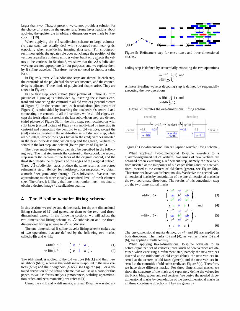
coding step is defined by sequentially executing the two operations

w-lift � � 12 � 1 � and

s-lift � 14 � 1 � �A linear B-spline wavelet decoding step is defined by sequentiallyexecuting the two operations

s-lift � � 14 � 1 � and

w-lift � 12 � 1 � �Figure 6 illustrates the one-dimensional lifting scheme.

w−lift

−0.5

waveletcoeff.

level n−

encoding

s−lift s−lift

w−lift

−0.250.25

11

1 1

decoding

0.5nlevel level n

1

Figure 6: One-dimensional linear B-spline wavelet lifting scheme.

When applying two-dimensional B-spline wavelets to aquadtree-organized set of vertices, two kinds of new vertices areobtained when executing a refinement step, namely the new ver-tices inserted at the midpoints of old edges (blue) and the new ver-tices inserted at the centers of old faces (green), see Figure 5(b).Therefore, we have two different masks. We derive the needed two-dimensional masks by convolution of the one-dimensional masks inthe two coordinate directions. The results of this convolution stepare the two-dimensional masks

s-lift � a � b � :

WXa2 ab a2

ab b2 aba2 ab a2

YZ� (3)

a b a and (4)

w-lift � a � b � :

WXa2 ab a2

ab b2 aba2 ab a2

YZ� (5)

a b a �� (6)

The one-dimensional masks defined by (4) and (6) are applied inboth directions. The masks (3) and (4), as well as masks (5) and(6), are applied simultaneously.

When applying three-dimensional B-spline wavelets to anoctree-organized set of vertices, three kinds of new vertices are ob-tained when executing a refinement step, namely the new verticesinserted at the midpoints of old edges (blue), the new vertices in-serted at the centers of old faces (green), and the new vertices in-serted at the centroids of old cubes (red), see Figure 5(c). Therefore,we have three different masks. For three-dimensional masks, weshow the structure of the mask and separately define the values forthe black, blue, green, and red vertices. We derive the needed three-dimensional masks by convolution of the one-dimensional masks inall three coordinate directions. They are given by

�� ������ �

�

�

��

�� ���� ����

��

��

��

!"#

$% &'()

*+

,- ./010234

56 78 9: ;<=> ?@ AB CDEF GH IJ KL MN OP QR S1ST

UV WXYZ [\

]^_`

abcdef

ghij

klmn

opqrs1stuv

Figure 3: 3�

2 subdivision.

wxyz {|

}~

���� ���� ��

��

�1�� ����

���1�� ����

��

����

� ¡¢

£¤ ¥¦

Figure 4: Polyhedral shapes created by 3�

2 subdivision: octahedron, octahedron with split faces, and cuboid.

§¨§©¨© ª¨ª«¬¨¬­¨­ ®¨®¯°¨°±

²¨²³

´¨´µ¨µ

¶¨¶·¨·

¸¨¸¹¨¹º¨º»

¼¨¼½ ¾¨¾¿À¨ÀÁ

¨Âà ĨÄÅ

ƨÆÇ¨Ç È¨ÈɨÉʨÊĘ̈ÌͨÍ

ΨÎÏ¨Ï Ð¨ÐѨÑÒ¨ÒÓ¨Ó Ô¨ÔÕ

Ö¨Öר×بØÙ¨Ù

Ú¨ÚÛ¨ÛܨÜÝ

ÞÞÞÞÞÞÞÞÞÞÞ

s-lift � a � b � :

b3

ab2

a2b �a3

(7)

WXa2 ab a2

ab b2 aba2 ab a2

YZ� (8)

a b a and (9)

ߨßà¨à á¨áâã¨ãä¨ä å¨åæç¨çè

é¨éê

ë¨ëì¨ì

í¨íî¨î

ï¨ïð¨ðñ¨ñò

ó¨óô õ¨õö÷¨÷ø

ù¨ùú û¨ûü

ý¨ýþ¨þ ÿ¨ÿ�������������

������ ����

���� ���

������

������������

����

�����������

w-lift � a � b � :

a3

a2bab2 �b3

(10)

WXa2 ab a2

ab b2 aba2 ab a2

YZ� (11)

a b a � (12)

� � � ��� ��� � � � ����� � ��� �2� � � � ��� ��� ��� �

Using�

2 subdivision instead of a quadtree-based scheme, we onlyobtain new vertices at the centers of old faces (green) when exe-cuting a subdivision step; at the midpoints of old edges (blue), novertices are inserted, see second picture in Figure 1 and compare toFigure 5(b). Thus, no data is available at the positions of the bluevertices, and we must adjust the two-dimensional masks (3) and (5).

For encoding with linear B-spline wavelets, the w-lift operationis executed first. Since we have no values at the blue positionsrequired for mask (5), we linearly interpolate the values at theblack vertices. Linear interpolation is appropriate, since we areusing linear wavelets. This approach changes mask (5) to

w-liftencode � a � b � :

WXa2 � ab a2 � ab

b2

a2 � ab a2 � ab

YZ� (13)

Next, the s-lift operation is executed. Again, we have entries atthe blue positions in mask (3). However, the w-lift operation has(theoretically) executed mask (6), and we assumed that the values

at the blue vertices were linear interpolations of the values atthe black vertices; therefore, the values at the blue vertices havevanished. Mask (3) changes to

s-liftencode � a � b � :

WXa2 a2

b2

a2 a2

YZ� (14)

For decoding, we first execute the s-lift operation. Prior toexecuting the s-lift operation of the encoding, the values at theblue vertices have vanished, but the s-lift operation (theoretically)executed mask (4). Hence, the values at the blue vertices are nowgiven by linear interpolation of the values at the green neighborvertices multiplied by the factor 2a of mask (4). We rename thefactor a to a and derive from mask (3) the new mask

s-liftdecode � a � b � :

WXa2 � 2aab a2 � 2aab

b2

a2 � 2aab a2 � 2aab

YZ� (15)

Finally, the w-lift operation is executed again. The s-lift decodingoperation has (theoretically) applied mask (4). Since mask (4) ap-plied by the s-lift decoding operation is the inverse of mask (4) ap-plied by the s-lift encoding operation, the values at the blue verticesare the same as before the execution of these two s-lift operations,i. e., they vanish. These considerations define a new mask derivedfrom mask (5), given by

w-liftdecode � a � b � :

WXa2 a2

b2

a2 a2

YZ� (16)

In the two-dimensional case, the masks are as narrow as they canbe.

� ��� � � � ��� ��� � ��� ��� � � �

In Figure 7, we provide an example for�

2 subdivision and two-dimensional wavelets. The original surface shown in Figure 7(a)results from sampling a two-dimensional Gaussian function at 642

vertices. The surface is encoded and decoded again. In Figure7(b), we show a coarse level of detail obtained by

�2-subdivision

wavelets. In Figure 7(c), we show the same level of detail obtainedwhen combining bilinear B-spline wavelets and

�2 subdivision in

the way described in the previous section.

(a)

(b)

(c)

Figure 7: (a)�

2-subdivision surfaces; (b) encoded and decoded by�2-subdivision wavelets; and (c) bilinear B-spline wavelets.

In Figure 7(b), the over- and undershoots caused by the�

2-subdivision wavelets can be recognized. No over- and undershootsare visible when combining

�2 subdivision with linear B-spline

wavelets, see Figure 7(c).

We also have developed a lifting scheme for cubic B-splinewavelets, but the masks are not as narrow as in the linear case, threeinstead of two lifting steps are required, see [2], and, most impor-tantly, over- and undershoots appear again. Since linear B-splinewavelets, contrary to cubic ones, have interpolating scaling func-tions, interpolating refinement filters are guaranteed, see [12], i. e.,no over- and undershoots can appear.

For progressive visualization, e. g. when generating images pro-gressively by loading data from slow external memory or via In-ternet, the storage of values can be reorganized as shown in Figure8. Progressive visualization starts by using the black block (right),then adding the green block (middle), and, finally, adding the blueblock (left).

reorder reorder

progressivevisualization

progressivevisualization

Figure 8: Reordering data for progressive visualization.

� � � ��� ��� � � � ����� � ��� 3�

2� � � � ��� ��� ��� �

In this section, we generalize the ideas of Section 5 to the three-dimensional case. Recalling the steps of a 3

�2-subdivision scheme

depicted in Figure 3, after the execution of the different steps dif-ferent kinds of polyhedral shapes arise, see Figure 4. Therefore,we have to distinguish between the different steps. The followingdescription starts with the situation shown in the second picture ofFigure 3 (volume case), proceeds with the situation shown in thethird picture of Figure 3 (face case), and finally treats the situa-tion shown in the fourth picture of Figure 3 (edge case), which istopologically equivalent to the situation shown in the first picture ofFigure 3.

The volume caseTo perform linear B-spline wavelet encoding in the situation shownin the second picture of Figure 3, we first execute a w-lift operation.Therefore, we apply three masks being similar to masks (10), (11),and (12), subject to the constraint that no values are available at theblue and green vertices.

Regarding the structures of masks (10), we assume that the valueat a blue vertex is defined by linear interpolation of the values at thetwo black vertices (with which the blue vertex shares an edge), andthat the value at a green vertex is defined by bilinear interpolationof the values at the four black vertices (with which the green vertexshares a face). One obtains the mask

������ ������

������ ���

����

��� �

������

����

����w-liftencode � a � b � :

a3 � 32 a2b � 3

4 ab2

b3 �The masks being analogous to masks (11) and (12) are only “ap-

plied theoretically.” However, since the values at the blue verticesare assumed to be linear interpolations of the values at the black ver-tices, and since the values at the green vertices are assumed to bebilinear interpolations of the values at the black vertices, the valuesat both the blue and green vertices vanish. Therefore, the mask forthe next s-lift operation, which is an analogue of mask (7), reducesto the mask

������ ������

������ ����

������

������

� !�!

"�"#

$�$%s-liftencode � a � b � :

b3

a3 �Again, the analogous versions of masks (8) and (9) are only appliedtheoretically.

For the decoding step, we start with the s-lift operation, i. e., weadjust mask (7). Having (theoretically) applied masks (8) and (9)with vanishing values at the blue and green vertices, the values atthe green vertices are linear interpolations of the values at the redneighbor vertices, multiplied by the factor 2a, and the values atthe blue vertices are bilinear interpolations of the values at the redneighbor vertices, multiplied by the factor 4a2. By renaming thefactor a to a, we obtain the mask

&�&'�' (�()�)

*�*+�+ ,�,-

.�./�/

0�01�1

2�23�3

4�45

6�67s-liftdecode � a � b � :

b3

a3 � 3aa2b � 3a2ab2 �Again, the analogous versions of masks (8) and (9) are only appliedtheoretically. Since masks (8) and (9) of this s-lift operation are theinverse masks of masks (8) and (9) of the encoding s-lift operation,

the blue and green vertices have their former values assigned again,i. e., the values vanish. Hence, the mask for the final w-lift opera-tion, which is the mask being analogous to mask (10), reduces tothe mask

������ ������������ ������ ������ � ��� ����

����w-liftencode � a � b � :

a3

b3 �In the three-dimensional case, the masks are as narrow as they

can be.

The face caseWhen applying linear B-spline wavelet encoding to the situation de-picted in the third picture of Figure 3, we have to make sure that wedo not violate the assumptions made for the volume case. We as-sume that the values at the green vertices are bilinear interpolationsof the values at the black neighbor vertices. Thus, when the valuesat the green vertices are available, their values should be computedonly from the values at the black vertices. This insight leaves uswith the two-dimensional case, and we can apply masks (13) – (16)of Section 5.

The edge caseWhen applying linear B-spline wavelet encoding to the situation il-lustrated in the fourth picture of Figure 3, we must not violate theassumption that the values at the blue vertices are linear interpola-tions of the values at the black neighbor vertices. When the valuesat the blue vertices are available, their values should be computedonly from the values at the black vertices. This insight leaves uswith the one-dimensional case, and we can apply masks (1) and (2)of Section 4.

It is a significant advantage of our scheme that the face and edgecases cover naturally boundary faces and boundary edges of thedomain.

� ��� � � � ��� ��� � ��� �� � � �

In this section, we compare the results obtained by applying a 3�

2-subdivision multiresolution scheme with and without trilinear B-spline wavelet encoding. Since we want to show how our waveletsimprove image quality at a low resolution, all examples are pro-vided at a coarse level of detail.

The data set used in Figure 9 is a 2563 uniform rectilinear grid,and at every vertex one scalar value between 0 and 255 is given.The data set represents a “bonsai tree solid.” It was obtained bycomputer tomography. For the visualization of the bonsai tree, weextracted and rendered the isosurface corresponding to the value80, which was generated by the marching-tetrahedra algorithm de-scribed in [9]. All the polyhedral shapes in Figure 4 have a uniquesubdivision into tetrahedra according to the longest-edge bisectionrefinement. Thus, all visualization methods based on tetrahedra,including the more sophisticated isosurface-extraction methods in[6, 20], could be applied.

Figure 9(a) shows the isosurface extracted from a coarse level ofdetail of a 3

�2-subdivision hierarchy without using wavelets. Figure

9(b) shows the same isosurface extracted from the same level ofdetail, where a 3

�2-subdivision hierarchy was combined with the

trilinear B-spline wavelet scheme described in the previous section.The resolution is not high enough to represent the finest details, likebranches and twigs, but the averaging steps of a wavelet encodingclearly leads to better approximations.

To quantify the improvement in approximation quality, we com-puted an approximation error for each coarser level of approxima-tion by comparing it to the original, highest resolution level. Given

the original function F discretely by sample values at locations xi,i ��� 1 � nx � � 1 � ny � � 1 � nz � , we used the root-mean-square error

�RMS �

�1

nxnynz∑

i F � xi � � f � xi � 2 �

where f � xi � denotes the approximated function value obtained bytrilinear interpolation applied to a “cell” in the coarser level of res-olution: If f is defined at corner locations yj � � yj � x � yj � y � yj � z � , andif xi is inside the interval � yj � x � yj � e1 � x ��� yj � y � yj � e2 � y ��� yj � z � yj � e3 � z � , the

approximated function value f � xi � results from trilinear interpola-tion of the eight corner values f � yj � � � � � � f � yj � 1 � .

Table 1 lists the root-mean-square errors of the shown examplesat various levels of resolution. We scaled the root-mean-square er-ror to the interval � 0 � 1 � . The “downsampling ratio” is defined asthe original number of vertices divided by the number of verticesat the used coarser resolution. For all examples and all resolutions,we obtained smaller root-mean-square errors when using trilinearB-spline wavelets.

Figure 10 shows a biomedical example. The data set representsa human brain. It is given as 753 slices, and each slice has a res-olution of 1050 � 970 points, where 24-bit RGB-color informationis stored. The original data set was preprocessed with a segmen-tation algorithm described in [28] to eliminate noise. We appliedthe wavelet scheme to each color channel independently and, afterconversion, used the value V of the HSV color model for isosurfaceextraction.

Since the data was too large to be stored in main memory, weused out-of-core techniques. Due to the narrow masks of our liftingscheme, at most three slices were used simultaneously.

For Figure 10, we used an interactive progressive slicing vi-sualization tool, see [21], to generate an arbitrary cutting planethrough the brain data set. Figure 10(a) shows the slice at the high-est resolution, Figure 10(b) after downsampling with 3

�2 subdivi-

sion (downsampling ratio 26), and Figure 10(c) after downsamplingwith 3

�2 subdivision (downsampling ratio 26) and trilinear B-spline

wavelets.Compared to Figure 10(b), the contours in Figure 10(c) are much

smoother. Moreover, the slice in Figure 10(c) contains informationof the full-resolution slices next to the slice in Figure 10(a). Withoutaveraging, some detailed information might get lost.

Figure 11 shows an isosurface for the value 78 extracted from thesame data set at the level of detail with downsampling ratio 29. ForFigure 11(a), we used a 3

�2-subdivision hierarchy without using

wavelets, and, for Figure 11(b), we combined the 3�

2-subdivisionhierarchy with trilinear B-spline wavelets. Figure 11(b) exhibitsmuch more detail information than Figure 11(a).

In Figure 12, we applied our techniques to numerically simu-lated hydrodynamics data. The data set is the result of a three-dimensional simulation of the Richtmyer-Meshkov instability andturbulent mixing in a shock tube experiment, see [17]. For eachvertex of a 10243 structured-rectilinear grid (one time step consid-ered only), an entropy value between 0 and 255 is stored. The fig-ure shows the isosurface corresponding to the value 225 extractedfrom three different levels of resolution of one time step. Again,we compared the results of the 3

�2-subdivision hierarchy without

(left column) and with (right column) trilinear B-spline wavelets,partially computed out-of-core.

Considering the example shown in Figure 12, when using thewavelet approach low-resolution visualizations suffice to under-stand where the turbulent mixing takes place. For example, Figure12(c) shows clearly the big “bubble” rising in the middle of the dataset. The bubble can hardly be seen in Figure 12(a).

(a) (b)

Figure 9: Comparing 3�

2-subdivision hierarchy without (a) and with (b) trilinear B-spline wavelets. Shown is the same isosurface extractedfrom the level of detail with downsampling ratios 26. (Data set courtesy of S. Roettger, Abteilung Visualisierung und Interaktive Systeme,University of Stuttgart, Germany)

�RMS Figure 9 Figures 10 and 11 Figure 12

downsampling ratio w/o wavelets wavelets w/o wavelets wavelets w/o wavelets wavelets

23 1 � 79% 1 � 59% 2 � 84% 2 � 58% 1 � 77% 1 � 57%

26 3 � 63% 3 � 13% 3 � 84% 3 � 46% 4 � 29% 3 � 90%

29 6 � 02% 5 � 05% 5 � 07% 4 � 61% 7 � 60% 6 � 98%

212 8 � 99% 7 � 51% 6 � 84% 6 � 25% 10 � 94% 9 � 90%

215 12 � 26% 9 � 64% 9 � 23% 8 � 72% 14 � 35% 12 � 71%

Table 1: Root-mean-square errors for three examples at different levels of resolution without (w/o) and with trilinear B-spline wavelets.

(a) (b) (c)

Figure 10: (a) Slice through three-dimensional brain data set at full resolution; (b) slice at level of detail with downsampling ratio 26 withoutand (c) with B-spline wavelets on a 3

�2-subdivision scheme. (Data set courtesy of A. Toga, Ahmanson-Lovelace Brain Mapping Center,

University of California, Los Angeles)

� � � � � ��� ��� � � � � � � � �� � � � �We have introduced n

�2 subdivision combined with n-variate B-

spline wavelets for n-dimensional multiresolution data represen-tation. Visualization of biomedical imaging data and numericallysimulated hydrodynamics data, for example, require efficient meth-ods of isosurface extraction. For this purpose, a three-dimensionalmultiresolution framework is desirable. We first have establisheda bivariate B-spline wavelet scheme for

�2 subdivision and have

generalized it to a trivariate B-spline wavelet scheme for 3�

2 subdi-vision. The provided examples document the value of our approachfor surface and volume modeling and visualization.

By using n�

2 subdivision, instead of using quad- or octrees,

a multiresolution hierarchy can be generated that provides muchmore levels of detail, since, in each subdivision step, the numberof vertices is only doubled instead of multiplied by a factor offour or eight, respectively. In the context of view-dependent andadaptive refinement and visualization, this characteristic supports ahigher level of adaptivity. Furthermore, n

�2 subdivision does not

only work for structured-rectilinear grids, but also for more generalstructured-curvilinear grids, and even for arbitrary grids, i. e., gridswith extraordinary vertices.

By integrating a wavelet scheme into the subdivision approach,we obtain, in general, much better approximations on each levelof detail. We have chosen n-variate B-spline wavelets and havedeveloped lifting schemes for n � 2 and n � 3, which use narrow

(a) (b)

Figure 11: Hierarchical visualization of brain data set, (a) based on 3�

2-subdivision without and (b) with B-spline wavelets. (Data set courtesyof A. Toga, Ahmanson-Lovelace Brain Mapping Center, University of California, Los Angeles)

(a) (c)

(b) (d)

Figure 12: Entropy in a three-dimensional simulation of Richtmyer-Meshkov instability, visualized by isosurface extraction from a 3�

2-subdivision hierarchy without (left column) and with (right column) B-spline wavelets (downsampling ratios 215 and 29).

masks. These narrow masks allow us to utilize the wavelet schemefor view-dependent, adaptive multiresolution visualization of large-scale data.

The wavelet encoding only reorganizes data and does not requireadditional memory. The n

�2-subdivision scheme also does not re-

quire us to store additional connectivity information. Thus, our ap-proach, as a whole, requires no additional storage.

Since the masks of our lifting scheme are of constant size andthe number of iterations for our lifting scheme is constant, our algo-rithms run in linear time with respect to the number of original data.Since the masks are narrow and only two iterations are needed, therun-time constants are small. Considering the examples shown, weconclude that our approach provides a valuable tool for the interac-

tive exploration of volumetric data at multiple level of resolution.Future work will include the application of our methods to

structured-curvilinear data, which requires a smooth and stablethree-dimensional averaging step for 3

�2 subdivision, and the gen-

eralization of our approach to four dimensions, where time is thefourth dimension. Furthermore, we want to combine our approachwith various sophisticated adaptive visualization techniques.

� � � � � ��� � � � � � ���This work was supported by the National Science Foundation under contractACI 9624034 (CAREER Award), through the Large Scientific and SoftwareData Set Visualization (LSSDSV) program under contract ACI 9982251,

and through the National Partnership for Advanced Computational Infra-structure (NPACI); the National Institute of Mental Health and the NationalScience Foundation under contract NIMH 2 P20 MH60975-06A2; the ArmyResearch Office under contract ARO 36598-MA-RIP; and the LawrenceLivermore National Laboratory under ASCI ASAP Level-2 MemorandumAgreement B347878 and under Memorandum Agreement B503159. Wealso acknowledge the support of ALSTOM Schilling Robotics and SGI. Wethank the members of the Visualization and Graphics Research Group at theCenter for Image Processing and Integrated Computing (CIPIC) at the Uni-versity of California, Davis, and the members of the Data Science Groupat the Center for Applied Scientific Computing (CASC) at the LawrenceLivermore National Laboratory. We especially thank Peer-Timo Bremer forsupplying us with an implementation of the � 2-subdivision wavelets.

��� � � � � � �[1] Martin Bertram. Multiresolution Modeling for Scientific Visualization.

PhD thesis, Department of Computer Science, University of Califor-nia - Davis, 2000.

[2] Martin Bertram, Mark A. Duchaineau, Bernd Hamann, and Kenneth I.Joy. Bicubic subdivision-surface wavelets for large-scale isosurfacerepresentation and visualization. In Thomas Ertl, Bernd Hamann, andAbitabh Varshney, editors, Proceedings of IEEE Conference on Visu-alization 2000, pages 389–396. IEEE, IEEE Computer Society Press,2000.

[3] Martin Bertram, Daniel E. Laney, Mark A. Duchaineau, Charles D.Hansen, Bernd Hamann, and Kenneth I. Joy. Wavelet representation ofcontour sets. In Thomas Ertl, Kenneth I. Joy, and Amitabh Varshney,editors, Proceedings of IEEE Conference on Visualization 2001, pages303–310. IEEE, IEEE Computer Society Press, 2001.

[4] Paolo Cignoni, Claudio Montani, Enrico Puppo, and RobertoScopigno. Multiresolution modeling and visualization of volumedata. IEEE Transactions on Visualization and Computer Graphics,3(4):352–369, 1997.

[5] Albert Cohen and Ingrid Daubechies. Nonseparable bidimensionalwavelet bases. Rev. Mat. Iberoamericana, 9(1):51–137, 1993.

[6] Thomas Gerstner and Renato Pajarola. Topology preserving and con-trolled topology simplifying multiresolution isosurface extraction. InThomas Ertl, Bernd Hamann, and Abitabh Varshney, editors, Proceed-ings of IEEE Conference on Visualization 2000, pages 259–266. IEEE,IEEE Computer Society Press, 2000.

[7] Roberto Grosso and Gunther Greiner. Hierarchical meshes for volumedata. In Proceedings of CGI ’98, Hanover, Germany, 1998.

[8] Roberto Grosso, Christoph Lurig, and Thomas Ertl. The multilevel fi-nite element method for adaptive mesh optimization and visualizationof volume data. In R. Yagel and H. Hagen, editors, Proceedings ofIEEE Conference on Visualization 1997, pages 135–142. IEEE, IEEEComputer Society Press, 1997.

[9] Andre Gueziec and Robert Hummel. Exploiting triangulated surfaceextraction using tetrahedral decomposition. IEEE Transactions on Vi-sualization and Computer Graphics, 1(4):328–342, 1995.

[10] Leif Kobbelt. � 3-subdivision. In Kurt Akeley, editor, Proceedings ofSIGGRAPH 2000, Computer Graphics Proceedings, Annual Confer-ence Series, pages 103–112. ACM, ACM Press / ACM SIGGRAPH,2000.

[11] Leif Kobbelt. Multiresolution techniques. In Farin, Hoschek, andKim, editors, Handbook of Computer Aided Geometric Design. toappear, Elsevier Science Publishing, Amsterdam, The Netherlands,2002.

[12] Jelena Kovacevic and Wim Sweldens. Wavelet families of increasingorder in arbitrary dimensions. IEEE Transactions on Image Process-ing, 9(3):480–496, 1999.

[13] Jelena Kovacevic and Martin Vetterli. Nonseparable multidimensionalperfect reconstruction filter banks and wavelet bases for rn. IEEETransactions on Information Theory, 38(2):533–555, 1992.

[14] L. Lippert, M. H. Gross, and C. Kurmann. Compression domain vol-ume rendering for distributed environments. In Proceedings of theEurographics ’97, volume 14, pages 95–107. COMPUTER GRAPH-ICS forum, 1997.

[15] Ron A. MacCracken and Kenneth I. Joy. Free-form deformations withlattices of arbitrary topology. In Holly Rushmeier, editor, Proceed-ings of SIGGRAPH 1996, Computer Graphics Proceedings, Annual

Conference Series, pages 181–188. ACM, ACM Press / ACM SIG-GRAPH, 1996.

[16] Joseph M. Maubach. Local bisection refinement for n-simplicial gridsgenerated by reflection. SIAM J. Scientific Computing, 16:210–227,1995.

[17] Arthur A. Mirin, Ron H. Cohen, Bruce C. Curtis, William P. Dan-nevik, Andris M. Dimits, Mark A. Duchaineau, D. E. Eliason,Daniel R. Schikore, S. E. Anderson, D. H. Porter, and Paul R. Wood-ward. Very high resolution simulation of compressible turbulence onthe ibm-sp system. In Sally Howe, editor, Proceedings of Supercom-puting ’99. IEEE, IEEE Computer Society Press, 1999.

[18] Mario Ohlberger and Martin Rumpf. Hierarchical and adaptive visu-alization on nested grids. Computing, 59:365–385, 1997.

[19] Valerio Pascucci. Slow-growing subdivisions in any dimension: To-wards removing the curse of dimensionality. Lawrence Livermore Na-tional Laboratory technical report UCRL-ID-144257, 2001.

[20] Valerio Pascucci and Chandrajit Bajaj. Time critical adaptive refine-ment and smoothing. In Roger Crawfis and Daniel Cohen-Or, edi-tors, Proceedings of the ACM/IEEE Volume Visualization and Graph-ics Symposium 2000, Salt Lake City, Utah, pages 33–42. ACM/IEEE,2000.

[21] Valerio Pascucci and Randall J. Frank. Global static indexing for real-time exploration of very large regular grids. In Supercomputing 2001.ACM, ACM Press, 2001.

[22] Dmitriy Pinskiy, Erie Brugger, Henry R. Childs, and Bernd Hamann.An octree-based multiresolution approach supporting interactive ren-dering of very large volume data sets. In H. Arabnia, R. Erbacher,X. He, C. Knight, B. Kovalerchuk, M. Lee, Y. Mun, M. Sarfraz,J. Schwing, and H. Tabrizi, editors, Proceedings of the 2001 Inter-national Conference on Imaging Science, Systems, and Technology(CISST 2001), Volume 1, pages 16–22. Computer Science Research,Education, and Applications Press (CSREA), Athens, Georgia, 2001.

[23] Hartmut Prautzsch, Wolfgang Boehm, and Marco Paluszny. Bezierand B-spline Techniques. Springer-Verlag, Heidelberg, Germany, toappear, 2002.

[24] Sherman D. Riemenschneider and Zuowei Shen. Wavelets and pre-wavelets in low dimensions. Journal Approximation Theory, 71:18–38, 1992.

[25] Raj Shekhar, Elias Fayyad, Roni Yagel, and J. Fredrick Cornhill.Octree-based decimation of marching cubes surfaces. In Roni Yageland Gregory M. Nielson, editors, Proceedings of IEEE Conference onVisualization 1997, pages 335–342. IEEE, IEEE Computer SocietyPress, 1996.

[26] Eric J. Stollnitz, Tony D. DeRose, and David H. Salesin. Waveletsfor Computer Graphics: Theory and Applications. The Morgan Kauf-mann Series in Computer Graphics and Geometric Modeling, Brian A.Barsky (series editor), Morgan Kaufmann Publishers, San Francisco,U.S.A., 1996.

[27] Wim Sweldens. The lifting scheme: A new philosophy in biorthog-onal wavelet constructions. In A. F. Laine and M. Unser, editors,Wavelet Applications in Signal and Image Processing III, pages 68–79. Proceedings of SPIE 2569, 1995.

[28] Ikuko Takanashi, Eric Lum, Kwan-Liu Ma, Jorg Meyer, BerndHamann, and Arthur J. Olson. Segmentation and 3d visualizationof high-resolution human brain cryosections. In Robert F. Erbacher,Philip C. Chen, Matti Grohn, Jonathan C. Roberts, and Craig M. Wit-tenbrink, editors, Proceedings of SPIE Visualization and Data Analy-sis 2002, pages 55–61. Proceedings of SPIE 4665, 2002.

[29] Geert Uytterhoeven. Wavelets: Software and Applications. PhD the-sis, Katholieke Universiteit Leuven, Belgium, 1999.

[30] Luiz Velho and Denis Zorin. 4-8 subdivision. Computer-Aided Geo-metric Design, 18(5):397–427, 2001.

[31] Joe Warren and Henrik Weimer. Subdivision Methods for GeometricDesign. Morgan Kaufmann Publishers, San Francisco, U.S.A., 2002.

[32] Rudiger Westermann, Leif Kobbelt, and Thomas Ertl. Real-time ex-ploration of regular volume data by adaptive reconstruction of isosur-faces. The Visual Computer, pages 100–111, 1999.

[33] Yong Zhou, Baoquan Chen, and Arie E. Kaufman. Multiresolutiontetrahedral framework for visualizing regular volume data. In RoniYagel and Hans Hagen, editors, Proceedings of IEEE Conference onVisualization 1997, pages 135–142. IEEE, IEEE Computer SocietyPress, 1997.