1

Hierarchical Cooperation Achieves Optimal

Capacity Scaling in Ad Hoc Networks

Ayfer Ozgur, Olivier Leveque

Faculte Informatique et Communications

Ecole Polytechnique Federale de Lausanne

1015 Lausanne, Switzerland

{ayfer.ozgur,olivier.leveque}@epfl.ch

David Tse

Department of EECS

University of California at Berkeley

Berkeley, CA 94720, USA

dtse@eecs.berkeley.edu

Abstract

n source and destination pairs randomly located in an area want to communicate with each other.

Signals transmitted from one user to another at distance r apart are subject to a power attenuation

of r−α as well as a random phase. We identify exactly the scaling laws of the information theoretic

capacity of the network. In the case of dense networks, where the area is fixed and the density of

nodes increasing, we show that the total capacity of the network scales linearly with n. In the case of

extended networks, where the density of nodes is fixed and the area increasing linearly with n, we show

that the sum capacity scales as n2−α/2 for α < 3 and√

n for α ≥ 3. Thus, much better scaling than

multihop can be achieved in dense networks, as well as in extended networks with low attenuation. The

performance gain is achieved by intelligent node cooperation and distributed MIMO communication.

The key ingredient is a hierarchical and digital architecture for nodal exchange of information for

realizing the cooperation.

I. INTRODUCTION

The seminal paper by Gupta and Kumar [1] initiated the study of scaling laws in large ad-

hoc wireless networks. Their by-now-familiar model considers n nodes randomly located in

the unit disk, each of which wants to communicate to a random destination node at a rate

R(n) bits/second. They ask what is the maximally achievable scaling of the total throughput

T (n) = nR(n) with the system size n. They showed that classical multihop architectures with

conventional single-user decoding and forwarding of packets cannot achieve a scaling of better

than O(√

n), and that a scheme that uses only nearest-neighbor communication can achieve a

February 13, 2007 DRAFT

throughput that scales as Θ(√

n/ log n). This gap was later closed by Franceschetti et al [2],

who showed using percolation theory that the Θ(√

n) scaling is indeed achievable.

Gupta-Kumar model makes certain assumptions on the physical-layer communication tech-

nology. In particular, it assumes that the signals received from nodes other than one particular

transmitter are interference to be regarded as noise degrading the communication link. Given

this assumption, long-range communication between nodes is not preferable, as the interference

generated would preclude most of the other nodes from communicating. Instead, the optimal strat-

egy is to confine to nearest neighbor communication and maximize the number of simultaneous

transmissions (spatial reuse). However, this means that each packet has to be retransmitted many

times before getting to the final destination, leading to a sub-linear scaling of system throughput.

Thus, fundamentally, the Gupta-Kumar result is an interference-limited result.

A natural question is whether this result is a consequence of the physical-layer assumptions or

whether one can do better using more sophisticated physical-layer processing. In a recent work

[3], Aeron and Saligrama have showed that the answer is the latter: they exhibited a scheme

which yields a throughput scaling of Θ(n2/3) bits/second. However, it is not clear if one can do

even better. In fact, how does the information theoretic capacity of the network scale? The first

main result in this paper is that one can in fact achieve arbitrarily close to linear scaling: for any

ε > 0, we present a scheme that achieves an aggregate rate of Θ(n1−ε). This is a surprising result:

a linear scaling means the rate for each source-destination pair does not degrade significantly

even as one puts more and more users in the network. It is easy to show that one cannot get a

better capacity scaling than O(n log n), so up to logarithmic terms, our scheme is optimal.

To achieve linear scaling, one must be able to perform many simultaneous long-range commu-

nications. A physical-layer technique which achieves this is MIMO (multi-input multi-output):

the use of multiple transmit and receive antennas to multiplex several streams of data and transmit

them simultaneously. MIMO was originally developed in the point-to-point setting, where the

transmit antennas are co-located at a single transmit node, each transmitting one data stream,

and the receive antennas are co-located at a single receive node, jointly processing the vector of

received observations at the antennas. A natural approach to apply this concept to the network

setting is to have both source nodes and destination nodes cooperate in clusters to form distributed

transmit and receive antenna arrays respectively. In this way, mutually interfering signals can be

turned into useful ones that can be jointly decoded at the receive cluster and spatial multiplexing

2

gain can be realized. In fact, if all the nodes in the network could cooperate for free, then a

classical MIMO result [4], [5] says that a sum rate scaling proportional to n could be achieved.

However, this may be over-optimistic : communication between nodes is required to set up the

cooperation and this may drastically reduce the useful throughput. The Aeron-Saligrama scheme

is MIMO-based and its performance is precisely limited by the cooperation overhead between

receive nodes. Our main contribution is a multi-scale, hierarchical cooperation architecture

without significant overhead. Cooperation is achieved by relaying techniques such as “Decode-

Forward” and “Compress-Forward”, well studied in the literature since their introduction in [6].

Such cooperation first takes place between nodes within very small local clusters to facilitate

MIMO communication over a larger spatial scale. This can then be used as a communication

infrastructure for cooperation within larger clusters at the next level of the hierarchy. Continuing

on this fashion, cooperation can be achieved at an almost global scale.

Since the publication of [1], there have been several works dealing with information theoretic

scaling laws of wireless adhoc networks. The problem was first addressed in [7], followed by [8],

[9], [10], [11] and [12]. All of these works deal with extended networks, which scale to cover

an increasing geographical extent with the density of nodes fixed and the source-destination

distances increasing large. The best result to date [11] shows that whenever the power path

loss exponent α of the environment is greater than 4 so that signal attenuates fast enough, the

nearest-neighbor multihop scheme is in fact order-optimal. No better scheme than multihop is

known for α ≤ 4. In contrast, the linear scaling result discussed above is for dense networks,

where the total area is fixed and the number of nodes is increasing. Extended networks are

more complicated to analyze since, in addition to interference, performance is also limited by

how much energy can be transferred across long geographical distances. Nevertheless, we show

that a simple modification of our hierarchical scheme can be applied to extended networks and

achieves a throughput scaling of n2−α/2. Thus, for α < 3, our scheme performs strictly better

than multihop. Moreover, by evaluating a cutset upper bound, we show that our scheme meets

the upper bound for α < 3, while multihop meets the bound for α ≥ 3. The scaling law for the

extended case is thus completely resolved.

The dense scaling is not only a useful step in studying extended networks, by isolating the

issue of interference, but it is of interest on its own right. It is relevant whenever one wants

to design networks to serve many nodes, all within communication range of each other (within

3

a campus, an urban block, etc.). This scaling is also a reasonable model to study problems

such as spectrum sharing, where many users in a geographical area are sharing a wide band of

spectrum. Consider the scenario where we segregate the total bandwidth into many orthogonal

bands, one for each separate network supporting a fixed number of users. As we increase the

number of users, the number of such segregated networks increases but the spectral efficiency, in

bits/s/Hz, does not scale with the total number of users. In contrast, if we build one large ad hoc

network for all the users on the entire bandwidth, then our result says that the spectral efficiency

actually increases linearly with the number of users. The gain is coming from a network effect

via cooperation between the many nodes in the system.

The rest of the paper is summarized as follows. In Section II, we present the model. Section III

contains the main result for dense networks and an outline of the proposed architecture together

with a back-of-the-envelope analysis of its performance. The details of its performance analysis

are given in Section IV. Section V characterizes the scaling law for extended networks. Section

VI contains our conclusions.

II. MODEL

There are n nodes uniformly and independently distributed in a square of unit area (dense

scaling). Every node is both a source and a destination. The sources and destinations are paired

up one-to-one in an arbitrary way. Each source has the same traffic rate R(n) to send to its

destination node and a common average transmit power budget of P Watts. The total throughput

of the system is T (n) = nR(n).1

We assume that communication takes place over a flat channel of bandwidth W Hz around a

carrier frequency of fc, fc À W . The complex baseband-equivalent channel gain between node

i and node k at time m is given by:

Hik[m] =√

Gr−α/2ik exp(jθik[m]) (1)

where rik is the distance between the nodes, θik[m] is the random phase at time m, uniformly

distributed in [0, 2π] and {θik[m], 1 ≤ i ≤ n, 1 ≤ k ≤ n} is a collection of i.i.d random processes.

The θik[m]’s and the rik’s are also assumed to be independent. The parameters G and α ≥ 2

1In the sequel, whenever we say a total throughput T (n) is achievable, we implicitly mean that a rate of T (n)/n is achievable

for every source-destination pair.

4

are assumed to be constants; α is called the path loss exponent. For example, under free-space

line-of-sight propagation, Friis’ formula applies and

|Hik[m]|2 =GTx ·GRx

(4πrik/λc)2 (2)

so that

G =GTx ·GRx · λ2

c

16π2, α = 2.

where GTx and GTx are the transmitter and receiver antenna gains respectively and λc is the

carrier wavelength.

Note that the channel is random, depending on the location of the users and the phases.

The locations are assumed to be fixed over the duration of the communication. The phases are

assumed to vary in a stationary ergodic manner (fast fading).2 We assume that the channel gains

are known at all the nodes. The signal received by node i at time m is given by

Yi[m] =n∑

k=1

Hik[m]Xk[m] + Zi[m]

where Xk[m] is the signal sent by node k at time m and Zi[m] is white circularly symmetric

Gaussian noise of variance N0 per symbol.

Several comments about the model are in order:

• The path loss model is based on a far-field assumption: the distance rik is assumed to be

much larger than the carrier wavelength. When the distance is of the order or shorter than

the carrier wavelength, the simple path loss model obviously does not hold anymore as path

loss can potentially become path “gain”. The reason is that near-field electromagnetics now

come into play.

• The phase θik[m] depends on the distance between the nodes modulo the carrier wave-

length [13]. The random phase model is thus also based on a far-field assumption: we are

assuming that the nodes’ separation is at a much larger spatial scale compared to the carrier

wavelength, so that the phases can be modelled as completely random and independent of

the actual positions.

2With more technical efforts, we believe our results can be extended to the slow fading setting where the phases are fixed as

well. See the remark at the end of Appendix I for further discussion on this point.

5

• It is realistic to assume the variation of the phases since they vary significantly when users

move a distance of the order of the carrier wavelength (fractions of a meter). The positions

determine the path losses and they on the other hand vary over a much larger spatial scale.

So the positions are assumed to be fixed.

• We essentially assume a line-of-sight type environment and ignore multipath effects. The

randomness in phases is sufficient for the long range MIMO transmissions needed in our

scheme. With multipaths, there is a further randomness due to random constructive and

destructive interference of these paths. It can be seen that our result easily extends to the

multipath case.

Theoretically, as the number of nodes increases, the far-field assumption eventually becomes

invalid as nodes become closer. In reality, the typical separation between nodes is so much

larger than the carrier wavelength that the number of nodes when the far-field assumption fails

is humongous, i.e. there is a clear separation between the large and the small spatial scales.

Consider the following numerical example. Suppose the area of interest is 1 sq. km, well within

the communication range of many radio devices. With a carrier frequency of 3 GHz, the carrier

wavelength is 0.1m. Even with a very large system size of n = 10000 nodes, the typical separation

between nearest neighbors is 10 m, very much in the far-field. Under free-space propagation and

assuming unit transmit and receive antenna gains, the attenuation given by Friis’ formula (2) is

about 10−6, much smaller than unity. To have a nearest-neighbor distance of 0.1m (the carrier

wavelength), 108 nodes would be needed in the area! Hence, there is a wide range of system

parameters for which simultaneously the number of nodes is large and the far-field assumption

holds.

In most of the following discussions, we will simplify the notation by suppressing the depen-

dency of the channel gains on the time index m.

III. MAIN RESULT FOR DENSE NETWORKS

We first give an information-theoretic upper bound on the achievable scaling law for the

aggregate throughput in the network. Before starting to look for good communication strategies,

Theorem 3.1 establishes the best we can hope for.

Theorem 3.1: The aggregate throughput in the network with n nodes is bounded above by

T (n) ≤ K ′n log n

6

with high probability3 for some constant K ′ > 0 independent of n.

Proof: Consider a source-destination pair (s, d) in the network. The transmission rate R(n)

from source node s to destination node d is upper bounded by the capacity of the single-input

multiple-output (SIMO) channel between source node s and the rest of the network. Using a

standard formula for this channel (see eg. [13]), we get:

R(n) ≤ log

1 +

P

N0

n∑i=1i 6=s

|His|2 = log

1 +

P

N0

n∑i=1i6=s

G

rαis

.

It is easy to see that in a random network with n nodes uniformly distributed on a fixed two-

dimensional area, the minimum distance between any two nodes in the network is larger than1

n1+δ with high probability, for any δ > 0. Consider one specific node in the network which

is at distance larger than 1n1+δ to all other nodes in the network. This is equivalent to saying

that there are no other nodes inside a circle of area πn2+2δ around this node. The probability of

such an event is(1− π

n2+2δ

)n−1. Moreover, the minimum distance between any two nodes in the

network is larger than 1n1+δ only if this condition is satisfied for all nodes in the network. Thus

by the union bound we have,

P

(minimum distance in the network is smaller than

1

n1+δ

)≤ n

(1−

(1− π

n2+2δ

)n−1)

which decreases to zero as 1/n2δ with increasing n.

Hence using this fact on the minimum distance in the network, we obtain

R(n) ≤ log

(1 +

GP

N0

nα(1+δ)+1

)≤ K ′ log n

for some constant K ′ > 0 independent of n for all-source destination pairs in the network with

high probability. The theorem follows. ¤

In the view of what is ultimately possible, established by Theorem 3.1, we are now ready to

state the main result of this paper.

Theorem 3.2: Let α ≥ 2. For any ε > 0, with high probability an aggregate throughput

T (n) ≥ Kn1−ε

3i.e. probability going to 1 as system size grows.

7

is achievable in the network for all possible pairings between sources and destinations. K > 0

is a constant independent of n and the source-destination pairing.

Theorem 3.2 states that it is actually possible to perform arbitrarily close to the bound given

in Theorem 3.1. The two theorems together establish the capacity scaling for the network up to

logarithmic terms. Note how dramatically different is this new linear capacity scaling law from

the well-known throughput scaling of Θ(√

n) implied by [1], [2] for the same model. Note also

that the upper bound in Theorem 3.1 assumes a genie-aided removal of interference between

simultaneous transmissions from different sources. By proving Theorem 3.2, we will show that

it is possible to mitigate such interference without a genie but with cooperation between the

nodes.

The proof of Theorem 3.2 relies on the construction of an explicit scheme that realizes the

promised scaling law. The construction is based on recursively using the following key lemma,

which addresses the case when α > 2.

Lemma 3.1: Consider α > 2 and a network with n nodes subject to interference from external

sources. The signal received by node i is given by

Yi =n∑

k=1

HikXk + Zi + Ii

where Ii is the external interference signal received by node i. Assume that {Ii, 1 ≤ i ≤ n} is

a collection of uncorrelated zero-mean stationary and ergodic random processes with power PIi

upper bounded by

PIi≤ KI , 1 ≤ i ≤ n

for a constant KI > 0 independent of n. Let us assume there exists a scheme such that for each

n, with probability at least 1− e−nc1 achieves an aggregate throughput

T (n) ≥ K1nb

for every possible source-destination pairing in this network of n nodes. K1 and c1 are positive

constants independent of n and the source-destination pairing, and 0 ≤ b < 1. Let us also assume

that the per node average power budget required to realize this scheme is upper bounded by

P/n as opposed to P .

8

Then one can construct another scheme for this network that achieves a higher aggregate

throughput

T (n) ≥ K2n1

2−b

for every source-destination pairing in the network, where K2 > 0 is another constant indepen-

dent of n and the pairing. Moreover, the failure rate for the new scheme is upper bounded by

e−nc2 for another positive constant c2 while the per node average power needed to realize the

scheme is also upper bounded by P/n.

Lemma 3.1 is the key step to build a hierarchical architecture. Since 12−b

> b for 0 ≤ b < 1,

the new scheme is always better than the old. We will now give a rough description of how the

new scheme can be constructed given the old scheme, as well as a back-of-the-envelope analysis

of the scaling law it achieves. Next section is devoted to its precise description and performance

analysis.

The constructed scheme is based on clustering and long-range MIMO transmissions between

clusters. We divide the network into clusters of M nodes. Let us focus for now on a particular

source node s and its destination node d. s will send M bits to d in 3 steps:

(1) Node s will distribute its M bits among the M nodes in its cluster, one for each node;

(2) These nodes together can then form a distributed transmit antenna array, sending the M

bits simultaneously to the destination cluster where d lies;

(3) Each node in the destination cluster obtained one observation from the MIMO transmission,

and it quantizes and ships the observation back to d, which can then do joint MIMO

processing of all the observations and decode the M transmitted bits.

From the network point of view, all source-destination pairs have to eventually accomplish

these three steps. Step 2 is long-range communication and only one source-destination pair can

operate at the same time. Steps 1 and 3 involve local communication and can be parallelized

across source-destination pairs. Combining all this leads to three phases in the operation of the

network:

Phase 1: Setting Up Transmit Cooperation Clusters work in parallel. Within a cluster, each

source node has to distribute M bits to the other nodes, 1 bit for each node, such that at the end

of the phase each node has 1 bit from each of the source nodes in the same cluster. Since there

are M source nodes in each cluster, this gives a traffic demand of exchanging M2 bits. (Recall

9

s1

s2

s3

G

F

J

H

d2

d1

d3

Fig. 1. Nodes inside clusters F , G, H and J are illustrated while exchanging bits in Phases 1 and 3. Note that in Phase 1 the

exchanged bits are the source bits whereas in Phase 3 they are the quantized MIMO observations. Clusters work in parallel. In

this and the following figure Fig. 2, we highlight three source-destination pairs s1 − d1, s2 − d2 and s3 − d3, such that nodes

s1 and d3 are located in F , nodes s2 and s3 are located in H and J respectively, and nodes d1 and d2 are located in G.

our assumption that each node is a source for some communication request and destination for

another.) The key observation is that this is similar to the original problem of communicating

between n source and destination pairs, but on a network of size M . More specifically, this

traffic demand of exchanging M2 bits is handled by setting up M sub-phases, and assigning

M source-destination pairs for each sub-phase. Since our channel model is scale invariant, note

that the scheme given in the hypothesis of the lemma can be used in each sub-phase by simply

scaling down the power with cluster area. Having aggregate throughput M b, each sub-phase is

completed in M1−b time slots while the whole phase takes M2−b time slots. See Figure 1.

Phase 2: MIMO Transmissions We perform successive long-distance MIMO transmissions

between source-destination pairs, one at a time. In each one of the MIMO transmissions , say

one between s and d, the M bits of s are simultaneously transmitted by the M nodes in its

cluster to the M nodes in the cluster of d. Each of the long-distance MIMO transmissions are

repeated for each source node in the network, hence we need n time slots to complete the phase.

See Figure 2.

Phase 3: Cooperate to Decode Clusters work in parallel. Since there are M destination nodes

inside the clusters, each cluster received M MIMO transmissions in phase 2, one intended for

each of the destination nodes in the cluster. Thus, each node in the cluster has M received

10

F

G

J

FH

G

Fig. 2. Successive MIMO transmissions are performed between clusters. The first figure depicts MIMO transmission from

cluster F to G, where bits originally belonging to s1 are simultaneously transmitted by all nodes in F to all nodes in G. The

second MIMO transmission is from H to G, while now bits of source node s2 are transmitted by nodes in H to nodes in G.

The third picture illustrates MIMO transmission from cluster J to F .

observations, one from each of the MIMO transmissions, and each observation is to be conveyed

to a different node in its cluster. Nodes quantize each observation into fixed Q bits so there are

now a total of at most QM2 bits to exchange inside each cluster. Using exactly the same scheme

as in Phase 1, we conclude the phase in QM2−b time slots. See again Figure 1.

Assuming that each destination node is able to decode the transmitted bits from its source

node from the M quantized signals it gathers by the end of Phase 3, we can calculate the rate

of the scheme as follows: Each source node is able to transmit M bits to its destination node,

hence nM bits in total are delivered to their destinations in M2−b + n + QM2−b time slots,

yielding an aggregate throughput of

nM

M2−b + n + QM2−b

bits per time slot. Maximizing this throughput by choosing M = n1

2−b yields T (n) = 12+Q

n1

2−b

for the aggregate throughput which is the result in Lemma 3.1.

Clusters can work in parallel in phases 1 and 3 because for α > 2, the aggregate interference

at a particular cluster caused by other active nodes is bounded, moreover the interference

signals received by different nodes in the cluster are zero-mean and uncorrelated satisfying

the assumptions of Lemma 3.1. For α = 2, the aggregate interference scales like log n, leading

to a slightly different version of the lemma.

Lemma 3.2: Consider α = 2 and a network with n nodes subject to interference from external

11

sources. The signal received by node i is given by

Yi =n∑

k=1

HikXk + Zi + Ii

where Ii is the external interference signal received by node i. Assume that {Ii, 1 ≤ i ≤ n} is

a collection of uncorrelated zero-mean stationary and ergodic random processes with power PIi

upper bounded by

PIi≤ KI log n, 1 ≤ i ≤ n

for a constant KI ≥ 0 and independent of n. Let us assume there exists a scheme such that for

each n with failure probability at most e−nc1 , achieves an aggregate throughput

T (n) ≥ K1nb

log n

for every source-destination pairing in this network. K1 and c1 are positive constants independent

of n and the source-destination pairing, and 0 ≤ b < 1. Let us also assume that the average

power budget required to realize this scheme is upper bounded by P/n, as opposed to P

Then one can construct another scheme for this network that achieves a higher aggregate

throughput scaling

T (n) ≥ K2n

12−b

(log n)2

for every source-destination pairing, where K2 > 0 is another constant independent of n and the

pairing. Moreover, the failure rate for the new scheme is upper bounded by e−nc2 for another

positive constant c2 while the per node average power needed to realize the scheme is also upper

bounded by P/n.

We can now use Lemma 3.1 and 3.2 to prove Theorem 3.2.

Proof of Theorem 3.2: We only focus on the case of α > 2. The case of α = 2 proceeds similarly.

We start by observing that the simple scheme of transmitting directly between the source-

destination pairs one at a time (TDMA) satisfies the requirements of the lemma. The aggregate

throughput is Θ(1), so b = 0. The failure probability is 0. Since each source is only transmitting1n

th of the time and the distance between the source and its destination is bounded, the average

power consumed per node is of the order of 1n

.

As soon as we have a scheme to start with, Lemma 3.1 can be applied recursively, yielding

a scheme that achieves higher throughput at each step of the recursion. More precisely, starting

12

PHASE 1 PHASE 2 PHASE 3

PHASE 1 PHASE 2 PHASE 3 PHASE 1 PHASE 2 PHASE 3

PHASE 1PHASE 2

PHASE 3

PHASE 1 PHASE 3PHASE 2

PHASE 3PHASE 1PHASE 2

Fig. 3. The time division in a hierarchical scheme as well as the salient features of the three phases are illustrated.

with a TDMA scheme with b = 0 and applying Lemma 3.1 recursively h times, one gets a

scheme achieving Θ(nh

h+1 ) aggregate throughput. Given any ε > 0, we can now choose h such

that hh+1

≥ 1− ε and we get a scheme that achieves Θ(n1−ε) aggregate throughput scaling with

high probability. This concludes the proof of Theorem 3.2. ¤

Gathering everything together, we have built a hierarchical scheme to achieve the desired

throughput. At the lowest level of the hierarchy, we use the simple TDMA scheme to exchange

bits for cooperation among small clusters. Combining this with longer range MIMO transmis-

sions, we get a higher throughput scheme for cooperation among nodes in larger clusters at the

next level of the hierarchy. Finally, at the top level of the hierarchy, the cooperation clusters are

almost the size of the network and the MIMO transmissions are over the global scale to meet

the desired traffic demands. Figure 3 shows the resulting hierarchical scheme with a focus on

the top two levels.

It is important to understand the aspects of the channel model which the scheme made use of

in achieving the linear capacity scaling:

• the random channel phases enable the long-range MIMO transmissions.

• the path attenuation decay law 1/rα (α ≥ 2) ensures that the aggregate signals from far

away nodes are much weaker than signals from close-by nodes. This enables spatial reuse.

13

Note that the second property is exactly the same one which allows multi-hop schemes to

achieve the√

n-scaling in the paper by Gupta-Kumar [1] and in many others after that. Although

the gain between nearby nodes becomes unbounded as n → ∞ in the model, the received

signal-to-interference-plus-noise ratio (SINR) is always bounded in the scheme at all levels of

the hierarchy. The scheme does not communicate with unbounded SINR, although it is possible

in the model.

IV. DETAILED DESCRIPTION AND PERFORMANCE ANALYSIS

In this section, we concentrate in more detail on the scheme that proves Lemma 3.1 and

Lemma 3.2. We first focus on Lemma 3.1 and then extend the proof to Lemma 3.2. As we

have already seen in the previous section, we start by dividing the unit square into smaller

squares of area Ac = Mn

. Since the node density is n, there will be on average M nodes inside

each of these small squares. The following lemma upper bounds the probability of having large

deviations from the average.

Lemma 4.1: Let us partition a unit area network of size n into cells of area Ac, where Ac can

be a function of n. The number of nodes inside each cell is between ((1− δ)Acn, (1 + δ)Acn)

with probability larger than 1− 1Ac

e−Λ(δ)Acn where Λ(δ) is independent of n and satisfies Λ(δ) > 0

when δ > 0.

Applying Lemma 4.1 to the squares of area M/n, we see that all squares contain order M

nodes with probability larger than 1 − nM

e−Λ(δ)M . We assume M = nγ where 0 < γ ≤ 1 in

which case this probability tends to 1 as n increases. In the following discussion, we will need

a stronger result, namely each of the 8 possible halves of a square should contain order M/2

nodes with high probability which again follows from the lemma together with the union bound.

This condition is sufficient for our below analysis on scaling laws to hold. However, in order

to simplify the presentation, we assume that there are exactly M/2 nodes inside each half, thus

exactly M nodes in each square. The clustering is used to realize a distributed MIMO system

in three successive steps:

Phase 1: Setting Up Transmit Cooperation In this phase, source nodes distribute their data

streams over their clusters and set up the stage for the long-range MIMO transmissions that we

want to perform in the next phase. Clusters work in parallel according to the 9-TDMA scheme

depicted in Figure 4, which divides the total time for this phase into 9 time-slots and assigns

14

simultaneous operation to clusters that are sufficiently separated. Let us focus on one specific

source node s located in cluster S with destination node d in cluster D. Node s will divide a

block of length LM bits of its data stream into M sub-blocks each of length L bits, where L

can be arbitrarily large but bounded. The destination of each sub-block in Phase 1 depends on

the relative position of clusters S and D:

(1) If S and D are either the same cluster or are not neighboring clusters: One sub-block is

to be kept in s and the rest M − 1 sub-blocks are to transmitted to the other M − 1 nodes

located in S, one sub-block for each node.

(2) If S and D are neighboring clusters: Divide the cluster S into two halves, each of area

Ac/2, one half located close to the border with D and the second half located farther to

D. The M sub-blocks of source node s are to be distributed to the M/2 nodes located in

the second half cluster (farther to D), each node gets two sub-blocks.

Since the above traffic is required for every source node in cluster S, we end up with a

highly uniform traffic demand of delivering M × LM bits in total to their destinations. A key

observation is that the problem can be separated into sub-problems, each similar to our original

problem, but on a network size M and area Ac. More specifically, the traffic of transporting

LM2 bits can be handled by organizing M sessions and assigning M source-destination pairs

for each session. (Note that due to the non-uniformity arising from point (2) above, one might

be able to assign only M/2 source-destination pairs in a session and hence need to handle the

traffic demand of transporting LM2 bits by organizing up to 2M sessions in the extreme case

instead of M .) The assigned source-destination pairs in each session can then communicate L

bits. Since our channel model is scale invariant, the scheme in the hypothesis of Lemma 3.1 can

be used to handle the traffic in each session, by simply scaling down the powers of the nodes by

(Ac)α/2. Hence, the power used by each node will be bounded above by P (Ac)α/2

M. The scheme

is to be operated simultaneously inside all the clusters in the 9-TDMA scheme, so we need to

ensure that the resultant inter-cluster interference satisfies the properties in Lemma 3.1.

Lemma 4.2: Consider clusters of size M and area Ac operating according to 9-TDMA scheme

in Figure 4 in a network of size n. Let each node be constrained to an average power P (Ac)α/2

M.

For α > 2, the interference power received by a node from the simultaneously operating clusters

is upperbounded by a constant KI1 independent of n. For α = 2, the interference power is

15

����

����

����

����

���

���

����

����

���

���

��������

��������

������

������

��������

��������

������

������

������

������

��������

��������

����

����

���

���

������

������

��������

��������

���

���

Data Exchangesin Phase 1

b1(M)

b2(M)

b1(3)

b2(3)

bM (3)

b1(2)

b2(2)

bM (2)

b1(1)

b2(1)

bM (1)

bM (1)

bM (2)

b3(1)

b3(2)

b2(1)

b2(2)

b3(M) b2(M) b1(M)

b1(2)

b1(1)

s = M

s = 1s = 1

s = M

s = 2 s = 2

bM (M) bM (M)

Fig. 4. Buffers of the nodes in a cluster are illustrated before and after the data exchanges in Phase 1. The data stream of the

source nodes are distributed to the M nodes in the network as depicted. bs(j) denotes the j’th sub-block of the source node s.

Note the 9-TDMA scheme that is employed over the network in this phase.

bounded by KI2 log n for KI2 independent of n. Moreover, the interference signals received by

different nodes in the cluster are zero-mean and uncorrelated.

Let us for now concentrate on the case α > 2. By Lemma 4.2, the inter-cluster interference has

bounded power and is uncorrelated across different nodes. Thus, the strategy in the hypothesis

of Lemma 3.1 can achieve an aggregate rate K1Mb in each session for some K1 > 0, with

probability larger than 1−e−Mc1 . Using the union bound, with probability larger than 1−2ne−Mc1 ,

the aggregate rate K1Mb is achieved inside all sessions in all clusters in the network. (Recall

that the number of sessions in one cluster can be 2M in the extreme case and there are n/M

clusters in total.) With this aggregate rate, each session can be completed in at most (L/K1)M1−b

channel uses and 2M successive sessions are completed in (2L/K1)M2−b channel uses. Using

the 9-TDMA scheme, the phase is completed in less than (18L/K1)M2−b channel uses all over

the network with probability larger than 1− 2ne−Mc1 .

Phase 2: MIMO Transmissions In this phase, we are performing the actual MIMO trans-

missions for all the source-destination pairs serially, i.e. one at a time. A MIMO transmission

from source s to destination d involves the M (or M/2) nodes in the cluster S, where s is in

16

(referred to as the source cluster for this MIMO transmission) to the M (or M/2) nodes of the

cluster D, where d is in (referred to as the destination cluster of the MIMO transmission).

Let the distance between the mid-points of the two clusters be rSD. If S and D are the

same cluster, we skip the step for this source-destination pair s − d. Otherwise, we operate in

two slightly different modes depending on the relative positions of S and D Each mode is a

continuation of the operations performed in the first phase. First consider the case where S and

D are not neighboring clusters. In this case, the M nodes in cluster S independently encode the

L bits-long sub-blocks they possess, originally belonging to node s, into C symbols by using a

randomly generated Gaussian code C that respects an average transmit power constraint P (rSD)α

M.

The nodes then transmit their encoded sequences of length C symbols simultaneously to the

M nodes in cluster D. The nodes in cluster D properly sample the signals they observe during

the C transmissions and store these samples (that we will simply refer to as observations in

the following text), without trying to decode the transmitted symbols. In the case where S and

D are neighbors, the strategy is slightly modified so that the MIMO transmission is from the

M/2 nodes in S, that possess the sub-blocks of s after Phase 1, to the M/2 nodes in D that

are located in the farther half of the cluster to S. Each of these M/2 nodes in S possess two

sub-blocks that come from s. They encode each sub-block into C symbols by again using a

Gaussian code of power P (rSD)α

M. The nodes then transmit the 2C symbols to the M/2 nodes

in D that in turn sample their received signals and store the observations. The observations

accumulated at various nodes in D at the end of this step are to be conveyed to node d during

the third phase.

After concluding the step for the pair s− d, the phase continues by repeating the same step

for the next source node s + 1 in S and its destination d′. Note that the destination cluster for

this new MIMO transmission is, in general, a different cluster D′, which is the one that contains

the destination node d′. The MIMO transmissions are repeated until the data originated from

all source nodes in the network are transmitted to their respective destination clusters. Since the

step for one source-destination pair takes either C or 2C channel uses, completing the operation

for all n source nodes in the network requires at most 2C × n = 2Cn channel uses.

Phase 3: Cooperate to Decode In this phase, we aim to provide each destination node,

the observations of the symbols that have been originally intended for it. With the MIMO

transmissions in the second phase, these observations have been accumulated at the nodes of its

17

cluster. As before, let us focus on a specific destination node d located in cluster D. Note that

depending on whether the source node of d is located in a neighboring cluster or not, either

each of the M nodes in D have C observations intended for d, or M/2 of the nodes have 2C

observations each. Note that these observations are some real numbers that need to be quantized

and encoded into bits before being transmitted. Let us assume that we are encoding each block

of C observations into CQ bits, by using fixed Q bits per observation on the average. The

situation is symmetric for all M destination nodes in D, since the cluster received M MIMO

transmissions in the previous phase, one for each destination node. (The destination nodes that

have source nodes in D are exception. Recall from Phase 1 and Phase 2 that in this case, each

node in D possesses sub-blocks of the original data stream for the destination node, not MIMO

observations. We will ignore this case by simply assuming L ≤ CQ in the below computation.)

The arising traffic demand of transporting M×CQM bits in total is similar to Phase 1 and can be

handled by using exactly the same scheme in less than (2CQ/K1)M2−b channel uses. Recalling

the discussion on the first phase, we conclude that the phase can be completed in less than

(18CQ/K1)M2−b channel uses all over the network with probability larger than 1− 2ne−Mc1 .

Note that if it were possible to encode each observation into fixed Q bits without introducing

any distortion, which is obviously not the case, the following lemma on MIMO capacity would

suggest that with the Gaussian code C used in Phase 2 satisfying L/C ≥ κ for some constant

κ > 0, the transmitted bits could be recovered by an arbitrarily small probability of error from

the observations gathered by the destination nodes at the end of Phase 3.

Lemma 4.3: The mutual information achieved by the M ×M MIMO transmission between

any two clusters grows at least linearly with M .

The following lemma states that there is actually a way to encode the observations using

fixed number of bits per observation and at the same time, not to degrade the performance of

the overall channel significantly, that is, to still get a linear capacity growth for the resulting

quantized MIMO channel.

Lemma 4.4: There exists a strategy to encode the observations at a fixed rate Q bits per

observation and get a linear growth of the mutual information for the resultant M×M quantized

MIMO channel.

18

We leave the proof of the lemma to Appendix II however the following small lemma may

provide motivation for the stated result. Lemma 4.5 points out a key observation on the way

we choose our transmit powers in the MIMO phase. It is central to the proof of Lemma 4.4

and states that the observations have bounded power, that does not scale with M . This in turn

suggests that one can use a fixed number of bits to encode them without degrading the scaling

performance of the scheme.

Lemma 4.5: In Phase 2, the power received by each node in the destination cluster is bounded

below and above by constants P1 and P2 respectively that are independent of M .

Putting it together, we have seen that the three phases described effectively realize virtual

MIMO channels achieving spatial multiplexing gain M between the source and destination

nodes in the network. Using these virtual MIMO channels, each source is able to transmit ML

bits in

Tt = T (phase 1) + T (phase 2) + T (phase 3)

=18L

K1

M2−b + 2Cn +18CQ

K1

M2−b

total channel uses where L/C ≥ κ for some κ > 0 independent of M (or n). This gives an

aggregate throughput of

T (n) =nML

(18L/K1)M2−b + 2Cn + (18CQ/K1)M2−b

≥ K2n1

2−b (3)

for some K2 > 0 independent of n, by choosing M = n1

2−b with 0 ≤ b < 1, which is the optimal

choice for the cluster size as a function of b. A failure arises if there are not order M/2 nodes in

each half cluster or the scheme used in Phases 1 and 3 fails to achieve the promised throughput.

Combining the result of Lemma 4.1 with the computed failure probabilities for Phases 1 and 3

yields

Pf ≤ 4ne−Mc1 +8n

Me−Λ(δ)M/2 ≤ e−nc2

for some c2 > 0.

Next, we show that per node average power used by the new scheme is also bounded above

by P/n: for Phases 1 and 3, we know that the scheme employed inside the clusters uses average

19

per node power bounded above by PAα/2c /M . Indeed, Ac = M/n, and for α ≥ 2 we have

PAα/2c

M=

P

M

(M

n

)α/2

=P

n

(M

n

)α/2−1

≤ P

n.

In Phase 2, each node is transmitting with power P (rSD)α

Min at most fraction M/n of the total

duration of the phase, while keeping silent during the rest of the time. This yields a per node

average power P (rSD)α

n. Recall that rSD is the distance between the mid-points of the source and

destination clusters and rSD < 1, which yields the upper bound P/n on the per-node average

power also for the second phase.

In order to conclude the proof of Lemma 3.1, we should note that the new scheme achieves

the same aggregate throughput scaling when the network experiences interference from the

exterior. In phases 1 and 3, this external interference with bounded power will simply add to

the inter-cluster interference experienced by the nodes. For the MIMO phase, this will result in

uncorrelated background-noise-plus-interference at the receiving nodes which is not necessarily

Gaussian. In Appendix I and II we prove the results stated in Lemma 4.3 and Lemma 4.4 for

this more general case. This concludes the proof of Lemma 3.1. ¤

Proof of Lemma 3.2: The scheme that proves Lemma 3.2 is completely similar to the one

described above. Lemma 4.2 states that when α = 2, the inter-cluster interference power

experienced during Phases 1 and 3 is upperbounded by KI2 log n = K ′I2

log M . From the

assumptions in the lemma, there is furthermore the external interference with power bounded by

KI log n that is adding to the inter-cluster interference. Under these conditions, the scheme in

the hypothesis of Lemma 3.2 achieves an aggregate rate K1Mb

log Mwhen used to handle the traffic

in these phases. For the second phase we have the following lemma which provides a lower

bound on the spatial multiplexing gain of the quantized MIMO channel under the interference

experienced.

Lemma 4.6: Let the MIMO signal received by the nodes in the destination cluster be corrupted

by an interference of power KI log M , uncorrelated over different nodes and independent of the

transmitted signals. There exists a strategy to encode these corrupted observations at a fixed rate

Q bits per observation and get a M/ log M growth of the mutual information for the resulting

M ×M quantized MIMO channel.

A capacity of M/ log M for the resulting MIMO channel implies that there exists a code C that

encodes L bits-long sub-blocks into C log M symbols, where L/C ≥ κ′ for a constant κ′ > 0, so

20

that the transmitted bits can be decoded at the destination nodes with arbitrarily small probability

of error for L and C sufficiently large. Hence, starting again with a block of LM bits in each

source node, the LM2 bits in the first phase can be delivered in (L/K1)M2−b log M channel

uses. In the second phase, the L bits-long sub-blocks now need to be encoded into C log M

symbols, hence the transmission for each source-destination pair takes C log M channel uses,

the whole phase taking Cn log M channel uses. Note that there are now CM2 log M observations

encoded into CQM2 log M bits that need to be transported in the third phase. With the scheme

of aggregate rate K1Mb

log M, we need (CQ/K1)M

2−b(log M)2 channel uses to complete the phase.

Choosing M = n1

2−b , gives an aggregate throughput of K2n1

2−b /(log n)2 for the new scheme.

This concludes the proof of Lemma 3.2. ¤

We continue with the proofs of the lemmas introduced in the section:

Proof of Lemma 4.1: The proof of the lemma is a standard application of Chebyshev’s inequality.

Note that the number of nodes in a given cell is a sum of n i.i.d Bernoulli random variables Bi,

such that P(Bi = 1) = Ac. Hence,

P

(n∑

i=1

Bi ≥ (1 + δ)Acn

)= P

(esPn

i=1 Bi ≥ es(1+δ)Acn)

≤ (E[esB1 ]

)ne−s(1+δ)Acn

= (esAc + (1− Ac))n e−s(1+δ)Acn

≤ e−Acn(s(1+δ)−es+1)

= e−AcnΛ+(δ)

where Λ+(δ) = (1 + δ) log(1 + δ) − δ by choosing s = log(1 + δ). The proof for the lower

bound follows similarly by considering the random variables −Bi. The conclusion follows from

the union bound. ¤

Proof of Lemma 4.2: Consider a node v in cluster V operating under the 9-TDMA scheme in

Figure 5. The interfering signal received by this node from the simultaneously operating clusters

UV is given by

Iv =∑

U∈UV

∑j∈U

Hvj Xj

21

V

2r5r

16 squares

8 squares

Fig. 5. Grouping of interfering clusters in the 9-TDMA Scheme.

where Hvj are the channel coefficients given by (1) and Xj is the signal transmitted by node j

which is located in a simultaneously operating cluster U . First note that the signals Iv and Iv′

received by two different nodes v and v′ in V are uncorrelated since the channel coefficients

Hvj and Hv′j are independent for all j. The power of the interfering signal Iv is given by

PI =∑

U∈UV

∑j∈U

GPj

(rvj)α

by using the fact that channel coefficients corresponding to different nodes j are independent.

As illustrated by Figure 5, the interfering clusters UV can be grouped such that each group UV (i)

contains 8i clusters or less and all clusters in group UV (i) are separated by a distance larger

than (3i − 1)√

Ac from V for i = 1, 2, . . . where Ac is the cluster area. The number of such

groups can be simply bounded by the number of clusters n/M in the network. Thus,

PI <

n/M∑i=1

∑

U∈UV (i)

∑j∈U

GPj

((3i− 1)√

Ac)α

≤n/M∑i=1

8iGP

(3i− 1)α(4)

where we have used the fact that the powers of the signals are bounded by Pj ≤ P Aα/2c /M, ∀j.

The sum in (4) is convergent for α > 2, thus is bounded by a constant KI1 . For α = 2, the sum

can be bounded by KI2 log n where KI2 is a constant independent of n.

Proof of Lemma 4.5: We consider only the case where the source cluster S and the destination

cluster D are not neighbors. The argument for the other case follows similarly. The signal

22

received by a destination node d located in cluster D during MIMO transmission from source

cluster S is given by

Yd =M∑

s=1

Hds Xs + Zd

where Xs is the signal sent by a source node s ∈ S constrained to power P (rSD)α

Mand Zd is

∼ NC(0, N0). The power of this signal is given by

E[|Yd|2

]=

M∑s=1

|Hds|2 P (rSD)α

M+ N0

=M∑

s=1

GP

M

(rSD

rsd

)α

+ N0

where we use the fact that all Hds, Xs and Zd are independent. Observe that rSD −√

2Ac ≤rsd ≤ rSD +

√2Ac, while rSD ≥ 2

√Ac. These two relations yield

( √2√

2 + 1

)α

≤(

rSD

rsd

)α

≤( √

2√2− 1

)α

which in turn yields the following lower and upper bounds for the received power at each

destination node

P1 ≡( √

2√2 + 1

)α

GP + N0 ≤ E[|Yd|2

] ≤( √

2√2− 1

)α

GP + N0 ≡ P2. (5)

¤

V. EXTENDED NETWORKS

A. Bursty Hierarchical Scheme does better than Multihop for α < 3

So far, we have considered dense networks, where the total geographical area is fixed and the

density of nodes increasing. Another natural scaling is the extended case, where the density of

nodes is fixed and the area is increasing, a√

n ×√n square. This models the situation where

we want to scale the network to cover an increasing geographical area.

As compared to dense networks, the distance between nodes is increased by a factor of√

n,

and hence for the same transmit powers, the received powers are all decreased by a factor of

nα/2. Equivalently, by rescaling space, an extended network can just be considered as a dense

network on a unit area but with the average power constraint per node reduced to P/nα/2 instead

of P .

23

Lemmas 3.1 and 3.2 state that the average power per node required to run our hierarchical

scheme in dense networks is not the full power P but P/n. In light of the observation above,

this immediately implies that when α = 2, we can directly apply our scheme to extended

networks and achieve a linear scaling. For extended networks with α > 2, our scheme would

not satisfy the equivalent power constraint P/nα/2 and we are now in the power-limited regime

(as opposed to the degrees-of-freedom limited regime). However, we can consider a simple

“bursty” modification of the hierarchical scheme which runs the hierarchical scheme a fraction

1

nα/2−1

of the time with power P/n per node and remains silent for the rest of the time.4 This meets

the given average power constraint of P/nα/2, and achieves an aggregate throughput of

1

nα/2−1· n1−ε = n2−α/2−ε bits/second.

Note that the quantity n2−α/2 = n2 · n−α/2 can be interpreted as the total power transferred

between a size n transmit cluster and a size n receive cluster, n2 node pairs in all, with a power

attenuation of n−α/2 for each node pair. This power transfer is taking place at the top level of the

hierarchy (see Figure 3). The fact that the achievable rate is proportional to the power transfer

further emphasizes that our scheme is power-limited rather than degrees-of-freedom limited in

extended networks.

Let us compare our scheme to multihop. For α < 3, it performs strictly better than multihop,

while for α > 3, it performs worse. Summarizing these observations, we have the following

achievability theorem for extended networks, the counterpart to Theorem 3.2 for dense networks.

Theorem 5.1: Consider an extended network on a√

n×√n square. There are two cases.

• 2 ≤ α < 3: For every ε > 0, with high probability, an aggregate throughput:

T (n) ≥ Kn2−α/2−ε

is achievable in the network for all possible pairings between sources and destinations.

K > 0 is a constant independent of n and the source-destination pairing.

4We talk in terms of time but such burstiness can just as well be implemented over frequency with only a fraction of the total

bandwidth W used.

24

• α ≥ 3: With high probability, an aggregate throughput:

T (n) ≥ K√

n

is achievable in the network for all possible pairings between sources and destinations.

K > 0 is a constant independent of n and the source-destination pairing.

B. Cutset Upper Bound for Random S-D Pairings

Can we do better than the scaling in Theorem 5.1? So far we have been considering arbitrary

source-destination pairings but clearly there are some pairings for which a much better scaling

can be achieved. For example, if the source-destinations are all nearest neighbour to each other,

then a linear capacity scaling can be achieved for any α. Thus, for the extended network case, we

need to narrow down the class of S-D pairings to prove a sensible upper bound. In this section,

we will therefore focus on random S-D pairings, assuming that the pairs are chosen according

to a random permutation of the set of nodes, without any consideration on node locations. We

prove a high probability upper bound which matches the achievability result in Theorem 5.1.

Theorem 5.2 together with Theorem 5.1 identify exactly the capacity scaling law in extended

networks for all values of α ≥ 2. The rest of the section is devoted to the proof of the theorem.

Theorem 5.2: Consider an extended network of n nodes with random source-destination pair-

ing. For any ε > 0, the aggregate throughput is bounded above by

T (n) ≤

K ′ n2−α/2+ε 2 ≤ α < 3

K ′ n1/2+ε α ≥ 3

with high probability for a constant K ′ > 0 independent of n.

Note that the hierarchical scheme is achieving near global cooperation. In the context of

dense networks, this yields a near linear number of degrees of freedom for communication. In

the context of extended networks, in addition to the degrees of freedom provided, this scheme

allows almost all nodes in the network to cooperate in transferring energy between any source-

destination pair. In fact, we saw that in extended networks with α > 2, our scheme is power-

limited rather than degrees-of-freedom limited. A natural place to look for a matching upper

bound is to consider a cutset bound on how much power can flow across the network. Our proof

of Theorem 5.2 is a careful evaluation of such a cutset bound.

25

VD

DS

Fig. 6. The cut-set considered in the proof of Theorem 5.2. The communication requests that pass across the cut from left to

right are depicted in bold lines.

Proof of Theorem 5.2: We start by considering several properties that are satisfied with high

probability in the random network. The following lemma is similar in spirit to Lemma 4.1 for

dense networks and can be proved using a similar technique. In parallel to the dense case, it

forms the groundwork for our following discussion.

Lemma 5.1: The random network with random source-destination pairing satisfies the follow-

ing properties with high probability:

a) Let the network area be divided into n squarelets of unit area. Then, there are less than

log n nodes inside all squarelets.

b) Let the network area be divided into n2 log n

squarelets each of area 2 log n. Then, there is at

least one node inside all squarelets.

c) Consider a cut dividing the network area into two equal halves. The number of commu-

nication requests with sources on the left-half network and destinations on the right-half

network is between ((1− δ)n/4, (1 + δ)n/4) for any δ > 0.

We consider a cut dividing the√

n×√n network area into two equal halves (see Figure 6).

We are interested in bounding above the sum of the rates of communications passing through

the cut from left to right. By Part (c) of the lemma, this sum-rate is equal to 1/4’th of the

total throughput T (n) with high probability. The maximum achievable sum-rate between these

26

source-destination pairs is bounded above by the capacity of the MIMO channel between nodes

S located to the left of the cut and nodes D located to the right. Under the fast fading assumption,

we have

∑

k∈S,i∈D

Rik ≤ maxQ(H)≥0

E(Qkk(H))≤P,∀k∈S

E (log det(I + HQ(H)H∗)) , (6)

where

Hik =

√G ej θik

rα/2ik

, k ∈ S, i ∈ D.

Q(·) is a mapping from the set of possible channel realizations H to the set of positive semi-

definite transmit covariance matrices. The diagonal element Qkk(H) corresponds to the power

allocated to the kth node at channel state H . A natural way to upperbound (6) is by relaxing the

individual power constraint to a total transmit power constraint. In the present context however,

this is not convenient: some nodes in S are close to the cut and some are far apart, so the impact

of these nodes on the system performance is quite different. A total transmit power constraint

allows the transfer of power from the nodes far apart to those nodes that are close to the cut,

resulting in a loose bound. Instead, we will relax the individual power constraints to a total

weighted power constraint, where the weight assigned to a node is set to be the total received

power on the other side of the cut per watt of transmit power from that node. However, before

doing that, we need to isolate the contribution of some nodes in D that are located very close

to the cut. Typically, there are few nodes on both sides of the cut that are located at a distance

as small as order 1√n

from the cut. If included, the contribution of these few pairs to the total

received power would be excessive, resulting in a loose bound in the discussion below.

Let VD denote the set of nodes located on the 1×√n rectangular area immediately to the right

of the cut. Note that there are no more than√

n log n nodes in VD by Part (a) of Lemma 5.1.

By generalized Hadamard’s inequality, we have

log det (I + HQ(H)H∗) ≤ log det(I + H(1)Q(H)H(1)∗) + log det

(I + H(2)Q(H)H(2)∗)

where H(1) and H(2) are obtained by partitioning the original matrix H: H(1) is the rectangular

matrix with entries Hik, k ∈ S, i ∈ VD and H(2) is the rectangular matrix with entries Hik, k ∈

27

S, i ∈ D \ VD. In turn, (6) is bounded above by

∑

k∈S,i∈D

Rik ≤ maxQ(H(1))≥0

E(Qkk(H(1)))≤P, ∀k∈S

E(log det

(I + H(1)Q

(H(1)

)H(1)∗))

+ maxQ(H(2))≥0

E(Qkk(H(2)))≤P,∀k∈S

E(log det

(I + H(2)Q

(H(2)

)H(2)∗)) . (7)

The first term in (7) can be easily upperbounded by applying Hadamard’s inequality once more or

equivalently by considering the sum of the capacities of the individual MISO channels between

nodes in S and each node in VD. A discussion similar to the proof of Theorem 3.1 that makes

use of the fact that the minimum distance between any two nodes in the network is larger than1

n1/2+δ with high probability for any δ > 0, yields the following upper bound for the first term

maxQ(H(1))≥0

E(Qkk(H(1)))≤P,∀k∈S

E(log det

(I + H(1)Q

(H(1)

)H(1)∗)) ≤ K ′√n(log n)2

where K ′ > 0 is a constant independent of n.

The second term in (7) is the capacity of the MIMO channel between nodes in S and nodes

in D \ VD. This is the term that dominates in (7) and thus its scaling determines the scaling of

(6). The result is given by the following lemma, which completes the proof of Theorem 5.2.

Lemma 5.2: Let Ptot(n) be the total power received by all the nodes in D \ VD, when nodes

in S are transmitting independent signals at full power. Then for every ε > 0,

maxQ(H(2))≥0

E(Qkk(H(2)))≤P,∀k∈S

E(log det

(I + H(2)Q

(H(2)

)H(2)∗)) ≤ nεPtot(n).

Moreover, the scaling of the total received power can be evaluated to be

Ptot(n) ≤

K ′ n (log n)3 α = 2

K ′ n2−α/2 (log n)2 2 < α < 3

K ′√n (log n)3 α = 3

K ′√n (log n)2 α > 3

with high probability for a constant K ′ > 0 independent of n.

¤

28

Lemma 5.2 says two things of importance. First, it says that independent signalling at the

transmit nodes is sufficient to achieve the cutset upper bound, as far as scaling is concerned.

There is therefore no need, in order for the transmit nodes to cooperate, to do any sort of

transmit beamforming. This is fortuitous since our hierarchical MIMO performs only indepen-

dent signalling across the transmit nodes in the long-range MIMO phase. Second, it identifies

the total received power under independent transmissions as the fundamental quantity limiting

performance. Depending on α, there is a dichotomy on how this quantity scales with the system

size. This dichotomy can be interpreted as follows.

The total received power is dominated either by the power transferred between nodes near the

cut (order 1 distance) or by the power transferred between nodes far away from the cut. There

are relatively fewer node pairs near the cut than away from the cut (order√

n versus order

n2), but the channels between the nodes near the cut are considerably stronger than between the

nodes far away from the cut. When the attenuation parameter α is less than 3, the received power

is dominated by transfer between nodes far away from the cut. The hierarchical scheme, which

involves at the top level of the hierarchy MIMO transmissions between clusters of size n1−ε

at distance√

n apart, achieves arbitrarily closely the required power transfer and is therefore

optimal in this regime. When α ≥ 3, the received power in the cutset bound is dominated by

the power transfer by the nodes near the cut. This can be achieved by nearest neighbor multihop

and multihop is therefore optimal in this regime.

It should be noted that earlier works identified thresholds on α above which nearest neighbor

multihop is order-optimal (α > 5 in [8], α > 4.5 in [12] and α > 4 in [11].) All of them

essentially use the same cutset bound as we did. The fact that they did not identify the tightest

threshold (which we are showing to be 3) is because their upper bounds on the cutset bound are

not tight.

Proof of Lemma 5.2: We are interested in the scaling of the MIMO capacity,

maxQ(H(2))≥0

E(Qkk(H(2)))≤P,∀k∈S

E(log det

(I + H(2)Q

(H(2)

)H(2)∗)) . (8)

Let us rescale each column k of the matrix by the (square root of the) total received power

on the right from source node k on the left. Let indeed Pk denote the total received power in

29

D \ VD of the signal sent by user k ∈ S:

Pk = P G∑

i∈D\VD

r−αik := P G dk.

The expression (8) is then equal to

maxQ(H)≥0

E(Qkk(H))≤Pk, ∀k∈S

E(log det

(I + HQ

(H

)H∗

)),

where

Hik =ej θik

rα/2ik

1√dk

, i ∈ D \ VD, k ∈ S.

The above expression is in turn bounded above by

maxQ(H)≥0

E(TrQ(H))≤Ptot(n)

E(log det(I + HQ(H)H∗)

),

where Ptot(n) =∑

k∈S Pk = P G∑

k∈S, i∈D\VDr−αik .

Let us now define, for given n ≥ 1 and ε > 0, the set

Bn,ε = {‖H‖2 > nε},

where ‖A‖ denotes the largest singular value of the matrix A. Note that the matrix H is better

conditioned than the original channel matrix H(2): all the diagonal elements of HH∗ are roughly

of the same order (up to a factor log n), and it can be shown that there exists K ′1 > 0 such that

E(‖H‖2) ≤ K ′1 (log n)3

for all n. In Appendix III, we show the following more precise statement.

Lemma 5.3: For any ε > 0 and p ≥ 1, there exists K ′1 > 0 such that for all n,

P(Bn,ε) ≤ K ′1

np.

It follows that

maxQ(H)≥0

E(TrQ(H))≤Ptot(n)

E(log det(I + HQ(H)H∗)

)

≤ maxQ(H)≥0

E(TrQ(H))≤Ptot(n)

E(log det(I + HQ(H)H∗) 1Bn,ε

)

+ maxQ(H)≥0

E(TrQ(H))≤Ptot(n)

E(

Tr(HQ(H)H∗) 1Bcn,ε

)(9)

30

The first term in (9) refers to the event that the channel matrix H is accidentally ill-conditioned.

Since the probability of such an event is polynomially small by Lemma 5.3, the contribution of

this first term is actually negligible. In the second term in (9), the matrix H is well conditioned,

and this term is actually proportional to the maximum power transfer from left to right. Details

follow below.

For the first term in (9), we use Hadamard’s inequality and obtain

maxQ(H)≥0

E(TrQ(H))≤Ptot(n)

E(log det(I + HQ(H)H∗) 1Bn,ε

)

≤ maxQ(H)≥0

E(TrQ(H))≤Ptot(n)

E

∑

i∈D\VD

log(1 + HiQ(H)H∗i )

∣∣∣∣∣ Bn,ε

P(Bn,ε)

where Hi is the ith row of H . By Jensen’s inequality, this expression in turn is bounded above

by

maxQ(H)≥0

E(TrQ(H))≤Ptot(n)

∑

i∈D\VD

log(1 + E

(‖Hi‖2 TrQ(H)

∣∣∣ Bn,ε

))P(Bn,ε)

≤ maxQ(H)≥0

E(TrQ(H))≤Ptot(n)

∑

i∈D\VD

log(1 + E

(‖Hi‖2 TrQ(H)

)/P(Bn,ε)

)P(Bn,ε)

≤ n log

(1 +

nPtot(n)

P(Bn,ε)

)P(Bn,ε),

since

‖hi‖2 =∑

k∈S

r−αik

1

dk

≤∑

k∈S

1 ≤ n.

The fact that the minimum distance between the nodes in S and D \ VD is at least 1 yields

Ptot(n) ≤ PGn2. Noting that x 7→ x log(1 + 1/x) is increasing on [0, 1] and using Lemma 5.3,

we obtain finally that for any p ≥ 1, there exists K ′1 > 0 such that

maxQ(H)≥0

E(TrQ(H))≤Ptot(n)

E(log det(I + HQ(H)H∗) 1Bn,ε

)≤ K ′

1 n1−p log

(1 +

n3+p

K ′1

),

which decays polynomially to zero with arbitrary exponent as n tends to infinity.

For the second term in (9), we simply have

maxQ(H)≥0

E(TrQ(H))≤Ptot(n)

E(

Tr(HQ(H)H∗) 1Bcn,ε

)≤ max

Q(H)≥0

E(TrQ(H))≤Ptot(n)

E(‖H‖2TrQ(H) 1Bc

n,ε

)

≤ nε Ptot(n).

31

Sm

Sm+1

Sm−1

S D \ VD

Fig. 7. The displacement of the nodes inside the squarelets to squarelet vertices, indicated by arrows.

The last thing that needs therefore to be checked is the scaling of Ptot(n) stated in Lemma 5.2.

Let us divide the network area into n squarelets of area 1. By Part (a) of Lemma 5.1, there

are no more than log n nodes in each squarelet with high probability. Let us consider grouping

the squarelets of S into√

n rectangular areas Sm of height 1 and width√

n as shown in Figure

8. Thus, S =⋃√

nm=1 Sm. We are interested in bounding above

Ptot(n) = PG∑

k∈S

dk = PG

√n∑

m=1

∑

k∈Sm

dk.

Let us consider ∑

k∈Sm

dk =∑

k∈Sm,i∈D\VD

r−αik (10)

for a given m. Note that if we move the points that lie in each squarelet of Sm together with the

nodes in the squarelets of D \ VD onto the squarelet vertex as indicated by the arrows in Figure

7, all the (positive) terms in the summation in (10) can only increase since the displacement can

only decrease the Euclidean distance between the nodes involved. Note that the modification

results in a regular network with at most log n nodes at each squarelet vertex on the left and at

most 2 log n nodes at each squarelet vertex on the right. Considering the same reasoning for all

rectangular slabs Sm, , m = 1, . . . ,√

n allows to conclude that Ptot(n) for the random network

is with high probability less than the same quantity computed for a regular network with log n

nodes at each left-hand side vertex and 2 log n nodes at each right-hand side vertex.

32

The most convenient way to index the node positions in the resulting regular network is to

use double indices. The left-hand side nodes are located at positions (−kx + 1, ky) and those on

the right at positions (ix, iy) where kx, ky, ix, iy = 1, . . . ,√

n, so that

Hik =ej θik

((ix + kx − 1)2 + (iy − ky)2)α/4

1√dkx,ky

and

dkx,ky =

√n∑

ix,iy=1

1

((ix + kx − 1)2 + (iy − ky)2)α/2(11)

which yields the following upper bound for Ptot(n) of the random network,

Ptot(n) ≤ 2(log n)2PG

√n∑

kx,ky=1

dkx,ky . (12)

The following lemma establishes the scaling of dkx,ky defined in (11).

Lemma 5.4: There exist constants K ′2, K

′3 > 0 independent of kx, ky and n such that

dkx,ky ≤

K ′2 log n if α = 2,

K ′2 k2−α

x if α > 2,

and

dkx,ky ≥ K ′3 k2−α

x for α ≥ 2.

The rigorous proof of the lemma is given at the end of Appendix III. A heuristic way of

thinking about the approximation

dkx,ky ≈ k2−αx

can be obtained through Laplace’s principle. The summation in dkx,ky scales the same as the

maximum term in the sum times the number of terms which have roughly this maximum value.

The maximum term is of the order of 1/kαx . The terms that take on roughly this value are those

for which ix runs from 1 to the order of kx and iy runs from ky to ky plus or minus the order

of kx. There are roughly k2x such terms. Hence dkx,ky ≈ 1/kα

x · k2x = k2−α

x .

We can now use the upper bound given in the above lemma to yield:

√n∑

kx,ky=1

dkx,ky ≤

K ′4 n log n if α = 2,

K ′4 n2−α/2 if 2 < α ≤ 3,

K ′4

√n log n if α = 3,

K ′4

√n if α > 3

for another constant K ′4 > 0 independent of n. This upper bound combined with (12) completes

the proof of Lemma 5.2. ¤

33

VI. CONCLUSIONS

In this paper, we have shown that near global MIMO cooperation between nodes can be

achieved in ad hoc networks without significant cooperation overhead. This is a surprising result,

as it allows the full degrees of freedom in the network to be shared among all nodes and implies

that interference is not a fundamental limitation. In dense networks where all nodes are within

communication range of each other, this yields a linear capacity scaling. In extended networks,

such near-global MIMO cooperation also allows the maximum transfer of energy between all

source-destination pairs. This leads to the identification of the optimal (power-limited) capacity

scaling law of extended networks for all values of α.

The key ideas behind our scheme are:

• using MIMO for long-range communication to achieve spatial multiplexing;

• local transmit and receive cooperation to maximize spatial reuse;

• setting up the intra-cluster cooperation such that it is yet another digital communication

problem, but in a smaller network, thus enabling a hierarchical cooperation architecture.

Our result is based on only very weak assumptions about the channel. It is valid for any

path loss exponent α ≥ 2. It holds regardless of whether there are multipaths, as long as nodal

separation is much larger than the carrier wavelength, so that the phases of the channels are

random. This is sufficient to enable MIMO. We have focused on the 2-D setting, where the

nodes are on the plane, but our results generalize naturally to d-dimensional networks.

ACKNOWLEDGMENT

David Reed raised the question of whether a linear capacity scaling is possible, that provided

part of the impetus for this research. The authors would also like to thank to Emre Telatar,

Shuchin Aeron and Venkatesh Saligrama for many helpful discussions. The work of Ayfer Ozgur

was supported by Swiss NSF grant Nr 200021-10808. Part of the work of Olivier Leveque was

performed when he was with the Electrical Engineering Department at Stanford University,

supported by Swiss NSF grant Nr PA002-108976. The work of David Tse was supported by

the U.S. National Science Foundation via an ITR grant: ”The 3R’s of Spectrum Management:

Reuse, Reduce and Recycle”.

34

APPENDIX I

LINEAR SCALING LAW FOR THE MIMO GAIN UNDER FAST FADING ASSUMPTION

Proof of Lemma 4.3: The M ×M MIMO channel between two clusters S and D is given by

Y = HX + Z, where Hik are given in (1). Recall that Z = (Zk) is uncorrelated background

noise plus interference at the receiver nodes. Assume that the transmitted signals X = (Xi) are

from an i.i.d. ∼ NC(0, σ2) randomly chosen codebook with

σ2 =P (rSD)α

M.

It is well known that the achievable mutual information is lower bounded by assuming that the

interference-plus-noise Z is i.i.d. Gaussian. (see for example Theorem 5 of [14] for a precise

statement and proof of this in the MIMO case.) With our transmission strategy in the MIMO

phase, there exists b > a > 0 with a and b independent of n, such that r−α/2ik = r

−α/2SD ρik, where

all ρik lie in the interval [a, b] both in the cases when S and D are neighboring clusters or not.

By assuming perfect channel state information at the receiver side, the mutual information of

the above MIMO channel is given by

I(X; Y,H) ≥ E(

log det

(I +

σ2

NHH∗

))= E

(log det

(I +

SNRM

FF ∗))

, (13)

where SNR = GPN

(N= total interference-plus-noise power) and Fik = ρik exp(j θik). Let λ be

chosen uniformly among the M eigenvalues of 1M

FF ∗. The above mutual information may be

rewritten as

I(X; Y, H) ≥ M E(log(1 + SNR λ)) ≥ M log(1 + SNR t)P(λ > t),

for any t ≥ 0. By the Paley-Zygmund inequality, if 0 ≤ t < E(λ), we have

P(λ > t) ≥ (E(λ)− t)2

E(λ2).

We therefore need to compute both E(λ) and E(λ2). We have,

E(λ) =1

ME

(Tr

(1

MFF ∗

))

=1

M2

M∑

i,k=1

E(|Fik|2)

=1

M2

M∑

i,k=1

ρ2ik ≥ a2

35

and

E(λ2) =1

ME

(Tr

(1

M2FF ∗FF ∗

))

=1

M3

M∑

iklm=1

E(FikFlkFlmFim)

≤ 2

M3

M∑

ikm=1

Er(|Fik|2)Er(|fim|2)

=2

M3

M∑

ikm=1

ρ2ik ρ2

im ≤ 2b4,

so E(λ) ≥ a2 and E(λ2) ≤ 2b4. This leads us to the conclusion that for any t < a, we have

I(X; Y,H) ≥ M log(1 + SNR t)(a2 − t)2

2b4, (14)

Choosing e.g. t = a/2 shows that I(X; Y,H) grows at least linearly with M . ¤

Lemma I.1 (Paley-Zygmund Inequality) Let X be a non-negative random variable such that

E(X2) < ∞. Then for any t ≥ 0 such that t < E(X), we have

P(X > t) ≥ (E(X)− t)2

E(X2).

Proof: By the Cauchy-Schwarz inequality, we have for any t ≥ 0:

E(X 1X>t) ≤√E(X2)P(X > t).

and also, if t < E(X),

E(X 1X>t) = E(X)− E(X 1X≤t) ≥ E(X)− t > 0.

Therefore,

P(X > t) ≥ (E(X)− t)2

E(X2).

¤Note that the achievability results in this paper can be extended to the slow fading case,

provided that Lemma 4.3 can be proved in the slow fading setting. In that case, one would

need to show that the expression inside the expectation in (13) concentrates around its mean

exponentially fast in M . However, another difficulty might arise from the lack of averaging of

the phases in the interference term, which leads to a non-spatially decorrelated noise term Z.

Although proving the result might require some technical effort, we believe it holds true, due to

the self-averaging effect of a large number of independent random variables.

36

APPENDIX II

ACHIEVABLE RATES ON QUANTIZED CHANNELS

In order to conclude the discussion on the throughput achieved by our scheme, we need

to show that the quantized MIMO channel achieves the same spatial multiplexing gain as the

MIMO channel. In Theorem II.1, we first establish a simple achievability region for general

quantized channels. (A stronger result is given in [15, Theorem 3].) The required result for the

quantized MIMO channel is then found as an easy application of Theorem II.1. We start by

formally defining the general quantized channel problem in a form that is of interest to us and

proceed with several definitions that will be needed in the sequel.

Let us consider a discrete-time memoryless channel with single input of alphabet X and M

outputs of respective alphabets Y1, . . . ,YM . The channel is statistically described by a conditional

probability distribution p(y1, . . . , yM |x) for each y1 ∈ Y1, . . . , yM ∈ YM and x ∈ X . The

outputs of the channel are to be followed by quantizers which independently map the output

alphabets Y1, . . . ,YM to the respective reproduction alphabets Y1, . . . , YM . The aim is to recover

the transmitted information through the channel by observing the outputs of the quantizers.

Communication over the channel takes place in the following manner: A message W , drawn

from the index set {1, 2, . . . , L} is encoded into a codeword Xm(W ) ∈ Xm, which is received

as M random sequences (Y m1 , . . . , Y m

M ) ∼ p(ym1 , . . . , ym

M |xm) at the outputs of the channel. The

quantizers themselves consist of encoders and decoders, where the j’th encoder describes its cor-

responding received sequence Y mj by an index Ij(Y

mj ) ∈ {1, 2, . . . , Lj}, and decoder j represents

Y mj by an estimate Y m

j (Ij) ∈ Ymj . The channel decoder then observes the reconstructed sequences

Y m1 , . . . , Y m

M and guesses the index W by an appropriate decoding rule W = g(Y m1 , . . . , Y m

M ).

An error occurs if W is not the same as the index W that was transmitted. The complete

model under investigation is shown in Fig. 7. An (L; L1, . . . , LM ; m) code for this channel is

a joint (L,m) channel and M quantization codes (L1,m), . . . , (LM ,m); more specifically, is

two sets of encoding and decoding functions, the first set being the channel encoding function

Xm : {1, 2, . . . , L} → Xm and the channel decoding function g : Ym1 ×· · ·×Ym

M → {1, 2, . . . , L},

and the second set consists of the encoding functions Ij : Ymj → {1, 2, . . . , Lj} and decoding

functions Y mj : {1, 2, . . . , Lj} → Ym

j for j = 1, . . . , M used for the quantizations. We define the

37

Y mM

Message

W ChannelEncoder p(y1, y2, ...yM |x)

ChannelXm

Y m1

Y mM

IM

I1 Y m1

Quantizer M

Quantizer 1

W

Estimate ofMessage

DecoderChannel

Encoder Decoder

Encoder Decoder1

M

1

M

Fig. 8. The Quantized Channel Problem.

(average) probability of error for the (L; L1, . . . , LM ; m) code by

Pme =

1

L

L∑

k=1

P(W 6= k | W = k).

A set of rates (R; R1, . . . , RM) is said to be achievable if there exists a sequence of

(2mR; 2mR1 , . . . , 2mRM ; m) codes with Pme → 0 as m → ∞. Note that determining achievable

rates (R; R1, . . . , RM) is not a trivial problem, since there is trade-off between maximizing R

and minimizing R1, . . . , RM .

Theorem II.1 (Achievability for the Quantized Channel Problem) Given a probability distribu-

tion q(x) on X and M conditional probability distributions qj(yj|yj) where yj ∈ Yj and yj ∈ Yj

and j = 1, . . . , M ; all rates (R; R1, . . . , RM) such that R < I(X; Y1, . . . , YM) and Rj > I(Yj; Yj)

are achievable. Specifically, given any δ > 0, q(x) and qj(yj|yj), together with rates R <

I(X; Y1, . . . , YM) and Rj > I(Yj; Yj) for j = 1, . . . , M ; there exists a (2mR; 2mR1 , . . . , 2mRM ; m)

code such that Pme < δ.

Proof: The proof of the theorem for discrete finite-size alphabets relies on a random coding

argument based on the idea of joint (strong) typicality. For the idea of strong typicality and

properties of typical sequences, see [16]. The proof can be outlined as follows. Given q(x)

generate a random channel codebook Cc with 2mR codewords, each of length m, independently

from the distribution

q(xm) =m∏

k=1

q(xm(k)).

38

and call them Xm(1), Xm(2), . . . , Xm(2mR). Also generate M quantization codebooks Cj, j =

1, . . . , M , each codebook Cj consisting of 2mRj codewords drawn independently from

pj(ymj ) =

m∏

k=1

∑x∈X

y1∈Y1,...,yM∈YM

q(x)p(y1, . . . , yM |x)qj(ymj (k)|yj).

and index them as Y mj (1), Y m

j (2), . . . Y mj (2mRj). Given the message w send the codeword Xm(w)

through the channel. The channel will yield Y m1 , . . . , Y m

M . Given the channel output Y mj at the

j’th quantizer, choose ij such that (Y mj , Y m

j (ij)) are jointly typical. If there exist no such ij ,

declare an error. If the number of codewords in the quantization codebook 2mRj is greater

than 2mI(Yj ;Yj), the probability of finding no such ij decreases to zero exponentially as m

increases. The probability of failing to find such an index in at least one of the M quantizers

is bounded above by the union bound with the sum of M exponentially decreasing probabili-

ties in m. Given Y m1 (i1), . . . , Y

mM (iM) at the channel decoder, choose the unique w such that

(Xm(w), Y m1 (i1), . . . , Y

mM (iM)) are jointly typical. The fact that (Xm(w), Y m

1 (i1), . . . , YmM (iM))

will be jointly typical with high probability can be established by identifying the Markov

chains in the problem and applying Markov Lemma [16, Lemma 14.8.1] repeatedly. Observing

that (Y m1 , . . . , Y m

M , Y m1 , . . . , Y m

j ) − Y mj+1 − Y m

j+1 form a Markov chain and recursively applying

Markov Lemma, we conclude that (Y m1 , . . . , Y m

M , Y m1 (i1), . . . , Y

mM (iM)) are jointly typical with

probability approaching 1 as m increases. Observing that Xm− (Y m1 , . . . , Y m

M )− (Y m1 , . . . , Y m

M )

form another Markov chain, again by Markov Lemma we have (Xm(w), Y m1 (i1), . . . , Y

mM (iM))

jointly typical with high probability. If there are more than one codewords Xm that are jointly

typical with (Y m1 (i1), . . . , Y

mM (iM)), we declare an error. The probability of having more than

one such sequence will decrease exponentially to zero as m increases, if the number of channel

codewords 2mR is less than 2mI(X;Y1,...,YM ). Hence if R < I(X; Y1, . . . , YM) and Rj > I(Yj; Yj),

the probability of error averaged over all codes decreases to zero as m → ∞. This shows the

existence of a code that achieves rates (R; R1, . . . , RM) with arbitrarily small probability of error.

The result can be readily extended to memoryless channels with discrete-time and continuous

alphabets by standard arguments (see [17, Ch.7]). ¤

Proof of Lemma 4.4: Now we turn to our original problem: We need to show that it is possible

to encode the observations at the outputs of the MIMO channel at a fixed rate, while preserving

the spatial multiplexing gain of the MIMO channel. This is a direct consequence of Theorem II.1:

39

Consider the conditional probability densities

qj(yj|yj) ∼ NC(yj, ∆2)

for the quantization process. From Theorem II.1 we know that for any distribution p(x) on the

input space, all rate pairs (R; R1, . . . , RM) are simultaneously achievable if

Rj > I(Yj; Yj) j = 1, . . . , M and R < I(X; Y1, . . . , YM)

where now Rj is the encoding rate of the j’th stream and R is the total transmission rate over

the MIMO channel. Using Lemma 4.5, we have that I(Yj; Yj) ≤ log(1+ P2

∆2 ) for any probability

distribution p(x) on the input space. So if we choose

Rj = log(1 +P2

∆2) + ε ∀j = 1, . . . , M

for some ε > 0, all rates

R ≤ I(X; Y1, . . . , YM)

are achievable on the quantized MIMO channel for any input distribution p(x). Note that now

the channel from X to Y1, . . . , YM is given by

Y = HX + Z + D

where D ∼ NC(0, ∆2I). Obviously, this channel has the same spatial multiplexing gain with the

original MIMO channel. ¤

Proof of Lemma 4.6: Consider the case where the MIMO signals are corrupted by interference

of increasing power KI log M . In this case, the power received by the destination nodes is not

bounded anymore and increases as P2 + KI log M with increasing M . In order to apply the

technique employed in the proof of Lemma 4.4, one can first normalize the received signal

by multiplying it by q =√

P2

P2+KI log Mand then do the quantization as before. Note that the

resultant scaled quantized MIMO channel is given by

Y = q(HX + Z) + D

where again D ∼ NC(0, ∆2I) and Z = (zk) is the background noise plus interference vector

independent of the signal with uncorrelated entries of power E[z2k] ≤ N0 + KI log M . Thus we

can apply the result of Lemma 4.3. Note that the resultant signal-to-noise-ratio SNR ≥ Klog M

for

a constant K > 0. Plugging this SNR expression into (14) yields M/ log M capacity scaling for

the resultant channel. ¤

40

APPENDIX III

LARGEST EIGENVALUE BEHAVIOUR OF THE EQUALIZED CHANNEL MATRIX H

In this appendix, we give the proofs of Lemma 5.3 and Lemma 5.4. We start with Lemma 5.3.

The proof of the second lemma is given at the end of the section.

Proof of Lemma 5.3: Let us start by considering the 2mth moment of the spectral norm of H

given by (see [18, Ch. 5])

‖H‖2m = ρ(H∗H)m = liml→∞

{Tr((H∗H)l)}m/l.

By dominated convergence theorem and Jensen’s inequality, we have

E(‖H‖2m) ≤ liml→∞

{E(Tr((H∗H)l))}m/l.

In the subsequent paragraphs, we will prove that the following upper bound holds with high

probability,

E(Tr((H∗H)l)) ≤ tl n (K ′1 log n)3l (15)

where tl = (2l)!l!(l+1)!

are the Catalan numbers and K ′1 > 0 is a constant independent of n. By

Chebyshev’s inequality, this allows to conclude that for any m,

P(Bn,ε) ≤ E(‖H‖2m)

nmε≤ 1

nmεliml→∞

(tl n (K ′1 log n)3l)m/l ≤ (4(K ′

1 log n)3)m

nmε,

since liml→∞ t1/ll = 4. For any ε > 0, choosing m sufficiently large shows therefore that P(Bn,ε)

decays polynomially with arbitrary exponent as n →∞, which is the result stated in Lemma 5.3.

There remains to prove the upperbound in (15). Expanding the expression gives

E(Tr((H∗H)l)) =∑

i1,...,il∈D\VDk1,...,kl∈S

E(Hi1k1Hi1k2Hi2k2Hi2k3Hi3k3Hi3k4 . . . Hilkl

Hilk1

). (16)

Recall that the random variables Hik are independent and zero-mean, so the expectation is only

non-zero when the terms in the product form conjugate pairs. Let us consider the case l = 2 as

an example. We have,

E(Tr((H∗H)2)) =∑

i1,i2∈D\VDk1,k2∈S

E(Hi1k1Hi1k2Hi2k2Hi2k1

)(17)

=∑

i1,i2∈D\VDk∈S

|Hi1k|2|Hi2k|2 +∑

i∈D\VDk1 6=k2∈S

|Hik1|2|Hik2|2 (18)

41

Hi1k2 Hi2k2

Hi2k1

i2

Hi1k1

k2

k1

i1

Fig. 9. The product in Eq. 17 illustrated as a ring.

since the expectation is non-zero only when either k1 = k2 = k or i1 = i2 = i. Note that we

have removed the expectations in (18) since |Hik|2 is a deterministic quantity in our case. The

expression can be bounded above by

E(Tr((H∗H)2)) ≤∑

i1,i2∈D\VDk∈S

|Hi1k|2|Hi2k|2 +∑

i∈D\VDk1,k2∈S

|Hik1|2|Hik2|2 (19)

where we now doublecount the terms with i1 = i2 = i and k1 = k2 = k, that is, the terms of

the form |Hik|4.

The non-vanishing terms in the sum in (17) can also be determined by the following approach,

which generalizes to larger l: let each index be associated to a vertex and each term in the product

in (17) to an edge between its corresponding vertices. Note that the resulting graph is in general

a ring with 4 edges as depicted in Figure 9. A term in the summation in (17) is only non-zero if

each edge of its corresponding graph has even multiplicity. Such a graph can be obtained from

the ring in Figure 9 by merging some of the vertices, thus equating their corresponding indices.

For example, merging the vertices k1 and k2 into a single vertex k gives the graph in Figure

10-a; on the other hand, merging i1 and i2 into a single vertex i gives Figure 10-b. Note that in

the first figure i1, i2 can take values in D \ VD and k can take values in S, thus the sum of all

such terms yields

∑

i1,i2∈D\VDk∈S

|Hi1k|2|Hi2k|2. (20)

42

i1i2

k2

k1k1 = k2 = k

i1 = i2 = i

a) b)

Fig. 10. Two possible graphs corresponding to the non-zero terms in (17).

Similarly, the terms of the form in Figure 10-b sum up to

∑

i∈D\VDk1,k2∈S

|Hik1|2|Hik2|2. (21)

Note that another possible graph composed of edges with even multiplicity can be obtained

by further merging the vertices i1 and i2 into a single vertex i in Figure 10-a, or equivalently

merging k1 and k2 into k in Figure 10-b. This will result in a graph with only two vertices

k and i and a quadruple edge in between which corresponds to terms of the form |Hik|4 with

i ∈ D \VD and k ∈ S. Note however that such terms have already been considered in both (20)

and (21) since we did not exclude the case i1 = i2 in (20) and k1 = k2 in (21). In fact, terms

corresponding to any graph with number of vertices less than 3 are already accounted for in

either one of the sums in (20) and (21), or simultaneously in both. Hence, the sum of (20) and

(21) is an upper bound for (17) yielding again (19).

In the general case with l ≥ 2, considering (16) leads to a larger ring with 2l edges, as

depicted in Figure 11. Similarly to the case l = 2, the non-vanishing terms in (16) are those that

correspond to a graph having only edges of even multiplicity. Since each edge can have at least

double multiplicity, such graphs can have at most l edges. In turn, a graph with l edges can

have at most l + 1 vertices which is the case of a tree. Hence, let us first start by considering

such trees; namely, planar trees with l branches that are rooted (at k1) and planted, implying

that rotating asymmetric trees around the root results in a new tree. See Figure 12 which depicts

the five possible trees with l = 3 branches where we relabel the resultant l + 1 = 4 vertices as

43

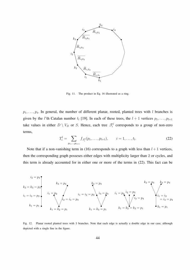
k1

k2

i2

k3

i3

k4

i4

i1Hi1k1

Hi1k2

Hi2k2

Hi2k3

Hi3k3

Hi3k4

Fig. 11. The product in Eq. 16 illustrated as a ring.

p1, . . . , p4. In general, the number of different planar, rooted, planted trees with l branches is

given by the l’th Catalan number tl [19]. In each of these trees, the l + 1 vertices p1, . . . , pl+1

take values in either D \ VD or S. Hence, each tree T li corresponds to a group of non-zero

terms,

T li =

∑p1,...,pl+1

fT li(p1, . . . , pl+1), i = 1, . . . , tl. (22)

Note that if a non-vanishing term in (16) corresponds to a graph with less than l + 1 vertices,

then the corresponding graph posseses either edges with multiplicity larger than 2 or cycles, and

this term is already accounted for in either one or more of the terms in (22). This fact can be

k1 = k2 = k3 = p1

i1 = p2

k1 = k3 = p1

k2 = p3

i3 = p4

i3 = p4

i1 = i2 = p2

i2 = p3

k1 = p1

k2 = p3 k3 = p4

i1 = i2= i3 = p2

k1 = k2 = p1

i1 = p2

k3 = p4

i2 = p4

k1 = p1

k2 = k3 = p3

i1 = i3 = p2

i2 = i3 = p3

Fig. 12. Planar rooted planted trees with 3 branches. Note that each edge is actually a double edge in our case, although

depicted with a single line in the figure.

44

p1

p2

p3

p5p4

a)

p1

p5

p6

p3

p2

p4

p1

p4

p5

p6

p3

p3

p2

b)

p1

p2

p5p4

p3p3

Fig. 13. The product in Eq. 16 illustrated as a ring.

observed by noticing that both edges with large multiplicity as well as cycles can be untied to

get trees with l branches, with some of the l + 1 indices constrained however to share the same

values (see Figure 13). Note that such cases are not excluded in the summations in (22), thus

we have

E(Tr((H∗H)l)) ≤tl∑

i=1

T li .

Below we show that

T li ≤ n(K ′

1 log n)l, ∀i (23)

in a regular network and

T li ≤ n(K ′

1 log n)3l, ∀i (24)

with high probability in a random network. We first concentrate on regular networks in order

to reveal the proof idea in the simplest setting. A binning argument then allows to extend the

result to random networks.

a) Regular network: Recall that in the regular case, the nodes on the left-half are located at

positions (−kx + 1, ky) and those on the right half at (ix, iy) for kx, ky, ix, iy = 1, . . . ,√

n. In

this case, the matrix elements of H are given by

Hik =ej θik

((ix + kx − 1)2 + (iy − ky)2)α/4

1√dkx,ky

45

p4 pl+1

p1

p3p2

Fig. 14. A simple tree with l branches.

and

dkx,ky =

√n∑

ix,iy=1

1

((ix + kx − 1)2 + (iy − ky)2)α/2.

In the discussion below, we will need an upper bound on the scaling of∑n

i=1 |Hik|2 and∑n

k=1 |Hik|2. By Lemma 5.4, we have

dkx,ky ≥ K ′3 k2−α

x

for a constant K ′3 > 0 independent of n which, in turn, yields the upper bound

|Hik|2 ≤ 1

K ′3

kα−2x

((ix + kx − 1)2 + (iy − ky)2)α/2≤ 1

K ′3

1

(ix + kx − 1)2 + (iy − ky)2.

Summing over either i or k, and using the upper bound in Lemma 5.4 for α = 2 yieldsn∑

i=1

|Hik|2,n∑

k=1

|Hik|2 ≤ K ′1 log n (25)

where K ′1 =

K′2

K′3

with K ′2 and K ′

3 being the constants appearing in the lemma.

Let us first consider the simplest case where the tree is composed of l height 1 branches and

denote it by T l1 (see Figure 14). We have

T l1 =

n∑p1,...,pl+1=1

fT l1(p1, . . . , pl+1) =

n∑p1,...,pl+1=1

|Hp2p1|2 |Hp3p1|2 . . . |Hpl+1p1|2

=n∑

p1=1

(n∑

p2=1

|Hp2p1|2)l

≤ n(K ′1 log n)l (26)

46

which follows from the upper bound (25).

Now let us consider the general case of an arbitrary tree T li having s leaves, where 1 ≤ s ≤ l

(see Figure 15). Let the indices corresponding to these leaves be m1, . . . , ms. Let us denote

the “parent” vertices of these leaves by p1, . . . , ps′ and assume that p1 is the common parent

vertex of leaves m1, . . . , md1; p2 is the common parent vertex of leaves m(d1+1), . . . , md2 etc.

and finally ps′ is the parent of m(dt+1), . . . , ms. The term T li corresponding to this tree is given

by

T li =

∑m1,...,ms

p1,...,p(l+1−s)

fT li(p1, . . . , pl+1)

=n∑

p1,...,p(l+1−s)=1

fT l−si′

(p1, . . . , p(l+1−s))

×n∑

m1,...,ms=1

|hm1p1|2 . . . |Hmd1p1|2 |Hm(d1+1)p2|2 . . . |Hmd2

p2|2 . . . |Hm(dt+1)ps′ |2 . . . |Hmsps′ |2

(27)

≤ T l−si′ (K ′

1 log n)s (28)

where T l−si′ corresponds to a smaller (and shorter) tree T (l−s)

i′ with l−s branches5. The argument

above decreases the height of the tree by 1, hence can be applied recursively to get a simple tree

composed only of height 1 branches in which case the upper bound in (26) applies. Thus, given

T li let h be the number of recursions to get a simple tree and s1, . . . , sh denote the number of

leaves in the trees observed at each step of the recursion. We have

T li ≤ (K ′

1 log n)s1(K ′1 log n)s2 . . . (K ′

1 log n)shT l−s1···−sh1

≤ n(K ′1 log n)l

since T l−s1···−sh1 ≤ n(K ′

1 log n)l−s1···−sh by (26). Thus, (23) follows.

b) Random network: We denote the locations of the nodes to the left of the cut by ak =

(−axk, a

yk) where ax

k is the x-coordinate and ayk is the y-coordinate of node k ∈ S and those to

5Note that the term corresponding to a leaf m can be either |Hmp|2 or |Hpm|2 depending on whether the height of the leaf

is even or odd. However, in (27), we ignore this issue in order to simplify the notation since the upper bound (28) applies in

both cases.

47

m1

m2m3

m4 m5

ms

p1

p3

ps′

p2

Fig. 15. A tree with leaves m1, m2, . . . , ms.

the right of the cut are similarly denoted by bi = (bxi , b

yi ) for i ∈ D \VD. In this case, the matrix

elements of H are given by

Hik =ej θik

((bxi + ax

k)2 + (by

i − ayk)

2)α/4

1√dk

and

dk =∑

i∈D\VD

1

((bxi + ax

k)2 + (by

i − ayk)

2)α/2.

In parallel to the regular case, we will need an upper bound on∑

i∈D\VD|Hik|2 and

∑k∈S |Hik|2.

The upper bound can be obtained in two steps by first showing that

dk ≥ K ′3

(axk)

2−α

log n(29)

with high probability for a constant K ′3 > 0 independent of n, which leads to

|Hik|2 ≤ 1

K ′3

log n(ax

k)α−2

((bxi + ax

k)2 + (by

i − axk)

2)α/2≤ 1

K ′3

log n1

(bxi + ax

k)2 + (by

i − ayk)

2(30)

for all i, k. This, in turn yields∑

k∈S

|Hik|2,∑

i∈D\VD

|Hik|2 ≤ K ′1(log n)3 (31)

with high probability for another constant K ′1 > 0 independent of n. Recalling the leaf removal

argument discussed for regular networks immediately leads to (24).

Both the lower bound in (29) and the upper bound in (31) regarding random networks can

be proved using binning arguments that provide the connection to regular networks. In order

48

to prove the lower bound, we consider Part (b) of Lemma 5.1, while the upper bound (31) is

proved using Part (a) of the same lemma.

Let us first consider dividing the right-half network into squarelets of area 2 log n. Given a

left-hand side node k located at (−axk, a

yk), let us move the nodes inside each right-hand side

squarelet onto the squarelet vertex that is farthest to k. Since this displacement can only increase

the Euclidean distance between the nodes involved, and since by Part (b) of Lemma 5.1, we

know that there is at least one node inside each squarelet, we have

dk =∑

i∈D\VD

1

((bxi + ax

k)2 + (by

i − ayk)

2)α/2

≥√

n/2 log n∑ix,iy=1

1

((ix√

2 log n + axk)

2 + (iy√

2 log n− axk)

2)α/2

≥ K ′3

(axk)

2−α

2 log n

by using the lower bound in Lemma 5.4.

Now having (30) in hand, in order to show (31), we divide the network into n squarelets of

area 1. By Part (a) of Lemma 5.1, there are at most log n nodes inside each squarelet. Considering

the argument in Section V and the displacement of the nodes as illustrated in Figure 7 yields a

regular network with at most 2 log n nodes at each vertex in the right-half network,

∑

i∈D\VD

|Hik|2 ≤ 2

K ′3

log n∑

i∈D\VD

1

(bxi + ax

k)2 + (by

i − ayk)

2

≤ 4

K ′3

(log n)2

√n∑

ix,iy=1

1

(ix + kx)2 + (iy − ky)2

≤ 4K ′1(log n)3.

by employing the upper bound in Lemma 5.4 for α = 2. The same bound follows similarly for∑

k∈S |Hik|2, thus the desired result in (31). ¤Proof of Lemma 5.4: Both the lower and upper bound for dkx,ky can be obtained by straight-

forward manipulations. Recall that

dkx,ky =

√n∑

ix,iy=1

1

((ix + kx − 1)2 + (iy − ky)2)α/2.

49

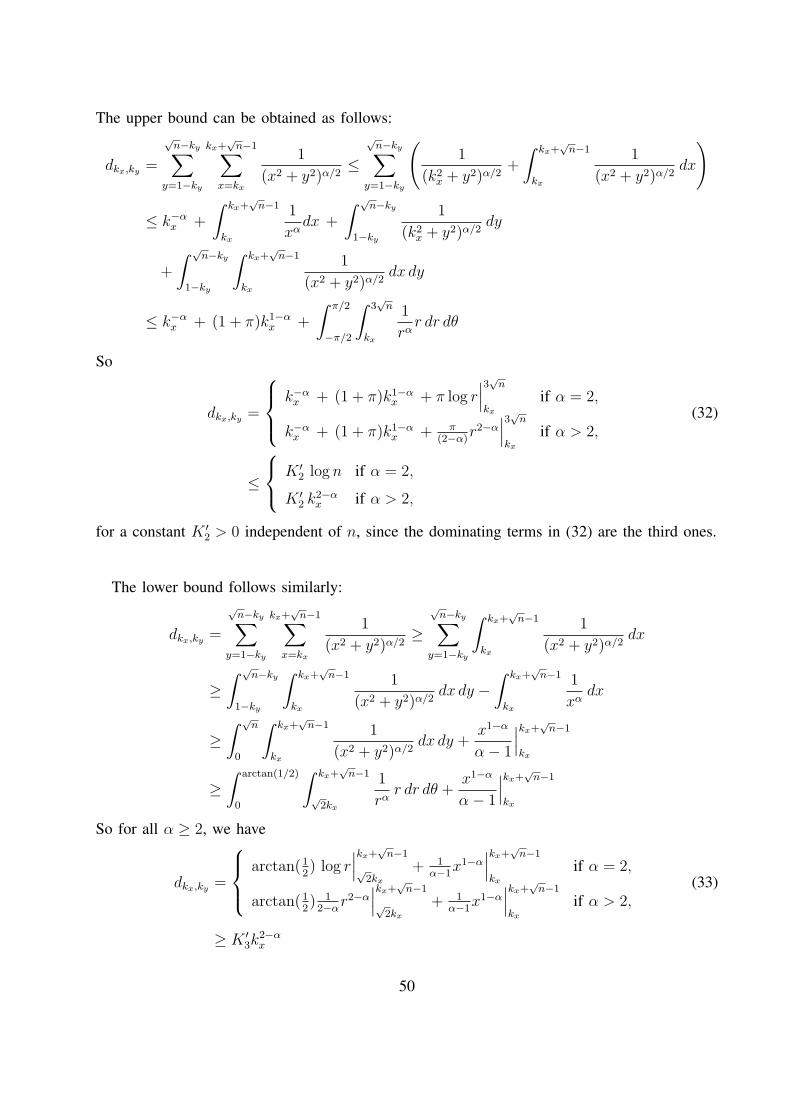
The upper bound can be obtained as follows:

dkx,ky =

√n−ky∑

y=1−ky

kx+√

n−1∑

x=kx

1

(x2 + y2)α/2≤

√n−ky∑

y=1−ky

(1

(k2x + y2)α/2

+

∫ kx+√

n−1

kx

1

(x2 + y2)α/2dx

)

≤ k−αx +

∫ kx+√

n−1

kx

1

xαdx +

∫ √n−ky

1−ky

1

(k2x + y2)α/2

dy

+

∫ √n−ky

1−ky

∫ kx+√

n−1

kx

1

(x2 + y2)α/2dx dy

≤ k−αx + (1 + π)k1−α

x +

∫ π/2

−π/2

∫ 3√

n

kx

1

rαr dr dθ

So

dkx,ky =

k−αx + (1 + π)k1−α

x + π log r∣∣∣3√

n

kx

if α = 2,

k−αx + (1 + π)k1−α

x + π(2−α)

r2−α∣∣∣3√

n

kx

if α > 2,(32)

≤

K ′2 log n if α = 2,

K ′2 k2−α

x if α > 2,

for a constant K ′2 > 0 independent of n, since the dominating terms in (32) are the third ones.

The lower bound follows similarly:

dkx,ky =

√n−ky∑

y=1−ky

kx+√

n−1∑

x=kx

1

(x2 + y2)α/2≥

√n−ky∑

y=1−ky

∫ kx+√

n−1

kx

1

(x2 + y2)α/2dx

≥∫ √

n−ky

1−ky

∫ kx+√

n−1

kx

1

(x2 + y2)α/2dx dy −

∫ kx+√

n−1

kx

1

xαdx

≥∫ √

n

0

∫ kx+√

n−1

kx

1

(x2 + y2)α/2dx dy +

x1−α

α− 1

∣∣∣kx+

√n−1

kx

≥∫ arctan(1/2)

0

∫ kx+√

n−1

√2kx

1

rαr dr dθ +

x1−α

α− 1

∣∣∣kx+

√n−1

kx

So for all α ≥ 2, we have

dkx,ky =

arctan(12) log r

∣∣∣kx+

√n−1

√2kx

+ 1α−1

x1−α∣∣∣kx+

√n−1

kx

if α = 2,

arctan(12) 1

2−αr2−α

∣∣∣kx+

√n−1

√2kx

+ 1α−1

x1−α∣∣∣kx+

√n−1

kx

if α > 2,(33)

≥ K ′3k

2−αx

50

where K ′3 > 0 is a constant independent of n, since the dominating terms in (33) are the first

ones. This concludes the proof of the lemma. ¤

REFERENCES

[1] P. Gupta and P. R. Kumar, The Capacity of Wireless Networks, IEEE Trans. on Information Theory 42 (2), 2000, 388-404.

[2] M. Franceschetti, O. Dousse, D. Tse, P. Thiran, On the Throughput Capacity of Random Wireless Networks, Preprint, 2006.

[3] S. Aeron, V. Saligrama, Wireless Ad hoc Networks: Strategies and Scaling Laws for the Fixed SNR Regime, Preprint, 2006.

[4] G. J. Foschini, Layered Space-Time Architecture For Wireless Communication in a Fading Environment when Using Multi-

Element Antennas, AT&T Bell Labs. Tech. J., vol.1 (2), pp.41-59, 1996.

[5] E. Telatar, Capacity of Multi-Antenna Gaussian Channels” European Trans. on Telecommunications, ETT, vol.10 (6), pp.

585-596, Nov. 1999.

[6] T. M. Cover and A. A. El Gamal, Capacity Theorems for the Relay Channel, IEEE Trans. on Information Theory, vol.25,

pp.572-584, Sept. 1979.

[7] L. -L. Xie and P. R. Kumar, A Network Information Theory for Wireless Communications: Scaling Laws and Optimal

Operation, IEEE Trans. on Information Theory 50 (5), 2004, 748-767.

[8] A. Jovicic, P. Viswanath and S. R. Kulkarni, Upper Bounds to Transport Capacity of Wireless Networks, IEEE Trans. on

Information Theory 50 (11), 2004, 2555-2565.

[9] O. Leveque and E. Telatar, Information Theoretic Upper Bounds on the Capacity of Large, Extended Ad-Hoc Wireless

Networks, IEEE Trans. on Information Theory 51 (3), March 2005.

[10] F. Xue, L. -L. Xie and P. R. Kumar, The Transport Capacity of Wireless Networks over Fading Channels, IEEE Trans. on

Information Theory, vol. 51, pp. 834-847, March 2005.

[11] L. -L. Xie, P. R. Kumar, On the Path-Loss Attenuation Regime for Positive Cost and Linear Scaling of Transport Capacity

in Wireless Networks, Preprint, 2006.

[12] S. Ahmad, A. Jovicic and P. Viswanath, Outer Bounds to the Capacity Region of Wireless Networks, IEEE Trans. Inform.

Theory, vol. 52, pp. 2770-2776, June 2006.

[13] D. Tse and P. Viswanath, Fundamentals of Wireless Communication, Cambridge University Press, 2005.

[14] R. Etkin and D. Tse, Degrees of freedom in some underspread MIMO fading channels, IEEE Trans. Inform. Theory, vol.

52, pp. 1576-1608, April 2006.

[15] G. Kramer, M. Gastpar and P. Gupta, Cooperative strategies and capacity theorems for relay networks, IEEE Trans. Inform.

Theory, vol. 51, pp. 3037-3063, September 2005.

[16] Cover, T.M, Thomas J. A., Elements of Information Theory, Wiley & Sons Inc., 1991.

[17] Gallager R. G., Information Theory and Reliable Communication, Wiley & Sons Inc., 1968.

[18] R. A. Horn, C. R. Johnson, Matrix Analysis, Cambridge University Press, 1985.

[19] R. P. Stanley, Enumerative Combinatorics, Vol. 2, Cambridge University Press, 1999.

51