Helen Trill Diagnostic Technologies for Wound Monitoring

CRANFIELD UNIVERSITY

Cranfield Health Department of Analytical Science and Informatics

Helen Trill Diagnostic Technologies for Wound Monitoring

Supervisors: S.Setford & S.Saini This thesis is submitted for the degree of Doctor of Philosophy

March 2006

i

Abstract Chronic wound infections represent a worldwide problem, generating high morbidity and medical expense. Failure to control infections such as MRSA in the reparative process of a wound can cause disruption of normal anatomical structure and function, resulting in a chronic wound. Existing approaches to identifying infection largely involve surveying a range of physical parameters, and a limited use of non-invasive technologies. Evaluation is time consuming, and often results in inconsistencies in patient care. This project researches three possible alternative methodologies/technologies for the monitoring of wounds, by measuring components of wound fluid. Two of the three technologies are designed to be used by physicians and patients, similarly to commercially available home blood glucose test kits, and are based on the measurement of three biomarkers: glucose, ethanol and H2O2 in PBS, and in serum as surrogate wound fluid. The first is a voltammetric technique known as dual pulse staircase voltametry (DPSV), which produces peaks characteristic of particular analytes at an electrode. The second is an amperometric biosensor array, based on screen printed three electrode assembies of carbon, rhodinised carbon (glucose biosensor only) and Ag/AgCl reference. The glucose biosensor uses glucose oxidase enzyme as the biorecognition agent, the H2O2 biosensor is a mediated system using horseradish peroxidase enzyme and dimethylferrocene mediator, and the ethanol biosensor is a bienzyme mediated system utilising alcohol oxidase enzyme horseradish peroxidase enzyme and coupled dimethylferrocene mediator. Wounds are known to produce characteristic odours, therefore the third technology studied is a single sensor odour analyser with advanced data analysis to detect five commonly occuring wound bacteria, S.aureus, K.pneumoniae, S.pyogenes, E.coli and P.aeruginosa in growth media and surrogate wound fluid. This technology would be used as a near patient monitoring system and is based on machine olfaction similar to that of a commercial electronic nose, but uses a single metal oxide sensor in combination with principle components analysis. DPSV scans of the individual analytes demonstrated distinctive peaks, exhibiting non-linear relationships with concentration. A great deal of useful information was generated using this technique, however, limitations were discovered regarding repeatability and inter-analyte interference in mixtures. Limits of detection in surrogate wound fluid with the glucose biosensor, hydrogen peroxide biosensor, and ethanol biosensor were as follows: 169.5 µM glucose, 8.43 µM hydrogen peroxide, and 7.94 µM ethanol respectively (all at 99.7% confidence). Direct detection of ethanol from metabolically active S.aureus in surrogate wound fluid yielded a limit of detection of 1.23 x 108 CFU/ml at 99.7% confidence, and 19 µM in terms of ethanol specific response. The single sensor odour analyser demonstrated the ability to detect and discriminate between the three biomarkers, between five bacteria individually, and partial discrimination of paired bacteria (in broth and surrogate wound fluid). It was also found that S.aureus could be detected down to a cell density of 5x106CFU/ml in surrogate wound fluid, lower than that found for the biosensor concept.

ii

Acknowledgements

Firstly Id like to thank Selly Saini for giving me the opportunity of working on this

project. Huge thanks to my supervisor Steve Setford for his continuous support and

guidance. Thanks also to the project consultants Laurie Ritchie, and Jon Lee-Davey for

their assistance, and to the many other staff who have contributed in some way to the

success of this project.

Thanks to my family and partner for their endless support during this enduring experience,

and to the many friends who have helped make my time at Silsoe memorable.

iii

Contents Abstract. .........................................................................................................................................i Acknowledgements ........................................................................................................................ii Contents........................................................................................................................................iii List of Figures. .............................................................................................................................vii List of Tables. ...............................................................................................................................xi Notation .......................................................................................................................................xii Abbreviations...............................................................................................................................xii

1. INTRODUCTION ................................................................................................................. I

1.1 BIOCHEMISTRY AND PHYSIOLOGY OF THE SKIN.................................................................1 1.1.1 Structure of the skin ..................................................................................................1 1.1.2 Carbohydrate metabolism of epidermis......................................................................3 1.1.3 Physiology of wound healing.....................................................................................4

1.1.3.1 Inflammatory phase...........................................................................................6 1.1.3.2 Fibroplastic phase ............................................................................................7 1.1.3.3 Remodelling phase............................................................................................8 1.1.3.4 Types of healing wounds ...................................................................................9

1.1.4 Body composition and body fluid compartments........................................................9 1.1.5 Biochemical composition of wound fluid.................................................................12 1.1.6 Factors affecting wound healing ..............................................................................17

1.1.6.1 Bacterial invasion ...........................................................................................17 1.1.6.2 Hospital acquired infection .............................................................................19

1.1.7 Conventional wound assessment..............................................................................23 1.1.8 Wound management .............................................................................................. 233

1.1.8.1 Odour and dressings .....................................................................................233 1.1.8.2 Antibiotic Treatment .....................................................................................255 1.1.8.3 Alternative treatments ...................................................................................255

1.2 ELECTROANALYTICAL CHEMISTRY ..................................................................................27 1.2.1 Fundamentals ..........................................................................................................27

1.2.1.1 Reference electrodes .......................................................................................28 1.2.1.2 Faradaic and non-Faradaic currents ..............................................................29

1.2.2 Electroanalytical techniques .................................................................................. 300 1.2.2.1 Diffusion.........................................................................................................32 1.2.2.2 Chronoamperometry .....................................................................................333 1.2.2.3 Pulsed amperometric detection .......................................................................35 1.2.2.4 Voltammetry .................................................................................................366 1.2.2.5 Dual pulse staircase voltammetry....................................................................38

1.2.3 Electroanalytical detection of H2O2..........................................................................39 1.3 BIOSENSORS .................................................................................................................40

1.3.1 Amperometric biosensors ........................................................................................41 1.3.1.1 Glucose measurement ...................................................................................422 1.3.1.2 Alcohol measurement ....................................................................................455

1.3.2 Screen-printed electrodes.........................................................................................46 1.3.3 Direct (label-free) detection of bacteria with biosensors ...........................................47 1.3.4 Indirect Detection of Bacteria ..................................................................................49

1.4 ELECTRONIC NOSE ..................................................................................................... 511 1.4.1 The human olfactory system and odours ................................................................ 511

1.4.1.1 Properties of odorous molecules .....................................................................52

iv

1.4.2 Machine olfaction....................................................................................................53 1.4.3 Sensors....................................................................................................................55

1.4.3.1 Metal-Oxide Sensors ....................................................................................566 1.4.3.2 Conducting Polymer Sensors.........................................................................588 1.4.3.3 Acoustic wave sensors.....................................................................................58

1.4.4 Signal pre-processing ............................................................................................ 599 1.4.5 Pattern recognition techniques ............................................................................... 611

1.4.5.1 Principle components analysis ......................................................................622 1.4.6 Applications of electronic nose technology ............................................................ 633

1.5 CHROMATOGRAPHIC TECHNIQUES AND TEST KITS...........................................................65 1.5.1 Liquid chromatography ......................................................................................... 666 1.5.2 Gas chromatography.............................................................................................. 677 1.5.3 Applications of Chromatography ........................................................................... 688

1.5.3.1 Chromatographic detection of bacteria .........................................................688 1.5.3.2 GC-MS analysis of urine ...............................................................................688

1.5.4 Test kits ..................................................................................................................72 1.6 PROJECT OBJECTIVES.................................................................................................. 733

2. STANDARD METHODS ..................................................................................................75

2.1 BACTERIA, BIOMARKERS AND SURROGATE WOUND FLUID ..............................75 2.1.1 Introduction ...................................................................................................................... 77

2.2 MATERIALS AND METHODS.............................................................................................78 2.2.1 Bacteria, growth media and equipment .......................................................................... 78 2.2.2 Revival of freeze dried bacteria ...................................................................................... 78 2.2.3 Cryopreservation of bacterial cultures ............................................................................ 79 2.2.4 Blood collection and separation ...................................................................................... 80 2.2.5 Bacterial calibration curves ............................................................................................. 81 2.2.6 Headspace GC-MS........................................................................................................... 84 2.2.7 Test kits............................................................................................................................. 85

2.3 RESULTS AND DISCUSSION.............................................................................................87 2.3.1 Bacterial growth curves ................................................................................................... 87 2.3.2 Detection of ethanol by headspace GC-MS ................................................................... 91 2.3.3 Detection of bacteria by headspace GC-MS .................................................................. 94 2.3.4 Detection of mixed bacteria by headspace GC-MS ....................................................... 97 2.3.5 Alcohol Draeger tube test ................................................................................................ 99 2.3.6 Glucose BioAssay ..........................................................................................................100 2.3.7 H2O2 Checkit test kit ...................................................................................................101

2.4 OVERALL CHAPTER CONCLUSIONS................................................................................ 101 3. DETECTION USING DUAL PULSE STAIRCASE VOLTAMMETRY......................102

3.1 INTRODUCTION........................................................................................................... 102 3.2 MATERIALS AND METHODS........................................................................................... 103

3.2.1 Reagents..........................................................................................................................103 3.2.2 Instrumentation...............................................................................................................104 3.2.3 Electrode materials.........................................................................................................105 3.2.4 Electrochemical techniques ..........................................................................................106

3.3 RESULTS AND DISCUSSION........................................................................................... 107 3.3.1 Comparison of amperometry and pulsed amperometric detection .............................107 3.3.2 Comparison of gold and platinum electrodes ...............................................................108

v

3.3.3 Dual pulse staircase voltammetry .................................................................................109 3.3.4 Comparison of platinum and gold solid electrodes for DPSV ....................................113 3.3.5 Investigation of interferents...........................................................................................114 3.3.6 DPSV of glucose, ethanol and H2O2 in PBS ................................................................122 3.3.7 DPSV of mixtures of glucose, ethanol and H2O2 in PBS ............................................126 3.3.8 DPSV with screen printed electrodes ...........................................................................127

3.4 CONCLUSIONS............................................................................................................. 129

4. DETECTION USING A BIOSENSOR ARRAY ............................................................131


4.2.1 Reagents..........................................................................................................................133 4.2.2 Instrumentation...............................................................................................................133 4.2.3 Measurement ..................................................................................................................134 4.2.4 Fabrication of screen printed electrodes .......................................................................134

4.3 GLUCOSE BIOSENSOR .................................................................................................. 136 4.3.1 Standard electrochemical measurement methodology.................................................137 4.3.2 Determination of optimum operating potential ............................................................138 4.3.3 Optimisation of glucose oxidase loading......................................................................140 4.3.4 Shelf life testing .............................................................................................................141 4.3.5 Determination of linear region and limit of detection .................................................143 4.3.6 Detection of glucose in model wound fluid with glucose biosensor ..........................145 4.3.7 Validation with glucose BioAssay test kit....................................................................147 4.3.8 Detection of glucose in model wound fluid containing S.aureus with biosensor ......148 4.3.9 Interferent testing ...........................................................................................................149 4.3.10 Conclusions: Glucose biosensor....................................................................................151

4.4 HYDROGEN PEROXIDE BIOSENSOR................................................................................ 151 4.4.1 Determination of optimum operating potential ............................................................154 4.4.2 Application of horseradish peroxidase, dimethylferrocene and cellulose acetate ....155 4.4.3 Shelf life testing .............................................................................................................156 4.4.4 Determination of linear region and limit of detection .................................................157 4.4.5 Validation with Checkit test kit ..................................................................................159 4.4.6 Detection of H2O2 in model wound fluid with H2O2 biosensor .................................160 4.4.7 Detection of H2O2 in model wound fluid containing S.aureus with H2O2 biosensor .162 4.4.8 Interferent testing ...........................................................................................................162 4.4.9 Conclusions: H2O2 biosensor .........................................................................................164

4.5 ETHANOL BIOSENSOR.................................................................................................. 164 4.5.1 Operating potential.........................................................................................................167 4.5.2 Determination of optimum alcohol oxidase loading....................................................167 4.5.3 Deposition of HRPx, AOx, dimethylferrocene and celluose acetate..........................169 4.5.4 Shelf life testing .............................................................................................................169 4.5.5 Determination of linear region and limit of detection .................................................170 4.5.6 Validation .......................................................................................................................172 4.5.7 Further ethanol biosensor development membranes and depostion regime............172 4.5.8 Detection of ethanol in model wound fluid with ethanol biosensor ...........................177 4.5.9 Detection of S.aureus in model wound fluid with ethanol biosensor .........................179 4.5.10 Interferent testing ...........................................................................................................180 4.5.11 Conclusions: Ethanol biosensor ....................................................................................181

4.6 OVERALL CONCLUSIONS.............................................................................................. 182

vi

5. BACTERIAL DETECTION USING A SINGLE SENSOR ODOUR ANALYSER......183


5.2.1 Odour analysis instrumentation.....................................................................................185 5.2.2 System operation ............................................................................................................187 5.2.3 Data analysis...................................................................................................................190 5.2.4 Preparation of non-bacterial samples ............................................................................192 5.2.5 Preparation of bacterial samples ...................................................................................193 5.2.6 Sample injection .............................................................................................................193

5.3 RESULTS AND DISCUSSION........................................................................................... 194 5.3.1 Effect of sample preparation temperature and pH on odour analyser response.........194 5.3.2 Detection of ethanol, glucose and H2O2 in PBS .........................................................196 5.3.3 Detection of ethanol in serum .......................................................................................203 5.3.4 Detection of S.aureus at different stages of growth .....................................................205 5.3.5 Detection of five species of bacteria grown in broth and PCA analysis ....................206 5.3.6 Detection of five species of bacteria grown in serum and PCA analysis ...................210 5.3.7 Examination of paried bacterial cultures grown in serum ...........................................212 5.3.8 Detection of different cell concentrations of S.aureus grown in serum......................214

5.4 OVERALL CHAPTER CONCLUSIONS................................................................................ 216

6. GENERAL DISCUSSION...............................................................................................217

6.1 CONCLUSIONS............................................................................................................. 217 6.2 SUGGESTIONS FOR FUTURE WORK................................................................................ 221

7. LIST OF REFERENCES ................................................................................................223

vii

List of Figures

1.1: The phases to scar formation in a full thickness wound (Gogia, 1995).........................5 1.2: Distribution of water in major body fluid compartments............................................10 1.3: Representation of a Gaussian concentration profile. .................................................33 1.4: A single PAD cycle....................................................................................................36 1.5: Example of a CV scan (ferricyanide). ........................................................................38 1.6: DPSV waveform. .......................................................................................................39 1.7: Diagram showing the analogy between the three basic stages of machine and human olfactiom........................................................................................................55 1.8:. Architecture and processing stages of an electronic nose, including unsupervised learning of unknown odour input......................................................................................60 2.1: Serial dilution and plating layout for production of bacterial growth curves. ............83 2.2: (a) Draeger Accuro pump and tubes, (b) experimental setup for the measurement of alcohol content of five bacteria in the headspace of a compressible bag. ......................86 2.3: Growth curves of bacteria grown in TSB. ..................................................................88 2.4: Calibration plots for bacteria grown in TSB..............................................................88 2.5: Calibration plots for bacteria grown in DMEM.........................................................89 2.6: Calibration plots for bacteria grown in 90:10 v/v serum: DMEM..............................89 2.7: Comparison of calibration plots for S.aureus grown in protein reduced plasma, serum, and 90:10 v/v serum:DMEM. ...................................................................90 2.8: Headspace GC-MS detection of ethanol standards example peak area integration and identification. ............................................................................................................92 2.9: Headspace GC-MS detection of ethanol standards (a)Ethanol peaks, (b) Calibration plot...................................................................................................................................93 2.10: Headspace GC-MS detection of bacteria S.pyogenes example Peak area integration and identification as ethanol. .........................................................................95 2.11: Ethanol concentrations detected by headspace GC-MS analysis of bacteria grown in 90:10 v/v serum:DMEM. ..................................................................................................97 2.12: Ethanol concentrations detected by headspace GC-MS analysis of bacteria combinations grown in 90:10 v/v serum:DMEM...............................................................99 2.13: Glucose BioAssay standards..................................................................................100 3.1: Assembly of solid electrodes. ...................................................................................104 3.2: Screen printed three electrode assembly electrodes .................................................105 3.3: . Comparison of fixed-potential amperometric and pulsed amperometric detection (PAD) to 64 mM increases in ethanol concentration in 0.1M NaOH, at a gold working electrode with Ag/AgCl reference..............................................................108 3.4: Comparison of platinum and gold working electrode vs. Ag/AgCl reference, for determination of 64mM increases in ethanol by pulsed amperometric detection .............109 3.5: DPSV responses for 1 mM glucose, 1 mM fructose, and 64 mM ethanol in 0.1 M NaOH at a platinum working electrode vs.Ag/AgCl. .........................................111 3.6: . DPSV responses for different concentrations of glucose in 0.1M NaOH, at a platinum working electrode with Ag/AgCl reference ................................................112 3.7: DPSV responses for different concentrations of ethanol in 0.1M NaOH, at a platinum working electrode with Ag/AgCl reference. ...............................................112

viii

3.8: DPSV responses to 64 mM Ethanol, 64mM Propanol, and 64 mM Methanol, at a platinum electrode, in 0.1 M NaOH, with Ag/AgCl reference. .................113 3.9: Comparison of blank subtracted DPSV responses to 64 mM ethanol at platinum and gold working electrodes in 0.1 M NaOH, with Ag/AgCl reference............................114 3.10: DPSV responses (blank subtracted) for: (a) Acetominophen (b) Ascorbic acid (c) Bilirubin (d) Cholesterol ( e) Creatinine ( f) Cysteine (g) Dopamine (h) Gentisic acid (i) Glutathione (j) Levo-dopa (k) Salicylic acid (l) Tetracycline (m) Tolazamide (n) Tolbutamide (o) Urea (p) Uric acid, , in 0.1 M NaOH at a platinum working electrode vs. Ag/AgCl reference.............................................118 3.11: DPSV (blank subtracted) of interferents in 0.1M PBS (blank) containing 5 mM ethanol. ................................................................................................................119 3.12: DPSV of interferents in 0.1M PBS containing 5 mM glucose. ................................121 3.13: DPSV of interferents in 0.1M PBS containing 5 mM H2O2.....................................121 3.14: DPSV of glucose in 0.1M PBS at platinum working electrode vs. Ag/AgCl reference. Scans are blank subtracted averages of 3 scans. ........................123 3.15: DPSV of ethanol in 0.1M PBS at platinum working electrode vs. Ag/AgCl reference. Scans are blank subtracted averages of 3 scans. ........................123 3.16: DPSV of H2O2 in 0.1M PBS at platinum working electrode vs. Ag/AgCl reference. Scans are blank subtracted averages of 3 scans..............................................................125 3.17: DPSV of 5 mM glucose, 5mM ethanol, 1mM H202 in 0.1 M PBS at platinum working electrode vs. Ag/AgCl reference. Scans are blank subtracted averages of 5 scans. Shaded areas represent +/- 1 standard deviation. ..........................125 3.18: . Blank subtracted DPSV scans of mixtures of 5mM ethanol, 5 mM glucose and 5 mM H2O2 in 0.1 M PBS at platinum working electrode vs. Ag/AgCl reference .............126 3.19: Aging effect of repeated DPSV scans in 0.1M PBS (blank) and 5 mM ethanol with a screen printed gold working electrode (vs. Ag/AgCl reference) ...............128 3.20: DPSV scans of 0.1 M PBS (blank) and 5 mM ethanol with a screen printed carbon working electrode (vs. Ag/AgCl reference) . ...........................................128 4.1 Flow diagram of biosensor development and testing stages: . ...................................132 4.2: Multichannel Eco Chemie Autolab and sensor connections. ....................................135 4.3: Biosensor connection. .............................................................................................135 4.4: Four layers of the screen printing process for three electrode assembly ..................135 4.5: Glucose biosensor reaction scheme .........................................................................136 4.6: Example amperometric measurement of H2O2 at rhodinised carbon working electrode vs. Ag/AgCl, at +300mV ....................................................................138 4.7: Hydrodynamic voltammogram of background current and response towards 10 mM H202 in 0.1M PBS (pH7.2) at screen printed three electrode system with rhodinised carbon working electrode vs. Ag/AgCl. Error bars=SD, n=3 ................139 4.8: The signal to noise ratio for rhodinised carbon three electrode system at 10 potentials in 10 mM H2O2 in 0.1M PBS pH7.2......................................................140 4.9: Signal to noise ratio for 7 glucose oxidase loadings on rhodinised carbon working electrode in 10mM glucose in 0.1M PBS pH7.2..............................................................141 4.10: Shelf life testing of glucose biosensor ....................................................................142 4.11: Calibration of screen printed three electrode glucose biosensor and determination of linear region for detection of glucose in 0.1M PBS.........................................................144

ix

4.12: Calibration of screen printed three electrode glucose biosensor and determination of linear region for detection of glucose in model wound fluid............................................146 4.13:Validation of glucose biosensor with BioAssay test kit............................................148 4.14: Calibration of screen printed three electrode glucose biosensor and determination .of linear region for detection of glucose in model wound fluid containing 2 x 108 CFU/ml S.aureus. ........................................................................................................................149 4.15: Affect of interferents on the measurement of 5 mM glucose in 0.1 M PBS with glucose biosensor ...................................................................................................150 4.16: Reaction scheme on the carbon working electrode of the dimethylferrocene .mediated horseradish-peroxidase H2O2 biosensor ........................................................................152 4.17: The signal to noise ratio for carbon three electrode system at 5 potentials in 3 mM H2O2 in 0.1M PBS pH7.2. ..............................................................................155 4.18: Shelf life testing of H2O2 biosensor.......................................................................157 4.19: Calibration of screen printed three electrode H2O2 biosensor and determination of linear region for detection of H2O2 in 0.1M PBS ............................................................158 4.20:Validation of H2O2 biosensor with Checkit test kit ..................................................160 4.21: Calibration of screen printed three electrode H2O2 biosensor and determination of linear region for detection of H2O2 in model wound fluid................................................161 4.22: Calibration of screen printed three electrode H2O2 biosensor and determination of linear region for detection of H2O2 in model wound fluid containing 2 x 108 CFU/ml S.aureus .........................................................................................................................163 4.23: Affect of interferents on the measurement of 0.5 mM H2O2 in 0.1 M PBS with H2O2 biosensor .....................................................................................163 4.24: Signal: noise ratios for alcohol oxidase loadings of bi-enzyme mediated system in 2mM ethanol in 0.1M PBS pH7.2. (a) C.boidinii and (b) P.pastoris. ..............................168 4.25: Shelf life testing of alcohol biosensor. ...................................................................170 4.26: Calibration of screen printed three electrode ethanol biosensor and determination of linear region for detection of ethanol in 0.1M PBS. ........................................................171 4.27: Comparison of signal: noise of ethanol biosensor using of a range of membranes. 174 4.28: Signal: noise ratio for the 7 deposition combinations of enzymes, ..dimethylferrocene, cellulose acetate and nafion used in alcohol biosensor construction...............................176 4.29: Comparison of cellulose acetate application methods and volumes applied to alcohol biosensor...........................................................................................177 4.30: Calibration of screen printed three electrode ethanol biosensor (2 layer deposition procedure, described in 4.5.7) and determination of linear region for detection of ethanol in model wound fluid. .....................................................................178 4.31: Detection of metabolic ethanol production by S.aureus with screen printed three electrode alcohol biosensor in serum.........................................................180 4.32: Affect of interferents on the measurement of 0.5 mM ethanol in 0.1 M PBS with ethanol biosensor .................................................................................181 5.1:The interior of the MMOS system sensor chamber, displaying the MMOS sensor, the relative humidity sensor, and the Peltier Thermoelectric Controller) temperature sensor.......................................................................................................................................186 5.2: Mode of operation of the single MMOS sensor odour analyser................................188

x

5.3: A typical MMOS sensor response curve showing the three main characteristics: a)the magnitude of the response b)the rising slope c)the decay slope ......................................191 5.4: Detection of 0.25% ethanol in water held at different temperatures before odour analyzer injection. (a) Deviation in baseline resistance with time. (b) Linear relationship between temperature and maximum deviation in baseline resistance ..............................195 5.5: Odour analyser detection of 0.1M PBS of different pH values.(a) Deviation from baseline resistance with time. (b) Mean maximum positive and negative deviations in baseline resistance with pH .........................................................197 5.6: Discrimination by PCA analysis of odour analyser detection of low concentration marker analytes with a pre-sampling temperature of 25°C. ............................................199 5.7: Discrimination by PCA analysis of odour analyser detection of higher ... concentration marker analytes with a pre-sampling temperature of 25°C .............................................200 5.8: Discrimination by PCA analysis of odour analyser detection of low concentration marker analytes with a pre-sampling temperature of 37°C. ............................................201 5.9: Discrimination by PCA analysis of odour analyser detection of higher ... concentration marker analytes with a pre-sampling temperature of 37°C .............................................202 5.10: Odour analyser detection of 0 to 20 mM ethanol in serum. (a) Deviation in baseline resistance with time, (b) Linear relationship between ethanol concentration and mean maximum deviation in baseline resistance.............................................................204 5.11: Illustration of the use of S.aureus growth curve to determine growth phase. Arrows indicate time of odour analysis for this study......................................................205 5.12: Deviation in baseline resistance with time for odour analyser detection of S.aureus from 0 to 12 hrs growth at 37 °C in TSB.........................................................................206 5.13: Discrimination by PCA analysis of odour analyser detection of Pseudomonus aeruginosa, Streptococcus pyogenes, Escherichia coli, Staphylococcus aureus and Klebsiella pneumoniae, after 6 hrs growth in YPD broth .........................................208 5.14: Discrimination by PCA analysis of odour analyser detection of Pseudomonus aeruginosa, Streptococcus pyogenes, Escherichia coli, Staphylococcus aureus and Klebsiella pneumoniae, after 24 hrs growth in YPD broth .......................................209 5.15: Discrimination by PCA analysis of odour analyser detection of 1.5x108 CFU/ml P.aeruginosa, S.pyogenes, E.coli, S.aureus and K.pneumoniae grown in 90:10 v/v serum: DMEM ...........................................................................................211 5.16: Discrimination by PCA analysis (PC1vPC3) of odour analyser detection of pairs of bacteria at 2x108 CFU/ml grown in 90:10 v/v serum:DMEM at 37 °C.......................213 5.17: Discrimination by PCA analysis (PC1v3) of odour analyser detection of three cell densities of S.aureus grown in serum at 37°C .................................................215

xi

List of Tables

1.1: Composition of major body fluid compartments.........................................................12 1.2: Comparison of selected biochemical analytes from non-healing and healing wound fluids.....................................................................................................................14 1.3: Factors affecting wound healing. ..............................................................................18 1.4: Information on common wound pathogens. ...............................................................21 1.5: Properties of some odour absorbing wound...............................................................24 1.6: Summary of the reported uses of chromatographic techniques to detect bacteria.......70 2.1: Integrated ethanol peak area values for headspace GC-MS of bacteria grown in 90% serum 10% DMEM...............................................................................................97 2.2: Bacteria combinations analysed by headspace GC-MS. ............................................98 2.3: Integrated ethanol peak area values for headspace GC-MS of combinations of bacteria grown in 90:10 v/v serum:DMEM. ...................................................................................98 2.4: Alcohol levels detected by Draeger tubes. ...............................................................100 3.1: Concentrations of possible interferents found in blood. ...........................................115 4.1: Results of glucose biosensor validation by glucose BioAssay test kit........................147 4.2: Results of H2O2 biosensor validation by H2O2 Checkit test kit..................................159 4.3: Membranes tested on ethanol biosensor. .................................................................172 4.4: Ethanol biosensor deposition parameters for the 4 biosensor reagents studied: AOx and HRPx enzymes, dimethylferrocene film, cellulose acetate and Nafion membrane materials. Numbers indicate layer number. ....................................................................175 5.1: Odour analyser system parameters..........................................................................187 5.2: The twenty seven principle components extracted from MMOS response curves . ....192 5.3: Bacteria abbreviations used in PCA plots................................................................207 5.4: Maximum deviations in baseline resistance of odour analysis of 1.5x108 CFU/ml bacteria grown in 90:10 v/v serum:DMEM. .....................................................212

xii

Notation A Amps C Concentration D Diffusion coefficient E Potential Edet Measurement potential Eox Oxidation potential Ered Reduction potential I or i Current J Flux L Litre mM Millimolar O or ox Oxidised Q Total charge R or red Reduced t Time tdet Detection period tox Oxidation period tred Reduction period U Units (of enzyme) µ Micro V Volts +ve Positive -ve Negative Ω Ohms

Abbreviations ADH Alcohol dehydrogenase Ag/AgCl Silver/silver chloride AOx Alcohol oxidase ATP Adenine triphosphate CFU Colony forming units CV Cyclic voltammetry C-NS Coagulase negative staphylococcus aureus DMEM Dulbeccos modified eagles medium DMFc Dimethylferrocene DNA Deoxyribonucleic acid DPSV Dual pulse staircase voltammetry ELISA Enzyme linked immunosorbent assay FAD Flavin adenine dinucleotide FET Field effect transistor FIA Fluorescent immunoassay FTIR Fourier transform infrared spectroscopy GAG Glycosaminoglycans GC-MS Gas chromatography mass spectrometry GDH Glucose dehydrogenase GOx Glucose oxidase

xiii

HPLC High performance liquid chromatography HRPx Horseradish peroxidase IR Infrared LAPS Light addressable potentiometric sensor LED Light emitting diode LSV Linear sweep voltametry MMP Matrix metalloproteinase MOS Metal oxide sensor MRSA Methicillin resistant Staphylococcus aureus MSSA Methicillin susceptible Staphylococcus aureus NA Nutrient agar NAD Nicotinamide adenine dinucleotide NHE Normal hydrogen electrode OHP Outer Helmholtz plane O/N Overnight PAD Pulsed amperometric detection PARC Pattern recognition engine PBS Phosphate buffered saline PCA Principle components analysis PYG Peptone yeast glucose broth PZ Piezoelectric RNA Ribonucleic acid RO Reverse osmosis RPM Revolutions per minute SAW Surface acoustic wave SCFA Short chain fatty acids TCA Trichloroacetic acid TSB Tryptone soy broth UTI Urinary tract infection VFA Volatile fatty acids VOC Volatile organic compounds VRSA Vancomycin resistant Staphylococcus aureus

1

1. Introduction

1.1 Biochemistry and Physiology of the Skin

1.1.1 Structure of the skin

The skin is a large organ covering every contour of the human body, conforming to the

movements of the organism inside. The skin provides the major interphase between the

organism and its environment, and is adapted to withstand the desiccation of dry

environments, as well as exposure to the many mechanical, chemical and microbial

variables. It also contains a vasculature and sweating system to thermally regulate the body,

and a neuroreceptor network to report environmental information. The skin is

conventionally recognised as having two major layers. The outer layer is a thin stratified

epithelium, known as the epidermis, ranging only from 75 to 150 µm in thickness around

the body (except palms and soles). Underlying the epidermis is a dense fibroelastic

connective tissue called the dermis. Unlike the epidermis, the thickness of the dermis varies

considerably throughout regions of the body. The dermis contains the extensive vascular

and nerve networks, as well as specialised excretory and secretory glands, and keratinised

appendage structures such as hair and nail. Beneath the skin lies the subcutaneous tissue

(hypodermis), which is composed of loose areolar connective tissue and fatty connective

tissue, and also has substantial variations in its thickness. Fibrous bands run from the

dermis through to the subcutaneous tissues, thereby providing attachment of the skin to the

fibrous skeletal components (Odland, 1983).

2

The epidermis is subdivided into (Odland, 1983):

1) A germinative basal cell layer of keratinocytes;

2) Above the germinal layer is the stratum spinosum, comprising several layers of

polyhedral cells;

3) Above this is the stratum granulosum, which is a layer of flattened nucleated cells

containing distinctive cytoplasmic inclusions, and keratohyalin granules.

4) The stratum granulosum is the transition to the overlying end product, the stratum

corneum, consisting of the keratinised lamellae of anucleate, thin flat cells. This

final layer ranges from 15 to 20 cellular layers in thickness.

The epidermis is constantly replacing itself, by keratinocyte daughter cells dividing and

migrating outward, and transforming to eventually becoming flattened anucleate cells of

the stratum corneum. On average, it takes a period ranging from 45 to 75 days for the

epidermis to completely renew itself. It is because of the constant renewal of the epidermal

cell population that the skin is able to react so diversely to both physiological and

pathological stimuli.

In psoriasis, there is a prominent increase in mitotic activity in the epidermis. In

hyperproliferative states, cell production can be governed by a reduction in cell cycle, or an

increase in the number or proportion of proliferating cells (Holbrook, 1983). The

mechanism for this is not yet understood.

3

1.1.2 Carbohydrate metabolism of epidermis

Glucose is a fuel for energy metabolism and a substrate for biosynthesis of

mucopolysaccharides, lipids, glycogen, nucleic acids, and proteins. Glucose circulates

freely in the interstitial fluid space of the dermis and epidermis and is thought to diffuse

freely across epidermal cell walls. The utilisation of glucose in the epidermis probably

differs in basal and upper cell layers (Freinkel, 1983), and is proportional to substrate

concentration, except at very high concentrations. The utilisation of glucose increases in

proliferative states, and glucose uptake is enhanced during wound repair and psoriatic

epidermis (Freinkel, 1983, Im & Hoopes, 1970).

Anaerobic glycolysis produces a high lactic acid content in the skin, far exceeding that of

blood by as much as three fold. Lactic acid is the major metabolite of glucose. When

glucose is absent, the epidermis oxidises endogenous lipids. This occurs in cornification

when exogenous substrate is limited, or as a result of a pathological or physiological

increase in circulating fatty acids (i.e. starvation or diabetes) to a level high enough to

compete for access to the tricarboxylic acid cycle. The increase in glucose and O2

utilisation in wound repair is accompanied by a decrease in the formation of lactic acid and

CO2. All of the sugar moieties used to form the carbohydrate components needed by the

skin are derived originally from glucose. Glycogen is one of the products of synthesis

derived from glucose metabolism in the skin. Except for in foetal epidermis, glycogen is

sparse in the human dermis. However, in proliferative responses to physical trauma, such

as a wound or exposure to radiation with UV light and X-ray, glycogen accumulates and

4

probably serves as an added source of energy during repair processes. In psoriasis, the

amount of glycogen is four or five times greater than the level in normal epidermis

(Freinkel, 1983, Im & Hoopes, 1974). X-ray irradiation also produces an inflammatory

reaction, caused by cellular damage, and ultraviolet light causes an increase in acid

proteinase in the skin. Healing wounds contain a methionine and valine napthylamide

hydrolase, which is different from normal skin enzymes (Frienkel, 1983), and also have

increased levels of the serum arylamidase and aminopeptidase activity

1.1.3 Physiology of wound healing

This Section is taken from Gogia (1995). Wound healing is a complex and highly regulated

series of biological events. Wounds are categorised on the basis of severity and extent of

injury to the dermis. Epidermal wounds extend into the epidermal layer and possibly the

superficial layer of the dermis. These are called partial thickness wounds. The wound

initially forms a crust of blood and debris particles, and then proceeds to heal by

regeneration i.e. re-epithelialisation. The new cells gradually thicken until healing is

complete, at which point the crust falls off leaving the proliferated cells to keratinize. It

takes 24 to 48 hrs for the epithelial cells to respond to injury, and the wound heals without

scar tissue. Dermal wounds extend through the epidermis and dermis to the subcutaneous

tissue, and may also involve muscles and bone. These are called full thickness wounds, and

heal by three mechanisms resulting in scar formation (Figure 1.1). The first phase is

inflammation, which prepares the wound for healing. The second is the fibroplastic phase,

which rebuilds damaged structures, and the third is the remodelling phase, which modifies

the scar to fit the wound. In normal healing, each phase overlaps.

5

Figure 1.1: The phases to scar formation in a full thickness wound (Gogia, 1995).

OPEN WOUND

INFLAMMATORY PHASE

Vasoconstriction

Vasodilation

Clot formation

Phagocytosis

Neovascularization

FIBROPLASTIC PHASE

Epithelialisation

Collagen synthesis

Wounds contraction

REMODELING PHASE

Collagen synthesis-lysis balance

Collagen fiber orientation

HEALED WOUND

6

1.1.3.1 Inflammatory phase

Inflammation is a prerequisite to wound healing. It is a vascular and cellular response to

dispose of bacteria, foreign material, and dead tissue. The first stage is the vasoconstriction

of the damaged blood and lymphatic vessels, to slow or stop blood loss. This is achieved

through the secretion of norepinephrine by the blood vessels, and serotonin by the platelets

and mast cells. The platelets also plug or stop blood loss.

At the same time, leukocytes cluster along the sticky vessel walls, which is known as

neutrophilic margination. Following vasoconstriction, the non-injured vessels dilate and

increase their permeability in response to the histamine released by the mast cells, and the

prostaglandin released by the injured cell membrane. Vasoconstriction lasts for about five

to ten minutes, and vasodilation lasts for less than one hour. The increase in vessel

permeability allows plasma to leak into the wound area, so that fibrin can block the

lymphatic flow and seal off the wound, localise the inflammatory reaction, and prevent the

spread of infection. The wound is red, hot, swollen, and painful at this stage of healing.

Leukocytes, erythrocytes and platelets adhere to the dilated blood vessel walls.

Polymorphonuclear leukocytes migrate through the capillary pores first, and prevent

infection by enzymatically dissolving and digesting debris and foreign material by the

process of phagocytosis. When these leukocytes die, they release their intracellular

enzymes and debris, which becomes part of the wound exudate. Mononuclear leukocytes

move from the capillary into the wound next, where they are transformed into

macrophages, the most important cells of the inflammatory stage. The macrophages ingest

7

the unsolubilised material, engulf leftover polymorphonuclear leukocytes, and ingest

microorganisms. The products of digestion of these materials are excreted, i.e., ascorbic

acid, hydrogen peroxide, and lactic acid. The hydrogen peroxide released helps to control

anaerobic microbial growth. Ascorbic acid and lactic acid accumulate and signal to

increase production of macrophages. The macrophage products result in greater pus

production, which can impair wound healing. At the end of this phase, fibrinolysin is

produced by the blood vessels to dissolve the blood clots, and the lymph channels then

open to help reduce wound edema.

1.1.3.2 Fibroplastic phase

This phase is also referred to as the proliferative phase, since rebuilding of the damaged

tissue occurs. Repair of the epithelium goes through a sequence of mobilisation, migration,

proliferation, and differentiation, and continues until the wound is healed. The epithelial

cells migrate into the wound area to form multiple layers beneath the clot. This provides a

protective barrier to prevent fluid and electrolyte loss from the wound, and to reduce the

chance of infection. The temporary crust loosens and detaches once epithelialisation is

completed.

While re-epithelialisation occurs, the wound contracts and is remodelled by mobilisation of

the surrounding tissues. The centripetal movement of normal skin, primarily

myofibroblasts, decreases the size of the wound by forcing granulation tissue to retract.

Contraction begins after five days of wounding and peaks at two weeks. Contraction

proceeds at a uniform rate, and is not affected by the size of the wound, though is affected

8

by the shape. However, if the wound has not closed by two to three weeks, contraction

stops.

Fibroblasts are produced by undifferentiated mesenchymal cells, and are stimulated to

synthesise collagen tissue by lactic acid, ascorbic acid, and other cofactors. Collagen tissue

is necessary to strengthen and stiffen the wound. Collagen molecules cross-link

intermolecularly to increase the tensile strength of the wound. A gel-like substance called

glycosaminoglycans (GAG) is also produced by fibroblasts, to give lubrication and density

to the connective tissue. As the amount of collagen increases, the number of fibroblasts is

reduced, marking the end of the fibroblastic phase.

1.1.3.3 Remodelling phase

This phase is also called the maturation phase, and begins after approximately two to four

weeks. The enlarged, dense scar formed in the fibroblastic phase is remodelled in form,

bulk and strength. New collagen is produced as the old breaks down. If the rate of collagen

production exceeds its breakdown, a hypertrophic scar or keloid forms, which is either

raised, or extends beyond the normal boundaries of the wound. If collagen breakdown

exceeds its production, a softer scar forms.

9

1.1.3.4 Types of healing wounds

Primary closure / healing by first intention: Occurs when full-thickness surgical incisions

or other wounds with minimal skin loss are approximated and sutured together. Healing is

completed by re-epithelialisation only.

Secondary closure / healing by secondary intention: Occurs in large, open, full-thickness

wounds with soft tissue loss. They heal by collagen deposition, wound contraction, and

granulation, followed by epithelialisation. These wounds take longer to heal, and form a

scar.

Delayed primary closure / healing by third intention: Occurs in contaminated more

extensive wounds, or wounds at risk of infection. By deliberately delaying wound closure,

infection can be treated and monitored, without delaying the formation of tensile strength.

The wounds are then sutured together and complete healing by re-epithelialisation.

1.1.4 Body composition and body fluid compartments

In an average male, body weight is split as follows (Ganong, 2003): 18% protein and related substances 7% mineral 15% fat 60% water

These values differ with sex, age, and degree of obesity. With age, the percentage of body

fat increases, which in turn decreases the percentage of water. Total body fluid is mostly

distributed between two compartments: extracellular and intracellular. A third and smaller

10

compartment is referred to as transcellular, and includes fluid from synovial, peritoneal,

pericardial, and intraocular spaces.

The distribution of the ~60% water in body fluid compartments can be divided as follows

as a percentage of body weight (Ganong, 2003, Guyton & Hall, 2000) :

Intracellular fluid40%

Cell membrane

Interstitial Fluid15%

Capillary membrane

Blood Plasma5%

Lym

phat

ics

Extra

cellu

lar f

luid

Tota

l 20%

OUTPUT:Kidneys, lungs

intestines, sweat,skin

INTAKE

Figure 1.2: Distribution of water in major body fluid compartments

11

The intracellular fluid is inside the cells of the body. The concentration of substances is

similar from one cell to another and is therefore considered to be one large fluid

compartment. The extracellular fluid is outside the cells and is further divided into blood

plasma and interstitial fluid, which is often referred to as a gel phase. Plasma is the

noncellular part of blood, and continuously communicates with the interstitial fluid through

the pores of the capillary membrane. The extracellular fluids are constantly mixing, and

almost all solutes in extracellular fluid can pass though the pores, except for proteins. For

this reason, the composition of the two fluids are approximately similar, except for the

protein content, which is higher in plasma (Guyton & Hall, 2000). The molecular masses of

the major proteins in plasma are (Ganong, 2003):

Albumin 69,000

Haemoglobin 64,450

β1Globulin 90,000

γ Globulin 156,000

Fibrinogen 340,000

Since the proteins cannot pass through to the interstitial fluid, they exert an osmotic force

across the capillary wall that pulls water into the blood. The proteins also provide ~15% of

the buffering capacity of blood in an anionic form at the normal plasma pH of 7.4. The

normal composition of the major body fluid compartments is listed in Table 1.1, though it

should be noted that these values vary slightly from book to book.

12

Table 1.1: Composition of major body fluid compartments (Guyton & Hall, 2000).

Constituent Plasma (mmol/L)

Interstitial fluid (mmol/L)

Intracellular fluid (mmol/L)

Na+ 142 139 14 K+ 4.2 4.0 140 Ca++ 1.3 1.2 0 Mg+ 0.8 0.7 20 Cl- 108 108 4 HCO3

- 24 28.3 10 HPO4

-, H2PO4- 2 2 11

SO4- 0.5 0.5 1

Amino acids 2 2 8 Creatine 0.2 0.2 9 Lactate 1.2 1.2 1.5 Glucose 5.6 5.6 Protein 1.2 0.2 4 Urea 4 4 4 Others 4.8 3.9 10

Although blood contains both extracellular fluid and intracellular fluid, it is considered a

separate fluid compartment because it is contained within the circulatory system.

1.1.5 Biochemical composition of wound fluid

Wound fluid bathes the tissue undergoing repair and regeneration. When tissue is damaged,

a cascade of reactions causes blood to coagulate by converting soluble fibrinogen (the

largest plasma protein) into insoluble fibrin. What remains is an exudate of plasma called

serum. Serum has the same components as plasma, except that it doesnt contain

fibrinogen. The wound fluid may also contain soluble tissue and cell-derived molecules

responsible for co-ordinating the healing process (Ganong, 2003, Clough & Noble, 2003).

13

It is a highly complex biomatrix containing thousands of species at steady state, including

essential trace elements of amino acids such as citrate and arginate, and metal ions such as

iron, copper and zinc. Proteins and enzymes uptake the metal ions to form metal ion-

protein complexes. The protein bound total metal fraction is not known in wound fluid, but

can be assumed to be analogous to that of blood plasma.

Jones, Taylor and Williams (2000) investigated the change in levels of these trace elements

in wound fluid by Potentiometric Stripping Analysis, a quantitative electro-analytical tool.

Wound fluid was sampled from 20 female breast cancer patients, and analysed for total

copper and zinc levels on the day of the operation, and each day for 5 days post-op. The

copper and zinc levels in blood plasma were also measured 1 day pre-op. Though there

were some day to day variations, they found that overall the mean total copper varied little

from the first day to the fifth post-op day, and were very similar to the levels measured in

blood plasma. The values measured in individual samples ranged from 7.5 µM to 61.2 µM .

The same observations were found for zinc, with individual values ranging from 10.1 µM

to 65.8 µM.

Recent studies in wound fluid have targeted metabolites such as creatinine, urea, lactate,

glucose, serum proteins, proteolytic enzymes and their inhibitors, inflammatory mediators

such as prostanoids and cytokines, and growth factors. Both total protein and albumin

(serum protein) are present in wound fluid, with total protein levels reaching >40g/l of

which ~60% was albumin (Clough & Noble, 2003). James, Hughes, Cherry et al (2000)

studied the exudate from the chronic wounds of 12 patients over 8 weeks, and found that

exudates from healing wounds had a significantly higher total protein concentration than

14

that from non-healing wounds. They also found that in wound fluid with albumin levels of

<20g/l the wound failed to heal. This is in agreement with Trengove, Langton and Stacey

(1996) who studied biochemical changes in paired serum and wound fluid samples from

non-healing and healing chronic leg ulcers. Trengrove et al (1996) also found that C-

reactive protein, a marker of inflammation, decreased in healing wounds, suggesting a

decreased inflammatory state in the wound. C-reactive protein is used as a clinical marker

of inflammation in disorders such as rheumatoid arthritis, pancreatitis, postoperative

complications, appendicitis, and infection. The wide range of other biochemical parameters

studied were: sodium, potassium, chloride, urea, creatinine, uric acid, calcium, magnesium,

phosphate, bicarbonate, glucose, lactate, LDH, alkaline phosphatase, ALT, AST, GGT,

CK, total bilirubin, α-1-globulin, α-2-globulin, β-globulin, γ-globulin, C3, C4, cholesterol,

and triglycerides.

The analysis of healing and non-healing wound fluid found that there was a significant

increase in six of the biochemical analytes, and a significant decrease in one from the non-

healing to healing phase. The values found are tabulated below.

Table 1.2: Comparison of selected biochemical analytes from non-healing and healing wound fluids (from Trengove, Langton and Stacey, 1996)

Biochemical Non-healing wound Healing wound Units Glucose 1.2 2 mM Biocarbonate 17.5 19 mM Albumin 19 23 g/L Total protein 34 41 g/L Gamma globulin 4.5 6 g/L Cholesterol 1.6 1.8 mM C-reactive protein 13 5 g/L

15

In the comparison between paired wound fluid and serum samples (from blood), no

significant difference was found in sodium, magnesium, phosphate, urea, creatinine,

potassium, or chloride. Lactate levels were greater and glucose and bicarbonate levels

lesser in wound fluid compared to serum. These results are thought to be consistent with

the existence of an acidotic, anaerobic environment. In wound fluid, LDH was almost

twenty times the value in serum, and albumin, total protein and the globulins were

approximately half the levels found in serum. Cholesterol and triglyceride levels were

reduced in wound fluid. The levels of C-reactive protein were similar in wound fluid and

serum. This study concluded that wound fluid has the electrolyte composition, urea,

creatinine levels and osmolarity equivalent to serum and therefore appears to reflect the

extracellular environment of the wound.

Earlier studies by Burton, Hohn & Hunt et al (1977) found that there is increased

consumption of oxygen, oxidation of glucose, and increased generation of hydrogen

peroxide and superoxide anion in surgical wounds. This is a result of phagocytosis by

mammalian polymorphonuclear leukocytes and monocytes. Hydrogen peroxide and

superoxide anions are either directly or indirectly important microbicidal agents, and their

generation by the leukocyte oxidase system is a necessary requisite for the killing of many

species of microorganisms.

Nanney & Wenczak (1993) investigated the role of growth factor-α and its receptor in

epithelial cell proliferation in human burn wounds. By isolating and labelling growth

factor-α with proliferating cell nuclear antigen, and using it to treat partial and full

16

thickness burn wounds 2 to 22 days after injury, they found that both growth factor-α and

its receptor are present in proliferating epidermis. The simultaneous intense localisation

supports an epidermal growth factor/transforming growth factor-α/epidermal growth factor

receptor-mediated growth repair mechanism. Growth factor-α and epidermal growth factor

receptor were also found to be present in non-proliferating populations within healing burn

wounds, which suggests additional roles for this growth factor pathway during wound

repair.

Differences also occur in proteolytic activity in acute and chronic wound environments.

During wound repair, many different matrix metalloproteinases (MMPs) are produced

which act on protein. Bennett, Buslem & Gibson et al (1999) analysed wound fluids from

acute surgical and chronic wounds of various types, and found MMP activity was elevated

by 30 fold more in chronic wounds than in acute wounds. There was also much higher

degradation of epidermal growth factor in chronic wound fluid samples than in acute

wound fluid samples. Levels of MMP activity decreased significantly from the non-healing

to healing phase in chronic leg ulcers, and therefore a reduction in MMP levels may be

required for healing to occur in chronic wounds. Proinflammatory cytokines IL-1 and TNF-

α stimulate the production of MMPs. TNF-α, IL-1, IL-6, and IL-8 elevate in chronic

wounds, and TNF-α, IL-1, and IL-6 then decrease as healing occurs. Parks (1999) reported

that MMPs are typically not expressed in normal, resting, healthy tissue. However,

expression occurs in any active cell involved in injury repair or remodelling process of

diseased, tumour or inflammatory conditions, and therefore expression of MMP does not

necessarily indicate a chronic wound. Though they are assumed to be involved in

17

remodelling the local extracellular environment, the different distinct functions and actual

substrates of the many MMPs are not known, but are likely to serve different functions in

different compartments. It is reasonable to assume that a wound that requires a large degree

of remodelling would have elevated levels of MMPs. Collagenase-1 is the best understood

MMP, and is thought to facilitate cell movement during re-epithelialisation by breaking

down matrix barriers that impede cell migration (Parks, 1999).

1.1.6 Factors affecting wound healing

There are many factors, both systemic and local, that affect the normal healing of wounds.

General/systemic factors include: age, obesity, malnutrition, endocrine and metabolic

disorders, hypoxia, anaemia, malignant disease and immunosuppression. Local factors

include: necrotic tissue, foreign bodies, tissue ischaemia, haematoma formation, and poor

surgical technique. Microbiological factors: type and virulence of organism, size of

bacterial dose, antibiotic resistance. Table 1.3 summarises the most common and important

clinical factors, (Gogia, 1995, Surgical-tutor.org., 2002).

1.1.6.1 Bacterial invasion

Skin and mucous membranes are the major protective boundaries between bacterial

pathogens and soft tissue. Mucosal membranes are covered with commensal flora that help

to prevent infection, and the skin is populated by certain bacteria and fungi. Physical

disruption of the bodys epithelial barrier physiologically and immunologically

compromises the host, and may result in the invasion of microorganisms. Even latent

organisms may become activated and invasive. Invading bacteria may translocate from the

18

Table 1.3: Factors affecting wound healing (Gogia, 1995).

FACTOR AFFECT ON WOUND HEALING Systemic factors: Nutrition

Balanced nutrition is crucial for normal healing. Deficiency of any nutrient during healing may result in impaired or delayed healing. Protein is one of the most important nutrients since its deficiency impairs the formation of new capillaries, fibroblastic proliferation, proteoglygans and collagen synthesis, and wound remodelling. Deficiencies in vitamins A, E, C and K also adversely affect wound healing. Minerals are also important. Deficiency of zinc and magnesium causes a decreased rate of epithelialisation and collagen synthesis. People with high fat content and poor dietary habits are at risk of delayed healing, and infection.

Vascularity Arterial insufficiency causes tissue hypoxia and results in chronic, non-healing wounds, which are susceptible to infection. Venous pressure causes leakage of fibrinogen around the capillaries into the dermis. This results in a blockage of tissue oxygenation, nutrient exchange, and waste removal. Venous stasis ulcers are at risk of infection and difficult to heal.

Systemic medications

Steroids decrease tensile strength, rate of epithelialisation and neovascularisation, and inhibit wound contraction. They also suppress the immune system. Other medications such as chemotherapeutic agents and immunosuppressive medications also increase susceptibility to infection, prolong inflammation, and impair the healing process.

Systemic diseases Diabetes mellitus adversely affects wound healing. Uncontrolled diabetes decreases collagen synthesis and phagocytosis, and increases the risk of infection. It also often causes atherosclerosis, resulting in circulatory deficiency. Acquired immune deficiency syndrome (AIDS), and diseases which reduce the blood supply, make the wound susceptible to infection and affect phagocytosis and collagen synthesis. Renal and liver failure significantly affect wound healing.

Age With aging, physiological changes occur that cause wounds to heal at a slower rate, and increase the risk of multiple breakdowns.

Local Factors: Local infection

All wounds are contaminated, but not all are infected. A bacterial concentration >105 organisms/gram of tissue is defined as infection. Approx. 50% of wound complications are due to local wound infection. The highest effect of infection is the reduction of collagen production. The toxicity of bacteria also kills cells needed for healing.

Blood supply The supply of blood and oxygen to the wound cells is vitally important, since it is depended upon to deliver components for healing. Therefore, wounds with decreased blood supply are at higher risk of infection and impairment.

Local medications Although topical agents help to prevent infection or promote healing, they have been known to have adverse affects on wound healing. Topical antimicrobials, such as acetic acid or hydrogen peroxide, can affect fibroblast function at certain concentrations. Other antimicrobials can cause slower re-epithelialisation and decreased collagen synthesis.

Dressings Dressings can facilitate and inhibit wound healing. The choice of dressings is vast, and all have advantages and disadvantages. The right type of dressing should be used for each stage of healing. The wrong choice could have a detrimental effect on the rate of healing.

Nectrotic tissue / Eschar

Eschar, and the presence of necrotic tissue, impairs healing and increase the risk of infection. This results in a chronic, non-healing wound.

Desiccation Moist wounds heal much faster than dry wounds. A moist environment has a 50% faster rate of epithelialisation.

19

gut and enter a wound by the slowed capillary blood flow. Bacteria also survive in skin

appendages, such as sweat glands and hair follicles, thereby enabling colonisation and

invasion by movement upwards, rather than from the surface of large wounds (Smith &

Thomson, 1994).

The primary pathogens isolated from wounds include Staphylococcus aureus and

Pseudomonas aeruginosa. Endogenous wound infections are usually caused by more than

one organism. Table 1.4 lists the organisms commonly isolated from wounds, their

percentage occurrence, the wounds they were isolated from, and the volatiles they are

reported to produce. However, quantitative biology alone cannot predict sepsis. The

presence of >105 organisms/g of tissue does not mean infection is present, since the

development of infection depends on the nature of the wound and of the organism(s)

involved. Attempts to use other systemic microbial indicators, such as endotoxin, have not

been successful since they do not cover the entire microbial population. Physiologic

indicators such as circulating tissue necrosis factor or other cytokines, do not differentiate

injury from sepsis and therefore also cannot predict wound infection or systemic sepsis

(Slack & Greenwood, 1992; Smith & Thomson, 1994).

1.1.6.2 Hospital acquired infection

Wounds are acquired in a number of ways. Hospital-acquired wounds, from surgery or

intravenous medical devices for example, are surprisingly one of the highest causes of

morbidity and medical expense, classified as follows:

20

Clean wounds: are not inflamed, and less than 1% of the wound has become infected.

Also, the wound is not located in a site with a heavy microflora population, and the surgical

practice was good.

Clean-contaminated wounds: are located at sites of heavy microflora load, but surgical

practice was good. 1 to 5% of the wound is infected.

Contaminated wounds: are located in the bowel, or previously infected areas where pus

has accumulated. 10 to 20% of the wound is infected.

21

Ta

ble

1.4:

Info

rmat

ion

on c

omm

on w

ound

pat

hoge

ns (B

arch

iesi

, De

rric

o, D

el P

rete

et a

l, 20

00; M

urra

y et

al,

1998

)B

acte

ria

Cha

ract

eris

tics

%

occu

rren

ce

in w

ound

s

Typ

e(s)

of w

ound

infe

cted

M

etab

olic

pro

duct

s / v

olat

iles

know

n to

be

prod

uced

Coa

gula

se -v

e

stap

hylo

cocc

us

epid

erm

idis

Facu

ltativ

e an

aero

be. G

ram

+ve

. (C

oNS)

(les

s in

vasi

ve th

an st

aph.

aur

eus,

but o

ften

pres

ent)

20.4

Su

rgic

al w

ound

s blo

odst

ream

in

fect

ions

, esp

ecia

lly p

atie

nts

with

wea

k im

mun

e sy

stem

s.

Aci

ds, a

lcoh

ols

Ente

roco

ccus

fa

ecal

is

Facu

ltativ

ely

anae

robe

. Gra

m +

ve c

occi

. C

atal

ase

-ve.

Hom

ofer

men

tativ

e, w

ithou

t gas

pr

oduc

tion.

7.1

UTI

and

intra

abd

omin

al a

nd

pelv

ic w

ound

infe

ctio

ns,

bact

erem

ia, e

ndoc

ardi

tis.

Pyru

vate

, lac

tic a

cid

Ente

roba

cter

sp

ecie

s

Facu

ltativ

e an

aero

be. G

ram

ve

rod.

Fer

men

t ra

ther

than

oxi

dize

ofte

n w

ith g

as p

rodu

ctio

n.

Cat

alas

e +v

e, o

xida

se -v

e

6.4

Wou

nds.

Buta

nedi

ol, e

than

ol, C

O2,

3-m

ethy

l-1-

buta

nol,

amm

onia

.

Esch

eric

hia

coli

Gra

m

ve ro

d. H

eter

olac

tic fe

rmen

ter o

ften

with

gas

pro

duct

ion.

Cat

alas

e +v

e,

oxid

ase

-ve

7.8

Pres

sure

sore

s. Su

rgic

al

wou

nds.

Lact

ic a

cid,

ace

tic a

cid,

succ

inic

ac

id, f

orm

ic a

cid,

eth

anol

, bu

tane

diol

. K

lebs

iella

pn

eum

onia

e Fa

culta

tive

anae

robe

. Gra

m

ve ro

d. F

erm

ent

rath

er th

an o

xidi

ze o

ften

with

gas

pro

duct

ion.

C

atal

ase

+ve,

oxi

dase

-ve

6.1

Surg

ical

wou

nds

Buta

nedi

ol, e

than

ol, C

O2.

Prot

eus m

irab

ilis

Facu

ltativ

e an

aero

be.

Gra

m

ve ro

d. F

erm

ent r

athe

r tha

n ox

idiz

e of

ten

with

gas

pro

duct

ion.

Cat

alas

e +v

e,

oxid

ase

-ve

8.7

U.T

infe

ctio

ns. P

ress

ure

sore

s, le

g ul

cers

La

ctic

aci

d, a

cetic

aci

d, su

ccin

ic

acid

, for

mic

aci

d, e

than

ol,

buta

nedi

ol, i

sobu

tyla

min

e,

isop

enty

lam

ine,

eth

ylam

ine,

is

obut

anol

, iso

pent

yl a

ceta

te,

1-un

dece

ne, m

ethy

l ket

ones

Ps

eudo

mon

as

aeru

gino

sa

Aer

obe.

Gra

m

ve ro

d. O

xida

se +

ve, c

atal

ase

+ve.

Nut

ritio

nally

ver

satil

e.

Che

moh

eter

otro

phic

.

25.1

W

ound

s/bu

rns.

UT

infe

ctio

ns,

sept

icae

mia

. Res

pira

tory

sy

stem

infe

ctio

ns. S

oft t

issu

e,

bone

, joi

nt in

fect

ions

.

Pyru

vate

.

Serr

atia

spp.

Facu

ltativ

e an

aero

be.

Gra

m

ve

7.4

Surg

ical

wou

nds.

Buta

nedi

ol, e

than

ol, C

O2,

by

buta

nedi

ol fe

rmen

tatio

n .

Stap

hylo

cocc

us

aure

us

Facu

ltativ

e an

aero

be. G

ram

+ve

coc

ci.

Cat

alas

e +v

e. O

xida

se -v

e.

Che

moo

rgan

otro

phic

. Coa

gula

se +

ve.

28.2

Sk

in/s

oft t

issu

e/bl

ood/

pre

ssur

e so

res.

Ente

rs th

roug

h su

rgic

al

wou

nds.

Leg

ulce

rs. B

oils

/ TS

S. P

neum

onia

. Pas

sed

on

easi

ly.

Isob

utan

ol, i

sope

ntyl

ace

tate

, 1-

unde

cene

, met

hyl k

eton

es,

amm

onia

, eth

anol

, trim

ethy

lam

ine,

2,

5 di

met

hylp

yraz

ine

isoa

myl

amin

e,

2-m

ethy

lam

ine,

ace

tic a

cid.

Stre

ptoc

occu

s sp

p. E

.g.

S.pn

eum

onia

e an

d S.

pyog

enes

Facu

ltativ

e an

aero

be.

Gra

m +

ve c

occi

. Oxi

dase

ve

. Cat

alas

e -v

e.

Hom

olac

tic fe

rmen

tativ

e. (F

astid

ious

, gro

wth

en

hanc

ed b

y bl

ood

or se

rum

).

13.8

Pr

essu

re so

res,

leg

ulce

rs, a

nd

caus

es re

spira

tory

infe

ctio

ns,

men

ingi

tis, p

uerp

eral

seps

is,

TSS

like

sym

ptom

s.

Lact

ic a

cid,

alc

ohol

s

22

In the United States in 1999, two million people with a wound caught bacterial and viral

infections in hospital. Ninety thousand of these people died, which made hospital infections

the number five killer in the U.S. (Plotkin & Shnayerson, 2002). In England one in ten

patients acquire an infection and there is a 10% chance of dying. The economic burden is

almost £1 billion a year for the NHS in England (Plowman, 2000). These patients also

spend 2.5 times longer in hospital than if they had not contracted a hospital acquired

infection. Such patients also often require additional treatment once they have left hospital.

The elderly and persons with spinal cord injury are two groups known to be at risk for

pressure ulcer development. A survey revealed the percentage of patients with ulcers to be:

9.2% in multiple acute care hospitals, 3 to 14% for hospitalised patients, and up to 25% in

nursing homes (Ablaza & Fisher, 2003). Pressure sores are not only a source of infection

and medical expense, but also have a significant impact on a number of quality of life

issues, including life satisfaction, mental health, and productive use of time.

The magnitude of the problem of wounds has prompted the development of telemedicine,

in which patient hospitalisation is shortened by being discharged to receive home health

care. Interactive video and transmission of high-resolution images allows a specialist to

review a wound without being present. The patient can then be treated by their local

practitioner or by nursing home visits. As well as cutting costs and increasing access to

care, home health care also improves psychosocial aspects.

23

1.1.7 Conventional wound assessment Conventional identification usually involves morphological evaluation by microscopic

methods, and growth tests on selective media under a range of conditions. These tests are

time consuming, taking up to 48 hours, manually intensive, and there is no single definitive

test for the identification of a particular bacteria. Also, before identification tests can be

performed, a series of basic steps, involving pre-enrichment, selective enrichment,

biochemical screening and seriological confirmation, must be performed (Bamberg,

Sullivan, Conner-Kerr, 2002). To reduce time, API bacterial identification strips are used

by bacteriologists throughout the world because they are easy to use, and give good

performance. The strips usually contain 20 miniature biochemical tests, the results of which

can be checked on a database to give the identity of the microorganism (Biomerieux,

2002). ELISA, gene probes, latex immunofluorescence and latex agglutination all require

obligatory and extensive sample preparation, are expensive and require a high competence

level.

1.1.8 Wound management

1.1.8.1 Odour and dressings

Many infected wounds produce an unpleasant odour. Malodour and exudate is thought to

be a result of the overgrowth of bacteria in damaged tissue. The smell is usually attributed

to anaerobic bacteria, although anaerobic bacteria only make up about 50% of bacteria

isolated from wounds. Discussions and data specifying the chemical nature and origin of

these wound odours are limited and often contradictory.

24

Since the formation of odour cannot be prevented, dressings have been developed to adsorb

the volatile molecules released from the wound responsible for the malodour. There are

over 2,000 dressing materials available commercially, which can be organised into eight

commonly used dressing categories: gauze dressings; non-adherent dressings; hydrocolloid

dressings; semi-permeable films; semi-permeable hydrogels; semi-permeable foams;

exudate absorbing dressings; biologic dressings (Cuzzell & Krasner, 1995). Many of the

odour absorbing dressings contain activated charcoal or carbon (Fisher, Fram & Thomas et

al 1999). The idea of integrating a sensor into a dressing to produce a smart bandage or

smart plaster to measure wound biomarkers is attractive. The properties of some

commercially available wound dressings are given in Table 1.5.

Table 1.5: Properties of some odour absorbing wound dressings (Fisher, Fram & Thomas et al 1999).

Dressing name Manufacturer Properties

Actisorb Plus Johnson and Johnson

Charcoal cloth of 95-98% carbon and viscose rayon fabric. Fabric is enclosed in a sleeve of spun-bonded non-woven nylon, and sealed. Designed to be placed directly on wound and covered with secondary absorbent layer to remove the odour causing molecules and toxins.

Carboflex ConvaTec Ltd Consists of a wound contact layer composed of alginate and carboxymethylcellulose fibres, bonded to a plastic film with perforations for one-way liquid flow. Behind film is charcoal cloth and absorbing layer, followed by a second perforated plastic layer and sealed all around.

Carbonet Smith and Nephew Medical

Wound contact layer of knitted viscose backed with absorbent fibrous cellulose, bonded to activated charcoal layer between two layers of polyethylene net. Completed with outer layer of polyester fleece.

Lyofoam C Seton Healthcare Can be applied directly. Two pieces of polyurethane foam bonded around the perimeter, and enclosing a non-woven fabric with activated carbon granules.

25

1.1.8.2 Antibiotic Treatment

The most effective way of treating wounds is to prevent or eradicate the infection. In some

cases this can be achieved with either antibiotics, or antimicrobial agents. Sensitivity

testing is performed on skin and wound cultures to help choose the antibiotic that will be

most effective. However, it is not possible to achieve the desired concentration of antibiotic

at the site of infection. Also, bacteria are becoming resistant to an increasing number of

antibiotics, and therefore wounds often cannot be treated in this way. For example,

Staphylococcus aureus (S.aureus) was a major killer until 60 years ago, before the advent

of Penicillin. However, now that certain strains (such as MRSA252) of S.aureus have

become resistant to penicillin, S. aureus preys on patients with weakened immune systems

again, and remains the fastest bacteria to develop resistance to each new antibiotic. S.

aureus has been resistant to methicillin for some time now. This strain of S.aureus is

referred to as methicillin resistant staphylococcus aureus (MRSA). It is now often found to

be resistant to vancomycin (VRSA), one of the few remaining antibiotic defences against

bacteria (Dorey, 2005). New antibiotics named Linezoid and Quinupristin are being used to

tackle S. aureus, but strains resistant to these have already been identified (Pearson, 2002;

Huycke, Sahm, Gilmore, 1998).

1.1.8.3 Alternative treatments

There are a vast range of topical medications and pharmacological agents used in wound

healing, including: cleansers and antiseptics, antimicrobials, anti-inflammatory agents,

anaesthetics and analgesics, debriding enzymes, and tissue glues. In addition, a new

alternative hydrogel treatment has been developed called metronidazole. Metronidazole

26

works by entering the cell where it is reduced and binds to DNA causing interference with

replication. This only occurs under a low redox potential. In studies discussed by Hampson

(1996), the data suggests that the odour is eradicated within seven days of treatment with

metronidazole, although, these studies were not standardised, and lacked adequate controls.

Nabi Biopharmaceuticals (Boca Raton, Fla.) are developing a vaccine called StaphVax to

combat S.aureus. Vaccines are much harder to develop and also to prove to be effective

than antibiotics, but all of natures obvious antibiotics have been found. Newly sequenced

genomes have yielded a number of possible new genetic targets, but it will take years to

develop new drugs. Vaccines must be tested more vigorously than antibiotics, since they

are given to healthy people and routinely to children. However, a vaccine against these

bacteria would have a huge advantage over antibiotics, since it would knock out the

bacteria before resistance develops. StaphVax was researched and developed by NIH for 17

years, before it was licensed to Nabi Biopharmaceuticals to try to complete and take it to

market. Nabi invested $100 million into the vaccine over the next 8 years, and results

showed that the vaccine may protect sick patients for at least a year. Nabi is currently

planning Phase III trials for the vaccine (Plotkin & Shnayerson 2002).

27

1.2 Electroanalytical chemistry

1.2.1 Fundamentals Electroanalytical chemistry is essential to results Chapters 3 and 4, where a scanning

voltametric technique and biosensor array were used to detect biomarkers of wound

infection. Therefore, this section covers the fundamental concepts of electroanalytical

chemistry. Electroanalytical chemistry is generally accepted as its own branch of analytical

chemistry, providing an overlap between physical electrochemistry and chemical analysis,

by practically applying the theories of physical electrochemistry to investigate the

properties of solutions. An electrode in solution is an ideal transducer between the chemical

and electrical domains, whether its role is to monitor species in the solution, or to generate

a new species that will interact with the medium, and itself be monitored. In

electrochemistry, charge is transported through the electrode by the movement of electrons.

Electrodes are typically composed of solid metals such as platinum or gold, liquid metals

such as mercury, carbon such as graphite, or semiconductors such as indium-tin oxide. The

passage of charge in the electrolyte phase, is carried via the movement of ions, and is

typically a liquid solution containing ionic species, such as H+, Na+, Cl-, usually in water.

Electrochemical properties are studied in an electrochemical cell, which commonly consists

of three electrodes immersed in an electrolyte phase. Two of these electrodes are typically

platinum, gold or carbon, and function as the working and counter electrodes, and the third

is a reference electrode, such as the Ag/AgCl reference electrode or the saturated calomel

electrode (SCE). The electrolyte phase is usually a liquid phase containing ionic species,

for example NaOH or PBS. In an electroactive system, the electric potential generated

28

between the electrodes can be measured in volts (V), or the resulting current at a particular

potential in amps (A). One is most often interested in the reaction at the working (or

indicator) electrode, and therefore a reference electrode is necessary to standardise

measurement.

1.2.1.1 Reference electrodes

The primary internationally recognised reference electrode is the standard hydrogen

electrode, or normal hydrogen electrode (NHE). However, there are several reference

electrodes to choose from, and therefore a measured potential is quoted with respect to the

reference electrode used. The two other common reference electrodes are the saturated

calomel electrode with a potential of 0.242 V vs. NHE, and the silver-silver chloride

electrode (Ag/AgCl) with a potential of 0.197 V vs. NHE (Bard & Faulkner, 2001).

Since reference electrodes have constant concentration of the complimentary ionic species,

and therefore a fixed potential, any changes in the electrochemical cell are attributed to the

working electrode. Therefore, the potential of the working electrode is controlled with

respect to the reference. If the working electrode is driven at a suitably negative potential,

electrons may be donated to ionic species within the supporting solution. This flow of

electrons from the working electrode to the electrolyte solution constitutes a reduction

current. For example, when a power supply and microammeter are connected across a cell,

and the potential at a platinum electrode is held at a sufficiently negative potential with

respect to a Ag/AgCl reference electrode, electrons flow from the electrode to ionic species

in the solution, i.e. reduction of such species to yield a reduction current. Conventionally,

29

this is called a cathodic current and is taken as negative (Bard & Faulkner, 2001). For

example:

2H+ + 2e- → H2

The reverse of this whole process generates an oxidation or positive anodic current. With a

Ag/AgCl reference, the reaction would be:

Cl2 + 2e- → 2Cl -

i.e. the Ag/AgCl is reduced to Ag, and Cl- is liberated into the solution. The rate of flow of

electrons is defined as current, i, with units of Amperes (A). By plotting a current vs.

potential curve, one can gain information about the nature of the solution, the electrodes,

electroactive species and the reactions that occur at the interfaces (Bard & Faulkner, 2001).

1.2.1.2 Faradaic and non-Faradaic currents

The arrangement of the charged species at the electrode interface is often referred to as an

electrical double layer, since its structure loosely resembles two layers. The electrode

double layer constitutes the non-faradaic current. The layer closest to the electrode, the

inner layer (or compact, Hermholtz, or Stern layer), contains solvent molecules and

sometimes ions or molecules that have been specifically adsorbed. The centre of the

specifically adsorbed ions is called the inner Helmholtz plane. The centre of the nearest

solvated ions is called the outer Helmholtz plane (OHP). Since the interactions between the

OHP and the charged metal only involve long-range electrostatic forces, their interaction is

30

essentially independent of the chemical properties of the ions. These ions are therefore non-

specifically adsorbed. Thermal agitation in the solution causes the non-specifically

adsorbed ions to be distributed in a region called the diffuse layer, from the OHP to the

bulk of the solution. The thickness of this diffuse layer depends on the ionic concentration

in the solution (concentrations >10-2M have a thickness < ~100Å) (Bard & Faulkner,

2001). Sometimes the effect of the non-faradaic double layer is negligible and can be

ignored, but at other times the presence of the double-layer capacitance or a charging

current is too great to be ignored. Advanced electroanalytical methods aim to reduce the

non-faradaic current since it limits analytical detection. Since Faradaic currents are

proportional to the concentration of chemical species, and non-faradaic currents are

independent of the concentration of species, at low concentrations, the observed current is

inaccurate and has limited sensitivity. This is because the non-faradaic current will be

greater than that of the faradaic current. The non-faradaic current is also larger at high scan

rates (rate of increase in potential with time in voltametric measurements), resulting in

distorted electrochemical responses. However, since non-faradaic current decays

exponentially with time, one can reduce its contribution to the signal by sampling the

current when the non-faradaic current has reached a steady state.

1.2.2 Electroanalytical techniques

To investigate electrochemical behaviour, certain variables of an electrochemical cell are

kept constant, and the resulting variation of the other variables (such as current, potential,

or concentration) is observed. Electroanalytical techniques are characterised as either static

or dynamic. In static methods, no experimental parameters are changed during

31

measurement of potential differences at zero current. In dynamic techniques, system

conditions change during measurement. Dynamic electrochemical techniques are largely

controlled by diffusion, which may or may not be coupled with chemical reactions in

solution or on the surface. Voltage, current and time variables can be adjusted to obtain

maximum information. Within these categories, there are two principle classes depending

on whether current or voltage is the controlled variable. Techniques within these classes are

often described by an operational nomenclature consisting of an independent-variable part,

followed by the dependent-variable part, i.e. (volt-ammetry, chrono-potentiometry).

Generally, an electrical excitation signal (often the independent variable) is applied to a

system, with particular electrodes, solution composition and geometry, and the response

signal is monitored (dependent variable). Together this gives a description of the properties

of the system (Heineman & Kissinger, 1984). In a generalised system:

O + ne- R

where O and R are oxidised and reduced forms of an electroactive species, in a solution

containing a relatively high concentration of inert supporting electrolyte, and the

heterogeneous electron transfer rate is fast and reversible. In dynamic experiments, the

sample is often either completely in the O or R form, whereas in static experiments, both

forms are usually present (Heineman & Kissinger, 1984).

32

1.2.2.1 Diffusion

An important process influencing electrochemistry is diffusion, a factor in almost every

analytical measurement. Derivation of Ficks mathematical laws of diffusion uses a

collection of inert particles in random motion as its model. In fluid media, a molecule

undergoes frequent and continuous collisions with other molecules, which generates

randomness to each molecules trajectory. In a closed isotropic system, with no thermal,

electromagnetic or concentration gradients, or phase boundaries, the number of molecules

moving in a given plane approximate the number moving in alternative planes, and thus

there is no net movement of molecules in any given direction. Therefore, the concentration,

or chemical potential, of the solute is uniform throughout the system, and at equilibrium. If

a dissimilar chemical potential region is created, the solute molecules will temporarily

move between regions until a homogeneous condition is restored. This is known as mass

transfer. The movement of molecules from a higher to a lower chemical potential is known

as diffusion, and is also an example of mass transfer. The driving force for diffusion is to

reach the most energetically favourable state, and thus maximise entropy. However, in real

systems, the transition between high and low chemical potential regions is not infinitely

sharp.

Another important concept is flux (mol/cm2 s). Flux is defined as the number of molecules

passing through a unit area of an imaginary plane per unit of time. As with mass transfer,

equilibrium requires the sum of all fluxes in a given system to equal zero. Flux is a measure

of the rate of mass transfer at a fixed point, and holds a direct relationship to electrode

current.

33

In an infinite system of pure solvent at equilibrium, we can imagine it divided into a

number of thin adjacent slabs of uniform thickness ∆x. If a number, N0, of solute molecules

is introduced at time t=0 into the central slab, at the start, the concentration profile exhibits

a sharp spike at the centre. The gradient at each boundary of the central slab is a huge

negative number, but is a short-lived behaviour. Bombardment by solvent molecules with

each other causes the molecules to move randomly from the central slab, the motion of

which is no more probable in one direction than the other. Therefore, the fluxes across

either boundary are equal at all times. However, the time steps are not evenly spaced. If the

distance increments become infinitesimally small (∆x → dx), the distribution will follow

the normal curve giving a Gaussian distribution (Figure 1.3) (Heineman & Kissinger,

1984),

Positive gradient / negative flux Negative gradient / positive flux

x1 x1+∆x slabs (thickness = ∆x)

Figure 1.3: Representation of a Gaussian concentration profile

1.2.2.2 Chronoamperometry

The Cottrell equation forms the foundation for chronoamperometric techniques. In

chronoamperometry, a potential is applied that is sufficient to reduce or oxidise species at

34

the electrode surface, and the current response is measured as a function of time, hence

chrono. This technique is more commonly referred to as amperometry, and is particularly

useful for the detection of individual analytes. It has been exploited as a detection method

in liquid chromatographic techniques, such as high performance liquid chromatography.

Amperometry is also widely used in biosensor applications where the use of biological

reagents confers specificity of the sensor, thus allowing individual electroactive species to

be determined.

At a favourable potential (the driving force), electrons will be donated to, or accepted from

an electrode and a current will flow. An increased potential above the standard electrode

potential (an over-potential), may be applied to increase the rate of electron transfer. The

magnitude of the current produced depends on two factors:

1) The rate of electron transfer between the electrode and the redox species in the

surrounding medium.

2) The rate of mass transfer of electroactive species to the electrode.

Since electroanalytical techniques are controlled by the mass transport of reactants or

products to or from the electrode, it is assumed that the rate of electron transfer at the

electrode is greater than the rate of mass transfer. The Cottrell equation relates the diffusion

limited current (ID) to the bulk concentration of the species (Heineman & Kissinger, 1984).

This equation tells us that the diffusion controlled current is proportional to the bulk

concentration of the species of interest.

35

iD = nFAC0√(D0/πt)

iD = Current (Amps, A) n = Number of electrons transferred by molecule (mol/mol)

F = Faraday constant (9.6485x104 C/mol) A = Electrode area (cm2) C0 = Concentration of the bulk (mol/cm3) D0 = Diffusion coefficient of the reactant (cm/s2)

t = Time (s)

1.2.2.3 Pulsed amperometric detection

Pulsed amperometric detection (PAD) is a sensitive method which has been used for the

detection of many compounds, including carbohydrates following separation by liquid

chromatography (Neuburger & Johnson, 1987; Johnson & LaCourse, 1991, 1993), the

detection of carbohydrates, amines and sulphur species (Johnson, Dobberpuhl, Roberts et

al, 1993), detection of thiols and disulfides (Owens & LaCourse, 1997) and more recently

for the detection of sulphur containing antibiotics following separation by HPLC

(LaCourse & Dasenbrock, 1999), and the detection of sulphur-containing amino acids with

disposable gold electrodes (Cheng, Jandik, Avdalovic, 2003). PAD is based on the

application of triple-step potential waveforms to incorporate amperometric detection with

alternated anodic and cathodic polarisations to clean and reactivate electrode surfaces

(Johnson & LaCourse, 1991) (Figure 1.4). These polarisations clean and reactivate the

electrode surface, thus improving its sensitivity with respect to fixed potential

amperometry.

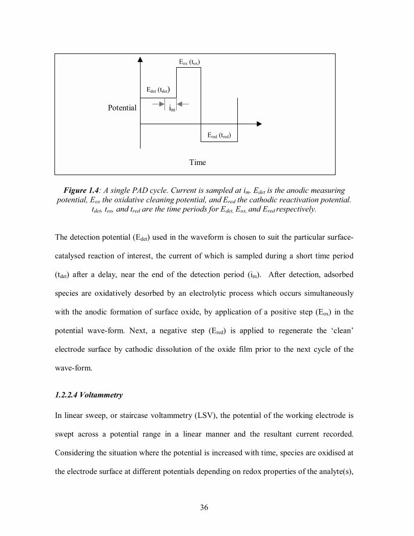
36

Eox (tox) Edet (tdet) Potential im

Ered (tred)

Time

Figure 1.4: A single PAD cycle. Current is sampled at im. Edet is the anodic measuring potential, Eox the oxidative cleaning potential, and Ered the cathodic reactivation potential.

tdet, tox, and tred are the time periods for Edet, Eox, and Ered respectively.

The detection potential (Edet) used in the waveform is chosen to suit the particular surface-

catalysed reaction of interest, the current of which is sampled during a short time period

(tdet) after a delay, near the end of the detection period (im). After detection, adsorbed

species are oxidatively desorbed by an electrolytic process which occurs simultaneously

with the anodic formation of surface oxide, by application of a positive step (Eox) in the

potential wave-form. Next, a negative step (Ered) is applied to regenerate the clean

electrode surface by cathodic dissolution of the oxide film prior to the next cycle of the

wave-form.

1.2.2.4 Voltammetry

In linear sweep, or staircase voltammetry (LSV), the potential of the working electrode is

swept across a potential range in a linear manner and the resultant current recorded.

Considering the situation where the potential is increased with time, species are oxidised at

the electrode surface at different potentials depending on redox properties of the analyte(s),

37

producing separate peaks at these potentials, pertaining to the analytes reacted. The current

produced is plotted against potential as a voltammogram, and can be used to give

information about different species in solution. In cyclic voltammetry (CV), as with LSV,

the potential is swept, for example, forward in a linear manner versus time, before the

direction of the scan is reversed and sweeps back in a negative manner. The term cyclic

arises from the closed loop drawn within the plot (Monk, 2001).

As Figure 1.5 shows, in the presence of a reversible redox species, a peak may be evident

in both the positive and negative CV scans. In ideal, fully reversible systems, these peaks

are of similar shape, and their peak heights and peak area will be the same. Oxidation

occurs in the forward scan, and reduction in the reverse. The magnitude of the current is

proportional to concentration. Cyclic voltammetry is a useful technique for identifying the

potentials of interest for a species in solution prior to the application of other

electrochemical methods (Owens & LaCourse 1997). It is also useful for determining

reaction kinetics, diffusion data and the reversibility of a system.

38

-0.100 0 0.100 0.200 0.300 0.400 0.500 0.600 0.700-4-0.400x10

-4-0.300x10

-4-0.200x10

-4-0.100x10

0

-40.100x10

-40.200x10

-40.300x10

-40.400x10

E / V

i / A

Figure 1.5: Example of a Cyclic Voltammetry scan of ferricyanide

1.2.2.5 Dual pulse staircase voltammetry

Dual pulse staircase voltammetry (DPSV) incorporates cleaning pulses to clean and

reactivate the electrode, as with PAD. In DPSV, the cleaning phase is applied at the start

of the scan, and followed by linear sweep (staircase) voltammetry, increasing in discrete

steps to approximate a continuous waveform (Figure 1.6). The scan yields a voltammogram

containing current-voltage peaks which correspond to different compounds present in the

solution. This technique has been used successfully for the simultaneous voltammetric

detection and quantification of glucose and fructose (Fung & Mo, 1995, Bessant & Saini,

1999), the detection of ethanol (Fung & Mo, 1996), and for the measurement of aliphatic

compounds (Bessant, 1998). This technique has not yet been incorporated into most

Forward

Reverse

39

commercially available potentiostats, but its use only requires simple modification of the

linear sweep method that is incorporated.

Dual pulse Potential Eox (tox) Erest

Estart Time

Ered (tred)

Linear sweep

Figure 1.6: DPSV waveform. Erest is the resting potential, Eox (tox) is the oxidative cleaning potential and time, Ered (tred) is the cathodic reactivation and time. Estart is the potential

at which the linear staircase sweep starts. 1.2.3 Electroanalytical detection of H2O2

As mentioned, hydrogen peroxide (H2O2) is produced in wounds by phagocytosis and is

therefore a potential marker of healing. H2O2 is also found in the tissues, since substantial

amounts of H2O2 are present in beverages (coffee), and in urine and exhaled air (Clement,

Halliwell & Long, 2000). Electrochemical determination of H2O2 is usually performed by

oxidation at a platinum electrode, which is often modified by deposition of a film with

enhanced electrocatalytic activity (Bertotti, Kosminsky & Matos et al, 2003). Detection of

H2O2 is also important in biosensor construction, because many oxidase enzymes used in

40

biosensors such as glucose oxidase or alcohol oxidase produce H2O2 as an end-product,

which can be directly electrochemically determined at the electrode (Gorton, Karyakin &

Palleschi et al, 2003).

1.3 Biosensors

Biosensors are currently defined as analytical devices incorporating either: a biological

material, such as a tissue, microorganism, organelle, cell receptor, enzyme, antibody or

nucleic acid; a biologically derived material, for example recombinant antibody,

engineered protein or aptamer; a biomimic such as a synthetic catalyst, combinatorial

ligand or imprinted polymer. Furthermore, the recognition element should be intimately

associated with, or integrated within, a physicochemical transducer or transducing

microsystem, which may be optical, electrochemical, thermometric, piezoelectric, magnetic

or micromechanical (Turner, 2005). Biosensors usually yield a digital electronic signal

which can be related to the concentration of a specific analyte or group of analytes.

Biosensors have been developed for use in a wide variety of sectors including medicine,

drug discovery, environment, food, process industries, security and defence.

Enzyme based electrochemical biosensors can be classified as (Saxena & Malhotra, 2003):

i) Potentiometric biosensors, which use ion-selective electrodes to determine changes in

concentration of chosen ions, for example hydrogen ions.

ii) Amperometric biosensors, which determine the electric current associated with the

electrons released during redox processes.

41

iii) Conductimetric/Impedimetric biosensors, which determine conductance/impedance

changes associated with changes in the overall environment.

The next section focuses on amperometric biosensors, since amperometric biosensors were

used in this thesis.

1.3.1 Amperometric biosensors

Amperometric biosensors have proven the most commercially successful biosensor devices

to date, with applications as diverse as breath alcohol detection and blood glucose

monitoring. Biosensors may be operated in a two electrode configuration (a working

electrode and joint reference/counter electrode) if currents are low enough to avoid

disturbing the reference electrode equilibrium potential, and the iR drop through the

solution does not significantly alter the applied potential from the potentiostat. To prevent

both these problems a three electrode configuration is often adopted using an auxiliary

(Counter) electrode through which the current arising from analyte-specific reactions at the

working electrode may pass.

Electrode designs are constantly evolving, ranging from the standard solid laboratory

electrodes, screen printed electrodes of varying composition, to needle type electrodes for

implantable devices. A discussion of the three generations of biosensors, exemplified by

the glucose sensor is included in the glucose measurement section that follows.

42

1.3.1.1 Glucose measurement

Glucose biosensors are by far the most commercially successful biosensors to date, with

over 40 home blood glucose meters on the market for those with diabetes (Newman &

Turner, 2005). The main share of the market is occupied by Roche Diagnostics, LifeScan,

Abbott and Bayer. The most commonly used enzymes in glucose biosensors are glucose

oxidase (GOx) and glucose dehydrogenase (GDH). GOx enzymes oxidise ß-D-glucose

substrate, accepting electrons at its FAD prosthetic site in the process. GOx is able to

transfer these electrons to molecular dioxygen present in the sample, resulting in the

production of hydrogen peroxide.

By immobilising GOx close to, or onto a suitable transducer, an amperometric biosensor

can be made, monitoring either O2 depletion of H2O2 production, and as such represents an

example of a first generation biosensor.

One difficulty in using GOx is the potential problem of dissolved dioxygen limitation. To

overcome this, oxygen can be replaced with an artificial mediator (electron acceptor). A

mediator is a redox couple that can shuttle electrons between the redox centre of the

enzyme and the electrode, and can be electrochemically regenerated at potentials where

interference from species such as ascorbic acid (vitamin C) and acetaminophen

(paracetamol) are minimised (Newman & Turner, 2005). Commonly employed mediators

include hydroquinone, ferrocene, certain redox dyes and ferro/ferricycanide. Mediated

enzyme systems represent the second generation of biosensors.

43

An alternative approach is offered by the so-called third generation biosensors. In this

case, the electrode is configured such that it is able to exchange electrons directly with the

enzyme active site deeply buried within the protein, thus negating the need for electron

shuttle molecules. The difficulty in engendering electrical contact between the active site of

the enzyme and the electrode make this a difficult and rarely reported approach (Varma et

al, 1993), but has been reported by Yang, Lanqun and Takeyoshi, et al (2005), Christenson,

Dock and Gorton et al (2004), Xu & Han (2004) for example.

The first widely-commercially successful glucose biosensor was a mediated device (second

generation) based on a screen printed disposable sensor design called the ExacTech device,

developed by MediSense in conjunction with the Universities of Cranfield and Oxford. The

majority of products today utilise similar technology, i.e. using the basic concept of an

amperometric biosensor, employing GOx and electrochemical mediators on a disposable

strip format. This type of glucose monitor is based on the measurement of glucose in a

blood sample typically taken from the finger using a small lancet.

Since finger pricking is uncomfortable, other sampling sites and methods have been

investigated. For example, the GlucoWatch® biographer - a continual, non-invasive,

automatic glucose monitor. This device incorporates the use of an amperometric biosensor,

which detects glucose in interstitial fluid as it is extracted through intact skin by a process

of reverse iontophoresis every 20 minutes, for 12 hours, after a 3 hour warm up period. The

amount of glucose extracted within one three minute iontophoresis cycle is estimated to be

between 50 500 picomol. It is favourable over the finger-prick methods, since it lacks the

44

discomfort, is convenient, automated, and facilitates intensive glucose control regimes. The

GlucoWatch® is a small, wrist-watch device capable of both sampling and detection,

contains all necessary circuitry, and a digital display. The operation of the device is

controlled by a microprocessor, which also converts the sensor signals into glucose

readings. The circuitry includes two independent potentiostat circuits to operate the

biosensors, and a galvanostat circuit for the iontophoresis. Temperature fluctuations and

perspiration are detected by the incorporation of temperature and skin conductivity sensors.

The AutoSensor itself is disposable, and fits into the skin-side of the biographer. It

contains two identical biosensors and iontophoresis electrodes, two hydrogel disks which

serve as biosensor electrolyte, glucose reservoirs, and also have the glucose oxidase

enzyme dissolved into them. The biosensor working electrodes have a screen-printed layer

of Pt/C composite ink. The reference and counter electrodes have screen-printed Ag and

Ag/AgCl layers. The counter electrode is also used as the iontophoresis electrode.

However, the Glucowatch has not been as successful as hoped, due to its high cost

compared to other glucose measurement devices available, and problems with skin

irritation after prolonged use (Garg, Jovanovic & Potts et al, 2000; Panchagnula, Pillai,

Nair et al, 2000)

For further information on finger prick biosensors, minimally invasive systems and the

potential of non-invasive systems such as fluorescence or IR spectroscopy, readers are

referred to Newman & Turner (2005) who have reviewed blood glucose biosensors from a

commercial perspective.

45

1.3.1.2 Alcohol measurement

Another major area of biosensor use is for the detection of characteristic odours of alcohol

in breath, and alcohol in beverages. Sprules, Hartley, Wedge et al (1996) investigated the

use of screen printed amperometric biosensors for the measurement of alcohol in beverages

for example. Kim, Lee, Lee et al (1999) investigated using an amperometric biosensor to

determine breath alcohol, and was able to measure over the concentration range 20-800

ppm. The selective, sensitive, and reliable detection of ethanol in the breath of a vehicle

driver is essential to determine whether a driver has consumed too much alcohol. This

biosensor utilises nicotinamide adenine dinucleotide (NAD+) cofactor, which is reduced in

the presence of ADH and ethanol to NADH (Kim, Lee & Lee et al, 1999) which can be

subsequently oxidised at an electrode poised at a suitable oxidising potential.

ADH CH3CH2OH + NAD+ → CH3CHO + NADH + H+

Electrode NADH → NAD+ + H+ + 2e-

This biosensor consists of an Ag/AgCl reference electrode, an active working electrode

containing ADH, and a compensator electrode containing a protein analogue (typically

bovine serum albumin) in place of ADH. The differential signal that is produced between

the active and inactive electrodes minimises the interference from oxidisable species in a

persons breath. Before measurement, the biosensor is hydrated in phosphate buffer at pH

7.4. Ethanol catalysis and stoichiometric levels of NADH are produced by the enzymatic

46

reaction, with the NADH being subsequently oxidised at the active electrode poised at a

potential of +470mV (vs. Ag/AgCl), and compared to the compensator electrode.

There are few commercially available amperometric biosensors based on gas-phase

analysis, as opposed to liquid-phase analysis. This is because of the difficulty associated

with the use of enzyme electrodes to monitor gaseous samples without aqueous media. For

this reason, gas-phase biosensors, like the differential-type amperometric biosensor

described above, are pre-hydrated in buffer, which is retained in the enzyme-immobilised

gel layers. Small thick-film based sensors can be made cheaply by conventional screen

printing technology.

1.3.2 Screen-printed electrodes

Screen-printed electrodes are commonly used instead of the conventional solid-state

electrodes because they lend themselves more easily to mass production and commercial

use. Layers of speciality inks are deposited sequentially onto an insulating support or

substrate. They have certain favourable characteristics that have contributed to their

widespread use in environmental, clinical or industrial applications. Benefits include their

small size, low cost, simplicity of manufacture and disposability. They have been used as

amperometric sensors and/or biosensors, for example in the detection of maltose and

glucose (Feng, Zhang & Zhang et al, 1998), sulphur-containing amino acids (Cheng,

Jandik & Avdalovic 2003), and alcohol in beverages (Sprules, Hartley & Wedge et al

1996). Gorton, de Mattos and Ruzgas (1996) have discussed the properties of modified

gold and platinum screen printed electrodes for use as sensors and biosensors, and Hart,

47

Turner & Hopcroft (1996) compared the use of screen- and ink-jet printing to produce

electrodes. Alegret, Albareda-Sirvent & Merkoci (2000) have reviewed the configurations

used in the designs of screen-printed enzymatic biosensors.

Often, the surface of the screen printed electrode is modified for a particular application.

For example, coating the electrode surface with a transition metal such as a

hexacyanoferrate (HCF) film, confers additional electrocatalytic properties on the

electrode. For example, reduced form Prussian blue (FeHCF) can electrocatalytically

reduce H2O2 by acting as an electrocatalytic mediator, (Gorton, de Mattos & Ruzgas, 1996;

Ricci & Palleschi, 2005; O'Halloran, Pravda and Guilbault, 2001). Certain analytes can be

amperometrically detected at low potentials by combination of catalytic materials with

oxidase enzymes,

The versatility and simplicity of screen-printing means that designs can be simply and

cheaply configured, and sensor and biosensor strips are increasingly being incorporated

into small hand held or portable devices.

1.3.3 Direct (label-free) detection of bacteria with biosensors

Most microbiological tests are performed in large centralised laboratories, and require

highly trained technical staff. However, the desire for tests to be portable, rapid and

sensitive has led to the development of biosensor technologies in the clinical field. Since

one aspect of this thesis is concerned with bacterial detection, a summary of the main direct

and indirect biosensor technologies reported for bacterial detection follows.

48

The monitoring of cells at solid-liquid interfaces is generally based on the direct

measurement of a biochemical reaction at the transducer surface, for example, changes in:

pH, oxygen consumption, ion concentrations, potential difference, current, resistance, or

optical properties. For example, certain optical biosensors can detect minute changes in the

refractive index when cells bind to immobilised receptors on the transducer surface. An

interferometer (Edwards, Hartman & Schneider, 1997) is an optical unit consisting of an

LED/filter excitation source, and a photodiode detection system. The increase in CO2

concentration that can arise from active bacterial metabolism, may be detected by the

change in emulsion of the aqueous colorimetric pH indicator, which in turn modulates the

fluorescence detected by the photodiode.

Bioiluminescence biosensors

Certain enzymes emit photons as a by-product of their catalytic degradation of substrate

molecules, a phenomenon known as bioiluminescence. This phenomenon maybe used to

detect the presence and physiological conditions of cells. These systems have been used to

detect a wide variety of microorganisms, for example of Salmonella Newport and E.coli

(Blasco, Murphy & Sanders et al, 1998). Bacteriophages are used to lyse bacteria, such that

the cell content released can be measured by ATP bioluminescence. This is an attractive

approach due to its high specificity and ability to distinguish between viable and non-viable

cells. However, the assay time is long, and the method is not suitable for determining low

bacterial numbers.

49

Piezoelectric biosensors

These systems may be used for direct label-free detection of bacteria, and other

applications, with real-time output. The surface of a PZ sensor is coated with selective

ligands, such as antibodies, and placed in a solution containing bacteria. Bacteria of the

required specificity will be bound by the antibodies, which results in an increase in the

mass of the crystal, and a proportional decrease in the resonant frequency of the crystal.

These have been developed for Vibrio cholerae (Carter et al, 1995) and Salmonella

typhimurium (Prusak-Sochaczewski et al, 1990) for example.

Electrical impedance biosensors

This method is useful in the detection of bacteria in clinical specimens, to monitor quality,

detect specific food pathogens, and in industrial microbial process control. Cell density,

growth, and long term behaviour of cells on the electrodes cause a change in the impedance

of the biosensor. A reusable Bulk Acoustic Wave Impedance Sensor has been developed to

continuously detect the growth of Proteus vulgaris on the surface of solid medium (Deng et

al (1996).

1.3.4 Indirect Detection of Bacteria

Fluorescent immunoassay techniques

The immunogenic nature of microorganisms, due to the presence of proteins and

polysaccharides in their outer coats, allows the development of fluorescent immunoassay

(FIA) techniques for bacterial detection. Fluorochrome molecules are used to label

50

immunoglobulins, absorb light at a short wavelength, and emit it at a higher wavelength

which is detected by fluorescent microscopy. FIA utilises the high degree of specificity

inherent in immunological reactions.

Microbial metabolism based biosensors

Microorganisms can transduce their metabolic redox reactions into quantifiable electrical

signals by oxidoreductase reactions and a mediator. The microbial content of a sample can

be determined by monitoring the microbial metabolism. For example, oxygen consumption

could be detected by a transducer. It may also be possible to detect other metabolic

products of bacteria.

Electrochemical immunodetection of bacteria

The advantages of electrochemical sensors over optical sensors are that they can operate in

turbid media, with comparable instrumental sensitivity, and are also easier to miniaturise.

The continuous response of an electrode system also allows on-line control. Light

addressable potentiometric sensors (LAPS) based on field effect transistor (FET)

technology has been used successfully for the immunoassay of bacteria (Abdel-Hamid,

Atanasov & Ivnitski et al, 1999).

Further information on biosensors for the detection of pathogenic bacteria can be found in

Abdel-Hamid, Atanasov, Ivnitski et al (1999) who have reviewed the aforementioned

techniques in 1.3.3 and 1.3.4 in detail.

51

1.4 Electronic Nose

1.4.1 The human olfactory system and odours

The inspiration behind the mechanisms of an electronic nose is that of human olfaction.

Therefore, to understand the operation of an electronic nose it is important to first

understand the biological act of smelling with the human olfactory system that enables us

to characterize an odour (Gardner, Craven & Bartlett, 1996). Therefore, a description of the

human olfactory system and the properties of odorous molecules shall follow before

discussing the so-called method of machine olfaction.

Humans have three sensory systems which play a part in the sensation of flavour. These are

olfaction or sense of smell, gustation or sense of taste and trigeminal sense (response to

irritant chemical species). Of these three, smell is the dominant contributor to the sensation

of flavour, and has much wider powers of classification than the taste or trigeminal senses.

Smell alone can often determine the flavour profile of a product.

Odorant molecules stimulate the human olfactory system located in the human nose. Here,

they are drawn into the nasal cavity across the epithelium, which contains a mucous layer

and olfactory hairs or cilia leading into olfactory cells. The cilia have G-receptor binding

proteins which act as chemosensory receptors. Since there are only a limited number

(~100) of receptor proteins, they require partially overlapping sensitivities in order to allow

complex smells to be identified. There are ~100 million olfactory cells, which serve as

signal amplifiers and generate secondary messengers. These messengers generate signals

which travel from the olfactory nerves to ~5000 glomeruli nodes in the olfactory bulb via

52

axons. In the olfactory bulb, the signals are further processed by ~100,000 mitral cells

before they are sent via a granular cell layer to the higher sensory centers in the cerebral

cortex of the brain. The receptor cells only live an average of 22 days, and are believed to

have a low sensitivity in the ppm range, and low specificity. However, the signal

amplification and neural processing that subsequently occur greatly enhance the sensitivity

and discrimination between thousands of odours (Gardner & Bartlett, 1994). The perceived

intensity of an odour is not linearly related to its concentration, but typically a sigmoidal

relationship. A more detailed analysis of each aspect of the human olfactory system can be

found in Gardner & Bartlett (1999).

1.4.1.1 Properties of odorous molecules

Many simple odours may arise from single molecular species. Such odorants are typically

hydrophobic and polar with a molecular mass of 30-300 Da. However, most natural

smells, perfumes and flavours are complex mixtures of chemical species frequently

containing hundreds or maybe thousands of constituents. Subtle differences between the

relative quantities of these constituents can determine the overall odour of a product. It is

essential that the molecules are volatile in order to be carried up into the nose via the nasal

passages to the olfactory receptors. Molecules heavier than 300 Da are generally not active

odorants at room temperature. However, volatility is not just determined by molecular

weight. The strength and type of interactions between molecular species is also important,

as is the geometrical shape and charge distribution of the odorant species. Typically, for

example, polar molecules are more volatile than non-polar molecules. Odorous molecules

generally possess one or two functional groups within the structure which makes them

53

more polar. Examples of two functional group structures that are associated with odorous

molecules are shown below.

Alcohol

R O H Acid O

R C OH Aromatic molecules are also important in odour chemistry, since they are often highly

odorous and are generally chemically stable. This is because they have six delocalized π

electrons involved in the π bonding molecular orbitals localized above and below the plane

of the molecules, referred to as aromaticity. A more in depth description of the molecular

structure of odour molecules and intermolecular forces can be found in Gardner & Bartlett

(1999).

1.4.2 Machine olfaction

In many industries, the human nose is still the main instrument used to evaluate the smell

and flavour of products, such as perfumes and foodstuffs. However, this is a costly process,

since trained panels of experts are required. Physicochemical properties are measured using

conventional analytical equipment, such as gas chromatography-mass spectroscopy (GC-

MS). As well as being time consuming, these methods often fail to detect some key flavour

constituents since they fall below the capability of the instrument. These factors generated

54

a demand for electronic instruments that can imitate the human olfactory system, and also

provide a low cost, rapid sensory system.

The first reported electronic nose was in 1964 by Wilkins & Hatman, who studied the

redox reactions of odorants at an electrode. However, the first report of the concept of an

electronic nose as an intelligent chemical array sensory system for odour classification, was

not until the early eighties, by Persaud & Dodd (1982) and Ikegami & Kaneyasu (1985).

The term electronic nose was first used in the late eighties and appeared at a conference

in 1987 in the UK (Gardner, 1987). There are various synonyms for electronic nose such

as artificial nose, mechanical nose, odour sensing system, and as yet the term has not been

defined. A definition proposed by Gardner & Bartlett (1994) shall be used for the purpose

of this thesis: An electronic nose is an instrument, which comprises an array of electronic

chemical sensors with partial specificity and an appropriate pattern-recognition system,

capable of recognizing simple or complex odours.

As the name machine olfaction suggests, it is an intelligent chemical array sensor system

analogous to the human nose. The process of machine olfaction fundamentally consists of

three stages: an electronic sensor array, a pre-processor and a pattern recognition engine

(PARC). The broadly responsive sensor array imitates the olfactory receptor cells, the pre-

processing corresponds to the processes of the olfactory bulb, and the computer based

pattern recognition system mimics the cerebral cortex of the brain. The diagram in Figure

1.7 illustrates the basic analogies between human and machine olfaction.

55

Figure 1.7: Diagram showing the analogy between the three basic stages of machine and human olfaction.

1.4.3 Sensors

The primary requirement of the sensor array is to generate a pattern of responses that is

discernibly different for different samples. The sensors in the array of an electronic nose

are therefore required to have partial sensitivity to permit response to a broad range of

gases or odours, i.e. they should differ but overlap between sensors across the array, in a

similar manor to biological olfactory receptors, thereby ensuring that the entire pattern of

response across the sensor array is analysed (Gardner & Bartlett, 1999). The sensor array

responses are processed by specialised computer software which produces profiles, and

thus converts smells into a digital representation, or fingerprint (Gibson, Prosser, Hulbert,

2000). This enables the identification of many odours that may contain hundreds of

individual chemical components. This is opposite to the requirements of an ideal gas

sensor, which should respond to only one gas.

SENSOR ARRAY

PRE- PROCESSING

PATTERN RECOGNITION

ENGINE

RECEPTOR CELLS

OLFACTORYBULB

CEREBRALCORTEX

HUMAN OLFACTION

MACHINE OLFACTION

Beer

56

It is desirable for the sensors to have a reasonable response time and recovery time. It is

also important that the individual sensors are reproducible in their response to a given

odour, and that the response is reproducible between sensors of nominally the same type.

This eliminates the need to fully retrain and recalibrate the system if a sensor needs

replacing. Numerous sensor technologies have been utilised in sensor arrays, most notably

inorganic semi-conducting materials such as metal-oxide sensors, acoustic wave sensors

and conducting polymers.

1.4.3.1 Metal-Oxide Sensors

Metal oxide semi-conductor (MOS) gas sensors are available commercially from suppliers

such as Fiagro Engineering (Japan) and Capteur mixed MOS sensors from City

Technology (UK), and are the most widely used sensors for construction of arrays for the

measurement of odours. The most widely used material in metal oxide sensors is tin-

dioxide, SnO2, doped with small amounts of catalytic metal such as palladium or platinum.

Varying the choice of catalyst and operating conditions enables these sensors to be used in

a wide range of applications. The construction of each of these sensors is similar,

consisting of a ceramic support tube coated with tin oxide (and catalysts), and containing a

platinum heater coil (Gardner & Bartlett, 1999).

The gas or odour is sensed by a change in resistance at the semiconductor. As the

concentration of adsorbed oxygen at the semiconductor surface changes, the change in

resistance proportional to the concentration of the analyte can be measured. At ambient

conditions, oxygen adsorbs to the surface of the metal oxide layer and dissociates to form

57

O-, by extracting electrons from the semiconductor. Semiconductors come in two types, n

or p. The electron extraction will respectively increase or decrease the resistance. For

example, if the semiconductor is exposed to a reducing gas, oxygen will be removed from

the surface and thus will gain electrons, leading to a positive (p) or negative (n) change in

resistance, depending on semiconductor type (Lee-Davey, 2004). Other factors such as

humidity also have an effect on resistance. At low temperatures it is possible that water

may form. This complicates the detection of volatile odours (Gibson, Prosser, Hulbert,

2000). However, these sensors are usually operated at elevated temperatures of 100-600 °C

which reduce the negative effects of water.

In terms of suitability to the application of wound monitoring, MOS sensors have the

advantages of low cost, and fast response times. They are also particularly sensitive to

volatiles such as alcohols (0.1-100 ppm) (Ragazzo-Sanchez, Chalier, Chevalier et al, 2006;

Hansen, Petersen, Byrne, 2005) and are not sensitive to the detection of sulphur- or

nitrogen-based odours. The disadvantage of MOS sensors and other chemical sensors is

that they are susceptible to baseline drift, defined by DAmico & Di Natale (2001) as: a

slow unpredictable change of the sensor response, undefined from the statistical point of

view, which is superimposed to both the signal and noise levels. Drift is particularly

insidious in machine olfaction, since their utility is based upon pattern recognition models

developed from particular responses. Therefore it is important that drift behaviour is

identified early on and compensated for by the incorporation of a suitable mathematical

models.

58

1.4.3.2 Conducting Polymer Sensors

Organic materials offer a wider choice of sensor materials, and more importantly, can

incorporate functional groups that can interact with different classes of odorant molecules.

For example, conducting polymers, such as poly(pyrrole), and biological lipid coatings.

They can also be operated closer to room temperature (20-60°C). As a result of this, the

first commercial electronic noses used conducting polymer gas sensor arrays.

Polymer sensors generate a change in resistance when analyte adsorbs onto the polymer

film and induces swelling. However, they are susceptible to changes in humidity, since it

affects the baseline structure and swelling behaviour of the polymer (Gardner &

Bartlett, 1994, 1999).

1.4.3.3 Acoustic wave sensors

Acoustic wave gas sensors detect the effect of sorbed molecules on the propagation of

acoustic waves. The basic device consists of a piezoelectric substrate, usually quartz,

coated with a suitable sorbant coating. Sorption of vapour molecules into the sorbant

coating is detected by changes in wave velocity, and hence frequency and amplitude of

oscillation of the sensor. Acoustic wave sensors operate at ultrasonic frequencies of

typically 1 to 500 MHz.

Two main types of acoustic wave sensors exist: bulk acoustic wave (BAW) and surface

acoustic wave (SAW). BAW sensors rely upon the application of an electric field to make

the quartz crystal oscillate at its resonant frequency. SAW sensors exploit wave

59

propagation across the sensor surface. Both of these acoustic wave-type sensors require

excitation by a.c. voltage.

1.4.4 Signal pre-processing

Figure 1.8 depicts the generic architecture of an electronic nose. Individual sensors i

produce a time-dependent electrical signal yij(t) in response to odour (a set of unknown

odour samples A, B, C of unknown class j). The rise and decay time of the sensor will

depend upon one or more of the following parameters (Gardner & Bartlett, 1994):

1) the flow delivery system that carries the odour from the source to the sensor array

e.g., the flow profile and type of carrier gas;

2) the nature of the odour, e.g., type, concentration;

3) the reaction kinetics of the odour and the active material;

4) the diffusion of the odour within the active material;

5) the nature of the sensing material e.g., physical structure, porosity, thermal time-

constant;

6) the nature of the substrate supporting the active material e.g., thermal conductivity,

acoustic impedance;

7) ambient conditions, e.g., temperature of active material, carrier gas, humidity,

pressure.

60

Figure 1.8: Architecture and processing stages of an electronic nose, including unsupervised learning of unknown odour inputs. The difference between the response

vectors xj are maximized in the transformed vector space, e.g. X-space for eigenvectors in PCA. (Based on Gardner & Bartlett, 1994, 1999).

An array of n sensors gives a response vector Xj. The array response vector may be pre-

processed to help the discrimination process. The technique of baseline manipulation

relates the sensor response to a constant signal value, the baseline. For example, with MOS

sensors, the baseline signal is the sensors response to air. The signal noise can be reduced

parametrically or as a specific requirement for the input to a pattern recognition engine.

The scale of the response vectors is often normalized so that the output of individual

sensors can be visualized within the range. This process conditions the data so that all

features in the response vectors are of the same magnitude. Next, the vectors are analysed

by a suitable pattern recognition technique.

OUTPUT PREDICTOR(Class j)

INPUT: UNKNOWN ODOURS

A,B,C, cj (t)

ACTIVE MATERIAL

SENSOR 1 SENSOR 1 PROCESSOR

ACTIVE MATERIAL

SENSOR n SENSOR n PROCESSOR

ARRAY PRE- PROCESSOR

PARC ENGINE

Analogue Sensing Digital Processing

y1j (t)

ynj (t)

x1j

xnj

Xj

Vectors Transformed

Odour A

Odour B

Odour C

X1

X2

X3

X-space

61

1.4.5 Pattern recognition techniques

The processing of input odour signals in an electronic nose can essentially be divided into

two methods: unsupervised and supervised. The objective of unsupervised learning is to

discriminate between unknown odours by enhancing the differences between their related

input vectors, while supervised learning aims to classify unknown odours as known ones

that have been learnt during earlier training and calibration of the PARC engine.

The pattern recognition technique of supervised learning essentially involves the

introduction of known sets of odours to the sensor array, which produce corresponding sets

of response vectors. These sets are known as training or calibration sets, and are used to

generate a knowledge base. The knowledge base is further extended by incorporating

regression coefficients in a parametric model, or a non-parametric model such as a neural

network. Once the system has been trained, unknown odours can be analysed with the

electronic nose using the knowledge base to assign the most likely class of odour. Artificial

neural networks can handle non-linear data, and are tolerant to sensor drift or noise

(≈10%). They also produce lower predictive error rates than chemometric techniques

(Gardner & Bartlett, 1994; Ciosek & Wroblewski, 2006).

Figure 1.8 also illustrates the spread of signals through an electronic nose using an

unsupervised pattern recognition technique. The set of N unknown odour samples produce

a corresponding set of N unknown array vector responses (x). The vectors are separated in

multidimensional space by maximizing the distances between the vectors. This can lead to

a set of p clusters in a feature space of reduced dimensionality, which can be associated

62

with the known classes of odour (i.e. j takes the value of 1 to p). Techniques such as

principle component analysis (PCA) and cluster analysis are useful for displaying the

differences of multivariate data in a reduced dimensionality.

1.4.5.1 Principle components analysis

Since PCA was the methodology implemented for the investigation of odour analyser

response to imitation wound odour in this thesis, a brief description of this technique

follows. Further details of PCA can be found in Gardner & Bartlett (1999), Wold, Esbensen

& Geladi (1987), and Massart, Wu & Guo et al (2002). PCA is an unsupervised technique

(i.e. does not require a training set), multivariate (i.e. can consider many variables

simultaneously), non-parametric statistical technique. It is widely used, due to its powerful

ability to discriminate between simple and complex datasets, such as array-generated odour

profiles. PCA analyses the inter-relationships between a large number of variables and

seeks to reduce them to a smaller number of indices, called principle components (Xp), that

describe their common underlying dimensions.

Each principle vector accounts for a degree of variance in the data. The principle

components are ordered so that the first component, X1 displays the greatest amount of

variance, followed by the second greatest as X2 and so on. It is typical for a large proportion

of the variance in the data to be within the first two principle components. Therefore, a plot

of these two principle components can be used to represent a large proportion of the

variance in the data, and thus determine any distinct groups of odours. High Xp values show

a disciminating sensor, whereas values nearer to zero contribute noise to the score. PCA is

63

a useful technique to explore the functionality of an electronic nose, by determining

differences in multivariate data.

1.4.6 Applications of electronic nose technology

Commercial electronic noses were first launched in the 1990s, for example, from Alpha

MOS in 1993, Neotronics and Aromascan in 1994, Bloodhound Sensors and HKR

Sensorsysteme in 1995 (Gibson, Hulbert, Prosser, 2000). Commercial odour monitors have

been produced for several years, such as the Portable odour monitor by Sensidyne Inc,

USA, which can detect the intensity of an odour using only one sensor.

Electronic noses have been used in a variety of applications, mostly to classify the smells

of beverages and foods (Schaller, Bosset and Escher, 1998), giving information about the

grade or quality of whiskeys, beers, and wines (Lamagna, Reich, Rodriguez, et al, 2004;

Marti, Busto, Guasch et al, 2005), or freshness of meat and fish (Blixt, Borch, 1999;

Olafsdottir, Nesvadba, Di Natale, et al, 2004) for example. They have also been reported

for use in monitoring cell culture (Bachinger, Riese, Eriksson, et al, 2000), the automotive

industry (Garrigues, Talou, Nesa, 2004), environmental monitoring (Onkal-Engin, Demir,

Engin, 2005; Nake, Dubreuil, Raynaud et al, 2005), and the characterisation of perfumes

(Penza, Cassano, Tortorella et al, 2001; Yang, Yang and Peng et al, 2000). Odour analysis

is also a promising area of interest in medical diagnostics. Portable, application specific

devices could be used for a wide range of diseases, and are likely to become more common

and user friendly for the detection and identification of clinical infections in the future.

64

Magan, Pavlou, McNulty et al (2002) have reported the use of an electronic nose for the

diagnosis of urinary tract infections (UTIs), by examining the volatile production patterns

produced by bacterial contaminants in urine samples. Larsson, Mardh and Odham (2000)

have investigated the use of an electronic nose to detect breath alcohol, using ANNs for the

prediction of ethanol concentration. Gibson, Prosser, Hulbert, Pavlou (2000) reported a

project carried out in 1996 between Bloodhound Sensors Ltd with Oxoid Ltd, investigating

selective culturing techniques and subsequent measurement of the odours generated by the

organisms. A 4-6 hour incubation time was found to be sufficient to produce characteristic

odours. A number of strains of E.coli, P.mirabilis, P.aeruginosa and S.aureus were used to

train a neural network, and were identified with 95% confidence match. Gibson, Prosser,

Hulbert et al (1997) have also studied the detection and simultaneous identification of 12

different bacteria and 1 yeast using headspace samples from plate cultures using an

electronic nose and neural networks with a classification rate of 93.4%. Gardner, Shin and

Hines (2000) have investigated the use of an electronic nose system based on an MOS

sensors array to diagnose illness from the breath of dairy cows. In 2005 the same group

also published a paper on the identification of Staphylococcus aureus (MRSA, MSSA and

C-NS) from ear, nose and throat infections using an electronic nose. An array of 32

polymer carbon black composite sensors were exposed to swab samples from patients in

hospital known to be infected, to produce distinctive response patterns for each vapour.

Swabs were cultured for 24 hours before sniffing with the electronic nose. This was

followed by a combination of three statistical techniques PCA, self-organising mapping,

and fuzzy C means, with the objective of producing clusters of the different bacteria

species and prediction with an accuracy of 99.69%.

65

Although in the aforementioned study culturing time was long, and no attempt was made to

determine the limits of detection or the chemical make up of the odours, the results from

this and other initial investigations into the use of odour analysis in clinical applications are

encouraging and suggest that odour analysis is a worthwhile area of continued investigation

for the identification of bacterial species for a range of clinical conditions, such as UTIs,

throat infections, lung cancer, diabetes or hospital acquired infection of wounds. Odour

analysis has the prospect of supplying answers to medical practitioners by measuring

distinct odours characteristic of certain clinical conditions, such as acetone of the breath of

diabetics for example. It is hoped that one day odour analysis may also form an integral

part of diagnostic medical practice in hospitals, and in the case of this thesis, be used to

provide rapid diagnostic information about the nature of a wound environment in an effort

to help combat the growing threat of hospital acquired infections such as MRSA.

1.5 Chromatographic techniques and test kits

Chromatography is a widely used standard technique, both for routine analysis and for the

validation of new and developing analytical technologies. It is a separation procedure for

resolving mixtures and isolating components, based on differential migration, i.e. the

selective retardation of solute molecules during passage through a bed of sorbant or porous

material (stationary phase). As solvent (mobile phase) flows through the column, the

solutes travel at different speeds depending on their relative affinities for the stationary

phase. The solutes are separated, and elute from the column at different times. The pattern

of solute peaks emerging from a chromatographic column is called a chromatogram.

66

Chromatographic analysis has been described in detail elsewhere (Kolb & Ettre, 1997) but

a brief description of the main chromatography techniques follows.

1.5.1 Liquid chromatography

Liquid chromatography can be classified into three types. In adsorption chromatography,

the stationary phase is an adsorbent such as gel, and separation is based on the repeated

adsorption and desorption of solute species on the stationary phase. There are two modes

for this type: normal and reverse. Normal phase chromatography utilises a more polar

stationary bed, with the mobile phase being more non-polar, thus polar species are retained

longer. Reverse phase chromatography is the opposite of this. In ion exchange

chromatography, ions are held on a porous insoluble solid and are exchanged for ions in a

solution that are brought in contact with the solid. Synthetic ion exchange resins are used in

applications such as water softening and solution purification. The resins are high-

molecular-weight polymers that contain large numbers of an ionic functional group per

molecule. Cation-exchange resins contain acidic groups such as sulfonic acid groups, and

anion-exchange resins contain basic groups. In size exclusion chromatography, the column

is filled with porous material, resulting in separation based on size. Larger molecules that

are too large to enter the pores are eluted first, whilst smaller molecules are more able to

penetrate the pores and thus take longer to elute. This technique is also often called gel

permeation chromatography. In all types, as molecules are eluted from the column, they

are detected and a chromatogram is produced (Skoog, West, Holler, 2000).

67

1.5.2 Gas chromatography

In gas chromatography (GC), the mobile phase is a gas. Gas chromatography is widely

used as an analytical tool for separating relatively volatile components such as alcohols,

ketones, aldehydes and many other organic and inorganic compounds. In gas

chromatography, the sample is vaporized and injected onto a chromatographic column. The

sample must be of a suitable volume, and is introduced as a plug of vapour. Calibrated

microsyringes are used to inject liquid samples through a rubber or silicone diaphragm or

septum into a heated sample port located at the head of the column. The sample port is

usually about 50 °C above the boiling point of the least volatile component of the sample.

Elution is brought about by the flow of an inert gaseous mobile phase, commonly helium.

Many changes and developments have occurred in gas chromatographic instruments since

their first commercial introduction. Microprocessors are used for automated control of most

parameters, such as column temperature, flow rates, and sample injection. Columns have

been developed that are capable of separating components of complex mixtures in

relatively short times.

Detection devices must be used which are able to respond to minute quantities of solutes as

they exit the column. The ideal detector would also have a linear response, stability, and

uniform response for a wide variety of chemical species. Several types of detector exist.

The effluent from a chromatographic column is often monitored continuously by selective

techniques such as spectroscopy or electrochemistry, such as mass spectroscopy (MS) or

Fourier Transform IR spectroscopy (FTIR), to give techniques such as GC-MS. These so-

called hyphenated techniques are powerful tools for the identification of components of

68

complex mixtures. Computer-based chromatography instrumentation often incorporate

large databases to compare spectra and identify compounds eluting from the

chromatographic column.

1.5.3 Applications of Chromatography

1.5.3.1 Chromatographic detection of bacteria

Bartlett, Gorbach & Mayhew et al (1976) hypothesized that short-chain fatty acids (SCFA)

produced by certain organisms might serve as markers in clinical samples. Table 1.6

summarises this and other reported cases of the use of different chromatographic

techniques.

1.5.3.2 GC-MS analysis of urine

GC-MS has been used in many clinical applications, such as in the analysis of urine. The

often characteristic odours of a culture often give a clue as to the identification of one or

more of the organisms present, and trained microbiologists can often identify a microbial

culture by smell alone. Traditionally, volatile species are determined by sample extraction

followed by GC-MS analysis. However, this approach requires some knowledge of the

molecules involved. Several variables, such as pH, acidity, carbohydrate content,

temperature and protein levels, need to be kept within a narrow range.

GC-MS is often used along with the e-nose in research, to provide valuable compositional

data and for validation purposes. For example, Evans, Persaud & Pisanelli (1996) used both

techniques in a diagnostic study of urine odour of UTI patients. Urine samples were

collected over a period of several days, and the urine headspace was analysed by GC-MS

69

and e-nose. The patterns obtained from the sensor array were captured and stored for

further processing. Mathematical treatment of the data enabled differentiation between the

normal population and myopathy population. GC-MS analysis found that the composition

of urine headspace is markedly different within normal and diseased populations. The key

volatile components found in normal urine were 2-heptanone and 4-heptanone. In diseased

urine, the amounts of these volatiles increased, and also contained 2(3H)phenanthrene-4-

4a, 10-tetrahydro-4a-methyl and phenyl-isopropylphenyl. The GC-MS analysis validated

the results obtained from the electronic nose, since the different patterns obtained from the

gas sensor apparatus correlated with the different volatiles detected by GC-MS.

Headspace GC-MS (HS-GCMS) was chosen as the standard method with which to

compare the electronic nose and generate information on the five bacteria used in this

thesis. Though not directly comparable, it was acknowledged to possess the most

similarities to the single sensor odour analyser.

70

Tec

hniq

ue

Ana

lysi

s spe

cific

atio

ns

Cul

turi

ng sp

ecifi

catio

ns

Sam

ple

type

M

etab

olite

s det

ecte

d R

efer

ence

Dire

ct G

LC

GC

: Pac

kard

419

and

Sh

imad

zu G

C4B

MPF

dua

l-co

lum

n ga

s chr

omat

ogra

ph

with

flam

e io

niza

tion

dete

ctor

. Sily

cate

d Py

rex

colu

mn.

Tem

ps:

inj.

and

dete

ct. 2

00°C

, ove

n iso

ther

mal

125

°C. N

2, H

2 an

d ai

r flo

ws 3

0, 3

0 an

d 30

0 m

l/min

resp

ectiv

ely.

Bact

eria

wer

e in

cuba

ted

anae

robi

cally

in P

YG

, the

n hu

man

asc

ites f

luid

for

prol

onge

d pe

riods

at 3

7°C

. 1

part

puru

lent

mat

eria

l:1 p

art

5% a

q H

2SO

4, ch

illed

, the

n N

aCl a

nd d

ieth

ylet

her a

dded

, th

en c

entri

fuge

d at

5°C

.

Pus/

sero

us

fluid

tha

t m

ay

cont

ain

anae

robi

c gr

am

nega

tive

baci

lli.

Baci

lli, p

artic

ular

ly

bact

eroi

des,

clos

tridi

a,

fuso

bact

eria

pro

duce

SC

FA

from

car

bohy

drat

e an

d pr

otei

n. P

ositi

ve re

spon

se if

>0

.1µm

ol/m

l iso

buty

ric,

buty

ric, s

ucci

nic

acid

s. (N

ote,

ext

ract

ion

of a

cetic

an

d pr

opio

nic

aci

ds p

oor)

. To

tal a

naly

sis ti

me:

48h

rs+

Bartl

ett,

J.G. e

t al

(197

6) R

apid

di

agno

sis o

f an

aero

bic

infe

ctio

ns b

y di

rect

ga

s liq

uid

chro

mat

ogra

phy

of

clin

ical

spec

imen

s.

HS-

GLC

G

C: P

erki

n-El

mer

F45

with

au

to H

S in

ject

or, f

lam

e io

niza

tion

dete

ctor

. C

olum

n: 0

.4%

Car

bow

ax.

Tem

ps: I

nj. n

eedl

e te

mp

150°

C, o

ven

tem

p 11

5°C

, in

j. an

d de

t. te

mp

140°

C.

N2 c

arrie

r pre

ssur

e 18

0kPa

, H

2 400

kPa,

air

380k

Pa. I

nj.

time

3s, a

naly

sis ti

me

1.8m

in.

MS:

30c

m ra

dius

60

° mag

netic

def

lect

ion

inst

rum

ent.

Spec

imen

s cul

ture

d 1

part

urin

e:1

part

med

ium

in y

east

ex

tract

pep

tone

med

ium

co

ntai

ning

lact

ose

met

hion

ine,

and

ana

lyse

d af

ter 3

hrs

. To

incr

ease

va

pour

pre

ssur

e of

vol

atile

co

mpo

unds

, 2m

l liq

uid

sam

ple

adde

d to

3g

pota

ssiu

m

carb

onat

e to

salt

out n

eutra

l an

d al

kalin

e co

mpo

unds

into

th

e H

S. S

eale

d, v

orte

xed,

he

ld a

t 60°

C fo

r inj

.

Urin

e sa

mpl

es

that

may

co

ntai

n en

tero

bact

eria

>1

05 CFU

, in

dica

tive

of

urin

ary

tract

in

fect

ion.

Dep

ends

on

prod

uctio

n of

et

hano

l fro

m la

ctos

e or

ar

abin

ose

by E

.col

i, an

d m

ethy

l mer

capt

an w

hich

ox

idiz

es to

dim

ethy

l di

sulp

hide

from

met

hion

ine

by P

rote

us.

Posit

ive

resp

onse

indi

cate

d by

: eth

anol

: 0.2

2mM

, di

met

hyl d

isulp

hide

: 0.

48m

M, m

ethy

l m

erca

ptan

: 2.4

mM

. To

tal a

naly

sis ti

me:

4 h

rs.

Hay

war

d,N

.J.

(198

3) H

S-G

LC fo

r th

e ra

pid

labo

rato

ry

diag

nosis

of U

TI

caus

ed b

y en

tero

bact

eria

. Si

mila

r des

crib

ed

by: C

oloe

, P.J.

(1

978)

HS-

GLC

for

rapi

d de

tect

ion

of

E.co

li an

d P.

m

irab

ilis i

n ur

ine.

G

C

GC

: HP

5751

G d

ual

colu

mn

GC

, with

hyd

roge

n fla

me

dete

ctor

and

3m

V

Serv

ogor

span

reco

rder

. C

olum

n: c

hrom

osor

b.

Col

umns

run

isoth

erm

ally

at

200

°C. T

emps

: Inl

et

200°

C, d

etec

tor 2

40°C

. N2

carr

ier g

as 1

0ml/m

in H

2 an

d ai

r opt

imiz

ed. D

irect

in

ject

ion.

Ana

erob

ic b

acte

ria g

row

n in

gl

ucos

e br

oth

cont

aini

ng

pept

one,

yea

st, g

luco

se,

cyst

eine

HC

l. B

efor

e an

alys

is, sa

mpl

e of

cul

ture

in

brot

h ap

plie

d on

1m

l pac

ked

catio

n-ex

chan

ge re

sin

on

glas

s woo

l in

a Pa

steu

r pi

pette

. Dra

ined

flui

d co

llect

ed a

nd d

irect

ly

anal

ysed

by

GC

for a

cids

.

Glu

cose

bro

th

cont

aini

ng

anae

robi

c ba

cter

ia.

Ace

tate

, pro

pion

ate,

iso

buty

rate

, but

yrat

e,

prop

iona

te, p

yruv

ate,

iso

vale

rate

, lac

tate

, va

lera

te, c

apro

ate,

fu

mar

ate,

succ

inat

e,

lact

ic

acid

, pyr

uvic

aci

d, su

ccin

ic

acid

. To

tal a

naly

sis ti

me

undi

sclo

sed:

est

imat

e 48

hrs

Car

lsson

,J. (1

973)

Si

mpl

ified

gas

ch

rom

atog

raph

ic

proc

edur

e fo

r id

entif

icat

ion

of

bact

eria

l met

abol

ic

prod

ucts

.

71

HS-

GC

H

S-G

C: P

erki

n-El

mer

F45

w

ith a

uto

inj.

devi

ce a

nd

flam

e io

niza

tion

dete

ctor

. C

olum

n: 1

6m g

lass

ca

pilla

ry c

olum

n, w

ith

SP10

00 a

s sta

tiona

ry p

hase

. Te

mps

: col

umn

100°

C, i

nj.

need

le 1

50°C

, det

ecto

r 15

0°C

. Spl

it ra

tio 1

:20.

Inj.

perio

d 4s

. N2 c

arrie

r gas

2m

l/min

.

Cul

ture

s ino

cula

ted

on P

YG

m

ediu

m a

nd in

cuba

ted

for 3

da

ys a

naer

obic

ally

. Bro

th a

nd

pus a

cidi

fied

to p

H2

usin

g di

lute

H2S

O4.

1m

l sam

ple

adde

d to

HD

via

l con

tain

ing

2g N

a 2SO

4, cr

imp

seal

ed, a

nd

anal

ysed

by

HS-

GC

. V

ials

kept

at 7

5°C

for 2

0min

be

fore

ana

lysis

.

Ana

erob

es in

pu

s and

pe

pton

e ye

ast

extra

ct

med

ium

.

Isov

aler

ic a

cid,

but

yric

ac

id, a

lcoh

ols.

(Not

e:

Una

ble

to a

naly

se

com

poun

ds o

f low

vo

latil

ity e

.g. l

actic

aci

d an

d su

ccin

ic a

cid

prod

uced

by

man

y an

aero

bes.)

Lars

son,

L. e

t al

(198

1) H

S-G

C a

s a

tool

in th

e id

entif

icat

ion

of

anae

robi

c ba

cter

ia

and

diag

nosi

s of

anae

robi

c in

fect

ions

.

HS-

GC

-MS

HS-

GC

: Una

con

810B

au

tom

ated

hea

dspa

ce

conc

entra

tion-

gas

chro

mat

ogra

ph w

ith tw

o

adso

rptio

n tra

ps a

nd fl

ame

ioni

zatio

n de

tect

or. T

rap

one

pack

ed w

ith T

enax

. Tr

appe

d or

gani

cs d

esor

bed

at 2

00-2

20°C

and

bac

k flu

shed

to th

e co

lum

n fo

r se

para

tion.

Col

umn:

C

PWA

X-5

7CB

Tem

ps:

oven

60

°C fo

r 4m

ins,

then

ris

ing

6°C

/min

from

60-

180°

C.

Prot

eus m

irab

ilis,

Kle

bsie

lla

pneu

mon

iae,

pse

udom

onas

ae

rugi

nosa

, and

st

aphy

loco

ccus

aur

eus g

row

n in

TSB

for 2

4hrs

in a

stirr

ed

flask

fitte

d w

ith a

one

hol

e pl

ug. F

lask

swep

t with

ni

troge

n fo

r 20m

ins a

t 60

ml/m

in a

nd tr

appe

d or

gani

cs a

utom

atic

ally

ad

sorb

ed a

t con

nect

ion

to

inst

rum

ent.

Clin

ical

iso

late

s of

path

ogen

ic

bact

eria

.

Isob

utan

ol, i

sope

ntan

ol,

acet

oin

prom

inen

tly

prod

uced

, and

also

but

anol

, un

deca

ne, u

ndec

ene,

bu

tano

l with

diff

erin

g pr

ofile

s for

eac

h ba

cter

ia.

Ald

ringe

r,S. e

t al

(198

6)

Cha

ract

erisa

tion

of

path

ogen

ic b

acte

ria

by a

utom

ated

he

adsp

ace

conc

entra

tion-

gas

chro

mat

ogra

phy.

Nb:

SC

FA: S

hort

chai

n fa

tty a

cids

/ V

FA: v

olat

ile fa

tty a

cids

Ta

ble

1.6:

Sum

mar

y of

the

repo

rted

use

s of c

hrom

atog

raph

ic te

chni

ques

to d

etec

t bac

teri

a

72

1.5.4 Test kits

Test kits are also often used to validate a new or emerging technology. For example, Draeger

Ltd (Blyth, UK) produce gas detection systems, such as their Accuro pump. These are used

in combination with a detection tube, specific to the analyte of interest, e.g. alcohol, carbon

monoxide, carbon dioxide, hydrogen sulphide, benzene, giving a colorimetric chemical

sensor. The pump pulls the sample through the detector tube at a precisely defined volume.

Direct reading is based on the chemical reaction of the measured substance with the

chemicals in the tube, which leads to a discoloration in the detector tube. The length of this

discoloration indicates the concentration of the reacting gas (Draeger, 1992). This system is

typically used for the measurement of emissions or for air investigation in the workplace.

However, such a system may be used to support the finding of work involving analysis of

volatile gaseous samples, e.g. HS GC-MS and machine olfaction.

Lovibond (Amesbury, UK) produce a number of test kits, which are designed for water

analysis e.g. washing water, ground and raw water, wastewater and effluents, industrial

processes, and swimming pools, but can be used for other applications. The Checkit range

contains a range of test kits, including for hydrogen peroxide, ammonia, aluminium, chlorine,

copper, and pH. Under the action of appropriate chemical reagents, samples develop a

specific colour that reveals the presence and concentration of the substance being tested.

A number of other colorimetric tests are available for validation of research data. For

example, BioAssay Systems (Hayward, USA) manufacture a range of QuantiChrom assay

kits, based on enzymatic colorimetric detection using standard 96 well plates and a plate

73

reader. A number of assay kits are available, such as for measurement of glucose, calcium,

magnesium, haemoglobin and uric acid, in blood, serum and urine.

1.6 Project objectives

Chronic wound infections, often acquired in hospital and caused by bacteria such as MRSA,

represent a worldwide problem generating high morbidity and medical expense. If a wound

becomes infected during the reparative process, the wound does not heal properly and may

result in a chronic wound, which may also lead to the bacterial infection spreading beyond

the initial site of infection. Existing approaches to identifying infection largely involve

surveying a range of physical parameters, and a limited use of non-invasive technologies.

Evaluation is time consuming, and often results in inconsistencies in patient care. Also, by

the time a bacterial infection has been identified, it is difficult to treat.

It is therefore preferable to detect a non-healing wound as early as possible. It is proposed

that this could be achieved by monitoring the wound environment with either: a small,

portable handheld device incorporating an array of single use disposable sensors; and/or a

simple and fast near-patient monitoring system. For both of these a sample would need to

be taken and analysed at regular intervals, giving almost instantaneous results.

Three possible monitoring concepts have been identified for investigation, the objectives of

which are listed below:

1) Identify a suitable model for wound fluid, and determine how best to produce it

2) Identify biomarkers indicative of healing/non-healing wounds

74

3) Identify key bacteria commonly isolated from wound infections

4) Investigate the feasability of using the scanning voltametric technique Dual Pulse

Staircase Voltametry to monitor wounds.

5) Construct and optimise a biosensor array (to measure each of the selected biomarkers)

and determine suitability for monitoring wounds

6) Investigate a single sensor odour analyser for its suitability as a near patient wound

monitoring system, by sniffing surrogate wound samples containing pathogenic

bacteria commonly isolated from wounds

7) Use headspace GC-MS as a standard laboratory technique to identify bacterial

metabolites. Use Draeger tubes to further verify findings.

8) Use enzyme based colorimetric test kits to validate biosensor measurements.

75

2. Standard methods

2.1 Bacteria, biomarkers and surrogate wound fluid From the extensive literature search, it was decided to use the following bacteria to

interrogate the discriminatory powers of the odour analyser: Staphylococcus aureus;

Streptococcus pyogenes; Klebsiella pneumoniae; Pseudomonus aeruginosa; Escherichia

coli. These bacteria were selected for their high occurrence in a range of wound infections,

as summarized in Table 1.4.

Three biomarkers indicative of healing/non-healing were selected though the literature

search (see Section 1.1.5 on the biochemical composition of wound fluid). Glucose was

selected because it has been reported to increase from the non-healing to healing phase of a

wound (Trengove, Langton and Stacey, 1996). H2O2 generation has been reported to

increase in surgical wounds as a result of phagocytosis by mammalian polymorphonuclear

leukocytes and monocytes. This is because hydrogen peroxide and superoxide anions are

either directly or indirectly important microbicidal agents, and their generation by the

leukocyte oxidase system is a necessary requisite for the killing of many species of

microorganisms (Burton, Hohn & Hunt et al (1977)). Ethanol was selected because it is

produced metabolically by certain pathogenic bacteria commonly isolated from wounds

(Barchiesi, Derrico, Del Prete et al, 2000; Murray et al, 1998 - Table 1.4), and could thus

indicate an increase or decrease in bacterial numbers in the wound environment.

76

As a proof of concept study, a surrogate wound fluid was required which represented real

wound fluid as closely as possible. Wound fluid bathes the tissue undergoing repair and

regeneration. When tissue is damaged, a cascade of reactions causes blood to coagulate by

converting soluble fibrinogen (the largest plasma protein) into insoluble fibrin, leaving an

exudate of plasma called serum (Ganong, 2003, Clough & Noble, 2003). A study by

(Trengove, Langton and Stacey, 1996) concluded that wound fluid has the electrolyte

composition, urea, creatinine levels and osmolarity equivalent to serum and therefore

appears to reflect the extracellular environment of the wound (Section 1.1.5). Given these

findings, serum was considered to be a suitable choice of surrogate wound fluid.

2.1.1 Introduction

The aim of this chapter is to provide information on the bacteria used in this thesis to

investigate the use of sensor technologies to monitor wounds. The five commonly

occurring wound bacteria: S.aureus, S.pyogenes, K.pneumoniae, E.coli, P.aeruginosa were

chosen for investigation in this thesis (see Table 1.4). Each of the 3 sensor technologies

investigated in this thesis were examined with respect to their ability to detect and possibly

discriminate between these bacteria in a model wound environment. Were such an

approach to be successful it is possible that such an approach would provide in situ

information on the pathogenic state of a wound. It is envisaged that wound fluid would be

sampled for analysis in a real situation, but at this early investigative stage, serum was

chosen as a model, or surrogate, for wound fluid, since this is the major component of

wound fluid. Bacteria could then be grown to the desired cell density in a controlled

environment.

77

In order to obtain information on the cell densities of a bacterial population at a given time

in a given growth medium, it was necessary to construct growth curves for the five bacteria

selected in each of the selected media. This is a standard microbiological technique,

described in Section 2.2.5. Controlling cell density enabled comparison of data within and

across experiments.

In the development of new technology, it is important to also use a standard technique to

provide a basis for comparison and validation. Headspace GC-MS (HS GC-MS) was

selected as the standard method to investigate the presence of volatiles in the headspace of

the five chosen bacteria. Although an off-line technique, gas chromatography (GC) has

been used for the analysis of fatty acids present in glucose-containing culture media.

However, HS GC-MS is also suitable for the study of acidic, neutral and alkaline

compounds, including fatty acids up to octanoic acid, alcohols up to octanol and amines up

to decylamine (Larsson, Mardh & Odham, 1981) and is thus a more preferable technique.

HS GC-MS is particularly suited to the detection of relatively volatile early eluting

compounds such as alcohols, which are commonly produced by bacteria. A Draeger tube

system for alcohol detection was also used for further verification of bacterial headspace

content. Glucose and hydrogen peroxide test kits were chosen to validate the detection of

the biomarkers glucose and hydrogen peroxide by the biosensor array investigated in

Chapter 4.

78

2.2 Materials and Methods 2.2.1 Bacteria, growth media and equipment

Five laboratory strains of bacterial cultures were obtained from NCIMB Ltd, Aberdeen,

UK, freeze dried in vacuum sealed ampoules. These were: Escherichia coli (NCIMB

11943), Klebsiella pneumoniae subsp. pneumoniae (NCIMB 13281), Pseudomonas

aeruginosa (NCIMB 8295), Staphylococcus aureus subsp. aureus (NCIMB 13062),

Streptococcus pyogenes (NCIMB 11841).

Agar and broth powders were dissolved in RO water at appropriate concentrations, and

sterilized by autoclaving. The growth mediums nutrient agar (NA), brain-heart infusion

agar from (BHI) and tryptone-soya broth (TSB) were supplied by Fisher, Loughborough,

UK. 28 ml capacity universal glass media vials, 500 ml Pyrex bottles, sterile disposable

Petri dishes, 10 µl inoculation loops, Bunsen burner, isopropanol, Laylette pipettes and tips

were also from Fisher, Loughborough, UK. 10 ml quantities of broth were made up in

28 ml universal bottles for sub-culturing, and 5 ml quantities in 20 ml HS GC-MS vials

(Sigma, Poole, UK) for HS GC-MS experiments, and autoclaved. The NA and BHI agar

were autoclaved in 500 ml Pyrex bottles, then poured into sterile Petri dishes in a laminar

flow cabinet, and left to set. Plates and broths were stored at 4 ûC in a constant temperature

room.

2.2.2 Revival of freeze dried bacteria Revival of the vacuum packed freeze dried cultures was carried out with aseptic technique

in a type II laminar flow cabinet. A file cut was made around the diameter of the vial at the

79

mid-point of the cotton wool plug inside the vial and then cracked open. The cotton plug

was removed and the open end of the vial flamed in a Bunsen burner. 0.5 ml of growth

media was added and mixed with a pipette. The suspension was sub-cultured onto pre-

labelled nutrient agar plates and tryptone soya broth, and incubated at 37 ûC to grow. The

organisms were sub-cultured at least twice before use in experiments, since resuscitated

freeze-dried cultures exhibit a lengthened lag period.

2.2.3 Cryopreservation of bacterial cultures As a precautionary method (in case of culture attenuation, death, suspected contamination

or cross contamination) after revival and subculture of the freeze dried culture, each

bacterial species was also cryopreserved with a cryopreservation kit from Sigma,

Loughborough, UK. This is a commonly used method for the long term preservation of

bacteria. Before preservation, each strain was grown up on NA plates for about 10 hours.

Under aseptic conditions in a type II laminar flow cabinet, individual colonies were picked

off plates of a particular culture using a sterile inoculation loop, and placed into duplicate

cryopreservation tubes which were supplied containing beads and liquid. This process was

repeated until a visibly dense suspension was formed. The caps were put onto the tubes,

and shaken a little to distribute the colonies amongst the beads before freezing. This was

repeated for each bacterial culture before freezing at -20 ûC. Therefore, when required, a

tube of a given bacteria could be removed from the freezer, and using aseptic technique, a

bead removed from the tube and placed into broth where the bacteria bound to the bead

formed a fresh bacterial suspension.

80

2.2.4 Blood collection and separation

To imitate wound fluid, serum was the model chosen for the reasons given in Section 2.1.

After obtaining ethical approval from The Cranfield Biomedical Ethics Committee

(Cranfield University, Cranfield, UK), blood samples were collected from volunteers

within the Faculty of Medicine and Biosciences by trained medical personnel. Volunteers

were asked to fast overnight before donating approximately 50 ml of blood early morning.

Blood was collected in Sarstedt (Nümbrecht, Germany), S-monovette 9 ml serum gel tubes

with multifly needle and adapter, which form a closed blood collection system. After

collection, the serum gel tubes were centrifuged at 3500 rpm for 20 minutes in a Jouan B4i

bench-top centrifuge. This separated the serum from the blood with a gel layer in-between

the two, to reduce the chance of contamination of the serum with red blood cells. Serum

was removed and transferred to new centrifuge tubes, and either placed in the refrigerator

for immediate use, or stored in the freezer. The blood collection tubes and remaining blood

content were treated with a 1% Virkon solution for 48 hours before being autoclaved and

discarded.

To produce imitation interstitial fluid, protein reduced plasma was produced, since the only

significant difference between plasma and interstitial fluid is the high protein content of

plasma (see Section 1.1.4). Blood was collected in S-monovette plasma gel tubes (instead

of serum), and centrifuged to separate the plasma. The plasma was transferred to Vivaspin

2 concentrator tubes (Sartorious, Epsom, UK) with a molecular weight cut off of 10,000.

The Vivaspin tubes could hold a 2 ml volume of plasma. Six tubes were used to remove

protein from a volume of 12 ml of plasma, by centrifugation at 4,700rpm for 1 hour. Build

81

up of protein occurred at the PES vertical membrane in the Vivaspin tube preventing all the

plasma from being filtered through. Therefore, the plasma that had not filtered through was

transferred to a fresh Vivaspin tube and the cycle repeated until filtration was complete.

The filtrate produced was a clear colour due to the protein removal, and thus considered a

reasonable representation of interstitial fluid. A discussion of the differences between

interstitial fluid, serum and plasma can be found in Sections 1.1.4 and 1.1.5.

2.2.5 Bacterial calibration curves In order to gain an understanding of the growth rates of each of the five bacteria used in

this study, it was necessary to establish growth curves. This also facilitated the control of

bacterial cell densities in later experiments. Therefore growth curves were constructed for

each bacteria in each of the media they were grown in. The methodology employed for the

construction of the growth curves follows.

9 ml of growth media (TSB, YPD, or serum + DMEM) was inoculated with 1 ml of

bacterial suspension and incubated overnight (O/N) at 37 ûC. The following morning, 1 ml

of medium was removed from the O/N broth and used to inoculate 9ml of fresh growth

media. The optical density was measured at 600nm with a Beckman DU-640

spectrophotometer immediately after inoculation, representing time zero. Non-inoculated

growth media was used as the blank for optical density readings. The freshly inoculated

broth and blank were incubated at 37 ûC in a Gallenkamp Orbital Incubator at 140 rev/min.

After every 1 hour, 1 ml of broth was removed, and its optical density measured. This was

followed by serial dilutions of the broth from 10-1 to 10-6 in sterile RO water. 10 µl of

82

dilutions 10-2, 10-3, 10-4, 10-5, 10-6 and blank were spotted and spread onto NA plates in

pre-marked 1/6 sections, as illustrated in Figure 2.1. Plates were allowed to dry near a

Bunsen flame, and then inverted and incubated at 37 ûC overnight. These steps were

repeated for each culture, and performed in triplicate.

Absorbance versus time values were plotted, illustrating the standard phases of growth: lag,

exponential and stationary, (death not recorded). The following morning, the colonies for

each dilution in each of the 1/6 sections of the plates were counted. The most appropriate

(countable) dilution was converted into colony forming units per ml (CFU/ml) and plotted

against absorbance. When growing bacteria in the studies that follow it was therefore

possible to approximate what time the bacteria would reach a particular cell density, and to

check this by measuring the optical density and referral to the relevant graphs.

83

Figure 2.1: Serial dilution and plating layout for production of bacterial growth curves

10-1 10-2 10-3 10-4 10-5 10-6

Growth medium (Inoculated from

O/N broth)

1ml 1ml 1ml 1ml 1ml 1ml

Serial dilution in vials containing 9 ml sterile diluent

10µl spread onto sections of NA plate,

and incubated at 37 ûC O/N.

10-6 blank 10-5 10-2

10-4 10-3

Colonies counted and converted into CFU/ml

84

2.2.6 Headspace GC-MS

Standards and bacterial samples were run on a Perkin Elmer (Wellesley, MA, USA)

Autosystem XL gas chromatograph, linked to a Turbomass mass spectrometer and

Turbomatrix 16 headspace sampler. A Perkin Elmer Elite FFAP GC column (30m x

0.25mm x 0.25µm) was used, the stationary phase being nitroterephthalic acid modified

polyethylene glycol, and features high polarity, a broad temperature range of 40°C to

260°C, and is especially suited for organic acids, free fatty acids and alcohols. The

headspace GC-MS hardware was operated via a Dell Optiplex GX110 PC, running

Turbomass version 4.1.1, Turbomatrix, and the National Institute of Standards and

Technology (NIST) mass spectral database. Glass sample vials (20 ml), aluminium caps,

starsprings, PTFE Butyl rubber septa, and hand crimper were also from Perkin Elmer.

The methods for the Turbomatrix, GC and MS follow:

Turbomatrix

Temperatures (°C) Times (min) Pressure (psi)

Vial oven: 75 Thermostat: 15 Column: 35

Needle temp: 80 Pressurise: 3

Transfer line temp: 85 Withdraw: 0.2

GC MS Equilibration 0.5 min Scan masses (m/z) 33 to 350

35 °C for 6 min Retention window 1 to 29.63 min

200 °C for 3 min increasing at 8 °C/min

Total run time 29.63 min

85

2.2.7 Test kits

To validate the biosensor data in this thesis, test kits were used. A Lovibond (Amesbury,

UK) Checkit hydrogen peroxide test kit based on colorimetric observation was supplied

by Fisher. The hydrogen peroxide kit involved adding and crushing a tablet supplied with

the kit to a 10 ml test sample (H2O2 in 0.1M PBS) transferred to the test compartment,

inverting and waiting for two minutes. The colour produced was then compared against

standards colours on the kit. It was not possible to use this kit to test the serum samples

because serum has an inherent colour similar to that generated by the kit. Only clear

samples, such as PBS, could be tested.

The glucose test kit selected was a BioAssay Systems (Hayward, USA) Quantichrom

glucose test kit. This assay was also based on colorimetric detection, but using 96 well

plates and a plate reader (Dynex Technologies MRX Revelation Micro Plate Reader) rather

than the eye. This kit is designed to be used with serum or plasma samples. Standards were

prepared and 5 µl added to centrifuge tubes, and 500 µl reagent added (supplied by kit).

The tubes were heated in boiling water for 8 minutes, and cooled for 4 minutes in cool

water. 200 µl of the standards were transferred to a 96 well plate, and the optical density

measured at 630nm. Optical density values were blank subtracted and plotted against

glucose concentration.

To support the findings of HS GC-MS, a Draeger short-term gas detector pump called an

Accuro pump was used with short term alcohol measurement tubes from Draeger Ltd,

Blyth, UK (also refer to Section 1.5.4). By connecting the Draeger pump with an alcohol

86

detector tube to a compressible bag, as illustrated in Figure 2.2 (b), it was possible to

measure the alcohol content of the headspace of bacteria, although it should be noted that

Draeger pumps and tubes are not designed for this application, and the tube does not

differentiate between different alcohols. Bacteria were grown up as normal to

5 x108 CFU/ml, and 5 ml transferred to a compressible bag. The bag was inflated using a

pump, and kept compressed by closing the clamp located around the tubing. The tubing

was then attached to the end of the Draeger tube, and the tubing clamp opened. The Accuro

was pumped 10x, and the change in colour over part of the alcohol tube was read off as

alcohol in ppm.

(a)

(b)

Figure 2.2: (a) Draeger Accuro pump and tubes, (b) experimental setup for the measurement of alcohol content of five bacteria in the headspace of a compressible bag.

87

2.3 Results and discussion

2.3.1 Bacterial growth curves

The calibration growth curves for each of the bacteria grown in TSB are shown in Figure

2.3. The three phases: lag, exponential and stationary can be seen, more obviously for

S.aureus and S.pyogenes than for others. P.aeruginosa appears to have had the smallest

overall change in absorbance, while E.coli has had the greatest, and all have grown

successfully. Figure 2.4 illustrates the calibration plot for these five bacteria in TSB. The

bacterial inoculation procedure was such that the curves produced were for bacterial

numbers of x108 CFU/ml. The reasons for this are two fold: firstly, to consider instrument

sensitivity, i.e. levels below this are not detected; secondly, to save time.

In order to move one step closer to that of a real wound environment, bacteria were later

grown in a variation of Eagles medium, a minimal medium called Dulbeccos modified

Eagles medium, which itself has many variations. Figure 2.5 shows the calibration plots for

the bacteria grown in DMEM. After successful initial investigations with the odour

analyser using DMEM (see Chapter 5), the bacteria were grown in serum as the surrogate

wound fluid. However, it was found that only S.aureus would grow in serum, therefore it

was necessary to supplement the serum with DMEM. It was found that 90:10 v/v

serum:DMEM was enough for the bacteria to grow, illustrated in Figure 2.6.

88

0

0.5

1

1.5

2

2.5

3

3.5

0 2 4 6 8 10 12Time (hours)

Abs

orba

nce

(600

nm

)

P.aeruginosaS.aureusE.coliS.pyrogenesK.pneumoniae

Figure 2.3: Growth curves of five bacteria grown in TSB

y = 22.95xR2 = 0.9916

y = 12.355xR2 = 0.9674y = 28.617x

R2 = 0.9863

y = 4.5388xR2 = 0.9919

y = 6.8471xR2 = 0.9762

0

10

20

30

40

50

60

0 0.5 1 1.5 2 2.5 3 3.5Absorbance 600nm

CFU

/ml x

108

P.aeruginosaS.aureusE.coliS.pyogenesK.pneumoniaeLinear (S.aureus)Linear (S.pyogenes)Linear (P.aeruginosa)Linear (E.coli)Linear (K.pneumoniae)

Figure 2.4: Calibration plots for five bacteria grown in TSB.

89

y = 41.744xR2 = 0.992

y = 16.436xR2 = 0.9793

y = 20.708xR2 = 0.9867

y = 19.372xR2 = 0.9848

y = 32.754xR2 = 0.9858

0

5

10

15

20

25

30

35

40

45

50

0 0.2 0.4 0.6 0.8 1 1.2 1.4Absorbance 600nm

CFU

/ml x

108

S.aureusS.pyogenesK.pneumoniaeP.aeruginosaE.coliLinear (S.aureus)Linear (K.pneumoniae)Linear (P.aeruginosa)Linear (S.pyogenes)Linear (E.coli)

Figure 2.5: Calibration plots for five bacteria grown in DMEM.

y = 38.441xR2 = 0.9923

y = 44.608xR2 = 0.9862

y = 29.469xR2 = 0.9824y = 46.408x

R2 = 0.9808

y = 30.676xR2 = 0.9871

0

2

4

6

8

10

12

14

16

18

20

22

24

26

0 0.1 0.2 0.3 0.4 0.5 0.6 0.7 0.8Absorbance 600 nm

CFU

/ml x

108

S.aureusS.pyogenesK.pneumoniaeP.aeruginosaE.coliLinear (S.aureus)Linear (E.coli)Linear (K.pneumoniae)Linear (P.aeruginosa)Linear (S.pyogenes)

Figure 2.6: Calibration plots for five bacteria grown in 90:10 v/v serum:DMEM.

90

Figure 2.7 demonstrates the large differences in cell densities produced by growing

S.aureus in serum, 90:10 v/v serum:DMEM, and protein reduced plasma. Although protein

reduced plasma was not used in the studies in this thesis, it was considered, since some

interstitial fluid may also be present in wounds, and may well be more of a major

component than serum in superficial wounds to the skin, and could be an area to investigate

in the future. It can be seen that S.aureus grown in serum reached much higher cell

densities than when grown in protein reduced plasma, and when grown in 90:10 v/v

serum: DMEM higher still densities were achieved.

y = 40.522xR2 = 0.9868

y = 11.567xR2 = 0.9758

y = 1.8339xR2 = 0.9885

0

1

2

3

4

5

6

7

8

9

10

0 0.05 0.1 0.15 0.2 0.25Absorbance 600 nm

CFU

/ml x

108

Protein reduced plasma ~ ISFSerum90% Serum 10% DMEMLinear (90% Serum 10% DMEM)Linear (Serum)Linear (Protein reduced plasma ~ ISF)

Figure 2.7: Comparison of calibration plots for S.aureus grown in protein reduced plasma, serum, and 90:10 v/v serum:DMEM.

91

2.3.2 Detection of ethanol by headspace GC-MS Information related to the detection of bacterial volatiles by chromatographic methods or

otherwise was limited. However, it was known that ethanol is the major metabolic product

of many bacteria, and it was known that ethanol could be detected by HS GC-MS

(Hayward et al 1977, 1983, Coloe, 1978).

100 ppm aqueous ethanol was used to optimise the Turbomatrix (headspace sampler) and

GC methods by varying the oven temperatures, temperature gradients, sample and injection

volumes pressures and temperatures to produce peaks of acceptable resolution and size. To

enable quantification of the concentrations of ethanol in the bacterial samples analysed, it

was necessary to produce a standard calibration curve for ethanol. Therefore, ethanol

standards were run and analysed. Figure 2.8 illustrates the process of converting the

chromatogram produced into appropriate quantitative information. Within the Turbomass

software it was possible to integrate the area of a peak, in this case ethanol. A value for the

area was also displayed. The peaks were confirmed as ethanol by using the peak

information to search the NIST database, which produced a list of possible matches, each

scored out of 1000 for probability of a match to the data.

Figure 2.9 (a) depicts the increase in ethanol peak size with increase in ethanol

concentration, and (b) the calibration graph generated from the integrated peak area data. A

clear linear relationship is present with an R2 value of 0.9826. This graph was used to

quantify the bacterial ethanol data

92

Figure 2.8: Headspace GC-MS detection of ethanol standards example peak area integration and identification.

93

(a)

y = 0.6862xR2 = 0.9826

0

200

400

600

800

1000

1200

1400

0 250 500 750 1000 1250 1500 1750 2000Ethanol concentration (µM)

Etha

nol p

eak

area

Ethanol peak areaLinear (Ethanol peak area)

(b)

Figure 2.9: Headspace GC-MS detection of ethanol standards

(a)Ethanol peaks, (b) Calibration plot.

Ethanol (µM) 1715 1300 860 430 170

94

2.3.3 Detection of bacteria by headspace GC-MS The headspace of the five bacteria: S.aureus, K.pneumoniae, E.coli, S.pyogenes, and

P.aeruginosa was analysed by HSGC-MS. The bacteria were grown as normal to three

different cell densities: 0.5x109, 1.0x109, 1.5x109 CFU/ml in duplicate in 90:10 v/v

serum: DMEM. 1 ml samples were pipetted into headspace vials, sealed and the headspace

analysed.

Selection of a peak revealed the molecular weights that made up the peak. The peaks

produced were verified as ethanol by removing background noise (Figure 2.10) and

importing the peak information into the NIST database. Following this, integrating the peak

yielded a value for the area. Figure 2.10 also illustrates the process of integration. It can be

seen that some small peaks (red line) that do not exist before integration (green line) are

generated in this process. This is simply the programs interpretation of the data, i.e. three

points increasing/decreasing in number is interpreted as a peak, however small. This

process could be manipulated within the program and the same parameters were used for

each bacterial sample peak integration.

It was hoped that other metabolic products would also be detected such as lactic acid,

however, it was found that in this instance, it was only possible to detect ethanol. It is

assumed other compounds produced were at levels too low to be detected by this method,

perhaps because of the minimal nature of the medium the bacteria were growing in.

95

Figure 2.10: Headspace GC-MS detection of bacteria S.pyogenes example Peak area

integration and identification as ethanol.

96

The peak areas, which are the average of duplicate runs, are recorded in Table 2.1. Using

the ethanol calibration graph the peak areas were converted to ethanol concentration,

shown in Figure 2.11. The concentration increased with cell density for all bacteria. The

most ethanol was produced by S.aureus, closely followed by S.pyogenes in the region of

325 µM at a cell density of 1.5x109 CFU/ml. K.pneumoniae, E.coli, and P.aeruginosa

produced similar concentrations of ethanol to each other at all three cell densities.

The data generated does reveal the limitations of a technique such as HS GC-MS. One

ethanol peak produced for each bacteria is not enough to be able to use a discriminatory

technique such as principle components analysis, and hence it may not be possible to use

this technique as a diagnostic tool with wound fluid samples containing unknown bacteria.

Development work beyond the scope of this project may improve the range of bacterial

metabolites detected. However, this data was useful, as it confirmed the metabolic

production of ethanol by the five bacteria, and that the concentrations produced were in a

range that could potentially be detected by other means with more diagnostic potential,

such as by electrochemical methods (Chapter 3), biosensors (Chapter 4), or by odour

analysis (Chapter 5). It has previously been shown that machine olfaction based

instruments, and more specifically the single sensor odour analyser developed by Lee-

Davey (2004) are particularly suited to detecting volatiles such as ethanol.

97

Table 2.1: Integrated ethanol peak area values for headspace GC-MS of bacteria grown in 90% serum 10% DMEM.

Integrated peak area CFU/ml S.aureus K.pneumoniae P.aeruginosa S.pyogenes E.Coli 1.5x109 224 156 144 219 138 1.0x109 145 56 53 65 51 0.5x109 52 6 19 13 26 0 0 0 1 0 1

0

50

100

150

200

250

300

350

S.aureus K.pneumoniae P.aeruginosa S.pyogenes E.ColiBacteria

Etha

nol c

once

ntra

tion

(µM

)

1.5x10^9 CFU/ml1.0x10^9 CFU/ml0.5x10^9 CFU/ml0 CFU/ml (blank)

Figure 2.11: Ethanol concentrations detected by headspace GC-MS analysis of bacteria

grown in 90:10 v/v serum:DMEM

2.3.4 Detection of mixed bacteria by headspace GC-MS It is normal for more than one bacteria to be seriologically confirmed as present in a sample

taken from a wound. Therefore paired combinations of the five bacteria, and one combined

sample of all five bacteria were analysed by headspace GC-MS. Two cell densities, 1.0x109

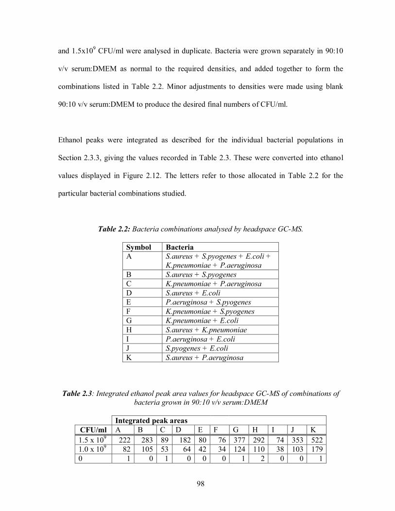
98

and 1.5x109 CFU/ml were analysed in duplicate. Bacteria were grown separately in 90:10

v/v serum:DMEM as normal to the required densities, and added together to form the

combinations listed in Table 2.2. Minor adjustments to densities were made using blank

90:10 v/v serum:DMEM to produce the desired final numbers of CFU/ml.

Ethanol peaks were integrated as described for the individual bacterial populations in

Section 2.3.3, giving the values recorded in Table 2.3. These were converted into ethanol

values displayed in Figure 2.12. The letters refer to those allocated in Table 2.2 for the

particular bacterial combinations studied.

Table 2.2: Bacteria combinations analysed by headspace GC-MS.

Symbol Bacteria A S.aureus + S.pyogenes + E.coli +

K.pneumoniae + P.aeruginosa B S.aureus + S.pyogenes C K.pneumoniae + P.aeruginosa D S.aureus + E.coli E P.aeruginosa + S.pyogenes F K.pneumoniae + S.pyogenes G K.pneumoniae + E.coli H S.aureus + K.pneumoniae I P.aeruginosa + E.coli J S.pyogenes + E.coli K S.aureus + P.aeruginosa

Table 2.3: Integrated ethanol peak area values for headspace GC-MS of combinations of bacteria grown in 90:10 v/v serum:DMEM

Integrated peak areas CFU/ml A B C D E F G H I J K 1.5 x 109 222 283 89 182 80 76 377 292 74 353 5221.0 x 109 82 105 53 64 42 34 124 110 38 103 1790 1 0 1 0 0 0 1 2 0 0 1

99

0

100

200

300

400

500

600

700

800

A B C D E F G H I J KBacteria combination

Etha

nol c

once

ntra

tion

(µM

)

1.5x10^9 CFU/ml1.0x10^9 CFU/ml0 CFU/ml (blank)

Figure 2.12: Ethanol concentrations detected by headspace GC-MS analysis of bacteria

combinations grown in 90:10 v/v serum:DMEM

As found with the individual bacteria, ethanol concentration increased with cell density,

and negligible amounts of ethanol were detected in the blanks. The amount of ethanol

produced for different combinations varied from 49.5 to 261 µM for 1.0x109 CFU/ml, and

from 111 to 761 µM for 1.5x109 CFU/ml. Combination K (S.aureus + P.aeruginosa)

produced the most ethanol at both densities. There does not appear to be a relationship

between the results for the combinations of bacteria and the individual bacteria.

2.3.5 Alcohol Draeger tube test Further authentication of the presence of ethanol in bacterial headspace was provided by

detection using an alcohol Draeger tube, as described in Section 2.2.7. The levels detected

are shown in Table 2.4. The values are lower than those detected by HS GC-MS, but as

already mentioned, the Draeger pump and tubes are not designed for this application, and

100

therefore care must be taken in interrogating these results. They do however suggest the

presence of ethanol at slightly higher levels in the headspace of S.aureus and S.pyogenes

than in P.aeruginosa, E.coli and K.pneumoniae, as found by HSGC-MS.

Table 2.4: Alcohol levels detected by Draeger tubes

Bacteria Alcohol (µM) P.aeruginosa 431 E.coli 431 S.pyogenes 517 K.pneumoniae 431 S.aureus 517 Blank 86

2.3.6 Glucose BioAssay The calibration graph generated from the QuantiChrom glucose BioAssay is displayed in

Figure 2.13. A clear linear relationship was present with an R2 value of 0.9975 for the

range 0 to 16 mM glucose.

y = 0.0217xR2 = 0.9975

0

0.05

0.1

0.15

0.2

0.25

0.3

0.35

0.4

0 2 4 6 8 10 12 14 16 18Glucose concentration (mM)

Abs

orba

nce

630n

m

Glucose stdsLinear (Glucose stds)

Figure 2.13: Glucose BioAssay standards

101

2.3.7 H2O2 Checkit test kit Standards tested produced colours matching those displayed on the Lovibond Checkit kit

box.

2.4 Overall Chapter Conclusions A suitable surrogate wound fluid (serum) was identified and produced successfully. It was

found that S.aureus was able to grow in serum alone, and that by supplementing the serum

so that it contained 90:10 v/v serum: DMEM, all five selected wound bacteria could grow

and be used for odour analysis. Growth curves and calibration plots were produced for the

five bacteria grown in TSB, DMEM, and 90:10 v/v serum: DMEM, providing useful

information on the growth cycles and cell densities of the bacteria, which will be used in

the studies on odour analysis that follow in Chapter 5. HS GC-MS and a Draeger pump and

tube system was used to detect volatiles in the headspace of five bacteria grown in 90:10

serum: DMEM, verifying the presence of ethanol, and that it is produced at a level

measurable by other means, such as by an alcohol biosensor. Standard calibrations were

produced for the glucose test kit, which is referred to in Chapter 4, to validate the biosensor

data.

102

3. Detection Using Dual Pulse Staircase Voltammetry 3.1 Introduction

This chapter investigates the first of three possible monitoring technologies, the

electrochemical technique of dual pulse staircase voltammetry (DPSV) described in

Section 1.2.2.5. This technique was identified as an appropriate technique, due to its

rapidity and ability to produce information rich voltammograms while also cleaning the

electrode surface of fouling agents. Using a standard three electrode system, this technique

has been reported to produce characteristic peaks for different analytes allowing both

qualitative and quantitative determination of analytes in solution (Bessant, 1998; Fung &

Mo, 1995). and may present an alternative to the more common approach of using

amperometric biosensors for such measurements. If successful, this approach would offer

the benefits of reduced cost of sensor fabrication, and it is possible that a single sensor may

be used to measure several components, rather than the necessity of using a biosensor array

to determine individual components, as investigated in Chapter 4. However, reports using

the technique of DPSV are limited, and there are none relating to its use in a complex

matrix such as a biological fluid, and therefore this study was undertaken to establish the

feasibility of this technique for wound monitoring.

Amperometric detection was not investigated for the monitoring of wounds, since it lacks

specificity in mixtures, however, cleaning pulses are common to the techniques of pulsed

amperometric detection (PAD) and DPSV. Therefore, for illustrative purposes, PAD was

compared with amperometry to demonstrate the functionality of the cleaning pulses for the

removal of fouling agents. Following this, gold and platinum solid electrode materials were

103

compared. The suitability of two screen printed electrodes for use in DPSV were tested,

since ultimately, if the technique was successful, it is envisioned that a portable device

using disposable electrodes would be produced. Work was carried out initially referring to

the work of Bessant (1998) to establish the system (using NaOH). Once established, PBS

was used as it is known to have similar electrolyte composition as serum. Each of the three

biomarkers identified (Section 2.1): ethanol, glucose and H2O2, were investigated

individually and in mixtures, and corresponding voltammograms produced. The influence

of a number of possible electrochemical interferents such as paracetamol (acetaminophen)

and vitamin C (ascorbic acid) that may be present in real (i.e. clinical) samples was also

investigated.

3.2 Materials and Methods

3.2.1 Reagents

Solutions of NaOH and NaCl (both Sigma, Poole, UK) were prepared in reverse osmosis

water. Ethanol (99.9% denatured HPLC grade) was from Aldrich (Poole, UK). 4-

Acetomidophenol, salicylic acid, L-ascorbic acid, bilirubin, distilled water, cholesterol,

cysteine and creatinine, methanol, propanol, acetone, glucose, trichloroacetic acid,

glutathione, dopamine were from Fisher (Loughborough, UK). Hydrogen peroxide (31.3%

v/v assay ACS reagent), fructose, gentisic acid, levo-dopa, tetracycline, tolazamide, and

tolbutamide were from Sigma (Poole, UK).

104

3.2.2 Instrumentation

Electrochemical measurements were made using a PGSTAT10 multichannel (4 channels)

Autolab (Eco Chemie, Utrecht, The Netherlands), which was operated by GPES (version

4.9) software under PC control.

A Chemlab SS3 stirrer was used during all amperometric experiments with an 8x6mm

magnetic follower (Fisher, Loughborough, UK). The electrochemical cell was a 10 ml glass

beaker (Fisher, Loughborough, UK). A standard laboratory clamp stand and clamps were

used to hold beakers and three electrode configuration with Autolab connections in position

(Figure 3.1). Screen printed electrodes were connected to the Autolab using connectors

made in house from standard components from Maplins, UK. The connectors are known as

FFC (Flat Flexible Cable) Connectors, using a 1.25mm pitch (Molex, part number 39-51-

3084). They are mounted onto Veroboard, and then connect via 4mm plugs and sockets to

the potentiostat. The wires were protected by heat shrink rubber, and the circuit board by

PVC tape.

Figure 3.1: Assembly of solid electrodes (working (w.e.), reference (r.e.), counter (c.e.)).

w.e. r.e. c.e.

105

3.2.3 Electrode materials

Gold and platinum solid-state electrodes and the Ag/AgCl solid-state reference electrode

were from Bioanalytical Systems (BAS), West Lafayette, USA. The reference electrode is

internally saturated with KCl to maintain a constant Cl- ion activity, and maintains its own

internal redox potential. The Ag/AgCl reference was stored in 3 M NaCl when not in use.

The screen printed three electrode assembly of carbon, carbon, and Ag/AgCl were made in

house. The carbon ink base layer 145R and Ag/AgCl reference electrode layer was from

MCA Services Ltd., Melbourn, UK, and the insulation layer 242-SB epoxy-based blue

protective coating ink was from Agmet ESL, Reading UK. A further description of the

screen printing process is given in Section 4.2.4. The screen printed electrodes with gold

working electrode (w.e.), carbon counter (c.e.) and Ag/AgCl reference (r.e.) were from an

existing in-house design and fabricated by Dupont (Bristol, UK). These two screen printed

sensors are shown in Figure 3.2.

Figure 3.2: Screen printed three electrode assembly electrodes

(a) carbon (w.e.), carbon (c.e.) Ag/AgCl (r.e.), (b) gold (w.e.), carbon (c.e.), Ag/AgCl (r.e.).

(a) (b)

106

To remove electroactive agents from the solid-state electrodes between measurements, they

were first polished with 0.05 µm alumina (Sigma) in reverse osmosis water and a polishing

pad, secondly washed with acetone, and thirdly, ultrasonicated in a beaker of acetone to

remove remaining alumina, and allowed to air dry.

3.2.4 Electrochemical techniques

In pulsed amperometric detection (PAD), the cleaning and detection parameters were as

follows: Eox = 0.8 V, Ered = -0.2 V, Edet = 0.2 V, tox = 0.2 s, tred = 0.4 s, tdet=0.2 s (Bessant,

1998 - refer to Section 1.2.2.2).

The technique of dual pulse staircase voltammetry (DPSV), described in Section 1.2.2.5,

consisted of two electrode cleaning pulses, (the first a 3 s pulse at +0.7 V (vs. Ag/AgCl

reference electrode), the second a 2 s pulse at -0.9 V) to clean the electrode surface,

followed by detection typically scanning the potential range - 0.9 V to +0.8 V, following

the work of Bessant (1998). A response was registered even before the addition of analyte,

due to electrode effects and the electrochemical activity of the buffer solution. This

response took time to reach steady state, and therefore no analyte was added until steady

state had been reached i.e. a scan of the blank (0.1 M NaOH or 0.1 M PBS as stated) was

repeatable, typically requiring 8 to 10 scans. This also allowed the option of blank

subtraction, since, in this study, the response of a system was taken as a summation of the

blank response and the response of the analyte. After each addition of analyte, the cell was

stirred for 10 s before being scanned until a repeatable response was obtained. Detection

107

was performed in 10 ml of either 0.1 M NaOH, 0.1 M HCl or 0.1M PBS as indicated for

each result.

3.3 Results and Discussion

3.3.1 Comparison of amperometry and pulsed amperometric detection

Although DPSV is the technique being investigated here, the effectiveness of the cleaning

pulses can be illustrated by comparing fixed potential amperometry with pulsed

amperometric detection. Figure 3.3 compares these two techniques for the detection of 64

mM increases in ethanol concentration in 0.1 M NaOH buffer at a gold working electrode.

It can be seen that PAD gives significantly higher current values with each step increase in

ethanol concentration when compared to fixed potential amperometry, therefore illustrating

that the cleaning pulses employed in PAD are effective. In fixed amperometry, the lower

sensitivity is thought to be due to the organic residue of the dehydrogenation reaction

remaining strongly adsorbed to the electrode surface, and therefore hindering further

adsorption of molecules from the bulk of the solution. The application of the three step

waveform aims to maintain a uniform electrode activity. After measurement, the anodic

polarisation step oxidatively degrades the adsorbed organic material to CO2 simultaneously

with the formation of the oxide layer. The cathodic polarisation step that follows reduces

the PtO and regenerates the active platinum electrode (Hughes, Meschi and Johnson, 1981;

Johnson & LaCourse, 1990; LaCourse, Johnson, Rey, et al, 1991; Tarnowski &

Korzeniewski, 1996).

108

Repeating this study for glucose at a platinum electrode found that as glucose concentration

was increased, the sensitivity of the platinum electrode was reduced, due to fouling.

Sensitivity to glucose was better with PAD than fixed-potential amperometry, but the

difference was far smaller than for ethanol. This may mean that glucose has less of a

fouling effect than ethanol, and therefore the effect of the desorption and regeneration

cleaning pulses of PAD would not be as significant. Further information on the use of PAD

to detect carbohydrates can be found in: Cai, Liu, Shi (2005); Neuburger & Johnson

(1987); Johnson & LaCourse (1991); Johnson, Dobberpuhl, Roberts, et al (1993).

0.0

0.5

1.0

1.5

2.0

2.5

3.0

0 50 100 150 200 250 300Time (s)

Cur

rent

(µA

)

AmperometryPAD

Figure 3.3: Comparison of fixed-potential amperometric and pulsed amperometric

detection (PAD) to 64 mM increases in ethanol concentration in 0.1M NaOH, at a gold working electrode with Ag/AgCl reference.

3.3.2 Comparison of gold and platinum electrodes

Figure 3.4 compares the responses of platinum and gold working electrodes in PAD. The

responses are similar in shape, and in magnitude of current, and both electrode materials

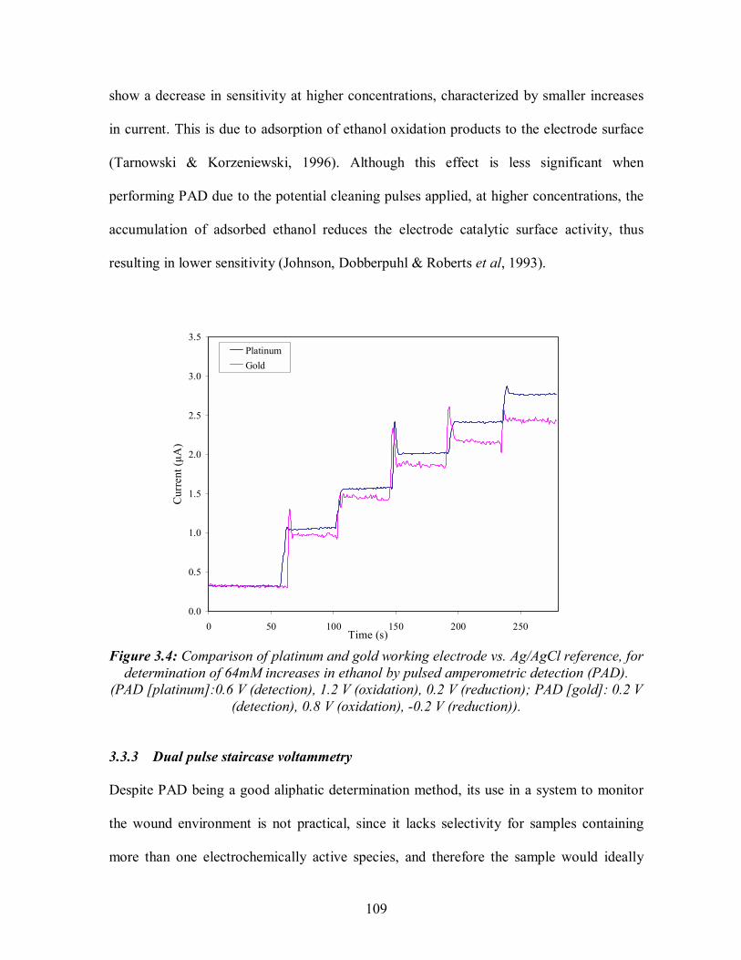
109

show a decrease in sensitivity at higher concentrations, characterized by smaller increases

in current. This is due to adsorption of ethanol oxidation products to the electrode surface

(Tarnowski & Korzeniewski, 1996). Although this effect is less significant when

performing PAD due to the potential cleaning pulses applied, at higher concentrations, the

accumulation of adsorbed ethanol reduces the electrode catalytic surface activity, thus

resulting in lower sensitivity (Johnson, Dobberpuhl & Roberts et al, 1993).

0.0

0.5

1.0

1.5

2.0

2.5

3.0

3.5

0 50 100 150 200 250Time (s)

Cur

rent

(µA

)

PlatinumGold

Figure 3.4: Comparison of platinum and gold working electrode vs. Ag/AgCl reference, for determination of 64mM increases in ethanol by pulsed amperometric detection (PAD).

(PAD [platinum]:0.6 V (detection), 1.2 V (oxidation), 0.2 V (reduction); PAD [gold]: 0.2 V (detection), 0.8 V (oxidation), -0.2 V (reduction)).

3.3.3 Dual pulse staircase voltammetry

Despite PAD being a good aliphatic determination method, its use in a system to monitor

the wound environment is not practical, since it lacks selectivity for samples containing

more than one electrochemically active species, and therefore the sample would ideally

110

require some form of pre-treatment, such as fractionation, by HPLC for example. However,

the cleaning parameters employed in PAD that are used to regenerate the surface of a

working electrode, can be used in combination with the greater selectivity of staircase

voltammetry to create the potentially useful method of DPSV. Voltammetry, incorporating

in situ cleaning reduces losses in electrode activity, a common phenomenon when using

solid, nobel metal electrodes for voltammetric measurements. Fung & Mo (1996) have also

shown that ethanol can be detected by DPSV over a large linear range (0.01 10 mM), a

useful characteristic in the context of this work.

Initial validation of the DPSV method was performed by repeating earlier studies

performed in this laboratory. Since the determination of glucose and ethanol are of interest

here, data first presented in a paper by Bessant & Saini (1999) was reproduced using the

system described in this Chapter (Figure 3.5). The potentials of the peaks in Figure 3.5 are

similar for glucose and fructose, though interestingly glucose gives a higher response in the

first peak (-0.7 V), and fructose the second peak (-0.14 V). The potential of the second

ethanol peak (-0.2 V) is slightly lower than that of glucose and fructose (-0.14 V) and the

peak is also broader. With regards to glucose and fructose, the peaks around -0.7 V were

due to hydrogen oxidation and reduction, and the oxidation peak around -0.14 was due to

the oxidation of the carbonyl group present in both fructose and glucose (Fung & Mo,

1995). Figure 3.6 and 3.7 show DPSV responses to increasing concentrations of glucose

and ethanol respectively in 0.1 M NaOH.

111

As observed for the two sugars studied, it is possible that other alcohols may produce

similar DPSV curves to ethanol. Therefore, DPSV of methanol and 1-propanol was carried

out. Figure 3.8 compares the DPSV responses of 64 mM ethanol, 64 mM methanol and

64 mM 1-propanol. The shape of the methanol response curve is similar to ethanol, but a

much lower current is observed. 1-Propanol produced less distinguishable peaks, similar to

that of the blank. Therefore, it seems that in the case of these three alcohols, there is the

possibility of inter-analyte interference, but with greater selectivity towards ethanol.

-10.0

0.0

10.0

20.0

30.0

40.0

50.0

60.0

-0.9 -0.7 -0.5 -0.3 -0.1 0.1Potential (V)

Curr

ent µ

A

1mM Glucose1mM Fructose64mM Ethanol0.1M NaOH

Figure 3.5: DPSV responses for 1 mM glucose, 1 mM fructose, and 64 mM ethanol in 0.1 M NaOH at a platinum working electrode vs. Ag/AgCl.

112

-2.0E-05

-1.0E-05

0.0E+00

1.0E-05

2.0E-05

3.0E-05

4.0E-05

5.0E-05

6.0E-05

7.0E-05

8.0E-05

-0.9 -0.7 -0.5 -0.3 -0.1 0.1Potential (V)

Cur

rent

(A)

0.5mM 1mM2mM 4mM6mM 8mM10mM 14mM0.1M NaOH

Figure 3.6: DPSV responses for different concentrations of glucose in 0.1M NaOH, at a platinum working electrode with Ag/AgCl reference.

-10.0

10.0

30.0

50.0

70.0

90.0

110.0

-0.9 -0.7 -0.5 -0.3 -0.1 0.1Potential (V)

Cur

rent

(uA

)

32mM64mM80mM96mM128mMNaOH blank

Figure 3.7: DPSV responses for different concentrations of ethanol in 0.1M NaOH, at a platinum working electrode with Ag/AgCl reference.

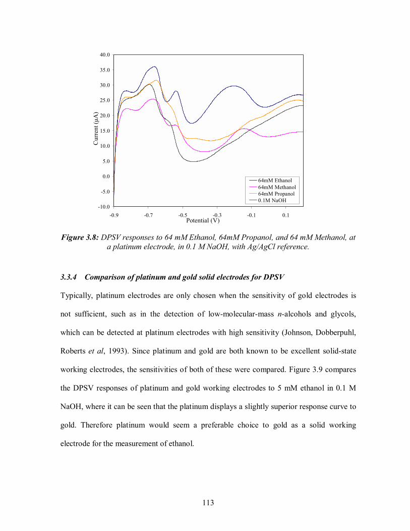
113

-10.0

-5.0

0.0

5.0

10.0

15.0

20.0

25.0

30.0

35.0

40.0

-0.9 -0.7 -0.5 -0.3 -0.1 0.1Potential (V)

Cur

rent

(µA

)

64mM Ethanol64mM Methanol64mM Propanol0.1M NaOH

Figure 3.8: DPSV responses to 64 mM Ethanol, 64mM Propanol, and 64 mM Methanol, at a platinum electrode, in 0.1 M NaOH, with Ag/AgCl reference.

3.3.4 Comparison of platinum and gold solid electrodes for DPSV

Typically, platinum electrodes are only chosen when the sensitivity of gold electrodes is

not sufficient, such as in the detection of low-molecular-mass n-alcohols and glycols,

which can be detected at platinum electrodes with high sensitivity (Johnson, Dobberpuhl,

Roberts et al, 1993). Since platinum and gold are both known to be excellent solid-state

working electrodes, the sensitivities of both of these were compared. Figure 3.9 compares

the DPSV responses of platinum and gold working electrodes to 5 mM ethanol in 0.1 M

NaOH, where it can be seen that the platinum displays a slightly superior response curve to

gold. Therefore platinum would seem a preferable choice to gold as a solid working

electrode for the measurement of ethanol.

114

-10.0

0.0

10.0

20.0

30.0

40.0

50.0

60.0

70.0

80.0

90.0

-0.9 -0.7 -0.5 -0.3 -0.1 0.1 0.3 0.5 0.7Potential (V)

Cur

rent

(µA

)

Gold blankGold 5 mM EthanolPlatinum blankPlatinum 5 mM Ethanol

Figure 3.9: Comparison of blank subtracted DPSV responses to 64 mM ethanol at platinum and gold working electrodes in 0.1 M NaOH, with Ag/AgCl reference.

3.3.5 Investigation of interferents

A common problem in the development of new sensor technologies is that of interfering

species i.e. chemicals present in the sample that yield an electrochemical signal that

conflicts with that of the analyte of interest, thereby reducing the effectiveness of the sensor

measurement. The most commonly problematic interferents in sensor/biosensor

construction with respect to clinical samples are ascorbic acid (vitamin C) and

acetaminophen (paracetamol). It was therefore of interest to determine whether a range of

possible interferents were electroactive in the potential regions of those peaks produced by

DPSV for the analytes of interest in this study. The potential interferents were measured

electrochemically in 0.1 M NaOH at clinically valid levels (Table 3.1) at a platinum

electrode vs. Ag/AgCl.

115

Table 3.1: Concentrations of possible interferents found in blood

Interferents Chemical Molecular Concentration

Name weight from: (mM/l) to: (mM/l)

Acetominophen 4-acetomidophenol 151 0.33 1.32

Ascorbic acid L-ascorbic acid 176.13 0.04 0.17

Bilirubin Bilirubin 584.67 0.17 0.68

Cholesterol Cholesterol 386.65 4.53 18.10

Creatinine Creatinine 113.12 0.66 2.65

Cysteine Cysteine 121.11 0.05 1.00

Dopamine 3-hydroxytyramine-hydrochloride 189.64 0.17 0.69

Gentisic acid 2,5-dihydroxybenzoic acid 154.12 0.81 3.24

Glutathione (y-GLU-CYS-GLY;GSH) 307.19 0.0081 0.032

Levo-dopa 3-3,4-dihydroxyphenyl-L-alanine 197.2 0.05 0.20

Salicylic acid 2-hydroxybenzoic acid 160.02 0.78 3.10

Tetracycline Tetracycline 444.18 0.056 0.23

Tolazamide 1-[hexahydro-1H-azepin-1-yl]-3-[p-tolyl-sulfonyl] urea 311.4 0.04 0.16

Tolbutamide 1-butyl-3-[4-methyl benzynes sulfonyl] urea 270.4 0.92 3.70

Urea Urea 60.06 20.63 82.50

Uric acid 2,6,8-trihydroxypurine 168.11 0.30 1.19

Some of the interferents tested occur naturally in the body, such as cholesterol or urea

(although this is also found in skin treatments such as emollients for eczema), but most are

substances taken to treat illness or other medical conditions. Some of these substances are

more commonly administered medications than others, such as acetominophen

(paracetamol), tetracycline (antibiotics), and ascorbic acid (vitamin C), whereas drugs such

as levo-dopa used to treat Parkinsons disease, and methyl-dopa for blood pressure

treatment, are only used by a small portion of the population. Figure 3.10 shows the

detection of these potential interferents in 0.1 M NaOH by DPSV. The voltammetric

responses are blank subtracted, and varied considerably as may be observed.

116

-15.0-10.0-5.00.05.0

10.015.020.025.030.035.0

-0.9 -0.4 0.1 0.6Potential (V)

Cur

rent

(µA

)

0.1 mM Acetominophen1 mM Acetominophen5 mM Acetominophen

-2.0

0.0

2.0

4.0

6.0

8.0

10.0

-0.9 -0.4 0.1 0.6Potential (V)

Cur

rent

(µA

)

0.05 mM Ascorbic acid0.1 mM Ascorbic acid0.5 mM Ascorbic acid

(a) (b)

-10.0

-5.0

0.0

5.0

10.0

15.0

-0.9 -0.4 0.1 0.6Potential (V)

Cur

rent

(µA

)

0.17 mM Bilirubin0.51 mM Bilirubin0.68 mM Bilirubin

-4.0

-2.0

0.0

2.0

4.0

6.0

8.0

10.0

12.0

-0.9 -0.4 0.1 0.6Potential (V)

Cur

rent

(µA

)

4.53 mM Cholesterol13.58 mM Cholesterol18.1 mM Cholesterol

(c) (d)

-4.0

-2.0

0.0

2.0

4.0

6.0

8.0

-0.9 -0.4 0.1 0.6Potential (V)

Curr

ent (µA

)

0.66 mM Creatinine1.98 mM Creatinine2.65 mM Creatinine

-12.0-10.0

-8.0-6.0-4.0-2.00.02.04.06.08.0

-0.9 -0.4 0.1 0.6Potential (V)

Cur

rent

(µA

)

0.05 mM Cysteine0.5 mM Cysteine1 mM Cysteine

(e) (f)

117

-10.0-5.00.05.0

10.015.020.025.030.035.0

-0.9 -0.4 0.1 0.6Potential (V)

Cur

rent

(µA

)

0.17 mM Dopamine0.34 mM Dopamine0.69 mM Dopamine

-10.0-5.00.05.0

10.015.020.025.030.035.040.0

-0.9 -0.4 0.1 0.6Potential (V)

Cur

rent

(µA

)

0.81 mM Gentisic acid2.43 mM Gentisic acid3.24 mM Gentisic acid

(g) (h)

-3.0-2.0-1.00.01.02.03.04.05.06.07.0

-0.9 -0.4 0.1 0.6Potential (V)

Cur

rent

(µA

)

0.0081 mM Glutathione0.024 mM Glutathione0.032 mM Glutathione

-10.0

-5.0

0.0

5.0

10.0

15.0

20.0

-0.9 -0.4 0.1 0.6Potential (V)

Cur

rent

(µA

)

0.05 mM Levo-dopa0.15 mM Levo-dopa0.2 mM Levo-dopa

(i) (j)

-20.0-10.0

0.010.020.030.040.050.060.070.0

-0.9 -0.4 0.1 0.6Potential (V)

Cur

rent

(µA

)

0.78 mM Salicylic acid2.34 mM Salicylic acid3.1 mM Salicylic acid

-2.00.02.04.06.08.0

10.012.014.016.0

-0.9 -0.4 0.1 0.6Potential (V)

Cur

rent

(µA

)

0.056 mM Tetracycline0.11 mM Tetracylcine0.23 mM Tetracycline

(k) (l)

118

-2.0

-1.0

0.0

1.0

2.0

3.0

4.0

5.0

-0.9 -0.4 0.1 0.6Potential (V)

Cur

rent

(µA

)

0.04 mM Tolazamide0.08 mM Tolazamide0.16 mM Tolazamide

-4.0

-2.0

0.0

2.0

4.0

6.0

8.0

10.0

-0.9 -0.4 0.1 0.6Potential (V)

Cur

rent

(µA

)

0.92 mM Tolbutamide1.85 mM Tolbutamide3.7 mM Tolbutamide

(m) (n)

-20.0

-10.0

0.0

10.0

20.0

30.0

40.0

-0.9 -0.4 0.1 0.6Potential (V)

Cur

rent

(µA

)

20.63 mM Urea41.25 mM Urea82.50 mM Urea

-6.0-4.0-2.00.02.04.06.08.0

10.012.0

-0.9 -0.4 0.1 0.6Potential (V)

Cur

rent

(µA

)

0.1 mM Uric acid1 mM Uric acid5 mM Uric acid

(o) (p) Figure 3.10: DPSV responses (blank subtracted) for: (a) Acetominophen (b) Ascorbic acid (c) Bilirubin (d) Cholesterol ( e) Creatinine ( f) Cysteine (g) Dopamine (h) Gentisic acid (i)

Glutathione (j) Levo-dopa (k) Salicylic acid (l) Tetracycline (m) Tolazamide (n) Tolbutamide (o) Urea (p) Uric acid, , in 0.1 M NaOH at a platinum working electrode vs.

Ag/AgCl reference.

It was evident that many of these species are electroactive and may cause interference

problems, therefore it was necessary to run DPSV of ethanol, glucose and H2O2 in 0.1 M

PBS in the presence of the most common and problematic of the interferent species, in

order to determine their effect on the scan data. Solutions representing the higher

concentrations found in the body of ascorbic acid (0.17 mM), acetaminophen (1.32 mM),

cysteine (1 mM), uric acid (1.19 mM) and urea (82.5 mM) were made up in 0.1 M PBS

119

containing 5 mM ethanol. Each of these were measured by DPSV and compared to a DPSV

scan of 5 mM ethanol in 0.1 M PBS alone (Figure 3.11). This process was repeated for

glucose and H2O2. All five species have interfered with the normal DPSV scan for 5 mM

ethanol to varying degrees. Ascorbic acid caused the current to increase but a similar

current versus potential profile was maintained. Cysteine, acetaminophen and urea

significantly altered the profile of the overall voltammetric response. The presence of uric

acid yielded a slight increase in current, also yielding an additional peak at around -0.5 V.

-70.0

-60.0

-50.0

-40.0

-30.0

-20.0

-10.0

0.0

10.0

20.0

30.0

-0.9 -0.7 -0.5 -0.3 -0.1 0.1 0.3 0.5 0.7Potential (V)

Cur

rent

(uA

)

5 mM Ethanol 0.17 mM Ascorbic acid1 mM Cysteine1.32 mM Acetominophen1.19 mM Uric acid82.5 mM Urea

Figure 3.11: DPSV (blank subtracted) of interferents in 0.1M PBS (blank)containing 5 mM

ethanol.

Figure 3.12 shows the effects of the species on the DPSV scan of 5 mM glucose in 0.1 M

PBS. As with ethanol, all five species tested had an effect. Ascorbic acid had the least

effect, causing the current to decrease slightly at the -0.25 V and -0.8 V peaks but remained

a similar shape scan. Cysteine, acetaminophen and urea significantly altered the shape of

120

the voltammograms. Uric acid decreased the current slightly at the -0.25 V peak region and

increased current in the -0.5 V and -0.8 V region.

Figure 3.13 shows the effects of the species on the DPSV scan of 5 mM H2O2 in 0.1 M

PBS. As for ethanol and glucose, cysteine had the most significant effect, altering the shape

of the whole scan. Uric acid and ascorbic acid had the least affect, remaining a similar

shape scan, but at a more negative current. Acetaminophen and urea had a similar shape but

a less negative current in the ~-0.4 V peak area, and different shapes and currents over the

remainder of the scan.

It seems that overall for DPSV of glucose, ethanol and H2O2, ascorbic acid has the least

significant effect, followed by uric acid. Cysteine has the most significant effect, followed

by urea and acetaminophen. Therefore the presence of any of these species in a sample,

will influence the voltammetric profile, making it more difficult to accurately predict

concentrations of ethanol, glucose or H2O2. It may be possible to reduce the effect of some

or all of these interferents by using a suitable membrane to exclude species based on size or

charge, such as Nafion, which is negatively charged and repulses negatively charged acids

such as ascorbic acid and uric acid. It should be noted that even commercially available

self-test glucose biosensors are susceptible to the affects of acetominophen (Cartier,

Leclerc, Pouliot et al, 1998). Also, if a patients medication is known, it may serve to aid

complex volatmmogram interpretation.

121

-70.0

-60.0

-50.0

-40.0

-30.0

-20.0

-10.0

0.0

10.0

20.0

30.0

40.0

-0.9 -0.7 -0.5 -0.3 -0.1 0.1 0.3 0.5 0.7Potential (V)

Cur

rent

(uA

)

5 mM Glucose0.17 mM Ascorbic acid1.32 mM Acetominophen2 mM Cysteine82.5 mM Urea1.19 mM Uric acid

Figure 3.12: DPSV of interferents in 0.1M PBS containing 5 mM glucose.

-80.0

-60.0

-40.0

-20.0

0.0

20.0

40.0

-0.9 -0.7 -0.5 -0.3 -0.1 0.1 0.3 0.5 0.7Potential (V)

Cur

rent

(uA

)

5 mM H2O21.32 mM Acetominophen0.17mM Ascorbic acid1 mM Cysteine1.19 mM Uric acid82.5 mM Urea

Figure 3.13: DPSV of interferents in 0.1M PBS containing 5 mM H2O2.

122

3.3.6 DPSV of glucose, ethanol and H2O2 in PBS Having established a working system, each of the three identified markers glucose, ethanol

and H2O2 were measured at different concentrations in 0.1 M PBS by DPSV. The data from

triplicate measurements was averaged and used to identify peaks in the scans that could be

used as a basis for the construction of a calibration curve.

Figure 3.14 illustrates the results for the measurement of 0.5 - 15 mM glucose in 0.1 M

PBS. Three main peaks have been identified as possible sources from which to produce

calibration plots. Peak one (-0.825 V) becomes increasingly negative in current with

increase in glucose concentration, while peaks two (-0.54 V) and three (-0.1 V) become

more positive with each increase in glucose concentration.

From these peaks, a given peak height value could be taken, as indicated by the red lines,

or the peak area measured using Autolab software. Ratios between peak areas may also

prove important indicators.

The DPSV scans for 0.5 to 10 mM ethanol can be seen in Figure 3.15. Three peaks were

identified. Peaks one (-0.8 V) and two (-0.36 V) become more negative in current with

increase in ethanol concentration, whilst peak three (-0.14 V) increases in peak height and

area with increasing ethanol concentration. Examination of the raw voltammetric data

suggests that peak three would provide the least linear relationship between peak current

and concentration.

123

-15.0

-12.5

-10.0

-7.5

-5.0

-2.5

0.0

2.5

5.0

7.5

10.0

12.5

-0.9 -0.7 -0.5 -0.3 -0.1 0.1Potential (V)

Cur

rent

(µA

)

0.5 mM 1 mM1.5 mM 2 mM3 mM 4 mM5 mM 6 mM7 mM 8 mM9 mM 10 mM12.5 mM 15 mM

Peak 1

Peak 2Peak 3

Figure 3.14: DPSV of glucose in 0.1M PBS at platinum working electrode vs. Ag/AgCl reference. Scans are blank subtracted averages of 3 scans.

-30.0

-20.0

-10.0

0.0

10.0

20.0

30.0

40.0

50.0

-0.9 -0.7 -0.5 -0.3 -0.1 0.1Potential (V)

Cur

rent

(µA

)

0.25 mM0.5 mM0.75 mM1 mM1.5 mM2 mM3 mM4 mM5 mM6 mM7 mM8 mM9 mM10 mM

Peak 1

Peak 2

Peak 3

Figure 3.15: DPSV of ethanol in 0.1M PBS at platinum working electrode vs. Ag/AgCl

reference. Scans are blank subtracted averages of 3 scans.

124

Two oxidation peaks (-0.76 V and -0.34 V) were identified for H2O2 across the

concentration range studied (0.25-10 mM), as illustrated in Figure 3.16. Both peaks exhibit

more negative peak currents with increasing concentration. However, it can be seen that for

peak one (-0.76 V) at concentrations less then 2 mM, this pattern is not followed. For peak

two (-0.34 V), it can be seen that increase in peak size does not follow an entirely linear

relationship until a concentration of 2 mM is exceeded.

Although patterns can be observed for averaged scans, the differences between scans of

different concentrations were not very large, making it especially important to check the

deviation that occurs with replicate scans. Therefore, a single concentration of ethanol (5

mM), glucose (5mM), and H2O2 (1 mM) in 0.1 M PBS were measured five times by

DPSV, and the variation determined. As normal, electrodes and cells were cleaned between

measurements, and each DPSV replicate was scanned ten times to establish blank

equilibrium, and again for measurement equilibrium. Figure 3.17 displays that average of

the five scans together with the standard deviation for each analyte.

The standard deviations were large, particularly for the glucose peak, which would make

accurate prediction of concentration difficult in a sample containing, for example, elevated

levels of ethanol. The major cause of this problem lies with the baseline (blank), since

despite establishing a stable baseline for each measurement, the location of this baseline

was found not to be reproducible between experiments. It is also clear that the analytes

studied yielded peaks with similar potentials. Consequently, mixtures of these three

analytes were examined to determine the effect of this factor on analyte determination.

125

-120.0

-100.0

-80.0

-60.0

-40.0

-20.0

0.0

20.0

40.0

60.0

-0.9 -0.7 -0.5 -0.3 -0.1 0.1Potential (V)

Cur

rent

(µA

)

0.25 mM0.5 mM0.75 mM1 mM1.5 mM2 mM2.5 mM3 mM4 mM5 mM6 mM7 mM8 mM9 mM10 mM

Peak 1

Peak 2

Figure 3.16: DPSV of H2O2 in 0.1M PBS at platinum working electrode vs. Ag/AgCl

reference. Scans are blank subtracted averages of 3 scans.

-10

-5

0

5

10

15

20

25

30

-0.9 -0.7 -0.5 -0.3 -0.1 0.1Potential (V)

Cur

rent

(µA

)

1 mM H2025 mM Glucose5 mM Ethanol

Figure 3.17: DPSV of 5 mM glucose, 5mM ethanol, 1mM H202 in 0.1 M PBS at platinum working electrode vs. Ag/AgCl reference. Scans are blank subtracted averages of 5 scans.

Shaded areas represent +/- 1 standard deviation.

Shaded areas = std devs

126

3.3.7 DPSV of mixtures of glucose, ethanol and H2O2 in PBS Solutions were prepared of combinations of the three selected target analytes in order to

examine the resultant DPSV scans. The results of four combinations in 0.1 M PBS at a

platinum working electrode vs. Ag/AgCl can be seen in Figure 3.18. By comparing the

scans for ethanol and ethanol with glucose, it can be seen that the presence of glucose

positively shifted the scan ~10 µA and added a broad peak between -0.6 and -0.9 V

mirroring that present in the scan of glucose alone. H2O2 alone produces the most negative

scan. The addition of ethanol to H2O2 shifted the scan positively between -0.9 and 0 V and

negatively from 0 to 0.6 V. The same pattern is replicated to a greater extent with the

presence of glucose with H2O2, and greater still with the presence of both glucose and

ethanol with H2O2.

-70.0

-60.0

-50.0

-40.0

-30.0

-20.0

-10.0

0.0

10.0

20.0

30.0

-0.9 -0.7 -0.5 -0.3 -0.1 0.1 0.3 0.5Potential (V)

Cur

rent

(uA

)

EthanolH2O2GlucoseEthanol and H2O2Glucose and H2O2Glucose and EthanolGlucose, Ethanol and H2O2

Figure 3.18: Blank subtracted DPSV scans of mixtures of 5mM ethanol, 5 mM glucose and 5 mM H2O2 in 0.1 M PBS at platinum working electrode vs. Ag/AgCl reference. n=3.

127

Observation alone of Figure 3.18 has revealed that since the presence of either or both of

glucose and ethanol in a solution containing H2O2 seems to yield voltammograms with a

number of similar features. In an unknown sample, it would prove challenging, even with

advanced statistical data treatment models, such as those employed by Bessant (1998), to

determine whether the solution contains H2O2 alone, or one or both of glucose and ethanol.

An unknown solution that does not contain H2O2, could be determined as containing

ethanol alone, and not ethanol and glucose, by the absence of a peak from -0.6 to -0.9 V. A

solution containing both glucose and ethanol may not be possible to determine from one

containing glucose alone due to inter-analyte interference.

3.3.8 DPSV with screen printed electrodes Despite the limitations of DPSV already uncovered, it was of interest to see whether the

technique of DPSV could be performed using screen printed electrodes, since a portable

device with disposable electrodes would be desirable for use with clinical material, and

therefore the use of solid state electrode is therefore not practical. Two screen printed

electrode assemblies were tested, both three electrode systems with a Ag/AgCl reference,

but one type having a carbon working electrode, and the other a gold working electrode.

Neither type was particularly successful, although the screen-printed gold electrode proved

superior with respect to the voltammetric response profiles obtained. Figure 3.19 illustrates

the problem encountered in establishing a stable baseline in 0.1 M PBS. The first eight

blank scans are shown. Only a very minor change in the response profile was noted on

addition of ethanol. The carbon design produced less of a distinctive peak for the baseline,

which decreased further with the addition of ethanol (Figure 3.20).

128

-500.0

-400.0

-300.0

-200.0

-100.0

0.0

100.0

200.0

300.0

400.0

-0.9 -0.7 -0.5 -0.3 -0.1 0.1 0.3 0.5 0.7Potential (V)

Cur

rent

(µA

)

Blank scan 1Blank scan 2Blank scan 3Blank scan 4Blank scan 5Blank scan 6Blank scan 7Blank scan 85 mM Ethanol 1 (scan 9)5 mM Ethanol 2 (scan 10)

Figure 3.19: Aging effect of repeated DPSV scans in 0.1M PBS (blank) and 5 mM ethanol with a screen printed gold working electrode (vs. Ag/AgCl reference).

-0.4

-0.3

-0.2

-0.1

0.0

0.1

0.2

0.3

0.4

-0.6 -0.4 -0.2 0 0.2 0.4

Potential (V)

Cur

rent

(µA

)

Blank scan 8

5 mM Ethanol 1 (scan 9)



Figure 3.20: DPSV scans of 0.1 M PBS (blank) and 5 mM ethanol with a screen printed carbon working electrode (vs. Ag/AgCl reference).

129

Therefore, neither of the two screen printed electrodes tested are suitable for DPSV, since

the response profiles obtained illustrate that they are not sufficiently electrochemically

sensitive to ethanol.

3.4 Conclusions PAD was shown to be more sensitive than fixed-potential amperometry, thus illustrating

the benefits of the cleaning pulse waveform, which was also employed in DPSV. The

DPSV procedure employed was based on that used in earlier published work from this

laboratory, for the determination of glucose, fructose and ethanol in complex solutions.

Initial experiments were performed using the same experimental set-up and were found to

concur with this earlier study (Bessant & Saini (1999)). Voltammograms of fructose and

glucose, and of ethanol, methanol and propanol were created and examined. Gold and

platinum solid-state working electrodes were compared, with platinum being found to be

more favourable in this case. Possible electrochemical interfering species were also

individually measured by DPSV in NaOH at clinically valid concentrations.

Following this, DPSV of ethanol, glucose and H2O2 was carried out in PBS in the presence

of five of these species, selected according to their frequency of usage by the general

population. All had an effect, cysteine being the most electrochemically active, followed by

urea, acetaminophen, uric acid and ascorbic acid. Measurement of different concentrations

of glucose, ethanol and H2O2 individually in PBS demonstrated clear peaks and

relationships between peak heights and concentration. However, repeat measurements at

one concentration for each analyte revealed high standard deviation values. DPSV of

130

mixtures of the three analytes illustrated potential difficulties in identifying individual

components and concentrations of the analytes due to inter-analyte interference. A limited

evaluation using carbon and gold screen printed electrodes found them to be of limited

value for DPSV measurement of the selected analytes in the context of this study.

Given the problems highlighted in this initial study with: baseline reproducibility; large

deviations (error); interfering species; identification in mixtures; and unsuitability of screen

printed electrodes; it was decided that DPSV was not a suitable technique for the

monitoring of wound biomarkers, and therefore not to progress the DPSV study further in

favour of the biosensor array and odour analyser which held more promise after initial

studies, and would be tested in surrogate wound fluid.

However, it is possible that incorporation of a negatively charged membrane such as

Nafion may reduce interferent effects. Also, there is still some potential for the use of

sophisticated data analysis, though this would be more difficult than anticipated due to the

similarities in some voltammetric profiles. Also, little has been reported regarding DPSV of

glucose and ethanol, and literature searches have not revealed any reports on DPSV of

hydrogen peroxide, or of clinical interferents. Also, none of the reports have been based on

measurements in PBS. Though a small section of work, no reports have been identified

investigating the use of screen printed electrodes for the technique of DPSV. Therefore the

work in this Chapter does hold the significant benefits of generating data and assessing the

feasibility of this approach for clinical measurements.

131

4. Detection Using a Biosensor Array

4.1 Introduction The objective of this Chapter, as outlined in Section 1.6, is to investigate whether a

biosensor array may be used as a diagnostic tool in the early stages of wound healing,

based on the detection of the bacterial metabolite ethanol, and the human markers glucose

and hydrogen peroxide, within the wound fluid sample.

The suitability of a glucose biosensor, hydrogen peroxide biosensor and ethanol biosensor

were investigated for the measurement of the selected biomarkers - glucose, hydrogen

peroxide and ethanol respectively (outlined in Section 2.1), in 0.1M PBS, and secondly in

model wound fluid. Since one of the main causes of complications in wound healing is

bacterial, as discussed in Section 1.1.6, the direct detection of metabolic ethanol production

by S.aureus with ethanol biosensor was also investigated. The effect of the presence of

bacteria on the performance of the glucose and hydrogen peroxide biosensors was also

tested. The effect of possible interferents such as ascorbic acid (vitamin C) was assessed for

each of the three biosensors.

The objectives were achieved by screen printing a three electrode (carbon working, carbon

counter, silver /silver-chloride reference) assembly (described in Section 4.2.3) which

could be used as the basic starting point for each of three amperometric biosensors, with

the exception of the glucose biosensor which had an additional layer, rhodinised carbon,

printed onto the working electrode (reasons outlined in Section 4.3). The experimental

programme followed for the biosensor work is illustrated in Figure 4.1:

132

Selection of amperometric biosensor

type e.g. mediated

Selection of enzyme(s), mediator, immobilisation

method

Determination of optimum operating

potential

Determination of optimum enzyme loading

Optimisation of deposition regime

Calibration, determination of linear region

and limit of detection in PBS

Calibration, determination of linear region and limit of detection in model

wound fluid

Shelf life testing Validation with test kit

Investigate effect of interferents on detection

limits

Investigate effect of bacteria in model wound

fluid on detection limit

Figure 4.1: Flow diagram of biosensor development and testing stages

133

The stages of Figure 4.1 are described in this chapter for each of the three biosensors.

Model wound fluid was made by separating serum from blood, as described in 2.2.4, giving

a surrogate wound fluid, based on the major component of wound fluid, namely serum.

4.2 Materials and Methods

4.2.1 Reagents

Aqueous solutions of phosphate buffer saline (Sigma, Poole, UK), ethanol ( 99.9%

denatured HPLC grade, Aldrich, (Poole, UK), hydrogen peroxide (31.3% v/v assay ACS

reagent, Sigma, Poole, UK), and glucose (reagent grade, Fisher, Loughborough, UK) were

made using reverse osmosis water. Cellulose acetate MW 37,000 (Sigma, Poole, UK), and

dimethylferrocene (Aldrich, Poole, UK) were prepared in acetone (Fisher, Loughborough,

UK). Glucose oxidase (from Aspergillus niger, E.C. 1.1.3.4) was in the form of a freeze

dried powder from Biozyme, Blaenavon, Wales. Horseradish peroxidase (from Amoracia

rusticana, E.C. 1.11.1.7) was from Sigma (Poole, UK) in lyophilized powdered form.

Buffered aqueous alcohol oxidase (from pichia pastoris, E.C. 1.1.3.13) and lyophilized

powdered alcohol oxidase (from Candida boidinii, EC 1.1.3.13) were also from Sigma,

(Poole, UK).

4.2.2 Instrumentation

Amperometric measurements were made using a PGSTAT10 multichannel (4 channel)

Autolab illustrated in Figure 4.2 (Eco Chemie, Utrecht, The Netherlands), operated using

GPES software (version 4.9). The biosensors were connected to the four channels of the

Autolab using connectors made in-house using basic electronic components from Maplins,

134

UK. The connectors are known as FFC (Flat Flexible Cable) Connectors, using a 1.25mm

pitch (Molex, part number 39-51-3084). They are mounted onto Veroboard, and then

connect via 4mm plugs and sockets to the potentiostat, as illustrated in Figures 4.2 and 4.3.

The wires were protected by heat shrink rubber, and the circuit board by PVC tape.

4.2.3 Measurement

Amperometric measurements were made using the Chrono methods > 0.1s method of the

GPES software. The interval time between points was 0.1 s, and measurements were made

for a period of 150 s. The operating potentials for each of the biosensors are discussed later

in the chapter.

4.2.4 Fabrication of screen-printed electrodes Identical screen-printed 3-electrode assembly designs were used for each of the three

biosensors, involving the successive deposition of ink layers. A DEK 248 printer (DEK,

Weymouth, UK) incorporating screens with appropriate stencil designs (60 sensors per

screen) were used for precision ink depositioning. The base material for electrode

fabrication was 250 µm polyester sheeting (Cadillac Plastic, Swindon, UK) onto which was

deposited successive ink layers. The hydrogen peroxide and ethanol sensors consisted of

three deposition layers. The first of these was carbon ink 145R layer (MCA Services Ltd.,

Melbourn, Cambs. UK) - the base layer for all three electrodes; the second was a Ag/AgCl

layer (MCA, UK) covering just the reference electrode; and the third an insulation layer

242-SB epoxy-based blue protective coating ink (Agmet ESL, Reading UK). The electrodes

were then heat-treated at 125°C for 1 h to cure the insulation shroud. The glucose sensor

135

had an additional layer applied before the insulation layer rhodinised carbon (MCA, UK).

Rhodinised carbon has been found to be a catalytic material with excellent properties for the

oxidation of H202, therefore one part rhodinised carbon 4a mixed with four parts 2.5% w/v

hydroxyethyl cellulose in 0.1M phosphate buffer (pH 7.2) was screen-printed over the

underlying working electrode (Kroger, Setford, & Turner (1998). The four layer assembly

of the glucose sensor can be seen in Figure 4.4.

Figure 4.2: Multichannel Eco Chemie Figure 4.3: Biosensor connection Autolab and sensor connections Ag/AgCl Rhodinised carbon Carbon Insulation layer

Figure 4.4: Four layers of the screen printing process for three electrode assembly

136

4.3 Glucose Biosensor Following from screen printing the three electrode assembly with rhodinised carbon

working electrode, the final stage of the glucose biosensor fabrication was the deposition of

the enzyme glucose oxidase. The glucose biosensors made were based on the amperometric

detection of H2O2 catalytically oxidised at the rhodinised carbon working electrode

(Newman, White, Tothill et al, 1995). Several studies have reported the benefits of using

rhodinised carbon in biosensor design, such as Turner, White, Schmid et al (1994), Kroger,

Setford & Turner (1998), and Cullen, Jawaheer, White et al (2003). The enzyme glucose

oxidase (GOx) (Biozyme, Blaenavon, Wales, UK) was acquired in the form of a freeze

dried powder with 261.7 U/mg material, originating from Aspergillus niger. GOx from

A.niger is a dimer of two identical subunits, each containing a tightly bound FAD molecule

as cofactor, and is highly specific for ß-D-glucose. The glucose biosensor operating

principle is depicted in Figure 4.5, where H2O2 was amperometrically detected at the

rhodinised carbon working electrode poised at a suitable operating potential:

Figure 4.5: Glucose biosensor reaction scheme

The GOx powder was dissolved in 0.1M PBS pH 7.2 to give the required activities for

glucose determination in the context of this study. The work of Kröger, Setford & Turner

(1998) was used as the basis for the optimisation of the glucose biosensor that follows.

H2O2 (red) O2 (ox)

GOX (ox) GOX (red)

Glucose (red) Glucolactone (ox)

Electrode

137

4.3.1 Standard electrochemical measurement methodology

Although electrochemical theory activities for glucose determination in the context of this

study suggests that amperometric measurements are best performed in stirred solutions, this

is not practical, nor commonplace with commercially available screen-printed biosensor

assemblies. It has also been shown previously with the sensors used in this study (Kröger,

Setford & Turner, 1998) that it is not necessary to stir the measurement solution. Therefore,

it was possible to carry out the experiments by pipetting a small droplet of test solution

onto the sensor, covering the three electrodes. It was found that a volume of 150 µl was

suitable.

Kröger, Setford & Turner (1998) also demonstrated that the background current for these

sensors was consistently within a narrow range, and therefore, it was possible for glucose

to be present in the measurement solution from the beginning. Using a four channel

Autolab, one channel was used to measure the background current (blank), whilst the three

remaining channels were used to simultaneously measure glucose in test solution. The

sensors were equilibrated in the measurement solution and a current plateau was reached. A

differential measurement was taken after 150 s (analyte current - background current =

signal). An example can be observed in Figure 4.6, where H2O2 is measured at the

rhodinised carbon working electrode. H2O2 was used for this example since H2O2 is the

reaction product detected at the electrode surface in the glucose oxidase based system that

follows.

138

0.0

2.0

4.0

6.0

8.0

10.0

12.0

14.0

0 20 40 60 80 100 120 140Time (s)

Cur

rent

(µA

)

Blank10mM H2O2 - 110mM H2O2 - 210mM H2O2 - 3

Figure 4.6: Example amperometric measurement of H2O2 at rhodinised carbon working electrode vs. Ag/AgCl, at +300mV.

4.3.2 Determination of optimum operating potential The operating potential for the amperometric detection of GOx generated H2O2 at

rhodinised carbon working electrodes has been reported in a number of publications as

+300mV or +350mV vs. Ag/AgCl (White, Turner, Bilitewski et al 1994; Kröger, Setford,

Turner, 1998; Cullen, Jawaheer, Rughooputh et al 2003).

To verify this, 10mM H2O2 was prepared in 0.1M PBS pH 7.2 for detection by the three

electrode assembly in the absence of GOx. The current was measured at operating

potentials from 100 to 600 mV, repeated in triplicate for each potential. The average

current response to 10mM H2O2 at each potential, and the background current are shown in

139

Figure 4.7. The ratio between H2O2 current and background current (Figure 4.8) revealed

the optimum potential to be in the region of +300mV to +350 mV.

The electrocatalytic activity of rhodinised carbon does indeed reduce the potential from

that required using a standard carbon working electrode (typically >700mV), thus reducing

the effect of interferences, as previously reported by Cullen, Jawaheer, Rughooputh et al

(2003) for example. Therefore a potential of +300 mV was used for all future amperometric

measurements of glucose using the screen printed three electrode system with rhodinised

carbon working electrode.

-5

0

5

10

15

20

25

100 200 300 400 500 600

Potential (mV)

Cur

rent

(uA

)

10 mM H2O2 Background current

Figure 4.7: Hydrodynamic voltammogram of background current and response towards 10

mM H202 in 0.1M PBS (pH7.2) at screen printed three electrode system with rhodinised carbon working electrode vs. Ag/AgCl. Error bars=SD, n=3.

140

0

100

200

300

400

500

600

700

800

900

1000

100 200 250 300 350 400 450 500 550 600Potenital (mV)

H20

2 Sig

nal/B

ackg

roun

d

Figure 4.8: The signal to background ratio for rhodinised carbon three electrode system at

10 potentials in 10 mM H2O2 in 0.1M PBS pH7.2. n=3.

4.3.3 Optimisation of glucose oxidase loading

To determine the optimum number of units of glucose oxidase required per sensor, a range

of GOx loadings were tested in the range 0.5 to 4 U/sensor using a substrate solution of

10mM glucose in 0.1M PBS (pH 7.2) and at an operating potential of +300mV (n=3). The

GOx preparations were applied to the rhodinised carbon electrode in a volume of 5 µl by

pipette. The small volume and the porous nature of rhodinised carbon meant that

immobilisation by an entrapment method or membrane was not necessary. The sensors

were also designed for single use, and therefore the water solubility of the enzyme was of

no concern. The signal: noise ratio was calculated for each enzyme loading

(differential signal / standard deviation) and the optimum GOx loading found to be

141

1U/sensor. It can be seen in Figure 4.9 that the signal: noise value increases up to 1U, with

no increase in response evident at higher enzyme loadings.

Figure 4.9: Signal to noise ratio for 7 glucose oxidase loadings on rhodinised carbon working electrode in 10mM glucose in 0.1M PBS pH7.2. n=3.

4.3.4 Shelf life testing In order to make glucose biosensors of sufficient batch size for large-scale testing, it was

decided to investigate the shelf life of the biosensors. This is of course also an important

factor to consider from a commercial point of view, where it could be many months

between the time of production and the use of a sensor by the patient or physician.

Therefore, a batch of 100 glucose biosensors were prepared using 1 U GOx per sensor. The

sensors were foil wrapped and stored in air tight glass jars containing one silica gel sachet

0

5

10

15

20

25

0 0.5 1 1.5 2 2.5 3 3.5 4 4.5Glucose oxidase units/sensor

Signal:Noise

142

and stored at 4 °C. On the day of biosensor production (day 0), 500 µM glucose in 0.1M

PBS was amperometrically measured with the biosensors in triplicate at +300 mV. This

measurement was repeated regularly over a period of 77 days (sensors were not stored for a

longer period than this during the project). The differential mean and standard deviations

were calculated, as shown in Figure 4.10. After the first few days, the signal subsided by

approximately 0.5 µA to a relatively stable value, averaging at 3.012 µA for the remaining

73 days, and showed no signs of significant further signal reduction.

0

0.5

1

1.5

2

2.5

3

3.5

4

4.5

0 10 20 30 40 50 60 70 80Age of glucose biosensor (Days)

Sign

al (µ

A)

Figure 4.10: Shelf life testing of glucose oxidase glucose biosensor.

Error bars are std dev, n=3.

143

4.3.5 Determination of linear region and limit of detection A batch of glucose biosensors containing 1 U GOx / sensor were prepared. Glucose

concentrations from 50 µM to 7500 µM were prepared in 0.1M PBS pH7.2. Each

concentration was determined amperometrically at +300mV (n=3). The resulting current

values were averaged, blank subtracted and plotted vs. glucose concentration,. The mean

background current was 0.0832 µA with a standard deviation of 0.0191 µA. The linear

region was determined to be between 0 and 2500 µM, with the equation: y = 0.0006x and

R2 value of 0.994 (Figure 4.11).

The limits of detection (LOD) were determined as follows:

At 99.7% confidence: 3 x SD of blank = 0.0573

y = 0.0006*x therefore

0.0573 = 0.0006*(LOD)

LOD = 95.5 µM

At 95% confidence: 2 x SD of blank = 0.0382

y = 0.0006*x therefore

0.0382 = 0.0006*(LOD)

LOD = 63.67 µM

144

-0.1

0.3

0.7

1.1

1.5

1.9

2.3

0 1000 2000 3000 4000 5000 6000 7000 8000Glucose concentration (µM)

Sign

al (µ

A)

y = 0.0006xR2 = 0.994

-0.1

0.1

0.3

0.5

0.7

0.9

1.1

1.3

1.5

1.7

1.9

0 500 1000 1500 2000 2500Glucose concentration (µM)

Sign

al (µ

A)

Figure 4.11: Calibration of screen printed three electrode glucose biosensor and determination of linear region for detection of glucose in 0.1M PBS.


LINEAR REGION

145

4.3.6 Detection of glucose in model wound fluid with glucose biosensor Having established the glucose biosensor could detect glucose down to 99.5 µM (99.7%

confidence) in 0.1 M PBS, the next stage was to detect glucose in serum, used as a model

for wound fluid in this thesis. As mentioned in the introduction, monitoring the glucose

levels in wound fluid may be one of a number of useful indicators as to whether a wound is

healing properly.

To reduce sensor fouling and hence signal reduction, and to provide necessary electrolyte

for electrochemical measurement, a single dilution step was required with 0.1M PBS to

give a 1:1 v/v ratio of serum: PBS. It should also be noted that although a glucose value of

0 mM was ascribed to the blank serum, the average blood glucose value of the donors

was 4.8 mM. Therefore after the 1:1 dilution step, the background glucose level was in the

region 2.4 mM, prior to spiking with glucose. However, as for measurements in PBS,

readings were blank subtracted. Concentrations of glucose were prepared from 0.25 mM to

7.5 mM in the serum/PBS. Glucose was detected amperometrically at +300mV. The results

are shown in Figure 4.12. The linear region of the calibration profile was determined to be

from 0 to 2500 µM, as for glucose in PBS, with a limit of detection of 169.5 µM at 99.7%

confidence, and 113 µM at 95% confidence. However, since 0 µM is really 2400 µM (due

to presence of glucose before spiking), the linear curve may be extendable to ~ 4900 µM in

a real situation, but may have slightly larger error bars. The detection limit was not quite as

low as for the detection of glucose in PBS, and the error bars were noticeably larger,

particularly from 3500 µM upwards. This was not unexpected, given the presence of more

complex biological components in the sample, such as proteins and protein fragments.

146

-0.1

0.4

0.9

1.4

1.9

2.4

2.9

3.4

3.9

0 1000 2000 3000 4000 5000 6000 7000Glucose concentration (µM)

Sign

al (µ

A)

y = 0.001xR2 = 0.9921

-0.1

0.4

0.9

1.4

1.9

2.4

0 500 1000 1500 2000 2500Glucose concentration (µM)

Sign

al (µ

A)

Figure 4.12: Calibration of screen printed three electrode glucose biosensor and

determination of linear region for detection of glucose in model wound fluid. Error bars are std dev, n=3.

LINEAR REGION

147

4.3.7 Validation with glucose BioAssay test kit

The results for the detection of glucose in serum with the glucose biosensors were validated

using the glucose BioAssay test kit described in Chapter 2. Four solutions of 1:1 v/v serum:

PBS were prepared containing unknown concentrations of glucose. The test kit procedure

was followed as in Chapter 2 and the optical densities of the glucose containing 1:1 v/v

serum: PBS solutions measured. The solutions were also measured amperometrically using

the glucose biosensors, and the current values recorded converted into glucose values using

the calibration graph in Figure 4.12. The test kit calibration graph (Figure 2.13) was used to

convert the optical density values into glucose concentrations, tabulated in 4.1, and plotted

against the glucose concentrations determined amperometrically (Figure 4.13).

Table 4.1: Results of glucose biosensor validation by glucose BioAssay test kit BioAssay: Biosensor:

The glucose concentrations determined by the BioAssay method were very similar to those

determined by the glucose biosensor, illustrated in Figure 4.13 with an R2 value of 0.9998.

Therefore the glucose biosensor could be considered a suitable rapid means of monitoring

glucose in model wound fluid.

Glucose solution # Optical density (630nm) Glucose conc. (µM) 1 0.0404 1862 2 0.1072 4940 3 0.0740 3408 4 0.1328 6120

Glucose solution # Current (µA) Glucose conc. (µM) 1 1.854 1854 2 3.056 4850 3 2.792 3400 4 3.321 6100

148

R2 = 0.9998

0

1000

2000

3000

4000

5000

6000

7000

0 1000 2000 3000 4000 5000 6000 7000

Glucose concentration (µM) determined by BioAssay

Glu

cose

con

cent

ratio

n (µ

M) d

eter

min

ed b

y bi

osen

sor

Figure 4.13:Validation of glucose biosensor with BioAssay test kit

4.3.8 Detection of glucose in model wound fluid containing S.aureus with glucose biosensor The final test with the glucose biosensor again involved the detection of glucose in model

wound fluid, but this time containing S.aureus, in order to test whether the presence of

bacteria affects the performance of the biosensor. S.aureus was grown in serum to a cell

density of 2 x 108 CFU/ml. This was then used to prepare known glucose concentrations as

before, which were measured at +300 mV in triplicate with the glucose biosensors.

Differential means and standard deviations were calculated shown in Figure 4.14 versus

concentration. The linear region was similar to detecting in serum without S.aureus, from 0

to 2000 µM. The blank standard deviation was 0.051 µA, with a limit of detection of 146

µM at 95% confidence and 218.77 µM at 99.7% confidence. At 99.7% confidence, this is

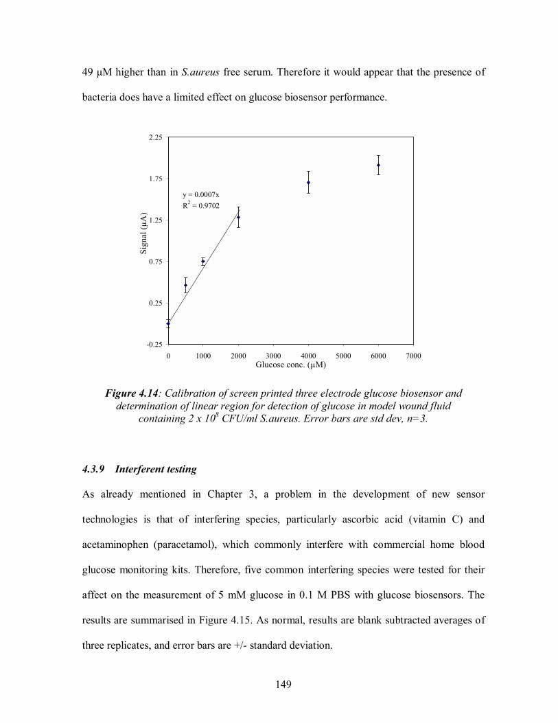
149

49 µM higher than in S.aureus free serum. Therefore it would appear that the presence of

bacteria does have a limited effect on glucose biosensor performance.

-0.25

0.25

0.75

1.25

1.75

2.25

0 1000 2000 3000 4000 5000 6000 7000Glucose conc. (µM)

Sign

al (µ

A)

y = 0.0007xR2 = 0.9702

Figure 4.14: Calibration of screen printed three electrode glucose biosensor and determination of linear region for detection of glucose in model wound fluid

containing 2 x 108 CFU/ml S.aureus. Error bars are std dev, n=3. 4.3.9 Interferent testing As already mentioned in Chapter 3, a problem in the development of new sensor

technologies is that of interfering species, particularly ascorbic acid (vitamin C) and

acetaminophen (paracetamol), which commonly interfere with commercial home blood

glucose monitoring kits. Therefore, five common interfering species were tested for their

affect on the measurement of 5 mM glucose in 0.1 M PBS with glucose biosensors. The

results are summarised in Figure 4.15. As normal, results are blank subtracted averages of

three replicates, and error bars are +/- standard deviation.

150

0

2

4

6

8

10

12

14

16

5 mM Glucose(no interferent)

1.32 mMAcetominophen

0.17 mMAscorbic acid

1 mM Cysteine 82.5 mM Urea 1.19 mM Uricacid

Interferent in 0.1 M PBS containing 5 mM glucose

Sign

al (µ

A)

Figure 4.15: Affect of interferents on the measurement of 5 mM glucose in 0.1 M PBS with

glucose biosensor. Error bars are std dev, n=3.

The levels of interferents tested were the highest concentrations of the ranges reported in

Table 3.1, and therefore represent worst case scenarios. Ascorbic acid had by far the largest

affect on the signal, increasing it by >4x the normal level. This was followed by cysteine,

which ~ doubled the signal. Acetominophen and uric acid had a similar smaller affect, and

urea had the opposite affect by decreasing the signal slightly. Clearly all have had some

affect, but ascorbic acid seems to pose the largest problem. These effects are either because

the interferents are electroactive at the operating potential of the biosensor, or they interfere

with the electrode signal though reaction with the analyte (McGrath, Iwuoha, Diamond, et

al, 1995). Some of these effects could be reduced or removed by incorporation of a perm-

selective layer (Palmisano, Centonze, Guerrieri, et al, 1993; Centonze, Guerrieri, Malitesta,

1992; Garjonyte & Malinauskas, 2000) or by incorporation of a compensator electrode

151

(which has no enzyme and measures the background current of the solution which can be

subtracted from the measurement by the enzyme electrode, assuming effects are additive)

4.3.10 Conclusions: Glucose biosensor

A rhodinised carbon three electrode assembly glucose biosensor was successfully

fabricated, optimised and tested in 0.1M PBS and model wound fluid. The limit of

detection was determined to be 170 µM at 99.7% confidence in model wound fluid with a

single dilution step. Ascorbic acid was identified as a key interferent, greatly increasing the

signal. The biosensor was tested in model wound fluid containing bacteria and validation

with BioAssay test kit was also successful. It was concluded that the glucose biosensor

approach is a suitable means of monitoring glucose in wound fluid and may form a useful

component of a wound fluid biosensor array.

4.4 Hydrogen peroxide biosensor The second of the three biosensor systems studied was a hydrogen peroxide (H2O2)

biosensor. Hydrogen peroxide biosensors have been widely investigated, and there are

many different variations of sensor construction. H2O2 biosensors were also fabricated in-

house. which gave the benefit of having full control over every parameter of the

construction and operation of the biosensor. For the purposes of this study, i.e. to

investigate the amperometric detection of hydrogen peroxide in model wound fluid, a

mediated enzyme reaction was chosen (a so-called second generation biosensor). Use of a

mediated system overcame problems associated with direct (non-mediated) detection of

H2O2, notably the need for higher operating potentials which increases the likelihood of

interference problems. The enzyme used was horseradish peroxidase (HRPx) (E.C.

152

1.11.1.7) sourced from Amoracia rusticana (Sigma, UK). It was supplied as a liquid with a

specific activity of 224U/mg, and stored in the freezer at -20 °C. HRPx is isolated from

horseradish roots and belongs to the ferroprotoporphyrin group of peroxidases. HRPx is a

single chain polypeptide containing four disulfide bridges and is a glycoprotein containing

18% carbohydrate. HRPx has been widely used in conjunction with electrochemical

transduction for the detection of hydrogen peroxide (Moody, Saini & Setford, 2001; Wang

& Wang, 2004; Kulys & Schmid, 1991; Johansson, Jonsson-Pettersson, Gorton et al,

1993).

The use of 1,1-dimethylferrocene (DMFc) as a mediator (i.e. a non-physiological small

redox mediator that shuttle electrons between the reduced enzyme prosthetic group and the

electrode) in a HRPx biosensor has been investigated by Kulys & Schmid (1991) and

Moody, Saini & Setford (2001) and found to be superior to other commonly used

alternative mediators such as tetrathiafulvalene and potassium hexacyanoferrate. Therefore,

the biosensor was developed using DMFc as the mediator. DMFc is a relatively stable dark

red crystalline solid with limited water solubility. The reaction is illustrated in Figure 4.16.

Figure 4.16: Reaction scheme on the carbon working electrode of the dimethylferrocene mediated horseradish-peroxidase H2O2 biosensor

DMFc (ox) DMFc (red)

HRPx (red)

HRPx (ox)

H2O2

H2O

e- Electrode

153

In this work, the working electrode was coated with a membrane. Membranes serve a

number of functions in biosensor applications. For example, a membrane may serve as a

protective layer to prevent interfering species from reaching the electrode surface, by size

exclusion or by charge repulsion. A membrane may also prevent soluble enzymes or

mediators such as DMFc, initially physically immobilised on the transducer surface from

desorbing and affecting the biosensor response. A membrane may also act as an additional

diffusion barrier between the transducer-immobilised bioligand on the electrode surface

and bulk solution, thus extending the dynamic range of the device (Johansson, Jonsson-

Pettersson, Gorton et al, 1993). A range of membrane materials such as nylon and

cellulose nitrate, and polymers have been investigated for use in biosensor construction. A

popular choice of polymer is Nafion, a highly negatively charged perfluorated polymer.

Nafion, by virtue of its negative charge, allows the passage of cations and repels anionic

species, and can be used either alone or in combination with other polymer materials such

as cellulose acetate (Wang & Wu, 1995). The use of electrochemically deposited polymers

such as polypyrrole, polyphenylenediamine, polyaniline and polyphenol as permselective

layers in the construction of biosensors is also commonplace, and has been recently

reviewed by Emr & Yacynych (2005).

Cellulose acetate can be formulated to create size exclusion membranes, the size of pore

being dictated by the particular molecular weight of the cellulose acetate used and the

drying regime applied. Cellulose acetate is ideal for use in biosensor construction, since in

solution form it can be dip coated, pipette deposited, or ink jet printed, making it amenable

154

to a range of mass production processes. It is also relatively cheap, easy to handle, and has

been used successfully in a number of studies involving the electrochemical measurement

of hydrogen peroxide (Ward, Jansen, Anderson et al, 2002; Cullen, Jawaheer, Rughooputh

et al, 2003; Moody, Saini & Setford, 2001). Therefore cellulose acetate was selected for

use with the hydrogen peroxide biosensor.

4.4.1 Determination of optimum operating potential

The basic electrochemical methodological approach used during the glucose biosensor

development was also used for the H2O2 biosensor. To determine the optimum operating

potential at which to operate the biosensor, staircase amperometry was performed across

the potential range -100 mV to -500 mV (100 mV steps) using 3 mM H2O2 in 0.1M PBS

(all tests in triplicate). The average current at each potential for 3 mM H2O2 and the blank

controls (background) were calculated. The ratio between the H2O2 generated current and

background current revealed the optimum operating potential to be -300 mV. Therefore this

potential was used for all future amperometric measurements with the H2O2 biosensor. This

concurs with the work of Moody, Saini & Setford (2001).

155

-18.0

-16.0

-14.0

-12.0

-10.0

-8.0

-6.0

-4.0

-2.0

0.0

-100-200-300-400-500Potential (mV)

H2O

2 Sig

nal/B

ackg

roun

d

Figure 4.17: The signal to background ratio for carbon three electrode system at 5 potentials, in 3 mM H2O2 in 0.1M PBS pH7.2. n=3.

4.4.2 Application of horseradish peroxidase, dimethylferrocene and cellulose acetate

Initially, HRPx, DMFc and cellulose acetate (CA) were applied to the carbon working

electrode, according to the procedure of Moody, Saini & Setford (2001). HRPx was made

to 5U/µl in 0.1M PBS pH 7.2, DMFc to 12.5 g/L in acetone, and CA to 20g/L in acetone.

The following volumes were applied to the working electrode:

HRPx (5U/µl) 5 µl

DMFc (12.5 g/L) 4 µl

CA (20 g/L) 4 µl

These volumes were applied together in a single solution deposition of 13 µl. In making a

batch of sensors, the three components were pre-mixed by pipette action in a tube in order

to provide a suitable batch size. However, it was found that preparing too large a volume at

156

one time, for example to make 100 sensors, resulted in acetone evaporation during the

depositioning procedure, resulting in poor sensor repeatability. It also proved difficult to

maintain a homogeneous mixture during the depositioning step, due to immiscibility

between the aqueous and solvent phases, also contributing to sensor irreproducibility.

Therefore a method was developed whereby a volume sufficient for the production of 60

sensors was prepared, but aliquotted into 10 microcentrifuge tubes. Therefore one tube

contained enough mix for 6 sensors, and while depositing the mix to 6 sensors, the

remaining 9 tubes remained capped thereby preventing evaporation until opened. This also

improved the uniformity of the mixture, and hence reduced inter batch variation. Once

prepared, sensors were allowed to dry at room temperature overnight, and then foil

wrapped and stored in an air tight glass jar bocal canette (Luminarc, France), with a silica

gel sachet inside to absorb moisture.

4.4.3 Shelf life testing Shelf life tests were carried out on the H2O2 biosensors for the same reasons given in

Section 4.3.4 for the glucose biosensors. A batch of 100 H2O2 biosensors was made as

described in Section 4.4.2. The sensors were foil wrapped and stored in air tight glass jars

(Luminarc, France) containing one silica gel sachet and stored at 4 °C. On the day of

biosensor production (day 0), 100 µM H2O2 in 0.1M PBS was amperometrically measured

with the biosensors in triplicate at -300 mV. This measurement was repeated regularly over

a period of 77 days, since the sensors were not stored for a longer period than this during

the project. The differential mean and standard deviations were calculated, and are shown

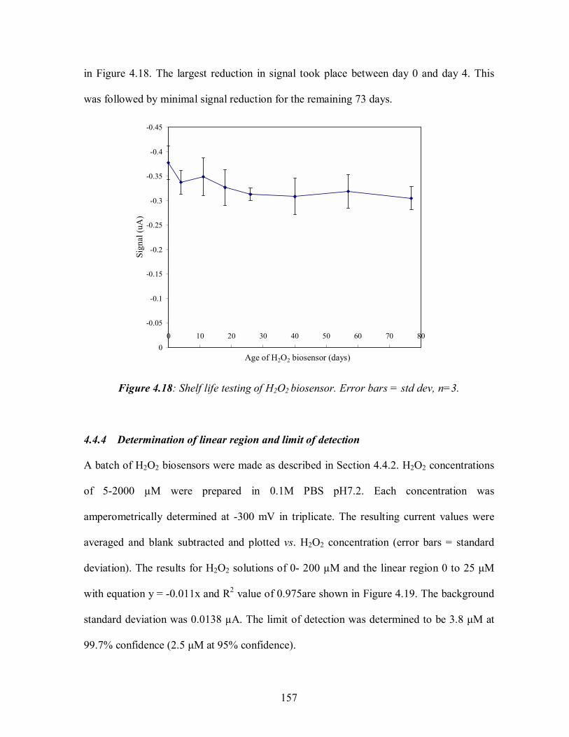
157

in Figure 4.18. The largest reduction in signal took place between day 0 and day 4. This

was followed by minimal signal reduction for the remaining 73 days.

-0.45

-0.4

-0.35

-0.3

-0.25

-0.2

-0.15

-0.1

-0.05

00 10 20 30 40 50 60 70 80

Age of H2O2 biosensor (days)

Sign

al (u

A)

Figure 4.18: Shelf life testing of H2O2 biosensor. Error bars = std dev, n=3.

4.4.4 Determination of linear region and limit of detection A batch of H2O2 biosensors were made as described in Section 4.4.2. H2O2 concentrations

of 5-2000 µM were prepared in 0.1M PBS pH7.2. Each concentration was

amperometrically determined at -300 mV in triplicate. The resulting current values were

averaged and blank subtracted and plotted vs. H2O2 concentration (error bars = standard

deviation). The results for H2O2 solutions of 0- 200 µM and the linear region 0 to 25 µM

with equation y = -0.011x and R2 value of 0.975are shown in Figure 4.19. The background

standard deviation was 0.0138 µA. The limit of detection was determined to be 3.8 µM at

99.7% confidence (2.5 µM at 95% confidence).

158

-0.75

-0.65

-0.55

-0.45

-0.35

-0.25

-0.15

-0.05

0.050 25 50 75 100 125 150 175 200 225

H2O2 concentration (µM)

Sign

al (µ

A)

y = -0.011xR2 = 0.975

-0.35

-0.3

-0.25

-0.2

-0.15

-0.1

-0.05

0

0.050 5 10 15 20 25

H2O2 concentration (µM)

Sign

al (µ

A)

Figure 4.19: Calibration of screen printed three electrode H2O2 biosensor and determination of linear region for detection of H2O2 in 0.1M PBS.


LINEAR REGION

159

4.4.5 Validation with Checkit H2O2 test kit The results for the detection of H2O2 in PBS with the hydrogen peroxide biosensors were

validated using the Lovibond H2O2 Checkit test kit described in Section 2.2.7. Four

solutions were prepared containing unknown concentrations of H2O2 in 0.1M PBS. The test

kit instructions were followed as described in Section 2.2.7, to determine the concentrations

of the four solutions. The solutions were also measured amperometrically using the H2O2

biosensors, and the currents recorded converted into H2O2 values using the calibration

graph in Figure 4.19. The H2O2 concentrations in Table 4.2 determined by each method are

plotted in Figure 4.20, where it can be seen that an R2 value of 0.997 demonstrates the

reliability of the H2O2 biosensor.

Table 4.2: Results of H2O2 biosensor validation by H2O2 Checkit test kit Test kit: Biosensor:

H2O2 solution # Checkit reading (mg/l) H2O2 conc. (µM) 1 0.20 5.80 2 0.50 14.70 3 0.70 20.60 4 0.85 25.00

H2O2 solution # Signal (µA) H2O2 conc. (µM) 1 -0.06655 6.05 2 -0.1672 15.20 3 -0.22902 20.82 4 -0.27852 25.32

160

y = 1.0164xR2 = 0.9997

0

5

10

15

20

25

30

0 5 10 15 20 25H2O2 concentration (µM) - Checkit test kit

H2O

2 con

cent

ratio

n (µ

M) -

Bio

sens

or

Figure 4.20: Validation of H2O2 biosensor with Checkit test kit 4.4.6 Detection of H2O2 in model wound fluid with hydrogen peroxide biosensor Having established the hydrogen peroxide biosensor could detect H2O2 down to 3.8 µM

(99.7% confidence) in 0.1 M PBS, the next stage was to detect H2O2 in 90:10 v/v serum in

0.1M PBS, as was also performed for the glucose biosensor in Section 4.3.8.

Concentrations of H2O2 were prepared from 200 µM to 2000 µM in the 90:10 v/v serum:

PBS and determined amperometrically as before. The results are shown in Figure 4.21. The

linear portion of the response profile was determined to be 0-1000 µM, a four-fold increase

in comparison to the PBS data, (y = -0.0028x: R2 value of 0.9846). The standard deviation

of the blank was 0.007865 µA, and the limit of detection was found to be 8.5 µM at 99.7%

confidence (6 µM at 95% confidence), similar to the limits found in PBS, having increased

from 3.8 µM to 8.5 µM at 99.7% confidence.

161

-4

-3.5

-3

-2.5

-2

-1.5

-1

-0.5

0

0.50 250 500 750 1000 1250 1500 1750 2000

H202 conc. (µM)

Sign

al (µ

A)

y = -0.0028xR2 = 0.9846

-3.5

-3

-2.5

-2

-1.5

-1

-0.5

0

0.50 100 200 300 400 500 600 700 800 900 1000

H202 conc. (µM)

Sign

al (µ

A)

Figure 4.21: Calibration of screen printed three electrode H2O2 biosensor and determination of linear region for detection of H2O2 in model wound fluid.


LINEAR REGION

162

4.4.7 Detection of H2O2 in model wound fluid containing S.aureus with

H2O2 biosensor

As with the glucose biosensor tests, the final test with the hydrogen peroxide biosensor

again involved the detection of H2O2 in model wound fluid, but this time containing

S.aureus to test whether the presence of bacteria affects the performance of the biosensor.

S.aureus was grown in serum to a cell density of 2 x 108 CFU/ml. This was then used to

prepare known H2O2 concentrations in 0.1M PBS from 250 to 2000 µM, which were

measured at -300 mV in triplicate with the H2O2 biosensors. Differential means and

standard deviations were calculated and plotted versus concentration as shown in Figure

4.22. The linear range of the sensor was equivalent to that obtained for H2O2 in serum

without S.aureus (0-1000 µM). The blank standard deviation was measured at 0.0897 µA,

with a limit of detection of 9.6 µM at 99.7% confidence (6.4 µM at 95% confidence), less

than 2 µM higher than in S.aureus free serum, indicating that the presence of bacteria does

not significantly effect biosensor performance.

4.4.8 Interferent testing As done so for the glucose biosensor, five common interfering species were tested for their

affect on the measurement of 0.5 mM H2O2 in 0.1 M PBS with H2O2 biosensors. The

results are summarised in Figure 4.23. As normal, results are blank subtracted averages of

three replicates, and error bars are +/- standard deviation.

163

-3.5

-3

-2.5

-2

-1.5

-1

-0.5

0

0.50 250 500 750 1000 1250 1500 1750 2000

H202 conc. (µM)

Sign

al (µ

A)

y = -0.0024xR2 = 0.9864

Figure 4.22: Calibration of screen printed three electrode H2O2 biosensor and determination of linear region for detection of H2O2 in model wound fluid

containing 2 x 108 CFU/ml S.aureus. Error bars are std dev, n=3.

-3.5

-3

-2.5

-2

-1.5

-1

-0.5

00.5

mM H

2O2 (

no in

terfer

ent)

1.32 m

M Acet

omino

phen

0.17 m

M Asco

rbic a

cid

1 mM Cyst

eine

82.5

mM Urea

1.19 m

M Uric

acid

Interferents in 0.1 M PBS containing 0.5 mM H2O2

Sign

al (µ

A)

Figure 4.23: Affect of interferents on the measurement of 0.5 mM H2O2 in 0.1 M PBS with

H2O2 biosensor. Error bars are std dev, n=3.

164

Inversely to the glucose biosensor (except for urea), the interferents reduced rather than

increased the signal by differing amounts. Acetominophen and ascorbic acid had the

greatest effect reducing the signal by ~7 times. The least effect was given by cysteine. Urea

and uric acid approximately halved the signal. This is because they are electroactive at the

same potential as H2O2, and are therefore adding to the reduction signal. As mentioned for

the glucose biosensor, the incorporation of a compensator electrode could help to alleviate

this.

4.4.9 Conclusions: H2O2 biosensor

A mediated three electrode H2O2 biosensor was fabricated and optimised in 0.1M PBS

spiked with H2O2. Testing of the biosensor in model wound fluid with a single dilution step

revealed the limit of detection to be 8.43 µM. The biosensor was tested in model wound

fluid in the presence of bacteria, which had no significant effect. Interferent effects were

tested where acetominophen and ascorbic acid were found to exhibit the most significant

affects on signal. Validation using a Checkit enzyme based colorimetric test kit was

successful. Although without data on the levels of H2O2 in the body one cannot be certain

that the levels are detectable, but as a concept, a hydrogen peroxide biosensor could

successfully be used to monitor H2O2 in wound fluid down to a level of approximately 8.4

µM. To take this further, real sample testing would be required.

4.5 Ethanol biosensor The third biosensor was designed for the detection of ethanol in 0.1M PBS and model

wound fluid. Many analytical methods have been developed for the measurement of

ethanol, including chemical, colorimetric, chromatographic and refractive index methods.

165

However, although these methods are precise and reliable, they are relatively complex and

time consuming, and also require expensive instrumentation and training of operators.

Much research has been directed towards overcoming these disadvantages by use of the

biosensor approach, particularly those based on electrochemical transduction.

Two enzymes, alcohol oxidase (AOx) and alcohol dehydrogenase (ADH) have been

extensively used in ethanol biosensor studies (Lee, Kim, Lee et al, 1999; Sprules, Hartley,

Wedge et al, 1996). ADH based biosensors require the co-enzyme nicotinamide adenine

dinucleotide (NAD+). However, the NAD+ also needs to be able to diffuse to the enzyme

active site without becoming irreversibly entrapped or otherwise linked (Fonseca, Azevedo,

Prazeres et al, 2004). AOx is an oligomeric enzyme consisting of eight identical sub-units

arranged in quasi-cubic arrangement, each containing a strongly bound co-factor, flavin

adenine dinucleotide (FAD) (Vonck & van Bruggen, 1990). It is produced by

methylotrophic yeasts, commonly Hansenula, Pichia, and Candida. AOx has been used

extensively in ethanol biosensors from each of these three yeast sources (Gorton, Heller,

Vijayakumar et al, 1996; Patel, Meier, Cammann et al, 2001, Kulys & Schmid, 1991). AOx

irreversibly oxidises short chain alcohols to the corresponding aldehyde, using molecular

oxygen as the electron acceptor. The reaction can be followed by either monitoring

decrease in O2 tension or the increase in H2O2 concentration.

RCH2OH + O2 AOx RCHO + H2O2

Sensors based on O2 measurement have the advantage of minimal electrochemical

interference in real samples. However, response values are relatively low with high

background signals, giving poorer detection limits when compared to H2O2 measurement

166

approaches. Furthermore, the dependence on oxygen can reduce sensor accuracy and

reproducibility, since O2 levels vary from sample to sample (Bott, 1998). Therefore H2O2

detection is the more commonly used and preferred method. H2O2 sensors have a greater

dynamic range and wider linear range, but as previously mentioned for the H2O2 biosensor

(Section 4.2), first generation sensors based on direct detection of H2O2 require an elevated

detection potential, increasing the likelihood of electrochemical interference in real

samples, for example from electroactive ascorbic acid or acetaminophen. Therefore, in a

similar manner to that employed for the H2O2 biosensor developed for this study, an

alternative direct detection route was employed. Options included: modifying the electrode

with an electrocatalyst (such as that used for the glucose biosensor see Section 4.3); using

an alternative electron acceptor to O2; to regenerate the oxidised form of FAD, (a rarely

used method); use of a mediator (second generation biosensor) such as ferrocene, (although

a literature search yielded no such mediator for AOx; use of a bienzyme system such as the

many examples where HRPx is used to catalyse the electro-reduction of H2O2 at reduced

potentials, either directly or by use of a mediator. The latter option of a bienzyme system

using HRPx and AOx has been utilised successfully by a number of groups for ethanol

detection, including Kulys & Schmid, (1991); Gorton, Heller, Vijayakumar et al. (1996).

After careful consideration, and based on the success of the HRPx sensor approach, a

mediated bienzyme (HRPx and AOx) system was chosen using DMFc as the mediator.

Having already developed a H2O2 biosensor utilising HRPx and DMFc, the simple

addition of AOx to the deposition medium resulted in the relatively straightforward

development of a mediated bienzyme ethanol biosensor.

167

4.5.1 Operating potential Since the ethanol biosensor had a similar operating procedure as for the H2O2 biosensor,

namely the current generated from the reduction of the oxidised form of the DMFc

mediator at a carbon working electrode, the same operating potential of -300 mV (vs.

Ag/AgCl reference electrode) was employed.

4.5.2 Determination of optimum alcohol oxidase loading Two sources of AOx were investigated: Candida boidinii and Pichia pastoris, both

purchased from Sigma (Poole, UK). AOx from C.boidinii was supplied with a specific

activity of 13.6U/mg protein and AOx from P.pastoris with 23U/mg protein, both as a

liquid stored at -20 °C. The optimum number of units of AOx per sensor was determined

for both sources. A range of AOx loadings were prepared and applied to the working

electrode at the same time as the HRPx, DMFc and CA as a total deposition volume of 15

µl, with the AOx fraction accounting for 2 µl of the total depositioning volume (as

described by Moody, Setford, Saini, 2001). A 2mM volume of ethanol in 0.1M PBS (pH

7.2) was determined amperometrically at -300mV (n=3). The signal: noise ratio was

calculated for each enzyme loading by determining the ratio of the differential signal versus

standard deviation for each AOx source. The optimum loading for AOx from C.boidinii

and P.pastoris was found to be 1.25 U/sensor and 1.15 U/sensor respectively, as illustrated

in Figure 4.24 (a) and (b). The optimum number of units of AOx/sensor was similar for

both sources, but AOx from C.boidinii was approximately twice as expensive, and also less

widely available, both of which are important issues when considering possible production

issues. Therefore AOx from P.pastoris was selected to prepare subsequent batches of

ethanol biosensors, at an enzyme loading of 1 U/sensor.

168

0

2

4

6

8

10

12

14

16

18

20

22

0 0.5 1 1.5 2 2.5 3 3.5 4 4.5 5 5.5 6 6.5Alcohol oxidase units/ sensor (Candida boidinii )

S/N

(a)

0

1

2

3

4

5

6

7

8

9

0 0.5 1 1.5 2 2.5 3 3.5 4Alcohol oxidase units/ sensor (P.pastoris )

S/N

(b)

Figure 4.24: Signal: noise ratios for alcohol oxidase loadings of bi-enzyme mediated system in 2mM ethanol in 0.1M PBS pH7.2. (a) C.boidinii and (b) P.pastoris. n=3.

169

4.5.3 Deposition of horseradish peroxidase, alcohol oxidase, dimethylferrocene and

cellulose acetate

As with the H2O2 sensors, deposition modification was required to increase uniformity and

reduce sensor losses. The batch volume made was split up into microcentrifuge tubes, as

described for the H2O2 sensors. However a reduction in deposition volume was also

required. A volume of 15µl/ sensor resulted in spread beyond the working electrode film on

a high percentage of sensors. Therefore, the depositioning volume was reduced which

eliminated the solution-spread problem. Accordingly, the concentration of DMFc was

raised from 12.5 to 25mg/ml thereby reducing the volume of DMFc per sensor from 4 to 2

µl and hence the overall deposition volume to 13 µl.

4.5.4 Shelf life testing Shelf life tests were carried out on the ethanol biosensors for the same reasons given in

Section 4.3.4. A batch of 100 ethanol biosensors was made as described in Section 4.5.3.

The sensors were foil wrapped and stored in air tight glass jars containing one silica gel

sachet and stored at 4 °C. On the day of biosensor production (day 0), 1000 µM ethanol in

0.1 M PBS was determined amperometrically in triplicate. This measurement was repeated

regularly over a period of 77 days, since the sensors were not stored for a longer period

than this during the project. The differential mean and standard deviations were calculated

and are shown in Figure 4.25. The largest reduction in signal took place between day 0 and

day 4, as observed for the glucose and H2O2 biosensors. Following this initial reduction, the

signal stabilised to an average of -0.90 µA for the remaining 73 days of the test.

170

-1.4

-1.2

-1

-0.8

-0.6

-0.4

-0.2

00 10 20 30 40 50 60 70 80

Age of alcohol biosensor (days)

Sign

al (u

A)

Figure 4.25: Shelf life testing of alcohol biosensor. Error bars = std dev, n=3.

4.5.5 Determination of linear region and limit of detection A batch of ethanol biosensors was prepared as described in Section 4.5.3. Ethanol

concentrations of 25-10,000 µM were prepared in 0.1M PBS pH7.2. Each concentration

was determined amperometrically (n=3). The resulting currents were averaged and blank

subtracted (signal) and plotted vs. ethanol concentration, with error bars. The background

standard deviation was 0.0366 µA. The linear region was determined to be between 0 and

750 µM, yielding the equation: y = -0.0011x with an R2 value of 0.9946, as illustrated in

Figure 4.26. The limit of detection was determined to be 99.8 µM at 99.7% confidence

(66.5 µM at 95% confidence).

171

-1.7

-1.5

-1.3

-1.1

-0.9

-0.7

-0.5

-0.3

-0.1

0.10 2000 4000 6000 8000 10000

Ethanol (µM)

Sign

al (µ

A)

y = -0.0011xR2 = 0.9946

-1.1

-0.9

-0.7

-0.5

-0.3

-0.1

0.10 100 200 300 400 500 600 700

Ethanol (µM)

Sign

al (µ

A)

Figure 4.26: Calibration of screen printed three electrode ethanol biosensor and

determination of linear region for detection of ethanol in 0.1M PBS. Error bars are std dev, n=3.

LINEAR REGION

172

4.5.6 Validation

A test kit was not available for the detection of ethanol in solution in the range required.

However, since the ethanol biosensor is ultimately based on the determination of hydrogen

peroxide at the working electrode and utilises the same HRPx enzyme loading and

mediator as for the hydrogen peroxide biosensor, it is not unreasonable to assume that the

ethanol biosensor has a similar operational capability.

4.5.7 Further ethanol biosensor development membranes and deposition regime Before commencing work on the detection on ethanol in simulated wound fluid, further

development work on the ethanol biosensor was carried out. To reduce the possible effects

of interferents and proteinacious material present in serum, a range of membranes were

investigated. Variations in the deposition of the enzymes, DMFc, CA and of Nafion were

also investigated. The aim was to improve the linear range and the limit of detection of the

sensor, by reducing inter-batch variation and hence noise. Table 4.3 below lists the

membranes investigated.

Table 4.3: Membranes tested on ethanol biosensor

Manufacturer Membrane name Membrane pore size (um) Pall, Portsmouth, UK Biodyne A 0.2 Pall, Portsmouth, UK Biodyne A 0.45 Pall, Portsmouth, UK Biodyne A 1.2 Pall, Portsmouth, UK Immunodyne ABC 0.45 Whatman, Loughborough, UK Cellulose nitrate 0.2 Whatman, Loughborough, UK Cellulose nitrate 0.45 Whatman, Loughborough, UK Cellulose nitrate 3 Whatman, Loughborough, UK Cyclopore polycarbonate 0.4 Sterlitech, Kent, WA, USA Nylon 0.45 Millipore, Watford, UK Nylon 0.45 Spectrum, Loughborough, UK Spectra membrane MWCO 6-8k

173

A batch of ethanol biosensors were made according to the single deposition method

described in Section 4.5.3. The membranes were cut into 1 cm squares, and placed on the

sensor such that they covered the three electrodes (pre-dosed with enzyme, DMFc and CA)

and secured using PVC tape. The amperometric procedure was initiated and 100 µl of 1:1

v/v serum: PBS deposited onto the membrane and the electrode response allowed to

equilibrate prior to addition of 100 µl of 5 mM ethanol in 1:1 v/v serum: PBS. Tests were

performed in triplicate, and the differential signal and signal: noise determined.

The Whatman Cyclopore proved unsuitable, since upon application of the serum/PBS, the

membrane proved relatively hydrophobic resulting in uneven sample spread, and the serum

did not filter though to the sensor surface. The Spectrum spectra membrane could not be

used since it disintegrated upon application of serum/PBS. For all of the remaining

membranes tested, there was a general difficulty in achieving full contact between the

sensor and the membrane, and retaining contact once serum had been applied. Figure 4.27

shows the signal: noise ratios obtained for each of the membranes incorporated into the

ethanol biosensors.

Only two of the membranes improved the signal to noise ratio beyond that of using no

membrane. These were both Biodyne A membranes of 0.2 µm and 0.45 µm pore size, with

a signal to noise of 54.4 and 10.4 respectively. Using no membrane gave a signal to noise

of 8.7, therefore using the 0.45 µm Biodyne membrane would not greatly improve the

sensor performance (compared to the improvement that follows through deposition

development).

174

0

10

20

30

40

50

60

No mem

brane

Membrane

Sign

al:N

oise

Figure 4.27: Comparison of signal: noise of ethanol biosensor using of a range of membranes.n=3.

Given the difficulties associated with membrane integration into the sensor, the regime of

applying AOx and HRPx enzymes, DMFc, and CA to the sensor, with the aim of

improving the signal to noise ratio without the use of a membrane, was investigated further.

Instead of applying all four components in one step, alternative depositioning regimes were

examined, including the application of combinations of the reagents in seven variations of

one, two or three layers, as shown in Table 4.4. The 13 µl deposition volume comprising

two enzymes HRPx and AOx, and the CA immobilisation/diffusion layer were prepared, as

described in Section 4.5.3. The same volumes per sensor also applied. A 5% v/v Nafion

perfluorated resin aqueous dispersion (Aldrich, Poole, UK) was also investigated, at two

drying temperatures to vary pore size. Except for the Nafion layers which were dried at 4°C

and 50 °C, each layer was allowed to dry at room temperature before deposition of the next

175

layer. Each variation was made and deposited in replicates of six sensors (three for

measurement, three for blank). 5 mM ethanol in 1:1 v/v serum: PBS was determined

amperometrically to compare the formulations.

Table 4.4: Ethanol biosensor deposition parameters for the 4 biosensor reagents studied: AOx and HRPx enzymes, dimethylferrocene film, cellulose acetate and Nafion membrane

materials. Numbers indicate layer number

Combination Enzymes Enzymes Enzymes + DMFc 5% Nafion 5% Nafion CA + DMFc DMFc + CA + CA Dried at 4 °C dried at 50 °C

1 1 2 2 1 2 3 3 1 2 3 4 1 2 5 1 2 6 1 7 1 2

.

The average signal, standard deviations and signal to noise ratio were calculated for each of

the seven combinations, plotted in Figure 4.28. It can be seen clearly that combination

number seven had by far the best signal to noise ratio of 19.1. This combination consisted

of two deposition layers - layer one: HRPx, AOx and DMFc, and layer two: CA. The

second best signal to noise was given by combination 6, the single deposition combination

as used earlier in the chapter to detect ethanol in PBS, but was still considerably less than

combination number 7. The addition of a Nafion layer increased the signal but had less

favourable signal to noise ratios, possibly due to difficulty achieving a uniform and

repeatable layer of nafion on the sensor surface. The very low signals and signal to noise

witnessed for combinations 4 and 5, where a CA layer is absent, illustrate the importance of

using CA as a diffusion layer on these sensors. Therefore, combination 7 was selected as

the deposition regime of choice.

176

-4.0

-3.5

-3.0

-2.5

-2.0

-1.5

-1.0

-0.5

0.0

0.5

1 2 3 4 5 6 7

Variation number

Sign

al (µ

A)

0

5

10

15

20

25

Sign

al:N

oise

ratio

Mean SignalSignal:Noise

Figure 4.28: Signal:noise ratio for the 7 deposition combinations of enzymes, dimethylferrocene, cellulose acetate and nafion used in alcohol biosensor construction.


Having decided to apply cellulose acetate as a separate second layer, a small investigation

was carried out to determine whether application of CA by pipette action or dip coating

was preferable. CA (20mg/ml) volumes of 0, 3 and 5 µl were applied to sensors by pipette

action in replicates of six, and six sensors were also dip coated in CA. The sensors were

then interrogated amperometrically using 5 mM ethanol in 1:1 v/v serum: PBS. The

resulting average signals and signal to noise ratios were calculated and are shown in Figure

4.29. It can be seen that a far greater signal to noise ratio was present for the dip coated

sensors, with a value of 238.0. This value far exceeded that produced when using the

Biodyne A (0.2 µm) membrane, indicating that the dip coating route was superior to the

pre-formed membrane depositioning approach, for the membranes studied in this work. CA

was therefore applied by dip coating for all subsequent alcohol biosensor batches produced.

177

-0.7

-0.6

-0.5

-0.4

-0.3

-0.2

-0.1

0.0dip coated 0 µl 3µl 5µl

Cellulose acetate depostion type / volume

Sign

al (µ

A)

0

50

100

150

200

250

Sign

al:N

oise

ratio

Signal (uA)Signal:Noise ratio

Figure 4.29: Comparison of cellulose acetate application methods and volumes applied to alcohol biosensor. Error bars are std dev, n=3.

4.5.8 Detection of ethanol in model wound fluid with ethanol biosensor Having established that the alcohol biosensor had a limit of detection of 99.8 µM (99.7%

confidence) in 0.1 M PBS using the single step reagent depositioning approach, the next

stage of development was to examine the performance of the reformulated ethanol

biosensors in 1:1 v/v serum: PBS, as performed for the glucose and hydrogen peroxide

biosensors. A batch of ethanol biosensors was prepared using the new two layer deposition

method, as described in Section 4.5.7

Concentrations of ethanol were prepared from 100-2000 µM in the 1:1 v/v serum: PBS.

Ethanol was determined amperometrically at -300mV as before. Results are shown in

Figure 4.30.

178

-5.5

-5

-4.5

-4

-3.5

-3

-2.5

-2

-1.5

-1

-0.5

0

0.50 500 1000 1500 2000

Ethanol Concentration (µM)

Sign

al (µ

A)

y = -0.0037xR2 = 0.9970

-4

-3.5

-3

-2.5

-2

-1.5

-1

-0.5

0

0.50 250 500 750 1000

Ethanol Concentration (µM)

Sign

al (µ

A)

Figure 4.30: Calibration of screen printed three electrode ethanol biosensor (2 layer deposition procedure, described in 4.5.7) and determination of linear region for detection

of ethanol in model wound fluid. Error bars are std dev, n=3.

LINEAR REGION

179

The linear range of the sensor response was determined to be 0-1000 µM, 250 µM longer

than in PBS alone, which were prepared by the single deposition formulation; (y = -

0.0037x, R2 value of 0.997). The standard deviation of the blank was found to be 0.0098

µA, yielding a limit of detection of 7.94 µM at 99.7% confidence (5.3 µM at 95%

confidence), much lower than the limits found in PBS with the single deposition

formulation (99.8 µM at 99.7% confidence).

4.5.9 Detection of S.aureus in model wound fluid with ethanol biosensor Having established the biosensor could detect ethanol in diluted model wound fluid (1:1

v/v serum: PBS), it was next tested for its ability to detect bacteria in model wound fluid,

by determining ethanol produced by metabolically active bacteria. However, as already

mentioned in Section 2.3.1 only S.aureus would grow in serum alone. Attempting detection

in serum supplemented with Dulbeccos modified Eagles medium (DMEM) (as

implemented in Chapter 5 for the odour analyser work), significantly interfered with the

performance of the biosensor and thus this approach was not suitable. S.aureus alone was

grown in serum (cultured as described in Section 2.2.5), and after a 1:1 dilution with 0.1 M

PBS, was determined amperometrically (n=3) at five different cell densities. The average

signals and standard deviations can be seen in Figure 4.31. The standard deviation of the

blank was 0.02355 µA, and a linear biosensor response was observed over the range

0 to 4 x 108 CFU/ml (y = -0.0574x). The limit of detection was found to be 1.23 x 108

CFU/ml at 99.7% confidence (0.82 x 108 CFU/ml at 95% confidence). By using the

mathematical relationship shown in Figure 4.30, the limit of detection in terms of the

ethanol specific response was 19.0 µm at 99.7% confidence (12.7 µm at 95% confidence).

180

-0.45

-0.4

-0.35

-0.3

-0.25

-0.2

-0.15

-0.1

-0.05

0

0.050 0.5 1 1.5 2 2.5 3 3.5 4 4.5

S.aureus CFU/ml x108

Sign

al (µ

A)

y = -0.0574xR2 = 0.9461

Figure 4.31: Detection of metabolic ethanol production by S.aureus with screen printed three electrode alcohol biosensor in serum. Error bars are std dev, n=3.

4.5.10 Interferent testing

As done so for the glucose and H2O2 biosensors, five common interfering species were

tested for their affect on the measurement of 0.5 mM ethanol in 0.1 M PBS with ethanol

biosensors. The results are summarised in Figure 4.32. Results are blank subtracted

averages of three replicates, and error bars are +/- standard deviation.

The results are similar to those observed for the H2O2 biosensor, with acetominophen and

ascorbic acid having the most significant affects on signal, and cysteine the least affect.

However, the effects of urea and uric acid are not so severe. The change in signal is either

because the species are electroactive at the same potentials as the analyte, or by electrode

181

fouling. These effects could be reduced by use of a perm-selective layer (Carelli, Centonze,

De Giglio, et al, 2006; Hamdi, Wang, Monbouquette, 2005).

-0.7

-0.6

-0.5

-0.4

-0.3

-0.2

-0.1

00.5

mM Etha

nol (n

o inter

feren

t)

1.32 m

M Acet

omino

phen

0.17 m

M Asco

rbic a

cid

1 mM C

ystein

e

82.5 m

M Urea

1.19 m

M Uric

acid

Interferents in 0.1 M PBS containing 0.5 mM ethanol

Sign

al (µ

A)

Figure 4.32: Affect of interferents on the measurement of 0.5 mM ethanol in 0.1 M PBS

with ethanol biosensor. Error bars are std dev, n=3. 4.5.11 Conclusions: Ethanol biosensor

A bienzyme mediated ethanol biosensor was fabricated using a screen-printed three

electrode assembly. AOx selection and optimisation determined that the optimum AOx

loading was 1U/sensor using AOx isolated from P.pastoris. This enzyme was combined

with HRPx and DMFc mediator. Cellulose acetate was found to be the most suitable

immobilisation / diffusion layer when compared to Nafion and other membrane materials,

with dip coating proving preferable to pipette application, with signal: noise values of

238.0 and 8.7 respectively. A detection potential of -300 mV was used for the detection of

182

H2O2 at the sensor surface. In model wound fluid with a single dilution step, the limit of

detection for ethanol was 7.94 µM at 99.7% confidence. Direct detection of metabolically

produced ethanol by S.aureus grown in model wound fluid by the ethanol biosensor, gave a

limit of detection of 1.23 x 108 CFU/ml. This level does represent a significant bacterial

count, since bacterial colonisation in wounds is considered problematic at levels of greater

than 106 CFU/ml. Therefore, further biosensor refinement and optimisation is required in

order to be used as an early warning system for bacterial invasion of a wound. However,

this sensor does have potential to be used for monitoring further rises in bacterial

colonisation, or indeed as part of a wound monitoring process where falls in ethanol

production below a certain level could indicate reducing bacterial numbers and hence the

success of a patient treatment regime.

4.6 Conclusions: Overall

The glucose, hydrogen peroxide and ethanol biosensors were all successful, detecting

glucose, hydrogen peroxide and ethanol in surrogate wound fluid with a single dilution

step, with limits of detection of 169.5 µM glucose, 8.43 µM hydrogen peroxide, and 7.94

µM ethanol respectively. The ethanol biosensor could detect S.aureus down to 1.23 x 108

CFU/ml, which could signal bacterial numbers falling below this level, possibly indicative

of healing, or rising above a safe level (i.e. >106 CFU/ml). Using the biosensor array,

perhaps within a suite of diagnostic wound monitoring tests, a non-healing wound could be

signalled to a busy physician more rapidly than it would otherwise be using conventional

methods.

183

5. Bacterial Detection Using a Single Sensor Odour Analyser 5.1 Introduction This Chapter aims to investigate whether a single sensor odour analyser may be used as a

diagnostic tool in the early stages of wound healing, based on the detection of volatile

bacterial metabolites and human markers of immune response within the localised wound

environment.

Using a single sensor based odour analyser instead of an array of sensors, as present in

commercially available electronic nose devices, has the advantages of reduced cost, and

reduced complexity with respect to the sensor array. This is achieved by augmenting the

volume of information gained from the sensor response by considering an increased

number of sensor response curve features. Further information on the development of this

machine can be found in the thesis of Lee-Davey (2004). There are many potentially

influencing factors in the wound environment, for example: antiseptics and other

antimicrobial agents; changing temperature of the wound environment; cell-derived

molecules responsible for co-ordinating the healing process; medications taken by the

patient, and though considered, could not all be investigated within the scope of this study.

However, by separating serum from blood, as described in Section 2.2.4, it was possible to

create a surrogate wound fluid, since the major component of wound fluid is serum. This

enabled experimentation to be confined to the laboratory under a controlled environment in

this preliminary feasibility study.

184

The objectives were limited to identifying whether the system could discriminate between

those five bacterial species commonly associated with wound infection: Staphylococcus

aureus, Streptococcus pyogenes, Klebsiella pneumoniae, Escherichia coli and

Pseudomonus Aeruginosa. Tests were performed on individual cultures, then culture pairs,

initially in broth and secondly in serum at fixed cell densities. By examining the headspace

at constant cell densities, the differences detected may be more directly attributed to

particular bacterial metabolic features, and not differences in cell numbers between

bacteria. Detection and discrimination of the biological markers glucose, ethanol and H2O2

was also investigated. Headspace GC-MS (results presented in Section 2.3.3.) was used as

the standard method as a basis for comparison.

Following odour analysis, discrimination of samples was based on principle component

analysis (PCA), an unsupervised technique executed in Matlab. It requires the user to

examine the data and select the principle components which provide the best virtual

discrimination of samples, realised through plots of one principle component versus

another. As described in Section 1.4.5.1, this technique reduces the dimensionality whilst

retaining the variance of the original data, providing a relatively fast method of determining

the success of the experiments at this developmental stage.

185

5.2 Materials and Methods 5.2.1 Odour analyser instrumentation The odour analyser, developed by Lee-Davey (2004) at a basic level may be considered a

relative of the traditional machine olfaction approach as exemplified by the so-called

electronic nose. However, instead of housing an array of sensors for odour detection, it

uses just one - a single mixed metal-oxide semiconductor sensor (MMOS). MMOS sensors

are designed for a range of applications, including air quality and volatile organic

compounds (VOCs), and have found application in commercial systems, such as the

Marconi eNOSE 5000 units. These sensors typically have a lifetime >5 years for some

applications, repeatability, and a broad range - useful characteristics for the detection of

multi component mixtures such as that of wound fluid.

G series CAP25 sensors from City Technologies Ltd, Portsmouth, UK, are p-type semi-

conductors based on a chromium titanium oxide layer sandwiched between two electrodes.

If the semiconductor is exposed to a reducing gas, oxygen is removed from the surface and

thus gains electrons, leading to a positive (p) change in resistance. Further details of sensor

operation can be found in Section 1.4.3 and from the suppliers website:

www.citytech.co.uk.

The pattern of response from the sensor is dependent on the sensor operation temperature,

which is 430 ± 50 °C. The sensor chamber is designed to be completely sealed and includes

temperature control using a Peltier thermoelectric controller - TEC (Oven Industries Inc.,

PA, USA). This is connected to a temperature sensor (also within the chamber) and

186

microprocessor heat sink and fan (exterior). The chamber also contained an elongated path

in order to equilibrate the volatilised sample at a uniform, desired temperature. An

annotated photograph of the sensor chamber is given in Figure 5.1.

Figure 5.1: The interior of the MMOS system sensor chamber, displaying the MMOS sensor, the relative humidity sensor, and the Peltier Thermoelectric Controller,

temperature sensor.

Resistance change is affected by humidity and water formation. At low temperatures,

hydrogen gas may react with OH- bonded to the surface of the sensor, however, by

operating the sensor at an elevated temperature, a reduction in the negative effect of water

is achieved. The sensor chamber also contains a sensor to monitor relative humidity

Direction of Gas Flow

100mm

50m

m

GasInlet Capteur G Series

MMOS Sensor (green diamond shape)

TEC Temperature Sensor

Relative Humidity Sensor

GasOutlet

187

(Honeywell Inc., IL, USA). The program LabVIEW is used to vary system parameters and

control the system. The system and sampling parameters employed are given in Table 5.1.

Table 5.1: Odour analyser system parameters

Parameter Value Bacterial sample volume (ml) 0.5 Injection volume (ml) 5 Sensor chamber temperature (°C) 30 Sample temperature (°C) 37 Carrier gas flow rate (ml/min) 150 Sensor baseline resistance (kΩ) 150 Sensor temperature (°C) 430

Achieving a stable baseline and response from an MMOS sensor is an important step to

ensure repeatable sensor performance. Sensor sensitivity can be manipulated by increasing

or decreasing the resistance baseline value and should be selected based on the particular

nature of the samples to be analysed. Therefore, after sensor installation or replacement, the

baseline resistance was adjusted to a final value of 150 KΩ after equilibration at the

operating temperature for 24 hours to allow sensor stabilisation. The sensitivity of newly

installed sensors was checked using 1.72 mM ethanol samples. This procedure was also

carried out routinely to periodically check the performance of the sensor by comparing the

response profile with that obtained when the sensor was first installed.

5.2.2 System operation

There are four stages to the sampling sequence:

Sensor preparation

Sampleinjection

Sample exposure

System Clean-up

188

First the sensor must adjust and stabilise to any differences between the sampling and

standby flow rates. Secondly, a fixed period of time (20 s) is allocated for sample injection.

Following this, data is collected and recorded for analysis. Fourthly, there is a clean-up

stage post analysis.

Figure 5.2 is a schematic representation of the odour analyser. The sensor manufacturer

recommends a continuous air flow, even in standby mode, therefore the carrier gas zero

grade air (BOC Ltd, Windlesham, UK) continually flowed over the sensor unit, allowing

the baseline resistance pre and post analysis to stabilise. Flow control was maintained by a

Mass Flow Controller (Brooks Instruments, PA, USA).

SensorChamber

- Relative Humidity Sensor- Temperature Sensor- MMOS Sensor- Peltier Thermoelectric Device

Mass FlowController

6-Port Valve

HydrocarbonTrap

CarrierGas

Supply

Flow Meter

Injection Port

Exhaust

Sample

4

56

1

23

6-Port Valve Legend

Position A (Standby)Position B (Injection)

Figure 5.2: Mode of operation of the single MMOS sensor odour analyser (Lee-Davey, 2004)

189

In sampling mode, a headspace sample was injected into the sample port, and the six-port

valve (Vici Valco Instruments Co., Houston, USA) switched so the zero grade air supply

passes through the injection valve. This directed the headspace sample over the sensor

surface in an undiluted plug and the sensor response was recorded over a period of 180 s.

The response could be viewed in real-time using the LabVIEW software (National

Instruments, Newbury, UK).

The sensor resistance response required data pre-processing in order to reduce noise.

Therefore, post acquisition digital filtering was used, also conducted through LabVIEW, to

automatically produce a noise-reduced sensor signal. Data from each analysis was recorded

in the form of a tab separated spreadsheet, accessible through programs such as MS Excel

and Mathworks Matlab for analysis. The parameters recorded in each file are listed below:

• Date and time of analysis

• Carrier gas flow rates in and out (ml/min)

• Relative humidity (%)

• MMOS sensor voltage (V)

• Sensor Resistance (Ω)

• Mean sensor resistance (Ω)

• Deviation from the sensor baseline resistance (%)

• Standard deviation of the mean resistance value (Ω)

190

After sample exposure there followed a system clean-up period of 600 s. Further

information on the design of this system, including operation, configuration and calibration

can be found in the thesis of (Lee-Davey, 2004).

5.2.3 Data Analysis

The second stage of the odour analysis procedure was that of data analysis, in this case by

principle component analysis (PCA) of key response curve values using Matlab. PCA was

considered a suitable chemometric technique for the validation of the odour analyser as a

potential diagnostic tool, since there was little knowledge regarding the response of the

sensor to various bacterial odours, and therefore an unsupervised learning technique (i.e.

does not require a training data set) has obvious advantages. This technique is widely used

as the analytical method of choice in the investigation of machine olfaction sensor

responses. By using PCA, many variables could be considered simultaneously and with

reduced dimensionality, making it easier to identify relationships between samples.

Individual features of the response curve recorded during sample analysis were used for

PCA. Three distinct aspects to the response curve produced by the odour analyser MMOS

sensor are immediately evident: a) the magnitude of the response curve, b) following a

brief negative deviation from baseline resistance, a sharp rising slope rising to a maximum

response value, and c) a decay slope as the sensor returned towards the baseline value.

These three portions of the sensor response can be observed in Figure 5.3, in which a

typical response to the headspace of a 1.72 mM (v/v) ethanol sample is shown.

191

-20

0

20

40

60

80

100

120

140

160

-50 0 50 100 150 200 250Time (seconds)

Dev

iatio

n fr

om b

asel

ine

resi

stan

ce (%

)

a

b

c

Figure 5.3: A typical MMOS sensor response curve showing the three main

characteristics: a) the magnitude of the response, b) the rising slope, c) the decay slope.

Twenty seven distinct measurable parameters were extracted from the response curves. A

list of the extracted features recorded from a sensor response curve can be found in Table

5.2. The curve features were obtained from the odour analyser output files using a program

written in Matlab (Allnostril). Features of the samples were compiled into a matrix

whereby principle component analysis could be conducted on the data using the pcagui

function of the PLS Toolbox (Eigenvector Research Inc., Washington, USA) which ran as

an ad-on in Matlab. Once the PCA model loaded, it was possible to view the sample

scores, eigenvalues, and to select the number of extracted features to apply to the model,

which was usually the first eight.

192

Table 5.2: The twenty seven components extracted from MMOS response curves.

PC number Extracted Components 1 Baseline resistance (Ω). 2 Maximum response (Ω). 3 Time of maximum response (s). 4 Signal to noise ratio (Ω). 5 Noise ratio (%). 6 Last value logged (%). 7 Minimum value (%). 8 Ratio of baseline resistance to maximum response. 9 Peak width (s). 10 Maximum gradient. 11 Time of maximum gradient (s). 12 Gradient of minimum to maximum slope. 13 Rising slope. 14 Area under the entire curve. 15 Area to maximum response value. 16 Area of peak width. 17 Area from maximum response to the end of file. 18 Decay curve half life (s). 19 Decay curve one third life (s). 20 Decay curve two third life (s). 21 Ratio of maximum response to half life. 22 Ratio of maximum response to one third life. 23 Ratio of maximum response to two third life. 24 Ratio of maximum response to last value logged. 25 Gradient of the logarithm linear curve of the decay slope. 26 Constant of the logarithm linear curve of the decay slope. 27 Coefficient of determination of the logarithm linear curve

of the decay slope.

5.2.4 Preparation of non-bacterial samples Aqueous solutions of phosphate buffer saline (Sigma, Poole, UK), ethanol (99.9%

denatured HPLC grade, Aldrich, Poole, UK), hydrogen peroxide (31.3% v/v assay ACS

reagent, Sigma, Poole, UK), and glucose (reagent grade, Fisher, Loughborough, UK) were

prepared in reverse osmosis water.

193

5.2.5 Preparation of bacterial samples Bacteria were grown up in glass universal vials (Fisher, Loughborough, UK) containing

5 ml of the growth media stated for each study (tryptone soy broth (TSB) or yeast peptone

dextrose (YPD) sterilized by autoclaving). For studies where serum or 90:10 v/v

serum: Dulbeccos modified Eagles medium (DMEM) was used, the bacteria were grown

in 40 ml clear plastic vials supplied sterile from Fisher, Loughborough, UK. All

inoculations and sampling was carried out in a type 2 laminar flow cabinet with aseptic

technique. The bacteria were cultured at 37 °C in a Gallenkamp orbital incubator at 140

rev/min.

By referring to the growth curves generated for each bacteria in the different media used

(Section 2.3.1), it was possible to determine the number of bacteria at a given time by

measuring optical density at 600nm. It was therefore possible to keep a constant bacterial

count (± 0.05 abs reading) for headspace measurements, when required.

5.2.6 Sample injection

It was found that 1 ml was a suitable sample volume for analysis of the marker analytes

ethanol, glucose and H2O2. However, for bacterial samples because the deviation in

baseline resistance in analysis was often very large, the time required for the sensor to

restabilise to its baseline value was much longer, and therefore a sample volume of 0.5 ml

was used in order to reduce the time required for the baseline signal to restabilise after

analysis, whilst still eliciting a sufficiently large sensor response.

194

Before analysis, all samples were held at 37°C in a water bath for 15 minutes to equilibrate,

unless otherwise stated. Each sample was held in a 20 ml glass vial (Sigma, Poole, UK) and

capped with air-tight aluminium pressure release seal caps pre-fitted with silicone septa

(Sigma, Poole, UK). After equilibration, 5 ml of headspace was withdrawn from the vial

and injected into the odour analyser system using a 5 ml gas tight syringe from SGE

International PTY Ltd., Ringwood, Australia. Samples were processed randomly with

replicate tests being performed as stated for each study.

5.3 Results and Discussion 5.3.1 Effect of sample preparation temperature and pH on odour analyser response

It was important to assess the impact of certain variables on the response produced by the

odour analyser before studies involving bacterial samples and marker analytes were

performed. Therefore initial studies on the key experimental parameters of sample

preparation temperature and pH were performed, since temperature has been reported as

having a major influence on headspace generation (Lee-Davey, 2004).

Using 1 ml of 4.31 mM ethanol in H2O as the test sample, the effect of sample preparation

temperature was tested by varying the water bath temperature for each sample from 19 °C

to 43 °C for the 15 minute equilibration period prior to headspace sampling. Figure 5.3 (a)

shows the direct response produced by the MMOS sensor in response to the headspace

from 4.31 mM ethanol equilibrated at different temperatures. The clear increase in

deviation from baseline resistance is depicted in Figure 5.4 (b) as a linear relationship.

195

0

50

100

150

200

250

300

0 25 50 75 100 125 150Time (s)

Dev

iatio

n fr

om b

asel

ine

resi

stan

ce (%

)

19°C21 °C25 °C28 °C31 °C34 °C37 °C40 °C43 °C

(a)

y = 8.5461x - 102.85R2 = 0.9259

0

40

80

120

160

200

240

280

320

19 23 27 31 35 39 43Temperature (°C)

Max

. dev

iatio

n fro

m b

asel

ine

resi

stan

ce (%

)

Max deviation from baselineresistance (%)Linear (Max deviation frombaseline resistance (%))

(b)

Figure 5.4: Detection of 4.31 mM ethanol in water held at different temperatures before odour analyzer injection. (a) Deviation in baseline resistance with time. (b) Linear relationship between temperature and maximum deviation in baseline resistance.

196

From this study it was clear that temperature has a large effect on MMOS response, which

concurs with the findings on Lee-Davey (2004). It was therefore essential to maintain

consistency in sample preparation temperature, and sensor operation temperature.

The effect of pH was tested by analysis of 0.1M phosphate buffer saline at pH values 6, 7

and 8 in triplicate, selected to cover the values either side of normal physiological pH

(pH7.2), with an equilibration temperature of 37 °C. The direct responses from the odour

analyser can be seen in Figure 5.5 (a). Figure 5.5 (b) was produced by taking the greatest

positive and negative deviations from baseline resistance. A slightly non-linear relationship

is apparent, but no significant effect was observed with pH change. Work that followed on

marker analytes was carried out at pH 7.2 since this is the normal pH of human serum.

5.3.2 Detection of ethanol, glucose and H2O2 in PBS Although the biological markers ethanol, glucose and H2O2 are not detected individually by

the odour analyser in the bacterial studies that follow, it was of interest to determine

whether the odour analyser was capable of detecting and/or discriminating between them. It

also provides some basis to compare the odour analyser system with the biosensor array

based system, which is able to detect these individual components.

197

-6

-5

-4

-3

-2

-1

0

1

2

3

0 50 100 150 200 250 300Time (s)

Dev

iatio

n fr

om b

asel

ine

resi

stan

ce (%

)

pH 6pH 6 pH 6pH 7pH 7pH 7pH 8pH 8pH 8

(a)

-6

-5

-4

-3

-2

-1

0

1

2

3

4

6 7 8

pH

Mea

n m

axim

um +

ve a

nd -v

e de

viat

ions

in

base

line

resi

stan

ce (%

)

NegativePositive

(b)

Figure 5.5: Odour analyser detection of 0.1M PBS of different pH values. (a) Deviation

from baseline resistance with time. (b) Mean maximum positive and negative deviations in baseline resistance with pH.

198

Therefore, samples of ethanol at 2 and 20 mM, H2O2 at 0.1 and 1mM, and glucose at 2 and

10mM were prepared in 0.1M PBS for analysis. Each concentration of each analyte were

tested in triplicate randomly at two equilibration temperatures, 25°C and 37°C, followed by

PCA analysis. The circles around the clusters on the PCA plots were added by hand after

PCA analysis in Matlab, and are there for illustrative purposes to highlight clustering for all

graphs that follow. The PCA scores-plot results presented in Figure 5.6 (a) and (b) depict

the lower concentration values of the three analytes studied at an equilibration temperature

of 25°C for PC1 vs. PC2 and PC1 vs. PC3 respectively. These scores-plots illustrate

overlapping between the glucose and 0.1 M PBS (blank) samples, although the virtual

separation was much better than expected, due to the low volatility of glucose and H2O2.

The circles around the points are for illustrative purposes only, of clustering. Ethanol, being

a more volatile species, was clearly discriminated from the other analytes which exhibited

much lower volatilities and hence response profile similarities. Figure 5.7 (a) and (b) shows

that at the same temperature, but with higher concentrations of these analytes, the virtual

separation is improved.

By raising the sample equilibration temperature to 37°C, even at the lower concentrations

studied, the marker analytes were more clearly separated as illustrated in Figure 5.8 (a) and

(b). Higher concentrations at 37°C are shown in Figure 5.9 (a) and (b). Spatial separation

of the analyte groups at this temperature does not appear to be significantly different

between the two concentrations studied.

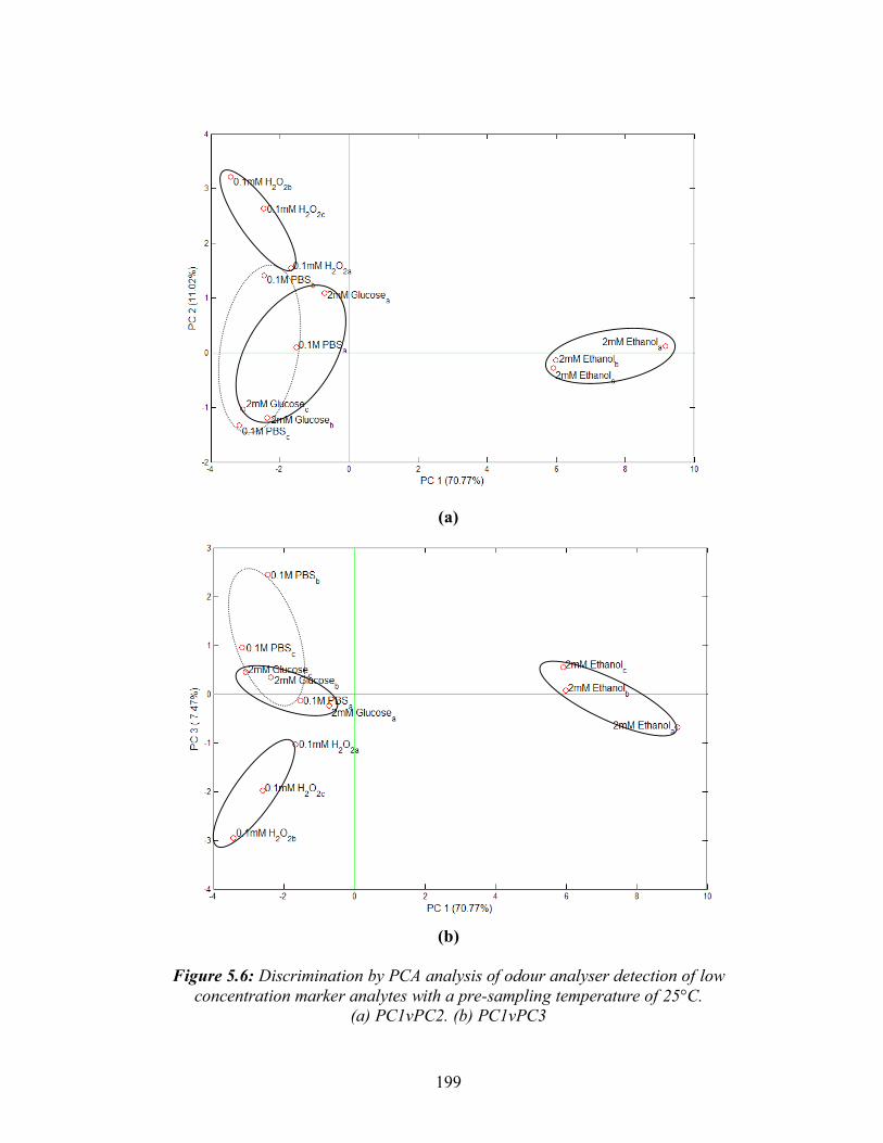
199

(a)

(b)

Figure 5.6: Discrimination by PCA analysis of odour analyser detection of low

concentration marker analytes with a pre-sampling temperature of 25°C. (a) PC1vPC2. (b) PC1vPC3

200

(a)

(b)

Figure 5.7: Discrimination by PCA analysis of odour analyser detection of higher


201

(a)

(b)

Figure 5.8: Discrimination by PCA analysis of odour analyser detection of low


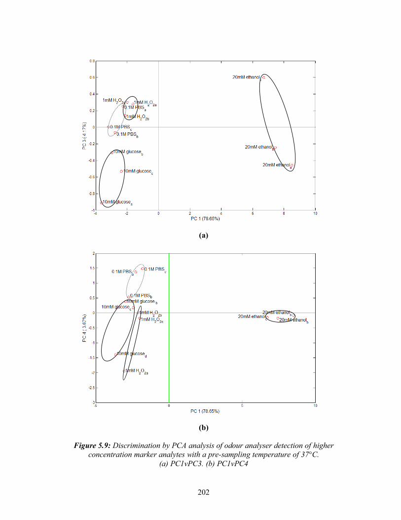
202

(a)

(b)

Figure 5.9: Discrimination by PCA analysis of odour analyser detection of higher


203

5.3.3 Detection of ethanol in serum

Since the main metabolite produced and detected by the bacteria being used in this thesis

was ethanol, as confirmed by headspace GC-MS in Section 2.3.3, the ability of the odour

analyser to detect different concentrations of ethanol was investigated. Ethanol solutions of

1, 5, 10 and 20 mM were prepared in serum, as a model for wound fluid (see Section 1.6).

Random tests for each of these concentrations were performed in triplicate.

Figure 5.10 (a) shows the direct deviation in baseline resistance produced by the odour

analyser. The triplicate mean maximum value from these deviations was used to produce

Figure 5.10 (b) which illustrates a linear relationship between ethanol concentration and

maximum deviation in baseline resistance. Therefore, the device is suited to the

determination of ethanol, and potentially to other similar metabolic markers in wound fluid.

Since the odour analyser would not be used to detect each of the marker components

separately in this application, the work that follows has focused on the detection and

discrimination of five bacteria commonly isolated from wounds.

204

-5

20

45

70

95

120

145

170

195

220

0 100 200 300 400 500 600 700 800Time (s)

Dev

iatio

n fr

om b

asel

ine

resi

stan

ce (%

)

serum (blank) 1mM 5mM 10mM 20mM

(a)

y = 10.489xR2 = 0.9945

0

50

100

150

200

250

0 5 10 15 20Ethanol concentration in serum (mM)

Mea

n m

ax. d

evia

tion

in b

asel

ine

resi

stan

ce (%

)

Mean max. deviationLinear (Mean max. deviation)

(b)

Figure 5.10: Odour analyser detection of 0 to 20 mM ethanol in serum. (a)

Deviation in baseline resistance with time, (b) Linear relationship between ethanol concentration and mean maximum deviation in baseline resistance.

205

5.3.4 Detection of Staphylococcus aureus at different stages of growth

In order to ascertain whether the odour analyser was able to detect differences in growth

phases of bacteria, a small proof of concept study was carried out. Staphylococcus aureus

was grown in TSB at 37 °C, and headspace analysis carried out at the start (inoculation),

lag, exponential and stationary phases of growth, determined by optical density readings

and referral to bacterial growth figures in Section 2.3.1. The use of growth curves is

illustrated in Figure 5.11, where the arrows indicate the times of odour analysis of S.aureus

for this study.

0

0.5

1

1.5

2

2.5

0 1 2 3 4 5 6 7 8 9 10 11 12 13Time (hours)

Abs

orba

nce

(600

nm

)

S.aureus growth curve

LAG

EXPONENTIAL

STATIONARY

Figure 5.11: Illustration of the use of S.aureus growth curve to determine growth phase. Arrows indicate time of odour analysis for this study.

Figure 5.12 shows the deviations in baseline resistance that occurred at each of these

stages. As expected, the deviation increased with the length of time the bacteria had been

206

growing, most probably due to the accumulation of volatile metabolic products such as

those listed in Table 1.4, with accumulation in cell mass. Volatile metabolic profiles may

also change with growth phase, with the production of volatile secondary metabolites as the

cultures mature in the stationary phase. This is also true of spoilage bacteria isolated from

milk (Haugen, Rudi, Langsrud, et al, 2006), and in cheese maturation (Marilley & Casey,

2004). Since the odour analyser was capable of detecting differences in concentration of

bacteria, further studies on the detection of wound bacteria were carried out.

0

10

20

30

40

50

60

70

0 50 100 150 200 250 300Time (s)

Dev

iatio

n fr

om b

asel

ine

resis

tanc

e (%

)

0 hrs1 hr (lag)5 hrs (exponential)12 hrs (stationary)

Figure 5.12: Deviation in baseline resistance with time for odour analyser detection of

S.aureus from 0 to 12 hrs growth at 37 °C in TSB. 5.3.5 Detection of five species of bacteria grown in broth and discrimination using PCA analysis

In this study five of the most commonly isolated wound bacteria were grown and subject to

headspace analysis using the odour analyser. The bacteria were grown up in YPD broth, a

207

more basic broth, in order to more closely represent the nutrients found in wound fluid.

Each type of bacteria was analysed in replicates of four randomly. The bacterial broths

headspace was analysed after 6 hours (exponential phase) and 24 hours (stationary phase).

The data recorded was again analysed by PCA as before. The abbreviations used in the

PCA plots that follow are tabulated below. Blank refers to growth media alone which was

also tested.

Table 5.3: Bacteria abbreviations used in PCA plots

Bacteria name Abbreviation used in graphs Staphylococcus aureus SA Streptococcus pyogenes SP Escherichia coli EC Klebsiella pneumoniae KP Pseudomonus aeruginosa PA

Depending on the study, different principle components provided better discrimination

between samples. The results of the best combinations of principle components for 6 hours

growth are illustrated in Figure 5.13 (a) and (b) and in Figure 5.14 (a) and (b) for 24 hours.

PCA analysis provided good discrimination after both 6 hour and 24 hour incubation,

although the virtual separation between each bacterial set appeared more distinct after 24

hours, where tighter clustering is evident. At both analysis times there was clear distinction

between all cultures and the blank samples. It therefore seems reasonable to conclude that

under this set of conditions, the odour analyser is capable of discriminating between these

five bacteria commonly isolated from wounds.

208

(a)

(b)

Figure 5.13: Discrimination by PCA analysis of odour analyser detection of Pseudomonus aeruginosa, Streptococcus pyogenes, Escherichia coli, Staphylococcus aureus and

Klebsiella pneumoniae, after 6 hrs growth in YPD broth (a) PC1vPC2. (b) PC1vPC3.

209

(a)

(b)

Figure 5.14: Discrimination by PCA analysis of odour analyser detection of Pseudomonus

aeruginosa, Streptococcus pyogenes, Escherichia coli, Staphylococcus aureus and Klebsiella pneumoniae, after 24 hrs growth in YPD broth (a)PC1vPC2, (b) PC1vPC3.

210

5.3.6 Detection of five species of bacteria grown in serum and discrimination using

PCA analysis

Following the positive findings of the detection of bacteria in broth, the tests performed in

the following study aimed to more accurately represent wound fluid samples, and hence

more accurately reflect the real-world situation. As previously stated, serum was used as

the model for wound fluid in this thesis. It was found however that only S.aureus would

grow in serum alone. It was established that by supplementing the serum with DMEM,

which is itself a minimal medium, all five bacteria would grow. After looking at different

ratios of serum:DMEM, it was found that 10% v/v DMEM in serum was a sufficient

supplement, without considerably altering the wound fluid model. Therefore the bacteria

were grown in a 90:10 v/v serum:DMEM mix.

Instead of keeping growth time constant, in this study CFU/ml was kept constant.

Therefore, differences detected by the odour analyser combined with PCA analysis were

based on differences in headspace content, and hence the volatile metabolic signatures of

each bacteria, and not numbers of bacteria (since the bacteria grow at different rates).

However, it should be noted that in a real situation, cell densities would vary depending

on the levels of growth, which itself may depend on the type of wound, and if more than

one bacterial species was present, it is likely that one species would be more prevalent than

another. For this study, bacteria were grown in replicates of five, and their headspace

sampled at 1.5x108 CFU/ml. Cell densities were determined by checking optical density

regularly and referral to the bacterial growth figures shown in Section 2.3.1.

211

Figure 5.15 demonstrates that virtual separation of the five bacteria and serum is possible

using the odour analyser. All bacterial clusters are well discriminated from the serum

cluster. E.coli has clustered around the centre of the plot, therefore having values closer to

0 for PC1 and PC3. S.aureus and K.pneumoniae are located relatively closely, and are both

tightly clustered.

Figure 5.15: Discrimination by PCA analysis of odour analyser detection of 1.5x108 CFU/ml Pseudomonus aeruginosa, Streptococcus pyogenes, Escherichia coli, Staphylococcus aureus and Klebsiella pneumoniae grown in 90:10 v/v serum: DMEM.

The average maximum deviations in baseline resistance with corresponding standard

deviations for each bacterial population grown in the serum culture, and the culture blank

are shown in Table 5.4. S.aureus produced the greatest change in resistance, followed by

S.pyogenes, K.pneumoniae, P.aeruginosa, and E.coli.

212

Table 5.4: Maximum deviations in baseline resistance of odour analysis of 1.5x108 CFU/ml

bacteria grown in 90:10 v/v serum:DMEM

Bacteria Mean max. deviation (%) Std dev. S.aureus 13.123 0.502 S.pyogenes 11.757 0.354 K.pneumoniae 10.853 1.628 P.aeruginosa 8.007 1.147 E.coli 5.539 0.777 Serum (blank) 4.303 0.274

Although a quantitative comparison cannot be made, this order correlates with that detected

by headspace GC-MS analysis under the same conditions (Section 2.3.3). During GC-MS

analysis, the ethanol peak produced for each bacteria could be quantified using the standard

curve produced. However, since only an ethanol peak was detected this was not sufficient

to discriminate between bacteria. With the odour analyser, it is not possible to quantify the

amount of ethanol in the headspace of the bacterial sample because of the broad specificity

of the sensor used (essential for the single sensor olfactory device to function). The sensor

responds to many more metabolites in the headspace than ethanol, and with the aid of PCA

has demonstrated an ability to discriminate between those bacteria most commonly found

to infect wounds.

5.3.7 Examination of paired bacterial cultures grown in serum

Having established that the odour analyser could discriminate between the five selected

bacteria at a fixed cell density, the study was further advanced by examining paired

samples of bacteria, since there is usually more than one main bacterial culture present in a

typical wound fluid. Therefore each possible paired combination of the five bacteria were

213

grown separately to a cell density of 1.5x108 CFU/ml, combined, and tested according to

the methods outlined in the preceding Sections. Again, it should be noted that in a real

situation, it is unlikely that different bacteria would be present at the same cell densities,

and that this is an artificial population mix. It is evident from Figure 5.16 that some

overlapping is evident following PCA analysis. Serum was clearly discriminated from the

bacterial preparations, although with a relatively broad clustering.

KPEC: K.pneumoniae + E.coli ECPA: E.coli + P.aeruginosa KPPA: K.pneumoniae + P.aeruginosa SAKP: S.aureus + K.pneumoniae SAPA: S.aureus + P.aeruginosa SPPA: S.pyogenes + P.aeruginosa SPKP: S.pyogenes + K.pneumoniae SPEC: S.pyogenes + E.coli SAEC: S.aureus + E.coli SASP: S.aureus + S.pyogenes

Figure 5.16: Discrimination by PCA analysis (PC1vPC3) of odour analyser detection of pairs of bacteria at 2x108 CFU/ml grown in 90:10 v/v serum:DMEM at 37 °C

214

Where significant overlapping was evident, it was usual for one of the bacterial species to

be present in both overlapping pairs, for example in the overlapping of SPPA (S.pyogenes

and P.aeruginosa) and SPEC (S.pyogenes and E.Coli), where S.pyogenes is common to

both, and therefore similarities in volatile metabolic signatures may be produced. Clearly,

discrimination of the paired bacteria has not been as successful as for individual bacteria,

but nevertheless, some bacterial combinations can be clearly differentiated, such as the

SASP and SPEC combinations suggesting that the approach can provide some useful

diagnostic information. If we compare Figure 5.16 of mixed bacteria and Figure 5.15 of

single bacteria (both compare PC1 and PC3), some similarities of cluster location are

evident. SA and SP clusters are located in the bottom right corner of the plot in Figures

5.15 and 5.16, and both SA and SP are prevalent in pairs in the bottom right quadrant.

Similarly, EC is located centrally in Figure 5.15, and finds itself located centrally in two of

its four pair combinations in Figure 5.16.

5.3.8 Detection of different cell concentrations of S.aureus grown in serum

The aim of the final study was to investigate whether the odour analyser was able to detect

differences in S.aureus cell density when grown in serum (un-supplemented), at a range of

bacterial cell densities as present in the wound environment. S.aureus was grown up in

serum alone under normal growth conditions. Three cell densities: 5x106, 8x107, and

2.25x108 CFU/ml were randomly tested in replicates of five with the odour analyser. Figure

5.17 of PC1v3 illustrates that a distinction between clusters based on cell density is evident.

215

It appears that the odour analyser is able to detect cell densities at least as low as

5x106 CFU/ml which is the level at which bacterial colonisation becomes problematic in

bacterial infection of wounds (Smith & Thomson, 1994). It may be that the odour analyser

is able to detect below this level, but lower levels were not tested. This level of bacteria is

not visible to the eye when growing bacteria in a broth or serum, and cannot be detected by

conventional methods such as spectroscopy where the optical density is measured, or by

GC-MS.

Figure 5.17: Discrimination by PCA analysis (PC1vPC3) of odour analyser detection of three cell densities of S.aureus grown in serum at 37 °C.

Some work has been carried out investigating the possibilities of using an electronic nose

device in a hospital environment as a diagnostic tool (Gardner, Dutta, Morgan et al, 2005),

216

no public-access literature has been identified in which an odour analysis study has been

successful in determining the differences in numbers of S.aureus (or other bacteria) with

which to compare these results. However, Haugen, Rudi, Langsrud, et al (2006) have

reported using a gas sensor array to detect milk spoilage bacteria down to 104 CFU/ml after

7 hours of growth.

5.4 Overall Chapter conclusions The single sensor odour analyser combined with the discriminatory powers of PCA

analysis was found to be capable of detecting and discriminating between three marker

analytes, and five wound bacteria. It was able to detect differences in ethanol concentration

in serum. Discrimination between individual bacteria was illustrated, and partial

discrimination of paired bacteria was possible. It was also found that S.aureus could be

detected down to a cell density of 5x106 CFU/ml. Although there is much interest in the

areas of combating hospital acquired infections, early detection, and electronic nose

technology, literature searches have not revealed any other investigations of the use odour

analysis to detect and discriminate these five bacteria, or differences in numbers of

bacteria, in a wound environment. The results from these studies are very encouraging.

Further research and development into this single sensor based system may potentially lead

to a near patient monitoring system whereby a wound could be monitored and provide

regular feedback and early warning of infection or other causes of non-healing. The system

may also potentially be used for monitoring a variety of other infections and diseases, by

detecting the odours from bodily fluids, such as urine or sputum.

217

6. General Discussion 6.1 Conclusions

Three possible wound monitoring concepts, with the potential to be integrated into wound

dressings, or for near patient monitoring applications, have been investigated. The overall

conclusions in the context of the initial objectives (Section 1.6) are discussed below:

1) From reviewing the literature, serum was identifed as a suitable model for wound

fluid in which to investigate the three concepts. Serum samples were obtained

from human volunteer whole blood samples which were spun down and the serum

fraction obtained.

2) Three biomarkers indicative of healing/non-healing were identified though

literature searches. These were: glucose reported to increase from the non-

healing to healing phase of a wound; H2O2 increased generation in surgical

wounds as a result of phagocytosis by mammalian polymorphonuclear leukocytes

and monocytes reported; ethanol - since it is produced metabolically by certain

pathogenic bacteria commonly isolated from wounds.

3) From literature searches, S.aureus, K.pneumoniae, E.coli, P.aeruginosa, and

S.pyogenes, were determined to be five key bacteria commonly isolated from

wound infections (Table 1.4). Laboratory strains were obtained, and growth

characteristics determined in each of the different growth media examined.

4) Dual Pulse Staircase Voltammetry (DPSV) was investigated for its feasability as a

technique for the monitoring of wounds, by detecting the biomarkers glucose,

218

ethanol and H2O2 in PBS. Scans of the individual analytes demonstrated

distinctive peaks exhibiting, non-linear relationships with concentration.

Limitations were discovered regarding repeatability and inter-analyte interference

in mixtures of the three biomarkers, due to similar peak potentials. This study

represents the first detailed study on the performsance of DPSV for determination

of metabolites in biological fluids. Although a great deal of useful information was

generated using this technique, it was decided not to progress this work further

due to the complexity of the voltammograms obtained and issues regarding

deconvolution of voltammograms obtained from analyte mixtures.

5) A biosensor array was constructed from three biosensors each consisting of a screen

printed three electrode assembly of carbon (w.e), carbon (c.e.) and Ag/AgCl (ref) as

the basal layer. The glucose biosensor also incorporated rhodinised carbon within

the working electrode to allow reduction in the operating potential required to

oxidise the enzymatic hydrogen peroxide by-product to +300 mV (vs Ag/AgCl).

The optimal sensor performance was obtained using 1U of glucose oxidase per

biosensor. The limit of detection was found to be 169.5 µM glucose (99.7%

confidence) in surrogate wound fluid with a single dilution step.

The hydrogen peroxide biosensor utilised 25U/sensor of horseradish peroxidase

with 12.5 mg/ml dimethylferrocene mediator, a cellulose acetate diffusion layer,

and operated at a potential of -300 mV relative to the reference electrode. The limit

219

of detection in surrogate wound fluid with a single dilution step was found to be

8.43 µM (99.7% confidence).

The ethanol biosensor was constructed with the same components as the hydrogen

peroxide biosensor, except that it also used 1U/biosensor of alcohol oxidase, giving

a mediated bi-enzyme system. Following optimisation of the deposition procedure,

the limit of detection in surrogate wound fluid with a single dilution step was

determined to be 7.94 µM (99.7% confidence). Direct detection of ethanol from

metabolically active S.aureus in surrogate wound fluid, (with a single dilution step)

yielded a limit of detection of 1.23 x 108 CFU/ml at 99.7% confidence, and 19 µM

in terms of ethanol specific response.

All three biosensors were successful, and subject to further study, could be

suitable for the monitoring of a wound, either alone or within a suite of diagnostic

tests. Although the alcohol biosensor could only detect S.aureus down to

1.23 x 108 CFU/ml, it could still provide useful diagnostic information. It could

signal bacterial numbers falling below this level, possibly indicative of healing, or

rising above a safe level (i.e. >106 CFU/ml), which would only take a matter of

hours, and would in all likelihood still signal a non-healing wound to a busy

physician more rapidly than would otherwise be observed.

6) Investigation of the single sensor odour analyser as a near patient wound

monitoring system found it to be capable of detecting and discriminating between

220

three biomarkers, glucose, ethanol and H2O2, and detecting differences in ethanol

concentration in surrogate wound fluid, when combined with principle

components analysis. Discrimination between individual bacteria and partial

discrimination of paired bacteria was illustrated, in broth and surrogate wound

fluid. It was also found that S.aureus could be detected down to a cell density of

5x106 CFU/ml in surrogate wound fluid, lower than that found for the biosensor

concept.

The odour analyser concept was particularly successful, and has the potential to

be used as a near patient monitoring system for patients with wounds, and

perhaps other infections or diseases by sniffing samples such as urine, sputum or

other excreted or exhaled body fluid.

7) Headspace GC-MS was used to detect volatiles in the headspace of five bacterial

preparations grown in surrogate wound fluid. A slightly higher concentration of

ethanol was detected in S.aureus and S.pyogenes than K.pneumoniae, E.Coli and

P.aeruginosa. Levels detected were at a concentration suitable for measurement

by other means, such as sensor technology or odour analysis. This data was

verified further using Alcohol Draeger tubes to detect alcohol in the headspace of

bacteria grown in surrogate wound fluid.

8) Hydrogen peroxide and glucose test kits were used successfully to validate the

biosensor data.

221

6.2 Suggestions for Future Work

Literature searches have revealed much interest in the area of hospital acquired infections,

most notably: in the prevention of infection after an operation; reducing further antibiotic

resistance of bacteria; exploring alternative treatments; the development of technologies to

monitor the progress of wound healing, in particular using electronic nose technology.

The results from the odour analyser work in Chapter 5 are very encouraging. Further

research and development into this single sensor based odour analyser system may

potentially lead to a near patient monitoring system for bacterial infection of wounds.

Suggestions for further work with the single sensor odour analyser follow:

1) Test system with clinical samples of wound fluid.

2) Investigate detection limits for the four other bacteria used in Chapter 5 (i.e.

E.coli, S.pyogenes, K.pneumoniae, P.aeruginosa) in supplemented surrogate

wound fluid (to enable bacterial growth).

3) Investigate ways of improving limit of detection, such as the use of different growth

media to increase production of volatile metabolic products.

4) Investigate discrimination and detection limits of other commonly isolated wound

bacteria, such as Enterobacter, Serratia, Enterococcus, Proteus individually and in

combinations.

5) Investigate whether the system can discriminate between different strains of

S.aureus, such as methicillin resistant S.aureus, coagulase negative S.aureus, and

methicillin susceptible S.aureus.

222

6) Investigate suitable supervised learning pattern recognition techniques, and train

and calibrate the system so that it can classify unknown odours as known ones

that have been learnt.

7) The system could be investigated for its use in the diagnosis of urinary tract

infections, by examining its ability to discriminate the bacteria commonly isolated

from UTI infections: E.coli and P.mirabilus.

8) The system could also be investigated for its potential as a diagnostic tool for

diabetes, by sniffing breath odour.

Though DPSV was concluded to be an unsuitable electrochemical technique for monitoring

wounds, the following suggestions are made:

1) Integration of a suitable membrane such as Nafion may improve repeatability, and

reduce interference effects.

2) Investigation of less complex mixtures.

The biosensor array holds potential either alone, or as part of a suite of tests, to monitor the

levels of three biomarkers present in the wound environment. The work in this thesis could

be continued as follows:

1) Investigate ways to improve the bacterial limit of detection, e.g. by using other

size exclusion techniques not studied in this thesis.

2) Investigate whether other possible biomarkers could be measured using biosensor

technology, e.g. C-reactive protein, lactate, albumin.

223

7. List of References

1) Abdel-Hamid I, Atanasov P, Ivnitski D, Wilkins E (1999), Review. Biosensors for detection of pathogenic bacteria., Biosensors and Bioelectronics 14: 599-624

2) Ablaza VJ, Fisher J. (2003) Wound care via telemedicine: the wave of the future. 1-6.

3) Aldringer S, Labows jr JN, Zechman JM (1986), Characterisation of pathogenic bacteria by automated headspace concentration-gas chromatography., journal of chromatography 377: 49-57

4) Alegret S, Albareda-Sirvent M, Merkoci A (2000), Configurations used in the design of screen-printed enzymatic biosensors. A review, Sensors and Actuators B 69: 153-163

5) Bachinger T, Riese U, Eriksson R, Mandenius CF (2000), Monitoring cellular state transitions in a production-scale CHO-cell process using an electronic nose, Journal of Biotechnology 76: 61-71

6) Bamberg R, Sullivan K, Conner-Kerr T (2002), Diagnosis of wound infections:Current culturing practices of US wound care professionals, Wounds 14: 314-327

7) Barchiesi F, D'errico MM, Del Prete MS, Giacometti A, Petrelli E, Scalise G, Schimizzi AM (2000), Epidemiology and microbiology of surgical wound infections, Journal of Clinical Microbiology 38: 918-922

8) Bard AJ, Faulkner LR (2001), Electrochemical methods: Fundamentals and applications, John Wiley and Sons, Inc.,

9) Bartlett JG, Gorbach SL, Mayhew JW, Onderdonk AB, Thadepalli H (1976), Rapid diagnosis of anaerobic infections by direct gas liquid chromatography of clinical specimens, The Journal of Clinical investigation 57: 478-484

10) Bennett N, Burslem F, Gibson J, Macauley S, Murphy G, Schultz G, Stacey MC, Trengrove NJ (1999), Analysis of the acute and chronic wound environments: the role of proteases and their inhibitors, Wound Repair and Regeneration 7: 442-452

11) Bertotti M, Kosminsky L, Matos RC, Tabacniks MH (2003), Electrochemical codeposition of platinum and molybdenum oxides: Formation of composite films with distinct electrocatalytic activity for hydrogen peroxide, electroanalysis 15: 733-738

12) Bessant C. (1998) Virtual separation and simultaneous electrochemical measurement of aliphatic compounds. Ref Type: Thesis/Dissertation

13) Bessant C, Saini S (1999), Simultaneous determination of ethanol, fructose and glucose at an unmodified platinum electrode using artificial neural networks, Analytical Chemistry 71: 2806-2813

14) Biomerieux. (2002) API, bacterial identification. www.biomerieux.com

224

15) Blasco R, Murphy MJ, Sanders MF, Squirrell DJ (1998), Specific assays for bacteria using phage mediated release of adenylate kinase., Journal of Applied Microbiology 84: 661-666

16) Blixt Y, Borch E (1999), Using an electronic nose for determining the spoilage of vacuum-packaged beef, International Journal of Food Microbiology 46: 123-134

17) Bott AW (1998), Electrochemical methods for the determination of glucose, Current Separations 17: 25-31

18) Burton RW, Hohn DC, Hunt TK, Ponce B (1977), Antimicrobial systems of the surgical wound, The American Journal of Surgery 133: 597-600

19) Cai Y, Liu J, Shi Y, Liang L, Mou S (2005), Determination of several sugars in serum by high-performance anion-exchange chromatography with pulsed amperometric detection, Journal of chromatography A 1085: 98-103

20) Carelli D, Centonze D, De Giglio A, Quinto M, Zambonin PG (2006), An interference-free first generation alcohol biosensor based on a gold electrode modified by an overoxidised non-conducting polypyrrole film, Analytica Chimica Acta 565: 27-35

21) Carlsson J (1972), Simplified gas chromatographic procedure for identification of bacterial metabolic products, Applied Microbiology 25: 287-289

22) Cartier LJ, Leclerc P, Pouliot M, Nadeau L, Turcotte G, Fruteau-de-Laclos B (1998), Toxic Levels of Acetaminophen Produce a Major Positive Interference on Glucometer Elite and Accu-chek Advantage Glucose Meters, Clinical chemistry 44: 893-894

23) Centonze D, Guerrieri A, Malitesta C, Palmisano F, Zambonin PG (1992), Interference-free glucose sensor based on glucose-oxidase immobilized in an overoxidized non-conducting polypyrrole film, Analytical and Bioanalytical Chemistry 342: 729-733

24) Cheng J, Jandik P, Avdalovic N (2003), Use of disposable gold working electrodes for cation chromatography-integrated pulsed amperometric detection of sulfur containing amino acids, Journal of chromatography A 1:

25) Christenson A, Dock E, Gorton L, Ruzgas T (2004), Direct heterogeneous electron transfer of theophylline oxidase, Biosensors and Bioelectronics 20: 176-183

26) Ciosek P, Wroblewski W (2006), The analysis of sensor array data with various pattern recognition techniques, Sensors and Actuators B: Chemical 114: 85-93

27) Clement MV, Halliwell B, Long LH (2000), Hydrogen peroxide in the body, FEBS Letters 486: 10-13

28) Clough G, Noble M (2003), Microdialysis - A model for studying chronic wounds, Lower Extremity Wounds 2: 233-239

29) Cohen IK, McCoy BJ (1983), Wound Healing, in Biochemistry and Physiology of the Skin, ed. Goldsmith LA, Oxford University Press,

225

30) Coloe PJ (1978), Head-space gas liquid chromatography for rapid detection of Escherichia coli and Proteus mirabilis., Journal of Clinical Pathology 31: 365-369

31) Cullen DC, Jawaheer S, Rughooputh SDDV, White SF (2003), Development of a common biosensor format for an enzyme based biosensor array to monitor fruit quality, Biosensors and Bioelectronics 18: 1429-1437

32) Cutting K (1994), Detecting infection, Nursing Times 90: 60-62

33) Cuzzell J, Krasner D (1995), Wound dressings, in Clinical wound Management, ed. Clarke DL, Drummond AE, and Dyer JJ, Slack Inc., p 131-144

34) D'Amico A, Di Natale C (2001), A contribution on some basic definitions of sensors properties, IEEE Sensors Journal 1: 189

35) Deng L, Tan H, Xu Y, Nie L, Yao S (1996) In-situ continuous detection of bacteria on the surface of solid medium with a bulk acoustic wave-impedance sensor. Enzyme Microbial Technology 21:258-264

36) Dermnet. Methicillin resistant staphylococcus aureus. Ref Type: Electronic Citation

37) Dickinson TA, White J, Kauer JS, Walt DR (1998), Current trends in 'artificial-nose' technology, Tibtech 16: 250-258

38) Dobberpuhl DA, Johnson DC (1995), Pulsed electrochemical detection at the ring of a ring-disk electode applied to a study of amine adsorption at gold electrodes, Analytical Chemistry 67: 1254-1258

39) Dorey E (2005), MRSA: deadly superbug, Chemistry and Industry 18 April: 12-13

40) Edwards JG, Hartman NF, Schneider BH (1997), Interferometer: versatile integrated optic sensor for label-free, real-time quantification of nucleic acids, proteins, and pathogens., Clinical chemistry 43: 1757-1763

41) Emr SA, Yacynych AM (2005), The use of polymer films in amperometric biosensors, electroanalysis 7: 913-923

42) Evans P, Persaud KC, Pisanelli AM (1996), Medical diagnostics and health monitoring., UMIST/Osmetech plc,

43) Feng G, Zhang X-E, Zhang Z-P, Zhang X-M (1998), Simultaneous determination of maltose and glucose using screen-printed electrode system, Biosensors and Bioelectronics 13: 333-339

44) Fisher B, Fram P, Thomas S, Waring M (1998), Odour absorbing dressings: A comparative study, World Wide Wounds

45) Fonseca LP, Azevedo AM, Prazeres MF, Cabral MS (2004), Ethanol biosensors based on alcohol oxidase, Biosens Bioelectron 21: 235-247

226

46) Freinkel RK (1983), Carbohydrate metabolism of epidermis, in Biochemicstry and physiology of the skin, ed. Goldsmith LA, Oxford University Press,

47) Fry DE (2003), Surgical Site Infection: Pathogenesis and Prevention, www.medscape.com

48) Fung YS, Mo SY (1995), Application of dual pulse staircase voltammetry for simultaneous determination of glucose and fructose, electroanalysis 7: 160-165

49) Fung YS, Mo SY (1996), Determination of ethanol in beer by flow injection dual-pulse staircase voltammetric detection, The Analyst 121: 369-372

50) Ganong WF (2003), Review of Medical Physiology, Lange Medical Books/McGraw-Hill,

51) Gardner JW. (1987) Pattern Recognition in the Warwick Electonic Nose. 8th International Congress of European Chemoreception Research Organisation. Ref Type: Conference Proceeding

52) Gardner JW, Bartlett PN (1994), A brief history of electronic noses, Sensors and Actuators B 18-19: 220

53) Gardner JW, Craven MA, Bartlett PN (1996), Electronic noses - development and future prospects, Trends in Analytical Chemistry 15: 486-493

54) Gardner JW, Bartlett PN (1999), Electronic Noses - Principles and Applications, Oxford University Press,

55) Gardner JW, Shin HW, Hines EL (2000), An electronic nose system to diagnose illness, Sensors and Actuators B 70: 19-24

56) Gardner JW, Dutta R, Morgan D, Baker N, Hines EL (2005), Identification of Staphylococcus aureus infections in hospital environment: electronic nose based approach, Sensors and Actuators B 109: 355-362

57) Garg S, Jovanovic L, Potts RO, Tamada JA, Tierney MJ (2000), Clinical evaluation of the GlucoWatch® biographer: a continual, non-invasive glucose monitor for patients with diabetes., Biosensors and Bioelectronics 16: 621-629

58) Garjonyte R, Malinauskas A (2000), Glucose biosensor based on glucose oxidase immobilized in electropolymerized polypyrrole and poly(o-phenylenediamine) films on a Prussian Blue-modified electrode, Sensors and Actuators B: Chemical 63: 122-128

59) Garrigues S, Talou T, Nesa D (2004), Comparative study between gas sensors arrays device, sensory evaluation and GC/MS analysis for QC in automotive industry, Sensors and Actuators B: Chemical 103: 55-68

60) Gibson TD, Prosser O, Hulbert JN (2000) Not to be sniffed at. Microbiology Today 27: 14-16

61) Gibson TD, Prosser O, Hulbert JN, Pavlou AK (2000) Electronic Noses: an inspired idea? Chemistry and Industry April 2000 (issue 8):287-289

227

62) Gibson TD, Prosser O, Hulbert JN, Marshall RW, Corcoran P, Lowery P, Ruck-Keene EA, Heron S (1997), Detection and simultaneous identification of microorganisms from headspace samples using an electronic nose, Sensors and Actuators B 44: 413-422

63) Gogia PP (1995), Physiology of wound healing, in Clinical wound management, ed. Drummond AE, Clarke DL, and Dyer JJ, Slack Inc., Thorofare, NJ, USA

64) Gorton L, Heller A, Vijayakumar AR, Csoregi E (1996), Alcohol biosensors based on coupled oxidase-peroxidase systems, Analytica Chimica Acta 327: 223-234

65) Gorton L, Mattos IL, Ruzgas T (2003), Sensor and biosensor based on prussian blue modified gold and platinum screen printed electrodes, Biosensors and Bioelectronics 18: 193-200

66) Gorton L, Karyakin A, Palleschi G, Ricci F, Ruzgas T, Yigsaw Y (2003), Investigation of the effect of different glassy carbon materials on the performance of prussian blue based sensors for hydrogen peroxide., electroanalysis 15: 175-182

67) Guyton AC, Hall JE (2000), Textbook of Medical Physiology, W.B.Saunders Company: A Harcourt Sciences Company, Philadelphia

68) Hamdi N, Wang J, Monbouquette HG (2005), Polymer films as permselective coatings for H2O2-sensing electrodes, Journal of Electroanalytical Chemistry 581: 258-264

69) Hampson JP (1996), The use of metronidazole in the treatment of malodorous wounds, Journal of wound Care 5: 421-425

70) Hansen T, Petersen MA, Byrne DV (2005), Sensory based quality control utilising an electronic nose and GC-MS analyses to predict end-product quality from raw materials, Meat Science 69: 621-634

71) Hart AL, Turner APF (1996), On the use of screen- and ink-jet printing to produce amperometric enzyme electrodes for lactate., Biosensors and Bioelectronics 11: 263-270

72) Haugen JE, Rudi K, Langsrud S, Bredholt S (2006), Application of gas-sensor array technology for detection and monitoring of growth of spoilage bacteria in milk: A model study, Analytica Chimica Acta 565: 10-16

73) Hayes DF, Rizvi N. (1999) A "breathalyser" for lung cancer ? The Lancet 353[5 June], 1897-1898.

74) Hayward NJ, Jeavons TH, Nicolson AJC, Thornton AG (1977), Development of specific tests for rapid detection of Eschericia coli and all species of Proteus in urine., Journal of Clinical Microbiology 6: 195-201

75) Hayward NJ (1983), Headspace gas-liquid chromatography for the rapid laboratory diagnosis of urinary tract infections caused by enterobacteria, journal of chromatography 274: 27-35

76) Heineman WR, Kissinger PT (1984), Laboratory techniques in electroanalytical chemistry, Marcel Dekker, New York

228

77) Holbrook KA (1983), Structure and function of the developing human skin, in Biochemistry and physiology of the skin, ed. Goldsmith LA, Oxford University Press,

78) Hughes S, Lawrence Meschi P, Johnson DC (1981), Amperometric detection of simple alcohols in aqueous solutions by application of a triple-pulse potential waveform at platinum electrodes, Analytica Chimica Acta 132: 1-10

79) Huycke MM, Sahm DF, Gilmore MS (1998), Multiple-drug resistant enterococci: the nature of the problem and an agenda for the future, Emerging infectious diseases 4: 239-249

80) Ikegami A, Kaneyasu M. (1985) Olfactory detection using integrated sensors. Proc.3rd Int.Conf.Solid-State Sensors and Actuators , 136-139. Ref Type: Conference Proceeding

81) Im MJC, Hoopes JE (1970), Energy metabolism in healing skin wounds, Journal of Surgical Research 10: 459-464

82) James TJ, Hughes MA, Cherry GW, Taylor RP (2000), Simple biochemical markers to assess chronic wounds, Wound Repair and Regeneration 8: 264-269

83) Johansson K, Jonsson-Pettersson G, Gorton L, Marko-Varga G, Csoregi E (1993), A reagentless amperometric biosensor for alcohol detection in column liquid chromatography based on co-immobilized peroxidase and alcohol oxidase in carbon paste, Journal of Biotechnology 31: 301-316

84) Johnson DC, LaCourse WR (1990), Liquid chromatography with pulsed amperometric detection at gold and platinum electrodes, Analytical Chemistry 62:

85) Johnson DC, LaCourse WR (1991), Optimisation of waveforms for pulsed amperometric detection (p.a.d.) of carbohydrates following separation by liquid chromatography, Carbohydrate Research 215: 159-178

86) Johnson DC, Dobberpuhl D, Roberts R, Vandeberg P (1993), Review: Pulsed amperometric detection of carbohydrates, amines and sulfur species in ion exchange chromatography-the current state of research, journal of chromatography 640: 79-96

87) Johnson DC, Dobberpuhl D, Roberts R, Vandeberg P (1993), Review: Pulsed amperometric detection of carbohydrates, amines and sulfur species in ion exchange chromatography-the current state of research, journal of chromatography 640: 79-96

88) Jones PW, Taylor DM, Williams DR (2000), Analysis and chemical speciation of copper and zinc in wound fluid, Journal of Inorganic Biochemistry 81: 1-10

89) Kolb B, Ettre LS (1997), Static headspace gas chromatography: theory and practice, Wiley-VCH, Inc., New York

90) Krasner D, Kane D (1997), Chronic wound care: a clinical source book for healthcare professionals, Health management publications, inc., Wayne, PA

229

91) Kroger S, Turner APF (1997), Solvent-resistant carbon electrodes screen printed onto plastic for use in biosensors, Analytica Chimica Acta 347: 9-18

92) Kroger S, Setford SJ, Turner APF (1998), Assessment of glucose oxidase behaviour in alcoholic solutions using disposable electrodes, Analytica Chimica Acta 368: 219-231

93) Kulys J, Schmid RD (1991), Bienzyme sensors based on chemically modified electrodes, Biosensors and Bioelectronics 6: 43-48

94) LaCourse WR, Johnson DC, Rey MA, Slingsby RW (1991), Pulsed amperometric detection of aliphatic alcohols in liquid chromatography, Analytical Chemistry 63: 134-139

95) LaCourse WR, Johnson DC (1993), Optimisation of waveforms for pulsed detection of carbohydrates based on pulsed voltammetry, Analytical Chemistry 65: 50-55

96) LaCourse WR, Dasenbrock CO (1999), Pulsed electrochemical detection of sulfur-containing antibiotics following high performance liquid chromatography, J Pharm Biomed Anal 19: 239-52

97) Lamagna A, Reich S, Rodriguez D, Scoccola NN (2004), Performance of an e-nose in hops classification, Sensors and Actuators B: Chemical 102: 278-283

98) Larsson L, Mardh P-A, Odham G (1981), Head-space gas chromatography as a tool in the identification of anaerobic bacteria and diagnosis of anaerobic infections, Scandinavian Journal of Infectious Diseases Suppl. 26: 14-18

99) Lee-Davey J. (2004) Application of machine olfaction principles for the detection of high voltage transformer oil degradation. Ref Type: Thesis/Dissertation

100) Lee J-W, Yeo I-H (2001), Integrated pulsed amperometry for the analysis of organic compounds, Microchemical Journal 70: 173-177

101) Lee W-Y, Kim T-H, Lee K-S, Park J-K, Shin M-C, Yee H-J (1999), Determination of breath alcohol using differential-type amperometric biosensor based on alcohol dehydrogenase, Analytica Chimica Acta 390: 91

102) Magan N, Pavlou AK, McNulty C, Jones JM, Sharp D, Brown J, Turner APF (2002), Use of an electronic nose system for diagnosis of urinary tract infections, Biosensors and Bioelectronics 17: 893-899

103) Marilley L, Casey MG (2004), Flavours of cheese products: metabolic pathways, analytical tools and identification of producing strains, International Journal of Food Microbiology 90: 139-159

104) Marti MP, Busto O, Guasch J, Boque R (2005), Electronic noses in the quality control of alcoholic beverages, TrAC Trends in Analytical Chemistry 24: 57-66

105) Massart DL, Wu W, Guo Q, Boucon C, de Jong S (2002), Feature selection in principle component analysis of analytical data, Chemometrics and Intelligent Laboratory Systems 61: 123-132

230

106) McGrath MJ, Iwuoha EI, Diamond D, Smyth MR (1995), The use of differential measurements with a glucose biosensor for interference compensation during glucose determinations by flow injection analysis, Biosensors and Bioelectronics 10: 937-943

107) Monk PS (2001), Fundamentals of electroanalytical chemistry, Wiley,

108) Moody A, Saini S, Setford S (2001), Peroxidase enzyme sensor for on-line monitoring of disinfection processes in the food industry., The Analyst 126: 1733-1739

109) Murray BE (1998), Diversity amoung multi-drug resistant enterococci, Emerging infectious diseases 4: 1-13

110) Nake A, Dubreuil B, Raynaud C, Talou T (2005), Outdoor in situ monitoring of volatile emissions from wastewater treatment plants with two portable technologies of electronic noses, Sensors and Actuators B: Chemical 106: 36-39

111) Nanney LB, Wenczak B (1993), Correlation of transforming growth factor-alpha and epidermal growth factor receptor with proliferating cell nuclear antigen in human burn wounds, Wound Repair and Regeneration 1: 219-230

112) Neuburger GG, Johnson DC (1987), Comparison of the pulsed amperometric detection of carbohydrates at gold and platinum electrodes for flow injection and liquid chromatographic systems, Anal Chem 59: 203-4

113) Neuburger GG, Johnson DC (1987), Pulsed coulometric detection of carbohydrates at a constant detection potential at gold electrodes in alkaline media, Analytica Chimica Acta 192: 205-213

114) Newman JD, White SF, Tothill IE, Turner APF (1995), Catalytic materials, membranes and fabrication technologies suitable for the construction of amperometric biosensors, Anal Chem 67: 4594-4599

115) Newman JD, Turner APF (2005), Home blood glucose biosensors: a commercial perspective, Biosens Bioelectron 20: 2435-2453

116) O'Halloran MP, Pravda M, Guilbault GG (2001), Prussian Blue bulk modified screen-printed electrodes for H2O2 detection and for biosensors, Talanta 55: 605-611

117) Odland GF (1983), Structure of the skin, in Biochemistry and physiology of the skin, ed. Goldsmith LA, Oxford University Press,

118) Olafsdottir G, Nesvadba P, Di Natale C, Careche M, Oehlenschlager J, Tryggvadottir SV, Schubring R, Kroeger M, Heia K, Esaiassen M (2004), Multisensor for fish quality determination, Trends in Food Science & Technology 15: 86-93

119) Onkal-Engin G, Demir I, Engin SN (2005), Determination of the relationship between sewage odour and BOD by neural networks, Environmental Modelling & Software 20: 843-850

120) Owens GS, LaCourse WR (1997), Pulsed electrochemical detection of thiols and disulfides following capillary electrophoresis, J Chromatogr B Biomed Sci Appl 695: 15-25

231

121) Palmisano F, Centonze D, Guerrieri A, Zambonin PG (1993), An interference-free biosensor based on glucose oxidase electrochemically immobilized in a non-conducting poly(pyrrole) film for continuous subcutaneous monitoring of glucose through microdialysis sampling, Biosensors and Bioelectronics 8: 393-399

122) Panchagnula R, Pillai O, Nair VB, Ramarao P (2000), Transdermal iontophoresis revisited, Current Opinion in Chemical Biology 4: 468-473

123) Parks WC (1999), Matrix metalloproteinases in repair, Wound Repair and Regeneration 7: 423-432

124) Patel NG, Meier S, Cammann K, Chemnitius G-C (2001), Screen-printed biosensors using different alcohol oxidases, Sensors and Actuators B: Chemical 75: 101-110

125) Patlak J. (1999) Fluid compartments in the body. 1999. http://physioweb.med.uvm.edu/bodyfluids/ionic.htm

126) Paulsson N, Larsson E, Winquist F (2000), Extraction and selection of parameters for evaluation of breath alcohol measurement with an electronic nose, Sensors and Actuators 84: 187-197

127) Pearson H. (2002) Bacteria defy last-resort antibiotic. http://www.nature.com/nsu/020722/020722-11.html

128) Penza M, Cassano G, Tortorella F, Zaccaria G (2001), Classification of food, beverages and perfumes by WO3 thin-film sensors array and pattern recognition techniques, Sensors and Actuators B: Chemical 73: 76-87

129) Persaud K, Dodd GH (1982), Analysis of discrimination mechanisms of the mammalian olfactory system using a model nose, Nature 299: 352-355

130) Plotkin MJ, Shnayerson M. (2002) The Killer Bug. Fortune [30 Sept], 47-51.

131) Plowman R, Graves N, Griffin M (2000). The socio-economic burden of hospital acquired infection. London: Public Health Laboratory Service.

132) Prusak-Sochaczewski E, Luong JHT, Guilbault GG (1990). Development of a piezoelectric immunosensor for the detection of Salmonella typhimurium. Enzyme Microbiol. Technol. 12:173-177

133) Ragazzo-Sanchez JA, Chalier P, Chevalier D, Ghommidh C (2006), Electronic nose discrimination of aroma compounds in alcoholised solutions, Sensors and Actuators B: Chemical 114: 665-673

134) Ricci F, Palleschi G (2005), Sensor and biosensor preparation, optimisation and applications of Prussian Blue modified electrodes, Biosensors and Bioelectronics 21: 389-407

135) Saxena V, Malhotra BD (2003) Electrochemical Biosensors In: Advances in Biosensors 5:63-100. Elsevier Science

232

136) Schaller E, Bosset JO, Escher F (1998), ‘Electronic Noses’ and Their Application to Food, Lebensmittel-Wissenschaft und-Technologie 31: 305-316

137) Skoog D, West D, Holler F, Crouch S (2000), Analytical Chemistry: An introduction, Saunders College Publishing, Orlando

138) Slack R, Greenwood D (1992), Medical Microbiology, Churchill-Livingston,

139) Smith DJ, Thomson PD (1994), What is infection?, The American Journal of Surgery 167: 7S-11S

140) Sprules SD, Hartley IC, Wedge R, Hart JP, Pittson R (1996), A disposable reagentless screen-printed amperometric biosensor for the measurement of alcohol in beverages, Analytical Chimica Acta 329: 215-221

141) Surgical-tutor.org. Wound infection. 2002.

142) Tarnowski D, Korneniewski C (1996), Amperometric detection with membrane-based sampling for percent level determinations of ethanol, Analytica Chimica Acta 332: 111-121

143) Tarnowski DJ, Korzeniewski C (1996), Amperometric detection with membrane-based sampling for percent-level determinations of ethanol, Analytica Chimica Acta 332: 111-121

144) Tian Y, Mao L, Okajima T, Ohsaka T (2005), A carbon fiber microelectrode-based third-generation biosensor for superoxide anion, Biosensors and Bioelectronics 21: 557-564

145) Trengrove NJ, Langton SR, Stacey MC (1996), Biochemical analysis of wound fluid from non-healing and healing chronic leg ulcers, Wound Repair and Regeneration 4: 234-239

146) Turner APF, White SF, Schmid RD, Bilitewski U, Bradley J (1994), Investigations of platinized and rhodinised carbon electrodes for use in glucose sensors, electroanalysis 6: 625-632

147) Turner APF. (2005) Biosensors and Bioelectronics homepage. http://www.elsevier.com/wps/find/journaldescription.cws_home/405913/description#description.

148) Varma S, Shantilatha P, Mitra CK (2003), Advances in biosensors: perspectives in biosensors, JAI Press Inc, Conneticut p 1-36

149) Vonck J, van Bruggen EJ (1990), Electron microscopy and image analysis of two-dimensional crystals and single molecules of alcohol oxidase from Hansenula polymorpha, Biochimica et Biophysica Acta (BBA) - Protein Structure and Molecular Enzymology 1038: 74-79

150) Wang J, Wu H (1995), Highly selective biosensing of glucose utilizing a glucose oxidase + rhodium + Nafion(R) biocatalytic-electrocatalytic-permselective surface microstructure, Journal of Electroanalytical Chemistry 395: 287-291

233

151) Wang L, Wang E (2004), A novel hydrogen peroxide sensor based on horseradish peroxidase immobilised on colloidal Au modified ITO electrode, Electrochemistry Communications 6: 225-229

152) Ward WK, Jansen LB, Anderson E, Reach G, Klein JC, Wilson GS (2002), A new amperometric glucose microsensor: in vitro and short-term in vivo evaluation, Biosensors and Bioelectronics 17: 181-189

153) White SF, Turner APF, Bilitewski U, Schmid RD, Bradley J (1994), Lactate, glutamate and glutamine biosensors based on rhodinised carbon electrodes, Analytica Chimica Acta 295: 243-251

154) Wilkins WF, Hatman AD (1964), An electronic analog for the olfactory processes, Ann.NY Acad.Science 116: 608

155) Wold S, Esbensen K, Geladi P (1987), Principle components analysis, Chemometrics and Intelligent Laboratory Systems 2: 52

156) Xu S, Han X (2004), A novel method to construct a third-generation biosensor: self-assembling gold nanoparticles on thiol-functionalized poly(styrene-co-acrylic acid) nanospheres, Biosensors and Bioelectronics 19: 1117-1120

157) Yang YM, Yang PY, Wang XR (2000), Electronic nose based on SAWS array and its odor identification capability, Sensors and Actuators B: Chemical 66: 167-170

Helen Trill Diagnostic Technologies for Wound Monitoring

Documents

Transcript of Helen Trill Diagnostic Technologies for Wound Monitoring