Applied Mathematical Modelling 33 (2009) 3430–3441

Contents lists available at ScienceDirect

Applied Mathematical Modelling

journal homepage: www.elsevier .com/locate /apm

Heat transfer in a liquid film over an unsteady stretching surfacewith viscous dissipation in presence of external magnetic field

M. Subhas Abel *, N. Mahesha, Jagadish TawadeDepartment of Mathematics, Gulbarga University, Gulbarga, 585 106 Karnataka, India

a r t i c l e i n f o

Article history:Received 29 May 2008Received in revised form 31 October 2008Accepted 10 November 2008Available online 7 December 2008

Keywords:Liquid filmUnsteady stretching surfaceSimilarity transformationViscous dissipationPrandtl numberMagnetic parameter

0307-904X/$ - see front matter � 2008 Elsevier Incdoi:10.1016/j.apm.2008.11.021

* Corresponding author. Tel.: +91 9886467609.E-mail address: msabel2001@yahoo.co.uk (M.S.

a b s t r a c t

This paper presents a mathematical analysis of MHD flow and heat transfer to a laminarliquid film from a horizontal stretching surface. The flow of a thin fluid film and subsequentheat transfer from the stretching surface is investigated with the aid of similarity transfor-mation. The transformation enables to reduce the unsteady boundary layer equations to asystem of non-linear ordinary differential equations. Numerical solution of resulting non-linear differential equations is found by using efficient shooting technique. Boundary layerthickness is explored numerically for some typical values of the unsteadiness parameter Sand Prandtl number Pr, Eckert number Ec and Magnetic parameter Mn. Present analysisshows that the combined effect of magnetic field and viscous dissipation is to enhancethe thermal boundary layer thickness.

� 2008 Elsevier Inc. All rights reserved.

1. Introduction

In recent years the analysis of flow of a thin liquid film have attracted the attention of number of researchers because ofits possible applications in many branches of science and technology. The knowledge of flow and heat transfer within a thinliquid film is crucial in understanding the coating process and design of various heat exchangers and chemical processingequipments. Other applications include wire and fiber coating, food stuff processing reactor fluidization, transpiration cool-ing and so on. The prime aim in almost every extrusion application is to maintain the surface quality of the extrudate. Allcoating processes demand a smooth glossy surface to meet the requirements for best appearance and optimum service prop-erties such as low friction, transparency and strength. The problem of extrusion of thin surface layers needs special attentionto gain some knowledge for controlling the coating product efficiently.

A class of flow problems with obvious relevance to polymer extrusion is the flow induced by the stretching motion of aflat elastic sheet. For example, in a melt spinning process, the extrudate from the die is generally drawn and simultaneouslystretched into a filament or sheet, which is thereafter solidified through rapid quenching or gradual cooling by direct contactwith water or the coolant liquid. The stretching provides a unidirectional orientation to the extrudate, thereby improving thefluid mechanical properties. The quality of the final product greatly depends on the rate of cooling and the stretching rate.The choice of an appropriate cooling liquid is crucial as it has a direct impact on rate of cooling and care must be taken toexercise optimum stretching rate otherwise sudden stretching may spoil the properties desired for the final outcome. Someindustrially important liquids like synthetic oils, dilute polymeric solutions such as 5.4% of polyisobutylene in cetane can beused as effective coolant liquids (see [1]). Since the quality of the final product in such extrusion processes depend

. All rights reserved.

Abel).

Nomenclature

b stretching rate [s�1]U sheet velocity [m s�1]x horizontal co-ordinate [m]y vertical co-ordinate [m]u horizontal velocity component [m s�1]v vertical velocity component [m s�1]T temperature [K]t time [s]h film thickness [m]S Unsteadiness parameter, a

bCp specific heat [J kg�1K�1]f dimensionless stream function, Eq. (10)Pr Prandtl number, t

kEc Eckert number, U2

CpðTs�T0Þ

Mn Magnetic parameter, rB20

qb

q heat flux, �k oToy ½Js

�1m�2�Rex local Reynolds numberNux local Nusselt number, Eq. (23)

Greek symbolsa constant [s�1]b dimensionless film thicknessg similarity variable, Eq. (12)h dimensionless temperature, Eq. (11)k thermal diffusivity [m2 s�1]l dynamic viscosity [kg m�1 s�1]t kinematic viscosity [m2 s�1]q density [kg m�3]s shear stress, lou/oy [kg m�1 s�2]w stream function [m2 s�1]

Subscriptso originref reference values sheetx local valueSuperscripts0 first derivative00 second derivative000 third derivative

M.S. Abel et al. / Applied Mathematical Modelling 33 (2009) 3430–3441 3431

considerably on the flow and heat transfer characteristics of a thin liquid film over a stretching sheet, the analysis and fun-damental understanding of the momentum and thermal transports for such processes are very important.

Crane [2] was the first among others to consider the steady two-dimensional flow of a Newtonian fluid driven by astretching elastic flat sheet which moves in its own plane with a velocity varying linearly with the distance from a fixedpoint. The pioneering works of Crane [2] are subsequently extended by many authors to explore various aspects of the flowand heat transfer occurring in an infinite domain of the fluid surrounding the stretching sheet (see [3–16]). Wang [17,18] hasstudied the three dimensional flow due to a stretching surface and that due to a stretching surface in a rotating fluid. Thehydrodynamics of the finite fluid domain (thin liquid film), over a stretching sheet was first considered by Wang [19]who reduced the unsteady Nervier–Stokes equations to a non-linear ordinary differential equations by means of similaritytransformation and solved the same using a kind of multiple shooting method (see Robert and Shipman [20]). However, Liao[21] has used homotopy analysis method to deal with the non-linear problems of similar kind. Wang [22] himself has usedhomotopy analysis method to reinvestigate the thin film flow over a stretching sheet. Of late the works of Wang [19] to thecase of finite fluid domain are extended by several authors [23–28] for fluids of both Newtonian and non-Newtonian kindsusing various velocity and thermal boundary conditions.

There are extensive works in literature concerning the production of thin fluid film either on a vertical wall achievedthrough the action of gravity or that over a rotating disc achieved through the action of centrifugal forces. The problem oflaminar-film condensation on a vertical plate was first considered by Sparrow and Gregg [29] based on the boundary layertheory and similarity transformation. They [30] have also considered the heat and mass transfer in a liquid film on a rotating

3432 M.S. Abel et al. / Applied Mathematical Modelling 33 (2009) 3430–3441

disk. The melting from a horizontal rotating disk was investigated by Wang [31] where the non-linear governing equationswere solved by perturbation method and numerical integration. Dandapat and Ray [32,33] have studied the thin liquid filmflow over a rotating horizontal disk. Kumari and Nath [34] studied the unsteady MHD film over a rotating infinite disk.Dandapat et al. [35] have investigated liquid film flow over an unsteady stretching sheet. Abbas et al. [36] have studiedthe flow of a second grade fluid film over an unsteady stretching sheet.

Most of the aforementioned studies have neglected the combined effect of viscous dissipation and magnetic field on theheat transfer which is important in view point of desired properties of the outcome. In the present study we include the samefor heat transfer analysis in a thin liquid film from an unsteady stretching sheet.

2. Mathematical formulation

2.1. Governing equations and Boundary conditions

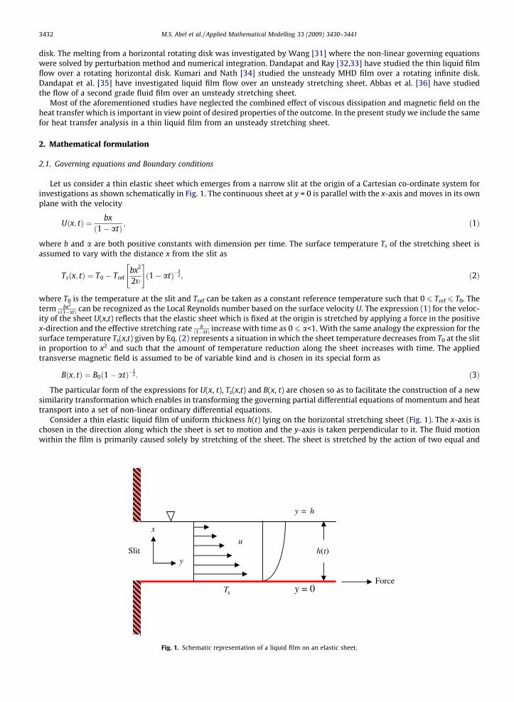
Let us consider a thin elastic sheet which emerges from a narrow slit at the origin of a Cartesian co-ordinate system forinvestigations as shown schematically in Fig. 1. The continuous sheet at y = 0 is parallel with the x-axis and moves in its ownplane with the velocity

Uðx; tÞ ¼ bxð1� atÞ ; ð1Þ

where b and a are both positive constants with dimension per time. The surface temperature Ts of the stretching sheet isassumed to vary with the distance x from the slit as

Tsðx; tÞ ¼ T0 � Trefbx2

2t

" #ð1� atÞ�

32; ð2Þ

where T0 is the temperature at the slit and Tref can be taken as a constant reference temperature such that 0 6 Tref 6 T0. Theterm bx2

tð1�atÞ can be recognized as the Local Reynolds number based on the surface velocity U. The expression (1) for the veloc-ity of the sheet U(x,t) reflects that the elastic sheet which is fixed at the origin is stretched by applying a force in the positivex-direction and the effective stretching rate b

ð1�atÞ increase with time as 0 6 a<1. With the same analogy the expression for thesurface temperature Ts(x,t) given by Eq. (2) represents a situation in which the sheet temperature decreases from T0 at the slitin proportion to x2 and such that the amount of temperature reduction along the sheet increases with time. The appliedtransverse magnetic field is assumed to be of variable kind and is chosen in its special form as

Bðx; tÞ ¼ B0ð1� atÞ�12: ð3Þ

The particular form of the expressions for U(x, t), Ts(x,t) and B(x, t) are chosen so as to facilitate the construction of a newsimilarity transformation which enables in transforming the governing partial differential equations of momentum and heattransport into a set of non-linear ordinary differential equations.

Consider a thin elastic liquid film of uniform thickness h(t) lying on the horizontal stretching sheet (Fig. 1). The x-axis ischosen in the direction along which the sheet is set to motion and the y-axis is taken perpendicular to it. The fluid motionwithin the film is primarily caused solely by stretching of the sheet. The sheet is stretched by the action of two equal and

Force

Slit u

Ts

h(t)

y = 0

y = h

y

x

Fig. 1. Schematic representation of a liquid film on an elastic sheet.

M.S. Abel et al. / Applied Mathematical Modelling 33 (2009) 3430–3441 3433

opposite forces along the x-axis. The sheet is assumed to have velocity U as defined in Eq. (1) and the flow field is exposed tothe influence of an external transverse magnetic field of strength B as defined in Eq. (3). We have neglected the effect of la-tent heat due to evaporation by assuming the liquid to be nonvolatile. Further the buoyancy is neglected due to the relativelythin liquid film, but it is not so thin that intermolecular forces come into play. The velocity and temperature fields of theliquid film obey the following boundary layer equations

ouoxþ ov

oy¼ 0; ð4Þ

ouotþ u

ouoxþ v ou

oy¼ t

o2uoy2 �

rB2

qu; ð5Þ

oTotþ u

oToxþ v oT

oy¼ k

qCp

o2Toy2 þ

lqCp

ouoy

� �2

: ð6Þ

The pressure in the surrounding gas phase is assumed to be uniform and the gravity force gives rise to a hydrostatic pres-sure variation in the liquid film. In order to justify the boundary layer approximation, the length scale in the primary flowdirection must be significantly larger than the length scale in the cross stream direction. We choose the representative mea-sure of the film thickness to be t

b

� �12 so that the scale ratio is large enough i.e., x

tbð Þ

12� 1. This choice of length scale enables us to

employ the boundary layer approximations. Further it is assumed that the induced magnetic field is negligibly small.The associated boundary conditions are given by

u ¼ U; v ¼ 0; T ¼ Ts at y ¼ 0; ð7Þouoy¼ oT

oy¼ 0 at y ¼ h; ð8Þ

v ¼ dhdt

at y ¼ h: ð9Þ

At this juncture we make a note that the mathematical problem is implicitly formulated only for x P 0. Further it is as-sumed that the surface of the planar liquid film is smooth so as to avoid the complications due to surface waves. The influ-ence of interfacial shear due to the quiescent atmosphere, in other words the effect of surface tension is assumed to benegligible. The viscous shear stress s ¼ l ou

oy

� �and the heat flux q ¼ �k oT

oy

� �vanish at the adiabatic free surface (at y = h).

2.2. Similarity transformations

We now introduce dimensionless variables f and h and the similarity variable g as

f ðgÞ ¼ wðx; y; tÞtb

1�at

� �12x; ð10Þ

hðgÞ ¼ T0 � Tðx; y; tÞ

Trefbx2

2tð1�atÞ�32

� � ; ð11Þ

g ¼ btð1� atÞ

� �12

y: ð12Þ

The physical stream function w(x, y, t) automatically assures mass conservation given in Eq. (4). The velocity componentsare readily obtained as

u ¼ owoy¼ bx

1� at

� �f 0ðgÞ; ð13Þ

v ¼ � owox¼ � tb

1� at

� �12

f ðgÞ: ð14Þ

The mathematical problem defined through Eqs. (4)–(9) transforms exactly into a set of ordinary differential equationsand associated boundary conditions as follows

S f 0 þ g2

f 00� �

þ ðf 0Þ2 � ff 00 ¼ f 000 �Mnf 0; ð15Þ

PrS2

3hþ gh0ð Þ þ 2hf 0 � h0f�

¼ h00 þ EcPrf 002; ð16Þ

f 0ð0Þ ¼ 1; f ð0Þ ¼ 0; hð0Þ ¼ 1; ð17Þf 00ðbÞ ¼ 0; h0ðbÞ ¼ 0; ð18Þ

f ðbÞ ¼ Sb2: ð19Þ

3434 M.S. Abel et al. / Applied Mathematical Modelling 33 (2009) 3430–3441

Here S � ab is the dimensionless measure of the unsteadiness and the prime indicates differentiation with respect to g.

Further, b denotes the value of the similarity variable g at the free surface so that Eq. (12) gives

b ¼ btð1� atÞ

� �12

h: ð20Þ

Yet b is an unknown constant, which should be determined as an integral part of the boundary value problem. The rate atwhich film thickness varies can be obtained by differentiating Eq. (20) with respect to t, in the form

dhdt¼ �ab

2t

bð1� atÞ

� �12

: ð21Þ

Thus the kinematic constraint at y = h(t) given by Eq. (9) transforms into the free surface condition (21). It is noteworthythat the momentum boundary layer equation defined by Eq. (15) subject to the relevant boundary conditions (17)–(19) isdecoupled from the thermal field; on the other hand the temperature field h(g) is coupled with the velocity field f(g). Sincethe sheet is stretched horizontally the convection least affects the flow (i.e., buoyancy effect is negligibly small) and hencethere is a one-way coupling of velocity and thermal fields.

The local skin friction coefficient, which of practical importance, is given by

Cf ��2l ou

oy

� �y¼0

qU2 ¼ �2Re�1

2x f 00ð0Þ; ð22Þ

and the heat transfer between the surface and the fluid conventionally expressed in dimensionless form as a local Nusseltnumber is given by

Nux � �x

Tref

oToy

� �y¼0¼ 1

2ð1� atÞ

�12 h0ð0ÞRe

32x; ð23Þ

where Rex ¼ Uxt the local Reynolds number and Tref denotes the same reference temperature (temperature difference) as in Eq.

(2).We now march on to find the solution of the boundary value problem (15)–(19).

3. Numerical solution

The non-linear differential Eqs. (15) and (16) with appropriate boundary conditions given in (17)–(19) are solved numer-ically, by the most efficient numerical shooting technique with fourth order Runge–Kutta algorithm (see Refs. [37,38]). Thenon-linear differential Eqs. (15) and (16) are first decomposed to a system of first order differential equations in the form

df0

dg¼ f1;

df1

dg¼ f2;

df2

dg¼ S f1 þ

g2

f2

� �þ ðf1Þ2 � f0f2 þMnf1;

dh0

dg¼ h1;

dh1

dg¼ Pr

S2

3h0 þ gh1ð Þ þ 2h0f1 � h1f0

� � EcPrf 2

2:

ð24Þ

Corresponding boundary conditions take the form,

f1ð0Þ ¼ 1; f 0ð0Þ ¼ 0; h0ð0Þ ¼ 1; ð25Þf2ðbÞ ¼ 0; h1ðbÞ ¼ 0; ð26Þ

f0ðbÞ ¼Sb2: ð27Þ

Here f0(g) = f(g) and h0(g) = h(g). The above boundary value problem is first converted into an initial value problem byappropriately guessing the missing slopes f2(0) and h1(0). The resulting IVP is solved by shooting method for a set of param-eters appearing in the governing equations and a known value of S. The value of b is so adjusted that condition (27) holds.This is done on the trial and error basis. The value for which condition (27) holds is taken as the appropriate film thicknessand the IVP is finally solved using this value of b. The step length of h = 0.01 is employed for the computation purpose. Theconvergence criterion largely depends on fairly good guesses of the initial conditions in the shooting technique. The iterative

M.S. Abel et al. / Applied Mathematical Modelling 33 (2009) 3430–3441 3435

process is terminated until the relative difference between the current and the previous iterative values of f(b) matches withthe value of Sb

2 up to a tolerance of 10�6. Once the convergence in achieved we integrate the resultant ordinary differentialequations using standard fourth order Runge–Kutta method with the given set of parameters to obtain the required solution.

Table 1Comparison of values of skin friction coefficient f00 (0) with Mn = 0.0.

S Wang [22] Present results

b f00(0) f 00 ð0Þb b f00(0)

0.4 5.122490 �6.699120 �1.307785 4.981455 �1.1340980.6 3.131250 �3.742330 �1.195155 3.131710 �1.1951280.8 2.151990 �2.680940 �1.245795 2.151990 �1.2458051.0 1.543620 �1.972380 �1.277762 1.543617 �1.2777691.2 1.127780 �1.442631 �1.279177 1.127780 �1.2791711.4 0.821032 �1.012784 �1.233549 0.821033 �1.2335451.6 0.576173 �0.642397 �1.114937 0.576176 �1.1149411.8 0.356389 �0.309137 �0.867414 0.356390 �0.867416

Note: Wang [22] has used different similarity transformation due to which the value of f 00 ð0Þb in his paper is the same as f00(0) of our results.

0.0 0.5 1.0 1.5 2.00

10

20

30

40

50

S

β

Fig. 2. Variation of film thickness b with unsteadiness parameter S with Mn = 0.0.

0 80.0

0.4

0.8

1.2

1.6

2.0

β

S = 1.2

S = 0.8

Mn642

Fig. 3. Variation of film thickeness b with magnetic parameter Mn.

0 2 4 6 80.0

0.1

0.2

0.3

0.4

0.5

f ' (β

)

Mn

S = 0.8

S = 1.2

Fig. 4. Variation of free surface velocity f0(b) with magnetic parameter Mn.

0 2 4 6 80.0

0.5

1.0

1.5

2.0

2.5

3.0

3.5

-f '' (

0)

Mn

S = 1.2

S = 0.8

Fig. 5. Variation of wall shear stress parameter �f00(0) with magnetic parameter Mn.

0.0

0.2

0.4

0.6

0.8

θ (β

)

S = 1.2

S = 0.8

0 2 4 6 8Mn

Fig. 6. Variation of free surface temperature h(b) with the magnetic parameter Mn.

3436 M.S. Abel et al. / Applied Mathematical Modelling 33 (2009) 3430–3441

1.3

1.4

1.5

1.6

1.7

1.8

-θ '

(0)

S = 0.8

S = 1.2

0 2 4 6 8Mn

Fig. 7. Variation of wall dimensionless heat flux �h0(0) with magnetic parameter Mn.

0.0

0.5

1.0

1.5

2.0

0.0 0.2 0.4 0.6 0.8 1.0

η

S = 0.8

Mn = 0,1,2,3,4

β = 1.067175β = 1.184197β = 1.350880

β = 1.616880

β = 2.151992

f '(η)

Fig. 8a. Variation in the velocity profiles f0(g) for different values of magnetic parameter Mn with S = 0.8.

0.0

0.2

0.4

0.6

0.8

1.0

1.2

η

S = 1.2

Mn = 0,1,2,3,4

β = 0.627910β = 0.690238β = 0.775795

β = 0.903878

β = 1.127780

0.0 0.2 0.4 0.6 0.8 1.0f '(η)

Fig. 8b. Variation in the velocity profiles f0(g) for different values of magnetic parameter Mn with S = 1.2.

M.S. Abel et al. / Applied Mathematical Modelling 33 (2009) 3430–3441 3437

3438 M.S. Abel et al. / Applied Mathematical Modelling 33 (2009) 3430–3441

4. Results and discussion

The exact solution do not seem to be feasible for a complete set of Eqs. (15) and (16) because of the non-linear form of themomentum and thermal boundary layer equations. This fact forces one to obtain the solution of the problem numerically.Appropriate similarity transformation is adopted to transform the governing partial differential equations of flow and heattransfer into a system of non-linear ordinary differential equations. The resultant boundary value problem is solved by theefficient shooting method. It is note worthy to mention that the solution exists only for a small range of values of unstead-iness parameter 0 6 S 6 2. Moreover, when S ? 0 the solution approaches to the analytical solution obtained by Crane [2]with infinitely thick layer of fluid (b ?1). The other limiting solution corresponding to S ? 2 represents a liquid film ofinfinitesimal thickness (b ? 0). The numerical results are obtained for 0 6 S 6 2. Present results are compared with someof the earlier published results in some limiting cases which are tabulated in Tables 1 and 2. The effects of magnetic param-eter on various fluid dynamic quantities are shown in Figs. 2–9 for different unsteadiness parameter.

Fig. 2 shows the variation of film thickness b with the unsteadiness parameter. It is evident from this plot that the filmthickness b decreases monotonically when S is increased from 0 to 2. This result concurs with that observed by Wang [22].The variation of film thickness b with respect to the magnetic parameter Mn is projected in Fig. 3 for different values ofunsteadiness parameter. It is clear from this plot that the increasing values of magnetic parameter decreases the film thick-ness. The result holds for different values of unsteadiness parameter S.

The variation of free surface velocity f0(b) with respect to Mn is shown in Fig. 4. The free surface velocity behaves almost asa constant function of Mn as can be seen from Fig. 4. The effect of Mn on the wall shear stress parameter �f00(0) is illustrated

0.0

0.2

0.4

0.6

0.8

1.0

1.2

β=0.627910

β=0.690238β=0.775795

β=0.903878

β=1.127780S = 1.2

η

θ (η) 0.0 0.2 0.4 0.6 0.8 1.0

Mn = 0, 1, 2, 4, 5

Fig. 9b. Variation of dimensionless temperature h(g) with the magnetic parameter with S = 1.2.

0.0

0.5

1.0

1.5

2.0

2.5

Mn = 0, 1, 2, 4, 5

θ (η)

S = 0.8

β=0.979193

β=1.067175

β=1.350880

β=1.616880

β=2.151990

0.0 0.2 0.4 0.6 0.8 1.0

η

Fig. 9a. Variation of dimensionless temperature h(g) with the magnetic parameter with S = 0.8.

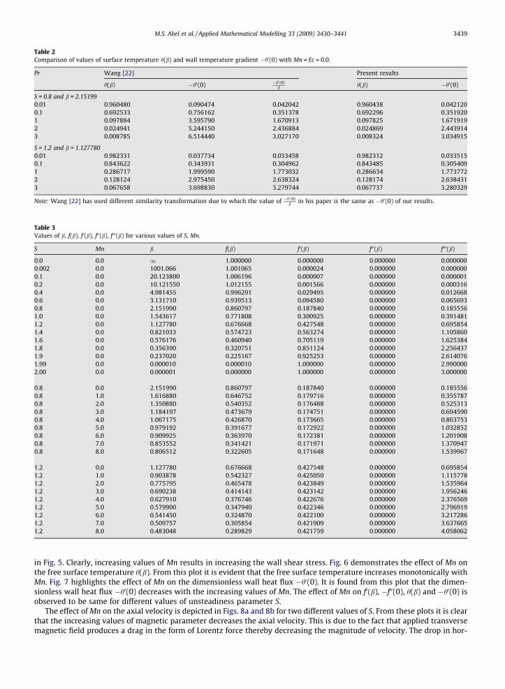
Table 2Comparison of values of surface temperature h(b) and wall temperature gradient �h0(0) with Mn = Ec = 0.0.

Pr Wang [22] Present results

h(b) �h0(0) �h0 ð0Þb h(b) �h0(0)

S = 0.8 and b = 2.151990.01 0.960480 0.090474 0.042042 0.960438 0.0421200.1 0.692533 0.756162 0.351378 0.692296 0.3519201 0.097884 3.595790 1.670913 0.097825 1.6719192 0.024941 5.244150 2.436884 0.024869 2.4439143 0.008785 6.514440 3.027170 0.008324 3.034915

S = 1.2 and b = 1.1277800.01 0.982331 0.037734 0.033458 0.982312 0.0335150.1 0.843622 0.343931 0.304962 0.843485 0.3054091 0.286717 1.999590 1.773032 0.286634 1.7737722 0.128124 2.975450 2.638324 0.128174 2.6384313 0.067658 3.698830 3.279744 0.067737 3.280329

Note: Wang [22] has used different similarity transformation due to which the value of �h0 ð0Þb in his paper is the same as �h0(0) of our results.

Table 3Values of b, f(b), f0(b), f00(b), f000(b) for various values of S, Mn.

S Mn b f(b) f0(b) f00(b) f000(b)

0.0 0.0 1 1.000000 0.000000 0.000000 0.0000000.002 0.0 1001.066 1.001065 0.000024 0.000000 0.0000000.1 0.0 20.123800 1.006196 0.000007 0.000000 0.0000010.2 0.0 10.121550 1.012155 0.001566 0.000000 0.0003160.4 0.0 4.981455 0.996291 0.029495 0.000000 0.0126680.6 0.0 3.131710 0.939513 0.094580 0.000000 0.0656930.8 0.0 2.151990 0.860797 0.187840 0.000000 0.1855561.0 0.0 1.543617 0.771808 0.300925 0.000000 0.3914811.2 0.0 1.127780 0.676668 0.427548 0.000000 0.6958541.4 0.0 0.821033 0.574723 0.563274 0.000000 1.1058601.6 0.0 0.576176 0.460940 0.705119 0.000000 1.6253841.8 0.0 0.356390 0.320751 0.851124 0.000000 2.2564371.9 0.0 0.237020 0.225167 0.925253 0.000000 2.6140761.99 0.0 0.000010 0.000010 1.000000 0.000000 2.9900002.00 0.0 0.000001 0.000000 1.000000 0.000000 3.000000

0.8 0.0 2.151990 0.860797 0.187840 0.000000 0.1855560.8 1.0 1.616880 0.646752 0.179716 0.000000 0.3557870.8 2.0 1.350880 0.540352 0.176488 0.000000 0.5253130.8 3.0 1.184197 0.473679 0.174751 0.000000 0.6945900.8 4.0 1.067175 0.426870 0.173665 0.000000 0.8637530.8 5.0 0.979192 0.391677 0.172922 0.000000 1.0328520.8 6.0 0.909925 0.363970 0.172381 0.000000 1.2019080.8 7.0 0.853552 0.341421 0.171971 0.000000 1.3709470.8 8.0 0.806512 0.322605 0.171648 0.000000 1.539967

1.2 0.0 1.127780 0.676668 0.427548 0.000000 0.6958541.2 1.0 0.903878 0.542327 0.425050 0.000000 1.1157781.2 2.0 0.775795 0.465478 0.423849 0.000000 1.5359641.2 3.0 0.690238 0.414143 0.423142 0.000000 1.9562461.2 4.0 0.627910 0.376746 0.422676 0.000000 2.3765691.2 5.0 0.579900 0.347940 0.422346 0.000000 2.7969191.2 6.0 0.541450 0.324870 0.422100 0.000000 3.2172861.2 7.0 0.509757 0.305854 0.421909 0.000000 3.6376651.2 8.0 0.483048 0.289829 0.421759 0.000000 4.058062

M.S. Abel et al. / Applied Mathematical Modelling 33 (2009) 3430–3441 3439

in Fig. 5. Clearly, increasing values of Mn results in increasing the wall shear stress. Fig. 6 demonstrates the effect of Mn onthe free surface temperature h(b). From this plot it is evident that the free surface temperature increases monotonically withMn. Fig. 7 highlights the effect of Mn on the dimensionless wall heat flux �h0(0). It is found from this plot that the dimen-sionless wall heat flux �h0(0) decreases with the increasing values of Mn. The effect of Mn on f0(b), �f00(0), h(b) and �h0(0) isobserved to be same for different values of unsteadiness parameter S.

The effect of Mn on the axial velocity is depicted in Figs. 8a and 8b for two different values of S. From these plots it is clearthat the increasing values of magnetic parameter decreases the axial velocity. This is due to the fact that applied transversemagnetic field produces a drag in the form of Lorentz force thereby decreasing the magnitude of velocity. The drop in hor-

3440 M.S. Abel et al. / Applied Mathematical Modelling 33 (2009) 3430–3441

izontal velocity as a consequence of increase in the strength of magnetic field is observed for both the values of S = 0.8 andS = 1.2.

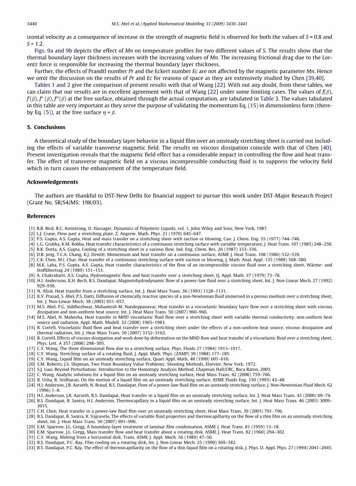
Figs. 9a and 9b depicts the effect of Mn on temperature profiles for two different values of S. The results show that thethermal boundary layer thickness increases with the increasing values of Mn. The increasing frictional drag due to the Lor-entz force is responsible for increasing the thermal boundary layer thickness.

Further, the effects of Prandtl number Pr and the Eckert number Ec are not affected by the magnetic parameter Mn. Hencewe omit the discussion on the results of Pr and Ec for reasons of space as they are extensively studied by Chen [39,40].

Tables 1 and 2 give the comparison of present results with that of Wang [22]. With out any doubt, from these tables, wecan claim that our results are in excellent agreement with that of Wang [22] under some limiting cases. The values of f(b),f0(b), f00 (b), f000(b) at the free surface, obtained through the actual computation, are tabulated in Table 3. The values tabulatedin this table are very important as they serve the purpose of validating the momentum Eq. (15) in dimensionless form (there-by Eq. (5)), at the free surface g = b.

5. Conclusions

A theoretical study of the boundary layer behavior in a liquid film over an unsteady stretching sheet is carried out includ-ing the effects of variable transverse magnetic field. The results on viscous dissipation coincide with that of Chen [40].Present investigation reveals that the magnetic field effect has a considerable impact in controlling the flow and heat trans-fer. The effect of transverse magnetic field on a viscous incompressible conducting fluid is to suppress the velocity fieldwhich in turn causes the enhancement of the temperature field.

Acknowledgements

The authors are thankful to DST-New Delhi for financial support to pursue this work under DST-Major Research Project(Grant No. SR/S4/MS: 198/03).

References

[1] R.B. Bird, R.C. Armstrong, O. Hassager, Dynamics of Polymeric Liquids, vol. 1, John Wiley and Sons, New York, 1987.[2] L.J. Crane, Flow past a stretching plate, Z. Angrew. Math. Phys. 21 (1970) 645–647.[3] P.S. Gupta, A.S. Gupta, Heat and mass transfer on a stretching sheet with suction or blowing, Can. J. Chem. Eng. 55 (1977) 744–746.[4] L.G. Grubka, K.M. Bobba, Heat transfer characteristics of a continuous stretching surface with variable temperature, J. Heat Trans. 107 (1985) 248–250.[5] B.K. Dutta, A.S. Gupta, Cooling of a stretching sheet in a various flow, Ind. Eng. Chem. Res. 26 (1987) 333–336.[6] D.R. Jeng, T.C.A. Chang, K.J. Dewitt, Momentum and heat transfer on a continuous surface, ASME J. Heat Trans. 108 (1986) 532–539.[7] C.K. Chen, M.I. Char, Heat transfer of a continuous stretching surface with suction or blowing, J. Math. Anal. Appl. 135 (1988) 568–580.[8] M.K. Laha, P.S. Gupta, A.S. Gupta, Heat transfer characteristics of the flow of an incompressible viscous fluid over a stretching sheet, Wärme- und

Stoffübertrag 24 (1989) 151–153.[9] A. Chakrabarti, A.S. Gupta, Hydromagnetic flow and heat transfer over a stretching sheet, Q. Appl. Math. 37 (1979) 73–78.

[10] H.I. Andersson, K.H. Bech, B.S. Dandapat, Magnetohydrodynamic flow of a power-law fluid over a stretching sheet, Int. J. Non-Linear Mech. 27 (1992)929–936.

[11] N. Afzal, Heat transfer from a stretching surface, Int. J. Heat Mass Trans. 36 (1993) 1128–1131.[12] K.V. Prasad, S. Abel, P.S. Datti, Diffusion of chemically reactive species of a non-Newtonian fluid immersed in a porous medium over a stretching sheet,

Int. J. Non-Linear Mech. 38 (2003) 651–657.[13] M.S. Abel, P.G. Siddheshwar, Mahantesh M. Nandeppanavar, Heat transfer in a viscoelastic boundary layer flow over a stretching sheet with viscous

dissipation and non-uniform heat source, Int. J. Heat Mass Trans. 50 (2007) 960–966.[14] M.S. Abel, N. Mahesha, Heat transfer in MHD viscoelastic fluid flow over a stretching sheet with variable thermal conductivity, non-uniform heat

source and radiation, Appl. Math. Modell. 32 (2008) 1965–1983.[15] R. Cortell, Viscoelastic fluid flow and heat transfer over a stretching sheet under the effects of a non-uniform heat source, viscous dissipation and

thermal radiation, Int. J. Heat Mass Trans. 50 (2007) 3152–3162.[16] R. Cortell, Effects of viscous dissipation and work done by deformation on the MHD flow and heat transfer of a viscoelastic fluid over a stretching sheet,

Phys. Lett. A 357 (2006) 298–305.[17] C.Y. Wang, The three dimensional flow due to a stretching surface, Phys. Fluids 27 (1984) 1915–1917.[18] C.Y. Wang, Stretching surface of a rotating fluid, J. Appl. Math. Phys. (ZAMP) 39 (1988) 177–185.[19] C.Y. Wang, Liquid film on an unsteady stretching surface, Quart Appl. Math. 48 (1990) 601–610.[20] S.M. Roberts, J.S. Shipman, Two Point Boundary Value Problems: Shooting Methods, Elsevier, New York, 1972.[21] S.J. Liao, Beyond Perturbation: Introduction to the Homotopy Analysis Method, Chapman Hall/CRC, Boca Raton, 2003.[22] C. Wang, Analytic solutions for a liquid film on an unsteady stretching surface, Heat Mass Trans. 42 (2006) 759–766.[23] R. Usha, R. Sridharan, On the motion of a liquid film on an unsteady stretching surface, ASME Fluids Eng. 150 (1993) 43–48.[24] H.I. Anderson, J.B. Aarseth, N. Braud, B.S. Dandapat, Flow of a power-law fluid film on an unsteady stretching surface, J. Non-Newtonian Fluid Mech. 62

(1996) 1–8.[25] H.I. Anderson, J.B. Aarseth, B.S. Dandapat, Heat transfer in a liquid film on an unsteady stretching surface, Int. J. Heat Mass Trans. 43 (2000) 69–74.[26] B.S. Dandapat, B. Santra, H.I. Anderson, Thermocapillary in a liquid film on an unsteady stretching surface, Int. J. Heat Mass Trans. 46 (2003) 3009–

3015.[27] C.H. Chen, Heat transfer in a power-law fluid film over an unsteady stretching sheet, Heat Mass Trans. 39 (2003) 791–796.[28] B.S. Dandapat, B. Santra, K. Vajravelu, The effects of variable fluid properties and thermocapillarity on the flow of a thin film on an unsteady stretching

sheet, Int. J. Heat Mass Trans. 50 (2007) 991–996.[29] E.M. Sparrow, J.L. Gregg, A boundary-layer treatment of laminar film condensation, ASME J. Heat Trans. 81 (1959) 13–18.[30] E.M. Sparrow, J.L. Gregg, Mass transfer flow and heat transfer about a rotating disk, ASME J. Heat Trans. 82 (1960) 294–302.[31] C.Y. Wang, Melting from a horizontal disk, Trans. ASME J. Appl. Mech. 56 (1989) 47–50.[32] B.S. Dandapat, P.C. Ray, Film cooling on a rotating disk, Int. J. Non-Linear Mech. 25 (1990) 569–582.[33] B.S. Dandapat, P.C. Ray, The effect of thermocapillarity on the flow of a thin liquid film on a rotating disk, J. Phys. D. Appl. Phys. 27 (1994) 2041–2045.

M.S. Abel et al. / Applied Mathematical Modelling 33 (2009) 3430–3441 3441

[34] M. Kumari, G. Nath, Unsteady MHD film flow over a rotating infinite disk, Int. J. Eng. Sci. 42 (2004) 1099–1117.[35] B.S. Dandapat, S. Maity, A. Kitamura, Liquid film flow due to an unsteady stretching sheet, Int. J. Non-Linear Mech. 43 (2008) 880–886.[36] Z. Abbas, T. Hayat, M. Sajid, S. Asghar, Unsteady flow of a second grade fluid film over an unsteady stretching sheet, Math. Comput. Modell. 48 (2008)

518–526.[37] S.D. Conte, C. de Boor, Elementary Numerical Analysis, McGraw-Hill, New York, 1972.[38] T. Cebeci, P. Bradshaw, Physical and Computational Aspects of Convective Heat Transfer, Springer-Verlag, New York, 1984.[39] C.-H. Chen, Heat transfer in a power-law fluid film over an unsteady stretching sheet, Heat Mass Trans. 39 (2003) 791.[40] C.-H. Chen, Effect of viscous dissipation on heat transfer in a non-Newtonian liquid film over an unsteady stretching sheet, J. Non-Newtonian Fluid

Mech. 135 (2006) 128.