Health system inequalities and poverty in Brazil
306
Investment in Social and Economic Returns Pan American Health Organization Scientific and Technical Publication No. 582 Health
Transcript of Health system inequalities and poverty in Brazil

Investmentin
Social and
Economic Returns
Pan American Health OrganizationScientific and Technical Publication No. 582
Health
Sc
ien
tific a
nd
Tec
hn
ica
l Pu
b. N
o. 5
82
PA
HO
Investmen
t in H
ealth
The Pan American Health Organization joined hands with the Inter-
American Development Bank and the World Bank, and also worked with
the United Nations Development Program and the United Nations
Economic Commission for Latin America and the Caribbean, to explore
how investing in health can benefit economic growth, household pro-
ductivity, and poverty alleviation in Latin America and the Caribbean.
This publication collects the final reports of three research projects that
examined these issues. The work published here includes cutting-
edge research by economists interested in health issues and by
health workers who are concerned about the broader implications of
good health. These findings will go a long way towards establishing the
critical role that health plays in overall human development.
Pan American Health OrganizationPan American Sanitary BureauRegional Office of theWorld Health Organization525 Twenty-third Street, N.W.Washington, D.C. 20037 U.S.A.
www.paho.orgISBN 92 75 11582 6
SP582I_Cover.qxd 11/1/01 10:59 AM Page 1

Scientific and Technical Publication No. 582
Investmentin
Health
Social andEconomic Returns
Produced in collaboration with
The Inter-American Development Bank and
The World Bank
PAN AMERICAN HEALTH ORGANIZATIONPan American Sanitary Bureau,Regional Office of theWORLD HEALTH ORGANIZATION525 23rd Street, N.W.Washington, D.C. 20037 U.S.A.

ii INTRODUCTION
Also published in Spanish with the title:Invertir en salud. Beneficios sociales y económicos
ISBN 92 75 31582 5
PAHO Cataloguing in Publication Data
Pan American Health OrganizationInvestment in health: social and economic returns — Washington, D.C.: PAHO, © 2001.
viii, 284 p. — (Scientific and Technical Publication No. 582)
ISBN 92 75 11582 6
I. Title II. SeriesIII. Author1. HEALTH ECONOMICS2. HUMAN DEVELOPMENT3. EQUITY4. POVERTY5. SOCIAL CONDITIONS6. SUSTAINABLE DEVELOPMENT
NLM W74.P187i
The Pan American Health Organization welcomes requests for permission to repro-duce or translate its publications, in part or in full. Applications and inquiries should beaddressed to the Publications Program, Pan American Health Organization, Washing-ton, D.C., U.S.A., which will be glad to provide the latest information on any changesmade to the text, plans for new editions, and reprints and translations already available.
© Pan American Health Organization, 2001
Publications of the Pan American Health Organization enjoy copyright protection inaccordance with the provisions of Protocol 2 of the Universal Copyright Convention. Allrights are reserved.
The designations employed and the presentation of the material in this publication donot imply the expression of any opinion whatsoever on the part of the Secretariat of thePan American Health Organization concerning the status of any country, territory, cityor area or of its authorities, or concerning the delimitation of its frontiers or boundaries.
The mention of specific companies or of certain manufacturers’ products does notimply that they are endorsed or recommended by the Pan American Health Organiza-tion in preference to others of a similar nature that are not mentioned. Errors and omis-sions excepted, the names of proprietary products are distinguished by initial capitalletters.

iii
CONTENTS
Prologue . . . . . . . . . . . . . . . . . . . . . . . . . . . . . . . . . . . . . . . . . . . . . . . . . . . . . . . . . . . . . . . . v
Introduction . . . . . . . . . . . . . . . . . . . . . . . . . . . . . . . . . . . . . . . . . . . . . . . . . . . . . . . . . . . . . vii
PART I: INVESTMENT IN HEALTH AND ECONOMIC GROWTH
Health, Growth, and Income Distribution in Latin America and the Caribbean:A Study of Determinants and Regional and Local Behavior . . . . . . . . . . . . . . . . . . . . 3
David Mayer, Humberto Mora, Rodolfo Cermeño, Ana Beatriz Barona,and Suzanne Duryeau
PART II: PRODUCTIVITY OF HOUSEHOLD INVESTMENT IN HEALTH
Productivity of Household Investment in Health: The Case of Colombia . . . . . . . . . 35Rocio Ribero and Jairo Nuñez
Linking Health, Nutrition, and Wages: The Evolution of Age at Menarche andLabor Earnings Among Adult Mexican Women . . . . . . . . . . . . . . . . . . . . . . . . . . . . . . 63
Felicia Marie KnaulHealth and Productivity in Peru: An Empirical Analysis by Gender and Region . . 87
Rafael Cortez
PART III: INVESTMENT IN HEALTH AND POVERTY REDUCTION
Health System Inequalities and Inequities in Latin America and the Caribbean:Findings and Policy Implications . . . . . . . . . . . . . . . . . . . . . . . . . . . . . . . . . . . . . . . . . . . 119
Rubén M. Suárez-BerenguelaHealth System Inequalities and Poverty in Brazil . . . . . . . . . . . . . . . . . . . . . . . . . . . . . 143
Antonio Carlos Coelho Campino, Maria Dolores M. Diaz, Leda Maria Paulani,Roberto G. de Oliveira, Sergio Piola, and Andres Nunes
Health System Inequality and Poverty in Ecuador . . . . . . . . . . . . . . . . . . . . . . . . . . . . 161Enrique Lasprilla, Jorge Granda, Carlos Obando, Eduardo Encalad, andChristian Lasprilla
Health Sector Inequalities and Poverty in Guatemala . . . . . . . . . . . . . . . . . . . . . . . . . . 175Edgard Barillas, Ricardo Valladares, and GSD Consultores Asociados
Health System Inequalities and Poverty in Jamaica . . . . . . . . . . . . . . . . . . . . . . . . . . . . 189Karl Theodore, Althea Lafoucade, Dominic Stoddard, Wendell Thomas,and Andrea Yearwood
Health System Inequalities and Poverty in Mexico . . . . . . . . . . . . . . . . . . . . . . . . . . . . 207Susan Wendy Parker and Eduardo Gonzales Pier
Health Sector Inequalities and Poverty in Peru . . . . . . . . . . . . . . . . . . . . . . . . . . . . . . . 218Margarita Petrera and Luis Cordero
Inequity in the Delivery of Health Care: Methods and Results for Jamaica . . . . . . . . 233Eddy van Doorslaer and Adam Wagstaff
Health Policies, Health Inequalities, and Poverty Alleviation: Experiencesfrom Outside Latin America and the Caribbean . . . . . . . . . . . . . . . . . . . . . . . . . . . . . . . 245
Margaret WhiteheadPolicy Implications of a Health Equity Focus for Latin America . . . . . . . . . . . . . . . . . 254
William Savedoff

iv CONTENTS
APPENDIX
Health and Economic Growth . . . . . . . . . . . . . . . . . . . . . . . . . . . . . . . . . . . . . . . . . . . . . . 265George A.O. Alleyne
Summary of Meeting Proceedings . . . . . . . . . . . . . . . . . . . . . . . . . . . . . . . . . . . . . . . . . . 271
List of Participants . . . . . . . . . . . . . . . . . . . . . . . . . . . . . . . . . . . . . . . . . . . . . . . . . . . . . . . . 281

v
PROLOGUE
The Pan American Health Organization (PAHO) as a whole, and myself in particu-lar, have been concerned with the relationship between health and the economy forquite some time. When we first shared this concern with Enrique Iglesias, President,and Nancy Birdsall, then-Executive Vice-President of the Inter-American Develop-ment Bank (IDB), both concurred with us on the necessity to further analyze thedifferent dimensions involved in this relationship. We then decided to implementtwo coordinated research projects: the first, sponsored by PAHO, dealt with theimpact of health on economic growth; the second, promoted by IDB, focused on theimpact of health on household productivity.
Encouraging reactions also emerged when we discussed this issue with the Eco-nomic Commission of Latin America and the Caribbean (ECLAC), the World Bank,and the United Nations Development Program (UNDP). As a result, a third researchproject—on investment in health, equity, and poverty reduction—was then launchedas a joint initiative between PAHO, the World Bank and UNDP. This book summa-rizes the results of all three research projects.
In reiterating our gratitude to these organizations for their support, I hope thatwe will continue to work together and support the efforts of our member statestowards bringing better health to their populations and, thus, contributing to theirhuman development.
The researchers from Latin America and the Caribbean who carried out thestudies reported here include economists interested in health issues, as well as healthspecialists interested in the broader consequences of good health. I thank them fortheir cooperation, and hope to continue to have them as our allies in the search forthe explanations of the relationship between health and human development.
The results of these studies reaffirm what some of us in the health field havealways believed to be true but could not always verify: the positive, still unquantifiedcontribution of health to different dimensions of human development. They showthat good health allows nations to accelerate their economic performance, and con-versely that disease is an obstacle to development. They also show that householdproductivity benefits from health improvements and demonstrate how the reduc-tion of health inequalities can contribute to poverty alleviation.
These findings open new possibilities for further exploring the role of health inhuman development, as well as opportunities for a better policy dialogue betweenhealth and development authorities. This dialogue will, I hope, benefit the people ofthe Americas.
George A. O. AlleyneDirector of the Pan American Sanitary Bureau

vii
INTRODUCTION
This publication brings together the final reports from three research projects thatexplored how investments in health affected economic growth, household produc-tivity, and poverty alleviation in Latin America and the Caribbean. The projects werecarried out in 1998 and 1999, and came about through the coordinated efforts of thePan American Health Organization (PAHO), the Inter-American Development Bank(IDB), the United Nations Development Program (UNDP), the United Nations Eco-nomic Commission for Latin America and the Caribbean (ECLAC), and the WorldBank.
The first project was designed to explore the extent to which improvements in apopulation’s health can help grow the national economy. PAHO’s Research GrantsProgram called for research proposals on the topic based on terms of reference pre-pared by Harvard University Professor Robert Barro. Subsequently, a specially con-vened committee integrated by Dr. Barbara Stalling, ECLAC’s Director of the Eco-nomic Development Division; Professor Maximo Vega Centeno, President, of theLatin American Econometric Society; and Professor José Luis Estrada, AutonomousUniversity of Mexico, worked with PAHO to review the seventeen research propos-als submitted by economic and health research centers from throughout the Regionin response to this call. The selected proposal was submitted by a group constitutedby two Mexican institutions—Centro de Investigación y Docencia Económicas (CIDE)and Fundación Mexicana para la Salud (FUNSALUD)—and one organization fromColombia—Fundación para la Educación Superior y el Desarrollo (FEDESA-RROLLO). The second project examined the effect of health improvements on house-hold productivity. Sponsored by IDB, the project was based on terms of referenceprepared by Professor T. Paul Schultz of Yale University and was carried out throughIDB’s Network of Research Centers. It involved six studies conducted in Colombia,Mexico, Nicaragua, and Peru.1 The third project—“Investment in Health, Equity andPoverty” (IHEP/EquiLAC)—addressed issues of equity and poverty alleviation andwas inspired on a similar study sponsored by the Organization for Economic Coop-eration and Development (OECD) in the early 1990s.2 Sponsored by PAHO, UNDP,and the World Bank the project conducted country studies in Brazil, Ecuador, Gua-temala, Jamaica, Mexico, and Peru that were coordinated by José Vicente Zevallosfrom UNDP, Rubén Suarez from the World Bank, and Edward Greene from PAHO.In October 1999, experts in economics, social development, and health, as well asrepresentatives from international and cooperation organizations, met at PAHO head-quarters in Washington, D.C., to review the impact of investments in health on eco-nomic growth, household productivity, and poverty reduction. Reports from the
1 A book with the all the reports from this project has been published by IDB: Savedoff W,Schultz T P. eds. Wealth from Health: Linking Social Investments to Earnings in Latin America., Wash-ington: IDB; 2000.
2 Van Doorslaer, E., Wagstaff, A., and Rutten, F., eds., Equity in the Finance and Delivery of HealthCare: An International Perspective”, Oxford Univwersity Press, NY, 1993.

viii INTRODUCTION
three above-mentioned projects and their respective policy implications were pre-sented and discussed at that time.
This book’s structure mirrors the agenda for the October 1999 meeting. Part Ipresents the final report of the study “Investment in Health and Economic Growth,”authored by the researchers who carried out the work. Part II includes the Colom-bia, Mexico, and Peru studies from the “Productivity of Household Investment inHealth” project. And Part III presents the ten country case reports from the IHEP/EquiLAC project, plus a review paper, two works on methodological issues, and areview of experiences from other regions in the world regarding health inequalitiesand poverty alleviation. Finally, the book’s annex includes the inaugural speech givenby Dr. George A. O. Alleyne, Director of the Pan American Sanitary Bureau, at theopening of the October 1999 meeting; the meeting’s agenda and list of participants;and a summary of discussions.
PAHO would like to acknowledge the efforts of the various groups and indi-viduals that contributed to make this venture a success. We are especially grateful toour colleagues at IDB, ECLAC, UNDP, and the World Bank for working so closelywith us to develop and review the studies published here. We also wish to com-mend the researchers’ efforts to complete their reports under conditions that made asometimes difficult task even more arduous. Third, we want to thank the partici-pants at the October 1999 meeting, particularly for their recommendations regard-ing the future steps to be taken in this area. Finally, we want to acknowledge thework of the Organization’s Public Policy and Health Program, Research Coordina-tion Program, Publications Program, and Public Policy and Health Program for help-ing make this book a reality.

iii
CONTENTS
Prologue . . . . . . . . . . . . . . . . . . . . . . . . . . . . . . . . . . . . . . . . . . . . . . . . . . . . . . . . . . . . . . . . v
Introduction . . . . . . . . . . . . . . . . . . . . . . . . . . . . . . . . . . . . . . . . . . . . . . . . . . . . . . . . . . . . . vii
PART I: INVESTMENT IN HEALTH AND ECONOMIC GROWTH
Health, Growth, and Income Distribution in Latin America and the Caribbean:A Study of Determinants and Regional and Local Behavior . . . . . . . . . . . . . . . . . . . . 3
David Mayer, Humberto Mora, Rodolfo Cermeño, Ana Beatriz Barona,and Suzanne Duryeau
PART II: PRODUCTIVITY OF HOUSEHOLD INVESTMENT IN HEALTH
Productivity of Household Investment in Health: The Case of Colombia . . . . . . . . . 35Rocio Ribero and Jairo Nuñez
Linking Health, Nutrition, and Wages: The Evolution of Age at Menarche andLabor Earnings Among Adult Mexican Women . . . . . . . . . . . . . . . . . . . . . . . . . . . . . . 63
Felicia Marie KnaulHealth and Productivity in Peru: An Empirical Analysis by Gender and Region . . 87
Rafael Cortez
PART III: INVESTMENT IN HEALTH AND POVERTY REDUCTION
Health System Inequalities and Inequities in Latin America and the Caribbean:Findings and Policy Implications . . . . . . . . . . . . . . . . . . . . . . . . . . . . . . . . . . . . . . . . . . . 119
Rubén M. Suárez-BerenguelaHealth System Inequalities and Poverty in Brazil . . . . . . . . . . . . . . . . . . . . . . . . . . . . . 143
Antonio Carlos Coelho Campino, Maria Dolores M. Diaz, Leda Maria Paulani,Roberto G. de Oliveira, Sergio Piola, and Andres Nunes
Health System Inequality and Poverty in Ecuador . . . . . . . . . . . . . . . . . . . . . . . . . . . . 161Enrique Lasprilla, Jorge Granda, Carlos Obando, Eduardo Encalad, andChristian Lasprilla
Health Sector Inequalities and Poverty in Guatemala . . . . . . . . . . . . . . . . . . . . . . . . . . 175Edgard Barillas, Ricardo Valladares, and GSD Consultores Asociados
Health System Inequalities and Poverty in Jamaica . . . . . . . . . . . . . . . . . . . . . . . . . . . . 189Karl Theodore, Althea Lafoucade, Dominic Stoddard, Wendell Thomas,and Andrea Yearwood
Health System Inequalities and Poverty in Mexico . . . . . . . . . . . . . . . . . . . . . . . . . . . . 207Susan Wendy Parker and Eduardo Gonzales Pier
Health Sector Inequalities and Poverty in Peru . . . . . . . . . . . . . . . . . . . . . . . . . . . . . . . 218Margarita Petrera and Luis Cordero
Inequity in the Delivery of Health Care: Methods and Results for Jamaica . . . . . . . . 233Eddy van Doorslaer and Adam Wagstaff
Health Policies, Health Inequalities, and Poverty Alleviation: Experiencesfrom Outside Latin America and the Caribbean . . . . . . . . . . . . . . . . . . . . . . . . . . . . . . . 245
Margaret WhiteheadPolicy Implications of a Health Equity Focus for Latin America . . . . . . . . . . . . . . . . . 254
William Savedoff

iv CONTENTS
APPENDIX
Health and Economic Growth . . . . . . . . . . . . . . . . . . . . . . . . . . . . . . . . . . . . . . . . . . . . . . 265George A.O. Alleyne
Summary of Meeting Proceedings . . . . . . . . . . . . . . . . . . . . . . . . . . . . . . . . . . . . . . . . . . 271
List of Participants . . . . . . . . . . . . . . . . . . . . . . . . . . . . . . . . . . . . . . . . . . . . . . . . . . . . . . . . 281

1
PART I
INVESTMENT IN HEALTH AND ECONOMIC GROWTH

3
INTRODUCTION
In recent years, Latin American and Caribbean countrieshave undergone an economic rationalization process inan attempt to achieve high levels of sustainable growth.Under these circumstances, important long-term policydecisions have arisen in the area of health investment.Although much attention is given to the problems ofhealth-sector restructuring and efficiency, it is essentialto determine how health affects economic growth, incomedistribution dynamics, and education. It also is necessaryto determine the best health indicators and to identifypossible policy proposals. We raise the following gen-eral questions:
• What is the importance of health in economic growthas an input for production?
• What is the importance of the distribution of healthin terms of the distribution of income and economicgrowth?
HEALTH, GROWTH, AND INCOME DISTRIBUTION IN LATIN AMERICA AND THE
CARIBBEAN: A STUDY OF DETERMINANTS AND REGIONAL AND LOCAL BEHAVIOR1
David Mayer,2 Humberto Mora,3 Rodolfo Cermeño,4 Ana Beatriz Barona,5 and Suzanne Duryeau6
• To what extent is health involved in the formation ofeducational capital resources in the different sectorsof the population?
• What is the causal relationship between economicgrowth and health?
• What is the importance of the quality of health indi-cators in measuring the effects indicated above?
To answer these questions, we use several analyticalframeworks developed in the field of economics. Ourresearch ranges from studying the most aggregate rela-tionships between socioeconomic and demographic vari-ables at the country level to more disaggregated ap-proaches to these relationships for specific populationgroups in a given country. We analyze the relationshipbetween health and economic development as well asincome distribution and the demographic transition infive studies with complementary analytical contexts.7
The quality of the data is fundamental to these studies.In particular, the health indicators were prepared specifi-
1 Research report submitted by CIDE-FEDESARROLLO-FUNSALUD to the Pan American Health Organization. This projectwas the winner of the 1997 Regional Research Competition Invest-ment in Health and Economic Development. The authors thank the fol-lowing persons for their work in gathering health information onMexico, Brazil, and Colombia, respectively: Rafael Lozano,Fundación Mexicana para la Salud (FUNSALUD, or Mexican Foun-dation for Health) and World Health Organization (WHO), Depart-ment of Epidemiology and Burden of Disease, Office 3070, CH-1211Geneva 27, Switzerland; phone: (+41-22) 791-3623; fax: (+41-22) 791-4194, 791-4328; email: [email protected]. María Helena Prado de MelloJorge, Professor at the University of São Paulo, School of PublicHealth, Department of Epidemiology, Avenida Dr. Arnaldo, 715,BRA-01246-904 São Paulo, SP, Brazil; phone: (+55-11) 282-3886; fax:(+55-11) 282-2920; email: [email protected]. Henry Mauricio Gallardo,Specialist in Health Administration and Head of the Health Area,Corona Foundation, Calle 100 No. 8A-55, 9th floor, Tower C, Bogotá,Colombia; phone: (+57-1) 610-5555; fax: (+57-1) 610-7620; email:[email protected].
2Researcher at the Centro de Investigación y Docencia Económicas,A.C. (CIDE, or Center for Research and Economic Studies), Eco-nomics Department, Carretera México-Toluca (Km. 16.5), No. 3655,
Apartado Postal 10-883, Colonia Lomas de Santa Fé, DelegaciónAlvaro Obregón, MEX-01210 Mexico City, Mexico; phone: (+52-5)727-9800; fax: (+52-5) 727-9878; email: [email protected].
3Associate Researcher at FEDESARROLLO, Calle 78 No. 9-91,Santafé de Bogotá, Colombia; phone: (+57-1) 312-5300 or 530-3717,Ext. 310; fax: (+57-1) 212-6073; email: [email protected].
4Researcher at the Centro de Investigación y Docencia Económicas,A.C. (CIDE, or Center for Research and Economic Sciences), Eco-nomics Department, Carretera México-Toluca (Km. 16.5), No. 3655,Apartado Postal 10-883, Colonia Lomas de Santa Fé, DelegaciónAlvaro Obregón, MEX-01210 Mexico City, Mexico; phone: (+52-5)727-9800; fax: (+52-5) 727-9878; email: rcermeno@ dis1.cide.mx.
5Assistant Researcher at FEDESARROLLO, Calle 78 No. 9-91,Santafé de Bogotá, Colombia; phone (+57-1) 312-5300.
6Economist at the Inter-American Development Bank (IDB), 1300New York Avenue, N.W., Stop W-0436, Office SW-404, Washing-ton, D.C. 20577, USA; phone: (+202) 623-3589; fax: (+202) 623-2481;email: [email protected].
7 The full text of each of the studies summarized in this documentis available from the Pan American Health Organization, PublicPolicy and Health Program, 525 Twenty-third Street, N.W., Wash-ington, D.C. 20037, or visit http://www.paho.org.

4 HEALTH, GROWTH, AND INCOME DISTRIBUTION IN LATIN AMERICA AND THE CARIBBEAN
cally for this project and are very high quality. We alsoassembled the detailed information required for the moredisaggregate analysis of specific aspects of the relation-ship between economic growth and health. We constructedfour databases of economic and health indicators—one bycountry for Latin America and the Caribbean and threeby states (or department) for Mexico, Brazil, and Colom-bia.8 In the case of Brazil, the economic database is orga-nized by income deciles.
In the first study, the econometric framework uses func-tional specifications of the economic growth equations,such as those used by Barro (1996) and others,9 which in-corporate few constraints derived from economic theory.These functional specifications include health among anextensive list of other socioeconomic, demographic, andinstitutional variables that, in theory, may be associatedwith economic growth. We apply the methodology ofLevine and Renelt (1992) to test for the robustness of theseresults. The second section of this paper contains the re-sults of this analysis for the four databases.
In the second study (third section), the relationship be-tween economic growth and human capital is evaluatedin an analytical framework including far more restrictiveconstraints in the functional specification, which corre-spond to the augmented Solow model as developed byMankiw et al. (1992) and applied by Islam (1995). In ourspecification, human capital is determined not only byeducation, as in the model used by these authors, but alsoby health. This analysis is applied to the four databases.
In the third study (fourth section) we analyze the long-term relationship between health and income for the caseof Mexico, taking advantage of the length of the time pe-riod covered by the database. The analytical framework issimilar to the one used by Barro (1996). However, it focuseson the causal relationship between health and income, us-ing Granger’s causality methodology to analyze the deter-minants of income growth and health improvement.
In the fourth study (fifth section), we study the role ofhealth in the economic and demographic dynamics ofBrazil. In this case, we take into account the different in-come levels, exploiting this aspect of the information con-tained in the Brazilian database. In particular, we exam-ine the simultaneous relationship between economicgrowth, health, education, participation in the workforce,and fertility for the different income groups in Brazil.
In the fifth study (sixth section), which is similar to thestudy carried out for Mexico, we analyze the long-termeffects of health on income growth for Latin America. Thisstudy also shares characteristics with the Brazilian studyin terms of the health indicators used. The consistency ofthe results with those of the other two studies strengthensthe hypothesis that the phenomena observed in Mexicoand Brazil also occur for other Latin American countries.
Conclusions and policy recommendations are foundin the last section.
HEALTH IN THE ECONOMIC GROWTH OFLATIN AMERICA
This component of the study conducts an empirical analy-sis of the impact of health capital on economic growth inthe countries of Latin America and the Caribbean. Ourpoint of departure is a verification of Barro’s results (1996)for the worldwide sample of countries. We use threemethodological approaches to address our objectives.
The first seeks to identify the existing correlation be-tween alternative measures of health and economicgrowth, for which we empirically evaluate statisticalmodels for growth similar to those formulated by Barro(1996). The measures of health used correspond to thoseavailable for a broad sample of Latin American countries.This is done to compare the results from Barro’s globalsample of countries (1996) with those obtained for LatinAmerica.
To supplement the above information, the second ap-proach seeks to analyze extreme limits of the type ap-plied by Levine and Renelt (1992), in order to assess byeconometric methods the strength of the results obtainedfrom the Barro-type specifications. Specifically, thestrength of the correlation between the variables of healthcapital and economic growth was analyzed.
Third, an effort was made to include in the analyseshealth measurements that are much more precise thanthose available for a broad sample of countries. Thesemore precise measurements correspond to mortality bycause and/or years of life lost due to premature death(YLPD). To this end, the analysis described was carriedout at two geographic levels. This was done first for agroup of Latin American countries, in order to observethe performance of the Region in general and the impactof health capital on the economic performance of thesecountries in particular, using the available health indica-tors. Traditionally, intercountry analyses have used thevariables of life expectancy at birth and infant mortalityas health measures; these variables represent a highlyaggregate measure. The second geographic level corre-sponds to a significantly more limited subset of coun-
8 The information on health was prepared by Rafael Lozano,Fundación Mexicana para la Salud (FUNSALUD); SuzanneDuryeau, Inter-American Development Bank (IDB); María HelenaPrado de Mello Jorge, Department of Epidemiology, University ofSão Paulo, Brazil; and Henry Mauricio Gallardo, Corona Founda-tion, Colombia.
9 For an extensive list of works on economic growth that analyzethe effect of different variables of interest, see, for example, Levineand Renelt (1992).

MAYER ET AL. 5
tries in the Region—specifically, Brazil, Colombia, andMexico—where the most precise health indicators areavailable. In these cases, the analysis is performed bydepartments or states within each country.
Correlation between Economic Growth and Health
Health is a very important element in the formation ofhuman capital. As Barro stated (1996), it is to be expectedthat its effect on economic growth is produced by thedirect impact on human capital stock and a reduction inthe rate of depreciation.
This section, using functional specifications similar tothose of Barro (1996), summarizes the principal resultsobtained from evaluation of this relationship at the dif-ferent geographic levels mentioned above.
When the geographic area changes, the available datachange as well, particularly the data on health. Thus, it isnot always possible to compare the effect of a single mea-surement of health on growth among different geo-graphic areas. In addition, there are variables for whichinformation cannot be obtained by department or statefor a particular country.
Table 1 shows the main results of estimating growthmodels by three-stage least-squares analysis. As a point ofdeparture in this research, an attempt was made to repro-duce the results of Barro (1996), as recorded in the firstcolumn of Table 1. That study, using a sample of 138 coun-tries worldwide, found that economic growth calculatedfor three periods (1965–1975, 1975–1985, and 1985–1990)correlates positively with schooling for males, the termsof trade, and variables that measure the level of democ-racy and the rule of law in countries. Moreover, healthcapital, represented by the variable of life expectancy atbirth, shows a positive correlation with economic growth.
The second column shows the results of reestimatingthat model. Although Barro’s results (1996) are not ex-actly reproducible, with the data used most of the vari-ables included by Barro are indeed significant. However,there may be room to improve the quality of the sampleand thus eliminate possible problems of bias in the esti-mations. Specifically, the rate of inflation did not turnout to be significant and the significance of the other vari-ables proved to be less than in Barro’s model.
The third column shows the results of estimating Barro’smodel for the sample of countries in Latin America andthe Caribbean. Several of the correlations found in thesample of countries worldwide persist. Nonetheless, thereare several variables, such as schooling, that traditionallyhave been identified as being closely linked to growth butthat do not turn out to be significant. The indexes of de-mocracy and inflation are also insignificant.
In addition, the fourth column shows the result of con-sidering male life expectancy, with a lag of 15 years, forthe Latin American and Caribbean countries. That vari-able is highly correlated with growth. The study soughtto establish the lagged effect of health on growth overtime. Unfortunately, information was not available forprevious periods that would allow us to study this rela-tionship to obtain more precise measurements of health.The sample of Latin American and Caribbean countriesis the only sample in which that analysis could be car-ried out, although highly aggregate health indicators wereused, as shown in the corresponding column of Table 1.These results are consistent with those on causality shownin the chapter on the reciprocal impact of health andgrowth in Mexico.
As mentioned previously, the most precise indicatorsof health are those available for the departments or statesof a subgroup of Latin American countries (Brazil, Co-lombia, and Mexico). Unfortunately, the price of hav-ing greater precision in measuring health is not havinginformation about other variables identified as being as-sociated with growth at the country level. This is themain reason why several of the variables included inthe growth equation for the sample of countries world-wide, or for Latin America and the Caribbean, are notincluded in the results in columns five through sevenof Table 1.
In the case of Brazil and Colombia, information couldbe obtained on YLPD by cause of death. This variable, aswell as the variable of schooling, is closely linked withgrowth. In the case of Mexico, information on mortalitycould be obtained only by cause; this is also highly corre-lated with growth, as shown in the last column of Table1. The extended report shows the correlation betweeneconomic growth and other health variables by agegroups and causes of death or causes of YLPD.
The above results indicate that, regardless of the sampleof countries used, health and education are variablesclosely linked with the growth of national or local econo-mies, at least in the functional specifications of Barro-typemodels. Policies aimed at achieving greater economicgrowth must necessarily affect the channels that influ-ence the formation of greater human capital throughhealth and education.
Analysis of Extremes
The analyses of extreme limits developed by Levine andRenelt (1992) evaluate the validity of the empirical re-sults obtained from a given specification of the growthequation when the conditional set of data in that equa-tion is modified.

6 HEALTH, GROWTH, AND INCOME DISTRIBUTION IN LATIN AMERICA AND THE CARIBBEAN
Levine and Renelt applied this analysis to evaluate thesoundness of a large number of results obtained in vari-ous studies on the significance of the correlation betweeneconomic growth and different groups of explanatoryvariables. Many of those results showed a very close cor-relation between economic growth and a subgroup ofexplanatory variables selected in each study. However,when all the remaining variables that were predeter-mined in the equation were modified, the apparentsoundness of the results broke down.
To carry out the analysis, Levine and Renelt begin byidentifying a set of variables that are always or almostalways included as explanatory variables in the different
analyses and that generally show high statistical signifi-cance in the analyses. In Equation 1 these variables areincluded in Matrix I and they correspond to the initiallevel of per capita gross domestic product (GDP), to therate of schooling, to the average annual level of popula-tion growth,10 and to the intercept
TABLE 1. Contribution to economic growth, using growth of per capita gross domestic product (GDP) as a dependentvariable and a three-stage least-squares analysis as a method of estimation.
Coefficients (t statistics)
Barro Region 4 Region 5 Region 13 Region 2 Region 4 Region 8Latin America Latin America
and the and theExplanatory variable World World Caribbean Caribbean Brazil Colombia Mexico
Log (GDP) –0.0254 –0.032 –0.0396 –0.0434 –0.043 –0.032 –0.076(–8.193) (–7.778) (–6.089) (–6.08) (–7.09) (–4.62) (–7.85)
Male (secondary schooling and 0.0118 0.0080 0.049 0.020higher) (4.720) (2.747) (4.99) (5.89)Log (life expectancy at birth) 0.0423 0.060 0.0554
(3.087) (3.285) (2.655)Log (GDP) male schooling –0.0062 –0.0033 –0.0236 –0.0384
(–3.647) (–1.702) (–2.344) (–3.44)Log (fertility rate) –0.0161 –0.0130
(–3.037) (–1.786)Government consumption ratio –0.136 –0.1657 –0.0817
(–5.230) (–5.734) (–1.766)Rule-of-law index 0.0293 0.038 0.0459 0.04169
(5.425) (5.520) (4.733) (4.67)Terms-of-trade change 0.137 0.2182 0.2415 0.1291
(4.566) (4.062) (4.480) (2.26)Democracy index 0.090 0.0487
(3.333) (1.702)Democracy index squared –0.088 –0.047
(–3.666) (–1.872)Inflation rate –0.043 –0.0427
(–5.375) (–1.220)Life expectancy 15-year lag 0.0606
(males) (3.40)Percentage of population with 0.028
sewerage connection (2.113)YLPD –0.365
(male population) (–2.65)YLPD –0.289
(total) (–3.44)Mortality from communicable –0.0123
disease (males) (–5.43)Participation of tertiary sector 0.042
(5.61)Adjusted R2 (Period 1, 1965–1975) 0.58 0.3795 0.1138 0.2418Adjusted R2 (Period 2, 1975–1985) 0.52 0.3883 0.3793 0.3110Adjusted R2 (Period 3, 1985–1990) 0.42 0.1562 0.2793 0.0934
10 Levine and Renelt also consider the share of investment in GDP,a potential variable to be included in Matrix I. However, as explainedby these authors, this variable is not included in the regressionsprimarily because of the ambiguity of the relationship: investmentas a determinant of economic growth or economic growth as a de-terminant of investment. If investment is included, the only mecha-nism by which other variables affect growth is more efficient re-source allocation.

MAYER ET AL. 7
TABLE 2. Analysis of extreme limits (three-stage least-squares analysis).t statistics
LatinVariables Limit World America Brazil Colombia MexicoDemocracy index High 5.8671
Base 2.5028Low 4.2793
Democracy index squared High 5.9793Base 2.8543Low 2.8001
Government consumption High –0.7619 1.1543Base –4.6745 –1.1374Low –3.2659 –3.7064
Inflation rate High 4.5826Base 3.8661Low 2.1432
Fertility rate High 0.6791Base –1.2572Low –2.8967
Life expectancy at birth High 1.9275 1.3590Base 2.4184 –1.7554Low –0.2495 –0.2826
Rule of law High 5.7535 3.5913Base 1.7828 3.8391Low 2.3475 1.4312
Terms of trade High 3.4482 3.7037Base 3.5080 3.0044Low –0.3299 1.0989
Exports/GDP High 1.3201 0.6360 0.1017Base 0.8349 –2.0063 –0.0366Low –0.8731 –2.3757 –0.1440
Mortality (working-age High 0.8733population) Base –3.5828
Low –1.5684Initial GDPa High –0.3264
Base –1.7570Low –2.1139
YLPD per capita (total High –84.7880 4.8124population aged 15–69) Base –125.4382 –18.7039
Low –186.3458 –9.5464
Y = IβI + βMM + ZβZ + u (1)
The other variables that enter Equation 1 are the Mvariable, whose soundness is being tested, and the Z vari-ables, corresponding to the remaining explanatory vari-ables included in the economic growth regression. Levineand Renelt include three type Z variables in each regres-sion, taken from all the possible combinations of threevariables. Thus, the total number of variables in each re-gression is seven.
This methodology was applied to confirm the sound-ness of each of the explanatory variables that proved tobe significant in the analyses for the global sample ofcountries (for Latin America and the Caribbean and forBrazil, Colombia, and Mexico; see Table 1). Table 2 sum-marizes the results of the analysis of extremes.
Once the results were obtained for all the regressionsfor each M variable, the specification with the highestcoefficient for the variable M was identified, with its re-spective t statistic. Table 2 records the t statistic for thatspecification that yielded the highest coefficient value andis denoted as the upper limit. Similarly, Table 2 recordsthe t statistic for the specification that yielded the lowestcoefficient, and it is denoted as the lower limit. Finally,for each M variable, the t statistic is reported in the caseof the base regression. The base regression includes onlythe M variable and the I variables, as indicated above,and no Z variable.
It is said that a variable is solid in the growth equationif its statistical significance is high at the upper and lowerlimits as well as in the base regression and also if the signof its coefficient does not change.
(Continued)

8 HEALTH, GROWTH, AND INCOME DISTRIBUTION IN LATIN AMERICA AND THE CARIBBEAN
YLPD per capita (total High –6.8175 39.3687population aged 0–4) Base –8.0448 –14.1027
Low –8.5256 –8.3922YLPD per capita (males) High –35.3517 32.3526
Base –48.1392 –40.0092Low –50.0437 –21.4957
YLPD per capita (total) High –38.5673 43.6136Base –51.1588 –23.8608Low –51.4556 –14.9298
Log (mortality from High –0.9008 0.3772 0.8041noncommunicable diseases) Base –1.0364 –0.3792 –0.8693(×104) Low –1.2954 –0.1933 –0.9608
Log (mortality from High –1.0681 0.9303 –1.0886communicable diseases) Base –1.3454 –2.7687 –1.6044(×104) Low –1.6802 –2.9900 –1.4322
Log (mortality from injuries) High –0.7144 0.4246 0.1532Base –0.8606 –1.1276 –1.5007Low –1.0762 –1.1694 –2.6513
YLPD between the ages of 0 High 4.8124and 15 (males) Base –18.7039
Low –9.5464YLPD between the ages of 0 High 20.6086
and 4 (males) Base –6.6622Low –3.4322
YLPD between the ages of 15 High 135.0077and 69 (males) Base –367.8901
Low –244.1799YLPD (females) High 57.4533
Base –5.4407Low –8.3278
Log (mortality from High 2.0075 –0.9047noncommunicable diseases) Base –1.3149 –0.9718(males) Low –1.8058 –1.0414
Log (mortality from High 2.5587 –1.0999noncommunicable diseases) Base –1.8752 –1.1677(females) Low –1.9934 –1.2564
Log (mortality from High 1.9225 –0.9726communicable diseases) Base –1.3565 –1.3259(males) Low –1.2269 –1.0607
Log (mortality from High 1.9442communicable diseases) Base –1.4287(females) Low –1.0681
Log (mortality from injuries) High 4.3987 –0.7545(males) Base –1.2479 –0.9553
Low –1.3237 –0.9719Log (mortality from injuries) High 2.4126 –1.2167
(females) Base –0.7455 –1.8477Low –0.4179 –1.5486
Annual average number of High 2.3372governors Base –1.5808
Low –2.5003Number of votes in presidential High –0.4788
elections as percentage of Base –3.6634registered voters Low –3.7870
Standard deviation of average High 3.2466 1.6355schooling by standard Base 0.8159 0.7906deviation of average Low –4.7469 0.1390per capita GDP
TABLE 2. Continued.t statistics
LatinVariables Limit World America Brazil Colombia Mexico

MAYER ET AL. 9
For the worldwide sample, only the democracy indexpasses the extreme limits test. The rate of inflation ishighly significant at the upper and lower limits as wellas in the base regression. However, the sign of the coeffi-cient is contrary to expectations from the standpoint ofeconomic theory. Life expectancy at birth is highly sig-nificant at the upper limit and in the base regression, butit shows the opposite sign and low significance at thelower limit. Of the variables that are almost always asso-ciated with growth, only the population growth rateproved to be solid.
In the sample for Latin America and the Caribbean,none of the variables is robust from the standpoint of thismethodology.
In the case of Brazil, YLPD for different causes and agegroups are solid, with high statistical significance, as isinitial GDP. This is not true for mortality by cause. Un-fortunately, the results are less robust than in the othersamples, because, owing to data constraints, the set ofvariables included in the regressions is much smaller.
In the case of Colombia, YLPD is highly significant inthe base regression and at the lower limit. However, thesign of the coefficient changes at the upper limit. This is
why it does not pass the extreme limits test. This alsooccurs with mortality by cause and by age group, al-though in this case the significance is less than for YLPD.The same situation occurs in the case of the Gini coeffi-cient of income distribution.
In the case of Mexico, none of the explanatory vari-ables is solid. Mortality by cause shows some significance.
In summary, the extreme limits test is rarely passed byany of the specifications in the growth equations and inthe different samples. Variables passed the test in onlytwo samples: the democracy index in the global countrysample and YLPD in the case of Brazil.
It is not superfluous to point out that similar tests arerarely applied in other areas of economic research. Theiruse in the case of economic growth is justified because ofthe broad range of statistical models that obtain correla-tion results between the growth of countries and the manyvariables of interest to particular researchers. In areaswhere the functional specification of the equation to beempirically estimated is clearly derived from economictheory, application of this type of analysis is rare. Thus,from the standpoint of expanding knowledge of the cor-relation between economic growth and formation of hu-
TABLE 2. Continued.t statistics
LatinVariables Limit World America Brazil Colombia MexicoGini coefficient at High –0.6550
departmental level Base –8.9784Low –8.3073
Total public spending per High 0.3822capita (departmental Base 0.2676administration) Low –0.0362
Log (life expectancy) High 1.0091(males) Base –0.2119
Low –1.5721Log (life expectancy) High 0.1532
(females) Base –1.5007Low –2.6513
Log (fertility rate with High 1.082320-year lag) Base –2.2920
Low –2.5069Log (fertility rate with High 1.9570
five-year lag) Base 2.1743Low –0.0762
Log (infant mortality rate with High 1.306720-year lag) Base 0.3123
Low –0.6646Log (infant mortality rate with High 1.4166
five-year lag) Base 1.4615Low 0.2151
Log (government High –0.4595spending/GDP ratio) Base –2.3720
Low –2.1061a Schooling.

10 HEALTH, GROWTH, AND INCOME DISTRIBUTION IN LATIN AMERICA AND THE CARIBBEAN
man capital, it seems more relevant to delve further intothe channels through which health and education of spe-cific groups in society affect the population’s socio-demographic dynamics and into the relationships be-tween these variables and growth. This type of analysisis performed in other sections of the project. The nextsection presents the results of estimating functional speci-fications derived directly from the economic theory ofgrowth, with health as one of the determinants of hu-man capital.
EDUCATION, HEALTH, AND GROWTH:PANEL REGRESSIONS FOR LATIN AMERICA, BRAZIL,COLOMBIA, AND MEXICO
The objective of this work is to empirically evaluate thecorrelation between the level of production per personand education and health considered as components ofhuman capital. This study was conducted for the LatinAmerican countries (1960–1990) and the respective statesor departments of Brazil (1980–1995), Colombia (1980–1990), and Mexico (1970–1995). We used panel informa-tion in five-year periods.
The analysis is based on a Solow-type growth modelaugmented by human capital, as formulated by Mankiwet al. (1992) and by Islam (1995). However, it should bepointed out, in reference to the aforementioned works,that this work considers health as a component of hu-man capital. Thus, production per person depends onlevels of education and health as well as on classic deter-minants such as savings rates and population growthrates.
According to the specified models, the level of produc-tion per person is expected to bear a positive relation-
ship to the savings rate (investment) and level of educa-tion and a negative relationship to population growthrate. In the case of Colombia, the coefficient of the illit-eracy rate is expected to be negative. With regard to thevariable health, economic growth is expected to be posi-tively correlated to life expectancy and the probability ofsurvival in the next five years, and it is expected to benegatively correlated to mortality. All the estimated re-gressions include individual effects (to control for fac-tors specific to each country, state, and department) andtemporal effects (to control for factors common to all theeconomies that change over time). Both effects are mod-eled with fictitious or “dummy” variables.
Four different specifications of the model are consid-ered in the study, depending on the treatment given tothe dynamics of the product per person and to the Solowmodel restriction that the coefficients of the savings rateand of the sum of the growth rates of population andtechnology and depreciation be equal but of opposite sign(positive and negative, respectively). These specificationsand their estimation are described in detail in the fullreport.
It is important to mention that, in the case of LatinAmerica, information for Brazil and Colombia was avail-able on health indicators by age and gender groups,which were included one by one in each regression, giv-ing a large number of results. For this reason, the studyconcentrates on two important aspects: (i) evaluating towhat point the expected relationships hold for the healthindicators independently of the results obtained for theremaining variables in the model, and (ii) identifying themost consistent results of the model as a whole.
Table 3 reports the total number of estimated regres-sions and the number for which health variables gavesignificant results at the 1%, 5%, 10%, and 20% levels in
TABLE 3. Number of regressions estimated and significance of the health indicatorcoefficients.
Positive effects Negative effects
1% 5% 10% 20% 1% 5% 10% 20% Total
Latin AmericaTotal LEa 20 31 7 7 0 0 0 0 136Total PSb 14 10 6 7 0 3 0 5 128Total Latin America 34 41 13 14 0 3 0 5 264
BrazilTotal LEa 5 6 9 12 0 0 0 0 128Total PSb 10 1 4 1 8 4 5 5 120Total Brazil 15 7 13 13 8 4 5 5 248
ColombiaTotal LEa 0 14 8 16 2 0 1 8 128Total PSb 16 4 9 14 0 0 0 1 128Total Colombia 16 18 17 30 2 0 1 9 256
aLE = life expectancy.bPS = probability of survival.

MAYER ET AL. 11
the cases of Latin America, Brazil, and Colombia. It mustbe stressed that the statistical significance of the indi-vidual parameters is evaluated by two-tailed t tests, whichis quite demanding, and applying robust errors to prob-lems of heteroskedasticity.
The proportion of regressions for which the health in-dicator coefficients are positive and significant at the 20%level or better is about one-third of all estimated regres-sions. Results have also been obtained in which, contraryto what was expected, the health indicator coefficientswere negative and significant. However, these cases rep-resent only 5% of the total. It must be noted that the great-est proportion of positive significant results is obtainedin the case of Latin America.
The case of Mexico differs from the other three in thathealth indicators are not available by age groups. For thisreason it is not included in Table 3. The results of models3 and 4, which explore purely contemporary relationshipsbetween production and its factors, are better than thosefor the dynamic models 1 and 2 (see full report). The bestresults are obtained in the case of the unrestricted model.These results are very significant and have the expectedsigns when the education indicators are illiteracy, school-ing, and complete primary education; they are somewhatless significant when “1 year of university” is used. In
the other cases, the coefficients tend to have the expectedsign and to be at least somewhat significant.
It is important to point out that the cases for which theexpected relationships for the health indicators are mostsignificant do not necessarily correspond to those casesfor which the results for the remaining variables in thespecified models are consistent. The full report presentssome regressions selected according to their consistencywith the expected results for the cases of Latin America,Brazil, and Colombia. In Table 4, we present those thatcorrespond to the less restricted specification of the model(Model 1).
This specification includes the lagged dependent vari-able (lagged per capita product) in addition to the vari-ables savings, population growth, health, and education.It is important to mention that in the case of Mexico thestates of Campeche and Tabasco are excluded, becausetheir petroleum production, which is registered as in-come, distorts the results. Similarly, in the case of Co-lombia the crime rate by department is included as anadditional control variable.
The results presented in Table 4 show a high goodnessof fit in every case, as measured by the adjusted R2. Ad-ditionally, the F test supports the joint significance of theexplanatory variables in the reported regressions. How-
TABLE 4. Growth regressions for Latin America, Brazil, Colombia, and Mexico (unrestricted model).Sample Savings Population No. of(period) rate growth Health Education Adjusted R2 F test objects
Latin America (1960–1990)(1) 0.157 –0.276 0.747 –0.217 0.992 1,485.8 85
(3.431)° (–3.511)° (2.272)* (–2.340)*(2) 0.219 –0.339 11.487 –0.157 0.993 1,127.8 62
(3.787)° (–3.032)° (3.358)° (–2.263)*Brazil (1980–1995)
(3) 0.0108 0.168 0.163 0.812 0.995 3,013.8 74(0.049) (4.071)° (2.883)^ (4.214)°0.098 0.224 62.331 0.649 0.996 2,757.3 73
(4) (0.498) (5.736)° (5.171)° (4.031)°Colombia (1980–1990)
(5) 0.028 –0.113 0.469 –0.002 0.975 298.7 46(1.362) (–1.488) (1.830)^ (–1.084)
(6) 0.037 –0.024 6.568 –0.000 0.979 307.2 46(1.636) (–0.266) (1.196) (–0.023)
Mexico (1970–1995)(7) 0.005 0.002 0.011 –0.011 0.950 401.0 150
(2.735)° (1.107) (1.759)^ (–1.383)(8) 0.005 0.002 0.006 –0.009 0.950 400.2 150
(2.710)° (1.055) (1.401) (–1.254)(9) 0.006 0.002 –0.014 –0.014 0.950 402.8 150
(2.674)° (1.311) (–1.519) (–1.406)Note: The dependent variable is the level of production per person. All the regressions are panel regressions and include the lagged dependent variable and
individual dummy and time variables. When the health indicator is the probability of surviving the next five years, the regression also includes the total rate of perinataldeaths. In the case of Colombia, the regressions also include the crime rate by department. Because of lack of space, the results for these additional variables are notreported. The health variables are not the same for all the regressions. Regressions (1), (3), and (5) use life expectancy for men at 5, 75, and 5 years of age, respectively.Regressions (2), (4), and (6) use the probability of surviving the next five years for men at the ages of 5, 5, and 15, respectively. Regressions (7), (8), and (9) use lifeexpectancy at birth for men and women and the infant mortality rate, respectively. In the case of Brazil, the health indicators are lagged one period. Values inparentheses are t statistics, estimated with errors robust to problems of heteroskedasticity. °, *, and ^, significance levels of 1%, 5%, and 10%, respectively.

12 HEALTH, GROWTH, AND INCOME DISTRIBUTION IN LATIN AMERICA AND THE CARIBBEAN
ever, it must be mentioned that these results are consis-tent with only some of the aspects of the model. In mostcases, the expected signs are obtained for the coefficientsof the explanatory variables, although in the case of Co-lombia, where there are few observations, acceptable lev-els of significance are not obtained. Possibly the weakconsistency of the results occurs because, in the case ofBrazil and partially in the case of Mexico and LatinAmerica, the periods under study are periods of economicadjustment instead of growth, which weakens the appli-cation of the Solow model.
The traditional factors (rate of investment in physical capi-tal and population growth) are related to the level of pro-duction per person as would be expected a priori. In par-ticular, production per capita shows a positive correlationwith the rate of investment (savings rate) and a negativecorrelation with the population growth rate. In the case ofBrazil, both factors show a positive correlation, althoughthe investment rate is not statistically significant. In the caseof Mexico, the population growth rate has a positive butinsignificant correlation with per capita production.
Education, here considered as a component of humancapital, relates negatively to the level of production perperson in the case of Latin America, which is inconsis-tent with a priori expectations. This also occurs in otherstudies, such as Barro’s study (1996), with no clear ex-planation. In the case of Mexico, there is also a negativerelationship, which is not significant. The presence of in-formation limitations must be taken into account, as inthe case of Colombia, for which the illiteracy rate is usedas an education indicator. In this case, the expected (nega-tive) sign is obtained, although it is not statistically sig-nificant. In the case of Brazil, there is evidence of a sig-nificant positive correlation between production perperson and education.
Finally, it should also be mentioned that the study findsevidence that the per capita products of groups of coun-tries or states (according to the database used) tend togrow at the same rate but maintain differences in theirlevels (conditional convergence). In practically every case,the parameter corresponding to lagged per capita incomehas a positive sign, is less than unity, and is statisticallysignificant, consistent with this type of dynamics. Also,except for the case of Colombia, the technological ten-dency obtained, modeled as a temporal tendency, is nega-tive. These results can be found in the complete report.
In general terms, some evidence is found in this studyin favor of a positive relationship between health and percapita product. On the other hand, the results obtainedare consistent with certain aspects of the model but notwith the model as a whole. This could be because thesamples include periods of economic adjustment insteadof growth.
Regarding the relationship between health and percapita product, in the case of Latin America and also toan extent in the case of Colombia, a relatively importantnumber of results (but not the majority) are positive andsignificant at the 10% level. However, these results arenot necessarily accompanied by consistent results for theremaining variables of the growth model used for theanalysis. Therefore, these results can be considered evi-dence in favor of a positive relationship between healthand economic growth (not necessarily causal) but not infavor of the model as a whole.
On the other hand, for those results that are as consis-tent as possible with the model as a whole, the healthindicators correspond in general to age and gendergroups at the extremes and not necessarily the most sta-tistically significant. These results constitute partial evi-dence in favor of the models used, although it must berecognized that these are obtained in few cases.
It is possible that the inconclusive results of this studyfollow from information limitations, possible omissionof additional control variables, and statistical problemsof simultaneity between the variables studied.
LONG-TERM RECIPROCAL IMPACT OF HEALTH ANDGROWTH IN MEXICO
Fogel’s study on the historical association between nu-trition, longevity, and economic growth is a source ofmotivation for the contemporary study of the interactionbetween health and the economy. One the most interest-ing findings of Fogel’s research is the persistence of im-provements in health. When health improves during theinitial years of life, it improves in all later stages and lifeexpectancy increases, which leads to the hypothesis thatincreases in health can have a long-term effect on income.The database on the Mexican states offers an opportu-nity to examine whether this type of correlation existsbetween health and future income, because it includesthe following five-year health indicators:
• Life expectancy for men and women, fertility, andinfant mortality for the years 1955–1995.
• Mortality by age group and gender for the years1950–1995.
It also contains five-year economic and educationalindicators for the period 1970–1995. The time series ofhealth indicators, which is much longer than that of theeconomic indicators, makes it possible to analyze the in-teraction between health and growth over a relativelylong period within the context of growth studies for de-veloping countries. We estimate economic growth regres-

MAYER ET AL. 13
sions in which we examine the role of health indicatorswith lags of up to 15 and 20 years. We also examine thesymmetrical equivalent—that is, regressions of growth(improvement) in health, specifically in life expectancyfor men and women, which turned out to be the mostsignificant health indicator in this database. The resultsyield evidence of long-term two-way causality. In par-ticular, the magnitude of the coefficients indicates a sig-nificant channel of causality from health to income.
For economic growth regressions, we used the respec-tive mortality indicators to disaggregate the results oflong-term interaction by age group and sex. We found apattern of lags similar to that for life expectancy associ-ated with the more economically active age groups andwith maternity.
Econometric Approach
The technique we used is similar to that of Barro in Healthand Economic Growth (1996). We estimated economicgrowth as a function of a series of explanatory variables.We performed these estimations not only for the log ofincome yt but also for life expectancy for men and womenEVt.
11 We estimated equations such as the following:12
(yt+T – yt)/T = α0yt + αpEVt-pTαpEVt-pT + β1X1 +...+ βrXr + ut (1)
(EVt+T – EVt)/T = γ0EVt + γqyt-qT + δ1Z1 +...+ δsZs + vt (2)
In these equations, T is the period of growth, t is theinitial period, α0 and γ0 are coefficients with negative signsexpected in the case of convergence, αp is the coefficientof life expectancy with a lag of pT years, and γq is thecoefficient of per capita income with a lag of qT years.Finally, X1, ..., Xr, Z1, ..., and Zs represent additional ex-planatory variables—dummy variables for each timeperiod in the case of Equation 1 and the constant termfor Equation 2.
Economic growth:
• The initial value of per capita income,• Some health indicator (life expectancy, fertility, infant
mortality, mortality by age group and gender),
• Percentage of the population speaking an indigenouslanguage,
• Public spending (ln),• Percentage of the population up to 4 years old,• Fixed temporal effects, and• Education indicators.
It would be desirable for the database to contain betterindicators of savings as well as public and private invest-ments in health. Those obtained were acquisition of bank-ing resources, construction, public spending on educa-tion and health, and the population eligible to use publichealth services. However, these were not very significant,nor was an indicator for migration.
When the rate of improvement in life expectancy isestimated, the initial value is that of life expectancy it-self, and a lagged GDP is used as an explanatory variable.
Equations 1 and 2 constitute a Granger causality testbetween yt and EVt, except for the presence of the addi-tional explanatory variables, and the use of a pattern oflags constrained by the available information. Thus, it isa conditional Granger causality test that studies causal-ity once the effects of the additional variables have beencontrolled.
A significant coefficient for a lagged variable indicatesthat the hypothesis that the correlation indicates causal-ity cannot be rejected. The magnitude of the coefficientsestablishes the magnitude of the causal relationship sug-gested by the regression.
The results indicate that, in economic growth regres-sions, the coefficients of life expectancy and their signifi-cance reach their maximums for lags of 15 or 20 years. Inthe opposite direction, for which the horizon is shorter,the coefficients and their significance reach their maxi-mums for lags of 10 years. The magnitude of the coeffi-cients indicates that the first Granger causality relation-ship is considerable, whereas the second relationship issmaller. This second result leads us to believe that theincome per capita of the Mexican states may not be a goodindicator of actions, including channeling of resources,that improve health.
We also broke down the effect of life expectancy oneconomic growth by using indicators of mortality accord-ing to age and gender. This confirmed the results oflagged impact that we have mentioned, and we foundthat the results cluster around the health of the economi-cally active population and possibly maternal health.
Results: Income Growth and Health
Here we summarize the results of the income growthregressions.
11 For life expectancy we use the transformation –ln(80 – EV); forthe other health indicators we use logarithms.
12 We used least-squares estimates for Mexico’s 31 states—i.e., allthe states including the Federal District, with the exception of thestate of Campeche, which we excluded because the oil boom it ex-perienced is recorded as part of its income and it introduces consid-erable distortions in the regressions.

14 HEALTH, GROWTH, AND INCOME DISTRIBUTION IN LATIN AMERICA AND THE CARIBBEAN
Life Expectancy, Fertility, and Mortality
Life expectancy for men and women shows a significantpositive correlation with growth of per capita income fortime lags ranging from 0 to 15 years after the initial pe-riod, with the maximum at 15 years. The coefficients havethe expected sign, are highly significant, and tend to in-crease as the lag increases from 0 to 15 years. The firstfour columns of Table 5 show these coefficients for 0 and15 years. The results are not significant when fertility isused, whereas infant mortality has a significant coeffi-cient with only 0 years of lag time.
Mortality by Age and Sex
We sought to identify the age groups and sex for whichhealth has a lagged impact on income growth. In Tables6 and 7, we show the coefficients of the regression thatyield the most significant coefficient for each age groupand sex for time lags of 15 and 20 years. Except for thegroup aged 30–49 years, the results are more significantfor women, for whom significant coefficients in the groupaged 5–14 and 15–29 years are obtained. The coefficientsare even higher for men between 30 and 49 years of age.In the case of women, the age groups point to maternityand economic participation as relevant to causality, giventhe characteristics of women’s participation in theworkforce. In the case of men, the economically activeages are the most important. It is noteworthy that mater-
nal mortality is an indicator of the availability of techno-logically feasible health services and thus shows the im-portance of broad coverage of health services.
Tables 8 and 9 are similar to the previous tables butdeal with a lag of 0 years, where the causal relationshipis less clear. These results are significant for women fromthe age of 15 on, but they are not significant for men.Several phenomena are present here. It is evident thatolder women are more vulnerable than men. For youngerwomen, the increased vulnerability may be related tomaternity and other health conditions that receive lesscare when economic resources decline.
In summary, there is strong evidence of causality fromlife expectancy of men and women to economic growthoccurring in the five-year period beginning 0–15 yearslater; both the coefficients and the confidence levels growduring this time. When we use the mortality indicatorsby age group and sex, we find that this causal relation-ship has greater significance for men aged 30–49 and forwomen aged 5–14 and 15–29. Thus, the causal relation-ship detected is associated with the more economicallyactive groups and with maternity.
TABLE 5. Economic growth regressions: comparison of the impact of several health indicatorsa (main coefficients).Life Life Life Life
expectancy expectancy expectancy expectancy Infantfor men for men for women for women Fertility mortality
Lag 0. 15 0 15. 0. 0.Health 0.118 0.153 0.085 0.114 –0.057 –0.046
indicator (3.569) (3.356) (3.631) (2.887) (–1.58) (–2.041)a We write the results by their confidence intervals according to the following scheme. Better than 1% (|t| ≥ 2.61), boldface; between 1% and 5% (1.97 ≤ |t| < 2.61),
boldface and italics; between 5% and 10% (1.65 ≤ |t| < 1.97), italics.
TABLE 6. Impact of male mortality by age on economicgrowth regressions: 15- or 20-year lag with the mostsignificant coefficient for each age groupa (maincoefficients).Age group 0–4 5–14 15–29 30–49 50–69 70+
Lag 15 20 15 20 20 20Health –0.002 –0.007 –0.005 –0.018 –0.019 –0.008indicator (–0.21) (–1.124) (–0.603) (–2.095) (–1.214) (–0.59)
a We write the results by their confidence intervals according to the followingscheme. Better than 1% (|t| ≥ 2.61), boldface; between 1% and 5% (1.97 ≤ |t|< 2.61), boldface and italics; between 5% and 10% (1.65 ≤ |t| < 1.97), italics.
TABLE 7. Impact of female mortality by age oneconomic growth regressions: 15- or 20-year lag withthe most significant coefficient for each age groupa
(main coefficients).Age group 0–4 5–14 15–29 30–49 50–69 70+
Lag 15 15 15 15 15 15Health –0.009 –0.011 –0.015 –0.016 –0.011 –0.018indicator (–1.337) (–1.909) (–2.078) (–1.568) (–1.148) (–1.77)
a We write the results by their confidence intervals according to the followingscheme. Better than 1% (|t| ≥ 2.61), boldface; between 1% and 5% (1.97 ≤ |t|< 2.61), boldface and italics; between 5% and 10% (1.65 ≤ |t| < 1.97), italics.
TABLE 8. Coefficient of male mortality by age in eco-nomic growth regression: 0-year laga (main coefficients).Age group 0–4 5–14 15–29 30–49 50–69 70+
Health 0.001 0.001 –0.007 –0.008 –0.014 –0.007indicator (0.147) (0.101) (–0.772) (–0.842) (–1.079) (–0.462)
a We write the results by their confidence intervals according to the followingscheme. Better than 1% (|t| ≥ 2.61), boldface; between 1% and 5% (1.97 ≤ |t|< 2.61), boldface and italics; between 5% and 10% (1.65 ≤ |t| < 1.97), italics.

MAYER ET AL. 15
In addition, the strongest correlations in the case of the0-year lag, in which causality is less clear, are found onlyfor women, with two peaks—one for the age groups inthe childbearing years and the other for the elderly.
Education
The education variables show colinearity with the healthindicators. Although they may be significant in the ab-sence of the health variables, their confidence levels de-cline when the latter are included. This may indicate thatpart of the effect of health on future growth occursthrough education, as is found in the study on Brazil. Italso may be a reflection of poor quality of the indicators.
Results: Life Expectancy Growth Regressions
In the life-expectancy growth regressions, the dependentvariable is the rate of growth in life expectancy for menor women (i.e., its rate of improvement).13 Tables 10 and11 show the main results.
For both sexes, the income variable is notably more sig-nificant when the lag is 10 years from the initial periodand with the expected positive sign. However, in the caseof women, the coefficient for 15 years is somewhat higher.Note that the number of available observations declineswith the lags. For the 10- and 15-year lags, the coefficientof initial life expectancy is negative, which indicatesconvergence. This sign is lost for the lag of 0 years, whichmay be the result of not having enough explanatoryvariables.
Education
Using per capita income with a 10-year lag, we now in-troduce the education variables (Table 11). The results
are much more significant for females than for males. Formales, literacy and primary education are significant,whereas for females all the education variables are sig-nificant. The most significant variable for men is primaryeducation; for women it is literacy. The negative lifeexpectancy coefficient represents convergence in lifeexpectancy.
Magnitude of the Coefficients
We read the magnitude of the coefficients of the inter-play between life expectancy and income in the best re-gressions for each causal direction. We find that, for ev-ery permanent one-year increase in life expectancy, thereis a 0.8% increase in the growth rate of per capita incomein the five-year period beginning 15 years later. In Mexico,during the period in question, the five-year increases inlife expectancy have values of 2.34 years for men and 2.77years for women. This means that the contribution to in-come growth is on the order of 2% per year. The increasesin life expectancy continue to be about two years perfive-year period in 1990.
In the opposite direction, the magnitude is the follow-ing. If income with a 10-year lag is doubled, life expect-ancy increases by about 70 days. However, the R2 of theregressions is smaller, which indicates that the variablesof the regression are not sufficiently explanatory withrespect to improvements in health.
Conclusions
The results strongly indicate that health is correlated withfuture economic growth—that is, it causes economicgrowth in the long term in the conditional Granger sense.When we examine the impact of mortality by age groupand sex, we see that this causality is associated with ma-ternity and with the most economically active age groups.We also detect causality in the opposite direction but themagnitude is small. This may be because the per capitaincome of the Mexican states is not a good indicator ofactions that improve health, including public spendingon health. It also may be because a significant portion ofhealth improvements occur for reasons other than in-come, such as technological and cultural change. Growthregressions, as Solow notes, do not take account of suchchanges, which appear in the residual. Particularly in thecase of the life expectancy growth regression, we shouldconsider that the residual, which is higher, includes notonly technology but also preferences—especially whenfertility is being considered, which in turn interactsstrongly with other health indicators. This means that
TABLE 9. Coefficient of female mortality by age in eco-nomic growth regression: 0-year laga (main coefficients).Age group 0–4 5–14 15–29 30–49 50–69 70+
Health 0 0 –0.022 –0.019 –0.025 –0.043indicator (–0.068) (–0.002) (–2.655) (–1.664) (–2.094) (–3.526)
a We write the results by their confidence intervals according to the followingscheme. Better than 1% (|t| ≥ 2.61), boldface; between 1% and 5% (1.97 ≤ |t|< 2.61), boldface and italics; between 5% and 10% (1.65 ≤ |t| < 1.97), italics.
13 The variable is –ln(80 – EV), as above, and minus the rate ofgrowth of (80 – EV) is estimated. The independent variables are lifeexpectancy in the initial period (for the same sex); per capita in-come, either at the beginning of the period or with a lag of 5, 10, or15 years; indigenous language; public spending by unit of income;and the percentage of the population under the age of 4.

16 HEALTH, GROWTH, AND INCOME DISTRIBUTION IN LATIN AMERICA AND THE CARIBBEAN
changes in health are highly dependent on technologyadvances, public policy, and behavioral patterns.
The 15- or 20-year lags between health and growthsurely result from the persistence of improvements inhealth and the intergenerational nature of the formationof educational and health capital. Investment in bring-ing up children involves lags of this length and dependson the wealth of the parents.
In this study, we found that improvements in healthindicators are correlated with future economic growthover long periods of time that do not exhaust the hori-zon of available information. The magnitude of the cor-relation indicates the possibility that the contributionof improvements in health to growth during this periodof Mexican development may be as significant as 2%annually.
HEALTH IN THE ECONOMIC AND DEMOGRAPHICTRANSITION OF BRAZIL, 1980–1995
Among the main objectives of studies on the economicimpact of health is identification of the main channels ofinteraction. In addition to its direct effect on productiv-ity, health has other effects on both economic develop-
ment and the demographic transition. For example, Barro(1996) stated that health reduces the depreciation rate ofhuman capital, making investments in education moreattractive. In fact, good infant health and nutrition di-rectly increase the benefits of education (World HealthOrganization, 1999; World Bank, 1993). Ehrlich and Lui(1991) examined the impact of longevity on economicgrowth through intergenerational economic exchange.Health can facilitate the economic participation ofwomen. This in itself is important for economic develop-ment (Galor and Weil, 1993). Health is a factor in fertil-ity, itself a pivotal phenomenon of the demographic tran-sition, which in turn has been studied extensively froman economic standpoint. Finally, it is important to studythe impact of each of these mechanisms on income dis-tribution dynamics and on the different sectors of thepopulation.
Together, these interactions paint a complex picture.Their simultaneous presence poses considerable difficul-ties to their study and to empirical detection of the di-verse processes. In the case of Brazil, an excellent data-base was compiled from Brazil’s National HouseholdSample Survey (PNAD household surveys) and from theclassification of mortality by causes as obtained fromdeath certificates. The quality of this database allows us
TABLE 10. Life expectancy growth regression with several per capita income lagsa (main coefficients).Men Women
0 5 10 15 0 5 10 15Income lag years years years years years years years years
Initial life expectancy 0.026 0.008 –0.023 –0.02 0.02 –0.004 –0.036 –0.042(2.773) (0.709) (–1.673) (–0.908) (3.117) (–0.508) (–4.413) (–3.327)
Per capita income (ln) 0.006 0.011 0.019 0.016 0.016 0.021 0.03 0.033(1.646) (2.771) (3.919) (1.771) (3.849) (4.614) (6.308) (4.202)
Observations 155 124 93 62 155 124 93 62a We write the results by their confidence intervals according to the following scheme. Better than 1% (|t| ≥ 2.61), boldface; between 1% and 5% (1.97 ≤ |t| < 2.61),
boldface and italics; between 5% and 10% (1.65 ≤ |t| < 1.97), italics.
TABLE 11. Life expectancy growth regression with several educational indicators (main coefficients; 93 observations).a
Men Women
Educational Primary Degree Primary Degreeindicator Literacy complete started Schooling Literacy complete started Schooling
Initial life –0.029 –0.033 –0.024 –0.046 –0.041 –0.040 –0.039 –0.068expectancy (–2.030) (–2.355) (–1.749) (–2.246) (–5.451) (–5.067) (–4.908) (–6.309)
Per capitaincome 0.015 0.020 0.017 0.015 0.019 0.029 0.023 0.018with a lag (2.848) (4.169) (3.224) (2.787) (3.955) (6.576) (4.550) (3.529)of 10 years
Education 0.001 0.001 0.008 0.007 0.001 0.001 0.032 0.016(1.713) (2.575) (0.819) (1.503) (4.733) (3.081) (3.238) (4.125)
a We write the results by their confidence intervals according to the following scheme. Better than 1% (|t| ≥ 2.61), boldface; between 1% and 5% (1.97 ≤ |t| < 2.61),boldface and italics; between 5% and 10% (1.65 ≤ |t| < 1.97), italics.

MAYER ET AL. 17
to pursue the detection of complex phenomena relatedto the role of health in changes in income, education, eco-nomic participation, employment, and fertility. From thisanalysis emerges a picture that consistently shows thathealth has important economic, demographic, and dis-tributive interactions that can be influenced by publicpolicy.
Database
We consolidated the information from the eight PNADsurveys (1977–1995), summarizing the data at 10 incomelevels (i.e., by deciles) for each Brazilian state.14 Alongwith other types of data, these surveys include informa-tion on the size and composition of households, on school-ing and school attendance, on the economic participa-tion and employment of men and women, on householdincome, and on the percentage of urban population. Twoadvantages of using this part of the database are that allthe information is tied to income distribution and thenumber of observations is large.
The health data obtained from death certificates includemortality and YLPD classified by cause and by age group,sex, and life expectancy for five-year periods between1980 and 1995. All these data are included for each statein Brazil.15
To harmonize the two sources of information, it wasnecessary to extrapolate the years 1980 (based on 1979and 1981) and 1985 (based on 1983 and 1986) from thePNAD survey.
From a descriptive standpoint, the indicators reveala major economic and demographic transition. Low-income households have more children, constitute apopulation that is less active economically (especially inthe case of women) and that has greater unemploymentand less education. These households also are less ur-ban. These differences decline considerably over time, al-though inequality in income distribution does not.
Used together, the databases allow us to examine howthe health variables by age group and gender correlatewith the growth or decline in income, fertility, educa-tion, and economic participation of each decile of thepopulation.
Econometric Estimation
To examine the role of health in Brazil’s economic anddemographic transition, we estimate a series of growth
regressions, similar to those used by Barro (1991, 1996),for several important indicators. This means that we ex-amine how health and certain other economic indicatorsintervene in the explanation of changes—that is, in thedynamics—of the principal indicators of Brazil’s eco-nomic development and demographic transition. In otherwords, the variables to explain (left-hand side) are thegrowth rates of
• Per capita income;• Percentage of the population under 1 year of age (a
proxy for fertility);• Schooling and the percentage of children aged 7, 10,
and 15 who attend school; and• Economic participation, unemployment, and wages
for men and women.
These variables describe the major aspects of the eco-nomic and demographic transition. As explanatory vari-ables, we use economic and demographic variables aswell as health variables (right-hand side, logarithms).
1. Economic and demographic variables (logarithms):• Initial level of the variable whose growth rate is be-
ing studied,• Per capita household income and its square (to ob-
tain a flexible functional form),• Schooling of the household head and its square,• Average schooling in the household,• Economically active population (male and female),• Percentage of urban population,• Population growth rate, and• Percentage of the population under 1 or 6 years of
age.
These variables include the principal indicators thatdescribe (in averages) the economic situation of the house-holds of each decile in each state. They are income, school-ing of the household head, average schooling of thehousehold as a whole, economic participation, percent-age of urban population, and percentage of newborns andyoung children in the household. The population growthrate is included to take into account the distributive ef-fects implicit in using per capita indicators from the left-hand side. However, it was not very significant, becausepopulation growth is taken into account by the percent-age of the population under 1 year of age. The initial levelof the variable to explain makes it possible to take intoaccount convergence-type effects in which the growth rateof a variable depends on its initial level. The squares ofthe income and schooling-of-the-household-head vari-ables are included to give the estimator functional flex-ibility, which simultaneously adjusts to the behavior of
14 This work was compiled by Suzanne Duryeau of IDB.15 This is the work of María Helena Prado de Mello Jorge, Depart-
ment of Epidemiology, University of São Paulo, Brazil.

18 HEALTH, GROWTH, AND INCOME DISTRIBUTION IN LATIN AMERICA AND THE CARIBBEAN
households with different levels of income. These squaresare also included as explanatory variables.
2. Health variables for ages 0, 1, 5, 10, ..., 70, or 75 andfor men and women (logarithms):
• Life expectancy;• Probability of survival to next age group, ptt+a; and• Maternal mortality, mortality from communicable
diseases, and mortality from noncommunicablediseases.
Of these, we used mainly the probability of survival.The other variables were used mostly for comparativepurposes. The probability of survival, a concept that initself is an excellent health indicator, was defined in amanner consistent with the mathematical concept of lifeexpectancy; that is, in time t, the probability ptt+a of sur-viving a years satisfies the following equation:
EV p EV p at tt a
t a tt a= + −+
++1
2 1( ) (1)
where EVt is life expectancy at age t (if the subject doesnot survive, life expectancy of half the period is assumed).Excellent results were obtained with this indicator.
Finally, we state the system of equations that describesthe estimation carried out for each dependent variable.Because information on health is not available by deciles,we estimated panel-type growth equations such as thefollowing:
y yy X S csd t sdt
sdt i i sdti
d st d d
sdt
( )+ −= + + +
+ + +∑5
85 85 90 90
5α β γ χ
θ χ θ χ ε
In this equation, states, deciles, and years are repre-sented by the indices 1 ≤ s ≤ 24, 1 ≤ d ≤ 10, and t = 1980,1985, and 1990, respectively. Each of the variables to ex-plain takes the place of y. The independent economic anddemographic variables are Xi. The health variable is S.The right-hand side also includes dummy variables bydecile χd and by date χ85, χ90 in order to control for therespective fixed effects.
The estimates include 24 Brazilian states. The regres-sions were estimated by generalized least squares, cor-recting for heteroskedasticity and correlation in the er-rors between deciles and states.
Interpretation of results must take into account the factthat the health indicators are state level indicators. Thesediffer from the remaining data, which refer to both statesand income levels. Thus, the regressions answer the ques-tion, “What is the correlation between the state healthindicators S (for a certain age group and sex) and thegrowth rate of the economic indicator y of each income
decile, once the variables Xi and the initial level of y havebeen taken into account?”
We estimate these regressions by sets in which thehealth indicator covers the population’s classification byage and sex. For each regression, coefficient γd is obtainedfor each income decile d, which estimates the correlationfor each decile between the state health indicator and thegrowth rate of the variable to be explained. We graphthese coefficients in three dimensions in order to observethe pattern they follow with respect to age group, sex,and income decile (nonsignificant coefficients aregraphed at zero).
To complete our analysis, in a different estimate wealso included as a variable to be explained the probabil-ity of survival for men and women. In this case, we usethe equation
S Se S e X cs t st
d st d i i sdti
sdt
( )+ −= + +
+ + +∑5
85 85 90 90
5α β
θ χ θ χ ε(2)
where ed = 1. Here, the relationship between the changein the health variable and the economic and demographicexplanatory variables by deciles is estimated uniformlyfor the different income levels but with the functionalflexibility provided by the squares of income andeducation.
Analysis and Results
A considerable number of the health indicator coeffi-cients were significant in many of the regressions. Incertain cases, the graphs of these coefficients of correla-tion between health indicators and the growth rates ofthe main variables of the economic and demographictransition show a high degree of regularity and consis-tency, which allows us to draw a series of conclusions.In other cases, the graphs show diverse behaviors thatraise more questions than they answer. Although wediscuss the overall results, here we show only the nu-merical results of some of the groups of regressions.These correspond to cases in which the dependent vari-ables are the growth rates of the following variables:income, female economic participation, percentage ofthe population under 1 year of age, and schooling. Ingeneral, the female health indicators yield higher andmore significant coefficients. Accordingly, here we showonly the graphs of the coefficients obtained by femalehealth indicators for this set of variables. Table 12 sum-marizes the coefficients obtained for economic anddemographic explanatory variables in the regression

MAYER ET AL. 19
groups mentioned, whereas Figures 1–4 show the coef-ficients of the health variables. The coefficients are com-parable, because they represent elasticities.16
Relationship between Health and Growth of PerCapita Income
We begin by using two indicators of health to study thegrowth of income per capita: life expectancy and the prob-ability of survival. With the second indicator, ptt+a (seeFigure 1), we obtain much more precise results, becauseit correctly separates the effects by age group, whereas
TABLE 12. Average coefficients in main groups of regressions,a 711 observations in the periods 1980, 1985, and 1990(GLS, CSW, white).b
Growth of Growth of percentageIncome economic of population under Growth
Dependent variable growth participation 1 year of age of schooling
Number of regressions 32 17 32 32Health indicators Both sexes Female Both sexes Both sexesAverage of fixed effects 1.532 0.33 –0.575 0.289
of deciles (16.06) (3.36) (–9.82) (2.72)Income –0.4544 –0.1377 0.096 –0.0455
(–14.48) (–4.75) (3.04) (–0.06)Income squared 0.0263 0.00924 –0.0188 0.00122Schooling 0.0065 0.0266 0.0115 0.0852
(8.3) (4.75) (–4.41)Schooling 0.0065 0.0266 0.0115 0.0852
of household head (0.5) (3.36) (1.23) (5.76)(0.5) (3.36) (1.23) (5.76)
Schooling of –0.0012 –0.0061 0.0199 –0.0095household head squared (–1.27) (6.35) (–1.5)
Average schooling — — –0.0237 –0.1767(–1.15) (–31.74)
Economically active –0.0002 –0.1129 0.0075 0.0114female population (–28.96) (0.21) (4.57)
Economically 0.0101 0.0016 –0.0674 –0.0794active male population (0.38) (–1.62) (–3.67)
Percentage urban 0.0023 –0.0214 –0.0022 0.004population (0.61) (–6.83) (–0.01)
Population growth –7.15 × 10⁻⁹ –8.27 ××××× 10–8 4.17 × 10⁻⁸ –9.12 ××××× 10–8
(–5.25) (0.6) (–6.48)Percentage of population –0.0018 0.0034 –0.1894 0.0055
under 1 year of age (–3.96) (0.88) (–26.23) (2.82)Percentage of population 0.0003 –0.0072 0.082 –0.0213
under 6 years of age (–0.78) (7.97) (–6.57)Dummy variable 1985 –0.0277 0.0255 –0.0406 0.0306
(–9.87) (16.61) (–8.87) (16.46)Dummy variable 1990 –0.052 0.0248 –0.0509 0.0203
(–71.78) (21.28) (–12.66) (15.23)R2 (minimum) 0.96 0.706 0.605 0.885R2 (maximum) 0.988 0.803 0.731 0.929Adjusted R2 (minimum) 0.958 0.692 0.586 0.88Adjusted R2 (maximum) 0.988 0.794 0.718 0.926Durbin-Watson (minimum) 1.935 2.156 2.189 1.965Durbin-Watson (maximum) 2.386 2.251 2.285 2.055F statistic (minimum) 528.01 52.54 32 163.06F statistic (maximum) 1,823.91 89.33 57 277.97
a Health variable: probability of survival.bGLS = generalized least squares; CSW = cross section weights; white = White’s method to correct for heteroskedasticity.Minimum t statistic in parentheses, if the signs coincide in all regressions.
16 The elasticity of dependent variable y with respect to indepen-dent variable x is [∂ log(y)]/[∂ log(x)]. This represents the percent-age change in y when x changes by 1%.

20 HEALTH, GROWTH, AND INCOME DISTRIBUTION IN LATIN AMERICA AND THE CARIBBEAN
0 5 15 25 35 45 55 65
Low
7–5
–4
–3
–2
–1
0
1
2
3
Significant Coefficients
Age
Decile
2–31–20–1−1 – −0−2 – −1−3 – −2−4 – −3−5 – −4
aGLS = generalized least squares; CSW = cross section weights; white = White’s method for correcting for heteroskedasticity.
oo
FIGURE 1. Significant coefficients (2.5%) in the correlation of the probability of survival for women and incomegrowth rate (GLS, CSW, and white).a
FIGURE 2. Significant coefficients (2.5%) in the correlation between the probability of survival for women and thegrowth rate of female economic participation (GLS, CSW, and white).a
0 5 15 25 35 45 55 65
Low
8–6
–4
–2
0
2
4
6
8
10
12
Significant Coefficients
Age
Decile
10–12
8–10
6–8
4–6
2–4
0–2
–2 – –0
–4 – –2
–6 – –4
aGLS = generalized least squares; CSW = cross section weights; white = White’s method for correcting for heteroskedasticity.
oo

MAYER ET AL. 21
0 10 25 40 55 70
Low
High
–30
−20
−10
0
10
20
Significant Coefficients
Age
Decile
10–20
0–10
−10–0
−20 – –10
−30 – –20
GLS = generalized least squares; CSW = cross section weights; White = White‘s method to correct for heteroskedasticity.
oo
0 5 15 25 35 45 55 65
Low
9–14
–10
–6
–2
2
6
Significant Coefficients
Age
Decile
2–6
–2–2
–6 – –2
–10 – –6
–14 – –10
FIGURE 3. Significant coefficients (2.5%) in the correlation between the probability of survival for women and thegrowth rate of the percentage of the population under 1 year of age (GLS, CSW, and White).a
FIGURE 4. Significant coefficients (2.5%) in the correlation between the probability of survival for women and thegrowth rate of schooling (GLS, CSW, and White).a
aGLS = generalized least squares; CSW = cross section weights; White = White’s method to correctfor heteroskedasticity.

22 HEALTH, GROWTH, AND INCOME DISTRIBUTION IN LATIN AMERICA AND THE CARIBBEAN
life expectancy at age t is a weighted mean of health forage groups t and thereafter.
Figure 1 shows that the probability of survival for fe-males aged 5–45 is positively correlated with incomegrowth, except for the sectors of the population with veryhigh or very low income levels. In these cases, the corre-lation is negative. In the case of high income, there ap-pears to be a wealth effect on health in which womenstop working and become involved in some other activ-ity. The main such activity is motherhood, when womenchoose to remain at home. This hypothesis is strength-ened by the results obtained when we take the growthrate of the economic participation of women, especiallyyoung women, as the variable to be explained (Figure 2).In upper-income levels, health correlates negatively withfuture female participation. This effect is corroboratedwhen unemployment is used instead of participation. Wedeal with the results for the lower-income deciles in thesection on participation and employment.
We consider it important to estimate the order of mag-nitude of the positive correlations between health andthe growth of income and economic participation. Forthis, we used as a reference the average increases thatoccurred in the probability of survival ptt+a for womenbetween 1985 and 1995. These estimates were hinderedby the fact that there was a decline in the health indica-tors for some age groups in this period. Therefore, weestimated only the ranges in which the coefficients wereobserved. The maximum range for the direct effect onincome of the average health increase from 1980 to 1995is 0.19% per year. The average of the maximum range ofthe effect on female participation of ptt+a for women aged15–35 is 0.39% per year. Because female participation isabout 50% of male participation, and male participationis practically 100%, this increase in participation trans-lates to an income growth of about 0.13% annually. Itshould be recalled that, because the increments in healthare persistent, these effects are probably greater overlonger periods of time, as indicated by the causality stud-ies for Mexico and Latin America.
The results for the other explanatory variables for in-come growth are consistent with economic theory and areshown in Table 12. There is income convergence, which issomewhat greater for low incomes than for high incomes.Schooling of the household head contributes positively togrowth, whereas schooling involving young people cor-relates negatively in that it represents an investment (inregressions not reported here). The appropriate indicatoris an intermediate one. The percentage of the urban popu-lation contributes positively to growth. The percentage ofthe population under 1 year of age contributes negatively,and this is consistent with the impact on per capita incomethat arises from a larger population. On the other hand, a
larger percentage of children under age 6 contributes posi-tively, which may indicate that households with youngchildren seek higher incomes.
With respect to the other explanatory variables for in-come growth, the results are consistent with economictheory (see Table 11). There is income convergence, a littlemore for low-income than for high-income groups.Schooling of the head of household contributes positivelyto growth, and average schooling, which refers more tothat of young people, contributes negatively (in regres-sions not reported here), because it represents an invest-ment. The ideal indicator is something in between. Ahigher percentage of the population living in urban ar-eas contributes positively to growth. A higher percent-age of the population under 1 year of age contributesnegatively, which is consistent with the effect of a largerpopulation on per capita income.
Relationship between Health and Fertility
To study the interaction between health and changes in fer-tility, we take as the dependent variable the growth rate inthe percentage of children under 1 year of age in the house-hold, a PNAD indicator determined by income levels.
The results show that health has a considerable impacton the demographic transition. Improvements in healthare associated with higher rates of fertility in deciles 1–8and with lower rates in deciles 9 and 10 (Figure 3). Ac-cording to a Wald test, the difference among the coeffi-cients is significant at the 0.0001 confidence level.
Average increases in the probability of female survivalduring the period 1985–1995 correlate with an increaseof approximately 1% per year in the percentage of chil-dren under age 1 for low-income levels and with a re-duction of the same order in the upper-income levels.These effects can be greater over longer periods of time.
Concerning the other explanatory variables (Table 12),the results indicate that, for the lower deciles, an increasein income correlates with an increase in fertility, whereasin decile 10 the relationship is reversed. This change insign is consistent with economic theory. Schooling of thehead of household contributes positively to fertility inall deciles and increases with wealth. However, averageschooling contributes negatively—i.e., in new generationseducation reduces fertility. In addition, there is a declin-ing trend in fertility over time.
Relationship between Health and Education
To study the interaction between health and changesin education we estimated regressions for the growth

MAYER ET AL. 23
rates of schooling and of school attendance at ages 7, 10,and 15.
In the case of schooling (Figure 5) as well as attendance,the results show effects of mixed signs. The followingare some of our hypotheses about these results. Health,both for children (who study) and adults (who supportthem so they can attend school), has a positive impacton education indicators. However, with regard to nega-tive effects, on observing the corresponding regions inthe graphs on economic participation, it appears thathealthier children join the workforce. This effect also maybe correlated with higher fertility and female unemploy-ment. Thus, it may be that a greater burden of youngchildren in the home reduces the level of schooling ofolder children. Other explanations could be that there areconflicts in the allocation of public resources betweenhealth and education or that there is some associationwith phenomena of adolescence, including drug addic-tion, in which healthier adolescents drop out of schoolmore frequently. Using the variable of violent deaths inmales between the ages of 10 and 20 as a proxy for somejuvenile problems, we obtain a decrease in the magni-tude of the coefficients in the negative area but not theirdisappearance. This study cannot distinguish betweenthese and other hypotheses. What the magnitude and
confidence levels of the coefficients do show is that therelationship between health and education is complex.
Again, using the increase in health from 1980 to 1995as a reference, we estimate the magnitude of health’scontribution to schooling, when this is positive. Themaximum range is 0.29%. An estimate of the returns ofeducation for the household head yields a coefficient of0.90.17 This implies, if the returns remain constant, thatthe contribution of health to economic growth througheducation has a maximum range of about 0.35% annu-ally. As before, these effects may be greater over thelonger term.
Concerning the other variables, in the case of school-ing (Table 11), income levels lead to convergence, andschooling of the household head leads to divergence. Bothprocesses are more intense at lower-income levels. Thepercentage of children aged 1–6 leads to growth in school-ing. As for school attendance at 7, 10, and 15 years of age,the results yield a mosaic that is difficult to interpret. Someof the complexity may be due to stratification of theeducational phenomena—for example, urban-rural or
aCoefficients significant at the 1% level, women.
bGLS = generalized least squares; CSW = cross section weights; White = White’s method to correct forheteroskedasticity.
0 5
15 25 35 45 55 65
750
3
0
0.5
1
1.5
2
2.5
3
3.5
Coe
ffici
ents
Age
Lag (5-yr periods)
3–3.5
2.5–3
2–2.5
1.5–2
1–1.5
0.5–1
0–0.5
FIGURE 5. Coefficientsa of the lagged probability of survival in 204 economic growth regressions (GLS, CSW, White),b
18 Latin American countries.
17 We control for participation and male and female employment,the population under ages 1 and 6, and temporal fixed effects. Weuse generalized least squares and correct for heteroskedasticity andcorrelation in the errors between deciles and states.

24 HEALTH, GROWTH, AND INCOME DISTRIBUTION IN LATIN AMERICA AND THE CARIBBEAN
through the schooling of household heads. There is apositive correlation between female economic participa-tion and increases in school attendance. The percentageof urban population has a positive effect on school atten-dance. Furthermore, there is a convergence effect on theinitial level of each education variable analyzed.
Relationship between Health and EconomicParticipation, Unemployment, and Wages
The correlation between increases in health and femaleeconomic participation was mentioned in the section onincome. In the case of males, there are increases in par-ticipation and decreases in unemployment.18 These areespecially sharp in the lowest decile and for the healthindicators of young men and women. For correspondingregions of the graphs, we find a decrease in wages, witha very high implicit elasticity of approximately –6. Thesefactors help to explain the reduction in income that oc-curs in the poorest decile when health indicators rise (Fig-ure 1). Increases in health increase participation and em-ployment in this decile (which is the one most vulnerableto unemployment, as indicated in the database) and theincreased supply leads to a reduction in real wages andincome.
With regard to the other explanatory variables (Table12), the picture is consistent. Income correlates positivelywith an increase in male participation and negatively withfemale participation, consistently with increased fertil-ity. Schooling of the household head correlates with anincrease in female participation and with the wages ofboth sexes. This decreases a little with income. An in-creased percentage of the urban population reduces par-ticipation and increases unemployment and wages. Anincreased percentage of the population under 1 year ofage increases female unemployment. An increased per-centage of the population under 6 years of age increasesmale participation and the wages of both sexes. Further-more, there is convergence on the initial levels of eachvariable analyzed.
Relationship between Health, Mortality,and Income Distribution
When we examine the correlation of income growth withthe health variables maternal mortality, mortality from
communicable diseases, and mortality from noncommu-nicable diseases, we find a surprisingly similar pattern.The correlation between increases in health (reducedmortality) and changes in income is positive for a broadsegment of the intermediate deciles, following an invertedU shape. However, it is negative for the very high andvery low deciles. We have shown that, in the high deciles,lower female participation reduces income, whereas inthe lower deciles higher participation and employmentreduce wages and income. Our previous explanationshave assumed that state health indicators correlate withthe health of every decile in every state and have beenbased mainly on the resulting sign. In fact, this assump-tion is confirmed by the existence of significant, differen-tiated, and consistent results for each decile. However,because the indicators are by state rather than by decile,the intensity of the correlation of the state indicator withthe health of each decile may be different.
The inverted U shape of the correlation between healthindicators and economic growth is evidence of such dif-ferences and is consistent with other work indicating thatdemographic segmentation of the health systems rein-forces the existing inequities (Londoño and Frenk, 1997;González Block et al., 1997; Frenk, 1994). This implies thefollowing: from its maximum on, which lies betweendeciles 4 and 6, state increases in health foster incomeconvergence. In contrast, for the lower deciles, incomedivergence is fostered—i.e., less growth or even mar-ginalization. The lower deciles receive fewer benefits fromthe health systems and must compete with deciles thatreceive better benefits. Additional evidence thathealth-related phenomena lead to divergence is that,when health indicators are included in the regressions,the coefficients indicating convergence become moresignificant.
In summary, we find evidence that increases in the statehealth indicators represent increases in health that areunevenly distributed among the population. Below decile4, this inequality leads to divergence in income growth,and above decile 6 it leads to convergence. In contrast,we find little difference in the pattern of income changedue to mortality from causes linked with maternity, com-municable diseases, and noncommunicable diseases.19
Relationship between Income and Improvements inthe Probability of Survival, pt
t+a
The results of these regressions show a pattern in whichhealth is increasingly sensitive to income with increasing
18 The distinction between employment and participation is some-what blurred in the results, probably because in surveys the ques-tions and answers may be ambiguous on this point or may be un-derstood differently by different population sectors.
19 This finding in the relationship between causes of mortalityand rates of income growth does not imply that the effect by in-come group of such causes of mortality is of a similar level.

MAYER ET AL. 25
age, especially for the older age groups, showing a largercorrelation between income and survival for men, with aslightly smaller correlation for the lower income deciles.
Conclusions
Our results clearly indicate that health processes are partof Brazil’s economic and demographic transition. Thelevels of health affect each of the principal aspects of thetransition—namely, income, fertility, education, andeconomic participation.
According to our estimates, health increases incomegrowth through three main channels: increases in edu-cational levels, direct productivity effects, and increasesin female participation. The period examined (1980–1995)is characterized by low or negative economic growth,which could mean that the economic potential of healthmight not have been fully realized. It is also a period ofsmall increases in health status (see Figures 7 and 8 ofthe study on Latin America). In the case of Brazil, thereare even some decreases in health status for some ageand gender groups. This makes it difficult to measurethe magnitude of the economic impact of health. Theupper levels observed for the effects of improvements inhealth for the period are 0.35, 0.19, and 0.13 percentagepoints annually for the income growth rates due to in-creases in educational levels, direct productivity effects,and increases in female participation, respectively. Evi-dence from the long-term studies for Mexico and LatinAmerica indicates that these effects are greater in the longrun.
Health increases fertility (or limits its decline) at allincome levels except for the highest, where it reduces fer-tility—a phenomenon consistent with the economictheory of endogenous fertility pioneered by Becker (see,for example, Becker et al., 1990; Dahan and Tsiddon,1998). The 2% magnitude of these differences in fertilitybetween upper and lower deciles could be even larger inthe long term. However, education reduces fertility inthe new generations, and fertility has a tendency to de-cline over time.
The health of both students and their parents increasesthe amount of schooling and school attendance. How-ever, there are also negative correlations when minorsapparently choose or are sent to work. This may be a sec-ondary effect of greater fertility, in which homes withmore children may provide less support from adults forschool attendance. Both this effect and women’s decisionsto work or remain at home during motherhood are notadequately studied in economic theory. The reduction inschooling or in school attendance may also be the resultof budgetary conflicts between health and education. In
addition, there may be choices linked to adolescence thatresult in a reduction in human-capital formation.
When the effects of income on the probability of sur-vival are studied, we confirm the conclusion arrived atin the study on the reciprocal impact of growth and healthin Mexico (fourth section) in the sense that the causal re-lationship from health to income growth is much stron-ger than its inverse.
With regard to the distribution of income, increases inhealth can reduce inequality in principle, because theireffects are greater when there is greater inequality. Forexample, increases in male and female participation oc-cur especially in the low- and middle-income sectors.However, evidence shows that the distribution of healthimprovements is inequitable and, in fact, leads to diver-gence in incomes among the lowest 40% of the popula-tion. No really strong differences were detected in thepatterns of the effects on income growth levels of mor-tality from causes related to maternity, communicablediseases, or noncommunicable diseases.
The results of the estimates show a high degree of con-sistency. The signs of the coefficients of income, educa-tion, proportion of urban population, and proportion ofthe population younger than 1 or younger than 6 yearsof age are the expected signs in almost every case. TheBrazilian database we studied has enough indicators ofthe necessary quality to establish that health has com-plex interactions in the economic and demographic tran-sition. Health manifests both positive and negative cor-relations with the trends of change of the main economicindicators. It increases income growth by fostering edu-cation, productivity, and economic participation. How-ever, it also increases fertility at low and average incomes.This induces vicious circles in both income and school-ing that revert only for high-income levels. Because ofmaternity, the economic participation of women in decile10 decreases, which reduces income through what can-not be viewed as a negative effect because it is a result ofthe household’s choice. Health also affects the distribu-tion of income. Probably because of its poor distribution,it originates lower-income growth in the lower 40% ofthe population. Finally, the lowest 10%, who are mostvulnerable to unemployment, see their income reducedbecause of increases in their economic participation thatreduce their wages.
THE LONG-TERM IMPACT OF HEALTH ON ECONOMICGROWTH IN LATIN AMERICA
In this study we analyze the long-term impact betweenhealth and economic growth in Latin America. Our mo-tivation is the same as in the section on the long-term

26 HEALTH, GROWTH, AND INCOME DISTRIBUTION IN LATIN AMERICA AND THE CARIBBEAN
reciprocal impact of health and growth in Mexico, andwe follow the conditional Granger causality methodol-ogy explained in that section. This analysis is possiblebecause life tables have been available at five-year in-tervals since 1950 for many Latin American countries.Besides establishing a strong long-term relationship be-tween health and economic growth, the results are inter-esting because they are directly comparable with boththe above-mentioned study for Mexico and the study onthe role of health on the economic and demographic tran-sition in Brazil. The first of these studies uses life expect-ancy and mortality by age group and sex for several five-year periods but not the full life tables, whereas the secondstudy uses only contemporary life tables.
The Study
We run the following economic growth regressions:
Y Yy X S cs t st
st i sti
is t l i i
ist
( )( )
+−
−= + + + +∑ ∑5
5α β γ χ ε
Times t take the values 1975, 1980, and 1985. The vari-ables are as follows: yst is the logarithm of income percapita. Variable Xi
st is the logarithm of the average num-ber of years of primary schooling of the population over25 years of age, real investment as a proportion of prod-uct, and real “consumption” expenditure of the govern-ment as a proportion of product and total fertility (chil-dren per woman).20 These variables include indicators forthe basic explanatory variables of economic growth—namely, education, saving, and population growth. Vari-ables χi are temporal dummies for the years 1975, 1980,and 1985, which take into account temporal effects com-mon to the countries in the sample, such as macroeco-nomic and technological shocks. Subindex i runs throughthe following 18 countries: Argentina, Bolivia, Brazil,Costa Rica, Chile, Ecuador, El Salvador, Guatemala, Haiti,Honduras, Mexico, Nicaragua, Panama, Paraguay, Peru,the Dominican Republic, Uruguay, and Venezuela. Dur-ing these years the average growth rates of these coun-tries for the five-year periods 1960–1965 to 1985–1990were 2.2%, 2.4%, 3%, 2.1%, –2.2%, and –0.6%, respectively.
The health variable Sit was the probability of survivalto the next age group obtained from life expectancy byage groups and sex as described in the previous section.The age groups are 0–1, 1–5, 5–10, ..., and 75–80 years.
The health variable was used with lags l of between 0and 5 for the 5-year periods. This means that the numberof regressions estimated was 17 age groups × 2 sexes × 6lags = 204.
Results
The regressions were estimated by generalized leastsquares, correcting for heteroskedasticity and correlationin the errors between countries. The main statistics ofthese regressions are found in Tables 13 and 14. Initialincome obtains a consistently negative sign (as expectedby the hypothesis of conditional convergence) and issomewhat or very significant. “Average years of primaryschooling for ages 25 and over” obtains a consistentlysignificant negative sign [contrary to what is expected,as in Barro (1991)]. Investment obtains a consistently posi-tive sign (as expected from economic theory), which issomewhat or very significant. The coefficients of the re-maining variables change sign. Additionally, the R2, F,and Durbin–Watson statistics are very good for all theregressions. Considering that each regression includesonly 52 observations, the results are very good.
The coefficients of the female health variables areshown in Figure 5, with nonsignificant coefficients (lessthan 1% confidence) set to 0. The coefficients obtained bythe male health indicators are somewhat smaller and lesssignificant, as holds almost generally in the studies onMexico and Brazil, but nevertheless follow the same pat-tern. The graph restricted to a zero lag is similar in shapeand magnitude to the graph obtained for the Braziliancase (Figure 1). The highest coefficients are concentratedat the 10-year-old age group and diminish toward theyounger and older age groups. What is important fromthe point of view of the long-term analysis is that the co-efficients increase significantly toward the past for almostall the age groups. The coefficients of the adult age groupsbecome larger (and, in the case of the male indicators,more significant). Such an increase would not take place,for example, if the lagged variable was income per capita.
These results are very similar to those obtained in thecase of the study on Mexico. They confirm that there is along-term relationship between health and economicgrowth and that adult health plays an important role inthis relationship.
We analyze the magnitudes that these interactions be-tween health and growth represent in real terms. To dothis, we take into account the percentage increase in theprobability of survival of men and women that actuallyoccurred in the decades 1950–1960 and 1980–1990 andcalculate the economic growth rates with which thesehealth improvements would be associated. Figure 6
20 The five variables are GDPSH5, PYR, INVSH5, GOVSH5, andFERT from the well-known Barro Lee database (available on theWorld Wide Web). The same database is used in this project for theLatin American economic indicators and is described in the secondsection of this paper.

MAYER ET AL. 27
shows that these health increments are lower for the laterdecade, especially for women. Figures 7 and 8 show theeconomic growth associated with these decades’ healthincrements obtained by using the coefficients of the re-gressions corresponding to the longest available lag (25years to the initial period)—that is, the coefficients aremultiplied by the health increments to obtain the associ-ated economic growth.21
Because improvements in the probability of survivalare relatively small between the ages of 5 and 15 (Figure6), the shape of these graphs differs from the shape of thegraph of the coefficients (Figure 5). The contribution ofthe different age groups is much more uniform, and thecontribution to growth associated with the health incre-ments of the old stands out. The male and female healthincrements of 1950–1960 are associated in the long termwith income growth rates of about 0.8% and 1.1%, andthe growth associated with the health increments of theolder segment of the population would be even higher.The contribution that would be associated with the healthincrements of 1980–1990 is much smaller. In this case,men would contribute more than women, but the typicallevel would descend to 0.6% or more for adults, with the
female contribution running at 0.3%. Only in the case of20-year-old men is the 1950–1960 level of contributionpreserved. However, this seems to happen because of anotable negative perturbation in the health of this sectorof the population that occurred in 1975 and 1980 (whichextends to a lesser degree to 35 years of age).
The comparison shown in Figure 7 between the levelsof economic growth associated with the health incrementsof two different decades has important implications. Thechanges in the quantity and distribution of health im-provements can considerably affect long-term economicgrowth. The impact of each age group and sex on eco-nomic growth is very sensitive to the health improve-ment experienced by each sector of the population. Evenwhen the coefficients of female health indicators are largerand more significant, male health improvements maycontribute more to growth. The diminished health incre-ments of the 1980–1990 decade (compared with those ofthe 1950–1960 decade), if not recuperated, may diminishincome permanently between 4% and 8%.22
Overall, we can conclude that each health incrementcontributes permanently with an income increment,which takes time to fully take effect. The trajectory of theimpact of health increments on income over time is shownin Figure 8, taking averages over female and male healthindicators and also over all the indicators (vertical axismeasures income in terms of percentage increments).Taking the form of this impact into account, as well asthe different contributions for each five-year period, theapproximate contribution of health increments to incomein Latin America over the years 1950–1985 is shown inFigure 9 (vertical axis measures income in terms of per-centage increments from 1950).
TABLE 14. Global statistics.Minimum Average Maximum
R2 0.86 0.92 0.97Adjusted R2 0.83 0.91 0.97F statistic 32.19 71.15 179.25Log probability 0.00000 0.00000 0.00000Durbin–Watson 1.88 2.08 2.37Number of observations 52 52 52
TABLE 13. Coefficients and their significance; results for 204 economic growth regressions for 18 Latin Americancountries (GLS, CSW, White).a
Coefficient Probability
Minimum Average Maximum Minimum Average Maximum
Initial income –9.17 × 10⁻⁶ –7.26 × 10⁻⁶ –1.82 × 10⁻⁶ 6.20 × 10⁻¹² 2.63 × 10⁻³ 1.21 × 10⁻¹
Primary –1.68 × 10⁻² –9.90 × 10⁻³ –3.35 × 10⁻³ 9.98 × 10⁻¹⁸ 1.22 × 10⁻⁴ 9.13 × 11,110–3
Investment 1.67 × 10⁻² 1.27 × 10⁻¹ 1.66 × 10⁻¹ 2.19 × 10⁻¹¹ 1.30 × 10⁻² 5.22 × 10⁻¹
Government consumption –1.18 × 10⁻² 1.96 × 10⁻² 6.47 × 10⁻² 8.29 × 10⁻² 6.80 × 10⁻¹ 9.98 × 10⁻¹
Fertility –6.87 × 10⁻³ –3.57 × 10⁻³ 3.10 × 10⁻³ 3.40 × 10⁻⁶ 3.30 × 10⁻¹ 9.96 × 10⁻¹
Dummy 1975 –3.30E+00 –8.47 × 10⁻¹ 8.65 × 10⁻² 8.93 × 10⁻⁶ 6.59 × 10⁻² 9.81 × 10⁻¹
Dummy 1980 –3.34E+00 –9.01 × 10⁻¹ 4.22 × 10⁻² 1.18 × 10⁻⁶ 3.88 × 10⁻² 8.83 × 10⁻¹
Dummy 1985 –3.33E+00 –8.81 × 10⁻¹ 6.17 × 10⁻² 2.98 × 10⁻⁶ 4.54 × 10⁻² 9.74 × 10⁻¹
Note: Boldface type indicates a confidence level better than 1%.aGLS = generalized least squares; CSW = cross section weights; White = White’s method to correct for heteroskedasticity.
22 Examination of the health increments over the period 1950–1990 shows that the possibility that health improvements decreasein the long term plays a small role in the low performance of the1980–1990 decade.
21 We replaced the nonsignificant coefficients that occur for the 5-year-old age groups and for the 55-year-old female age group withthe average of the neighboring coefficients.

28 HEALTH, GROWTH, AND INCOME DISTRIBUTION IN LATIN AMERICA AND THE CARIBBEAN
0
1
2
3
4
5
6
7
0 1 5 10 15 20 25 30 35 40 45 50 55 60 65
Age
One
dec
ade
incr
emen
t (%
)Women1950–1960Men 1950–1960Women1980–1990Men 1980–1990
70 75
FIGURE 6. Percentage increase in the probability of survival, by age group and sex, 18 Latin American countries,1950–1960 and 1980–1990.
0
0.2
0.4
0.6
0.8
1
1.2
1.4
1.6
1.8
0 5 15 25 35 45 55 65 75
Age
%
1950–1960 1980–1990
0
0.2
0.4
0.6
0.8
1
1.2
1.4
1.6
1.8
0 5 15 25 35 45 55 65 75
Age
%
1950–1960 1980–1990
MenWomen
FIGURE 7. Contribution by age group and sex of increments in the probability of survival to the annual incomegrowth rate (five-year period beginning with a 25-year lag); health increments typical of the decades 1950–1960 and1980–1990.
Conclusions
With regard to the long-term relationship between healthand economic growth, this study confirms the results ofthe study on Mexico—namely, that there exists long-termconditional Granger causality from health to economicgrowth. The horizon of this phenomenon is not exhaustedby the available information, which includes a lag of upto 25 years on the initial period—that is, a total of 30 yearsof lagged effects.
With regard to the coefficients of the impact on growththat the different age groups exert, there is a marked con-
sistency between the results for Brazil and Latin America,in which the largest coefficients correspond to young agegroups and the most significant correspond to women.When the real changes in health are taken into account,the results coincide with those of the Mexican study inthat adult health has a considerable long-term impact,which could be linked with intergenerational processes.
The impact of actual health increments at the longestlag of the period analyzed is found to be considerable,with an order of magnitude between 0.8% and 1.5% ofannual economic growth. The impact of different age andsex groups depends on the health improvements each

MAYER ET AL. 29
group may experience. In particular, it is notable thathealth improvements can contribute more in the elderlythan in other age groups.
The results in the different studies show a high degreeof consistency. Thus, the detailed and complex phenom-ena observed for Brazil, in which health affects income,education, economic participation, and fertility, as wellas the causality results for Mexico probably take placenot only in these countries but also in the Latin Ameri-can region as a whole.
CONCLUSIONS AND POLICY RECOMMENDATIONS
The five research projects we have presented concludethat health plays an important role in economic growth.In the basic regressions of the Barro type (1991, 1996) onLatin America, as well as in the regressions for Brazil,Colombia, and Mexico, health plays a stronger role thaneducation. The extreme limits test of Levine and Renelt(1992), which may be considered to be too strict, is con-firmed in the case of Brazil for YLPD and in no case for
FIGURE 8. Temporal trajectory of the impact of health on income.
0
0.2
0.4
0.6
0.8
1
1.2
1.4
0
Lag (Year) %
Women
Average
Men
252015105
�������������������yyyyyyyyyyyyyy
0
10
20
30
40
50
60
70
80
Year %
Total
80–85
75–80
70–75
65–70
�y60–65
55–60
�50–55
50 60 70 80 8565 7555
FIGURE 9. Approximate contribution to income growth of five-year-periodhealth increments, Latin America, 1950–1985.

30 HEALTH, GROWTH, AND INCOME DISTRIBUTION IN LATIN AMERICA AND THE CARIBBEAN
an educational indicator. From the point of view of eco-nomic theory, these analyses use relatively lax functionalspecifications, particularly compared with the augmentedSolow model, which incorporates health as a determi-nant of human capital.
We include health in an application of the method ofIslam (1995), who tests the augmented Solow model ofeconomic growth of Mankiw et al. (1992). Given that sig-nificant results are obtained in the context of the economicconstraints implied by a Solow-type growth model, theresults may be considered as strong evidence of a recip-rocal relationship between health and growth. In thissame application, and contrary to expectations, the rela-tionship between education and growth is generally nega-tive, possibly because the indicators capture the level ofeducation in age groups where it represents investment.
The panel regressions based on the method of Islam(1995) test an augmented Solow model in which healthcontributes to human capital. The results can be consid-ered as evidence of a positive relationship between healthand growth, because significant results are obtained inthe restricted framework implied by the economics of themodel.
The study on the long-term correlation between healthand future income shows a very strong link for Mexicofor the years 1955–1995, with lags of up to 15 and 20 years.These imply that there exists conditional Granger cau-sality. The effects, which can be up to 2% of annualgrowth, cluster around the health of the economicallystrongest segment of the population and on maternity.The inverse causal relationship, from income to changesin health, also exists, although it is detected to be smaller.A larger residue is also present in these regressions. Im-provements in health seem to depend more on publicpolicies and on technological and behavioral changes asin the case of fertility.
The study of the role of health in the economic and de-mographic transition of Brazil (1980–1995) reveals com-plex relationships that induce both positive and negativecorrelations for all the indicators. This fact in itself explainsthe difficulties encountered in trying to find consistent andsignificant results in studies with a lower level of informa-tion, such as state-level studies or studies using samplesof countries. With more information, a consistent pictureemerges in which health plays a role that is not too differ-ent from what common sense would indicate.
Health increases income growth by fostering educa-tion, productivity, and economic participation, especiallyfor women. The maximum positive ranges detected forthese components, in a context of low growth and lowand even negative health improvements, were 0.35%,0.19%, and 0.13% percentage points of income, respec-tively. The channel with the largest contribution is edu-
cation. These effects can be larger in the long term, asestablished by the studies on Mexico and Latin America.
However, health increases fertility at low- and me-dium-income levels. This tends to reduce both incomeand schooling, except at high-income levels. The choicebetween working and staying at home, which occurs be-cause of maternity, plays an important role as well.
Health also affects income distribution. In Brazil, thepoor distribution leads to divergence processes in theincome of the lowest 40% of the population. The lowest10% even see their income reduced because of increasesin economic participation that lead to reductions in realwages.
It is important to observe that the coefficients obtainedby female health indicators tend to be larger and moresignificant. Health has economic impacts through mater-nity and female participation decisions, which also mayhave secondary effects on education. Thus, studies on theimpact of health intersect with studies on women andthe family.
The study of the long-term correlation between healthand future income in the case of Latin America confirmsthe results of the study on Mexico, this time for a 25-yearhorizon. This study also reproduces the distribution ofthe regression coefficients by age groups and sex obtainedfor Brazil, and it shows that, once the real increments inhealth are taken into account, the contribution of adultand old age health improvements is the highest. The rela-tive importance of male and female health depends onthe health improvements that actually take place. Finally,the health improvements lost during the 1980–1990 de-cade may have a considerable impact on long-term eco-nomic growth.
Economic growth is linked to higher levels of health.Because of characteristics inherent to the health sector,an optimal allocation of investment resources in healthnecessarily involves the implementation of adequatepublic policies that not only make the health sector effi-cient but also take into account its effects on growth. Theseare long-term effects, an important portion of which occurthrough improvements in human capital in education.
Because this is another sector in which public policiesare important, the efficiency problems are compounded.Except at the high-income levels, health may increasefertility and through this mechanism curb the increase inper capita income and education, which means that con-sistent policies must be maintained in health, education,and fertility. Policies that support women during moth-erhood and help make the choice between working andstaying at home easier also may be successful. Healthpolicies should also take distributive aspects into account.If the benefits do not reach the lower-income population,they contribute to a polarization of income and cease to

MAYER ET AL. 31
have an effect on those sectors of the population for whomhealth investments produce the highest yield.
With regard to the magnitude of the aggregate impactof health on economic growth, the last three studies (onMexico, Brazil, and Latin America) give a consistent pic-ture once the different contexts are taken into account.The 2% estimate for the Mexican case corresponds to ahigh-growth environment with considerable health im-provements. In the Latin American case, with an estimateof between 0.8% and 1.5%, the environment is one ofmedium growth with good health improvements. How-ever, the parameters obtained for this case would yield along-term contribution of only between 0.4% and 1% forthe health improvements of the 1980–1990 decade. Fi-nally, for the case of Brazil, which corresponds to thislast period and for which the environment is of low ornegative growth, the total short-term contribution ob-tained is a maximum of 0.67%, without taking into ac-count some possible negative effects. In any case, thesemagnitudes must be considered as tentative, because themethodologies applied are not designed specifically forthe purpose of estimating them and because of the defi-ciencies of the economic indicators in the databases.
Given the complexity of the interactions of health, andits relationship to education, the efficient implementa-tion of public policies in a changing environment requiresthat information be sufficient to evaluate effects, costs,and benefits. The database we have worked with hererepresents a bare minimum that is nonetheless absent inpractically every country in Latin America. We believethe systematic development of information sources of thebreadth and depth necessary for these purposes shouldbe promoted systematically both inside and outside thesphere of public services and health. This would yieldenormous results. These sources should systematicallycross-reference demographic (including maternity) andhealth indicators with information on education, econom-ics, and the effect of public subsidies. Information shouldbe obtained comprehensively from broader householdsurveys and from the institutions that furnish the vari-ous public services.
We now address the subject of efficiency in the alloca-tion of resources among age groups. Recall first that eco-nomic growth is not an objective in itself. The theory ofeconomic growth rests on the optimal allocation of con-sumption over time, in keeping with individual prefer-ences. In this context, for example, better health may in-crease the number of women who choose to remain athome instead of working outside the home, which oc-curs in high-income households in Brazil because of awealth effect, and a lower income may result. Far frombeing a negative effect, what we see here is a phenom-enon whereby households are better able to pursue their
preferences. Analogously, the differentiated impact ofhealth improvements by age and sex on increases in in-come, economic participation, and education only impliesthat an additional proportional weight should be givento the health of these groups, accounting for theintertemporal aspect of the allocation of health resources.
A topic for additional research could be the rigorousdetermination of these weights, which would also pro-vide the economic basis for the weights involved in theformulation of life-year-type health indicators and wouldestimate the benefits to be obtained from using these torationalize public spending. A related subject would beprecise determination of the preferences that underlie theindividual decisions that lead to the dynamics we haveanalyzed. This requires the development of theoreticaland technical tools that include both the consideration ofepidemiological risks and of household decisions on fer-tility, on whether mothers work outside the home or stayat home, and on education versus work at different stagesin the family cycle. It is feasible to base this study on theinformation generated by this project.
Besides efficiency, technological absorption and devel-opment play an important role in the health sector, asthey do in economic growth. It must be taken into ac-count that facilitating the implementation of new healthtechnologies, as well as updating existing health systems,has the potential of generating large benefits in terms ofhealth and future economic growth at a cost that may berelatively low.
It is clear that, to carry out systematic analyses that in-corporate the differences and socioeconomic and demo-graphic characteristics of the various countries, it is nec-essary to count with enough comparable and periodicinformation. Such information must be obtained fromhousehold or life quality surveys, including questions onhealth, income, expenditure, availability of public ser-vices, economic participation, childcare, etc., for all mem-bers of the household. Based on this information, it wouldbe possible to evaluate, in each period, the successes andlimitations of those policies most closely related to eco-nomic growth, alleviation of poverty, and development.It is to be expected that the relationships between eco-nomic growth and health analyzed in this study may dif-fer among countries and therefore that the emphasis onspecific population groups, which public policies musthave, could also be different.
Surveys incorporating measures of the state of healthand of the use of health services by household membershave been developed. Nevertheless, there exists an amplepotential to obtain information that can be combined withother sources to periodically measure indicators such asYLPD or years of healthy life. In this study, it was pos-sible to establish that such precise indicators can capture

32 HEALTH, GROWTH, AND INCOME DISTRIBUTION IN LATIN AMERICA AND THE CARIBBEAN
relationships with economic variables that are not sig-nificant when less accurate indicators are used.
This study analyzes the relationship between healthand economic growth. However, it is necessary to inves-tigate the processes that determine the conformation of apopulation’s particular state of health, or, in other terms,how health capital is accumulated. This subject raisesnumerous questions. For example, it is necessary to ana-lyze whether different subsidy schemes have differenteffects on the population’s health; whether access tohealth services is differentiated across socioeconomicgroups and service systems or is conditioned by employ-ment; whether the insurance system induces the selec-tion of risks among the population; etc.
From an economic point of view, health and educa-tion are both important components of human capital.However, the existing measures of one or the other vari-able do not incorporate the simultaneous determinationof these two dimensions of human capital or their recip-rocal interactions. The development of coherent and in-tegral measures of these two dimensions of human capi-tal as a factor of production is very important. However,besides productivity, health has other important chan-nels of impact. One of them is education, in which im-portant temporal lags exist. Another is female economicparticipation. Indicators complementary to health capi-tal can be developed to account for the role of health as afactor of production of education and as a conditioningfactor of female participation. Together, these differentmeasures would highlight different aspects of a popu-lation’s health. They could be used as observational vari-ables to evaluate the effects of public policy in the areasof education and health as well as in the analysis of therelationship of health and other social, demographic, andeconomic variables. Measurement of the component ofhuman capital that is determined by education has con-tributed valuable instruments for the analysis of such
economic relationships and for policy design. However,a notable gap exists in relation to the economic effects ofhealth.
REFERENCES
Barro R. Economic growth in a cross section of countries. QuarterlyJournal of Economics. 1991; 196 (2/May):407–443.
Barro R. Health and Economic Growth. Annex I of Convocatoria parapropuestas de investigación sobre Inversión en Salud y CrecimientoEconómico de la Organización Panamericana de la Salud. Washing-ton, D.C.: Pan American Health Organization (PAHO); 1996.
Becker GS, Murphy KM, Tamura R. Human capital, fertility, andeconomic growth. Journal of Political Economy. 1990; 98(5–2/Oct):S12–S37.
Dahan M, Tsiddon D. Demographic transition, income distribution,and economic growth. Journal of Economic Growth. 1998; 3(1/March):29–52.
Ehrlich I, Lui F. Intergenerational rade, longevity and economicgrowth. Journal of Policital Economy. 1991; 99 (5): 1029–1059.
Frenk J. Dimensions of health system reform. Health Policy 1994; 27.Galor O, Weil DN. The gender gap, fertility, and growth. National
Bureau of Economic Research Working Paper. 1993; (Nov.) No.4550.
González Block et al. Experiencias de reforma en los sistemas desalud en el mundo. In: Frenk J., ed. Observatorio de la salud:necesidades, servicios, politicas. Mexico City: Fundación Mexicanapara la Salud; 1997.
Islam N. Growth empirics: a panel data approach. Quarterly Journalof Economics. 1995; 110(4):1127–1170.
Levine R, Renelt D. A sensitivity analysis of cross-country growthregressions. American Economic Review. 1992; 82(4/Sept.):942–963.
Londoño JLL, Frenk J. Structured pluralism: towards an innovativemodel for health system reform in Latin America. Health Policy.1997; 41 (1/July): 1–36.
Mankiw NG, Romer D, Weil D. A contribution to the empirics ofeconomic growth. Quarterly Journal of Economics. 1992; May: 407–437.
World Bank. World Development Report 1993. Investing in Health. Lon-don/New York: Oxford University Press; 1993.
World Health Organization. The World Health Report. Geneva: WorldHealth Organization; 1999.

33
PART II
PRODUCTIVITY OF HOUSEHOLD INVESTMENT IN HEALTH

35
PRODUCTIVITY OF HOUSEHOLD INVESTMENT IN HEALTH:THE CASE OF COLOMBIA
Rocio Ribero1 and Jairo Nuñez2
INTRODUCTION
The purpose of this study is to understand how publicand private investments in health in Colombia relate tothe future earnings of individuals. The effects of being ingood health as well as the determinants of health pro-duction functions are studied at the individual level. Thischapter attempts to identify the magnitude of the returnsof having good health status through the direct effect ofhealth variables on the earnings of individuals. Regional(rural-urban)3 and gender aspects are considered sepa-rately. The aim of this study is to use the information inthe optimal design of policy interventions that may en-hance health and increase labor productivity among low-income and disadvantaged groups.
This is the first study to analyze the links betweenprimary indicators of health and individual labor prod-uctivity in Colombia and how additional public expen-ditures in health may improve individuals’ health. In-vestments in health, as well as investments in schooling,affect an individual’s productivity. Household resourceallocation and consumption decisions determine nutri-tional status and the health of children and adults withinthe household. These decisions have an impact on adultanthropometric measures such as height or body massindex (BMI), acute and chronic morbidity, and patternsof illness and disability.
Human capital has many forms besides schooling.Migration, the capacity to avoid unwanted fertility, andhealth outcomes also are forms of reproducible humancapital. The framework set up by Mincer (1974) is en-
riched to allow for additional forms of human capitalbesides schooling. Schultz (1997) analyzed how state andfamily investments influence the formation of reproduc-ible human capital and, also, how these affect labor earn-ings and growth. The main questions he studied are whatdetermine the household demand for human capital andwhat are the wage returns of human capital stock in thelabor market. Schultz (1997) found that adult height isan important determinant of adult productivity and thatit emerges as inversely correlated to chronic health prob-lems among the middle-aged and elderly. Moreover, re-sults show that height is inversely related to mortalityand, consequently, directly related to length of produc-tive life. Fogel (1994) also found that height and BMI arerelated to male mortality at later ages and to chronic dis-eases between the ages of 20 and 50. This study confirmsthat height is positively related to individual earnings inColombia.
According to Schultz and Tansel (1997), most studiesthat measure morbidity are related to high-income coun-tries and focus on chronic disabilities among the elderly(degenerative diseases). Other studies have analyzed theproductivity effects of nutrition in developing countries(Behrman, 1993; Deolalikar, 1988; Behrman and Deola-likar, 1988; Sahn and Alderman, 1988), and extensive lit-erature has focused on child morbidity and malnutritioneffects for children (Rosenzweig and Wolpin, 1988;Rosenzweig and Schultz, 1982a, 1983). Schultz (1984) hasanalyzed the relation between child mortality and pub-lic program interventions. Adult health status measures,such as height, reflect cumulative health, early childhoodconditions, and nutrition investments undertaken by theparents of the individual (Strauss and Thomas, 1995;Martorell and Habicht, 1986). In addition, changes inheight over time may be attributed to changes in repro-ducible human capital investments or in disease environ-ments (Fogel, 1994). Strauss and Thomas (1997) usedhousehold urban Brazilian data containing height andBMI information and found that height has a large and
1 Professor, Universidad de los Andes; Researcher, Centro deEstudios sobre Desarrollo Económico; Postdoctoral Fellow, Eco-nomic Growth Center, Yale University.
2 Researcher, Departamento Nacional de Planeación.3 The patterns of illness in Colombia differ highly between rural
and urban areas, and communicable diseases occur more frequentlyin rural areas. In 1993, approximately 30% of the Colombian popu-lation lived in rural areas (United Nations Development Program,1998).

36 PRODUCTIVITY OF HOUSEHOLD INVESTMENT IN HEALTH: THE CASE OF COLOMBIA
significant effect on wages for males and females. Basedon this evidence, this study focuses on the relationshipbetween height and other indicators of the current healthof adults and their productivity. Exploring this relation-ship will help to identify policy tools to improve adulthealth outcomes and promote growth efficiently andequitably.
Strauss and Thomas (1995, 1997) used survey data fromurban Brazil to show that, even after controlling for edu-cation, different dimensions of health such as height, BMI,calorie intake, and protein intake affect the wages of menand women positively. They found that, relative to thereturns to education without controlling for health, theestimated returns to education with health controls were45% smaller for literate men and 30% smaller for menwith a secondary education or more. Schultz (1996) foundthat the estimated wage returns to schooling are reducedbetween 10% and 20% with the addition of three otherhuman capital inputs in the regression: migration, BMI,and height. In this paper, however, it is found that thereturns to education are almost invariant to the introduc-tion of health in the earnings equations. They change from9.7% without height to 9.1% with height for urban menand from 9.6% without height to 9.0% with height forurban women. They are identical when the dummy fordisability or the number of days disabled is included inthe instrument variable (IV) estimates of the earningsequation.
This study finds significant and positive effects ofheight on wages. Taller men receive hourly earnings 8%higher per centimeter and women receive hourly earn-ings 7% higher per centimeter. The size of the returns inColombia are in line with the returns found in Ghana(Schultz, 1996), where a 1 cm increase is associated witha 5.7% wage gain for males and a 7.5% gain for females,holding constant for BMI and migration. In Côte d’Ivoire,the returns for male height are not significantly associ-ated with a wage gain, holding constant for BMI andmigration. These estimated returns to height in Colom-bia reveal that investments in nutrition may be impor-tant for future increases in productivity and growth.
Strauss and Thomas (1995) found that the effects ofnutrition on height and adult productivity are subject todiminishing returns. The proportionate increase in heightdue to better nutrition may be greater for those who areespecially malnourished. As a consequence, human capi-tal returns are expected to be higher at lower levels ofinvestments. In this way, nutritional programs targetedto the poor would help reduce income inequalities andpromote efficient growth. Although information on nu-tritional programs to test this hypothesis was unavail-able for this study, the models tried to capture nonlinearreturns to adult health outcomes by introducing height
in linear and quadratic specifications in the earnings func-tion. However, this study relies on the linear specifica-tion because the quadratic specification did not yieldmore precise estimates.
The approach used in this paper to evaluate health-related programs is an integrated human capital demandand wage framework presented by Schultz (1997) inwhich it is necessary to coordinate many types of data,some of which are not readily available. Two householdlabor market surveys were used to collect informationon hourly earnings, labor force participation, and non-labor income and assets as well as measures of humancapital stocks, such as height and disability.
The unit of analysis is the individual. The health indi-cators expected to be associated with current productiv-ity of workers are a dummy for having been disabled4 inthe past month, the number of days disabled in the pastmonth, and height. These are indicators of human capi-tal because they can be affected by social investments,although they may vary across individuals because ofgenetic or environmental factors not controlled by theindividual, family, or society. Based on an extended earn-ings function that includes health measures as humancapital stocks in addition to schooling, productivity gainsassociated with these forms of human capital in Colom-bia are estimated. The possibility that health measuresmay be endogenous or measured with error is taken intoaccount by the use of instrumental variable estimation.
This chapter’s second section describes data sourcesand main characteristics of each survey as well as thehealth indicators. The third section presents descriptivestatistics of the data. Empirical specification issues, esti-mation, and policy simulations are discussed further inthe fourth section and the fifth section presents the mainconclusions derived from the analysis.
THE DATA
This section describes the main sources of data and thevariables used for the study. Apart from two major house-hold surveys conducted by the Departamento Admi-nistrativo Nacional de Estadística (DANE), differentsources were consulted to obtain regional data on envi-ronmental factors. That data were merged with the indi-vidual household survey data, so that each individualwas linked to the characteristics of his or her community.
The socioeconomic characterization survey (CASEN)is a national survey conducted in 1993, which has spe-cific modules on health, education, and child mortality.The survey interviewed 27,271 households: 22,257 in an
4 Not able to attend work because of illness.

RIBERO AND NUÑEZ 37
urban area and the remainder in rural areas. The size ofthe sample of individuals between 18 and 70 years oldwith positive wages or earnings was 35,395, of whom 64%were male and 74% lived in urban areas.
From this survey two indicators of health were used,which are the dependent variables of the health produc-tion functions:
1. Disability: a dummy variable equal to one if the in-dividual reports that he or she was not able to workin the month before the survey because of his or herillness,5 and
2. Number of days disabled: the actual number of daysof work lost because of the specific illness6 (as re-ported by the individual).
The variables to describe the individuals’ characteris-tics are age, education, logarithm of hourly earnings,whether the person is a salaried worker, nonlabor in-come, and whether the individual lives in a house or anapartment.
To explain the health outcomes, a series of variablesthat describe the environmental factors was constructedfrom CASEN. By averaging the observations in rural andurban areas in each departamento,7 the following commu-nity characteristics were linked to each individual:
1. Availability of credit (from either the public or theprivate sector) to buy a house in the departamento byrural and urban subareas;
2. Education level in the departamento by rural and ur-ban subareas (illiteracy rates, primary and second-ary coverage);
3. Percentage of persons affiliated with social securityin the departamento by rural and urban subareas; and
4. Infrastructure conditions (water, electricity) in thedepartamento by rural and urban subareas.
The Instituto Geográfico Agustín Codazzi (1996) pro-vided information about the following environmentalfactors used to account for health outcomes:
1. temperature, altitude, and rainfall in each munici-pality;
2. distance from each town to the capital of the de-partmento, where major hospitals are located;
3. average times to reach schools in the municipality;4. average times to reach hospitals in the municipal-
ity;5. availability of water in the municipality;6. availability of electricity in the municipality;7. availability of primary schools in the municipality;8. availability of secondary schools in the municipality;9. availability of hospitals in the municipality; and
10. availability of health centers in the municipality.
The Ministry of Health provided information aboutcoverage of vaccination programs by municipality,8 num-ber of hospitals available in each municipality, and qual-ity of those hospitals,9 among others. From another ex-ternal source10 an index of the kilometers of paved roadsper population and area in each departamento wasobtained.
The urban part of the national household survey—stage74 (ENH-91)11 was collected in December 1991. This is ahousehold survey that covers the 11 major cities of Co-lombia: Bogotá, Cali, Medellín, Barranquilla, Bucara-manga, Manizales, Pasto, Cúcuta, Pereira, Ibagué, andMontería. Surrounding metropolitan areas of the citiesare included. These cities represent close to 40% of thetotal population of the country and about 70% of the ur-ban population; the smallest of these cities at the time ofthe survey had at least 200,000 people.
The urban portion of ENH-91 is the only survey inColombia that includes a person’s height,12 which is usedhere as the adult health outcome. This survey does notinclude the information about previous illness or lost daysof work. The sample population was between 18 and 70years old, but the age range is restricted in some estima-tions and figures (the wages and health equations areestimated for those between 18 and 60 years old). Thiscutoff is made because we believe that individuals may
5 A preceding question included in the survey was: “During thelast month did you have any illness, accident, and dental problemor health problem?” The question used here is: “During the lastmonth did you not go to work or did not do your ordinary activi-ties because of the illness or health problem mentioned above?” (inSpanish: “durante el último mes dejó usted de asistir al trabajo orealizar sus actividades ordinarias debido a la enfermedad oproblema de salud señalado antes?”). The answers to these twoquestions were either “yes” or “no.”
6 The actual question used here says in Spanish “cuántos díasestuvo incapacitado o en cama durante el último mes?” which canbe translated as “for how many days during the last month did younot go to work or did you stay in bed?” In the questionnaire there isa space for the interviewer to write the number of days.
7 Colombia is divided in 26 departamentos.
8 This is measured as a percentage of coverage relative to the vac-cination goal of the Ministry of Health for that municipality.
9 A number between 1 and 6 to indicate the level of attention (fromattending minor wounds to performing major medical interventions)in the institution.
10 Económica Consultores (1996).11 We refer to this survey as ENH-91 to emphasize the year when
it was conducted.12 The survey also includes a rural area, but it does not record the
height of individuals for this rural area.

38 PRODUCTIVITY OF HOUSEHOLD INVESTMENT IN HEALTH: THE CASE OF COLOMBIA
shrink after age 60 (not necessarily reflecting childhoodnutritional status) and individuals may still be growingbefore age 18. From all persons who earn positive wagesor earnings, those with unreasonable heights (less than135 cm) were excluded,13 leaving a working sample of23,910 adults.
The variables used to describe individuals’ character-istics are age, education, logarithm of hourly earnings,whether the person is a salaried worker, nonlabor income,and whether the house where the respondent lives isowned by him (her) or his (her) family (owner-occupiedhousing).14
To explain adult height, the following environmentalhealth factors were derived from ENH-91:
1. percentage of households in the community withaccess to basic services (water, sewerage, and elec-tricity);15 and
2. percentage of households in the community withfavorable population density according to povertystandards.16
The characterization of the community where the in-dividual lives was made first by city and, within eachcity, by strata. In Colombia, the major cities are dividedinto six socioeconomic strata depending on the economiccapabilities of the households, in order to charge differ-ential rates for public services such as water, electricity,and telephone service.17 Persons know how their housesare rated.18
It is assumed that a person’s place of residence is ex-ogenous, although people may have migrated to a spe-cific area or community because of the variables treatedhere as exogenous, introducing potential bias in our esti-mates (Rosenzweig and Wolpin, 1988).19
DESCRIPTIVE STATISTICS OF THECOLOMBIAN DATA
Two samples were consulted. The first sample (CASEN)involves persons who lived in rural or urban areas in 1993,were earning a wage or had positive labor earnings, andwere between 18 and 70 years old. This sample is 36%female and 64% male; only 9% have more than 13 yearsof schooling, 8% have 0 years of schooling, and 46% havepartial or complete primary schooling; 74% live in urbanareas. This sample is used to estimate the models withdisability and the number of days disabled. The secondsample (ENH-91) is urban only. It includes the healthvariable height. We used wage earners or individualsbetween 18 and 60 years old with positive labor earn-ings; 59% of this sample are males and 41% are females;4% have 0 years of schooling and 13% have more than13 years of education. The main characteristics of thesamples and health indicators are reported in Tables1–4.
In general, illness is more frequent among women thanamong men, and it increases with age. Illness is more com-mon among less educated individuals than among themore educated (within rural and urban populations), andit occurs more frequently among rural than urban resi-dents at all levels of education. The patterns for disabilityand number of days disabled shown in Tables 1 and 2 aresimilar to each other. However, the number of days dis-abled diminishes with education until 12 years of school-ing; oddly, it increases at 13 or more years of schooling inurban areas. Note that this happens only for days disabledand not for disability. As shown in Table 1, the percentageof more educated individuals who have a disability islower than among the less educated at all levels of educa-tion. This result is contrary to what was found by Schultzand Tansel (1997) in Ghana and Côte d’Ivoire, where thepropensity of adults to report illness was positively relatedto education. The average number of days disabled mayincrease for urban residents with more than 13 years ofschooling because they may have higher expectationsabout their health, be more able to perceive illness, or bemore willing to seek professional advice (Johansson, 1991).In addition, more educated individuals may have moreresources to indulge their illnesses and consume more daysdisabled when they are ill.
Figure 1 shows the histogram of the number of daysdisabled for the population with a positive number ofdays disabled. The bulk of this sample (78%) has fewerthan 10 days of disability, 10% have 15 days of disability,and 7% of the sample have been disabled for the entirepast month (they may be chronically disabled).
The patterns of height summarized in Table 3 refer tothe whole sample between 18 and 70 years old and not
13 The number of observations dropped at this stage was approxi-mately 7% of the total sample.
14 In Spanish, “casa propia.”15 The survey provides information of access to each service sepa-
rately. The dummy variable used to construct the “percentageof households in the community with access to basic services” was1 when the house had access to all three basic services and 0otherwise.
16 The percentage of households in the community withoutovercrowding in the houses based on DANE’s definition ofovercrowding.
17 Because there are only 11 cities, a second characterization thatgave more variability to the community variables for the samplewas needed. Using strata, also provided by the survey, allowedhaving 66 different values for the community variables.
18 Sometimes the interviewer is ordered to ask the respondent forreceipts from the electricity, phone, and water companies to con-firm that the information of strata is accurate.
19 In this paper, we do not try to explain migration decisions,because the surveys do not provide sufficient information on mi-gration histories or height information on rural populations.

RIBERO AND NUÑEZ 39
only to participants in the labor market. They indicatethat between young (18–24) and old (60–70) age groups,women have gained 2.88 cm and men have gained 2.91cm. Most of the gain occurs between age groups 45–59and 60–70, which suggests that gains to height from nu-trition may be subject to sharply diminishing returns.However, part of the gain observed between these twoage ranges may be because old people shrink for biologi-cal reasons and, therefore, the gain may be overstated.The best educated have an 8.36-cm advantage over the 0-year educated, although this result mixes age and class.There is less than 1 cm of gain within all the educationgroups and across ages (between the youngest and old-est age groups), except for the group with 0 years ofschooling, where there was a 2 cm gain. Across educa-tion groups (between 0 and >13 years of schooling) and
within age groups, the gap has declined from 9 cm forthe oldest to 5 cm for the youngest. However, for the 25-to 34-year-olds, the gap remains 9 cm.
Figure 2 shows the trends in height for the entire popu-lation aged 25–55 in 1991 in relation to their dates of birth.Figure 3 shows the same but only for participants in thelabor force. There is a secular increase in height similarin shape and size to the one observed by Strauss andThomas (1998) in Brazil. As shown in Table 3, the slopein the trend line is steeper for females than for males.Additionally, comparing the slopes in Figure 2 and Fig-ure 3 shows that the slopes for labor force participantsare higher than those for the entire population. This mayindicate that the urban labor market has been selectingindividuals who have higher child nutritional levels. Fig-ure 2 implies an estimate that in Colombia the height
TABLE 1. Weighted share with disability by education, area, and sex.Area Sex
Education Rural Urban Total Education Male Female Total
0 years 52,184 24,606 76,790 0 years 53,164 23,626 76,790% population 9.60% 6.46% 8.31% % population 7.99% 9.13% 8.31%
1–6 years 139,580 222,164 361,744 1–6 years 237,664 124,080 361,744% population 6.78% 6.80% 6.79% % population 6.46% 7.55% 6.79%
7–12 years 18,315 237,096 255,411 7–12 years 150,262 105,149 255,411% population 4.83% 6.29% 6.16% % population 6.11% 6.23% 6.16%
+13 years 1,298 42,179 43,477 +13 years 13,723 29,754 43,477% population 3.61% 4.31% 4.28% % population 2.44% 6.57% 4.28%
Total 211,377 526,045 737,422 Total 454,813 282,609 737,422% population 7.01% 6.27% 6.46% % population 6.17% 6.99% 6.46%
Education Sex
Age 1–6 years 7–12 years >13 years Total Age Male Female Total
18–24 2,466 49,186 64,010 3,139 118,801 18–24 70,496 48,305 118,801% pop. 3.84% 5.44% 5.77% 3.15% 5.45% % pop. 5.03% 6.23% 5.45%
25–34 7,597 85,494 87,591 18,020 198,702 25–34 118,245 80,457 198,702% pop. 5.88% 6.19% 5.33% 4.10% 5.53% % pop. 5.22% 6.05% 5.53%
35–44 12,764 81,775 68,222 15,559 178,320 35–44 98,094 80,226 178,320% pop. 6.29% 6.36% 7.44% 4.78% 6.53% % pop. 5.85% 7.61% 6.53%
45–59 26,716 98,301 28,814 6,544 160,375 45–59 104,983 55,392 160,375% pop. 8.23% 7.33% 7.21% 4.88% 7.29% % pop. 6.99% 7.93% 7.29%
60–70 27,247 46,988 6,774 215 81,224 60–70 62,995 18,229 81,224% pop. 13.40% 11.48% 8.75% 1.26% 11.49% % pop. 12.11% 9.76% 11.49%
Total 76,790 361,744 255,411 43,477 737,422 Total 454,813 282,609 737,422% pop. 8.31% 6.79% 6.16% 4.28% 6.46% % pop. 6.17% 6.99% 6.46%
Source: CASEN.% of total population below numbers. Sample including all persons in the labor force between 18 and 70 years of age.

40 PRODUCTIVITY OF HOUSEHOLD INVESTMENT IN HEALTH: THE CASE OF COLOMBIA
TABLE 2. Mean number of days disabled by age, sex, education, and area.Sex Area
Age Male Female Total Education Rural Urban Total
18–24 6.87 4.28 5.82 0 years 8.54 10.55 9.18(6.25) (4.23) (5.66) (8.24) (9.52) (8.72)
25–34 6.38 6.36 6.37 1–6 years 8.77 7.37 7.91(6.44) (6.26) (6.37) (8.34) (7.49) (7.86)
35–44 7.53 7.05 7.31 7–12 years 6.62 6.22 6.24(8.35) (8.37) (8.36) (5.15) (6.7) (6.6)
45–59 10.17 7.12 9.12 +13 years 3.67 9.66 9.48(9.47) (6.8) (8.76) (0.95) (10.29) (10.19)
60–70 10.30 10.95 10.44 Total 8.49 7.18 7.56(8.57) (9.61) (8.82) (8.09) (7.62) (7.78)
Total 8.12 6.65 7.56(8.09) (7.17) (7.78)
Education Sex
Age 0 years 1–6 years 7–12 years >13 years Total Education Male Female Total
18–24 6.153 5.862 5.51 11.244 5.82 0 years 9.38 8.74 9.18(4.66) (5.9) (5.02) (10.25) (5.66) (8.93) (8.21) (8.72)
25–34 7.821 6.943 5.866 5.521 6.37 1–6 years 8.45 6.87 7.91(6.5) (6.54) (6.14) (6.24) (6.37) (8.32) (6.77) (7.86)
35–44 8.026 6.936 6.213 13.551 7.314 7–12 7.07 5.06 6.24(8.81) (6.77) (8.03) (12.99) (8.36) years (7.07) (5.66) (6.60)
45–59 8.922 9.549 7.672 9.737 9.115 +13 years 9.15 9.63 9.48(8.83) (9.35) (6.66) (6.41) (8.76) (9.67) (10.41) (10.19)
60–70 10.627 10.057 12.304 13.046 10.443 Total 8.12 6.65 7.56(9.14) (8.97) (5.26) (13.08) (8.82) (8.09) (7.17) (7.78)
Total 9.18 7.907 6.244 9.479 7.556(8.72) (7.86) (6.6) (10.19) (7.78)
Source: CASEN.Standard deviations are in parentheses. Sample including all persons between 18 and 70 years of age in the labor force.
17%
14%
3%
10%
2%
7%
0
0.04
0.08
0.12
0.16
0.2
freq
uenc
y
1 8 15 22 29
FIGURE 1. Histogram of number of days disabled.
Source: CASEN

RIBERO AND NUÑEZ 41
TABLE 3. Mean height in centimeters by age, sex, and education.Sex Sex
Age Male Female Total Education Male Female Total
18–24 169.32 160.40 164.23 0 years 164.66 155.25 158.58(11.43) (9.98) (11.49) (9.52) (12.79) (12.46)
25–34 169.50 160.38 164.55 1–6 years 167.01 158.30 162.04(10.10) (9.93) (10.96) (9.10) (10.28) (10.68)
35–44 169.13 160.21 164.30 7–12 years 169.44 160.72 164.63(9.57) (9.75) (10.57) (10.63) (9.80) (11.05)
45–59 168.05 158.63 162.94 >13 years 171.64 162.01 166.94(8.51) (10.86) (10.91) (10.25) (9.05) (10.74)
60–70 166.41 157.52 161.32 Total 168.89 159.81 163.89(10.67) (10.62) (11.47) (10.14) (10.17) (11.08)
Total 168.89 159.81 163.89(10.14) (10.17) (11.08)
Education
Age 0 years 1–6 years 7–12 years >13 years Total
18–24 160.37 162.11 164.72 165.76 164.23(14.81) (11.06) (10.97) (14.03) (11.49)
25–34 158.27 162.69 164.75 166.84 164.55(15.98) (10.82) (10.97) (9.97) (10.96)
35–44 160.28 162.50 164.73 167.61 164.30(8.27) (10.53) (11.20) (8.15) (10.57)
45–59 158.28 161.62 164.47 168.08 162.94(13.19) (10.53) (10.86) (8.56) (10.91)
60–70 157.59 160.92 162.85 166.10 161.32(10.74) (10.41) (12.44) (19.11) (11.47)
Total 158.58 162.04 164.63 166.94 163.89(12.46) (10.68) (11.05) (10.74) (11.08)
Source: ENH-91.Standard deviations are in parentheses. Sample includes all persons between the ages of 18 and 70 in and out of the labor force.
trendline (y = 0.065x + 168.08)
trendline (y = 0.071x + 159.11)
156
159
162
165
168
171
Female
Male
1936 1941 1946 1951 1956 1961 1966
Source: ENH-91.
FIGURE 2. Mean height by year of birth, all sampleages 25–55.
trendline (y = 0.077x + 159.31)
trendline (y = 0.067x + 168.17)
156
159
162
165
168
171
Female
Male
1936 1941 1946 1951 1956 1961 1966
FIGURE 3. Mean height by year of birth, labor forceages 25–55.
Source: ENH-91.

42 PRODUCTIVITY OF HOUSEHOLD INVESTMENT IN HEALTH: THE CASE OF COLOMBIA
gains per decade are approximately 0.65 cm for urbanmen and 0.71 cm for urban women.20
To our knowledge, this is the first time secular heightgains have been quantified in Latin America, except for inBrazil. This type of information is available for some Eu-ropean countries, some African countries, and Brazil.Strauss and Thomas (1998) showed that in the United Statesthe mean male stature increased 1.25 cm. per decade be-tween 1910 and 1950. The relative figure in Vietnam was1.05 cm per decade and in Brazil it was 0.77 cm per de-cade. Fogel (1994) used historical European data on stat-ure and weight and reported that, in Sweden, between thethird quarter of the nineteenth century and the third quar-ter of the twentieth century, mean height in males in-creased 0.81 cm per decade and in France it increased 0.64cm per decade. For the same period, the increase per de-cade in male stature was 0.57 cm in Norway and 1.07 cmin Denmark. Schultz (1996) reported that the gain in heightper decade has been almost 1.33 cm for men and 1 cm forwomen in Côte d’Ivoire and 0.66 cm. for men and 0.33 cmfor women in Ghana. Although the figures across coun-tries are not strictly comparable because they were takenat different times and at different historical and economicmoments of each country, they help to show that the or-der of magnitude of height changes in Colombia are simi-lar to evidence from other countries in the world.
The main question of this study is whether health andproductivity are related at the level of an individual. Table4 shows the mean values of the natural logarithm ofhourly earnings for males and females by educationranges and by different values of the health indicators.On average, labor earnings of persons who were disabledin the preceding month are lower than earnings of thosewho were healthy, although this is not true for femaleswith more than 13 years of schooling. For both males andfemales, those who earn higher wages on average arethose who had between 15 and 29 days of disability andmore than 13 years of schooling. A very small percent-age of the population lies in this category. These tablesshow that taller individuals (men and women) earn moreat all education levels.
ESTIMATION OF PRODUCTIVITY OF HEALTHINVESTMENTS
To assess the returns to health investments, a Mincerianearnings function is estimated that depends on human
capital. This section is divided into five subsections. Inthe first subsection, Mincerian log earnings equationsare estimated considering the health indicators ashourly earnings determinants. In the second subsection,the selection bias introduced by considering only indi-viduals with positive labor earnings is corrected. Thethird subsection analyzes the connection between lo-cal health policy instruments and adult health out-comes, similar to the one analyzed by Strauss and Tho-mas (1995). Once these health equations are estimated,the results are used to construct instrumental variableestimators of health that are inserted in the originalhourly earnings equation. This procedure generatesestimators of health that are free of noise and that bet-ter indicate the relationship between health status andproductivity of adults. The instrumental variable esti-mation of earnings is shown in the fourth subsection,and the fifth subsection simulates the way changes inpolicy variables are likely to affect lifetime earnings.The sample means and standard deviations of the vari-ables used in this section are shown in Tables A1 andA2 in the Annex.
Earnings Equations
An earnings function of the following type is estimated:
log( )w a b X c C d H fi j ji k ki h hi i= + ∑ + ∑ + ∑ + (1)
where wi is the productivity measure (hourly earnings),Xji contains only exogenous endowments that are notmodified by the individual or the family, Cki are repro-ducible forms of human capital, and Hhi are the healthstatus indicators. In this section, the health status indica-tors are assumed to be exogenous to the hourly earningsfunction and not correlated with the errors f in Equation1. The parameters a, b, c, and d are estimated; the errorterm f is assumed to be 0 mean independently distrib-uted; i refers to individuals; and j, k, and h refer to thespecific variables in the sets denoted X, C, and H, respec-tively. The sample includes wage earners as well asnonwage workers with positive earnings.
Among the exogenous endowments X, age, and agesquared are included. The variable in Cki is the numberof years of schooling. Although a dummy variable formigration (equal to 1 if the person lives in a different placefrom where he or she did five years before the surveyand 0 otherwise) was initially included in set C, this didnot substantially affect the coefficients of health or edu-cation in any manner; therefore, these results are notreported.
As health status indicators Hhi , three variables are con-sidered in separate regressions:
20 The age ranges in these figures are restricted to avoid bias atthe ends of age ranges. Younger people may still be growing andtherefore have a lower height than their actual adult height, andolder people may be shrinking. The growth reported here is free ofbiological growth or shrinkage.

RIBERO AND NUÑEZ 43
1. A dummy variable that is 1 when the person didnot go to work at least 1 day in the previous monthbecause of illness (incidence of disability);
2. The number of days the person was disabled in theprevious month21 (duration of disability); and
3. Height of individual (measured in centimeters).
The “number of days disabled” uses the threshold ofinability to work to make the sickness less subjective andadds the information on how long the individual is inca-pacitated, although much of the information is containedin the first binary variable “disability.” However, as theempirical results show, both variables explain more orless the same facts. On the other hand, height for adultsis used as an indicator of child nutritional status, expo-
sure to diseases, and variation in other environmentalfactors (Schultz, 1997).
The equation was estimated with and without domes-tic servants but the parameters did not differ.22 Similarly,the model was estimated separately for wage earners andself-employed persons without uncovering many inter-esting differences. These factors are summarized in termsof two dummy variables: one for domestic service andone for wage earners. The working assumption is thatthey are exogenously determined. Similarly, although inestimating Equation 1 the human capital variables maybe correlated with the error, education is treated as anexogenous variable. The earnings function was estimatedseparately for men and women, taking into account thatsome of the health status and control variables may dif-
TABLE 4. Ln (hourly earnings) by education and health indicators.Males Females
Health Years of schooling Years of schooling
indicators 0 1–6 7–12 >13 Total 0 1–6 7–12 >13 Total
Disability No 5.64 5.95 6.37 7.20 6.16 5.41 5.68 6.22 6.99 6.05(0.88) (0.85) (0.82) (0.78) (0.92) (1.14) (1.02) (0.86) (0.73) (1.03)
Yes 5.55 5.99 6.42 7.10 6.11 5.37 5.65 6.24 7.13 5.99(1.12) (0.90) (0.74) (0.81) (0.96) (1.08) (1.01) (0.78) (0.64) (1.03)
Total 5.63 5.96 6.37 7.20 6.16 5.41 5.68 6.22 7.00 6.05(0.90) (0.85) (0.81) (0.78) (0.92) (1.14) (1.02) (0.86) (0.72) (1.03)
Days disabled0 5.64 5.95 6.37 7.20 6.16 5.41 5.68 6.22 6.99 6.05
(0.88) (0.85) (0.82) (0.78) (0.92) (1.14) (1.02) (0.86) (0.73) (1.03)1–7 5.41 5.97 6.41 6.96 6.11 5.36 5.57 6.24 7.12 5.99
(1.21) (0.86) (0.71) (0.80) (0.94) (1.27) (1.04) (0.79) (0.65) (1.06)8–14 5.77 6.04 6.49 7.42 6.16 5.49 5.80 6.26 6.97 6.01
(0.90) (0.96) (0.72) (0.46) (0.93) (0.77) (0.95) (0.68) (0.60) (0.89)15–29 5.72 5.95 6.38 7.78 6.09 5.30 5.62 6.11 7.44 5.83
(1.05) (0.91) (0.90) (1.01) (1.00) (0.96) (1.01) (0.74) (0.77) (1.04)30 5.58 6.04 6.56 7.02 6.10 5.28 6.18 6.35 7.18 6.33
(1.15) (1.04) (0.80) (0.55) (1.06) (1.13) (0.73) (1.00) (0.56) (0.92)Total 5.63 5.96 6.37 7.20 6.16 5.41 5.68 6.22 7.00 6.05
(0.90) (0.85) (0.81) (0.78) (0.92) (1.14) (1.02) (0.86) (0.72) (1.03)Height (cm)
135–154 6.90 7.14 7.43 7.94 7.24 6.59 6.73 7.15 7.93 7.02(0.61) (0.71) (0.78) (0.47) (0.74) (0.72) (0.72) (0.72) (0.60) (0.81)
155–159 6.78 7.14 7.41 8.20 7.29 6.58 6.83 7.27 8.02 7.19(1.00) (0.65) (0.66) (0.73) (0.72) (0.63) (0.73) (0.72) (0.66) (0.82)
160–164 6.94 7.16 7.38 8.19 7.33 6.65 6.88 7.31 8.01 7.28(0.65) (0.63) (0.70) (0.67) (0.72) (0.59) (0.65) (0.65) (0.69) (0.77)
165–169 6.96 7.16 7.47 8.26 7.43 6.90 6.86 7.34 8.03 7.36(0.60) (0.66) (0.62) (0.75) (0.74) (0.69) (0.73) (0.64) (0.68) (0.79)
>169 6.98 7.21 7.51 8.34 7.58 6.56 6.84 7.34 8.07 7.39(0.62) (0.59) (0.63) (0.78) (0.77) (0.94) (0.70) (0.63) (0.65) (0.79)
Total 6.95 7.18 7.48 8.31 7.50 6.65 6.83 7.29 8.02 7.26(0.64) (0.62) (0.64) (0.76) (0.76) (0.68) (0.71) (0.67) (0.67) (0.80)
Sources: CASEN (excluding domestic servants) for disability and number of days disabled. ENH-91 for heightStandard deviations are in parentheses.
21 Persons who were not disabled in the previous month had avalue of 0 in this variable.
22 The coefficients of all the other variables except for the inter-cept are the same when domestic servants are included and excludedfrom the sample.

44 PRODUCTIVITY OF HOUSEHOLD INVESTMENT IN HEALTH: THE CASE OF COLOMBIA
fer by sex, especially height. The earnings function wasalso estimated separately for rural and urban areas, al-though they are linked by the choice of migration.
The hourly earnings regressions are shown in Table 5.A surprisingly weak correlation is observed betweenwages, the number of days disabled, and disability. Thevariables are not significant and do not even have theexpected signs. Otherwise, the basic logarithms of earn-ings regressions are plausible. Because the health vari-
ables may be simultaneously determined and measuredwith error, a next step of instrumenting for health statusis undertaken. The model is also estimated excluding thehealth variables from the right-hand side of Equation 1.Note that inclusion of health variables in the regressionsdoes not alter the returns to education.
The regressions with height show that this variable issignificant and has the correct sign. Height benefits men’searnings more than women’s earnings (comparing the
TABLE 5. Hourly earnings equations: dependent variable log(hourly earnings).a
Male
Urban Rural
Individual variablesb (1) (2) (3) (4) (5) (6) (7) (8) (9) (10) (11)
[1] Age 0.069* 0.069* 0.069* 0.069* 0.057* 0.056* 0.057* 0.036* 0.036* 0.036* 0.036*(25) (25) (25) (25) (16) (16) (16) (6.9) (7) (7) (6.9)
[2] Age squared/1000 –0.674* –0.675* –0.675* –0.675* –0.507* –0.502* –0.504* –0.349* –0.352* –0.352* –0.350*(20) (20) (20) (20) (11) (11) (11) (5.6) (5.7) (5.7) (5.6)
[3] Years of schooling 0.087* 0.087* 0.087* 0.087* 0.098* 0.095* 0.095* 0.078* 0.078* 0.078* 0.078*(61) (61) (61) (61) (76) (71) (71) (19) (19) (19) (19)
[4] Dummy salaried worker 0.003 0.003 0.003 0.003 –0.070* –0.068* –0.067* 0.210* 0.210* 0.210* 0.210*(person earns a wage = 1) (0.23) (0.24) (0.24) (0.23) (6) (6) (6) (8) (8) (8) (8)
[5] Dummy domestic –0.326* –0.311* –0.312*servant = 1 (3) (2.9) (2.9)
[6] Number of days 0.200 0.865 0.400 –0.221disabled/100 (0.89) (1.38) (0.99) (0.21)
[7] (Number of days –0.292 0.278disabled)2/103 (1.14) (0.63)
[8] Dummy disabled = 1 0.028 0.021(1.07) (0.45)
[9] Height/100 0.782 –9.02*(8.7) (3.7)
[10] Height2/104 2.88*(4)
[11] Intercept 4.160 4.159 4.158 4.159 5.397 4.201 12.430 4.496 4.492 4.493 4.495
Test joint significance[1]–[2] 607* 607* 607* 607* 698* 715* 712* 49* 49* 49* 49*
Test joint significance [6]–[7] 1.88 0.05Test joint significance [9]–[10] 46*Maximum ln(w)
attained at age 51.09 50.95 50.95 51.06 55.79 56.21 56.07 52.19 51.52 51.52 52.13Critical ln(w) attained at
days disabled 14.83 3.97Critical ln(w) attained at
height 156.75Adjusted R2 0.20 0.20 0.20 0.20 0.33 0.33 0.33 0.08 0.08 0.08 0.08Number of observations 18,666 18,666 18,666 18,666 13,721 13,721 13,721 4,966 4,966 4,966 4,966
Sources: ENH -91 for columns 5, 6, 7, 16, 17, and 18. CASEN (excluding domestic servants) for all others.aHourly labor income measured in pesos of the year of the survey. A 1991 peso is equivalent to 1.53 pesos of 1993.

RIBERO AND NUÑEZ 45
coefficient of the linear term for males and females). Qua-dratic terms in height and in number of days disabledare included to check for nonlinearities, and only heightand height squared are significant. Along the relevantinterval of height (1.35 to 2 m), the productivity effects ofheight were always increasing and convex. In additionalregressions (not included), it was found that height andeducation are positively correlated in Colombia, so that,when controlling for education, the coefficient of height
drops markedly.23 Estimations of the model for the wholesample with a gender dummy indicated that being fe-male is negatively related to productivity, a result thathad already been found in other studies (Ribero andMeza, 1997). Similarly, rural areas have lower produc-
Female
Urban Rural
Individual variablesb (12) (13) (14) (15) (16) (17) (18) (19) (20) (21) (22)
[1] Age 0.074* 0.074* 0.074* 0.074* 0.047* 0.047* 0.047* 0.047* 0.047* 0.047* 0.047*(16) (16) (16) (16) (10) (10) (10) (3) (3) (3) (3)
[2] Age2/103 –0.705* –0.705* –0.704* –0.705* –0.429* –0.424* –0.420* –0.421* –0.421* –0.420* –0.417*(13) (13) (13) (13) (6.8) (7) (7) (2.5) (3) (2.5) (2.5)
[3] Years of schooling 0.106* 0.106* 0.106* 0.106* 0.096* 0.095* 0.095* 0.102* 0.102* 0.102* 0.102*(47) (47) (47) (47) (55) (53) (53) (11) (11) (11) (11)
[4] Dummy salaried worker 0.211* 0.211* 0.211* 0.211* 0.141* 0.139* 0.139* 0.276* 0.276* 0.274* 0.274* (person earns a wage = 1) (11) (11) (11) (11) (8) (8) (8) (4) (4) (4) (4)
[5] Dummy domestic –0.322* –0.317* –0.303*servant = 1 (14) (13) (13)
Health variables[6] Number of days 0.297 –0.601 0.004 –1.532
disabled/100 (0.92) (0.73) (0.0) (0.63)
[7] (Number of days 0.411 0.738disabled)2/103 (1.18) (0.69)
[8] Dummy disabled = 1 0.010 –0.055(0.30) (0.5)
[9] Height/100 0.48* 10.08*(4.7) (3.1)
[10] Height2/104 –2.99*(2.9)
[11] Intercept 3.488 3.487 3.490 3.487 5.294 4.542 –3.143 3.890 3.889 3.896 3.899Test joint significance
[1]–[2] 607* 607* 607* 328* 262* 265* 267* 17* 17* 17* 17*Test joint significance
[6]–[7] 1.88 0.50Test joint significance
[9]–[10] 15*Maximum ln(w) attained
at age 52.21 52.39 52.28 52.36 54.82 55.17 55.43 56.44 56.43 56.41 56.66Critical ln(w) attained at
days disabled 7.32 10.39Critical ln(w) attained
at height 168.43Adjusted R2 0.25 0.25 0.25 0.25 0.35 0.35 0.35 0.12 0.12 0.12 0.13Number of observations 10,464 10,464 10,464 10,464 9,332 9,332 9,332 1,299 1,299 1,299 1,299
Sources: ENH -91 for columns 5, 6, 7, 16, 17, and 18. CASEN (excluding domestic servants) for all others.aHourly labor income measured in pesos of the year of the survey. A 1991 peso is equivalent to 1.53 pesos of 1993.bt statistics are in parentheses.*Statistically significant.
23 In similar earnings equations, the coefficients of height/100without education were 2.1 and 1.5 for men and women, respec-tively. When education is included, they drop to 0.71 and 0.47, re-spectively. These coefficients are significant.

46 PRODUCTIVITY OF HOUSEHOLD INVESTMENT IN HEALTH: THE CASE OF COLOMBIA
tivity, a result also previously documented by Leibovichet al. (1997). The age variables are significant and havethe expected signs.24
Being a salaried worker exerts different effects in thetwo data sources. With the survey of 1993, which includesurban and rural sectors (CASEN), a salaried worker hashigher wages. The variable is positive and significant forrural males and females and for urban females, but it isnot significant for urban males. In the urban survey of1991 (ENH-91), the effect of being a salaried worker isnegative for males and positive for females. Domesticservants have systematically lower earnings.25
Hourly Earnings Equations with SelectionBias Correction
When an earnings equation is estimated to calculate thereturns to human capital in the population based on onlya sample of individuals who are participating in the mar-ket, the estimated returns may be biased (Heckman, 1979).The selection bias may be particularly serious in estima-tions of female earnings, because relatively fewer womendecide to enter the labor force. If other variables that de-termine the decision of participation and are unrelatedto the market wage offers are observed, it is possible toobtain corrected estimates of the returns to human capi-tal by joint estimation of the probability of receiving posi-tive earnings and Equation 1.
The econometric model to estimate has the followingtwo parts:26
1. Probit for labor force participation (selectionmechanism):
z p u z z
z z
z pz p
i i i i i
i i
i i
i i
∗ ∗
∗= ′ + = >
= ≤
= = ′= = − ′
γ
γγ
1 00 0
10 1
ifif
ProbProb (2)
( ) ( )( ) ( )
ΦΦ
where zi = 1 when individual i participates in the labormarket, and zi = 0 when individual i does not participatein the labor market. Φ is the standard normal cumulativedistribution function, the error term u is assumed to be
distributed with mean 0 and variance 1, i refers to indi-viduals, and γ’ are the parameters estimated in the probitmodel. The variables pi determine the decision of partici-pation and are exogenous to the market wage offer. Intheory, the individual will enter the market if the wageoffer he or she receives is higher than his or her reserva-tion wage. It is theoretically appealing to consider vari-ables such as nonlabor income as determinants of theprobability of working, because those variables determinethe reservation wages of individuals and may affect theirentrance into the labor market.
2. Hourly earnings equation:
log( )
,
( , ) ~ ( , , , , )
w a b X c C
d H f z
u f
i j ji k ki
h hi i i
i i f
= + ∑ + ∑
+ ∑ + =observed if
bivariate normal (3)
1
0 0 1 2σ ρ
The hourly earnings in Equation 3 are equal to that inEquation 1, but it is observed only when the individual isa participant in the market. σf is the standard deviation ofthe error term f, and ρ is the correlation coefficient betweenthe error terms u and f. The variables zi and pi are observedfor a random sample of individuals, but log(wi) is observedonly when zi = 1. The model to estimate is as follows:
E w z a b X c C
d H pi i j ji k ki
h hi f i
[log( )| ]
( )
= = + ∑ + ∑
+∑ + ′
1
ρσ λ γ (4)
where λ(γ′pi) = ϕ(γ’pi)/Φ(γ′pi) and ϕ is the standard nor-mal probability density function.
Besides age and education, the additional variablesused to explain participation in the labor force pi werenonlabor income,27 the dummy for living in a house orapartment,28 a dummy variable for having adequatefloors29 in the house, and a dummy for owning the housewhere the individual lives.30 These variables proxy the
24 When the regressions involve quadratic terms in the explana-tory variables and the coefficients are significant, the critical valuesare reported at the bottom of the tables. These are calculated bydifferentiating totally the fitted equation of the model with respectto the variable of interest, equating the derivative to 0, and solvingfor the optimal value.
25 When the model was estimated with the domestic servants inthe CASEN sample and the dummy for domestic servants (theseregressions are not reported), the same pattern was found, but thevariable is not significant for rural males.
26 The model is based on Greene (1997).
27 Nonlabor income is defined as the sum of four variables in thesurvey. The actual question in the survey is: did you receive moneyin the last month from any of the following sources: a) interest (yes,no, amount), b) rent (yes, no, amount), c) pensions or retirement ben-efits (yes, no, amount), and d) monetary assistance (yes, no, amount).Because nonlabor income was not a very powerful instrument forexplanation of participation in the labor force, other housing vari-ables were used as proxies for wealth. Note that nonlabor income ismeasured at the level of the individual and not for the family.
28 The survey question for “tipo de vivienda” (type of housing)has four options: a) “casa” (house), b) “apartamento” (condominiumor apartment), c) “cuarto o cuartos” (room or rooms), and d) “otro:vivienda móvil, refugio natural, carpa, etc.” (other: trailer, naturalshelter, tent, etc.). The dummy built here takes the value 1 when theanswer is a or b and 0 when the answer is c or d.
29 Adequate floors are defined as those made of tile, brick, carpet,marble, or hardwood. The alternatives were cement and dirt(“tierra”).
30 This variable, called “owner-occupied housing,” is a dummy vari-able equal to 1 if the individual lives in a house that is owned by him(her) or his (her) family, and 0 if he (she) lives in a rented or other place.

RIBERO AND NUÑEZ 47
individual’s nonhuman wealth and are expected to re-duce his or her likelihood of participating in the laborforce. When the coefficient of the λ value is positive andsignificant, the unobservables that contribute to the prob-ability of participation are positively associated with re-ceiving higher market earnings for reasons not accountedfor in the earnings equation. When the coefficient for λ isnegative and significant, the opposite happens. It is notobvious a priori what sign to expect for λ.
The results of this estimation for females are shown inTable 6. The variables explaining participation in the la-bor force are significant and have the expected signs. Thenonlabor income and the other proxies for wealth dimin-ish the probability of participation for the rural and ur-ban samples, except for adequate floors in the ruralsample.
The returns to schooling in Table 6 are basically equalto those shown in Table 5 for the urban areas,31 but theyare smaller (less than one-third) for the rural areas. Thesignificance of the coefficient for λ indicates that the re-turns to schooling estimated without the Heckman cor-rection are not biased for the urban sample, but they arebiased for the rural sample. According to the sign of λ,rural women who work, holding the observables in Equa-tions 2 and 3 constant, are those who are paid less.
The productivity effects of disability remain nonsig-nificant after the correction. The coefficients of height andheight squared change when selection bias is corrected,but the derivatives of earnings with respect to heightevaluated at the sample mean remain equal with andwithout the correction. The parameter λ is significant inthe specifications of columns 5, 7, and 8 but remains in-significant for the others.32
The model was also estimated for males, but theseresults are not reported. The negative effect of the wealthproxies on participation that was found for femalesholds for males. However, for males the parameter λwas insignificant, which implies no sample selectionbias. In the absence of selection bias, the uncorrectedestimates are more efficient as well as consistent(Heckman, 1979).
Health Equations
In this subsection the determinants of the observed healthoutcomes are explored. Using information on anindividual’s education and wealth, local prices (O), and
the community health infrastructure prices and policies(P), the model tries to account for the individual indica-tors of health status (H). The estimated equation is asfollows:
H g c X h O r P ti l li j ji k k i= + ∑ + ∑ + ∑ + (5)
where g, c, h, and r are estimable parameters; t is the er-ror term; l, j, and k index the sets of exogenous endow-ments to the individual (X), private opportunities (O),and public policies (P), respectively; and i indexes theindividual. Equation 5 was estimated with probit mod-els when the health variable was the dichotomous vari-able for disability. The model was estimated with ordi-nary least squares (OLS) when the health variables were“number of days disabled in the last month”33 and“height.”
When the health variables are “disability” and “num-ber of days disabled in the last month,” the data are ru-ral and urban for the year 1993. Age of the individual isspecified as an exogenous endowment.34 Consideringthat wealth might shift health outcomes positively(given that wealthier individuals have more resourcesto spend on health), nonlabor income and a dummy toindicate the type of housing35 were specified as indi-vidual private opportunities (O). With data from CASENand from other sources,36 a list of variables to describethe community-specific environment (P) was matchedto sample clusters. The variables P are defined for 52regions (approximately twice the number of departa-mentos, because most of the regions have rural and ur-ban areas).37 At the municipality level, characteristicsthat were expected to be related to the health outcomeswere climate,38 availability of health centers, enrollmentin social security,39 transportation infrastructure, trans-portation time to reach hospitals, transportation timeto reach schools, and availability of water and electric-ity. Among those, few result in significant correlationsand some have a counterintuitive sign. At the departa-mento level, the only significant variable was the num-
31 Note that in these cases the coefficient for λ is not significant.32 Although the correction for selection bias was found relevant
in some cases, in the rest of the paper it is ignored because it isparticularly difficult to implement instrumental variables togetherwith selection bias correction.
33 Because the variable is truncated at 0 and 30, Tobit models werealso, but the results do not differ substantially from the OLS.
34 Because older individuals tend to have lower levels of health,age and age squared were taken into account to capture possiblediminishing returns.
35 The same variable “lives in house or apartment” defined in thesecond subsection.
36 The Ministry of Health and the Instituto Geográfico AgustinCodazzi.
37 Some regions are urban only and others are rural only.38 Altitude, temperature, and average yearly rainfall for each
municipality.39 In 1993, approximately 25% of urban residents and 8% of rural
residents were affiliated with or beneficiaries of the Social SecurityInstitute for health services, 10% of the Colombian population usedprivate health care, and 5% were covered by other services.

48 PRODUCTIVITY OF HOUSEHOLD INVESTMENT IN HEALTH: THE CASE OF COLOMBIA
ber of yearly transfers from the central government tothe departamento for health.40
Regional differences are very important in Colombia.Levels of earnings, formality of labor markets, and levels
TABLE 6. Heckman selection model, female.Urban Rural
Probit1 Earnings2 Earnings Probit Earnings Probit Earnings Earnings(1) (2) (3) (4) (5) (6) (7) (8)
Individual variables3
1–Age 0.127* 0.083* 0.083* 0.286* 0.099* 0.066* –0.016 –0.016(35.63) (12.80) (12.82) (41.37) (24.97) (8.20) (1.04) (1.05)
2–Age squared/1,000 –1.558* –0.826* –0.826* –3.551* –1.040 –0.693* 0.244 0.248(35.26) (10.17) (10.18) (38.60) (20.10) (7.22) (1.35) (1.37)
3–Years of education 0.051* 0.106* 0.106* –0.014* 0.090* 0.062* 0.032* 0.032*(22.64) (37.90) (37.93) (4.24) (66.64) (9.43) (2.78) (2.79)
4–Dummy salaried worker 0.224* 0.224* –0.032* 0.155* 0.155*(person earns a wage = 1) (11.72) (11.70) (2.79) (2.25) (2.25)
5–Dummy domestic servant = 1 –0.700* –0.700* –0.029 –0.580* –0.579*(25.49) (25.46) (0.26) (6.33) (6.31)
6–Non-labor income/106 –0.946* –1.160* 0.161(6.69) (11.37) (0.28)
7–Dummy lives in house –0.135* –0.366*or apartment = 1 (a) (3.63) (4.11)
8–Dummy adequate floor (b) –0.009 0.103*(0.49) (2.02)
9–Dummy owner ocuppied house (c) 0.021(1.24)
Health variables
10–Number of days disabled/100 –0.480 –1.543(0.61) (0.71)
11–Number of days 0.302 0.821disabled squared/1,000 (0.92) (0.87)12–Dummy (disabled = 1) 0.004 –0.032
(0.14) (0.33)13–Height/100 –0.986*
(5.89)14–Height squared/104 0.515*
(7.98)15–Intercept –2.653 3.225 3.222 –3.970 4.764 –1.865 7.099 7.10216–Lambdad 0.113 0.114 0.404 –1.291 –1.292
(0.06) (0.06) (0.02) (0.08) (0.08)
Critical valuesMax. dependent variable attained
at age 40.87 50.46 50.45 40.26 47.64 47.74 32.85 32.75Min. ln(w) attained at height 95.68Rho 0.131 0.132 0.628 –0.851 –0.851Sigma 0.865 0.865 0.643 1.518 1.519Log. likelihood –32807 –32807 –19395 –5200 –5200Number of observations 27,292 11,956 11,956 16,974 9,824 5,390 1,472 1,472
Sources: ENH-91 for columns (4) and (5); CASEN for all others.1Dependent variable: participation in labor force.2Dependent variable: log (hourly earnings)3Z-statistic in brackets*Statistically significant(a) Type of housing: rents or owns house or apartment = 1; rents room or other = 0(b) Floors made of tile, brick, marble, hardwood, or carpeted = 1; otherwise = 0(c) Figure in brackets for lambda is standard error
40 Other variables that were available but not included in thisfinal model were the number of primary and secondary schools,the number of hospital beds, average times to reach schools, andaverage hours spent in schools daily.
of education and health are generally worse in coastalregions than in the interior. The Pacific Coast in particu-lar is known to be the poorest region in the country. Al-though the variable altitude may capture some of theseregional differences,41 cultural, racial, and institutionaldifferences that persist among these regions go beyond
41 Coastal regions are closer to sea level

RIBERO AND NUÑEZ 49
the climate. To capture some differences due to these el-ements, two regional dummy variables were introduced:one for living in a Pacific Coast departamento and one forliving in an Atlantic Coast departamento.42
When height is used as a health indicator, data are onlyfor the urban population in 1991.43 At the individual levelthe model controls for age,44 nonlabor income, and adummy to indicate owner-occupied housing.45 The vari-ables that capture environmental health risks (P) are twoindicators constructed at the city level from ENH-91. Thefirst one measures availability of basic services in thehouseholds of the community where the person lives.46
The second one measures percentage of houses in thecommunity that are not overcrowded. City and stratadefine the communities or sample clusters for urbanareas.
The estimation results are presented Table 7. Age is animportant factor that explains the three health indicators,with older individuals tending to have worse health. Thecoefficients of age and age squared are individually sig-nificant for the number of days disabled and jointly sig-nificant for the probability of having a disability.47 Thenegative effects of age on health are greater in rural thanin urban areas and among females than males. Nonlaborincome is not significant, but the wealth proxy “living ina house or apartment” is negatively related to the num-ber of days disabled and to the incidence of disability,and it is significant in the urban samples. Home owner-ship is positively related to height. These results coin-cide with the intuition that wealthier individuals tend tohave better health, controlling for the individual and com-munity characteristics listed in Table 7.
The number of hospitals or clinics per capita is not sig-nificant, except for the explanation of the number of daysdisabled for the male urban sample. In this case, how-ever, this variable has a counterintuitive sign that impliesthat more hospitals or clinics per capita lead to more daysdisabled in this subsample.
In rural areas, the model shows the expected negativesign for the variable “percentage of people directly en-
rolled in or beneficiaries of social security,” and it is sig-nificant when the health outcome is the number of daysdisabled. The econometric model reveals that a 10% in-crease in the percentage enrolled reduces the mean dis-ability for a man in rural areas by more than 0.2 day. Withthat same increase, the incidence of disability for ruralfemales is reduced by 2 percentage points. In urban ar-eas, however, the “percentage of people directly enrolledor beneficiaries of social security” has a positive coeffi-cient on disability, although theoretically access to socialinsurance is expected to improve health. This may bebecause in urban regions more individuals are affiliatedwith social security;48 they may tend to report more dis-abilities because they can more readily access diagnosticservices and not necessarily because they are more fre-quently ill.
The coverage of electricity was expected to affect healthoutcomes, because almost all households in rural areashave access to potable water,49 but the coverage of elec-tricity remains low.50 However, electrification did notshow any significance. Climate variables such as alti-tude51 were significant in the rural samples for the num-ber of days disabled, with a negative sign, which impliesthat health tends to be better in places with higher alti-tude. The negative sign of the coefficient for altitude wasexpected, given that regions closer to sea level are morehumid and the prevalence of communicable diseases ismore common. This coincides with a general perceptionthat people who live in the lowlands in Colombia are lesshealthy (Rosenzweig and Schultz, 1982b).52 Estimationswith altitude and altitude squared (these regressions arenot reported) suggested that nonlinearities in the effectof altitude on our health indicators are not strong.
The distance in kilometers between the municipalityand the capital of the departamento53 is an approximationof commuting time or the price of metropolitan healthservices. This variable was significant only for the expla-nation of the number of days of disability in the rural
42 The reference category was living in the interior.43 It was impossible to find for 1991 the same information found
for 1993 at the municipality level.44 Age is more important for height than for the other health
outcomes.45 The same variable “owner-occupied housing” defined in the
second subsection.46 The availability in the community of each basic service sepa-
rately was insignificant. The variable used here, which aggregatesthe availability of the three basic services (electricity, water, andsewerage) in the households, provided significant estimates.
47 Estimation of this model only with a linear term for age showedthat one additional year of age increases the probability of havingdisability by 0.6% and 0.8% for urban males and females, respec-tively, and by 1.1% and 1.3% for rural males and females, respec-tively. These regressions are not reported.
48 Only 8% of the rural labor force is covered by social insurancecompared with 25% of the urban labor force.
49 Usually the houses are built in places close to potable watersources (rivers, creeks, or irrigation systems).
50 Because electricity allows households to have a refrigerator andkeep food in safer conditions and also helps to make public healthprograms more widely known through television, it maybe a morepowerful explanatory variable than potable water in rural areas.
51 When the model is estimated with temperature instead of alti-tude the results are very similar. The reader has to take into accountthat Colombia’s proximity to the equator implies a strong correla-tion between temperature and altitude.
52 They find that altitude and altitude squared are significant inthe determination of child mortality and that child mortality is lowerin regions with higher altitudes.
53 It would have been more useful to have the commuting time tothe nearest hospital or medical center, but unfortunately this infor-mation was not available.

50P
RO
DU
CTIV
ITY OF H
OU
SEHO
LD INV
ESTMEN
T IN HEA
LTH: TH
E CA
SE OF C
OLO
MB
IATABLE 7. Individual Health Production Functions(a).Dependent health variable: Dummy disabled(b) Number of days disabled Height
Region: Urban Rural Urban Rural Urban
Gender: Male Female Male Female Male Female Male Female Male Female
(1) (2) (3) (4) (5) (6) (7) (8) (9) (10)
Individual variables1–Age –0.004 0.013 0.005 –0.004( –0.013 0.013 –0.029 –0.070 0.088* 0.119*
(0.62) (1.32) (0.42) 0.16) (1.46) (0.97) (1.59) (1.74) (2.31) (2.47)2–Age squared/1,000 0.136 –0.058 0.075 0.204 0.311* –0.009 0.608* 1.205* –1.989* –2.514*
(1.58) (0.49) (0.55) (0.74) (2.84) (0.05) (2.80) (2.56) (4.04) (3.90)3–Dummy type of housing (rents or owns house –0.215* –0.280* –0.182 –0.166 –0.131 –0.355* –0.270 –0.060
or apartment = 1; rents room or rooms or other, (3.58) (3.54) (1.14) (0.58) (1.62) (2.89) (1.04) (0.13)e.g., squatter = 0)
4–Dummy owner occupied housing (house or 0.29* 0.32*apartment is own = 1; rented or other = 0) (2.41) (2.11)
5–Non-labor income/106 c 0.012 0.308 0.447 1.049 0.167 0.809 –1.256 –0.893 –7.21 –66.1(0.09) (1.19) (0.59) (0.69) (0.97) (1.90) (0.93) (0.30) (0.40) (1.85)
Municipality variables6–Hospitals/clinics per capita* 1,000 0.592 0.045 0.270 0.014 1.425* –1.167 –0.030 0.074
(1.53) (0.08) (0.86) (0.02) (2.78) (1.57) (0.06) (0.63)7–Community % of people directly enrolled or 0.497* 0.79* –0.731 –2.05* 0.482 –0.109 –2.115* –3.101
beneficiaries of social security (1.96) (2.56) (1.24) (1.98) (1.57) (0.26) (2.30) (1.87)8–Community % of households with electricity 0.151 0.011 0.130 –0.086 –0.034 0.243 0.239 –0.306
(0.51) (0.03) (0.90) (0.36) (0.11) (0.44) (1.04) (0.71)9–Altitude (in mts above sea level)/100,000 –0.57 –2.08 –6.67 –10.56 –2.201 –3.95 –11.98* –27.04*
(0.25) (0.79) (1.65) (1.54) (0.79) (1.10) (1.91) (2.42)10–Distance to “capital” of “departamento” in 0.206 0.272 0.441 –0.052 0.004 0.262 1.251* –1.098
km/1,000 (1.14) (1.32) (1.17) (0.07) (0.02) (0.87) (2.16) (0.94)11–Community % of houses with basic services: 7.002* 0.495
electricity, water, sewage (4.40) (0.32)12–Community % of houses with adequate 10.84* 11.70*
number of rooms per person (14.14) (12.51)13–(Non-labor income/1,000,000)* (Community 9.60 76.50*
% of houses with adequate number of (0.49) (2.04)rooms per person
Departamental variable14–Transfers per capita from central government –2.474 –4.803 16.368 –28.591 –6.678 –2.524 14.257 23.118
to “departamento” for health (0.82) (1.25) (0.70) (0.61) (1.88) (0.55) (0.40) (0.32)
Individual regional variablesd
15–Dummy (lives in Atlantic Coast = 1) 0.052 0.079 –0.084 –0.001 –0.019 –0.083 –0.257* –0.432(1.19) (1.45) (1.02) (0.01) (0.36) (1.13) (2.07) (1.65)
16–Dummy (lives in Pacific Coast = 1) 0.047 0.147* 0.211* 0.574* 0.019 0.249* 0.314* 0.872*(1.02) (2.89) (2.79) (4.34) (0.33) (3.42) (2.59) (4.03)
Intercept –1.780 –1.826 –1.816 –1.107 0.527 0.188 0.827 1.940 159.37 149.31Test of joint significance Var. 3 to Var. 16 22.67* 34.07* 15.95 28.19* 1.68 3.41* 2.22* 2.99* 68.06* 43.05*Prob > F or Prob > chi2 0.01 0.00 0.10 0.00 0.08 0.00 0.01 0.00 0.00 0.00Log likelihood –3965 –2613 –1224 –356Adjusted R squared 0.007 0.011 0.021 0.056 0.004 0.005 0.014 0.038 0.033 0.032Number of observations 18,666 10,464 4,966 1,299 18,666 10,464 4,966 1,299 13,721 9.332
Sources: ENH-91 for columns (9) and (10); CASEN for all others.a Econometric models used: probit for dummy disabled; OLS for number of days disabled and for height.b z-statistics in brackets columns (1) to (4) and t-statistics in brackets for other columns.c Monetary variables (5, 13, and 14) are in 1993 pesos for columns (1) to (8) and in 1991 pesos for columns (9) and (10). A 1991 peso is equivalent to 1.53 1993 pesos.d Reference interior.

RIBERO AND NUÑEZ 51
male sample; more distance to the capital of the depar-tamento implies more days of disability. It is intuitive thatdistance is significant for a rural sample because urbanareas usually have at least one health center, whereasrural individuals have to commute to find one. However,it is difficult to find an economic explanation for the gen-der difference in this result.
In addition to the other factors taken into account inTable 7, living on the Pacific Coast contributes positivelyto disability and to the number of days disabled for allfemales (rural and urban) and for rural males. People wholive in that region experience an average of 0.25–0.87 ad-ditional day disabled. The dummy variable for the At-lantic Coast was significant in reducing the number ofdays disabled for the rural male sample, but it did notcontribute in a special way to individual health in theother samples. When the models were estimated with-out the regional dummies, the other coefficients were verysimilar.54
The estimations for height by gender are shown in col-umns 9 and 10 of Table 7. Height increases with age untilaround 23 years, and then begins to decrease. The shapeof a graph with height on the y axis and age on the x axiswith the coefficients from Table 7 is an inverse U, whichindicates that height is subject to diminishing returns toage—i.e., for older individuals an additional year impliesa larger decrease in height than for younger individuals.This behavior was expected from the analysis of the de-scriptive statistics included in the third section. The heightpatterns are further explored in Table A3 in the Annex.Disaggregating by sex, a regression is first reported onage as a linear and then as a quadratic function to quan-tify the trend of improvement in height and nutrition,holding nothing else constant. The trend indicates thatcohorts 1 year older have 0.06 cm less stature, and that ismore or less the same for males and females. A womanwith 1 additional year of schooling is expected to be0.3 cm taller and a man is expected to be 0.4 cm taller,holding only age constant. When other individual vari-ables such as nonlabor income, owner-occupied housing,and community characteristics are taken into account, thepartial association between schooling and heightdecreases.
“Owner-occupied housing” is a significant determinantof height and has the expected positive sign. The wealthieran individual is, the better is his or her health status indi-cator. The “percentage of houses in the community withbasic services” is significant to explain heights of indi-viduals and it has a positive sign. To live in a communitywith a high level of basic services contributes to moreheight for the individual, although the coefficient is sig-
nificant only for males. Similarly, the supply of adequatehousing, measured by the “percentage of houses in thecommunity with adequate number of rooms per person,”is associated with better health outcomes for individu-als, measured by height.
When wealth is interacted with public policies55 toanalyze the personal distribution of health benefits, theproduct of nonlabor income and the “percentage ofhouses with adequate number of rooms per person” issignificant and positive, indicating that nonlabor incomeand the adequacy of houses in the community are“complements.”56 In parallel regressions run with thesame explanatory variables but excluding the interactionterm, nonlabor income was significant and positive, andthe effect was greater for females than for males.57
Tests of joint significance of the identifying variables58
imply that they are jointly significant. The hypothesis thatthe coefficients of the identifying variables in each modelare jointly equal to 0 can be rejected at the 5% level. Onlyin columns 3 and 5 can the null hypothesis be rejected atthe 10% level.
Hourly Earnings Equations with InstrumentalHealth Variables
In this section, the earnings function (Equation 1) is reesti-mated because the human capital health stocks (H) may becorrelated with the earnings error or be measured with er-ror, imparting bias to single equation estimates of the earn-ings equation. These problems are solved by estimatingEquation 1 with IV methods. The estimated equation is
log( )w a b X c C d H fi j ji k ki h hi i= + ∑ + ∑ + ∑ +∗ (6)
where wi is the hourly earnings, Xji contains only exog-enous endowments, Cki are forms of human capital, andHhi
* are the endogenous health status indicators. Thehealth status variables are assumed to be endogenousbecause they result from a process that involves indi-vidual resource opportunities, local prices (O), and com-munity prices and policies (P). Hi
* are computed usingthe estimated parameters from the preceding subsection
H g c X h O r Pi l li j ji k k∗ = + ∑ + ∑ + ∑ˆ ˆ ˆ ˆ (7)
54 These regressions are not reported.
55 The interaction is similar to the one between mother’s educationand program treatment mentioned by Rosenzweig and Schultz (1982a).
56 See Schultz (1984): the fact that they are complements meansthat having adequate housing in the community does not reducethe lower health caused by a lack of nonlabor income.
57 The regressions are not included in the paper. The estimatedcoefficient of “nonlabor income/106” in the height female regres-sion was 6.60 (t statistic = 2.68). For males, the coefficient was 1.72 (tstatistic = 2.24).
58 All except age and age squared.

52 PRODUCTIVITY OF HOUSEHOLD INVESTMENT IN HEALTH: THE CASE OF COLOMBIA
The identifying instruments used to predict H* are in-cluded in the environmental variables P and O.59
Table 8 reports the estimation results for the model withinstrumental variables for health variables. This was donefor rural and urban areas and by gender separately.60 Thepattern of effects of the health indicator changes signifi-cantly with the IV method, and health variables arenow more significant and affect wages in the expecteddirections.
For the dummy variable disability, the effects becomenegative and significant for all the samples, although they
are more significant for males than for females.61 This isthe expected sign for this variable and it was not observedin the estimations without IV methods shown in Table 5.The effect of number of days disabled on earnings is nega-tive and significant for rural samples, and the size of thecoefficients indicates that one additional day of disabil-ity reduces male earnings more significantly than femaleearnings. In the urban samples, the pattern for ln(w) de-picted by the coefficients of the quadratic specificationfor number of days disabled is U-shaped. The returns tothe number of days disabled decrease in the first 9 (formales)62 or 11 (for females) days of disability. For more
TABLE 8. Hourly earnings equations, health instrumental variables; dependent variable, log (hourly earnings).Urban Rural
Male Female Male Female
(1) (2) (3) (4) (5) (6) (7) (8)
Individual variables1–Age 0.070* 0.070* 0.075* 0.068* 0.026* 0.026* 0.036* 0.034*
(21.3) (21.3) (15.5) (13.2) (4.49) (4.50) (2.29) (2.09)2–Age squared/1,000 –0.072* –0.714* –0.704* –0.601* –0.143* –0.150* –0.238 –0.201
(14.8) (15.1) (11.4) (9.0) (1.85) (1.93) (1.22) (1.00)3–Years of education 0.087* 0.087* 0.106* 0.105* 0.075* 0.074* 0.100* 0.101*
(62.1) (61.6) (47.9) (47.2) (18.1) (17.97) (11.8) (11.73)4–Dummy salaried worker 0.003 0.002 0.211* 0.209* 0.191* 0.190* 0.262* 0.259*
(person earns a wage = 1; (0.2) (0.11) (9.6) (9.53) (7.32) (7.19) (3.77) (3.67)owns a business = 0)
I.V. Health variablesa
6–Fitted number of days 8.756 –96.027* –6.780 –90.633* –32.930* –3.555 –13.475* 0.545 disabled/1,000** (0.98) (3.98) (1.14) (4.36) (5.04) (0.09) (2.04) (0.03)
7–Fitted number of days disabled 51.104* 42.780* –12.968 –7.965squared/1,000** (4.45) (4.22) (0.79) (0.74)
Intercept 4.1 4.2 3.5 3.7 4.8 4.7 4.1 4.1Critical valuesMax ln(w) attained at age: 49.81 48.81 53.05 56.18 89.90 85.59 75.70 83.67Critical ln(w) attained at days: 9.40 10.59 –1.37 0.34
Adjusted R-squared 0.20 0.20 0.25 0.25 0.09 0.09 0.12 0.13Joint test Var. 1 & Var. 2 450* 416* 232* 226* 59* 48* 16* 16*Joint test Var. 6 & Var 7 13* 11* 15* 2*
No. of observations 18,666 18,666 10,464 10,464 4,966 4,966 1,299 1,299Sources: ENH-91 for columns (13) to (16); CASEN for all others.aInstrumental variables for health indicators based on models from Table 7.*t-statistics for robust standard errors in brackets.**Squared fitted variables are computed running first stage regressions on the quadratic term and using that auxiliary equation to predict squared fitted. Auxiliary
regressions included in Table A-4.
59 The squared endogenous variables are computed by runningfirst-stage regressions on the quadratic term and using that auxil-iary regression to predict the squared endogenous variable. Theauxiliary regressions are included in Table A4 in the Appendix.
60 Given that the percentage of domestic servants is only 4.6%,the model with disability and number of days disabled was esti-mated excluding domestic servants.
61 The endogenous probability of disability for urban and ruralfemales is significant at the 10% level.
62 The critical values reported in the tables are calculated by dif-ferentiating totally the fitted equation of the model with respect tothe variable of interest, equating the derivative to 0, and solving forthe optimal value.

RIBERO AND NUÑEZ 53
TABLE 8. (continued)Urban Rural
Male Female Male Female
(9) (10) (11) (12) (13) (14) (15) (16)
Individual variables1–Age 0.067* 0.076* 0.038* 0.045* 0.049* 0.056* 0.038* 0.037*
(22) (16) (6.9) (3.1) (13) (13) (7.2) (6.7)2–Age squared/1,000 –0.634* –0.713* –0.313* –0.366* –0.357* –0.497* –0.260* –0.240*
(16) (11) (4.7) (2.1) (7.1) (8) (3.5) (3.0)3–Years of education 0.087* 0.106* 0.076* 0.101* 0.091* 0.091* 0.090* 0.090*
(62) (48) (19) (11.9) (62) (62) (47) (46)4–Dummy salaried worker 0.003 0.212* 0.201* 0.268* –0.069* –0.072* 0.141* 0.140*
(person earns awage = 1; (0.21) (10) (8) (3.88) (5.51) (5.74) (7) (7)owns a business = 0)
5–Dummy domestic servant = 1 –0.381* –0.372* –0.370* –0.370*(3.97) (3.92) (14) (14)
I.V. Health variablesa
8–Fitted dummy –0.281* –0.144 –0.410* –0.188(disabled = 1) (3.17) (1.73) (3.35) (1.75)
9–Fitted height/100 7.973* –477.4* 6.888* 56.10(14.2) (3.63) (9.28) (0.65)
10–Fitted height squared/104** 142.92* –15.36(3.69) (0.57)
Intercept 3.7 3.2 3.8 3.6 –8.0 403.4 –5.6 –45.0Critical valuesMax ln(w) attained at age: 53.03 53.11 60 61.37 68.76 56.71 73.03 76.8Critical point of ln(w) attained 167.02 182.64
at height:Adjusted R squared 0.20 0.25 0.08 0.13 0.34 0.34 0.35 0.35Joint test Var. 1 & Var. 2 526* 237* 44* 15* 736* 404* 288* 262*Joint test Var. 9 & Var. 10 119* 48*
No. of observations 18,666 10,464 4,966 1,299 13,721 13,721 9,332 9,322Sources: ENH-91 for columns (13) to (16); CASEN for all others.aInstrumental variables for health indicators based on models from Table 7.*t-statistics for robust standard errors in brackets.**Squared fitted variables are computed running first stage regressions on the quadratic term and using that auxiliary equation to predict squared fitted. Auxiliary
regressions included in Table A-4.
days of disability the returns reverse and increase. In fact,the bulk of the sample has fewer than 10 days of disabil-ity as shown in Figure 1. In the rural samples, the shapeof ln(w) depicted by the quadratic specification for num-ber of days disabled is decreasing and concave in all therelevant range,63 which indicates that the effects on earn-ings of the number of days disabled are negative and areworse for a larger number of days. The education returnsare approximately the same as those shown in Table 5.
When the endogeneity of health is taken into account,the estimated effects of being salaried for all the samplesare equal to the ones shown in Table 5. Similarly, domes-tic servants continue to be paid less, but according to theIV methodology the coefficient’s absolute value increases.
The IV models in the last four columns of Table 8 showthat height is significant in the determination of wagesin the linear and quadratic specifications for both malesand females.64 The size of the coefficients in the linearspecifications of columns 13 and 15 is much larger thanthe corresponding OLS estimates from Table 5 (the malecoefficient is 11 times larger, and the female coefficient is15 times larger). This indicates that, when the endogenousdeterminants of height are taken into account, the effectof endogenous variation in height on productivity is in-creased substantially. The quadratic effects of height onhourly earnings estimated by instrumental variables arenot defined precisely by our data for females or plausi-bly for males (Table 8). Therefore, the discussion here (and
63 Although in rural samples both terms are not individually sig-nificant, they are jointly significant as indicated by the test reportedin the table.
64 Although for females both terms are not individually signifi-cant, they are jointly significant as indicated by the joint test re-ported in the table.

54 PRODUCTIVITY OF HOUSEHOLD INVESTMENT IN HEALTH: THE CASE OF COLOMBIA
subsequent simulations) relies on the uniformly signifi-cant estimates of the linear specification by instrumentalvariables, which can be interpreted as the expected wageeffects of height for the average person in our sample.65
Simulations with Health Production Functions andHourly Earnings IV Equations
The last step of the research combined the estimates fromthe earnings function and the health outcome equationsto simulate how changes in policy variables are likely toaffect lifetime earnings. To apply this procedure, the sim-plifying assumption that the effects of health on wagesare uniform over the life cycle is introduced. The effectsof policy changes on the probability of having a disabil-ity,66 on height, and on productivity are presented. Thissection is based on estimates from Tables 7 and 8.
Table 7 shows that most of the policy variables werenot significant for the explanation of disability, whichmakes it difficult to draw many policy inferences fromthe model. Therefore, the only variable considered forsimulations with disability was the coverage of affilia-tion to social security. Table 9 shows the results in theprobability of being disabled for the different modelswhen the percentage of individuals affiliated to socialsecurity in the departamento and area (urban or rural) isincreased by 10%, 20%, and 30%. The second part of Table9 shows the consequent changes in log earnings impliedby such a policy.
As expected from the sign of the coefficients in Table7, more affiliation to social security in rural areas de-creases the probability of being disabled and increasesproductivity; the opposite holds in urban areas. Accord-ing to the model described by Equation 5, and control-ling for the other variables included in columns 1–4 ofTable 7, an increase of 20% in the social security cover-age in rural areas could reduce the probability of beingdisabled by 5.3% for rural females and by 2.1% for ruralmales. This particular change would reflect increases inthe productivity for rural women of 0.7% and for ruralmen of 0.5%, controlling for the other variables included
in columns 9–12 of Table 8. Assuming that all other vari-ables are held constant, all these conclusions hold. Inaddition, the link between social security and better healthmay not be causal. In urban areas, social security is asso-ciated with a greater tendency to report illness, and ourindicator may be revealing only the formality of the la-bor markets in the subregions.
The effect on height and the consequent changes inearnings of performing diverse simulations are shownin Table 10. The first row shows the estimated modelwithout variations. Subsequent rows show diverse simu-lations with “percentage of houses in the community withbasic services” and “percentage of houses in the commu-nity with adequate number of rooms per person.” Simu-lations confirm that both policies are positively associ-ated with stature and earnings, as expected from Tables7 and 8. Almost all the simulations produced a higherpercentage effect on female height than on male height,but the related increases in earnings to each policy arehigher for males than for females. This is consistent withthe fact that the productivity effects of height for malesare higher than those for females. The effect on earningsof increasing the provision of adequate housing is greaterthan the effect of increasing the provision of public ser-vices. Holding constant all the other variables includedin the models, and assuming that it is possible to increaseby one-third the “percentage of houses with adequatenumber of rooms per person,” females’ height wouldincrease by 2.2% and males’ height would increase by1.9%, which in turn could imply increases in hourly earn-ings of 27% and 29%, respectively.
CONCLUSIONS
The purpose of this study was to understand how publicand private investments in health in Colombia might berelated to future earnings of individuals. There are noprevious studies in Colombia that considered health as adeterminant of an individual’s income. Human capitalhad always been viewed from an educational perspec-tive, although health is obviously an important compo-nent of individual human capital in increasing work pro-ductivity and enhancing the functioning of the economyas a whole. As with education, public policies can im-prove the health status of individuals. The study identi-fied the magnitude of the returns to having good healthstatus through the direct effect of health variables on earn-ings of individuals. One additional day of disability de-creased male rural earnings by 32% and female earningsby 13%, having a disability in a given month decreasedthe earnings of urban males by 28% and of urban femalesby 14%, and having an additional 1 cm of stature in-
65 The estimated values for height and height squared imply thatearnings increase with height, as expected, for 99.9% of the femalesample (those < 182 cm tall). However, the quadratic specificationdid not provide reasonable predictions for 33% of the male sample(those < 167 cm. tall). The estimated model exhibits negative in-come effects of height for that group, because the U-shaped curveof ln(w) against height reaches a minimum at 167 cm. This problempersisted when the sample was restricted to men older than 25, be-cause younger men may not have reached their adult height andmay receive low incomes.
66 The results of the simulations with number of days disabledare very similar and are not included.

RIBERO AND NUÑEZ 55
creased urban male earnings by 8% and urban femaleearnings by 7%.
At the descriptive level, illness is more frequent forwomen than for men, for less educated than for moreeducated persons, for rural than for urban residents, andfor older individuals. Corresponding patterns were foundwith height, although this sample was only for urbanindividuals. The well educated are almost 9 cm taller thanthose with no years of education, and mean height islower for older age groups. Investments in health affectan individual’s productivity, and the impact is greaterthan was found in one African study. A Mincerian log-earnings equation that included health indicators as aparallel form of human capital was estimated. The initialOLS regressions with number of days disabled and dis-ability exhibited a weak correlation between health sta-tus variables and earnings. When health status variablesare treated as endogenous and estimated by instrumen-tal variables, both variables become significant and havethe expected signs. The regressions with height showedthe correct sign and high significance even without theIV correction for health, but the coefficients increased sig-nificantly with IV methods. The linear returns to heightare increasing. Correcting for the selection bias introducedwhen only individuals who are earning positive wagesare analyzed made little difference in the hourly earn-ings equation estimates.
Significant and positive effects of height have been es-timated. They were greater than those found in othercountries. A taller man receives hourly earnings 8%
higher per additional centimeter in height and a womanreceives hourly earnings that are 7% higher per additionalcentimeter. Contrary to results observed in other stud-ies, the returns to education are almost invariant to theintroduction of health in the earnings equations. Theychange from 9.8% without height to 9.1% with height forurban men and from 9.6% without height to 9.0% withheight for urban women. They are identical when thedummy for disability or the number of days disabled isincluded in the IV estimates of the earnings function.
Social security coverage and altitude were among themost important determinants of incidence of disabilityand number of days disabled in rural areas. In those ar-eas where the coverage of social security is low, moresocial security implies fewer disabilities and also fewerdays disabled. On the contrary, in urban areas, higherlevels of social security are associated with reporting dis-abilities more frequently. This led to the conclusion thatincreasing social security in rural areas could be associ-ated with a lower incidence or duration of illness in theseregions. However, social security may not necessarilyimprove the health of individuals and it may be associ-ated with the tendency of respondents to report illnessesmore often, as is the case in urban areas.
A general result that does not depend on the measureof health status used is that wealthier individuals (thosewho have higher nonlabor incomes, own the house wherethey live, or live in a house or apartment), controlling forage, community characteristics, and geographic locationtend to have better health. Also, a complementarity be-
TABLE 9. Simulations of Policies by Area and SexIncidence of Disability
Urban male Urban female Rural male Rural female
Model 0.050 0.069 0.068 0.077
Coverage of social security (1 + 10%) 0.051 0.071 0.067 0.075% change 1 2.40% 3.36% –1.03% –2.71%Coverage of social security (1 + 20%) 0.052 0.073 0.067 0.073% change 2 5.01% 7.01% –2.06% –5.30%Coverage of social security (1 + 30%) 0.054 0.076 0.066 0.071% change 3 7.41% 10.66% –2.94% –7.88%
Mean hourly labor earnings
Urban male Urban female Rural male Rural female
Model 535.500 448.855 293.536 262.146
Coverage of social security (1 + 10%) 533.415 447.332 294.241 263.934% change 1 –0.39% –0.34% 0.24% 0.34%Coverage of social security (1 + 20%) 531.339 445.813 294.919 263.934% change 2 –0.78% –0.68% 0.47% 0.68%Coverage of social security (1 + 30%) 529.271 444.300 295.62 264.860% change 3 –1.16% –1.01% 0.71% 1.04%
Sources: Model of Tables 7 and 8 and CASEN.

56P
RO
DU
CTIV
ITY OF H
OU
SEHO
LD INV
ESTMEN
T IN HEA
LTH: TH
E CA
SE OF C
OLO
MB
IA
TABLE 10. Simulation of policies, by sex.Height ln (hourly earnings)
Female Male Female MaleChange in Change in
real realChange Change Change Change earnings earnings
Simulations Mean in comm. (%) Mean in comm. (%) Mean (%) Mean (%)
1–Mean values at original modela 160.90 169.40 7.2784 7.4982(1.21) (1.22) (0.476) (0.440)
2–(Community % of houses with lack of one basic service: electricity, 164.42 3.53 2.19 172.63 3.22 1.90 7.5216 27.54 7.7553 29.32water, sewage) * (1–33%) and (community % of houses with adequate (1.70) (1.45) (0.491) 0.476 (0.451)number of rooms per person) *(1+50%)
3–(Community % of houses with lack of one basic service: electricity, 166.24 5.34 3.32 174.28 4.88 2.88 7.6469 44.56 7.8876 47.60water, sewage) * (1–50%) and (community % of houses with adequate (2.02) (1.59) (0.500) (0.458)number of rooms per person) * (1+ 50%)
4–(community % of houses with lack of one basic service: electricity, 160.90 0.00 0.00 169.45 0.05 0.03 7.2786 0.03 7.5025 0.43water, sewage) * (1–33%) (1.21) (1.17) (0.476) (0.438)
5–(community % of houses with adequate number of rooms per 164.42 3.52 2.19 172.57 3.17 1.87 7.5214 27.51 7.7511 28.77person) * (1+33%) (1.70) (1.49) (0.491) (0.454)
6–(community % of houses with lack of one basic service: electricity, 160.90 0.01 0.00 169.48 0.08 0.05 7.2787 0.04 7.5045 0.63water, sewage) * (1–50%) (1.20) (1.16) (0.476) (0.437)
7–(community % of houses with adequate number of rooms per 166.23 5.34 3.32 174.21 4.80 2.84 7.6465 44.51 7.8813 46.68person) * (1+50%) (2.03) (1.65) (0.501) 0.462Sources: Models from Tables 7 and 8 and ENH-91.a Standard deviations in parentheses.

RIBERO AND NUÑEZ 57
tween the nonlabor income (wealth) of the individual andthe number of rooms per person in the houses of the com-munity where the person lives was found in the produc-tion of health. The interaction of these two variables posi-tively affects the health status of individuals.
Individual wealth and favorable environmental con-ditions, such as the provision of public services and ad-equate housing in the community, were the most impor-tant determinants of health in urban areas. Under theassumptions specified in the models, policies oriented toincrease the coverage of basic services in the households(electricity, potable water, or sewerage) were found tohave a negligible effect on height and, through height,on productivity. An increase in the supply of adequatehousing would translate into better health conditions andproductivity for individuals. These changes, in general,would benefit male earnings more than female earnings.
Finally, it should be noted that the quality of informa-tion available about public health interventions is a limi-tation of the study. The answers to the questions “Wereyou disabled in the last month?” and “How many dayswere you disabled in the last month?” are subjective andmay exhibit recall errors. Although height may also besubject to measurement errors, the study showed that itoffers a better measure of health status, revealing thevalue of using anthropometric measures as adult healthindicators. Despite a large effort of collecting data at thedepartamento and municipality levels to describe the in-dividuals’ environment and merging it with the house-hold surveys data for the analysis, most of these indica-tors could not account for the variation in individualhealth indicators. Although several patterns are sugges-tive, variables that were expected to be correlated withhealth outcomes, such as coverage of vaccination pro-grams for different diseases, supply of hospitals in theregion, number of hospital beds in each region, and num-ber of primary and secondary schools, were not signifi-cant in explaining the available health indicators. Thisfact may reveal the poor quality of the information col-lected from sources other than the surveys and the needfor better indicators of the quality and prices of healthservices. It may reveal also that the health services of-fered may be of poor quality or that they are not relevantin improving the adult health indicators used in the study.
Future research should extend this analysis of heightin combination with household survey measures of acuteand chronic illnesses and weight-to-height ratios (BMI),which could be jointly explained by local policy and en-vironmental factors. With these data, a firmer case maybe made for investing in particular health programs andpolicies that would be expected to raise labor productiv-ity by improving the Colombian population’s currenthealth status.
REFERENCES
Behrman J. The economic rationale for investing in nutrition in de-veloping countries. World Development. 1993; 21(11): 749–771.
Behrman J, Deolalikar AB. Health and nutrition. In: Chenery HB,Srinivasan TN, eds. Handbook of Economic Development, Vol. 1.Amsterdam: North Holland; 1988.
Deolalikar AB. Nutrition and labor productivity in agriculture: es-timates for rural South India. Review of Economics and Statistics.1988; 70(3): 406–413.
Económica Consultores. Estudio para la implementación del sistema decargos a los usuarios de carreteras. Bogotá: Economic Consultors;February 1996.
Encuesta CASEN. Material de soporte. Bogotá: DNP; December 1993.Fogel RW. Economic growth, population theory and physiology:
the bearing of long term processes on the making of economicpolicy. American Economic Review. 1994; 84(3):369–395.
Greene W. Econometric Analysis. Englewood Cliffs: Prentice Hall;1997.
Heckman J. Sample selection bias as a specification error. Econo-metrica. 1979; 47(1):153–161.
Instituto Geográfico Agustín Codazzi. Diccionario geográfico de Co-lombia. Bogotá: Instituto Geográfico Agustín Codazzi; 1996.
Johansson SR. The health transition: the cultural inflation of mor-bidity during the decline of mortality. Health Transition Review.1991;1:39–68.
Leibovich J, Rodriguez LA, Nupia O. El empleo en el sector ruralcolombiano: qué ha pasado en los últimos años? qué se puede prever?Documento CEDE 97-08. Bogotá: CEDE; 1997.
Martorell R, Habicht JP. Growth in early childhood in developingcountries. In: Falkner F, Tanner JM, eds. Human Growth, Vol. 3.New York: Plenum Press; 1986.
Mincer J. Schooling, Experience and Earnings. New York: ColumbiaUniversity Press; 1974.
Ribero R, Meza C. Earnings of men and women in Colombia: 1976–1995. Archivos de macroeconomía. Bogotá: Departamento Nacionalde Planeación; 1997. Mimeograph.
Rosenzweig MR, Schultz TP. Market opportunities, genetic en-dowments and intrafamily resource distribution: child sur-vival in rural India. American Economic Review. 1982a; 72(4):803–815.
Rosenzweig MR, Schultz TP. Determinants of fertility and child mor-tality in Colombia: interactions between mother’s education and healthand family planning programs. Final Report. New Haven: Eco-nomic Growth Center; 1982b.
Rosenzweig MR, Schultz TP. Estimating a household productionfunction: heterogeneity, the demand for health inputs and theireffects on birthweight. Journal of Political Economy. 1983; 91(5):723–746.
Rosenzewig MR, Wolpin K. Heterogeneity, intrafamily distributionand child health. Journal of Human Resources. 1988; 23(4):437–461.
Schultz TP. 1984. Studying the impact of household economic andcommunity variables on child mortality. Population and Devel-opment Review. 1984; 10(Suppl.):215–235.
Schultz TP. Wage Rentals for Reproducible Human Capital: Evidencefrom Two West African Countries. Working Draft. New Haven,CT: Yale University; 1996.
Schultz TP. Assessing the productive benefits of nutrition and health:an integrated human capital approach. Journal of Econometrics.1997; 77(1):141–158.
Schultz TP, Tansel A. Wage and labor supply effects of illness in Coted’Ivoire and Ghana: instrumental variable estimates for daysdisabled. Journal of Development Economics. 1997; 53(2):251–286.

58 PRODUCTIVITY OF HOUSEHOLD INVESTMENT IN HEALTH: THE CASE OF COLOMBIA
Sahn DE, Alderman H. The effect of human capital on wages, onthe determinants of labor supply in a developing country. Jour-nal of Development Economics. 1988; 29(2):157–183.
Strauss J, Thomas D. Human resources: empirical modeling ofhousehold and family decisions. In: Behrman J, Srinivasan TN,eds. Handbook in Development Economics, Vol. 3A. Amsterdam:Elsevier Science; 1995.
Strauss J, Thomas D. Health and wages: evidence on men andwomen in urban Brazil. Journal of Econometrics. 1997; 77(1):159–186.
Strauss J, Thomas D. Health, nutrition and economic development.Journal of Economic Literature. 1998; 36(2):766–817.
United Nations Development Program. Human Development Report.New York: Oxford University Press; 1998.

RIBERO AND NUÑEZ 59
TABLE A-1. Descriptive statistics, ENH-91 survey.All Women Men
Individual variables1 - Age 33.9 32.8 34.7
(10.38) (9.93) (10.61)2 - Age squared 1260 1175 1319
(777) (726) (805)3 - Height (in cm) 165.91 160.87 169.41
(7.91) (6.77) (6.65)4 - Height squared 27590 25924 28743
(2618) (2173) (2253)5 - ln (hourly wages) 7.380 7.236 7.480
(0.79) (0.80) (0.76)6 - Non-labor income (in 1991 pesos) 3997 3503 4497
(58062) (27682) (73014)7 - Education 8.57 8.75 8.51
(4.23) (4.30) (4.18)8 - Dummy wage earner =1 0.711 0.759 0.6779 - Dummy domestic servant =1 0.053 0.127 0.00210 - Owner occupied housinga 0.687 0.697 0.680
Municipality variables11 - % of houses in community with basic services (electricity, water, and sewage) 0.977 0.978 0.97712 - % of houses in community with favorable number of persons per room 0.885 0.890 0.8828 - Var. 6 * Var. 12 3655 3230 3950
(54171) (26363) (66978)Source: ENH-91 (labor force participants, with height >135 cm, ages 18-60).Standard deviations in parentheses.a Dummy: owns house or apartment where lives = 1; rented or other = 0.

60 PRODUCTIVITY OF HOUSEHOLD INVESTMENT IN HEALTH: THE CASE OF COLOMBIA
TABLE A-2. Descriptive Statistics, CASEN Survey.a
Urban Rural
Male Female Male Female
Individual variables1–ln (hourly labor earnings) 6.28 6.11 5.68 5.57
(0.89) (1.00) (0.88) (1.15)2–Age 36.63 35.75 38.07 38.96
(12.55) (11.33) (13.92) (13.26)3–Age squared 1499 1406 1643 1694
(1033) (910) (1169) (1126)4–Years of education 7.04 7.94 3.45 4.27
(4.26) (4.40) (3.00) (3.71)5–Dummy wage earner =1 0.63 0.59 0.55 0.386–Non-labor income (in 1993 pesos) 9823 10329 3874 4941
(109298) (61026) (31092) (28131)7–Type of housingb 0.94 0.95 0.97 0.96
Health variables8–Dummy disabled = 1 0.0503 0.0696 0.0693 0.08479–Number of days disabled 0.42 0.49 0.58 0.67
(2.58) (2.65) (2.96) (3.06)10–Number of days disabled squared 6.80 7.25 9.12 9.79
(62.9) (62.8) (71.4) (69.4)
Municipality variables11–Hospitals per capita * 105 1.36 1.26 3.69 3.06
(3.93) (3.75) (9.60) (8.63)12–% enrolled in social security 0.248 0.254 0.066 0.06613–% of houses with electricity 0.983 0.985 0.718 0.74514–Altitude (mts) 776.74 823.79 104.09 1154.18
(835) (865) (928) (999)15–Kms to capital 57.71 54.79 104.73 96.15
(90.6) (93.1) (87.1) (85.0)
Departamental variables16–Transfers for health per capita * 103 8.56 8.78 7.42 7.37
(5.65) (6.06) (1.25) (1.29)
Regional variablesc
17–Dummy Atlantic Coast 0.34 0.30 0.32 0.2818–Dummy Pacific Coast 0.15 0.18 0.20 0.28
Sources: CASEN, Instituto Geográfico Agustín Codazzi, Ministerio de Salud, author’s calculations.Standard deviations in parentheses.a Samples exclude domestic service.b Type of housing: lives in house or apartment = 1; lives in room or other = 0.c Reference interior.

RIBERO AND NUÑEZ 61
TABLE A-3. Height regressions, labor force ages 25–55.Height
Female Male
Dependent variable: (1) (2) (3) (4) (5) (6) (7) (8)
Individual variables1–Age –0.061* 0.208* 0.187* 0.169 –0.064* 0.012 –0.053 –0.055
(6.05) (2.23) (2.05) (1.87) (8.44) (0.17) (0.76) (0.78)2–Age squared/1,000 –3.544* –2.702* –2.63* –0.986 0.340 0.277
(2.91) (2.26) (2.21) (1.05) (0.38) (0.31)3–Education 0.304* 0.251* 0.391* 0.350*
(16.95) (13.20) (27.24) (22.51)4–Non-labor income/106 –47.62 –11.28(in 1991 pesos) (1.22) (0.62)5–Dummy owner occupied housing 0.287 0.043(owns house or apartment where (1.69) (0.33)lives = 1; rents or other = 0)
Municipality variables6–% of houses in community with –2.989 0.754basic services (electricity, water, sewage) (1.77) (0.42)7–% of houses in community with favorable 9.66* 5.76*number of persons per room (8.96) (6.60)8–Var. 4* Var. 7 52.51 12.87
(1.26) (0.66)
Intercept 163.1 158.2 155.2 150.2 171.8 170.4 167.6 162.2Adjusted R squared 0.005 0.006 0.044 0.055 0.006 0.006 0.069 0.074No. of observations 7,260 7,260 7,260 7,260 10,940 10,940 10,940 10,940
Source: ENH-91.t-statistics in parentheses.

62 PRODUCTIVITY OF HOUSEHOLD INVESTMENT IN HEALTH: THE CASE OF COLOMBIA
TABLE A-4. Quadratic health production functions.Dependent health variable: Quadratic of number of days disabled Quadratic of Height
Region: Urban Rural Urban
Gender: (1) (2) (3) (4) (5) 6)
Individual variables1–Age –0.270 0.418 –0.645 –1.584 29.43* 37.59
(1.22) (1.30) (1.47) (1.73) (2.28) (2.42)2–Age squared/1,000 6.604* –2.571 13.16* 26.42* –666* –793*
(2.47) (0.64) (2.51) (2.46) (4.00) (3.83)3–Dummy type of housing (rents or owns house or –1.167 –4.130 –6.319 –0.686
apartment =1; rents room or rooms or other, e.g., squatter =0) (0.59) (1.41) (1.01) (0.07)4–Dummy owner occupied housing (owns house or 99.65* 99.59*
apartment where lives = 1; rents or other = 0) (2.44) (2.05)5–Non-labor income/104 (a) 50760 187534 –330618 –350236 7.980 34.669*
(1.20) (1.86) (1.01) (0.52) (1.50) (3.50)Municipality variables6–Hospitals/clinics per capita* 1,000 33.30* –30.93 –3.76 26.72
(2.66) (1.75) (0.31) (1.05)7–Community % of people directly enrolled or 8.57 –6.69 –50.38* –65.09
beneficiaries of social security (1.14) (0.67) (2.27) (1.72)8–Community % of households with electricity –2.17 12.01 4.16 0.001
(0.28) (0.92) (0.75) (0.00)9–Altitude (in mts above sea level)/100,000 –36.78 –91.40 –272 –581*
(0.54) (1.07) (1.79) (2.27)10–Distance to capital of departamento in kms/1,000 –3.23 4.766 30.65* –35.16
(0.59) (0.67) (2.20) (1.31)11–Community % of houses with basic services: 2422* 120
electricity,water, sewage (4.49) (0.24)12–Community % of houses with adequate 3668* 3745*
number of rooms per person (14.13) (12.48)13–(Non-labor income/104)* (community % of houses 29.63 258*
with adequate number of rooms per person) (0.45) (2.14)
Departmental variable14–Transfers per capita from central government –161.4 –9.75 82.21 1914
to departamento for health (1.86) (0.09) (0.10) (1.15)
Individual regional variables(b)15–Dummy (lives in Atlantic Coast = 1) –0.89 –2.74 –6.82* –8.35
(0.70) (1.57) (2.27) (1.40)16–Dummy (lives in Pacific Coast = 1) 0.024 5.109* 5.533* 14.68*
(0.02) (2.95) (1.89) (2.97)Intercept 9.55 –9.59 18.87 25.27 29020 25980
Adjusted R-squared 0.0033 0.003 0.0106 0.0264 0.0329 0.0305No. of observations 18,666 10,464 4,966 1,299 13,721 9,332
Sources: ENH-91 for columns (5) and (6); CASEN for all others. Different sources for variables 6, 9, 10, and 14.t-statistics in parentheses.(a) Monetary variables (5, 13, and 14) are in 1993 pesos for columns (1) to (4) and in 1991 pesos for columns (5) and (6). A 1991 peso is equivalent to 1.53 1993
pesos.(b) Reference interior.

63
LINKING HEALTH, NUTRITION, AND WAGES:THE EVOLUTION OF AGE AT MENARCHE AND LABOR EARNINGS
AMONG ADULT MEXICAN WOMEN
Felicia Marie Knaul1
INTRODUCTION
A nation’s potential to achieve economic growth anddevelopment is reflected in the health and nutritional sta-tus of its population. For the individual, particularly atlow levels of income, health may be an essential deter-minant of productive capacity in the labor market and,hence, of earnings and the capacity to escape poverty.
The relationships among health, nutrition, and incomehave been important elements in theories of economicdevelopment, particularly as expressed in nutrition-basedefficiency wages (Leibenstein, 1957; Rosenzweig, 1988;Strauss and Thomas, 1998). Economic history also hasbeen advanced considerably by recent efforts to furtherthe analysis of the relationship between long-termchanges in the health of populations and the process ofeconomic development and structural transformation(Fogel, 1994; Steckel, 1995). Recently, knowledge of thelink between health and income has been enriched byempirical evidence of the causal impact of health onwages and productivity among poorer populations(Strauss and Thomas, 1998). The relationship betweenlabor productivity and health is now being explored inan integrated human capital framework (Schultz, 1997;Schultz and Tansel, 1997; Schultz, 1996; Strauss and Tho-mas, 1997). Models of economic growth have been ex-tended to include the importance of health as a humancapital input (Barro, 1995). These breakthroughs are aproduct of advances in economic theory and in the qual-ity of data. The surge in research on this topic also re-
flects an increased recognition of the opportunities andchallenges for formulating relevant and effective healthpolicies.
This study uses a human capital framework to evalu-ate the impact that investments in health and nutritionin Mexico have on labor market productivity. The re-search extends existing literature by proposing age atmenarche as an effective indicator for analyzing the im-pact of health and nutritional investments during child-hood and adolescence on productivity in the labor mar-ket. As in the case of adult height and body mass index(BMI), indicators that have been widely used in the analy-sis of the health–productivity relationship, menarche isa variable that reflects the secular increase in the level ofeconomic development of many countries in the region(Brundtland and Walløe, 1973; Marshall, 1978; Malcolm,1978; Wyshak and Frisch, 1982; Wyshak, 1983; Manniche,1983; Wellens et al., 1990; Hulanicka and Waliszko, 1991;Liestøl and Rosenberg, 1995). Over the past 150 years,age at menarche has shown a steady decrease of ap-proximately three-to-four months per decade in manycountries. This decrease is a reflection of a variety of so-cioeconomic factors, particularly nutritional status inchildhood. Despite the parallels between menarche andadult height as indicators of cumulative health status, ageat menarche apparently has not been previously incor-porated into the analysis of the impact of health on eco-nomic development.
This chapter considers the correlates of age at menarchein the framework of a reduced form health productionfunction. Particular emphasis is placed on the importanceof policy-sensitive health variables as determinants of ageat menarche and, hence, of female health in the long term.Hourly wages are used to measure the impact on labormarket productivity of investment in health and nutri-
1Director of Development and of the Program on Health Eco-nomics, Centro de Investigación y Docencia Económicas (CIDE),Carr. México-Toluca 3655, Lomas de Santa Fe, Deleg. AlvaroObregon, 01210, México, DF, México. Tel: 525-727-9840/9813/9800;Fax: 727-9878; email: [email protected].

64 LINKING HEALTH, NUTRITION, AND WAGES: THE EVOLUTION OF AGE AT MENARCHE AND LABOR EARNINGS AMONG ADULT MEXICAN WOMEN
tion early in the life cycle. Age at menarche is presentedas a proxy for certain aspects of the health and nutritionalcomponents of human capital. The integrated humancapital framework that underlies the theoretical modelwas developed by Schultz (1997) and was applied inworks such as that of Schultz (1996), Schultz and Tansel(1997), and Strauss and Thomas (1997).
The chapter’s first section provides a brief introduc-tion to the recent evolution of health in Mexico. The nextsection discusses menarche as an indicator of health andnutritional status. The third section provides an overviewof the data used in the analysis. The fourth section sum-marizes the model and the estimation strategy followingSchultz (1996) and Schultz and Tansel (1997). The fifthsection provides descriptive statistics, with particularemphasis on the distribution of menarche by cohort, levelof education, and hourly wages. The results of the first-stage, reduced form estimates of the health productionfunction are given in the sixth section. The seventh sec-tion presents the instrumental variable estimates of thewage regressions, emphasizing the relationship betweenage at menarche and wages. Conclusions and policy rec-ommendations are given in the final section.
The model uses an instrumental variable approachgiven the significant degree of measurement error that isinherent in retrospective information about menarche.The instruments used to identify menarche are based onthe availability of personal health services, public services,housing quality, average levels of education, and accessto educational facilities in the community. A number ofvariables are included in the wage function to control forvariation that is related to genetic and other determinantsof menarche. These variables are expected to be un-correlated with the reproducible component of health,human capital.
It is important to note that the measure of the impactof age at menarche on labor market productivity is alower-bound estimate of the welfare impact of ill health(Schultz and Tansel, 1997). First, age at menarche mea-sures only a few of many dimensions of health. In par-ticular, it is a cumulative measure reflecting investmentsin early nutritional status and other investments in child-hood health. In addition, labor market productivity andwages reflect only one aspect of the myriad implicationsof adult ill health in terms of personal and family welfare.
It is useful to clarify that, given the nature of the data,in this chapter menarche is considered as the onset of thefirst menstrual cycle. Puberty is a collective term thatsummarizes a set of morphological and physiologicalprocesses that are the result of complex developmentalprocesses in the central nervous and endocrine systems.In women, these processes include the adolescent growthspurt, the development of secondary reproductive organs
and sex characteristics, changes in body composition, anddevelopment of the circulatory and respiratory systemsleading to increases in strength and endurance. Menarcheis a relatively late event in physical development thattypically occurs after the adolescent growth spurt andafter the peak in growth (Marshall, 1978; Tanner, 1962).
TRANSFORMATION OF HEALTH ANDNUTRITION IN MEXICO
Mexico is a particularly interesting case for studying theevolution of age at menarche. Although the country iswell into its epidemiologic transition, the process has beencharacterized as “protracted and polarized” (Frenk et al.,1989). This is a reflection of inequalities that include bothincome and access to resources such as health services.Mexico faces a combined challenge. “Pretransitional”diseases—many of which are infectious or based on nu-tritional deficiencies—that are related to infant and ma-ternal mortality and preventable with relatively inexpen-sive public health interventions are juxtaposed with anincreasing health burden from chronic, noninfectious ill-ness. Pretransitional diseases disproportionately affect thepoor (Frenk et al., 1989; Frenk et al., 1994c).
As has been the case in many Latin American coun-tries, Mexico’s decline in mortality has occurred quickly.Life expectancy almost doubled between the early 1900sand 1950, and it is currently over 70 years. Infant mortal-ity has dropped considerably, from 323 per 1,000 livebirths in 1910 to nearly 40 in the past decade (Frenk et al.,1989; Bobadilla et al., 1993). Similarly, the proportions ofdeaths related to maternal mortality and malnutritionhave declined substantially (Frenk et al., 1994b).
Although historical data on nutrition are scarce, thereis evidence that the prevalence of malnutrition has beenrising in some rural areas and declining in others. Over-all, the proportion of rural children 1–5 years old withnormal height for age increased from 49% in 1974 to 52%in 1996. Further, both mortality and morbidity attribut-able to nutritional deficiencies declined based on datafrom 1990 to 1996 (Salud Pública de México, 1998; Avilaet al., 1998). Figures for the Region are both more acces-sible and more dramatic. The prevalence of nutritionaldeficiency dropped from affecting 19% of the populationof Latin America and the Caribbean in 1969–1971 to 15%in 1990–1992, and it is projected to reach 7% in 2010 (Foodand Agriculture Organization, 1996).
Health indicators for Mexico, although clearly dem-onstrating a tendency to improve, are less advanced thanthey should be when considered as a function of thecountry’s economic development level. The reduction inthe proportion of deaths attributable to infectious diseases

KNAUL 65
has been slower than in many other Latin American coun-tries. The number went from 30% in 1960 to 13% in 1985.By comparison, in Argentina, Cuba, Costa Rica, and Chilethe number is now well below 10% (Frenk et al., 1994c).Similarly, the ratio of deaths from infectious and para-sitic diseases to deaths from noncommunicable diseasesapproximates unity, whereas the values are below 0.5 forseveral other countries with similar levels of per capitaincome.
The differences within and among regions and munici-palities reflect the high degree of inequality in both healthstatus and distribution of health services. Infant mortal-ity in the southern, poorer states was about 147 per 1,000live births in the early 1960s and 92 in the 1980s. In thewealthier, northern region the numbers are 92 and 28,respectively. The ratio of infant mortality between thesouthern and northern regions increased from 1.6 to 3.3over the same period (Bobadilla et al., 1993). The differ-ences within states also suggest important inequalitiesbased on rural versus urban residence.
The health situation that has resulted from this pro-longed and polarized epidemiologic transition places aheavy burden on a relatively extensive but inefficienthealth system. The Mexican system is dualistic. The poorand uninsured have access to the public health systemrun by the Secretariat of Health. In contrast, the insured,working population have the right to use the MexicanSocial Security Institute, which covers close to half thelabor force and its families. Despite this coverage, manypeople use and pay out of pocket for private services.This is an indicator of overlap in, inefficiencies of, anddissatisfaction with the system (Zurita et al., 1997; Knaulet al., 1997; Frenk et al., 1994b).
Further, the distribution of health services parallels andhence often intensifies the existing inequalities in thehealth status of the population. For example, Frenk et al.(1995, 1997) showed that there are approximately 200 in-habitants per physician in Mexico City, a number thatexceeds the average in many developed countries. How-ever, the numbers are much higher in the poorer statesand in rural areas. In Oaxaca there are an estimated 1,120inhabitants per doctor, and in Chiapas there are 1,370.As a partial response to the deficiencies in the health sys-tem, reforms have been initiated at the Instituto Mexicanodel Seguro Social (IMSS) and a system-wide process ofdecentralization is well under way (Frenk, 1997).
MENARCHE AS A MEASURE OF HEALTH ANDNUTRITIONAL STATUS
Fogel (1994) and Steckel (1995) highlight the secular im-provements in mortality and morbidity and their rela-
tionship to a complex set of factors associated with eco-nomic development. These factors include improvementsin nutritional status, medical technology, access to healthcare, education, public health facilities, and hygiene.
Traditionally, height and weight have been used aspredictors of morbidity and mortality risk among chil-dren. More recently, adult height and BMI have been putforward as indicators of the probability of dying or ofdeveloping chronic diseases at middle and older ages(Fogel, 1994; Strauss and Thomas, 1997; Schultz, 1996)and as measures of living standards (Steckel, 1995).
Adult height and BMI measure different aspects ofnutrition and health. Adult height is considered an indi-cator of nutritional status during infancy, childhood, andadolescence. BMI is a measure of current nutritional sta-tus. This evidence was analyzed and extended by Fogel(1994), who documented the secular increase in averageheight and BMI in several European countries betweenthe seventeenth and nineteenth centuries. This evidenceis used to develop an argument for the importance ofphysiological factors in economic growth.
The research summarized here adds another dimen-sion to the existing literature on the importance of healthas a reproducible form of human capital. In this chapter,age at menarche is used as an indicator of the result ofinvestments in nutrition and health during childhood andadolescence. This parallels the work that other research-ers have undertaken using adult height as an indicator.The logic of the association between menarche or adultheight and investments in health and nutrition is basedon the idea that, in a fixed population that does not expe-rience variation in its mix of biological groups, changesover time in average height or age at menarche may beattributed to changes in reproducible human capital in-vestments and changes in disease environments (Schultz,1996; Fogel, 1994; Steckel, 1995). Further, several studieshave shown the significant impact on labor productivityof investment in health and nutrition as measured byheight and BMI in an integrated human capital frame-work. These include the studies of Schultz (1996) for Côted’Ivoire and Ghana and of Thomas and Strauss (1997)for urban Brazil.
Several authors have pointed to the importance of av-erage age at menarche as an overall, comparative indica-tor of population health, timing of maturation, and nu-tritional status (Hediger and Stine, 1987; Malcolm, 1978).Further, there is a close link between adult height, thetiming of the adolescent growth spurt, height for age, andage of menarche that has been documented in a varietyof countries and settings (Malcolm, 1978). Trussel andSteckel (1978) used data on height velocity for femaleslaves transported within the United States in the 1800sto predict probable age at menarche. Díaz de Mathman,

66 LINKING HEALTH, NUTRITION, AND WAGES: THE EVOLUTION OF AGE AT MENARCHE AND LABOR EARNINGS AMONG ADULT MEXICAN WOMEN
Ramos Galván, and Landa Rico (1968a and 1968b) foundthat malnourished Mexican adolescents were signifi-cantly older at menarche than the well nourished. In astudy of Japanese girls, Nagata and Sakamoto (1988)found that age at menarche was an important predictorof adult height.
Some evidence suggests that age at menarche may bean important complementary indicator to adult heightand possibly a more accurate tracer of early nutritionalstatus in certain cases. Specifically, catch-up growth mayallow certain individuals to attain a normal height, giventhe expectations of their genetic group, despite havingsuffered from malnutrition or poor health during child-hood (Floud, 1994). Catch-up growth reduces the effec-tiveness of adult height as a measure of cumulative healthstatus to the extent that malnutrition and ill health areexpected to have effects on productivity that are inde-pendent of completed height. A delay in menarche, onthe other hand, may be a more dependable tracer of mal-nutrition and ill health during childhood and adolescencebecause it is a one-time event that occurs during puberty.For example, Eveleth (1978) citing the study by Dreizenet al. (1967) suggests that girls with chronic malnutritionin a poor, rural area of the United States were delayed inage at menarche and skeletal maturation compared witha control group. The completed height of these twogroups was not significantly different, although the mal-nourished group was shorter than the control group dur-ing the period of adolescent growth. Laska-Meirzejewska(1970) found that age at first menstruation was more sen-sitive to external conditions related to socioeconomic sta-tus and family well-being than height or weight amonga sample of Polish girls. Further, Liestøl and Rosenberg(1995) suggested that menarcheal age, possibly relatedto changes in weight, may be more sensitive than heightto regional differences in poverty among schoolchildrenin Oslo.
Both age at menarche and adult height have demon-strated secular improvements. These improvements arelikely to be closely related to increased nutritional stan-dards (Trussell and Steckel, 1978). Marshall (1978) evalu-ated a group of studies of age at menarche and concludedthat, despite differences in data quality, they were re-markably consistent in illustrating an average decline ofthree-to-four months per decade over the past 100 years.The secular decline is also evident over the past 100–150years in a variety of developed countries based on ag-gregate trends (Wyshak and Frisch, 1982). The estimatedrate of decline is between two and three months per de-cade. Brundtland and Walløe (1973) cited evidence fromNorth America, Japan, and Europe to show that girls havebeen maturing faster over the past 50 years—at a rate ofabout four-to-five months per decade. More recent stud-
ies have confirmed this tendency for well-nourishedwomen in the United States born since 1920 (Wyshak,1983), in Denmark born since the 1940s (Manniche, 1983),in Flemish women in the nineteenth century (Wellenset al., 1990), in Poland since about 1950 (Hulanicka andWalizko, 1991), and in Norway among schoolchildrensince the 1920s (Brundtland and Walløe, 1973; Liestøl andRosenberg, 1995). Further, these studies suggest that thetrend is coming to a halt among some well-nourishedgroups of high economic status in developed countries,coincident with a threshold age at menarche (Brundtlandand Walløe, 1973).
The determinants of age at menarche can be dividedinto genetic and environmental factors, and the latter arewidely thought to reflect nutritional differences. The lit-erature on adolescent growth widely concurs in estab-lishing the link between malnourishment in infancy andchildhood, later age at menarche, and a slowdown ingrowth (Díaz de Mathman, Landa Rico, and RamosGalván, 1968a and 1986b; Marshall, 1978; Eveleth, 1978;Frisch and Revelle, 1970; Maclure, 1991; Liestøl, 1982;Trussell and Steckel, 1978). Environmental factors suchas socioeconomic status, urban residence, number of sib-lings, birth order, racial differences, climate, altitude,physical activity, psychological stress, season of year, andpresence of a related male in the family have all been putforward, with the first two being the most consistentlyassociated with menarche (Eveleth, 1978; Marshall, 1978;Malcolm, 1978; Moisan et al., 1990; Weir et al., 1971;Komlos, 1989; Ulijaszek et al., 1991; Bojlén and Weis, 1971;Valenzuela et al., 1991; Delgado and Hurtado, 1990;Cumming, 1990; Treloar and Martin, 1990; Graber et al.,1995; Bielicki et al., 1986). Racial differences also figureprominently in many of these studies. These partiallyreflect variation in socioeconomic and climatic factors butalso may have an important genetic component.
Heredity-related or genetic factors may dominateamong well-nourished populations (Stark et al., 1989) andappear to be more important among later cohorts (Treloarand Martin, 1990). This is supported both by importantpopulation differences and by studies comparing twinswith other siblings. These studies show much larger dif-ferences in age at menarche between nontwins (Eveleth,1978; Marshall, 1978).
In summary, literature from a variety of countries dem-onstrates a secular decline in the age at menarchethroughout the world. This research suggests that, al-though a variety of environmental and genetic factorsmay make the analysis less precise, menarche occurs ear-lier among healthier and better-nourished girls and ado-lescents. For the purposes of the research presented be-low, the crucial hypothesis developed in this section ofthe chapter is that age at menarche is a plausible proxy

KNAUL 67
for measuring part of the differences in adult labor mar-ket productivity among women that result from invest-ments in nutrition and health during childhood andadolescence.
DATA
The main data source for this study is the EncuestaNacional de Planificación Familiar [National Family Plan-ning Survey] (NFPS), undertaken by Consejo Nacionalde Población (CONAPO) in 1995. The NFPS includes anindividual, a household, and a community questionnaire.The individual survey is directed toward the target popu-lation of women ages 15–54 who are living permanentlyor temporarily in the household included in the survey.This part of the NFPS was answered directly by eachwoman and includes detailed fertility and marital histo-ries as well as socioeconomic characteristics and workactivity. The household questionnaire considers socioeco-nomic characteristics, family structure, work activities,and condition of the dwelling. The community surveywas carried out in sites (primarily those with fewer than5,000 inhabitants)2 and was directed at a communityleader. This part of the NFPS contains information onbasic characteristics of the community including infor-mation on access to and use of health and educationalfacilities.
The sampling frame of the NFPS is designed to over-represent the poorest, most rural states. In particular, ninestates account for 90% of the sample. The informationfor the other 23 and most populous states is given by theremaining observations, which amount to about 1,000cases in the overall sample of women and 300 femalewage earners. The survey includes expansion factors thatare designed to restore the balance between states and toprovide appropriate estimates for the country as a whole.Still, given the small number of observations for the 23undersampled states, the analysis of age at menarcheusing the expansion factors proved to be somewhat un-stable. As a result, the information provided here is basedon the unexpanded numbers, which implies that the es-timates do not necessarily reflect the distributions withinthe population as a whole.3 To account for the importantgeographic differences in socioeconomic status and theavailability of health services, the regressions include ei-
ther a dummy variable for rural versus urban residence(rural = 1) and another for the overrepresented states(Chiapas, Guanajato, Guerrero, Hidalgo, Mexico, Mi-choacán, Oaxaca, Puebla, and Veracruz = 1) or a full setof state dummies.
It is important to highlight that, in the NFPS, womenwho are interviewed in the individual survey self-reportall variables.4 This clearly improves the quality of the datain the sense that self-reported responses are likely to bemore correct. In particular, the labor market variables arereported both as part of the household survey, and inmany cases by a proxy respondent, and then repeated bythe individual as own-respondent. Comparison of the tworesponses suggests that they differ substantially. For thisreason, the data in this research are based on the self-reported information.5
There are two severe restrictions in terms of the dataavailable from the NFPS. First, the only measure of adulthealth is menarche so that it is impossible to be moreencompassing of the impact of different aspects of healthstatus on wages. Further, the data include no informa-tion on place of birth or migration.
In addition to the information available from the com-munity segment of the NFPS, this research uses twosources of municipality-level information. The first is theIndicadores Socioeconómicos e Indice de MarginaciónMuncipal generated by CONAPO in conjunction with theComisión Nacional del Agua in 1993 and based on theresults of the XI Censo General de Población undertakenby the Instituto Nacional de Estadística, Geografia eInformática (INEGI) in 1990. These indicators are dissemi-nated as the Sistema del Indice de Marginación Munici-pal (SIMM). These data were compiled with the purposeof developing an indicator of marginality applicable toall the municipalities in Mexico and include, as propor-tions of the inhabitants of each municipality, the illiter-ate adult population, the adult population without com-plete primary education, those without electricity, those
2 While the questionnaire and manuals report that the commu-nity segment was exclusively directed at sites with a maximum of2,500 inhabitants, the data analysis shows that a large proportioncontain between 2,500 and 5,000 inhabitants according to responsesof community leaders.
3 The descriptive figures using expansion factors are availablefrom the author upon request.
4 The fact that only self-reported information is accepted in thesurvey also generates a sampling problem. Approximately 10% ofwomen ages 18–54 identified in the household survey are excludedfrom the individual data that include age at menarche. Most areexcluded because they could not be located for the interview. Thisintroduces a particular form of selection bias into the research, be-cause the women who were identified in the household survey andnot found for the individual interview are more likely to be younger,working, more educated, and earning a higher income (see AnnexTable 1). This bias cannot be explicitly dealt with using the econo-metric techniques applied in this paper given that age at menarche,as the key variable, is missing for these women. Given that womenwith these characteristics tend to be younger at menarche accord-ing to the available sample, the results of the impact of menarcheon productivity may be biased downward.
5 It would be interesting to conduct a more careful analysis ofthese differences in the future as a means of bounding the possibleerror in household surveys where proxy respondents are common.

68 LINKING HEALTH, NUTRITION, AND WAGES: THE EVOLUTION OF AGE AT MENARCHE AND LABOR EARNINGS AMONG ADULT MEXICAN WOMEN
whose homes have earthen floors, those who lack toiletand drainage facilities, those without running water,those who live in overcrowded homes, individuals in siteswith fewer than 5,000 inhabitants, and the working pop-ulation earning less than two minimum salaries permonth.6
The second source of information at the municipalitylevel is a database jointly developed by researchers at theColegio de México, CONAPO, and Johns Hopkins Uni-versity based on the records of the Secretariat of Health(Secretaría de Salud) and IMSS (Wong et al., 1997). Thisdatabase also includes information on private sectorhealth services and personnel taken from the EconomicCensus undertaken by INEGI. The information on alti-tude comes from the Sistema de Información Municipalen Bases de Datos (SIMBAD) compiled by INEGI and isbased on cartographic data (INEGI, 1995). All three datasets were merged with the NFPS at the level of the mu-nicipality, with information available for both urban andrural areas.
THEORETICAL AND EMPIRICAL FRAMEWORKFOR MODELING HEALTH PRODUCTIONAND LABOR PRODUCTIVITY
Schultz (1996, 1997) modeled household demand for hu-man capital as a derived demand for the services of thesehuman capital stocks. Summarizing this work, householddemand for input j for individual i is given as:
Iij = α jYi + βjXi + µij j = H or M, E, R, and B (1)
where the distinction between the Y and X variables iscritical. The Y variables affect the demand for humancapital through the impact on wage structures and hencevia the incentive for investing in human capital as wellas through other channels. By contrast, the X variablesaffect the demand for human capital without affectingwage opportunities. The error term is given by µ.
The inputs in an integrated framework include indica-tors of early investments in nutrition and health (H foradult height and M for age at menarche) (Fogel, 1994; seealso discussion above), education (E) (Becker, 1993;Mincer, 1974; Griliches, 1977), migration from region ofbirth (R) (Schultz, 1982), and BMI (B) as an indicator ofadult nutritional status and current health (Fogel, 1994;Strauss and Thomas, 1997). In this chapter, and given datalimitations, only age at menarche and education areconsidered.
The girl and her family maximize a single period util-ity function that includes health (h*), proxied by menarche(m*), the non-health-related consumption bundle (C), andannual time allocated to nonwage activities (H2)
U = U(h*, C, H2) (2)
Equation 2 is maximized subject to the budget, time, andhealth production constraints
RI = HI*P1 + C*P2 = W*H1 + V (3)
T = H1 + H2 (4)
where RI is market income, P values are market prices,W is the wage rate, and V is annual household incomefrom nonhuman wealth. Total available time (T) isdivided into wage work (H1) and nonwage activities(H2).
Cumulative health status is produced over an in-dividual’s lifetime and begins with parents’ and own in-vestment in nutrition, disease-preventing interventionsand practices, and health-conserving behaviors. Thesehealth inputs (HI) and heterogeneous endowments of theindividual (G) unaffected by family or individual behav-ior combine to determine an individual’s cumulativehealth status (h*), proxied by age at menarche (m*)
h* = f(m*) (5)where
m* = m*(HI, G, ε) (6)
In Equation 6, ε is the error term in the health function.The estimates of the determinants of age at menarche areused as the first stage of the estimation of the wagefunction.
Expanding on the Mincerian semilogarithmic frame-work (Mincer, 1974), the hourly wage of an individual isa function of her cumulative health status as proxied byage at menarche, acquired skills related to education,experience as a quadratic function of aging, the vector ofexogenous variables (Y) that are included additively, andother unobserved forms of human capital transfers andgenetic endowments
Wi = Σ (djIij) + tYi + φi (7)j=1
This chapter includes only reduced form estimates ofthe health production function in Equation 2.
The econometric strategy is based on an errors-in-vari-ables model identified with instrumental variables. Thisparallels Schultz (1996), Schultz and Tansel (1997), andStrauss and Thomas (1997). The two-stage, instrumentalvariables approach is designed to correct for the down-ward bias of the estimated effect of health on wages dueto the errors in measuring age at menarche. Reported age
6 The minimum salary is a government-imposed floor on wagesthat applies in the formal sector of the economy.

KNAUL 69
at menarche may diverge from true age at menarche bymeasurement error e
m i = m i* + e i (8)
where e is assumed to be a random variable that isuncorrelated with the other determinants of health ormodeled aspects of behavior. Note that it is the correla-tion between φ and e that gives rise to bias due to hetero-geneity or simultaneity in estimating the wage function.The correlation between the error in the wage functionand unobserved health heterogeneity leads to simulta-neous equation bias if the observed health inputs are re-lated to the unobserved health heterogeneity. To correctfor this problem, it is necessary to include in the healthdemand function variables that affect health input de-mand, such as prices or access to health services, but arenot correlated with health heterogeneity. These variablesgenerate a series of exclusion restrictions that permit iden-tification of the unbiased wage function.
There is ample evidence to support the hypothesis thatage at menarche is measured with considerable error,particularly using the type of retrospective data avail-able for this research. The literature on measuring age atmenarche highlights the issue of recall error in these typesof data. Of the existing means of determining age at me-narche, the cross-sectional retrospective method is con-sidered inferior to longitudinal (repeated questioning ofadolescents) or status quo (proportion of adolescents whohave menstruated by a given age) methods (Marshall,1978; Brundtland and Walløe, 1973). Several studies havemeasured the recall error by comparing the results fromthese different methods. Most notably for this study,Cravioto et al. (1987) found that, among adolescents fromrural Mexico, the correlation coefficient between age atmenarche from longitudinal data and from recall datacollected four years after menarche was only 0.61. Simi-larly, only 70% of the adolescents could recall the age atmenarche within one year of the actual date. In a studyof Swedish teens, Bergsten (1976) found that, four yearsafter menarche, only 63% could recall age at menarchewithin three months of the correct date. Hediger and Stine(1987) discussed studies showing that recall capacity fallsoff rapidly four-to-five years after the event and then sta-bilizes. They highlight the finding by Bean et al. (1979)that, in a group of U.S. women, an average of 34 yearsafter the event, about 90% were able to recall age at me-narche within one year. In their own work, Hediger andStine (1987) found that, using information on a group ofU.S. adolescents, about half the sample have low recallability and the other half remember relatively accuratelyfor several years after the event. They suggested that theprobability of recall is not as closely related to the lengthof time since the event as in other studies.
Recall bias is likely to be associated with three othertypes of error in the data used in this study. First, age atmenarche is reported in completed years so that therewill be a consistent downward bias in the mean age.Women are likely to state age based on the precedingbirthday, even if they began to menstruate in the secondhalf of the year (Marshall, 1978). As the data from theNFPS does not record month at menarche it is impos-sible to correct for this bias directly.
Second, there are many conflicting feelings associ-ated with adolescence and therefore with menstruationthat may induce young women to provide inaccurateinformation, particularly if menarche was very early,very late, or especially traumatic. It is difficult to judgethe nature or direction of the bias as some women mayexperience negative feelings and embarrassment, caus-ing them to downplay late or early events, and othersmay do the same because of the positive feelings asso-ciated with particular cultural or religious practices(Hediger and Stine, 1987; Amann, 1986; Ruble andBrooks-Gunn, 1982). To the extent that older womenare less likely than teens to suffer from embarrass-ment, recall data such as those used here may be moreaccurate.
Another source of error may be due to women notclearly identifying the onset of menstruation. The par-ticular question used in the NFPS is related to how oldthe person was when she first menstruated. The exactwording is “Cuántos años tenía usted cuando le bajó laregla por primera vez?” Given the uneven pattern that iscommon at the onset of menstruation, it is possible thatthe women might not associate the first incidence ofbleeding with menstruation if it was either very mild ornot closely followed in time by another occurrence. Theremay also be some misinformation and confusion associ-ated with the differences between menstruation, otheraspects of puberty, and events such as fertility, pregnancy,and marriage.
Finally, another source of error may be related to “tele-scoping.” Women may tend to report a later, or an ear-lier, age at menarche as they grow older or as the eventbecomes more distant in time. This is related to the per-ception that an event occurred “a certain number of yearsin the past.” Although the direction of the error may berandomly distributed, it is possible that the accuracy ofrecall is related to some other factor such as intelligence,education, or literacy. Further, these factors also may berelated to a woman’s ability to interact with the healthsystem. Therefore, this source of error may be more prob-lematic than those outlined above, as it may be system-atically correlated with the instrument set. Unfortunately,additional data on the accuracy of recall are necessary toevaluate the severity of this problem.

70 LINKING HEALTH, NUTRITION, AND WAGES: THE EVOLUTION OF AGE AT MENARCHE AND LABOR EARNINGS AMONG ADULT MEXICAN WOMEN
As mentioned above, in order to control for the biasdue to simultaneity and measurement error, the econo-metric analysis in this paper is based on an instrumentalvariables approach. The instrument set consists of com-munity health infrastructure and water and sanitationconditions as well as the level of education in the com-munity. These variables are assumed to affect the demandfor health human capital inputs and to be uncorrelatedwith unobserved health heterogeneity or measurementerror, thus identifying the wage equation. The instru-ments are selected by using the results of the literaturereview, the descriptive analysis, and the regressions ofthe production function of health measured by age atmenarche. The specification of the instrumental variablesapproach to the errors in variables is evaluated withHausman tests (Hausman, 1978; Greene, 1997). In addi-tion, the robustness of the instrumental variable estimateis explored by varying the instrument set.
The other human capital inputs that can be measuredwith the NFPS are education and postschooling—poten-tial years of experience. Education is analyzed by usingboth a linear specification in years and dummy variablesfor levels. In the latter, 0 years of education is the excludedcategory and the dummies represent some or completeprimary education (1–6 years), some or complete second-ary education including preparatory and technicalschools (7–12 years), and higher education includingnonuniversity training (13 or more years). Experience inthe wage equations is formulated in the traditionalMincerian fashion as age minus years of education mi-nus 6 and is included as a quadratic (Mincer, 1974).
Another potential source of bias in the analysis of theimpact of health on wages, as measured by age at me-narche, results from what Schultz (1996) referred to asaggregation. This bias arises when inputs that have dif-ferent productive effects on wages are combined in asingle indicator. In a cross section, the fraction of the vari-ance in menarche that can be explained by environmen-tal factors may have either a smaller or a larger impacton productivity than the fraction that is largely unac-counted for and based in part on genetic variability. Ag-gregating the two sources of variation in the single mea-sure of age at menarche may provide misleading resultsabout the impact on productivity of changes in variablesthat affect only the environmental aspects of menarche.
This form of bias is partially offset by including, in boththe wage and human capital demand functions, a seriesof variables that are related to the genetic component ofage at menarche and to environmental factors. These con-trols are included in order to avoid relying on intergroupgenetic variation to identify the wage effects of the re-producible component of health human capital (Schultz,1996).The independent, exogenous control variables are
selected based on the results of the literature review andthe findings for the determinants of age at menarche dis-cussed below. Individual characteristics include age andplace of residence. Using the information from the ruralsite survey included in the NFPS, the proportion of thepopulation who do not speak Spanish (this informationis not available for individuals) and distance in km to thenearest and most frequented market are also used. Asmentioned above, this information is available only forsmall, rural communities. For the larger municipalitiesand cities, these two variables are coded as zero. The con-trols also include altitude in m above sea level for eachmunicipality, a dummy for rural residence, and anotherfor the poorer states that are overrepresented in thesample.
Because the proportion of women who declared thatage at menarche was below age 10 or above age 18 isvery small, this sample is restricted to women who de-clared that age at menarche was between 10 and 17 years.In addition, this restriction makes it possible to excludefrom the production function and wage equations womenages 17 and younger. The restriction of age at menarcheto 10–17 is useful for the later extension to the wage func-tion as it guarantees a completed profile of menarche forthe women ages 18 and over at the time of the survey.The exclusion of these youths from the wage equation isalso supported by the fact that many are still in schooland not earning a wage. This restriction reduces thesample by only 1%. (See Table 1.)
Just under 30% of the adult women in the sample workand earn a positive wage, which suggests the need toidentify, and correct for, sample selection bias using fullinformation maximum-likelihood estimates of the two-stage technique originally developed by Heckman (1979).Unfortunately, the available data do not include suffi-cient information on exogenous determinants of laborforce participation to identify the selection equation. Theonly exogenous measures of wealth included in the sur-vey are the physical characteristics of the home, and thesample correction term is repeatedly insignificant whenidentified based on these variables. For this reason, theanalysis does not include a correction for sample selec-tion. Based on the selection-corrected regressions thatwere undertaken, this omission is unlikely to bias the find-ings about the impact of age at menarche on productiv-ity and wages.7 The results of the sample selection cor-rected model are presented in the Annex.
7 The instrumental variable wage equations were also calculatedwith a selection equation for labor force participation. The selectionterm was identified by including a series of arguably endogenousvariables in the participation equations. In particular, a dummyvariable for marriage as well as a series of indirect indicators ofwealth (measured by physical characteristics of the home and ac-cess to services) were included in the probit regression. The results

KNAUL 71
sistent, estimator (White, 1980; Greene, 1997). Further, allthe instrumental and exogenous control variables thatsuffer from a small number of missing values are recodedwith the median value. A dummy value for each vari-able is added to signal that the observations originallyhad a missing value. This guarantees comparability acrossregressions as the number of observations remainsconstant.
The wage regression uses hourly wages as the depen-dent variable. The adjustment to hourly wages is doneby converting hours worked, when reported by day ormonth, to hours worked per week using days workedlast week. Similarly, when labor earnings are reported
TABLE 1. Mean and standard deviation (SD), women ages 18–54, menarche between ages 10 and 17 years.All Wage earners
Variable Mean SD Mean SD
Hourly wages (ln) 1.477032 1.04837Menarche (years) 13.146 1.343 13.127 1.373Menarche (ln) 2.571 0.102 2.569 0.105Menarche squared 174.629 35.714 174.193 36.435(Menarche) × (years of education) 75.819 53.797 91.732 60.431Community level policy variables
Public health services% of population with dirt floor 33.958 24.135 30.742 22.902% of population without toilet or drainage facilities 34.654 24.050 31.877 24.372% of population living in overcrowded conditions 65.289 10.590 63.673 10.665% of population without running water 30.755 23.415 27.988 22.292
Personal health servicesDistance (km) to nearest nonprivate health center (urban = 0 km)a 2.429 6.579 1.308 4.445Dummy distance to health center missing (1 = missing values)c 0.137 0.343 0.083 0.275Number of physicians per capita in localidad or municipality (×100) 0.001 0.001 0.001 0.001Dummy for the presence of a community health center in localidad 0.679 0.467 0.743 0.437
Educational capital% of population over age 15 with incomplete primary education 48.881 17.657 45.751 17.915% of population over age 15 who are illiterate 20.763 13.808 19.196 13.448Distance (km) to nearest secondary school (urban = 0 km) 12.622 17.864 8.717 15.813Dummy distance to school missing (1 = missing)c 0.361 0.480 0.254 0.435Dummy for no secondary school in the localidad 0.454 0.498 0.318 0.466
Other human capital variablesEducation in years 5.811 4.115 7.049 4.631Experience (age – education – 6) 18.983 11.971 18.740 11.872Experience2 503.653 529.992 492.070 516.056
Controls for ethnicity and residence% of population in localidad who do not speak Spanish (×100) 0.042 0.150 0.023 0.104Dummy for missing values (1 = missing value)c 0.025 0.156 0.022 0.145Altitude (km above sea level) 1.408 1.452 1.401 1.451Dummy for missing values (1 = missing value)c 0.016 0.127 0.013 0.113Dummy rural-urban (rural = 1) 1.588 0.492 0.452 0.498Dummy oversampled states (oversampled = 1)b 0.918 0.274 0.921 0.270Distance (km) to most common market (urban = 0) 10.016 15.102 7.652 13.969Dummy distance to market missing (1 = missing values)c 0.020 0.139 0.008 0.087
Age of woman 31.779 9.846 32.779 9.584n 10,839 3,158
aSee text for explanation.bOversampled states: Chiapas, Estado de México, Guanajuato, Guerrero, Hidalgo, Michoacán, Oaxaca, Puebla, and Veracruz.cApplies only to rural areas as the variable is assumed to be 0 for urban areas.
of including the sample selection term derived from this analysishave very little impact on the magnitude, sign, or level of signifi-cance of the menarche variable in the wage equations. The analysiswas again repeated using only the measures of the physical charac-teristics of the home. When this estimation strategy is used, thesample selection term is repeatedly insignificant, which suggeststhat the identifying variables are too weak to permit a precise esti-mation of the characteristics of exclusion from the labor force. Schultzand Tansel (1997), using data from Cote d’Ivoire and Ghana, foundthat the selectivity correction term is insignificant in predicting theimpact of disabled days on productivity.
It is important to mention two general points aboutthe regression analysis. First, all the standard errors arecalculated using the robust, White heteroskedasticity con-

72 LINKING HEALTH, NUTRITION, AND WAGES: THE EVOLUTION OF AGE AT MENARCHE AND LABOR EARNINGS AMONG ADULT MEXICAN WOMEN
by a period other than the week, they are first adjustedto weeks and then divided by hours worked per week.8
The means and standard deviations (SDs) of all vari-ables are reported in Table 1 for the full sample of 18- to54-year-old women as well as for those with positivewages and for the sample of women living with theirmothers. Given the sampling features of the survey dis-cussed above, the numbers are presented without expan-sion factors.
PATTERNS IN THE AGE AT MENARCHE IN MEXICO
The mean age in the sample of women in the NFPS whoexperienced menarche between ages 10 and 17 is 13.1years with an SD of 1.3 (Figure 1, Table 2). The distribu-tion of age at menarche is concentrated at ages 12, 13,and 14 years. Further, only 1.2% of the sample of 521youths aged 15 said they had not yet menstruated. Theaverage age of 13.1 years coincides relatively closely withfigures collected for the 1960s and 1970s for certain Eu-ropean countries, although in several other developedcountries, including the United States, average ages ap-
proach 12.5 years (Marshall, 1978). By comparison, Díazde Mathman, Landa Rico, and Ramos Galván (1968a and1968b) reported an average age of 12 years (confidenceinterval, ±13 months) among well-nourished youngwomen and an average age of 13.4 years (confidence in-terval, ±10 months) among poorly nourished youngwomen from Mexico City. The overall average age was12.8 years (confidence interval, ±16 months). Using thestatus quo method, Jacobo and Malacara (1985) found anaverage age at menarche of 12.8 years (confidence inter-val, ±1.3 years) in a population of urban, Mexican ado-lescents with no significant difference based on socioeco-nomic status.
There is a small but consistent negative correlationbetween menarche and age cohort (Table 3). The time
0
5
10
15
20
25
30
10 11 12 13 14 15 16 17
Menarche
Perc
ent
0
20
40
60
80
100
120
Cum
ulat
ive
Percent
Cumulative
FIGURE 1. Distribution at menarche, ages 18–54.
TABLE 2. Distribution of age at menarche.Menarche Frequency % Cumulative (%)
10 184 1.69 1.6911 871 7.99 9.6812 2,596 23.82 33.5013 3,066 28.13 61.6314 2,423 22.23 83.8615 1,345 12.34 96.2016 323 2.96 99.1717 91 0.83 100.00
Total 10,899 100.00Mean = 13.14SD = 1.34Kurtosis = 2.81Observed = 10,899
8It is important to note that the information on hours refers to theprincipal job, whereas labor earnings refers to all jobs. There is noway to adjust for this difference, as the survey does not mention thetotal number of jobs. Still, the proportion of women in the NationalUrban Employment Surveys (undertaken by INEGI on a quarterlybasis) who report a second job is very low.

KNAUL 73
trend in age at menarche across birth cohorts is measuredwith more precision following Schultz (1996), by regress-ing menarche on age and controlling for the proportionof the population in a community that does not speakSpanish—the only information available on ethnic back-ground. The ordinary least squares (OLS) linear trendsuggests a rate of decline of slightly less than one monthper decade in Mexico (b = 0.011, t = 8.54). The finding ofa long-run decline is consistent with other studies sum-marized above that show a secular decline over the past100–150 years in a variety of countries (Wyshak andFrisch, 1982; Marshall, 1978). Still, the rate of decline isone-quarter to one-half the reported fall in developedcountries.9
Increases in education are also associated with a slightlymore pronounced decline in age at menarche (Table 3).Women with no formal education report an average ageof menarche of 13.3 years compared with 13.2, 13.0, and12.8 years for women with at least some primary, sec-ondary, and higher education, respectively. This partlyexplains the cohort effect, as education levels have in-creased substantially in Mexico during the past decades.Still, the inverse relationship between menarche and edu-cation is also evident within cohorts (Table 4).
Rural residence is associated with older onset me-narche. The average age is 13.2 compared with 13.0 yearsin urban areas.10 This is a lower-bound estimate, as it isbased on current residence. It is likely that half the sampleof women living in urban areas at the time of the surveywere rural residents during infancy and childhood or at
the time of menarche. The higher number is related to avariety of factors including the greater prevalence ofmalnutrition and the scarcity of health services in ruralareas as well as selective migration, poverty, and educa-tional achievement.
Menarche shows a weak but steadily declining patternwith respect to the distribution of hourly labor income(Figure 2, Table 5). Women in the lowest wage quartilehave a reported mean age at menarche of 13.3 years com-pared with 13.0 in the highest decile. It is interesting tonote that the average age at menarche is virtually identi-cal among labor force participants and those who do notwork.
In summary, the tabulations show that, in cross-sec-tional data, menarche tends to be inversely related to age,education, and wages, and it tends to be lower in urbanareas. Although the trends tend to be small, the patternsare consistent both overall and within cohorts. The find-ings coincide with the expected link to malnutrition andto the socioeconomic determinants of age at menarchecited above.
DETERMINANTS OF AGE AT MENARCHE AND THEINSTRUMENT SET
A reduced-form, health production function is estimatedin this section to evaluate individual, community, andregional determinants of age at menarche. The variablesinclude both exogenous controls and variables that areexcluded in the second stage and used as instruments inthe wage equation.
The instrument set is composed of 11 variables relatedto the accessibility of public and health services, the qual-ity of housing, and the level and availability of educa-
TABLE 3. Age at menarche by age cohort, level of education, and rural-urban residence.
Age at menarche
Mean Mode SD Skewness Kurtosis ObservedAge cohort
18–24 13.03 13 1.32 0.30 2.88 3,25825–34 13.10 13 1.35 0.19 2.92 3,53735–44 13.23 13 1.34 0.15 2.79 2,55645–54 13.35 14 1.36 –0.07 2.66 1,546
Education(years) 0 13.27 13 1.31 0.03 2.79 1,574
1–6 13.23 13 1.31 0.16 2.82 5,5747–12 12.99 13 1.38 0.30 2.89 3,12713+ 12.83 12 1.41 0.35 2.80 616
ResidenceRural 13.00 13 1.37 0.21 2.81 4,483Urban 13.24 13 1.73 0.18 2.80 6,416
9 A large part of this divergence is likely to be attributable to dif-ferences in data collection strategies.
10 Although there are only six cases of 15-year-olds who have notmenstruated, it is interesting to note that the proportion is higher inrural areas.

74 LINKING HEALTH, NUTRITION, AND WAGES: THE EVOLUTION OF AGE AT MENARCHE AND LABOR EARNINGS AMONG ADULT MEXICAN WOMEN
TABLE 4. Age at menarche by age cohort and level of education.Mean age
Age cohort at menarche SD Skewness Kurtosis Observed
18–24Education (years)
0 13.11 1.21 –0.08 2.65 1711–6 13.14 1.28 0.32 2.95 1,4037–12 12.95 1.36 0.32 2.84 1,48113+ 12.81 1.35 0.57 3.12 186
25–34Education (years)
0 13.20 1.30 0.08 3.02 3791–6 13.21 1.30 0.19 2.94 1,7557–12 12.97 1.40 0.31 2.98 1,12513+ 12.84 1.41 0.20 2.58 268
35–44Education (years)
0 13.30 1.32 0.10 2.91 5091–6 13.25 1.33 0.13 2.70 1,5447–12 13.17 1.35 0.25 2.99 35113+ 12.80 1.51 0.50 2.89 125
45–54Education (years)
0 13.33 1.34 –0.06 2.53 5141–6 13.39 1.33 –0.09 2.79 8517–12 13.23 1.55 0.15 2.40 13213+ 12.97 1.42 –0.13 2.58 37
0
5
10
15
20
25
30
35
10 11 12 13 14 15 16 17
Menarche
Perc
ent
0 – 25*
25 – 50*
50 – 75*
75 – 90*
90 +
FIGURE 2. Age at menarche by hourly wage, ages 18–54.

KNAUL 75
tional resources. This assumes that the present distribu-tion of services and resources is correlated with the dis-tribution that prevailed at the time when, and in the placewhere, a woman grew up and experienced menarche. Thefirst four instruments are indicators of the lack of avail-ability of basic services in the community and poor qual-ity of housing. These factors should be associated withan older age at menarche as they indicate higher healthrisks and poverty. The variables included in the instru-ment set are the proportion of individuals in each mu-nicipality whose homes have an earthen floor, who donot have indoor drainage or sanitary facilities, who livein overcrowded conditions, and who do not have accessto running water. This information is from SIMM.
Increasing availability and access to health servicesshould be negatively correlated with age at menarche.Three instruments are used as indicators of the availabil-ity or accessibility of personal health services. The firstvariable is distance in km from the site to the nearesthealth center using data from the NFPS. The sign is ex-pected to be positive. This variable is somewhat difficultto interpret given the multiplicity of providers of per-sonal health services discussed in the first section of thispaper. Services may be provided through the Secretariatof Health, the social security system, state and other pub-lic welfare systems, pharmacies, and, to a lesser degreein rural areas, private clinics and individual physiciansand practitioners. The survey includes information on allthe public and social security clinics, although no infor-mation is given about distance to private clinics. The vari-able is designed to measure the distance to the nearestpublic or social security clinic. Although the uninsuredtheoretically are unable to use social security clinics, manyof the units in rural areas form part of the IMSS system,which is open to the general public and targeted towardthe poor and uninsured.11
The other two instrumental variables for the accessi-bility of personal health services are related to the pres-ence of trained practitioners. The number of physiciansper capita is constructed by combining the information
from the community survey of the NFPS with the infor-mation on municipalities. Thus, physicians per capita iscalculated for all individuals living in sites using the NFPSand for residents of larger conglomerates using the in-formation at the level of the municipality.12 This variableenters into the second set of instruments in addition tothe variables for earthen floors, drainage, and distanceto clinics.13 A dummy variable indicating the presence ofa community health worker at the level of the site is de-rived from the NFPS data. This variable is expected to beparticularly important in the smaller and poorer com-munities. Both variables are expected to be negativelyrelated to age at menarche.
Education is considered an important input in enhanc-ing the ability of the individual and the family to makemore efficient use of health technology (World Bank,1993). Given the externalities that apply to public healthservices, the impact of education is likely to operate atthe level of both the individual and the community. Forthis reason, measures of the level of education and ac-cess to educational services of the community constituteanother group of instruments. The average level of edu-cation is measured as the proportion of the populationwith incomplete primary schooling and the proportionover age 15 who report that they are illiterate accordingto SIMM data. Access to education, under the assump-tion that the present allocation of educational services isrelated to earlier patterns, is measured by the distance inkilometers to the nearest secondary school and a dummyif the site has no secondary school. These data come fromthe community model of the NFPS. Each of these mea-sures is expected to be associated with being older atmenarche.
The empirical results suggest that, as hypothesized, thepublic service and housing variables are significant in theregression of wages on age at menarche (Table 6). Thelargest and most significant effect is through the pres-ence of sanitary facilities and the proportion of the popu-lation living in housing with earthen floors. The marginalimpact of overcrowding and running water is insignifi-cant. Of particular interest are the findings that the per-sonal health service variables have almost no significant
TABLE 5. Wage percentiles.0–25 26–50 51–75 76–90 91+
Mean 13.25 13.08 13.18 13.02 12.99SD 1.30 1.36 1.42 1.39 1.43Skewness 0.17 0.11 0.14 0.30 0.23Kurtosis 2.68 2.79 2.74 2.85 2.68Observed 770 835 762 476 313
11 For a more detailed discussion of the organization and usagepatterns of the different parts of the system see Frenk et al. (1994b)and Secretaría de Salud (1994).
12 Physicians include only those individuals who have completedtheir medical training and obtained a license. Students undertak-ing their social service are not counted.
13 Another instrumental variable for health services that was ex-plored in the composite indicator of accessibility of health serviceswas developed by Wong et al. (1997). This indicator uses factor analy-sis to optimally combine information on health personnel, clinics,and hospitals within a 10-km radius of the political center (cabecera)of each municipality. The coefficients are somewhat difficult to in-terpret given that the women under consideration in this study maynot live in the cabeceras and the results of the instrumental variableregressions do not differ substantially from those reported below.

76 LINKING HEALTH, NUTRITION, AND WAGES: THE EVOLUTION OF AGE AT MENARCHE AND LABOR EARNINGS AMONG ADULT MEXICAN WOMEN
TABLE 6. Determinants of age at menarche by residence.a
Independent variables All Urban Rural
Community level policy variables (instrumental variables)Public services and quality of housing
% of population with earth floor (×100) 0.473 1.233 0.297(3.61) (4.04) (2.02)
% of population without toilet or drainage facilities (×100) 0.404 0.630 0.397(3.50) (2.42) (2.98)
% of population living in overcrowded conditions (×100) 0.150 0.343 –0.023(0.57) (0.79) (0.07)
% of population without running water (×100) 0.028 –0.326 0.074(0.31) (1.58) (0.68)
Personal health servicesDistance (km) to nearest nonprivate health center (urban = 0 km) (×100) 0.091 0.125
(0.35) (0.48)Dummy distance to health center missing (1 = missing values)a –0.097 –0.087
(2.15) (1.90)Number of physicians per capita in localidad or municipality (1/100) –0.288 –0.264 –0.369
(1.61) (0.63) (1.76)Dummy for the presence of a community health worker in localidad 0.037 0.029
(1.03) (0.77)Educational capital
% of population over age 15 with incomplete primary education (×100) –0.167 –0.399 –0.343(0.71) (0.90) (1.11)
% of population over age 15 that is illiterate (×100) –0.284 –1.428 0.316(1.08) (3.04) (0.97)
Distance (km) to nearest secondary school (urban = 0) (×100) 0.148 0.195(1.44) (1.85)
Dummy distance to school missing (1 = missing values)b –0.049 –0.046(1.07) (1.00)
Dummy for no secondary school in the localidad –0.096 –0.083(1.56) (1.35)
Other human capital variablesEducation in years (×10) –0.122 –0.247 0.012
(3.18) (4.56) (0.21)Age of woman (×100) –0.147 0.172 –0.159
(0.16) (0.12) (0.13)(Age of woman)2 (×100) 0.014 0.005 0.018
(1.04) (0.24) (1.06)Controls for ethnicity and residence
% of population in localidad who do not speak Spanish –0.038 –0.071(0.37) (0.65)
Dummy for missing values (1 = missing values)b –0.447 –0.464(4.24) (4.30)
Altitude (km above sea level) 0.009 –0.015 0.008(0.92) (0.55) (0.72)
Dummy values for altitude missing (1 = missing values)b –0.096 –0.142(0.91) (1.30)
Dummy rural-urban (rural = 1) 0.250(4.35)
Dummy oversampled states (oversampled = 1)c 0.126 0.137 0.129(2.48) (1.95) (1.68)
Distance (km) to most common market (urban = 0) (×100) –0.372 –0.318(2.97) (2.39)
Dummy distance to market missing (1 = missing values)a 0.292 0.323(2.50) (2.76)
Constant 12.659 12.796 12.903(60.93) (37.41) (47.33)
F statistic 15.16 11.87 7.53R2 0.03 0.03 0.03n 10,831 4,459 6,372
(Continued)

KNAUL 77
impact. Only the variable for physicians is significant atthe 10% level in rural areas. The sign, as hypothesized, isnegative. The variables measuring the average level ofeducation in the community are also generally insignifi-cant. One surprising result is the negative, significantcoefficient on illiteracy in the urban areas. This could berelated to multicolinearity. The measure of distance tothe nearest secondary school is positive and significantin the rural equation. The rest of the measures are gener-ally insignificant.
Based on the results of the F tests reported at the bot-tom of the table, the instrument set is jointly significantfor the regression on the full sample as well as for each ofthe rural and urban areas. Further, the public service andhousing variables are also jointly significant in each ofthe regressions. The group of personal health service vari-ables is much weaker and is significant at the 11% levelonly for the full sample. The educational capital variablesare also weak, although they are jointly significant at the4% level for the full sample.
The coefficients on the control variables support thedescriptive results presented in the first section. Educa-tion, and especially age, are also important determinantsof menarche. Coincident with the descriptive results,menarche decreases with level of education and occursearlier among younger cohorts. It is somewhat challeng-ing to interpret the role of the education variable giventhat menarche and secondary school are likely to be co-incident. It is probable that this variable is measuring is-sues related to the educational capital of the family inwhich the women grew up. Further, the fact that all theeducation variables, at the level of both the woman andthe community, are significant only in the urban areasmay be related to differential migration. It is probable
that more educated women are more likely to move fromrural to urban areas.
The age variable is presented using a quadratic speci-fication in order to more closely approximate the specifi-cation used later in the wage equation. Although each ofthe terms in the quadratic specification is insignificant,the Wald tests of joint significance show that age is animportant determinant of menarche. The linear specifi-cation (not presented in the table) suggests that an in-crease of 1 year in age is associated with an increase of 1month in the age at menarche for the complete sample.The effect is larger and more significant in rural areas,reaching approximately 1.5 months per year. In urbanareas, the effect is only 0.5 month.
The results for the control variables for ethnicity andresidence also reinforce the descriptive results. Age atmenarche is older in rural areas and older in the over-sampled, poorer states.14 The variable for distance to thenearest market is negative and significant, again suggest-ing that more urbanized areas have younger ages of me-narche. Further, ease of contact with other populationsand with a flow of goods and services may reflect bothhigher incomes and better access to health care services.Finally, the term for the missing values on the variablefor the proportion of the population that does not speakSpanish is negative and significant. This is likely to re-
Wald test of joint significanceAll community-level policy variables 9.26 7.8 5.77
(0.00, 13) (0.00, 7) (0.00, 13)Public service and quality of housing variables 9.77 6.46 4.89
(0.00, 4) (0.00, 4) (0.00, 4)Personal health service variables 1.91 0.4 1.68
(0.12, 4) (0.53, 1) (0.15, 4)Educational capital variables 2.39 6.81 1.71
(0.04, 5) (0.00, 2) (0.13, 5)Age and age2 16.63 2.71 17.96
(0.00, 2) (0.07, 2) (0.00, 2)aDependent variable: age at menarche (restricted to 10–17), OLS regressions (absolute value of t in parentheses). Sample: women ages 18–54; menarche between
ages 10 and 17.bApplies only to rural areas because the variable is assumed to be 0 for urban areas.cOversampled states: Chiapas, Estado de México, Guanajuato, Guerrero, Hidalgo, Michoacán, Oaxaca, Puebla, and Veracruz.dWald test of joint significance, F statistic with probability at 10% significance and degrees of freedom in parentheses.eStandard errors calculated using robust (Huber, White, Sandwich) estimator of variance provided with STATA.
14 The regressions on the determinants of menarche were repeatedexcluding the dummy for missing values of the variable for thepopulation who do not speak Spanish. The variable for not speak-ing Spanish remains insignificant and negative, and the other vari-ables in the regression show no significant change either in sign orin magnitude. The only notable impact is that the variable indicat-ing missing values for distance to the nearest market becomes in-significant, which suggests some degree of multicollinearity betweenthe indicators of missing values.
TABLE 6. (continued)Independent variables All Urban Rural

78 LINKING HEALTH, NUTRITION, AND WAGES: THE EVOLUTION OF AGE AT MENARCHE AND LABOR EARNINGS AMONG ADULT MEXICAN WOMEN
flect the fact that the information is missing for a fewlarger municipios that are registered in the NFPS as sitesyet are registered with much larger populations in othersources.
The findings of this section underscore the importanceof a variety of individual factors in explaining the evolu-tion in age at menarche. There is a strong, positive asso-ciation with the age of the women, rural residence, andliving in a poorer state. This is likely to reflect the impor-tant improvements over time and with economic de-velopment of nutritional and health status. Further, thecommunity-level variables have a significant overalleffect on age at menarche. Still, personal health servicesshow a negligible impact, and public services and hous-ing are the dominant determinants.
WAGE REGRESSIONS
This section develops the empirical estimates of the im-pact of investment in the health and nutrition of womenon wages by using variation in the age at menarche as aproxy for health and nutrition. Although previous sec-tions of this paper developed arguments to support theexistence of an important link between childhood andadolescent nutritional status, labor market productivity,and age at menarche, the functional form of the associa-tions is not clear. There may be a linear relationship be-tween wages and menarche, but it is also possible thatthis linkage involves returns to scale or is mediated bycomplementarity between health and education. Giventhis potentially nonlinear relationship, a variety of speci-fications of the menarche variable in the wage equationare explored in this section. In particular, the regressionsare run using a linear, a logarithmic, a quadratic, and aninteraction with education as different specifications forthe menarche variable.
The results of the instrumental variable estimates ofthe impact of age at menarche on the wage equationsfor the full sample are given in Table 7. As a point ofreference, the OLS result is given for the double-loga-rithmic specification and the menarche variable is insig-nificant.15 This, contrasted with the significant resultsfor the instrumental variable regressions, suggests thepresence of downward attenuation bias due to errors ofmeasurement.
The first column of the instrumental variable regres-sions refers to the double-logarithmic, the second columnrefers to the linear, and the third column refers to thequadratic specification of the functional relationship be-tween menarche and wages. The fourth column presentsthe results including a linear term for menarche and aninteraction term with years of education. The final col-umn includes both a quadratic specification of the me-narche variable and the education interaction term.
The effect of age at menarche, in both the double-loga-rithmic (column 1) and the semilogarithmic specifications(column 2), is negative and significant. The quadraticfunction (column 3) also shows an inverse relationshipbetween menarche and wages. Further, the three func-tions give very similar results in terms of the marginalimpact of menarche on wages. The coefficients in thesemilogarithmic equation indicate that a decrease of oneyear in the age at menarche is associated with an increaseof 26% in hourly wages. The results of the double-loga-rithmic specification suggest that a fall of 1% in menarcheresults in an increase of 3.54% in wages. This number isvery similar to the coefficient for the linear specificationin that a decline of 1 year in menarche is equivalent to achange of 7.63% at the mean age of menarche of 13.15years, resulting in a wage increase of 24%. Further, thequadratic specification suggests that a change of 1 yearin menarche is associated with a 23% difference in wagesat the mean age at menarche.
The quadratic specification of the menarche variablegives especially interesting results. The coefficient on thelinear term is negative and significant and that of thesquared terms is positive and significant. This suggestssome nonlinearity in the variable and that the gains toinvestments in childhood nutrition and health have agreater payoff at higher levels of nutritional status. Inother words, the impact on wages is more pronouncedat younger ages of menarche that correspond to healthier,better nourished women. The function reaches a mini-mum between ages 13 and 14 and demonstrates a rangewith a positive slope between ages 14 and 17.
The finding of higher returns among healthier and bet-ter nourished women contrasts with previous work andmust be interpreted with caution. Strauss (1986), for ex-ample, evaluated the impact of health on productivity inSierra Leone and found decreasing returns to scale usingcalories as a measure of health. Further, the low explana-tory power of the instruments, the lack of previous re-search using age at menarche, and the nature of the sur-vey and its sample used in this research suggest the needto be careful in interpreting the result of increasing re-turns. Still, the finding does suggest many interestinghypotheses for further study. First, it is possible thatmenarche is a variable that is very nonlinear in terms of
15 Other OLS regressions were also run, but they are not reported.The relationship between menarche and wages is negative and sig-nificant in a simple OLS regression with no other control variables.Adding education and experience to the human capital equationreduces the impact of menarche and renders the coefficient statisti-cally insignificant.

KNAUL 79
TABLE 7. Wage functionsa with various specifications of the menarche variable estimated by instrumental variables;b
sample, women ages 18 to 54, menarche between ages 10 to 17 (absolute value of t in parentheses).Instrumental variable
Independent variables OLS (1) (2) (3) (4) (5)
Menarche (estimated by instrumental variables)ln(menarche) 0.089 –3.524
(0.56) (2.44)Menarche –0.261 –7.258 –0.569 –6.688
(2.35) (2.26) (2.31) (2.01)Menarche squared 0.266 0.240
(2.18) (1.84)(Menarche) × (years of education) 0.047 0.019
(1.44) (0.49)Other human capital variables
Education in years 0.135 0.130 0.131 0.117 –0.484 –0.127(29.51) (24.50) (25.06) (13.04) (1.13) (0.26)
Experience (age – education in years – 6) (×10) 0.34 0.375 0.375 0.363 0.336 0.349(6.60) (6.41) (6.41) (5.18) (5.06) (4.78)
Experience2 (×1,000) –0.414 –0.438 –0.435 –0.503 –0.324 –0.452(3.44) (3.34) (3.33) (3.25) (1.97) (2.46)
Control for ethnicity and residence% of population in localidad who do not speak Spanish –0.527 –0.503 –0.498 –0.655 –0.546 –0.659
(2.24) (2.11) (2.09) (2.45) (2.23) (2.51)Dummy for missing values (1 = missing values)c –0.033 –0.164 –0.165 –0.007 –0.060 0.020
(0.24) (1.09) (1.09) (0.04) (0.35) (0.10)Altitude (km above sea level) 0.012 –0.013 –0.013 –0.012 –0.003 –0.008
(0.72) (0.79) (0.79) (0.68) (0.14) (0.42)Dummy for missing values (1 = missing values)c 0.077 –0.098 –0.091 –0.107 –0.151 –0.130
(0.46) (0.53) (0.49) (0.47) (0.79) (0.57)Dummy rural–urban (rural = 1) –0.025 0.062 0.061 0.007 0.064 0.014
(0.56) (1.06) (1.03) (0.10) (1.05) (0.19)Dummy oversampled states (oversampled = 1)d –0.132 –0.038 –0.041 –0.046 –0.046 –0.047
(2.56) (0.57) (0.62) (0.54) (0.69) (0.59)Distance (km) to most common market (urban = 0) (×100) 0.026 –0.020 –0.030 0.259 –0.105 0.200
(0.17) (0.12) (0.17) (1.13) (0.57) (0.77)Dummy distance to market missing (1 = missing values)c –0.163 –0.145 –0.140 –0.300 –0.267 –0.335
(0.75) (0.65) (0.62) (1.21) (1.07) (1.33)Constant 0.021 9.170 3.546 49.147 7.599 46.251
(0.05) (2.51) (2.53) (2.35) (2.36) (2.18)n = 3,155R2 0.26F statistic 99.61 83.12 84.22 51.29 73.41 53.81Hausman test 6.714 6.177 5.648 7.242 9.503
[P > χ2, degrees of freedom (df)] (0.01, 1) (0.01, 1) (0.01, 2) (0.03, 2) (0.001, 3)Overidentification test 33.37 33.92 34.51 32.65 23.58
(P > χ2, df = 13) (0.00) (0.00) (0.00) (0.00) (0.04)F test for joint significance of instruments using sample of positive wage earnings: 3.77 (P > F = 0.00, df = 13)aStandard errors are calculated using robust (Huber, White, Sandwich) estimator of variance provided with STATA. There is no correction for sample selection as the
inverse Mills ratio is insignificant using available identifying variables. Hourly positive wages of salaried and unsalaried workers using weekly wages as the base.bThe instrumental variables are % of population in municipality with earth floor in their homes and distance to the nearest nonprivate health center. % of population
without running water, % of population over age 15 with incomplete primary education, % of population over age 15 who are illiterate, distance (km) to nearestnonprivate health center (urban = 0 km), dummy distance to health center missing (1 = missing values), number of physicians in localidad or municipality, dummy forthe presence of a community health center in localidad, distance (km) to nearest secondary school (urban = 0), dummy distance to school missing (1 = missing values),dummy for no secondary school in the localidad, controls for ethnicity and residence, % of population in localidad who do not speak Spanish, dummy for missingvalues (1 = missing value), altitude (km above sea level), dummy for missing values (1 = missing value), dummy rural–urban (rural = 1), distance (km) to most commonmarket (urban = 0), dummy distance to market missing (1 = missing values), dummy oversampled states (oversampled = 1). Dummies for missing values are includedfor distance to nearest health clinic and for distance to nearest secondary school.
cApplies only to rural areas because distance is assumed to be 0 for urban areas.dOversampled states are Chiapas, Estado de México, Guanajuato, Guerrero, Hidalgo, Michoacán, Oaxaca, Puebla, and Veracruz.

80 LINKING HEALTH, NUTRITION, AND WAGES: THE EVOLUTION OF AGE AT MENARCHE AND LABOR EARNINGS AMONG ADULT MEXICAN WOMEN
the investment in health and nutrition required to gain areduction at younger ages. Specifically, it may be the casethat a small investment in health or nutrition results in areduction from age 17 to age 16 but that further reduc-tions around the age of 13 are related to much greaterinvestment in nutritional and health status. Further, itmay be that the earlier gains are related to genetic or otherfactors not well measured in the model. It is also possiblethat labor market productivity gains related to invest-ment and nutrition are associated with a higher payoff atthe upper end of the productivity distribution. Finally,the cross-sectional nature of the data may drive part ofthe results in the quadratic specification, suggesting thatlongitudinal data will be needed to develop a strongerexplanation of nonlinearities in the health, nutrition, la-bor market productivity nexus.
The last two specifications of the wage function includethe interaction of age at menarche with years of school-ing. The instrument set remains the same, and the linearterm on years of education is treated as exogenous,whereas the menarche variable and the interaction termare treated as endogenous. The interaction term is addedunder the hypothesis that improvements in nutrition andhealth may operate through the individual’s capacity toobtain educational capital (Mook and Leslie, 1986). Theresults of introducing this term are much weaker (Table7, columns 4 and 5). The menarche variable retains itsnegative sign and significance in both the semilogarith-mic (column 4) and the quadratic specifications (column5). The magnitude of the coefficient increases with theaddition of the interaction term in the semilogarithmiccase, yet the coefficients for the quadratic are similar tocolumn 3 without the interaction term. The coefficientson the interaction term are insignificant. Further, the co-efficient on the exogenous, years of education variablebecomes insignificant. These results may reflect the needto endogenize both education and menarche as well asto use additional variables to measure health inputs.Neither of these techniques is feasible with the existingdata set.
The results for the other variables in the regressionsare consistent with human capital theory. The experienceterms display increasing returns to scale in all the regres-sions. The returns to education vary between 12% and13%. The insignificance of the rural and of the over-sampled state dummies is surprising given the results ofthe first stage of the regression. Still, this may be due todifferential rural-to-urban migration or to the specialcharacteristics of the sample of the NFPS. When the re-gressions are repeated on the urban and rural samplesseparately, the impact of menarche is stronger for theurban areas. Given that the urban areas and the moreurbanized states are underrepresented in the sample, it
is possible that these types of differences are understated.It is also possible that the other independent variablesexplain a large part of the rural-urban differences inwages.
The Hausman tests are generally significant and rejectthe hypothesis of exogeneity. This is a particularly strongfinding given that Hausman tests may be indecisive ifthe OLS estimates are imprecise or if the instrumentalvariables do not explain a significant portion of the vari-ance in the endogenous variable of interest (Staiger andStock, 1997). Still, the overidentification tests reject theequality of coefficients, which suggests some misspec-ification of the instrumental variables.
Although the set of instruments is jointly significanteven for the restricted sample of positive wage earners,it is important to highlight the limitations of these vari-ables. First, the explanatory power of the overall regres-sion is very low. Although this is not unusual in estimatesof health production functions (see, for example, Schultzand Tansel, 1997), it is worrisome. Recent studies on thevalidity of instrumental variable estimation with weakinstruments suggest that results may be biased (Boundet al., 1995). Further, the available instruments for thisstudy are all indicators of community-level factors andrefer to current conditions. In the absence of informationon migratory histories, it is impossible to analyze howclosely these are correlated with the conditions in theplace and at the time when the women were growingup. Given these considerations, the robustness of the find-ings is tested by repeating the analysis with a variety ofinstrument sets including state-level fixed effects by in-cluding information on the mother for a subset of thewomen under study and by restricting the sample toyounger cohorts. The results of these robustness tests aresummarized below.
The sign of the menarche variable is quite robust tovarying the instrument set, although the magnitude ofthe impact of menarche on wages increases when thenumber of instruments is reduced. These results are pre-sented for the double-logarithmic specification in Table8. Further, the differences in the strength and magnitudeof the coefficient underscore the unimportance of thepersonal health service variables (line 3) and the contrast-ing strength of the public service and housing variables(line 2) as determinants of age at menarche. These resultscoincide with the findings from the estimates of the healthproduction function presented in the previous section. Ifthe instruments are limited to the four public service andhousing variables (line 2), the effect of a 1% increase inage at menarche increases to 6.36%. The effect is 6.53% ifonly type of flooring and drainage facilities are used asinstruments (line 5). If personal health services and edu-cational capital are included, the effect is 4.76% (line 10).
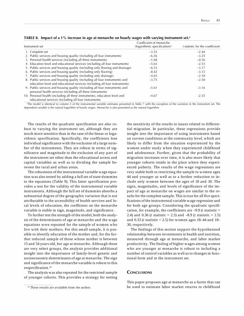
KNAUL 81
The results of the quadratic specification are also ro-bust to varying the instrument set, although they aremuch more sensitive than in the case of the linear or loga-rithmic specification. Specifically, the coefficients loseindividual significance with the exclusion of a large num-ber of the instruments. They are robust in terms of sig-nificance and magnitude to the exclusion of any part ofthe instrument set other than the educational access andcapital variables as well as to dividing the sample be-tween the rural and urban areas.
The robustness of the instrumental variable wage equa-tion was also tested by adding a full set of state dummiesto the equations (Table 9). This latter specification pro-vides a test for the validity of the instrumental variableinstruments. Although the full set of dummies absorbs asubstantial degree of the geographic variation that is notattributable to the accessibility of health services and lo-cal levels of education, the coefficient on the menarchevariable is stable in sign, magnitude, and significance.
To further test the strength of the model, both the analy-sis of the determinants of age at menarche and the wageequations were repeated for the sample of women wholive with their mothers. For this small sample, it is pos-sible to identify education of the mother and, for the fur-ther reduced sample of those whose mother is between15 and 54 years old, her age at menarche. Although theseare very select groups, the analysis provides additionalinsight into the importance of family-level genetic andsocioeconomic determinants of age at menarche. The signand significance of the menarche variable is robust to thisrespecification.16
The analysis was also repeated for the restricted sampleof younger cohorts. This provides a strategy for testing
the sensitivity of the results to issues related to differen-tial migration. In particular, these regressions provideinsight into the importance of using instruments basedon current conditions at the community level, which arelikely to differ from the situation experienced by thewomen under study when they experienced childhoodand adolescence. Further, given that the probability ofmigration increases over time, it is also more likely thatyounger cohorts reside in the place where they experi-enced puberty. The results of the wage regressions arevery stable both to restricting the sample to women ages44 and younger as well as to a further reduction to in-clude only women between the ages of 18 and 30. Thesigns, magnitudes, and levels of significance of the im-pact of age at menarche on wages are similar to the re-sults for the complete sample. This is true for all five speci-fications of the instrumental variable wage regression andfor both age groups. Considering the quadratic specifi-cation, for example, the coefficients are –9.9 (t statistic =2.4) and 0.36 (t statistic = 2.3) and –8.9 (t statistic = 2.5)and 0.33 (t statistic = 2.5) for women ages 18–44 and 18–30, respectively.
The findings of this section support the hypothesizedrelationship between investments in health and nutrition,measured through age at menarche, and labor marketproductivity. The finding of higher wages among womenwho are younger at menarche is robust to including anumber of control variables as well as to changes in func-tional form and in the instrument set.
CONCLUSIONS
This paper proposes age at menarche as a factor that canbe used to estimate labor market returns to childhood
TABLE 8. Impact of a 1% increase in age at menarche on hourly wages with varying instrument set.a
Coefficient of menarcheInstrument set (logarithmic specification)a t statistic for the coefficient
1. Complete set –3.52 –2.442. Public services and housing quality (including all four instruments) –6.36 –3.253. Personal health services (including all three instruments) –1.68 –0.364. Education level and educational services (including all four instruments) –5.63 –2.535. Public services and housing quality (including only flooring and drainage) –6.53 –3.176. Public services and housing quality (including only flooring) –8.42 –3.337. Public services and housing quality (including only drainage) –4.65 –2.188. Public services and housing quality (including all four instruments) and –3.75 –2.50
education level and educational services (including all four instruments)9. Public services and housing quality (including all four instruments) and –5.61 –3.16
personal health services (including all three instruments)10. Personal health (including all three instruments), education level and –4.67 –2.35
educational services (including all four instruments)aThe model is identical to column 2 of the instrumental variable estimates presented in Table 7 with the exception of the variation in the instrument set. The
dependent variable is the natural logarithm of hourly wages. Menarche is also presented as the natural logarithm.
16 These results are available from the author.

82 LINKING HEALTH, NUTRITION, AND WAGES: THE EVOLUTION OF AGE AT MENARCHE AND LABOR EARNINGS AMONG ADULT MEXICAN WOMEN
TABLE 9. Wage functiona with varying specifications of the menarche variable and including full set of statedummies,b estimated by instrumental variables;c sample, women ages 18–54, menarche between ages 10 and 17(absolute value of t in parentheses).
Instrumental variable
Independent variables OLS (1) (2) (3) (4) (5)
Menarche (estimated by instrumental variables)ln(menarche) (restricted to 10–17) 0.116 –3.264
(0.73) (1.57)Menarche –0.238 –5.303 –0.632 –3.474
(1.51) (1.43) (2.17) (0.86)Menarche squared 0.190 0.110
(1.37) (0.71)Menarche and years of education 0.055 0.041
(1.67) (1.10)Other human capital variables
Education in years 0.132 0.128 0.129 0.119 –0.593 –0.414(28.09) (22.12) (22.91) (12.39) (1.38) (0.86)
Out-of-school experience 0.035 0.038 0.038 0.038 0.034 0.035(6.86) (6.54) (6.56) (5.78) (5.00) (5.13)
Experience2 (×100) –0.043 0.000 0.000 0.000 0.000 0.000(3.62) (3.42) (3.42) (3.33) (1.87) (2.09)
Controls for ethnicity and residence% of population in localidad who do not speak Spanish –0.423 –0.417 –0.414 –0.485 –0.478 –0.503
(1.76) (1.71) (1.70) (1.89) (1.88) (1.98)Dummy for missing values (1 = missing value)e –0.043 –0.167 –0.166 –0.070 –0.052 –0.025
(0.32) (1.02) (1.01) (0.35) (0.28) (0.13)Altitude (km above sea level) –0.027 –0.028 –0.028 –0.027 –0.012 –0.016
(1.39) (1.47) (1.47) (1.39) (0.57) (0.72)Dummy for missing values (1 = missing value)e –0.059 –0.188 –0.179 –0.269 –0.231 –0.270
(0.34) (0.97) (0.93) (1.16) (1.15) (1.23)Dummy rural-urban (rural = 1) –0.030 0.046 0.044 0.030 0.059 0.047
(0.68) (0.67) (0.64) (0.40) (0.80) (0.62)Distance to most common market (km) (×100) 0.046 0.001 –0.007 0.193 –0.126 0.021
(0.29) (0.01) (0.04) (0.82) (0.64) (0.07)Dummy distance to market missing (1 = missing value)e –0.188 –0.172 –0.167 –0.296 –0.293 –0.335
(0.86) (0.77) (0.75) (1.24) (1.16) (1.36)Constant –0.164 8.450 3.189 36.623 8.372 26.466
(0.39) (1.59) (1.58) (1.50) (2.20) (1.02)n = 3,155R2 0.2711F statistic 45.43 40.69 41.50 28.15 35.22 38.04Hausman test 6.176 6.050 4.024 4.546 6.536
[P > χ2, degrees of freedom (df)] (0.13, 1) (0.01, 1) (0.13, 2) (0.10, 2) (0.09, 3)Overidentification tests 29.22 29.64 22.73 24.93 24.28
(P > χ2, df = 13) (0.01) (0.01) (0.05) (0.02) (0.03)
F test for joint significance of instruments using positive wage earners: 1.87 (P > F = 0.0291, df = 13)aStandard errors are calculated using robust (Huber, White, Sandwich) estimator of variance provided with STATA. There is no correction for sample selection as the
inverse Mills ratio is insignificant using available identifying variables. bIndividual state dummies are included but not reported.cThe instrumental variables are % of population in municipality with earth floor in their homes and distance to the nearest nonprivate health center. % of population
without running water, % of population over age 15 with incomplete primary education, % of population over age 15 that is illiterate, distance (km) to nearestnonprivate health center (urban = 0 km), dummy distance to health center missing (1 = missing values), number of physicians in localidad or municipality, dummy forthe presence of a community health center in localidad, distance (km) to nearest secondary school (urban = 0), dummy distance to school missing (1 = missing values),dummy for no secondary school in the localidad, controls for ethnicity and residence, % of population in localidad who do not speak Spanish, dummy for missingvalues (1 = missing value), altitude (km above sea level), dummy for missing values (1 = missing value), dummy rural-urban (rural = 1), distance (km) to most commonmarket (urban = 0), dummy distance to market missing (1 = missing values), dummy oversampled states (oversampled = 1). Dummies for missing values are includedfor distance to nearest health clinic and for distance to nearest secondary school.
dOversampled states are Chiapas, Estado de México, Guanajuato, Guerrero, Hidalgo, Michoacán, Oaxaca, Puebla, and Veracruz.eApplies only to rural areas because the variable is assumed to be 0 for urban areas.

KNAUL 83
investments in health and nutrition. Measurement error,combined with simultaneity, however, suggests the needto use instrumental variable techniques when estimat-ing such wage functions.
The retrospective recall data available for this studyshow that average age at menarche has been decreasingin Mexico over the past 40–50 years. The decline has beensomewhat slower than in the developed world. Factorsassociated with this decline include urbanization, in-creased levels of education, and improved living condi-tions. In particular, variables that measure access to pub-lic services and the quality of housing appear to have animportant impact. The proportion of the community withearth flooring in their homes and the proportion who lacktoilet or drainage facilities are particularly strong corre-lates of menarche. Access to personal health servicesappears to have little marginal impact on the age atmenarche.
The findings reported here suggest that nutrition andcumulative health status, measured by age at menarche,have a significant effect on the labor market productivityof Mexican women. Younger ages at menarche are asso-ciated with higher wages. The overall effect is masked inan OLS wage equation because of errors of recall, round-ing by year, and misreporting of the variable. The instru-mental, errors-in-variables model suggests that a declineof one year in age at menarche is associated with a wageincrease of 23%–26%. This value is consistent using adouble-logarithmic, semilogarithmic, or quadratic speci-fication of the menarche variable. The results suggest thepossibility of higher returns to some health investmentsamong the healthier segments of the population. Thisfinding deserves further research as it contrasts with theexisting evidence that suggests that health has a largerreturn at lower levels of health and that the importanceof health investments as inputs into labor productivitywill decline with economic development (Strauss andThomas, 1998).
Future research should use other data sets to includeother human capital inputs. It will also be interesting tobroaden the conceptualization of female health by con-sidering additional measures of health and nutrition.These should be compared and combined with age atmenarche. Further, it will be important to include addi-tional information on the origin and migration patternsof the women in order to better identify the impact ofhealth, education, and other public services as well aspoverty and living conditions during infancy and child-hood on health outcomes.
The results of this paper lend support to the impor-tance of investing in health and early nutrition, particu-larly through sanitation and housing conditions, in or-der to improve individual and family well-being and to
reduce poverty. Health has an important, independenteffect as an investment in human capital in addition toeducation. Further, the findings suggest that, for the pur-poses of economic analysis, age at menarche should beconsidered a complement to adult height as a measureof secular changes in the health and nutritional condi-tion of women.
REFERENCES
Amann GM. Sexual socialization during early adolescence: themenarche. Adolescence. 1986; 21(83):703–710.
Avila A. La desnutrición infantil en el medio rural. Salud Pública deMéxico. 1998; 40:150–160.
Barro R. Economic Growth. New York: McGraw Hill; 1995.Bean JA, Leeper JD, Wallace PB. Variations in the reporting of men-
strual histories. American Journal of Epidemiology. 1979;109(2):181–185.
Becker GS. Human Capital. Chicago: University of Chicago Press;1993.
Bergsten BA. A note on the accuracy of recalled age at menarche.Annals of Human Biology. 1976; 3(1):71–73.
Bielicki T, Waliszho A, Hulanicka B. Social-class gradients in me-narcheal age in Poland. Annals of Human Biology. 1986; 13(1):1–11.
Bobadilla JL, Frenk J, Lozano R. The epidemiologic transition andhealth priorities. In: Jamison D. (ed.) Disease Control Priorities inDeveloping Countries. Oxford: Oxford University Press for theWorld Bank; 1993.
Bojlén K, Weis BM. Seasonal variation in the occurrence of menarchein Copenhagen girls. Human Biology. 1971; 43(4):493–501.
Bound J, Jaeger D, Baker R. Problems with instrumental variablesestimation when the correlation between the instruments andthe endogenous explanatory variable is weak. Journal of theAmerican Statistical Association. 1995; 90(430):443–450.
Brundtland G, Walloe L. Menarchal age in Norway: halt in the trendtowards earlier maturation. Nature. 1973; 241:478–479.
Cravioto P, Cravioto J, Bravo G. Age of menarche in a rural popula-tion: accuracy of records four years later. Boletín Médico del Hos-pital Infantil de México. 1987; 44(10):589–593.
Cumming DC. Menarche, menses and menopause: a brief review.Cleveland Clinical Journal of Medicine. 1990; 57(2):169–175.
Delgado HL, Hurtado E. Physical growth and menarche in Guate-malan adolescents. Archives Latinoamerican of Nutrition. 1990;40(4):503–517.
Díaz de Mathman C, Ramos GR, Landa RV. Crecimiento y desarrolloen adolescentes femeninos: edad de la menarquía. Boletín Médicodel Hospital Infantil de México. 1968a; 25:787–793.
Díaz de Mathman C, Ramos GR, Landa RV. Crecimiento y desarrolloen adolescentes femeninos: menarquía y crecimiento. BoletínMédico del Hospital Infantil de México. 1968b; 25:795–802.
Dreizen S, Spirakis CN, Stone RE. A comparison of skeletal growthand maturation in undernourished and well-nourished girlsbefore and after menarche. Journal of Pediatrics. 1967; 70:256.
Eveleth P. Population differences in growth: environmental andgenetic factors. In: Falkner F, Tanner JM, eds. Human Growth:A Comprehensive Treatise, Vol. 2. New York: Plenum Press;1978.
Floud R. The heights of Europeans since 1750: a new source forEuropean economic history. In: Komlos J, ed. Stature, LivingStandards, and Economic Development: Essays in AnthropometricHistory. Chicago: The University of Chicago Press; 1994.

84 LINKING HEALTH, NUTRITION, AND WAGES: THE EVOLUTION OF AGE AT MENARCHE AND LABOR EARNINGS AMONG ADULT MEXICAN WOMEN
Fogel RW. Economic growth, population theory and physiology.American Economic Review. 1994; 84(3):369–395.
Food and Agriculture Organization of the United Nations. The Stateof Food and Agriculture. Rome: Food and Agriculture Organiza-tion of the United Nations; 1996.
Frenk J. Reformar sin deformar: la necesidad de una visión integralen la transformación del sistema de salud mexicano. In: FrenkJ, ed. Observatorio de la salud: necesidades, servicios y políticas.México, DF: Fundación Mexicana para la Salud; 1997.
Frenk J, Bobadilla JL, Sepúlveda J. Health transition in middle-income countries: new challenges for health care. Health Policyand Planning. 1989; 4(1).
Frenk J, González-Block MA, Lozano R. Economía y salud: propuestaspara el avance del sistema de salud en México. Informe final. México,DF: Fundación Mexicana para la Salud; 1994b.
Frenk J, Lozano R, Bobadilla JL. La transición epidemiológica enAmérica Latina. Notas de Población, Santiago de Chile. 1994c;XXII(60).
Frenk J, Duran-Arenas I, Vázquez-Segovia A. Los médicos enMéxico, 1970–1990. Salud Pública de México. 1995; 37:19–30.
Frenk J, Knaul F, Vázquez-Segovia A. Trends in Medical Employment:Persistent Imbalances in Urban México. México, DF: Centro deInvestigación y Docencia Económicas; 1997.
Frisch R, Revelle R. Height and weight at menarche and a hypoth-esis of critical body weights and adolescent events. Science. 1970;169:397–398.
Graber J, Brooks-Gunn J, Warren J. The antecedents of menarchealage: heredity, family environment and stressful life events. ChildDevelopment. 1995; 66:346–359.
Greene WH. Econometric Analysis. Englewood Cliffs, NJ: PrenticeHall, 1997.
Griliches Z. Estimating the return to schooling: a progress report.Econometrica. 1977; 45(1):1–22.
Hausman JA. Specification tests in econometrics. Econometrica. 1978;46(6):1251–1272.
Heckman JJ. Sample selection bias as a specification error. Econo-metrica. 1979; 47(1):153–162.
Hediger ML, Stine RA. Age at menarche based on recall informa-tion. Annals of Human Biology. 1987; 14(2):133–142.
Hulanicka B, Waliszko A. Deceleration of age at menarche in Po-land. Annals of Human Biology. 1991; 18(6):507–513.
Instituto Nacional de Estadística, Geografia e Informática (INEGI).Anuarios Estadísticos Estatales, 1995. México, DF: INEGI; 1995.
Jacobo M, Malacara JM. Correlation of menarche with age and vari-ous somatometric indexes. Boletín Médico del Hospital Infantil deMéxico. 1985; 42(1): 37–41.
Knaul F, Parker S, Ramírez R. El prepago por servicios médicosprivados en México: determinantes socio-económicos y cambiosa través del tiempo. In: Frenk J, ed. Observatorio de la salud:necesidades, servicios y políticas. México, DF: Fundación Mexicanapara la Salud; 1997.
Komlos J. The age at menarche and age at first birth in an under-nourished population. Annals of Human Biology. 1989; 16(5):559–562.
Laska-Mierzejewska T. Effect of ecological and socio-economic fac-tors on the age at menarche, body height and weight of ruralgirls in Poland. Human Biology. 1970; 42(2):284–292.
Leibenstein H. Economic Backwardness and Economic Growth: Studiesin the Theory of Economic Development. New York: Wiley andSons; 1957.
Liestøl K. Social conditions and menarcheal age: the importanceof early years of life. Annals of Human Biology. 1982; 9(6):521–537.
Liestøl K, Rosenberg M. Height, weight and menarcheal age ofschoolgirls in Oslo. An update. Annals of Human Biology. 1995;22(3):199–205.
Maclure M. A prospective cohort study of nutrient intake and ageat menarche. American Journal of Clinical Nutrition. 1991; 54(4):649–656.
Malcolm L. Protein-energy malnutrition and growth. In: Falkner F,Tanner JM, eds. Human Growth: A Comprehensive Treatise, Vol.2. New York: Plenum Press; 1978.
Manniche E. Age at menarche: Nicolai Edvard Ravn’s data on 3385women in mid-19th century Denmark. Annals of Human Biol-ogy. 1983; 10(1):79–82.
Marshall WA. Puberty. In: Falkner F, Tanner JM, eds. Human Growth:A Comprehensive Treatise, Vol. 2. New York: Plenum Press; 1978.
Mascie, Taylor CGN, Boldsen JL. Recalled age of menarche in Brit-ain. Annals of Human Biology. 1986; 13(3):253–257.
Mincer J. Schooling, Experience and Earnings. New York: ColumbiaUniversity Press; 1974.
Moisan J, Meyer F, Gingras S. A nested case control study of thecorrelates of early menarche. American Journal of Epidemiology.1990; 132(5):953–961.
Moock P, Leslie J. Childhood malnutrition and schooling in the Terairegion of Nepal. Journal of Development Economics. 1986; 20:33–52.
Nagata H, Sakamoto Y. A comparison of height growth curvesamong girls with different ages of menarche. Human Biology.1988; 60(1):33–41.
Rosenzweig M. Labor markets in low income countries. In: CheneryH, Srinivasan TN, eds. Handbook of Development Economics, Vol.1.Amsterdam: North-Holland Press; 1988.
Ruble D, Brooks-Gunn J. The experience of menarche. Child Devel-opment. 1982; 53:1557–1566.
Salud Pública de México. Aspectos relevantes sobre la estadísticade deficiencias de la nutrición. Salud Pública de México. 1998;40(2):206–215.
Schultz TP. Lifetime migration within educational strata. EconomicDevelopment and Cultural Change. 1982; 30(3):559–593.
Schultz TP. Wage Rentals for Reproducible Human Capital: Evidencefrom Two West African Countries. Working Draft; New Haven:Yale University, mimeo; 1996.
Schultz TP. Assessing the productive benefits of nutrition and health:an integrated human capital approach. Journal of Econometrics.1997; 77(1):141–158.
Schultz TP, Tansel A. Wage and labor supply effects of illness inCôte d’ Ivoire and Ghana: instrumental variable estimates fordays disabled. Journal of Development Economics. 1997; 53(2):251–286.
Secretaría de Salud. Encuesta nacional de salud II. México, DF:Secretaría de Salud; 1994.
Staiger D, Stock J. Instrumental variables regression with weak in-struments. Econometrica. 1997; 65(3):557–586.
Stark O, Peckham CS, Moynihan C. Weight and age at menarche.Archives of Disease in Childhood. 1989; 64(3): 383–387.
Steckel RH. Stature and the standard of living. Journal of EconomicLiterature. 1995; 33(4):1903–1940.
Strauss J. Does better nutrition raise farm productivity? Journal ofPolitical Economy. 1986; 94(2):297–320.
Strauss J, Thomas D. Health and wages: evidence on men andwomen in urban Brazil. Journal of Econometrics. 1997; 77(1):159–186.
Strauss J, Thomas D. Health, nutrition and economic development.Journal of Economic Literature. 1998; 36(2):766–817.
Tanner JM. Growth at Adolescence. Oxford: Blackwell Scientific Pub-lications; 1962.

KNAUL 85
Treloar SA, Martin NG. Age at menarche as a fitness trait: nonaddi-tive genetic variance detected in a large twin sample. AmericanJournal of Human Genetics. 1990; 47(1):137–148.
Trussel J, Steckel R. The age of slaves at menarche and their firstbirth. Journal of Interdisciplinary History. 1978; 8(3):477–505.
Ulijaszek SJ, Evans E, Miller DS. Age at menarche of European, Afro-Caribbean and Indo-Pakistani schoolgirls living in London.Annals of Human Biology. 1991; 18(2):167–175.
Valenzuela CY, Nuñez E, Tapia C. Month at menarche: a re-evalu-ation of the seasonal hypothesis. Annals of Human Biology. 1991;18(5):383–393.
Weir J, Dunn JE, Jones EG. Race and age at menarche. Communica-tions in Brief. 1971; 111(4):594–596.
Wellens R, Malina RM, Beunen G. Age at menarche in Flemish girls:current status and secular change in the 20th century. Annals ofHuman Biology. 1990; 17(2):145–152.
White H. A heteroskedasticity-consistent covariance matrix estima-tor and a direct test for heteroskedasticity. Econometrica. 1980; 48:817–838.
Wong R, Parker S, de la Vega S. Household Health Expenditures inMexico: The Influence of the Local Health Sector. Presented at theAnnual Meeting of the Population Association of America;Washington, DC, March 1997.
World Bank. Investment in Health, World Development Report. Wash-ington, DC: World Bank; 1993.
Wyshak G, Frisch R. Evidence for a secular trend in age of menarche.New England Journal of Medicine. 1982; 306(17):1033–1035.
Wyshak G. Secular changes in age at menarche in a sample of USwomen. Annals of Human Biology. 1983; 10(1):75–77.
Zurita B, Nigenda G, Ramírez T. Encuesta de satisfacción con losservicios de salud 1994. In: Frenk J, ed. Observatorio de la salud:necesidades, servicios y políticas. México, DF: Fundación Mexicanapara la Salud; 1997.
TABLE 1A. Differences between women included in the individualquestionnaire and those not interviewed.
Variable Included ExcludedAge
Mean 31.91 30.18Median 30 27Observed 11,058 1,392
Groups18–24 3,246 56425–35 3,615 38935–44 2,604 24445–54 1,588 195
EducationMean 5.80 6.57Median 6 6Observed 11,049 1,374
Labor force participationMean 0.29 0.37Observed 11,058 1,392
Weekly wagesMean 263.47 265.31Median 140 175Observed 3,273 535
ANNEX

86 LINKING HEALTH, NUTRITION, AND WAGES: THE EVOLUTION OF AGE AT MENARCHE AND LABOR EARNINGS AMONG ADULT MEXICAN WOMEN
TABLE 2A. Wage functions1 with sample selection correction for labor force participation. Log menarche estimatedwith instrumental variables;2 sample, women ages 18–54, menarche between ages 10 and 17 (absolute value of z inparentheses).
InstrumentalProbit for labor OLS variable
Independent variables force participation wage function5 wage function
Menarcheln(menarche) 0.162 0.080 –3.639
(1.25) (0.50) (2.53)Other human capital variables
Experience (age – years of education – 6) 0.039 0.030 0.037(8.79) (3.19) (3.51)
Experience squared (×100) –0.046 –0.035 –0.042(4.91) (2.43) (2.56)
Education in years 0.084 0.127 0.132(16.92) (6.73) (6.46)
Controls for ethnicity and residence% of population in localidad who do not speak Spanish –0.359 –0.446 –0.480
(3.23) (2.27) (1.86)Dummy for missing values (1 = missing value)3 0.375 –0.087 –0.173
(3.41) (0.56) (1.00)Altitude (km above sea level) 0.012 –0.015 –0.015
(1.20) (1.26) (0.92)Dummy for missing values (1 = missing value)3 0.123 0.099 –0.077
(1.09) (0.64) (0.41)Dummy rural-urban (rural = 1) –0.277 –0.003 0.050
(7.55) (0.04) (0.58)Dummy oversampled states (oversampled = 1)4 0.134 –0.145 –0.033
(2.77) (2.17) (0.43)Distance (km) to most common market (urban = 0) (×100) –0.142 0.075 0.024
(1.27) (0.49) (0.14)Dummy distance to market missing (1 = missing values)2 –0.668 –0.095 –0.157
(4.80) (0.38) (0.56)
Identification of labor force participationIf house has interior sewage connection (sewage = 1) 0.039
(1.14)Number of bedrooms per family member 0.304
(4.52)If house has own kitchen (kitchen = 1) –0.119
(2.79)If house has interior running water (water = 1) –0.058
(1.76)Inverse Mills ratio5 –0.129 0.032
(0.43) (0.10)Constant –1.950 0.294 9.409
(5.71) (0.39) (2.62)
F statistic 848.81 83.70 33.82[P > F, degrees of freedom (df)] (values for χ2 given for probit model) (0.00, 16) (0.00, 13) (0.00, 13)
R2 0.26n 10,774 3,133 3,133Hausman statistic: H = 7.22, df = 1, P > χ2 = 0.01
1Standard errors are calculated using robust (Huber, White, Sandwich) estimator of variance provided with STATA. Hourly positive wages of all salaried andunsalaried workers, using weekly hours and wages as the base and dividing by weekly hours.
2The instrumental variables are % of population with earth floor, % of population without toilet or drainage facilities, % of population living in overcrowdedconditions, % of population without running water, % of population over age 15 with incomplete primary education, % of population over age 15 who are illiterate,distance (km) to nearest nonprivate health center (urban = 0 km), dummy distance to health center missing (1 = missing values, rural), number of physicians in localidador municipality, dummy for the presence of a community health center in localidad, distance (km) to nearest secondary school (urban = 0), dummy distance to schoolmissing (1 = missing, rural), dummy for no secondary school in the localidad, controls for ethnicity and residence, % of population in localidad who do not speakSpanish, dummy for missing values (1 = missing value, rural), altitude (meters above sea level), dummy for missing values (1 = missing value, rural), dummy rural–urban(rural = 1), distance (km) to most common market (urban = 0), dummy distance to market missing (1 = missing values, rural), dummy oversampled states (oversampled= 1). Dummies for missing values are included for distance to nearest health clinic and for distance to nearest secondary school.
3Applies only to rural communities, because the variable is assumed to be 0 for urban areas.4Oversampled states: Chiapas, Estado de México, Guanajuato, Guerrero, Hidalgo, Michoacán, Oaxaca, Puebla, and Veracruz.5The inverse Mills ratio is entered into the instrumental variable wage equation by a two-step procedure.

87
HEALTH AND PRODUCTIVITY IN PERU:AN EMPIRICAL ANALYSIS BY GENDER AND REGION1
Rafael Cortez2
INTRODUCTION
This study aims to measure the association betweenhealth and wages in Peru, in order to then explore theimpact that health has on productivity. It also seeks toassess the consequences of omitting the variable healthfrom the estimates of other variables included in the wageequation. Finally, it examines the impact that availabil-ity of public health care services has on productivity, allof the above based on the existence of a relationship ofsimultaneity between earnings and self-reported healthstatus.
In the study of economic growth and distribution ofwealth, increasing importance is being attached to hu-man capital factors as determinants of economic growthand wage rates. However, only recently have the returnson investment in health begun to be studied in develop-ing countries. Recent studies (Schultz, 1997; Schultz andTansel, 1997; Thomas and Strauss, 1997) confirm the ideathat health is a form of human capital that influences wagelevels and, therefore, the capacity of individuals to gen-erate sustained and rising income over time, with imme-diate positive consequences on the level of expenditureand living standard of their household members.
The earliest studies that associated health with produc-tivity were carried out in the framework of the efficiency
wage hypothesis (Pitt, Rosenzwei, and Hassan, 1990;Behrman and Deolaliker, 1988; Sahn and Alderman,1988). These were the first studies that looked at devel-oping countries and linked nutrition with productivity.
Recently, literature on economics has placed greateremphasis on the measurement of health status throughthe use of indicators included in household surveys.These health indicators include adult height data, re-ported morbidity rates, days disabled, and days ill. Thesevariables are subject to measurement errors, given thebiases that result from self-reporting. Such biases areobviously correlated with the educational level of therespondent, household income, and other unobservedvariables.
The inclusion of the health indicator in the wage equa-tion represents an attempt to measure the returns tohealth in the labor market and, at the same time, facili-tate the evaluation of the effects that public investmentpolicies have on health status and, consequently, on in-come. Within this analytical framework, Thomas andStrauss (1997) used the results of the Brazilian householdsurvey, which contains information on adult height. Theauthors conclude that greater height has a positive effecton individual productivity. Another interesting findingfrom their study is that, when the health variable wasincluded, the estimated returns to education were 45%lower for men with no education and 30% lower for menwith secondary or higher education.
Schultz and Tansel (1997) used instrumental variableestimates for days of disability to estimate wage equa-tions in Ghana and Côte d’Ivoire. Their principal findingwas that health status is an explanatory factor in wagelevel and that better health status also is associated withlonger productive life.
This study estimated the effects of health on produc-tivity in Peru. For that purpose, a health indicator basedon days of illness reported by adults in the 15 days prior
1 This study was conducted as part of the Latin American Re-search Network project “Productivity of Household Investment inHealth,” sponsored by the Inter-American Development Bank (IDB).The author is grateful for the contribution of César Calvo, who as-sisted in the research, and for the valuable comments of Dr. PaulSchultz of Yale University, Dr. Bill Savedoff of IDB, and all the par-ticipants in the seminar “Impact of Public and Private Investmentin Health on Productivity.” The author alone is responsible for anyerrors or omissions.
2 Professor and investigator at Centro de Investigación de laUniversidad del Pacífico and Post-doctoral Fellow of the EconomicGrowth Center of the Economics Department of Yale University.

88 HEALTH AND PRODUCTIVITY IN PERU: AN EMPIRICAL ANALYSIS BY GENDER AND REGION
to the interview was used. The data for the study werederived from Peru’s 1995 National Household Survey.
First, the wage functions for adults by sex and geo-graphic area (rural and urban) were estimated, with thehealth variable instrumented as one of the human capi-tal variables. Second, the study analyzed the impact thatpublic investment in health has on wages. The estima-tion process corrected for the selection bias and controlledfor endogeneity and measurement error in the health sta-tus indicator. The health variable equation used a set ofidentifiers such as health infrastructure (number of healthcare facilities per capita), housing infrastructure (hoursof water supply, availability of adequate sewerage, andtype of flooring in the housing unit), and price of healthinputs, which directly affect health but do not directlyinfluence the determination of wages.
Given the nature of the indicator, the health equationwas estimated using a tobit model censored at zero. Theinstruments used were robust, and an inverse relation-ship was found between age and health status, which isconsistent with the fact that morbidity rates and numberof days ill generally rise with age. Access to adequatehousing infrastructure had a positive effect on health;conversely, low living standards at the community levelhave a negative effect on individual health status for com-munity residents. In rural areas, non-labor income levelswere not significant.
The wage equation was estimated using a two-stageprocedure (Heckman, 1979; Lee, 1983) and corrected forthe selection bias resulting from the inclusion of non-participants in the labor market. The wage equationsshowed that the rate of return to education was overesti-mated if the health variable was omitted and that the dif-ference was greater for the female population than forthe male population in urban areas. The difference in ratesof return (wage equation without health versus wageequation with health [IV]) was 9.5% and 1.3% for urbanand rural men, respectively, and 15.7% and 1.3% for ur-ban and rural women, respectively. The results clearlyshow the positive effect of health on productivity; thecoefficients were significant and indicated that the im-pact of more healthy days on wages was greater in ruralpopulations than in urban ones.
Section 2 describes the database for the study—the 1995Peruvian National Household Survey—which includesdemographic, social, economic, and health informationon 98,984 individuals in 19,975 households. It also pre-sents a brief overview of the health and well-being of thePeruvian population. Section 3 deals with how to mea-sure health and correct for measurement error, and Sec-tion 4 is about the simultaneity between health and pro-ductivity. Section 5 describes the model of analysis, whichis based on the conceptual framework suggested by
Becker (1965). Section 6 explains the econometric estima-tion model, which takes account of the relationship ofsimultaneity that exists between health and wages, theproblem of omission of variables, and measurement er-ror. Section 7 summarizes the empirical findings of thestudy, and Section 8 presents the conclusions and somepolicy recommendations.
BASIC DESCRIPTION OF THE DATABASE
The data for this study were drawn from Peru’s 1995National Household Survey (NHS), which included so-cioeconomic and demographic information on 19,975households. The information was compiled betweenOctober and December of that year by the National Sta-tistics and Informatics Institute (INEI). A total of 98,984individuals were surveyed.3
Using information from the NHS, Table 1 provides abasic profile of health and poverty conditions in Peru.Because of the study’s focus on the productive impact ofhealth, the data in column 1 of the table relate only topersons aged from over 17 and under 70 years old—i.e.,potential wage-earners. According to Table 1, 36.0% ofthis population lives in poverty, and 13.2% live in ex-treme poverty.4
Health status is measured on the basis of morbidityrates and average number of days ill (in the 15 days pre-ceding the survey). The latter data are also illustrated inFigure 1. In both cases, Table 1 shows a negative correla-tion between poverty and health. Morbidity rates amongthe population living in extreme poverty (31.6%) areclearly higher than the rates in the non-poor population(25.9%). The average morbidity rate for the working-agepopulation is 27.0%.
The association between higher poverty and poorhealth captures several effects of the interaction of thetwo variables and constitutes the subject of this study.Even as a first approximation to the problem, Table 1 re-veals that poverty is also associated with lower rates ofhealth service usage among ill individuals. The rate ismarkedly lower among the extremely poor (26.2%) com-pared to the non-poor (42.9%). Health service usage mightpartly explain the negative association between povertyand health.
Table 2 shows the important role that the public sectorplays in providing health services. On average, 60.0% ofthe population that seeks medical attention in case of ill-ness does so in a public health care facility. The percent-
3 The population group analyzed in the study included 51,545persons over 17 and under 70 years of age.
4 The NHS yielded lower percentages of poverty for the popula-tion as a whole: 32.6% and 12.6%, respectively.

CORTEZ 89
age is higher for the poor population (63.2%) and evenhigher for the population living in extreme poverty(66.0%). Hence, reliance on public health care services isgreater among lower-income households. On the fewoccasions that these households do seek medical care,they receive a greater proportion of such care from min-istry of health establishments.
In this context, public investment in health is essentialto improve health conditions in the country. Presumably,poverty would also be alleviated by investing in health, ifhealth leads to higher earnings and if it can be shown thathealth yields positive and substantial returns. Table 3
TABLE 1. Health conditions, health care, and povertylevels in Peru: population over 17 and under 70 yearsof age.
Averagenumber
Percentage Reported of days of HealthPoverty of the morbidity reported carelevels population rate illness rates
Non-poor 64.0% 25.9% 2.58 42.9%Poor 22.8% 27.5% 2.74 32.8%Extremely poor 13.2% 31.6% 2.88 26.2%
Total – 27.0% 2.65 38.0%
Source: National Household Survey, Peru, 1995.Table prepared by the author.
TABLE 2. Percentages of the total number of ill persons who receivemedical attention at different health service providers, by poverty level inthe population.
Poverty levels
ExtremelyHealth service provider Total Non-poor Poor poor
Public providers 60.0 57.9 63.2 66.0Ministry of Health post or center 26.3 22.5 31.1 38.7Social security hospital 16.6 18.0 15.3 11.2Ministry of Health hospital 12.6 12.4 12.9 13.3Other 4.5 5.0 3.8 2.8
Private providers 40.0 42.1 36.8 34.0Pharmacy 17.8 17.6 19.7 15.1Private physician 9.9 11.5 7.7 4.8Private clinic 4.1 4.9 2.7 2.6Traditional healer 0.9 0.8 1.1 1.2Other 7.3 6.3 5.6 10.3
Total 100.0 100.0 100.0 100.0
Source: National Household Survey, Peru, 1995.Table prepared by the author.
0%
10%
20%
30%
40%
50%
60%
70%
80%
90%
Days ill
Freq
uenc
y %
0 1 2 3 4 5 6 7 8 9 10 11 12 13 14 15
Males Females
FIGURE 1. Distribution of days ill.

90 HEALTH AND PRODUCTIVITY IN PERU: AN EMPIRICAL ANALYSIS BY GENDER AND REGION
describes the relationship to be tested through the designand estimation of an explicit model: the association be-tween health status and poverty (see Figure 2). The resultsof the NHS show a positive relationship between indi-vidual health status and productivity (measured by hourlywage).
The population in the highest hourly wage quintilesexperiences the lowest rates of illness. Among males, therate falls from 29.0% to 19.3% between the highest andlowest quintiles, while among women the difference be-tween quintiles is less marked: 35.1% in the highestquintile versus 28.3% in the lowest (see Figure 2). Thefollowing sections use parametric methods to estimatethe relationship between health and productivity. Thisapproach affords the possibility of assessing the conse-quences of greater or lesser public investment in health(for a specific population group) and estimating the re-turns to health.
MEASURING HEALTH: SELF-REPORTED HEALTH STATUSAND MEASUREMENT ERROR
Measuring health is difficult for several reasons. Someindicators are not objective, some are associated with onlyone dimension of health, and some do not measure a com-plete range of conditions. By analyzing the measurementprocess, it is possible to pinpoint the main problems anddevise methods for dealing with them. In particular, themodel selected can correct for the problem of bias intro-duced by measurement errors and the loss of informa-tion due to downward censoring of the indicator.
Recent economic literature has used health indicatorssuch as standardized anthropometric measures of heightand/or weight (i.e., Rosenzweig and Schultz, 1983;Rosezweig and Wolpin, 1986; Barrera, 1990; Pitt, Rosen-zweig, and Hassan, 1990; Schultz, 1996) and self-reportedillness or disability (Wolfe and Behrman, 1984; Pitt andRosenzweig, 1985; Schultz and Tansel, 1997). At a moreaggregate level, average values of the foregoing variableshave been used, as have mortality or survival rates(Rosenzweig and Schultz, 1982; Pitt, Rosenzweig, andGibbons, 1995).
In comparison with other forms of human capital,health status is especially difficult to measure. Health sta-tus (H*) can be considered a latent variable that is notobservable and that is approximated by imperfect indi-cators (H), such as days of illness, days during which theindividual was unable to work due to illness, and others.When these indicators are obtained from household sur-
TABLE 3. Relationship between self-reported healthstatus and hourly wage.
Hourly wage Morbidity rates (%)
quintiles Males Females
1 29.0 35.12 21.4 29.53 20.4 28.04 21.4 25.75 19.3 28.3
Source: National Household Survey, 1995.Table prepared by the author.
0%
5%
10%
15%
20%
25%
30%
35%
1 2 3 4 5
Income quintiles
Mor
bidi
ty r
ate
Males Females
FIGURE 2. Reported morbidity rate by income level.

CORTEZ 91
veys, they are self-reported values and they are there-fore contaminated by measurement errors. The problemis that if measurement errors κ (κ = H – H*) are not re-duced, the estimated effect of health on another variable,such as wage, can be expected to be biased toward zero.
Measurement errors are especially significant when theavailable information on health status is self-reported.Self-perception of health (or illness) may be correlatedwith certain personal characteristics. For example, peoplewith more education or greater access to health servicesmay be more likely to detect and report symptoms of ill-ness. In an equation in which health is a variable to beexplained, these effects might confound the direct im-pact of education or medical care.5 Another possible con-sequence of the subjectivity of self-reporting of health isthe presence of heteroskedasticity in the health equation,since the variability of the measurement error would alsodepend on some of its explanatory variables.
In addition, there is an inevitable underestimation ofthe severity of recent illness, which may not be fully re-solved at the time of the survey interview.6 Using a di-chotomous variable (i.e., occurrence or non-occurrenceof illness) or a variable of non-recent illness avoids thispossible distortion, but all sensitivity to the severity ornature of the illness is lost. In any case, the longer therecall period used in the survey (e.g., last week or duringthe last three months), the more reliably true health sta-tus will be approximated. To a certain extent, a lengthierrecall period increases the number of observations andtherefore reduces the sensitivity of the indicators totemporal or random factors.
Going back further in time is also desirable because ofthe impact that earlier health conditions generally haveon current health status. In accordance with the intra-personal variations proposed by Behrman (1990), thehuman body can maintain similar levels of productivityin the short term, despite adverse health conditions. Withdata from the south of India, Deolalikar (1988) observedthat current nutrition indicators lose significance whenindicators that reflect longer-term nutritional status areincluded.
In practice, the problem of selecting the best indicatorof health status is usually “solved” by the lack of a betteralternative in the majority of household (or individual)surveys available.7 Peru’s 1995 National Household Sur-vey offers two possible indicators: a dichotomous vari-able of recent occurrence of illness and number of daysthat a person was affected by the illness or condition. Inthe first case, it must be assumed that the illness is a situ-ation caused by poor health status. In other words, if H*is the true and unobservable indicator of health status,then:
G = 1, if H* < HC,and G = 0, if H* ≥ HC,
where G is the dichotomous variable and HC is a certaincritical level of health. Below that level, the individualgets sick.
Using number of days ill as an indicator of health sta-tus requires this additional assumption—the weaker theindividual’s health (i.e., the less capacity he/she has forrecovery), the longer the period of illness will be. In thiscase, the duration of the illness (D) would be negativelydependent on H*:
D = D(H*), if H* < HC, where D’< 0,and D = 0, if H* ≥ HC.
It is important to bear in mind that the description ofhealth by means of days of illness would be censored forvalues higher than HC. Despite differences in the healthstatus of individuals who have not been ill, the indicatorD attributes the same value (zero) to all of them (see Fig-ure 2). However, the indicator “days ill” takes account ofinterpersonal differences in health better than the dichoto-mous variable and it is therefore employed in this studyto calculate the health indicator used in the wageequation.
An additional distortion associated with the use of daysof illness as the basis for the health indicator is rooted inthe fact that individuals tend to round their responses.As a result, differences between individuals whose ill-ness had a duration close to the same round number ofdays (3, 5, 10, 15) are lost. The tendency toward round-ing is especially marked when the illness is lengthy. Aprecise response is more likely when the illness lasts onlya few days.
5 Butler et al. compared self-reporting of arthritis with objectivediagnosis. The authors found that correct reporting was more likelyamong male wage-earners with a secondary education. The prob-ability of reporting an illness appeared to rise with severity of theillness, income, and age. On the other hand, Wolfe and Behrman(1984), with data from Nicaragua, found that women with the mostschooling were less likely to report the occurrence of parasitic dis-eases.
6 Assuming that the duration of the illness (D) perfectly reflectedits severity, a survey would find D*=Min{D;L}, where L is the timeelapsed between the onset of the illness and the moment when thesurvey is conducted. If, in addition, the time of onset were relatedto some individual characteristic (e.g., occupation, place of resi-dence), the estimate of the impact of this characteristic would beeven more biased in a health equation.
7 In the empirical sphere, investigators in the field of economicshave a limited number of health indicators at their disposal andgenerally choose the one that has the least measurement error. Theevidence does not show any conclusive divergence among the mostfrequent indicators. Haddad, Kennedy, and Sullivan (1994) com-pared databases from the Philippines, Brazil, Ghana, and Mexicoand found that both absolute occurrence of illness and the numberof days ill are “useful” approximations to indicators based on weightand height.

92 HEALTH AND PRODUCTIVITY IN PERU: AN EMPIRICAL ANALYSIS BY GENDER AND REGION
The relationship between health status and days ill(D=D(H*)) may not be linear. It is therefore advisable totest several transformations of D in order to generate ahealth indicator H. Of course, all these transformationsimply an inverse relationship between the two variablesand recognize upward censoring in the indicator H. Theupper limit would be HS = D–1 (0).
SIMULTANEITY BETWEEN HEALTH ANDPRODUCTIVITY
Estimating the impact of health on productivity is a com-plex undertaking because the interactions between wageand health are not limited to this impact. Just as health isa form of human capital that enhances the level of pro-ductivity, wage level (W) also affects health.
The income effect is the most obvious means by whichproductivity contributes to better health status (consid-ering health a normal good): the capability to earn morepermits an individual to consume more health “inputs”(e.g., foods or drugs). However, greater productivity maygenerate certain incentives that affect individuals’ behav-ior. For example, productivity may encourage an indi-vidual to work harder, which, in turn, may affect his/her health negatively, or a family might opt to utilize agreater portion of its disposable income to strengthen thehealth of the most productive member of the household.
The concept of endowment figures prominently in theliterature on the subject. The term refers to a set of unob-servable characteristics inherent in individuals that af-fect their health and, therefore, their productivity. Theseare unalterable features (a certain physical constitution,for example) that are exogenous and random. It is gener-ally assumed that endowments (µ) are a component ofthe error term of the equations of the variables they af-fect. In this case, simultaneity between two variables doesnot occur only in the presence of explicit effects of onevariable on the other. The correlation of their error termsalso distorts the estimates. If εW and εH* are the error termsof equations that explain wage and health, a problem ofsimultaneity would occur if Cov (εW, εH*) were not equalto zero.
Thus, ϕW and ϕH* being the true error terms, εW = µW
+ ϕW, y εH* = µH* + ϕH*. Hence, even if the terms ϕW and ϕH*
are distributed independently, Cov (εW, εH*) = Cov (µW,µH*). The relationship between µW and µH* may be the re-sult of the fact that the same endowment (a particularskill or physical ability, or a psychological trait) both en-genders greater productivity and enables the individualto maintain better health status. In addition, such a rela-tionship may be linked to individual behavior. For ex-
ample, if an individual is endowed with qualities thatgreatly enhance productivity (µW), he/she has an incen-tive to invest in reinforcing those qualities (or in com-pensating for them within the family unit) through un-observable variables captured by µH* (e.g., special effortsto promote health).
THE MODEL
According to Becker (1965), household decisions can beseen as the result of maximization of a utility function,whose variables are consumer goods (Ci), consumergoods that improve health (Y), health status (Hi), andamount of leisure (li). It is assumed that household deci-sions are unitary (i.e, the head of the household imposeshis/her preferences on the rest of the individuals) andthat the household faces time and full-income constraints.Summarizing, the model is expressed as follows.
A household has n members and is run by the house-hold head, who seeks to maximize the utility function:
U = U (Ci, Yi, Hi, li) i = 1,2,…,n (1)
The utility function is assumed to have the desired con-ditions, i.e., the function is continuous, strictly increas-ing, and quasi-concave, and twice-continuously differ-entiable in all its arguments.
The first constraint is the health production function:
Hi = Hi(Ci, Yi, li, X–i, Zi, Z–i, F, ui, u–i) I = 1,2,…,n (2)
where Ci, Yi, and li represent, respectively, level of con-sumption of goods, health inputs, and leisure for an in-dividual i. X-i denotes the level of consumption, health,and leisure of other members of the household, and Z-i,u-i are the vectors of observed and unobserved character-istics of these individuals, respectively; F denotes avail-ability of health or welfare programs and communityinfrastructure.
The second constraint is the full-income (S) constraint,which indicates that all available resources of the house-hold are being devoted to the purchase of goods and ser-vices and to leisure activities.
p c p Y
wl wT V S
j ji
ij
J
k ki
ik j
K
i i
ii
∑∑ ∑∑∑∑
= = +
+ +
= + =
1 1(3)
V represents non-labor income, pj and pk represent theprices of consumer goods and health inputs, Ti is the to-tal amount of time available, and w is the wage rate.

CORTEZ 93
The reduced-form health demand function would beas follows:
Hi = h (Pc, Py, S, F, Zi, ui) (4)
where Pc and Py are the prices of the consumer goods im-portant for health and health inputs, respectively.
The wage equation (6) is estimated on the basis of theframework used by Mincer (1974) and therefore takes intoaccount the presence of an equation that explains thedecision to participate in the labor market (7), whichshould make it possible to correct for the wage function’sproblem of selection bias. The wage function dependson individual characteristics (age, sex), human capitalvariables (years of schooling and work experience), andregional variables that describe the characteristics of thelabor market.
Owing to (a) errors in the measurement of health and(b) its simultaneity with respect to wage or endogeneityof the variable health, the estimate must be correctedthrough the use of instrumental variables. The latter re-quires that the variables that explain wage be includedin the equation used to instrument the health indicatorH:
H = β0 + β1 XH + β2 XW + εH, (5)
where the error term eH captures the measurement errorκ (εH = εH* + κ).
In this context, the acceptance of health as a form ofhuman capital leads to its inclusion among the explana-tory variables of productivity. The wage equation wouldthus take the form:
ln(W) = α0 + α1 XW + αH H* + εW, (6)
where XW is a group of relevant variables; H* denotescorrected individual health status; and εW is a randomerror term. A semilogarithmic specification is used be-cause it is the type most commonly employed in empiri-cal studies on the returns to human capital.
The wage equation (6) has a selection bias which mustbe corrected by using the Heckman procedure, or two-stage estimation (Heckman, 1979; Lee, 1983). The dichoto-mous equation that expresses the decision to participatein the labor market (L) includes as explanatory variableswage, health, and a set of variables XL, which identifythe system. In the estimate, wage is not directly includedbecause it is not observable when the individual does notparticipate in the labor market; it is therefore replaced bythe explanatory variables XW. Similarly, health is replacedby a set of instrumental variables XH .
L = L (W, H*, XL)L = L (XW, XH, XL)
(7)
The set of equations (5), (6), and (7) make up the sys-tem of equations to be estimated. Health is predicted inequation (5)—which is estimated using a tobit model dueto censorship of the health indicator H—and is includedin the wage equation (6).
THE ECONOMETRIC ESTIMATION STRATEGY
Following the practice generally used in previous em-pirical studies, the sample is divided by sex, so that spe-cific equations are estimated for males and females. Totake account of differences between urban and rural en-
0%
10%
20%
30%
40%
50%
60%
70%
80%
90%
100%
[0] [1–6] [7–12] [13– ]
Years of schooling
Labo
r pa
rtic
ipat
ion
rate
Males Females Total
FIGURE 3. Labor participation by years of schooling.

94 HEALTH AND PRODUCTIVITY IN PERU: AN EMPIRICAL ANALYSIS BY GENDER AND REGION
vironments, the wage functions for males and femalesare estimated separately in each geographic area. Deter-mination of the explanatory variables XW, XH, and XL alsofollow the practice customarily found in the literature.Annex I shows the definitions and sample moments forall the variables used in the estimates in the study.
In addition to the health variable, the wage equationincludes age, years of schooling, and the quadratic termsof both. These terms take account of possible non-linearities in the impacts of these variables. The variableXW incorporates two additional variables: residence in thecountry’s capital city and local unemployment rate. Theaim in including the latter variable is to capture inter-district differences in labor markets.
For exploratory purposes, the wage equation was esti-mated without including health. The results show thatthe signs of the human capital coefficients and individualcharacteristics are predicted by the theory that health hasan effect on productivity. These results were robust tochanges in the equation specification.8
With regard to the determinant variables of health XH,it should be noted that the literature suggests that thereare unobserved characteristics µH, associated with indi-
vidual heterogeneity, which would be incorporated inthe error term εH = ϕH* + µH + κ.
Moreover, equation (5) is a function of demand andnot a function of health production and, therefore, thevector XH should incorporate income and prices of health-related products as explanatory variables. These variablesinfluence the quantity of health “inputs” (e.g., nutrients,medical services) consumed by the family unit.
When families demand health inputs for their mem-bers, they are aware of their endowments and other un-observed characteristics µH. The level of consumption ofthese inputs is therefore probably correlated with the er-ror term εH. In fact, health demand only can include fac-tors that, while they affect the production of health, arenot determined by households, at least in the short term.Such is the case with age, education, food prices, supplyof public services, etc.
Among the variables that explain health, access to State-provided health care is important to a subsequent analy-sis of the impact of public investments in personal health.Access to health services is not measured on the basis ofthe services received by each individual because to do sowould introduce the endogenous nature of those services.Use is a decision based on, among other variables, theindividual’s income, opportunity cost of time (in bothcases, measured by wage), and health status.
To simplify the analysis, the number of per capita pub-lic health care facilities in each district was introducedinto the health equation (5). This variable makes it pos-sible to more directly assess the impact of public invest-
8 Replacing age by potential experience maintained the adjust-ment in the regression. The coefficients of the variables were modi-fied in accordance with the linear relationship between experience,age, and years of schooling (EXPERIENCE = AGE – SCHOOLING – 6). Thespecification that incorporates age was chosen, as it also capturespart of the impact of the work experience.
0
0.2
0.4
0.6
0.8
1
1.2
[18–24] [25–34] [35–44] [45–59] [60–70]
Age
Labo
r pa
rtic
ipat
ion
rate
Males Females Total
FIGURE 4. Labor participation by age.

CORTEZ 95
S/.0.0
S/.0.5
S/.1.0
S/.1.5
S/.2.0
S/.2.5
S/.3.0
S/.3.5
[0] [1–6] [7–12] [13– ]
Years of schooling
Hou
rly
wag
e
Males Females Total
FIGURE 5. Hourly wage by years of schooling.
S/.0.0
S/.0.5
S/.1.0
S/.1.5
S/.2.0
S/.2.5
S/.3.0
[18–24] [25–34] [35–44] [45–59] [60–70]
Age
Hou
rly
wag
e
Males Females Total
FIGURE 6. Wage by age group.

96 HEALTH AND PRODUCTIVITY IN PERU: AN EMPIRICAL ANALYSIS BY GENDER AND REGION
ment on health in terms of the supply side. The quadraticterm of this variable was also included in order to ob-serve possible non-linear effects.9
ANALYSIS OF THE RESULTS
The sample used in the regressions includes only indi-viduals over 17 and under 70 years of age—i.e., adultswho are potential participants in the labor market. Theprobit equation of participation in the market is shownin Annex II. Wald tests indicate that the set of instruments,XL, is significant in the four samples comprising men andwomen in urban and rural areas.
Table 4 shows the regressions that include health as adependent variable. The transformation H = 1/(1 + D)was used as a health indicator. This transformation pro-poses an inverse relationship between the duration of ill-ness and the health indicator. It is upwardly censored at1 = [1/(1+0)].
An advantage of the proposed health indicator is thatit shows a marginally declining impact for a larger num-ber of days ill. This is desirable owing to respondents’tendency to round their answers when they do not re-member exactly how many days their illness lasted, whichis more likely when the illness has been prolonged. Theindicator H reduces the importance of variations in re-ported days ill as the number of days rises.10
9 The introduction of the number of public health care facilitiesinto equation (5) raises a problem of endogeneity. Presumably, theState does not distribute its services randomly, with no criteriawhatsoever. Sen (1995) presents a brief description of the politicaleconomy of the distribution of the benefits of social programs. Be-yond the desire to target those who most need these benefits—assuggested by Rosenzweig and Wolpin (1986) and Pitt, Rosenzweig,and Gibbons (1995)—there are problems to be overcome, includingpolitical feasibility and the influence of the most powerful groups.The theory of pressure groups models this phenomenon. On theother hand, the theory of altruism gives formal expression to thedesire to compensate the neediest members of society. In particu-lar, if the public infrastructure is placed preferentially in localitieswith the fewest health resources, the correlation between the errorterm εH and the number of public facilities would be a number otherthan zero, and their impact on health would be downwardly bi-ased. This endogeneity of public health infrastructure necessitatesthe use of instrumental methods. For the sake of simplicity, thisanalysis has not been undertaken here, though the possibility ofdownward biasing of the results is recognized.
10 Other transformations were tried, and it was found that thosethat showed marginally declining impacts for D (reported days ill)had higher levels of likelihood. The following showed the highestlevels: Ha = –÷D, Hb = –ln (1 + D), and H = 1/(1 + D). The lattertransformation yielded the highest values for the logarithm of thelikelihood function in all samples (Annex III). It was therefore pre-ferred to the alternatives. The results presented in the followingsections were robust to changes in the selection of the health indica-tor as long as the indicator preserved the characteristic of margin-ally reducing the impact of D.
11 Only some consumer prices were available for all the country’sdepartments. The data in this case were obtained from the 24departmental statistical compendiums for 1995 published by theNational Statistics and Informatics Institute (INEI).
The results of the health equation (see Table 4) are pre-dicted by the theory. In the case of age, both the linearand the quadratic terms obtain negative coefficients inmost cases. In general, aging is associated with deterio-rating health status, and it also accelerates that deterio-ration. The final effect of age on health is always nega-tive, except in the sample of rural men.
The variables indicative of wealth are significant onlyin some cases. Per capita non-labor family income is sig-nificant only for women, and for women in rural areasan unexpected negative coefficient was obtained. Thisresult is difficult to explain, but it is, nevertheless, con-sistent with the concept of health as a normal good. Hoursof access to the public drinking water supply system andavailability of adequate floors have a positive and sig-nificant impact on health among the population in urbanareas. In this case, in addition to the effect associated withwealth, there appears to be a direct impact on the pro-duction of health.
Education yields a positive impact that is probably as-sociated with better use of knowledge and available in-puts, which enable better care of health. In general, theeducation coefficients in Table 4 would be downwardlybiased if it were true that individuals with more school-ing tend to report symptoms of illness more frequently.
As for the impact of prices of health inputs, with the ex-ception of milk, increases in food prices significantly reducehealth demand in all the samples. The positive coefficientfor milk price might be explained by its correlation with theprices of other foods not included in the estimate.11
Conditions in the community affect the health statusof individuals. Quality of housing construction (non-dirtfloors), provincial poverty index, and local unemploy-ment rate show a positive impact on health. Health ispresumably affected by the living conditions in whichthe individual develops. In addition, residence in the cityof Lima and the coastal region has a positive impact onhealth, controlling for local level of poverty and access topublic health services, which might be associated withthe use of other inputs (e.g., private services) and otherconditions (e.g., climatic factors).
In rural areas, the number of public health facilities percapita has a positive and significant impact on health sta-tus. Table 4 evaluates the implicit effect on the coefficientsof the linear and quadratic terms at the sample mean.The negative coefficient of the quadratic term indicatesdeclining returns on public investment in health. In ur-ban areas, the impacts are negative, and among women

CORTEZ 97
TABLE 4. Health equation by sex and region: censored tobit.a
Males Females
Independent variables Urban Rural Urban Rural
Constant 3.020* 1.408*** 2.367*** 1.572***[10.54] [3.74] [10.84] [4.98]
Individual traits 180.3*** 70.7*** 280.5*** 128.5***Age [10–2] –0.578 0.105 –1.163*** –1.537**
[–1.11] [0.13] [–2.93] [–2.25]Age squared [10–4] –0.871 –1.584* –0.192 0.093
[–1.36] [–1.68] [–0.39] [0.12]Human capital variables 49.7*** 22.5*** 56.1*** 13.2***
Years of schooling [× 10–2] 3.827* 5.899*** 2.296*** –0.480[2.62] [3.26] [2.63] [–0.36]
Years of schooling squared (× 10–1) –0.071 –0.275** –0.024 0.178[–0.76] [–2.05] [–0.39] [1.64]
Household assetsNon-labor income 0.018 –0.017 0.041*** –0.097*
[1.35] [–0.53] [3.55] [–1.85]Housing infrastructure 16.4*** 6.1 26.4*** 8.6***
Hours of water supply [× 10–4] 1.538 3.762* –0.155 2.907*[1.25] [1.86] [–0.16] [1.75]
Adequate sewerage system 0.006 0.049 0.013 –0.113[0.22] [0.57] [0.61] [–1.63]
Non-dirt floor 0.276* 0.093 0.283*** 0.124*[3.66] [1.22] [4.96] [1.93]
Regional variables 13.9*** – 21.2*** –Residence in the coastal region –0.130* 0.131** –0.101*** 0.228***
[–2.98] [2.31] [–3.05] [4.86]Residence in Lima 0.182* – 0.176*** –
[3.64] [4.60]
Community variables 9.7*** 6.2** 17.4*** 6.7**Poverty indicator –0.978** –7.095** –0.711* –1.214
[–1.99] [–2.20] [–1.76] [–0.45]Unemployment rate –1.095** –1.036* –1.361*** –1.236**
[–2.22] [–1.74] [–3.65] [–2.57]Health infrastructure 2.3 – 6.7** –
Number of health care facilities per capita –0.321 0.139** –0.797** 0.089*[–0.66] [2.15] [–2.18] [1.70]
Number of health care facilities per capita squared 0.224 –0.014** 0.699** –0.012***[0.48] [–2.50] [1.99] [–2.73]
Food prices 101.2*** 17.0*** 97.4*** 14.4***Price of rice –0.977* –0.410*** –0.718*** –0.322***
[–9.32] [–2.92] [–9.08] [–2.77Price of tomatoes –0.285* –0.092 –0.198*** –0.088
[–6.64] [–1.37] [–6.03] [–1.53]Price of milk 0.276** 0.607*** 0.286*** 0.475***
[2.08] [3.26] [2.77] [2.92]∂H/∂ [facilities] –0.304 0.135** –0.740** 0.085*
[–0.68] [2.14] [–2.20] [1.67]Ln (likelihood function) –12,209 –4,174 –16,107 –4,721Chi-square 483.3*** – 755.4*** –Prob [H*<1] 22.7% 29.1% 32.7% 38.0%Number of observations 18,787 5,633 20,435 5,671
a Dependent variable: H = 1/(1+ number of days ill).[t-statistic in brackets] and joint significance test italicized.(*) Statistically significant at 10% confidence level; (**) Statistically significant at 5% confidence level; (***) Statistically significant at 1% confidence level.

98 HEALTH AND PRODUCTIVITY IN PERU: AN EMPIRICAL ANALYSIS BY GENDER AND REGION
this effect is statistically significant. These results mightbe explained by the possible presence of heteroske-dasticity in the health equation, as discussed in section3.12 Only the sample of urban women appears to be af-fected by this problem.13
Tables 5 a and b and Tables 6 a and b show the esti-mates of the wage equations in three different cases: (a)excluding the health variable, (b) including the observedhealth values, and (c) including the estimated values ofthe health indicator. The latter were obtained from theregressions in Table 4 and are free from simultaneity andmeasurement error biases.
As predicted by the theory and suggested by Table 3,health status has a significant and positive effect on pro-ductivity. An improvement in health status raises wagesin all population groups for both sexes and in both ur-ban and rural areas. The coefficient of the health indicatoris positive both with the health variable as exogenousand instrumented (IV). However, both the coefficient andthe significance level of the variable health are muchgreater in the latter case.
The extent to which health impacts productivity var-ies according to the population group. Improvements inhealth status have a greater impact on productivity inrural areas, and this effect is greater among rural menthan among rural women.14 Table 7, which shows theimpact of one additional healthy day per month, illus-trates this finding.15
The results for the rest of the variables show that, whenhealth is not controlled for, the coefficients of age andeducation obtained are upwardly biased. This suggeststhat when the health variable is omitted, age and educa-tion capture part of its effects on productivity.
The negative signs of the quadratic terms of age implythat the impact of age on productivity, though initiallypositive, declines and, at a certain point, turns negative.The critical age that marks the beginning of the declinein productivity varies from one sample to another. Ac-cording to the regressions that omit health, in urban ar-eas, maximum productivity is achieved at 49.2 and 46.7
years of age among men and women, respectively. Whenhealth is controlled for, the critical age is later: 53.0 and50.4 years.16,17
The inclusion of the instrumented health variable re-sults in an extension of the cycle of productive life for allindividuals. This result is explained by the fact that ageincreases the probability of suffering from some illnessor ailment (see Table 4). If health is not controlled for asan explanatory factor, the effect of poor health character-istic of older adults is attributed to age. When health iscontrolled for, age has a less negative effect on wage level,and the period of productive life is longer.
The effect of one additional year of education dependson the coefficients of the linear and quadratic terms ofthe education variable and on the individual’s years ofschooling.18 Tables 5a and 5b and 6a and 6b evaluate, atthe sample mean, the marginal return and its significance.The magnitude of the impact varies from one sample toanother. When health is instrumented, the returns toeducation in urban areas are 7.4% and 5.1% for men andwomen, respectively, while in rural areas the figures are5.8% and 10.4%.
When the instrumented health variable is used in thewage equation, it is observed that the returns to educa-tion for men are 9.5% and 55.2% higher in urban and ru-ral areas, respectively, than if the observed health vari-able is used. In the case of women, the proportion ofoverestimation is 15.7% and 2.9% in urban and rural areas,respectively. This upward bias is explained by an ex-pected positive correlation between the two forms ofhuman capital: education and health (Schultz, 1996). Inthe absence of the latter, the education variable capturespart of the impact of the omitted health variable.
The theory suggests several justifications for this typeof correlation. In addition to the existence of individualtraits and heterogeneity, the rational behavior of invest-ment in human capital offers other arguments. One isthat intertemporal preferences (of the parents) affect in-
12 The endogeneity discussed in footnote 7 might also be important.13 Only in this sample did the logarithm of the likelihood func-
tion decrease appreciably after correcting for hetereoskedasticity(from -16,107 to -16,069) and significant coefficients were obtainedin the explanatory regression of the quadratic error term. As notedin section 3, the heteroskedasticity model included education andnumber of health facilities per capita as explanatory variables inthis regression.
14 As noted earlier, these results are robust to changes in the healthindicator, as long as the indicator shows a marginally decreasingimpact for increased days of illness.
15 Given that H = 1/(1 + D), then ∂W/∂D = (∂W/∂H) × (∂H/∂D) =–αH/(1 + D)2, where –αH is the coefficient of the indicator H in thewage equation and D is evaluated at the sample means.
16 Given that the estimated function describes the relationshipbetween health and productivity as an inverted U, the age of maxi-mum productivity (the apex of the parabola) is calculated as E* =–aE1 / [2 H aE2], where aE1 and aE2 are the coefficients of the linearand quadratic terms of age, respectively. In the case of urban men,for example, productivity reaches its maximum at 53.0 years =–0.051 / [2 H – 0.00048].
17For women who live in rural areas, the increase in the criticalage is much greater, rising from 37.4 to 62.0 years of age when healthis controlled for. In the case of rural men, productivity increaseswith age.
18 Given equation (1), one more year of education yields ∆ln(W)= ∆% W = αS1 + 2αS2 S, where αS1 and αS2 represent the coeffi-cients of the linar and quadratic terms of the years of education.Specifically, for urban males, the return (∆% W) is equal to 0.074 =0.094 + 2 (–0.00101) (9.13), where 9.13 is the sample mean of theyears of education.

CORTEZ 99
vestment in the education and health of children. In ad-dition, credit restrictions may reduce investment in healthand education. Finally, certain personal characteristics—such as intellectual ability—that have an effect on pro-ductivity could create incentives for greater investmentin human capital in general.19
The impact of residing in Lima is always positive andinsensitive to the inclusion of health status, whether ob-
served or instrumented. For men, participation in theLima labor market implies a 28% higher wage and forwomen, 37% higher. The inclusion of local unemploy-ment (measured at the district level) should control forinter-district differences in labor markets. Except for ur-ban women, positive and significant coefficients are ob-tained. It could be hypothesized that individuals who areemployed achieve higher wage rates in areas with highunemployment. The explanation could be that the ex-pected wage rate in areas with high unemployment ishigher than in areas with less unemployment.
The correction term of the selection bias (λ) is signifi-cant and negative in the case of urban men. This is anindication that the non-observable characteristics that
19 The preferences or tastes of households and individual hetero-geneity could prompt a decision to invest in education and/orhealth. Given the individual characteristics of the members of thehousehold, it is possible that the household may make certain deci-sions in order to compensate for or reinforce the innate endowments(e.g., aspects of health, genetic ability) of its members.
TABLE 5A. Salary equation: males (OLS corrected by Heckman two-stage estimation).a
Urban areas
Health HealthVariables Without health exogenous [IV]
1. Constant –1.374*** –1.421*** –2.103***[–8.50] [–8.77] [–8.79]
Individual characteristics2. Age 0.052*** 0.051*** 0.051***
[7.12] [6.94] [6.96]3. Age squared [××××× 10–2] –0.053*** –0.051*** –0.048***
[–5.98] [–5.77] [–5.39]Human capital variables4. Years of schooling 0.108*** 0.107*** 0.094***
[10.14] [10.07] [8.40]5. Years of schooling squared [××××× 10–2] –0.143** –0.140** –0.101
[–2.07] [–2.02] [–1.45]6. Health indicator – 0.090*** 0.933***
[4.19] [4.13]Local market variables7. Residence in Lima 0.265*** 0.265*** 0.276***
[13.91] [13.90] [14.32]8. Unemployment rate [at district level] 0.387* 0.398* 0.486**
[1.65] [1.70] [2.06]9. Selection term –0.184*** –0.196*** –0.193***
[–3.36] [–3.57] [–3.53]
Rate of return to education 8.1% 8.0% 7.4%Return to health – 0.5% 4.7%Age of maximum productivity 49.2 49.7 53.0Joint test of significance [2]–[3] 197.1*** 202.1*** 181.6***Joint test of significance [4]–[6] 1,175.3*** 1,192.8*** 1,192.7***Joint test of significance [4]–[5] 1,175.3*** 1,165.6*** 621.6***Joint test of significance [7]–[8] 233.8*** 236.3*** 247.9***Hausman Test – – 184.1***Log likelihood –18,478 –18,469 –18,469Chi-square 295.5*** 261.1*** 261.0***Adjusted R2 0.126 0.127 0.127Number of observations 14,321 14,321 14,321
a Dependent variable: ln[W], natural logarithm of hourly wage.[t-statistics in brackets](*) Statistically significant at 10% confidence level; (**) Statistically significant at 5% confidence level; (***) Statistically signifi-
cant at 1% confidence level.

100 HEALTH AND PRODUCTIVITY IN PERU: AN EMPIRICAL ANALYSIS BY GENDER AND REGION
determine the probability of labor participation are nega-tively associated with the wage level in the market andthat they are not captured by the explanatory variablesin the wage equation.
The interaction effect of health and education was alsoanalyzed. Annex IV shows the results. After instrument-ing the interaction term Health ××××× Education, this termwas introduced into the wage equation, which revealedthat, for men, a positive interaction between the two formsof human capital exists. In the sample comprising males,education and health complement each other. The rateof return to education is higher when the individual ishealthy, and health leads to greater productivity when
the individual is better educated. This interpretationwould reject the argument that health status is more im-portant when the individual is engaged in physical laboras opposed to intellectual work.
Finally, inclusion of the interaction term of the instru-mented health indicator and age shows that productiv-ity is more sensitive to changes in health status especiallyfor older persons. Policies aimed at improving health sta-tus in the older adult population would have effects onthe relative increase in wages for this population group.A positive coefficient for the crossed term of the healthindicator and age is obtained in all the samples, and inthe case of rural men and urban women, the coefficients
TABLE 5B. Wage equation: males (OLS corrected by Heckman two-stage estimation).a
Rural areas
Health HealthVariables Without health exogenous [IV]
1. Constant –1.496*** –1.551*** –3.944***[–6.03] [–6.21] [–9.17]
Individual characteristics2. Age 0.029** 0.028** 0.015
[2.57] [2.52] [1.36]3. Age squared [××××× 10–2] –0.038*** –0.037*** –0.006
[–3.05] [–2.97] [–0.46]Human capital variables4. Years of schooling 0.024 0.022 –0.057***
[1.25] [1.17] [–2.60]5. Years of schooling squared [××××× 10–2] 0.537*** 0.545*** 0.938***
[3.79] [3.85] [6.16]6. Health indicator – 0.086* 3.464***
[1.77] [6.95]Local market variables7. Residence in Lima – – –8. Unemployment rate [at district level] 1.180** 1.163** 0.787
[2.35] [2.32] [1.57]9. Selection term 0.147 0.143 0.129
[1.61] [1.56] [1.42]
Rate of return to education 9.0% 8.9% 5.8%Return to health – 0.4% 14.2%Age of maximum productivity 37.4 37.6 125.6Joint test of significance [2]–[3] 17.9*** 16.2*** 15.8***Joint test of significance [4]–[6] 291.5*** 294.8*** 343.1***Joint test of significance [4]–[5] 291.5*** 288.6*** 150.5***Joint test of significance [7]–[8] 10.2*** 9.8*** 5.6*Hausman Test – – 122.1***Log likelihood –7,164 –7,162 –7,139Chi-square 76.6*** 66.1*** 73.2***Adjusted R2 0.093 0.093 0.102Number of observations 4,445 4,445 4,445
a Dependent variable: ln[W], natural logarithm of hourly wage.[t-statistics in brackets](*) Statistically significant at 10% confidence level; (**) Statistically significant at 5% confidence level; (***) Statistically signifi-
cant at 1% confidence level.

CORTEZ 101
are significant. Moreover, as noted above, when the in-teraction between health and education was introducedinto the wage equation, it was found that it was signifi-cant in the case of men and that the two forms of humancapital complement each other.
Higher quality of available housing infrastructure hasa favorable effect on wages through better health condi-tions. This relationship is evaluated by means of simula-tions that are illustrated in Annex IV. The results suggestthat the wages of urban women and rural men are mostsusceptible to these changes, although the differences arenot of great magnitude. For example, an increase of 50%in hours of water supply, quality of flooring, and sewer-
age system at the community level produces an increaseof 3.5% and 1.8% in women’s wages in urban and ruralareas, respectively. In the case of men, the increases are2.1% and 2.3%.
CONCLUSIONS
This study considers health as one of the determinants ofhuman capital that has an influence on wage level, and itshows that public policies that serve to improve the healthstatus of individuals can also raise their wages and con-sequently improve living standards in their households.
TABLE 6A. Wage equation: females (OLS corrected by Heckman two-stage estimation).a
Urban areas
Health HealthVariables Without health exogenous [IV]
1. Constant –1.752*** –1.784*** –2.577***[–10.44] [–10.61] [–9.81]
Individual characteristics2. Age 0.074*** 0.073*** 0.074***
[10.26] [10.18] [10.26]3. Age squared [××××× 10–2] –0.079*** –0.078*** –0.073***
[–8.77] [–8.64] [–8.03]Human capital variables4. Years of schooling 0.105*** 0.104*** 0.091***
[10.45] [10.34] [8.53]5. Years of schooling squared [××××× 10–2] –0.279*** –0.275*** –0.243***
[–3.96] [–3.90] [–3.43]6. Health indicator – 0.064*** 1.060***
[2.60] [4.08]Local market variables7. Residence in Lima 0.383*** 0.381*** 0.374***
[15.45] [15.37] [15.05]8. Unemployment rate [at district level] –0.468 –0.435 –0.125
[–1.43] [–1.33] [–0.37]9. Selection term 0.002 –0.007 –0.011
[0.04] [–0.12] [–0.19]
Rate of return to education 5.9% 5.9% 5.1%Return to health – 0.2% 3.4%Age of maximum productivity 46.7 47.0 50.4Joint test of significance [2]–[3] 221.4*** 225.7*** 206.6***Joint test of significance [4]–[6] 630.2*** 637.3*** 647.9***Joint test of significance [4]–[5] 630.2*** 620.4*** 268.8***Joint test of significance [7]–[8] 239.8*** 237.7*** 227.9***Hausman Test – – 229.3***Log likelihood –13,040 –13,036 –13,031Chi-square 174.3*** 153.5*** 154.8***Adjusted R2 0.112 0.113 0.114Number of observations 9,598 9,598 9,598
a Dependent variable: ln[W], natural logarithm of hourly wage.[t-statistics in brackets](*) Statistically significant at 10% confidence level; (**) Statistically significant at 5% confidence level; (***) Statistically signifi-
cant at 1% confidence level.

102 HEALTH AND PRODUCTIVITY IN PERU: AN EMPIRICAL ANALYSIS BY GENDER AND REGION
The technique of instrumental variables makes it possibleto reduce the measurement errors associated with the self-reported health information available in the householdsurvey, and it also takes into account the endogeneity ofthe health variable. One of the main findings is that, whenthe observed health variable is used, the returns to edu-cation in urban areas appear to be overestimated. It also
was found that one additional healthy day has a greaterimpact on wages among men (4.7% and 10.4% for menin rural and urban areas, respectively) than among wo-men (3.4% and 6.2%).
Results of Peru’s 1995 Household Survey show thatthe reported morbidity rate and number of days ill arenegatively associated with individual wages and level ofhousehold income. It also shows that individuals withmore years of education report higher rates of illness andreceive more health care.
Significant and positive effects of health were estimatedin the wage equation. The results are the same regard-less of whether the dummy variable “reported morbid-ity rate” or “days ill” is used as a health indicator. Theproductivity of rural men and women was most sensi-tive to health status. Empirically, if the simultaneity and
TABLE 6B. Wage equation: Females (OLS corrected by Heckman two-stage estimation).a
Rural areas
Health HealthVariables Without health exogenous [IV]
1. Constant –2.418*** –2.487*** –4.267***–6.78 [–6.95] [–7.25]
Individual characteristics2. Age 0.052*** 0.051*** 0.054***
[3.43] [3.32] [3.51]3. Age squared [××××× 10–2] –0.058*** –0.055*** –0.043**
[–3.27] [–3.10] [–2.40]Human capital variables4. Years of schooling 0.124*** 0.124*** 0.116***
[4.78] [4.78] [4.44]5. Years of schooling squared [××××× 10–2] –0.086 –0.093 –0.130
[–0.42] [–0.45] [–0.63]6. Health indicator – 0.146* 2.247***
[1.93] [3.94]Local market variables7. Residence in Lima – – –8. Unemployment rate [at district level] 3.694*** 3.646*** 3.384***
[4.52] [4.47] [4.14]9. Selection term 0.087 0.075 0.082
[1.08] [0.94] [1.02]
Rate of return to education 11.7% 11.6% 10.4%Return to health – 0.4% 6.2%Age of maximum productivity 45.3 46.2 62.0Joint test of significance [2]–[3] 12.0*** 11.7*** 23.4***Joint test of significance [4]–[6] 171.5*** 175.6*** 188.4***Joint test of significance [4]–[5] 171.5*** 168.7*** 114.4***Joint test of significance [7]–[8] 23.5*** 22.5*** 19.8***Hausman Test – – 182.5***Log likelihood –3,254 –3,252 –3,246Chi-square 41.5*** 36.2*** 38.1***Adjusted R2 0.113 0.114 0.120Number of observations 1,908 1,908 1,908
a Dependent variable: ln[W], natural logarithm of hourly wage.[t-statistics in brackets](*) Statistically significant at 10% confidence level; (**) Statistically significant at 5% confidence level; (***) Statistically signifi-
cant at 1% confidence level.
TABLE 7. Productivity returns to health (percentages).Population group Rate of return to health (%)a
Urban males 4.7Urban females 3.4Rural males 14.2Rural females 6.2
aEffect on wage rate of one additional day of good health in 30 days.

CORTEZ 103
measurement error had not been corrected, they wouldhave biased the health coefficients downward.
In all the samples, the effects of age and education de-creased when health was controlled for. As predicted bythe theory, when the health variable is omitted from thewage equation, the estimates for the education variableare overestimated, especially in the case of rural men andurban women.
When the impact of public health care services wasstudied, health status in rural areas was found to be sen-sitive to access to such services and the health of ruralmen appeared to benefit the most from increased access.However, there is evidence that the returns to health areslightly underestimated if the interaction terms are omit-ted. An omitted positive interaction downwardly biasesthe health coefficient, while a negative interaction pro-duces an upward bias.
Wealthier individuals—excluding rural men and con-trolling for age, education, variables of housing and healthinfrastructure, regional variables, and food prices—havebetter health status. However, the health status of indi-viduals was found to be negatively influenced by livingconditions and by the labor market in the districts inwhich they reside. Hence, the poverty indicator and dis-trict unemployment rate variables have a negative effecton individual health status.
In rural areas, housing infrastructure, the communityenvironment, and availability of health infrastructurewere significant in explaining health status. This findingis important in that it may facilitate the identification ofpublic policy measures that lead to improved health sta-tus for individuals and, consequently, higher wages. Theresults of the simulations indicate that the hourly wagesof urban men and rural women are positively sensitiveto investment in housing infrastructure, which generatespositive effects on their health status and thus on the levelof their wages. It would, therefore, appear that publicinvestment can be targeted so as to improve the level ofequity in the labor market.
One of the problems encountered in this study was thescant availability of information on other policy variablesthat might be incorporated into the health equation.Peru’s 1995 NHS includes only information on morbid-ity rate and reported number of days ill. Some variablesthat might, in theory, explain health status—such as num-ber of doctors and/or nurses per 10,000 population, num-ber of beds per district, and level of coverage of the SocialSecurity Institute per district—were not among the ex-pected coefficients in accordance with the theory. It isimpossible to discern whether this was due to poor qual-ity of information, insufficient disaggregation, seriousmeasurement problems, or the simple fact that they donot have an impact on health status.
Number of days disabled by illness was not reportedin the survey. To the author’s knowledge, neither is an-thropometric information for adults available in any ofPeru’s household surveys to date. Future studies shouldattempt to verify the trend of returns to health with theinclusion of these other indicators, as well as informa-tion from other variables derived from other sources ofinformation, especially those associated with policy in-struments—for example, indicators of the availabilityof the health and feeding programs that they are ofgreat importance in the country’s budget and whoseevaluation in terms of effects on the health of individu-als would make it possible to evaluate their indirect im-pacts on wage rates. Such research could be enormouslyuseful in the design of new schemes for targeting socialexpenditure.
REFERENCES
Becker SG. A theory of the allocation of time. Economic Journal1965;LXXX (200):493–517.
Barrera A. The role of maternal schooling and its interaction withpublic health programs in child health production. Journal ofDevelopment Economics 1990;32:69–91.
Behrman J, Deolalikar A. Health and nutrition. In: Chenery H andSrinivasan TN (eds.). Handbook of Development Economics. NewYork: North Holland; 1988. pp. 631–711.
Behrman JR. Macroeconomic adjustment, household food consump-tion, nutrient intakes, and health status. In: Macroeconomic Re-forms, Poverty and Nutrition: Analytical Methodologies. New York:Cornell Food and Nutrition Policy Program; 1990.
Behrman J. The economic rationale for investing in nutrition in de-veloping countries. World Development 1993;21(11): 749–771.
Deolalikar A. Nutrition and labor productivity in agriculture: esti-mates for rural south India. The Review of Economics and Statis-tics 1988;70(3):406–413.
Haddad L, Kennedy E, Sullivan J. Choice of indicators for food se-curity and nutrition monitoring. Food Policy 1994;19 (3):329–343.
Heckman J. Sample selection bias as a specification error.Econometrica 1979;47(1):143–161.
Lee L-F. Generalized econometric models with selectivity.Econometrica. 1983;51(2):507–512.
Lee, L-F. Some approaches to the correction of selectivity bias. Re-view of Economic Studies 49:355–372.
Maddala GS. Limited Dependent and Qualitative Variables in Econo-metrics. Cambridge: Cambridge University Press; 1983. (Econo-metric Society Monographs 3).
Mincer J. On-the-job training: costs, returns and some implications.Journal of Political Economy 1962;70(5):50–79.
Pitt MM, Rosenzweig M. Health and nutrient consumption acrossand within farm households. The Review of Economics and Statis-tics 1985;67(2):212–223.
Pitt MM, Rosenzweig MR, Gibbons DM. The determinants and conse-quences of the placement of government programs in Indonesia.In: van de Walle D, Nead K (Eds). Public Spending and the Poor:Theory and Evidence. Baltimore and London: World Bank; 1995.
Pitt MM, Rosenzweig M, Hassan MN. Productivity, health and in-equality in the intrahousehold distribution of food in low-income countries. The American Economic Review 1990;80(5):1139–1156.

104 HEALTH AND PRODUCTIVITY IN PERU: AN EMPIRICAL ANALYSIS BY GENDER AND REGION
Rosenzweig MR, Schultz TP. Market opportunities, genetic endow-ments and intrafamily resource distribution: child survival inrural India. The American Economic Review 1982;72(4):803–815.
Rosenzweig MR, Schultz TP. Estimating a household productionfunction: heterogeneity, the demand for health inputs, and theireffects on birth weight. Journal of Political Economy 1983;91(5):723–746.
Rosenzweig RM, Wolpin KI. Evaluating the effects of optimally dis-tributed public programs: child health and family planning in-terventions. The American Economic Review 1986;76(3):470–482.
Sahn DE, Alderman H. The effects of variables of human capital onwages, and the determinants of labor supply in a developingcountry. Journal of Development Economics 1988;29(2):157–183.
Schultz TP. Wage rentals for reproducible variables of human capi-tal: evidence from two West African countries. 1996. (mimeo-graph).
Schultz TP, Tansel A. Wage and labor supply effects of illness inCôte d’Ivoire and Ghana: instrumental variable estimates for
days disabled. Journal of Development Economics 1997;53(2):251–286.
Strauss J, Gertler P, Rahman O, Fox K. Gender and life-cycle differ-entials in the patterns and determinants of adult health. TheJournal of Human Resources 1993;28(4):791–837.
Thomas D, Strauss J. Health and wages: evidence on men and womenin urban Brazil. Journal of Econometrics 1997;77(1):159–186.
Sen A. The political economy of targeting. In: van de Walle D, NeadK (Eds). Public Spending and the Poor: Theory and Evidence. Balti-more and London: World Bank; 1995.
Strauss J. Does better nutrition raise farm productivity? Journal ofPolitical Economy 1986;94(2):297–320.
Wolfe B, Behrman J. Is income overrated in determining adequatenutrition? Economic Development and Cultural Change 1983;31(3):525–549.
Wolfe B, Behrman J. Determinants of women’s health status andhealth-care utilization in a developing country: a latent variableapproach. Review of Economics and Statistics 1984;56(4):703–720.

CORTEZ 105
Dependent VariablesReported days illReported illness rate
Ln(Wage)
Independent VariablesAgeYears of schoolingAutomobileOther vehicle
Non-labor income
Residence in the coastal regionResidence in LimaHours of water supplyAdequate sewerage system
Non-dirt floorHealth care facilities per capita
Unemployment ratePoverty rateHead of householdPrice of rice
Price of milk
Price of tomatoes
Residence in urban area
ANNEX I. DEFINITIONS AND SAMPLE MOMENTS OF THE VARIABLES.
StandardVariable Definition Mean† deviation†
Number of days of illness during the 15 days preceding the interviewReported ailment or illness in the 15 days preceding the interview = 1,
otherwise = 0Natural logarithm of the individual’s hourly wage in new soles (Peruvian
currency) calculated on the basis of hours worked per week and monthlysalaries, weekly wages, and half-year earnings
Years of age (not including any fractions of years)Years of schooling (calculated on the basis of grades passed)Dichotomous: Owns an automobile = 1; otherwise = 0.Dichotomous: Household has any vehicle other than an automobile = 1;
otherwise = 0Income in new soles (labor and non-labor) received by the household as a whole
in the preceding month, excluding labor income of the individual underobservation, divided by family size.
Dichotomous: Resides in the coastal region = 1; otherwise = 0.Dichotomous: Resides in Lima = 1; otherwise = 0.Hours of drinking water supply from the public system during the last weekDichotomous: Access to the public sewerage system in the household = 1;
otherwise = 0District rate of households without dirt floorsNumber of hospitals, health posts or centers operated by the Ministry of Health,
Peruvian Social Security Institute, local government, or other state agency inthe district, per 10,000 population
District rate of unemploymentProvincial rate of unmet needs calculated by FONCODESDichotomous: The individual is the head of household = 1; otherwise = 0.Price in new soles of a kilogram of ordinary rice in the department as of
November 1995Price in new soles of a large can of evaporated milk in the department as of
November 1995Price in new soles of a kilogram of tomatoes in the department as of November
1995Dichotomous: Resides in urban or semi-urban area = 1 (based on INEI classifica-
tion included in the survey); otherwise = 0.
2.21 4.490.27 0.44
0.34 1.15
23.22 82.928.07 4.080.10 0.310.32 0.47
6.23 57.37
0.44 0.500.14 0.35
76.22 98.780.56 0.50
0.60 0.254.06 8.72
7.76 3.132.22 2.220.35 0.481.27 0.15
1.57 0.11
1.12 0.33
0.78 0.42
† Calculated for the sample aged over 17 to under 70 years of age.

106 HEALTH AND PRODUCTIVITY IN PERU: AN EMPIRICAL ANALYSIS BY GENDER AND REGION
ANNEX II. LABOR PARTICIPATION EQUATION BY SEX AND REGION: PROBIT REGRESSION.a
Males Females
Independent variables Urban Rural Urban Rural
1. Constant –3.251*** –1.847*** –2.067*** –1.876***[–11.69] [–4.02] [–9.26] [–4.89]
Individual characteristics 1,735.9*** 101.5*** 1,021.5*** 109.1***2. Age [10–2] 0.213*** 0.107*** 0.131*** 0.088***
[38.60] [10.07] 31.21 [10.39]3. Age squared [× 10–4] –0.267*** –0.123*** –0.171*** –0.103***
[–41.01] [–9.80] –31.96 [–9.98]Human capital variables 173.5*** 22.2*** 2.5 79.7***4. Years of schooling [10–2] 0.133*** 0.067*** 0.014 0.044***
[9.48] 2.81 [1.57] [2.74]5. Years of schooling squared [× 10-2] –1.017*** –0.637*** –0.089 0.050
[–11.69] [–3.76] [–1.41] [0.40]Household characteristics6. Head of household [XL] 0.753*** 1.369*** 0.794*** 1.763***
[22.93] [22.65] [24.70] [24.10]Household assets 135.6*** 4.7 22.1*** 13.2***7. Non-labor income –0.126*** –0.001 –0.041*** –0.242***
[–11.42] –0.01 [–3.74] [–3.00]8. Automobile [XL] 0.006 –0.242** –0.005 –0.092
[0.16] –2.15 [–0.17] [–0.91]9. Other vehicle [XL] 0.044* –0.006 0.053*** 0.081*
[1.84] [–0.12] [2.75] [1.75]Housing infrastructure 14.8*** 11.4*** 11.7*** 49.2***10. Hours of water supply [× 10–4] 1.134 6.625*** –0.577 7.488***
[0.90] [2.64] –0.59 [4.28]11. Adequate sewerage system –0.104*** –0.236** 0.074*** 0.218***
[–3.74] [–2.47] [3.40] [2.68]12. Non-dirt floor –0.022 –0.007 –0.011 0.320***
[–0.30] [–0.08] [–0.19] [4.15]Regional variables 111.2*** – 6.3** –13. Residence in coastal region 0.074* 0.098 –0.076** 0.062
[1.79] [1.41] [–2.28] [1.11]14. Residence in Lima 0.346*** – 0.089** –
[6.93] [2.27]Community variables 10.3*** 18.0*** 38.6*** 21.6***15. Poverty indicator –0.141 –1.035 0.578 6.691**
[–0.27] [–0.26] [1.31] [2.02]16. Unemployment rate –1.499*** –2.966*** –2.354*** –2.024***
[–3.17] [–4.15] [–6.15] [–3.42]Health infrastructure 2.0 3.1 4.1 –17. Number of health care facilities per capita –0.319 –0.220 0.522 –0.251***
[–0.58] [–0.96] [1.38] [–3.86]18. Number of health care facilities per capita squared 0.385 0.092 –0.569 0.018***
[0.72] [0.47] [–1.55] [3.11]Food prices 14.8*** 18.1*** 80.6*** 33.5***19. Price of rice –0.348*** –0.270 0.060 –0.154
[–3.43] [–1.59] [0.74] [–1.10]20. Price of tomatoes 0.002 –0.128 0.033 0.040
[0.04] [–1.55] [1.00] [0.59]21. Price of milk 0.205 0.366 –0.203* –0.393**
[1.55] [1.60] [–1.90] [–1.99]
Joint test of significance [13]–[16] 120.8*** 18.9*** 74.8*** 34.7***Ln (Likelihood function) –7,908 –2,003 –13,201 –3,107Chi-square 4,791*** 1,798.2*** 1,853*** 1,029.2***X2 [XL] (identification variables) 529.7*** 524.8*** 615.4*** 584.5***Percentage accuracy 81.9% 84.1% 61.0% 73.9%Number of observations 18,787 5,633 20,465 5,671
a Dependent variable: L = 1, if the individual works; otherwise, l = 0.[t-statistics in brackets] and joint significance tests italicized(*) Statistically significant at 10% confidence level; (**) Statistically significant at 5% confidence level; (***) Statistically significant at 1% confidence level.

CORTEZ 107
ANNEX III. POLICY INSTRUMENT SIMULATIONS BY SEX AND REGION.
Simulation 1
Urban Rural Urban RuralPolicy males males females females
Mean of hours of water supply (by district) * 1.1 0% 0.1% 0% 0.1%Mean of adequate drainage system (by district) * 1.1 0.1% 0% 0% –0.1%Mean of quality of flooring (by district) * 1.1 0.4% 0.3% 0.7% 0.3%Percentage increase in hourly wage due to a 50% improvement 0.4% 0.4% 0.7% 0.3%
in housing infrastructure at the district level
Simulation 2
Urban Rural Urban RuralPolicy males males females females
Mean of hours of water supply (by district) * 1.3 0.1% 0.4% 0.0% 0.3%Mean of adequate drainage system (by district) * 1.3 0.0% 0.1% 0.1% –0.2%Mean of quality of flooring (by district) * 1.3 1.2% 0.9% 2.0% 1.0%Percentage increase in hourly wage due to a 50% improvement 1.3% 1.4% 2.1% 1.1%
in housing infrastructure at the district level
Simulation 3
Urban Rural Urban RuralPolicy males males females females
Mean of hours of water supply (by district) * 1.5 0.1% 0.7% 0.0% 0.4%Mean of adequate sewerage system (by district) * 1.5 0.0% 0.1% 0.2% –0.3%Mean of quality of flooring (by district) * 1.5 2.0% 1.5% 3.3% 1.7%Percentage increase in hourly wage due to a 50% improvement 2.1% 2.3% 3.5% 1.8%
in housing infrastructure at the district level

108 HEALTH AND PRODUCTIVITY IN PERU: AN EMPIRICAL ANALYSIS BY GENDER AND REGION
ANNEX IV. WAGE EQUATIONS BY SEX AND REGION.
A. Wage Equation by Sex and Region, Including the Interaction Term of Health (IV) x Years of Schooling,Two-stage Estimation.a
Males Females
Variables Urban Rural Urban Rural
1. Constant –1.291** –1.237* –2.744*** –4.575***[–2.48] [–1.65] [–5.12] [–5.82]
Individual characteristics2. Age 0.053*** 0.056*** 0.072*** 0.047**
[7.12] [3.85] [7.51] [2.47]3. Age squared [×10–2] –0.050*** –0.060*** –0.071*** –0.034
[–5.53] [–3.30] [–5.84] [–1.46]Human capital variables4. Years of schooling 0.001 –0.635*** 0.117 0.221
[0.02] [–4.76] [1.59] [1.23]5. Years of schooling squared [×10-2] –0.280** –0.715* –0.177 0.153
[–2.27] [–1.76] –0.89 [0.29]6. Health [IV] –0.261 –1.462 1.379 2.864**
[–0.36] [–1.19] 1.48 [2.41]7. Health × Years of Schooling [IV] 0.154* 1.011*** –0.049 –0.182
[1.76] [4.39] [–0.36] [–0.59]Local labor market variables8. Residence in Lima 0.278*** – 0.375*** –
[14.40] [15.00]9. Unemployment rate 0.526** –0.211 –0.112 3.456***
[2.22] [–0.38] [–0.33] [4.18]10. Selection term –0.205*** 0.139 –0.011 0.084
[–3.71] [1.53] [–0.18] [1.05]
Impact of health 1.193*** 4.749*** 0.972*** 2.065***[4.4] [8.2] [2.7] [3.2]
Rate of return to education 7.4%*** 5.8%*** 5.1%*** 10.6%***[18.2] [8.1] [12.0] [9.2]
Rate of return to health 6.0% 19.5% 3.1% 5.7%Joint significance test [2]–[3] 182.6*** 22.1*** 163.6*** 22.1***Joint significance test [4]–[7] 1,194.4*** 363.7*** 648.0*** 188.8***Joint significance test [4]–[5] 10.1*** 42.7*** 24.9*** 3.6Joint significance test [8]–[10] 250.7*** 2.4 226.1*** 20.1***Ln (Likelihood function) –18,467 –7,129 –13,030 –3,245Chi-square 232.4*** 66.8*** 137.6*** 33.3***Adjusted R2 0.127 0.106 0.114 0.119Number of observations 14,321 4,445 9,598 1,908
a Dependent variable: ln(W), natural logarithm of hourly wage.[t-statistic in brackets](*) Statistically significant at 10% confidence level; (**) Statistically significant at 5% confidence level; (***) Statistically significant at 1% confidence level.

CORTEZ 109
B. Wage Equation by Sex and Region, Including the Interaction Term of Health (IV) x Age, Two-stage Estimation.a
Males Females
Variables Urban Rural Urban Rural
1. Constant –2.025*** –0.145 0.244 –3.877**[–2.66] [–0.11] [0.31] [–2.36]
Individual characteristics2. Age 0.049* –0.114** –0.030 0.040
[1.88] [–2.47] [–1.05] [0.72]3. Age squared [×10–2] –0.047*** 0.052** –0.023 –0.036
[–3.50] [2.16] [–1.44] [–1.10]Human capital variables4. Years of schooling 0.093*** –0.092*** 0.076*** 0.113***
[8.07] [–3.67] [6.70] [4.13]5. Years of schooling squared [×10-2] –0.099 1.161*** –0.177** –0.110
[–1.37] [6.81] [–2.41] [–0.50]6. Health [IV] 0.857 –0.296 –1.748** 1.841
[1.16] [–0.21] [–2.23] [1.08]7. Health × Age [IV] 0.002 0.115*** 0.092*** 0.012
[0.11] [2.88] [3.79] [0.25]Local labor market variables8. Residence in Lima 0.275*** – 0.359*** –
[14.24] [14.26]9. Unemployment rate 0.493** 0.689 0.188 3.387***
[2.02] [1.37] [0.54] [4.15]10. Selection term –0.194*** 0.136 –0.031 0.083
[–3.51] [1.50] [–0.52] [1.04]
Impact of health 0.940*** 3.952*** 1.500*** 2.285***[4.0] [7.5] [5.3] [3.9]
Rate of return to education 7.4%*** 5.0%*** 4.7%*** 10.4%***[18.4] [6.6] [11.5] [9.1]
Rate of return to health 4.7% 16.2% 4.8% 6.4%Joint significance test [2]–[3] 21.2*** 6.3** 49.8*** 2.2Joint significance test [4]–[7] 1,192.6*** 352.0*** 663.0*** 188.5***Joint significance test [4]–[5] 615.2*** 182.5*** 156.3*** 114.4***Joint significance test [8]–[10] 247.8*** 5.2* 208.8*** 19.9***Ln (Likelihood function) –18,468 –7,134 –13,023 –3,245Chi-square 232.0*** 65.2*** 139.4*** 33.3***Adjusted R2 0.127 0.104 0.115 0.119Number of observations 14,321 4,445 9,598 1,908
a Dependent variable: ln(W), natural logarithm of hourly wage.[t-statistic in brackets](*) Statistically significant at 10% confidence level; (**) Statistically significant at 5% confidence level; (***) Statistically significant at 1% confidence level.

110 HEALTH AND PRODUCTIVITY IN PERU: AN EMPIRICAL ANALYSIS BY GENDER AND REGION
ANNEX V. HEALTH AND SALARY EQUATIONS BY SEX AND REGION.
TABLE Va. Health Equation by Sex and Region: Censured Tobit.a
Males Females
Variables Urban Rural Urban Rural
1. Constant –29.091*** –4.158 –22.100*** –11.736**[–5.46] [–0.67] [–5.60] [–2.21]
Individual characteristics2. Age –0.017 –0.146 0.149** 0.202*
[–0.18] [–1.14] [2.08] [1.76]3. Age squared [×10–2] 0.274** 0.376** 0.085 0.021
[2.30] [2.44] [0.97] [0.16]Human capital variables4. Years of schooling –1.398*** –1.431*** –0.619*** –0.229
[–5.19] [–4.87] [–3.94] [–1.03]5. Years of schooling squared [×10–2] 0.046*** 0.070*** 0.016 –0.008
[2.66] [3.19] [1.46] [–0.45]Household assets7. Non-labor income –0.262 0.439 –0.507** 1.221
[–1.04] [0.86] [–2.47] [1.39]Housing infrastructure10. Hours of water supply [×10–2] –0.104 –0.266 0.080 –0.577**
[–0.46] [–0.83] [0.47] [–2.05]11. Adequate sewerage system 0.340 –1.329 –0.105 2.705**
[0.66] [–0.93] [–0.27] [2.32]12. Non-dirt floor –4.152*** –0.954 –4.262*** –2.112*
[–2.96] [–0.77] [–4.14] [–1.95]Regional variables13. Residence in coastal region 1.864** –1.467 1.903*** –2.934***
[2.30] [–1.58] [3.19] [–3.72]14. Residence in Lima –2.729*** – –2.557*** –
[–2.93] [–3.69]Community variables15. Poverty indicator (at district level) 0.138 0.921* 0.103 0.012
[1.50] [1.74] [1.41] [0.03]16. Unemployment rate (at district level) 0.174* 0.162* 0.198*** 0.213***
[1.90] [1.66] [2.94] [2.63]Health infrastructure17. Number of health care facilities per capita [×10–2] 0.053 –0.023** 0.127* –0.011
[0.58] [–2.18] [1.91] [–1.26]18. Number of health care facilities per capita 4.040 0.221** –11.254* 0.160**
squared [×10–2] [–0.46] [2.38] [–1.76] [2.13]
Food prices19. Price of rice 15.590*** 5.295** 10.761*** 5.033**
[7.99] [2.30] [7.53] [2.57]20. Price of tomatoes 4.266*** 0.737 2.980*** 1.115
[5.33] [0.67] [5.02] [1.15]21. Price of milk –5.430** –8.001*** –4.983*** –6.033**
[–2.20] [–2.63] [–2.68] [–2.21]
∂H/∂ [Facilities] 4.045 –0.653** 3.852* –0.402[0.35] [4.72] [3.70] [1.53]
Joint test of significance [2]–[3] 135.6*** 53.3*** 236.0*** 104.1***Joint test of significance [4]–[5] 102.0*** 45.3*** 73.0*** 16.4***Joint test of significance [7]–[9] 9.1** 2.6 17.9*** 11.9**Joint test of significance [10]–[11] 8.9** – 14.7*** –Joint test of significance [12]–[13] 6.3** 4.5 11.3*** 7.6**Joint test of significance [14]–[15] 1.2 5.7* 4.8* 9.7***Joint test of significance [16]–[18] 73.8*** 10.4** 69.1*** 9.8**Ln (Likelihood function) –23,367 –8,231 –33,104 –10,013Chi-square 481.9*** 214.0*** 693.1*** 288.0***Prob [H*<1] 22.7% 29.1% 32.7% 38.0%Number of observations 18,787 5,633 20,435 5,671
aDependent variable: number of days ill.[t–statistic in brackets]

CORTEZ 111
TABLE Vb. Health Equation by Sex and Region: Probit Regression.a
Males Females
Variables Urban Rural Urban Rural
1. Constant –1.790*** –0.399 –1.449*** –0.621*[–7.04] [–1.06] [–6.33] [–1.71]
Individual characteristics2. Age [×10–2] 0.472 –0.188 0.996** 1.306*
[1.01] [–0.24] [2.38] [1.65]3. Age squared [×10–4] 0.808 1.666* 0.447 0.399
[1.40] [1.75] [0.86] [0.42]Human capital variables4. Years of schooling –0.034*** –0.060*** –0.027*** 0.004
[–2.58] [–3.32] [–2.91] [0.26]5. Years of schooling squared [×10-2] 0.067 0.294** 0.045 –0.185
[0.79] [2.18] [0.69] [–1.49]Household assets7. Non-labor income –0.016 0.014 –0.043*** 0.145**
[–1.34] [0.42] [–3.57] [2.09]Housing infrastructure10. Hours of water supply [×10–4] –1.359 –3.668* 0.116 –3.196*
[–1.24] [–1.84] [0.12] [–1.69]11. Adequate drainage system –0.006 –0.047 –0.015 0.127
[–0.26] [–0.55] [–0.68] [1.57]12. Non-dirt floor –0.246*** –0.086 –0.295*** –0.140*
[–3.67] [–1.13] [–4.91] [–1.89]Regional variables13. Residence in coastal region 0.113*** –0.136** 0.102*** –0.267***
[2.91] [–2.40] [2.94] [–4.95]14. Residence in Lima –0.164*** – –0.188*** –
[–3.69] [–4.66]Community variables15. Poverty indicator [×10–2] 0.921** 7.260** 0.785* 1.609
[2.07] [2.25] [1.79] [0.51]16. Unemployment rate [×10–2] 1.021** 1.096* 1.515*** 1.520***
[2.33] [1.84] [3.86] [2.72]Health infrastructure17. Number of health care facilities per capita 0.301 –0.146** 0.856** –0.109*
[0.68] [–2.28] [2.24] [–1.82]18. Number of health care facilities per capita squared –0.206 0.015* –0.749** 0.016***
[–0.49] [2.63] [–2.04] [3.00]Food prices19. Price of rice 0.872*** 0.412*** 0.765*** 0.366***
[9.39] [2.94] [9.20] [2.73]20. Price of tomatoes 0.261*** 0.101 0.219*** 0.115*
[6.85] [1.50] [6.37] [1.74]21. Price of milk –0.259** –0.629*** –0.303*** –0.567***
[–2.19] [–3.36] [–2.79] [–2.99]∂H/∂ [Facilities] 0.285 0.795** –0.142** –0.104*
[0.49] [5.10] [5.14] [3.18]Joint test of significance [2]–[3] 176.3*** 68.9*** 270.4*** 120.5***Joint test of significance [4]–[5] 46.8*** 21.6*** 56.8*** 12.4***Joint test of significance [7]–[9] 16.5*** 5.7 7.1** 8.1**Joint test of significance [10]–[11] 14.1*** – 21.8*** –Joint test of significance [12]–[13] 10.5*** 6.6** 19.1*** 7.5**Joint test of significance [14]–[15] 2.8 – 7.1** –Joint test of significance [16]–[18] 104.4*** 17.9*** 101.2*** 15.0***Ln (Likelihood function) –9,492 –3,176 –12,116 –3,492Chi-square 501.0*** 219.0*** 773.1*** 327.8***Percentage accuracy 78.6% 73.4% 70.0% 70.0%Number of observations 18,787 5,633 20,435 5,671
aDependent variable: reported illness rate.[t-statistic in brackets]

112 HEALTH AND PRODUCTIVITY IN PERU: AN EMPIRICAL ANALYSIS BY GENDER AND REGION
TABLE Vc. Salary Equation: Use of Number of Days Ill (OLS corrected by Heckman two-stage estimation).a
Males Females
Variables Urban Rural Urban Rural
1. Constant –1.164*** –0.091 –1.561*** –2.034***[–6.54] [–0.27] [–8.56] [–5.42]
Individual characteristics2. Age 0.051*** 0.004 0.073*** 0.051***
[6.87] [0.32] [10.14] [3.35]3. Age squared [× 10–2] –0.049*** 0.007 –0.074*** –0.043**
[–5.38] [0.49] [–8.02] [–2.35]Human capital variables4. Years of schooling 0.088*** –0.109*** 0.091*** 0.103***
[6.92] [–3.86] [8.02] [3.84]5. Years of schooling squared [× 10-2] –0.067 1.242*** –0.231*** –0.026
[–0.90] [6.88] [–3.18] [–0.12]6. Health indicator –0.045*** –0.269*** –0.053*** –0.142***
[–2.80] [–6.25] [–2.69] [–3.19]Local labor market variables7. Residence in Lima 0.274*** – 0.383*** –
[14.17] [15.44]8. Unemployment rate (at district level) 0.455* 1.246** –0.211 3.722***
[1.93] [2.50] [–0.62] [4.57]9. Selection term –0.187*** 0.117 –0.005 0.084
[–3.41] [1.28] [–0.09] [1.05]
Rate of return to education 7.5% 4.3% 5.3% 10.%Age of maximum productivity 52.1 – 49.4 59.6Joint test of significance [2]–[3] 159.5*** 12.7*** 184.0*** 37.2***Joint test of significance [4]–[6] 1,183.5*** 333.4*** 637.9*** 182.6***Joint test of significance [4]–[5] 429.0*** 151.3*** 232.5*** 104.2***Joint test of significance [7]–[8] 199.0*** – 238.7*** –Hausman Test 127.9*** 13.3*** 405.5*** 27.3***Ln (Likelihood function) –18,474 –7,144 –13,036 –3,248Chi-square 259.7*** 71.8*** 153.5*** 19.6***Adjusted R2 0.127 0.100 0.113 0.117Number of observations 14,321 4,445 9,598 1,908
a Dependent variable: ln[W], natural logarithm of hourly wage.[t-statistics in brackets]

CORTEZ 113
TABLE Vd. Salary Equation: Including Reported Illness Rate (OLS Corrected by Heckman Two-stage Estimation).a
Males Females
Variables Urban Rural Urban Rural
1. Constant –1.378*** –1.473*** –1.753*** –2.357***[–8.53] [–5.79] –[10.23] [–6.34]
Individual characteristics2. Age 0.052*** 0.028** 0.074*** 0.049***
[7.14] [2.41] [10.00] [2.91]3. Age squared [× 10–2] –0.053*** –0.037*** –0.079*** –0.052**
[–6.01] [–2.83] [–8.46] [–2.55]Human capital variables4. Years of schooling 0.108*** 0.022 0.105*** 0.124***
[10.18] [1.14] [10.22] [4.74]5. Years of schooling squared [× 10-2] –0.146** 0.548*** –0.280*** –0.080
[–2.11] [3.80] [–3.90] [–0.39]6. Health indicator 0.296 –0.057 0.001 –0.078
[1.12] [–0.41] [0.01] [–0.58]Local labor market variables7. Residence in Lima 0.266*** – 0.383*** –
[13.91] [15.44]8. Unemployment rate (at district level) 0.384 1.183** –0.469 3.703***
[1.64] [2.36] [–1.42] [4.53]9. Selection term –0.185*** 0.145 0.002 0.086
[–3.38] [1.59] [0.04] [1.08]
Rate of return to education 8.1% 8.9% 5.9% 11.7%Age of maximum productivity 49.1 37.3 46.7 46.8Joint test of significance [2]–[3] 195.4*** 14.7*** 220.2*** 10.8***Joint test of significance [4]–[6] 1,176.5*** 291.7*** 630.2*** 171.8***Joint test of significance [4]–[5] 1,176.5*** 290.6*** 610.8*** 170.7***Joint test of significance [7]–[8] 238.6*** – 238.5*** –Hausman Test 176.0*** 0.0 272.4*** 42.4***Ln (Likelihood function) –18,477 –7,163 –13,039 –3,253Chi-square 258.8*** 65.4*** 152.5*** 35.6***Adjusted R2 0.126 0.092 0.112 0.113Number of observations 14,321 4,445 9,598 1,908
a Dependent variable: ln[W], natural logarithm of hourly wage.[t-statistics in brackets]

114 HEALTH AND PRODUCTIVITY IN PERU: AN EMPIRICAL ANALYSIS BY GENDER AND REGION
ANNEX VI. HEALTH AND PRODUCTIVITY STATISTICS.
TABLE VIb. Illness rate by per capita income.Per capita Reported illness rate (%)
income quintiles Males Females
1 25.4 32.02 23.0 33.03 22.8 29.14 21.7 29.95 18.3 22.8
Total 22.2 29.4
Source: National Household Survey, Peru, 1995.Table prepared by the author.
TABLES VIc. Reported illness rate.1. By age and sex
Sex (%)
Age Males Females Total (%)
[18–24] 17.7 21.5 19.7[25–34] 20.1 27.3 23.8[35–44] 22.7 32.3 27.7[45–59] 28.4 38.8 33.7[60–70] 37.9 47.7 42.9
Total 23.2 30.8 27.2
Source: National Household Survey, Peru, 1995.Table prepared by the author.
2. By age and years of schooling
Years of schooling (%)
Age [0] [1–6] [7–12] [13–] Total (%)
[18–24] 29.0 22.8 19.0 17.1 19.7[25–34] 34.3 27.8 22.7 20.7 23.9[35–44] 38.8 30.7 26.6 21.7 27.7[45–59] 45.3 34.8 29.2 24.7 33.8[60–70] 51.5 43.2 35.8 31.4 42.9
Total 43.1 31.6 23.3 21.2 27.2
Source: National Household Survey, Peru, 1995.Table prepared by the author.
TABLES VId. Reported number of days ill.1. By age and sex
Sex
Age Males Females Total
[18–24] 9.7 8.9 9.2[25–34] 8.8 9.1 9.0[35–44] 9.5 9.8 9.7[45–59] 10.2 10.1 10.2[60–70] 12.4 11.8 12.0
Total 9.9 9.8 9.9
Source: National Household Survey, Peru, 1995.Table prepared by the author.
2. By age and years of schooling
Years of schooling
Age [0] [1–6] [7–12] [13–] Total
[18–24] 17.8 9.7 8.4 9.2 9.2[25–34] 14.0 9.0 8.4 8.7 9.0[35–44] 12.4 9.8 8.6 9.4 9.6[45–59] 10.7 9.6 11.3 9.0 10.2[60–70] 11.6 12.7 11.6 10.3 12.0
Total 12.0 10.1 9.0 9.1 9.8
Source: National Household Survey, Peru, 1995.Table prepared by the author.
3. By years of schooling and area of residence
Schooling Area
(years) Urban Rural Total
[0] 11.9 12.1 12.0[1–6] 10.4 9.4 10.1[7–12] 9.0 8.8 9.0[13–] 9.2 8.5 9.1
Total 12.5 11.8 9.8
Source: National Household Survey, Peru, 1995.Table prepared by the author.
4. By years of schooling and sex
Schooling Sex
(years) Males Females Total
[0] 15.5 10.9 12.0[1–6] 10.5 9.8 10.1[7–12] 9.0 9.0 9.0[13–] 8.3 9.9 9.1
Total 9.9 9.8 9.8
Source: National Household Survey, 1995.Table prepared by the author.
TABLE VIa. Reported Illness Rates (%), by Age.Reported illness rates (%)
Distribution of theAge groups Illness rate ill population
[0–10] 35.2 32.3[11–20] 22.8 17.8[21–30] 21.3 12.0[31–40] 26.2 11.3[41–50] 30.9 9.0[51–60] 36.2 7.3[61–70] 44.1 5.8[70–] 50.3 4.5
Total – 100.0
Source: National Household Survey, Peru, 1995.Table prepared by the author.

CORTEZ 115
TABLE VIe. Health care by income deciles (percentages).Health services received by
individuals who reported illnessDeciles of per capita income (%)
1 34.02 36.13 36.84 37.95 41.26 41.77 45.38 45.99 50.010 51.3
Total 41.4
Source: National Household Survey, Peru, 1995.Table prepared by the author.
TABLE VIf. Household poverty rate by region(percentages).
Poverty rate (%)
Region Non-poor Poor Extremely poor Total (%)
Northern coast 63.9 21.7 14.4 100.0Central coast 68.5 22.1 9.5 100.0Southern coast 69.3 19.8 11.0 100.0Northern highlands 53.5 25.6 20.9 100.0Central highlands 61.9 20.2 17.8 100.0Southern highlands 65.0 19.6 15.5 100.0Jungle 61.0 20.1 18.9 100.0Metropolitan Lima 78.8 17.4 3.8 100.0
Total 67.6 20.0 12.6 100.0
Source: National Household Survey, Peru, 1995.Table prepared by the author.

117
PART III
INVESTMENT IN HEALTH AND POVERTY REDUCTION

119
BACKGROUND
This paper summarizes the results of studies on healthsystem inequalities, inequities, and poverty carried outwithin the framework of the World Bank’s EquiLACProject and the PAHO/UNDP-sponsored Investments inHealth Equity and Poverty Project (IHEP). Developmentof the EquiLAC and IHEP projects involved adopting ananalytical framework and producing background anddemonstration papers, regional overviews, and countrycase studies. The analytical framework adopted was anextension of the framework used in a comparative studyon equity in the finance and delivery of health care sys-tems in 10 developed countries—the ECuity Project—which was sponsored by the Commission of the Euro-pean Communities (van Doorslaer et al., 1993).
The background papers include a review of state-of-the-art concepts and methods for assessing health sys-tem inequalities and inequities in developed and devel-oping countries (van Doorslaer and Wagstaff, 1997) andof concepts and issues related to the analysis of povertyand health inequalities (Whitehead, 1999). Two demon-stration papers use data from a 1988 Jamaican LivingStandard Measurement Survey (LSMS) to show the ap-
HEALTH SYSTEM INEQUALITIES AND INEQUITIES IN LATIN AMERICA AND THE
CARIBBEAN: FINDINGS AND POLICY IMPLICATIONS
Rubén M. Suárez-Berenguela1
plications of some of these concepts and methods. Onepaper focuses on concepts and methods for measuringhealth status inequalities (van Doorslaer and Wagstaff,1998a), and another deals with measuring inequities inthe delivery of health care (van Doorslaer and Wagstaff,1998b). The regional overviews include a paper on healthsystems and health sector reform policies in Latin Ameri-can and Caribbean countries (Bengoa et al., 1998) and apaper that proposes a taxonomy of national health sys-tems of countries of the Latin America and Caribbeanregion (Suárez, 1998a).
The EquiLAC and IHEP projects sponsored eight casestudies covering different aspects of health system in-equalities, inequities, and poverty in six countries. TheEquiLAC case studies focused on measuring health sys-tem inequalities in Brazil, Ecuador, Jamaica, and Mexico.The IHEP case studies focused on assessing the nature ofhealth system inequalities affecting the poor (the lowest20% of the income distribution) in Brazil, Ecuador, Gua-temala, Jamaica, and Peru. These countries account formore than two-thirds of the Latin America and Carib-bean region’s population, GDP, and overall healthexpenditures.
All the case studies shared similar terms of referenceand were based on intensive use of micro-data, or house-hold-level data; health status; health service utilization;income and expenditures; and other socioeconomic char-acteristics of individuals and populations. The countrycase study reports include a description of the institu-tional structure and organization of national health sys-tems, as well as a summary of national health expendi-ture accounts (flows of expenditure and sources offinance). They also include the results of the measure-ment and analysis of health care system inequalities andinequities: health status inequalities, inequalities and in-equities in access to or utilization of health care services,and inequalities and inequities in the financing of national
1 Economic Adviser, Consultant to the World Bank’s “Equity inHealth in LAC” (EquiLAC) project and to the Pan American HealthOrganization (PAHO)–United Nations Development Program(UNDP) project on “Investments in Health Equity and Poverty”(IHEP). My thanks to Noberto Dachs, Edward Greene, DavidGwatkin, Amparo Gordillo, Cesar Vieira, and Jose Vicente Zevallosfor their helpful comments on the earlier drafts. Also, I thank fortheir comments Arnab Acharya, George Alleyne, Ichiro Kawachi,Elsie Le Franc, William Savedoff, Michael Ward, Adam Wagstaff,and other participants at the International High-Level Meeting ofExperts in Economics, Social Development, and Health on the “Im-pact of the Investments in Health on the Economic Growth, House-hold Productivity, and Poverty Reduction,” organized by PAHO,at which partial results of the EquiLAC and IHEP projects werepresented (5–6 October 1999). The usual disclaimer applies.

120 HEALTH SYSTEM INEQUALITIES AND INEQUITIES IN LATIN AMERICA AND THE CARIBBEAN: FINDINGS AND POLICY IMPLICATIONS
health systems. Most of the data were obtained from themost recent national household surveys, mainly LivingStandards Measurement Study (LSMS) and nationalHousehold Income-Expenditure Surveys (HIES).
Most of the country case studies were carried out bylocal multidisciplinary research teams between June 1998and January 1999. The Mexico case study began in No-vember 1998, and a first draft of the report was completedin June 1999; preliminary findings of that report are in-cluded here. The team coordinators for the country casestudies were Antonio Campino for Brazil, EnriqueLasprilla for Ecuador, Edgard Barillas for Guatemala,Karlt Theodore and Althea Lafoucade for Jamaica,Eduardo Gonzales and Susan Parker for Mexico, andMargarita Petrera and Luis Cordero for Peru. A list ofcountry reports and members of national teams is in-cluded in this chapter’s Annex.
LIVING CONDITIONS, INCOME INEQUALITIES, ANDPOVERTY: RESULTS
The countries included in the EquiLAC and IHEP stud-ies differ widely in terms of population size and livingconditions as assessed by the level of per capita income,income inequalities, and poverty. Despite this heteroge-neity, however, these countries share some characteris-tics—a relatively high degree of income inequality, ascompared with other countries in the world, and a largeproportion of their population living in poverty.
Table 1 summarizes the indicators of the socioeconomiccharacteristics of these countries. In 1998, these countries’population ranged from 2.5 million in Jamaica, to 94 mil-lion in Mexico, and 165 million in Brazil. Ecuador andGuatemala had a total population of around 12 millioneach, and Peru’s population was twice that size. All thecountries included in the study can be classified asmiddle-income countries (per capita income aboveUS$ 400). Per capita income in these countries, expressedin United States dollars (US$) adjusted for purchasingpower parity (PPP), ranged from less than US$3,500 inJamaica to around US$4,000 in Guatemala, US$4,500 inEcuador and Peru, US$6,200 in Brazil, and more thanUS$8,000 in Mexico.
The countries included in the study can be character-ized as countries with a relatively high degree of incomeinequality and a high percentage of their population liv-ing in poverty. The average Gini coefficient for countriesof the Latin American and Caribbean region is 0.50. TheGini coefficients for these countries range from 0.41 to0.60, which is above the average of 0.32 for developedcountries. Moreover, the lowest degree of income inequal-ity in the region, around 0.41 for Jamaica and Uruguay,
is similar to the average value of the Gini coefficient forEast Asian countries.2
The relationship between the level of per capita incomeand the degree of income inequality and poverty is weak.Brazil, with almost twice the level of income as Jamaica,is the country with the greatest degree of income inequal-ity; Jamaica has the lowest degree of income inequality.The Gini coefficient for Brazil is 0.60, and the ratio of theshare of income going to the top and bottom quintiles ofthe income distribution is 26. Jamaica has a Gini coeffi-cient of 0.41 and an income share ratio of top to bottomquintiles of 8. However, in spite of the high degree ofincome inequality, Brazil is the country with the lowestpercentage of the population living in poverty—around28%—because of its level of income per capita. For therest of the countries included in the case studies, the Ginicoefficient ranged from 0.46 (Peru) to 0.54 (Mexico), withlarge variations in the income share ratio of top to bot-tom quintiles (see Table 1). The population living in pov-erty—defined as those whose income is below the cost ofa market basket of commodities providing a minimumintake or consumption of calories and proteins—rangedfrom less than one-third of the population in Brazil tomore than three-fourths of the population in Guatemala.For the rest of the countries, the percentage of the popu-lation living in poverty fluctuated between 34% inJamaica, 38.6% in Mexico, 49% in Peru, and 54.7% inEcuador.
NATIONAL HEALTH SYSTEMS: A TAXONOMY
The national health care systems of Latin American andCaribbean countries are very diverse. History, ideology,and economic conditions have shaped and constantlymodified the structure of national health systems. Na-tional health systems differ in terms of their organiza-tional structure or institutional configuration, the prin-ciples guiding the role of government, and the role of thepublic and private sectors in the provision (financingand/or delivery) of health care services.
To analyze how national health systems performed interms of equity, the systems were broadly classified intothree categories: national health service systems (NHS),
2 The Gini coefficient is an index for measuring income distribu-tion inequality. The values of the coefficient range from 0 to 1. Thevalue of the coefficient is close to 0 for a low degree of income dis-tribution inequality and close to 1 for a high degree of income in-equality. Data on regional averages of income distribution Gini co-efficients are based on data from Denninger and Squire (1996) andare taken from the Inter-American Development Bank (1999). Ginicoefficients for the countries presented in Table 1 were taken fromthe World Bank (1999) and the Inter-American Development Bank(1999).

SUÁREZ-BERENGUELA 121
national health insurance systems (NHIS), and highlyfragmented or mixed national health systems (MNHS).3
The systems were then ranked according to the relativeimportance of the government’s role, from more statu-tory (mostly public) to less statutory (mostly private,market-oriented) national health systems.
The national health systems of countries included inthe case studies range from a predominantly public na-tional health services system (NHS) in Jamaica to a highlyfragmented, market-oriented (predominantly private)mixed health system in Guatemala. In between, areMexico, with a national social insurance system (NHIS),and Brazil, Ecuador, and Peru, with mixed national healthsystems (MNHS) characterized by various degrees ofparticipation by public sector institutions (ministry ofhealth and social security) in the provision of health care.
Countries with NHS were defined as those in which acentral government institution plays a major role in theprovision of health care services. Social health insuranceinstitutions are nonexistent or play a minor role in thefinancing of the systems. The presence of private provid-ers and the magnitude of private expenditures variesacross the countries. To differentiate countries with ef-fective restriction of the private market of health servicesand health insurance, NHS were further subdivided intononmarket and open-market systems. Cuba is the onlycountry with a nonmarket NHS system, as it is the onlycountry in the Region where market transactions of healthcare services and health insurance are not allowed.
Countries defined as NHIS were those in which one ormore social insurance institutions play a major role inproviding (delivery and/or financing) health care ser-vices. Statutory social insurance systems cover about 50%or more of the total population. Health care expendituresthrough social insurance schemes are the main compo-
nent of public expenditures on health. The presence andrelative importance of private sector institutions involvedin managing social insurance funds and providing healthcare and health insurance services (including prepaidhealth plans) varies greatly across these countries. TableA1 in the Annex further differentiates NHIS accordingto their public or private nature and whether the healthinsurance system is organized into a single nationalsystem or multiple provincial or occupational-basedsystems.
Countries with MNHS were characterized as those inwhich public sector institutions play a relatively minorrole in the provision of health care services. Resources ofcentral government institutions involved in the deliveryof health care services are limited (less than US$20 percapita). The coverage of mandatory social health-insurance systems is limited to fewer than one-third ofthe total population. The magnitude of private out-of-pocket expenditures on health services is relatively large,and the presence and relative importance of private in-surance and prepaid health plans varies greatly accord-ing to the country’s income per capita.
The broad classification categories presented above aresimilar to those used to classify national health systemsof developed countries, based on the predominance ofactual or planned methods of financing (Organization ofEconomic Cooperation and Development [OECD], 1987;van Doorslaer et al., 1993; WHO, 1997). However, withinthe framework of the OECD and WHO classification,most national health systems of Latin American and Car-ibbean countries would be classified as MNHS. Despitethis, national health systems in Latin American and Car-ibbean countries are rather heterogeneous, with a rela-tively weak predominance of a “main” institution orsource of finance characterizing most national health sys-tems. None of the systems provides the universal andcomprehensive coverage of health care services achievedby European national health systems.
TABLE 1. Summary indicators of countries participating in the EquiLAC and IHEP projects.Population Per capita % of(millions) income, 1998 Gini Ratio population
Country 1998 PPP* coefficient 20/20 below PL-C†
Brazil 165.2 6,160 0.60 26 27.2Ecuador 12.2 4,630 0.47 10 54.7Guatemala 11.6 4,070 0.60 30 75.2Jamaica 2.5 3,210 0.41 8 34.2Mexico 95.8 8,190 0.54 16 38.6Peru 24.7 4,410 0.46 12 49.0
Source: World Bank, Social Indicators of Development, database, 1999 (CD-ROM). PAHO Health Status Indicators, 1999.*PPP = purchasing power parity, international dollars.†PL-C = consumption-based poverty line.
3 This section of the chapter is based on the background paperson health systems in Latin America and the Caribbean prepared byBengoa et al. (1998) and Suárez (1998b).

122 HEALTH SYSTEM INEQUALITIES AND INEQUITIES IN LATIN AMERICA AND THE CARIBBEAN: FINDINGS AND POLICY IMPLICATIONS
Table 2 illustrates the characteristics of national healthsystems in terms of selected indicators. It includes thetype of national health system, the number of public andprivate institutional providers of health care services, thelevel and public-private composition of national healthcare expenditures (total, per capita, and as a percentageof GDP), and the percentage of the population coveredby the national social insurance systems.
The national health care systems of these countries canbe characterized as open-market systems. The numberof for-profit institutional providers of health care and theirmarket share are relatively large compared with nationalhealth systems in developed countries. There are a sig-nificant number of private providers of health care and arelatively large private sector in the provision of healthcare services. Private expenditure on health—i.e., directout-of-pocket expenditures and voluntary contributionsto privately managed prepaid health plans and healthinsurance schemes—is the largest component of nationalhealth care expenditures. It represents around 53% inMexico and 66% in Brazil. In Ecuador, Jamaica, and Peru,the public-private mix is around 50/50. In developed
countries, excluding the United States, most institutionalproviders are public and not-for-profit institutions; thecoverage of the systems is universal; and public expen-diture and financing represent more than 70% of nationalexpenditures on health.
In Brazil, whose system is classified as an MNHS, thepublic component of the Unified National Health Sys-tem (Sistema Único de Saúde, SUS) has been financedthrough consolidation of the funds of public-sector insti-tutions since 1989. Resources from the social insurancefund, managed by a decentralized government institu-tion (INAMPS), were transferred to a national healthfund. The management of the national health fund is be-ing decentralized and administered by local (municipal)governments. In addition, there are a large number ofdecentralized public sector institutions (62) involved inproviding specialized health care services or managingspecific public health programs. These institutions havetheir own budgets but also receive transfers from the cen-tral government. In Brazil it is estimated that there are atotal of 6,124 institutional care providers (hospitals andclinics). Of a total of 2,874 private hospitals, more than
TABLE 2. National health systems in Latin America and the Caribbean, selected indicators.Brazil Ecuador Jamaica Mexico Peru Guatemala
Type of system MNHS MNHS NHS NHIS MNHS MNHSTotal national health
expenditure (NHE)(millions US$, PPP) 74,410 3,010 470 38,160 5,190 1,080
NHE (% GDP) 7 5 5 5 5 3NHE per capita
(per capita US$, PPP) 456 251 186 406 216 103Number of health sector
institutionsPublic sector
General budget 1 (24) 21 1 16 (31) n.a. n.a.Own budget 62 2Of which
Social security 4 1 (1) 4 1 1Coverage of SI n.a. 19% n.a. 60% 30% 16%
Total institutional providers 6,124 299 31 3,033 n.a. n.aOf which
Private sectorhospital 2,874 132 7 2,096 n.a. n.a.
Not-for-profit hospital 1,197 4 0 16 n.a. n.a.
NHE compositionPublic (%) 34 52 49 47 51 45Private (%) 66 48 51 53 49 55
Total (%) 100 100 100 100 100 100
Numbers in parentheses in Brazil and Mexico indicate the number of local governments; for Jamaica the number indicates theexistence of a National Insurance Board that deals with health care insurance issues.
n.a. = not available.Source: Developed by the author based on information from PAHO (1998, 1999), Suárez (1998a), World Bank (1999), and the
country case study reports.

SUÁREZ-BERENGUELA 123
half are for-profit institutions. Direct out-of-pocket ex-penditures account for 40% of total national health ex-penditures. Contributions to privately managed prepaidhealth plans or private health insurance schemes repre-sented 26% of national health care expenditures. It is es-timated that around 30 million Brazilians (20% of thepopulation) are enrolled in private health insurance orprepaid plans.
In Jamaica, which is classified as an NHS country, theMinistry of Health operates an extensive network ofhealth posts, clinics, and hospitals. There are a limitednumber of private institutional care providers (privatehospitals and clinics) and an incipient health insurancemarket. Seven of the thirty-one institutional providersare private for-profit hospitals. User fees are charged atmany public facilities. There is a tendency for health pro-fessionals from the Ministry of Health to supplement lowgovernment salaries through private practice, often ingovernment facilities, for which they pay a nominal feeto the government. Private practice by Ministry physi-cians and other health sector workers is widespread.
Mexico’s system is classified as an NHIS. More than60% of the population (around 54 million persons) is cov-ered by a national health insurance system: the MexicanSocial Security Institute (Instituto Mexicano de SeguridadSocial; IMSS) for private sector workers and the SocialSecurity and Services Institute for Government Employ-ees (Instituto de Seguridad y Servicios Sociales de losTrabajadores del Estado; ISSSTE) for government em-ployees. These two institutions own and manage a largenetwork of health facilities. Participation of the Ministryof Health in the provision of curative services and in ex-penditure on health care delivery is relatively minor.There are many private providers of institutional andindividual health care. Private hospitals account foraround two-thirds of the total number of institutionalproviders, mostly for-profit institutions. The proportionof the population using private health care services islarger in the lowest and highest income quintiles than inthe middle quintiles of the income distribution.
The national health systems of Ecuador, Guatemala,and Peru are classified as MNHS. In these countries thenational health insurance fund is financed by compul-sory employee-employer contributions to a national so-cial insurance scheme, which is managed by decentral-ized public sector institutions. Coverage of the socialinsurance system is limited to fewer than 20% of the popu-lation. Ministry of Health budgets are relatively small—about half the amount of the budget managed by the so-cial insurance institutions. Direct out-of-pocket paymentsare the main source of financing for national health ex-penditures. Coverage of and expenditures on privatehealth plans and health insurance schemes are negligible.
The national health systems of these countries wereranked from more statutory (mostly public) to less statu-tory (mostly private, market-oriented): Jamaica (NHS)and Mexico (NHIS) thus form a first group, Brazil andPeru are a second group, and Ecuador and Guatemalaare a third group. All the countries in the second andthird groups have MNHS. This ranking is based on theinstitutional configuration of the systems and the rela-tive importance of public sector institutions, the cover-age of the population, and the relative importance of theresources managed by the systems. The relationship be-tween the type of system and the degree of health in-equalities is explored in the following section.
MEASURING HEALTH SYSTEM INEQUALITIESAND INEQUITIES
Concepts
Illness and medical care concentration curves, concepts ofvertical and horizontal equity, and inequality and ineq-uity indices were used to describe and measure the extentof health system inequalities and inequities: health statusinequalities, inequities and inequalities in access/utiliza-tion of health care services, and inequities in financing.
Assessment of the inequalities in the health status ofthe population was based on the concept of illness con-centration curves and an inequality index proposed byWagstaff, van Doorslaer, and Paci (1989). The illness con-centration curve (similar to Lorenz curves) plots thecumulative proportion of the population ranked by so-cioeconomic status (SES) against the cumulative propor-tion of ill health. Ill health or health status of the popula-tion was assessed in terms of the observed distributionof self-reported health status–related variables from sur-vey questionnaires (LSMS). Depending on the countryand year, surveys included questions on self-assessedhealth status (SAH) or on self-reported symptoms of ill-ness or accident (SIA), and, in a few cases, questions onthe number of restricted activity days (RAD) or days ofimpairment due to illness or accident. A direct standard-ization procedure was used to isolate the inequalities inhealth status and health needs arising from differencesin the age and sex composition of different socioeconomicor income groups. The standardized illness concentra-tion curve describes what have been called avoidable in-equalities (Whitehead, 1998)—health inequalities attrib-utable to differences in socioeconomic status. A healthstatus inequality index (I*) is defined as twice the areabetween the unstandardized and standardized illnessconcentration curves. The value of the inequality indexis negative (<0) if there are avoidable inequalities favor-

124 HEALTH SYSTEM INEQUALITIES AND INEQUITIES IN LATIN AMERICA AND THE CARIBBEAN: FINDINGS AND POLICY IMPLICATIONS
ing the rich; it is positive (>0) if inequalities favor the poor.A value of the inequality index close to zero indicatesthat existing inequalities are due to differences in thedemographic characteristics of different socioeconomicgroups rather than to differences in socioeconomic char-acteristics.
Inequalities in the delivery or access to health care ser-vices were assessed by the distribution of the utilizationof health care services—curative, preventive, chronic care,or hospitalization—by socioeconomic groups. It was de-scribed by medical care concentration curves and healthcare and was measured by a medical care use concentra-tion index (similar to Lorenz curves and Gini coefficient,respectively). A summary of the concepts for measuringhealth status inequalities is presented in Box 1.
Concepts of vertical and horizontal equity similar tothose developed in the literature on public finance wereused to assess inequities in the delivery and financing ofhealth care systems.4 The concept of horizontal equityapplied to the delivery or utilization of health care ser-vices refers to the principle or requirement that personswith equal health needs be treated equally. The conceptof vertical equity implies that persons with unequal healthneeds should be treated differently. The EquiLAC stud-ies focus on assessing the horizontal equity principle: theextent to which persons in equal need have similaraccess/utilization of health care services.
Inequities in access to health care services were assessedby comparing observed patterns of utilization of healthcare services with estimates of the distribution of healthcare needs for those services. The “need for health careservices” was derived by estimating what utilization ofhealth care services would have been, by income group,once differences in utilization due to differences in age,sex, and differences in SAH, SIA, etc., were taken intoaccount (standardized distribution of the utilization ofhealth care). Several regression models and techniqueswere used to derive the (standardized) distribution ofneed for health care services. Differences between esti-mated “health care needs” and observed utilization ofhealth care services were used to derive the index of (hori-zontal) inequity in access (Hiwv). The inequity in accessis positive in the case of pro-rich inequity and negativein the case of pro-poor inequity. A comprehensive pre-sentation of alternative concepts, methods, and statisti-cal and econometric techniques for measuring health sta-tus inequalities and inequalities and inequities in deliveryis contained in the background and demonstration pa-
pers prepared for the EquiLAC project (van Doorslaerand Wagstaff, 1997; 1998a; 1998b). A summary of the con-cepts for measuring inequalities and inequities in access/delivery of health care services is presented in Box 2.
Equity in the financing of national health systems wasassessed in terms of the progressivity, regressivity, orproportionality or neutrality of the sources of revenue tofinance government expenditures on health. The conceptsof vertical and horizontal equity, combined with the ben-efit principle or the ability-to-pay principle, provide theframework for different approaches commonly used inassessing the equity of a tax system. The benefit prin-ciple states that individuals should be taxed according tothe benefits they receive from the expenditure that is fi-nanced by tax revenue. The ability-to-pay principle statesthat individuals should be taxed according to their abili-ties to bear the tax burden. Under the benefit principlethe concepts of horizontal and vertical equity will implythat individuals receiving the same (different) benefitswill be identically (differentially) taxed. The concepts ofhorizontal and vertical equity imply that individuals withthe same (different) ability to pay should be taxed simi-larly (differentially).
The EquiLAC studies assessed the equity in financingconsidering the ability to pay principle: the extent towhich payments for health care services or contributionsto the financing of national health care systems shouldbe commensurate with the individual’s or the family’sability to pay.5 To assess the distribution of the benefitsof government expenditures on health, the country casestudies focused on a partial benefit incidence analysis,which measured the distribution of government expen-diture on health care services by income groups. The con-cepts and methods used were similar to those used inthe analytical and empirical work on fiscal incidenceanalysis sponsored by the World Bank and the Interna-tional Monetary Fund (Selowsky, 1979; May, 1996; Inter-national Monetary Fund, 1998). Concerns about policyrelevance and methods used in assessing the full fiscalincidence, coupled with limited availability of empiricalstudies and micro-level data, prevented us from askinginvestigators to conduct a full fiscal incidence analysis ofgovernment expenditure on health similar to the one con-ducted for the OECD countries.6
4A summary presentation of concepts and issues of equity andtaxation can be found in an article by Zee H. in the IMF Tax PolicyHandbook (Shome, 1995). Application of the concepts of verticaland horizontal equity to measure health system inequities is pre-sented by Kakwani et al. (1997).
5Several methodological issues remain to be resolved, includingthe definition of income to be used, whether the ability to pay shouldbe measured in relative or absolute terms, the degree of pro-gressivity, and others.
6The case was made that an analysis of the distributive impact ofgovernment expenditures on health was a more relevant policy is-sue than the fiscal incidence of the sources of revenue. A commonargument was that optimal revenue (tax) collection policies are basedon efficiency rather than on equity considerations. Sector policiesshould focus on maximizing the distributive impact of governmentexpenditures if equity is the main policy objective.

SUÁREZ-BERENGUELA 125
All case studies used a common analytical framework,shared similar terms of reference, and were based on in-tensive use of micro-data, or household-level data, fromthe most recent national household surveys, mainlyLSMS, national health surveys (ENSA), and (HIES). Asummary of surveys used in the country case studies ispresented in Table A2 of the Annex at the end of thischapter. Table 3 summarizes health status and health ser-vices variables used in the country studies to measurehealth status inequalities, inequalities and inequities inaccess/delivery of health care services, and the distribu-tion of the benefits of government expenditures on health.The table also includes a description of the most com-mon ranking variables used to assess the population’ssocioeconomic status.
The results obtained from country case studies shouldbe seen as a first systematic attempt to measure health
system inequalities in Latin American and Caribbeancountries. The qualitative results, particularly those as-sessing health status inequalities, inequities in the deliv-ery of or access to health care services, and distributionof the benefits of government expenditures on health, arevery robust. Cross-country comparison of quantitativeresults is somewhat more limited. Differences in defini-tion of variables, coverage, reference period, and contentsof the surveys, together with some differences in estima-tion procedure, limit a direct cross-country comparisonof all the quantitative results.
Different variables and models were used to assesshealth status inequalities. All the country case studiesreported or acknowledged the existence of large healthstatus inequalities, as measured by difference in mortal-ity and/or incidence or prevalence of diseases and inju-ries (Zt) by different socioeconomic groups. However,
BOX 1: ILLNESS CONCENTRATION CURVE, STANDARDIZATION METHODS, INEQUALITY INDEX,AND MEASURING AVOIDABLE INEQUALITIES
The illness concentration curve L(s) plots the cumulative proportion of the population ranked by socioeconomic status(SES), beginning with the least advantaged, against the cumulative proportion of illness, perception of illness, or anotherhealth status variable. If illness is equally distributed across all socioeconomic groups, the illness concentration curve willcoincide with the diagonal line, the perfect equality line. If the illness concentration curve lies above (below) the diagonal,inequalities in illness favor the more (less) advantaged member of society. Health inequality is measured by a concentrationindex C, the value of which is twice the area between the illness concentration curve and the equality line. If the illnessconcentration curve coincides with the diagonal, the difference is zero (C = 0). If all illness is concentrated among the leastadvantaged, the illness concentration curve will be bowed out, above the equality line, and the concentration index C willbe negative with values tending to –1. If illness is concentrated among the most advantaged, the illness concentration curvewill be bowed in, below the equality line, and the value of C will tend to +1.
Direct and indirect standardization procedures were used to take into account the confounding effects of demographicfactors on inequalities—i.e., differences in illness associated with differences in the age-sex structure of different SES groupsor individuals. The standardized illness concentration curves describe health inequalities attributable to socioeconomiccharacteristics (avoidable inequalities). Direct standardization involves applying the age-sex-specific average illness rate ofeach SES group (ranked by social class, groups of persons with similar levels of educational attainment, or income groups)to the age-gender structure of the population. A concentration index (C+ or I+) is defined as twice the area between L+(s)and the equality line. If the standardized illness concentration curve [L+(s)] is close to diagonal, the corresponding concen-tration indices will tend to zero (C+ > 0). If the demographic characteristics of the least-advantaged groups of the society(the poor) make them more prone to illness, the standardized concentration curves will be bowed out, above the equalityline, and the concentration indices will be negative (<0). If the demographic characteristics of the least-disadvantagedgroup of the society (the rich) make them more prone to illness, the concentration curve will be bowed in, below theequality line, and the value of the concentration index will be positive (>0).
Indirect standardization uses individual-level data. It involves substituting an individual’s degree of illness with thedegree of illness suffered on average by persons of the same age and gender. The standardized concentration curve isdenoted by L*(s) and is measured by concentration index C*, defined as twice the area between the standardized concen-tration curve and the equality line. An alternative inequality index (I*) for measuring avoidable inequalities is defined as thedifference between the concentration indices for the unstandardized and standardized illness concentration curves (I* =C – C*). The value of I* is negative (<0) if there are avoidable inequalities favoring the rich (pro-rich inequalities) andpositive (>0) if there are avoidable inequalities favoring the less-advantaged members of society (pro-poor inequalities).
Further readings: Wagstaff, van Doorslaer, and Paci (1991); Kakwani et al. (1997); van Doorslaer and Wagstaff (1998a).

126 HEALTH SYSTEM INEQUALITIES AND INEQUITIES IN LATIN AMERICA AND THE CARIBBEAN: FINDINGS AND POLICY IMPLICATIONS
the analysis of health status inequalities focuses on theanalysis of self-reported health status variables belong-ing to the subjective, medical, and functional models.Questions on qualitative (very poor, poor, fair, good, orvery good) SAH—the subjective model—were includedin the questionnaire of one round of the LSMS in Brazil(1996–1997), Jamaica (1989), and Mexico (1994). The coun-try reports from these three countries present the find-ings on illness concentration curves and the inequalityindex of SAH variables. All the surveys included ques-tions on self-reported SIA—the medical model. Few sur-veys (only those in Brazil, Ecuador, and Jamaica) includedquestions on the days of disability or RAD due to illnessor injury—the functional model. Several of the surveysincluded specific questions on whether the onset of theillness or injury occurred in the preceding four weeks,the number of days suffered from the symptoms of re-
ported illness or injury, and the existence of a chronichealth problem.
In all the surveys the general questions about SAH,SIA, and RAD were very similar. However, there weresome differences in the reference period and the personanswering the surveys. In most surveys (LSMS) the ref-erence period for the general health questions was thefour weeks before the interview. The Mexican survey(ENSA), however, used a reference period of only twoweeks. Also, whereas in most countries the reporting onSAH and/or SIA was done by the person concerned, inthe Mexican case study the woman in the home (motheror wife) answered for all the household members.
The perceived health status questions were aimed atdetecting subjective factors that may affect the demandfor services rather than the actual health status of indi-viduals. However, it was noted that self-reported health
BOX 2: EQUITY IN DELIVERY/UTILIZATION OF HEALTH SERVICES: INEQUALITY AND INEQUITY INDICES
Equity in the delivery/utilization of health care is defined as a system in which consumption of health care is allocated ordistributed according to need rather than socioeconomic status. This egalitarian view is consistent with policy statements inEuropean countries and Canada, with national health care systems providing universal coverage, as well as policy objec-tives of health sector reform in countries of the Latin America and Caribbean region. The principle of horizontal equityapplied to the delivery of health care requires that persons with equal needs should be treated the same; thus, persons withequal needs should have similar patterns of utilization of health care services. The distribution of utilization of health careservices is described by a medical care concentration curve [Lm(s)]. The Lm(s) curve plots the cumulative proportion ofutilization of health care services (vertical axis) ranked by socioeconomic group (horizontal axis) similar to the Lorenzcurve. Inequality in the utilization of health care services is measured by the corresponding concentration index Cm(similar to a Gini concentration coefficient). It is defined as the area between the medical care concentration curve and theequality line (horizontal).
Need for medical care utilization of different socioeconomic groups is estimated by the method of indirect standardiza-tion. This method provides estimates of the amount of medical care a person would have received if he/she had beentreated in the same way that others with the same characteristics of need were, on average, treated. Distribution of “need”is described by a need concentration curve [Ln(s)]. The Ln(s) curve plots the cumulative proportion of the population—ranked by SES—against the cumulative proportion of “needed” medical care utilization. The corresponding index of in-equality of health needs is denoted by Cn and defined by the area between the need concentration curve and the equalityline.
Horizontal inequity is assessed by comparing the distribution of utilization (medical care concentration curve) with thedistribution of need (need concentration curve). If the need concentration curve [Ln(s)] lies above the medical care concen-tration curve [Lm(s)], there is horizontal inequity favoring the better off (pro-rich inequity). If the Ln(s) lies below Lm(s), thereis inequity favoring the worst-off (pro-poor inequities in access/utilization). Inequity in the delivery is measured by aninequity index (Hiwv) derived by comparing the actual distribution of the utilization of health care across socioeconomicgroups with the distribution of need. Hiwv is defined as twice the area between the need and utilization or medical careconcentration curves, or, equivalently, as the difference between the concentration index of utilization of health care (Cm)and the concentration index for need (Cn): Hiwv = Cm – Cn. If the distribution of utilization of medical care and needcoincide, health services are being used according to need, and the inequity index is equal to zero. It indicates proportion-ality in the distribution of health need and utilization of health care services. A positive value of the inequity index (Hiwv >0) indicates horizontal inequity favoring the rich (pro-rich inequity), and a negative value of the inequity index (Hiwv < 0)indicates horizontal inequity favoring the poor (pro-poor inequity).
Further readings: Wagstaff, van Doorslaer, and Paci (1991), van Doorslaer and Wagstaff (1997, 1998b).

SUÁREZ-BERENGUELA 127
status variables do not reflect actual health status inequali-ties as measured by differences in morbidity and mortal-ity by different socioeconomic groups. In addition, con-cerns were expressed by the investigators involved in thestudies about the fact that the inequality index of stan-dardized variables, by eliminating existing differences inthe age and sex composition of different socioeconomicgroups, would show a lesser degree of inequality.
Estimates of inequalities and inequities in access toand/or delivery of health care services were based ondata on health care utilization patterns. General questionson care-seeking behavior by income group were supple-mented with detailed information on the type of servicesand type of providers. However, not all the countries clas-sify health care services in the same way. The Brazil studywas based on a differentiation between curative, preven-tive, and chronic care. Services were classified into out-patient and hospital services in the case of Ecuador. TheMexican case study used curative, preventive, and hos-pital-type services, whereas in Peru services were classi-fied as institutional (hospitals, health centers, and healthposts) and noninstitutional (private). Several surveys in-cluded basic and follow-up questions on the type of ill-ness or condition for which health care services weresought. The country case studies went to different lengthsand depths in analyzing detailed data on more specifictypes of services and illness conditions.
The population’s socioeconomic status (the rankingvariable) was measured by household income, householdexpenditure, or the percentage of population living inpoverty in the place of residence or province/department.It was suggested that, ideally, households should beranked in terms of expenditure per adult equivalent tocorrect for differences in household size and composi-tion (numbers of adults and children). The equivalencescales suggested were similar to those proposed byAronson et al. (1994).7 However, not all the case studieswere able to follow this adjustment procedure. In Ecua-dor, Jamaica, and Mexico, the distribution of householdincome was adjusted by using consumption adult equiva-lence scales (Pce) by quintiles and deciles. The rankingvariable used in the Brazil study was per capita incomeby quintiles; in Peru, per capita household income bydeciles and quintiles (Phy) was used. Data on income orexpenditures were not available for Guatemala, so thepopulation was grouped by quintiles according to de-gree of rural poverty in the province or department (Geo).
In addition to income or expenditure variables, someof the case studies explored inequalities with othersocioeconomic ranking variables. Urban/rural and indig-enous/nonindigenous categories were used in the
TABLE 3. Variables used in assessing health system inequalities and inequities, selectedcountries, summary.
Countries
Brazil Ecuador Jamaica Mexico Peru Guatemala
Health statusMortality/morbidity indicators (Zt) x x x x x xSAH x x xSIAa x x x x xRAD due to illness or accident x xHealth care servicesCurative x xChronic xPreventive x xOutpatient xHospitalization x xInstitutional xNoninstitutional (private) xOther x xBenefit incidence analysis (partial) n.a. n.a.MOH, total x x xMOH, hospitals and health center/posts xRanking SES variable(s) Pcy Pce Pce Pce Phy Geo
aIn general a four-week reference period, with the exception of Mexico, where it was two weeks.x = variables included in the analysis. n.a. = not applicable.Definitions of ranking SES variables: Pcy, per capita income; Pce, per capita consumption expenditure (adult) equivalent; Phy,
average household income; Geo, geographical, by province or department according to level of poverty.
7The rationale for this adjustment procedure is discussed in thedemonstration paper by van Doorslaer and Wagstaff (1998b, p. 11).

128 HEALTH SYSTEM INEQUALITIES AND INEQUITIES IN LATIN AMERICA AND THE CARIBBEAN: FINDINGS AND POLICY IMPLICATIONS
Ecuador and Guatemala case studies. City size and ruralarea categories were used in Ecuador and Jamaica, andextremely poor, poor, and nonpoor categories were usedin the Guatemala and Peru studies. Gender and age varia-tions were analyzed in the Jamaica, Mexico, and Peru casestudies.
Most of the estimates on inequity in the financing ofnational health care systems were based on results fromsecondary sources on the fiscal incidence of differentsources of government revenues. These results, combinedwith those relating to the structure of financing of healthsector public institutions, were used to assess the pro-portionality, progressivity, or regressivity of the financ-ing of government expenditures on health. Methods usedin assessing fiscal incidence varied significantly acrosscountries, and the authors of the country case studies ofthe EquiLAC and IHEP projects expressed concerns aboutthe methods and some of the results of those studies. Lim-ited availability of micro-level data on taxes and contri-butions to social security by different income groups didnot allow estimation of an inequity index (Kakwani’s in-dex) for financing; instead, only qualitative results arepresented.8
In general, all the countries reporting estimates of thedistribution of the benefits of government expenditureson health followed a similar procedure. Data on govern-ment expenditures by different types of services, com-bined with data on health care utilization patterns (bothpublic and private services), were used to allocate gov-ernment expenditures to different income groups on acost-of-services basis (average expenditure by type ofservices). Differences in allocation procedures will notsignificantly change the distribution of benefits by dif-ferent socioeconomic or income groups.9
Differences in the definition of variables and estima-tion methods are major drawbacks for a direct cross-country comparison of the quantitative results of concen-tration curves and inequality and inequity indices.10
However, in spite of these differences, there are somecommon findings with regard to the signs of inequalitiesand the relative magnitudes of health inequalities that
seem to hold across countries. These findings are sum-marized in the following section.
Findings
The general findings from the country case studies are asfollows:
• In all the countries except Jamaica, the studies foundsignificant pro-rich health status inequalities. Thesepro-rich health status inequalities were constant re-gardless of the proxy variables used to measure suchinequalities: SAH status in Brazil, Jamaica, andMexico; SIA in Brazil, Ecuador, Mexico, and Peru;and chronic illness in Brazil and Jamaica. Althoughsmall pro-poor inequalities were found in Jamaica(SIA) and in Mexico (chronic illness), they were sta-tistically significant only in the case of Mexico (TableA3).
• Inequalities in perceived health status were relativelysmall compared with the large overall socioeconomicand income inequalities and with inequalities inmortality rates by income groups. The health statusinequalities index (I*) ranged from –0.09 to +0.018,over possible values of –1 to +1. Socioeconomic in-equalities measured by Gini coefficients of the incomedistribution ranged from 0.41 to 0.60, over possiblevalues of 0 to 1.11
• All the country case studies found significant pro-rich inequities in access (Hiwv > 0). Inequities in ac-cess to preventive care (Brazil, Ecuador, and Mexico)were more pronounced than inequities in access tocurative care. The average Hiwv of these countrieswas +0.130 for preventive care and +0.080 for cura-tive care. Jamaica and Peru were the two countrieswith the largest inequities in access to curative care:inequity indices of +0.170 and +0.111, respectively. Alower degree of inequity in access to chronic care wasfound in the case of Brazil (+0.06). Inequalities inaccess/delivery of health care were less pronouncedoverall than socioeconomic or income inequalities(see Table A4).
• Private expenditures—which are the main source offinancing for national health systems, accounting forbetween 48% and 66% of overall national expendi-tures on health—were found to be progressive. Pri-vate expenditure inequalities are closely related toincome inequalities. Private expenditures on health
8The Kakwani index of inequity measures the changes in the dis-tribution of income resulting from different types of taxes; it isequivalent to the difference in the Gini coefficients of the pretaxand the actual income distributions (after taxes).
9An alternative method, although more difficult, would have beento allocate the benefits of government expenditures on a “willing-ness to pay” basis. This method would have better captured differ-ences in the quality of services provided by public and private pro-viders.
10These problems with differences in definition of health statusand health variables of data sources and estimation procedures arenot more severe than the ones encountered in the ECuity study [seevan Doorslaer et al. (1993, pp. 50–97)].
11Inequalities in infant mortality rates were –0.284 in Brazil and–0.150 in Nicaragua. These values of the infant mortality concentra-tion index are from Wagstaff (1999).

SUÁREZ-BERENGUELA 129
were more concentrated than the distribution of in-come in the cases of Brazil, Guatemala, Jamaica,Mexico, and Peru. In these countries, the share ofprivate expenditure on health increased with levelof income (income elasticity >1). In Ecuador the studyfound that the share of private expenditures on healthwas higher in the third and fourth quintiles than inthe first, second, and fifth quintiles.
• Inequalities in the health status of the populationwere less pronounced than inequalities and inequi-ties in access. Inequalities and inequities in access,in turn, were less pronounced than inequalities inprivate expenditure on health-related goods andservices.
• The results suggest that financing of public healthsystems tends to be regressive (Ecuador, Guatemala,Jamaica, and Mexico) or, at best, neutral (Jamaica).Progressivity (or regressivity) in financing was un-determined in the case of Brazil and unknown in thecase of Peru. Taxes (direct and indirect) were the mainsource of financing for government programs inJamaica and Brazil. Contributions to social securitywere the main component of the public health sys-tem in Mexico. Taxes and contributions to social se-curity were of equal importance in Ecuador, Guate-mala, and Peru.
• The distribution of the benefits of government ex-penditures on health were pro-poor in the case ofJamaica, neutral in Peru, and pro-rich in Ecuador andGuatemala. No estimates were presented for the casesof Mexico and Brazil. In Jamaica, government expen-ditures represented 2.8% of GDP, 25% of which wasreceived by the poorest 20% (first quintile) of thepopulation. In Peru, MOH expenditures on healthrepresented 1.5% of GDP, and each quintile receivedone-fifth of the benefits. In Ecuador and Guatemala,the MOH budget represented <1% of GDP, andaround 30% of government expenditures benefitedthe richest 20% (the top quintile).
More detailed findings with regard to the various di-mensions of health system inequalities are summarizedbelow.
Inequalities in Health Status
Differences in self-reported health status by socioeco-nomic groups are relatively small compared with thelarge differences in health status measured by rates ofdisease incidence and prevalence and mortality (Zt). Thisis so even though low-income groups are more exposedto environmental risks, suffer illness more frequently than
the rich, live shorter lives, and report more days of dis-ability due to illness and accidents. This conclusion holdsfor almost all the countries, regardless of the variableused: SAH variables (subjective model) or self-reportedSIA variables (medical model).
Figure 1 shows the slope of the relationship betweenthese health status variables and income (by quintiles).The numerical values of these indices have been createdfor illustrative purposes only. The equality line indicatesthat all members of the population have similar healthstatus, regardless of their income level. Points above theequality line indicate values of that particular indicatorgreater than the national average. Values below the equal-ity line indicate values of the indicator below the nationalaverage. The slope or gradient of the illness distributionline is equivalent to the health status inequality coeffi-cient. A negative slope indicates pro-rich inequalities inthe distribution of ill health. Positive values—an upwardsloping illness–income line—indicate pro-poor inequali-ties. Actual values of the concentration curves and in-equality indices for different self-reported health statusvariables are shown in Table A3 in the Annex.
SAH. The Brazil and Mexico surveys included a qualita-tive question on SAH status that could be answered asexcellent, very good, good, fair, or poor. The Brazil studyfound that the percentage of people reporting better-than-good health increased with income, from 76% in the low-est quintile to 87% in the top quintile (pro-rich inequali-ties). An opposite result was found in the case of Mexico:around 37% of the population in the lowest quintile re-ported good or very good health, whereas in the highestquintile the proportion was around 26%. In the case ofBrazil, standardization enhanced the positive correlationbetween SAH and income. In the case of Mexico, stan-dardization procedures yielded the opposite result: health
ESIASAHZt
200
150
100
50
0Q5Q4Q3Q2Q1
Income Quintiles (Socioeconomic groups)
E = Equality Line SIA = Symptoms of Illness or AccidentSAH = Self Assessed Health StatusZt = Mortality/Morbidity Rates
Ineq
ualit
y In
dex
(gra
dien
t)Eq
ualit
y Li
ne =
100
(gra
dien
t)
FIGURE 1. Inequalities in health status. Inequity index(gradient) by income quintiles or socioeconomic groups.

130 HEALTH SYSTEM INEQUALITIES AND INEQUITIES IN LATIN AMERICA AND THE CARIBBEAN: FINDINGS AND POLICY IMPLICATIONS
status improved with income, but there was little varia-tion between percentage of population in the lower andupper quintiles. These findings are similar to those de-rived from an analysis of an early round of the JamaicanLSMS survey contained in one of the demonstration pa-pers produced for the EquiLAC project (van Doorslaerand Wagstaff, 1998a).
The lack of significant pro-rich inequalities in SAH isreflected in the shape of the concentration curves, whichare close to the equality line, and in the values of the con-centration (C, C*/C+) and inequality (I*) indices, whichare close to zero (see Table A3). The values of the coeffi-cients are similar to those observed in Sweden and otherdeveloped countries with quite egalitarian health caresystems (Wagstaff and van Doorslaer, 1998a).
SIA. In general, perception of SIA is inversely related tolevel of income and is much closer to the perfect equalityline. Differences in the perception of illness or accidentare relatively small compared with differences in the dis-tribution of income or inequalities in the distribution ofother socioeconomic variables.
In Brazil the relationship between SIA and income wasnegative: 27% of the population in the first (poorest)quintile versus 21% in the highest (richest) incomequintile (the national average was 23.4%). In Ecuador theproportion of the population reporting SIA showed littlevariation across income groups or by urban and rurallocation. The population reporting SIA ranged from 40.3%in the second quintile to 42.8% in the third quintile. Theproportions of population reporting SIA in the lowest andhighest quintiles were similar—around 46%. For thepopulation in urban and rural areas, the average wasaround 42%. Differences in the perception of SIA by dif-ferent ethnic groups showed that indigenous populations,mainly rural and poor, reported less SIA than those self-classified as nonindigenous (36% versus 42%).12
The population in Jamaica reported fewer symptomsof illness or accidents than in other countries: 11.8%. Nosystematic variation seems to exist in the percentage ofpeople reporting SIA by income group (quintiles) or byage group (adults and children). Reporting of SIA wasmore frequent in females than in males, and reporting ofSIA was also higher in rural than in urban areas.
The Mexico case study found a negative relationshipbetween percentage of population reporting SIA and in-come level, indicating some pro-rich inequalities. Stan-dardization procedures resulted in a change in the slopeof the relationship between these two variables (pro-poorinequalities) but, again, with little variation in the per-
centage of population by income group. In the case ofPeru, the proportion of population reporting SIA in 1997was 36%. Perception of SIA and income showed a posi-tive correlation: the percentage of population reportingSIA in the poorest quintile was 33%, whereas the aver-age for the highest-income quintile was 40%.
The relationship between SIA by type of symptom orillness and income, on the other hand, was not homoge-neous. In the case of Brazil, the proportion of SIA relatedto respiratory illnesses (flu, cold, pneumonia) and diges-tive tract infections was higher in the lower-income groupthan in the higher-income quintile, signifying pro-richinequalities. Reporting of SIA associated with infectiousdiseases, accidents, dental problems, and other non-specified symptoms was positively correlated with in-come, again indicating pro-poor inequalities.
Although no clear relationship was found betweenoverall reporting of chronic diseases by income level,some specific chronic diseases did show a correlation withlevel of income. In Brazil, chronic heart problems, hy-pertension, and diabetes were more prevalent in high-income groups, whereas chronic respiratory, digestivetract, and neuropsychiatric illnesses were reported morefrequently in low-income groups. In the case of Mexico,both standardized and nonstandardized distributionsshowed pro-poor inequalities, with a positive relation-ship between overall reporting of chronic illness and in-come. Because standardized distribution corrects for dif-ferences in the demographic characteristics of differentincome groups, findings of pro-rich inequalities in theperception of chronic illness suggest that the poor maybe less aware of chronic diseases. Lack of awareness ofchronic conditions may be due to cultural or educationalfactors and to relatively low levels of access to or utiliza-tion of health care services.
Jamaica is the only country with continuous and sys-tematic collection of data from 1989 to 1996 throughLSMS-type surveys. Results from these surveys show asignificant decline in the percentage of persons report-ing SIA during the reference period: from around 17% ofthe population in 1989–1990 to around 10% in 1995–1996.The largest reduction in the perception of SIA occurredin the low-income groups. However, results with regardto protracted (extended period) illness or injury suggesta different pattern. The percentage of the population re-porting protracted illness or injury has been increasingover time: from around 23% in 1989–1990 to 33% in 1995–1996. With the exception of the results for 1990, no sys-tematic variation in the percentage of population report-ing protracted illness by income group was found.However, over this period, the slope of the relationshipbetween protracted illness by income group seems tohave tilted upward, and the increase in the percentage of
12The percentage of population classified as indigenous is verylow: only about 5% of the total population.

SUÁREZ-BERENGUELA 131
the population reporting protracted illness was greaterin the high-income groups.
RAD. In Brazil, around 40% of the population reportedan average of 3 RAD due to some symptom or healthproblem or accident. No significant variations existed inthe percentage of the population reporting RAD byquintile. In Ecuador, the population reported an averageof 6.7 days of inactivity due to illness or accident—morethan twice the number of days reported in Brazil. More-over, the number of RAD in Ecuador was inversely cor-related with level of income. The lowest quintile reportedan average of nine days of inactivity due to illness,whereas the average for the fourth and fifth quintiles wasfive days.
Inequalities and Inequities in Access: Pro-richInequalities in Preventive and Curative Care Services
Inequalities in access are relatively large and significant.Utilization of health care services is, in general, positivelycorrelated with level of income. Inequities in access, mea-sured by the gap between health needs and actual utili-zation of health care services, are inversely correlated withincome level. The lower the level of income, the largerthe gap between health needs and utilization of healthcare services. This finding holds regardless of the mea-sure of health needs used (Figure 2). In addition, stan-dardization procedures to derive the inequity-in-accessindex yielded similar results—namely, pro-rich inequi-ties in access to health care services.
The Brazil study analyzed access/utilization of healthcare services by grouping questionnaire data on utiliza-tion into three types of health care services: curative,
chronic, and preventive care. Pro-rich inequalities andinequities in access were more pronounced for preven-tive care than for chronic and curative care. For the threetypes of health care services, the study found a positiveassociation between frequency of utilization of health careservices and income levels (deciles or quintiles). Althoughthere was little difference in reporting of SIA by differentincome groups, health care services were more frequentlyused by high-income groups than by low-income groups.The slope of the relationship between utilization and in-come declines as one moves from preventive to chronicto curative care.
The study also found significant differences by incomegroup in the type of providers and facilities used. Healthcenters and public hospitals were more often used by poorand low-income groups, whereas use of private physi-cians, clinics, and hospitals was more frequent amonghigher-income groups. Nevertheless, the study found thatthe inverse relationship between income level and use ofpublic hospitals did not hold in the case of specializedpublic hospitals. The higher-income group tended tomake intensive use of specialized public hospitals, par-ticularly those offering costly medical treatments andclinical procedures. The survey showed small differencesby income group in the type of provider consulted.
In the Ecuador study, inequalities in access/utilizationwere assessed by comparing the use of outpatient andinpatient services by income group overall; by type offacility, hospital, clinic, or health center; and by geo-graphic location of the facility (large metropolitan area,medium or small urban area, or rural area). Use of out-patient services by high-income groups (the top quintile)was more than twice that of the low-income group (thebottom quintile). Eighty percent of outpatient serviceswere provided at hospitals and clinics and 20% in healthcenters; 70% of outpatient visits occurred in urban areasand 30% in rural areas. High-income groups made moreintensive use of hospitals and clinics than low-incomegroups—between two and three times more. In both ur-ban and rural areas, the poorest 20% of the populationaccounted for fewer than 12% of outpatient visits at hos-pitals and clinics. Variations in the use of health centersfor outpatient consultations by income group were rela-tively small. The middle-income groups, those in the sec-ond to fourth quintiles, made more use of outpatient ser-vices at health centers than the population in the lowestand highest income groups. Inequalities in the utiliza-tion of inpatient services were more concentrated thanutilization of outpatient services. Utilization of health careservices by the high-income group was two to three timesgreater than that of the low-income group. The low-income group accounted for 8.4% of total inpatient ser-vices, and the high-income group accounted for 28.4%.
200
150
100
50
0
Q1 Q2 Q3 Q4 Q5
PRE
CHR
CUR
EQ
Income Quintiles (Socioeconomic groups)
PRE = PreventiveCHR = ChronicCUR = Curative
EQ = Equity Line
Ineq
uity
Inde
x (g
radi
ent)
Equi
ty L
ine
= 1
00 (g
radi
ent =
0)
FIGURE 2. Inequity in the delivery/access to healthcare services: preventive, curative, and chronic care.

132 HEALTH SYSTEM INEQUALITIES AND INEQUITIES IN LATIN AMERICA AND THE CARIBBEAN: FINDINGS AND POLICY IMPLICATIONS
More than two-thirds (69%) of inpatient health care ser-vices were provided at clinics and fewer than a third (31%)were provided at hospitals. Approximately 77% of inpa-tient services were provided in urban facilities. The ruralpoor—the rural population in the lowest 20% of the in-come distribution—accounted for less than 5% of totaluse of inpatient services at hospitals and clinics.
The Peru study presents a breakdown of utilization byinstitutional and noninstitutional providers and utiliza-tion of institutional services by type of provider: Minis-try of Health, social insurance, or private provider. Nodifferences were found in the distribution of access to oruse of institutional or noninstitutional providers, butthere were large differences between income groups inthe distribution of service use by type of providers. Al-though still favoring the rich, visits at Ministry of Healthfacilities were more equally distributed than visits to so-cial insurance facilities and visits to private providers.Within the Ministry of Health services, visits to healthposts and centers were more equally distributed thanvisits to hospitals (Gini coefficients of 0.0694 and 0.1793,respectively).
It was found that the poor in Peru made more inten-sive use of government services than did high-incomegroups: 61% of visits by low-income groups were to MOHfacilities versus only 18% of visits by high-income groups.However, because of large differences in utilization ratesbetween these two groups, there were only small differ-ences in the distribution of public subsidies accruing tolow- and high-income groups. Only 25% of the popula-tion with SIA in low-income groups sought medical at-tention, whereas this proportion was 62% in the high-income group. Inequalities in the use of prenatal careservices by low- and high-income groups were even moremarked: 1.4 prenatal visits per newborn in the lowestquintile versus 6 in the highest (Francke, 1998).
In the case of Mexico, the study found that, althoughhealth needs were evenly distributed across differentsocioeconomic groups, there were significant disparitiesand inequities in access to health care services. The Mexicocase study reported utilization patterns for adults only(18 years of age and over) and for the total population.The study examined the utilization of hospitalization,curative care, and preventive care services. The referenceperiod was one year for hospitalization and two weeksfor preventive and curative services. Unstandardized datashow a steep slope for utilization of all types of healthcare services by income group. The proportion of peoplereporting use of hospital and preventive services in thelower quintiles was half the proportion of those in thetop quintile of the income distribution: 1.2% versus 2.1%in the case of preventive services, and 2% versus 4.2% inthe case of hospital services. In terms of utilization of
curative health services, the proportion ranged from 40%in low-income groups to 61% in the high-income group.Standardized distribution of utilization of health careservices—used as a proxy for health needs—showed littlevariation in the health needs of the population.
In all the countries studied, the poor used services pro-vided at public-sector facilities (hospitals, clinics, andprimary health care posts) more intensively. Use of pri-vate providers was positively correlated with incomelevel. Higher-income groups used private-sector provid-ers (visits and medical services at private physicians’offices, private clinics, or private hospitals) more inten-sively. Use of public clinics and health posts by high-income groups was minimal.
A separate study on health inequalities carried out re-cently in Chile with a similar methodology found thatdifferences in the reporting of SIA across income groupswere not significant. Although results from the EquiLACproject found pro-rich inequalities in access, the findingsof this study suggest that utilization of health services isvery similar across income groups (Sapelli and Vial, 1998).
Inequalities in the Financing and Distributive Impactof Government Expenditure on Health Care Services
Financing. Results from the country case studies suggestthat financing of national health systems tends to be re-gressive or, at best, neutral. Full fiscal incidence analysiswas limited by lack of current data or studies on fiscalincidence of different revenue collection instruments.Most of the empirical evidence on the fiscal incidence ofdifferent sources of revenue for countries of the regionseems to show that, while direct taxes are progressive,indirect taxes are highly regressive (Inter-American De-velopment Bank, 1999).13 The country case studies bearout that finding. The argument is made that becausegovernment expenditure on health is financed with gen-eral tax revenues—mainly indirect taxes—the financingof the public component of national health systems is, ingeneral, regressive.
However, the studies reveal that there are importantdifferences in the way national health systems are fi-nanced. Taxes were an important source of financing forthe national health systems of Jamaica and Brazil; theyrepresented more than 2% of GDP. Contributions to so-cial insurance systems were the main source of financingfor the public health system in Mexico, accounting for
13The relationship between taxes and income (or any other abil-ity-to-pay measure) is said to be regressive if the tax burden de-clines as income rises, proportional or neutral if the taxes constitutethe same percentage of income at all levels, and progressive if taxincreases as income increases.

SUÁREZ-BERENGUELA 133
1.7% of GDP. Social insurance and taxes were of equalimportance in the cases of Ecuador, Guatemala, and Peru(around 1% of GDP); they were of minor importance inthe case of Brazil and nonexistent in the case of Jamaica(Figure 3).
In all the countries, direct out-of-pocket expenditureswere a main source of financing for the national healthcare system, accounting for proportions that ranged fromaround 30% in Brazil to more than 60% in Ecuador. As apercentage of GDP, out-of-pocket expenditures fluctu-ated between 2.3% in the case of Guatemala to 3.3% inthe case of Ecuador. Voluntary contributions to privateinsurance schemes as a source of financing were signifi-cant only in the case of Brazil: more than one-fourth oftotal financing or 2.3% of the GDP. Private insurance rep-resented less than 0.5% of GDP in all the other countries.
For the countries of the Latin America and Caribbeanregion as a whole, the share of direct taxes as a percent-age of total government revenues, or as a percentage ofGDP, is relatively small compared with that in more de-veloped countries (OECD countries). During 1986–1992direct taxes on individuals represented less than 8% ofgovernment revenues, less than 2% of GDP in LAC coun-tries. For OECD countries, this type of tax accounted for28% of total government revenues, around 8% of GDP.
Contributions to social security are also more impor-tant in OECD countries than in Latin American and Ca-ribbean countries. In 1986–1992, social security contribu-tions in OECD countries accounted for 25.6% ofgovernment revenue, around 8.3% of GDP. For LatinAmerican and Caribbean countries this source of revenueaccounted for 17% of total revenue, less than 3% of theGDP. In most countries of Latin America and the Carib-
bean, indirect taxes, value-added taxes, excise taxes, andtaxes on international transactions are the main sourcesof fiscal revenues.14 In the same period, indirect taxesaccounted for 58% of total revenues in Latin Americanand Caribbean countries. For OECD countries, indirecttaxes were around 33% of total revenues during the sameperiod.
The results of the case studies with regard to the inci-dence of different sources of revenue were mixed. In thecase of Brazil, during 1995–1997, public sector health ex-penditures were financed from taxes on net profits offirms (direct) and from contributions to finance socialprograms (health, social security, and social welfare pro-grams) that were raised from taxes on enterprises’ grossrevenues from sales of merchandise and services. In 1997,these two sources accounted for 70% of MOH financing.In 1996, a transitory tax on financial transactions wasapproved: a 0.20% surcharge on all financial transactions,the Contribuicão Provisória de Movimentação Financeira(CPMF), which was earmarked to finance the implemen-tation of the Unified National Health System (SUS). By1998 resources from the CPMF represented 46% of MOHrevenues. Contributions from the Contribuição para ofinanciamento de Seguridad Social [tax for financingsocial security] (COFINS) represented 25% of overall rev-enues, and revenues from net profits from enterprisesdeclined from 20% during 1995–1997 to 9% in 1998. Al-though there is general agreement that COFINS taxes are
Brazil (1998)
Ecuador (1995)
Guatemala (1994)
Jamaica (1993)
Peru (1996)
Mexico (1995)
Taxes Social Insurance Private Insurance Direct out-of-pocket
0% 10% 20% 30% 40% 50% 60% 70% 80% 90% 100%
FIGURE 3. Health financing mix in six countries of the Latin America and Caribbean region.
14Also, for countries of the LAC Region, the share of governmentrevenues as a percentage of GDP was around 19.7%, almost halfthat observed in OECD countries (34.3%, unweighted average) forthe period 1986–1992 (International Monetary Fund, 1995, pp. 289–310).

134 HEALTH SYSTEM INEQUALITIES AND INEQUITIES IN LATIN AMERICA AND THE CARIBBEAN: FINDINGS AND POLICY IMPLICATIONS
regressive, the authors questioned the assumption thattaxes on net profits would be regressive as well as pre-liminary empirical findings that indicated the CPMF wasprogressive. In fact, a detailed analysis of the incidenceof these instruments is not available. Household surveys(LSMS or household income and expenditure surveys)do not capture data on direct or indirect taxes or on taxeslevied on financial transactions to finance health pro-grams, which makes it impossible to arrive at a preciseestimation of the distribution of the burden of differentrevenue instruments.
The same is true of Jamaica: it was not possible to ac-curately measure the relative progressiveness or regres-siveness of the two major components of governmentrevenues used to finance health expenditure—incometaxes (direct) and the general consumption tax (indirect).These two sources accounted for 67% of government rev-enues. Based on the characteristics of the income tax struc-ture in Jamaica, the authors concluded that the incometax was nominally regressive. There is a flat rate of 33%for income above $Jamaica 10,400 and an effective 0%tax for the lowest income quintile. Estimates of the effec-tive general consumption tax (GCT) rate by quintilesfound it to be regressive; the effective GCT rate was 7.7%for the lowest quintile and 3.9% for the highest quintile.The authors’ conclusion is that “…the public revenuesource is dominated by two taxes which seem to be biasedtoward regressivity” (Theodore and Lafoucade, 1998).
In Ecuador, progressivity indices were estimated forthe following three main components of government rev-enue: direct and indirect taxes and contributions to so-cial security. The case study found that, while direct taxeswere relatively neutral (progressive in rural areas andregressive in urban areas), indirect taxes were highly re-gressive. Contributions to social security were also foundto be regressive. In Mexico, the case study reported that,although direct taxes appear to be neutral, indirect taxesare somewhat more regressive. Overall, the distributionof payments for health—including private out-of-pocketexpenditure, which was found to be progressive—wasassumed to be neutral.
Analysis of the source of financing for national healthsystems was not included in the reports from Guatemalaand Peru. However, based on Guatemala’s tax structure,the authors argue that the financing of government pro-grams, including the public component of the nationalhealth system, tends to be regressive. Indirect taxes, whichin general are regressive, accounted for nearly 80% ofgovernment revenues.
All the country case studies reported large differencesin the level of private expenditures on health by incomegroups. Private expenditures on health were found to beprogressive and more concentrated than the distribution
of income in the cases of Brazil, Jamaica, Mexico, andPeru. In these countries the share of private expenditureson health increased with the level of income (income elas-ticity greater than one). The Mexican study reported thatfindings from the 1994 survey were different from thoseobtained in an earlier survey (1992), which found thatthe share of expenditures on health care services washigher in low-income groups than in the higher-incomegroups. In Guatemala, the most recent National House-hold Income Expenditure survey reported a similar re-sult. The share of expenditure on health services increasedwith income, from 3.0% in the lowest-income group toan average of 6% in the higher-income groups.15 In thecase of Ecuador, the study found that the share of expen-ditures on health was higher in the third and fourthquintiles than in the first, second, and fifth quintiles.Cross-country comparisons of data on the compositionof national health care expenditures suggest that thelarger the share of government expenditure on health asa percentage of GDP (Jamaica and Mexico), the smallerthe differences in overall consumption expenditures be-tween low- and high-income groups (Brazil, Ecuador,Guatemala, and Peru).
Data on the share of private expenditures on healthinsurance and prepaid plans for these countries revealsthat these are of some significance in the case of Brazil(around 3.5% of household income, in 1994–1995) for allincome levels. For the other countries for which this in-formation is available (Ecuador, Guatemala, Mexico, andPeru), private insurance expenditures represent less than0.5% of total household income and are concentrated inthe upper-income groups.16
Distribution of Benefits
In most cases, the studies revealed that public sector ex-penditures do very little to correct health care expendi-ture inequalities associated with private consumption andincome inequalities. In four of the countries, the reportsincluded an analysis or data that served to reveal the dis-tribution of government expenditures on health-relatedgoods and services (benefit-incidence): Ecuador, Guate-mala, Jamaica, and Peru. The results are presented inTable 4 and Figure 4. The table shows the distribution of
15Income groups are classified by income range, not by quintilesor deciles. Results from this survey were not available when theGuatemala case study was completed (Instituto Nacional deEstadística, 1999).
16The estimates for Ecuador were 0.15% of household income in1995; 0.03% in Guatemala in 1998; 0.14% in Mexico for 1995; and0.15% in Peru in 1985–1986 (Suárez, 1995, 1998b). Data for Guate-mala are from the Instituto Nacional de Estadística (1999).

SUÁREZ-BERENGUELA 135
the benefits of government expenditures by income orsocioeconomic quintiles. The last column indicates theamount of public expenditures being distributed as apercentage of GDP.
Jamaica (1996) is the only country in which a large partof government expenditure went to the lower-incomegroups; thus, it is the only country in which governmentexpenditure inequalities were clearly pro-poor.17 It was
estimated that 25.3% of government expenditures wentto the poorest 20% of the population. In the case of Peru,the distributive impact is neutral; all income groups ben-efited equally from government (Ministry of Health) ex-penditures on health care services. Results from Peru for1997 are similar to the findings from earlier studies. Abenefit incidence analysis of public expenditures onhealth in Peru, with data from a 1996 LSMS-type survey,
TABLE 4. Distribution of the benefits of government expenditure on health: Ecuador,Guatemala, Jamaica, and Peru.
% ofQuintile 1 Quintile 2 Quintile 3 Quintile 4 Quintile 5 GDPa
Brazil ... ... ... ... ... ...Ecuador 12.5 15.0 19.4 22.5 30.5 0.86Guatemala 12.8 12.7 16.9 26.3 31.3 0.97Jamaica 25.3 23.9 19.4 16.2 15.2 2.75Peru 20.1 20.7 21.0 20.7 17.5 1.45Mexico ... ... ... ... ... ...
... = not available.aMinistry of Health budget only.Sources: Benefit incidence estimates taken or derived from country case studies.
17The relationship between benefits and income (or any other abil-ity-to-pay or wealth measure) is said to be pro-poor (pro-rich) if thedistribution of government expenditures going to low-incomegroups as a proportion of overall government expenditures on healthis more (less) concentrated in the low- (high-) income groups. Thepro-rich and pro-poor definitions differ from the definition of
0
20
40
60
80
100
120
140
160
180
Quintiles
Inde
x of
gov
ernm
ent h
ealth
exp
endi
ture
by
quin
tiles
: A
vera
ge=
100
Equality Line (Neutral) Ecuador Guatemala Jamaica Peru
Q1 Q2 Q3 Q4 Q5
FIGURE 4. Distribution of benefits of government expenditures in health.
progressivity and regressivity of the distribution of the benefits ofgovernment expenditures. Progressivity (regressivity) requires, inthe relative version, that the benefits as a share of household in-come increase (decline) as income rises. Distribution of the benefitsis said to be proportional or neutral if the benefits constitute thesame percentage for all income groups.

136 HEALTH SYSTEM INEQUALITIES AND INEQUITIES IN LATIN AMERICA AND THE CARIBBEAN: FINDINGS AND POLICY IMPLICATIONS
also found that these expenditures had little significantimpact on overall health sector inequalities. Public ex-penditure was equally distributed among different in-come groups (Francke, 1998).
In the cases of Ecuador and Guatemala, a larger pro-portion of government expenditure on health went tohigh-income groups, leading to pro-rich inequalities. Inthese two countries, the richest 20% received more than30% of the benefits of government expenditures on health.The lowest 20%, the poorest quintile, received around13% of the benefits. The distributive impact of govern-ment expenditure on health care services was limited bythe relatively low level of utilization of health care ser-vices by the poor. In addition, these two countries areamong the countries in which Ministry of Health expen-diture as a proportion of GDP was relatively low: lessthan 1% of GDP.
The results from the EquiLAC and IHEP studies areconsistent with previous findings about the distributionof the benefits of government expenditures on health.Results for Argentina, Colombia, and Chile are presentedin Table A5 in the Annex. These results show that a greaterdistributive impact of government health expendituresis found in Argentina and Chile, two countries whosesystems can be classified as statutory national social in-surance health systems (NHIS). In these two countries,31% of government expenditures accrued to the popula-tion in the poorest quintile. The high-income group, therichest 20%, received less than 8% of the benefits of gov-ernment expenditures on health. Historically, public sec-tor expenditures on health have represented around 3%of GDP.
However, government expenditures in countries withMNHS also have the potential for achieving an impor-tant distributive effect. Results for Colombia for 1970,1974, and 1993 show that the distributive impact of gov-ernment expenditures can be changed in favor of thepoorest group of the population (see Table A3). In thecase of Colombia, the percentage of government expen-ditures that accrued to the lowest quintile increased from21% in 1970 to around 28% in 1974 and 1993. However,these gains were made at the expense of the middle class,the population in the fourth quintile of the income distri-bution. The share of government expenditure going tothat income group decreased from 26% in 1970 to 17.7%in 1974 and 15.9% in 1993. The percentage of governmentexpenditure benefiting the top 20% of the income distri-bution almost doubled, rising from 6.8% in 1970 to around12% in 1974 and 1993.
The qualitative results obtained by putting together theestimates and hypotheses on the incidence of the sourcesof financing and the distribution of the benefits of publicexpenditures on health are summarized in Table 5. In four
of the six countries included in the study, financing ofthe public component of national health systems wasdeemed regressive (ability-to-pay principle): Ecuador,Guatemala, Jamaica, and Mexico. It was undeterminedin the case of Brazil and unknown in the case of Peru.Analysis of the distribution of the benefits of governmentexpenditures on health found them to be pro-poor in thecase of Jamaica. The share of government expendituresaccruing to low-income groups was larger than that ac-cruing to high-income groups. The benefits of govern-ment expenditures on health as a share of incomedeclined as income rose (pro-poor). However, as the fi-nancing is regressive, the overall distribution of the ben-efits remains undetermined. The poor paid relativelymore and received relatively more, but, it was not pos-sible to determine whether they received more of whatthey paid for.
In the case of Peru, the benefits of government expen-ditures on health were equally distributed across incomequintiles, with each quintile receiving around one-fifth.Therefore, government benefits as a percentage of incomedeclined as income rose (progressive). Because no dataon the fiscal incidence of the financing are presented, theoverall impact of government expenditures on health isunknown.
In Ecuador and Guatemala, the overall distributiveimpact of the financing and benefits of government ex-penditures on health seemed to be pro-rich. In these coun-tries the distribution of the benefits of government ex-penditures on health favored the rich. The first quintile,the poorest, received around 12% of government expen-ditures on health. The top quintile, the richest, receivedmore than 30% of the benefits. As the financing of thesystem is regressive, the overall fiscal incidence seems tobe regressive (pro-rich).
POLICY IMPLICATIONS OF THE FINDINGS
• Lack of significant differences in the perception ofSIA among income groups suggests that service avail-
TABLE 5. Fiscal incidence of the financing and distribu-tion of benefits of government expenditures on health.
Financing Benefits Overall results
Brazil ? U UEcuador R PR PRGuatemala R PR PRJamaica R PP ?Mexico R U UPeru U N U
R = regressive; P = progressive; ? = undetermined; U = unknown; PR = pro-rich; PP = pro-poor; N = neutral.

SUÁREZ-BERENGUELA 137
ability may not be a major constraint for the poor inaccessing health care services.
In general, poor people do not feel sicker than rich ones.Although low quality of health care services available tothe poor may be a deterrent to demand for health careservices among the poor, results from the country casestudies show that, in general, they do not suffer illnessmore frequently or more severely than the rich. This is inspite of strong evidence from morbidity and mortalitydata showing an inverse correlation between income andthe incidence and prevalence of morbidity and higherrates of mortality among low-income groups.
• Increasing the availability of health care services maynot result in an increase in utilization of these ser-vices, even if services are provided free of charge orat a low nominal fee.
For cultural reasons or because of a lack of education,the poor are not taking advantage of health care servicesprovided by government institutions. Increasing aware-ness of the disproportionately high incidence and preva-lence of disease among low-income groups is one mecha-nism for ensuring that the poor make full use of healthcare services where they exist.
• Low perception of SIA is also an indicator of the lim-ited scope of “community participation” or demand-oriented policies that rely on people’s perception ofillness or health risks to decide on the type of ser-vices a community needs.
A more technocratic public health policy approach,based on an educated evaluation of the determinants ofhealth status of different income groups, may provide abetter understanding of the type of health policies andhealth care services that will be most conducive to break-ing the cycle of disease and poverty.
• Community participation in financing, through costrecovery or fee-for-service schemes, may aggravateinequalities in access to quality health care servicesas measured by differences in the level of consump-tion expenditures by income group.
The relatively large magnitude of private expendituresas a proportion of overall national health care expendi-tures, coupled with an income-expenditure elasticitygreater than one (share of expenditures as a percentageof total expenditures increases as income increases), sug-gests that inequalities in access are closely related to in-dividuals’ ability to pay. Inequalities in private consump-
tion expenditures, which are more pronounced than in-equalities in the utilization of health care services andoverall socioeconomic inequalities, suggest that inequal-ity and inequity indices are not capturing differences inthe quality of services used by different income and so-cioeconomic groups as measured by the average expen-diture for those services. Increasing the cost of access topublic health care services through cost recovery or fee-for-service schemes will reduce the demand for thoseservices and increase differences in the level of consump-tion by low- and high-income groups. The larger theshare of out-of-pocket expenditures as a source of financ-ing for health systems, the closer the relationship isbetween access and ability to pay and, therefore, thelarger the inequalities in access/utilization of health careservices.
• There is ample room to improve what governmentscan do to enhance the distributive impact of publicexpenditures on health: increasing the amount of re-sources, reducing regressivity in the financing ofhealth systems, and—by redirecting public expen-ditures to intervention—inducing greater utilizationof health care services by the poor.
The findings with regard to the distributive impact ofgovernment expenditures on health from the EquiLACand IHEP projects, as well as other studies, suggest thatthe relative importance of government expenditures onhealth as a proportion of GDP matters. Government ex-penditures on health had some significant redistributiveimpacts (favoring the poor) in countries where they rep-resented 2.5% or more of GDP (Argentina, Colombia,Chile, and Jamaica). Government expenditure on healthwas found to favor the rich in countries where it repre-sented around 1% of GDP or less (Ecuador and Guate-mala). Changing the financing of the system from an in-direct tax-based system toward a direct tax-based systemwill reduce the regressivity of health system financing.In most countries, financing of the (public) system wasregressive, as it was based on indirect taxes. Financingwas considered progressive only in the case of Brazil,where in 1997–1998 an earmarked tax on financial trans-actions and direct taxes on net profits of businesses werethe main sources of revenue for the Ministry of Health.Redirecting public expenditures toward policies aimedat improving individuals’ perceptions of their own healthstatus and health risks may be one effective way to re-duce the gap between actual and self-assessed health sta-tus, make people aware of their health care service needs,and increase the demand for those services. Such poli-cies also may help improve the distributive impact ofgovernment expenditures on health.

138 HEALTH SYSTEM INEQUALITIES AND INEQUITIES IN LATIN AMERICA AND THE CARIBBEAN: FINDINGS AND POLICY IMPLICATIONS
The results from the country case studies shed somelight on the way applied research can be used to assesshealth system inequalities and inequities and to measureinequalities in health status and inequalities and inequi-ties in the delivery/access to health care services. In ad-dition, the studies show that general principles of fiscalincidence analysis can be applied to assess the likely dis-tributive impact of government financing and expendi-tures on health care services. All these tools can be usedfor an empirically based assessment of the equity impactof health sector (reform) policies and programs.
However, the studies also raise many questions aboutconceptual and methodological issues, including concep-tual issues relating to the definition of proxy variablesfor measuring health status, health needs, and access/utilization of health services; the concept of equityadopted; and the variables used in ranking socioeconomicgroups. Some of the methodological issues are related tothe models and standardization procedures used, theconsistency between survey results and data from ad-ministrative sources, and whether the benefits of gov-ernment expenditures on health should be assessed on acost-of-services or a willingness-to-pay basis.
There is also the issue of international comparabilityof results. Wide variations in the coverage, contents, andquality of survey and primary data available in differentcountries impose some constraints on the accuracy andinterpretation of summary statistics, as well as of inequal-ity and inequity indexes across countries. Also, more re-search is needed to determine the impact that changes inthe organization and financing of national health systemshave on observed health care inequalities and how longit takes for such changes to translate into any measur-able effect.
REFERENCES
Aronson JR, Johnson P, Lambert PJ. Redistributive effect and un-equal tax treatment. Economic Journal. 1994; 104:262–270.
Bengoa R, Fernandez JM, Nuno R, Key P, Nichol D. A DescriptiveReview of the Health Systems of Latin American Countries. Interna-tional Health Partnership, a consortium of B & F Gestion y Salud,Dearden Management, and HMSU-University of Manchester.Prepared for the Equity in Health in LAC project; Human De-velopment Network, The World Bank. Washington, DC: TheWorld Bank Group; 1998.
Inter-American Development Bank. Progreso económico y social enAmérica Latina: América Latina frente a la desigualdad. Informe1998-99. Washington, DC: Inter-American Development Bank;1999.
Fundación para la Investigación de Estudios Económicos Latino-americanos. El sistema de seguridad social: una propuesta de reforma.Buenos Aires, Argentina: Fundación para la Investigación deEstudios Económicos Latinoamericanos; 1995.
Francke P. ¿Como hacer para que la salud publica lleguer a lospobres? Consultant report; Prepared for Abt Associates Inc.Washington, DC: Abt Associates, Inc; 1998.
Insituto Nacional de Estadística. Encuesta Nacional de Ingresos yGastos de los Hogares, 1998-99. Guatemala: Insituto Nacional deEstadística; 1999.
International Monetary Fund. Economic Policy and Equity: Issues Paper.Paper presented at the Conference on Economic Policy andEquity, 8–9 June, 1998. Washington, DC: IMF Fiscal AffairsDepartment, Expenditure Policy Division; 1998.
Kakwani NC, Wagstaff A, van Doorslaer E. Socioeconomic inequali-ties in health: measurement, computation and statistical infer-ence. Journal of Econometrics. 1997; 77:87–103.
May E. La pobreza en Colombia: un estudio del Banco Mundial. Bogota,Colombia: TM Editores, Banco Mundial; 1996.
Meldau EC. Benefit Incidence: Public Health Expenditures and IncomeDistribution: A Case Study of Colombia. North Quincy, MA: Chris-topher Publishing House; 1980.
Molina CG, Rueda MC, Alviar M, Gieidon U. El gasto publico en saludy distribución de subsidios en Colombia. Santa Fe de Bogota,Colombia: Fedesarrollo; 1993. Cited in World Bank. Poverty inColombia. A World Bank Country Study Report. Washington, DC:World Bank; 1994.
Organization of Economic Cooperation and Development. Financ-ing and delivering health care: A comparative analysis of OECDcountries. OECD Policy Studies No. 4. Paris: OECD; 1987.
Pan American Health Organization. Health in the Americas, 1998Edition. Washington, DC: PAHO; 1998.
Pan American Health Organization. Health Situation in the Americas:Basic Indicators, 1998. Program of Health Situation Analysis,Division of Health and Human Development, Pan AmericanHealth Organization. Washington, DC: PAHO; 1999.
Sapelli C, Vial B. Utilización y prestación de salud en Chile: Esdiferente entre grupos de ingreso? Cuadernos de Economía 35(106). Santiago: Universidad Pontificia Católica de Chile; 1998.
Selowsky M. Who Benefits from Government Expenditures? A CaseStudy of Colombia. Washington, DC: The World Bank. OxfordUniversity Press; 1979.
Shome P (ed). Tax Policy Handbook. Washington, DC: Fiscal AffairsDepartment, International Monetary Fund; 1995.
Suárez R. Cobertura y gasto en seguros de salud en America Latina: losseguros privados. Washington, DC: Programa de PolíticasPúblicas y Salud, Organización Panamericana de la Salud; 1995.
Suárez R. Health Systems in Latin America: A Taxonomy. Prepared forthe Human Development Network and Human ResourcesManagement Unit of the Latin America and Caribbean Region.Washington, DC: The World Bank Group; October 1998a.
Suárez R. National Health Expenditure Accounts, A SNA based approach:Concepts, Methods and Results. Washington, DC: Paper preparedfor the Human Development Network of The World BankGroup; March 1998b.
Theodore K, Lafoucade A. Health Systems Inequality and Poverty inJamaica. Washington, DC: Prepared for the PAHO-UNDP In-vestment in Health, Equity and Poverty project and the WorldBank Equity in Health in Latin America and the CaribbeanProject; January 1998.
van Doorslaer E, Wagstaff A, Rutten F. Equity in the Finance andDelivery of Health Care: An International Perspective. Health Ser-vice Research Series No. 5, Commission of the European Com-munities. Oxford, UK: Oxford Medical Publications; 1993.
van Doorslaer E, Wagstaff. A. Equity in the Finance and Delivery ofHealth Care: A Review of the ECuity Project Findings. Washing-ton, DC: Paper prepared for the Human Development Network

SUÁREZ-BERENGUELA 139
and the Latin American and Caribbean Region Office of theWorld Bank; 1997.
van Doorslaer E, Wagstaff. A. Inequity in Health: Methods and Resultsfor Jamaica. Washington, DC: Paper prepared for the HumanDevelopment Network and the Latin American and CaribbeanRegion Office of the World Bank; May 1998a.
van Doorslaer E, Wagstaff. A. Inequity in the Delivery of Health Care:Methods and Results for Jamaica. Washington, DC: Paper pre-pared for the Human Development Network and the LatinAmerican and Caribbean Region Office of the World Bank;June 1998b.
Wagstaff A, van Doorslaer E, Paci P. Equity in the finance and de-livery of health care: some tentative cross country comparisons.London: Oxford Review of Economic Policy; 1989, pp. 89–112.
Wagstaff A, van Doorslaer E, Paci P. On the measurement of hori-zontal inequity in the delivery of health care. Journal of HealthEconomics. 1991, 169–206.
Wagstaff A. Inequalities in Child Mortality in the Developing World:How Large Are They? How Can They Be Reduced? Washington,
DC: Paper prepared for the Human Development Network ofthe World Bank; May 1999.
Whitehead M. (1998). The Contribution of Health Policies and ImprovedHealth to Poverty Alleviation and the Reduction of Inequalities inAccess to Health Services: Experiences from Outside Latin Americaand the Caribbean. Washington, DC: Paper prepared for thePAHO-UNDP Investments in Health Equity and PovertyProject; August 1999.
World Bank. Chile: Poverty and Income Distribution in a High-GrowthEconomy, 1987–1995. Washington, DC: World Bank; 1997a.
World Bank. Social Indicators of Development [CD-ROM]. Washing-ton, DC: World Bank Group; 1999.
World Health Organization. Health Care Reform: Analysis of Cur-rent Strategies. Edited and written by Richard B. Saltman andJosep Figueres. Regional Office for Europe, World Health Or-ganization. Copenhagen: WHO; 1997.
Zee H. Taxation and Equity. In: Shome P (ed). (1995). Tax Policy Hand-book. Washington, DC: Fiscal Affairs Department, InternationalMonetary Fund; 1995; pp. 30–34.

140 HEALTH SYSTEM INEQUALITIES AND INEQUITIES IN LATIN AMERICA AND THE CARIBBEAN: FINDINGS AND POLICY IMPLICATIONS
ANNEX
List of Country Case Studies, Members of Research Teams, and Their Institutional Affiliation.BrazilEquity in Health in LAC—Brazil; January 1999.Investments in Health, Equity and Poverty in Latin America—Brazil; January 1999.Prof. Antonio Carlos Coelho Campino*†
Prof. Maria Dolores M. Diaz†
Prof. Leda Maria Paulani†
Prof. Roberto G. de Oliveira†
Dr. Sergio Piola‡
Dr. Andres Nunes‡
* Project Coordinator†Department of Economics, University of Sao Paulo, Sao Paulo, Brazil (USP)‡Instituto do Pesquisas Económicas Aplicadas (IPEA)/Brazilian Research Insitute of Applied Economics
EcuadorEquity in Health in LAC, Country Studies: Ecuador; November 1998.Inversiones en Salud, Equidad y Pobreza; Estudio de Caso: Ecuador; November 30, 1998.Ec. MSPH. Enrique Lasprilla*Ec. Jorge GrandaIngo. Carlos ObandoLic. Eduardo EncaladSr. Christian Lasprilla
*Project Coordinator
GuatemalaInversiones en Salud. Equidad y Pobreza: Guatemala, Informe Final; October 1998.Ricardo ValladaresEdgard Barillas*GSD Consultores Asociados; Ciudad de Guatemala, Guatemala
*Project Coordinator
JamaicaHealth and Equity in Jamaica; Investments in Health, Equity and Poverty in LAC (EquiLAC and IHEP); December 1998.Prof. Karl Theodore*†
Prof. Dominic Stoddard†
Prof. Andrea Yearwood†
Prof. Wendell Thomas†
*Project Coordinator†Health Economic Unit, University of West Indies, St. Augustine, Trinidad
MexicoEquity in the Finance and Delivery of Health Care: Results from MexicoJune 1999.Susan Wendy Parker*†
Eduardo Gonzales Pier‡
*Project Coordinator†Progresa-Social Development‡Mexican Institute of Social Security/Instituto Mexicano de Seguridad Social (IMSS)
PeruEquidad en la Atención en Salud; Peru 1997. Informe Final; Enero 1999.Margarita Petrera*†
Luis Cordero‡
Augusto Portocarrero§
*Project Coordinator†Pan American Health Organization (PAHO)‡Superintendencia de Entidades Prestadoras de Servicios de Salud (SEPS)§Ministerio de Salud, Oficina General de Planificación (MINSA-Peru)

SUÁREZ-BERENGUELA 141
TABLE A1. Types of national health care systems according to institutional providers:LAC region.
Type I Type II Type IIINHS NHIS MNHS
Institutional configuration I.1 I.2 II.1 II.2 II.3 III.
Public sector (statutory)Central government (MOH and
other public institutions)*Local governments (state/
provincial, municipal)†
Social insurance systems(mandatory)
Single (national)Multiple: provincial, depart-
mental, occupationalMix-managed sickness funds
(competitive, occupational)Private sector (voluntary)Institutional providers‡
Individual providers‡
Health insurance andrepayment schemes
Nonprofit institutions servinghouseholds (NPISH) (r)
Households
*Other public health programs and institutions receiving transfers from the central government but operating with their ownbudgets.
†Countries with federal systems, in which local governments (provincial, state, departmental) play an active role in deciding onresource allocation and revenue collection.
‡Providers, in the public-finance sense, means individuals or institutions involved in the financing, production, or provision ofhealth care services and health insurance plans.
(r) = restricted role.Shaded cells indicate the degree of importance of the type of institution in the health system (darker shading indicates the
institution plays a greater role); blank cells indicate the absence of that type of institution in the corresponding health system.Source: Suárez (1998).
TABLE A2. EquiLAC-IHEP country case studies: data sources by country, year, type of survey,coverage, and institutions conducting the survey.Country Year Type of surveys Coverage Institutions
Brazil 1996/97 LSMS (PPV) Partial; urban and rural areas IBGE/World Bank
Ecuador 1995 LSMS (ENCV) National INECGuatemala 1998/99 ENIG National INEJamaica 1993 LSMS National PIOJ
INEGIMexico 1994 ENSA National
1994 ENIGH
Peru 1997 LSMS (ENIV) National Cuanto S.A.World Bank
ENCV = Encuesta Nacional de Condiciones de Vida (National Survey of Living Conditions).ENIG = Encuesta Nacional de Ingresos y Gastos (National Income-Expenditure Survey).ENIGH = Encuesta Nacional de Ingresos y Gastos de los Hogares (National Household Income-Expenditure Survey).IBGE, INE, INEC, INEGI: National statistics offices of the corresponding countries. PIOJ = Planning Institute of Jamaica. Cuanto
S.A. is a private consulting firm.

142 HEALTH SYSTEM INEQUALITIES AND INEQUITIES IN LATIN AMERICA AND THE CARIBBEAN: FINDINGS AND POLICY IMPLICATIONS
TABLE A3. Health status inequalities, summary of findings: SAH, SIA, and chronic illness.Countries C C* I* (t statistic)
SAHBrazil (< 0) (n.a.)Jamaica (1989) –0.0919 –0.0345 (–6.3917)Mexico –0.2120 –0.0970 (–7.0410)
SIA/(curative care):Brazil* LSQ –0.0402 0.0034 –0.0436 (–5.8491)
Logit –0.0402 0.0034 –0.0436 (–5.8483)Probit –0.0402 0.0036 –0.0435 (–5.8306)
Ecuador* 0.0090 0.0075 –0.0015 (n.a.)Jamaica (1993–1996)* –0.0300 0.0018 (n.a.)Jamaica† –0.0458 –0.0042 (n.a.)Mexico‡ 0.0014 –0.0185 (–2.5110)Peru§ (0.062)
Chronic illness§ 0.902Brazil 0.0424 –0.0420 (–5.6091)Jamaica (1989) –0.0603 (–2.4480)Jamaica (1993–1996) –0.0866 –0.0051 (n.a.)Mexico 0.1660 0.0889 (–10.123)
*All individuals reporting SIA within the past four weeks.†Number of days ill in the past four weeks.‡All individuals reporting SIA within past two weeks.§Reported as “long-term illness” or specific chronic conditions.I* value refers to the value of the Gini coefficient. It indicates pro-poor inequalities in the distribution of SIA.1989 data for Jamaica are from van Doorslaer and Wagstaff (1998a).n.a. = not available.Source: Prepared with information from the country case study reports and background papers.
TABLE A4. Inequalities and inequity in the delivery/utilization of health care services: curative, chronic, andpreventive.*Countries/variables Cm Cn Hiwv
Curative careBrazil 0.0568 0.0401 + 0.0969Ecuador 0.07728 0.0090 + 0.0682Jamaica† 0.1670 –0.0032 + 0.1700Mexico 0.0820 –0.0040 + 0.0860Peru 0.1672 –0.0563 + 0.1109
Chronic careBrazil 0.1192 0.0544 + 0.0648
HospitalizationMexico 0.1300 –0.0051 + 0.099
Preventive careBrazil 0.1943 0.0122 + 0.1821Ecuador 0.1167 0.0099 + 0.1077Mexico 0.1220 0.0230 + 0.1250
*Least squares estimates only. In general, the studies found little difference inestimates using alternative econometric techniques (Logit or Probit).
†Estimates derived from estimates of C* from Table A.3 and of C presented inthe section on computation methods.
Source: Prepared with information from the country case study reports.
TABLE A5. Distribution of benefits of governmentexpenditures on health in selected LAC countries.
Quintile Quintile Quintile Quintile Quintile1 2 3 4 5
Argentina 31.0 18.0 26.0 18.0 7.0Brazil ... ... ... ... ...Colombia, 1970 21.4 26.9 19.0 25.9 6.8Colombia, 1974 28.0 22.0 20.1 17.7 12.2Colombia, 1993 27.4 25.6 18.7 15.9 12.5Chile 31.0 25.0 22.0 14.0 8.0Ecuador 12.5 15.0 19.4 22.5 30.5Guatemala 12.8 12.7 16.9 26.3 31.3Jamaica 25.3 23.9 19.4 16.2 15.2Peru 20.1 20.7 21.0 20.7 17.5Mexico ... ... ... ... ...
... = not available.Sources: Estimates for Ecuador, Guatemala, Jamaica, and Peru are taken or
derived from EquiLAC-IHEP country case study reports. Estimates for Argentinaare from Fundación para la Investigación de Estudios Económicos Latino-americanos (1995). Estimates for Colombia for 1970 are from Meldau (1980)—distribution of health services benefits by income class estimated at cost-of-service basis; for 1974 from Selowsky (1979); and for 1993 from Molina et al.(1993) reported by May (1996). Estimates for Chile are from World Bank (1997a).Values for Argentina and Chile are rounded.

143
HEALTH SYSTEM INEQUALITIES AND POVERTY IN BRAZIL
Antonio Carlos Coelho Campino, Maria Dolores M. Diaz, Leda Maria Paulani,Roberto G. de Oliveira, Sergio Piola, and Andres Nunes
BACKGROUND
Brazil has one of the most unequal distributions of in-come in the world. According to the Inter-American De-velopment Bank, the wealthiest 10% of Brazilians receive47% of the national income, and the poorest 10% receiveonly 0.8% of the national income.
Although the Brazilian government is constitutionallycharged with providing universal health care to its citi-zens, in practice the public health care system is inad-equate and underfunded. A radical reorganization of thesystem from a centrally controlled system to a munici-pally controlled and operated system is ongoing—withmixed results.
Inequalities in income distribution are reflected in ac-cess to and utilization of health services as well as in thehealth conditions of individuals across income groups.Unfortunately, relatively little attention has been devotedto investigating these issues. One of the few studies ana-lyzing the Brazilian health system is the 1995 World Bankstudy “Organização, prestação e financiamento da saúde noBrasil: uma agenda para os anos 90” (“Organization, Deliv-ery, and Financing of Health Care in Brazil: An Agenda forthe 1990s”). This study shows that the Brazilian healthsystem differs sharply from others in developing coun-tries. In Brazil, the public health care system provides70% of ambulatory care, but 80% of hospital beds are inprivate institutions. The study also assesses health careexpenditure in Brazil, which was estimated at 4.8% ofgross domestic product in 1990, and describes the financ-ing structure of public health care expenditures.
Although the World Bank study provides some im-portant insights into the main challenges facing the pub-lic and private health care systems in Brazil, it does notinvestigate inequalities in health status and in access tohealth services. These issues will be examined in the fol-lowing sections.
HEALTH CARE SYSTEM
According to the 1988 Constitution, all Brazilian citizenshave the right to obtain health care services. The Uni-fied Health System (Sistema Único de Saúde; SUS) wascreated in 1989 to decentralize the provision of servicesand bring it closer to people. Within SUS, the munici-pal governments manage public health services, and thecentral government has more general responsibilities.However, this shift of responsibility to the municipalgovernments has been a slow process.1 Economic, po-litical, and administrative issues have further delayeddecentralization.
Structure of SUS
Central Government
Within SUS, the central government defines the princi-pal features of national health policy and regulates theprovision of public and private health care services. Inaddition to the Ministry of Health, which directs SUS,two other institutions participate in decision-makingand regulate the relationship between different levels ofgovernment. The first is the National Health Council(Conselho Nacional de Saúde), which is composed of rep-resentatives of consumers, public and private providers,government entities, and health sector workers. TheCouncil serves as an advisory and auxiliary organ of theMinistry of Health, reviewing national health policy andsupervising SUS management. The second institution isthe Tripartite Management Committee (Comissão Inter-gestores Tripartite), a commission that coordinates the
1This is partly due to the fact that the country has so many ex-tremely small cities. Brazil has more than 5,000 cities, 25% of whichhave fewer than 5,000 inhabitants.

144 HEALTH SYSTEM INEQUALITIES AND POVERTY IN BRAZIL
three levels of SUS management in the implementationof national health policy.2
Role of State Governments within SUS
Under the original design of SUS, the role of state gov-ernments was not sufficiently defined. Subsequent revi-sions of the design made state governments responsiblefor coordinating the “municipalization process,” whichis defined as the gradual transfer of health care functionsto municipal governments. During the first phase of thisprocess, state governments are responsible for support-ing municipal governments as they take on their newtasks. During the transition period, state governments areresponsible for managing public health services in citiesthat have not yet adapted to the new requirements.
Once the municipal government is adequately man-aging public health services, the role of the state gov-ernment is limited to coordinating health services anddesigning state health policy, following the general di-rectives of national health policy. Coordination of mu-nicipal health services is a critical task, because many cit-ies are very small and lack the ability to provide andmanage a complete package of services.3 To ensure thesupply of services, especially complex ones, states mustcoordinate the use of facilities in larger cities by patientsfrom rural areas and small towns. In addition to thiscoordinating role, state governments are responsible forcontrolling and inspecting the quality of health care ser-vices, both public and private. Each state has an organi-zational structure that parallels the national structure: thestate health secretariat operates like the national Minis-try of Health, whereas the state health council and thebipartite management commission (Comissão Inter-gestores Bipartite; CIB)4 have structures and functionssimilar to those of the tripartite commission at the cen-tral government level.
Role of Municipal Governments within SUS
As previously noted, the principal change introduced bythe creation of SUS is decentralization of public healthservices to the municipal level. Under this system, mu-
nicipalities manage and provide health care services di-rectly. They are also responsible for ensuring the qualityof these services, although they do not have primary re-sponsibility for this function. The municipal organiza-tional structure is similar to the central and state healthcare organizations, with the municipal health counciloverseeing local SUS management.
The private sector legally can participate in the SUSstructure as a provider. The relationship between publicmanagers and private providers is administered throughcontracts, and payments generally take the form of fee-for-service. In most cases, this type of relationship be-tween private providers and SUS is restricted to second-level providers (hospitals).
Decentralization Process
The development of a regulatory scheme to guide the sig-nificant transfer of power and financial resources broughtabout by the decentralization process has been very slow.The Basic Operational Regulations of 1993 (NormaOperacional Básica de 1993; NOB93) were enacted fiveyears after the new Constitution. This legislation estab-lished three distinct stages in the process of incorporatingmunicipal governments into the SUS health care system:incipient, partial, and complete.5 According to NOB93,the municipal governments should be fully managinghealth care services at the third stage. However, very fewmunicipal governments have been able to meet the op-erational requirements at this stage. Between 1993 and1997, fewer than 3% of Brazilian cities were in a positionto assume management of health services at the mostadvanced stage.
The rules were changed in 1996 to accelerate the decen-tralization process. The Basic Operational Regulations of1996 (Norma Operacional Básica de 1996; NOB96) estab-lished only two stages in the transfer of control: CompleteManagement of Basic Health Care (CMBHC) and Com-plete Management of the Health System (CMHS). Toqualify for the first stage, the municipal government musthave a health fund and an organized health database. Itmust also demonstrate the existence of a working munici-pal health council. NOB96 has yielded very positive re-sults and has even exceeded some of its own goals. In thefirst half of 1998, more than 4,000 municipal governmentsqualified for the CMBHC stage and over 400 municipalgovernments qualified for the CMHS stage. This increasein the number of municipal governments that are fullyresponsible for health care service delivery, or that are tak-
2The central government still works as a provider and managessome facilities, such as national hospitals (particularly those linkedto universities). Its role as a health care provider, however, is mi-nor, which is in keeping with the changes introduced by SUS.
3For this reason, some state governments have retained their roleas service providers despite the general tendency toward munici-palization.
4 CIB is charged with coordinating the municipal and state gov-ernment levels in the execution of health policy.
5A literal translation of the third level is “semicomplete.” Theterm “complete” is used here for the sake of clarity.

145COELHO CAMPINO ET AL.
ing concrete steps toward full control, has important im-plications for the financing of health care in Brazil (see thesection on health care expenditures and financing).
Relationship Between the Private and thePublic Systems
As mentioned above, private health care providers mayparticipate in the SUS structure by means of contracts.6
However, these providers act more as competitors thanas partners in delivery of services. Given the endemicproblems with the public health services (waiting lists,shortage of doctors for basic care services, less comfortand fewer amenities than private services), the privatesystem has had propitious conditions for growth. Recentstudies show that about 37 million people (23% of theBrazilian population) use the private system.
Private health care is the preference of middle-classpersons who buy their own health plans and of individ-uals in the formal labor market who are covered byemployer-provided health plans. In most cases, the rela-tionship between private insurers and providers is con-tractual, with very few cases of patient reimbursementin the system. The upper classes also buy health plans,but they also make substantial out-of-pocket paymentsto private providers, unlike the middle classes, whichrarely incur out-of-pocket expenditures. Out-of-pocketpayment is also quite common among poor people in theinformal sector. The explanation for this paradoxical situ-ation lies in the weakness of the public health system.Given that the public system pays service providers verylittle, patients often have to make additional out-of-pocketpayments for health services in order to obtain them.
The middle and upper classes and people employed inthe formal labor market tend to use private providers toobtain primary care and inpatient services. In the case ofmore complex services, even these classes use the publichealth services because they tend to be better than the pri-vate services, despite the lack of higher standards of com-fort and privacy. This produces another paradoxical re-sult: low-income people and workers in the informal labormarket have less access to this type of public service. Theyoften are unaware that they are entitled to the services orthey lack the necessary information to obtain them.7
INEQUALITIES IN HEALTH CONDITIONS
The most recent and relevant source of data on Brazilianhealth conditions is found in the Living Standards Mea-surement Survey (LSMS) carried out by the InstitutoBrasileiro de Geografia e Estatística from March 1996 toMarch 1997. The survey gathered information on vari-ous themes in the areas of education, health, housing,employment, fertility, contraception, migration, and timeuse, among others. Although the survey was quite ex-tensive, the sampled population did not include all re-gions of the country. Therefore, the results are not com-pletely representative of Brazil. Nevertheless, it is animportant source of information on health and other so-cial and economic issues.8
For the purposes of this study, the analysis focuses ondistribution of responses to health issues across incomequintiles. Table 1 presents a general overview of the per-ception of health status by the 19,049 individuals whoparticipated in the survey. Perception of health improvesslightly as income increases; the proportion of individu-als who described their health as excellent, good, or verygood increased from 76% for the first quintile to 87% forthe fifth quintile. The inverse occurred with those whoindicated their health status was average or bad.
A more unequal distribution is observed with respectto the practice of physical exercise. The proportion of in-dividuals who exercise regularly or practice a sport morethan doubles from the first to the fifth quintile (from 14.7%to 34.4%), a trend that can be attributed to increased lei-sure time, greater financial resources, and higher educa-tional level of individuals in the high-income groups.9
Reporting a chronic health problem increases slightlyfrom the first to the fifth quintile; however, the propor-tion of those with a chronic health problem is greatest inquintile 3, which includes the main distribution. Withrespect to the type of chronic health problem, wealthiergroups report a higher incidence of heart problems, hy-pertension, and diabetes. Respiratory, digestive tract, andneuropsychiatric illnesses are more frequent among low-income groups. The other types of chronic health prob-lems do not show a very clear pattern in relation to in-come. The proportion of people who reported a healthproblem in the past 30 days decreases slightly with in-
6In fact, the private sector has little interest in participating in theSUS structure. In most cases, private providers consider the fees setby the central government for health services too low.
7The Brazilian system, therefore, is a blend of four models in-cluded in the taxonomy developed by the Organization for Eco-nomic Cooperation and Development. Its predominant featuresderive from the voluntary contract model and the public integratedmodel, but it also has features from the voluntary out-of-pocketmodel and the public contract model.
8The study concentrated on the northeastern and southeastern re-gions of the country. It included the following geographic areas: theMetropolitan Region of Fortaleza, the Metropolitan Region of Recife,the Metropolitan Region of Salvador, the remaining urban area ofthe Northeast, the remaining rural area of the Northeast, the Metro-politan Region of Belo Horizonte, the Metropolitan Region of Rio deJaneiro, the Metropolitan Region of São Paulo, the remaining urbanarea of the Southeast, and the remaining rural area of the Southeast.
9A higher educational level is likely to be associated with a betterunderstanding of the benefits of physical exercise.

146 HEALTH SYSTEM INEQUALITIES AND POVERTY IN BRAZIL
come. Across all income groups, the most common healthproblem is in the category “flu-cold-pneumonia,” fol-lowed by “pain” (14.4%) and “infection” (13.0%). Table 2provides complete information. This variable is used inthe definition of the variable curative need.
On average, 40% of the respondents reporting a healthproblem stopped their activities in the past 30 days. Therewas little difference across income groups in terms of thelength of inactivity. A large majority of respondents (55%)were inactive for up to three days. The first and fifthquintiles present the same proportion of people who wereaway from their regular activities for up to 7 days (76%);the same occurred with quintiles 2, 3, and 4 (79%). Com-plete data are presented in Table 3.
HEALTH CARE EXPENDITURES AND FINANCING
In 199510 the combined expenditures on health care forthe three levels of government totaled R$ 21.7 billion(about 3.3% of the gross domestic product). Annual percapita expenditure by the central government is close toUS$ 100, and there are plans to raise this amount toUS$ 170. The two largest categories of expenditure in theMinistry of Health budget are hospital services (35.9%)and medical and dental clinics (36.5%). A third category,public health services (which includes vaccinations, sani-tation, nutrition, blood and related programs, informa-tion and screening, and communicable disease control),accounts for 12.8%.11
Private expenditures (including expenditures on healthplans, out-of-pocket payments, medicines) reach about
US$ 11 billion per year, which represents 50% of annualpublic health expenditure.
Sources of Financing for PublicHealth Care Expenditures
About 65% of public health expenditures in Brazil arefinanced by the central government. Other levels of gov-ernment contribute 20% (states) and 15% (municipali-ties).12 At the level of states and cities, resources comefrom general tax revenue. At the level of the central gov-ernment, resources come basically from compulsoryincome-related contributions that are tied to individualwages, firm profits, and business turnover.
To cope with the permanent budgetary shortfall, a flat-rate tax of 0.2% on all bank account transactions by per-sons and firms was recently created (contribuição pro-visória sobre movimentações financeiras; CPMF).
The method whereby resources are transferred fromthe central government to states and municipalities de-pends on the services that are being financed and the stagethe municipality has reached in the decentralization pro-cess (described in the section Health Care System).
When municipalities achieve the CMBHC stage theybegin to receive monthly payments from the central gov-ernment. These payments, referred to as the basic carefloor (piso de atenção básica), have two components. Thefirst is directed at financing basic ambulatory care (in-cluding sanitary actions) and payments are on a per capitabasis.13 This arrangement for transferring resources fromthe federal to the municipal levels constitutes a major
TABLE 1. Perception of health status by income group, Brazil, 1997.Income quintile
1 2 3 4 5 Total
Evaluation No. % No. % No. % No. % No. % No. %
Excellent 338 9.5 506 13.1 583 16.4 691 19.7 918 24.8 3,036 16.7Very good 705 19.9 977 25.4 967 27.1 882 25.2 1,057 28.6 4,588 25.3Good 1,659 46.8 1,578 40.9 1,289 36.2 1,284 36.6 1,263 34.1 7,073 38.9Regular 678 19.1 632 16.4 580 16.3 566 16.2 419 11.3 2,875 15.8Bad 154 4.3 152 3.9 141 4.0 76 2.2 40 1.1 563 3.1Not evaluated 11 0.3 8 0.2 3 0.1 4 0.1 2 0.1 28 0.2Does not know 2 0.1 1 0.0 ... ... 1 0.0 ... ... 4 0.0
Total 3,547 100.0 3,854 100.0 3,563 100.0 3,504 100.0 3,699 100.0 18,167 100.0
... = not available.Source: LSMS, 1997.
10This is the most recent year for which there is consolidated in-formation on public health care expenditures.
11These figures are estimates based on a reclassification of the1997 outlays reported by the Ministry of Health. The reclassifica-tion was based on the Manual on Government Finance Statistics,Part 2 (Classification of the Function of the Government) of the In-ternational Monetary Fund. Some aggregations and simplifying as-sumptions were necessary to complete this exercise.
12 Article 198 of the Brazilian Federal Constitution (CF) prescribesthat “the Single Health System (SUS) shall be financed, in the termsof Art. 195, with resources from the social security budget of theUnion, the States, the Federal District, and the Municipalities, inaddition to other sources.” In other words, the CF does not connectspecific sources of financing to health, thereby leaving open whichtaxes will finance SUS.
13The value of this per capita transfer is centrally defined.

147COELHO CAMPINO ET AL.
change with respect to the previous fee-for-service sys-tem, because it forces municipal managers of health careservices to take costs into account. The second compo-nent of the basic care floor supports priority programs ofthe central government. In this case, the amount of re-sources transferred to the municipalities varies with thedegree to which programs are implemented. The pro-grams may be offered by municipalities themselves orby private providers by means of contracts. The special-ized ambulatory care and hospital services are still paidby the Ministry of Health or by the State Health Secre-tary on a fee-for-service basis. Both public and privatehealth care entities can provide these services.
When municipalities reach the next stage, the CMHS,they become responsible for all types of health services.Each month the central government transfers a fixedamount of resources. The amount is determined by aver-age expenditures on health services in prior years.
The municipalities that have not qualified for eitherthe CMBHC or the CMHS stage have no autonomy inthe management of local health care; instead, they func-tion as service providers, following a fee-for-service sys-tem. However, the fees do not go directly to the munici-pal government; instead they go to the state government,which then makes the payments. In these cases, the man-ager of SUS at the municipal level is the state govern-ment, and the municipal government receives no re-sources for sanitary actions and programs.
Financing of Central Government Expenditures
Resources for health care provided by the central gov-ernment come primarily from the social security budget.In 1988, the Act of Transitory Arrangements establishedthat “thirty percent, at least, of the social security bud-
TABLE 2. Type of health problem in the past 30 days by income group, Brazil, 1997.Income quintile
Type of 1 2 3 4 5 Total
health problem No. % No. % No. % No. % No. % No. %
Cold-flu-pneumonia 470 49.3 417 46.7 417 50.0 350 44.8 372 47.1 2,026 47.7Infection 103 10.8 118 13.2 109 13.1 112 14.3 112 14.2 554 13.0Accident-injury 28 2.9 34 3.8 27 3.2 36 4.6 45 5.7 170 4.0Digestive problems 47 4.9 45 5.0 32 3.8 33 4.2 27 3.4 184 4.3Pain 160 16.8 142 15.9 117 14.0 100 12.8 92 11.7 611 14.4Heart attack … … 1 0.1 0.20 … … … … … 3 0.1Dental problem 15 1.6 19 2.1 11 1.3 20 2.6 20 2.5 85 2.0Other 130 13.6 116 13.0 119 14.3 130 16.6 121 15.3 616 14.5
Total 953 100.0 892 100.0 834 100.0 781 100.0 789 100.0 4,249 100.0
Source: LSMS, 1997.
TABLE 3. Days of inactivity due to illness by income group, Brazil, 1997.Income quintile
1 2 3 4 5 Total
Days No. % No. % No. % No. % No. % No. %
1 60 16.0 76 19.9 68 20.1 67 21.1 51 18.0 322 19.02 80 21.3 91 23.9 68 20.1 73 23.0 62 21.9 374 22.13 52 13.9 64 16.8 42 12.4 47 14.8 37 13.1 242 14.34 36 9.6 18 4.7 24 7.1 19 6.0 24 8.5 121 7.15 38 10.1 29 7.6 32 9.5 24 7.5 20 7.1 143 8.46–7 20 1.9 26 3.1 33 2.7 25 3.1 23 1.8 137 7.58–9 24 5.9 20 5.0 17 5.0 15 4.7 7 2.5 83 4.910–12 11 2.4 11 2.1 10 2.4 15 2.5 16 4.2 63 3.713–15 29 0.3 22 … 18 0.6 8 … 23 … 100 6.016–20 5 0.3 10 0.3 6 … 10 0.3 6 … 37 2.221–29 2 0.3 3 0.3 4 0.6 3 30 … … 12 0.630 or more 18 4.8 11 2.9 16 4.7 12 3.8 14 4.9 71 4.2
Total 375 100.0 381 100.0 338 100.0 318 100.0 283 100.0 1,695 100.0
Source: LSMS, 1997.

148 HEALTH SYSTEM INEQUALITIES AND POVERTY IN BRAZIL
get, excluding unemployment insurance, shall be des-tined to the health sector.” However, the permanent Lawof Budgetary Guidelines (LDO) did not mandate a per-centage of revenue to be directed to health care. Subse-quent LDOs have defined a nominal amount of resourcesfor health care out of the social security budget, but therehas been pressure to decrease this funding. In response,technical and political groups in the health sector haveproposed earmarking revenue sources for health care fi-nancing or establishing a fixed percentage of the socialsecurity budget for health care expenditures.
In the past, an important source of financing for SUSwas the employers’ and laborers’ contribution to socialsecurity, which historically represented the largest sourceof funds for medical assistance in the country. As of 1993,however, because of problems with social security, thisparticipation was no longer available, which led to ear-marking of other revenue sources to finance federal ex-penditures on health.
During the past five years, federal health care expen-ditures have been financed by five sources:
• The Social Contribution on Net Profit of Firms(Contribuição Social sobre Lucro Líquido; CSLL) fi-nanced 12.8% of the expenditures of the Ministry ofHealth in 1994 and approximately 20% during 1995–1997. The share dropped to 9.27% in 1998.
• The Social Contribution for Financing Social Secu-rity (Contribuição para o financiamento de SeguridadSocial; COFINS) financed 49% of federal expendi-tures in 1995, but the figure dropped to 25% in 1998.
• The CPMF (the flat-rate tax of 0.2% on all bank ac-count transactions, with revenues linked to health)has become increasingly important in the financingof the health sector since its creation in 1997. In 1998it financed 46% of the Ministry of Health’s budget.14
• The Fiscal Stabilization Fund (Fundo de EstabiliçãoFiscal [FEF]) contributed 12% of the Ministry ofHealth’s resources in 1998.
• Other sources, with contributions that vary from yearto year.
Inequalities in Public Health Care Financing
A broad analysis of the impact of social spending shouldalso take into account the impact of taxation (direct andindirect taxes, fees, and contributions) on income distri-bution. Verifying the incidence of taxes and, further, the
degree of progressivity and regressivity of the sources ofhealth financing, however, is a difficult task in Brazil be-cause public health care is financed by several sources,as indicated in the preceding section.15 Two of the fi-nancing mechanisms for public health expenditures arecorporate taxes; a third mechanism is a tax on financialtransactions. A detailed description of these three tax in-struments follows, with an analysis of the regressive orprogressive nature of each.
COFINS is a tax on the monthly revenue of firms. Be-cause the tax is levied on all firms (producers, wholesal-ers, and retailers), it affects all stages of the productiveprocess. This results in the so-called “cascade effect,”which increases the tax load on the final product, cumu-latively affecting its price. If it is assumed that the firmmanages to pass on the full value of the tax through anincrease in prices, the tax burden falls on consumers.Consequently, it can be classified as an indirect tax andvery probably is regressive, considering that the tax inci-dence occurs regardless of the contributive capacity ofthe payer.16 COFINS has also been criticized on severalgrounds, mainly because its tax base (turnover and grossoperational revenue of firms) nearly coincides with an-other tax, the CSLL (see below). Other criticisms ofCOFINS are that it violates the principles of neutrality,equity, and competitiveness.
As a cascade tax, it distorts relative prices and encour-ages the vertical integration of firms in their productionand commercialization phases. Vertical integration, inturn, inhibits specialization and negatively affects pro-ductivity. Also, two factors tend to aggravate the regres-sivity of COFINS. First, because the tax rate is fixed, itdoes not take into account the income levels of the popu-lation and therefore tax payments are proportionallygreater for the poor. Second, as a cascade tax, it discrimi-nates against products with an extensive production andcommercialization cycle.17
CSLL, established in 1988, taxes the net profits of firms,but its incidence does not cascade along the chain of pro-duction. The tax base for a firm is gross profits (before
14 This figure includes the resources that went to funds such asthe Fiscal Stabilization Fund, which replaced the Social EmergencyFund, in 1997. These funds came from the retention of CPMF (theflat-rate tax of 0.2% on all bank account transactions).
15 The great difficulty with this type of analysis is that householdsurveys, the most commonly used method in the country for mea-suring the incidence of social spending, do not capture expenditureson indirect taxes or on the contribution on financial transactions.This makes it impossible to analyze tax incidence by income class.
16 Some authors (for example, Diana, 1995a) point out that thedebate on equity and tributary progressivity can no longer simplybe limited to direct versus indirect taxes. Nevertheless, for the pur-poses of this analysis, direct taxes are considered progressive be-cause the burden increases with income. Indirect taxes, on the otherhand, are considered regressive in the sense that they do not dis-criminate between consumers according to income, which causesthe poor to bear a proportionally greater burden.
17 Because of these problems, COFINS is quite likely to be replacedin the near future.

149COELHO CAMPINO ET AL.
tax), with some adjustments. The tax rates in effect forthe CSLL today are 10% for firms and 23% for financialinstitutions.
For this type of tax, it is difficult to precisely determinethe degree of regressivity or progressiveness. The degreeof regressivity depends on the firm’s capacity to pass onthe taxes to consumers. The share of CSLL in financinghealth has been reduced over the past few years, havingreached its lowest level in 1998 (9%).
Temporary Tax on Financial Transactions (CPMF)
CPMF was instituted in 1996, exclusively destined to fi-nance SUS. CPMF is a flat-rate tax of 0.2% on all financialtransactions. In 1998, this tax provided about 46% of allMinistry of Health resources. CPMF has generated muchcontroversy. Like COFINS, CPMF is an indirect tax andtherefore should be regressive. However, some analystspoint out that a tax on financial transactions may be pro-gressive if there is a strong, positive relationship betweenincome and utilization of financial transactions. A simu-lation carried out by Tavares (1995) supports the argu-ment that CPMF is progressive.18 This study found thatthe highest income strata, representing only 3.4% ofthe population, pays 63.5% of the CPMF tax. However,this and other findings rest on certain rather strict as-sumptions and many questions and issues remain to beinvestigated.19
Family Health Expenditures
Families also finance health care through out-of-pocketexpenditures and private insurance schemes. Householdsurvey data provide interesting insights into the type offinancing used by different socioeconomic groups.
For example, a survey of living conditions in São Paulo(1994)20 found that use of paid health services increased
significantly with income, from 3.9% among the indigentto 14.8% among the poor and to 25.8% for the highestincome group. The use of prepaid services followed anincreasing pattern also, from 14.8% in the case of the in-digent to 62.3% among the highest income group. Theindigent use free services at six times the rate of prepaidservices (81% compared with 14.8%), whereas the sec-ond poorest quintile uses more prepaid services (44%)than free ones (41%).
Using the results of the LSMS once again, Table 4 sum-marizes the responses of individuals to the question ofwhether they pay for the visit. As expected, the proportionof those who pay grows with income, but what is sur-prising is the proportion. Only 19% of the people in thehighest income quintile claimed that they pay for visits,yet the proportion of this group who do not seek publicestablishments was exactly the complement of this, 81%!From this contradictory information, it appears that manyindividuals who subscribe to health plans responded thatthey do not pay for visits, because their health plan reim-burses the health care provider (they forgot they are theones who pay for the health plan).
The LSMS also reveals that family health care expen-ditures (including insurance premiums, medications,consultations, hospital stays, and medical exams) grewdramatically with income. The highest income quintilespent on average 6.5 times the amount spent by the poor-est quintile. The increase in expenditures is most signifi-cant between the fourth and fifth quintiles (it grew by157%).
Coverage by a health insurance plan increases appre-ciably with income. Only 1.4% of the people in quintile 1(the poorest) reported having a health plan. This percent-age increased across quintiles, reaching 34% in quintile4 and then almost doubling to 63.4% in quintile 5 (seeTable 5).
The previously mentioned survey of living conditionsin São Paulo (1994) found that 19% of the families classi-fied as indigent reported that at least one of their mem-bers had health insurance. The average monthly expen-diture on health insurance grows with income and, again,the increase is most significant between the top incomegroups, jumping 145% from the second highest to thehighest income strata.
Returning once again to the LSMS, the number ofpeople who had medical expenditures in the past 30 daysgrows with income as well as the amount of expendi-ture. As in the previous cases, the most substantial in-crease in expenditures (86%) is observed between thefourth and the fifth quintiles (see Table 6).
The number of people reporting expenditures on medi-cal exams grows with income; the same occurs with av-erage expenditures on exams and medication. Again,
18The simulations included only individual banking transactions,which represent only a portion of the total taxable base.
19For example, this study does not investigate the incidence ofCPMF on firms, its indirect impact on individuals who do not usethe banking system, its effect on interest rates, and how increases inthe CPMF tax rate promote evasion through transactions outsidethe banking system.
20The 1994 Survey of Living Conditions was conducted by theState Service for Analysis of Statistical Data Foundation (SEADE),an organ of the Secretary of Planning of the State of São Paulo. Thesample was limited to families living in metropolitan São Paulo.The population is classified into five socioeconomic strata by incor-porating characteristics of housing, instruction, employment, andincome by means of synthetic indicators that reveal privations orneeds in each of these aspects. Thus, the groups can be differenti-ated among themselves by type and degrees of need they presentand not merely by the variable income.

150 HEALTH SYSTEM INEQUALITIES AND POVERTY IN BRAZIL
there is a jump from quintile 4 to quintile 5; expenditureson lab exams increase by 40% and expenditures on medi-cation increase by 67%.
INEQUALITIES IN ACCESS TO AND UTILIZATION OFHEALTH SERVICES
The utilization of health services was divided into threecategories: supervision of a chronic problem, curativecare, and preventive care. This division is based on theassumption that individuals with different health careproblems have distinct patterns of health service utiliza-tion. In the 1997 LSMS survey respondents answered aseries of questions about the type of care, facilities andtype of professional consulted, and time spent waitingto be seen. Following is a summary of the patterns ofhealth care utilization for chronic, curative, and preven-tive care of the sampled population by income groups.
Utilization of Health Services in Treatment ofChronic Health Problems
Individuals who responded affirmatively to the questionabout whether they suffer from chronic health problemswere asked to categorize their problem (heart related,hypertension, diabetes, respiratory, digestive, gynecologi-cal, prostate related, cancer, bone/muscular/joint, neu-ropsychiatric, hypercholesterolemia, and others). As dis-cussed previously, there was a pattern associated withincome level: individuals belonging to the upper quintiles
reported more heart problems, hypertension, and diabe-tes but fewer respiratory, digestive, and neuropsychiat-ric problems.
Among the survey participants, the percentage ofpeople who use medical care and periodic exams to treatchronic health problems grows visibly with income; simi-larly, the percentage of individuals who have follow-upswith the same doctor for a chronic health problem in-creases with income (Table 7).
Among individuals with chronic problems, the re-sponse to the question where do you get medical care dem-onstrates unequivocal behavior, with the poorer quintilesseeking health care in public hospitals or clinics andhigher income groups seeking care in private facilities(hospitals, clinics, and doctor’s offices). The distributiondoes not have a smooth pattern; the percentage of indi-viduals who go to public facilities in the first three quin-tiles is very similar (between 48% and 49%), but begin-ning with the fourth quintile there is a heavy decline. Theuse of public health centers or stations, however, de-creases smoothly with income (Table 8).
When asked who cared for them, most people indi-cated that a doctor saw them (89%), a proportion thatdid vary significantly with income. Care by a nurse orpharmacist, however, decreased with income.
Utilization of Curative Services
The demand for curative health care services clearlygrows with income. Only 47% of the people in the firstquintile (the poorest) sought health care for curative rea-
TABLE 4. Payment of medical consultations by income quintile, Brazil, 1997.Income quintile
Medical 1 2 3 4 5 Total
consultation No. % No. % No. % No. % No. % No. %
Patient paid 12 5.0 35 9.9 52 12.0 48 10.4 95 18.7 242 12.1Patient did not pay 226 95.0 317 90.1 382 88.0 412 89.6 414 81.3 1,751 87.9
Total 238 100.0 352 100.0 434 100.0 460 100.0 509 100.0 1,993 100.0
Source: LSMS, 1997.
TABLE 5. Population with health insurance by income group, Brazil, 1997.Income quintile
1 2 3 4 5 Total
Population No. % No. % No. % No. % No. % No. %
Insured 50 1.4 191 5.0 598 16.8 1,210 34.5 2,347 63.4 4,396 24.2Uninsured 3,497 98.6 3,663 95.0 2,965 83.2 2,294 65.5 1,352 36.6 13,771 75.8
Total 3,547 100.0 3,854 100.0 3,563 100.0 3,504 100.0 3,699 100.0 18,167 100.0
Source: LSMS, 1997.

151COELHO CAMPINO ET AL.
sons, reaching 69% in the last quintile. Similarly, the re-sults of the survey of living conditions in São Paulo (1994)show that the demand for health care in the preceding30 days by the indigent is similar to that of the poor andmiddle strata (27%) but increases considerably in thehighest income strata.
As in the case of chronic problems, poor individualsreceived curative care in public hospitals, health centers,and stations, and—in a much less significant proportion—pharmacies, whereas the wealthy went to doctor’s offices,clinics, and private hospitals. Moreover, when individu-als from the higher income groups seek care in publichospitals, it is often because the treatment involves hightechnology, is costly, and is not necessarily available inthe private sector.
The time that people wait to be seen is a relevant vari-able in terms of equity because, from an ethical and medi-cal viewpoint, waiting time should be a function of theseverity of the case. Waiting time is also important fromthe viewpoint of accessibility; for some, waiting can betoo costly and inhibit utilization. The results of the studyare encouraging. Two-thirds of the interviewees reported
TABLE 6. Expenditures (R$) on medical treatments and consultations in thepast 30 days, by income group, Brazil, 1997.
Average Median Maximum Standard Number ofQuintile expenditure expenditure expenditure deviation observations
1 28.21 20.00 80.00 1.57 192 38.41 40.00 150.00 2.44 293 57.35 35.00 570.00 11.35 654 67.23 50.00 350.00 9.95 795 124.94 70.00 1,500.00 35.53 170
Source: LSMS, 1997.
waiting less than an hour, but this proportion clearly grewwith income, going from 50% in the first quintile to 81.5%in the fifth quintile. Extremely long waiting periods of 7–12 hours were not reported in the highest quintile.
QUANTIFICATION OF INEQUITY
The previous sections provide mixed evidence support-ing the hypothesis that the poor in Brazil face disadvan-tages in terms of health conditions and access to healthcare compared with high-income groups. As incomegrows, the incidence of temporary illnesses diminishes,but the incidence of chronic illnesses increases slightly.However, the poorer income groups reported a worseperception of their health status than the higher incomegroups. Indicators of health care utilization showed apattern favoring high-income groups.
According to Kakwani et al. (1997), an assessment ofhealth care need and utilization cannot ignore the factthat biological and demographic factors decisively influ-ence the patterns observed across income groups. The
TABLE 7. Indicators of medical attention for individuals reporting chronic health problems, Brazil, 1997.Income quintile
1 2 3 4 5 Total
LSMS question No. % No. % No. % No. % No. % No. %
Have you seen a medical professional about this health problem?Yes 238 54.7 352 63.3 434 70.3 460 78.9 509 82.9 1,993 71.1No 197 45.3 204 36.7 183 29.7 123 21.1 105 17.1 812 28.9Total 435 100.0 556 100.0 617 100.0 583 100.0 614 100.0 2,805 100.0
Was there a follow-up visit with the same professional?Yes 123 51.7 207 58.8 285 65.7 336 73.0 411 80.7 1,362 68.3No 115 48.3 145 41.2 149 34.3 124 27.0 98 19.3 631 31.7Total 238 100.0 352 100.0 434 100.0 460 100.0 509 100.0 1,993 100.0
Do you have periodic exams for this health problem?Yes 145 60.9 230 65.3 305 70.3 357 77.6 420 82.5 1,457 73.1No 93 39.1 122 34.7 129 29.7 103 22.4 89 17.5 536 26.9Total 238 100.0 352 100.0 434 100.0 460 100.0 509 100.0 1,993 100.0
Source: LSMS, 1997.

152 HEALTH SYSTEM INEQUALITIES AND POVERTY IN BRAZIL
analysis must take these factors into account through astandardization procedure (see the chapter titled “Ineq-uity in the Delivery of Health Care: Methods and Resultsfor Jamaica,” which appears later in this section) that iden-tifies the portion of the observed inequalities that resultfrom demographic characteristics instead of income. Es-sentially, standardization creates variables to representthe health care needs and utilization of services of an in-dividual based on his or her sex and age.
Using the model developed by van Doorslaer andWagstaff, concentration indexes were constructed bothfor chronic need and for curative need (see the Annex atthe end of this chapter for a more detailed discussion ofestimation methods and results). The nonstandardizedconcentration indexes for curative need and chronic needswere calculated. Figure 1 presents the corresponding con-centration curves.
In the case of chronic need, the concentration curve issituated below the line of equality. This shows that indi-viduals in the higher quintiles of income distribution havea clear tendency to indicate the presence of chronic prob-lems more frequently than those individuals in the firsttwo quintiles. There are two possible explanations for this:either individuals with less purchasing power are lessaware of their health status and thus report less chronicillness, or these individuals may, because of their demo-graphic profile, have fewer chronic health problems. Tobetter understand the underlying causes of this pattern,the age profile of the respondents was analyzed; the av-erage age of individuals in the first quintile is 21 yearsand it grows systematically until it reaches 33.8 years forthe highest income quintile. According to the demo-
graphic profile of the poorer population groups—essen-tially younger—the lower quintiles should report fewerchronic health problems than they do, whereas the higherincome quintiles should report more chronic health prob-lems than they do. This result may mean, for example,that, because of greater access to preventive health careservices, chronic health problems are reduced among thehigher income groups. This point is the target of analysisin the next section.
A second set of concentration indexes were estimatedby the standardization procedure (see the Annex for de-tailed results).21 The difference between the standardizedand nonstandardized indexes for chronic need indicatethat the most economically challenged group should re-port fewer problems than it does, whereas those whobelong to the upper quintiles of income distributionshould report more chronic problems than they do.
In the case of curative need (see Figure 1), the fact thatthe curve is slightly above the line of equality indicatesthat there is a tendency of individuals in low-incomequintiles to report temporary health problems more fre-quently than individuals in high-income quintiles. Thestandardized index for curative need is slightly greaterthan the nonstandardized index but the difference is sta-tistically significant. This means that individuals in thelower quintiles of income report greater temporary healthproblems than those in the upper quintiles and more thanthey should given their demographic profile. Once again,it can be hypothesized that reduced access to preventive
TABLE 8. Place of treatment for chronic health problems, Brazil, 1997.Income quintile
1 2 3 4 5 Total
Place of treatment No. % No. % No. % No. % No. % No. %
Public hospital 114 47.9 173 49.1 213 49.1 158 34.3 76 14.9 734 36.8Health center/post 102 42.9 112 31.8 97 22.4 71 15.4 21 4.1 403 20.2Private hospital 2 0.8 7 2.0 13 3.0 27 5.9 34 6.7 83 4.2Private hospital
(with agreementwith thegovernment) 3 1.3 22 6.3 21 4.8 39 8.5 50 9.8 135 6.8
Private clinic(with agreementwith thegovernment) 9 3.8 16 4.5 37 8.5 88 19.1 162 31.8 312 15.7
Private doctor’soffice or clinic 7 2.9 16 4.5 47 10.8 70 15.2 157 30.8 297 14.9
Home 1 0.4 2 0.6 1 0.2 2 0.4 6 0.3Other 4 1.1 6 1.4 6 1.3 7 1.4 23 1.2Total 238 100.0 352 100.0 434 100.0 460 100.0 509 100.0 1,993 100.0
Source: LSMS, 1997.
21Several models were used. For details see the Annex at the endof this chapter.

153COELHO CAMPINO ET AL.
health services may be generating greater curative needon the part of those in the less economically favoredclasses.
These inequalities in health status suggest the need toinvestigate whether unequal access to services, particu-larly preventive care, negatively affects the health of theeconomically disadvantaged in Brazil. When the concen-tration indexes are calculated for the three types of healthcare services (curative, chronic, and preventive), there isconsistently greater utilization by the high-income groupsthan by the low-income groups, as illustrated by concen-tration curves below the line of equity (Figure 2).
The estimated differences between the standardizedand nonstandardized indexes indicate the existence ofpro-wealthy inequities in terms of utilization of healthcare services for all three categories.22 These calculationsshow that actual use is lower than that determined bythe need of the individuals in the lower quintiles of theincome distribution. The greatest level of inequity isfound in preventive health care utilization, which sup-ports the hypothesis that the demand for this type of ser-vice by the poor is insufficient and may contribute to the
existence of pro-wealthy inequalities in the health statusof individuals.
CONCLUSIONS AND CURRENT TRENDS INPREVENTIVE HEALTH CARE
Conclusions
The analysis of household survey data demonstrates thepresence of pro-wealthy inequalities both in terms ofpopulation health and in terms of utilization of healthservices. The analysis also revealed inequities in the uti-lization of health services, particularly for preventive ser-vices. One of the hypotheses raised is that inequity inthe access to this type of service has serious implicationsfor the health status of the lower income population.
Although universal health care is guaranteed by theconstitution, health care expenditure per capita is quitelow. Private health expenditures are 50% lower than pub-lic sector expenditures and individuals in low-incomegroups often resort to private services and pay out-of-pocket expenditures and health insurance premiums.Also, it is striking that preventive health care service hasthe most unequal pattern of utilization, yet it is one ofthe smallest categories of public health care expenditures.
A. Concentration Curves for Chronic Need of Health Services
0%
20%
40%60%
80%
100%
0% 20% 40% 60% 80% 100% Cumulative proportion of sample, ranked by income
Line of Equality Chronic Need
B. Concentration Curves for Curative Need of Health Services
0% 10% 20% 30% 40% 50% 60% 70% 80% 90%
100%
0% 10% 20% 30% 40% 50% 60% 70% 80% 90% 100% Cumulative proportion of sample, ranked by income Line of Equality Curative Need
Cum
ulat
ive
prop
ortio
nof
nee
dC
umul
ativ
e pr
opor
tion
of n
eed
FIGURE 1. Concentration curves for health needs, Brazil, 1997.
22The magnitude of the inequity varies depending on whetherthe model includes a variable representing chronic health need. Seethe Annex for more discussion of alternative models.

154 HEALTH SYSTEM INEQUALITIES AND POVERTY IN BRAZIL
A. Concentration curves for utilization of health services for chronic illnesses
0%10%
20%30%
40%50%60%
70%80%
90%100%
0% 10% 20% 30% 40% 50% 60% 70% 80% 90% 100% Cumulative proportion of sample, ranked by income
Line of equality Chronic utilization
Cum
ulat
ive
prop
ortio
n of
util
izat
ion,
actu
al a
nd s
tand
ardi
zed
B. Concentration curves for utilization of preventive services
0%
10% 20%
30%
40% 50%
60%
70%
80% 90%
100%
0% 10% 20% 30% 40% 50% 60% 70% 80% 90% 100% Cumulative proportion of sample, ranked by income
Line of equality Preventive utilization
Cum
ulat
ive
prop
ortio
n of
util
izat
ion,
actu
al a
nd s
tand
ardi
zed
Cum
ulat
ive
prop
ortio
n of
util
izat
ion,
actu
al a
nd s
tand
ardi
zed
C. Concentration curves for utilization of curative services
0%
10%
20%
30%
40%
50%
60%
70%
80%
90%
100%
0% 10% 20% 30% 40% 50% 60% 70% 80% 90% 100% Cumulative proportion of sample, ranked by income
Line of equality Curative utilization
FIGURE 2. Concentration curves for utilization of health services, Brazil, 1997.

155COELHO CAMPINO ET AL.
Preventive Health Care: Progress to Date
Given the inequalities in public financing and utilization,it is reassuring to note that the Ministry of Health hasacknowledged the importance of projects that prioritizepreventive health care services. Among the Ministry’sprogram priorities are the Programs of CommunityHealth Agents (Programa de Agentes Comunitários;PACs) and the Family Health Program (Programa deSaúde da Família; PSF).
Community Health Worker Programs
Inspired by previous experiences with disease preven-tion through information and with advisement on healthcare to high-risk groups, the Ministry of Health initiatedthe PACs in 1991. According to the information from theMinistry, by 1998 the PACs operated in all 27 states andthe Federal District and were integrally tied to the ongo-ing process of municipalization and decentralization ofhealth care.
Figures 3 and 4 illustrate the performance of PACs inthe areas of preventive health care, prenatal care, andinfant weight monitoring. As Figure 3 shows, the pro-portion of women with up-to-date prenatal care in areasserved by PACs is higher than the national average of56.4%, with the exception of Maranhão and Alagoas. Fig-ure 4 shows the proportion of infants weighed at birth inareas served by PACs in northeastern Brazil. Again, onlythe states of Maranhão and Alagoas have percentagesbelow the national average. These results suggest thatimplementation of the PACs program has improved someindicators of preventive care.
Family Health Unit (PSF)
PACs is part of an ongoing process in Brazil to reorientpublic health services toward a system based on the fam-ily health unit. The PSF has been officially described as“a public health unit, with a multi-professional team” thatdevelops actions to promote health, prevent disease, andtreat injuries. According to the Ministry of Health, bySeptember 1998, 953 municipalities had formed a total of2,616 family health teams. The descriptive document ofthe family health program emphasizes that the familyhealth unit should focus on preventive care and provi-sion of primary services. It should be connected to thenetwork of services to guarantee integral attention to in-dividuals and families and ensure reference and counter-reference to the various levels of the system. PACs workswithin a defined territory and is responsible for the reg-istration and care of the population enrolled in that area.The family health team is composed minimally by a gen-eral practitioner or a family doctor, a nurse, a nursingaide, and four to six community health agents.
Impact of the Municipalizationof Health Care
It is hoped that the growing emphasis by the public sec-tor on decentralization and primary care through thefamily health teams will have a positive effect on indi-viduals’ health and will reduce inequalities. An agencyof the Secretary of the State of Health of São Paulo23
0
20
40
60
80
1994
1995
1996
1997
MA PI CE RN PB PE AL SE BA
FIGURE 3. Proportion of pregnant women with up-to-date prenatal care in areas covered by PACs in theNortheast, Brazil, 1994–1997.
Source: Ministry of Health, Brazil, Program of community health agents (1998).
23The Nucleus of Investigation in Health Services and Systems ofthe Health Institute prepared the report and financing for the projectwas provided by the International Development Research Center,Canada.
0
50
100
150
1994
1995
1996
1997
MA PI CE RN PB PE AL SE BA
Source: Ministry of Health, Brazil, Program of community health agents (1998).
(percentage)
FIGURE 4. Proportion of children weighed at birth inareas covered by PACs in the Northeast, Brazil, 1994–1997.
(%)

156 HEALTH SYSTEM INEQUALITIES AND POVERTY IN BRAZIL
evaluated the impact of decentralized management onvarious aspects of health services in 12 municipalities.24
Interestingly, the researchers discovered that between1994 and 1996 (during the period of implementation ofthe semicomplete management of the municipalities)there was an expansion of the supply of preventive ser-vices through several agents—family health teams,basic health units, dental clinics, health stations. In allthe municipalities studied, the preventive and health-promoting actions were being developed in partner-ship with other sectors of municipal administration,such as education, sanitation, housing, culture, andsports. One project, Cidades Saudáveis (Healthy Cities),developed in Fortim, Diadema, and Santos, was identi-
fied as being the broadest in terms of intersector partici-pation for preventive and health-promoting actions.
REFERENCES
Instituto Brasileiro de Geografia e Estatística. Living Standards Mea-surement Survey. Rio de Janeiro: Instituto Brasileiro de Geografiae Estatística; March 1997.
Kakwani N, Wagstaff A, van Doorslaer E. Socioeconomic inequali-ties in health: measurement, computation, and statistical infer-ence. Journal of Econometrics. 1997; 77:87–103.
Tavares M. Conceição, Tributação sobre Circulação Financeira. São Paulo:Folha de São Paulo, edição de 24/09/95; 1995.
van Doorslaer E, Wagstaff A. Inequity in the Delivery of Health Care:Methods and Results for Jamaica. Paper prepared for the HumanDevelopment Department of the World Bank; June 1998.
24The specific objectives of the project were “to investigate theimpact of decentralized management on the planning and schedul-ing process; on the structure and mechanisms of financing; on hu-man resource administration; on the system of reference andcounter-reference; on the supply of health services and care; and onpeople’s participation and social control of the municipal healthsystems.”

157COELHO CAMPINO ET AL.
ESTIMATION OF INEQUITIES IN HEALTH STATUS
The presence of a chronic health problem is representedby a dummy variable, NECCRON, whose unit value isassociated to those individuals who responded affirma-tively to the question about whether they suffer from achronic health problem that requires constant medicalcare. The presence of a health problem within the past30 days was represented by another dummy variable—NECCURAT; an affirmative response by an individualwas taken to signal a curative need.
The nonstandardized concentration index for chronicneed was 0.0424, with a t statistic of 4.71 (see Table 1A).The nonstandardized concentration index correspond-ing to curative need was –0.0402, with a t statistic of–5.3828 (see Table 2).
Both indices were obtained by means of the followingmodel estimated by ordinary least squares (OLS) as dem-onstrated by van Doorslaer and Wagstaff (1998):
2 122 2σ γ δR i i im m R u i N/ , ( )[ ] = + + with 1 = =
where N is the sample size, Ri is the relative rank of theith person, mi is the value of NECCRON (or NECCURAT)of the ith person, m is the mean of NECCRON (orNECCURAT), and σ2
R is the variance of the variable R.The t statistic was obtained by means of the results ob-tained in Equation 1 for the standard error of δ1.
Standardized concentration indices were calculated byincorporating the sex and age of the individual into themodel to estimate the level of illness of individuals inde-pendent of their socioeconomic status. The standardizedlevel of illness was obtained by means of three distinctmodels: OLS, Logit, and Probit.25 The procedure consistsof retaining the predicted values of the explanatory vari-able from the parameters estimated.
The standardized concentration index for chronic needvaries from 0.083 to 0.09, depending on the methodadopted (see Table 1A). It is important to note that thet statistics are very elevated, guaranteeing the represen-
tativeness of the results. In the case of curative need, thevalues of the standardized concentration index were situ-ated around 0.0034, with the t statistic between 15.3 and15.8 depending on the method of estimation (see Table2A).
The variable I*, which is simply C – C*, measures thedifference between the nonstandardized and standardizedconcentration indices. This variable provides an alterna-
ANNEX: ESTIMATION OF INEQUITIES
25The results of the models (parameters, tests) are found in Tables1–5 of this Annex.
TABLE 1A. Descriptive statistics for NECCRON, catego-rized by quintile values (included observations: 19,409).
Logit Least ProbitActual model squares model
Quintile Mean Mean Mean Mean
1 0.122639 0.119721 0.115897 0.1201772 0.144266 0.139910 0.139062 0.1403123 0.173169 0.164339 0.163750 0.1642004 0.166381 0.170624 0.172119 0.1707405 0.165991 0.186963 0.189842 0.187060
All 0.155289 0.155289 0.155289 0.155532C, C* 0.0424 0.0840 0.0902 0.0831
t statistic 4.7129 26.3004 29.3974 27.0284I* .… –0.0416 –0.0478 –0.0406
t statistic .… –4.9337 –5.6091 –4.8134
TABLE 2A. Descriptive statistics for NECCURAT,categorized by quintile values (included observations:19,409).
Logit Least ProbitActual model squares model
Quintile Mean Mean Mean Mean
1 0.268678 0.233173 0.233165 0.2332632 0.231448 0.234501 0.234499 0.2345403 0.234072 0.235992 0.235994 0.2359774 0.222888 0.236509 0.236512 0.2364765 0.213301 0.237433 0.237438 0.237360
All 0.235458 0.235458 0.235458 0.235461C, C* –0.0402 0.0034 0.0034 0.0033
t statistic –5.3828 15.7872 15.8207 15.3841I* .… –0.0436 –0.0436 –0.0435
t statistic .… –5.8483 –5.8491 –5.8306

158 HEALTH SYSTEM INEQUALITIES AND POVERTY IN BRAZIL
tive means of measuring the existent inequities.26 The nega-tive value of I* for the case of chronic need indicates thatthe most economically challenged group should reportfewer problems than it does, whereas those who belong toupper quintiles of income distribution should report morechronic problems than they do. Thus, there are indicationsto conclude that the existent inequities in the health of thepopulation act in favor of the individuals who belong tothose groups higher in the income distribution.
The results for curative need find a slightly positivevalue for C*, the standardized concentration index; how-ever, this value is not statistically different from 0. Asverified from the analysis of the values in Table 2A, thestandardized values for the variable NECCURAT, ob-tained by any of the three models, are quite similar forall the quintiles. This is represented by the near coinci-dence of the concentration curves for the standardizedvalues with the line of equality (see text).
As in the case of chronic need, the curative need I* isalso negative and statistically different from 0.
Inequities in the Utilization of Health Services
The calculation of indices for the utilization of healthservices followed the same methodology describedabove. The dummy variable (UTILCRON) that repre-sented utilization of services for treatment of chronichealth problems was constructed from two questionsin the questionnaire:
• Do you get medical care because of this problem?• Do you do periodical exams as a result of this health
problem?
An affirmative answer to either or both of the ques-tions resulted in a unit value for UTILCRON. Using ques-tions about the dates of most recent exams and consulta-tions, it was verified that, in the vast majority of cases,27
individuals who reported the use of services for chronichealth problems had had at least one consultation or examwithin the preceding year.
In the case of curative and preventive health care utili-zation, variables were constructed from the combinationof answers provided for the following questions:
• Did you seek health care for treatment of a healthproblem you have had in the past 30 days?
• Did you seek health treatment for any other reasonin the past 30 days?
• For what reason did you seek care?1. Accident or injury2. Dental problem3. Check-up4. Birth5. Obtainment of medical note6. Rehabilitation treatment7. Prenatal8. Vaccination9. Other
The dummy variable (UTILCURA) that characterizescurative care takes the unit value for every affirmativeanswer to the first of the three questions or when the af-firmative answer to the second question is accompaniedby the motives represented by items 1, 2, 4, 6, and 9 ofthe third question.28
The dummy variable (UTILPREV) that represents pre-ventive care takes the unit value when there is an affir-mative answer to question 2 combined with a selectionof one of the remaining items in the third question.
It is important to highlight that the variables referringto utilization of health services are binary. Thus, the uti-lization will be represented by the fact of the individualhaving used some health service at least once.
In a manner analogous to that adopted in the measure-ment of inequities in the health of individuals, a stan-dardization procedure for the utilization of health ser-vices was adopted. According to van Doorslaer andWagstaff (1998) “. . . an equitable distribution of healthcare is one in which health care is allocated according toneed.”29 Thus, it is necessary to construct a standardizedvariable of utilization that characterizes what would havebeen the utilization of health services simply as a resultof elements that characterize need.
The following variables were used in construction ofthe variable that characterizes this standardized utiliza-tion of health services:
• Sex (1, female; 0, male)• Age (completed years)• Self-assessed health: set of five dummy variables to
distinguish six categories—indeterminate (SAHIN-DET), bad (SAHRUIM), average (SAHREGUL), good(SAHBOA), very good (SAHMUIBO), excellent.
• Dummy (NECCURAT) representing the curative
28 This association of others to curative reasons was based on thediscovery that the professional sought was usually a doctor (94%)or a pharmacist (2%).
29The authors agree that this is a controversial point and indicateother references dedicated to analyzing alternative viewpoints toaddress the definition of equity.
26It should be remembered, however, that these were obtained,as demonstrated by van Doorslaer and Wagstaff (1998), by meansof the following convenient regression:
2 22 2σ γ δR
i ii i
mm
mm
R u−
= + +∗
∗
27More than 90% in the case of consults and about 88% in the caseof exams.
, where δ2 corresponds to I*.

159COELHO CAMPINO ET AL.
need determined by the question: Have you had anyhealth problem within the past 30 days?
• Dummy (NECCRON) representing the “need due toa chronic problem” determined by the question: Doyou have a chronic health problem that requires con-stant care?
Three standardized indicators were estimated for eachtype of utilization—chronic, curative, and preventive.Each of the three indicators was estimated by using threemethods: OLS, Logit, and Probit.30 The idea is to obtainresults that can be compared with those generated byanalyses done in other countries.
The results of the three models used to estimate stan-dardized utilization indices demonstrate coherence inrelation to the importance of the variables sex, age,NECCURAT, and a subset of the variables representa-tive of self-assessed health (Tables 3A to 5A). It shouldbe remembered that these models play an intermediaryrole in estimation of the inequality coefficients, and theresults should not be interpreted in terms of a structuralrelationship between the explanatory variables and theutilization of health services.
The calculation of the inequity index was obtained in aform analogous to that expressed in Equation 1 of thepreceding section. The index HIWV, which can be ex-pressed by the equation,31
HIWV = CM – CN
in fact was also obtained by a method equivalent to thatpresented in the preceding section for calculation of in-dicator I*.
Tables 3A–5A present the results of the different mod-els for the three classes of utilization: chronic problems,curative, and preventive. The values of the inequity in-dex can be found in the last lines of each table.
The tables show that, in general, for the three types ofutilization the different statistical models obtain similarresults. The only exception is the model estimated by OLSfor utilization for chronic problems, which differs signifi-cantly from the other models.
The result of index HIWV, equivalent to index I* fromthe preceding section, was positive in all the models esti-mated. The difference resides in the magnitude of theinequalities—that is, the index oscillated between 0.065and 0.155. When considering the comparison of the ac-tual situation given by the variable UTILCRON or by thechronic utilization curve, with the standardized, whichis synthesized by index HIWV, inequality favoring thegroup belonging to the upper quintiles of income distri-bution is verified. Indeed, the positive value of HIWV in-dicates the existence of pro-wealthy inequities.
This can be easily visualized by comparing the meanof actual utilization with those obtained by means of stan-dardization. Thus, it is clearly verified that actual utiliza-tion is lower than that determined by the need of the in-dividuals belonging to the lower quintiles of the incomedistribution, with the reverse occurring in the situationof those belonging to the upper quintiles. Thus, regard-less of the model utilized—that is, with or without theincorporation of NECCRON—the pro-wealthy inequityis unequivocally present. The distinction resides in themagnitude of said inequity.
30The estimation of the standardized index for chronic health careutilization was somewhat different. In this case, two models wereestimated by OLS. The model that presents the best fit included theindependent variable representing chronic need (NECCRON). Thus,estimation of a model by means of Logit and Probit was not pos-sible. A choice was made to reestimate the model by the OLS methodwith a specification equivalent to that which generated the best re-sults in the other two methods.
31It should be remembered, however, that these were obtained, asdemonstrated by van Doorslaer and Wagstaff (1998), by means of
the following convenient regression: 2 22 2σ γ δR
i ii i
mm
mm
R u−
= + +
∗
∗ ,
where δ2 corresponds to HIWV.
TABLE 3A. Need-predicted chronic visits, categorized by quintile income values (includedobservations: 19,409).
Logit model Least squares Least squares 1 Probit modelwithout with without without
Actual NECCRON NECCRON NECCRON NECCRON
UTILCRON UTILCRONFLOG UTILCRONFLS UTILCRONFLS1 UTILCRONFPRO
Quintile Mean Mean Mean Mean Mean
1 0.067099 0.114043 0.084001 0.11479 0.1142562 0.091334 0.112322 0.101019 0.109817 0.1118163 0.121807 0.119805 0.123257 0.116677 0.1191374 0.131279 0.111429 0.119005 0.110191 0.1110455 0.137605 0.090503 0.119929 0.095135 0.091015
All 0.109949 0.109949 0.109949 0.109949 0.109833Cm, Cn 0.1192 –0.0356 0.0544 –0.0323 –0.0356
HIwv … 0.1549 0.0648 0.1515 0.1548

160 HEALTH SYSTEM INEQUALITIES AND POVERTY IN BRAZIL
TABLE 4A. Need-predicted curative visits, categorized by quintile incomevalues (included observations: 19,409).
Actual Logit model Least squares Probit model
UTILCURA UTILCURAFLOG UTILCURAFLS UTILCURAFPRO
Quintile Mean Mean Mean Mean
1 0.098393 0.133286 0.133699 0.1330282 0.106902 0.118813 0.118596 0.118643 0.125175 0.119414 0.119596 0.1194694 0.127568 0.114442 0.113718 0.1144155 0.135712 0.106265 0.106653 0.106325
All 0.11912 0.11912 0.11912 0.119044Cm, Cn 0.0568 –0.0399 –0.0401 –0.0394
HIwv … 0.0967 0.0969 0.0962
TABLE 5A. Need-predicted preventive visits, categorized by quintileincome values (included observations: 19,409).
Actual Logit model Least squares Probit model
UTILPREV UTILPREVFLOG UTILPREVFLS UTILPREVFPRO
Quintile Mean Mean Mean Mean
1 0.014378 0.026347 0.026284 0.0263482 0.01972 0.026536 0.026433 0.0265313 0.021892 0.027375 0.027313 0.0273754 0.037671 0.027951 0.027934 0.0279495 0.041363 0.027648 0.027864 0.02766
All 0.027152 0.027152 0.027152 0.027155Cm, Cn 0.1943 0.0108 0.0122 0.0107
HIwv … 0.1836 0.1821 0.1836

143
HEALTH SYSTEM INEQUALITIES AND POVERTY IN BRAZIL
Antonio Carlos Coelho Campino, Maria Dolores M. Diaz, Leda Maria Paulani,Roberto G. de Oliveira, Sergio Piola, and Andres Nunes
BACKGROUND
Brazil has one of the most unequal distributions of in-come in the world. According to the Inter-American De-velopment Bank, the wealthiest 10% of Brazilians receive47% of the national income, and the poorest 10% receiveonly 0.8% of the national income.
Although the Brazilian government is constitutionallycharged with providing universal health care to its citi-zens, in practice the public health care system is inad-equate and underfunded. A radical reorganization of thesystem from a centrally controlled system to a munici-pally controlled and operated system is ongoing—withmixed results.
Inequalities in income distribution are reflected in ac-cess to and utilization of health services as well as in thehealth conditions of individuals across income groups.Unfortunately, relatively little attention has been devotedto investigating these issues. One of the few studies ana-lyzing the Brazilian health system is the 1995 World Bankstudy “Organização, prestação e financiamento da saúde noBrasil: uma agenda para os anos 90” (“Organization, Deliv-ery, and Financing of Health Care in Brazil: An Agenda forthe 1990s”). This study shows that the Brazilian healthsystem differs sharply from others in developing coun-tries. In Brazil, the public health care system provides70% of ambulatory care, but 80% of hospital beds are inprivate institutions. The study also assesses health careexpenditure in Brazil, which was estimated at 4.8% ofgross domestic product in 1990, and describes the financ-ing structure of public health care expenditures.
Although the World Bank study provides some im-portant insights into the main challenges facing the pub-lic and private health care systems in Brazil, it does notinvestigate inequalities in health status and in access tohealth services. These issues will be examined in the fol-lowing sections.
HEALTH CARE SYSTEM
According to the 1988 Constitution, all Brazilian citizenshave the right to obtain health care services. The Uni-fied Health System (Sistema Único de Saúde; SUS) wascreated in 1989 to decentralize the provision of servicesand bring it closer to people. Within SUS, the munici-pal governments manage public health services, and thecentral government has more general responsibilities.However, this shift of responsibility to the municipalgovernments has been a slow process.1 Economic, po-litical, and administrative issues have further delayeddecentralization.
Structure of SUS
Central Government
Within SUS, the central government defines the princi-pal features of national health policy and regulates theprovision of public and private health care services. Inaddition to the Ministry of Health, which directs SUS,two other institutions participate in decision-makingand regulate the relationship between different levels ofgovernment. The first is the National Health Council(Conselho Nacional de Saúde), which is composed of rep-resentatives of consumers, public and private providers,government entities, and health sector workers. TheCouncil serves as an advisory and auxiliary organ of theMinistry of Health, reviewing national health policy andsupervising SUS management. The second institution isthe Tripartite Management Committee (Comissão Inter-gestores Tripartite), a commission that coordinates the
1This is partly due to the fact that the country has so many ex-tremely small cities. Brazil has more than 5,000 cities, 25% of whichhave fewer than 5,000 inhabitants.

144 HEALTH SYSTEM INEQUALITIES AND POVERTY IN BRAZIL
three levels of SUS management in the implementationof national health policy.2
Role of State Governments within SUS
Under the original design of SUS, the role of state gov-ernments was not sufficiently defined. Subsequent revi-sions of the design made state governments responsiblefor coordinating the “municipalization process,” whichis defined as the gradual transfer of health care functionsto municipal governments. During the first phase of thisprocess, state governments are responsible for support-ing municipal governments as they take on their newtasks. During the transition period, state governments areresponsible for managing public health services in citiesthat have not yet adapted to the new requirements.
Once the municipal government is adequately man-aging public health services, the role of the state gov-ernment is limited to coordinating health services anddesigning state health policy, following the general di-rectives of national health policy. Coordination of mu-nicipal health services is a critical task, because many cit-ies are very small and lack the ability to provide andmanage a complete package of services.3 To ensure thesupply of services, especially complex ones, states mustcoordinate the use of facilities in larger cities by patientsfrom rural areas and small towns. In addition to thiscoordinating role, state governments are responsible forcontrolling and inspecting the quality of health care ser-vices, both public and private. Each state has an organi-zational structure that parallels the national structure: thestate health secretariat operates like the national Minis-try of Health, whereas the state health council and thebipartite management commission (Comissão Inter-gestores Bipartite; CIB)4 have structures and functionssimilar to those of the tripartite commission at the cen-tral government level.
Role of Municipal Governments within SUS
As previously noted, the principal change introduced bythe creation of SUS is decentralization of public healthservices to the municipal level. Under this system, mu-
nicipalities manage and provide health care services di-rectly. They are also responsible for ensuring the qualityof these services, although they do not have primary re-sponsibility for this function. The municipal organiza-tional structure is similar to the central and state healthcare organizations, with the municipal health counciloverseeing local SUS management.
The private sector legally can participate in the SUSstructure as a provider. The relationship between publicmanagers and private providers is administered throughcontracts, and payments generally take the form of fee-for-service. In most cases, this type of relationship be-tween private providers and SUS is restricted to second-level providers (hospitals).
Decentralization Process
The development of a regulatory scheme to guide the sig-nificant transfer of power and financial resources broughtabout by the decentralization process has been very slow.The Basic Operational Regulations of 1993 (NormaOperacional Básica de 1993; NOB93) were enacted fiveyears after the new Constitution. This legislation estab-lished three distinct stages in the process of incorporatingmunicipal governments into the SUS health care system:incipient, partial, and complete.5 According to NOB93,the municipal governments should be fully managinghealth care services at the third stage. However, very fewmunicipal governments have been able to meet the op-erational requirements at this stage. Between 1993 and1997, fewer than 3% of Brazilian cities were in a positionto assume management of health services at the mostadvanced stage.
The rules were changed in 1996 to accelerate the decen-tralization process. The Basic Operational Regulations of1996 (Norma Operacional Básica de 1996; NOB96) estab-lished only two stages in the transfer of control: CompleteManagement of Basic Health Care (CMBHC) and Com-plete Management of the Health System (CMHS). Toqualify for the first stage, the municipal government musthave a health fund and an organized health database. Itmust also demonstrate the existence of a working munici-pal health council. NOB96 has yielded very positive re-sults and has even exceeded some of its own goals. In thefirst half of 1998, more than 4,000 municipal governmentsqualified for the CMBHC stage and over 400 municipalgovernments qualified for the CMHS stage. This increasein the number of municipal governments that are fullyresponsible for health care service delivery, or that are tak-
2The central government still works as a provider and managessome facilities, such as national hospitals (particularly those linkedto universities). Its role as a health care provider, however, is mi-nor, which is in keeping with the changes introduced by SUS.
3For this reason, some state governments have retained their roleas service providers despite the general tendency toward munici-palization.
4 CIB is charged with coordinating the municipal and state gov-ernment levels in the execution of health policy.
5A literal translation of the third level is “semicomplete.” Theterm “complete” is used here for the sake of clarity.

145COELHO CAMPINO ET AL.
ing concrete steps toward full control, has important im-plications for the financing of health care in Brazil (see thesection on health care expenditures and financing).
Relationship Between the Private and thePublic Systems
As mentioned above, private health care providers mayparticipate in the SUS structure by means of contracts.6
However, these providers act more as competitors thanas partners in delivery of services. Given the endemicproblems with the public health services (waiting lists,shortage of doctors for basic care services, less comfortand fewer amenities than private services), the privatesystem has had propitious conditions for growth. Recentstudies show that about 37 million people (23% of theBrazilian population) use the private system.
Private health care is the preference of middle-classpersons who buy their own health plans and of individ-uals in the formal labor market who are covered byemployer-provided health plans. In most cases, the rela-tionship between private insurers and providers is con-tractual, with very few cases of patient reimbursementin the system. The upper classes also buy health plans,but they also make substantial out-of-pocket paymentsto private providers, unlike the middle classes, whichrarely incur out-of-pocket expenditures. Out-of-pocketpayment is also quite common among poor people in theinformal sector. The explanation for this paradoxical situ-ation lies in the weakness of the public health system.Given that the public system pays service providers verylittle, patients often have to make additional out-of-pocketpayments for health services in order to obtain them.
The middle and upper classes and people employed inthe formal labor market tend to use private providers toobtain primary care and inpatient services. In the case ofmore complex services, even these classes use the publichealth services because they tend to be better than the pri-vate services, despite the lack of higher standards of com-fort and privacy. This produces another paradoxical re-sult: low-income people and workers in the informal labormarket have less access to this type of public service. Theyoften are unaware that they are entitled to the services orthey lack the necessary information to obtain them.7
INEQUALITIES IN HEALTH CONDITIONS
The most recent and relevant source of data on Brazilianhealth conditions is found in the Living Standards Mea-surement Survey (LSMS) carried out by the InstitutoBrasileiro de Geografia e Estatística from March 1996 toMarch 1997. The survey gathered information on vari-ous themes in the areas of education, health, housing,employment, fertility, contraception, migration, and timeuse, among others. Although the survey was quite ex-tensive, the sampled population did not include all re-gions of the country. Therefore, the results are not com-pletely representative of Brazil. Nevertheless, it is animportant source of information on health and other so-cial and economic issues.8
For the purposes of this study, the analysis focuses ondistribution of responses to health issues across incomequintiles. Table 1 presents a general overview of the per-ception of health status by the 19,049 individuals whoparticipated in the survey. Perception of health improvesslightly as income increases; the proportion of individu-als who described their health as excellent, good, or verygood increased from 76% for the first quintile to 87% forthe fifth quintile. The inverse occurred with those whoindicated their health status was average or bad.
A more unequal distribution is observed with respectto the practice of physical exercise. The proportion of in-dividuals who exercise regularly or practice a sport morethan doubles from the first to the fifth quintile (from 14.7%to 34.4%), a trend that can be attributed to increased lei-sure time, greater financial resources, and higher educa-tional level of individuals in the high-income groups.9
Reporting a chronic health problem increases slightlyfrom the first to the fifth quintile; however, the propor-tion of those with a chronic health problem is greatest inquintile 3, which includes the main distribution. Withrespect to the type of chronic health problem, wealthiergroups report a higher incidence of heart problems, hy-pertension, and diabetes. Respiratory, digestive tract, andneuropsychiatric illnesses are more frequent among low-income groups. The other types of chronic health prob-lems do not show a very clear pattern in relation to in-come. The proportion of people who reported a healthproblem in the past 30 days decreases slightly with in-
6In fact, the private sector has little interest in participating in theSUS structure. In most cases, private providers consider the fees setby the central government for health services too low.
7The Brazilian system, therefore, is a blend of four models in-cluded in the taxonomy developed by the Organization for Eco-nomic Cooperation and Development. Its predominant featuresderive from the voluntary contract model and the public integratedmodel, but it also has features from the voluntary out-of-pocketmodel and the public contract model.
8The study concentrated on the northeastern and southeastern re-gions of the country. It included the following geographic areas: theMetropolitan Region of Fortaleza, the Metropolitan Region of Recife,the Metropolitan Region of Salvador, the remaining urban area ofthe Northeast, the remaining rural area of the Northeast, the Metro-politan Region of Belo Horizonte, the Metropolitan Region of Rio deJaneiro, the Metropolitan Region of São Paulo, the remaining urbanarea of the Southeast, and the remaining rural area of the Southeast.
9A higher educational level is likely to be associated with a betterunderstanding of the benefits of physical exercise.

146 HEALTH SYSTEM INEQUALITIES AND POVERTY IN BRAZIL
come. Across all income groups, the most common healthproblem is in the category “flu-cold-pneumonia,” fol-lowed by “pain” (14.4%) and “infection” (13.0%). Table 2provides complete information. This variable is used inthe definition of the variable curative need.
On average, 40% of the respondents reporting a healthproblem stopped their activities in the past 30 days. Therewas little difference across income groups in terms of thelength of inactivity. A large majority of respondents (55%)were inactive for up to three days. The first and fifthquintiles present the same proportion of people who wereaway from their regular activities for up to 7 days (76%);the same occurred with quintiles 2, 3, and 4 (79%). Com-plete data are presented in Table 3.
HEALTH CARE EXPENDITURES AND FINANCING
In 199510 the combined expenditures on health care forthe three levels of government totaled R$ 21.7 billion(about 3.3% of the gross domestic product). Annual percapita expenditure by the central government is close toUS$ 100, and there are plans to raise this amount toUS$ 170. The two largest categories of expenditure in theMinistry of Health budget are hospital services (35.9%)and medical and dental clinics (36.5%). A third category,public health services (which includes vaccinations, sani-tation, nutrition, blood and related programs, informa-tion and screening, and communicable disease control),accounts for 12.8%.11
Private expenditures (including expenditures on healthplans, out-of-pocket payments, medicines) reach about
US$ 11 billion per year, which represents 50% of annualpublic health expenditure.
Sources of Financing for PublicHealth Care Expenditures
About 65% of public health expenditures in Brazil arefinanced by the central government. Other levels of gov-ernment contribute 20% (states) and 15% (municipali-ties).12 At the level of states and cities, resources comefrom general tax revenue. At the level of the central gov-ernment, resources come basically from compulsoryincome-related contributions that are tied to individualwages, firm profits, and business turnover.
To cope with the permanent budgetary shortfall, a flat-rate tax of 0.2% on all bank account transactions by per-sons and firms was recently created (contribuição pro-visória sobre movimentações financeiras; CPMF).
The method whereby resources are transferred fromthe central government to states and municipalities de-pends on the services that are being financed and the stagethe municipality has reached in the decentralization pro-cess (described in the section Health Care System).
When municipalities achieve the CMBHC stage theybegin to receive monthly payments from the central gov-ernment. These payments, referred to as the basic carefloor (piso de atenção básica), have two components. Thefirst is directed at financing basic ambulatory care (in-cluding sanitary actions) and payments are on a per capitabasis.13 This arrangement for transferring resources fromthe federal to the municipal levels constitutes a major
TABLE 1. Perception of health status by income group, Brazil, 1997.Income quintile
1 2 3 4 5 Total
Evaluation No. % No. % No. % No. % No. % No. %
Excellent 338 9.5 506 13.1 583 16.4 691 19.7 918 24.8 3,036 16.7Very good 705 19.9 977 25.4 967 27.1 882 25.2 1,057 28.6 4,588 25.3Good 1,659 46.8 1,578 40.9 1,289 36.2 1,284 36.6 1,263 34.1 7,073 38.9Regular 678 19.1 632 16.4 580 16.3 566 16.2 419 11.3 2,875 15.8Bad 154 4.3 152 3.9 141 4.0 76 2.2 40 1.1 563 3.1Not evaluated 11 0.3 8 0.2 3 0.1 4 0.1 2 0.1 28 0.2Does not know 2 0.1 1 0.0 ... ... 1 0.0 ... ... 4 0.0
Total 3,547 100.0 3,854 100.0 3,563 100.0 3,504 100.0 3,699 100.0 18,167 100.0
... = not available.Source: LSMS, 1997.
10This is the most recent year for which there is consolidated in-formation on public health care expenditures.
11These figures are estimates based on a reclassification of the1997 outlays reported by the Ministry of Health. The reclassifica-tion was based on the Manual on Government Finance Statistics,Part 2 (Classification of the Function of the Government) of the In-ternational Monetary Fund. Some aggregations and simplifying as-sumptions were necessary to complete this exercise.
12 Article 198 of the Brazilian Federal Constitution (CF) prescribesthat “the Single Health System (SUS) shall be financed, in the termsof Art. 195, with resources from the social security budget of theUnion, the States, the Federal District, and the Municipalities, inaddition to other sources.” In other words, the CF does not connectspecific sources of financing to health, thereby leaving open whichtaxes will finance SUS.
13The value of this per capita transfer is centrally defined.

147COELHO CAMPINO ET AL.
change with respect to the previous fee-for-service sys-tem, because it forces municipal managers of health careservices to take costs into account. The second compo-nent of the basic care floor supports priority programs ofthe central government. In this case, the amount of re-sources transferred to the municipalities varies with thedegree to which programs are implemented. The pro-grams may be offered by municipalities themselves orby private providers by means of contracts. The special-ized ambulatory care and hospital services are still paidby the Ministry of Health or by the State Health Secre-tary on a fee-for-service basis. Both public and privatehealth care entities can provide these services.
When municipalities reach the next stage, the CMHS,they become responsible for all types of health services.Each month the central government transfers a fixedamount of resources. The amount is determined by aver-age expenditures on health services in prior years.
The municipalities that have not qualified for eitherthe CMBHC or the CMHS stage have no autonomy inthe management of local health care; instead, they func-tion as service providers, following a fee-for-service sys-tem. However, the fees do not go directly to the munici-pal government; instead they go to the state government,which then makes the payments. In these cases, the man-ager of SUS at the municipal level is the state govern-ment, and the municipal government receives no re-sources for sanitary actions and programs.
Financing of Central Government Expenditures
Resources for health care provided by the central gov-ernment come primarily from the social security budget.In 1988, the Act of Transitory Arrangements establishedthat “thirty percent, at least, of the social security bud-
TABLE 2. Type of health problem in the past 30 days by income group, Brazil, 1997.Income quintile
Type of 1 2 3 4 5 Total
health problem No. % No. % No. % No. % No. % No. %
Cold-flu-pneumonia 470 49.3 417 46.7 417 50.0 350 44.8 372 47.1 2,026 47.7Infection 103 10.8 118 13.2 109 13.1 112 14.3 112 14.2 554 13.0Accident-injury 28 2.9 34 3.8 27 3.2 36 4.6 45 5.7 170 4.0Digestive problems 47 4.9 45 5.0 32 3.8 33 4.2 27 3.4 184 4.3Pain 160 16.8 142 15.9 117 14.0 100 12.8 92 11.7 611 14.4Heart attack … … 1 0.1 0.20 … … … … … 3 0.1Dental problem 15 1.6 19 2.1 11 1.3 20 2.6 20 2.5 85 2.0Other 130 13.6 116 13.0 119 14.3 130 16.6 121 15.3 616 14.5
Total 953 100.0 892 100.0 834 100.0 781 100.0 789 100.0 4,249 100.0
Source: LSMS, 1997.
TABLE 3. Days of inactivity due to illness by income group, Brazil, 1997.Income quintile
1 2 3 4 5 Total
Days No. % No. % No. % No. % No. % No. %
1 60 16.0 76 19.9 68 20.1 67 21.1 51 18.0 322 19.02 80 21.3 91 23.9 68 20.1 73 23.0 62 21.9 374 22.13 52 13.9 64 16.8 42 12.4 47 14.8 37 13.1 242 14.34 36 9.6 18 4.7 24 7.1 19 6.0 24 8.5 121 7.15 38 10.1 29 7.6 32 9.5 24 7.5 20 7.1 143 8.46–7 20 1.9 26 3.1 33 2.7 25 3.1 23 1.8 137 7.58–9 24 5.9 20 5.0 17 5.0 15 4.7 7 2.5 83 4.910–12 11 2.4 11 2.1 10 2.4 15 2.5 16 4.2 63 3.713–15 29 0.3 22 … 18 0.6 8 … 23 … 100 6.016–20 5 0.3 10 0.3 6 … 10 0.3 6 … 37 2.221–29 2 0.3 3 0.3 4 0.6 3 30 … … 12 0.630 or more 18 4.8 11 2.9 16 4.7 12 3.8 14 4.9 71 4.2
Total 375 100.0 381 100.0 338 100.0 318 100.0 283 100.0 1,695 100.0
Source: LSMS, 1997.

148 HEALTH SYSTEM INEQUALITIES AND POVERTY IN BRAZIL
get, excluding unemployment insurance, shall be des-tined to the health sector.” However, the permanent Lawof Budgetary Guidelines (LDO) did not mandate a per-centage of revenue to be directed to health care. Subse-quent LDOs have defined a nominal amount of resourcesfor health care out of the social security budget, but therehas been pressure to decrease this funding. In response,technical and political groups in the health sector haveproposed earmarking revenue sources for health care fi-nancing or establishing a fixed percentage of the socialsecurity budget for health care expenditures.
In the past, an important source of financing for SUSwas the employers’ and laborers’ contribution to socialsecurity, which historically represented the largest sourceof funds for medical assistance in the country. As of 1993,however, because of problems with social security, thisparticipation was no longer available, which led to ear-marking of other revenue sources to finance federal ex-penditures on health.
During the past five years, federal health care expen-ditures have been financed by five sources:
• The Social Contribution on Net Profit of Firms(Contribuição Social sobre Lucro Líquido; CSLL) fi-nanced 12.8% of the expenditures of the Ministry ofHealth in 1994 and approximately 20% during 1995–1997. The share dropped to 9.27% in 1998.
• The Social Contribution for Financing Social Secu-rity (Contribuição para o financiamento de SeguridadSocial; COFINS) financed 49% of federal expendi-tures in 1995, but the figure dropped to 25% in 1998.
• The CPMF (the flat-rate tax of 0.2% on all bank ac-count transactions, with revenues linked to health)has become increasingly important in the financingof the health sector since its creation in 1997. In 1998it financed 46% of the Ministry of Health’s budget.14
• The Fiscal Stabilization Fund (Fundo de EstabiliçãoFiscal [FEF]) contributed 12% of the Ministry ofHealth’s resources in 1998.
• Other sources, with contributions that vary from yearto year.
Inequalities in Public Health Care Financing
A broad analysis of the impact of social spending shouldalso take into account the impact of taxation (direct andindirect taxes, fees, and contributions) on income distri-bution. Verifying the incidence of taxes and, further, the
degree of progressivity and regressivity of the sources ofhealth financing, however, is a difficult task in Brazil be-cause public health care is financed by several sources,as indicated in the preceding section.15 Two of the fi-nancing mechanisms for public health expenditures arecorporate taxes; a third mechanism is a tax on financialtransactions. A detailed description of these three tax in-struments follows, with an analysis of the regressive orprogressive nature of each.
COFINS is a tax on the monthly revenue of firms. Be-cause the tax is levied on all firms (producers, wholesal-ers, and retailers), it affects all stages of the productiveprocess. This results in the so-called “cascade effect,”which increases the tax load on the final product, cumu-latively affecting its price. If it is assumed that the firmmanages to pass on the full value of the tax through anincrease in prices, the tax burden falls on consumers.Consequently, it can be classified as an indirect tax andvery probably is regressive, considering that the tax inci-dence occurs regardless of the contributive capacity ofthe payer.16 COFINS has also been criticized on severalgrounds, mainly because its tax base (turnover and grossoperational revenue of firms) nearly coincides with an-other tax, the CSLL (see below). Other criticisms ofCOFINS are that it violates the principles of neutrality,equity, and competitiveness.
As a cascade tax, it distorts relative prices and encour-ages the vertical integration of firms in their productionand commercialization phases. Vertical integration, inturn, inhibits specialization and negatively affects pro-ductivity. Also, two factors tend to aggravate the regres-sivity of COFINS. First, because the tax rate is fixed, itdoes not take into account the income levels of the popu-lation and therefore tax payments are proportionallygreater for the poor. Second, as a cascade tax, it discrimi-nates against products with an extensive production andcommercialization cycle.17
CSLL, established in 1988, taxes the net profits of firms,but its incidence does not cascade along the chain of pro-duction. The tax base for a firm is gross profits (before
14 This figure includes the resources that went to funds such asthe Fiscal Stabilization Fund, which replaced the Social EmergencyFund, in 1997. These funds came from the retention of CPMF (theflat-rate tax of 0.2% on all bank account transactions).
15 The great difficulty with this type of analysis is that householdsurveys, the most commonly used method in the country for mea-suring the incidence of social spending, do not capture expenditureson indirect taxes or on the contribution on financial transactions.This makes it impossible to analyze tax incidence by income class.
16 Some authors (for example, Diana, 1995a) point out that thedebate on equity and tributary progressivity can no longer simplybe limited to direct versus indirect taxes. Nevertheless, for the pur-poses of this analysis, direct taxes are considered progressive be-cause the burden increases with income. Indirect taxes, on the otherhand, are considered regressive in the sense that they do not dis-criminate between consumers according to income, which causesthe poor to bear a proportionally greater burden.
17 Because of these problems, COFINS is quite likely to be replacedin the near future.
149COELHO CAMPINO ET AL.
tax), with some adjustments. The tax rates in effect forthe CSLL today are 10% for firms and 23% for financialinstitutions.
For this type of tax, it is difficult to precisely determinethe degree of regressivity or progressiveness. The degreeof regressivity depends on the firm’s capacity to pass onthe taxes to consumers. The share of CSLL in financinghealth has been reduced over the past few years, havingreached its lowest level in 1998 (9%).
Temporary Tax on Financial Transactions (CPMF)
CPMF was instituted in 1996, exclusively destined to fi-nance SUS. CPMF is a flat-rate tax of 0.2% on all financialtransactions. In 1998, this tax provided about 46% of allMinistry of Health resources. CPMF has generated muchcontroversy. Like COFINS, CPMF is an indirect tax andtherefore should be regressive. However, some analystspoint out that a tax on financial transactions may be pro-gressive if there is a strong, positive relationship betweenincome and utilization of financial transactions. A simu-lation carried out by Tavares (1995) supports the argu-ment that CPMF is progressive.18 This study found thatthe highest income strata, representing only 3.4% ofthe population, pays 63.5% of the CPMF tax. However,this and other findings rest on certain rather strict as-sumptions and many questions and issues remain to beinvestigated.19
Family Health Expenditures
Families also finance health care through out-of-pocketexpenditures and private insurance schemes. Householdsurvey data provide interesting insights into the type offinancing used by different socioeconomic groups.
For example, a survey of living conditions in São Paulo(1994)20 found that use of paid health services increased
significantly with income, from 3.9% among the indigentto 14.8% among the poor and to 25.8% for the highestincome group. The use of prepaid services followed anincreasing pattern also, from 14.8% in the case of the in-digent to 62.3% among the highest income group. Theindigent use free services at six times the rate of prepaidservices (81% compared with 14.8%), whereas the sec-ond poorest quintile uses more prepaid services (44%)than free ones (41%).
Using the results of the LSMS once again, Table 4 sum-marizes the responses of individuals to the question ofwhether they pay for the visit. As expected, the proportionof those who pay grows with income, but what is sur-prising is the proportion. Only 19% of the people in thehighest income quintile claimed that they pay for visits,yet the proportion of this group who do not seek publicestablishments was exactly the complement of this, 81%!From this contradictory information, it appears that manyindividuals who subscribe to health plans responded thatthey do not pay for visits, because their health plan reim-burses the health care provider (they forgot they are theones who pay for the health plan).
The LSMS also reveals that family health care expen-ditures (including insurance premiums, medications,consultations, hospital stays, and medical exams) grewdramatically with income. The highest income quintilespent on average 6.5 times the amount spent by the poor-est quintile. The increase in expenditures is most signifi-cant between the fourth and fifth quintiles (it grew by157%).
Coverage by a health insurance plan increases appre-ciably with income. Only 1.4% of the people in quintile 1(the poorest) reported having a health plan. This percent-age increased across quintiles, reaching 34% in quintile4 and then almost doubling to 63.4% in quintile 5 (seeTable 5).
The previously mentioned survey of living conditionsin São Paulo (1994) found that 19% of the families classi-fied as indigent reported that at least one of their mem-bers had health insurance. The average monthly expen-diture on health insurance grows with income and, again,the increase is most significant between the top incomegroups, jumping 145% from the second highest to thehighest income strata.
Returning once again to the LSMS, the number ofpeople who had medical expenditures in the past 30 daysgrows with income as well as the amount of expendi-ture. As in the previous cases, the most substantial in-crease in expenditures (86%) is observed between thefourth and the fifth quintiles (see Table 6).
The number of people reporting expenditures on medi-cal exams grows with income; the same occurs with av-erage expenditures on exams and medication. Again,
18The simulations included only individual banking transactions,which represent only a portion of the total taxable base.
19For example, this study does not investigate the incidence ofCPMF on firms, its indirect impact on individuals who do not usethe banking system, its effect on interest rates, and how increases inthe CPMF tax rate promote evasion through transactions outsidethe banking system.
20The 1994 Survey of Living Conditions was conducted by theState Service for Analysis of Statistical Data Foundation (SEADE),an organ of the Secretary of Planning of the State of São Paulo. Thesample was limited to families living in metropolitan São Paulo.The population is classified into five socioeconomic strata by incor-porating characteristics of housing, instruction, employment, andincome by means of synthetic indicators that reveal privations orneeds in each of these aspects. Thus, the groups can be differenti-ated among themselves by type and degrees of need they presentand not merely by the variable income.

150 HEALTH SYSTEM INEQUALITIES AND POVERTY IN BRAZIL
there is a jump from quintile 4 to quintile 5; expenditureson lab exams increase by 40% and expenditures on medi-cation increase by 67%.
INEQUALITIES IN ACCESS TO AND UTILIZATION OFHEALTH SERVICES
The utilization of health services was divided into threecategories: supervision of a chronic problem, curativecare, and preventive care. This division is based on theassumption that individuals with different health careproblems have distinct patterns of health service utiliza-tion. In the 1997 LSMS survey respondents answered aseries of questions about the type of care, facilities andtype of professional consulted, and time spent waitingto be seen. Following is a summary of the patterns ofhealth care utilization for chronic, curative, and preven-tive care of the sampled population by income groups.
Utilization of Health Services in Treatment ofChronic Health Problems
Individuals who responded affirmatively to the questionabout whether they suffer from chronic health problemswere asked to categorize their problem (heart related,hypertension, diabetes, respiratory, digestive, gynecologi-cal, prostate related, cancer, bone/muscular/joint, neu-ropsychiatric, hypercholesterolemia, and others). As dis-cussed previously, there was a pattern associated withincome level: individuals belonging to the upper quintiles
reported more heart problems, hypertension, and diabe-tes but fewer respiratory, digestive, and neuropsychiat-ric problems.
Among the survey participants, the percentage ofpeople who use medical care and periodic exams to treatchronic health problems grows visibly with income; simi-larly, the percentage of individuals who have follow-upswith the same doctor for a chronic health problem in-creases with income (Table 7).
Among individuals with chronic problems, the re-sponse to the question where do you get medical care dem-onstrates unequivocal behavior, with the poorer quintilesseeking health care in public hospitals or clinics andhigher income groups seeking care in private facilities(hospitals, clinics, and doctor’s offices). The distributiondoes not have a smooth pattern; the percentage of indi-viduals who go to public facilities in the first three quin-tiles is very similar (between 48% and 49%), but begin-ning with the fourth quintile there is a heavy decline. Theuse of public health centers or stations, however, de-creases smoothly with income (Table 8).
When asked who cared for them, most people indi-cated that a doctor saw them (89%), a proportion thatdid vary significantly with income. Care by a nurse orpharmacist, however, decreased with income.
Utilization of Curative Services
The demand for curative health care services clearlygrows with income. Only 47% of the people in the firstquintile (the poorest) sought health care for curative rea-
TABLE 4. Payment of medical consultations by income quintile, Brazil, 1997.Income quintile
Medical 1 2 3 4 5 Total
consultation No. % No. % No. % No. % No. % No. %
Patient paid 12 5.0 35 9.9 52 12.0 48 10.4 95 18.7 242 12.1Patient did not pay 226 95.0 317 90.1 382 88.0 412 89.6 414 81.3 1,751 87.9
Total 238 100.0 352 100.0 434 100.0 460 100.0 509 100.0 1,993 100.0
Source: LSMS, 1997.
TABLE 5. Population with health insurance by income group, Brazil, 1997.Income quintile
1 2 3 4 5 Total
Population No. % No. % No. % No. % No. % No. %
Insured 50 1.4 191 5.0 598 16.8 1,210 34.5 2,347 63.4 4,396 24.2Uninsured 3,497 98.6 3,663 95.0 2,965 83.2 2,294 65.5 1,352 36.6 13,771 75.8
Total 3,547 100.0 3,854 100.0 3,563 100.0 3,504 100.0 3,699 100.0 18,167 100.0
Source: LSMS, 1997.

151COELHO CAMPINO ET AL.
sons, reaching 69% in the last quintile. Similarly, the re-sults of the survey of living conditions in São Paulo (1994)show that the demand for health care in the preceding30 days by the indigent is similar to that of the poor andmiddle strata (27%) but increases considerably in thehighest income strata.
As in the case of chronic problems, poor individualsreceived curative care in public hospitals, health centers,and stations, and—in a much less significant proportion—pharmacies, whereas the wealthy went to doctor’s offices,clinics, and private hospitals. Moreover, when individu-als from the higher income groups seek care in publichospitals, it is often because the treatment involves hightechnology, is costly, and is not necessarily available inthe private sector.
The time that people wait to be seen is a relevant vari-able in terms of equity because, from an ethical and medi-cal viewpoint, waiting time should be a function of theseverity of the case. Waiting time is also important fromthe viewpoint of accessibility; for some, waiting can betoo costly and inhibit utilization. The results of the studyare encouraging. Two-thirds of the interviewees reported
TABLE 6. Expenditures (R$) on medical treatments and consultations in thepast 30 days, by income group, Brazil, 1997.
Average Median Maximum Standard Number ofQuintile expenditure expenditure expenditure deviation observations
1 28.21 20.00 80.00 1.57 192 38.41 40.00 150.00 2.44 293 57.35 35.00 570.00 11.35 654 67.23 50.00 350.00 9.95 795 124.94 70.00 1,500.00 35.53 170
Source: LSMS, 1997.
waiting less than an hour, but this proportion clearly grewwith income, going from 50% in the first quintile to 81.5%in the fifth quintile. Extremely long waiting periods of 7–12 hours were not reported in the highest quintile.
QUANTIFICATION OF INEQUITY
The previous sections provide mixed evidence support-ing the hypothesis that the poor in Brazil face disadvan-tages in terms of health conditions and access to healthcare compared with high-income groups. As incomegrows, the incidence of temporary illnesses diminishes,but the incidence of chronic illnesses increases slightly.However, the poorer income groups reported a worseperception of their health status than the higher incomegroups. Indicators of health care utilization showed apattern favoring high-income groups.
According to Kakwani et al. (1997), an assessment ofhealth care need and utilization cannot ignore the factthat biological and demographic factors decisively influ-ence the patterns observed across income groups. The
TABLE 7. Indicators of medical attention for individuals reporting chronic health problems, Brazil, 1997.Income quintile
1 2 3 4 5 Total
LSMS question No. % No. % No. % No. % No. % No. %
Have you seen a medical professional about this health problem?Yes 238 54.7 352 63.3 434 70.3 460 78.9 509 82.9 1,993 71.1No 197 45.3 204 36.7 183 29.7 123 21.1 105 17.1 812 28.9Total 435 100.0 556 100.0 617 100.0 583 100.0 614 100.0 2,805 100.0
Was there a follow-up visit with the same professional?Yes 123 51.7 207 58.8 285 65.7 336 73.0 411 80.7 1,362 68.3No 115 48.3 145 41.2 149 34.3 124 27.0 98 19.3 631 31.7Total 238 100.0 352 100.0 434 100.0 460 100.0 509 100.0 1,993 100.0
Do you have periodic exams for this health problem?Yes 145 60.9 230 65.3 305 70.3 357 77.6 420 82.5 1,457 73.1No 93 39.1 122 34.7 129 29.7 103 22.4 89 17.5 536 26.9Total 238 100.0 352 100.0 434 100.0 460 100.0 509 100.0 1,993 100.0
Source: LSMS, 1997.

152 HEALTH SYSTEM INEQUALITIES AND POVERTY IN BRAZIL
analysis must take these factors into account through astandardization procedure (see the chapter titled “Ineq-uity in the Delivery of Health Care: Methods and Resultsfor Jamaica,” which appears later in this section) that iden-tifies the portion of the observed inequalities that resultfrom demographic characteristics instead of income. Es-sentially, standardization creates variables to representthe health care needs and utilization of services of an in-dividual based on his or her sex and age.
Using the model developed by van Doorslaer andWagstaff, concentration indexes were constructed bothfor chronic need and for curative need (see the Annex atthe end of this chapter for a more detailed discussion ofestimation methods and results). The nonstandardizedconcentration indexes for curative need and chronic needswere calculated. Figure 1 presents the corresponding con-centration curves.
In the case of chronic need, the concentration curve issituated below the line of equality. This shows that indi-viduals in the higher quintiles of income distribution havea clear tendency to indicate the presence of chronic prob-lems more frequently than those individuals in the firsttwo quintiles. There are two possible explanations for this:either individuals with less purchasing power are lessaware of their health status and thus report less chronicillness, or these individuals may, because of their demo-graphic profile, have fewer chronic health problems. Tobetter understand the underlying causes of this pattern,the age profile of the respondents was analyzed; the av-erage age of individuals in the first quintile is 21 yearsand it grows systematically until it reaches 33.8 years forthe highest income quintile. According to the demo-
graphic profile of the poorer population groups—essen-tially younger—the lower quintiles should report fewerchronic health problems than they do, whereas the higherincome quintiles should report more chronic health prob-lems than they do. This result may mean, for example,that, because of greater access to preventive health careservices, chronic health problems are reduced among thehigher income groups. This point is the target of analysisin the next section.
A second set of concentration indexes were estimatedby the standardization procedure (see the Annex for de-tailed results).21 The difference between the standardizedand nonstandardized indexes for chronic need indicatethat the most economically challenged group should re-port fewer problems than it does, whereas those whobelong to the upper quintiles of income distributionshould report more chronic problems than they do.
In the case of curative need (see Figure 1), the fact thatthe curve is slightly above the line of equality indicatesthat there is a tendency of individuals in low-incomequintiles to report temporary health problems more fre-quently than individuals in high-income quintiles. Thestandardized index for curative need is slightly greaterthan the nonstandardized index but the difference is sta-tistically significant. This means that individuals in thelower quintiles of income report greater temporary healthproblems than those in the upper quintiles and more thanthey should given their demographic profile. Once again,it can be hypothesized that reduced access to preventive
TABLE 8. Place of treatment for chronic health problems, Brazil, 1997.Income quintile
1 2 3 4 5 Total
Place of treatment No. % No. % No. % No. % No. % No. %
Public hospital 114 47.9 173 49.1 213 49.1 158 34.3 76 14.9 734 36.8Health center/post 102 42.9 112 31.8 97 22.4 71 15.4 21 4.1 403 20.2Private hospital 2 0.8 7 2.0 13 3.0 27 5.9 34 6.7 83 4.2Private hospital
(with agreementwith thegovernment) 3 1.3 22 6.3 21 4.8 39 8.5 50 9.8 135 6.8
Private clinic(with agreementwith thegovernment) 9 3.8 16 4.5 37 8.5 88 19.1 162 31.8 312 15.7
Private doctor’soffice or clinic 7 2.9 16 4.5 47 10.8 70 15.2 157 30.8 297 14.9
Home 1 0.4 2 0.6 1 0.2 2 0.4 6 0.3Other 4 1.1 6 1.4 6 1.3 7 1.4 23 1.2Total 238 100.0 352 100.0 434 100.0 460 100.0 509 100.0 1,993 100.0
Source: LSMS, 1997.
21Several models were used. For details see the Annex at the endof this chapter.

153COELHO CAMPINO ET AL.
health services may be generating greater curative needon the part of those in the less economically favoredclasses.
These inequalities in health status suggest the need toinvestigate whether unequal access to services, particu-larly preventive care, negatively affects the health of theeconomically disadvantaged in Brazil. When the concen-tration indexes are calculated for the three types of healthcare services (curative, chronic, and preventive), there isconsistently greater utilization by the high-income groupsthan by the low-income groups, as illustrated by concen-tration curves below the line of equity (Figure 2).
The estimated differences between the standardizedand nonstandardized indexes indicate the existence ofpro-wealthy inequities in terms of utilization of healthcare services for all three categories.22 These calculationsshow that actual use is lower than that determined bythe need of the individuals in the lower quintiles of theincome distribution. The greatest level of inequity isfound in preventive health care utilization, which sup-ports the hypothesis that the demand for this type of ser-vice by the poor is insufficient and may contribute to the
existence of pro-wealthy inequalities in the health statusof individuals.
CONCLUSIONS AND CURRENT TRENDS INPREVENTIVE HEALTH CARE
Conclusions
The analysis of household survey data demonstrates thepresence of pro-wealthy inequalities both in terms ofpopulation health and in terms of utilization of healthservices. The analysis also revealed inequities in the uti-lization of health services, particularly for preventive ser-vices. One of the hypotheses raised is that inequity inthe access to this type of service has serious implicationsfor the health status of the lower income population.
Although universal health care is guaranteed by theconstitution, health care expenditure per capita is quitelow. Private health expenditures are 50% lower than pub-lic sector expenditures and individuals in low-incomegroups often resort to private services and pay out-of-pocket expenditures and health insurance premiums.Also, it is striking that preventive health care service hasthe most unequal pattern of utilization, yet it is one ofthe smallest categories of public health care expenditures.
A. Concentration Curves for Chronic Need of Health Services
0%
20%
40%60%
80%
100%
0% 20% 40% 60% 80% 100% Cumulative proportion of sample, ranked by income
Line of Equality Chronic Need
B. Concentration Curves for Curative Need of Health Services
0% 10% 20% 30% 40% 50% 60% 70% 80% 90%
100%
0% 10% 20% 30% 40% 50% 60% 70% 80% 90% 100% Cumulative proportion of sample, ranked by income Line of Equality Curative Need
Cum
ulat
ive
prop
ortio
nof
nee
dC
umul
ativ
e pr
opor
tion
of n
eed
FIGURE 1. Concentration curves for health needs, Brazil, 1997.
22The magnitude of the inequity varies depending on whetherthe model includes a variable representing chronic health need. Seethe Annex for more discussion of alternative models.

154 HEALTH SYSTEM INEQUALITIES AND POVERTY IN BRAZIL
A. Concentration curves for utilization of health services for chronic illnesses
0%10%
20%30%
40%50%60%
70%80%
90%100%
0% 10% 20% 30% 40% 50% 60% 70% 80% 90% 100% Cumulative proportion of sample, ranked by income
Line of equality Chronic utilization
Cum
ulat
ive
prop
ortio
n of
util
izat
ion,
actu
al a
nd s
tand
ardi
zed
B. Concentration curves for utilization of preventive services
0%
10% 20%
30%
40% 50%
60%
70%
80% 90%
100%
0% 10% 20% 30% 40% 50% 60% 70% 80% 90% 100% Cumulative proportion of sample, ranked by income
Line of equality Preventive utilization
Cum
ulat
ive
prop
ortio
n of
util
izat
ion,
actu
al a
nd s
tand
ardi
zed
Cum
ulat
ive
prop
ortio
n of
util
izat
ion,
actu
al a
nd s
tand
ardi
zed
C. Concentration curves for utilization of curative services
0%
10%
20%
30%
40%
50%
60%
70%
80%
90%
100%
0% 10% 20% 30% 40% 50% 60% 70% 80% 90% 100% Cumulative proportion of sample, ranked by income
Line of equality Curative utilization
FIGURE 2. Concentration curves for utilization of health services, Brazil, 1997.

155COELHO CAMPINO ET AL.
Preventive Health Care: Progress to Date
Given the inequalities in public financing and utilization,it is reassuring to note that the Ministry of Health hasacknowledged the importance of projects that prioritizepreventive health care services. Among the Ministry’sprogram priorities are the Programs of CommunityHealth Agents (Programa de Agentes Comunitários;PACs) and the Family Health Program (Programa deSaúde da Família; PSF).
Community Health Worker Programs
Inspired by previous experiences with disease preven-tion through information and with advisement on healthcare to high-risk groups, the Ministry of Health initiatedthe PACs in 1991. According to the information from theMinistry, by 1998 the PACs operated in all 27 states andthe Federal District and were integrally tied to the ongo-ing process of municipalization and decentralization ofhealth care.
Figures 3 and 4 illustrate the performance of PACs inthe areas of preventive health care, prenatal care, andinfant weight monitoring. As Figure 3 shows, the pro-portion of women with up-to-date prenatal care in areasserved by PACs is higher than the national average of56.4%, with the exception of Maranhão and Alagoas. Fig-ure 4 shows the proportion of infants weighed at birth inareas served by PACs in northeastern Brazil. Again, onlythe states of Maranhão and Alagoas have percentagesbelow the national average. These results suggest thatimplementation of the PACs program has improved someindicators of preventive care.
Family Health Unit (PSF)
PACs is part of an ongoing process in Brazil to reorientpublic health services toward a system based on the fam-ily health unit. The PSF has been officially described as“a public health unit, with a multi-professional team” thatdevelops actions to promote health, prevent disease, andtreat injuries. According to the Ministry of Health, bySeptember 1998, 953 municipalities had formed a total of2,616 family health teams. The descriptive document ofthe family health program emphasizes that the familyhealth unit should focus on preventive care and provi-sion of primary services. It should be connected to thenetwork of services to guarantee integral attention to in-dividuals and families and ensure reference and counter-reference to the various levels of the system. PACs workswithin a defined territory and is responsible for the reg-istration and care of the population enrolled in that area.The family health team is composed minimally by a gen-eral practitioner or a family doctor, a nurse, a nursingaide, and four to six community health agents.
Impact of the Municipalizationof Health Care
It is hoped that the growing emphasis by the public sec-tor on decentralization and primary care through thefamily health teams will have a positive effect on indi-viduals’ health and will reduce inequalities. An agencyof the Secretary of the State of Health of São Paulo23
0
20
40
60
80
1994
1995
1996
1997
MA PI CE RN PB PE AL SE BA
FIGURE 3. Proportion of pregnant women with up-to-date prenatal care in areas covered by PACs in theNortheast, Brazil, 1994–1997.
Source: Ministry of Health, Brazil, Program of community health agents (1998).
23The Nucleus of Investigation in Health Services and Systems ofthe Health Institute prepared the report and financing for the projectwas provided by the International Development Research Center,Canada.
0
50
100
150
1994
1995
1996
1997
MA PI CE RN PB PE AL SE BA
Source: Ministry of Health, Brazil, Program of community health agents (1998).
(percentage)
FIGURE 4. Proportion of children weighed at birth inareas covered by PACs in the Northeast, Brazil, 1994–1997.
(%)

156 HEALTH SYSTEM INEQUALITIES AND POVERTY IN BRAZIL
evaluated the impact of decentralized management onvarious aspects of health services in 12 municipalities.24
Interestingly, the researchers discovered that between1994 and 1996 (during the period of implementation ofthe semicomplete management of the municipalities)there was an expansion of the supply of preventive ser-vices through several agents—family health teams,basic health units, dental clinics, health stations. In allthe municipalities studied, the preventive and health-promoting actions were being developed in partner-ship with other sectors of municipal administration,such as education, sanitation, housing, culture, andsports. One project, Cidades Saudáveis (Healthy Cities),developed in Fortim, Diadema, and Santos, was identi-
fied as being the broadest in terms of intersector partici-pation for preventive and health-promoting actions.
REFERENCES
Instituto Brasileiro de Geografia e Estatística. Living Standards Mea-surement Survey. Rio de Janeiro: Instituto Brasileiro de Geografiae Estatística; March 1997.
Kakwani N, Wagstaff A, van Doorslaer E. Socioeconomic inequali-ties in health: measurement, computation, and statistical infer-ence. Journal of Econometrics. 1997; 77:87–103.
Tavares M. Conceição, Tributação sobre Circulação Financeira. São Paulo:Folha de São Paulo, edição de 24/09/95; 1995.
van Doorslaer E, Wagstaff A. Inequity in the Delivery of Health Care:Methods and Results for Jamaica. Paper prepared for the HumanDevelopment Department of the World Bank; June 1998.
24The specific objectives of the project were “to investigate theimpact of decentralized management on the planning and schedul-ing process; on the structure and mechanisms of financing; on hu-man resource administration; on the system of reference andcounter-reference; on the supply of health services and care; and onpeople’s participation and social control of the municipal healthsystems.”

157COELHO CAMPINO ET AL.
ESTIMATION OF INEQUITIES IN HEALTH STATUS
The presence of a chronic health problem is representedby a dummy variable, NECCRON, whose unit value isassociated to those individuals who responded affirma-tively to the question about whether they suffer from achronic health problem that requires constant medicalcare. The presence of a health problem within the past30 days was represented by another dummy variable—NECCURAT; an affirmative response by an individualwas taken to signal a curative need.
The nonstandardized concentration index for chronicneed was 0.0424, with a t statistic of 4.71 (see Table 1A).The nonstandardized concentration index correspond-ing to curative need was –0.0402, with a t statistic of–5.3828 (see Table 2).
Both indices were obtained by means of the followingmodel estimated by ordinary least squares (OLS) as dem-onstrated by van Doorslaer and Wagstaff (1998):
2 122 2σ γ δR i i im m R u i N/ , ( )[ ] = + + with 1 = =
where N is the sample size, Ri is the relative rank of theith person, mi is the value of NECCRON (or NECCURAT)of the ith person, m is the mean of NECCRON (orNECCURAT), and σ2
R is the variance of the variable R.The t statistic was obtained by means of the results ob-tained in Equation 1 for the standard error of δ1.
Standardized concentration indices were calculated byincorporating the sex and age of the individual into themodel to estimate the level of illness of individuals inde-pendent of their socioeconomic status. The standardizedlevel of illness was obtained by means of three distinctmodels: OLS, Logit, and Probit.25 The procedure consistsof retaining the predicted values of the explanatory vari-able from the parameters estimated.
The standardized concentration index for chronic needvaries from 0.083 to 0.09, depending on the methodadopted (see Table 1A). It is important to note that thet statistics are very elevated, guaranteeing the represen-
tativeness of the results. In the case of curative need, thevalues of the standardized concentration index were situ-ated around 0.0034, with the t statistic between 15.3 and15.8 depending on the method of estimation (see Table2A).
The variable I*, which is simply C – C*, measures thedifference between the nonstandardized and standardizedconcentration indices. This variable provides an alterna-
ANNEX: ESTIMATION OF INEQUITIES
25The results of the models (parameters, tests) are found in Tables1–5 of this Annex.
TABLE 1A. Descriptive statistics for NECCRON, catego-rized by quintile values (included observations: 19,409).
Logit Least ProbitActual model squares model
Quintile Mean Mean Mean Mean
1 0.122639 0.119721 0.115897 0.1201772 0.144266 0.139910 0.139062 0.1403123 0.173169 0.164339 0.163750 0.1642004 0.166381 0.170624 0.172119 0.1707405 0.165991 0.186963 0.189842 0.187060
All 0.155289 0.155289 0.155289 0.155532C, C* 0.0424 0.0840 0.0902 0.0831
t statistic 4.7129 26.3004 29.3974 27.0284I* .… –0.0416 –0.0478 –0.0406
t statistic .… –4.9337 –5.6091 –4.8134
TABLE 2A. Descriptive statistics for NECCURAT,categorized by quintile values (included observations:19,409).
Logit Least ProbitActual model squares model
Quintile Mean Mean Mean Mean
1 0.268678 0.233173 0.233165 0.2332632 0.231448 0.234501 0.234499 0.2345403 0.234072 0.235992 0.235994 0.2359774 0.222888 0.236509 0.236512 0.2364765 0.213301 0.237433 0.237438 0.237360
All 0.235458 0.235458 0.235458 0.235461C, C* –0.0402 0.0034 0.0034 0.0033
t statistic –5.3828 15.7872 15.8207 15.3841I* .… –0.0436 –0.0436 –0.0435
t statistic .… –5.8483 –5.8491 –5.8306

158 HEALTH SYSTEM INEQUALITIES AND POVERTY IN BRAZIL
tive means of measuring the existent inequities.26 The nega-tive value of I* for the case of chronic need indicates thatthe most economically challenged group should reportfewer problems than it does, whereas those who belong toupper quintiles of income distribution should report morechronic problems than they do. Thus, there are indicationsto conclude that the existent inequities in the health of thepopulation act in favor of the individuals who belong tothose groups higher in the income distribution.
The results for curative need find a slightly positivevalue for C*, the standardized concentration index; how-ever, this value is not statistically different from 0. Asverified from the analysis of the values in Table 2A, thestandardized values for the variable NECCURAT, ob-tained by any of the three models, are quite similar forall the quintiles. This is represented by the near coinci-dence of the concentration curves for the standardizedvalues with the line of equality (see text).
As in the case of chronic need, the curative need I* isalso negative and statistically different from 0.
Inequities in the Utilization of Health Services
The calculation of indices for the utilization of healthservices followed the same methodology describedabove. The dummy variable (UTILCRON) that repre-sented utilization of services for treatment of chronichealth problems was constructed from two questionsin the questionnaire:
• Do you get medical care because of this problem?• Do you do periodical exams as a result of this health
problem?
An affirmative answer to either or both of the ques-tions resulted in a unit value for UTILCRON. Using ques-tions about the dates of most recent exams and consulta-tions, it was verified that, in the vast majority of cases,27
individuals who reported the use of services for chronichealth problems had had at least one consultation or examwithin the preceding year.
In the case of curative and preventive health care utili-zation, variables were constructed from the combinationof answers provided for the following questions:
• Did you seek health care for treatment of a healthproblem you have had in the past 30 days?
• Did you seek health treatment for any other reasonin the past 30 days?
• For what reason did you seek care?1. Accident or injury2. Dental problem3. Check-up4. Birth5. Obtainment of medical note6. Rehabilitation treatment7. Prenatal8. Vaccination9. Other
The dummy variable (UTILCURA) that characterizescurative care takes the unit value for every affirmativeanswer to the first of the three questions or when the af-firmative answer to the second question is accompaniedby the motives represented by items 1, 2, 4, 6, and 9 ofthe third question.28
The dummy variable (UTILPREV) that represents pre-ventive care takes the unit value when there is an affir-mative answer to question 2 combined with a selectionof one of the remaining items in the third question.
It is important to highlight that the variables referringto utilization of health services are binary. Thus, the uti-lization will be represented by the fact of the individualhaving used some health service at least once.
In a manner analogous to that adopted in the measure-ment of inequities in the health of individuals, a stan-dardization procedure for the utilization of health ser-vices was adopted. According to van Doorslaer andWagstaff (1998) “. . . an equitable distribution of healthcare is one in which health care is allocated according toneed.”29 Thus, it is necessary to construct a standardizedvariable of utilization that characterizes what would havebeen the utilization of health services simply as a resultof elements that characterize need.
The following variables were used in construction ofthe variable that characterizes this standardized utiliza-tion of health services:
• Sex (1, female; 0, male)• Age (completed years)• Self-assessed health: set of five dummy variables to
distinguish six categories—indeterminate (SAHIN-DET), bad (SAHRUIM), average (SAHREGUL), good(SAHBOA), very good (SAHMUIBO), excellent.
• Dummy (NECCURAT) representing the curative
28 This association of others to curative reasons was based on thediscovery that the professional sought was usually a doctor (94%)or a pharmacist (2%).
29The authors agree that this is a controversial point and indicateother references dedicated to analyzing alternative viewpoints toaddress the definition of equity.
26It should be remembered, however, that these were obtained,as demonstrated by van Doorslaer and Wagstaff (1998), by meansof the following convenient regression:
2 22 2σ γ δR
i ii i
mm
mm
R u−
= + +∗
∗
27More than 90% in the case of consults and about 88% in the caseof exams.
, where δ2 corresponds to I*.

159COELHO CAMPINO ET AL.
need determined by the question: Have you had anyhealth problem within the past 30 days?
• Dummy (NECCRON) representing the “need due toa chronic problem” determined by the question: Doyou have a chronic health problem that requires con-stant care?
Three standardized indicators were estimated for eachtype of utilization—chronic, curative, and preventive.Each of the three indicators was estimated by using threemethods: OLS, Logit, and Probit.30 The idea is to obtainresults that can be compared with those generated byanalyses done in other countries.
The results of the three models used to estimate stan-dardized utilization indices demonstrate coherence inrelation to the importance of the variables sex, age,NECCURAT, and a subset of the variables representa-tive of self-assessed health (Tables 3A to 5A). It shouldbe remembered that these models play an intermediaryrole in estimation of the inequality coefficients, and theresults should not be interpreted in terms of a structuralrelationship between the explanatory variables and theutilization of health services.
The calculation of the inequity index was obtained in aform analogous to that expressed in Equation 1 of thepreceding section. The index HIWV, which can be ex-pressed by the equation,31
HIWV = CM – CN
in fact was also obtained by a method equivalent to thatpresented in the preceding section for calculation of in-dicator I*.
Tables 3A–5A present the results of the different mod-els for the three classes of utilization: chronic problems,curative, and preventive. The values of the inequity in-dex can be found in the last lines of each table.
The tables show that, in general, for the three types ofutilization the different statistical models obtain similarresults. The only exception is the model estimated by OLSfor utilization for chronic problems, which differs signifi-cantly from the other models.
The result of index HIWV, equivalent to index I* fromthe preceding section, was positive in all the models esti-mated. The difference resides in the magnitude of theinequalities—that is, the index oscillated between 0.065and 0.155. When considering the comparison of the ac-tual situation given by the variable UTILCRON or by thechronic utilization curve, with the standardized, whichis synthesized by index HIWV, inequality favoring thegroup belonging to the upper quintiles of income distri-bution is verified. Indeed, the positive value of HIWV in-dicates the existence of pro-wealthy inequities.
This can be easily visualized by comparing the meanof actual utilization with those obtained by means of stan-dardization. Thus, it is clearly verified that actual utiliza-tion is lower than that determined by the need of the in-dividuals belonging to the lower quintiles of the incomedistribution, with the reverse occurring in the situationof those belonging to the upper quintiles. Thus, regard-less of the model utilized—that is, with or without theincorporation of NECCRON—the pro-wealthy inequityis unequivocally present. The distinction resides in themagnitude of said inequity.
30The estimation of the standardized index for chronic health careutilization was somewhat different. In this case, two models wereestimated by OLS. The model that presents the best fit included theindependent variable representing chronic need (NECCRON). Thus,estimation of a model by means of Logit and Probit was not pos-sible. A choice was made to reestimate the model by the OLS methodwith a specification equivalent to that which generated the best re-sults in the other two methods.
31It should be remembered, however, that these were obtained, asdemonstrated by van Doorslaer and Wagstaff (1998), by means of
the following convenient regression: 2 22 2σ γ δR
i ii i
mm
mm
R u−
= + +
∗
∗ ,
where δ2 corresponds to HIWV.
TABLE 3A. Need-predicted chronic visits, categorized by quintile income values (includedobservations: 19,409).
Logit model Least squares Least squares 1 Probit modelwithout with without without
Actual NECCRON NECCRON NECCRON NECCRON
UTILCRON UTILCRONFLOG UTILCRONFLS UTILCRONFLS1 UTILCRONFPRO
Quintile Mean Mean Mean Mean Mean
1 0.067099 0.114043 0.084001 0.11479 0.1142562 0.091334 0.112322 0.101019 0.109817 0.1118163 0.121807 0.119805 0.123257 0.116677 0.1191374 0.131279 0.111429 0.119005 0.110191 0.1110455 0.137605 0.090503 0.119929 0.095135 0.091015
All 0.109949 0.109949 0.109949 0.109949 0.109833Cm, Cn 0.1192 –0.0356 0.0544 –0.0323 –0.0356
HIwv … 0.1549 0.0648 0.1515 0.1548

160 HEALTH SYSTEM INEQUALITIES AND POVERTY IN BRAZIL
TABLE 4A. Need-predicted curative visits, categorized by quintile incomevalues (included observations: 19,409).
Actual Logit model Least squares Probit model
UTILCURA UTILCURAFLOG UTILCURAFLS UTILCURAFPRO
Quintile Mean Mean Mean Mean
1 0.098393 0.133286 0.133699 0.1330282 0.106902 0.118813 0.118596 0.118643 0.125175 0.119414 0.119596 0.1194694 0.127568 0.114442 0.113718 0.1144155 0.135712 0.106265 0.106653 0.106325
All 0.11912 0.11912 0.11912 0.119044Cm, Cn 0.0568 –0.0399 –0.0401 –0.0394
HIwv … 0.0967 0.0969 0.0962
TABLE 5A. Need-predicted preventive visits, categorized by quintileincome values (included observations: 19,409).
Actual Logit model Least squares Probit model
UTILPREV UTILPREVFLOG UTILPREVFLS UTILPREVFPRO
Quintile Mean Mean Mean Mean
1 0.014378 0.026347 0.026284 0.0263482 0.01972 0.026536 0.026433 0.0265313 0.021892 0.027375 0.027313 0.0273754 0.037671 0.027951 0.027934 0.0279495 0.041363 0.027648 0.027864 0.02766
All 0.027152 0.027152 0.027152 0.027155Cm, Cn 0.1943 0.0108 0.0122 0.0107
HIwv … 0.1836 0.1821 0.1836

161
HEALTH SYSTEM INEQUALITY AND POVERTY IN ECUADOR
Enrique Lasprilla, Jorge Granda, Carlos Obando, Eduardo Encalad, and Christian Lasprilla
BACKGROUND
Ecuador’s population (11.9 million in 1997)1 is predomi-nantly urban and relatively young. Approximately 62.4%of Ecuadorians live in urban areas and 37% are 14 yearsof age or younger; the annual population growth rate is2.2%.2
Ecuador’s economic performance has been disappoint-ing since the onset of the debt crisis in 1982. Structuraladjustment was pursued haltingly in the 1980s, but twonatural disasters and a sharp decline in the terms of tradeslowed economic growth. The implementation of adjust-ment policies was gradual, slow, and selective, and so-cial conflict resulted in frequent setbacks (Berry, 1997).
The stabilization and reform programs carried out inthe early 1990s reduced the public sector deficit, increasedforeign exchange reserves, and lowered inflation. In 1995,however, the border conflict with Peru and a drought-induced electricity crisis had negative effects on economicactivity and led to a deterioration of macroeconomic con-ditions. The sharp rise in nominal interest rates duringthe conflict placed considerable strain on borrowers andfinancial institutions. Although nominal interest ratesreturned to more normal levels in 1996, real interest ratesremained high and many enterprises faced difficultiesservicing their bank debts.
During 1996–1998 the country’s economic problemswere exacerbated by political instability (a president wasousted after six months in power and was succeeded byan 18-month interim administration) and low oil prices.Ecuador will end the decade with negative growth rates,widespread financial crisis, declining foreign exchangereserves, worsening fiscal and external imbalances, andthe highest inflation rate in Latin America.
Income Inequality and Poverty
Ecuador has an extremely unequal distribution of income.In 1995, its Gini coefficient (0.57) was one of the highestin Latin America. The wealthiest 10% of the populationreceived 44% of total household income. The poorestdecile, on the other hand, received only 0.6% of totalhousehold income (Inter-American Development Bank,1999).
According to various estimates, between 33% and 38%of Ecuadorians are poor (Table 1). The incidence of pov-erty is even higher in rural areas, where estimates rangefrom 47% to 64%.
Health Care System: Public Sector
Within the public sector, health services are providedmainly by the Ministry of Public Health and the Ecuador-ian Social Security Institute (Instituto Ecuatoriano deSeguridad Social; IESS). Several specialized public agen-cies, the municipal government of Quito, the ArmedForces, and the National Police also provide health services.
TABLE 1. Poor population by geographic area and byvarious measures of poverty (%), Ecuador, 1995.
Income-basedpoverty line Consumption-based poverty line
Geographicarea Larrea* Hentschel† Roberts‡ Roberts§
National 33 35 38 38
Urban 17 25 24 20Rural 56 47 58 64
Sources: Larrea et al. (1995); Jácome et al. (1997); Roberts (1998a).*Based on LSMS (1995); income-based, purchasing power parity (PPP)-
adjusted poverty line of US$2 (1985) per person per day.†Based on LSMS (1995); consumption-based poverty line equivalent to the
cost of 1.25 baskets of basic goods and services.‡Based on LSMS (1995); consumption-based poverty line of 60,876 Ecuador-
ian sucres per person semimonthly.§Based on projections using data from the national census of 1990 and con-
sumption models developed using LSMS (1995).
1Inter-American Development Bank (1999: 229).2Inter-American Development Bank estimates based on data from
Latin America Demographic Center and United Nations Popula-tion Division.

162 HEALTH SYSTEM INEQUALITY AND POVERTY IN ECUADOR
Ministry of Public Health
The Ministry of Public Health designs and executes poli-cies and health programs, regulates and coordinates thehealth sector, and administers units that deliver healthservices directly. As the regulatory entity of the healthsector, the Ministry of Public Health presides over theNational Health Council, the entity responsible for inter-and intrainstitutional coordination.
As part of the process of sectoral reform, the Ministryof Public Health is expected to expand its regulatory roleand reduce its participation in the delivery of health ser-vices. Currently, however, the Ministry provides healthservices at three levels of complexity. Care at the first levelis provided by various kinds of health centers, which areorganized in “health areas;” care at the second and thirdlevels is provided by general and specialized hospitals.
Other Public Sector Entities
Other entities in the public health sector include the Na-tional Malaria Eradication Service (Servicio Nacional deErradicación de la Malaria; SNEM), the State Center forDrugs and Medical Supplies (Centro Estatal de Medi-camentos e Insumos Médicos; CEMEIN), and the Na-tional Institute for the Child and the Family (InstitutoNacional del Niño y la Familia; INNFA). For the purposesof this study, INNFA was considered part of the centralgovernment because it is financed mainly by tax revenues.
Local Government
Traditionally, Ecuadorian municipal governments havenot offered health services, except for the Quito metro-politan government. Several pilot projects were carriedout recently in some municipalities (Cuenca, Tena, andCotacachi), which could result in the establishment ofpermanent, government-managed health care units in thefuture. In addition, the Special Law on Decentralizationof the State and Social Participation of October 1997 as-signs responsibilities to the municipal governments inthe area of primary care. Similarly, the law reforming theFree Maternity Care Law, enacted in August 1998, man-dates the creation of local solidarity funds to provide carefor pregnant women and for children.
The Quito municipal government provides health ser-vices mainly through the units of the Patronato San José(San José Foundation), which specializes in the care ofsenior citizens, maternal and childcare, pneumology,traumatology, and ophthalmology. In addition, the mu-nicipal government maintains various health programs,
such as the School Health Program and the Health andFamily Planning Program.
Ecuadorian Social Security Institute
IESS provides health services to urban workers employedin the formal labor market through a general insuranceprogram and to rural families through a special rural so-cial insurance program (Seguro Social Campesino; SSC).IESS covers about 18% of the Ecuadorian population.
The general insurance program covers about 10% ofthe population. It provides ambulatory and hospital ser-vices of various degrees of complexity. The services ben-efit workers in the formal sector who, along with theiremployers, make mandatory contributions to the socialsecurity system. The program does not cover other mem-bers of the workers’ families except for children under1 year of age.
SSC covers rural families, who make up about 8% ofthe Ecuadorian population. Unlike the general insuranceprogram, it does cover all family members. SSC providescoverage for primary health services delivered through“medical dispensaries.” Limited access to hospital ser-vices is available through referrals to the general insur-ance program. Families affiliated with SSC make mini-mal contributions to the system.
Armed Forces Social Security Institute
ISSFA offers services through health units of varying com-plexity and health centers and subcenters distributedthroughout the country. The services are available to per-sonnel of the different branches of the Armed Forces andtheir immediate families. ISSFA services are financedthrough obligatory contributions of Armed Forces per-sonnel, budget allocations from the Ministry of Defense,and payment of user fees.
Police Social Security Institute
ISSPOL offers health services to police personnel, simi-lar to those provided by ISSFA.
Health Care System: Private Sector
The private health sector includes for-profit establish-ments, NGOs, and informal providers. The for-profit sec-tor provides services through private medical centers orhospitals, clinics, and doctors’ offices. Deterioration in

LASPRILLA ET AL. 163
the quality of care provided by the Ministry of Healthand the IESS has increased the demand for privateservices.
Various NGOS carry out health-related activities, butthe most important are the Society to Combat Cancer(Sociedad de Lucha contra el Cáncer; SOLCA) and theSocial Welfare Institute of Guayaquil (Junta de Bene-ficiencia Social de Guayaquil; JBSG). SOLCA providesambulatory and hospital services in Quito, Guayaquil,and Cuenca, focusing on cancer prevention and treat-ment. It finances its operations through donations anduser fees. JBSG provides hospital care, services for theelderly, and outpatient pediatric, maternal, and psychi-atric services. It finances its operations through resourcesgenerated by the national lottery, investment income, anduser fees.
Informal health care providers cover a significant por-tion of the country’s rural and poor population. Mostengage in traditional health care practices and are un-registered, unregulated, and subject to the drawbacksassociated with working outside the formal health carestructure.
Health Care System: Institutions That Serve the Poor
Of the entities listed above, those that serve predomi-nantly poor populations are the Ministry of Public Health(particularly through the services provided by healthcenters and subcenters), SSC, INNFA, the municipal gov-ernment of Quito, SOLCA, and JBSG. A study by Youngeret al. (1997) on demand for health services provides in-formation on the services available to the poor throughthe Ministry of Public Health. A study on INNFA pro-vides evidence that this institution mainly serves the poor(Lasprilla et al., 1997a). SSC, SOLCA, JBSG, and the mu-nicipal government of Quito also target and subsidizehealth care for the poor.
INEQUALITIES IN HEALTH CONDITIONS
Epidemiological, Mortality, and Morbidity Profile
Preventable or easily treatable diseases are the main causeof premature death in Ecuador. Intestinal infections andvarious respiratory diseases are the primary causes ofboth infant and adult mortality (Instituto Nacional deEstadísticas y Censos, 1995). This profile suggests thatearly death is closely associated with poverty and lack ofaccess to basic health care.
Ecuador’s morbidity profile also reflects poverty andlack of access to basic health and sanitation services. The
main causes of infant morbidity are intestinal infectionsand pneumonia, with rates of 163 and 111 per thousand,respectively, whereas the main causes of general mor-bidity are obstetric infections, intestinal infections, andabortion (Instituto Nacional de Estadísticas y Censos,1995). These outcomes reflect the lack of access to basicprenatal and maternity services in poor communities.
Self-Assessed Health
Data from the 1995 LSMS show that self-assessed healthdoes not vary significantly across income groups. Ap-proximately 41% of the poor and the nonpoor reportedillness during the preceding month.3 However, illnesscaused more days of inactivity among the poor thanamong the nonpoor: persons in the poorest incomequintile reported an average of nine days of inactivity,whereas the number was eight for the second quintileand five for the remaining income groups. Preexistingdebilitating conditions in poor communities and limitedaccess to health services are the probable causes of thisfinding. Prolonged inactivity, in turn, perpetuates thevicious cycle of illness→poverty→illness, as the reduc-tion in family income caused by loss of work days cre-ates propitious conditions for the advent of new diseasesand lessens the capacity to obtain the services that arenecessary to treat them.
Other findings with regard to the health status of thepopulation are the following:
• The indigenous population (defined as people whospeak indigenous languages) reported fewer illnessesduring the preceding month (36.6%) than the non-indigenous population (42.1%).
• The urban and rural populations reported illnesses insimilar proportions (41.3% and 42.6%, respectively).
HEALTH CARE EXPENDITURES AND FINANCING
Health Care Expenditures
Ecuador’s health care expenditures represent about 5.1%of gross domestic product (GDP), a figure below the LatinAmerican average (7.3%). Per capita expenditure wasUS$ 71, one of the lowest levels in Latin America (PAHO,1998).
Households account for the largest proportion of healthcare spending (37.0%), followed by the central govern-
3The poor were defined as those in the first income quintile. Thenonpoor were defined as the population in quintiles 2–5.

164 HEALTH SYSTEM INEQUALITY AND POVERTY IN ECUADOR
ment (27.7%) and social security institutions (23.8%). Pri-vate insurance accounts for 4.6%, NGOs for 5.2%, andprivate companies for 0.8%. Figure 1 illustrates thisdistribution and Table 1 provides a more detailedbreakdown.
The structure of health care expenditures (Tables 2 and3) shows that the health system in Ecuador emphasizescurative care to the detriment of primary health care andpublic health services. Hospital services account for thelargest share of health expenditures (34.4%), followed byclinics and medical services (23.6%), public health ser-vices (4.2%), drugs (36.6%), and research (0.9%).
At the household level, drugs account for most of theexpenditure (73.8%), followed in importance by medicalvisits (20%) and hospitalization (6.3%). As Table 4 shows,there is an inverse correlation between level of expendi-ture on drugs and family income. This situation reflectsthe limited access of poor families to private and publicinsurance schemes and the limited coverage provided bythe Ministry of Public Health for drugs. Out-of-pocketexpenditures for medical visits, on the other hand, arepositively related to family income. Hospitalization ex-penditures do not show any clear pattern among incomegroups.
Health Care Financing
As mentioned earlier, Ecuador’s health care expendituresrepresent approximately 5.1% of GDP, a figure below theLatin American average (7.3%). Per capita expenditurewas US$ 71, one of the lowest levels in Latin America(PAHO, 1998).
As Figure 2 shows, the most important sources of fi-nancing for the national health system are fees paid di-rectly by households (38.6%), contributions to the socialsecurity scheme by formal-sector employers and work-ers (24.1%),4 tax revenues (15%), and oil revenues (13%).Less important sources include private insurance premi-ums (4.6%), payments of firms to private insurance, andthe national lottery. A large proportion of the popula-tion are not covered by any insurance scheme, public orprivate.
Inequalities in Health Care Expendituresand Financing
The pattern of distribution of income and private ex-penditure in Ecuador’s health sector is highly skewed.The two deciles with the highest income account for 59%of national income, 30% of private health expenditures,and 31% of government expenditure on health. On theother hand, the two deciles with the lowest income re-ceive 3.0% of the national income and account for 13.7%of private health expenditures and 12.2% of public healthexpenditures.5
In all income groups except the wealthiest (the 9th and10th deciles), the share of households in health expendi-tures is smaller than their share of national income. The10th decile’s share of national income is dramaticallyhigher than its share of total public and private expendi-tures on health (see Figure 3).
Progressivity indices (Kakwani’s indices) were calcu-lated for the different sources of financing for the Na-tional Health Service Systems (NHS) (van Doorslaer andWagstaff, 1998). The main results follow, and the com-putations appear in the Annex.
• Taxes. The Ecuadorian tax system is highly regres-sive because it relies primarily on indirect taxes,which were found to be regressive in both urban andrural areas. Direct taxes were found to be progres-sive in rural areas and regressive in urban areas (seeAnnex).
• Private insurance, out-of-pocket expenditures, andIESS contributions. The results show that out-of-pocket expenditures and private insurance arethe most regressive sources of financing in both ur-ban and rural areas. IESS contributions are less re-
Out of pocket37.0%
Private insurance4.6%
NGOs5.2% Other
0.8%
Central government
27.7%
Social insurance23.8%
Local government
1.0%
FIGURE 1. Health expenditures by institutional source,Ecuador, 1995.
Source: Lasprilla (1997b).
4Includes contributions to the IESS, ISSPOL, and ISSFA.5LSMS (1995); Instituto Nacional de Estadísticas y Censos (1995).
The coefficients used for applying the concept of private expendi-ture per equivalent were as follows: zero children—1, one child—1.26, two children—1.52, three children—1.78, four children—2.04,five children—2.30, seven children—2.82.

LASPRILLA ET AL. 165
gressive than private insurance at the national leveland particularly in rural areas, because the ruralsocial insurance program is subsidized and providesfamily coverage. Moreover, the IESS contributionscheme is directly proportional to the affiliates’ in-come level in the five lower deciles of the incomedistribution.
TABLE 2. Types of health care expenditures by source, Ecuador, 1996 (percentages).Public sector
Central Local Social securitygovernment government funds Private sector
ISSFA Quitoand municipal General Private Nonprofit
Expenditure MSP ISSPOL INNFA government insurance SSC Households insurance institutions Other Total
Hospital services 44.8 0.9 24.6 6.7 7.6 15.0 0.4 100Clinics and medical services 22.8 0.2 1.0 0.9 25.9 6.7 31.4 8.4 2.7 100Public health services 83.8 16.2 100Drugs, prostheses 4.2 0.6 0.2 20.4 0.4 74.1 0.0 100Applied research 100.0 100Total 26.9 0.6 0.2 1.0 22.1 1.7 37.0 4.6 5.2 0.8 100
Source: Lasprilla (1997b).
TABLE 3. Health expenditures of public and private institutions by type of service, Ecuador, 1996 (percentages).Public sector
Central Local Social securitygovernment government funds Private sector
Quito municipal General Private NonprofitExpenditure MSP ISSPOL INNFA government insurance SSC Households insurance institutions Other Total
Hospital services 57.5 50.8 38.4 6.2 57.0 100.0 18.0 34.4Clinics and medical
services 20.0 9.1 100.0 22.3 27.6 91.3 20.0 43.0 81.5 23.6Public health services 13.2 70.7 4.2Drugs, prostheses 5.8 40.1 6.9 34.0 8.7 73.8 0.5 36.8Applied research 3.5 0.9Total 100.0 100.0 100.0 100.0 100.0 100.0 100.0 100.0 100.0 100.0 100.0
Source: Lasprilla (1997b).
TABLE 4. Household expenditures, by income decilesand type of expenditure, Ecuador, 1995 (percentages).
MedicalDeciles visits (%) Drugs (%) Hospitals (%) Total (%)
Total 20.0 73.8 6.2 1001 15.4 82.6 2.0 1002 13.9 82.3 3.8 1003 14.0 78.6 7.4 1004 13.8 76.2 10.1 1005 16.1 79.1 4.2 1006 19.5 77.3 3.2 1007 16.0 73.8 10.2 1008 19.3 76.7 4.0 1009 28.0 67.3 4.7 10010 24.3 67.5 8.2 100
Source: LSMS, 1995; Income and Expenditure Survey, 1995.
Privateinsurance
5%
Oil revenues13%
Taxes15%
Contributionsto socialsecurity
24%
Other5%38%
Fees paid byhouseholds
FIGURE 2. Sources of financing of national healthexpenditures, Ecuador, 1995.
Source: National Health Expenditure Accounts.
Inequalities in Utilization of Health Services
Utilization of public and private hospitals and clinics in-creases with income (Table 5). Self-treatment in pharma-cies and at home is common among all income groupsbut particularly among the poorest. The use of health

166 HEALTH SYSTEM INEQUALITY AND POVERTY IN ECUADOR
subcenters administered by the Ministry of Public Healthdecreases with income.
High-income groups have greater access to physiciansand dentists than low-income groups; self-treatment, on theother hand, is more frequent among the poor (Table 6).
The urban population has greater access to public hos-pitals, health centers, private clinics, and doctors’ officesthan the rural population. The latter received care at homemore often. Similarly, the urban population has greateraccess to care by physicians and dentists than the rural
TABLE 5. Place of medical visits during previous month by income quintiles, Ecuador, 1995.Quintile 1 Quintile 2 Quintile 3 Quintile 4 Quintile 5 Total
Place of medical attention (%) (%) (%) (%) (%) (%)
Public hospital* 6.19 7.68 8.75 9.46 9.53 8.35Health center† 2.21 3.54 3.43 3.54 2.98 3.15Health subcenter‡ 5.64 6.18 4.50 4.82 2.94 4.79Private hospitals, clinics,
and doctors’ offices 17.60 18.11 22.71 26.48 34.85 24.07Pharmacies 10.99 13.51 13.62 12.82 8.05 11.80Other 1.43 1.54 1.81 1.75 2.59 1.83Home 55.94 49.45 45.19 41.13 39.07 46.01Total 100 100 100 100 100 100
Source: LSMS, 1995; Instituto Nacional de Estadísticas y Censos, 1995.*Ministry of Public Health, IESS, and Armed Forces.†Ministry of Public Health and IESS.‡NHS Ministry of Public Health.
population, which relies on self-treatment more often(Tables 7 and 8).
The nonindigenous population used public hospitals,health centers, private clinics, and doctors’ offices inlarger proportion than the indigenous population(Table 9). The latter received care at home and atsubcenters managed by the Ministry of Public Healthmore often.
In addition, the nonindigenous population has greateraccess to care by physicians than the indigenous popula-
0
5
10
15
20
25
30
35
40
45
50
Gross income Private expenditure Government expenditure
DECILE1 DECILE2 DECILE3 DECILE4 DECILE5 DECILE6 DECILE7 DECILE8 DECILE9 DECILE10
FIGURE 3. Income distribution compared with distribution of private and public expenditures on health, Ecuador,1995.
Source: LSMS, 1995; Instituto Nacional de Estadísticas y Censos, 1995.

LASPRILLA ET AL. 167
TABLE 6. Health care providers during previous month by income quintiles, Ecuador, 1995.Quintile 1 Quintile 2 Quintile 3 Quintile 4 Quintile 5 Total
Provider (%) (%) (%) (%) (%) (%)
Traditional healer 2.47 1.67 1.28 1.61 1.48 1.69Midwife 0.00 0.00 0.10 0.00 0.00 0.02Pharmacist 10.56 13.78 12.91 12.45 7.60 11.45Nurse/practitioner 1.11 0.91 0.69 0.46 0.59 0.75Physician 26.98 31.11 36.52 41.20 47.31 36.80Dentist 4.28 4.06 4.75 4.92 6.86 4.99Self-treatment 54.60 48.47 43.76 39.36 36.16 44.31Total 100.00 100.00 100.00 100.00 100.00 100.00
Source: LSMS, 1995; Instituto Nacional de Estadísticas y Censos, 1995.
tion (Table 10). The latter more often relies on self-treat-ment and traditional healers.
Utilization of outpatient services increases with incomein urban areas (Table 11). However, the pattern reversesamong the rural population, probably as a result of thelow quality of these services in rural areas. It appears thathigh-income rural residents obtain outpatient services inurban areas.
The utilization of inpatient services also tends to in-crease with income in urban areas (Table 12). This is par-ticularly true in the case of inpatient services providedby private hospitals and clinics (LSMS, 1995). The utili-zation pattern in the rural sector is unclear.
Quantification of Inequities
The ECuity method (see the chapter titled “Inequity inthe Delivery of Health Care: Methods and Results for Ja-maica,” which appears later in this section) was applied
to test for inequities in health status and in the utilizationof health services. When the variables were standardized,it was found that the system showed a clear pro-rich biasin the utilization of health services. Inequalities in theutilization of preventive services were greater than forcurative services. However, no bias was found in healthstatus. The standardization procedures are described inthe Annex.
Conclusions and Policy Recommendations
• Households account for the largest proportion ofhealth care expenditure (37.0%) followed by the cen-tral government (27.7%) and social security institu-tions (23.8%). Private insurance accounts for 4.6%,NGOs for 5.2%, and private companies for 0.8%.
• The health system in Ecuador emphasizes curativecare, to the detriment of primary health care andpublic health services. Hospital services account forthe largest share of health expenditures (34.4%) fol-lowed by clinics and medical services (23.6%), pub-lic health services (4.2%), drugs (36.6%), and research(0.9%).TABLE 7. Place where medical attention was provided
during previous month by area of residence, Ecuador,1995 (percentages).Place ofmedical attention Urban areas Rural areas Total
Public hospital* 9.70 6.44 8.35Health center† 3.75 2.30 3.15Health subcenter‡ 2.94 7.40 4.79Private hospitals, clinics,
and doctors’ offices 27.31 19.48 24.07Pharmacies 12.36 11.01 11.80Other 2.21 1.29 1.83Home 41.71 52.08 46.01Total 100.00 100.00 100.00
Source: LSMS (1995), Instituto Nacional de Estadísticas y Censos (1995).*Ministry of Public Health, IESS, and Armed Forces.†Ministry of Public Health and IESS.‡Ministry of Public Health.
TABLE 8. Health care providers during previous month,by area of residence, Ecuador, 1995 (percentages).Provider Urban areas Rural areas Total
Healer 0.99 2.67 1.69Midwife 0.02 0.02 0.02Pharmacist 11.78 10.99 11.45Nurse/practitioner 0.36 1.30 0.75Physician 41.51 30.14 36.80Dentist 5.54 4.20 4.99Self-treatment 39.80 50.67 44.31Total 100.00 100.00 100.00
Source: LSMS, 1995; Instituto Nacional de Estadísticas y Censos, 1995.

168 HEALTH SYSTEM INEQUALITY AND POVERTY IN ECUADOR
• The most important sources of financing for the na-tional health system are fees paid directly by house-holds (38.6%), contributions to social security byformal-sector employers and workers (24.1%), taxrevenues (15%), and oil revenues (13%). Less impor-tant sources include private insurance premiums(4.6%), contributions of firms to private insurance,and the national lottery. A large proportion of thepopulation is not covered by any insurance scheme,public or private.
• The descriptive tables presented in this study showthat the patterns of health expenditure and utiliza-tion of health services benefit the population in thehigher-income groups. The computation of inequityindices related to use of health care facilities and fi-nancing of health services also shows that there is abias favoring the wealthiest groups.
These conclusions lead to the following recommen-dations:
TABLE 11. Use of outpatient services by income groupand geographic location, Ecuador, 1995 (percentage).
Big Medium Small RuralIncome group Total cities cities cities sector
1 13.46 3.53 8.25 7.23 28.952 16.25 11.46 9.79 21.73 24.003 20.17 16.44 24.14 24.11 19.414 22.63 26.63 24.97 23.15 16.845 27.50 41.94 32.84 23.78 10.80Total 100.00 100.00 100.00 100.00 100.00
TABLE 12. Use of inpatient services by income groupand geographic location, Ecuador, 1995 (percentage).
Big Medium Small RuralIncome group Total cities cities cities sector
1 8.40 5.91 7.82 3.34 15.692 24.06 19.58 12.95 0.15 30.843 18.78 27.08 13.87 1.04 18.864 20.34 21.27 28.75 2.46 13.495 28.43 26.16 36.61 93.01 21.12Total 100.00 100.00 100.00 100.00 100.00
• It is necessary to change the structure of nationalhealth expenditures by transferring resources fromhouseholds to the social security system.
• The relative importance of direct taxation should beincreased in order to reduce inequalities in healthfinancing.
• It is important to provide more financial resourcesfor the rural social insurance program in order toreduce the bias that exists against the rural popula-tion in the provision of health services.
• It is necessary to modify the structure of health careexpenditure by reducing the importance of hospitalservices and improving and expanding public healthservices. In particular, more resources should be al-located for the provision of primary health care ser-vices by health centers and subcenters and for pub-lic health interventions.
• Public insurance schemes should be developed inorder to address the needs of the population that iscurrently uninsured. These schemes should ensurecoverage of children and mothers in order to reducemorbidity and mortality related to lack of access tohealth services by these segments of the population.
• Differential tariffs should be established for publichealth services on a sliding scale proportional to theusers’ income.
TABLE 9. Place where medical attention was receivedduring previous month by ethnicity, Ecuador, 1995(percentages).Place of Indigenous Nonindigenousmedical attention population population Total
Public hospital* 6.39 8.45 8.35Health center† 2.39 3.19 3.15Health subcenter‡ 5.27 4.77 4.79Private hospitals, clinics,
and doctors’ offices 14.64 24.53 24.07Pharmacies 10.03 11.89 11.80Other 2.04 1.82 1.83Home 59.24 45.36 46.01Total 100.00 100.00 100.00
Source: LSMS, 1995; Instituto Nacional de Estadísticas y Censos, 1995.*Ministry of Public Health, IESS, and Armed Forces.†Ministry of Public Health and IESS.‡Ministry of Public Health.
TABLE 10. Health care providers during the previousmonth, by ethnicity, Ecuador, 1995 (percentages).Provider Indigenous Nonindigenous Total
Traditional healer 2.36 1.66 1.69Midwife 0.00 0.02 0.02Pharmacist 9.12 11.56 11.45Nurse/practitioner 1.87 0.69 0.75Physician 22.99 37.47 36.80Dentist 6.02 4.94 4.99Self-treatment 57.63 43.66 44.31Total 100.00 100.00 100.00
Source: LSMS (1995), Instituto Nacional de Estadísticas y Censos (1995).

LASPRILLA ET AL. 169
REFERENCES
Berry A. Contexto macroeconómico de las políticas para combatirla pobreza. In: Zevallos JV (ed). Estrategias para reducir la pobrezaen América Latina y el Caribe. Quito: Programa de las NacionesUnidas para el Desarrollo; 1997, pp 29–104.
Instituto Nacional de Estadísticas y Censos. Anuario de estadísticasvitales, 1995. Quito: Instituto Nacional de Estadísticas y Censos;1995.
Inter-American Development Bank. Progreso económico y socialen América Latina, Informe 1998–99 Washington, DC: Inter-American Development Bank; 1999.
Jácome L, Larrea C, Vos R. Políticas macroeconómicas, distribucióny pobreza en el Ecuador. Quito: Programa de las NacionesUnidas para el Desarrollo [working paper]; 1997.
Larrea C. (ed.). La geografía de la pobreza en el Ecuador. Quito: Programade las Naciones Unidas para el Desarrollo; 1995.
Lasprilla E. Estudio sobre sistema tarifario de recuperación de costos yreinversión para los servicios del Programa de Acción MédicaSolidaria. Quito: Instituto Nacional del Niño y la Familia; 1997a.Mimeograph.
Lasprilla E, Granda J, Casas J, Cisneros O, Lasprilla C. Gasto yfinanciamiento del sector salud en Ecuador, 1996, Quito: Pan
American Health Organization/World Health Organization;1997b.
Pan American Health Organization. La Salud en las Américas. Wash-ington, DC: Pan American Health Organization; 1998.
Roberts S. La distribución geográfica de la pobreza en el Ecuador.Metodología y resultados [unpublished]; 1998a.
Roberts S. Acceso y utilización de servicios públicos en el Ecuador:características geográficas, étnicas y económicas [unpublished];1998b.
van Doorslaer E, Wagstaff A. Inequity in the Delivery of Health Care:Methods and Results for Jamaica. Washington, DC: World Bank;1998.
World Bank. Ecuador Poverty Report, Vol. 1. Washington, DC: WorldBank; 1995.
World Bank, United Nations Development Program, Commissionof the European Communities, International Monetary Fund,Organization for Economic Cooperation and Development.System of National Accounts. Washington, DC: CEC, IMF, OECD,UNDP, WB; 1993.
Younger S, Villafuerte M, Jara L. Incidencia distributiva del gasto públicoy funciones de demanda en el Ecuador: educación, salud y créditoagrícola del BNF. Quito: Facultad Latinoamericana de CienciasSociales; 1997.

170 HEALTH SYSTEM INEQUALITY AND POVERTY IN ECUADOR
INEQUITIES IN HEALTH STATUS ANDHEALTH SERVICE UTILIZATION
Standardized procedures based on regression methodswere used to estimate “health needs” to derive the corre-sponding inequity in access indexes.
• Standardization procedure
Crude data on utilization of curative and preventivehealth care services were adjusted to obtain predictedneeds for curative and preventive health care services atthe national level. Estimation procedures were made ina segmented way for different age groups. Regressionmodels (logit and probit) were used for each of the dif-ferent age groups to compare the estimated needs withthe observed utilization patterns (see Table 1A).
A summary of computations of distribution of needand utilization of curative and preventive health care byquintiles, standardized and not standardized, at a na-tional level, as well as estimated Gini coefficients andhealth inequity indexes appear in Tables 2A and 3A.
• Findings
The results in Table 2A (national standardized) showinequity indexes (HI) favoring the rich. The inequity in-dex is higher for preventive utilization than for curativeutilization. When the unstandardized distribution in-dexes of inequity (HI) are used, results remain basicallythe same. The only difference is that the magnitude ofthe HI index for unstandardized regressions is a little bitlower than the standardized ones (Table 3A).
Apparently all income groups are in equal need, buthigher income groups make more use of curative healthcare and even a higher use of preventive health care ser-vices. See the Gini coefficient in Tables 2A and 3A.
Comparisons of Gini coefficient and inequality indexesfor the urban versus rural areas confirm that there areinequities favoring the richest in the population in both
urban and rural areas. Inequalities are of greater magni-tude for preventive than for curative health care. Inequali-ties in access to curative care seem to be more severe inrural areas. For preventive health care, inequity indexesfor urban and rural areas are very similar (see Table 4A).
INEQUITIES IN HEALTH FINANCING
• Income distribution, private and government expen-ditures on health
In Ecuador, there is a highly skewed pattern of distri-bution of income and of private expenditure in healthcare–related goods and services. Segments of the popu-lation occupying the highest two deciles of income percapita concentrate 59% of the household income, whereassegments of the population occupying the lowest twodeciles of income per capita represent only 3.0% of totalhousehold gross income. With regard to distribution ofexpenditure levels devoted to health, it can be said thatthe two segments of the population representing a higherlevel of income per capita concentrate approximately 30%of private expenditure per adult equivalent.6 The first twodeciles of income per capita participate in scarcely 13.7%of private health expenditures. In terms of the distribu-tion of public expenditures on health, data show thatlarger percentages of government health expenditures goto the two higher income groups of the population thanto the lower income groups.
For every decile of per capita income except the 9thand 10th, households devote a larger portion to healthexpenditure than their participation in the distributionof income. For the last decile, the level of income is muchhigher than the expenditures on health. These indicators
ANNEX: QUANTIFICATION OF INEQUITIES IN HEALTH STATUS, HEALTH
SERVICE UTILIZATION, AND HEALTH FINANCING IN ECUADOR
6The coefficients used for applying the concept of private expen-diture per adult equivalent were as follows: no children, 1; one child,1.26; two children, 1.52; three children, 1.78; four children, 2.04; fivechildren, 2.30; seven children, 2.82.

LASPRILLA ET AL. 171
represent a first approximation, which reveals the un-equal distribution of private expenditure in the healthsector.
• Analysis of the various sources of financing underthe NHS, by means of progressivity indexes
Results of computations of progressivity indexes(Kakwani’s) for different sources of financing the NHS,such as taxes, IESS contributions, private insurance, andout-of-pocket expenditures, are summarized below.
TABLE 1A. Description of variables used to carry out the standardization of need for health services and utilization ofcurative and preventive health services.
Need Curative utilization Preventive utilization
Regression Regression RegressionAge group Variables model* Variables model Variables model
Less than 1 year Sex OLS Illness OLS Vaccination LogisticVaccination Per capita income Sewerage
1–4 years Sex OLS Illness OLS Vaccination OLSVaccination Per capita incomeSewerage Sewerage
5–14 years Sex Logistic Illness OLS Per capita income OLSSewerage Per capita Income SewerageInstruction level Insurance Instruction levelPer capita income Sewerage
15–49 years Sex OLS Illness OLS Sex OLSPregnancy Delivery PregnancyDelivery Per capita income Per capita income
Insurance InsuranceSewerage Sewerage
50 years and over Sex OLS Illness OLS Sex OLSInstruction level Per capita income Per capita income
Insurance InsuranceSewerage Sewerage
Variables Categories Variables Categories
Sex 1 = Man Per capita income 1 = First quintile2 = Woman 2 = Second quintile
Vaccination 1 = Received BCG, DTP, ATT, and 3 = Third quintile measles† vaccinations 4 = Fourth quintile
0 = Did not receive vaccination 5 = Fifth quintileSewerage 1 = Have sewerage in the dwelling 1 = Pregnancy, woman
0 = Have no sewerage in the dwelling Pregnancy 0 = No pregnancy, womanInstruction level 1 = None 1 = Women with delivery in 1995
2 = Primary school Delivery 0 = Women without delivery in 19953 = Secondary school 1 = Insane or uncomfort4 = High school Illness 0 = Sane or comfort
Insurance 1 = With insurance 1 = Used curative services0 = Without insurance Curative use 0 = Did not use curative service
1 = Used preventive servicePreventive use 0 = Did not use preventive service
*OLS = ordinary least squares.†BCG = tuberculosis vaccine; DTP = diphtheria/tetanus/pertussis; ATT = tetanus antitoxoid.
Findings show that direct taxes have practically a nileffect with respect to progressivity. Indirect taxes arehighly regressive; this probably reflects the distortionsfound in the tributary system prevailing in the country,especially considering that indirect taxes are more im-portant within the tax system of the country. Neverthe-less, this should be compared with the progressivity ofother sources of financing of the NHS. In urban and ru-ral areas indirect taxes were also remarkably regressive;meanwhile direct taxes were found to be progressive inthe rural area and regressive in the urban area.

172 HEALTH SYSTEM INEQUALITY AND POVERTY IN ECUADOR
TABLE 2A. Distribution of the need for health services, standardized national.DISTRIBUTION OF THE NEED FOR HEALTH SERVICES
Population Cumulative Optimal cumulative EstimatedQuintile in need Distribution distribution distribution Gini coefficient
0 0 0 0 0 01 2948.87 0.195977011 0.195977011 0.2 0.0195977012 2983.47 0.198276469 0.39425348 0.4 0.0590230493 3011.72 0.200153918 0.594407398 0.6 0.0988660884 3039.95 0.202030037 0.796437434 0.8 0.1390844835 3063.01 0.203562566 1 1 0.179643743Total 15047.02 1 0.007569871
DISTRIBUTION OF THE NEED FOR CURATIVE SERVICES
Pop. actually using Cumulative Optimal cumulative EstimatedQuintile curative services Distribution distribution distribution Gini coefficient
0 0 0 0 0 01 1033.84 0.161967473 0.161967473 0.2 0.0161967472 1130.53 0.177115499 0.339082972 0.4 0.0501050443 1306.69 0.204713764 0.543796735 0.6 0.0882879714 1392.67 0.218183898 0.761980633 0.8 0.1305777375 1519.28 0.238019367 1 1 0.176198063Total 6383.01 1 0.077268875
DISTRIBUTION OF THE USE OF PREVENTIVE SERVICES
Pop. actually using Cumulative Optimal cumulative EstimatedQuintile preventive services Distribution distribution distribution Gini coefficient
0 0 0 0 0 01 969.73 0.146839794 0.146839794 0.2 0.0146839792 1102.47 0.166939733 0.313779528 0.4 0.0460619323 1293.38 0.195847971 0.509627498 0.6 0.0823407034 1489.65 0.225567838 0.735195336 0.8 0.1244822835 1748.77 0.264804664 1 1 0.173519534Total 6604.00 1 0.117823137
DISTRIBUTION OF THE NEED FOR HEALTH SERVICES
Cumulative distribution of the use of Cumulative OptimalQuintile curative services preventive services distribution of need cumulative distrib.
1 0.160582798 0.152180497 0.19645112 0.22 0.338398872 0.315112053 0.390177444 0.43 0.545824847 0.50938825 0.594204825 0.64 0.762024127 0.731526348 0.796637203 0.85 1 1 1 1
CM 0.077268875 0.117823137CN 0.007569871HI 0.069699004 0.110253267
Source: ECV-95, INEC.Note: Figure in bold = Gini coefficient.

LASPRILLA ET AL. 173
TABLE 3A. Distribution of the need for health services, nonstandardized national.DISTRIBUTION OF THE NEED FOR HEALTH SERVICES
Population Cumulative Optimal cumulative EstimatedQuintile in need Distribution distribution distribution Gini coefficient
0 0 0 0 0 01 2956.00 0.19645112 0.19645112 0.2 0.0196451122 2915.00 0.193726324 0.390177444 0.4 0.0586628563 3070.00 0.204027381 0.594204825 0.6 0.0984382274 3046.00 0.202432379 0.796637203 0.8 0.1390842035 3060.00 0.203362797 1 1 0.17966372Total 15047.00 1 0.009011763
DISTRIBUTION OF THE USE OF CURATIVE HEALTH SERVICES
Pop. actually using Cumulative Optimal cumulative EstimatedQuintile curative services Distribution distribution distribution Gini coefficient
0 0 0 0 0 01 1025.00 0.160582798 0.160582798 0.2 0.016058282 1135.00 0.177816074 0.338398872 0.4 0.0498981673 1324.00 0.207425975 0.545824847 0.6 0.0884223724 1380.00 0.216199279 0.762024127 0.8 0.1307848975 1519.00 0.237975873 1 1 0.176202413Total 6383.00 1 0.077267742
DISTRIBUTION OF THE USE OF PREVENTIVE SERVICES
Pop. actually using Cumulative Optimal cumulative EstimatedQuintile preventive services Distribution distribution distribution Gini coefficient
0 0 0 0 0 01 1005.00 0.152180497 0.152180497 0.2 0.015218052 1076.00 0.162931557 0.315112053 0.4 0.0467292553 1283.00 0.194276196 0.50938825 0.6 0.082450034 1467.00 0.222138098 0.731526348 0.8 0.124091465 1773.00 0.268473652 1 1 0.173152635Total 6604.00 1 0.116717141
DISTRIBUTION OF THE NEED FOR HEALTH SERVICES
Cumulative distribution of the use of Cumulative OptimalQuintile curative services preventive services distribution of need cumulative distrib.
1 0.160582798 0.152180497 0.19645112 0.22 0.338398872 0.315112053 0.390177444 0.43 0.545824847 0.50938825 0.594204825 0.64 0.762024127 0.731526348 0.796637203 0.85 1 1 1 1
CM 0.077267742 0.116717141CN 0.009011763HI 0.068255979 0.107705378
Source: ECV-95, INEC.Note: Figure in bold = Gini coefficient.

174 HEALTH SYSTEM INEQUALITY AND POVERTY IN ECUADOR
TABLE 4A. Distribution of the need for health services, standardized urban.DISTRIBUTION OF THE NEED FOR HEALTH SERVICES
Cumulative distribution of the use of Cumulative distrib. Optimal cumulativeQuintile curative services preventive services of need distribution
1 0.167875339 0.149354782 0.196095125 0.22 0.352627035 0.328219126 0.393847898 0.43 0.562376041 0.5309191 0.596057007 0.64 0.776279312 0.752994789 0.796974606 0.85 1 1 1 1CM 0.056336909 0.095404881CN 0.006810146HI 0.049526764 0.088594736
DISTRIBUTION OF THE NEED FOR HEALTH SERVICES
Cumulative distribution of the use of Cumulative distrib. Optimal cumulativeQuintile curative services preventive services of need distribution
1 0.175714239 0.1660313 0.199000543 0.22 0.357933593 0.341095208 0.395539209 0.43 0.541545345 0.528714107 0.594101394 0.64 0.760616137 0.744411747 0.795497353 0.85 1 1 1 1CM 0.065676274 0.087899055CN 0.006344601HI 0.059331674 0.081554454
DISTRIBUTION OF THE NEED FOR HEALTH SERVICES
Cumulative distribution of the use of Cumulative distrib. Optimal cumulativeQuintile curative services preventive services of need distribution
1 0.178745268 0.1592089 0.196939537 0.22 0.364250946 0.336959209 0.392510575 0.43 0.576798269 0.541656366 0.601268972 0.64 0.783126014 0.754511743 0.801443145 0.85 1 1 1 1CM 0.038831801 0.083065513CN 0.003135108HI 0.035696693 0.079930405
DISTRIBUTION OF THE NEED FOR HEALTH SERVICES
Cumulative distribution of the use of Cumulative distrib. Optimal cumulativeQuintile curative services preventive services of need distribution
1 0.166480447 0.165298945 0.200171208 0.22 0.354562384 0.354044549 0.399629048 0.43 0.534450652 0.536928488 0.589242403 0.64 0.755679702 0.745603751 0.793693822 0.85 1 1 1 1CM 0.075530726 0.079249707CN 0.006905407HI 0.068625319 0.0723443
Source: ECV-95, INEC.

175
BACKGROUND
Guatemala’s population (8.3 million in 1994) is relativelyyoung, predominantly rural, and ethnically complex(Instituto Nacional de Estadística, 1996b). Approximately44% of Guatemalans are 14 years of age or younger, and65% live in rural areas (Table 1). Nearly 80% of the ruralinhabitants are indigenous peoples belonging to one ofthree major ethnic groups: Xincas, Garifunas, and Mayas;the last group speak 22 different languages. The regionsof the country with a high proportion of rural and indig-enous population tend to be the poorest.
Income Inequality
Guatemala has an extremely unequal distribution of in-come. According to the World Bank, in 1989 the Gini co-efficient for Guatemala (0.59) was the second highest inLatin America, surpassed only by that of Brazil (0.64).The most recent social and demographic survey revealedthat the 10% of the population with the highest incomeaccounted for 46.6% of national income, whereas the re-maining 90% accounted for only 53.4%. The 20% of thepopulation with the lowest income received only about2.1% of total income (World Bank, 1997).
Income inequality is related to several factors: (a) theconcentration of land ownership;1 (b) the growing gapbetween the salaries of skilled and unskilled workers; (c)a regressive tax system;2 (d) the concentration of publicspending in metropolitan areas;3 and (e) the paucity of
public services and low coverage of social security in ru-ral areas and marginal urban areas.
Poverty
According to government sources, 79% of Guatemalansare poor. The percentage is even higher in rural areas(85.7%) and in those regions of the country that are mostdeprived of basic infrastructure and social services(Northwest, 93.7%; North, 91.3%).4
Table 2 shows that the incidence of poverty and ex-treme poverty is greater for indigenous populations, therural population, households with low educational lev-els, and workers in the agricultural sector.
Policies to Reduce Poverty
Since the mid-1990s, the three principal instruments forpoverty reduction have been social investment funds, thevarious peace agreements signed in recent years, and theGovernment Plan, 1996–2000 (Programa de Gobierno1996–2000).
HEALTH SECTOR INEQUALITIES AND POVERTY IN GUATEMALA
Edgard Barillas, Ricardo Valladares, and GSD Consultores Asociados
1In 1979, 88.2% of the farms occupied 16.2% of the agriculturalland; 2.6% occupied 65.1% of the total area.
2Nearly 80% of the tax revenues are generated by indirect taxes,the most important of which is the value-added tax (Ministerio deFinanzas Públicas, 1997).
3According to data for 1995, approximately half the budgets ofthe ministries of education and health were allocated to the Guate-mala state, Metropolitan Region (Centro de Investigación y EstudiosNacionales, 1977; Ministerio de Finanzas Públicas, 1997).
4The distinction between poor and nonpoor was made on thebasis of a poverty line equal to the cost of a basket of basic goodsand services. The source of the figures presented is Secretaría Ge-neral de Planificación (1996a).
TABLE 1. Distribution of population by area and ethnicorigin, Guatemala, 1994.
Population (%)
Area Total Indigenous Nonindigenous
Urban 35.0 20.5 46.7Rural 65.0 79.5 54.3
Total 100.0 100.0 100.0
Source: Instituto Nacional de Estadística (1996b).

176 HEALTH SECTOR INEQUALITIES AND POVERTY IN GUATEMALA
The social investment funds promoted decentraliza-tion and community participation by channeling re-sources toward local governments, communities, andnongovernmental organizations (NGOs). The funds di-rected resources toward the poor, particularly in the formof infrastructure projects.
Poverty reduction is one of the four major goals of thethird public policy instrument, the Government Plan1996–2000. The plan’s medium-term objective is to miti-gate poverty by increasing the coverage and the qualityof basic social services as well as the productive capaci-ties of the poor. In operational terms, the antipovertypolicy consists of three lines of action: (a) emergency pro-grams directed toward priority groups and regions andimplemented through the social investment funds;(b) institutional reforms aimed at increasing the effective-ness of the programs with the greatest impact on the poor;and (c) redirection of public spending toward the mostvulnerable groups and regions, along with reduction ofadministrative costs and increased participation of com-munities and NGOs (Secretaría General de Planificación,1996b). Within this general framework, the government’sAction and Social Development Program (PLADES 1996–2000) establishes as priority goals the expansion of edu-cational and health services for poor and vulnerablepopulations (Secretaría General de Planificación, 1996a).
The government’s antipoverty strategies are reflectedin the health sector in several ways. First, the social fundsinclude health projects that provide for investment ininfrastructure services, such as latrine building, drink-ing water supply, and community first-aid services(botiquines comunitarios), as well as personnel training.Second, the Ministry of Public Health and Social Welfare(Ministerio de Salud Pública y Asistencia Social; MSPAS)has undergone a process of financial decentralization and
is adopting a new model of care known as the Compre-hensive Health Care System (Sistema Integral deAtención de Salud; SIAS).5 Third, both the Ministry ofPublic Health and Social Welfare and the GuatemalanSocial Security Institute (Instituto Guatemalteco deSeguridad Social; IGSS) are making efforts to reduce thecosts of service delivery. These efforts have led to thecontracting of other providers and outsourcing of gen-eral services.6
HEALTH CARE SYSTEM
Coverage
Only 67% of Guatemalans have access to health services,and the figure drops to 49% for poor people living in ru-ral areas (Instituto Nacional de Estadística, 1990). Thislow coverage reflects physical barriers (e.g., residence ina remote area, rugged topography in rural areas) as wellas economic factors. Poor people often have difficultiescovering even the nominal fees that are collected in pub-lic facilities. In addition, seeking services usually involveshigh transportation costs (relative to family income) andloss of working days. Forty-one percent of the rural poormust travel over 1 hour to reach a health care facility(Instituto Nacional de Estadística, 1990).
The low coverage also reflects the inefficient distribu-tion of resources. The country has nearly one physicianand one hospital bed per 1,000 people; however, 80% ofthe physicians and 50% of the nurses are based in theurban areas, which are home to only 35% of the popula-tion (Pan American Health Organization/World HealthOrganization, 1997).
Within the public sector, health services are providedby the Ministry of Public Health and Social Welfare,which is part of the central government, and the IGSS,which operates as a decentralized and autonomousentity. It has been estimated that the public health caresystem serves 48% of the population: the Ministry of Pub-lic Health and Social Welfare accounts for 32% of thatfigure, and the IGSS accounts for the other 16%. Approxi-mately 20% of the population relies on private services,7
leaving 33% of Guatemalans without health carecoverage.
TABLE 2. Variations in the incidence of poverty andextreme poverty, Guatemala, 1990.
Population (%)
Variable Poor Extremely poor
Ethnicity Indigenous 92.6 81.3Nonindigenous 65.8 45.2
Place of residence Rural 85.7 71.9Urban 57.2 33.7
Educational level None 78.8 61.5of head of Primary 48.1 24.3household Secondary 16.1 7.0
Higher 8.6 5.7
Sector of activity Agriculture 85.5 71.8Manufacturing 61.6 36.3Commerce 50.0 28.0Service 38.8 19.9
Source: World Bank (1995).
5Currently the first level of the system is being implemented inpriority regions. See Unidad Sectorial de Planificación de la Salud,Ministerio de Salud Pública y Asistencia Social (1998b).
6See Unidad Sectorial de Planificación de la Salud, Ministerio deSalud Pública y Asistencia Social (1998b).
7Ministerio de Salud Pública y Asistencia Social (1996). Privatefor-profit health providers and NGOS cover 16% and 4% of the popu-lation, respectively (Pan American Health Organization/WorldHealth Organization, 1997).

BARILLAS ET AL. 177
Public Health Care System
The Ministry of Public Health and Social Welfare is themain publicly funded health care provider. It operatesthrough 28 area health authorities, which supervise theoperation of 36 hospitals, 3 peripheral clinics, 256 healthcenters, and 857 health posts.
The IGSS, a semiautonomous entity, serves affiliatedworkers and their dependents as well as retirees. The IGSSadministers 24 hospitals, 35 physicians’ offices, 2 periph-eral clinics, and 6 health posts.
There are other public sector entities that provide healthservices to specific populations, but their coverage is quitelimited.8
Private Health Care Providers
The private health sector includes for-profit establish-ments, NGOS, and informal providers. The for-profit sec-tor provides services through insurance companies, pre-paid medical services, medical centers or hospitals, andclinics and doctors’ offices in Guatemala City and otherurban areas. Deterioration in the quality of care providedby the public sector (particularly during the crisis of the1980s and the early 1990s) resulted in a boom in privateestablishments, mainly in the capital city. These estab-lishments often recruited poorly paid public employeeswho were happy to supplement their income in the pri-vate sector, which led to widespread moonlighting byhealth care professionals. Around 1997, over 170 privatehospitals and 1,786 private physicians’ offices were inoperation. One of the basic objectives of health reform atpresent is to increase the ability of the Ministry of PublicHealth and Social Welfare to regulate and control theactivities of private health care establishments.
Of the 1,100 NGOS in Guatemala, 197 carry out health-related activities, primarily in the field of preventivemedicine. Of these, 39 are devoted primarily or exclu-sively to providing treatment or preventive services, andtogether they cover all 22 departments of Guatemala(Consejo de Población, 1995; United Nations Develop-ment Program, 1997).
Informal health care providers cover a major segmentof the country’s rural and poor population. Most engagein traditional health care practices and are unregistered,
unregulated, and subject to all the drawbacks associatedwith practicing outside the formal health structure. Sincethe 1970s, some efforts have been made to integrate tra-ditional health care providers into the formal health caresystem.9 In recent years, naturopaths, chiropractors, allo-paths, and others have joined traditional practitioners.Although it is difficult to quantify their importance, it isclear that there is a demand for their services and thatthey capture some of the out-of-pocket expenditures ofthe population.
INEQUALITIES IN HEALTH CONDITIONS
Inequalities in Reported Illness
The data on reported illness in Guatemala are contradic-tory. In a national survey carried out in 1989 (InstitutoNacional de Estadística, 1990), the poor reported less ill-ness than the nonpoor, and individuals living in ruralareas reported less illness than persons living in urbanareas (Table 3). However, a more recent survey carriedout in a region with high proportions of rural, indigenous,and poor population found that the perception of illnessdeclined with income [Instituto Nacional de Estadística,1997 (Figure 1)].
Data from the 1989 survey (Instituto Nacional deEstadística, 1990) indicate that in all areas of Guatemalathe average number of days of inactivity due to sicknesswas higher among the poor (Table 4), probably becausethey often do not have access to health services or theyreceive low-quality services.
Inequalities in Health Indicators
Guatemala continues to have a morbidity and mortalityprofile in which infectious diseases and illnesses relatedto nutritional deficiencies have greater importance thanchronic and degenerative diseases. The leading causesof illness and death are still upper respiratory infections,various perinatal disorders, and diarrheal diseases. Thisprofile is a logical consequence of the poverty that af-fects many Guatemalan families and of other related de-terminants, such as illiteracy, inadequate sanitary infra-structure, and limited access to health services. Next toBolivia, Guatemala has the lowest life expectancy at birthin Latin America (Table 5).
These figures—in themselves alarming—do not revealthe enormous disparities between the health conditions
8The Military Health Services (Sanidad Nacional) provide ser-vices to members of the army and their dependents. Municipal gov-ernments carry out infrastructure works in some communities tosupply water and dispose of sewerage. Three social funds have mademinor investments in health (the National Fund for Peace, the Soli-darity Fund for Community Development, and the Social Invest-ment Fund).
9For example, midwives were trained in the following areas: earlyidentification of risks, safe and hygienic delivery, postpartum care,and referral of complications to formal health care establishments.

178 HEALTH SECTOR INEQUALITIES AND POVERTY IN GUATEMALA
of different groups. For example, neonatal, infant, andchild mortality rates are notably higher in rural areas andamong indigenous populations (Table 6).
The columns in Table 6 combine two variables: area ofresidence and ethnicity. This is done to call attention to acharacteristic common to several indicators: there is amore or less fluid scale that goes from the most favorableconditions (in urban areas) to the worst conditions(among the indigenous population). Within this spec-trum, indicators for the nonindigenous population arebetter than those for the rural population. Although thesecategories are not mutually exclusive, indigenous peopleare a majority in rural areas, whereas nonindigenouspeople are a majority in urban areas (see Figure 1).
Inequalities between urban, rural, indigenous, andnonindigenous populations follow the indicated patternwhen other indicators related to health are examined (Table7). Poverty rates, for example, display the same pattern:the urban population has the lowest rates and the indig-enous population has the highest rates (Figure 2).
To examine the distribution of disease and death inthe country, morbidity information by department10 wasanalyzed in relation to a number of social variables. Themain findings of this exercise were the following:
• The maternal mortality rate tended to be higher indepartments with a high incidence of illiteracy, whichis more common among the poor, indigenous popu-lations, and rural populations.
• Child mortality rates were higher in departmentswith large proportions of indigenous populationand in departments with high percentages of ruralpoverty.
• The percentage of death due to respiratory diseasestended to be higher in departments with predomi-nantly poor and rural populations and in those withlarge proportions of indigenous population.11
TABLE 3. Individuals reporting illness or accidentduring the past four weeks, by area of residence andeconomic situation, Guatemala, 1990.
Extremely Poor Nonpoor TotalArea poor (%) (%) (%) (%)
Guatemala City 6.2 6.9 6.9 6.9Other urban areas 4.5 4.9 7.0 5.6Rural areas 4.5 4.5 6.5 4.8
All areas 4.6 4.9 6.8 5.3
Source: World Bank (1995, Annex 4; based on Instituto Nacional deEstadística, 1990).
TABLE 4. Average days of inactivity due to illness,Guatemala, 1990.
ExtremelyArea poor Poor Nonpoor Total
Guatemala City 7.6 6.9 6.5 6.7Other urban areas 6.8 6.3 4.9 5.7Rural areas 7.5 7.4 5.4 7.0
Total 7.4 7.1 5.7 6.7
Source: World Bank (1995, Annex 4; based on Instituto Nacional deEstadística, 1990).
10As reported by Ministerio de Salud Pública y Asistencia Social(1998b) and Instituto Nacional de Estadística (1990).
11Respiratory diseases are the principal cause of death in Guate-mala. They accounted for 19% of all deaths reported during 1997(United Nations, 1998).
Ruralnonindigenous
31%
Ruralindigenous
34%
Urbannonindigenous
26%
Urbanindigenous
9%
FIGURE 1. Geographic distribution of indigenous andnonindigenous population, Guatemala, 1994.
Source: Instituto de Estadística (1996b).
TABLE 5. Selected health indicators, Guatemala, 1995.Indicator Measurement
Crude birth rate* 37 per 1,000 populationGeneral fertility rate* 176 per 1,000 women of childbearing
ageTotal death rate† 9.0 per 1,000 populationPopulation growth rate† 3.1%Life expectancy at birth† 63 yearsInfant mortality‡ 51 per 1,000 live birthsNeonatal mortality‡ 26 per 1,000 live birthsChild mortality‡ 68 per 1,000 live birthsMaternal mortality‡ 19 per 10,000 live birthsLow birth weight‡ 9.7%
Source: Instituto Nacional de Estadística (1996a).Reference period: *1993–1995; †1995; ‡1990–1995.
TABLE 6. Mortality by area of residence and ethnicity(per 1,000 live births), Guatemala, 1995.
Urban RuralMortality area Nonindigenous area Indigenous
Neonatal 18 27 29 32Infant (under
1 year) 41 53 56 64Child (1–4 years) 55 69 74 94
Source: Instituto Nacional de Estadística (1996a).

BARILLAS ET AL. 179
• These findings confirm that the risk of illness anddeath is greater in poor, rural, and indigenous com-munities. This situation reflects the living conditionsof poor families and their limited access to educa-tional and health services.
HEALTH CARE EXPENDITURES AND FINANCING
The level of health expenditures in Guatemala is quitelow compared with other countries, and in recent yearsit has declined as a percentage of GDP (Table 8). The lowlevel of expenditures reflects the limited development ofthe health care infrastructure, the moderate growth ofthe health market, and the concentration of resources inthe Guatemala City area. Data for 1990 show that privatehealth expenditures in Guatemala were also well belowthe level in other countries of the region (Table 9).
Flow of Financial Resources for Health Care
The financial resources for health care come from differ-ent sources and are channeled through intermediaryagents to public and private providers of health services.
Sources
The government, international development organiza-tions, private companies, and individual households pro-vide the financial resources for health care. The govern-ment allocates between 8% and 10% of its budget to healthexpenditures; international development organizationsprovide loans and grants; private companies contributeto the social security regime and purchase private insur-ance for their employees; and households finance healthcare directly (through the purchase of goods and services)and indirectly (through contributions to the social secu-rity system). Table 10 shows how contributions from thesefour sources have varied in recent years.
Intermediary Agents
Within the public sector, the Ministry of Public Healthand Social Welfare and the IGSS manage most financialresources for health care.12 The Ministry of Public Healthand Social Welfare receives funds from the governmentand international development organizations, whereasthe IGSS is funded through mandatory contributions
12Social investment funds also operate with government funds,but the allocations they receive are relatively small. Other minis-tries (Interior and National Defense) have a minimum participa-tion in national health expenditure through budget allocations forthe operation of hospitals for their personnel and their families.
TABLE 7. Selected health indicators by area of residence and ethnicity,Guatemala, 1995.
Urban RuralIndicator area Nonindigenous area Indigenous
Total fertility rate 3.8 4.3 6.2 6.8Children with chronic malnutrition (%)
(height-for-age)* 35.3 36.7 56.6 67.8Children with acute malnutrition (%)
(weight-for-age)* 18.2 20.9 30.6 34.6Women of childbearing age without
schooling (%) 14.2 16.0 39.2 53.4
Source: Instituto Nacional de Estadística (1996a).*Malnutrition is defined as two standard deviations below the recommended international median.
0
1 0
2 0
3 0
4 0
5 0
6 0
7 0
8 0
9 0
1 0 0
U rb an No n ind ig en ous Ru ra l Ind ig en ous
FIGURE 2. Poverty rates (%) by area of residence andethnicity, Guatemala, 1994.
Source: World Bank (1995).

180 HEALTH SECTOR INEQUALITIES AND POVERTY IN GUATEMALA
from employers and employees in the formal sector.13
Both institutions then distribute resources among differ-ent health care providers.
Private resources for health care are managed by in-surance companies and “second tier” NGOs. Insurancecompanies receive funds from households and firms in
the form of premiums and other charges, which are thentransferred to health care providers in the form of pay-ments for services rendered. Second tier NGOs are thosethat obtain resources from different sources and distrib-ute them to other NGOs that provide services directly.
Table 11 shows the participation of public and privateagents in national health expenditures. The Ministry ofPublic Health and Social Welfare and the IGSS managesimilar amounts of resources; each accounts for approxi-mately 30% of national health expenditure. The IGSS, how-ever, covers a smaller population (formal-sector workers).NGOs and insurance companies together account for 8%of national health expenditures. The contribution of house-holds is significant, accounting for more than 30% of totalhealth expenditures.
Service Providers
Financial intermediaries distribute resources among pub-lic and private providers of services. The Ministry of Pub-lic Health and Social Welfare and the IGSS account foralmost all public-sector health care expenditures (Table12). NGOs contribute less than 3%, but this figure includesonly activities that are exclusively related to health care.If multiprogrammatic NGOs were included, the figurewould be higher.14 Private, for-profit providers of healthservices do not report their income; the figures in Table12 were calculated by distributing direct out-of-pocketexpenditures among pharmacies and other service pro-viders. Pharmacies capture 10% of expenditures andaccount for one-third of household spending for healthservices.
TABLE 8. Evolution of national health expenditures,Guatemala, 1990–1997.Indicator 1990 1997
Per capita GDP (US$) 868.00 1,693.00National health expenditure
(thousands of US$) 265,491.00 409,627.00National health expenditure
(% of GDP) 3.33 2.30Per capita health expenditure (US$) 28.87 38.93
Source: Suárez et al. (1994); Unidad Sectorial de Planificación de la Salud,Ministerio de Salud Pública y Asistencia Social (in press).
TABLE 9. Private health expenditures, Guatemala andselected countries, 1990.
Country % of GDP
El Salvador 3.70Nicaragua 3.42Dominican Republic 3.28Bolivia 3.10Ecuador 2.80Mexico 2.76Peru 2.30Guatemala 1.54
Source: Suárez et al. (1994).
TABLE 10. Sources of financing for health care,Guatemala, 1990, 1995–1997 (%).Source 1990 1995 1996 1997
Government* 36.5 31.9 31.7 27.3International cooperation† NA 5.9 5.3 7.8Households 48.3 43.0 44.2 42.9Private companies‡ 15.2 19.2 18.8 22.0Total 100.0 100.0 100.0 100.0
Sources: Pan American Health Organization (1994) for the data for 1990;Ministerio de Salud Pública y Asistencia Social (1998) for the figures for 1995,1996, and 1997.
NA = not applicable.*Investments in water and sanitation are not included. The figure for 1990
[from the Pan American Health Organization (1994)] includes the contribu-tions of international agencies.
†Includes loans and donations given to government entities.‡Does not include the cost of purchasing group health insurance (accurate data
are not available). The figure for 1990 [from the Pan American Health Organiza-tion (1994)] refers to health care expenditures of the social security system.
14The records of multiprogrammatic NGOS do not permit identi-fication of health expenditures separate from other expenditures.
TABLE 11. National health expenditure by agent,Guatemala, 1995–1997 (%).Intermediary agents 1995 1996 1997
Ministry of Health 28.53 26.57 29.58Other ministries 2.77 0.67 NASocial investment funds 0.18 0.38 0.32IGSS 27.82 30.22 30.54
Subtotal (public sector) 59.30 57.84 60.44
NGOS 3.99 4.29 4.17Insurance companies 3.94 4.15 3.95Households 32.78 33.73 31.44
Subtotal (private sector) 40.70 42.16 39.56
Total 100.00 100.00 100.00
Source: Ministerio de Salud Pública y Asistencia Social (1998).Note: The definition of health expenditure does not include investments in
water and sanitation.
13The Ministry of Public Health and Social Welfare also receivesfinancial contributions from individual households in the form ofpayments for services. The IGSS should also receive governmentsupport, but this has not occurred for many years; as a result, thegovernment has amassed a large debt to the IGSS.

BARILLAS ET AL. 181
Family Expenditures
Health expenditures by households vary according toincome and place of residence (Figure 3). Among poorpeople in rural areas, more than 50% of health spendingis for the purchase of remedies and drugs, whereas thefigure for the nonpoor in urban areas is only 20%. On theother hand, spending on hospitalization and diagnosisis greater for groups that have better physical and eco-nomic access to health services: more than 50% of theexpenditures of the nonpoor in urban areas fall into this
category, whereas the proportion for the rural poor isscarcely 10%.
Health expenditures represent between 2% and 5% oftotal household expenditures and between 3% and 11%of current expenditures (for basic goods and services).The proportion of both kinds of expenditure is greaterfor the population with better access to health services—that is, the nonpoor and urban population (Figure 4).
Poor families (predominantly members of indigenouscommunities living in rural areas) spend a smaller pro-portion of their income on health care than do thenonpoor (Instituto Nacional de Estadística, 1997). Indi-viduals who are poor are less likely to seek professionalhelp to deal with health problems; when they do decideto address them, most commonly they resort to self-medi-cation. Financial constraints force poor people to rationthe utilization of health services and to rely on less effec-tive therapies. This in turn prolongs periods of inactivitydue to illness, with the consequent loss of income.
Inequalities in Health Care Financing
The information needed to establish the exact contribu-tion of different income groups to health care financingis not available (tax-related information is not brokendown by socioeconomic categories and surveys of incomeand expenditures do not report these types of data). How-ever, it is possible to derive a general picture of how con-tributions differ across groups based on existing infor-mation on the sources of health care financing.
Financing of Health Services Provided by theSocial Security System
The social security system is financed by contributionsof formal-sector employers and workers in amounts that
TABLE 12. National health expenditure (%) by serviceprovider, Guatemala, 1995–1997.Service provider 1995 1996 1997
Ministry of Health 31.24 27.40 28.59IGSS 27.82 30.22 30.54Hospital–National Police 0.25 0.00 0.23Municipalities 0.29 0.01 NA
Subtotal (public sector) 59.61 57.63 59.36
NGO supplier 2.27 2.46 2.94Private for-profit 23.93 25.14 23.49Pharmacies 10.00 10.29 9.59
Subtotal (private sector) 36.20 37.89 36.02
Others 4.19 4.49 4.62
Total 100.00 100.00 100.00
Source: Unidad Sectorial de Planificación de la Salud, Ministerio de SaludPública y Asistencia Social (1998a).
Note: The definition of health expenditure does not include investments inwater and sanitation.
NA = not applicable.
0
10
20
30
40
50
60
Ruralpoor
Urbanpoor
Ruralnon-poor
Urbannon-poor
Doctor’s visits Hospitalizationand diagnosis
Otherexpenditures
Medicines
FIGURE 3. Distribution of household healthexpenditures (% of total health expenditure),Guatemala, 1997.
Source: Ministerio de Salud Pública y Asistencia Social (in press).
0
2
4
6
8
10
12
Ruralpoor
Urbanpoor
Ruralnon-poor
Urbannon-poor
Healthexpenditures/
totalexpenditures
Healthexpenditures/
currentexpenditures
FIGURE 4. Health expenditure as a percentage ofhousehold expenditures, Guatemala, 1997.
Source: Ministerio de Salud Pública y Asistencia Social (in press).

182 HEALTH SECTOR INEQUALITIES AND POVERTY IN GUATEMALA
are proportional to wages. A recent study showed thatthe expenditures of the Guatemalan Social Security In-stitute on health care represent 0.7% of GDP and 30% ofnational health expenditures (Ministerio de Salud Públicay Asistencia Social, 1998a). However, the IGSS serves thefamilies of only one-fourth of all Guatemalan workers(those employed in the formal sector). The services of theIGSS reach only a very small proportion of indigenousand rural families.
The government is required by the Constitution to con-tribute to the social security system, but it has not doneso for more than a decade. Payment of the cumulativedebt would benefit formal sector workers but not thepoorest and most unprotected workers in rural areas andin the urban informal sector.
Financing of Health Services Provided by theCentral Government
Health expenditures of the central government are fi-nanced mainly through tax revenues. Guatemala’s taxstructure tends to be regressive. Indirect taxes on con-sumption (accounting for nearly 80% of all tax revenue)reduce the real income of the poor disproportionatelyrelative to the nonpoor. The value-added tax (VAT) ac-counts for half of indirect tax revenue, and customs du-ties account for one-fourth of indirect tax revenue. Cus-toms duties are normally transferred to consumersthrough the impact on the general price level.
Inequalities in Public Spending in Health
An examination of expenditure data across the country’s22 departments leads to the conclusion that public spend-ing for health in Guatemala is very unequal and tends tobe inversely related to poverty levels. Per capita expendi-tures range between 75.24 quetzals (Q75.25) in the Depart-ment of Guatemala (where the rural poor account for 75%of the population) and Q18.75 in the Department ofHuehuetenango (where the proportion of rural poor is97%). The inverse relationship between the level of spend-ing and the degree of poverty is evident when departmentsare organized by quartiles, according to the proportion ofthe rural population living in poverty (Table 13).
As shown in column two of Table 13, the departmentswith the lowest percentages of rural population living inpoverty receive the highest per capita allocations. Thispattern reflects the distribution of expenditures on hos-pital care. As shown in the last column, per capita alloca-tions of this type decline as the proportion of rural poorincreases. Interestingly, per capita health care investmentsare higher in departments with a greater incidence of ruralpoverty.
This reflects the recent growth of investments in im-poverished departments, a trend that ultimately couldbalance the distribution of public spending. Currently,however, nearly 70% of public funds are being used tofund hospitals. In departments with high percentages ofurban and nonpoor population, the proportion rises to83% (Table 14).
TABLE 13. Per capita expenditures (quetzals) of decentralized units of the Ministry ofHealth by departments grouped according to degree of rural poverty, Guatemala, 1996.
Per capitaexpenditures on
Departments (grouped establishments Per capita Per capita Per capitaaccording to degree that provide expenditures health care expendituresof rural poverty) ambulatory services on hospitals investments (all types)
Quartile 1* 9.94 54.59 1.00 65.52Quartile 2† 12.86 30.43 1.14 44.43Quartile 3‡ 11.11 14.64 0.66 26.41Quartile 4§ 11.34 11.12 4.32 26.78All departments 11.08 30.14 2.04 43.26
*Departments with the lowest proportion of rural population living in poverty (Izabal, Sacatepéquez, Guatemala, Escuintla, ElProgreso, and Zacapa).
†Santa Rosa, Retalhuleu, El Petén, Jutiapa, and Quetzaltenango.‡Jalapa, Sololá, Suchitepéquez, Chimaltenango, and Totonicapán.§Departments with the highest proportions of rural population living in poverty (San Marcos, El Quiché, Chiquimula, Alta
Verapaz, Huehuetenango, and Baja Verapaz).

BARILLAS ET AL. 183
Thus, an obvious way to reduce inequalities in the al-location of resources for health care is to increase the fund-ing of the Ministry of Health, particularly for ambula-tory services in poor rural communities. This Ministry iswell suited to serve these communities through its broadnetwork of services.
INEQUALITIES IN THE UTILIZATION OF HEALTH SERVICES
Access to health care is significantly lower among poorfamilies in rural areas. According to 1990 INE data, fewerthan 50% of the rural poor consulted health profession-als when they were sick, compared with 75% in Guate-mala City and 71% in other urban areas (Table 15). Themost common places to obtain medical attention for allsocioeconomic groups were private clinics, followed inimportance by health centers in the case of the poor andhospitals in the case of the nonpoor (Table 16). Inequali-ties in access to and utilization of services vary accord-ing to the type of care, as shown below.
Reproductive Health and Maternal and Child Care
As Figure 5 shows, access to prenatal care is significantlylower among rural and indigenous communities. Fewer
pregnant women in indigenous communities are vacci-nated against tetanus (to prevent complications causedby poor sanitary conditions during and after delivery).However, coverage is higher in rural than in urban ar-eas, which reflects the impact of “vertical” vaccinationprograms targeted to rural communities without accessto hospital services.
Information on the place where births occur shows thatpublic and private entities tend to reinforce inequalitiesbetween social groups (Figure 6). Access to delivery careprovided by the Ministry of Public Health and SocialWelfare, the IGSS, and private clinics and hospitals is sig-nificantly lower among the rural and indigenous popu-lation. Nearly 90% of births in indigenous communitiesand 80% of births in rural areas take place at home. Thispattern of service utilization subsidizes the nonpoor andhelps to explain the higher maternal mortality rates inrural and indigenous communities.
Government efforts have expanded the coverage ofimmunization programs in rural areas, but the percent-age of children without access to any form of immuniza-tion is still higher among indigenous and rural commu-nities (Figure 7).
TABLE 14. Distribution of the budget of the decentralized units of the Ministry of Health bydepartment (grouped according to degree of rural poverty), Guatemala, 1996.Departments (grouped Expenditures on Expenditures on Per capita healthaccording to degree of ambulatory services hospital services care investments Totalrural poverty) (%) (%) (%) (%)
Quartile 1* 15.16 83.31 1.52 100Quartile 2† 28.94 68.48 2.57 100Quartile 3‡ 42.08 55.42 2.50 100Quartile 4§ 42.36 41.53 16.12 100All departments 25.61 69.67 4.72 100
*Departments with the lowest proportions of rural population living in poverty (Izabal, Sacatepéquez, Guatemala, Escuintla, ElProgreso, and Zacapa).
†Santa Rosa, Retalhuleu, El Petén, Jutiapa, and Quetzaltenango.‡Jalapa, Sololá, Suchitepéquez, Chimaltenango, and Totonicapán.§Departments with the highest proportions of rural population living in poverty (San Marcos, El Quiché, Chiquimula, Alta
Verapaz, Huehuetenango, and Baja Verapaz).
TABLE 15. Patients who consulted health professionalsduring illness (%), Guatemala, 1990.Area Extreme poverty Poor Nonpoor Total
Guatemala City 59.6 67.3 75.2 71.5Other urban areas 66.2 65.4 70.8 67.7Rural areas 47.7 48.9 66.0 52.2
Total 51.5 54.6 70.8 59.7
Source: World Bank (1995, Annex 4; based on Instituto Nacional deEstadística, 1990).
TABLE 16. Place where health services were received,by socioeconomic group (%), Guatemala, 1990.
ExtremePlace poverty Poor Nonpoor Total
Hospital 22.5 21.0 18.1 19.9Health center 30.6 26.0 9.4 10.8Social Security Institute 4.2 7.0 9.4 7.9Private clinic 32.5 35.9 51.1 41.6Nurse’s house 3.0 3.2 8.5 5.2Others 7.3 6.9 3.4 5.6All 100.0 100.0 100.0 100.0
Source: World Bank (1995, Annex 4; based on Instituto Nacional deEstadística, 1990).

184 HEALTH SECTOR INEQUALITIES AND POVERTY IN GUATEMALA
The level of utilization of family planning methods isalso significantly lower among the indigenous and ruralpopulations (Instituto Nacional de Estadística, 1996a).Educational level influences most of the gaps betweensocial groups. Utilization of prenatal services, medicalcare at delivery, and family planning increase with levelof education (Table 17A). These services reach a verysmall percentage of rural and indigenous women, becausetheir educational level tends to be very low (Table 17B).
The lack of access to education and health services in-creases the risks of illness and death in rural and indig-
enous communities. This is evident when data aboutAIDS are compared among women from different socio-economic groups. Rural and indigenous women clearlyknow less about the disease and about ways to protectthemselves (Figure 8).
Medical Treatment
A survey carried out in a region with a predominantlyrural, indigenous, and poor population (Instituto Na-
0 10 20 30 40 50 60 70
Prenatal medical care Tetanus toxoid vaccine
Indigenous
Rural
Nonindigenous
Urban
0
10
20
30
40
50
60
70
80
90
100
Urban Nonindigenous Rural Indigenous
%
Ministry ofHealth
SocialSecurityInstitute
Private
Home
FIGURE 5. Gaps in prenatal care: access to prenatal examination by a physician and coverage of tetanus toxoidvaccine* (%), Guatemala, 1995.
Source: Instituto Nacional de Estadística (1996a).*Coverage with two or more doses.
FIGURE 6. Gaps in delivery care: place of birthing by ethnic group and area of residence, Guatemala, 1995.
Source: Instituto Nacional de Estadística (1996a).

BARILLAS ET AL. 185
cional de Estadística, 1997)15 found that 24% had per-ceived a health problem within the past 30 days,16 andthat the percentage of people who sought medical careincreased with income (Figure 9). The same surveyshowed that self-medication is frequent, particularlyamong lower income groups (Figure 10), and that it isineffective. The data indicate that 84% of individuals whotook home remedies and 89% of those who took medi-cines purchased without prescription were unable tosolve their health problem and had to take other action.
The incidence of diarrheal diseases does not show im-portant differences between socioeconomic and ethnicgroups. However, rural and indigenous children seek careless frequently and tend to reduce the intake of liquidsand food during episodes of diarrhea (Figure 11). Thisfact suggests that their parents lack the necessary infor-mation to manage the disease at home.
CONCLUSIONS AND POLICY RECOMMENDATIONS
The risk of illness and death in Guatemala is greateramong the indigenous and rural population. Awarenessof this fact should facilitate the implementation of healthpolicies aimed at correcting inequalities, because peoplewith greater risks of disease and death can be locatedwith relative precision throughout the country. However,the data presented in the study show that frequency ofhealth interventions is inversely related to epidemiologi-cal and social risk. Guatemala’s departments that have agreater proportion of indigenous and rural population
(and, thus, of poor people) benefit from fewer interven-tions and receive smaller proportions of public resourcesthan the nonindigenous population in urban areas.
The high risk of dying at an early age in rural and in-digenous communities as a consequence of preventableor easily treatable diseases calls for reallocation of publicresources. Investments in health should target the mostneglected departments and municipalities through inter-ventions with the greatest potential impact. However, theevidence presented in the study demonstrates that bud-getary allocations for health care are inversely related tothe health needs of the targeted population. The indig-enous populations in rural areas receive a smaller pro-portion of public resources than the nonindigenous popu-lation in urban areas.
Data show that disease causes more days of inactivityamong the poor than among the nonpoor. Preexistingdebilitating conditions in poor communities and theirlimited access to health services are the probable causesof this finding. Prolonged inactivity, in turn, perpetuatesthe vicious cycle of illness–poverty–illness: the reductionof family income caused by loss of workdays creates con-ditions that are propitious for the advent of new diseasesand lessens the family’s capacity to obtain the servicesnecessary to treat them.
This study suggests that lack of education limits theperception of disease and leads to a failure to seek timelycare, with negative consequences (prolonged illness, fi-nancial losses, death). It follows that policies aimed atimproving the educational level of poor families can helpto improve the health and financial condition of theirmembers. Concrete efforts in the field of health educa-tion can have a significant impact. For example, intro-duction of health education in the formal curriculum ofschools can increase the ability to perceive disease ad-equately and to seek specialized care when the situationwarrants it. Policies of this type can eliminate barriers tohealth care access and also contribute to poverty allevia-tion by reducing days of inactivity due to sickness.
The study demonstrates that rural and indigenouspopulations have less access to public services than otherGuatemalans. In this regard, the performance of the pub-lic sector is very similar to that of the private sector—itfavors those who have the least need—that is, the non-indigenous and urban populations. Health policies thusserve to exacerbate social inequities. Some measures thatwould contribute to the reduction of these inequitiesare:
• Strengthening the financial function of the Guatema-lan Social Security Institute. This entity, because ofthe way it finances its activities, has the capacity toextend the coverage of health services expeditiously.
15Encuesta de Demanda y Gastos en Salud, carried out in the de-partments of San Marcos, Sololá, Totonicapán, and Quetzaltenango.
16An earlier survey at the national level (Instituto Nacional deEstadística, 1990) found that only 5.3% of the population reportedillness during the previous 30 days (see Table 13).
05
101520253035404550
%
Allvaccines
Novaccines
Urban Nonindigenous Rural Indigenous
FIGURE 7. Gaps in immunization: percentage ofchildren with complete immunization and with noimmunization, by area of residence and ethnicity,Guatemala, 1995.
Source: Instituto Nacional de Estadística (1996a).

186 HEALTH SECTOR INEQUALITIES AND POVERTY IN GUATEMALA
Experiences in other Latin American countries showthat it is possible to use the resources availablethrough social security institutes to establish inno-vative service delivery systems. To do so, the Guate-malan Social Security Institute has to concentrate itsefforts on financing health services instead of pro-viding them directly. To extend the coverage of healthservices to the most neglected communities, the in-stitute needs a governmental subsidy to finance thepurchase of health insurance for poor families. Inaddition, it must allow self-employed persons toparticipate.
• Targeting subsidies to the indigent. The contributionof the State to the social security system constitutes,in the final analysis, a subsidy to the formal laborforce in urban areas. Although this population can-not be considered privileged from an economicstandpoint, it undoubtedly faces less health risk thanthe indigenous population in rural areas. From anequity perspective, it is better to utilize the currentState contribution to establish a sort of solidarity fundthat would enable the IGSS to purchase a basic pack-age of services for the indigent.
• Promoting the participation of NGOs in efforts aimedat extending the coverage of health services. This andother studies have demonstrated the ineffectivenessof traditional strategies in increasing the access of
TABLE 17A. Utilization of reproductive health services and maternal and child care byeducational level, Guatemala, 1995.
Without With primary With secondary With higherService education education education education
Prenatal care by physician 26.0 47.3 89.6 99.8Hospital birth 16.1 35.5 88.3 95.5Know some method of family planning 65.4 87.1 99.8 100.0Utilize some method of family planning 14.1 32.5 61.2 72.1
Source: Instituto Nacional de Estadística (1996a).
TABLE 17B. Distribution of rural and indigenous women of childbearing age by educationallevel, Guatemala, 1995.
Without With primary With secondary With higherService education education education education
Rural women of childbearing age 39.2 50.5 9.1 1.2Indigenous women of childbearing age 53.4 41.6 4.6 0.4
Source: Instituto Nacional de Estadística (1996a).
0
10
20
30
40
50
60
70
80
90
100
%
Urban Nonindigenous Rural Indigenous
% of women who know about AIDS% of women who know how to protect themselvesagainst AIDS (among those who know about AIDS)
0
10
20
30
40
50
60
70
80
90
Quintile1
Quintile2
Quintile3
Quintile4
Quintile5
Hadhealth
problem
Soughtmedical
help
FIGURE 8. Women of childbearing age who knowabout AIDS and percentage of those who are aware ofprotection methods, Guatemala, 1995.
Source: Instituto Nacional de Estadística (1996a).
FIGURE 9. Population that perceived a health problemand percentage of those who sought medical help, byquintiles of income expenditure, Guatemala, 1996.
Source: Instituto Nacional de Estadística (1996a).

BARILLAS ET AL. 187
rural and indigenous populations to health services.The new Comprehensive Health Care System hasonly recently designed a strategy to expand cover-age based on contracts or agreements with NGOs. Itis still too early to evaluate the impact of this initia-tive, but theoretically it seems appropriate to leavethe delivery of services in the hands of entities thatare physically and culturally close to the users.
The study indicates that the purchase of drugs (with-out consultation of specialized personnel) accounts for
most of the private health expenditure of poor people.The rich, on the other hand, consult physicians more fre-quently and direct most of their private health expendi-ture to treatment services. The implication of this find-ing is that the health expenditures of poor families notonly compete with other expenditures, many of whichare fundamental for survival, but they are also highlyinefficient in terms of solving health problems. Somepublic policies that could correct this situation are thefollowing:
• Subsidizing essential drugs. The high cost of drugsaffects the poor disproportionately. Subsidies to re-duce the price of drugs with proven effectiveness intreating pathologies that are common among thepoor would permit a more efficient use of resourcesby poor families. This, in turn, would improve boththeir health status and their living conditions.
• Informing the user. This study demonstrates thatprivate health expenditure represents a high propor-tion of national health expenditure in Guatemala. Theefficiency of private expenditure depends, to a largeextent, on comparable access to information by boththe user and the provider of services. It is reasonableto assume, therefore, that lack of information abouthealth issues contributes to an inefficient pattern ofexpenditure by poor families. A key function of theState in this respect is to increase the access of poorfamilies to health information, especially in the con-text of reforms that increase private-sector partici-pation in the provision of services and give consum-ers more freedom of choice.
• Using native languages in health education. Someof the data presented reveal the negative impact of
0
10
20
30
40
50
60
70
80
90
100
Q1 Q2 Q3 Q4 Q5
Income groups (quintiles)
Self-medication* Health careestablishments**
Other***
FIGURE 10. Percentage of people who sought care bytype of therapy and income group, Guatemala, 1996.
Source: Instituto Nacional de Estadística (1996a).*Includes purchase of medicines in pharmacies without a prescription and
consumption of home remedies and of medicines kept at home.**Includes hospitals, clinics, health centers, and health posts.***Includes attention at home, purchase of medicines with prescriptions, and
traditional medicine.
% of children whohad diarrhea
% of children whoreceived care (amongthose who had diarrhea)
% of children who reducedliquid intake (among thosewho had diarrhea)
0 5 10 15 20 25 30 35
Indigenous
Nonindigenous
Urban
Rural
Source: Instituto Nacional de Estadística (1996a).
FIGURE 11. Children who had diarrhea and percentage of those who received care and reduced the intake of liquids,by area of residence and ethnic group (%), Guatemala, 1996.

188 HEALTH SECTOR INEQUALITIES AND POVERTY IN GUATEMALA
lack of health information (high rates of infant mor-tality caused by diarrhea, for example) and show thateducational services make little or no contributiontoward improving the health of the poor. It is criticalto transmit this information and to do so in the na-tive language of the target population.
The evidence presented suggests that “vertical pro-grams” that depend more on supply than on demandare often more appropriate for attending to the healthneeds of the poor. The high coverage of the ExpandedProgram on Immunization supports this hypothesis. Onthe other hand, the limited progress achieved by projectsaimed at increasing the utilization of contraceptivesamong rural and indigenous populations suggests thatthe sequence
education of the user →identification of the need → spontaneous demand
is difficult to complete when the targeted population haslow levels of schooling. Although it is clear that verticalinterventions can be effective in terms of increasing thecoverage of services and improving health indicators,they do not contribute to community self-determinationor freedom of choice, which are fundamental ingredientsof a long-term strategy to reduce poverty. Nevertheless,to address the health problems of poor Guatemalans in apragmatic manner, a high degree of reliance on supply-dependent and vertical interventions seems inevitable,at least until it is possible to build a health system drivenby the spontaneous demand of informed users.
REFERENCES
Centro de Investigación y Estudios Nacionales. La educación en Guate-mala. Guatemala: Centro de Investigación y Estudios Nacionales;1977.
Consejo de Población. Inventario de ONGS que trabajan en el sectorsocial de Guatemala, con énfasis en salud, mujer y desarrollo. Guate-mala: Consejo de Población, U.S. Agency for International De-velopment; 1995.
Instituto Nacional de Estadística. Encuesta nacional sociodemográfica:1989. Guatemala: Instituto Nacional de Estadística; 1990.
Instituto Nacional de Estadística. Encuesta nacional de salud maternoinfantil 1995. Guatemala: Instituto Nacional de Estadística; 1996a.
Instituto Nacional de Estadística. República de Guatemala: caracte-rísticas generales de población y habitación 1994, X Censo dePoblación y V de Habitación. Guatemala: Instituto Nacional deEstadística; 1996b.
Instituto Nacional de Estadística. Encuesta de demanda y gastos ensalud 1997. Guatemala: Instituto Nacional de Estadística; 1997.
Ministerio de Finanzas Públicas de Guatemala. Presupuesto generalde ingresos y egresos del Estado. Ejercicio fiscal 1997. Guatemala:Ministerio de Finanzas Públicas; 1997.
Ministerio de Salud Pública y Asistencia Social. PLADES 1996–2000:sector salud. Guatemala: Ministerio de Salud Pública y AsistenciaSocial; 1996.
Ministerio de Salud Pública y Asistencia Social. Cuentas nacionalesde salud 1995–1997. [Report on research project on national healthaccounts sponsored by U.S. Agency for International Develop-ment, Pan American Health Organization, and Harvard Uni-versity]. Guatemala: Ministerio de Salud Pública y AsistenciaSocial; 1998a.
Ministerio de Salud Pública y Asistencia Social. Situación de salud1997 por departamentos. Guatemala: Ministerio de Salud Públicay Asistencia Social; 1998b.
Pan American Health Organization. National Expenditure and Financ-ing of the Health Sector in Latin America and the Caribbean: Chal-lenges for the 1990s. Technical Report 30. Washington, DC: PanAmerican Health Organization; 1994.
Pan American Health Organization/World Health Organization.Estudio sobre la red de servicios públicos de salud en Belice, El Salva-dor, Guatemala y Honduras. Washington, DC: Pan AmericanHealth Organization/World Health Organization; 1997.
Secretaría General de Planificación. Desarrollo social y construcciónde la paz. Plan de Acción 1996–2000. Guatemala: Gabinete Social;1996a.
Secretaría General de Planificación. Programa de Gobierno 1996–2000.Guatemala: Secretaría General de Planificación; 1996b.
Suárez R, Henderson P, Barillas E, Vieira C. Gasto nacional yfinanciamiento del sector de la salud en América Latina y el Caribe:desafíos para la década de los noventa. Serie Informes Técnicos No.30. Washington, DC: Pan American Health Organization/WorldHealth Organization; 1994.
Unidad Sectorial de Planificación de la Salud, Ministerio de SaludPública y Asistencia Social. Bases de programación anual y elcumplimiento de los compromisos de gestión. Guatemala: UnidadSectorial de Planificación de la Salud; 1998a.
Unidad Sectorial de Planificación de la Salud, Ministerio de SaludPública y Asistencia Social. Informe anual de trabajo del Ministeriode Salud: 1997. Guatemala: Unidad Sectorial de Planificación dela Salud; 1998b.
Unidad Sectorial de Planificación de la Salud, Ministerio de SaludPública y Asistencia Social. National health accounts: 1995–1997.Research project sponsored by U.S. Agency for InternationalDevelopment, Pan American Health Organization/WorldHealth Organization, and Harvard University; in press.
United Nations. Guatemala: los contrastes del desarrollo humano. NewYork: United Nations; 1998.
United Nations Development Program. Directorio de ONGS yentidades de desarrollo y derechos humanos en Guatemala. Guate-mala: United Nations Development Program; 1997.
World Bank. Guatemala, an Assessment of Poverty. Report 12313-GU.Washington, DC: World Bank, Country Department II, HumanResources Operations Division, Latin America and the Carib-bean Regional Office; 1995.
World Bank. Informe sobre el desarrollo mundial 1997. El Estado en unmundo en transformación, primera edición. Washington, DC:World Bank; 1997.

189
HEALTH SYSTEM INEQUALITIES AND POVERTY IN JAMAICA
Karl Theodore, Althea Lafoucade, Dominic Stoddard, Wendell Thomas, and Andrea Yearwood
BACKGROUND
Macroeconomic Context
Jamaica has a total area of 10,991 km2 and a populationof roughly 2.51 million. Per capita income is US$ 1,340(1994), which puts it among the world’s lower middle-income countries. After several years of adjustment en-tailing fiscal, monetary, wage, price, foreign exchange,trade, and institutional reforms, the Jamaican economyis still struggling to achieve the basis for macroeconomicgrowth and stability. The rate of unemployment, whichdeclined considerably from about 25% in the 1970s and1980s, stood at 16.2% in 1995, while the general price in-dex continued its upward climb of about 29% per annum(Table 1).
One of the major macroeconomic challenges the gov-ernment faces is the need to accelerate growth. The pri-vate sector has been identified as a key player in achiev-ing this objective, and incentives for private-sector-leddevelopment continue to be provided. Another majorissue is the need to stem the slide in the country’s ex-change rate parity, the value of which decreased by morethan 19% from 1994 to 1995. The financial sector has un-dergone a near crisis in recent years with the collapse ofseveral commercial banks and trust companies. Mostprobably this was due to insufficiently prudent regula-tion as well as to wider structural problems in theeconomy.
Another crucial challenge is the reform and modern-ization of the public sector. This, however, is being pur-sued within the constraints of a tight fiscal environmentand an overall deficit, in 1995, of 5.35% of gross domesticproduct (GDP).1 Divestment of state corporations anddecentralization of key state functions therefore have
become important elements of the public sector reformprogram.
Poverty
Adverse economic conditions in Jamaica have resultedin high levels of poverty, which are aggravated by thecountry’s unequal income distribution. Jamaica’s nationalincome traditionally has been unequally distributed.Declines in real GDP, high rates of inflation, and the con-traction in public spending have led to declines in livingstandards and greater levels of poverty. During the 1970sand the 1980s, coinciding with the fall in bauxite produc-tion and the introduction of economic adjustment pro-grams, there were higher levels of poverty than in theimmediate postindependence era. Between 1989 and1995, poverty levels oscillated within a relatively widerange. The percentage of the population unable to meetnutritional and other basic requirements during this pe-riod fluctuated from 29.3% in 1989, to 49.5% in 1991, to32.3% in 1995 (Table 2).
Almost two-thirds of the poor live in rural areas; 23.4%live in the Kingston Metropolitan Area (KMA) and16.6% live in other urban areas (Theodore et al., 1997).Among the poor, most (61%) are below the age of 25. Forthe country as a whole, poverty seems to be evenly dis-tributed among females (51%) and males (49%). In theKMA, poverty is slightly more concentrated among fe-males (53%). Interestingly, Jamaica has a relatively lowunemployment rate among the poor (20% in 1993). Thissuggests the possibility of severe underemployment, ex-acerbated perhaps by low wage rates.
The level of poverty has been of great concern and thegovernment has committed itself to a policy of povertyeradication. The government recognized that, in the wakeof its efforts to balance the budget and meet high levelsof debt service, inadequate investments in social infra-structure, such as water, sanitation, roads, and transpor-
1See pages 1.2 and 6.2 of Economic and Social Survey, Jamaica (Plan-ning Institute of Jamaica, 1995).

190 HEALTH SYSTEM INEQUALITIES AND POVERTY IN JAMAICA
tation, may have occurred. This “public poverty” existsin addition to individual “private poverty”—i.e., the in-ability to meet nutritional and other basic needs. TheNational Poverty Eradication Program (NPEP), whichcommenced in 1995, targets poverty eradication throughfood security and development of human resource po-tential. This program uses the preexisting Food StampProgram to target beneficiaries. Street and working chil-dren are also covered through the use of nongovernmen-tal organizations (NGOs) and community-based organi-zations as outreach mechanisms.
The success of programs such as NPEP depends,among other things, on identifying the geographic loca-tion of the poor, as well as understanding their demo-graphic and social characteristics. Toward that end, thePlanning Institute of Jamaica measured national povertyin the various geographic regions, using five poverty in-dicators: water supply, toilet facilities, unemployment,education, and overcrowding (Planning Institute of Ja-maica, 1996). The result of this work showed that theparishes with large urban centers, such as Kingston andSt. Andrew, St. Catherine, and St. James, ranked betterthan the national average on all indicators (Table 3).
HEALTH CARE SYSTEM
Health services in Jamaica are provided by both the pub-lic and private sectors. The Ministry of Health is the main
provider of secondary care, with approximately 95% of allhospital beds. At the secondary level, there are 27 hospi-tals that offer mainly curative care, with a total capacity ofnearly 5,000 beds. Of these hospitals, 18 are acute-care fa-cilities, 6 are specialty hospitals, and 3 are chronic-carehospitals. The acute-care institutions are classified accord-ing to types (A, B, and C), depending on the level and so-phistication of the services offered. Primary health servicesare provided through a network of institutions spreadacross the island’s four administrative units or regionalhealth authorities. There are 371 health centers in total,which, like hospitals, are divided into five types.
The private sector is quite intensely involved in thedelivery of ambulatory care. These services are providedmainly through private hospitals and doctors’ offices. Theprivate sector is also active in providing diagnostic ser-vices. There are six private hospitals on the island, with atotal capacity of approximately 270 beds.
Health sector reform in Jamaica is not a new phenom-enon. It began as early as 1984 with the introduction ofrevised service charges for public hospitals and the ra-tionalization of the public sector’s health delivery sys-tem. In 1991, the Health Reform Unit was created to co-ordinate and monitor sectorwide reform activities. Thusfar, the reform process has concentrated on seven keyareas: decentralization, quality assurance, private part-nership, alternative financing, hospital restoration, hu-man resource development, and legislative moderniza-tion to support the sectorwide changes.
TABLE 1. Macroeconomic indicators, Jamaica, 1988–1995.Consumer Overall balanceprice index Real GDP Unemployment Exchange rate of fiscal account
Year (×100) growth (%) rate (%) (J$ = US$ 1) (J$ million)
1988 109.2 2.90 18.9 5.5 –262.91989 128.0 6.90 18.0 6.5 –1,206.41990 166.1 5.50 15.4 8.2 –398.71991 299.3 0.73 15.4 20.9 578.91992 419.6 1.50 15.7 22.2 1,542.21993 546.0 1.40 16.3 32.7 2,941.41994 692.3 0.74 15.4 33.4 4,329.91995 778.8 0.50 16.2 39.8 ....
Source: Theodore (1997); World Bank (1996); Planning Institute of Jamaica (1995).
TABLE 2. Poverty estimates, Jamaica, 1989–1995 (individuals).Indicator 1989 1990 1991 1992 1993 1994 1995
Percentage poor 29.1 28.1 49.5 35.9 28.4 26.2 32.3Poverty gap index 7.1 7.0 16.3 10.7 8.2 6.7 8.1Poverty severity index 3.2 2.8 7.8 4.7 3.6 2.7 3.0
Source: Theodore et al. (1997).

THEODORE ET AL. 191
Several institutions and programs are especially de-signed for disadvantaged groups. Some are direct pro-grams within the health sector that target the poor, andothers are indirect programs, which do not necessarilyform part of the national health system but target the poorfor health and health-related services.
Direct Programs of Primary Health Care
All primary health care services are provided to the en-tire population free of charge. Primary health care is amajor component of the health care system. The objec-tives of the primary health care network are to promotehealthy lifestyles and prevent disease by making careaccessible to all. The physical infrastructure of the pri-mary health care system consists of a total of 371 healthfacilities of the following types:
• Type I health centers (a total of 172 that serve a popu-lation of 2,000–4,000 people) provide basic maternaland child health services—prenatal, postnatal, childhealth, immunization, family planning, and nutritioncounseling.
• Type II health centers (a total of 85 that serve a popu-lation of 4,000–12,000) provide curative, dental, andenvironmental health services in addition to the ser-vices given at the Type I facilities. However, theseservices are not provided on a full-time basis.
• Type III health centers (a total of 66 that serve a popu-lation of 12,000–30,000) provide the services given atthe Type II facilities on a regular basis. In addition,some specialized services may be offered, such as
treatment of sexually transmitted diseases and men-tal health services.
• Type IV health centers (a total of 5) provide servicessimilar to those provided at the Type III centers. Theyare located in the capital townships of Spanish Town,Lucea, Port Antonio, and Falmouth.
• Type V health centers (a total of 4) provide compre-hensive health care services for densely populatedurban areas. Laboratory support and facilities forresearch and accommodation for zonal or parishadministrative staff are also provided.
• Community hospitals/polyclinics (a total of 6) pro-vide services similar to those provided in Type IIIcenters but also have maternity wards for intrapar-tum (delivery) care.
Other Direct Programs
Although the primary health care system is available atno cost, user fees are charged at hospital facilities. TheMinistry of Health has a schedule of exemptions, whichseeks to respond to the needs of the indigent as well asother risk groups. This schedule identifies the indigentas persons on poor relief, persons whose income is lessthan the minimum wage, persons whose sole income isthe national insurance pension, and individuals receiv-ing food aid. Identified as vulnerable with special needsare persons who use the following services: family plan-ning, immunization, prenatal visits, postnatal and nutri-tion clinics, and child health services.
The Ministry of Health introduced the Drugs for theElderly Program as a means of subsidizing pharmaceu-
TABLE 3. Ranking of parishes based on poverty indicators (average values), Jamaica, 1996.% 15–29 % households % households
with primary % labor force without exclusive without piped waterParish education only 15–29 unemployed water closet in dwelling
Kingston 17.19 25.80 57.03 47.64St. Andrew 15.15 20.08 40.93 31.70St. Thomas 27.91 26.20 78.88 81.76Portland 42.96 30.61 76.23 80.49St. Mary 34.75 30.45 80.00 81.11St. Ann 38.86 22.46 67.71 71.87Trelawny 41.64 26.22 79.43 84.38St. James 27.24 21.78 61.09 58.15Hanover 35.25 28.38 80.64 85.57Westmoreland 35.80 26.44 81.83 86.88St. Elizabeth 43.36 29.29 79.70 79.79Manchester 39.93 27.70 73.97 76.44Clarendon 36.06 30.59 80.56 83.04St. Catherine 25.22 25.09 57.09 48.23National average 30.79 25.70 72.97 65.62
Source: Planning Institute of Jamaica (1996).

192 HEALTH SYSTEM INEQUALITIES AND POVERTY IN JAMAICA
ticals for major conditions that afflict the aged. Condi-tions include hypertension, diabetes, glaucoma, arthri-tis, and heart disease. This move was motivated by thehigh cost of drugs to the elderly, estimated in 1996–1997to be approximately J$ 30 million (Jamaican dollars) (Min-istry of Health of Jamaica, 1997).
The Ministry of Health also operates a number of out-lets that provide lower-cost generic pharmaceuticals tothe public. These outlets are available throughout theisland.
Indirect Programs
The Diabetes Association, created in 1976, is responsiblefor developing and implementing a nationwide plan fortreatment, education, and training of diabetic patients.The Diabetes Association is a private, voluntary, non-profit organization. It monitors and evaluates the effec-tiveness of the country’s public diabetes services and pro-vides subsidized care to its members.
In 1984, the Jamaican Food Stamp Program was intro-duced after general food subsidies were eliminated. TheJamaican Food Stamp Program is a social program de-signed to transfer income in the form of food purchasingpower to low-income households. The program aims atprotecting target groups from the negative effects of therising cost of domestic and imported food items and sus-taining the nutritional status of these groups at a sociallyacceptable level. The program is financed by the centralgovernment and forms part of the wider social safety net.Those eligible are pregnant women, lactating mothers,children under 5 years old, the elderly, Poor Relief andPublic Assistance beneficiaries, and indigent households.Over the period 1989–1996, the Jamaican Food StampProgram served an average of 6% of the population (Plan-ning Institute of Jamaica, 1996). In 1996, two categoriesof beneficiaries—children aged under 6 and the elderly/poor/disabled—accounted for 71% of the total value ofstamps distributed (Planning Institute of Jamaica, 1996).
INEQUALITIES IN HEALTH CONDITIONS
Jamaica’s health indicators are more favorable than thoseof most countries in the developing world. Life expect-ancy at birth was 73 years in 1994. The crude birth ratewas 25 per 1,000; the crude death rate, 8 per 1,000; infantmortality, 15 per 1,000; and fertility rate, 3 per woman ofchildbearing age. The country’s morbidity/mortality pro-file is indicative of a transition in epidemiology away frominfectious diseases. Chronic noncommunicable diseasesare the main threat to the health of the adult population.
Cardiovascular disease, cerebrovascular disease, malig-nant neoplasms, and diabetes mellitus rank as the topcauses of death. Accidents and trauma also contributesignificantly to the overall disease burden.
Gender and Age Variations
The disease pattern in Jamaica, as is the case in other coun-tries, is gender and age specific. Over one-third of allmorbidity and mortality among males is caused by in-jury, whereas among women, noncommunicable diseasesaccounted for 70%. Among children under 5, communi-cable diseases are the leading causes of death and dis-ability, and among persons 45 and over the leading causeis noncommunicable chronic illness (World Bank, 1996).
Differences across Socioeconomic Groups
Differences in health status across socioeconomic groupsare found in many countries. Several factors may accountfor this, including differences in access to and utilizationof health services, nutritional imbalances across groups,and unevenness in the quality of care or use of preven-tive services. Action or nonaction by the central govern-ment—such as poor maintenance of the medical infra-structure—also may affect the health status of low-incomegroups, who are greatly dependent on publicly providedservices. Private as well as public poverty, therefore, caninfluence health outcomes.
The percentage of the population reporting an illnessor injury decreased by six percentage points over theperiod 1989–1996 (Table 4). What this suggests, in a mostgeneral sense, is that either the health status of the popu-lation improved or the perception of illness changed overthe survey period. There is very little geographic differ-ence in the level of self-reported illnesses, except that thenumbers in KMA were just below those in rural areasand other urban areas. The percentage of the populationreporting illness during the four-week reference periodaveraged 14% in other urban areas and in rural areas and11% in KMA.
The issue of the perception of illness also arises whenwe note that cases of reported illness/injury are greateramong the nonpoor sections of the population. In fact,when one compares the results for the poorest and thewealthiest consumption quintiles for each year the sur-vey was conducted, there is an unexpected positive cor-relation between the level of illness/injury reported andconsumption levels. This seems to conflict with otherempirical findings of this report that suggest that pro-rich inequalities exist. The latter results of this report are
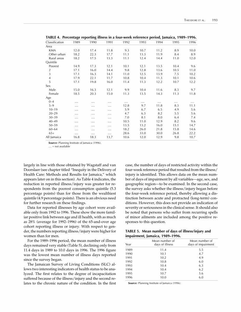
THEODORE ET AL. 193
largely in line with those obtained by Wagstaff and vanDoorslaer (see chapter titled “Inequity in the Delivery ofHealth Care: Methods and Results for Jamaica,” whichappears later on in this section). As Table 4 indicates, thereduction in reported illness/injury was greater for re-spondents from the poorest consumption quintile (5.3percentage points) than for those from the wealthiestquintile (4.9 percentage points). There is an obvious needfor further research on these findings.
Data for reported illnesses by age cohort were avail-able only from 1992 to 1996. These show the more famil-iar positive link between age and ill health, with as muchas 28% (average for 1992–1996) of the 65-and-over agecohort reporting illness or injury. With respect to gen-der, the numbers reporting illness/injury were higher forwomen than for men.
For the 1989–1996 period, the mean number of illnessdays remained very stable (Table 5), declining only from11.4 days in 1989 to 10.0 days in 1996. The 1996 figurewas the lowest mean number of illness days reportedsince the survey began.
The Jamaican Survey of Living Conditions (SLC) al-lows two interesting indicators of health status to be ana-lyzed. The first relates to the degree of incapacitationsuffered because of the illness/injury and the second re-lates to the chronic nature of the condition. In the first
case, the number of days of restricted activity within thefour-week reference period that resulted from the illness/injury is identified. This allows data on the mean num-ber of days of impairment by all variables—age, sex, andgeographic region—to be examined. In the second case,the survey asks whether the illness/injury began beforethe four-week reference period, thereby allowing a dis-tinction between acute and protracted (long-term) con-ditions. However, this does not provide an indication ofseverity or seriousness in the clinical sense. It should alsobe noted that persons who suffer from recurring spellsof minor ailments are included among the positive re-sponses to this question.
TABLE 4. Percentage reporting illness in a four-week reference period, Jamaica, 1989–1996.Classification 1989 1990 1991 1992 1993 1994 1995 1996Area
KMA 12.0 17.4 11.8 9.3 10.7 11.2 8.9 10.0Other urban 18.2 22.3 17.7 11.1 13.3 11.9 8.4 8.9Rural areas 18.2 17.5 13.3 11.1 12.4 14.4 11.0 12.0
QuintilePoorest 14.9 17.3 12.1 10.1 12.1 13.5 10.4 9.62 17.1 16.0 14.4 9.8 12.8 13.6 10.5 11.03 17.1 16.3 14.1 11.0 12.5 13.9 7.5 10.24 17.9 22.1 11.7 10.8 10.4 11.3 10.1 10.65 17.1 19.8 16.0 11.4 11.3 12.2 10.7 12.2
SexMale 15.0 16.3 12.1 9.9 10.4 11.6 8.3 9.7Female 18.5 20.3 15.0 11.3 13.5 14.3 11.3 11.8
Age0–4 .... .... .... .... .... .... .... ....5–9 .... .... .... 12.8 9.7 11.8 8.3 11.110–19 .... .... .... 5.9 6.7 6.5 4.9 5.620–29 .... .... .... 4.7 6.3 8.2 5.5 5.630–39 .... .... .... 7.0 8.1 8.0 6.4 7.440–49 .... .... .... 10.5 11.0 12.9 8.2 9.650–59 .... .... .... 13.5 13.2 16.0 15.1 14.760–64 .... .... .... 18.2 26.0 21.8 15.8 14.665+ .... .... .... 28.6 33.0 30.0 26.8 22.2
All Jamaica 16.8 18.3 13.7 10.6 12.0 12.9 9.8 10.7
Source: Planning Institute of Jamaica (1996)..... = not available
TABLE 5. Mean number of days of illness/injury andimpairment, Jamaica, 1989–1996.
Mean number of Mean number ofYear days of illness days of impairment
1989 11.4 5.51990 10.1 4.71991 10.2 4.91992 10.8 6.01993 10.4 6.31994 10.4 6.21995 10.7 5.61996 10.0 6.0
Source: Planning Institute of Jamaica (1996).

194 HEALTH SYSTEM INEQUALITIES AND POVERTY IN JAMAICA
The number of days of restricted activity in 1996 was9% above the mean number of days reported in 1989(Table 5). The number reporting protracted illness in-creased significantly between 1990 and 1996. In 1990,about 20% of those reporting illness/injury also reportedthat it began before the four-week period; in 1996, thisfigure climbed to 33%. Females reported a higher inci-dence of protracted illness/injury than did men, and theelderly (65+) reported higher levels than all other agegroups (Table 6). These results meet our a priori expecta-tions because they are in keeping with the country’s epi-demiologic profile, reflecting increases in chronic non-communicable diseases. It is important to take intoaccount such differences inherent among the demo-graphic groups before making judgments about healthinequalities.
Protracted illnesses/injuries are concentrated in thelower-income groups. On average, the poorest consump-tion quintile reports a higher incidence of protractedillness/injury than the richest quintile. However, theincrease in protracted illness/injury over the six yearswas much greater for those in the wealthiest quintile—a16.3 percentage point increase for quintile 5 as opposedto 8.3 percentage points for quintile 1 (Table 6).
If we were able to manipulate the data set to restrictattention to protracted illnesses instead of illnesses/in-
jury, we could gain a better understanding of what mayappear to be inequalities. This is because there are asso-ciations between employment, conflict management, andinjury. Unskilled, semiskilled, and skilled manual andnonmanual workers are prone to occupational injury, andviolence is rampant among the poor in the inner-city ar-eas of Kingston, the capital city. The unknown effects ofthese associations complicate this analysis. We will ad-dress this situation later in the study with data for 1993.
It must be noted that the usefulness of the data in mea-suring health inequalities is somewhat limited becauseof the absence of information about disease types. In otherwords, a better index of health status would be providedif the results could be interpreted within the context ofspecific medical conditions. Questions about chronicmedical conditions were asked in the health module for1991. Of those surveyed, 8.5% reported that they hadhypertension, and 2.4% had diabetes. Of course, chronicnoncommunicable diseases are age specific. As many asone-third of those over the age of 50 reported that theyhad hypertension, and 10% percent reported that theyhad diabetes. The prevalence of hypertension was higheramong women and among the highest-income quintile.However, this may reflect better detection rates, as thehigher-income groups often tend to use more preventiveservices. The prevalence of diabetes was also higher
TABLE 6. Percentage reporting protracted illness/injury, Jamaica, 1990–1996.Classification 1990 1991 1992 1993 1994 1995 1996
AreaKMA 18.2 23.1 31.3 28.5 36.8 36.0 29.8Other urban 15.5 25.9 27.4 33.6 27.6 31.6 27.7Rural areas 22.1 26.4 37.5 40.2 28.9 30.0 36.8
QuintilePoorest 24.9 26.8 40.8 37.1 32.8 25.0 33.62 24.8 27.8 31.6 34.6 29.8 30.4 27.33 17.6 34.5 35.2 26.1 26.4 35.4 34.64 16.9 23.9 35.4 43.9 36.4 34.0 39.35 15.5 15.9 28.6 36.7 26.2 36.3 31.8
SexMale 18.4 25.4 31.6 35.0 26.3 28.4 30.4Female 20.6 25.5 36.2 35.8 34.4 34.6 35.6
Age0–4 .... .... .... 15.2 15.6 12.9 14.85–9 .... .... 16.5 20.4 20.0 18.1 25.110–19 .... .... 15.2 19.4 17.0 17.5 18.020–29 .... .... 18.5 22.5 21.6 12.0 22.630–39 .... .... 22.4 29.4 27.7 29.4 28.340–49 .... .... 39.4 32.8 26.2 26.4 46.850–59 .... .... 46.1 41.3 38.7 44.9 47.860–64 .... .... 57.3 61.4 43.2 53.5 46.565+ .... .... 63.4 62.4 61.3 66.8 66.2
All Jamaica 19.6 25.5 34.8 35.5 30.9 32.0 33.3
Source: Planning Institute of Jamaica (1996).*Percentage protracted illness for children 0–9 years..... = not available
*

THEODORE ET AL. 195
among females and among the higher consumptionquintiles (Table 7). It is safe to assume that these popula-tion characteristics had not changed significantly by 1993.
HEALTH CARE EXPENDITURES AND FINANCING
Public Health Care Expenditures
Expenditures of the Ministry of Health Based onOfficial Estimates
According to estimates of expenditures of the Ministryof Health,2 62.1% of public health funds are allocated tosecondary care—i.e., hospital services. In contrast, only19.6% of the funds are utilized for primary health care.Other items in the national health budget include phar-maceutical services3 (6.8%), administrative costs of theMinistry of Health (4%), health services support4 (3.6%),training (2.3%), family planning5 (1.2%), and regional andinternational cooperation (0.4%).
We reclassified expenditures based on the COICOP6
system, which identifies four categories of individualconsumption as follows:
• medical and pharmaceutical products and therapeu-tic appliances and equipment,
• nonhospital medical and paramedical services,• hospital services, and• sickness and accident insurance services.
Only the first three categories are relevant because inJamaica there is no health insurance system, which fuelspublic spending. We also included the category “other”for expenditures that are not directly related to the pro-vision of services. The results of the reclassification exer-cise are shown in Table 8. The central government spendsthe largest share of the health budget on hospital services(49.43%). Medical and pharmaceutical products, thera-peutic appliances, and equipment account for about 24%,and nonhospital and paramedical services account for16.6%. Other miscellaneous spending takes up 10.29% ofthe national health budget.
Health Care Financing
Structure of Health Financing
Table 9 summarizes the structure of health financing inJamaica. The data indicate that the financing burden isshared almost equally between the public sector and pri-vate individuals and that these two contributors accountfor the lion’s share—85%. Social security, as already in-dicated, makes no direct contribution to health financingin Jamaica. This is one of the major changes being con-sidered by the health sector reform program.
Evaluating Progressivity of Sources of Financing
In the case of taxation, although it was not possible tomeasure the extent of progressivity of the different com-ponents, a few general comments are in order. To beginwith, the personal income tax structure seems to containboth progressive and regressive elements. In 1993, incomewas taxed at a flat rate of 33% for all income above
TABLE 7. Hypertension and diabetes prevalence, byquintile, residence, sex, and age, Jamaica, 1991.Category Hypertension Diabetes
QuintilePoorest 8.2 1.82 8.0 2.23 7.8 2.74 7.8 2.35 10.0 3.0
SexMale 5.6 2.0Female 11.9 2.8
Age group0–9 0.0 0.110–19 0.5 0.120–24 1.6 0.225–29 3.5 0.930–34 5.4 1.035–39 7.5 0.940–44 11.2 2.745–49 11.9 3.565+ 34.1 10.7
All Jamaica 8.5 2.4
Source: Armstrong (1994).
2Estimates of the Ministry of Finance and Planning for the finan-cial year 1992/1993. We assume that a similar breakdown holds formore recent years.
3“Pharmaceutical services” includes the procurement, storage,and supply of pharmaceuticals and medical sundries by the agen-cies delivering health care and by the public.
4“Health services support” covers surveillance (prevention andcontrol activities aimed at reducing the occurrence of endemic dis-eases), paramedical services, and hospital maintenance.
5Operated by the National Family Planning Board.
6 Classification of Individual Consumption by Purpose (COICOP)was developed by the Organization for Economic Cooperation andDevelopment and is used to classify individual consumption ex-penditures of households, nonprofit institutions serving households,and general government. “Individual consumption expenditures”are defined as expenditures made for the benefit of individual per-sons or households.

196 HEALTH SYSTEM INEQUALITIES AND POVERTY IN JAMAICA
J$ 10,400. This means that for the lowest quintile the ef-fective income tax rate was zero. However, it also means,if we assume diminishing marginal utility of income, thatfor the other quintiles the utility cost of the tax systemdeclines with income. The personal income tax system istherefore nominally regressive.
Turning to the indirect tax, the general consumptiontax (GCT), although the overall rate was 12.5% for 1993,the effective rate for the different quintiles varies depend-ing on the way the different exemptions or zero ratingsaffect their budgets. Table 10 presents estimates of theeffective quintile-related rates of GCT based on a reviewof purchases recorded in the survey of living conditions.
The fact that the rates decline as incomes rise is a fea-ture of most indirect tax systems. This is the manifesta-tion of nominal regressivity in this type of system.
In 1993, income taxation and the GCT accounted for67% of all government revenues (J$ 19,500 million ofJ$ 29,100 million). The other major contributors were cus-toms duty (J$ 3,640 million), stamp duty (J$ 1,610 mil-lion), education tax (J$ 1,050 million), and special con-sumption tax (J$ 1,990 million). Other taxes accountedfor J$ 1,840 million.
Without knowing the income and payment profilesof all taxpayers, it is difficult to comment on the pro-gressivity of the financing mechanisms for the health sys-tem. We do know that the sources of public revenues aremainly two taxes that seem biased toward regressivity.Therefore, the issue is whether public expenditure onhealth care counteracts regressivity in the tax system. Inthis sense, the focus of inequality analysis should be onthe uses of public funds. In other words, the real issue inthe context of Jamaica is whether the utilization of publichealth facilities has the potential to modify the overalllevel of inequality. This issue is examined in the nextsection.
INEQUALITIES IN ACCESS TO AND UTILIZATION OFHEALTH SERVICES
The Question of Equality of Accessin Policy Documents
Policy documents reveal that the public sector providesa spread of services, which are geographically situatedto serve defined populations. The physical facility net-work was generally found to be equitably distributed.However, when both supply and demand factors aretaken into account, some concerns emerge from a reviewof the literature. This is because, despite the evenness ofservices supplied by the public health system, variationsin quality between the private and public sector compro-mised equity principles (Armstrong, 1994; Lalta, 1995;Bicknell, 1994). It was generally noted that private care
TABLE 8. Expenditures of the Ministry of Health basedon the Classification of Individual Consumption byPurpose (COICOP), Jamaica, 1992–1993.
Expenditure fiscal year:1992–1993
Category (thousands of J$) %
Medical and pharmaceutical 299,733 23.95products, therapeuticappliances, and equipment*
Nonhospital medical and 204,213 16.32paramedical services†
Hospital services‡ 618,538 49.43
Other 128,836 10.30
Total 1,251,320 100.00
*Medical and pharmaceutical products and therapeutic appliances and equip-ment include purchase of goods and services and purchase of equipment andcapital goods from the following programs: primary health care, secondary healthcare, health services support, and pharmaceutical services.
†Nonhospital medical and paramedical services include expenditure of theprimary health care system, excluding purchases (goods and services and capi-tal items)—that is, compensation to employees, travel and subsidies, rent, pub-lic utilities, awards, and grants.
‡Hospital services cover expenditure of the primary health care system, ex-cluding purchases (goods and services and capital items)—that is, compensa-tion to employees, travel and subsidies, rent, public utilities, awards, and grants.
TABLE 9. Structure of health financing, Jamaica, 1993.Source Amount (million J$) %
Taxation* 2,890 0.43Out-of-pocket† 2,800 0.42Private insurance 760 0.11NGOs 75 0.01Social security 0 0.00Other 221 0.03Total 6,746 1.00
Source: Theodore (1997).*Includes income, indirect, and other taxes, and there is no earmarking for
health.†Based on a doubling of the figure derived from the 1993 Jamaican Survey of
Living Conditions. This is still more than 40% smaller than Boston Universityestimates of J$ 4,920 million, derived on the basis of a few interviews withhealth providers.
TABLE 10. Effective consumption tax rates, Jamaica,1993.
Quintile Effective GCT rate (%)
1 7.72 6.13 4.74 4.15 3.9
Average 4.6

THEODORE ET AL. 197
was demanded by those able to afford such services, andpublic services that failed to meet acceptable standardswere reserved for the poor. Project HOPE (1985) andBicknell (1994) noted, furthermore, that unevenness alsoexisted within private service utilization across broadeconomic groups, because wealthier persons could affordeither domestic or foreign private services, whereas othergroups were limited to private domestic care.
Bicknell (1994) and Armstrong (1994) addressed equal-ity of access as it relates to rationing. They noted that inJamaica, because doctors are allowed to care for privatepatients at public facilities, inpatient care in fact was be-ing rationed through the market mechanism. Persons ableto pay often were allowed to jump queues, which resultedin a “crowding out” effect. These studies also observedthat the distribution of physicians’ time between private(paying) patients and public (nonpaying) patients ap-peared to be unjust.
The opportunity cost of time was found to be instru-mental in reducing the likelihood of particular economicgroups utilizing services (Armstrong, 1994). It waspointed out that some persons did not possess the abilityto pay, either directly for private care or indirectly (inthe form of waiting time) for public sector care. For suchpersons, self-treatment or nontreatment may be substi-tuted for medical attention. This type of inequity is per-haps higher for informal-sector workers who were un-able to abandon their jobs to wait extended periods forattention.
Utilization Patterns
Based on the findings of the various surveys of livingconditions, the percentage of persons reporting illness/
injury and seeking care has been increasing since 1989(Table 11). As many as 54.9% of those persons soughtcare in 1996. There continues to be roughly a 60:40 distri-bution in the utilization of private and public health ser-vices. Although this ratio has remained relatively stablesince 1989 (Table 12), it should not be taken as an indica-tor of ability to pay for health care services, because manylow-income households deplete assets or forgo other ba-sic needs to purchase health services (World Bank, 1994).More of the ill or injured from rural areas (66%) werefound to utilize private health care providers than wasthe case for their counterparts from other geographic re-gions (Planning Institute of Jamaica, 1996). This may bebecause the well-equipped public facilities are located inmetropolitan areas, leaving rural communities with littlechoice but to seek care from private providers.
For persons utilizing the services of private providers,the mean individual expenditure on visits was J$ 598.30(Table 13). However, mean expenditures were highest inthe rural areas (Planning Institute of Jamaica, 1996). Meanannual expenditure for private care was also found toincrease with consumption quintile. However, the high-est mean private patient expenditure was observed forindividuals 65 years and over (Planning Institute of Ja-maica, 1996), which obviously reflects the greater needfor care among the aged.
Equity in the Distribution of Health Benefits
Financing of the health system should not create accessbarriers to those in need of health care. Horizontal eq-uity demands that health services be distributed accord-ing to need. To provide a sense of the extent of the need,the utilization findings of the 1993 Survey of Living Con-
TABLE 11. Percentage of ill/injured seeking medical care by area, consumption quintile, andsex, Jamaica, 1989–1996.Classification 1989 1990 1991 1992 1993 1994 1995 1996
AreaKMA 56.7 40.5 48.0 58.8 60.1 55.9 52.6 53.8Other urban 45.5 40.9 45.6 52.4 51.6 59.0 57.5 55.5Rural areas 47.2 36.8 48.6 47.1 47.2 47.0 62.8 55.4
Quintile1 (poorest) 43.7 35.7 38.7 34.7 39.0 44.3 55.4 53.42 49.8 38.0 52.0 45.8 48.7 44.6 60.1 45.63 47.5 38.8 48.7 53.5 45.4 50.8 58.4 51.14 52.7 40.2 50.6 55.9 63.4 56.8 63.4 59.05 51.6 39.7 47.8 60.3 60.3 63.4 58.4 63.0
SexMale 44.7 37.9 48.5 49.0 48.0 49.0 59.0 50.5Female 52.8 39.2 47.4 52.5 54.7 53.4 58.9 58.5
Jamaica 49.0 39.0 47.7 50.9 51.8 51.5 58.9 54.9
Source: Planning Institute of Jamaica (1996).

198 HEALTH SYSTEM INEQUALITIES AND POVERTY IN JAMAICA
ditions are summarized in the tables and in Figure 1. It isapparent that almost one-half of those reporting illnessdid not seek care, which raises the question: Is this aperception-of-illness result or is it a problem of accessbarriers and therefore a problem of equity?
Health benefits delivered through the public healthsystem include the services available at both primary andsecondary care institutions. Figure 1 presents the gen-eral utilization patterns observed for 1993. Table 14 sum-marizes these patterns across income groups and allo-cates expenditures accordingly; the table indicates thenumber of days of reported illness and the correspond-ing treatment “hits” at public facilities.
Table 14 shows that the distribution of benefits clearlyfavors the lower-income groups. The lowest quintile en-joys more than twice the benefits (29%) enjoyed by thewealthiest quintile (12%). This means that, although morepersons in the top quintile sought medical attention, they
clearly showed a preference for private facilities. Almostby default, the public facilities became the haven for thelower-income groups.
To assess the impact of the public health expenditurewe have sought to compare, under two scenarios, thedistribution of consumption expenditure of those whosought attention at public facilities. In the first scenario,we consider the distribution including the tax compo-nent only. In the second scenario, we allow for the pres-ence of both the tax and the health benefit. Presumably,the latter scenario comes closer to capturing the net ben-efit incidence of the public health benefit. Table 15 showsthe structure of consumption under the two scenarios.
Of course there are two factors at work here. On theone hand, distribution of the health benefit itself clearlyfavored the lower-income groups. On the other hand, theshare of the health benefit in the combined consumption/health welfare package was extremely large. The ratio of
TABLE 12. Use of public/private sector by ill/injured for medical care, purchase of medica-tion, and hospitalization during the four-week reference period, Jamaica, 1989–1996.
Percentage of those Percentage hospitalization of thoseseeking medical care Percentage purchasing medication seeking medical care
Year Public Private Both Public Private Both Public Private
1989 39.0 61.0 NA NA NA NA NA NA1990 39.4 60.6 NA NA NA NA NA NA1991 35.6 57.7 6.7 NA NA NA NA NA1992 28.5 63.4 8.1 8.9 58.5 2.4 1.0 NA1993 30.9 63.8 5.3 15.9 79.9 4.2 6.9 0.51994 28.8 66.7 4.5 21.4 75.6 3.0 4.6 0.81995 27.2 66.4 6.3 16.4 81.9 1.7 6.0 0.21996 31.8 63.6 4.6 19.1 78.0 2.9 5.1 0.5
Source: Planning Institute of Jamaica (1996).NA = not applicable.
TABLE 13. Mean patient expenditure on health care in public and private facilities in thefour-week reference period, Jamaica, 1989–1996.
Visits Drugs
Private PrivatePrivate real Public Private Private real Public
nominal 1990 nominal real J$ nominal 1990 nominalYear (J$) (J$) (J$) 1990 (J$) (J$) (J$)
1989 57 74.0 11 14 48 62 51990 72 72.0 11 11 43 43 41991 82 44.0 11 6 95 51 81992 167 63.0 14 5 234 88 171993 298 85.0 115 33 331 94 1311994 461 109.0 91 21 417 98 1631995 496 98.8 130 26 509 101 2341996 598 103.6 148 26 685 119 176
Source: Planning Institute of Jamaica (1996).

THEODORE ET AL. 199
the health benefit to the consumption of those accessingpublic facilities is almost 4:1. In other words, the healthbenefit is large enough to make a difference.7
Table 15 shows an example of perfect rank reversal—literally, the first becomes last, and the last, first. On theface of it, the health benefit could not be asked to do more.The final share of the lowest quintile more than doubledand that of the next lowest quintile increased by morethan 25%. The shares of the other three quintiles fell at anincreasing rate, as progressivity requires.
This result raises a number of questions. Although itsuggests that the health system in Jamaica has the poten-tial to make a difference to the overall equity situation inthe country, persons with a working knowledge of thesystem point to a high degree of dissatisfaction amongthose seeking care in the public system. The reason is mostprobably one highlighted by Wagstaff and van Doorslaer(see the chapter titled “Inequity in the Delivery of HealthCare: Methods and Results for Jamaica,” which appearslater in this section)—the equity measures being used do notcapture the quality of the services delivered. Linked to this isthe second question raised by the results. Why is the num-ber of persons seeking care in the public sector less thanhalf those who seek care in the private sector, even though
care in the public sector is free at the point of service?Again, the issue seems to be one of the perceived qualityof care in the public sector. It would be useful if futureliving standard surveys were to seek to capture this qual-ity perception, as this information could be a useful guideto policy making.
In closing, it also must be noted that, in spite of theapparent perception of lower service quality in the pub-lic health system, the nonpoor continue to seek servicesthere. The explanation for this phenomenon appears tolie in the fact that public providers not only have the op-tion to engage in private practice but in some cases thispractice takes place in the public facilities. Thus, it is quitepossible that services of different quality are being pro-vided in the same facility. This is one of the main chal-lenges the health reform process faces, because that pro-cess is grounded on the principle of universal provisionof a basic package of health services of equal quality forall citizens, regardless of income status.
QUANTIFICATION OF INEQUALITIES
The ECuity method (see the chapter titled “Inequity inthe Delivery of Health Care: Methods and Results for Ja-maica,” which appears later in this section) was appliedto test for biases in health status and in utilization of healthservices. When the variables were standardized, it wasfound that the system showed a clear pro-rich bias in threeof four health status indicators and an unambiguous pro-
7Of the 7,316 persons in the 1993 sample, 865 (11.8%) reportedbeing ill, 438 (6%) sought care, and 135 (1.8%) chose to go to a pub-lic facility. This fraction (1.8%) corresponds to the consumption levelused in Table 15—that is, J$ 776.6 million or 1.4% of total consump-tion of J$ 56,800 million.
Personsill,
100%
Soughttreatment,
50.8%
Public hospital, 20.5%
Private hospital, 4.1%
Private health center, 2.3%
Private doctor, 52.5%
Pharmacy, 6.1%
Public health center, 10.2%
Admitted, 0.06%
Did not seektreatment,
49.2%
Admitted, 1.4%
Not admitted, 19.1%
Not admitted, 4.04%
FIGURE 1. Perceptions of persons suffering from illness over the past four weeks and level of utilization of healthservices, Jamaica, 1993.

200 HEALTH SYSTEM INEQUALITIES AND POVERTY IN JAMAICA
rich bias in the utilization of health services. The stan-dardization procedures are described in the Annex.
CONCLUSIONS AND POLICY RECOMMENDATIONS
Jamaica’s economic context is one of a country strugglingto regain balance in its key accounts. Since 1990, the coun-try has barely managed to achieve 1% annual growth andthe level of unemployment seems to have settled ataround 15%–16%. The average rate of poverty between1989 and 1996 has been 35%, and the mean consumptionratio between the highest and the lowest quintile wasmore than 7:1. In other words, the situation has been onein which the growing demand for social services and astrong safety net have been met with a weakening ca-pacity to respond.
Nevertheless, it is important to point out that the Ja-maican government has sought to respond in two waysthat are relevant to the health equity concerns of thisproject. First, the government has put in place a fairlyextensive poverty alleviation program, including a foodstamp program that covers a wide cross section of theindigent population. This measure was taken in responseto growing evidence that the ongoing structural adjust-ment program was having a deleterious effect on childnutrition. Second, the government has embarked on ahealth sector reform program that has three main ele-ments: decentralization of services in an effort to reach
TABLE 14. Use of public health facilities by income quintiles, Jamaica, 1993.Treatment at Value Value Combined
Quintile Days of illness public facilities Primary no. (million J$) Secondary no. (million J$) (million J$) Distribution
1 790 393 261 186.5 132 561.1 836.2 0.2892 1,096 419 352 166.5 67 459.0 729.0 0.2523 960 306 188 93.2 118 612.1 557.5 0.1934 1,026 178 72 66.6 106 510.0 428.8 0.1485 1,028 209 165 86.6 44 153.0 343.1 0.119Total 4,900 1,505 1,038 599.5 467 2,295.2 2,894.7 1.000
the rural population better; refurbishment and restruc-turing of the public sector primary care system; and in-troduction of a national health insurance program thatwill make a basic package of health services available toall citizens regardless of income.
Because the national health system operates within anenvironment of poverty and inequity, it is not surprisingto find that the system itself is infected with these socialcharacteristics. This project attempted to determine theinequality bias of the health system with respect to threespecific concerns:
• The health status of the population: Is the system pro-poor or pro-rich with respect to its health outcomes?
• Access to or utilization of health services: Is the sys-tem responding to the health needs of the popula-tion with a pro-rich or a pro-poor bias?
• Financing of the system: Is the system progressiveor regressive in terms of sources and allocation of itsfinances?
With regard to health status, there were three salientsurvey results:
• According to the surveys of living conditions from1989 to 1996, with the exception of 1995, the poorconsistently reported less illness than the nonpoor.This may be an illness perception phenomenon thatmerits further investigation.
TABLE 15. Distribution of consumption with and without tax and healthbenefits, Jamaica, 1993.
Consumption Consumptionwith tax but no with tax and health
Quintile health benefit (million J$) Share benefit (million J$) Share
1 93.9 0.121 930.2 0.2532 147.4 0.190 876.5 0.2393 154.4 0.199 711.9 0.1944 165.6 0.213 595.4 0.1625 215.2 0.277 558.3 0.152
Total 776.6 1.000 3,672.3 1.000

THEODORE ET AL. 201
• With regard to protracted illness, however, the pat-tern was clearly one in which the poor were moreseverely affected.
• With regard to chronic illness, the 1993 surveyshowed no clear picture; the poor were neither morenor less afflicted than the nonpoor.
In applying the EquiLAC methodology to test for bi-ases in health status, it was found that, when the vari-ables were standardized, in three of four health statusindicators the system showed a clear pro-rich bias.
With regard to utilization of health services there werealso three salient survey results:
• Using the variable “illness days,” it was found that,although the very poor reported less illness, theyused the public facilities much more than thenonpoor.
• However, it was observed that even the very poor-est Jamaicans were heavy users of private sectorhealth services—almost half their services weresought in the private sector.
• For all quintiles except the first, the use of privatesector facilities was almost twice the use of publicsector facilities.
In applying the EquiLAC methodology to test for biasin the utilization of health services, again, standardiza-tion of the variable showed an unambiguous pro-richbias.
These results are somewhat puzzling when we recallthat the Jamaican public health system is an open-accesssystem. Primary care services are free on demand, onesection of the public sector drug service is free, and, al-though there are fees at hospitals, the range of personsexempted is so large that the secondary care system isalso substantially free.
Seemingly, these results are consistent with a two-tiered health system in which even the very poor feelmore confident about getting the quality of service theyneed in the private sector. The fact that some of thenonpoor use the public system points to the possibilityof queue jumping and differential treatment at publicsector facilities. This is consistent with the known prac-tice in Jamaica of allowing public sector doctors to en-gage in private practice within the confines of publicfacilities.
As for financing, there were three noteworthy findings:
• On the sources side, taxation and out-of-pocketexpenditures accounted for 85% of all health financ-ing in Jamaica, with an almost even split betweenthe two.
• Because out-of-pocket payment is known to be re-gressive, and because both the proportional incomesystem and the main consumption tax (GCT) in thecountry are also deemed to be regressive, the primafacie conclusion is that there is regressivity on thesources side. In the absence of data on the distribu-tion of the income tax burden, this study acceptedthis inference.
• On the usage side, the 1993 survey shows that theuse of the public health facilities was strongly skewedin favor of the lower quintiles, with the lowestquintile accounting for almost one-third of the pub-lic resources applied to health.
This last result appears to suggest that the public healthsystem has the potential to correct any prior regressivitythat may result from the way the health system is fi-nanced. Assuming that the mode of financing is reflectedin the overall distribution of income or consumption, weconducted an analysis that showed that, in fact, the pub-lic health system could change a regressive distributionof benefits into a progressive one.
Having found this, however, a number of questionsremain unanswered. Why are so few persons using the“free” health service? Why are so many of the poor mak-ing the sacrifice to gain access to private sector facilities?Why do the nonpoor use the public health system at all?
It would seem that the answer to these questions liesin the quality of services available within the public healthsystem. In fact, the answer probably lies in the differen-tial quality of public sector services. With a multitieredsystem of hospitals and health centers it would seem thatthose who seek attention in the public sector are not guar-anteed an acceptable basic quality of health services. Inother words, although the public health system clearlyneeds to be made more attractive to the poor, it also mustseek to avoid service differentiation between the poor andthe nonpoor. This is one important means by which theapparent “correction” by public financing will be trans-lated into better health status for the poor.
In a system in which only a small number of personsseek care in the public sector and in which poverty levelsare very high, there is a distinct possibility that more andmore poor people are seeking care in the private sector—a private sector that not only employs many of the sameproviders as the public sector, but one in which the priceof services over the full range of health services neededis known to present access barriers to large segments ofthe population. Patients may barely manage to find thefunds to visit a doctor, but then they are unable to payfor lab tests and prescriptions.
It is important to note that the welfare impact of thehealth system depends on three factors: the availability

202 HEALTH SYSTEM INEQUALITIES AND POVERTY IN JAMAICA
of epidemiologically appropriate services, the accessibil-ity of these services to all citizens, and the quality of theseservices. Moreover, in a society in which the informalsector is becoming more and more important and moreand more competitive, people simply are not willing towait long hours at public facilities. It is important foroverall equity improvements and for health status im-provements among the poor that steps be taken to makethe public sector facilities more attractive to those in needof health services. A public health system that attractsmore patients will be in a position, given its size, to setprice and quality standards for the entire health caresystem.
Finally, and most importantly, the government shouldinvest in upgrading public health facilities and existingsystems in order to expeditiously meet the health needsof the population.
REFERENCES
Armstrong J. Jamaica Health Sector Review: Present Status and FutureOptions. Report 13407 JM. Washington, DC: World Bank; 1994.
Bicknell WJ. Jamaica Health Sector Assessment: Policy Implications andRecommendations. Report prepared for the Ministry of Health
under contract by Touche Ross Management Consultants. Lon-don: Touche Ross Management Consultants; 1994.
Blaxter M. A companion of measures of inequality in morbidity. InFox J. (ed.) Health Inequalities in European Countries. London:Gower, Aldershot and London; 1989.
Lalta S. Review of Health Financing in Jamaica and a Survey of the Feasi-bility of National Health Insurance. Study funded by the U.S.Agency for International Development through the LatinAmerica and Caribbean Health Nutrition Sustainability Project.Washington, DC: U.S. Agency for International Development;1995.
Ministry of Health. Jamaica Green Paper on the National Health Insur-ance Plan. Kingston: Ministry of Health; 1997.
Planning Institute of Jamaica. Economic and Social Survey Jamaica,1995. Kingston: Planning Institute of Jamaica; 1995.
Planning Institute of Jamaica. Survey of Living Conditions, 1996.Kingston: Planning Institute of Jamaica; 1996.
Project HOPE. Health Insurance Options. Millwood, VA: ProjectHOPE; 1985.
Theodore K. Macroeconomic Implications of a National Health Insur-ance Programme for Jamaica. Report for the Ministry of Health.Kingston: Ministry of Health; 1997.
Theodore K et al. Health and Poverty in the Caribbean. Report for theCaribbean Development Bank. 1997. Bridgetown: CaribbeanDevelopment Bank. Mimeograph.
World Bank. Jamaica: Achieving Macro-stability and Removing Con-straints on Growth. Country Economic Memorandum. Washing-ton, DC: World Bank; 1996.

THEODORE ET AL. 203
EQUITY AND MORBIDITY
In the analysis of health care outcomes, data from theJamaican 1993 SLC were used.1 As with other living con-ditions inquiries, the main socioeconomic variable wasper capita expenditures, adjusted for adult equivalentsby a factor of 0.75, which yielded 1.00, 1.40, and 1.68 for acouple, a couple with one child, and a couple with twochildren, respectively. No specific distinction was madefor morbidity patterns between adults and children andthe effective sample size was 7,316 cases.
In 1993, reported morbidity was 11.8%, with approxi-mately 7.7% reporting acute illnesses and 4.1% reportingchronic illness. There were no questions about the de-gree of self-assessed ill health in the 1993 survey. Of thosereporting illness, 42.8% were male and 57.8% were fe-male. This corresponds to 10.3% of the male respondentsand 13.3% of the female respondents. Averages for adultsand children showed a similar pattern in that 10.5% ofthose reporting ill health were adults and 12.8% werechildren.
Observed morbidity did not vary significantly by con-sumption decile. However, at higher levels of aggrega-tion, differences were evident (see Figure A1). Groupedby per capita consumption quintile adjusted for adultequivalent units, observed morbidity showed significantvariation.2 Noteworthy in this respect, morbidity did notdecline gradually as one moved upward in the consump-tion scale. Instead, the two highest quintiles showedhigher-than-expected morbidity rates relative to the otherconsumption groups.
Morbidity patterns are likely not to vary simply interms of socioeconomic differences but also by demo-
graphic factors. This gives rise to the notion of morbiditythat can be eliminated—i.e., variation in morbidity acrossincome groups adjusted for differences in age and gen-der. This adjustment is on the whole necessary becauseage and ill health are necessarily correlated, but more im-portantly income and age often manifest a statisticallysignificant relationship. This can be further compoundedwhen differences in attitude on the basis of gender de-termine whether one perceives oneself ill. Indices ofhealth inequality therefore adjust for these differences.In this study, we have used the standardization proce-dure for ungrouped data articulated by Wagstaff and vanDoorslaer (see chapter titled “Inequity in the Delivery ofHealth Care: Methods and Results for Jamaica,” whichappears later in this section) to derive a measure of Cand C*. The derivation is as follows:
Assuming that the illness concentration curve is piece-wise linear, we can represent the concentration index Cby
C f Rt t tt
T
= −=∑2
11
µµ
ANNEX: STANDARDIZATION OF VARIABLES
1In addition to providing a rich data set, the survey can be con-sidered an improvement on its predecessors in that it benefited fromseveral refinements, which led to a higher response rate and en-hanced survey execution.
2Not adjusted for demographic differences.
1 2 3 4 5Consumption quintile
0.10
0.15
0.20
0.25
0.30
0.35
0.40
0.45
Chr
onic
illn
ess
rate
FIGURE A1. Chronic illness rates by income quintile,Jamaica, 1993.
Source: Planning Institute of Jamaica, Survey of Living Conditions, 1993.

204 HEALTH SYSTEM INEQUALITIES AND POVERTY IN JAMAICA
where the mean morbidity rate is
µ µ==∑ ft tt
T
1
and Rt is the relative rank of the tth socioeconomic groupand ft is the fraction of segment t in the entire population.
FRAMEWORK FOR ANALYSIS
Inequality in health care outcomes may be assessed in anumber of ways. Notable among them is the frameworkproposed by Blaxter (1989). Three models are proposedin this schema: (1) a medical model, which considersillness/injury affecting the respondents’ physical well-being; (2) a functional model, which ranks physical inca-pacitation by degree or extent, measured by the inabilityto perform what are considered normal functions; and(3) a subjective model, in which ill-health is assessed sub-jectively compared with persons of similar age. The 1993SLC poses several limitations on the strict application ofthese models in that the subjective model could not beevaluated as the question about the degree of self-reported illness was omitted. In addition, no useful dis-tinction could be made between illness per se and injury.3
Table A1 details the available indicators. The main re-sults for the medical model are presented in Table A2and Figure A2. For all the indicators except illness/in-jury, in the past 4 weeks the inequality index (I*) reflectsa bias against the poor. The standardized health statusconcentration curve is shown in Figure A3. All preva-lence rates and means of illness days, except for long-term illness, show a decline with rising expenditure lev-els—again, a bias against lower-income groups.
Table A3 shows pro-poor inequality—a positive con-centration index (C*) with respect to the health status in-dicator (i.e., reported illness); however, the estimator isnot statistically significant. This is in contrast to the indi-cator of utilization; it clearly shows a pro-rich pattern,which, although not by any means severe, is statisticallysignificant. I* also shows a similar pattern for utilization.
The cumulative distribution of utilization by consump-tion quintiles is shown in Figure A4. We have not tabu-lated the unstandardized measures, because the un-standardized indicator of utilization as measured by theconcentration (Gini) index (reported below) was similar
in order of magnitude to the standardized concentrationindex, measuring 0.167, and was similarly insignificant.
What can be observed in general is that demographicstandardization does indeed influence the measure ofexisting health inequality to the extent that the indexchanges from pro-rich to pro-poor. This result createssome discomfort, because an experimental raw data cross-tabulation to determine whether the gender of the respon-dent affected the seeking of medical attention generallyshowed no significant variation across the sexes. How-ever, when age was superimposed, it was evident that itaccounts for a substantial degree of the variation. Forexample, for children under 5 years of age, a poor childwas more than 3.5 times as likely to seek medical atten-tion as his/her counterpart from the highest quintile. Forpersons between the ages of 16 and 59 years, however,only 9.7% of the poorest 20% sought medical attention,compared with 31.2% of the wealthiest 20%.
COMPUTATION METHODS
In all cases, the indirect method of standardization wasused and indices were computed on individual level data.Standard errors were not computed along the lines of therefinements suggested by Wagstaff and van Doorslaer(1998) but were derived directly from the regression es-timates. In addition to those included in Table A3, un-standardized estimates for the health services utilizationconcentration index were derived as follows:
Health care utilizationC = 0.167 t(C) = 0.047 Se(C) = 3.542
Standardizations were confined to age and gender, asit was often the case that other demographic variables—specifically, education—did not account for significantvariation in either observed morbidity or the choice toseek medical attention (the utilization variable used inthe analysis).
INTERPRETATION
For health inequity indices (I* and C), negative valuesindicate distributions favoring the nonpoor, and positivevalues indicate distributions favoring the poor. However,the size of the standard errors and the t statistics are tobe considered in determining the reliability of the results.
3A filter variable identifying ill-health due to injury would beused.

THEODORE ET AL. 205
TABLE A1. Health indicators in Jamaica.Indicator Definition Mean
Medical modelIllness/injury in past four weeks Have you had an illness or injury in the past 4 weeks?
For example, have you had a cold, diarrhea, injury due to an accident,or any other illness? 0.118
No. of illness days during past four weeks For how many days during the past four weeks have you sufferedfrom this illness or injury? 6.349
Acute illness Have you had an illness/injury during the past 4 weeks? 0.649
Long-term illness Have you had an illness/injury during the past four weeks thatstarted more than four weeks ago? 0.351
Functional modelNo. of restricted-activity days For how many days during the past 4 weeks were you
incapacitated because of illness or injury? 6.35
Activity limitation Does your health limit you from running, walking, eating,bathing, climbing stairs, etc.? NA
Major limitation Does your illness/injury limit you severely from any of the above activities? NA
Minor limitation Does your illness/injury limit you slightly from any of the above activities? NA
Source: Planning Institute of Jamaica, Survey of Living Conditions, 1993.NA = not applicable.
TABLE A2. Inequality index values and t values for medical model.Health indicator C t(C) Se(C) I*
Illness/injury in past four weeks –0.0300 –1.131 0.026530 0.0018No. of days ill in past four weeks –0.0458 –5.347 0.008570 –0.0042Acute illness –0.0341 –1.835 0.018579 –0.0010Long-term illness –0.0866 –5.184 0.016702 –0.0051
0.00
0.02
0.04
0.06
0.08
0.10
0.12
0.14
Expenditure quintiles
Prev
alen
ce r
ates
0.00
0.50
1.00
1.50
2.00
2.50
3.00
Illne
ss d
ays
Illness/Injury
Acute Illness
Long-termIllnessIllness days
1 2 3 4 5
FIGURE A2. Medical model: unstandardized means for expenditure quintiles.

206 HEALTH SYSTEM INEQUALITIES AND POVERTY IN JAMAICA
% of population ranked by expenditure
% o
f Ill-
heal
th
0
20
40
60
80
100
0 20 60 8040 100
Cum
ulat
ive
% u
tiliz
atio
n
Unadjusted L(s)
0
20
40
60
80
100
0 20 40 60 80 100Cumulative % of consumption
TABLE A3. Standardized health inequality indicators forservice utilization and health care status.
HealthStandardized Health Health care Inequality careindicators status utilization index utilization
C* 0.100 –0.00032 I* –0.0319t(C*) –0.874 –0.50900 t(I*) –4.9270Se(C*) 0.115 0.00063 Se(I*) 0.006473
FIGURE A3. Health status concentration curve(standardized).
FIGURE A4. Utilization by consumption quintiles.

207
BACKGROUND
Macroeconomic Context
Mexico has an area of approximately 1.96 million km2
and a population of 94 million. A per capita annual in-come of US$ 8,370 places it among the world’s uppermiddle-income countries. Since 1994, the country’seconomy has grown steadily, with the gross domesticproduct (GDP) increasing by 7.3%. Unemployment stoodat 6.2% in 1995, but it fell to 3.3% by the end of 1997.There has been an upturn in domestic demand as well asin exports. Inflation has declined continuously over thepast four years, but so have real wages, largely becauseof the sharp declines registered in the manufacturing sec-tor every year since 1995. Still, economic growth hasboosted job creation.
The financial crisis in Southeast Asia has had some re-percussions on Mexico’s financial markets. The slowingof capital flows, for example, has resulted in adjustmentsin exchange rates and increases in interest rates. Althoughthese developments have not affected overall macroeco-nomic outcomes, they have no doubt accounted for theuneven performance of the country’s productive base.Large firms, exporters, and companies that have accessto external financing have performed quite well, but smallfirms geared toward the domestic market have had diffi-culty obtaining financing and therefore achieving theirformer levels of activity. This situation has had a greaterimpact on people in the poorest groups of society, whotend to be employed in smaller business enterprises andin the informal sector.
Poverty and Inequality
Despite some favorable economic trends, poverty levelsin Mexico have hovered around 24% of the populationsince 1990. Rural poverty, at 36% in 1997, was much
HEALTH SYSTEM INEQUALITIES AND POVERTY IN MEXICO
Susan Wendy Parker and Eduardo Gonzales Pier
higher than the urban rate (19%). This situation also hasimplications for inequalities in health status between thepoor and nonpoor in rural and urban areas.
HEALTH CARE SYSTEM
The Mexican Constitution makes health care a fundamen-tal right of all persons. Although there have been consid-erable improvements in the health status of the popula-tion, inequalities in access, utilization, and financing ofhealth care persist. Mexico is undergoing a protracteddemographic transition. Life expectancy is increasing andthe elderly population is growing in relative and abso-lute terms. The proportion of persons under 15 years ofage is expected to decrease from 39% to 30% between1990 and 2030, and the number of people over 65 is ex-pected to increase threefold during the same period. Theeconomic progress of the past few decades has had un-even effects across the different regions. The wealthiernorthern states have experienced significant increases inliving standards, while the southern and more rural stateshave lagged behind. Large regional differences in the paceof economic development and demographic transitionhave resulted in the coexistence of two epidemiologicprofiles: malnutrition, maternal and perinatal deaths, andthe reemergence of communicable diseases commonlyassociated with poverty and underdevelopment prevailin the rural and southern states, whereas chronic condi-tions, cardiovascular disease, and mental health disor-ders are the most common health problems in the urbannorthern and central states.
The observed inequalities in health status are com-pounded by an equally uneven distribution of resourcesand supply of quality care. In general, higher-incomegroups in urban centers and northern states receive higherquality medical care and also enjoy broader consumerchoice. At the same time, lower-income Mexicans insouthern rural states are left with limited choice among

208 HEALTH SYSTEM INEQUALITIES AND POVERTY IN MEXICO
mostly public providers with long waiting lists andchronic shortages of medical supplies and qualified per-sonnel. The uneven distribution of hospital beds, physi-cians, and nurses is only partially explained by the greaterpurchasing power of the wealthier northern and urbandwellers. Inefficient, centralized “top-down” manage-ment, coupled with insufficient planning and collabora-tion across independent public system delivery networks,has led to duplication of resources and excess capacity inurban areas. Budget allocations based on historical spend-ing rather than on health needs, including inflexible line-item budgeting practices, have meant that poorer states—which have the highest burden of disease—receive lessspending per beneficiary. As a result, the differences insupply of health care between the poor and the nonpoorhave persisted.
Organizational problems in the Mexican health caresystem generate inequities in health, health care deliv-ery, and health financing. Although, in principle, allMexicans have access to basic public health care servicesfree of charge (or for a nominal user fee) at the point ofservice delivery, in practice, some 10 million people inneed of health care have limited or no access. Others arerequired by law to contribute to and receive coveragefrom one of several social security institutes. Addition-ally, many workers employed in the formal sector andtheir families, who are covered by the social security sys-tem, find the available services inferior in quality andscope. Those dissatisfied with the public alternatives andgroups that lack access to public health care serviceschoose, or are forced, to pay out of pocket to private pro-viders for health care.1 As a result, although more than90% of the population is covered by some form of publichealth care service, almost half of the national health ex-penditure each year occurs through the private sector.
National Health System
The reasons for the fragmented nature of the Mexicanhealth care system can be traced to its historical develop-ment over the past 50 years. Currently, the network ofhealth services includes the Ministry of Health (Secretaríade Salud; SSA) and the Mexican Social Security Institute(Instituto Mexicano de Seguridad Social; IMSS). The Min-istry is the coordinating authority for the whole sector. Itis concerned with public health, epidemic control, andhealth care delivery to the urban poor—a rapidly expand-ing segment of the population. The IMSS was created to
respond to the needs of a newly industrialized labor force.New legal and organizational arrangements have en-hanced its responses to demands from special popula-tion groups. In 1956, a separate social security institute(Instituto de Seguridad Social de los Trabajadores delEstado; ISSSTE) was created for public sector workers,while the national oil industry (Petróleos Mexicanos;PEMEX) and the armed forces (Instituto de SeguridadSocial de las Fuerzas Armadas Mexicanas; ISSFAM) con-tinued to operate their own independent health care fa-cilities. More recently, the IMSS-Solidaridad program wasestablished to address the needs of the rural poor. Along-side this public network, the private sector offers care ona mostly out-of-pocket, fee-for-service basis to those with-out public coverage or who are dissatisfied with the qual-ity of public services.
Hence, the national health system in Mexico comprisesthree major components, each with a distinctive healthcare financing arrangement:
• Social security institutions are vertically integratedproviders financed by compulsory employment-based insurance paid for by employers and workersthrough a payroll tax and complemented by generalpublic funds.
• Governmental providers, who cover the uninsuredpopulation and are financed mostly from general taxrevenues and partially by user fees.
• The private sector, which relies mostly on out-of-pocket payments and insurance premiums.
Each of these sectors runs its own services and is sepa-rately financed and regulated. Therefore, each determinesindependently the amount of care it will provide to itsbeneficiaries.
Social Security Institutions
The IMSS is the largest social security provider, coveringformal private-sector workers, retirees, and their fami-lies—a population of about 40 million.2 Health care isdelivered directly by the Institute’s own vertically inte-grated network of medical units, which are staffed byfull-time salaried physicians. Theoretically, the entirecontinuum of care, from preventive to tertiary services,is covered. The IMSS provides not only health care but
1The 1994 National Health Survey reports that about one-third ofthose who are eligible for social security benefits regularly pay outof pocket to receive private health care.
2Although the IMSS insures mostly formal-sector workers andtheir families through compulsory employment-related contribu-tions, recent legal changes have allowed for voluntary “opt-in” en-rollment of informal workers and other workers who do not holdregular salaried jobs (mostly small businesses, the self-employed,and agricultural workers).

PARKER AND PIER 209
also a variety of social security benefits, including injurycompensation for workers; old age, severance, and re-tirement pensions; and child care benefits.
The ISSSTE is the second-largest social security insti-tute, covering federal, state, and municipal public sectoremployees, retirees, and their families—approximatelynine million beneficiaries. ISSSTE is similar to IMSS interms of the services it offers and the organization of itshealth care delivery.
Two other public sector institutions form part of thesocial security system. The national oil corporation(PEMEX) and the armed forces (ISSFAM) operate as in-tegrated financiers and providers of health care and othersocial security benefits. PEMEX covers a total populationof 0.6 million oil industry workers, retirees, and their fami-lies, and ISSFAM covers 0.8 million beneficiaries.
Public Sector Providers for the Uninsured
The Ministry of Health (SSA) combines the role of regu-lator of the health care system—including strategic plan-ning, monitoring of food and drug safety, public healthcampaigns, and control of communicable diseases—withhealth care delivery as the largest provider of health careservices for the uninsured population. Public services aresupplied in exchange for a small user charge, which seeksto take into account the economic situation of the patient.Although in principle all Mexicans are eligible to receiveSSA services, in practice those without access to SSA fa-cilities—in particular, the rural poor and those with pri-vate insurance or social security coverage—do not nor-mally use these services. Estimates of the Ministry’scoverage are therefore difficult to obtain. The official fig-ure is approximately 30 million persons.
IMSS-Solidaridad is a recently established program runby the IMSS but funded with federal tax revenues. Theprogram, which operates in only 17 of the 32 states, isfree of charge at the point of delivery and targeted to therural poor who do not have access to alternative publicproviders. Again, difficulties in tracking beneficiariesmake it difficult to estimate the program’s actual cover-age. According to official statistics, it is delivering basichealth care to 10–12 million people living in the 140,000very small poor rural communities scattered throughoutthe country.
Other smaller governmental health care institutionsinclude the decentralized services in the Department ofthe Federal District (Mexico City); the National Indig-enous Institute (Instituto Nacional Indigenista; INI),which provides health care services in areas with largeindigenous populations, as part of its mission to supportsocioeconomic development of indigenous groups; and
the National Comprehensive Family Development Sys-tem (Sistema Nacional para el Desarrollo Integral de laFamilia; DIF), which provides health and social servicesto socially disadvantaged groups, including women, chil-dren, the disabled, and the elderly. These institutions alsooperate their own facilities and deliver services free ofcharge. Their total combined coverage is estimated atfewer than 1.2 million.
Private Sector
A significant portion of the population relies on the pri-vate sector as its primary source of health care or as analternative to social security health care coverage. Theprivate sector is made up of a collection of small urbanhospitals and ambulatory clinics, physicians, newlyformed managed care organizations, and practitioners oftraditional medicine. This sector accounts for approxi-mately 45% of total health expenditures. Although a to-tal of just over two million indemnity health insuranceplans exist, fee for service is by far the most prevalentpayment arrangement.
Private insurers offer coverage that is generally pur-chased by the wealthiest 10% of the population. Indem-nity insurance covers only about 3%–4% of the popula-tion and is relatively concentrated in large urban areasand among fewer than four insurance companies andsome large hospitals. A few sectors (e.g., the banking sec-tor) have been allowed by law to opt out of the IMSS andmaintain their own arrangements for provision and fi-nancing of health care. A few private charitable institu-tions, including the Mexican Red Cross and churchgroups, provide services throughout the country. In ad-dition, a significant number of Mexicans living in ruralareas regularly seek care from traditional healers (cu-randeros) to treat their health needs. Unfortunately, esti-mates of coverage and costs are difficult to obtain fromavailable data.
INEQUITIES IN HEALTH CONDITIONS
There are three main variables of health status identifiedin Table 1 for all individuals and for adults over 20 yearsof age:
• The indicator “self-assessed health,” ranging fromvery good to very poor, shows a slight to moderatepro-rich bias and is further elaborated in Tables 2and 3.
• The indicator “illness/injury in the past twoweeks”—i.e., health problems affecting each mem-

210 HEALTH SYSTEM INEQUALITIES AND POVERTY IN MEXICO
ber of the household, due to either disease or acci-dent, in the two weeks preceding the survey—showsa greater incidence among the adult population.
• The indicator “chronic diseases” also shows a higherincidence among the adult population.
Gender and Age Variations
In Tables 2 and 3, the information is presented in the formof standardized and unstandardized means of the healthstatus of various income groups. The standardized re-
TABLE 1. Health indicators in the Mexican National Health Survey, 1994.*Mean,
Mean, all individuals overIndicator Definition individuals the age of 20
Self-assessed health In general, would you say your health is very good, good, fair, poor, or Slightly Moderatelyvery poor? (1–5) pro-rich† pro-rich†
Illness/accident in past In the past two weeks, have you had any health problem due to diseasetwo weeks or injury? 0.0912 0.111
Chronic condition Do you have any of the following conditions: diabetes, hypertension,arthritis, asthma, heart disease, ulcer, rheumatic fever, Parkinsondisease, mental health problem, disabilities including blindness,deafness, paralysis 0.0599 0.100
*Estimations are for the entire population and for adults over the age of 20 only, as children tend to suffer from different health problems.†Shown more explicitly in Tables 2 and 3.
TABLE 3. Self-assessed health measures, standardized versusunstandardized results, Mexico, 1994.*
Adults 20 and over only All individuals
Decile Unstandardized Standardized Unstandardized Standardized
1 2.0 1.90 1.79 1.742 2.11 1.91 1.87 1.753 1.99 1.91 1.89 1.764 1.97 1.90 1.81 1.775 1.90 1.90 1.81 1.786 1.90 1.90 1.77 1.787 1.90 1.91 1.80 1.798 1.86 1.91 1.76 1.819 1.77 1.91 1.69 1.81
10 1.65 1.92 1.60 1.82
*Standardized results use predicted probabilities from ordinary least squares (OLS) regressions.
TABLE 2. Self-assessed health by income categories, adults over 20 yearsof age and all individuals, Mexico, 1994.
Adults 20 and over only All individuals
Decile Unstandardized Standardized Unstandardized Standardized
1 0.441 0.389 0.357 0.3212 0.498 0.393 0.392 0.3273 0.443 0.391 0.399 0.3314 0.432 0.389 0.364 0.3335 0.396 0.388 0.359 0.3376 0.396 0.388 0.340 0.3387 0.391 0.394 0.349 0.3448 0.364 0.395 0.320 0.3499 0.317 0.395 0.284 0.349
10 0.239 0.398 0.216 0.356

PARKER AND PIER 211
sults control only for gender and age groups. It is unfea-sible for each income group to achieve the same healthstatus level with different age and gender distributions.For instance, if older individuals have worse health sta-tus than younger individuals and if they are concentratedin lower-income deciles, unstandardized inequity indi-cators will tend to make inequality (favoring the rich)look worse than is actually the case.
With respect to self-assessed health, unstandardizedmeasures of health and health status show that improve-ments are related to increases in income. The standard-ized measures show the opposite. Similarly, the un-standardized health measure of individuals reportingillness in the previous two weeks shows some evidenceof pro-rich inequalities for the sample of adults, althoughthese trends are less evident for the sample of all indi-viduals. The standardized results for reported illnessesare similar to those based on self-assessed health mea-sures, in which richer groups are more likely to have ageand sex characteristics (they tend to be older and includemore female members) that make them more likely toreport illness than poorer groups.
For the indicator “chronic conditions” in Table 4, theunstandardized results are somewhat different. Theyshow an increasing probability of illness with rising in-come. The standardized indicators are similar, althoughthey show less of a tendency in this regard, and differ-ences appear to favor the poor. Unlike the other healthmeasures, chronic illnesses appear to affect the rich muchmore frequently or to be reported more frequently bythem. It is possible that, because these illnesses strike laterin life, the poor are less likely to suffer from them, be-cause they tend to die earlier from other causes, such asinfectious diseases. Mexico’s epidemiologic transition ischaracterized by higher mortality from infectious diseasesamong poorer groups and higher mortality from non-
contagious diseases among richer groups. Most of thelatter diseases (diabetes, hypertension, etc.) require con-sultation with a physician and medical tests to be diag-nosed. Even when the poorer groups suffer from thesediseases, they are less likely to be diagnosed because thereare fewer medical and diagnostic services in poor ruralareas of Mexico.
The inequality index (Annex Tables A4 and A5) is nega-tive, showing pro-rich inequalities for both the self-as-sessed health index and the probability of being sick.Nevertheless, for the chronic illness indicator, the in-equalities in health are pro-poor. This may be because,as explained above, this health indicator reflects diseasesthat are more likely to strike the rich, but it is probablethat the poor are just as likely to suffer from these dis-eases as the rich, but they are less likely to be aware ofthem.
In general, the results show greater inequality in healthconditions in Mexico than in Jamaica and Ecuador. Thisis not surprising, because Mexico has a much larger de-gree of income disparity between upper- and lower-in-come groups than do Jamaica and Ecuador. At the sametime, the level of inequality is less than in the United Statesand is similar to that reported by European countries suchas the Netherlands and Finland. In drawing such com-parisons, however, it is necessary to take account of cul-tural differences, which influence perceptions of illnessand the action taken in response (e.g., visiting a physi-cian in the case of those with adequate health coverage).
HEALTH CARE EXPENDITURES AND FINANCING
National Health Expenditures Accounts
Although some information can be shown, it should besaid that no figures for national health expenditures arefully authoritative.3 For example, it can be stated that in1994 Mexico spent approximately US$ 21,000 million onhealth care, and per capita spending was US$ 223, or 5.6%of GDP. This is well below both Organization for Eco-nomic Cooperation and Development and Latin Ameri-can standards. Other Latin American countries withlower per capita income, such as Venezuela and Colom-bia, spend in excess of 7% of GDP on health. Health care
TABLE 4. Percentage of individuals with chronicsickness or disease, standardized versus unstandardizedresults, Mexico, 1994.
Adults 20 and over
Decile Unstandardized Standardized
1 0.057 0.0892 0.073 0.0943 0.096 0.0924 0.099 0.0935 0.110 0.0906 0.109 0.0907 0.126 0.0958 0.129 0.0959 0.110 0.095
10 0.112 0.098
3 Data are often unreliable and available information on healthexpenditure accounts is limited. There are three potential sources:(1) budgetary data from public institutions obtained through theSSA statistics office and the Ministry of Finance budget report; (2)information from the system of national accounts, produced accord-ing to international standards by the national statistics office; and(3) national income and expenditure and household health surveys.

212 HEALTH SYSTEM INEQUALITIES AND POVERTY IN MEXICO
expenditure is evenly distributed between the public andprivate sectors.
Public Sector Expenditures and Financing
Public sector institutions are financed mainly from twosources of revenue: federal budget appropriations andpayroll tax contributions. The social security institutesaccount for a combined 43% of total public spending onhealth. The IMSS, the largest single provider, accountsfor more than half that amount, spending approximatelyUS$ 5,500 million on health care each year. The IMSSdraws its resources from employer/employee contribu-tions (approximately 70%), which are complemented bya federal subsidy calculated according to a legally estab-lished formula. IMSS spending per registered beneficiaryamounts to approximately US$ 210 per year.
Social security health benefits for civil servants, oilworkers, and members of the armed forces are also fi-nanced through employee/employer contributions, withthe federal government contributing the largest share inits dual role as employer and subsidizer. Per capita spend-ing for the ISSSTE was approximately US$54 in 1997. Thebetter-funded PEMEX spent US$ 293 per beneficiary dur-ing the same year.
The principal health care providers for the uninsured,the SSA and the IMSS-Solidaridad program, receive theirfunds from yearly federal budget appropriations.4 Theshare of total health care funds allocated to providers whoserve the uninsured amounts to 13%. It is estimated thatthe SSA spends approximately US$ 28 per beneficiary,whereas IMSS-Solidaridad reports a per-beneficiary ex-penditure of US$ 18.
Private Sector Financing
Total private health care expenditure was estimatedat US$ 8,600 million during 1997. Most of this spendingconsists of out-of-pocket payments to private providers.The burden traditionally has been disproportionatelyweighted against the poor. A small component of pri-vate health care financing is money spent directly onhealth insurance (mostly indemnity-type policies). Theinsurance industry provides partial coverage to approxi-mately three to four million people and accounts for only2% of total health care spending. Private health insur-ance is geographically concentrated in the northern
urban centers and among the top income decile of thepopulation.
Inequalities in Health Financing
The study of inequalities in health financing in Mexico iscomplicated for a number of reasons. First, health expen-ditures are financed in a variety of ways, including thefollowing:
• several coexisting social security systems that pro-vide benefits out of taxes and contributions collectedfrom insured workers;
• a separate SSA system that provides benefits to allworkers (but is principally oriented toward thosewith no other health coverage), financed out of gen-eral tax funds; and
• private expenditures.
Second, assessing inequalities in the portion of healthfinancing derived from general tax funds requires anunderstanding of the complexities of the Mexican taxcode, which includes, among other features, 10 differentincome tax rates. It also includes a national sales tax, withfour levels that apply to different categories of goods,and taxes on gasoline. Third, actual taxes paid—throughsales tax or individual income tax—bear little relation tothe taxes officially levied on individuals and groups, be-cause tax evasion is widespread, especially among work-ers and consumers in the informal sector. Finally, infor-mation about the fiscal incidence of the various taxes isnot readily available.
To derive useful estimates on inequality in financing,the National Income and Expenditures Survey of 1996was used. This survey facilitated direct calculations ofmonetary expenditures on health care. However, becausethere is no information on taxes paid, for each householdit was necessary to estimate the amount of tax that wenttoward health care by prorating health expenditure ac-cording to its share in overall financing.5
The principal results are shown in Table 5. Clearly, theGini coefficient for inequality in pretax income is quitehigh—just over 0.500. Nevertheless, it is surprising to notethat private health spending appears to be progressive
4In the case of the SSA, nominal user fees are charged at the pointof service. These fees are adjusted for the income level of the recipi-ent and do not represent a major source of funding for the SSA.
5An interesting area for future research in this regard is the changein the Mexican Social Security Law with regard to health financingof the IMSS. In July 1997, a change was introduced that replacedthe high proportional tax formerly levied on workers’ earnings witha fixed fee for workers who earn less than three times the minimumwage and a low proportional tax on earnings of workers who makemore than three times the minimum wage. Additionally, federalcontributions were increased significantly—from about 5% of totalIMSS health financing to about 30%.

PARKER AND PIER 213
compared with income levels. This contradicts earlierfindings, which show that out-of-pocket health costs arenormally higher as a percentage of total income for lower-income groups (Parker and Wong, 1997). It is possiblethat the severe economic crisis of 1995 led households toreduce their expenditures on health care, and the poor-est groups reduced their expenditures the most.
Both social security taxes and indirect taxes appear tobe somewhat more regressive than the distribution ofpretax income, whereas direct taxes are more or less neu-tral with respect to pretax income.6 Overall, the distribu-tion of payments/taxes for health care is approximatelyneutral, which suggests that taxes/private payments forhealth care neither improve nor make worse the initialdistribution of income in Mexico.
INEQUALITIES IN ACCESS TO AND UTILIZATION OFHEALTH CARE
The methods for measuring utilization patterns are simi-lar to those for measuring health status. The three indi-cators of health care utilization in Table 6 are based on
reported hospitalization and curative and preventive carevisits. Although reported hospitalizations were 1.3 timeshigher for those over the age of 20 than for the entirepopulation, there were a relatively higher number of pre-ventive and curative visits for the entire population.
However, what emerges in the inequality indices inTables 7 and 8 is that inequalities favor the rich. The in-dices show that inequalities in hospitalization (0.95), inpreventive health care (0.90), and in curative care (0.80)are all highly pro-rich. Although wealthier income groupstend to receive more preventive care than poorer groups,standardizing for need reveals that the need for preven-tive and curative care is fairly constant across incomegroups and that children apparently suffer the greatestinequality with respect to preventive care.
The levels of inequality in curative care are much higherin Mexico than in Jamaica. Compared with Ecuador, in-equalities in preventive care and curative care are slightly
TABLE 5. Inequities in health care financing in Mexico.Total household Private Totaladult equivalent spending Direct Indirect Social health
income on health taxes taxes security financing
% of totalhealth taxes ... 42.7% 13.4% 8.6% 35.3% 100%
Gini 0.513 0.558 0.534 0.474 0.441 0.511Kakwani
inequity index ... 0.045 0.022 –0.114 –0.072 –0.02
... = not available.
TABLE 6. Utilization indicators in Mexican National Health Survey, 1994.Mean,
Mean, all individuals overIndicator Definition individuals the age of 20
Hospitalization During the past year have you been hospitalized? 0.033 0.049Preventive health care In the past two weeks, have you received
services in any of the following areas:immunization, child health checkup, familyplanning, prenatal care, rehabilitation, Pap smear,dental visit, attention from mobile health clinic,or have you attended health talks? 0.017 0.015
Curative health care (If the respondent reported suffering a healthproblem in the previous two weeks) Did youseek care in the past two weeks? If so, where? 0.508 0.474
TABLE 7. Concentration indices for health utilizationvariables: all individuals.
Hospitalization Preventive care Curative care
C 0.130 0.122 0.082Se(C) 0.00125 0.0179 0.0077t test: C 10.4 6.81 10.7HI 0.099 0.125 0.086Se(HI) 0.0123 0.018 0.0076t test: HI 7.99 7.01 11.2
6We believe the results concerning pretax income may be mis-leading, however, as we have used the actual tax law to estimatethe tax burden, but it is probable that underreporting of income,nonreporting of informal sector activities, and deductions make thedistribution of direct taxes more regressive than appears to be thecase.

214 HEALTH SYSTEM INEQUALITIES AND POVERTY IN MEXICO
TABLE 8. Concentration indices for health utilizationvariables: all individuals over the age of 20.
Hospitalization Preventive care Curative care
C 0.067 0.0873 0.078Se(C) 0.0141 0.0259 0.0102t test: C 4.79 3.37 7.64HI 0.086 0.098 0.077Se(HI) 0.0139 0.0257 0.0102t test: HI 6.17 3.81 7.51
higher. Health care utilization is much more unequal inMexico than it is in Europe and the United States. In Fin-land and the Netherlands, only outpatient specialist vis-its show a degree of inequality approaching the levelfound in Mexico.
CONCLUSIONS
This chapter provides evidence of substantial inequitiesin both health status and utilization of health services inMexico, and it is possible that the figures presented actu-ally underestimate the levels of inequality in both areas.It has been shown that poor groups tend to report a lowerincidence of illness than richer groups, but illness is more
likely to be underreported for poorer groups than forricher groups. If this is the case, the inequity indices re-ported here would be even more pro-rich.
Perhaps the best that can be said on the issue of ineq-uities in health in Mexico is that the financing systemappears to be neutral. This is a recent development re-sulting, apparently, from a change in the distribution ofprivate expenditures. The likely explanation is that, inthe years between 1989 and 1996, the period for whichdata were examined, the tax structure became more re-gressive. There is need for further study of the health tax/payment burden and of the extent to which the tax struc-ture adequately reflects the actual incidence of taxes usedto finance health care.
REFERENCES
Parker S, Wong R. Household Health Expenditures in Mexico. Wash-ington, DC: Paper Presented at the Meeting of the PopulationAssociation of America; 1997.
Wagstaff A, van Doorslaer E. Inequalities in Health: Methods and Re-sults for Jamaica. Paper prepared for the Human DevelopmentDepartment of the World Bank. Washington, DC: World Bank;1998a.
Wagstaff A, van Doorslaer E. Equity in the Finance and Delivery ofHealth Care: A Review of the ECuity Project Findings. Paper pre-pared for the Human Development Department of the WorldBank. Washington, DC: World Bank; 1998b.

PARKER AND PIER 215
METHODOLOGICAL ISSUES
The principal empirical analysis of inequities within theMexican health sector followed the methods suggestedby van Doorslaer and Wagstaff (1998a), who divide thepotential inequities in health systems into three groups:financing of the system, health outcomes, and utilizationbased on need and assessed in terms of health status.
Two types of data sets were used. One was the Na-tional Survey of Income and Expenditures (1996) to ex-amine financing issues. It provides detailed data on alltypes of expenditures and income for a nationally repre-sentative sample of Mexican households. For the evalua-tion of inequities in health status and health utilization,two surveys were used. The first is the National HealthSurvey (ENSA) carried out in 1994. ENSA is the onlynationally representative survey with information onhealth outcomes, and it provides fairly detailed informa-tion on recent health problems and utilization patternsof the population. However, it asks only one questionabout total family income. The solution to this problemis to impute family income levels with another surveycontaining similar socioeconomic information (i.e., edu-cation levels, etc.) but better information on income: theNational Survey of Household Income and Expenditure(ENIGH) for 1994.7
ENIGH provides expenditure measures, which gener-ally are preferred to income as measures of well-being.They are thought to be better measures of permanent in-come or consumption that is subject to less variation thanincome. It is well known that the assumption of adult
equivalence scales can drastically alter conclusions aboutpoverty and inequality within a population. In this case,the assumption of adult equivalent scales is important asit can alter the distribution of households along the in-come distribution. Per capita income measures tend tooverstate the poverty (income) of families with small chil-dren as they weight the needs of children to the samedegree as those of adults. Using adult equivalence scalesis generally justified by the need to weight children to alesser degree than adults. Nevertheless, the problem ofwhich set of weights to use then arises. The appropriateweights are likely country specific, and unfortunately inour case there are no studies in Mexico that might guideus in identifying them. In the absence of such studies, wehave decided to use those used by Wagstaff and vanDoorslaer (1998a):
eh = (Ah + ΦKh)θ,
where eh is the equivalence factor for household h, Ah isthe number of adults in household h, and Kh is the num-ber of children. We have set the two parameters Φ and θequal to 0.75 and defined children as those under 14 yearsof age.
We began with the self-assessed health indicator andwe experimented with two alternative specifications. Inone case, a dummy variable was defined in which indi-viduals in good and very good health were classified inone category and all those who rated their health as lessthan good were placed in the other category.8 In the othercase, we left this variable as a continuous measure. Theproblem with our self-assessed health measure, however,is that it is ordinal—that is, it runs from 1 to 5. Usingsimple averages or OLS regressions might be inappro-priate as they assume that the difference between, say, 1and 2 (very good and good health) is the same as thedifference between 2 and 3 (good health and fair health),but there is no logical basis for believing this is true.
ANNEX
7Given the deficiencies of the data in ENSA, we also used an-other survey, the National Aging Survey. This nationally represen-tative survey was applied to a sample of households in which atleast one member was over 60 years of age. The survey containsexcellent health and utilization information for elderly householdmembers and thus is a good source of information with which tosupplement our analysis. Of course, the results cannot be general-ized to apply to inequities in health status for the entire population,but they may be revealing nonetheless. Its principal defect is thatthe income information is asked only of elderly members so that nototal household income information is available. Again, we turnedto the 1994 ENIGH to impute household income. These results willbe included in the final version of this report.
8So that all our health measures would be higher with worsehealth, we classified those with good or very good health as 0 andall others as 1.

216 HEALTH SYSTEM INEQUALITIES AND POVERTY IN MEXICO
One solution to this problem was to create a bivariatevariable, for instance by creating a dummy variable inwhich individuals who report having good or very goodhealth are classified as 0 and individuals reporting worsehealth are classified as 1. We provide one set of estima-tions using this classification. Nevertheless, this reclassi-fication is clearly arbitrary and loses some information.Therefore, we also experimented with a continuous vari-able estimation using ordered probits, which are designedprecisely for cases in which the order of the values is theimportant factor. From our ordered probits we were ableto estimate the predicted probability of each outcome andhence the expected value of the ordinal indicator.9 How-ever, these results were almost identical to the OLS re-sults, so for our present purposes the OLS results areincluded.
9The ordered probit model can be expressed in the followingmanner: y* = β + ε where y* is unobserved and y = 0 if y* ≤ 0; y = 1 if0 < y* < µ1; y = 2 if µ1 < y* < µ2; ...; y = J if µJ–1 < y*. The thresholdparameters (µJ) are estimated in the model.
UTILIZATION MEASURES
To construct the measure of health care needs, we car-ried out a probit regression of the determinants of eachof the three indicators described above, controlling forage, sex, and health indicators for each individual. Weused dummy variables for the following age groups: 0–4, 5–9, 10–14, 15–19, 20–44, 45–64, 65–75, and 75 years oldand over. The health indicators are those used in the pre-vious section (illness in the previous two weeks, self-assessed health, and chronic conditions).
The inequality index is represented in two ways. TablesA4 and A5 show the unstandardized index (C). In Table7 the relevant indicator of health inequity is I, which rep-resents the difference between the unstandardized indexof health inequality and the standardized index.
TABLE A1. Probit determinants of hospitalizationduring previous year: regression results of utilization ofhealth care.
Adults 18Age group and over only All individuals
0–4 –0.014(–0.19)
5–9 –0.305(–3.95)
10–14 –0.359(–4.59)
15–19 –0.130(–1.75)
20–34 0.279 0.326(4.16) (4.87)
35–44 –0.039 0.077(–0.55) (1.10)
45–64 –0.044 –0.027(–0.647) (–0.39)
65–74 0.070 0.071(0.87) (0.89)
Gender (1 = female) 0.418 0.275(16.0) (13.5)
Reported health problem in 0.323 0.358past two weeks (8.90) (11.7)
SAH: Very good health –0.573 –0.622(–4.27) (–5.61)
SAH: Good health –0.640 –0.621(–4.44) (–5.24)
SAH: Fair health –0.416 –0.458(–3.11) (–4.14)
SAH: Poor health –0.089 –0.091(–0.65) (–0.78)
Chronic condition or disease 0.375 0.441(10.2) (12.9)
Constant –2.09 –1.87(–14.0) (–14.6)
N 32,144 60,101
SAH = self-assessed health status.

PARKER AND PIER 217
TABLE A4. Concentration indices for health status variables: all individuals.SAH: dummy
variable for good or SAH: continuous Sick within Chronic conditionvery good health variable past 2 weeks or disease
C –0.074 –0.0212 0.00144 0.166Se(C) 0.0032 0.0013 0.007 0.009t test: C –22.7 –0.161 0.195 17.9I* –0.091 –0.0097 –0.0185 0.0889Se(I*) 0.0032 0.00137 0.00735 0.0088t test: I –28.9 –7.04 –2.511 10.1
TABLE A5. Concentration indices for health status variables: all individuals over the age of 20.SAH: dummy SAH: continuous Sick within Chronic condition
variable variable past 2 weeks or disease
C –0.093 –0.0367 –0.568 0.096Se(C) 0.0040 0.0018 0.009 0.009t test: C –23.2 –0.196 –6.28 10.01I* –0.096 –0.0397 –0.063 0.0868Se(I*) 0.0038 0.0018 0.0089 0.0092t test: I –25.2 –20.9 –7.02 9.40
TABLE A2. Probit determinants of preventive care visitduring past 2 weeks.
Adults 18Age group and over only All individuals
0–4 1.11(6.87)
5–9 0.678(4.14)
10–14 0.515(3.11)
15–19 0.455(2.73)
20–34 0.715 0.721(4.46) (4.48)
35–44 0.587 0.604(3.61) (3.70)
45–64 0.358 0.367(2.20) (2.24)
65–74 0.500 0.498(2.86) (2.82)
Gender (1 = female) 0.428 0.190(10.5) (13.9)
Reported health problem in 0.546 0.597past 2 weeks (10.9) (16.7)
SAH: Very good health –0.338 –0.125(–1.68) (–0.754)
SAH: Good health –0.348 –0.027(–1.63) (–0.156)
SAH: Fair health –0.302 –0.170(–1.51) (–1.02)
SAH: Poor health –0.374 –0.182(–1.76) (–1.03)
Chronic condition or disease 0.210 0.242(3.57) (4.49)
Constant –3.26 –3.07(–12.7) (–13.4)
N 32,311 60,465
SAH = self-assessed health status.
TABLE A3. Percentage of individuals receiving curativecare during past 2 weeks, conditional on having anillness/injury during the preceding 2 weeks.
Adults 18Age group and over only All individuals
0–4 0.076(0.62)
5–9 0.029(0.22)
10–14 –0.266(–2.04)
15–19 –0.253(–1.93)
20–34 –0.334 –0.328(–2.87) (–2.85)
35–44 –0.228 –0.221(–1.89) (–1.84)
45–64 –0.116 –0.114(–1.008) (–0.992)
65–74 –0.104 –0.107(–0.76) (–0.790)
Gender (1 = female) 0.068 0.044(1.31) (1.06)
Reported health problemin past 2 weeks
SAH: Very good health –0.341 –0.157(–1.57) (–0.947)
SAH: Good health –0.087 0.180(–0.319) (0.834)
SAH: Fair health –0.233 –0.058(–1.08) (–0.36)
SAH: Poor health –0.206 –0.0002(–0.936) (–0.001)
Chronic condition or disease 0.152 0.176(2.15) (2.65)
Constant 1.17 1.02(4.78) (5.12)
N 3,141 5,010
SAH = self-assessed health status.

218
BACKGROUND
In 1997 Peru had a population of 24.4 million, with 71.7%living in urban areas. The annual population growth rateis 1.7%.
The performance of Peru’s economy has varied con-siderably during recent years. The depression of 1988–1992 was followed by a 52% expansion of national out-put between 1993 and 1997. In 1998 the economy grewonly 1%, however, and modest growth is expected for1999. Moreover, the period of high growth produced onlymodest reductions in unemployment and poverty.
In 1998, 8% of the economically active population wasunemployed and 44% was underemployed. These highrates are difficult to reduce because the Peruvian work-force is growing at an annual rate of 3.5% and the ratio ofemployment to gross growth in Peru is 0.5 (World Bank,1998a). This means that in order to absorb all new work-ers, the economy has to grow 7% or more annually.
As Table 1 shows, poverty decreased from 57% to 51%between 1991 and 1997, and extreme poverty droppedfrom 27% to 15%.1 In 1997 the number of urban poor (6.7million) was greater than the number of rural poor (5.6million), but the proportion of poor people in rural areas(64%) was significantly higher than in Lima (36%) andother urban areas (49%). Extreme poverty is concentratedin rural areas.
The public sector reform that began in 1995 seeks toincrease the impact of spending on poverty reduction andto direct State activities toward financing, regulating,and controlling social services, leaving their delivery inthe hands of private and community agents.
According to a World Bank study,2 the population’saccess to basic social services increased between 1994 and
1997. As a result, several social indicators improved: therate of child malnutrition declined from 30% to 23.8%;illiteracy decreased from 13% to 10%; access to drinkingwater increased from 65% to 73%; and visits to publichealth care facilities increased from 21% to 36%.
The same study concluded, however, that inequalitiesincreased during the same period. The Gini coefficientfor income rose from 0.469 to 0.484 and the Gini coeffi-cient for wealth increased from 0.695 to 0.726. One of thefactors behind this outcome is the urban bias in publicspending. Most improvements in the areas of education,health, and infrastructure (water, sewerage, and electric-ity) occurred in cities. Rural and indigenous communi-ties were largely excluded. Between 1994 and 1997, theprobability of being poor for an indigenous householdrose from 24% to 29%.
HEALTH CARE SYSTEM
Within the public sector, health services are providedby the Ministry of Health (Ministerio de Salud; MINSA),the social security health care program (Seguro Socialde Salud; ESSALUD),3 and various hospitals operatedby the armed forces.
The Ministry of Health provides centralized servicesthrough hospitals, national institutes of health, and healthbureaus; the latter supervise the operation of departmen-tal hospitals, health centers, and health posts. ESSALUDcovers workers in the formal sector4 and their immedi-ate families; it operates through 24 departmental man-agement units (gerencias departamentales). The armedforces hospitals serve military personnel and their im-mediate families.
HEALTH SECTOR INEQUALITIES AND POVERTY IN PERU
Margarita Petrera and Luis Cordero
1Poor households were defined as those whose expenditurescould not cover the cost of a basic basket of food and other goodsand services. Extremely poor households were defined as thosewhose expenditures could not cover the cost of a basket of foodthat satisfies minimal nutritional requirements.
2 World Bank (1998b).
3Formally called Instituto Peruano de Seguridad Social (PeruvianSocial Security Institute).
4In 1997, 94% of the workers insured by ESSALUD were formal-sector employees; only 6% were self-employed workers coveredunder the “voluntary affiliation” regime.

PETRERA AND CORDERO 219
Private health services are provided by clinics, physi-cians, and, to a lesser degree, nongovernmental organi-zations (NGOs). They are concentrated in the country’smain cities.
Figure 1 shows the level of utilization of health ser-vices, based on information on reported illness, symp-toms of illness, and accidents in the 1997 Living Stan-dards Measurement Survey (LSMS). Approximately 36%of the respondents said they had experienced illness orsymptoms of illness or had an accident during the fourweeks preceding the survey. Of this group, 73.5% con-sidered it advisable to consult a health professional, andthe remaining 26.5% did not. Among those who wishedto consult a health professional, 19.5% were unable to doso. Of the 54% who were able to consult, 10.5% receivednoninstitutional help (mostly in pharmacies), and 43.5%obtained institutional care. Within this group, 25% re-ceived care in a facility operated by the Ministry of Health(which has the broadest network of health care establish-ments), 9.5% received care in an ESSALUD facility, 8%received care from private sector providers, and 1% re-ceived care at hospitals of the armed forces.
INEQUALITIES IN HEALTH CONDITIONS
Health Needs
Health needs in Peru were estimated through the proxyvariable infant mortality rate (IMR).5 IMR expresses the
risk of a child dying at birth or before his/her first birth-day. The greatest threat to the life of the newborn is dis-ease, especially infectious disease. Diseases are difficultto avoid, especially in infants, but generally they do nothave to cause death. The death of infants in countries witha high IMR, such as Peru, tends to be related to incorrectperceptions about the severity of certain diseases (andthus of health needs) and/or lack of access to health ser-vices. Misperception of disease leads to misperceptionof health needs and to death from diseases that are bothpreventable and treatable.
IMR was estimated for each of the 188 provinces ofPeru on the basis of the information provided by thenational census of 1993. Each child under the age of 1 atthe time of the 1997 LSMS6 was assigned a probability ofdeath equal to the IMR of the province where he or sheresided in 1997. Family income tended to be significantlylower in provinces with high IMR.
To calculate the distribution curve and the Gini coeffi-cient,7 the average IMR of each income decile was multi-plied by the number of children under the age of 1. Inthis manner, the total number of deaths was obtained, aswas the structure by deciles (Figure 2). The distributionof IMR by income decile is inequitable. The Gini coeffi-cient is 0.0464, which indicates a higher death rate amongthe poor.
The analysis also revealed that provinces with highIMR tended to have large proportions of rural and indig-enous population,8 high illiteracy rates, and low percent-ages of housing with running water.
5Household surveys do not always provide adequate informa-tion about health needs because people’s perceptions vary accord-ing to factors such as their educational level and place of residence.These factors can distort survey information, especially in societieswith high social and economic heterogeneity, such as the Peruviansociety. Estimations of the National Institute of Statistics and Infor-mation Science.
6The LSMS obtained data from a nationally representative sampleof 3,843 households, stratified according to geographic divisions.The survey was developed and conducted by the How Much Insti-tute Inc., with technical assistance from the World Bank.
7The Gini coefficient takes values from zero to one. Zero indi-cates total equity and one indicates the total absence of equity.
8Defined as people who speak Quechua, Aymara, and otherAmerindian languages.
TABLE 1. Evolution of poverty, Peru, 1991, 1994, and 1997.1991 1994 1997
Levels of poverty Number (%) Number (%) Number (%)
Extremely poor 5,886,507 26.8 4,326,950 19.0 3,564,498 14.7Metropolitan Lima 633,738 10.1 360,342 5.5 1,867,259 2.4Other urban 1,649,809 20.7 1,076,955 13.0 658,292 7.5Rural 3,602,960 46.8 2,889,653 36.2 2,743,947 31.9
Poor 12,607,673 57.4 12,660,050 53.4 12,324,161 50.7Metropolitan Lima 2,996,653 47.6 2,767,733 42.4 2,466,981 35.5Other urban 4,160,388 52.2 4,162,973 50.4 4,279,640 48.8Rural 5,450,632 70.8 5,249,944 65.6 5,577,539 64.8
Source: Cuánto SA. Based on the living standards measurement surveys (LSMS) for 1991, 1994, and 1997.

220 HEALTH SECTOR INEQUALITIES AND POVERTY IN PERU
Persons who reportedsickness, symptoms
of illness, oraccidents: 100%
Was unable toconsult: 19.5%
Consulted:54.0%
Institutionalconsultation:
43.5%
Noninstitutionalconsultation:
10.5%
Ministry of Health:25.0%
Armed forces: 1.0%
Private providers:8.0%
Pharmacy: 7.6%
Other: 2.2%
ESSALUD: 9.5%Considerednecessary to
consult: 73.5%
Did not considernecessary to
consult: 26.5%
Healer: 0.7%
FIGURE 1. Levels of utilization of health services based on reported illness, symptoms of illness, and accidents,* Peru,1997.
Source: LSMS, 1997.*Utilization of services by people who reported illness or symptoms of illness or accidents during the four weeks preceding the 1997 LSMS.
0
20
40
60
80
100
0 20 40 60 80 100
IMR
Cumulative % of population by income decile
Cum
ulat
ive
% fo
r in
dica
tor
FIGURE 2. Distribution of infant mortality rate (IMR) by level of income, Peru, 1996–1997.
Sources: LSMS, 1997 and National Census, 1993.
Reported Illness, Symptoms of Illness, and Accidents
The 1997 LSMS provided information on reported illness,symptoms of illness, and accidents. During the four weeksbefore the survey, 11.6% of those interviewed experienced
illness, whereas 23.9% perceived symptoms of illness and0.5% had accidents.
As Table 2 shows, reports of illness, symptoms of ill-ness, and accidents increased with income. In all cases,the distribution across income groups displays a pattern

PETRERA AND CORDERO 221
that is only slightly inequitable, with a Gini coefficient of0.00455 for illness, 0.0626 for symptoms of illness, and0.078 for accidents.
Women reported more illness and symptoms of illnessthan did men, especially during the second half of thelife cycle (Figure 3A and 3B).
The perception of illness and symptoms of illness dif-fer across some socioeconomic categories. Perception ofillness tends to be greater among the indigenous popula-tion and among families without access to basic sanita-tion services. On the other hand, perception of symptomsof illness tends to be greater among the nonindigenous
population and among families without access to basicsanitation.
HEALTH CARE EXPENDITURES AND FINANCING
Health Care Expenditures
Peru’s health care expenditures in 1996 represented ap-proximately 4.0% of gross domestic product, which isbelow the Latin American average. Per capita expendi-ture was US$ 121. The Ministry of Health spent an aver-
TABLE 2. Reported illness, symptoms of illness, and accidents by incomegroup, Peru, 1997.
Symptoms of No healthIncome decile Illness illness Accident problem Total (%)
1 11.9 21.0 0.5 66.7 1002 10.8 21.2 0.4 67.5 1003 11.2 21.9 0.5 66.4 1004 11.9 22.3 0.5 65.3 1005 10.7 23.4 0.4 65.5 1006 10.6 26.4 0.5 62.5 1007 11.5 26.2 0.6 61.8 1008 12.9 22.1 0.5 64.5 1009 12.1 25.4 0.8 61.7 100
10 12.2 29.4 0.6 57.8 100
Source: LSMS, 1997. Decile 1 is the poorest.
AgeSource: LSMS, 1997.
0 10 20 30 40 50 60 70 80 90 100
1.0
.9
.8
.7
.6
.5
.4
.3
.2
.1
0
Prob
abili
ty o
f rep
ortin
g di
seas
e
Female
Male
FIGURE 3A. Report of illness by age and gender, Peru, 1997.

222 HEALTH SECTOR INEQUALITIES AND POVERTY IN PERU
age of US$ 91 per patient, and private health service pro-viders spent US$ 174 (Grupo Técnico Interinstitucional,1997).
Health Service Providers and Sources of Financing
Health service providers can be grouped into four cat-egories: those who fall within the Ministry of Health net-work, those affiliated with ESSALUD, private sector pro-viders, and NGOs. Table 3 shows the sources of financingfor each of these categories.
Financial Flows
Figure 4 shows the financial flows between sources offinancing, intermediate funders (i.e., insurance systems),and service providers. The government, households, andprivate companies account for 38%, 32%, and 29%, re-spectively, of health care financing. Government fundsare channeled to the Ministry of Health and the healthbureaus. Household financial resources are used to buymedicines in pharmacies, cover the fees charged by Min-istry of Health health care facilities, and pay for privateservices. Few households make voluntary contributionsto ESSALUD or purchase private insurance. Private com-panies make obligatory payments to ESSALUD to insuretheir workers, and some also purchase private insurance.ESSALUD and private insurance companies operate asfinancial intermediaries. Purchases in pharmacies account
for 27% of total health expenditures, a fact that suggeststhat self-medication is common and possibly ineffective.
Progressivity of Ministry of Health Subsidization
Public expenditures on health were defined as those ofthe health establishments of the Ministry of Health (hos-pitals, health centers, and health posts). The expendituresof ESSALUD were not considered because its source offunding is not the public sector but obligatory privatecontributions.
The public subsidy for the health sector was definedas the expenditures of the Ministry of Health minus theexpenditures of its central administration and minus therevenue generated by user fees. The distribution of thesubsidy was calculated on the basis of information on(a) geographic location of hospitals, health centers, andhealth posts and (b) the salaries of the health profession-als in the different types of establishments.9 Tables 4Aand 4B show the distribution of expenditures by quintiles,
9Information on health expenditures classified by type of healthestablishment (health centers, health posts, and hospitals) is not avail-able. Salary information was utilized to distinguish between expen-ditures for health centers and posts, on the one hand, and hospitals,on the other. It was assumed that the composition of the salaries ofhealth workers in health centers/posts and in hospitals was the sameas the composition of the subsidy for these categories of establish-ments. It was also assumed that the structure of the expenditure byincome decile within each category (health center/post and hospital)was determined by the structure of the consultation. Finally, it wasassumed that spending on children (persons under the age of 15 years)was equivalent to 0.75 of the spending on adults.
AgeSource: LSMS, 1997.
0 10 20 30 40 50 60 70 80 90 100
1.0
.9
.8
.7
.6
.5
.4
.3
.2
.1
0
Prob
abili
ty o
f rep
ortin
g sy
mpt
oms
of il
lnes
s
Female
Male
FIGURE 3B. Report of symptoms of illness by age and sex, Peru, 1997.

PETRERA AND CORDERO 223
and Figure 5 shows the distribution of the public sub-sidy of the Ministry of Health and the utilization of healthservices by income quintile. The Gini coefficient is 0.1655,which indicates that the distribution of income is regres-sive. The degree of inequity is greater than that found inthe case of service utilization (Gini coefficient = 0.1043).
Figure 6 shows the distribution of the public subsidyof the Ministry of Health, distinguishing between serviceprovider (hospital and health centers/posts) and region(urban and rural). The subsidy for the first level of care(health centers/posts) in urban areas is progressive. Incontrast, the subsidy for hospital care is regressive forrural residents, because hospitals are not available in ru-ral areas. Their utilization by rural residents involvestransportation and accommodation costs that poor fami-lies often are unable to cover.
INEQUALITIES IN ACCESS TO AND UTILIZATION OFHEALTH SERVICES
Distribution of the Utilization of Health Services
The utilization of health services in Peru increases withincome. As Table 5 indicates, only 36% of individuals inthe first income decile consulted health service provid-ers during illness. The figure rises to 66% for individualsin the tenth income decile. The utilization of health ser-vices in Peru is inequitable (Gini coefficient = 0.1043)when no distinction is made between service providers(public or private), level of complexity of the services,and degree of user satisfaction.
Figure 7 shows the pattern of health service utilization(U) by income group, compared with the distribution of
TABLE 3. Sources of financing and health service providers, Peru, 1998.Sources of financing
Contributions VoluntaryCentral to social private Out-of-pocket International
Health service providers government* security† insurance expenditures donors‡
Minister of Health x x xESSALUD xPrivate for-profit x xNGOs x x
*Primarily tax revenue. There are no specific taxes earmarked for health.†Employer contributions account for 94% of ESSALUD revenues. The remaining 6% come from employee contributions.‡Includes loans and grants.
FIGURE 4. Financial flows in health care, Peru, 1996.
MINSA(34.2%)
Insurance(17.8%)
Companies(29.2%)
ESSALUD
(82.2%)
ESSALUD
(25.6%)
External(0.7%)
Government(37.7%)
Pharmacy(26.6%)
Private clinicsand doctor’s
offices(13.6%)
Households(32.4%)
Sources(100% offinancing)
Funds(100% of
insurance funds)
ServiceProviders(100% of
expenditures)
Sources: Reyes and Ventocilla (1997) and Grupo Técnico Interinstitucional (1997).Note: Arrows with dotted lines indicate minor flows.

224 HEALTH SECTOR INEQUALITIES AND POVERTY IN PERU
TABLE 4A. Distribution of the Ministry of Health subsidy by income quintiles, Peru, 1997(figures expressed in Peruvian currency—thousands of new soles).
Urban Rural
MINSA health MINSA healthQuintile Hospitals centers/posts Total Hospitals centers/posts Total
1 127,254 104,541 231,795 21,295 27,617 27,6382 144,413 96,499 240,911 36,782 25,664 25,7013 138,693 92,478 231,171 67,756 38,775 38,8434 148,702 90,066 238,768 112,282 27,059 27,1715 144,412 45,837 190,249 114,218 35,707 35,821
Total 703,474 429,421 1,132,894 352,333 154,822 155,174
Sources: Portocarrero (1998) and LSMS, 1997.
TABLE 4B. Distribution of the Ministry of Health subsidy by income quintiles,Peru, 1997 (percentages).
Urban Rural
MINSA health MINSA healthQuintile Hospitals centers/posts Hospitals centers/posts Total
1 18.09 24.34 6.04 17.84 20.102 20.53 22.47 10.44 16.58 20.703 19.72 21.54 19.23 25.05 21.004 21.14 20.97 31.87 17.48 20.605 20.53 10.67 32.42 23.06 17.60
Total 100.00 100.00 100.00 100.00 100.00
Sources: Portocarrero (1998) and LSMS, 1997.
Utilization (U)
Subsidy
80
60
40
20
0
100
0 20 40 60 10080Cumulative % of population by income decile
Cum
ulat
ive
% fo
r in
dica
tor
FIGURE 5. Distribution of the Ministry of Health subsidy and utilization of healthservices, Peru, 1997.
Source: LSMS, 1997.

PETRERA AND CORDERO 225
IMR, as a proxy variable of health need (N) and percep-tion of health need (P).
Barriers to Health Care Utilization
Individuals who experience illness face several barriersto access to health care services. Table 6 shows that lack
of financial resources is by far the most common obstacleto obtaining health services. Physical inaccessibility (dueto excessive distance between potential user and pro-vider) follows in importance. The perception that the ser-vices are of low quality is also an important barrier, es-pecially for people who have health insurance.
Gender Differences
The pattern of health service utilization varies by gen-der. In general, women use health services more than domen. The difference reflects the greater use by women ofprivate health care services and of those provided by theMinistry of Health, especially in Metropolitan Lima(Table 7). The differences between males and females aremore marked as income grows (Table 8).
Access to Different Types of Health Care Services
Utilization of services can be analyzed according to typeof provider, level of complexity of the services, and thequality attributed to them. Providers can be categorized
TABLE 5. Reported health service utilization by incomedecile, Peru, 1997.
Number of Percentage ofpersons who individuals who
Income decile reported illness utilized health services
1 233 36.12 283 44.13 283 43.04 324 48.25 357 53.06 426 58.67 436 58.48 444 64.39 464 61.6
10 563 66.1
Source: LSMS, 1997.
FIGURE 6. Distribution of the Ministry of Health subsidy by service provider (hospitaland health centers/posts) and region (urban and rural), Peru, 1997.
Urban hospital
Urban healthcenters/posts
Rural healthcenters/posts
Rural hospital
0 20 40 60 80 100
0
20
40
60
80
100
Cumulative % of population by income decile
Cum
ulat
ive
% fo
r in
dica
tor
Source: LSMS, 1997.

226 HEALTH SECTOR INEQUALITIES AND POVERTY IN PERU
TABLE 6. Reasons for not consulting a health professional, Peru, 1997.Health service Long distance
Lack of Insufficient Lack is not to health Service is Totalmedicine service of money available service not good Other (%)
Income quintile1 0.17 1.41 84.82 0.71 6.71 2.47 3.71 1002 0.22 1.79 79.90 2.68 4.68 2.01 8.71 1003 0.52 1.03 75.20 1.80 6.71 6.71 8.01 1004 NA 1.86 66.29 1.86 10.01 7.05 12.97 1005 NA 2.08 57.86 0.81 9.51 10.75 19.00 100
PovertyPoor (extreme) 0.18 1.98 79.82 2.34 9.18 2.16 4.33 100Poor (nonextreme) 0.29 1.54 81.14 0.85 5.21 3.38 7.61 100Nonpoor 0.15 1.24 66.25 1.71 7.25 8.93 14.49 100
Area of residenceMetropolitan Lima NA 1.32 76.73 NA 2.33 1.67 17.95 100Urban 0.37 1.11 81.48 NA 0.74 7.52 8.81 100Rural 0.18 1.87 72.47 2.82 11.62 4.49 6.56 100
Geographic regionCoast NA 1.10 75.55 2.50 4.06 4.67 12.14 100Highlands 0.56 2.43 70.68 1.44 12.45 6.15 6.29 100Amazon Region NA 1.04 82.04 0.69 3.84 3.66 8.73 100
GenderMen 0.36 2.23 74.56 1.64 6.68 4.80 9.74 100Women 0.09 1.03 76.62 1.51 7.35 4.99 8.39 100
Health insuranceYes 0.55 3.79 38.38 NA 10.28 17.31 29.74 100No 0.17 1.33 79.69 1.73 6.70 3.59 6.77 100
Total 0.21 1.57 75.72 1.57 7.06 4.91 8.98 100
Source: LSMS, 1997.NA = not applicable.
Perception (P)
IMR (N)
Utilization (U)
100
80
60
40
20
00 20 40 60 80 100
Cumulative % of population by income decile
Cum
ulat
ive
% fo
r in
dica
tor
FIGURE 7. Distribution of health needs, perception of health needs, and utilization of healthservices by income group, Peru, 1997.
Source: LSMS, 1997.

PETRERA AND CORDERO 227
as institutional (health professionals) and noninstitutional(traditional healers, pharmacists, family members). Thelevel of complexity ranges from relatively simple servicesprovided by health centers and posts to the relativelycomplex services provided by hospitals. The level of usersatisfaction varies among service providers and accord-ing to the degree of complexity of the service.
Utilization of Institutional andNoninstitutional Services
No significant differences were found between the dis-tribution of institutional and noninstitutional services byincome group (Figure 8). The utilization of both types ofservices is inequitable across income groups, with amarked pro-rich pattern. The Gini coefficient is 0.1043for institutional services and 0.1019 for noninstitutionalservices.
Utilization of Public and Private Services
Utilization of private services is more inequitable thanuse of public services. Among the latter, the services ofthe Ministry of Health are more equitable than those of
ESSALUD (Figure 9). This pattern reflects the higher costof obtaining services from private providers and the factthat ESSALUD covers formal sector workers only. TheGini coefficient is 0.0447 for the Ministry of Health, 0.158for ESSALUD, and 0.259 for private providers.
Utilization of Services with DifferentLevel of Complexity
Utilization of first-level establishments (health centersand posts) shows the distribution that comes closest tobeing equitable (Gini = 0.020), and hospitals are at theopposite extreme (Gini = 0.086). The high cost of hospitalservices and their location in urban areas limit the abilityof the poor to use them. As Figure 10 shows, the servicesof the Ministry of Health are less inequitable than thoseof ESSALUD and private providers. This reflects the pub-lic subsidization of first-level services.
Service Utilization According to Attributed Quality
Attributed quality is measured by the degree of reporteduser satisfaction with health services. In both the institu-tional and noninstitutional services, satisfaction has a pro-
TABLE 7. Utilization of health services by provider, gender, and area, Peru, 1997.Metropolitan Lima Other urban Rural
Place of service Men Women Men Women Men Women
ESSALUD 12.1 11.2 14.6 14.1 2.7 2.0Private 9.6 13.0 7.4 8.9 4.0 4.4Ministry of Health 19.2 23.6 21.7 23.5 25.1 27.7Armed forces 2.5 1.7 1.1 0.9 0.2 0.1Noninstitutional 12.5 10.5 11.7 9.4 9.6 7.9Did not seek service 44.1 40.0 43.5 43.3 58.5 57.7Total (%) 100.0 100.0 100.0 100.0 100.0 100.0
χ2 Significant at 99% Significant at 75% Significant at 95%
Source: LSMS, 1997.
TABLE 8. Utilization of health services by provider, gender, and income quintile, Peru, 1997.Quintile 1 Quintile 2 Quintile 3 Quintile 4 Quintile 5
Place of service Men Women Men Women Men Women Men Women Men Women
ESSALUD 4.9 3.9 6.1 6.4 10.2 7.9 13.4 11.8 11.4 12.5Private 1.7 2.3 3.6 5.2 5.2 5.6 7.1 9.2 14.4 17.0Ministry of Health 26.3 23.4 21.6 26.3 23.6 28.4 22.0 26.3 18.5 21.6Armed forces ... 0.1 10.0 0.5 1.9 1.1 1.2 1.7 1.6 0.5Noninstitutional 8.4 6.9 10.5 7.6 11.5 10.6 12.4 10.2 12.8 9.9Did not seek service 58.7 63.3 57.8 54.1 47.6 46.4 44.0 40.8 41.3 38.4Total (%) 100.0 100.0 100.0 100.0 100.0 100.0 100.0 100.0 100.0 100.0
χ2 Significant at 63% Significant at 88% Significant at 80% Significant at 88% Significant at 98%
Source: LSMS, 1997.

228 HEALTH SECTOR INEQUALITIES AND POVERTY IN PERU
rich distribution (Gini = 0.1043, 0.1019). Satisfaction islower among the poor (Figure 11).
Table 9 shows the degree of satisfaction by area (ru-ral, urban, and Metropolitan Lima), sex, and type ofprovider for each income quintile. In all quintiles, there
is more satisfaction with private services. Care at thefirst level (centers/health posts) is the most satisfac-tory among public services in all the quintiles, whichreflects increases in government expenditure at thislevel.
Institutionalconsultation
Noninstitutionalconsultation
0 20 40 60 80 100
100
80
60
40
20
0
Cumulative % of population by income decile
Cum
ulat
ive
% fo
r in
dica
tor
FIGURE 8. Distribution of health service utilization: institutional and noninstitutionalservices, Peru, 1997.
Source: LSMS, 1997.
Private provider
ESSALUD
Ministry of Health
20 40 60 80 1000
100
80
60
40
20
0
Cumulative % of population by income decile
Cum
ulat
ive
% fo
r in
dica
tor
FIGURE 9. Distribution of health service utilization: Ministry of Health, ESSALUD, andprivate, Peru, 1997.
Source: LSMS, 1997.

PETRERA AND CORDERO 229
The degree of satisfaction with ESSALUD services isthe lowest for all income categories. The rural popula-tion tends to be less satisfied than the urban population.Both women and men (except women in the poorest
Health center/health post (MOH)
PrivateProvider
Hospital (MOH)
ESSALUD
100
80
60
40
20
0
0 20 40 60 80 100
Cumulative % of population by income decile
Cum
ulat
ive
% fo
r in
dica
tor
FIGURE 10. Distribution of utilization by level of complexity, Peru, 1997.
Source: LSMS, 1997.
Institutional
Noninstitutional
0 20 40 60 80 100
100
80
60
40
20
0
Cumulative % of population by income decile
Cum
ulat
ive
% fo
r in
dica
tor
FIGURE 11. Distribution of satisfaction with institutional and noninstitutional care, Peru,1997.
Source: LSMS, 1997.
quintile) reported greater satisfaction with the servicesof health centers and posts operated by the Ministry ofHealth than with the services provided by the Ministry’shospitals.
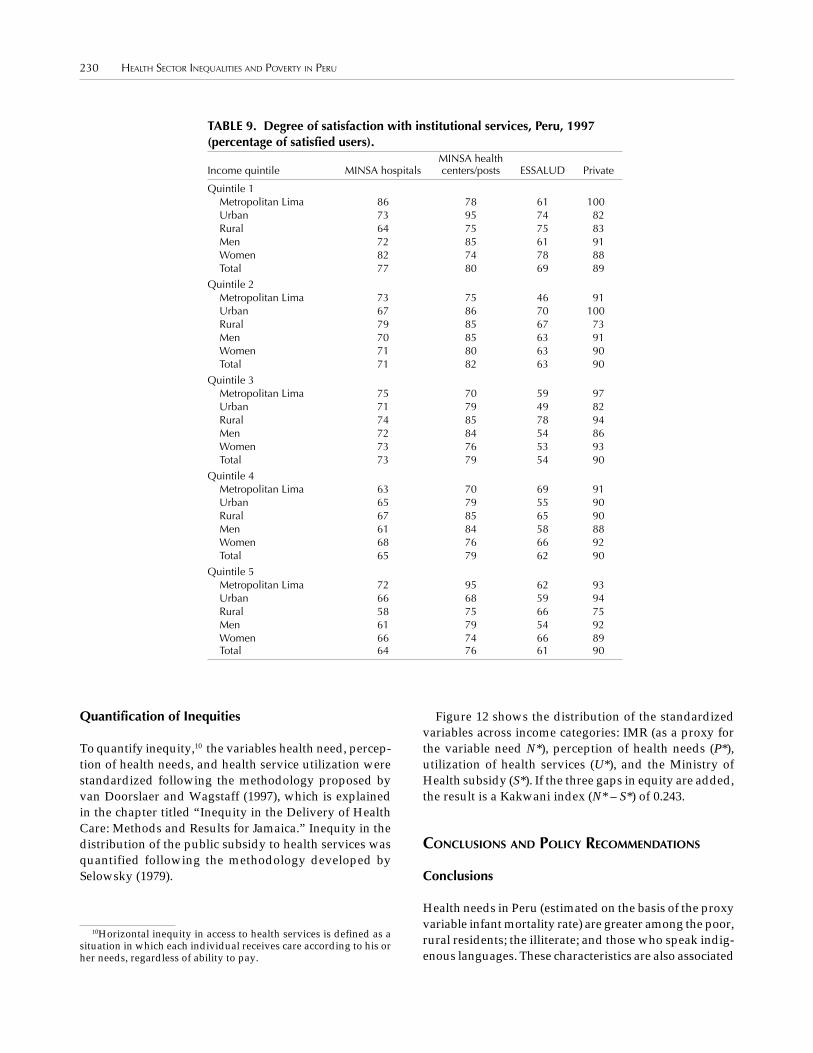
230 HEALTH SECTOR INEQUALITIES AND POVERTY IN PERU
Quantification of Inequities
To quantify inequity,10 the variables health need, percep-tion of health needs, and health service utilization werestandardized following the methodology proposed byvan Doorslaer and Wagstaff (1997), which is explainedin the chapter titled “Inequity in the Delivery of HealthCare: Methods and Results for Jamaica.” Inequity in thedistribution of the public subsidy to health services wasquantified following the methodology developed bySelowsky (1979).
Figure 12 shows the distribution of the standardizedvariables across income categories: IMR (as a proxy forthe variable need N*), perception of health needs (P*),utilization of health services (U*), and the Ministry ofHealth subsidy (S*). If the three gaps in equity are added,the result is a Kakwani index (N* – S*) of 0.243.
CONCLUSIONS AND POLICY RECOMMENDATIONS
Conclusions
Health needs in Peru (estimated on the basis of the proxyvariable infant mortality rate) are greater among the poor,rural residents; the illiterate; and those who speak indig-enous languages. These characteristics are also associated
10Horizontal inequity in access to health services is defined as asituation in which each individual receives care according to his orher needs, regardless of ability to pay.
TABLE 9. Degree of satisfaction with institutional services, Peru, 1997(percentage of satisfied users).
MINSA healthIncome quintile MINSA hospitals centers/posts ESSALUD Private
Quintile 1Metropolitan Lima 86 78 61 100Urban 73 95 74 82Rural 64 75 75 83Men 72 85 61 91Women 82 74 78 88Total 77 80 69 89
Quintile 2Metropolitan Lima 73 75 46 91Urban 67 86 70 100Rural 79 85 67 73Men 70 85 63 91Women 71 80 63 90Total 71 82 63 90
Quintile 3Metropolitan Lima 75 70 59 97Urban 71 79 49 82Rural 74 85 78 94Men 72 84 54 86Women 73 76 53 93Total 73 79 54 90
Quintile 4Metropolitan Lima 63 70 69 91Urban 65 79 55 90Rural 67 85 65 90Men 61 84 58 88Women 68 76 66 92Total 65 79 62 90
Quintile 5Metropolitan Lima 72 95 62 93Urban 66 68 59 94Rural 58 75 66 75Men 61 79 54 92Women 66 74 66 89Total 64 76 61 90

PETRERA AND CORDERO 231
with a lack of access to basic social services and socioeco-nomic marginalization.
The perception of symptoms of illness tends to increasewith income; reported illness and accidents, on the otherhand, do not vary significantly across income groups.
Reports of illness, symptoms of illness, and accidentsvary considerably according to age and gender. Womenreport more illness, especially in the second half of thelife cycle.
Although health needs are clearly greater among thepoor, distribution of the utilization of health services fa-vors the wealthy. When health services are classified bytype and location, the only ones that show a nonregressivepattern of utilization are the health centers and postsoperated by the Ministry of Health in urban areas. Pri-vate services display the most regressive pattern (only4% of the population in the poorest income quintile uti-lizes private services). The pattern of utilization ofESSALUD services is also skewed toward the rich butless so than for private services. Utilization of the ser-vices of the Ministry of Health is the least regressive, buteven in this case utilization of hospitals increases withincome.
Users reported greater satisfaction with private servicesthan with public services, and the satisfaction gap grew
with income. Users reported higher satisfaction with theservices of the Ministry of Health than with the servicesof ESSALUD. Among the services of the Ministry ofHealth, those provided by health centers/posts were themost satisfactory for all the income categories. The in-crease in public spending at this level of care helps toexplain this finding.
Public subsidies in the health sector (defined as theexpenditure of the Ministry of Health less user fees andadministrative costs at the central level) are regressive innature, except the subsidy to the first level of care (healthcenters and posts) in urban areas. The progressivity ofthe latter reflects the important and sustained increase ingovernmental spending on the first level of care. How-ever, the financing of first-level services in rural areas isregressive.
Public expenditure for hospital care reaches a verysmall proportion of the poor population. Access to hos-pital services is particularly limited among the rural poor.This reflects (a) the absence of an effective system to trans-fer patients from rural health services/posts to hospitals,and (b) the difficulties the rural poor have in coveringthe costs involved (hospital charges and travel expenses).
Utilization of health care services decreases amongpeople with low educational levels and among the in-
Cum
ulat
ive
% fo
r in
dica
tor
IMR (N*)
Subsidy (S*)
Utilization (U*)
P*
Cumulative % of population by income decile
Kakwani index (N* – S*) = 0.2043
100
80
60
40
20
0
0 20 40 60 80 100
FIGURE 12. Distribution of health need (N*), perception (P*), utilization ofservices (U*), and Ministry of Health subsidy (S*) (standardized).
Source: LSMS, 1997.

232 HEALTH SECTOR INEQUALITIES AND POVERTY IN PERU
digenous population. This is particularly true in the caseof hospital services. The rural population reported lesssatisfaction with health care services than the urban popu-lation, reflecting the fact that the quality of the servicestends to be lower in rural areas.
Distribution of the public subsidy to health care ser-vices was found to be inequitable. The degree of ineq-uity was greater when health needs were measuredthrough a proxy variable (infant mortality rates) thanwhen they were measured through reports of disease andsymptoms of illness. The Kakwani index increased from0.1454 when the first measure was applied to 0.243 whenthe second measure was used. In spite of the inequityfound, health care in Peru has a significant redistributiveeffect. This can be deduced by comparing the distribu-tion of income (Gini coefficient = 0.48) with the distribu-tion of health care service utilization (Gini coefficient =0.1043) and the distribution of the public subsidy to healthcare (Gini coefficient = 0.1655).
Policy Recommendations
Reducing the gap between the health needs of the poorand their perception of illness requires intensive educa-tional campaigns directed toward the rural and indig-enous populations. The goal of these campaigns shouldbe to translate health needs into greater demand for healthcare. There also should be an effort to redesign preven-tive health systems in order to identify health needs thatare difficult to perceive, such as malnutrition.
Reducing the gap between health needs and utiliza-tion of services should focus on accessibility and effec-tiveness of care. To this end, three different types of in-terventions should be considered: (a) interventions aimedat increasing efficient use of resources in both the publicand private sectors, encouraging competition among pro-
viders, and integrating private and public services; (b)interventions aimed at strengthening the response capac-ity of service providers by establishing networks thatpermit an expeditious mobilization of resources and pa-tients; and (c) high-impact interventions targeted to thepoor, such as national campaigns to reduce maternalmortality and spatially defined actions to combat diseaseslike malaria and dengue fever.
To increase the impact of public expenditures on thepoor, three types of policies can be identified: (a) policiesthat create payment systems that provide positive incen-tives for providers; (b) policies aimed at modernizingadministrative procedures in order to reduce expendi-tures and increase the effectiveness of interventions inpoor areas; and (c) policies that mobilize resources basedon the needs of specific populations and localities.
REFERENCES
Grupo Técnico Interinstitucional. El sector salud en el Perú. Informepreliminar no. 1. Lima: Grupo Técnico Interinstitucional; Octo-ber 1997.
Portocarrero A. Equidad en el gasto en público en salud Perú: 1997. Lima:Informe de Consultoría Organización Panamericana de la Salud-Perú; October 1998.
Reyes C, Ventocilla M. Revisión y actualización del financiamiento delsector salud 1995–1996. Lima: Ministerio de Salud; August 1997.
Selowsky M. Who Benefits from Government Expenditure? DiscussionPaper. Washington, DC: World Bank; June 1979.
van Doorslaer E, Wagstaff A. Equity in the Finance and Delivery ofHealth Care: A Review of the ECuity Project Findings. Washing-ton, DC: World Bank; September 1997.
World Bank. Comparaciones de pobreza 1994–97. Resumen delinforme principal. In Diálogo sobre experiencias y retos en la luchacontra la pobreza. First Forum October 26–27 1998. Lima: OficinaSubregional 6, Región de América Latina y El Caribe; October1998a.
World Bank. Reforma laboral y creación de empleo: la agendaincompleta de los países de América Latina y El Caribe. Wash-ington, DC: World Bank; 1998b.

233
INTRODUCTION
Equity is widely recognized to be an important policyobjective in the health care field. Indeed, some authorsgo so far as to suggest that, among the population at large,equity takes precedence over other objectives, such asefficiency. Equity concerns take two forms. The first isthe impact of health care financing and delivery arrange-ments on the distribution of income. In the ECuity project,we call this “equity in health care finance.” The otherconcern is the impact of health care financing and deliv-ery arrangements on the distribution of health care utili-zation. We call this “equity in the delivery of health care.”The latter concern is the subject of this paper.
The literature in this field seeks to assess not just howutilization is distributed but rather whether it is distrib-uted fairly. This calls for a notion of fairness. In our workto date we have taken as our starting point the notionthat an equitable distribution of health care is one in whichhealth care is allocated according to need.2 Our work has
focused on the horizontal version of this principle—therequirement that persons with equal need be treated thesame—and we have focused exclusively on the extent towhich violations of this principle are systematically re-lated to income. That is, our work has explored the ex-tent to which persons in equal need end up being treatedthe same regardless of where they happen to be in theincome distribution. This chapter follows this tradition,as do similar studies for other countries in the WorldBank’s project on equity in health care finance anddelivery.
Comparative research on this topic clearly is potentiallyuseful. Cross-country comparisons or comparisons overtime may help shed light on the issue of whether, on thewhole, health care is distributed more equitably in onetype of health care system than in another. Undertakingresearch along these lines clearly requires a means ofmeasuring inequity. One cannot answer questions suchas “Is health care allocated less equitably in, say, Colom-bia than it is in, say, Brazil?” or “Has health care beenallocated more equitably in Colombia since the recentreforms?” without an index of inequity. One of the aimsof this paper is to set out in some detail a relatively simpleset of methods that can be used to measure inequity inthe delivery of health care. These methods build on thosethat were developed and applied to a number of indus-trialized countries in a forerunner of the ECuity project.3
The methods employed and applied in the ECuity projectitself differ from those used in earlier work in that theyuse the indirect method of standardization to adjust forneed differences rather than the direct method of stan-dardization.4 The method is far simpler to implement and
INEQUITY IN THE DELIVERY OF HEALTH CARE: METHODS
AND RESULTS FOR JAMAICA1
Eddy van Doorslaer and Adam Wagstaff
1Paper prepared for the Human Development Department of theWorld Bank. Second Version, June 1998.
2This notion is not uncontroversial. Wagstaff et al. (1989) exploredthe alternative ideological points of view on equity. One is the “lib-ertarian” viewpoint (e.g., Maynard and Williams, 1984). This re-gards health care as part of society’s reward system and sees noth-ing wrong with people using their income and wealth to purchasemore and better quality health care than others with similar medi-cal needs if they so wish. The other is the “egalitarian” viewpoint,which views “access to health care [as] a citizen’s right . . . , whichought not to be influenced by income and wealth” (Maynard andWilliams, 1984: p. 96). Some people are more attracted to one view-point; some to the other. Policy statements in most European coun-tries and Canada suggest a greater degree of support for the egali-tarian viewpoint. This is consistent with a number of differentpositions on how medical care ought to be allocated. Allocation ac-cording to need, rather than income, is one view, but typically littlejustification for adopting this allocation rule instead of another isoffered. Culyer and Wagstaff (1993) argue that allocating medicalcare so as to reduce health inequalities is a more ethically defen-sible position for an egalitarian.
3See Wagstaff et al. (1991a) for methods. For results, see vanDoorslaer et al. (1992, 1993).
4See Wagstaff and van Doorslaer (1993) for the new methods.For international comparisons obtained using them, see vanDoorslaer et al. (1997a).

234 INEQUITY IN THE DELIVERY OF HEALTH CARE: METHODS AND RESULTS FOR JAMAICA
can be used on individual-level data. Therefore, it oughtto be more accurate. In practice, it appears to producebroadly similar results for categories of utilization whereinequity is statistically significant.5
The second aim of this work is to apply these methodsto the 1989 Jamaican Survey of Living Conditions (SLC).Clearly, Jamaica is not typical of the developing worldor even of Latin America and the Caribbean (LAC). It isperhaps typical in terms of per capita gross domesticproduct—Jamaica lies among the lower middle-incomecountries. However, Jamaica’s life expectancy (73.1 yearsin 1990) and infant mortality rate (15 per 1,000 in 1991)are comparatively good [e.g., United Nations Develop-ment Program (1993)]. By LAC standards, its income dis-tribution is also fairly equal (a Gini coefficient of 0.435,compared with an LAC average of 0.500), the propor-tions of people living in poverty (below US$ 60 per dayin 1989) and in extreme poverty (below US$ 30 per day)are fairly low, and the corresponding aggregate povertygaps are also fairly low (cf. Psacharopoulos et al., 1997).Jamaica’s predominantly publicly financed centralizedhealth care system ensures that all members of the popu-lation have access to relatively good quality health care,even if the better off privately insured are able to obtainbetter quality privately provided care (e.g., Gertler andSturm, 1997). However, the relative richness of the SLC—compared with the standard living standards measure-ment surveys (LSMS)—makes Jamaica an interesting testcase. In Jamaica’s case, the traditional LSMS health mod-ule has been supplemented with additional health andmedical care utilization questions, many of which are ofthe type encountered in health interview surveys in in-dustrialized countries and some of which are to be foundin the new-generation LSMS surveys (cf. Planning Insti-tute of Jamaica, 1992).
This chapter is organized as follows. The second sec-tion outlines the methods used to assess the extent of anyinequity in the delivery of health care. The third sectiondescribes the data used and the variable definitions em-ployed. The fourth section contains the empirical resultsfor Jamaica. In addition to measuring and testing for in-equity in the utilization of curative and preventive care,we also explore the role of private insurance coverage.The final section contains our conclusions.
METHODS
This section begins with a discussion of the new methodfor measuring inequity in health care delivery—the so-called HIWV index.6 Then a simple-but-accurate regres-sion-based method is set out by which the indirect stan-dardization underlying this index can be implemented.The techniques that are available for computing the HIWV
index, including a simple-but-accurate convenient regres-sion method, are discussed. The issue of statistical infer-ence is addressed and a simple but inaccurate way tocompute standard errors for the HIWV index, as well as amore complex but accurate method, is presented. Thenthe methods are summarized.
Measuring Inequity
The idea underlying the HIWV index is simple. It involvescomparing the actual distribution of medical care acrossincome groups with the distribution of need. Let mi de-note the amount of medical care received by individual iin a given period. The distribution of medical care by in-come is captured by the medical care concentration curveLM(s) in Figure 1, which graphs the cumulative propor-tion of medical care against the cumulative proportionof the sample ranked by income. The concentration in-dex CM corresponding to LM(s) indicates the degree of in-equality in the distribution of medical care. In itself, thistells us something about the degree of inequity in thedistribution of medical care only in the unlikely eventthat need for medical care does not vary with income.
The next step, therefore, is to take into account need dif-ferences, which we do by using the method of indirect stan-dardization. This generates a figure for each individualindicating the amount of medical care she would have re-ceived if she had been treated in the same way as otherpeople with the same need characteristics were, on aver-age, treated. We interpret this as her need for medical care.In the case in which there are just two need categories, theneed of individual i for medical care is simply m1 if she isin need category 1 and m2 otherwise. Or, if one is workingwith income groups, each income group’s need is aweighted average (or sum) of the sample mean quantitiesof medical care for need categories 1 and 2, where theweights are the proportions (or numbers) of persons inthe income group who are in need categories 1 and 2. Thus,the gth income group’s need can be measured as follows:
m f m f mg g g∗ = +1 1 2 2 (1)
where the terms are as defined above.
5See Wagstaff and van Doorslaer (1993) for comparative resultson Dutch data with the two methods. The only appreciable differ-ence is for hospital days, but in neither case is the inequity indexsignificant. The results suggest that, regardless of which method ofstandardization is used, there is significant pro-rich inequity in out-patient care utilization in the Netherlands but no significant ineq-uity in general practitioner care or inpatient care. Similar resultsare found for about half the countries studied by van Doorslaer(1997a and 1997b), even though the countries in question havewidely differing health care delivery systems.
6This subsection and the others in this section draw heavily onWagstaff and van Doorslaer (1993).

VAN DOORSLAER AND WAGSTAFF 235
Each income group’s share of need is then comparedwith its share of unstandardized medical care. If hori-zontal equity obtains, each group’s medical care sharewill equal its share of need. Thus, for example, if thereare just two income groups, the rich group’s share of needis equal to
Sr f m f m
p f m f m r f m f mr
r r
p p r r
∗ =+( )
+( ) + +( )1 1 2 2
1 1 2 2 1 1 2 2(2)
and its share of unstandardized medical care is equal to
Sr f m f m
p f m f m r f m f mr
r r r r
p p p p r r r r
=+( )
+( ) + +( )1 1 2 2
1 1 2 2 1 1 2 2(3)
If horizontal equity obtains, m1r = m1
p = m1 and m2r = m2
p =m2—i.e., people are treated alike in each need categoryregardless of whether they are rich or poor. In this case,we have Sr
* = Sr. If, by contrast, there is horizontal ineq-uity favoring the rich, so that, within each need category,the better off receive more medical care, we have Sr
* < Sr.In the more general case, in which there are more than
two income groups and more than two need categories,it is useful to utilize the concept of a “need” concentra-tion curve. This curve, labeled LN(s) in Figure 1, plots thecumulative proportion of the population—ranked by in-come—against the cumulative proportion of “need-ex-pected” medical care utilization. The extent of horizon-tal inequity can then be assessed by comparing LM(s) withLN(s). If the latter lies above the former, there is horizon-
tal inequity favoring the better off; if the latter lies belowthe former, there is inequity favoring the worse off. Themeasure of horizontal inequity, HIWV, is defined as twicethe area between the need and medical care concentra-tion curves:
HI L p L p p C CWV N M M N= − = −∫20
1[ ( )] ( )]d (4)
where CN is the concentration index for need (i.e., indi-rectly standardized medical care). A positive value ofHIWV indicates horizontal inequity favoring the better off,a negative value indicates inequity favoring the worseoff, and 0 indicates that the factor of proportionality (be-tween medical care and need) is the same regardless ofincome.
Computation I: Standardization
The indirectly standardized medical care utilization m*i
and the concentration index CM can easily be computedby regression methods. The standardized values are sim-ply the predicted values saved from the appropriatelyspecified regression equation. Let xi be a dummy vari-able taking a value of 1 if person i is in need category 2,and mi is her use of medical care. Then we have
m x ui i i= + +α β (5)whereby
E m x mE m x m
i i
i i
[ | ] ,[ | ] ,
= = == = + =
01
1
2αα β (6)
and hence
E m x x mi i i i[ | ] = + = ∗α β (7)
Thus, the need of person i can be obtained simply by re-taining the predicted value from Equation 5. This ap-proach too is easily extended in cases in which a vectorof need indicators is used. Thus, let xi be a vector of needindicators together defining the various need categories,and let x be the vector of sample means of xi. In this case,we have
E m mi i i i[ | ]x x= ′ = ∗β (8)
so that one simply runs a multiple regression of utiliza-tion on the vector of need variables and retains the pre-dicted values. It is important to remember that, for thepurpose of standardization, the vector x should containonly (proxy) indicators of need for medical care. As a re-sult, Equation 8 is not to be interpreted as a behavioralmodel capturing all determinants of medical care utili-
1.0
0.0 1.0Cumulative proportion of population, ranked by income
Cum
ulat
ive
prop
ortio
n of
med
ical
car
e
LN (R)
LM (R)
FIGURE 1. Concentration curves.
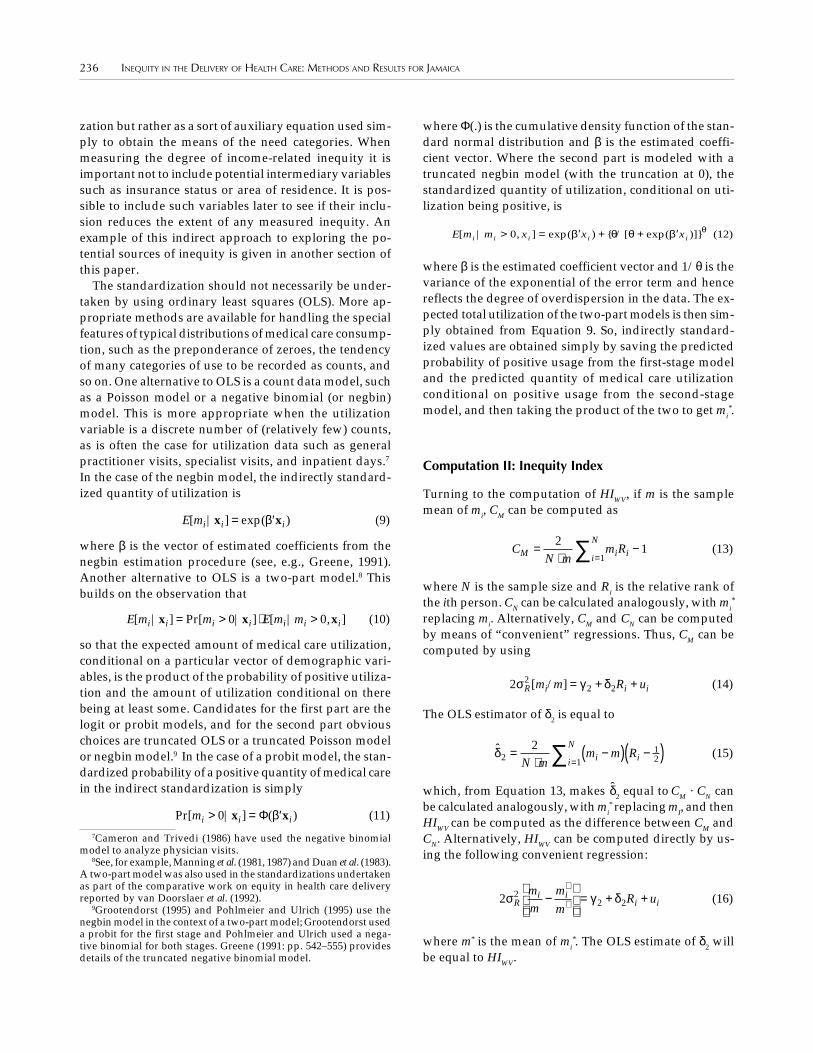
236 INEQUITY IN THE DELIVERY OF HEALTH CARE: METHODS AND RESULTS FOR JAMAICA
zation but rather as a sort of auxiliary equation used sim-ply to obtain the means of the need categories. Whenmeasuring the degree of income-related inequity it isimportant not to include potential intermediary variablessuch as insurance status or area of residence. It is pos-sible to include such variables later to see if their inclu-sion reduces the extent of any measured inequity. Anexample of this indirect approach to exploring the po-tential sources of inequity is given in another section ofthis paper.
The standardization should not necessarily be under-taken by using ordinary least squares (OLS). More ap-propriate methods are available for handling the specialfeatures of typical distributions of medical care consump-tion, such as the preponderance of zeroes, the tendencyof many categories of use to be recorded as counts, andso on. One alternative to OLS is a count data model, suchas a Poisson model or a negative binomial (or negbin)model. This is more appropriate when the utilizationvariable is a discrete number of (relatively few) counts,as is often the case for utilization data such as generalpractitioner visits, specialist visits, and inpatient days.7
In the case of the negbin model, the indirectly standard-ized quantity of utilization is
E mi i i[ | ] exp( )x x= ′β (9)
where β is the vector of estimated coefficients from thenegbin estimation procedure (see, e.g., Greene, 1991).Another alternative to OLS is a two-part model.8 Thisbuilds on the observation that
E m m E m mi i i i i i i[ | ] Pr[ | ] [ | , ]x x x= > ⋅ >0 0 (10)
so that the expected amount of medical care utilization,conditional on a particular vector of demographic vari-ables, is the product of the probability of positive utiliza-tion and the amount of utilization conditional on therebeing at least some. Candidates for the first part are thelogit or probit models, and for the second part obviouschoices are truncated OLS or a truncated Poisson modelor negbin model.9 In the case of a probit model, the stan-dardized probability of a positive quantity of medical carein the indirect standardization is simply
Pr[ | ] ( )mi i i> = ′0 x xΦ β (11)
where Φ(.) is the cumulative density function of the stan-dard normal distribution and β is the estimated coeffi-cient vector. Where the second part is modeled with atruncated negbin model (with the truncation at 0), thestandardized quantity of utilization, conditional on uti-lization being positive, is
E m m xi i i i i[ | , ] exp( ) { /[ exp( )]}> = ′ + + ′0 x xβ θ θ β θ (12)
where β is the estimated coefficient vector and 1/θ is thevariance of the exponential of the error term and hencereflects the degree of overdispersion in the data. The ex-pected total utilization of the two-part models is then sim-ply obtained from Equation 9. So, indirectly standard-ized values are obtained simply by saving the predictedprobability of positive usage from the first-stage modeland the predicted quantity of medical care utilizationconditional on positive usage from the second-stagemodel, and then taking the product of the two to get mi
*.
Computation II: Inequity Index
Turning to the computation of HIWV, if m is the samplemean of mi, CM can be computed as
CN m
m RM i ii
N=
⋅−
=∑21
1(13)
where N is the sample size and Ri is the relative rank ofthe ith person. CN can be calculated analogously, with mi
*
replacing mi. Alternatively, CM and CN can be computedby means of “convenient” regressions. Thus, CM can becomputed by using
2 22 2σ γ δR i i im m R u[ / ] = + + (14)
The OLS estimator of δ2 is equal to
δ̂2 112
2=⋅
−( ) −( )=∑N m
m m Rii
Ni (15)
which, from Equation 13, makes δ̂2 equal to CM · CN canbe calculated analogously, with mi
* replacing mI, and thenHIWV can be computed as the difference between CM andCN. Alternatively, HIWV can be computed directly by us-ing the following convenient regression:
2 22 2σ γ δR
i ii i
mm
mm
R u−
= + +∗
∗ (16)
where m* is the mean of mi*. The OLS estimate of δ2 will
be equal to HIWV.
7Cameron and Trivedi (1986) have used the negative binomialmodel to analyze physician visits.
8See, for example, Manning et al. (1981, 1987) and Duan et al. (1983).A two-part model was also used in the standardizations undertakenas part of the comparative work on equity in health care deliveryreported by van Doorslaer et al. (1992).
9Grootendorst (1995) and Pohlmeier and Ulrich (1995) use thenegbin model in the context of a two-part model; Grootendorst useda probit for the first stage and Pohlmeier and Ulrich used a nega-tive binomial for both stages. Greene (1991: pp. 542–555) providesdetails of the truncated negative binomial model.

VAN DOORSLAER AND WAGSTAFF 237
Statistical Inference
Given that inequity indices are computed from samples,it is important to compute standard errors to assess thestatistical significance of indices and of changes over timeand differences among countries. Building on resultsobtained by Kakwani et al. (1997) we present estimatorsfor the standard errors of both indices.
Application of OLS to Equation 14 automatically pro-vides a standard error for CM and, when using indirectlystandardized values, for CN. OLS applied to Equation 16provides a standard error for HIWV. However, in each casethis method of obtaining standard errors overlooks thefact that the observations of Equations 14 and 16, beingranks, are not independent of one another. A more accu-rate estimator for the standard error of HIWV that takesinto account the serial correlation in ui can be obtained asfollows:
var( ˆ ) ( ) ˆHI a a HIWV N N i i WVi
N= − −
∗=∑1 1 2
1(17)
where ai is defined as in Equation 18 below and ai* is de-
fined analogously to ai except that indirectly standard-ized values are used instead of actual values in itscalculation.
amm
R C q qii
i M i i= − − + − −−( ˆ )2 1 2 1 (18)
with
qm
m fii
==∑1
1 γγ γ (19)
being the ordinate of LM (R), with q0 = 0.
Summary of Methods
Our aim is to measure the extent to which persons inequal need are treated the same, regardless of their in-come. In this paper, we have used an index that is basedon a comparison of two concentration curves. The first,labeled LM(s) in Figure 1, graphs the cumulative pro-portion of utilization against the cumulative proportionof the sample ranked by income. Comparing this withthe diagonal, or “line of equality,” shows the degree ofinequality—across income groups—in the distributionof utilization. This says nothing about inequity in thesense of persons in equal need being treated unequallydepending on their income, except in the unlikely casethat need and income are uncorrelated. The relevantcurve against which to compare LM(s) is not the diago-nal but the curve labeled LN(s) in Figure 1, which graphsthe cumulative proportion of need against the cumula-
tive proportion of the sample ranked, as before, by in-come. If LN(s) lies above LM(s), the implication is thatneed is distributed more unequally across incomegroups than is utilization and, hence, among persons inequal need, persons at the top end of the income distri-bution are being treated more favorably than those atthe bottom. The HIWV index is simply twice the area be-tween these two concentration curves and therefore isequal to the difference between the corresponding con-centration indices CM and CN. It is positive in the case ofpro-rich inequity and negative in the case of pro-poorinequity [LN(s) lies below LM(s)].
The indirect method of standardization is used to ob-tain the amount of medical care a person needs. Thisindicates the amount of medical care the person wouldhave received if she had been treated as other peoplewith the same need characteristics were, on average,treated. This can be computed simply by means of re-gression analysis, retaining the predicted values of aregression of utilization on the vector of variables cap-turing the person’s need characteristics. Although OLScan be used for this regression, alternative methods maybe better, such as a negbin model or a two-part model,with a probit model being used for the first part andeither truncated OLS or a truncated negbin being usedfor the second part.
Once the standardized utilization (or need) values havebeen obtained for each individual, the values of CM, CN,and HIWV can be obtained by means of convenient regres-sion equations. In the case of CM, for example, this in-volves regressing a simple transformation of theindividual’s utilization on the individual’s relative rankin the income distribution. The same procedure can beused in the case of CN, replacing the individual’s utiliza-tion by his need. The slope coefficients in each case areequal to the relevant inequality index. The HIWV indexcan be computed directly by regressing a transformationof the difference between the individual’s utilization andhis need on this relative rank. Although the convenientregression approach gives a standard error for CM, CN,and HIWV, it is not entirely reliable because of theautocorrelation induced by the relative rank variable.Accurate estimators for the standard errors have beenderived by building on the work of Kakwani et al. (1997)and are reproduced in the paper. These are used in thenext section.
DATA AND VARIABLE DEFINITIONS
The survey used is the 1989–1992 Jamaican SLC. Thisshares features of the LSMS surveys used extensively inWorld Bank work, but it also contains some variables,

238 INEQUITY IN THE DELIVERY OF HEALTH CARE: METHODS AND RESULTS FOR JAMAICA
notably in the health module, that are not contained inthe typical LSMS. Our focus in this version of the paperis on adults (i.e., 16 and older); after deletion of cases withmissing information, the sample size is 10,132 cases.
Socioeconomic Status
Our measure of socioeconomic status (i.e., our rankingvariable) is household expenditure per equivalent adult.There seems to be a general preference among LSMS us-ers for using household expenditure as a measure of ahousehold’s command over resources rather than incomedue to factors such as underreporting of income, assign-ment of monetary values to homegrown produce, andso on. Our equivalence scale is that proposed by Aronsonet al. (1994),
e A Kh h h= +( )Φ θ (20)
where eh is the equivalence factor for household h, Ah isthe number of adults in household h, and Kh is the num-ber of children. We have set the two parameters Φ and θequal to 0.75. This results in an equivalence scale that liessomewhere between the Rothbath and Engel scales dis-cussed by Deaton and Muellbauer (1986).10
Medical Care Utilization
The amount of medical care received, mi, was measuredwith four measures of medical care utilization: (a) theprobability of reporting at least one curative visit in thelast month before the survey, (b) the number of curativevisits, (c) the probability of reporting at least one preven-tive care visit in the past 6 months, and (d) the number ofpreventive visits. As shown in Table 1, curative visits aredefined as due to injury or illness, whereas preventivevisits are defined as occurring besides injury or illness.We analyzed the probability of a visit and the number ofvisits separately to see whether any inequity differed
between the likelihood of use and the amount of healthcare usage.
The question about preventive visits is unconditional,but the question about curative visits is conditional on apositive reply to the question “Have you had any illnessor injury during the past 4 weeks?” Only those with apositive response are then asked “Due to this illness orinjury, have you visited a doctor, nurse, pharmacist, mid-wife, healer, or any other health practitioner during thepast 4 weeks?” and “How many times did you visit thisplace?”11 Both questions were repeated for those who alsovisited a second place during the past four weeks. Weused the total number of visits reported in both ques-tions as the rate of curative visits.
Need Indicators
The vector of variables used in the need standardizationxi always includes a vector of demographic characteris-tics consisting of a gender dummy and a vector of agedummies corresponding to the age categories 18–34, 35–44, 45–64, 65–74, and 75+ years old. The various addi-tional health questions used as need indicators are listedin Table 2. Appropriate vectors of dummy variables werecreated in each case.
10 The Engel scales reported by Deaton and Muellbauer (1986) fora couple, a couple with one child, and a couple with two childrenare 1.00, 1.41, 1.77 for Sri Lanka; 1.00, 1.45, 1.86 for Indonesia (chil-dren under 5); and 1.00, 1.58, 2.22 for Indonesia (children older than5). Their Rothbath scales are lower: 1.00, 1.12, 1.21 for Sri Lanka;1.00, 1.10, 1.16 for Indonesia (children under 5); and 1.00, 1.12, 1.22for Indonesia (children over 5). They argue that “true costs are gen-erally overstated by the Engel method and understated by theRothbath method, but the latter unlike the former can provide asensible starting point for cost measurement” (p. 720). The Aronsonet al. (1994) scale, with the two parameters both set at 0.75, is 1.00,1.27, and 1.52. On the basis of Deaton and Muellbauer’s advice, thescale of Aronson et al. (0.75, 0.75) is a reasonably good one to use.
TABLE 1. Medical care utilization variables used.Indicator Definition
Number of curative visits First question: Due to illness orinjury, have you visited a doctor,nurse, pharmacist, midwife, healer,or any other health practitionerduring the past four weeks?
Second question: How many timesdid you visit this place?
Probability of curative visit Dummy variable equals 1 if at leastone curative visit was reported
Number of preventive visits First question: Besides illness orinjury did you seek health carewithin the past six months? Haveyou had prenatal checkups,preventive health checkups, family-planning services, or other?
Second question: How many visitsdid you make in the past 6 monthsto health practitioners?
Probability of preventive visit Dummy variable equals 1 if at leastone preventive visit was reported
11The questionnaire further allows one to distinguish betweenthe type of practitioner, public and private visits, etc.

VAN DOORSLAER AND WAGSTAFF 239
RESULTS
Regression Results
The indirect standardization was undertaken with vari-ous combinations of need indicators to allow for futurecomparisons with results from LSMS surveys for othercountries with less detailed health information than theJamaican 1989 SLC. In Tables 3 and 4 we compare thebasic OLS regression results for “at least one curativevisit” and “number of visits” for one such specificationwith the results obtained using alternative model speci-fications. As an alternative to OLS for “at least one visit”we used a probit equation. We used a negbin model anda two-part model consisting of a probit equation for thefirst part and truncated OLS for the second part to modelthe number of visits.12
The prediction of any curative care utilization and ofthe number of visits is largely dominated by the very sig-nificant dummy for “illness or injury in the past fourweeks.” This is not surprising because reporting of anyuse is conditional on such illness or injury. When it is
TABLE 2. Additional need indicators used.Indicator Definition
Self-assessed health In general, would you say your health isexcellent, very good, good, fair, or poor?
Activity limitation Does your health limit you at all in any ofthe following activities: (a) vigorousactivities such as running, lifting heavyobjects, participating in strenuous sports,doing hard labor; (b) moderate activities,such as moving a table or doing repairs;(c) walking uphill or climbing stairs;(d) bending, kneeling, or stooping; (e)walking more than a mile; (f) walking 100yards; (g) eating, bathing, or using a toilet?
Illness or injury Have you had any illness or injury duringthe past four weeks? For example, have youhad a cold, diarrhea, injury due to anaccident, or any other illness?
Illness days For how many days during the past fourweeks have you suffered from this illness orinjury?
Restricted-activity days For how many days during the past fourweeks were you unable to carry on yourusual activities because of this illness orinjury?
12 Because only about 7% of individuals in the sample report atleast one curative visit (mean 0.11) and about 19% a preventive visit(mean 0.45), a two-part model may be more suitable to predict medi-cal care utilization. We report only the results of the probit + trun-cated OLS model here because the truncated negbin model failedto converge for the curative visits model.
included in the equation, the adjusted R2 dramaticallyincreases, but few coefficients for other variables remainsignificant. Interestingly, neither age, sex, nor self-as-sessed health still has a significant and consistent effecton the utilization rate after controlling for reported ill-ness. Only some of the functional limitations still show asignificant effect. It can also be seen that there is littledifference between the OLS and the non-OLS modelspecifications in terms of significance of explanatory vari-ables. Interestingly, in the truncated OLS regression onpositive users only the dummy “illness or injury” couldnot be included and none of the remaining explanatoryvariables remains significant. Therefore, it seems thatmost of the impact of the need indicators on utilizationof curative care is through their influence on the decisionwhether to use rather than on the number of visits.
The regression results for preventive visits show amuch more significant impact of age and self-assessedhealth both on the probability of usage and on the num-ber of visits. The female dummy is very significant be-cause of the importance of prenatal checkups. The largeand significant estimate of α (=1/θ) in the negbin modelindicates that overdispersion in the data is an issue andthat a negbin model is preferred over the simpler Pois-son count model. However, because the results of themore sophisticated models do not differ dramaticallyfrom the simpler OLS models, we have used OLS regres-sions in the sensitivity analysis of the inequity indiceswith respect to different specifications.
Quintile Distributions and Inequity Indices
The next step is to compare the quintile distributions ofactual and need-predicted utilization rates. These arepresented in Table 5 for curative visits and in Table 6 forpreventive visits.
The actual probability of someone in the first quintilereporting a contact with the health care system in the pastfour weeks appears to be a good deal lower than the prob-ability that would be expected on the basis of a set ofself-reported need indicators. The opposite is true for thetop quintile. There is not a particular gradient but rathera U-shaped pattern in the distribution of the actual num-ber of curative visits, with the middle quintile reportingthe smallest share of visits. Only the first and thirdquintiles appear to be having fewer visits than expected;the opposite is true for all other quintiles.
These patterns are also reflected by the estimates ofCM, CN, and HIWV, which are presented at the bottom ofthe table. Both the “needed” visit probability and the“needed” visit rate show a negative concentration index,whereas the actual visit probability and visit rate show a

240 INEQUITY IN THE DELIVERY OF HEALTH CARE: METHODS AND RESULTS FOR JAMAICA
TABLE 4. Regression results for preventive visits.Log
At least one visit Number of visits (posit visits)
TruncatedVariable OLS Probit OLS Negbin OLS
Female 0.1370* 0.4602* 0.2681* 0.8420* 0.0950*Age 35–44 –0.0032 0.0734 0.0096 0.0540* –0.0971*Age 45–64 0.0154 0.0375 –0.0286 0.0993 –0.1080*Age 65–74 0.0859* 0.2552* 0.0786 0.1940 –0.1594*Age 75+ 0.1050* 0.2508* 0.0416 0.2947* –0.1775*SAH poor 0.0471 0.5491* 0.7774* 1.0677* 0.2320*SAH fair 0.0012 0.4289* 0.4586* 0.8374* 0.2104*SAH good –0.1080* 0.1089* 0.0597 0.1729* 0.0408SAH very good –0.1280* 0.0291 –0.0133 –0.03801 –0.0359Limitation in vigorous activities 0.0301* 0.1170 0.1470* 0.3842* 0.0406Limitation in moderate activities 0.0041 0.0102 –0.0426 –0.0244 –0.0002Difficulty walking up stairs –0.0083 –0.0315 –0.0461 –0.1096 –0.0494Difficulty bending, kneeling, or stooping 0.0941* 0.2590* 0.2302* 0.2750 0.0775Difficulty walking 1 mile 0.0219 0.0592 0.1316 0.1381 0.0735Difficulty walking 100 yards –0.0115 –0.0361 0.0552 –0.0046 0.1122Difficulty eating, dressing, toilet –0.0700* –0.1616* –0.0701 –0.0280 –0.0068Constant 0.2040* –1.4351* 0.1388* –1.8582* 0.48901/θAdjusted R2 0.075 0.068 4.669* 0.049
SAH = self-assessed health.* Asterisk denotes statistical significance at the 95% level.
TABLE 3. Regression results for curative visits.Log
At least one visit Number of visits (posit visits)
TruncatedVariable OLS Probit OLS Negbin OLS
Female 0.0061 0.1023 0.0091 0.0906 –0.0321Age 35–44 0.0151* 0.2689* 0.0432* 0.4569* 0.0640Age 45–64 –0.0018 0.0582 0.0030 0.1880 0.0081Age 65–74 –0.0069 0.0005 –0.0116 0.1034 –0.0100Age 75+ –0.0159 –0.0765 –0.0485 –0.0353 –0.1104Illness last month 0.4900* 2.8482* 0.7674* 5.2679* n.a.SAH poor 0.0091 0.1157 0.0755* 0.2102 0.0945SAH fair 0.0200* 0.2796* 0.0515* 0.2226 –0.0095SAH good 0.0060 0.1519 –0.0069 –0.0187 –0.0591SAH very good –0.0049 –0.0379 –0.0177 –0.1455 –0.0901Limitation in vigorous activities –0.0011 –0.0222 –0.0075 –0.0674 –0.0562Limitation in moderate activities 0.0340* 0.3143* 0.0634* 0.3000* 0.5067Difficulty walking up stairs –0.0394* –0.3510* 0.0159 –0.0728 0.0031Difficulty bending, kneeling, or stooping 0.0001 –0.0186 –0.1616* –0.4816* –0.1369Difficulty walking 1 mile 0.0147 0.1518 0.0833 0.3273* 0.1437Difficulty walking 100 yards 0.0375* 0.1910 0.0748 0.1604 0.0009Difficulty eating, dressing, toilet –0.0005 0.0471 –0.0083 –0.0056 –0.0190Constant –0.0073 –3.1297* –0.0109 –5.8114* 0.3207*1/θ 0.7358*Adjusted R2 0.457 0.192 0.0062
SAH = self-assessed health.* Asterisk denotes statistical significance at the 95% level. n.a. = not applicable.

VAN DOORSLAER AND WAGSTAFF 241
positive concentration index. As a result, both variablesshow a positive HIWV index, but it is smaller in magni-tude for the number of visits. Only the visit probability’sinequity index is significant on the basis of the t test.Again, there are hardly any differences between the OLSand more sophisticated models. Therefore, it seems as ifthere is some inequity favoring the rich with respect tothe probability of a contact but a clear pattern of inequityin the distribution of the number of visits does not emergefor Jamaica. We will explore the sensitivity of this resultto different “need” specifications in the next section.
The picture is quite different for preventive visits. Boththe probability and the number of actual visits show aclear upward-sloping gradient by income quintile:higher-income groups make more use of preventive ser-vices. In contrast, the opposite gradient emerges for thepattern of “needed” preventive care: lower-incomegroups seem to be in greater need of preventive care.Large positive values of CM coupled with (in absolutevalue) large negative values of CN generate significantlypositive values of HIWV. The index values for the numberof visits are about twice the size of those for the visit prob-ability but, again, they do not differ substantially between
the various regression models used in estimating the needfor preventive care. Clearly, the utilization of preventivecare is not distributed according to these measures of needand there is a strong indication of inequity favoring thericher groups.
Both curative care and preventive care are, on balance,pro-rich in their distribution. By contrast, the need forboth types of care is concentrated among the poor. Re-gardless of the regression model used, both the probabil-ity and the number of curative and preventive visits showa positive HIWV index, but the value is not statisticallysignificant in the case of the number of curative visits.
The situation is illustrated in Figure 2, which graphsthe corresponding concentration curves for numbers ofvisits. The number of curative visits and the need for cura-tive visits are both fairly equally distributed on balance.As a result, both concentration curves are fairly close toeach other and the area between the two curves is verysmall. By contrast, preventive visits are appreciably pro-rich in their distribution and their concentration curve iswell below the diagonal, whereas the need for preven-tive visits is appreciably pro-poor in its distribution witha concentration curve well above the diagonal. Therefore,
TABLE 6. Quintile distributions of actual and need-predicted preventive visits.At least one visit Number of visits
Quintile Actual OLS Probit Actual OLS Negbin Probit + OLS
1 0.227 0.265 0.212 0.345 0.526 0.568 0.4112 0.250 0.259 0.196 0.427 0.474 0.500 0.3713 0.236 0.250 0.192 0.463 0.462 0.489 0.3624 0.242 0.237 0.176 0.453 0.416 0.429 0.3265 0.290 0.233 0.174 0.593 0.403 0.418 0.319CM , CN 0.047 –0.0274 –0.0274 0.1075 –0.0537 –0.064 –0.0526HIWV n.a. 0.0744 0.0744 n.a. 0.1611 0.1715 0.1601t value n.a. 7.61 7.61 n.a. 9.1 9.58 9.05
Note: Need for preventive visits is estimated on the basis of regressions in Table 4; CM and CN are computed using Equation 13,HIWV index computed as the difference of the two, and standard error computed using Equations 17–19.
n.a. = not applicable.
TABLE 5. Quintile distributions of actual and need-predicted curative visits.At least one visit Number of visits
Quintile Actual OLS Probit Actual OLS Negbin Probit + OLS
1 0.071 0.080 0.080 0.121 0.129 0.129 0.1072 0.064 0.066 0.065 0.112 0.106 0.106 0.0873 0.065 0.070 0.071 0.097 0.112 0.114 0.0944 0.078 0.070 0.079 0.117 0.110 0.111 0.0935 0.077 0.069 0.067 0.120 0.110 0.108 0.089CM , CN 0.0403 –0.0158 –0.018 0.0126 –0.0188 –0.0223 –0.0199HIWV n.a. 0.056 0.0583 n.a. 0.0313 0.0349 0.0324t value n.a. 3.57 3.76 n.a. 0.95 1.07 0.99
Note: Need for curative visits estimated on the basis of regressions presented in Table 3; CM and CN computed using Equation 13,HIWV index computed as the difference of the two, and standard error computed using Equations 17–19.
n.a. = not applicable.

242 INEQUITY IN THE DELIVERY OF HEALTH CARE: METHODS AND RESULTS FOR JAMAICA
it is not surprising that the area between the two curvesis significantly different from zero for preventive but notfor curative visits.
Sensitivity Analysis
It is clear that the distribution of “need” depends cru-cially on the number and type of indicators included inthe regression equation estimating need-expected utili-zation. In this section, we explore the sensitivity of ourbaseline results for changes in the set of variables used inthe vector of need indicators. Because we did not observesubstantial differences between the results obtained us-ing the simpler OLS regressions or other techniques, weconfine ourselves in the sensitivity analysis to OLS meth-ods. In the selection of (combinations of) need indicatorswe were largely guided by the availability of variables inthe LSMS-type surveys. Because the Jamaican SLC 1989–1992 is unusually rich in terms of health variables andbecause for most other LSMS surveys the choice of needindicators is substantially more limited, we have lookedprimarily at the impact on the inequity index of usingmore limited sets of need indicators. The results are pre-sented in Table 7.
The table does not exhaust all possible combinationsof indicators but serves to illustrate that most of the re-
sults are not dramatically sensitive to the selection of needindicators used. All indicators referring to the past fourweeks could not be used as need indicators for preven-tive visits in the past six months. It might even be ob-jected that an individual’s need for preventive care doesnot, in fact, depend on his health, as we have assumed,but rather depends only on his age and gender. Table 7shows that the “purely demographic” need model resultsin large positive and significant inequity indices. Inclu-sion of indicators of more permanent health status in-creases the HIWV index values only slightly.
With regard to curative visits, only one variable has alarge impact on the HIWV index: inclusion of ILLIN (ill-ness or injury in the past four weeks) substantially re-duces both the index and the t values. In the case of thenumber of curative visits, it even reduces it below con-ventional levels of significance, as was the case in ourbaseline estimates in the preceding section. In all otherspecifications, inequity favoring the rich is significant forboth types of utilization. Apparently, illness or restricted-activity days are more heavily concentrated among thepoorer segments of the population than the illness or in-jury dummy. This may be an indication of greater sever-ity of illness in lower-income groups that does not showup in the illness/injury prevalence. We can conclude thatinequity favoring the rich emerges in all specificationsand for all types of utilization, except when the illness/
Cumulative proportion of sample, ranked by income
Cu
mu
lati
ve p
rop
ort
ion
of
uti
liza
tio
n a
nd
nee
d
Line of equality
Curative visits
Preventive visits
Need (curative)
Need (preventive)
0.0 0.1 0.2 0.3 0.4 0.5 0.6 0.7 0.8 0.9 1.00.0
0.1
0.2
0.3
0.4
0.5
0.6
0.7
0.8
0.9
1.0
FIGURE 2. Concentration curves for visits and need (need estimated using ordinary least squares (OLS), with “illnessor injury in the past month” included in case of curative visits and full model in the case of preventive visits).

VAN DOORSLAER AND WAGSTAFF 243
injury dummy is included in the number of curative vis-its equation. The fact that this result is not very sensitiveto the particular combination of need indicators used inthe standardization is reassuring with regard to futurecomparisons with results from LSMS or other surveysfrom other countries.
Exploring Potential Causes of Inequity
Finally, it seems worth considering the question: “Whatmight drive the inequity found for utilization of curativeand preventive care in Jamaica?” Several possibilities interms of system characteristics might be explored. Onesuch possibility is differential insurance coverage amongthe rich and the poor. Although all Jamaicans have accessto the public health care system, the higher-income groups,especially, take out supplementary insurance coverage,which gives them access to higher-priced and higher-qual-ity private sector care. The proportions of respondents withprivate insurance coverage in each of our quintiles are 1.0%,1.8%, 5.2%, 10.1%, and 24.0%, respectively.
Gertler and Sturm (1997), using the same data set,13
showed that lower-income groups in Jamaica make rela-tively more use of the public sector than higher-income
individuals, whereas the opposite is true for the use ofthe private sector. They also show that this is largely dueto the effect of health insurance being strongly positivelyassociated with income and that the effect of insuranceon the use of private care is particularly strong for pre-ventive care visits.
To test indirectly whether the uneven distribution ofprivate insurance coverage could account for (part of)the observed inequities, we reestimated the standard-ization regressions reported in Table 7 with a dummyvariable for private insurance coverage among the re-gressors and then recalculated the HIWV indices. The in-surance dummy was never significant for the probabil-ity of a curative visit but was always positive and highlysignificant for the number of curative visits and for theprobability and the number of preventive visits. Its in-clusion also reduces the HIWV index to below significancein the case of the number of curative visits but not inthe case of preventive visits or the probability of cura-tive visits. So, in all cases, including insurance coveragedoes somewhat reduce the significant pro-rich inequityin the expected direction, but it does not “explain away”the phenomenon—significant pro-rich inequity remainsin most cases, even after “standardizing” for privateinsurance coverage. Consequently, the inequity we findis not merely a matter of unequal distribution of pri-vate insurance coverage across the income distribution.Other factors seem to be playing a role too.
13In fact, their sample is taken from the combined Jamaican SLCin 1989 and 1990 and is about twice as large as ours (n = 19,708).
TABLE 7. Inequity indices and t values for various need specifications.Dummy Number of Dummy Number of
Specification: curative visit curative visits preventive visit preventive visitsage-sex variables plus (four weeks) (four weeks) (six months) (six months)
None 0.0762 (3.67) 0.0479 (1.32) 0.0652 (6.59) 0.1388 (7.75)ILLIN 0.0496 (3.16) 0.0215 (0.65) ... ...ILLIN + RADs 0.0617 (3.97) 0.0468 (1.43) ... ...ILLIN + SAH 0.0543 (3.46) 0.0315 (0.95) ... ...ILLIN + ACTLIM 0.0524 (3.34) 0.0254 (0.77) ... ...ILLIN + RADs + SAH 0.0636 (4.10) 0.0506 (1.55) ... ...ILLDAYS 0.0997 (5.66) 0.0747 (2.26) ... ...ILLDAYS + SAH 0.1035 (5.91) 0.0799 (2.42) ... ...ILLDAYS + ACTLIM 0.1049 (5.97) 0.0792 (2.39) ... ....RADs 0.1071 (5.70) 0.0862 (2.54) ... ...RADs + SAH 0.1162 (6.21) 0.0961 (2.83) ... ...RADs + ACTLIM 0.1167 (6.21) 0.0952 (2.81) ... ...SAH 0.1011 (4.92) 0.0774 (2.17) 0.0722 (7.37) 0.1567 (8.85)SAH + ACTLIM 0.1071 (5.22) 0.0831 (2.33) 0.0744 (7.59) 0.1617 (9.16)ACTLIM 0.0926 (4.48) 0.0652 (2.96) 0.0688 (6.95) 0.1512 (8.49)
Notes: Health indicators:(1) Have you had an illness or injury during past four weeks (ILLIN)?(2) How many days have you suffered from this illness or injury during the past four weeks (ILLDAYS)?(3) How many days were you unable to carry on usual activities during the past four weeks (RAD)?(4) How would you say in general your health is (SAH vector)?(5) Does your health limit your activities (ACTLIM)?

244 INEQUITY IN THE DELIVERY OF HEALTH CARE: METHODS AND RESULTS FOR JAMAICA
CONCLUSIONS
This chapter describes how inequity in the delivery ofhealth care can be measured and tested by the methodof indirect standardization by comparing actual with“needed” utilization. We show how regression-basedmethods can be used to compute standardized values ofhealth care utilization and to calculate a quantitative sum-mary of the extent of inequity by means of an index. Thepaper also presents estimators for the standard error ofthis index.
The empirical part of the paper contains an analysis ofinequity in Jamaica. The findings are fairly robust withrespect to the set of need indicators used in the standard-ization procedure. Curative visits in the 4 weeks prior tothe survey are distributed fairly randomly across the popu-lation, as is the need for these visits, as computed using aregression of utilization of visits on a vector of health indi-cators and demographic variables. There is evidence ofsignificant inequity in the likelihood of reporting a cura-tive visit over this short period, but the evidence is lessclear for the total number of curative visits. However, itmay well be that the four-week recall period for both ill-ness and curative care visits is too short to capture sys-tematic differences in utilization and need across incomegroups. This is worth remembering when designing thenext generation of LSMS surveys. It may be worthwhile toconsider, for example, extending the four week recall pe-riod for outpatient care to two or three months or, alterna-tively, supplementing the fairly detailed utilization ques-tions for the four-week reference period with some lessdetailed questions for a longer recall period.
A different picture emerges for preventive visits. Theseare substantially pro-rich in their distribution, but theneed for them appears to be concentrated among thelower income groups. Significant pro-rich inequityemerges whichever econometric technique is used toundertake the standardization and even if need is as-sessed simply on the basis of age and gender. The con-centration of private insurance coverage among thehigher-income groups contributes to this finding of pro-rich inequity, but it does not appear to be the sole factorresponsible for this phenomenon.
REFERENCES
Aronson JR, Johnson P, Lambert PJ. Redistributive effect and un-equal tax treatment. Economic Journal 1994; 104:262–270.
Cameron AC, Trivedi PK. Econometric models based on count data:comparisons and applications of some estimators and tests. Jour-nal of Applied Econometrics 1986; 1(1):29–53.
Culyer AJ, Wagstaff A. Equity and equality in health and healthcare. Journal of Health Economics 1993; 12:431–457.
Deaton A, Muellbauer J. On measuring child costs: with applica-tions to poor countries. Journal of Political Economy 1986; 4:720–744.
Duan N, Manning WG, Morris CN, Newhouse JP. A comparison ofalternative models for the demand for medical care. Journal ofBusiness and Economic Statistics 1983; 1:115–126.
Gertler P, Sturm R. Private health insurance and public expen-ditures in Jamaica. Journal of Econometrics 1997; 77(1):237–258.
Greene WH. LIMDEP Version 6 User’s Manual and Reference Guide.Bellport: Econometric Software, Inc.; 1991.
Grootendorst PV. A comparison of alternative models of prescrip-tion drug utilisation. Health Economics 1995; 4(3):183–198.
Kakwani N, Wagstaff A, van Doorslaer E. Socioeconomic inequali-ties in health: measurement, computation and statistical infer-ence. Journal of Econometrics 1997; 77(1):87–104.
Manning WG, et al. A two-part model of the demand for medicalcare: preliminary results from the health insurance study. In:van der Gaag J, Perlman M (eds). Health, Economics and HealthEconomics. Amsterdam: North Holland; 1981, pp. 103–123.
Manning WG, Newhouse JP, Duan N, Keeler EB, Leivowitz A,Marquis MS. Health insurance and the demand for medical care:evidence from a randomized experiment. American EconomicReview 1987; 77(3):251–277.
Maynard A, Williams A. Privatisation and the National Health Ser-vice. In: Le Grand J, Robinson R (eds). Privatisation and the Wel-fare State. London: Allen & Unwin; 1984.
Planning Institute of Jamaica. Survey of Living Conditions. Kingston:Planning Institute of Jamaica; 1992.
Polmeier W, Ulrich V. An econometric model of the two-partdecisionmaking process in the demand for health care. Journalof Human Resources 1995; 30(2):339–361.
Psacharopoluos G, Morley SA, Fiszbein A, Lee H, Wood B. Povertyand Income Distribution in Latin America. Washington, DC: WorldBank; 1997.
Rothman K. Modern Epidemiology. Boston: Little, Brown & Co.;1986.
United Nations Development Program. Human Development Report1993. New York: Oxford University Press; 1993.
van Doorslaer E, Wagstaff A. Equity in the delivery of health care:some international comparisons. Journal of Health Economics1992; 11:389–411.
van Doorslaer E, Wagstaff A, Rutten F (eds.). Equity in the Financeand Delivery of Health Care: An International Perspective. Oxford:Oxford University Press; 1993.
van Doorslaer E, Wagstaff A, Bleichrodt H, et al. Income-relatedinequalities in health: some international comparisons. Journalof Health Economics 1997a; 16:93–112.
van Doorslaer E, Wagstaff A, et al. Equity in the Delivery of HealthCare: Further International Comparisons. ECuity Project WorkingPaper 10. Rotterdam: Erasmus University; 1997b.
Wagstaff A, van Doorslaer E. Equity in the delivery of health care:methods and findings. In: van Doorslaer E, Wagstaff A, RuttenF (eds). Equity in the Finance and Delivery of Health Care: An In-ternational Perspective. Oxford: Oxford University Press; 1993,pp. 7–97.
Wagstaff A, van Doorslaer E, Paci P. Equity in the finance and de-livery of health care: some tentative cross-country comparisons.Oxford Review of Economic Policy 1989; 5:89–112.
Wagstaff A, van Doorslaer E, Paci P. On the measurement of hori-zontal inequity in the delivery of health care. Journal of HealthEconomics 1991a; 10:169–205.

245
INTRODUCTION
The purpose of this work is to review selected experi-ences from outside Latin America and the Caribbean toidentify the role of health policies and improved healthin poverty alleviation and the reduction of inequalitiesin access to services. A companion paper assesses theextent of inequities in the health systems of Latin Americaand the Caribbean with special emphasis on the charac-teristics and the sources of inequities affecting the poor-est 20% of the population.
To understand how health policies may help to allevi-ate poverty, however, it is first necessary to put the issueinto context. What is included in the definition of pov-erty used here? What are the principal causes and conse-quences of poverty? How might these causes and conse-quences be reduced? It is then possible to consider wherehealth policies fit in: What is the most effective contribu-tion the health sector can make to the overall process ofpoverty alleviation and to the promotion of equity inhealth care?
This chapter aims to cover these questions and it isdivided into two parts. The first part draws on the litera-ture to identify the emerging consensus about what pov-erty is and what its main causes and consequences arefor health. The second part focuses more specifically onequity in health care: on policies for improving access oflow-income groups to health services and to allocate re-sources more equitably.
POVERTY: CAUSES AND CONSEQUENCES
What Is Poverty?
In the literature of both health and development, there isa concept of absolute poverty, equated with starvation,hunger, and destitution—insufficient income to survivein a physically fit condition. Although poverty by thisdefinition is still widespread in some developing coun-tries and demands attention, the concept has proved in-sufficient to encapsulate the state that many people findthemselves in today. Human needs go beyond merephysical survival, and income is not the only resourcethat is important. In recent development literature, pov-erty is seen as an inadequacy of a range of resourcesneeded to reach and maintain “well-being”—includinghealth, knowledge, and education; environmental well-being; and income (Marga Institute, 1995).
There is also a relative element in the notion of pov-erty that is now in common usage. Relative povertymeans poverty defined in relation to the living standardsand expectations of the time and place in which a personlives. For example, Townsend’s widely quoted definition,which emphasizes the relative aspect of poverty, states:
Individuals, families and groups in the population canbe said to be in poverty when they lack the resourcesto obtain the kinds of diet, participate in the activitiesand have the living conditions and amenities which arecustomary, or are at least widely encouraged and ap-proved, in the societies to which they belong. . . . Theirresources are so seriously below those commanded bythe average individual or family that they are, in ef-fect, excluded from ordinary living patterns, customsand activities (Townsend, 1979: 31).
The notion of exclusion from social participation isgaining a particularly strong emphasis in the European
HEALTH POLICIES, HEALTH INEQUALITIES, AND POVERTY ALLEVIATION:EXPERIENCES FROM OUTSIDE LATIN AMERICA AND THE CARIBBEAN1
Margaret Whitehead
1This is an excerpted version of a paper prepared for the PanAmerican Health Organization/United Nations Development Pro-gram/World Bank, Investment in Health, Equity, and Poverty inLatin America and the Caribbean Project 1998–1999. Revised 24August 1999.

246 HEALTH POLICIES, HEALTH INEQUALITIES, AND POVERTY ALLEVIATION: EXPERIENCES FROM OUTSIDE LATIN AMERICA AND THE CARIBBEAN
definition of poverty. The European Union, for example,which encompasses 15 affluent countries in Western Eu-rope, states in its official documents:
The poor shall be taken to mean persons, families andgroups of persons whose resources (material, culturaland social) are so limited as to exclude them from theminimum acceptable way of life in the member statesin which they live (Commission of the European Com-munities, 1993).
This shift to the notion of social exclusion is signifi-cant, because it introduces issues of social relations acrosssociety—how power is shared out and what society over-all is doing to include or to marginalize sections of thepopulation from their full participation. It requires anexamination of what is happening in the whole of soci-ety and not just in the most disadvantaged groups withinthe population, leading to an emphasis on the right of allcitizens to respect and dignity.
For management of poverty alleviation, the concept ofpoverty needs to be expressed in more operational terms,with measurable indicators. For operational purposes,Gross (1997) suggests that poverty exists when individu-als or groups are not able to satisfy their basic needs ad-equately. Basic needs are considered in Gross’s model toinclude food, social and cultural life, primary education,health, and favorable living and environmental condi-tions. Poverty occurs when individuals or groups are “toofar” from essential resources, and the means, such as timeand income, are not sufficient for adequate access to ba-sic needs. Gross concludes that:
Poverty consists of at least three dimensions that mustbe considered by poverty alleviation strategies: (a) theavailability of essential resources for basic needs; (b)financial and other means of poor individuals andgroups; and (c) the physical, intellectual, social andcultural status and position of poor individuals andgroups. The severity of poverty is the collective gapbetween the availability of the essential resources (a)and the individual ability to meet basic needs (b) and(c). (Gross, 1997)
To this he adds a fourth dimension that must be con-sidered in any analysis of policies—the political and cul-tural overall condition of a society, which has great in-fluence on the nature of poverty experienced by thepopulation.
Ill Health and Poverty: How Are They Linked?
Poverty and ill health are closely interrelated. Ill healthcan lead to poverty, but equally poverty can cause ill
health. This means that people who are chronically sickor disabled can face a double jeopardy: their ill healthputs them at greater risk of poverty, and their poverty islikely to further damage their health.
Disease, disability, and injuries are major causes ofabsence from work and greatly reduce opportunities toearn income through employment. Without work, therisks of financial poverty and also of social exclusion in-crease in many countries. From a national perspective,productivity lost through poor health is a hindrance toeconomic growth. It is important, however, to make aclear distinction between a focus on health as it relates toeconomic growth in general and a focus on the relation-ship between health and the poverty of different groupsin the population, as discussed below.
The Relationship between Health andEconomic Development
There are a number of studies by the World Bank andother international organizations on the issue of the posi-tive relationship between improved health and economicdevelopment in general. For example, in a study of lep-rosy prevention it was calculated that if deformity hadbeen eliminated in India’s 654,000 lepers, then $130 mil-lion would have been added to the 1985 gross nationalproduct (GNP) of the country (World Bank, 1993). Formany African countries, the human immunodeficiencyvirus (HIV)/AIDS epidemic is causing much sufferingand is threatening productive capacity. In Tanzania, forexample, it is estimated that because of HIV/AIDS, GDPis between 14% and 24% lower than it would have beenwithout the epidemic (World Bank, 1993).
Malnutrition is another factor that takes a devastatingtoll on development. The loss of social productivitycaused by four overlapping types of malnutrition—nu-tritional stunting and wasting, iodine deficiency disor-ders, and deficiencies of iron and vitamin A—amountedto almost 46 million years of productive, disability-freelife in 1990 alone (World Bank, 1993). Studies of womentea planters and mill workers in China and Sri Lanka haveshown reduced productivity due to anemia in most preg-nant women. The United Nations Children’s Fund(UNICEF) reports that vitamin and mineral deficienciescost some countries the equivalent of more than 5% oftheir GNP. In Bangladesh and India, which are greatlyaffected by these deficiencies, the loss of GNP wouldamount to a total of US$ 18 billion in 1995 (United Na-tions Children’s Fund, 1998).
A note of caution should be sounded at this point. Themajor problem with these types of studies is that theyoften focus on economic growth in general without any

WHITEHEAD 247
consideration of how the resources are distributed in so-ciety. In this macroeconomic perspective, there is a dan-ger that the most efficient interventions may be judgedto be those that secure or improve the health of “highlyproductive people,” such as the well-educated with a“productive” job. When they get sick or die early, thereis a greater loss in terms of economic growth than forillness and premature deaths among poor children andunemployed adults.
This has been recognized as an ethical problem amonghealth economists for some time, and it is now almostroutine to put the same “value” on everyone, regardlessof economic status. From an equity perspective, however,this does not go far enough. One has to go one step fur-ther and ask how better health can improve the economicsituation of poor families—that is, how it can contributeto poverty alleviation. At the same time it is of criticalimportance to analyze why poor health is a main causeof poverty in many countries.
The Relationship between Health andPoverty of Households
It is estimated that 200 million people with mental orphysical disabilities are living in deep financial poverty(having a consumption power of less than US$ 1 perday); they represent one-sixth of the total populationexperiencing this level of poverty. Analyses to estimatethe effects of different health conditions on the incomeof the affected individuals have been carried out. Forexample, leprosy is still a common disease in parts ofAfrica and South Asia. It causes serious deformities in30% of those affected, which inhibits their ability towork. In a study of lepers in Tamil Nadu, India, it wasestimated that the elimination of deformity would morethan triple the expected earnings of those with jobs(World Bank, 1993).
Complications of pregnancy and childbirth are lead-ing causes of death, disease, and disability in women ofreproductive age in developing countries, accounting forbetween 25% and 33% of all deaths of women in manydeveloping countries in this age group, and for 18% ofthe global burden of disease for women of reproductiveage. The problem is particularly acute in Asia and sub-Saharan Africa: in parts of eastern and western Africathe lifetime risk of maternal death is 40 times higher thanin the developed world (World Health Organization,1996c). Poor maternal health also jeopardizes fetal sur-vival and the newborn’s health.
The social and economic costs of maternal morbidityand mortality are enormous, increasing a woman’s ownrisks of poverty and reducing productivity, but also af-
fecting her household and children’s life chances. In par-ticular, household income for children’s food, education,and health care is reduced when the mother is ill. A studyof households in Tanzania where an adult woman haddied within the previous year found that children spenthalf as much time in school as children from householdswhere an adult woman had not died. Pregnancy-relatedhealth problems hinder women’s ability to work and canlead families into debt. It has been estimated that the fe-male labor force in India would be about 20% higher ifwomen’s health problems were addressed (World HealthOrganization, 1995).
Armed conflicts are a cause of physical handicap andsubsequent poverty among civilians, even more so thanamong the military. One factor is the widespread exist-ence of land mines: an estimated 65 to 100 million in theground and a further 100 million in storage. In Angola,there are 50,000 amputees who are victims of land mineexplosions, out of a population of 10 million; in Cambo-dia there are 100,000 persons in the same condition, outof a population of 8.5 million (Dahlgren, 1996).
Furthermore, access to many of the prerequisites forhealth is restricted by poverty. Malnutrition, for example,is widespread and can be both a cause and a consequenceof poverty. As well as causing death and morbiditythrough starvation, inadequate nutrition weakens peo-ple’s ability to fight off infections. It stunts children andhinders their capacity to learn in school. It interferes withphysical development of young women so that they havehigh risks of complications in pregnancy and childbirth,and it weakens adults’ ability to work productively. Dis-crimination and violence against women are majorcauses of malnutrition in some developing countries(United Nations Children’s Fund, 1998). All these effectsput people at greater risk of poverty and suffering. Ac-cess to other prerequisites for health—such as clean wa-ter and sanitation, shelter and education, social support,and participation—can be compromised by poverty andput health at risk in a downward spiral.
From the experiences in Africa and Asia, four possiblehealth policy approaches to poverty alleviation have beenadvocated.
1. Identify specific diseases or health conditions preva-lent among the poor and single them out for con-certed effort. Examples include the near eradicationof malaria in Sri Lanka between 1947 and 1977 andthe accumulative gain in national income. Similareffects have resulted from programs to control riverblindness in 11 northern and central African coun-tries and international programs to control parasiticworms, which cause stunted growth, delayed pu-berty, and severe anemia in children.

248 HEALTH POLICIES, HEALTH INEQUALITIES, AND POVERTY ALLEVIATION: EXPERIENCES FROM OUTSIDE LATIN AMERICA AND THE CARIBBEAN
2. Concentrate on some of the basic prerequisites forhealth such as food and nutrition and public health.This will tend to remove precarious living condi-tions in what is referred to as the strategy of sup-port-led security. The case of Sri Lanka is identifiedas a benchmark of how good health can be achieved:(a) at a low cost through universal support and notby economic growth per se and (b) by the use ofavailable resources to benefit all sections of the popu-lation.
3. Empower disadvantaged groups by promoting hu-man rights. Carry out programs to increase the lit-eracy rate, particularly female literacy, and to im-prove the social status of women. The benefits ofthese policies are illustrated in the experiences inthe Indian state of Kerala and in 13 African stateswhere a 10% increase in female literacy rates wasassociated with a 10% reduction in child mortality.
4. Widen eligibility and access to essential preventiveand clinical services. This includes improving finan-cial, geographic, and cultural access to challenge thecommon state of affairs in which health services aresparser and of poorer quality in areas serving dis-advantaged populations.
It is important that health policies are seen as one es-sential element in a broader, intersectoral strategy forpoverty alleviation.
PROMOTING ACCESS, UTILIZATION, AND QUALITY OFHEALTH CARE FOR ALL
The basic fact that poor people tend to be sicker raisesfundamental issues for the organization of any health caresystem itself. It means that poor people, because of theirgreater morbidity and risk of mortality, have greater needfor health care services. In addition, because of their dep-rivation they may find it more difficult to gain access toservices. Even when they have gained access, poor peoplemay not respond as well or as rapidly to treatment astheir more affluent counterparts. This could be due totheir poorer nutritional and immunological status andto disadvantaged living conditions, which make it harderto recover from illness. In spite of all these aspects ofgreater need, a common finding is that health servicesare sparser and of poorer quality in areas serving disad-vantaged populations and access is more difficult. Thisphenomenon has become known as the “inverse carelaw”—that is, the provision of services is inversely re-lated to the need for those services (Tudor Hart, 1971).There are several dimensions of access to which this “law”can be seen to apply:
• Financial access: Regulations on eligibility and en-titlement may bar poorer groups from using the ser-vices; user charges may be prohibitive. High user feesnot only reduce access and utilization of health ser-vices but also make people bypass medical person-nel when in need of drugs. In countries where al-most all drugs can be bought over the counterwithout prescription, this can lead to overconsump-tion of antibiotics and consequently resistance totreatment when needed. This worrying developmentis already under way in several countries.
• Geographic or physical access: There may be unevendistribution between urban and rural areas, for ex-ample, or concentration of the system on providingtertiary services serving relatively few, while primarycare services, which benefit many, are neglected.
• Cultural access: Negative attitudes of health work-ers to poor people may discourage their utilizationof services; there may be discrimination against girlsand women for health care when resources are scarce;discrimination against ethnic minorities is also animportant issue.
The following examples outline policies in both devel-oping and developed countries that have been devisedto challenge this state of affairs.
Promoting Reproductive Health Rights and Services
In the developing world, women use health services lessthan men do (World Health Organization, 1995). Thereis a particular problem of access to care for women be-cause of a combination of cultural factors (outlined abovein relation to “missing women”) and the greater povertysuffered by women with all the added barriers that pre-sents. The most pressing needs are for improvements inaccess and quality of maternal health services, and this isan area where clinical and preventive services can makean immense difference to the lives of many poor women.It is important to note that maternal deaths are experi-enced almost exclusively by poor women. Reduction ofmaternal deaths, therefore, has a very strong link to pov-erty alleviation.
Each year, over half a million women die from the com-plications of pregnancy and childbirth, predominantly inAsia and sub-Saharan Africa. This cause represents be-tween 25% and 33% of all deaths of women of reproduc-tive age in many developing countries (United NationsChildren’s Fund, 1996). In addition, half of all perinataldeaths (eight million) are estimated to be due primarily toinadequate maternal care during pregnancy and delivery(World Health Organization, 1996a). Moreover, up to 300

WHITEHEAD 249
million women—more than one-quarter of all adultwomen now living in the developing world—suffer fromshort- or long-term illness related to pregnancy and child-birth (United Nations Children’s Fund, 1996), accountingfor 18% of the burden of disease among women of repro-ductive age in developing countries (World Health Orga-nization, 1996a). When the causes of this morbidity andmortality are analyzed, the conclusion is that:
Quality health care during and immediately after thecritical period of labor and delivery is the single mostimportant intervention for preventing maternal andnew-born mortality and morbidity. (WHO, 1998)
Such health care provision has been shown to be ahighly cost-effective investment in health. It has beenestimated that to provide antenatal, postpartum, anddelivery care, together with family planning, for womenin low-income countries would cost between US$ 1 andUS$ 3 per woman per year. The associated alleviation ofpoverty and increase in productivity are predicted to beconsiderable (World Health Organization, 1998).
However, the current picture reveals low access andutilization rates, with only 53% of deliveries in develop-ing countries taking place with the assistance of a skilledbirth attendant, fewer than 30% of women receiving post-partum care, and only 63% of women in Africa and 65%in Asia receiving antenatal care. When the reasons forlow utilization rates are examined the causes reflect fi-nancial, geographic, and cultural barriers to access to care.These include long distances to travel to health services,particularly in rural areas; user fees and costs for trans-port, drugs, and supplies; poor quality of services, in-cluding the attitude of health providers to poor women,which can discourage them; multiple demands onwomen’s time, including child care; and women’s lackof decision-making power within the family (WorldHealth Organization, 1996a). This last factor is illustratedby a study in Zaria, Nigeria, which found that womenalmost always needed their husbands’ permission to seekhealth services, including life-saving care. If a womanwent into labor while her husband was away from home,others often were unwilling to take the woman for care,even if the need was urgent.
A two-pronged strategy is recommended to addressthese problems:
• Ensuring access to maternal health services by tack-ling the barriers listed above. This needs analysis ineach locality of what the specific barriers are for ac-cess to a service.
• Addressing gender inequalities and the poverty anddiscrimination women face. It has been proposed that
maternal mortality should be redefined as a “socialinjustice” rather than as a “health disadvantage.”This would then provide stronger arguments forgovernments to ensure maternal health care for allwomen (World Health Organization, 1998).
Experiences in Africa and Asia show that improve-ments in access to maternal health services can be madewith a concerted effort to identify the barriers and enlistcommunity support in devising solutions. Box 1 lists someexamples of the types of initiatives that have been devel-oped that are showing promise.
Improving the quality of maternal health services alsois of critical importance. Audits of maternal deaths high-light the role played by substandard care. A study inEgypt, for example, found that 92% of 718 maternaldeaths could have been avoided if standard health carehad been provided. Causes of poor quality include sub-standard care (due to staff being poorly supervised, un-derpaid, and/or overworked); supply shortages and in-frastructure problems; delays in referrals; and insensitivetreatment of women by providers. Box 2 lists some strat-egies that have proved successful in improving the qual-ity of care in these services, even under conditions of se-vere resource constraints.
Protecting Equity in Universal Health Care Systems
Many developed countries are facing common problemsof ensuring access to health services for people experi-encing poverty. In the 20 years after World War II, all thecountries in Western Europe greatly extended public sup-port for health care, accepting that ensuring access tohealth care for all sections of the population was a collec-tive responsibility. Most are compulsory insurance-basedschemes for social security. Some systems, like those inthe United Kingdom and Sweden, are based on generaltaxation. All are universal systems, although some aremore comprehensive than others in the range of servicesthey cover. Although in theory they all provide exten-sive access to health care for the whole population, in-cluding poor and vulnerable groups, continual vigilanceis required to ensure that access is equitable in practice.
The issue of maintaining equitable systems has becomemore pressing in Europe since the early 1980s, as manyhave been facing common problems: economic recessionand rising unemployment, which have pushed morepeople into poverty and ill health (Whitehead, 1992),coupled with retrenchment and cost containment inhealth systems in response to the economic climate, aswell as the introduction of market-oriented reforms. Theneed for health care for poorer groups is greater than ever,

250 HEALTH POLICIES, HEALTH INEQUALITIES, AND POVERTY ALLEVIATION: EXPERIENCES FROM OUTSIDE LATIN AMERICA AND THE CARIBBEAN
BOX 1: STRATEGIES TO IMPROVE ACCESS TO MATERNAL HEALTH SERVICES IN DEVELOPING COUNTRIES
Reducing the barriers of distance and lack of transport by:
• Assigning health workers trained in midwifery to the village health post level, backed up by a functioning referralsystem (e.g., put in place in Matlab in Bangladesh, in Sri Lanka, and in Cuba).
• Upgrading local health facilities to provide additional services such as obstetric first aid.• Decentralizing care to the lowest level of the health care system that is able to provide it adequately (e.g.,
Mozambique, nurses trained to perform cesarean sections).• Setting up systems for emergency transport and referral of complications (e.g., Uganda—the “rescuer” project
ensures that trained birth assistants have radio communication to call for help and that local transport can beobtained at short notice).
• Establishing maternity waiting homes close to formal health facilities to bridge the gap between women and thehealth system (e.g., Cuba, Ethiopia, and Mongolia).
Tackling cost barriers, including ensuring access for poor women through government action:
• Providing maternal and infant heath services for free (e.g., South Africa, Bangladesh, Sri Lanka).• Instituting fee structures to make services affordable—such as flat fees that cover routine prenatal and delivery
care, including complications.• Promoting insurance schemes that are affordable for poor women and their families, plus government subsidies to
ensure access.• When fees are charged, retaining at least some of the funds locally and using them to improve the quality of
services.
Overcoming cultural barriers:
• Improving attitude and response of providers through training in patient care, counseling, and interpersonal skills;improving working conditions for providers.
• Community education and mobilization.• Increasing women’s status and power, by education of women and girls, and by raising awareness of the critical
importance of women’s health to children and families.
Source: Adapted from the World Health Organization (1998).
Box 2: STRATEGIES FOR IMPROVING THE QUALITY OF MATERNAL HEALTH SERVICES
IN LOW-INCOME COUNTRIES
• Decentralize services—to make them available close to homes (e.g., in Bangladesh, a mentoring program links 11 districthospitals with the obstetric and gynecology departments of 11 medical colleges. The program emphasizes decentralizingobstetric care by upgrading skills and facilities, developing clinical protocols, and mobilizing communities).
• Set standards and ensure supervision.• Develop and use protocols for managing obstetric complications (e.g., in Ghana).• Improve training and upgrade provider skills (e.g., South Africa).• Improve infrastructure and upgrade facilities.• Establish referral systems (e.g., China).• Establish and strengthen mechanisms to evaluate the quality of services, including both client and provider perspectives
(e.g., Malaysia), and introduce tools to improve quality including home-based maternal records, maternal deaths casereviews, and audits.
Source: World Health Organization (1998).

WHITEHEAD 251
yet some of the cost-containment and market-orientedpolicies have a tendency to work against access for poorergroups if they are not tightly regulated (Whitehead, 1994).Currently, a pressing task for Western European systemsis to maintain the access that has been achieved for allsections of the population, including poorer groups,in the face of mounting forces working against thisaim. More intense focus has been put on devising mecha-nisms for:
• More equitable resource allocation for purchasinghealth care, by using assessments of need for carebased not only on a given population’s size and agestructure, but also according to disease burden andsocioeconomic characteristics of that population;
• Equity audit of the provision of care; and• Tackling the identified barriers to access to care for
different groups in the population.
In addition, several countries are reviewing the evi-dence on the most effective ways to improve access tomarginalized groups, including the needs of minorityethnic populations (Arblaster et al., 1995; Gepkens andGunning-Shepers, 1993).
Methods of Resource Allocation
Against this background there has been renewed inter-est in devising methods of resource allocation that takeinto account the differential need for care in differentpopulations. This involves taking into consideration the
identified social inequalities in mortality and morbiditythat exist and that indicate differential levels of need indifferent places and for different groups of people. If in-sufficient account is taken of the differential need for care,then some health service providers will be underfundedfor the individuals they are contracted to serve and qual-ity may suffer, while others will make windfall profits.
The United Kingdom and Sweden, for example, haveNational Health Services (NHS) with universal coveragefunded from general taxation. Funds are allocated on ageographic basis to official health authorities to cover thehealth care needs of the residents in each administrativearea. A certain amount is allocated to the authorities perperson per year. But if full account is not taken of heavierneed and use of services in more disadvantaged popula-tions, then access and quality may deteriorate in the ar-eas with poorer communities. Both countries have de-veloped resource allocation formulas to allocate publicfunds to local health authorities for purchase of hospitalcare based on weighted capitation to try to overcome thisproblem (Diderichsen et al., 1997). Both have used theextensive routine data available on social inequalities inhealth and use of services to identify the best indicatorsof increased need for care in poorer groups. Box 3 showsthe variables chosen in the latest formulas to take intoaccount increased need in poorer communities—bothcountries have selected lack of employment and livingalone as important indicators of increased need for healthcare resources. Sweden has added indicators of poorerhousing, and the United Kingdom has taken into accountthe proportion of households with single parents as wellas direct health indicators (Carr-Hill et al., 1994).
BOX 3: NEED INDICATORS USED IN ALLOCATING RESOURCES TO HEALTH SERVICE
PURCHASERS IN THE UNITED KINGDOM AND SWEDISH NHS
United Kingdom: The York formula—area-based need indicators
• All-cause standardized mortality ratio• Proportion of people of pensionable age living alone• Proportion of dependents living in households with only one career• Standardized limiting long-standing illness ration• Proportion of economically active persons unemployed (Carr-Hill et al., 1994)
Sweden: The Stockholm model
The Swedish approach does not use direct health indicators but concentrates entirely on socioeconomic characteristics ofindividuals:• Age• Socioeconomic group based on occupation and employment• Cohabitation and marital status• Housing conditions based on tenure and size of dwelling (Diderichsen et al., 1997)

252 HEALTH POLICIES, HEALTH INEQUALITIES, AND POVERTY ALLEVIATION: EXPERIENCES FROM OUTSIDE LATIN AMERICA AND THE CARIBBEAN
There is continual adjustment and refinement of suchresource allocation models, but the need to adjust for dep-rivation is well accepted in both countries. This principleforms the basis of continuing efforts to find equitable allo-cation methods not just for hospital care but recently alsofor primary and community health services. Similar issuesarise for other countries introducing reforms in which thefunction of purchase of services is separated from the pro-vision of care—the so-called purchaser-provider splits.
Equity Audits
There is increasing recognition that equitable resourceallocation is a necessary, but not sufficient, requirementfor achieving equity of access for all social groups. Theway the resources are deployed is also influential in de-termining the quality of care received and any barriersto access faced by people living in poverty. Tools for eq-uity audit are being developed in some European sys-tems in response to this need. Audit in its medical senseis a cyclical process for the review and improvement ofhealth care, involving standard setting, collection ofbaseline data, comparison against standards, identifica-tion of required change, implementation of change, andevaluation. An equity audit introduces the concept ofequity as the basis for the standards against which ser-vices are reviewed (Johnstone et al., 1996). For example,an equity audit undertaken in a health authority in north-ern England led to discussions among all the providersand purchasers of health care in the area about fairer dis-tribution of community nursing and primary medicalservices in response to the excess need identified in thepoorer localities (Johnstone et al., 1996).
In the United Kingdom, authorities responsible forpurchasing services for their resident populations arenow being required by the NHS to carry out equity au-dits of the services under their control (Department ofHealth, 1995, 1997). As a way to ensure that responsibil-ity for providing equitable access to services is taken se-riously, assessment of fair access is being built into thestatutory management performance review in the NHS.This supplements the narrower concentration on moni-toring financial efficiency, which characterized the earlyyears of market-oriented reforms in the country (Goddardand Smith, 1998). This includes cultural sensitivity train-ing of professionals, increasing access to female doctorsand nurses for communities where this is a sensitive is-sue, providing link workers and health advocates forpeople whose first language is not English, and provid-ing outreach preventive and health promotion servicesto take the services closer to where people live instead ofwaiting for them to come to the services.
The Ethics of Resource Allocation inDeveloping Countries
The question of how to allocate resources in the healthsector is also an important policy issue for most develop-ing countries, although the challenge for policy makersis clearly more pressing and severe. In many low-incomecountries, universal and comprehensive health systemsare not available. The quality of the public services insome tends to be low and important segments of the poordo not have access to them. There is a tendency undersuch conditions for the rich and the middle classes to relyincreasingly on private services and insurers, and invest-ment in the public sector may fall still further. Under suchconditions, far from alleviating poverty, some health carepolicy choices run the risk of causing greater poverty inthe population. The possibility of such an outcome hasalready been mentioned in Part I, where it was suggestedthat introduction of a policy based on very high directuser charges, with the intention of raising more financesfor public services, may have a disproportionately greatereffect on the poorer and sicker members of the popula-tion, deepening their poverty and ill health.
Given these circumstances, some analysts (Dahlgren,1994) are advocating the adoption of conceptual frame-works for analyzing the policy options that make the ethi-cal values and equity objectives explicit and at the fore-front of the development of any strategy.
CONCLUSION
This review emphasizes that poverty is not only related toinadequate income but also encompasses the experienceof social exclusion and inadequate access to education andto the prerequisites for health. The close interrelationshipbetween poverty and ill health has been stressed: ill healthleads to poverty, but poverty is also a cause of ill health.This means that action to improve health needs to be anintegral part of any strategy to alleviate poverty.
Policy discussions in Europe have been developingalong the same lines. In some European countries facingsevere pressures to contain costs, national debates on howto set priorities for health care that maintain the prin-ciple of equitable access have been initiated. Nationalcommissions have been set up in the Netherlands, Fin-land, and Sweden, with extensive consultation to try toreach a consensus on the principles of fair allocation ofavailable health care resources. The emphasis is on es-tablishing the underlying ethical and moral values inthose societies concerning rights of citizens to health andhealth care—before devising the practical mechanismsfor any priority setting or rationing of services.

WHITEHEAD 253
When considering what contribution health policiesand improved health can make to the overall strategy ofpoverty reduction, four main entry points can be distin-guished: a focus on specific diseases or health conditions,direct public support across a broad front to raise the stan-dard of living and quality of life, empowerment and pro-motion of human rights, and widening eligibility andaccess to essential health care services. Each has advan-tages and disadvantages, but experiences cited fromaround the world indicate that health policies in all fourareas have much to offer.
Three concluding points from this review need to bestressed. First, there is a need for the health sector to getmore involved in issues of poverty alleviation. There ismuch still to do to increase understanding of the manyways poor health causes poverty and how poverty causesill health. Second, there are some dangers to avoid in thisline of inquiry. If too much stress is put on how healthcan improve productivity and the national economy, then“human development is […] reduced to a tool for eco-nomic growth” (Dahlgren, 1993). The goal of promotingequity must be kept firmly in sight. The ultimate goals ofdevelopment must be expressed in terms of human de-velopment and not economic growth per se.
Third, there are promising lines of health policy devel-opment, but policy makers themselves need to be mademore aware of the evidence and the urgency of the situ-ation—the need to take action. Being aware of the prob-lem is of course only the first step in a process of change.This process also must include development of realisticstrategies and methods to implement policies and thepolitical will and capacity (power) to do so.
REFERENCES
Arblaster L, Entwistle V, Lambert M, Forster M, Sheldon T, Watt I.Review of Research on the Effectiveness of Health Service Interven-tions to Reduce Variations in Health. CRD Report No. 3. York:NHS Centre for Reviews and Dissemination, University of York;1995.
Carr-Hill R, Sheldon T, Smith P, Martin S, Peacock S, Hardman G.Allocating resources to health authorities: development of meth-ods for small area analysis and use of inpatient services. BritishMedical Journal 1994; 309:1046–1049.
Commission of the European Communities. Background Report onSocial Exclusion—Poverty and Other Social Problems in the Euro-pean Community. Brussels: Commission of the European Com-munities; 6 April 1993.
Dahlgren G. Economic analyses of health development. NU Newson Health Care in Developing Countries 1993; 7(2):4–7.
Dahlgren G. The political economy of health financing strategies inKenya. In: Chen L, Kleinman A, Ware N (eds). Health and SocialChange in International Perspective. Boston: Harvard UniversityPress; 1994.
Dahlgren G. Sectoral approaches to poverty reduction: health. In:Swedish International Development Agency. Promoting Sustain-
able Livelihoods: A Report from the Task Force on Poverty Reduc-tion. Stockholm: Swedish International Development Agency;1996.
Department of Health. Variations in Health: What Can the Depart-ment of Health and the NHS Do? London: Department of Health;1995.
Department of Health. The New NHS White Paper. London: The Sta-tionery Office; 1997.
Diderichsen F, Varde E, Whitehead M. Allocating resources to healthauthorities: the quest for an equitable formula in Britain andSweden. British Medical Journal 1997; 315:875–878.
Dunning A (Chairman). Choices in Health Care: A Report by the Gov-ernment Committee on Choices in Health Care. Ryjwijk: Ministryof Welfare, Health, and Cultural Affairs of the Netherlands;1992.
Finnish National Research and Development Centre for Welfare andHealth. From Values to Choices: Report of a Working Group onPrioritisation in Health Care. Helsinki: Finnish National Researchand Development Centre for Welfare and Health; 1995.
Gepkens A, Gunning-Schepers L. Interventions for Addressing Socio-economic Inequalities in Health. Amsterdam: Institute of SocialMedicine, University of Amsterdam; 1993.
Goddard M, Smith P. A Review of Equity of Access to Health Care inthe English National Health Service. York: NHS Centre for Re-views and Dissemination, University of York; 1998.
Gross R. Nutrition and the alleviation of absolute poverty in com-munities: concept and measurement. In: ACC/SCN Nutrition andPoverty Symposium Report. Nutrition Policy Paper 16, Novem-ber 1997. Vietnam: Subcommittee on Nutrition; 1997.
Johnstone F, Lucy J, Scott-Samuel A, Whitehead M. Deprivation andHealth in North Cheshire: An Equity Audit of Health Services.Liverpool: Liverpool Public Health Observatory; 1996.
Marga Institute. Poverty Alleviation Strategies to Reach and Mobilizethe Poorer Section of the Population: The Sri Lanka Experience. Studycommissioned by Swedish International Development AgencyTask Force on Poverty Reduction. Colombo: Marga Institute;1995.
Townsend P. Poverty in the UK. Harmondsworth: Penguin; 1979.Tudor Hart J. The inverse care law. Lancet 1971; i:405–412.United Nations Children’s Fund. The Progress of Nations 1996. Ox-
ford: Oxford University Press; 1996.United Nations Children’s Fund. The State of the World’s Children
1998. Oxford: Oxford University Press; 1998.Whitehead M. The health divide. In: Townsend P, Whitehead M,
Davidson N (eds). Inequalities in Health: The Black Report and theHealth Divide, 2nd Ed. London: Penguin; 1992.
Whitehead M. Is it fair? Evaluating the equity implications of theNHS reforms. In: Robinson R, Le Grand J (eds). Evaluating theNHS Reforms. London: King’s Fund; 1994.
World Bank. Investing in Health. World Development Report for 1993.Oxford: Oxford University Press; 1993.
World Health Organization. Women’s Health: Improve Our Health,Improve the World. Geneva: World Health Organization; 1995.
World Health Organization. Safe Motherhood Progress Report 1993–1995. Geneva: World Health Organization; 1996a.
World Health Organization. Maternity Waiting Homes: A Review ofExperiences. Geneva: World Health Organization; 1996b.
World Health Organization. Revised 1990 Estimates of Maternal Mor-tality: A New Approach by WHO and UNICEF. Geneva: WorldHealth Organization; 1996c.
World Health Organization. Report of the Technical Consultation onSafe Motherhood, 18–23 October 1997, Sri Lanka. Geneva: WorldHealth Organization; 1998.

254
In recent decades, international assistance to LatinAmerica in the health sector has been largely orientedtoward improving the health conditions of the poor.Within this broad objective, however, a range of differ-ent policies have been promoted and tried. In the 1980s,efforts were focused on increasing access, largely throughthe expansion of primary health clinics to previouslyunserved areas. In the 1990s, the World Bank’s 1993 WorldDevelopment Report outlined a complementary, but notidentical, approach to increase the efficiency of publichealth spending by directing it toward cost-effective ac-tivities. Also in the 1990s, programs to “modernize thestate” began to influence policy in the health sector, withsignificant changes occurring in countries as diverse asArgentina, Venezuela, Jamaica, and Mexico with regardto forms of insurance, financing, coverage, and paymentsin the health sector. Such programs hold the promise ofaddressing the health conditions of the poor by chang-ing the structure of incentives in a way that would leadresources to be allocated more effectively to policies andprograms that address the health problems of the poor.
A large part of the political debate about the healthsector since the 1980s has been focused on the problemof equity. A great deal of this attention has been gener-ated by dissatisfaction with how state reforms have af-fected the health sector—the structural reforms of the1980s in Latin America or, in the case of Britain, theThatcher reforms of the same decade. Studies of the eq-uity of health in Europe have advanced quite steadilyover the past few decades, with a substantial literature
on the wide variation in health status across socioeco-nomic classes.2 In examining this literature and apply-ing modern techniques of distributional analysis to house-hold surveys in Europe, van Doorslaer et al. (1993) foundinequities in different countries in the Organization forEconomic Cooperation and Development that could berelated to the structures of their health systems.3 Morerecently, this approach has been applied with World Bankand Pan American Health Organization (PAHO) fund-ing to Latin American countries under the EquiLACproject, whose papers are presented here. PAHO’s in-volvement in the project is understandable, given theprominent attention that has been given to equity in mostof PAHO’s deliberative bodies since at least the mid-1980s.
A key difficulty in most studies of equity, whether ofhealth status or anything else, hinges on choosing theappropriate definition of equity. This choice is not merelyan issue of choosing the right technical instruments formeasurement. Rather, it has a critical impact on the in-terpretation of results and implications for policy. In thesecomments, I question the particular definitions of “healthequity” that are commonly used in political debates inLatin America by demonstrating that they can lead topolicies that result in less equitable rather than more eq-uitable health systems. This paradox occurs because themost common definitions focus attention on measures ofinequality that overlook behavioral responses to policiesin terms of (a) individual choices about utilization ofpublic or private care, (b) performance of public provid-ers, and (c) the effectiveness of tax enforcement. As a re-sult of these behavioral responses, appropriate publicpolicies—those aimed at improving the conditions of thepoor—will have to accept, and sometimes even encour-age, apparent “inequities” in the health system as a whole.
POLICY IMPLICATIONS OF A HEALTH EQUITY FOCUS FOR LATIN AMERICA1
William D. Savedoff
1 I would like to thank Ruben Suarez and Adam Wagstaff fortheir invitation to comment on the papers prepared under theEquiLAC project at the World Bank, and for various formative con-versations and ideas. Philip Musgrove provided valuable commentson an earlier version of these comments and provided continuinginspiration. I would also like to thank Norberto Dachs for introduc-ing me to a broad literature on this subject. The views and interpre-tations in this document are mine and should not be attributed tothe Inter-American Development Bank. Any remaining errors areclearly my responsibility as well.
2See, for example, Wilkinson (1996) and Whitehead (1990, 1992).3See van Doorslaer et al. (1993) and Wagstaff and van Doorslaer
(in press).

SAVEDOFF 255
Addressing health inequities through the policies thatLatin America tried in the past—namely, seeking to de-liver the same care to everyone free of charge—has beenineffective and counterproductive. Countries must adoptpolicies that aim to make their health systems efficient sothat they can become effective instruments for raising thehealth conditions of the poorest.
These comments cannot attempt a complete review ofthe literature or discussion of health equity, which is ex-tensive. Rather, I begin by reviewing some evidence that,in some cases, health conditions and utilization of ser-vices are distributed much more equitably than othersocial measures. I then evaluate the implications of someof the most common definitions of equity and follow witha discussion of some misconceptions about equity inhealth financing. Finally, I conclude with a discussion ofthe policy implications for the health systems of LatinAmerica.
DISTRIBUTION OF HEALTH IN PERSPECTIVE
How much inequity is a lot? Is a Gini index of 0.06 forchild mortality or self-assessed health status a lot of in-equity or a little? Rather than establish an arbitrary level,van Doorslaer et al. (1993) wisely sought to address thisquestion by comparing countries. Finding out that a coun-try is as equitable as Sweden or as inequitable as theUnited States has more meaning than a single index num-ber. Although this is a significant advance, the index num-bers also need to be put in perspective relative to otherdistributional outcomes in society—certainly income, ifnot also other indicators of social status or well-being. Inthis regard, given the high income elasticity of healthexpenditures and the association of higher income withhigher education (with all its attendant benefits for anindividual’s health through behavior modifications), oneexpects health outcomes to be more inequitably distrib-uted than income.4 From another perspective, income hasno relevant upper limit, whereas health status is capped,relatively speaking, by good health. Therefore, health sta-tus is expected to be better distributed than income. Infact, by almost any measure, the latter is a more accuratecharacterization. Health outcomes appear to be distrib-uted more equitably than income. This fact is not pre-sented by way of apology but rather to indicate that thestandard against which public policy affects the distri-bution of health conditions matters for the conclusionswe draw.
An example can be used to illustrate this point. Brazilis among the most inequitable countries in the world, as
measured by the distribution of income. The Gini indexfor income is about 0.59, with the bottom quintile receiv-ing about 2.5% of national income and the top quintilereceiving 63% (see Figure 1).5 The distribution of educa-tion is also one of the most inequitable in the world. It ishighly skewed: for heads of household between the agesof 25 and 65 in 1995, the bottom quintile had an averageeducational attainment of about 2.4 years compared withan average of 8.5 years for the top quintile of this agegroup. As shown in Figure 1, this represents a skeweddistribution but one that is somewhat more equitablydistributed than income, particularly for the lowest in-come groups.6
Comparing the distribution of health service utiliza-tion, we find that it is much more equitably distributedthan education. Campino et al. (1999) calculated the num-ber of visits for supervision of a chronic problem by in-come quintile. These range from about 10% of individu-als in the lowest quintile seeking care to about 14% in thehighest quintile.7 It is obvious that the utilization by in-come class is substantially more equitably distributedthan income and perhaps even better distributed thaneducation. The findings for preventive and curative careare similar, with concentration indices on the order of0.1 to 0.2. When adjustments are made for age, sex, andself-assessed health status, the distributions are muchbetter, with concentration indices below 0.10.8 Even whenattention is shifted toward the distribution of need forchronic and curative care, the concentration indices hoverclose to 0 (0.04 and –0.04, respectively).
Peru offers another instructive example (Ministerio deSalud [MINSA], 1998) (Figure 2). Here also the distribu-tion of income is highly unequal, with a Gini index of0.46. Again, the utilization of services is much more eq-
4Clearly, this also assumes that health expenditures have a posi-tive impact on health, which is always true.
5The figures on inequality are taken from Inter-American Devel-opment Bank (1998).
6These estimates of the educational distribution curve are actu-ally a lower bound because they are based on an average for thequintile, which should shift each of the points on the curve someamount to the right (i.e., toward greater equality). The estimatesalso need to be qualified as possibly underestimating the degree ofinequality for two reasons: (a) the quality of each school year re-ceived by poorer students is likely to be lower than the quality forricher ones, and (b) the “value” of each school year may be differ-ent (i.e., higher returns per year at higher levels of schooling; seeInter-American Development Bank, 1998). On the other hand, look-ing at an alternative measure would demonstrate much greaterequality: the average 18 year old from families in the bottom quintilehad a little more than 4 years of education in 1995, compared with8.8 years for those from families in the top quintile. This is muchmore equitably distributed than for the population heads of house-hold or for the population as a whole, and it indicates that publicpolicy and/or social behavior has offset the country’s huge incomeinequities to a strong (although still insufficient) extent.
7The unadjusted rates range from 12% to 17%.8Note that self-assessed health status is not necessarily indepen-
dent of income and education, although the impact appears to varyby country and study.

256 POLICY IMPLICATIONS OF A HEALTH EQUITY FOCUS FOR LATIN AMERICA
uitably distributed, with a concentration index of 0.17.However, when services are differentiated betweenMINSA, the Social Security Institute (IPSS), and the pri-vate sector, the distributions are quite different. Privatesector consultations are distributed quite close to the in-equitable distribution of income; consultations with IPSS(which largely serves formal sector workers) by incomequintile are more equitably distributed; and MINSA ser-vices are distributed quite equitably. It is also apparentthat public health care utilization is more equitably dis-tributed than education.
As the MINSA study points out, the main issue of eq-uity in its broader sense for Peru is that particular dis-eases and causes of mortality that are relatively easy toprevent are highly concentrated among the poor. Infant
and maternal mortality rates are indicators of this. Thestudy estimates that the concentration index for the in-fant mortality rate in Peru is about –0.05—that is, infantmortality is overrepresented among the poor. As for theallocation of public resources, it appears that MINSA ac-tually does reach the poor more than one would predictbased on income alone, but the poor continue to experi-ence certain illnesses that are relatively simple to preventand cure.
So, if health service utilization and outcomes are com-pared with income distribution or other social services,they do not look quite as bad as one would expect. Thisis not to belittle or minimize the impact of the remaininginequities on the people whose lives are affected, but itdoes provide a standard against which to evaluate how
Note: Education is the average educational attainment for heads of household between 25 and 65years of age (PNAD, 1995); income is per capita household income (Inter-American Development Bank,1998); and health services are estimated from utilization curves in Figure 12 of MINSA (1998).
Quintile (from poor to rich)
45 degree line
Income
Education
Health
1 2 3 4 500
20
40
60
80
100
(%)
FIGURE 2. Distribution of income, education, and health, Peru.
Quintiles (poor to rich)
45 degree line
Income
Education
Health
0 1 2 3 4 5
0
20
40
60
80
100
(%)
FIGURE 1. Distribution of income, health, and education, Brazil.
Note: Education is the average educational attainment for heads of household between 25 and 65 years of age (Brazil’sNational Household Sample Survey [PNAD], 1995); income is per capita household income (Inter-American DevelopmentBank, 1998); and health services are the “need predicted chronic visits” as reported by Campino et al. (1999).

SAVEDOFF 257
“unfair” the utilization rates are in Latin America, and itprovides some perspective for policy. This is only a firststep. We know that poorer individuals tend to receivepoorer quality medical attention and that they have moreillness. We also know that all illnesses are not alike—someare life threatening and some are temporary or mild. Aproper evaluation of the distribution of health status re-quires that these factors be taken into account. The pre-sentation of the distribution of infant mortality in Peru isone step in this direction and may be representative tothe degree that infant mortality is a proxy for the distri-bution of other health status indicators. Nevertheless, therelatively equitable distribution of utilization shown heredoes contradict common beliefs about the equity of LatinAmerican health systems and demonstrates the need forgood data to properly evaluate the political debate.
HEALTH EQUITY
What is an appropriate definition of equity? Various defi-nitions can be found in the literature and appear to be in-tuitive. An explicit statement of a very strong definition ofequity is a situation in which a person’s health status isindependent of his or her income. This clearly involves amaximal level of policy interventions to equalize not onlythe utilization of services and knowledge but also behav-iors. A somewhat more modest definition is a system inwhich those with equal need receive equal treatment. Thissets a standard for public policy to ensure that everyonegets the services they need, and it is implicit in the policyof offering health care services free of charge either uni-versally or for those with insufficient means. A third defi-nition, almost identical to the second, is a health system inwhich a person’s utilization of health services is indepen-dent of his or her income. This standard is slightly weakerthan the previous one because it sets a standard only ofensuring that everyone who seeks care receives it; the eq-uity standard is based on the demand for services ratherthan some objective measure of need.
The primary difficulty encountered by these and simi-lar definitions is that they are unattainable unless youare willing to give everyone the same level of insuranceas Donald Trump and Bill Gates. This is fundamentallytrue because richer people are prepared to pay more for,and thereby receive more, health services than the pooror the middle class. The only way to keep the upper in-come classes from obtaining more or better quality healthservices is to make private health services illegal—andeven then the rich will opt out by flying to Miami, theHague, or Toronto.
Instead of getting angry and frustrated by the wide-open options of the rich, we can move toward another
definition of equity that sets a better standard for publicpolicy and not by lowering our sights. If, instead of de-fining health equity against an independent standard, wejudge public policies by whether they are equity increas-ing, then we can state that any health policy that improvesthe health conditions of the least well off is equitable. Thisdefinition is attractive because it is feasible in the contextof feedback responses within the limit of the productionfrontier and it provides a more useful guide to designingpolicies that really improve the health conditions of thelower socioeconomic classes.
The problem with the earlier three definitions is thatthey measure equity in ways that provide positive valueto a decline in the service utilization or health status ofthe rich even if there is no associated gain for the poor.These are all equity measures that can be considered egali-tarian in the sense that they value the equality amongindividuals independent of the consequences for the dis-tance from society’s total production of services or healthstatus. Utilitarian measures of equity are only slightlybetter. Although a reduction in service utilization orhealth status of the rich has to be offset by a gain for thepoor, the utilitarian standard also could lead to solutionsin which more services are provided to the rich whentheir potential health gain is greater than for the poor.The equity-increasing definition provided above is closerto the maximin solution advocated by John Rawls in hisTheory of Justice. The maximin solution seeks to improvethe condition of the least well off. This standard can ac-cept some degree of inequality whenever it is justifiedby net gains to society. The health sector represents a casein which this could not be more critical.
To understand this point, it is useful to consider thestandard equity-versus-efficiency argument. Figure 3shows a standard production possibility frontier, whichcan be interpreted as the production of services or healthstatus, distributed between rich and poor. Point X repre-sents a situation that is producing efficiently but not eq-uitably—i.e., the rich get more services or enjoy betterhealth than the poor. The situation is inequitable whethermeasured by an egalitarian standard (represented by theline) or a maximin standard (represented by the L shape).9
The usual argument is that society is better off by redis-tributing from the rich toward the poor, even if this meansproducing services or health status inefficiently (indicatedby point Y being inside the production possibility fron-tier). Being unable to reach the egalitarian point on the
9The maximin solution is a gross simplification of a standard es-tablished by Rawls in his Theory of Justice in which society seeks toimprove the condition of the least well off. In this simple figure, theoptimal allocation under a utilitarian standard coincides with theegalitarian and maximin solutions. This discussion and the figuresare drawn from Olsen (1997).

258 POLICY IMPLICATIONS OF A HEALTH EQUITY FOCUS FOR LATIN AMERICA
production frontier can be due to a variety of complex(e.g., incentive effects) or simple (e.g., administrativecosts) reasons.
Nevertheless, Figure 3 grossly simplifies behavioralresponses that alter the likely shape of the productionfrontier. Figure 4 shows a situation in which productionis on the frontier (point X), but the production frontier isupward sloping over various ranges. For example, therich might be better off if they privately purchase ser-vices that maximize their health status (moving from Xto X’), but these services could have externalities thatincidentally improve the health of the poor (e.g., install-ing sanitation and drainage). In this case, there is no effi-ciency/equity tradeoff. An alternative example is redi-recting funds spent on curing the rich of contagiousdiseases that could have been avoided if cost-effectivebasic services (vaccinations, screening) had been providedto the poor.10
This kind of argument is not consistent with the pre-sumption that society is probably far from the efficiencyindicated by the production frontier. In fact, an internalpoint (such as that marked by the asterisk) is more likelyto reflect the actual situation. In such a case, how do wemove toward a more equitable situation? Note that, be-cause of the slope of the production frontier, the egalitar-ian and maximin solutions diverge. Moving toward anegalitarian solution (point Y) represents accepting lowerutilization or health status for both rich and poor. Mov-ing from point Y to point M can represent net benefits forall for a variety of reasons. Externalities of increasedhealth services for the rich can improve the health ser-vices of the poor, as in the case of sanitation or econo-mies of scale in production of new medications. Morerelevant to the case in Latin America, when rich peopleopt out of public systems, they can be left with the po-tential for applying more resources to the health needs
of the poor. Competition from private providers can in-duce more efficient and better production of health ser-vices in the public sector for the poor, or public systemsthat are more effective at reaching the poor may enjoygreater public support. All these reasons, which begin toconsider the relationship between consumer and pro-ducer behavior, force a change in the shape of produc-tion possibilities that cause the egalitarian solution todiverge from the maximin solution. It is important to rec-ognize the implications: an equity-increasing policy (mov-ing from * to M) does not necessarily reduce the gap be-tween rich and poor, but it does reduce the gap betweenthe current and potential health status of the poor.11
HEALTH EQUITY AND HEALTH SERVICE PROVISION
The complexity of the notion of equity leads to numer-ous difficulties in the Latin American debates about im-proving health in the region. One of the key problems inthe debate about health equity is that perfectly reason-able goals, coupled with some knowledge, can be a dan-gerous thing. Most countries have adopted laudablegoals: universal coverage and equitable access. Mostpeople are aware that publicly funded systems (e.g.,Sweden) tend to be more equitable than those that relylargely on private spending (e.g., the United States).12 Thepolitical process in most Latin American countries putsa high premium on equity (in rhetoric if not in practice)and leaps from these positions to aim for public provi-sion of free health services. This has even been enshrinedin several constitutions.
Difficulties arise when we recognize that people in so-ciety respond to public policy in ways that undermine
Source: Adapted from Olsen (1997).
Poor Egalitarian solutions
Maximin solutions
X
Y
Rich
FIGURE 3.
10This kind of argument is presented by Birdsall and Hecht (1995).
Poor
X
Y
*
M
X’
Source: Adapted from Olsen (1997).
Egalitarian solutions
Rich
11Note that this argument glosses over the definition of least welloff. For a discussion of the potential contradiction between treatingthose with the most severe illnesses and treating those who can behelped most by treatment, see Musgrove (1999).
12For more information see Wagstaff and van Doorslaer (in press).
FIGURE 4.

SAVEDOFF 259
the original goals. In particular, two such processes arecommon in Latin America. First, unless public servicesare of high quality, the upper income classes opt for pri-vate services that compete for medical personnel anddrive up public sector costs.13 They also seek to evadetaxes earmarked for services they do not utilize. Alongwith this, it is not uncommon for governments to finance(or provide) high-quality care for particularly costly in-terventions. Upper income groups then have the oppor-tunity to reduce their insurance premiums by agreeingto exclude such coverage and resort to the public sectorfor these costly events.
The second process derives from an agency problemwhen the public sector finances or provides medical ser-vices. Accountability within public agencies that purchaseor provide medical services is very difficult and fre-quently is constrained by civil service provisions andpolitical interference. This is compounded by the politi-cal-economic difficulties of establishing sustained collec-tive action around public health programs that are eitherunderfunded or ineffectively promoted.
For both these reasons, the advantage of public financ-ing (or provision of services) in terms of increased equityas demonstrated by European countries can be radicallyoffset by reasonable responses of wealthier individualsand public sector personnel. In many Latin Americancountries, these disadvantages have been large enoughto undermine the goals of universal equitable coverage.Only policies that fully recognize these behavioral re-sponses can be expected to redress inequities.
Attempting to equalize utilization or health expendi-ture at this time runs against these two processes. Pursu-ing equity under these conditions, when it is defined asequal care for equal need, equal utilization independentof income, or equal health status independent of income,is simply unattainable because of the opportunities ofprivate spending and provision. They can be reached onlyby some kind of leveling. By contrast, improving thehealth conditions of the least well off is equitable in thesense of being fair or desirable even when it may, strictlyspeaking, increase the gap in health status, utilization, orcare between rich and poor.
In essence, public policy should aim to establish a mini-mum service guarantee (e.g., something like a basic heathservice package oriented toward diseases concentratedamong the poor) coupled with efforts to improve the qual-ity of care financed by the public sector. An example ofthe first part of this prescription can be found in the MINSAstudy analysis of the provision of rural health posts. Ex-panding access to rural areas may thin out public resources
in the urban areas, encouraging more households to optout of the public system and evade tax or social securitypayments; it may further exacerbate poor public servicequality because it is difficult to attract qualified personnelto those areas. Nevertheless, the net impact on health sta-tus may be more equitable, even if those health posts areof worse quality than urban ones and even if health ser-vice consumption in the private sector increased more thanproportionally. An example of improving the quality ofprovision can be found in Costa Rica where, despite itsdifficulties, the public sector is sufficiently good to reducedemand for private sector services.14
FINANCE AND HEALTH EQUITY
Up to this point, the source of funding for health servicesor health-promoting actions has not been addressed. Thisis not an accident. Another part of the general debate ar-gues that not only should health services be equitablydistributed but they also should be paid for according toability to pay. Just as in the case of the distribution ofservices or health status, most of the discussion of financ-ing health services fails to recognize that the form of rais-ing funds affects the total volume of resources available.This section argues that in some cases health status ofthe poor is best served by raising taxes proportionallyand in some cases even regressively.
We can begin by asking what is an appropriate defini-tion of equitable financing for health services? The answerto this question has been made difficult by the use of twodifferent standards against which the progressivity of taxa-tion and expenditures are measured. In common parlance,a tax is considered progressive relative to the income dis-tribution curve. It is considered progressive if the rich paya larger share of their income than the poor and it is re-gressive in the opposite instance. By contrast, expendituresare judged against per capita spending and not income.Consequently, expenditures are considered progressive ifa larger amount per person goes to the poor than to therich and regressive if the poor receive less per person.
As a result of these definitions, it is entirely possible tohave a regressive tax policy and a regressive expendi-ture policy that nevertheless redistribute resources fromthe rich to the poor.15 Consider Figure 5. The tax curve
13Costs can be driven up by raising salaries or, more commonly,by absenteeism in public facilities.
14For a discussion of the relationship between the private andpublic health sectors, see Inter-American Bank (1996), Maceira (1996,1998), and Musgrove (1996). Costa Rica cannot be considered a para-gon of public service provision either. Costa Rica spends a very highshare of national income on its services, which have been demon-strated to be very inefficient. One study estimated that absenteeismin Costa Rican public facilities was as high as 30%.
15A more complete discussion of this can be found in a report by theInter-American Development Bank (1998), from which it is derived.

260 POLICY IMPLICATIONS OF A HEALTH EQUITY FOCUS FOR LATIN AMERICA
lies above the income curve representing a regressive taxpolicy: in the example, the bottom quintile receives 3%of the nation’s income but pays 8% of the taxes. The ex-penditure curve lies below the 45-degree line, indicatinga regressive expenditure policy: in the example, the bot-tom quintile represents 20% of the population but it re-ceives only 16% of the spending. Nevertheless, there is anet redistribution from the rich to the poor representedby subtracting the area between the tax and income curvefrom the area between the expenditure and income curve.A numeric example is also shown in Table 1.
This is not an idle curiosity. In Latin America, much ofhealth spending is closer to the 45-degree line than to theincome curve and the countries that have the most pro-gressive impact are those that spend more. Therefore, thekey problem in Latin American countries is to have taxpolicies that are effective in raising revenue more thanbeing progressive. Essentially, a country that raises a lotof revenues through a value added tax and spends themroughly in proportion to the population in each quintile(e.g., Argentina) can have a much more redistributiveimpact than a country that raises very little revenuethrough a highly progressive income tax and spends verylittle (e.g., Guatemala).
Theodore et al. (1998) demonstrate this clearly for Ja-maica. The authors find a very equitable public health
system, with resources coming from general revenues andgoing to the population in roughly equal shares—exceptfor the upper class, which is underrepresented. Effec-tively, the rich opt out of the public system, but their taxes(through general revenues) continue to support it. Ironi-cally, a country like Costa Rica, whose public sector healthservices are utilized by a broader share of the popula-tion, may have an apparently regressive spending struc-ture simply because the middle and upper middle classesactually use the services their taxes are supporting! Yet,the Costa Rican health system is still, at least anecdot-ally, preferable to what currently exists in Jamaica.
The Chilean health system, which is regularly criticizedas being inequitable, may be the most progressive healthsystem in the world in terms of the distribution of publicspending by income quintile. Milanovic (1995) showedthat the concentration curve for public health spendingin Chile is significantly above the 45-degree line, indicat-ing highly progressive spending. By contrast, Britishhealth spending is close to but above the 45-degree lineand Hungarian spending lies below. A more recent studyby Bitrán (1998) also shows that the top income classes(those who are enrolled in private insurance companiescalled ISAPRES) receive only 2.5% of public health sub-sidies, whereas the rest of the income classes redistributeresources toward the least well off. The reputation Chilehas for being inequitable may be the result of the rapidexpansion of higher quality private care available tomiddle and upper income groups since the health reformof the early 1980s. Yet, it may be precisely because richerfamilies can opt out of the system that the remainingpublic spending is so progressive. In other words, largeinequities can exist in health systems that are stronglyredistributive.
TABLE 1. Example to demonstrate the impact ofhypothetical regressive policies.
Initial Minus Plusincome taxes subsidies Total
Poor 20 15% = 3 5 22Rich 80 10% = 8 6 78Total 100 11 11 100
Decile Source: Author’s simulation.
45 Degree Line
Taxes
Spending
Income
0 2 4 6 8 10
0
20
40
60
80
100
(%)
FIGURE 5. Regressive policies that redistribute resources.

SAVEDOFF 261
The key issues for the equity of health finance thenare not whether taxation and expenditures are progres-sive. Instead, there are three primary implications forpolicy. First, what is the best way to ensure funding forhealth services? This is a difficult question because ofthe political-economic context that makes every solu-tion imperfect. Earmarked taxes have been tried in manycountries (including a tax on financial transactions thatfunds a large part of Brazilian health services today).This solution is imperfect, however, if the middle andupper classes find ways to evade the tax (because theydo not believe they receive any benefits from it). Financ-ing health services from general revenues may be moreequitable, but it is not always assured because it mustcompete with other important public demands. Lasprillaet al. (1998) showed that the social security program inEcuador for a particular group of peasants is quite pro-gressive. It is tempting to look at such a program as amodel for other countries. However, it is questionablewhether such a scheme could be replicated in a differ-ent context, where the peasants are less well organizedand the central authorities are under pressure to usetheir limited resources elsewhere. It is also attractive tothink of redirecting private spending on health throughthe public health system channels, but this is an illu-sory source of funding. Private spending is high pre-cisely because those who do it receive direct and im-mediate benefits from it, whereas a tax or publicinsurance premium is not clearly directed toward indi-vidual benefit.
The second issue in financing health services is theeffectiveness of the tax system. This is much more im-portant than the progressivity of taxes, as discussedabove, because without tax revenues, there can be noredistribution. The third issue is to make public spend-ing on health services gradually more progressive. Thiscannot be done by offering services free of charge toeveryone. The Brazilian experience with the 1988 Con-stitution, which guarantees free health care for every-one, effectively allowed the wealthier classes to beginraiding federal revenues to pay for health services theypreviously paid for themselves. As a consequence, pub-lic spending on health has become more inequitable inthe past 10 years, and out-of-pocket expenditures havebecome more regressive.16 Health spending can be mademore progressive (a) by ensuring basic minimum ser-vices that address the health problems most concen-trated among the poor, and (b) by improving the qual-ity of health services provided with public funding sothat the floor of health service quality in the country isgradually but steadily raised.
SUMMARY
Attention to equity in health care is important but full ofpitfalls. The benchmark against which equity is measured,and the choice of definition, can confuse the policy de-bates by holding up the health system to an unattainablestandard. The studies done as part of the EquiLAC projectdemonstrate that health conditions are generally worseamong the poor and that services are also utilized un-evenly across income classes. Nevertheless, the inequali-ties detected in the distribution of public health servicesand public health spending are generally small relativeto the inequitable distribution of income that prevails inmost of these countries.
Given that families of means will always spend on whatthey perceive to be the highest quality of care attainable,equity measured as the distribution of services and spend-ing may be an unhelpful measure. Rather, equity mea-sured by access to basic services among the poor may bean attainable and effective policy—even if it has a mini-mal impact on the overall distribution of spending orservices.
In the case of equity in health care financing, theprogressivity of taxes or even spending is not of greatimportance relative to three other issues. The first issueis how to ensure funding for the health sector, takinginto account politics, tax evasion, and flight. The sec-ond issue is how to effectively raise revenues, even if inequal proportion to income across the income scale,rather than enacting progressive taxes that generate littlemoney for redistributive programs. Finally, spendingneeds to be made progressive in the sense of ensuringaccess to basic cost-effective services while steadily im-proving the quality of services provided with the back-ing of public funds.
REFERENCES
Birdsall N, Hecht R. Swimming Against the Tide: Strategies for Improv-ing Equity in Health. Working Paper Series 305. Washington, DC:Office of the Chief Economist, Inter-American DevelopmentBank; 1995.
Bitrán R. Equity in the Financing of Social Security for Health in Chile.Bethesda, MD: Partnerships for Health Reform, Abt Associates;1998.
Campino A, Coelho C, Diaz DM, Paulani LM, de Oliveira RG, PiolaS, Nunes A. Equity in health in LAC–Brazil. Presented at theWorld Bank/United Nations Development Program/PanAmerican Health Organization/World Health OrganizationTechnical Project Workshop Investment in Health, Equity, andPoverty in Latin America and the Caribbean, January 22, 1999.Washington, DC; 1999.
Inter-American Development Bank. Making Social Services Work,Economic and Social Progress in Latin America, 1996 Report. Balti-more: Johns Hopkins University Press; 1996.16Medici (1998).

262 POLICY IMPLICATIONS OF A HEALTH EQUITY FOCUS FOR LATIN AMERICA
Inter-American Development Bank. Facing up to Inequality in LatinAmerica, Economic and Social Progress in Latin America, 1998–1999Report. Baltimore: Johns Hopkins University Press; 1998.
Maceira D. Fragmentación e incentivos en los sistemas de atención de lasalud en América Latina y el Caribe. WP-335. Washington, DC:Office of the Chief Economist, Inter-American DevelopmentBank; 1996.
Lasprilla E, Granda J, Obando C, Lasprilla C. Equity in health inLAC, country studies: Ecuador. Presented at the World Bank/United Nations Development Program/Pan American HealthOrganization/World Health Organization Technical ProjectWorkshop Investment in Health, Equity, and Poverty in LatinAmerica and the Caribbean, January 22, 1999. Washington, DC;November 1998.
Maceira D. Income Distribution and the Public-Private Mix in HealthCare Provision: The Latin American Case. WP-391. Washington,DC: Office of the Chief Economist, Inter-American Develop-ment Bank; 1998. http://www.iadb.org/oce/324a.cfm?CODE=WP-391.
Medici A. O SUS e a política ‘Hood Robin’ de saude. Washington, DC:1998. Mimeograph.
Milanovic B. The distributional impact of cash and in-kind trans-fers. In: Van de Walle D, Nead K (eds). Public Spending and thePoor: Theory and Evidence. Washington, DC: World Bank; 1995.
Ministerio de Salud. Equidad en la atención de salud, Perú 1997.Informe final preliminar, December, Oficina General dePlanificación del Ministerio de Salud, Peru. Presented at theWorld Bank/United Nations Development Program/PanAmerican Health Organization/World Health OrganizationTechnical Project Workshop Investment in Health, Equity, andPoverty in Latin America and the Caribbean, January 22, 1999.Washington, DC; 1998.
Musgrove P. Un faundamento conceptual para el rol público yprivado en salud. Revista de Analisis Económico 1996; 11(Novem-ber):2. Also available in English as a World Bank DiscussionPaper.
Musgrove P. Public Spending on Health Care: How Are Different Crite-ria Related? Washington, DC: World Bank Institute, World Bank;1999.
Olsen JA. Theories of justice and their implications for priority set-ting in health care. Journal of Health Economics 1997; 16:625–639.
Theodore K, Stoddard D, Yearwood A, Thomas W. Health and eq-uity in Jamaica. Presented at the World Bank/United NationsDevelopment Program/Pan American Health Organization/World Health Organization Technical Project Workshop Invest-ment in Health, Equity, and Poverty in Latin America and the Carib-bean, January 22, 1999. Health Economics Unit, University ofthe West Indies; December 1998. Washington, DC; 1998.
van Doorslaer E, Wagstaff A, Rutten F. Equity in the Finance andDelivery of Health Care: An International Perspective. Commissionof the European Communities, Health Services Research Se-ries, No. 8. Oxford: Oxford Medical Publications; 1993.
Wagstaff A, van Doorslaer E. Equity in health care finance and de-livery. In: Culyer AJ, Newhouse JP (eds), Chapter 40. NorthHolland Handbook of Heath Economics. Amsterdam: North Hol-land Press; in press.
Whitehead M. The Concepts and Principles of Equity and Health.Copenhagen: World Health Organization, Regional Office forEurope; 1990.
Whitehead M. Inequalities in Health. London: Penguin; 1992.Wilkinson RG. Unhealthy Societies: The Afflictions of Inequality. Lon-
don: Routledge; 1996.World Bank. World Development Report. Washington, DC: World
Bank; 1993.

263
APPENDIX
High-Level Meeting of Experts in Economics,Social Development, and Health on
IMPACT OF THE INVESTMENT IN HEALTH ON
ECONOMIC GROWTH, HOUSEHOLD
PRODUCTIVITY, AND POVERTY REDUCTION

265
Health and Economic Growth1
George A. O. AlleyneDirector, Pan American Sanitary Bureau
This meeting will deal with a topic that is of great interest to me, and I wish to giveyou some background on this interest and also explain how it will be relevant toPAHO’s work in the immediate future. I will also indicate my expectations in termsof the results of this meeting.
My interest in health and economic growth perhaps can be traced to the timewhen I was a practicing physician and Professor of Medicine at the University of theWest Indies. I saw the need to expand my thinking beyond the care of the problemsof individual patients and wrote a paper entitled “Health and Development,” whichI submitted to our Journal of Social and Economic Research. It was rejected, and I stillrecall the reviewer’s comment, which was that the paper “contained an interestinggerm of an idea.”
When I came to PAHO in 1981, there was more sympathy for this line of think-ing, and the paper was published in the then-PAHO Bulletin. As I read the papernow I appreciate that it was not a brilliant piece of work, in that my ideas about theissue were still quite primitive. But even at that time I appreciated that the indicatorsof social progress were not very good. I believed that at the turn of the last centurythe indicators of social progress included consideration of such variables as healthand housing, and there was not the exclusive focus on measures of national wealthsuch as the gross domestic product. So, about 15 years ago I telephoned Sir ArthurLewis, who was then at Princeton University, and asked if he could think of waysone might relate social indicators, such as health, to some markers of development.He listened to me carefully and in typical fashion said “I know nothing of this sub-ject, but I suggest you speak to someone like Burton Weisbrod.” That rang a bell,because Weisbrod had written a book in the early 1970s on the eradication of schis-tosomiasis from Saint Lucia. His thesis was that if you could eradicate schistosomia-sis, the economic performance of Saint Lucia would improve. I read Weisbrod’s bookagain, and one of the factors that complicated his analysis was the high level ofunemployment. If my memory serves me correctly now, one of his observations wasthat there was some relationship between sex and the cure of the disease.
Weisbrod’s book caused me to look again at some of the work of earlier econo-mists such as Marshall, who had stated that the health and strength of the popula-tion are the basis of industrial wealth. I could find several references to the effect
1 Inaugural speech delivered at the opening of the “High-level Meeting of Experts in Economics,Social Development, and Health on Impact of Investment in Health on Economic Growth, House-hold Productivity, and Poverty Reduction,” held at PAHO Headquarters, Washington, DC, 5–6October 1999.

266 HEALTH AND ECONOMIC GROWTH
that the eradication of specific diseases had on productivity, but little reference tohealth in the aggregate. For example, in a speech Dr. Eric Williams gave at the Uni-versity of the West Indies, he made the point that if hookworm were eliminatedfrom Caroni, the productivity of the workers would increase.
And there were other examples from the Caribbean. Dr. George Giglioli wasone of the most famous investigators to work in that part of the world. When heworked in the mines in McKenzie, in what was then British Guyana, he discovereda very high hookworm infestation rate among miners. He treated them with te-trachloroethylene, which, parenthetically, is hepatotoxic, but it did get rid of thehookworms. He then showed that workers could shovel considerably more ore aftertreatment.
There are many other studies of this nature. Viteri showed that productivity ofsugar cane cutters improved after treatment for anemia. Ram and Schultz, showedincreased productivity after malaria control and, of course, I must mention the PAHO-supported study carried out by Gladys Conley in Paraguay on the economic impactof malaria.
It appeared to me at the time that it was obvious, as Marshall had said, thathealth was important for national economic growth, but I could not find any clearformulation of a general mechanism. Then I came across Theodore Schultz’s papers,in which he advanced the thesis that human capital was an essential factor in esti-mating national economic performance. I have sometimes offended certain sensi-bilities by alluding to human capital, but that is not significant. Partly as a result ofreading Schultz’s work, I found much comfort in the work of Sir William Petty—aphysician and a fellow of my college, the Royal College of Physicians—who wasperhaps the first to express the view that human capital was important. In puttingforward the idea of the worth of human lives, he went as far as to calculate theeconomic value of a life. Indeed, William Petty’s work made me bolder in my dis-cussions with my economist friends, as I could point out that their profession wasborn out of the accurate observation of a good physician. I am not sure that thisendeared me to them.
I wondered why economists were not more concerned with the possibility thathealth would stimulate economic growth, and came to think that perhaps most healtheconomists, certainly in this country, were much more interested in the cost andefficiency of health care. By the mid to late 1980’s it was clear to me that we in PAHOshould be looking at the impact of health on economic growth and also the contribu-tion of health to enhancing the impact of education on economic growth. Many ofyou will be familiar with George Psacharopoulos’ work on education and I won-dered why we did not have a Psacharopoulos in health. Why did health not receivethe same treatment as education?
I frequently tell a story of an acquaintance of mine who was close to the govern-ment in one of the Caribbean countries. The story perhaps is a caricature of the truth.When ministers sat around the Cabinet table discussing the budget, the minister oftransport would say that if they invested so much in roads then produce wouldreach the ports more quickly. The minister of mines would say that investment inthat sector would increase productivity and, therefore, increase the gross domesticproduct. Then the minister of health would fold his arms and say that health is abasic human right. To whom do you think the money went?
I began to wonder if we at PAHO were not being deficient in not producing thedata for our ministers that would allow them to make a better case for investing in

GEORGE A. O. ALLEYNE 267
health. It was also apparent that the two approaches to health should be centeredaround health as a desideratum that had its own intrinsic merits and health as beinginstrumental for development.
At that time I became fascinated by Mahbub Ul Haq’s Human Development Re-port and the idea that health was one of the critical life options. When we read ArthurLewis we find that he points out that we value the essentials of human developmentas being important for all human beings. We wish to be healthy in order to enjoy thebest of what life has to offer. These are what Amartya Sen refers to, perhaps in adifferent formulation, as the “basic freedoms.” The idea that health could be impor-tant in itself as well as being instrumental in securing the other life options was veryattractive to me. Health is an important aspect of human development, but it is alsoimportant in ensuring that those other life options are available. Health is importantin ensuring that there will be economic growth. It is important for optimizing edu-cation. It is important in ensuring that we enjoy the essential political freedoms andrights.
That is the background to my decision to stimulate this area of work at PAHO.Perhaps we can still find a Psacharopoulos for health. We are now involved in ex-amining the mechanism by which health can lead to wealth. At the 1998 Santiago,Chile, Meeting of Heads of State I said that the health of nations was the wealth ofnations and thought it was original, but I believe it was Will Durant who first usedthe expression. Our thinking in this area has also been supported by the work of theeconomic historian Fogel, who points out that much of the economic growth of Eu-rope in about the last one and one-half centuries was due to improvements in healthand nutrition.
I had many fruitful discussions with Antonio Campino, when he was here, onthe relationship between measures of wealth and health. He convinced me that onehad to look not only at wealth, but at the distribution of both wealth and health. Onehad to look at the distribution of those factors that are thought to be determinants ofhealth. One of my regrets is that we did not pursue this and publish our data on theeffect of income distribution on health before this became popular and has beennow shown in numerous settings.
I have come to the conclusion that this move to consider distributional charac-teristics of the determinants of health is one of the major shifts of the last 20 years.Much of the former work stratified groups in terms of what is known as socioeco-nomic status and related these groupings to health status. The tendency has been toapply the risk factor approach to individual characteristics. Campino and I agreedthat measures such as income inequality represented fundamental characteristics ofour social structures, and that examining the distribution of characteristics would bea significant conceptual advance.
I am currently intrigued by the possibility that income inequality is just anothermarker of what is called social incongruence. Dressler, who worked with FernandoViteri while he was at PAHO, has published data on the effect of social incongru-ence on some aspects of health. Blood pressure, for example, is higher in those soci-eties with a high degree of social incongruence. If we go back 100 years, we will findthat Durkheim said the same thing. These social differences that produce what hecalled “anomie” may result in severe stresses that provoke suicide, for example.
Let me now explain PAHO’s current and future interest in this area. I believethat institutions and organizations such as ours have a responsibility to find newforms of conceptualizing the importance of health and its place in the social agenda.

268 HEALTH AND ECONOMIC GROWTH
Of course, the political agenda is a part of the social agenda. This must be donewithout causing damage to the very laudable appreciation of health from the moraland humanitarian point of view. Let me be clear. I am not disputing the advantageof good health or the attention to providing services to the population. We are add-ing another dimension to the debate. We cannot ignore the effect of health on pov-erty. The standard approach is that the poor are unhealthy and one must first allevi-ate poverty. We now believe that we should also consider income inequality inaddition to poverty, and health may be instrumental in alleviating both.
When I became Director, I said that there were two principles that would guideour Organization. One of them is equity. As many of you know, income distributionin the Americas is the worst in the world, and I am concerned that I do not see majorefforts in terms of improving that situation. The standard mode of economic organi-zation in our part of the world virtually predicates a worsening of income distribu-tion in the coming years. Does that mean that we in health should throw up ourhands in despair? I do not believe so. If we can demonstrate that we can reduceinequalities in social spheres such as health perhaps this may contribute to reducingincome inequalities.
I am going to support work on the inequalities in health outcomes, because theyare important for determining where inequities lie, as you can only speak of ineq-uity if the disparities or inequalities are socially unjust. Of course, the notion of whatis fair or just is one that has exercised philosophers for a long time.
But we think that it is our task as an organization to help countries demonstratewhat are the inequalities and where they lie, as well as what are the distributioncharacteristics of the health indicators that we normally measure as averages. As Ihave said on various occasions, my reluctance to remain only with averages is basedon my own inclination towards egalitarianism. We have concentrated attention onhealth and its relation to economic growth, but I wish to see us becoming involvedin the relation between health and education as well as between health and the otheressential life options.
We cannot do all this alone, and that is why I am delighted to see so many otheragencies here and so many persons from disciplines related to the social sciences.But our field is very much one of the social sciences. I refer often to one of the quotesof one of my heroes—Rudolf Virchow—who said about 150 years ago “medicine isa social science and politics is nothing more than medicine on a grand scale.” Wereally do seek partnerships with other agencies and disciplines.
But let me share with you one of my concerns or deficiencies in relation to yourdiscipline of economics. I abhor the mathematical formulations, but I take comfortin what Arthur Lewis once said to me, “if it is not written in plain English, do notread it.” Most of these strange formulations are for the cognoscenti in the disciplineand are their means of communicating with one another. So I hope that the furtherwork in this area will be in plain English, Spanish, Portuguese, or French. Math-ematics is not one of the official languages of the Organization.
What do I expect of this meeting? I expect that some of the studies we havepromoted and developed will come in for scrutiny and debate. I hope that at theend, my bias is confirmed or refuted and perhaps you will show why it is importantthat we go deeper into the problem of the manner by which health investment con-tributes to the enhancement of other life options.
This meeting has taken a long time to be developed, but it has been worthwhilewaiting to have a group of experts examine the work we are promoting. I have only

GEORGE A. O. ALLEYNE 269
alluded in passing to the problem of poverty, even though its relationship with healthis clear. Luckily, in the Americas there has been a slowing of the increase in poverty.But that is cold comfort because there are still 200 million persons living in poverty.This presents a challenge in terms of providing health services. We must note herethe work of Birdsall and Londoño, who have shown that inequality in access toassets like land and those that produce human capital contribute to poverty. We areinterested in this line of work because if we can reduce inequalities in health thismay reduce poverty, in the sense that health is a major contributor to human capitalformation.
So, once more, let me welcome you and indicate how enthusiastic I am aboutthis meeting. I hope that the work that has gone into its preparation will be rewardedby the intensity of your participation and the final outcome.
Thank you.

271
SUMMARY OF MEETING PROCEEDINGS
OBJECTIVES
1) To submit for the consideration of high-level experts in economics, social devel-opment, and health the findings of the following research projects:
• “Investment in Health and Economic Growth” (IDB, ECLAC, PAHO)• “Investment in Health and Household Productivity” (IDB, ECLAC, PAHO)• “Investment in Health and Poverty Reduction” (UNDP, the World Bank, PAHO)
2) To collect participants’ recommendations regarding monitoring the economic andsocial impact of investing in health; the policies to strengthen the mutually ben-eficial relationships among investment in health, economic growth, and povertyreduction; and the new research designed to fill the gaps remaining after the afore-mentioned projects.
ISSUES AND CHALLENGES
Discussions about the technical, policy, and general aspects of the research led to theidentification of research gaps and of general suggestions from the institutions topromote and develop this research agenda.
Technical and Methodological Findings
Discussions revolved around issues related to the information used, the interpreta-tion of results, and the points to consider for further analysis.
Data/Information Issues
• There is a need to combine quantitative and qualitative data.• Future research may benefit more from combining data sources and improving
the overall quality of data. The amount of data is not a problem for Latin Americaand the Caribbean—there are more than 100 household surveys on living condi-tions and health, mainly Living Standards Measurement Study (LSMS) house-hold surveys and demographic and health surveys (DHS). In addition, there aremany surveys on household income and expenditures.
• The methodology must be standardized before useful comparisons can be made.Definitions, concepts, and variables must be reviewed, and before any compari-

272 SUMMARY OF MEETING PROCEEDINGS
son is drawn, it is important to identify the questions the research wants to an-swer and the type of information being used.
• The inclusion of revenue periodicity in the analysis of income may enrich theanalysis, because the timing of the earnings is often an important determinant ofutilization.
Result Interpretation
• The interpretation of results should be done carefully. It is important not to as-sume more than what the results offer.1
• The assessment of health needs is not clear cut among the studies. A point that isimportant for developing policies is the assessment of the difference betweenestimated health care needs and the observed utilization of health care.
• The terms “equity” and “inequality” could be better applied. They should ad-equately represent whether a national health system is pursuing equity per se,whether it can be proven that health systems are driving towards equity, or whetherthere is a trade off between equity and efficiency.
• Research recommendations should also be practical. It is impractical to advocatea given idea without thinking through all the aspects required to make it work. Ifmore investment in health is advocated, consideration should be given to wherethe funds would come from.
Points to be Considered for Future Analysis
• Considering the “dynamics” of the utilization of health services may offer a richerpicture than the more static one offered by income inequality versus health utili-zation. This approach could be introduced into the analysis of the patterns ofdisease and sick absences to understand the dynamics of maladies on income.
• Considering such elements as geographical differences, mortality indicators fordifferent age groups, and comprehensive health care needs might enrich the as-sessment of inequality.
• Considering the analysis of the supply side of the equation, like the normativecriteria, is important for deciding what is a need for health care and the circu-larity of multiple factors that can enabling or hinder the population’s use ofservices.
• The models could benefit from the incorporation of institutional specifica-tions. However, this should be done with care, considering that health insti-tutions in Latin America and the Caribbean have undergone profound struc-tural changes.
1 For example, in asserting that “hospitalization that benefits the rich is related to some corrup-tion,” it is important to keep in mind that other factors may play an important role among thepoor, such as the extra cost that being hospitalized represents to them. Therefore, it is important toconsider not only corruption, but also any self-selection pattern that may have occurred becausethe additional costs prevented poor families from staying in hospital.

SUMMARY OF MEETING PROCEEDINGS 273
Policy Applicability
• Communicating and disseminating results should be considered part of the re-searchers’ responsibility; they should seek ways to easily present their results topolicy makers.
• Research utilization may be more easily promoted when the research topic emergesout of a national health policy issue. Researchers must propitiate the interactionwith policy makers.
• Suggestions for policy makers should lead health systems toward means of soli-darity and equitable funding.
• The “political culture” should be taken into consideration—policy makers, as arule, are not accustomed to the use of research information in formulating poli-cies. To offset this, the involvement of every institution must be sought.
General Comments
• A review of similar research conducted outside the Region would greatly benefitthis exercise.
• The three research projects reviewed here only begin to scratch the surface of theproblem; they should be considered as the initial step in the learning process.There are still not enough elements in hand to be able to advise ministers of health,of finance, or of economy about what they should do with these results.
• The whole area of the relationship between health and inequities, although fairlyold by now in some parts of the developed world, is still relatively new to manycountries in this Region.
• PAHO should take the lead and quickly work to organize the data. Participantscommended PAHO for calling for research in health, economic growth, and pov-erty reduction in Latin America and the Caribbean.
• There have been examples of how economic development policies sometimes areinequitable, with investments going to unique areas or regions, and not beingdistributed where people might get healthier.2
• Interdisciplinary work is necessary.
Research Gaps
The research agenda for the future should build on existing knowledge regardinghow the research is conducted. Some of the gaps are:
• Understanding the pathways and the specific mechanisms that lead to inequityand inequalities.
• Understanding the determinants of health and the perception and the meaning ofillnesses for different population groups, including age, gender, and ethnic groups.
• Understanding how much people are willing to pay for health care, the reasonsfor differential use, the best way to measure illnesses, and the real value of self-reporting in predicting such indicators as actual morbidity and mortality.
2 The case of Mongolia, for example.

274 SUMMARY OF MEETING PROCEEDINGS
• Understanding the institutional setup of health systems, their organization, regu-lation, financing, payment systems, and these factors’ impact on different popu-lation groups.
• Understanding inequities in the distribution of different services.• Understanding the role of health in the labor market.• Understanding the role that enterprises and professional organizations play in
health and economic growth.
Instrumental Issues
• It is important to be able to produce research that addresses comparative issuesbetween countries or within countries, or both simultaneously.
• Sets of variables and their pathways in health financing, health sector organiza-tion, and health service delivery should be identified, as should issues involvingsupply and demand of health services.
• Strictly quantitative research has left many unanswered questions. The time hascome to integrate qualitative tools in the analysis and incorporate the insights,theories, and approaches of disciplines such as history, sociology, and politicalscience. It is relevant to use past examples from Latin America and the Carib-bean, such as the poverty assessment surveys conducted in the eastern Carib-bean, which carried out in-depth interviews in households.
Statements
• Few relationships have been proved wrong elsewhere in the world, such asthat increased official health care expenditure would lead to greater equity inhealth care utilization, or that greater national income would lead to greaterequity.
• Healthier countries tend to grow faster, but not always—there are extraordinaryexceptions, such as Cuba. There is a missing link here. At what point people orcountries get healthier growth isn’t understood automatically. A qualitative analy-sis or a better understanding of the labor market once people get healthier prob-ably are necessary.
General Suggestions
• To develop sound partnerships among institutions, so that each one will bring itscomparative advantage to this research agenda.
• To develop a strategy for disseminating research results and discussing them withpolicy makers.
INTERVENTIONS ON BEHALF OF INSTITUTIONS
After briefly introducing their respective organizations, participants discuss howthe meeting’s topic would fit in their area of cooperation and/or the possibilities

SUMMARY OF MEETING PROCEEDINGS 275
integration or contribution in the future for this line of work. (The list of participantsfollows this section.)
United Kingdom Cooperation
The Department for International Development (DFID) is a British Government co-operation organization that works through resource centers. These centers, whichpursue various areas of interest, include the Institute for Health Sector Develop-ment and the Center of Resources for Sectoral Reform. The topics discussed duringthe meeting are extremely well suited to the cooperation strategy of the British Gov-ernment. Equity and poverty are completely interwoven. Moreover, this topic ofresearch and collaboration should be discussed and presented to the European Re-gion as a whole. There are many countries that want to collaborate with Latin Americaand the Caribbean in different ways, and this could become one way to channel thatcooperation.
Great Britain has supported health sector programs in Bolivia, Peru, Brazil,Mexico, and the Central American region in three areas: health sector reform, repro-ductive health, and disease control and surveillance. These areas are believed tocomplement the main objective of Great Britain’s cooperation in Latin America, theCaribbean, and other regions—poverty elimination.
However, DFID still needs to answer specific questions to the ministries or theperson who represents some continuity at the government level, such as “how shouldfinancing options be organized” and “which is the best option with the organiza-tion.” The answer should not begin with “depends” or “maybe,” because this lack ofspecificity may generate more inequity than it solves. Clearer answers must be sought.
DFID considers it convenient to disseminate research results with more in-depthdiscussions on fundamental issues germane to a given country. This could become astrategy for the dissemination of publications at the country level.
Rockefeller Foundation
The new strategy of the Rockefeller Foundation’s Health Sciences Division includesa very strong health equity program. Through this program, the Foundation is work-ing to strengthen the global knowledge base and its application for health equity.The Rockefeller Foundation is open to form partnerships and to be a part of furtherdiscussions.
The institution has been undergoing a major transition. Upon reviewing effortsin the health sciences, the Foundation has embraced a new framework that entailslooking at the root causes of health outcomes. Of the three areas that the Foundationhas chosen to focus on, one ties into this meeting’s discussions—the strengtheningof global leadership. This component will support leaders who are working to de-velop actions that effectively enhance equity. In addition, a “Global Health Watch”component will bring transparency and accountability to key global institutions intheir effort to prevent health threats.
To pursue this goal the Rockefeller Foundation would participate in the cre-ation of more powerful and effective coalitions, networks, and public and privatepartnerships; it also will invest in human and technological resource development.

276 SUMMARY OF MEETING PROCEEDINGS
The mechanisms whereby the Foundation hopes to support this work would bethrough fostering research, developing tools to enable policy makers to address healthequity, and by ensuring that key institutional actors are monitored and kept trans-parent and accountable through health watch efforts.
The Global Health Equity Initiative—which the Rockefeller Foundation has co-sponsored with the Swedish International Development Agency (SIDA)—includesa network of more than 100 researchers conducting health equity research in 13 coun-tries. The researchers have uncovered three shared key findings: i) data disaggre-gated by social group is needed to uncover inequities, ii) many health sector reformpolicies fuel rather than address inequities, and iii) social policies also are powerfuldeterminants of health equity.
Two case studies offer interesting parallels—Chile and Bangladesh. Chile’s studyfound that during the study period, per capita GDP had increased and life expectancyat birth had risen dramatically. However, the gap between rich and the poor in healthhad continued to widen. A striking finding is that overall growth has been coupledwith an actual backsliding: men who were at the lower level of life expectancy at birthactually declined over the past decade, so their life expectancy, in fact, dropped.
The Bangladesh case study, conducted by Brack, reported that the micro-creditintervention allowed the child survival rate of participants in that program to ap-proach the level of child survival in wealthy households. This particular interven-tion, which wasn’t a health intervention per se but a micro-credit intervention, en-hanced health equity by reducing the gap between rich and poor in terms of healthoutcomes. The Foundation is very interested in analyzing what was the particularpathway for these results. Was it the mother’s empowerment? Was it knowledgegained? It is not clear what the specific link was and what it was that improved thechild survival. What does this means for the Foundation’s programming strategy?The challenge will be to shift to an outcome oriented approach to health care. TheFoundation will focus on individuals who are unable to pay user fees and on thosewho are unable to pay but somehow still find the way to cover the costs.
Financing, particularly through taxes and financing arrangements in poor ruralareas, will be a major line of inquiry for the Initiative’s policy group. Further priorityareas will include integrating equity oriented policies into the context of rapid healthsector reform and developing user friendly tools to measure, monitor, and evaluatethe parity dimensions of health equity. In addition to the Global Health Equity Ini-tiative, interest in new initiatives related to health equity has mushroomed, whichprovides for an extremely favorable advance of the health equity agenda at the globallevel.
United Nations Development Program (UNDP)
UNDP’s unit in charge of these issues is the Program and Policy Group, whose man-date is to collaborate with other UN agencies and other partners in the areas re-viewed at this meeting, especially in poverty; equity; gender issues; education; and,more recently, children.
Pairing economic research with social research may provide information on at-titudes and practices supported by some social research tools. We need to have bet-ter links between data from the models and current work and transmission to thepolicy makers.

SUMMARY OF MEETING PROCEEDINGS 277
UNDP’s role has been to analyze the research’s implications for policy, advice,and advocacy. The agency should aim at providing more support for comparativestudies and for exchanges among researchers, and shift towards smaller meetings inwhich both decision-makers and the researchers can participate. This could be a firststep in disseminating the results.
UNDP also would like to ensure that gender issues and the special needs ofwomen are taken into account. We strive on being credible and we need to try todevelop across the board norms and standards that will make our research resultsmore user friendly. The importance of reviving past research in Latin America andthe Caribbean, such as the Jamaica Poverty Report, also should be noted.
In terms of advocacy, UNDP works with parliamentarians, ensuring that health,equity, and gender figure prominently in our government’s agenda.
Finally, UNDP is talking not only about poverty alleviation, but also about pov-erty eradication. We will continue the commitment to work with PAHO in the dis-semination of research and publication in the area of gender, gender equity, andhealth, and will participate in the dialogue between our counterparts and ourselves.UNDP will support mechanisms that will further discussions and the sensitizationof social research.
The World Bank
The World Bank is currently undergoing a period of introspection, realizing that themission of the Bank, which is poverty reduction, will need to be more effective atreducing poverty than it had been in the past. Broadly defined, the new emphasis onpoverty reduction means not just raising the incomes of the poor, but also improv-ing human development outcomes. This would include, for example, improvinghealth nutrition and population incomes of the poor.
Clearly, this is a shift away from thinking about processes, projects, and pro-grams and toward outcomes, and showing clear linkages between what the Bankdoes and outcomes. In fact, many of the indicators that the Bank will be using infuture documents to monitor its performance will be outcome indicators and projecttype indicators.
This inevitably means rethinking the support functions within the Bank. For ex-ample, the poverty reduction network has changed from devoting its time to opera-tions to figuring out what the Bank should be doing in this new wave of thinking.Health nutrition and population features high in this new way of thinking. New docu-ments will be published next Spring, including the document “The Poverty ReductionStrategy Paper”, which will be a joint World Bank, International Monetary Fund work.
There also will be a summary document on poverty as part of the World Bank’sweb site, which will attempt to synthesize what is known about the determinants ofpoverty and health and poverty outcomes among the poorest. We hope that this willbe useful to other agencies as well.
The Health, Nutrition, and Population (HPN) sector is producing fact sheetsbased on demographic and health survey data, which are presented by wealth quintileconstructed through a principle component analysis of information on householdcharacteristics and asset ownership, as well as information on a full range of healthand poverty outcome indicators and usage indicators. Those will be accessible fromoutside the Bank through the Worldwide Web.

278 SUMMARY OF MEETING PROCEEDINGS
HPN has a research program that functions in tandem with the development ofan economic research group that looks at various issues related to poverty and health.Health nutrition outcomes among the poor can be enhanced by improving access toan equalization of care and establishing the financial protection of households.
We look forward to an international conference that will boost this new way ofthinking within the health nutrition population sector and the appearance of newsector strategy documents with stronger emphasis given to the poor.
World Health Organization (WHO)
A task force on health and poverty has been recently created in the Organization.The task force will coordinate and research on issues related to poverty reduction,health and economic growth, and policy development, among others.
In terms of the work of the Sustainable Development and Healthy Environmentcluster and, especially, of the Department of Health and Sustainable Development,there already is work in that direction. A closer look may be taken at health sectorpractices that can benefit the poor, perhaps through the area of health care financ-ing. Or, other sectors that influence poverty and poverty reduction, such as the envi-ronmental sector, may be examined.
WHO also needs to look at other sectors, such as education and internationaltrade. In addition, the Organization intends to work on health matters as a part ofthe development process in particular initiatives, such as micro-credit schemes. Whatcan they do for health? How can health be put to some of the regulations of micro-credit schemes?
There are several projects that relate more directly to the work that we havebeen discussing here. One project looks at the relationship between health and growthat the microeconomic level, using international panel data. Another looks at ineq-uity in health and another, at equity in financing. Moreover, there are currently fourpilot health, health state, and health status projects being undertaken, and they areimproving the instruments that are currently being used for self reporting of healthstatus. Finally, the World Health Report 2000 focuses on health systems and addressessome of the issues that will interest the audience here, such as the interaction be-tween public and private sectors and the role of the State.
Inter-American Development Bank (IDB)
The Inter-American Development Bank’s main activities include lending money togovernments from the 26 member countries in Latin America and the Caribbean.The lending level has increased dramatically in the last five years, from aroundUS$ 5 billion a year to US$ 10 billion dollars a year. Health represents only about 3%of that portfolio. The Bank is basically a net consumer of research, not a net producerof research; but we want good quality information because we are trying to improveour programs.
IDB is undertaking little research, and we also have very little administrativebudget allocated to do research. The Bank spends around US$ 250,000 a year onresearch and health in various topics, but the real money in IDB-financed research isthrough the loans. The governments, through IDB loans, have funds available for

SUMMARY OF MEETING PROCEEDINGS 279
doing research related to the focus or the objectives of the loan, whether it is improv-ing financing or delivery systems, or targeting the poor. One of the challenges forthe Bank is to make sure that that money is directed to the areas of our priority forresearch, and that the research is of good quality.
IDB does not have a specific strategy in health, but there are two related activi-ties in place. One is the work to improve health service systems, and the secondinvolves health promotion activities. There is an increasing emphasis on those ac-tivities in Bank loans, but they tend to be within the context of projects.
In coordination with other institutions the Bank is trying to finance research onnational health accounts. It has studies on hospital management, and there also arejoint studies with PAHO and the World Bank on reproductive health. Now there arethree new areas of research being developed, related to the best ways to deliverbasic services to the poor, occupational health questions, and insurance regulations.
As international organizations, we must strive to do a better job at improvingdata collection, standardization of data, and availability of data. Demographic andhealth surveys are an excellent way to generate a great deal of data and making itavailable. Studies would emerge if data were available. If you look at studies oninequality—for example, studies on inequality done in the 1960s and 1970s—onefinds a great deal of literature on Brazil and nothing on Mexico. This is basicallybecause Brazil made its data available and Mexico did not. There are academic com-munities interested in doing this kind of work, if we make the data available.
IDB’s Office of the Chief Economist has systematized a series of household la-bor surveys, and it is trying to make those available on the web. The same thingcould be done with PAHO’s epidemiological data, such as the health accounts datathat it is being generated. If possible, real data on institutions and so forth could bemade available. Advocacy for better research and evaluations is an important thingto be doing.
The Pan American Health Organization (PAHO)
PAHO’s unit responsible for bringing about this meeting is the Division of Healthand Human Development. The Organization is fully committed to the work dis-cussed in this meeting, as well as to the development of methodologies, conceptualframeworks, and new measurement tools. It must be done and the best way to do itis through partnerships. PAHO has excellent working relationships with each andevery partner that has spoken here, as well as with others.
Many issues that are crucial for this work have been addressed during this meet-ing. PAHO is engaged in identifying existing sources of data and information sothey can be better utilized. The information has potential, but the health sector musthave more say in how these tools are designed and deployed. This—helping thehealth sector become part of these systems and methods—is one of the greater chal-lenges that that the Organization faces.
PAHO also needs to have a better and clearer conceptual framework of the rela-tionships among health, economic growth, and poverty reduction and a frameworkthat must rest on solid information and on data. Therefore, there is a great need tostrengthen the resource capabilities within institutions and to conduct research thoseissues that have policy implications. We need to have a better dialogue with policymakers regarding how to utilize these research findings, and this dialogue must

280 SUMMARY OF MEETING PROCEEDINGS
embrace both government policy makers and the emerging and ever-stronger civilsociety in the Region. This could become one of the main determinants in the changesthat inevitably will have to come about.
In a year, the Organization will be able to show data from a multilevel analysisconducted in Bolivia, Nicaragua, Peru, Colombia and Brazil. PAHO also has begunto study the impact of health sector reform on gender equity, which clearly is an-other area of concern that needs to be better documented. There is empirical evi-dence that some health sector reform processes have been detrimental to women’saccess to health care and to the quality of care that they receive. In fact, womenalready pay more than men do for health care in our Region. This is another issuethat the Organization wants to better document and to provide information aboutfor those groups that can raise these issues and advocate for them at the properlevel. PAHO’s Division of Health Systems and Services Development also is coordi-nating an important effort to monitor equity and access to health care.
The Organization’s work on national health accounts is helping to standardizethe information that countries produce, and this information provides a baseline toanalyze how the health sector expenditure is behaving. It is an extremely importantinput for understanding equity and distribution issues in the countries. PAHO alsois working to understand how globalization and integration affect health and equityand health, particularly in terms of access to certain quotes and services at global orregional scales.
The dissemination of research results is one of the key areas that the Organiza-tion must focus on. Information can be disseminated at the country level throughmeetings, policy discussions, meetings with top level advisers or policy makers, aswell as with civil-society organizations. Moreover, traditional and new ways of dis-seminating information, including electronic means, must be tapped. These are someof the challenges that lie ahead for all of us, so that our goals remain interesting,useful, and feasible.
We are pleased to see that every organization here has expressed an interest inthis issue, and also to see that what we do in this Region can complement what isdone at the global level. This meeting holds great promise, as it heralds ourinstitution’s future work together. We must guide our joint efforts by areas of mu-tual interest, specificity in our objectives, and joint programming. PAHO is preparedto harness some of its resources to see that these specific things get done. We lookforward to cooperating with all of you.

LIST OF PARTICIPANTS 281
Arnab AcharyaUniversity of SussexProgram Manager/Team LeaderBrighton, BN1 9REUnited KingdomEmail: [email protected]: (44) 1273-621202Telephone: (44) 1273-606261
Mrs. Danielle BenjaminSenior Program Advisor for Gender andHealthRegional Bureau for LACUNDPNew York, N.Y. 10017Telephone: (212) 906-6303Fax: (212) 906-5363Email: [email protected]
Dennis BrownThe University of the West IndiesSt. Autustine Campus, Trinidad and TobagoEmail: [email protected]: (868) 663-4948Telephone: (868) 645-3232 (X-3053)
Guy CarrinWHO/HSD1211 Geneva 27, SwitzerlandEmail: [email protected]: (41 22) 791-4153
José Luis EstradaUAM-IztapalapaCol. Purísima y Michoacán s/nIztapalapaMéxico, D.F., MexicoEmail: [email protected]: (52 5) 7243-6403Telephone: (52 5) 724-4771
Julio FrenkEvidence and Information for PolicyWHOCH - 1211 Geneva 27, SwitzerlandEmail: [email protected]
Debra JonesThe Rockefeller FoundationHealth Sciences420 Fifth Ave.New York, N.Y. 10018-2702Email: [email protected]: (212) 852-8279Telephone: (212) 852-8321
Deon FilmerThe World Bank1818 H St., N.W.Room MC3 615Washington, D.C. 20433Fax: (202) 522-1153Telephone: (202) 483-3510Email: [email protected]
Davidson GwatkinThe World Bank1818 H St., N.W.Room G7 - 091Washington, D.C. 20433Email: [email protected]: (202) 522-3235Telephone: (202) 473-3223
David MayerCIDECarretera México-Toluca 3655Lomas de Santa Fé01210 México, D.F., MexicoEmail: [email protected]: (525) 727-9878Telephone: (525) 727-9800
LIST OF PARTICIPANTS

282 LIST OF PARTICIPANTS
Carlos MontoyaUniversidad de ChileCondell 303Providencia, Santiago, ChileEmail: [email protected]: (56 2) 204-7848, Anexo 754Telephone: (56 2) 204-7848
Humberto MoraFEDESARROLLOInvestigador AsociadoCalle 78 No. 9-91Santafé de Bogotá, ColombiaEmail: [email protected]: (571) 212-6073Telephone: (571) 312-5300/3717 (X-310)
María Dolores Montoya DíazUniversidad de São PauloRibeirão PretoBrasilEmail: [email protected]: (55 11) 6959-5281
Brian NolanEconomic and Social Research Institute4 Burlington RoadDublin 4, IrelandEmail: [email protected]: (353 1) 668-6231Telephone: (353 1) 667-1525
Margarita PetreraOPS/OMSLima, PeruEmail: [email protected]: (511) 442-4634Telephone: (511) 421-3030, ext. 272
Martín ValdiviaGrupo de Análisis para el Desarrollo -GRADEAv. Del Ejército1870 Lima 27Apartado 18-0572Lima 18, PeruEmail: [email protected]: (511) 264-1882
Adam WagstaffThe World Bank1818 H St., N.W., Room MC3-559Washington, D.C. 20433Email: [email protected]: (202) 473-0566Fax: (202) 522-1153
Michael WardThe World Bank1818 H St., N.W., Room MC2-729Washington, D.C. 204433Email: [email protected]: (202) 522-364Telephone: (202) 473-6318
José Vicente ZevallosInternational Finance Corporation2121 Pennsylvania Ave., R- 8K-120Washington, D.C. 20433Fax: (202) 974-4348Telephone: (202) 458-9657Email: [email protected]/[email protected]
PAHO/WHO Officers
George AlleyneDirectorPAHO/WHO525 23rd Street, N.W.Washington, D.C. 20037
Carol DabbsUSAIDTeam Leader, LAC/RSD-PHNRoom 5.09-103, RRB1300 Pennsylvania Av., N.W.Washington, D.C. 20523Email: [email protected]: (202) 216-3262Telephone: (202) 712-0473
Sonia M. DraibeUniversity of CampinasRua São Vicente de Paula 526 Apt. 91CEP 01229-010Sao Paulo, BrasilEmail: [email protected]

LIST OF PARTICIPANTS 283
Telefax: (55 11) 3667-0289Fax: (55 11) 3667-0631
Suzanne DureyaConsultantInter-American Development Bank1300 New York Av., OCE-W 0436Washington, D.C. 20577
Bob EmreyUSAIDG- PHN- HN-HSPR3.07-1031300 Penn. Ave.Washington, D.C. 20523Email: [email protected]: (202) 216-3702Telephone: (202) 712-4583
Ichiro KawachiHarvard School of Public Health677 Huntington Ave.Boston, MA 02115Email: [email protected]: (617) 432-3123Telephone: (617) 432-0235
Felicia KnaulWHO - AHEGeneva, SwitzerlandEmail: [email protected]: (41 22) 791-4839
Gerald T. KeushDirector, Fogarty International CenterNational Institutes of HealthBethesda, MD 20892Email: [email protected]: (301) 402-2173Telephone: (301) 496-1491
Elsie Le FrancThe University of the West IndiesCave Hill, Barbadosemail: [email protected]: (246) 424-7291Telephone: (246) 417-4478
Eduardo LoraIADB1300 New York Av., OCE-W 0436Washington, D.C. 20577
Javier MartínezDFID’s Latin America ProgramsC/Ausias March 6B08810 Sant Pere de RibesBarcelona, SpainEmail: [email protected]: (34) 93 896-4806Telephone: (34) 93 896-4803
William SavedoffInter-American Development BankOffice of Chief Economist1300 New York Av., OCE-W 0436Washington, D.C. 20577Fax: (202) 623-2481Telephone: (202) 623-1932
Amala de Silvac/o Mrs. Kei Kawabata, Team CoordinatorWHOCH - 1211 Geneva 27, SwitzerlandEmail: [email protected]: (41 22) 791-4828Telephone: (41 22) 791-3160
Alfredo SolariSenior Health Advisor IADB1300 New York Av., OCE-W 0436Washington, D.c. 20577
Rubén Suárez6208 Leeke Forest Ct.Bethesda, MD 20817Email: [email protected]
Karl TheodoreThe University of the West IndiesDirectorSt. Augustine, Trinidad & TobagoEmail: [email protected]: (868) 662-9459

284 LIST OF PARTICIPANTS
Duncan ThomasRAND/UCLA1700 Main St.Santa Monica, CA 90401Email: [email protected]: (310) 451-6935Telephone: (310) 825-5304
Juan Antonio CasasDirectorDivision of Health and Human DevelopmentPAHO/WHOWashington, D.C. 20037Telephone: (202) 974-3210Fax: (202) 974-3652Email: [email protected]
Edward GreenePublic Policy and Health ProgramDivision of Health and Human DevelopmentPAHO/WHOWashington, D.C. 20037Telephone: (202) 974-3122Fax: (202) 974-3675Email: [email protected]
Ana MendozaInternational ResidentPublic Policy and Health ProgramDivision of Health and Human DevelopmentPAHO/WHOWashington, D.C. 20037Telephone: (202) 974-3690
Raúl MolinaPublic Policy and Health ProgramDivision of Health and Human DevelopmentPAHO/WHOWashington, D.C. 20037Telephone: (202) 974-3142Fax: (202) 974-3675Email: [email protected]
César VieiraCoordinatorPublic Policy and Health ProgramDivision of Health and Human DevelopmentPAHO/WHOWashington, D.C. 20037Telephone: (202) 974-3235Fax: (202) 974-3675Email: [email protected]