arX

iv:1

106.

1212

v1 [

astr

o-ph

.EP]

6 J

un 2

011

Draft version June 8, 2011Preprint typeset using LATEX style emulateapj v. 11/10/09

HAT-P-32b AND HAT-P-33b: TWO HIGHLY INFLATED HOT JUPITERSTRANSITING HIGH-JITTER STARS†

J. D. Hartman1, G. A. Bakos1, G. Torres1, D. W. Latham1, Geza. Kovacs2, B. Beky1, S. N. Quinn1, T. Mazeh3,A. Shporer4, G. W. Marcy5, A. W. Howard5, D. A. Fischer6, J. A. Johnson7, G. A. Esquerdo1, R. W. Noyes1,

D. D. Sasselov1, R. P. Stefanik1, J. M. Fernandez8, T. Szklenar1, J. Lazar9, I. Papp9, P. Sari9

Draft version June 8, 2011

ABSTRACT

We report the discovery of two exoplanets transiting high-jitter stars. HAT-P-32b orbits the brightV=11.289 late-F–early-G dwarf star GSC 3281-00800, with a period P = 2.150008± 0.000001d. Thestellar and planetary masses and radii depend on the eccentricity of the system, which is poorlyconstrained due to the high velocity jitter (∼ 80m s−1). Assuming a circular orbit, the star has amass of 1.16± 0.04M⊙, and radius of 1.22± 0.02R⊙, while the planet has a mass of 0.860± 0.164MJ,and a radius of 1.789 ± 0.025RJ. When the eccentricity is allowed to vary, the best-fit model hase = 0.177 ± 0.079 and results in a planet which is close to filling its Roche Lobe. We determinean analytic approximation for the transit-inferred radius of an eccentric planet which fills its RocheLobe; including the constraint that the planet cannot exceed its Roche Lobe results in the followingbest-fit parameters: e = 0.163± 0.061,Mp = 0.94± 0.17MJ, Rp = 2.04± 0.10RJ, M⋆ = 1.18+0.04

−0.07M⊙

and R⋆ = 1.39 ± 0.07R⊙. The second planet, HAT-P-33b, orbits the bright V=11.188 late-F dwarfstar GSC 2461-00988, with a period P = 3.474474± 0.000001d. As for HAT-P-32, the stellar andplanetary masses and radii of HAT-P-33 depend on the eccentricity, which is poorly constrained dueto the high jitter (∼ 50m s−1). In this case spectral line bisector spans are significantly anti-correlatedwith the radial velocity residuals, and we are able to use this correlation to reduce the residual rmsto ∼ 35m s−1. We find the star has a mass of either 1.38± 0.04M⊙ or 1.40± 0.10M⊙, and a radiusof either 1.64± 0.03R⊙ or 1.78± 0.28R⊙, while the planet has a mass of either 0.762± 0.101MJ or0.763± 0.117MJ, and a radius of either 1.686± 0.045RJ or 1.827± 0.290RJ, for an assumed circularorbit or for the best-fit eccentric orbit respectively. Due to the large bisector span variations exhibitedby both stars we rely on detailed modeling of the photometric light curves to rule out blend scenarios.Both planets are among the largest radii transiting planets discovered to date.Subject headings: planetary systems — stars: individual ( HAT-P-32, GSC 3281-00800, HAT-P-33,

GSC 2461-00988 ) techniques: spectroscopic, photometric

1. INTRODUCTION

One of the most significant findings that has resultedfrom the study of transiting exoplanets (TEPs) over thepast decade is the discovery that some close-in “hotJupiters” have radii that are substantially larger thanwhat was thought to be theoretically possible. Thethree most inflated TEPs, including WASP-17b (R =

1 Harvard-Smithsonian Center for Astrophysics, Cambridge,MA; email: gbakos@cfa.harvard.edu

2 Konkoly Observatory, Budapest, Hungary3 School of Physics and Astronomy, Raymond & Beverly Sack-

ler Faculty of Exact Sciences, Tel Aviv University, Tel Aviv69978, Israel

4 LCOGT, 6740 Cortona Drive, Santa Barbara, CA, & De-partment of Physics, Broida Hall, UC Santa Barbara, CA

5 Department of Astronomy, University of California, Berke-ley, CA

6 Department of Astronomy, Yale University, New Haven, CT7 Department of Astrophysics, California Institute of Technol-

ogy, Pasadena, CA8 Georg-August-Universitat Gottingen, Institut fur Astro-

physik, Gottingen, Germany9 Hungarian Astronomical Association, Budapest, Hungary† Based in part on observations obtained at the W. M. Keck

Observatory, which is operated by the University of Californiaand the California Institute of Technology. Keck time has beengranted by NOAO (A285Hr, A146Hr, A201Hr, A289Hr), NASA(N128Hr, N145Hr, N049Hr, N018Hr, N167Hr, N029Hr), and theNOAO Gemini/Keck time-exchange program (G329Hr).

1.99 ± 0.08RJ; Anderson et al. 2011), WASP-12b (R =1.79 ± 0.09RJ; Hebb et al. 2009), and TrES-4b (R =1.78 ± 0.09RJ; Sozzetti et al. 2009) have radii that areas much as 50% larger than expected from, for example,the coreless Fortney et al. (2007) models. Recently it hasbecome clear that the degree to which TEPs are inflatedis correlated with the planet equilibrium temperature(Fortney et al. 2007; Enoch et al. 2011; Kovacs et al.2010; Faedi et al. 2011; Beky et al. 2011; Laughlin et al.2011) and anti-correlated with stellar metallicity(Guillot et al. 2006; Fortney et al. 2007; Burrows et al.2007; Enoch et al. 2011; Beky et al. 2011). Several mech-anisms that might explain the correlation with equi-librium temperature in particular have been proposed(Bodenheimer et al. 2001; Guillot and Showman 2002;Batygin and Stevenson 2010), though to date this issueremains unresolved.In this work we report the discovery of two new

TEPs, HAT-P-32b and HAT-P-33b (orbiting the starsGSC 3281-00800 and GSC 2461-00988, respectively),with radii among the largest found to date. These plan-ets have high equilibrium temperatures, supporting theaforementioned correlation. Both of these highly inflatedhot Jupiters were discovered by the Hungarian-made Au-tomated Telescope Network (HATNet; Bakos et al. 2004)survey for TEPs orbiting bright stars (9 . r . 14.5).

2 Hartman et al.

HATNet operates six wide-field instruments, includingfour at the Fred LawrenceWhipple Observatory (FLWO)in Arizona, and two on the roof of the hangar servic-ing the Smithsonian Astrophysical Observatory’s Sub-millimeter Array, in Hawaii.Although the two planets presented here were among

the first candidates identified by HATNet, with discov-ery observations dating back to 2004, they proved to bedifficult to confirm due to the significant radial veloc-ity (RV) jitter exhibited by the stellar hosts (78.7m s−1

and 55.1m s−1 for HAT-P-32 and HAT-P-33, respec-tively), which limits the power of the traditional spec-tral line bisector technique used to rule out blend scenar-ios. We argue that the jitter is astrophysical in origin,and likely related to convective inhomogeneities whichvary in time, perhaps due to time-varying photosphericmagnetic fields, and we conduct detailed blend model-ing of the observations to confirm the planetary natureof these systems. The high jitter values for both starsresult in poor constraints on the orbital eccentricities ofthe two systems. While we could assume circular orbitsas has been done for other TEPs, we choose not to do sobecause several eccentric short-period TEPs have beendiscovered (e.g. XO-3b, Johns-Krull et al. 2008; WASP-14b, Joshi et al. 2009; HAT-P-21b, Bakos et al. 2010b),so the possibility that either planet is eccentric shouldbe included in the parameter uncertainties. Importantlythe inferred planetary radii depend strongly on the or-bital eccentricities. In particular, if HAT-P-32b has aneccentric orbit its radius may be larger than any otherknown TEP.The structure of the paper is as follows. In Section 2

we summarize the detection of the photometric transitsignal and the subsequent spectroscopic and photomet-ric observations of each star to confirm the planets. InSection 3 we analyze the data to rule out false positivescenarios, and to determine the stellar and planetary pa-rameters. Our conclusions are discussed in Section 4.

2. OBSERVATIONS

2.1. Photometric detection

Table 1 summarizes the HATNet discovery observa-tions of each new planetary system. The HATNet im-ages were processed and reduced to trend-filtered lightcurves following the procedure described by Bakos et al.(2010a). The light curves were searched for periodicbox-shaped signals using the Box Least-Squares (BLS;see Kovacs et al. 2002) method. For HAT-P-33 sup-porting observations of the discovery were obtained withthe Wise-HAT (WHAT; Shporer et al. 2009) telescope atWise Observatory in Israel; these were analyzed in thesame manner as the HATNet images. We detected signif-icant signals in the light curves of the stars summarizedbelow:

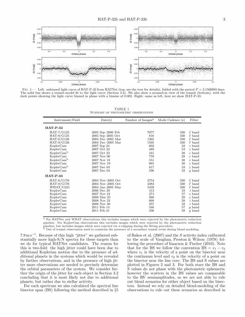
• HAT-P-32 – GSC 3281-00800 (also known as2MASS 02041028+4641162; α = 02h04m10.27s,δ = +4641′16.2′′; J2000; V=11.289 Droege et al.2006). A signal was detected for this star with anapparent depth of ∼20.3mmag, and a period ofP =2.1500days (see Figure 1, left).

• HAT-P-33 – GSC 2461-00988 (also known as2MASS 07324421+3350061; α = 07h32m44.20s,

δ = +3350′06.2′′; J2000; V=11.188 Droege et al.2006). A signal was detected for this star withan apparent depth of ∼8.5mmag, and a period ofP =3.4745days (see Figure 1, right).

2.2. Reconnaissance Spectroscopy

High-resolution, low-S/N “reconnaissance” spectrawere obtained for both HAT-P-32 and HAT-P-33 us-ing the Harvard-Smithsonian Center for Astrophysics(CfA) Digital Speedometer (DS; Latham 1992) on theFLWO 1.5m telescope. These observations, which aresummarized in Table 2, were reduced and analyzed fol-lowing the procedure described by Torres et al. (2002)(see also Latham et al. 2009). We find that both starsshow no velocity variation at the 1 km s−1 precision ofthe observations, and all spectra are consistent withsingle, moderately-rotating dwarf stars. For HAT-P-32 the stellar atmospheric parameters that we find, as-suming solar composition, are Teff⋆ = 6500 ± 100K,log g⋆ = 4.5 ± 0.25, v sin i = 21.9 ± 1.0 km s−1, andγRV = −23.21 ± 0.26 km s−1. For HAT-P-33 we findTeff⋆ = 6500 ± 100K, log g⋆ = 4.0 ± 0.25, v sin i =15.6± 1.0 km s−1, and γRV = 23.03± 0.28km s−1.In addition to the DS observations for HAT-P-33,

we also obtained several initial reconnaissance observa-tions of this target with the SOPHIE spectrograph onthe Observatoire de Haute-Provence 1.93m telescope.These observations showed ∼ 100m s−1 scatter, withonly a very faint hint of phasing with the photometricephemeris, hinting on the possibility that the system is ablend. Based on these observations we postponed furtherfollow-up of the target for several years.

2.3. High resolution, high S/N spectroscopy

We obtained high-resolution, high-S/N spectra forboth stars using HIRES (Vogt et al. 1994) on the Keck-Itelescope in Hawaii. For HAT-P-32 we gathered 28 spec-tra with the I2 absorption cell (Marcy & Butler 1992)between 2007 August and 2010 December, together witha single I2-free template spectrum. We rejected one low-S/N spectrum for which we were unable to obtain ahigh-precision RV measurement, and exclude from theanalysis two spectra which were obtained during tran-sit and thus may be affected by the Rossiter-McLaughlineffect (e.g. Queloz et al. 2000). For HAT-P-33 we gath-ered 22 spectra with the I2 cell between 2008 Septem-ber and 2010 December, and two template spectra. TheHIRES spectra were reduced to barycentric RVs follow-ing Butler et al. (1996). The resulting measurements aregiven in Tables 3 and 4 for HAT-P-32 and HAT-P-33respectively. The phased data, along with our best fitmodels for both circular and eccentric orbits, are dis-played in Figures 2 and 3.For both candidates the RV residuals from the best-fit

model show significant scatter greatly in excess of whatis expected based on the measurement uncertainties. ForHAT-P-32 the residual RMS is 80.3m s−1 or 75.0m s−1

for circular and eccentric models respectively, while theRMS expected from instrumental variations plus pho-ton noise is only 15.7m s−1. For HAT-P-33 the residualRMS is 55.7m s−1 or 54.1m s−1, again for circular andeccentric models respectively, while the expected RMS is

HAT-P-32b and HAT-P-33b 3

-0.04

-0.02

0

0.02

0.04

-0.4 -0.2 0 0.2 0.4

∆I (

mag

)

Orbital phase

-0.04

-0.02

0

0.02

0.04

-0.1 -0.05 0 0.05 0.1

∆I (

mag

)

Orbital phase

-0.04

-0.02

0

0.02

0.04

-0.4 -0.2 0 0.2 0.4

∆I (

mag

)

Orbital phase

-0.04

-0.02

0

0.02

0.04

-0.1 -0.05 0 0.05 0.1

∆I (

mag

)

Orbital phase

Fig. 1.— Left: unbinned light curve of HAT-P-32 from HATNet (top, see the text for details), folded with the period P = 2.1500085 days.The solid line shows a transit-model fit to the light curve (Section 3.4). We also show a zoomed-in view of the transit (bottom), with thedark points showing the light curve binned in phase with a binsize of 0.002. Right: same as left, here we show HAT-P-33.

TABLE 1Summary of photometric observations

Instrument/Field Date(s) Number of Imagesa Mode Cadence (s) Filter

HAT-P-32

HAT-7/G125 2005 Sep–2006 Feb 7077 330 I bandHAT-8/G125 2005 Sep–2005 Oct 816 330 I bandHAT-6/G126 2004 Dec–2005 Mar 1365 330 I bandHAT-9/G126 2004 Dec–2005 Mar 1505 330 I bandKeplerCam 2007 Sep 24 602 33 z bandKeplerCam 2007 Oct 22 489 53 z bandKeplerCamb 2007 Oct 23 161 38 z bandKeplerCam 2007 Nov 06 759 28 z bandKeplerCamb 2007 Nov 18 551 38 z bandKeplerCam 2007 Nov 19 665 38 z bandKeplerCamb 2007 Dec 03 817 33 z bandKeplerCam 2007 Dec 04 596 33 g band

HAT-P-33

HAT-6/G176 2004 Nov–2005 Oct 2754 330 I bandHAT-9/G176 2004 Nov–2005 Oct 4383 330 I bandWHAT/G221 2004 Jan–2005 May 5439 330 I bandKeplerCam 2006 Dec 29 413 33 i bandKeplerCam 2007 Nov 24 274 57 z bandKeplerCam 2008 Mar 25 260 29 z bandKeplerCam 2008 Nov 23 668 28 i bandKeplerCam 2008 Nov 30 257 32 i bandKeplerCam 2011 Feb 14 346 57 g bandKeplerCam 2011 Feb 21 336 58 g band

a For HATNet and WHAT observations this includes images which were rejected by the photometric reductionpipeline. For KeplerCam observations this excludes images which were rejected by the photometric reductionpipeline, but includes images which were rejected via σ-clipping during the fitting procedure.b Out of transit observation used to constrain the presence of a secondary transit event during blend modeling.

7.9m s−1. Because of this high “jitter” we gathered sub-stantially more high-S/N spectra for these targets thanwe do for typical HATNet candidates. The reason forthis is two-fold: the high jitter could have been due toadditional Keplerian motion due to the presence of ad-ditional planets in the systems which would be revealedby further observations, and in the presence of high jit-ter more observations are needed to precisely determinethe orbital parameters of the system. We consider fur-ther the origin of the jitter for each object in Section 3.2concluding that it is most likely not due to additionalplanets, but rather due to stellar activity.For each spectrum we also calculated the spectral line

bisector span (BS) following the method described in §5

of Bakos et al. (2007) and the S activity index calibratedto the scale of Vaughan, Preston & Wilson (1978) fol-lowing the procedure of Isaacson & Fischer (2010). Notethat for the BS we follow the convention BS = v1 − v2where v1 is the velocity of a point on the bisector nearthe continuum level and v2 is the velocity of a point onthe bisector near the line core. The BS and S values areplotted in Figures 2 and 3. For both stars the BS andS values do not phase with the photometric ephemeris;however the scatters in the BS values are comparableto the RV semiamplitudes, so we are not able to ruleout blend scenarios for either object based on the bisec-tors. Instead we rely on detailed blend-modeling of theobservations to rule out these scenarios as described in

4 Hartman et al.

TABLE 2DS reconnaissance spectroscopy

observations

JD - 2400000 RVa σRVb

(km s−1) (km s−1)

HAT-P-32

53988.0008 -24.58 1.3753992.9400 -24.02 1.0554016.7473 -23.51 0.7554070.7298 -23.80 1.0854072.7003 -24.07 0.7154075.8081 -22.86 0.6254077.7263 -23.25 0.7554421.8025 -21.91 0.8154422.7370 -23.67 0.9254423.7596 -23.03 0.8654424.7471 -23.80 0.7854425.8210 -22.60 0.7754427.7552 -22.34 1.0054430.6748 -20.83 1.7054726.8681 -23.50 0.90

HAT-P-33

53864.6428 22.10 0.6253865.6274 21.91 0.4853866.6480 22.41 0.4853873.6285 24.07 0.6354041.9844 23.21 0.7654043.9879 24.41 0.7954047.0178 22.75 0.6454047.9772 23.54 0.5054048.9252 22.84 0.66

a The measured heliocentric RV of thetarget quoted on the native CfA system.Our best guess is that 0.14 km s−1 shouldbe added to put the CfA velocities onto anabsolute system defined by observations ofminor planets.b The RV measurement uncertainty.

Section 3.3. For HAT-P-33 we found that the RV residu-als are correlated with the BS (see also Section 3.2), andwere thus able to use the BS to correct the RVs, reducingthe effective jitter to ∼ 35m s−1.

2.4. Photometric follow-up observations

We conducted high-precision photometric observationsof HAT-P-32 and HAT-P-33 using the KeplerCam CCDcamera on the FLWO 1.2m telescope. The observationsfor each target are summarized in Table 1. For HAT-P-32, in addition to observations taken during transit,we also obtained three sets of observations taken out oftransit at the predicted times of secondary eclipse (as-suming a circular orbit). These data are excluded fromthe global analysis described in Section 3.4, but are usedin Section 3.3 in ruling out blend-scenarios.The reduction of the KeplerCam images was performed

as described by Bakos et al. (2010a). We performedExternal Parameter Decorrelation (EPD) and used theTrend Filtering Algorithm (TFA; Kovacs et al. 2005) toremove trends simultaneously with the light curve mod-eling (for more details, see Bakos et al. 2010a). The finaltime series, together with our best-fit transit light curvemodels, are shown in Figure 4; the individual measure-ments are reported in Table 5 and Table 6 for HAT-P-32and HAT-P-33 respectively.

3. ANALYSIS

-300

-200

-100

0

100

200

300

400

RV

(m

s-1)

-100

0

100

200

300

O-C

(m

s-1)

Circular

-100

0

100

200

300

O-C

(m

s-1)

Eccentric

-100

-50

0

50

100

150

BS

(m

s-1)

0.224

0.228

0.232

0.236

0.240

0.0 0.2 0.4 0.6 0.8 1.0

S in

dex

Phase with respect to Tc

Fig. 2.— Top panel: Keck/HIRES RV measurements forHAT-P-32 shown as a function of orbital phase, along with ourbest-fit circular (solid line) and eccentric (dashed line) models asdetermined from our global modeling procedure (Section 3.4); seeTable 8. Zero phase corresponds to the time of mid-transit. Thecenter-of-mass velocity has been subtracted. Second panel: Veloc-ity O−C residuals from the best fit circular orbit. Jitter is notincluded in the error bars. Third panel: Velocity O−C residu-als from the best fit eccentric orbit. Fourth panel: Bisector spans(BS), with the mean value subtracted. The measurement from thetemplate spectrum is included (see Section 3.3). Bottom panel:Chromospheric activity index S measured from the Keck spectra.Note the different vertical scales of the panels. Observations showntwice are represented with open symbols.

3.1. Properties of the parent stars

Planetary parameters, such as the mass and radius,depend strongly on the stellar mass and radius, whichin turn are constrained by the observed stellar spec-tra as well as the light curves and RV curves. We fol-lowed an iterative procedure, described by Bakos et al.(2010a), to determine the relevant stellar parame-ters. The procedure involves iterating between infer-ing stellar atmospheric parameters (including the effec-tive temperature Teff⋆, surface gravity log g⋆, metallicity[Fe/H], and projected rotation velocity v sin i) from theKeck/HIRES template spectrum using the SpectroscopyMade Easy package (SME; Valenti & Piskunov 1996)and the Valenti & Fischer (2005) atomic line database,and modeling the light curves and RV curves (seeSection 3.4) to determine the stellar density ρ⋆. At a

HAT-P-32b and HAT-P-33b 5

TABLE 3Relative radial velocities, bisector spans, and activity index

measurements of HAT-P-32.

BJDa RVb σRVc BS σBS Sd Phase

(2,454,000+) (m s−1) (m s−1) (m s−1) (m s−1)

336.95660 −12.33 13.77 −4.23 22.35 0.240 0.168337.12852 −51.77 12.83 −35.38 13.61 0.238 0.248337.93027 · · · · · · 8.77 12.61 0.233 0.621337.93908 91.89 13.58 22.03 15.06 0.232 0.625339.12681 −32.01 12.59 −5.23 17.10 0.239 0.177339.92225 60.33 13.50 31.99 9.65 0.239 0.547344.05490 −56.05 12.94 −7.56 12.17 0.232 0.469345.14032e −7.96 12.44 56.66 19.42 0.235 0.974397.81437 −75.23 14.22 −36.38 9.63 0.236 0.474398.09647 35.38 14.70 −41.76 8.10 0.234 0.605427.84636 55.80 14.45 −55.48 12.13 0.235 0.442428.85791 312.16 15.38 −57.89 15.15 0.240 0.912429.92102 −3.17 14.43 −29.84 8.73 0.233 0.407455.90267 −11.30 14.42 −35.44 17.49 0.231 0.491458.93801 144.46 16.08 −9.85 11.93 0.232 0.903460.86208 103.67 18.28 −9.84 11.05 0.230 0.798548.72493 88.38 16.21 −19.13 14.89 0.240 0.664635.11482 73.67 16.94 155.85 24.14 0.236 0.845636.11275 −187.30 17.27 100.10 16.18 0.235 0.310724.02617 −170.37 15.27 7.97 13.53 0.237 0.199725.07143 37.66 16.62 89.82 14.96 0.241 0.686727.11674 40.79 16.16 90.24 15.73 0.241 0.637777.92375 −153.16 15.28 −28.12 10.06 0.232 0.268810.82619 150.64 17.27 −20.45 12.98 0.230 0.571838.93902 46.30 19.26 −33.20 13.87 0.225 0.6471192.92153 −143.71 19.01 −28.23 13.83 0.236 0.2891250.81416 −211.65 17.65 −30.15 10.29 0.238 0.2161376.10348 −80.92 17.65 6.54 11.60 0.241 0.4901544.91306e −186.72 18.93 −81.83 21.62 0.224 0.006

Note. — For the iodine-free template exposures we do not measure theRV but do measure the BS and S index. Such template exposures can bedistinguished by the missing RV value.a Barycentric Julian dates throughout the paper are calculated from Coordi-nated Universal Time (UTC).b The zero-point of these velocities is arbitrary. An overall offset γrel fitted tothese velocities in Section 3.4 has not been subtracted.c Internal errors excluding the component of astrophysical jitter considered inSection 3.4.d Chromospheric activity index calibrated to the scale ofVaughan, Preston & Wilson (1978) following Isaacson & Fischer (2010).e Observation during transit which was excluded from the analysis.

given cycle in the iteration we combine our estimates ofTeff⋆, [Fe/H] and ρ⋆ with the Yonsei-Yale (YY; Yi et al.2001) series of stellar evolution models to determine thestellar mass, radius, and surface gravity among other pa-rameters. If the resulting surface gravity differs signifi-cantly from the value determined from the spectrum withSME, we repeat the analysis fixing the surface gravity inSME to the new value.For each star, the initial SME analysis, in which the

surface gravity was allowed to vary, yielded the followingvalues and uncertainties:

• HAT-P-32: Teff⋆ = 6001± 88K, [Fe/H] = −0.16±0.08 dex, log g⋆ = 4.02 ± 0.07 (cgs), and v sin i =21± 0.5 km s−1.

• HAT-P-33: Teff⋆ = 6234±114K, [Fe/H] = −0.04±0.08 dex, log g⋆ = 3.86 ± 0.10 (cgs), and v sin i =13.9± 0.5 km s−1.

As described in Section 3.4 the inferred stellar densi-ties, and hence radii, for HAT-P-32 and HAT-P-33 de-pend strongly on the orbital eccentricities, which due to

the high RV jitters are poorly constrained. For each sys-tem we conducted separate analyses, first assuming a cir-cular orbit and then allowing the eccentricity to vary. Ineach case we obtained a new value of log g⋆ which weheld fixed during a second SME iteration. The final stel-lar parameters for each star, assuming both circular andeccentric models, are listed in Table 7.The inferred location of each star for both the circular

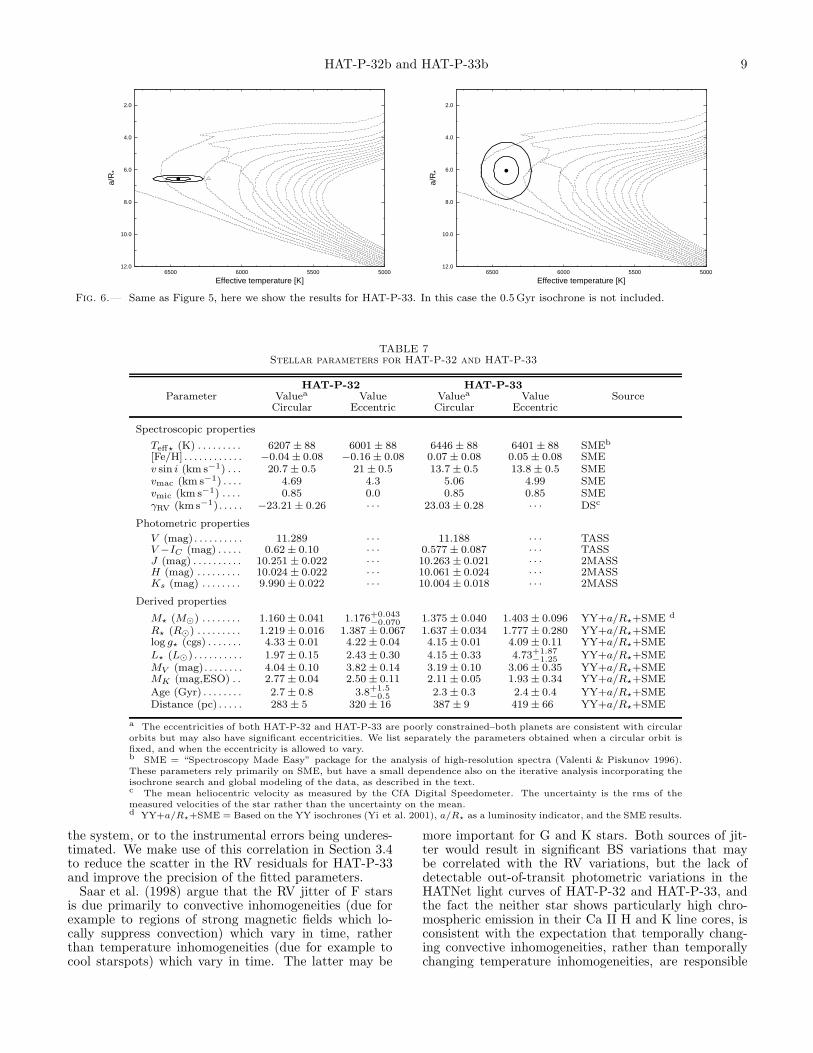
and eccentric models, in diagrams of a/R⋆ (which is re-lated to ρ⋆) versus Teff⋆, analogous to the classical H-Rdiagram, is shown in Figures 5-6. In each case the stellarproperties and their 1σ and 2σ confidence ellipsoids aredisplayed against the backdrop of model isochrones for arange of ages, and the appropriate stellar metallicity.As a check on our stellar parameter determinations

we compare the measured photometric colors of the twostars to the predicted values based on the models. HAT-P-32 has J−K = 0.281±0.00811 and V −IC = 0.62±0.10(from TASS; Droege et al. 2006), whereas the predicted

11 Taken from 2MASS (Skrutskie et al. 2006) and convertedto the ESO photometric system using the transformations byCarpenter (2001).

6 Hartman et al.

TABLE 4Relative radial velocities, bisector spans, and activity index

measurements of HAT-P-33.

BJDa RVb σRVc BS σBS Sd Phase

(2,454,000+) (m s−1) (m s−1) (m s−1) (m s−1)

728.11380 · · · · · · −60.23 2.93 0.171 0.822728.12071 107.70 6.84 −56.67 4.32 0.172 0.824778.03749 −88.19 6.47 −59.99 4.67 0.174 0.190779.11168 39.67 7.79 −16.02 6.12 0.173 0.499780.05973 106.79 7.40 −2.11 4.05 0.173 0.772791.11863 76.24 7.97 −4.56 4.00 0.174 0.955805.96712 −168.48 7.63 83.04 6.79 0.171 0.229807.00978 −76.74 9.16 74.87 7.06 0.170 0.529807.99835 125.68 6.92 0.18 3.79 0.172 0.813809.98993 13.78 9.01 −69.27 5.86 0.170 0.387810.88079 125.60 8.34 −31.31 4.57 0.172 0.643838.95648 41.95 7.70 5.62 5.71 0.172 0.724865.01789 −25.12 8.25 16.88 4.31 0.171 0.224954.83936 −67.35 7.49 7.29 4.92 0.175 0.076955.85129 −52.75 8.95 −4.96 7.02 0.173 0.3671192.01643 · · · · · · 13.37 2.83 0.172 0.3391192.02324 −93.30 7.19 22.62 3.46 0.173 0.3411193.09374 −24.35 7.52 60.32 5.56 0.175 0.6491193.93089 −8.61 8.57 38.64 5.33 0.170 0.8901251.91465 13.52 7.72 16.56 4.23 0.172 0.5781468.06245 22.33 7.86 91.25 6.82 0.173 0.7891470.09079 18.65 8.16 −127.71 8.71 0.174 0.3721545.09930 26.89 8.37 −5.60 5.38 0.170 0.9611545.93211 −31.18 7.91 7.80 4.89 0.165 0.201

Note. — For the iodine-free template exposures we do not measure the RVbut do measure the BS and S index. Such template exposures can be distin-guished by the missing RV value.a Barycentric Julian dates throughout the paper are calculated from Coordi-nated Universal Time (UTC).b The zero-point of these velocities is arbitrary. An overall offset γrel fitted tothese velocities in Section 3.4 has not been subtracted.c Internal errors excluding the component of astrophysical jitter considered inSection 3.4.d Chromospheric activity index calibrated to the scale ofVaughan, Preston & Wilson (1978) following Isaacson & Fischer (2010).

TABLE 5High-precision differential photometry of HAT-P-32.

BJD Maga σMag Mag(orig)b Filter(2,400,000+)

54368.74140 −0.00204 0.00143 10.54500 z54368.74180 0.00090 0.00144 10.54840 z54368.74217 0.00417 0.00143 10.55120 z54368.74255 −0.00158 0.00143 10.54590 z54368.74296 0.00016 0.00142 10.54740 z54368.74335 0.00079 0.00143 10.54810 z54368.74373 0.00331 0.00144 10.55080 z54368.74411 0.00071 0.00142 10.54810 z54368.74449 −0.00132 0.00142 10.54610 z54368.74489 −0.00129 0.00141 10.54610 z

Note. — This table is available in a machine-readable form in theonline journal. A portion is shown here for guidance regarding its formand content.a The out-of-transit level has been subtracted. These magnitudes havebeen subjected to the EPD and TFA procedures, carried out simulta-neously with the transit fit.b Raw magnitude values without application of the EPD and TFAprocedures.

values are J−K = 0.32±0.02 and V −IC = 0.574±0.023for the circular model, and J − K = 0.34 ± 0.02 andV − IC = 0.592± 0.024 for the eccentric model. In bothcases the model V − IC colors are consistent with themeasurements, but the model J − K colors are slightly

TABLE 6High-precision differential photometry of HAT-P-33.

BJD Maga σMag Mag(orig)b Filter(2,400,000+)

54099.68885 0.00058 0.00085 9.51222 i54099.69425 0.00071 0.00083 9.51224 i54099.69465 −0.00123 0.00083 9.51016 i54099.69502 −0.00319 0.00083 9.50882 i54099.69541 0.00122 0.00083 9.51279 i54099.69579 0.00204 0.00083 9.51399 i54099.69619 0.00045 0.00083 9.51219 i54099.69659 −0.00038 0.00083 9.51120 i54099.69697 −0.00305 0.00083 9.50858 i54099.69735 −0.00342 0.00083 9.50826 i

Note. — This table is available in a machine-readable form in theonline journal. A portion is shown here for guidance regarding its formand content.a The out-of-transit level has been subtracted. These magnitudes havebeen subjected to the EPD and TFA procedures, carried out simulta-neously with the transit fit.b Raw magnitude values without application of the EPD and TFAprocedures.

(∼ 2σ) redder than the measurements. HAT-P-33 hasJ − K = 0.280 ± 0.030 and V − IC = 0.577 ± 0.087(also from 2MASS and TASS), and has predicted valuesof J − K = 0.27 ± 0.02 and V − IC = 0.511 ± 0.022for the circular model, and J − K = 0.28 ± 0.02 and

HAT-P-32b and HAT-P-33b 7

-200

-150

-100

-50

0

50

100

150

200

RV

(m

s-1)

-200

-150

-100

-50

0

50

100

150

200

RV

(m

s-1)

-200

-100

0

100

200

O-C

(m

s-1)

Circular

-200

-100

0

100

200

O-C

(m

s-1)

Eccentric

-100

-50

0

50

BS

(m

s-1)

0.166

0.168

0.170

0.172

0.174

0.0 0.2 0.4 0.6 0.8 1.0

S in

dex

Phase with respect to Tc

Fig. 3.— Top panel: Keck/HIRES RV measurements forHAT-P-33 shown as a function of orbital phase, along with ourbest-fit circular (solid line) and eccentric (dashed line) models asdetermined from our global modeling procedure (Section 3.4); seeTable 9. Zero phase corresponds to the time of mid-transit. Thecenter-of-mass velocity has been subtracted. Second panel: Sameas top panel, here we have subtracted a linear correlation with thespectral line bisector spans (BS) from the RV measurements. Thiscorrelation was determined simultaneously with the fit, and sig-nificantly reduces the residual RMS. For the displayed points wesubtract the correlation determined in the circular orbit fit. Thirdpanel: Velocity O−C residuals from the best fit circular orbit in-cluding the BS correlation. Jitter is not included in the error bars.Fourth panel: Velocity O−C residuals from the best fit eccentricorbit including the BS correlation. Fifth panel: BS, with the meanvalue subtracted. The measurement from the template spectrum isincluded (see Section 3.3). Bottom panel: Chromospheric activityindex S measured from the Keck spectra. Note the different verti-cal scales of the panels. Observations shown twice are representedwith open symbols.

V − IC = 0.522 ± 0.022 for the eccentric model. The

measured photometric colors of HAT-P-33 are within 1σof the predicted values for both models.Neither HAT-P-32 nor HAT-P-33 shows significant

chromospheric emission in their Ca II H and K line cores.Following the procedure of Isaacson & Fischer (2010), wefind median logR′

HK (Noyes et al. 1984) values of −4.62and −4.88 for HAT-P-32 and HAT-P-33, respectively.

3.2. Stellar Jitter

Both HAT-P-32 and HAT-P-33 exhibit notably highscatter in their velocity residuals. Stellar jitter values of78.7m s−1 and 55.1m s−1 for HAT-P-32 and HAT-P-33respectively must be added in quadrature to their veloc-ity errors to achieve reduced χ2 values of unity for thebest-fit circular orbits (see Section 3.4).A possible cause of the jitter is the presence of one

or more additional planets in either system, though thiswould not explain the high scatter seen in the BS mea-surements. Figure 7 shows the Lomb-Scargle frequencyspectra (L-S; Lomb 1976; Scargle 1982; Press & Rybicki1989) of the RV observations for both stars. In both casesthere is a peak in the spectrum at the transit frequency;in the case of HAT-P-32 this is the highest peak in thespectrum, while in the case of HAT-P-33 the highest peakis at a high frequency alias of the transit frequency (ifwe restrict the search to frequencies shorter than 0.49 d−1

the transit frequency is the highest peak). We note thatin neither case would the planet be detectable from theRV data alone. For HAT-P-32, the false alarm proba-bility of detecting a peak in the L-S periodogram with aheight greater than or equal to the measured peak heightis ∼ 8% (this is determined by applying L-S to simulatedGaussian white noise RV curves with the same time sam-pling as the observations). For HAT-P-33 the false alarmprobability of the transit peak is 79% (the false alarmprobability for the highest peak in the spectrum is 30%).We also show the L-S spectra of the RV residuals fromthe best-fit circular orbit models, in order to see if thereis evidence for additional short period planets in the sys-tems. The highest peaks in these spectra are at periodsof 18.104d and 0.8507d for HAT-P-32 and HAT-P-33 re-spectively (for each system there is some ambiguity in thepeak that depends on the frequency range searched andwhether or not a multiharmonic period search is used). Ifwe assume that each system has an additional planet atthe above stated periods, the RMS of the RV residualsdecreases to ∼ 40m s−1 and ∼ 30m s−1 for HAT-P-32and HAT-P-33 respecitvely. However, these peaks havecorresponding false alarm probabilities of 8% and 8.9%,so they are not statistically significant detections. Weconclude that while either system may host additionalshort period planets, there are not at present enough RVobservations to make a statistically significant detection.Another potential source of RV and BS jitter is vary-

ing scattered moonlight contaminating the spectra. Fol-lowing Kovacs et al. (2010) we investigated the possi-bility that the BS and RV may be affected by vary-ing sky contamination, and found no evidence that thisis the case. Alternatively, RV and BS jitter might becaused by variable contamination from a nearby star.Based on our KeplerCam observations of HAT-P-32 andHAT-P-33, we can rule out contaminating neighbors with∆i . 5mag at a separation greater than 3′′, or neigh-bors with ∆i . 2mag at a separation greater than 1′′

8 Hartman et al.

0

0.05

0.1

0.15

0.2

-0.2 -0.15 -0.1 -0.05 0 0.05 0.1 0.15 0.2

Time from transit center (days)

∆z (

mag

)∆z

(m

ag)

∆z (

mag

)∆z

(m

ag)

∆g (

mag

)2007 Sep 24

2007 Oct 22

2007 Nov 06

2007 Nov 19

2007 Dec 04

0

0.05

0.1

0.15

0.2

0.25

0.3

-0.2 -0.15 -0.1 -0.05 0 0.05 0.1 0.15 0.2

Time from transit center (days)

∆i (

mag

)∆z

∆z∆i

∆i∆g

∆g

2006 Dec 29

2007 Nov 24

2008 Mar 25

2008 Nov 23

2008 Nov 30

2011 Feb 14

2011 Feb 21

Fig. 4.— Unbinned transit light curves for HAT-P-32 (left) and HAT-P-33 (right), acquired with KeplerCam at the FLWO 1.2mtelescope. The light curves have been EPD and TFA processed, as described in Bakos et al. (2010a). The dates of the events are indicated.Curves after the first are displaced vertically for clarity. Our best fits from the global modeling described in Section 3.4 are shown by thesolid lines. Residuals from the fits are displayed at the bottom, in the same order as the top curves. The error bars represent the photonand background shot noise, plus the readout noise.

1.0

2.0

3.0

4.0

5.0

6.0

7.0

8.0

9.05000550060006500

a/R

*

Effective temperature [K]

1.0

2.0

3.0

4.0

5.0

6.0

7.0

8.0

9.05000550060006500

a/R

*

Effective temperature [K]

Fig. 5.— Model isochrones from Yi et al. (2001) assuming a circular orbit (left) and the best-fit eccentric orbit (right) for the measuredmetallicity of HAT-P-32, and ages of 0.5Gyr and 1–14Gyr in 1Gyr steps (left to right in each plot). The adopted values of Teff⋆ and a/R⋆

are shown together with their 1σ and 2σ confidence ellipsoids. The initial values of Teff⋆ and a/R⋆ from the first SME and light curveanalyses are represented with a triangle.

of either star. We cannot rule out fainter close neigh-bors which could be responsible for at least some of thejitter. Constraints on potential neighbors based on mod-eling the photometric light curves are further consideredin Section 3.3.Figure 8 compares the RV residuals to the BSs for

HAT-P-32 and HAT-P-33. For HAT-P-33 there is a clearanti-correlation between these quantities (the Spearmanrank-order correlation test (e.g. Press et al. 1992) yieldsa correlation coefficient of rs = −0.77 with a false-alarm

probability of 0.04% assuming a circular orbit, while forthe best-fit eccentric orbit rs = −0.72 with a 0.1% falsealarm probability). For HAT-P-32 there is a hint ofan anti-correlation, but it is not statistically significant(rs = −0.30 with a false-alarm probability of 14% as-suming a circular orbit, and rs = −0.39 with 4.9% falsealarm probability for the best-fit eccentric orbit). Theanti-correlation for HAT-P-33 is an indication that themeasured jitter for this star is dominated by intrinsic stel-lar variations, rather than being due to another planet in

HAT-P-32b and HAT-P-33b 9

2.0

4.0

6.0

8.0

10.0

12.05000550060006500

a/R

*

Effective temperature [K]

2.0

4.0

6.0

8.0

10.0

12.05000550060006500

a/R

*

Effective temperature [K]

Fig. 6.— Same as Figure 5, here we show the results for HAT-P-33. In this case the 0.5Gyr isochrone is not included.

TABLE 7Stellar parameters for HAT-P-32 and HAT-P-33

HAT-P-32 HAT-P-33

Parameter Valuea Value Valuea Value SourceCircular Eccentric Circular Eccentric

Spectroscopic properties

Teff⋆ (K) . . . . . . . . . 6207 ± 88 6001 ± 88 6446± 88 6401 ± 88 SMEb

[Fe/H] . . . . . . . . . . . . −0.04± 0.08 −0.16± 0.08 0.07± 0.08 0.05± 0.08 SMEv sin i (km s−1) . . . 20.7± 0.5 21± 0.5 13.7± 0.5 13.8± 0.5 SMEvmac (km s−1) . . . . 4.69 4.3 5.06 4.99 SMEvmic (km s−1) . . . . 0.85 0.0 0.85 0.85 SMEγRV (km s−1) . . . . . −23.21± 0.26 · · · 23.03 ± 0.28 · · · DSc

Photometric properties

V (mag). . . . . . . . . . 11.289 · · · 11.188 · · · TASSV −IC (mag) . . . . . 0.62± 0.10 · · · 0.577± 0.087 · · · TASSJ (mag) . . . . . . . . . . 10.251 ± 0.022 · · · 10.263 ± 0.021 · · · 2MASSH (mag) . . . . . . . . . 10.024 ± 0.022 · · · 10.061 ± 0.024 · · · 2MASSKs (mag) . . . . . . . . 9.990± 0.022 · · · 10.004 ± 0.018 · · · 2MASS

Derived properties

M⋆ (M⊙) . . . . . . . . 1.160± 0.041 1.176+0.043−0.070 1.375± 0.040 1.403± 0.096 YY+a/R⋆+SME d

R⋆ (R⊙) . . . . . . . . . 1.219± 0.016 1.387 ± 0.067 1.637± 0.034 1.777± 0.280 YY+a/R⋆+SMElog g⋆ (cgs) . . . . . . . 4.33± 0.01 4.22± 0.04 4.15± 0.01 4.09± 0.11 YY+a/R⋆+SMEL⋆ (L⊙) . . . . . . . . . . 1.97± 0.15 2.43± 0.30 4.15± 0.33 4.73+1.87

−1.25 YY+a/R⋆+SMEMV (mag). . . . . . . . 4.04± 0.10 3.82± 0.14 3.19± 0.10 3.06± 0.35 YY+a/R⋆+SMEMK (mag,ESO) . . 2.77± 0.04 2.50± 0.11 2.11± 0.05 1.93± 0.34 YY+a/R⋆+SMEAge (Gyr) . . . . . . . . 2.7± 0.8 3.8+1.5

−0.5 2.3± 0.3 2.4± 0.4 YY+a/R⋆+SMEDistance (pc) . . . . . 283 ± 5 320 ± 16 387 ± 9 419± 66 YY+a/R⋆+SME

a The eccentricities of both HAT-P-32 and HAT-P-33 are poorly constrained–both planets are consistent with circularorbits but may also have significant eccentricities. We list separately the parameters obtained when a circular orbit isfixed, and when the eccentricity is allowed to vary.b SME = “Spectroscopy Made Easy” package for the analysis of high-resolution spectra (Valenti & Piskunov 1996).These parameters rely primarily on SME, but have a small dependence also on the iterative analysis incorporating theisochrone search and global modeling of the data, as described in the text.c The mean heliocentric velocity as measured by the CfA Digital Speedometer. The uncertainty is the rms of themeasured velocities of the star rather than the uncertainty on the mean.d YY+a/R⋆+SME = Based on the YY isochrones (Yi et al. 2001), a/R⋆ as a luminosity indicator, and the SME results.

the system, or to the instrumental errors being underes-timated. We make use of this correlation in Section 3.4to reduce the scatter in the RV residuals for HAT-P-33and improve the precision of the fitted parameters.Saar et al. (1998) argue that the RV jitter of F stars

is due primarily to convective inhomogeneities (due forexample to regions of strong magnetic fields which lo-cally suppress convection) which vary in time, ratherthan temperature inhomogeneities (due for example tocool starspots) which vary in time. The latter may be

more important for G and K stars. Both sources of jit-ter would result in significant BS variations that maybe correlated with the RV variations, but the lack ofdetectable out-of-transit photometric variations in theHATNet light curves of HAT-P-32 and HAT-P-33, andthe fact the neither star shows particularly high chro-mospheric emission in their Ca II H and K line cores, isconsistent with the expectation that temporally chang-ing convective inhomogeneities, rather than temporallychanging temperature inhomogeneities, are responsible

10 Hartman et al.

0

2

4

6

8

10

0 0.2 0.4 0.6 0.8 1 1.2 1.4 1.6 1.8 2

Pow

er

Frequency [d-1]

HAT-P-32 RVs

2.150008 d

0

2

4

6

8

10

0 0.2 0.4 0.6 0.8 1 1.2 1.4 1.6 1.8 2

Pow

er

Frequency [d-1]

HAT-P-32 Residual RVs

18.10360418 d

0

2

4

6

8

10

0 0.2 0.4 0.6 0.8 1 1.2 1.4 1.6 1.8 2

Pow

er

Frequency [d-1]

HAT-P-33 RVs

3.474474 d

0

2

4

6

8

10

0 0.2 0.4 0.6 0.8 1 1.2 1.4 1.6 1.8 2

Pow

er

Frequency [d-1]

HAT-P-33 Residual RVs

0.85073484 d

Fig. 7.— Lomb-Scargle frequency spectra for the RVs (top) and residual RVs from the best-fit circular orbit models (bottom) forHAT-P-32 (left) and HAT-P-33 (right). In the top panels we mark the transit frequencies, while in the bottom panels we mark the highestpeaks in the spectra. In all cases the false alarm probability of finding a peak as high the marked peak in a Gaussian white-noise RV curveis greater than 8%.

for the jitter of these two stars.Jitter values as high as those found for HAT-P-32 and

HAT-P-33 are typical of stars with similar spectral typesand rotation velocities. From the v sin i–jitter correlationmeasured by Saar et al. (2003), the expected jitter for anF dwarf with v sin i = 20km s−1 is ∼ 50m s−1, whilefor an F dwarf with v sin i = 14km s−1 the expectedjitter is ∼ 30m s−1. The sample used by Saar et al.(2003) to determine this correlation includes only a hand-ful of stars with v sin i > 10 km s−1, and the scatterabout the relation is fairly significant—one star withv sin i ∼ 15 km s−1 was found to have a jitter in ex-cess of 100m s−1. The planet hosting star HAT-P-2,which has a similar temperature and rotation velocity toHAT-P-32 and HAT-P-33 (Teff⋆ = 6290± 60K, v sin i =20.8 ± 0.3 km s−1; Pal et al. 2010) has been reported tohave a high jitter of ∼ 60m s−1 based on data from Keckand Lick (Bakos et al. 2007). A subsequent analysis byWinn et al. (2007), using only Keck/HIRES data, founda somewhat lower jitter of ∼ 30m s−1, though this isstill quite a bit higher than most planet-hosting starsdiscovered to date (e.g. the median jitter of the pre-viously published HATNet planets is ∼ 7m s−1). Theprimary difference between HAT-P-2 and the two sys-tems presented here is that the planet HAT-P-2b is sig-nificantly more massive than either HAT-P-32b or HAT-P-33b (HAT-P-2b has Mp = 9.09 ± 0.24MJ; Pal et al.2010); as a result, the RV semiamplitude of HAT-P-2b(K = 984± 17m s−1) greatly exceeds the jitter, makingthis planet more straightforward to confirm than either

HAT-P-32b or HAT-P-33b.

3.3. Excluding blend scenarios

Both HAT-P-32 and HAT-P-33 exhibit significantspectral line bisector span (BS) variations (Figures 2-3;the RMS of the BS is 53m s−1 and 51m s−1 for HAT-P-32and HAT-P-33 respectively). In neither case are the vari-ations in phase with the transit ephemeris, as one mightexpect if the observed RV variation were due to a blendbetween an eclipsing binary system and another star. Asdiscussed in Section 3.2, these variations are likely dueto temporally changing convective inhomogeneities, per-haps created by variable photospheric magnetic faculaeas in the Sun, which we suspect are responsible for thesignificant RV jitter seen in both of these stars. Nonethe-less the large BS variations, which are comparable to thesemiamplitudes of the RV signals, prevent us from usingthe BSs to rule out the possibility that either of thesesystems is a blend.To rule out blend scenarios we made use of the

blendanal program (Hartman et al. 2011b; see also,Hartman et al. 2011a) which models the observed lightcurves, stellar atmospheric parameters, and calibratedphotometric magnitudes using various blended eclips-ing binary scenarios as well as scenarios involvinga transiting planet system potentially blended withlight from another star. The program relies on acombination of the Padova (Girardi et al. 2000) andBaraffe et al. (1998) stellar evolution models, the Eclips-ing Binary Orbit Program (Popper & Etzel 1981; Etzel1981; Nelson & Davis 1972, EBOP) as modified by

HAT-P-32b and HAT-P-33b 11

-150

-100

-50

0

50

100

150

200

250

300

-100 -50 0 50 100 150 200

RV

(O

- C

) [m

/s]

BS [m/s]

HAT-P-32 circular

-150

-100

-50

0

50

100

150

200

-100 -50 0 50 100 150 200

RV

(O

- C

) [m

/s]

BS [m/s]

HAT-P-32 eccentric

-120

-100

-80

-60

-40

-20

0

20

40

60

80

-150 -100 -50 0 50 100

RV

(O

- C

) [m

/s]

BS [m/s]

HAT-P-33 circular

-120-100

-80-60-40-20

0 20 40 60 80

100

-150 -100 -50 0 50 100

RV

(O

- C

) [m

/s]

BS [m/s]

HAT-P-33 eccentric

Fig. 8.— RV residuals from the best-fit circular (top) and eccentric (bottom) model orbits vs. BS for HAT-P-32 (left) and HAT-P-33(right). There is a hint of an anti-correlation between these quantities for HAT-P-32, though it is not statistically significant. For HAT-P-33the quantities are clearly anti-correlated. See the discussion in Section 3.2.

Southworth et al. (2004a,b), and stellar limb darkeningparameters from Claret (2004). It is similar to theblender program (Torres et al. 2005) which has beenused to confirm Kepler planets (e.g. Torres et al. 2011),but with a number of technical differences which are de-scribed by Hartman et al. (2011b).For each object we fit 4 classes of models:

1. A single star with a transiting planet.

2. A planet transiting one component of a binary starsystem.

3. A hierarchical triple stellar system.

4. A blend between a bright stationary star, and afainter, physically unrelated eclipsing binary.

Initially we assume that the eclipsing components havea circular orbit. For both HAT-P-32 and HAT-P-33 wefind that the class 1 model (a single star with a transitingplanet), or the class 2 model with a planet-host star thatis much brighter than its binary star companion, providebetter fits (lower χ2) than the class 3 and class 4 models.To evaluate the statistical significance with which theclass 3 and class 4 models may be rejected, we followthe Monte Carlo procedure described in Hartman et al.(2011a). We find that for HAT-P-32 we may reject boththe class 3 and 4 models with ∼ 13σ confidence (the best-fit class 4 model consists of a group of stars with similarparameters to the best-fit class 3 model), while for HAT-P-33 we may reject the class 3 and 4 models with ∼ 6σconfidence (e.g. Figure 9).

0.9 1 1.1 1.2 1.3 1.4 1.5M1 [Msun]

0.9

1

1.1

1.2

1.3

1.4

1.5

M2

[Msu

n]

0

5

10

15

20

σ R

ejec

ted

Fig. 9.— The σ-level at which the class 3 blend model (hier-archical triple stellar system) can be rejected for HAT-P-33 as afunction of the masses of the two largest stars in the system: M1 isthe mass of the uneclipsed star, and M2 is the mass of the primarystar in the eclipsing system. Note that the lack of several km s−1

RV variations leads to the constraint M1 > M2. The best-fit modelis rejected with ∼ 6σ confidence.

For both HAT-P-32 and HAT-P-33 the eclipsing binarystar blend scenarios (classes 3 and 4) are excluded in partdue to the lack of an apparent secondary eclipse or outof transit variation that are predicted by models capableof fitting the observed primary transits. For HAT-P-33 the HATNet light curve provides these constraints,while for HAT-P-32 three sets of KeplerCam observationscollected during predicted secondary eclipses (assuming acircular orbit) augment the constraints provided by theHATNet light curve. Figure 10 shows a few examplemodel light curves for the best-fit class 4 model for HAT-

12 Hartman et al.

P-32 which illustrate this.Because the time of secondary eclipse depends on the

eccentricity, which is poorly constrained by the RV ob-servations, we repeat the blend analysis for both systemsfixing the eccentricities to the best-fit values as deter-mined in Section 3.4. While for HAT-P-32 this scenariocauses the secondary eclipses to not occur during the outof transit KeplerCam observations, the eccentric eclips-ing binary results in stronger out of transit variationswhich are ruled out by the HATNet data. In this casefor HAT-P-32 we may reject the class 3 and 4 modelswith > 11σ confidence. For HAT-P-33 we may reject theclass 3 and 4 models with > 7σ confidence.For the class 2 models we consider two cases, one in

which the transiting planet orbits the brighter binarystar component, and the other in which the planet or-bits the fainter binary star component. In both casesthe spectroscopic temperature and the photometric col-ors constrain the brighter star to have a mass of & 1M⊙

for both systems. We find that the case of the planetorbiting the fainter component can be rejected outrightwith > 4σ confidence for both HAT-P-32 and HAT-P-33. The case of a planet orbiting the brighter binarystar component amounts to including third light in thefit. When the secondary star contributes negligible lightto the system the model becomes indistinguishable fromthe best-fit case 1 model, such a model cannot be ruledout with the available data. Instead we may place an up-per limit on the mass of any binary star companion. ForHAT-P-32 we find that a putative companion must haveM < 0.5M⊙ with 5σ confidence, while for HAT-P-33 acompanion must have M < 0.55M⊙ with 5σ confidence.These translate into upper limits on the secondary toprimary V -band luminosity ratio of ∼ 1% for both HAT-P-32 and HAT-P-33.Based on the above discussion we conclude that the

signals detected in the HAT-P-32 and HAT-P-33 lightcurves and RV curves are planetary in nature.

3.4. Global modeling of the data

We modeled the HATNet photometry, the follow-upphotometry, and the high-precision RV measurementsusing the procedure described in detail by Pal et al.(2008); Bakos et al. (2010a). One significant differ-ence from our previous planet discoveries is that weuse a Mandel & Agol (2002) transit model to describethe HATNet photometry, rather than a simplified no-limb-darkening model. This was necessary due to thehigh S/N HATNet detections, especially for HAT-P-32. To describe the follow-up light curves we use aMandel & Agol (2002) transit model together with thesimultaneous External-Parameter-Decorellation (EPD)and Trend-Filtering Algorithm model of instrumentalvariations (Bakos et al. 2010a), and we use a Keplerianorbit to describe the RV curves. For HAT-P-33 we in-clude a term αBS × BS in the RV model, where αBS isa free parameter describing the residual RV–BS corre-lation, as we found that this significantly reduces theRV residuals. For HAT-P-32 we do not include this cor-rection because the residual RV–BS correlation is notstatistically significant. For each planetary system wefit two models, one in which the eccentricity is fixed tozero, and another in which the eccentricity varies. Theparameters for each system are listed in Tables 8-9. Nei-

ther system has a clearly non-zero eccentricity. Usingthe Lucy & Sweeney (1971) test we find that there isa non-negligible ∼ 3% probability that the eccentricityfound for HAT-P-32 arises by chance from a circular or-bit, while for HAT-P-33 the probability is ∼ 20%.Because the resulting planets have large radii (partic-

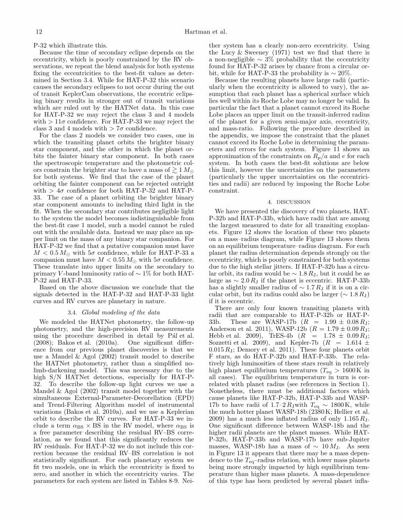
ularly when the eccentricity is allowed to vary), the as-sumption that each planet has a spherical surface whichlies well within its Roche Lobe may no longer be valid. Inparticular the fact that a planet cannot exceed its RocheLobe places an upper limit on the transit-inferred radiusof the planet for a given semi-major axis, eccentricity,and mass-ratio. Following the procedure described inthe appendix, we impose the constraint that the planetcannot exceed its Roche Lobe in determining the param-eters and errors for each system. Figure 11 shows anapproximation of the constraints on Rp/a and e for eachsystem. In both cases the best-fit solutions are belowthis limit, however the uncertainties on the parameters(particularly the upper uncertainties on the eccentrici-ties and radii) are reduced by imposing the Roche Lobeconstraint.

4. DISCUSSION

We have presented the discovery of two planets, HAT-P-32b and HAT-P-33b, which have radii that are amongthe largest measured to date for all transiting exoplan-ets. Figure 12 shows the location of these two planetson a mass–radius diagram, while Figure 13 shows themon an equilibrium temperature–radius diagram. For eachplanet the radius determination depends strongly on theeccentricity, which is poorly constrained for both systemsdue to the high stellar jitters. If HAT-P-32b has a circu-lar orbit, its radius would be ∼ 1.8RJ, but it could be aslarge as ∼ 2.0RJ if the planet is eccentric. HAT-P-33bhas a slightly smaller radius of ∼ 1.7RJ if it is on a cir-cular orbit, but its radius could also be larger (∼ 1.8RJ)if it is eccentric.There are only four known transiting planets with

radii that are comparable to HAT-P-32b or HAT-P-33b. These are WASP-17b (R = 1.99 ± 0.08RJ;Anderson et al. 2011), WASP-12b (R = 1.79 ± 0.09RJ;Hebb et al. 2009), TrES-4b (R = 1.78 ± 0.09RJ;Sozzetti et al. 2009), and Kepler-7b (R = 1.614 ±0.015RJ; Demory et al. 2011). These four planets orbitF stars, as do HAT-P-32b and HAT-P-33b. The rela-tively high luminosities of these stars result in relativelyhigh planet equilibrium temperatures (Teq > 1600K inall cases). The equilibrium temperature in turn is cor-related with planet radius (see references in Section 1).Nonetheless, there must be additional factors whichcause planets like HAT-P-32b, HAT-P-33b and WASP-17b to have radii of 1.7–2RJwith Teq ∼ 1800K, whilethe much hotter planet WASP-18b (2380K; Hellier et al.2009) has a much less inflated radius of only 1.165RJ.One significant difference between WASP-18b and thehigher radii planets are the planet masses. While HAT-P-32b, HAT-P-33b and WASP-17b have sub-Jupitermasses, WASP-18b has a mass of ∼ 10MJ. As seenin Figure 13 it appears that there may be a mass depen-dence to the Teq–radius relation, with lower mass planetsbeing more strongly impacted by high equilibrium tem-perature than higher mass planets. A mass-dependenceof this type has been predicted by several planet infla-

HAT-P-32b and HAT-P-33b 13

TABLE 8Orbital and planetary parameters for HAT-P-32b

Parameter Valuea ValueCircular Eccentric

Light curve parameters

P (days) . . . . . . . . . . . . . . . . . . . . 2.150008 ± 0.000001 2.150009 ± 0.000001Tc (BJD) b . . . . . . . . . . . . . . . . . 2454420.44637 ± 0.00009 2454416.14639 ± 0.00009T14 (days) b . . . . . . . . . . . . . . . . 0.1295 ± 0.0003 0.1292± 0.0003T12 = T34 (days) b . . . . . . . . . . 0.0172 ± 0.0002 0.0171± 0.0002a/R⋆ . . . . . . . . . . . . . . . . . . . . . . . . 6.05+0.03

−0.04 5.32± 0.22ζ/R⋆ . . . . . . . . . . . . . . . . . . . . . . . . 17.80 ± 0.03 17.84± 0.03Rp/R⋆ . . . . . . . . . . . . . . . . . . . . . . 0.1508 ± 0.0004 0.1508± 0.0004b2 . . . . . . . . . . . . . . . . . . . . . . . . . . . 0.014+0.014

−0.008 0.012+0.012−0.007

b ≡ a cos i/R⋆ . . . . . . . . . . . . . . . 0.117+0.045−0.047 0.108+0.043

−0.044

i (deg) . . . . . . . . . . . . . . . . . . . . . . 88.9± 0.4 88.7± 0.6

Limb-darkening coefficients c

c1, i (linear term) . . . . . . . . . . . 0.2045 0.2098c2, i (quadratic term) . . . . . . . . 0.3593 0.3562c1, z . . . . . . . . . . . . . . . . . . . . . . . . . 0.1527 0.1580c2, z . . . . . . . . . . . . . . . . . . . . . . . . . 0.3513 0.3476c1, g . . . . . . . . . . . . . . . . . . . . . . . . 0.4460 0.4564c2, g . . . . . . . . . . . . . . . . . . . . . . . . 0.3107 0.3027

RV parameters

K (m s−1) . . . . . . . . . . . . . . . . . . 122.8± 23.2 136.1± 23.8e cos(ω)d . . . . . . . . . . . . . . . . . . . . 0.000± 0.000 0.099± 0.080e sin(ω)d . . . . . . . . . . . . . . . . . . . . 0.000 ± 0.000 0.124± 0.037e . . . . . . . . . . . . . . . . . . . . . . . . . . . . 0.000 ± 0.000 0.163± 0.061ω (deg) . . . . . . . . . . . . . . . . . . . . . 0± 0 52± 29RV jitter (m s−1) . . . . . . . . . . . . 78.7 73.3

Secondary eclipse parameters

Ts (BJD) . . . . . . . . . . . . . . . . . . . 2454421.521 ± 0.000 2454417.357 ± 0.109Ts,14 . . . . . . . . . . . . . . . . . . . . . . . . 0.1295 ± 0.0003 0.1653± 0.0120Ts,12 . . . . . . . . . . . . . . . . . . . . . . . . 0.0172 ± 0.0002 0.0221± 0.0017

Planetary parameters

Mp (MJ) . . . . . . . . . . . . . . . . . . . . 0.860 ± 0.164 0.941± 0.166Rp (RJ) . . . . . . . . . . . . . . . . . . . . . 1.789 ± 0.025 2.037± 0.099C(Mp, Rp) e . . . . . . . . . . . . . . . . 0.10 0.27ρp (g cm−3) . . . . . . . . . . . . . . . . . 0.19± 0.04 0.14+0.03

−0.02

log gp (cgs) . . . . . . . . . . . . . . . . . . 2.82+0.07−0.10 2.75± 0.07

a (AU) . . . . . . . . . . . . . . . . . . . . . . 0.0343 ± 0.0004 0.0344+0.0004−0.0007

Teq (K) . . . . . . . . . . . . . . . . . . . . . 1786 ± 26 1888 ± 51Θf . . . . . . . . . . . . . . . . . . . . . . . . . . 0.028 ± 0.005 0.027± 0.004〈F 〉 (109erg s−1 cm−2) g . . . . . 2.29± 0.13 2.86± 0.31

a The eccentricity of HAT-P-32 is poorly constrained. We list separately the parameters ob-tained when a circular orbit is fixed, and when the eccentricity is allowed to vary.b Tc: Reference epoch of mid transit that minimizes the correlation with the orbital period.T14: total transit duration, time between first to last contact; T12 = T34: ingress/egress time,time between first and second, or third and fourth contact.c Values for a quadratic law, adopted from the tabulations by Claret (2004) according to thespectroscopic (SME) parameters listed in Table 7.d Lagrangian orbital parameters derived from the global modeling, and primarily determinedby the RV data.e Correlation coefficient between the planetary mass Mp and radius Rp.f The Safronov number is given by Θ = 1

2(Vesc/Vorb)

2 = (a/Rp)(Mp/M⋆) (seeHansen & Barman 2007).g Incoming flux per unit surface area, averaged over the orbit.

14 Hartman et al.

-0.01

0

0.01

0.02

0.03

0.04

0.05

0.06-0.06 -0.04 -0.02 0 0.02 0.04 0.06

-0.01

0

0.01

0.02

0.03

0.04

0.05

0.06-0.06 -0.04 -0.02 0 0.02 0.04 0.06

-0.01

-0.005

0

0.005

0.01

0.015

0.02

0.025

0.03

0.035 0.44 0.46 0.48 0.5 0.52 0.54 0.56

-0.01

-0.005

0

0.005

0.01

0.015

0.02

0.025

0.03

0.035 0.44 0.46 0.48 0.5 0.52 0.54 0.56

-0.01

0

0.01

0.02

0.03

0.04

0.05

0.06-0.4 -0.2 0 0.2 0.4

-0.01

0

0.01

0.02

0.03

0.04

0.05

0.06-0.4 -0.2 0 0.2 0.4

∆ M

agni

tude

Phase

Background EB Blend

Phase

Transiting Planet No Blend

Fig. 10.— Comparison of the best-fit class 4 (background eclipsing binary; left) and class 1 (single star with a transiting planet; right)blend-models for HAT-P-32. The results are shown for three illustrative light curves: a KeplerCam z band primary transit from 2007September 24 (top), a KeplerCam z band out-of-transit light curve from 2007 December 3 (middle), and the IC band HATNet field G125light curve (bottom). The HATNet light curve is folded and binned in phase, using a binsize of 0.002 (note that this is only for displaypurposes, we do not bin the data in the modeling). In each panel the light curve is shown at top together with the model, and the residualis shown below. Note that for the KeplerCam observations we plot the EPD/TFA-corrected light curve, this correction is determinedsimultaneously with the fit, as a result there are slight differences in the plotted KeplerCam light curves for the two classes of blend models.The class 4 blend model provides a notably poorer fit to the light curves than the class 1 model–this includes slight differences in theingress/egress of the primary transit, and a secondary transit and out of transit variation which are not seen in the KeplerCam or HATNetdata.

HAT-P-32b and HAT-P-33b 15

TABLE 9Orbital and planetary parameters for HAT-P-33b

Parameter Value ValueCircular Eccentric

Light curve parameters

P (days) . . . . . . . . . . . . . . . . . . . . 3.474474 ± 0.000001 3.474474 ± 0.000001Tc (BJD) b . . . . . . . . . . . . . . . . . 2455110.92595 ± 0.00022 2455100.50255 ± 0.00023T14 (days) b . . . . . . . . . . . . . . . . 0.1839 ± 0.0005 0.1836± 0.0007T12 = T34 (days) b . . . . . . . . . . 0.0195 ± 0.0002 0.0194± 0.0002a/R⋆ . . . . . . . . . . . . . . . . . . . . . . . . 6.56+0.09

−0.12 6.08+0.98−0.72

ζ/R⋆ . . . . . . . . . . . . . . . . . . . . . . . . 12.16 ± 0.03 12.17± 0.05Rp/R⋆ . . . . . . . . . . . . . . . . . . . . . . 0.1058 ± 0.0011 0.1057± 0.0011b2 . . . . . . . . . . . . . . . . . . . . . . . . . . . 0.106+0.001

−0.001 0.106+0.001−0.001

b ≡ a cos i/R⋆ . . . . . . . . . . . . . . . 0.325+0.002−0.002 0.325+0.002

−0.002

i (deg) . . . . . . . . . . . . . . . . . . . . . . 87.2+0.0−0.1 86.7+0.8

−1.2

Limb-darkening coefficients c

c1, i (linear term) . . . . . . . . . . . 0.1762 0.1799c2, i (quadratic term) . . . . . . . . 0.3768 0.3748c1, z . . . . . . . . . . . . . . . . . . . . . . . . . 0.1260 0.1294c2, z . . . . . . . . . . . . . . . . . . . . . . . . . 0.3671 0.3656c1, g . . . . . . . . . . . . . . . . . . . . . . . . 0.4149 0.4216c2, g . . . . . . . . . . . . . . . . . . . . . . . . 0.3327 0.3278

RV parameters

K (m s−1) . . . . . . . . . . . . . . . . . . 82.7± 10.8 82.8± 12.0e cos(ω)d . . . . . . . . . . . . . . . . . . . . 0.000± 0.000 0.040 ± 0.078e sin(ω)d . . . . . . . . . . . . . . . . . . . . 0.000 ± 0.000 0.073± 0.138e . . . . . . . . . . . . . . . . . . . . . . . . . . . . 0.000 ± 0.000 0.148± 0.081ω (deg) . . . . . . . . . . . . . . . . . . . . . 0± 0 96± 119RV jitter (m s−1) . . . . . . . . . . . . 34.4 36.0αBS

e . . . . . . . . . . . . . . . . . . . . . . . . −0.814± 0.164 −0.794 ± 0.179

Secondary eclipse parameters

Ts (BJD) . . . . . . . . . . . . . . . . . . . 2455112.663 ± 0.000 2455102.330 ± 0.175Ts,14 . . . . . . . . . . . . . . . . . . . . . . . . 0.1839 ± 0.0005 0.2090± 0.0480Ts,12 . . . . . . . . . . . . . . . . . . . . . . . . 0.0195 ± 0.0002 0.0230± 0.0085

Planetary parameters

Mp (MJ) . . . . . . . . . . . . . . . . . . . . 0.762 ± 0.101 0.763± 0.117Rp (RJ) . . . . . . . . . . . . . . . . . . . . . 1.686 ± 0.045 1.827± 0.290C(Mp, Rp) f . . . . . . . . . . . . . . . . 0.10 0.34ρp (g cm−3) . . . . . . . . . . . . . . . . . 0.20± 0.03 0.15+0.11

−0.05

log gp (cgs) . . . . . . . . . . . . . . . . . . 2.82± 0.06 2.75± 0.13a (AU) . . . . . . . . . . . . . . . . . . . . . . 0.0499 ± 0.0005 0.0503± 0.0011Teq (K) . . . . . . . . . . . . . . . . . . . . . 1782 ± 28 1838 ± 133Θg . . . . . . . . . . . . . . . . . . . . . . . . . . 0.033 ± 0.004 0.030+0.007

−0.005

〈F 〉 (109erg s−1 cm−2) h . . . . 2.27± 0.14 2.58+0.93−0.61

a The eccentricity of HAT-P-33 is poorly constrained. We list separately the parameters ob-tained when a circular orbit is fixed, and when the eccentricity is allowed to vary.b Tc: Reference epoch of mid transit that minimizes the correlation with the orbital period.T14: total transit duration, time between first to last contact; T12 = T34: ingress/egress time,time between first and second, or third and fourth contact.c Values for a quadratic law, adopted from the tabulations by Claret (2004) according to thespectroscopic (SME) parameters listed in Table 7.d Lagrangian orbital parameters derived from the global modeling, and primarily determinedby the RV data.e Parameter describing a linear dependence of the RVs on the BS values.f Correlation coefficient between the planetary mass Mp and radius Rp.g The Safronov number is given by Θ = 1

2(Vesc/Vorb)

2 = (a/Rp)(Mp/M⋆) (seeHansen & Barman 2007).h Incoming flux per unit surface area, averaged over the orbit.

16 Hartman et al.

0.02

0.025

0.03

0.035

0.04

0.045

0 0.1 0.2 0.3 0.4 0.5 0.6

RP/a

Eccentricity

HAT-P-32b

0.01

0.02

0.03

0.04

0.05

0.06

0 0.1 0.2 0.3 0.4 0.5 0.6

RP/a

Eccentricity

HAT-P-33b

Fig. 11.— Planet radius normalized to the semi-major axis vs. eccentricity for HAT-P-32b (left) and HAT-P-33b (right). Each pointcorresponds to a single MCMC parameter realization. The solid lines show the maximum allowed transit-inferred planet radius as a functionof eccentricity corresponding to a planet which fills its Roche-Lobe at periastron (Section A). These are calculated using the median mass-ratio and argument of periastron for each system. The wiggles seen for HAT-P-32b are due to numerical noise in the calculation.

HAT-P-32b and HAT-P-33b 17

tion mechanisms (e.g. Fig. 10 of Guillot 2005; see alsoBatygin et al. 2011).Due to the high jitters of the two stars studied in this

paper, further high-precision RV observations will notsignificantly constrain the eccentricities of the planetarysystems. A more promising method would be to ob-serve the planetary occultations with the Spitzer spacetelescope. Fortunately both stars are relatively bright,(KS ∼ 10.0mag in both cases), and have expected occul-tations deeper than 0.1% in both the 3.5µm and 4.6µmbandpasses. Thus we expect that it should be possibleto obtain high S/N occultation events (S/N> 10) withSpitzer for both systems.From standard tidal theory we expect the circulariza-

tion time-scales to be much shorter than the & 2Gyr agesof the systems. Using equation 1 of Matsumura et al.(2008), and assuming planetary and stellar tidal damp-ing factors of Q′

p = Q′⋆ = 106, the expected circular-

ization timescales are ∼ 3Myr and ∼ 30Myr for HAT-P-32b and HAT-P-33b respectively. We note, however,that Penev & Sasselov (2011) have recently argued thatstandard tidal theory, which is calibrated from observa-tions of binary stars, significantly overestimates the tidalinteraction between planets and stars and thereby under-estimates the true circularization time-scale. It is possi-ble that a short period planet may maintain an eccentricorbit for the entire life of the system.Finally we note that the difficulty of confirming the

planets presented here illustrates the selection bias im-posed on transit surveys by the need for RV confirmation.For both planets the HATNet transit detection was clearand robust. This, together with the high S/N box-shapedtransits observed with KeplerCam, motivated us to con-

tinue obtaining high-precision RVs for these objects de-spite the initial RVs not phasing with the photometricephemerides, and the stars showing significant spectral-line bisector span variations. If either target had a shal-lower, less obviously planet-like transit, it is likely thatwe would not have continued the intensive RV monitor-ing necessary for confirmation, and it is also likely thatwe would not have been able to conclusively rule outblends based on analyzing the light curves. Moreover, ifeither planet had a significantly lower mass (Saturn-massor smaller), such that the orbital variation could not bedetected, it is also likely that the planet would not havebeen confirmed.

HATNet operations have been funded by NASA grantsNNG04GN74G, NNX08AF23G and SAO IR&D grants.Work of G.A.B. and J. Johnson were supported bythe Postdoctoral Fellowship of the NSF Astronomyand Astrophysics Program (AST-0702843 and AST-0702821, respectively). GT acknowledges partial sup-port from NASA grant NNX09AF59G. We acknowl-edge partial support also from the Kepler Mission un-der NASA Cooperative Agreement NCC2-1390 (D.W.L.,PI). G.K. thanks the Hungarian Scientific ResearchFoundation (OTKA) for support through grant K-81373.This research has made use of Keck telescope timegranted through NOAO (A285Hr, A146Hr, A201Hr,A289Hr), NASA (N128Hr, N145Hr, N049Hr, N018Hr,N167Hr, N029Hr), and the NOAO Gemini/Keck time-exchange program (G329Hr). We gratefully acknowledgeF. Bouchy, F. Pont and the SOPHIE team for their ef-forts in gathering OHP/SOPHIE observations of HAT-P-33.

APPENDIX

CALCULATING THE TRANSIT-INFERRED RADIUS OF AN ECCENTRIC, ROCHE-LOBE FILLING PLANET

The condition that the surface of a planet cannot extend beyond its Roche-Lobe (assuming the system is not anovercontact binary, which is true for the systems considered in this paper since in both cases the inferred stellar radiusis well within the stellar Roche Lobe for eccentricities that are consistent with the RV curves) sets a maximum limiton its size for a given semi-major axis, eccentricity, and star-planet mass ratio. This in turn places an upper limit onthe radius of a planet inferred from a transit measurement. Here we briefly review how to calculate this constraint.Following Wilson (1979), the binary potential for the general case of nonsynchronously rotating components on a

non-circular orbit is given by:

Ω = r−1 + q[

(D2 + r2 − 2rλD)−1/2 − rλ/D2]

+1

2F 2(1 + q)r2(1− ν2). (A1)

The polar coordinates r, θ, and φ (θ is the polar angle) have an origin at the center of one of the binary components(in our case we choose the planet), distance is measured in units of the semi-major axis of the relative orbit, λ andν are direction cosines (λ = sin θ cosφ, ν = cos θ), D is the instantaneous separation between the planet and star(D = 1 − e cosE where e is the eccentricity and E is the eccentric anomaly), q is the mass ratio (q = M⋆/Mp in ourcase), and F is the synchronicity parameter equal to the ratio of the angular rotation velocity of the component atthe origin (the planet in our case) to the “average” angular velocity of the orbit (2π/P where P is the orbital period).For an eccentric system the tidal interaction drives the components towards pseudo-synchronous rotation, which isbetween the average angular velocity and the angular velocity at periastron (Hut 1981, eq. 42):

F =1 + 15

2 e2 + 45

8 e4 + 516e

6

(1 + 3e2 + 38e

4)(1− e2)3/2. (A2)

We assume pseudo-synchronous rotation for the planet.The surface of a gas giant planet is expected to follow a surface of constant potential. For the eccentric case the

value and shape of the surface potential varies with the orbital phase, in this case Wilson (1979) argues that to a goodapproximation the volume of the object is constant over the orbit, and suggests a procedure, which we adopt, for finding

18 Hartman et al.

0.5

1

1.5

2

2.5

0.01 0.1 1 10

RP [R

Jup]

MP [MJUP]

HAT-P-32b

HAT-P-33b

Fortney,irr,1Gyr,Mc=0,10

Fortney,irr,4Gyr,Mc=0,10

Fig. 12.— Mass–radius diagram of TEPs. HAT-P-32b and HAT-P-33b are indicated. The triangles indicate the parameters for assumedcircular orbits, while the squares indicate the parameters when the eccentricity is allowed to vary. Filled circles are all other TEPS, andfilled squares are solar system planets. We also show lines of constant density (dotted lines running from lower left to upper right) andtheoretical planet mass-radius relations from Fortney et al. (2007).

the surface of a Roche-Lobe filling object at different orbital phases. Because the volume of the Roche Lobe is smallestat periastron, it follows that an eccentric planet which fills its Roche Lobe will do so only at periastron. The potentialΩ0 corresponding to the Roche Lobe of the planet at periastron can be determined by taking D = 1− e and finding rbetween 0 and D that minimizes Eq. A1 for ν = 0, λ = 1. The volume V0 of this surface can be calculated numerically.We perform a Monte Carlo integration randomly generating points uniformly distributed within a spherical shell withan inner radius r0 that satisfies the condition Ω(r0, θ, λ) > Ω0 for all θ and λ and an outer radius r1 that satisfiesΩ(r1), θ, λ) < Ω0 for all θ and λ, and taking the volume to be equal to

V0 =4

3π(r30 + f(r31 − r30)) (A3)

where f is the fraction of generated points with Ω > Ω0. The surface potential during transit Ω1 may then bedetermined by setting D equal to the appropriate value at transit and finding Ω such that V (Ω = Ω1) = V0. We solvethis using a simple bisection search noting that the volume of the Roche Lobe potential at transit phase (which canbe determined as at periastron) is greater than V0. Finally the radius of the planet which would be inferred from atransit observation (corresponding to the radius of a circle with area equal to the projected area of the planet surfacepotential as viewed by an Earth-bound observer) is given approximately by

Rp,RL =√yz (A4)

where y = r such that Ω(r, θ = π/2, φ = π/2) = Ω1, z = r such that Ω(r, θ = 0, φ = 0) = Ω1, and we assumefor simplicity an edge-on orbit (which is reasonable for a transiting planet). We have also conducted a Monte Carlointegration to calculate the projected area of the planet surface potential accounting for inclination, and found thedifference from the approximation to be negligible (less than 0.1%).In principle one may apply the Roche-Lobe constraint in the global modeling of the photometry and RVs by cal-

culating Rp,RL for each set of trial MCMC parameters, and rejecting the trial if it yields Rp/a > Rp,RL. In practicethis is unwieldy because of the slow numerical integrations required by the above procedure. We therefore searchedfor an analytic approximation to Rp,RL that depends on the mass ratio q, the eccentricity e and the argument ofperiastron ω. We numerically determined Rp,RL over a grid of parameters spanning 10 ≤ q ≤ 105, 0 ≤ e ≤ 0.5, andπ/2 ≤ ω ≤ 3π/2, and find that the following empirically chosen analytic function reproduces Rp,RL to ∼ 1% accuracyover this parameter range:

Rp,RL(q, ω, e) ≈ f1(q)g1(ω)e2 + f2(q)g2(ω)e + f3(q)g3(ω) (A5)

HAT-P-32b and HAT-P-33b 19

0.1

1

10

Mass [M

J ]

0.5

1

1.5

2

2.5

500 1000 1500 2000 2500 3000

RP [R

Jup]

Teq [K]

HAT-P-32b

HAT-P-33b

Fortney,1Gyr,Mc=0,25,Mpl=0.2

Fortney,1Gyr,Mc=0,25,Mpl=1.0

Bodenheimer,Mpl=0.2

Bodenheimer,Mpl=1.0

0.1

1

10

Mass [M

J ]

0.5

1

1.5

2

2.5

500 1000 1500 2000 2500 3000

RP [R

Jup]

Teq [K]

HAT-P-32b

HAT-P-33b

Fortney,1Gyr,Mc=0,25,Mpl=0.2

Fortney,1Gyr,Mc=0,25,Mpl=1.0

Bodenheimer,Mpl=0.2

Bodenheimer,Mpl=1.0

Fig. 13.— Top: Teq–radius diagram of TEPs with 0.1MJ < Mp. HAT-P-32b and HAT-P-33b are indicated with triangles (circularmodels) and squares (eccentric models). The shading of the planets indicates their masses. HAT-P-32b and HAT-P-33b continue the trendof higher Teq planets having larger radii. Bottom: the same as above, here we only show planets discovered by the HATNet survey. TheTeq–radius correlation is clearly apparent when restricted to this sample of planets, which we take as evidence that the correlation is notdue to combining planets found by different surveys that have different selection biases.

20 Hartman et al.

TABLE 10Best fit parameters for equation A5

Parameter Value

a1 0.0033 ± 0.0011a2 −0.385± 0.016a3 −1.673± 0.056a4 −0.487± 0.036a5 −0.00222 ± 0.00032a6 −0.2927 ± 0.0046a7 −1.199± 0.017a8 0.1397 ± 0.0086a9 −1.434× 10−3 ± 6.9× 10−5

a10 −0.30528 ± 0.00097a11 −0.9238 ± 0.0031a12 −0.00399 ± 0.00088

where

f1(q)=− exp(a1 ln(q)2 + a2 ln(q) + a3)

g1(ω)=a4 cos(ω − π/2) + 1

f2(q)=− exp(a5 ln(q)2 + a6 ln(q) + a7)

g2(ω)=a8 cos(ω − π/2) + 1

f3(q)=exp(a9 ln(q)2 + a10 ln(q) + a11)

g3(ω)=a12 cos(ω − π/2) + 1

and a1 through a12 are fitted parameters given in Table 10.

REFERENCES

Anderson, D. R., et al. 2011, MNRAS, submitted,arXiv:1101.5620

Bakos, G. A., Noyes, R. W., Kovacs, G., Stanek, K. Z., Sasselov,D. D., & Domsa, I. 2004, PASP, 116, 266

Bakos, G. A., et al. 2007, ApJ, 670, 826

Bakos, G. A., et al. 2010a, ApJ, 710, 1724

Bakos, G. A., et al. 2010b, arXiv:1008.3388Baraffe, I., Chabrier, G., Allard, F., & Hauschildt, P. H. 1998,

A&A, 337, 403Batygin, K., & Stevenson, D. J. 2010, ApJ, 714, L238Batygin, K., Stevenson, D. J., & Bodenheimer, P. H. 2011,

arXiv:1101.3800Beky, B., et al. 2011, ApJ, submitted, arXiv:1101.3511Bodenheimer, P., Lin, D. N. C., & Mardling, R. A. 2001, ApJ,

548, 466Burrows, A., Hubeny, I., Budaj, J., & Hubbard, W. B. 2007, ApJ,

661, 502Butler, R. P. et al. 1996, PASP, 108, 500Carpenter, J. M. 2001, AJ, 121, 2851Claret, A. 2004, A&A, 428, 1001Demory, B. O., et al. 2011, ApJL in press, arXiv:1105.5143Droege, T. F., Richmond, M. W., & Sallman, M. 2006, PASP,

118, 1666Enoch, B., et al. 2011, MNRAS, 410, 1631Etzel, P. B. 1981, in NATO ASI, Photometric and Spectroscopic

Binary Systems, ed. E. Carling & Z. Kopal (Dordrecht: Reidel),111

Faedi, F., et al. 2011, A&A, submitted, arXiv:1102.1375Fortney, J. J., Marley, M. S., & Barnes, J. W. 2007, ApJ, 659,

1661Girardi, L., Bressan, A., Bertelli, G., & Chiosi, C. 2000, A&AS,

141, 371Guillot, T., & Showman, A. P. 2002, A&A, 385, 156Guillot, T. 2005, Annual Review of Earth and Planetary Sciences,

33, 493Guillot, T., Santos, N. C., Pont, F., Iro, N., Melo, C., & Ribas, I.

2006, A&A, 453, L21Hansen, B. M. S., & Barman, T. 2007, ApJ, 671, 861Hartman, J. D., et al. 2011a, ApJ, 728, 138

Hartman, J. D., Bakos, G. A., & Torres, G. 2011b, Detection andDynamics of Transiting Exoplanets, St. Michel l’Observatoire,France, Edited by F. Bouchy; R. Dıaz; C. Moutou; EPJ Web ofConferences, Volume 11, id.02002, 11, 2002

Hebb, L., et al. 2009, ApJ, 693, 1920Hellier, C., et al. 2009, Nature, 460, 1098Hut, P. 1981, A&A, 99, 126Isaacson, H., & Fischer, D. 2010, ApJ, 725, 875Johns-Krull, C. M., et al. 2008, ApJ, 677, 657Joshi, Y. C., et al. 2009, MNRAS, 392, 1532Kovacs, G., Zucker, S., & Mazeh, T. 2002, A&A, 391, 369

Kovacs, G., Bakos, G. A., & Noyes, R. W. 2005, MNRAS, 356,557

Kovacs, G., et al. 2010, ApJ, 724, 866Latham, D. W. 1992, in IAU Coll. 135, Complementary

Approaches to Double and Multiple Star Research, ASPConf. Ser. 32, eds. H. A. McAlister & W. I. Hartkopf (SanFrancisco: ASP), 110

Latham, D. W., et al. 2009, ApJ, 704, 1107Laughlin, G., Crismani, M., & Adams, F. C. 2011, ApJ, 729, L7Lomb, N. R. 1976, A&SS, 39, 447Lucy, L. B., & Sweeney, M. A. 1971, AJ, 76, 544Mandel, K., & Agol, E. 2002, ApJ, 580, L171Marcy, G. W., & Butler, R. P. 1992, PASP, 104, 270Matsumura, S., Takeda, G., & Rasio, F. A. 2008, ApJ, 686, L29Nelson, B., & Davis, W. D. 1972, ApJ, 174, 617Noyes, R. W., Hartmann, L. W., Baliunas, S. L., Duncan, D. K.,

& Vaughan, A. H. 1984, ApJ, 279, 763Pal, A., et al. 2008, ApJ, 680, 1450Pal, A., et al. 2010, MNRAS, 401, 2665Penev, K., & Sasselov, D. 2011, ApJ, 731, 67Popper, D. M., & Etzel, P. B. 1981, AJ, 86, 102Press, W. H., & Rybicki, G. B. 1989, ApJ, 338, 277Press, W. H., Teukolsky, S. A., Vetterling, W. T., & Flannery

B. P. 1992, “Numerical Recipes in C: The Art of ScientificComputing”, second edition, (Cambridge University Press:NY), p. 640

Queloz, D., Eggenberger, A., Mayor, M., Perrier, C., Beuzit,J. L., Naef, D., Sivan, J. P., & Udry, S. 2000, A&A, 359, L13

HAT-P-32b and HAT-P-33b 21

Saar, S. H., Butler, R. P., & Marcy, G. W. 1998, ApJ, 498, L153Saar, S. H., Hatzes, A., Cochran, W., & Paulson, D. 2003, The

Future of Cool-Star Astrophysics: 12th Cambridge Workshopon Cool Stars, Stellar Systems, and the Sun , 12, 694

Scargle, J. D. 1982, ApJ, 263, 835Sepinsky, J. F., Willems, B., Kalogera, V., & Rasio, F. A. 2007,

ApJ, 667, 1170

Shporer, A., Bakos, G. A., Mazeh, T., Kovacs, G., & Sipocz, B.2009, IAU Symposium, 253, 331

Skrutskie, M. F., et al. 2006, AJ, 131, 1163Southworth, J., Maxted, P. F. L., & Smalley, B. 2004a, MNRAS,

351, 1277Southworth, J., Zucker, S., Maxted, P. F. L., & Smalley, B.

2004b, MNRAS, 355, 986

Sozzetti, A., et al. 2009, ApJ, 691, 1145Torres, G., Boden, A. F., Latham, D. W., Pan, M. & Stefanik,

R. P. 2002, AJ, 124, 1716Torres, G., Konacki, M., Sasselov, D. D., & Jha, S. 2005, ApJ,

619, 558Torres, G., et al. 2011, ApJ, 727, 24Valenti, J. A., & Piskunov, N. 1996, A&AS, 118, 595Valenti, J. A., & Fischer, D. A. 2005, ApJS, 159, 141Vaughan, A. H., Preston, G. W., & Wilson, O. C. 1978, PASP,

90, 267Vogt, S. S. et al. 1994, Proc. SPIE, 2198, 362Wilson, R. E. 1979, ApJ, 234, 1054Winn, J. N., et al. 2007, ApJ, 655, L167Yi, S. K. et al. 2001, ApJS, 136, 417