Mon. Not. R. Astron. Soc. 401, 2665–2674 (2010) doi:10.1111/j.1365-2966.2009.15849.x

Refined stellar, orbital and planetary parameters of the eccentric HAT-P-2planetary system

Andras Pal,1,2,3� Gaspar A. Bakos,1† Guillermo Torres,1 Robert W. Noyes,1

Debra A. Fischer,4 John A. Johnson,5 Gregory W. Henry,6 R. Paul Butler,7

Geoffrey W. Marcy,8 Andrew W. Howard,8 Brigitta Sipocz,1,3 David W. Latham1

and Gilbert A. Esquerdo1

1Harvard-Smithsonian Center for Astrophysics, 60 Garden street, Cambridge, MA 02138, USA2Konkoly Observatory of the Hungarian Academy of Sciences, Konkoly Thege Miklos ut 15-17, Budapest 1121, Hungary3Department of Astronomy, Lorand Eotvos University, Pazmany P. st. 1/A, Budapest 1117, Hungary4Department of Physics and Astronomy, San Francisco State University, San Francisco, CA 94132, USA5Institute for Astronomy, University of Hawaii, Honolulu, HI 96822, USA6Center of Excellence in Information Systems, Tennessee State University, Nashville, TN 37209, USA7Department of Terrestrial Magnetism, Carnegie Institute of Washington, Washington, DC 20015, USA8Department of Astronomy, University of California, Berkeley, CA 94720, USA

Accepted 2009 October 8. Received 2009 October 7; in original form 2009 August 12

ABSTRACTWe present refined parameters for the extrasolar planetary system HAT-P-2 (also known asHD 147506), based on new radial velocity and photometric data. HAT-P-2b is a transitingextrasolar planet that exhibits an eccentric orbit. We present a detailed analysis of the plan-etary and stellar parameters, yielding consistent results for the mass and radius of the star,better constraints on the orbital eccentricity and refined planetary parameters. The improvedparameters for the host star are M� = 1.36 ± 0.04 M� and R� = 1.64 ± 0.08 R�, whilethe planet has a mass of Mp = 9.09 ± 0.24 MJup and radius of Rp = 1.16 ± 0.08 RJup. Therefined transit epoch and period for the planet are E = 245 4387.49375 ± 0.00074 (BJD) andP = 5.6334729 ± 0.0000061 (d), and the orbital eccentricity and argument of periastron aree = 0.5171 ± 0.0033 and ω = 185.◦22 ± 0.◦95. These orbital elements allow us to predictthe timings of secondary eclipses with a reasonable accuracy of ∼15 min. We also discussthe effects of this significant eccentricity including the characterization of the asymmetryin the transit light curve. Simple formulae are presented for the above, and these, in turn,can be used to constrain the orbital eccentricity using purely photometric data. These will beparticularly useful for very high precision, space-borne observations of transiting planets.

Key words: techniques: spectroscopic – stars: fundamental parameters – stars: individual:HD 147506, HAT-P-2 – planetary systems.

1 IN T RO D U C T I O N

At the time of its discovery, HAT-P-2b was the longest period andmost massive transiting extrasolar planet (TEP), and the only oneknown to exhibit an eccentric orbit (Bakos et al. 2007a). In the fol-lowing years, other TEPs have also been discovered with significantorbital eccentricities and long periods: GJ 436b (Gillon et al. 2007),HD 17156b (Barbieri et al. 2007), XO-3b (Johns-Krull et al. 2008)

�E-mail: apal@szofi.net†NSF fellow.

and most notably HD 80606 (Naef et al. 2001; Winn et al. 2009b).See http://exoplanet.eu for an up-to-date data base for transitingextrasolar planets.

The planetary companion to HAT-P-2 (HD 147506) was detectedas a transiting object during regular operations of the HATNet tele-scopes (Bakos et al. (2002, 2004) and the Wise HAT telescope(WHAT, located at the Wise Observatory, Israel; see Shporer et al.2006). Approximately 26 000 individual photometric measurementsof good signal-to-noise ratio (S/N) were gathered with the HAT-Net telescopes at the Fred Lawrence Whipple Observatory (FLWO,Arizona) and on Mauna Kea (Hawaii), and with the WHAT tele-scope. The planetary transit was followed up with the FLWO 1.2-m

C© 2009 The Authors. Journal compilation C© 2009 RAS

2666 A. Pal et al.

telescope and its KeplerCam detector. The planetary properties havebeen confirmed by radial velocity (RV) measurements and an anal-ysis of the spectral line profiles. The lack of bisector span varia-tions rules out the possibility that the photometric and spectroscopicsignatures are due to a blended background eclipsing binary or ahierarchical system of three stars.

The spin–orbit alignment of the HAT-P-2(b) system was recentlymeasured by Winn et al. (2007a) and Loeillet et al. (2008). Bothstudies reported an angle λ between the projections of the spin andorbital axes consistent with zero, within an uncertainty of ∼10◦.These results are particularly interesting because short-period plan-ets are thought to form at much larger distances and to then migrateinward. During this process, orbital eccentricity is tidally damped,yielding an almost circular orbit (D’Angelo, Lubow & Bate 2006).Physical mechanisms such as Kozai interaction between the tran-siting planet and an unknown massive companion on an inclinedorbit could result in tight eccentric orbits (Fabrycky & Tremaine2007; Takeda, Kita & Rasio 2008). However, in such a scenario,the spin–orbit alignment as represented by λ can be expected tobe significantly larger. For instance, in the case of XO-3b, the re-ported alignments are λ = 70◦ ± 15◦ (Hebrard et al. 2008) andλ = 37.◦3 ± 3.◦7 (although there are indications of systematic obser-vational effects; Winn et al. 2009a). In multiple planetary systems,planet–planet scattering can also yield eccentric and/or inclinedorbits (see e.g. Ford & Rasio 2008).

The physical properties of the host star HAT-P-2 have been con-troversial, since different methods for stellar characterization haveresulted in stellar radii between ∼1.4 and ∼1.8 R� (see Bakoset al. 2007a). Moreover, the true distance to the star has been uncer-tain in previous studies, with the Hipparcos-based distance beingirreconcilable with the luminosity from stellar evolutionary models.

In this paper we present new photometric and spectroscopic ob-servations of the planetary system HAT-P-2(b). The new photomet-ric measurements significantly improve the light curve parameters,and therefore some of the stellar parameters are more accuratelyconstrained. Our new RV measurements yield significantly smalleruncertainties for the spectroscopic properties, including the orbitaleccentricity, which have an impact also on the results of the stellarevolution modelling. In Section 2 we summarize our photometricobservations of this system, and in Section 3 our new RV measure-ments. The details of the analysis are discussed in Section 4. Wesummarize our results in Section 5.

2 PH OTO M E T R I C O B S E RVAT I O N SA N D R E D U C T I O N S

In the present analysis we make use of photometric data obtainedwith a variety of telescope/detector combinations, including theHATNet telescopes, the KeplerCam detector mounted on the FLWO1.2-m telescope, the Nickel 1-m telescope at Lick Observatory onMount Hamilton, California, and four of the automated photometrictelescopes (APTs) at Fairborn Observatory in southern Arizona. Thephotometric analysis of the HATNet data has been described byBakos et al. (2007a). These HATNet data are shown in Fig. 1, withour new best-fitting model superimposed (see Section 4 for detailson the light-curve modelling). We observed the planetary transit onnine occasions: 2007 March 181 (Sloan z band), 2007 April 21 (z),2007 May 08 (z), 2007 June 22 (z), 2008 March 24 (z), 2008 May

1 All of the dates are local (MST or HT) calendar dates for the first half ofthe night.

8.06

8.07

8.08

8.09

8.1

8.11

8.12

8.13

8.14-0.3 -0.2 -0.1 0 0.1 0.2 0.3

I-b

an

d m

ag

nitu

de

Time from transit center (days)

Figure 1. The folded HATNet light curve of HAT-P-2 (published in Bakoset al. 2007a), showing the points only near the transit. The upper panel issuperimposed with our best-fitting model and the lower panel shows theresiduals from the fit. See text for further details.

25 (z), 2008 July 26 (z), 2009 April 28 (Stromgren b + y band)and 2009 May 15 (b + y). These yielded six complete or nearlycomplete transit light curves, and three partial events. One of thesefollow-up light curves (2007 April 21) was reported in the discoverypaper. All of our individual high precision follow-up photometrydata are plotted in Fig. 2, along with our best-fitting transit light-curve model. The folded and binned light curve (computed only forthe z-band observations) is displayed in Fig. 3.

The frames taken with the KeplerCam detector were calibratedand reduced in the same way for the six nights at FLWO. Forthe calibrations we omitted saturated pixels, and applied standardprocedures for bias, dark and sky-flat corrections.

Following the calibration, the detection of stars and the derivationof the astrometric solution were carried out in two steps. First,an initial astrometric transformation was derived using the ∼50brightest and non-saturated stars from each frame, and by usingthe Two Micron All Sky Survey (2MASS) catalogue (Skrutskieet al. 2006) as a reference. We utilized the algorithm of Pal &Bakos (2006) with a second-order polynomial fit. The astrometricdata from the 2MASS catalogue were obtained from images withroughly the same S/N as ours. However, we expect significantlybetter precision from the FLWO 1.2 m owing to the larger numberof individual observations (by two orders of magnitude). Indeed,an internal catalogue which was derived from the stellar centroidsby registering them to the same reference system has shown aninternal precision of ∼0.005 arcsec for the brighter stars, whilethe 2MASS catalogue reports an uncertainty that is an order ofmagnitude larger: nearly ∼0.06 arcsec. Therefore, in the secondstep of the astrometry, we used this new internal catalogue to derivethe individual astrometric solutions for each frame, still using asecond-order polynomial fit. We note here that this method alsocorrects for systematic errors in the photometry resulting from theproper motions of the stars, which have changed their position sincethe epoch of the 2MASS catalogue (∼2000).

Using the astrometric solutions above we performed aperturephotometry on fixed centroids, employing a set of five aperturesbetween 7.5 and 17.5 pixels in radius. The results of the aperturephotometry were then transformed to the same instrumental magni-tude system using a correction to the spatial distortions and the dif-ferential extinction (the former depends on the celestial coordinateswhile the latter depends on the intrinsic colours of the stars). Both

C© 2009 The Authors. Journal compilation C© 2009 RAS, MNRAS 401, 2665–2674

Refined parameters of HAT-P-2b 2667

-0.01

0

0.01

0.02

0.03

0.04

0.05

0.06

0.07

0.08

0.09

0.1

0.11

0.12

0.13

0.14

z-b

an

d m

ag

nitu

de

2007.03.18

2007.04.21

2007.05.08

2007.06.22

2008.03.24

2008.05.25

2008.07.26

-0.01

0

0.01

0.02

0.03

-0.15 -0.1 -0.05 0 0.05 0.1 0.15

(b+

y)/

2 m

ag

nitu

de

Time from transit center (days)

2009.04.28

2009.05.15

Figure 2. Follow-up light curves of HAT-P-2. The top panel shows thez-band light curves acquired on 2007 March 18, 2007 April 21, 2007 May08, 2007 June 22, 2008 March 24, 2008 May 25 and 2008 July 26; therespective transit sequence numbers are N tr = −6, 0, + 3, + 11, + 60, +71 and +82. The lower panel shows the Stromgren (b + y)/2 light curves,gathered on 2009 April 28 and 2009 May 15, with transit sequence numbersN tr = +131 and +134. Our best-fitting model is superimposed. See text forfurther details.

corrections were linear in the pixel coordinates and linear in thecolours. Experience shows that significant correlations can occurbetween the instrumental magnitudes and some of the external pa-rameters of the light curves [such as the full width at half-maximum(FWHM) of the stars, and positions at the subpixel level]. Ide-ally, one should detrend these correlations using only out-of-transitdata (i.e. before ingress and after egress). Because of the lack ofout-of-transit data, we instead carried out an external parameterdecorrelation (EPD) simultaneous with the light-curve modelling(Section 4) as described in Bakos et al. (2009). After the simultane-

-0.002

0

0.002

0.004

0.006

0.008

0.01

0.012-0.15 -0.1 -0.05 0 0.05 0.1 0.15

z-b

an

d d

iffe

ren

tia

l m

ag

nitu

de

Time from transit center (days)

Figure 3. Folded and binned follow-up light curve of HAT-P-2, calculatedfrom the seven individual z-band events. The flux values at each point havebeen derived from ∼35 to 50 individual measurements, and the bin sizecorresponds to a cadence of 3.6 min (0.0025 d). The error bars are derivedfrom the statistical scatter of the points in each bin. Typical uncertainties are∼0.4 mmag.

ous light-curve modelling and de-trending, we chose the aperturefor each night that yielded the smallest residual. In all cases this‘best aperture’ was neither the smallest nor the largest one from theset, confirming the requirement to select a good aperture series. Wenote here that since all of the stars on the frames were well isolated,such choice of different radii for the apertures does not induce sys-tematics related to variable blending of stars in different apertures.In addition, due to the high apparent brightness of HAT-P-2 andthe comparison stars, the frames were acquired under a slightlyextrafocal setting (in order to avoid saturation). This resulted in adifferent characteristic FWHM for each night. Thus, the optimalapertures yielding the highest S/N also have different radii for eachnight. Additional and more technical details about the photometricreductions are discussed in chapter 2 of Pal (2009b).

For the observations at Lick Observatory, we used the NickelDirect Imaging Camera, which is a thinned Loral 20482 CCD witha 6.3 arcmin2 field of view. We observed through a Gunn Z filter, andused 2 × 2 binning for an effective pixel scale of 0.37 arcsec pixel−1.The exposure times were 25 s, with a readout and refresh timebetween exposures of 12 s. The conditions were clear for most of thistransit with ∼1.0 arcsec seeing. We defocused the images to drawout the exposure time while avoiding saturation for the target andreference stars. We applied the flat-field and bias calibrations, anddetermined the instrumental magnitude of HAT-P-2 using customroutines written in IDL as described previously by Winn et al. (2007b)and Johnson et al. (2008). We measured the flux of the target relativeto two comparison stars using an aperture with a 17-pixel radius anda sky background annulus extending from 18 to 60 pixels.

All four of the APTs at Fairborn Observatory have two channelphotometers that measure the Stromgren b and Stromgren y countrates simultaneously (Henry 1999). Since the Stromgren b and ybands are fairly close together and do not provide any useful colourinformation for such shallow transits, we averaged the b and ydifferential magnitudes to create a (b + y)/2 ‘band pass’, whichgives roughly a

√2 improvement in precision. The comparison star

for all of the APT observations is HD 145435.

3 R ADI AL V ELOCI TY OBSERVATI ONS

In the discovery paper for HAT-P-2b (Bakos et al. 2007a) wereported 13 individual RV measurements from High Resolution

C© 2009 The Authors. Journal compilation C© 2009 RAS, MNRAS 401, 2665–2674

2668 A. Pal et al.

Table 1. Complete list of relative RV measurements forHAT-P-2.

BJD RV σRV Observatory(m s−1) (m s−1)

245 3981.77748 12.0 7.3 Kecka

245 3982.87168 −288.3 7.9 Kecka

245 3983.81485 569.0 7.3 Kecka

245 4023.69150 727.3 7.8 Kecka

245 4186.99824 721.3 7.7 Kecka

245 4187.10415 711.0 6.7 Kecka

245 4187.15987 738.1 6.8 Kecka

245 4188.01687 783.6 7.1 Kecka

245 4188.15961 801.8 6.7 Kecka

245 4189.01037 671.0 6.7 Kecka

245 4189.08890 656.7 6.8 Kecka

245 4189.15771 640.2 6.9 Kecka

245 4216.95938 747.7 8.1 Keck245 4279.87688 402.0 8.3 Keck245 4285.82384 168.3 5.7 Keck245 4294.87869 756.8 6.5 Keck245 4304.86497 615.5 6.2 Keck245 4305.87010 764.2 6.3 Keck245 4306.86520 761.4 7.6 Keck245 4307.91236 479.1 6.5 Keck245 4335.81260 574.7 6.8 Keck245 4546.09817 −670.9 10.1 Keck245 4547.11569 554.6 7.4 Keck245 4549.05046 784.8 9.2 Keck245 4602.91654 296.3 7.0 Keck245 4603.93210 688.0 5.9 Keck245 4168.96790 −152.7 42.1 Licka

245 4169.95190 542.4 41.3 Licka

245 4170.86190 556.8 42.6 Licka

245 4171.03650 719.1 49.6 Licka

245 4218.80810 −1165.2 88.3 Licka

245 4218.98560 −1492.6 90.8 Licka

245 4219.93730 −28.2 43.9 Licka

245 4219.96000 −14.8 43.9 Licka

245 4220.96410 451.6 38.4 Licka

245 4220.99340 590.7 37.1 Licka

245 4227.50160 −19401.4 8.8 OHPb

245 4227.60000 −19408.2 6.5 OHPb

245 4228.58420 −19558.1 18.8 OHPb

245 4229.59930 −20187.4 16.1 OHPb

245 4230.44750 −21224.9 14.1 OHPb

245 4230.60290 −20853.6 14.8 OHPb

245 4231.59870 −19531.1 12.1 OHPb

245 4236.51900 −20220.7 5.6 OHPb

aPublished in Bakos et al. (2007a).bPublished in Loeillet et al. (2008).

Echelle Spectrometer (HIRES) on the Keck I telescope, and 10 RVmeasurements from the Hamilton echelle spectrograph at the LickObservatory (Vogt 1987). In the last year we have acquired 14 ad-ditional RV measurements using the HIRES instrument on Keck.In the analysis we have incorporated as well the RV data reportedby Loeillet et al. (2008) obtained with the OHP/SOPHIE spec-trograph. We use only their out-of-transit measurements, therebyavoiding the measurements affected by the Rossiter–McLaughlineffect. With these additional eight observations, we have a total of23 + 14 + 8 = 45 high-precision RV data points at hand for arefined analysis.

In Table 1 we list all previously published RV measure-ments as well as our own new observations. These data are

-1500

-1000

-500

0

500

1000

RV

(m

/s)

-200

-100

0

100

200

0.0 0.2 0.4 0.6 0.8 1.0

RV

fit r

esid

ua

l (m

/s)

Orbital phase

Figure 4. RV measurements for HAT-P-2 folded with the best-fitting or-bital period. Filled dots represent the OHP data, open circles show theLick/Hamilton and the open boxes mark the Keck/HIRES observations. Inthe upper panel, all of these three RV data sets are shifted to zero meanbarycentric velocity. The RV data are superimposed with our best-fittingmodel. The lower panel shows the residuals from the best fit. Note the dif-ferent vertical scales in the two panels. The transit occurs at zero orbitalphase. See text for further details.

shown in Fig. 4, along with our best-fitting model describedbelow.

4 A NA LY SIS

In this section we describe the analysis of the available photometricand RV data in order to determine the planetary parameters asaccurately as possible.

To model transit light curves taken in optical or near-infraredphotometric passbands, we include the effect of the stellar limbdarkening. We have adopted the analytic formulae of Mandel &Agol (2002) to model the flux decrease during transits under the as-sumption of a quadratic limb darkening law. Since the limb darken-ing coefficients are functions of the stellar atmospheric parameters(such as effective temperature Teff , surface gravity log g� and metal-licity), the light-curve analysis is preceded by an initial derivationof these parameters using the iodine-free template spectrum ob-tained with the HIRES instrument on Keck I. We employed theSPECTROSCOPY MADE EASY (SME) software package (see Valenti &Piskunov 1996), supported by the atomic line data base of Valenti& Fischer (2005). This analysis yields the T eff , log g�, [Fe/H]and the projected rotational velocity v sin i. When all of theseare free parameters, the initial SME analysis gives log g� = 4.22± 0.14 (cgs), T eff = 6290 ± 110 K, [Fe/H] = +0.12 ± 0.08 andv sin i = 20.8 ± 0.2 km s−1. The limb darkening coefficients werethen derived for the z′, I and (b + y)/2 photometric bands by inter-polation, using the tables provided by Claret (2000), Claret (2004).The initial values for these coefficients were used in the subsequentglobal modelling of the data (Section 4.1), and also in refining thestellar parameters through a constraint on the mean stellar den-sity (see below). A second SME iteration was then performed with afixed stellar surface gravity. The final limb darkening parameters are

C© 2009 The Authors. Journal compilation C© 2009 RAS, MNRAS 401, 2665–2674

Refined parameters of HAT-P-2b 2669

γ(z)1 = 0.1419, γ

(z)2 = 0.3634, γ

(b+y)1 = 0.4734, γ

(b+y)2 = 0.2928,

γ(I)1 = 0.1752 and γ

(I)2 = 0.3707.

4.1 Light curve and radial velocity parameters

The first step of the analysis is the determination of the light curveand RV parameters. The parameters can be classified into threegroups. The light-curve parameters that are related to the physicalproperties of the planetary system are the transit epoch E, the periodP, the fractional planetary radius p ≡ Rp/R�, the impact parameterb and the normalized semimajor axis a/R�. The physical RV pa-rameters are the RV semi-amplitude K, the orbital eccentricity e andthe argument of periastron ω. In the third group there are parametersthat are not related to the physical properties of the system, but arerather instrument specific. These are the out-of-transit instrumentalmagnitudes of the follow-up (and HATNet) light curves, and thezero-points γ Keck, γ Lick and γ OHP of the three individual RV datasets.2

To minimize the correlation between the adjusted parameters,we use a slightly different parameter set than that listed above.Instead of adjusting the epoch and period, we fitted the first andlast available transit centre times, T −148 and T +134. Here the indicesdenote the transit event number: the N tr ≡ 0 event was defined asthe first complete follow-up light curve taken on 2007 April 21,the first available transit observation from the HATNet data wasevent N tr ≡ −148 and the last complete follow-up event (N tr ≡+134) was observed on 2009 May 15. Note that if we assume thetransit events are equally spaced in time, all of the transit centresavailable in the HATNet and follow-up photometry are constrainedby these two transit times. Similarly, instead of the eccentricity e andargument of periastron ω, we have used as adjustable parametersthe Lagrangian orbital elements k ≡ e cos ω and h ≡ e sin ω. Thesetwo quantities have the advantage of being uncorrelated for allpractical purposes. Moreover, the RV curve is an analytic functionof k and h even for cases where e → 0 (Pal 2009a). As is well known(Winn et al. 2007b; Pal 2008), the impact parameter b and a/R� arealso strongly correlated, especially for small values of p ≡ Rp/R�.Therefore, following the suggestion by Bakos et al. (2007b), wehave chosen the parameters ζ/R� and b2 for fitting instead of a/R�

and b, where ζ/R� is related to a/R� as

ζ

R�

=(

a

R�

)2π

P

1√1 − b2

1 + h√1 − e2

. (1)

The quantity ζ/R� is related to the transit duration as T dur = 2(ζ/R�)−1, the duration here being defined between the time instantswhen the centre of the planet crosses the limb of the star inwardsand outwards, respectively.

The actual flux decrease caused by the transiting planet can beestimated from the projected radial distance between the centreof the planet and the centre of the star d (normalized to R�). Forcircular orbits the time dependence of d is trivial (see e.g. Mandel& Agol 2002). For eccentric orbits, it is necessary to use a preciseparametrization of d as a function of time. As was shown by Pal

2 Since a synthetic stellar spectrum was used as the reference in the reductionof the Loeillet et al. (2008) data, γ OHP is the actual barycentric RV of thesystem. In the reductions of the Keck and Lick data we used an observedspectrum as the template, so the zero-points of these two sets are arbitraryand lack any real physical meaning.

(2008), d can be expressed in a second-order approximation as

d2 = (1 − b2)

(ζ

R�

)2

(�t)2 + b2, (2)

where �t is the time between the actual transit time and the RV-based transit centre. Here the RV-based transit centre is definedwhen the planet reaches its maximal tangential velocity during thetransit. Throughout this paper we give the ephemeris for the RV-based transit centres and denote these simply by Tc. Although thetangential velocity cannot be measured directly, the RV-based transitcentre is constrained purely by the RV data, without requiring anyprior knowledge of the transit geometry.3 For eccentric orbits theimpact parameter b is related to the orbital inclination i by

b =(

a

R�

)1 − e2

1 + hcos i. (3)

In order to have a better description of the transit light curve, weused a higher order expansion in the d(�t) function (equation 2).For circular orbits, such an expansion is straightforward. To de-rive the expansion for elliptical orbits, we employed the method ofLie-integration which gives the solution of any ordinary differentialequation (here the equations for the two-body problem) in a recur-sive series for the Taylor expansion with respect to the independentvariable (here the time). By substituting the initial conditions fora body of which spatial coordinates are written as functions of theorbital elements, using equations (C1)–(C8) of Pal & Suli (2007)one can derive that the normalized projected distance d up to fourthorder is

d2 = b2

[1 − 2Rϕ − (Q − R2)ϕ2 − 1

3QRϕ3

]

+(

ζ

R�

)2

(1 − b2)�t2

(1 − 1

3Qϕ2 + 1

2QRϕ3

),

(4)

where

Q =(

1 + h

1 − e2

)3

(5)

and

R = 1 + h

(1 − e2)3/2k. (6)

Here n = 2π/P is the mean motion, and ϕ is defined as ϕ = n�t .For circular orbits, Q = 1 and R = 0, and for small eccentricities(e 1), Q ≈ 1 + 3h and R ≈ k.

4.2 Joint fit

Given the physical model parametrized above, we performed a si-multaneous fit of all of the light curve and RV data. We used equa-tion (4) to model the light curves, where the parameters Q and Rwere derived from the actual values of k and h, using equations (5)and (6). To find the best-fitting values for the parameters we em-ployed the downhill simplex algorithm (see Press et al. 1992) and weused the method of refitting to synthetic data sets to infer the prob-ability distribution for the adjusted values. In order to characterizethe effects of red noise properly, the mock data sets in this bootstrapmethod were generated by perturbing randomly only the phases

3 In other words, predictions can only be made for the RV-based transit centrein the cases where the planet was discovered by a RV survey and initiallythere are no further constraints on the geometry of the system, notably itsimpact parameter.

C© 2009 The Authors. Journal compilation C© 2009 RAS, MNRAS 401, 2665–2674

2670 A. Pal et al.

in the Fourier spectrum of the residuals. The final results of the fitwere T −148 = 245 3379.10210 ± 0.00121, T +134 = 245 4967.74146± 0.00093, K = 983.9 ± 17.2 m s−1, k = −0.5152 ± 0.0036,h = −0.0441 ± 0.0084, Rp/R� ≡ p = 0.07227 ± 0.00061, b2 =0.156 ± 0.074, ζ/R� = 12.147 ± 0.046 d−1, γ Keck = 316.0 ±6.0 m s−1, γ Lick = 88.9 ± 10.4 m s−1 and γ OHP = −19860.5 ±10.2 m s−1. The uncertainties of the out-of-transit magnitudes werein the range 6–21 × 10−5 mag for the follow-up light curves, and16 × 10−5 mag for the HATNet data.4 The fit resulted in a reducedχ 2 value of 0.992. As described in the following subsection, theresulting distributions of parameters have been used subsequentlyas inputs for the stellar evolution modelling.

4.3 Effects of the orbital eccentricity on the transit

In this section we summarize how the orbital eccentricity affects theshape of the transit light curve. The leading-order correction termin equation (4) in ϕ, − 2b2Rϕ, is related to the time lag betweenthe photometric and RV-based transit centres (see also Kopal 1959).The photometric transit centre, denoted T c,phot, is defined halfwaybetween the instants when the centre of the planet crosses the limbof the star inward and outward. It is easy to show by solving theequation d(ϕ) = 1, yielding two solutions (ϕI and ϕE), that thisphase lag is

�ϕ = ϕI + ϕE

2(7)

= − b2R

[(ζ/R�)(1/n)]2 (1 − b2) − (Q − R2)b2(8)

≈ −(

a

R�

)−2b2k

(1 + h)√

1 − e2, (9)

which can result in a time lag of several minutes. For instance, inthe case of HAT-P-2b, T c,phot − T c,RV = n−1 �ϕ = 1.6 ± 0.9 min.

In equation (4) the third-order terms in ϕ describe the asymmetrybetween the slopes of the ingress and egress parts of the light curve.For other aspects of light-curve asymmetries, see Loeb (2005) andBarnes (2007). In cases where no constraints on the orbital eccen-tricity are available (such as when there are no RV measurements),one cannot treat the parameters R and Q as independent since thephotometric transit centre and R have an exceptionally high corre-lation. However, if we assume a simpler model function, with onlythird-order terms in ϕ with fitted coefficients present, i.e.

d2 = b2

(1 − ϕ2 − 1

3Cϕ3

)

+(

ζ

R�

)2

(1 − b2)�t2

(1 − 1

3ϕ2 + 1

2Cϕ3

),

(10)

these will yield a non-zero value for the C coefficient for asymmetriclight curves. In the case of HAT-P-2b, the derived values for Q andR are Q = 2.204 ± 0.074 and R = −0.784 ± 0.015 (obtained fromthe values of k and h; see Section 4.2). Therefore, the coefficientfor the third-order term in ϕ will be QR = −1.73 ± 0.09. Usingequation (10), for an ‘ideal’ light curve (with similar parameters ofk, h, ζ/R� and b2 as for HAT-P-2b), the best-fitting value for Cwill be C = −2.23, which is close to the value of QR ≈ −1.73. The

4 Note that these small uncertainties reflect only the uncertainties of theinstrumental magnitudes, and not the intrinsic magnitudes in some absolutephotometric system.

difference between the best-fitting value of C and the fiducial valueof QR is explained by the fact that in equation (10) we adjusted thecoefficient for the third-order term in ϕ that causes the asymmetryin the light curve, and therefore the corrections in the lower orderterms (such as −2R, Q − R2 and Q/3 in equation 4) have beenneglected.

Although this asymmetry can in principle be measured directly(without leading to any degeneracy between the fit parameters),in practice one needs extreme photometric precision to obtain asignificant detection for a non-zero C parameter. Assuming a pho-tometric time series for a single transit of HAT-P-2b with 5 s ca-dence where each individual measurement has a photometric errorof 0.01 mmag(!), the uncertainty in C will be ±0.47, equivalent toa 5σ detection of the light-curve asymmetry. This detection wouldbe difficult with ground-based instrumentation. For example, for a1σ detection one would need to achieve a photometric precisionof 0.05 mmag at the same cadence (assuming purely white noise).Space missions such as Kepler (Borucki et al. 2007) will be ableto detect orbital eccentricity of other planets relying only on transitphotometry.

4.4 Stellar parameters

As pointed out by Sozzetti et al. (2007), the ratio a/R� is a moreeffective luminosity indicator than the spectroscopically determinedstellar surface gravity. In the cases where the mass of the transitingplanet is negligible, the mean stellar density is

ρ� ≈ 3π

GP 2

(a

R�

)3

. (11)

The normalized semimajor axis a/R� can be obtained from thetransit light-curve model parameters, the orbital eccentricity andthe argument of periastron (see equation 1).

Since HAT-P-2b is quite a massive planet, (Mp/M� ∼0.01), re-lation (11) requires a small but significant correction, which alsodepends on observable quantities (see Pal et al. 2008b, for moredetails). For HAT-P-2b this correction is not negligible becauseMp/M� is comparable to the typical relative uncertainties in thelight-curve parameters. Following Pal et al. (2008a) the density ofthe star can be written as

ρ� = ρ0 − �0

R�

, (12)

where both ρ0 and �0 are observables, namely,

ρ0 = 3π

GP 2

(a

R�

)3

, (13)

�0 = 3K√

1 − e2

2PG sin i

(a

R�

)2

. (14)

In equation (12) the only unknown quantity is the radius of thestar, which can be derived using a stellar evolution model, and itdepends on a luminosity indicator,5 the effective temperature Teff

(obtained from the SME analysis) and the chemical composition[Fe/H]. Therefore, one can write

R� = R�(ρ�, Teff, [Fe/H]). (15)

Since both Teff and [Fe/H] are known, we may solve for the twounknowns in equations (12) and (15). Note that in order to solve

5 In practice this is either the surface gravity, the density of the star, or theabsolute magnitude (if a parallax is available).

C© 2009 The Authors. Journal compilation C© 2009 RAS, MNRAS 401, 2665–2674

Refined parameters of HAT-P-2b 2671

equation (15), supposing its parameters are known in advance, oneneeds to make use of a certain stellar evolution model. Such modelsare available only in tabulated form, and therefore the solution ofthe equation requires the inversion of the interpolating function onthe tabulated data. Thus, equation (15) is only a symbolical notationfor the algorithm which provides the solution. Moreover, if the staris evolved, the isochrones and/or evolutionary tracks for the stellarmodels can intersect each other, resulting in an ambiguous solution(i.e. one no longer has a ‘function’, strictly speaking). For HAT-P-2,however, the solution of equation (15) is definite since the host staris a relatively unevolved main-sequence star. To obtain the physicalparameters (such as the stellar radius) we used the evolution modelsof Yi et al. (2001), and interpolated the values of ρ�, T eff and [Fe/H]using the interpolator provided by Demarque et al. (2004).

The procedure described above has been applied to all of the pa-rameters in the input set in a complete Monte Carlo fashion (see alsoPal et al. 2008a), where the values of ρ0 have been derived fromthe values of a/R� and the orbital period P using equation (13),while the values for Teff and [Fe/H] have been drawn from Gaus-sian distributions with the mean and standard deviation of the firstSME results (T eff = 6290 ± 110 K and [Fe/H] = +0.12 ± 0.08).This step produced the probability distribution of the physical stellarparameters, including the surface gravity. The value and associateduncertainty for that particular quantity is log g� = 4.16 ± 0.04 (cgs),which is slightly smaller than the result from the SME analysis. Toavoid systematic errors in Teff and [Fe/H] stemming from their cor-relation with the spectroscopically determined (and usually weaklyconstrained) log g�, we repeated the SME analysis by fixing the valueof log g� to the above value from the modelling. This second SME

run gave T eff = 6290 ± 60 K and [Fe/H] = +0.14 ± 0.08. Wethen updated the values for the limb darkening parameters, and re-peated the simultaneous light curve and RV fit. The results of thisfit were then used to repeat the stellar evolution modelling, whichyielded among other parameters log g� = 4.138 ± 0.035 (cgs). Thechange compared to the previous iteration is small enough that nofurther iterations were necessary. Our use here of this classic treat-ment of error propagation instead of a Bayesian approach in orderto derive the final stellar parameters is essentially determined bythe functionalities of the SME package. In view of the fact that thesurface gravity from the stellar evolution modelling (constrainedby the photometric and RV data) has a significantly smaller uncer-

Table 2. Stellar parameters for HAT-P-2.

Parameter Value Source

Teff (K) 6290 ± 60 SMEa

[Fe/H] +0.14 ± 0.08 SME

log g� (cgs) 4.16 ± 0.03 SME

v sin i (km s−1) 20.8 ± 0.3 SME

M�(M�) 1.36 ± 0.04 Y2+LC+SMEb

R�(R�) 1.64+0.09−0.08 Y2+LC+SME

log g� (cgs) 4.138 ± 0.035 Y2+LC+SME

L�(L�) 3.78+0.48−0.38 Y2+LC+SME

MV (mag) 3.31 ± 0.13 Y2+LC+SME

Age (Gyr) 2.6 ± 0.5 Y2+LC+SME

Distance (pc) 119 ± 8 Y2+LC+SME

aSME = ‘SPECTROSCOPY MADE EASY’ package for analy-sis of high-resolution spectra by Valenti & Piskunov(1996). See text.bY2+LC+SME = Yonsei–Yale isochrones (Yi et al.2001), light-curve parameters and SME results.

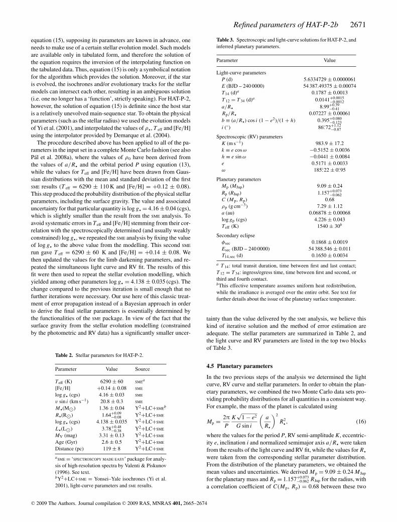
Table 3. Spectroscopic and light-curve solutions for HAT-P-2, andinferred planetary parameters.

Parameter Value

Light-curve parametersP (d) 5.6334729 ± 0.0000061E (BJD – 240 0000) 54 387.49375 ± 0.00074T14 (d)a 0.1787 ± 0.0013T 12 = T 34 (d)a 0.0141+0.0015

−0.0012a/R� 8.99+0.39

−0.41Rp/R� 0.07227 ± 0.00061b ≡ (a/R�) cos i (1 − e2)/(1 + h) 0.395+0.080

−0.123i (◦) 86.◦72+1.12

−0.87

Spectroscopic (RV) parametersK (m s−1) 983.9 ± 17.2k ≡ e cos ω −0.5152 ± 0.0036h ≡ e sin ω −0.0441 ± 0.0084e 0.5171 ± 0.0033ω 185.◦22 ± 0.◦95

Planetary parametersMp (MJup) 9.09 ± 0.24Rp (RJup) 1.157+0.073

−0.062C (Mp, Rp) 0.68ρp (g cm−3) 7.29 ± 1.12a (au) 0.06878 ± 0.00068log gp (cgs) 4.226 ± 0.043Teff (K) 1540 ± 30b

Secondary eclipseφsec 0.1868 ± 0.0019Esec (BJD – 240 0000) 54 388.546 ± 0.011T14,sec (d) 0.1650 ± 0.0034

a T 14: total transit duration, time between first and last contact;T 12 = T 34: ingress/egress time, time between first and second, orthird and fourth contact.bThis effective temperature assumes uniform heat redistribution,while the irradiance is averaged over the entire orbit. See text forfurther details about the issue of the planetary surface temperature.

tainty than the value delivered by the SME analysis, we believe thiskind of iterative solution and the method of error estimation areadequate. The stellar parameters are summarized in Table 2, andthe light curve and RV parameters are listed in the top two blocksof Table 3.

4.5 Planetary parameters

In the two previous steps of the analysis we determined the lightcurve, RV curve and stellar parameters. In order to obtain the plan-etary parameters, we combined the two Monte Carlo data sets pro-viding probability distributions for all quantities in a consistent way.For example, the mass of the planet is calculated using

Mp = 2π

P

K√

1 − e2

G sin i

(a

R�

)2

R2� , (16)

where the values for the period P, RV semi-amplitude K, eccentric-ity e, inclination i and normalized semimajor axis a/R� were takenfrom the results of the light curve and RV fit, while the values for R�

were taken from the corresponding stellar parameter distribution.From the distribution of the planetary parameters, we obtained themean values and uncertainties. We derived Mp = 9.09 ± 0.24 M Jup

for the planetary mass and Rp = 1.157+0.073−0.062 RJup for the radius, with

a correlation coefficient of C(Mp, Rp) = 0.68 between these two

C© 2009 The Authors. Journal compilation C© 2009 RAS, MNRAS 401, 2665–2674

2672 A. Pal et al.

parameters. The planetary parameters are summarized in the thirdblock of Table 3. Compared with the values reported by Bakos et al.(2007a), the mass of the planet has not changed significantly (fromMp = 9.04 ± 0.50 M Jup), but the uncertainty is now smaller by afactor of 2. The new estimate of the planetary radius is larger byroughly 2σ , while its uncertainty is similar or slightly smaller thanbefore (Rp = 0.982+0.038

−0.105 RJup for Bakos et al. 2007a).The surface temperature of the planet is poorly constrained be-

cause of the lack of knowledge about redistribution of the incomingstellar flux or the effects of significant orbital eccentricity. Assum-ing complete heat redistribution, the surface temperature can beestimated by time averaging the incoming flux, which varies as1/r2 = a−2 (1 − e cos E)−2 due to the orbital eccentricity. The timeaverage of 1/r2 is⟨

1

r2

⟩= 1

T

∫ T

0

dt

r2(t)= 1

2π

∫ 2π

0

dM

r2(M), (17)

where M is the mean anomaly of the planet. Since r = a(1 −e cos E) and d M = (1 − e cos E) dE, where E is the eccentricanomaly, the above integral can be calculated analytically and theresult is⟨

1

r2

⟩= 1

a2√

1 − e2. (18)

Using this time-averaged weight for the incoming flux, we derivedT p = 1540 ± 30 K. However, the planet surface temperature wouldbe ∼2975 K on the dayside during periastron assuming no heatredistribution, while the equilibrium temperature would be only∼1190 K at apastron. Thus, we conclude that the surface tempera-ture can vary by a factor of ∼3, depending on the actual atmosphericdynamics.

4.6 Photometric parameters and the distance of the system

The measured colour index of the star as reported in the TASScatalogue (Droege, Richmond & Sallman 2006) is (V − I )TASS =0.55 ± 0.06, which is in excellent agreement with the result of (V −I )YY = 0.552 ± 0.016 we obtain from the stellar evolution modelling(see Section 4.4). The models also provide the absolute visual mag-nitude of the star as MV = 3.31 ± 0.13, which gives a distance mod-ulus of V TASS − MV = 5.39 ± 0.13 corresponding to a distance of119 ± 8 pc, assuming no interstellar extinction. This distanceestimate is intermediate between the values inferred from thetrigonometric parallax in the original Hipparcos catalogue (πHIP =7.39 ± 0.88 mas, corresponding to a distance of 135 ± 18 pc;Perryman et al. 1997), and in the revised reduction of the orig-inal Hipparcos observations by van Leeuwen (2007a,b) (πHIP =10.14 ± 0.73 mas, equivalent to a distance of 99 ± 7 pc). In Fig. 5the model isochrones are shown for the measured metallicity ofHAT-P-2 against the measured effective temperature and two setsof luminosity constraints: those provided by the estimates of theHipparcos distance (original and revised) together with the TASSapparent magnitudes (top panel), and the constraint from the stellardensity inferred from the light curve (bottom panel). We note inpassing that the distance derived using the near-infrared 2MASSphotometry agrees well with the distance that relies on the TASSoptical magnitudes.

4.7 Limits on the presence of a second companion

In this section we discuss limits on the presence of an additionalplanet in this system. We performed two types of tests. In both of

2.0

4.0

6.0

8.0

10.0

12.0

14.0

16.0

18.0

4000450050005500600065007000

Rela

tive

sem

imajo

r axis

Stellar effective temperature [K]

2.0

2.5

3.0

3.5

4.0

4.5

5.0

5.5

6.0

Absolu

te V

magnitude

Figure 5. Observational constraints for HAT-P-2 compared with stellar evo-lution calculations from the Yonsei–Yale models, represented by isochronesfor [ Fe/H ] = +0.14 between 0.5 and 5.5 Gyr, in steps of 0.5 Gyr. Theluminosities on the vertical axis are rendered in two ways: as absolute visualmagnitudes MV in the top panel, and with the ratio a/R� as a proxy inthe lower panel. The effective temperature along with the absolute magni-tudes inferred from the apparent brightness in the TASS catalogue and theoriginal and revised Hipparcos parallaxes are shown in the top panel withthe corresponding 1σ and 2σ confidence ellipsoids (upper ellipsoid for theoriginal Hipparcos reductions, lower for the revision). The diamond repre-sents the value of MV derived from our best-fitting stellar evolution modelsusing a/R� as a constrain on the luminosity. In the lower panel we show theconfidence ellipsoids for the temperature and our estimate of a/R� from thelight curve.

these tests we have fitted the RV semi-amplitude K, the Lagrangianorbital elements (k, h), the three velocity zero-points (γ Keck, γ Lick

and γ OHP) and the additional terms required by the respective testmethods (drift coefficients or orbital amplitudes). In these fits, theorbital epoch E and period P of HAT-P-2b have been kept fixedat the values yielded by the joint photometric and RV fit. Thisis a plausible assumption since without the constraints given bythe photometry, the best-fitting epoch and period would be ERV =245 4342.455 ± 0.016 (BJD) and P = 5.6337 ± 0.0016, i.e. theuncertainties would be roughly 20–25 times larger.

In the first test, a linear, quadratic and cubic polynomialwere added to the RV model functions in addition to the γ

C© 2009 The Authors. Journal compilation C© 2009 RAS, MNRAS 401, 2665–2674

Refined parameters of HAT-P-2b 2673

44

46

48

50

52

54

56

580.0 0.1 0.2 0.3 0.4 0.5

Un

bia

se

d χ

2

Mean motion (d-1

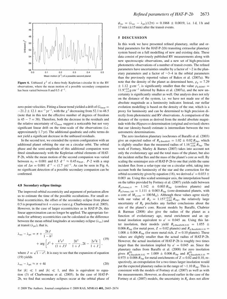
) of a possible second planet

Figure 6. Unbiased χ2 of a three-body Keplerian+circular fit to the RVobservations, where the mean motion of a possible secondary companionhas been varied between 0 and 0.5 d−1.

zero-point velocities. Fitting a linear trend yielded a drift of Glinear =−21.2 ± 12.1 m s−1 yr−1, with the χ 2 decreasing from 52.1 to 48.5(note that in this test the effective number of degrees of freedomis 45 − 7 = 38). Therefore, both the decrease in the residuals andthe relative uncertainty of Glinear suggest a noticeable but not verysignificant linear drift on the time-scale of the observations (i.e.approximately 1.7 yr). The additional quadratic and cubic terms donot yield a significant decrease in the unbiased residuals.

In the second test, we extended the system configuration with anadditional planet orbiting the star on a circular orbit. The orbitalphase and the semi-amplitude of this additional companion werefitted simultaneously with the Keplerian orbital elements of HAT-P-2b, while the mean motion of the second companion was variedbetween n2 = 0.001 and 0.5 d−1 ≈ 0.45 nHAT− P -2 with a stepsize of �n = 0.001 d−1 < (1.7 yr)−1. As can be seen in Fig. 6,no significant detection of a possible secondary companion can beconfirmed.

4.8 Secondary eclipse timings

The improved orbital eccentricity and argument of periastron allowus to estimate the time of the possible occultations. For small or-bital eccentricities, the offset of the secondary eclipse from phase0.5 is proportional to k = ecos ω (see e.g. Charbonneau et al. 2005).However, in the case of larger eccentricities as in HAT-P-2b, thislinear approximation can no longer be applied. The appropriate for-mula for arbitrary eccentricities can be calculated as the differencebetween the mean orbital longitudes at secondary eclipse (λsec) andat transit (λpri), that is,

λsec − λpri = π + 2kJ

1 − h2

+ arg

[J 2 + k2e2

(1 + J )2− 2k2

1 + J, 2k − 2e2k

1 + J

],

(19)

where J = √1 − e2. It is easy to see that the expansion of equation

(19) yields

λsec − λpri ≈ π + 4k (20)

for |k| 1 and |h| 1, and this is equivalent to equa-tion (3) of Charbonneau et al. (2005). In the case of HAT-P-2b, we find that secondary eclipses occur at the orbital phase of

φsec = (λsec − λpri)/(2π) = 0.1868 ± 0.0019, i.e. 1 d, 1 h and17 min (±15 min) after the transit events.

5 D ISCUSSION

In this work we have presented refined planetary, stellar and or-bital parameters for the HAT-P-2(b) transiting extrasolar planetarysystem based on a full modelling of new and existing data. Thesedata consist of previously published RV measurements along withnew spectroscopic observations, and a new set of high-precisionphotometric observations of a number of transit events. The refinedparameters have uncertainties smaller by a factor of ∼2 in the plan-etary parameters and a factor of ∼3–4 in the orbital parametersthan the previously reported values of Bakos et al. (2007a). Wenote that the density of the planet as determined here, ρp = 7.29± 1.12 g cm−3, is significantly smaller than the value ρp,B2007 =11.9+4.8

−1.6 g cm−3 inferred by Bakos et al. (2007a), and the new un-certainty is significantly smaller as well. Our analysis does not relyon the distance of the system, i.e. we have not made use of theabsolute magnitude as a luminosity indicator. Instead, our stellarevolution modelling is based on the density of the star, which is aproxy for luminosity and can be determined to high precision di-rectly from photometric and RV observations. A comparison of thedistance of the system as derived from the model absolute magni-tude with the Hipparcos determination (original and revised) showsthat our (density-based) estimate is intermediate between the twoastrometric determinations.

The zero insolation planetary isochrones of Baraffe et al. (2003)give an expected radius of Rp,Baraffe03 = 1.02 ± 0.02 RJup, whichis slightly smaller than the measured radius of 1.16+0.07

−0.06 RJup. Thework of Fortney, Marley & Barnes (2007) takes into account notonly the evolutionary age and the total mass of the planet, but alsothe incident stellar flux and the mass of the planet’s core as well. Byscaling the semimajor axis of HAT-P-2b to one that yields the sameincident flux from a solar-type star on a circular orbit, taking intoaccount both the luminosity of the star and the correction for theorbital eccentricity given by equation (18), we derived a′ = 0.033 ±0.003 au. Using this scaled semimajor axis, the interpolation basedon the tables provided by Fortney et al. (2007) yields radii betweenRp,Fortney,0 = 1.142 ± 0.003 RJup (coreless planets) andRp,Fortney,100 = 1.111 ± 0.003 RJup (core-dominated planets, witha core of Mp,core = 100 M⊕). Although these values agree nicelywith our value of Rp = 1.157+0.073

−0.062 RJup, the relatively largeuncertainty of Rp precludes any further conclusions about thesize of the planet’s core. Recent models by Baraffe, Chabrier& Barman (2008) also give the radius of the planet as afunction of evolutionary age, metal enrichment and an op-tional insolation equivalent to a′ = 0.045 au. Using this lat-ter insolation, their models yield Rp,Baraffe08,0.02 = 1.055 ±0.006 RJup (for metal poor, Z = 0.02 planets) and Rp,Baraffe08,0.10 =1.008 ± 0.006 RJup (for more metal rich, Z = 0.10 planets). Thesevalues are slightly smaller than the actual radius of HAT-P-2b.However, the actual insolation of HAT-P-2b is roughly two timeslarger than the insolation implied by a′ = 0.045 au. Since theplanetary radius from Baraffe et al. (2008) for zero insolationgives R

(0)p,Baraffe08,0.02 = 1.009 ± 0.006 RJup and R

(0)p,Baraffe08,0.10 =

0.975 ± 0.006 RJup for metal enrichments of Z = 0.02 and 0.10, re-spectively, an extrapolation for a two times larger insolation wouldput the expected planetary radius in the range of ∼1.10 RJup. This isconsistent with the models of Fortney et al. (2007) as well as withthe measurements. However, as discussed earlier in the case of theFortney et al. (2007) models, the uncertainty in Rp does not allow

C© 2009 The Authors. Journal compilation C© 2009 RAS, MNRAS 401, 2665–2674

2674 A. Pal et al.

us to properly constrain the metal enrichment for the recent Baraffemodels.

AC K N OW L E D G M E N T S

The work by AP was supported by the HATNet project and in partby ESA grant PECS 98073. HATNet operations have been fundedby NASA grants NNG04GN74G, NNX08AF23G and SAO IR&Dgrants. Work of GAB and JAJ were supported by the Post-doctoralFellowship of the NSF Astronomy and Astrophysics Program (AST-0702843 and AST-0702821, respectively). GT received partial sup-port from NASA Origins grant NNX09AF59G. We acknowledgepartial support also from the Kepler Mission under NASA Cooper-ative Agreement NCC2-1390 (DWL, PI). This research has madeuse of Keck telescope time granted through NOAO and NASA.We thank the UCO/Lick technical staff for supporting the remote-observing capability of the Nickel Telescope, allowing the photom-etry to be carried out from UC Berkeley. Automated Astronomy atTennessee State University has been supported long term by NASAand NSF as well as Tennessee State University and the State of Ten-nessee through its Centers of Excellence program. We are gratefulfor the comments and suggestions by the referee, Frederic Pont. Weacknowledge the use of the VizieR service (Ochsenbein, Bauer &Marcout 2000) operated at CDS, Strasbourg, France, of NASA’sAstrophysics Data System Abstract Service, and of the 2MASSCatalogue.

REFERENCES

Bakos G. A., Lazar J., Papp I., Sari P., Green E. M., 2002, PASP, 114, 974Bakos G. A., Noyes R. W., Kovacs G., Stanek K. Z., Sasselov D. D., Domsa

I., 2004, PASP, 116, 266Bakos G. A. et al., 2007a, ApJ, 670, 826Bakos G. A. et al., 2007b, ApJ, 671, L173Bakos G. A. et al., 2009, ApJ, submitted (arXiv:0901.0282)Baraffe I., Chabrier G., Barman T. S., Allard F., Hauschildt P. H., 2003,

A&A, 402, 701Baraffe I., Chabrier G., Barman T., 2008, A&A, 482, 315Barbieri M. et al., 2007, A&A, 476, L13Barnes J. W., 2007, PASP, 119, 986Borucki W. J. et al., 2007, in Afonso C., Weldrake D., Henning Th., eds, ASP

Conf. Ser. Vol. 366, Transiting Extrasolar Planets Workshop. Astron.Soc. Pac., San Francisco, p. 309

Charbonneau D. et al., 2005, ApJ, 626, 523Claret A., 2000, A&A, 363, 1081Claret A., 2004, A&A, 428, 1001D’Angelo G., Lubow S. H., Bate M. R., 2006, ApJ, 652, 1698Demarque P., Woo J.-H., Kim Y.-C., Yi S. K., 2004, ApJS, 155, 667

Droege T. F., Richmond M. W., Sallman M., 2006, PASP, 118, 1666Fabrycky D., Tremaine S., 2007, ApJ, 669, 1298Ford E. B., Rasio F. A., 2008, ApJ, 686, 621Fortney J. J., Marley M. S., Barnes W., 2007, ApJ, 659, 1661Gillon M. et al., 2007, A&A, 472, L13Hebrard G. et al., 2008, A&A, 488, 763Henry G. W., 1999, PASP, 111, 845Johns-Krull C. M. et al., 2008, ApJ, 677, 657Johnson J. A. et al., 2008, ApJ, 686, 649Kopal Z., 1959, Close Binary Systems. Wiley, New YorkLoeb A., 2005, ApJ, 623, L45Loeillet B. et al., 2008, A&A, 481, 529Mandel K., Agol E., 2002, ApJ, 580, L171Naef D. et al., 2001, A&A, 375, 27Ochsenbein F., Bauer P., Marcout J., 2000, A&AS, 143, 23Pal A., 2008, MNRAS, 390, 281Pal A., 2009a, MNRAS, 396, 1737Pal A., 2009b, PhD thesis, Eotvos Lorand Univ., BudapestPal A., Bakos G. A., 2006, PASP, 118, 1474Pal A., Suli A., 2007, MNRAS, 381, 1515Pal A. et al., 2008a, ApJ, 680, 1450Pal A., Bakos G. A., Noyes R. W., Torres G., 2008b, in Pont F., ed., Proc.

IAU Symp. 253, Transiting Planets. Cambridge Univ. Press, Cambridge,p. 428

Perryman M. A. C. et al., 1997, A&A, 323, 49Press W. H., Teukolsky S. A., Vetterling W. T., Flannery B. P., 1992, Numer-

ical Recipes in C: the Art of Scientific Computing, 2nd edn. CambridgeUniv. Press, Cambridge

Shporer A., Mazeh T., Moran A., Bakos G. A., Kovacs G., Mashal E., 2006,in Arnold L., Bouchy F., Moutou C., eds, Tenth Anniversary of 51 Peg-b:Status of and Prospects for Hot Jupiter Studies. Frontier Group, Paris,p. 196

Skrutskie M. F. et al., 2006, AJ, 131, 1163Sozzetti A., Torres G., Charbonneau D., Latham D. W., Holman M. J., Winn

J. N., Laird J. B., O’Donovan F. T., 2007, ApJ, 664, 1190Takeda G., Kita R., Rasio F. A., 2008, ApJ, 683, 1063Valenti J. A., Fischer D. A., 2005, ApJS, 159, 141Valenti J. A., Piskunov N., 1996, A&AS, 118, 595van Leeuwen F., 2007a, Hipparcos, the New Reduction of the Raw Data,

Astrophys. Space Sci. Libr. Vol. 350. Springer, Berlinvan Leeuwen F., 2007b, A&A, 474, 653Vogt S. S., 1987, PASP, 99, 1214Winn J. N. et al., 2007a, ApJ, 665, 167Winn J. N. et al., 2007b, AJ, 134, 1707Winn J. N. et al., 2009a, ApJ, 700, 302Winn J. N. et al., 2009b, ApJ, in press (arXiv:0907.5205)Yi S. K., Demarque P., Kim Y.-C., Lee Y.-W., Ree C. H., Lejeune T., Barnes

S., 2001, ApJS, 136, 417

This paper has been typeset from a TEX/LATEX file prepared by the author.

C© 2009 The Authors. Journal compilation C© 2009 RAS, MNRAS 401, 2665–2674