������������������ ��� ������������������������ ������������������������������������������������������������������������������

����������������������������������������������������������������������� �

�������������!�∀�!�#���!�∃�!�%���&������∋�!������ �#����!�∃��(����)�∗��∋�����+�%��,�����������−����.������/� 0���1�������∃�+���������������∋�2���������� �#������������+�∀������/������3�+����0�!���������0������ ���

/������3�+����0������+�∀����������

���������������� ����!�����������������

������4���������������������������������������

WORKING PAPER 00/05

HARMONISING DATABASES FORTHE CROSS NATIONAL STUDY OF INTERNAL MIGRATION:

LESSONS FROM AUSTRALIA AND BRITAIN

Philip Rees1

Martin Bell2

Oliver Duke-Williams3

andMarcus Blake4

1School of Geography,University of Leeds, Leeds LS2 9JT, UK,

e-mail p.rees@geog.leeds.ac.uk,phone +44 (0)113 233 3341, fax +44 (0)113 233 3308

2Department of Geographical and nvironmental Studies,University of Adelaide, Adelaide, South Australia 5005,

e-mail martin.bell@adelaide.edu.au,phone +61-7-38782376, fax +61-7-38786667

3Centre for Computational Geography, School of Geography,University of Leeds, Leeds LS2 9JT, UK,e-mail o.duke-williams@geog.leeds.ac.uk

4Key Centre for Social Applications of Geographic Information Systems,University of Adelaide, Adelaide, South Australia 5005,

e-mail mblake@gisca.adelaide.edu.au

PUBLISHED NOVEMBER 2000

ALL RIGHTS RESERVED

For further copies contact the Working Paper Secretary,School of Geography, University of Leeds, Leeds LS2 9JT

Telephone 0113 233 3300

ii

iii

TABLE OF CONTENTS

Page

CONTENTS iiiLIST OF TABLES ivLIST OF FIGURES ivABSTRACT vACKNOWLEDGMENTS vi

1. INTRODUCTION1.1 Why Construct Parallel Time Series of Migration Statistics?1.2 The Nature of the Parallel Databases1.3 The Tasks in Database Creation

2. THE AUSTRALIAN AND BRITISH MIGRATION STATISTICS2.1 Sources of Australian and British Migration Data2.2 Concepts in the Australian and British Migration Data2.3 The Temporal Stability of Spatial Units2.4 Age-Time Plans in the Australian and British Migration Data

3. PRELIMINARY PROCESSING AND FILLING THE GAPS3.1 Processing the Australian Migration Data3.2 Processing the British Data

4. CONSTRUCTING TEMPORALLY CONSISTENT REGIONS4.1 Defining Temporally Consistent Regions, Australia, 1976-964.2 Defining Temporally Consistent Regions, Britain, 1976-96

5. DEFINING FUNCTIONALLY COMPARABLE REGIONS5.1 City regions in Australia5.2 City regions in Britain5.3 Migration in a City-Region Framework

6. HARMONISING THE AGE-TIME PLANS FOR THE MIGRATION DATA6.1 Disaggregating the Australian Migration Data into Age-Period-Cohort Flows6.2 Disaggregating the British Migration Data into Age-Period-Cohort Flows6.3 Illustrations6.4 Deriving Populations at Risk

7. CONCLUSIONS

REFERENCES

iv

LIST OF TABLESPage

1. Migration flows between city regions for period-cohorts and age-period-cohortsand period-ages, 1991-96 for Australia

2. Migration flows between city regions for period-cohorts and age-period-cohortsand period-ages, 1991-96 for the UK

LIST OF FIGURES

1. Dimensions of the harmonised database: sex-origin-destination by age-period-cohort

2. A flow diagram of the procedures used to assemble the harmonised Australianand UK databases

3. Age-time observation plans for migration data: period-cohort and period-age datasplit into APC spaces

4. The iterative proportional fitting routine to estimate ODAS migration flows inBritain, 1975-76 to 1982-83

5. City regions in Australia6. City regions in the UK7. Net migration rates (all ages) for city regions in Australia and the UK: 1976-81

and 1991-968. Frameworks for age-period-cohort processing of Australian and UK migration

data

v

ABSTRACT

This paper describes the way in which harmonised databases of inter-regional migration in

Australia and Britain were created, classified by five year ages and birth cohorts for four five

year periods between 1976 and 1996. The data processing involved estimation of migration

data for temporally comparable spatial units, the aggregation of those units to a meaningful

set of city regions, the extraction of migration data from official data files supplied by the

Australian Bureau of Statistics and the Office for National Statistics, the filling of gaps in

these files through use of various techniques including iterative proportional fitting, and the

harmonisation of age time-plans through estimation of the numbers of transitions (Australia)

or movements (Britain) for common age-period-cohort spaces. The final stage in preparation

of the databases was to specify the populations at risk for computation of migration

intensities. The creation of such databases requires integration of demographic concepts,

social science estimation methods and careful bespoke computer programs: once the goal of

harmonisation has been achieved standard database and statistical software can be used in the

parallel analysis of migration in Australia and Britain.

Keywords. Internal migration; Australia; Britain; comparative studies

vi

ACKNOWLEDGEMENTS

This research was part of a research project entitled Migration Trends in Australia and

Britain: Levels and Trends in an Age-Period-Cohort Framework funded by Award

A79803552 from the Australian Research Council and by Award R000237375 from the

Economic and Social Research Council.

1

1. INTRODUCTION

1.1 Why Construct Parallel Time Series of Migration Statistics?

Relatively little attention has been given to the ways in which within-country migration

changes over time. In countries that do not have a comprehensive population register and its

accompanying compulsory change-of-address recording system, the reason for this neglect is

the difficulty of assembling consistent and accurate time series from partial data. To

understand migration behaviour, it is essential to construct time series which are fully

classified by age at migration, period of migration and cohort of birth. Such a database makes

it possible to track changes over time in age-specific migration intensities and hence to

analyse the influence of life course events, secular trends and birth cohort size on these

intensities.

This paper sets out the procedures for constructing parallel migration databases, with

the same spatial and demographic structure, for Australia and Britain as part of a project

comparing inter-regional migration in the two countries. Cross-national comparisons of

internal migration present a number of challenges (Bell et al., forthcoming, Rees et al., 2000)

and these are especially apparent in the case of Australia and Britain. The migration data

collected in the two countries differ in a number of crucial respects, including the way in

which migration is measured (events versus transitions), the intervals over which they are

collected, the populations they cover and the treatment accorded to missing data. There are

marked differences, too, in the physical geography and settlement patterns of Britain and

Australia.

If reliable comparisons are to be made, it is essential that the effect of such variations

be minimised and, where possible, eliminated. Ideally this requires the creation of parallel

databases that are harmonised in respect of four key dimensions: the time periods over which

migration is recorded; the system of spatial zones between which the moves are registered;

2

the conceptual basis on which the migration is measured; and the age-time plan from which

the movement is observed.

While the creation of databases that are fully harmonised on all of these dimensions is

out of reach, it has been possible to assemble time series datasets for the two countries which

are closely comparable. In practice, this meant assembling data for about 35 regions in each

country, over four 5-year time periods (1976-81, 1981-86, 1986-91, 1991-96), using two

sexes, fifteen five-year age groups (0-4, 5-9, ... , 65-69, 70+), and nineteen five-year birth

cohorts (pre-1906, 1906-11, ... , 1986-91, 1991-96). Several of the issues involved in this

harmonisation of databases are described in discrete contributions elsewhere (see Bell et al.,

1999; Blake et al., 2000; Rees et al., 2000; Bell and Rees, 2000). The purpose of this paper is

to bring together the various elements and procedures in a single overview of the

harmonisation process.

1.2 The Nature of the Parallel Databases

The organising framework for the databases in each country is a Sex-Origin-Destination-

Age-Period-Cohort (SODAPC) array of migration flows. Figure 1 provides a picture of what

a SODAPC array looks like in conceptual form. It is not, of course, possible to represent a six

dimensional array on a two dimensional plane, so the array is shown as two sets of three-

dimensional diagrams, which are combined to form the full database.

The top diagram in Figure 1 shows the SOD face of the full array: Sex by Origin by

Destination. The interior of the cube is occupied by triply classified cells, which contain

counts of migrants or migrations. The sex component plays a very simple role in the

database: every migration flow is given for males and females, and therefore implicitly for

persons. The origin-destination face of the SOD array is symmetrical: origin and destination

regions are defined to be similar kinds of region, city regions (spheres of influence) in both

countries,

3

Figure 1. Dimensions of the harmonised database: sex-origin-destination by age-period-cohort

4

because this is the only geographical classification that makes sense in the real space-

economy. These regions need to be defined consistently over time, because otherwise the

change measured over time is artefactual rather than real.

The bottom diagram in Figure 1 shows the APC face of the full array. Each triangular

APC space in this diagram is occupied by a count of migrants or migrations. Migration flows

are classified in this array by age at time of migration, by period of migration and by birth

cohort membership. An explicit third dimension for birth cohort is not needed if there is exact

information on time of migration and birth date of migrant, because the birth cohort can then

be deduced directly. However, these data are lacking in both Britain and Australia so in order

to make the data fully comparable we need to so develop methods to estimate the triple

classification of register-based migration in Britain and census-based migration in Australia.

Each element in the SOD array can be cross-classified against any element in the APC

array and any subset of information retrieved from the full database. For example, we can

look at the way in which migrations in a particular age group from an origin vary by period.

Or we can examine how the origin to destination flows of a particular birth cohort vary over

the four periods for which we have information. Once the full array has been “populated”

with reliable estimates, the information can also be used to compare migration behaviour in

the two countries at the national scale (Bell et al., forthcoming).

1.3 The Tasks in Database Creation

The main tasks to be accomplished are set out in Figure 2 as a series of steps in two parallel

sets of processes, which transform the raw data into harmonised databases. The first task was

to acquire from the Australian Bureau of Statistics (ABS) and the Office for National

Statistics (ONS) data files relating to migration over a common 20-year period from 1976 to

1996. The raw Australian data are stored by ABS as origin-destination flows between

5

Figure 2. A flow diagram of the procedures used to assemble the harmonised Australianand UK databases

6

Statistical Local Areas (SLAs - the main sub-State reporting areas used in the Australian

Census). The data are contained in four separate files from the censuses of 1981, 1986, 1991

and 1996, each covering a five year interval. The raw British data consist of quarterly files of

inter-FHSA migration from the third quarter (Q3) of 1975 to the second quarter (Q2) of 1996.

In the period Q3-1975 to Q2-1983, the migration data are provided as three tables: origins by

destinations (OD), origins by age and sex (OAS) and destinations by age and sex (DAS).

From Q3-1983 to Q2-1996, the data are available as individual migration records from which

full flow arrays can be constructed (ODAS). The characteristics of the Australian and British

migration data are set out in more detail detailed in section 2.

The second task was to carry out preliminary processing of the Australian and British

migration statistics into suitable formats. For example, the British quarterly data were

aggregated into annual, mid-year to mid-year periods. There was also the need to estimate

the full ODAS array for 1975-83 for Britain so that the same migration flows were available

for all five-year periods. Details of preliminary processing are given in section 3.

The third task was to aggregate the data from the spatial units provided in the raw files

to a temporally-consistent set of spatial units. This is essential if time series analysis of the

harmonised data is planned, but national statistical offices rarely provide data series

retrospectively adjusted to achieve spatial consistency. The methods adopted are described in

section 4.

Because the spatial units available in Australia and Britain differed so much in original

purpose - statistical reporting area (Australia) versus administrative unit in the public health

service (Britain) - it is important for cross-national comparison to identify some common

zonal system. We achieved this by aggregation to city regions, which are the organisers and

driving forces of the space-economies of both countries. The logic of these spatial structures

is explained in section 5.

7

The final task is to process the data into age-period-cohort migration flows. This is

necessary because the Australian data are reported in period-cohort form, whereas the British

data are reported in period-age form. So that comparisons can be made each Australian

period-cohort migration flow and each British migration period-age flow is disaggregated

into age-period-cohort elements. An overview of the procedures is provided in section 6, with

a full account set out in Bell and Rees (2000).

The final section of the paper briefly summarises the content of the two harmonised

databases and indicates the comparative analyses that are made possible. It also draws

lessons for the extension of harmonisation to migration data sets in other countries.

2. THE AUSTRALIAN AND BRITISH MIGRATION STATISTICS

2.1 Sources of Australian and British Migration Data

In Australia the only comprehensive source of data on internal migration is the Population

Census. Australian Census data on internal migration derive from a series of multi-part

questions that seek each person’s place of usual residence on Census night and their usual

address five years previously. Similar data have been collected at each quinquennial Census

since 1971. Since 1976 a question on place of usual residence one year ago has also been

included. Except for the 1991 Census, when the one year question was restricted to the state

level, usual address has been coded to SLA level (Census Local Government Area level prior

to 1986).

The strengths of the Australian migration data derive from consistently low levels of

underenumeration (under 2 per cent), the extensive range of individual and housing

characteristics collected (which can be cross-tabulated with migration status), and the fine

spatial mesh which is available (since current and previous residence is coded to more than

1300 SLAs). It’s main limitations reflect the conventional problems of transition data:

8

relatively high rates of non-response to questions on place of previous residence (around 5

per cent); the fact that only a single change of residence is captured, thereby missing any

intervening moves; and the frequent changes that have occurred in the boundaries of SLAs,

which seriously prejudice temporal comparability. The quality of data from the 1996 Census

was also affected by deficiencies in coding (Bell and Stratton, 1998). Despite these

shortcomings, migration data from the Census have been subjected to rigorous analysis

following each successive enumeration since 1971 (McKay and Whitelaw, 1978; Rowland,

1979; Maher, 1984; Bell, 1992, 1995; Bell and Hugo, 2000).

The APC database covers the period 1976 to 1996 and draws on five year interval

migration data from the 1981, 1986, 1991 and 1996 enumerations. The data were acquired as

special multidimensional ODAS tabulations from the ABS in two file formats: as Supertable

output files which are convenient for generating aggregated tables but cannot be readily used

as inputs to further processes, and as ASCII database records giving sex, origin code,

destination code, age code and the migrant count, which can be input to other computer

programs or statistical packages.

In the United Kingdom decennial censuses since 1961 have asked migration questions,

but they cover only one year in the decade (except in 1971 when a five-year question was

also asked). Since 1975 the Office for National Statistics (formerly the Office for Population

Censuses and Surveys) has published migration statistics for each quarter based on

information generated from the maintenance of the National Health Service Central Register

(NHSCR). This information consists of records of NHS patient re-registrations that cross the

boundaries of the administrative areas of the family doctor service. From 1975 to 1983 these

areas were referred to as Family Practitioner Committee areas (FPCs) and between 1983 and

1996 as Family Health Service Authorities (FHSAs). FHSAs have recently been merged into

Health Area authorities, which procure patient services within the NHS and from 1999

9

migration statistics will be published for these new spatial units. A full account of the

NHSCR migration statistics is provided by Duke-Williams and Stillwell (1999).

The NHSCR migration statistics are not quite comprehensive. They do not measure

migration within FHSA area; they undercount migrations by young adult males who may

migrate several times before registering; and they omit groups whose medical care is wholly

provided by non-NHS bodies (the Armed Forces, the Prison Service, private health schemes).

However, they are the best time series data available and have been extensively used in

previous research (Stillwell et al., 1992, 1996).

The British migration data have been acquired from the Migration Statistics division of

the Office for National Statistics over a number of years as a standard set of files and used in

other projects (see Stillwell et al., 1992; Duke-Williams and Stillwell, 1999). The data files

provided by ONS are available for licensing quarter by quarter from 1975-Q3 to the latest

quarter (usually two or three quarters in lag from the current). In this work we restrict

attention to the period 1976-Q3 to 1996-Q2. For the period 1976-Q3 to 1983-Q2, the files

consist of records with three separate arrays: an Origin-Age-Sex (OAS) array, a Destination-

Age-Sex (DAS) array and an Origin-Destination (OD) array. Between 1983-Q3 and 1996-

Q2, the files contain person unit data (PUD) made up of migration records classified by sex,

origin, destination, age at time of migration and date of birth. ONS are planning in the near

future to make available a new source of local migration data based on address matching of

NHS Register individual files one year apart (Scott and Kilbey, 1999). This new source

would make possible the reporting of migration flows between Local Government Areas and

Wards.

10

2.2 Concepts in the Australian and British Migration Data

The British NHSCR migration statistics refer to movements or migration events. It is thus

possible for an individual to make more than one migration in a given time interval. By

contrast, the Australian Census data measure migration as a transition between two fixed

points in time and therefore capture only a single migration (see Rees, 1977). To convert

movement statistics to transition data, or vice versa is not possible except in a very crude

way, because any conversion method would need data on the number of moves per transition

at different scales, and to our knowledge no such information exists either in Australia or

Britain. So, ultimately, the migration data for the two countries remain non-comparable,

although we have used census data for single years as the basis for comparison in other

analyses (Bell et al., forthcoming; Rees et al., 2000). Despite this inconsistency, it is of great

value for comparison to harmonise the spatial, temporal and age definitions in the data.

2.3 The Temporal Stability of Spatial Units

The geography of the migration data was handled in two stages: first, the data were

assembled for the most detailed zonal system feasible in each country; they were then

aggregated into comparable city-region systems for analysis (see section 5). In Australia,

although migration data are available from each census at SLA level, these areas are subject

to frequent shifts in municipal boundaries. The ABS attempts to solve this problem by

publishing data for Statistical Divisions (SDs), designed as relatively large, functional regions

which would remain stable for statistical purposes over a period of 20 years or more (ABS,

1996:15). In practice, however, SD boundaries underwent a number of changes over the

1976-1996 period, so a new regional structure consisting of 69 zones which are spatially

consistent over the full twenty year period was created. The derivation of this set of zones,

termed Temporally-consistent Statistical Divisions or TSDs, is summarised in section 4 and

11

set out in detail in Blake et al. (2000). The FHSAs in Britain posed fewer problems of

temporal consistency, being based on large administrative units such as shire counties or

metropolitan districts, but some aggregation was necessary.

2.4 Age-Time Plans in the Australian and British Migration Data

Another important variation between the Australian and British migration data is that they are

based on differing observation plans. The nature of this variation, and its implications for

cross-national comparison, are most readily understood by reference to the well-known Lexis

diagram which graphs age against time (Vanderschrick, 1992). This diagram makes possible

the identification of several types of age-time observation plan, two of which are shown in

Figure 3. Migration data generated from a retrospective question in the census are reported in

period-cohort form, and conventionally labelled by reference to age at the end of the

recording interval. So, for example, migrants recorded as aged 50-54 in the 1986 Australian

Census were aged 45-49 five years earlier. The transition therefore occured somewhere in the

period-cohort space labeled ‘A’ but it is not possible to determine the precise age at which

migration took place: in fact, as noted above, several moves may have occurred. The British

data, by contrast, record the age at which the migration event took place, reflecting a period-

age observation plan. Thus the period-age space labelled ’B’ captures counts of migration

events occuring between 1976 and 1981 to people aged 40-44 at the time of the event. Some

of these would have occurred to the cohort aged 40-44 in 1981, and some to their

predecessors, the cohort aged 45-49, but the British data do allow us to segment the

contributions of these two cohorts directly.

12

Figure 3. Age-time observation plans for migration data: period-cohort and period-agedata split into APC spaces

13

To provide for maximum flexibility in comparing the two datasets, we estimate for

each the number of migrations (events or transitions) taking place in each age-period-cohort

(APC) space. In Figure 3, for example, we segment the transitions recorded among the cohort

aged 50-54 in 1991, into those occurring at ages 45-49 and at ages 50-54 (areas A1 and A2 in

the diagram). Similarly, period-age spaces need to be divided into component age-period-

cohort spaces, as shown in areas B1 and B2 for migrations occurring at ages 40-44 between

1986 and 1991. Solutions to this estimation problem are summarised in section 6 and

discussed in detail by Bell and Rees (in preparation).

3. PRELIMINARY PROCESSING AND FILLING IN THE GAPS

Ideally, we wished to follow the migration careers of birth cohorts over their lifetimes, for at

least seven decades, as other researchers are able to track mortality and fertility experience.

In practice, good inter-area migration data were only available from the 1976 Census in

Australia (covering the 1971-76 period). Although British censuses have generated inter-

regional migration data since 1961, the Census question has generally refered to the one year

interval immediately prior to the census. Comprehensive coverage of inter-area migration for

all years only starts in mid-1975, with the release of data from the patient re-registration

records of the National Health Service Central Register, although these only record migration

across the boundaries of NHS administrative areas. So the period of study was effectively

defined by the data available in the two countries: that is, 1976 to 1996. More precisely, the

database covers the period from mid-1976 to mid-1996 in the UK, and from June 1976 to

August 1996 in Australia, since the date of the Australian census was shifted from 30th June

in 1981 and 1986, to 6th August in 1991 and 1996 in the endeavour to minimise the incidence

of temporary absences from home (ABS, 1991).

14

3.1 Processing the Australian Migration Data

Four origin-destination-age-sex arrays were acquired from ABS containing migration flows

between the 69 TSDs over the five year periods 1976-81, 1981-86, 1986-91 and 1991-96.

ABS was supplied with look-up tables for each census that converted Statistical Local Areas

(SLAs) to TSDs (see section 4.1 for details). ABS produced special multi-dimensional tables

to the project’s specification. Each origin-destination flow was cross-classified by sex and 16

five year age groups (0-4 to 75 and over). A migration indicator was also included to

differentiate people who moved within the same region from those who remained at the same

address. These arrays came in two forms: a binary format that could only be read by

specialised Supertable software, and an ASCII format that could be more readily accessed by

other packages or by user-written programs. While Supertable provides a quick and user-

friendly means of table generation, the procedures involved in harmonisation with the British

data necessitated the more flexible ASCII format. This subsequent processing was undertaken

using a purpose-written Visual Basic program.

3.2 Processing the British Data

The migration statistics from the NHSCR have been progressively assembled at the School of

Geography, University of Leeds, into a database and extraction system called Time Series of

Migration Data or TIMMIG. The original version of this system (described in Rees and

Duke-Williams, 1993) has been upgraded with the addition of migration data from Quarter 3,

1992 to Quarter 2, 1998, to form a sequence that runs for 23 consecutive years from mid-year

1975 to mid-year 1998 (Duke-Williams and Stillwell, 1999). For the current project

migration statistics were extracted from the TIMMIG database for mid-year to mid-year

periods from July 1 1976 to June 30 1996.

The files for mid-year 1983 to mid-year 1996 are full origin-destination-age-sex

(SODA) arrays. The origins and destinations are FHSAs in England and Wales and Area

15

Health Boards in Scotland. Aggregations were carried out on these files to achieve full time-

consistency of areas over the whole mid-1976 to mid-1996 period (see section 4.2 for details)

and then directly from TIMMIG to the harmonised city region geography (see section 5.2).

These files were then input to the age-period-cohort processing described in section 6.2.

Full SODA arrays are not available for the mid-1976 to mid-1983 period. OPCS has

only published separate origin-destination (OD), origin-age-sex (OAS) and destination (DAS)

sub-arrays. To create a uniform dataset through the study period, it was decided to model the

contents of the full SODA array from this partial information using iterative proportional

fitting (IPF). The framework and techniques for filling such arrays were developed by

Willekens in the 1970s (Willekens et al., 1978; Rees and Willekens, 1986). Although these

techniques do not recover the original SODA flows with full accuracy, use of the OD, OAS

and DAS arrays aggregated to 35 regions and the later aggregation of the results to five year

time periods yield estimates very close to the observed flows.

Figure 4 shows the IPF routine used. Before the routine is initiated, a check is made

that the contents of each of the sub-arrays sums to the same total. Unless this condition is

met the IPF routine will not converge. In Step 1, the simple assumption is made that each

cell in the array contains one migration. The alternative assumption that the migration

elements were the same as those observed during the previous period proved unsatisfactory

with such a potentially sparse array because any zeroes in the assumed initial array are

carried forward to the final array estimates. In Step 2 the initial migration values are adjusted

by the ratio of the OAS totals to the relevant sum of migration elements to ensure that the

estimates are OAS-consistent. The Step 2 values pass to Step 3 where they are similarly

adjusted to be DAS-consistent, and Step 3 values pass on to Step 4 where they are factored to

be OD-consistent.

16

Figure 4. The iterative proportional fitting routine to estimate ODAS migration flows inBritain, 1975-76 to 1982-83

Target variable to be estimated:

M(i,j,a,s) = migrations from origin i to destination j, by persons in age a and sex s. Information known:

M(i,j) = migrations from origin i to destination j O(i,a,s) = total out-migrations from origin i in age group a and sex s =j M(i,j,a,s) D(j,a,s) = total in-migrations to destination j in age group a and sex s =i M(i,j,a,s)

Repeat Steps [0] to [5] for all periods and sexes

Step [0]: check that the sub-arrays add to the same total

Does i,a,s O(i,a,s) = j,a,s D(j,a,s) = i,j M(i,j)? If not, resolve the difficulty before proceeding.

Step [1]: define the initial values

For all i, j and a M(i,j,a,s)[1] = 1

Step [2]: adjust to known origins by age

M(i,j,a,s) [2] = M(i,j,a,s)[1] {O(i,a,s)/ j M(i,j,a,s)[1]}

Step [3]: adjust to known destinations by age

M(i,j,a,s)[3] = M(i,j,a,s)[2] {D(j,a,s)/ i M(i,j,a,s)[2]}

Step [4]: adjust to known origin-destination flows

M(i,j,a,s)[4] = M(i,j,a,s)[3} {M(i,j)/ a,s M(i,j,a,s)[3]}

Step [5]: check for convergence

D= abs{M(i,j,a,s)[4] - M(i,j,a,s) [1]}

If all D < ½, then stop the process and write out M(i,j,a,s)[4]

else set all M(i,j,a,s)[1] = M(i,j,a,s)[4} and return to Step 2.

17

At Step 5 a check is made for convergence of values by computing the absolute

differences between Step 1 and Step 4 values for each element of the SODA array. The test

criterion was set to a half, which, if satisfied, ensures that the rounded result does not change

further between iterations. If the test criterion is not satisfied, the Step 1 values are refreshed

with the Step 4 results and a new iteration is effected. Normally, convergence is achieved

within 10 iterations. Many cells will contain small fractional numbers but these will be

aggregated when the single years used for the IPF routine are assembled into the five year

periods required for the harmonised database.

4. CONSTRUCTING TEMPORALLY CONSISTENT REGIONS

Two spatial aggregations were performed in preparing the harmonised databases for Australia

and Britain. These were: (1) defining temporally consistent building blocks, and (2)

aggregating those building blocks into city regions. The first process was carried out in

different situations in the two countries. In Australia the first aggregation (to TSDs) was

performed by ABS in preparing the requested special tables, but TSDs had first to be defined.

In Britain the first aggregation was performed on the standard files assembled into the

TIMMIG database and combined with the second aggregation into harmonised regions. This

section of the paper describes the first aggregations.

4.1 Defining Temporally Consistent Regions, Australia, 1976-96

A common problem that confronts time series analysis of Census and other demographic data

is change in the boundaries of spatial units. In Australia, information on usual residence,

which form the basis for migration flow matrices, is coded to Statistical Local Area (SLA)

level. SLAs consist of a single local government area (LGA) or part thereof. Derivation of a

regional framework for migration analysis over the four intercensal periods 1976-81 to 1991-

18

96 therefore required identification of regions each comprising one or more whole SLAs with

a common outer boundary.

The approach adopted for this project builds on the Statistical Division (SD) level of

the Australian Standard Geographic Classification (ABS, 1996). SDs were designed to be

large… ‘relatively homogeneous regions characterised by identifiable social and economic

links between the inhabitants and between the economic units in the region, under the

unifying influence of one or more major towns or cities’ (ABS, 1992). They were first

introduced in the 1966 Census and were expected to remain unchanged for a period of 20-30

years. In practice, however, some amalgamations and numerous boundary changes have

occurred over this period. At the 1996 Census there were 58 SDs (excluding the newly

defined ‘Other Territories’ and various special purpose codes), each representing a defined,

identifiable geographic area. The capital city in each state or territory is represented by a

single SD and the non-metropolitan parts of the six states were split into a variable number of

SDs, ranging from eleven in New South Wales to three in Tasmania.

The problems and issues involved in constructing a temporally consistent set of zonal

boundaries are discussed by Blake et al. (2000) who identify four main approaches to

establishing temporally consistent geographies: freezing history; updating to contemporary

zones; constructing designer-zones; and geo-referencing. This project adopted the designer-

zone solution which involves the construction of purpose-built zones from smaller building

blocks so as to harmonise the zonal systems from various Censuses on a common set of

boundaries. The task then is to find the best fit to optimise specified criteria. The procedures

adopted are set out in Blake, et al. (2000). To summarise: Geographical Information System

(GIS) spatial overlay techniques were used to compare SD and SLA boundaries at each of the

four Censuses from 1981 to 1996; visual comparisons were made to identify boundary

changes; and a heuristic procedure was used to search for the best set of temporally consistent

19

boundaries while minimising the overall departure from the functional structure of the SD

system. Four main principles were adopted to guide this search and adjustment procedure:

• As far as possible the SD boundaries from the latest (1996) census were adopted as the

standard and earlier boundaries adjusted to match. This was possible only where the

change was confined to the transfer between SDs of one or more compete, pre-existing

SLAs.

• SD boundaries for earlier Censuses were adopted when the 1996 boundary did not

provide a viable option. This could occur, for example, if the 1996 SD boundary was

shifted to encompass a newly created SLA.

• Where none of the SD boundaries provided consistency, the nearest temporally coincident

SLA boundaries were adopted. If more than one option was available, the choice was

made so as to minimise the aggregate deviation, in terms of total population, from the

1996 SD boundary.

• Where minor realignments had been made to SD boundaries involving part SLAs with

comparatively small geographic areas, the size of the population involved was estimated.

If the population in the realigned area represented less than one per cent of the aggregate

population of any of the affected SDs, the inconsistency was accepted: that is, no

realignment was made.

Australia is highly urbanised and together the five SDs which cover the capital cities in the

mainland states account for almost 60 per cent of the total population. Leaving these as five

single regions would therefore mask a considerable proportion of total internal migration. It

would also obscure one of the key dimensions of migration within Australia – the movements

between inner, middle and outer suburban areas. In order to capture this type of movement,

each of the five capital city SDs was split into three concentric zones differentiating inner,

middle and outer suburbs. In each case, these were defined by reference to SLA boundaries

20

and designed to be consistent with definitions adopted by land use planning agencies in the

various States.

The result of this analysis is a set of 69 TSDs which for practical purposes are spatially

consistent over the 1981, 1986 1991 and 1996 Censuses. These are mapped in Bell et al.

(1999) and in Blake et al. (2000). While complete comparability is out of reach in work such

as this, the residual discrepancies between TSDs are small, at least in terms of population.

Defining these TSDs are four concordance or look-up tables, one for each census year, which

list the SLA codes and the code of the TSD to which they were assigned.

4.2 Defining Temporally Consistent Regions, Britain, 1976-96

Apart from very minor changes, the boundaries of the spatial units used in the NHSCR

migration counting system remained remarkably stable over the 20 year period 1976-1996. In

England and Wales the spatial unit was the Family Health Service Authority area, while in

Scotland it was the Area Health Board (AHB). In Northern Ireland Health Board Areas also

exist but are not used in the NHSCR migration statistics. The period of interest is sandwiched

between a major local government and health area re-organization, which took place in 1974-

75 and another which took place in 1996-98 (see Wilson and Rees, 1999a, 1999b). There are,

however, two major exceptions, which forced us to carry out some aggregations.

In the 1976-83 period, statistics for migration flows between AHBs in Scotland are

available, but statistics for migration flows between English or Welsh FHSAs and Scottish

AHBs are missing. In the 1983-96 period these latter flows are available but not the flows

within Scotland. Given these missing flows in the official data sources, a decision was taken

to treat Scotland as a single zone in the system. Major investment is required by the NHS and

the General Register Office Scotland to improve these statistics. The second boundary change

that necessitated some aggregation involved FHSAs in London. Before 1983, the West

21

London FHSAs of Barnet, Hillingdon, Brent-Harrow and Ealing-Hammersmith-Hounslow

were combined as the Middlesex Family Practitioner Committee (FPC). To maintain

consistency through the 20-year period, therefore, statistics from mid-1983 forwards were

aggregated into a Middlesex zone. A map of the 96 FHSAs and the corresponding 69 TSDs is

provided in Bell et al. (1999).

5. DEFINING FUNCTIONALLY COMPARABLE REGIONS

The 69 TSDs and 96 FHSAs provide systems of temporally consistent spatial boundaries

which could be employed directly as a basis for comparing migration in the two countries.

However, there are two strong arguments for further spatial aggregation. The first is the need

to reduce the size of the SODA arrays in order to detect the main structure of the migration

system without being overwhelmed by the geographical detail. The second argument derives

from the need to compare the two countries in terms of regional systems that, as far as

possible, capture both commonalities and uniqueness in the functional structure of their

national space economies.

The concept chosen as the basis for aggregating TSDs and FHSAs was that of the

functional city region. Cities are the organisers of national space: they house the higher order

functions of government, finance for business, ownership of capital, the creation of

information and its dissemination, research and development and the stimulation of

innovations. They continue to dominate surrounding territory by providing jobs to

commuters, markets and finance to rural industries, even though many routine activities have

moved to peripheral suburbs or small towns. Cities are surrounded by zones that they

organise in different ways, depending on accessibility and resources, so that the whole

national territory can be divided into competing city spheres of influence. Thus, a city region

framework enables us to examine the migration flows and shifts between economic regions

22

and between zones within them differing in density and accessibility to metropolitan

functions. We can rank how well city regions are doing in terms of migration attractiveness

as a whole without getting misled by the way conventional administrative boundaries carve

up functional geographic space.

Sophisticated methods have been developed to define such city region zones, based

mainly on daily journey to work relationships (e.g. Coombes et al., 1983; Champion et al.,

1986 on functional urban regions in Britain). Here we use a very simplified version of the

city region building process. The assembly of TSDs and FHSAs into city regions was based

on principles of contiguity and functional linkages, but was implemented through subjective

knowledge rather than being performed through an objective mathematical algorithm. The

procedure involved a series of steps:

• Select building block units (TSDs or FHSAs) that have large urban populations and make

those city region cores.

• Define the adjacent urbanised areas which have close functional linkages with the cores

as rest regions.

• Place adjoining areas into near regions: these are generally more distant from the cores

(though they may be contiguous) but are closely connected by commuting flows.

• Allocate the next layer of building blocks to the appropriate cores, according to their

transport links and migration flows. In Britain these are essentially the most non-

metropolitan parts of the country and are designated coastal/country regions. In Australia,

a further division is made between the rapidly growing coastal regions (located on the

east coast of New South Wales and Queensland), and a set of stable or declining

agricultural regions, generally located inland, termed far regions.

• In Australia, assign the remaining regions to the remote category attached to the city

region core to which they are most connected. These are the ‘outback’ regions of

23

Australia for which there is no equivalent in England and Wales. In Britain, assign

Scotland and Northern Ireland to a residual, other category.

In Australia, the city regions aggregate exactly to States, but they do not aggregate to

countries in the UK because Wales is divided between Liverpool, Birmingham and Cardiff

city regions.

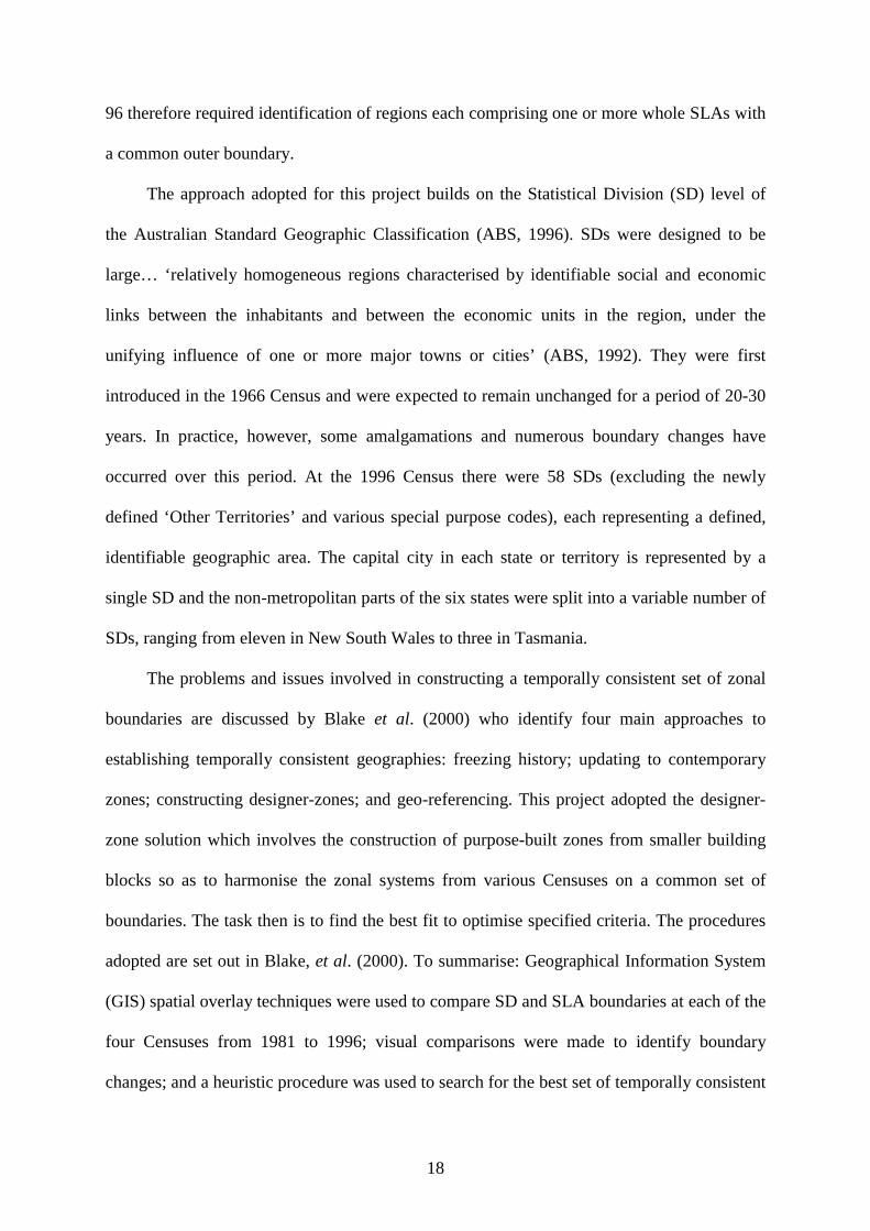
5.1 City Regions in Australia

In Australia, the city-region system divides readily into eight major spheres of influence

reflecting the original pattern of colonial settlement, subsequently transformed into the states

and territories, each of which is dominated by its respective metropolitan centre. Thus,

Sydney, Melbourne, Brisbane, Adelaide, Perth, Hobart, Darwin and Canberra represent the

cores of a system of 38 Australian city regions, also termed ACRs. In the case of the

mainland state capitals, the cores were defined to comprise the inner and middle suburbs

TSDs while the outer rings, which include the newly urbanising periphery and inner parts of

the peri-metropolitan hinterland of these cities, were classified as ‘Rest’. Elsewhere the

allocation of TSDs to ACRs was structured around previous analyses of inter-regional

migration flows and networks which distinguished the markedly different roles and functions

of near city regions, specialised economic regions, the amenity-rich coast, the wheat-sheep

belt and the outback (Bell and Maher, 1995). The resulting city-region structure is mapped in

Figure 5. The map also provides a 1991 population based cartogram of the regions, developed

using the Dorling (1996) algorithm. The classification can be collapsed to states and

territories, to region type (city cores, rest, near, far, coast and remote) or to a metropolitan-

non-metropolitan dichotomy.

24

Figure 5. City regions in Australia

25

5.2 City Regions in Britain

Figure 6 maps the British city region boundaries and provides a 1991 population based

cartogram. The classification recognizes 9 city regions in England and Wales (London,

Bristol, Birmingham, Manchester, Liverpool, Leeds, Sheffield, Newcastle, Cardiff) plus

Scotland and Northern Ireland. Each city region has a Core (usually the largest metropolitan

district or its county equivalent, and a system of satellite nonmetropolitan counties classified

as Rest, Near or Far. Like their Australian counterparts, the British regions can be aggregated

into a number of different classifications including city regions and regional types, and into

metropolitan-non-metropolitan or north-south divisions. In the following section we provide

a brief illustration of the insights to be derived from comparison of the two databases using

these classifications.

5.3 Migration in a City-Region Framework

Over the course of their lives Australians change residence nearly twice as often as Britons

(Rees et al., 2000). This difference is mantained in migration statistics for our systems of city

regions: 14.7 per cent of the Australian population of 16.8 million migrated between regions

at least once between 1991 and 1996 while the number of moves between city regions in

Britain recorded by the NHSCR, which includes multiple moves made by the same individual,

involved around 12.5 per cent of the 1991 population of 58.4 million. Inter-regional migration

in Australia also displays a significantly higher level of effectiveness than is the case in

Britain, bringing about a substantially larger redistribution of population between regions

relative to the overall volume of migration. Elsewhere, the authors with colleagues have

shown that the Migration Efficiency Index (MEI), which measures the ratio between net

population redistribution and total interregional migration flows, was almost twice as large in

Australia (11.1 per cent) as in Britain (6 per cent), although in both countries migration has

26

Figure 6. City regions in the UK

27

become progressively less influential as a mechanism for population redistribution over time

(see Stillwell et al., 2000).

Despite these variations in migration intensity and effectiveness between the two

countries, there are striking parallels in the patterns of net population movement which the

city region systems help to reveal. These are readily apparent when the pattern of net

migration rates in the two regional systems is mapped. We illustrate this for the first and last

of our four five year intervals (1976-81 and 1991-96) using cartograms in Figure 7.

At the broadest scale, the contrast in Britain is between southern England, which has

generally experienced net migration gains, and the northern regions, where gains have been

smaller or losses have occurred. In Australia, on the other hand, the major contrast is between

the east coast, whose regions have registered sustained net migration gains, and the inland and

outback regions where persistent losses have been recorded. Superimposed on these

broadscale shifts, a second pattern of redistribution evident in both countries is the net

outmovement from city cores, and offsetting gains in adjacent nonmetropolitan and coastal

regions. These similarities come into sharp focus through a systematic analysis of migration

patterns in each regional type, but subtle differences also come to light:

• The urban Cores in both countries have principally been characterised by heavy out-

migration but all cities shared a common trend towards reduced migration losses between the

1976-81 and 1991-96 periods. The outflows reflect the widespread emergence of

counterurbanisation during the 1970s, shifts in family and household type, and industrial

restructuring which has generated pronounced outflows from cities such as London and

Manchester in Britain, and from Sydney, Melbourne and Adelaide in Australia. Reduced

losses during the 1990s mirror the economic and social revitalisation of the inner cities in

both countries. Bristol, Darwin and Canberra owe more positive performance to their

specialised roles in their countries’ space economies.

28

Figure 7. Net migration rates (all ages) for city regions in Australia and the UK:1976-81 and 1991-96

29

• Rest regions in the two countries registered quite different outcomes, with gains in Australia

but losses in Britain. This variation reflects marked differences in the settlement pattern of

the two countries: in Britain rest regions are dominated by older industrial towns still

undergoing economic restructuring whereas in Australia they encompass the post-war

metropolitan suburbs with more viable local economies and fringe housing opportunities.

• Near regions take their migration gains from major cities and have been a major focus for

counterurban migration since the 1970s. While these regions have attracted sustained net

migration gains over the two periods in both countries, local economies are beginning to

reach maturity and the epicentre of growth has now moved to more attractive settlements in

Coast and Coast and Country regions beyond.

• Coast (Australia) and Coast and Country (Britain) regions gained heavily in both periods,

reflecting the shift to a services economy, and the rise of consumption-led migration,

especially among retirees. The attraction of climate, beaches and scenery is more pronounced

in Australia, especially in coastal Queensland and New South Wales (Sydney North and

South Coasts, Brisbane Gold and Sunshine Coasts) than in their counterparts in Britain

(Bristol Far - the South West peninsula; Birmingham Far - Mid-Wales, and London Far - the

Norfolk coast), but the underlying forces are the same.

• Far and Remote regions in Australia have no equivalents in Britain but both types of region

experienced increasing rates of net migration loss over the two periods. Out-migration of

young adults from the limited job opportunities available in rural areas and small towns has

been a persistent feature of rural Australia but this has accelerated since the late 1980s with

deteriorating terms of trade, farm amalgamation, recurrent drought, the widespread

withdrawal of services and the progressive economic decline of older industrial towns.

• In Scotland and Northern Ireland (classified in the Other region type in Britain) migration

flows from core to rest, rest to near, and near to coast also occur at a smaller spatial scale, not

30

captured in this macro-analysis. In aggregate, however, these regions display the reverse of

the declining performance of the Australian outback: Scotland reversed its losses of the

1970s to register a migration gain in the 1991-96 interval while in Northern Ireland the rate

of net outflow was cut by an order of magnitude to a little over 0.1 per cent.

6. HARMONISING THE AGE-TIME PLANS FOR THE MIGRATION DATA

The final task in preparing the two migration databases for comparative analysis is to

harmonise age-time plans. The procedures used are complex though the principles are

straightforward. A full account is given in Bell et al. (1999) and in Bell and Rees (2000).

Why is it essential to convert both data sets to a full APC classification? The answer is

because that is the only way that data assembled under a period-cohort observation plan can

be reliably compared with data from a period-age plan. When five-year age and time intervals

are used, there is considerable difference between measures under the two observation plans.

If age-specific migration measures from one country computed using period-cohort data are

compared with those from another country using period-age data, real differences between

the two situations cannot be distinguished from the artefactual variations resulting from the

different age-time observation plans.

It should be noted that the estimation routine outlined below to convert movement data

to APC spaces is only a substitute for better data than could be generated at source. For

example, the NHSCR movement data in person unit record form could have been doubly

classified because date of birth and date of move are known. However, this information was

not available for the 1976-83 period (Duke-Williams and Stillwell, 1999). Migration data

classified by age at time of migration cannot be generated from census data unless the right

question is asked, so direct generation of the APC migrant data was not possible for

Australia.

31

The target aim is that all migration flows are classified by age, period and cohort

simultaneously, so that when migration measures are computed the calculations can be made

for comparable APC spaces. Figure 8 shows three age-period-cohort diagrams that illustrate

what is involved. Figure 8A, which applies to the Australian data, shows how a period-cohort

space is made up of two APC triangles aligned on top of each other. Figure 8B, which applies

to the British data, shows how the period-age space is also composed of two APC triangles,

aligned next to each other. In the first case, the APC spaces are naturally labeled “younger”

and “older”, referring to the assumed age at which migration takes place. In the second

diagram, the APC spaces are naturally labelled “earlier” and “later”, referring to the timing of

the birth cohorts that contribute to each APC space. Because we use both views of the data

confusion can develop. A more generic terminology is described in Figure 10C, which

defines the two APCspaces as “down” and “up”, labels that remain constant over different

age-period plans. “Down” means that the triangle points downwards from the horizontal,

while the “up” triangle points upwards.

6.1 Disaggregating the Australian Migration Data into Age-Period-Cohort Flows

Creating the Australian database requires that the period-cohorts, in which Australian census

data are naturally reported, be decomposed into the older age (up) and younger age (down)

APC spaces. One option would be to divide each period-cohort group into equal parts.

However, mobility rates vary markedly by age and this approach would radically overstate

the volume of movements occurring in some age groups and understate them in others. For

example, data for a single year migration interval indicate that mobility rates climb sharply to

peak at around age 23. Consider, then, the movement of the cohort aged 20-24 at time t. This

high mobility group were aged 15-19 at time t-5 but the bulk of the movement recorded

32

Figure 8. Frameworks for age-period-cohort processing of Australian and UKmigration data

33

among this group almost certainly occurred at older ages: that is in the ‘Up’ triangle of the

period-cohort space.

In order to capture these variations, the period-cohort data for each inter-regional flow

were divided between APC spaces using a set of separation factors derived from national

mobility profiles for single year intervals classified by sex and single years of age. Age-sex

profiles of movement between SDs were acquired from ABS for the single year intervals

1975-76, 1980-81, 1985-86 and 1995-96, and converted to conditional migration probabilities

[movers/(movers+non-movers)] . Probabilities for intermediate years were then derived by

linear interpolation. The interpolation procedure was extended to ten years between the 1985-

86 and 1995-96 intervals because no sub-state migration data were collected at the 1991

Census. This procedure delivers a matrix of migration probabilities by sex and single years of

age from age 1 to age 99 and over (age measured at the end of the interval) by single year

intervals from 1975-76 to 1995-96. Separation factors for each period-cohort in each interval

were then derived by summing the appropriate propensities in each APC segment of the

period-cohort space and expressing each sum as a proportion of the whole. Period-cohort

probabilities at the horizontal margin of the two APC spaces were split between segments as

weighted averages of the probabilities in the adjacent period-cohorts.

The single year of age migration profiles also provide a mechanism for estimating the

number of transitions occurring in the youngest APC space: that is to the cohort who were

aged 0-4 at the time of the Census, having been born during the preceding five year interval.

Since this group were not alive five years previously, Censuses generally do not collect

information on their movements. However, some estimate of the transitions made by this

group is needed to match the corresponding figure from the British NHSCR database, since

the latter records information about migration at all ages, including among infants. The

solution adopted here was to estimate the number of transitions in this space by applying a

34

multiplier to the number occurring to the immediately older period cohort (ie those aged 5-9

at the Census) during the same interval. The multipliers were derived in the same way as the

separation factors described above, that is by summing the appropriate propensities from the

national single year of age migration profiles and comparing the results for the two cohorts.

6.2 Disaggregating the British Migration Data into Age-Period-Cohort Flows

In Britain, the NHSCR migration statistics are reported by period-age, which must be

disaggregated into the earlier cohort (down) and later cohort (up) APC spaces. In this case the

procedures are complicated by variations in the extent of disaggregation in the available data.

The 1976-77 to 1982-83 files classify migration by five-year age groups, whereas in the

1983-84 to 1995-96 files it is classified by single years of age. To estimate migration flows

for each age-period-cohort space, slightly different schemes are needed for each five-year

time interval. In 1976-81 only five year age group data are input; in 1981-86 both five year

and single year of age data are input; for 1986-91 and 1991-96 only single year of age data

are input. We consider the 1976-81 case first, then the 1986-91 and 1991-96 cases, and

finally the procedures for 1981-86 where there is a mixture of data.

The method for the period 1976-81 involved summing the five-year period-age counts

for single years to a five year total, using weights that varied with the position of the year in

the sequence. So, nine-tenths of a period-age migration count for the first year is assigned to

the down APC element and one-tenth to the up APC element. For the second year the

corresponding fractions are seven-tenths and three-tenths. The sequence continues five-

tenths/five-tenths for year 3, three-tenths/seven-tenths for year 4 and one-tenth/nine-tenths for

year five. The implicit assumption is that migration events are evenly distributed within a

five-year period-age observation for a single year.

35

For the periods 1986-91 and 1991-96 we have migration data for single years of age

and time. Most of these observations the period-age counts can be assigned directly to a five-

year APC element. For those period-age counts straddling the diagonal separating up and

down APC elements, we simply assume that half the migrations occur in the up APC element

and half in the down.

For the period 1981-86 we must combine the two estimation methods, using the five

year age group information for the first two years (1981-82 and 1982-83) and the single year

method for the last three years (1983-84, 1984-85, 1985-86).

The method for the last APC element is slightly different. The methods described above

are applied to period-ages 0-4 to ages 65-69. The final APC space, 70-74 to 75+, is an open-

ended trapezium. We add the migrations of the down APC for ages 70-74 to all migrations

for age 75+.

6.3 Illustrations

Tables 1 and 2 show the results of the age-period-cohort disaggregation procedures. Table 1

contains migration flows between city regions for period-cohorts, age-period-cohorts and

period-ages in 1991-96 for Australia, while Table 2 displays parallel flows for period-ages,

age-period-cohorts and period-cohorts for Britain. In both tables the left hand sub-table

contains the summary migration flows derived from the source data; the middle sub-table

shows those counts broken down into age-period-cohort elements; the rightmost sub-table

shows the counts re aggregated into the target age-time plan. Without going through the age-

time plan disaggregation, we would be forced to compare Australia’s period-cohort data with

Britain’s period-age data. With the harmonised database, we can compare Australian or

British data using either the period-cohort or the period-age plan.

36

Table 1. Migration flows between city regions for period-cohorts and age-period-cohorts and period-ages, 1991-96 for Australia

SOURCE DATA INTERMEDIATE DATA TRANSFORMED DATA Age atstart ofinterval

Age atend ofinterval

Period-cohortcode

Migrationbetween

cityregions i,n

1991-96

Agegroup atmigration

Birthcohort

Age-period-cohortcode

Migrationbetween

cityregions in

1991-96

Agegroup atmigration

Period- AgeCode

Migrationbetween

cityregions in

1991-96 Birth 0-4 1 128,704 0-4 1991-96 1 128,704 0-4 1 243,514 0-4 5-9 2 205,157 0-4 1986-91 2 114,810 5-9 2 178,459 5-9 10-14 3 166,765 5-9 1986-91 3 90,347 10-14 3 151,330 10-14 15-19 4 176,478 5-9 1981-86 4 88,112 15-19 4 222,992 15-19 20-24 5 294,127 10-14 1981-86 5 78,653 20-24 5 351,265 20p-24 25-29 6 328,277 10-14 1976-81 6 72,677 25-29 6 307,407 25-29 30-34 7 278,823 15-19 1976-81 7 103,801 30-34 7 249,014 30-34 35-39 8 228,028 15-19 1971-76 8 119,191 35-39 8 193,705 35-39 40-44 9 169,217 20-24 1971-76 9 174,936 40-44 9 149,656 40-44 45-49 10 136,429 20-24 1966-71 10 176,329 45-49 10 114,340 45-49 50-54 11 96,394 25-29 1966-71 11 151,948 50-54 11 85,298 50-54 55-59 12 76,168 25-29 1961-66 12 155,458 55-59 12 68,221 55-59 60-64 13 60,917 30-34 1961-66 13 123,365 60-64 13 56,998 60-64 65-69 14 52,859 30-34 1956-61 14 125,650 65-69 14 44,289 65-69 70-74 15 36,761 35-39 1956-61 15 102,378 70+ 15 72,619 70+ 75+ 16 54,003 35-39 1951-56 16 91,327 40-44 1951-56 17 77,890 Total * 2,489,107 Total * 2,489,107 40-44 1946-51 18 71,766 45-49 1946-51 19 64,663 45-49 1941-46 20 49,677 50-54 1941-46 21 46,717 50-54 1936-41 22 38,581 55-59 1936-41 23 37,587 55-59 1931-36 24 30,634 60-64 1931-36 25 30,283 60-64 1926-31 26 26,716 65-69 1926-31 27 26,143 65-69 1921-26 28 18,145 70+ 1921-26 29 18,616 70+ pre1921 30 54,003 Total * * 2,489,107

37

Table 2. Migration flows between city regions for period-ages, age-period-cohorts andperiod-cohorts, 1991-96 for the UK

SOURCE DATA INTERMEDIATE DATA TRANSFORMED DATA Agegroup atmigra-tion

Period-AgeCode

Migrationbetween

cityregions in

1991-96

Agegroup atmigration

Birthcohort

Age-period-cohortcode

Migrationbetween

cityregions in

1991-96

Age atstart ofinterval

Age atend ofinterval

Period-cohortcode

Migrationbetween

cityregions in1991-96p

0-4 1 500,668 0-4 1991-96 1 248,299 Birth 0-4 1 248,299 5-9 2 365,109 0-4 1986-91 2 252,369 0-4 5-9 2 446,676 10-14 3 295,033 5-9 1986-91 3 194,307 5-9 10-14 3 320,737 15-19 4 871932 5-9 1981-86 4 170,802 10-14 15-19 4 432,392 20-24 5 1,496,696 10-14 1981-86 5 149,935 15-19 20-24 5 1,335,539 25-29 6 1,132,022 10-14 1976-81 6 145,099 20p-24 25-29 6 1,342,796 30-34 7 744,864 15-19 1976-81 7 287,294 25-29 30-34 7 945,278 35-39 8 454,874 15-19 1971-76 8 584,639 30-34 35-39 8 582,564 40-44 9 315,269 20-24 1971-76 9 750,900 35-39 40-44 9 370,187 45-49 10 264,184 20-24 1966-71 10 745,796 40-44 45-49 10 294,529 50-54 11 187,256 25-29 1966-71 11 597,000 45-49 50-54 11 223,624 55-59 12 152,711 25-29 1961-66 12 535,022 50-54 55-59 12 166,277 60-64 13 139,384 30-34 1961-66 13 410,256 55-59 60-64 13 143,159 65-69 14 119,732 30-34 1956-61 14 334,609 60-64 65-69 14 131,347 70+ 15 313,393 35-39 1956-61 15 247,955 65-69 70-74 15 106,237 35-39 1951-56 16 206,919 70+ 75+ 16 263,489 Total * 7,353,127 40-44 1951-56 17 163,268 40-44 1946-51 18 152,001 Total * * 7,353,127 45-49 1946-51 19 142,528 45-49 1941-46 20 121,656 50-54 1941-46 21 101,968 50-54 1936-41 22 85,288 55-59 1936-41 23 80,989 55-59 1931-36 24 71,722 60-64 1931-36 25 71,437 60-64 1926-31 26 67,948 65-69 1926-31 27 63,400 65-69 1921-26 28 56,333 70+ 1921-26 29 49,904 70+ pre1921 30 263,489 Total * * 7,353,127

38

6.4 Deriving Populations at Risk

In order to compute intensities of migration, it is necessary to match migration flow counts

with populations at risk. Appropriate population stocks must be used to compute transition

probabilities or occurrence-exposure rates. This is not quite as straightforward as it sounds

but space prevents full discussion here. Rees et al. (2000) discuss the transition case in

detail, while Bell et al. (1999) provides a full account of the population at risk equations. You

need population stocks at the start and end of each period to construct occurrence-exposure or

movement populations at risk. For transition probabilities, the start population is most

appropriate but when census data are used it is appropriate, for reasons explained in Rees et

al. (2000) to use a particular transformation: people who survived and remained within the

country at the end of the period, as measured by the the end of period census, but recorded at

their origin at the start of the period.

7. CONCLUSIONS

If the history of fertility and mortality research provides a reliable guide, understanding of the

dynamics of internal migration will be aided by two key forms of research: longitudinal

analyses which enable the relative influence of age, period and cohort effects to be

disentangled; and cross-national studies which place the phenomenon in a range of spatial

contexts. Neither type of study is in plentiful supply, but research which combines both

dimensions is particularly scarce. This can be traced, at least in part, to the difficulties of

assembling the requisite data.

This paper has examined the issues involved in the construction of harmonised data

bases of internal migration and set out the basic steps needed for two countries that are

ostensibly similar in their socio-political traditions, if not in their physical geography. The

main burden of the paper is to underline the need for care and rigour when when handling

39

superficially similar data. We identified four key dimensions in which such datasets need to

be harmonised. These relate to: the conceptual basis on which migration is measured; the

time periods over which it is recorded; the system of spatial zones between which the moves

are registered; and the age-time plan from which the movement is observed.

There is no simple basis by which to convert event data to transitions, or vice versa, and

in the case of Australia and Britain the discrepancies arising from these differences in the

way migration is measured in the census and in population registers can only be accepted.

Harmonisation is possible on the other three dimensions, but the task is by no means

straightforward. It calls for the understanding of complex demographic and geographic

concepts, the application of these principles to develop solutions targeted to the strengths,

limitations and idiosyncracies of the local context and data sources, the development of

purpose-written software to implement these solutions, and the exercise of fastidious

attention to detail in carrying out the computations. These tasks, in turn, call for a wide range

of skills.

The benefit to be drawn from the construction of such harmonised datasets lies in the

facility it provides to make comprehensive, reliable comparisons of the dynamics, causes and

consequences of internal migration in different countries, free from the uncertainties created

by variations in time intervals, zonal systems and observation plans. Together with our co-

researchers on this project we have argued elsewhere that such comparisons have a number of

advantages: they offer a more meaningful context within which to interpret research findings;

they assist in differentiating patterns and processes that are unique to a country from those

that are more generally applicable; they provide a more rigorous test bed for migration

theorisation; they may also lead to greater rigor and consistency in empirical research on

individual countries and regions (Bell et al., forthcoming). That paper also identified four key

dimensions on which such comparisons might be made and suggested a series of appropriate

40

measures for each. The construction of the database described here provides the foundation

for such comparisons and a series of papers utilising this unique dataset are now in

preparation, focussing on overall trends in migration intensity (Rees et al., 2000), the

response of migration to the effects of distance (Stillwell et al., in preparation), migration

connectivity between regions (Stillwell and Bell, in preparation), and the impact of migration

on population change (Stillwell et al., 2000 and forthcoming).

41

REFERENCES

Australian Bureau of Statistics. 1991. 1991 Census Dictionary. Catalogue No. 2901.0.Australian Bureau of Statistics: Canberra

Australian Bureau of Statistics .1992. 1991 Census Geographic Areas. Catalogue No. 2905.0.Australian Bureau of Statistics: Canberra

Australian Bureau of Statistics. 1996. Statistical Geography: Volume 1. Australian StandardGeographical Classification (ASGC) 1996 Edition. Catalogue No. 1216.0. AustralianBureau of Statistics: Canberra

Bell M. 1992. Internal Migration in Australia, 1981-1986. Australian Government PublishingService: Canberra

Bell M, Blake M, Boyle P, Duke-Williams O, Hugo G, Rees P, Stillwell J. forthcoming.Cross-national comparison of internal migration: issues and measures. Paper submittedfor publication

Bell M, Hugo GJ. 2000. Internal Migration in Australia 1991-96: Overview and theOverseas-born. Department of Immigration and Multicultural Affairs: Canberra

Bell M, Maher C. 1995. Internal Migration in Australia 1986-1991: the Labour Force. .Australian Government Publishing Service: Canberra

Bell M, Rees P. 2000. Lexis diagrams in the context of migration: a review and application toBritish and Australian data. Paper presented to a workshop on Lexis in Context:German and Eastern & Northern European Contributions to Demography 1860-1910,Max Planck Institute for Demographic Research, Rostock Germany, 28-29 August

Blake M, Bell M, Rees P. 2000. Creating a temporally consistent spatial framework for theanalysis of interregional migration in Australia. International Journal of PopulationGeography 6: 155-174

Blake M, Duke-Williams O. 1999. Database fusion for the comparative study of migrationdata. Proceedings of the Fourth International Conference on Geocomputation, July1999, Fredericksburg, Virginia

Dorling D. 1996. Area Cartograms: Their Use and Creation. CATMOG 59Duke-Williams O, Stillwell J. 1999. Understanding the National Health Service Central

Register migration statistics. Draft paper, School of Geography, University of Leeds,Leeds, UK

McKay J, Whitelaw JS. 1978. Internal migration and the Australian urban system. Progress inPlanning 10(1): 1-83

Maher CA. 1984. Residential Mobility Within Australian Cities. ABS Census MonographSeries. Catalogue No 3410.0. Australian Bureau of Statistics: Canberra

Rees PH. 1977. The measurement of migration from censuses and other sources. Environmentand Planning A 9: 65-73

Rees P, Bell M, Duke-Williams O, Blake M. 2000. Problems and solutions in themeasurement of migration intensities: Australia and Britain compared. PopulationStudies 54(2): 207-222

Rowland DT. 1979. Internal Migration in Australia. ABS Census Monograph Series,Catalogue No. 3409.0. Australian Bureau of Statistics: Canberra

Scott A, Kilbey T. 1999. Can patient registers give an improved measure of internalmigration in England and Wales? Population Trends 96: 44-55

Stillwell J, Bell M. in preparation. Regional connectivity in Australia and Britain: acomparison of internal migration flows

Stillwell J, Bell M, Blake M, Duke-Williams O. in preparation. Migration as spatialinteraction in Australia and Britain: Variation over time, space and age

42

Stillwell J, Bell M, Blake M, Duke-Williams O, Rees P. 2000. A comparison of net migrationflows and migration effectiveness in Australia and Britain: Part 1, total migrationpatterns. Journal of Population Research 17(1): 17-38

Stillwell J, Bell M, Blake M, Duke-Williams O, Rees P. forthcoming. A comparison of netmigration flows and migration effectiveness in Australia and Britain: Part 2, age-relatedmigration patterns. Journal of Population Research

Stillwell J, Rees P, Boden P (eds.). 1992. Migration processes and patterns. Vol.2.Population redistribution in the United Kingdom. Belhaven Press: London

Stillwell J, Rees P, Duke-Williams O. 1996. Migration between NUTS level 2 regions in theUnited Kingdom. In Population Migration in the European Union, Rees P, Stillwell J,Convey A, Kupiszewski M (eds.); John Wiley; Chichester; 275-307

Vanderschrick C. 1992. Le diagramme de Lexis revisité. Population 92-5: 1241-1262