Hardware Implementation and RF High-Fidelity Modeling and ...

sensors

Article

Hardware Implementation and RF High-Fidelity Modeling andSimulation of Compressive Sensing Based 2D Angle-of-ArrivalMeasurement System for 2–18 GHz Radar ElectronicSupport Measures

Chen Wu *, Denesh Krishnasamy and Janaka Elangage

Citation: Wu, C.; Krishnasamy, D.;

Elangage, J. Hardware

Implementation and RF High-Fidelity

Modeling and Simulation of

Compressive Sensing Based 2D

Angle-of-Arrival Measurement

System for 2–18 GHz Radar

Electronic Support Measures. Sensors

2021, 21, 6823. https://doi.org/

10.3390/s21206823

Academic Editors: Mohammad

Abdolrazzaghi, Vahid Nayyeri and

Ferran Martín

Received: 12 August 2021

Accepted: 9 October 2021

Published: 14 October 2021

Publisher’s Note: MDPI stays neutral

with regard to jurisdictional claims in

published maps and institutional affil-

iations.

Copyright: © 2021 by the authors.

Licensee MDPI, Basel, Switzerland.

This article is an open access article

distributed under the terms and

conditions of the Creative Commons

Attribution (CC BY) license (https://

creativecommons.org/licenses/by/

4.0/).

Defence Research and Development Canada-Ottawa Research Centre, Ottawa, ON K1A 0Z4, Canada;[email protected] (D.K.); [email protected] (J.E.)* Correspondence: [email protected]

Abstract: This article presents the hardware implementation and a behavioral model-based RFsystem modeling and simulation (M&S) study of compressive sensing (CS) based 2D angle-of-arrival(AoA) measurement system for 2–18 GHz radar electronic support measures (RESM). A 6-channelultra-wideband RF digital receiver was first developed using a PXIe-based multi-channel digitalreceiver paired with a 6-element random-spaced 2D cavity-backed-spiral-antenna array. Then thesystem was tested in an open lab environment. The measurement results showed that the systemcan measure AoA of impinging signals from 2–18 (GHz) with overall RMSE of estimation at 3.60,2.74, 1.16, 0.67 and 0.56 (deg) in L, S, C, X and Ku bands, respectively. After that, using the RFhigh-fidelity M&S (RF HF-M&S) approach, a 6-channel AoA measurement system behavioral modelwas also developed and studied using a radar electronic warfare (REW) engagement scenario. Thesimulation result showed that the airborne AoA measurement system could successfully measure anS-band ground-based target acquisition radar signal in the dynamic REW environment. Using theRF HF-M&S model, the applicability of the system in other frequencies within 2–18 (GHz) was alsostudied. The simulation results demonstrated that the airborne AoA measurement system can beused for 2–18 GHz RESM applications.

Keywords: angle of arrival; random spaced array; ultra-wideband digital receiver; compressive sensing;RF high-fidelity modeling and simulation; radar electronic support measures; radar electronic warfare

1. Introduction

The angle-of-arrival (AoA) of the signal of interest (SOI) is the most important andexpensive measurement parameter in any radar electronic support measures (RESM) sys-tem to de-interleave intercepted signals [1–4] since the frequency agility technology hasbeen widely used in modern military radar systems, and multiple RF/microwave receiv-ing channels are often needed in an AoA measurement system. Traditionally, spinningdirection-finding (DF) antenna, amplitude-comparison, phase-comparison, interferome-try [5–7], and time difference of arrival methods are popular AoA measurement approachesused in RESM systems [8–12]. In addition, there are many RF/microwave DF systems de-veloped for wireless communication applications. Tuncer et al. [13] give a good discussionof these systems. From signal processing perspective, there are a number of algorithms usedfor signal DF in both military and commercial applications. Among them, multiple signalclassification (MUSIC) [14] and estimation of signal parameters via rotation invariancetechniques (ESPIRT) [15] are commonly used. However, to apply these methods, generally,a stable signal environment is required since the measured signal covariance matrix needsto be used in these algorithms. Many other AoA estimators have also been developed,focusing on different array structures and fast processing speeds. Some examples of suchdevelopments were given in [16–23]. Lonkeng et al. [24] presented the research work on

Sensors 2021, 21, 6823. https://doi.org/10.3390/s21206823 https://www.mdpi.com/journal/sensors

https://www.mdpi.com/journal/sensors

https://www.mdpi.com

https://doi.org/10.3390/s21206823

https://doi.org/10.3390/s21206823

https://creativecommons.org/

https://creativecommons.org/licenses/by/4.0/

https://creativecommons.org/licenses/by/4.0/

https://doi.org/10.3390/s21206823

https://www.mdpi.com/journal/sensors

https://www.mdpi.com/article/10.3390/s21206823?type=check_update&version=2

Sensors 2021, 21, 6823 2 of 27

2D DF estimation using arbitrary arrays in MIMO systems and introduced the 2D Fourierdomain line search MUSIC algorithm. Recently, based on information geometry (IG), Donget al. [25] introduced a simple scaling transform-based information geometry method,which had more consistent performance than the original IG method with higher AoAestimation resolution.

To estimate SOI AoA in a non-stationary environment, the Direct Data Domain (D3)method was introduced in [26–30], and it was applied to 2D AoA measurement for RESMapplication. Wu et al. [31] introduced a D3-based 2D AoA estimator operating from 6 to18 GHz and focused on measuring the low probability of intercept radar signals [1,32].The approach can measure the SOI AoA with just two complex snapshots from a 2D7-element nonuniformly spaced array in high SNR scenarios. Using more snapshots(e.g., 1024 samples), it can estimate intercepted signal’s AoA in low SNR scenarios. In [31],commonly used radar signals were studied, including Barker code of length 13, two-valuefrequency-coded waveform, poly-phase waveform, and frequency-modulated continuouswave signal.

The compressive sensing (CS) framework [33–35] has been used in many areas.Refs. [36,37] give some examples. Recently, Wu et al. [38,39] introduced a new multi-emitter 2D AoA estimator from 2–18 GHz based on signal spatial-sparsity [40] and DantzigSelector [41] methods. The key features of the estimator are no requirement of a prioriknowledge of intercepted signals, including signal frequencies, and its capability of pro-cessing multiple simultaneous incoming signals within the 2D array field-of-view (FOV)and the instantaneous bandwidth of microwave digital receivers. A good summary ofthe current CS-based AoA methods, including Bayesian CS for direction-of-arrival estima-tion [42,43], is also given in [39].

To develop the CS-based AoA measurement system introduced in [39] with the con-siderations of using the system in RESM for radar electronic warfare (REW) applications,this article presents the research results of (1) the AoA estimation system hardware im-plementation, (2) the open lab-based AoA measurement setup, (3) the system-level RFhigh-fidelity modeling and simulation (RF HF-M&S), and (4) measurement and simulationresults. More specifically, the article presents the following in detail:

• A 6-channel 2–18 GHz RF/digital receiver hardware, using PXIe form-factor, inte-grated with a 6-element 2–18 GHz cavity-backed-spiral-antenna (CBSA) array withrandomly located element positions given in [39];

• To demonstrate that the CS-based AoA method introduced in [39] can be used in dy-namic REW engagement environment, the RF HF-M&S approach was used to model:

# An engagement scenario in the System Tool Kit (STK) [44] with a ground-basedS-band target acquisition radar (TAR) and an aircraft equipped with a RESMsystem that has the CS-based AoA measurement capability;

# The S-band radar transmitting system behavioral model in SystemVue (SVE) [45];# A 6-channel microwave-digital receiving system behavioral model in SVE, and# The CS-based AoA algorithm [39] in Matlab.

• The measurement setup for AoA lab test from 2 to 18 GHz, and• Measurement and simulation results.

The main contributions of this article are: this is the first demonstration of the novelCS-based AoA estimation scheme used in the REW scenario through the RF HF-M&S, andthe hardware implementation and measurements that validate the scheme can producecorrect AoA estimations from 2 to 18 GHz. The results presented in this article provethat the theory developed in [39] can be applied in RESM application, and the system canproduce good quality AoA estimations in an ultra-wide frequency band.

Sensors 2021, 21, 6823 3 of 27

The remainder of this paper is organized as follows. Next section briefly outlines theCS-based 2D AoA algorithm using randomly-spaced 2D antenna arrays. The details ofthe method and its studies can be found in [39]. A 6-channel PXIe-based ultra-widebandRF receiver and antenna array hardware and the AoA open lab test setup are presentedin Section 3. In Section 4, using the RF HF-M&S approach, a REW engagement scenariomodeled in the STK is first discussed, and then the top-level of the RF system behavioralmodel in SEV is presented. The measurement and M&S results are in Section 5. Section 6has the conclusions. Appendix A has a brief introduction of the RF HF-M&S method,and Appendix B gives the detailed behavioral models and RF performance of the TARtransmitter and the 6-channel RESM receiver modeled in the SVE. Appendix C has theacronym list.

2. CS-Based 2D AoA Algorithm Using Randomly-Spaced Array (RSA)2.1. Outline of the Method

Let us consider a 2D RSA with a 2D-angle-grid defined as in Figure 1. The 2D-angle-grid is defined by the icosphere structure [46], which is formed by subdividing the trianglesof a regular icosahedron, and the number of subdivisions (W) determines the density ofthe vertices on the surface of an icosphere [47]. The line between the origin and one ofthe vertices defines an AoA direction and is represented by azimuth (Az) and elevation(El) angles. The mesh’s angular resolution level can be determined by averaging El-angledifferences between the vertex on the z-axis (marked by a circle) and surrounding 6 vertices(marked by cross). For example, the resolution is 0.54 degrees, when W is equal to 7,and there are total of 29,495 vertices that are close to evenly distributed on 4π solid angle.Suppose the array FOV is defined within [Az1 Az2]× [El1 El2] and it is discretized into a2D-angle-grid in front of the RSA. For example, the red vertices in Figure 1 are inside thearray FOV.

Sensors 2021, 21, x FOR PEER REVIEW 4 of 29

Figure 1. An illustration of a 2D-angle-grid formed by an icosphere-based mesh, and a 6-element RSA. The array phase-reference center (defined at the first element in the center of the array) and the icosphere center are collocated at the origin of the XYZ-coordinate system [39].

In the rest of the section, we highlight how to apply the AoA method to wideband RESM applications without a priori knowledge of incoming signal frequencies using the 2–18 GHz CBSAs and ultra-wideband digital receivers.

2.2. Measured Data from K Digital Receivers Connected to A K-Element RSA It was assumed that the sampled time-domain signal voltage from the k digital

receiver is 𝐯𝐤 = [v (1) v (2) ⋯ v (m) ⋯ v (N )] (2)

where m indicates the m time-step. After N -point FFT on the measured time-do-main data, we have K-set of frequency-domain data. If there are S local-peaks higher than a pre-defined detection-threshold level in the frequency-domain data obtained from the first element in the center of the RSA, then we can have a set of measured frequency-domain complex data u (s), where k = 1, 2, ⋯ , K and s = 1, 2, ⋯ , S. We also have S esti-mated frequencies f (s) from FFT. Thus the measured data at each estimated frequency is 𝐌(s) = 1 u (s)u (s) ⋯ u (s)u (s) ⋯ u (s)u (s) (3)

Here, the intercepted signal sources are in far-field of the RSA, and the mutual cou-pling between CBSA elements is negligible [48]. Note that (3) is the measured array steer-ing vector (ASV) in the sth direction, and the phase references the first (center) element.

2.3. Dictionary, Sensing and Recover Matrices Using (az , el ) (n = 1, 2, 3, … N), the dictionary matrix in our problem is defined as

𝚿 = k (1)k (1)k (1) ⋯ k (n)k (n)k (n) ⋯ k (N)k (N)k (N) × (4)

where k (n)k (n)k (n) = cos(el ) cos(az )cos(el ) sin (az ) sin(el ) (5)

note that each column in (4) has a unit norm, and the nth column is the normalized-wave-vector in nth direction.

The random element locations define the sensing matrix

Figure 1. An illustration of a 2D-angle-grid formed by an icosphere-based mesh, and a 6-elementRSA. The array phase-reference center (defined at the first element in the center of the array) and theicosphere center are collocated at the origin of the XYZ-coordinate system [39].

Within [Az1 Az2]× [El1 El2], there are total N close to equally spaced vertices, andeach vertex defines a direction (azn, eln) (n = 1, 2, 3, . . . N), on which the CS dictionary Ψ

matrix is defined. If there are S non-coherent signals from (azs, els) (s = 1, 2, 3, . . . S N)directions received by the array, this forms an S-sparse problem and can be expressedas Ψx, and x = [0 · · · 1 · · · 0 1 · · · 0]T, ‖x‖0 = S. T is non-conjugate transposition. In orderto find nonzero locations in x, K ( N) measurements have to be performed in the CSframework. In our AoA measurement system, a 2–18 GHz CBSA array with K randomly

Sensors 2021, 21, 6823 4 of 27

located elements provides the measurement data y. Equation (1) gives the relation betweenx and y.

y = Ax (1)

where A = ΦΨ is the CS recovery matrix, in which Φ is known as the CS sensingmatrix. Then the problem can be solved by using the Dantzig selector to find those nonzerolocations in x as described in [38,39].

In the rest of the section, we highlight how to apply the AoA method to widebandRESM applications without a priori knowledge of incoming signal frequencies using the2–18 GHz CBSAs and ultra-wideband digital receivers.

2.2. Measured Data from K Digital Receivers Connected to A K-Element RSA

It was assumed that the sampled time-domain signal voltage from the kth digitalreceiver is

vk = [vk(1) vk(2) · · · vk(m) · · · vk(NFFT)] (2)

where m indicates the mth time-step. After NFFT-point FFT on the measured time-domaindata, we have K-set of frequency-domain data. If there are S local-peaks higher than apre-defined detection-threshold level in the frequency-domain data obtained from the firstelement in the center of the RSA, then we can have a set of measured frequency-domaincomplex data uk(s), where k = 1, 2, · · · , K and s = 1, 2, · · · , S. We also have S estimatedfrequencies fe(s) from FFT. Thus the measured data at each estimated frequency is

M(s) =[

1u2(s)u1(s)

· · · uk(s)u1(s)

· · · uK(s)u1(s)

]T(3)

Here, the intercepted signal sources are in far-field of the RSA, and the mutual couplingbetween CBSA elements is negligible [48]. Note that (3) is the measured array steeringvector (ASV) in the sth direction, and the phase references the first (center) element.

2.3. Dictionary, Sensing and Recover Matrices

Using (azn, eln) (n = 1, 2, 3, . . . N), the dictionary matrix in our problem is defined as

Ψ =

kx(1)ky(1)kz(1)

· · ·kx(n)ky(n)kz(n)

· · ·kx(N)ky(N)kz(N)

3×N

(4)

where kx(n)ky(n)kz(n)

=

cos(eln) cos(azn)cos(eln) sin(azn)

sin(eln)

(5)

note that each column in (4) has a unit norm, and the nth column is the normalized-wave-vector in nth direction.

The random element locations define the sensing matrix

Φ =

x1 y1 z1x2 y2 z2

...xk yk zk

...xK yK zK

K×3

(6)

and it was assumed zk = 0, and [x1 y1 z1] = [0 0 0] in following discussion. The locationsamples in Φ are independent and identically distributed. Then the recovery matrix (A)from (4) and (6) is

Sensors 2021, 21, 6823 5 of 27

A =

x1kx(1) + y1ky(1) · · · x1kx(n) + y1ky(n) · · · x1kx(N) + y1ky(N)...

......

xkkx(1) + ykky(1) · · · xkkx(n) + ykky(n) · · · xkkx(N) + ykky(N)...

......

xKkx(1) + yKky(1) · · · xKkx(n) + yKky(n) · · · xKkx(N) + yKky(N)

K×N

(7)

if there is only one signal from sth direction, we have

Axs = A(s) =

x1 cos(els) cos(azs) + y1 cos(els) sin(azs)...

xk cos(els) cos(azs) + yk cos(els) sin(azs)...

xK cos(els) cos(azs) + yK cos(els) sin(azs)

K×1

(8)

where xs = [0 · · · 1 · · · 0]T , i.e., only the sth element is nonzero. It was also assumed thatthe sth signal direction is on one of the vertices of the 2D-angle-grid, which is called theon-grid case. Source signal direction off the 2D-angle-grid is called the off-grid case. Testsignals from both cases are used in the study.

Moreover, based on ASV definition and considering (8), we have

A(s) =λ

j2πln(ASV(s)) (9)

where λ is the free-space wavelength.

2.4. Equations Used for Recovering xs

Since all the concurrent signals are non-coherent signals and digital receivers operateat their linear conditions, the multiple-signal AoA estimation problem can be decomposedinto S equations in (10), using measured data in (3).

λe(s)j2π

ln(M(s)) = Axs + η, (s = 1, 2, 3, · · · S) (10)

λe(s) = c/ fe(s) is the estimated free-space wavelength, η is the receiver noise, and cis the light speed in free space. Then (10) is solved by the Dantzig selector.

For the off-grid case, our method just picks the location of the maximum number foreach xs obtained by the Dantzig selector. The Matlab code developed in [39] was used inthis study, and the Dantzig selector solver was obtained from [49].

3. Hardware Implementation of the 6-Channel RESM Digital Receiver and Open LabMeasurement Setup3.1. Randomly-Spaced CBSA Array

Ref. [39] studied a number RSA structures. Based on the system cost and AoAmeasurement performance, it suggested using the 6-element array. Note that the studyin [39] also suggested that the element locations of element-2 to -6 can be randomly pickedon the aluminum disk, as long as they do not bias too much in one area.

A drawing of a 6-element array using 2–18 GHz CBSA is shown in Figure 2a, and itshardware is shown in Figure 2b. The locations of the elements in this study are given inTable 1. To reduce the reflection from the aluminate plate, microwave absorbing materialwas inserted between elements, as shown in Figure 2c. The details of CBSAs can be foundin [50].

Sensors 2021, 21, 6823 6 of 27


Table 1. To reduce the reflection from the aluminate plate, microwave absorbing material was inserted between elements, as shown in Figure 2c. The details of CBSAs can be found in [50].

(a) (b) (c)

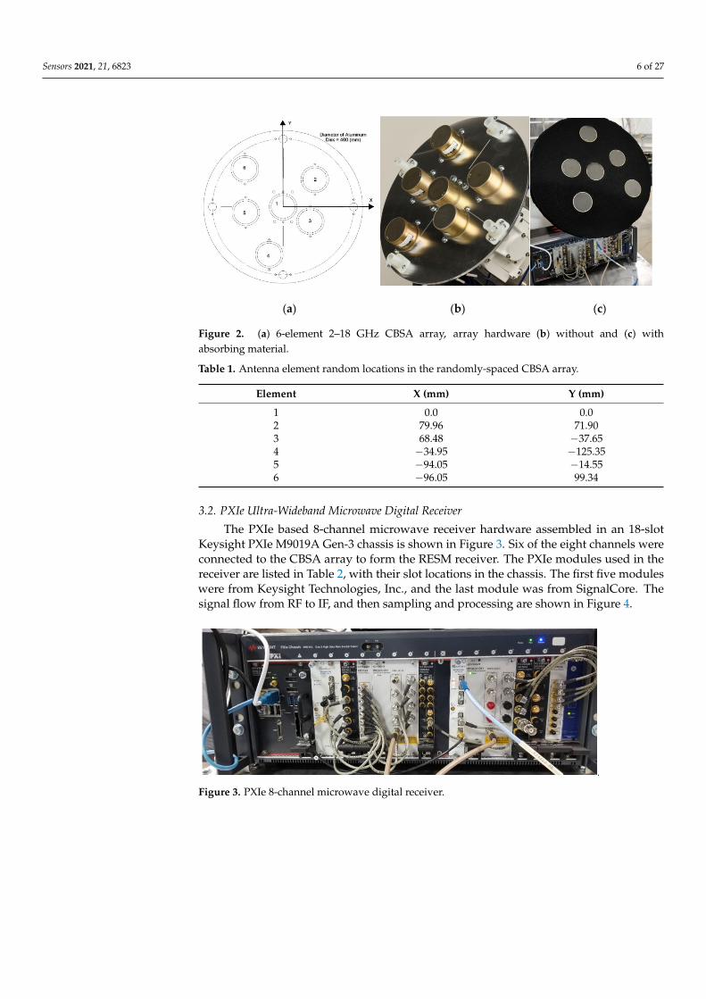
Figure 2. (a) 6-element 2–18 GHz CBSA array, array hardware (b) without and (c) with absorbing material.

Table 1. Antenna element random locations in the randomly-spaced CBSA array.

Element X (mm) Y (mm) 1 0.0 0.0 2 79.96 71.90 3 68.48 −37.65 4 −34.95 −125.35 5 −94.05 −14.55 6 −96.05 99.34

3.2. PXIe Ultra-Wideband Microwave Digital Receiver The PXIe based 8-channel microwave receiver hardware assembled in an 18-slot

Keysight PXIe M9019A Gen-3 chassis is shown in Figure 3. Six of the eight channels were connected to the CBSA array to form the RESM receiver. The PXIe modules used in the receiver are listed in Table 2, with their slot locations in the chassis. The first five modules were from Keysight Technologies, Inc., and the last module was from SignalCore. The signal flow from RF to IF, and then sampling and processing are shown in Figure 4.

.

Figure 3. PXIe 8-channel microwave digital receiver.

Figure 2. (a) 6-element 2–18 GHz CBSA array, array hardware (b) without and (c) withabsorbing material.


Element X (mm) Y (mm)

1 0.0 0.02 79.96 71.903 68.48 −37.654 −34.95 −125.355 −94.05 −14.556 −96.05 99.34

3.2. PXIe Ultra-Wideband Microwave Digital Receiver

The PXIe based 8-channel microwave receiver hardware assembled in an 18-slotKeysight PXIe M9019A Gen-3 chassis is shown in Figure 3. Six of the eight channels wereconnected to the CBSA array to form the RESM receiver. The PXIe modules used in thereceiver are listed in Table 2, with their slot locations in the chassis. The first five moduleswere from Keysight Technologies, Inc., and the last module was from SignalCore. Thesignal flow from RF to IF, and then sampling and processing are shown in Figure 4.


Table 1. To reduce the reflection from the aluminate plate, microwave absorbing material was inserted between elements, as shown in Figure 2c. The details of CBSAs can be found in [50].

(a) (b) (c)

Figure 2. (a) 6-element 2–18 GHz CBSA array, array hardware (b) without and (c) with absorbing material.


Element X (mm) Y (mm) 1 0.0 0.0 2 79.96 71.90 3 68.48 −37.65 4 −34.95 −125.35 5 −94.05 −14.55 6 −96.05 99.34

3.2. PXIe Ultra-Wideband Microwave Digital Receiver The PXIe based 8-channel microwave receiver hardware assembled in an 18-slot

Keysight PXIe M9019A Gen-3 chassis is shown in Figure 3. Six of the eight channels were connected to the CBSA array to form the RESM receiver. The PXIe modules used in the receiver are listed in Table 2, with their slot locations in the chassis. The first five modules were from Keysight Technologies, Inc., and the last module was from SignalCore. The signal flow from RF to IF, and then sampling and processing are shown in Figure 4.

.



Sensors 2021, 21, 6823 7 of 27

Table 2. PXIe modules used in the microwave digital receiver.

# Module Names Slot Number on M9018APXIe Chassis

1 M9037A embedded controller 12 M3102A 500MS/s Digitizer 4, 153 M9352A Hybrid Amplifier/Attenuator 5, 174 M9362A-D01 Quad Down-converter 6–8, 12–145 M9300A Frequency Reference Source 96 SC5510A 20 GHz Signal Source 11


Table 2. PXIe modules used in the microwave digital receiver.

# Module Names Slot Number on M9018A

PXIe Chassis 1 M9037A embedded controller 1 2 M3102A 500MS/s Digitizer 4, 15 3 M9352A Hybrid Amplifier/Attenuator 5, 17 4 M9362A-D01 Quad Down-converter 6-8, 12-14 5 M9300A Frequency Reference Source 9 6 SC5510A 20 GHz Signal Source 11

Figure 4. Signal paths in the PXIe receiving system in Figure 3.

In the receiver, the RF signal down-converted to 100 MHz and sampled at 500 Meg-sample/s. 4096-point Fast Fourier Transform (FFT) was used to process the real data in the CS-based AoA estimation algorithm. The detail of the algorithm was discussed in [39].

3.3. The Open Lab AoA Measurement Setup The CBSA array and multi-channel receiver were integrated together, as shown in

Figure 5. In the figure, the array was installed on an antenna positioner, which is an azi-muth-on-elevation positioner system, and connected to 6 channels of the PXIe digital re-ceiver. The receiving array was placed in the far-field of the TX antenna that was a 2–18 GHz dual-ridge dual-linear polarization circular horn antenna that has the same perfor-mance as the antenna in [51]. In the test, only a horizontal polarized signal was used. Mi-crowave absorbing materials were also placed (not shown in the figure) on the ground in front of the antenna positioner.

Figure 4. Signal paths in the PXIe receiving system in Figure 3.

In the receiver, the RF signal down-converted to 100 MHz and sampled at 500 Meg-sample/s. 4096-point Fast Fourier Transform (FFT) was used to process the real data in theCS-based AoA estimation algorithm. The detail of the algorithm was discussed in [39].

3.3. The Open Lab AoA Measurement Setup

The CBSA array and multi-channel receiver were integrated together, as shown inFigure 5. In the figure, the array was installed on an antenna positioner, which is anazimuth-on-elevation positioner system, and connected to 6 channels of the PXIe digitalreceiver. The receiving array was placed in the far-field of the TX antenna that was a2–18 GHz dual-ridge dual-linear polarization circular horn antenna that has the sameperformance as the antenna in [51]. In the test, only a horizontal polarized signal was used.Microwave absorbing materials were also placed (not shown in the figure) on the groundin front of the antenna positioner.

Sensors 2021, 21, 6823 8 of 27Sensors 2021, 21, x FOR PEER REVIEW 8 of 29

Figure 5. The TX and RX array assemblies for an open lab test: the measurement setup was in an open area, and the microwave absorbing materials were placed in front of the antenna positioner to absorb ground reflections.

Before the measurement, the height of the TX antenna was selected by adjusting the antenna mast, thus that the incident angle was at El = 90 (deg). Then by rotating the antenna positioner angles, the incident Az-angle of the TX-signal was changed and rec-orded.

The tested incident angles were: • Az from −180 to 180 (deg) at 30 (deg) interval, and • El from 30 to 90 (deg) at 10 (deg) interval. Thus, there were a total of 13 and 7 angles measured for Az and El, respectively, i.e.,

at each frequency, there were 91 directions. During the measurement, since the positioner was an azimuth-on-elevation system, we set an El-angle first and then rotated the Az-angle. At each Az-angle, the frequency was scanned from 2 to 18 (GHz) at 1 (GHz) inter-val. The Az- and El-angles define the directions in the UV-sphere, as illustrated in Figure 6.

Figure 6. An example of defining the directions on the UV-sphere.

The received RF signal was down-converted to IF frequency, sampled by 14-bit high-speed digitizer at 500 (Mega-Sample/s), and then the sampled data were processed by 4096-point real data FFT. At each incident angle (El, Az), using the first channel FFT data,

Figure 5. The TX and RX array assemblies for an open lab test: the measurement setup was in anopen area, and the microwave absorbing materials were placed in front of the antenna positioner toabsorb ground reflections.

Before the measurement, the height of the TX antenna was selected by adjusting the an-tenna mast, thus that the incident angle was at El = 90 (deg). Then by rotating the antennapositioner angles, the incident Az-angle of the TX-signal was changed and recorded.

The tested incident angles were:

• Az from −180 to 180 (deg) at 30 (deg) interval, and• El from 30 to 90 (deg) at 10 (deg) interval.

Thus, there were a total of 13 and 7 angles measured for Az and El, respectively, i.e.,at each frequency, there were 91 directions. During the measurement, since the positionerwas an azimuth-on-elevation system, we set an El-angle first and then rotated the Az-angle.At each Az-angle, the frequency was scanned from 2 to 18 (GHz) at 1 (GHz) interval. TheAz- and El-angles define the directions in the UV-sphere, as illustrated in Figure 6.


Figure 5. The TX and RX array assemblies for an open lab test: the measurement setup was in an open area, and the microwave absorbing materials were placed in front of the antenna positioner to absorb ground reflections.

Before the measurement, the height of the TX antenna was selected by adjusting the antenna mast, thus that the incident angle was at El = 90 (deg). Then by rotating the antenna positioner angles, the incident Az-angle of the TX-signal was changed and rec-orded.

The tested incident angles were: • Az from −180 to 180 (deg) at 30 (deg) interval, and • El from 30 to 90 (deg) at 10 (deg) interval. Thus, there were a total of 13 and 7 angles measured for Az and El, respectively, i.e.,

at each frequency, there were 91 directions. During the measurement, since the positioner was an azimuth-on-elevation system, we set an El-angle first and then rotated the Az-angle. At each Az-angle, the frequency was scanned from 2 to 18 (GHz) at 1 (GHz) inter-val. The Az- and El-angles define the directions in the UV-sphere, as illustrated in Figure 6.


The received RF signal was down-converted to IF frequency, sampled by 14-bit high-speed digitizer at 500 (Mega-Sample/s), and then the sampled data were processed by 4096-point real data FFT. At each incident angle (El, Az), using the first channel FFT data,


Sensors 2021, 21, 6823 9 of 27

The received RF signal was down-converted to IF frequency, sampled by 14-bit high-speed digitizer at 500 (Mega-Sample/s), and then the sampled data were processed by4096-point real data FFT. At each incident angle (El, Az), using the first channel FFT data,the frequency (fIF) that had the peak FFT value was found. Using this fIF, a set of 6 complexnumbers (Mi(El, Az, fIF), i = 1, . . . 6) can be obtained from the 6 channels. The normalizeddata were mi(El, Az, fIF) = Mi(El, Az, fIF) /M1(El, Az, fIF), where M1(El, Az, fIF) wasthe data from the first channel.

Note that, since the 6 CBSAs were not phase-matched elements and the RF receiverswere not identical, at each frequency, the 13 measured data at El = 90 (deg) were usedas the calibration data to remove the amplitude and phase discrepancies caused by theCBSAs and RF digital receivers. Therefore, at each frequency measurement point, thedata sent to CS-based AoA algorithm was mi(El, Az, fIF)/mi(90, Az, fIF). The frequencyused to estimate AoA is fLO + fIF, in which fLO was receiver local oscillator frequency.As mentioned earlier, this is one of the advantages of the CS-based AoA method thatit does not need to know the intercepted signal frequency, and the frequency used forAoA calculations was measured by the receiver itself. Hence, the method can be used inan ultra-wide frequency band. The operational frequency band was determined by theantenna elements and receiver hardware.

4. Using RF HF-M&S Methodology to Study CS-Based AoA Estimator in REWEnvironment

This section presents a vignette that demonstrates the use of the CS-base 2D AoAmeasurement sensor in REW scenario in the RF HF-M&S. The vignette had a 6-channelairborne RESM receiver intercepted a ground-based TAR signal, and the receiver estimatedthe direction of the radar signal. A brief introduction of the RF HF-M&S methodology canbe found in Appendix A.

4.1. The Vignette of the TAR Signal AoA Measurement by the Airborne CS-Based AoA Estimator

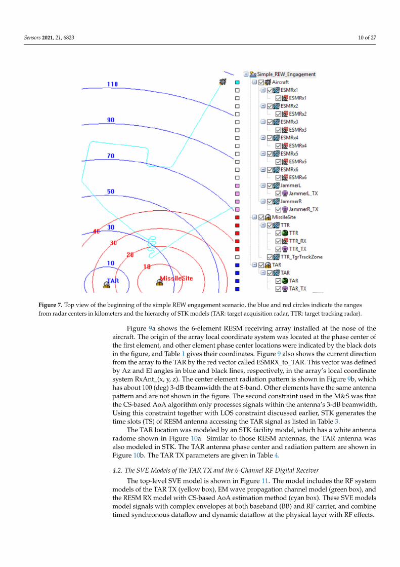
Figure 7 shows the top view of a REW engagement scenario. An aircraft installed witha multi-channel RESM sensor (ESMRxi (i = 1 to 6)) and a jammer system was approachingan area defended by an RF guided missile system, which was modeled by TAR andMissileSite. The cyan-line shows the aircraft flight path projected on the ground. In thefigure, the aircraft icon was located at the beginning of the scenario. The vignette ofthe scenario to be used to demonstrate the multi-channel CS-based AoA measurementsystem was that the RESM receiver intercepts the TAR signal whenever the RESM receivingantennas intercept the TAR signal during the flight, the signal’s AoA is measured by theRESM system. The constraints that define the RESM receiver can intercept the TAR signalwill be discussed later.

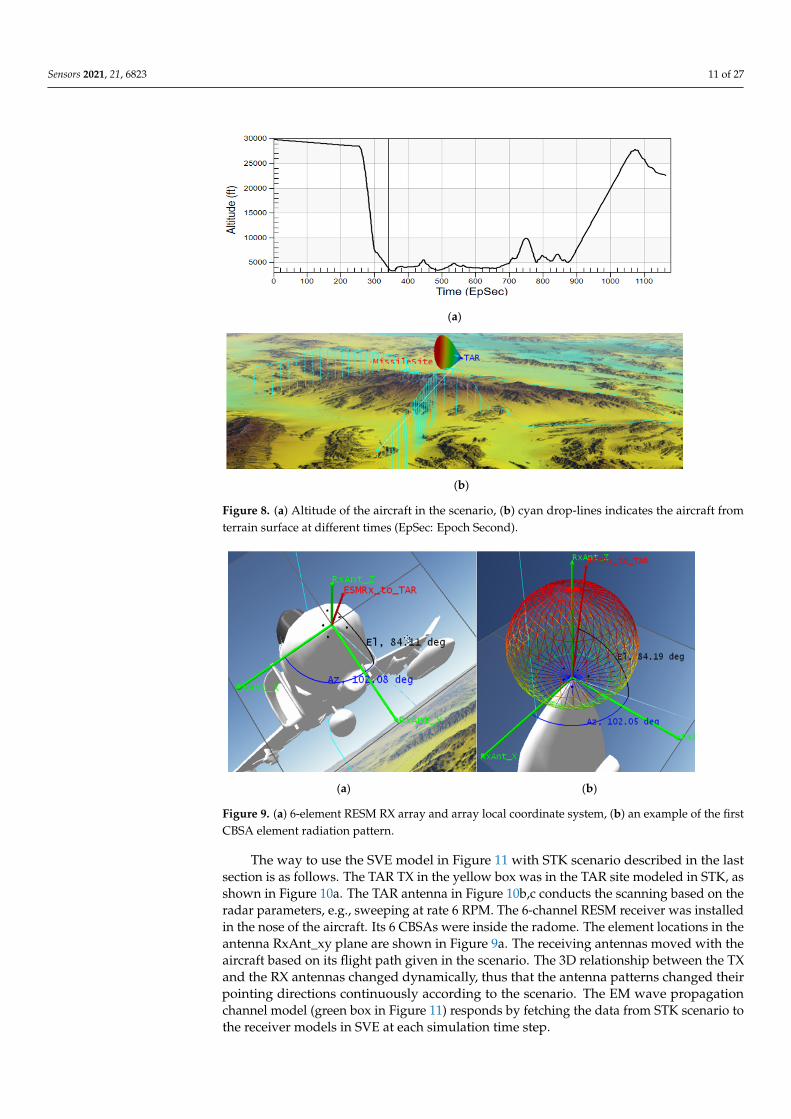
The aircraft altitude in the scenario is plotted in Figure 8a. The vertical cyan lines inFigure 8b show the distances between the aircraft and terrain surface at different moments.One can see that after the onboard RESM detects and measures TAR signal, the aircraftdramatically reduces its altitude and flies in between mountains. The dynamically changingaircraft flight trajectory and attitude form the first constraint in the RF HF-M&S. The RESMreceiving antennas can only intercept the TAR signal when the line-of-sight (LOS) conditionis met.

Sensors 2021, 21, 6823 10 of 27


Figure 7. Top view of the beginning of the simple REW engagement scenario, the blue and red cir-cles indicate the ranges from radar centers in kilometers and the hierarchy of STK models (TAR: target acquisition radar, TTR: target tracking radar).

The aircraft altitude in the scenario is plotted in Figure 8a. The vertical cyan lines in Figure 8b show the distances between the aircraft and terrain surface at different mo-ments. One can see that after the onboard RESM detects and measures TAR signal, the aircraft dramatically reduces its altitude and flies in between mountains. The dynamically changing aircraft flight trajectory and attitude form the first constraint in the RF HF-M&S. The RESM receiving antennas can only intercept the TAR signal when the line-of-sight (LOS) condition is met.

(a)

Figure 7. Top view of the beginning of the simple REW engagement scenario, the blue and red circles indicate the rangesfrom radar centers in kilometers and the hierarchy of STK models (TAR: target acquisition radar, TTR: target tracking radar).

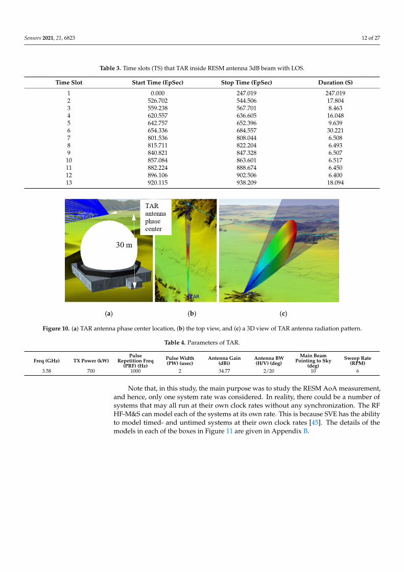
Figure 9a shows the 6-element RESM receiving array installed at the nose of theaircraft. The origin of the array local coordinate system was located at the phase center ofthe first element, and other element phase center locations were indicated by the black dotsin the figure, and Table 1 gives their coordinates. Figure 9 also shows the current directionfrom the array to the TAR by the red vector called ESMRX_to_TAR. This vector was definedby Az and El angles in blue and black lines, respectively, in the array’s local coordinatesystem RxAnt_(x, y, z). The center element radiation pattern is shown in Figure 9b, whichhas about 100 (deg) 3-dB tbeamwidth the at S-band. Other elements have the same antennapattern and are not shown in the figure. The second constraint used in the M&S was thatthe CS-based AoA algorithm only processes signals within the antenna’s 3-dB beamwidth.Using this constraint together with LOS constraint discussed earlier, STK generates thetime slots (TS) of RESM antenna accessing the TAR signal as listed in Table 3.

The TAR location was modeled by an STK facility model, which has a white antennaradome shown in Figure 10a. Similar to those RESM antennas, the TAR antenna wasalso modeled in STK. The TAR antenna phase center and radiation pattern are shown inFigure 10b. The TAR TX parameters are given in Table 4.

4.2. The SVE Models of the TAR TX and the 6-Channel RF Digital Receiver

The top-level SVE model is shown in Figure 11. The model includes the RF systemmodels of the TAR TX (yellow box), EM wave propagation channel model (green box), andthe RESM RX model with CS-based AoA estimation method (cyan box). These SVE modelsmodel signals with complex envelopes at both baseband (BB) and RF carrier, and combinetimed synchronous dataflow and dynamic dataflow at the physical layer with RF effects.

Sensors 2021, 21, 6823 11 of 27


Figure 7. Top view of the beginning of the simple REW engagement scenario, the blue and red cir-cles indicate the ranges from radar centers in kilometers and the hierarchy of STK models (TAR: target acquisition radar, TTR: target tracking radar).

The aircraft altitude in the scenario is plotted in Figure 8a. The vertical cyan lines in Figure 8b show the distances between the aircraft and terrain surface at different mo-ments. One can see that after the onboard RESM detects and measures TAR signal, the aircraft dramatically reduces its altitude and flies in between mountains. The dynamically changing aircraft flight trajectory and attitude form the first constraint in the RF HF-M&S. The RESM receiving antennas can only intercept the TAR signal when the line-of-sight (LOS) condition is met.

(a)


(b)

Figure 8. (a) Altitude of the aircraft in the scenario, (b) cyan drop-lines indicates the aircraft from terrain surface at different times (EpSec: Epoch Second).

Figure 9a shows the 6-element RESM receiving array installed at the nose of the air-craft. The origin of the array local coordinate system was located at the phase center of the first element, and other element phase center locations were indicated by the black dots in the figure, and Table 1 gives their coordinates. Figure 9 also shows the current direction from the array to the TAR by the red vector called ESMRX_to_TAR. This vector was de-fined by Az and El angles in blue and black lines, respectively, in the array’s local coordi-nate system RxAnt_(x, y, z). The center element radiation pattern is shown in Figure 9b, which has about 100 (deg) 3-dB tbeamwidth the at S-band. Other elements have the same antenna pattern and are not shown in the figure. The second constraint used in the M&S was that the CS-based AoA algorithm only processes signals within the antenna’s 3-dB beamwidth. Using this constraint together with LOS constraint discussed earlier, STK generates the time slots (TS) of RESM antenna accessing the TAR signal as listed in Table 3.

Table 3. Time slots (TS) that TAR inside RESM antenna 3dB beam with LOS.

Time Slot Start Time (EpSec) Stop Time (EpSec) Duration (S) 1 0.000 247.019 247.019 2 526.702 544.506 17.804 3 559.238 567.701 8.463 4 620.557 636.605 16.048 5 642.757 652.396 9.639 6 654.336 684.557 30.221 7 801.536 808.044 6.508 8 815.711 822.204 6.493 9 840.821 847.328 6.507

10 857.084 863.601 6.517 11 882.224 888.674 6.450 12 896.106 902.506 6.400 13 920.115 938.209 18.094

Figure 8. (a) Altitude of the aircraft in the scenario, (b) cyan drop-lines indicates the aircraft fromterrain surface at different times (EpSec: Epoch Second).


(a) (b)

Figure 9. (a) 6-element RESM RX array and array local coordinate system, (b) an example of the first CBSA element radiation pattern.

The TAR location was modeled by an STK facility model, which has a white antenna radome shown in Figure 10a. Similar to those RESM antennas, the TAR antenna was also modeled in STK. The TAR antenna phase center and radiation pattern are shown in Figure 10b. The TAR TX parameters are given in Table 4.

(a) (b) (c)

Figure 10. (a) TAR antenna phase center location, (b) the top view, and (c) a 3D view of TAR antenna radiation pattern.

Table 4. Parameters of TAR.

Freq (GHz) TX Power

(kW) Pulse Repetition Freq (PRF) (Hz)

Pulse Width (PW) (usec)

Antenna Gain (dBi)

Antenna BW (H/V) (deg)

Main Beam Pointing to Sky (deg)

Sweep Rate (RPM)

3.58 700 1000 2 34.77 2/20 10 6

4.2. The SVE Models of the TAR TX and the 6-Channel RF Digital Receiver The top-level SVE model is shown in Figure 11. The model includes the RF system

models of the TAR TX (yellow box), EM wave propagation channel model (green box), and the RESM RX model with CS-based AoA estimation method (cyan box). These SVE models model signals with complex envelopes at both baseband (BB) and RF carrier, and combine timed synchronous dataflow and dynamic dataflow at the physical layer with RF effects.

Figure 9. (a) 6-element RESM RX array and array local coordinate system, (b) an example of the firstCBSA element radiation pattern.

The way to use the SVE model in Figure 11 with STK scenario described in the lastsection is as follows. The TAR TX in the yellow box was in the TAR site modeled in STK, asshown in Figure 10a. The TAR antenna in Figure 10b,c conducts the scanning based on theradar parameters, e.g., sweeping at rate 6 RPM. The 6-channel RESM receiver was installedin the nose of the aircraft. Its 6 CBSAs were inside the radome. The element locations in theantenna RxAnt_xy plane are shown in Figure 9a. The receiving antennas moved with theaircraft based on its flight path given in the scenario. The 3D relationship between the TXand the RX antennas changed dynamically, thus that the antenna patterns changed theirpointing directions continuously according to the scenario. The EM wave propagationchannel model (green box in Figure 11) responds by fetching the data from STK scenario tothe receiver models in SVE at each simulation time step.

Sensors 2021, 21, 6823 12 of 27

Table 3. Time slots (TS) that TAR inside RESM antenna 3dB beam with LOS.

Time Slot Start Time (EpSec) Stop Time (EpSec) Duration (S)

1 0.000 247.019 247.0192 526.702 544.506 17.8043 559.238 567.701 8.4634 620.557 636.605 16.0485 642.757 652.396 9.6396 654.336 684.557 30.2217 801.536 808.044 6.5088 815.711 822.204 6.4939 840.821 847.328 6.507

10 857.084 863.601 6.51711 882.224 888.674 6.45012 896.106 902.506 6.40013 920.115 938.209 18.094


(a) (b)

Figure 9. (a) 6-element RESM RX array and array local coordinate system, (b) an example of the first CBSA element radiation pattern.

The TAR location was modeled by an STK facility model, which has a white antenna radome shown in Figure 10a. Similar to those RESM antennas, the TAR antenna was also modeled in STK. The TAR antenna phase center and radiation pattern are shown in Figure 10b. The TAR TX parameters are given in Table 4.

(a) (b) (c)



Freq (GHz) TX Power

(kW) Pulse Repetition Freq (PRF) (Hz)

Pulse Width (PW) (usec)

Antenna Gain (dBi)

Antenna BW (H/V) (deg)

Main Beam Pointing to Sky (deg)

Sweep Rate (RPM)

3.58 700 1000 2 34.77 2/20 10 6

4.2. The SVE Models of the TAR TX and the 6-Channel RF Digital Receiver The top-level SVE model is shown in Figure 11. The model includes the RF system

models of the TAR TX (yellow box), EM wave propagation channel model (green box), and the RESM RX model with CS-based AoA estimation method (cyan box). These SVE models model signals with complex envelopes at both baseband (BB) and RF carrier, and combine timed synchronous dataflow and dynamic dataflow at the physical layer with RF effects.



Freq (GHz) TX Power (kW)Pulse

Repetition Freq(PRF) (Hz)

Pulse Width(PW) (usec)

Antenna Gain(dBi)

Antenna BW(H/V) (deg)

Main BeamPointing to Sky

(deg)Sweep Rate

(RPM)3.58 700 1000 2 34.77 2/20 10 6

Note that, in this study, the main purpose was to study the RESM AoA measurement,and hence, only one system rate was considered. In reality, there could be a number ofsystems that may all run at their own clock rates without any synchronization. The RFHF-M&S can model each of the systems at its own rate. This is because SVE has the abilityto model timed- and untimed systems at their own clock rates [45]. The details of themodels in each of the boxes in Figure 11 are given in Appendix B.

Sensors 2021, 21, 6823 13 of 27Sensors 2021, 21, x FOR PEER REVIEW 13 of 29

Figure 11. The top-level SVE model for the RESM system to estimate of the TAR signal AoA.

The way to use the SVE model in Figure 11 with STK scenario described in the last section is as follows. The TAR TX in the yellow box was in the TAR site modeled in STK, as shown in Figure 10a. The TAR antenna in Figure 10b,c conducts the scanning based on the radar parameters, e.g., sweeping at rate 6 RPM. The 6-channel RESM receiver was installed in the nose of the aircraft. Its 6 CBSAs were inside the radome. The element lo-cations in the antenna RxAnt_xy plane are shown in Figure 9a. The receiving antennas moved with the aircraft based on its flight path given in the scenario. The 3D relationship between the TX and the RX antennas changed dynamically, thus that the antenna patterns changed their pointing directions continuously according to the scenario. The EM wave propagation channel model (green box in Figure 11) responds by fetching the data from STK scenario to the receiver models in SVE at each simulation time step.

Note that, in this study, the main purpose was to study the RESM AoA measurement, and hence, only one system rate was considered. In reality, there could be a number of systems that may all run at their own clock rates without any synchronization. The RF HF-M&S can model each of the systems at its own rate. This is because SVE has the ability to model timed- and untimed systems at their own clock rates [45]. The details of the mod-els in each of the boxes in Figure 11 are given in Appendix B.

5. Measurement and RF HF-M&S Results 5.1. Lab Measurement Results

The RMSEs of Az- and El-angle estimations from the open lab test are plotted in Fig-ure 12. At each frequency, the RMSEs of Az and El were obtained from 13 Az-directions

Figure 11. The top-level SVE model for the RESM system to estimate of the TAR signal AoA.

5. Measurement and RF HF-M&S Results5.1. Lab Measurement Results

The RMSEs of Az- and El-angle estimations from the open lab test are plotted inFigure 12. At each frequency, the RMSEs of Az and El were obtained from 13 Az-directionsat each El-angle. The data were removed from RMSE calculations if the estimation errorwas bigger than 10 (deg) in Az and/or 5 (deg) in El.

From Figure 12, one can find that:

• The AoA measurement system had better AoA estimation when frequency increasedfrom 2 to 8 (GHz). After 8 (GHz), the estimation errors were almost the same. Theobservation was the same as the results obtained in the M&S in Table 6.

• It shows that El = 80 (deg) has bigger estimation errors than that of other El-angles,especially for Az estimations at different frequencies. We believe that this is because ofthe Az-angles at this level were much closer to each other in the UV-sphere, as shownin Figure 6. Hence, when El-angle was closer to 90 (deg), the algorithm has morechallenges to separate Az-angles, and the angular error of the antenna positioner hasmore influence on AoA measurement results.

• The data also show that the hardware gives better AoA estimations in the El = 60 to70 (deg) range than those of lower El-angles. It is because the problem discussed in thelast item is relaxed at these El-angles, and at lower El-angles, the array has a smallereffective aperture, and circular-polarization performance gets worse. One will see laterthat this effect was not reflected in the M&S, as the perfect circular-polarization was

Sensors 2021, 21, 6823 14 of 27

assumed. However, had the measured CBSA circular-polarization data been available,the STK antenna model could have been properly adopted into the M&S.

• Since the CBSA antenna has wider antenna beamwidth at a lower frequency than thatat a higher frequency, the measurement results show that:

# AoA measurement can be conducted from 30 to 90 (deg) in El at 2 GHz.# Up to 7 (GHz), the AoA can be estimated when El reaches 40 (deg). The system

cannot give the right measurements at El = 30 (deg). Thus data at El = 30 (deg)will not be included in the following calculations.

# At higher frequencies, the AoA measurement can only perform El at about50 (deg), and the system cannot produce any accurate measurements at El = 30and 40 (deg). Hence, the data at El = 30 and 40 (deg) will not be included inthe following calculations.

• Measurements were repeated at 16 (GHz), and the results had good consistency, asshown in Figure 12.


at each El-angle. The data were removed from RMSE calculations if the estimation error was bigger than 10 (deg) in Az and/or 5 (deg) in El.

Figure 12. The RMSE of the measured AoA at a different frequency. Red*: RMSE of Az, and blue+: RMSE of El using 13 data points at each El-angle.

From Figure 12, one can find that: • The AoA measurement system had better AoA estimation when frequency increased

from 2 to 8 (GHz). After 8 (GHz), the estimation errors were almost the same. The observation was the same as the results obtained in the M&S in Table 6.

• It shows that 𝐸𝑙 = 80 (deg) has bigger estimation errors than that of other El-angles, especially for Az estimations at different frequencies. We believe that this is because of the Az-angles at this level were much closer to each other in the UV-sphere, as shown in Figure 6. Hence, when El-angle was closer to 90 (deg), the algorithm has more challenges to separate Az-angles, and the angular error of the antenna posi-tioner has more influence on AoA measurement results.

Figure 12. The RMSE of the measured AoA at a different frequency. Red*: RMSE of Az, and blue+:RMSE of El using 13 data points at each El-angle.

The RMSEs given in Table 5 are the AoA measurement system overall performance inAz- and El-angles at different frequencies and different IEEE frequency bands. The columnof ‘total test/used data’ tells how many data points were supposed to be used in theoverall RMSE calculations and how many data points were actually used since at certain

Sensors 2021, 21, 6823 15 of 27

measurement points, the estimation error of Az and/or El was bigger than 10 and 5 (deg),respectively, and those data points were removed from the RMSE calculations.

Table 5. RMSE of AoA estimations at frequencies and frequency bands.

Freq (GHz) RMSE in Az(deg)

RMSE in El(deg)

RMSE in BothAngles (deg) Total Test/Used Data Overall Performance in Diff. IEEE

Frequency Bands (deg)

2 4.46 2.44 3.60 78/64 L-band: 3.603 2.98 1.79 2.46 65/55 S-band: 2.74

(avg. of RMSE from 2 to 4 (GHz))4 2.87 1.07 2.16 65/595 1.21 1.00 1.11 65/56

C-band: 1.16(avg. of the RMSE from 4 to 8 (GHz))

6 1.38 0.78 1.12 65/577 0.83 0.67 0.75 65/548 0.67 0.68 0.68 52/529 0.75 0.71 0.73 52/52

X-band: 0.67(avg. of the RMSE from 8 to 12 (GHz))

10 0.54 0.64 0.59 52/5211 0.66 0.70 0.68 52/5212 0.78 0.51 0.66 52/5013 0.57 0.26 0.45 52/52

Ku-band: 0.56(avg. of the RMSE from 12 to 18

(GHz))

14 0.58 0.51 0.55 52/5215 0.59 0.20 0.44 52/5016 0.62 0.37 0.51 104/10117 0.71 0.16 0.51 52/5018 1.05 0.43 0.81 52/46

5.2. RF HF-M&S Results of the TAR Signal Direction Estimation by the Airborne AoAMeasurement System

Figure 13 shows the M&S results of AoA estimation comparison with the groundtruth data from STK. As discussed in Section 4, there was a total of 13 TSs within whichthe TAR signal was within the 3-dB beamwidth of the receiving antennas, and meets LOScondition, i.e., the TAR signal was not blocked by the terrain. The estimation errors forboth Az and El are plotted in Figure 14. The RMSEs were 0.95 (deg) and 0.29 (deg) for Azand El, respectively. Note that there were 7 data points (see Figure 13 circled by ellipses)that had big estimation errors, and they were removed from RMSE calculations.


5.2. RF HF-M&S Results of the TAR Signal Direction Estimation by the Airborne AoA Meas-urement System

Figure 13 shows the M&S results of AoA estimation comparison with the ground truth data from STK. As discussed in Section 4, there was a total of 13 TSs within which the TAR signal was within the 3-dB beamwidth of the receiving antennas, and meets LOS condition, i.e., the TAR signal was not blocked by the terrain. The estimation errors for both Az and El are plotted in Figure 14. The RMSEs were 0.95 (deg) and 0.29 (deg) for Az and El, respectively. Note that there were 7 data points (see Figure 13 circled by ellipses) that had big estimation errors, and they were removed from RMSE calculations.

Figure 13. CS based AoA estimated Az and El (red ‘x’) vs. STK data (blue lines). The details around the last line (in the bottom plot) of the TS1 are given in Figure 15.

Figure 14. The estimation errors in Az and El.

The last line of TS1

Figure 13. CS—based AoA estimated Az and El (red ‘x’) vs. STK data (blue lines). The details around the last line (in thebottom plot) of the TS1 are given in Figure 15.

Sensors 2021, 21, 6823 16 of 27

1

Figure 14. The estimation errors in Az and El.


The bottom plot of Figure 13 also shows the received signal power level from the first IF output port that is node-3 in the cyan box of Figure 11. Each line in the plot tells the TAR antenna scans over the aircraft in the scenario, and the RESM receiver has the oppor-tunity to conduct AoA measurement. Figure 15 displays the data in between 240 to 240.35 (EpSec), which is the last line of TS1 in the bottom plot of Figure 13.

Figure 15. Zoom in plot of the last line of the TS1 in the bottom plot of Figure 13.

From Figure 15, one can find that: • The received signal power level follows the radiation pattern of the TAR antenna

when the beam scans through the aircraft. • The RESM receiver can measure the signal’s AoA even using the TAR antenna side-

lobes, since there is only one-way wave propagation from TAR antenna to RESM receiving antennas.

• Although during TAR side-lobe scanning through the aircraft, the IF signal can be as low as about -90 (dBm), the receiver still can estimate TAR signal’s AoA. This is be-cause the IF signal of each channel is processed by the AGC circuit, and 2048-point I/Q data FFT are used in the AoA estimation.

• The received IF power plot is also formed by many lines as shown in the bottom plot of Figure 15. The width of those lines is equal to the PW of the TAR. The time between lines is equal to the radar pulse repetition interval. The main lobe and one of these lines is detailed in Figure 16, which shows the RF HF-M&S is a waveform-level REW M&S.

Figure 15. Zoom in plot of the last line of the TS1 in the bottom plot of Figure 13.

The bottom plot of Figure 13 also shows the received signal power level from the firstIF output port that is node-3 in the cyan box of Figure 11. Each line in the plot tells the TARantenna scans over the aircraft in the scenario, and the RESM receiver has the opportunityto conduct AoA measurement. Figure 15 displays the data in between 240 to 240.35 (EpSec),which is the last line of TS1 in the bottom plot of Figure 13.

From Figure 15, one can find that:

• The received signal power level follows the radiation pattern of the TAR antennawhen the beam scans through the aircraft.

• The RESM receiver can measure the signal’s AoA even using the TAR antenna side-lobes, since there is only one-way wave propagation from TAR antenna to RESMreceiving antennas.

Sensors 2021, 21, 6823 17 of 27

• Although during TAR side-lobe scanning through the aircraft, the IF signal can beas low as about -90 (dBm), the receiver still can estimate TAR signal’s AoA. This isbecause the IF signal of each channel is processed by the AGC circuit, and 2048-pointI/Q data FFT are used in the AoA estimation.

• The received IF power plot is also formed by many lines as shown in the bottom plotof Figure 15. The width of those lines is equal to the PW of the TAR. The time betweenlines is equal to the radar pulse repetition interval. The main lobe and one of theselines is detailed in Figure 16, which shows the RF HF-M&S is a waveform-level REWM&S.


Figure 16. Signal in the main lobe shown in the bottom plot in Figure 15 (top), the detailed waveform in the middle line of the top plot (bottom).

Although there are a total of 13 LOS TSs (Table 3) that the RESM can measure TAR signal AoA, one can see from Figure 13 that some TSs have no AoA measurements, e.g., TS7 and TS9. This is because the TAR antenna main beam does not have a chance to scan over the aircraft during those TSs.

5.3. RF HF-M&S Results of AoA Estimation at other Frequencies between 2 to 18 (GHz) Just for demonstration that the AoA measurement system can be used from 2 to 18

(GHz), using the same TAR and aircraft flight in the vignette, AoA estimations at other frequencies were also simulated by properly adjusting TX and RX parameters accordingly for the frequencies listed in Table 6. Since for different frequencies TX and RX EM prop-erties are different, when the aircraft takes the same flight path, the number of AoA cal-culations were different. The estimation RMSEs are given in Table 6. It can be seen that the system had better estimation capability (1) in El-angle than in Az-angle, and (2) when frequency increased. These observations were consistent with the measured results.

Table 6. RF HF-M&S results of AoA estimation RMSE (Deg) at other frequencies.

Freq (GHz) Total Number of AoA Points Calculated

Number of Points Est. Error > 10 (deg)

Az and El (without Points Est. Error > 10 (deg))

2.00 10891 26 2.42 1.42 3.58 8889 7 0.95 0.29 7.12 6941 4 0.83 0.11 10.13 6152 4 0.88 0.20 13.17 5525 5 0.71 0.10 15.13 5233 7 0.79 0.30 18.00 4655 5 0.77 0.08

Note that, in reality, TARs were hardly operating at high frequencies, as most long range TARs use L- and S-band frequencies. Here we just used M&S to demonstrate the CS-based 2D AoA scheme can be used from 2 to 18 (GHz).

6. Conclusions Using PXIe form-factor digital receiver hardware and 2–18 GHz CBSA elements, an

AoA measurement system was developed and tested in an open lab environment. The lab

Figure 16. Signal in the main lobe shown in the bottom plot in Figure 15 (top), the detailed waveformin the middle line of the top plot (bottom).

Although there are a total of 13 LOS TSs (Table 3) that the RESM can measure TARsignal AoA, one can see from Figure 13 that some TSs have no AoA measurements, e.g.,TS7 and TS9. This is because the TAR antenna main beam does not have a chance to scanover the aircraft during those TSs.

5.3. RF HF-M&S Results of AoA Estimation at Other Frequencies between 2 to 18 (GHz)

Just for demonstration that the AoA measurement system can be used from 2 to 18 (GHz),using the same TAR and aircraft flight in the vignette, AoA estimations at other frequen-cies were also simulated by properly adjusting TX and RX parameters accordingly for thefrequencies listed in Table 6. Since for different frequencies TX and RX EM properties aredifferent, when the aircraft takes the same flight path, the number of AoA calculations weredifferent. The estimation RMSEs are given in Table 6. It can be seen that the system hadbetter estimation capability (1) in El-angle than in Az-angle, and (2) when frequency increased.These observations were consistent with the measured results.

Sensors 2021, 21, 6823 18 of 27

Table 6. RF HF-M&S results of AoA estimation RMSE (Deg) at other frequencies.

Freq (GHz) Total Number of AoAPoints Calculated

Number of Points Est.Error > 10 (deg) Az and El (without Points Est. Error > 10 (deg))

2.00 10891 26 2.42 1.423.58 8889 7 0.95 0.297.12 6941 4 0.83 0.11

10.13 6152 4 0.88 0.2013.17 5525 5 0.71 0.1015.13 5233 7 0.79 0.3018.00 4655 5 0.77 0.08

Note that, in reality, TARs were hardly operating at high frequencies, as most long range TARs use L- and S-band frequencies. Here we justused M&S to demonstrate the CS-based 2D AoA scheme can be used from 2 to 18 (GHz).

6. Conclusions

Using PXIe form-factor digital receiver hardware and 2–18 GHz CBSA elements, anAoA measurement system was developed and tested in an open lab environment. The labmeasurement results show that the CS-based 2D AoA measurement system can accuratelyestimate signal AoA from 2–18 GHz. This article also demonstrates the application of theCS-based 2D AoA method for RESM application through the RF HF-M&S. The M&S andlab test give consistent results with the following observations:

• The CS-based AoA measurement system can be operated from 2 to 18 (GHz);• The estimation error increases when it operates at lower frequencies;• The system has better angle estimation in the El-angle than that in the Az-angle;

The overall measured RMSE of estimations are 3.6, 2.74, 1.16, 0.67, and 0.56 (deg) at L,S, C, X, and Ku bands, respectively.

A set of phase-matched CBSA elements will be used in the next version of therandomly-spaced CBSA array. The advanced real-time calibration method will be in-troduced for the system calibration during the operation, and the system will be installedon an aircraft for the field test.

Author Contributions: Conceptualization, algorithm software, funding, project managing, andoriginal draft preparation are conducted by C.W.; hardware implementation and lab measurementare conducted by D.K.; concept discussions and reviewing and editing are conducted by J.E. Allauthors have read and agreed to the published version of the manuscript.

Funding: This research was supported by the Radar Electronic Warfare Capability Developmentin the Radar Electronic Warfare Section at the Defense Research and Development Canada-OttawaResearch Centre, Department of National Defense, Ottawa, ON, Canada.

Institutional Review Board Statement: Not applicable.

Informed Consent Statement: Not applicable.

Data Availability Statement: All simulated data except the model and measured data except hard-ware are available to the readers.

Conflicts of Interest: The authors declare no conflict of interest.

Appendix A. Brief on the RF HF-M&S for REW Engagement Study

The RF HF-M&S is an approach that allows researchers to study REW methodsthrough modeling radar and REW system behaviors at the system level and simulatingsignals at the waveform level with close to realty REW engagement environment. Differ-ent from conventional multi-channel radar signal generation that only produces phase-continuous and phase-coherent (PC-PC) signals at pulse-by-pulse-level, the RF HF-M&Scan be used to generate multi-channel PC-PC signals at sample-level in RF and/or interme-diate frequency (IF) used by the high-performance signal generators, such as agile signal

Sensors 2021, 21, 6823 19 of 27

generator [52] and arbitrary waveform generator [53,54], for REW hardware-in-the-looptests and studies.

Taking the advantages of different software packages, the RF HF-M&S essentially is aco-simulation of STK, SVE, and Matlab/ Simulink. STK provides a detailed 3D environmentand time-based physical and electromagnetic (EM) relationship between any pair of RFTransmitter (TX) and receiver (RX) antennas installed on different platforms, while theseplatforms move according to the scenario. The RF hardware (not including the antennas)of any TX-RX pair in the scenario is modeled in SVE. This includes RF/microwave systems,signal generation in the TX, digital sampling, and signal processing in the RX (whichis modeled in Matlab). The feedback and logic control loops between different partsin TX and/or RX are modeled in SVE as well. The RF TX models in the SVE can bedesigned/modeled as detailed as possible, such as using measured S- and X-parameters,phase noise data, RF component non-linearity, etc., to generate the signal with the TX-specific signal signature [55,56] to test REW algorithms. Normally, signal processingmethods are coded in Matlab/Simulink [57–59]. The highlights of this M&S approach areas follows:

• It preserves signals’ fidelity from their generation in TXs to the signal processing inRXs at waveform-level;

• The simulation rates are determined by the nature of different RF/microwave andelectronic systems, which normally relate to the signal bandwidths. This means it is atrue multi-rate RF M&S;

• It models REW problem in spatial-, time-, and frequency-domains (including Dopplerfrequency) with consideration of the RF/microwave system impairments acting onthe signals, and

• As mentioned earlier, the signal amplitude, phase (propagation delay), and Doppler/frequency are changed at each sample in the simulation. More on this will be shownin Appendix B.

Appendix B. Detail SVE Models in TAR and 6-Channel RESM Receiver

Appendix B.1. TAR TX Model

A baseband (BB) pulse signal (BB_Pulse_Sig) model shown in the yellow box inFigure 11 produces a complex-valued pulsed waveform signal that has parameters givenin Table 4. The BB signal up-converted to TAR carrier frequency (3.58 GHz) by an RFup-converter (Figure A1) that was designed using SVE RF analog signal model softwareSpectrasys. Its cascaded gain, compression curve, and total output power at the TxOutport, when input BB signal at −10 dBm, are shown in Figure A2. The total output power atthe carrier is about 700 kW. Then, the frequency-domain model in Figure A1 is wrapped bythe RF-Link model in SVE, called TX_UpConv in Figure 11, and used in the time-domainSVE dataflow simulation.


• It preserves signals’ fidelity from their generation in TXs to the signal processing in RXs at waveform-level;

• The simulation rates are determined by the nature of different RF/microwave and electronic systems, which normally relate to the signal bandwidths. This means it is a true multi-rate RF M&S;

• It models REW problem in spatial-, time-, and frequency-domains (including Doppler frequency) with consideration of the RF/microwave system impair-ments acting on the signals, and

• As mentioned earlier, the signal amplitude, phase (propagation delay), and Doppler/frequency are changed at each sample in the simulation. More on this will be shown in Appendix B.

Appendix B. Detail SVE Models in TAR and 6-Channel RESM Receiver Appendix B.1. TAR TX Model

A baseband (BB) pulse signal (BB_Pulse_Sig) model shown in the yellow box in Fig-ure 11 produces a complex-valued pulsed waveform signal that has parameters given in Table 4. The BB signal up-converted to TAR carrier frequency (3.58 GHz) by an RF up-converter (Figure A1) that was designed using SVE RF analog signal model software Spec-trasys. Its cascaded gain, compression curve, and total output power at the TxOut port, when input BB signal at -10 dBm, are shown in Figure A2. The total output power at the carrier is about 700 kW. Then, the frequency-domain model in Figure A1 is wrapped by the RF-Link model in SVE, called TX_UpConv in Figure 11, and used in the time-domain SVE dataflow simulation.

Figure A1. RF up-converter of TAR in TX_UpConv block of Figure 11.

(a) (b)


Sensors 2021, 21, 6823 20 of 27


• It preserves signals’ fidelity from their generation in TXs to the signal processing in RXs at waveform-level;

• The simulation rates are determined by the nature of different RF/microwave and electronic systems, which normally relate to the signal bandwidths. This means it is a true multi-rate RF M&S;

• It models REW problem in spatial-, time-, and frequency-domains (including Doppler frequency) with consideration of the RF/microwave system impair-ments acting on the signals, and

• As mentioned earlier, the signal amplitude, phase (propagation delay), and Doppler/frequency are changed at each sample in the simulation. More on this will be shown in Appendix B.

Appendix B. Detail SVE Models in TAR and 6-Channel RESM Receiver Appendix B.1. TAR TX Model

A baseband (BB) pulse signal (BB_Pulse_Sig) model shown in the yellow box in Fig-ure 11 produces a complex-valued pulsed waveform signal that has parameters given in Table 4. The BB signal up-converted to TAR carrier frequency (3.58 GHz) by an RF up-converter (Figure A1) that was designed using SVE RF analog signal model software Spec-trasys. Its cascaded gain, compression curve, and total output power at the TxOut port, when input BB signal at -10 dBm, are shown in Figure A2. The total output power at the carrier is about 700 kW. Then, the frequency-domain model in Figure A1 is wrapped by the RF-Link model in SVE, called TX_UpConv in Figure 11, and used in the time-domain SVE dataflow simulation.


(a) (b)


(c)

Figure A2. The cascaded gain (a), compression curve (b), and output power (with input -10dBm) (c) of the TAR RF up-converter section.

Appendix B.2. Six Sets of EM Wave Propagation Channel Data Since the RESM receiver has six receiving antennas and RF down-converters, there

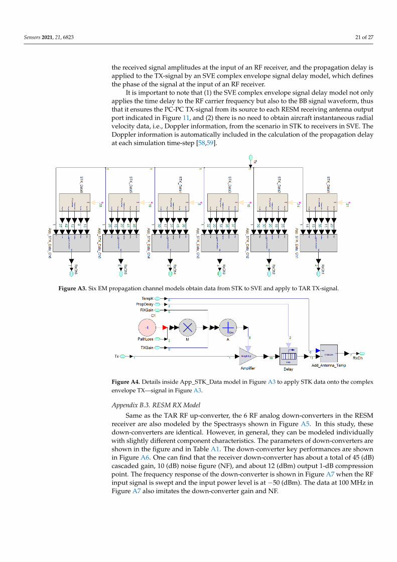
are six pairs of TX-RX from the TAR antenna to RESM receiving antennas. To take into account the EM wave propagation between TX-RX pairs, there are six EM propagation channels in the Six_TX_to_RX_Prop_Ch (green box in Figure 11), and their details are given in Figure A3. In the figure, the STK_Data models are the STK to SVE interfaces, which obtain the SVE simulation required data from the scenario to the SVE RESM re-ceiver at each SVE simulation time step. More details of the simulation time-step or sim-ulation sample rate will be discussed in the following section. For this RF HF-M&S study, the data from STK to SVE are TX antenna gain (TXGain (dB)), EM wave propagation loss (PathLoss (dB)) and delay (PropDelay (sec)), RX antenna gain (RXGain (dB)) and environ-ment temperature, i.e., RX antenna temperature, (TempK (Kelvin)). Here the PathLoss and PropDelay are calculated from the TAR antenna phase center (shown in Figure 10) to each receiving antenna phase center (shown in Figure 9) by STK. Figure A4 shows how these data are applied to the TX-signal inside the App_STK_Data_Ch models and form six sig-nals that output from RESM antennas in Figure 11.

From Figure A4, one can see that the antenna gains and propagation loss are added together and then applied to the TX-signal by an SVE amplifier model, which determines the received signal amplitudes at the input of an RF receiver, and the propagation delay is applied to the TX-signal by an SVE complex envelope signal delay model, which defines the phase of the signal at the input of an RF receiver.

It is important to note that (1) the SVE complex envelope signal delay model not only applies the time delay to the RF carrier frequency but also to the BB signal waveform, thus that it ensures the PC-PC TX-signal from its source to each RESM receiving antenna out-put port indicated in Figure 11, and (2) there is no need to obtain aircraft instantaneous radial velocity data, i.e., Doppler information, from the scenario in STK to receivers in SVE. The Doppler information is automatically included in the calculation of the propa-gation delay at each simulation time-step [58,59].

Figure A2. The cascaded gain (a), compression curve (b), and output power (with input −10 dBm) (c) of the TAR RFup-converter section.

Appendix B.2. Six Sets of EM Wave Propagation Channel Data

Since the RESM receiver has six receiving antennas and RF down-converters, there aresix pairs of TX-RX from the TAR antenna to RESM receiving antennas. To take into accountthe EM wave propagation between TX-RX pairs, there are six EM propagation channelsin the Six_TX_to_RX_Prop_Ch (green box in Figure 11), and their details are given inFigure A3. In the figure, the STK_Data models are the STK to SVE interfaces, which obtainthe SVE simulation required data from the scenario to the SVE RESM receiver at each SVEsimulation time step. More details of the simulation time-step or simulation sample ratewill be discussed in the following section. For this RF HF-M&S study, the data from STK toSVE are TX antenna gain (TXGain (dB)), EM wave propagation loss (PathLoss (dB)) anddelay (PropDelay (sec)), RX antenna gain (RXGain (dB)) and environment temperature,i.e., RX antenna temperature, (TempK (Kelvin)). Here the PathLoss and PropDelay arecalculated from the TAR antenna phase center (shown in Figure 10) to each receivingantenna phase center (shown in Figure 9) by STK. Figure A4 shows how these data areapplied to the TX-signal inside the App_STK_Data_Ch models and form six signals thatoutput from RESM antennas in Figure 11.

From Figure A4, one can see that the antenna gains and propagation loss are addedtogether and then applied to the TX-signal by an SVE amplifier model, which determines

Sensors 2021, 21, 6823 21 of 27

the received signal amplitudes at the input of an RF receiver, and the propagation delay isapplied to the TX-signal by an SVE complex envelope signal delay model, which definesthe phase of the signal at the input of an RF receiver.

It is important to note that (1) the SVE complex envelope signal delay model not onlyapplies the time delay to the RF carrier frequency but also to the BB signal waveform, thusthat it ensures the PC-PC TX-signal from its source to each RESM receiving antenna outputport indicated in Figure 11, and (2) there is no need to obtain aircraft instantaneous radialvelocity data, i.e., Doppler information, from the scenario in STK to receivers in SVE. TheDoppler information is automatically included in the calculation of the propagation delayat each simulation time-step [58,59].


Figure A3. Six EM propagation channel models obtain data from STK to SVE and apply to TAR TX-signal.

Figure A4. Details inside App_STK_Data model in Figure A3 to apply STK data onto the complex envelope TX signal in Figure A3.

Appendix B.3. RESM RX Model Same as the TAR RF up-converter, the 6 RF analog down-converters in the RESM

receiver are also modeled by the Spectrasys shown in Figure A5. In this study, these down-converters are identical. However, in general, they can be modeled individually with slightly different component characteristics. The parameters of down-converters are shown in the figure and in Table A1. The down-converter key performances are shown in Figure A6. One can find that the receiver down-converter has about a total of 45 (dB) cas-caded gain, 10 (dB) noise figure (NF), and about 12 (dBm) output 1-dB compression point. The frequency response of the down-converter is shown in Figure A7 when the RF input signal is swept and the input power level is at −50 (dBm). The data at 100 MHz in Figure A7 also imitates the down-converter gain and NF.




Figure A4. Details inside App_STK_Data model in Figure A3 to apply STK data onto the complex envelope TX signal in Figure A3.

Appendix B.3. RESM RX Model Same as the TAR RF up-converter, the 6 RF analog down-converters in the RESM

receiver are also modeled by the Spectrasys shown in Figure A5. In this study, these down-converters are identical. However, in general, they can be modeled individually with slightly different component characteristics. The parameters of down-converters are shown in the figure and in Table A1. The down-converter key performances are shown in Figure A6. One can find that the receiver down-converter has about a total of 45 (dB) cas-caded gain, 10 (dB) noise figure (NF), and about 12 (dBm) output 1-dB compression point. The frequency response of the down-converter is shown in Figure A7 when the RF input signal is swept and the input power level is at −50 (dBm). The data at 100 MHz in Figure A7 also imitates the down-converter gain and NF.

Figure A4. Details inside App_STK_Data model in Figure A3 to apply STK data onto the complexenvelope TX—signal in Figure A3.

Appendix B.3. RESM RX Model

Same as the TAR RF up-converter, the 6 RF analog down-converters in the RESMreceiver are also modeled by the Spectrasys shown in Figure A5. In this study, thesedown-converters are identical. However, in general, they can be modeled individuallywith slightly different component characteristics. The parameters of down-converters areshown in the figure and in Table A1. The down-converter key performances are shownin Figure A6. One can find that the receiver down-converter has about a total of 45 (dB)cascaded gain, 10 (dB) noise figure (NF), and about 12 (dBm) output 1-dB compressionpoint. The frequency response of the down-converter is shown in Figure A7 when the RFinput signal is swept and the input power level is at −50 (dBm). The data at 100 MHz inFigure A7 also imitates the down-converter gain and NF.

Sensors 2021, 21, 6823 22 of 27


Figure A5. Six RF down-converter model of the RESM receiver.

Table A1. Parmeters Used RF TX and RX Models.

f_IF (MHz)

f_LO (MHz)

IF_BW (MHz)

RF_BW (MHz)

LO_PW (dBm)

IF_ Gain1 (dB)

IF_ Gain2 (dB)

LNA_NF (dB)

100 3480 60 80 13 20 25 2.1

(a) (b)





f_IF (MHz)

f_LO (MHz)

IF_BW (MHz)

RF_BW (MHz)

LO_PW (dBm)

IF_ Gain1 (dB)

IF_ Gain2 (dB)

LNA_NF (dB)

100 3480 60 80 13 20 25 2.1

(a) (b)


(c)

Figure A6. (a) The RF down-converter cascaded gain, (b) cascaded noise figure, (c) compression curve, from RF frequency 3580 MHz to 100 MHz IF frequency.

Figure A7. The IF output power of the RF down-converter when sweeping RF signal with an input power level at -50 dBm.

After the RF signal is converted to IF, six IF signals are connected to ADC_AGC mod-els in the Six_ADC_with_AGC block shown in Figure 11. The RxIFOut1 port (node 3 of RF_Link in the cyan box in Figure 11) is monitored by the power measurement circuit inside the Pwr_Measure_for_AGC block in Figure A8, which generates a control signal to change the gain of 6 IF signals inside the AGC_Amplier block as shown in Figure A10. A 4-point moving average IF signal power measurement circuit model is given in Figure A8.

Figure A6. (a) The RF down-converter cascaded gain, (b) cascaded noise figure, (c) compressioncurve, from RF frequency 3580 MHz to 100 MHz IF frequency.

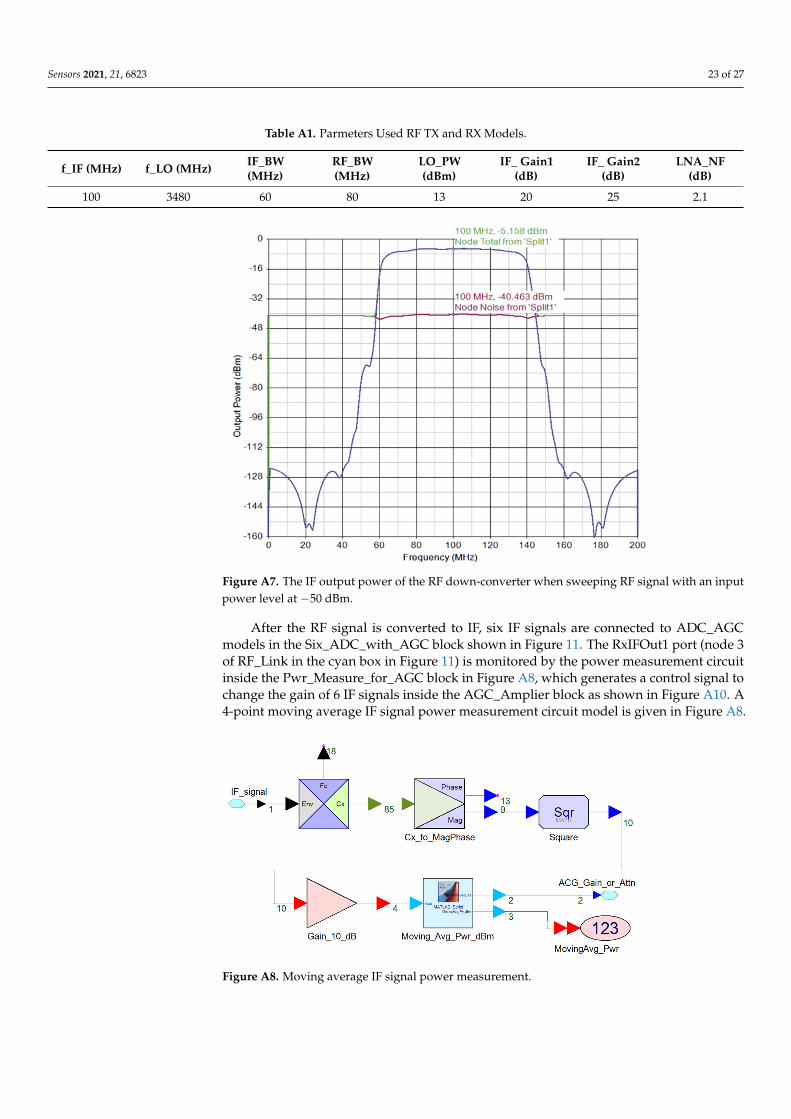
Sensors 2021, 21, 6823 23 of 27


f_IF (MHz) f_LO (MHz) IF_BW(MHz)

RF_BW(MHz)

LO_PW(dBm)

IF_ Gain1(dB)

IF_ Gain2(dB)

LNA_NF(dB)

100 3480 60 80 13 20 25 2.1


(c)

Figure A6. (a) The RF down-converter cascaded gain, (b) cascaded noise figure, (c) compression curve, from RF frequency 3580 MHz to 100 MHz IF frequency.

Figure A7. The IF output power of the RF down-converter when sweeping RF signal with an input power level at -50 dBm.

After the RF signal is converted to IF, six IF signals are connected to ADC_AGC mod-els in the Six_ADC_with_AGC block shown in Figure 11. The RxIFOut1 port (node 3 of RF_Link in the cyan box in Figure 11) is monitored by the power measurement circuit inside the Pwr_Measure_for_AGC block in Figure A8, which generates a control signal to change the gain of 6 IF signals inside the AGC_Amplier block as shown in Figure A10. A 4-point moving average IF signal power measurement circuit model is given in Figure A8.

Figure A7. The IF output power of the RF down-converter when sweeping RF signal with an inputpower level at −50 dBm.

After the RF signal is converted to IF, six IF signals are connected to ADC_AGCmodels in the Six_ADC_with_AGC block shown in Figure 11. The RxIFOut1 port (node 3of RF_Link in the cyan box in Figure 11) is monitored by the power measurement circuitinside the Pwr_Measure_for_AGC block in Figure A8, which generates a control signal tochange the gain of 6 IF signals inside the AGC_Amplier block as shown in Figure A10. A4-point moving average IF signal power measurement circuit model is given in Figure A8.


Figure A8. Moving average IF signal power measurement.

Appendix B.4. Automatic Gain Control (AGC) and Analog to Digital Converter (ADC) The model inside the Six_ADC_with_AGC block is shown in Figure A9. The ADC

input ports receive the IF analog signals at a sample rate of 50.1 (Mega-Sample/sec)). The digitized data are sent to CS-AoA processing block after SVE complex-envelope signal to complex signal conversion blocks (E1 to E6 in Figure A9).

Figure A9. The model inside Six_ADC_with_AGC block.

Figure A10 shows the details of ADC_AGC model in Figure A9. The gain of the AGC_Amplifier is controlled by the AGC_GainControl signal that is the


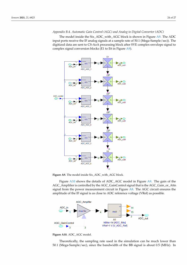
Sensors 2021, 21, 6823 24 of 27

Appendix B.4. Automatic Gain Control (AGC) and Analog to Digital Converter (ADC)

The model inside the Six_ADC_with_AGC block is shown in Figure A9. The ADCinput ports receive the IF analog signals at a sample rate of 50.1 (Mega-Sample/sec)). Thedigitized data are sent to CS-AoA processing block after SVE complex-envelope signal tocomplex signal conversion blocks (E1 to E6 in Figure A9).



Appendix B.4. Automatic Gain Control (AGC) and Analog to Digital Converter (ADC) The model inside the Six_ADC_with_AGC block is shown in Figure A9. The ADC

input ports receive the IF analog signals at a sample rate of 50.1 (Mega-Sample/sec)). The digitized data are sent to CS-AoA processing block after SVE complex-envelope signal to complex signal conversion blocks (E1 to E6 in Figure A9).


Figure A10 shows the details of ADC_AGC model in Figure A9. The gain of the AGC_Amplifier is controlled by the AGC_GainControl signal that is the


Figure A10 shows the details of ADC_AGC model in Figure A9. The gain of theAGC_Amplifier is controlled by the AGC_GainControl signal that is the AGC_Gain_or_Attnsignal from the power measurement circuit in Figure A8. The AGC circuit ensures theamplitude of the IF signal is as close to ADC reference voltage (VRef) as possible.


AGC_Gain_or_Attn signal from the power measurement circuit in Figure A8. The AGC circuit ensures the amplitude of the IF signal is as close to ADC reference voltage (VRef) as possible.

Figure A10. ADC_AGC model.

Theoretically, the sampling rate used in the simulation can be much lower than 50.1 (Mega-Sample/sec), since the bandwidth of the BB signal is about 0.5 (MHz). In order to ensure there are enough sample points within each radar pulse, 50.1 (Mega-Sample/sec) is selected. Thus, there are about 100 sampled points in each pulse, and the M&S time-step is about 19.96 × 10−9 (s). As discussed above, at each time step the STK-SVE interface needs to provide data for SVE simulation. Since the finest time-step in the STK simulation is 0.001 (s), the interpolation is used in the STK-SVE interface to obtain data in between STK simulation time-step. There is a trade-off between simulation accuracy and simula-tion speed since the smaller SVE time-step needs more data points from STK and longer computer simulation time.

Appendix C. Acronym List 2D Two-dimensional AoA Angle of Arrival ADC Analog to Digital Converter AGC Automatic Gain Control ASV Array Steering Vector Az Azimuth BB Base Band BW Bandwidth or Beamwidth CBSA Cavity Backed Spiral Antenna CS Compressive Sensing DF Direction Finding El Elevation EM Electromagnetic EpSec Epoch Second ESPIRT Estimation of Signal Parameters Via Rotation Invariance Techniques FFT Fast Fourier Transform FOV Field of View H/V Horizontal/Vertical IF Intermediate Frequency IG Information Geometry LO Local Oscillator LOS Line of Sight M&S Modeling and Simulation MIMO Multiple-Input Multiple-Output MUSIC Multiple Signal Classification NF Noise Figure PC-PC Phase-Continuous and Phase-Coherent PRF Pulse Repetition Frequency

Figure A10. ADC_AGC model.

Theoretically, the sampling rate used in the simulation can be much lower than50.1 (Mega-Sample/sec), since the bandwidth of the BB signal is about 0.5 (MHz). In

Sensors 2021, 21, 6823 25 of 27

order to ensure there are enough sample points within each radar pulse, 50.1 (Mega-Sample/sec) is selected. Thus, there are about 100 sampled points in each pulse, andthe M&S time-step is about 19.96 × 10−9 (s). As discussed above, at each time step theSTK-SVE interface needs to provide data for SVE simulation. Since the finest time-stepin the STK simulation is 0.001 (s), the interpolation is used in the STK-SVE interface toobtain data in between STK simulation time-step. There is a trade-off between simulationaccuracy and simulation speed since the smaller SVE time-step needs more data pointsfrom STK and longer computer simulation time.

Appendix C. Acronym List

2D Two-dimensionalAoA Angle of ArrivalADC Analog to Digital ConverterAGC Automatic Gain ControlASV Array Steering VectorAz AzimuthBB Base BandBW Bandwidth or BeamwidthCBSA Cavity Backed Spiral AntennaCS Compressive SensingDF Direction FindingEl ElevationEM ElectromagneticEpSec Epoch SecondESPIRT Estimation of Signal Parameters Via Rotation Invariance TechniquesFFT Fast Fourier TransformFOV Field of ViewH/V Horizontal/VerticalIF Intermediate FrequencyIG Information GeometryLO Local OscillatorLOS Line of SightM&S Modeling and SimulationMIMO Multiple-Input Multiple-OutputMUSIC Multiple Signal ClassificationNF Noise FigurePC-PC Phase-Continuous and Phase-CoherentPRF Pulse Repetition FrequencyPW Pulse WidthPXIe PCI Express Extension for InstrumentationRESM Radar Electronic Support MeasuresREW Radar Electronic WarfareRF Radio FrequencyRF HF-M&S RF High-Fidelity M&SRMSE Root Mean Square ErrorRPM Revolutions per MinuteRSA Randomly Spaced ArrayRx or RX ReceiverSNR Signal to Noise RatioSOI Signal of InterestSTK System Tool KitSVE SystemVueTAR Target Tracking RadarTS Time SlotTTR Target Tracking RadarTx or TX Transmitter

Sensors 2021, 21, 6823 26 of 27

References1. Pace, P.E. Detecting and Classifying Low Probability of Intercept Radar, 2nd ed.; Artech House: Boston, MA, USA, 2009.2. Wiley, R. ELINT—The Interception and Analysis of Radar Signals; Artech House: Boston, MA, USA, 2006.3. Neri, F. Introduction to Electronic Defence Systems, 2nd ed.; Artech House: Boston, MA, USA, 2006; pp. 324–330.4. Vakin, S.A.; Shustov, L.N.; Dunwell, R.H. Fundamentals of Electronic Warfare; Artech House: Boston, MA, USA, 2001.5. Jacobs, E.A.; Ralston, E.W. Ambiguity resolution in interferometry. IEEE Trans. Aerosp. Electron. Syst. 1981, 17, 766–780. [CrossRef]6. Pasala, K.; Penno, R.; Schneider, S. Novel wideband multimode hybrid interferometer system. IEEE Trans. Aerosp. Electron. Syst.

2003, 39, 1396–1406. [CrossRef]7. Moghaddasi, J.; Djerafi, T.; Wu, K. Multiport interferometer-enabled 2-D angle of arrival (AOA) estimation system. IEEE Trans.

Microw. Theory Tech. 2017, 65, 1767–1779. [CrossRef]8. Tsui, J.B.Y. Microwave Receivers with Electronic Warfare Applications; John Wiley & Sons: New York, NY, USA, 1986; pp. 94–108.9. Holder, E.J. Angle-of-Arrival Estimation Using Radar Interferometry—Methods and Application; Scitech Publishing: Edison, NJ,

USA, 2014.10. Lipsky, E.S. Microwave Passive Direction Finding; Scitech Publishing, Inc.: Raleigh, NC, USA, 2004.11. De Martino, A. Introduction to Modern EW Systems; Artech House: Boston, MA, USA, 2012.12. Chandran, S. Advances in Direction-of-Arrival Estimation; Artech House: Boston, MA, USA, 2006.13. Tuncer, T.E.; Friedlander, B. Classical and Modern Direction-of-Arrival Estimation; Academic Press: Burlington, MA, USA, 2009.14. Schmidt, R. Multiple emitter location and signal parameter estimation. IEEE Trans. Antennas Propag. 1986, 34, 276–280. [CrossRef]15. Roy, R.; Kailath, T. ESPRIT-estimation of signal parameters via rotational invariance techniques. IEEE Trans. Acoust. Speech Signal

Process. 1989, 37, 984–995. [CrossRef]16. Zhang, Z.; Wang, W.; Huang, Y.; Liu, S. Decoupled 2-D direction of arrival estimation in L-shaped array. IEEE Commun. Lett. 2017,

21, 1989–1992. [CrossRef]17. Asif, M.A.G.R.; Al-Yasir, Y.I.A.R.; Abd-Alhameed, A.; Excell, P.S. AOA Localization for vehicle-tracking systems using a dual-band

sensor array. IEEE Trans. Antennas Propag. 2020, 68, 6330–6345.18. Shi, H.P.; Leng, W.; Guan, Z.W.; Jin, T.Z. Two novel two-stage direction of arrival estimation algorithms for two-dimensional

mixed noncircular and circular sources. Sensors 2017, 17, 1433. [CrossRef]19. Wu, Y.; Liao, G.S.; So, H.C. A fast algorithm for 2-D directional-of-arrival estimation. Signal Process. 2003, 83, 1827–1831. [CrossRef]20. van der Veen, A.J. Asymptotic properties of the algebraic constant modulus algorithm. IEEE Trans. Signal Process. 2001, 49,

1796–1807. [CrossRef]21. Wang, Q.; Yang, H.; Chen, H.; Dong, Y.Y.; Wang, L.H. Complexity method for two-dimensional direction-of-arrival estimation

using an L-shaped array. Sensors 2017, 17, 190. [CrossRef]22. Gershman, A.B.; Rubsaman, M.; Pesavento, M. One- and two-dimensional direction-od-arrival estimation, an overview for

search-free techniques. Signal Process. 2010, 90, 1338–1349. [CrossRef]23. Al-Jazzar, S.O.; Hamici, Z.; Aldalahmeh, S. Tow-dimensional AOA estimation based on a constant modulus algorithm. Int. J.

Antennas Propag. 2017, 2017, 3214021. [CrossRef]24. Lonkeng, A.D.; Zhuang, J. Two-dimensional DOA estimation using arbitrary arrays for massive MIMO systems. Int. J. Antennas

Propag. 2017, 2017, 6794920. [CrossRef]25. Dong, Y.Y.; Dong, C.X.; Liu, W.; Liu, M.M.; Tang, Z.Z. Scaling transform based information geometry method for DOA Estimation.

IEEE Trans. Aerosp. Electron. Syst. 2019, 55, 3640–3650. [CrossRef]26. Sarkar, T.K.; Wang, H.; Park, S.; Adve, R.; Koh, J.; Kim, K.; Zhang, Y.; Wicks, M.; Brown, R.D. A deterministic least-squares

approach to space-time adaptive processing (STAP). IEEE Trans. Antennas Propag. 2001, 49, 91–103. [CrossRef]27. Kim, K.; Sarkar, T.K.; Palma, M.S. Adaptive processing using a single snapshot for a nonuniformly spaced array in the presence

of mutual coupling and near-field scatterers. IEEE Trans. Antennas Propag. 2002, 50, 582–590.28. Sarkar, T.K.; Schwarzlander, H.; Choi, S.; Palma, M.S.; Wicks, M.C. Stochastic versus deterministic models in the analysis of

communication systems. IEEE Antennas Propag. Mag. 2002, 44, 40–50. [CrossRef]29. Sarkar, T.K.; Wicks, M.C.; Salazar-Palma, M.; Bonneau, R.J. Smart Antennas; IEEE Press: New Jersey, NJ, USA, 2003.30. Zhang, P.; Li, J.; Zhou, A.Z.; Xu, H.B.; Bi, J. A robust direct data domain least squares beamforming with sparse constraint. Prog.

Electromagn. Res. C 2013, 43, 53–65. [CrossRef]31. Wu, C.; Elangage, J. Nonuniformly spaced array with the Direct Data Domain method for 2D angle-of-Arrival measurement in

electronic support measures application from 6 to 18 GHz. Int. J. Antennas Propag. 2020, 2020, 9651650. [CrossRef]32. Stove, A.G.; Hume, A.L.; Baker, C.J. Low probability of intercept radar strategies. IEE Proc.—Radar Sonar Navig. 2004, 151, 249–260.

[CrossRef]33. Candes, E.J.; Tao, T. Decoding by linear programming. IEEE Trans. Inf. Theory 2005, 51, 4203–4215. [CrossRef]34. Donoho, D.L. Compressed sensing. IEEE Trans. Inf. Theory 2006, 52, 1289–1306. [CrossRef]35. Candes, E.J.; Romberg, J.; Tao, T. Robust uncertainty principles: Exact signal reconstruction from highly incomplete frequency

information. IEEE Trans. Inf. Theory 2006, 52, 489–509. [CrossRef]36. Conde, M.H. Compressive Sensing for the Photonic Mixer Device: Fundamentals, Methods and Results; Springer: Berlin/Heidelberg,

Germany, 2016.37. Han, Z.; Li, H.; Yin, W. Compressive Sensing for Wireless Networks; Cambridge University Press: Cambridge, UK, 2013.

http://doi.org/10.1109/TAES.1981.309127

http://doi.org/10.1109/TAES.2003.1261135

http://doi.org/10.1109/TMTT.2017.2690869

http://doi.org/10.1109/TAP.1986.1143830

http://doi.org/10.1109/29.32276

http://doi.org/10.1109/LCOMM.2017.2708698

http://doi.org/10.3390/s17061433

http://doi.org/10.1016/S0165-1684(03)00118-X

http://doi.org/10.1109/78.934150

http://doi.org/10.3390/s17010190

http://doi.org/10.1016/j.sigpro.2009.12.008

http://doi.org/10.1155/2017/3214021

http://doi.org/10.1155/2017/6794920

http://doi.org/10.1109/TAES.2019.2910363

http://doi.org/10.1109/8.910535

http://doi.org/10.1109/MAP.2002.1043146

http://doi.org/10.2528/PIERC13052605

http://doi.org/10.1155/2020/9651650

http://doi.org/10.1049/ip-rsn:20041056

http://doi.org/10.1109/TIT.2005.858979

http://doi.org/10.1109/TIT.2006.871582

http://doi.org/10.1109/TIT.2005.862083

Sensors 2021, 21, 6823 27 of 27

38. Wu, C.; Elangage, J. 2D-angle of arrival estimation using signal spatial sparsity and Dantzig selector. Def. Res. Dev. Can. Sci. Rep.2019. DRDC-RDDC-2019-R079.

39. Wu, C.; Elangage, J. Multi-emitter Two-Dimensional Angle-of-Arrival Estimator via Compressive Sensing. IEEE Trans. Aerosp.Electron. Syst. 2020, 56, 2884–2895. [CrossRef]

40. Gurbuz, A.C.; Cevher, V.; Mcclellan, J.H. Bearing Estimation via Spatial Sparsity using Compressive Sensing. IEEE Trans. Aerosp.Electron. Syst. 2012, 48, 1358–1369. [CrossRef]

41. Candes, E.; Tao, T. The Dantzig selector: Statistical estimation when p is much larger than n. Ann. Stat. 2007, 35, 2313–2351.42. Zhang, Z.; Rao, B.D. Sparse signal recovery with temporally correlated source vectors using sparse Bayesian learning. IEEE J. Sel.

Top. Signal Process. 2011, 5, 912–926. [CrossRef]43. Rocca, P.; Hannan, M.A.; Salucci, M.; Massa, A. Single-snapshot DoA estimation in array antennas with mutual coupling through

a multi-scaling BCS strategy. IEEE Trans. Antennas Propag. 2017, 65, 3203–3213. [CrossRef]44. Analytical Graphics, Inc. Available online: https://agi.com/products (accessed on 12 January 2021).45. Keysight Technologies, Inc. Available online: https://www.keysight.com/m/ca/en/products/software/pathwave-design-

software.htm (accessed on 12 January 2021).46. Wikipedia The Free Encyclopedia, “Icosphere”. Available online: https://en.wikipedia.org/wiki/Icosphere (accessed on 11

May 2021).47. Ward, W.O.C. Icosphere, Generate Unit Geodesic Sphere Created by Subdividing a Regular Icosahedron. Available online:

https://www.mathworks.com/matlabcentral/fileexchange/50105-icosphere?focused=3865223&tab=function (accessed on 11May 2021).

48. Li, X.; Yagoub, M.C. Wideband cavity-backed spiral antenna design and mutual coupling study in a closely-spaced array. InProceedings of the 18th Symposium on Antenna Technology and Applied Electromagnetics (ANTEM), Session TU3B: SS: Researchon Antenna for Defence and Security Applications, Waterloo, ON, Canada, 19–22 August 2018.

49. Candes, E.; Romberg, J. l1-Magic: Recovery of Sparse Signals via Convex Programming. Available online: https://statweb.stanford.edu/~candes/l1magic/ (accessed on 12 May 2021).

50. TECOM Smith Microwave, Planar Cavity-Backed Spiral Antennas. Available online: https://www.smithsinterconnect.com/products/defence-antenna-systems/wideband-antennas/planar-cavity-backed-spiral-antennas/ (accessed on 23September 2021).

51. L3Harris, Dual-Polarized Quad-Ridged Horn Antenna. Available online: https://www.l3harris.com/all-capabilities/48461-series-dual-polarized-quad-ridged-horn-antenna (accessed on 23 September 2021).

52. Keysight Technologies Inc. X-Series Agile Signal Generators (UXG). Available online: https://www.keysight.com/en/pcx-x205221/x-series-agile-signal-generators-uxg?cc=CA&lc=eng (accessed on 25 November 2019).

53. Keysight Technologies Inc. M8121A 12 GSa/s Arbitrary Waveform Generator. Available online: https://www.keysight.com/en/pd-2959357-pn-M8121A/12-gsa-s-arbitrary-waveform-generator?cc=US&lc=eng (accessed on 3 March 2020).

54. Van de Sande, F.; Lugil, N.; Demarsin, F.; Hendrix, Z.; Andries, A.; Brandt, P.; Anklam, W.; Patterson, J.S.; Miller, B.; Rytting, M.;et al. A 7.2 GSa/s, 14 Bit or 12 GSa/s, 12 Bit Signal Generator on a Chip in a 165 GHz fT BiCMOS Process. IEEE J. Solid-StateCircuits 2012, 47, 1003–1012. [CrossRef]

55. D’Agostino, S.; Foglia, G.; Pistoia, D. Specific emitter identification: Analysis on real radar signal data. In Proceedings of the 2009European Radar Conference (EuRAD), Rome, Italy, 30 September–2 October 2009; pp. 242–245.

56. Ding, L.; Wang, S.L.; Wang, F.G.; Zhang, W. Specific emitter identification via convolution neural networks. IEEE Commun. Lett.2018, 22, 2591–2594. [CrossRef]

57. Wu, C. Using Matlab/Simulink to Model and Simulate Electronic Support Measure FR/Microwave Receiver Front-End; DRDC Ottawa,TM-2010-071: Ottawa, ON, Canada, 2010.

58. Wu, C.; Young, A. High-fidelity modeling and simulation for radar electronic warfare system concepts. In SPIE 2012 DefenceSecurity + Sensing; SPIE: Baltimore, MD, USA, 23–27 April 2012; Volume 8403, p. 3.

59. Wu, C.; Rajan, S.; Young, A.; O’Regan, C. RF/microwave system high-fidelity modeling and simulation: Application to airbornemulti-channel receiver system for angle of arrival estimation. In Proceedings of the SPIE Defence Security + Sensing, Baltimore,ML, USA, 5–9 May 2014; Volume 9095, p. 5.

http://doi.org/10.1109/TAES.2019.2958397

http://doi.org/10.1109/TAES.2012.6178067

http://doi.org/10.1109/JSTSP.2011.2159773

http://doi.org/10.1109/TAP.2017.2684137

https://agi.com/products

https://www.keysight.com/m/ca/en/products/software/pathwave-design-software.htm

https://www.keysight.com/m/ca/en/products/software/pathwave-design-software.htm

https://en.wikipedia.org/wiki/Icosphere

https://www.mathworks.com/matlabcentral/fileexchange/50105-icosphere?focused=3865223&tab=function

https://statweb.stanford.edu/~candes/l1magic/

https://statweb.stanford.edu/~candes/l1magic/

https://www.smithsinterconnect.com/products/defence-antenna-systems/wideband-antennas/planar-cavity-backed-spiral-antennas/

https://www.smithsinterconnect.com/products/defence-antenna-systems/wideband-antennas/planar-cavity-backed-spiral-antennas/

https://www.l3harris.com/all-capabilities/48461-series-dual-polarized-quad-ridged-horn-antenna

https://www.l3harris.com/all-capabilities/48461-series-dual-polarized-quad-ridged-horn-antenna

https://www.keysight.com/en/pcx-x205221/x-series-agile-signal-generators-uxg?cc=CA&lc=eng

https://www.keysight.com/en/pcx-x205221/x-series-agile-signal-generators-uxg?cc=CA&lc=eng

https://www.keysight.com/en/pd-2959357-pn-M8121A/12-gsa-s-arbitrary-waveform-generator?cc=US&lc=eng

https://www.keysight.com/en/pd-2959357-pn-M8121A/12-gsa-s-arbitrary-waveform-generator?cc=US&lc=eng

http://doi.org/10.1109/JSSC.2012.2185172

http://doi.org/10.1109/LCOMM.2018.2871465

Hardware Implementation and RF High-Fidelity Modeling and ...

Documents

Transcript of Hardware Implementation and RF High-Fidelity Modeling and ...