1

ON ANALOG FEEDBACK CONTROL FOR MAGNETOSTRICTIVE TRANSDUCER LINEARIZATION

David L. Hall and Alison B. Flatau

Department of Aerospace Engineering and Engineering Mechanics

Iowa State University

2019 Black Engineering Building

Ames, Iowa 50011

Running Headline: "Magnetostrictive Transducer Linearization"

Total number of pages: 28

Total number of tables: 1

Total number of figures: 10

Please send proofs to Alison Flatau at the above address

2

ABSTRACT

Magnetostrictive transducer output force, displacement, and bandwidth

characteristics are well suited for a variety of active vibration control

applications. However, their use is limited in part because these transducers

are known to be nonlinear. The transducer in this study is assumed to be a

linear system and its output harmonics are assumed to be disturbance inputs.

Two feedback control models are proposed and one is used to obtain expressions

for predicting the change in harmonic amplitudes of displacement and

acceleration as functions of frequency and parameters for the controller,

load, and transducer. An approach based on magnetostrictive transduction

modeling is presented for experimentally determining appropriate transducer

model parameters for use in the feedback control model. Experimental

measurements using simple, analog, PD (proportional plus derivative)

acceleration feedback control are presented to validate the expressions. The

closed loop feedback control system model resulted in predicted changes in

harmonic acceleration amplitudes ranging from +2 to -30 dB, (depending upon

the frequency of the disturbance input) that were verified experimentally. A

significant extension of the linear range of transducer behavior, due to

feedback control, is also demonstrated.

1. INTRODUCTION

Magnetostrictive materials are the magnetic analogs of the more familiar

piezoelectric materials. Magnetostrictives transduce strain and magnetic

3

energies. Terfenol-D* is a "giant" magnetostrictive material offering

mechanical strains of up to 2000 x10-6 m/m (2000 µ strain). Magnetostrictive

transducers constructed using Terfenol-D rods of lengths up to 24 cm offer

displacements based on approximately ±500 µ strain with output over a

bandwidth of from DC to over 20 kHz. In spite of nonlinearities inherent in

the cyclic strain of this magnetic material, it has received considerable

attention for use in sonar applications, and is beginning to be recognized as

an attractive material for design of certain smart structural system.

A nonlinearity of particular importance when using Terfenol-D transducers

is wave form distortion. The distortion is a result of a quadratic nonlinear

strain versus magnetization relationship and magnetic hysteresis occurring

within the Terfenol-D. The net result is varying amplitude integer harmonics

present in the transducer voltage, current, and output velocity. These

amplitudes typically increase with increasing excitation level.

Magnetostrictive transducers are traditionally considered as being

reasonable approximations of linear systems at low drive amplitudes1,2,4 and as

becoming very nonlinear at high drive amplitudes.3,4,5 (Linear in the sense

that sinusoidal input produces sinusoidal output.) These are all relative

terms. A more concrete example is shown in Fig. 1a and 1b which respectively

display plots of percent displacement from current (||u/I|| as a percentage of

the displacement measured when driven at 800 mA) and percent harmonic

distortion (%HD) versus drive current amplitude. The data in Fig. 1 were

calculated from information given in Table 5.1 of reference 2, which also

provides a full description of the transducer used. For these tests, the

* Terfenol-D is a magnetostrictive material which was discovered at the NavalOrdinance Laboratory and it is produced by alloying the rare-earths terbiumand dysprosium with iron. Thus, Terfenol-D stands for Ter(bium) + fe (iron) +nol (Naval Ordinance Laboratory) + D(ysprosium). It has been commerciallyavailable since the late 1980s. An authoritative discussion of the physics ofthe material is available in reference 4.

4

transducer was driven by 200 Hz sinusoidal drive currents of various

amplitudes using an amplifier with a current-control module. As operated, a

"high" drive current amplitude for this transducer was 800 mA zero to peak.

Measured acceleration autospectral density functions (0 - 2 kHz) were obtained

for each drive-current amplitude. Displacement from current values were those

corresponding to the 200 Hz component only, and all are shown as percentages

of the 800 mA value (11.2 µm/A) and thus show the change in output sensitivity

as a function of input. %HD was calculated as the ratio of the summation of

the harmonic amplitudes to that of all of the amplitudes (the harmonics

occurred at integer multiples of the fundamental).

Displacement per amp is clearly not a constant for this transducer.

Driving this system harder produces significant gains in output displacement

per unit input current. (Linearization of this output/input relationship is

not addressed in this study.) Unfortunately, wave form harmonic distortion

also increases with increasing drive current amplitudes. Thus, although

significant increases in output displacement and force (and therefore control

authority) occur with increasing drive amplitudes (Fig. 1a), increased

harmonic distortion with increasing drive amplitudes (Fig. 1b) limits the

utility of these transducers in vibration control applications, where

undesirable excitation of structural modes by transducer harmonics can occur.

Thus, one would like to decrease the output harmonics in order to take

advantage of the significant increases in the useful displacement range of

transducer operation with higher drive amplitudes. That was the impetus for

the investigation reported here.

5

0

20

40

60

80

100

0 0.1 0.2 0.3 0.4 0.5 0.6 0.7 0.8||u/I||, % of 0.8

amp value

Drive Current, ||I|| (amp)

01020304050607080

0 0.1 0.2 0.3 0.4 0.5 0.6 0.7 0.8

% Harmonic Distortion

Drive Current, ||I|| (amp)

Figure 1 . (a) Displacement from drive-current and (b) harmonic distortion at

different 200 Hz drive-current amplitudes as a percentage of their respective

0.8 Amp values.

2. MODELING APPROACH

The magnetostrictive transducer is modeled as a linear system satisfying a

pair of linear simultaneous equations. The harmonic frequencies present in

the state variables will be thought of as disturbances.

The canonical form of the transduction equations, as applied to a

magnetostrictive transducer, is:1

V = ZeI + Temv (1a)

0 = TmeI + zxv (1b)

where: V = voltage across the transducer leads, volts; Ze = blocked electrical

impedance of the transducer (blocked physically, i.e., the electrical

impedance one would measure if the output velocity were held at zero) = sLe +

Re, where s is the Laplace operator, Le is the blocked electrical inductance,

henries, and Re is the dc resistance of the wound wire solenoid, in units of

6

ohms, Ω; I = electric current passing through the wound wire solenoid,

amperes, A; Tem = the transduction coefficient, electrical due to mechanical,

in units of volts per meter per second, V/(m/s); v = the mechanical output

velocity of the transducer, m/s; Tme = the transduction coefficient,

mechanical due to electrical, Newton/A; and zx = the mechanical impedance,

based on velocity, of the transducer and the load, which, in its simplest

applicable form is given as: zx = smx + bx + kx/s, where mx is the sum of the

internal dynamic mass of the transducer plus the load mass, in kg, bx is the

sum of the damping within the transducer and that due to the load,

Newton/(m/s), and kx is the combined stiffness of the transducer and the load,

Newton/m. It is shown in the literature1,2,6 that for magnetostrictive

transducers, ignoring eddy current effects, Tem = -Tme = a drive amplitude

dependent pseudo-constant. Thus, for transduction, T defined as T = Tem = -Tme

is used. Using this substitution in Eqns. (1), one can solve for the useful

fundamental transducer relationships when operating in its linear range given

in equations 2-6:

vI

=T

zx(s)

,

V

I

2(s) =

Zezx+ T

zx ,

v

V(s) = =

T

Zezx + T2(2-4)

(v/I)

(V/I)

u

V(s) = =

T

s Zezx + T2V

1

sv

)(,

s= v

V=

T

Zezx + T2(5,6)

sa

V(s)

where: u = transducer output displacement, meters m, a = transducer output

acceleration, m/s2, and equations presented are functions of the Laplacian

operator s. All of these equations will be useful when modeling the

transducer as part of the overall controlled system.

7

2.1. FEEDBACK MODELS USING A CURRENT-CONTROL AMPLIFIER

The magnetic field applied inside a transducer is directly proportional to

the product of the number of turns per meter of the transducer's solenoid and

the current through the solenoid. Figure 2 shows a block diagram for the

system consisting of a PID (proportional, integral, and derivative)

controller; a current-controlled amplifier, of gain Ka, A/V; the transducer

(expressed as displacement per ampere = Eqn. (2) divided by s); disturbance

displacements, ud; and a displacement transducer of sensitivity, Su, V/m. The

reference signal is shown as Vr; it is the input for the controlled system.

Using the definitions for the impedances (Ze and zx) detailed below Eqns. (1),

the system transfer function u/Vr is calculated as:

V K uI

S

u

u

kk + k +d p

ia

u

d

r ss

(s)(s)

(s)

(s)

Figure 2 . Block diagram of feedback system assuming a PID controller, a

current-controlled amplifier of gain Ka, a displacement sensor of sensitivity

Su, and disturbance displacements, ud.

u

Vr(s)

T

=d + kp + ki/ s( ) Ka szx

1 + d + kp + ki/ s( ) Ka Tszx

Susk

sk

which reduces to:

8

u

Vr

2((s)=

s kd + p + ki T

s3mx+ s2 bx+ kd TSu( )+ s kx+ kpKaTSu( )+ kiKaTSu

(7))sk

Ka

Ka

This function has two, possibly complex zeros in the LHP (left half-plane)

given as:

s1,2 = [-kp ± (kp2 - 4kdki)1/2]/2kd

and the Routh-Hurwitz criteria10 guarantees that it will have its three poles

in the LHP (be stable) if:

kxbx + kd(kx + kpKaTSu)KaTSu + kpkxKaTSu > mxkiKaTSu

This derivation assumes that the system parameters are constants, independent

of drive magnitude and frequency. These are tenuous assumptions when dealing

with Terfenol-D transducers, as discussed in references 11 and 12. (T, Re,

Le, Ka, and kx are all of particular concern with these actuators.).

Other relations could be developed assuming one had a current-controlled

amplifier that was robust enough to be a reasonable approximation of the

constant Ka. That was not the case in this investigation. Although current

control was attempted, magnetostrictive transducers are very active loads and

the amplifier current output did not follow the input signal sufficiently at

different frequencies to study the case of constant Ka.

2.2. FEEDBACK MODELS USING A VOLTAGE CONTROL AMPLIFIER

The rest of the work presented employs models based on a voltage-controlled

amplifier. This model is a bit more complex in that the applied magnetic

9

field in the transducer is now proportional to the product of the turns per

meter of the solenoid, the voltage across the solenoid, and the inverse of

Eqn. 3, a complex valued electrical impedance function that varies with

operating conditions.

In addition, emphasis will be placed on oscillatory drive conditions using

an accelerometer as the feedback transducer. This was done for two reasons:

1) The equipment was available. 2) Small amplitude disturbance displacements

are anticipated and using an accelerometer as the feedback transducer exploits

the ω2 signal amplification inherent to acceleration measurements.

Figure 3 is a block diagram of the feedback system assuming a voltage-

controlled amplifier. (Voltage was much easier for the amplifier used to

control than current when driving a Terfenol-D transducer.) The transducer's

transfer function for acceleration per volt is given in Eqn. (6). Using the

PID controller defined in Fig. 3, the relations for the impedances detailed

below Eqns. (1), and Eqn. (6), the transfer function for the closed loop

system, as a/Vr, is given as:

V =

kd s + kp + ki/ s( )KV T

Zezx + T2

1 + kd s + kp + ki/ s( ) KVSaZezx + T2

Ts

s

(s)a

r

which reduces to:

V=

s kd s2 + kps + ki( ) KVT

Lemx + kdKVSaT( )s3 + Lebx + Remx + kpKVSaT( )s2 + Lekx + Rebx + T2 + kiKVSaT( )s + Rekx

a

r(s)

(8)

The transfer function for output acceleration from a given input disturbance

acceleration is given as:

=1

1 + kd s + kp + ki/ s( )K VSaZezx + T2

s Ta

ad(s)

10

which reduces to:

a

ad=

Lemxs3 + Lebx + Remx( ) + Lekx + Rebx + T2( )s + R ekx

+ Lekx + Rebx + T2 + kiKVSaT( )s + Rekx

s2

s2) ( )e x d V a e x e x p V aL m + k K S T( s3 + L b + R m + k K S T(s)

(9)

Note that Eqns. (8) and (9) have the same characteristic equations (same

denominators) and that the control parameters appear as coefficients of

different powers of s (which contains the frequency). Thus, it can be

expected that derivative feedback will be most helpful at reducing harmonics

at the high frequencies. Similarly, kp will be most useful at medium to high

frequencies and ki will help in the low to medium frequency range.

Classical stability analysis might be applied to these characteristic

equations. However, it was not done in this study owing to the variability of

coefficients with excitation frequency, excitation amplitude, magnetic bias

point, material prestress, and even actuator load (T changes with different

loads in the presence of eddy currents2). Reasonable estimates of stability

criteria might be obtained by using empirical and/or analytical relationships

for Le, Re, bx, kx, and T, as functions of all of the parameters mentioned

previously, if they all existed. However, models of the functional trends in

the behavior of system parameters with changes in operating conditions are not

available. Nonetheless, as will be shown, parameter estimates for a fixed

input drive magnitude and frequency can be measured and used to provide

reasonable models of both the system open loop and closed loop system

behavior, as run. (Note that until such time as improved material models

become available, an empirical approach to parameter estimation is advised.

Measure parameters over the range of operating conditions of interest to

determine whether or not the parameters change; use appropriate parameters for

11

control under different operating conditions.) Awaiting further research into

those

V K aV

S

a

a

sk + k +d pi

v

a

d

rks (s)

(s)

(s)(s)

Figure 3 . Block diagram of feedback system assuming a PID controller, a

voltage-controlled amplifier of gain KV, an acceleration sensor of sensitivity

Sa, and disturbance accelerations, ad.

relationships, the work presented demonstrates the improvements achievable

without addressing stability issues, which were resolved empirically by

restricting gains to values below those which produced instabilities.

Models have been developed for prediction of magnetostrictive transducer

behavior using a PID controller in the forward loop. It has been assumed that

the transducer was a linear system which satisfied the pair of simultaneous

equations, Eqns. (1), with the harmonic frequencies (that are known to exist)

modeled as disturbance inputs. The primary goal of this endeavor is to reduce

the harmonic signal content of the magnetostrictive transducer; thus extending

its linear range to larger displacements, velocities, and accelerations. To

test the modeling technique, a PD controller was fabricated and experimental

measurements were performed.

3. RESULTS

12

In this section, experimental evidence is offered to show that the control

system generally improves the linearity of the transducer. Also, realities of

the circuits and components employed will be discussed (including procedures

for obtaining transducer parameters) and model predictions will be compared

with experimental measurements of magnetostrictive transducer behavior.

Emphasis is placed on voltage-control.

3.1 Trends

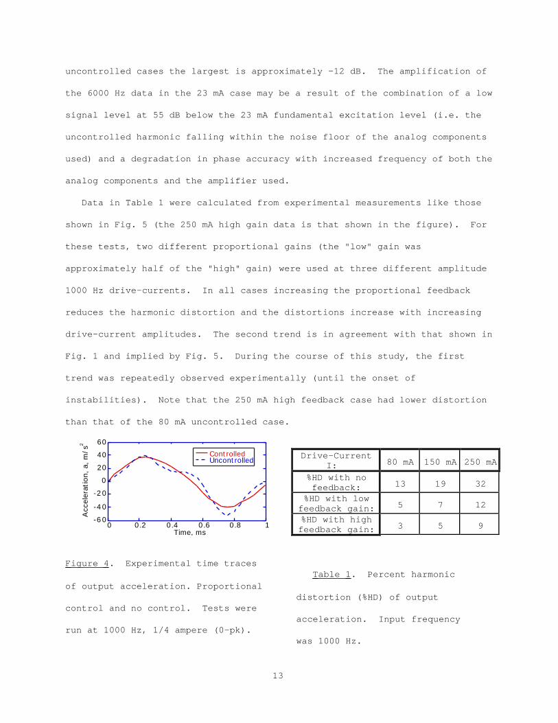
An example of the effects of simple proportional feedback on the output

acceleration of the transducer is shown in Fig. 4. In the figure are two

different experimental measurements of transducer output acceleration as

functions of time. For both tests, the transducer was driven by a 1000 Hz,

1/4 amp drive-current. As shown in the figure, the proportional feedback made

a significant difference in the output wave form. Note that the second

harmonic frequency component (3000 Hz) was reduced dramatically by simple

proportional feedback.

Figure 5 shows experimental acceleration amplitudes for controlled (simple

proportional acceleration feedback) and uncontrolled cases of three different

drive-current amplitudes. In all cases the drive-current was oscillating at

1000 Hz. The other frequencies were harmonics. Each set of data was

normalized by its acceleration amplitude at 1000 Hz (thus all show 0 dB at

1000 Hz). As shown in the figure, proportional acceleration feedback control

generally decreased the harmonic amplitudes, over this frequency range, when

compared with the corresponding uncontrolled drive-current test. Note that at

4 kHz for the 250 mA drives, the controlled harmonic is approximately 30 dB

below the uncontrolled case. Note also that for this range of drive-currents

the largest harmonic for the controlled cases is about 25 dB down; for the

13

uncontrolled cases the largest is approximately -12 dB. The amplification of

the 6000 Hz data in the 23 mA case may be a result of the combination of a low

signal level at 55 dB below the 23 mA fundamental excitation level (i.e. the

uncontrolled harmonic falling within the noise floor of the analog components

used) and a degradation in phase accuracy with increased frequency of both the

analog components and the amplifier used.

Data in Table 1 were calculated from experimental measurements like those

shown in Fig. 5 (the 250 mA high gain data is that shown in the figure). For

these tests, two different proportional gains (the "low" gain was

approximately half of the "high" gain) were used at three different amplitude

1000 Hz drive-currents. In all cases increasing the proportional feedback

reduces the harmonic distortion and the distortions increase with increasing

drive-current amplitudes. The second trend is in agreement with that shown in

Fig. 1 and implied by Fig. 5. During the course of this study, the first

trend was repeatedly observed experimentally (until the onset of

instabilities). Note that the 250 mA high feedback case had lower distortion

than that of the 80 mA uncontrolled case.

-60

-40

-20

0

20

40

60

0 0.2 0.4 0.6 0.8 1

ControlledUncontrolled

Acc

eler

atio

n, a

, m

/s2

Time, ms

Figure 4 . Experimental time traces

of output acceleration. Proportional

control and no control. Tests were

run at 1000 Hz, 1/4 ampere (0-pk).

Drive-CurrentI: 80 mA 150 mA 250 mA

%HD with nofeedback: 13 19 32

%HD with lowfeedback gain: 5 7 12

%HD with highfeedback gain: 3 5 9

Table 1 . Percent harmonic

distortion (%HD) of output

acceleration. Input frequency

was 1000 Hz.

14

-70

-60

-50

-40

-30

-20

-10

0

10

00

20

00

30

00

40

00

50

00

60

00

no controlcontrol

Acc

eler

atio

n Am

plit

ude ||a

||, dB

Frequency, ƒ, Hz

23 mA

-70

-60

-50

-40

-30

-20

-10

0

10

00

20

00

30

00

40

00

50

00

60

00

no controlcontrol

Acc

eler

atio

n Am

plit

ude ||a

||, dB

Frequency, ƒ, Hz

115 mA

-70

-60

-50

-40

-30

-20

-10

0

10

00

20

00

30

00

40

00

50

00

60

00

no controlcontrol

Acc

eler

atio

n Am

plit

ude ||a

||, dB

Frequency, ƒ, Hz

250 mA

Figure 5 . Experimental acceleration amplitudes resulting from 1000 Hz

drive-currents at three different amplitudes. Data were taken from

acceleration autospectral density functions. Percent harmonic distortion was

calculated as 100 x (Σ all amplitudes - 1000 Hz amplitude) / Σ all amplitudes.

3.2 Transducer-Controller System Modeling

The input-output relationship for the Techron 7520 amplifier was measured.

(The amplifier was fitted with a 75A08 control module, set for voltage

control.) The system behaved somewhat like a first order system with a -3 dB

point at about 57 kHz. Unless specified otherwise, it was modeled as a

constant gain with a linear phase lag over the appropriate frequency range

(usually 0 to 6 or 10 kHz).

The analog control circuit was built in-house. Input-output relationships

for each stage of the circuit were measured and compared with the theoretical

relationships. Theory and experiment were found to be in excellent agreement.

However, difficulties were encountered. The resonant frequency of the

accelerometer as mounted was at 47 kHz. This frequency was fed back to the

15

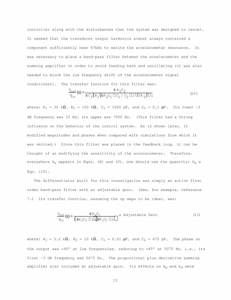
controller along with the disturbances that the system was designed to cancel.

It seemed that the transducer output harmonics almost always contained a

component sufficiently near 47kHz to excite the accelerometer resonance. It

was necessary to place a band-pass filter between the accelerometer and the

summing amplifier in order to avoid feeding back and oscillating (it was also

needed to block the low frequency drift of the accelerometer signal

conditioner). The transfer function for this filter was:

VoutVin

(10)(s)1

= R2C2

C2 R1 R2C1 + C1/ C2 + 1( )+ R 2 +s

s s

where: R1 = 30 kΩ, R2 = 100 kΩ, C1 = 1000 pF, and C2 = 0.1 µF. Its lower -3

dB frequency was 10 Hz; its upper was 7000 Hz. (This filter had a strong

influence on the behavior of the control system. As is shown later, it

modified magnitudes and phases when compared with simulations from which it

was omitted.) Since this filter was placed in the feedback loop, it can be

thought of as modifying the sensitivity of the accelerometer. Therefore,

everywhere Sa appears in Eqns. (8) and (9), one should use the quantity: Sa x

Eqn. (10).

The differentiator built for this investigation was simply an active first

order band-pass filter with an adjustable gain. (See, for example, reference

7.) Its transfer function, assuming the op amps to be ideal, was:

VoutVin

(11)(s) = 2C1

2C2 + 1( ) R1C1 + 1( ) x Adjustable Gain R

R s

s

s

where: R1 = 2.2 kΩ, R2 = 10 kΩ, C1 = 0.01 µF, and C2 = 470 pF. The phase on

the output was +90° at low frequencies, reducing to +45° at 5075 Hz, i.e., its

first -3 dB frequency was 5075 Hz. The proportional plus derivative summing

amplifier also included an adjustable gain. Its effects on kp and kd were

16

included in the reported values. Since the differentiator was not a pure

derivative, skd values in Eqns (8) and (9) were replaced with:

skd/(sR2C2 +1)(sR1C1 +1).

The reported values of kd were calculated as the product of R2C1 x Adjustable

Gain x Summing Gain.

At this point, circuit parameters were known. The transducer was mass

loaded such that the first axial mechanical resonance occurred between 2500

and 4000 Hz for all tests discussed. Unfortunately, the transducer used in

this study had a radial mode of vibration which affected transducer axial

behavior around 7 kHz. As a result, model values reported (which are based on

a 1-DOF mechanical model) are limited to frequencies less than 6 kHz.

Quantities applicable to the magnetostrictive transducer must be estimated

in order to model the transducer behavior. One needs estimates of T, the

transduction coefficient, Ze, the blocked electrical impedance of the

transducer, and zx, the sum of the mechanical impedances of the transducer and

the load. One might consult the literature for "nominal" material properties,

or build a transducer and measure them. Typical results from both methods are

shown in Fig. 6 for the case of simple proportional feedback control. Also,

measured accelerometer voltage per unit input reference voltage were taken at

several different input frequencies, and are indicated on the plots with an

'X'. The figure shows the magnitude and phase of the product of Sa and Eqn.

(6) = Vacc/Vr = accelerometer voltage over input or reference voltage.

In Fig. 6, Model 1 was calculated using published "nominal" Terfenol-D

parameters,8 relations from the literature,6 and the details of the control

circuit discussed above. The transduction coefficient was calculated as: T =

17

N d EyH π r2/ lr where: N = turns of the wound wire solenoid (N = 1300 turns);

d = the linear coupling coefficient of the Terfenol-D rod (d ≈ 1.5 x 10-8 m/A);

EyH = Terfenol-D's Young's modulus measured at constant applied magnetic field

(EyH ≈ 3.0 x 1010 Pa); r = the radius of the Terfenol-D rod (r = 3.175 mm); and

lr = the rod length (l = 0.0508 m). Thus, T ≈ 365 N/A. The blocked electrical

impedance of the transducer, Ze, was estimated as the DC resistance (Re ≈ 6 Ω)

plus jωLe, where j = √(-1), ω = 2πƒ = frequency of oscillation in radians per

second, and Le ≈ µε n2 π rs2 ls = 2.5 µo 232642 π 0.003852 0.0559 = 4.43 mH (µε

is the blocked magnetic permeability of Terfenol-D ≈ 2.5 µo, µo = 4π x 10-7

Tesla meter per amp-turn, n is the number of turns per unit length of the

solenoid, rs is the inner radius of the solenoid, and ls is the length of the

solenoid). The mechanical impedance of the transducer, as loaded, was

calculated using simple second order mechanical relations9, i.e., kx = E A / lr

= EyH π r2/ lr = 18.7 MN/m, mx was measured = mass of the load plus some

attaching components plus 1/3 the mass of the Terfenol-D rod (mx = 0.086 kg),

ωn = (kx/mx)1/2, and bx was estimated based on a four-percent damping

coefficient, i.e., bx ≈ 2 x 0.04 ωn mx.

a)

0

0.5

1

1.5

2

2.5

0 1000 2000 3000 4000 5000 6000

Model 1Model 2Experiment||V

acc/V

ref||,

V

/V

Frequency, ƒ, Hz

b)

-45

0

45

90

135

180

0 1000 2000 3000 4000 5000 6000

Model 1Model 2Experiment

Phas

e of

Vac

c/Vre

f, deg

.

Frequency, ƒ, Hz

Figure 6 . Predicted accelerometer voltage per unit reference voltage for

proportional feedback control. (a) Magnitude and (b) phase. Models are based

on Eqn. (6). Model 1 used "nominal" material properties. Model 2 used

measured properties. 'X's indicate measured values of accelerometer voltage

per unit reference voltage from sinusoidal input at different frequencies.

18

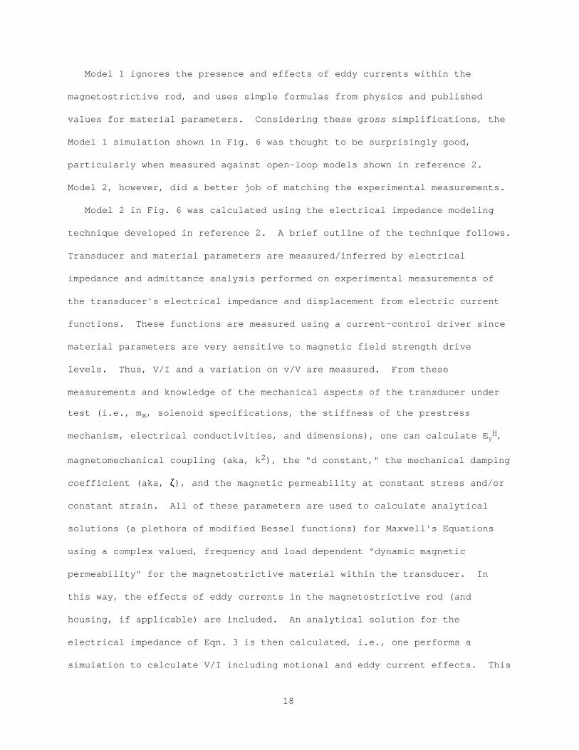
Model 1 ignores the presence and effects of eddy currents within the

magnetostrictive rod, and uses simple formulas from physics and published

values for material parameters. Considering these gross simplifications, the

Model 1 simulation shown in Fig. 6 was thought to be surprisingly good,

particularly when measured against open-loop models shown in reference 2.

Model 2, however, did a better job of matching the experimental measurements.

Model 2 in Fig. 6 was calculated using the electrical impedance modeling

technique developed in reference 2. A brief outline of the technique follows.

Transducer and material parameters are measured/inferred by electrical

impedance and admittance analysis performed on experimental measurements of

the transducer's electrical impedance and displacement from electric current

functions. These functions are measured using a current-control driver since

material parameters are very sensitive to magnetic field strength drive

levels. Thus, V/I and a variation on v/V are measured. From these

measurements and knowledge of the mechanical aspects of the transducer under

test (i.e., mx, solenoid specifications, the stiffness of the prestress

mechanism, electrical conductivities, and dimensions), one can calculate EyH,

magnetomechanical coupling (aka, k2), the "d constant," the mechanical damping

coefficient (aka, ζ), and the magnetic permeability at constant stress and/or

constant strain. All of these parameters are used to calculate analytical

solutions (a plethora of modified Bessel functions) for Maxwell's Equations

using a complex valued, frequency and load dependent "dynamic magnetic

permeability" for the magnetostrictive material within the transducer. In

this way, the effects of eddy currents in the magnetostrictive rod (and

housing, if applicable) are included. An analytical solution for the

electrical impedance of Eqn. 3 is then calculated, i.e., one performs a

simulation to calculate V/I including motional and eddy current effects. This

19

calculated V/I should be a reasonable approximation (±10% in both magnitude

and phase) of the experimental measurement performed earlier.

What remains to be done is to calculate the yet unknown coefficients, Ze

and T, which are needed for the controls modeling. One can calculate Ze, the

blocked electrical impedance of the transducer, including the effects of eddy

currents, by calculating V/I again. However, this time through, use the

measured/calculated value of the blocked magnetic permeability of the

magnetostrictive material instead of the "dynamic magnetic permeability" which

was used the first time through. The transduction coefficient, T, can now be

calculated——including the effects of the load and frequency dependent eddy

currents——by solving Eqn. (3) for T, i.e., [(V/I - Ze)zx]1/2 = T.

The procedure outlined above was carried through one time with the

transducer operated at a representative drive-current amplitude and with a

representative load. The process would likely need to be repeated if either

the magnetic bias point or the prestress of the transducer was changed.

However, they remained constant for the experiments which are compared with

the model calculations.

It should be mentioned that a third method of estimating Ze and T was

tried, and it resulted in fairly reasonable approximations of the feedback

control system behavior. One can measure V/I for the transducer, as run,

perform a linear curve fit to the real and imaginary parts separately, and use

the resulting empirical relations for Ze(ƒ). These relations will include an

approximation of the eddy current effects, i.e., the real part will be a

function of frequency. One can then estimate T by solving Eqn. (3) as above,

only this time using the experimental measurement of V/I.

20

3.3 Feedback Control System Performance

Attention will now be paid to the effects of the feedback control system on

the amplitudes of the harmonic accelerations. (Recall Eqn. (9) for a/ad.)

For the experimental "measurements" of this function, one test was run at a

given current amplitude at a single frequency (e.g., 0.15 A @ 1000 Hz) without

feedback control, followed by an otherwise identical test with feedback

control. In each case, acceleration autospectral density functions were

calculated over an extended frequency range (e.g., 0 - 10000 Hz) in order to

measure the harmonics. The experimental "measurement" of a/ad was calculated

as the difference, in dB, between the uncontrolled and the controlled

experimental measurements.

Figure 7 displays experimental measurements (X) and model predictions

(line) for simple proportional feedback control of the transducer. The model

used was that of Eqn. (9) for the reduction in disturbance (harmonic)

acceleration amplitudes. Transducer parameters used in the simulation were

obtained by the method of reference 2. For both experimental measurements

(controlled and uncontrolled), the transducer was driven with a 0.25 amp, 500

Hz sinusoidal current. Thus, the first disturbance/harmonic would be at 1000

Hz, the second at 1500 Hz, the third at 2000 Hz, etc. The largest

discrepancies between model and experiment occurred at 4000, 5000, and 6000

Hz. The experimental measurements at these frequencies were in excess of 60

dB below the fundamental's amplitude; thus, while still above the noise floor,

they are suspect due to the instrumentation's dynamic range. For this test

the mechanical resonant frequency was approximately 3200 Hz. Note the 15 dB

attenuation near resonance and the increase in amplitude of the disturbance

accelerations for 5000 Hz and above, and for frequencies below 1000 Hz.

21

-20

-15

-10

- 5

0

5

0 1000 2000 3000 4000 5000 6000

ModelExperiment

||a/a

ref||

dB

Frequency, ƒ, Hz

Figure 7 . Output acceleration due

to input disturbance accelerations

using proportional feedback

control, kp = 2.73 V/V.

-25

-20

-15

-10

- 5

0

5

0 1000 2000 3000 4000 5000 6000

ModelExperiment

||a/a

ref||

dB

Frequency, ƒ, Hz

Figure 8 . PD feedback control of

magnetostrictive transducer, kp =

6.2 V/V, kd ≈ 90 x 10-6 Vs/V.

The effects of including a derivative controller are seen by comparing

Figs. 7 and 8. Note that the differentiator improved the high frequency

disturbance attenuation of the system. This trend was anticipated in the

discussion below Eqn. (9). As in Fig. 7, the 4, 5, and 6 kHz experimental

measurements in Fig. 8 were more than 60 dB down, thus they are suspect.

Note, however, the substantial agreement between experiment and the model

simulation. It is also apparent from the data that adding differential

feedback slightly increases the harmonic distortion at the lower frequencies

and decreases the distortion as frequencies increase.

4. DISCUSSION

Now that some confidence exists that the models developed in this study

yield predictions which resemble transducer behavior, the models are used to

predict some performance trends. First, the influence of the band pass filter

22

is removed. Recall that this filter was added to avoid feedback of a signal

due to resonance of the accelerometer. Ideally this filter should have not

effected the acceleration disturbances produced as a result of transducer

nonlinearities. Removing the filter simulates control using a low drift, low

noise accelerometer and conditioner. This is done in the model by simply

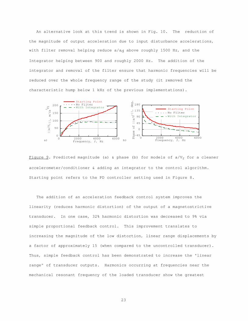
removing Eqn. 10. Figure 9 shows magnitude and phase of acceleration per unit

reference voltage for the PD controller conditions of Fig. 8, with the band

pass filter, as a solid line, and without the band pass filter as a dotted

line. Removal of the filter results in a fairly large improvement in output

linearity, with a substantial shift towards constant magnitude apparent in the

dashed line. It has the net effect of restoring the high frequency feedback

signal. From almost 2000 Hz out to 6000 Hz a relatively constant acceleration

per input reference voltage is exhibited and a phase angle closer to a zero

is achieved.

In addition, Fig. 9 illustrates the influence of an integrator, although no

integrator was experimentally implemented. The dashed curves labeled "with

integrator" show the effects of adding a modest amount of integration to the

"no filter" control algorithm. (Integrators are usually high gain, first

order low pass active filters. The integrator modeled here had the transfer

function: 1/(s x 2.2 kΩ x 0.1 µF + 2.2 kΩ / 22 kΩ) x Summing Gain. The -3 dB

point for this circuit was approximately 90 Hz, i.e., it resembled an

integrator (1/s) for frequencies greater than 90 Hz. As presented, ki ≈

16,500 V/(sV).)

As shown in the figures, removing the filter would significantly improve

output accelerations per unit reference voltage. Incorporating an integrator

into the controller would improve the system behavior at the lower

frequencies.

23

An alternative look at this trend is shown in Fig. 10. The reduction of

the magnitude of output acceleration due to input disturbance accelerations,

with filter removal helping reduce a/ad above roughly 1500 Hz, and the

Integrator helping between 900 and roughly 2000 Hz. The addition of the

integrator and removal of the filter ensure that harmonic frequencies will be

reduced over the whole frequency range of the study (it removed the

characteristic hump below 1 kHz of the previous implementations).

0

50

100

150

200

0 2000 4000 6000

Starting PointNo FilterWith Integrator

||a/Vr||, m/(s2 V

)

Frequency, ƒ, Hza)

-45

0

45

90

135

180

0 2000 4000 6000

Starting PointNo FilterWith Integrator

Phase of ||a/Vr||, deg.

Frequency, ƒ, Hzb)

Figure 9 . Predicted magnitude (a) & phase (b) for models of a/Vr for a cleaner

accelerometer/conditioner & adding an integrator to the control algorithm.

Starting point refers to the PD controller setting used in Figure 8.

The addition of an acceleration feedback control system improves the

linearity (reduces harmonic distortion) of the output of a magnetostrictive

transducer. In one case, 32% harmonic distortion was decreased to 9% via

simple proportional feedback control. This improvement translates to

increasing the magnitude of the low distortion, linear range displacements by

a factor of approximately 15 (when compared to the uncontrolled transducer).

Thus, simple feedback control has been demonstrated to increase the "linear

range" of transducer outputs. Harmonics occurring at frequencies near the

mechanical resonant frequency of the loaded transducer show the greatest

24

attenuations (approaching 30 dB in this study). Differential feedback tended

to increase harmonics at the lower frequencies and decrease those occurring at

the higher frequencies. Modeling implies that adding an integrator to the

control algorithm would tend to reduce the low frequency harmonics.

-30

-25

-20

-15

-10

-5

0

5

0 2000 4000 6000

Starting PointNo FilterWith Integrator

||a/ad||, dB

Frequency, ƒ, Hz

Figure 10 . Model predictions of the

output acceleration magnitude due to

input disturbance accelerations.

Starting point refers to the PD

controller setting used in Figure 8,

with a band pass filter and no

integrator.

5. CONCLUSIONS

The utility of simple analog feedback control for the linearization of

nonlinear magnetostrictive transducers has been demonstrated experimentally.

Both proportional and proportional plus derivative acceleration feedback

control were shown to reduce the harmonic frequency content of the transducer;

though not in a simple or intuitive way. Thus, attentions were turned to

developing models to predict and explain the behavior of the closed loop

system.

Using only simple linear systems relations (linear feedback control &

transduction theories), expressions were

developed for predicting closed loop system behavior. Specifically, two cases

were examined. In the first it was assumed that a current control amplifier

25

of appreciable robustness were used. There, expressions were developed for

output displacement from input reference voltage, u/V_r (s), and output

displacement from input disturbance displacement, u/u_d (s). Equipment

problems forbade experimental verification of those expressions. For the

second case, that of a voltage control amplifier, expressions were developed

for output acceleration from input reference voltage, a/V_r (s), and output

acceleration from input disturbance acceleration, a/a_d (s). These

expressions were experimentally verified. Thus, one can, with confidence,

analytically model the behavior of the closed loop system predicting the

observed reductions in output harmonics and predicting the "desired" system

output as a function of frequency.

Three methods one might use to estimate magnetostrictive transducer model

parameters were presented. Model predictions from two of the methods were

compared with experimental measurements. The more elaborate method, that

which included the effects of eddy currents within the transducer, produced

the better of the two closed loop model predictions.

The analytical expressions previously developed were used to explore system

behavior under the assumptions that one used better components and then added

an integrator to the controller. Model predictions indicate that there is a

lot to be gained by employing both an integrator and higher quality

components. The techniques developed in this paper are applicable to general

vibration control applications that employ magnetostrictive transducers.

ACKNOWLEDGMENTS

We would like to acknowledge financial support of this study by the

National Science Foundation. Support was provided through a Research

Initiation Award, MSS-9212065, and a Young Investigator Award, CMS-9457288.

26

Our thanks go out to Tad Calkins and Rick Zrostlik, for their input and

patience, to Chad Bouton who gave up space, capacitors, and serenity in

service to this research, and to Toby Hansen and Kevin Shoop at Edge

Technologies, Inc., for their magnetization, availability, and parts services.

27

REFERENCES

1. Hunt, F. V. 1982 "Electroacoustics: The Analysis of Transduction, and

Its Historical Background," Acoustical Society of America, Woodbury, NY.

2. Hall, D. L. 1994 "Dynamics and vibrations of magnetostrictive

transducers," a PhD Dissertation, Iowa State University, Ames, IA.

3. Clark, A. E., Teter, J. P., Wun-Fogle, M., Moffett, M. B., Lindberg, J.

1990 "Magnetomechanical Coupling in Bridgman-Grown Tb0.3Dy0.7Fe1.9 at High

Drive Levels," J. Appl. Phys., Vol. 67, pp. 5007-9.

4. Clark, A. E. 1980 "Magnetostrictive rare earth-Fe2 compounds," Ch. 7 of

Ferromagnetic Materials, Vol. 1, E. P. Wohlfarth Editor, North-Holland

Publishing Co., Amsterdam, pp. 531-589.

5. "Measurements of ultrasonic magnetostrictive transducers, 1984,

"International Electrotechnical Commission IEC Report, Publication 782.

6. Hall, D. L., Flatau, A. B. 1995 "One-Dimensional Analytical Constant

Parameter Linear Electromagnetic-Magnetomechanical Models of a Cylindrical

Magnetostrictive (Terfenol-D) Transducer," J. of Intelligent Materials Systems

and Structure, Technomic Publ. Co., Inc., Lancaster, Vol. 6, No.3 pp.315-328.

7. Horowitz, P., Hill, W., The Art of Electronics, 2nd Ed., Cambridge

University Press, Cambridge, pp. 224-5, 1989.

8. Edge Technologies, Inc. 1988 "Typical Material Properties," Ames, IA.

9. James, M. L., Smith, G. M., Wolford, J. C., Whaley, P. W. 1989 Vibration

of Mechanical and Structural Systems: With Microcomputer Applications, Harper

& Row Publishing, Inc., New York.

10. Franklin, G. F., Powel, J. D., Emami-Naeini, A. 1986 Feedback Control of

Dynamic Systems, Addison-Wesley Publishing Co., Reading, pp. 113-8.

28

11. Dapino, M.J., Calkins, F.T., Hall, D.L. and Flatau, A.B. 1996 "Measured

Terfenol-D material properties under varied operating conditions", SPIE

Proceedings on Smart Structures and Integrated Systems , paper #66, Vol. 2717,

pp. 697-708.

12. Calkins, F.T., Dapino, M.J., and Flatau, A.B. 1997 "Effect of Prestress

on Terfenol-D Material Properties", SPIE 1997 Proceedings on Smart Structures

and Integrated Systems , in press.