CSIR–National Physical Laboratory Metrology Society of India ...
Upload
khangminh22Category
view
2download
0
Guide to Engineering Metrology
Carl Hitchens MSc. CEng FIMechE Technical contributions: S. Cavill, R. Smalley and P. Hulme
Version 4

1
C. Hitchens The contents of this document should not be reprinted or redistributed.
TABLE OF CONTENTS
Introduction.............................................................................................................................................. 3
Dimensional Metrology ............................................................................................................................ 4
SI units, the international system ............................................................................................................ 5
The 10% Rule ......................................................................................................................................... 7
Hand Tools .............................................................................................................................................. 8
Abbe’s Principle .................................................................................................................................... 11
Accuracy and Precision ......................................................................................................................... 12
Measurement Process .......................................................................................................................... 13
Calibration ............................................................................................................................................. 16
Traceability ............................................................................................................................................ 17
Design for Inspection ............................................................................................................................ 18
Measurement Strategy .......................................................................................................................... 20
Measurement System Analysis ............................................................................................................. 21
Uncertainty ............................................................................................................................................ 29
Introduction to GD&T (Geometric Dimensioning and Tolerancing) ...................................................... 32
Variations of Form Rule #1: Envelope Principle Taylor Principle ............................................................. 33
Material Condition Modifiers ................................................................................................................................ 34
Bonus Tolerance ......................................................................................................................................................... 34
Regardless of feature size (RFS).......................................................................................................................... 37
Virtual Condition ........................................................................................................................................................ 37
Datum ............................................................................................................................................................................. 38
Airy and Bessel points ........................................................................................................................... 40
Inspection Methods for GD&T ............................................................................................................... 41
Straightness Feature ................................................................................................................................................. 41
Flatness Feature ......................................................................................................................................................... 44
Circularity (Roundness) Feature ......................................................................................................................... 46
Cylindricity Feature ................................................................................................................................................... 46
Profile of a Line Feature .......................................................................................................................................... 49
Profile of a Surface Feature .................................................................................................................................... 51
Angularity ...................................................................................................................................................................... 52
Perpendicularity ......................................................................................................................................................... 55
Parallelism..................................................................................................................................................................... 58

2
C. Hitchens The contents of this document should not be reprinted or redistributed.
Position ..........................................................................................................................................................................60
Concentricity (Coaxiality) Feature ...................................................................................................................... 61
Symmetry ...................................................................................................................................................................... 62
Runout Feature ........................................................................................................................................................... 63
Total Runout Feature ................................................................................................................................................ 63
Inspection Gauges ................................................................................................................................ 66
Threads ................................................................................................................................................. 67
Coordinate Measuring Machine ............................................................................................................ 71
Coordinate Measuring Machines and GD&T .................................................................................................. 75
On-Machine Probing ............................................................................................................................. 77
Large Volume Metrology ....................................................................................................................... 83
Laser Tracker .............................................................................................................................................................. 83
Optical Tracking ......................................................................................................................................................... 85
Auto Collimator, Optical Alignment Telescope and Inclinometer .......................................................... 86
Autocollimator ............................................................................................................................................................ 86
Optical Alignment Telescope ................................................................................................................................. 86
Inclinometer ................................................................................................................................................................. 87
Non-Contact Measurement and Scanning Instruments ........................................................................ 88
Laser Line Scanners and laser strip scanners ................................................................................................88
Structured light .......................................................................................................................................................... 89
Photogrammetry ....................................................................................................................................................... 90
Inspection Process for Scanning Instruments ....................................................................................... 92
Reverse Engineering ............................................................................................................................. 94
Manufacturing Process Capabilities .................................................................................................... 100
Bibliography ........................................................................................................................................ 102

3
C. Hitchens The contents of this document should not be reprinted or redistributed.
INTRODUCTION
Metrology is the science of measurement and the understanding of a measurements quantity and quality.
Quality is shown by providing evidence of traceability and accuracy. Measurements should be repeatable,
reproducible and reliable and the engineer making these measurements should have an understanding of their
uncertainty.
The origins of Metrology date back to 1550-1069 BC when the Egyptian cubit was brought into existence and is
believed to be the first unit of measurement. It was a defined length based on the distance from the Pharaoh's
elbow to the tip of his middle finger (52cm) and divided into 7 palms and 28 fingers. Today in Europe we use the
metre developed in 1789 after the French revolution and this is subsequently divided into the millimetre and
the micron. The meter is no longer defined by a Platinum-Iridium as it was for many decades; it is now defined
by the distance that the light from an Iodine-stabilised Helium Neon laser takes to travels through a vacuum in
1/299,792,458 of a second. With the second defined to be the duration of 9192631770 periods of radiation
corresponding to the transition between the two hyperfine levels of the ground state of the Caesium 133 atom.
It is not essential for the engineer to know or understand this detail, it is, however, important that we appreciate
the fundamental science that maintains the SI units we use and how they ensure standardisation around the
world.
This book is intended to be a quick guide for the engineer and to inform the reader of the important
considerations to be mindful of when making measurements and to also raise awareness of techniques and
technologies available to aid the engineer in the measurement process. This book is not intended to provide a
highly detailed source of information neither is it intended to replace the many existing and excellent publications
available, the intention is to complement these existing publications. Where I have made recommendations on
best practice these are always stated in good faith, however, there are always exceptions to the rule and it is
impossible to cover every variable and eventuality.
4
C. Hitchens The contents of this document should not be reprinted or redistributed.
DIMENSIONAL METROLOGY
When manufacturing components it is essential that we employ good measurement practice with repeatable
and controlled processes. This ensures that parts conform to dimensional and tolerance specifications, meeting
the design intent. Metrology enables the manufacturer to monitor process capability and variation over time.
Traditionally, coordinate measuring machines have been the technology against which all other measurements
are validated. While these technologies are extremely accurate they are also labour intensive and relatively slow,
especially when capturing free form surfaces. Recent developments in measurement technologies present us
with a wide range of possible methodologies. In general, they will reside in one of two groups, in-process and
post-process; these can then be subdivided further into contact and non-contact. Contact methods provide
more confidence in measurement as a physical interaction occurs during the measurement process. Contact
methods are also more readily traceable to the SI unit (metre) by means of physical artefacts often referred to
as transfer standards. Non-contact methods have some ambiguity as to what specific point was measured and
whether the surface texture of reflectivity caused any change in the recorded value.
In-process inspection technologies:
Advantages:
Improved process capability and component quality.
Increased conformance confidence.
Automated inspection removes human error.
The necessity to transfer large components to CMM is removed.
Disadvantages:
May not be an independent validation of the component conformity.
If not independent the requirement to validate the machine tool as a measurement instrument is
necessary.
Post-process inspection technologies:
Advantages:
Independent validation of component conformity.
Technology is validated as a measurement instrument.
Automated inspection removes human error.
Disadvantages:
The transfer of components to CMM is required.
Errors are detected after manufacture.
Re-working of components requires setting and re-establishing of datum.
Significant capital cost.

5
C. Hitchens The contents of this document should not be reprinted or redistributed.
SI UNITS, THE INTERNATIONAL SYSTEM
The metre is one of the SI base units of which there are seven. These units were agreed by the 11th General
Conference on Weights and Measures in 1960 and form the basis for all modern science and technology. Two
classes of unit exist, base units and derived units. Derived units as the name suggests are products of the bases.
Quantity Unit Symbol
Mass Kilogram kg
Time Second s
Length Metre m
Temperature Kelvin K
Electric Current Ampere A
Luminescence Candela cd
Amount of Substance Mole mol
SI base units
(a) The symbol '1' is generally omitted in combination with a numerical value.
SI derived units
In precision engineering the metre is not directly used, preference is given to the millimetre (mm) a division of
the metre is preferred when dimensioning components and the micron (µm) is preferred when stating the
Derived Quantity Unit Symbol
Area square metre m2
Volume cubic metre m3
Velocity metre per second m/s
Acceleration metre per second squared m/s2
Wavenumber 1 per metre m-1
Density, mass density kilogram per cubic metre kg/m3
Specific volume cubic metre per kilogram m3/kg
Current density ampere per square metre A/m2
Magnetic field strength ampere per metre A/m
Concentration mole per cubic metre mol/m3
Luminance candela per square metre cd/m2
refractive index (the number) one 1(a)

6
C. Hitchens The contents of this document should not be reprinted or redistributed.
precision of the measurement instrument. It is important to appreciate the magnitude of these divisions of the
metre. If I state that the millimetre is 10-3 and the micron is 10-6 relative to the metre, you will find it hard to
visualise. Alternatively stating that a millimetre is 0.001and a micron is 0.000001 of a metre is equally unhelpful.
Appreciating the millimetre is easily achieved by picking up any rule but the micron needs to be compared
relative to items we can relate; such the human hair typically 100µm or at singular micron values, fine dust and
smoke; as shown below.
Having given some thought to the magnitude of the micron, we should consider carefully accuracy when
specifying tolerances for the features of a component. High precision comes at a significant price, not only at
the point of manufacture but also during the measurements process. As we pursue precisions of less than 50µm
we need to find increasingly more sophisticated manufacturing methods and machinery and therefore
measurement instruments with a resolution to validate the component conformity. The relationship between
cost and precision is not a linear and you will find that linear reductions in a specified tolerance will cause an
exponential growth in the cost. To compete in the global market we should always question if the feature
tolerances are appropriate to achieve component performance and also economical manufacture. A
compromise is often required to achieve a functional and yet commercially competitive product.
7
C. Hitchens The contents of this document should not be reprinted or redistributed.
THE 10% RULE
Measurement uncertainty as defined by the GUM “Guide to the expression of uncertainty in measurement” is
commonly stated as a ± value or a range of values in which the true value is estimated to lie. Uncertainty is,
therefore, the doubt that exists about the measurement. Understanding measurement uncertainty is critical to
the selection of a technology and methodology. As a guide, the uncertainty should be 10% of the dimensional
tolerance required. Although in demanding application 20% is often considered acceptable. We should keep this
in mind when reporting measurement values close to the tolerance limits. As an example, a dimension of
20mm±0.1 mm is measured and the value recorded is 19.91mm. The measurement instrument has a stated
uncertainty of ±0.1mm at a confidence level of 95%, this is 2 standard deviations, often referred to as Kx2
expanded coverage factor (this is how calibration certificates commonly state uncertainty, this also means that
5% of recorded values will be distributed outside this uncertainty tolerance). Taking account of the instrument
uncertainty and combining with the displayed value, the true measurement lies in the range of 19.81mm to
20.01mm and therefore potentially out of tolerance. Whenever the displayed value nears tolerance limits the
uncertainty of the instrument should be considered and stated on the measurement report. You should also
consider your uncertainty budget; this is explained in more detail in the chapter “Uncertainty”.
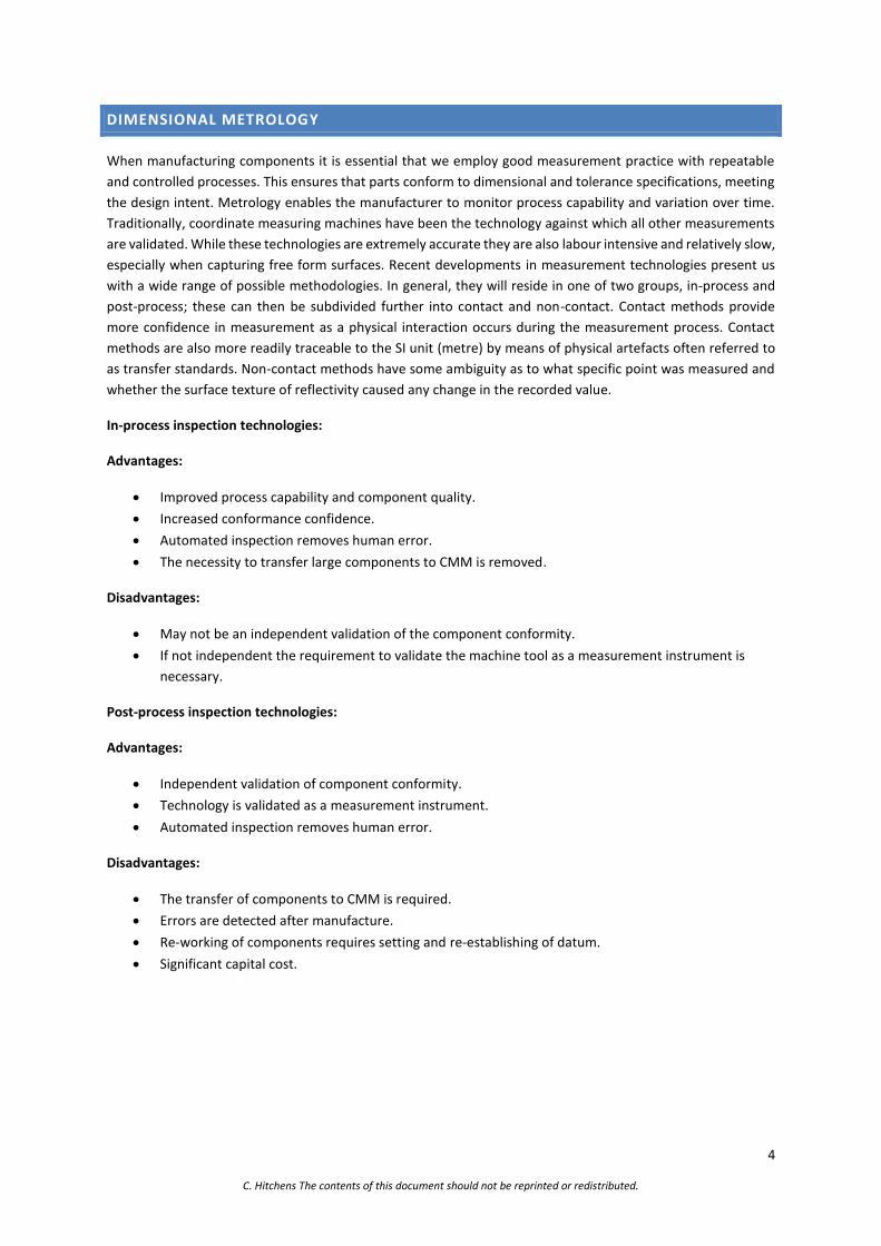
With many measurement technologies, as the length of measurement increases so does the uncertainty of
measurement. The image below provides a depiction of typical measurement technologies and their typical
working range and how measurement uncertainty increases with the increase in dimension.
Depicts a generalisation of instrument performance and how accuracy decreases in relation to the measured
size. (Please note the scales are not linear in this depiction).

8
C. Hitchens The contents of this document should not be reprinted or redistributed.
HAND TOOLS
When selecting a hand tool instrument to perform a measurement, you should consider the tolerance
requirements of the component and perform a measurement system analysis; information on this is provided
in chapter “Measurement System Analysis”. It is worth investing in good quality instruments and checking their
specification before purchasing.
Vernier caliper is a versatile measurement instrument that can measure internal and external features and can
also measure depth. Due to this versatility and operator variability, accuracy and precision are compromised.
The primary reason for this is explained in the “Abbe’s Principle” chapter. The Vernier scale provides the
measurement reading, digital calipers are available.
Height gauge has a single axis of measurement and is commonly used in first principle inspection. They do
require experience to determine the appropriate force “feel” when we make fine adjustments during the
measurement process. Digital versions are available and some have electronically triggered measurement
recording, this removes much of the feel required during measurement and greatly improves repeatability.

9
C. Hitchens The contents of this document should not be reprinted or redistributed.
A micrometer is one of the most accurate instruments readily available in engineering. Where practical they
should be used whenever possible, they are also one of the few instruments that obey Abbe’s Principle. The
Ratchet and not the thimble should be used to maintain a consistently applied force and greatly improve the
repeatability of the measurement.
The micrometer is available in a wide variety of configurations to enable the inspection of bores, grooves,
threads and depths.
Below is a demonstration of how to read the Vernier scale of a micrometer with a resolution of two decimal
places. Micrometers are available with an additional scale providing a resolution of three decimal places.

10
C. Hitchens The contents of this document should not be reprinted or redistributed.
A dial test indicator is an extremely accurate instrument and is used in many of the first principle method
described in this document. A dial test indicator measures the deflection of the arm as it swings around its
rotation point. These indicators actually measure angular displacement; linear distance is converted from the
angular displacement. If the direction of movement is perpendicular to the probe, the linear displacement error
(cosine error) will be small and within the resolution of the dial. However, this error starts to become an
important consideration when the angle increases beyond 10°. Cosine error is shown in more detail below and
as an example, an angle 40° with an indicator Reading 0.05mm requires a correction Factor .940 (cos 40°)
therefore 0.05 x .940 = 0.038mm corrected. The instrument is also subject to the effects Hysteresis or drift due
to backlash and should be reset after a number of measurement cycles.
Angle A Correction Factor
10° .985
20° .940
30° .866
40° .766
50° .643
0° .500
Pear shaped contact probe eliminates cosine error up to 36⁰ the drawing of the contact point shows another
way of thinking about cosine error; the relationship of the horizontal distance between two centres. If the
distance between the two centres is reduced, an error will occur. The pear shaped contact allows for the centre
distance to the contact point to remain constant.

11
C. Hitchens The contents of this document should not be reprinted or redistributed.
ABBE’S PRINCIPLE
Abbe’s principle is based on the simple fact that mechanical structures are prone to
deflection. To have a precise instrument the line of measurement should be coincidental
with the scale of the measurement instrument and aligned with the applied force. As you
will see below the micrometer demonstrates this principle perfectly. However, the caliper
does not and is prone to measurement error due to deflection of the measuring faces
resulting from applied pressure. In order to minimise this effect, measurements should
always be taken close to the scale and the root of the measurement faces where it is
practical to do so. It should be noted that very few measurement instruments obey Abbe’s
principle.
Error =A*sin(θ)

12
C. Hitchens The contents of this document should not be reprinted or redistributed.
ACCURACY AND PRECISION
When we are to consider a measurement technology and its application we should first consider its accuracy.
Accuracy is how well the recorded value of an instrument agrees with the actual true value of the measurand.
The precision of the instrument should not be confused with accuracy; precision is the variance in the recorded
value of a repeated measurement. It is possible to have an instrument with high precision and poor accuracy.
This would result in repeated measurement showing good correlation. However, the recorded value would not
represent the true value. This is referred to as a systematic error and in many cases, the instrument can be
calibrated to compensate. With common engineering measurement instruments such as micrometres and
callipers, accuracy and precision can be confirmed by means of a transfer standard such as gauge blocks (this is
not the full picture and a gauge R&R study is required to reveal the measurement uncertainty, this is discussed
later).
Accuracy and precision (left), precision without accuracy (middle) and low accuracy without precision (right)
Transfer standards provide an unbroken traceable path to the SI unit held by the National Measurement
Institute. When working with large volume dimensions, establishing measurement performance becomes
difficult due to the lack of transfer standards at lengths greater than a metre and also the expense of such large
standards. It is tempting to refer to the instrument resolution and the number of decimal places that the
instrument can display or divisions on the scale that can be read, it is important not to confuse this with accuracy.
Many digital instruments will display values in millimetres down to the third decimal place however the accuracy
of many of these instruments resides at the second decimal place.

13
C. Hitchens The contents of this document should not be reprinted or redistributed.
MEASUREMENT PROCESS
It is important to introduce the correct terminology used in the science of measurement. By using standards
terms we reduce the risk of misinterpretation when communicating verbally or in written reports. When we
need to understand the dimensions of a component we employ “Measurement”. Measurement is the process
that we use to obtain the true value of a quantity. The quantity being determined is called the “Measurand” and
in the case of dimensional metrology, it is the physical object being measured. To report the value of the
measurand, we use instruments to convert the physical into a value that we can record; in the case of
engineering, the value is typically recorded in millimetres. Many engineers will be familiar with the inch (in) unit
of measurement, but it wasn’t until 1930 that the standardisation of the inch across countries started to take
place and the modern international inch was established as 25.4 mm. The international inch is actually 1.7
millionths of an inch longer than the old British Imperial unit. Surprisingly, the old US inch was larger and had to
be reduced by 2 millionths of an inch.
Summary:
Measurement is the process to obtain the true value of a quantity.
Quantity being determined is called the measurand.
Measurand is the physical object being measured.
Measurement Instrument is used to convert the measurand into a unit value.
Measurements are never perfect and we can never be certain that the displayed value is the “True value” of the
measurand. Therefore a measurement is only ever an estimate. The instrument is only one component of the
“Measurement system” and many factors exist in the system. The term used to describe all the factors
influencing or interacting with the measurement process is “Measurement system”. I have endeavoured to list
the most influential factors on the measurement system below and also provide a more comprehensive list as
an Ishikawa diagram in the chapter on “Uncertainty”.
Age and Wear
Applied Pressure
Calibration
Cleanliness
Fixture
Knowledge-instrument
Lighting
Parallax Error
Reading error
Surface Texture
Temperature
Performing multiple measurements of the Measurand will generally form a normal or Gaussian distribution with
the majority of the recorded values will be grouped around the true value and a diminishing number of values
drifting away from the true value out towards a remaining few outlying values; this is called a random error. A
random error exists in all measurements and is introduced by the factors of the measurement system. A high
precision instrument and robust measurement system have the effect of reducing the overall spread of the
distribution.
14
C. Hitchens The contents of this document should not be reprinted or redistributed.
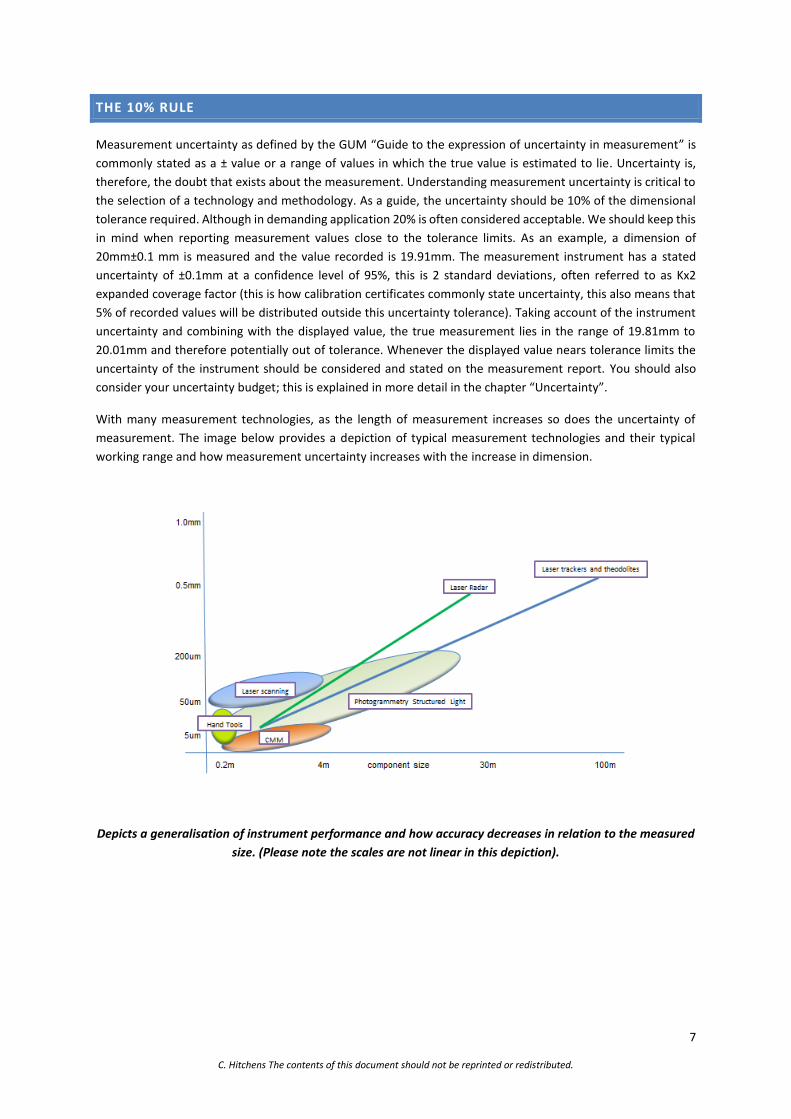
A systematic error is a skew in the measurement distribution, where we see a shift in the centre of the normal
distribution away from the true value, this is referred to as “Bias”. This bias is most often a result of instrument
error and is often corrected by calibration. As a simple example, if you zero a digital Caliper when the measuring
faces are open. All subsequent measurements with this instrument will be displaced by the value of the gap
between the measurement surfaces at the time of zeroing the instrument. The precision of the instrument will
not have changed but the error will influence the measured values and indicate an incorrect reading. Other
factors of the measurement system, for example, applied pressure, temperature, fixtures, etc. can create a
systematic error and a bias in measured values.
Normal or Gaussian distribution and a skewed distribution.
I previously mentioned that one of the causes of bias can be applied pressure. Many micrometers now have a
ratchet attached to the end of the thimble, which is designed to control the applied pressure and therefore
increase the consistency of the measurements taken. In the case of calipers and height gauges, thumb wheels
have been introduced but are still prone to a greater variation in applied pressure.
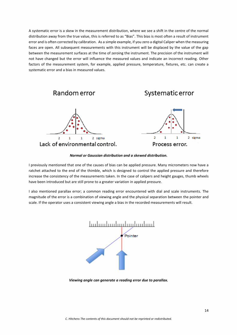
I also mentioned parallax error; a common reading error encountered with dial and scale instruments. The
magnitude of the error is a combination of viewing angle and the physical separation between the pointer and
scale. If the operator uses a consistent viewing angle a bias in the recorded measurements will result.
Viewing angle can generate a reading error due to parallax.

15
C. Hitchens The contents of this document should not be reprinted or redistributed.
Temperature can also create a bias. The agreed international temperature for measurement is set at 20⁰C and
any deviation from this will result in expansion or contraction of the measurand. The typical coefficient of
expansion for steel is around 12µm per metre per degree; dependant on its composition. If you know the
coefficient of expansion of the measurand and the temperature is recorded at the time of performing the
measurement it is possible to compensate the measurement by using the calculation below.
Calculation:
L20 =LT + (20 - T) α LT
LT = Length measured.
T = Ambient temperature when the measurement was taken.
α = The coefficient of expansion of the measurand.
Always ensure the thermometer is functioning correctly and in calibration to ensure traceability of the recorded
measurements.

16
C. Hitchens The contents of this document should not be reprinted or redistributed.
CALIBRATION
The purpose of calibration is to detect, correct and document the instrument performance and uncertainty.
Instruments require calibration because their accuracy may drift over time, generating a systematic error and a
bias in the recorded measurement, which requires correction. This recalibration is performed by comparison of
the measurement instrument against a standard of higher accuracy such as a gauge block. Engineers frequently
perform a calibration when using a digital Caliper; they clean and close the measuring faces than the digital
display is zeroed, performing a calibration of the instrument. However, this is not formally recorded.
No standard is available that dictates how frequently an instrument should be calibrated. To determine the time
interval between calibrations, one should initially monitor instruments stability. As an example, a micrometer
used infrequently in a clean final inspection department should initially be calibrated every three months and
the result should be recorded and reviewed against previous calibration results to check for instrument stability.
If over time no change is observed, then it could be considered acceptable to extend the interval between
calibrations. I have suggested three months as an example; however, if the instrument is in constant use in an
area where cleanliness is an issue, perhaps a shorter interval would be more appropriate. Another important
consideration is the quantity and value of components that the instrument will have validated during the
calibration interval. Should the instrument be found to be out of calibration at what time during the three
months period did this occur? To be sure of product quality all products measured during the three months will
need to be checked and validated again, this could be an expensive and potentially embarrassing scenario.
Things to consider when defining the calibration period:
How stable is the instrument over time.
How often is the instrument used.
The quantity and value of the components validated by the instrument.
The environment and storage.
The manufacturer's specification for the instrument.
When calibrating a measurement instrument it is the convention to use a standard with accuracy greater than
4 to 1 of the accuracy of the instrument being calibrated. Specifically, micrometers, calipers and height gauges
should always be check for wear and damage not only of the measurement faces but also the frame of the
instrument and that it operates smoothly; any repairs should be performed prior to calibration. Then 5 points
over the measurement range should be checked, returning to zero between each measurement. It is also
important not to choose integer values, especially with digital instruments. Until recently the specification of
these types of the instrument was defined by international standards and instrument manufacturers had to
meet these specifications. This has now changed and it is now the responsibility of the instrument manufacturer
to state the specification for their product. This means as engineers we need to be more cautious when selecting
a measurement instrument. It may also mean that we see instruments of a lower quality being produced.
With any instrument, it is unwise to simply rely on the calibration procedure and the calibration sticker. When
using an instrument always check for damage and wear. It is also good practice to perform simple measurement
validation against a standard. For a micrometer and caliper measuring a range of gauge blocks over the
instruments measuring the range to check it is performing as expected, is time worthwhile spent prior to
performing your measurement task.
17
C. Hitchens The contents of this document should not be reprinted or redistributed.
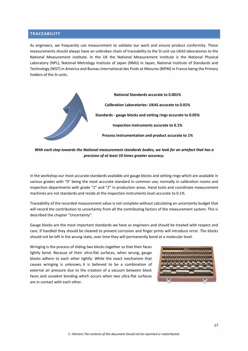
TRACEABILITY
As engineers, we frequently use measurement to validate our work and ensure product conformity. These
measurements should always have an unbroken chain of traceability to the SI unit via UKAS laboratories to the
National Measurement institute. In the UK the National Measurement institute is the National Physical
Laboratory (NPL), National Metrology Institute of Japan (NMIJ) in Japan, National Institute of Standards and
Technology (NIST) in America and Bureau International des Poids et Mesures (BIPM) in France being the Primary
holders of the SI units.
National Standards accurate to 0.001%
Calibration Laboratories- UKAS accurate to 0.01%
Standards - gauge blocks and setting rings accurate to 0.05%
Inspection instruments accurate to 0.1%
Process instrumentation and product accurate to 1%
With each step towards the National measurement standards bodies, we look for an artefact that has a
precision of at least 10 times greater accuracy.
In the workshop our most accurate standards available are gauge blocks and setting rings which are available in
various grades with “0” being the most accurate standard in common use; normally in calibration rooms and
inspection departments with grade “1” and “2” in production areas. Hand tools and coordinate measurement
machines are not standards and reside at the inspection instruments level accurate to 0.1%
Traceability of the recorded measurement value is not complete without calculating an uncertainty budget that
will record the contribution to uncertainty from all the contributing factors of the measurement system. This is
described the chapter “Uncertainty”.
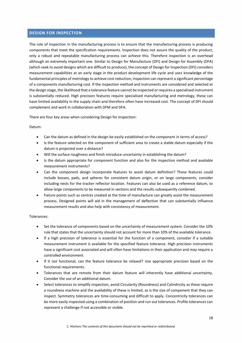
Gauge blocks are the most important standards we have as engineers and should be treated with respect and
care. If handled they should be cleaned to prevent corrosion and finger prints will introduce error. The blocks
should not be left in the wrung state, over time they will permanently bond at a molecular level.
Wringing is the process of sliding two blocks together so that their faces
lightly bond. Because of their ultra-flat surfaces, when wrung, gauge
blocks adhere to each other tightly. While the exact mechanism that
causes wringing is unknown, it is believed to be a combination of
external air pressure due to the creation of a vacuum between block
faces and covalent bonding which occurs when two ultra-flat surfaces
are in contact with each other.
18
C. Hitchens The contents of this document should not be reprinted or redistributed.
DESIGN FOR INSPECTION
The role of inspection in the manufacturing process is to ensure that the manufacturing process is producing
components that meet the specification requirements. Inspection does not assure the quality of the product,
only a robust and repeatable manufacturing process can achieve this. Therefore inspection is an overhead
although an extremely important one. Similar to Design for Manufacture (DFI) and Design for Assembly (DFA)
(which seek to avoid designs which are difficult to produce), the concept of Design for Inspection (DFI) considers
measurement capabilities at an early stage in the product development life cycle and uses knowledge of the
fundamental principles of metrology to achieve cost reduction; inspection can represent a significant percentage
of a components manufacturing cost. If the inspection method and instruments are considered and selected at
the design stage, the likelihood that a tolerance feature cannot be inspected or requires a specialised instrument
is substantially reduced. High precision features require specialised manufacturing and metrology, these can
have limited availability in the supply chain and therefore often have increased cost. The concept of DFI should
complement and work in collaboration with DFM and DFA.
There are four key areas when considering Design for Inspection:
Datum:
Can the datum as defined in the design be easily established on the component in terms of access?
Is the feature selected on the component of sufficient area to create a stable datum especially if the
datum is projected over a distance?
Will the surface roughness and finish introduce uncertainty in establishing the datum?
Is the datum appropriate for component function and also for the inspection method and available
measurement instruments?
Can the component design incorporate features to assist datum definition? These features could
include bosses, pads, and spheres for consistent datum origin, or on large components, consider
including nests for the tracker reflector location. Features can also be used as a reference datum, to
allow large components to be measured in sections and the results subsequently combined.
Fixture points such as centres created at the time of manufacture can greatly assist the measurement
process. Designed points will aid in the management of deflection that can substantially influence
measurement results and also help with consistency of measurement.
Tolerances:
Set the tolerance of components based on the uncertainty of measurement system. Consider the 10%
rule that states that the uncertainty should not account for more than 10% of the available tolerance.
If a high precision of tolerance is essential for the function of a component, consider if a suitable
measurement instrument is available for the specified feature tolerance. High precision instruments
have a significant cost associated and will often have limitations in their application and may require a
controlled environment.
If it not functional, can the feature tolerance be relaxed? Use appropriate precision based on the
functional requirements.
Tolerances that are remote from their datum feature will inherently have additional uncertainty.
Consider the use of an additional datum.
Select tolerances to simplify inspection, avoid Circularity (Roundness) and Cylindricity as these require
a roundness machine and the availability of these is limited, as is the size of component that they can
inspect. Symmetry tolerances are time-consuming and difficult to apply. Concentricity tolerances can
be more easily inspected using a combination of position and run out tolerances. Profile tolerances can
represent a challenge if not accessible or visible.

19
C. Hitchens The contents of this document should not be reprinted or redistributed.
Accessibility:
Can instruments access the feature? Consider how hand tools will be deployed and the available lengths
of styli for the required uncertainty.
Will restricted access add to the uncertainty of the measurement system? Difficulty in operating the
instrument, lack of visibility of the interaction between the instrument and component and also reading
the results may all increase uncertainty.
Should we tolerance features that cannot be inspected? Aspirational tolerances are a constant source
of concern for manufacturers and inspectors.
Considerations:
Partial arc less than 90˚ represent a significant challenge to establish their true value.
Large dimensions with tight tolerances. These combinations are often outside the capability
measurement instruments.
Projected tolerances over substantial distance are difficult to measure and have a high uncertainty.
In process inspection, should be used where practicable. Find errors early in the manufacturing process
and in a worst case scrap the component before adding more value. Use the inspection results to
identify process issues before they impact on other components and use the results to improve the
production process.
Avoid repeated inspection; pass off features in the process and only visually inspect for damage at final
inspection. Extend this out to the suppliers to further reduce final inspection.
Surface roughness can influence measurement results, the smoother the surface the
more consistent the measurement will be. However, this will increase the cost of manufacture. Select
regions to apply higher surface finishes specifically for inspection and datum construction.
Inspection pre or post coating. What is the process control of the depth of coating and consider how
this may impact on the inspection process.
Component and measurement system, how susceptible are these to environmental change?
Many of the points highlighted in the Design for Inspection guide are discussed in more detail in subsequent
chapters.

20
C. Hitchens The contents of this document should not be reprinted or redistributed.
MEASUREMENT STRATEGY
Understanding the uncertainty of the measurement system can be difficult and often using first principles allows
the uncertainty of the measurement system to be more readily understood. All instruments and gauges are
known from the calibration certificates. Additional uncertainties from fixtures operators and environment can
be tested and by performing measurement system analysis. This is explained in the chapter “Measurement
System Analysis”. Before we can analyze the measurement system you first require a measurement strategy.
Below is a check list of key points that should be a consideration when developing the measurement strategy.
Check List:
Selection of features on the work piece to be measured.
Understand the work piece datum feature and its relationship to the coordinate system.
Selection of work piece orientation and fixtures.
Selection and qualification of measurement instruments it is critical to remember the 10% rule.
Understand how to use the instrument, especially the scale.
Check the calibration status and the instrument for damage.
Clean the instrument before use, in particular, the measurement faces.
Take more than one measurement and review the recorded values; do they make sense.
Perform an uncertainty budget calculation.
It is extremely important to check the instrument specification and its suitability for the measurement task and
tolerance requirements. We should not be influenced by the resolution of the instrument display; below we see
a digital caliper displaying a value of 0.4560in or 11.582mm. However, reviewing the instrument specification it
has an accuracy of +/-0.002in or 0.05mm. The fact that the resolution is displaying four decimal places in the
inch unit and 3 decimal places in the metric unit is irrelevant when the instrument has an accuracy of 3 decimal
place in inch mode and 2 decimal places in metric.
Display reading: 0.4560in 11.582mm Manufactures specification: Resolution 0.0005“ (0.001mm). Accuracy +/-0.002“ (0.05mm). At 2 sigma.
Furthermore, the instrument specification states that accuracy is at 2 sigma. This is a statement of the
percentage of measurements that will statistically fall within the stated accuracy. At 1 sigma (two standard
deviations) only 68.26% of measurement will be within the stated accuracy. This instrument is stated at 2 sigma
(four standard deviations) 95.44% of all measurements will comply. You could look for a specification that states
6 sigma (six standard deviations), an instrument of this type would provide the confidence that 99.73% of all
your measurements will be compliant.

21
C. Hitchens The contents of this document should not be reprinted or redistributed.
MEASUREMENT SYSTEM ANALYSIS
When you perform a measurement you should always question the values you are recording. All measurements
are an estimation of the true value and it is important to check the measurement system that is used. It is always
advisable to repeat each measurement three times this removes the risk of reading or recording errors. It is also
advisable to check the scale of the part with an alternative measurement instrument and question if the values
being recorded are realistic. This is more important when using measurement instruments where you are not
physically interacting with the measurand; instruments such as the coordinate measuring machine, laser tracker
and non-contact scanner. A quick secondary check with a caliper, tape or rule will provide a level of confidence
that the measurements are in the expected range.
Measurement systems have two main attributes, precision and accuracy.
Bias:
A shift in the centre of the normal distribution of recorded values away from the true value, bias can
be established by performing repeated measurements of a known artefact or standard. A minimum of
ten measurements is required. Although increasing the number to 25 would be preferable.
Linearity:
The difference in the recorded bias values over the expected operating range of the measurement
instrument.
Stability:
The variation observed in the average of recorded values, over a time period.
Repeatability:
Variation of measurement instrument established by performing repeated measurements under the
same conditions (same component, same operator, same fixture, same environment, etc.).
Accuracy
Bias
Linearity
Stability
Precision
Repeatabilty
Reproducability
22
C. Hitchens The contents of this document should not be reprinted or redistributed.
Reproducibility:
Variation resulting from the different configurations of the measurement system encountered in
normal use. These include a change of appraiser, change in time, changes in environment or location,
etc. Note: the measurement instrument must not be changed.
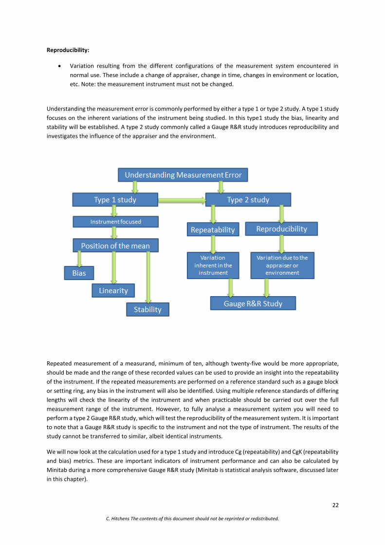
Understanding the measurement error is commonly performed by either a type 1 or type 2 study. A type 1 study
focuses on the inherent variations of the instrument being studied. In this type1 study the bias, linearity and
stability will be established. A type 2 study commonly called a Gauge R&R study introduces reproducibility and
investigates the influence of the appraiser and the environment.
Repeated measurement of a measurand, minimum of ten, although twenty-five would be more appropriate,
should be made and the range of these recorded values can be used to provide an insight into the repeatability
of the instrument. If the repeated measurements are performed on a reference standard such as a gauge block
or setting ring, any bias in the instrument will also be identified. Using multiple reference standards of differing
lengths will check the linearity of the instrument and when practicable should be carried out over the full
measurement range of the instrument. However, to fully analyse a measurement system you will need to
perform a type 2 Gauge R&R study, which will test the reproducibility of the measurement system. It is important
to note that a Gauge R&R study is specific to the instrument and not the type of instrument. The results of the
study cannot be transferred to similar, albeit identical instruments.
We will now look at the calculation used for a type 1 study and introduce Cg (repeatability) and CgK (repeatability
and bias) metrics. These are important indicators of instrument performance and can also be calculated by
Minitab during a more comprehensive Gauge R&R study (Minitab is statistical analysis software, discussed later
in this chapter).

23
C. Hitchens The contents of this document should not be reprinted or redistributed.
To determine bias and its relationship with component tolerance we can use the calculation.
Bias% = 100 × (Mean of Measured Values − Reference Measurement
Feature Tolerance)
Bias relative to feature tolerance, note: The mean of measured values is normally represented by 𝒙 and this
convention will be used for the remainder of the chapter.
The Reference Measurement should be a standard or alternatively an artefact that has a known value confirmed
by a measurement instrument with an accuracy significantly greater than that of the instrument being studied.
The feature tolerance is the total tolerance range available for the component feature of interest. Mean of the
measured values is derived from repeated measurement, a minimum of 10 measurements are required,
although increasing the number to 25 would be preferable.
As an example; a feature with a specified dimensional length has a tolerance defined at ±0.05mm, a mean
measured value of 15.36mm and a reference value of 15.37mm, the bias calculation would be (100 ×(15.36 –
15.37) ÷0.1) = 10% of the tolerance. Ideally, the required bias should be less than 10% of the feature tolerance.
Remember to also consider the uncertainty budget for the measurement system as described later in this
chapter.
This leads into a measurement system’s repeatability or type 1 study where a single appraiser performs the
repeated measurements and looks at how the measurement instrument performs on a single feature of a
component. A type 1 study is instrument focused and does not investigate all sources of uncertainty.
The Cg metric is a measure of the instruments repeatability and provides an understanding of how the range of
the measurements resides in the percentage of the feature tolerance.
Cg =(K ÷ 100) × Feature Tolerance
L × σ
Cg metric is a measure of the instruments repeatability.
K = the percentage of the Feature Tolerance, 20% is commonly used although 10% for a high precision
component may be advisable.
L = the number of standard deviations, 3 is commonly used in this calculation.
σ = the standard deviation.
A Cg benchmark value of 1.33 is widely used and indicates that the distribution of the measurements is
sufficiently narrow in relation to the allowable tolerance. For example, with the value of “K” at 20% and “L” at 3
standard distributions, a Cg metric of 2 would indicate that 20% of the tolerance range will cover the entire
distribution of measurements twice over. These are the normal defaults as specified In the Minitab software
discussed later in this chapter, in this software the calculation is referred to as the “study variation”.
24
C. Hitchens The contents of this document should not be reprinted or redistributed.
Repeated measurements will generally form a normally distributed, which is the reason we use 3 standard
deviations and 20% of the feature tolerance is the typical default values for the calculation (as specified in
Minitab), however sometimes 10% is used on critical components. Capability metric CgK, takes the Cg metric
(repeatability) calculation and incorporates the bias calculation. Values of between 1.33 and 1 may also be
acceptable dependant on the application of the measurement and values less than 1 indicate a system that is
not acceptable.
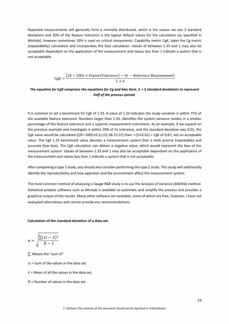
CgK =((K ÷ 200) × FeatureTolerance) − (x̅ − Reference Measurement)
L × σ
The equation for CgK comprises the equations for Cg and bias Here, 𝑳 = 3 standard deviations to represent
half of the process spread.
It is common to set a benchmark for CgK of 1.33. A value of 1.33 indicates the study variation is within 75% of
the available feature tolerance. Numbers larger than 1.33, identifies the system variance resides in a smaller
percentage of the feature tolerance and a superior measurement instrument. As an example; if we expand on
the previous example and investigate it within 20% of its tolerance, and the standard deviation was 0.01, the
CgK value would be calculated ((20÷200)×0.1)-(15.36-15.37) then ÷(3×0.01) = CgK of 0.67; not an acceptable
value. The CgK 1.33 benchmark value denotes a measurement system that is both precise (repeatable) and
accurate (low bias). The CgK calculation can deliver a negative value, which would represent the bias of the
measurement system. Values of between 1.33 and 1 may also be acceptable dependant on the application of
the measurement and values less than 1 indicate a system that is not acceptable.
After completing a type 1 study, you should also consider performing the type 2 study. This study will additionally
identify the reproducibility and how appraiser and the environment affect the measurement system.
The most common method of analysing a Gauge R&R study is to use the Analysis of Variance (ANOVA) method.
Statistical analysis software such as Minitab is available to automate and simplify the process and provides a
graphical output of the results. Many other software are available, some of which are free, however, I have not
evaluated alternatives and cannot provide any recommendations.
Calculation of the standard deviation of a data set.
σ = √∑(𝑥𝑖 − �̅�)2
𝑁 − 1
∑ Means the “sum of”.
𝑥𝑖 = Sum of the values in the data set.
�̅� = Mean of all the values in the data set.
𝑁 = Number of values in the data set.
25
C. Hitchens The contents of this document should not be reprinted or redistributed.
A typical study requires a minimum number of inputs to create meaningful results:
10 Parts (components to be measured should have a variation within the tolerance limits).
3 Appraisers (People performing the measurements).
3 Repeats (Each appraiser performs and records the same measurement three times).
Should insufficient parts or appraisers be available, the number of repeats should be increased to ensure a
minimum of 30 measurement values are generated for the analysis; 30 values are required to generate a
normal distribution and meet the requirements of the central limit theorem.
Where a fixture could influence the recorded value, the component must be removed from the fixture between
each measurement.
There are typically three main sources of variation:
Variation in the components.
appraiser performing the measurements.
Instrument used to perform the measurement.
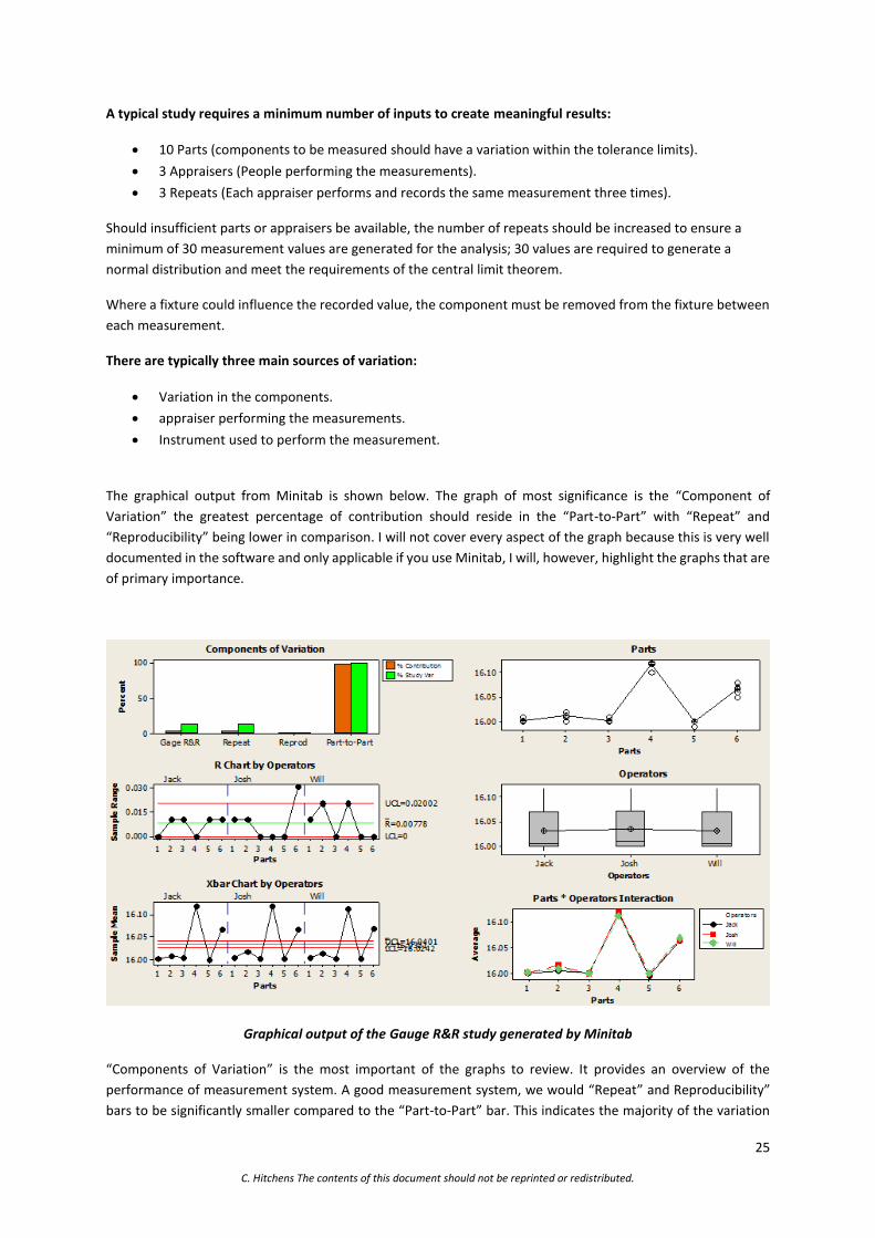
The graphical output from Minitab is shown below. The graph of most significance is the “Component of
Variation” the greatest percentage of contribution should reside in the “Part-to-Part” with “Repeat” and
“Reproducibility” being lower in comparison. I will not cover every aspect of the graph because this is very well
documented in the software and only applicable if you use Minitab, I will, however, highlight the graphs that are
of primary importance.
Graphical output of the Gauge R&R study generated by Minitab
“Components of Variation” is the most important of the graphs to review. It provides an overview of the
performance of measurement system. A good measurement system, we would “Repeat” and Reproducibility”
bars to be significantly smaller compared to the “Part-to-Part” bar. This indicates the majority of the variation
26
C. Hitchens The contents of this document should not be reprinted or redistributed.
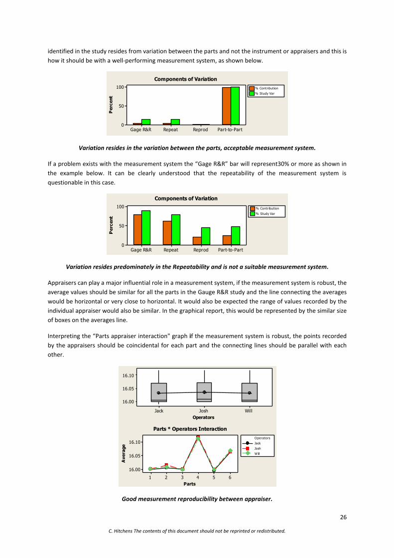
identified in the study resides from variation between the parts and not the instrument or appraisers and this is
how it should be with a well-performing measurement system, as shown below.
Part-to-PartReprodRepeatGage R&R
100
50
0
Perc
ent
% Contribution
% Study Var
654321654321654321
0.030
0.015
0.000
Parts
Sam
ple
Range
_R=0.00778
UCL=0.02002
LCL=0
Jack Josh Will
654321654321654321
16.10
16.05
16.00
Parts
Sam
ple
Mean
__X=16.0321UCL=16.0401LCL=16.0242
Jack Josh Will
654321
16.10
16.05
16.00
Parts
WillJoshJack
16.10
16.05
16.00
Operators
654321
16.10
16.05
16.00
Parts
Avera
ge
Jack
Josh
Will
Operators
Gage name:
Date of study :
Reported by :
Tolerance:
M isc:
Components of Variation
R Chart by Operators
Xbar Chart by Operators
C4 by Parts
C4 by Operators
Parts * Operators Interaction
Gage R&R (ANOVA) for C4
Variation resides in the variation between the parts, acceptable measurement system.
If a problem exists with the measurement system the “Gage R&R” bar will represent30% or more as shown in
the example below. It can be clearly understood that the repeatability of the measurement system is
questionable in this case.
Part-to-PartReprodRepeatGage R&R
100
50
0
Perc
ent
% Contribution
% Study Var
654321654321654321
0.050
0.025
0.000
Parts
Sam
ple
Range
_R=0.015
UCL=0.03861
LCL=0
Jack Josh Will
654321654321654321
16.04
16.02
16.00
Parts
Sam
ple
Mean
__X=16.01844
UCL=16.03379
LCL=16.00310
Jack Josh Will
654321
16.050
16.025
16.000
Parts
WillJoshJack
16.050
16.025
16.000
Operators
654321
16.04
16.02
16.00
Parts
Avera
ge
Jack
Josh
Will
Operators
Gage name:
Date of study :
Reported by :
Tolerance:
M isc:
Components of Variation
R Chart by Operators
Xbar Chart by Operators
C9 by Parts
C9 by Operators
Parts * Operators Interaction
Gage R&R (ANOVA) for C9
Variation resides predominately in the Repeatability and is not a suitable measurement system.
Appraisers can play a major influential role in a measurement system, if the measurement system is robust, the
average values should be similar for all the parts in the Gauge R&R study and the line connecting the averages
would be horizontal or very close to horizontal. It would also be expected the range of values recorded by the
individual appraiser would also be similar. In the graphical report, this would be represented by the similar size
of boxes on the averages line.
Interpreting the “Parts appraiser interaction" graph if the measurement system is robust, the points recorded
by the appraisers should be coincidental for each part and the connecting lines should be parallel with each
other.
Part-to-PartReprodRepeatGage R&R
100
50
0
Perc
ent
% Contribution
% Study Var
654321654321654321
0.030
0.015
0.000
Parts
Sam
ple
Range
_R=0.00778
UCL=0.02002
LCL=0
Jack Josh Will
654321654321654321
16.10
16.05
16.00
Parts
Sam
ple
Mean
__X=16.0321UCL=16.0401LCL=16.0242
Jack Josh Will
654321
16.10
16.05
16.00
Parts
WillJoshJack
16.10
16.05
16.00
Operators
654321
16.10
16.05
16.00
Parts
Avera
ge
Jack
Josh
Will
Operators
Gage name:
Date of study :
Reported by :
Tolerance:
M isc:
Components of Variation
R Chart by Operators
Xbar Chart by Operators
C4 by Parts
C4 by Operators
Parts * Operators Interaction
Gage R&R (ANOVA) for C4
Good measurement reproducibility between appraiser.

27
C. Hitchens The contents of this document should not be reprinted or redistributed.
If the averages connecting line is not a horizontal, with an appraiser being above or below the horizontal this
would suggest a systematic error. This appraiser is consistently performing the measurement or reading the
instrument in a different way to the others, creating poor reproducibility between the appraisers.
If any of the appraisers have a noticeably larger variation (box size) than the others, this indicates that the
appraiser is inconsistent in his method from one measurement to the next creating poor repeatability in the
measurement system. Conversely, in the examples below you will see “Will” has a better repeatability of
measurement than the others and a robust measurement system should not be susceptible to the influence of
the appraisers.
Part-to-PartReprodRepeatGage R&R
100
50
0
Perc
ent
% Contribution
% Study Var
654321654321654321
0.050
0.025
0.000
Parts
Sam
ple
Range
_R=0.015
UCL=0.03861
LCL=0
Jack Josh Will
654321654321654321
16.04
16.02
16.00
Parts
Sam
ple
Mean
__X=16.01844
UCL=16.03379
LCL=16.00310
Jack Josh Will
654321
16.050
16.025
16.000
Parts
WillJoshJack
16.050
16.025
16.000
Operators
654321
16.04
16.02
16.00
Parts
Avera
ge
Jack
Josh
Will
Operators
Gage name:
Date of study :
Reported by :
Tolerance:
M isc:
Components of Variation
R Chart by Operators
Xbar Chart by Operators
C9 by Parts
C9 by Operators
Parts * Operators Interaction
Gage R&R (ANOVA) for C9
The issue resides with appraiser repeatability measurement.
Looking at the three appraisers in the “Parts” graph above, it is clear that variation exists between the three.
However, Jack had an issue with part five highlighted by the sudden deviation of the black line. Further
investigation is required to understand the issue with this particular measurement. Also, the line connecting the
averages in the “Operators” chart is not a straight and “Parts Operator Interaction” is not parallel between
appraisers.
In addition to the graphical output, Minitab also provides numerical data. The output of most interest in the
values is highlighted below.
28
C. Hitchens The contents of this document should not be reprinted or redistributed.
In the above example, it can be seen that the Total Gage R&R “%Contribution (of VarComp)” is 5.80%.
<1% measurement system is acceptable.
≥1% <9% measurement system potentially acceptable depending on the application.
>9% measurement system is unacceptable.
“%Study Var (%SV)” is 24.08% of the process tolerance. The acceptable range Total Gage R&R contribution in
the “%Study Var (%SV)” is described below.
<10% measurement system is acceptable.
≥10% <30% measurement system potentially acceptable depending on the application.
>30% measurement system is unacceptable.
Minitab also calculates and displays the Number of Distinct Categories (NDC). This is an estimation of the
number of groups within the process data that the measurement system was able to identify.
<2 System is not acceptable and cannot distinguish between parts.
≤2<5 Parts can be divided into high and low groups.
≥5 System is acceptable and can distinguish between parts.
29
C. Hitchens The contents of this document should not be reprinted or redistributed.
UNCERTAINTY
Uncertainty is the measure of doubt that the recorded value represents the true value of the measurand. It may
be easier to think of this concept in a slightly different way. I have certainty that 95% of the recorded
measurements are within ±0.05mm of the true value; 95% is a commonly quoted confidence level. However,
uncertainty is the term defined in the standards and this is the one that shall be used. In this chapter statistical
calculation and uncertainty analysis are not covered in great detail, only the concept is provided and I would
recommend that the ISO 14253-2:2011 which provides the comprehensive and the up-to-date guidance on the
implementation of the concept of the GUM "Guide to the expression of uncertainty in measurement" should be
consulted. As discussed in the chapter “10% Rule” whenever the displayed value nears tolerance limits of the
component, the uncertainty of the measurement system should be considered and stated on the measurement
report. I would recommend the book “An Introduction to Uncertainty in Measurement” by Kirkup and Frenkel
as a starting point before reading the GUM.
The sources of uncertainty are divided into two groups.
Type A:
Estimated by means of statistical analysis of repeated measurements or from measurement system
analysis.
Type B:
Estimated from other information. Such as calibration certificates, instrument specifications and
experience.
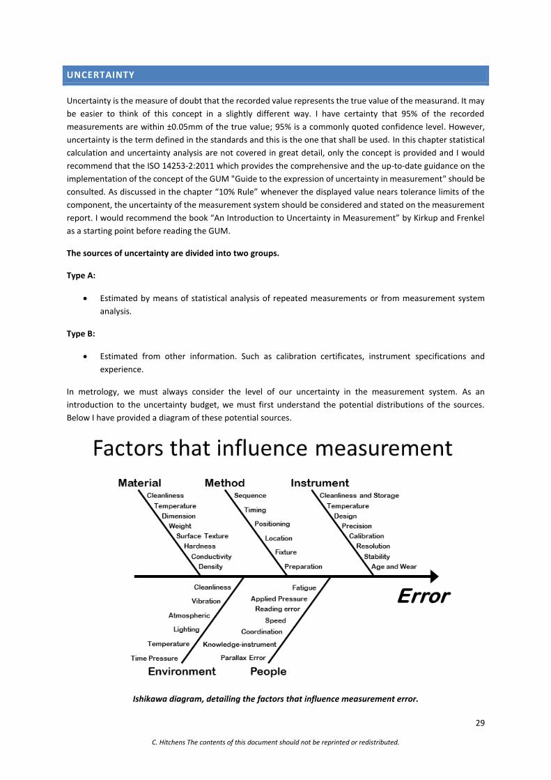
In metrology, we must always consider the level of our uncertainty in the measurement system. As an
introduction to the uncertainty budget, we must first understand the potential distributions of the sources.
Below I have provided a diagram of these potential sources.
Ishikawa diagram, detailing the factors that influence measurement error.
30
C. Hitchens The contents of this document should not be reprinted or redistributed.
It is important to combine the identified sources of uncertainty to determine the overall uncertainty of the
measurement system. The term used for these combined sources is the “Uncertainty Budget”.
As a simplified example to introduce the principles of calculating the uncertainty budget consider a micrometer
and presume it has only two errors, temperature, and the instrument capability. The measurement recorded
value “Y” will, therefore, be a product of the true value “𝑋“ and the error due to temperature “Δ𝑇𝑒𝑚𝑝𝑒𝑟𝑎𝑡𝑢𝑟𝑒”
and the instrument “Δ𝐼𝑛𝑠𝑡𝑟𝑢𝑚𝑒𝑛𝑡”.
Y = 𝑋 + Δ𝑇𝑒𝑚𝑝𝑒𝑟𝑎𝑡𝑢𝑟𝑒 + Δ𝐼𝑛𝑠𝑡𝑟𝑢𝑚𝑒𝑛𝑡
The symbol 𝛥denotes a changeable value.
The probability that all errors will simultaneously coincide with the maximum or minimum values is statistically
unlikely, we must, therefore, combine them statistically. We need to calculate the individual uncertainties “𝑢”
before combining “𝛥𝑇𝑒𝑚𝑝𝑒𝑟𝑎𝑡𝑢𝑟𝑒” and “𝛥𝐼𝑛𝑠𝑡𝑟𝑢𝑚𝑒𝑛𝑡” and these all need to be at one standard distribution
(2 sigma) and not expanded distribution. It should be noted that the true value”X” has no uncertainty.
To calculate the standard distributions we need to divide by the appropriate “𝑘” coverage factor. Coverage
factor provides the relationship between a standard uncertainty “𝑢” and an expanded uncertainty “𝑈”
𝑈 = 𝑢 × 𝑘
𝑘 Coverage factor.
𝑈 Expanded uncertainty.
𝑢 Standard uncertainty.
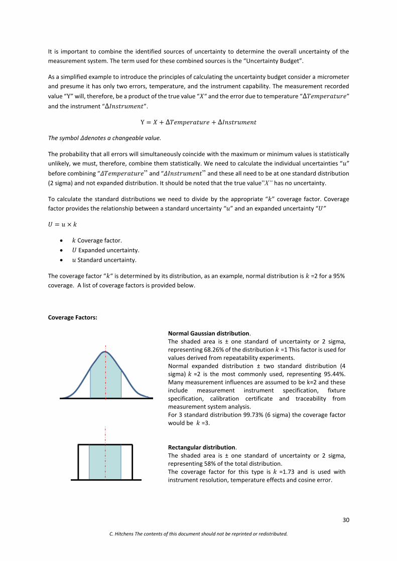
The coverage factor “𝑘“ is determined by its distribution, as an example, normal distribution is 𝑘 =2 for a 95%
coverage. A list of coverage factors is provided below.
Coverage Factors:
Normal Gaussian distribution. The shaded area is ± one standard of uncertainty or 2 sigma, representing 68.26% of the distribution 𝑘 =1 This factor is used for values derived from repeatability experiments. Normal expanded distribution ± two standard distribution (4 sigma) 𝑘 =2 is the most commonly used, representing 95.44%. Many measurement influences are assumed to be k=2 and these include measurement instrument specification, fixture specification, calibration certificate and traceability from measurement system analysis. For 3 standard distribution 99.73% (6 sigma) the coverage factor would be 𝑘 =3.
Rectangular distribution. The shaded area is ± one standard of uncertainty or 2 sigma, representing 58% of the total distribution. The coverage factor for this type is 𝑘 =1.73 and is used with instrument resolution, temperature effects and cosine error.

31
C. Hitchens The contents of this document should not be reprinted or redistributed.
Triangular distribution. The shaded area is ± one standard of uncertainty or 2sigma, representing 65 % of the total distribution. The coverage factor for this type is 𝑘 =1.73 and seldom used in dimensional metrology and only when limited information is available.
From the information that has been gathered from the measurement system analysis, calibration certificates,
instrument specifications etc. We can then generate the standard uncertainty for each of the contributing
factors by dividing by the appropriate coverage factor𝑘 . The coverage factor 𝑘 value is used to reduce all
expanded uncertainties to standard uncertainties two standard distributions. The standard distributions of the
combined contributing factors can then be calculated by using the root sum of the squares. All contributing
factors are squared and then added together to create a total; the square root of the total is then calculated.
The combined uncertainties 𝑢𝑐 can then be expanded using the coverage factor 𝑘 = 2 to give a final expanded
uncertainty value for the measurement system with 95% confidence level. Ensure that the contributing factors
are independent and are not influenced or influencing others.
We should also consider the uncertainty due to changes in temperature. Steels typically have a coefficient of
expansion in the region of 12µm per meter per degree. The length of measurand is known and a determination
should be made on the potential fluctuation in ambient and component at the time of measurement. If we are
to make a detailed study of the temperature variations, a calibrated thermometer should be used and noted
that the agreed international standard temperature for measurement is 20˚C. As an example, a 500mm
measurement in an environment that changes between 18˚C and 22˚C degrees has the potential to change
length by ± 12µm. This needs to be included in the measurement budget.
An example is demonstrated below. This example is not meant to be used for all measurements; each
measurement system is unique and requires its own specific calculation.
Ref No.
Component of
Uncertainty
Distribution
Type
Expanded
Uncertainty 𝑈
Divisor
𝑘
Standard Uncertainty 𝑢
𝑢 = 𝑈 ÷ 𝑘
𝑢1 Instrument calibration Normal 0.050 2 0.025
𝑢2 Resolution Rectangular 0.010 1.73 0.006
𝑢3 Temperature Rectangular 0.012 1.73 0.007
𝑢4 Fixture Normal 0.020 2 0.010
𝑢5 Repeatability Normal 0.100 2 0.050
Combined uncertainty 𝑢𝑐 = √𝑢12 + 𝑢22+ 𝑢32+ 𝑢42 + ….etc. 0.058
Combined expanded uncertainty(𝑘 = 2) for a 95% confidence level= 𝑢𝑐 × 𝑘 0.115

32
C. Hitchens The contents of this document should not be reprinted or redistributed.
INTRODUCTION TO GD&T (GEOMETRIC DIMENSIONING AND TOLERANCING)
GD&T is a method of dimensioning and tolerance a drawing with respect to the actual function or relationship
of the part. It was developed primarily to ensure interchangeability of components and assist in their assembly.
The function of the part should be clearly demonstrated by the application of the tolerances.
Two standards bodies exist ASME in America and ISO predominantly in Europe the standards have 90-95%
correlation but this is slowly being addressed; the following information is based on ASME Y14.5M and correct
at time of creation. Please always refer to the current standard.
This type of tolerance should be used for features that have a critical function or where interchangeability is
required or when consistent datum from design, manufacture and inspection are required.
5 types of geometric characteristics:
Form: states how far an actual surface may vary from that implied by the drawing.
Orientation states: how far a surface may vary relative to a datum.
Profile: states how far a surface or feature may vary from the desired drawing detail or specified
datum.
Runout: states how far a surface or feature may vary from the desired during a full 360 degree
revolution.
Location: state how far a size feature may vary from that specified by the drawing related to a datum
or feature.

33
C. Hitchens The contents of this document should not be reprinted or redistributed.
The geometric tolerance is constructed inside a Feature Control Frame. The primary compartment defines which
of the 14 geometric tolerances will be controlling the feature. A secondary feature control frame can be applied
if and additional geometric tolerance is required. The secondary compartment states the tolerance for the
geometric feature if a diameter symbol is shown then the tolerance zone is circular or cylindrical. Material
condition modifiers can appear in this secondary compartment. The tertiary compartment indicates the primary
datum, additional compartments can be added for secondary and tertiary datums. Every related tolerance
requires a minimum of one datum, however, independent tolerances, such as form tolerances, can be applied
independently. Information on when a datum is required and not required is stated in the chapter on “Inspection
Methods for GD&T”.
Feature Control Frame
VARIATIONS OF FORM RULE #1: ENVELOPE PRINCIPLE TAYLOR PRINCIPLE
“The surface or surfaces of a regular feature of size shall not extend beyond a boundary (envelope) of perfect
form at MMC. This boundary is the true geometric form represented by the drawing. No variation in form is
permitted if the regular feature of size is produced at its MMC limit of size unless a straightness or flatness
tolerance is associated with the size dimension or the Independency symbol is applied”.BE AWARE: There is a
discrepancy between standards on this fundamental principle, check the standards ASMI and ISO.
ASME Y14.5M
34
C. Hitchens The contents of this document should not be reprinted or redistributed.
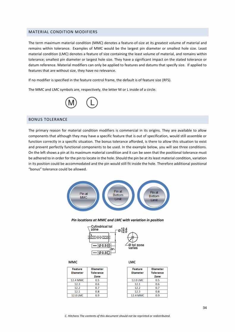
MATERIAL CONDITION MODIFIERS
The term maximum material condition (MMC) denotes a feature-of-size at its greatest volume of material and
remains within tolerance. Examples of MMC would be the largest pin diameter or smallest hole size. Least
material condition (LMC) denotes a feature of size containing the least volume of material, and remains within
tolerance; smallest pin diameter or largest hole size. They have a significant impact on the stated tolerance or
datum reference. Material modifiers can only be applied to features and datums that specify size. If applied to
features that are without size, they have no relevance.
If no modifier is specified in the feature control frame, the default is of feature size (RFS).
The MMC and LMC symbols are, respectively, the letter M or L inside of a circle.
BONUS TOLERANCE
The primary reason for material condition modifiers is commercial in its origins. They are available to allow
components that although they may have a specific feature that is out of specification, would still assemble or
function correctly in a specific situation. The bonus tolerance afforded, is there to allow this situation to exist
and prevent perfectly functional components to be used. In the example below, you will see three conditions.
On the left shows a pin at its maximum material condition and it can be seen that the positional tolerance must
be adhered to in order for the pin to locate in the hole. Should the pin be at its least material condition, variation
in its position could be accommodated and the pin would still fit inside the hole. Therefore additional positional
“bonus” tolerance could be allowed.
Pin locations at MMC and LMC with variation in position
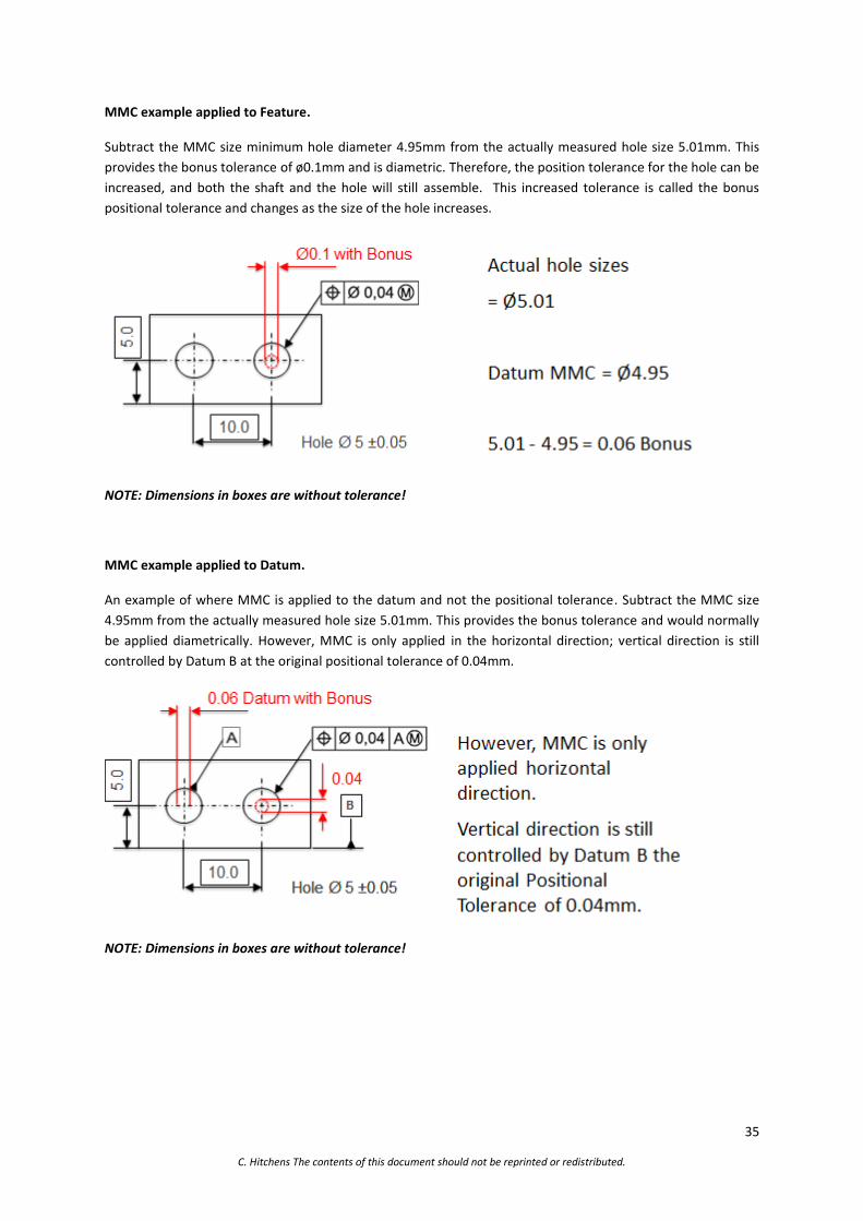
35
C. Hitchens The contents of this document should not be reprinted or redistributed.
MMC example applied to Feature.
Subtract the MMC size minimum hole diameter 4.95mm from the actually measured hole size 5.01mm. This
provides the bonus tolerance of ø0.1mm and is diametric. Therefore, the position tolerance for the hole can be
increased, and both the shaft and the hole will still assemble. This increased tolerance is called the bonus
positional tolerance and changes as the size of the hole increases.
NOTE: Dimensions in boxes are without tolerance!
MMC example applied to Datum.
An example of where MMC is applied to the datum and not the positional tolerance. Subtract the MMC size
4.95mm from the actually measured hole size 5.01mm. This provides the bonus tolerance and would normally
be applied diametrically. However, MMC is only applied in the horizontal direction; vertical direction is still
controlled by Datum B at the original positional tolerance of 0.04mm.
NOTE: Dimensions in boxes are without tolerance!
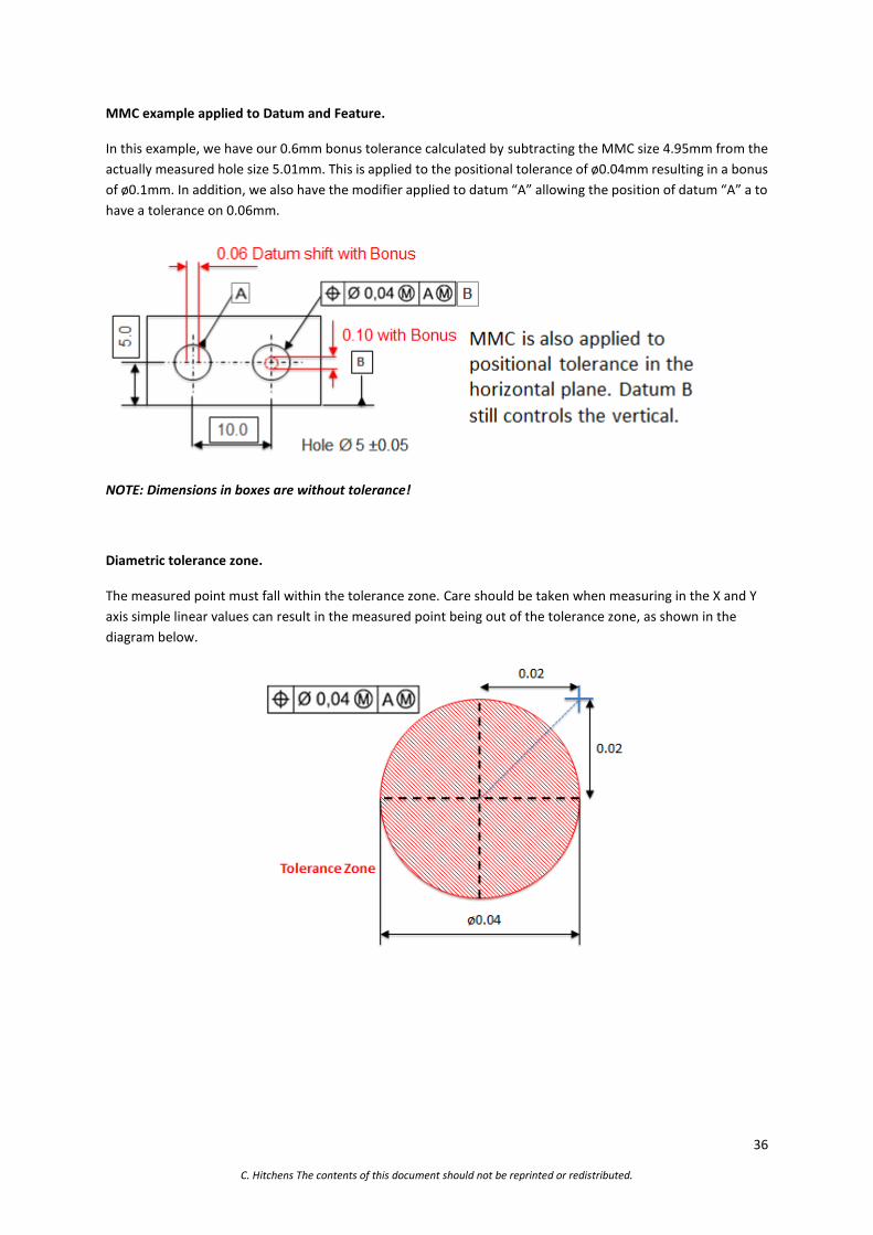
36
C. Hitchens The contents of this document should not be reprinted or redistributed.
MMC example applied to Datum and Feature.
In this example, we have our 0.6mm bonus tolerance calculated by subtracting the MMC size 4.95mm from the
actually measured hole size 5.01mm. This is applied to the positional tolerance of ø0.04mm resulting in a bonus
of ø0.1mm. In addition, we also have the modifier applied to datum “A” allowing the position of datum “A” a to
have a tolerance on 0.06mm.
NOTE: Dimensions in boxes are without tolerance!
Diametric tolerance zone.
The measured point must fall within the tolerance zone. Care should be taken when measuring in the X and Y
axis simple linear values can result in the measured point being out of the tolerance zone, as shown in the
diagram below.

37
C. Hitchens The contents of this document should not be reprinted or redistributed.
REGARDLESS OF FEATURE SIZE (RFS)
“Indicates a geometric tolerance applies at any increment of size of the actual mating envelope of the feature of
size”. In older standards, this was indicated by the letter “S” in a circle inside the feature control frame. This is
now the default condition for all geometric tolerance and no bonus tolerances are allowed unless stated by a
material modifier.
VIRTUAL CONDITION
“A constant boundary generated by the collective effects of a considered feature of the size’s specified MMC or
LMC and the geometric tolerance for that material condition”. The collective total effects of these factors define
the available clearances between mating components and are also used to establish gage feature sizes. When
calculating the virtual size of a hole, you must consider the rules governing Maximum Material Condition (MMC)
and Least Material Condition (LMC).
ASME Y14.5M
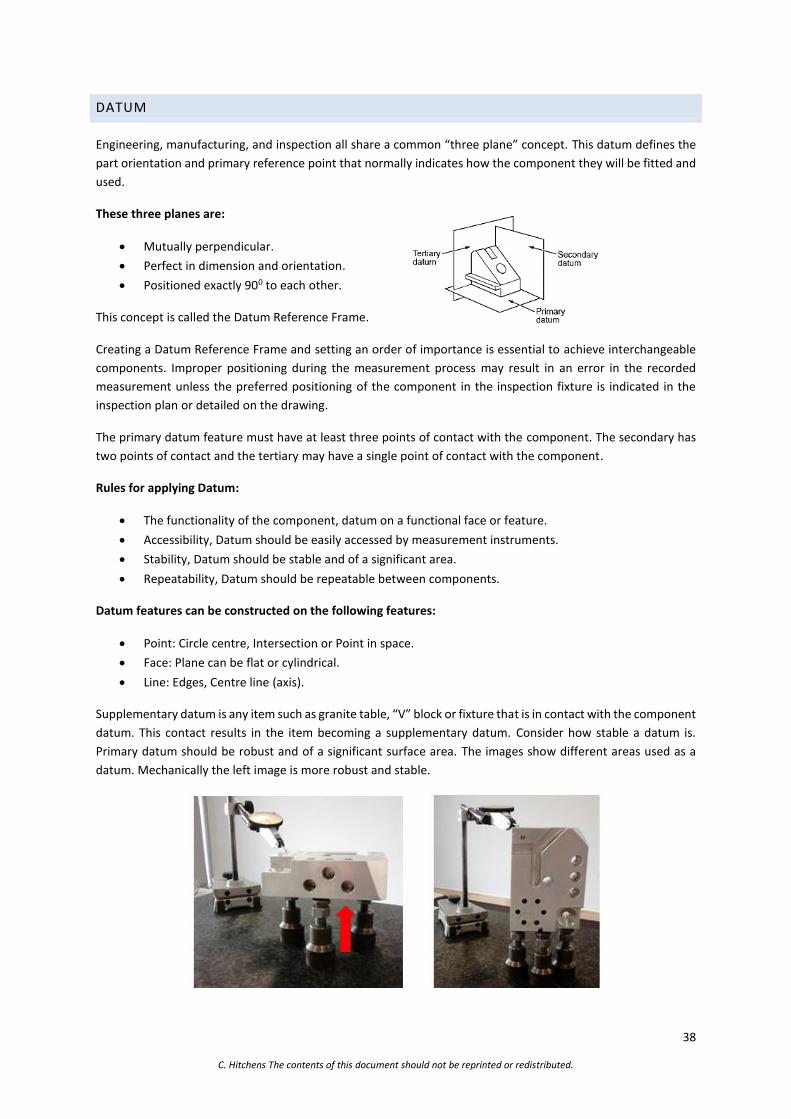
38
C. Hitchens The contents of this document should not be reprinted or redistributed.
DATUM
Engineering, manufacturing, and inspection all share a common “three plane” concept. This datum defines the
part orientation and primary reference point that normally indicates how the component they will be fitted and
used.
These three planes are:
Mutually perpendicular.
Perfect in dimension and orientation.
Positioned exactly 900 to each other.
This concept is called the Datum Reference Frame.
Creating a Datum Reference Frame and setting an order of importance is essential to achieve interchangeable
components. Improper positioning during the measurement process may result in an error in the recorded
measurement unless the preferred positioning of the component in the inspection fixture is indicated in the
inspection plan or detailed on the drawing.
The primary datum feature must have at least three points of contact with the component. The secondary has
two points of contact and the tertiary may have a single point of contact with the component.
Rules for applying Datum:
The functionality of the component, datum on a functional face or feature.
Accessibility, Datum should be easily accessed by measurement instruments.
Stability, Datum should be stable and of a significant area.
Repeatability, Datum should be repeatable between components.
Datum features can be constructed on the following features:
Point: Circle centre, Intersection or Point in space.
Face: Plane can be flat or cylindrical.
Line: Edges, Centre line (axis).
Supplementary datum is any item such as granite table, “V” block or fixture that is in contact with the component
datum. This contact results in the item becoming a supplementary datum. Consider how stable a datum is.
Primary datum should be robust and of a significant surface area. The images show different areas used as a
datum. Mechanically the left image is more robust and stable.
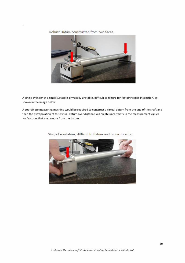
39
C. Hitchens The contents of this document should not be reprinted or redistributed.
.
A single cylinder of a small surface is physically unstable, difficult to fixture for first principles inspection, as
shown in the image below.
A coordinate measuring machine would be required to construct a virtual datum from the end of the shaft and
then the extrapolation of this virtual datum over distance will create uncertainty in the measurement values
for features that are remote from the datum.
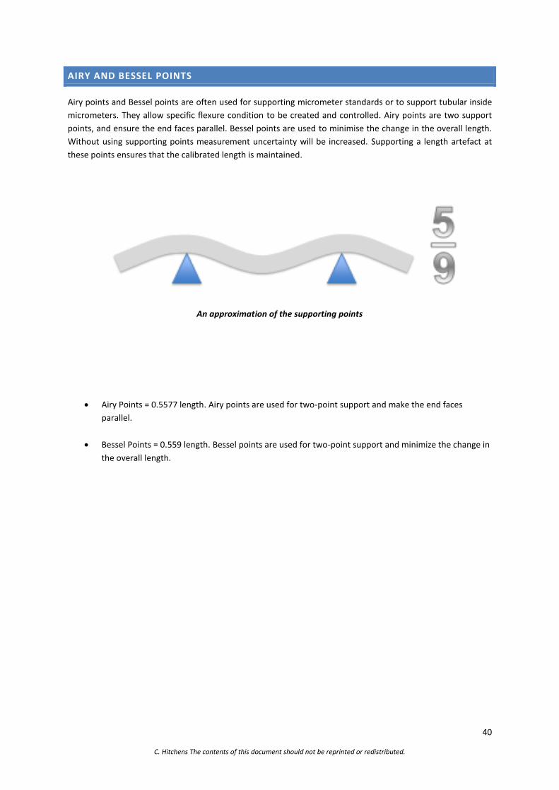
40
C. Hitchens The contents of this document should not be reprinted or redistributed.
AIRY AND BESSEL POINTS
Airy points and Bessel points are often used for supporting micrometer standards or to support tubular inside
micrometers. They allow specific flexure condition to be created and controlled. Airy points are two support
points, and ensure the end faces parallel. Bessel points are used to minimise the change in the overall length.
Without using supporting points measurement uncertainty will be increased. Supporting a length artefact at
these points ensures that the calibrated length is maintained.
An approximation of the supporting points
Airy Points = 0.5577 length. Airy points are used for two-point support and make the end faces
parallel.
Bessel Points = 0.559 length. Bessel points are used for two-point support and minimize the change in
the overall length.

41
C. Hitchens The contents of this document should not be reprinted or redistributed.
INSPECTION METHODS FOR GD&T
Limited standards exist on how to inspect a component feature and this is due to the complexity of the problem
and the wide range of possibilities available to us. Due to the lack of standards as engineers, we need to use
good judgment and develop robust repeatable measurement based on fundamental engineering knowledge. In
this section, I will show methods that can be used to inspect GD&T tolerances and highlight what considerations
should be made. This is not an exhaustive list and it is the intention to provide some guidance that I hope will
assist. I will focus on first principle measurement methods as these are the simplest measurement system to
calculate the uncertainty of. The methods described and the notes provided are intended to create a questioning
attitude and to encourage you to look critically at methods used and how their robustness of the measurement
system could be improved.
STRAIGHTNESS FEATURE
2D Feature Datum is not applied, MMC or LMC can apply to a feature of size.
“Any extracted line on the upper surface, parallel to the plane of projection in which the indication is shown,
shall be contained between two parallel straight lines 0.04 apart”.
Straight-Edge Dial Test Indicator Method.
Flat components can be inspected by using a DTI mounted on a surface gauge and located on a surface plate.
We should be aware of the interaction of bottom face with surface and ensure we are not checking Parallelism.
Using 3 point jacks would avoid this potential error. You should also consider controlling the traverse of the dial
test indicator. The total indicator reading should be less or equal to the tolerance for a conforming feature.
For shafts controlling the traverse of the dial test indicator would be optimal but the measurement can be
performed without this control by recording the total indicator reading only at the high point of the shaft body.
A pair of matched V blocks (record the specification for your uncertainty budget) can be used with a dial test
indicator but deviations in diameter can influence the recorded values. Using inspection centres would be an
optimal method but this requires features to be present on the component to locate the centres.

42
C. Hitchens The contents of this document should not be reprinted or redistributed.
Wedge Method.
In this method, the straight edge to be inspected is supported at the points for minimum deflection (Airy and
Bessel points) on two unequal piles of slip gauge with a difference of 0.1mm that then sit on a surface plate. The
distance between the two piles of slips should then be divided into ten equal parts of shown in the image below.
The distance 0.1mm can then be divided by the 10 equal parts, resulting in each division to have an increase in
height of 0.01mm. If the straight edge to be inspected is truly straight then piles of slip gauges at increments
increasing by 0.01mm will intersect perfectly with their corresponding divisions. Any error can be determined
by increasing or decreasing the slip gauge heights until an intersection is achieved. This is a time-consuming
method and great care is required when marking out the divisions.
Feeler Gauge Method.
Locating the component against a straight edge or on a surface plate feeler gauges can be used to determine
the dimension of any gap. If the visible light between the component and straight edge has a blue tint to this
indicates a gap of 2-5 microns.

43
C. Hitchens The contents of this document should not be reprinted or redistributed.
Straightness Applied to Axis.
Straightness applied to the diameter of the cylinder has a cylindrical tolerance zone over the length of the
feature. In the method shown below, the straightness of a central axis can be checked by taking surface error
readings from opposing dial test indicators and rotating the component in a three jaw chuck. The dial test
indicators will need to be set using a reference cylinder in order to zero the system before the inspection can
take place. The difference between highest and lowest values will be the total deviation recorded.
This method could be applied on a lathe during manufacture with a single dial test indicator being mounted and
traversed of the tool post. You should, however, be aware of any errors in the lathe construction as these will
be included in the measurement values recorded.
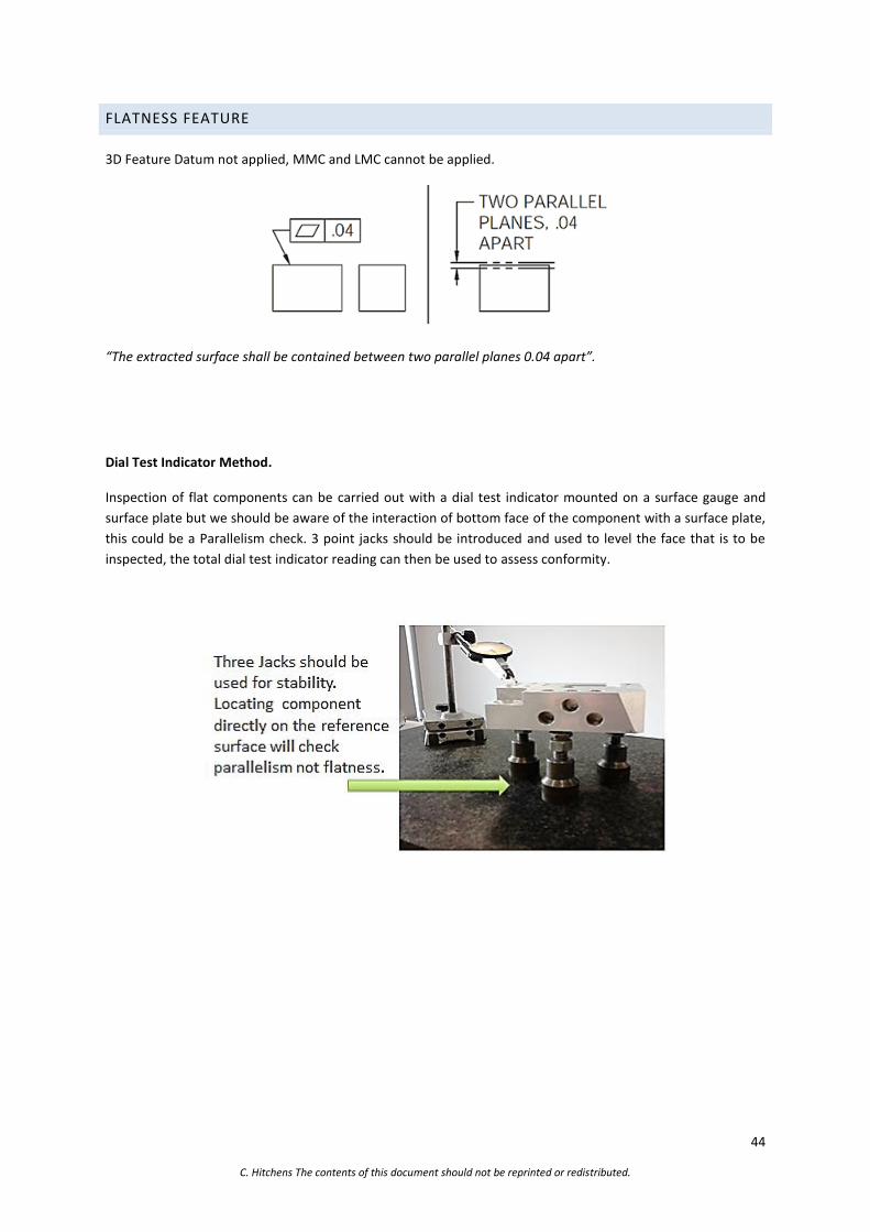
44
C. Hitchens The contents of this document should not be reprinted or redistributed.
FLATNESS FEATURE
3D Feature Datum not applied, MMC and LMC cannot be applied.
“The extracted surface shall be contained between two parallel planes 0.04 apart”.
Dial Test Indicator Method.
Inspection of flat components can be carried out with a dial test indicator mounted on a surface gauge and
surface plate but we should be aware of the interaction of bottom face of the component with a surface plate,
this could be a Parallelism check. 3 point jacks should be introduced and used to level the face that is to be
inspected, the total dial test indicator reading can then be used to assess conformity.

45
C. Hitchens The contents of this document should not be reprinted or redistributed.
Optical Flats Method.
An optical flat is an optical-grade piece of glass that has been lapped and polished to create ultra-flat faces on
both sides, usually about 0.1µm. The spacing between fringes is smaller in areas where the flatness is changing
more rapidly. These fringes indicate a departure from a truly flatness condition. Each fringe represents 0.3µm
this value is approximate only because it depends on the light source. They are commonly used to check the
flatness of the anvils on measurement instruments such as Micrometers. A set of four is typically used, each
with a different overall thickness so that when the thimble is rotated four different rotational positions are
checked. Anvil faces may be parallel in one specific rotatory location only and this may not be detected with a
single optical flat.
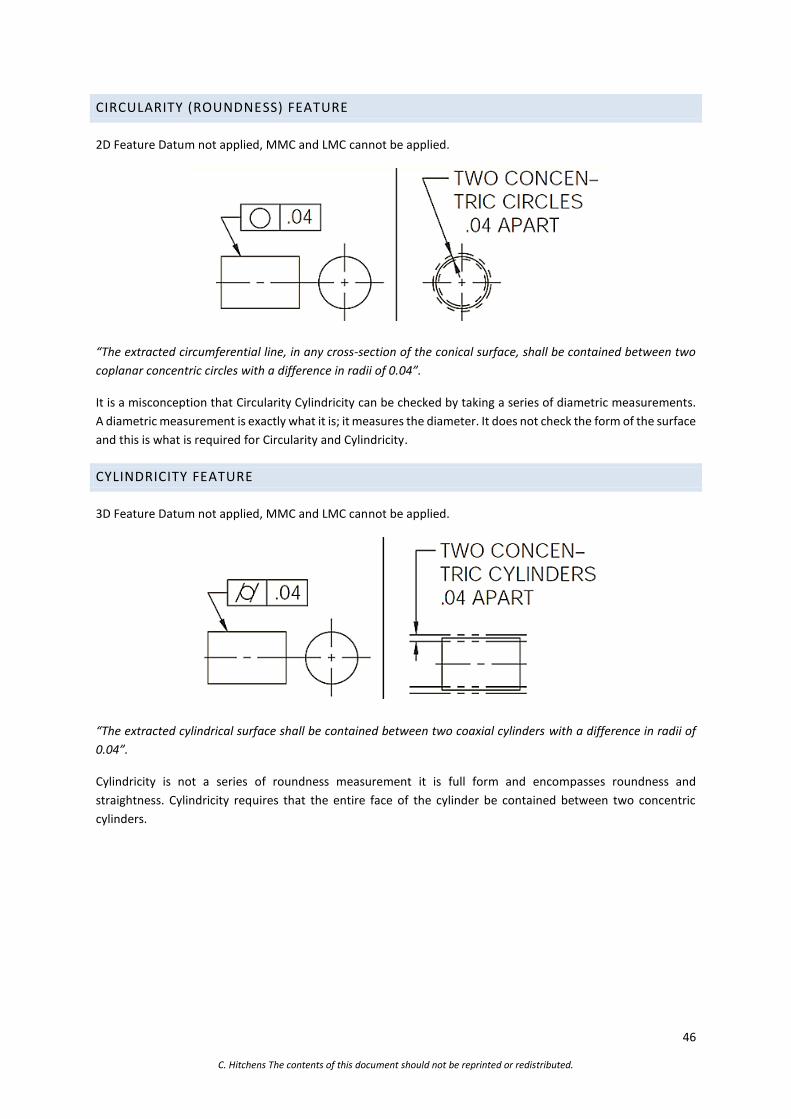
46
C. Hitchens The contents of this document should not be reprinted or redistributed.
CIRCULARITY (ROUNDNESS) FEATURE
2D Feature Datum not applied, MMC and LMC cannot be applied.
“The extracted circumferential line, in any cross-section of the conical surface, shall be contained between two
coplanar concentric circles with a difference in radii of 0.04”.
It is a misconception that Circularity Cylindricity can be checked by taking a series of diametric measurements.
A diametric measurement is exactly what it is; it measures the diameter. It does not check the form of the surface
and this is what is required for Circularity and Cylindricity.
CYLINDRICITY FEATURE
3D Feature Datum not applied, MMC and LMC cannot be applied.
“The extracted cylindrical surface shall be contained between two coaxial cylinders with a difference in radii of
0.04”.
Cylindricity is not a series of roundness measurement it is full form and encompasses roundness and
straightness. Cylindricity requires that the entire face of the cylinder be contained between two concentric
cylinders.

47
C. Hitchens The contents of this document should not be reprinted or redistributed.
Roundness machine
The roundness testing machine is the optimal instrument to determine roundness and circularity. A roundness
testing system consists of a base with either a mechanical or air-bearing spindle, on which a vertical column
stand, the radial arm which houses the probe extends from the vertical column. The component is rotated and
the probe traces the form. The machines are capable of recording thousands of data points at sub-micron
accuracy, and data are stored and typically reported as plots. There is, however, limitation in component size
that can be assessed due to the dimensions of the machines available.
Typical report plot, machine dimension, and component assessment.
Roundness testing machine can also measure Flatness, Concentricity, Perpendicularity, Diameter and Runout.
They represent the most accurate method of form analysis.
IMPORTANT: I will introduce methods of assessing the circularity and Cylindricity of a form in the remainder
of this chapter. Please note; the only truly robust method is the roundness testing machine. All alternative methods including coordinate measurement machine as described in a later chapter should be assessed against a reference standard of known form. Rotating a component between inspection centres is not a check of the Roundness form because it relates the component surface to an axis, this is a check of Runout.
Dial Test Indicator and V Block Method.
The use of V blocks which create a 3 point measurement system between the V block, component, and
instrument, is not ideal because the ovality of the component and its interaction with the V blocks will influence
the measurements recorded. Should you use this method you can be confident that if the part is within tolerance
the values will include lobe effect and the actual circularity will be better.

48
C. Hitchens The contents of this document should not be reprinted or redistributed.
Ideally, prior to assessing the circularity or cylindricity, we should first evaluate the existence and severity of any
lobbing errors. A standard 90⁰included angle V block can be used to detect and count the number of lobes
present on a given component. To measure the exact amount of lobes requires a V block with an angle which is
related to the number of lobes. Note: with Cylindricity lobe effects will form part of the tolerance requirement.
Dial Test Indicator and 3 Jaw Chuck Method.
It is important that we clamp the jaw on the face being assessed in the case of the datum being a bore this would
require an internal three jaw chuck. It is important to fixture in this method i.e. do not check a bore with the
component held on an external face, this will introduce additional errors such as concentricity. The work piece
must be centred by checking opposing points. Then the total dial test indicator reading thereafter will indicate
the circularity; Cylindricity is full form along the full work piece length. The difference between the minimum
and maximum readings is the recorded value. Lobe effect can still influence the measurement result. It is also
possible to employ this measurement method at the point of manufacture by mounting the dial test indicator
to the turret of the lathe for circularity. In the case of Cylindricity when the dial test indicator is required to travel
the length of the component, errors in the machine travel will also be introduced into the recorded results. If
the dial test indicator is mounted on the same machine guides that were used to manufacture the component,
you will be repeating any errors in the machine guides and will not record the form value correctly.
IMPORTANT: Although I have introduced methods of assessing the circularity and cylindricity of a form, the
only truly robust method is the roundness testing machine. All alternative methods including coordinate
measurement machine as described in a later chapter should be assessed against a reference standard of known
form.
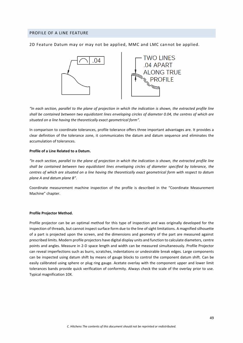
49
C. Hitchens The contents of this document should not be reprinted or redistributed.
PROFILE OF A LINE FEATURE
2D Feature Datum may or may not be applied, MMC and LMC can not be applied.
“In each section, parallel to the plane of projection in which the indication is shown, the extracted profile line
shall be contained between two equidistant lines enveloping circles of diameter 0.04, the centres of which are
situated on a line having the theoretically exact geometrical form”.
In comparison to coordinate tolerances, profile tolerance offers three important advantages are. It provides a
clear definition of the tolerance zone, it communicates the datum and datum sequence and eliminates the
accumulation of tolerances.
Profile of a Line Related to a Datum.
“In each section, parallel to the plane of projection in which the indication is shown, the extracted profile line
shall be contained between two equidistant lines enveloping circles of diameter specified by tolerance, the
centres of which are situated on a line having the theoretically exact geometrical form with respect to datum
plane A and datum plane B”.
Coordinate measurement machine inspection of the profile is described in the “Coordinate Measurement
Machine” chapter.
Profile Projector Method.
Profile projector can be an optimal method for this type of inspection and was originally developed for the
inspection of threads, but cannot inspect surface form due to the line of sight limitations. A magnified silhouette
of a part is projected upon the screen, and the dimensions and geometry of the part are measured against
prescribed limits. Modern profile projectors have digital display units and function to calculate diameters, centre
points and angles. Measure in 2-D space length and width can be measured simultaneously. Profile Projector
can reveal imperfections such as burrs, scratches, indentations or undesirable break edges. Large components
can be inspected using datum shift by means of gauge blocks to control the component datum shift. Can be
easily calibrated using sphere or plug ring gauge. Acetate overlay with the component upper and lower limit
tolerances bands provide quick verification of conformity. Always check the scale of the overlay prior to use.
Typical magnification 10X.

50
C. Hitchens The contents of this document should not be reprinted or redistributed.
Profile Projector.
Tool Makers Microscope Method.
For small components, you may consider the tool makers microscope. The main application of a tool maker
microscope is to measure the form, size, angle, and the position of components that falls within the microscope’s
measuring range. Typical 30x magnification. Commonly used for threads, templates, form and milling cutters,
punching tools, surface finishes and surface defects and hardness test indentations.
Profile Tracer Method.
Is an instrument that employs a stylus and traverse mechanism to record form, it can detect and evaluation
contours and make comparisons between internal and external faces. Component size is limited by the total
travel of the instrument.

51
C. Hitchens The contents of this document should not be reprinted or redistributed.
PROFILE OF A SURFACE FEATURE
3D Feature Datum may or may not be applied, MMC and LMC cannot be applied.
“The extracted surface shall be contained between two equidistant surfaces enveloping spheres of diameter 0.04,
the centres of which are situated on a surface having the theoretically exact geometrical form”.
Profile of a Surface Related to a Datum.
“The extracted surface shall be contained between two equidistant surfaces enveloping spheres of diameter
specified by tolerance, the centres of which are situated on a surface having the theoretically exact geometrical
form with respect to datum plane A”.
Profile of a Surface using First Principles. Not a practical method of inspection!
The measurement of 3D form which is an evaluation of the entire surface is not practical using first principle
methods. Coordinate measuring machine would be more appropriate as the form can be measured against the
nominal CAD and indications of deviation reported. Beware that most reports will state the total form error out
of specification condition and not the location of the form error. Components could be rejected for small areas
on non-conformance; further information is provided in the “Coordinate Measuring Machine” chapter. In
addition, non-contact scanning technologies such as structured light, photogrammetry and laser strip scanning
provide intuitive colour maps of form error from nominal CAD additional information is available in the chapter
“No-contact Scanning Technologies”. Profile projector can only see a single outline of part surface profiling
machine but will not provide full form measurement.
3D form evaluation using first principle methods is not practical for complex geometries

52
C. Hitchens The contents of this document should not be reprinted or redistributed.
ANGULARITY
At least one datum must be referenced, MMC or LMC can apply to a feature of size.
“The extracted surface shall be contained between two parallel planes 0.04 apart that are inclined at a
theoretically exact angle of 15° to datum plane A”.
Features not at zero or 90⁰, the tolerance defines the form within planes that the actual face should fall between.
The tolerance value is not in degrees
Angularity Related to a Datum.
“The extracted median line shall be within a cylindrical tolerance zone of diameter specified by the tolerance that
is parallel to datum plane and inclined at a theoretically exact angle”.
Tolerance can also be specified as a “ø” creating a cylindrical tolerance zone; typically applied to holes.
Sin Bar Method.
Sin bar or Sin table with slips on a surface plate is the most appropriate and also more accurate than many other
methods. The distance between rollers and parallelism of the rollers to each other and the distance relative to
the top face are all controlled to a high precision, as is the Cylindricity of the rollers. The sin bar is especially
useful when measuring or checking angles. For tolerances of 5 minutes or less the sin bar is appropriate because
of its positive location and contact with precision gauge blocks selected at an appropriate value to obtain a given
angle. Sine-bar consists of a hardened, ground and lapped steel bar with very accurate cylindrical plugs of equal
diameter and commonly available in 5 or 10 inches lengths. Bevel protractors are equipped with Vernier scales
which read to 5 minutes but are not capable of the same level of measurement uncertainty.
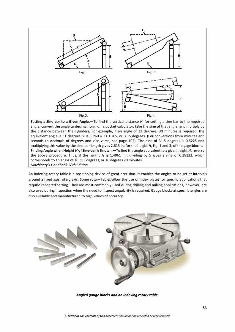
53
C. Hitchens The contents of this document should not be reprinted or redistributed.
Setting a Sine-bar to a Given Angle.—To find the vertical distance H, for setting a sine bar to the required angle, convert the angle to decimal form on a pocket calculator, take the sine of that angle, and multiply by the distance between the cylinders. For example, if an angle of 31 degrees, 30 minutes is required, the equivalent angle is 31 degrees plus 30⁄60 = 31 + 0.5, or 31.5 degrees. (For conversions from minutes and seconds to decimals of degrees and vice versa, see page 102). The sine of 31.5 degrees is 0.5225 and multiplying this value by the sine-bar length gives 2.613 in. for the height H, Fig. 1 and 3, of the gage blocks. Finding Angle when Height H of Sine-bar is Known.—To find the angle equivalent to a given height H, reverse the above procedure. Thus, if the height H is 1.4061 in., dividing by 5 gives a sine of 0.28122, which corresponds to an angle of 16.333 degrees, or 16 degrees 20 minutes. Machinery's Handbook 28th Edition
An indexing rotary table is a positioning device of great precision. It enables the angles to be set at intervals
around a fixed axis rotary axis. Some rotary tables allow the use of index plates for specific applications that
require repeated setting. They are most commonly used during drilling and milling applications, however, are
also used during inspection when the need to inspect angularity is required. Gauge blocks at specific angles are
also available and manufactured to high values of accuracy.
Angled gauge blocks and an indexing rotary table.

54
C. Hitchens The contents of this document should not be reprinted or redistributed.
Height Gauge Method.
Using a gauge block to define a known distance difference between two height measurements on the
components angled face will provide us with two values; distance and height. From these, we can calculate the
angle of the face.
Universal Bevel Protractor.
Probably the simplest instrument for measuring the angle between faces. The instrument itself consists of a base
plate from which and an adjustable blade extends from a rotating centre with a Vernier scale. The adjustable
blade is rotated about the centre of the main scale which engraved with the appropriate divisions. Digital
versions are also available however the specification should be considered as it will be the accuracy of the
electronic encoder that will govern the instrument performance.
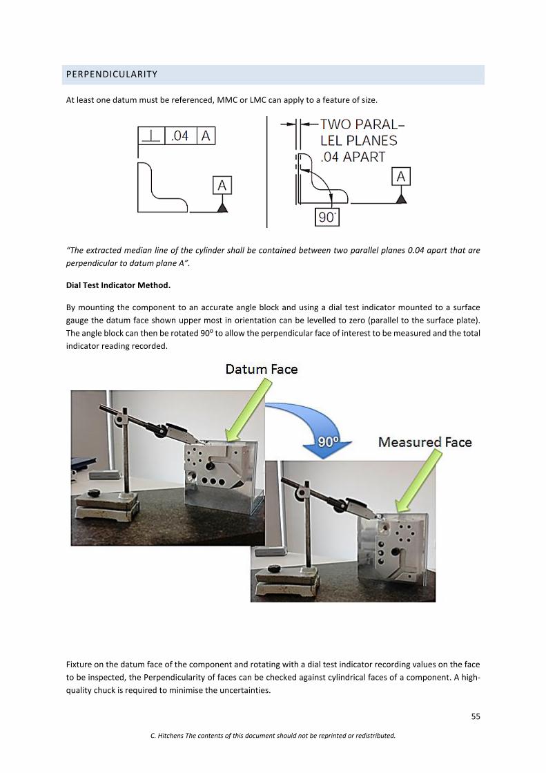
55
C. Hitchens The contents of this document should not be reprinted or redistributed.
PERPENDICULARITY
At least one datum must be referenced, MMC or LMC can apply to a feature of size.
“The extracted median line of the cylinder shall be contained between two parallel planes 0.04 apart that are
perpendicular to datum plane A”.
Dial Test Indicator Method.
By mounting the component to an accurate angle block and using a dial test indicator mounted to a surface
gauge the datum face shown upper most in orientation can be levelled to zero (parallel to the surface plate).
The angle block can then be rotated 90⁰ to allow the perpendicular face of interest to be measured and the total
indicator reading recorded.
Fixture on the datum face of the component and rotating with a dial test indicator recording values on the face
to be inspected, the Perpendicularity of faces can be checked against cylindrical faces of a component. A high-
quality chuck is required to minimise the uncertainties.
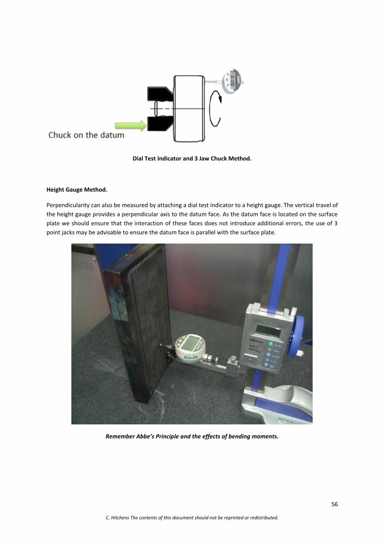
56
C. Hitchens The contents of this document should not be reprinted or redistributed.
Dial Test Indicator and 3 Jaw Chuck Method.
Height Gauge Method.
Perpendicularity can also be measured by attaching a dial test indicator to a height gauge. The vertical travel of
the height gauge provides a perpendicular axis to the datum face. As the datum face is located on the surface
plate we should ensure that the interaction of these faces does not introduce additional errors, the use of 3
point jacks may be advisable to ensure the datum face is parallel with the surface plate.
Remember Abbe’s Principle and the effects of bending moments.

57
C. Hitchens The contents of this document should not be reprinted or redistributed.
Engineers Square and Cylindrical Squares Method.
An engineer’s square with a surface plate, gauge blocks or feeler gauges can be used to determine the
Perpendicularity of faces. The gauge blocks or calibrated feeler gauges are used to determine the magnitude of
any gaps between the component and the engineers square and will provide traceability of measurement. It is
important to note that feeler gauges are not normally calibrated.
The cylindrical square can replace the engineers square as a more robust standard. The cylindrical square is
manufactured to a high accuracy of Cylindricity and the end face of the cylinder to a high accuracy of
Perpendicularity with the main body of the cylinder. Magnetic cylindrical squares allow the standard to be placed
directly on the component; assuming it is magnetic.
Engineers square, cylindrical square and magnetic cylindrical square.

58
C. Hitchens The contents of this document should not be reprinted or redistributed.
PARALLELISM
At least one datum must be referenced, MMC or LMC can apply to a feature of size.
“The extracted median line shall be within a cylindrical zone of diameter 0.04 parallel to the datum A”.
Dial Test Indicator Method.
Use the dial test indicator to set the bottom face parallel to the surface plate, once set the top face can be
checked for parallelism and the total indicator reading recorded. This method could also be used to check
flatness and straightness if required relative to an opposing face. Flat components can be used with a dial test
indicator and located directly on the surface plate, but we should be aware of the interaction of bottom face
with surface this could be a parallelism check.
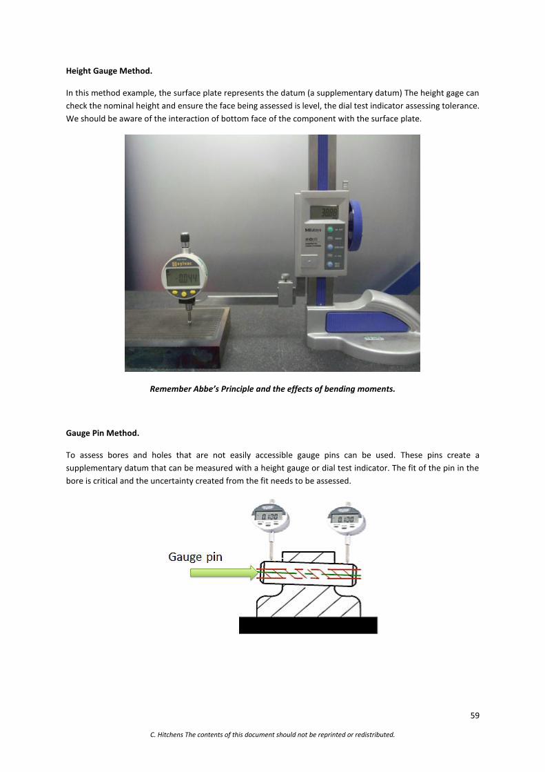
59
C. Hitchens The contents of this document should not be reprinted or redistributed.
Height Gauge Method.
In this method example, the surface plate represents the datum (a supplementary datum) The height gage can
check the nominal height and ensure the face being assessed is level, the dial test indicator assessing tolerance.
We should be aware of the interaction of bottom face of the component with the surface plate.
Remember Abbe’s Principle and the effects of bending moments.
Gauge Pin Method.
To assess bores and holes that are not easily accessible gauge pins can be used. These pins create a
supplementary datum that can be measured with a height gauge or dial test indicator. The fit of the pin in the
bore is critical and the uncertainty created from the fit needs to be assessed.
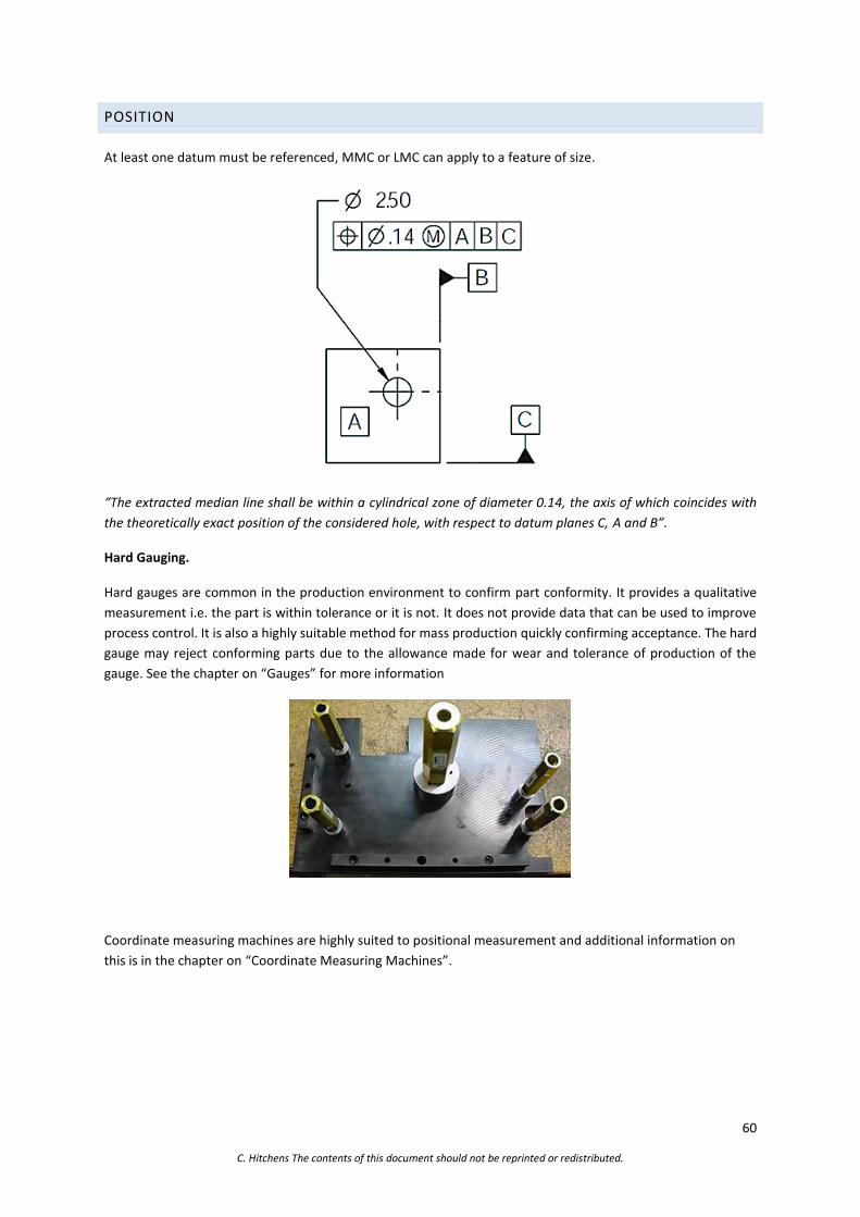
60
C. Hitchens The contents of this document should not be reprinted or redistributed.
POSITION
At least one datum must be referenced, MMC or LMC can apply to a feature of size.
“The extracted median line shall be within a cylindrical zone of diameter 0.14, the axis of which coincides with
the theoretically exact position of the considered hole, with respect to datum planes C, A and B”.
Hard Gauging.
Hard gauges are common in the production environment to confirm part conformity. It provides a qualitative
measurement i.e. the part is within tolerance or it is not. It does not provide data that can be used to improve
process control. It is also a highly suitable method for mass production quickly confirming acceptance. The hard
gauge may reject conforming parts due to the allowance made for wear and tolerance of production of the
gauge. See the chapter on “Gauges” for more information
Coordinate measuring machines are highly suited to positional measurement and additional information on
this is in the chapter on “Coordinate Measuring Machines”.

61
C. Hitchens The contents of this document should not be reprinted or redistributed.
CONCENTRICITY (COAXIALITY) FEATURE
2D 3D Feature At least one datum must be referenced. Always regardless of a feature of size, MMC and LMC
cannot be applied.
“The extracted centre of the inner circle shall be within a circle of diameter 0.04 concentric with datum point in
the cross-section”.
Dial Test Indicator Method.
Concentricity or coaxially is a 2D feature different standards use different term i.e. ASMI and ISO subtle
differences. Tolerance is applied as diametrical, to define a tolerance zone. Coordinate measuring machines
have the ability to measure the diameters of interest and then compare the centre positions of each. Can be
achieved using first principle measurement with rotary tables or three jaw chucks by fixing on one the feature
of interest. The dial test indicator will incorporate any form errors and these need to be understood. If it is
applied to a circular edge it is Concentricity if applied to a cylinder face it becomes Coaxiality.
An alternative method to Tolerancing would be to use “Position” and “Runout” to achieve feature and would be
easier to inspect. Verifying concentricity is a time-consuming process.
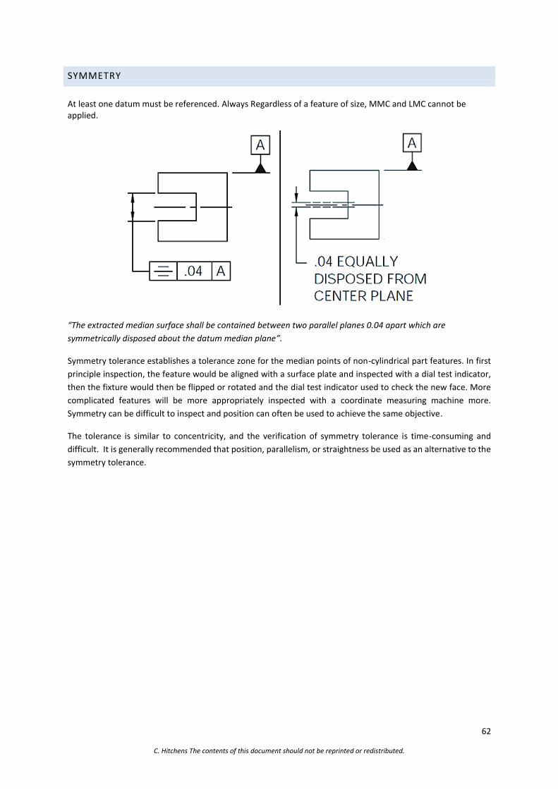
62
C. Hitchens The contents of this document should not be reprinted or redistributed.
SYMMETRY
At least one datum must be referenced. Always Regardless of a feature of size, MMC and LMC cannot be applied.
“The extracted median surface shall be contained between two parallel planes 0.04 apart which are
symmetrically disposed about the datum median plane”.
Symmetry tolerance establishes a tolerance zone for the median points of non-cylindrical part features. In first
principle inspection, the feature would be aligned with a surface plate and inspected with a dial test indicator,
then the fixture would then be flipped or rotated and the dial test indicator used to check the new face. More
complicated features will be more appropriately inspected with a coordinate measuring machine more.
Symmetry can be difficult to inspect and position can often be used to achieve the same objective.
The tolerance is similar to concentricity, and the verification of symmetry tolerance is time-consuming and
difficult. It is generally recommended that position, parallelism, or straightness be used as an alternative to the
symmetry tolerance.
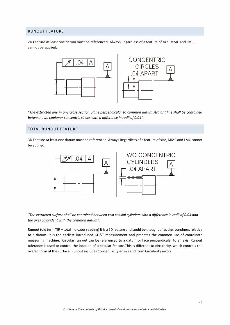
63
C. Hitchens The contents of this document should not be reprinted or redistributed.
RUNOUT FEATURE
2D Feature At least one datum must be referenced. Always Regardless of a feature of size, MMC and LMC
cannot be applied.
“The extracted line in any cross section plane perpendicular to common datum straight line shall be contained
between two coplanar concentric circles with a difference in radii of 0.04”.
TOTAL RUNOUT FEATURE
3D Feature At least one datum must be referenced. Always Regardless of a feature of size, MMC and LMC cannot
be applied.
“The extracted surface shall be contained between two coaxial cylinders with a difference in radii of 0.04 and
the axes coincident with the common datum”.
Runout (old term TIR – total indicator reading) It is a 2D feature and could be thought of as the roundness relative
to a datum. It is the earliest introduced GD&T measurement and predates the common use of coordinate
measuring machine. Circular run out can be referenced to a datum or face perpendicular to an axis. Runout
tolerance is used to control the location of a circular feature.This is different to circularity, which controls the
overall form of the surface. Runout includes Concentricity errors and form Circularity errors.
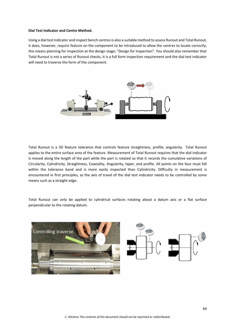
64
C. Hitchens The contents of this document should not be reprinted or redistributed.
Dial Test Indicator and Centre Method.
Using a dial test indicator and inspect bench centres is also a suitable method to assess Runout and Total Runout,
it does, however, require feature on the component to be introduced to allow the centres to locate correctly,
this means planning for inspection at the design stage; “Design for Inspection”. You should also remember that
Total Runout is not a series of Runout checks, it is a full form inspection requirement and the dial test indicator
will need to traverse the form of the component.
Total Runout is a 3D feature tolerance that controls feature straightness, profile, angularity. Total Runout
applies to the entire surface area of the feature. Measurement of Total Runout requires that the dial indicator
is moved along the length of the part while the part is rotated so that it records the cumulative variations of
Circularity, Cylindricity, Straightness, Coaxiality, Angularity, taper, and profile. All points on the face must fall
within the tolerance band and is more easily inspected than Cylindricity. Difficulty in measurement is
encountered in first principles, as the axis of travel of the dial test indicator needs to be controlled by some
means such as a straight edge.
Total Runout can only be applied to cylindrical surfaces rotating about a datum axis or a flat surface
perpendicular to the rotating datum.

65
C. Hitchens The contents of this document should not be reprinted or redistributed.
Runout and Total Runout measured with a dial test indicator are by far more appropriate and reliable with the
part located in V blocks or between centre. The total indicator reading should be less than the tolerance stated
and can be radial or axial.
The measurement can also be made at the point of manufacture, in the case of a lathe by mounting the dial test
indicator to the turret of the machine. For Total Runout remember to consider the potential errors in the
machine tool traverse. If the dial test indicator is mounted on the same machine guides that were used to
manufacture the component, you will be repeating any errors in the machine guides and will not record the
Total Runout value correctly.
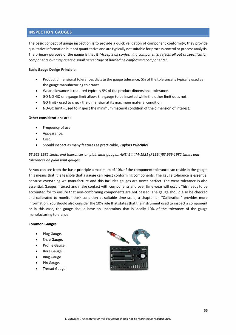
66
C. Hitchens The contents of this document should not be reprinted or redistributed.
INSPECTION GAUGES
The basic concept of gauge inspection is to provide a quick validation of component conformity; they provide
qualitative information but not quantitative and are typically not suitable for process control or process analysis.
The primary purpose of the gauge is that it “Accepts all conforming components, rejects all out of specification
components but may reject a small percentage of borderline conforming components”.
Basic Gauge Design Principle:
Product dimensional tolerances dictate the gauge tolerance; 5% of the tolerance is typically used as
the gauge manufacturing tolerance.
Wear allowance is required typically 5% of the product dimensional tolerance.
GO NO-GO one gauge limit allows the gauge to be inserted while the other limit does not.
GO limit - used to check the dimension at its maximum material condition.
NO-GO limit - used to inspect the minimum material condition of the dimension of interest.
Other considerations are:
Frequency of use.
Appearance.
Cost.
Should inspect as many features as practicable, Taylors Principle!
BS 969:1982 Limits and tolerances on plain limit gauges. ANSI B4.4M-1981 (R1994)BS 969:1982 Limits and
tolerances on plain limit gauges.
As you can see from the basic principle a maximum of 10% of the component tolerance can reside in the gauge.
This means that it is feasible that a gauge can reject conforming components. The gauge tolerance is essential
because everything we manufacture and this includes gauges are never perfect. The wear tolerance is also
essential. Gauges interact and make contact with components and over time wear will occur. This needs to be
accounted for to ensure that non-conforming components are not passed. The gauge should also be checked
and calibrated to monitor their condition at suitable time scale; a chapter on “Calibration” provides more
information. You should also consider the 10% rule that states that the instrument used to inspect a component
or in this case, the gauge should have an uncertainty that is ideally 10% of the tolerance of the gauge
manufacturing tolerance.
Common Gauges:
Plug Gauge.
Snap Gauge.
Profile Gauge.
Bore Gauge.
Ring Gauge.
Pin Gauge.
Thread Gauge.

67
C. Hitchens The contents of this document should not be reprinted or redistributed.
THREADS
Thread Nomenclature.
• Pitch: The distance measured from crest to crest or root to root.
• Lead: The distance moved by a nut or a bolt in the axial direction in one complete revolution.
• Crest: The outermost part of the thread.
• Root: The inner most part of the thread.
• Flank: The surface between the crest and the root.
• The angle of thread: The angle between the flanks.
• Depth: It is the distance between crest and root.
• Nominal diameter: The diameter of the cylindrical piece on which threads are cut is called.
• Major diameter: Diameter at the crest of the thread.
• Minor diameter: The diameter of the core or root.
• Effective Diameter: An imaginary cylinder, which has equal metal and space widths. It is often
referred to as pitch diameter.

68
C. Hitchens The contents of this document should not be reprinted or redistributed.
Common Thread Forms.
Thread forms reside in groups based on their function. Threads for fixing, include the Sharp V, Unified
and Whitworth. Load bearing threads include Square often referred to as Buttress, ACME and B&S
Worm. There are also more specifically functional threads such as the single direction load bearing
types Modified Buttress, Knuckle and the Dardelet.
Shop Reference for Students and Apprentices, Second Edition
The Diagram shows how lead can affect the measurement of the effective pitch diameter. This same
effect can occur with flank angle variation. As the pitch diameter nears its tolerance limits any lead
angle error may not be detected. It is therefore essential to check the thread form and not just the pitch
diameter.
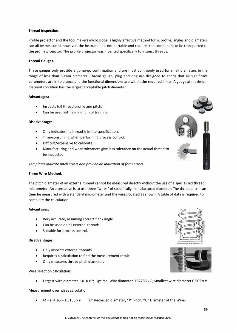
69
C. Hitchens The contents of this document should not be reprinted or redistributed.
Thread Inspection.
Profile projector and the tool makers microscope is highly effective method form, profile, angles and diameters
can all be measured, however, the instrument is not portable and requires the component to be transported to
the profile projector. The profile projector was invented specifically to inspect threads.
Thread Gauges.
These gauges only provide a go no-go confirmation and are most commonly used for small diameters in the
range of less than 50mm diameter. Thread gauge, plug and ring are designed to check that all significant
parameters are in tolerance and the functional dimensions are within the required limits. A gauge at maximum
material condition has the largest acceptable pitch diameter.
Advantages:
Inspects full thread profile and pitch.
Can be used with a minimum of training.
Disadvantages:
Only indicates if a thread is in the specification.
Time-consuming when performing process control.
Difficult/expensive to calibrate.
Manufacturing and wear tolerances give less tolerance on the actual thread to
be inspected.
Templates indicate pitch errors and provide an indication of form errors.
Three Wire Method.
The pitch diameter of an external thread cannot be measured directly without the use of a specialised thread
micrometer. An alternative is to use three “wires” of specifically manufactured diameter. The thread pitch can
then be measured with a standard micrometer and the wires located as shown. A table of data is required to
complete the calculation.
Advantages:
Very accurate, assuming correct flank angle.
Can be used on all external threads.
Suitable for process control.
Disadvantages:
Only inspects external threads.
Requires a calculation to find the measurement result.
Only measures thread pitch diameter.
Wire selection calculation:
Largest wire diameter 1.010 x P, Optimal Wire diameter 0.57735 x P, Smallest wire diameter 0.505 x P
Measurement over wires calculation:
M = D + 3G – 1,5155 x P “D” Recorded diameter, “P” Pitch, “G” Diameter of the Wires

70
C. Hitchens The contents of this document should not be reprinted or redistributed.
Thread Micrometer.
Advantages:
Accurate, assuming correct flank angle.
Can be used on all threads with the same flank angle.
Suitable for process control.
Disadvantage:
Only suitable for external threads.
Requires set-up/reference master when used with a micrometer larger
than25mm.
Only measures thread pitch diameter.
Thread Gauge.
Advantages:
Measures the total thread geometry (diameters and pitch).
Possible for both external and internal threads.
Thread gauge provides quantitative measurement on tolerance.
Suitable for process control.
Disadvantages:
Can only be used for a specific thread.
Requires a master for correct setup.
One wrong dimension on the threaded component can give a false
indication.
CMM Inspection of Threads.
Capable for threads with a pitch greater than 5mm.
Capable of checking Angles with limited repeatability.
Major Minor diameter possible.
Pitch and Pitch Diameter possible.
Other features are not measurable.
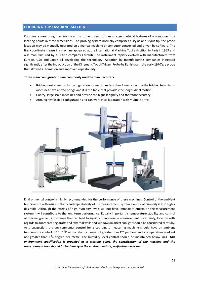
71
C. Hitchens The contents of this document should not be reprinted or redistributed.
COORDINATE MEASURING MACHINE
Coordinate measuring machines is an instrument used to measure geometrical features of a component by
locating points in three dimensions. The probing system normally comprises a stylus and stylus tip, the probe
location may be manually operated on a manual machine or computer controlled and driven by software. The
first coordinate measuring machine appeared at the International Machine Tool exhibition in Paris in 1959 and
was manufactured by a British company Ferranti. The instrument rapidly evolved with manufacturers from
Europe, USA and Japan all developing the technology. Adoption by manufacturing companies increased
significantly after the introduction of the Kinematic Touch Trigger Probe by Renishaw in the early 1970’s; a probe
that allowed automation and improved repeatability.
Three main configurations are commonly used by manufacturers.
Bridge, most common for configuration for machines less than 2 metres across the bridge. Sub-micron
machines have a fixed bridge and it is the table that provides the longitudinal motion.
Gantry, large scale machines and provide the highest rigidity and therefore accuracy.
Arm, highly flexible configuration and can work in collaboration with multiple arms.
Environmental control is highly recommended for the performance of these machines. Control of the ambient
temperature will ensure stability and repeatability of the measurement system. Control of humidity is also highly
desirable. Although the effects of high humidity levels will not have immediate effects on the measurement
system it will contribute to the long term performance. Equally important is temperature stability and control
of thermal gradients in volume that can lead to significant increase in measurement uncertainty, location with
regards to doors creating drafts and external walls and windows in direct sunlight should be considered carefully.
As a suggestion, the environmental control for a coordinate measuring machine should have an ambient
temperature control of 20 ±1⁰C with a rate of change not greater than 1⁰C per hour and a temperature gradient
not greater than 1⁰C degree per metre. The humidity level control should be maintained below 70%. This
environment specification is provided as a starting point, the specification of the machine and the
measurement task should factor heavily in the environmental specification decision.

72
C. Hitchens The contents of this document should not be reprinted or redistributed.
Coordinate measurement machine errors are due to the manufacturing and assembly process and have 21
geometric potential errors. These errors include Roll, Pitch and Yaw, Straightness, Squareness and scale errors.
Volumetric compensation is used to reduce these mechanical errors and regular calibration and maintenance
are required.
Reducing Uncertainty:
Check the calibration status of the CMM.
Use a re-verification artefact and perform interim checks to monitor drift. ISO10360
Ensure CMM’s are calibrated and maintained regularly.
Probe Selection:
Use the shortest probe to increases the stiffness.
A large ruby eliminates any misalignment of the part to the probe, particularly when measuring deep
holes and reduces the effect of surface roughness.
Styli can wear, so periodically check the tip and shank for signs of wear or damage.
Minimise probe changes during measurement and indexing of the head.
Probe setup:
Correct probe qualification is vital to ensure accurate measurement.
Ensure that the reference sphere is calibrated, in good condition and its size is correctly referenced in
the CMM software.
Before qualification, ensure reference sphere and stylus tip are clean and not loose.
Ensure qualification speed is the same as the planned measurement speed.
Re-qualify probes at regular intervals and always after a collision.
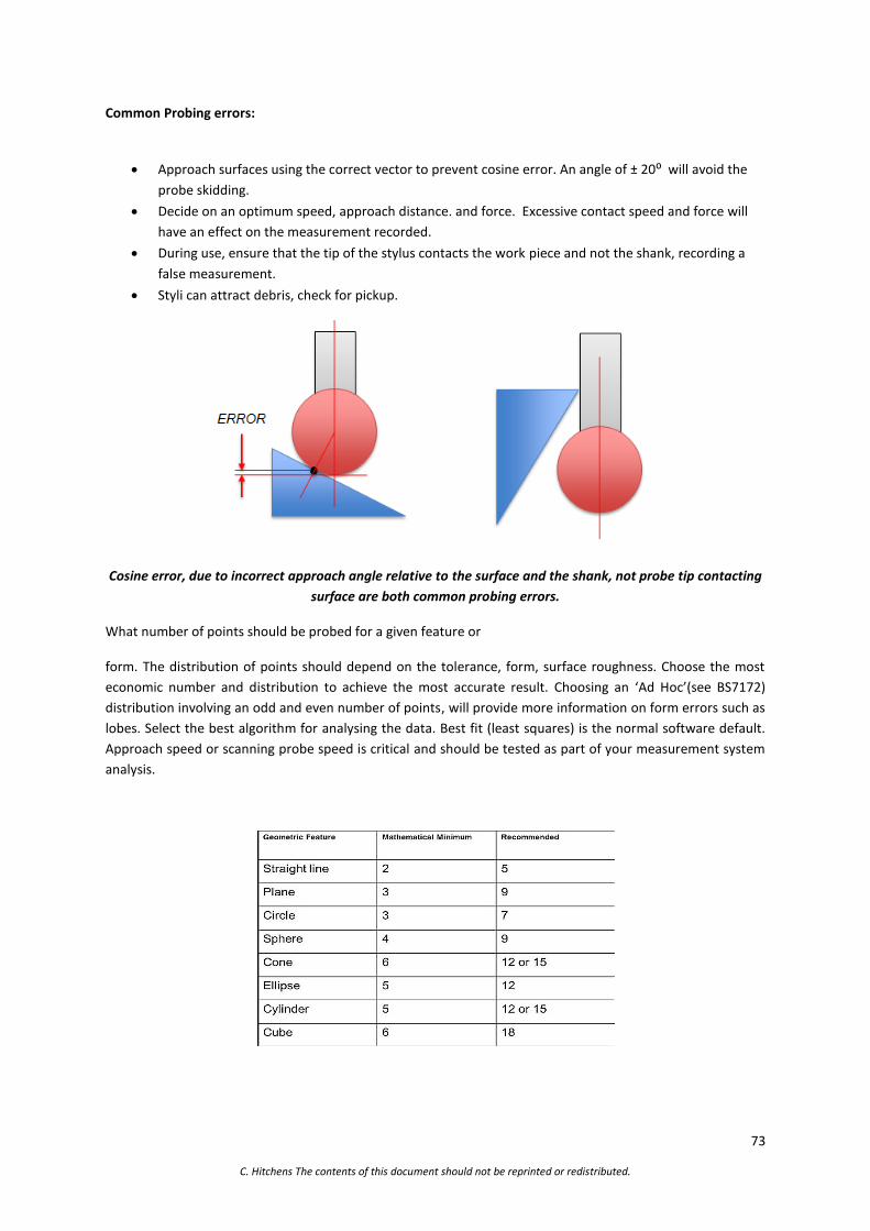
73
C. Hitchens The contents of this document should not be reprinted or redistributed.
Common Probing errors:
Approach surfaces using the correct vector to prevent cosine error. An angle of ± 20⁰ will avoid the
probe skidding.
Decide on an optimum speed, approach distance. and force. Excessive contact speed and force will
have an effect on the measurement recorded.
During use, ensure that the tip of the stylus contacts the work piece and not the shank, recording a
false measurement.
Styli can attract debris, check for pickup.
Cosine error, due to incorrect approach angle relative to the surface and the shank, not probe tip contacting
surface are both common probing errors.
What number of points should be probed for a given feature or
form. The distribution of points should depend on the tolerance, form, surface roughness. Choose the most
economic number and distribution to achieve the most accurate result. Choosing an ‘Ad Hoc’(see BS7172)
distribution involving an odd and even number of points, will provide more information on form errors such as
lobes. Select the best algorithm for analysing the data. Best fit (least squares) is the normal software default.
Approach speed or scanning probe speed is critical and should be tested as part of your measurement system
analysis.
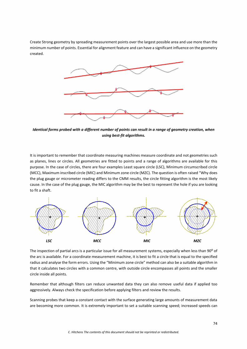
74
C. Hitchens The contents of this document should not be reprinted or redistributed.
Create Strong geometry by spreading measurement points over the largest possible area and use more than the
minimum number of points. Essential for alignment feature and can have a significant influence on the geometry
created.
Identical forms probed with a different number of points can result in a range of geometry creation, when
using best-fit algorithms.
It is important to remember that coordinate measuring machines measure coordinate and not geometries such
as planes, lines or circles. All geometries are fitted to points and a range of algorithms are available for this
purpose. In the case of circles, there are four examples Least square circle (LSC), Minimum circumscribed circle
(MCC), Maximum inscribed circle (MIC) and Minimum zone circle (MZC). The question is often raised “Why does
the plug gauge or micrometer reading differs to the CMM results, the circle fitting algorithm is the most likely
cause. In the case of the plug gauge, the MIC algorithm may be the best to represent the hole if you are looking
to fit a shaft.
LSC MCC MIC MZC
The inspection of partial arcs is a particular issue for all measurement systems, especially when less than 90⁰ of
the arc is available. For a coordinate measurement machine, it is best to fit a circle that is equal to the specified
radius and analyse the form errors. Using the “Minimum zone circle” method can also be a suitable algorithm in
that it calculates two circles with a common centre, with outside circle encompasses all points and the smaller
circle inside all points.
Remember that although filters can reduce unwanted data they can also remove useful data if applied too
aggressively. Always check the specification before applying filters and review the results.
Scanning probes that keep a constant contact with the surface generating large amounts of measurement data
are becoming more common. It is extremely important to set a suitable scanning speed; increased speeds can
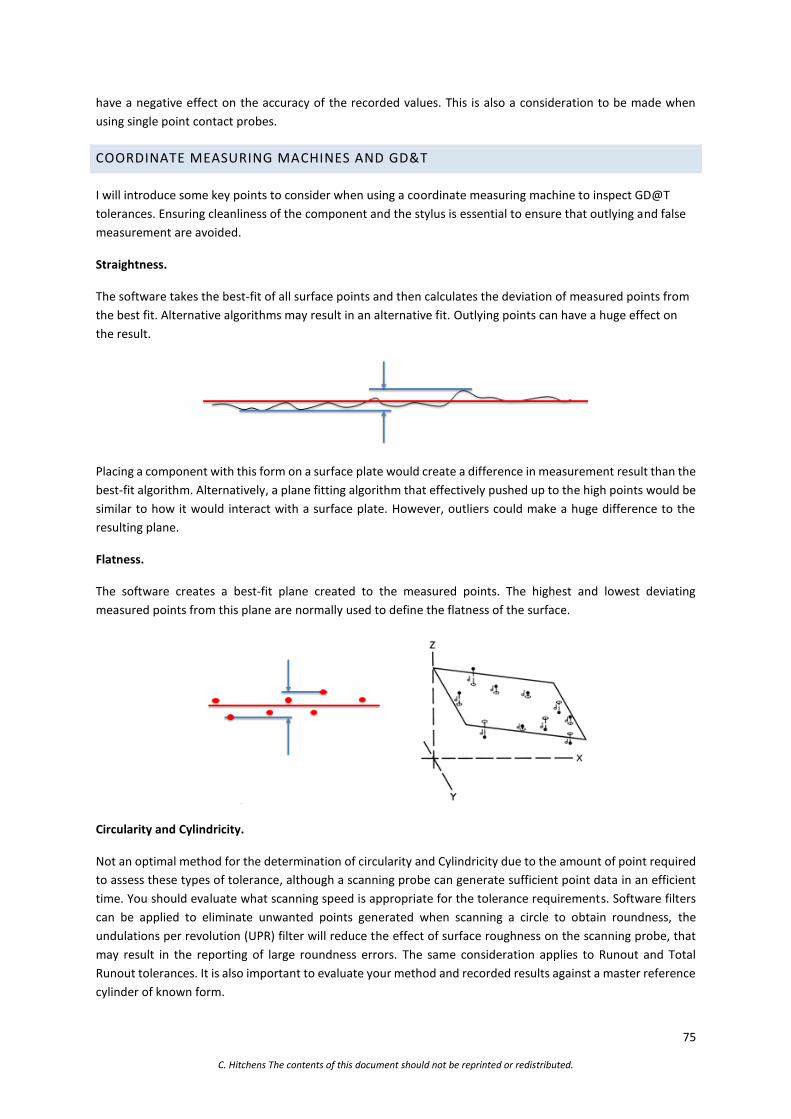
75
C. Hitchens The contents of this document should not be reprinted or redistributed.
have a negative effect on the accuracy of the recorded values. This is also a consideration to be made when
using single point contact probes.
COORDINATE MEASURING MACHINES AND GD&T
I will introduce some key points to consider when using a coordinate measuring machine to inspect GD@T
tolerances. Ensuring cleanliness of the component and the stylus is essential to ensure that outlying and false
measurement are avoided.
Straightness.
The software takes the best-fit of all surface points and then calculates the deviation of measured points from
the best fit. Alternative algorithms may result in an alternative fit. Outlying points can have a huge effect on
the result.
Placing a component with this form on a surface plate would create a difference in measurement result than the
best-fit algorithm. Alternatively, a plane fitting algorithm that effectively pushed up to the high points would be
similar to how it would interact with a surface plate. However, outliers could make a huge difference to the
resulting plane.
Flatness.
The software creates a best-fit plane created to the measured points. The highest and lowest deviating
measured points from this plane are normally used to define the flatness of the surface.
Circularity and Cylindricity.
Not an optimal method for the determination of circularity and Cylindricity due to the amount of point required
to assess these types of tolerance, although a scanning probe can generate sufficient point data in an efficient
time. You should evaluate what scanning speed is appropriate for the tolerance requirements. Software filters
can be applied to eliminate unwanted points generated when scanning a circle to obtain roundness, the
undulations per revolution (UPR) filter will reduce the effect of surface roughness on the scanning probe, that
may result in the reporting of large roundness errors. The same consideration applies to Runout and Total
Runout tolerances. It is also important to evaluate your method and recorded results against a master reference
cylinder of known form.

76
C. Hitchens The contents of this document should not be reprinted or redistributed.
IMPORTANT: Please note; the only truly robust method is the roundness testing machine. Coordinate
measurement machine measurement should be assessed against a reference standard of known form.
Profile of a line or Surface.
Coordinate measuring machines use the shadowgraph principle to check all points fall within the minimum and
maximum limits and are very effective because they can reference one measured point to another along the
required profile and some forms especially freeform geometries can only be inspected with a CMM. One should
also consider cosine error of the stylus contact angle with the part. It will, however, only report that the part is
in our out of limit and the total value. It can be difficult to determine where exactly the out of tolerance condition
exists unless this is detailed in the measurement plan. It may only be a small area or even a rogue point due to
a false trigger.
Position.
Coordinate measuring machines are highly suitable for measuring the position of feature to the datum and
relative to other features. Be aware that when using coordinate measuring machines to calculate the position
of holes it will not include the diameter size, if locating parts on an assembly it may not fit unless the diameters
are included in the measurement assessments. Material condition modifiers can be included in the
measurement strategy and this makes for easier assessment of tolerances that are interacting
Concentricity and Cylindricity.
Can be susceptible to arc fitting algorithms and these should be considered and tested to check they are
appropriate for the inspection strategy.
Symmetry, Angularity, Perpendicularity and Parallelism.
The software can effectively manage this type of GD&T tolerance if programmed correctly and is an efficient
method. The results can be susceptible to plane fitting errors.

77
C. Hitchens The contents of this document should not be reprinted or redistributed.
ON-MACHINE PROBING
The majority of modern machine tools are supplied with or can be equipped with touch probes that can be
employed in the dimensional measurement of component features. Equipping a machine tool with a probe
effectively turns it into a coordinate measuring machine. However, limitations exist that should be considered
when measuring on a machine tool compared with on the coordinate measuring machine. A Primary and
significant limitation of on-machine probing is that the same axes of motion used to machine the form will be
used to record the measured values. Any errors in the axes of motion will therefore contribute and reside in the
measured data and will not be evident in the recorded values. In addition, the thermal expansion of the machine
will not be detectable in the values recorded, therefore machine tool alignment and health monitoring, thermal
control and regular probe calibration are essential. The chapter “Coordinate Measuring Machines” should be
referenced as the principles discussed in this chapter are directly relevant to achieving good measurement
results on the machine tool.
Probe Types.
Originally only single point kinematic touch-trigger probes were available, mechanical in design and highly
repeatable. In a kinematic design, the stylus is connected to a kinematic mechanism held in place by a spring.
The kinematic mechanism consists of three cylinders, each resting on two spheres providing six points of contact.
This design provides a stable home position for the stylus when not in contact and a known position relative to
the machine tool coordinate system. Each of the six kinematic points of contact forms an electrical circuit when
the stylus deflects due to contact with a components surface the force generated by the contact will result in
one or more of the circuits ultimately being broken and the probe will be triggered.
Renishaw Touch Trigger Probe
The contact force is opposed by the force of the spring acting on the kinematic mechanism. When the force
transferred to the kinematic mechanism from the stylus overcomes the force of the spring the contact between
six kinematic points is affected, resulting in an increase in the electrical resistance. Ultimately the contacts will
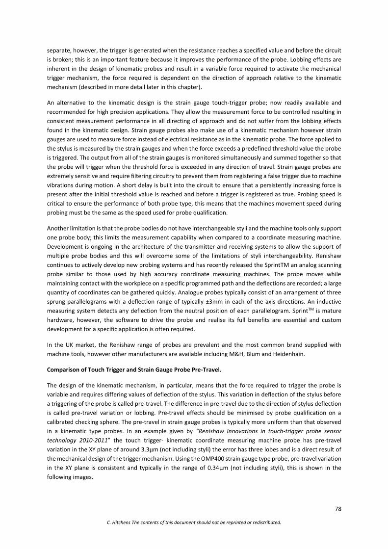
78
C. Hitchens The contents of this document should not be reprinted or redistributed.
separate, however, the trigger is generated when the resistance reaches a specified value and before the circuit
is broken; this is an important feature because it improves the performance of the probe. Lobbing effects are
inherent in the design of kinematic probes and result in a variable force required to activate the mechanical
trigger mechanism, the force required is dependent on the direction of approach relative to the kinematic
mechanism (described in more detail later in this chapter).
An alternative to the kinematic design is the strain gauge touch-trigger probe; now readily available and
recommended for high precision applications. They allow the measurement force to be controlled resulting in
consistent measurement performance in all directing of approach and do not suffer from the lobbing effects
found in the kinematic design. Strain gauge probes also make use of a kinematic mechanism however strain
gauges are used to measure force instead of electrical resistance as in the kinematic probe. The force applied to
the stylus is measured by the strain gauges and when the force exceeds a predefined threshold value the probe
is triggered. The output from all of the strain gauges is monitored simultaneously and summed together so that
the probe will trigger when the threshold force is exceeded in any direction of travel. Strain gauge probes are
extremely sensitive and require filtering circuitry to prevent them from registering a false trigger due to machine
vibrations during motion. A short delay is built into the circuit to ensure that a persistently increasing force is
present after the initial threshold value is reached and before a trigger is registered as true. Probing speed is
critical to ensure the performance of both probe type, this means that the machines movement speed during
probing must be the same as the speed used for probe qualification.
Another limitation is that the probe bodies do not have interchangeable styli and the machine tools only support
one probe body; this limits the measurement capability when compared to a coordinate measuring machine.
Development is ongoing in the architecture of the transmitter and receiving systems to allow the support of
multiple probe bodies and this will overcome some of the limitations of styli interchangeability. Renishaw
continues to actively develop new probing systems and has recently released the SprintTM an analog scanning
probe similar to those used by high accuracy coordinate measuring machines. The probe moves while
maintaining contact with the workpiece on a specific programmed path and the deflections are recorded; a large
quantity of coordinates can be gathered quickly. Analogue probes typically consist of an arrangement of three
sprung parallelograms with a deflection range of typically ±3mm in each of the axis directions. An inductive
measuring system detects any deflection from the neutral position of each parallelogram. SprintTM is mature
hardware, however, the software to drive the probe and realise its full benefits are essential and custom
development for a specific application is often required.
In the UK market, the Renishaw range of probes are prevalent and the most common brand supplied with
machine tools, however other manufacturers are available including M&H, Blum and Heidenhain.
Comparison of Touch Trigger and Strain Gauge Probe Pre-Travel.
The design of the kinematic mechanism, in particular, means that the force required to trigger the probe is
variable and requires differing values of deflection of the stylus. This variation in deflection of the stylus before
a triggering of the probe is called pre-travel. The difference in pre-travel due to the direction of stylus deflection
is called pre-travel variation or lobbing. Pre-travel effects should be minimised by probe qualification on a
calibrated checking sphere. The pre-travel in strain gauge probes is typically more uniform than that observed
in a kinematic type probes. In an example given by “Renishaw Innovations in touch-trigger probe sensor
technology 2010-2011” the touch trigger- kinematic coordinate measuring machine probe has pre-travel
variation in the XY plane of around 3.3µm (not including styli) the error has three lobes and is a direct result of
the mechanical design of the trigger mechanism. Using the OMP400 strain gauge type probe, pre-travel variation
in the XY plane is consistent and typically in the range of 0.34µm (not including styli), this is shown in the
following images.

79
C. Hitchens The contents of this document should not be reprinted or redistributed.
Typical Pre-travel variation in a kinematic probe. Renishaw Innovations in touch-trigger probe sensor
technology. 2010-2011
Typical pre-travel variation in a strain gauge probe. Renishaw Innovations in touch-trigger probe sensor
technology. 2010-2011
Pre-travel variation can be between 10 and 50µm in touch trigger probes and are heavily influenced by the stylus
length and probing speed, however, a value as little as 3µm for a strain gauge probe should be achievable. It is
important to note that the strain gauge probes are prone to false triggering during rapid motion, due to their
sensitivity and the inertia of the stylus especially long styli.
80
C. Hitchens The contents of this document should not be reprinted or redistributed.
Cycles and Programming
Limitation in the programming software and cycles available on the machine tool frequently lack the
functionality required for complex geometries, even diameter measurements are often crude and calculated
from minimal coordinate information. As an example, measuring the diameter of a bore is often derived from
as little as four probed points on the bore surface. The first two points are used to construct a perpendicular
centre line at an equidistant position between these points. The second two points measured along the
constructed perpendicular centre line are used to record the diameter. As a measurement system, this very poor
and has no mitigation against form error (ovality) or cosine errors during probing of the surface. The majority of
computer aided manufacturing software’s have incorporated functions to allow the user to create more complex
inspection routines. However and more interestingly, coordinate measuring machine manufacturers are
developing interfaces with machine tools, enabling much of the capability of the coordinate measuring machine
software to be utilised on the machine tool. Products such as Renishaw’s Productivity Plus, Hexagon’s PC-DMIS
NC and Delcam’s Power Inspect are such software’s; please note this is not an exhaustive list of software.
Despite these limitations, on-machine probing can delivery productivity and process robustness benefits by
checking a semi-finished machined surface prior to the finishing cut. This allows adjustment of the tool offsets
in order to compensate the finish cutter path based on the recorded values at a semi-finished stage by removing
specific values of material. This process is often referred to as “measured cuts“; when applied correctly will
greatly reduce the risk of dimensional non-conformance. On-machine probing is also commonly used to
establish a datum and the position of the raw material. The coordinate information can then be used to adapt
the NC program accordingly by means of a global program offset. This reduces setting time and mitigation
against setting errors.
There is a distinct difference between the terms “on-machine verification” and “on-machine inspection”. On-
machine verification is widely used for process capability monitoring, measured cutting and datum setting.
Verification cannot be considered inspection and the recorded values cannot be treated or reported as such
because the values have no traceability. On-machine inspection performs measurements that are traceable via
an unbroken chain to the SI unit (metre). In the case of coordinate measuring machines this is achieved by the
adherence to international standards for the calibration of the instrument; specifically in Europe, this is
ISO10360. In the case of machine tools a calibration standard does not exist, the closest relevant standard would
be ISO230 describing the process for alignment of the machine structure. It is, however, possible with robust
procedures to create a body of evidence to support the validity of the recorded values.
Understanding the machine tool construction is essential. Machine tool sources of error can be grouped into
three categories; Static, Kinematic and Dynamic. As an example of static errors, a 3 axis machine tool has 21
potential sources of mechanical error that require measuring. These 21 errors are Roll, Pitch and Yaw along the
X, Y and Z axes of motion, and Straightness, Squareness and scale errors in the construction. Machine tools with
multiple rotary axes have additional errors with the rotary axes being significant sources of uncertainty.
Static Errors:
Straightness of function surfaces
Flatness of functional surfaces
Position, orientation and alignment of functional surface
Squareness and Perpendicularity
Kinematic Errors:

81
C. Hitchens The contents of this document should not be reprinted or redistributed.
Parallelism of the axes of motion
Squareness (Perpendicularity) of axes of motion
Coaxiality of axes
Backlash
Hysteresis
Dynamic Errors:
Vibration
Thermal effect
Controller error
Deflection resulting from cutting forces
If we are to ensure the quality of our recorded values, it is therefore essential that the uncertainty of the machine
tool resulting from the Static, Kinematic and Dynamic errors should be investigated, understood and
documented. A machine tool’s positional accuracy can also be verified to some extent by using the probe by
measuring known positions on the machine tool or an artefact that are not susceptible to effects of thermal
expansion. Rotational, positional and repeatability checks can be conducted by probing a calibration sphere and
determining the sphere centre at a range of positions and orientations inside the machine tool volume. Many
modern machine tools have specific cycles available as standard to perform these reverifications; please note
that these checks do not validate volumetric positioning errors. A specific reverification methodology based on
the machine tool configuration is required to ensure the machine is in the specification and understand the
uncertainties. This could involve relatively simple checks using granite reference edges and squares with dial
test indicators and the use of Ballbar checks to identify backlash, axis reversal, scale mismatch, squareness, servo
mismatch, master slave mismatch and stick-slip of axis traverse at slow feed rates. Reverification should be
introduced as part of on-going strategy to monitor the machine tool condition and identify early signs of wear
and deterioration in the machine tool performance. The Ballbar check cannot fully validate a machine tool alone.
These interim checks are only reverification, they should not replace the guidance of ISO230.
Depending on the machine tool configuration it may not be possible to independently validate every axis. Some
axes may be dependant or influenced by another and it is, therefore, the accumulative effects of multiple axes
that is being measured and the actual source of any error will be difficult to isolate.
Good Practice:
Use the shortest probe to increases the stiffness.
Styli can wear, so periodically check the tip and shank for signs of wear or damage and cleanliness.
Ensure machine tool is at the operating temperature before calibration.
Perform regular probe qualification (calibration).
Use the same probing approach speed for measurement as that used for qualification of the probe.
Be aware of the probing approach angle relative to the face being measured. Angles of approach not
perpendicular to the surface will have a cosine error. More advanced software can compensate for this
error.
82
C. Hitchens The contents of this document should not be reprinted or redistributed.
Perform regular reverification of the machine tool and the calibration artefacts.
High precision requirements:
Where possible calibrate the probe with an artefact that is geometrically similar in form and dimension
to that of the feature of interest. In effect, the probe can then be used to create a comparative
measurement to a known traceable standard.
Locate the calibration artefact as close to the feature of interest as is possible. This will limit thermal
effect and errors that reside in the axes of the machine tool.
Manufacture the calibration artefact in a material with the same coefficient of expansion as that of the
component.
Ensure the machine temperature at the time of measurement is consistent with the temperature at the
time of probe calibration. The time interval between calibration and measurement should be
minimised.
Use strain gauge probe bodies.
Perform reverification of the machine tool prior to manufacture of the component.
On-machine inspection is a technology that does have the potential to deliver significant benefits in the
manufacturing process of large machined components (those being over 2 metre for example). The logistics
involved in relocating large components from the machining centre to a coordinate measuring machine are
difficult and often account for a significant amount of the overall manufacturing time. Inspection times on the
machine are most likely to be a fraction of the machining and handling times, which makes the case to inspect
on the machine tool more compelling and the effort involved more rewarding. In addition, the infrastructure
and investment required to provide efficient and effective handling equipment and a coordinate measuring
machine of sufficient measuring volume require significant capital investment. An investment that could be
spent on increased manufacturing capability. In addition for high value components the consequence of errors
during manufacture is not an acceptable proposition because of the limited options for component rectification
and the potential cost implications on downstream engineering projects due to delays in sourcing materials and
remanufacture is often not acceptable. On machine probing has significant benefits for the manufacturing
process but should be applied appropriately to be most effective. The level of effort required to achieve on-
machine inspection measurements that are traceable is often not commercially viable for small complex
components. Having a modern high value multi-axis machine tool performing inspection tasks will result in lost
manufacturing time, time that could be used to produce more products. This is compounded when you consider
that a coordinate measuring machine would typically have a capital cost of 10-30% of a machine tool with a
comparable working volume.

83
C. Hitchens The contents of this document should not be reprinted or redistributed.
LARGE VOLUME METROLOGY
No strict definition exists for at what point a measurement can be considered to be large volume, we can,
however, consider dimension over one metre to be problematic for conventional measurement instruments
such as micrometer and CMMs, although CMMs of 4 meter in width and longer in length are available. We,
therefore, need to consider alternative instrument technologies and in the main, the laser tracker, developed in
the late 80’s, has become the most popular solution. However, optical tracking is developing quickly and in the
future looks likely to provide an alternative solution. The instruments described if the chapter “Non-Contact
Measurement” can also be employed in large volume metrology applications.
LASER TRACKER
A laser tracker is a non-contact portable CMM capable of static and dynamic measurements in large volume
applications. A line-of-sight technology, it measures 3D coordinates by tracking a laser beam to a retro-reflector
target held in contact with the object being measured. A typical range of a laser tracker can be 160 m radially
with measurements having a typical accuracy of 15 µm plus 6 µm for every additional meter. Manufacturers
include Leica, API and Faro. Traditionally two operators were required, one to move the retro-reflector target
through the points requiring measurement and one to operate the tracker, however the latest trackers can be
operated by remote control.
Laser tracker coordinate system
Two types of tracker are commonly available; interferometer (IFM) and absolute distance measurement (ADM).
IFM provides an incremental measurement of distance by splitting the laser beam into two beams, one part is
used as a reference and the second for distance measurement. The reference part of the beam travels directly
into the interferometer. The other part of the beam travels out to the spherically mounted retro-reflector (SMR),
on the beams return it then also passes into the interferometer. The two beams are compared inside the
interferometer and the cyclic change is calculated. As the SMR moves closer to or farther away from the laser
tracker by a distance the cyclic changes are counted; these changes are equal to one-quarter of the light’s
wavelength (~0.158 microns). The total number of changes is counted to determine the total distance travelled.
Older IFM trackers had a major drawback in use. Should the beam be broken the incremental counting would

84
C. Hitchens The contents of this document should not be reprinted or redistributed.
be interrupted and the distance calculation lost and requiring the operator to return to a known home position
and start the measurement process again. Modern IFM trackers also incorporate ADM technology to overcome
this usability issue and still maintain the performance of the interferometer. ADM systems directly measure the
distance to the SMR, infrared light from a semiconductor laser reflects off the SMR and returns to the laser
tracker. On its return, the time of flight is recorded and by using the known speed of light in air the distance
from the laser tracker to the SMR can be calculated.
Both systems measure the optical distance to a target and the atmosphere refractive index, air pressure and
humidity can have an effect. Laser tracker systems should include a weather station to compensate for the
refractive index and environmental effects. Therefore the weather station and tracker both need calibration.
The IFM itself is traceable if its laser frequency is known. An ADM does not normally have the stability of the
IFM and calibration of ADM is normally performed by comparison with an interferometer or a reference length
artefact. This means that the ADM calibration is typically further removed from the primary reference standards.
Angular encoders are the weak point in the measurement system; small angular errors will be magnified over a
large distance.
Leica has enhanced the capability of the basic laser tracker with the addition of their T-Cam (see chapter “Optical
Tracking”) and several T-products that allow 6 degrees of freedom tracking and additional ways to gather 3D
coordinates. The T-products available are the wireless T-Probe, a ‘walk-around’ contact probe and a T-Scan, a
non-contact high-speed laser scanner. The T-Cam uses optical tracking to determine the orientation of the T-
Products by monitoring a set of embedded LEDs. This with the positional tracking of the laser tracker completes
the 6 degrees of freedom system and ensures all measurements taken are contained within one coordinate
system. Some loss of precision and accuracy will be encountered as the optical tracking is not as precise as the
laser tracker.
Advantages:
Portable.
Accurate over very large distances.
Unaffected by optical properties of the object.
Optional extra 6 DOF (Degrees of Freedom).
Disadvantages:
Contact process SMR target required.
Manual process.
Relatively slow (target can be used for scanning surface).
SMR target compensation required.
Subjectable to the effects of the atmosphere.
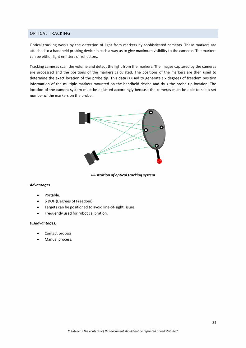
85
C. Hitchens The contents of this document should not be reprinted or redistributed.
OPTICAL TRACKING
Optical tracking works by the detection of light from markers by sophisticated cameras. These markers are
attached to a handheld probing device in such a way as to give maximum visibility to the cameras. The markers
can be either light emitters or reflectors.
Tracking cameras scan the volume and detect the light from the markers. The images captured by the cameras
are processed and the positions of the markers calculated. The positions of the markers are then used to
determine the exact location of the probe tip. This data is used to generate six degrees of freedom position
information of the multiple markers mounted on the handheld device and thus the probe tip location. The
location of the camera system must be adjusted accordingly because the cameras must be able to see a set
number of the markers on the probe.
Illustration of optical tracking system
Advantages:
Portable.
6 DOF (Degrees of Freedom).
Targets can be positioned to avoid line-of-sight issues.
Frequently used for robot calibration.
Disadvantages:
Contact process.
Manual process.

86
C. Hitchens The contents of this document should not be reprinted or redistributed.
AUTO COLLIMATOR, OPTICAL ALIGNMENT TELESCOPE AND INCLINOMETER
These instruments can accurately measure flatness, straightness, angles and perpendicularity and are capable
of performing measurements over considerable distances. Unlike laser based instruments they are less
susceptible to humidity and environmental effects that can distort a laser beams path.
AUTOCOLLIMATOR
An autocollimator is an optical instrument that uses the deviations in the reflection of a mirror from a projected
beam of light. The deviations in the beam reflection can be measured visually or by means of an electronic
detector. The electronic detector can have accuracy significantly higher as much as 100 times that of visual
detection.
OPTICAL ALIGNMENT TELESCOPE
An optical alignment telescope uses glass targets to accurately align and measure objects that are within its
optical axis (line of site). The telescope is accurately located inside a stainless steel cylinder and this represents
the instruments datum for position and orientation. The instrument is commonly used for aligning bores and
bearings by using a precision bush to locate the stainless steel cylinder centrally in the bore or bush being
aligned.
Optical alignment telescope showing the glass target used for measurement.

87
C. Hitchens The contents of this document should not be reprinted or redistributed.
Shows the setup required to measure Perpendicularity when using an Auto Collimator or Optical Alignment
Telescope.
INCLINOMETER
An inclinometer is an instrument that measures tilt (pitch and roll) relative to gravity and is essentially a high
precision spirit level. The tilt angles recorded can be used to calculate elevation and angles of a component
surface. The instrument shown below is the Telyvel 6 and widely used for checking granite reference surfaces
and coordinate measurement machine tables.
Inclinometer and computer generated plot of a components surface displacements.

88
C. Hitchens The contents of this document should not be reprinted or redistributed.
NON-CONTACT MEASUREMENT AND SCANNING INSTRUMENTS
Non-Contact Measurement and Scanning Instruments have developed significantly over the last decade and
with this development, the capital costs are reducing. This section will detail three of the principal technologies
commonly used, although this is not an exhaustive list. When using these types of technologies it is important
to consider measurement traceability.
LASER LINE SCANNERS AND LASER STRIP SCANNERS
Laser Line Scanners and laser strip scanners project a strip of points which are then reflected from the
component surface and collected by the detector. The length of one side of the triangle, namely the distance
between the camera and the laser emitter, is a known value. The angle of the laser emitter is known as is the
return angle determined by the location that the dot returns in the detector’s field of view. From these values,
the surface position can be calculated and recorded, as shown in below. Depending on the system, data capture
can range from 20 000 points per second to 100 000 points per second. This is a non-contact line-of-sight
technology which has a focal range, requiring the operator to keep the scanner at a reasonably constant distance
from the object being scanned.
Laser source and receiver are mounted at a distance and angle so the path can be triangulated Single laser
beam passing through a rotating polygon mirror.
Recent developments employ a flying dot approach to assimilate the laser strip. This in part solves the surface
variation and reflectivity problems found with some scanners and avoids the need to treat the component to
provide a matt surface. Measurements are performed by using the same basic system as shown in Figure above,
but forming a laser line by sweeping the laser spot over an angle using a rotating polygon mirror shown in the
figure above. This has the advantage of allowing surface contrast to be assessed before measurement by
sampling the returned laser strength and adjusting the intensity of the output. This gives the ability to measure
composite materials in a single scanning session and allows the system to be adjusted to light and dark contrast
areas, which assists with processing reflective surfaces.
A laser line scanner can also be used in combination with a Laser Tracker to provide a datum. For background
information on how laser scanners work, see the chapter on “Non-Contact Measurement”.

89
C. Hitchens The contents of this document should not be reprinted or redistributed.
Advantages:
Non-contact.
No probe diameter to consider.
15,000 points/set or greater.
Disadvantages:
Affected by optical properties of the object.
Affected by ambient light.
Not good on near vertical surfaces
Line-of-sight limitations.
STRUCTURED LIGHT
Structured light digitisers work by illuminating an object with a structured light fringe pattern and the distortion
of the light pattern is recorded by a camera. The distortion of the light pattern over the object is used to
triangulate the surface and calculate the coordinates.
The relationship of fringe pattern projection and camera image capture
These scanning systems are portable and available from a number of suppliers such as Steinbichler and GOM to
name two. The speeds of data capture are much higher than laser or CMMs, typically in the 200 000 points per
second range. The accuracy of points is approximately 0.01 mm at a measurement volume of 100 mm in x,y and
z. The measurement volume can be adjusted and this affects the accuracy of the technique. At a large volume
400 mm the accuracy is reduced to approximately 0.03 mm. Ambient light conditions can affect the scanning
accuracy. The newer systems are being developed to automatically calibrate against this.
This scanning method offers fast and accurate data capture and multiple scans can be combined with the use of
markers. The process is non-contact through surface reflections can be an issue and if possible it is advised to
treat the component to produce a matt finish. This is a line-of-sight scanner and limited to external scanning.
To take scans from multiple orientations it is necessary to introduce markers. This is normally done by means of
adding photogrammetry targets, which are temporarily glued to the component. When one scan is aligned with

90
C. Hitchens The contents of this document should not be reprinted or redistributed.
another it is essential to see a minimum of three of these targets, as they are manually added the relationship
of these targets and their position to neighbours forms a unique pattern. It is this uniqueness which is exploited
in the alignment algorithms.
Advantages:
Non-contact.
Large area coverage.
up to 100,000 points/sec.
High accuracy achievable.
Disadvantages:
Expensive although costs are reducing.
Affected ambient light conditions.
Vertical surfaces are an issue.
Line-of-sight limitations.
PHOTOGRAMMETRY
Photogrammetry uses images taken by fixed focus digital cameras. The images are taken at different positions
and angles. By comparing the position of common points on the images the angle and distance of the camera
positions can be calculated and from this, the surface coordinates can also be derived. Often the cameras are
mounted together and the distance between cameras and the angles are already known.
Illustration of how multiple locations of camera image can be combined and point positions calculated.
Manufactures include GOM, Cognitens and Solutionix. The image below shows the Cognitens system with its
positioned cameras.
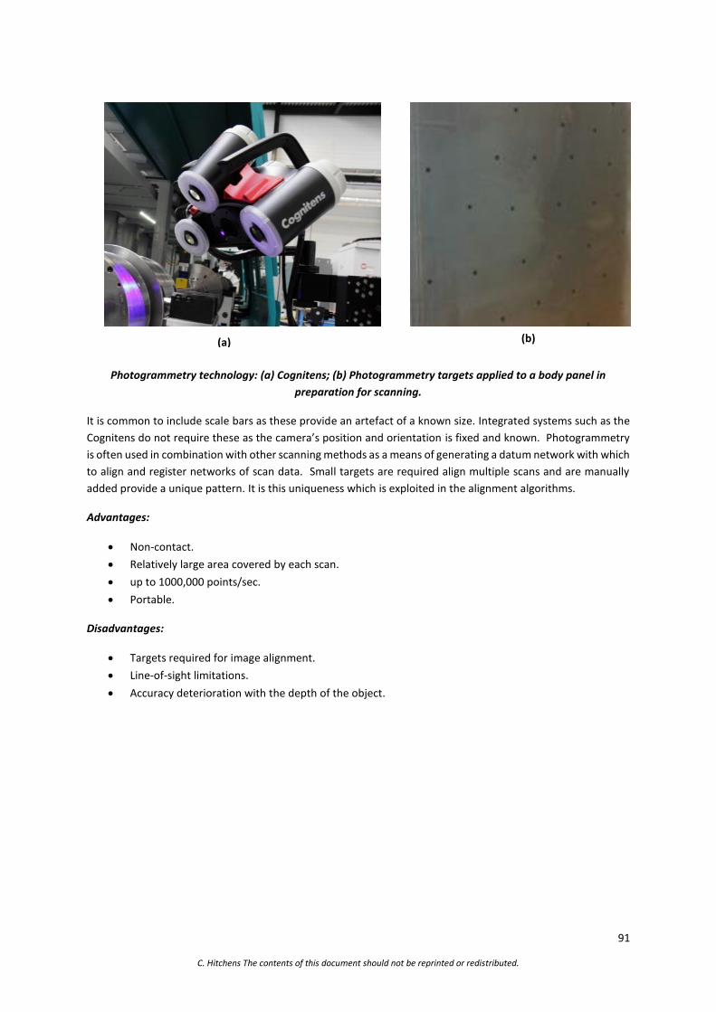
91
C. Hitchens The contents of this document should not be reprinted or redistributed.
Photogrammetry technology: (a) Cognitens; (b) Photogrammetry targets applied to a body panel in
preparation for scanning.
It is common to include scale bars as these provide an artefact of a known size. Integrated systems such as the
Cognitens do not require these as the camera’s position and orientation is fixed and known. Photogrammetry
is often used in combination with other scanning methods as a means of generating a datum network with which
to align and register networks of scan data. Small targets are required align multiple scans and are manually
added provide a unique pattern. It is this uniqueness which is exploited in the alignment algorithms.
Advantages:
Non-contact.
Relatively large area covered by each scan.
up to 1000,000 points/sec.
Portable.
Disadvantages:
Targets required for image alignment.
Line-of-sight limitations.
Accuracy deterioration with the depth of the object.
(b) (a)

92
C. Hitchens The contents of this document should not be reprinted or redistributed.
INSPECTION PROCESS FOR SCANNING INSTRUMENTS
Non-Contact Measurement and Scanning Instruments this range of technologies and techniques are also being
exploited in measurement and inspection applications. No standards exist at present to control the direct
traceability to the SI unit, although the National Physical Laboratory is actively working on this. We can, however,
employ good practice with the scans data that we generate by including known artefacts. The inclusion of gauge
blocks, length bars and calibrations spheres of known dimensions into our scanning projects. Subsequent
checking of these artefacts will provide a level of confidence and indirect traceability to our scan data.
Once the surface coordinate point data is captured by the scanning instrument, the typical next stage is to
generate a polygon (triangle) mesh; primitives are then constructed overlaying the polygon mesh. These
primitives can then have dimensions applied and measurements recorded. Alternatively, CAD data is often
aligned to the polygon mesh and algorithms automatically calculate the deviation from the nominal CAD
geometry. This provides a global measurement assessment of deviations from nominal CAD model values and is
often displayed as colour map the convention is to display maximum negative variations in blue and maximum
positive variations in red. Areas that have zero variation are displayed in green with the remaining spectrum of
colours used to depict gradients of change. This graphical full field depiction of measurement can provide the
engineer with a greater understanding of the component and where geometrical issues reside.
Typical CAD comparison showing surface deviations from a nominal CAD model is shown above.
It is important to have an appreciation of the process flow required to use scan data for inspection applications.
A number of conversions take place and often multiple software are involved. The chart below details the
process steps commonly used, however, it is also possible to calculate the deviations between the raw point

93
C. Hitchens The contents of this document should not be reprinted or redistributed.
cloud and nominal CAD and it could be argued that this is more efficient and less susceptible to potential errors
during conversion from one format to the next. Unfortunately point data does not include a vector or direction
that is readily available from the polygonised format.
Details the steps involved and the typical file formats used at each stage.
94
C. Hitchens The contents of this document should not be reprinted or redistributed.
REVERSE ENGINEERING
Reverse engineering commonly refers to the process of taking an existing object or component and by means of
measurement produce a replica in either an electronic or physical format. The replica may be used for analysis,
reproduction or as a digital record. The most common means of measurement deployed is the recording of
surface point coordinates, using either a contact or non-contact method. Reverse engineering is in common use
in these application areas.
Legacy components or competitive analysis:
Original CAD data is not available (component may predate CAD) and components that have been
manufactured or modified by manual processes.
Historical monuments, art and architecture:
Structures that have been manufactured by a manual process or cannot be designed in CAD or described
mathematically.
Natural organic structures:
Structures that are not possible to be designed in CAD or described mathematically.
Many components in use today were designed and manufactured before Computer aided design (CAD) or
computer aided manufacture (CAM) software existed or was in common use. This poses a problem when
replacements are required; often the only reference is the existing component that may be in use. If drawings
are available it is still advised to make reference to the actual component, modifications may have been made
during manufacture or to assist assembly. These modifications may not have been recorded and therefore the
drawings do not reflect reality. Reverse engineering can be used to record and update the CAD data. It can also
be used to understand a components function or as a starting point for an improved design. The reverse
engineering processes is widely employed to make records of historic relics and monuments as a means of
preservation and also to monitor erosion and aid conservation; it is also often applied in the production of
replicas.
Reverse engineering is a linear process and in its simplest application, point data is collected, polygonised and
primitive geometries such as planes, cylinders and spheres are fitted to polygonised mesh to aid measurement.
For prismatic parts, minimal point data is required for the primitive reconstruction and can be created directly
as part of the surface coordinate recording. More complicated or freeform geometries require greater fidelity.
This is achieved by increasing the number of surface coordinates recorded and is commonly referred to as a
point cloud. The means of recording a large number of coordinates is most efficiently achieved by optical
metrology technologies and these include laser strip, photogrammetry and structured light scanning; to name
the most common. These scanning technologies collect thousands of surface coordinates in a short space of
time. Once the point cloud is in existence it is then polygonised; the Delaunay algorithm is a common method
of connecting the points with triangular elements; other algorithms are also used that produce a more uniform
and equilateral element distribution.
During the scanning process, it is not always possible to capture the full geometry due to the line of site issues,
size of object or surface reflectivity. Multiple scans from different orientations and locations can be performed
to overcome some of these issues. Multiple scans require registration (alignment relative to each other) and will
then be subsequently merged to produce a single point cloud. Registration is often done by identifying similar

95
C. Hitchens The contents of this document should not be reprinted or redistributed.
points on the scans; these could be uniquely identifiable geometry, photogrammetric markers or registration
spheres. This method provides an initial registration, often a second global registration process can be
performed in order to optimise. Global registration is a software algorithm that analyses the entire polygon
mesh to mathematically find the optimum registration based on areas of overlap that describe a unique form
that can be found in other scans and matched. Sharp edges are difficult to capture; scanned points never exactly
lie on a corners vertex or along a sharp edge. When the point data is polygonised it results in chamfering of
edges. This is because flat polygon elements are created to connect points creating a faceted description of the
component. As the points being used in the polygonisation may lie on adjacent faces of a sharp edge the
connections will be direct and therefore create chamfering. The size of chamfering is related to the point spacing
of the scanner being used. The chamfering effect is often minimal but in some applications it may be necessary
to reconstruct these areas in order to meet the requirement of project.
Above shows the typical process flow of reverse engineering from point cloud to application.
It is a typical requirement to import the scanned data into CAD software to perform modification in preparation
for analysis or manufacture. Polygonised data can be exported directly as VRML (Virtual Reality Modelling
Language) of STL (Standard Triangle Language) file format, of which the most commonly used is STL. The main
functional difference between the formats is that VRML can contain additional information describing colour
that some scanning technologies can record. Although these file formats are supported by the majority of CAD
software in terms of visualisation, functionality to interact and modify the geometry is typically limited. To make
the data usable a process called reverse engineering is employed. Reverse engineering is an umbrella term that
covers the fitting of primitive shapes to provide dimensional information that can be used to create a new CAD
model using standard CAD functions or alternatively the overlaying of NURBS (Non-Uniform Rational B-Splines)
surfaces directly onto the polygon mesh. This requires the polygons to be segmented into discrete groups that
define the boundaries of faces that will express the form of the component. In the figure below, we see a
graphical representation of the point cloud, the polygonisation of the point cloud and subsequent segmentation
into NURBS patches.

96
C. Hitchens The contents of this document should not be reprinted or redistributed.
Details the transition from point cloud to polygonised representation and structured surface data recreating
the design intent.
This process of polygon segmentation is a manual and labour intensive process that often accounts for the vast
majority of time invested in a project. In comparison the actual time invested scanning the original components
is often insignificant, although ensuring good quality of scan data is generated will reap benefits and is time well
spent. The requirement for NURBS surface creation is of absolute necessity to utilise the full functionality of CAD
software. It is also important to note that not all CAD software are created equally; CAD software typically falls
into one of two groups, they are either based on solid modelling kernels or surface modelling kernels, the later
will modify and edit the NURBS surface with greater dexterity. Over recent years a convergence of the CAD
kernels has taken place and surface modelling kernels have been incorporated into some of the solid CAD
modelling software.
Many reverse engineering software has developed algorithms to automate the segmentation and NURBS
creation process. The usefulness of these types of automatic segmentations is questionable. As can be seen in
the figure below, the random nature of automatic segmentation boundaries means that manipulation and
modification in CAD can be problematic; no features or design intent exists, it is simply a representation of shape.
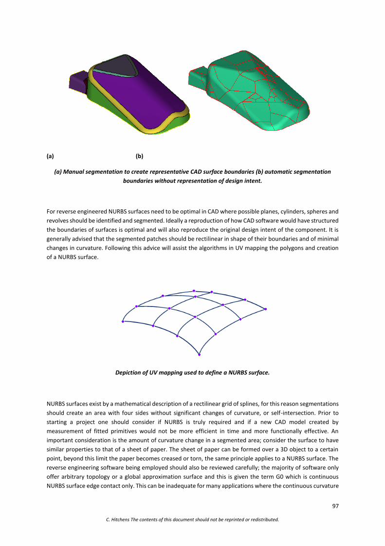
97
C. Hitchens The contents of this document should not be reprinted or redistributed.
(a) (b)
(a) Manual segmentation to create representative CAD surface boundaries (b) automatic segmentation
boundaries without representation of design intent.
For reverse engineered NURBS surfaces need to be optimal in CAD where possible planes, cylinders, spheres and
revolves should be identified and segmented. Ideally a reproduction of how CAD software would have structured
the boundaries of surfaces is optimal and will also reproduce the original design intent of the component. It is
generally advised that the segmented patches should be rectilinear in shape of their boundaries and of minimal
changes in curvature. Following this advice will assist the algorithms in UV mapping the polygons and creation
of a NURBS surface.
Depiction of UV mapping used to define a NURBS surface.
NURBS surfaces exist by a mathematical description of a rectilinear grid of splines, for this reason segmentations
should create an area with four sides without significant changes of curvature, or self-intersection. Prior to
starting a project one should consider if NURBS is truly required and if a new CAD model created by
measurement of fitted primitives would not be more efficient in time and more functionally effective. An
important consideration is the amount of curvature change in a segmented area; consider the surface to have
similar properties to that of a sheet of paper. The sheet of paper can be formed over a 3D object to a certain
point, beyond this limit the paper becomes creased or torn, the same principle applies to a NURBS surface. The
reverse engineering software being employed should also be reviewed carefully; the majority of software only
offer arbitrary topology or a global approximation surface and this is given the term G0 which is continuous
NURBS surface edge contact only. This can be inadequate for many applications where the continuous curvature
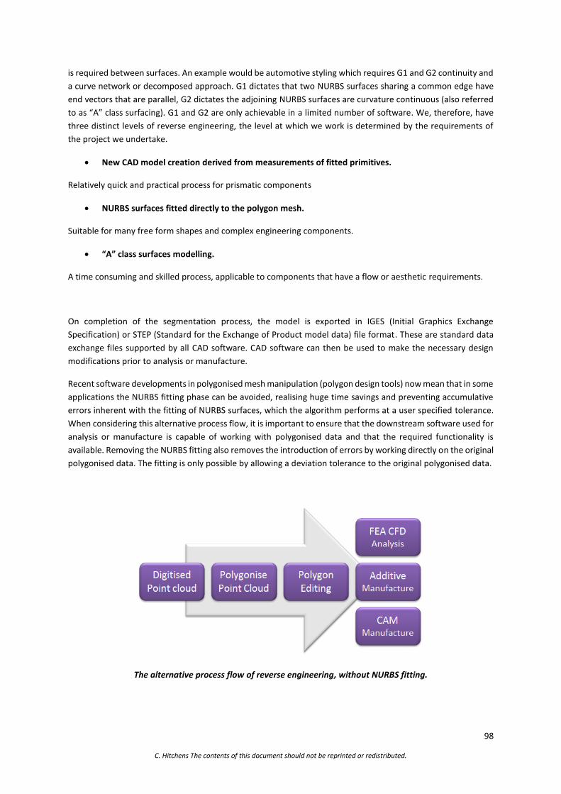
98
C. Hitchens The contents of this document should not be reprinted or redistributed.
is required between surfaces. An example would be automotive styling which requires G1 and G2 continuity and
a curve network or decomposed approach. G1 dictates that two NURBS surfaces sharing a common edge have
end vectors that are parallel, G2 dictates the adjoining NURBS surfaces are curvature continuous (also referred
to as “A” class surfacing). G1 and G2 are only achievable in a limited number of software. We, therefore, have
three distinct levels of reverse engineering, the level at which we work is determined by the requirements of
the project we undertake.
New CAD model creation derived from measurements of fitted primitives.
Relatively quick and practical process for prismatic components
NURBS surfaces fitted directly to the polygon mesh.
Suitable for many free form shapes and complex engineering components.
“A” class surfaces modelling.
A time consuming and skilled process, applicable to components that have a flow or aesthetic requirements.
On completion of the segmentation process, the model is exported in IGES (Initial Graphics Exchange
Specification) or STEP (Standard for the Exchange of Product model data) file format. These are standard data
exchange files supported by all CAD software. CAD software can then be used to make the necessary design
modifications prior to analysis or manufacture.
Recent software developments in polygonised mesh manipulation (polygon design tools) now mean that in some
applications the NURBS fitting phase can be avoided, realising huge time savings and preventing accumulative
errors inherent with the fitting of NURBS surfaces, which the algorithm performs at a user specified tolerance.
When considering this alternative process flow, it is important to ensure that the downstream software used for
analysis or manufacture is capable of working with polygonised data and that the required functionality is
available. Removing the NURBS fitting also removes the introduction of errors by working directly on the original
polygonised data. The fitting is only possible by allowing a deviation tolerance to the original polygonised data.
The alternative process flow of reverse engineering, without NURBS fitting.

99
C. Hitchens The contents of this document should not be reprinted or redistributed.
This polygonised data can be imported directly into the majority of finite element analysis and computational
fluid dynamics software if the skewed value of the polygon elements is controlled to a low value (skew is a
measure of how equilateral a triangle is). It is also possible in some of the reverse engineering software to
convert the triangular elements into quads (squares).This is especially useful for finite element analysis. The STL
file can be directly exported after polygonisation, this is the essential format for additive manufacturing systems
and is supported by the majority of CAM software. This alternative process flow is not often employed because
the polygon model often requires modification with addition or removal of features. The ability to do
modification and design on the polygonised geometry is a relatively new possibility. However, it is on the
increase with new software being developed to meet the growing demand of the computer game and film
industry, both industries are heavily dependent on polygon modelling for animation and rendering purposes.
This approach of polygon modelling can offer significant time savings, it does, however, require investment in
time to understand and develop the process and methods.
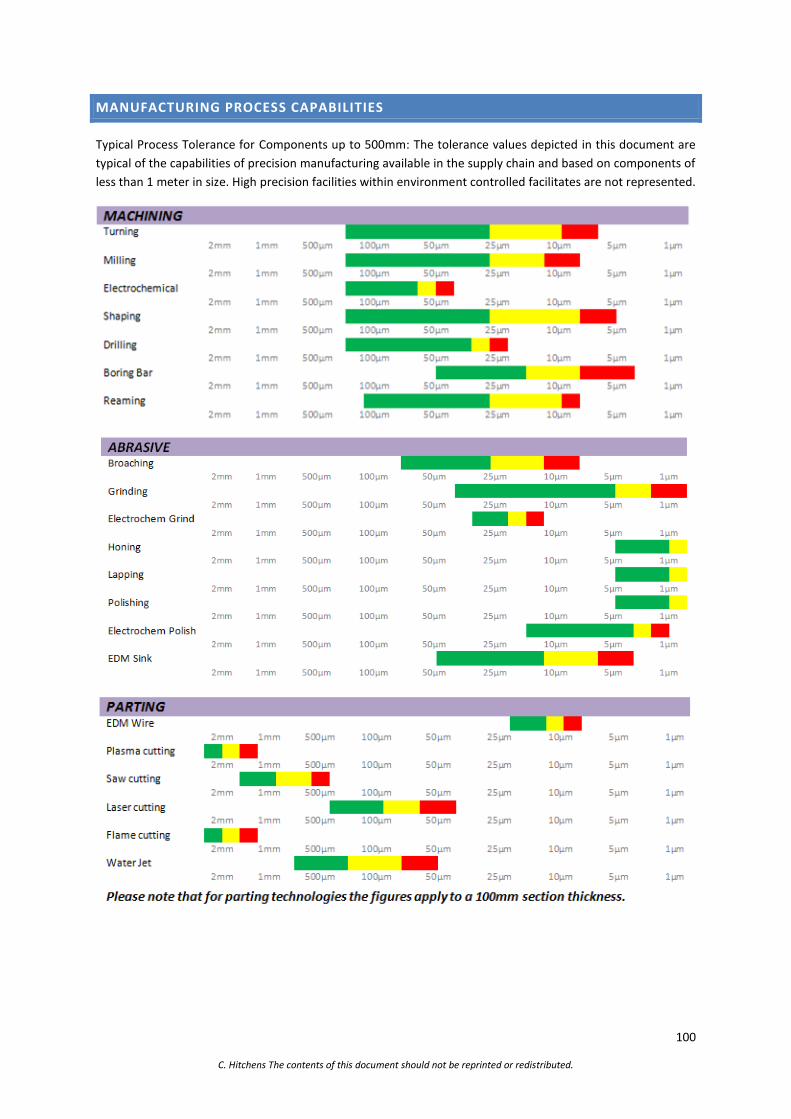
100
C. Hitchens The contents of this document should not be reprinted or redistributed.
MANUFACTURING PROCESS CAPABILITIES
Typical Process Tolerance for Components up to 500mm: The tolerance values depicted in this document are
typical of the capabilities of precision manufacturing available in the supply chain and based on components of
less than 1 meter in size. High precision facilities within environment controlled facilitates are not represented.

101
C. Hitchens The contents of this document should not be reprinted or redistributed.
Surface Roughness ANSI B46.1

102
C. Hitchens The contents of this document should not be reprinted or redistributed.
BIBLIOGRAPHY
A Beginner's Guide to Uncertainty of Measurement. Bell, Stephanie. 2001, Vol. 11, 2.
BIPM. Evaluation of Measurement Data. A Guide to the Expression of Uncertainty in Measurement. 2008.
Evaluating the Usefulness of Data By Gage Repeatability and Reproducibility. Touchton, Keith Bower and
Michelle. 2015.
Fundamentals of Dimensional Metrology. C. Dotson, R. Harlow and R. L. Thompson
Geometric Dimensioning and Tolerancing. J. Meadows.
Handbook of Dimensional Measurement 2nd Edition. F. T. Farago and M. Curtis
Metrology for Engineers. J.F.W. Galyer and C. R. Shotbolt
Machinery’s Handbook 28th Edition. Industrial Pressing
Mathematics of Measurement Systems Analysis. I, Vol. 1, 1. Rolls-Royce
Measurement Systems Analysis. Rolls Royce. 2015.
Minitab 17. Methods and Formulae. s.l. : Minitab Inc, 2015.
Six Sigma Operational. Measurement Systems Analysis. 2013.
Copyright © 2022 FDOKUMEN