Engineering Metrology - Modern Academy
151
Engineering Metrology MNF 325 Professor Dr. Nabil Gadallah Department of Manufacturing Engineering and Production 1 Engineering Metrology - Professor Nabil Gadallah
-
Upload
khangminh22 -
Category
Documents
-
view
2 -
download
0
Transcript of Engineering Metrology - Modern Academy

Engineering Metrology MNF 325
Professor Dr. Nabil Gadallah
Department of Manufacturing Engineering and Production
1 Engineering Metrology - Professor Nabil Gadallah

Course Outline
Lecturer: Prof. Dr. Nabil Gadallah
Text Book: Nabil Gadallah, "Engineering Metrology", Modern Academy for Engineering &
Technology, 2014
Course Outline: 1. Introduction to concept of metrology and quality
2. History and units of measurement
3. Analysis of errors and uncertainties in measurement
4. Linear and angular measurements
5. Advanced measurement techniques (optical, laser, ultrasound, etc.)
6. Measurement of geometric shape (roundness, flatness, etc.)
7. Measurement of surface texture (surface roughness and waviness)
8. Measurement of screw threads
9. Measurement of gears
10. Limits and limit gauges
Exams, Projects, Practices: • Workshop and/or classroom practices (10%)
• Midterm Exam (10%)
• Practical Exam (20)
• Term Exam (60%)
Engineering Metrology - Professor Nabil Gadallah 2

Engineering Metrology and Quality Control
CHAPTER (1)
Introduction to Metrology and Quality
3 Engineering Metrology - Professor Nabil Gadallah

Metrology
• from greek “metron” (measure) and –logy.
• the science of measurement.
• includes all theoretical and practical aspects of measurement.
Measurement
• Comparison of a specimen (a thing or a quantity) to a standard, within
some agreement upon reference frame.
• A successful measurement must maintain (i.e. apply controls to)
specimen, standard, and a stable reference frame.
• All measurements based on standard.
• Maintenance of standards & reference frame critical to any
measurement.
Definition of Metrology and Measurement
4 Engineering Metrology - Professor Nabil Gadallah

Engineering Metrology - Professor Nabil Gadallah 5
Objective Classification of Measuring Technological Concept

Product Quality
• a product’s fitness for use.
• the totality of features that bear on a product’s ability to satisfy a given
need.
Need for Quality
• Quality is a very important aspect of manufacturing.
• It is a big issue (consider TQM, Six Sigma, Taguchi, ISO Standards, etc.)
• Needed for interchangeable manufacturing.
• Basic concept of standardization and mass production.
• Components of a product must fit together, assemble properly and be
replaceable.
• Quality should be built into a product.
• Prevention of defects is a major goal.
What is Quality?
6 Engineering Metrology - Professor Nabil Gadallah

☺ performs its functions conveniently
High Quality Product
☺ performs its functions reliably
☺ performs its functions for a long time
® difficult to use
® does not perform its function reliably
® fails or breaks after short time of use
Low Quality Product
GOAL
Continuous Quality Improvement
(functionality, reliability, durability, …)
Inspection (Measurement)
When? What? How?
Measure of Quality
7 Engineering Metrology - Professor Nabil Gadallah

Inspection specific to PRODUCTS • Electronic parts (circuits, chips, etc.)
• Machine elements (engines, brakes, gears, etc.)
• Heat and thermodynamic components (engines, fuel injectors, etc.)
• Medical and Bio-related products (implants, dental devices, surgical
parts, etc.)
• Aerospace components (turbine blades and discs, airplane body, etc.)
Inspection specific to PROCESSES
• Chip removal processes (turning, milling, drilling, etc.)
• Chipless manufacturing (casting, molding, forging, etc.)
• Non-traditional methods (EDM, ECM, ultrasonics, etc.)
What to Inspect?
8 Engineering Metrology - Professor Nabil Gadallah

Inspection AFTER production x costly production steps already complete
x high cost of rejection or rework
x difficult to test for all possible defects
x difficult to identify responsibility for defect
Inspection DURING production
✓defects found early, at each production step
✓reduced cost of rejection or rework
✓facilitates continuous process improvement
When to Inspect?
9 Engineering Metrology - Professor Nabil Gadallah

Measurement of DIMENSIONS • Linear measurements (length, thickness, etc.)
• Angular measurements (taper, angle, etc.)
• Measurement of surface texture (roughness, waviness, etc.)
• Measurement of geometric shape (roundness, flatness, squareness, etc.)
• Measurement of screw threads and gears …
Inspection for DIMENSIONAL ACCURACY
• post-process (traditional)
• in-process (modern trend)
DIMENSIONAL TOLERANCES
• permissible variation in dimensions
• directly affects product quality and cost
How to Inspect?
1
0
Engineering Metrology - Professor Nabil Gadallah

Large scale (low frequency) measurements
• Measurements at macro levels
• Dimension (length, angle, etc.)
• Tolerance
• Form error (contour measurement)
Medium scale (medium frequency) measurements • Measurements at meso levels
• Surface texture/topography (waviness)
• Geometric shape (flatness, roundness, etc.)
Small scale (high frequency) measurements
• Measurements at micro levels
Scale of Measurement
• Surface texture/topography (surface roughness)
1
1
Engineering Metrology - Professor Nabil Gadallah

Engineering Metrology
History and Units of Measurement
CHAPTER (2)
12 Engineering Metrology - Professor Nabil Gadallah

Measurement and Mathematics
> Measurement constitutes the first steps towards mathematics.
> In other words, associating numbers with physical objects...
> Thus, compare the objects by comparing the associated numbers...
1 FOOT FOR LENGTH SEEDS AND BEANS FOR WEIGHT
Introduction
13 Engineering Metrology - Professor Nabil Gadallah

Current measurement systems have been derived from 3000 BC.
2
Egyptians (around 3000 BC)
> Earliest known measurement was Egyptian cubit.
Babylonians (around 1700 BC)
> Their weights and measures had a wider influence.
> Their system was approximately same with Egyptians.
> However, there were small differences about lengths.
Harappans (between 2500 BC and 1700 BC)
> They had flourished in Punjab (in India).
> They adopted a uniform system of weights
and measures.
> Several scales for the measurement of
length were also discovered during
excavations.
In summary:
> European system based on Roman measures
> Roman system based on Greek measures
> Greek system based on breadth of finger
Vitruvian Man (Leonardo Da Vinci)
Brief History of Measurement
14 Engineering Metrology - Professor Nabil Gadallah

Digit : Egyptians - breadth of forefinger
Inch : breadth of thumb
Palm : breadth of four fingers
Span : tip of thumb to tip of little finger (hand spread)
Cubit : Egyptians - elbow to tip of middle finger
Foot : length of man's foot
Yard : King Henry I of England - tip of his nose to end of thumb
Mile : 5000 Roman feet
Pace : Romans - a full stride
and many others...
Anthropic Measurements and Units
15 Engineering Metrology - Professor Nabil Gadallah

Solution was to develope a standard measurement:
a black granite rod !!! There were a lot of different lengths
which change from human to human.
But there was a problem!
There were 28 digits in a cubit, 4 digits in a palm, 5 digits in a hand, 3 palms (so 12 digits) in a small span, 14 digits (or a half cubit) in a large span, 24 digits in a small cubit, and so on...
But a problem again: How could they measure a measurement smaller than 1 digit ?
For this, the Egyptians used measures composed of unit fractions...
Early Measurements
16 Engineering Metrology - Professor Nabil Gadallah

System of Units SI System
> Le systeme International d’unites or International System of Units
> Also called Metric System (i.e. all measurements based on m, kg, s).
> Seven base units (m, kg, s, A, °K, mol, cd) and other derived units.
> Used throughout the world except USA and some part of UK.
English (British or Imperial) System
> Various measurements based on different units:
> Length: inches / feet / yards / miles / ...
> Mass: ounces / pounds / tones / ...
> Volume: fluid ounce / cups / quarts / gallons / ...
Why do we prefer SI system?
> SI units work in 10s, so it is very easy to convert big units to small
units, or vice versa (e.g. 1 m = 100 cm). However, English units are
not easy to convert. Can you easily convert mile to inches?
> In SI system, a unique unit is used for a quantity (e.g. the unit of
distance is meter). However, various units may be used in English
system (e.g. for distance: inch, foot, yard, mile, and so on.)
17 Engineering Metrology - Professor Nabil Gadallah

1670 Gabriel Moulton, a French mathematician, proposes a measurement system based on a physical quantity of nature and not on human anatomy.
1790 The French Academy of Science recommends the adoption of a system with a unit of length equal to one ten-millionth of the distance on a meridian between the Earth’s North Pole and equator.
1870 A French conference is set up to work out standards for a unified metric system.
1875 The Treaty of Meter is signed by 17 nations (including United States). This has established a permanent body with the authority to set standards.
1893 The United States officially adopts the metric system standards as bases for weights and measures (but continues to use British units).
1975 The Metric Conversion Act is enacted by Congress. It states “The policy of the United States shall be to coordinate and plan the increasing use of the metric system in the United States and to establish a United States Metric Board to coordinate the voluntary conversion to the metric system.” (This means that no mandatory requirements are made.)
Chronological History of Metric System
18 Engineering Metrology - Professor Nabil Gadallah

International Prototype
> International Prototype Metre bar,
made of an alloy of platinum and iridium,
was the standard from 1889 to 1960.
> It is kept at Bureau International des
Poids et Measures (International Bureau
of Weights and Measures) near Paris.
Definition
> Meter (m) is the unit of length.
> It was originally defined as a unit equal to one ten-millionth part of a
quadrant of Earth's meridian as measured from North Pole to Equator.
> It is now precisely equal to the length of path traveled by light in
vacuum during a time interval of 1/299 792 458 of a second.
SI Base Units - Meter
19 Engineering Metrology - Professor Nabil Gadallah

SI Base Units - Kilogram
Definition
> Kilogram (kg) is the unit of mass.
> Originally, it was defined as the mass of a volume of pure water equal
to a cube of one tenth meter at the temperature of melting ice.
> It is now equal to the mass of international prototype of kilogram.
International Prototype
> There are currently two prototypes: the one kept at Bureau
International des Poids et Measures (BIPM) in Paris, and the
other one at National Institute of Standards and Technology
(NIST) in Washington D.C.
> The prototype at BIPM is made of a platinum alloy known as
“Pt-10Ir”, which is 90% platinum and 10% iridium (by mass).
> It was machined into a right-circular cylinder with equal height
and diameter (39.17 mm) to minimize its surface area.
> The protoype at NIST is actually 0.999 999 961 kg of the one
at BIPM.
20 Engineering Metrology - Professor Nabil Gadallah

> Mass is stuff (a quantity of matter) regardless of what it is made of, any number of other conditions
(including shape, temperature, color), where it is, and how it moves (disregarding relativistic effects).
> Weight is force (specifically gravitational force) acting on the stuff in a special way. It is the force
necessary to cause the stuff to accelerate at gravitational acceleration of 9.81 m/s2 (32.174 ft/s2).
mass (kg or lb) remains constant
but
weight (kgf or lbf) varies
1 kg of cotton and 1 kg of iron are
EQUAL in mass
(NOT EQUAL in weight)
Mass vs Weight
21 Engineering Metrology - Professor Nabil Gadallah

Definition
> Second (s) is the unit of time.
> It was originally defined as 1/86 400 of a solar day.
> Today, it is equal to the duration of 9 192 631 770 periods of
the radiation corresponding to the transition between two
hyperfine levels of the ground state of cesium-133 atom.
> The frequency of a specific transition between two of cesium's
energy levels can be accurately monitored, and thus it is used
to define the second.
10
SI Base Units - Second
22 Engineering Metrology - Professor Nabil Gadallah

Ampere
> Ampere (A) is the unit of electric current.
> Being maintained in two straight parallel conductors of infinite length with negligible circular cross
section and placed 1 m apart in vacuum, it is equal to that constant current which would produce
a force (between these conductors) equal to 2 * 10-7 Newton per meter of length.
Kelvin
> Kelvin (°K) is the unit of thermodynamic temperature.
> It is equal to the fraction of thermodynamic temperature of triple point of water (i.e. the point where
water exists in gaseous, liquid and solid phases simultaneously) at 273.16 °K (0.01 °C, 32.02 °F).
Mole
> Mole (mol) is the unit of the amount of substance of a system.
> It is equal to the amount of substance of a system which contains as many elementary entities
(i.e. atoms, molecules, ions, electrons) as there are atoms in 0.012 kilogram of carbon-12.
Candela
> Candela (cd) is the unit of luminous intensity.
> It is equal to luminous intensity of a source in a given direction that emits monochromatic radiation
of frequency (540 x 1012 hertz) and that has a radiant intensity of 1/683 watt per steradian.
SI Base Units – Ampere, Kelvin, Mole, Candela
23 Engineering Metrology - Professor Nabil Gadallah

SI Coherent Derived Units with Special Names and Symbols
24 Engineering Metrology - Professor Nabil Gadallah
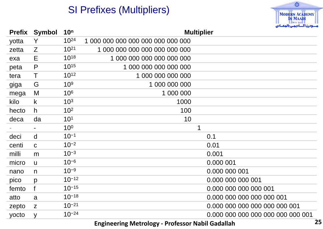
SI Prefixes (Multipliers)
Prefix Symbol 10n Multiplier
yotta Y 1024 1 000 000 000 000 000 000 000 000
zetta Z 1021 1 000 000 000 000 000 000 000
exa E 1018 1 000 000 000 000 000 000
peta P 1015 1 000 000 000 000 000
tera T 1012 1 000 000 000 000
giga G 109 1 000 000 000
mega M 106 1 000 000
kilo k 103 1000
hecto h 102 100
deca da 101 10
- - 100 1
deci d 10−1 0.1
centi c 10−2 0.01
milli m 10−3 0.001
micro u 10−6 0.000 001
nano n 10−9 0.000 000 001
pico p 10−12 0.000 000 000 001
femto f 10−15 0.000 000 000 000 001
atto a 10−18 0.000 000 000 000 000 001
zepto z 10−21 0.000 000 000 000 000 000 001
yocto y 10−24 0.000 000 000 000 000 000 000 001 25 Engineering Metrology - Professor Nabil Gadallah

Conversion of Units
26 Engineering Metrology - Professor Nabil Gadallah

> Almost all developed and developing countries have a National
Metrology Institute (NMI), having relations with BIPM.
> The main objectives of NMIs are to build and maintain national
standards for all measurements carried out within that country and to
calibrate the measurement standards and devices of lower level
laboratories.
> This chain extends to production, quality control and to all scientific,
commercial and military devices which are used for measurements.
> This way, all measurements are traceable to the national standards.
National standards are linked to the standards in other countries or those
of BIPM by a process of international comparisons. This is called
traceability.
> List of NMIs in the world can be found at:
www.ume.tubitak.gov.tr/menu_links.php?f=301
National Metrology Institutes
27 Engineering Metrology - Professor Nabil Gadallah

Useful Links
> Bureau International des Poids et Measures (BIPM):
www.bipm.org
> International Organization for Standardization (ISO):
www.iso.org
> European Association of National Metrology Institutes (EURAMET):
www.euramet.org
> Online unit converter:
www.digitaldutch.com/unitconverter
> Scale of universe:
http://scaleofuniverse.com
28 Engineering Metrology - Professor Nabil Gadallah

Engineering Metrology
CHAPTER (3)
Analysis of Errors and Uncertainties
in Measurement
29 Engineering Metrology - Professor Nabil Gadallah

Calibration (Kalibrasyon)
> Adjustment or setting of an instrument to obtain
accurate readings within a reference standard
Readibility (Okunabilirlik)
> Susceptibility of an instrument for having its
indications converted to a meaningful number
(e.g. converting voltage signals to electric current)
Precision (Kesinlik)
> Degree of refinement to which a measurement can
be stated (e.g. number of digits)
> Degree of agreement within the measurements of
the same quantity
Repeatability (Tekrar edilebilirlik)
> Error between a number of successive attempts to
move a machine to the same position
> Ability to do the same thing over and over
Accuracy (Doğruluk)
> Degree of agreement of the measured
dimension with its true magnitude
Sensitivity (Hassasiyet)
> Smallest difference in a dimension that an
instrument can distinguish or detect
(e.g. a scale with sensitivity of ± 1 mg)
Resolution (Çözünürlük)
> Smallest dimension/feature on a device
(e.g. resolution of LCD TV)
> Smallest programmable step that machine
can make during point to point motion
Reproducibility (Tekrar üretilebilirlik)
> Degree of agreement within the individual
results using the same method, the same
test substance, but under different set of
laboratory conditions
Some Terminology
30 Engineering Metrology - Professor Nabil Gadallah

Nominal value: 10
Readings: 10.220, 9.886,
10.147, 10.126,
9.914
Average: 10.05860
Displayed: 10.06
Resolution: 0.001 units
Precision: 2 digits
Accuracy: 0.586% A.H. Slocum, ―Precision Machine Design‖, Prentice,1992.
Understanding the terminology
31 Engineering Metrology - Professor Nabil Gadallah

✓Accuracy
x Precision
x Accuracy
x Precision
✓Accuracy
✓Precision
A process or measurement can be accurate without being precise,
or vice versa.
The aim is to obtain high
accuracy with high precision
x Accuracy
✓Precision
Accuracy vs Precision
30 Engineering Metrology - Professor Nabil Gadallah

Whenever a physical parameter is measured by any means, an estimate is made on
the value of the quantity being measured. There are two features of such estimation:
measurement error & measurement uncertainty
Measurement Error
> It is the difference between the value of a measured quantity and a measurement estimate of its
value (i.e. the accuracy of the measurement).
> This error may be systematic or random depending upon the type of measurement, the
measurement device, the person making the measurement, and the environmental factors.
Measurement Uncertainty
> Measurement errors are never known exactly. In some instances, they may be estimated and
tolerated or corrected, or they may be simply acknowledged as being present.
> Whether an error is estimated or acknowledged, its existence introduces a certain amount of
measurement uncertainty.
> Thus, it is a lack of knowledge concerning the error in the measurement.
Measurement Error vs Measurement Uncertainty
33 Engineering Metrology - Professor Nabil Gadallah

Systematic Errors
> Come from the measuring instruments.
> Something is wrong with the instrument or its
data handling system, or instrument is wrongly
used by the experimenter.
> errors in temperature measurements due to
poor thermal contact between thermometer
and substance.
> errors in measurements of solar radiation as
trees or buildings shade the radiometer.
A thermometer that always reads 3 ºC
colder than the actual temperature
A thermometer that gives random
values within 3 ºC either side of
the actual temperature
Systematic Error vs Random Error
Random Errors
> Caused by unknown and/or unpredictable
changes in the experiment.
> Occur in the measuring instruments or in the
environmental conditions (e.g. humidity,
temperature, etc.)
> errors in voltage measurements because of
an electronic noise in the circuit of electrical
instrument.
> irregular changes in the heat loss rate from
a solar collector due to the wind.
34 Engineering Metrology - Professor Nabil Gadallah

Systematic Errors
> Reproducible between measurements.
> In principle, they can be eliminated
partially or completely.
> Accuracy is often reduced by systematic
errors, which are difficult to detect even
for experienced researchers.
They can be estimated so that
the measured value can be
adjusted to allow for them.
We must define their size to estimate
what confidence we have in our
measured value.
Standard Deviation &
Least Square Method
Evaluation of Errors
Random Errors
> Not reproducible, but fluctuate in magnitude
and sign between measurements.
> We can only know the probable range over
which a random error lies.
> Precision is limited by random errors, that
are usually determined by repeating the
measurements.
35 Engineering Metrology - Professor Nabil Gadallah

2 _ ⎞
1 i=1 ⎝
1 ∑⎜ xi − x ⎟
⎠
⎛
n − σ =
n
x = ∑ xi
n i=1
where x is the arithmetic mean:
n _ 1
Standard Deviation (Statistical Uncertainty)
Standard Deviation
> A measure of the spread of a probability distribution, a random variable, or multiset of values.
> More formally, it is the root mean square deviation of values from their arithmetic mean.
Sample standard deviation (σ) of a
random variable (x) for a number of
samples (n) is defined as:
In practice, it is often assumed that the data are from an
approximately normally distributed population. According
to this, the confidence intervals are:
xIn order to improve the precision,
sampling distribution is used:
σ → σ n
σ: 68.26894921371 % 4σ: 99.99366575163 %
2σ: 95.44997361036 % 5σ: 99.99994266969 %
3σ: 99.73002039367 % 6σ: 99.99999980268 %
36 Engineering Metrology - Professor Nabil Gadallah

Suppose that our data points are (x1,y1),
(x2,y2), … , (xn,yn) where x and y are
independent and dependent values.
The fitting curve f(x) has the deviation of
d from each data point:
di = yi − f (xi )
Hence, according to LSM, the best-
fitting curve has the property that: n
Π = ∑ di = a minimum i=1
Least Square Method (LSM)
Least Square Method (also called “Regression Model”)
> This is a statistical approach to estimate an expected value or function with the highest probability
from the observations with random errors.
> It assumes that the best-fit curve is the curve that has the minimal sum of the deviations squared
(least square error) from a given set of data.
> Thus, it provides the best-curve fitting (a curve with a minimal deviation from all data points)
37 Engineering Metrology - Professor Nabil Gadallah

y = mx + b
Regression Formulae
y = c ln x + b
A curved line is used when data fluctuates. The order
n is defined by number of fluctuations in the data, or by
how many bends appear in the curve (e.g. Order 2
generally has one hill or valley).
y = b + c1 x + ... + cn x
y = cxb
y = cebx
Remarks
A straight line is used with simple linear data sets
(i.e. increasing or decreasing at a steady rate).
A curved line is used when the rate of change in the
data increases/decreases quickly and then levels out.
Negative and/or positive values can be used.
A curved line is used with data sets that compare
measurements increasing at a specific rate (cannot
be used for data containing zero or negative values).
A curved line is used when data values rise or fall at
increasingly higher rates (cannot be used for data
containing zero or negative values).
Regression Methods (Trend Lines)
38 Engineering Metrology - Professor Nabil Gadallah
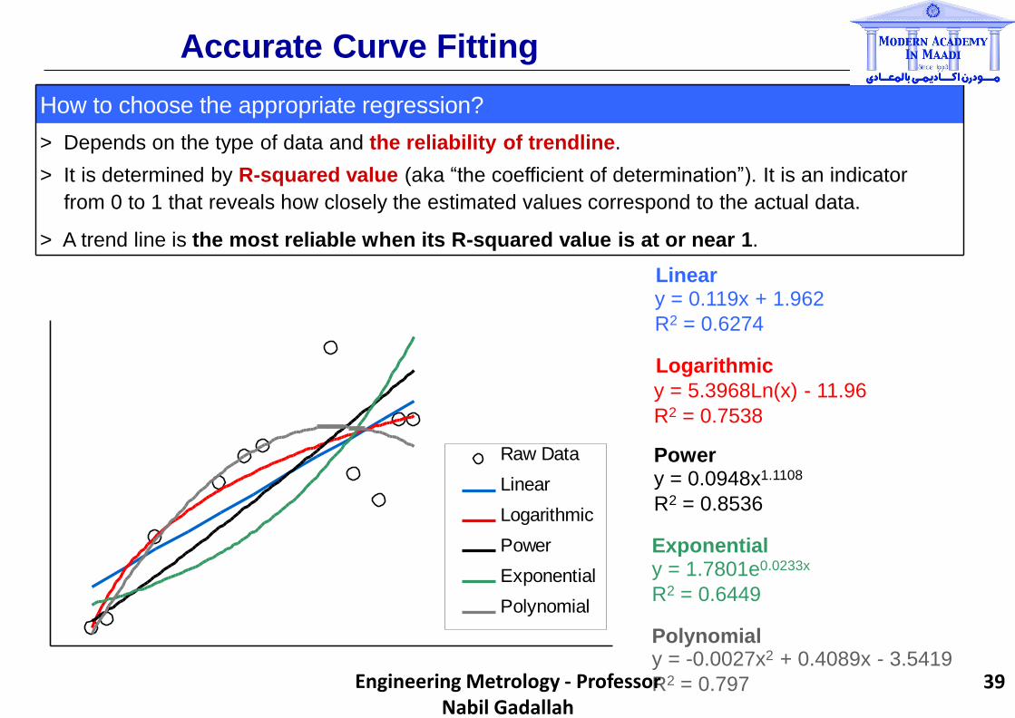
Raw Data
Linear
Logarithmic
Power
Exponential
Polynomial
Power y = 0.0948x1.1108
R2 = 0.8536
Exponential y = 1.7801e0.0233x
R2 = 0.6449
Polynomial y = -0.0027x2 + 0.4089x - 3.5419
R2 = 0.797
How to choose the appropriate regression?
> Depends on the type of data and the reliability of trendline.
> It is determined by R-squared value (aka “the coefficient of determination”). It is an indicator
from 0 to 1 that reveals how closely the estimated values correspond to the actual data.
> A trend line is the most reliable when its R-squared value is at or near 1.
Linear y = 0.119x + 1.962
R2 = 0.6274
Logarithmic
y = 5.3968Ln(x) - 11.96
R2 = 0.7538
Accurate Curve Fitting
39 Engineering Metrology - Professor Nabil Gadallah
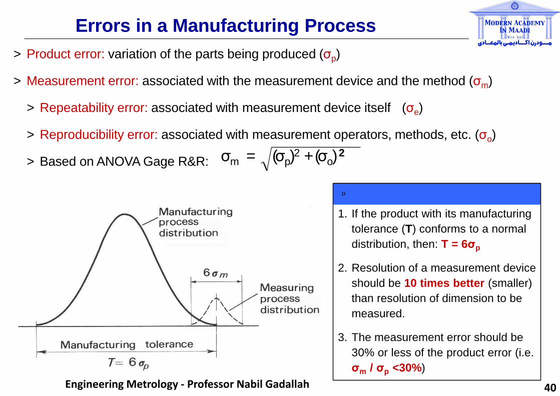
Rules of Thumb
1. If the product with its manufacturing
tolerance (T) conforms to a normal
distribution, then: T = 6σp
2. Resolution of a measurement device
should be 10 times better (smaller)
than resolution of dimension to be
measured.
3. The measurement error should be
30% or less of the product error (i.e.
σm / σp <30%)
> Based on ANOVA Gage R&R:
> Product error: variation of the parts being produced (σp)
> Measurement error: associated with the measurement device and the method (σm)
> Repeatability error: associated with measurement device itself (σe)
> Reproducibility error: associated with measurement operators, methods, etc. (σo)
Errors in a Manufacturing Process
σm = (σp)2 + (σo)
2
o
40 Engineering Metrology - Professor Nabil Gadallah

Engineering Metrology and
CHAPTER (3)
Linear and Angular Measurements
41 Engineering Metrology - Professor Nabil Gadallah


44 Engineering Metrology - Professor Nabil Gadallah

45 Engineering Metrology - Professor Nabil Gadallah

46 Engineering Metrology - Professor Nabil Gadallah

47 Engineering Metrology - Professor Nabil Gadallah

48 Engineering Metrology - Professor Nabil Gadallah

49 Engineering Metrology - Professor Nabil Gadallah

50 Engineering Metrology - Professor Nabil Gadallah

51 Engineering Metrology - Professor Nabil Gadallah

52 Engineering Metrology - Professor Nabil Gadallah

53 Engineering Metrology - Professor Nabil Gadallah

54 Engineering Metrology - Professor Nabil Gadallah
55 Engineering Metrology - Professor Nabil Gadallah

56 Engineering Metrology - Professor Nabil Gadallah

57 Engineering Metrology - Professor Nabil Gadallah
58 Engineering Metrology - Professor Nabil Gadallah
59 Engineering Metrology - Professor Nabil Gadallah

Engineering Metrology
CHAPTER (4)
Statistical Quality Control and
Use of Control Charts
60 Engineering Metrology - Professor Nabil Gadallah
Statistical Process Control (SPC) & Control Charts
Definition of SPC
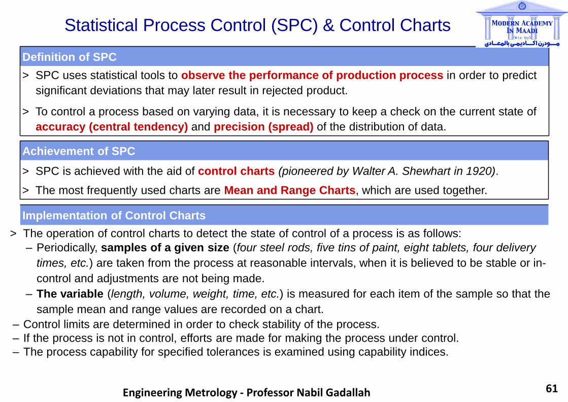
> SPC uses statistical tools to observe the performance of production process in order to predict
significant deviations that may later result in rejected product.
> To control a process based on varying data, it is necessary to keep a check on the current state of
accuracy (central tendency) and precision (spread) of the distribution of data.
Achievement of SPC
> SPC is achieved with the aid of control charts (pioneered by Walter A. Shewhart in 1920).
> The most frequently used charts are Mean and Range Charts, which are used together.
Implementation of Control Charts
> The operation of control charts to detect the state of control of a process is as follows:
– Periodically, samples of a given size (four steel rods, five tins of paint, eight tablets, four delivery
times, etc.) are taken from the process at reasonable intervals, when it is believed to be stable or in-
control and adjustments are not being made.
– The variable (length, volume, weight, time, etc.) is measured for each item of the sample so that the
sample mean and range values are recorded on a chart.
– Control limits are determined in order to check stability of the process.
– If the process is not in control, efforts are made for making the process under control.
– The process capability for specified tolerances is examined using capability indices.
61 Engineering Metrology - Professor Nabil Gadallah

A Case Study
151 157 140 154 25
149 157 152 151 24
151 151 156 143 23
154 158 147 152 22
160 148 156 146 21
150 150 142 155 20
151 149 155 153 19
153 149 148 157 18
148 153 150 155 17
149 148 144 147 16
157 148 146 150 15
149 150 160 144 14
142 152 146 152 13
148 152 145 155 12
153 154 150 151 11
154 152 148 145 10
156 149 150 158 9
155 149 147 141 8
155 137 144 149 7
147 145 150 157 6
157 155 153 157 5
148 152 146 154 4
152 143 139 145 3
153 134 150 151 2
146 154 146 144 1
iv iii ii i
Rod Lengths (mm) Sample No.
Lets represent this data using a histogram chart, which is used
for showing the frequency of data values. First, we must define
the bins (i.e. intervals).
For this purpose, we search for the min. and the max. values
in the data set (which are 134 and 160).
154
151
149
151
143
152
155
145
137
149
149
152
154
152
152
150
148
148
153
149
149
150
148
158
151
157
157
150
139
146
153
150
144
147
150
148
150
145
146
160
146
144
150
148
155
142
156
147
156
152
140
151
145
154
157
157
149
141
158
145
151
155
152
144
150
147
155
157
153
155
146
152
143
151
154
1
2
3
4
5
6
7
8
9
10
11
12
13
14
15
16
17
18
19
20
21
22
23
24
25
160
153
152
148
157
147
155
155
156
154
153
148
142
149
157
149
148
153
151
150
134
146 144
Rod Lengths (mm)
ii iii
146 154
iv i
Sample No.
Then, we define starting & end values for the bins (i.e. 133.5 &
160.5). After this, we divide the difference between these values
by equal intervals (i.e. 27/3 which gives 9 equal intervals).
Therefore, the bins for this data set can be:
133.5 – 136.5
136.5 – 139.5
139.5 – 142.5
142.5 – 145.5
145.5 – 148.5
148.5 – 151.5
151.5 – 154.5
154.5 – 157.5
157.5 – 160.5
Suppose that, for production of rods, we have 100 rod lengths
as 25 samples of size 4 were taken.
62 Engineering Metrology - Professor Nabil Gadallah

0
26
24
22
20
18 y 16 nc
14
que 12 e Fr 10
8
6
4
2
135
138
141
144
147
150
153
156
159
M idpoint
Histogram Chart
Select the data set (i.e. 100 rod
lengths) and the intervals so that
the histogram chart will be built.
The frequency of each value within
the data set according to each bin
will be calculated automatically.
Sometimes, it is more practical to
show midpoints in the chart rather
than intervals. In such cases, the
midpoint of each bin is calculated
and used in the chart (e.g. mean
of interval 133.5 – 136.5 is 135).
Histogram charts are also useful for
showing the distribution of data sets.
4 2 0
8 6
12 10
14
18 16
24 22 20
26
135 138 141 144 147 150 153 156 159
Midpoint
Fre
qu
en
c
y
133.5
136.5
139.5
142.5
145.5
148.5
151.5
154.5
157.5
160.5
Intervals
The histogram chart is obtained using Microsoft Excel software (Click on the “Data Analysis” under
“Tools” menu and choose “Histogram” option from the list. If you can’t see “Data Analysis” function,
then go to “Add-ins” under “Tools” menu and click on “Analysis Toolpak”).
63 Engineering Metrology - Professor Nabil Gadallah
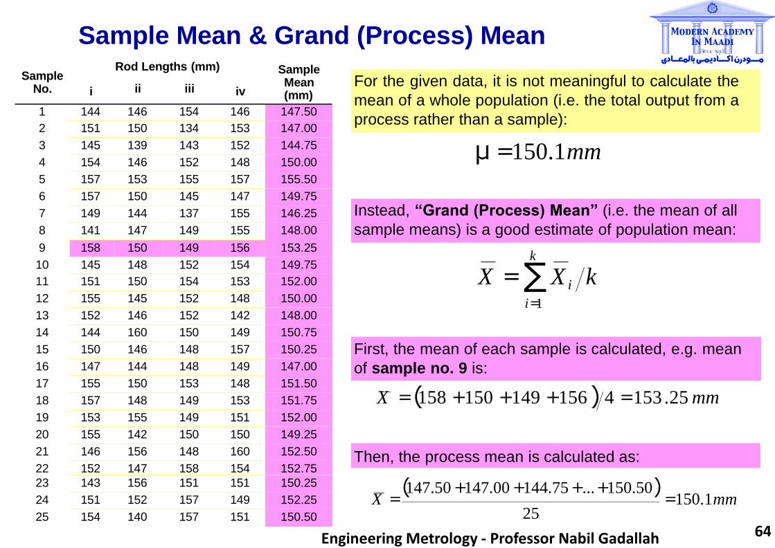
Sample Mean & Grand (Process) Mean
Instead, “Grand (Process) Mean” (i.e. the mean of all
sample means) is a good estimate of population mean:
k
X = ∑ X i k i=1
First, the mean of each sample is calculated, e.g. mean
of sample no. 9 is:
X = (158 + 150 + 149 + 156 ) 4 = 153 .25 mm
Then, the process mean is calculated as:
μ = 150.1mm
(147.50 +147.00 +144.75 + ... +150.50) = 150.1mm X =
25 151 157 140 154 25
149 157 152 151 24
151 151 156 143 23
154 158 147 152 22
160 148 156 146 21
150 150 142 155 20
151 149 155 153 19
153 149 148 157 18
148 153 150 155 17
149 148 144 147 16
157 148 146 150 15
149 150 160 144 14
142 152 146 152 13
148 152 145 155 12
153 154 150 151 11
154 152 148 145 10
156 149 150 158 9
155 149 147 141 8
155 137 144 149 7
147 145 150 157 6
157 155 153 157 5
148 152 146 154 4
152 143 139 145 3
153 134 150 151 2
146 154 146 144 1
iv iii ii i
Rod Lengths (mm) Sample No.
151 157 140 154 25
149 157 152 151 24
151 151 156 143 23
154 158 147 152 22
160 148 156 146 21
150 150 142 155 20
151 149 155 153 19
153 149 148 157 18
148 153 150 155 17
149 148 144 147 16
157 148 146 150 15
149 150 160 144 14
142 152 146 152 13
148 152 145 155 12
153 154 150 151 11
154 152 148 145 10
156 149 150 158 9
155 149 147 141 8
155 137 144 149 7
147 145 150 157 6
157 155 153 157 5
148 152 146 154 4
152 143 139 145 3
153 134 150 151 2
146 154 146 144 1
iv iii ii i
Rod Lengths (mm) Sample No. iv
Rod Lengths (mm)
ii iii i
Sample Mean (mm)
Sample No.
For the given data, it is not meaningful to calculate the
mean of a whole population (i.e. the total output from a
process rather than a sample): 1 144 146 154 146 147.50
2 151 150 134 153 147.00
3 145 139 143 152 144.75
4 154 146 152 148 150.00
5 157 153 155 157 155.50
6 157 150 145 147 149.75
7 149 144 137 155 146.25
8 141 147 149 155 148.00
9 158 150 149 156 153.25
10 145 148 152 154 149.75
11 151 150 154 153 152.00
12 155 145 152 148 150.00
13 152 146 152 142 148.00
14 144 160 150 149 150.75
15 150 146 148 157 150.25
16 147 144 148 149 147.00
17 155 150 153 148 151.50
18 157 148 149 153 151.75
19 153 155 149 151 152.00
20 155 142 150 150 149.25
21 146 156 148 160 152.50
22 152 147 158 154 152.75
23 143 156 151 151 150.25
24 151 152 157 149 152.25
25 154 140 157 151 150.50
64 Engineering Metrology - Professor Nabil Gadallah

Standard Error (Deviation) of Means
Population of
individuals, x
Distribution of
sample means, X (sample size n)
Fre
qu
en
cy
Fre
quency
µ
X
SE
σ
Based on the information in previous slides, it is
now better to use “the standard deviation of
sample means” instead of using “standard
deviation of the population”.
Standard Error (SE) of Means is defined as:
SE = σ n
where σ is the standard deviation of population,
n is the sample size (total number of samples).
In case of our example, n is 4.
SE of means is more reliable than SD of whole
population. As seen from the graph, the scatter
(i.e. the precision) of the sample means is much
less than the scatter of the individual rod lengths.
On the other hand, the mean (i.e. the accuracy)
remains unchanged as population is the same:
μ = X = 150 .1mm 65 Engineering Metrology - Professor Nabil Gadallah

Range (Measure of Precision or Spread)
150.50 151 157 140 154 25
152.25 149 157 152 151 24
150.25 151 151 156 143 23
152.75 154 158 147 152 22
152.50 160 148 156 146 21
149.25 150 150 142 155 20
152.00 151 149 155 153 19
151.75 153 149 148 157 18
151.50 148 153 150 155 17
147.00 149 148 144 147 16
150.25 157 148 146 150 15
150.75 149 150 160 144 14
148.00 142 152 146 152 13
150.00 148 152 145 155 12
152.00 153 154 150 151 11
149.75 154 152 148 145 10
153.25 156 149 150 158 9
148.00 155 149 147 141 8
146.25 155 137 144 149 7
149.75 147 145 150 157 6
155.50 157 155 153 157 5
150.00 148 152 146 154 4
144.75 152 143 139 145 3
147.00 153 134 150 151 2
147.50 146 154 146 144 1
iv iii ii i
Sample Mean (mm)
Rod Lengths (mm) Sample
No. It is possible to simplify the calculation of warning
and action limits. In statistical process control for
variables, the sample size is usually less than 10;
so it is possible to use an alternative measure of
spread of process: the mean range of samples.
The range (i.e. difference between the highest
and the lowest observations) is the simplest
possible measure of scatter:
k
R = ∑ Ri k i=1
For instance, the range in sample no. 9 is the
difference between the longest (158 mm) and
the shortest (149 mm), which is 9 mm. Hence,
the mean range (i.e. the mean of all sample
ranges) is found as:
(10 +19 +13 + ... +17) = 10.8 mm R =
25
Sample No.
i Rod Lengths
(mm) ii iii
iv Sample Mean (mm)
Sample Range (mm)
1 144 146 154 146 147.50 10
2 151 150 134 153 147.00 19
3 145 139 143 152 144.75 13
4 154 146 152 148 150.00 8
5 157 153 155 157 155.50 4
6 157 150 145 147 149.75 12
7 149 144 137 155 146.25 18
8 141 147 149 155 148.00 14
9 158 150 149 156 153.25 9
10 145 148 152 154 149.75 9
11 151 150 154 153 152.00 4
12 155 145 152 148 150.00 10
13 152 146 152 142 148.00 10
14 144 160 150 149 150.75 16
15 150 146 148 157 150.25 11
16 147 144 148 149 147.00 5
17 155 150 153 148 151.50 7
18 157 148 149 153 151.75 9
19 153 155 149 151 152.00 6
20 155 142 150 150 149.25 13
21 146 156 148 160 152.50 14
22 152 147 158 154 152.75 11
23 143 156 151 151 150.25 13
24 151 152 157 149 152.25 8
25 154 140 157 151 150.50 17
66 Engineering Metrology - Professor Nabil Gadallah

Building X-Bar (Mean) Chart
In a stable process, most of the sample means lie within the range of X ± 3SE . So, we extrapolate
the process mean by ± 3SE on both sides in order to obtain “upper and lower action limits”. If the
process is running satisfactorily, we expect from the normal distribution that at least 0.27% (≈ 1 in 370)
of the means of successive samples should lie out of action limits.
We can extrapolate process mean by
to obtain “upper and lower
warning limits”. Thus, at least 4.45%
(≈ 1 in 22) of the means of successive
samples should lie out of warning limits.
± 2SE
stable zone
warning zone
action zone
stable zone
warning zone
action zone
Chance of having two consecutive
sample means in the warning zone is
about 1/22 x 1/22 = 1/484, which is
even lower than the chance of one
value in action zone, suggests that
the process is out of control.
First of all, we draw the distribution of sample means graph, and then turn this bell-shape graph onto
its side having process mean in x-axis and sample mean in y-axis.
67 Engineering Metrology - Professor Nabil Gadallah

Calculation of Action and Warning Limits
= X ± R d n n n
3
R dn n
Warning Limits = X ± 2SE = X ± 2 σ
= X ± n
2
As dn and n are all constants for the same sample size, it is possible to replace numbers and symbols
with just one constant, called A2:
= A2 & = 2 3 A2
d n d n
3 2
n n
As a result, action and warning limits can be written in terms of the mean range and a constant:
Warning Limits = X ± 2 3 A2 R Action Limits = X ± A2 R &
Standard deviation can be expressed in terms of the mean range and Hartley’s constant (dn or d2) :
σ = R / dn = R / d2
Hence, when the limits are being calculated, the mean range can be used instead of SE:
Action Limits = X ± 3SE = X ± 3 σ
68 Engineering Metrology - Professor Nabil Gadallah

Constants for Mean Charts
0.27
0.29
0.31
0.34
0.37
0.42
0.48
0.58
0.73
1.02
1.88
A2
Constant for use with
Sample Range
3.258
3.173
3.078
2.970
2.847
2.704
2.534
2.326
2.059
1.693
1.128
Hartley’s Constant
(dn or d2)
0.18 12
0.19 11
0.21 10
0.20 9
0.25 8
0.28 7
0.32 6
0.39 5
0.49 4
0.68 3
1.25 2
2/3 A2
Sample
Size (n)
The constants (dn and A2) for sample
sizes (n) from 2 to 12 are available.
For the sample sizes up to 12, the range
method of estimating action and warning
limit is relatively efficient.
For the values greater than 12, the range
loses its efficiency rapidly as it ignores all
the information in the sample between the
highest and the lowest values.
The sample sizes of 4 or 5 are generally
employed in control charts, which gives
satisfactory results.
In case of our example, the sample size
(n) is 4. Therefore, the constants (dn and
A2) are selected accordingly.
0.58
0.48
0.42
0.37
0.34
0.31
0.29
0.27
0.73
1.88
1.02
2.326
2.534
2.704
2.847
2.970
3.078
3.173
3.258
2.059
1.128
1.693
0.39
0.32
0.28
0.25
0.20
0.21
0.19
0.18
4
5
6
7
8
9
10
11
12
0.49
1.25
0.68
2
3
Sample Range
A2 2/3 A2
Constant for use with Hartley’s Constant
(dn or d2)
Sample
Size (n)
69 Engineering Metrology - Professor Nabil Gadallah

Case Study – Mean Chart
Process Mean
160
158
156
ean 154
M 152
e 150 l p m 148
a S 146
144
142
140
Sa
mp
le M
ea
n
Upper Action Limit
Upper Warning Limit
Lower Warning Limit
Lower Action Limit
The mean chart is constructed by turning the bell-shape histogram chart onto its side, hence we have
sample mean as y-axis and the process mean as x-axis (which was calculated before as 150.1 mm).
Then, action and warning limits are determined based on mean range and constants:
Hartley's Constant (from table) : d = 2.059 n
Mean Range (calculated) : R = 10.8 mm Sample Range Constants (from table) :
A = 0.73 & 2 3A = 0.49 2 2
Upper Action Limit : X + A2 R = 157 .98 mm
Lower Action Limit : X − A2 R = 142 .22 mm
Upper Warn ing Limit : X + 2 3 A2 R = 155 .40 mm
Lower Warn ing Limit : X − 2 3 A2 R = 144 .81 mm
160
158
156
154
152
150
148
146
144
142
140 70 Engineering Metrology - Professor Nabil Gadallah
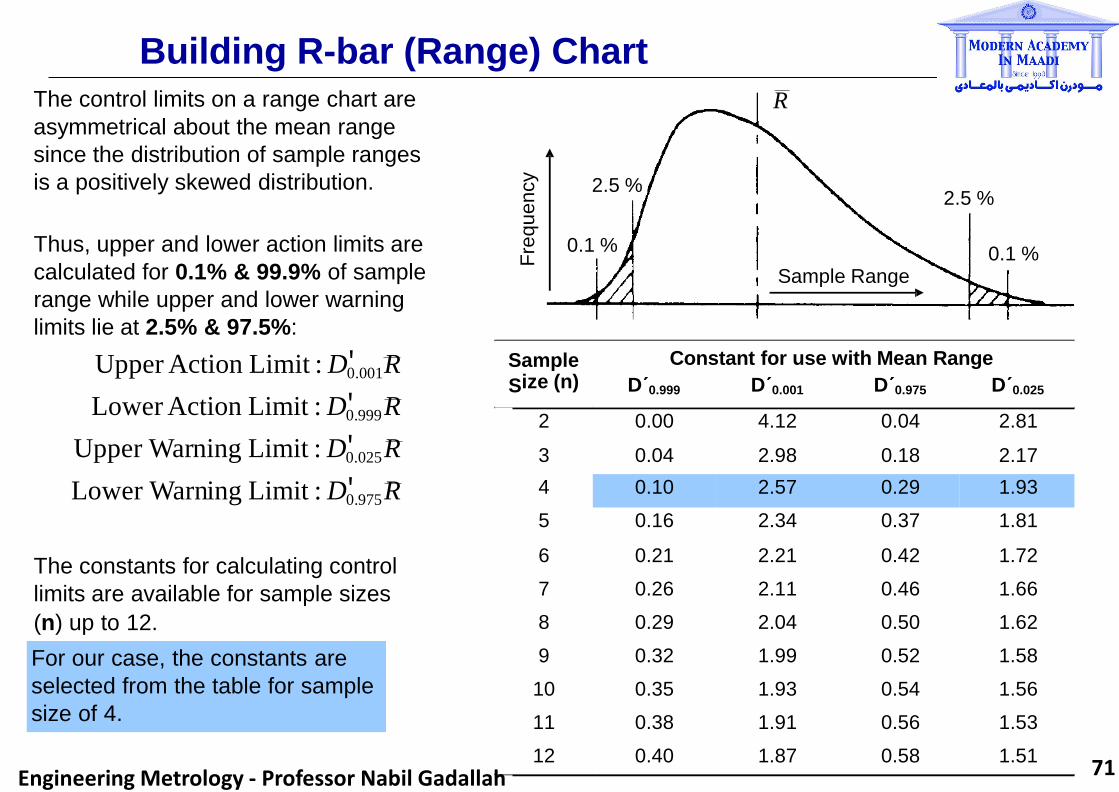
Building R-bar (Range) Chart The control limits on a range chart are
asymmetrical about the mean range
since the distribution of sample ranges
is a positively skewed distribution.
0.1 % Fre
qu
en
cy
Sample Range
0.1 %
2.5 % 2.5 %
R
1.87
1.91
1.93
1.99
2.04
2.11
2.21
2.34
2.57
2.98
4.12
D´0.001
0.40
0.38
0.35
0.32
0.29
0.26
0.21
0.16
0.10
0.04
0.00
D´0.999
0.58
0.56
0.54
0.52
0.50
0.46
0.42
0.37
0.29
0.18
0.04
D´0.975
Constant for use with Mean Range
1.51 12
1.53 11
1.56 10
1.58 9
1.62 8
1.66 7
1.72 6
1.81 5
1.93 4
2.17 3
2.81 2
D´0.025
Sample
Size (n)
The constants for calculating control
limits are available for sample sizes
(n) up to 12.
For our case, the constants are
selected from the table for sample
size of 4.
Constant for use with Mean Range
Thus, upper and lower action limits are
calculated for 0.1% & 99.9% of sample
range while upper and lower warning
limits lie at 2.5% & 97.5%:
Upper Action Limit : D0′.001R
Lower Action Limit : D0′.999 R
Upper Warning Limit : D0′.025 R
Lower Warning Limit : D0′.975 R
Sample
S ize (n) D´0.999 D´0.001 D´0.975 D´0.025
2 0.00 4.12 0.04 2.81
3 0.04 2.98 0.18 2.17
4 0.10 2.57 0.29 1.93
5 0.16 2.34 0.37 1.81
6 0.21 2.21 0.42 1.72
7 0.26 2.11 0.46 1.66
8 0.29 2.04 0.50 1.62
9 0.32 1.99 0.52 1.58
10 0.35 1.93 0.54 1.56
11 0.38 1.91 0.56 1.53
12 0.40 1.87 0.58 1.51 71 Engineering Metrology - Professor Nabil Gadallah

3 0
2 8
2 6
2 4
2 2 e
g 2 0 n
a 1 8 R 1 6 e p 1 4 l
m 1 2
Sa 1 0
8
6
4
2
0
Case Study – Range Chart
3 0
2 8
2 6
2 4
2 2
2 0
1 8
1 6
1 4
1 2
1 0
8
6
4
2
0
Sam
ple
Ran
ge
Mean Range
Upper Warning Limit
Upper Action Limit
Lower Action Limit
Lower Warning Limit
from
ta
ble
Lower Action Limit : D0′ .999 R = 1.1mm
Upper Action Limit : D0′ .001 R = 27.8 mm
Lower Warning Limit : D0′.975 R = 3.1mm
The range chart is constructed by turning the bell-shape histogram chart onto its side, hence we have
sample range as y-axis and mean range as x-axis (which was calculated before as 10.8 mm).
Then, action and warning limits are determined based on mean range and constants:
D0′.001 = 2.57
D0′.999 = 0.10
D0′.025 = 1.93
D0′.975 = 0.29
Upper Warning Limit : D0′.025 R = 20.8 mm
72 Engineering Metrology - Professor Nabil Gadallah

Is the process in control?
160
158
156
154
152
150
148
146
144
142
140
Sa
mp
le M
ea
n
30
27
24
21
18
15
12
9
6
3
0
Sa
mp
le R
an
ge
MEAN CHART
✓NO mean or range values which lie outside the action limits (action zone)?
✓NO more than about 1 in 22 values between warning and action limits (warning zone)?
✓NO incidence of two consecutive mean or range values which lie outside the same warning limit on either mean or range chart (warning zone)?
✓NO run or trend of five or more consecutive mean or range values, which also infringes a warning or action limit (warning zone and/or action zone)?
✓NO run of more than six sample means which lie either above or below the process mean (stable zone)?
✓NO trend of more than six values of the sample means which are either rising or falling (stable zone)?
PROCESS IS IN CONTROL !!!
RANGE CHART
(should be examined first)
73 Engineering Metrology - Professor Nabil Gadallah

What if the process is out of control?
Do not use the control charts and investigate the assignable causes of
The assignable causes of variation have been identified, and now to be eliminated.
variation.
Another set of samples from
the process is taken and control
limits are recalculated.
Approximate control limits are recalculated by simply
excluding the out of control results for which special
causes have been found and corrected.
The exclusion of samples representing unstable
conditions is not just throwing away bad data.
By excluding the data affected by known causes,
we have a better estimate of variation due to
common causes only.
The process is re-examined to see if it is in statistical control.
If the process is shown to be in statistical control, the next task is to
compare the limits of this control with the required tolerance.
74 Engineering Metrology - Professor Nabil Gadallah

Process Variability and Tolerances
Control Limits vs. Tolerance Limits
> Tolerance limits should be based on the functional requirements of the product.
Limits on control charts are based on the stability and actual capability of the process.
> A process may not meet the specification requirements, but still be in a state of statistical control.
> A comparison of process capability and tolerance can only take place, with confidence, when
the process is statistically in control. Thus, in controlling a process, it is necessary to establish
first that it is in statistical control and then to compare its centring & spread with the specified
target value and the specification tolerance.
The relationship between process variability and tolerances can be formalized by consideration of
standard deviation of the process. In order to manufacture within the specification, distance between
Upper Specification Limit (USL) or Upper Tolerance (+T) and Lower Specification Limit (LSL) or
Lower Tolerance (–T) must be analyzed.
There are three precision levels:
> High Relative Precision: 2T >> 6σ
> Medium Relative Precision: 2T ≥ 6σ
> Low Relative Precision: 2T < 6σ
75 Engineering Metrology - Professor Nabil Gadallah

Process Capability Indices
Process Capability Index
> It is a measure relating the actual performance of a process to its specified performance,
where the processes are considered to be a combination of plant or equipment, the method itself,
the people, the materials, and the environment.
> Process capability indices are simply a means of indicating the variability of a process relative
to the product specification tolerance.
Calculation of process capability indices estimates the short-term variations within the process.
This short-term is the period over which the process remains relatively stable. However, we know
that processes do not remain stable for all time, and therefore we need to allow within the specified
tolerance limits for:
> some movement of the mean
> detection of changes of the mean
> possible changes in the scatter (range)
> detection of changes in the scatter
> possible complications of non-normal distributions
76 Engineering Metrology - Professor Nabil Gadallah

Relative Precision Index (RPI)
We know that: Hartle y′s Constant
R Mean of Sample Ranges = σ =
d n
Then, we obtain: 2T 6
R d n
≥
In our case study: Min. RPI = = = 2.914 d n 2.059
6 6
If we are asked to produce
rods within ± 10 mm of the
target length:
2T = 20 mm = 1.852 R 10 .8
2T 20 RPI = = Reject
Material
If the specified tolerances
are widened to ± 20 mm: 2T = 40 mm = 3.704
R 10.8
40 RPI =
2T =
Avoid
Rejecting
Material
2T / R is known as Relative Precision Index (RPI) and the value of is the minimum RPI
to avoid the production of a material outside the specification limits. Moreover, RPI index does not
comment on the centring of a process as it deals only with its relative spread or variation.
6 / d n
This is the oldest index based on a ratio of the mean range of samples to the tolerance band.
In order to avoid the production of defective material, the specification width must be greater than
the process variation: 2T ≥ 6σ
77 Engineering Metrology - Professor Nabil Gadallah

Cp Index
= USL − LSL
= 2T
6σ 6σ C
p
Process variation is greater than tolerance band, so the process is incapable. (a) Cp < 1
For increasing values of Cp, the process becomes increasingly capable. (b) Cp ≥ 1
Similar with RPI, Cp index makes no comment about the centring of the process, which means
that it is a simple comparison of total variation with tolerances.
In order to manufacture within a specification, difference between USL and LSL must be less than
total process variation. So, a comparison of 6σ with (USL - LSL) or 2T gives Cp index:
78 Engineering Metrology - Professor Nabil Gadallah

Cpk Index
A situation like this invalidate the use of Cp index, hence
there is a need for another index which takes account of
both the process variation and the centring. Such an
index is called Cpk index, which is widely accepted as a
means of communicating process capability.
For USL and LSL limits, there are two Cpk values (Cpku and Cpkl
). These relate the difference between
process mean and USL/LSL respectively, and the lesser of these two will be the value of Cpk index:
⎟ ⎟
⎛ USL − X ⎞ ⎛ X − LSL ⎞ = ⎟ or ⎟ C = C = lesser of ⎟ C
⎝ ⎟ ⎝ 3σ 3σ pk l pk u pk
> Cpk < 1 means that, considering the process variation and its centring, at least one of the tolerance
limits is exceeded and the process is incapable.
> As in the case of Cp, increasing values of Cpk correspond to increasing capability.
> It may be possible to increase Cpk value by centring the process so that its mean value coincides
with the mid-specification (target).
> Comparison of Cp and Cpk shows no difference if the process is centred on the target.
> Cpk can be used when there is only one specification limit, but Cp cannot be used in such cases.
79 Engineering Metrology - Professor Nabil Gadallah

Engineering Metrology
CH (6)
Measurement of Geometric Shape
80 Engineering Metrology - Professor Nabil Gadallah

Measurement of Roundness using Intrinsic Datum
The conventional method using the points on the surface of
the part for a reference is called “intrinsic” datum system.
For large shafts
For large bores
81 Engineering Metrology - Professor Nabil Gadallah

Measurement of Roundness using Extrinsic Datum
In such system, measurements are taken based on an external reference of known precision.
82 Engineering Metrology - Professor Nabil Gadallah

Analysis of Roundness using Reference Circles
There are four types of reference circle in the analysis of Peak toValley out-of-roundness (RON):
> Least Squares Reference Circle (LSCI): A circle is fitted such that the sum of squares of the deviations is a minimum. RON is the distance from the highest peak to the lowest valley.
> Minimum Zone Reference Circles (MZCI): Two concentric circles positioned to enclose the measured
profile such that their radial deviation is a minimum. RON is the radial separation of the two circles.
> Minimum Circumscribed Circle (MCCI): The circle of minimum radius enclosing the profile (aka Ring
Gauge Reference Circle). RON is the maximum deviation of the profile from this circle.
> Maximum Inscribed Circle (MICI): The circle of maximum radius enclosing the profile (aka Plug Gauge Reference Circle). RON is the maximum deviation of the profile from this circle.
83 Engineering Metrology - Professor Nabil Gadallah

Defining Least Squares Circle > Equally-spaced radial ordinates are drawn relative to polar
roundness diagram.
> The rectangular coordinates of intersection of each point
(X & Y) are measured.
> After that, radial distance (r) for each point is obtained.
> Finally, the radius of LSC (R) is defined. 1.544
1.348
1.406
1.613
No. X Y X′ Y′
1 0.00 1.77 0.090 1.675
2 0.83 1.43 0.740 1.335
3 1.28 0.71 1.190 0.615
4 1.50 0.00 1.410 0.095
5 1.45 -0.84 1.360 -0.935
6 0.73 -1.31 0.640 -1.405
7 0.00 -1.25 0.090 -1.345
8 -0.65 -1.10 -0.740 -1.195
9 -1.29 -0.74 -1.380 -0.835
10 -1.42 0.00 -1.510 0.095
11 -1.14 0.63 -1.230 0.535
12 -0.75 1.27 -0.840 1.175
r
1.677
1.526
> Then, the updated coordinates of each point (X′ & Y′) are
calculated based on center of least square circle (a & b).
1.340
1.413
1.650
1.513
1.341
1.444
a = 2Σx
= 0.090 b = 2Σy
= 0.095 n n
R = Σr
= 1.485 n
r = (X ′)2 + (Y ′)2
84 Engineering Metrology - Professor Nabil Gadallah

Other Parameters Eccentricity
> The position of center of a profile relative to a datum point.
> It is a vector quantity with magnitude and direction.
> The magnitude is the distance between profile center (center of the fitted reference circle) and the datum point.
> The direction is an angle from the datum point.
Concentricity
> The diameter of circle described by the profile center when rotated about
the datum point.
> It has only magnitude and no direction.
Runout
> The radial difference between two concentric circles centered on the datum
point which are drawn such that one coincides with the nearest and the other
coincides with the farthest point on the profile.
> It combines the effect of form error and the concentricity to give a predicted
performance when rotated about a datum.
85 Engineering Metrology - Professor Nabil Gadallah

Other Parameters Flatness
> The peak-to-valley departure from a reference plane.
> Either least square (LS) or minimum zone (MZ) can be used.
Squareness
> The minimum axial separation of two parallel planes normal to
the reference axis and which totally encloses the reference plane.
> Either least square (LS) or minimum zone (MZ) can be used.
Coaxiality
> The diameter of a cylinder that is coaxial with the datum axis and
just encloses the axis of the cylinder referred for coaxiality evaluation.
Cylindricity
> The minimum radial separation of two cylinders, coaxial with the fitted reference axis, which totall encloses the measured data.
> Either least square, minimum zone, maximum inscribed or minimum circumscribed cylinders (LSCY, MZCY, MICY, MCCY) can be used.
86 Engineering Metrology - Professor Nabil Gadallah

Measurement of Geometric Shapes
Laser
Interferometry Autocollimator
Laser
Alignment
Electronic Level
and Clinometer
Dial Indicator
Circular Tracing
Talyrond
365
Flatness
Straightness
Parallelism
Squareness
Roundness
Concentricity
Cylindricity
Coaxiality
Eccentricity
Runout
87 Engineering Metrology - Professor Nabil Gadallah

Rotational Measurement
CONCENTRICITY CYLINDRICITY
COAXIALITY (OF SECTION) SIMPLIFIED CYLINDRICITY
COAXIALITY (OF AXIS) MEAN CYLINDRICITY
88 Engineering Metrology - Professor Nabil Gadallah
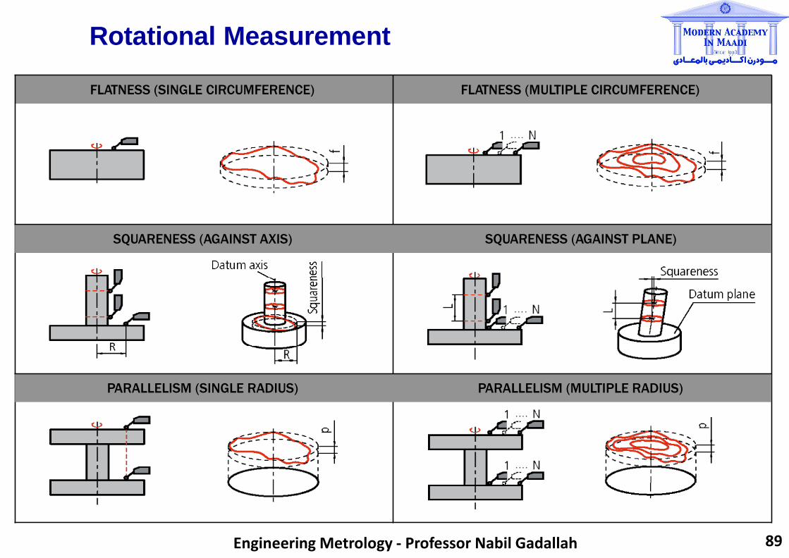
Rotational Measurement
FLATNESS (SINGLE CIRCUMFERENCE) FLATNESS (MULTIPLE CIRCUMFERENCE)
SQUARENESS (AGAINST AXIS) SQUARENESS (AGAINST PLANE)
PARALLELISM (SINGLE RADIUS) PARALLELISM (MULTIPLE RADIUS)
89 Engineering Metrology - Professor Nabil Gadallah

Rotational Measurement
CIRCULAR RUN-OUT (RADIAL) CIRCULAR RUN-OUT (AXIAL)
TOTAL RUN-OUT (RADIAL) TOTAL RUN-OUT (AXIAL)
THICKNESS DEVIATION (RADIAL) THICKNESS DEVIATION (AXIAL)
90 Engineering Metrology - Professor Nabil Gadallah

Rectilinear Measurement
FLATNESS SQUARENESS
STRAIGHTNESS (VERTICAL) SQUARENESS (AGAINST AXIS)
STRAIGHTNESS (HORIZONTAL) SQUARENESS (AGAINST PLANE)
91 Engineering Metrology - Professor Nabil Gadallah

Rectilinear Measurement
PARALLELISM (VERTICAL) PARALLELISM (HORIZONTAL)
TAPER RATIO (VERTICAL) TAPER RATIO (HORIZONTAL)
SLOPE (VERTICAL) SLOPE (HORIZONTAL)
92 Engineering Metrology - Professor Nabil Gadallah

Rectilinear Measurement
CYLINDRICITY CYLINDRICITY
COAXIALITY COAXIALITY
TOTAL RUN-OUT (RADIAL) TOTAL RUN-OUT (AXIAL)
93 Engineering Metrology - Professor Nabil Gadallah

Engineering Metrology
CHAPTER (6)
Advanced Measurement Systems
94 Engineering Metrology - Professor Nabil Gadallah

Coordinate Measuring Machine (CMM)
Coordinate Measuring Machine
Coordinate Measuring Machines (CMMs)
provide precise and accurate measurements
of 3D coordinates of components using small-
head touching probes via movable axes.
95 Engineering Metrology - Professor Nabil Gadallah
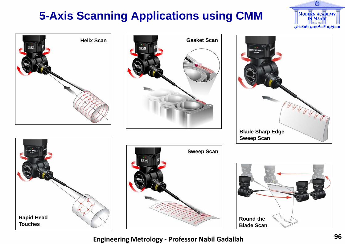
5-Axis Scanning Applications using CMM
Helix Scan
Round the
Blade Scan
Gasket Scan
Sweep Scan
Rapid Head
Touches
Blade Sharp Edge
Sweep Scan
96 Engineering Metrology - Professor Nabil Gadallah
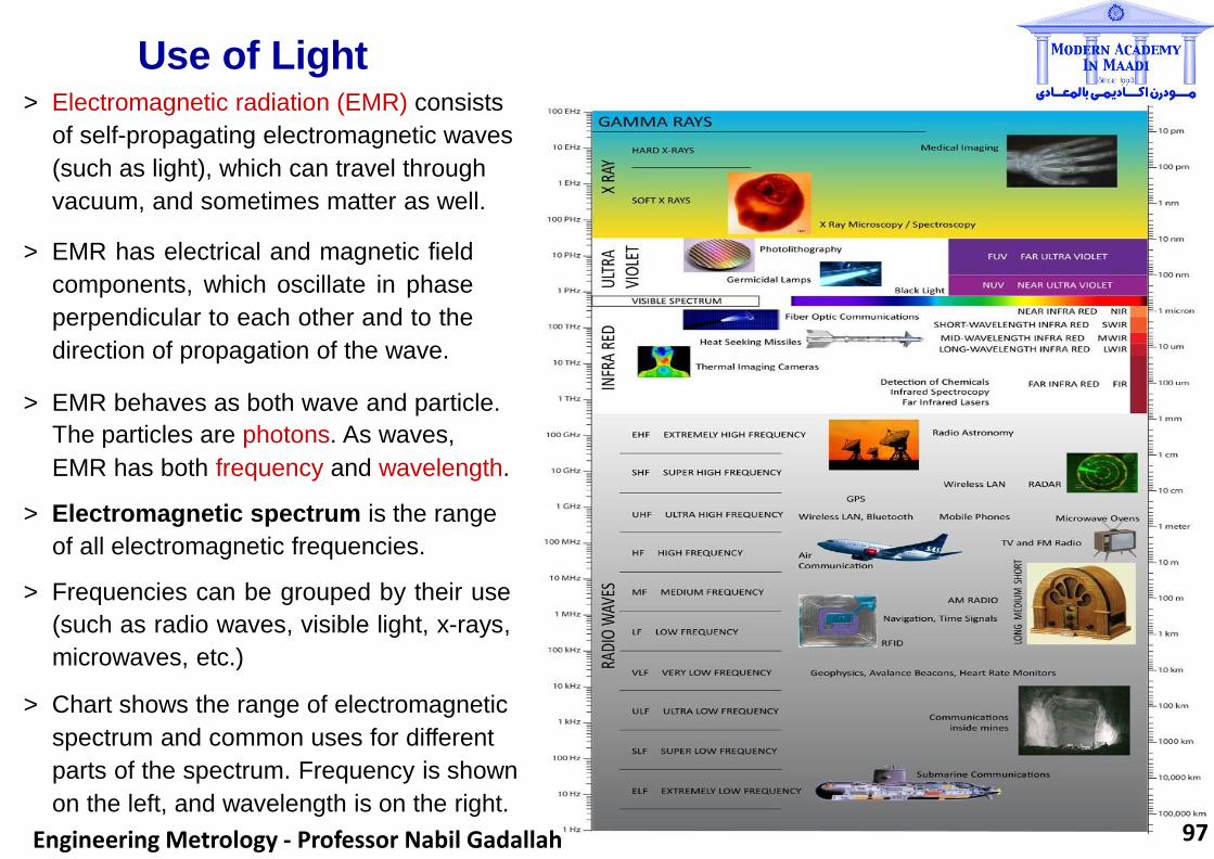
Use of Light > Electromagnetic radiation (EMR) consists
of self-propagating electromagnetic waves
(such as light), which can travel through
vacuum, and sometimes matter as well.
> EMR has electrical and magnetic field
components, which oscillate in phase
perpendicular to each other and to the
direction of propagation of the wave.
> EMR behaves as both wave and particle.
The particles are photons. As waves,
EMR has both frequency and wavelength.
> Electromagnetic spectrum is the range
of all electromagnetic frequencies.
> Frequencies can be grouped by their use
(such as radio waves, visible light, x-rays,
microwaves, etc.)
> Chart shows the range of electromagnetic
spectrum and common uses for different
parts of the spectrum. Frequency is shown
on the left, and wavelength is on the right.
97 Engineering Metrology - Professor Nabil Gadallah

Introduction to Interferometry
> Interferometry is the technique of superimposing (i.e. interfering) two or more waves in order to
detect differences between them.
> It is applied in a wide variety of fields including astronomy, fiber optics, optical metrology, seismology,
oceanography, quantum mechanics, and plasma physics.
> From metrology viewpoint, it is a series of non-contact techniques using the interference of light waves
to determine surface shape and transmission properties.
Principle of Interferometry
> Whenever two waves comes together at the same time
and place, interference occurs.
> If both waves are in phase (i.e. their crests coincide),
they will add together to form a single wave with higher
crest (i.e. larger amplitude). This is called constructive
interference.
> Destructive interference occurs when the waves are
out of phase (i.e. the crest of one wave coincides with
the through of other wave). Therefore, the amount of
interference depends on both the amplitudes of those
waves and their frequencies (the degree to which their
respective crests are in phase with each other). 98 Engineering Metrology - Professor Nabil Gadallah

Principle of Interferometry
time
t
sinθ = (λ 2)∗ t
interference fringes (red bands)
inte
ns
ity
> Simple interferometry setup includes the use of parallel beam of monochromatic light.
> For this purpose, an optical flat (a disc of stress-free glass or quartz with a highly polished surface)
is placed on top of the surface to be measured at a very small angle of θ.
> The light beam from source (S) is projected onto the optical flat. Two reflected components of light
wave (partially reflected from a and b) are collected, and hence the combined view is obtained.
> Further along the surface at a distance of half-wavelength (λ/2) and due to the angle θ, the ray (light
beam) leaving source S will again split into two components whose path lengths are different.
> Therefore, the surface will be crossed by a pattern of dark bands (fringes), which are straight for
the case of a flat surface.
99 Engineering Metrology - Professor Nabil Gadallah

Fringe Analysis
Straight Fringe Pattern:
> Such pattern indicates a very flat surface.
> Suppose that the wavelength (λ) is 0.6328 µm.
> Thus, the flatness is 0.3164 µm.
Curved Fringe Pattern:
> In such cases, two red lines tangent to the center
of two adjacent fringes are drawn. The blue line
indicates the center of a single fringe.
> If the distance between red lines (a) is 5.02 µm and
the distance between red and blue lines (b) is 1.24
µm, then, the flatness is ≈ 0.078 µm.
Circular Fringe Pattern:
> This pattern is obtained when the surface to be
measured is convex or concave.
> So, the total distance between the peak and the
deepest point (i.e. height) can be calculated.
> Since there are 5 fringes, then the height is found
to be 1.582 µm.
b
Height = (λ 2)∗ (# of fringes)
Optical Flat
Spherical
Flat Surface
Flatness = (λ 2)
a
Flatness = (λ 2)∗ (b a)
Flatter Spherical
100
Engineering Metrology - Professor Nabil Gadallah

Fringe Analysis Software
In most cases, fringe patterns are quite sophisticated.
Therefore, special-purpose software with advanced
techniques may be required for accurate fringe analysis.
101 Engineering Metrology - Professor Nabil Gadallah

Common Types of Interferometers
Michelson Interferometer Mach-Zehnder Interferometer
Sagnac Interferometer Fabry-Perot Interferometer
Various systems are available for different type of measurements based on the application area.
102 Engineering Metrology - Professor Nabil Gadallah
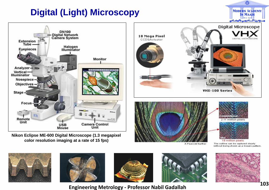
Digital (Light) Microscopy
Nikon Eclipse ME-600 Digital Microscope (1.3 megapixel
color resolution imaging at a rate of 15 fps)
103 Engineering Metrology - Professor Nabil Gadallah

Electron Microscopy 1
cm
1 m
m
100
µm
10 µ
m
1 µ
m
100
nm
10 n
m
1 n
m
0.1
nm
(1
Å)
Electron Microscopy
Light Microscopy
Transmission Electron Microscopy (TEM) is used to
analyse the inner structure of objects (such as tissues,
cells, viruses) while Scanning Electron Microscopy
(SEM) is used to visualize the surface of tissues,
macromolecular aggregates and materials.
Both TEM and SEM use a source (an electron gun),
lenses (electro-magnetic lenses that deflect electrons),
a condenser (that concentrates beam), and an objective
to focus (the thing to be measured).
Unlike light microscopy, the object is not illuminated
with light, but bombarded by electrons.
Recently emerging as an
advanced technology in
many engineering fields,
electron microscopy allows
to visualize objects that are
as small as 0.1 nm (1Å).
104 Engineering Metrology - Professor Nabil Gadallah

Electron Microscopy Examples
pollen
Micro-scale circuiting uranium waste bacteria witherite (barium
carbonate crystal)
escherichia (coli basili) nylon stocking fibres
105 Engineering Metrology - Professor Nabil Gadallah

Use of Laser
> The term “laser” is an acronym for “Light Amplification by Stimulated Emission of Radiation”.
> It is a device that emits light (electromagnetic radiation) through a process of optical amplification
based on the stimulated emission of photons.
> Different types of laser are used for research and industrial purposes (such as metal cutting, welding,
dynamic alignment or positioning, dimensional measurements, nondestructive testing, lithography,
medical treatments, military applications, and so on).
> For more information on type of lasers and their specific use: http://en.wikipedia.org/wiki/Laser_types
106 Engineering Metrology - Professor Nabil Gadallah

Laser Displacement Sensors with CCD Detectors
Laser-triangular sensor uses a high-speed, noncontact line-range laser
probe to perform complex-part profile measurements. Laser beam is
spread out into a plane that forms a line of light on the part surface.
CCD (Charge Coupled Device) sensor mounted in the probe takes range
measurements over the entire line of laser light at the same time (instead
of measuring just one point), which dramatically decreases scan time.
laser
scanner
laser
pointer
107 Engineering Metrology - Professor Nabil Gadallah

Laser Interferometers
Laser Interferometer for Vision Laser Interferometer System for Precise
Positioning and Accurate Measurement
Compared with common interferometers, laser
interferometry provides precise and accurate
optical measurements as well as positioning
and movement systems.
108 Engineering Metrology - Professor Nabil Gadallah

Use of Sound
Elephant (5 - 12000)
Human (20 - 20000)
Cat (45 - 64000)
Dog (67 - 45000)
Mouse (100 - 91000)
Dolphin (75 - 150000)
Bat (2000 - 200000)
1 10 100 1000 10000 100000
Frequency (Hz)
> Sound is a sequence of waves of pressure
propagating through a compressible media
(such as air, water or solids).
> During propagation, waves are reflected,
refracted or attenuated by the medium.
> Sound waves are classified into specific
ranges according to their frequencies:
infrasound, acoustic, and ultrasound.
> Infrasound has the frequency of less than
20 Hz, which is the normal limit of human
hearing. The sound having frequencies of
greater than 20 kHz is ultrasound, which
is not audible by humans.
> Mach number (M = V/C) is used to define
speed of an object travelling in a medium
(V) in relation with speed of sound (C).
> From metrology viewpoint, sounds waves
with certain frequencies and amplitudes
are used in various applications (such as
underwater, seismology, medical, NDT,
infrasound & ultrasonic inspection).
Regime Subsonic Transonic Sonic Supersonic Hypersonic High-hypersonic
Mach < 1.0 0.8 - 1.2 1.0 1.2 - 5.0 5.0 - 10.0 > 10.0
109 Engineering Metrology - Professor Nabil Gadallah

SONAR
> SONAR stands for “SOund NAvigation and Ranging”.
> It is a technique using underwater sound propagation
to navigate, communicate with or detect the objects.
> It directs a beam of sound waves downward. After
the sound wave hits bottom of ocean or an object,
it will bounce off and return back causing an echo.
This is recorded on a depth recorder on the ship.
> There are two SONAR systems: Active (deploys and
recevies its own signal) & Passive (just listening)
110 Engineering Metrology - Professor Nabil Gadallah

Ultrasonic Testing
> Ultrasonic Testing (UT) uses high frequency sound energy
to conduct flaw detection, dimensional inspection, material
characterization, and more.
> Typical UT system consists of a pulser/receiver, a transducer,
and a display software/device. Pulser/receiver produces high
voltage electrical pulses. Driven by the pulser, the transducer
generates high frequency ultrasonic energy, which propagates
through the part in form of waves. When there is discontinuity
(such as crack/flaw) in the wave path, some part of energy is
reflected back from the flaw surface. Based on voltage signals
of reflecting energy, loaction and size of flaws are displayed.
pulser/receiver
ultrasonic
trasducer
flaw
part
Typical schemes of UT
a) one axis through testing b) angle testing
c) one surface testing d) curve surface testing
111 Engineering Metrology - Professor Nabil Gadallah

Engineering Metrology
CHAPTER (7)
Measurement of Surface Texture
112 Engineering Metrology - Professor Nabil Gadallah
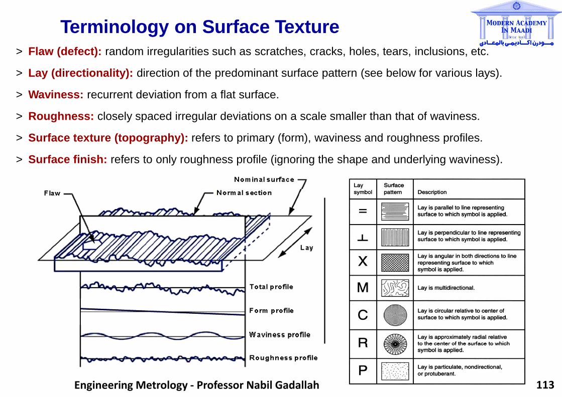
Terminology on Surface Texture
> Flaw (defect): random irregularities such as scratches, cracks, holes, tears, inclusions, etc.
> Lay (directionality): direction of the predominant surface pattern (see below for various lays).
> Waviness: recurrent deviation from a flat surface.
> Roughness: closely spaced irregular deviations on a scale smaller than that of waviness.
> Surface texture (topography): refers to primary (form), waviness and roughness profiles.
> Surface finish: refers to only roughness profile (ignoring the shape and underlying waviness).
113 Engineering Metrology - Professor Nabil Gadallah
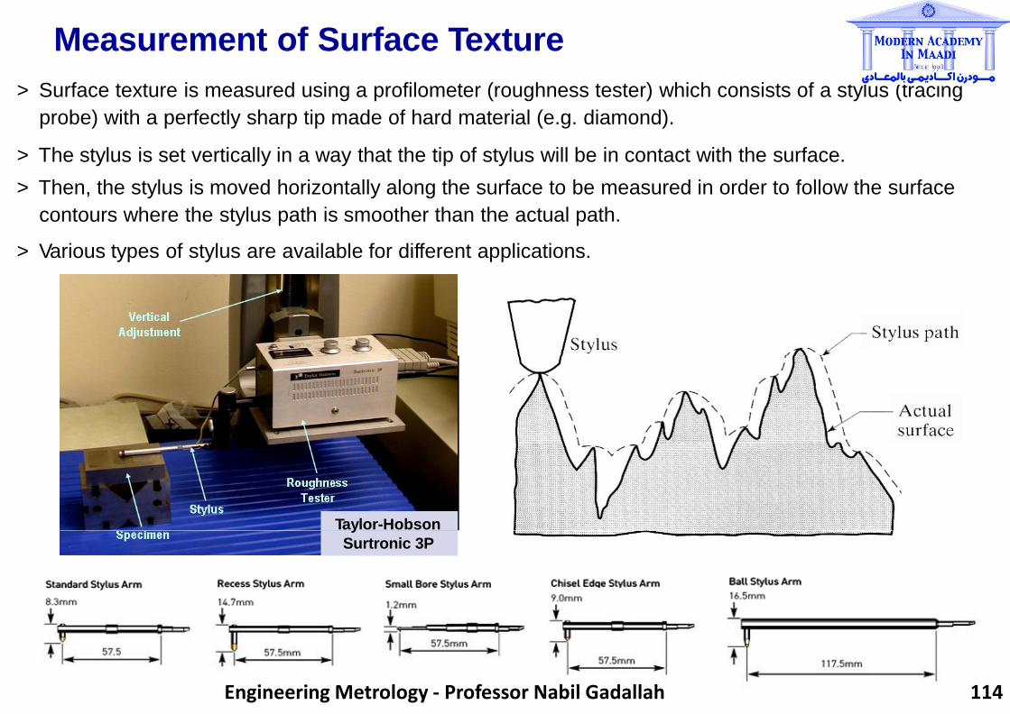
Measurement of Surface Texture
> Surface texture is measured using a profilometer (roughness tester) which consists of a stylus (tracing
probe) with a perfectly sharp tip made of hard material (e.g. diamond).
> The stylus is set vertically in a way that the tip of stylus will be in contact with the surface.
> Then, the stylus is moved horizontally along the surface to be measured in order to follow the surface
contours where the stylus path is smoother than the actual path.
> Various types of stylus are available for different applications.
Taylor-Hobson
Surtronic 3P
114 Engineering Metrology - Professor Nabil Gadallah

Profilometers (Roughness Testers) The profilometers are classified as with or without skid:
> Profilometer with skidded gage: In skidded gages, the sensitive diamond-tipped stylus is contained
within a probe, which has a skid that rests on the workpiece. Thus, skidded gages use the workpiece
itself as the reference surface to measure roughness only.
> Skidless gage profilometer: Skidless gages use an internal precision surface as a reference. This
enables skidless gages to be used not only for roughness, but also waviness and form profiles.
Profilometer with
skidded gage
Skidless gage
profilometer
115 Engineering Metrology - Professor Nabil Gadallah

Typical Measurements
Dimension, form and texture can be measured at once
over curved or straight surfaces
Measurement of ball tracks and ring
grooves using skidless tracing arms
Measurement of inner surfaces of gears
The measured profiles can be evaluated using dedicated software
to suppress roughness and waviness profiles
116 Engineering Metrology - Professor Nabil Gadallah

Surface Texture Parameters
The parameters related with measurement of surface texture are divided into three groups.
Table shows the parameters for primary, waviness and roughness measurements:
Parameter
Group Explanation
Parameters
Primary Waviness Roughness
Amplitude
Parameters
The vertical characteristics of
the surface deviations
Pa, Pq, Pv, Pp,
Pt, Psk, Pku, Pz
Wa, Wq, Wv, Wp,
Wt, Wsk, Wku, Wz
Ra, Rq, Rv, Rp, Rt,
Rsk, Rku, Rz, R3z
Spacing The horizontal characteristics
Parameters of the surface deviations Psm Wsm Rsm, RHSC, RPc
Hybrid
Parameters and horizontal characteristics
Combination of both vertical
of the surface deviations
P∆q, Pλq W∆q, Wλq
R∆q, Rλq, Rmr,
Rpk, Rk, Rvk, Mr1
and Mr2
117 Engineering Metrology - Professor Nabil Gadallah

Assessment of Roughness Profile
The profile shown below is a typical 2D roughness profile:
> Assesment (evaluation) length (L): Length used for assesing the profile for roughness
measurement. For this length, at least five consecutive lengths are taken as standard.
> Sampling length (l): The profile mean line is determined and the profile is divided into
equal sampling lengths (from l1 to l5).
> Cut-off length (λC): A filter to remove or reduce unwanted data to look at wavelengths in
the assesment region. Sampling length is also known as cut-off length.
Z
X
l1 l2 l5 l4 l3
L 118 Engineering Metrology - Professor Nabil Gadallah

Roughness Parameters – Ra and Rq
> Roughness Average (Ra): Universally recognised and commonly used roughness parameter, which is
the arithmetic mean of departures from the mean line. It is also known as Center Line Average (CLA)
or Arithmetic Average (AA).
> Root Mean Square (RMS) Roughness (Rq): It is the RMS average of roughness profile ordinates.
> Ra is a very stable and repeatable parameter, which makes it good for random type surfaces. However,
it cannot provide distinction between peaks and valleys.
> Rq is more sensitive to peaks and valleys due to the reason that the amplitudes are squared.
1 L 1 L Ra = ∫0
z ( x) d x L
2 Rq = ∫0
z ( x) d x L
Ra Rq
119 Engineering Metrology - Professor Nabil Gadallah

Misinterpretation of Surface Roughness based on Ra
> As said before, it is not possible to make a distinction between peaks and valleys by using Ra.
> Three roughness profiles shown below have the same Ra value although they seem to be different.
Therefore, the assesment of these profiles using Ra will cause inaccurate conclusions to be made.
> For this purpose, there is need for more specific and sensitive roughness parameters in order to make
a more reliable assesment.
120 Engineering Metrology - Professor Nabil Gadallah

Roughness Parameters – Rz and Rzmax
> Mean Roughness Height/Depth (Rz): The mean of roughness heights/depths at each sample length.
> Maximum Roughness (Rzmax): The largest of five roughness heights/depths at each sample length.
> Rz is more sensitive than Ra to changes on the surface as the maximum profile heights are examined
rather than average of peak and valleys. In addition, Rzmax is useful for surfaces where a single defect
is not permissible (e.g. a seal with a scratch).
> Rz and Rzmax are used together to monitor the variations of surface finish in a production process.
Similar values of them indicate a consistent surface finish, while a significant difference between them
indicates a surface defect in an otherwise consistent surface.
1 n
Rz = n ∑ Rzi
i=1 R = (R )
max zmax zi
Rz1 Rz 2 Rz = Rz 3 max Rz 4 Rz 5
121 Engineering Metrology - Professor Nabil Gadallah

Roughness Parameters – Rp, Rv, Rt
> Maximum Height (Rp): The maximum roughness height (peak) within each sampling length.
> Maximum Depth (Rv): The maximum roughness depth (valley) within each sampling length.
> Mean Levelling (Rpm): The mean of five consecutive heights (peaks) from each sampling length.
> Peak-to-Valley Roughness (Rt): The largest peak-to-valley in the entire profile.
> Rpm is recommended for bearing and sliding surfaces and surface substrates prior to coating.
> A low value of Rpm and a large value of Rz indicates a plateau surface.
> The ratio of Rpm / Rz quantifies the asymmetry of profile.
> Rv is a good parameter where stress is a major factor whereas Rp is to control coating quality.
Rt
Rp5
Rv5
122 Engineering Metrology - Professor Nabil Gadallah

Spacing Parameter – Rsm
> Mean Spacing (Rsm): The mean spacing of S1, S2, .., Sn between profile peaks as they pass through
the mean line (spacing is the distance between points that cross the mean line in an upward direction).
S1 S2 S3
> Rz to Ra Conversion: Based on BS 1134/1-1972 standard, Rz = x4 - x7 Ra. The actual ratio depends
upon the shape of the profile.
> For more information on surface texture parameters measurements, go to Taylor Hobson’s website:
http://www.taylor-hobson.com/faqsurface.php
123 Engineering Metrology - Professor Nabil Gadallah

Selection of Cutt-off Length > Changing cut-off value (which changes
amount of "averaging" and "smoothing")
can have huge impact on measurement
of roughness and waviness.
> Choosing smaller cut-off lengths will
result in smaller roughness values
even though the real surface could be
very rough. The picture shown presents
the same surface with different cut-offs.
The profile on the left gives twice the Ra
value of the profile on the right.
> Thus, there are recommended values
for choosing the appropriate cut-offs,
which were defined by ISO 4288-1996.
RECOMMENDED CUT-OFF LENGTHS (ISO 4288-1996)
Periodic Profiles Non-Periodic Profiles Cut-offs Evaluation Length
Sm (mm) Rz (µm) Ra (µm) λC (mm) L (mm)
>0.013 to 0.04 (0.025) to 0.1 (0.006) to 0.02 0.08 0.4
>0.04 to 0.13 >0.1 to 0.5 >0.02 to 0.1 0.25 1.25
>0.13 to 0.4 >0.5 to 10 >0.1 to 2 0.8 4
>0.4 to 1.3 >10 to 50 >2 to 10 2.5 12.5
>1.3 to 4 >50 to 200 >10 to 80 8 40
124 Engineering Metrology - Professor Nabil Gadallah

ISO Standards on Surface Texture
ISO 1302 - 2001 Indication of Surface Texture
ISO 3274 - 1996 Nominal Characteristics of Contact (Stylus) Instruments
ISO 4287 - 1997 Terms, Definition and Surface Texture Parameters
ISO 4288 - 1996 Rules and Procedures for Assessment of Surface Texture
ISO 5436-1 - 2000 Calibration, Measurement Standards
ISO 5436-2 - 2000 Calibration, Soft Gages
ISO 8785 - 1999 Surface Imperfections - Terms, Definitions and Parameters
ISO 11562 - 1996 Metrological Characteristics of Phase Correct Filters
ISO 12085 - 1996 Motif Parameters
ISO 12179 - 2000 Calibration of Contact (Stylus) Instruments
ISO 13565 - 1996 Characterization of Surfaces Having Stratified Functional Properties
125 Engineering Metrology - Professor Nabil Gadallah

Surface Finish Tolerances in Manufacturing Ra j1ll1 2000
METAL CUITING
sawing
planing, shaping
drilling
milling
boring, turning
broa ching
reaming
1 000 500 250 1 2 5 6 3 32 16 8
I I I I I
4 2 1 . 5
I
I common - I I I I Iless frequent
I I I
I I I I ' I '
' I '
' I '
I I
ABRASIVE
grinding
barrel finishing
honing
electro-polishing
electrolytic grinding
polishing
lapping
superfinishing
I I I I I I I I I
I I I
I I I I I
I I
I I
I I I I I
I I I I I
I I I
CASTING
sand casting
perm mold
casting investment
casting
die casting
FORMING hot rolling
forging
extruding
I I I I I
I I '
'
I I
I
I I
I l '
cold rolling, drawing
rolle r burnishing
I '
I I I
I
I
l
OTHER
flame cutting
chemical milling
electron beam cutting
laser cutting
EDM
I I I
I I I I I
I I I I
I I I I
I 126 Engineering Metrology - Professor Nabil Gadallah

Engineering Metrology
CHAPTER (8)
Measurement of Screw Threads
127 Engineering Metrology - Professor Nabil Gadallah

Thread Terminology
> Thread: the helical grooves opened to inner and outer surfaces.
> External thread (screw): A thread on the external surface of a cylinder.
> Internal thread (nut): A thread on the internal surface of a cylinder.
> Major diameter (diş üstü çap): The largest diameter of a screw thread.
> Minor diameter (diş dibi çap): The smallest diameter of a screw thread.
> Pitch diameter (bölüm çapı): The diameter of an imaginary cylinder the ,
surface of which cuts the thread forms where the width of the thread and
groove are equal.
> Crest: The edge or surface that joins the sides of a thread and is farthest
from the cylinder or cone from which the thread projects.
> Root: The edge or surface that joins the sides of adjacent thread forms and
coincides with the cylinder or cone from which the thread projects.
> Thread Depth: The distance between crest and root.
> Pitch (hatve, adım): The distance between corresponding points on adjacent
thread forms measured parallel to the axis.> Right-hand thread: A thread that
when viewed axially winds in a CW and receding direction. Threads are RH
unless otherwise specified.
> Left-hand thread: A thread that when viewed axially winds in a CCW and
receding direction. These threads are designated as LH.
128 Engineering Metrology - Professor Nabil Gadallah
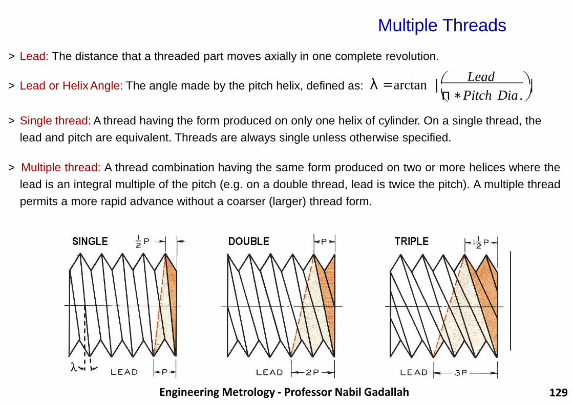
Multiple Threads
> Lead: The distance that a threaded part moves axially in one complete revolution.
> Lead or Helix Angle: The angle made by the pitch helix, defined as: λ = arctan ⎟ ⎟ ⎝ π ∗ Pitch Dia . ⎟
⎛ Lead ⎞
> Single thread: A thread having the form produced on only one helix of cylinder. On a single thread, the
lead and pitch are equivalent. Threads are always single unless otherwise specified.
> Multiple thread: A thread combination having the same form produced on two or more helices where the
lead is an integral multiple of the pitch (e.g. on a double thread, lead is twice the pitch). A multiple thread
permits a more rapid advance without a coarser (larger) thread form.
λ
129 Engineering Metrology - Professor Nabil Gadallah

Thread Types and Designation
> There are several thread forms used for specific applications. Selection of the appropriate thread form
depends upon the functionality, size and purpose of the required job.
> The threads are designated in Metric or British system as shown below.
British System a: Major diameter (inch)
b: Threads per inch
.250-20 UNC-2A-LH c: Form (i.e. Unified National Coarse)
d: External thread (B for internal)
Metric System
x: Metric screw thread M20 x 2 y: Major diameter (mm)
a b c d e e: Left-hand thread (RH for right-hand) x y z z: Pitch (mm)
130 Engineering Metrology - Professor Nabil Gadallah

Thread Gauges
> The threads can be measured
(checked) using fixed limit gauges
such as adjustable thread ring
and plug gauges, which provide
GO (green) or NOT-GO (red) type
of measurement.
> Screw pitch gauge (consisting of
a metal case having several leaves)
can also be used. Each leaf has
teeth corresponding to a definite
pitch. By matching these teeth with
threads on work, the correct pitch
can be read directly from the leaf.
> Thread rolls (with various forms
and known dimensions) are used
to measure (check) internal threads.
Thread ring gauge
Screw pitch
gauge
Thread rolls
131 Engineering Metrology - Professor Nabil Gadallah

Thread Micrometers
> Screw thread micrometers having various type and size of interchangeable spindle and anvils are
used for measuring the pitch diameter of external threads.
> The pitch diameter of internal threads are measured by inside thread micrometers with various
type and dimensions for different applications.
Screw thread micrometer
with interchangeable
spindle and anvil
Inside thread micrometer with various
type and size
132 Engineering Metrology - Professor Nabil Gadallah

Three-Wire Method
> Three-wire method is one of the most accurate and versatile ways of measuring the pitch diameter
of a thread by using three lapped and polished wires and a micrometer.
> Wires touching the threads at the pitch diameter are “Best Size Wires”. Such wires are used since
the measurements are least affected by errors that may be present in the angle of the thread.
Di : Minor diameter h : Depth of thread p : Pitch
Dp : Pitch diameter λ : Lead (helix) angle Dw : Wire diameter
Do : Major diameter α : Flank angle Hw : Measurement over wires
133 Engineering Metrology - Professor Nabil Gadallah
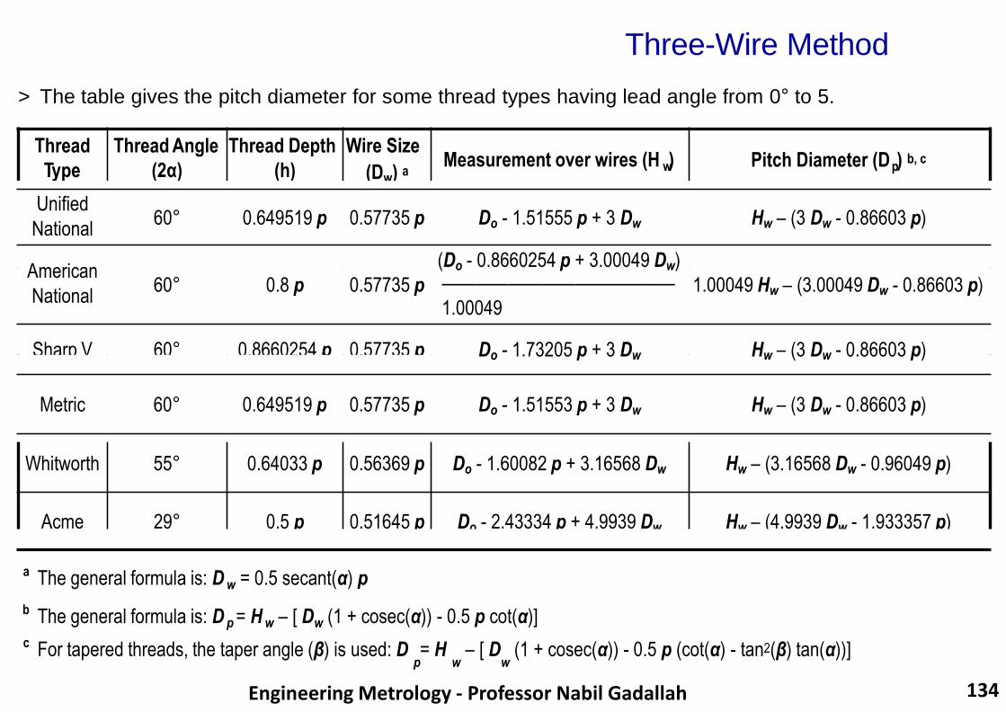
Three-Wire Method
> The table gives the pitch diameter for some thread types having lead angle from 0° to 5.
Thread Thread Angle Thread Depth Wire Size
Type (2α) (h) (Dw) a Measurement over wires (H ) w Pitch Diameter (D ) b, c
p
Unified
National 60° 0.649519 p 0.57735 p Do - 1.51555 p + 3 Dw Hw – (3 Dw - 0.86603 p)
(Do - 0.8660254 p + 3.00049 Dw) ——————————————
1.00049
American
National 60° 0.8 p 0.57735 p 1.00049 Hw – (3.00049 Dw - 0.86603 p)
Sharp V 60° 0.8660254 p 0.57735 p Do - 1.73205 p + 3 Dw Hw – (3 Dw - 0.86603 p)
Metric 60° 0.649519 p 0.57735 p Do - 1.51553 p + 3 Dw Hw – (3 Dw - 0.86603 p)
Whitworth 55° 0.64033 p 0.56369 p Do - 1.60082 p + 3.16568 Dw Hw – (3.16568 Dw - 0.96049 p)
Acme 29° 0.5 p 0.51645 p Do - 2.43334 p + 4.9939 Dw Hw – (4.9939 Dw - 1.933357 p)
a The general formula is: D = 0.5 secant(α) p w
b The general formula is: D = H – [ D (1 + cosec(α)) - 0.5 p cot(α)] p w w
c For tapered threads, the taper angle (β) is used: D = H – [ D (1 + cosec(α)) - 0.5 p (cot(α) - tan2(β) tan(α))] p w w
134 Engineering Metrology - Professor Nabil Gadallah

Comparison of Measurement Methods
METHOD ADVANTAGES DISADVANTAGES
Thread
Gauges
&
☺ Inspects the complete thread profile
☺ Simple to use with minimum training
® Reveals only if the thread is correct or incorrect (i.e. it gives
no information related to its tolerance)
Thread Rolls ☺ The inspected thread can be judged correct or
incorrect by assuming use of both GO and NOT-GO
® Time consuming when setting up and controlling the process,
and difficult and/or expensive to calibrate
® Manufacturing tolerances and wear allowances on the gauge
give reduced tolerances on the thread
® Only suitable for the specific thread denomination (tolerance)
stated on the gauge
☺ Accurate if the flank angle is correct ® Requires special (and thus costly) micrometer
☺ Can be used on most thread types with the same ® Measures only pitch diameter
Thread
Micrometer
flank angle
☺ Suitable for machine set-up and process control
Three-Wire ☺ Very accurate results if the flank angle and pitch
System of threads are correct ® Only external threads can be inspected
® Requires calculation to find the correct measurement result
☺ Can be used for almost all thread types
® Measuring wires must fit the appropriate micrometer
☺ Suitable for machine set-up and process control
135 Engineering Metrology - Professor Nabil Gadallah

Engineering Metrology
CHAPTER (9)
Measurement of Gears
136 Engineering Metrology - Professor Nabil Gadallah

Gear Tooth Terminology
Face width: The width of the tooth
Root Diameter : Diameter of root circle
Pitch Diameter : Diameter of imaginary pitch circle specifying
addendum and dedendum
Outside Diameter : Diameter of addendum (outside) circle
Addendum : Radial distance from pitch to top of tooth
Dedendum : Radial distance from pitch to bottom of tooth
Circular Pitch : Distance on pitch circle from a point on one tooth to
corresponding point on the adjacent tooth
Tooth Thickness : Thickness of a tooth along the pitch circle
Clearance : Distance between top of a tooth and bottom of mating
space
Working Depth : Distance a tooth projects into mating space
Whole Depth: Total height of the tooth
137 Engineering Metrology - Professor Nabil Gadallah

Gear Meshing
Line of Action
> Two gears having an identical module can be meshed. Meshing of two
spur gears with a center distance is shown below.
> The line of action (also known as “pressure line”) is a line that is drawn
tangent to the base circle of pinion and gear.
> When two gear teeth are in contact, the kinematic principle of gearing is
demonstrated: angular velocity ratio of meshing gears is constant
along the line of action.
> The pressure angle is the angle between the tangent to the pitch circles
and the line of action.
> Gear catalogs are classified according to number of teeth and pressure
angle.
138 Engineering Metrology - Professor Nabil Gadallah

Tooth Thickness Measurement
Measurement
over Pins
Span
Masuremen
t
Vernier Gear
Tooth Caliper
The measurement of tooth thickness is a common feature for gears to be checked using following
methods (see the standards by American Gear Manufacturers Association – www.agma.org):
> Measurement over Pins: Special size pins are placed between the teeth and the distance
between pins are measured (AGMA 231.52 and AGMA 239.03 for spur and helical gears).
> Vernier Gear Tooth Caliper: The chordal tooth thickness and height are measured.
> Span Measurement: The distance between a number of teeth is measured (AGMA 239.01)
139 Engineering Metrology - Professor Nabil Gadallah

If a large number of gears for a set (having different
values of z) are to be measured, calculations would
become laborious. Hence, constant chord thickness
(Xc) and height (Yc), which are independent of z, are
calculated:
Constant chord is defined as the chord joining points
on opposite faces of tooth that make contact with the
mating teeth at the line of action. It should be noted
that formulas above are for spur gears. For helical
gears, normal module (mn) must be employed in
calculations.
The chordal thickness (X) and height (Y) are:
where
Measurement using Vernier Gear Tooth Caliper
and Y = a + R p (1 − cos θ ) X = 2 R p sin θ
z 2z z
2R a = m = and θ = p
π 90° =
X = πm
cos2 ψ and Y = m − πm
sin 2ψ 4 8
C C
a : addendum
Rp : pitch radius
Ψ : pressure angle
m : module
z : number of teeth 140 Engineering Metrology - Professor Nabil Gadallah

5
Measurement over Pins
The tooth thickness is found as:
z ⎟ ⎟ ⎟
π ⎞ p ⎟ t = D ⎟ inv e − invψ − ⎝
⎛ D +
D ∗ cosψ p
g
h
90º z
t : tooth thickness
Dp : pitch diameter
Dg : pin diameter
z : number of teeth inv : involute of an angle
H : Distance over pins
m : Module
ψ : pressure angle
⎝ Dp (H e − Dg )⎟ ⎟ ⎟ ⎟ ⎞
e = arccos⎟ ⎛ z ∗ cosψ
⎝ Dp (Ho − Dg ) ⎟⎟ ⎟
⎝ z ⎟⎟
⎛ 90 ⎞⎞ e = arccos⎟
⎟ ⎛ z ∗ cosψ
∗ cos⎟ The measurement over pins equals to:
For z is even:
For z is odd: H o
H e = 2h + Dg
= 2h ∗ cos (90 z ) + Dg
The involute of angle e is calculated by:
inv e = tan e − (e ∗π 180)
Even number of teeth Odd number of teeth
Pin diameter (for internal gears): Dg
Pin diameter (for external gears):
= 13 .58 m
Dg = 13.97 m
The angle e is calculated as:
For z is even:
For z is odd:
141 Engineering Metrology - Professor Nabil Gadallah

Span Measurement
The distance M is expressed as:
Thus, the tooth thickness can be obtained
based on base circle pitch and measured
distance of M.
⎟ ⎟ ⎟
M = D ∗ cosψ ∗ ⎛ π + inv ψ +
π ∗ s ⎞
⎝ 2 z z p
M : span distance
Dp : pitch diameter
ψ : pressure angle
z : number of teeth
s : number of tooth spaces within M
Pb : base circle pitch
tb : tooth thickness at base circle
It should be noted that module in normal
plane (mn) and pressure angle in normal
plane (ψn) must be employed in case of
helical gears.
142 Engineering Metrology - Professor Nabil Gadallah

Comparison of Measurement Methods
METHOD ADVANTAGES DISADVANTAGES
Measurement
over Pins
☺ Measurements are not
affected by outside diameter
variations or by runout of the
outside diameter.
® It is crucial that the most appropriate pins must be
selected. For gears having non-standard features, the
estimate of pin diameter may be a bottleneck.
Vernier Gear
Tooth Caliper
☺ It is relatively easier to use
and cheaper as compared with
other methods.
® The precision of vernier caliper directly affects the
measurements.
® The measurements depend on two vernier readings,
each of which is a function of each other.
® Measurement is made with an “edge” of the
measuring jaw (not its “face”), which again does not
lend itself to accurate measurement.
Span
Measurement
☺ Measurements are not
affected by outside diameter
variations or by runout of the
outside diameter.
® It cannot be applied when a combination of high helix
angle and narrow face width prevent the caliper from
spanning a sufficient number of teeth.
® Readings are influenced by errors in base pitch and
tooth profile. Readings would be erroneous if attempted
on a portion of profile which had been modified from true
involute shape.
143 Engineering Metrology - Professor Nabil Gadallah

Gear Tooth Profile Measurements using CMM
_.o-.:.:.·:......N::c::t.: s . . , . ......
"-4Nf« .,:. _-, . . _ t D
Q, . . . .. ........ r A J ,
. . . .
. . .... .-. . . ... -...
IE; I f , _
.........,.._·..-.._·.-...t..f..t_ e q m r e
I I l(
•
".,'
. ------
G I .. ....,.. ..
144 Engineering Metrology - Professor Nabil Gadallah

Engineering Metrology
CHAPTER (10)
Limits and Limit Gauges
145 Engineering Metrology - Professor Nabil Gadallah

Various Types of Limit Gauges
Adjustable Snap Gauge Plain Ring Gauge
Adjustable Thread
Ring Gauge
Progressive Cylindrical
Plug Gauge
Cylindrical Pin Gauge
Thread Plug Gauge
Cylindrical Plug Gauge
146 Engineering Metrology - Professor Nabil Gadallah

Taylor’s Theory of Gauging
Least Material Condition (LMC)
Maximum Material
Condition (MMC)
Min
. W
idth
Min. Length
Max. Length
Max
. W
idth
NOT GO Gauge
Ac
tua
l W
idth
Actual Length (Oversize)
> NOT-GO gauge is always relatively shorter, and approximately
equal in length to the hole diameter. GO gauge should be equal
in length to about three or four diameters. This would enable
to check that the MMC is not exceeded due to geometric errors
(e.g. straightness as illustrated in figure).
> However, if NOT-GO gauge is made to both dimensions of LMC,
a condition would arise where the width of work is within specified
limits whereas the length is oversize. Such a gauge will not enter
the work, and therefore the work will be accepted although the
length is outside the limits (see the figure). Thus, a separate
NOT-GO gauge is required for each individual dimension.
> GO gauge is used to ensure that the MMC is not exceeded.
Thus, it should be made to the MMC based on wear and gauge
tolerances which are explained in the following slides.
> NOT-GO gauge checks the Least Material Condition (LMC),
and it should only check one dimension.
> GO gauge checks the Maximum Material Condition (MMC),
and it should check as many dimensions as possible.
> This theory is the key to design of limit gauges, and thus it
defines the function (i.e. the form) of most limit gauges.
Length of GO plug gauge prevents it
entering a non-straight hole
WO
RK
GO Gauge
147 Engineering Metrology - Professor Nabil Gadallah

Tolerances in Limit Gauges > For a hole to be checked; GO gauge is
a cylinder with diameter equal to the
minimum hole size whereas NOT-GO
gauge is a cylinder with diameter equal
to the maximum hole size.
> However, this is not as simple as it is
due to the fact that the limits of size are
required for the work which states that
nothing can be made to an exact size
including also the gauges.
> The gauge maker needs a tolerance to
which the gauges may work. Defining
this gauge tolerance relative to the
nominal gauge size is critical.
> For instance; if the gauge tolerance
increases the size of GO gauge and
decreases the size of NOT-GO gauge,
then the gauge will tend to reject good
work which is near the upper or lower
size of limits.
> If the otherwise happens, the gauge will
tend to accept doubtful work which is
2) Wear allowance = 5% of work tolerance just outside the specified limits.
> Allowance must also be made for the initial wear which takes
place on a new gauge. Thus, the tolerances shall be:
1) Gauge tolerance = 10% of work tolerance
> This decision has been made in B.S. 969 as follows:
1) The tolerance on GO gauge shall be within the work
tolerance zone.
2) The tolerance on NOT-GO gauge shall be outside the
work tolerance zone.
148 Engineering Metrology - Professor Nabil Gadallah
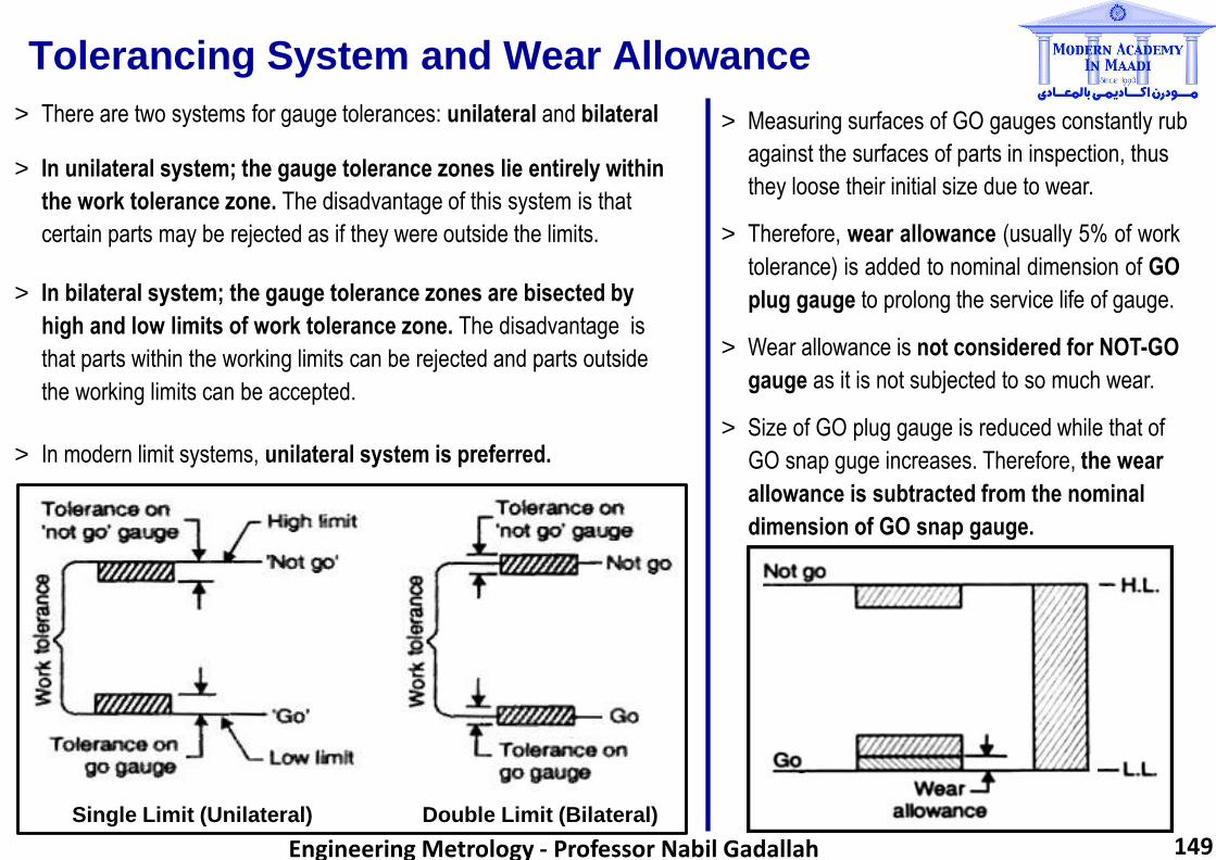
Tolerancing System and Wear Allowance
> There are two systems for gauge tolerances: unilateral and bilateral
> In unilateral system; the gauge tolerance zones lie entirely within
the work tolerance zone. The disadvantage of this system is that
certain parts may be rejected as if they were outside the limits.
> In bilateral system; the gauge tolerance zones are bisected by
high and low limits of work tolerance zone. The disadvantage is
that parts within the working limits can be rejected and parts outside
the working limits can be accepted.
> In modern limit systems, unilateral system is preferred.
Single Limit (Unilateral) Double Limit (Bilateral)
> Measuring surfaces of GO gauges constantly rub
against the surfaces of parts in inspection, thus
they loose their initial size due to wear.
> Therefore, wear allowance (usually 5% of work
tolerance) is added to nominal dimension of GO
plug gauge to prolong the service life of gauge.
> Wear allowance is not considered for NOT-GO
gauge as it is not subjected to so much wear.
> Size of GO plug gauge is reduced while that of
GO snap guge increases. Therefore, the wear
allowance is subtracted from the nominal
dimension of GO snap gauge.
149 Engineering Metrology - Professor Nabil Gadallah
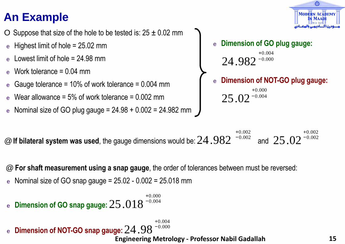
An Example
@ For shaft measurement using a snap gauge, the order of tolerances between must be reversed:
e Nominal size of GO snap gauge = 25.02 - 0.002 = 25.018 mm
+0.000
e Dimension of NOT-GO snap gauge: 24 .98
e Dimension of GO snap gauge: 25 .018
O Suppose that size of the hole to be tested is: 25 ± 0.02 mm
e Highest limit of hole = 25.02 mm
e Lowest limit of hole = 24.98 mm
e Work tolerance = 0.04 mm
e Gauge tolerance = 10% of work tolerance = 0.004 mm
e Wear allowance = 5% of work tolerance = 0.002 mm
e Nominal size of GO plug gauge = 24.98 + 0.002 = 24.982 mm
e Dimension of NOT-GO plug gauge:
+0.000
25 .02 − 0.004
e Dimension of GO plug gauge: +0.004
24 .982 − 0.000
@ If bilateral system was used, the gauge dimensions would be: 24 .982 and 25 .02 +0.002 − 0.002
+0.002 − 0.002
+0.004 − 0.000
− 0.004
150
Engineering Metrology - Professor Nabil Gadallah

Pros and Cons of Limit Gauges
The advantages of limit gauges can be summarised as follows:
☺ Limit gauges are conveniently used in mass production for controlling various dimensions.
☺ They can easily be used by semi-skilled people.
☺ They are economical in their own cost as well as engaging cost.
The followings are the limitations of limit gauges:
® Do not indicate the actual size of the component
® Susceptible for wear, expansion and collapse
® Large number of gauges is required necessitating larger space
® Cannot handle finer quality jobs due to precision issues
® Require frequent checking of gauge dimensions
151 Engineering Metrology - Professor Nabil Gadallah