GÖTEBORGS UNIVERSITET Institutionen för geovetenskaper Avdelningen för Naturgeografi Geovetarcentrum

GROWING SEASON TRENDS IN THE GREATER BALTIC AREA

Hans W. Linderholm Alexander Walther

Deliang Chen

ISSN 1400-383X C69

Rapport Göteborg 2005

Acknowledgement

The work that is presented in this report has been done within the project EMULATE (European and North Atlantic daily to Multidecadal climate variability) supported by the European Commission under the Fifth Framework Programme, contract no: EVK2-CT-2002-00161 EMULATE. Göteborg, 15 December 2005 Hans Linderholm

Contents

Page

Growing season changes in the last century - a review 1

Hans W. Linderholm

A comparison of growing season indices for the Greater Baltic Area 21

Alexander Walther and Hans W. Linderholm

Twentieth-century trends in the thermal growing-season in 56 The Greater Baltic Area Hans W. Linderholm, Alexander Walther, Deliang Chen and Anders Moberg

Growing season changes in the last century - a review

Hans W. Linderholm a, b

a) Regional Climate Group, Earth Sciences Centre, Göteborg University, SE-405 30 Göteborg, Sweden b) Laboratory for Climate Studies, National Climate Center, China Meteorological Administration, 46

Zhongguancun Nandajie, Haidian, Beijing 100081, China

Abstract In recent years, an increasing number of studies have reported shifts in the timing and length of the growing season, based on phenological, satellite and climatological studies. The majority of these investigations indicate a lengthening of the growing season, of c. 10-20 days in the last few decades, where the most prominent change has been an earlier onset of the start of the growing season. In general, the extension of the growing season has been associated with recent global warming (some authors have, however, reported strong relationships with large-scale weather phenomena, e.g. NAO and ENSO), and consequently, we may see further changes in the growing season in the future. Changes in the timing and length of the growing season (GSL) may not only have far reaching consequences for plant and animal ecosystems, e.g. pollen spreading, breeding, frost and insect damage, but persistent increases in GSL may lead to long-term increases in carbon storage and changes in vegetation cover which may affect the climate system. This paper reviews the recent literature concerned with GSL variability.

1

1. Introduction Over the twentieth century, the global average surface temperature has increased by 0.6 ± 0.2°C, where most of the warming occurred between 1976 and 2000, and is projected to increase by 1.4 to 5.8°C over the period 1990 to 2100 (IPCC, 2001). Furthermore, the IPCC (2001) stated that “most of the observed warming over the last 50 years is likely to have been due to the increase in greenhouse gas concentrations”, where CO2 has the strongest radiative forcing. Climate models of a warming world predict that a number of climate, weather and biological phenomena will be affected by the atmosphere’s increasing CO2 concentration. One such phenomenon is the growing-season length (GSL), i.e. the period between bud burst and leaf fall, which is expected to lengthen, especially at higher latitudes (EEA, 2004). The GSL has rendered substantial interest since it exerts a strong control on ecosystem function (White et al., 1999). GSL variations are a useful climatic indicator and have several important climatological applications (Robeson, 2002). A decrease in GSL could result, for example, in alteration of planting dates determining lower yields of traditionally planting crops, which may not fully mature. Increasing GSL, however, may provide opportunities for earlier planting, ensuring maturation and even possibilities for multiple cropping (depending on water availability). Keeling et al. (1996) showed an association between surface air temperatures and variations in the timing and amplitude of the seasonal cycle of atmospheric CO2. This is in agreement with the idea that warmer temperatures promote increases in plant growth in summer and/or respiration in winter. An increase of the annual amplitude of the seasonal CO2 cycle by 40% in the Arctic (20% in Hawaii) since the early 1960s was linked to a lengthening of the growing season by about 7 days. Barford et al. (2001) found that seasonal and annual fluctuations of the uptake of CO2 in a northern hardwood forest were regulated by weather and seasonal climate (e.g. variations in growing-season length). Myneni et al. (1997) showed that the increase in photosynthetic activity of terrestrial vegetation observed from satellite data during the period 1981 – 1991 suggested an increase in plant growth associated with a lengthening of the active growing season. Consequently, persistent increases in GSL may lead to long-term increases in carbon storage (White et al., 1999).

It is becoming evident that studies of the growing season of land vegetation have become an important scientific issue for research into global climate change (Chen et al., 2000). Most recent studies have utilized three main techniques to determine growing season change in the twentieth century; phenology, the normalized difference vegetation index (NDVI) from satellite data, and surface air temperatures. This paper reviews some of the most important findings in recent GSL research, grouping them into three discussion areas. Table 1 summarizes the studies which have quantified changes in growing season parameters. Furthermore, the implications of GSL change are briefly discussed.

2. Phenology

2.1 The importance of phenology in global change studies

Phenology can be defined as: “the study of the timing of recurring biological phases, the causes of their timing with regard to biotic and abiotic forces, and the interrelation among phases of the same or different species” (Global Phenological Monitoring, http://www.dow.wau.nl/msa/gpm/). In temperate zones the reproductive cycles of plants is foremost controlled by temperature and day length (Menzel, 2002), while at lower latitudes rainfall and evapotranspiration must be taken into account (e.g. Spano et al., 1999). The timing of spring events in mid- to high-latitude plants, such as budding, leafing and flowering, is mainly regulated by temperatures after the dormancy is released, and a number of studies have found good correlation between spring phases and air temperatures (Menzel and Fabian, 1999; Wielgolaski, 1999; Abu-Asab et al., 2001; Chmielewski and Rötzer, 2002; Fitter and

2

Fitter, 2002; Sparks and Menzel, 2002; Chmielewski et al., 2004). Thus phenological phases may serve as proxies for spring temperatures. While the climate signal controlling spring phenology is quite well understood, autumn phenology is less clearly explained in terms of climate (Walther et al., 2002), possibly because temporal changes in the autumn seem to be less pronounced and show more heterogeneous patterns (Menzel, 2002). Several studies have linked inter annual variability in phenology to large-scale weather features, such as the North Atlantic Oscillation (NAO) and El Niño – Southern Oscillation (ENSO) (D’Odorico et al., 2002; Stenseth et al., 2002; Menzel, 2003; Menzel et al., 2005). Changes in plant phenology is considered to be a most sensitive and observable indicator of plant responses to climate change. Unfortunately, there are few phenological records that extend beyond the instrumental records, e.g. the Marsham phenological record in the UK, spanning more than two centuries (Sparks and Carey, 1995), and the relationship between phenological records and temperature may be disturbed by other environmental factors (Menzel, 2003). Since non-climatic influences (e.g. land-use change) dominate local, short term biological change, attributing recent biological changes to global warming is complicated (Parmesan and Yohe, 2003). However, there is a great potential for the use of phenological observations to assess ecological responses to climate change, and assembling data into phenological observation programs provides datasets to evaluate spatial and temporal impacts of climate on vegetation and animals (e.g. Chmielewski and Rötzer, 2002; Van Vliet et al., 2003). Furthermore, phenology has shown considerable promise to address questions in global modelling (e.g. downscaling), monitoring and impact assessments of climate change (Schwartz, 1999).

2.2 Observed phenological changes in the twentieth century

The recent focus on phenology is partly due to the large number of studies that have documented long-term changes in phenology, which have been linked to global change. Because of the large quantity of phenological data available, as well as the establishment of data banks, there is a dominance of large-scale European phenological studies. However, due to the increased focus on phenology, more data are being analysed in other parts of the world. The following review of recently reported findings will mainly be focused on terrestrial plant phenology. However, there exist a large number of studies of changes in the phenology of animal species, migration (Bradley et al., 1999; Peñuelas et al., 2002; Cotton, 2003), breeding (Crick et al., 1998; Forchhammer et al., 1998; Crick and Sparks, 1999), all which have indicated recent impacts of global change (see also McCarthy, 2001; Walther et al., 2002).

2.2.1. Local studies

2.2.1.1. Europe

To predict future responses of species to a changed climate, it is necessary to know how plants have responded to climate in the past. Unfortunately, few phenological records are of sufficient length to show responses to natural climate variability. There do, however, exist phenological records that extend beyond the twentieth century. Sparks and Carey (1995) examined the Marsham phenological record (1736 to 1947). This is a record of the first dates of observations, or indications, of spring for 27 phenological events at the Marsham family estates in south eastern England. The 27 phenological events came from taxa common to the British countryside. Clear relationships were found between phenological events and early spring weather. During the analysed period there had been a rise in temperatures, and the species responded to this, some by coming into leaf or flowering earlier, others by later coming into leaf or flowering. They also estimated how a future temperature increase of 3.5ºC in winter and 3ºC outside winter, together with increased precipitation would affect the

3

observed species. The results suggested a dramatic change of species responses, with species appearing 2 to 3 weeks earlier than present. Ahas (1999) studied phenological time series (ranging from 132 to 44 years) from eight common plant, fish, and bird species at three different observation points in Estonia. It was concluded that Estonian springs had advanced 8 days on average over the 80-year study period, and that the last 40-year period has warmed even faster. Furthermore, spring was advancing about two times more rapidly in coastal regions than in inland areas. This difference was associated with the temperature regime and ice cover of the Baltic Sea, where a cold winter with a stable ice cover will cause the following spring will be very late in the coastal region, while at the same time the inland areas warm up faster and spring will arrive much earlier, and vice versa. The resulting larger variations observed in the phenological data for a marine climate changes the hypothesis that the marine influence is a generally stabilizing seasonal factor. Menzel et al. (2001) analysed phenological seasons in Germany of more than four decades (1951-96) and found clear advances in the key indicators of earliest and early spring (-0.18 to -0.23 days/year) and notable advances in the succeeding spring phenophases such as leaf unfolding of deciduous trees (-0.16 to -0.08 days/year). However, phenological changes were less strong during autumn (delayed by + 0.03 to + 0.10 days/year on average). In general, the growing season has been lengthened by up to 0.2 days/year, where the mean 1974-96 growing season was up to 5 days longer than in the 1951-73 period. Fitter and Fitter (2002) noted a major shift in first flowering date (FFD) in British plants from the 1980s after four decades of little variation. On average, FFD of the studied 385 plant species had advanced by 4.5 days; 16% showed an average advancement of 15 days. As the FFD is sensitive to temperature, the change in the 1990s was attributed to climate warming. Examination of a large number of phenological records kept by a farmer in Sussex, UK, from 1980 to 2000, showed that 25 out of 29 events were earlier in 1990-2000 than in 1980-1989 (Sparks et al., 2005). The average advancement of all events was 5.5 days, and more than half of the events were significantly related to temperatures of the three months preceding the mean event date. 2.2.1.2. North America

Over a 61-year period (1936 to 1947 and 1976 to 1998), 55 phenophases were studied in southern Wisconsin (Bradley et al., 1999). Approximately one third of the phenophases appeared to advance in earliness over the period, and the mean trend for all 55 phenophases was -0.12 day/year. As springtime advanced, the number of phenophases increasing in earliness decreased, suggesting that the largest change in phenophases occurs in early spring. In Canada, where warmer winter and spring temperatures have been noted over the last century, first-bloom dates from Edmonton, Alberta, extracted from four historical data sets showed progressively earlier development in spring flowering (Beaubien and Freeland, 2000). The timing of the flowering was largely a response to temperature, with earlier blooms seen in years of higher spring temperatures. Correlations were found between stronger El-Niño events, warmer ocean temperatures and warmer winter-spring temperatures and early flowering. Over the last decades there was an 8-day trend to earlier flowering in central Alberta and the early blooming of Populus tremuloides showed a 26-day change in bloom time over the twentieth century. Abu-Asab et al. (2001) investigated the trend of average “first-flowering times” (which was defined as the stage at which a mono- or diclinous flower begins anthesis or is receptive to pollen) for 100 selected plants from the Washington DC area. They found a significant advance of 2.4 days over a 30-year period and excluding 11 plants which exhibited later first-flowering times, the remaining 89 species showed a significant advance of 4.5 days. The advancement of the first flowering in 89 species was directly correlated to increase in local minimum temperatures. Cayan et al. (2001) described fluctuations in spring climate, in the western USA, since the 1950s by examining changes in

4

the Western Region Phenological Network data of first bloom of lilac and honeysuckle and the timing of snowmelt-runoff pulses. Both records showed year-to-year fluctuations (typically of one to three weeks), which were regionally consistent for most of the west. Analyses indicated that anomalous temperature had the greatest influence upon both inter-annual and secular changes in the onset of spring in these networks. The records showed earlier spring onsets since the late 1970s, where bloom-dates (and spring pulses) occurred 5-10 days earlier than in the previous part of the record, reflecting the unusual spell of warmer-than-normal springs in western North America during this period. The warm episodes were clearly related to larger-scale atmospheric conditions across North America and the North Pacific, but whether this is predominantly an expression of natural variability or also a symptom of global warming is not certain. Wolfe et al. (2005) evaluated the first leaf date (FLD) and FFD of woody plants (lilac, apple and grape) for the period 1965 to 2001 in the north eastern parts of USA. They concluded that the general warming trend of the past several decades in north eastern USA had resulted in an advance in spring phenology ranging from 2 to 8 days for the studied species. Table 1. Observed changes in growing season parameters as seen in phenological records (P), normalized difference vegetation index (NDVI) from satellites, and climatological records (C).

Change (days) Type Time span Geographic range start end length

Reference

P 1980-2000 UK -5.5 Sparks et al., 2005 P 1991-2000 UK -4.5 Fitter & Fitter, 2002 P 1951-1996 Germany 9.2 Menzel et al., 2001 P 1961-2000 Germany -9.2 Chmielewski et al., 2004 P 1952-2000 Spain -16 13 29 Peñuelas et al., 2002 P 1930-1998 NW Russia -15 – -20 Kozlov & Berlina, 2002 P 1951-1996 Europe -6.3 4.5 10.8 Menzel & Fabian, 1999 P P

1951-1998 1951-1998

C & W Europe E Europe

-28 +7 – +14

Ahas et al., 2002 Ahas et al., 2002

P 1969-1998 Europe -8 Chmielewski & Rötzer, 2002 P 1936-1996† Canada -8 Beaubien & Freeland, 2000 P 1936- 1998‡ NE USA -7 Bradley et al., 1999 P 1970-1999 E USA -2.4 Abu-Asab et al., 2001 P 1965-2001 NE USA -2 – -8 Wolfe et al., 2005 P 1922-2004 Korea -13 Ho et al., 2005 NDVI 1982-1993 China ~ 17 Chen et al., 2005 NDVI 1982-2000 Europe -10.8 19.2 Stöckli & Vidale, 2004 NDVI NDVI

1981-1999 1981-1999

Eurasia North America

-7 -8

18 12

Zhou et al., 2001 Zhou et al., 2001

NDVI NDVI

1982-1991 1992-1999

45°N - 75°N 45°N - 75°N

-6 -2

4 0.4

Tucker et al., 2001 Tucker et al., 2001

NDVI 1981-1991 Global -8 ~ 12 Myneni et al., 1997 C 1890-1995 Fennoscandia -4 – -12 1 – 9 7 – 21 Carter, 1998 C 1951-2000 Greater Baltic Area†† -6.3 1.3 7.4 Linderholm et al., 2005 C 1950-2000 Germany -6.5 – -12 12.5 5.5 – 24.5 Menzel et al. 2003 C 1961-1990 Austria 11 Hasenauer et al., 1999 C 1899-1982 NC USA ~ 14* Skaggs & Baker, 1985 C 1906-1997 EC USA ~ 7 Robeson, 2002 C 1959-1993 China -6 4 10 Schwartz & Chen, 2002. C 1964-1992 NH ~ 7 Keeling et al., 1996 †: 1936-1961, 1973-1982 and 1987-1996 ‡: 1936-1947 and 1976-1998 ††: Average for 36 stations *: Average for three out of five stations used

5

2.2.1.3. Asia

Zheng et al. (2002) analyzed the change of plant phenophase in spring and the impact of climate warming on the plant phenophase in China for the last 40 years, using plant phenology data from 26 stations in the Chinese Phenology Observation Network. They showed that the response of phenophase advance (or delay) to temperature change was nonlinear. The rate of phenophase advance days decreases with temperature increase amplitude, and the rate of phenophase delay days increases with temperature decrease amplitude. Since the 1980s, phenophases had advanced in north and north eastern China, and the lower reaches of the Chang Jiang (Yangtze) River, and delayed in the eastern part of south western China and the middle reaches of the Chang Jiang River. Also, the rate of phenophase difference decreased with latitude. Using a simple phenological model driven by surface-level minimum-maximum temperatures, Schwartz and Chen (2002) found that the onset of spring growth in China had no apparent change over 1959 to 1993, which is in contrast to findings in North America and Europe. However, during that time last spring frost dates had become earlier (6 days), especially in the north eastern part of the country, and first frost dates had become later (4 days, especially in north-central China), resulting in an increase in the frost free period of 10 days, mainly over the northern part of the country. In Seoul, Korea, Ho et al. (2005) studied long-term (1922-2004) changes in the first bloom of five tree species. All species showed an advance in spring bloom (-1.4 to -2.4 days/decade for early spring flowering trees, and -0.5 days/decade for late-spring trees), associated with a 2°C warming over the 83 years.

2.2.1.4. High latitude and altitude studies

A number of phenological variables in the northern Russian taiga were examined by Kozlov and Berlina (2002), to look for possible changes in the length of the growing season for the period 1930 to 1998. They found that snow-melt in spring occurred 16 days later and that the dates of permanent snow cover in the forests began 13 days earlier at the end of the study period than at its beginning. Furthermore, the duration of the snow- and ice-free periods in the forests decreased by 15-20 days over the 68-year period. It was concluded that the length of the growing season on the Kola Peninsula declined during the past 60 years, due to delayed spring and advanced autumn/winter. Similar findings were observed in the Colorado Rocky Mountains, USA, where Inouye et al. (2000) found no significant change in the beginning of the growing season over the 1975 to 1999 period. Here the beginning of the growing season is controlled by melting of the previous winters snowpack, and despite a trend for warmer spring temperatures, the dates for snowmelt had not changed, possibly due to an increase in winter precipitation. However, migrants and hibernators seemed to respond to increasing temperatures by arriving (American robins) and emerging (yellow-bellied marmots) earlier (14 and 38 days respectively). The combination of changes in winter snowpack (starting earlier and lasting longer) and increased air temperatures at high altitudes could disrupt historical patterns for hibernating and migrating species.

2.2.2. Regional and global studies

Menzel and Fabian (1999) and Menzel (2000) analysed observational data from the International Phenological Gardens (IPG). The IPG is a Europe-wide network with a large spatial coverage (42°N-69°N, 10°W-27°E) which holds genetical clones from trees and shrubs, and dates for phases, such as leaf unfolding, flowering and leaf fall, have been collected since 1959. Analyses revealed that in the last four decades (1959-1996) spring events had advanced on average 6.3 days and autumn events had been delayed on average by

6

4.5 days, resulting in an average lengthening of the growing season by 10.8 days. The extension of the growing season was related to contemporary temperature increase. Chmielewski and Rötzer (2002) also utilised data from the IPG to investigate the beginning of the growing season (BGS) across Europe for the period 1969-1998. Using canonical correlation analysis, they established a relationship between air temperatures in February to April and BGS, where above (below) normal temperatures in whole Europe and advanced (delayed) BGS were related. In the last decade of their study period, early spring temperatures increased by approximately 0.8°C, resulting in an advance in BGS of 8 days. Ahas et al. (2002) analysed data from the European phyto-phenological database (composed from different national databases of Eastern and Western Europe) for the time-period 1951-1998. Results suggested that the spring phase had advanced by four weeks in Western and Central Europe, because of intensified flow of warm Atlantic air masses in connection with a strong NAO. The advance in Eastern Europe was slighter, up to two weeks. There were some exceptions, with trends for delayed spring phase starts, in Eastern Europe which were related to the Siberian high-pressure system. Root et al. (2003) calculated linear trends and analysed the regression slopes for a number of studies on spring phenology in the last 50 years. The analysis was based on 61 studies reporting results on 694 plant and animal species. A set of criteria was used to include the studies; the time series should have a length of at least 10 yr, a change for at least one trait analysed should be found and, either a temporal trend in temperature or a strong association between the trait and site temperature should be found. The estimated mean number of days of advancement in the phenological phases per decade was 5.1 with a standard error (SE) equal to ± 0.1. Because the warming trend is higher in higher latitudes, separate analyses were performed for the latitudinal belts 32–49.9° and 50–72° N that resulted in trends per decade of 4.2 (± 0.2 SE) and 5.5 (±0.1 SE), respectively. Parmesan and Yohe (2003) quantitatively assessed 667 phenological shifts in species reported in the literature. Over a time-period range of 16 – 132 years, 62% showed trends towards spring advancement, while 9% showed trends toward delayed spring events. They performed a meta-analysis of trends in phenology for 172 species, for which time series of at least 17 years and observations over large geographical regions were available. Meta-analysis resulted in a mean advancement of spring phases by 2.3 days per decade (95% confidence interval, 1.7-3.2). As Badeck et al. (2004) noted, the differences in trend estimates provided by the two above studies could be related to differences in the relative number of observations in higher and lower latitudes, different taxa or groups of phases (flowering vs. leafing; early vs. late) and/or to the length of the time series analysed. 2.3. Phenological changes and large-scale weather phenomena

In the northern Atlantic region, a significant proportion of inter-annual climate variability is attributed to the dynamics of the North Atlantic Oscillation (NAO), which is a measure of the pressure difference between the Azores and Iceland and hence affects westerly winds blowing across the North Atlantic. Seasons of high positive NAO are associated with warming and increased rainfall over Northwest Europe (Hurrell, 1995). This relationship is most pronounced in winter and early spring and substantially weaker in summer (Rogers, 1990). Since the late 1960’s there has been a strengthening of the wintertime NAO, with unprecedented strongly positive NAO index values since the 1970’s (Hurrell, 1995). As the strengthening of the NAO coincides with late-twentieth century global warming, the influence of large-scale atmospheric circulation on a variety of ecosystems has gained increased attention in the North Atlantic region (e.g. Post and Stenseth, 1999; Weyhenmeyer et al., 1999; Mysterud et al., 2000; Linderholm, 2002; Solberg et al., 2002; Stenseth et al., 2002).

7

Chmielewski and Rötzer (2001) used leafing dates of trees from the International Phenological Gardens for the period 1969–1998, to define the beginning and the end of the growing season. A nearly Europe-wide warming in the early spring (February–April) over the last 30 years (1969–1998) led to an earlier beginning of growing season by 8 days. The observed trends in the onset of spring corresponded well with changes in air temperature and circulation (NAO-index) across Europe. In late winter and early spring, the positive phase of NAO increased clearly, leading to prevailing westerly winds and thus to higher temperatures in the period February–April. Since the end of the 1980s the changes in circulation, air temperature and the beginning of spring time were striking. The investigation showed that a warming in the early spring (February–April) by 1°C causes an advance in the beginning of growing season of 7 days. The observed extension of growing season was mainly the result of an earlier onset of spring. D'Odorico et al. (2002) also examined the link between earlier onsets of the growing season in Europe and warmer winters associated with phase changes in the NAO. They found that spring phenology in Europe was significantly affected by the NAO, where high-NAO winters (warm) speeded up the occurrence of spring phenophases (budburst and bloom). Furthermore, the NAO could provide a partial explanation for both high- and low-frequency variability of plant phenology of the British Isles. Scheifinger et al. (2002) noted a relationship between inter-annual variability in NAO and the temporal variability in central European phenological events in 1951 to 1998. The trend in phenological time series from the late 1980s could largely be explained by the NAO. They showed that the influence of the NAO was strongest on early phases and decreased later in spring. The influence of the NAO was reduced with increasing distance from the Atlantic coast and also in mountainous terrain. Menzel (2003) investigated seasonal phases from the phenological network of the German Weather Service in relation to climate and NAO in 1951 to 2000. Using regression between phenological anomalies and NAO, she found a quite strong relationship between February-March NAO and spring phenological anomalies (R2 ranging from 0.37 to 0.56), with early spring phases being more sensitive to NAO, and that January-February NAO explained c. 40% of the variance in the length of the growing season. Similar results were obtained by Ahas et al. (2004) for Europe (data from the European plant phenology database). They studied relationships between start dates of spring phenological phases, for three species, and large scale circulation patterns in form of NAO and the Arctic oscillation, AO, defined as a nearly axisymetric spatial pattern of inter-annual variability of Northern Hemisphere winter sea level pressure centred over the Arctic (Thompson and Wallace, 1998). In the period 1951-1998, the highest correlations between spring phenophases and NAO/AO were found during winter (December –March) and the three first months of the year (January – March) over Europe, where correlations were particularly strong in the Baltic Sea region. In the eastern part of the studied area (near Ural Mountains) correlations were opposite of the rest of the study area. Also in North America links between large-scale atmospheric conditions and changes in spring phenology have been suggested. Correlations of the spring flowering index with the incidence of El Niño events was found in western Canada (Beaubien and Freeland, 2000). Earlier onsets of spring since the late 1970s in western USA were related to shifts in the Pacific Decadal Oscillation (PDO, defined as the leading principal component of North Pacific monthly sea surface temperature variability; Mantua et al., 1997) in the study by Cayan et al. (2001).

3. Remote sensing Land cover mapping produces archives that are used to parameterize global climate models, and since the progressive change of land cover over periods of decades is of interest, high-

8

resolution remotely sensed data is needed (e.g. Wang and Tenhunen, 2004). In recent years, determining the growing season of large-scale land vegetation has become an important question in global climate change research. Because of the synoptic coverage and repeated temporal sampling satellites offer, remotely sensed data have a great potential for monitoring vegetation dynamics at regional to global scales (Myneni et al., 1997; Zhang et al., 2003). One of the most striking events in spring is the first appearance of foliage, generally called the “green wave” (e.g. Schwartz, 1998). This is a prominent event and can be well captured in satellite images which then can be used to calibrate remote sensing data. To quantify the spatial and temporal variation in vegetation growth and activity, vegetation indices can be calculated from satellite images. One such vegetation index is the normalized difference vegetation index (NDVI), which will be described in the following part.

3.1 NDVI

NDVI data captures the contrast between red and near-infrared reflectance of vegetation, which indicates the abundance and energy absorption by leaf pigments such as chlorophyll (Zhou et al., 2001). NDVI is a general biophysical parameter and it provides an indication of the “greenness” of the vegetation, but not land-cover type directly. A time series of NDVI values can, however, separate different land-cover types based on their phenology or seasonal signals (Wang and Tenhunen, 2004). Because the NDVI is well correlated to the fraction of photosynthetically active radiation absorbed by plant canopies (and thus leaf area, leaf biomass and potential photosynthesis), it can be used as a proxy for the vegetation’s responses to climate changes (Myneni et al., 1995). When investigating changes and variability in global vegetation activity, it is assumed that changes in NDVI yield information about the response of vegetation to climate. However, many factors unrelated to ecosystem variability, associated with the obtaining of remotely sensed data (e.g. satellite drift, calibration uncertainties, inter-satellite sensor differences, bidirectional and atmospheric effects and volcanic eruptions), may cause unrelated variability in NDVI which may be interpreted a s real changes in NDVI (Zhou et al., 2001 and references therein). Much effort is thus placed on developing (and testing) corrections to provide consistent and calibrated time series for NDVI from satellite data. Previously, NDVI data was obtained from AVHRR (Advanced Very High-Resolution Radiometer) instruments carried by meteorological satellites in the NOAA/NASA Earth Observing System or the Global Inventory Monitoring and Modelling Studies (GIMMS). Recently, a new sensor system called MODIS (Moderate Resolution Imaging Spectroradiometer) has been developed, which offers improved calibration and atmospheric corrections, as well as higher spatial resolution, compared to AVHRR (Zhang et al., 2003; Beck et al., 2005). Usually, NDVI are of global extent, and the data has a spatial resolution of 1.1-8 km and a 10-15 day temporal frequency, while MODIS NDVI exist at spatial resolutions as high as 250 and 500 m for the entire globe (Beck et al., 2005).

3.2 Growing season change from satellite data

Myneni et al. (1997) explored two NDVI data sets (from NOAA and GIMMS) form July 1981 to end of June 1991 to evaluate the photosynthetic activity of terrestrial vegetation. This paper reported an increase in the photosynthetic activity for the period, and it was associated with a lengthening of the active growing season (AGS, the period when photosynthesis actually occurs). They estimated an advance in the AGS of c. 8 days and a prolongation of the declining phase of the AGS by c. 4 days, resulting in a total lengthening of the AGS by 12 days. Furthermore, the increase was greatest between 45ºN and 70ºN, an area where marked warming in spring have occurred due to earlier snowmelt. This result, together with that of

9

Keeling et al. (1996, see above), indicates increased biospheric activity at high northern latitudes.

Zhou et al. (2001) extended the analysis period of NDVI data presented by Myneni et al. (1997) to December 1999. They found that c. 61% of the total vegetated area between 40ºN and 70ºN in Eurasia showed a persistent increase in growing season NDVI from central Europe through Siberia to the Aldan plateau, an area which mainly consists of forests and woodland. The pattern was not that consistent in North America. Also, the growing season had increased by 18 days in Eurasia and 12 days in North America, caused by earlier spring and later autumn. NDVI decreases observed in northern North America and north eastern Asia were interpreted as responses to temperature induced drought. Additional analyses of higher northern latitude NDVI by Tucker et al. (2001) for the period 1982 to 1999 yielded similar results as previous studies: an earlier start and increased length of the growing season which was a response to warmer temperatures. Furthermore, they noted that there was a delay in the start of the growing season in 1992, caused by the temporary global cooling resulting from the Mt Pinatubo volcanic eruption in 1991. Furthermore, their analyses suggested greater gross photosynthesis in Eurasia than North America for the later 1990s than the 1980s.

Stöckli and Vidale (2004) used the NOAA/NASA Pathfinder NDVI data to create a continuous European vegetation phenology dataset (10-day temporal and 0.1° spatial resolution) for the years 1982–2001. They found strong seasonal and inter-annual variability in European land surface vegetation state. Phenological metrics indicated a late and short growing season for the years 1985–1987, in addition to early and prolonged activity in the years 1989, 1990, 1994 and 1995. Spring phenology was also shown to correlate particularly well with anomalies in winter temperature and winter North Atlantic Oscillation (NAO) index. Trends in the phenological phases revealed a general shift to earlier (-0.54 days/year) and prolonged (0.96 days/year) growing periods (statistically significant), especially for central Europe. Hogda et al. (2001) made a regional study of growing season changes in Fennoscandia, Denmark and the Kola Peninsula using the GIMMS NDVI dataset. During the period 1981 to 1998, they found a delay of spring in the alpine belts and the northern boreal zone, where the strongest delay occurred on the most continental parts of the northern boreal zone. In southern Fennoscandia and western Norway spring started earlier. Furthermore, autumn was delayed in the whole area, except for the most continental part of northern Scandinavia. Thus, the GSL was prolonged for the whole area, except for the northern continental section. Beck et al. (2005) use MODIS NDVI data to map the onset of the spring 2000-2004 in Fennoscandia. During this short analysis period, they found large temporal and spatial difference within the area in the arrival of spring, varying by more than two months within the study area and more than a month between the years. Latitude, elevation gradients and distance from the seas appeared to be the determining factors.

Combining phenological and NDVI (from NOAA/NASA Pathfinder) data from 1982 to 1993 at seven sample stations in temperate eastern China, Chen et al. (2005) determined the growing season beginning and end dates at seven phenological sample stations for each year, and then made a spatial extrapolation of growing season parameters to all possible meteorological stations in the study area. The spatial patterns of growing season beginning and end dates correlated significantly with spatial patterns of mean air temperatures in spring and autumn, respectively. Unlike some results from similar studies in Europe and North America, their results suggested a significant delay in leaf coloration dates, along with a less pronounced advance of leaf unfolding dates from 1982 to 1993. The growing season in China had been extended by 1.4–3.6 days/year in the northern parts, 1.4 days/year averaged across the entire study area. The apparent delay in growing season end dates was associated with regional cooling from late spring to summer, while the insignificant advancement in

10

beginning dates corresponded to inconsistent temperature trend changes from late winter to spring.

Kaufmann et al. (2004) attempted to answer the question of what the physiological significance of the findings by Myneni et al. (1997) and Zhou et al. (2001) was. They investigated the physiological effects of the elongation of the growing season and the increase in summer greenness on northern hemisphere forests by examining the relationship between NDVI and tree rings. They used NDVI time series and tree-ring data from 48 mid- to high-latitude sites in North America and Eurasia. They found correlations between NDVI and tree rings in June and July, but not for months at the start or the end of the growing season. This may imply that advances in spring and delays in autumn of the growing season are less important to the physiological status of trees. Thus, although changes in spring time may be easier to detect, summer-time changes may have bigger effects on the terrestrial carbon cycle.

4. The climatological growing season

4.1. Defining the climatological growing season

The climatological growing “season” can be viewed as the entire period in which growth can theoretically take place, and should be distinguished from the growing “period” which is the period of actual growth (Carter, 1998). There are a number of ways to define GSL. One definition of GSL is the period between the date of the last spring freeze and first autumn freeze (e.g. Robeson, 2002), where the frost may be determined by thresholds of daily minimum temperatures. Other investigations have used threshold temperatures in a predefined number of days to start and end the growing season, e.g. GSL can be defined as the period between when daily temperatures are >5°C for >5 days and when daily temperatures are <5°C for >5 days (Frich et al., 2002). The physiological significance of this period naturally differs among plant types, but at high latitudes it can be assumed to be relevant to perennial plants that are exposed to the weather throughout the year, e.g. trees and shrubs (Carter, 1998). In the literature, there exists a wide variety of growing season definitions, but only few comparisons have been made between different definitions on a single data set. Brinkmann (1979) compared differently defined growing seasons at four stations in Wisconsin, USA, over an 80-year period, using freeze criteria as well as temperatures averaged over a number of days as definitions of the growing season. The results showed that depending on definition, a variety of trends were obtained for one single station, meaning that the trend in the GSL is sensitive to the particular definition used. Walther and Linderholm (2006) examined a number of definitions of growing season parameters (start, end and length) from a large station network in the Greater Baltic Area, and they also found large differences in GSL trends depending on the definition used. The exclusion of a frost criterion in the definition could lead to erroneous GSL, especially in the south western parts of the studied area. Consequently, it seems that, in order to be physiologically appropriate, regional GSL definitions should be used, so that finding one world-wide definition is quite unlikely. Furthermore, definitions of the GSL using temperatures may be considered valid in areas where the growing season is largely temperature-limited, but at lower latitudes other factors such as precipitation and evapotranspiration must be taken into consideration.

4.2. The growing season in relation to seasonal temperatures

Vedin (1990) compared the GSL in northernmost Sweden for two ten-year periods, where 1931-1940 was extraordinary warm and 1979-1988 was much colder. To his surprise, he found that the average GSL had been somewhat longer during the period 1979-1988 than during the warmer period 1931-1940. He reasoned that this was warmer springs and autumn

11

in the latter period, but stated that a generally warm period may still be unfavourable with respect to the GSL. Jones and Briffa (1995) analysed daily mean temperatures during the growing season (here defined as days >5°C) from c. 200 stations in the former Soviet Union. They found that little change in a number of growing-season related variables had occurred in the last 110 years. Among other findings, they noted that there was little correlation between the duration of the growing season and the number of degree-days (above 5°C) in the season at station level. Consequently, a longer growing season does not automatically imply an increased number of warmer days. In a later study Jones et al. (2002) examined extreme temperatures, GSL and degree days for four meteorological records which extend back into the eighteenth century (Central England, Stockholm, Uppsala and St. Petersburg). They found that in northern Europe (Fennoscandia) growing seasons were clearly warmer before 1860, with only the late 1930s of recent times reaching the earlier levels. Similarly to the Russian study, they found that the duration of the growing season was only weakly correlated (r ~ 0.2-0.4) with seasonal temperatures (May through September) or number of degree days, and therefore a warmer growing season need not necessarily be longer. In addition, the GSL was better correlated to annual temperatures than seasonal in all station records, and there was a strong (negative) relationship between GSL and number of cold days in a year. 4.3. Observed changes in the thermal GSL

4.3.1. Europe

Carter (1998) analysed parameters (start, end, duration and intensity) of the thermal growing season for the period 1890 to 1995 at nine sites in the Nordic region. He found that the GSL had increased considerably in the past century, between 1 to 3 weeks, but that the lengthening had been less pronounced since the 1960 in most parts. The absolute magnitude of lengthening showed a declining west-east gradient between Denmark and Finland, and higher inter-annual variability at the western sites. Furthermore, the intensity (expressed by accumulated temperatures, the effective temperature sum above 5ºC) increased regionally between 1890 and 1960, but decreased slightly after 1960 at all sites except in south western Finland. Linderholm et al. (2006) investigated twentieth-century thermal growing season trends in the Greater Baltic Area. Yearly dates for the start, end and length of the growing season were computed for 49 stations in the studied area, using daily mean temperature measurements. Analyses of trends and tendencies of the growing season components showed a general increase in the length of the growing season in the whole region. Averaged over the 1951-2000 period, the growing season had increased by 7.4 days, where the largest change had occurred during spring (6.3 days earlier growing season start). The largest increases were found at stations adjacent to the Baltic Sea and Skagerrak/Kattegatt, where the Danish stations showed an increase in GSL of more than 20 days in the twentieth century. Furthermore, three long records (starting before 1850) from the region were examined, showing high inter-annual and decadal variability, far more prominent that the increasing trends. There were, however, tendencies for increased frequencies of longer growing seasons since the 1950s. Menzel et al. (2003) analysed the climatological growing season in Germany using data from 41 stations (1951-2000). The growing season was defined by single-value thresholds of daily minimum and mean air temperatures, and during this 50-year period they found a lengthening of the growing season of 0.11 to 0.49 days/year depending on the definition used. The greatest change was found in the frost-free period, due to observed stronger increase in daily minimum rather than maximum temperatures. Similar results of increased frost-free period were found in Austria, Switzerland (both 0.5 days/year) and Estonia (0.36 days/year). Furthermore, they noted that the trend was weakening at high-elevation stations (>950 m a.s.l.).

12

4.3.2. North America

In the 1980s, Skaggs and Baker (1985) studied fluctuations in GSL between 1899 and 1982 in Minnesota, USA. Temperature data from five rural stations were used. They found a general increase in GSL, where three stations showed increases of an average 14 days from 1899 to 1982. The increase in GSL came from combinations of earlier last freezes and later first freezes. At one station, however, the tendency was opposite, with a decrease in GSL. The patterns of inter-annual variation in GSL duration was substantial among the stations, and it was concluded that care should be taken when extrapolating results of GSL studies in space and relating them to mean temperature fluctuations. Bootsma (1994) examined long term (c. 100 year) trend for a wide range of agro-climatic variables from five stations across Canada, to determine if significant changes had occurred in climatic parameters that are important to agriculture. He found evidence for warming during the growing season for stations in western, but not in eastern, Canada. Warming of the growing season was accompanied by earlier dates of last spring frost, later dates of first autumn frost and longer frost free periods. Only data from the westernmost station (Agassiz) showed a significant positive trend in GSL: at the other stations GSL fluctuated around the long term normal, although there were tendencies for increased number of above normal values in the last 60-20 years. There was no trend in GSL at the easternmost station (Charlottetown). In the state of Illinois, USA, Robeson (2002) examined temperature data from the Daily Historical Climate Network for trends towards earlier spring freezes in the period 1906 to 1997. Most of the 36 stations showed trends towards earlier spring freezes, however, there was no consistent trend in the network. The time series showed large inter-annual variability, but the results suggested that the GSL became c. one week longer during the twentieth century. 4.3.3. Global

Utilizing a new global dataset (daily, homogenised meteorological records from the Australian Climate Centre and National Climate Data Center), Frich et al. (2002) observed changes in climatic extremes in the second half of the twentieth century. One of the observed parameters was GSL, and they found a significant lengthening of the thermal GSL throughout major parts of the Northern Hemisphere mid-latitudes, accompanying a systematic increase in the 90th percentile of daily minimum temperatures and a reduction in frost days. However, exceptions were found all over the Northern Hemisphere, most notably on Iceland (see Fig. 3 in Frich et al., 2002).

5. Limitations and possibilities It is evident that the methods of calculating GSL changes presented here all have their inherited limitations and possibilities. Phenological records have the benefit of providing information of biological phases with high temporal resolution. Presently, however, the phenological records are limited in their spatial distribution and do not extend far back in time. This makes it difficult to assess twentieth century changes in a longer time perspective. The recent focus on developing international observation networks is therefore encouraging. Satellite data have the advantage of high spatial coverage, allowing for studies of regional and global studies. Still, there are some problems associated with this method, e.g. the temporal resolution, problems with reflectance and calibration, and the short records that are available. Also, there is a problem how to relate the species-averaged information from satellite observations (over large and potentially diverse spatial areas) to species-level phenological events (Schwartz, 1999). Using the climatological growing season has the advantage of good spatial coverage (at least in parts of the world) of meteorological stations. Furthermore, numerous records cover the twentieth century, or beyond, making it possible to study long-

13

term changes in GSL variability. Nevertheless, there is no universal definition of the climatological growing season, mainly because large regional (and local) differences in climates (Walther and Linderholm, 2006). Also, the climatological growing season is broadly defined, and may not truly represent the actual biological growing season, especially if only temperatures are used.

6. Implications of GSL change Climate change is projected to increase the length of the growing season (e.g. IPCC, 2001; ACIA, 2004). Such an increase in GSL, together with a warmer growing season, is expected to advance the potential for crop production at high northern latitudes and increase the potential number of harvests and hence seasonal yields for perennial forage crops (ACIA, 2004). However, in warmer areas, increased warmth during the growing season may cause slight decreases in yields since higher temperatures speed development, reducing time to accumulate dry mater (ACIA, 2004). Effects in Fennoscandia could be elevated tree line and favourable conditions for growing of more southerly fruits (Wielgolaski, 2003), and in alpine areas with maximum precipitation during the growing season, lengthening of the growing season as a result of warmer temperatures could lead to improved forest productivity (Hasenauer et al., 1999). However, two recent studies have shown that recent warming has resulted in negative growth responses of trees at tree line sites in Alaska and the central Scandinavian Mountains (Linderholm and Linderholm, 2004; Wilmking et al., 2004). Consequently, a rapid climate change, occurring within the next hundred years, would have a large impact on already living trees which would be less adaptive to the prevailing climate. Also, if tree species respond differently to climate change, then the competitive relationships between species will alter and hence, in the long run, the species composition of forests and possibly the geographical ranges of species (Kramer et al., 2000). The accelerated rates of change observed in the past three decades indicate that in a near future we will see large changes in ecosystems; latitudinal/altitudinal extension of species’ range boundaries by establishment of new local populations and, consequently, extinction of low latitude/altitude populations; increasing invasion of opportunistic, weedy and/or highly mobile species; progressive decoupling of species interaction (e.g. plants and pollinators) because of out–of–phase phenology (e.g. Hughes, 2000; Peñuelas and Filella, 2001). However, ecosystems are dynamic systems that vary over time, even in the absence of human disturbance, and changes in geographic range, breeding and population size will occur even in the absence of climate change (McCarthy, 2001). Thus, in order to address important questions in global modelling, ecosystem monitoring and global change, increased knowledge of atmosphere-biosphere interactions, both spatially and temporally, is needed.

7. Concluding remarks The research that has been reviewed here shows that the growing season has high inter-annual variability and that the most pronounced changes in growing-season parameters has occurred in the last 30 years of the twentieth century. The majority of phenological studies suggest that significantly advancing spring, as a consequence of warmer winters and springs and earlier last frosts, has been responsible for the most of the reported changes in the growing season. Phenological observations, NDVI from satellites and climatological data suggest links between recently observed changes in natural systems and twentieth century climate change. However, several authors have found strong associations between large-scale weather phenomena (e.g. the NAO) and growing season variability, suggesting that global warming may not be the only explanation. Also, other factors like land use change may have been of importance. It must be kept in mind that the observed changes in GSL are not uniform; while

14

increased GSL has been observed in low-to- mid latitudes; the GSL seems to decrease at some high latitude and altitude sites. Numerous studies reveal that an already significant impact on natural systems is associated with twentieth century warming. Increased temperatures of 1.4 to 5.8°C (globally) in the next century will most certainly have large consequences, where some species will benefit from warmer and longer growing season, while others will disappear.

Acknowledgements This work was supported by the Swedish Research Council (VR), and the EU-project EMULATE (European and North Atlantic daily to Multidecadal climate variability) supported by the European Commission under the Fifth Framework Programme, contract no: EVK2-CT-2002-00161 EMULATE. The author acknowledges the useful comments provided by two anonymous reviewers and the editor Dr John Stewart.

References Abu-Asab, M.S., Peterson, P.M., Shelter, S.G. and Orli, S.S. 2001: Earlier plant flowering in

spring as a response to global warming in the Washington, DC, area. Biodiversity and Conservation, 10: 597–612.

ACIA, Impacts of a warming Arctic: Arctic Climate Impact Assessment. Cambridge University Press, 2004. 140 pp.

Ahas, R. 1999: Long-term phyto-, ornitho- and ichthyophenological time-series analyses in Estonia. International Journal of Biometeorology, 42: 119-123.

Ahas, R., Aasa, A., Menzel, A., Fedotova, V.G. and Scheifinger, H. 2002: Changes in European spring phenology. International Journal of Climatology, 22, 1727-1738.

Ahas, A., Jaagus, J., Ahas, R. and Sepp, M. 2004: The influence of atmospheric circulation on plant phenological phases in central and eastern Europe. International Journal of Climatology, 24: 1551-1564.

Badeck, F-W., Bondeau, A., Böttcher, K., Doktor, D., Lucht, W., Schaber, J. and Sitch, S. 2004: Responses of spring phenology to climate change. New Phytologist, 162: 295-309.

Barford, C.C., Wofsy, S.C., Goulden, M.L., Munger, J.W., Pyle, E.H., Ubranski, S.P., Hutyra, L. Saleska, S.R., Fitzjarrald, D. and Moore, K. 2001: Factors controlling long- and short-term sequestration of atmospheric CO2 in a mid-latitude forest. Science, 294: 1688-1691.

Beck, P.S.A., Karlsen, S.R., Skidmore, A., Nielsen, L. and Høgda, K.A. 2005: The onset of the growing season in northwestern Europe, mapped using MODIS NDVI and calibrated using phenological ground observations. 31st International Symposium on remote Sensing on Environment – Global Monitoring for Sustainability and Security, 20-24 June, St Petersburg. (www.isprs.org/publications/related/ISRSE/html/welcome.html)

Beaubien, E.G. and Freeland, H.J. 2000: Spring phenology trends in Alberta, Canada: links to ocean temperature. International Journal of Biometeorology, 44: 53-59.

Bootsma, A. 1994: Long term (100 yr) climate trends for agriculture at selected locations in Canada. Climatic Change, 26: 65-88.

15

Bradley, N.L., Leopold, A.C., Ross, J. and Huffaker, W. 1999: Phenological changes reflect climate change in Wisconsin. Proceedings of the National Academy of Sciences USA, 96: 9701-9704.

Brinkmann, W.A.R. 1979: Growing season length as an indicator of climatic variations? Climatic Change, 2: 127-138.

Carter, T.R. 1998: Changes in the thermal growing season in Nordic countries during the past century and prospects for the future. Agricultural and Food Science in Finland, 7: 161-179.

Cayan, D.R., Kammerdiener, S.A., Dettinger, M.D., Caprio, J.M. and Peterson, D.H. 2001: Changes in the onset of spring in the western United States, Bulletin of the American Meteorological Society, 82: 399–415.

Chen, X., Tan, Z., Schwartz, M.D. and Xu, C. 2000: Determining the growing season of land vegetation on the basis of plant phenology and satellite data in Northern China. International Journal of Biometeorology, 44: 97-101.

Chen, X., Hu, B. and Yu, R. 2005: Spatial and temporal variation of phenological growing season and climate change impacts in temperate eastern China. Global Change Biology, 11: 1118-1130.

Chmielewski, F-M. and Rötzer, T. 2001: response to phenology to climate change across Europe. Agricultural and Forest Meteorology, 108: 101-112.

Chmielewski, F-M. and Rötzer, T. 2002: Annual and spatial variability of the beginning of growing season in Europe in relation to air temperature changes. Climate Research, 19: 257-264.

Chmielewski, F-M., Müller, A. and Bruns, E. 2004: Climate changes and trends in phenology of fruit trees and field crops in Germany, 1961-2000. Agricultural and Forest Meteorology, 121: 69-78.

Cotton, P.A. 2003: Avian migration phenology and global climate change. Proceedings of the National Academy of Sciences USA, 100: 12219-12222.

Crick, H. Q. P., Dudley, C., Glue, D.E. and Thomson, D.L. 1998: UK birds are laying eggs earlier. Nature, 388: 526.

Crick, H.Q.P. and Sparks, T.H. 1999: Climate change related to egg-laying trends. Nature, 399: 423-424.

D'Odorico, P., Yoo, J-C. and Jaeger, S. 2002: Changing seasons: An effect of the North Atlantic Oscillation? Journal of Climate, 15: 435-445.

EEA 2004: Impacts of Europe’s changing climate – an indicator based assessment. European Environment Agency report no 2/2004. 107 pp.

Fitter, A.H. and Fitter, R.S.R. 2002: Rapid changes in flowering time in British plants. Science, 296: 1689-1691.

Forchhammer, M.C., Post, E. and Stenseth, N.C. 1998: Breeding phenology and climate… Nature, 391: 29-30.

Frich, P., Alexander, L.V. Della-Marta, P. Gleason, B. Haylock, M. Klein Tank, A.M.G. and Peterson T. 2002: Observed coherent changes in climatic extremes during the second half of the twentieth century. Climate Research, 19: 193-212.

16

Hasenauer, H., Nemani, R.R., Schadauer, K. and Running, S.W. 1999: Forest growth response to changing climate between 1961 and 1990 in Austria. Forest Ecology and Management, 122: 209-219.

Ho, C-H., Lee, E.-J., Lee, I. and Kim, W. 2005: Earlier Spring in Seoul, Korea. Submitted to International Journal of Climatology.

Hogda, K. A., Karlsen, S. R. & I. Solheim. 2001. Climatic change impact on growing season in Fennoscandia studied by a time series of NOAA AVHRR NDVI data. Proceedings of IGARSS. 9-13 July 2001, Sydney, Australia. ISBN 0-7803-7033-3.

Hughes, L. 2000: Biological consequences of global warming: is the signal already apparent? Trends in Ecological Evolution, 15: 56-61.

Hurrell, J.W. 1995: Decadal trends in the North Atlantic Oscillation: Regional temperatures and precipitation. Science, 269: 676-679.

Inouye, D.W., Barr, B., Armitage, K.B. and Inouye, B.D. 2000: Climate change is affecting altitudinal migrants and hibernating species. Proceedings of the National Academy of Sciences USA, 97: 1630-1633.

IPCC. 2001: Climate Change 2001: The Scientific Basis. Contribution of Working Group I to the Third Assessment Report of the International Panel on Climate Change. [Houghton, J.T., Y. Ding, D.J. Griggs, M. Noguer, P.J. van der Linden, X. Dai, K. Manskell, and C.A. Johnson (eds.)]. Cambridge University Press, Cambridge, United Kingdom and New York, NY, USA, 881 pp.

Jones, P.D. and Briffa, K.R. 1995: Growing season temperatures over the former Soviet Union. International Journal of Climatology, 15: 943-959.

Jones, P.D., Briffa, K.R. Osborn, T.J. Moberg, A. and Bergström, H. 2002: Relationships between circulation strength and the variability of growing-season and cold-season climate in northern and central Europe. The Holocene, 12: 643-656.

Kaufmann, R.K., D’Arrigo, R.D., Laskowski, C., Myneni, R.B., Zhou, L. and Davi, N.K. 2004: The effects of growing season and summer greenness on northern forests. Geophysical Research Letters, 31: L09205, doi:10.1029/2004GL019608.

Keeling, C.D., Chin, J.F.S. and Whorf, T.P. 1996: Increased activity of northern vegetation inferred from atmospheric CO2 measurements. Nature, 382: 146-149.

Kozlov, M.V. and Berlina, N.G. 2002: Decline in length of the summer season on the Kola Peninsula, Russia. Climatic Change, 54: 387-398.’

Kramer, K., Leinonen, I and Loustau, D. 2000: The importance of phenology for the evaluation of impact of climate change on growth of boreal, temperate and Mediterranean forests ecosystems: an overview. International Journal of Biometeorology, 44:67–75

Linderholm, H.W. 2002: 20th century Scots pine growth variations in the central Scandinavian Mountains related to climate change. Arctic, Antarctic, and Alpine Research, 34: 440-449.

Linderholm, H.W. and Linderholm, K., 2004: Age-dependent climate sensitivity of Pinus sylvestris L. in the central Scandinavian Mountains. Boreal Environmental Research, 9: 307-317.

Linderholm, H.W., Walther, A., Chen, D. and Moberg, A. 2006: Twentieth-century trends in the thermal growing-season in the Greater Baltic Area. Submitted to Climatic Change

17

Mantua, N.J., Hare, S.R., Zhang, Y.J., Wallace, M. and Francis, R.C. 1997: A Pacific interdecadal climate oscillation with impacts on salmon production. Bulletin of the American Meteorological Society, 78: 1069-1079.

McCarthy, J.P. 2001: Ecological consequences of recent climate change. Conservation Biology, 15: 320-331.

Menzel, A. and Fabian, P. 1999: Growing season extended in Europe. Nature, 397: 659.

Menzel, A. 2000: Trends in phenological phases in Europe between 1951 and 1996. International Journal of Biometeorology, 44: 76-81.

Menzel, A., Estrella, N. and Fabian, P. 2001: Spatial and temporal variability of the phenological seasons in Germany from 1951-1996. Global Change Biology, 7: 657-666.

Menzel, A. 2002: Phenology, its importance to the Global Change Community. Editorial Comment. Climatic Change, 54: 379-385.

Menzel, A. 2003: Phenological anomalies in Germany and their relation to air temperature and NAO. Climatic Change, 57: 243-263.

Menzel. A., Jakobi, G., Ahas, R., Scheifinger, H. and Estrella, N. 2003: Variations of the climatological growing season (1951-2000) in Germany compared with other countries. International Journal of Climatology, 23: 793-812.

Menzel, A., Sparks, T.H., Estrella, N. and Eckhardt, S. 2005: 'SSW to NNE' North Atlantic Oscillation affects the progress of seasons across Europe. Global Change Biology, 11: 909-918.

Myneni, R.B., Hall, F.G., Sellers, P.J. and Marshak, A,.L. 1995: The interpretation of spectral vegetation indexes. IEEE Transactions on Geoscience & Remote Sensing, 33: 481-486.

Myneni, R.C., Keeling, C.D., Tucker, C.J., Asrar, G. and Nemani, R.R. 1997: Increased plant growth in the northern high latitudes from 1981 to 1991. Nature, 386: 698-702.

Mysterud, A., Yoccoz, N.G., Stenseth, N.C. and Langvatn, R. 2000: Relationship between sex ratio, climate and density in red deer: the importance of spatial scale. Journal of Animal Ecology, 69: 959-974.

Parmesan, C. and Yohe, G. 2003: A globally coherent fingerprint of climate change impacts across natural systems. Nature, 421; 37-42

Peñuelas, J. and Filella, I. 2001: Responses to a warming world. Science, 294: 793-794.

Peñuelas, J., Filella, I. and Comas, P. 2002: Changed plant and animal life cycles from 1952 to 2000 in the Mediterranean region. Global Change Biology, 8: 531-544.

Post, E. and Stenseth, N.C. 1999: Climatic variability, plant phenology, and northern ungulates. Ecology, 80: 1322-1339.

Robeson, S.M. 2002: Increasing growing-season length in Illinois during the 20th century. Climatic Change, 52: 219-238.

Rogers, J.C. 1990: Patterns of low-frequency monthly sea level pressure variability (1899-1986) and associated wave cyclone frequencies. Journal of Climate, 3: 1364-1379.

Root, T.L., Price, J.T., Hall, K.R., Schneider, S.H., Rosenzweig, C. and Pounds, J.A. 2003: Fingerprints of global warming on wild animals and plants. Nature, 421: 57-60.

18

Scheifinger, H., Menzel, A., Koch, E., Peter, C. and Ahas, R. 2002: Atmospheric Mechanisms Governing the Spatial and Temporal Variability of Phenological Phases in Central Europe. International Journal of Climatology, 22: 1739-1755.

Schwartz, M.D. 1998: Green-wave phenology. Nature, 394: 839-840.

Schwartz, M.D. 1999: Advancing to full bloom: planning phenological research for the 21st century. International Journal of Biometeorology, 42: 113-118.

Schwartz, M.D. and Chen, X. 2002: Examining the onset of spring in China. Climate Research, 21: 157-164.

Skaggs, R.H. and Baker, D.G. 1985: Fluctuations in the length of the growing season in Minnesota. Climatic Change, 7: 403-414.

Solberg, B.Ø., Hofgaard, A. and Hytteborn, H. 2002: Shifts in radial growth responses of coastal Picea abies induced by climatic change during the 20th century, Central Norway. Ecoscience, 9: 79-88.

Spano, D., Cesaraccio, C., Duce, P. and Snyder, R.L. 1999: Phenological stages of natural species and their use as climate indicators. International Journal of Biometeorology, 42: 124-133.

Sparks, T.H. and Carey, P.D. 1995: The responses of species to climate over two centuries: an analysis of the Marsham phenological record, 1736-1947. Journal of Ecology, 83: 321-329.

Sparks, T.H. and Menzel, A. 2002: Observed changes in seasons: an overview. International Journal of Climatology, 22: 1715-1725.

Sparks, T.H., Croxton, P.J., Collinson, N and Taylor, P.W. 2005: Examples of phenological change, past and present, in UK farming. Annals of Applied Biology, 146: 531-537.

Stenseth, N.C., Mysterud, A., Ottersen, G., Hurrell, J.W., Chan, K-S. and Lima, M. 2002: Ecological effects of climate fluctuations. Science, 297: 1292-1296.

Stöckli, R. and Vidale, P.L. 2004: European plant phenology and climate as seen in a 20-year AVHRR land-surface parameter dataset. International Journal of Remote Sensing, 25: 3303-3330.

Thompson, D.W.J. and Wallace, J.M. 1998: The Arctic Oscillation signature in wintertime geopotential height and temperature fields. Geophysical Research Letters, 25: 1297-1300.

Tucker, C.J., Slayback, D.A., Pinzon, J.E., Los, S.O., Myneni, R.B. and Taylor, M.G. 2001: Higher northern latitude normalized difference vegetation index and growing season trends from 1982 to 1999. International Journal of Biometeorology, 45: 184-190.

Vedin, H. 1990: Frequency of rare weather events during periods of extreme climate. Geografiska Annaler, 72 A: 151-155.

Van Vliet, A., De Groot, R., Bellens, Y., Braun, P., Bruegger, R., Bruns, E., Clevers, J., Estreguil, C., Flechsig, M., Jeanneret, J., Maggi, M., Martens, P., Menne, B., Menzel, A. and Sparks, T. 2003: The European Phenological Network. International Journal of Biometeorology, 47: 202-212.

Walther, A. and Linderholm, H.W. 2006: A comparison of growing season indices for the Greater Baltic Area. Submitted to International Journal of Biometeorology.

19

Walther, G.R., Post. E., Convey, P., Menzel, A., Parmesan, C., Beebee, T.J.C., Fromentin, J.M., Hoegh-Guldberg, O. and Bairlein, F. 2002: Ecological responses to recent climate change. Nature, 416: 389-395.

Wang, Q. and Tenhunen, J.D. 2004: Vegetation mapping with multitemporal NDVI in North Eastern China Transect (NECT). International Journal of Applied Earth Observation and Geoinformation, 6: 17-31.

Weyhenmeyer, G.A., Bleckner, T. and Pettersson, K. 1999: Changes of the plankton spring outburst related to the North Atlantic Oscillation. Limnology and Oceanography, 44: 1788-1792.

White, M.A., Running, S.W. and Thornton, P.E. 1999: The impact of growing-season length variability on carbon assimilation and evapotranspiration over 88 years in the eastern US deciduous forest. International Journal of Biometeorology, 42: 139-145.

Wielgolaski, F-E. 1999: Starting dates and basic temperatures in phenological observation of plants. International Journal of Biometeorology, 42: 158-168.

Wielgolaski, F-E. 2003: Climatic factors governing plant phenological phases along a Norwegian fjord. International Journal of Biometeorology, 47: 213-220.

Wilmking, M., Juday, G.P., Barber, V.A. and Zald, H.S.J. 2004: Recent climate warming forces contrasting growth responses of white spruce at treeline in Alaska through temperature thresholds. Global Change Biology, 10: 1742-1736.

Wolfe, D.W., Schwartz, M.D., Lakso, A.N., Otsuki, Y., Pool, R.M. and Shaulis, N.J. 2005: Climate change and shifts in phenology of three horticultural woody perennials in northeastern USA. International Journal of Biometeorology, 49: 303-309.

Zhang, X., Friedl, M.A., Schaaf, C.B., Strahler, A.H., Hodges, J.C.F., Gao, F., Reed, B.C. and Huete, A. 2003: Monitoring vegetation phenology using MODIS. Remote Sensing of Environment, 84: 471-475.

Zheng, J., Ge, Q. and Hao, Z. 2002: Impacts of climate warming on plants phenophases in China for the last 40 years. Chinese Science Bulletin, 47: 1826-1831.

Zhou, L., Tucker, C.J., Kaufmann, R.K., Slayback, D., Shabanov, N.V. and Myneni, R.B. 2001: Variations in northern vegetation activity inferred from satellite data of vegetation index during 1981 to 1999. Journal of Geophysical Research, 106: 20,069-20,083.

20

A comparison of growing season indices for the Greater Baltic Area

Alexander Walther and Hans W. Linderholm

Regional Climate Group, Earth Sciences Centre, Göteborg University, SE-405 30 Göteborg, Sweden

Abstract Predictions of the effects of global warming suggest that the climate change may have large impacts on ecosystems. The length of the growing season is predicted to increase in a response to increasing global temperatures. The object of this study was to evaluate different indices used for calculating the thermal growing season for the Greater Baltic Area (GBA). We included established indices of growing season start, end and length, as well as new and modified indices. It was found that including a frost criterion (i.e. the growing season cannot start until the last spring frost) or not had significant influence on the initiation of the growing season in the western, maritime, parts of the GBA. Frost has not the same importance for the end. But still, some end indices can result in a “never ending” growing season. Consequently, the choice of definitions of the growing season parameters had largest effect in western GBA. When looking at twentieth century trends in growing season parameters, it was found that when averaged over the whole GBA, there was little difference in trends depending on the indices used. The general mean trend in the GBA for the twentieth century discloses an earlier onset of ca 12 days, a delayed end of ca 8 days and consequently a lengthening of the growing season of about 20 days.

21

Introduction The period during which plant growth takes place is referred to as the growing season. In the past few years an increasing number of papers have reported on changes in the length of the growing season during the twentieth century, based on climatological or phenological data. This recent interest in the growing season is due to the strong control it exerts on ecosystem function (White et al. 1999). Variations in the length of the growing season are a useful climatic indicator and have several important climatological applications (Robeson 2002), where a decrease could result in alteration of planting dates and that traditionally planted crops may not fully mature, which would give lower yields. Increasing growing season length (GSL) however, may provide opportunities for earlier planting, ensuring maturation and even possibilities for multiple cropping. Keeling et al. (1996) showed an association between surface air temperatures and variations in the timing and amplitude of the seasonal cycle of atmospheric CO2. This is in agreement with the idea that warmer temperatures promote increases in plant growth in summer and/or respiration in winter. An increase of the annual amplitude of the seasonal CO2 cycle by 40% in the Arctic (20% in Hawaii) since the early 1960s was linked to a lengthening of the growing season by about 7 days. Barford et al. (2001) found that seasonal and annual fluctuations of the uptake of CO2 in a northern hardwood forest were regulated by weather and climatological factors such as variations in GSL. Increased photosynthetic activity of terrestrial vegetation from 1981 to 1991, as seen in satellite data, was also associated with a lengthening of the active growing season (Myneni et al. 1997). Consequently, persistent increases in GSL may lead to long-term increases in carbon storage (White et al. 1999). The growing season may be defined by phenological data (Menzel and Fabian 1999, Menzel et al. 2003). The timing of spring events in mid- to high-latitude plants, such as budding, leafing and flowering, is mainly regulated by temperatures after the dormancy is released, and a number of studies have found good correlation between spring phases and air temperatures (e.g. Menzel and Fabian 1999, Chmielewski and Rötzer, 2002, Fitter and Fitter 2002). Thus phenological phases may serve as proxies for spring temperatures. The autumn phenology is less clearly explained in terms of climate (Walther et al., 2002), possibly because temporal changes in the autumn seems to be less pronounced and show more heterogeneous patterns (Menzel, 2002). In phenological studies, certain plants are being observed in different regions around the world. However, a large number of studies are of plants from single sites. These observations are valid for the particular area where the plants grow and, to some extent, the surroundings. The dates for the start and end of the growing season may be seen as an integration of all environmental factors which effect the growth of a particular plant. The effort to collect phenological data for large areas is huge, and as a consequence such data are generally available for a few decades only. The growing season can also be climatologically defined. Depending on climate conditions in a particular area, different limiting factors have to be considered. Temperature thresholds and light availability are two of the main factors to initiate plant growth, especially in higher latitudes. Additional factors, e.g. soil parameters, precipitation and water availability, may be of great importance in some areas, e.g. in continental and lower-latitude regions. However, in order to make a large scale spatial and temporal assessment of the growing season, the thermal growing season, temperature data alone may be used. In this context temperature is considered to be the main limiting factor for plant growth. This approach has low requirements on raw data which are needed, which makes it more straightforward and less time consuming. Also, using the thermal approach of the growing season we can utilize better data availability, in particular long-term temperature records reaching back into the nineteenth

22

or even the eighteenth century. Still, the thermal growing season is a kind of generalized model to assess the growing season for a particular area, so the results should only be treated as an estimation of the growing season since only one climate variable is involved. Variations in the length of the growing season are a useful indicator of climate change, and in previous studies of the thermal growing season, several definitions have been used to calculate start, end, and length of the growing season. For instance, the GSL has been defined as the period between the date of the last spring frost and first autumn frost (e.g. Skaggs and Baker, 1985; Robeson, 2002), where the frost may be determined by thresholds of daily minimum temperatures. Others have used threshold temperatures in a predefined number of days to define start and end of the growing season. Bootsma (1994) defined the GSL as the period when 5-day weighted mean temperatures reaches and stays above 5.5°C and below 5.5°C. Jones and Briffa (1995) defined the start of the growing season as the fourth day of the first sequence of four consecutive days with temperatures above the 5°C threshold, and the end was defined as the last day of the last 4-day sequence above the 5°C threshold. Later, Jones et al. (2002) revised the definition, so that the growing season start/end was defined as the first/last five-day period with temperatures above the 5°C threshold occurring after/before the last/first frost of the winter season. Frich et al. (2002), in a global study, defined the GSL as the period from when daily temperatures remain >5°C for >5 days to when temperatures falls <5°C for >5 days. Carter (1998) defined the start of the growing season as >5°C for ≥5 days and the end as the 10-day running mean when daily temperatures fall below 5°C.

0o 15oE 30oE 45oE 60oE

56oN

60oN

64oN

68oN

6 152122

1 2 3 4 5 7

8 9

10

1112 13

14

16

17

1819

20

2324 25

35

36 37

3847

48

49

26

27

28

29

30313233

34

39

40

41

42

43

44

45

46

Figure 1. Map of the Greater Baltic Area (GBA) showing the locations of the 49 daily Tmean observations used in this study. Presently, no universal definition of growing season parameters exists; possibly because regional differences in climates associated with the growing season. In the context of climate change, changing mean temperatures are expected to be reflected in growing season parameters as well. Mean temperatures don’t change homogeneously in time and space. Changes in spring can be different from those in autumn. Changes during time can have different amplitudes in different parts of a large geographic area. Not all indices may reflect

23

changing climate in the same way. Using different indices on an area, partly with only small changes in the index definition, may lead to heterogeneous results. In this paper, we make a comparison of different definitions of start, end, and length of the thermal growing season in northern Europe. Our aim is to assess how well these definitions express the “true” growing season in the area, i.e. do the definitions create growing seasons that fall into the real vegetation period. Furthermore, we evaluate the growing season definitions in terms of spatial representation of the study area. Finally, we look at twentieth-century trends in growing season parameters obtained from the different definitions. Table 1. Station data for the stations used in the study of growing season indices in the Greater Baltic Area. The numbers in the left hand columns refer to the locations of the stations in Fig. 1. Also given are the latitude, longitude, station name, country, start and end year of the Tmean data used in the study, and references to the data sets.

lat lon elev Station start end lat lon elev Station start end

1 55.3 14.8 12 Hammer-Odde-Fyr DK 1874 2004 1) 26 62.4 25.7 137 Jyvaskyla FIN 1951 2004 1)

2 55.7 12.5 9 Koebenhavn DK 1874 2003 1) 27 59.0 10.5 6 Faerder-Fyr N 1951 2004 1)

3 55.5 8.4 4 Nordby DK 1874 2003 1) 28 66.8 14.0 39 Glomfjord N 1943 2001 1)

4 55.9 10.6 11 Tranebjerg DK 1873 2003 1) 29 69.5 25.5 129 Karasjok N 1943 2001 1)

5 56.8 8.3 18 Vestervig DK 1874 2003 1) 30 62.1 9.1 626 Kjoeremsgrende N 1954 2004 1)

6 60.3 25.0 51 Helsinki FIN 1828 2001 4) 31 60.6 9.1 167 Nesbyen-Skoglund N 1943 2004 1)

7 56.7 21.0 4 Liepaja LV 1881 1989 2) 32 60.0 10.7 94 Oslo-Blindern N 1938 2004 1)

8 54.9 23.8 75 Kaunas LT 1901 2004 1) 33 59.3 4.9 55 Utsira-Fyr N 1943 2004 1)

9 54.6 25.3 162 Vilnjus LT 1881 1989 1,2) 34 70.4 31.1 14 Vardoe N 1951 2004 1)

10 64.6 40.5 8 Archangelsk RUS 1881 1999 1) 35 67.2 32.4 25 Kandalaksa RUS 1912 2004 1)

11 55.0 41.8 132 Elatma RUS 1886 1999 1) 36 65.0 34.8 8 Kem RUS 1916 2000 1)

12 56.2 43.8 161 Gorkij RUS 1881 1989 2) 37 64.8 47.7 64 Kojnas RUS 1912 1999 1)

13 55.8 49.2 116 Kazan RUS 1881 1989 2) 38 57.7 40.8 126 Kostroma RUS 1925 1999 1)

14 58.7 49.6 165 Kirov RUS 1881 1989 2) 39 61.2 46.7 56 Kotlas RUS 1936 1999 1)

15 60.0 30.3 4 St-Petersburg RUS 1743 1999 3) 40 69.0 33.1 51 Moermansk RUS 1936 1999 1)

16 61.7 50.9 96 Syktyvar RUS 1888 1999 1) 41 55.8 37.6 156 Moskou RUS 1948 1999 1)

17 56.4 30.6 98 Velikie-Luki RUS 1881 1999 1) 42 63.9 38.1 13 Onega RUS 1936 2004 1)

18 61.0 36.5 55 Vytegra RUS 1881 1999 1) 43 61.8 34.3 110 Petrozawodsk RUS 1936 1999 1)

19 60.6 15.7 157 Falun S 1860 2002 44 57.8 28.4 45 Pskow RUS 1936 2004 1)

20 65.1 17.2 325 Stensele S 1918 2003 45 61.7 30.7 19 Sortavala RUS 1945 2004 1)

21 59.4 18.1 44 Stockholm S 1756 2003 5) 46 59.3 39.9 130 Wologda RUS 1938 1999 1)

22 59.9 17.6 13 Uppsala S 1722 2001 5) 47 59.4 13.5 46 Karlstad S 1918 2001 1)

23 56.9 14.8 166 Vaexjoe S 1918 2003 48 58.4 15.5 93 Linkoeping S 1931 2004 1)

24 58.4 21.8 6 Vilsandi EST 1920 2004 1) 49 63.2 14.5 376 Oestersund S 1918 2004 1)

25 57.9 27.0 82 Voru EST 1923 2001 1) 1) ECA&D: http://eca.knmi.nl 2) Carbon Dioxide Information Analysis Centre (CDIAC): http://cdiac.ornl.gov/ftp/ndp0403) JONES & LISTER (2002) 4) HEINO (1994) 5) MOBERG et al. (2002) Material and methods A set of 49 daily mean temperature (Tmean) records for the Greater Baltic Area (GBA, see Fig. 1, Table 1), mainly being provided by the European Climate Assessment & Dataset (ECA&D: http://eca.knmi.nl; Klein Tank et al. 2002), was used. Furthermore, the long records from Stockholm and Uppsala (Moberg et al. 2002), St. Petersburg (Jones and Lister 2002), Helsinki (Heino 1994) and Falun were included. Only the daily series of Stockholm and St. Petersburg have been adjusted for inhomogeneities. The other series used have been partly assessed for inhomogeneities but not corrected. A set of growing-season indices were computed from Tmean data, based on different criteria (see below) for start (SI), end (EI), and growing season

24

length (GSL). The growing season indices for a particular year and station were only calculated if there were less than 12 missing values in that year. Only up to 4 missing years (GSL indices) in 100 years were allowed for the calculation of the trends for this period. After applying these criteria there were 9 series left to be used for the analysis of linear trends in the twentieth century (1901-2000). The majority of the records start well after 1900, so in order to include as many stations as possible to get the best spatial overview, the common period for comparing different indices was set to 1951-2000. To evaluate different growing season definitions, four different indices were used to determine the start and another four indices to determine the end of the growing season. Start and end indices were then combined to five different indices for GSL. In general the 5°C Tmean threshold is widely accepted for determining the thermal growing season, in particular for mid and high latitudes (Jones and Briffa 1995, Carter 1998, Frich et al. 2002, Jones et al. 2002). Consequently, this threshold was used in all of the selected indices. The main differences between the indices lie in the length of the spells this threshold has to be exceeded (start) or fallen below (end). All indices that were used are listed in Table 2. Definitions of growing season start Start index, SI, 1 was defined as the first 5-day spell with Tmean remaining above 5°C according to Carter (1998). To define SI 2, the first 6-day spell with Tmean above the 5°C threshold was used. This definition was used by Frich et al. (2002), as well as in the STARDEX (http://cru.uea.ac.uk/projects/stardex), and EMULATE (http://www.cru.uea.ac.uk/projects/emulate) projects. In SI 3 and 4, the occurrence of frost was taken into account, where the growing season cannot start before the last winter/spring Tmean frost has occurred. To define SI 3, a 5-day spell with Tmean above the 5°C threshold after the last winter/spring frost was used (Jones et al. 2002), whereas in SI 4 a 6-day spell with Tmean above the 5°C threshold after the last winter/spring frost was used. Definitions of growing season end End indices, EI, 1 and 2 correspond to SI 1 and 2, being defined by the first autumn/winter 5-day and 6-day spells, respectively, with Tmean remaining below the 5°C threshold. Carter (1998) defined the end of the growing season as the first 10-day running mean of daily Tmean falling below 5°C, and this definition was used for EI 3. The first autumn/winter Tmean frost or the first 5-day autumn/winter spell with Tmean below 5°C were set as criteria for ending the growing season in EI 4. This index is a modified version of the growing season end used by Jones et al. (2002). In their work the first 5-day spell before the first autumn/winter Tmean frost was registered. Examination of the data used in this study showed that the first frost may occur before the first 5-day spell with Tmean below 5°C can be registered. However, in most cases the first 5-day spell with Tmean below the threshold occurs before the first frost. Thus, we decided to consider the first autumn/winter Tmean frost in the way described above (EI 4). Førland et al. (2004), who studied thermal growing season indices in the Nordic Arctic, defined the growing season as the period of the year when the smoothed daily mean temperature is above 5°C. Menzel at al. (2003) used daily minimum temperatures to define frost and daily mean temperature threshold of 5, 7 and 10 °C as criteria for the growing season. These two methods of calculating growing season indices were not taken into account in this study. Definitions of growing season length Combining start and end indices, 5 different GSL indices were obtained. GSL 1 and 2 have previously been described in the literature (see Table 2 for references), while GSL 3 to 5 are

25

modified versions or new combinations. For GSL 3 and 4, we modified the growing season start criteria used by Carter (1998). Originally he used start index 1 which does not take the occurrence of frost into account. GSL 5 is the combination of the original start index used by Jones et al. (2002) and a modified end index from the same paper (EI 4). These combinations were chosen to cover the most reasonable features of the thermal growing season for our research area. Table 2. Definition of the various indices of the start, end and length of the thermal growing season indices used in this study.

1 =5d>5°C 5-day spell with Tmean remaining above 5°C Carter 1998, Jones &Briffa 1995

2 >5d>5°C 6-day spell with Tmean remaining above 5°C

STARDEX, EMULATE, Frich et al. 2002

3 =5d>5°C Fr 5-day spell after the last Tmean spring frost with Tmean remaining above 5°C

Jones et al. 2002 Start

4 >5d>5°C Fr 6-day spell after the last Tmean spring frost with Tmean remaining above 5°C

1 =5d<5°C 5-day spell with Tmean remaining below 5°C Jones &Briffa 1995

2 >5d<5°C 6-day spell with Tmean remaining below 5°C

STARDEX, EMULATE, Frich et al. 2002

3 10d<5°C 10-day running mean of Tmean falling below 5°C Carter 1998 End

4 Fr OR =5d<5°C First autumn/winter Tmean-frost OR 5 day spell with Tmean remaining below 5°C

Jones et al. 2002 (modified)

1 =5d>5°C | =5d<5°C Start (1), End (1) Jones &Briffa 1995

2 >5d>5°C | >5d<5°C Start (2), End (2) STARDEX, EMULATE, Frich et al. 2002

3 =5d>5°C Fr | 10d<5°C Start (3), End (3) Carter 1998 (modified) 4 >5d>5°C Fr | 10d<5°C Start (4), End (3) Carter 1998 (modified)

Length

5 =5d>5°C Fr | Fr OR =5d<5°C Start (3), End (4) Jones et al. 2002 (modified) Correlation and trend analyses Start, end and length of the growing season were analyzed separately. Correlation analyses were carried out in order to assess the strength of the interrelation between indices from each group (start, end, and length). The Pearson coefficient of correlation was used. The research area turned out to be very heterogeneous regarding the growing season features. In this context we also looked at both, mean and maximum differences between certain indices. Using these absolute values the spatial heterogeneity becomes clear. To include as many Tmean records as possible, and to obtain comparable results, we used 1951-2000 as the base period for analyses of correlations and differences in days. All coefficients of correlation presented are significant at the 5% level. Finally, we investigated the index time-series for linear trends. We selected the 9 longest records in order to have sufficient data for computing trends, and in order to obtain information about the influence of using different indices on the long-term trend results.

26

Table 3. Coefficients of correlation for combinations of different indices for growing season start, end, and length. See table 1 for definitions of the indices. Single bold values show the mean coefficient over the whole GBA, the paired values below show the minimum (left) and maximum (right) coefficients.

GS start >5>5 (SI 2) =5>5Fr (SI 3) >5>5Fr (SI 4) 0.84 0.71 0.65 =5>5 (SI 1)

0.56 0.99 0.40 1.00 0.4 0.96 0.70 0.79 >5>5 (SI 2) ⎯ 0.40 0.96 0.45 1.00

0.91 =5>5Fr (SI 3) ⎯ ⎯ 0.68 0.99

GS end >5<5 (EI 2) 10<5 (EI 3) Fr OR =5<5 (EI 4) 0.86 0.70 0.96 =5<5 (EI 1)

0.68 0.98 0.44 0.89 0.85 1.00 0.65 0.83 >5<5 (EI 2) ⎯ 0.36 0.88 0.60 0.60

0.72 10d <5°C (EI 3) ⎯ ⎯ 0.44 0.90

GS length >5>5|>5<5 (GSL 2) =5>5Fr|10d<5 (GSL 3)

>5>5Fr|10d<5 (GSL 4)

=5>5Fr|Fr OR =5<5 (GSL 5)

0.85 0.68 0.65 0.81 =5>5|=5<5 (GSL 1) 0.64 0.96 0.49 0.92 0.47 0.91 0.53 1.00

0.64 0.68 0.73 >5>5|>5<5 (GSL 2) ⎯ 0.41 0.88 0.44 0.90 0.49 0.95

0.95 0.84 =5>5Fr|10d<5 (GSL 3) ⎯ ⎯ 0.79 0.99 0.65 0.95

0.80 >5>5Fr|10d<5 (GSL 4) ⎯ ⎯ ⎯ 0.62 0.93

Results Correlation and differences SI: The results of the correlation analyses were spatially differentiated. There is no constant strength of relation between different indices covering the whole research area. The coefficients of correlation for the start indices are listed in Table 3. The maximum correlation (rmax) coefficient among pairs of indices ranged from 0.96 to 1.00. So for every correlation pair we can find at least one station with almost no difference between a particular set of indices. Stations with such high correlations between different indices are mostly located in the eastern part of the research area (Russia). In fact, it is not one and the same station having the highest correlation values for each index pair. A more detailed picture is given when mean correlation (rmean) and minimum correlation (rmin) are considered, since the ranges of rmean (0.65-0.91) and rmin (0.40-0.68) are much bigger. The weakest relationships (correlations) are found when indices which do not consider frost are compared with indices including the frost criteria, and when the length of the spells exceeding the threshold is different (e.g. SI 1 vs. SI 4: rmean=0.65). If only one parameter differs (e.g. same spell length but frost or not), correlation coefficients are slightly higher (e.g. SI 1 vs. SI 3: rmean=0.71). The highest correlations were obtained by comparing the two indices which include the frost criterion; SI 3 vs. SI 4: rmean=0.91, rmin=0.68. For this pair the mean differences (in days) are relatively low

27

and not bigger than 4 days (whole area mean: 1.6). But even for this combination the maximum values go up to 57 days (mean: 21.6), which means that in this case the first 5-day spell with Tmean>5°C occurred almost two months before the first 6-day spell. The mean as well as the maximum differences between a frost index and a non-frost index are considerably higher. Comparing ‘=5d>5°C’ vs ‘=5d>5°C Fr’ we get a mean of 4.2 days for the GBA, whereas the maximum difference goes up to 107 days at the Norwegian west-coast (GBA mean 43 days).

1940 1950 1960 1970 1980 1990 2000

Glomfjord

jan

feb

mar

apr

may

jun

jul

aug

sep

oct

nov

dec

GS

sta

rt

G

S e

nd

1880 1900 1920 1940 1960 1980 2000

Archangelsk

jan

feb

mar

apr

may

jun

jul

aug

sep

oct

nov

dec

GS

sta

rt

G

S e

nd

1880 1900 1920 1940 1960 1980 2000

Nordby

jan

feb

mar

apr

may

jun

jul

aug

sep

oct

nov

dec

GS

sta

rt

G

S e

nd

1880 1900 1920 1940 1960 1980 2000

Kazan

jan

feb

mar

apr

may

jun

jul

aug

sep

oct

nov

dec

GS

sta

rt

G

S e

nd

Figure 2. The effect of including the frost criterion at different locations in the Greater Baltic Area (GBA). Growing season start: ‘=5>5’ (thin line) vs. ‘=5>5Fr’ (bold line) Growing season end: ‘=5<5’ (thin line) vs. ‘=10d<5’ (bold line). In figure 2, time series of selected start and end indices are displayed for four stations that represent four regions of the Greater Baltic Area. For growing season start, an index that including the frost criteria (SI 3) is compared to one that does not (SI 1). In general, SI 1 produces earlier starts of the growing season than SI 3. Furthermore, it is evident that using SI 1 results in several years with unrealistic starts of the growing season in western GBA, especially at the Danish station (Nordby) in the south-western part of GBA. This is a feature that was observed in the other Danish station records. Also in north-western GBA (here represented by Glomfjord, Norway), a few unrealistic starts of the growing season were observed. The number of outliers (unrealistic early starts) decreases to the east. In the Archangelsk (representing the north-eastern part of GBA) and Kazan (representing the south-eastern part of GBA) records, no outliers were found, although SI 1 produced earlier starts in some years.

28

Occasionally, the difference in growing season start provided by the two definitions differs by more than two months. Jones et al. (2002) noted similar features in European station records, and called these unrealistic early starts ‘false starts’. Indeed, it is quite improbable that the growing season will start in January of February even in the southern parts of GBA. Despite occasional periods of warm temperatures, low light levels at these latitudes would prevent the growing season to start this early. In conclusion, including the frost criterion or not in the definition can provide large differences in starting dates of the growing season. This is further highlighted in figure 3a. Here the difference in days between SI 1 and SI 3 are displayed for all stations. The highest mean and maximum differences are observed in western GBA (mean difference 27 days, maximum difference 107 days), while the difference are considerably smaller in eastern GBA (mean difference 7 days, maximum difference. In the central part of GBA mean differences are generally small (<6 days) whereas the maximum differences are relatively high (up to 51 days). So, the consideration of spring frost seems to be less important for parts of the study area regarding the mean differences, while the maximum differences reflect higher values which influence the long term trends. The GBA mean for mean difference is 4 days and 43 days for maximum difference. Thus, the low GBA average of the mean difference does not reflect the big range of values over the whole area. The area mean of the maximum difference is very high (more than one month difference on average). EI: The coefficients of correlation among pairs of EIs range from rmean: 0.65-0.96, rmax, rmax: 0.88-1.00, and rmin and rmin: 0.36-0.85 (Table 3). This range was considerably higher than observed for SI, and indicates a less homogenous pattern of the end of the growing season in GBA. Out of the four indices, EI 1 and 4 (‘=5d<5°C’ and ‘Fr OR =5d<5°C’) showed the highest correlations, indicating a high common variability between those two. As described earlier, the first autumn Tmean frost usually occurs anyway after the first 5- or 6-day spell below the 5°C threshold, so in this context a frost criterion is already included. Thus, the additional consideration of frost in EI 4 did not make this index much different from the other EIs, and disregarding the frost criterion during autumn did not produce anomalous growing season ends, which were observed during spring. However, a few unrealistic late growing season ends (e.g. late December) were produced by EI 1 and 2 for some Danish stations. These two indices – only looking at 5- and 6-day spells – were not able to detect an end of the growing season in some years. This might be due to maritime climate conditions and a high inter-annual variability in this part of the research area. The ends computed with these two indices occur very often at the same time. The differences are not systematic. EI 3 (‘10d<5°C’) showed the weakest correlations with the other EIs (rmean: 0.65-0.72, rmax: 0.88-0.89 and rmin: 0.36-0.44). In contrast to the comparison above, the growing season ends produced by EI 3 occur systematically earlier than the ends computed with the other indices (see Fig. 2). This may be due to the difference in the method. In fact, the established 5°C is used, but here for the 10-day-running mean instead of 5- or 6-day spells. In figure 2 EIs 1 and 3 are compared. Similar to the start of the growing season, the biggest difference between the indices are found in western GBA. In the south-west EI 1 leads to a few cases of “never ending” growing seasons, which probably is unrealistic. Looking at mean and maximum differences for the same pair of indices at each station (Fig. 3b), there is high variability in the maximum differences in days (24 – 66 days) within GBA with a tendency to higher values in the west. The highest mean differences in days can also be found in the western part (15 days), whereas the lowest values are found in eastern GBA (7 days). Averaged for the GBA, the mean difference in days between the two indices is 11 days, and the maximum difference 43 days.

29

Figure 3. Differences in the start, end, and length of the growing season between selected indices. Shown are the mean(max) values at each station (in [days]). (a). SI 1 (‘=5d>5°C’) and 3 (‘=5d>5°C Fr’). Area means: mean=4d, max=43d. (b) EI 1 (‘=5d<5°C’) and 3 (‘10d<5°C’). Area means: mean=11d, max=43d. (c) GSL 1 (SI1, EI1) and 3 (SI3, EI3). Area means: mean=15d, max=62d. GSL: Finally we looked at correlations among the five indices for growing season length. Correlation coefficients for rmean ranged from 0.64 to 0.95. Correlations including GSL indices 3 and 4, containing EI 3 (10d<5), gave the lowest mean and minimum coefficients (rmean=0.64-0.68, rmin=0.41-0.49), which is a similar to the findings for the comparison of the end indices where EI 3 was involved. The highest correlation (rmean=0.95) was found between GSL 3 and 4. This is in line with the results of the SI correlations; there is little difference between =5 or >5 days with 5°C after the last frost, so high correlations are obtained. Even for the GSL comparison we get very high maximum correlation coefficients. They range from

30

rmax=0.88 to rmax=1.00. The highest values systematically occur in the Russian part (Kotlas, Kazan, Moermansk, Onega). So once again the research area is divided into a western and an eastern part: low differences and high correlations between the indices in the east (e.g. Russia) contrast to higher variability and higher differences between the indices in the west (e.g. Denmark). In figure 3c we compare GSL1 and GSL 3 regarding the differences in length at each station. These two indices reflect the biggest contrast in index definitions: GSL1 is simply looking at 5-day spells without considering frost. As shown in both the SI and EI section quite often these criteria can be reached unrealistic early or late respectively. On the other hand GSL 3 is considering frost for the start and is using EI 3 which turned out to be the most significant difference compared with the other end indices. Even here we find the east-west pattern. The highest values (mean 42 days, max 132 days) can be observed in the south-western part of the GBA, whereas in the east and north the values vary between 12 days (37 days) and 17 days (69 days) for the mean (max) difference. Taking the area mean of the mean differences at each station we get 15 days. Thus, depending on the chosen definition, the length of the growing season may differ by as much as a month, which almost up to 1/10th of the whole season at some stations. The GBA mean of the maximum differences of 62 days is even higher than the values found for SI and EI. This can be up to 40% of the whole growing season if we consider the relatively short growing season in the north-eastern part of the study-area. Trends Long-term trends of all growing season start, end, and length indices for the nine longest records are listed in Table 4. Averaging all start, end and length indices used we find, that the growing starts 12 days (16 days) earlier, ends 8 days (11 days) later, and is 19 days (23 days) longer (the numbers in parentheses are based on significant trends only). In general, the trends for earlier start, delayed end and extended GSL are stronger in western GBA independent of the indices used. Also, it is evident that the lowest trend ranges, in all indices, are found in the eastern part of the GBA (Eastern Sweden, Finland, and Russia). SI: All stations show earlier onset of the growing season, regardless of the index used, although the trend differs with the index used. The mean trends for the start indices over all stations range from -11.1 to -13 days. The differences at single stations can be much higher (e.g. Vestervig -5.3 to -18.1 days). Again we see a west/east division of the stations: the ranges are bigger at the stations in the western part of the study area. Here indices disregarding frost produce trends of more than 10 days earlier onset of the growing season than indices including the frost criterion. The difference between the mean (significant) trends is increased to 5.2 days. The trends difference between SI1 and SI3 is about 4 days. So even if these two indices correlated quite high (r=0.84), the trend values are affected by the method chosen. EI: The trend range among the end indices is smaller. The maximum differences are 3.3 days for the mean trend and 3.1 days for the mean (significant) trend. The maximum difference at a single station is 7.7 days at the station Vestervig/Denmark. Here we get a trend of 6.1 days using EI3 and 13.8 days using EI1. Only for one station, Archangelsk in northern Russia, an earlier end (c. one week, only significant for one index) was computed, while the remaining stations showed delayed growing season ends. GSL: The trends for the growing season lengths range from 17.1 to 22.3 days (mean trend) and from 18.8 to 28.2 days (mean(significant) trend), respectively. Both the lowest and the highest trend value are based on the same number of stations which allows a direct comparison. Again we find higher ranges at single stations, at Nordby/Denmark the maximum

31

difference is 20.3 days. Stockholm/Sweden is the station which seems most insensitive to the chosen method, both, for start, end, and lengths. The biggest part of the stations show trends towards an extension of the growing season by two to three weeks in the twentieth century. Exceptions are Koebenhavn and Nordby, where the GSL increase is more than one month, and Archangelsk where there is a small decrease in the GSL (not significant). If the trends are averaged for each index, it is evident that when looking at a large spatial scale different indices will still provide similar results. Table 4. Long term trends (1901-2000) for growing season starts, ends, and lengths derived from the different indices used in this study. Bold numbers indicate significance (0.05 level).

start end length station

=5>5 =5>5Fr >5>5 >5>5Fr =5<5 >5<5 10d <5 Fr OR =5<5

=5>5 | =5<5

>5>5 | >5<5

=5>5Fr | 10<5

>5>5 Fr | 10<5

=5>5 | Fr OR =5<5

2 Koebenhavn -23.8 -21.0 -23 -17.1 16 13.6 12.6 14.9 39.7 36.7 33.5 29.7 35.9 3 Nordby -26.4 -15.6 -28.9 -17.2 14.2 14.5 7.6 10.6 40.7 43.4 23.1 24.8 26.2 5 Vestervig -5.3 -16.5 -15.5 -18.1 13.8 13.3 6.1 12.9 19.1 28.9 22.6 24.2 29.4 6 Helsinki -9 -9.5 -8.5 -9.8 14.2 15.9 10.5 13.6 23.2 24.5 19.9 20.3 23.1

10 Archangelsk -9.3 -4.4 -8.9 -3.6 -8.4 -6.9 -6.9 -7.3 0.9 1.9 -2.5 -3.2 -2.9 15 St-petersburg -14.9 -10.6 -13.2 -12.1 5.8 8.5 3.5 4.5 20.7 21.7 14.2 15.6 15.1 19 Falun -6.8 -8.6 -7.1 -9.4 3.2 5.5 1.1 3.2 10 12.6 9.7 10.5 11.8 21 Stockholm -6.6 -6.2 -6.8 -5.6 9.2 10.8 11.7 11.3 15.8 17.6 17.9 17.3 17.5 22 Uppsala -4.7 -7.8 -5.4 -6.8 12 8.4 7.6 11.9 16.8 13.8 15.4 14.3 19.7

meantrend: -11.9 -11.1 -13.0 -11.1 8.9 9.3 6.0 8.4 20.8 22.3 17.1 17.1 19.5 mean (sig. only): -18.5 -16.6 -14.9 -13.3 10.3 12.8 11.6 9.7 28.2 26.5 19.5 18.8 22.3

Discussion Defining frost In this study the definition of frost was based on Tmean, but it can also be defined using daily minimum temperatures (Tmin<0°C) (e.g. Menzel et al. 2003). During the transition seasons night frost is usually registered in Tmin whereas Tmean can stay positive. Consequently, the first Tmin frost can be expected to occur much earlier than the first Tmean frost. For practical reasons the use of Tmean frost can be easier, because only one variable is needed to compute the growing season. Furthermore, quite often neither Tmin nor Tmean are available. Evaluating the indices The SIs which did not include frost produced too many unrealistic (false) growing season starts. Even if the first 6-day spell >5°C usually comes later than the first 5-day spell, still the start was too early. The number of false starts was highest in the south-western part of the study area. Including the last Tmean frost in spring (SI 3 and 4) provided much more realistic results. Sometimes the first 6-day spell after frost occurs some days later than the first 5-day spell. Usually this difference is not longer than a few days. The correlation coefficient between these two indices over the entire research area is relatively high (r=0.91). The consideration of frost should be the main criterion when choosing a reasonable start index. In the analyzed station records the first autumn frost rarely occurs before the 10d<5°C (EI 3) end criteria (only 10 occasions were encountered), whereas in 482 cases the first frost comes before the first ‘6-day-tmean<5°C-spell’ (EI 2) and 280 times before ‘5-day-tmean<5°C’ (EI 1). That means that the consideration of autumn frost is already included in EI 3 to some extent. A further problem with using 5- or 6-day spells as end criterion (EI1 and 2) is the occurrence of “never ending” growing seasons or unrealistic late ends in November/December, respectively (see fig 2b). So these methods produced the worst results in general and seem to be not suitable, at least for a number of stations. Very reasonable and stable results were obtained by applying EI 3 (10d running mean <5°C). The running mean over the 10-day

32

period smoothes the Tmean variability to some extent, and is in this context much more insensible to high day to day changes. In some Tmean series it was evident that several cold spells shorter than 5 days occur in short intervals in autumn. Those spells often lead to a 10-day running mean below 5°C, whereas they will not be considered by the indices looking at 5- or 6-day spells. In this context, the combination of SI 3 (‘=5d>5°C Fr’) and EI 3 (‘10d<5°C’) seems to be the most suitable solution for studying growing season variability in this region. Trends Two factors affected the trend amplitudes: station location and index used. Depending on index used, large differences were observed in the twentieth century trends. If these trends are viewed in the context of climate change, it is clear that the results of different indices used can provide very different pictures. For example we could draw conclusions on a lengthening of the growing season of 19 days (GSL1) or 29 days (GSL2) for Vestervig. A difference of 10 days is already 50% of the 1901-2000 average GSL trend. Consequently, the influence of the different indices on the long-term trends can be remarkable. However, these differences are not consequent throughout the area; In Helsinki the difference between the two indices is negligible (1 day). In this context, applying one index for the whole area can only be a compromise. It turns out that even on this relatively small spatial scale the application of one and the same index is not suitable for all stations. Results for some stations will be biased towards others. The spatial patterns obtained from the indices differ from each other. Growing season indices tend to be biased towards the mid-latitudes (Kiktev et al., 2003). But even in our high latitude research area we find biases of different amplitudes depending on the method used. Global studies using one index for a global dataset might deliver misleading results because regional patterns are not considered sufficiently. Our findings suggest that efforts to provide better information about growing season changes should be undertaken. Thermal growing season indices can only estimate the real growing season to some extent, but this is an easy approach because only one climate variable, Tmean, is needed to compute them. Ideally, the climatological approach should be combined with actual observations vegetation responses such as phenology. Growing season parameters obtained from phenological data can give real and exact results due to the integration of all relevant environmental factors driving the plant growth in the particular area. The availability of data of both types and the similar coverage may be one problem when aiming on that, since the availability of phenological datasets is even more limited to shorter time scales. Conclusion Our results suggest a division of the GBA in terms of growing season variability; a maritime western part (mainly the Danish stations), and a more continental eastern part. Results from the south western stations proved to react most sensitive to changes in index definitions. The largest trend ranges were found at stations in the south-western part of the area (Denmark), where differences may exceed half a month. At Stockholm (Sweden), located between the two main regions, little differences in growing season parameters were observed regardless of definition used. Determining the thermal growing season using Tmean should be seen as a model approach. The results were of different quality for different areas and stations and differences between indices were not homogeneous over the whole area. Furthermore, there is also remarkable temporal variability in the different indices at individual stations, which is reflected in the

33

very large area means of the maximum differences. For all SI, EI, and GSL these values range from 21 days to 62 days, whereas the GBA average of the mean differences can be as low as 1.5 days. Even with a relatively low number of stations used, well separated patterns are found. However, careful selection of indices should provide an acceptable estimate of the growing season for a large area. Acknowledgement This work was done within EMULATE (European and North Atlantic daily to Multidecadal climate variability) supported by the European Commission under the Fifth Framework Programme, contract no: EVK2-CT-2002-00161 EMULATE. References Barford CC, Wofsy SC, Goulden ML, Munger JW, Pyle EH, Ubranski SP, Hutyra L, Saleska

SR, Fitzjarrald D, Moore K (2001) Factors controlling long- and short-term sequestration of atmospheric CO2 in a mid-latitude forest. Science 294: 1688-1691

Bootsma A (1994) Long term (100 yr) climate trends for agriculture at selected locations in Canada. Climatic Change 26: 65-88

Carter TR (1998) Changes in the thermal growing season in Nordic countries during the past century and prospects for the future. Agricultural and Food Science in Finland 7: 161-179

Chmielewski F-M, Rötzer T (2002) Annual and spatial variability of the beginning of growing season in Europe in relation to air temperature changes. Climate Research 19: 257-264

Fitter, A.H. and Fitter, R.S.R. 2002: rapid changes in flowering time in British plants. Science, 296: 1689-1691.

Førland EJ, Skaugen TE, Benestad RE, Hanssen-Bauer I, Tveito OE (2004) Variations in Thermal Growing, Heating, and Freezing Indices in the Nordic Arctic, 1900-2050. Arctic, Antarctic, and Alpine Research 36. 347-356

Frich P, Alexander LV, Della-Marta P, Gleason B, Haylock M, Klein Tank AMG, Peterson T (2002) Observed coherent changes in climatic extremes during the second half of the twentieth century. Climate Research 19: 193-212

Heino R (1994) Climate in Finland during the period of meteorological observations. Finnish Meteorological Institute Contributions, No. 12, Finnish Meteorological Institute, 209 pp.

Jones PD, Briffa KR (1995) Growing season temperatures over the former Soviet Union. International Journal of Climatology 15: 943-959

Jones PD, Briffa KR, Osborn TJ, Moberg A, Bergström H (2002) Relationships between circulation strength and the variability of growing-season and cold-season climate in northern and central Europe. The Holocene 12: 643-656

Jones PD, Lister DH (2002) The daily temperature record for St. Petersburg. Climate Change 53: 253-267

Keeling CD, Chin JFS, Whorf TP (1996) Increased activity of northern vegetation inferred from atmospheric CO2 measurements. Nature 382: 146-149

Menzel A, Fabian P (1999) Growing season extended in Europe. Nature 397: 659. Menzel A (20029 Phenology, its importance to the Global Change Community. Editorial

Comment. Climatic Change 54: 379-385

34

Menzel A, Jakobi G, Ahas R, Scheifinger H, Estrella N (2003) Variations of the climatological growing season (1951-2000) in Germany compared with other countries. International Journal of Climatology 23: 793-812

Moberg A, Bergström H, Ruiz Krigsman J, Svanered O (2002) Daily air temperature and pressure series for Stockholm (1756-1998). Climate Change 53: 171-212

Myneni RC, Keeling CD, Tucker CJ, Asrar G, Nemani RR (1997) Increased plant growth in the northern high latitudes from 1981 to 1991. Nature 386: 698-702

Kiktev D, Sexton DMH, Alexander L, Folland C (2003) Comparison of modeled and observed trends in indices of daily climate extremes. Journal of Climate 16: 3560-3571.

Klein Tank AMG et al. (2002) Daily dataset of 20th-century surface air temperature and precipitation series for the European Climate Assessment. International Journal of Climatology 22: 1441-1453

Robeson SM (2002) Increasing growing-season length in Illinois during the 20th century.Climatic Change 52: 219-238

Skaggs RH, Baker DG (1985) Fluctuations in the length of the growing season in Minnesota. Climatic Change 7: 403-414

Walther GR, Post E, Convey P, Menzel A, Parmesan C, Beebee TJC, Fromentin JM, Hoegh-Guldberg O, Bairlein F (2002) Ecological responses to recent climate change. Nature 416: 389-395

White MA, Running SW, Thornton PE (1999) The impact of growing-season length variability on carbon assimilation and evapotranspiration over 88 years in the eastern US deciduous forest. International Journal of Biometeorology 42: 139-145

35

Appendix 1, Differences of growing season start and end (for all stations analysed in the Greater Baltic Area) depending if frost is or isn’t taken into consideration. Two definitions are compared for growing season start: [=5>5] (blue) vs. [=5>5Fr] (black), for growing season end: [ =5<5] (blue) vs. [=10d<5] (black). The definitions are explained in the text. See map 1 for site locations.

1940 1950 1960 1970 1980 1990 2000

Wologda

jan

feb

mar

apr

may

jun

jul

aug

sep

oct

nov

dec

GS

sta

rt

G

S e

nd

1880 1900 1920 1940 1960 1980 2000

Archangelsk

jan

feb

mar

apr

may

jun

jul

aug

sep

oct

nov

dec

GS

sta

rt

G

S e

nd

36

1880 1900 1920 1940 1960 1980 2000

Elatma

jan

feb

mar

apr

may

jun

jul

aug

sep

oct

nov

dec

GS

sta

rt

G

S e

nd

1950 1960 1970 1980 1990 2000

Faerder-fyr

jan

feb

mar

apr

may

jun

jul

aug

sep

oct

nov

dec

GS

sta

rt

G

S e

nd

1860 1880 1900 1920 1940 1960 1980 2000

Falun

jan

feb

mar

apr

may

jun

jul

aug

sep

oct

nov

dec

GS

sta

rt

G

S e

nd

37

1940 1950 1960 1970 1980 1990 2000

Glomfjord

jan

feb

mar

apr

may

jun

jul

aug

sep

oct

nov

dec

GS

sta

rt

G

S e

nd

1880 1900 1920 1940 1960 1980 2000

Gorkij

jan

feb

mar

apr

may

jun

jul

aug

sep

oct

nov

dec

GS

sta

rt

G

S e

nd

1880 1900 1920 1940 1960 1980 2000

Hammer-odde-fyr

jan

feb

mar

apr

may

jun

jul

aug

sep

oct

nov

dec

GS

sta

rt

G

S e

nd

38

1840 1860 1880 1900 1920 1940 1960 1980 2000

Helsinki

jan

feb

mar

apr

may

jun

jul

aug

sep

oct

nov

dec

GS

sta

rt

G

S e

nd

1950 1960 1970 1980 1990 2000

Jyvaskyla

jan

feb

mar

apr

may

jun

jul

aug

sep

oct

nov

dec

GS

sta

rt

G

S e

nd

1910 1920 1930 1940 1950 1960 1970 1980 1990 2000

Kandalaksa

jan

feb

mar

apr

may

jun

jul

aug

sep

oct

nov

dec

GS

sta

rt

G

S e

nd

39

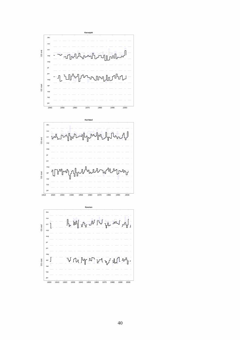
1940 1950 1960 1970 1980 1990 2000

Karasjok

jan

feb

mar

apr

may

jun

jul

aug

sep

oct

nov

dec

GS

sta

rt

G

S e

nd

1910 1920 1930 1940 1950 1960 1970 1980 1990 2000

Karlstad

jan

feb

mar

apr

may

jun

jul

aug

sep

oct

nov

dec

GS

sta

rt

G

S e

nd

1900 1910 1920 1930 1940 1950 1960 1970 1980 1990 2000

Kaunas

jan

feb

mar

apr

may

jun

jul

aug

sep

oct

nov

dec

GS

sta

rt

G

S e

nd

40

1880 1900 1920 1940 1960 1980 2000

Kazan

jan

feb

mar

apr

may

jun

jul

aug

sep

oct

nov

dec

GS

sta

rt

G

S e

nd

1910 1920 1930 1940 1950 1960 1970 1980 1990 2000

Kem

jan

feb

mar

apr

may

jun

jul

aug

sep

oct

nov

dec

GS

sta

rt

G

S e

nd

1880 1900 1920 1940 1960 1980 2000

Kirov

jan

feb

mar

apr

may

jun

jul

aug

sep

oct

nov

dec

GS

sta

rt

G

S e

nd

41

1950 1960 1970 1980 1990 2000

Kjoeremsgrende

jan

feb

mar

apr

may

jun

jul

aug

sep

oct

nov

dec

GS

sta

rt

G

S e

nd

1880 1900 1920 1940 1960 1980 2000

Koebenhavn

jan

feb

mar

apr

may

jun

jul

aug

sep

oct

nov

dec

GS

sta

rt

G

S e

nd

1910 1920 1930 1940 1950 1960 1970 1980 1990 2000

Kojnas

jan

feb

mar

apr

may

jun

jul

aug

sep

oct

nov

dec

GS

sta

rt

G

S e

nd

42

1920 1930 1940 1950 1960 1970 1980 1990 2000

Kostroma

jan

feb

mar

apr

may

jun

jul

aug

sep

oct

nov

dec

GS

sta

rt

G

S e

nd

1930 1940 1950 1960 1970 1980 1990 2000

Kotlas

jan

feb

mar

apr

may

jun

jul

aug

sep

oct

nov

dec

GS

sta

rt

G

S e

nd

1880 1900 1920 1940 1960 1980 2000

Liepaja

jan

feb

mar

apr

may

jun

jul

aug

sep

oct

nov

dec

GS

sta

rt

G

S e

nd

43

1930 1940 1950 1960 1970 1980 1990 2000

Linkoeping

jan

feb

mar

apr

may

jun

jul

aug

sep

oct

nov

dec

GS

sta

rt

G

S e

nd

1930 1940 1950 1960 1970 1980 1990 2000

Moermansk

jan

feb

mar

apr

may

jun

jul

aug

sep

oct

nov

dec

GS

sta

rt

G

S e

nd

1950 1960 1970 1980 1990 2000

Moskou

jan

feb

mar

apr

may

jun

jul

aug

sep

oct

nov

dec

GS

sta

rt

G

S e

nd

44

1940 1950 1960 1970 1980 1990 2000

Nesbyen-skoglund

jan

feb

mar

apr

may

jun

jul

aug

sep

oct

nov

dec

GS

sta

rt

G

S e

nd

1880 1900 1920 1940 1960 1980 2000

Nordby

jan

feb

mar

apr

may

jun

jul

aug

sep

oct

nov

dec

GS

sta

rt

G

S e

nd

1910 1920 1930 1940 1950 1960 1970 1980 1990 2000

Oestersund

jan

feb

mar

apr

may

jun

jul

aug

sep

oct

nov

dec

GS

sta

rt

G

S e

nd

45

1930 1940 1950 1960 1970 1980 1990 2000

Onega

jan

feb

mar

apr

may

jun

jul

aug

sep

oct

nov

dec

GS

sta

rt

G

S e

nd

1930 1940 1950 1960 1970 1980 1990 2000

Oslo-blindern

jan

feb

mar

apr

may

jun

jul

aug

sep

oct

nov

dec

GS

sta

rt

G

S e

nd

1930 1940 1950 1960 1970 1980 1990 2000

Petrozawodsk

jan

feb

mar

apr

may

jun

jul

aug

sep

oct

nov

dec

GS

sta

rt

G

S e

nd

46

1930 1940 1950 1960 1970 1980 1990 2000

Pskow

jan

feb

mar

apr

may

jun

jul

aug

sep

oct

nov

dec

GS

sta

rt

G

S e

nd

1940 1950 1960 1970 1980 1990 2000

Sortavala

jan

feb

mar

apr

may

jun

jul

aug

sep

oct

nov

dec

GS

sta

rt

G

S e

nd

1910 1920 1930 1940 1950 1960 1970 1980 1990 2000

Stensele

jan

feb

mar

apr

may

jun

jul

aug

sep

oct

nov

dec

GS

sta

rt

G

S e

nd

47

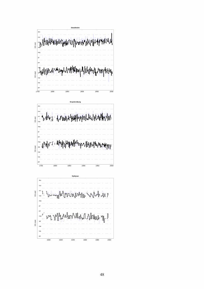
1750 1800 1850 1900 1950 2000

Stockholm

jan

feb

mar

apr

may

jun

jul

aug

sep

oct

nov

dec

GS

sta

rt

G

S e

nd

1750 1800 1850 1900 1950 2000

St-petersburg

jan

feb

mar

apr

may

jun

jul

aug

sep

oct

nov

dec

GS

sta

rt

G

S e

nd

1900 1920 1940 1960 1980 2000

Syktyvar

jan

feb

mar

apr

may

jun

jul

aug

sep

oct

nov

dec

GS

sta

rt

G

S e

nd

48

1880 1900 1920 1940 1960 1980 2000

Tranebjerg

jan

feb

mar

apr

may

jun

jul

aug

sep

oct

nov

dec

GS

sta

rt

G

S e

nd

1750 1800 1850 1900 1950 2000

Uppsala

jan

feb

mar

apr

may

jun

jul

aug

sep

oct

nov

dec

GS

sta

rt

G

S e

nd

1940 1950 1960 1970 1980 1990 2000

Utsira-fyr

jan

feb

mar

apr

may

jun

jul

aug

sep

oct

nov

dec

GS

sta

rt

G

S e

nd

49

1910 1920 1930 1940 1950 1960 1970 1980 1990 2000

Vaexjoe

jan

feb

mar

apr

may

jun

jul

aug

sep

oct

nov

dec

GS

sta

rt

G

S e

nd

1950 1960 1970 1980 1990 2000

Vardoe

jan

feb

mar

apr

may

jun

jul

aug

sep

oct

nov

dec

GS

sta

rt

G

S e

nd

1880 1900 1920 1940 1960 1980 2000

Velikie

jan

feb

mar

apr

may

jun

jul

aug

sep

oct

nov

dec

GS

sta

rt

G

S e

nd

50

1880 1900 1920 1940 1960 1980 2000

Vestervig

jan

feb

mar

apr

may

jun

jul

aug

sep

oct

nov

dec

GS

sta

rt

G

S e

nd

1880 1900 1920 1940 1960 1980 2000

Vilnjus

jan

feb

mar

apr

may

jun

jul

aug

sep

oct

nov

dec

GS

sta

rt

G

S e

nd

1920 1930 1940 1950 1960 1970 1980 1990 2000

Vilsandi

jan

feb

mar

apr

may

jun

jul

aug

sep

oct

nov

dec

GS

sta

rt

G

S e

nd

51

1920 1930 1940 1950 1960 1970 1980 1990 2000

Voru

jan

feb

mar

apr

may

jun

jul

aug

sep

oct

nov

dec

GS

sta

rt

G

S e

nd

1880 1900 1920 1940 1960 1980 2000

Vytegra

jan

feb

mar

apr

may

jun

jul

aug

sep

oct

nov

dec

GS

sta

rt

G

S e

nd

52

Appendix 2. A comparison of twentieth century trends in start, end and length of the thermal growing season depending on definition used (see text for explanation of definitions). 2.1 Trends in growing season start

1901-1950 (=5>5F)

0o 10oE 20oE 30oE 40oE 50oE 52oN

56oN

60oN

64oN

68oN

72oN 1951-2000 (=5>5F)

0o 10oE 20oE 30oE 40oE 50oE 52oN

56oN

60oN

64oN

68oN

72oN 1901-2000 (=5>5F)

0o 10oE 20oE 30oE 40oE 50oE 52oN

56oN

60oN

64oN

68oN

72oN

1901-1950 (=5>5)

0o 10oE 20oE 30oE 40oE 50oE 52oN

56oN

60oN

64oN

68oN

72oN 1951-2000 (=5>5)

0o 10oE 20oE 30oE 40oE 50oE 52oN

56oN

60oN

64oN

68oN

72oN 1901-2000 (=5>5)

0o 10oE 20oE 30oE 40oE 50oE 52oN

56oN

60oN

64oN

68oN

72oN

1901-1950 (>5>5)

0o 10oE 20oE 30oE 40oE 50oE 52oN

56oN

60oN

64oN

68oN

72oN 1951-2000 (>5>5)

0o 10oE 20oE 30oE 40oE 50oE 52oN

56oN

60oN

64oN

68oN

72oN 1901-2000 (>5>5)

0o 10oE 20oE 30oE 40oE 50oE 52oN

56oN

60oN

64oN

68oN

72oN

1901-1950 (>5>5F)

0o 10oE 20oE 30oE 40oE 50oE 52oN

56oN

60oN

64oN

68oN

72oN 1951-2000 (>5>5F)

0o 10oE 20oE 30oE 40oE 50oE 52oN

56oN

60oN

64oN

68oN

72oN 1901-2000 (>5>5F)

0o 10oE 20oE 30oE 40oE 50oE 52oN

56oN

60oN

64oN

68oN

72oN

53

2.2. Trends in growing season end 1901-1950 (frostOR=5<5)

0o 10oE 20oE 30oE 40oE 50oE 52oN

56oN

60oN

64oN

68oN

72oN 1951-2000 (frostOR=5<5)

0o 10oE 20oE 30oE 40oE 50oE 52oN

56oN

60oN

64oN

68oN

72oN 1901-2000 (frostOR=5<5)

0o 10oE 20oE 30oE 40oE 50oE 52oN

56oN

60oN

64oN

68oN

72oN

1901-1950 (=5<5)

0o 10oE 20oE 30oE 40oE 50oE 52oN

56oN

60oN

64oN

68oN

72oN 1951-2000 (=5<5)

0o 10oE 20oE 30oE 40oE 50oE 52oN

56oN

60oN

64oN

68oN

72oN 1901-2000 (=5<5)

0o 10oE 20oE 30oE 40oE 50oE 52oN

56oN

60oN

64oN

68oN

72oN

1901-1950 (>5<5)

0o 10oE 20oE 30oE 40oE 50oE 52oN

56oN

60oN

64oN

68oN

72oN 1951-2000 (>5<5)

0o 10oE 20oE 30oE 40oE 50oE 52oN

56oN

60oN

64oN

68oN

72oN 1901-2000 (>5<5)

0o 10oE 20oE 30oE 40oE 50oE 52oN

56oN

60oN

64oN

68oN

72oN

1901-1950 (10d<5)

0o 10oE 20oE 30oE 40oE 50oE 52oN

56oN

60oN

64oN

68oN

72oN 1951-2000 (10d<5)

0o 10oE 20oE 30oE 40oE 50oE 52oN

56oN

60oN

64oN

68oN

72oN 1901-2000 (10d<5)

0o 10oE 20oE 30oE 40oE 50oE 52oN

56oN

60oN

64oN

68oN

72oN

54

2.3. Trends in growing season length

1901-1950 (=5>5Fr|frostOR=5<5)

0o 10oE 20oE 30oE 40oE 50oE 52oN

56oN

60oN

64oN

68oN

72oN 1951-2000 (=5>5Fr|frostOR=5<5)

0o 10oE 20oE 30oE 40oE 50oE 52oN

56oN

60oN

64oN

68oN

72oN 1901-2000 (=5>5Fr|frostOR=5<5)

0o 10oE 20oE 30oE 40oE 50oE 52oN

56oN

60oN

64oN

68oN

72oN

1901-1950 (=5>5|=5<5)

0o 10oE 20oE 30oE 40oE 50oE 52oN

56oN

60oN

64oN

68oN

72oN 1951-2000 (=5>5|=5<5)

0o 10oE 20oE 30oE 40oE 50oE 52oN

56oN

60oN

64oN

68oN

72oN 1901-2000 (=5>5|=5<5)

0o 10oE 20oE 30oE 40oE 50oE 52oN

56oN

60oN

64oN

68oN

72oN

1901-1950 (>5>5|>5<5)

0o 10oE 20oE 30oE 40oE 50oE 52oN

56oN

60oN

64oN

68oN

72oN 1951-2000 (>5>5|>5<5)

0o 10oE 20oE 30oE 40oE 50oE 52oN

56oN

60oN

64oN

68oN

72oN 1901-2000 (>5>5|>5<5)

0o 10oE 20oE 30oE 40oE 50oE 52oN

56oN

60oN

64oN

68oN

72oN

1901-1950 (=5>5Fr|10d)

0o 10oE 20oE 30oE 40oE 50oE 52oN

56oN

60oN

64oN

68oN

72oN 1951-2000 (=5>5Fr|10d)

0o 10oE 20oE 30oE 40oE 50oE 52oN

56oN

60oN

64oN

68oN

72oN 1901-2000 (=5>5Fr|10d)

0o 10oE 20oE 30oE 40oE 50oE 52oN

56oN

60oN

64oN

68oN

72oN

1901-1950 (>5>5F|10d)

0o 10oE 20oE 30oE 40oE 50oE 52oN

56oN

60oN

64oN

68oN

72oN 1951-2000 (>5>5F|10d)

0o 10oE 20oE 30oE 40oE 50oE 52oN

56oN

60oN

64oN

68oN

72oN 1901-2000 (>5>5F|10d)

0o 10oE 20oE 30oE 40oE 50oE 52oN

56oN

60oN

64oN

68oN

72oN

55

Twentieth-century trends in the thermal growing season in the Greater Baltic Area

Hans W. Linderholm1, 3*), Alexander Walther1), Deliang Chen1) and Anders Moberg2)

1) Regional Climate Group, Earth Sciences Centre, Göteborg University, SE-405 30 Göteborg,

Sweden 2) Department of Meteorology, Stockholm University, SE-106 91 Stockholm, Sweden

3) Laboratory for Climate Studies, National Climate Center, China Meteorological Administration, 46 Zhongguancun Nandajie, Haidian, Beijing 100081, China

Abstract: Phenological data have shown an increase of c. 10 days in European growing season length in the latter part of the twentieth century. In general, these changes have been associated with global warming. Here we present a study of thermal growing season (GS) trends in the Greater Baltic Area, northern Europe. Yearly dates for the start, end and length of the GS were computed for 49 stations in the studied area, using daily mean temperature measurements. Trends and tendencies of the GS parameters were analysed within the twentieth century. We also examined GS trends in long records (starting before 1850) from the region. The results show a general increase of the length of the GS of ca one week since 1951 in the area, where the most considerable change has occurred in spring (starting ~ 6 days earlier). The largest increases were found at stations adjacent to the Baltic Sea and North Sea, where some Danish stations showed significant increasing trends in the length of the GS of more than 20 days. The only tendency for a shorter GS was found in Archangelsk, north western Russia. The three longest records displayed large inter-annual and decadal variability, with tendencies for increased frequencies of longer growing seasons since the 1950s.

56

1. Introduction In the past decade, a growing number of studies have reported on a late-twentieth century lengthening of the growing season for most of the Northern Hemisphere, associated with increasing temperatures (e.g., Frich et al., 2002; Parmesan and Yohe, 2003; Root et al., 2003). The relationship between climate and growing season (GS) parameters (start, end and length), makes GS variability an important indicator of climate change. Evidence for lengthening of the growing season in the late twentieth century has come from satellite data, phenological and meteorological observations. Keeling et al. (1996) showed an association between surface air temperatures and variations in the timing and amplitude of the seasonal cycle of atmospheric CO2. An increase of the annual amplitude of the seasonal CO2 cycle by 40% in the Arctic (20% in Hawaii) since the early 1960s, where warmer temperatures promote increases in plant growth in summer and/or respiration in winter, was linked to a lengthening of the GS by about 7 days. Furthermore, the photosynthetic activity of terrestrial vegetation, as seen in satellite data, increased from 1981 to 1991 which is also associated with a lengthening of the active growing season (Myneni et al., 1997). I large number of phenological studies has reported on recent changes in timing of GS start and end, resulting in an extension of the GS. Phenology studies plant and animal life stages driven by environmental factors (Schwartz, 1999). Species whose phenophases (e.g. flowering, leafing, breeding, leaf fall etc.) are linked to temperatures, will respond to changing temperatures with shifts in the phenophases. Phenological data have indicated shifts to earlier start of the GS in the latter half of the twentieth century, which has been coupled to warmer winters associated with the North Atlantic Oscillation, NAO (Chmielewski and Rötzer, 2001; Ahas et al., 2002; D’Odorico et al., 2002; Scheifinger et al., 2002; Menzel, 2003; Ahas et al., 2004), warming in spring (Cayan et al., 2001; Chmielewski and Rötzer, 2002; Chmielewski et al., 2004) and increases in minimum temperatures or longer frost-free period (Abu-Asab et al., 2001; Scheifinger et al. 2003). Common results for most recent phenological studies are an extended GS, which mainly is caused by earlier onset of the GS start in spring (Ahas, 1999; Menzel and Fabian, 1999; Menzel 2000; Menzel et al., 2001; Ahs et al., 2002; Peñuelas et al., 2002). However, Kozlov and Berlina (2002) found a shift to later snow-melt by 16 days in spring in the northern Russian taiga for the period 1930 to 1998. In addition, there was a shift of 13 days towards earlier dates of permanent snow during that period. Similar findings, i.e. an extended GS during the late twentieth century, have also been observed when the climatological GS is studied for large parts of the Northern Hemisphere (Frich et al., 2002). The reported increases in growing season length (GSL) are in a range of c. 1 to 3 weeks (Skaggs and Baker, 1985; Carter, 1998; Hasenauer et al., 1999; Robeson, 2002; Schwartz and Chen, 2002; Menzel et al., 2003). Climate change is projected to increase the length of the growing season (e.g., IPCC, 2001). An increase in GSL, together with a warmer GS, may advance the potential for crop production at high northern latitudes and increase the potential number of harvests and hence seasonal yields for perennial forage crops (ACIA, 2004). Effects at high northern latitudes could be elevated tree line, improved forest productivity and favourable conditions for growing of more southerly fruits (e.g. Hasenauer et al., 1999; Wielgolaski, 2003). However, the accelerated rates of change seen in the past three decades indicates that in a near future we will see large changes in ecosystems which may have negative effects on ecosystems, such as extension of species’ range boundaries by establishment of new local populations causing extinction of former

57

populations, and progressive decoupling of species interaction (e.g. plants and pollinators) because of out–of–phase phenology (e.g. Hughes, 2000; Peñuelas and Filella, 2001). Barford et al. (2001) found that seasonal and annual fluctuations of the uptake of CO2 in a northern hardwood forest were regulated by weather and seasonal climate (e.g. variations in growing-season length). Consequently, persistent increases in GSL may lead to long-term increases in carbon storage (White et al., 1999). In this paper we analyse twentieth century trends in the thermal growing season from a network of stations in Greater Baltic Area (GBA, Walther and Linderholm, 2005). This region, which largely belongs to the boreal region, may be especially sensitive to changes in the growing season. Recent climate warming in the boreal region has increased the probability of occurrence of critical temperature thresholds for the production of existing agricultural crops. Possible future climate warming almost certainly would increase the land area on which crops could be produced successfully, and very likely the variety of agricultural crops that could be grown (Juday et al., 2005).

2. Data We analysed temperature records from 49 stations where daily observations were available. This datasets has been collected, processed and made available within two large projects: the European Climate Assessment & Dataset (ECA&D, Klein Tank et al. 2002, http://eca.knmi.nl) and European and North Atlantic daily to Multidecadal climate variability (EMULATE, http://www.cru.uea.ac.uk/cru/projects/emulate/). The locations of the stations and information about the start and end years of each record are shown in Fig. 1 and table 1. Only 21 of 49 records start 1901 or earlier. The long (starting at least 1901) and very long records (starting before 1850) are concentrated in the southern part of the GBA. In order to increase the station density and the possibility to obtain spatial patterns from a higher number of records a number of shorter records (starting after 1901) have been included as well.

Figure 1. Locations of the stations in the Greater Baltic Area used in the study. See table 1 for station data.

58

Table 1. Station data for the 49 station used in the analyses.

lat lon elev Station start end lat lon elev Station start end

1 55.3 14.8 12 Hammer-Odde-Fyr DK 1874 2004 1) 26 62.4 25.7 137 Jyvaskyla FIN 1951 2004 1)

2 55.7 12.5 9 Koebenhavn DK 1874 2003 1) 27 59.0 10.5 6 Faerder-Fyr N 1951 2004 1)

3 55.5 8.4 4 Nordby DK 1874 2003 1) 28 66.8 14.0 39 Glomfjord N 1943 2001 1)

4 55.9 10.6 11 Tranebjerg DK 1873 2003 1) 29 69.5 25.5 129 Karasjok N 1943 2001 1)

5 56.8 8.3 18 Vestervig DK 1874 2003 1) 30 62.1 9.1 626 Kjoeremsgrende N 1954 2004 1)

6 60.3 25.0 51 Helsinki FIN 1828 2001 4) 31 60.6 9.1 167 Nesbyen-Skoglund N 1943 2004 1)

7 56.7 21.0 4 Liepaja LV 1881 1989 2) 32 60.0 10.7 94 Oslo-Blindern N 1938 2004 1)

8 54.9 23.8 75 Kaunas LT 1901 2004 1) 33 59.3 4.9 55 Utsira-Fyr N 1943 2004 1)

9 54.6 25.3 162 Vilnjus LT 1881 1989 1,2) 34 70.4 31.1 14 Vardoe N 1951 2004 1)

10 64.6 40.5 8 Archangelsk RUS 1881 1999 1) 35 67.2 32.4 25 Kandalaksa RUS 1912 2004 1)

11 55.0 41.8 132 Elatma RUS 1886 1999 1) 36 65.0 34.8 8 Kem RUS 1916 2000 1)

12 56.2 43.8 161 Gorkij RUS 1881 1989 2) 37 64.8 47.7 64 Kojnas RUS 1912 1999 1)

13 55.8 49.2 116 Kazan RUS 1881 1989 2) 38 57.7 40.8 126 Kostroma RUS 1925 1999 1)

14 58.7 49.6 165 Kirov RUS 1881 1989 2) 39 61.2 46.7 56 Kotlas RUS 1936 1999 1)

15 60.0 30.3 4 St-Petersburg RUS 1743 1999 3) 40 69.0 33.1 51 Moermansk RUS 1936 1999 1)

16 61.7 50.9 96 Syktyvar RUS 1888 1999 1) 41 55.8 37.6 156 Moskou RUS 1948 1999 1)

7 56.4 30.6 98 Velikie-Luki RUS 1881 1999 1) 42 63.9 38.1 13 Onega RUS 1936 2004 1)

18 61.0 36.5 55 Vytegra RUS 1881 1999 1) 43 61.8 34.3 110 Petrozawodsk RUS 1936 1999 1)

19 60.6 15.7 157 Falun S 1860 2002 44 57.8 28.4 45 Pskow RUS 1936 2004 1)

20 65.1 17.2 325 Stensele S 1918 2003 45 61.7 30.7 19 Sortavala RUS 1945 2004 1)

21 59.4 18.1 44 Stockholm S 1756 2003 5) 46 59.3 39.9 130 Wologda RUS 1938 1999 1)

22 59.9 17.6 13 Uppsala S 1722 2001 5) 47 59.4 13.5 46 Karlstad S 1918 2001 1)

23 56.9 14.8 166 Vaexjoe S 1918 2003 48 58.4 15.5 93 Linkoeping S 1931 2004 1)

24 58.4 21.8 6 Vilsandi EST 1920 2004 1) 49 63.2 14.5 376 Oestersund S 1918 2004 1)

25 57.9 27.0 82 Voru EST 1923 2001 1) 1) European Climate Assessment & Dataset (ECA&D): http://eca.knmi.nl2) Carbon Dioxide Information Analysis Centre (CDIAC): http://cdiac.ornl.gov/ftp/ndp0403) Jones and Lister, 2002 4) Heino, 1994 5) Moberg et al., 2002

3. Methods The climatological growing season can be defined as the entire period in which growth can theoretically take place; it is not the period of actual growth. There are a number of ways to define start, end and length of the growing season. One definition of GSL that has been used in USA is the period between the date of the last spring frost and first autumn frost (e.g. Skaggs and Baker, 1985; Robeson, 2002), where the frost may be determined by thresholds of daily minimum temperatures. Other investigations have used threshold temperatures in a predefined number of days to start and end the growing season. Bootsma (1994) defined GSL in Canada as the period when 5-day weighted mean temperatures is and stays above 5.5°C and below 5.5°C. Jones and Briffa (1995) defined the start of the growing season in Russia as the fourth day of the first sequence of four consecutive days with temperatures above the 5°C threshold, and the end was defined as the last day of the last 4-day sequence above the 5°C. Later, Jones et al. (2002) revised the definition, so that the growing season start/end was defined as the first/last five-day period occurring after/before the last/first frost of the winter season. Frich et al. (2002), in a global study, used the period when daily temperatures remain above >5°C for >5 days and below <5°C for >5 days. Carter (1998) defined the start of the growing season as >5°C for ≥5 and the end as the 10-day running mean of mean daily temperatures falls below 5°C. In a comparison of different indices for the start and end of the growing season in the Greater Baltic Area (GBA), Walther and Linderholm

59

(2005) noted that disregarding the frost criteria might lead to false starts and ends of the growing season. In this study we use the definition that was suggested for the GBA, where the start day of the growing season is defined as the last day of the first six-day spell with daily Tmean above 5°C after the last winter/spring frost (based on Tmean). The end-day of the growing season is defined as the first day of the first 10-day period with a mean below 5°C. Finally, the GSL is the number of days between the particular start- and end-day. Using the 5°C threshold in northern Europe can be justified, since the growing season is largely temperature limited. The physiological significance of this period naturally differs among plant types, but it can be assumed to be relevant to perennial plants that are exposed to weather throughout the year, e.g. trees and shrubs (Carter, 1998). Using these definitions we produced time series of the start, end and length of the GS for each station included in the data set. Trend analyses were made in three time periods: 1901-1950, 1951-2000 and 1901-2000. Due to the different lengths of the station records (several stations ending in the 1980s) we also computed trends for the entire lengths of each record. An overall missing value criteria was applied when computing the growing season parameters. Up to 12 missing values in the particular annual Tmean series were allowed (=1 missing value/month). If there more were found, the growing season parameters were set missing values as well. The temperature series generally contained either high or very low rates of missing values. In order to be able to include also series with high missing value rates, we looked at the distribution of these within the series. In this context the growing season parameters was computed, if the dates of the missing values clearly did not affect the start or the end of the particular growing season (e.g. missing values before the last spring frost or after the first 10-day mean period below 5°C). For computing the linear trends up to 5% missing growing season parameters in the particular period to be analysed were allowed (= 5 years missing/100 years). The growing season time-series was analysed for linear trends using the Mann-Kendall trend test (Yue et al., 2002).

4. Twentieth century trends and tendencies Due to the large variation in station record lengths and occasionally large numbers of missing values, the number of stations in each analysed period was lower than expected, especially in the periods starting before 1951; 1901-1950: 11 stations, 1951-2000: 37 stations and 1901-2000: 11 stations. The results of the trend analyses of start, end and length of the growing season are shown in Figure 2 and table 2.

4.1. Start Between 1901 and 1950 a significant trend in the start of the GS was only found Koebenhavn, Denmark, with an earlier onset of almost 20 days. Similar tendencies (i.e. not significant trends) of shifts by > -10 — <-20 days were found at the remaining Danish stations, Stockholm and Uppsala. At the remaining stations in the central part of the GBA, tendencies indicated an earlier GS onset as well, although only with >0 — ≤-10 days. In the eastern parts, the tendency at Syktyvkar, Russia, showed a delay in the GS start of 5.7 days. Between 1951 and 2000, the majority of the stations show tendencies for an earlier GS start of around >0 — ≤-10 days. Significant trends of c. 10 days were only found in St Petersburg (Russia) and Vilsandi (Estonia). The largest changes, though not significant, were found in the south-western part of the GBA: Koebenhavn, Vestervig and Norby (Denmark, -24.5, -22.1 and -18.1 days respectively) and Utsira Fyr – Faerder Fyr (Norway, -19.1 and -16.6 days respectively). Four stations

60

indicated a delayed (not significant) GS start in this period: Oestersund (Sweden, +2 days), Vardoe (Norway, +3 days) and Moskou and Kandalaksa (Russia, +0.5 and +1.2 days respectively). For the whole 1901 to 2000 period, all available stations showed earlier starts of the GS, and significant trends were found in Koebenhavn, Nordby and Vestervig (Denmark, -22,8, -18.2 and -16.5 days respectively), Helsinki (Finland, -9.5 days), St Petersburg (Russia, -10.6 days) and Falun (Sweden, -8.6 days). There were tendencies for earlier GS starts at the remaining stations of >0 — ≤-10 days.

GS

star

t

1901-1950 (=5>5F)

0o 10oE 20oE 30oE 40oE 50oE 52oN

56oN

60oN

64oN

68oN

72oN 1951-2000 (=5>5F)

0o 10oE 20oE 30oE 40oE 50oE 52oN

56oN

60oN

64oN

68oN

72oN 1901-2000 (=5>5F)

0o 10oE 20oE 30oE 40oE 50oE 52oN

56oN

60oN

64oN

68oN

72oN

GS

end

1901-1950 (10d<5)

0o 10oE 20oE 30oE 40oE 50oE 52oN

56oN

60oN

64oN

68oN

72oN 1951-2000 (10d<5)

0o 10oE 20oE 30oE 40oE 50oE 52oN

56oN

60oN

64oN

68oN

72oN 1901-2000 (10d<5)

0o 10oE 20oE 30oE 40oE 50oE 52oN

56oN

60oN

64oN

68oN

72oN

GS

leng

th

1901-1950 (=5>5Fr|10d)

0o 10oE 20oE 30oE 40oE 50oE 52oN

56oN

60oN

64oN

68oN

72oN 1951-2000 (=5>5Fr|10d)

0o 10oE 20oE 30oE 40oE 50oE 52oN

56oN

60oN

64oN

68oN

72oN 1901-2000 (=5>5Fr|10d)

0o 10oE 20oE 30oE 40oE 50oE 52oN

56oN

60oN

64oN

68oN

72oN

Figure 2. Trends in start, end and length of the thermal growing season for three periods in the twentieth century (see text for explanation of definitions).

4.2. End No significant trends in GS end were found in 1901-1950. However, there were tendencies for later GS ends at all stations of 0.5 to 10 days, except in Vestervig and Nordby (Denmark), where tendencies for a shift of 7.3 and 0.8 days respectively to an earlier GS end were found. In the following period (1951-2000) stations close to the North Atlantic, nine of the Russian stations and Karlstad (Sweden) show tendencies for an earlier end of the GS (>0 — ≤-10 days), where Elatma and Moskou show earlier GS ends of ca one week. The remaining stations display tendencies for later GS end (>0 —

61

≤+10 days). The significant trends in GS end for the 1901 to 2000 period were found around the Baltic Sea (Koebenhavn: +12.6 days, Stockholm: +11.7 days and Helsinki: +10.5 days). Tendencies for later GS ends (>0—<+10 days) were found at the remaining stations. In Archangelsk (Russia), there was a significant trend of earlier GS end of one week. Table 2. Linear trends in growing season parameters for three periods in the twentieth century. See text for definitions of start and end. A few series were included which started later than 1950 (**: start year 1954) and ended before 2000 (*: end year 1999). For a number of stations more than 5% of the data was missing, so the were excluded from the analyses (station No: 4, 7-9, 12-14, 18, 37, 39-40 and 46, see table for station locations). Significant trends (95% level) are bold.

1901-1950 1951-2000 1901-2000 start end length start end length start end length 1 Hammer-Odde-Fyr DK -11,1 9 20,2 -- -- -- -0,3 10,2 10,5 2 Koebenhavn DK -19,2 5,7 24,9 -24.5** -4** 17.2** -22,8 12,6 33,5 3 Nordby DK -13,9 -0,8 13,1 -18,1 4 22,5 -18,2 8,3 26,5 5 Vestervig DK -10,9 -7,3 3,6 -22,1 -3,3 18,8 -16,5 6,1 22,6 6 Helsinki FIN -6,6 0,8 7,3 -1 2,8 3,8 -9,5 10,5 19,9 10 Archangelsk RUS -1,1 3,8 4,9 -4.5** -4** 0.5** -3,6 -7,1 -3,6 11 Elatma RUS -- -- -- -0,9 -6,7 -5,8 -- -- -- 15 St-Petersburg RUS -2,9 2 4,9 -10,7 -3,1 7,6 -10,6 3,5 14,2 16 Syktyvkar RUS 5,7 3 -2,7 -5.5** -1.1** 4.3** -9,1 0,2 9,2 17 Velikie-Luki RUS -- -- -- -5.1* -3.3* 1.8* -- -- -- 19 Falun S -6,7 2,9 9,6 -2,4 5,5 7,9 -8,6 1,1 9,7 20 Stensele S -- -- -- -1,4 1 2,3 -- -- -- 21 Stockholm S -10,5 5,1 15,6 -5,2 5,5 10,6 -6,2 11,7 17,9 22 Uppsala S -11 2,9 13,9 -4,7 1,4 6,1 -7,8 7,6 15,4 23 Vaexjoe S -- -- -- -4,8 1,3 6,2 -- -- -- 24 Vilsandi EST -- -- -- -10,8 1,4 12,2 -- -- -- 25 Voru EST -- -- -- -8,7 2,8 11,5 -- -- -- 26 Jyvaskyla FIN -- -- -- -1,5 3,7 5,2 -- -- -- 27 Faerder-Fyr N -- -- -- -16,6 3,5 20 -- -- -- 28 Glomfjord N -- -- -- -2,9 -1,1 1,8 -- -- -- 29 Karasjok N -- -- -- -7,1 0,4 7,5 -- -- -- 30 Kjoeremsgrende N -- -- -- -3*** -3*** 0*** -- -- -- 31 Nesbyen-Skoglund N -- -- -- -4,4 1,4 5,8 -- -- -- 32 Oslo-Blindern N -- -- -- -7,3 2,8 10,1 -- -- -- 33 Utsira-Fyr N -- -- -- -19,1 -4,8 14,3 -- -- -- 34 Vardoe N -- -- -- 3 8,4 5,5 -- -- -- 35 Kandalaksa RUS -- -- -- 1,2 0,9 -0,3 -- -- -- 36 Kem RUS -- -- -- -6.1* 5* 11.1* -- -- -- 38 Kostroma RUS -- -- -- -4.3* -0.9* 3.3* -- -- -- 41 Moskou RUS -- -- -- 0.5* -9.3* -9.8* -- -- -- 42 Onega RUS -- -- -- -4,9 2,3 7,2 -- -- -- 43 Petrozawodsk RUS -- -- -- -5.9* 2* 7.9* -- -- -- 44 Pskow RUS -- -- -- -7,6 -1,3 6,3 -- -- -- 45 Sortavala RUS -- -- -- -5,6 -1,9 3,7 -- -- -- 47 Karlstad S -- -- -- -4,8 -0,2 4,5 -- -- -- 48 Linkoeping S -- -- -- -4,1 2,8 6,9 -- -- -- 49 Oestersund S -- -- -- 2 0,6 -1,3 -- -- --

62

4.3. GSL Significant trends in the GSL in 1901-1950 were found in the two eastern Danish stations (Koebenhavn and Hammer-Odde Fyr). These showed increased trends of more than 20 days in the fifty-year period. All other stations close to the Baltic Sea or North Atlantic coasts displayed tendencies for increased GSL of >0 — ≤+10 days, where the tendencies in Nordby, Stockholm and Uppsala were of >+10—<+20 days. One Russian station (Syktyvkar) in the easternmost part of GBA showed a negative tendency for GSL (-2.7 days). No significant trends were found in 1951-2000, but tendencies show increased GSL in most of the GBA of >0 — ≤20 days: over 10 days increase in Estonia, Stockholm, Kem (Russia) and the south western part GBA (including a increases of ≥20 days at Nordby and Faerder Fyr in western Norway). In Oestersund (Sweden), Moscou, Kandalaksa and Elatma (Russia), this period displayed a tendency for shorter GSL. There is a clear trend towards and increasing GSL around the Baltic Sea in 1901 to 2000. The significant increases of >+10 — ≤+20 days were found in Stockholm, Uppsala, Helsinki and St Petersburg, and, slightly lower, in Falun (+9.7 days), Hammer-Odde Fyr (+10.5 days, not significant) and Syktyvkar (+9.2 days, not significant). Three Danish mainland stations show and even greater trends: +22.6 days in Vestervig, +26.5 days in Nordby and +33.5 days in Koebenhavn. The only tendency for a twentieth century shortening of the GSL was found in Archangelsk in Russia (-3.6 days).

4.4. Long-term trends When the linear trends of growing season parameters was computed for the longest consecutive period, with less than 5% missing values, for each record, an increasing growing season is the main feature in the GBA (Table 3). The most prominent changes have occurred in Denmark with increases in GSL of up to 40 days since the late nineteenth century. Significant increases are also observed in central Sweden and St. Petersburg and Kirov in Russia, but not of the same magnitude. The remaining stations that display tendencies for extended GS are in the range of 0.3 to 14.1 days. Only 7 stations out of 49 show tendencies for a shorter GS, but only with a few days (-1.4 to -9.6 days). More significant changes in GS start (all earlier) were observed than in GS end (all later except kandalaksa, Russia). Only five (59 stations out of 49 disclosed tendencies for later GS start (Liepaja, Latvia; Vilnjus, Lithuania; Moscou, Russia; Karlstad and Linkoeping, Sweden). Twenty one (21) stations disclosed and earlier GS ends, the majority being Russian stations (17 out of 21 stations), but also one Lithuanian and three Norwegian (two coastal) stations.

5. Trends in the longest records The long-term growing season trends in the longest records show significant increases in GSL of 6.6 (Uppsala, p < 0.1), 8.4 (Stockholm, p < 0.1) and 16 (St. Petersburg, p < 0.05) days since the eighteenth century (Figure 3). In the Swedish records, the increased GSL was due to earlier springs (4.6 days in Uppsala, p < 0.1 and 7.6 days in Stockholm, p < 0.05), while in St. Petersburg, delayed autumn of 9 days (p < 0.05) had greater impact on GSL. The trends of delayed autumn in the Swedish records were small and not significant. The shorter Helsinki record displayed significant increases in GSL of 33 days (p < 0.05), with a trend for earlier springs (14 days, p < 0.05) and delayed autumn (18 days, p < 0.05). The records three longest records display high inter-annual and decadal variability, and there are tendencies for increased frequencies of longer growing seasons since the 1950s.

63

Table 3. Linear trends in growing season parameters over longest consecutive periods with missing values <5% for. See Fig. 1 for station location and text for start and end definitions.

Trend period start end length 1 Hammer-Odde-Fyr DK 1875 - 2003 -13,6 12,9 26,5 2 Koebenhavn DK 1874 - 2003 -22,6 18,2 40,8 3 Nordby DK 1875 - 2003 -17,2 4,4 21,6 4 Tranebjerg DK 1874 - 1938 -11,5 12,8 24,4 5 Vestervig DK 1874 - 2003 -19,5 12,3 31,8 6 Helsinki FIN 1834 - 2001 -17,6 14,2 31,8 7 Liepaja LV 1946 - 1989 2,7 10,6 7,9

8 Kaunas LT 1901 - 2003 -999 -999 -999

9 Vilnjus LT 1945 - 1989 7,2 -0,2 -7,4

10 Archangelsk RUS 1883 - 1999 -5,6 -2 3,6

11 Elatma RUS 1922 - 1999 -7,5 -7,2 0,3

12 Gorkij RUS 1923 - 1989 -13,3 -4,9 8,4

13 Kazan RUS 1881 - 1983 -5,1 -2,3 2,8

14 Kirov RUS 1940 - 1989 -8,4 6,6 15 15 St-Petersburg RUS 1798 - 1999 -15,8 7,1 22,9 16 Syktyvkar RUS 1896 - 1998 -8 -0,9 7,1

17 Velikie-Luki RUS 1947 - 1999 -4,5 -2,1 2,4

18 Vytegra RUS 1933 - 1998 -6,4 -4,8 1,7

19 Falun S 1897 - 2002 -10,6 0,8 11,5 20 Stensele S 1918 - 2003 -7,6 7,8 15,4 21 Stockholm S 1756 - 2003 -1,4 7,6 8,9 22 Uppsala S 1722 - 2001 -1,6 4,6 6,2 23 Vaexjoe S 1918 - 2003 -3,6 4,4 8

24 Vilsandi EST 1948 - 2001 -8,5 2,3 10,8

25 Voru EST 1945 - 2001 -6,8 5,7 12,5

26 Jyvaskyla FIN 1951 - 2003 -3 2,7 5,8

27 Faerder-Fyr N 1951 - 2003 -15,9 -1,8 14,1

28 Glomfjord N 1956 - 2001 -4,8 0,7 5,6

29 Karasjok N 1951 - 2001 -5,7 1,3 7

30 Kjoeremsgrende N 1954 - 2001 -3,1 -2,6 0,5

31 Nesbyen-Skoglund N 1943 - 2002 -0,5 1,2 1,7

32 Oslo-Blindern N 1938 - 2003 -0,3 1,6 1,9

33 Utsira-Fyr N 1943 - 2003 -1,4 -3,7 -2,2

34 Vardoe N 1951 - 2003 -2,6 7,7 10,3

35 Kandalaksa RUS 1912 - 2003 -2,6 -6,7 -4,1

36 Kem RUS 1917 - 2000 -5,6 -1 4,5

37 Kojnas RUS 1922 - 1998 -3,2 -4,6 -1,4

38 Kostroma RUS 1925 - 1999 -7,8 -3,3 4,6

39 Kotlas RUS 1936 - 1999 -6,3 -4,3 2

40 Moermansk RUS 1938 - 1998 -10,3 -6 4,3

41 Moskou RUS 1949 - 1999 0,2 -9,4 -9,6

42 Onega RUS 1936 - 2002 -3,1 -1,2 2

43 Petrozawodsk RUS 1945 - 1999 -0,3 1,1 1,4

44 Pskow RUS 1945 - 2002 -7,5 0,9 8,3

45 Sortavala RUS 1945 - 2000 -2,9 -0,4 2,5

46 Wologda RUS 1939 - 1998 -5,2 -1,9 3,3

47 Karlstad S 1918 - 2001 5,2 2,2 -3

48 Linkoeping S 1931 - 2003 4,9 1,7 -3,1

49 Oestersund S 1918 - 2003 -3,5 0,3 3,9

64

6. Discussion 6.1. General trends in the GBA Unfortunately, the many missing values in the analysed data set makes it difficult to evaluate the evolution of GSL within the entire twentieth century over the entire GBA. The reason for the general lack of significant trends in growing season parameters may be attributed to the large inter-annual variability in the records. This is exemplified by the long records in Figure 3, especially the Stockholm and Uppsala records, where the observed trend is far lower then the yearly and decadal variations. This has also been observed in climatological growing season records for North America (Bootsma, 1994; Robeson, 2002).

1750 1800 1850 1900 1950 2000

Uppsala

jan

feb

mar

apr

may

jun

jul

aug

sep

oct

nov

dec

GS

sta

rt

G

S e

nd

-1.6

4.6*

0

50

100

150

200

250

300G

S L

engt

h [d

ays]6.6

1750 1800 1850 1900 1950 2000

Stockholm

jan

feb

mar

apr

may

jun

jul

aug

sep

oct

nov

dec

GS

sta

rt

G

S e

nd

-1.4

7.6**

0

50

100

150

200

250

300

GS

Len

gth

[day

s]8.4*

1750 1800 1850 1900 1950 2000

St-petersburg

jan

feb

mar

apr

may

jun

jul

aug

sep

oct

nov

dec

GS

sta

rt

G

S e

nd

(-9**)

(5.1)

0

50

100

150

200

250

300

GS

Len

gth

[day

s](16**)

1840 1860 1880 1900 1920 1940 1960 1980 2000

Helsinki

jan

feb

mar

apr

may

jun

jul

aug

sep

oct

nov

dec

GS

sta

rt

G

S e

nd

-18**

14**

0

50

100

150

200

250

300

GS

Len

gth

[day

s]33**

Figure 3. Trends in growing season start, end and length in the longest records (starting before 1850) in the Greater Baltic Area. Significant trends are indicated by * (p<0.05) and ** (p<0.01). Our results show that, in general, there is a trend for earlier starts and delayed end, and thus a prolongation, of the GBA thermal growing season in the twentieth century. Averaged for 36 stations over the 1951 to 2000 period, the growing season started 6.3 days earlier, ended 1.1 days later, yielding an increased GSL of 7.4 days. Consequently, on regional (GBA) scale, the largest changes have occurred in spring, most likely consequences of warmer temperatures and earlier last frost. Regional changes in autumn

65

are less pronounced, and were only significant for three stations for the 1901-2000 period. Larger changes in spring than autumn in Europe have also been observed in l phenological records (e.g. Menzel et al., 2001; Sparks and Menzel, 2002). Our results agree well with those obtained for 9 stations in the Nordic region by Carter (1998). He found that the GSL had increased considerably in the past century, between 1 to 3 weeks, but that the lengthening had been less pronounced since the 1960 in most parts. Also, he noted that the absolute magnitude of lengthening showed a declining west-east gradient between Denmark and Finland, and higher inter-annual variability at the western sites. In Germany, Menzel et al. (2003) analysed 41 stations were in the 1951-2000 period. The growing season was defined by single-value thresholds of daily minimum and mean air temperatures, and during this 50-year period they found a lengthening of the growing season of 5,5 to 24,5 days depending on the definition used. The greatest change was found in the frost-free period, due to observed stronger increase in daily minimum rather than maximum temperatures. Similar results of increased frost-free period were found in Austria, Switzerland (both 25 days) and Estonia (18 days). Furthermore, they noted that the trend was weakening at high-elevation stations (>950 m a.s.l.). The averaged changes in GBA growing season parameters agree fairly well with previous phenological studies in Europe. Estonian springs had advanced 8 days on average over the 1919-1996 period (Ahas, 1999), Dates for phenological phases (e.g., leaf unfolding, flowering and leaf fall), from the International Phenological Gardens, a Europe-wide network with a large spatial coverage (42°N-69°N, 10°W-27°E), showed that from 1959 to 1996, spring events had advanced on average 6.3 days and autumn events had been delayed on average by 4.5 days, resulting in an average lengthening of the growing season by 10.8 days (Menzel and Fabian, 1999; Menzel, 2000). In Germany, phenological data suggested a GSL increased by c. 9 days over the 1951-96 period, where changes were less strong during autumn (Menzel et al., 2001).

6.2. Regional patterns

Due to the low spatial coverage of station data over the 1901-2000 period, together with a general lack in significant trends in 1951-2000, it is difficult to draw any conclusions about regional patterns. However, the observed tendencies suggest that earlier GS start and extended GSL is a more prominent feature in coastal areas in the southern part of the GBA. Furthermore, the most pronounced changes have occurred in Denmark, where a significant extension of the GSL of 30-40 days was observed. This is in agreement with the findings of Ahas (1999) who, using phenological data, found that spring was advancing more rapidly in coastal regions than in inland areas.

The only station showing a tendency delayed GS start and earlier GS end (and hence shorter GS) from 1901 to 2000 was Archangelsk, in NW Russia. This station is located close to the Kola Peninsula, where Kozlov and Berlina (2002) examined a number of phenological variables from 1930-1998 and found that snow-melt in spring occurred 16 days later and that the dates of permanent snow cover in the forests began 13 days earlier at the end of the study period than at its beginning. They concluded that the length of the growing season on the Kola Peninsula declined during the past 60 years, due to delayed spring and advanced autumn/winter. However, the station record from Moermansk (150 km north of their study area) showed a significant trend towards

66

earlier GS start (-10.3 days) and a tendency for later GS end (4.3 days) from 1938 to 1998.

The pattern for GS starts from 1951 to 2000, corresponds to the results of satellite study of GS changes in Fennoscandia, Denmark and the Kola Peninsula by Hogda et al. (2001). Using the GIMMS NDVI dataset for the period 1981 to 1998, they found a delay of spring in the alpine belts and the northern boreal zone, where the strongest delay occurred on the most continental parts of the northern boreal zone. They also noted that spring started earlier in southern Fennoscandia and western Norway. However, their result the autumn was delayed in the whole area, except for the most continental part of northern Scandinavia, does not agree with our results, where tendencies for earlier GS ends were found at coastal as well as continental stations within the GBA.

On the long term, the longest records show that there is a substantial variability in GS parameters on inter-annual to decadal time scales. In the two Swedish station records from Stockholm and Uppsala, the trend shows an increase in GSL of only around one week in the last 250 years. This is much less that the short-term variability in those records. Furthermore, longer growing seasons need not necessary be warmer in terms of number of days above a certain temperature threshold. This has previously been shown in Russia and northern Europe by Jones and Briffa (1995) and Jones et al. (2002). Vedin (1990) noted when studying the GS in northernmost Sweden in two ten-year periods, one warm (1931-1940) and one colder (1979-1988), that GSL was shorter in the warmer period than the warmer. Also, examining the relationship between NDVI and tree rings in North America and Eurasia, Kaufmann et al. (2004), suggested that summer temperatures were more important to tree growth than the duration of the GS. Thus, some care should be taken when interpreting the observed changes in GS parameters.

6.3. Implications of an extended GS

Our data suggests that during the period when a significant part of the increase in global temperatures of c. 0.6°C (IPCC, 2001), the GS has become on average one week longer in the GBA. Future climate change is projected to increase the length of the growing season even further (e.g. IPCC, 2001; ACIA, 2004; EEA, 2004). Such an increase in GSL, together with a warmer growing season, is expected to advance the potential for crop production at high northern latitudes and increase the potential number of harvests and hence seasonal yields for perennial forage crops (ACIA, 2004). Effects in Fennoscandia could be (but see above) elevated tree line and favourable conditions for growing of more southerly fruits (Wielgolaski, 2003), and in alpine areas with maximum precipitation during the growing season, lengthening if the growing season as a result of warmer temperatures could lead to improved forest productivity (Hasenauer et al., 1999). However, in climates with distinct seasonality, the vegetation adapts to this seasonality by its phenology, and if a significant climate change occurs, plant species will be less adaptive to this new climate (Kramer et al., 2000). Thus, a rapid climate change, occurring within the next hundred years, could have a large impact on already living trees which would be less adaptive to the prevailing climate. This has been shown in two recent studies, where recent warming has been associated with negative growth responses of trees at treeline sites in Alaska and the central Scandinavian Mountains (Linderholm and Linderholm, 2004; Wilmking et al., 2004). Also, if tree species

67

respond differently to climate change, then the competitive relationships between species will alter and hence, in the long run, the species composition of forests and possibly the geographical ranges of species (Kramer et al., 2000).

7. Conclusions This study of trends in growing season parameters from a network of stations in the Greater Baltic Area (GBA), disclosed that, in general, the growing season has been extended in the twentieth century. Averaged for the 1951-2000 period, the GS has become ~7 days longer, where most of this change is due to earlier onsets of the GS in spring (-6 days). However, there are large spatial and temporal differences in GS evolution in the GBA, where the largest changes have occurred in the south western part of the area. Examination of the longest records available, three starting in the 1700s, suggested that over the past 200-250 years, the trend in GSL has been moderate, and that inter-annual to decadal variability is much more pronounced.

Acknowledgements This work was part of EMULATE (European and North Atlantic daily to Multidecadal climate variability) funded by supported by the European Commission under the Fifth Framework Programme, contract no: EVK2-CT-2002-00161 EMULATE.

References Abu-Asab, M.S., Peterson, P.M., Shelter, S.G. and Orli, S.S. 2001: Earlier plant

flowering in spring as a response to global warming in the Washington, DC, area. Biodiversity and Conservation, 10: 597–612.

ACIA, Impacts of a warming Arctic: Arctic Climate Impact Assessment. Cambridge University Press, 2004. 140 pp.

Ahas, R. 1999: Long-term phyto-, ornitho- and ichthyophenological time-series analyses in Estonia. International Journal of Biometeorology, 42: 119-123.

Ahas, R., Aasa, A., Menzel, A., Fedotova, V.G. and Scheifinger, H. 2002: Changes in European spring phenology. International Journal of Climatology, 22, 1727-1738.

Ahas, A., Jaagus, J., Ahas, R. and Sepp, M. 2004: The influence of atmospheric circulation on plant phenological phases in central and eastern Europe. International Journal of Climatology, 24: 1551-1564.

Barford, C.C., Wofsy, S.C., Goulden, M.L., Munger, J.W., Pyle, E.H., Ubranski, S.P., Hutyra, L. saleska, S.R., Fitzjarrald, D. and Moore, K. 2001: Factors controlling long- and short-term sequestration of atmospheric CO2 in a mid-latitude forest. Science, 294: 1688-1691.

Bootsma, A. 1994: Long term (100 yr) climate trends for agriculture at selected locations in Canada. Climatic Change, 26: 65-88.

Carter, T.R. 1998: Changes in the thermal growing season in Nordic countries during the past century and prospects for the future. Agricultural and Food Science in Finland, 7: 161-179.

Cayan, D.R., Kammerdiener, S.A., Dettinger, M.D., Caprio, J.M. and Peterson, D.H. 2001: Changes in the onset of spring in the western United States, Bulletin of the American Meteorological Society, 82: 399–415.

Chmielewski, F-M. and Rötzer, T. 2001: response to phenology to climate change across Europe. Agricultural and Forest Meteorology, 108: 101-112.

68

Chmielewski, F-M. and Rötzer, T. 2002: Annual and spatial variability of the beginning of growing season in Europe in relation to air temperature changes. Climate Research, 19: 257-264.

Chmielewski, F-M., Müller, A. and bruns, E. 2004: Climate changes and trends in phenology of fruit trees and field crops in Germany, 1961-2000. Agricultural and Forest Meteorology, 121: 69-78.

D'Odorico, P., Yoo, J-C. and Jaeger, S. 2002: Changing seasons: An effect of the North Atlantic Oscillation? Journal of Climate, 15: 435-445.

EEA 2004: Impacts of Europe’s changing climate – an indicator based assessment. European Environment Agency report no 2/2004. 107 pp.

Frich, P., Alexander, L.V. Della-Marta, P. Gleason, B. Haylock, M. Klein Tank, A.M.G. and Peterson T. 2002: Observed coherent changes in climatic extremes during the second half of the twentieth century. Climate Research, 19: 193-212.

Hasenauer, H., Nemani, R.R., Schadauer, K. and Running, S.W. 1999: Forest growth response to changing climate between 1961 and 1990 in Austria. Forest Ecology and Management, 122: 209-219.

Heino, R.: 1994, Climate in Finland during the period of meteorological observations. Finnish Meteorological Institute Contributions, No. 12, Finnish Meteorological Institute, 209 pp.

Hogda, K. A., Karlsen, S. R. & I. Solheim. 2001. Climatic change impact on growing season in Fennoscandia studied by a time series of NOAA AVHRR NDVI data. Proceedings of IGARSS. 9-13 July 2001, Sydney, Australia. ISBN 0-7803-7033-3.

Hughes, L. 2000: Biological consequences of global warming: is the signal already apparent? Trends in Ecological Evolution, 15: 56-61.

IPCC. 2001: Climate Change 2001: The Scientific Basis. Contribution of Working Group I to the Third Assessment Report of the International Panel on Climate Change. [Houghton, J.T., Y. Ding, D.J. Griggs, M. Noguer, P.J. van der Linden, X. Dai, K. Manskell, and C.A. Johnson (eds.)]. Cambridge University Press, Cambridge, United Kingdom and New York, NY, USA, 881 pp.

Jones, P.D. and Briffa, K.R. 1995: Growing season temperatures over the former Soviet Union. International Journal of Climatology, 15: 943-959.

Jones, P.D. and Lister, D.H.: 2002, ‘The daily temperature record for St. Petersburg, Climatic Change, 53: 253-267.

Jones, P.D., Briffa, K.R. Osborn, T.J. Moberg, A. and Bergström, H. 2002: Relationships between circulation strength and the variability of growing-season and cold-season climate in northern and central Europe. The Holocene, 12: 643-656.

Kaufmann, R.K., D’Arrigo, R.D., Laskowski, C., Myneni, R.B., Zhou, L. and Davi, N.K. 2004: The effects of growing season and summer greenness on northern forests. Geophysical Research Letters, 31: L09205, doi:10.1029/2004GL019608.

Keeling, C.D., Chin, J.F.S. and Whorf, T.P. 1996: Increased activity of northern vegetation inferred from atmospheric CO2 measurements. Nature, 382: 146-149.

Klein Tank, A.M.G. et al.: 2002, ‘Daily dataset of 20th-century surface air temperature and precipitation series for the European Climate Assessment’, Int. J. of Climatol. 22, 1441-1453.

Kozlov, M.V. and Berlina, N.G. 2002: Decline in length of the summer season on the Kola Peninsula, Russia. Climatic Change, 54: 387-398.’

Kramer, K., Leinonen, I and Loustau, D. 2000: The importance of phenology for the evaluation of impact of climate change on growth of boreal, temperate and

69

Mediterranean forests ecosystems: an overview. International Journal of Biometeorology, 44:67–75

Linderholm, H.W. and Linderholm, K., 2004: Age-dependent climate sensitivity of Pinus sylvestris L. in the central Scandinavian Mountains. Boreal Environmental Research, 9: 307-317.

Menzel, A. and Fabian, P. 1999: Growing season extended in Europe. Nature, 397: 659. Menzel, A. 2000: Trends in phenological phases in Europe between 1951 and 1996.

International Journal of Biometeorology, 44: 76-81. Menzel, A., Estrella, N. and Fabian, P. 2001: Spatial and temporal variability of the

phenological seasons in Germany from 1951-1996. Global Change Biology, 7: 657-666.

Menzel, A. 2003: Phenological anomalies in Germany and their relation to air temperature and NAO. Climatic Change, 57: 243-263.

Menzel. A., Jakobi, G., Ahas, R., Scheifinger, H. and Estrella, N. 2003: Variations of the climatological growing season (1951-2000) in Germany compared with other countries. International Journal of Climatology, 23: 793-812.

Moberg, A., Bergström, H., Ruiz Krigsman, J. and Svanered, O.: 2002, ‘Daily air temperature and pressure series for Stockholm (1756-1998)’ Climatic Change 53, 171-212.

Myneni, R.C., Keeling, C.D., Tucker, C.J., Asrar, G. and Nemani, R.R. 1997: Increased plant growth in the northern high latitudes from 1981 to 1991. Nature, 386: 698-702.

Parmesan, C. and Yohe, G. 2003: A globally coherent fingerprint of climate change impacts across natural systems. Nature, 421; 37-42

Peñuelas, J. and Filella, I. 2001: Responses to a warming world. Science, 294: 793-794. Peñuelas, J., Filella, I. and Comas, P. 2002: Changed plant and animal life cycles from

1952 to 2000 in the Mediterranean region. Global Change Biology, 8: 531-544. Robeson, S.M. 2002: Increasing growing-season length in Illinois during the 20th

century. Climatic Change, 52: 219-238. Root, T.L., Price, J.T., Hall, K.R., Schneider, S.H., Rosenzweig, C. and Pounds, J.A.

2003: Fingerprints of global warming on wild animals and plants. Nature, 421: 57-60.

Scheifinger, H., Menzel, A., Koch, E., Peter, C. and Ahas, R. 2002: Atmospheric Mechanisms Governing the Spatial and Temporal Variability of Phenological Phases in Central Europe. International Journal of Climatology, 22: 1739-1755.

Scheifinger, H., Menzel, A., Koch, E., and Peter, C. 2003: Trends of spring time frost events and phenological dates in Central Europe. Theoretical and Applied Climatology, 74: 41-51.

Schwartz, M.D. 1999: advancing to full bloom: planning phenological research for the 21st century. International Journal of Biometeorology, 42: 113-118.

Schwartz, M.D. and Chen, X. 2002: Examining the onset of spring in China. Climate Research, 21: 157-164.

Skaggs, R.H. and Baker, D.G. 1985: Fluctuations in the length of the growing season in Minnesota. Climatic Change, 7: 403-414.

Sparks, T. and Menzel, A. 2002: Observed changes in seasons: an overview. International Journal of Climatology, 22: 1715-1725.

Vedin, H. 1990: frequency of rare weather events during periods of extreme climate. Geografiska Annaler, 72 A: 151-155.

Walther, A. and Linderholm, H.W. 2005: A comparison of growing season indices for the Greater Baltic Area. submitted to International Journal of Biometeorology.

70

White, M.A., Running, S.W. and Thornton, P.E. 1999: The impact of growing-season length variability on carbon assimilation and evapotranspiration over 88 years in the eastern US deciduous forest. International Journal of Biometeorology, 42: 139-145.

Wielgolaski, F-E. 2003: Climatic factors governing plant phenological phases along a Norwegian fjord. International Journal of Biometeorology, 47: 213-220.

Wilmking, M., Juday, G.P., Barber, V.A. and Zald, H.S.J. 2004: Recent climate warming forces contrasting growth responses of white spruce at treeline in Alaska through temperature thresholds. Global Change Biology, 10: 1742-1736.

Yue, S., Pilon, P. and Cavadias, G. 2002: Power of the Mann-Kendall and Spearman’s rho tests for detecting monotonous trends in hydrological series. Journal of Hydrology, 259: 254-271.

71

Appendix, selected Indices (start: =5>5Fr end: 10d<5), Trends over whole particular period, for all stations in the GBA. Missing values are disregarded in the analyses.

1940 1950 1960 1970 1980 1990 2000 2010

Wologda

jan

feb

mar

apr

may

jun

jul

aug

sep

oct

nov

dec

GS

sta

rt

G

S e

nd

-5.2

-1.9

0

50

100

150

200

250

300

GS

Len

gth

[day

s]

4.9

1880 1900 1920 1940 1960 1980 2000

Archangelsk

jan

feb

mar

apr

may

jun

jul

aug

sep

oct

nov

dec

GS

sta

rt

G

S e

nd

-5.5

-2

-50

0

50

100

150

200

250

GS

Len

gth

[day

s]

4.8

72

1880 1900 1920 1940 1960 1980 2000

Elatma

jan

feb

mar

apr

may

jun

jul

aug

sep

oct

nov

dec

GS

sta

rt

G

S e

nd

(-8.7**)

(-1.6)

0

50

100

150

200

250

300

GS

Len

gth

[day

s]

(4.7)

1950 1960 1970 1980 1990 2000 2010

Faerder-fyr

jan

feb

mar

apr

may

jun

jul

aug

sep

oct

nov

dec

GS

sta

rt

G

S e

nd

-16

-1.8

0

50

100

150

200

250

300

350

GS

Len

gth

[day

s]16

1860 1880 1900 1920 1940 1960 1980 2000

Falun

jan

feb

mar

apr

may

jun

jul

aug

sep

oct

nov

dec

GS

sta

rt

G

S e

nd

(-16**)

(5.1)

0

50

100

150

200

250

300

GS

Len

gth

[day

s](22**)

73

1940 1950 1960 1970 1980 1990 2000 2010

Glomfjord

jan

feb

mar

apr

may

jun

jul

aug

sep

oct

nov

dec

GS

sta

rt

G

S e

nd

1.5

2.6

0

50

100

150

200

250

300

GS

Len

gth

[day

s]

5.8

1880 1900 1920 1940 1960 1980 2000

Gorkij

jan

feb

mar

apr

may

jun

jul

aug

sep

oct

nov

dec

GS

sta

rt

G

S e

nd

(-9.5*)

(-3.1)

0

50

100

150

200

250

300

GS

Len

gth

[day

s]

(7)

1880 1900 1920 1940 1960 1980 2000

Hammer-odde-fyr

jan

feb

mar

apr

may

jun

jul

aug

sep

oct

nov

dec

GS

sta

rt

G

S e

nd

-14*

13**

0

50

100

150

200

250

300

350

GS

Len

gth

[day

s]

27**

74

1840 1860 1880 1900 1920 1940 1960 1980 2000

Helsinki

jan

feb

mar

apr

may

jun

jul

aug

sep

oct

nov

dec

GS

sta

rt

G

S e

nd

-18**

14**

0

50

100

150

200

250

300

GS

Len

gth

[day

s]33**

1950 1960 1970 1980 1990 2000 2010

Jyvaskyla

jan

feb

mar

apr

may

jun

jul

aug

sep

oct

nov

dec

GS

sta

rt

G

S e

nd

-3

2.7

0

50

100

150

200

250

300

GS

Len

gth

[day

s]

7.2

1910 1920 1930 1940 1950 1960 1970 1980 1990 2000 2010

Kandalaksa

jan

feb

mar

apr

may

jun

jul

aug

sep

oct

nov

dec

GS

sta

rt

G

S e

nd

-2.6

-6.7*

-50

0

50

100

150

200

250

GS

Len

gth

[day

s]

-1.5

75

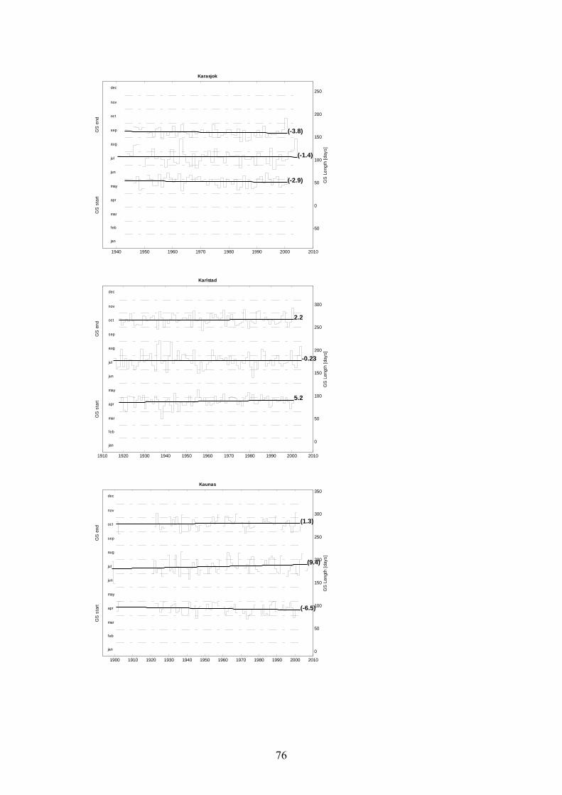
1940 1950 1960 1970 1980 1990 2000 2010

Karasjok

jan

feb

mar

apr

may

jun

jul

aug

sep

oct

nov

dec

GS

sta

rt

G

S e

nd

(-2.9)

(-3.8)

-50

0

50

100

150

200

250

GS

Len

gth

[day

s]

(-1.4)

1910 1920 1930 1940 1950 1960 1970 1980 1990 2000 2010

Karlstad

jan

feb

mar

apr

may

jun

jul

aug

sep

oct

nov

dec

GS

sta

rt

G

S e

nd

5.2

2.2

0

50

100

150

200

250

300

GS

Len

gth

[day

s]

-0.23

1900 1910 1920 1930 1940 1950 1960 1970 1980 1990 2000 2010

Kaunas

jan

feb

mar

apr

may

jun

jul

aug

sep

oct

nov

dec

GS

sta

rt

G

S e

nd

(-6.5)

(1.3)

0

50

100

150

200

250

300

350

GS

Len

gth

[day

s]

(9.4)

76

1880 1900 1920 1940 1960 1980 2000

Kazan

jan

feb

mar

apr

may

jun

jul

aug

sep

oct

nov

dec

GS

sta

rt

G

S e

nd

(-3.9)

(-3)

0

50

100

150

200

250

300

GS

Len

gth

[day

s]

(-0.54)

1910 1920 1930 1940 1950 1960 1970 1980 1990 2000 2010

Kem

jan

feb

mar

apr

may

jun

jul

aug

sep

oct

nov

dec

GS

sta

rt

G

S e

nd

-5.5

-1

-50

0

50

100

150

200

250

GS

Len

gth

[day

s]0.67

1880 1900 1920 1940 1960 1980 2000

Kirov

jan

feb

mar

apr

may

jun

jul

aug

sep

oct

nov

dec

GS

sta

rt

G

S e

nd

-11**

2.2

0

50

100

150

200

250

300

GS

Len

gth

[day

s]

13*

77

1950 1960 1970 1980 1990 2000 2010

Kjoeremsgrende

jan

feb

mar

apr

may

jun

jul

aug

sep

oct

nov

dec

GS

sta

rt

G

S e

nd

(-2)

(-2.7)

-50

0

50

100

150

200

250

300

GS

Len

gth

[day

s]

(-1.2)

1880 1900 1920 1940 1960 1980 2000

Koebenhavn

jan

feb

mar

apr

may

jun

jul

aug

sep

oct

nov

dec

GS

sta

rt

G

S e

nd

-22**

18**

0

50

100

150

200

250

300

350

GS

Len

gth

[day

s]

39**

1910 1920 1930 1940 1950 1960 1970 1980 1990 2000 2010

Kojnas

jan

feb

mar

apr

may

jun

jul

aug

sep

oct

nov

dec

GS

sta

rt

G

S e

nd

(-6.3)

(-0.87)

-50

0

50

100

150

200

250

GS

Len

gth

[day

s]

(1.9)

78

1920 1930 1940 1950 1960 1970 1980 1990 2000 2010

Kostroma

jan

feb

mar

apr

may

jun

jul

aug

sep

oct

nov

dec

GS

sta

rt

G

S e

nd

-7.6*

-3.2

0

50

100

150

200

250

300

GS

Len

gth

[day

s]

4.6

1930 1940 1950 1960 1970 1980 1990 2000 2010

Kotlas

jan

feb

mar

apr

may

jun

jul

aug

sep

oct

nov

dec

GS

sta

rt

G

S e

nd

-6.2

-4.2

-50

0

50

100

150

200

250

300

GS

Len

gth

[day

s]

0.18

1880 1900 1920 1940 1960 1980 2000

Liepaja

jan

feb

mar

apr

may

jun

jul

aug

sep

oct

nov

dec

GS

sta

rt

G

S e

nd

(1.3)

(13*)

0

50

100

150

200

250

300

GS

Len

gth

[day

s](10)

79

1930 1940 1950 1960 1970 1980 1990 2000 2010

Linkoeping

jan

feb

mar

apr

may

jun

jul

aug

sep

oct

nov

dec

GS

sta

rt

G

S e

nd

4.9

1.7

0

50

100

150

200

250

300

GS

Len

gth

[day

s]

-3.9

1930 1940 1950 1960 1970 1980 1990 2000 2010

Moermansk

jan

feb

mar

apr

may

jun

jul

aug

sep

oct

nov

dec

GS

sta

rt

G

S e

nd

(-10)

(-6.3)

-50

0

50

100

150

200

250

GS

Len

gth

[day

s](-0.94)

1950 1960 1970 1980 1990 2000 2010

Moskou

jan

feb

mar

apr

may

jun

jul

aug

sep

oct

nov

dec

GS

sta

rt

G

S e

nd

0.22

-9.2

0

50

100

150

200

250

300

GS

Len

gth

[day

s]

-10

80

1940 1950 1960 1970 1980 1990 2000 2010

Nesbyen-skoglund

jan

feb

mar

apr

may

jun

jul

aug

sep

oct

nov

dec

GS

sta

rt

G

S e

nd

-0.48

1.1

0

50

100

150

200

250

300

GS

Len

gth

[day

s]

5.1

1880 1900 1920 1940 1960 1980 2000

Nordby

jan

feb

mar

apr

may

jun

jul

aug

sep

oct

nov

dec

GS

sta

rt

G

S e

nd

-17**

4.4

0

50

100

150

200

250

300

350

GS

Len

gth

[day

s]

22**

1910 1920 1930 1940 1950 1960 1970 1980 1990 2000 2010

Oestersund

jan

feb

mar

apr

may

jun

jul

aug

sep

oct

nov

dec

GS

sta

rt

G

S e

nd

-3.5

0.35

-50

0

50

100

150

200

250

300

GS

Len

gth

[day

s]

2.7

81

1930 1940 1950 1960 1970 1980 1990 2000 2010

Onega

jan

feb

mar

apr

may

jun

jul

aug

sep

oct

nov

dec

GS

sta

rt

G

S e

nd

-3

-1.1

-50

0

50

100

150

200

250

GS

Len

gth

[day

s]7.2

1930 1940 1950 1960 1970 1980 1990 2000 2010

Oslo-blindern

jan

feb

mar

apr

may

jun

jul

aug

sep

oct

nov

dec

GS

sta

rt

G

S e

nd

-0.32

1.6

0

50

100

150

200

250

300

GS

Len

gth

[day

s]

2.3

1930 1940 1950 1960 1970 1980 1990 2000 2010

Petrozawodsk

jan

feb

mar

apr

may

jun

jul

aug

sep

oct

nov

dec

GS

sta

rt

G

S e

nd

(1.7)

(-0.029)

-50

0

50

100

150

200

250

300

GS

Len

gth

[day

s]

(-1.5)

82

1930 1940 1950 1960 1970 1980 1990 2000 2010

Pskow

jan

feb

mar

apr

may

jun

jul

aug

sep

oct

nov

dec

GS

sta

rt

G

S e

nd

(-6.9)

(2.9)

0

50

100

150

200

250

300

GS

Len

gth

[day

s]

(9.9)

1940 1950 1960 1970 1980 1990 2000 2010

Sortavala

jan

feb

mar

apr

may

jun

jul

aug

sep

oct

nov

dec

GS

sta

rt

G

S e

nd

-2.9

-0.42

0

50

100

150

200

250

300

GS

Len

gth

[day

s]

5.2

1910 1920 1930 1940 1950 1960 1970 1980 1990 2000 2010

Stensele

jan

feb

mar

apr

may

jun

jul

aug

sep

oct

nov

dec

GS

sta

rt

G

S e

nd

-7.5*

7.7*

-50

0

50

100

150

200

250

GS

Len

gth

[day

s]15**

83

1750 1800 1850 1900 1950 2000

Stockholm

jan

feb

mar

apr

may

jun

jul

aug

sep

oct

nov

dec

GS

sta

rt

G

S e

nd

-1.4

7.6**

0

50

100

150

200

250

300

GS

Len

gth

[day

s]8.4*

1750 1800 1850 1900 1950 2000

St-petersburg

jan

feb

mar

apr

may

jun

jul

aug

sep

oct

nov

dec

GS

sta

rt

G

S e

nd

(-9**)

(5.1)

0

50

100

150

200

250

300

GS

Len

gth

[day

s](16**)

1900 1920 1940 1960 1980 2000

Syktyvar

jan

feb

mar

apr

may

jun

jul

aug

sep

oct

nov

dec

GS

sta

rt

G

S e

nd

(-11*)

(-2.9)

-50

0

50

100

150

200

250

GS

Len

gth

[day

s]

(5.2)

84

1880 1900 1920 1940 1960 1980 2000

Tranebjerg

jan

feb

mar

apr

may

jun

jul

aug

sep

oct

nov

dec

GS

sta

rt

G

S e

nd

(-19**)

(15**)

0

50

100

150

200

250

300

350

GS

Len

gth

[day

s]

(33**)

1750 1800 1850 1900 1950 2000

Uppsala

jan

feb

mar

apr

may

jun

jul

aug

sep

oct

nov

dec

GS

sta

rt

G

S e

nd

-1.6

4.6*

0

50

100

150

200

250

300

GS

Len

gth

[day

s]6.6

1940 1950 1960 1970 1980 1990 2000 2010

Utsira-fyr

jan

feb

mar

apr

may

jun

jul

aug

sep

oct

nov

dec

GS

sta

rt

G

S e

nd

-1.4

-3.5

0

50

100

150

200

250

300

350

GS

Len

gth

[day

s]5.6

85

1910 1920 1930 1940 1950 1960 1970 1980 1990 2000 2010

Vaexjoe

jan

feb

mar

apr

may

jun

jul

aug

sep

oct

nov

dec

GS

sta

rt

G

S e

nd

-3.6

4.4

0

50

100

150

200

250

300

350

GS

Len

gth

[day

s]8.7

1950 1960 1970 1980 1990 2000 2010

Vardoe

jan

feb

mar

apr

may

jun

jul

aug

sep

oct

nov

dec

GS

sta

rt

G

S e

nd

-2.5

7.6

-100

-50

0

50

100

150

200

250

GS

Len

gth

[day

s]11

1880 1900 1920 1940 1960 1980 2000

Velikie

jan

feb

mar

apr

may

jun

jul

aug

sep

oct

nov

dec

GS

sta

rt

G

S e

nd

(-2.9)

(-2)

0

50

100

150

200

250

300

GS

Len

gth

[day

s]

(0.25)

86

1880 1900 1920 1940 1960 1980 2000

Vestervig

jan

feb

mar

apr

may

jun

jul

aug

sep

oct

nov

dec

GS

sta

rt

G

S e

nd

-19**

12**

0

50

100

150

200

250

300

350

GS

Len

gth

[day

s]

36**

1880 1900 1920 1940 1960 1980 2000

Vilnjus

jan

feb

mar

apr

may

jun

jul

aug

sep

oct

nov

dec

GS

sta

rt

G

S e

nd

(3.2)

(4.6)

0

50

100

150

200

250

300

GS

Len

gth

[day

s]

(3.5)

1920 1930 1940 1950 1960 1970 1980 1990 2000 2010

Vilsandi

jan

feb

mar

apr

may

jun

jul

aug

sep

oct

nov

dec

GS

sta

rt

G

S e

nd

(-4)

(7.3)

0

50

100

150

200

250

300

GS

Len

gth

[day

s](12)

87

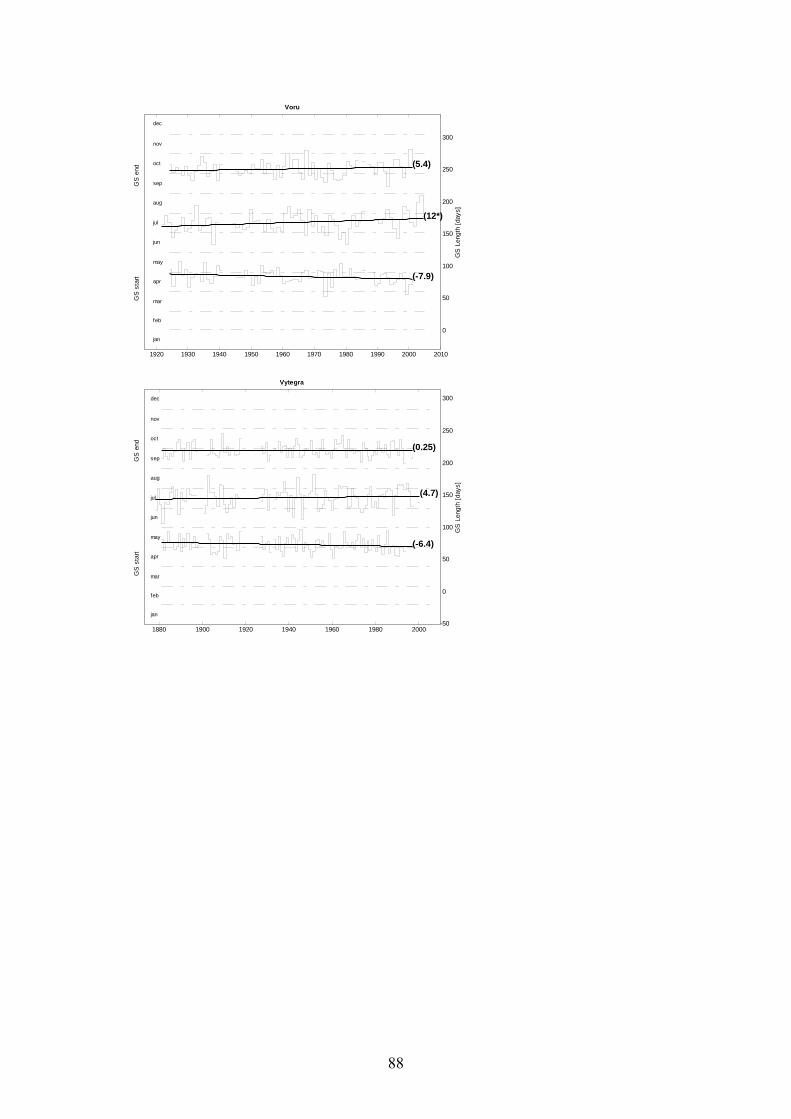
1920 1930 1940 1950 1960 1970 1980 1990 2000 2010

Voru

jan

feb

mar

apr

may

jun

jul

aug

sep

oct

nov

dec

GS

sta

rt

G

S e

nd

(-7.9)

(5.4)

0

50

100

150

200

250

300

GS

Len

gth

[day

s]

(12*)

1880 1900 1920 1940 1960 1980 2000

Vytegra

jan

feb

mar

apr

may

jun

jul

aug

sep

oct

nov

dec

GS

sta

rt

G

S e

nd

(-6.4)

(0.25)

-50

0

50

100

150

200

250

300

GS

Len

gth

[day

s]

(4.7)

88