Greenhouse climate control In simulation and in reality

Feije de Zwart - May 2021

- 1 -

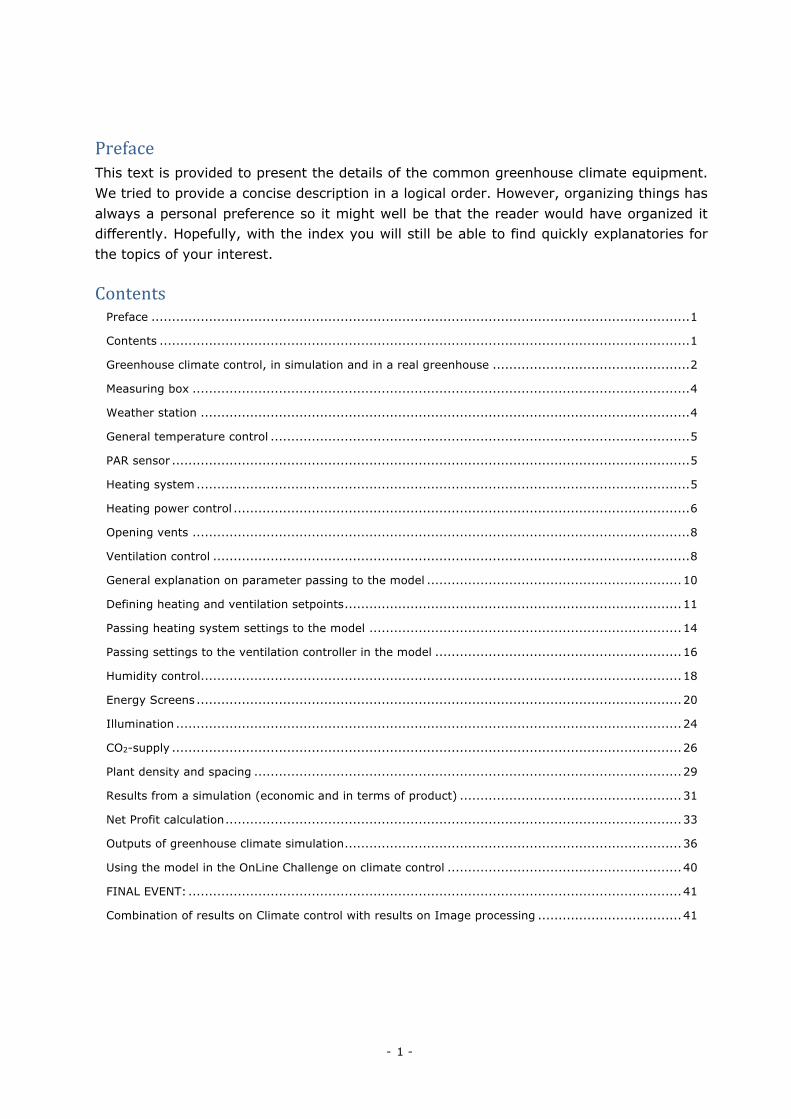
PrefaceThis text is provided to present the details of the common greenhouse climate equipment. We tried to provide a concise description in a logical order. However, organizing things has always a personal preference so it might well be that the reader would have organized it differently. Hopefully, with the index you will still be able to find quickly explanatories for the topics of your interest.

ContentsPreface ................................................................................................................................... 1

Contents ................................................................................................................................. 1

Greenhouse climate control, in simulation and in a real greenhouse ................................................ 2

Measuring box ......................................................................................................................... 4

Weather station ....................................................................................................................... 4

General temperature control ...................................................................................................... 5

PAR sensor .............................................................................................................................. 5

Heating system ........................................................................................................................ 5

Heating power control ............................................................................................................... 6

Opening vents ......................................................................................................................... 8

Ventilation control .................................................................................................................... 8

General explanation on parameter passing to the model .............................................................. 10

Defining heating and ventilation setpoints .................................................................................. 11

Passing heating system settings to the model ............................................................................ 14

Passing settings to the ventilation controller in the model ............................................................ 16

Humidity control ..................................................................................................................... 18

Energy Screens ...................................................................................................................... 20

Illumination ........................................................................................................................... 24

CO2-supply ............................................................................................................................ 26

Plant density and spacing ........................................................................................................ 29

Results from a simulation (economic and in terms of product) ...................................................... 31

Net Profit calculation ............................................................................................................... 33

Outputs of greenhouse climate simulation .................................................................................. 36

Using the model in the OnLine Challenge on climate control ......................................................... 40

FINAL EVENT: ........................................................................................................................ 41

Combination of results on Climate control with results on Image processing ................................... 41

- 2 -

Greenhouseclimatecontrol,insimulationandinarealgreenhouseThe inside climate of modern greenhouses can be controlled to a large extent, but is still quite dependent on outside weather conditions. This is due to the highly transparent and (therefore) poorly insulating enclosure. These properties of the enclosure give large amounts of free solar energy for growth of the crop. The disadvantage, however is that it needs quite some heating during cold days and the dependency on solar radiation results for cold climate condtions in large day-to-day variation. Sunny days can easily be followed by a number of dull days, and in summer the availability of light is a lot higher than in winter. Still, this abundant amount of light, entering the greenhouse in summer for free, in general outweighs these disadvantages. However, for a grower it needs growing skills to manage the crop growth in such varying conditions and it needs technical skills to make as much as possible use of this solar energy for the greenhouse climate control.

Experienced growers manage quite well to perform this complex task. However, it is likely that with the aid of Artificial Intelligence, this complex task can even be performed better. Once Artificial Intelligence shows to be capable of doing the job, progress will be made in the production of greenhouse products in a sustainable way.

In the 3rd International Autonomous Greenhouse Challenge, contesters are challenged to show the achievements that can be realised today and will throw light on the possibilities of tomorrow. In the Greenhouse Growing Challenge in 2022, five teams will have to define the growing conditions in a greenhouse compartment in such a way that a lettuce crop gives a good production at affordable expenses on commodities like heat, electricity CO2. These commodities will be used by the greenhouse controller that realizes the setpoints for climate, screens, CO2, and lighting. The goal will be to define optimised setpoints for the greenhouse climate computer in a feed-back loop between greenhouse climate, outside weather conditions and crop development. Next to the day-to-day control, the algorithm will have to decide on the spacing of the crop. Modern lettuce growing is a continuous process where in principle every day new young plants are planted, and ready-to-sell heads of lettuce are harvested. In the Greenhouse Growing Challenge, the greenhouse crop growing will consist of two unique crop cyles in time. Decisions taken cannot be undone and the crop will grow with its history included.

In this OnLine challenge, the lettuce cultivation is described by a deterministic model, provided with a number of fixed sets of weather data, which allows for repeated simulations and hence an iterative procedure that may find the best possible control sequence. The simulation model provides a realistic dynamic behaviour of the greenhouse climate as a result of the outside weather and the actions taken by the greenhouse climate controller and computes the resulting growth of the lettuce crop. To do so, the simulation model has a description of the physics that govern the greenhouse climate, a model that describes crop growth and a close to common practice version of a modern greenhouse climate controller. This means that the interface between the greenhouse simulation model and the greenhouse

- 3 -

operator in a way very similar to a real greenhouse. Control of actuators is similar, and the physical limitations of an actual greenhouse are close to practice.

This paper describes how common greenhouse climate computers control a greenhouse. And due to the large resemblance between model and reality, by describing how greenhouse control works in a real greenhouse, it describes the working of the simulated greenhouse as well. The big difference, of course, is that the result of settings for a 6-weeks lettuce growing cycle in the OnLine simulation will give a result in about 6 seconds. This gives teams the opportunity to test and refine their approach.

The simulation can be performed by sending a json-file with all the controls to a web service. After a few seconds, the web-service will respond with a json file containing the results of the simulation in the form of some 30 variables showing the greenhouse climate and crop results on an hour-to-hour time base. Also, the computed net profit as a result of the expenses on commodities and greenhouse surface occupation and the revenue from the crop is provided as a result of the simulation. In the following, all sensors and actuators of the greenhouse compartment that will be used in the eventual challenge are described, together with the interface that controls the actuators.

- 4 -

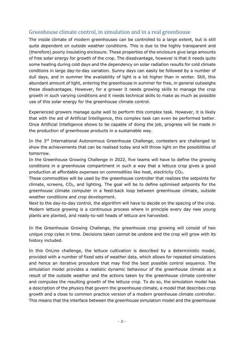
MeasuringboxGreenhouse air temperature and humidity is considered to be the most important factor to steer the crop development. Although everyone is aware of the fact that there is no such thing as one greenhouse temperature, but rather a wide distribution of temperatures around an average value, in most greenhouses, no attempt is made to measure with a large grid of sensors. Most of the time, up to maximum three sensors are used per temperature control group. Sometimes growers hang them on the same height at different places in a greenhouse section to get an idea of horizontal distribution. However, in the greenhouse compartments used in the challenge, only one measuring box is available.

It is an aspirated measuring box (e.g. picture at the right). Without such an aspirator that constantly refreshes the air in the box, the readings of air temperature of sunlit boxes would be easily be some 5 °C higher in sunlit boxes. In general, the sensor box also includes also a humidity sensor and one of the boxes will also contain a CO2 sensor. In the simulated greenhouse the readings of the measuring box appear as ‘comp1_Air_T’ for the air temperature as ‘comp1_Air_RH’ for the relative humidity of the air and 'comp1_Air_ppm' for the CO2-concentration.

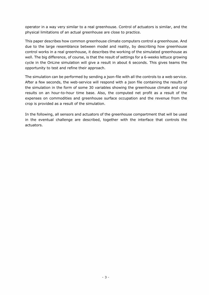
WeatherstationBecause of the transparent and poorly insulated character of the greenhouse enclosure, the outside conditions have a strong influence on the inner climate. Also, the amount of solar light, driving the photosynthesis, influences the temperature that one wants to achieve in the greenhouse. In general, more light for the crop means that a higher temperature should be achieved.

To act pro-actively or to include feed forward control every modern greenhouse has a weather station. The weather station measures solar radiation, outside air temperature and humidity and wind speed and wind direction. Also, rain is detected and sometimes the weather station has a pyrgeometer that measures the radiative loss (quite different for a clear sky or (party) overcast sky). The pyrgeometer-reading is sometimes used to influence the screening (see section ‘screening’).

In the simulated greenhouse, the weather data are deterministic, and therefore every run will get the same weather data. The data from the meteo station appear as 'common_Iglob_Value', 'common_Tout_Value', 'common_RHout_Value', ‘common_Windsp_Value' and 'common_Tsky_Value'. These data are provided predominantly as a background that may help to better understand the greenhouse climate. However, as will be explained later, some controllers may be parameterised such that they respond to outside conditions like radiation, wind speed and temperature.

T, RH and CO2

- 5 -

GeneraltemperaturecontrolThe greenhouse temperature is controlled by comparing the measured temperature with a setpoint, as defined by the grower (see section ‘setpoint’). In general, there is a setpoint for heating and, a few degrees higher, a setpoint for ventilation (venting). This dead zone between heating and venting setpoint prevents that the controller is accidently heating and cooling at the same time. Another, and probably more important reason is that a cooling demand generally coincides with abundant radiation and, as said earlier, more light requires a higher temperature. By creating a dead zone between the heating and venting setpoint some implicit correlation between light and temperature is created.

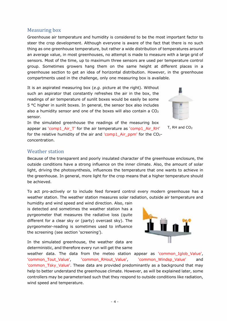
PARsensorLight, and more precisely PAR-light (Photosynthetically Active Radiation) is the base of biomass production. Photons with a wavelength of 700 through 400 nm trigger a biochemical reaction that removes the C-atoms from CO2 and bind it to hydrogen to form carbohydrates (H2O + CO2 = CH2O + O2). The more photons per second, the faster the reaction, until it reaches limits in the cascade of the supply of CO2 and water to the leaves and other nutrients that play a role in the formation of sugars.

Because of the importance of PAR as a driving force for plant growth, greenhouses keep track of the PAR-level by measuring the photon flux density, expressed in µmol/(m² s). The intensity may reach 1000 to 1200 µmol/(m² s). Suppose the average PAR-intensity is 500 µmol/(m² s) for 12 hours a day, the integral PAR-sum is 12*3600*500=21.6·106 µmol/(m² day) = 21.6 mol/(m² day). Such numbers are common for sunny days. In the midst of summer, with long sunny days, the PAR-sum inside the greenhouse may reach 30 mol/(m² day).

In the simulated greenhouse, a PAR sensor is modelled to describe the PAR-level just above the crop. It appears as 'comp1_PARsensor_Above' in the simulation results and it shows the PAR-radiation to which the crop is exposed.

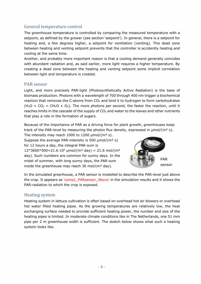
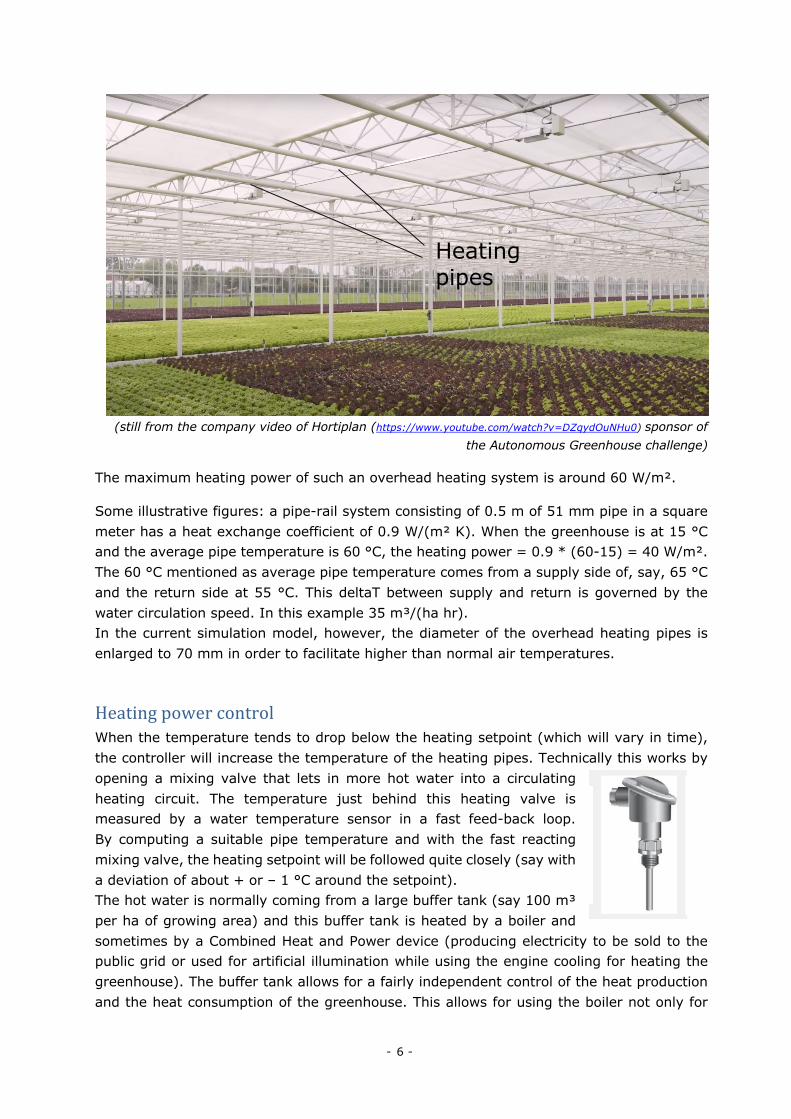
HeatingsystemHeating system in lettuce cultivation is often based on overhead hot air blowers or overhead hot water filled heating pipes. As the growing temperatures are relatively low, the heat exchanging surface needed to provide sufficient heating power, the number and size of the heating pipes is limited. In moderate climate conditions like in The Netherlands, one 51 mm pipe per 2 m greenhouse width is sufficient. The sketch below shows what such a heating system looks like.

PAR sensor

- 6 -

(still from the company video of Hortiplan (https://www.youtube.com/watch?v=DZqydOuNHu0) sponsor of

the Autonomous Greenhouse challenge)

The maximum heating power of such an overhead heating system is around 60 W/m².

Some illustrative figures: a pipe-rail system consisting of 0.5 m of 51 mm pipe in a square meter has a heat exchange coefficient of 0.9 W/(m² K). When the greenhouse is at 15 °C and the average pipe temperature is 60 °C, the heating power = 0.9 * (60-15) = 40 W/m². The 60 °C mentioned as average pipe temperature comes from a supply side of, say, 65 °C and the return side at 55 °C. This deltaT between supply and return is governed by the water circulation speed. In this example 35 m³/(ha hr). In the current simulation model, however, the diameter of the overhead heating pipes is enlarged to 70 mm in order to facilitate higher than normal air temperatures.

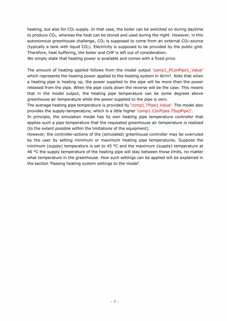
HeatingpowercontrolWhen the temperature tends to drop below the heating setpoint (which will vary in time), the controller will increase the temperature of the heating pipes. Technically this works by opening a mixing valve that lets in more hot water into a circulating heating circuit. The temperature just behind this heating valve is measured by a water temperature sensor in a fast feed-back loop. By computing a suitable pipe temperature and with the fast reacting mixing valve, the heating setpoint will be followed quite closely (say with a deviation of about + or – 1 °C around the setpoint). The hot water is normally coming from a large buffer tank (say 100 m³ per ha of growing area) and this buffer tank is heated by a boiler and sometimes by a Combined Heat and Power device (producing electricity to be sold to the public grid or used for artificial illumination while using the engine cooling for heating the greenhouse). The buffer tank allows for a fairly independent control of the heat production and the heat consumption of the greenhouse. This allows for using the boiler not only for

Heating pipes

- 7 -

heating, but also for CO2 supply. In that case, the boiler can be switched on during daytime to produce CO2, whereas the heat can be stored and used during the night. However, in this autonomous greenhouse challenge, CO2 is supposed to come from an external CO2-source (typically a tank with liquid CO2). Electricity is supposed to be provided by the public grid. Therefore, heat buffering, the boiler and CHP is left out of consideration. We simply state that heating power is available and comes with a fixed price. The amount of heating applied follows from the model output ’comp1_PConPipe1_Value’ which represents the heating power applied to the heating system in W/m². Note that when a heating pipe is heating up, the power supplied to the pipe will be more than the power released from the pipe. When the pipe cools down the reverse will be the case. This means that in the model output, the heating pipe temperature can be some degrees above greenhouse air temperature while the power supplied to the pipe is zero. The average heating pipe temperature is provided by ‘comp1.TPipe1.Value’. The model also provides the supply-temperature, which is a little higher ‘comp1.ConPipes.TSupPipe1’. In principle, the simulation model has its own heating pipe temperature controller that applies such a pipe temperature that the requested greenhouse air temperature is realized (to the extent possible within the limitations of the equipment). However, the controller-actions of the (simulated) greenhouse controller may be overruled by the user by setting minimum or maximum heating pipe temperatures. Suppose the minimum (supply) temperature is set to 45 °C and the maximum (supply) temperature at 46 °C the supply temperature of the heating pipe will stay between those limits, no matter what temperature in the greenhouse. How such settings can be applied will be explained in the section ‘Passing heating system settings to the model’.

- 8 -

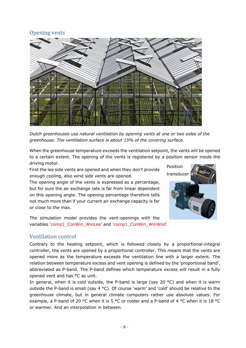
Openingvents

Dutch greenhouses use natural ventilation by opening vents at one or two sides of the greenhouse. The ventilation surface is about 15% of the covering surface.

When the greenhouse temperature exceeds the ventilation setpoint, the vents will be opened to a certain extent. The opening of the vents is registered by a position sensor inside the driving motor. First the lee side vents are opened and when they don’t provide enough cooling, also wind side vents are opened. The opening angle of the vents is expressed as a percentage, but for sure the air exchange rate is far from linear dependent on this opening angle. The opening percentage therefore tells not much more than if your current air exchange capacity is far or close to the max.

The simulation model provides the vent-openings with the variables ‘comp1_ConWin_WinLee’ and ‘comp1_ConWin_WinWnd’

VentilationcontrolContrary to the heating setpoint, which is followed closely by a proportional-integral controller, the vents are opened by a proportional controller. This means that the vents are opened more as the temperature exceeds the ventilation line with a larger extent. The relation between temperature excess and vent opening is defined by the ‘proportional band’, abbreviated as P-band. The P-band defines which temperature excess will result in a fully opened vent and has °C as unit. In general, when it is cold outside, the P-band is large (say 20 °C) and when it is warm outside the P-band is small (say 4 °C). Of course ‘warm’ and ‘cold’ should be relative to the greenhouse climate, but in general climate computers rather use absolute values. For example, a P-band of 20 °C when it is 5 °C or colder and a P-band of 4 °C when it is 18 °C or warmer. And an interpolation in between.

Position

transducer

sensor

- 9 -

To make it even more complicated, the P-band will in general be enlarged at increasing wind speed (say 0.5 °C for every m/s that it exceeds 6 m/s). As can be understood from the description above, most greenhouse climate computers do not put any (artificial) intelligence in the control of opening aperture of the vents. This is remarkable, since the state-of-the-art computers do have quite sophisticated, self-tuning algorithms for the heating control. Probably an explanation for this is that growers can define quite well their minimum temperature but feel less confident about suitable temperatures during periods of high radiation. Therefore, they want that the climate computer takes some action when the temperature exceeds the ventilation setpoint, but accept that they don’t know how all their settings on the venting exactly result in a certain air temperature during sunny days.

And on top of this, a proportional controller gives less risks on oscillatory behaviour of the actuators (in this case the vents).

Because of the proportional control of the vents, and because of the dead zone between the heating and ventilation setpoint, the actual and average temperature in a greenhouse, even for modern well automated greenhouses, is not straightforward related to the setpoints for heating and ventilation. Probably, in near future, when artificial intelligence will be capable to define better which exact course of temperature should be achieved, growers will be relieved from the large amount of settings associated with the control of vents. In the OnLine challenge we will stay close to common practice so, you will still have to set (simplified) settings for the P-band (see ‘Passing settings to the ventilation controller in the model’).

- 10 -

GeneralexplanationonparameterpassingtothemodelIn the following text all parameters that are used by the model will be discussed in detail, clarified with some snippets of json-strings. Among the documentation on the OnLine challenge, a complete sample json-file will be provided where you will find all snippets discussed in an aggregated form. The example shows the data types. Many figures are just numbers. Some parameters are logicals and are clearly shown as true of false in the examples. Then there are parameters that have to be entered as strings, recognizable by double quotes “ ” around them. Sometimes you will see arrays which are shown as series of numbers surrounded with double quote “ ”. Where an array represents a table, you will see semi-colons (;) marking new lines. Sometimes tables are interpolated and sometimes a table represent step functions. This is everywhere clarified in the documentation (but can actually also be guessed giving the purpose of the table). Interfacing with the server is done by sending a web-request. When we use Matlab2018 to process the web-request it looks like:

key = 'C03A-WXaB-Aj1B-ZgaH-KQS9'; %(this is just an example) url = 'https://www.digigreenhouse.wur.nl/Kasprobeta/model.aspx'; opt = weboptions('Timeout',300,'ContentType','json','RequestMethod','post'); Res = webwrite(url,'key',key, 'parameters', param, opt);

Note that the key shown is just a sample key, each team during the challenge will have two different keys. Your keys will be made available through the

challenge website . In this piece of sample code, param is a json string that contains all the model parameters, which will be discussed in the following pages. The response of the model is a json structure with the simulation model results, see section ‘Modelresults’. The input json-string has a large number of sections that can be placed in arbitrary order. The first (small) section describes the end date of the simulation. “simset" : { "@endDate" : "15-04-2021" } Note that there is an endDate, but no startDate. This is because in order to have a level playing field, all teams will have to start their simulation on the same date, March 4th 2021. The model assumes that the start date corresponds to the planting date of the crop. At the @endDate, the lettuce is harvested and sold according to the value of the lettuce in its state at that time. An early endDate will lead to lower costs on commodities and greenhouse space, but also to al lower value of the crop as the lettuce might have a low plant weight.

- 11 -

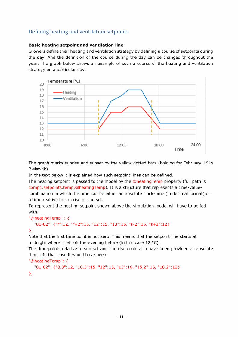
Definingheatingandventilationsetpoints Basic heating setpoint and ventilation line Growers define their heating and ventilation strategy by defining a course of setpoints during the day. And the definition of the course during the day can be changed throughout the year. The graph below shows an example of such a course of the heating and ventilation strategy on a particular day.

The graph marks sunrise and sunset by the yellow dotted bars (holding for February 1st in Bleiswijk). In the text below it is explained how such setpoint lines can be defined. The heating setpoint is passed to the model by the @heatingTemp property (full path is comp1.setpoints.temp.@heatingTemp). It is a structure that represents a time-value- combination in which the time can be either an absolute clock-time (in decimal format) or a time realtive to sun rise or sun set. To represent the heating setpoint shown above the simulation model will have to be fed with. "@heatingTemp" : { "01-02": {"r":12, "r+2":15, "12":15, "13":16, "s-2":16, "s+1":12} }, Note that the first time point is not zero. This means that the setpoint line starts at midnight where it left off the evening before (in this case 12 °C). The time-points relative to sun set and sun rise could also have been provided as absolute times. In that case it would have been: "@heatingTemp": { "01-02": {"8.3":12, "10.3":15, "12":15, "13":16, "15.2":16, "18.2":12} },

- 12 -

but of course, if you want to respond to the varying rise and set times, the definition will have to be changed, say every week "@heatingTemp" : { "01-02": {"8.3":12, "10.3":15, "12":15, "13":16, "15.2":16, "18.2":12}, "08-02": {"8.1":12, "10.1":15, "12":15, "13":16, "15.5":16, "18.5":12}, "15-02": {"7.9":12, "9.9":15, "12":15, "13":16, "15.7":16, "18.7":12} }, Note that the date-specifier needs to be in the format dd-mm. The model continues with the latest specified date, so if only the three above mentioned lines would be applied the model would continue with the line defined for 15 February for the rest of the simulation period. Also be aware that the time values are in ascending order. So especially when you use a mixture of times relative to sunset or sunrise and absolute times, times might unintendently start to overlap. In case this happens, the model exits with an error code like: responsecode: 3 responsemsg:'Cannot parse value [17] of parameter [comp1.setpoints.temp.@heatingTemp] to a floatParameter x-values are not increasing, probably due to sun rise and set [{"r+0": 17, "r+2": 19, "12.0": 19, "13.0": 20, "s-2": 20, "s+1": 16, "21.0": 16, "23.0": 17}]' If you want to work with only one setting for the whole year (which is quite unlikely, but may be useful in a first exercise) you simply provide one line and set the date specifier at "01-01". As always, there will be limitations in the number of rows that can be passed, however, we have tested with a maximum of 50 rows, which has not given problems. Also entering 24 time-value combinations in a row (each hour another value) has not given problems. We have to admit that we don’t have tried to push it to the maximum yet. In the current model, the ventilation line is defined as an offset relative to the heating setpoint. In the graph shown, the ventilation line is 1 °C above the heating setpoint in the night period and 2 to 3 °C higher during day time. This offset is described by the @ventOffset property (full path is comp1.setpoints.temp.@ventOffset). Also this ventilation offset can be time-varying and date varying. The profile above can be described by: "@ventOffset" : { "01-01": {"r":1, "r+2":2, "12":3, "s-2":3, "s+1":1} }, Note that in this example I have set only one line, dated “01-01” which means that this offset will be applied all the time.

- 13 -

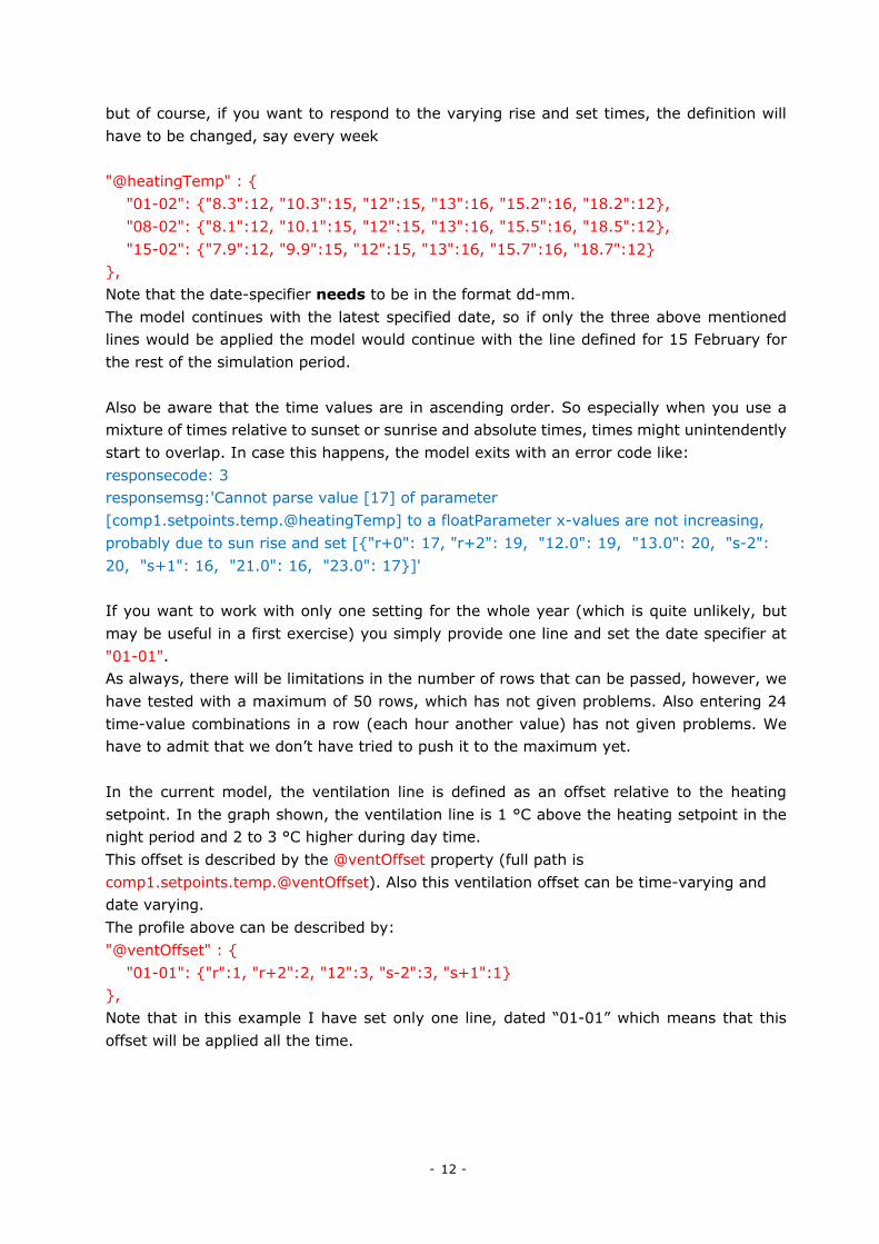
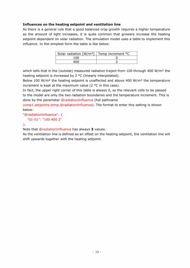
Influences on the heating setpoint and ventilation line As there is a general rule that a good balanced crop growth requires a higher temperature as the amount of light increases, it is quite common that growers increase the heating setpoint dependent on solar radiation. The simulation model uses a table to implement this influence. In the simplest form the table is like below:

Solar radiation [W/m²] Temp increment °C

100 0 400 2

which tells that in the (outside) measured radiation traject from 100 through 400 W/m² the heating setpoint is increased by 2 °C (linearly interpolated). Below 100 W/m² the heating setpoint is unaffected and above 400 W/m² the temperature increment is kept at the maximum value (2 °C in this case). In fact, the upper right corner of this table is always 0, so the relevant cells to be passed to the model are only the two radiation boundaries and the temperature increment. This is done by the parameter @radiationInfluence (full pathname comp1.setpoints.temp.@radiationInfluence). The format to enter this setting is shown below: "@radiationInfluence": { "01-01": "100 400 2" }, Note that @radiationInfluence has always 3 values. As the ventilation line is defined as an offset on the heating setpoint, the ventilation line will shift upwards together with the heating setpoint.

- 14 -

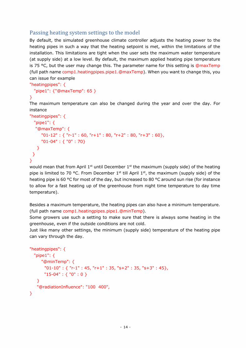
PassingheatingsystemsettingstothemodelBy default, the simulated greenhouse climate controller adjusts the heating power to the heating pipes in such a way that the heating setpoint is met, within the limitations of the installation. This limitations are tight when the user sets the maximum water temperature (at supply side) at a low level. By default, the maximum applied heating pipe temperature is 75 °C, but the user may change this. The parameter name for this setting is @maxTemp (full path name comp1.heatingpipes.pipe1.@maxTemp). When you want to change this, you can issue for example "heatingpipes": { "pipe1": {"@maxTemp": 65 } } The maximum temperature can also be changed during the year and over the day. For instance "heatingpipes": { "pipe1": { "@maxTemp": { "01-12" : { "r-1" : 60, "r+1" : 80, "r+2" : 80, "r+3" : 60}, "01-04" : { "0" : 70} } } } would mean that from April 1st until December 1st the maximum (supply side) of the heating pipe is limited to 70 °C. From December 1st till April 1st, the maximum (supply side) of the heating pipe is 60 °C for most of the day, but increased to 80 °C around sun rise (for instance to allow for a fast heating up of the greenhouse from night time temperature to day time temperature). Besides a maximum temperature, the heating pipes can also have a minimum temperature. (full path name comp1.heatingpipes.pipe1.@minTemp). Some growers use such a setting to make sure that there is always some heating in the greenhouse, even if the outside conditions are not cold. Just like many other settings, the minimum (supply side) temperature of the heating pipe can vary through the day. "heatingpipes": { "pipe1": { "@minTemp": { "01-10" : { "r-1" : 45, "r+1" : 35, "s+2" : 35, "s+3" : 45}, "15-04" : { "0" : 0 } } "@radiationInfluence": "100 400", }

- 15 -

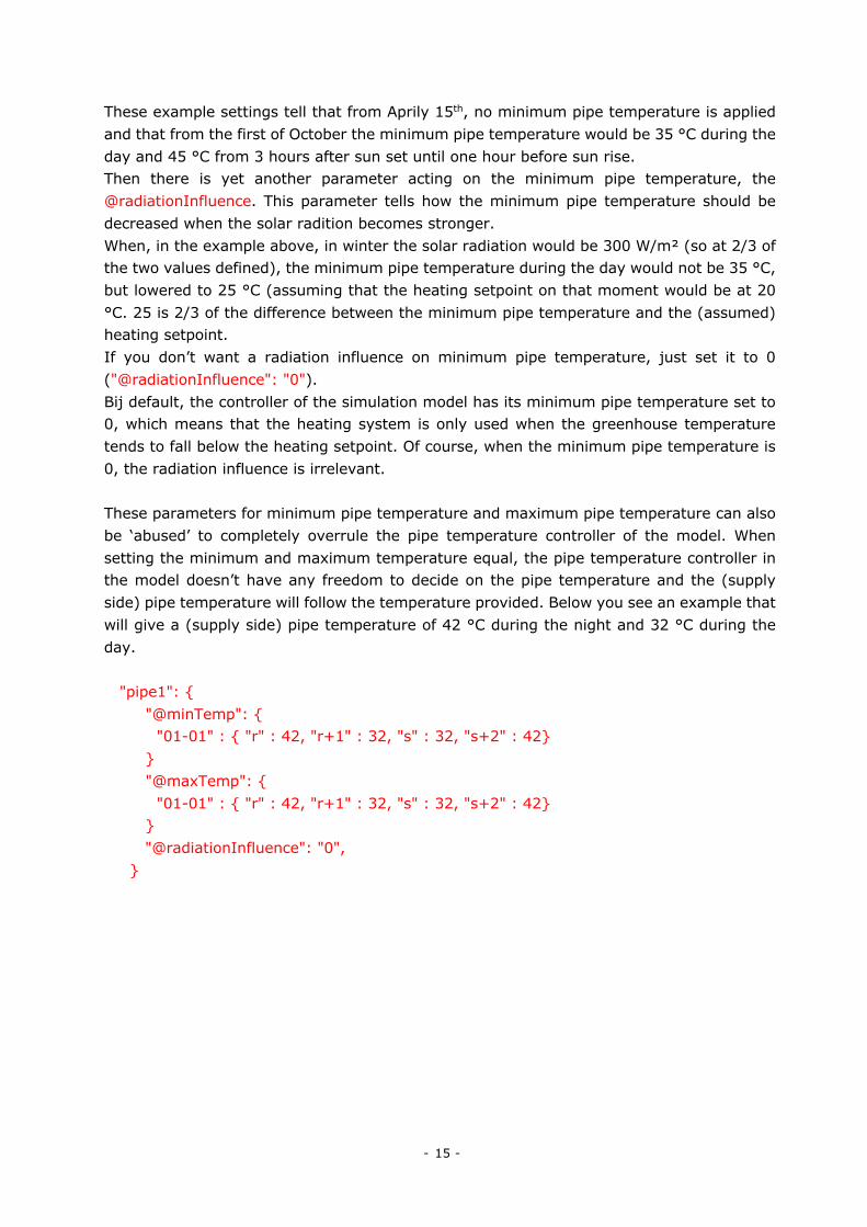
These example settings tell that from Aprily 15th, no minimum pipe temperature is applied and that from the first of October the minimum pipe temperature would be 35 °C during the day and 45 °C from 3 hours after sun set until one hour before sun rise. Then there is yet another parameter acting on the minimum pipe temperature, the @radiationInfluence. This parameter tells how the minimum pipe temperature should be decreased when the solar radition becomes stronger. When, in the example above, in winter the solar radiation would be 300 W/m² (so at 2/3 of the two values defined), the minimum pipe temperature during the day would not be 35 °C, but lowered to 25 °C (assuming that the heating setpoint on that moment would be at 20 °C. 25 is 2/3 of the difference between the minimum pipe temperature and the (assumed) heating setpoint. If you don’t want a radiation influence on minimum pipe temperature, just set it to 0 ("@radiationInfluence": "0"). Bij default, the controller of the simulation model has its minimum pipe temperature set to 0, which means that the heating system is only used when the greenhouse temperature tends to fall below the heating setpoint. Of course, when the minimum pipe temperature is 0, the radiation influence is irrelevant. These parameters for minimum pipe temperature and maximum pipe temperature can also be ‘abused’ to completely overrule the pipe temperature controller of the model. When setting the minimum and maximum temperature equal, the pipe temperature controller in the model doesn’t have any freedom to decide on the pipe temperature and the (supply side) pipe temperature will follow the temperature provided. Below you see an example that will give a (supply side) pipe temperature of 42 °C during the night and 32 °C during the day. "pipe1": { "@minTemp": { "01-01" : { "r" : 42, "r+1" : 32, "s" : 32, "s+2" : 42} } "@maxTemp": { "01-01" : { "r" : 42, "r+1" : 32, "s" : 32, "s+2" : 42} } "@radiationInfluence": "0", }

- 16 -

PassingsettingstotheventilationcontrollerinthemodelIn principle, the greenhouse controller opens the vents proportional to the temperature excess relative to the ventilation line. The key parameter here is the P-band, which tells how big the temperature excess has to be before the leeward vents are fully opened. Suppose the P-band is 6 °C, and the ventilation line is at 18 °C. Then, the leeward vents will be fully opened when the greenhouse is at 18+6=24 °C. When the greenhouse is 21 °C the vents will be opened halfway.

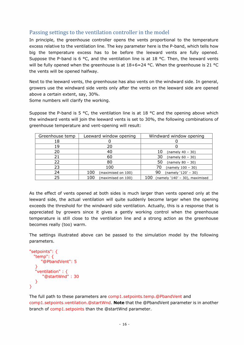
Next to the leeward vents, the greenhouse has also vents on the windward side. In general, growers use the windward side vents only after the vents on the leeward side are opened above a certain extent, say, 30%. Some numbers will clarify the working. Suppose the P-band is 5 °C, the ventilation line is at 18 °C and the opening above which the windward vents will join the leeward vents is set to 30%, the following combinations of greenhouse temperature and vent-opening will result:

Greenhouse temp Leeward window opening Windward window opening 18 0 0 19 20 0 20 40 10 (namely 40 – 30) 21 60 30 (namely 60 – 30) 22 80 50 (namely 80 – 30) 23 100 70 (namely 100 – 30) 24 100 (maximised on 100) 90 (namely ‘120’ – 30) 25 100 (maximised on 100) 100 (namely ‘140’ – 30), maximised

As the effect of vents opened at both sides is much larger than vents opened only at the leeward side, the actual ventilation will quite suddenly become larger when the opening exceeds the threshold for the windward side ventilation. Actually, this is a response that is appreciated by growers since it gives a gently working control when the greenhouse temperature is still close to the ventilation line and a strong action as the greenhouse becomes really (too) warm.

The settings illustrated above can be passed to the simulation model by the following parameters.

"setpoints": { "temp": { "@PbandVent": 5 } "ventilation" : { "@startWnd" : 30 } } The full path to these parameters are comp1.setpoints.temp.@PbandVent and comp1.setpoints.ventilation.@startWnd. Note that the @PbandVent parameter is in another branch of comp1.setpoints than the @startWnd parameter.

- 17 -

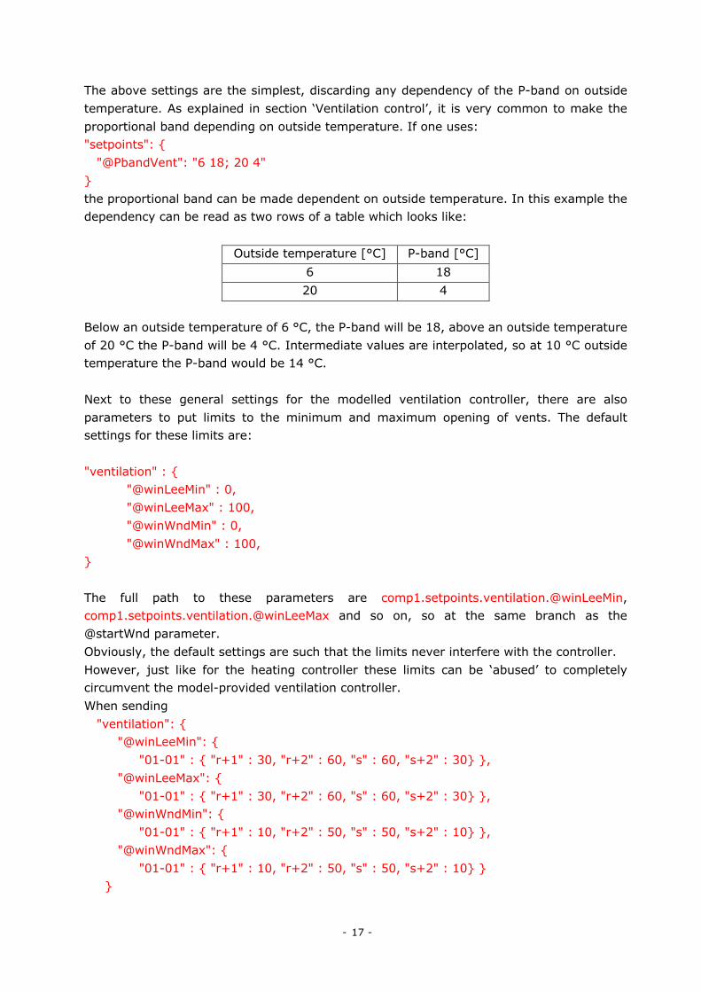
The above settings are the simplest, discarding any dependency of the P-band on outside temperature. As explained in section ‘Ventilation control’, it is very common to make the proportional band depending on outside temperature. If one uses: "setpoints": { "@PbandVent": "6 18; 20 4" } the proportional band can be made dependent on outside temperature. In this example the dependency can be read as two rows of a table which looks like:

Outside temperature [°C] P-band [°C] 6 18 20 4

Below an outside temperature of 6 °C, the P-band will be 18, above an outside temperature of 20 °C the P-band will be 4 °C. Intermediate values are interpolated, so at 10 °C outside temperature the P-band would be 14 °C. Next to these general settings for the modelled ventilation controller, there are also parameters to put limits to the minimum and maximum opening of vents. The default settings for these limits are: "ventilation" : {

"@winLeeMin" : 0, "@winLeeMax" : 100, "@winWndMin" : 0, "@winWndMax" : 100, } The full path to these parameters are comp1.setpoints.ventilation.@winLeeMin, comp1.setpoints.ventilation.@winLeeMax and so on, so at the same branch as the @startWnd parameter. Obviously, the default settings are such that the limits never interfere with the controller. However, just like for the heating controller these limits can be ‘abused’ to completely circumvent the model-provided ventilation controller. When sending "ventilation": { "@winLeeMin": { "01-01" : { "r+1" : 30, "r+2" : 60, "s" : 60, "s+2" : 30} }, "@winLeeMax": { "01-01" : { "r+1" : 30, "r+2" : 60, "s" : 60, "s+2" : 30} }, "@winWndMin": { "01-01" : { "r+1" : 10, "r+2" : 50, "s" : 50, "s+2" : 10} }, "@winWndMax": { "01-01" : { "r+1" : 10, "r+2" : 50, "s" : 50, "s+2" : 10} } }

- 18 -

the leeward vents will be opened for 30% during the night and for 60% during the day. The windward side vents will be opened for 10% during the night and 50% during the day. The 30% as a maximum opening for the leeward vents is the lowest possible value accepted by the model. For the windward side, 10% is the lowest maximum opening accepted. This means that one cannot force the model to keep its vents completely closed.

HumiditycontrolLight, temperature and CO2 are the main parameters for plant growth, together with nutrition of course. Humidity is an important climate factor as well, but more in an indirect way since it affects the risk on diseases. Unfortunately, the relation between humidity and disease is far from clear, but in general vegetable growers are feeling comfortable at growing at 85% relative humidity and 88% is considered to be high. Higher levels of humidity do not automatically mean that the crop is affected be diseases (especially fungi), but because the risk on such disease increases as humidity becomes higher, growers try to avoid such high moisture contents. Because in Dutch weather conditions the outside absolute humidity is practically always lower than the maximally accepted humidity of the greenhouse air, reducing the humidity can be achieved by opening the vents. Therefore, the opening of the vents is not only controlled by observing the temperature in the greenhouse, but also by observing the humidity. When the humidity exceeds a threshold (e.g. 87% RH), vents are opened with a proportional controller. Just like for temperature control, the proportional band for humidity control can be made dependent on outside temperature. At low outside temperatures, which go along with a low humidity of the outside air, vents are opened less at a certain humidity excess than at higher outside temperatures.

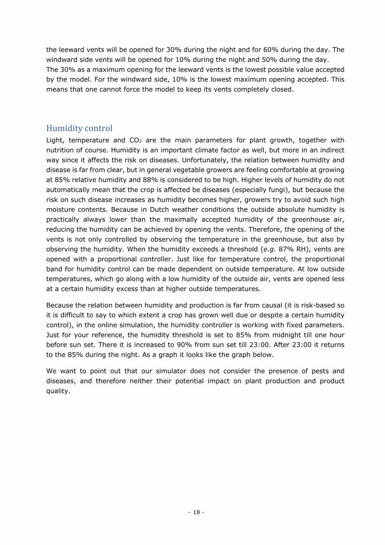
Because the relation between humidity and production is far from causal (it is risk-based so it is difficult to say to which extent a crop has grown well due or despite a certain humidity control), in the online simulation, the humidity controller is working with fixed parameters. Just for your reference, the humidity threshold is set to 85% from midnight till one hour before sun set. There it is increased to 90% from sun set till 23:00. After 23:00 it returns to the 85% during the night. As a graph it looks like the graph below.

We want to point out that our simulator does not consider the presence of pests and diseases, and therefore neither their potential impact on plant production and product quality.

- 19 -

When the greenhouse humidity exceeds the threshold, the vents will be opened in a proportional band being 15%-points at an outside temperature of 5 °C or lower and 5%-points at an outside temperature of 20 °C or higher, with interpolated values in between.

It is because of this humidity control that you may still find the vents opened to a certain extent during periods when the greenhouse air temperature is below the ventilation line.

Just like the case with ventilation on temperature, as the computed vent opening for the lee side vents exceeds the @startWnd setting windward side vents will start to join the leeward vents.

Control of vents on humidity is subject to the same settings for maximum opening as control vents on temperature.

- 20 -

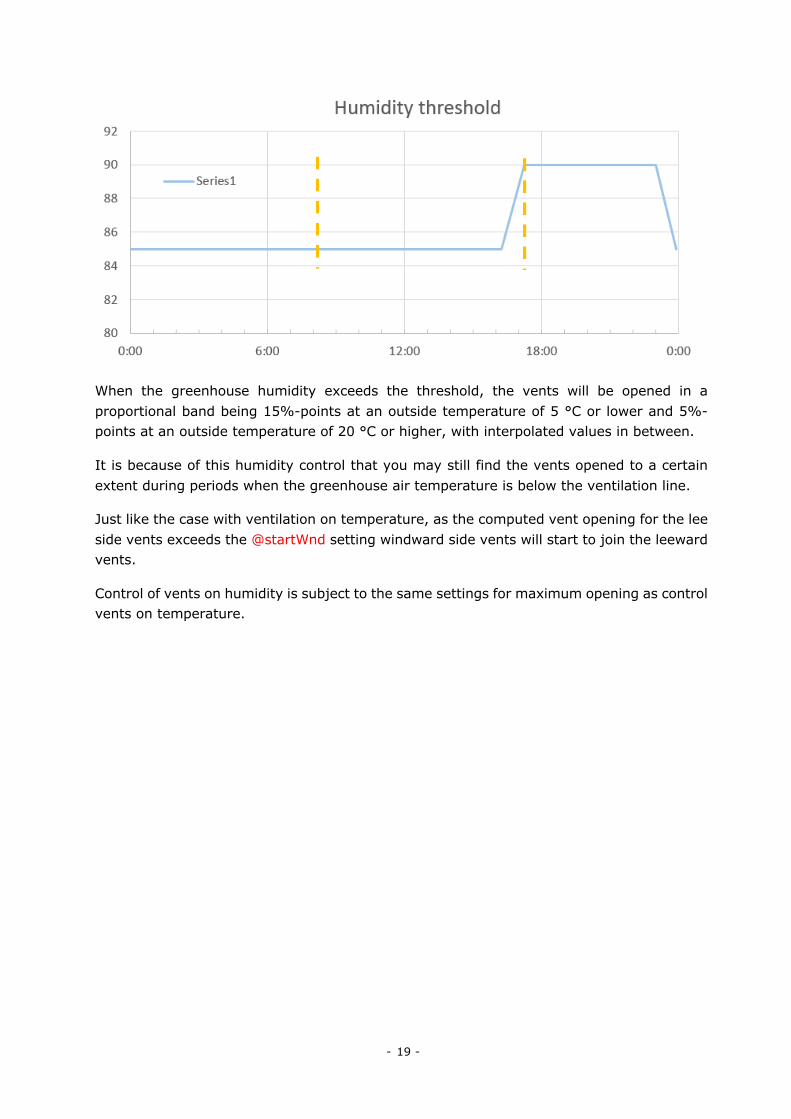
EnergyScreensTo reduce the energy consumption during cold nights greenhouses can be equipped with one, two or sometimes even three screens. Screens can also be used to reduce the light intensity on sunny days.

Greenhouse with two energy screens.

For different purposes there are different types of screens. There are typical energy saving screens to be used during daytime (transparent screens), screens to provide shade while keeping a good air permeability, and completely light-tight screens to be used in crops that require a carefully regulated day length. These blackout screens are also used prevent ‘light pollution’ to the environment when artificial illumination is on.

When using screens, the actual screen position is provided through the output variables ‘comp1_Scr1_Pos’ and ‘comp1_Scr2_Pos’.

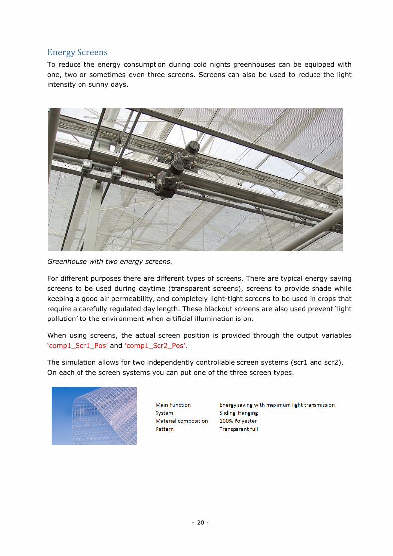
The simulation allows for two independently controllable screen systems (scr1 and scr2). On each of the screen systems you can put one of the three screen types.

- 21 -

To assign a certain screen type to a screen the following json-structure has to be applied:

"screens": { "scr1": { "@enabled": true, "@material": "scr_Blackout.par" }, "scr2": { "@enabled": true, "@material": "scr_Transparent.par" } } Of course, when the second screen would be equipped with a harmony screen the @material parameter would have been "@material": "scr_Shade.par". Note that the material descriptions are prefixed with ‘scr_’ and suffixed with ‘.par’.

With the "@enabled" parameter, screens can simply be enabled and disabled, which means that they will be added to or removed from the model. To control the screens, a number of parameters are available. Each screen system has the parameter "@ToutMax", which tells above what outside temperature the screen is not used. If you want to prevent a screen to be used in a certain period of the year, the easiest way is to set "@ToutMax" to e.g. -20 °C. In Bleiswijk the temperature never drops below that value so the screen will not be used. "@ToutMax": { "01-04" : -20, "01-09" : 15 } would practically mean that this particular screen is not used from April through September 1st.

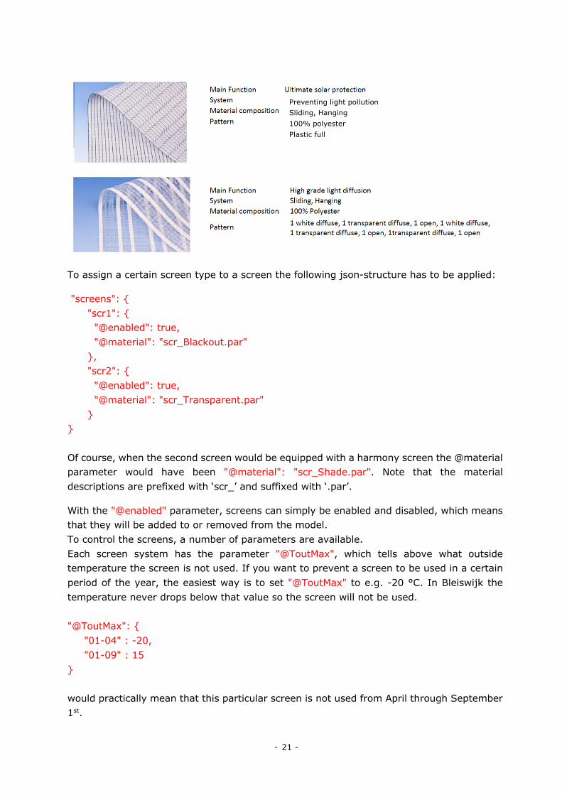
OBSCURA_9950_FR_W

Preventing light pollution Sliding, Hanging 100% polyester Plastic full

- 22 -

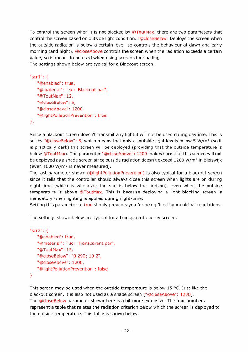
To control the screen when it is not blocked by @ToutMax, there are two parameters that control the screen based on outside light condition. "@closeBelow" Deploys the screen when the outside radiation is below a certain level, so controls the behaviour at dawn and early morning (and night). @closeAbove controls the screen when the radiation exceeds a certain value, so is meant to be used when using screens for shading. The settings shown below are typical for a Blackout screen. "scr1": { "@enabled": true, "@material": " scr_Blackout.par", "@ToutMax": 12, "@closeBelow": 5, "@closeAbove": 1200, "@lightPollutionPrevention": true }, Since a blackout screen doesn’t transmit any light it will not be used during daytime. This is set by "@closeBelow": 5, which means that only at outside light levels below 5 W/m² (so it is practically dark) this screen will be deployed (providing that the outside temperature is below @ToutMax). The parameter "@closeAbove": 1200 makes sure that this screen will not be deployed as a shade screen since outside radiation doesn’t exceed 1200 W/m² in Bleiswijk (even 1000 W/m² is never measured). The last parameter shown (@lightPollutionPrevention) is also typical for a blackout screen since it tells that the controller should always close this screen when lights are on during night-time (which is whenever the sun is below the horizon), even when the outside temperature is above @ToutMax. This is because deploying a light blocking screen is mandatory when lighting is applied during night-time. Setting this parameter to true simply prevents you for being fined by municipal regulations. The settings shown below are typical for a transparent energy screen. "scr2": { "@enabled": true, "@material": " scr_Transparent.par", "@ToutMax": 15, "@closeBelow": "0 290; 10 2", "@closeAbove": 1200, "@lightPollutionPrevention": false } This screen may be used when the outside temperature is below 15 °C. Just like the blackout screen, it is also not used as a shade screen ("@closeAbove": 1200). The @closeBelow parameter shown here is a bit more extensive. The four numbers represent a table that relates the radiation criterion below which the screen is deployed to the outside temperature. This table is shown below.

- 23 -

Outside temperature [°C] Radiation criterion [W/m²]

0 290 10 2

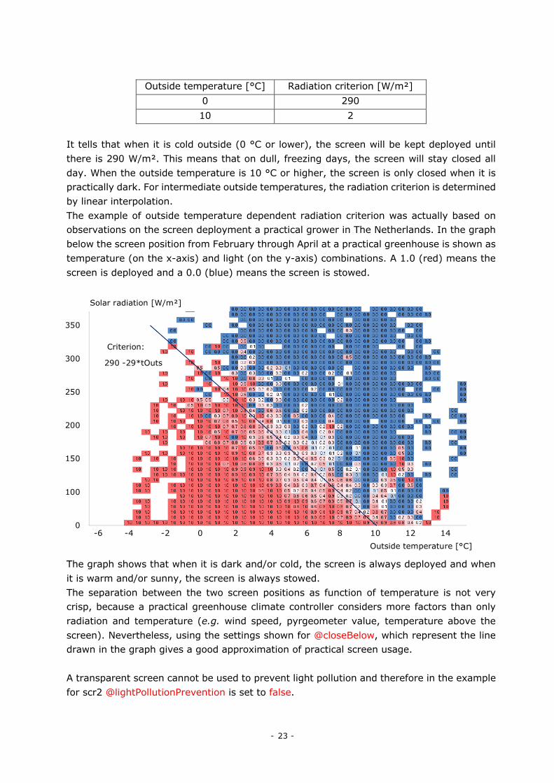
It tells that when it is cold outside (0 °C or lower), the screen will be kept deployed until there is 290 W/m². This means that on dull, freezing days, the screen will stay closed all day. When the outside temperature is 10 °C or higher, the screen is only closed when it is practically dark. For intermediate outside temperatures, the radiation criterion is determined by linear interpolation. The example of outside temperature dependent radiation criterion was actually based on observations on the screen deployment a practical grower in The Netherlands. In the graph below the screen position from February through April at a practical greenhouse is shown as temperature (on the x-axis) and light (on the y-axis) combinations. A 1.0 (red) means the screen is deployed and a 0.0 (blue) means the screen is stowed.

The graph shows that when it is dark and/or cold, the screen is always deployed and when it is warm and/or sunny, the screen is always stowed. The separation between the two screen positions as function of temperature is not very crisp, because a practical greenhouse climate controller considers more factors than only radiation and temperature (e.g. wind speed, pyrgeometer value, temperature above the screen). Nevertheless, using the settings shown for @closeBelow, which represent the line drawn in the graph gives a good approximation of practical screen usage. A transparent screen cannot be used to prevent light pollution and therefore in the example for scr2 @lightPollutionPrevention is set to false.

350

300

250

200

150

100

0 -6 -4 -2 0 2 4 6 8 10 12 14

Solar radiation [W/m²]

Outside temperature [°C]

Criterion:

290 -29*tOuts

- 24 -

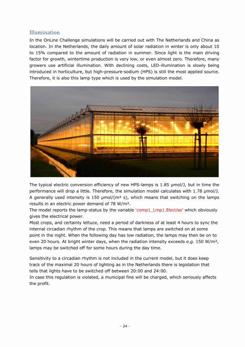
IlluminationIn the OnLine Challenge simulations will be carried out with The Netherlands and China as location. In the Netherlands, the daily amount of solar radiation in winter is only about 10 to 15% compared to the amount of radiation in summer. Since light is the main driving factor for growth, wintertime production is very low, or even almost zero. Therefore, many growers use artificial illumination. With declining costs, LED-illumination is slowly being introduced in horticulture, but high-pressure-sodium (HPS) is still the most applied source. Therefore, it is also this lamp type which is used by the simulation model.

The typical electric conversion efficiency of new HPS-lamps is 1.85 µmol/J, but in time the performance will drop a little. Therefore, the simulation model calculates with 1.78 µmol/J. A generally used intensity is 150 µmol/(m² s), which means that switching on the lamps results in an electric power demand of 78 W/m². The model reports the lamp-status by the variable ‘comp1_Lmp1.ElecUse’ which obviously gives the electrical power. Most crops, and certainly lettuce, need a period of darkness of at least 4 hours to sync the internal circadian rhythm of the crop. This means that lamps are switched on at some point in the night. When the following day has low radiation, the lamps may then be on to even 20 hours. At bright winter days, when the radiation intensity exceeds e.g. 150 W/m², lamps may be switched off for some hours during the day time.

Sensitivity to a circadian rhythm is not included in the current model, but it does keep track of the maximal 20 hours of lighting as in the Netherlands there is legislation that tells that lights have to be switched off between 20:00 and 24:00. In case this regulation is violated, a municipal fine will be charged, which seriously affects the profit.

- 25 -

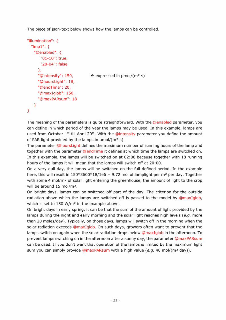
The piece of json-text below shows how the lamps can be controlled. "illumination": { "lmp1": { "@enabled": { "01-10": true, "20-04": false }, "@intensity": 150, ß expressed in µmol/(m² s) "@hoursLight": 18, "@endTime": 20, "@maxIglob": 150, "@maxPARsum": 18 } } The meaning of the parameters is quite straightforward. With the @enabled parameter, you can define in which period of the year the lamps may be used. In this example, lamps are used from October 1st till April 20th. With the @intensity parameter you define the amount of PAR light provided by the lamps in µmol/(m² s). The parameter @hoursLight defines the maximum number of running hours of the lamp and together with the parameter @endTime it defines at which time the lamps are switched on. In this example, the lamps will be switched on at 02:00 because together with 18 running hours of the lamps it will mean that the lamps will switch off at 20:00. On a very dull day, the lamps will be switched on the full defined period. In the example here, this will result in 150*3600*18/1e6 = 9.72 mol of lamplight per m² per day. Together with some 4 mol/m² of solar light entering the greenhouse, the amount of light to the crop will be around 15 mol/m². On bright days, lamps can be switched off part of the day. The criterion for the outside radiation above which the lamps are switched off is passed to the model by @maxIglob, which is set to 150 W/m² in the example above. On bright days in early spring, it can be that the sum of the amount of light provided by the lamps during the night and early morning and the solar light reaches high levels (e.g. more than 20 moles/day). Typically, on those days, lamps will switch off in the morning when the solar radiation exceeds @maxIglob. On such days, growers often want to prevent that the lamps switch on again when the solar radiation drops below @maxIglob in the afternoon. To prevent lamps switching on in the afternoon after a sunny day, the parameter @maxPARsum can be used. If you don’t want that operation of the lamps is limited by the maximum light sum you can simply provide @maxPARsum with a high value (e.g. 40 mol/(m² day)).

- 26 -

The parameters @hoursLight, @endTime, @maxIglob and @maxPARsum may vary over the year. The example below shows a setting that reduces the number of lamp-hours in spring. "illumination": { "lmp1": { "@hoursLight": { "01-10": 18, "15-02": 16, "15-03": 15 } } } In this case, when @endTime would stay the same (20), the lamps would switch on at 02:00 during winter, at 04:00 for February 15th and at 05:00 for March 15th.

CO2-supplyAs plants consume CO2 when they are exposed to light, the CO2 in the greenhouse air will get depleted when it is not added. Moreover, at elevated CO2-concentration, crops grow notably faster. Therefore, CO2-dosing is standard in Dutch greenhouses. The CO2 comes from the flue gases from the boiler or CHP, but the application of industrial waste-CO2 is also quite common. This CO2 is the supplied by deliveries in liquid form, or by a regional piping-network. In this project we assume the latter, CO2 supply through a piping network. This means that CO2 can simply be added when the inside concentration drops below a certain threshold. Typically, the control ensures that the CO2-conentration fluctuates closely around the CO2-setpoint as long as the supply rate is sufficient to compensate for the sum of crop uptake and losses through ventilation. Typical supply rates are 100 kg/(ha hr), which is equivalent to 10 gr/(m² hr). However, some growers go up to 200 kg/(ha hr) in case CO2 can be obtained cheaply.

- 27 -

The CO2 supply rate is provided by the simulation model as ‘comp1_McPureAir_Value’ expressed in kg/(m² s). The main parameters to control the CO2 supply are:

"common": { "CO2dosing": { "@pureCO2cap": 100 ß Note: expressed in kg/(ha hr) } } and "setpoints": { "CO2": { "@setpoint": { ßexpressed in ppm "01-01": {"r+0.5": 400, "r+1": 800, "s-1.5": 800, "s": 400} }, "@setpIfLamps": 700 } } Note that the parameter to pass the capacity is in a different branch of the json-structure (comp1.common.CO2dosing) than the parameters that control the control of the CO2-supply (comp1.setpoints.CO2).

You can see that the setpoint for CO2 distinguishes between a setpoint applied when the lamps are on during the night, and a setpoint related to the solar daytime. Of course, lamps can also be switched on during daytime. In that case, the maximum of these setpoints is used.

As the CO2 consumption of a lettuce crop never exceeds 5 gram/(m² hr), the supply rate shown in the example (which comes down to 10 gram/(m² hr) accommodate an elevated CO2 setpoint as long as the vents are closed. However, losses will increase fast when the greenhouse is ventilated. Typically, this means that the setpoints set can only be met in winter or in the early morning. In periods with high radiation, the actual CO2 concentration may be far below the setpoint despite the supply rate being at its maximum.

To prevent large losses of CO2, some growers reduce the CO2 setpoint when the vents are opened. Others decrease the maximum supply rate. The simulation model offers this second possibility by the parameter comp1.setpoints.CO2.@doseCapacity (Note: not to be confused with common.CO2dosing.@pureCO2cap, which denotes the maximum capacity of the CO2 supply and named quite similar).

- 28 -

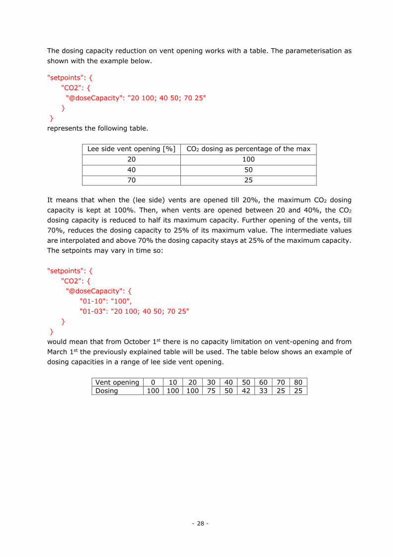
The dosing capacity reduction on vent opening works with a table. The parameterisation as shown with the example below.

"setpoints": { "CO2": { "@doseCapacity": "20 100; 40 50; 70 25" } } represents the following table.

Lee side vent opening [%] CO2 dosing as percentage of the max 20 100 40 50 70 25

It means that when the (lee side) vents are opened till 20%, the maximum CO2 dosing capacity is kept at 100%. Then, when vents are opened between 20 and 40%, the CO2 dosing capacity is reduced to half its maximum capacity. Further opening of the vents, till 70%, reduces the dosing capacity to 25% of its maximum value. The intermediate values are interpolated and above 70% the dosing capacity stays at 25% of the maximum capacity. The setpoints may vary in time so: "setpoints": { "CO2": { "@doseCapacity": { "01-10": "100", "01-03": "20 100; 40 50; 70 25" } } would mean that from October 1st there is no capacity limitation on vent-opening and from March 1st the previously explained table will be used. The table below shows an example of dosing capacities in a range of lee side vent opening.

Vent opening 0 10 20 30 40 50 60 70 80 Dosing 100 100 100 75 50 42 33 25 25

- 29 -

PlantdensityandspacingLettuce is a crop that is harvested early when crop stature is still compact and the stem has not yet stretched to expose the flower. It starts with a small plantlet and is ready for harvest in around 40 days. When the lettuce heads are at their final fresh weight of approximately 250 g, they need about 0.065 m² per head. This means that in the final stage, around 16 plants per m² can be grown (the exact number depending on the plant diameter of a particular cultivar). Of course, also the young plants can be planted in a density of 16 plants per m², but as the plants are then still small, a large amount of greenhouse space is then used quite inefficiently. Modern lettuce greenhouses have therefore all kind of systems that allow for an decreasing plant density over time. Seedlings are planted in a high density of about 80 plants per m². Then, gradually the plants are spaced by sliding the gutters in which the plants are growing further apart. Also, plants can be transplanted from a high density gutter to a low density gutter.

Figure: Transplanting for spacing from a high density gutter to a low density gutter

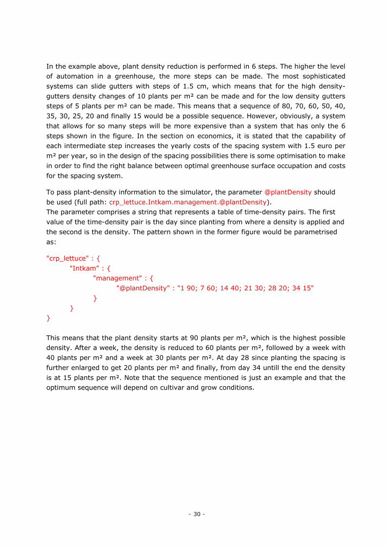
Figure: Reducing plant density by enlarging the gutter-to-gutter distance.

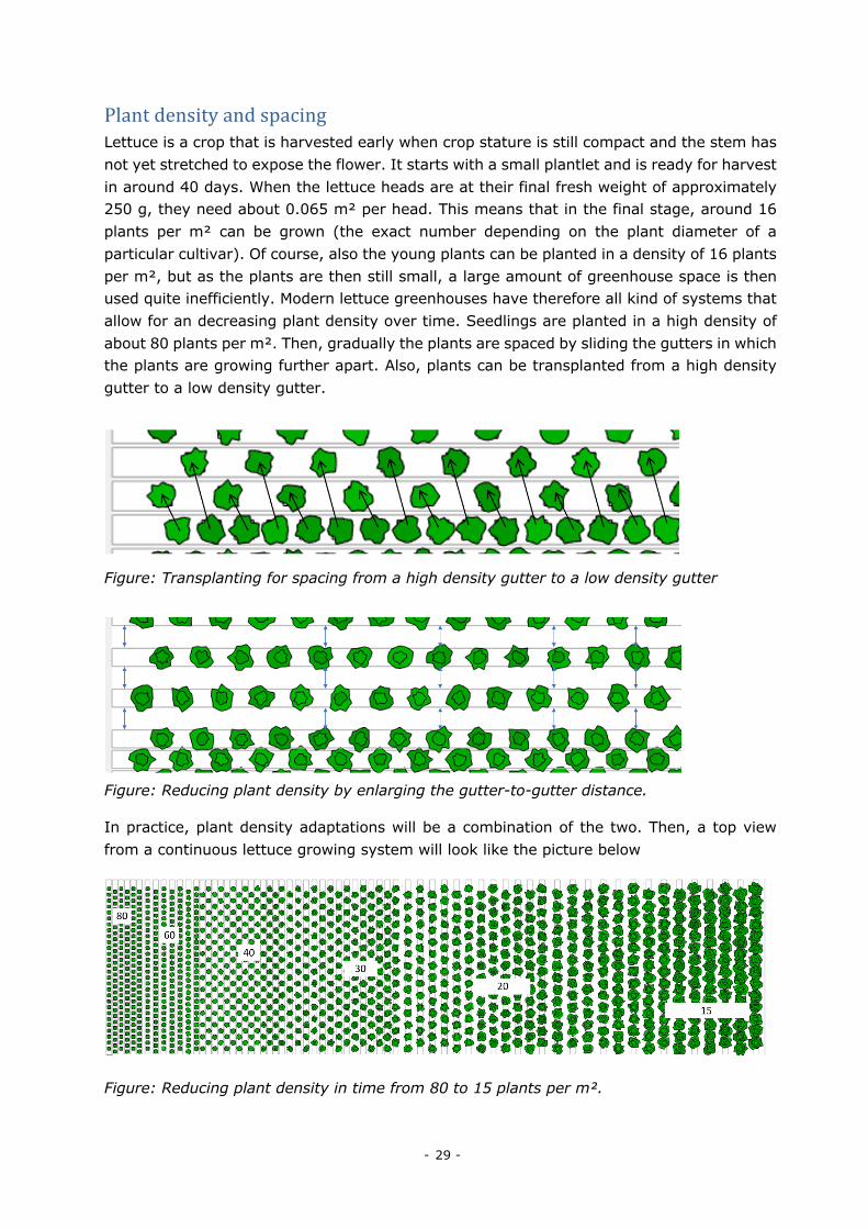
In practice, plant density adaptations will be a combination of the two. Then, a top view from a continuous lettuce growing system will look like the picture below

Figure: Reducing plant density in time from 80 to 15 plants per m².

- 30 -

In the example above, plant density reduction is performed in 6 steps. The higher the level of automation in a greenhouse, the more steps can be made. The most sophisticated systems can slide gutters with steps of 1.5 cm, which means that for the high density-gutters density changes of 10 plants per m² can be made and for the low density gutters steps of 5 plants per m² can be made. This means that a sequence of 80, 70, 60, 50, 40, 35, 30, 25, 20 and finally 15 would be a possible sequence. However, obviously, a system that allows for so many steps will be more expensive than a system that has only the 6 steps shown in the figure. In the section on economics, it is stated that the capability of each intermediate step increases the yearly costs of the spacing system with 1.5 euro per m² per year, so in the design of the spacing possibilities there is some optimisation to make in order to find the right balance between optimal greenhouse surface occupation and costs for the spacing system.

To pass plant-density information to the simulator, the parameter @plantDensity should be used (full path: crp_lettuce.Intkam.management.@plantDensity). The parameter comprises a string that represents a table of time-density pairs. The first value of the time-density pair is the day since planting from where a density is applied and the second is the density. The pattern shown in the former figure would be parametrised as:

"crp_lettuce" : { "Intkam" : {

"management" : { "@plantDensity" : "1 90; 7 60; 14 40; 21 30; 28 20; 34 15" } } } This means that the plant density starts at 90 plants per m², which is the highest possible density. After a week, the density is reduced to 60 plants per m², followed by a week with 40 plants per m² and a week at 30 plants per m². At day 28 since planting the spacing is further enlarged to get 20 plants per m² and finally, from day 34 untill the end the density is at 15 plants per m². Note that the sequence mentioned is just an example and that the optimum sequence will depend on cultivar and grow conditions.

- 31 -

Resultsfromasimulation(economicandintermsofproduct)

Greenhouses are meant to produce valuable horticultural products. Tasteful and healthy vegetables or fruits or beautiful flowers or ornamental plants. Some greenhouses are meant for propagation from seed or (tissue) cuttings to young plants only. The plantlets are grown further in other greenhouses or in the open field.

In this case, the greenhouse produces heads of lettuce, which are sold per piece. The simulation describes the growth of one batch of seedlings from planting until harvest, but in a real lettuce greenhouse, there will be a more or less continuous process of daily planting of young plantlets and harvesting the full-grown plants that has been planted 6 through 8 weeks before.

The participating teams in the challenge are supposed to develop the optimal strategy to grow the young plants towards their desired harvest state. The teams may intensify the production by speeding up the growth at the expense of additional heating, electricity and CO2 in a shorter period of time, but taking a few days more and reducing the costs on energy and CO Transparent might lead to a higher margin per head of lettuce produced.

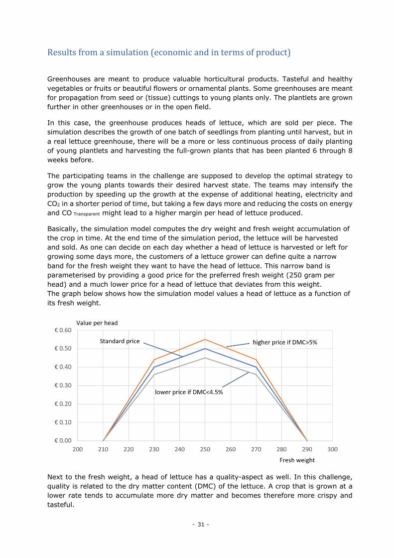
Basically, the simulation model computes the dry weight and fresh weight accumulation of the crop in time. At the end time of the simulation period, the lettuce will be harvested and sold. As one can decide on each day whether a head of lettuce is harvested or left for growing some days more, the customers of a lettuce grower can define quite a narrow band for the fresh weight they want to have the head of lettuce. This narrow band is parameterised by providing a good price for the preferred fresh weight (250 gram per head) and a much lower price for a head of lettuce that deviates from this weight. The graph below shows how the simulation model values a head of lettuce as a function of its fresh weight.

Next to the fresh weight, a head of lettuce has a quality-aspect as well. In this challenge, quality is related to the dry matter content (DMC) of the lettuce. A crop that is grown at a lower rate tends to accumulate more dry matter and becomes therefore more crispy and tasteful.

- 32 -

In this challenge, a focus on quality is achieved by assigning a 10% premium price in case the dry matter content exceeds 5% and a 10% lower price if the lettuce has become too watery, defined as a dry matter content below 4.5%.

As it is assumed that within the zone between 4.5 and 5% dry matter content there will not be a clear difference in quality, the price is not interpolated on dry matter content. This means that for each fresh weight, three prices are possible.

The output of the model clearly shows at which price the lettuce is sold, as the economic statistics are expressed per head of lettuce.

Apart from the crop performance data at the final day, the user of the model can observe the development of fresh weight and some more plant characteristics in time. The supplied characteristics are:

plant.headfw [g/plant]

plant.shootdrymattercontent [g/g]

plant.plantprojection [m²] (the area occupied by a head of lettuce on a horizontal plane)

plant.fractiongroundcover [-] (the fraction of the ground that is covered by the plants)

As the heads will start to be hindered by neighbouring plants, the fractiongroundcover should not exceed 0.9. If it does exceed, the further growth of the heads is notably slowed down.

Finally, as a check on the input provided by the user the model shows:

plant.plantdensity [plant/m²]

Note that the simulation model stops at midnight, whereas of course in reality the harvest will be somewhere during the day. Therefore, the development of fresh weight and dry weight are represented as a step-function holding for the values at noon for the particular day.

At the final date of the simulation, the model looks at the accumulated fresh weight, and the computed dry matter content and determines the gain obtained by selling the head of lettuce.

- 33 -

NetProfitcalculation

After ‘selling’ the head of lettuce, the Net Profit can be a calculated from

Net Profit = Gains – Fixed costs – Variable costs

Of course, the gains follow from the head of lettuce sold at its value on harvest day. The fixed costs are composed from the maintenance and depreciation of the greenhouse and the equipment installed. The variable costs follow from the commodities used during the growing period. The model shows these components and the parts from which they are composed. They are all stored in the json-structure with the root-name "economics", which is a branch from "stats" (see last paragraphs of the section ‘Outputs of greenhouse climate simulation’).

Price for the lettuce heads.

The price of a head of lettuce is shown in the former section. It is composed of a base-price, depending on the weight of the head of lettuce. On top of this there can be 10% bonus if the dry matter content is exceptionally high or a 10% malus if the dry matter content is very low. The bonus/malus component is shown in the model output.

However, the economics are not expressed per head of lettuce, but per m² greenhouse. Therefore, the selling price of the lettuce is multiplied by the average number of heads per m². The average number of heads per m² is a result of the spacing strategy applied (see Figure on page 27) and can be calculated by

𝐴𝑣𝑒𝑟𝑎𝑔𝑒𝐻𝑒𝑎𝑑𝑚2 = 𝑛𝑑𝑎𝑦/ 0 1/𝑑𝑒𝑛𝑠𝑖𝑡𝑦(𝑑𝑎𝑦)!"#$

"#$%&

This formula is computed by the simulation model and returned in the statistics part of the output (stats.economics.averageHeadPerM2).

The gain of the simulation run is now computed by multiplying the price of a head of lettuce (as a function of its fresh weight and dry matter content) by the AverageHeadPerM2. The result of this computation is shown as stats.economics.gains.total in the simulation output.

Fixed costs

The fixed costs are composed form the plant costs and maintenance and depreciation costs of the greenhouse equipment. As the teams in the challenge can decide on the intensity of illumination, the amount of screens applied, the capacity of the CO2-dosing equipment and the level of sophistication of the spacing equipment only these costs are made dependent on the user-inputs. Next to these user-defined inputs, there is a general defined fixed cost component for the maintenance and depreciation of the greenhouse.

- 34 -

Plant costs The plant costs are set to 0.5 euro per piece for every simulation run (so actually this cost component could have been left out from the computation since it only gives an offset in all profit computations).

Greenhouse costs The basic depreciation and maintenance costs of a greenhouse, excluding the illumination system, the screens, CO2-supply and a sophisticated spacing system are on an average 11.50 euro per m² per year. To translate this number to greenhouse costs per head of lettuce, this figure is multiplied by the fractional time of the year that it takes to grow the small plantlet to a harvestable product (in general somewhere between 0.08 and 0.15). As a formula:

greenhouseOccupation = 11.5 * fractionOfYear

The variable fractionOfYear is computed by

fractionOfYear = (crop cycle period [days])/365.

CO2 dosing capacity The costs of a CO2 dosing system are € 0.015 per m² per year per kg/(ha hr) of capacity. Since kg/(ha hr) is the parameter by which you define the maximum dosing capacity (common.CO2dosing.@pureCO2cap) you can simply multiply this figure by 0.015 to get the yearly costs for the CO2 connection per m² greenhouse area. And also here, this amount has to be multiplied by fraction of the year that the greenhouse is used to grow a head of lettuce. As a formula:

Fixed CO2 costs = common.CO2dosing.@pureCO2cap * 0.015 * fractionOfYear

Depreciation and maintenance of lamps A 1000 W HPS lamp cost 50 euros per year in terms of depreciation and maintenance. It gives an output of 1780 µmol/s and with these figures it can be computed that the yearly costs are € 0.0281 per µmol/(m² s) per year. Also, the fixed costs for lamps are multiplied by the fractionOfYear. The formula therefore becomes:

Fixed Lamp costs = comp1.illumination.lmp1.@intensity*0.0281*fractionOfYear

Depreciation and maintenance of screens Having a movable screen in the greenhouse costs € 1 per screen per year also this figure is multiplied by the fractionOfYear so the formula becomes:

Screen costs = Number of screens * 1 * fractionOfYear / averageHeadPerM2

Level of sophistication of the spacing system A lettuce planting system with many spacing options is more expensive than a system with a single spacing. In the approach for the challenge, we will simply state that each additional spacing option increases the yearly costs for spacing equipment with € 1.50 per m² per year. This results in the formula:

Spacing costs = NumberOfSpacieChanges *1.5*fractionOfYear

- 35 -

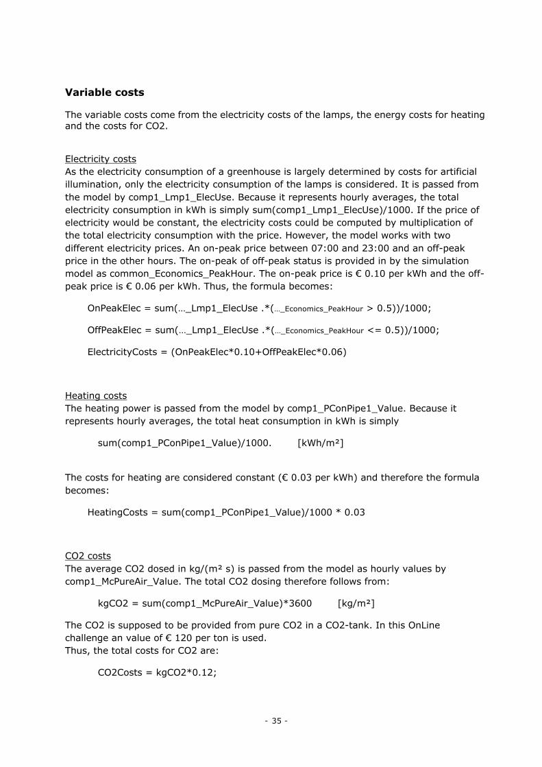
Variable costs

The variable costs come from the electricity costs of the lamps, the energy costs for heating and the costs for CO2.

Electricity costs As the electricity consumption of a greenhouse is largely determined by costs for artificial illumination, only the electricity consumption of the lamps is considered. It is passed from the model by comp1_Lmp1_ElecUse. Because it represents hourly averages, the total electricity consumption in kWh is simply sum(comp1_Lmp1_ElecUse)/1000. If the price of electricity would be constant, the electricity costs could be computed by multiplication of the total electricity consumption with the price. However, the model works with two different electricity prices. An on-peak price between 07:00 and 23:00 and an off-peak price in the other hours. The on-peak of off-peak status is provided in by the simulation model as common_Economics_PeakHour. The on-peak price is € 0.10 per kWh and the off-peak price is € 0.06 per kWh. Thus, the formula becomes:

OnPeakElec = sum(…_Lmp1_ElecUse .*(…_Economics_PeakHour > 0.5))/1000;

OffPeakElec = sum(…_Lmp1_ElecUse .*(…_Economics_PeakHour <= 0.5))/1000;

ElectricityCosts = (OnPeakElec*0.10+OffPeakElec*0.06)

Heating costs The heating power is passed from the model by comp1_PConPipe1_Value. Because it represents hourly averages, the total heat consumption in kWh is simply

sum(comp1_PConPipe1_Value)/1000. [kWh/m²]

The costs for heating are considered constant (€ 0.03 per kWh) and therefore the formula becomes:

HeatingCosts = sum(comp1_PConPipe1_Value)/1000 * 0.03

CO2 costs The average CO2 dosed in kg/(m² s) is passed from the model as hourly values by comp1_McPureAir_Value. The total CO2 dosing therefore follows from:

kgCO2 = sum(comp1_McPureAir_Value)*3600 [kg/m²]

The CO2 is supposed to be provided from pure CO2 in a CO2-tank. In this OnLine challenge an value of € 120 per ton is used. Thus, the total costs for CO2 are:

CO2Costs = kgCO2*0.12;

- 36 -

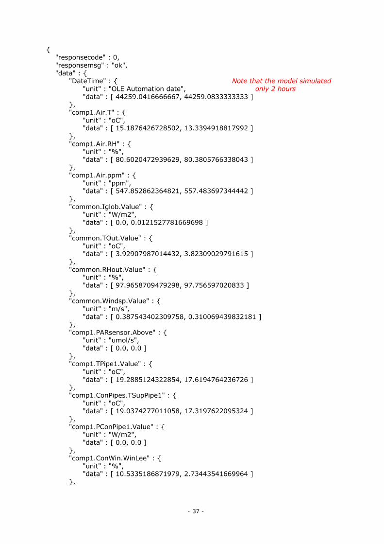
OutputsofgreenhouseclimatesimulationThe simulation model gives the results as a json-structure in which the branches are the different model outputs. If there are no errors in the input variables, the model gives a response like: { "responsecode" : 0, "responsemsg" : "ok", "data" : { "DateTime" : { "unit" : "OLE Automation date", "data" : [ 44259.0416666667, 44259.0833333333 ………….. ] Etc. All outputs are listed and explained in the table below.

Below you can find an example of the output file (corresponding to 2 hour simulation period):

Variable Unit Short description 1 DateTime Time in Excel data format 2 comp1.Air.T °C Greenhouse air temperature 3 comp1.Air.RH % Greenhouse air humidity 4 comp1.Air.ppm ppm Greenhouse CO2 concentration 5 common.Iglob.Value W/m² Outside solar radiation 6 common.TOut.Value °C Outside temperature 7 common.RHOut.Value % Outside humidity 8 common.Windsp.Value m/s Outside wind speed 9 comp1.PARsensor.Above µmol/(m² s) Light intensity just above crop 10 comp1.TPipe1.Value °C Average heating pipe temperature 11 comp1.ConPipes.TSupPipe1 °C Supply temperature heating pipe 12 comp1.PConPipe1.Value W/m² Heating power 13 comp1.ConWin.WinLee % Lee side window opening 14 comp1.ConWin.WinWnd % Windward side window opening 15 comp1.Setpoints.SpHeat °C Setpoint for heating 16 comp1.Setpoints.SpVent °C Ventilation line 17 comp1.Scr1.Pos 0-1 Position of upper most screen 18 comp1.Scr2.Pos 0-1 Position of the second screen 19 comp1.Lmp1.ElecUse W/m² Electricity consumption of lamps 20 comp1.McPureAir.Value kg/(m² s) Co2 dosing 21 comp1.Plant.headFW gram Fresh weight of the lettuce 22 comp1.Plant.fractionGroundCover - Fraction of ground covered 23 comp1.Plant.shootDryMatterContent gr/gr Dry matter content of the lettuce 24 comp1.Plant.plantProjection m² Horizontal area per plant 25 comp1.Plant.PlantDensity #/m² Number of plants per m² 26 common.Economics.PeakHour 0-1 Is it (an expensive) peak hour

- 37 -

{ "responsecode" : 0, "responsemsg" : "ok", "data" : { "DateTime" : { Note that the model simulated "unit" : "OLE Automation date", only 2 hours "data" : [ 44259.0416666667, 44259.0833333333 ] }, "comp1.Air.T" : { "unit" : "oC", "data" : [ 15.1876426728502, 13.3394918817992 ] }, "comp1.Air.RH" : { "unit" : "%", "data" : [ 80.6020472939629, 80.3805766338043 ] }, "comp1.Air.ppm" : { "unit" : "ppm", "data" : [ 547.852862364821, 557.483697344442 ] }, "common.Iglob.Value" : { "unit" : "W/m2", "data" : [ 0.0, 0.0121527781669698 ] }, "common.TOut.Value" : { "unit" : "oC", "data" : [ 3.92907987014432, 3.82309029791615 ] }, "common.RHout.Value" : { "unit" : "%", "data" : [ 97.9658709479298, 97.756597020833 ] }, "common.Windsp.Value" : { "unit" : "m/s", "data" : [ 0.387543402309758, 0.310069439832181 ] }, "comp1.PARsensor.Above" : { "unit" : "umol/s", "data" : [ 0.0, 0.0 ] }, "comp1.TPipe1.Value" : { "unit" : "oC", "data" : [ 19.2885124322854, 17.6194764236726 ] }, "comp1.ConPipes.TSupPipe1" : { "unit" : "oC", "data" : [ 19.0374277011058, 17.3197622095324 ] }, "comp1.PConPipe1.Value" : { "unit" : "W/m2", "data" : [ 0.0, 0.0 ] }, "comp1.ConWin.WinLee" : { "unit" : "%", "data" : [ 10.5335186871979, 2.73443541669964 ] },

- 38 -

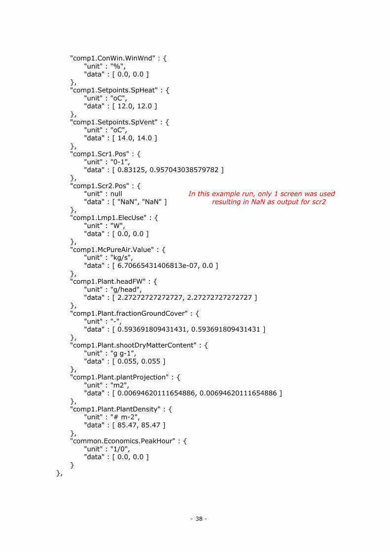
"comp1.ConWin.WinWnd" : { "unit" : "%", "data" : [ 0.0, 0.0 ] }, "comp1.Setpoints.SpHeat" : { "unit" : "oC", "data" : [ 12.0, 12.0 ] }, "comp1.Setpoints.SpVent" : { "unit" : "oC", "data" : [ 14.0, 14.0 ] }, "comp1.Scr1.Pos" : { "unit" : "0-1", "data" : [ 0.83125, 0.957043038579782 ] }, "comp1.Scr2.Pos" : { "unit" : null In this example run, only 1 screen was used "data" : [ "NaN", "NaN" ] resulting in NaN as output for scr2 }, "comp1.Lmp1.ElecUse" : { "unit" : "W", "data" : [ 0.0, 0.0 ] }, "comp1.McPureAir.Value" : { "unit" : "kg/s", "data" : [ 6.70665431406813e-07, 0.0 ] }, "comp1.Plant.headFW" : { "unit" : "g/head", "data" : [ 2.27272727272727, 2.27272727272727 ] }, "comp1.Plant.fractionGroundCover" : { "unit" : "-", "data" : [ 0.593691809431431, 0.593691809431431 ] }, "comp1.Plant.shootDryMatterContent" : { "unit" : "g g-1", "data" : [ 0.055, 0.055 ] }, "comp1.Plant.plantProjection" : { "unit" : "m2", "data" : [ 0.00694620111654886, 0.00694620111654886 ] }, "comp1.Plant.PlantDensity" : { "unit" : "# m-2", "data" : [ 85.47, 85.47 ] }, "common.Economics.PeakHour" : { "unit" : "1/0", "data" : [ 0.0, 0.0 ] } },

- 39 -

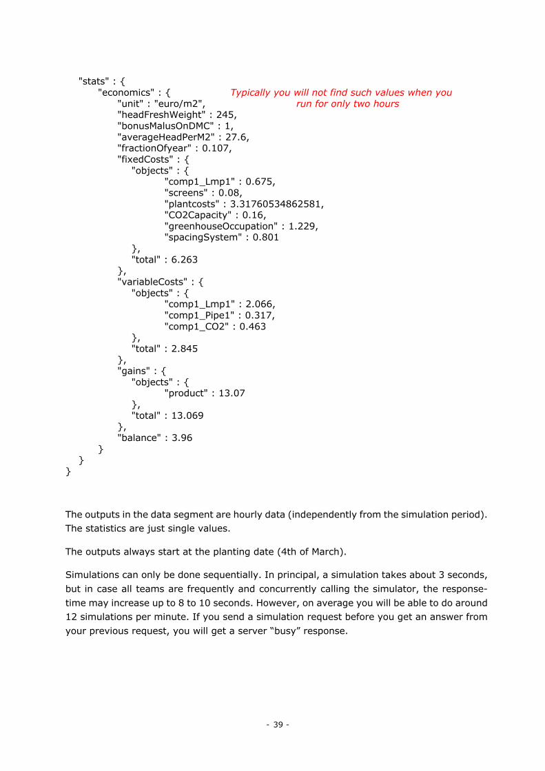
"stats" : { "economics" : { Typically you will not find such values when you "unit" : "euro/m2", run for only two hours "headFreshWeight" : 245, "bonusMalusOnDMC" : 1, "averageHeadPerM2" : 27.6, "fractionOfyear" : 0.107, "fixedCosts" : { "objects" : { "comp1_Lmp1" : 0.675, "screens" : 0.08, "plantcosts" : 3.31760534862581, "CO2Capacity" : 0.16, "greenhouseOccupation" : 1.229, "spacingSystem" : 0.801 }, "total" : 6.263 }, "variableCosts" : { "objects" : { "comp1_Lmp1" : 2.066, "comp1_Pipe1" : 0.317, "comp1_CO2" : 0.463 }, "total" : 2.845 }, "gains" : { "objects" : { "product" : 13.07 }, "total" : 13.069 }, "balance" : 3.96 } } }

The outputs in the data segment are hourly data (independently from the simulation period). The statistics are just single values.

The outputs always start at the planting date (4th of March).

Simulations can only be done sequentially. In principal, a simulation takes about 3 seconds, but in case all teams are frequently and concurrently calling the simulator, the response-time may increase up to 8 to 10 seconds. However, on average you will be able to do around 12 simulations per minute. If you send a simulation request before you get an answer from your previous request, you will get a server “busy” response.

- 40 -

UsingthemodelintheOnLineChallengeonclimatecontrol

The autonomous greenhouse challenge aims at full automated control, which means that some algorithm has to respond in a proper way to disruptions and variations that will occur in any practical greenhouse operation. The level at which the algorithm is capable of coping with such deviations from the expected behaviour is considered to be the most important quality. Also, the transferability of the control algorithm from one location to another is a key quality of the developed control system.

In order to observe this quality, the simulation which is used to describe the cropping result as a function of operational decisions will be notably different in different phases of the OnLine Challenge.

During the OnLine Challenge, teams will have two keys with which they can run the simulator. The first key, marked with C**A-****-…. gives access to the simulation model meant for training purposes of a machine learning algorithm. The simulator’s responses can be used to find the most relevant factors for achieving an optimal result and to train an algorithm that controls the lettuce production in an optimal way. Throughout the 6 weeks preparation period, the model behind this A-key will stay the same, meaning that an equal set of inputs will give every time the same output (Simulator A).

For testing the robustness of the control algorithm for controlling under adapted conditions, there is also a model running on a B-key, marked with C**B-****-…. The model on the B-key, referred to as Simulator B, is similar but a little different to the model on the A-key. Simulator A and Simulator B describe both a lettuce production system located in the Netherlands, but for Simulator B, the outside weather conditions to which the greenhouse is exposed are changed and the lettuce crop will grow a little different. This mimics reality in the sense that another cropping cycle will always be different than previous ones.

Contrary to the simulator on the A-key model, the simulator on the B-key key is only accessible on Mondays and on July 13th, and always only from 14:00 CET till 15:00 CET. Another difference is that the simulator’s output is not only sent to the teams, but also stored on the server (always only the last model output). In case the teams try the robustness of their approach which was trained on simulator A for the control of simulator B, the last result left after 15:00 CET can be viewed by the challenge organizers to keep track of the intermediate result of all the teams.

These intermediate results will be published as a ranking on the public score board so along the preparation period teams can get an impression of the performance of their algorithm in comparison to others.

The same mechanism of using the model on the A-key for training purposes and the model on the B-key for ranking the performance is used in the final phase of the challenge.

From July 12th onwards, the model on the A-key will describe a lettuce growing system in Beijing. The physics of the greenhouse stays the same, but environmental conditions, daylength, price of product and commodities will be changed. In this phase of the

- 41 -

challenge, it is Simulator C that runs on the A-key and teams will have more than a day to have their controller adapted to the new conditions. Then, on July 13th Simulator D will be accessible from 14:00 till 15:00 CET (one hour). Simulator D runs on the B-key and will therefore keep the last simulator’s result stored. Providing that the teams have their best performing control strategy applied in the last run on the B-key, the challenge organizer can see each team’s achievement in terms of net profit. Ranking the net profits results in ranking the quality of the greenhouse climate controllers and shows the best performing algorithm. ‘Best performing’ means the algorithm that found the way to achieve the highest net profit.

Note that the procedure of using the A-key for training and the B-key for evaluation is applied during the whole challenge. This means that teams can practice with this procedure and score mechanism on 6 successive Mondays in order to be ready to show their performance on July 13th.

FINALEVENT:

CombinationofresultsonClimatecontrolwithresultsonImageprocessing

On the 14th of July 14:00-15:30 CET, in the final event ceremony, the ranking of the team on the climate control part of the challenge will be combined with the ranking of the team in the Image processing part of the challenge to get an overall performance. In case of a draw in the two best performing teams, the performance in the image processing will prevail.