1

E E A A

Egyptian Environmental Affairs Agency ,EEAA

Nature Conservation Sector, NCS

St. Katherine Protectorate

A study of :

Grazing Patterns In High Altitude MountainsAround St. Katherine Town. (A GIS integrated approach)

Team :Husam El AlqamySabreen RashadYousria Abdul BassetMohamed HemeedNature Conservation Sector,St. Katherine Protectorate

Consultant :Dr. Tim Wacher

Zoological Society of London

2002

2

This study is part of the Natural Resources Monitoring Program conducted by theranger team of Saint Katherine Protectorate. The program was funded by theEuropean Union (EU) as part of Saint Katherine Protectorate DevelopmentProjects (SKPDP) during the period 1996-2003. Technical consultancy on variousoccasions was provided by Zoological Society of London represented by Dr. TimWacher as for both approach, field methods and analysis. Field work wasconducted during the period 2000-2002. Final report drafted and reviewed during2002.

St. Katherine Protectorate , Souyh SinaiEgyptian Environmental Affairs Agency, 2002

3

A study of : ..............................................................1

Grazing Patterns In High Altitude Mountains ..........1

1. Introduction & prospective: .................................4

2. Study Region : ....................................................4

3. Materials & Methods ...........................................51- Setting the scene: ...................................................................................................7

2. GPS logging: ..........................................................................................................7

3-Estimating Ranges: .................................................................................................8

4-Food preference & Biomass estimates: ..................................................................9

5-Grazing spatial & temporal parameters : ..............................................................10

4. Results :............................................................114.1 –Spatial patterns:................................................................................................11

4.1-a Grazing Range : ..................................................................................................... 11

4.1-b Altitude profile : .................................................................................................... 16

4.1-c Estimating Spatial heterogeniety : ......................................................................... 17

4.2 –Feeding Properties : .........................................................................................21

4.2-a Food Spectrum :..................................................................................................... 21

4.2-b Consumed Biomass Estimation :........................................................................... 25

5. Conclusion & extension of work : ......................29

4

1. Introduction & prospective:The high altitude area of St. Katherine town and its vicinity is reported to harbor the

highest percentage of endemism among floral species of Egypt. Out of 33 endemics

species of Sinai, 19 are present in this area on such a small geographical area. The

area has been inhabited by Bedouins for hundreds of years. Bedouins are normally

keeping herds of goats and sheep. Goats and sheep are of high value for the Bedouins

since they provide them with valuable sources of meat and milk in addition to the

other products and derivatives like the hair, wool and Skin. These herds are in always

need for fodders and ration. In such arid climate, grazing is the only alternative.

Previously, grazing rotation or range management was not of such a problem because

the Bedouins are normally nomadic traveling from one place to the other shifting their

grazing pressure over changing ranges. Nomadism provided the chance for exploited

range lands to recover while others are being exploited. However, Bedouins of South

Sinai had already developed a system for rotating their grazing pressure. They have a

system of “Dakhal” and “Helf”. Where in these systems certain Bedouins agrees

among them selves on banning grazing in certain lands for a particular period of time.

Different regulations are specified for both Dakhal & Helf.

The current study is aiming to address three main issues concerning the issue of

grazing patterns in St. Katherine. The first one is to quantify the grazing pressure in

terms of time and area units. The second is to define the spatial parameters of the

grazing process. In other words, its targeting on estimating the area of the range land

and predicting the spatial heterogeneity of the grazing pressure over this range. The

third aim is to define the palatable plant species for both goats and sheep. Also an

attempt is made to quantify the collectively consumed biomass and the specific

consumed biomass.

2. Study Region :The targeted area is the high altitude mountains of St. Katherine and its

vicinity. The total area of the investigation region is about 170 Km². The area is of

varying altitudes. It includes the highest peak of Egypt, St. Katherine Mt. 2664m

(msl). The lowest area involved in the study is of altitude of about 1200 to 1300 m

(msl) and sloping upwards to reach 2600 m. The topography of the area includes

variable features. Hanging wadies are not un common among the high mountains of

5

the area. Saddles and basins forms most of the open lands in the area. Steep ascends

and prismatic peaks are so common amongst which narrow wadies are entrapped.

Plant communities around the areas are confined to areas where soil is collecting in

beds

3. Materials & MethodsSeven Bedouin settlements around St. Katherine were selected to sample their grazing

activity. These settlements are : Wadie El Raha , Upper Esbaia, Lower Esbaia, Oskof,

El Arbaien, Kharazeen and Abou sela. Map (1) shows the study area and the locations

of the sampled settlements.

Map (1) The roughed terrain of the high altitude mountainous area of St. Katherinetown and vicinity with sampled settlements posted

6

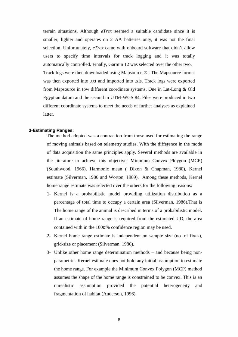
Sampling involved two main approaches. The first was using GPS receivers to track

log the position of the goat or sheep on constant intervals and then using different

maping & GIS software to elucidate the various spatial products. Garmin GPS 12

receivers were fitted to goats & sheep back using a harness like those used for pets

customized to accommodate the GPS receiver and not affecting the forage of the

animal. Picture (1) show the harness fitted to a female sheep. The second approach

involved the direct observation of a marked goat or sheep.

There was a considerable difficulty convincing the Bedouins to cooperate with the

team. At first there was enormous refusal of cooperation and they feared for their

goats from the impact of the device. Others thought that –as we told them it is a

recording device- the device will record voices & pictures of the shepardesses as well

as for the goats. Thus they had a strong repulsive attitude. A cultural moderation for

the study was introduced by Ranger Yousria Abdul Basset which enabled the set on of

the study. A brief explanations of the study aims and methods were delivered to the

men and women of the bedouin community through several sessions held in the

summer of 2000. However, these repulsive situations arose often along the course of

the study during 2001 & 2002. These again were moderated by the social rule of R.

Mohamed El Sana’a where he acted as social worker to ease the problem. Also R.

Pic(1)Female sheep fitted withthe customized pet-harness carrying the GPSreceiver with track loginterval set to 1 minute.

7

Sabreen Rashad took the responsibility of explaining what the process really is for the

girl shepardesses.

As stated in the introduction, the present work have a range of objectives. Thus,

methods used are varying subjectively. In the following sections, a description of the

each adopted methods is provided. The methods are generally categorized as

1- Setting the scene:A 500m grid was laid on the study region where nodes represented the nodes

of the UTM grid. The grid was created by The grid was using ArcView’s

planemetric script applied over the study area. A digital elevation model was

developed by digitizing contour lines at a 20-m altitude interval. Digitization

utilized a 1:50000 source map with the following specification;

transverse mercator projection -1000 m Grid, Old Egyptian

1907 (Red Zone)

European datum and international spheroid.

Digitization of contours resulted in points of X & Y coordinates and assigned

latitude value as Z. Universal Kriging and variogram was used to produce a

.GRD file which then could be displayed as a wireframe map as a 3D

visualization of the model. Surfer 7.0 was used for this purpose.

2. GPS logging:The target was to record the position of the grazing animals at 1 minute time

intervals. Using the track log function of GPS receivers seemed to be suitable

realization of this objective. Thus it was decided to adopt this approach

provided the potential of analyses applicable to the data collected.

Garmin GPS 12, Garmin GPS 48 and Garmin eTrex receivers were tested for

their suitability for the study. Garmin 48 showed considerable disadvantages.

It had an external rotatable antenna that posed a great challenge to being fitted

in a customized harness. In addition since Garmin 48 is an 8-channel receiver

it required considerably long time for initial acquiring position. Also it was

easily losing signal in the shadows of mountains and under ledges causing the

sampling effort to lose valuable parts of the grazing forage time.

To over come these problems Garmin 12 & eTrex were tested, since both of

them has 12-channels receivers. Tests showed that receivers are very able to

attain a considerable level of signal and position acquisition through variable

8

terrain situations. Although eTrex seemed a suitable candidate since it is

smaller, lighter and operates on 2 AA batteries only, it was not the final

selection. Unfortunately, eTrex came with onboard software that didn’t allow

users to specify time intervals for track logging and it was totally

automatically controlled. Finally, Garmin 12 was selected over the other two.

Track logs were then downloaded using Mapsource ® . The Mapsource format

was then exported into .txt and imported into .xls. Track logs were exported

from Mapsource in tow different coordinate systems. One in Lat-Long & Old

Egyptian datum and the second in UTM-WGS 84. Files were produced in two

different coordinate systems to meet the needs of further analyses as explained

latter.

3-Estimating Ranges:The method adopted was a contraction from those used for estimating the range

of moving animals based on telemetry studies. With the difference in the mode

of data acquisition the same principles apply. Several methods are available in

the literature to achieve this objective; Minimum Convex Ploygon (MCP)

(Southwood, 1966), Harmonic mean ( Dixon & Chapman, 1980), Kernel

estimate (Silverman, 1986 and Worton, 1989). Among these methods, Kernel

home range estimate was selected over the others for the following reasons:

1- Kernel is a probabilistic model providing utilization distribution as a

percentage of total time to occupy a certain area (Silverman, 1986).That is

The home range of the animal is described in terms of a probabilistic model.

If an estimate of home range is required from the estimated UD, the area

contained with in the 100% confidence region may be used.

2- Kernel home range estimate is independent on sample size (no. of fixes),

grid-size or placement (Silverman, 1986).

3- Unlike other home range determination methods – and because being non-

parametric- Kernel estimate does not hold any initial assumption to estimate

the home range. For example the Minimum Convex Polygon (MCP) method

assumes the shape of the home range is constrained to be convex. This is an

unrealistic assumption provided the potential heterogeneity and

fragmentation of habitat (Anderson, 1996).

9

The GPS acquired Track logs from every settlement were collected into one point file

which was plotted in ArcView® shape file ( *.shp) and plotted as point theme . The

ArcView® extensinon Animal Movement SA ver. 2.04 beta -developed by Philip

Hoogh (1999) USGS-Glacier Bay National Park Projects-

(www.absc.usgs.gov/glba/gistools/index.htm) was used to calculate the fixed Kernel

utilization distribution.

The area of Kernel UD was estimated for 90%, and 95% probabilities. The width of

the window (h) value was chosen automatically (ad hoc) by the program. Better fit of

kernel home range is obtained when (h) is selected by Least Squares Cross Validation

method LSCV. The LSCV gives a clearer picture of the underlying UD density while

the ad hoc choice results in more smoothing the data. However, provided the large

sample size in the log files handled in the study (4000+ fixes) the difference between

adaptive and kernel estimates becomes tolerable. In addition enormous computer-time

is required for computing the LSCV selected (h). Thus, it was decided that ad hoc (h)

will be enough.

The home range was displayed as concentric contour lines. Though only the area of

95% UD will be used as the estimate of range size for each settlement and will be

used for quantifying the grazing impact. Home range area was estimated in square

kilometer for 95% utilization distribution.

4-Food preference & Biomass estimates:Direct observation was used to account for the palatable plant species utilized

by sheep and goats. The method was aiming at defining the food spectrum of both

sheep and goats in addition to determine the relative proportions that each of these

plant species comprised in the diet. An adult goat or sheep was marked for

observation at the beginning of each grazing day. The observer kept a distance of at

least 3-4 meters to reduce behavioral changes of the subject. During observation, bite

frequency for each plant utilized was recorded as number of bites per plant. Also the

time spent biting each plant was also recorded per species.

10

Further, a quantitative estimate of the consumed biomass of each species is also

pursued. Approximate bite size of each of the utilized plants was collected, oven dried

at 60° C for 24 Hrs. and weighed.

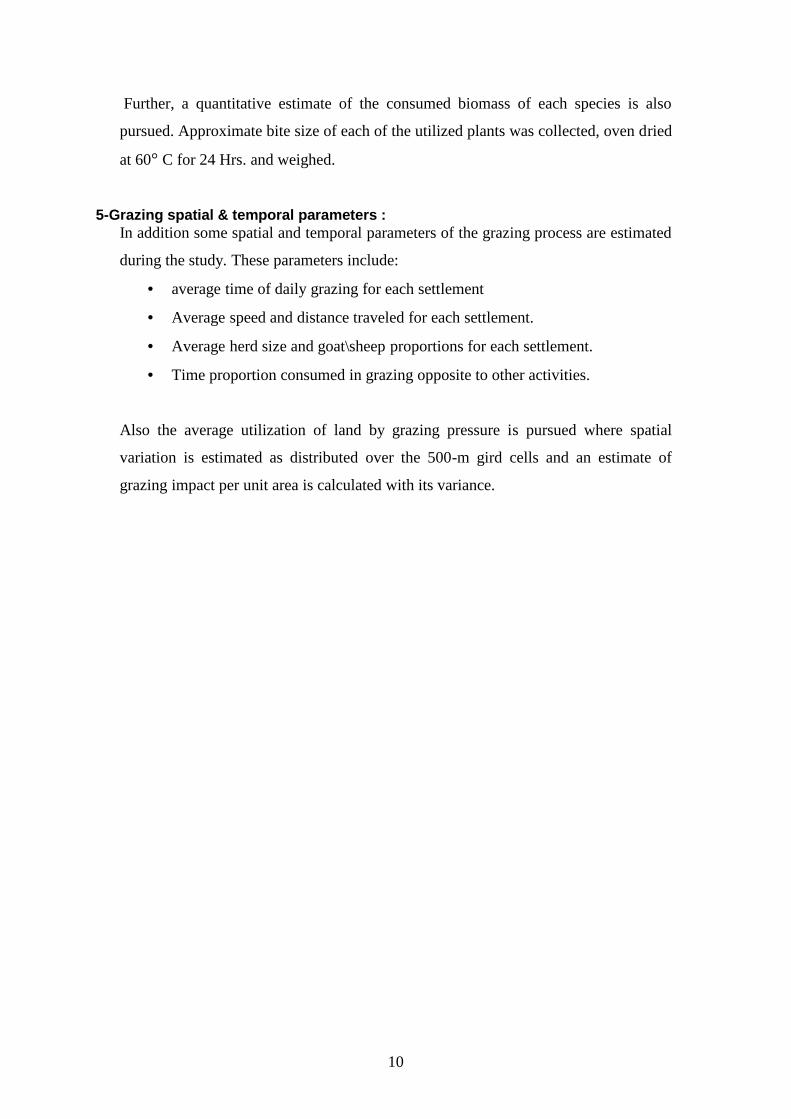
5-Grazing spatial & temporal parameters :In addition some spatial and temporal parameters of the grazing process are estimated

during the study. These parameters include:

average time of daily grazing for each settlement

Average speed and distance traveled for each settlement.

Average herd size and goat\sheep proportions for each settlement.

Time proportion consumed in grazing opposite to other activities.

Also the average utilization of land by grazing pressure is pursued where spatial

variation is estimated as distributed over the 500-m gird cells and an estimate of

grazing impact per unit area is calculated with its variance.

11

4. Results :

4.1 –Spatial patterns:4.1-a Grazing Range :

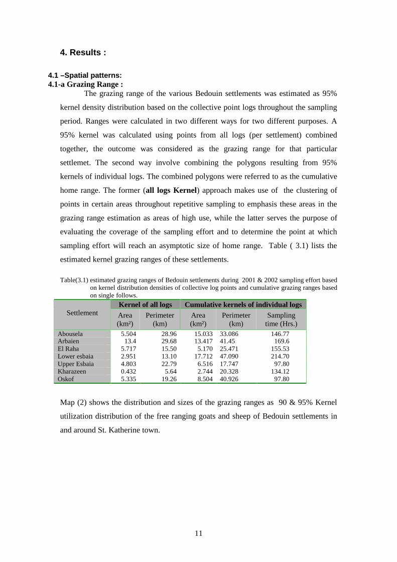
The grazing range of the various Bedouin settlements was estimated as 95%

kernel density distribution based on the collective point logs throughout the sampling

period. Ranges were calculated in two different ways for two different purposes. A

95% kernel was calculated using points from all logs (per settlement) combined

together, the outcome was considered as the grazing range for that particular

settlemet. The second way involve combining the polygons resulting from 95%

kernels of individual logs. The combined polygons were referred to as the cumulative

home range. The former (all logs Kernel) approach makes use of the clustering of

points in certain areas throughout repetitive sampling to emphasis these areas in the

grazing range estimation as areas of high use, while the latter serves the purpose of

evaluating the coverage of the sampling effort and to determine the point at which

sampling effort will reach an asymptotic size of home range. Table ( 3.1) lists the

estimated kernel grazing ranges of these settlements.

Table(3.1) estimated grazing ranges of Bedouin settlements during 2001 & 2002 sampling effort basedon kernel distribution densities of collective log points and cumulative grazing ranges basedon single follows.

SettlementKernel of all logs Cumulative kernels of individual logsArea(km²)

Perimeter(km)

Area(km²)

Perimeter(km)

Samplingtime (Hrs.)

Abousela 5.504 28.96 15.033 33.086 146.77Arbaien 13.4 29.68 13.417 41.45 169.6El Raha 5.717 15.50 5.170 25.471 155.53Lower esbaia 2.951 13.10 17.712 47.090 214.70Upper Esbaia 4.803 22.79 6.516 17.747 97.80Kharazeen 0.432 5.64 2.744 20.328 134.12Oskof 5.335 19.26 8.504 40.926 97.80

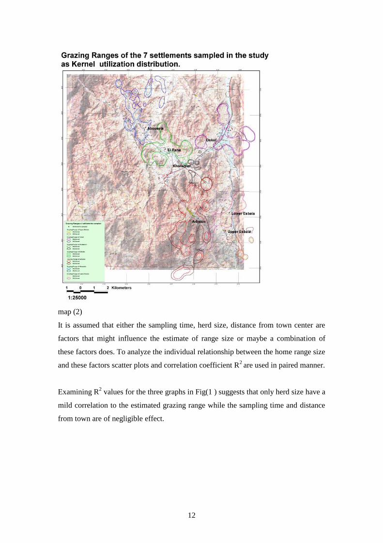
Map (2) shows the distribution and sizes of the grazing ranges as 90 & 95% Kernel

utilization distribution of the free ranging goats and sheep of Bedouin settlements in

and around St. Katherine town.

12

map (2)

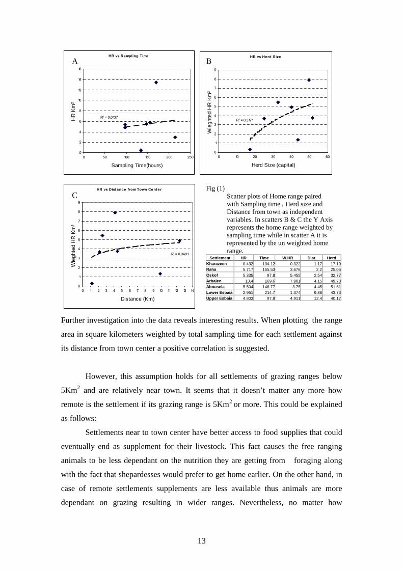
It is assumed that either the sampling time, herd size, distance from town center are

factors that might influence the estimate of range size or maybe a combination of

these factors does. To analyze the individual relationship between the home range size

and these factors scatter plots and correlation coefficient R2 are used in paired manner.

Examining R2 values for the three graphs in Fig(1 ) suggests that only herd size have a

mild correlation to the estimated grazing range while the sampling time and distance

from town are of negligible effect.

13

HR vs Sampling Time

R2 = 0.0137

0

2

4

6

8

10

12

14

16

0 50 100 150 200 250

Sampling Time(hours)

HR

Km

²

HR vs Herd Size

R2 = 0.3171

0

1

2

3

4

5

6

7

8

9

0 10 20 30 40 50 60

Herd Size (capital)

Wie

ghte

d H

R K

m²

HR vs Distance from Town Center

R2 = 0.0491

0

1

2

3

4

5

6

7

8

9

0 1 2 3 4 5 6 7 8 9 10 11 12 13 14

Distance (Km)

Wie

ghte

d H

R K

m²

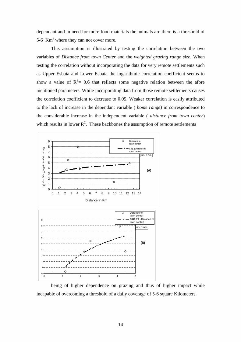
Further investigation into the data reveals interesting results. When plotting the range

area in square kilometers weighted by total sampling time for each settlement against

its distance from town center a positive correlation is suggested.

However, this assumption holds for all settlements of grazing ranges below

5Km2 and are relatively near town. It seems that it doesn’t matter any more how

remote is the settlement if its grazing range is 5Km2 or more. This could be explained

as follows:

Settlements near to town center have better access to food supplies that could

eventually end as supplement for their livestock. This fact causes the free ranging

animals to be less dependant on the nutrition they are getting from foraging along

with the fact that shepardesses would prefer to get home earlier. On the other hand, in

case of remote settlements supplements are less available thus animals are more

dependant on grazing resulting in wider ranges. Nevertheless, no matter how

Fig (1)Scatter plots of Home range pairedwith Sampling time , Herd size andDistance from town as independentvariables. In scatters B & C the Y Axisrepresents the home range weighted bysampling time while in scatter A it isrepresented by the un weighted homerange.

Settlement HR Time W.HR Dist HerdKharazeen 0.432 134.12 0.322 1.17 17.19Raha 5.717 155.53 3.676 2.2 25.05Oskof 5.335 97.8 5.455 2.54 32.77Arbaien 13.4 169.6 7.901 4.15 49.73Abousela 5.504 146.77 3.75 4.45 51.61Lower Esbaia 2.951 214.7 1.374 9.88 43.73Upper Esbaia 4.803 97.8 4.911 12.4 40.17

A B

C

14

dependant and in need for more food materials the animals are there is a threshold of

5-6 Km2 where they can not cover more.

This assumption is illustrated by testing the correlation between the two

variables of Distance from town Center and the weighted grazing range size. When

testing the correlation without incorporating the data for very remote settlements such

as Upper Esbaia and Lower Esbaia the logarithmic correlation coefficient seems to

show a value of R2= 0.6 that reflects some negative relation between the afore

mentioned parameters. While incorporating data from those remote settlements causes

the correlation coefficient to decrease to 0.05. Weaker correlation is easily attributed

to the lack of increase in the dependant variable ( home range) in correspondence to

the considerable increase in the independent variable ( distance from town center)

which results in lower R2. These backbones the assumption of remote settlements

being of higher dependence on grazing and thus of higher impact while

incapable of overcoming a threshold of a daily coverage of 5-6 square Kilometers.

R2 = 0.5965

0

1

2

3

4

5

6

7

8

9

0 1 2 3 4 5

Distance totown centeráæÛÇÑí Êãí (Distance totown center)

(B)

R² = 0.049

01

23

45

67

89

0 1 2 3 4 5 6 7 8 9 10 11 12 13 14

WightedHomerangeinKm

Distance in Km

Distance totown center

Log. (Distance totown center)

(A)

15

To assure that the sample size (no. Of follows) is efficient enough to account

for the grazing rang of the respective settlements, the cumulative range area was

plotted against number of follows for each settlement involved in the study. Figure (2)

shows that generally a plateau of the range size is attained after 10 follows. The only

exception for this rule is in Abou-sela where the plateau is reached shortly after 12

follows.

Commulative Range size aginst Sample size(no. of follows)

0

2

4

6

8

10

12

14

16

18

20

0 5 10 15 20

No. of follows

Com

mul

ativ

rang

e si

ze in

Km²

AbouselaRahaOskofLower esbaiaArbaienKharazeenUpper Esbaia

Figure (2) relation between sample size ( no. of follows) and the estimates kernel home range forBedouin settlements involved in the study.

16

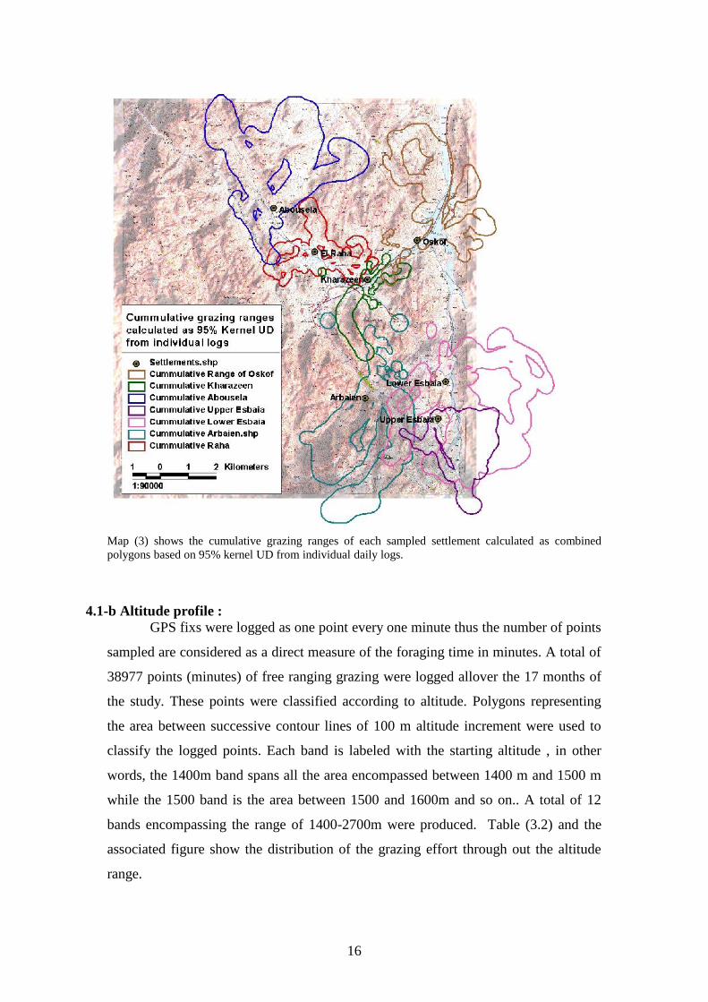
Map (3) shows the cumulative grazing ranges of each sampled settlement calculated as combinedpolygons based on 95% kernel UD from individual daily logs.

4.1-b Altitude profile :GPS fixs were logged as one point every one minute thus the number of points

sampled are considered as a direct measure of the foraging time in minutes. A total of

38977 points (minutes) of free ranging grazing were logged allover the 17 months of

the study. These points were classified according to altitude. Polygons representing

the area between successive contour lines of 100 m altitude increment were used to

classify the logged points. Each band is labeled with the starting altitude , in other

words, the 1400m band spans all the area encompassed between 1400 m and 1500 m

while the 1500 band is the area between 1500 and 1600m and so on.. A total of 12

bands encompassing the range of 1400-2700m were produced. Table (3.2) and the

associated figure show the distribution of the grazing effort through out the altitude

range.

17

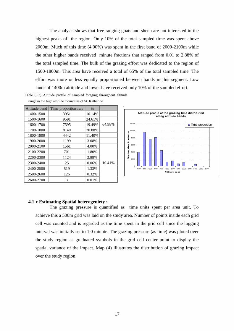
The analysis shows that free ranging goats and sheep are not interested in the

highest peaks of the region. Only 10% of the total sampled time was spent above

2000m. Much of this time (4.00%) was spent in the first band of 2000-2100m while

the other higher bands received minute fractions that ranged from 0.01 to 2.88% of

the total sampled time. The bulk of the grazing effort was dedicated to the region of

1500-1800m. This area have received a total of 65% of the total sampled time. The

effort was more or less equally proportioned between bands in this segment. Low

lands of 1400m altitude and lower have received only 10% of the sampled effort.

Table (3.2) Altitude profile of sampled foraging throughout altitude

range in the high altitude mountains of St. Katherine.

Altitude band Time proportion in min. %1400-1500 3951 10.14%1500-1600 9591 24.61%

64.98%1600-1700 7595 19.49%1700-1800 8140 20.88%1800-1900 4442 11.40%1900-2000 1199 3.08%2000-2100 1561 4.00%

10.41%

2100-2200 701 1.80%

2200-2300 1124 2.88%

2300-2400 25 0.06%

2400-2500 519 1.33%

2500-2600 126 0.32%

2600-2700 3 0.01%

4.1-c Estimating Spatial heterogeniety :The grazing pressure is quantified as time units spent per area unit. To

achieve this a 500m grid was laid on the study area. Number of points inside each grid

cell was counted and is regarded as the time spent in the grid cell since the logging

interval was initially set to 1.0 minute. The grazing pressure (as time) was ploted over

the study region as graduated symbols in the grid cell center point to display the

spatial variance of the impact. Map (4) illustrates the distribution of grazing impact

over the study region.

.

Altitude profile of the grazing time distributedalong altitude bands

0

2000

4000

6000

8000

10000

12000

1400 1500 1600 1700 1800 1900 2000 2100 2200 2300 2400 2500 2600

A lt it u d e b a n d

Time proportion

18

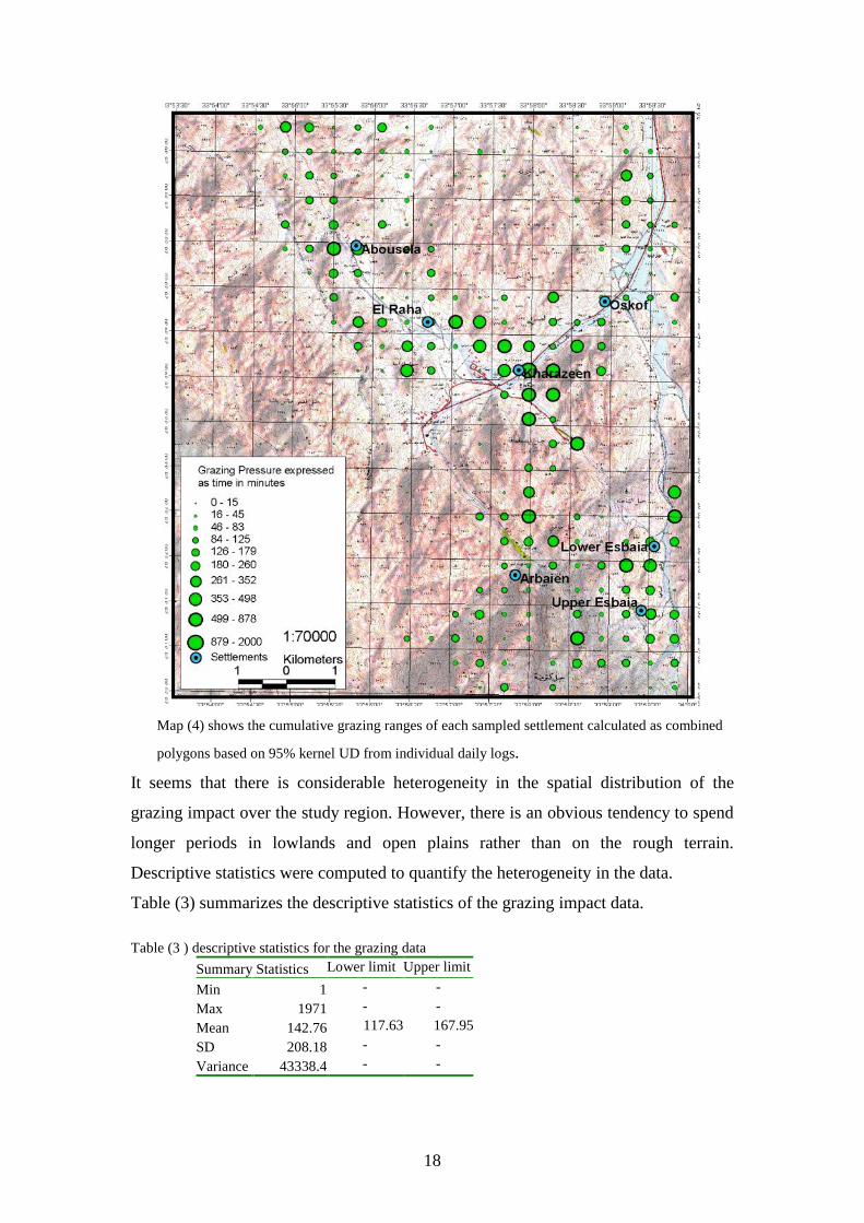
Map (4) shows the cumulative grazing ranges of each sampled settlement calculated as combined

polygons based on 95% kernel UD from individual daily logs.

It seems that there is considerable heterogeneity in the spatial distribution of the

grazing impact over the study region. However, there is an obvious tendency to spend

longer periods in lowlands and open plains rather than on the rough terrain.

Descriptive statistics were computed to quantify the heterogeneity in the data.

Table (3) summarizes the descriptive statistics of the grazing impact data.

Table (3 ) descriptive statistics for the grazing data

Summary Statistics Lower limit Upper limit

Min 1 - -

Max 1971 - -

Mean 142.76 117.63 167.95

SD 208.18 - -

Variance 43338.4 - -

19

N o o f m in u te s s p e n t p e r 5 0 0 m g rid c e l l

po ints pe r g r idce ll (m inutes )

Freq

uenc

y

0 500 1000 1500 2000

020

4060

80

0 500 1000 1500 2000

0.00

00.

001

0.00

20.

003

0.00

40.

005

K e rn e l d is trib u tio n o f g ra z in g im p a c t

po ints pe r g r idce ll (m inutes )

Dens

ity

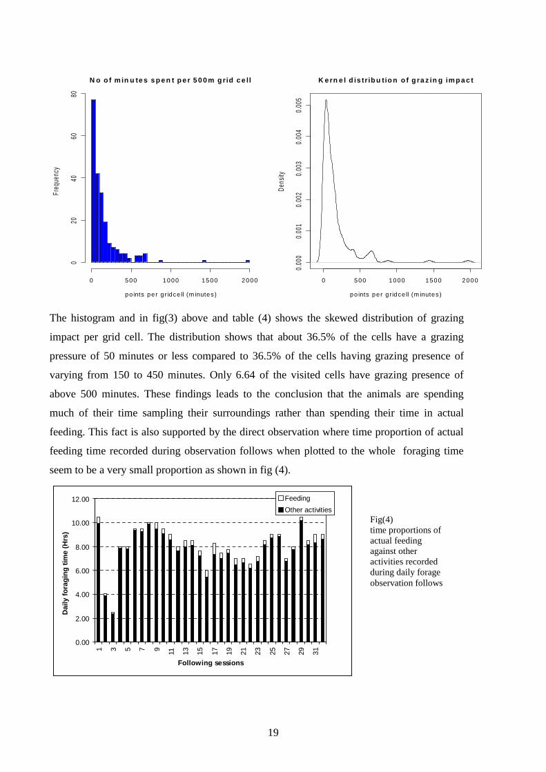
The histogram and in fig(3) above and table (4) shows the skewed distribution of grazing

impact per grid cell. The distribution shows that about 36.5% of the cells have a grazing

pressure of 50 minutes or less compared to 36.5% of the cells having grazing presence of

varying from 150 to 450 minutes. Only 6.64 of the visited cells have grazing presence of

above 500 minutes. These findings leads to the conclusion that the animals are spending

much of their time sampling their surroundings rather than spending their time in actual

feeding. This fact is also supported by the direct observation where time proportion of actual

feeding time recorded during observation follows when plotted to the whole foraging time

seem to be a very small proportion as shown in fig (4).

0.00

2.00

4.00

6.00

8.00

10.00

12.00

1 3 5 7 9 11 13 15 17 19 21 23 25 27 29 31

Following sessions

Dai

ly fo

ragi

ng ti

me

(Hrs

)

FeedingOther activities

Fig(4)time proportions ofactual feedingagainst otheractivities recordedduring daily forageobservation follows

20

Table (4) shows the bin range distribution of the grazing presence over the 500m grid cells over the studyregion. Note that only visited cells are included where all cells with 0 points were initially excluded.

min/ grid cell Frequency Percentage Cumulative percentage

50 96 36.50%100 54 20.53%150 40 15.21%

36.50%

200 23 8.75%250 10 3.80%300 9 3.42%350 6 2.28%400 4 1.52%450 4 1.52%500 3 1.14%

63.46%

550 0 0.00%

600 3 1.14%

650 3 1.14%

700 4 1.52%

750 1 0.38%

800 0 0.00%

850 0 0.00%

900 1 0.38%

950 0 0.00%

1000 0 0.00%

1050 0 0.00%

1100 0 0.00%

1150 0 0.00%

1200 0 0.00%

1250 0 0.00%

1300 0 0.00%

1350 0 0.00%

1400 0 0.00%

1450 1 0.38%

1500 0 0.00%

1550 0 0.00%

1600 0 0.00%

1650 0 0.00%

1700 0 0.00%

1750 0 0.00%

1800 0 0.00%

1850 0 0.00%

1900 0 0.00%

1950 0 0.00%

2000 1 0.38%

A fast calculation shows that the estimated grazing impact per square kilometer is about 33.6

minutes per month.

21

4.2 –Feeding Properties :4.2-a Food Spectrum :

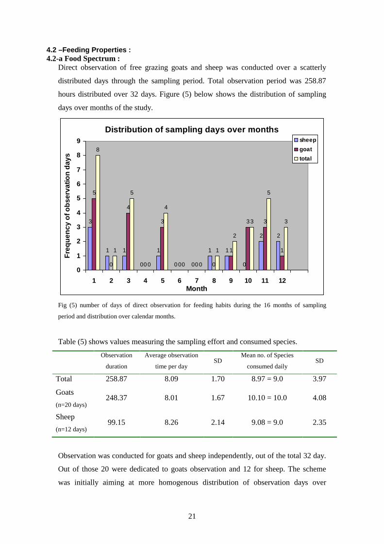
Direct observation of free grazing goats and sheep was conducted over a scatterly

distributed days through the sampling period. Total observation period was 258.87

hours distributed over 32 days. Figure (5) below shows the distribution of sampling

days over months of the study.

Distribution of sampling days over months

3

1 1

0

1

0 0

1 1

0

2 2

5

0

4

0

3

0 0 0

1

3 3

1

8

1

5

0

4

0 0

1

2

3

5

3

0

1

2

3

4

5

6

7

8

9

1 2 3 4 5 6 7 8 9 10 11 12Month

Freq

uenc

y of

obs

erva

tion

days

sheepgoattotal

Fig (5) number of days of direct observation for feeding habits during the 16 months of sampling

period and distribution over calendar months.

Table (5) shows values measuring the sampling effort and consumed species.

Observation

duration

Average observation

time per daySD

Mean no. of Species

consumed dailySD

Total 258.87 8.09 1.70 8.97 = 9.0 3.97

Goats

(n=20 days)248.37 8.01 1.67 10.10 = 10.0 4.08

Sheep

(n=12 days)99.15 8.26 2.14 9.08 = 9.0 2.35

Observation was conducted for goats and sheep independently, out of the total 32 day.

Out of those 20 were dedicated to goats observation and 12 for sheep. The scheme

was initially aiming at more homogenous distribution of observation days over

22

calendar months and more equal proportions for both of the focal species of grazing

animals. However, being very understaffed – only the female ranger could accompany

the girls during grazing- rendered this aim hard to achieve in consideration the leave

schedule of the rangers.

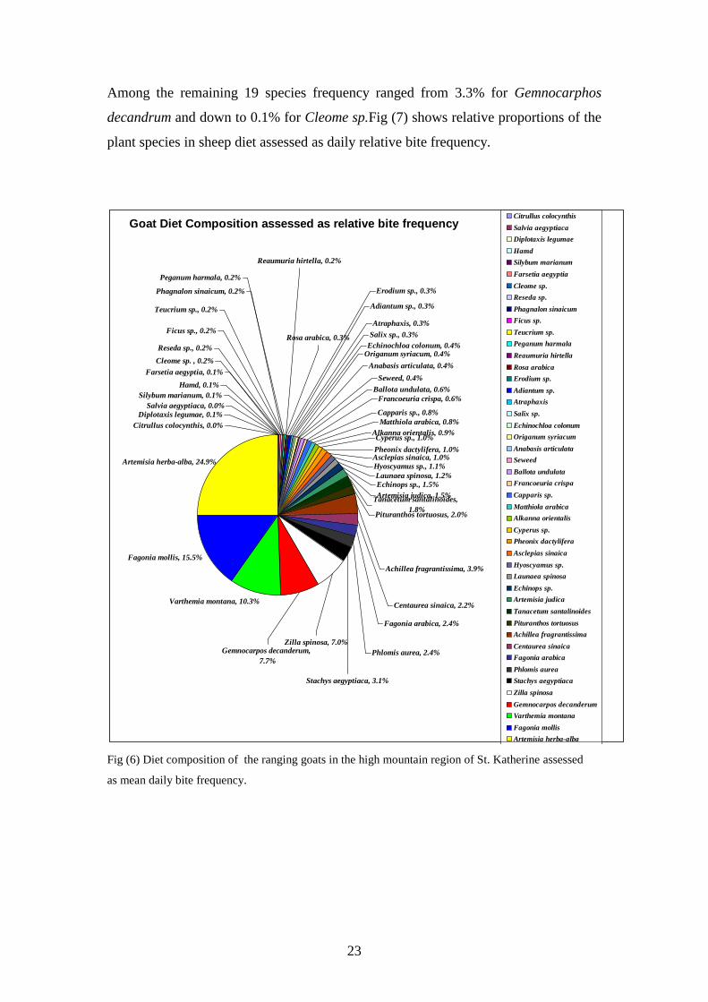
Goats were found to have a wider food spectrum compared to sheep. Goats utilized 49

plant species as food while sheep utilized only 26 species. Although these numbers

are suggesting variable diet, those number could be misleading if the relative

proportions are not considered. Out of the 49 floral species utilized by goats only 6

species comprised 68% of the diet. These were Artemesia herba alba 24.94%,

Fagonia moillis 15.47%, Varthemia montana 10.26%, Gymnocaropos decandrum

7.66%, Zilla spinosa 6.96%, and Stachys aegyptiaca 3.10%. These are assessed as

percentage of bite frequency. The remaining 31% comprises about 43 species, these

species are considered as complimentary to the major six since the individual

proportions of individual species ranged from 0.03% for Citrullus colocynthis to up to

2.42% for Phlomes aurea. Fig (6) shows relative proportions of the plant species in

goats diet.

The diet of goats included 4 endemic species, namely Phlomes aurea 2.42%,

Oryganum sinaicum 0.36%, Rosa arabica 0.25%, and Phagnalon sinaicum 0.19%.

The total proportion of endemic plants utilized was 3.22% only of the total diet

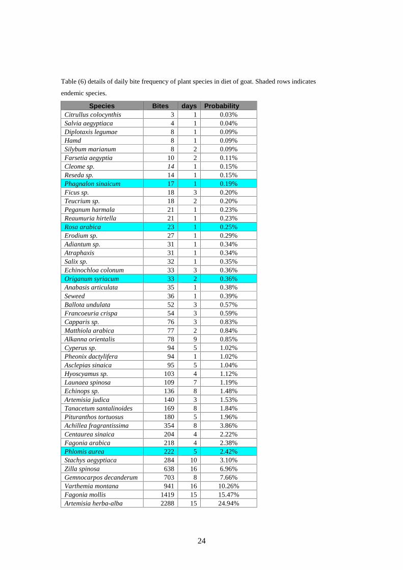
evaluated as bite frequency percentage. Table (6) shows a list of the utilized species

and their relative proportions as bite frequency percentage.

On the other hand, sheep showed narrower food spectrum where they were observed

to utilize only 25 plant species. All the plant species utilized by sheep are readily

contained in the diet of goats except for Ochradenus buccatus which was not

observed in the diet of goats. However, this might be of no significance since it is

only one incidence with 11 bites. Thus it is highly likely that it could be a pure chance

of a sheep being accidentally sampling a new plant species and found it unsatisfying .

Out of the 25 eaten plant species 6 comprised about 85% of the diet leaving only 13%

for all other species. The most preferred plant species were namely; Artemisia herba-

alba 20.7%, Fagonia moills 20.6%, Varethemia montana 18.67%, Cyprus sp 11.67%,

Zilla spinosa 8.0% and Stachys aegyptiaca 4.31%.

23

Among the remaining 19 species frequency ranged from 3.3% for Gemnocarphos

decandrum and down to 0.1% for Cleome sp.Fig (7) shows relative proportions of the

plant species in sheep diet assessed as daily relative bite frequency.

Goat Diet Composition assessed as relative bite frequency

Varthemia montana, 10.3%

Fagonia mollis, 15.5%

Peganum harmala, 0.2%

Salix sp., 0.3%Echinochloa colonum, 0.4%

Seweed, 0.4%

Teucrium sp., 0.2%

Ficus sp., 0.2%

Cleome sp. , 0.2%

Hamd, 0.1%

Origanum syriacum, 0.4%

Centaurea sinaica, 2.2%

Fagonia arabica, 2.4%

Phlomis aurea, 2.4%

Stachys aegyptiaca, 3.1%

Zilla spinosa, 7.0%Gemnocarpos decanderum,

7.7%

Salvia aegyptiaca, 0.0%Diplotaxis legumae, 0.1%

Citrullus colocynthis, 0.0%

Achillea fragrantissima, 3.9%

Pituranthos tortuosus, 2.0%

Tanacetum santalinoides,1.8%

Artemisia judica, 1.5%Echinops sp., 1.5%Launaea spinosa, 1.2%Hyoscyamus sp., 1.1%Asclepias sinaica, 1.0%Pheonix dactylifera, 1.0%

Cyperus sp., 1.0%Alkanna orientalis, 0.9%

Matthiola arabica, 0.8%Capparis sp., 0.8%

Francoeuria crispa, 0.6%Ballota undulata, 0.6%

Anabasis articulata, 0.4%Farsetia aegyptia, 0.1%

Silybum marianum, 0.1%

Phagnalon sinaicum, 0.2%

Reseda sp., 0.2%

Reaumuria hirtella, 0.2%

Atraphaxis, 0.3%

Adiantum sp., 0.3%

Rosa arabica, 0.3%

Erodium sp., 0.3%

Artemisia herba-alba, 24.9%

Citrullus colocynthis

Salvia aegyptiaca

Diplotaxis legumae

Hamd

Silybum marianum

Farsetia aegyptia

Cleome sp.

Reseda sp.

Phagnalon sinaicum

Ficus sp.

Teucrium sp.

Peganum harmala

Reaumuria hirtella

Rosa arabica

Erodium sp.

Adiantum sp.

Atraphaxis

Salix sp.

Echinochloa colonum

Origanum syriacum

Anabasis articulata

Seweed

Ballota undulata

Francoeuria crispa

Capparis sp.

Matthiola arabica

Alkanna orientalis

Cyperus sp.

Pheonix dactylifera

Asclepias sinaica

Hyoscyamus sp.

Launaea spinosa

Echinops sp.

Artemisia judica

Tanacetum santalinoides

Pituranthos tortuosus

Achillea fragrantissima

Centaurea sinaica

Fagonia arabica

Phlomis aurea

Stachys aegyptiaca

Zilla spinosa

Gemnocarpos decanderum

Varthemia montana

Fagonia mollis

Artemisia herba-alba

Fig (6) Diet composition of the ranging goats in the high mountain region of St. Katherine assessed

as mean daily bite frequency.

24

Table (6) details of daily bite frequency of plant species in diet of goat. Shaded rows indicates

endemic species.

Species Bites days ProbabilityCitrullus colocynthis 3 1 0.03%Salvia aegyptiaca 4 1 0.04%Diplotaxis legumae 8 1 0.09%Hamd 8 1 0.09%Silybum marianum 8 2 0.09%Farsetia aegyptia 10 2 0.11%Cleome sp. 14 1 0.15%Reseda sp. 14 1 0.15%Phagnalon sinaicum 17 1 0.19%Ficus sp. 18 3 0.20%Teucrium sp. 18 2 0.20%Peganum harmala 21 1 0.23%Reaumuria hirtella 21 1 0.23%Rosa arabica 23 1 0.25%Erodium sp. 27 1 0.29%Adiantum sp. 31 1 0.34%Atraphaxis 31 1 0.34%Salix sp. 32 1 0.35%Echinochloa colonum 33 3 0.36%Origanum syriacum 33 2 0.36%Anabasis articulata 35 1 0.38%Seweed 36 1 0.39%Ballota undulata 52 3 0.57%Francoeuria crispa 54 3 0.59%Capparis sp. 76 3 0.83%Matthiola arabica 77 2 0.84%Alkanna orientalis 78 9 0.85%Cyperus sp. 94 5 1.02%Pheonix dactylifera 94 1 1.02%Asclepias sinaica 95 5 1.04%Hyoscyamus sp. 103 4 1.12%Launaea spinosa 109 7 1.19%Echinops sp. 136 8 1.48%Artemisia judica 140 3 1.53%Tanacetum santalinoides 169 8 1.84%Pituranthos tortuosus 180 5 1.96%Achillea fragrantissima 354 8 3.86%Centaurea sinaica 204 4 2.22%Fagonia arabica 218 4 2.38%Phlomis aurea 222 5 2.42%Stachys aegyptiaca 284 10 3.10%Zilla spinosa 638 16 6.96%Gemnocarpos decanderum 703 8 7.66%Varthemia montana 941 16 10.26%Fagonia mollis 1419 15 15.47%Artemisia herba-alba 2288 15 24.94%

25

Diet composition of Sheep assessed as relative bite frequency

Zilla spinosa, 20.81%

Ochradenus sp. , 0.50%

Asclepias sinaica, 0.59%

Phoenex dactylifera, 0.90%

Teucrium sp., 1.22%

Cynodon dactylon, 1.40%

Alkanna orientalis, 1.40%

Matthiola arabica, 1.49%

Echinops sp. , 1.94%

Launaea spinosa, 1.94%

Artemisia judica, 2.13%

Tanacetum santalinoides, 2.49%

Fagonia arabica, 3.48%

Anabasis articulata, 3.71%

Achillea fragrantissima, 0.00%

Peganum harmala, 5.02%

Gemnocarpos decanderum, 8.41%

Stachys aegyptiaca, 11.22%

Cleome sp, 0.14%

Phlomis aurea, 0.32%Reaumuria hirtella, 0.27%

Origanum syriacum, 0.05%

Cyperus sp., 30.57%

Origanum syriacum

Cleome sp

Reaumuria hirtella

Phlomis aurea

Ochradenus sp.

Asclepias sinaica

Phoenex dactylifera

Teucrium sp.

Cynodon dactylon

Alkanna orientalis

Matthiola arabica

Echinops sp.

Launaea spinosa

Artemisia judica

Tanacetum santalinoides

Fagonia arabica

Anabasis articulata

Achillea fragrantissima

Peganum harmala

Gemnocarpos decanderum

Stachys aegyptiaca

Zilla spinosa

Cyperus sp.

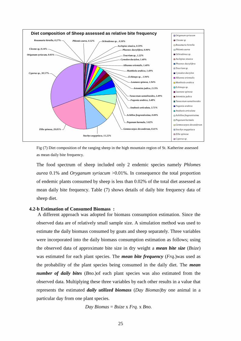
Fig (7) Diet composition of the ranging sheep in the high mountain region of St. Katherine assessed

as mean daily bite frequency.

The food spectrum of sheep included only 2 endemic species namely Phlomes

aurea 0.1% and Oryganum syriacum >0.01%. In consequence the total proportion

of endemic plants consumed by sheep is less than 0.02% of the total diet assessed as

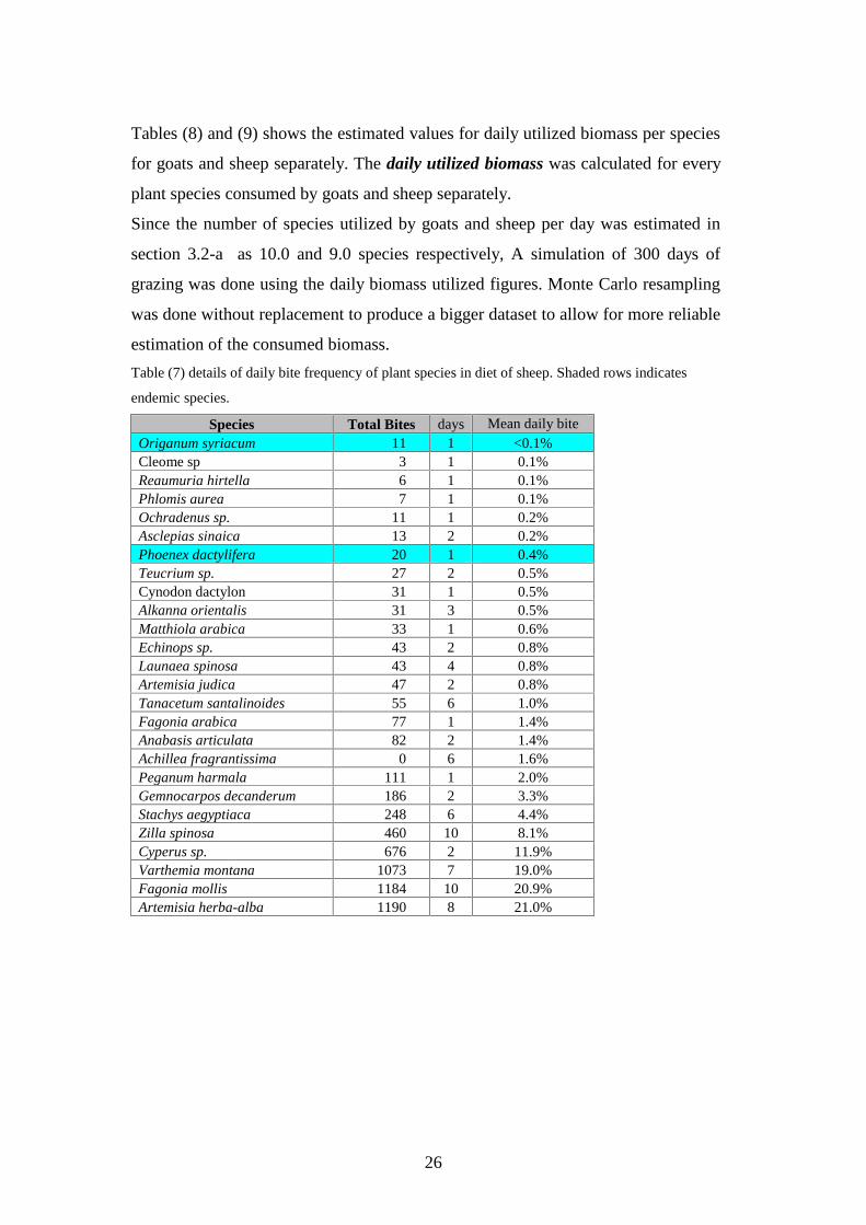
mean daily bite frequency. Table (7) shows details of daily bite frequency data of

sheep diet.

4.2-b Estimation of Consumed Biomass :A different approach was adopted for biomass consumption estimation. Since the

observed data are of relatively small sample size. A simulation method was used to

estimate the daily biomass consumed by goats and sheep separately. Three variables

were incorporated into the daily biomass consumption estimation as follows; using

the observed data of approximate bite size in dry weight a mean bite size (Bsize)

was estimated for each plant species. The mean bite frequency (Frq.)was used as

the probability of the plant species being consumed in the daily diet. The mean

number of daily bites (Bno.)of each plant species was also estimated from the

observed data. Multiplying these three variables by each other results in a value that

represents the estimated daily utilized biomass (Day Biomas)by one animal in a

particular day from one plant species.

Day Biomas = Bsize x Frq. x Bno.

26

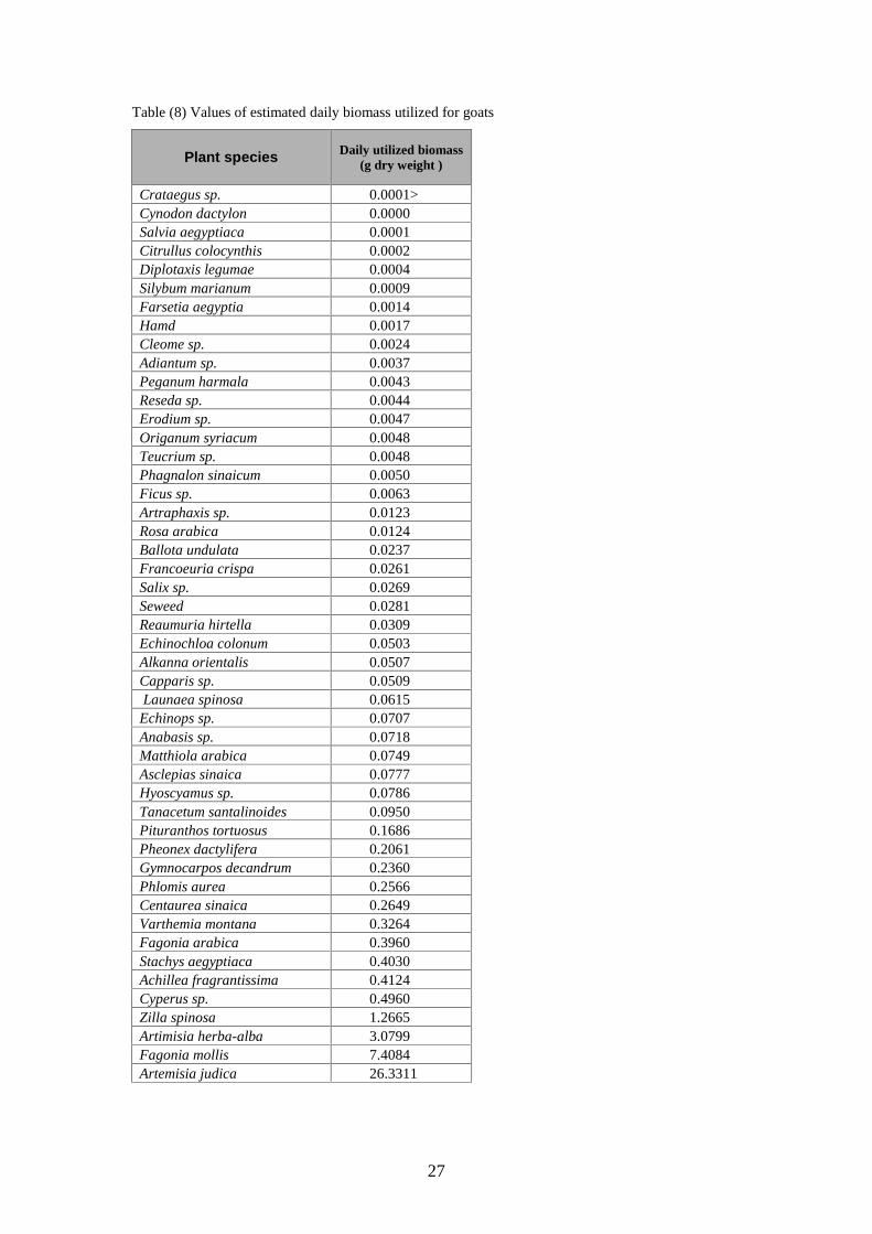
Tables (8) and (9) shows the estimated values for daily utilized biomass per species

for goats and sheep separately. The daily utilized biomass was calculated for every

plant species consumed by goats and sheep separately.

Since the number of species utilized by goats and sheep per day was estimated in

section 3.2-a as 10.0 and 9.0 species respectively, A simulation of 300 days of

grazing was done using the daily biomass utilized figures. Monte Carlo resampling

was done without replacement to produce a bigger dataset to allow for more reliable

estimation of the consumed biomass.

Table (7) details of daily bite frequency of plant species in diet of sheep. Shaded rows indicates

endemic species.

Species Total Bites days Mean daily bitefreq. As %Origanum syriacum 11 1 <0.1%

Cleome sp 3 1 0.1%Reaumuria hirtella 6 1 0.1%Phlomis aurea 7 1 0.1%Ochradenus sp. 11 1 0.2%Asclepias sinaica 13 2 0.2%Phoenex dactylifera 20 1 0.4%Teucrium sp. 27 2 0.5%Cynodon dactylon 31 1 0.5%Alkanna orientalis 31 3 0.5%Matthiola arabica 33 1 0.6%Echinops sp. 43 2 0.8%Launaea spinosa 43 4 0.8%Artemisia judica 47 2 0.8%Tanacetum santalinoides 55 6 1.0%Fagonia arabica 77 1 1.4%Anabasis articulata 82 2 1.4%Achillea fragrantissima 0 6 1.6%Peganum harmala 111 1 2.0%Gemnocarpos decanderum 186 2 3.3%Stachys aegyptiaca 248 6 4.4%Zilla spinosa 460 10 8.1%Cyperus sp. 676 2 11.9%Varthemia montana 1073 7 19.0%Fagonia mollis 1184 10 20.9%Artemisia herba-alba 1190 8 21.0%

27

Table (8) Values of estimated daily biomass utilized for goats

Plant species Daily utilized biomass(g dry weight )

Crataegus sp. 0.0001>Cynodon dactylon 0.0000Salvia aegyptiaca 0.0001Citrullus colocynthis 0.0002Diplotaxis legumae 0.0004Silybum marianum 0.0009Farsetia aegyptia 0.0014Hamd 0.0017Cleome sp. 0.0024Adiantum sp. 0.0037Peganum harmala 0.0043Reseda sp. 0.0044Erodium sp. 0.0047Origanum syriacum 0.0048Teucrium sp. 0.0048Phagnalon sinaicum 0.0050Ficus sp. 0.0063Artraphaxis sp. 0.0123Rosa arabica 0.0124Ballota undulata 0.0237Francoeuria crispa 0.0261Salix sp. 0.0269Seweed 0.0281Reaumuria hirtella 0.0309Echinochloa colonum 0.0503Alkanna orientalis 0.0507Capparis sp. 0.0509Launaea spinosa 0.0615

Echinops sp. 0.0707Anabasis sp. 0.0718Matthiola arabica 0.0749Asclepias sinaica 0.0777Hyoscyamus sp. 0.0786Tanacetum santalinoides 0.0950Pituranthos tortuosus 0.1686Pheonex dactylifera 0.2061Gymnocarpos decandrum 0.2360Phlomis aurea 0.2566Centaurea sinaica 0.2649Varthemia montana 0.3264Fagonia arabica 0.3960Stachys aegyptiaca 0.4030Achillea fragrantissima 0.4124Cyperus sp. 0.4960Zilla spinosa 1.2665Artimisia herba-alba 3.0799Fagonia mollis 7.4084Artemisia judica 26.3311

28

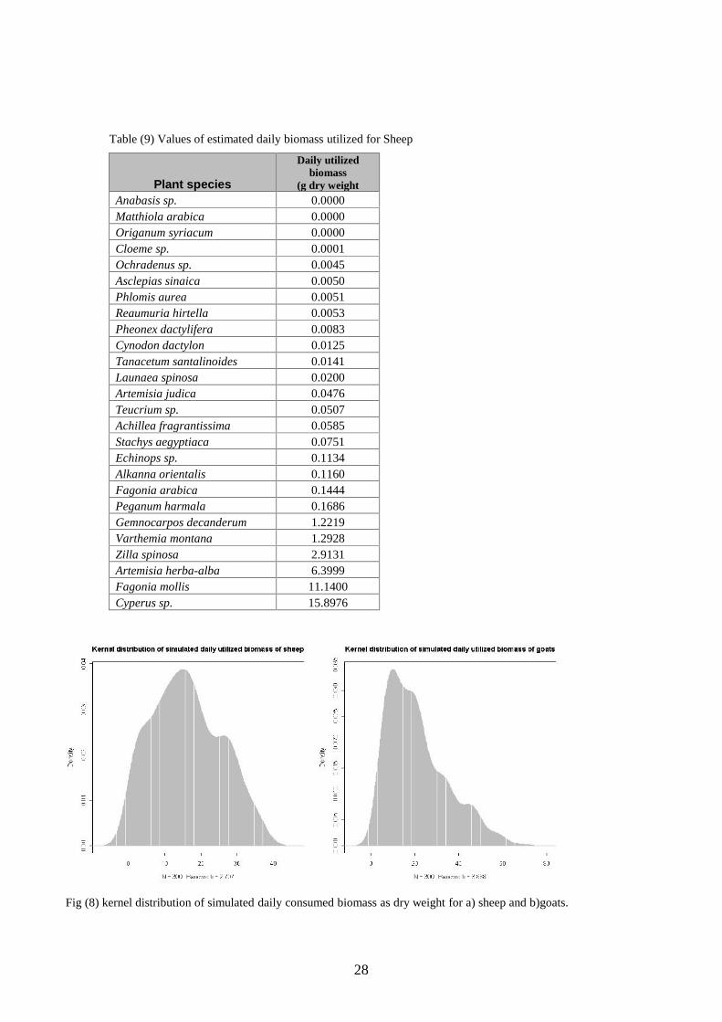
Table (9) Values of estimated daily biomass utilized for Sheep

Plant species

Daily utilizedbiomass

(g dry weightAnabasis sp. 0.0000Matthiola arabica 0.0000Origanum syriacum 0.0000Cloeme sp. 0.0001Ochradenus sp. 0.0045Asclepias sinaica 0.0050Phlomis aurea 0.0051Reaumuria hirtella 0.0053Pheonex dactylifera 0.0083Cynodon dactylon 0.0125Tanacetum santalinoides 0.0141Launaea spinosa 0.0200Artemisia judica 0.0476Teucrium sp. 0.0507Achillea fragrantissima 0.0585Stachys aegyptiaca 0.0751Echinops sp. 0.1134Alkanna orientalis 0.1160Fagonia arabica 0.1444Peganum harmala 0.1686Gemnocarpos decanderum 1.2219Varthemia montana 1.2928Zilla spinosa 2.9131Artemisia herba-alba 6.3999Fagonia mollis 11.1400Cyperus sp. 15.8976

Fig (8) kernel distribution of simulated daily consumed biomass as dry weight for a) sheep and b)goats.

29

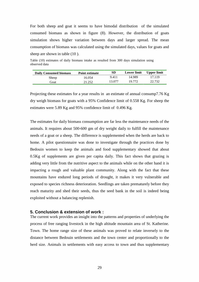
For both sheep and goat it seems to have bimodal distribution of the simulated

consumed biomass as shown in figure (8). However, the distribution of goats

simulation shows higher variation between days and larger spread. The mean

consumption of biomass was calculated using the simulated days, values for goats and

sheep are shown in table (10 ).

Table (10) estimates of daily biomass intake as resulted from 300 days simulation usingobserved data

Daily Consumed biomass Point estimate SD Lower limit Upper limit

Sheep 16.054 9.411 14.989 17.119

Goat 21.252 13.077 19.772 22.732

Projecting these estimates for a year results in an estimate of annual consump7.76 Kg

dry weigh biomass for goats with a 95% Confidence limit of 0.558 Kg. For sheep the

estimates were 5.89 Kg and 95% confidence limit of 0.496 Kg.

The estimates for daily biomass consumption are far less the maintenance needs of the

animals. It requires about 500-600 gm of dry weight daily to fulfill the maintenance

needs of a goat or a sheep. The difference is supplemented when the herds are back to

home. A pilot questionnaire was done to investigate through the practices done by

Bedouin women to keep the animals and food supplementary showed that about

0.5Kg of supplements are given per capita daily. This fact shows that grazing is

adding very little from the nutritive aspect to the animals while on the other hand it is

impacting a rough and valuable plant community. Along with the fact that these

mountains have endured long periods of drought, it makes it very vulnerable and

exposed to species richness deterioration. Seedlings are taken prematurely before they

reach maturity and shed their seeds, thus the seed bank in the soil is indeed being

exploited without a balancing replenish.

5. Conclusion & extension of work :The current work provides an insight into the patterns and properties of underlying the

process of free ranging livestock in the high altitude mountain area of St. Katherine.

Town. The home range size of these animals was proved to relate inversely to the

distance between Bedouin settlements and the town center and proportionally to the

herd size. Animals in settlements with easy access to town and thus supplementary

30

fooders found to have smaller home-range. A ceiling of 6.0 Km2 of daily home range

area was estimated for free ranging livestock.

The grazing impact was quantified as 33.6 minutes per square kilometer as grazing

impact per month. However, the impact is not uniformly spatially distributed and

involves great deal of spatial heterogeneity. Spatial heterogeneity was also mapped.

The direct observation of grazing livestock showed that the proportion of time during

which animals are involved in direct feeding activities comprises minute proportion

on the temporal scale of a grazing day suggesting the shortage of available resources

and that animals spend longer time sampling their environment rather than getting

their nutritional requirements.

The food spectrum of both goats and sheep was determined, involving 46 species

utilized by the former and 25 by the latter. Five endemic species were utilized by

goats and only two utilized by sheep. Endemic species comprised 3.22% of the total

diet assessed as bite frequency while it was only 0.02% for sheep. The altitude profile

of the grazing process showed that animals are less likely to consume endemics as

they spend only 10% of grazing time within the altitude range of endemic plant

species.

Extension of work.

The expected extension of work is to be addressed on two approaches. The

current study was done during the period (2001 – 2002) where very little amount of

precipitation was received by the mountains, thus the available plants were almost

exclusively perennials. A second sampling round is strongly recommended following

a good rainy season to update the food spectrum composition and proportions with the

added annuals by then.

It is known that the plant community of the study region is unique due to the

exceptional altitude range. Therefore it is essential to conduct the same approach of

the whole sampling scheme in the southern parts of the protectorate to account for

changes or differences induced by different terrain and plant community.

The current study has managed to determine the composition of livestock diet but

unfortunately nothing was available about the preference of the utilized species. The

31

team failed to account for the available amount of each species of the utilized plants

in the grazing ranges due to manpower constrains and thus comparing percentages of

the species as represented in the diet and that available to the animals in the grazing

range was not possible. Future studies are strongly recommended to be preceded by a

botanical assessment for species richness, coverage and abundance.

Finally we hope that this study was helpful, meaningful and would offer insight into

future grazing management practices imposed by decision makers.