Graduation Project

Palestine Polytechnic University

College of Engineering &Technology

Mechanical Engineering department

Mechatronics Engineering

Graduation Project

Rehabilitation and Control of Articulated HydraulicManipulator

Project Team

Majid Alhroosh Mujahed Masharqa

Project Supervisor

Dr.Yousef Alswati

Hebron-Palestine

2012

I

CERTIFICATION

Palestine Polytechnic University

PPU

Hebron-Palestine

Rehabilitation and Control of Articulated HydraulicManipulator

Prepared By

Majid Alhroosh Mujahed Masharqa

In accordance with the recommendations of the project supervisor, andthe acceptance of all examining committee members, this project hasbeen submitted to the department of mechanical engineering in thecollege of engineering and technology in the partial fulfillment of therequirement of department for the degree of Bachelor of Science inengineering.

Project Supervisor signature

----------------------

Committee Member signature

----------------- -------------------- -------------------

Department Head Signature

-------------------------

II

Acknowledgment

We wish to thank our parents for their tremendous contributions andsupport both morally and financially towards the completion of thisproject.

We also grateful to our project supervisor Dr. Yousef Alswati whowithout his help and guidance this project would not have beencompleted.I also show my gratitude to my friends and all who contributed in oneway or the other in the course of the project.

III

Abstract

The articulated hydraulic manipulator is a manipulator with three revolute

joints and attached gripper. Each joint in this robot is driven by a

hydraulic actuator. This robot is belongs to the mechatronics laboratory

of Palestine Polytechnic University (ppu), and it has a five degree of

freedom.

We will use the logic controller (plc) to control the movement of the

manipulator end-effectors in the working envelop, so by using the HMI

touch screen the coordinate will be entered and the end effecter move to

the desired location in the workspace of manipulator, hence we will

design a robotic system to make the manipulator pick an object from one

location and move it to another.

In order to make this, many challenging problems will be covered in this

project; these problems are kinematic, dynamitic, actuation, motion

planning, control and programming.

IV

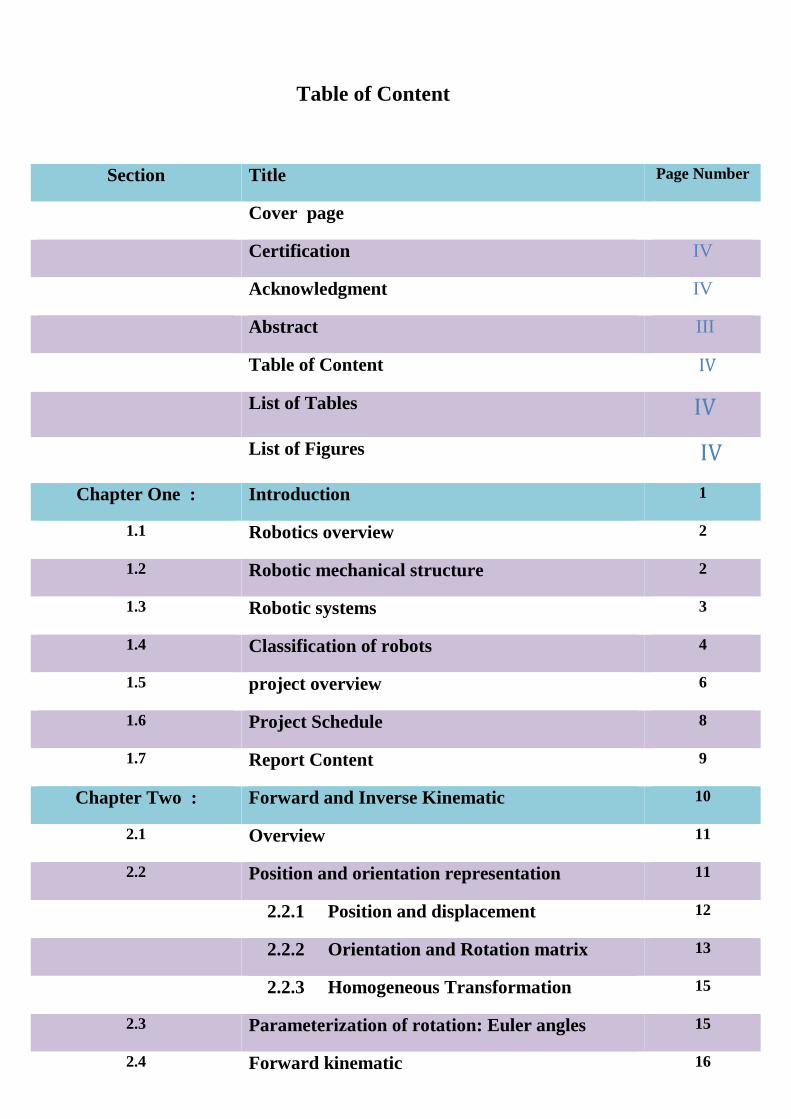
Section Title Page Number

Cover page

Certification IV

Acknowledgment IV

Abstract III

Table of Content IVList of Tables IVList of Figures IV

Chapter One : Introduction 1

1.1 Robotics overview 2

1.2 Robotic mechanical structure 2

1.3 Robotic systems 3

1.4 Classification of robots 4

1.5 project overview 6

1.6 Project Schedule 8

1.7 Report Content 9

Chapter Two : Forward and Inverse Kinematic 10

2.1 Overview 11

2.2 Position and orientation representation 11

2.2.1 Position and displacement 12

2.2.2 Orientation and Rotation matrix 13

2.2.3 Homogeneous Transformation 15

2.3 Parameterization of rotation: Euler angles 15

2.4 Forward kinematic 16

Table of Content

V

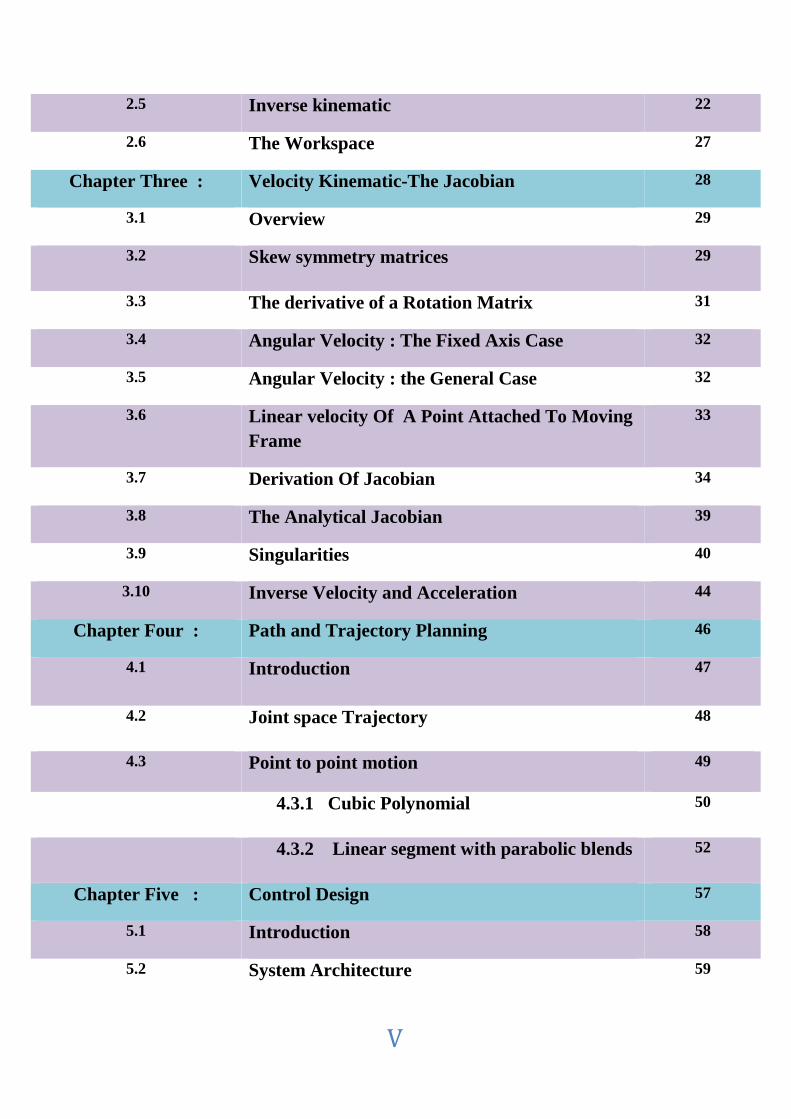
2.5 Inverse kinematic 22

2.6 The Workspace 27

Chapter Three : Velocity Kinematic-The Jacobian 28

3.1 Overview 29

3.2 Skew symmetry matrices 29

3.3 The derivative of a Rotation Matrix 31

3.4 Angular Velocity : The Fixed Axis Case 32

3.5 Angular Velocity : the General Case 32

3.6 Linear velocity Of A Point Attached To MovingFrame

33

3.7 Derivation Of Jacobian 34

3.8 The Analytical Jacobian 39

3.9 Singularities 40

3.10 Inverse Velocity and Acceleration 44

Chapter Four : Path and Trajectory Planning 46

4.1 Introduction 47

4.2 Joint space Trajectory 48

4.3 Point to point motion 49

4.3.1 Cubic Polynomial 50

4.3.2 Linear segment with parabolic blends 52

Chapter Five : Control Design 57

5.1 Introduction 58

5.2 System Architecture 59

VI

5.2.1 Physical System Description 59

5.2.2 Functional description 60

5.2.3 Hydraulic Description 60

5.2.4 Electrical Description 62

5.3 Closed Loop Control 63

5.3.1 Feedback Sensors 64

5.3.2 Controller and software 68

Chapter Six : Hardware and Software Description 72

6.1 Introductions 73

6.2 Hardware and Software Components 73

6.3 Sequence function chart –SFC (State Graph) 74

6.4 PID functions on Plc. 79

6.4.1 Introduction 79

6.4.2 The PID Controller Model 80

6.4.3 Operating Principles 83

6.4.4 Principal of the Regulation Loop 85

6.4.5 Role and Influence of PID Parameters 86

6.5 Touch Screen and Vijeo Designer 89

Chapter Seven : Experiments and Results 92

7.1 Introduction 93

7.2 Experimental results 93

7.3 Conclusion 95

7.4 Future Work 95

VII

References 96

Appendices 97

VIII

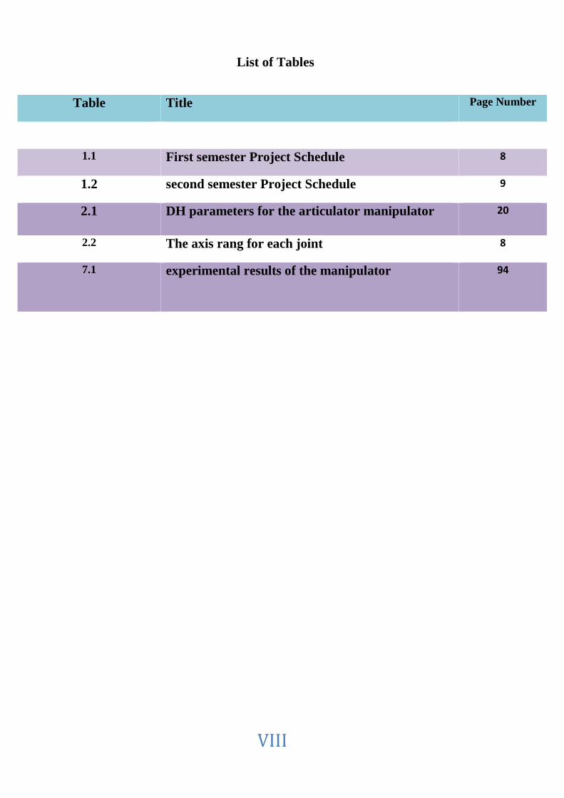
Table Title Page Number

1.1 First semester Project Schedule 8

1.2 second semester Project Schedule 9

2.1 DH parameters for the articulator manipulator 20

2.2 The axis rang for each joint 8

7.1 experimental results of the manipulator 94

List of Tables

IX

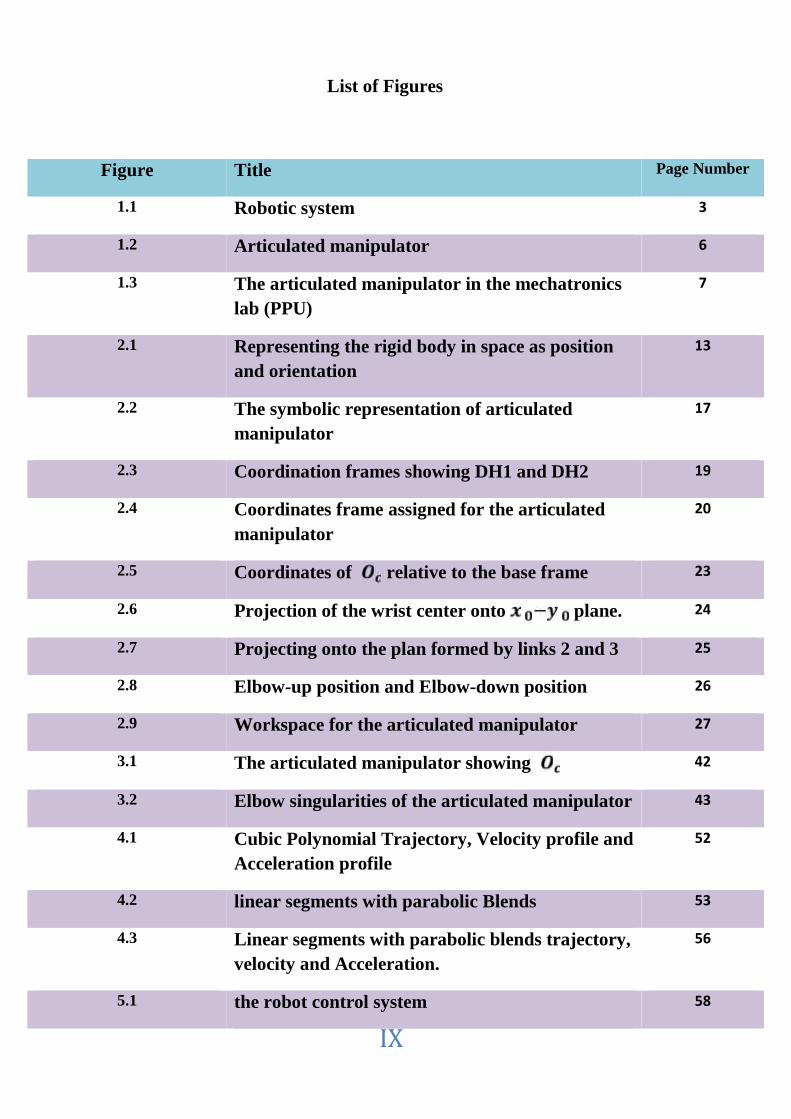
Figure Title Page Number

1.1 Robotic system 3

1.2 Articulated manipulator 6

1.3 The articulated manipulator in the mechatronicslab (PPU)

7

2.1 Representing the rigid body in space as positionand orientation

13

2.2 The symbolic representation of articulatedmanipulator

17

2.3 Coordination frames showing DH1 and DH2 19

2.4 Coordinates frame assigned for the articulatedmanipulator

20

2.5 Coordinates of relative to the base frame 23

2.6 Projection of the wrist center onto plane. 24

2.7 Projecting onto the plan formed by links 2 and 3 25

2.8 Elbow-up position and Elbow-down position 26

2.9 Workspace for the articulated manipulator 27

3.1 The articulated manipulator showing 42

3.2 Elbow singularities of the articulated manipulator 43

4.1 Cubic Polynomial Trajectory, Velocity profile andAcceleration profile

52

4.2 linear segments with parabolic Blends 53

4.3 Linear segments with parabolic blends trajectory,velocity and Acceleration.

56

5.1 the robot control system 58

List of Figures

X

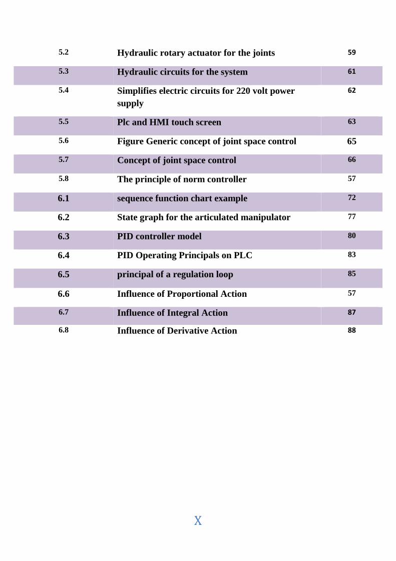
5.2 Hydraulic rotary actuator for the joints 59

5.3 Hydraulic circuits for the system 61

5.4 Simplifies electric circuits for 220 volt powersupply

62

5.5 Plc and HMI touch screen 63

5.6 Figure Generic concept of joint space control 65

5.7 Concept of joint space control 66

5.8 The principle of norm controller 57

6.1 sequence function chart example 72

6.2 State graph for the articulated manipulator 77

6.3 PID controller model 80

6.4 PID Operating Principals on PLC 83

6.5 principal of a regulation loop 85

6.6 Influence of Proportional Action 57

6.7 Influence of Integral Action 87

6.8 Influence of Derivative Action 88

١

Chapter One

Introduction

1.1 Robotics overview

1.2 Robotic mechanical structure

1.3 Robotic systems

1.4 Classification of robots

1.5 project overview

1.6 Project Schedule

1.7 Report Content

٢

1.1 Robotics overview

Robotics is concerned with the study of those machines that can replace

human being in the execution of a task, as regards both physical activity

and decision making.

At the present time, the industrial robots have a significant impact on the

industry, such that the robot can improve the quality of life by freeing

workers from dirty, boring, dangerous and heavy labor.

An official definition of such a robot comes from the Robotic Institute of

America (RIA): a robot is a re-programmable multi-functional

manipulator designed to move materials, parts, tools, or specialized

devices through variable programmed motions for the performance of a

variety of tasks.

1.2 Robotic mechanical structure

Robots are classified as those with fixed base "robot manipulators", and

those with mobile base "mobile robots", in our project we have a robot

with fixed base.

The mechanical structure of a robot manipulator consist of rigid link

connected by a joint to form the kinematic chain, the joint can be revolute

(rotary) or linear (prismatic).

In the case of revolute joint, this joint allows relative rotation between

two links, these displacements are called joint angles .while prismatic

joint allows a linear relative motion between tow links, which called the

joint offset.

٣

To construct the manipulator, the first link in a chain is connected to the

base and the last link is connected to the end effecter, this end effecter

can be anything from a welding device to a mechanical hand used to

manipulate the environment. The kinematic chain of manipulator is

characterized by number of degree of freedom (DOF).

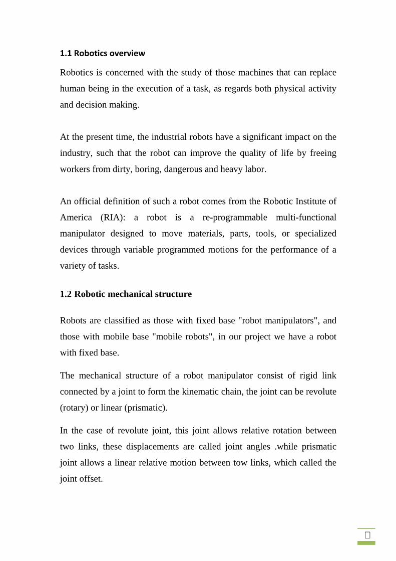
1.3 Robotic systems

The basic component of robotic system is

Manipulator (robotic arm)

the end effecter (which is part of the manipulator)

power supply

the controller

And this can be viewed in figure (1.1)

Figure 1.1: robotic system

Input device(touch screen)

Program storageor network

Controller

(Plc)

End _of armtooling

Robotic arm

(Manipulator)

Power supply

Commands

Sensors

٤

The manipulator, which is the robotic arm, consists of segments joined

together with axes capable of motion in various directions allowing the

robot to perform work.

The end effecter, which is the gripper tool, a special device, or fixture

attached to the robotic arm, actually performs the work.

The power supply provides and regulates the energy that is converted to

motion by robotic actuator, and it may be either electric m pneumatic, or

hydraulic.

The controller initiate, terminates, and coordinates the motion of

sequences of a robot. Also it accepts the necessary input to the robot and

provides the outputs to interface with the outside world.

1.4 Classification of robots

Robotic manipulators can be classified by several categories, such as

their power source, geometry, application area, or their method

control. Such classification is useful primarily in order to determine

Which robot is righty for given task. For example, a hydraulic robot

would not be suitable for food handling or clean room application.

Power source: Most robots are eclectically, hydraulically, or

pneumatically powered. The advantage of use hydraulic power is that

the hydraulic actuators are unrivaled in their speed of response and

torque producing capability. These hydraulic robots are used primary

for lifting heavy loads

Application area: Robots are often classified by application into

assembly and non-assembly robots.

٥

Method of control: Robots are classified by control method into

servo (high technology) and non-servo (low technology) robots.

Geometry: Robot manipulators are usually classified cinematically on

the basis of the first three joints of the arm. The majority of these

manipulators fall into one of the five geometry types: articulated

(RRR), spherical (RRP), SCARA (RRP), cylindrical (RPP), or

Cartesian (PPP).

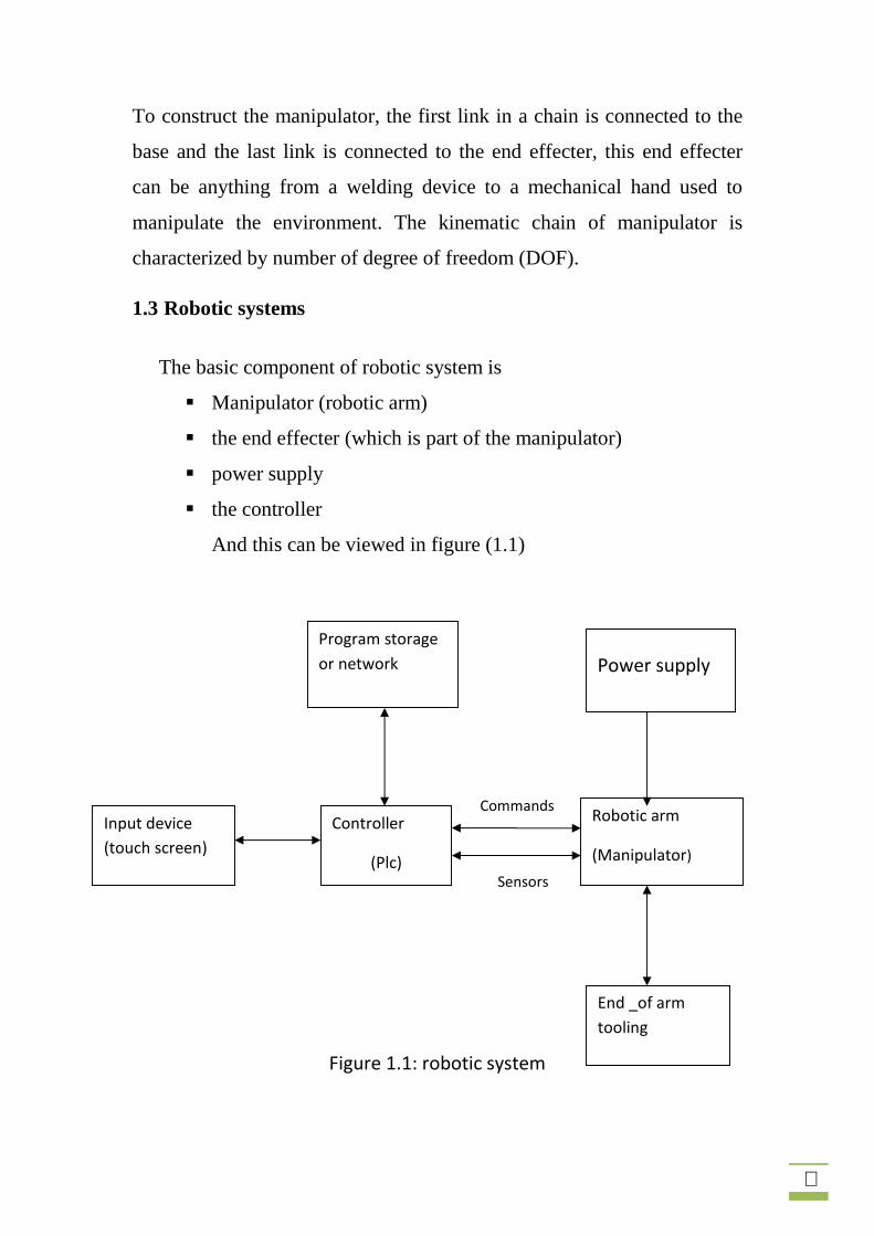
The common industrial manipulator is often referred to as a robot arm,

with links and joints described in similar terms. Manipulators which

emulate the characteristics of a human arm are called articulated arms

(articulated manipulator). All their joints are rotary (or revolute).

The motion of articulated robot arms differs from the motion of the

human arm. While robot joints have fewer degrees of freedom, they can

move through greater angles. For example, the elbow of an articulated

robot can bend up or down whereas a person can only bend their elbow in

one direction with respect to the straight arm position

٦

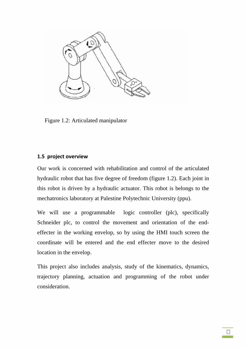
Figure 1.2: Articulated manipulator

1.5 project overview

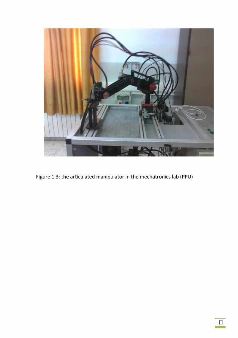
Our work is concerned with rehabilitation and control of the articulated

hydraulic robot that has five degree of freedom (figure 1.2). Each joint in

this robot is driven by a hydraulic actuator. This robot is belongs to the

mechatronics laboratory at Palestine Polytechnic University (ppu).

We will use a programmable logic controller (plc), specifically

Schneider plc, to control the movement and orientation of the end-

effecter in the working envelop, so by using the HMI touch screen the

coordinate will be entered and the end effecter move to the desired

location in the envelop.

This project also includes analysis, study of the kinematics, dynamics,

trajectory planning, actuation and programming of the robot under

consideration.

٧

Figure 1.3: the ar culated manipulator in the mechatronics lab (PPU)

٨

1.6 Project Schedule

First Semester

ProcessWeek

1 2 3 4 5 6 7 8 9 10 11 12 13 14 15 16

Selected theproject

Collection of theneeded data forthe project

Modeling ofArticulatedhydraulic robot

Writing theDocumentation

Table1.1: first semester Project Schedule

٩

Second Semester

Table1.2: seconded semester Project Schedule

1.7 Report Content

Now we provide a brief description of each chapter:

Chapter one: introduce an overview to robotic systems,classification of robots, and the project goal.

Chapter two: present solutions to the forward kinematics problemsusing Denevative-Haetenberg convention and to the inversekinematics problem using Geometric Approach.

ProcessWeek

1 2 3 4 5 6 7 8 9 10 11 12 13 14 15 16

Building ManualControl Circuits

Programming

Building PLCcircuit

Testing andWriting theDocumentation

١٠

Chapter Three: introduce forward and inverse velocity kinematicsusing geometric Jacobean matrix, also this chapter provide asolution to singularities which is configurations that make themanipulator loss one or more degree of freedom.

Chapter Four: is concerned with describing motion of themanipulator in terms of trajectories through space.

Chapter Five: present we study the methods of controlling themanipulator (by digital controller) so that it will tack a desiredposition trajectory through space.

١١

Chapter Two

Forward and Inverse Kinematics

2.1 Overview

2.2 Position and orientation representation

2.2.1 Position and displacement

2.2.2 Orientation and Rotation matrix

2.2.3 Homogeneous Transformation

2.3 Forward kinematic

2.4 Parameterization of rotation: Euler angles

2.5 Inverse kinematic

2.6 The Workspace

١٢

2.1 Overview

Kinematics is the branch of classical mechanics that describes

the motion of points or bodies without consideration of the causes of

motion. To describe motion, kinematics studies the trajectories of points,

lines and other geometric objects and their differential properties such as

velocity and acceleration.

For the articulated manipulator we have to consider the forward and

inverse kinematic. First consider the forward kinematic problem which is

to determine the position and orientation of the end-effectors by given the

values of joint variables of the robot. Then we solve the inverse

kinematics problem which is to determine the values of the joint variables

given the end-effectors position and orientation.

To perform the kinematics analysis, we must establish various coordinate

frames to represent the position and orientations of rigid body objects,

and with transformations among these coordinate frames.

2.2 Position and orientation representation

A rigid body (robot link) is completely described in space by its position

and orientation with respect to reference frame. A coordinate reference

frame consist of an origin, denoted , and a triad of mutually

orthogonal bases vectors, denoted ( ), that are all fixed within a

particular body. The pose of a body will always be expressed relative to

some other body, so it can be expressed as the pose of one coordinate

frame relative to another. Similarly, rigid-body displacements can be

expressed as displacements between two coordinate frames, one of which

١٣

may be referred to as moving, while the other may be referred to as fixed.

This indicates that the observer is located in a stationary position within

the fixed reference frame, not that there exists any absolutely fixed frame.

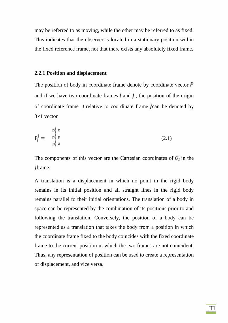
2.2.1 Position and displacement

The position of body in coordinate frame denote by coordinate vector

and if we have two coordinate frames and , the position of the origin

of coordinate frame relative to coordinate frame can be denoted by

3×1 vector

P (2.1)

The components of this vector are the Cartesian coordinates of in the

frame.

A translation is a displacement in which no point in the rigid body

remains in its initial position and all straight lines in the rigid body

remains parallel to their initial orientations. The translation of a body in

space can be represented by the combination of its positions prior to and

following the translation. Conversely, the position of a body can be

represented as a translation that takes the body from a position in which

the coordinate frame fixed to the body coincides with the fixed coordinate

frame to the current position in which the two frames are not coincident.

Thus, any representation of position can be used to create a representation

of displacement, and vice versa.

١٤

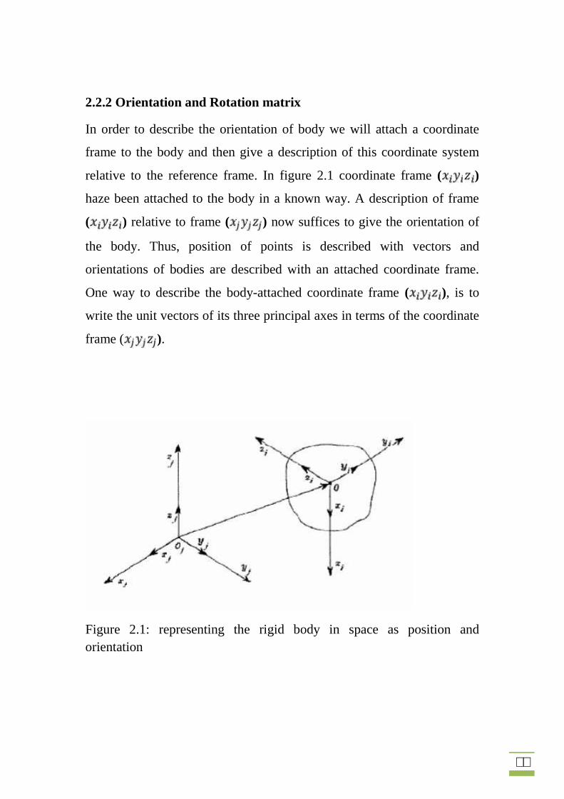
2.2.2 Orientation and Rotation matrix

In order to describe the orientation of body we will attach a coordinate

frame to the body and then give a description of this coordinate system

relative to the reference frame. In figure 2.1 coordinate frame ( )

haze been attached to the body in a known way. A description of frame

( ) relative to frame ( ) now suffices to give the orientation of

the body. Thus, position of points is described with vectors and

orientations of bodies are described with an attached coordinate frame.

One way to describe the body-attached coordinate frame ( ), is to

write the unit vectors of its three principal axes in terms of the coordinate

frame ( ).

Figure 2.1: representing the rigid body in space as position andorientation

١٥

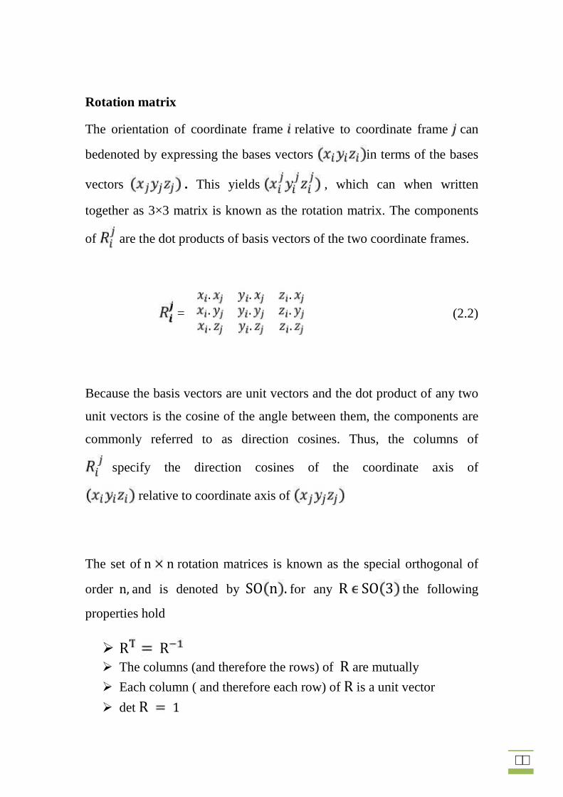
Rotation matrix

The orientation of coordinate frame relative to coordinate frame can

bedenoted by expressing the bases vectors in terms of the bases

vectors . This yields , which can when written

together as 3×3 matrix is known as the rotation matrix. The components

of are the dot products of basis vectors of the two coordinate frames.

=. . .. . .. . . (2.2)

Because the basis vectors are unit vectors and the dot product of any two

unit vectors is the cosine of the angle between them, the components are

commonly referred to as direction cosines. Thus, the columns of

specify the direction cosines of the coordinate axis of

relative to coordinate axis of

The set of n n rotation matrices is known as the special orthogonal of

order n, and is denoted by SO n . for any R SO 3 the following

properties hold

R R The columns (and therefore the rows) of R are mutually

Each column ( and therefore each row) of R is a unit vector

det R 1

١٦

Rotation matrices are combined through simple matrix multiplication

such that the orientation of frame k relative to frame j can be expressed asR R R (2.3)

2.2.3 Homogeneous Transformation

Homogeneous transformations combine rotation and translation onto onematrix. A homogeneous transformation has the form of

H = 0 1 , R SO (3), P ,H (2.4)

Where is the rotation matrix and is the translational matrix.

Homogeneous transformation matrices can be used to perform coordinate

Transformations between frames that differ in orientation and translation.

2.3 Parameterization of rotation: Euler Angles

A common method for specifying a rotation matrix in three independent

quantities is to use Euler angles. Consider the fixed coordinate frame

and the rotated frame we can specify the orientation

of frame relative to the frame by three angles

( , , ) called Euler angles, and obtained by three successive rotation as

follow. First rotate about the -axis by an angle , next rotate about the

current -axis by the angle ,finally rotate about the current -axis by an

angle . In terms of the basic rotation matrices the resulting rotational

transformation can be generated as the product:

, , ,

١٧

(2.5)

For the articulated manipulator the Euler angles are the angles of the wrist

rotation so:

, , 0The rotation matrix of frame relative to wrist frame

0 (2.6)

2.4 Forward kinematic:

A robot manipulator is composed of a set of links connected together by

joints, the joints may be simple, such as a revolute joint, or a prismatic

joint or they can be more complex such as a ball and socket joint.

A robot manipulator with n joints will have 1 links, since each joint

connects two links, we number the joints from 1 to n, and we number the

links from 0 to n, starting from the base. by convention joints connects

link 1 to link .We will consider the location of joint to be fixed

with respect to 1.When joint is actuated ,link moves .Therefore

,link 0 (the first link )is fixed ,and does not move when the joints are

actuated.

١٨

Joint 1 is called base, joint 2 is called shoulder, joint 3 is called elbow as

shown in figure 2.2

Figure 2.2: the symbolic representation of articulated manipulator

To perform the kinematic analysis, we attach the coordinate frame rigidly

to each link .In particular, we attach to link .This means that,

whatever motion the robot executes, the coordinates of each point on

link are constant when expressed in the coordinate frame.

Furthermore, when joint is actuated, link and its attached

frame , experience a resulting motion. The frame ,

which attached to the robot base, is referred to as the inertial frame. We

will assign the coordinates frames that satisfy the Denative_Hartenberg

convention.

١٩

The Denative_Hartenberg convention:

This convention is concerned about assigning a coordinate frame to each

link in the manipulator .In this convention, each homogenous

transformation is representing as a product of four basic

transformations.

, , , ,

= 00 0 0 1 (2.7)

Where the four quantities , , and are parameters associated with

link and joint .So if the DH convention is satisfied then thetransformation matrix can be written as the above form.

The attached frame must have the following features according to the DHconvention:

(DH1) the axis is perpendicular to the axis .

(DH2) the axis intersects the axis .

The tow features are shown in figure 2.3.

٢٠

Figure 2.3: coordination frames showing DH1 and DH2.

Below we will describe the DH parameters that used in thetransformation: ,

: ,: ,.: The distance from the origin to the interconnection between

is and .

٢١

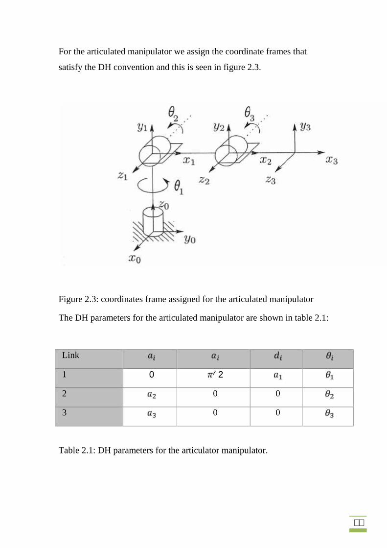
For the articulated manipulator we assign the coordinate frames that

satisfy the DH convention and this is seen in figure 2.3.

Figure 2.3: coordinates frame assigned for the articulated manipulator

The DH parameters for the articulated manipulator are shown in table 2.1:

Link

1 0 2⁄2 0 0

3 0 0

Table 2.1: DH parameters for the articulator manipulator.

٢٢

The A-matrices are obtained using equation 2.5:

=

00 01 00 0 0001

00 0 010 0 0 01==

00 0 010 0 0 01 (2.8)

The homogenous transformation "T-matrices" are thus given by:

00 0 0 1 (2.9)

00 0 0 1Notice that the first three entries of the last column of are the , and

component of the origin with respect to the base frame; that is,

(2.10)

٢٣

are the coordinate of the end effecter with respect to the base frame. The

rotational part of gives the orientation of the frame relative to the

base frame.

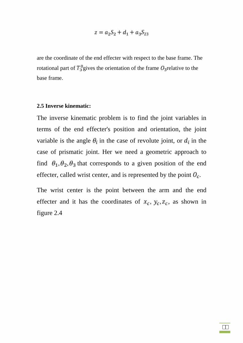
2.5 Inverse kinematic:

The inverse kinematic problem is to find the joint variables in

terms of the end effecter's position and orientation, the joint

variable is the angle in the case of revolute joint, or in the

case of prismatic joint. Her we need a geometric approach to

find , , that corresponds to a given position of the end

effecter, called wrist center, and is represented by the point .

The wrist center is the point between the arm and the end

effecter and it has the coordinates of , , , as shown in

figure 2.4

٢٤

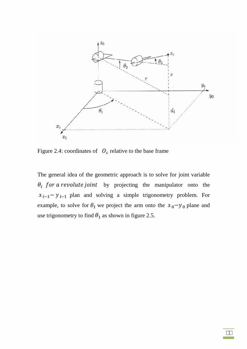
Figure 2.4: coordinates of relative to the base frame

The general idea of the geometric approach is to solve for joint variable

by projecting the manipulator onto the

plan and solving a simple trigonometry problem. For

example, to solve for we project the arm onto the plane and

use trigonometry to find as shown in figure 2.5.

٢٥

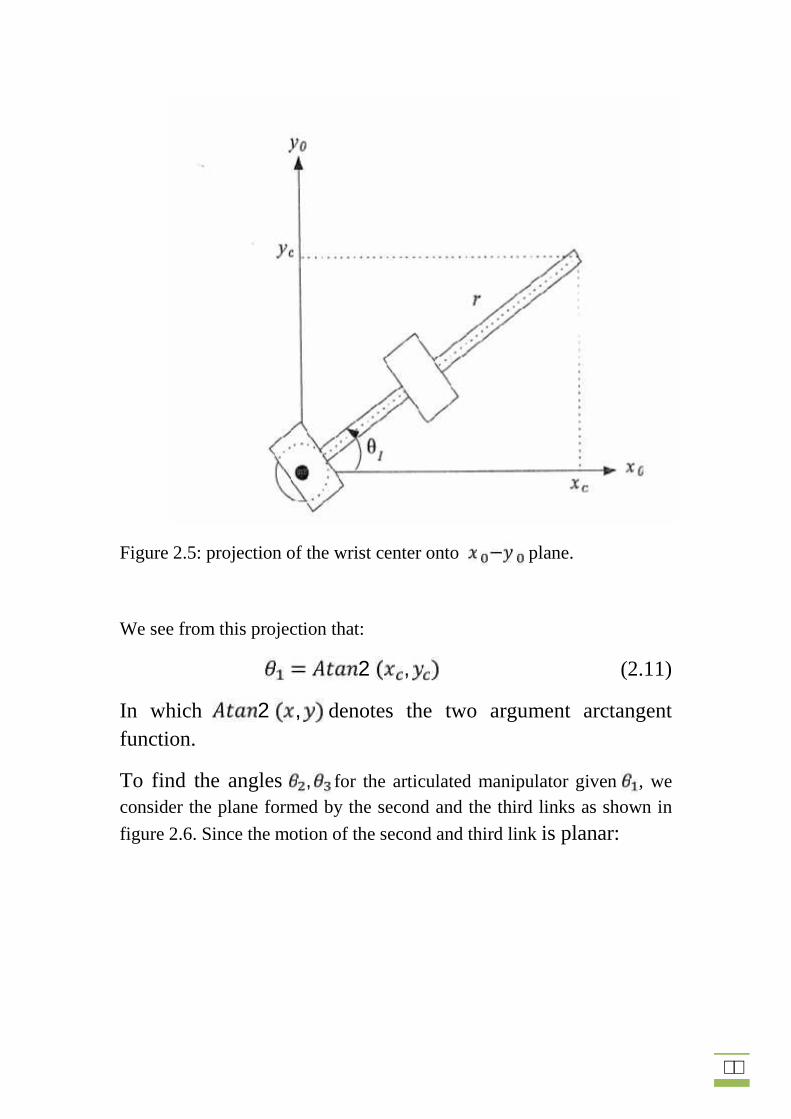
Figure 2.5: projection of the wrist center onto plane.

We see from this projection that:2 , (2.11)

In which 2 , denotes the two argument arctangentfunction.

To find the angles , for the articulated manipulator given , weconsider the plane formed by the second and the third links as shown in

figure 2.6. Since the motion of the second and third link is planar:

٢٦

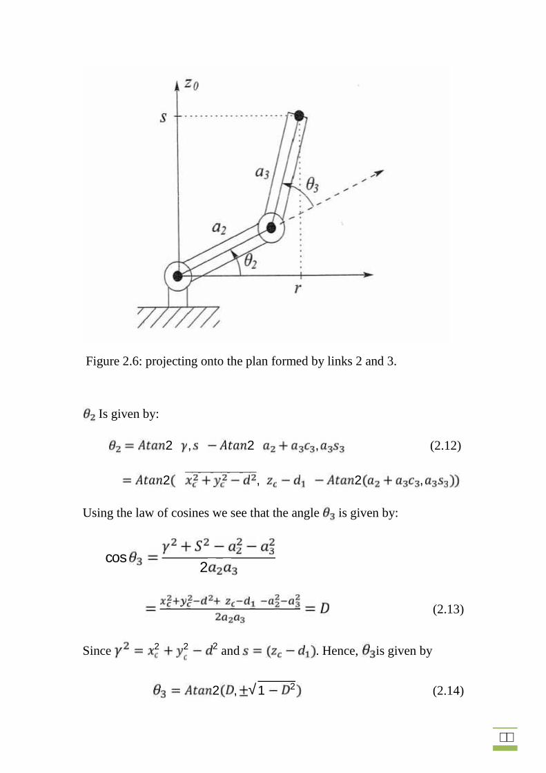
Figure 2.6: projecting onto the plan formed by links 2 and 3.

Is given by: 2 , 2 , (2.12)2 , 2 ,Using the law of cosines we see that the angle is given by:

cos 2(2.13)

Since 2 2 2 and . Hence, is given by

2 , √1 2 (2.14)

٢٧

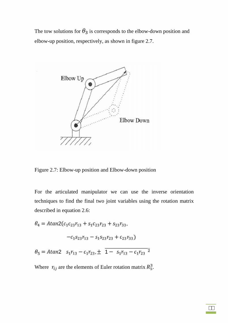
The tow solutions for is corresponds to the elbow-down position and

elbow-up position, respectively, as shown in figure 2.7.

Figure 2.7: Elbow-up position and Elbow-down position

For the articulated manipulator we can use the inverse orientation

techniques to find the final two joint variables using the rotation matrix

described in equation 2.6:2 ,2 , 1

Where are the elements of Euler rotation matrix .

٢٨

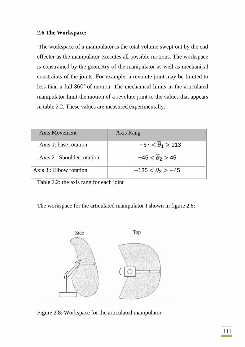
2.6 The Workspace:

The workspace of a manipulator is the total volume swept out by the end

effecter as the manipulator executes all possible motions. The workspace

is constrained by the geometry of the manipulator as well as mechanical

constraints of the joints. For example, a revolute joint may be limited to

less than a full 360° of motion. The mechanical limits in the articulated

manipulator limit the motion of a revolute joint to the values that appears

in table 2.2. These values are measured experimentally.

Axis Movement Axis Rang

Axis 1: base rotation 67 1 113Axis 2 : Shoulder rotation 45 2 45

Axis 3 : Elbow rotation 135 3 45Table 2.2: the axis rang for each joint

The workspace for the articulated manipulator I shown in figure 2.8:

Figure 2.8: Workspace for the articulated manipulator

29

Chapter Three

Velocity Kinematic - The Jacobian

3.1 Overview

3.2 Skew symmetry matrices

3.3 The derivative of a Rotation Matrix

3.4 Angular Velocity : The Fixed Axis Case

3.5 Angular Velocity : the General Case

3.6 Linear velocity Of A Point Attached To Moving Frame

3.7 Derivation Of Jacobian

3.8 The Analytical Jacobian

3.9 Singularities

3.10 Inverse Velocity and Acceleration

30

3.1 Overview

In this chapter we derive the velocity relations, relating the linear and

angular velocities of the end effecter to the joint velocities. First we consider

the forward kinematics of velocity which is to determine the linear and

angular velocities of the end effectors by giving the joint velocities, and then

we solve the inverse kinematic of velocity which is to determine the joint

velocities that produce the desired end effectors velocities.

To determine the velocities relationships we need to attach coordinate frame

rigidly to each link and find the forward kinematic equations that define a

function between the space of Cartesian positions and orientations and the

space of joint positions as we done in the previous chapter. Then the

velocities relationships are determined by the Jacobian of this function.

The Jacobian is a matrix that generalizes the notion of the ordinary

derivative of a scalar function. The derivative of kinematic equations is done

with aid of skew symmetric matrices.

3.2 SKEW SYMMETRY MATRICES

This section derives the properties of rotation matrices that can be used to

compute relative velocity transformations between coordinate frames.

An matrix is said to be skew symmetric if and only if

0

31

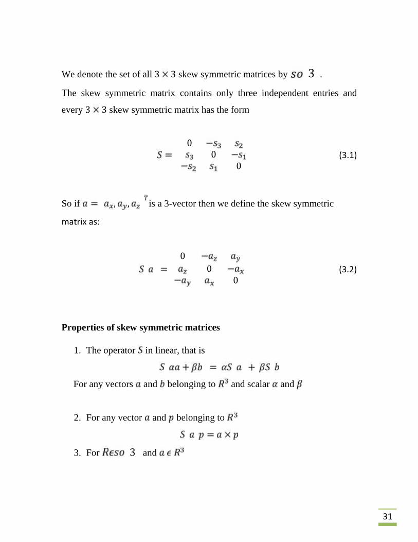
We denote the set of all 3 3 skew symmetric matrices by 3 .

The skew symmetric matrix contains only three independent entries and

every 3 3 skew symmetric matrix has the form

0 0 0 (3.1)

So if , , is a 3-vector then we define the skew symmetric

matrix as:

0 0 0 (3.2)

Properties of skew symmetric matrices

1. The operator in linear, that is

For any vectors and belonging to and scalar and

2. For any vector and belonging to

3. For 3 and

32

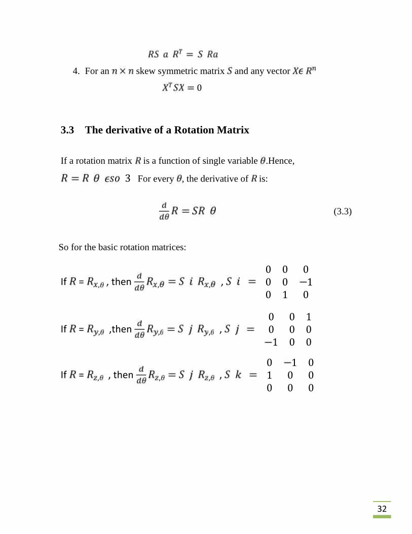
4. For an skew symmetric matrix and any vector03.3 The derivative of a Rotation Matrix

If a rotation matrix is a function of single variable .Hence,3 For every , the derivative of is:

(3.3)

So for the basic rotation matrices:

If = , , then , , ,0 0 00 0 10 1 0

If = , ,then , , ,0 0 10 0 01 0 0

If = , , then , , ,0 1 01 0 00 0 0

33

3.4 Angular Velocity : The Fixed Axis Case

When a body moves in pure rotation about fixed axis, and if is a vector in

the direction of the axis of rotation, then the angular velocity is given by

(3.4)

In which is the time derivative of . And the linear velocity of any point

on the body is given by

(3.5)

In which is a vector from the origin to the point.

3.5 Angular Velocity : the General Case

Suppose that a Rotational matrix is time varying, so that3 For every , the derivative of is

(3.6)

Where the matrix is a skew symmetric. The vector is the

angular velocity of the rotating frame with respect to fixed frame at time .

The previous equation shows the relationship between angular velocity and

the derivative of rotation matrix.

34

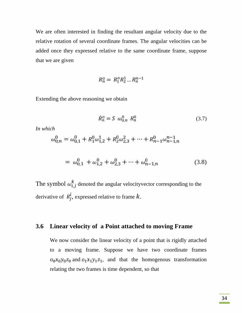
We are often interested in finding the resultant angular velocity due to the

relative rotation of several coordinate frames. The angular velocities can be

added once they expressed relative to the same coordinate frame, suppose

that we are given

…Extending the above reasoning we obtain

, (3.7)

In which , , , , ,, , , , (3.8)

The symbol , denoted the angular velocityvector corresponding to the

derivative of , expressed relative to frame .

3.6 Linear velocity of a Point attached to moving Frame

We now consider the linear velocity of a point that is rigidly attached

to a moving frame. Suppose we have two coordinate frames

and , and that the homogenous transformation

relating the two frames is time dependent, so that

35

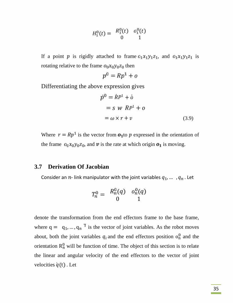
0 1If a point is rigidly attached to frame , and is

rotating relative to the frame then

Differentiating the above expression gives11

(3.9)

Where is the vector from to expressed in the orientation of

the frame , and is the rate at which origin is moving.

3.7 Derivation Of Jacobian

Consider an - link manipulator with the joint variables , … , . Let

0 1denote the transformation from the end effectors frame to the base frame,

where q q , … , q is the vector of joint variables. As the robot moves

about, both the joint variables and the end effectors position o and the

orientation R will be function of time. The object of this section is to relate

the linear and angular velocity of the end effectors to the vector of joint

velocities t . Let

36

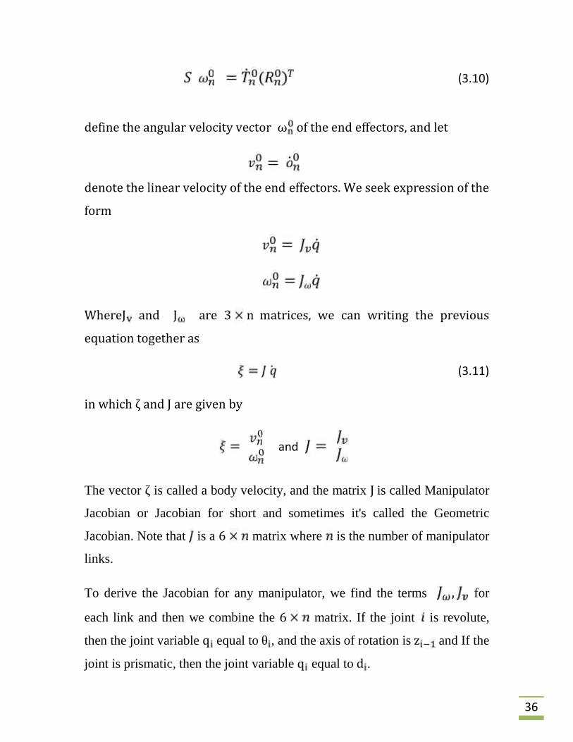
(3.10)

define the angular velocity vector ω of the end effectors, and letdenote the linear velocity of the end effectors. We seek expression of theform

WhereJ and J are 3 n matrices, we can writing the previousequation together as(3.11)in which ζ and J are given by 00 and

The vector ζ is called a body velocity, and the matrix J is called Manipulator

Jacobian or Jacobian for short and sometimes it's called the Geometric

Jacobian. Note that is a 6 matrix where is the number of manipulator

links.

To derive the Jacobian for any manipulator, we find the terms , for

each link and then we combine the 6 matrix. If the joint is revolute,

then the joint variable q equal to θ , and the axis of rotation is z and If the

joint is prismatic, then the joint variable q equal to d .

37

For an -link manipulator, the upper half of the jacobian is given as…In which the column of is

for revolute joint (3.12)The lower half f the Jacobian is given as

…In which the column of is

for revolute joint0 3.13Where zi 1 Ri 10 , and 0,0,1 (3.14)

The above formulas make the determination of the Jacobian of any

manipulator simple since all the quantities needed are available once the

forward kinematic worked out. The coordinate for with respect to the base

frame are given by the first three elements in the third column of .

While is given by the first three elements in the fourth column of .

38

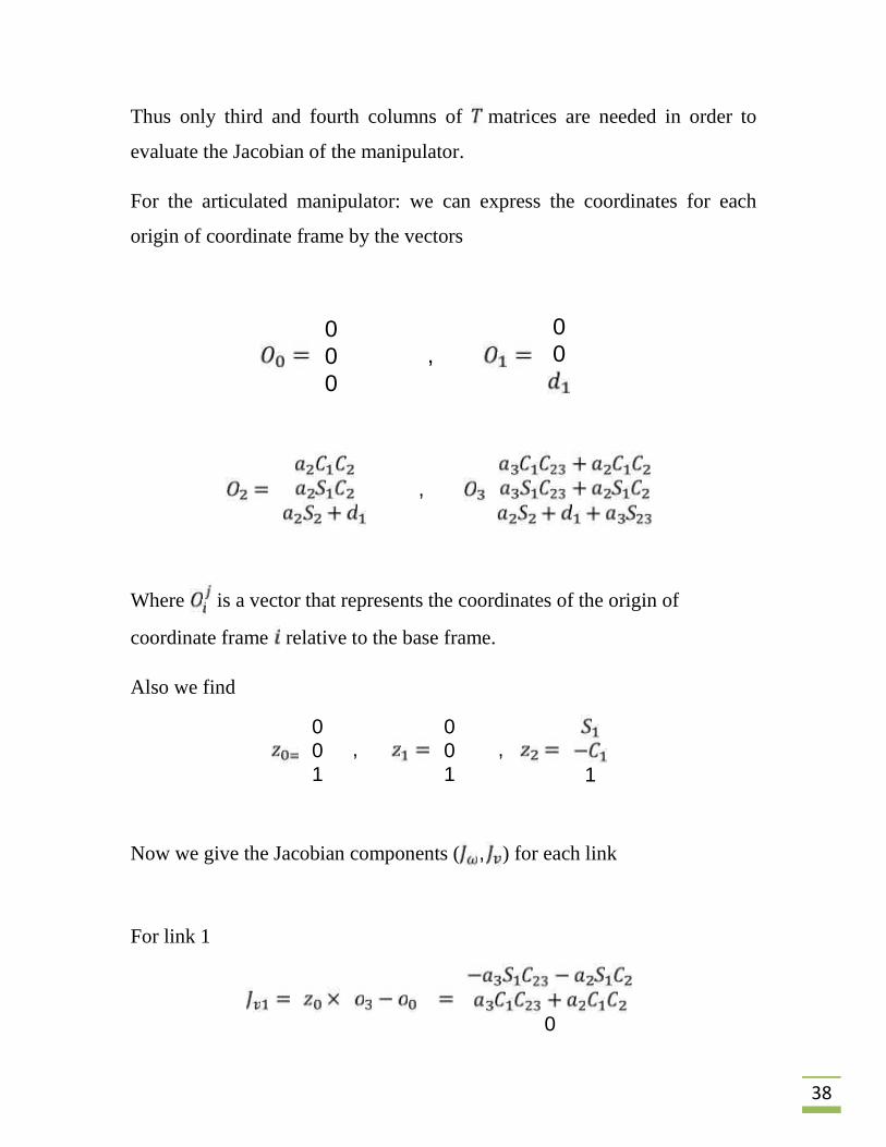
Thus only third and fourth columns of matrices are needed in order to

evaluate the Jacobian of the manipulator.

For the articulated manipulator: we can express the coordinates for each

origin of coordinate frame by the vectors

000 , 00,

Where is a vector that represents the coordinates of the origin of

coordinate frame relative to the base frame.

Also we find 001 , 001 , 1Now we give the Jacobian components ( , ) for each link

For link 1

0

39

001For link 2

0001For link 3

1

The Jacobian for the first three links of the articulated manipulatoris:

40

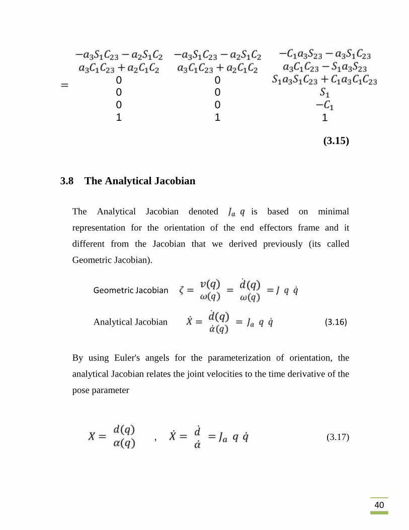
0 0001 001 1(3.15)

3.8 The Analytical Jacobian

The Analytical Jacobian denoted is based on minimal

representation for the orientation of the end effectors frame and it

different from the Jacobian that we derived previously (its called

Geometric Jacobian).

Geometric Jacobian

Analytical Jacobian (3.16)

By using Euler's angels for the parameterization of orientation, the

analytical Jacobian relates the joint velocities to the time derivative of the

pose parameter

, (3.17)

41

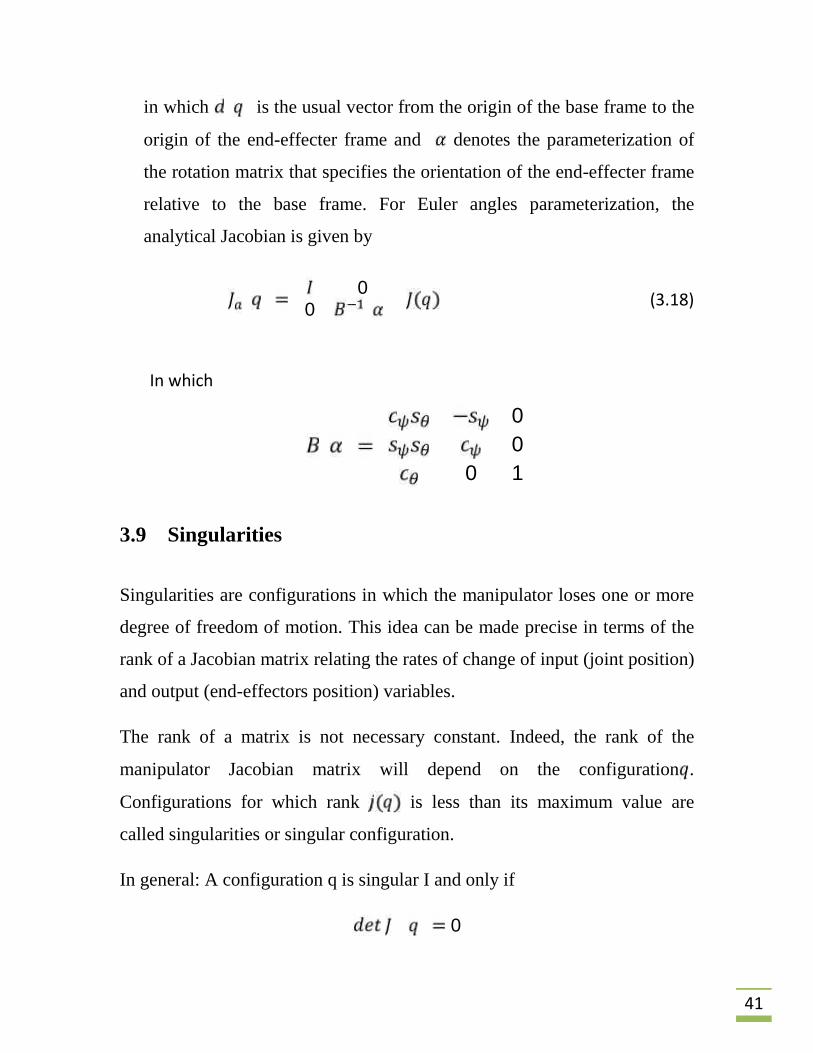
in which is the usual vector from the origin of the base frame to the

origin of the end-effecter frame and denotes the parameterization of

the rotation matrix that specifies the orientation of the end-effecter frame

relative to the base frame. For Euler angles parameterization, the

analytical Jacobian is given by00 (3.18)

In which 000 13.9 Singularities

Singularities are configurations in which the manipulator loses one or more

degree of freedom of motion. This idea can be made precise in terms of the

rank of a Jacobian matrix relating the rates of change of input (joint position)

and output (end-effectors position) variables.

The rank of a matrix is not necessary constant. Indeed, the rank of the

manipulator Jacobian matrix will depend on the configuration .

Configurations for which rank is less than its maximum value are

called singularities or singular configuration.

In general: A configuration q is singular I and only if0

42

It's difficult to solve this nonlinear equation, there for we use the method of

decupling singularities, which is applicable whenever, for example, the

manipulator is equipped with spherical manipulator, so we decouple the

determination of singular configuration into two simpler problems .The first

is to determine the singularities results from the motion of the arm (arm

singularities) while the second is to determine the wrist singularities

resulting from the motion of the wrist.

For spherical wrist manipulators, the Jacobian matrix has the block triangle

form 0(3.19)

With determinates det det detThe set of singular configurations of the manipulator is the union of the set

of arm configurations satisfying det 0 (arm configuration) and the set

of wrist configurations satisfying 0 .

For the articulated manipulator with coordinate frames attached as shown

in figure 3.1

43

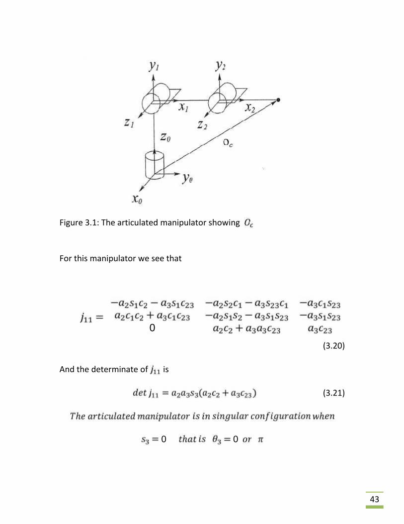
Figure 3.1: The articulated manipulator showing

For this manipulator we see that

0(3.20)

And the determinate of is

(3.21)

0 0

44

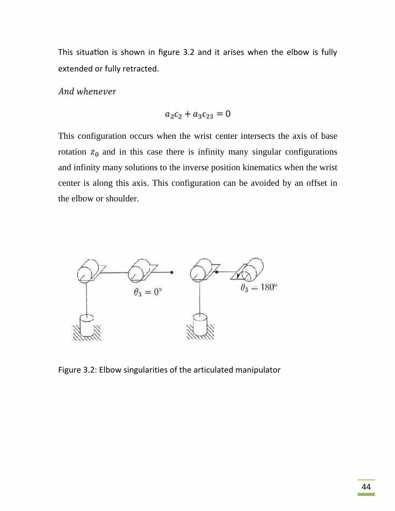
This situa on is shown in figure 3.2 and it arises when the elbow is fully

extended or fully retracted.

0This configuration occurs when the wrist center intersects the axis of base

rotation and in this case there is infinity many singular configurations

and infinity many solutions to the inverse position kinematics when the wrist

center is along this axis. This configuration can be avoided by an offset in

the elbow or shoulder.

Figure 3.2: Elbow singularities of the articulated manipulator

45

3.10 Inverse Velocity And AccelerationThe inverse velocity problem is the problem of finding the joint velocities

that produce the desired end effector velocity or acceleration .

For manipulators that have six joints and the Jacobian matrix is square and

nonsingular (det 0 , this problem can be solved by simply

inverting the Jacobian matrix to give 3.22)For manipulators with 6 we can solve for (joint velocities) using

the right pseudoinverse of . To construct this pseudoinverse, we use the

fact that when , if m < n and , then ( exist.

in this case , and has a rank . using this we can find that:

(3.23)

Pseudoinverse of the j , and if we multiply it by j this

will give the identity matrix , that to say but since the

matrix multiplication is not cumulative.

By using the right pseudoinverse we can find a solution for

for nonsingular configurations as

(3.24)

We can apply a similar approach when the analytical Jacobian is used in

place of manipulator Jacobian. The joint velocities and the end-effectors

velocities are related by the analytical Jacobian as

46

(3.25)

Thus, the inverse velocity problem becomes one of solving the linear

system given by the above equation.

Differentiating equation (3.23) yield an expression for the acceleration:

(3.26)

Thus, given vector of end-effecter, the instantaneous joint acceleration

vector is given as a solution of

(3.27)

47

Chapter Four

Trajectory Planning

4.1 Introduction

4.2 Joint space Trajectory

4.3 Point to point motion

4.3.1 Cubic Polynomial

4.3.2 Linear segment with parabolic blends (LSPB

48

4.1 Introduction

Trajectory planning relates to the way a robot is moved from one location to

another in a controlled manner. So that in this chapter we will plan a

trajectory; a trajectory refers to the time history of position, velocity and

acceleration for each joint in the manipulator. Trajectory planning requires

the use of kinematic and dynamic equation of the manipulator.

When we dealing with trajectory there are many constants we expect to see

in solving this problem, these constrain could be:

1. Spatial constrain, if we have on obstacle in the environment that we

don’t want to collide with. We will neglect this constrain in our

project and assume that there is no obstacle in the workplace of the

robot arm.

2. Time constrain, if the motion ha to be done in particular time.

3. Smoothness, we want the manipulator to have a smooth motion

because that uses less energy and easy to control.

The trajectory planning can be done in two main spaces, joint space

and Cartesian space .In joint pace it easy to go through point, there is

no problems with singularities and it requires less calculation. In the

other hand, the actual end-effectors path of this approach can't be

predicted and can't follow straight lines.

The trajectory planning in Cartesian space may involve problems

difficult to solve. However, Cartesian space is more computationally

expensive to execute since at run time, inverse kinematics must be

solved at the path update rate. Other major problems that we may

49

face in Cartesian space is singularity ;if there are some points on the

path that the manipulator should follow are in singular configuration,

but in this space we can specify the shape of the path between path

points.

In Our project we will use the joint space trajectory planning for the

articulated manipulator, because we want to move the end-effectors

from initial position to final position regardless of the path to follow.

4.2 Joint space Trajectory

The joint space is a method of path generation in which the path

shapes (in space and in time) are described in terms of function of

joint angles.

Each path joint is usually specified in terms of a desired position and

orientation of the tool frame, relative to the base frame, each of these

points in converted into a set of desired joint angels by application of

inverse kinematics .Then a smooth function is found for each of the njoints to describe the motion between the initial and final joint.

Through the remaining of this chapter we interest in establishing

formulas for the angels of each DOF as a function of time in the case

of the initial and final points on the path and traveling time are

specified (point-to-point)

50

4.3 Point to point motion

In the trajectory planning, a complete description of all location of

every point on the robot is referred to as a configuration. For our

purpose, the vector of joint variables provide a convenient

representation of a configuration

The task of point to point motion is to plan a trajectory from an

initial configuration to a final configuration . In some

cases, there may be constrains on the trajectory (for example, if the

robot must start and end with zero velocity). Nevertheless, it’s easy to

realize that there are infinitely many trajectories that will satisfy a

finite number of constrains on the end points.

It’s a common practice therefore to choose trajectories from a finitely

parameterizable family, for example, polynomials of degree, where

depends on the number of constrains to be satisfied. This is the

approach that we will take in our project.

We will consider tow smooth functions for point to point motion,

cubic polynomial and linear segments with parabolic blends, then

these functions are substituted on the dynamic equation of the robot

to see which function produce less torque and thus less power

consumption.

51

4.3.1 Cubic Polynomials

Consider the problem of moving the end-effectors from its initial position to

a final position in a particular time. The set of goal joint angles can be

calculated using the inverse kinematic for particular values of end effectors

position. The initial position of the manipulator is also known on the form of

a set of joint angles. To make a smooth motion between the initial and final

position of the manipulator, we first have to generate a polynomial joint

trajectory between the two configurations, and specify the start and end

velocities of the trajectory. This gives four constraints that the trajectory

must satisfy, two constrains comes from the selection of initial and final

values:

For the velocity constraints, if we want to have continuous velocity the final

and initial velocities must be zero: 00Thus we require polynomial with four independent coefficients to satisfy

these constraints, so we can consider a cubic polynomial. The cubic

polynomial will have this form

(4.1)

52

For the manipulator we have the initial position is known in the form of a

set of joint angle, and the final position can be determined using inverse

kinematic. The velocity and acceleration is given as2 3 (4.2)2 6 (4.3)

Combine equations 4.2 and 4.3 with four constraints yields four equation in

four unknowns:

3Solving these equations for we obtain

032

53

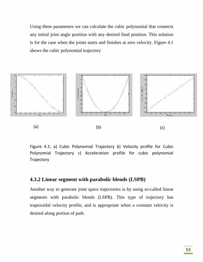
Using these parameters we can calculate the cubic polynomial that connects

any initial joint angle position with any desired final position. This solution

is for the case when the joints starts and finishes at zero velocity. Figure 4.1

shows the cubic polynomial trajectory

Figure 4.1: a) Cubic Polynomial Trajectory b) Velocity profile for CubicPolynomial Trajectory c) Acceleration profile for cubic polynomialTrajectory

4.3.2 Linear segment with parabolic blends (LSPB)

Another way to generate joint space trajectories is by using so-called linear

segments with parabolic blends (LSPB). This type of trajectory has

trapezoidal velocity profile, and is appropriate when a constant velocity is

desired along portion of path.

(a) (b) (c)

54

This is a linear function but we add a parabolic blend region at the beginning

and end of the path. These blend regions create a smooth path with

continuous position and velocity. Thus, during the blend portion of the

trajectory, constant acceleration is used to change velocity smoothly. Figure

4.2 shows a simple path constructed in this way.

In order to construct this single segment we will assume that the parabolic

blend both have the same duration, and therefore, they have the same

constant acceleration.

Figure 4.2: linear segments with parabolic Blends

For parabolic blends near the path points with the same duration (blend

time) the whole trajectory is symmetric about the halfway point in time

and about the halfway point in position .

55

The velocity at the end of first blend or at the beginning of second blend

must equal to linear segment, thus we have:q (4.4)

Where is the value of joint variable at the end of blend segment at

time t , is the acceleration during the blend segment, and the joint

variable is given by

(4.5)

Combining equations 3 and 4 and 2 0 (4.6)

Where is the desired duration of the motion. Usually equation 3.10 is

solved for a corresponding , and the acceleration is chosen. Solving

equation (4.5) for

(4.7)

The constraint on the choice of acceleration used in blend segment is4

56

The complete LSPB trajectory is given by

2 , 02 ,12 , 4.8

So the joint velocity and acceleration is given by

, 0, , 4.9, 0,, (4.10)

Figure 4.3 shows the LSPB Trajectory, velocity profile and acceleration

profile.

57

Figure 4.3: a) LSPB trajectory b) velocity profile for LSPB trajectory

c) Acceleration profile for LSPB trajectory.

In Our project we use Cubic Polynomial method since its easier to program

and need less user specification than LSPB method

58

Chapter Five

Control Design

5.1 Introduction

5.2 System Architecture

5.2.1 Physical System Description

5.2.2 Functional description

5.2.3 Hydraulic Description

5.2.4 Electrical Description

5.3 Closed Loop Control

5.3.1 Feedback Sensors

5.3.2 Controller and software

59

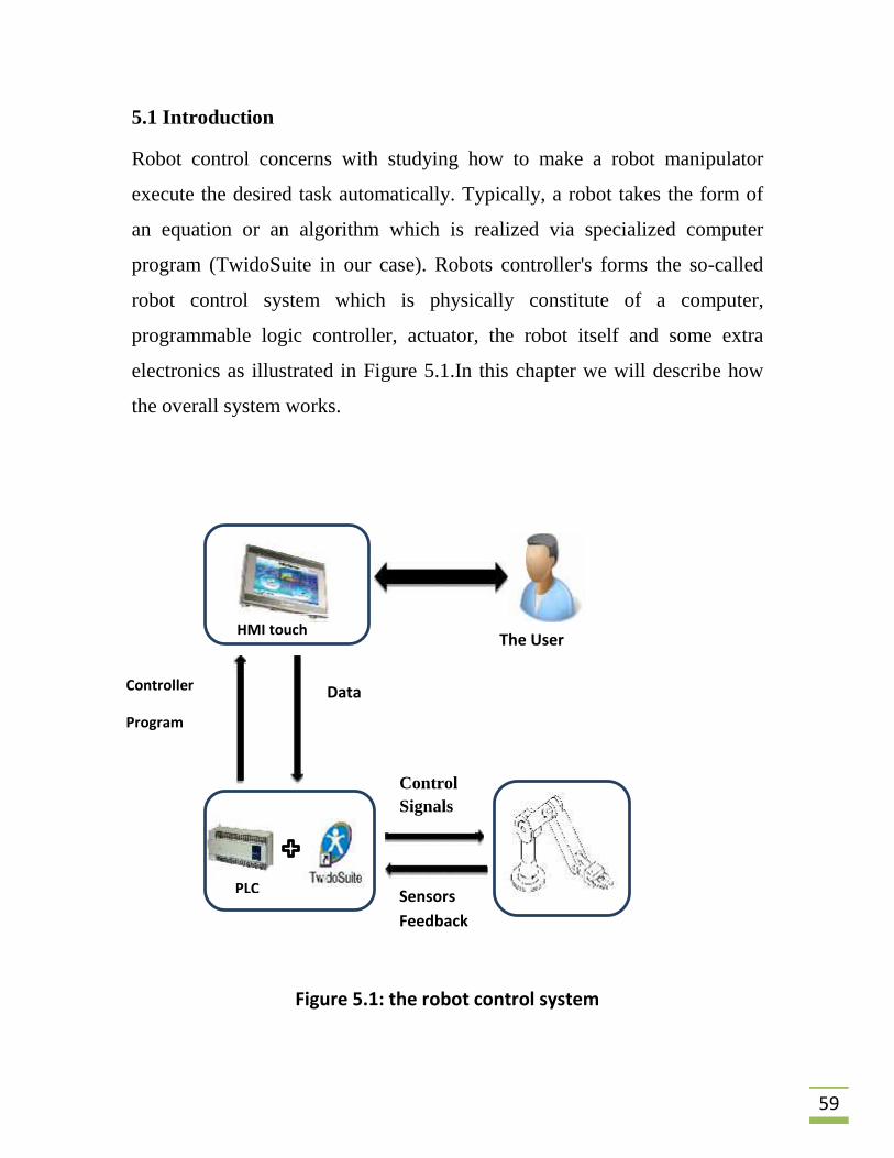
5.1 Introduction

Robot control concerns with studying how to make a robot manipulator

execute the desired task automatically. Typically, a robot takes the form of

an equation or an algorithm which is realized via specialized computer

program (TwidoSuite in our case). Robots controller's forms the so-called

robot control system which is physically constitute of a computer,

programmable logic controller, actuator, the robot itself and some extra

electronics as illustrated in Figure 5.1.In this chapter we will describe how

the overall system works.

Figure 5.1: the robot control system

Controller

Program

Data

ControlSignals

SensorsFeedback

The UserHMI touch

screen

PLC

60

5.2 System Architecture

5.2.1 Physical System Description

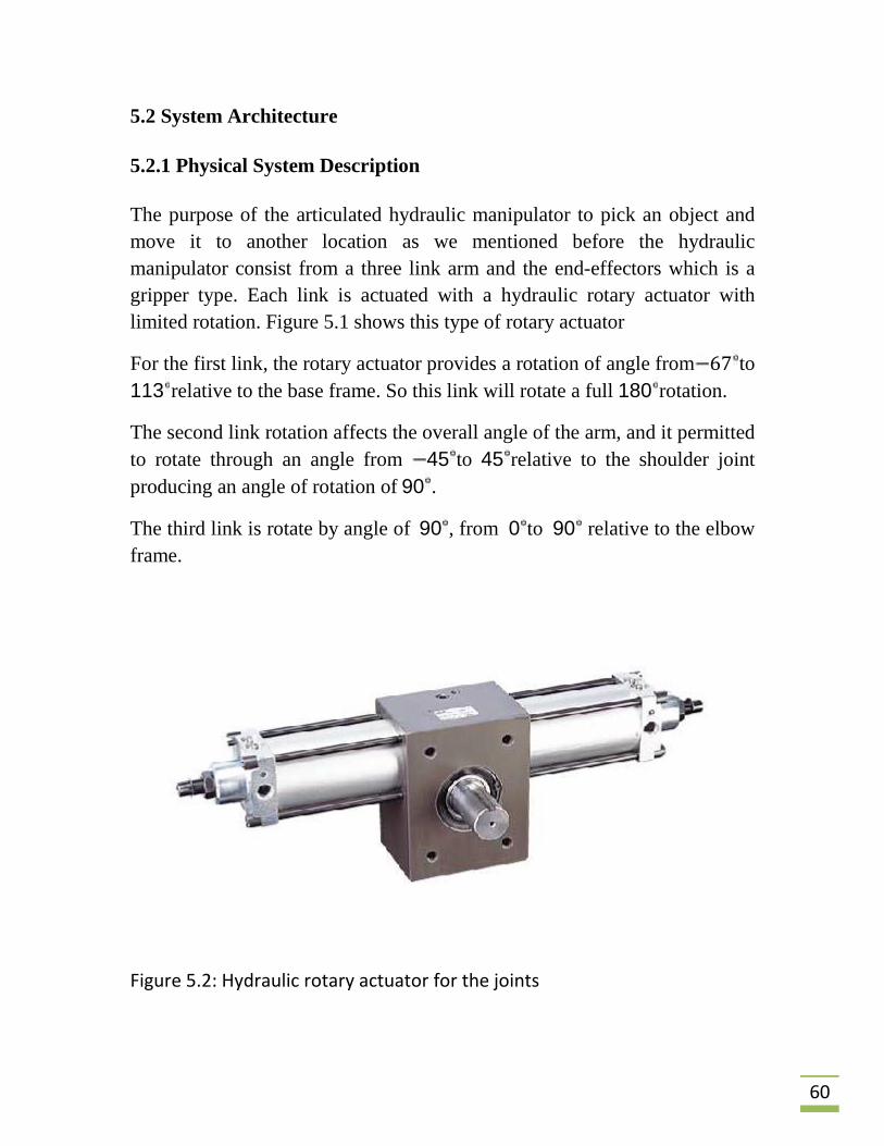
The purpose of the articulated hydraulic manipulator to pick an object andmove it to another location as we mentioned before the hydraulicmanipulator consist from a three link arm and the end-effectors which is agripper type. Each link is actuated with a hydraulic rotary actuator withlimited rotation. Figure 5.1 shows this type of rotary actuator

For the first link, the rotary actuator provides a rotation of angle from 67 to113 relative to the base frame. So this link will rotate a full 180 rotation.

The second link rotation affects the overall angle of the arm, and it permittedto rotate through an angle from 45 to 45 relative to the shoulder jointproducing an angle of rotation of 90 .

The third link is rotate by angle of 90 , from 0 to 90 relative to the elbowframe.

Figure 5.2: Hydraulic rotary actuator for the joints

61

5.2.2 Functional description

The user is asked to enter the coordinates of the initial position and thefinal position of the end effectors through the touch screen, themanipulator go the initial position, pick an object and move to the finallocation. After the final position is reached the object is released, if there isno new coordinates are entered the manipulator may be programmed tomove to an assigning suit which is the position where is no motion isexecuted.

5.2.3 Hydraulic Description

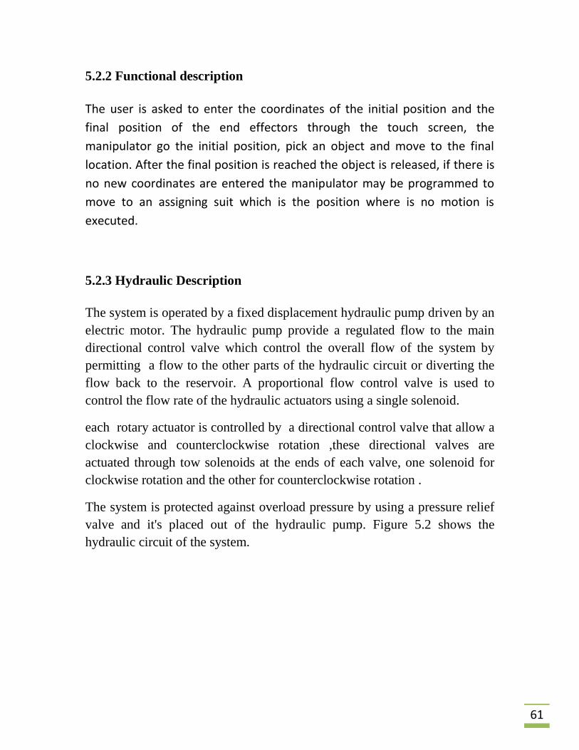
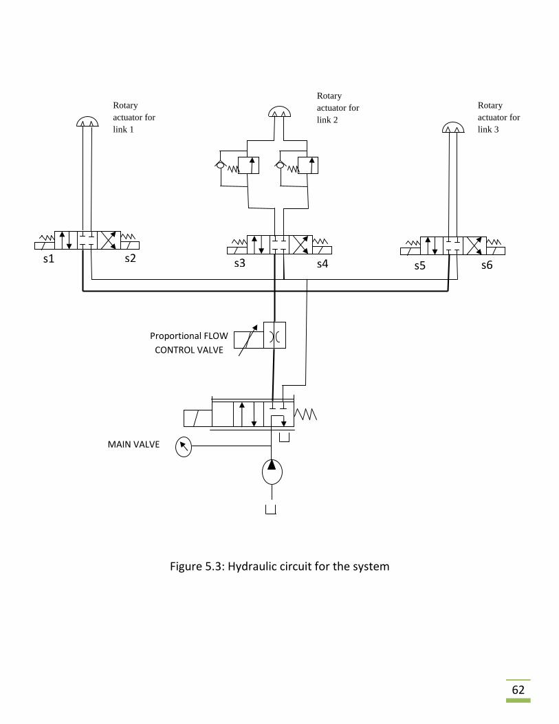
The system is operated by a fixed displacement hydraulic pump driven by anelectric motor. The hydraulic pump provide a regulated flow to the maindirectional control valve which control the overall flow of the system bypermitting a flow to the other parts of the hydraulic circuit or diverting theflow back to the reservoir. A proportional flow control valve is used tocontrol the flow rate of the hydraulic actuators using a single solenoid.

each rotary actuator is controlled by a directional control valve that allow aclockwise and counterclockwise rotation ,these directional valves areactuated through tow solenoids at the ends of each valve, one solenoid forclockwise rotation and the other for counterclockwise rotation .

The system is protected against overload pressure by using a pressure reliefvalve and it's placed out of the hydraulic pump. Figure 5.2 shows thehydraulic circuit of the system.

62

Figure 5.3: Hydraulic circuit for the system

s1 s2 s3 s4 s5 s6

Rotaryactuator forlink 1



Proportional FLOWCONTROL VALVE

MAIN VALVE

63

5.2.4 Electrical Description

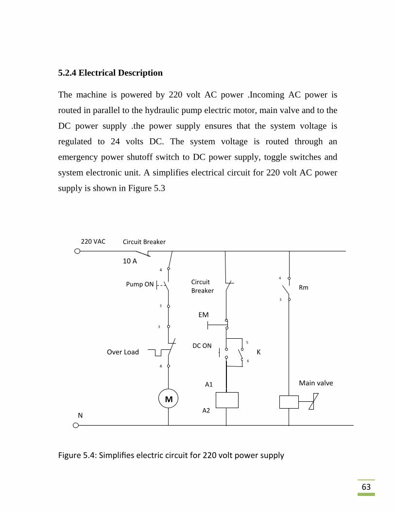
The machine is powered by 220 volt AC power .Incoming AC power is

routed in parallel to the hydraulic pump electric motor, main valve and to the

DC power supply .the power supply ensures that the system voltage is

regulated to 24 volts DC. The system voltage is routed through an

emergency power shutoff switch to DC power supply, toggle switches and

system electronic unit. A simplifies electrical circuit for 220 volt AC power

supply is shown in Figure 5.3

Figure 5.4: Simplifies electric circuit for 220 volt power supply

Mm

220 VACC

Pump ON

Circuit Breaker

CircuitBreaker

EM

k

DC ON

Rm

Main valveA1

A2

Over Load K

N

10 A4

4

3

4

3

3

5

6

64

5.3 Closed Loop Control

The term closed-loop control refers to the robot system managing the flowdemand by routing the valve system to achieve the desired movement ordesired position with smooth motion, and using sensors that give afeedback read for the final position for each link angle. We used the PLC forthis operation, this logic controller have the following specification:

1. Four analog inputs to read the position for each link through thepotentiometer.

2. Seven digital output; each output is connected to each solenoid togive a signal for desired motion.

3. One analog output to control the flow through proportional valve.

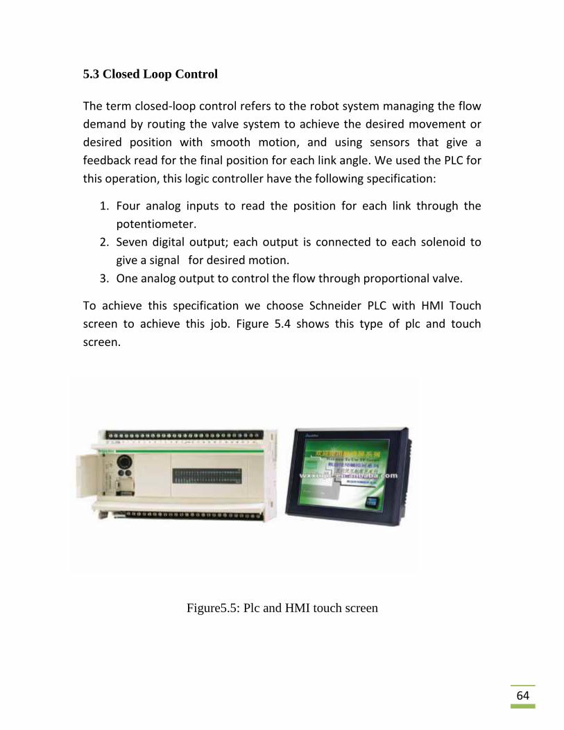
To achieve this specification we choose Schneider PLC with HMI Touchscreen to achieve this job. Figure 5.4 shows this type of plc and touchscreen.

Figure5.5: Plc and HMI touch screen

65

As we mentioned before the amount of flow can be controlled byproportional valve through an analog signal (0-10 v), this signal can bechanged through an analog output port of the controller.

5.3.1 Feedback Sensors

In a closed loop control system, four sensors monitor the system output(joint Angeles) and feed the data to a controller which adjusts the control(joint angle) as necessary to maintain the desired system output (match thedesired position which is , and coordinates of the end effectors). Thisrobot uses potentiometers to determines where it and then controls theirjoints to match the desired position. The output of the potentiometer is ananalog voltage that is proportional to the angle of rotation for each joint.These analog signals are connecting to the analog input of the PLC.

66

Potentiometer calibration

The calibration of potentiometer aims to find and represent the angles of thejoints according to the output voltage of each potentiometer attached to itsjoint, this voltages inter to the module as analog input, the by someequations we determine the equivalent angle.

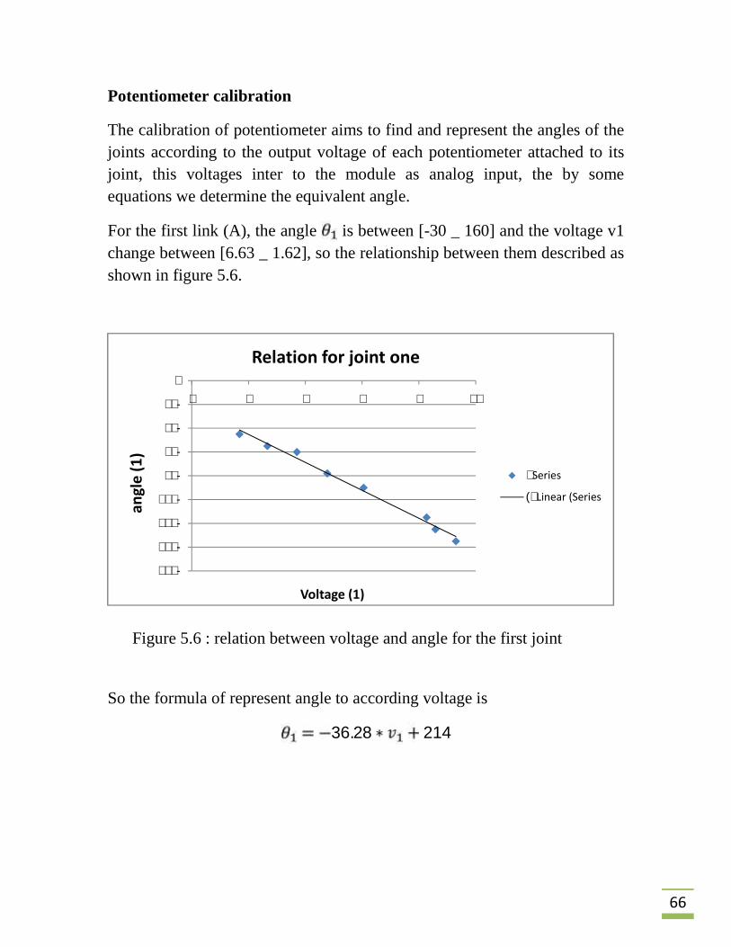
For the first link (A), the angle is between [-30 _ 160] and the voltage v1change between [6.63 _ 1.62], so the relationship between them described asshown in figure 5.6.

So the formula of represent angle to according voltage is36.28 214

-١٦٠

-١٤٠

-١٢٠

-١٠٠

-٨٠

-٦٠

-٤٠

-٢٠

٠٠ ٢ ٤ ٦ ٨ ١٠

angl

e (1

)

Voltage (1)

Relation for joint one

Series١

Linear (Series١(

Figure 5.6 : relation between voltage and angle for the first joint

67

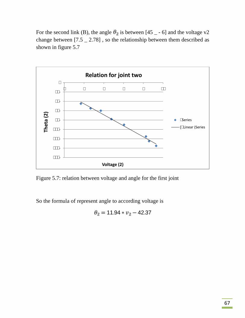
For the second link (B), the angle is between [45 _ - 6] and the voltage v2change between [7.5 _ 2.78] , so the relationship between them described asshown in figure 5.7

Figure 5.7: relation between voltage and angle for the first joint

So the formula of represent angle to according voltage is11.94 42.37

-١٦٠

-١٤٠

-١٢٠

-١٠٠

-٨٠

-٦٠

-٤٠

-٢٠

٠٠ ٢ ٤ ٦ ٨ ١٠

Thet

a (2

)

Voltage (2)

Relation for joint two

Series١

Linear (Series١(

68

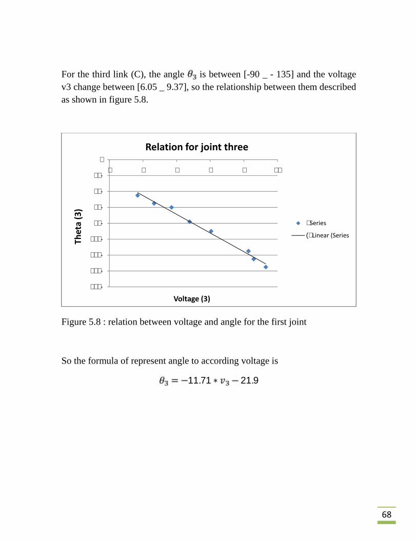
For the third link (C), the angle is between [-90 _ - 135] and the voltagev3 change between [6.05 _ 9.37], so the relationship between them describedas shown in figure 5.8.

Figure 5.8 : relation between voltage and angle for the first joint

So the formula of represent angle to according voltage is11.71 21.9

-١٦٠

-١٤٠

-١٢٠

-١٠٠

-٨٠

-٦٠

-٤٠

-٢٠

٠٠ ٢ ٤ ٦ ٨ ١٠

Thet

a (3

)

Voltage (3)

Relation for joint three

Series١

Linear (Series١(

69

5.3.2 Controllers and software

We are now interested in solving motion control problem .In motion control

problem, the manipulator moves to a position to pick up an object, transport

that project to another location, and deposit it. We treat this problem in the

joint space.

Joint space control

The main goal of the joint space control is to design a feedback controllersuch that the joint coordinates track the desired motion as closely as possible.the control of robot manipulators is naturally achieved in the joint space.Since the control inputs are the joint torques

Figure 5.6 shows the basic outline of the joint space control methods. Firstlythe desired motion, which is described in terms of end-effectors coordinates,is converted to a corresponding joint trajectory using the invest kinematicsof the manipulator, Then the feedback controller determines the joint torquenecessary to move the manipulator along the desired trajectory specified injoint coordinates starting from measurements of the current joint states.

Figure 5.6 Generic concept of joint space control

Inversekinematic

Controller Manipulator

70

Independent joint control

We adapt independent joint control to control the robot manipulator. Byindependent-joint control (i.e.., decentralized control) we mean that thecontrol inputs of each joint only depends on the measurement of thecorresponding joint displacement and velocity. Due to its simple structure,this kind of control schemes offers many advantages. For example by usingindependent- joint control, communication among different joint is saved.Moreover, since the computational load of controller may be reduced, onlylow-cost hardware is required in actual implementations. Finally,independent-joint control has the feature of scalability, since the controlleron all joints has the same formulation.

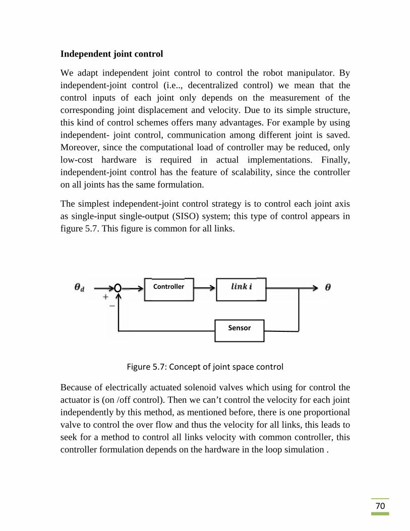
The simplest independent-joint control strategy is to control each joint axisas single-input single-output (SISO) system; this type of control appears infigure 5.7. This figure is common for all links.

Figure 5.7: Concept of joint space control

Because of electrically actuated solenoid valves which using for control theactuator is (on /off control). Then we can’t control the velocity for each jointindependently by this method, as mentioned before, there is one proportionalvalve to control the over flow and thus the velocity for all links, this leads toseek for a method to control all links velocity with common controller, thiscontroller formulation depends on the hardware in the loop simulation .

Controller

Sensor

71

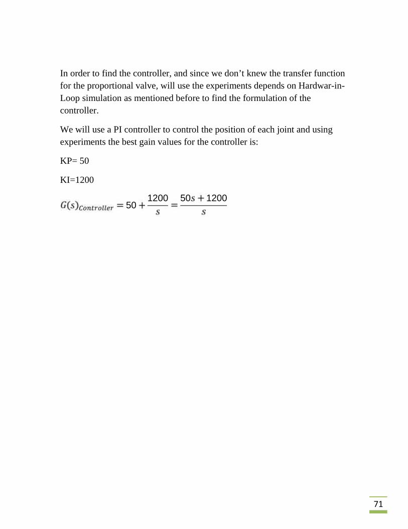
In order to find the controller, and since we don’t knew the transfer functionfor the proportional valve, will use the experiments depends on Hardwar-in-Loop simulation as mentioned before to find the formulation of thecontroller.

We will use a PI controller to control the position of each joint and usingexperiments the best gain values for the controller is:

KP= 50

KI=1200 50 1200 50 1200

72

Chapter six

Hardware and Software Description

6.1 Introduction

6.2 Hardware and Software Components

6.3 Sequence function chart –SFC (State Graph)

6.4 PID functions on Plc.

6.4.1 Introduction

6.4.2 The PID Controller Model

6.4.3 Operating Principles

6.4.4 Principal of the Regulation Loop

6.4.5 Role and Influence of PID Parameters

6.5 Touch Screen and Vijeo Designer

73

6.1 Introductions

In this chapter we will describe the hardware and software components that used inour project, and then we introduce Sequence function chart - SFC (or State graph)and the Concept of PID function, following by an introduction to HMI Software.

6.2Hardware and Software Components:

In our project we use these Types of Hardware:

1) TWDLCDE40DRF Twido Controller: which is a compact base controller,24v DC, 40 points, 24v DC inputs, 12-2A relay output, 2-1A transistoroutput, Timer and Calendar and Ethernet 100Base Tx, Removable Batteryand Non-removable terminal blocks.

2) TM2AMM6HT Analog Expansion Module: it’s an Expansion Module with4Analog inputs and 2 analog outputs (0 – 10v, 4– 20 mA), 12 bit resolution,removable screw terminals.

3) XBT OT 2210 Touch Screen: its 256 color and has a Supply Voltage Range19.2V DC to 28.8V DC.

In this project we use TwidoSuit V2.31.04 for programming the PlCusing sequence function chart (SFC) method.

And we used Vijeo Designer Opti for Programming the Xbt OT 2210 Touchscreen.

74

6.3 Sequence function chart –SFC (State Graph)

Sequential Function Charts (SFCs) are a graphical technique for writing concurrentcontrol programs or sequential control algorithms, and they are also known asGrafcet or IEC 848.

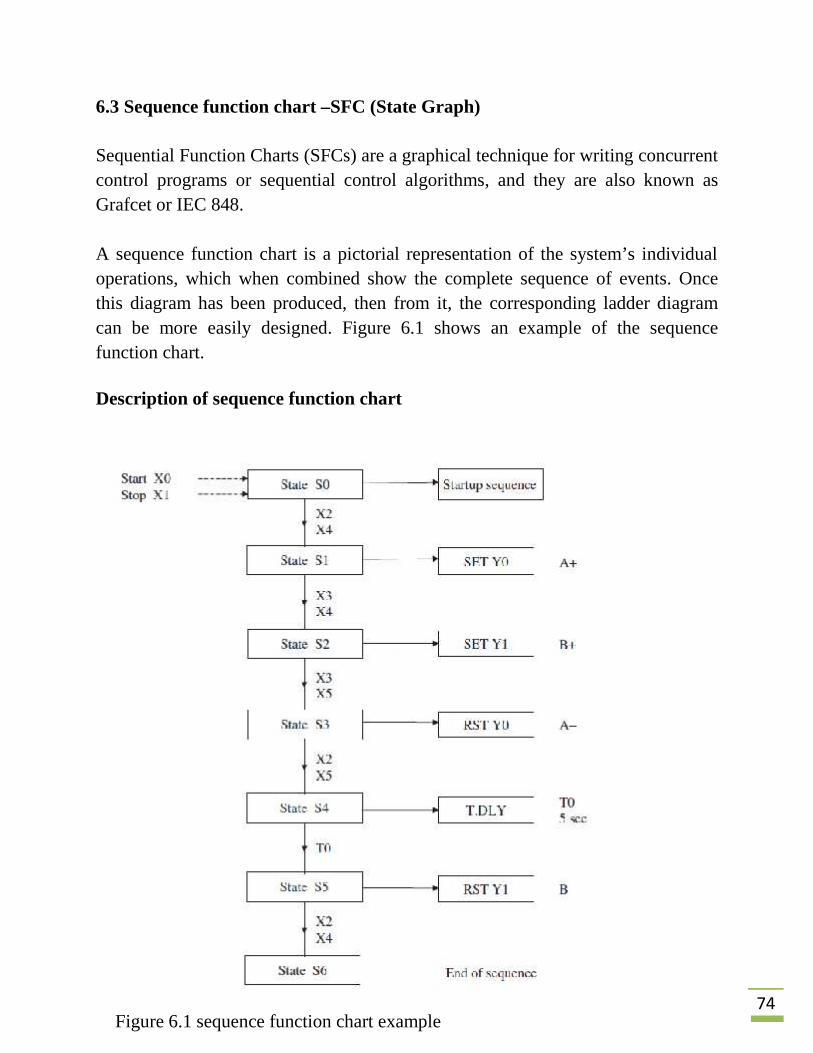
A sequence function chart is a pictorial representation of the system’s individualoperations, which when combined show the complete sequence of events. Oncethis diagram has been produced, then from it, the corresponding ladder diagramcan be more easily designed. Figure 6.1 shows an example of the sequencefunction chart.

Description of sequence function chart

Figure 6.1 sequence function chart example

75

The above figure is an example of sequence function chart and we willdescribe it in the following points:

1) The sequence function chart consists, basically, of a number of separatesequentially connected states, which are the individual constituents of thecomplete machine cycle that controls the system. An analogy is that eachstate is like a piece of a jigsaw puzzle; on its own it does not show verymuch, but when all the pieces are correctly assembled, then the completepicture is revealed.

Each state has the following:(a) An input condition.(b) An output condition.

(c) A transfer condition.

When the input condition into a state is correct, then that state will producean output condition. That is, an output device or devices will be:(a) Turned ON and remain ON.(b) Turned OFF and remain OFF.

2) When the output or outputs are turned ON/OFF, then the system’s inputconditions will change to produce a transfer condition.

3) The transfer condition is now connected to the input condition of the nextsequential state.

4) If the new input condition is correct, then the sequence moves to the nextstate.

5) From the sequence function chart, it can be seen that when the startpushbutton is operated, this is the input condition for state 0.

76

6) The output condition from State 0 is the startup sequence, which will resetboth Solenoid A and Solenoid B. With Inputs X2 and X4 now made, thetransfer from State 0 can take place.

7) The transfer conditions from State 0 are the correct input conditions forState 1, and hence the process now moves from State 0 to State 1.

8) The process will now continue from one state to the next, until the completemachine cycle is complete.

9) From the sequence function chart, the ladder diagram can now be produced

77

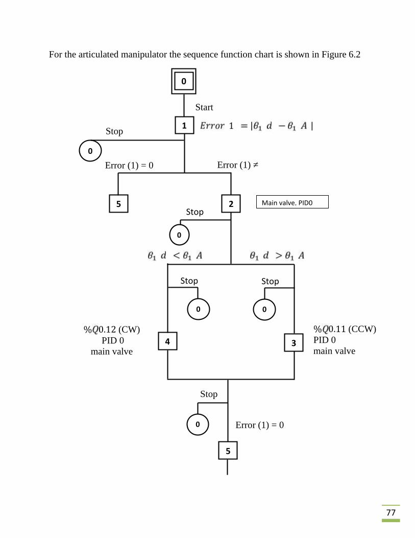
For the articulated manipulator the sequence function chart is shown in Figure 6.2

1

Error (1) ≠0

Error (1) = 0

2

0

34

0

0

% 0.11 (CCW)PID 0main valve

0

Start

Error (1) = 0

5

% 0.12 (CW)PID 0

main valve

Stop

Stop Stop

1 | |

Stop

0

0

5

Stop

Main valve, PID0

78

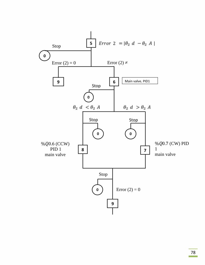
5

Error (2) ≠0

Error (2) = 0

6

0

78

0

0

% 0.7 (CW) PID1main valve

Error (2) = 0

9

% 0.6 (CCW)PID 1

main valve

Stop

Stop Stop

2 | |

Stop

0

0

9

Stop

Main valve, PID1

79

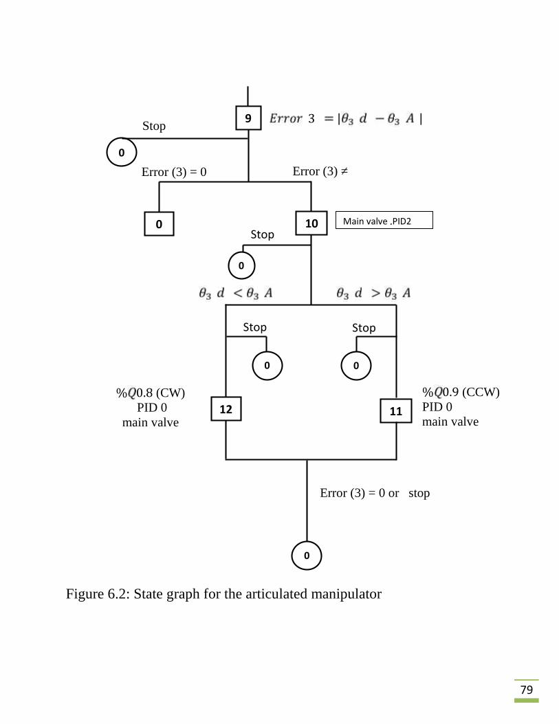
Figure 6.2: State graph for the articulated manipulator

9

Error (3) ≠0

Error (3) = 0

10

0

1112

0

0

% 0.9 (CCW)PID 0main valve

Error (3) = 0 or stop

% 0.8 (CW)PID 0

main valve

Stop

Stop Stop

3 | |

0

0

Stop

0

Main valve ,PID2

80

This state graph is for three joint controls, the state graph sequence start atstate zero and at this state nothing is active. And as we see there is Stopcondition input at each state, this input reset all states and take the sequenceto state 0, and any active device will turn OFF.

When the user push on start switch which is the input condition to next state,the state one is active but there is not outputs, it just take to two choices (two input conditions ) to the next step.

The input conditions now are a comparison of the error (1) it equal zero ornot, if the error is equal zero then sequence go to step five which to movejoint two, if the error (1) is not equal zero then the sequence go to state twoand there is another comparison between the desired and actual angle.

If the desired angle is more than the actual state three will activated and themain valve, PID 0 and 0.11 is turned on, the result of this is move link Acounter clock wise according to the desired angle. If the desired angle is lessthan the actual state four ( 0.12 turned on) which move link A clock wise tothe desired angle. After link A reach desired angle the sequence move tostate five.

The same thing do to the joint two and joint three until the end effectors ofthe Robot reach to the desired position.

Note: The Ladder Program is shown in Appendix A

81

6.4 PID functions on Plc

6.4.1 Introduction

The PID control function onboard all Twido controllers provides an efficientcontrol to simple industrial processes that consist of one system stimulus (referredto as Set point in this Book) and one measurable property of the system (referred toas Measure or Process Variable).

The approach of PID controller used in this project is to achieve responsive andaccurate positioning performance of the end effectors of the Robot, for each link(joint) we have a PID controller. By the PID controller the end effectors startmoving at somewhat high speed then the speed decreased according to the errorwhich is the difference between actual angle of joint and the desired angle.

This regulation function is particularly adapted to:

1) Answering the needs of the sequential process which need the auxiliaryadjustment functions (examples: plastic film packaging machine, finishingtreatment machine, presses, etc.)

2) Responding to the needs of the simple adjustment process (examples: metalfurnaces, ceramic furnaces, small refrigerating groups, etc.)

It is very easy to install as it is carried out in the:1. Configuration2. and Debug

Screens associated with a program line (operation block in Ladder Language or bysimply calling the PID in Instruction List) indicating the number of the PID used.The correct syntax when writing a PID instruction is: PID<space>n, when n is thePID number.

82

Example of a program line in Ladder Language:

NOTE: In any given Twido automation application, the maximum number ofconfigurable PID functions is 14.

6.4.2 The PID Controller Model

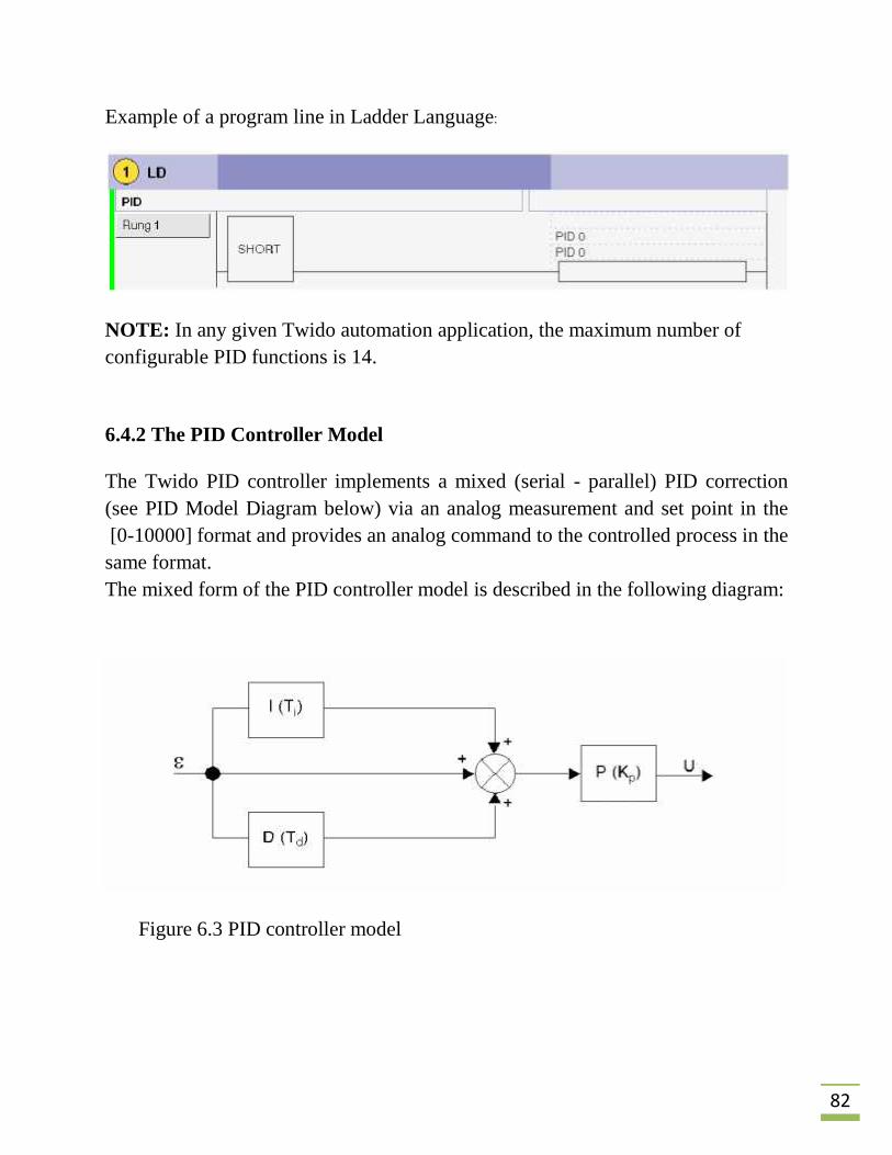
The Twido PID controller implements a mixed (serial - parallel) PID correction(see PID Model Diagram below) via an analog measurement and set point in the[0-10000] format and provides an analog command to the controlled process in thesame format.The mixed form of the PID controller model is described in the following diagram:

Figure 6.3 PID controller model

83

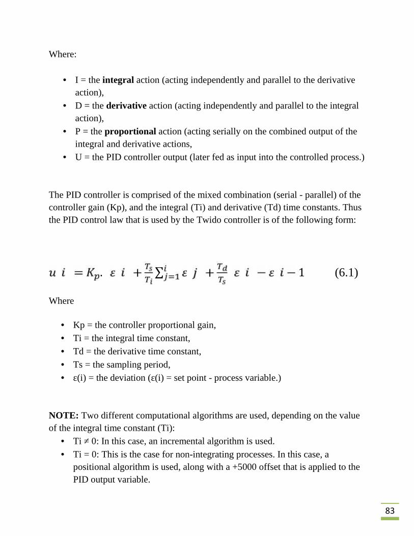
Where:

I = the integral action (acting independently and parallel to the derivativeaction),

D = the derivative action (acting independently and parallel to the integralaction),

P = the proportional action (acting serially on the combined output of theintegral and derivative actions,

U = the PID controller output (later fed as input into the controlled process.)

The PID controller is comprised of the mixed combination (serial - parallel) of thecontroller gain (Kp), and the integral (Ti) and derivative (Td) time constants. Thusthe PID control law that is used by the Twido controller is of the following form:

. ∑ 1 (6.1)

Where

Kp = the controller proportional gain, Ti = the integral time constant, Td = the derivative time constant, Ts = the sampling period, ε(i) = the deviation (ε(i) = set point - process variable.)

NOTE: Two different computational algorithms are used, depending on the valueof the integral time constant (Ti):

Ti ≠ 0: In this case, an incremental algorithm is used. Ti = 0: This is the case for non-integrating processes. In this case, a

positional algorithm is used, along with a +5000 offset that is applied to thePID output variable.

84

6.4.3 Operating Principles

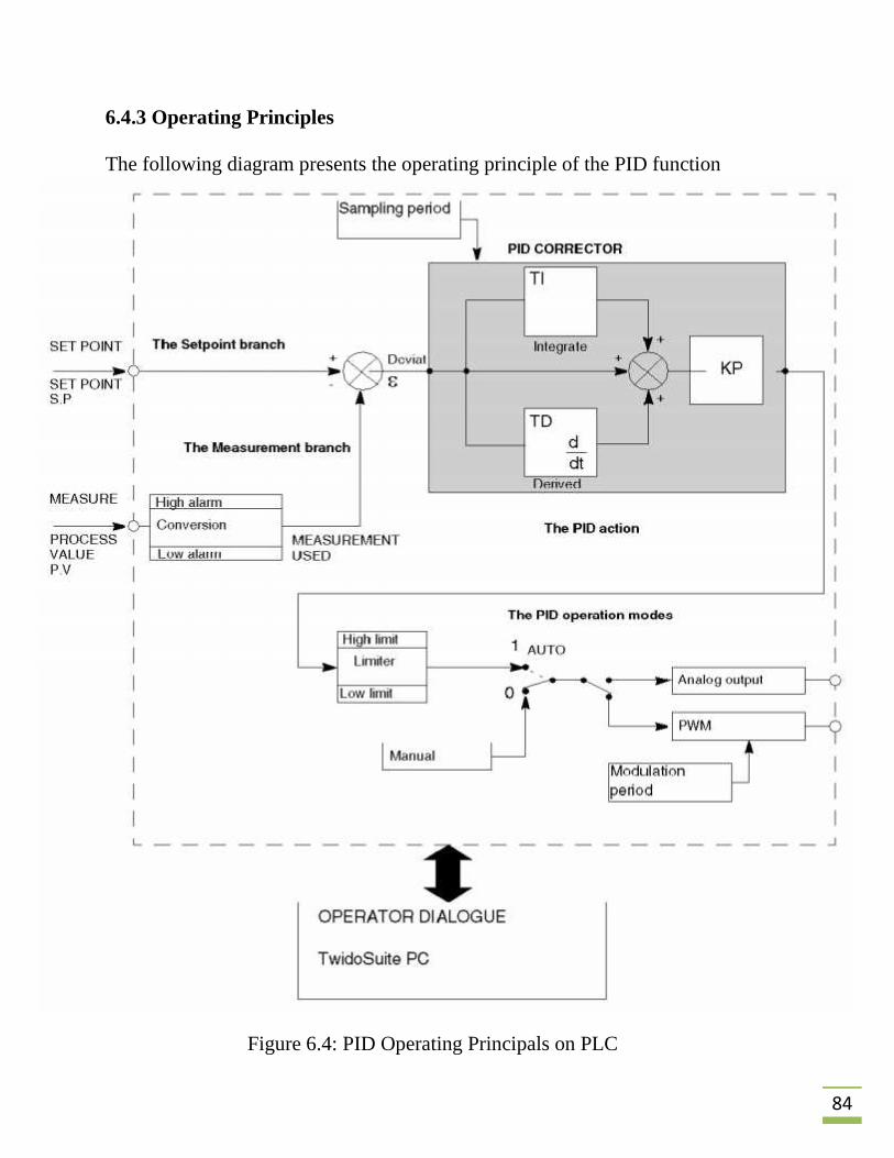
The following diagram presents the operating principle of the PID function

Figure 6.4: PID Operating Principals on PLC

85

Her the setpoint represent the desired angle that the joint should go and themeasure point is the actual angle of the respective joint, the error of the summingpoint enters to the PID controller (PI in our case) .According to Controller gainsthere will be an output, this output can be limited using saturation or limiter asshown in the figure .In our project we use saturation for each joint with min value3 v and max value 7 v ,since we don’t need a very high speed or very low speed .

The PID function has two modes: analog output or PWM output, in our project weuse the analog output to control the proportional valve opening which control theflow of the system.

86

6.4.4 Principal of the Regulation Loop

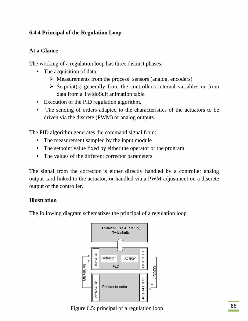
At a Glance

The working of a regulation loop has three distinct phases: The acquisition of data:

Measurements from the process’ sensors (analog, encoders) Setpoint(s) generally from the controller's internal variables or from

data from a TwidoSuit animation table Execution of the PID regulation algorithm. The sending of orders adapted to the characteristics of the actuators to be

driven via the discrete (PWM) or analog outputs.

The PID algorithm generates the command signal from: The measurement sampled by the input module The setpoint value fixed by either the operator or the program The values of the different corrector parameters

The signal from the corrector is either directly handled by a controller analogoutput card linked to the actuator, or handled via a PWM adjustment on a discreteoutput of the controller.

Illustration

The following diagram schematizes the principal of a regulation loop

Figure 6.5: principal of a regulation loop

87


Influence of Proportional Action

Proportional action is used to influence the process response speed. The higher thegain, the faster the response and the lower the static error (in direct proportion),though the more stability deteriorates. A suitable compromise between speed andstability must be found. The influence of Proportional on process response to aScale division is as follows:

Figure 6.6: Influence of Proportional Action

87





87





88

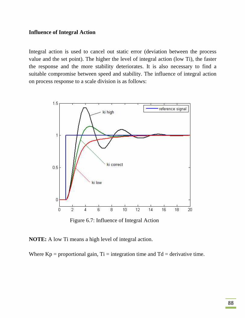
Influence of Integral Action

Integral action is used to cancel out static error (deviation between the processvalue and the set point). The higher the level of integral action (low Ti), the fasterthe response and the more stability deteriorates. It is also necessary to find asuitable compromise between speed and stability. The influence of integral actionon process response to a scale division is as follows:

Figure 6.7: Influence of Integral Action

NOTE: A low Ti means a high level of integral action.

Where Kp = proportional gain, Ti = integration time and Td = derivative time.

88






88






89

Influence of Derivative Action

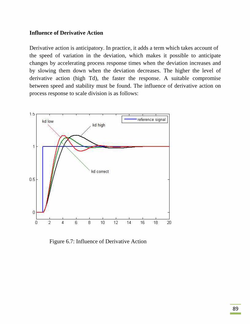
Derivative action is anticipatory. In practice, it adds a term which takes account ofthe speed of variation in the deviation, which makes it possible to anticipatechanges by accelerating process response times when the deviation increases andby slowing them down when the deviation decreases. The higher the level ofderivative action (high Td), the faster the response. A suitable compromisebetween speed and stability must be found. The influence of derivative action onprocess response to scale division is as follows:

Figure 6.7: Influence of Derivative Action

89




89




90

6.5 Touch Screen and Vijeo Designer

The touch screen that we use in this project is Magelis XPT OT 2110 SchneiderTouch screen; we decide to choose this touch screen because it meet thespecification required and hiveless cost and have the following specification:

Type Advanced touch screen panel

Display type Backlit monochrome STN LCD

Supply Voltage Range: 19.2V DC to 28.8V DC

Display color 16 levels of grey Blue and white

Display resolution 320 x 240 pixels QVGA

Display size 5.7 inch

Software type Configuration software

Software designation Vijeo Designer

Operating system Magelis

Processor name CPU RISC

Processor frequency 133 MHz

Memory description Back up of data SRAM 128 kB lithium battery

Application memory flash EPROM 16 MB

We use Vijeo Designer Opti software to program the touch screen, and by touchscreen the user can inter the desired coordinate of the end effectors (X, Y,Z).Thiscoordinates are transferred to PLC via Modbus communication protocol which is amaster/slave protocol that’s allow for one, and only one, master to requestresponses from slaves or to act based on the request.

91

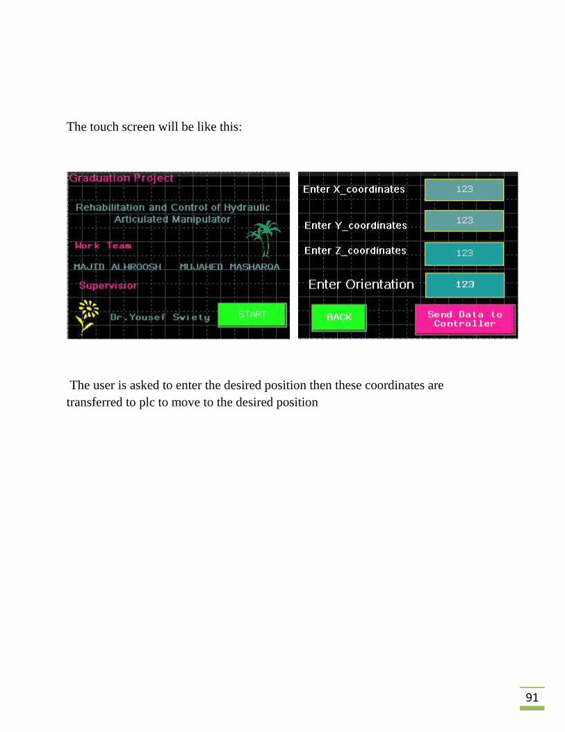
The touch screen will be like this:

The user is asked to enter the desired position then these coordinates aretransferred to plc to move to the desired position

92

Chapter Seven

Experiments and results

7.1 Introduction

7.2 Experimental results

7.3 Conclusion

7.4 Future Work

93

7.1 Introduction

This chapter contains the results that are obtained from the experiments which are

done to verify the theoretical results that disused on the previous chapters. Then

these results are discussed and explained from the experimental side.


In this section we mention the experimental results that we performed, here we

show the step response of each joint as shown below:

First Joint

Figure7.1:step response of first joint

Posi

tion(

degr

ee)

Time(sec)

93

7.1 Introduction







First Joint


Posi

tion(

degr

ee)

Time(sec)

93

7.1 Introduction







First Joint


Posi

tion(

degr

ee)

Time(sec)

94

second Joint

Figure7.2:step response of second joint

Posi

tion(

degr

ee)

Time(sec)

94

second Joint


Posi

tion(

degr

ee)

Time(sec)

94

second Joint


Posi

tion(

degr

ee)

Time(sec)

95

Third Joint

Figure7.3:step response of third joint

Posi

tion(

degr

ee)

Time(sec)

95

Third Joint


Posi

tion(

degr

ee)

Time(sec)

95

Third Joint


Posi

tion(

degr

ee)

Time(sec)

96

Each time we perform the experiments there is an error on each angle and this

error appear due to several Reasons:

1) The hydraulic system is a non linear system so we can’t model the system to

find the appropriate controller, however we use tuning process to find the

most suitable controller based on experimental computation.

2) The feedback sensors are potiometers so there must be an error associated

with the mechanical part of the sensor, and as a result the robot will reach

the desired position with some certain errors.

7.3 Conclusion

Robotics has become recently an interesting area of research. In our project we

apply robotic theories, control techniques to accomplish the main goal of our

project which is to move the robot to the desired position.

Moving the robot requires a control system, we used the Twido controller for this

task, and based on some control algorithms we program our system. Moving all the

joint together can’t be accomplished using PLC so we design control technique to

move the first joint followed by the second joint and then the third joint.

7.4 Future Work

The results of this work can be a basic point for the future studies .we can design

different control algorithms with different hardware and servo system to produce a

high performance robot arm. Another subject is that we could use another method

of control; it may be microcontroller or DAQ system.

Appendices A

TwidoSuit Programs

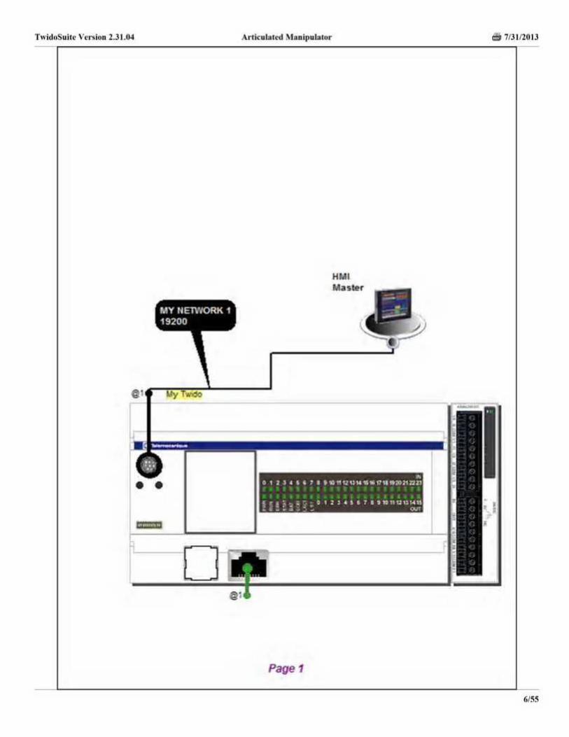
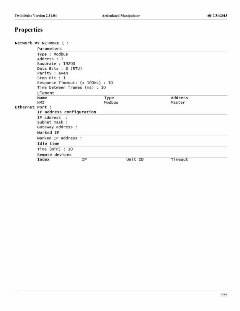
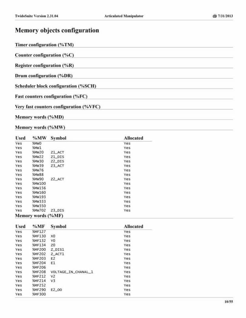
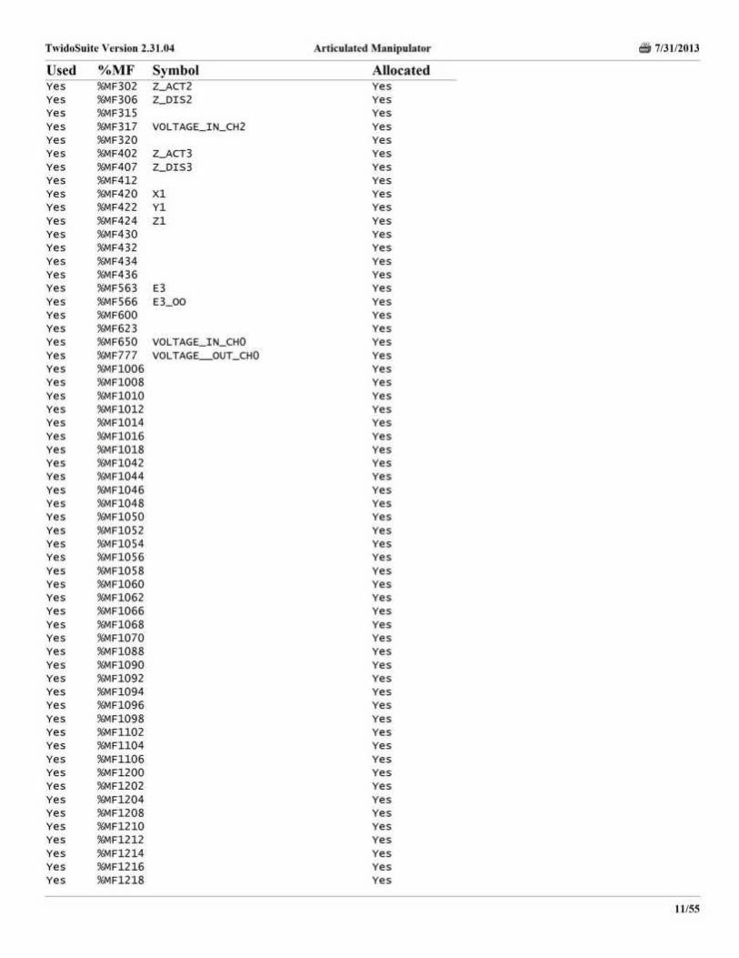
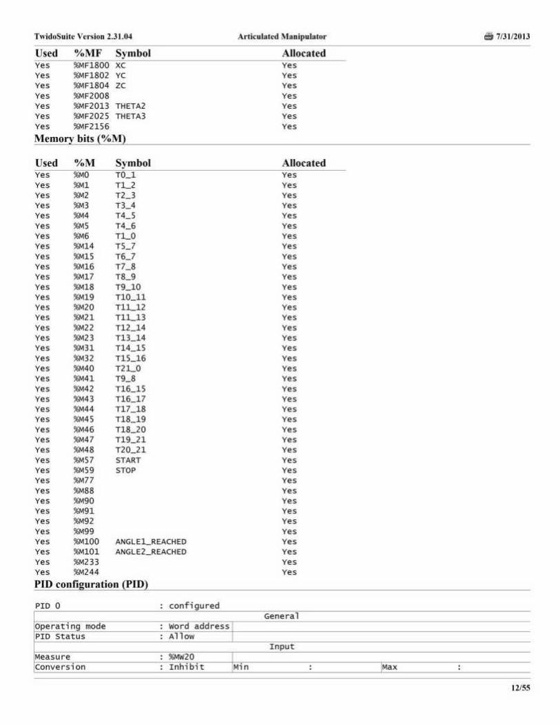
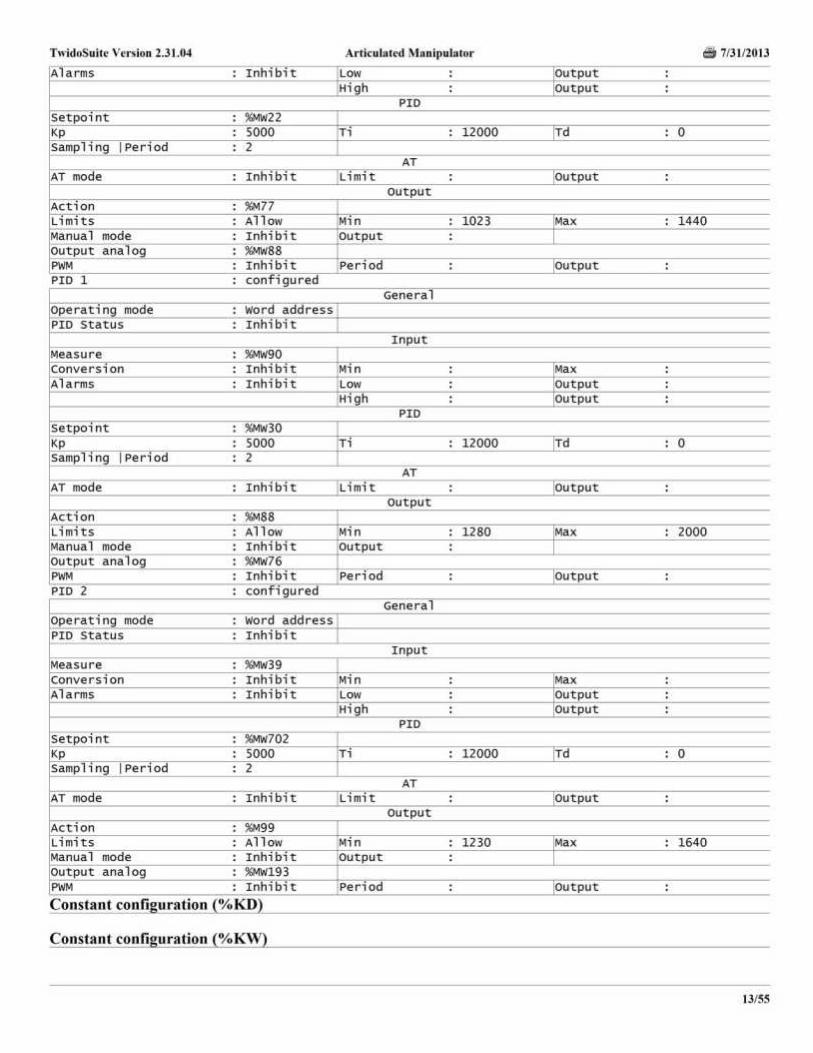
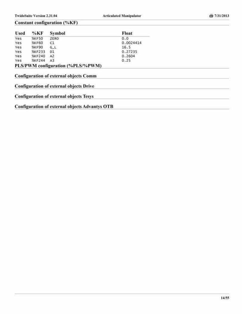
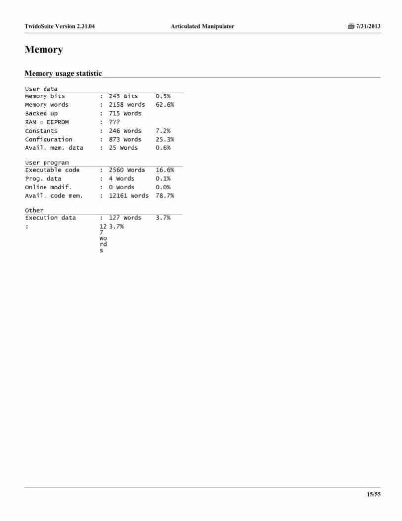
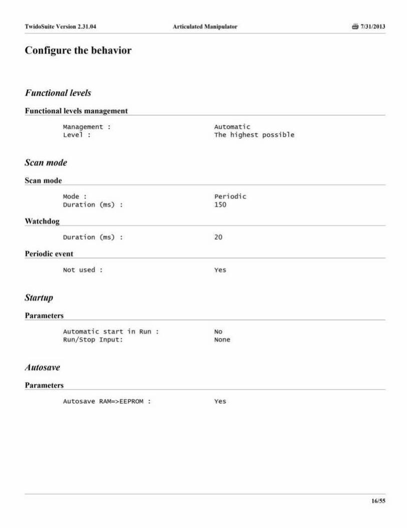
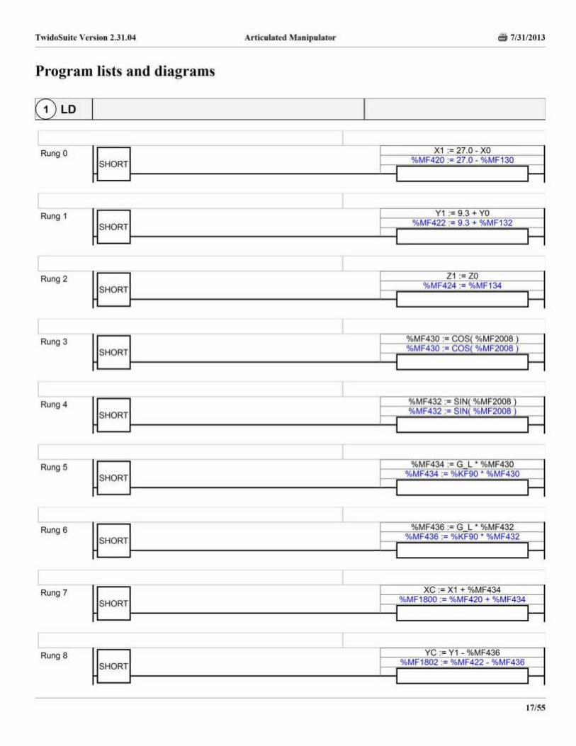
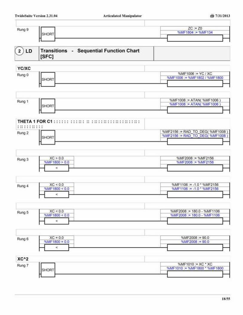
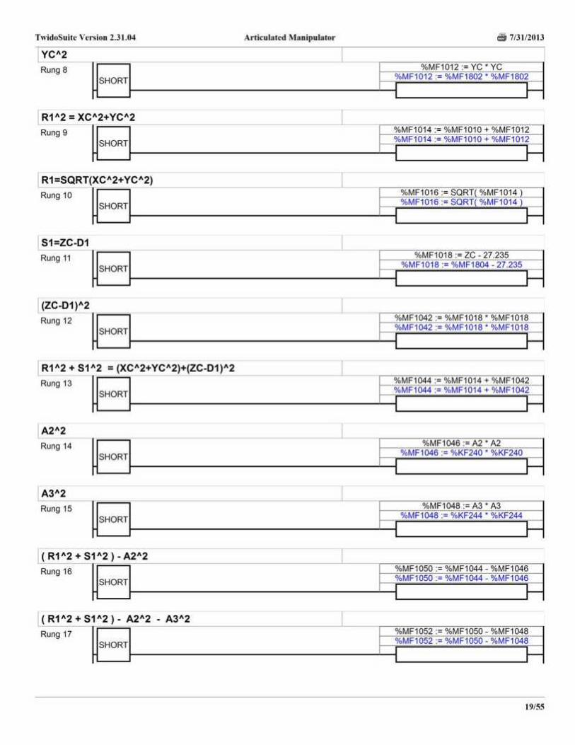
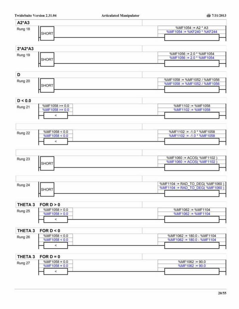
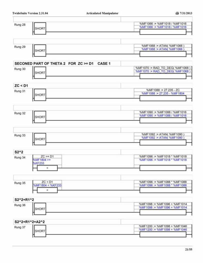
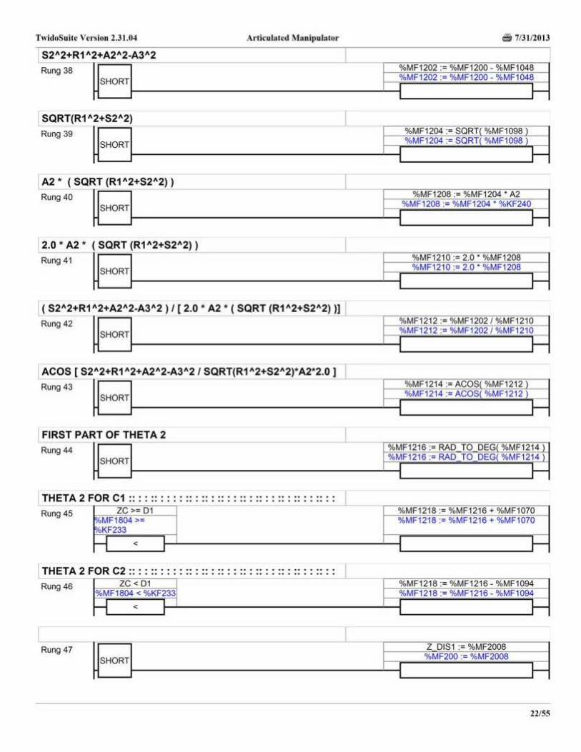
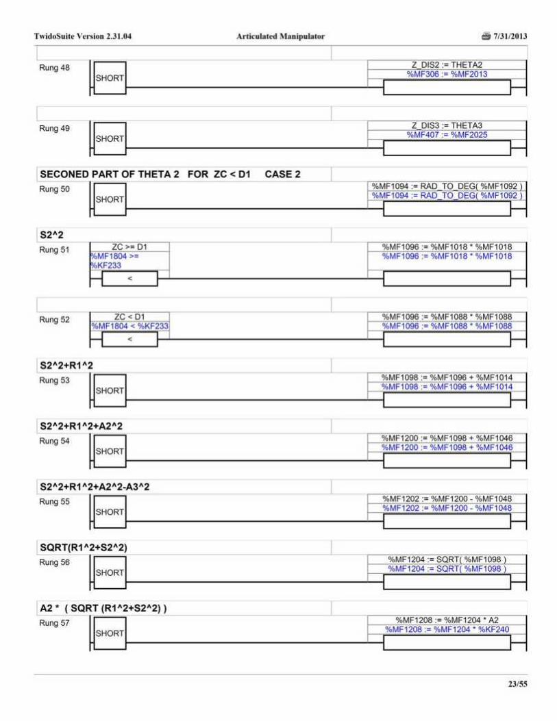
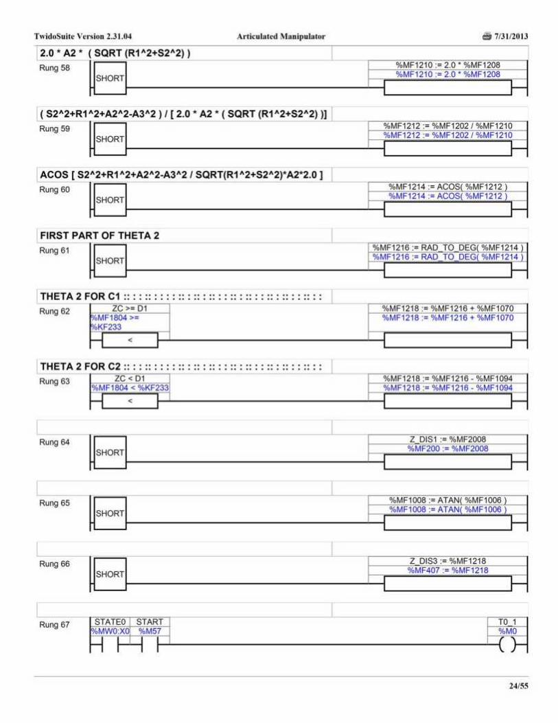
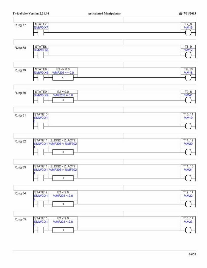
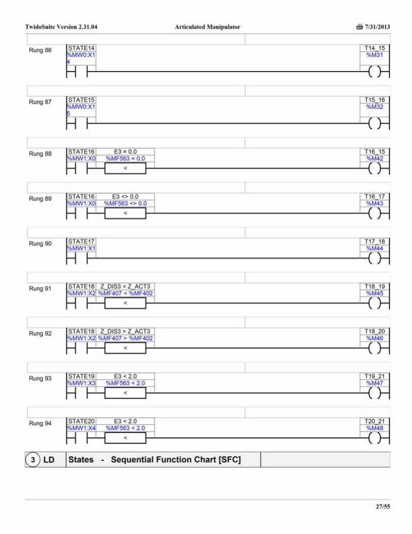
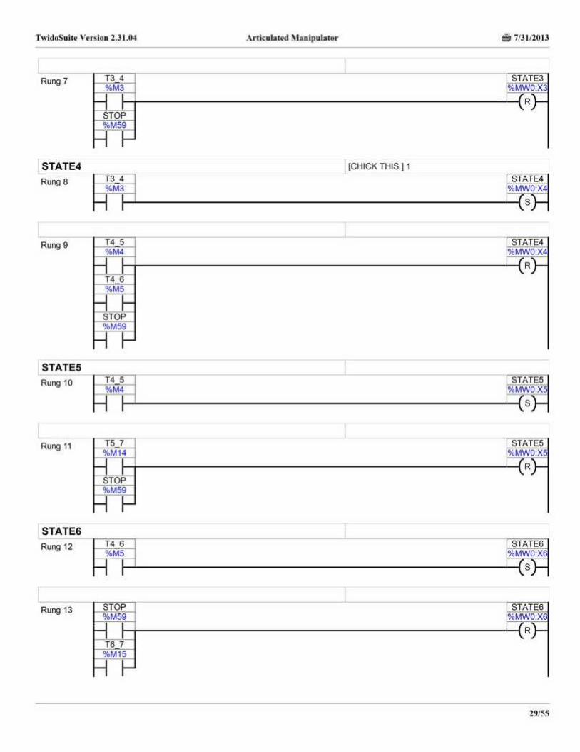
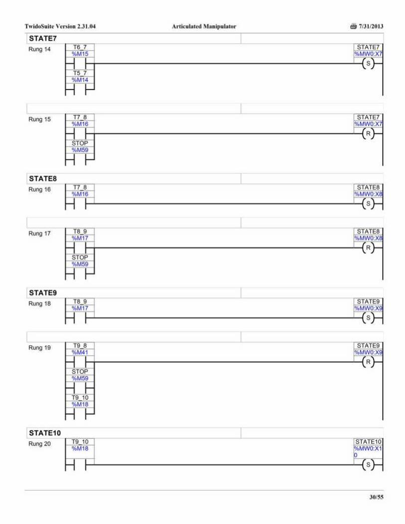
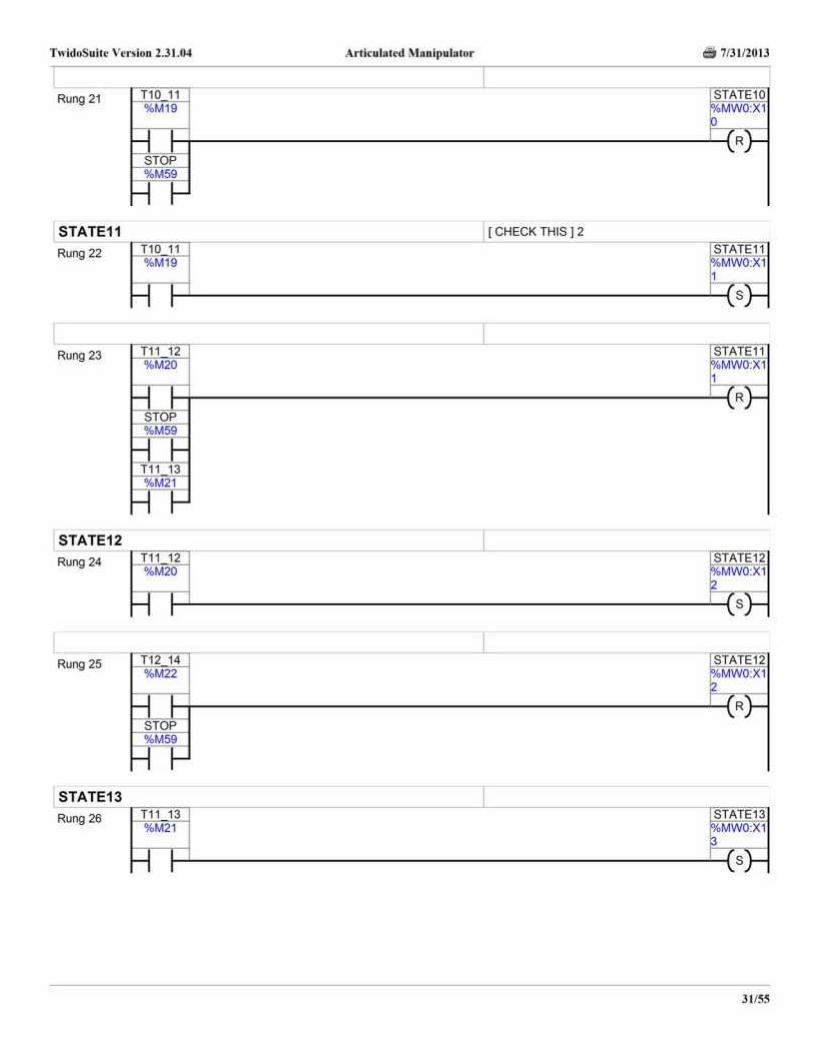
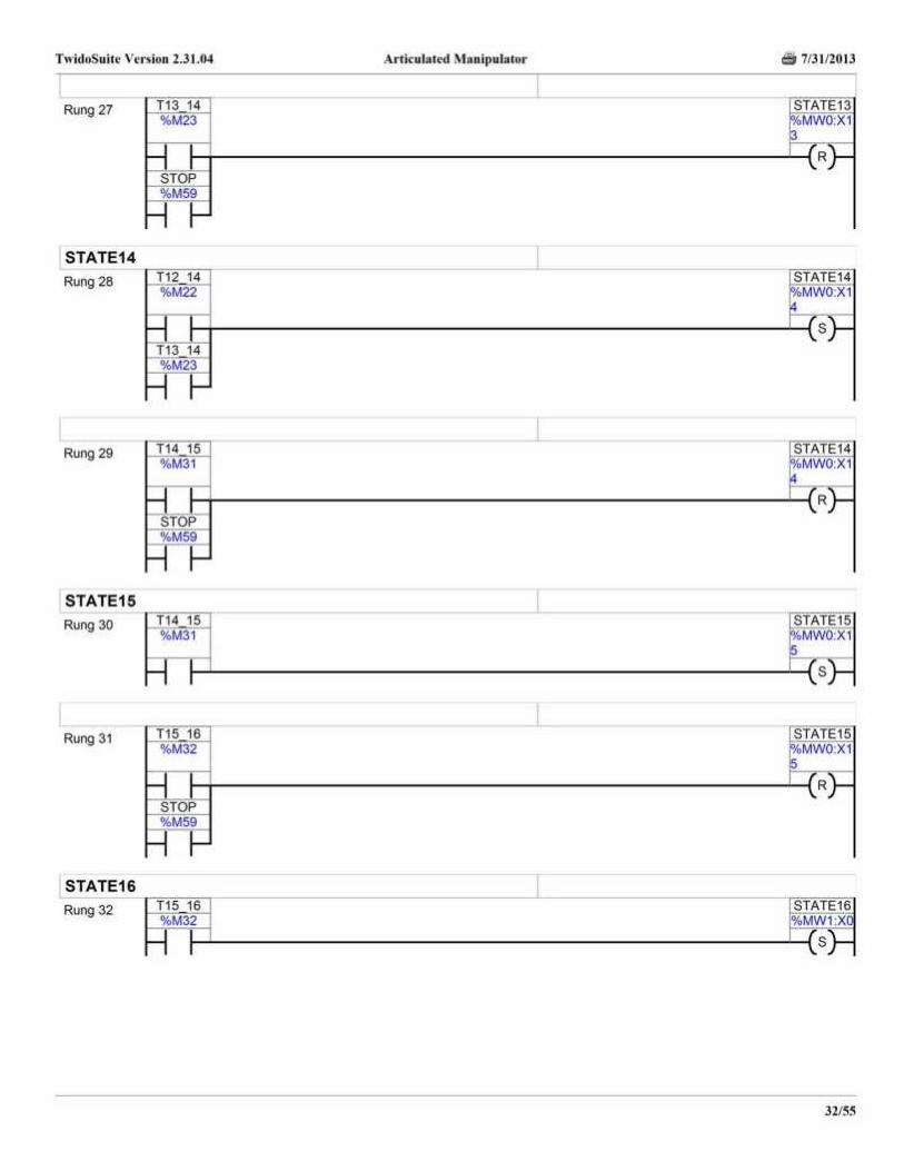
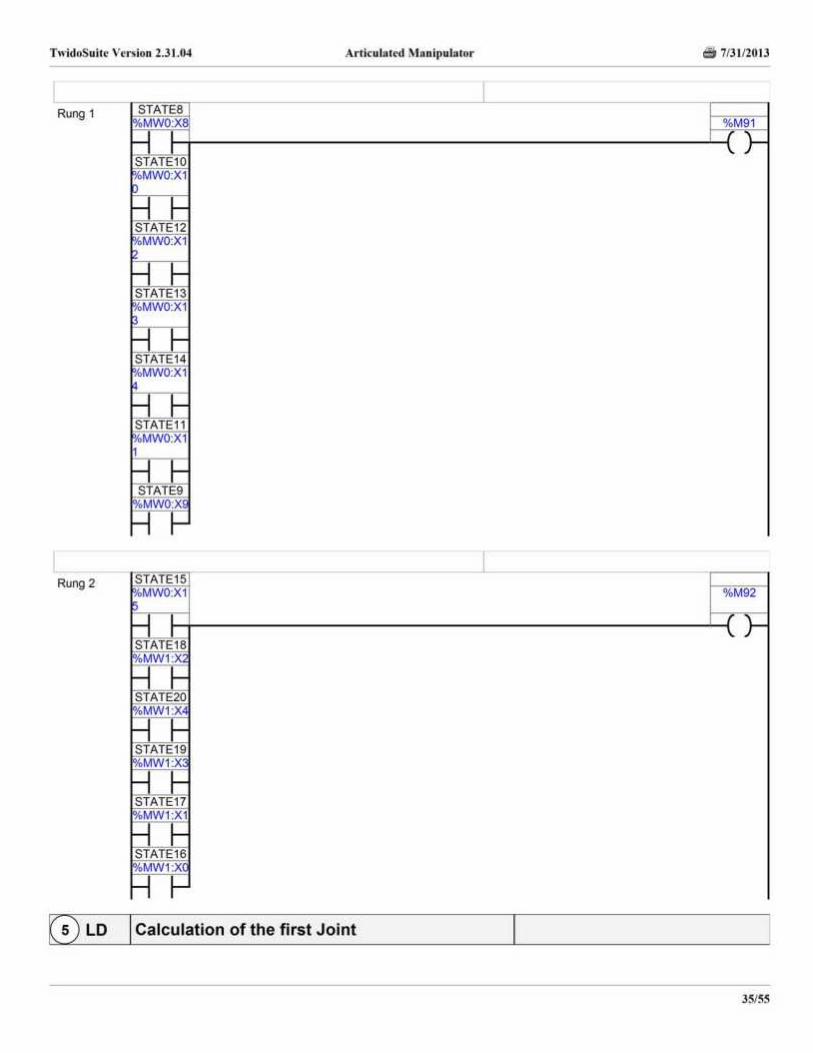
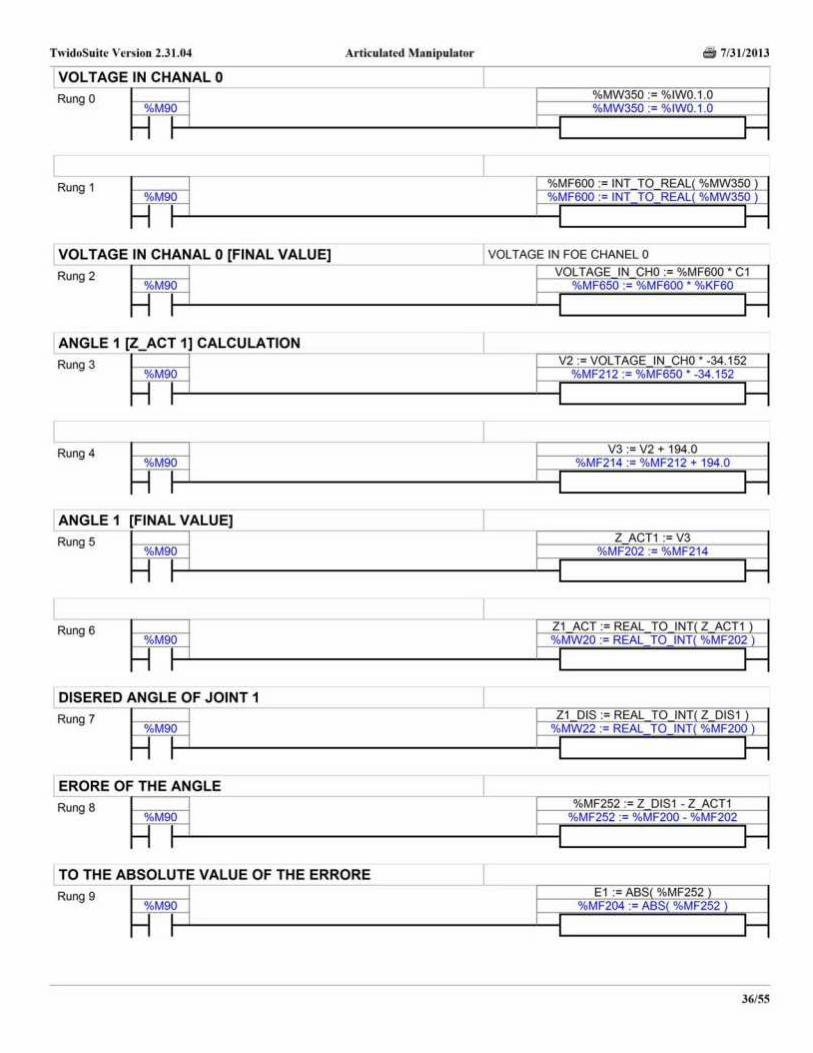
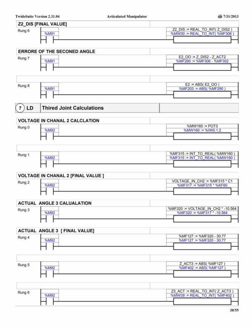
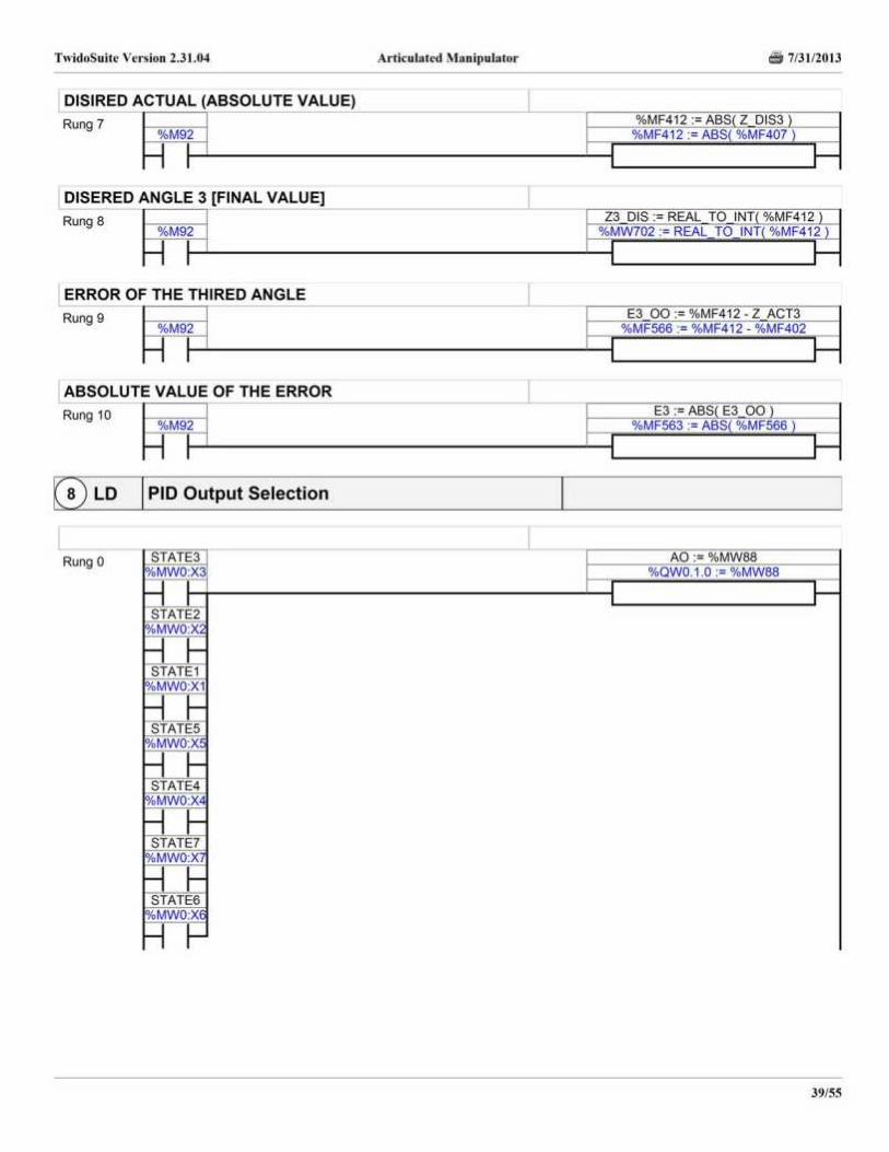
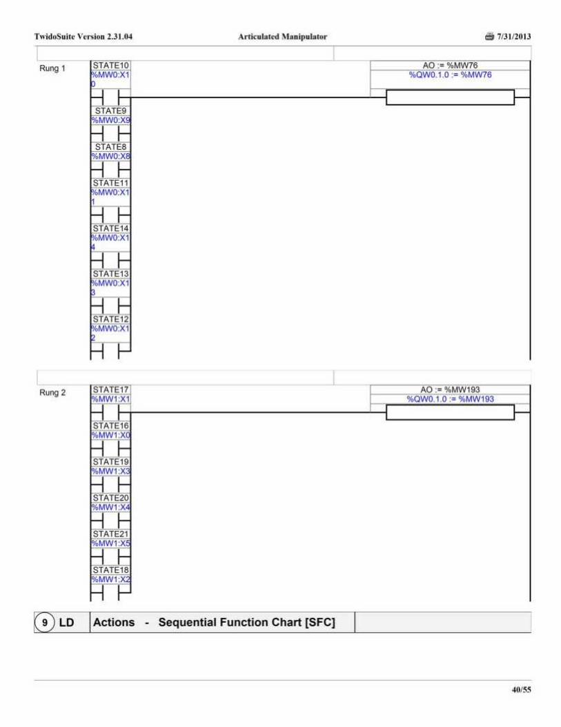
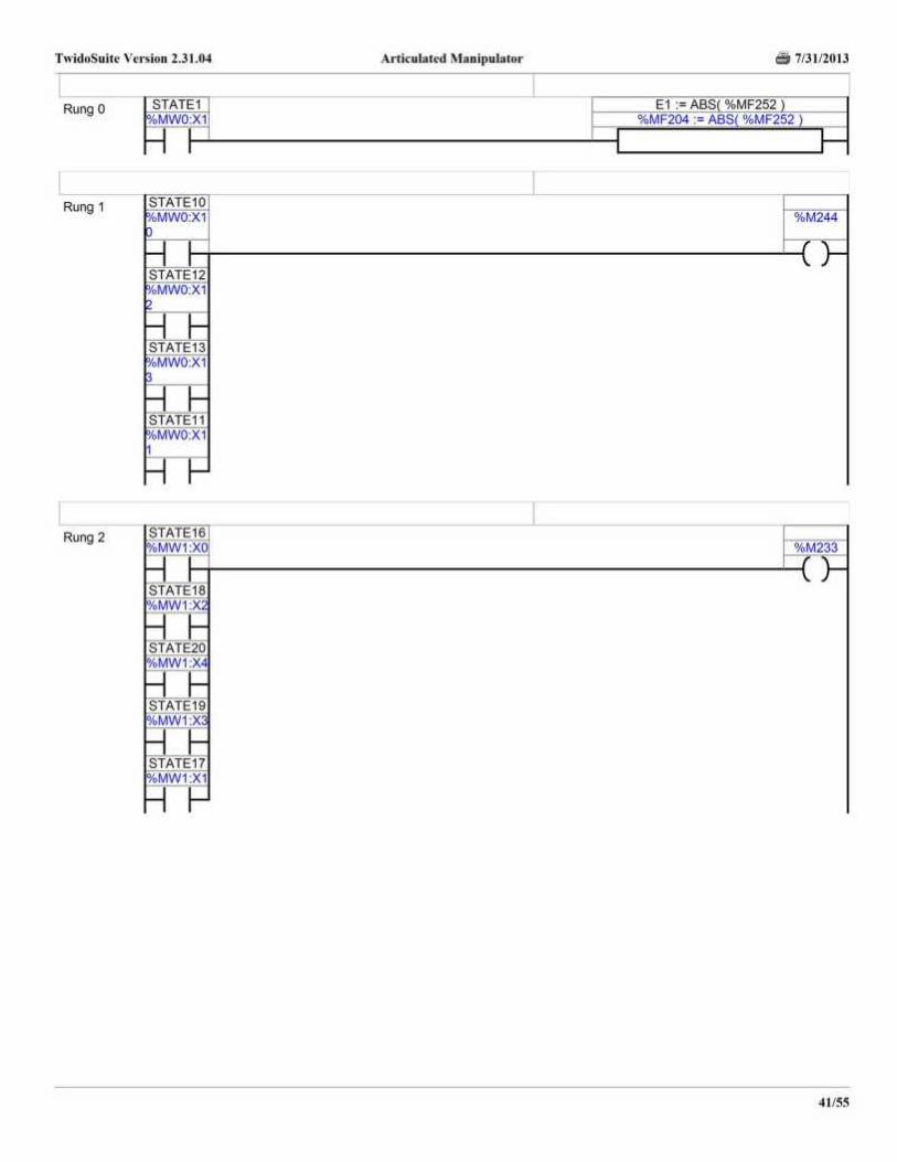
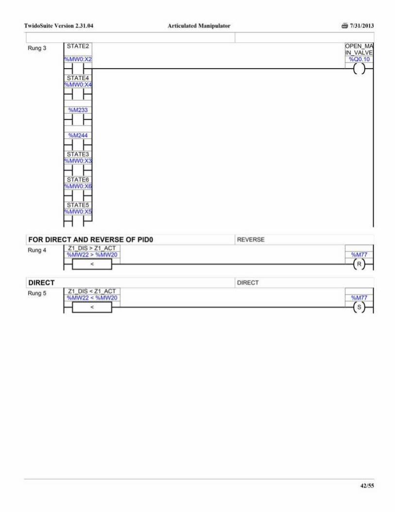
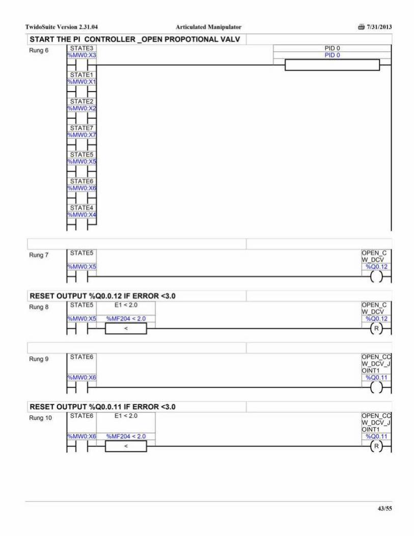
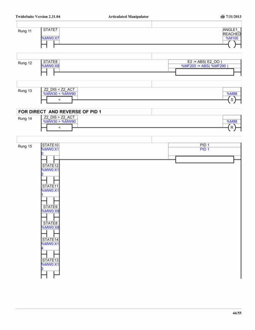
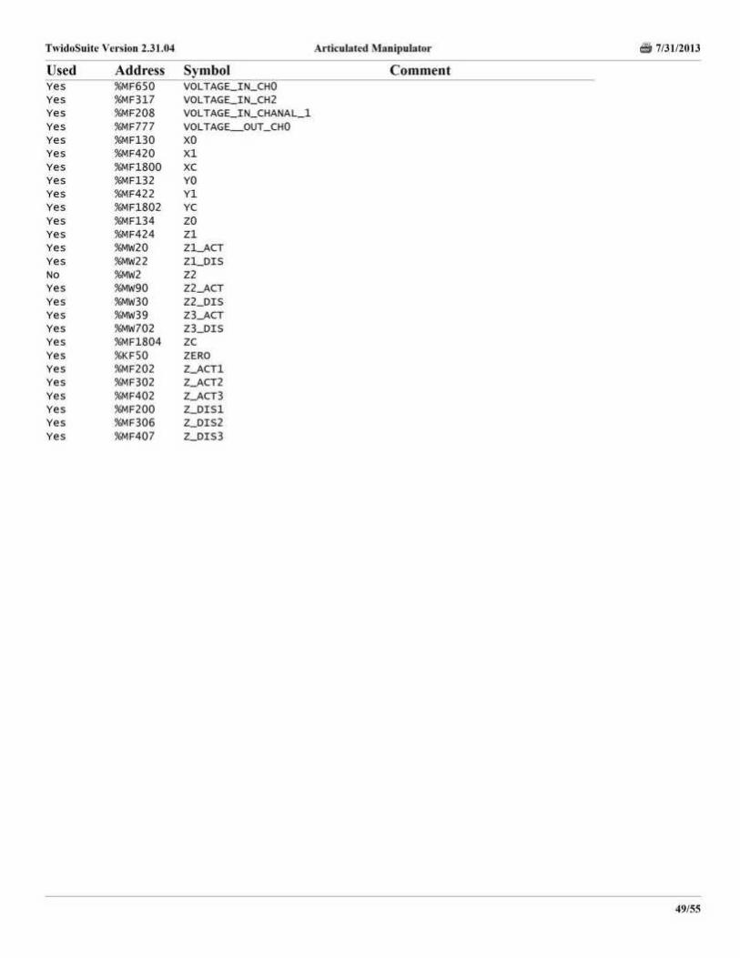
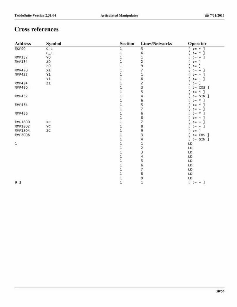
96

References

1) M. W. Song, S.Hutchinsons, and M. Vidyasagar, “Robot Modeling andcontrol”, John Wiley & Sons, Inc, 2006

2) B. Siciliana, L. Sciavicoo, L. Villain, and G. Oriolo, “Robotics modeling,planning and control”, Springer- Verlag London Limited, 2009

3) J.J Craig, “Introduction to Robotics Mechanics and Control”, second edition,Silma. Inc, 1989

4) R. Kelly, V. Santibanes and A. Loria “Control of Robot Manipulator in JointSpace”, Spring- Verlag London Limited, 2005

5) Andrew J. smith and Van Batavia, “Electronic Control for HydraulicApplications”, Eaton Corporation, 2008

Graduation Project

Documents

Transcript of Graduation Project