GPS/INS Based Lateral and Longitudinal Control Demonstration

ISSN 1055-1425

August 1998

This work was performed as part of the California PATH Program of theUniversity of California, in cooperation with the State of California Business,Transportation, and Housing Agency, Department of Transportation; and theUnited States Department of Transportation, Federal Highway Administration.

The contents of this report reflect the views of the authors who are responsiblefor the facts and the accuracy of the data presented herein. The contents do notnecessarily reflect the official views or policies of the State of California. Thisreport does not constitute a standard, specification, or regulation.

Report for MOU 292

CALIFORNIA PATH PROGRAMINSTITUTE OF TRANSPORTATION STUDIESUNIVERSITY OF CALIFORNIA, BERKELEY

GPS/INS Based Lateral andLongitudinal Control Demonstration:Final Report

UCB-ITS-PRR-98-28California PATH Research Report

Jay Farrell, Matthew Barth,Randy Galijan, Jim Sinko

CALIFORNIA PARTNERS FOR ADVANCED TRANSIT AND HIGHWAYS

GPS/INS Based Lateral and Longitudinal Control Demonstration

Final Report

Principal Investigator: Jay Farrell

Department of Electrical Engineering

University of California, Riverside

[email protected]

Co-Principal Investigator: Matthew Barth

Center for Environmental Research and Technology

University of California, Riverside

[email protected]

Co-Principal Investigator: Randy Galijan

Stanford Research Institute

Menlo Park, CA

randy [email protected]

Co-Principal Investigator: Jim Sinko

Stanford Research Institute

Menlo Park, CA

jim [email protected]

July 31, 1998

Abstract

This report describes the results of a one year e�ort to implement and analyze the performance of a Di�er-

ential Global Positioning System (DGPS) aided Inertial Navigation System (INS) for possible future use in

Advanced Vehicle Control Systems (AVCS).

The initial premise of this project was that DGPS/INS technology has the potential to serve as a

centimeter-level position reference system as necessary for automated driving functions. Key advantages

of this approach include: 1) no changes to the highway infrastructure are required; therefore, the DGPS/INS

system should be less expensive to install and maintain than alternative reference systems; 2) knowledge

of the DGPS position of a vehicle allows the use of signi�cantly more path preview information than al-

ternative position reference systems; therefore, control performance could be improved; 3) the navigation

system would output the full vehicle state (position, velocity, and attitude) and inertial measurements at

signi�cantly higher rates than alternative navigation systems would provide even a subset of the vehicle

state.

The overall objective of this study was to implement a DGPS aided INS system and to analyze the

technical feasibility of such a system relative to the requirements for vehicle control. The one year e�ort

incorporated two main tasks: 1) Implementation of a real-time DGPS/INS; and, 2) Experimental analysis of

the DGPS/INS performance. The DGPS/INS system provided estimates of vehicle position, linear velocities,

and angular rates. State estimates are currently available at a rate of 100 Hertz, but signi�cantly higher rates

are feasible. Position accuracy at the centimeter level is achieved and demonstrated via two experiments.

Integration of the DGPS aided INS into a control algorithm was not included in this one year study, but is

one of the items discussed under future work.

A few potential follow-on projects include: implementation of the DGPS/INS system in a control demon-

stration, development and demonstration of more advanced (higher rates and increased accuracy) DGPS/INS

systems, analysis of DGPS/INS systems with other sensor systems to achieve required system level relia-

bility speci�cations, analysis of DGPS/INS AVCS protocols, and analysis of the need and performance of

pseudolites in AHS systems. Speci�c detail regarding such e�orts is included in the report conclusions.

Keywords: Global Positioning System, Inertial Navigation, Di�erential Carrier Phase, Advanced Vehicle

Control

Executive SummaryThis project was a one year e�ort to implement and analyze the performance of a Di�erential Global

Positioning System (DGPS) aided Inertial Navigation System (INS) for possible future use in Advanced

Vehicle Control Systems (AVCS).

The initial premise of this project was that DGPS/INS technology has the potential to serve as a

centimeter-level position reference system as necessary for automated driving functions. Key advantages

of this approach include:

1. no changes to the highway infrastructure are required; therefore, the DGPS/INS system should be less

expensive to install and maintain than alternative reference systems;

2. knowledge of the DGPS position of a vehicle allows the use of signi�cantly more path preview infor-

mation than alternative position reference systems; therefore, control performance could be improved;

3. the navigation system would output the full vehicle state (position, velocity, and attitude) and inertial

measurements (accelerations and angular rates) at signi�cantly higher rates than alternative navigation

systems would provide even a subset of the vehicle state.

The overall objective of this study was to implement a DGPS aided INS system and to analyze the

technical feasibility of such a system relative to the requirements for vehicle control. The one year e�ort

incorporated two main tasks:

1. Implementation of a real-time DGPS/INS,

2. Experimental analysis of the DGPS/INS performance.

The DGPS/INS system provided estimates of vehicle position, linear velocities, and angular rates. State

estimates are currently available at a rate of 100 Hertz, but signi�cantly higher rates are feasible. Position

accuracy at the centimeter level is achieved and demonstrated via two experiments. Integration of the DGPS

aided INS into a control algorithm was not included in this one year study, but is one of the items discussed

under future work.

A few potential follow-on projects include:

1. implementation of the DGPS/INS system in a control demonstration,

2. development and demonstration of more advanced (higher rates and increased accuracy) DGPS/INS

systems

3. analysis of DGPS/INS systems with other sensor systems to achieve required system level reliability

speci�cations

4. analysis of DGPS/INS AVCS protocols, and

5. analysis of the need and performance of pseudolites in AHS systems.

Speci�c details regarding such e�orts are included in the report conclusions.

i

Contents

1 Project Introduction 1

1.1 Global Positioning System and Vehicle Control . . . . . . . . . . . . . . . . . . . . . . . . . . 1

1.2 Inertial Navigation and Vehicle Control . . . . . . . . . . . . . . . . . . . . . . . . . . . . . . 2

1.3 Redundant Positioning Systems . . . . . . . . . . . . . . . . . . . . . . . . . . . . . . . . . . . 3

2 Project Scope and Objectives 4

2.1 Project Objectives . . . . . . . . . . . . . . . . . . . . . . . . . . . . . . . . . . . . . . . . . . 4

2.2 Project Scope . . . . . . . . . . . . . . . . . . . . . . . . . . . . . . . . . . . . . . . . . . . . . 4

3 Methodology 6

3.1 Inertial Navigation System (INS) . . . . . . . . . . . . . . . . . . . . . . . . . . . . . . . . . . 6

3.1.1 Tangent Plane Mechanization Equations . . . . . . . . . . . . . . . . . . . . . . . . . . 6

3.1.2 Tangent Plane INS Nominal Error Equations . . . . . . . . . . . . . . . . . . . . . . . 7

3.1.3 Numeric Integration . . . . . . . . . . . . . . . . . . . . . . . . . . . . . . . . . . . . . 9

3.2 Di�erential Global Positioning (DGPS) . . . . . . . . . . . . . . . . . . . . . . . . . . . . . . 9

3.2.1 GPS Observables . . . . . . . . . . . . . . . . . . . . . . . . . . . . . . . . . . . . . . . 9

3.2.2 Di�erential GPS Operation . . . . . . . . . . . . . . . . . . . . . . . . . . . . . . . . . 17

3.3 DGPS Aided INS . . . . . . . . . . . . . . . . . . . . . . . . . . . . . . . . . . . . . . . . . . . 20

3.4 Overall System Design . . . . . . . . . . . . . . . . . . . . . . . . . . . . . . . . . . . . . . . . 21

3.4.1 Hardware Description . . . . . . . . . . . . . . . . . . . . . . . . . . . . . . . . . . . . 21

3.4.2 Software Description . . . . . . . . . . . . . . . . . . . . . . . . . . . . . . . . . . . . . 22

4 Performance Analysis 25

4.1 Time to Phase Lock Analysis . . . . . . . . . . . . . . . . . . . . . . . . . . . . . . . . . . . . 25

4.2 Table Top Testing . . . . . . . . . . . . . . . . . . . . . . . . . . . . . . . . . . . . . . . . . . 26

4.3 Amusement Park Ride Testing . . . . . . . . . . . . . . . . . . . . . . . . . . . . . . . . . . . 28

5 Conclusions and Future Research 36

5.1 Future Research . . . . . . . . . . . . . . . . . . . . . . . . . . . . . . . . . . . . . . . . . . . 36

5.2 Publications Resulting from this Project . . . . . . . . . . . . . . . . . . . . . . . . . . . . . . 37

ii

A Appendix: Constant and Notation De�nition 42

A.1 Notation . . . . . . . . . . . . . . . . . . . . . . . . . . . . . . . . . . . . . . . . . . . . . . . . 42

A.2 Constants . . . . . . . . . . . . . . . . . . . . . . . . . . . . . . . . . . . . . . . . . . . . . . . 43

B Appendix: Platform and Experiment Photographs 45

C Appendix: Receiver Price and Performance History 49

C.1 GPS Positioning Accuracy . . . . . . . . . . . . . . . . . . . . . . . . . . . . . . . . . . . . . . 49

C.2 Receiver Cost . . . . . . . . . . . . . . . . . . . . . . . . . . . . . . . . . . . . . . . . . . . . . 49

iii

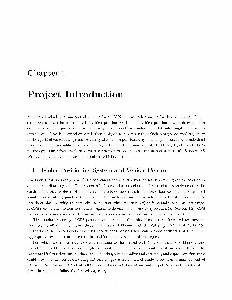
Chapter 1

Project Introduction

Automated vehicle position control systems for an AHS require both a means for determining vehicle po-

sition and a means for controlling the vehicle position [38, 16]. The vehicle position may be determined in

either relative (e.g., position relative to nearby known point) or absolute (e.g., latitude, longitude, altitude)

coordinates. A vehicle control system is then designed to maneuver the vehicle along a speci�ed trajectory

in the speci�ed coordinate system. A variety of reference positioning systems may be considered: embedded

wires [16, 9, 17], embedded magnets [38, 43], radar [16, 31], vision [26, 19, 10, 11, 30, 37, 40], and DGPS

technology. This e�ort has focused on research to develop, analyze, and demonstrate a DGPS aided INS

with accuracy and sample rates su�cient for vehicle control.

1.1 Global Positioning System and Vehicle Control

The Global Positioning System [1] is a convenient and accurate method for determining vehicle position in

a global coordinate system. The system is built around a constellation of 24 satellites already orbiting the

earth. The orbits are designed in a manner that allows the signals from at least four satellites to be received

simultaneously at any point on the surface of the earth with an unobstructed via of the sky. Each satellite

broadcasts data allowing a user receiver to calculate the satellite (x,y,z) position and user to satellite range.

A GPS receiver can use four sets of these signals to determine its own (x,y,z) position (see Section 3.2). GPS

navigation systems are currently used in many applications including aircraft [32] and ships [36].

The standard accuracy of GPS position estimates is on the order of 50 meters. Increased accuracy (at

the meter level) can be achieved through the use of Di�erential GPS (DGPS) [32, 25, 42, 4, 5, 12, 15].

Furthermore, a DGPS system that uses carrier phase observations can provide accuracies of 1 to 3 cm.

Appropriate techniques are discussed in the Methodology Section of this report.

For vehicle control, a trajectory corresponding to the desired path (i.e., the automated highway lane

trajectory) would be de�ned in the global coordinate reference frame and stored on-board the vehicle.

Additional information such as the road inclination, turning radius and direction, and super-elevation angle

could also be stored on-board (using CD technology) as a function of roadway position to improve control

performance. The vehicle control system would then drive the steering and propulsion actuation systems to

force the vehicle to follow the desired trajectory.

1

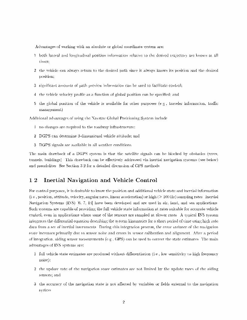
Advantages of working with an absolute or global coordinate system are:

1. both lateral and longitudinal position information relative to the desired trajectory are known at all

times;

2. the vehicle can always return to the desired path since it always knows its position and the desired

position;

3. signi�cant amounts of path preview information can be used to facilitate control;

4. the vehicle velocity pro�le as a function of global position can be speci�ed; and

5. the global position of the vehicle is available for other purposes (e.g., traveler information, tra�c

management).

Additional advantages of using the Navstar Global Positioning System include

1. no changes are required to the roadway infrastructure;

2. DGPS can determine 3-dimensional vehicle attitude; and

3. DGPS signals are available in all weather conditions.

The main drawback of a DGPS system is that the satellite signals can be blocked by obstacles (trees,

tunnels, buildings). This drawback can be e�ectively addressed via inertial navigation systems (see below)

and pseudolites. See Section 3.2 for a detailed discussion of GPS methods.

1.2 Inertial Navigation and Vehicle Control

For control purposes, it is desirable to know the position and additional vehicle state and inertial information

(i.e., position, attitude, velocity, angular rates, linear acceleration) at high (� 100 Hz) sampling rates. Inertial

Navigation Systems (INS) [6, 7, 14] have been developed and are used in air, land, and sea applications.

Such systems are capable of providing the full vehicle state information at rates suitable for accurate vehicle

control, even in applications where some of the sensors are sampled at slower rates. A typical INS system

integrates the di�erential equation describing the system kinematics for a short period of time using high rate

data from a set of inertial instruments. During this integration process, the error variance of the navigation

state increases primarily due to sensor noise and errors in sensor calibration and alignment. After a period

of integration, aiding sensor measurements (e.g., GPS) can be used to correct the state estimates. The main

advantages of INS systems are:

1. full vehicle state estimates are produced without di�erentiation (i.e., low sensitivity to high frequency

noise);

2. the update rate of the navigation state estimates are not limited by the update rates of the aiding

sensors; and

3. the accuracy of the navigation state is not a�ected by variables or �elds external to the navigation

system.

2

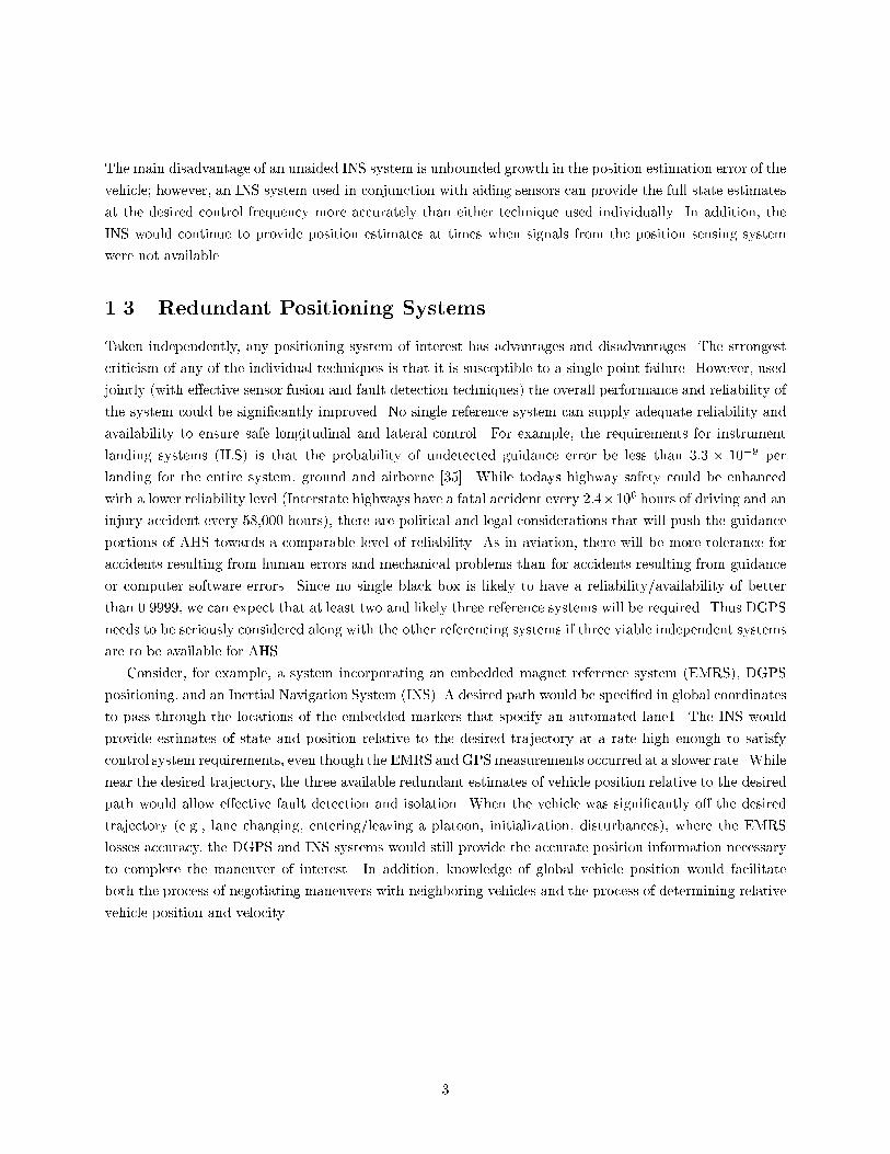
The main disadvantage of an unaided INS system is unbounded growth in the position estimation error of the

vehicle; however, an INS system used in conjunction with aiding sensors can provide the full state estimates

at the desired control frequency more accurately than either technique used individually. In addition, the

INS would continue to provide position estimates at times when signals from the position sensing system

were not available.

1.3 Redundant Positioning Systems

Taken independently, any positioning system of interest has advantages and disadvantages. The strongest

criticism of any of the individual techniques is that it is susceptible to a single point failure. However, used

jointly (with e�ective sensor fusion and fault detection techniques) the overall performance and reliability of

the system could be signi�cantly improved. No single reference system can supply adequate reliability and

availability to ensure safe longitudinal and lateral control. For example, the requirements for instrument

landing systems (ILS) is that the probability of undetected guidance error be less than 3:3 � 10�9 per

landing for the entire system, ground and airborne [35]. While todays highway safety could be enhanced

with a lower reliability level (Interstate highways have a fatal accident every 2:4�106 hours of driving and an

injury accident every 58,000 hours), there are political and legal considerations that will push the guidance

portions of AHS towards a comparable level of reliability. As in aviation, there will be more tolerance for

accidents resulting from human errors and mechanical problems than for accidents resulting from guidance

or computer software errors. Since no single black box is likely to have a reliability/availability of better

than 0.9999, we can expect that at least two and likely three reference systems will be required. Thus DGPS

needs to be seriously considered along with the other referencing systems if three viable independent systems

are to be available for AHS.

Consider, for example, a system incorporating an embedded magnet reference system (EMRS), DGPS

positioning, and an Inertial Navigation System (INS). A desired path would be speci�ed in global coordinates

to pass through the locations of the embedded markers that specify an automated lane1. The INS would

provide estimates of state and position relative to the desired trajectory at a rate high enough to satisfy

control system requirements, even though the EMRS and GPS measurements occurred at a slower rate. While

near the desired trajectory, the three available redundant estimates of vehicle position relative to the desired

path would allow e�ective fault detection and isolation. When the vehicle was signi�cantly o� the desired

trajectory (e.g., lane changing, entering/leaving a platoon, initialization, disturbances), where the EMRS

losses accuracy, the DGPS and INS systems would still provide the accurate position information necessary

to complete the maneuver of interest. In addition, knowledge of global vehicle position would facilitate

both the process of negotiating maneuvers with neighboring vehicles and the process of determining relative

vehicle position and velocity.

3

Chapter 2

Project Scope and Objectives

Vehicle control based on some form of absolute or global sensing techniques, such as the use of GPS-based

sensing, has advantages over relative or local sensing techniques. Used in a complementary fashion, local

and global positioning techniques would have substantial reliability and system performance bene�ts over

either positioning system when used independently. However, to date, very little work has been done to

harvest the potential utility of global positioning techniques. Technical reasons against the use of the GPS

system include 1) the low sampling rates of previously available receivers1, and 2) the possibility of satellite

occlusion which could temporarily eliminate the availability of position estimates. In this project, unique

advanced GPS techniques in conjunction with an inertial navigation system have been used to overcome

these technical shortcomings.

2.1 Project Objectives

Based on the ideas discussed above, our ultimate objective is to develop and demonstrate an automobile

driving autonomously on the DGPS/INS portion of such a navigation system. The immediate objectives

for this current one year project are to demonstrate that DGPS/INS systems can ultimately achieve the

accuracy and update speci�cations required for AHS applications. The motivations for pursuing DGPS/INS

alone at this time are: 1) to prove the feasibility of the concept; 2) to simplify test and evaluation, as the

DGPS/INS demonstration alone can be accomplished at many locations.

2.2 Project Scope

The INS and GPS systems for this e�ort were collaboratively developed by UCR and SRI. The INS, data

acquisition system, and GPS processing software were developed at UCR. SRI provided technical expertise

related to carrier phase integer ambiguity resolution. Implementing the DGPS/INS system required the

following hardware: two GPS receivers, an INS sensor package, a datalink between a �xed receiver and

the mobile receiver on the vehicle, a computer with data acquisition equipment, and ancillary equipment.

1Receivers are currently available with raw data output rates above 10 Hz.

4

Two Ashtech Z-12 GPS receivers, an INS sensor suite, a radio modem system, and two IBM486 compatible

personal computers were be supplied by UCR.

Two advanced carrier phase DGPS technologies{carrier smoothing of code measurements and carrier

double di�erencing{ were originally proposed for investigation. Using carrier data to smooth code measure-

ments could have resulted in per sample position estimation accuracies of approximately 50 cm (horizontal

RMS). Double di�erencing the o�set between the code and carrier measurements to arrive at an average

o�set would have the potential to improve location accuracies, with 10 cm accuracies seen as possible.

Based on initial analysis, an alternative set of GPS techniques were selected and implemented. The overall

approach is de�ned in Section 3.2. The alternative approach was de�ned to increase accuracy, reliability,

and compatibility with real-time operation.

This project used an existing INS system previously developed at UCR. The scope of the project required

the INS system to be modi�ed to include GPS carrier phase aiding, and required experimental analysis of

the system performance. The scope of the project did not allow extensive theoretical analysis of system

performance in various operating scenarios, advancement of the INS implementation, or vehicle control.

Further research in these directions is discussed herein.

5

Chapter 3

Methodology

The navigation system developed for this project incorporates a strapdown inertial navigation system with

various modes of GPS aiding. The following sections discuss each component of the system design. Section

3.1 discusses the INS implementation and error equations. Section 3.2 discusses various issues related to

obtaining high accuracy position information from the GPS system. Section 3.3 discusses the use of GPS as

an INS aid. Section 3.4 speci�es the remainder of the overall system design.

3.1 Inertial Navigation System (INS)

This section summarizes the mechanization equations for a strapdown tangent plane INS. The derivations

using the same notation can be found in [14]. The mechanization equations are the computer solution of

the INS di�erential equations based on computed and measured variables. These equations are summarized

below, in the Britting notation [6], where x and ~x denote respectively, the computed and measured values

of the variable x.

3.1.1 Tangent Plane Mechanization Equations

The (local �xed) tangent plane INS mechanization di�erential equations are26666666664

_n_e_h_vN_vE_vD

37777777775

=

26666666664

1 0 0

0 1 0

0 0 �1

0 �2!ie sin(�) 0

2!ie sin(�) 0 2!ie cos(�)

0 �2!ie cos(�) 0

37777777775

264vN

vE

vD

375+

26666666664

0

0

0

fN

fE

fD

37777777775+

26666666664

0

0

0

0

0

g

37777777775

(3.1)

6

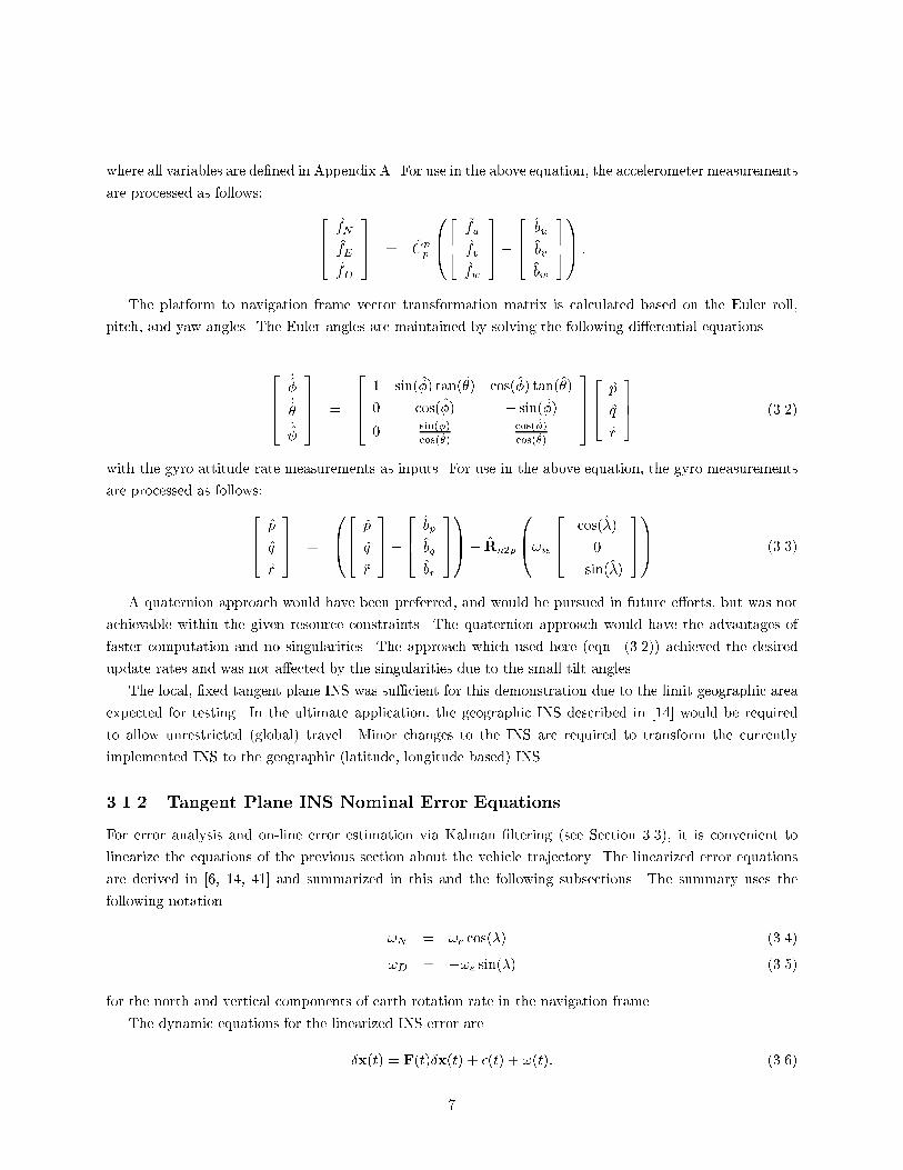
where all variables are de�ned in Appendix A. For use in the above equation, the accelerometer measurements

are processed as follows: 264fN

fE

fD

375 = Cn

p

0B@264

~fu~fv~fw

375�

264bu

bv

bw

3751CA :

The platform to navigation frame vector transformation matrix is calculated based on the Euler roll,

pitch, and yaw angles. The Euler angles are maintained by solving the following di�erential equations

2664

_�_�_

3775 =

2664

1 sin(�) tan(�) cos(�) tan(�)

0 cos(�) � sin(�)

0 sin(�)

cos(�)

cos(�)

cos(�)

3775264p

q

r

375 (3.2)

with the gyro attitude rate measurements as inputs. For use in the above equation, the gyro measurements

are processed as follows:264p

q

r

375 =

0B@264

~p

~q

~r

375�

264bp

bq

br

3751CA� Rn2p

0B@!ie

264

cos(�)

0

� sin(�)

3751CA (3.3)

A quaternion approach would have been preferred, and would be pursued in future e�orts, but was not

achievable within the given resource constraints. The quaternion approach would have the advantages of

faster computation and no singularities. The approach which used here (eqn. (3.2)) achieved the desired

update rates and was not a�ected by the singularities due to the small tilt angles.

The local, �xed tangent plane INS was su�cient for this demonstration due to the limit geographic area

expected for testing. In the ultimate application, the geographic INS described in [14] would be required

to allow unrestricted (global) travel. Minor changes to the INS are required to transform the currently

implemented INS to the geographic (latitude, longitude based) INS.

3.1.2 Tangent Plane INS Nominal Error Equations

For error analysis and on-line error estimation via Kalman �ltering (see Section 3.3), it is convenient to

linearize the equations of the previous section about the vehicle trajectory. The linearized error equations

are derived in [6, 14, 41] and summarized in this and the following subsections. The summary uses the

following notation

!N = !e cos(�) (3.4)

!D = �!e sin(�) (3.5)

for the north and vertical components of earth rotation rate in the navigation frame

The dynamic equations for the linearized INS error are

�x(t) = F(t)�x(t) + �(t) + !(t): (3.6)

7

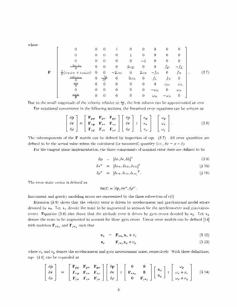
where

F =

266666666666666664

0 0 0 1 0 0 0 0 0

0 0 0 0 1 0 0 0 0

0 0 0 0 0 �1 0 0 0�2!nvE

R0 0 0 2!D 0 0 fD �fE

2R(vN!N + vD!D) 0 0 �2!D 0 2!N �fD 0 fN

�2vE!DR

0 �2�R3 0 �2!N 0 fE �fN 0

!DR

0 0 0 0 0 0 !D �!E

0 0 0 0 0 0 �!D 0 !N�!NR

0 0 0 0 0 !E �!N 0

377777777777777775

: (3.7)

Due to the small magnitude of the velocity relative to !eR, the �rst column can be approximated as zero.

For notational convenience in the following sections, the linearized error equations can be written as264� _p

� _v

� _�

375 =

264Fpp Fpv Fp�

Fvp Fvv Fv�

F�p F�v F��

375264�p

�v

��

375+

264ep

ev

e�

375+

264!p

!v

!�

375 : (3.8)

The subcomponents of the F matrix can be de�ned by inspection of eqn. (3.7). All error quantities are

de�ned to be the actual value minus the calculated (or measured) quantity (i.e., �x = x� x).

For the tangent plane implementation, the three components of nominal error state are de�ned to be

�p = [�n; �e; �h]T (3.9)

�vn = [�vN ; �vE ; �vD ]T (3.10)

��n = [��N ; ��E; ��D]T : (3.11)

The error state vector is de�ned as

�x(t) = [�p; �vn; ��n]:

Instrument and gravity modeling errors are represented by the three subvectors of �(t).

Equation (3.8) shows that the velocity error is driven by accelerometer and gravitational model errors

denoted by ev. Let xa denote the state to be augmented to account for the accelerometer and gravitation

errors. Equation (3.8) also shows that the attitude error is driven by gyro errors denoted by e�. Let xg

denote the state to be augmented to account for these gyro errors. Linear error models can be de�ned [14]

with matrices Fvxa and F�xg such that

ev = Fvxaxa + �a (3.12)

e� = F�xgxg + �g (3.13)

where �a and �g denote the accelerometer and gyro measurement noise, respectively. With these de�nitions,

eqn. (3.8) can be expanded as

264� _p

� _v

� _�

375 =

264Fpp Fpv Fp�

Fvp Fvv Fv�

F�p F�v F��

375264�p

�v

��

375+

264

0 0

Fvxa 0

0 F�xg

375"xa

xg

#+

264

!p

!v + �a

!� + �g

375 (3.14)

8

26666664

� _p

� _v

� _�

_xa

_xg

37777775

=

26666664

Fpp Fpv Fp� 0 0

Fvp Fvv Fv� Fvxa 0

F�p F�v F�� 0 F�xg

0 0 0 Fxaxa 0

0 0 0 0 Fxgxg

37777775

26666664

�p

�v

��

xa

xg

37777775+

26666664

!p

!v + �a

!� + �g

!a

!g

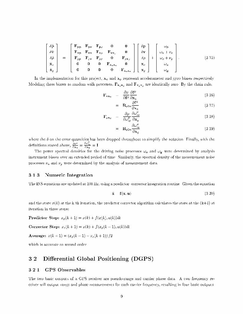
37777775: (3.15)

In the implementation for this project, xa and xg represent accelerometer and gyro biases respectively.

Modeling these biases as random walk processes, Fxaxa and Fxgxg are identically zero. By the chain rule,

Fvxa =@v

@fp@fp

@xa(3.16)

= Rp2n@fp

@xa(3.17)

F�xg =@�

@!pip

@!pip@xg

(3.18)

= Rp2n

@!pip@xg

(3.19)

where the � on the error quantities has been dropped throughout to simplify the notation. Finally, with the

de�nitions stated above, @fp

@xa=

@!p

ip

@xg= I.

The power spectral densities for the driving noise processes !a and !g were determined by analysis

instrument biases over an extended period of time. Similarly, the spectral density of the measurement noise

processes �a and �g were determined by the analysis of measurement data.

3.1.3 Numeric Integration

The INS equations are updated at 100 Hz, using a predictor{corrector integration routine. Given the equation

_x = f(x;u) (3.20)

and the state x(k) at the k-th iteration, the predictor corrector algorithm calculates the state at the (k+1)-st

iteration in three steps:

Predictor Step: xp(k + 1) = x(k) + f(x(k); u(k))dt

Corrector Step: xc(k + 1) = x(k) + f(xp(k + 1); u(k))dt

Average: x(k + 1) = (xp(k + 1) + xc(k + 1)) =2

which is accurate to second order.

3.2 Di�erential Global Positioning (DGPS)

3.2.1 GPS Observables

The two basic outputs of a GPS receiver are pseudo-range and carrier phase data. A two frequency re-

ceiver will output range and phase measurements for each carrier frequency, resulting in four basic outputs.

9

Common Mode Errors Standard Deviation

Selective Availability 24.0 m

Ionosphere 7.0 m

Clock and Ephemeris 3.6 m

Troposphere 0.7 m

Non-common Mode Errors

Receiver Noise 0.1-0.7 m

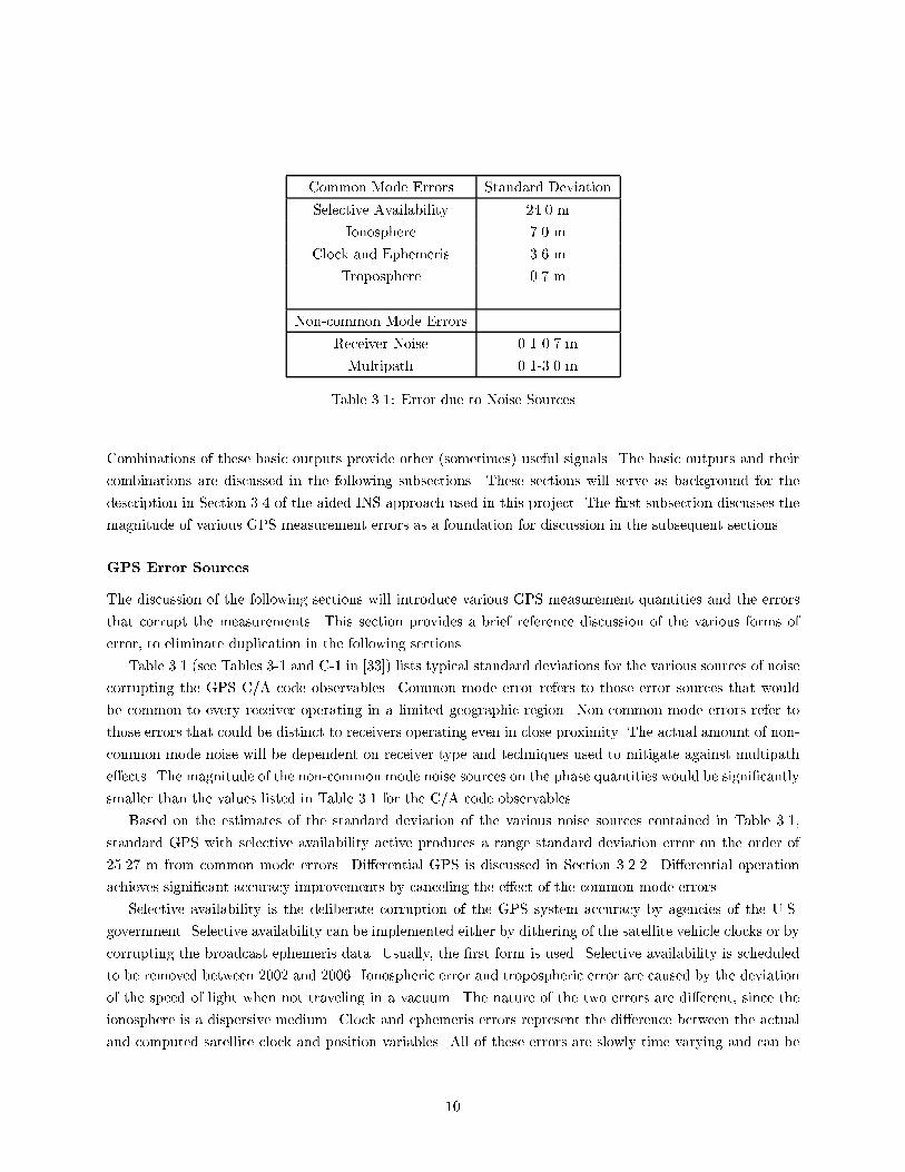
Multipath 0.1-3.0 m

Table 3.1: Error due to Noise Sources

Combinations of these basic outputs provide other (sometimes) useful signals. The basic outputs and their

combinations are discussed in the following subsections. These sections will serve as background for the

description in Section 3.4 of the aided INS approach used in this project. The �rst subsection discusses the

magnitude of various GPS measurement errors as a foundation for discussion in the subsequent sections.

GPS Error Sources

The discussion of the following sections will introduce various GPS measurement quantities and the errors

that corrupt the measurements. This section provides a brief reference discussion of the various forms of

error, to eliminate duplication in the following sections.

Table 3.1 (see Tables 3-1 and C-1 in [33]) lists typical standard deviations for the various sources of noise

corrupting the GPS C/A code observables. Common mode error refers to those error sources that would

be common to every receiver operating in a limited geographic region. Non-common mode errors refer to

those errors that could be distinct to receivers operating even in close proximity. The actual amount of non-

common mode noise will be dependent on receiver type and techniques used to mitigate against multipath

e�ects. The magnitude of the non-common mode noise sources on the phase quantities would be signi�cantly

smaller than the values listed in Table 3.1 for the C/A code observables.

Based on the estimates of the standard deviation of the various noise sources contained in Table 3.1,

standard GPS with selective availability active produces a range standard deviation error on the order of

25.27 m from common mode errors. Di�erential GPS is discussed in Section 3.2.2. Di�erential operation

achieves signi�cant accuracy improvements by canceling the e�ect of the common mode errors.

Selective availability is the deliberate corruption of the GPS system accuracy by agencies of the U.S.

government. Selective availability can be implemented either by dithering of the satellite vehicle clocks or by

corrupting the broadcast ephemeris data. Usually, the �rst form is used. Selective availability is scheduled

to be removed between 2002 and 2006. Ionospheric error and tropospheric error are caused by the deviation

of the speed of light when not traveling in a vacuum. The nature of the two errors are di�erent, since the

ionosphere is a dispersive medium. Clock and ephemeris errors represent the di�erence between the actual

and computed satellite clock and position variables. All of these errors are slowly time varying and can be

10

e�ectively removed by the use of broadcast range corrections.

Pseudo-range Observables

Let the receiver clock o�set from the satellite system time be denoted by �tr. The receiver clock o�set is

the error between the GPS system time and time measured on the receiver. The receiver clock o�set exists

due to drift in the local oscillator of the receiver.

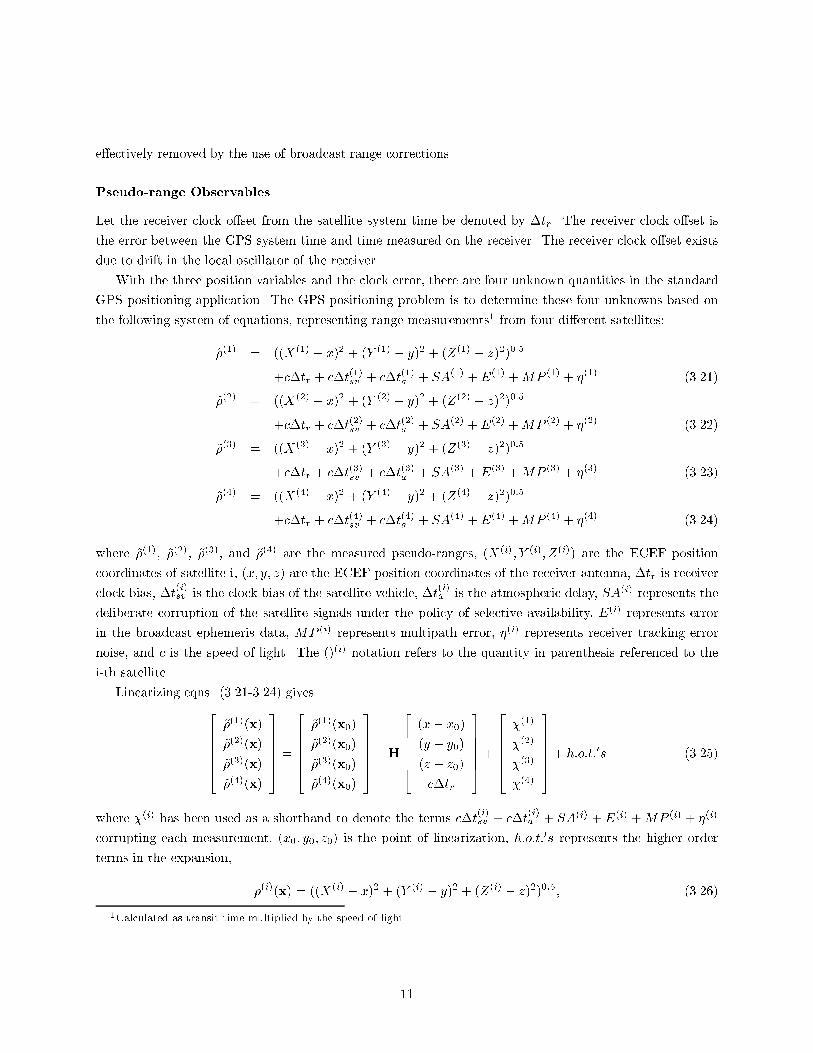
With the three position variables and the clock error, there are four unknown quantities in the standard

GPS positioning application. The GPS positioning problem is to determine these four unknowns based on

the following system of equations, representing range measurements1 from four di�erent satellites:

~�(1) = ((X(1) � x)2 + (Y (1) � y)2 + (Z(1) � z)2)0:5

+c�tr + c�t(1)sv + c�t(1)a + SA(1) +E(1) +MP (1) + �(1) (3.21)

~�(2) = ((X(2) � x)2 + (Y (2) � y)2 + (Z(2) � z)2)0:5


~�(3) = ((X(3) � x)2 + (Y (3) � y)2 + (Z(3) � z)2)0:5


~�(4) = ((X(4) � x)2 + (Y (4) � y)2 + (Z(4) � z)2)0:5


where ~�(1), ~�(2), ~�(3); and ~�(4) are the measured pseudo-ranges, (X(i); Y (i); Z(i)) are the ECEF position

coordinates of satellite i, (x; y; z) are the ECEF position coordinates of the receiver antenna, �tr is receiver

clock bias, �t(i)sv is the clock bias of the satellite vehicle, �t

(i)a is the atmospheric delay, SA(i) represents the

deliberate corruption of the satellite signals under the policy of selective availability, E(i) represents error

in the broadcast ephemeris data, MP (i) represents multipath error, �(i) represents receiver tracking error

noise, and c is the speed of light. The ()(i) notation refers to the quantity in parenthesis referenced to the

i-th satellite.

Linearizing eqns. (3.21-3.24) gives266664

~�(1)(x)

~�(2)(x)

~�(3)(x)

~�(4)(x)

377775 =

266664

~�(1)(x0)

~�(2)(x0)

~�(3)(x0)

~�(4)(x0)

377775+H

266664

(x� x0)

(y � y0)

(z � z0)

c�tr

377775+

266664�(1)

�(2)

�(3)

�(4)

377775+ h:o:t:0s (3.25)

where �(i) has been used as a shorthand to denote the terms c�t(i)sv + c�t

(i)a + SA(i) + E(i) +MP (i) + �(i)

corrupting each measurement, (x0; y0; z0) is the point of linearization, h:o:t:0s represents the higher order

terms in the expansion,

�(i)(x) = ((X(i) � x)2 + (Y (i) � y)2 + (Z(i) � z)2)0:5; (3.26)

1Calculated as transit time multiplied by the speed of light.

11

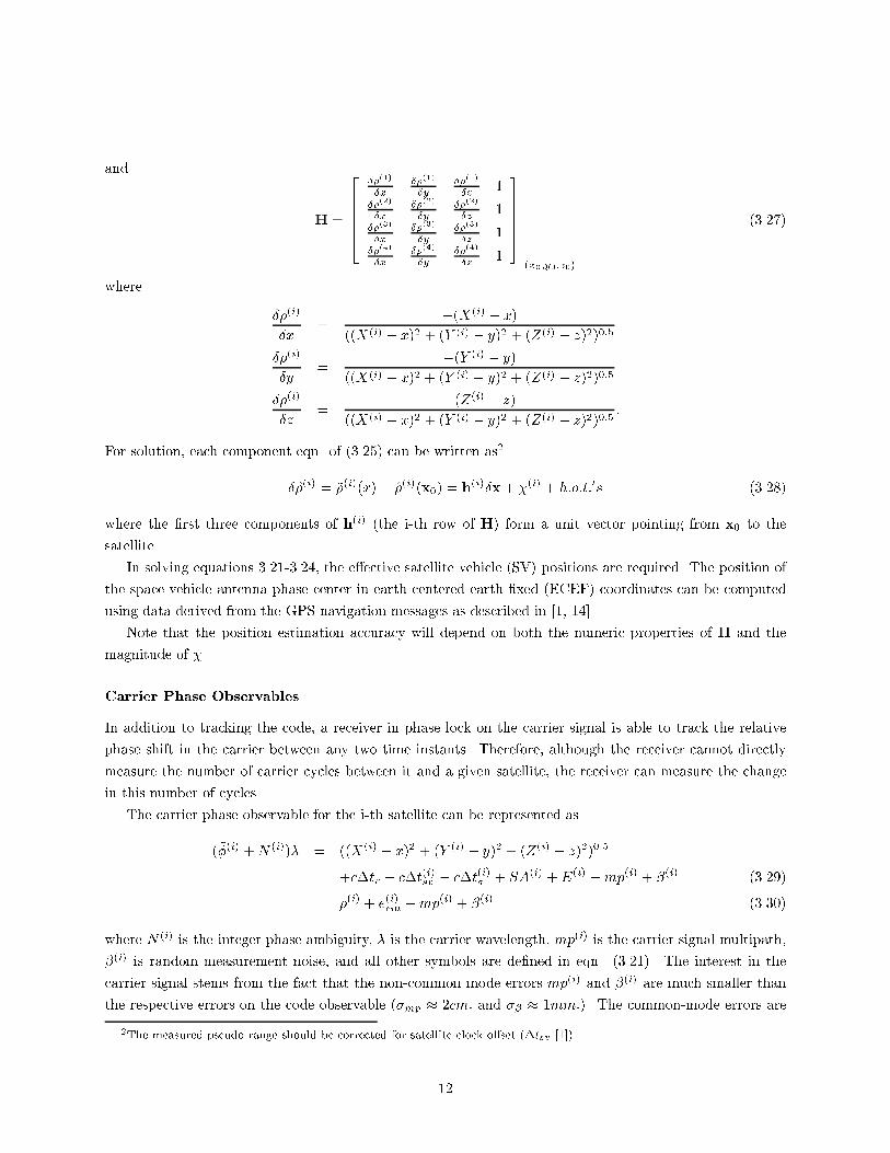
and

H =

266664

��(1)

�x��(1)

�y��(1)

�z1

��(2)

�x��(2)

�y��(2)

�z1

��(3)

�x��(3)

�y��(3)

�z1

��(4)

�x��(4)

�y��(4)

�z1

377775

��(x0;y0;z0)

(3.27)

where

��(i)

�x=

�(X(i) � x)

((X(i) � x)2 + (Y (i) � y)2 + (Z(i) � z)2)0:5

��(i)

�y=

�(Y (i) � y)

((X(i) � x)2 + (Y (i) � y)2 + (Z(i) � z)2)0:5

��(i)

�z=

�(Z(i) � z)

((X(i) � x)2 + (Y (i) � y)2 + (Z(i) � z)2)0:5:

For solution, each component eqn. of (3.25) can be written as2

��(i) = ~�(i)(x)� �(i)(x0) = h(i)�x+ �(i) + h:o:t:0s (3.28)

where the �rst three components of h(i) (the i-th row of H) form a unit vector pointing from x0 to the

satellite.

In solving equations 3.21-3.24, the e�ective satellite vehicle (SV) positions are required. The position of

the space vehicle antenna phase center in earth centered earth �xed (ECEF) coordinates can be computed

using data derived from the GPS navigation messages as described in [1, 14].

Note that the position estimation accuracy will depend on both the numeric properties of H and the

magnitude of �.

Carrier Phase Observables

In addition to tracking the code, a receiver in phase lock on the carrier signal is able to track the relative

phase shift in the carrier between any two time instants. Therefore, although the receiver cannot directly

measure the number of carrier cycles between it and a given satellite, the receiver can measure the change

in this number of cycles.

The carrier phase observable for the i-th satellite can be represented as

(~�(i) +N (i))� = ((X(i) � x)2 + (Y (i) � y)2 + (Z(i) � z)2)0:5

+c�tr + c�t(i)sv � c�t(i)a + SA(i) +E(i) +mp(i) + �(i) (3.29)

= �(i) + e(i)cm +mp(i) + �(i) (3.30)

where N (i) is the integer phase ambiguity, � is the carrier wavelength, mp(i) is the carrier signal multipath,

�(i) is random measurement noise, and all other symbols are de�ned in eqn. (3.21). The interest in the

carrier signal stems from the fact that the non-common mode errors mp(i) and �(i) are much smaller than

the respective errors on the code observable (�mp � 2cm: and �� 1mm:). The common-mode errors are

2The measured pseudo-range should be corrected for satellite clock o�set (�tsv [1])

12

essentially the same as those on the code observable, except that the ionospheric error enters eqns. (3.21)

and (3.29) with opposite signs.

In the di�erential mode of operation (see Section 3.2.2), the common mode errors can be reduced to

produce an observable accurate to a few centimeters. Let this di�erentially corrected phase be described as

4�(i)� = (~�(i) � ~�(i)o )� (3.31)

= h(i)(x� xo)��N (i) �N (i)

o

��+ (mp(i) �mp(i)o ) + (�(i) � �(i)o ) (3.32)

where the subscript in (�)(i)o refers the generic quantity � to the DGPS base station. The di�erentially

corrected phase of eqn. (3.32) provides a very accurate measure of range, if the integer ambiguity can be

determined.

The integer phase ambiguity is the whole number of carrier phase cycles between the receiver and satellite

at an initial measurement time. It is a (usually large) unknown integer constant (barring cycle slips). To make

use of carrier phase observable as a range estimate, the integer ambiguity must be estimated. Alternatively,

the carrier phase measurement could be di�erenced across time epochs, eliminating the constant integer

o�set, to provide an accurate measurement of the change in range.

Doppler Carrier Phase Processing

Note that if eqn. (3.32) is di�erenced between two measurement times, an accurate measure of the change

in satellite to receiver range results

(4�(i)(k)�4�(i)(k � 1))� = h(i)(k)4x(k)� h(i)(k � 1)4x(k � 1) + �mpi(k) + ��i(k) (3.33)

where 4x(k) = (x(k) � xo(k)), and the relative clock error is included in 4x(k). If the relative acceleration

of the base and rover is small during the di�erencing time, then a set of four `Doppler' measurements can

be processed to yield an accurate estimate of relative velocity

(4�(i)(k)�4�(i)(k � 1))�=dt = h(i)(k)4v(k) + (�mpi(k) + ��i(k)) =dt (3.34)

where dt is the di�erencing time, and h(i)(k) = h(i)(k � 1) has been assumed. This assumption is accurate

for small dt. If one antenna (the base) is known to be at rest, then earth relative velocity of the second

antenna (the rover) results.

In the GPS literature, Doppler and carrier phase are also referred to as delta range and integrated

Doppler, respectively. The latter are the more accurate names, as they describe the manner in which the

measurements are actually made. Doppler is measured by the receiver as the change in phase (range) over

a given time interval (i.e., delta range). Carrier phase is the integral of the delta ranges (i.e., integrated

Doppler). Both measurements (Doppler and carrier phase) should not be used together, as they represent

the same information. In choosing between the two there is a tradeo�. Carrier phase (once the integer

ambiguity is resolved) gives a very accurate measure of range, but requires continuous phase lock. Loss of

lock requires that the integers be re-estimated. Doppler gives a very accurate estimate of velocity only, but

does not require continuous phase lock. Various methods have been suggested to utilize phase information

(e.g., [5, 8, 18, 21, 22, 24, 27, 29]).

13

Wide and Narrow Lane Variables

This section develops the equations for the so called narrow-lane and wide-lane phase variables [23]. The

interest in the wide-lane signal is that its wavelength is larger enough that the wide-lane variable is often

used to facilitate the problem of integer ambiguity resolution.

The phase measurements of eqn. (3.32) at the L1 and L2 frequencies for a single satellite can be written

as

(~�1 +N1) =f1cr �

f2cIa +

f1c(mp1 + �1) (3.35)

(~�2 +N2) =f2cr �

f1cIa +

f2c(mp2 + �2) (3.36)

where �1 = cf1

and �2 = cf2,the common mode errors have been eliminated through di�erential operation,

and the 4's have been dropped for convenience of notation. For small di�erential distances, the residual

ionospheric error Ia should be small.

Forming the sum and di�erence of equations (3.35-3.36) results in

(~�1 + ~�2) + (N2 +N1) = (f1c+f2c)r � (

f2c+f1c)Ia +

f1c(mp1 + �1) +

f2c(mp2 + �2) (3.37)

(~�1 � ~�2) + (N1 �N2) = (f1c�f2c)r � (

f2c�f1c)Ia +

f1c(mp1 + �1)�

f2c(mp2 + �2) (3.38)

By de�ning

�w =c

f1� f2(3.39)

�n =c

f1 + f2(3.40)

(3.41)

eqns. (3.37) and (3.38) are written in meters as

(~�1 + ~�2)�n = r � Ia � (N2 +N1)�n +�n�1

(mp1 + �1) +�n�2

(mp2 + �2) (3.42)

(~�1 � ~�2)�w = r + Ia � (N1 �N2)�w +�w�1

(mp1 + �1)��w�2

(mp2 + �2) (3.43)

The pseudo-range estimates can be processed similarly yielding

(~�1�1��2�2

)�w = r � Ia +�w�1

(MP1 + �1)��w�2

(MP2 + �2) (3.44)

(~�1�1

+�2�2

)�n = r + Ia +�n�1

(MP1 + �1) +�n�2

(MP2 + �2) (3.45)

Note that the right hand sides of eqns. (3.43) and (3.45) are directly comparable. Since the residual

ionospheric delay and the carrier noise are expected to be small and the coe�cient of the code noise is

signi�cantly less than one, the di�erence of the two equations, described as

(~�1�1

+~�2�2

)�n � (~�1 � ~�2)�w = (N1 �N2)�w +�n�1

(MP1 + �1) +�n�2

(MP2 + �2)

��w�1

(mp1 + �1) +�w�2

(mp2 + �2); (3.46)

14

should provide a basis for estimating the wide lane integer (N1 �N2). The standard deviation of the noise

on each estimate of (N1 � N2) produced by eqn. (3.46) is approximately 0.7 times the code multipath in

meters. Therefore, the correct integer ambiguity can be reasonably expected to be within three integers of

the estimate from eqn. (3.46). Averaging of the above estimate of (N1 �N2) does not signi�cantly decrease

the estimation error unless the sampling time is long (i.e., minutes ) since the multipath is slowly time

varying. Instead, an integer search will be required around the estimated value. Once this search is complete

and (N1�N2) is determined, eqn. (3.43) is available for accurate carrier phase positioning and for aiding in

direct estimation of the N1 and N2 variables.

Integer Ambiguity Resolution

Due to the dependence of eqn. (3.46) on the code measurement, which may be corrupted by signi�cant

levels of multipath, that equation is usually not used alone, but only to initialize an integer search. One

such integer search approach based on least squares estimation and hypothesis testing [22, 39] is presented

below. The method will be presented for a generic phase measurement and wavelength, and works equally

well for any of the four phase variables previously discussed.

Consider a set of n > 4 di�erentially corrected phase measurements of wavelength �"~�p~�s

#�+

"Np

Ns

#� =

"Hp

Hs

#x+

"�p

�s

#(3.47)

where the measurements are partitioned into a primary and a secondary measurement set. The ambiguity

resolution algorithm proceeds by hypothesizing a set of integers for the primary set of measurements and

using the secondary set of measurements as a test of each hypothesis. The primary set of measurements

must have at least four satellites and these four should be selected to have a reasonable GDOP3.

Assume also that at the initial algorithm step, x = 0, var(�) = R = ��I , and �x � �� . These

assumptions, although realistic are not necessary for the algorithm to work, but allow a theoretical basis for

the algorithm derivation by the standard recursive least squares process.

The search algorithm will be implemented as a nested triple `for' loop. Prior to initializing the loop, the

following variables should be de�ned to minimize calculations within the loop:

x� = H�1p~�p (3.48)

Bp = H�1p � (3.49)

K =�HTH

��1Hs (3.50)

The meaning of each variable is de�ned below.

The algorithm proceeds as follows:

1. Hypothesize a set of integers Np = [0; N2; N3; N4]T for the primary measurements. Each of the three

`for' loops counts over a range of one of these three integers (i.e., Ni; i = 2; 3; 4). If m integer values

on each side of a nominal integer are hypothesized, then the entire algorithm will iterated (2m+ 1)3

times. The �rst integer is arti�cially set to zero to make the solution unique. Note that without this

3Geometric Dilution of Precision. Good GDOP implies that the measurement matrix H is well conditioned

15

assumption, all the integers and the clock bias estimate could be increased by one wavelength without

a�ecting the position solution. The clock bias that results from the following algorithm is c�tr �N1�.

If it is necessary that the code and phase clock estimates match, then N1 can be estimated based on

the average of the discrepancy.

2. For the hypothesized integer vector, calculate the resulting position

xp = H�1p (~�p +Np)�

= x� +BpNp: (3.51)

This position estimate has variance

P�1xp = HT

p

1

��IHp

Pxp = ��(HTpHp)

�1:

3. Predict a value for the secondary measurement using xp

�s =1

�Hsxp: (3.52)

4. Calculate the residual between the predicted and measured secondary phase

^ressp = (~�s � �s): (3.53)

This quantity is biased by the secondary integer, which is estimated as

Ns = �round( ^ressp): (3.54)

This choice of Ns does not guarantee a minimal residual for the corrected position due to the possible

ill-conditioning ofH, but is still used as the alternative is another search over Ns to �nd the minimizing

integer set.

5. Correct the secondary phase residual for the estimate secondary integer estimate and convert to meters

^ressm = ( ^ressp + Ns)�: (3.55)

6. Calculate the correction to xp due to the secondary measurements. This requires calculation of the

gain vector K = PxsHTsR

�1. Using the standard recursive least squares equations,

P�1xs = P�1

xp +HTs

1

��IHs

P�1xs = HT

pHp

1

��+HT

sHs

1

��

Pxs = ��(HTH)�1:

Therefore,

K =�HTH

��1HT

s (3.56)

and

4x =K ^ressm (3.57)

16

7. Calculate the output residual of the position corrected by the secondary measurement

4y =

0BBBBBB@

26666664

0

0

0

0

^ressm

37777775�H4x

1CCCCCCA

(3.58)

8. Calculate the �-squared variable q associated with 4y and use it to evaluate the hypothesized integer

Np. The properly de�ned �-squared variable q would account for the covariance matrix of 4y which

is straightforward to calculate give Pxs. However, due to the required number of on-line calculations

the covariance matrix is dropped in favor of the following simpler calculation

q =4yT4y

n� 4: (3.59)

If the hypothesized integer set Np is correct, then q will be small. Depending on the number of satellites

available, the noise level, and the satellite geometry it may take several iteration epochs to identify the

correct integer set. In this process other criteria such as the previously estimated position, the position

variance, and the size of Ns can also be used to eliminate candidate integer sets.

Note that the algorithm is equally valid for the L1, L2, and wide-lane frequencies. In the implementation

of this project, the algorithm is used �rst to determine the wide-lane integers. Then, the increased position

accuracy achieved using the wide-lane phase range facilitates the L1 or L2 integer initialization and search.

In the implementation of this project, the above algorithm is processed (in each mode: widelane, L1, or

L2) until only a single vector integer candidate remains. The algorithm is then processed again using the

identi�ed integer vector as the initial condition until a single vector integer candidate remains. The integer

vector is only accepted as correct if the output vector identically con�rms (i.e., matches) the initial condition.

Once the correct integers are identi�ed, a similar algorithm is run with q monitored to determine if

cycle slips have occurred. Cycle slip detection is also implemented by comparing and monitoring the code,

widelane phase, L1, and L2 ranges.

3.2.2 Di�erential GPS Operation

The common mode error sources described previously severely limit the accuracy attainable using GPS. These

errors are generally not observable using a single receiver unless its position is already known. However, the

common mode errors are the same for all receivers in a local area. Therefore, if the errors could be estimated

by one receiver and broadcast to all other receivers, the GPS accuracy could be substantially improved.

Three Di�erential GPS (DGPS) techniques are described in [14]. Range based di�erential GPS was selected

for this implementation as this approach allows the most exibility in a system involving multiple roving

vehicles.

Di�erential GPS involves a GPS receiver/antenna at a location (xo; yo; zo), a receiver/antenna at an

unknown possibly changing position (x; y; z), a satellite at the calculated position (xsv ; ysv; zsv), and a

communication medium from the �rst receiver to the second receiver. In the discussion of this section, the

17

��

��

��

��

��

��

��

��

��

��

��

��

��

��

��

��

��

��

��

��

c c....... ...........................

...........................

.........

xx

@@��

��@@

��

��

��

��

��

��

��

��=

��)

?

AAAAAAAAAAAAAAAAAU

ZZZZZZZZZZZZZZZZZZZZZ~

SSSSSSSw

HHHHHHHHHHHHHHHHHHHHHHHHHHHHj

XXXXXXXXXX

XXXXXXXXXXXXzBase Station Rover vehicleDi�erential Corrections

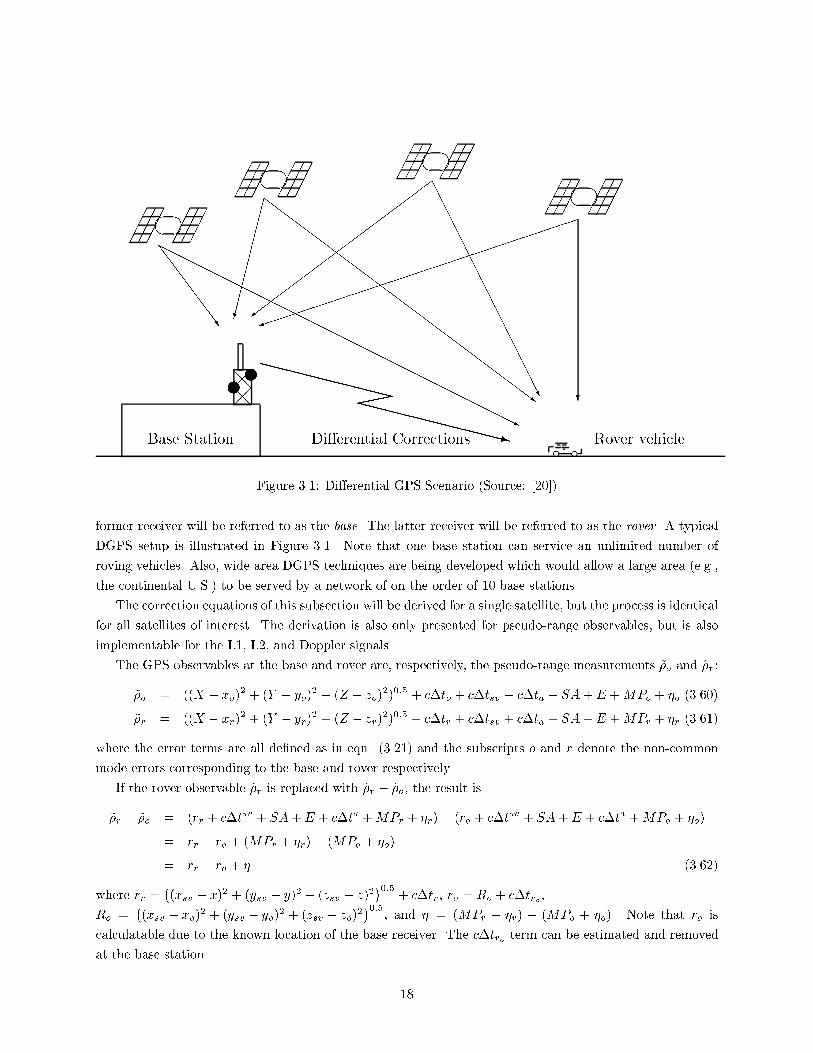
Figure 3.1: Di�erential GPS Scenario (Source: [20])

former receiver will be referred to as the base. The latter receiver will be referred to as the rover. A typical

DGPS setup is illustrated in Figure 3.1. Note that one base station can service an unlimited number of

roving vehicles. Also, wide area DGPS techniques are being developed which would allow a large area (e.g.,

the continental U.S.) to be served by a network of on the order of 10 base stations.

The correction equations of this subsection will be derived for a single satellite, but the process is identical

for all satellites of interest. The derivation is also only presented for pseudo-range observables, but is also

implementable for the L1, L2, and Doppler signals.

The GPS observables at the base and rover are, respectively, the pseudo-range measurements ~�o and ~�r:

~�o = ((X � xo)2 + (Y � yo)

2 + (Z � zo)2)0:5 + c�to + c�tsv + c�ta + SA+E +MPo + �o (3.60)

~�r = ((X � xr)2 + (Y � yr)

2 + (Z � zr)2)0:5 + c�tr + c�tsv + c�ta + SA+E +MPr + �r (3.61)

where the error terms are all de�ned as in eqn. (3.21) and the subscripts o and r denote the non-common

mode errors corresponding to the base and rover respectively.

If the rover observable ~�r is replaced with ~�r � ~�o, the result is

~�r � ~�o = (rr + c�tsv + SA+E + c�ta +MPr + �r)� (ro + c�tsv + SA+E + c�ta +MPo + �o)

= rr � ro + (MPr + �r)� (MPo + �o)

= rr � ro + � (3.62)

where rr =�(xsv � x)2 + (ysv � y)2 + (zsv � z)2

�0:5+ c�tr, ro = Ro + c�tro ,

Ro =�(xsv � xo)

2 + (ysv � yo)2 + (zsv � zo)

2�0:5

, and � = (MPr + �r) � (MPo + �o). Note that ro is

calculatable due to the known location of the base receiver. The c�tro term can be estimated and removed

at the base station.

18

x 1055.945 5.95 5.955 5.96 5.965 5.97 5.975 5.98 5.985 5.99

-60

-40

-20

0

20

40

60

80

100

GPS Time of Week, seconds

Diff

eren

tial C

orre

ctio

n, m

eter

s

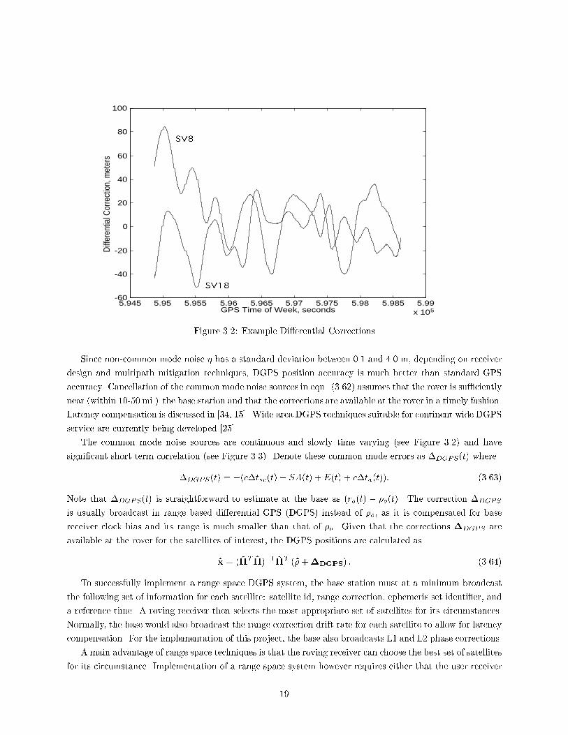
Figure 3.2: Example Di�erential Corrections

Since non-common mode noise � has a standard deviation between 0.1 and 4.0 m, depending on receiver

design and multipath mitigation techniques, DGPS position accuracy is much better than standard GPS

accuracy. Cancellation of the common mode noise sources in eqn. (3.62) assumes that the rover is su�ciently

near (within 10-50 mi.) the base station and that the corrections are available at the rover in a timely fashion.

Latency compensation is discussed in [34, 15]. Wide area DGPS techniques suitable for continent wide DGPS

service are currently being developed [25].

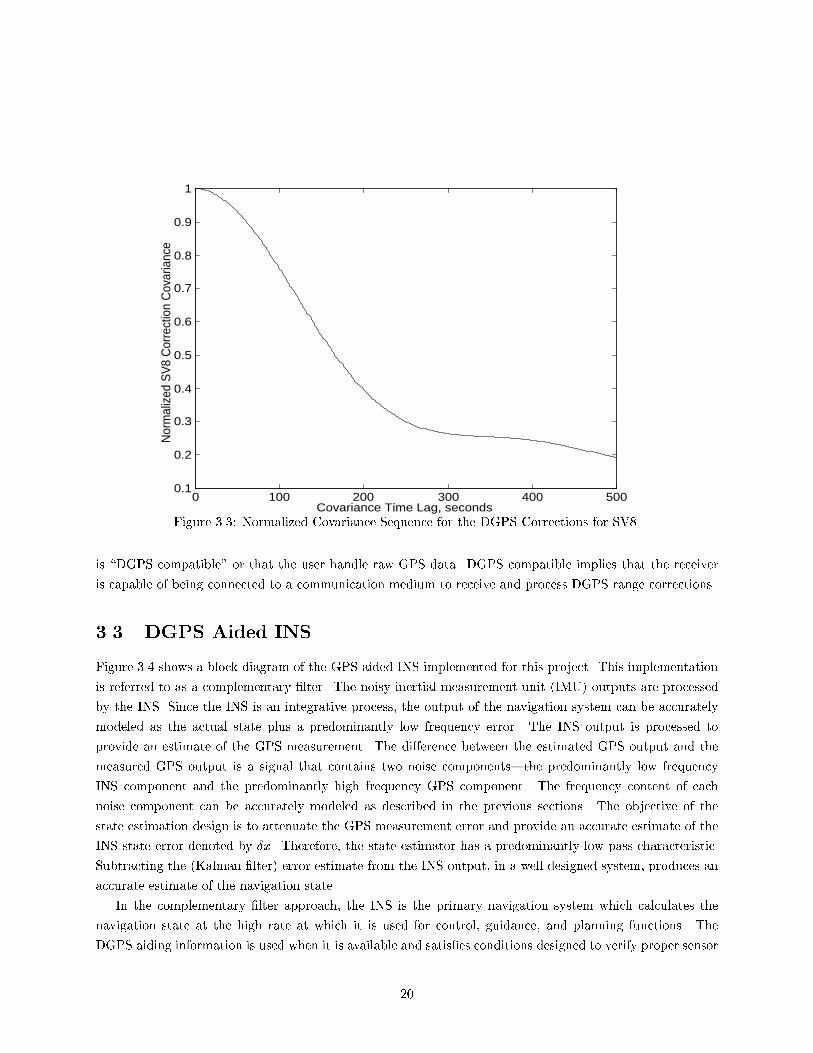
The common mode noise sources are continuous and slowly time varying (see Figure 3.2) and have

signi�cant short term correlation (see Figure 3.3). Denote these common mode errors as �DGPS(t) where

�DGPS(t) = �(c�tsv(t) + SA(t) +E(t) + c�ta(t)): (3.63)

Note that �DGPS(t) is straightforward to estimate at the base as (ro(t) � �o(t). The correction �DGPS

is usually broadcast in range based di�erential GPS (DGPS) instead of �o, as it is compensated for base

receiver clock bias and its range is much smaller than that of �o. Given that the corrections �DGPS are

available at the rover for the satellites of interest, the DGPS positions are calculated as

x = (HT H)�1HT (~�+�DGPS) : (3.64)

To successfully implement a range space DGPS system, the base station must at a minimum broadcast

the following set of information for each satellite: satellite id, range correction, ephemeris set identi�er, and

a reference time. A roving receiver then selects the most appropriate set of satellites for its circumstances.

Normally, the base would also broadcast the range correction drift rate for each satellite to allow for latency

compensation. For the implementation of this project, the base also broadcasts L1 and L2 phase corrections.

A main advantage of range space techniques is that the roving receiver can choose the best set of satellites

for its circumstance. Implementation of a range space system however requires either that the user receiver

19

0 100 200 300 400 5000.1

0.2

0.3

0.4

0.5

0.6

0.7

0.8

0.9

1

Covariance Time Lag, seconds

Nor

mal

ized

SV

8 C

orre

ctio

n C

ovar

ianc

e

Figure 3.3: Normalized Covariance Sequence for the DGPS Corrections for SV8.

is \DGPS compatible" or that the user handle raw GPS data. DGPS compatible implies that the receiver

is capable of being connected to a communication medium to receive and process DGPS range corrections.

3.3 DGPS Aided INS

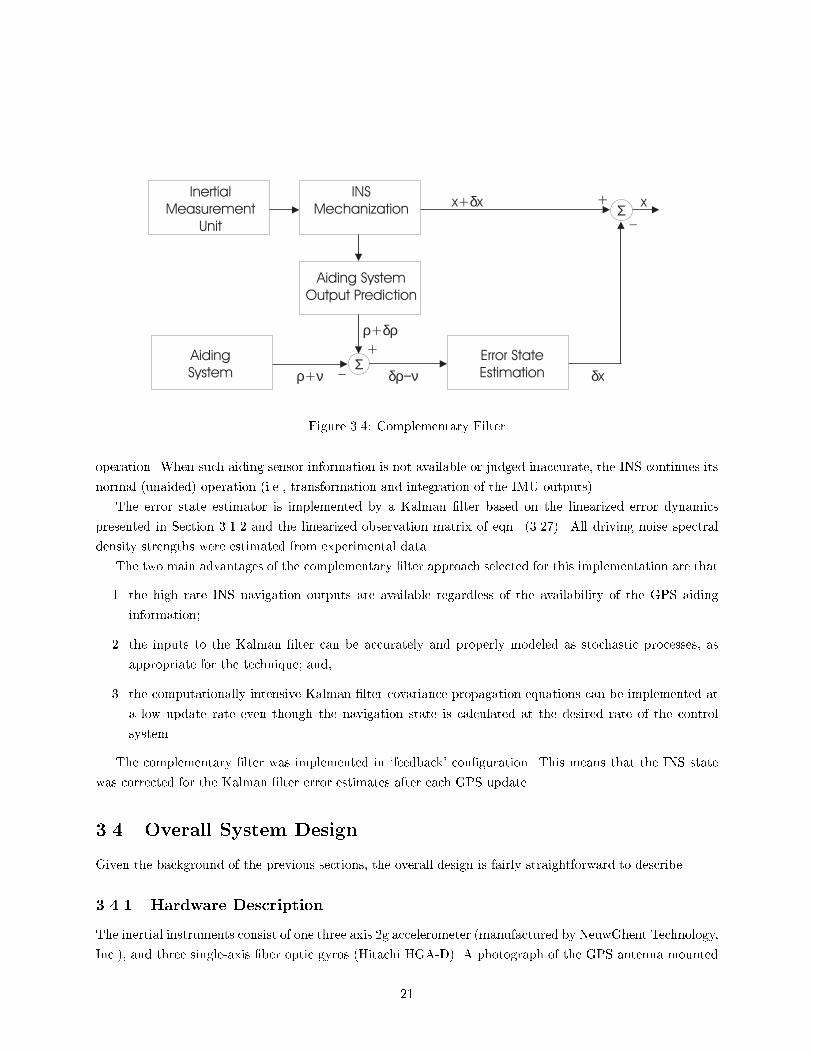
Figure 3.4 shows a block diagram of the GPS aided INS implemented for this project. This implementation

is referred to as a complementary �lter. The noisy inertial measurement unit (IMU) outputs are processed

by the INS. Since the INS is an integrative process, the output of the navigation system can be accurately

modeled as the actual state plus a predominantly low frequency error. The INS output is processed to

provide an estimate of the GPS measurement. The di�erence between the estimated GPS output and the

measured GPS output is a signal that contains two noise components|the predominantly low frequency

INS component and the predominantly high frequency GPS component. The frequency content of each

noise component can be accurately modeled as described in the previous sections. The objective of the

state estimation design is to attenuate the GPS measurement error and provide an accurate estimate of the

INS state error denoted by �x. Therefore, the state estimator has a predominantly low pass characteristic.

Subtracting the (Kalman �lter) error estimate from the INS output, in a well designed system, produces an

accurate estimate of the navigation state.

In the complementary �lter approach, the INS is the primary navigation system which calculates the

navigation state at the high rate at which it is used for control, guidance, and planning functions. The

DGPS aiding information is used when it is available and satis�es conditions designed to verify proper sensor

20

AidingSystem

Aiding SystemOutput Prediction

InertialMeasurement

Unit

INSMechanization Σ

Σ Error StateEstimation

x+ x xδ

ρ δ+ ρ

ρ ν δρ−ν δ+ x

+

_

+

_

Figure 3.4: Complementary Filter

operation. When such aiding sensor information is not available or judged inaccurate, the INS continues its

normal (unaided) operation (i.e., transformation and integration of the IMU outputs).

The error state estimator is implemented by a Kalman �lter based on the linearized error dynamics

presented in Section 3.1.2 and the linearized observation matrix of eqn. (3.27). All driving noise spectral

density strengths were estimated from experimental data.

The two main advantages of the complementary �lter approach selected for this implementation are that

1. the high rate INS navigation outputs are available regardless of the availability of the GPS aiding

information;

2. the inputs to the Kalman �lter can be accurately and properly modeled as stochastic processes, as

appropriate for the technique; and,

3. the computationally intensive Kalman �lter covariance propagation equations can be implemented at

a low update rate even though the navigation state is calculated at the desired rate of the control

system.

The complementary �lter was implemented in `feedback' con�guration. This means that the INS state

was corrected for the Kalman �lter error estimates after each GPS update.

3.4 Overall System Design

Given the background of the previous sections, the overall design is fairly straightforward to describe.

3.4.1 Hardware Description

The inertial instruments consist of one three axis 2g accelerometer (manufactured by NeuwGhent Technology,

Inc.), and three single-axis �ber optic gyros (Hitachi HGA-D). A photograph of the GPS antenna mounted

21

on the instrument platform is shown in Appendix B.

The 2g accelerometer range is too large for the lateral and longitudinal accelerations under typical

conditions, but required for the vertical acceleration due to the nominal 1g gravitational acceleration. The

accelerometer is an inexpensive solid state device which would be similar to the type of instrument expected

in commercial automotive applications.

The gyros have a 10 Hz bandwidth and 60 degree per second input range. Both characteristics are

reasonable for the expected application conditions. A larger bandwidth and input range may be required

for emergency maneuvering. The input range must be carefully considered, as resolution and scale factor

errors may become signi�cant for large input ranges. The major drawback of the available set of gyros

was the designer limited maximum sample rate of 50 Hz via a serial port connection. Although this is �ve

times the sensor bandwidth, it still limits the (proper) INS update rate to 50 Hz. To achieve the desired

implementation rate of 100 Hz with minimal delay, each sensed gyro output was assumed constant for two

0.01 s. sample periods.

Although these instruments were not ideally matched to the application, the project budget precluded

purchasing alternative instruments. Even with the sensor de�ciencies, the navigation system achieved the

desired accuracies and the desired update rate was demonstrated. Overcoming the sensor de�ciencies will

only improve the demonstrated performance. Also, no special coding was required to achieve the results

presented herein. Additional e�orts in algorithm design could substantially increase the INS update and

GPS correction rates.

For the experimental results shown later in the report, a compass and tilt meter manufactured by Precision

Navigation were used to initialize the heading, roll, and pitch. The compass was not compensated for local

magnetic �elds. Even without these sensors, attitude error was rapidly (e.g., one trip around the parking lot)

estimated by the Kalman �lter. In a commercial application, logic to store and use the last best navigation

estimates (prior to the ignition turning o�) as the initial conditions for the next run could be considered.

Given that the vehicle must be driven from its initial location (e.g., a parking lot) to the automated highway,

the attitude errors should be observable and hence corrected by the navigation system; therefore, this sensor

is not expected to be necessary in commercial applications.

Neither speedometer, odometer, nor brake pulse information was used in this implementation. Such

information could be used and is available for free on many vehicles. Incorporating such signals would require

extra computation for sensor calibration, but could provide both additional aiding and failure detection

information.

The data acquisition system consists of an IBM 486 compatible with a National Instruments data acqui-

sition board. GPS data was acquired from two Ashtech Z-12 Receivers via a serial port connection. The

base station to rover serial port connection included a 19200 baud radio modem connection.

3.4.2 Software Description

The INS implemented a �xed tangent plane system at 100 Hz4. The origin was �xed at the location of

the based station antenna phase center. The navigation states included: north, east, and vertical (up {

positive) positions in meters; north, east, and down velocity in meters per second; roll, pitch, and yaw angles

4Higher rates could be achieved even with the current hardware and software.

22

in radians; receiver clock error and drift rate in meters and meters per second; platform frame gyro drift

rates in radians per second; and, platform frame accelerometer bias in meters per second per second. The

navigation error states were identical with the exception of the attitude errors. The estimate attitude errors

were estimated in navigation frame as the north, east, and down tilt errors. The INS was implemented as

an interrupt driven background process to ensure the designed update rate.

GPS aiding was implemented at a 1.0 Hz rate with scalar measurement processing. Four primary modes

of GPS aiding were implemented:

1. INS only: This is the default mode of operation. Since INS is implemented as a background process,

it will continue to run at 100 Hz regardless of the availability of aiding information. When GPS

measurements are available, the software automatically switches to Mode 2.

2. Di�erential Pseudo-range: This is the default start-up mode. The primary objectives of this mode are to

accurately estimate the navigation state errors and to switch to the widelane phase mode. Therefore,

in this mode the system begins a search and veri�cation process for the widelane integer ambiguities

using the algorithm of Section 3.2.1 with � = �w. In parallel with the integer ambiguity search, the

Kalman �lter estimates the navigation state on the basis of the di�erentially corrected pseudo-range

measurements. In this mode, the measurement noise covariance for each measurement is set to R = 2:02

m2. When the search process is complete, the software automatically switches to Mode 3.

3. Di�erential Widelane Phase: In this mode, the software attempts to estimate and verify the L1 integer

ambiguities using the algorithm of Section 3.2.1 with � = �1. In parallel with this integer search, the

Kalman �lter estimates the navigation state errors using the di�erentially corrected widelane phase

measurements. In this mode, the measurement noise covariance for each measurement is set to R = 0:12

m2. When this search process is complete, the software automatically switches to Mode 4. If widelock

to at least four satellites is lost, the system automatically reverts to Mode 2.

4. Di�erential L1 Phase: This is the desired system operating mode. To be in this mode, the system will

have estimated and veri�ed the L1 integer ambiguities for at least four satellites. While in this mode,

the Kalman �lter will estimate the navigation error state using the di�erentially corrected L1 phase

measurements. The measurement noise covariance for each L1 phase measurement is set to R = 0:012

m2.

The INS is running in the background in all four modes. Also, the GPS measurement matrix in all GPS

related modes is speci�ed in equation (3.27). Analysis of the typical time to achieve each mode of operation

is presented in Section 4.1.

In modes 3 and 4, the system monitors for loss of lock on each of the `locked' satellites. If lock is lost

on the satellite, then the Kalman �lter will utilize the di�erentially corrected pseudo-range for that satellite

instead of the corresponding phase measurement. The measurement information is correctly weighted by

the Kalman �lter by speci�cation of the R matrix. As long as the system has lock to at least four satellites,

it is usually able to correctly determine the integer ambiguities for `unlocked' satellites by direct estimation

instead of search. While in Mode 4, the system will search for L2 integer ambiguities. Once estimated, the

L2 phase range is used as a consistency check on the L1 and widelane phase ranges. The consistency check

is that the three ranges are statistically equal and that the integers satisfy Nw = N1 �N2.

23

In the Di�erential Pseudo-range Mode it is possible to also use the di�erentially corrected Doppler. This

would allow on-the- y (i.e., the vehicle could be moving) integer ambiguity resolution. The 9600 baud packet

modem for this implementation could not accommodate Doppler corrections along with the pseudo-range,

L1, and L2 corrections. Therefore, we assumed the vehicle was stopped in this mode, and synthesized a zero

velocity `measurement' with a corresponding value for the sensor uncertainty. This limitation (stationary

vehicle) could be eliminated through a faster (or non-packet) modem, improved message formatting, or

polynomial type correction prediction to decrease the required throughput..

The GPS receiver supplies a pulse aligned with the time of applicability of the GPS measurements.

Receipt of this pulse by the INS computer causes the INS state to be saved and used for computation of the

predicted GPS observables. The GPS measurements are received over the serial connection 0.4-0.6 seconds

after the pulse (time of applicability). The delay is dependent on the number of satellites. Base corrections

also transmitted serially do not arrive until approximately 0.7 seconds after the time of applicability of the

GPS measurement. This left 0.3 seconds to complete the Kalman �lter computation of the navigation error

state and correct the navigation system prior to beginning the processing for the next measurement epoch.

Additional improvements which could be added include delay and lever arm compensation. In the

approach described above, the navigation error state for each epoch is not available until approximately 0.8

seconds after its time of applicability. It is straightforward to propagate the error state from its time of

applicability (i.e., t) to its time of availability (i.e., t+0:8). This is most important at system initialization,

since in steady state the errors are all quite small and slowly time varying. This delay compensation will be

implemented in the near future.

The antenna phase center and accelerometer position do not coincide in most applications. For the

platform for this project, the separation is approximately 0.6 meters. Therefore, the INS and GPS estimates

of position and velocity will di�er as the vehicle roll and pitch angles change. For example, a 10 degree roll

or pitch error would result in 10 cm. of position error. Lever arm compensation can be achieved through a

more involved algorithm for predicting the GPS outputs as a function of the INS state, and an alternative

(fuller) measurement matrix. For higher accuracy, lever arm compensation can be implemented.

24

Chapter 4

Performance Analysis

Two methods were designed to test the positioning accuracy of the DGPS aided inertial navigation system.

The primary variable of interest in the analysis, due to the focus on lateral control, was the lateral position

accuracy. Accurate analysis of the positioning accuracy was di�cult to achieve due to the lack of independent

methods to measure ground truth at the centimeter level. Sections 4.2 and 4.3 describe system testing on a

table top and on an amusement park ride, respectively. Section 4.1 analyzes the time from initialization to

each mode of system operation.

4.1 Time to Phase Lock Analysis

This section describes an experiment that was designed to analyze the time required for the software to

achieve each mode of phase lock described in Section 3.4.2. For each iteration of the experiment, the

navigation system software was allowed to run normally until widelock, L1 lock, and L2 lock were all

achieved and veri�ed. At this point, the time that each lock status was achieved, the number of satellites,

and the estimated position were written to a �le. Then a software reset re-initialized the navigation system

for the next iteration. The test was performed with a known baseline separation and the estimated position

was use to veri�ed correct integer lock.

In the 170 iterations used to generate the following data, there were no instances of incorrect phase lock.

There was one 8 satellite iteration which did not achieve lock until approximately 900 seconds. This iteration

was excluded from the statistical analysis.

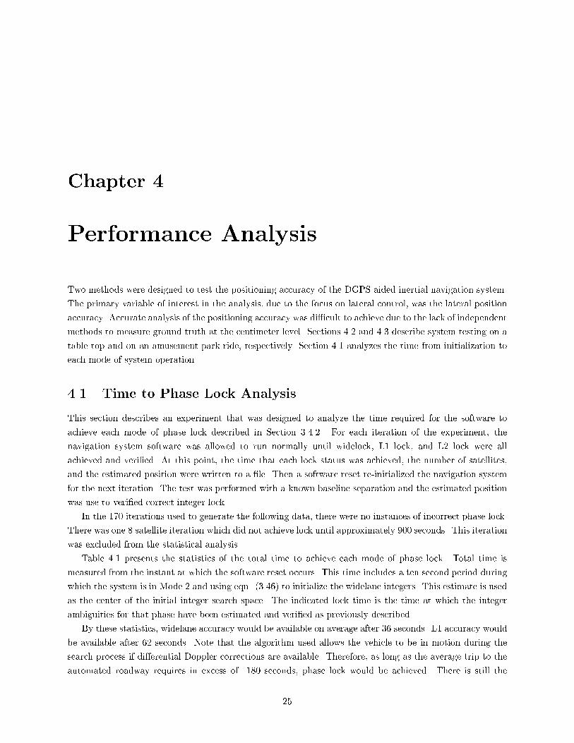
Table 4.1 presents the statistics of the total time to achieve each mode of phase lock. Total time is

measured from the instant at which the software reset occurs. This time includes a ten second period during

which the system is in Mode 2 and using eqn. (3.46) to initialize the widelane integers. This estimate is used

as the center of the initial integer search space. The indicated lock time is the time at which the integer

ambiguities for that phase have been estimated and veri�ed as previously described.

By these statistics, widelane accuracy would be available on average after 36 seconds. L1 accuracy would

be available after 62 seconds. Note that the algorithm used allows the vehicle to be in motion during the

search process if di�erential Doppler corrections are available. Therefore, as long as the average trip to the

automated roadway requires in excess of 180 seconds, phase lock would be achieved. There is still the

25

Widelock Time L1 Lock Time L2 Lock Time

Mean, 7 SV's 35.6 62.0 67.2

STD, 7 SV's 31.5 39.1 40.3

Mean, 8 SV's 40.5 60.1 65.9

STD, 8 SV's 33.9 38.5 38.6

Table 4.1: Statistics of the Time to Achieve each Mode of Phase Lock. Time is in Seconds from the Initial

Turn on.

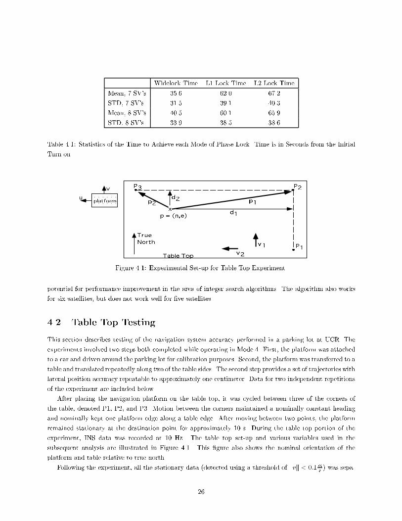
Figure 4.1: Experimental Set-up for Table Top Experiment.

potential for performance improvement in the area of integer search algorithms. The algorithm also works

for six satellites, but does not work well for �ve satellites.

4.2 Table Top Testing

This section describes testing of the navigation system accuracy performed in a parking lot at UCR. The

experiments involved two steps both completed while operating in Mode 4. First, the platform was attached

to a car and driven around the parking lot for calibration purposes. Second, the platform was transferred to a

table and translated repeatedly along two of the table sides. The second step provides a set of trajectories with

lateral position accuracy repeatable to approximately one centimeter. Data for two independent repetitions

of the experiment are included below.

After placing the navigation platform on the table top, it was cycled between three of the corners of

the table, denoted P1, P2, and P3. Motion between the corners maintained a nominally constant heading

and nominally kept one platform edge along a table edge. After moving between two points, the platform

remained stationary at the destination point for approximately 10 s. During the table top portion of the

experiment, INS data was recorded at 10 Hz. The table top set-up and various variables used in the

subsequent analysis are illustrated in Figure 4.1. This �gure also shows the nominal orientation of the

platform and table relative to true north.

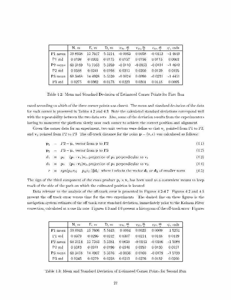
Following the experiment, all the stationary data (detected using a threshold of kvk < 0:1ms) was sepa-

26

N, m E, m D, m vN ;ms

vE ;ms

vD;ms

, rads.

P1 mean 59.8938 15.7627 5.5214 -0.0063 0.0058 -0.0112 -1.4649

P1 std. 0.0198 0.0203 0.0175 0.0157 0.0156 0.0115 0.0002

P2 mean 60.3189 15.7563 5.5259 -0.0110 -0.0053 -0.0124 -1.4642

P2 std. 0.0388 0.0241 0.0198 0.0315 0.0200 0.0129 0.0195

P3 mean 60.3468 14.4928 5.5520 -0.0074 0.0090 -0.0231 -1.4451

P3 std. 0.0275 0.0362 0.0173 0.0223 0.0301 0.0118 0.0095

Table 4.2: Mean and Standard Deviation of Estimated Corner Points for First Run

rated according to which of the three corner points was closest. The mean and standard deviation of the data

for each corner is presented in Tables 4.2 and 4.3. Note the calculated standard deviations correspond well

with the repeatability between the two data sets. Also, some of the deviation results from the experimenters

having to maneuver the platform slowly near each corner to achieve the correct position and alignment.

Given the corner data for an experiment, two unit vectors were de�ne so that v1 pointed from P1 to P2,

and v2 pointed from P2 to P3. The o�-track distance for the point p = (n; e) was calculated as follows:

p1 = P2� p; vector from p to P2 (4.1)

p2 = P3� p; vector from p to P3 (4.2)

d1 = p1 � (p1 � v1)v1; projection of p1 perpendicular to v1 (4.3)

d2 = p2 � (p2 � v2)v2; projection of p2 perpendicular to v2 (4.4)

e = sgn(pi1vi2 � pi2vi1)kdik where i selects the vector d1 or d2 of smaller norm (4.5)

The sign of the third component of the cross product pi � vi has been used as a convenient means to keep

track of the side of the path on which the estimated position is located.

Data relevant to the analysis of the o�-track error is presented in Figures 4.2-4.7. Figures 4.2 and 4.5

present the o�-track error versus time for the two experiments. The dashed line on these �gures is the

navigation system estimate of the o�-track error standard deviation, immediately prior to the Kalman Filter

correction, calculated at a one Hz rate. Figures 4.3 and 4.6 present a histogram of the o�-track error. Figures

N, m E, m D, m vN ;ms

vE ;ms

vD;ms

, rads.

P1 mean 59.8943 15.7606 5.5443 -0.0064 0.0025 0.0009 -1.5251

P1 std. 0.0379 0.0296 0.0242 0.0307 0.0214 0.0148 0.0449

P2 mean 60.3414 15.7503 5.5381 0.0050 -0.0143 -0.0106 -1.5088

P2 std. 0.0313 0.0241 0.0196 0.0246 0.0252 0.0130 0.0251

P3 mean 60.3478 14.4907 5.5616 -0.0056 0.0160 -0.0179 -1.5199

P3 std. 0.0243 0.0279 0.0228 0.0213 0.0276 0.0132 0.0260

Table 4.3: Mean and Standard Deviation of Estimated Corner Points for Second Run

27

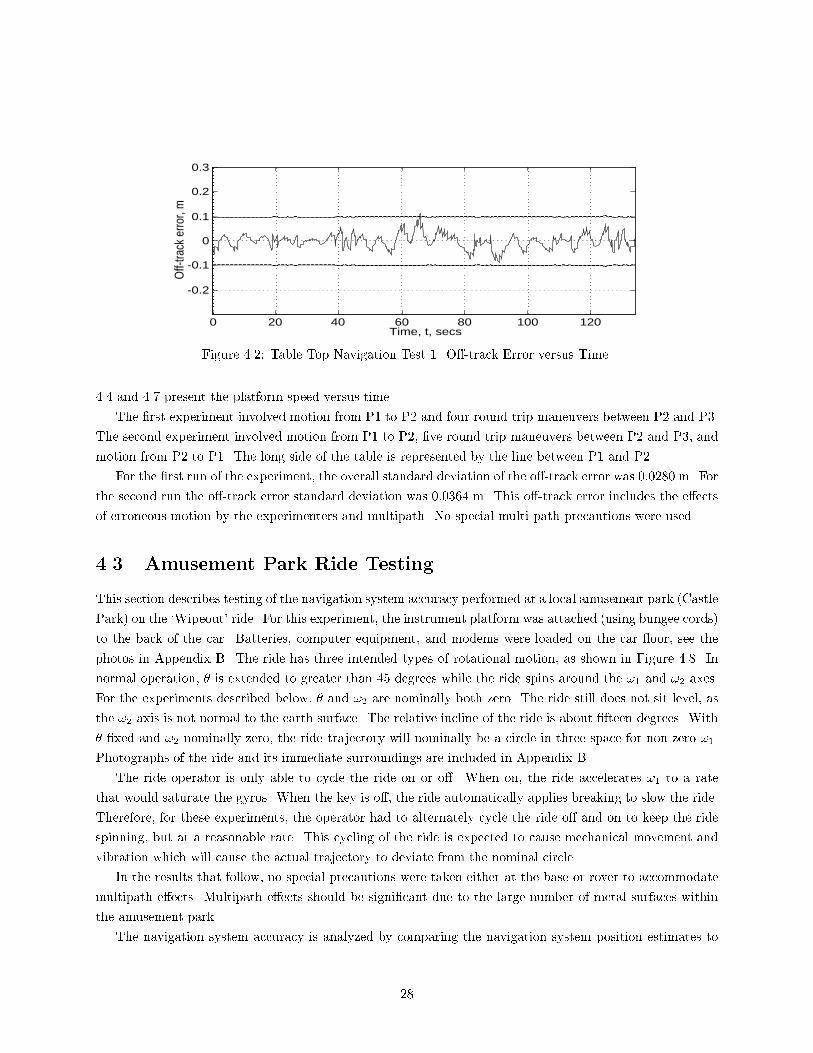
0 20 40 60 80 100 120

-0.2

-0.1

0

0.1

0.2

0.3

Time, t, secs

Off-

track

erro

r, m

Figure 4.2: Table Top Navigation Test 1. O�-track Error versus Time.

4.4 and 4.7 present the platform speed versus time.

The �rst experiment involved motion from P1 to P2 and four round trip maneuvers between P2 and P3.

The second experiment involved motion from P1 to P2, �ve round trip maneuvers between P2 and P3, and

motion from P2 to P1. The long side of the table is represented by the line between P1 and P2.

For the �rst run of the experiment, the overall standard deviation of the o�-track error was 0:0280 m. For

the second run the o�-track error standard deviation was 0:0364 m. This o�-track error includes the e�ects

of erroneous motion by the experimenters and multipath. No special multi-path precautions were used.

4.3 Amusement Park Ride Testing

This section describes testing of the navigation system accuracy performed at a local amusement park (Castle

Park) on the `Wipeout' ride. For this experiment, the instrument platform was attached (using bungee cords)

to the back of the car. Batteries, computer equipment, and modems were loaded on the car oor, see the

photos in Appendix B. The ride has three intended types of rotational motion, as shown in Figure 4.8. In

normal operation, � is extended to greater than 45 degrees while the ride spins around the !1 and !2 axes.

For the experiments described below, � and !2 are nominally both zero. The ride still does not sit level, as

the !2 axis is not normal to the earth surface. The relative incline of the ride is about �fteen degrees. With

� �xed and !2 nominally zero, the ride trajectory will nominally be a circle in three space for non-zero !1.

Photographs of the ride and its immediate surroundings are included in Appendix B.

The ride operator is only able to cycle the ride on or o�. When on, the ride accelerates !1 to a rate

that would saturate the gyros. When the key is o�, the ride automatically applies breaking to slow the ride.

Therefore, for these experiments, the operator had to alternately cycle the ride o� and on to keep the ride

spinning, but at a reasonable rate. This cycling of the ride is expected to cause mechanical movement and

vibration which will cause the actual trajectory to deviate from the nominal circle.

In the results that follow, no special precautions were taken either at the base or rover to accommodate

multipath e�ects. Multipath e�ects should be signi�cant due to the large number of metal surfaces within

the amusement park.

The navigation system accuracy is analyzed by comparing the navigation system position estimates to

28

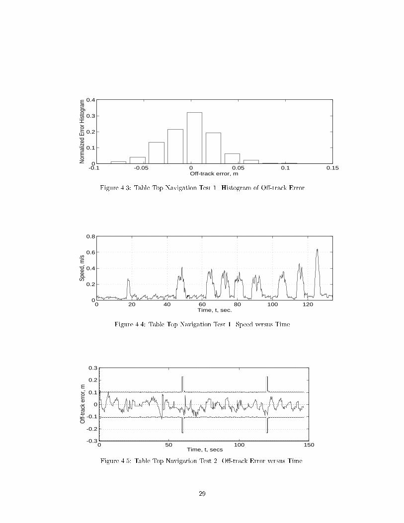
-0.1 -0.05 0 0.05 0.1 0.150

0.1

0.2

0.3

0.4

Off-track error, m

Nor

mal

ized

Erro

r His

togr

am

Figure 4.3: Table Top Navigation Test 1. Histogram of O�-track Error

0 20 40 60 80 100 1200

0.2

0.4

0.6

0.8

Time, t, sec.

Spee

d, m

/s

Figure 4.4: Table Top Navigation Test 1. Speed versus Time

0 50 100 150-0.3

-0.2

-0.1

0

0.1

0.2

0.3

Time, t, secs

Off-

track

erro

r, m

Figure 4.5: Table Top Navigation Test 2. O�-track Error versus Time.

29

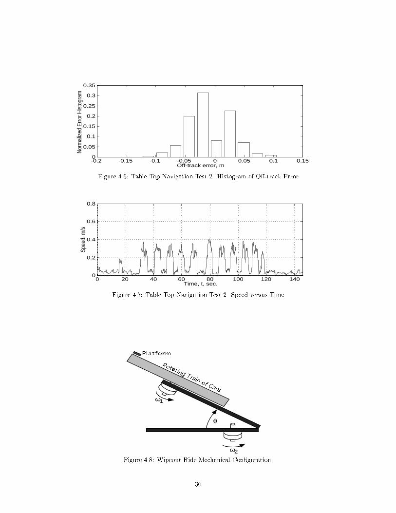
-0.2 -0.15 -0.1 -0.05 0 0.05 0.1 0.150

0.05

0.1

0.15

0.2

0.25

0.3

0.35

Off-track error, m

Nor

mal

ized

Erro

r His

togr

am

Figure 4.6: Table Top Navigation Test 2. Histogram of O�-track Error

0 20 40 60 80 100 120 1400

0.2

0.4

0.6

0.8

Time, t, sec.

Spee

d, m

/s

Figure 4.7: Table Top Navigation Test 2. Speed versus Time

θ

ω1

ω2

Figure 4.8: Wipeout Ride Mechanical Con�guration.

30

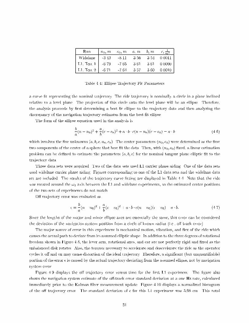
Run n0; m. e0; m. a; m. b; m. c; 1m2

Widelane -3.43 -8.11 3.56 3.54 0.0011

L1, Test 1 -6.79 -7.65 3.61 3.61 0.0000

L1, Test 2 -6.71 -7.64 3.57 3.60 0.0010

Table 4.4: Ellipse Trajectory Fit Parameters

a curve �t representing the nominal trajectory. The ride trajectory is nominally a circle in a plane inclined

relative to a level plane. The projection of this circle onto the level plane will be an ellipse. Therefore,

the analysis proceeds by �rst determining a best �t ellipse to the trajectory data and then analyzing the

discrepancy of the navigation trajectory estimates from the best �t ellipse.

The form of the ellipse equation used in the analysis is

b

a(n� n0)

2 +a

b(e� e0)

2 + a � b � c(n� n0)(e� e0) = a � b (4.6)

which involves the �ve unknowns (a; b; c; n0; e0). The center parameters (n0; e0) were determined as the �rst

two components of the center of a sphere that best �t the data. Then, with (n0; e0) �xed, a linear estimation

problem can be de�ned to estimate the parameters (a; b; c) for the nominal tangent plane elliptic �t to the

trajectory data.

Three data sets were acquired. Two of the data sets used L1 carrier phase aiding. One of the data sets

used widelane carrier phase aiding. Figures corresponding to one of the L1 data sets and the widelane data

set are included. The results of the trajectory curve �tting are displayed in Table 4.4. Note that the ride

was rotated around the !2 axis between the L1 and widelane experiments, so the estimated center positions

of the two sets of experiments do not match.

O� trajectory error was evaluated as

� =b

a(n� n0)

2 +a

b(e� e0)

2 + a � b � c(n� n0)(e� e0)� a � b: (4.7)

Since the lengths of the major and minor ellipse axes are essentially the same, this error can be considered

the deviation of the navigation system position from a circle of known radius (i.e., o� track error).

The major source of error in this experiment is mechanical motion, vibration, and ex of the ride which

causes the actual path to deviate from its assumed elliptic shape. In addition to the three degrees of rotational

freedom shown in Figure 4.8, the lever arm, rotational axes, and car are not perfectly rigid and �xed as the

unbalanced disk rotates. Also, the torques necessary to accelerate and deaccelerate the ride as the operator

cycles it o� and on may cause distortion of the ideal trajectory. Therefore, a signi�cant (but unquanti�able)

portion of the error � is caused by the actual trajectory deviating from the assumed ellipse, not by navigation

system error.

Figure 4.9 displays the o� trajectory error versus time for the �rst L1 experiment. The �gure also

shows the navigation system estimate of the o�-track error standard deviation at a one Hz rate, calculated

immediately prior to the Kalman �lter measurement update. Figure 4.10 displays a normalized histogram

of the o� trajectory error. The standard deviation of � for this L1 experiment was 5:98 cm. This total

31

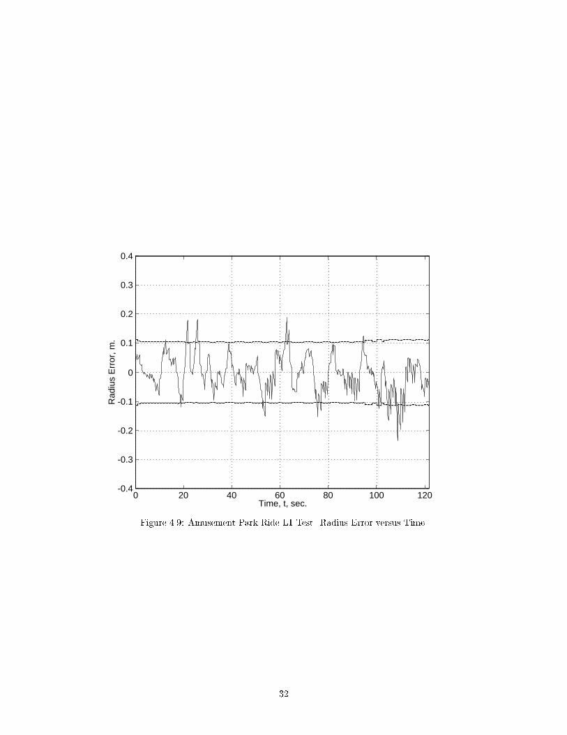
0 20 40 60 80 100 120-0.4

-0.3

-0.2

-0.1

0

0.1

0.2

0.3

0.4

Rad

ius

Err

or, m

.

Time, t, sec.

Figure 4.9: Amusement Park Ride L1 Test. Radius Error versus Time.

32

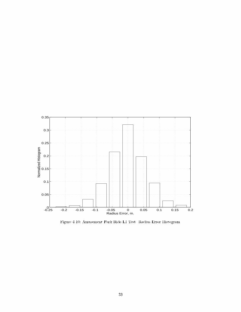
-0.25 -0.2 -0.15 -0.1 -0.05 0 0.05 0.1 0.15 0.20

0.05

0.1

0.15

0.2

0.25

0.3

0.35

Radius Error, m.

Nor

mal

ized

His

togr

am

Figure 4.10: Amusement Park Ride L1 Test. Radius Error Histogram.

33

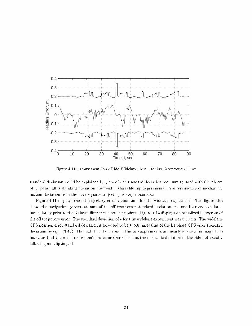
0 10 20 30 40 50 60 70 80 90-0.4

-0.3

-0.2

-0.1

0

0.1

0.2

0.3

0.4

Radiu

s E

rror,

m.

Time, t, sec.

Figure 4.11: Amusement Park Ride Widelane Test. Radius Error versus Time.

standard deviation would be explained by 5 cm of ride standard deviation root sum squared with the 2:5 cm

of L1 phase GPS standard deviation observed in the table top experiments. Five centimeters of mechanical

motion deviation from the least squares trajectory is very reasonable

Figure 4.11 displays the o� trajectory error versus time for the widelane experiment. The �gure also

shows the navigation system estimate of the o�-track error standard deviation at a one Hz rate, calculated

immediately prior to the Kalman �lter measurement update. Figure 4.12 displays a normalized histogram of

the o� trajectory error. The standard deviation of � for this widelane experiment was 5:50 cm. The widelane

GPS position error standard deviation is expected to be � 5:6 times that of the L1 phase GPS error standard

deviation by eqn. (3.43). The fact that the errors in the two experiments are nearly identical in magnitude

indicates that there is a more dominant error source such as the mechanical motion of the ride not exactly

following an elliptic path.

34

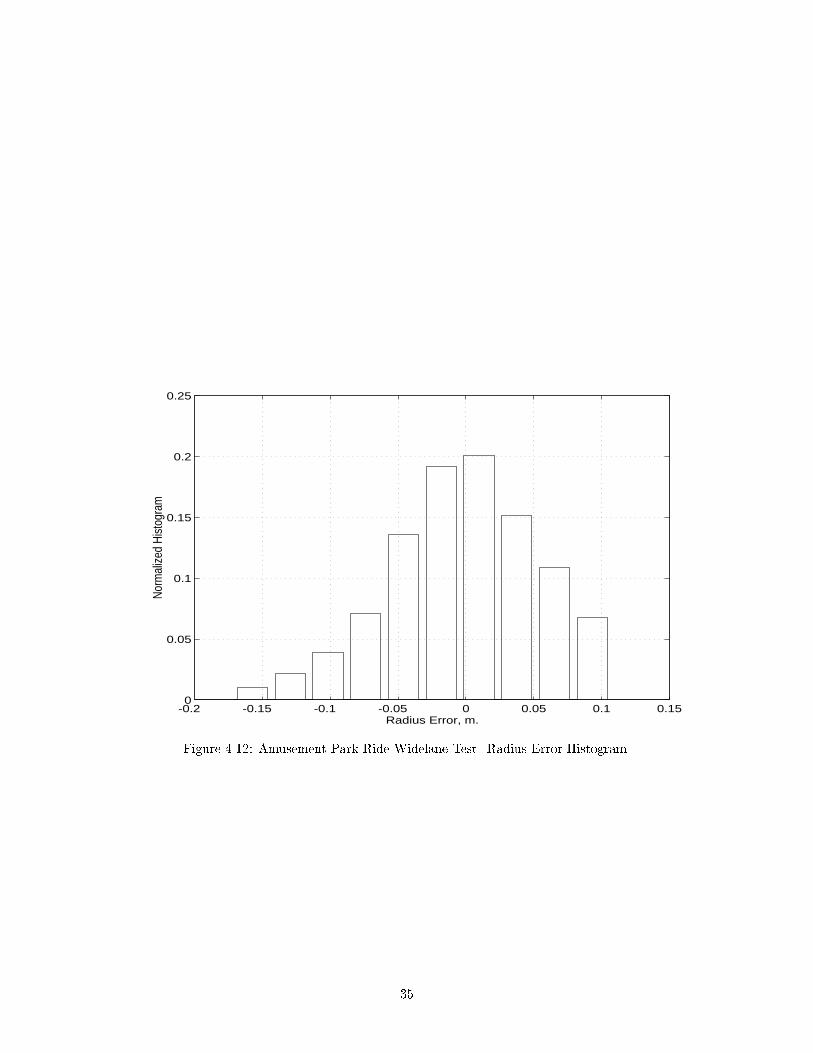
-0.2 -0.15 -0.1 -0.05 0 0.05 0.1 0.150

0.05

0.1

0.15

0.2

0.25

Radius Error, m.

Nor

mal

ized

His

togr

am

Figure 4.12: Amusement Park Ride Widelane Test. Radius Error Histogram.

35

Chapter 5

Conclusions and Future Research

This project has achieved its objective of implementing a DGPS aided INS system with a 100 Hz update

rate and centimeter level accuracy. The exact position accuracy achieved is di�cult to quantify due to the

di�culty of obtaining a second ground truth measurement accurate to at least the centimeter level. The table

top evaluation described herein demonstrates an accuracy of approximately 2.5 centimeter, with no special

precautions taken to mitigate multipath e�ects. The amusement park ride demonstration demonstrated that

the position accuracy was better than 6.0 cm, but beyond this level the navigation system error could not

be discriminated from the mechanical system trajectory error.

As described in the following section, better accuracy can be achieved by research in several directions.

Higher update rates are de�nitely achievable.

5.1 Future Research

Several directions are available for future research:

1. Integration of this stand alone navigation system into the PATH vehicles. This would have several

bene�ts. First, PATH researchers would be able to use the results of this PATH funded research.

The results of this project and existing magnetic and vision based positioning systems could be used

synergistically. This would allow more accurate analysis of positioning accuracy, development and

evaluation of vehicle control performance with additional navigation state information, and enhanced

fault accommodation. Second, GPS aided INS navigation provides the full vehicle state and control

preview information at update rates high enough to enable advanced control methods.

2. INS performance could be enhanced in several ways.

(a) Delay compensation should be added to account for the latency between the time of applicability

of the Kalman �lter error estimates and their time of availability. The delay compensation is not

critical, since the error states are slowly changing, but the �x is easy and will improve performance.

(b) Lever arm compensation should be added to account for the � 0:5 meter antenna phase center

to accelerometer lever arm. The lever arm compensation is slightly more involved than the delay

36

compensation, but straightforward. This improvement should increase the observability of the

attitude error and increase the position estimation accuracy when the vehicle is rolled or pitched.

(c) The INS update could still increase above 100 Hz. We did not implement special algorithms for

higher updates, as our gyros could only be sampled at 50 Hz. The gyros should be replaced

with gyros more typical of those which would be used in the �nal commercial application. In the

process, the INS could be switched to a higher update rate and a quaternion implementation.

The quaternions implementation is written, but was not integrated into the INS due to time and

funding constraints.

3. The GPS performance could be improved by the following.

(a) The GPS update rate could also be increased. Although our receivers have a maximum 2 Hz

update rate and a 0.3 second latency, receivers are now available with 20 Hz update rates and

milliseconds of latency. In addition to the receiver latency, our di�erential corrections were de-

layed by 0.7 seconds due to computation and communication bandwidth constraints. It was this

di�erential correction delay that limited the GPS update rate to 1 Hz. A higher bandwidth com-

munication channel or improved base station design would have allowed correction information

to be broadcast at higher rates and with shorter latency. Correction rate information would have

allowed the communication channel delay to be compensated. The base station design is described

in Chapter 7 of [14], but its implementation was not within the scope of this project.

(b) The correction rate information would also have allowed the use of di�erential Doppler observables.

This would allow integer phase ambiguities to be estimated while the vehicle was in motion. This

would be a very useful area for future research.

(c) Advanced integer ambiguity resolution techniques would decrease the time required to determine

and verify the correct integers.

(d) Dynamic system fault detection techniques could be applied to reliably monitor for the loss of

phase lock.

The IMU platform for this project was crude by typical INS standards. In this preliminary e�ort, the

PI's did not use special test labs or manufacturing facilities for accurate system calibration and alignment.

Still, very accurate navigation accuracy was achieved. Better accuracy should be achievable at low cost with

a well designed automated manufacturing process which (1) places each instrument on the platform in a

repeatable fashion; (2) performs an automated set of simple calibration procedures of each platform; and,

(3) stores the calibration parameters in on board ROM. Such a process is not unreasonable for the high

volume production that could be expected in the automotive industry.

5.2 Publications Resulting from this Project

At least two publications, which were partially funded by this project, are expected.

The �rst publication is reference [14]. This book is under contract, in the production stage, for publication

with McGraw-Hill. The book provides an indepth discussion of the theory and design of GPS aided inertial

navigation systems. The �nal draft of this text was submitted to McGraw-Hill in April 1998.

37

The second publication is a journal article, still in preparation, which describes the design and analysis

results of this project. It will be submitted to either IEEE Transactions on Vehicular Technologies, IEEE

Tansactions on Control Systems Technology, or the Journal of Navigation. This article is in its �nal draft

stage.

38

Bibliography

[1] \Navstar GPS Interface Control Document,\ Report #ICD-GPS-200B-PR, Joint GPS Program O�ce,

1991.

[2] Anderson, J. and S. Lazar, \Lm and Lc: How the Military and Civilian Users of GPS can Share

our Existing Spectrum," ION GPS 97 Presentation, September 18, 1997, Kansas City, MO. See also

`http://www.laafb.af.mil/SMC/CZ/homepage/lm/overview.htm'

[3] Bancroft, S., \An Algebraic Solution of the GPS Equations," IEEE Transactions Aerospace and Elec-

tronic Systems, Vol. AES-21, No. 7, Jan 1985, pp. 56-59.

[4] M. Barth and E. Johnston, \Using GPS Technology to Obtain Accurate Speed, Acceleration, and

Grade Information for On-Road Emissions Measurement", in Fifth CRC On-Road Vehicle Emissions

Workshop, San Diego, CA, 1995.

[5] Blomenhofer, H., G. Hein, E. Blomenhofer, andW.Werner, \Development of a Real-Time DGPS System

in the Centimeter Range," IEEE 1994 Position, Location, and Navigation Symposium, Las Vegas, NV,

1994, pp. 532-539.

[6] Britting, K. R., Inertial Navigation Systems Analysis, Wiley-Interscience, New York, 1971.

[7] Brown, R. G., Y.C. Hwang, Introduction to Random Signals and Applied Kalman Filtering, 2nd ed.

New York : J. Wiley, c1992.

[8] Cannon, E. \High-Accuracy GPS Semikinematic Positioning: Modeling and Results," Navigation: Jour-

nal of the Institute of Navigation, Vol. 37, No. 1, Summer 1990, pp. 53-64.

[9] W. Cormier and R. Fenton, \On the Steering of Automated VehiclesA Velocity Adaptive Controller,"

IEEE Trans. on Vehicular Technology, Vol. 29, no.4, pp. 375-385, 1980.

[10] R. T. Dunlay, \Obstacle avoidance perception processing for the autonomous land vehicle," in Proceed-

ings of the IEEE International Conference on Robotics and Automation, pp. 912-917, 1987.

[11] E. Dickmanns and B. Mysliwetz, \Recursive 3-D road and relative ego-state recognition," IEEE Trans-

actions on Pattern Analysis and Machine Intelligence, Vol. 14, pp. 199-213, 1992.

[12] [23] H. Euler, \Achieving High-Accuracy Relative Position in Real-time: System Design, Performance,

and Real-Time Results," in IEEE 1994 Position Location and Navigation Symposium, Las Vegas, NV,

USA, pp. 540-546, 1994.

39

[13] Fang, B. T., \Trilateration and Extension fo Global Positioning System Navigation," Journal of Guid-

ance, COntrol, and Dynamics, Vol. 9, No. 6, Nov./Dec. 1986, pp. 715-717.

[14] Farrell, J. and M. Barth, The Global Positioning System and Inertial Navigation: Theory and Practice,

In Preperation, expected publication in 1998.

[15] Farrell, J., M. Djodat, M. Barth, and M. Grewal, \Latency Compensation for Di�erential GPS," Navi-

gation: Journal of the Institute of Navigation, Vol. 44, No. 1, Spring 1997, 99-107.

[16] R. Fenton and R. Mayhan, \Automated Highway Studies at The Ohio State UniversityAn Overview,"

IEEE Trans. on Vehicular Technology, Vol. 40, no.1, pp. 100-113, 1991.

[17] R. Fenton, G. Melocik, and K. Olson, \On the Steering of Automated Vehicles: Theory and Experi-

ment," IEEE Transactions of Automatic Control, Vol. 21, no.3, pp. 306-315, 1976.

[18] Frodge, S.,S. Deloach, B. Remondi, D. Lapucha, and R. Barker, \Real-Time on-the-Fly Kinematic GPS

System Results," Navigation: Journal of the Institute of Navigation, Vol. 41, No. 2, Summer 1994, pp.

175-186.

[19] A. Hanson, E. Riseman, and C. Weems, \Progress in computer vision at the University of Mas-

sachusetts," in DARPA Image Understanding Workshop, pp. 39-47, 1993.

[20] Grissom, L. \DGPS Correction Communication System Design," EE Senior Design Report, University

of California, Riverside, June 1995.

[21] Hatch, R., \The Synergism of GPS Code and Carrier Measurements," Proc. 3rd Int. Geodetic Sympo-

sium on Sat. Doppler Pos., 1982, Las Cruces, NM.

[22] Hatch, R., \Instantaneous Ambiguity Resolution," Symposium No. 107, Kinematic Systems in Geodesy,

Surveying and Remote Sensing, Ban�, Canada, September 10-13, 1990, pp. 299-308, Springer Verlag.

[23] Hatch, R., \The Promise of a Third Frequency," GPS World, May 1996, pp. 55-58.

[24] Hwang, P. and R. Brown, \GPS Navigation: Combining Pseudorange with Continuous Carrier Phase

using a Kalman Filter," Navigation: Journal of the Institute of Navigation, Vol. 37, No. 2, Summer

1990, pp. 181-196.

[25] C. Kee and B. Parkinson, \Wide Area Di�erential GPS as a Future Navigation System in the US," in

IEEE 1994 Position Location and Navigation Symposium, Las Vegas, NV, USA, pp. 788-795, 1994.

[26] Kuan, Phipps, and Hsueh, \Autonomous Robotic Vehicle Road Following," IEEE Transactions on

Pattern Analysis and Machine Intelligence, Vol. 10, pp. 648-658, 1988.

[27] Lachapelle, G., M. Cannon, and G. Lu, \High-Precision GPS Navigation with Emphasis on Carrier-

Phase Ambiguity Resolution," Marine Geodesy, 15, pp. 253-269, 1992.

[28] Leva, J., \An Alternative Closed Form Solution to the GPS Pseudorange Equations," Institute of

Navigation (ION) National Technical Meeting, Anahiem, CA, Jan. 1995.

40

[29] Mader, G., \Dynamic Positioning using GPS Carrier Phase Measurements," Manuscripta Geodetica,

Springer-Verlag, Vol. 11, 1986, pp. 272-277.

[30] I. Masaki, Vision-Based Vehicle Guidance, New York: Springer-Verlag, 1992.

[31] R. Mayhan and R. Bishel, \A Two-Frequency Radar for Vehicle Automatic Lateral Control," IEEE

Trans. on Vehicular Technology, Vol. 31, no.1, pp. 32-39, 1982.

[32] J. Meyer-Hilberg and T. Jacob, \High Accuracy Navigation and Landing System using GPS/IMU

System Integration," in IEEE 1994 Position Location and Navigation Symposium, Las Vegas, NV,

USA, pp. 298-305, 1994.

[33] The Global Positioning System: A Shared National Asset, National Research Council, Washington,

D.C.: National Academy Press, 1995.

[34] RTCM Recommended Standards for Di�erential Navstar GPS Service, Version 2.1, RTCM Special Com-

mittee No. 104, January 3, 1994.

[35] Rowson, S. V., G. R. Courtneyand, and R. M. Hueschen, \Performance of Category IIIB Automatic

Landings Using C/A Code Tracking Di�erential GPS," Navigation, Vol. 41, No. 3, pp 127-143, 1994.

[36] J. W. Spalding and L. A. Luft, \Di�erential GPS Integrity Monitor," in IEEE 1994 Position Location

and Navigation Symposium, Las Vegas, NV, USA, pp. 225-232, 1994.

[37] H. Schneidermann and M. Nashman, \Visual processing for autonomous driving," in IEEE Workshop

on Applications of Computer Vision, Palm Springs, CA, pp. 164-171, 1992.

[38] S. Shladover, et al., \Automatic Vehicle Control Developments in the PATH Program," IEEE Trans.

on Vehicular Technology, Vol. 40, no.1, pp. 114-130, 1991.

[39] Teunissen, P. \A New Method for Fast Carrier Phase Ambiguity Estimation," IEEE 1994 PLANS, pp.

562-573.

[40] C. Thorpe, et al, \Toward autonomous driving: the CMU Navlab", Part 1-Perception, IEEE Expert,

Vol. 6, pp. 31-42, 1991.

[41] Widnall, W. S. and P. A. Grundy, \Inertial Navigations System Error Models," Intermetrics Inc., TR-

03-73, May 11, 1973.

[42] T. Younglove, E. Johnston, and M. Barth, \DGPS Technology for Vehicle Parameter Estimation," in

International Workshop on Driving Cycles and Vehicle Data-logging, Ottawa, Canada, 1995.

[43] Zhang, et al., \An Intelligent Roadway Reference system for Vehicle Lateral Guidance/Control," in

American Control Conference, San Diego, CA, pp. 281-286, 1990.

41

Appendix A

Appendix: Constant and Notation

De�nition

A.1 Notation

The notational conventions described in Table A.1 will be used throughout this report. They are based on

those de�ned in [6].

x denotes the true value of x

x denotes the calculated value of x

~x denotes the measured value of x

�x denotes the error x� x

Ra2b denotes the transformation from coordinate system a to coordinate system b

(x)a denotes vector x being coordinatized in frame a

Table A.1: Notation De�nition

Coordinate systems will be designated by the abbreviations of Table A.2. Therefore, the rotation for a vector

a accelerometer coordinates (non-orthogonal)

b body coordinates

e ECEF coordinates

g gyro coordinates (non-orthogonal)

i inertial coordinates

p platform coordinates

t tangent plane coordinates

Table A.2: Reference Frame Abbreviations

42

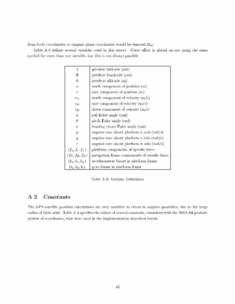
from body coordinates to tangent plane coordinates would be denoted Rb2t.

Table A.3 de�nes several variables used in this report. Great e�ort is placed on not using the same

symbol for more than one variable, but this is not always possible.

� geodetic latitude (rad)

� geodetic longitude (rad)

h geodetic altitude (m)

n north component of position (m)

e east component of position (m)

vN north component of velocity (m/s)

vE east component of velocity (m/s)

vD down component of velocity (m/s)

� roll Euler angle (rad)

� pitch Euler angle (rad)

heading (true) Euler angle (rad)

p angular rate about platform u axis (rad/s)

q angular rate about platform v axis (rad/s)

r angular rate about platform w axis (rad/s)

(fu; fv; fw) platform components of speci�c force

(fN ; fE ; fD) navigation frame components of speci�c force

(bu; bv; bw) accelerometer biases in platform frame

(bp; bq; br) gyro biases in platform frame

Table A.3: Variable De�nitions

A.2 Constants

The GPS satellite position calculations are very sensitive to errors in angular quantities, due to the large

radius of their orbit. Table A.4 speci�es the values of several constants, consistent with the WGS-84 geodetic

system of coordinates, that were used in the implementation described herein.

43

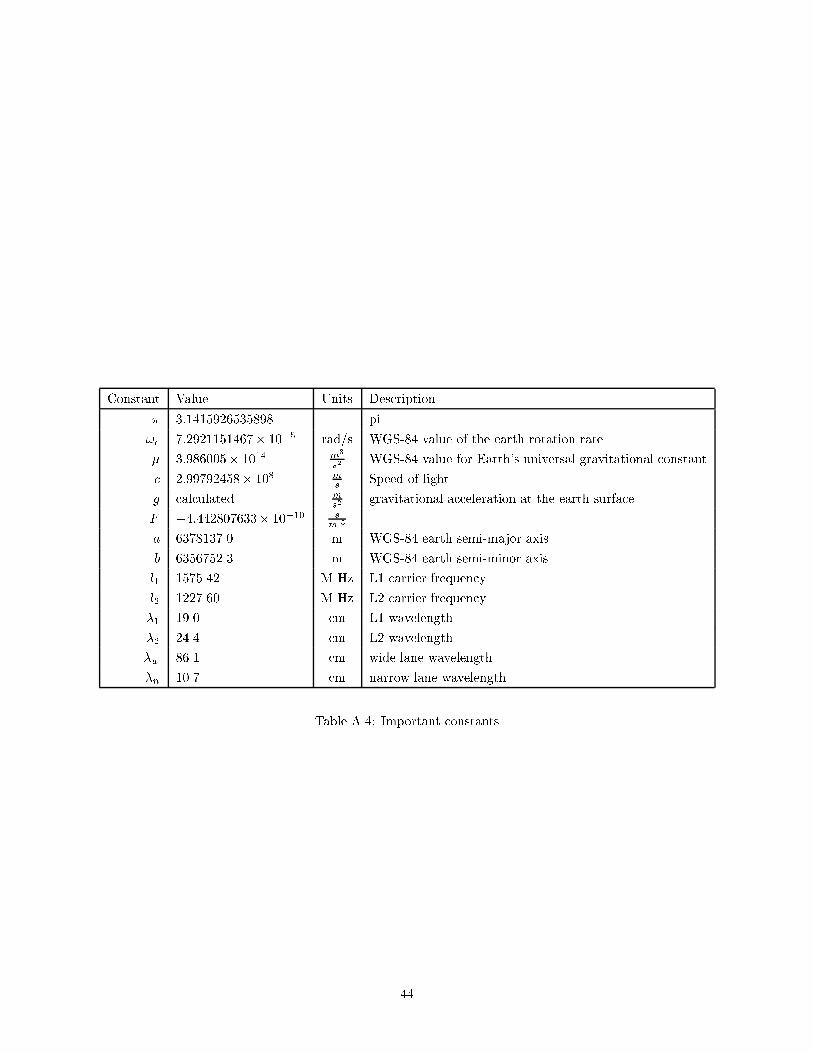
Constant Value Units Description

� 3:1415926535898 pi

!e 7:2921151467� 10�5 rad/s WGS-84 value of the earth rotation rate

� 3:986005� 1014 m3

s2WGS-84 value for Earth's universal gravitational constant

c 2:99792458� 108 ms

Speed of light

g calculated ms2

gravitational acceleration at the earth surface

F �4:442807633� 10�10 sm:5

a 6378137.0 m WGS-84 earth semi-major axis

b 6356752.3 m WGS-84 earth semi-minor axis

l1 1575.42 M Hz L1 carrier frequency

l2 1227.60 M Hz L2 carrier frequency

�1 19.0 cm L1 wavelength

�2 24.4 cm L2 wavelength

�w 86.1 cm wide lane wavelength

�n 10.7 cm narrow lane wavelength

Table A.4: Important constants

44

Appendix B

Appendix: Platform and Experiment

Photographs

This appendix contains three photographs. Figure B.1 is a photograph of the GPS antenna mounted on the

instrument platform. The ultimate product would be smaller and rigidly attached to the vehicle frame. This

rigid, yet movable, platform was required to allow various forms of testing. Figure B.2 shows the platform and

computer equipment mounted on the 'Wipeout' ride at Castle Amusement Park. The instrument portion of

the platform is enclosed in styrofoam to decrease air ow and sunlight induced temperature changes. Figure

B.3 shows the location of the `Wipeout' ride. Note the nearby metal surfaces and foilage.

45

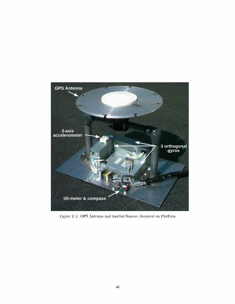
GPS Antenna

3-axisaccelerometer

tilt-meter & compass

3 orthogonalgyros

Figure B.1: GPS Antenna and Inertial Sensors Mounted on Platform

46

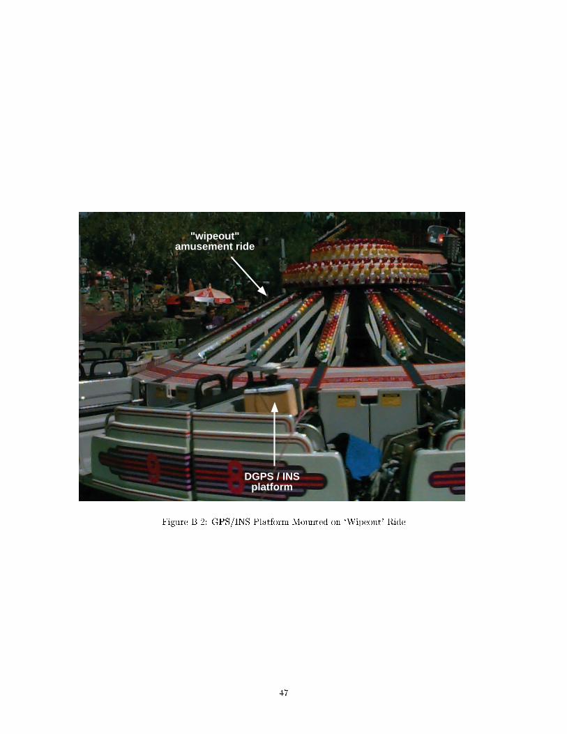
DGPS / INSplatform

"wipeout"amusement ride

Figure B.2: GPS/INS Platform Mounted on `Wipeout' Ride

47

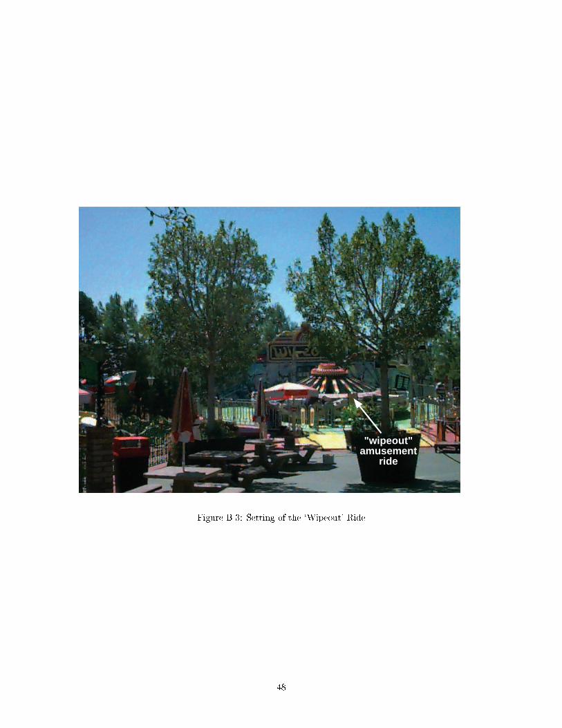
"wipeout"amusement

ride

Figure B.3: Setting of the `Wipeout' Ride

48

Appendix C

Appendix: Receiver Price and

Performance History

C.1 GPS Positioning Accuracy

As shown in Figure C.1, GPS accuracies have improved considerably over the operational goal of 15m. In

the early 1980's carrier phase techniques were developed that gave accuracies of a few centimeters. These

techniques required post processing so they were not useful for real time applications. From the mid 1980's

code di�erential systems were producing accuracies of about 1 meter. In the early 1990's algorithm improve-

ments and increased processing power allowed for real time carrier phase techniques. All of these techniques

require di�erential reference stations and the accuracy is dependent on the distance between the reference

station and the rover. Continuing advances in algorithms, receivers, and the GPS satellite system are still

improving GPS positioning accuracy.

C.2 Receiver Cost

The cost of receivers, see Figure C.2, has declined dramatically as the price of processors (a signi�cant

part of a receiver) has decreased and as production volume has increased. Dual frequency receivers are still

expensive primarily due to low production volume. As the use of two frequency receivers for high accuracy

applications becomes more widespread, their cost should decrease signi�cantly.

There have recently been a number of proposals to add a second civilian frequency (L5 or Lc) or a new

military frequency (Lm), but it has been very di�cult to �nd a suitable frequency spectrum. The utility of

a second civilian frequency is becoming clear in the FAA's attempts to use GPS for Category I instrument

landings. The most recent proposal by the GPS Joint Program O�ce [2] is a frequency partitioning in which

civilians would get the +/- 4 MHz either side of the current L1 and L2 frequencies and the military would

get from 4 to 12 MHz above and below the current L1 and L2 center frequencies. If this proposal is adopted

dual frequency receivers should not cost more than twice the cost of a single frequency receiver because C/A

code will be available for the L2 frequency.

49

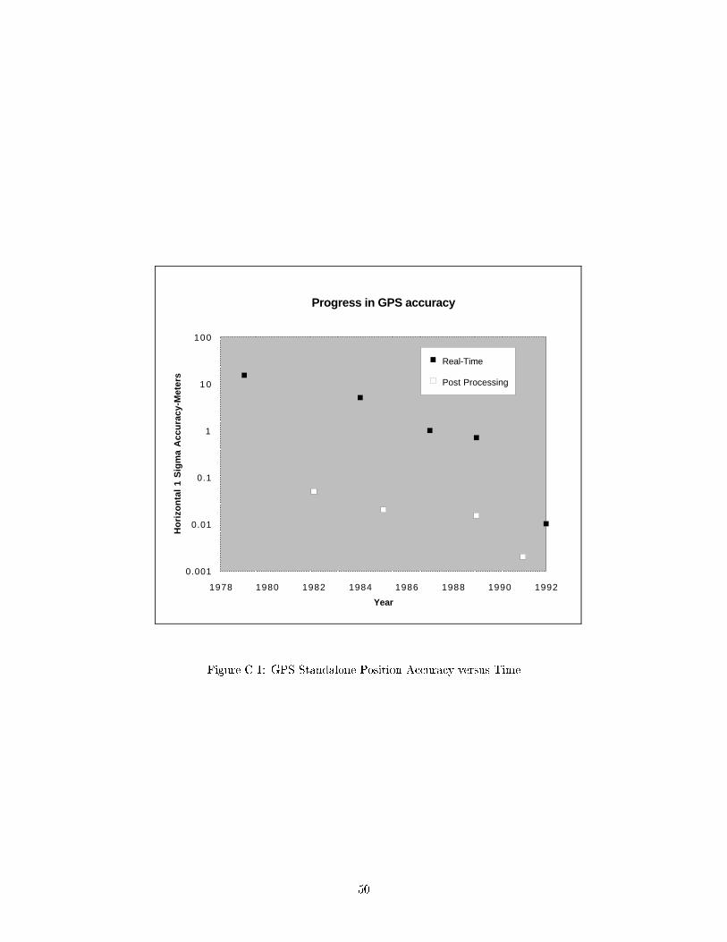
Progress in GPS accuracy

Year

Ho

rizo

nta

l 1

Sig

ma

Acc

ura

cy-M

eter

s

0.001

0.01

0.1

1

1 0

100

1978 1980 1982 1984 1986 1988 1990 1992

Real-Time

Post Processing

Figure C.1: GPS Standalone Position Accuracy versus Time

50

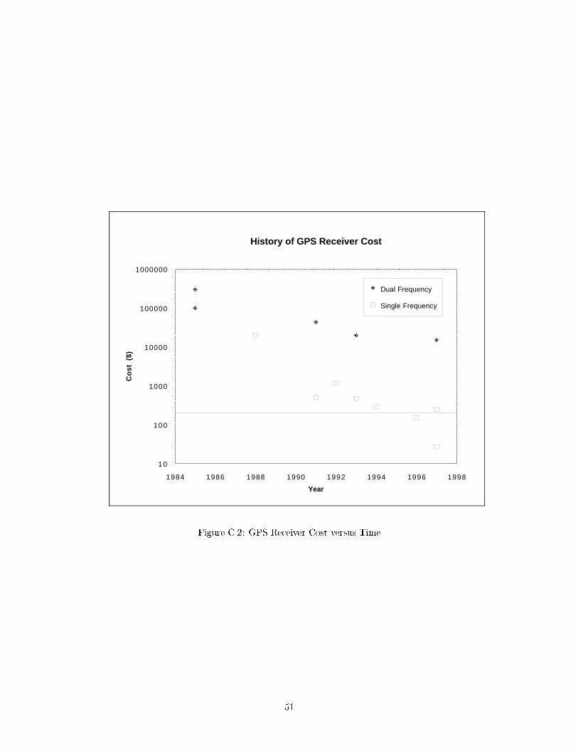
History of GPS Receiver Cost

Year

Co

st (

$)

1 0

100

1000

10000

100000

1000000

1984 1986 1988 1990 1992 1994 1996 1998

Dual Frequency

Single Frequency

Figure C.2: GPS Receiver Cost versus Time

51

GPS/INS Based Lateral and Longitudinal Control Demonstration

Documents

Transcript of GPS/INS Based Lateral and Longitudinal Control Demonstration