1

Forthcoming in

International Tax and Public Finance

Government size, composition of public expenditure, and economic development

Susana Martins a , Francisco José Veiga

b,*

a,b Universidade do Minho and NIPE, Escola de Economia e Gestão, 4710-057 Braga, Portugal.

a scmartins@eeg.uminho.pt ,

b fjveiga@eeg.uminho.pt

Abstract

This paper analyzes the effects of government size and of the composition of public

expenditure on economic development. Using the system-GMM estimator for linear

dynamic panel data models, on a sample covering up to 156 countries and 5-year periods

from 1980 to 2010, we find that government size as a percentage of GDP has a quadratic

(inverted U-shaped) effect on the growth rate of the Human Development Index (HDI).

This effect is especially pronounced in developed and high income countries. We also find

that the composition of public expenditure affects development, with the share of five

subcomponents exhibiting non-linear relationships with HDI growth.

JEL Classifications: H50, O15, O23, O43

Keywords: Economic Development, Government Size, Composition of public

expenditure; Human Development Index

* Corresponding author. Tel.: +351 253604534; fax: +351 253601380.

2

1. Introduction

How can a country become economically more developed? Why, in 2010, an

inhabitant of Liechtenstein lived with $222 per day, while a Zimbabwean lived with only

$0.48?1 Why is life expectancy 83 years for a Japanese and only 45 years for an Afghan?

In addition to the wide differences between developed and developing countries, there are

also dissimilarities within each group of countries. Since among the functions of

government is the redistribution of income among citizens, in order to enable them to

access education and health, differences in the size of government and in the composition

of public expenditure across countries may help explain differences in development.

Although the government has grown incredibly and sometimes dramatically in most

countries, government size growth is neither a recent phenomenon nor a simple one.

Governments must promote social development and economic growth, but it is hard to

determine if an increase in public intervention by increasing public spending will have a

positive impact on economic performance. Economic growth is necessary for economic

development, but income distribution2 and the economic structure are also determinants of

the level of development. Therefore, studying only the impact of public spending on

economic growth is a somewhat partial analysis.

There are many studies on the effects of government expenditures on economic

growth, but the literature analyzing the effects on economic development is much scarcer.

Furthermore, there is a very reduced number of studies examining the growth effects of

the composition of public expenditure using samples that cover developing countries and

data since the 1970s. This is essentially due to the fact that the historical fiscal data

reported to the IMF’s Government Finance Statistics follows two different classification

1 Just over a third of the poverty line of $1 25 per day. Values obtained from UNDP (2011).

2 If part of the population does not go to school (or to good schools), or does not have access to proper medical care, the

country’s health and education indexes (which are used to compute the Human Development Index - HDI) will be

lower than when income and access to education and health are more equally distributed. Thus, in the presence of high

income inequality, economic growth may not be completely reflected in the growth rate of the HDI.

3

standards which are hard to combine. Acosta-Ormaechea and Morozumi (2013) have

recently merged GFSM1986 and GFSM2001 to assemble a new dataset which covers the

period 1970-2010. They then analyze the effects of public expenditure reallocations in

long-run economic growth and conclude that increases in the share of education spendi ng

tend to be growth-enhancing.3

The main objective of the present study is to fill an important gap in the literature

by empirically examining the effects of government size and of expenditure composition

on economic development. To the best of our knowledge, no previous studies have

analyzed the effects of expenditure composition on economic development. We perform

system-GMM estimations for a linear dynamic panel data model using a sample that

covers up to 156 countries,4 for consecutive and non-overlapping 5-year periods from

1980 to 2010. The dependent variable is the growth rate of the UNCTAD’s Human

Development Index (HDI) over a 5-year period. Our results indicate that government size

has a quadratic (inverted U-shaped) effect on the HDI growth rate, especially in developed

and high income countries. Thus, in these countries, excessive government size is

detrimental to economic development. Regarding expenditure composition, we find that

the shares of defense, education and social protection expense in total public expenditure

have inverted U-shaped relationships with development, while health and the group of

remaining expenses have U-shaped relationships.

The paper is structured as follows. Section 2 summarizes the literature on

government size and economic development, also comprising the literature which relates

government size with economic performance. The data and the empirical model are

3 Kneller et al. (1999) empirically analyze the effects of the structure of taxation and public expenditure on economic

growth for a sample of 22 OECD countries. They find that distortionary taxation reduces growth, whilst non-

distortionary taxation does not, and that productive public expenditure enhances growth, whilst non-productive

expenditure does not.

4 When using data on public expenditure composition, the estimations cover 79 countries.

4

presented in section 3, and the results are shown and discussed in section 4. Finally, the

conclusions are presented in section 5.

2. Government size and economic performance

2.1 Government size

Despite the growth of government in the last fifty years, this is neither a recent nor a

simple phenomenon. Government, in greater or lesser extent and clarity, centralized or

not, is present in almost all daily activities. It is possible to compare in time and between

countries the relative size of governments or even the efficiency of some activities, but it

is not possible to say in absolute when there is excessive government. Comparing

observations requires some care, especially when comparing over time, as they have to be

adjusted to inflation and demographic growth (Ulbrich 2003). The most common and less

disadvantageous variable to measure government size is public expenditure5

as a

percentage of Gross Domestic Product (GDP).

The size and role of government have always been closely linked: changes in the

growth of government were related to changes in its role in the economy. Since the late

nineteenth century that public expenditures have been increasing considerably, on

average,6

but more rapidly in the period before 1980 (Peltzman 1980; Tanzi and

Schuknecht 2000). It was a protective and welfare state government, seeking for a greater

redistribution of income and wealth from the richest to the poorest, playing roles that the

markets alone could or would not play, such as the provision of public goods and services

and the mitigation of externalities. A growing skepticism about governmental intervention

in the economy and the view of the public sector as "excessive" and expensive, and as a

5 Public expenditure is less volatile and less susceptible to measurement errors than public revenue

(Labonte 2010).

6 On average, considering there is an asymmetry in government growth. For example, faster development of public

expenditure in less institutionally constrained countries.

5

welfare state that creates disincentives to private initiative through high taxes, are among

the explanations for the slowdown of public expenditure after 1980.

2.2 Economic development

Because of their strict relationship, economic development is often confused with

economic growth (see Pomfret 1997). Actually, they are quite different. Economic

development can be defined as a qualitative change and restructuring of a country,

reflecting not only technological progress, but also social progress. In turn, economic

growth can be defined as a quantitative change in a country’s economy, measured by

changes in GDP over one year. Nevertheless, despite these differences, GDP and economic

growth are the most commonly used indicators of economic development.

Economic growth is necessary but not sufficient for economic development: the

income distribution and economic structure are also examples of essential indicators of

economic development (Nafziger 2006). It is not correct to say that a country has

developed economically just because its GDP per capita has increased, when a great part

of the population still lives in precarious conditions. For Seers (1969), the income level

only represents the potential for economic development; to register economic development

it is essential to verify reductions of poverty, unemployment and inequality in a country.

That is, the richest countries are not necessarily the most developed. This is illustrated in

Table 1, which reports per capita income and human development for five countries. Four

of them are in the top-10 ranking of income, but drop 28 to 42 places when the ranking is

based on the HDI. It also shows the case of New Zealand, which ranks 33th

in income but

jumps to third place when the HDI is considered.

[Insert Table 1 about here]

Defining and measuring economic development is still a problem that generates as

much controversy as measuring government size. There isn’t a proper measure, but some

6

that may be more plausible and acceptable than others. Faced with this measurement

problem, several alternatives were developed to measure the welfare of a population ,

combining several indicators of economic development. The most commonly accepted is

the Human Development Index (HDI). The HDI was first developed by the United Nations

Development Program (UNDP) in 1990, stating that the differences between developed

and developing countries were smaller when measured by human development than by the

simple comparison of per capita income. According to the Human Development Report

(UNDP 2011), this is a summary index that results from the geometric mean7 of three

basic dimensions of human development: (1) long and healthy life, (2) access to

knowledge and education, and (3) decent and stable living standards. To each of the

indices included, the maximum value (observed) and minimum value (observed or not) are

assigned, resulting in the index value8 for each country i in year t as explained in the

Appendix.

The HDI also presents some limitations, such as scaling index values between 0 and

1, the weight assigned to each of the basic dimensions, or difficulties encountered when

comparing countries by other factors related to the enrollment rate, such as quality of

schools or dropout rates, which vary substantially from year to year. Nevertheless,

Nafziger (2006) considers that the HDI is better, more complete and multifaceted than any

other indicator or index, being useful for the qualitative aspects of development,

influencing countries with low levels of development to review their policies of nutrition,

health and education. In this sense, the HDI is the indicator used in the present study to

compare countries regarding their levels of development.

7 The authors argue for the replacement of the arithmetic mean (used in previous reports) by the geometric mean

because the values obtained for the indices are lower, occurring major changes only for countries where there is a

greater inequality between the dimensions of development.

8 As these maximum and minimum values vary over time, every year all indexes for all countries are recalculated.

Hence, for temporal consistency, comparisons should not be made using different publications of the UNDP for the

HDI. Thus, all HDI data used in this paper comes from UNDP (2011).

7

2.3 Effects on economic growth and development

Since economic growth is a common indicator of economic development, it is

important to take the impact of government size on economic growth into account. This

literature is immense, as many authors dedicated attention to it and found a variety of

results. Therefore, we describe only a small part of the existing literature.

An important empirical study was that of Barro (1991). Despite the difficulties in

measuring public services and growth rates, or in treating government size as an

endogenous variable, for a relatively low level of productive public expenditure ,9 he finds

that government size positively influences economic growth. From a certain (optimum)

level on, increasing government size has a negative impact.10

Barro also concluded that for

a given value of the government size, an increase in unproductive expenditure leads to a

decrease in growth rates and saving; despite not having a direct impact on productivity in

the private sector, the increase in income leads to a tax disincentive to investment. These

empirical results are consistent with his analysis of government spending in an

endogenous growth model (Barro 1990).11

Easterly and Rebelo (1993) find that fiscal

policy is influenced by the scale of the economy and that investment in transport and

communication is consistently correlated with growth.

According to Gwartney et al. (1998), channeling resources from the free functioning

private markets to the public sector implies higher taxes that create disincentives for

9 Corsetti and Roubini (1996), in their study of the effects of government expenditure in endogenous growth models,

ensure that many forms of public expenditure are directly or indirectly productive affecting productivity in different

ways.

10 Labonte (2010) also highlighted the need to distinguish fluctuations in short-term growth, resulting from

economic cycles, from sustainable long term growth rates. The four action forms of the public sector

(spending, transfers, taxes and regulation) have the potential to influence long-term growth through labor

supply, physical capital and productivity. Tanzi and Zee (1997) concluded that, by using public financial

instruments, tax policy can play a fundamental role in the performance and long-term growth of countries.

11 For other theoretical models analyzing the effects of public expenditure on economic growth see, among others, King

and Rebelo (1990), Lucas (1988), and Meltzer and Richard (1981).

8

workers and investment, inefficiency, low returns, and lack of dynamics and innovation in

the political process (when compared to the market process). These effects may even

dominate and generate a negative impact on growth. Furthermore, there is no reason to

expect that most goods can be allocated or provisioned more efficiently by the public

sector than by the private sector.12

Other works such as those of Barro and Sala-i-Martin

(1995), Bassanini et al. (2001), Fölster and Henrekson (1999) and Heitger (2001) found

empirical evidence of a negative and statistically significant effect on economic growth,

using general public expenditure. Similarly, Fölster and Henrekson (2001), with an

analysis for industrial countries (OECD), obtained strong, robust and statistically

significant results for a negative effect of total public expenditure on economic growth,

but not statistically significant for the negative effect of taxes. Afonso and Furceri (2010)

found that the impact of public expenditure and revenue on economic growth (measured

by the growth rate of per capita real GDP), was negative, substantial , and statistically

significant.

Although they are closely related, the variables that affect economic growth may not

affect (or affect differently) economic development, given the qualitative nature of the

latter, which also considers dimensions such as longevity and education. In an attempt to

find the optimal size of government (public spending on consumption and investment, as a

percentage of GDP), Davies (2009) concluded that the optimum level of government size

would be higher for economic development (using HDI) than for economic growth (using

GDP), explaining that education and health do not improve current GDP, but contribute to current

HDI. His results also indicate that: (1) for all countries and relatively low government

size, there is a positive relationship between expenditure on consumption and investment

and changes in the HDI. Above the optimum government size (17% of GDP for

12

See also Hauner and Kyobe (2010) and Afonso, Schuknecht and Tanzi (2005), who empirically analyzed the

efficiency and performance of the public sector, finding evidence of a negative relationship between these indicators

and government size.

9

government consumption and 13% of GDP for government investment) , the relationship

would be negative; (2) an increasing positive effect of government consumption and a negative

effect of government investment (until 40% of GDP) on economic development for low income

countries.13

Yavas (1998) argued that this relationship is due to the strong need for

provision of infrastructure and public services in countries with low development, hence

benefiting more of an expansion in public spending. According to these authors, different

effects are expected for countries with high and low development and with high and low

income.

Mourmouras and Rangazas (2009) developed an overlapping generations model and

concluded that countries where the government is less democratic or more elitist,

benefiting landlords, who are richer, will face higher tax rates and slower growth. They

confirmed their hypothesis through a quantitative analysis which indicated that, for lower

stages of development, high taxes and public consumption may slow down economic

growth and development. They do not deny, however, a positive association between high

taxes and growth if there is at the same time large public investment. The authors also

suggested that, as a country develops over time, the natural tendency is for an increasing

government size.

3. Data and econometric model

To estimate the proposed model, we use a panel data base, with a cross -sectional

component of up to 156 countries and a temporal component covering the period from

1980 to 2010, for a wide range of variables.

13

The functions representing (1) and (2) have, respectively, downward and upward concavity.

10

3.1 The data

The availability of repeated observations (years) for the same units (countries) on the

basis of panel data allows us to specify and estimate more complex and realistic models.

However, they also have some practical disadvantages, as it is no longer appropriate to

assume that the different points are independent, hampering analysis, particularly for

nonlinear and dynamic models (Verbeek, 2008).

Many advantages are taken into account by choosing panel data for smaller periods

of observation, especially in studies like this which include fiscal policy variables. Fölster

and Henrekson (2001) argue that using longer periods (30 or 40 years) makes it less

effective to capture the effects on growth, increases the difficulty in eliminating the effect

of economic cycles, or the demographic influence on government size or on GDP growth.

Afonso and Furceri (2010) also add that the information on the variation of growth or

government size in a country is lost and dummies for each period or country should be

used for their ability to capture these specific effects of each period or country.

Furthermore, as the HDI is constructed and available for periods of five years,14

in the

present study the temporal section shall consist of consecutive and non-overlapping 5-year

periods between 1980 and 2010.

The dependent variable used is the growth rate of the Human Development Index

(HDI), provided by the Human Development Report (UNDP 2011):

– : HDI annual average growth rate for country i in period t. It is calculated as the

logarithmic change between two consecutive periods.

The explanatory variables included in the baseline model are the level of HDI in the end

of the previous period and variables that represent government size, investment, health

and education.

14

HDI is available for periods of five years between 1980 and 2000. Only since 2000 till 2010 it is provided annually.

11

– : log of HDI for country i at period at t–1. Assuming that conditional

development convergence among countries occurs, a negative coefficient is expected.

– Size of government: average government expenditure as a percentage of GDP

for country i and period t. Sources: United Nations and PWT 7.0 (Heston et al. 2011).

– Size of government squared: It is introduced to catch the quadratic effect of

government size growth on HDI. A negative coefficient is expected, as an excessive

size of government will be detrimental to the private sector, to economic growth and,

consequently, to economic development.

– Investment growth it: growth rate of domestic investment. A positive coefficient is

expected, as a higher growth rate of investment should lead to higher GDP growth rates

and to higher development. Source: PWT 7.0, National Accounts file, variable ikon.

– Infant mortalityit: Infant (under 5 years old) mortality rate (per thousand births). This

variable is a proxy of the quality of the health system. A negative coefficient is

expected, as higher infant mortality rates reflect lower quality of the health system.

Source: WDI, World Bank.

– Secondary school enrollmentit: Total enrollment in secondary education, regardless of

age, expressed as a percentage of the population of official secondary education age.

Since greater enrollment rates lead to a more educated population, it should also lead

to greater levels of human development. Thus, a positive coefficient is expected.

Source: WDI, World Bank.

Except for the HDI level at the end of the previous period, 5-year period averages of the

explanatory variables will be used in the estimations.15

The descriptive statistics are

summarized in Table 2.

[Insert Table 2 about here]

15

Since life expectancy and years of education are used in the computation of the HDI, we use alternative indicators of

health (infant mortality) and education (secondary school enrollment).

12

3.2 Econometric model

Since the HDI in any period is similar to that of the previous period, we estimate a

dynamic model, allowing for the quadratic impact of government size:

(1)

countries

non-overlapping periods of five years: 1976-80, 1981-85, 1986-90,

1991-95, 1996-2000, 2001-05 and 2006-10.

: individual specific effect

matrix of k explanatory variables

: fixed effect for period t (one dummy variable for each period)

: error term

According to Arellano and Bond (1991), the conditions of moments approach may

be used to estimate a dynamic model from a panel data base16

more consistently and

efficiently. This is known as the Generalized Method of Moments (GMM). Taking first

differences of (1), levels of the explanatory variables may be used as instruments to avoid

correlation between lagged variables and the country specific effect. For this difference

GMM estimator to be consistent, it must be ensured that there is no autocorrelation in the

errors and no correlation between individuals in residuals. When N is large, a binary

variable, one for each period, should be included to avoid this problem.

Arrelano and Bover (1995) and Blundell and Bond (1998) also suggested additional

moment conditions,17

since, as long as valid, they increase the efficiency of the estimators.

16

Two problems are associated with these models and should be taken into account: autocorrelation due to

the existence of a lagged dependent variable and the presence of a specific effect for each country.

17 These can be obtained assuming the presence of stationarity of the dependent variable (the variable is

convergent) and the lack of correlation between first differences of the instruments and the specific

effects. Fisher-type unit root tests were performed for the dependent and independent variables used in our

13

This GMM estimator which combines the moment conditions of the model in first

differences and those of the model in levels (differences are used as instruments for the

level equations), is known as system-GMM. This allows estimating with lower bias and

higher accuracy (Bond, 2002).

4. Results

The results of system-GMM estimations of the baseline model are shown in Table 3. Since all

explanatory variables, except the period dummies, may be affected by economic development, they

were treated as endogenous.18

Two-step results using robust standard errors corrected for finite

samples are reported, t-statistics are in parenthesis, the significance level is indicated with stars, and

the number of observations, countries and instruments, and the p-values of the Hansen, difference-

in-Hansen and autocorrelation tests are reported in the bottom part of the Table. Finally, the

variable that was used as proxy for the size of government in each estimation is indicated at the top

of the respective column.19

[Insert Table 3 about here]

The empirical results reported in column 1 indicate that, according to our expectations, the size

of government has a quadratic effect on the HDI. There is a positive effect for moderate sizes of

government, but after a certain point the effect begins to be negative. Concretely, government

estimations. The null hypothesis that all panel contain unit roots was always rejected. These results are

available from the authors upon request.

18 Lagged levels, two and three periods were used as instruments in the first differences equation, and lagged first

differences were used in the levels equation. The choice of the number of lagged levels also took into account the

validity of AR(2), Hansen, and difference-in-Hansen tests.

19 UN: General government final consumption expenditure (% GDP). Source: National Accounts Estimates of Main

Aggregates, United Nations Statistics Division.

PWT-kg: Government Consumption Share of PPP Converted GDP Per Capita at 2005 constant prices. Source: PWT

7.0, main file, variable kg.

PWT-NA: Sum of government collective consumption expenditure and government individual consumption

expenditure, i.e. gckon plus health and education services of Government consumed by households. (at constant prices).

Source: PWT 7.0, National Accounts file, variable gkon.

14

expenditure will have a positive impact on development until it reaches 17 percent of GDP. From

then on, further increases in government size will have a negative effect on development. Regarding

the other explanatory variables, investment growth and secondary school enrollment have positive

effects, while infant mortality has a negative effect on the growth rate of the human development

index. These results conform to our expectations, since more investment is associated with higher

economic growth, secondary school enrollment with more education, while infant mortality is

associated with worse health and living conditions. Finally, since some of the period dummies are

statistically significant, they must be included in the model.

Since the results could be affected by the choice of the variable that represents the size of

government, two other proxies were used in the estimations of columns 2 and 3. The results are

very similar to those of column 1, as there is evidence of a quadratic effect of the size of

government on the growth rate of the human development index. The results for the control

variables are also similar to those of column 1.

The results of an estimation for GDP per capita growth are presented in column 4, so that we

can compare the effects of government size on HDI growth (described above) with those for GDP

growth.20

There is no evidence of an inverted U-shaped relationship between the size of government

and GDP growth. Instead, there is weak evidence of a linear negative effect. It is worth noting that

this result is not robust. In some occasions, when using other proxies for the size of government or

slight modifications in the estimation, the linear term of the size of government is not statistically

significant. Thus, the evidence for size of government and composition of expenditure effects is

much more robust for HDI growth than for GDP growth. 21

A matter of concern to empirical studies of economic development is the possibility that the

explanatory variables are endogenous. The system-GMM estimator used here controls for the

20

In order to facilitate the comparison, we used exactly the same model and the same observations of the sample.

21 The same happens for the estimations of the other tables. This difference in results may be explained by the fact that,

although HDI and GDP are related, they are different concepts. In fact, the correlation between the levels of GDP and

HDI is 0.72, and the correlation between their growth rates is only 0.36. Given this low correlation, estimating models

for HDI growth is by no means the same than running GDP per capita growth regressions.

15

potential endogeneity of all explanatory variables by using their lagged instruments in the first-

difference and level equations. Additionally, it accounts for the dynamic bias that results from the

inclusion of lagged HDI in the regressions. Nevertheless, the problem may not completely go away,

as this estimation method assumes weak exogeneity of the explanatory variables, meaning that they

can be affected by past and current HDI growth rates but must be uncorrelated with future

realizations of the error term. That is, future unanticipated shocks to HDI growth should not affect

the current value of the explanatory variables. The statistical validity of this assumption is

supported by the results of the Hansen test, reported at the foot of the tables, which never rejects the

validity of the overidentifying restrictions. Furthermore, Difference-in-Hansen tests were used to

assess the validity of the GMM instruments of the levels equation and of other subsets of

instruments. Their validity was never rejected. Finally, the tests for autocorrelation of the

differenced residuals, also reported at the foot of the tables, clearly reject second order

autocorrelation, further supporting the validity of the instruments used. Nevertheless, we may

still do not find the causal relationship, as the contemporary causation between size of

government and economic development can go either way, and the system-GMM estimator

does not completely take care of this correlation.

It is possible that the impact of the size of government on the growth rate of the

human development index in a given country depends on the level of development or of

income that it has reached. In order to account for that possibility, the size of government

was interacted with the following dummy variables:

– Developedit: Dummy variable that equals 1 for countries classified by the UNDP as of

high or very high development, and equals zero otherwise.

– Developingit: Dummy variable that equals 1 for countries classified by the UNDP as of

medium or low development, and equals zero otherwise.

– High Incomeit: Dummy variable that equals 1 for high income and upper middle income

countries (according to the World Bank), and equals zero otherwise.

16

– Low Incomeit: Dummy variable that equals 1 for low income and lower middle income

countries (according to the World Bank), and equals zero otherwise.

The results presented in columns 1 and 2 of Table 4 indicate that the quadratic effect

found in the estimations of Table 2 may be present only in developed countries. In fact,

while both the linear and the quadratic terms of the interactions of the size of government

with the dummy variable for developed countries are always statistically significant, the

interactions are not statistically significant for developing countries. In the estimations of

columns 3 and 4, the size of government was interacted with dummy variables for high

and low income countries. The quadratic effect (inverted U-shaped relationship) is present

for high income countries. Regarding low income countries, no effects seem to be present

in the estimation of column 3, while there is evidence of a quadratic, U-shaped, effect in

column 4. That is, the size of government may have opposite effects in high and low

income countries, a result that is consistent with those of Davies (2009) .

[Insert Table 4 about here]

There are many studies indicating that institutional quality matters for economic

growth (e.g., North 1990, Hall and Jones 1999, and Acemoglu et al. 2005). Since

economic growth leads to higher levels of GDP per capita, which are considered i n the

computation of the HDI, we expect that institutions are also among the determinants of

HDI growth. Furthermore, public expenditures are expected to have more positive

outcomes in countries with stronger institutions and governance, as wasteful spending and

rent seeking activities will be less prevalent. That hypothesis is taken into account in the

estimations whose results are reported in Table 5, where four main areas of the Index of

Economic Freedom (Gwartney and Lawson 2012) were considered. The results indicate

that access to sound money (column 2), freedom to trade internationally (column 3), and

more business friendly regulations of credit, labor and business (column 4) are associated

17

with higher rates of human development growth.22

Thus, the results shown in Table 5

support the hypothesis that institutions matter for economic development, and they also

provide additional evidence of a quadratic effect of government size (both the linear and

the quadratic terms are always statistically significant and have the expected signs). Since

more developed and richer countries generally have institutions of higher quality, there

results may help explain the weak effects of government spending in developing countries.

[Insert Table 5 about here]

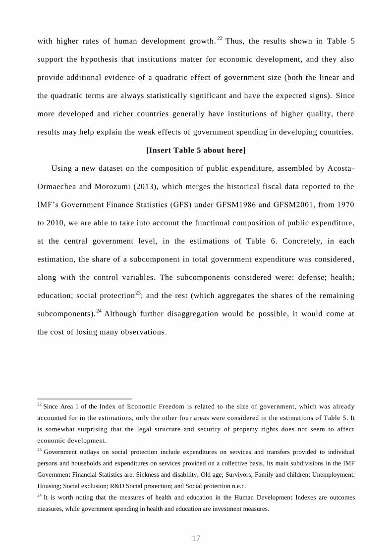
Using a new dataset on the composition of public expenditure, assembled by Acosta -

Ormaechea and Morozumi (2013), which merges the historical fiscal data reported to the

IMF’s Government Finance Statistics (GFS) under GFSM1986 and GFSM2001, from 1970

to 2010, we are able to take into account the functional composition of public expenditure,

at the central government level, in the estimations of Table 6. Concretely, in each

estimation, the share of a subcomponent in total government expenditure was considered ,

along with the control variables. The subcomponents considered were: defense; health;

education; social protection23

; and the rest (which aggregates the shares of the remaining

subcomponents).24

Although further disaggregation would be possible, it would come at

the cost of losing many observations.

22

Since Area 1 of the Index of Economic Freedom is related to the size of government, which was already

accounted for in the estimations, only the other four areas were considered in the estimations of Table 5. It

is somewhat surprising that the legal structure and security of property rights does not seem to affect

economic development.

23 Government outlays on social protection include expenditures on services and transfers provided to individual

persons and households and expenditures on services provided on a collective basis. Its main subdivisions in the IMF

Government Financial Statistics are: Sickness and disability; Old age; Survivors; Family and children; Unemployment;

Housing; Social exclusion; R&D Social protection; and Social protection n.e.c.

24 It is worth noting that the measures of health and education in the Human Development Indexes are outcomes

measures, while government spending in health and education are investment measures.

18

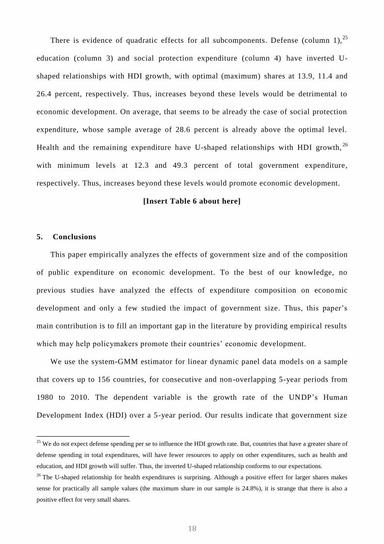
There is evidence of quadratic effects for all subcomponents. Defense (column 1),25

education (column 3) and social protection expenditure (column 4) have inverted U-

shaped relationships with HDI growth, with optimal (maximum) shares at 13.9, 11.4 and

26.4 percent, respectively. Thus, increases beyond these levels would be detrimental to

economic development. On average, that seems to be already the case of social protection

expenditure, whose sample average of 28.6 percent is already above the optimal level.

Health and the remaining expenditure have U-shaped relationships with HDI growth,26

with minimum levels at 12.3 and 49.3 percent of total government expenditure,

respectively. Thus, increases beyond these levels would promote economic development.

[Insert Table 6 about here]

5. Conclusions

This paper empirically analyzes the effects of government size and of the composition

of public expenditure on economic development. To the best of our knowledge, no

previous studies have analyzed the effects of expenditure composition on economic

development and only a few studied the impact of government size. Thus, this paper’s

main contribution is to fill an important gap in the literature by providing empirical results

which may help policymakers promote their countries’ economic development.

We use the system-GMM estimator for linear dynamic panel data models on a sample

that covers up to 156 countries, for consecutive and non-overlapping 5-year periods from

1980 to 2010. The dependent variable is the growth rate of the UNDP’s Human

Development Index (HDI) over a 5-year period. Our results indicate that government size

25

We do not expect defense spending per se to influence the HDI growth rate. But, countries that have a greater share of

defense spending in total expenditures, will have fewer resources to apply on other expenditures, such as health and

education, and HDI growth will suffer. Thus, the inverted U-shaped relationship conforms to our expectations.

26 The U-shaped relationship for health expenditures is surprising. Although a positive effect for larger shares makes

sense for practically all sample values (the maximum share in our sample is 24.8%), it is strange that there is also a

positive effect for very small shares.

19

has a quadratic (inverted U-shaped) effect on the HDI growth rate, especially in developed

and high income countries. Thus, in these countries, excessive government size is

detrimental to economic development. Regarding expenditure composition, we find that

the shares of defense, education and social protection expense in total public expenditure

have inverted U-shaped relationships with development, while health and the aggregated

remaining expenses have U-shaped relationships. The latter may result from the fact that

those remaining expenditures include transport and communication, which is generally

regarded as productive and growth-inducing expenditure.

It is also interesting that these results do not robustly hold when the dependent

variable is GDP per capita growth. This difference in results may be due to the fact that

the Human Development Index is a more comprehensive measure. That is, although GDP

per capita is used to compute the HDI (see the Appendix), the latter also takes into

account the difference in GDP per capita between the richer and poorer countries, and

indexes for life expectancy and education. Thus, government expenditures in these areas

which lead to increases in life expectancy and schooling have a direct positive effect on

the HDI, while their effects on GDP growth may take longer to materialize and be

somewhat smaller.

Since public resources are scarce, and we find that greater sizes of government

beyond an optimal point have a detrimental effect on human development, the major

policy implication of our results is that governments should worry more about how they

spend resources than on how much they spend. Regarding the composition of spending,

greater shares of spending in health and education have the potential to generate higher

development levels, but great attention must be paid to the efficiency of public spending

and to covering most of the population. Our results indicate that better institutions are

associated with higher human development growth. This may be due to the fact that public

spending tends to be more efficient and have more general coverage in countr ies with

20

better institutions and governance, as there is smaller incidence of wasteful spending, rent -

seeking activities, and state capture by elites. Regarding the latter, greater public spending

will not produce the desired development effects if a considerable share of the population

does not benefit from it. As the 2004 World Development Report suggests, governments

should make services work also for the poor (World Bank, 2004).

Acknowledgements

The authors wish to thank Atsuyoshi Morozumi, participants at the 2013 Congress of the

International Institute of Public Finance, and three anonymous referees for very helpful comments,

and Atsuyoshi Morozumi and Santiago Acosta-Ormaechea for sharing their data on the composition

of public expenditure. The authors are also thankful for the financial support provided by ERDF

funds through the Operational Program Factors of Competitiveness - COMPETE and by the

Portuguese Foundation for Science and Technology (FCT) under research grants PEst-

C/EGE/UI3182/2011 and PTDC/EGE-ECO/118501/2010.

21

REFERENCES

Acemoglu, D., Johnson, S. and Robinson, J. (2005). Institutions as the fundamental cause

of long-run growth. In Aghion, P. e Durlauf, S. (eds.) Handbook of Economic

Growth, 385-472. Elsevier, Amsterdam, The Netherlands.

Acosta-Ormaechea, S. and Morozumi, A. (2013). Can a government enhance long-run growth by

changing the composition of public expenditure? IMF Working Paper WP/13/162.

Afonso, A. and Furceri, D. (2010). Government Size Composition, Volatility and Economic

Growth. European Journal of Political Economy, 26, 517-532.

Afonso, A., Schuknecht, L. and Tanzi, V. (2005). Public Sector Efficiency: An international

comparison. Public Choice, 123, 321-347.

Arellano, M. and Bond, S. (1991). Some Tests of Specification for Panel Data: Monte Carlo

Evidence and an Application to Employment Equations. Review of Economic Studies, 58:

277-297.

Arellano, M. and Bover, S. R. (1995). Another look at the instrumental variable estimation of error-

components models. Journal of Econometrics, 68: 29-51.

Barro, R. (1990). Government Spending in a Simple Model of Endogenous Growth. Journal of

Political Economy, 98(5), S103-S125.

Barro, R. (1991). Economic Growth in a cross section of countries. Quarterly Journal of

Economics, 106, 407-443.

Barro, R. and Sala-i-Martin, X. (1995). Economic Growth. New York: McGraw-Hill.

Bassanini, A., Scarpetta, S. and Hemmings, P. (2001). Economic Growth: the role of policies and

institutions. Panel Data evidence from OECD countries. OECD Economics Department

Working Paper 283.

Blundel, R. and Bond, S. (1998). Initial conditions and moment restrictions in dynamic panel data

models. Journal of Econometrics, 87: 115-143.

Bond, S. (2002). Dynamic panel data models: a guide to micro data methods and practice .

Portuguese Economic Journal 1: 141-162.

Corsetti, G. and Roubini, N. (1996). Optimal Government Spending and Taxation in Endogenous

Growth Models. NBER Working Paper 5851.

22

Davies, A. (2009). Human development and the optimal size of government. The Journal of Socio-

Economics, 38, 326-330.

Easterly, W. and Rebelo, S. (1993). Fiscal policy and economic growth: An empirical investigation.

Journal of Monetary Economics 32(3), 417-458.

Fölster, S. and Henrekson, M. (1999). Growth and the Public Sector: A Critique of the Critics.

European Journal of Political Economy, Volume 15, 337-358.

Fölster, S. and Henrekson, M. (2001). Growth effects of government expenditure and taxation in

rich countries. European Economic Review, 45(8), 1501-1520.

Gwartney, J. and Lawson, R. (2012). Economic Freedom of the World - 2012 Annual Report. Fraser

Institute, Vancouver, BC.

Gwartney, J., Lawson, R. and Holcombe, R. (1998). The Size and Functions of Government and

Economic Growth. Washington: Joint Economic Committee Study.

Hall, R. and Jones, C., 1999. Why do some countries produce so much more output per worker than

others? Quarterly Journal of Economics 114, 83–116.

Hauner, D. and Kyobe, A. (2010). Determinants of Government Efficiency. World Development,

38(11), 1527-1542.

Heitger, B. (2001). The Scope of Government and Its Impact on Economic Growth in OECD

Countries. Kiel Working Paper No. 103.

Heston, A., Summers, R. and Aten, B. (2011). Penn World Table Version 7.0. University of

Pennsylvania: Center for International Comparisons of Production, Income and Prices.

King, R. and Rebelo, S. (1990). Public Policy and Economic Growth: Developing Neoclassical

Implications. The Journal of Political Economy, 98(5), 126-150.

Kneller, R., Bleaney, M. and Gemmel, N. (1999). Fiscal policy and growth: evidence from OECD

countries. Journal of Public Economics 74, 171–190

Labonte, M. (2010). The Size and Role of Government: Economic Issues. CRS Report for

Congress. RL 32162.

Lucas, R. (1988). On the mechanics of economic development. Journal of Monetary Economics,

22, 3-42.

23

Meltzer, A. and Richard, S. (1981). A Rational Theory of the Size of government. The Journal of

Political Economy, 89(5), 914-927.

Mourmouras, A. and Rangazas, P. (2009). Fiscal Policy and Economic Development.

Macroeconomic Dynamics 13(4), 450-476.

Nafziger, E. W. (2012). Economic Development. 5th

ed. New York: Cambridge University Press.

North, D. (1990). Institutions, Institutional Change and Economic Performance. Cambridge

University Press, Cambridge, UK.

Peltzman, S. (1980). The Growth of Government. Journal of Law and Economics, 23(2), 209-287.

Pomfret, R. (1997). Development Economics. Hertfordshire: Prentice Hall Europe.

Seers, D. (1969). The Meaning of Development. International Development Review, 11(4), 3-4.

Tanzi, V. and Schuknecht, L. (2000). Public Spending in the 20th Century. Cambridge: The Press

Syndicate of the University of Cambridge.

Tanzi, V. and Zee, H. (1997). Fiscal Policy and Long-Run Growth. IMF Staff Papers, 44(2), 179-

209.

Ulbrich, H. (2003). Public Finance: in Theory and Practice. Mason, Ohio: Thomson.

UNDP - United Nations Development Program (2011). Human Development Report. New York,

NY: United Nations.

Verbeek, M. (2008). A Guide to Modern Econometrics (3ª ed.). Chichester: John Wiley and Sons,

Ltd.

World Bank (2004). World Development Report: Making Services Work for the Poor. Washington,

DC: The World Bank.

Yavas, A. (1998). Does too much government investment retard the economic development of a

country? Journal of Economic Studies, 25(4), 296-330.

24

APPENDIX

√

√

Source: UNDP (2011)

25

Table 1: HDI versus GNI Index

Country GNI per capita

(2008 PPP US$)

GNI per

capita

Rank

HDI

value

HDI

Rank

GNI Rank

minus HDI

Rank

Qatar 79 426 2 0.803 38 - 36

United Arab Emirates 58 006 4 0.815 32 - 28

Kuwait 55 719 5 0.771 47 - 42

Brunei Darussalam 49 915 7 0.805 37 - 30

New Zealand 25 438 33 0.907 3 +30

Source: UNDP (2011).

26

Table 2: Descriptive Statistics

Variable Observations Mean Standard

Deviation Minimum Maximum

HDI growth rate 618 .009 .008 -.047 .073

Log(HDI) (-1) 618 -.588 .376 -180 -.070

Size of government (UN) 610 .156 .064 .025 .729

Size of government (PWT-KG) 618 .105 .059 .026 .620

Size of government (PWT-NA) 618 .153 .193 .014 .860

Investment growth 618 -.016 .129 -.686 .951

Infant mortality 618 54.491 60.277 3.000 310.500

Secondary school enrollment 618 67.707 32.658 2.984 155.578

Area 2: Legal structure and security

of property rights 512 5.909 1.983 1.143 9.624

Area 3: Access to sound money 525 7.738 1.579 1.213 9.838

Area 4: Freedom to trade

internationally

504 6.730 1.829 0.000 9.565

Area 5: Regulation of credit, labor,

and business 523 6.263 1.096 2.615 8.781

Defense (% T.Expense) 237 .074 .061 .007 .377

Health (% T.Expense) 237 .091 .056 .005 .248

Education (% T.Expense) 237 .113 .055 .016 .246

Social Protection (% T.Expense) 237 .286 .156 .006 .622

Rest (% T.Expense) 237 .434 .139 .206 .848

Sources: Acosta-Ormaechea and Morozumi (2013), Gwartney and Lawson (2012), PWT 7.0 (Heston et

al. 2011), UNDP (2011), World Development Indicators (World Bank).

27

Table 3: Government size and Economic Development

(1) (2) (3) (4)

VARIABLES UN PWT-kg PWT-NA UN

Log(HDI) (-1) -0.0590*** -0.0630*** -0.0611***

(-4.607) (-5.090) (-3.934)

Log(GDPpc) (-1) -0.0219***

(-3.962)

Size of government 0.138* 0.136* 0.0117* -0.620*

(1.862) (1.717) (1.958) (-1.898)

Size of government2

-0.404** -0.431** -0.00487* 0.975

(-2.032) (-2.007) (-1.776) (1.199)

Investment growth 0.0135** 0.0113** 0.0190*** 0.0539**

(2.332) (2.472) (3.823) (1.991)

Infant mortality -0.000197*** -0.000209** -0.000191** 0.000109

(-3.036) (-2.527) (-2.408) (0.752)

Secondary school

enrollment

0.000184** 0.000191** 0.000210*** 0.00125***

(2.327) (2.544) (2.792) (4.326)

Period 2 0.00258* 0.00127 0.00325** 0.194***

(1.839) (0.881) (2.425) (4.969)

Period 3 0.000899 2.68e-05 0.00115 0.195***

(0.663) (0.0214) (0.971) (5.081)

Period 4 0.00255** 0.00170 0.00315*** 0.189***

(2.451) (1.473) (3.412) (4.975)

Period 5 0.00191** 0.00128 0.00327*** 0.194***

(2.245) (1.272) (4.056) (5.183)

Period 6 0.00169** 0.00167** 0.00343*** 0.192***

(2.047) (2.046) (5.341) (5.102)

Constant -0.0384*** -0.0381*** -0.0338*** 0.181***

(-3.469) (-3.618) (-3.249) (4.748)

# Observations 610 618 618 610

# Countries 156 156 156 156

# Instruments 99 90 87 99

Hansen Test 0.300 0.441 0.256 0.371

Diff.-Hansen Test 0.319 0.365 0.427 0.507

AR (1) 0.0491 0.0467 0.0286 0.000249

AR (2) 0.190 0.194 0.202 0.371

Sources: see Table 2.

Notes:

- System-GMM estimations for dynamic panel-data models. Sample period: 1980-2010;

- The dependent variable in columns 1 to 3 is the growth of the HDI, while in column 4 it is

the growth rate of GDP per capita;

- All explanatory variables were treated as endogenous. Their lagged values were used as

instruments in the first-difference equations and their lagged first-differences were used in

the levels equation;

- Two-step results using robust standard errors corrected for finite samples.

- The government size proxy used is indicated in the top of the respective column;

- t-statistics are in parenthesis. Significance level at which the null hypothesis is rejected:

***, 1%; **, 5%, and *, 10%.

28

Table 4: Interactions with Dummies for Development and Income Levels

(1) (2) (3) (4)

VARIABLES UN PWT-kg UN PWT-kg

Log(HDI) (-1) -0.0634*** -0.0623*** -0.0672*** -0.0782***

(-6.034) (-6.174) (-5.994) (-5.620)

Size of government*Developed 0.142* 0.122*

(1.665) (1.675)

(Size of government*Developed)2

-0.408* -0.590*

(-1.728) (-1.751)

Size of government*Developing 0.0301 -0.0326

(0.323) (-0.742)

(Size of government*Developing)2

-0.120 0.0359

(-0.471) (0.357)

Size of government*High Income 0.112* 0.137*

(1.815) (1.724)

(Size of government*High Income)2

-0.303* -0.815**

(-1.731) (-1.994)

Size of government*Low Income -0.0385 -0.0988***

(-0.665) (-2.637)

(Size of government*Low Income)2

0.0384 0.197***

(0.208) (3.058)

Investment growth 0.0142** 0.0165*** 0.0121** 0.0116**

(2.141) (3.331) (2.396) (2.356)

Infant mortality -0.000174*** -0.000212*** -0.000186*** -0.000230***

(-3.083) (-3.384) (-3.407) (-3.329)

Secondary school enrollment 0.000143** 8.26e-05* 0.000113** 0.000164***

(2.538) (1.731) (2.099) (2.973)

Constant -0.0355*** -0.0237*** -0.0309*** -0.0345***

(-3.355) (-3.560) (-3.396) (-4.363)

# Observations 610 618 610 618

# Countries 156 156 156 156

# Instruments 82 84 56 58

Hansen Test 0.113 0.473 0.311 0.299

Diff.-Hansen Test 0.214 0.692 0.135 0.552

AR (1) 0.0904 0.0435 0.0864 0.0387

AR (2) 0.191 0.190 0.195 0.199

Sources: see Table 2.

Notes:

- System-GMM estimations for dynamic panel-data models. Sample period: 1980-2010;

- All explanatory variables were treated as endogenous. Their lagged values were used as instruments in the

first-difference equations and their lagged first-differences were used in the levels equation. Period dummies

were included;

- Two-step results using robust standard errors corrected for finite samples.

- The government size proxy used is indicated in the top of the respective column;

- t-statistics are in parenthesis. Significance level at which the null hypothesis is rejected: ***, 1%; **, 5%,

and *, 10%.

29

Table 5: Economic Development, Government Size and Economic Freedom

(1) (2) (3) (4)

Log(HDI) (-1) -0.0597*** -0.0596*** -0.0647*** -0.0740***

(-5.753) (-5.100) (-5.368) (-6.028)

Size of government 0.272** 0.257* 0.167* 0.272**

(2.250) (1.742) (1.851) (2.078)

Size of government2

-0.775** -0.755* -0.510* -0.774**

(-2.271) (-1.818) (-1.923) (-2.119)

Investment growth 0.0126*** 0.00733 0.000328 0.00733

(2.595) (1.264) (0.0430) (1.303)

Infant mortality -0.00023*** -0.00021*** -0.00023*** -0.00027***

(-3.973) (-3.294) (-4.102) (-4.662)

Secondary school enrollment 0.000131** 0.000139** 0.000156*** 0.000212***

(2.456) (2.191) (2.977) (3.622)

Area 2: Legal structure and security

of property rights

2.64e-05

(0.0414)

Area 3: Access to sound money

0.00125*

(1.903)

Area 4: Freedom to trade

internationally

0.00183**

(2.113)

Area 5: Regulation of credit, labor,

and business

0.00197**

(1.984)

Constant -0.0444*** -0.0541*** -0.0509*** -0.0687***

(-3.720) (-3.243) (-4.022) (-3.520)

# Observations 504 517 496 515

# Countries 114 115 114 115

# Instruments 70 84 99 99

Hansen Test 0.779 0.216 0.510 0.778

Diff.Hansen Test 0.930 0.395 0.843 0.859

AR (1) 0.0411 0.115 0.119 0.0868

AR (2) 0.155 0.192 0.434 0.226 Sources: see Table 2.

Notes:

- System-GMM estimations for dynamic panel-data models. Sample period: 1980-2010;

- All explanatory variables were treated as endogenous. Their lagged values were used as instruments in the

first-difference equations and their lagged first-differences were used in the levels equation. Period

dummies were included;

- Two-step results using robust standard errors corrected for finite samples.

- The government size proxy was that of the United Nation database;

- t-statistics are in parenthesis. Significance level at which the null hypothesis is rejected: ***, 1%; **, 5%,

and *, 10%.

30

Table 6: Composition of Public Expenditure and Economic Development

(1) (2) (3) (4) (5)

Log(HDI) (-1) -0.0341*** -0.0460*** -0.0442*** -0.0394*** -0.0445***

(-7.259) (-6.744) (-7.873) (-4.610) (-7.807)

Defense (% T.Expense) 0.0478*

(1.924)

Defense (% T.Expense)2

-0.172**

(-2.470)

Health (% T.Expense) -0.0810**

(-2.194)

Health (% T.Expense)2

0.329**

(2.105)

Education (% T.Expense) 0.0872*

(1.704)

Education (% T.Expense)2

-0.381*

(-1.728)

Social Protection (%

T.Expense)

0.0437*

(1.874)

Social Protection (%

T.Expense)2

-0.0826**

(-2.025)

Rest (% T.Expense) -0.0457*

(-1.793)

Rest (% T.Expense)2

0.0463*

(1.904)

Investment growth 0.0105* 0.0145*** 0.0139*** 0.00764 0.0135***

(1.865) (4.132) (3.522) (1.121) (2.696)

Infant mortality -7.56e-05** -0.00018*** -0.00015*** -0.00012** -0.00017***

(-1.963) (-4.131) (-3.407) (-2.439) (-5.140)

Secondary school

enrollment

8.68e-05** 0.000107*** 9.17e-05* 0.000120*** 9.73e-05***

(2.126) (3.084) (1.950) (2.750) (2.726)

Constant -0.0152*** -0.0134*** -0.0195*** -0.0207*** -0.00581

(-3.297) (-2.627) (-3.907) (-3.137) (-0.980)

# Observations 237 237 237 237 237

# Countries 79 79 79 79 79

# Instruments 58 60 69 43 66

Hansen Test 0.508 0.795 0.380 0.354 0.472

Diff.-Hansen Test 0.652 0.775 0.618 0.787 0.641

AR (1) 0.226 0.201 0.137 0.261 0.157

AR (2) 0.408 0.190 0.459 0.469 0.343 Sources: see Table 2.

Notes:

- System-GMM estimations for dynamic panel-data models. Sample period: 1980-2010;

- All explanatory variables were treated as endogenous. Their lagged values were used as instruments in the

first-difference equations and their lagged first-differences were used in the levels equation. Period

dummies were included;

- Two-step results using robust standard errors corrected for finite samples.

- t-statistics are in parenthesis. Significance level at which the null hypothesis is rejected: ***, 1%; **, 5%,

and *, 10%.