NBER WORKING PAPER SERIES

ELECTORAL MANIPULATION VIA EXPENDITURE COMPOSITION:THEORY AND EVIDENCE

Allan DrazenMarcela Eslava

Working Paper 11085http://www.nber.org/papers/w11085

NATIONAL BUREAU OF ECONOMIC RESEARCH1050 Massachusetts Avenue

Cambridge, MA 02138January 2005

We wish to thank Miguel Rueda for excellent research assistance, and participants at seminars at Universityof Maryland and Hebrew University of Jerusalem, the Vth meeting of the Political Economy Network ofLACEA, and the 9th Annual Meeting of LACEA for many useful comments. The first author wishes to thankNational Science Foundation, grant 418412, the Israel Science Foundation, and the Yael Chair ofComparative Economics, Tel Aviv University, for financial support. The views expressed herein are thoseof the author(s) and do not necessarily reflect the views of the National Bureau of Economic Research.

© 2005 by Allan Drazen and Marcela Eslava. All rights reserved. Short sections of text, not to exceed twoparagraphs, may be quoted without explicit permission provided that full credit, including © notice, is givento the source.

Electoral Manipulation via Expenditure Composition: Theory and EvidenceAllan Drazen and Marcela EslavaNBER Working Paper No. 11085January 2005JEL No. ID72, E62, D78

ABSTRACT

We present a model of the Political Budget Cycle in which voters and politicians have preferences

for different types of government spending. Incumbents try to influence voters by changing the

composition of government spending, rather than overall spending or revenues. Rational voters may

support an incumbent who targets them with spending before the election even though such spending

may be due to opportunistic manipulation, because it can also reflect sincere preference of the

incumbent for types of spending voters favor. Classifying expenditures into those which are targeted

to voters and those that are not, we provide evidence supporting our model in data on local public

finances for all Colombian municipalities. Our findings indicate both a pre-electoral increase in

targeted expenditures, combined with a contraction of other types of expenditure, and a voter

response to targeting.

Allan Drazen

Department of Economics

University of Maryland

College Park, MA 20742

and NBER

drazen@econ.umd.edu

Marcela Eslava

Universidad de Los Andes

Carrera 1 N 18A-70, Bloque C

Bogota, Colombia

eslava@uniandes.edu.co

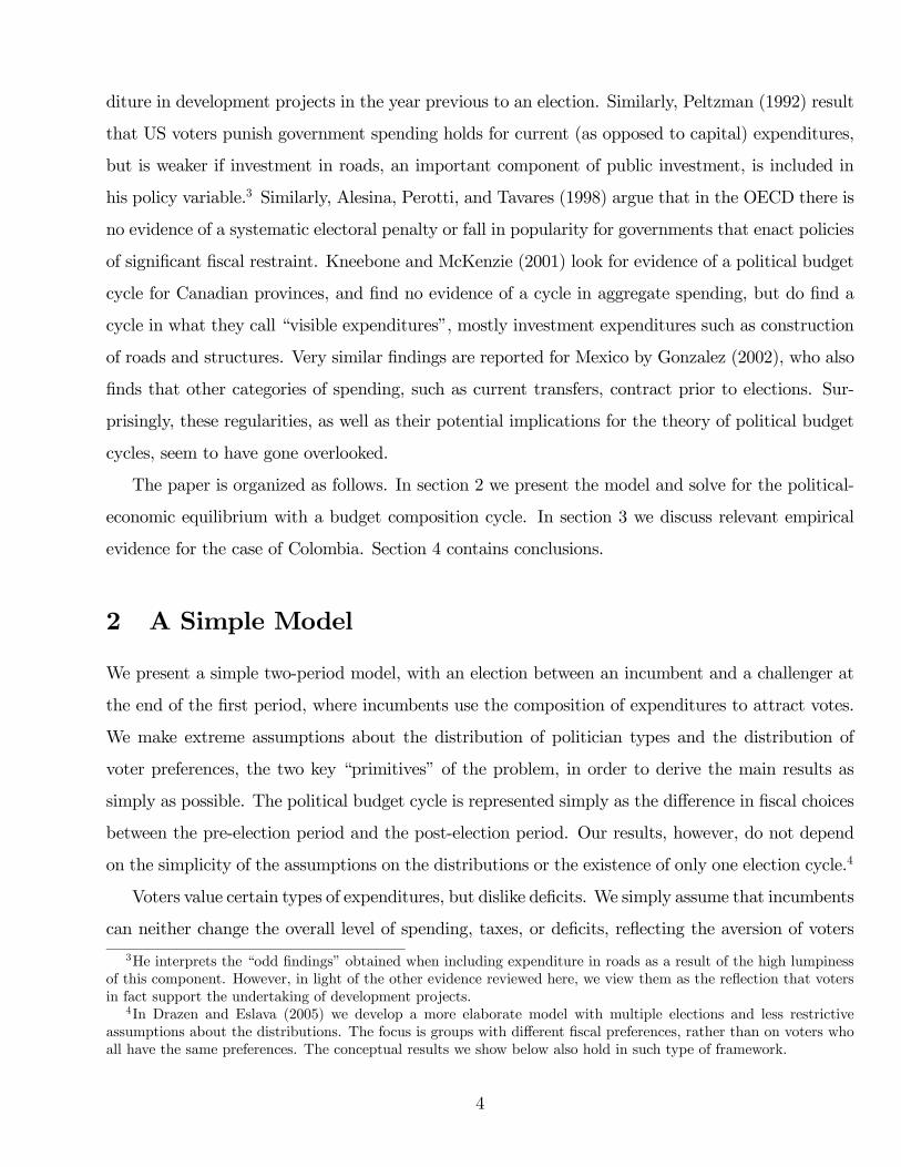
1 Introduction

It is widely believed that incumbent politicians increase public spending before elections to improve

the chances that they (or their party) will be re-elected. It is not obvious however why such changes

would generate electoral benefits if voters are rational. Rational individuals should vote on the basis

of the policies they expect each candidate will undertake after the election, rather than on past

outcomes. Furthermore, they should anticipate eventual incentives of the incumbent to manipulate

fiscal policy before an election, and therefore not respond to such manipulation.

To reconcile fiscal expansions before elections with voter rationality, Rogoff (1990) and Rogoff

and Sibert (1988) suggested that high pre-election expenditures that are visible to voters may serve

as a signal of “competence”, meaning the ability to provide more public goods. A politician has

private information about his own level of competence, which exhibits some persistence over time.

Voters face a signal extraction problem: they cannot observe competence directly and therefore use

spending on some types of goods before an election to infer post-electoral competence. As a result,

an incumbent running for re-election has an incentive to increase spending in those items voters

observe. For instance, while in Rogoff (1990) voters observe some types of government expenditure,

in Shi and Svensson (2002) they observe the overall level of spending, but not all voters observe

the deficit. In this approach, a fiscal expansion before an election can be an effective tool to gain

support from imperfectly informed voters.

However, the view that increasing aggregate spending or deficits before an election is an effective

tool to gain votes has been questioned. Peltzman (1992) shows that voters in the US are less likely to

support a local official who has increased overall spending before the election. Brender (2003) finds

evidence that, when voters in Israel are able to effectively monitor the fiscal choices of local officials,

incurring in large pre-election deficits actually harms an incumbent’s chances of being re-elected.

Brender and Drazen (2005) find in a large panel of countries that deficits over the previous three

years reduce an incumbent’s re-election chances in developed countries and established democracies.

Similarly, our findings below indicate that the share of votes received by the incumbent’s party is

decreasing in the level of the deficit in the year preceding the election. It would therefore appear

that well informed voters not only are hard to “buy” through spending increases, they are actually

averse to high overall government spending and deficits.

Politicians appear to be aware of this. Brender and Drazen (2004) show that empirical results

1

suggesting that election-year increases in spending or deficits are a widespread phenomenon (see Shi

and Svensson [2002a, 2002b] and Persson and Tabellini [2003]) are driven by the experience of “new”

democracies, that is, by the first few elections in countries that have made the transition to democ-

racy.1 Once new democracies are removed from a larger sample, no statistically significant political

deficit cycle is found among established democracies. One is left with the question of whether there

is room for electoral manipulation of the budget in established democracies, characterized by well

informed and sophisticated voters.

We therefore suggest a different approach, where political budget cycles emerge even if voters

dislike high government expenditure and budget deficits, and even if they are able (unlike the models

in the Rogoff tradition) to perfectly observe fiscal policy. Political manipulation takes the form of

changing the composition of government spending, allowing its overall level (and the deficit) to

remain unchanged. Voters value some goods more than others, so that an opportunistic politician

may be induced to shift the composition of pre-election spending towards these goods. What voters

want to infer is then whether a politician’s preferences over the composition of the budget are actually

close to their own or whether his pre-election spending choices are meant simply to gain votes. This

would explain why there is an incentive for incumbents to increase some types of spending, even

if voters are “fiscal conservatives” in the sense of being averse to large overall levels of government

spending. Electoral manipulation arises even with fully rational voters, given that they must try

to infer the incumbent’s preferences from his fiscal behavior. Voters thus rationally respond to

pre-election increases in their most preferred types of spending.2

The strength of the political cycle in our model depends on the distribution of ideological prefer-

ences, and on the amount of information voters have about the political environment. As is probably

not surprising, targeted spending increases more prior to elections the larger is the fraction of swing

voters in the electorate. However, in our model voters anticipate this behavior. As a result, when

a large fraction of voters is undecided, high levels of targeted spending are recognized as being

politically motivated, rather than being interpreted as an effective signal of the politician’s fiscal

1Akhmedov and Zhuravskaya (2004) find an electoral expenditure cycle in regional elections in Russia after itstransition to democracy, which becomes smaller with each new round of regional elections.

2Lindbeck and Weibull (1987) and Dixit and Londregan (1996) present formal models of balanced-budget targetingof voter groups, but these models assume that a politician can commit himself to a post-electoral fiscal policy. Thereis no voter inference problem about post-electoral utility based on pre-electoral economic magnitudes, so the questionof why rational, forward-looking voters who are targeted before the election vote for the incumbent is not reallyanswered.

2

preferences. This creates a natural limit to electorally motivated increases in spending. On the

other hand, the incumbent’s ability to engage in this form of electoral manipulation is increased by

its access to privileged information about the political environment. In particular, politicians in our

model may have more information than voters about the potential electoral benefits of increasing

targeted expenditures (i.e. how “swing” voters are). This increases their ability to obtain politi-

cal support from increases in targeted expenditures, as voters cannot determine if the targeting is

politically motivated.

In a related paper (Drazen and Eslava [2005]), we develop a model where expenditures can be

targeted to different groups with heterogeneous preferences, and politicians have preferences over

different interest groups. As a result, before elections the composition of expenditures is tilted

towards the goods favored by groups with greater electoral importance. The incumbent’s privileged

information about the relative electoral impact of targeting one group or another gives him the

ability to raise votes from targeting those groups with spending, even though all voters are aware of

the electoral incentives he faces.

We present empirical evidence below on these electoral composition effects, using a new data

set we compiled on local government spending and local elections for all Colombian municipalities.

Obviously, a classification of government expenditure into targeted and non-targeted expenditures

is not readily available, or straightforward. In fact, all government expenditures (probably with the

exception of interest payments on external debt) generate benefits for at least some groups in society,

even if it is only to those individuals who provide the services and goods to the government. However,

we argue that some of the components of expenditure that local governments report separately — in

Colombia in particular, most categories of investment expenditures — are more likely to reflect what

we call targeted expenditures than others. Consistent with our model, we find that most categories

of investment of spending show pre-election expansions, while many components of current spending

contract. Furthermore, we investigate the effect of pre-election fiscal policy on the share of votes

received by the incumbent party. We find evidence that voters reward incumbents who increase

investment spending, but only to the extent that they do so without running large election-year

deficits.

Our results on electoral composition effects are consistent with some previous findings. Brender

(2003) finds that voters in Israel penalize election year deficits, but also that they reward high expen-

3

diture in development projects in the year previous to an election. Similarly, Peltzman (1992) result

that US voters punish government spending holds for current (as opposed to capital) expenditures,

but is weaker if investment in roads, an important component of public investment, is included in

his policy variable.3 Similarly, Alesina, Perotti, and Tavares (1998) argue that in the OECD there is

no evidence of a systematic electoral penalty or fall in popularity for governments that enact policies

of significant fiscal restraint. Kneebone and McKenzie (2001) look for evidence of a political budget

cycle for Canadian provinces, and find no evidence of a cycle in aggregate spending, but do find a

cycle in what they call “visible expenditures”, mostly investment expenditures such as construction

of roads and structures. Very similar findings are reported for Mexico by Gonzalez (2002), who also

finds that other categories of spending, such as current transfers, contract prior to elections. Sur-

prisingly, these regularities, as well as their potential implications for the theory of political budget

cycles, seem to have gone overlooked.

The paper is organized as follows. In section 2 we present the model and solve for the political-

economic equilibrium with a budget composition cycle. In section 3 we discuss relevant empirical

evidence for the case of Colombia. Section 4 contains conclusions.

2 A Simple Model

We present a simple two-period model, with an election between an incumbent and a challenger at

the end of the first period, where incumbents use the composition of expenditures to attract votes.

We make extreme assumptions about the distribution of politician types and the distribution of

voter preferences, the two key “primitives” of the problem, in order to derive the main results as

simply as possible. The political budget cycle is represented simply as the difference in fiscal choices

between the pre-election period and the post-election period. Our results, however, do not depend

on the simplicity of the assumptions on the distributions or the existence of only one election cycle.4

Voters value certain types of expenditures, but dislike deficits. We simply assume that incumbents

can neither change the overall level of spending, taxes, or deficits, reflecting the aversion of voters

3He interprets the “odd findings” obtained when including expenditure in roads as a result of the high lumpinessof this component. However, in light of the other evidence reviewed here, we view them as the reflection that votersin fact support the undertaking of development projects.

4In Drazen and Eslava (2005) we develop a more elaborate model with multiple elections and less restrictiveassumptions about the distributions. The focus is groups with different fiscal preferences, rather than on voters whoall have the same preferences. The conceptual results we show below also hold in such type of framework.

4

to high overall spending and deficits. Targeting voters with one type of spending requires reducing

another type, where we focus on such targeting. The choice of fiscal policy is thus the composition

of the budget.

The incumbent politician has preferences over the composition of the budget which may differ

from those of voters. For simplicity, we assume that all voters have the same preferences over

types of expenditure and receive the same amount of goods, so the heterogeneity of interest over

the budget is between voters and politicians, rather than across groups of voters, as in Drazen and

Eslava (2005). Here, voters differ from one another only in their preferences over policies other than

targeted expenditures (termed “ideology”).

2.1 Voters

An voter trades off ideology over non-fiscal policy, π, and utility from targeted expenditures, gt,

in deciding whether to support a candidate. The idea of targeted expenditures is close to that in

Lindbeck and Weibull (1987) or Dixit and Londregan (1996), but in a setting where expectations of

future policy are key to determining how an individual votes. (See footnote 2.)

Utility of an individual depends on two factors, each of which may be influenced by government

policy. First, there is the consumption of the government supplied good gt ≥ 0 which provides utilitydirectly. (We abstract here from private consumption, since taxes are fixed.) Second, an individual

j also cares about the distance between his most desired position πj over non-fiscal policies (which

is immutable) and the positions πI of the current incumbent I and πC of the challenger. We take

these as fixed and, without loss of generality, assume πI < πC. In the post-election period, either

the initial incumbent I or the challenger C may be in power, depending on the election outcome.

Single period utility of individual j in period t if politician P ∈ I, C is in power may be written:

U jt (P ) = V

¡gPt¢− ¡πj − πP

¢2(1)

where V 0 (·) > 0, V 00 (·) < 0, and gPt is expenditure chosen by policymaker P . A voter j is thus

characterized by πj. (To help in following the exposition, note that V (gPt ) does not depend on j.

Hence in discussing the problem of inferring g2 from g1, we may ignore the index j.)

An individual’s only decision is whether to vote for the incumbent or the challenger, and only in

an election period. We therefore focus on utility as of period 1, when the election takes place. The

5

present expected discounted utility of individual j as of period 1 is:

W j1 = U j

1 (I) + βE1Uj2(P ) (2)

where β is the discount factor, and P ∈ I, C. In the election, a voter prefers the incumbent overthe challenger if he expects to receive more utility from the former in t = 2.

2.2 Politicians

There are two government provided goods: gt; and Kt, a good which the politician values but which

voters do not. One may think, for example, of politicians who value managing a large bureaucracy.

(For simplicity of exposition we call Kt “desks”.) However, the idea we have in mind is more general:

voters may value some government services less than others for many reasons, such as voters’ failure

to recognize the positive externalities these services produce, or the low visibility of some types of

expenditure. The characterization ofKt as total waste in the eyes of voters is simply an extreme way

to capture those differences in the value assigned by voters to different goods and services provided

by the government. Each period, the government thus faces a budget constraint:

T = Kt + gt (3)

where T is a fixed and exogenous level of tax revenue.

The politician’s objective is to maximize a weighted sum of voters’ utility, a fixed value χ of

being in office, and the value of “desks” Kt. We denote by ωPt the weight a politician P puts on

voters relative to desks in period t. A politician P 0s objective in the post-election period, t = 2, can

then be written:

ΩP2 = ωP2

"V (g2) +

NXj=1

¡πj − πP

¢2N

#+ a(K2) + χ (4)

where N is the size of the voting population, which we assume to be constant and a(K) is an

increasing, concave function. We have written this objective in per-capita terms for simplicity.

The weight ωPt, known to the politician but not observed by voters, is crucial to a voter’s choice.

The level of g2 the politician would choose is, by (4), known to be a function of ωP2, so that rational

voters vote on the basis of their beliefs about ωI2 and ωC2. The crucial assumptions in our argument

6

that election-year fiscal policy may be used to gain votes are that the weight the politician puts on

voters’ utility is not observed by the voters (and hence must be inferred), but is correlated over time

(so that fiscal policy observed before the election provides information on the politician’s preferences

and hence spending allocation in the post-election period). Voters must try to infer the value of ωI2

from observations on g1, that is, on expenditures before the election. For clarity of exposition, we

assume the process governing the evolution of the ωPt takes the simplest possible form that satisfies

the conditions discussed above. First, ωPt does not change from t = 1 to t = 2, with ωP1 = ωP2 ≡ ωP

for P ∈ I, C.5 Second, for any politician P , ωP can take on two values: ωP = ω, ω with priorprobabilities Pr(ω = ω) = p and Pr(ω = ω) = (1 − p). We suppose ω > ω, so that a politician of

type ω cares more about targeting expenditures to people (a people politician), while ωP = ω makes

the politician more interested in bureaucracy than targeting (a desks politician).

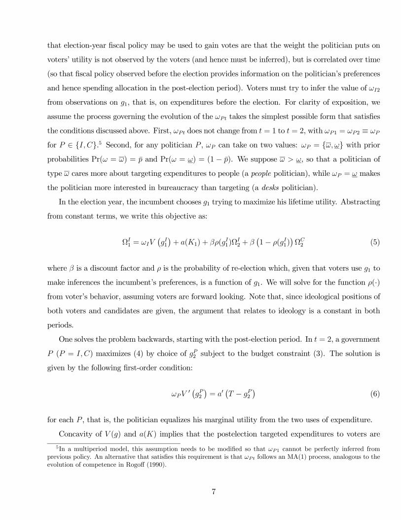
In the election year, the incumbent chooses g1 trying to maximize his lifetime utility. Abstracting

from constant terms, we write this objective as:

ΩI1 = ωIV

¡gI1¢+ a(K1) + βρ(gI1)Ω

I2 + β

¡1− ρ(gI1)

¢ΩC2 (5)

where β is a discount factor and ρ is the probability of re-election which, given that voters use g1 to

make inferences the incumbent’s preferences, is a function of g1. We will solve for the function ρ(·)from voter’s behavior, assuming voters are forward looking. Note that, since ideological positions of

both voters and candidates are given, the argument that relates to ideology is a constant in both

periods.

One solves the problem backwards, starting with the post-election period. In t = 2, a government

P (P = I, C) maximizes (4) by choice of gP2 subject to the budget constraint (3). The solution is

given by the following first-order condition:

ωPV0 ¡gP2 ¢ = a0

¡T − gP2

¢(6)

for each P , that is, the politician equalizes his marginal utility from the two uses of expenditure.

Concavity of V (g) and a(K) implies that the postelection targeted expenditures to voters are

5In a multiperiod model, this assumption needs to be modified so that ωP1 cannot be perfectly inferred fromprevious policy. An alternative that satisfies this requirement is that ωPt follows an MA(1) process, analogous to theevolution of competence in Rogoff (1990).

7

increasing in the weight the politician gives to voter welfare, so that g2(ω) > g2(ω). We will denote

g2(ω) = g, and suppose for simplicity that ω =∞, so that a “people-type” politician always choosesthe maximum level of expenditures possible, that is, g2(ω) = T > g. This assumption simplifies the

solution but, as we discuss later, we could dispense of it and still prove that politicians are expected

to engage in pre-election increases in targeted expenditures.

In the election period, the incumbent chooses g1 to maximize his objective (5), subject to the

budget constraint (3). A politician may then choose a value of g1 different from what he would

choose in the non-election period, if by doing so he can significantly increase his chances of being

reelected, represented by ρ. Given our assumption that ω = ∞, a people politician would providethe maximum possible gt even in the non-election period, so he would not change his policy in

the election period. A desks policymaker (one characterized by ω), however, has two choices. He

may choose g1(ω) = g, his non-election period optimum, but thus reveal his type. Or, he may

choose g1(ω) = T > g to influence the election outcome by mimicking a people policymaker, whom

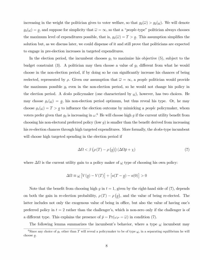
voters prefer given that g2 is increasing in ω.6 He will choose high g if the current utility benefit from

choosing his non-electoral preferred policy (low g) is smaller than the benefit derived from increasing

his re-election chances through high targeted expenditures. More formally, the desks-type incumbent

will choose high targeted spending in the election period if

∆Ω < β¡ρ (T )− ρ

¡g¢¢(∆Ωp+ χ) (7)

where ∆Ω is the current utility gain to a policy maker of ω type of choosing his own policy:

∆Ω ≡ ω£V (g)− V (T )

¤+£a(T − g)− a(0)

¤> 0

Note that the benefit from choosing high g in t = 1, given by the right-hand side of (7), depends

on both the gain in re-election probability, ρ (T ) − ρ¡g¢, and the value of being re-elected. The

latter includes not only the exogenous value of being in office, but also the value of having one’s

preferred policy in t = 2 rather than the challenger’s, which is non-zero only if the challenger is of

a different type. This explains the presence of p = Pr(ωP = ω) in condition (7).

The following lemma summarizes the incumbent’s behavior, where a type ω incumbent may

6Since any choice of g1 other than T will reveal a policymaker to be of type ω, in a separating equilibrium he willchoose g.

8

either pool with a type ω or separate from him:

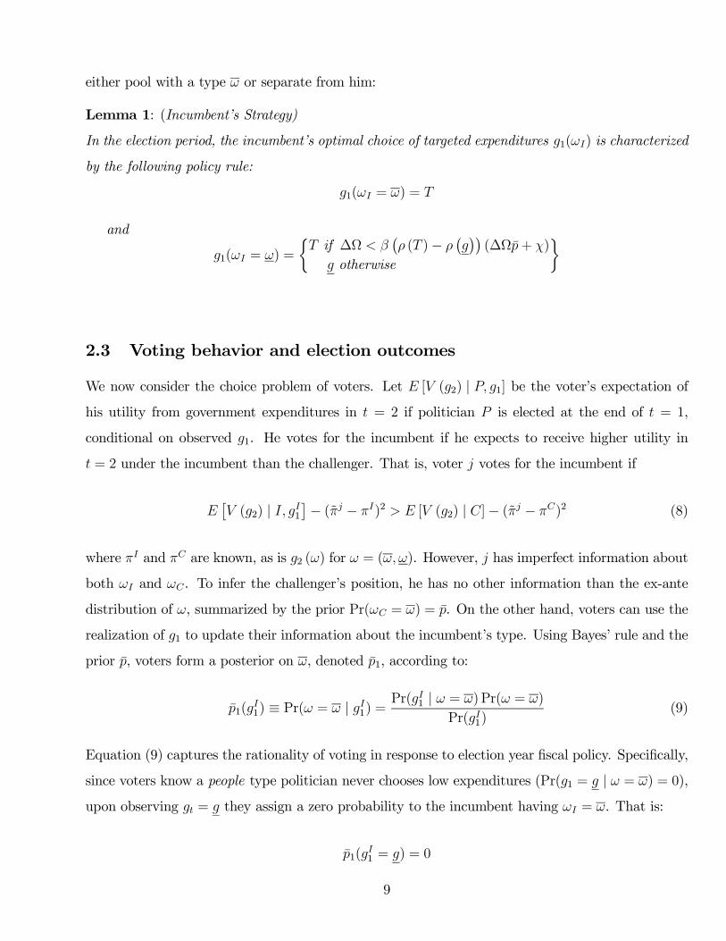
Lemma 1: (Incumbent’s Strategy)

In the election period, the incumbent’s optimal choice of targeted expenditures g1(ωI) is characterized

by the following policy rule:

g1(ωI = ω) = T

and

g1(ωI = ω) =

½T if ∆Ω < β

¡ρ (T )− ρ

¡g¢¢(∆Ωp+ χ)

g otherwise

¾

2.3 Voting behavior and election outcomes

We now consider the choice problem of voters. Let E [V (g2) | P, g1] be the voter’s expectation ofhis utility from government expenditures in t = 2 if politician P is elected at the end of t = 1,

conditional on observed g1. He votes for the incumbent if he expects to receive higher utility in

t = 2 under the incumbent than the challenger. That is, voter j votes for the incumbent if

E£V (g2) | I, gI1

¤− (πj − πI)2 > E [V (g2) | C]− (πj − πC)2 (8)

where πI and πC are known, as is g2 (ω) for ω = (ω, ω). However, j has imperfect information about

both ωI and ωC . To infer the challenger’s position, he has no other information than the ex-ante

distribution of ω, summarized by the prior Pr(ωC = ω) = p. On the other hand, voters can use the

realization of g1 to update their information about the incumbent’s type. Using Bayes’ rule and the

prior p, voters form a posterior on ω, denoted p1, according to:

p1(gI1) ≡ Pr(ω = ω | gI1) =

Pr(gI1 | ω = ω) Pr(ω = ω)

Pr(gI1)(9)

Equation (9) captures the rationality of voting in response to election year fiscal policy. Specifically,

since voters know a people type politician never chooses low expenditures (Pr(g1 = g | ω = ω) = 0),

upon observing gt = g they assign a zero probability to the incumbent having ωI = ω. That is:

p1(gI1 = g) = 0

9

On the other hand,

p1(gI1 = T ) =

p

p+ (1− p)q(10)

where q = Pr(g1 = T | ω = ω) ≤ 1 is the probability that a desk-type politician will choose g1 = T

in the election period. Note the obvious characteristic of Bayesian updating: p1(gI1 = T ) > p iff

q < 1; if q = 1, then p1(T ) = p.

The nature of voters’ posterior beliefs reflects an essential characteristic of the political equilib-

rium. A politician provides high election year expenditures favored by voters in order to convince

them that he would also choose high targeted expenditures after the election. However, this signal

is only effective to in affecting voters’ perceptions if this political incentive is not so large that any

politician would provide high electoral expenditures, no matter what his post-election preferences

will be. Formally, setting gI1 = T has no effect on voting if q = 1.

We can now rewrite the condition under which voter j prefers the incumbent over the challenger,

condition (8), as:

(p1(g1)− p)£V (T )− V (g)

¤> (πj − πI)2 − (πj − πC)2 (11)

where the left hand side represents the expected gain in utility from consumption if the incumbent

is reelected, and the right hand side represents the expected loss in utility from ideological issues if

reelection occurs.

To illustrate, we consider the following simple example of voters’ ideological preferences. Voters

may hold one of three ideological positions: πj = πI , πM = πI+πC

2, πC. Voters with πj = πI are

the incumbent’s core voters: they are sufficiently left of center that they vote for the incumbent

even if he is known to be of the desks type, that is, even if p1 = 0. Analogously, voters with πj = πC

are the challenger’s core voters: they are sufficiently right of center that they vote for the challenger

even if the incumbent is known to be of the people type.7 In the middle are voters with πj = πM ,

swing voters in that they are ideologically as close to one candidate as they are to the other. They

7Formally, using (11), one may derive

πI <πI + πC

2− p

·V (T )− V (g)

2 (πC − πI)

¸and

πC >πI + πC

2+ (1− p)

·V (T )− V (g)

2 (πC − πI)

¸

10

therefore vote on the basis of the fiscal policy they expect to see from the candidates. They vote

for the incumbent if and only if they believe he is more likely than the challenger to have high

ω, that is, iff p1(gI1) > p. (If p1(gI1) = p, swing voters are indifferent between the two candidates,

and vote to reelect the incumbent with some probability r, which will be analyzed in section 2.4,

where we study the equilibrium.8 The crucial point is that swing voters may be led to vote for the

incumbent by high pre-election targeted expenditure, since they assign some probability to the event

that targeting reflects high preference of the incumbent for targeted spending, rather than purely

electoral motives.

We summarize the behavior of voters in:

Lemma 2: (Voting Strategies)

In an election between the incumbent and a challenger, the optimal voting strategy of an individual

j is given by:

1) If eπj = πI individual j votes for the incumbent with probability 1

2) If eπj = πC individual j votes for the challenger with probability 1

3) If eπj = πM ≡ πC+πI

2individual j votes for the incumbent with probability r(g1), where

r(gt) = 1 if p1(g1) > pr(gt) ∈ [0, 1] if p1(g1) = pr(gt) = 0 if p1(g1) < p

where p1(g1) is derived from Bayes’ rule, so that p1(g) = 0, and p1(T ) =p

p+(1−p)q .

Given the voting strategies in lemma 2, election outcomes are easy to characterize. Let φI, φC ,

and φM be the fraction of voters with πj equal to πI , πC , and πM , respectively. The election is

decided by simple majority rule.9 The incumbent obtains φI of the votes if p1 < p, φI + rφM if

p1 = p, and φI + φM of the votes otherwise. In other words, the incumbent is re-elected if p1 > p or

if p1 = p and φI + rφM ≥ 12. For the time being, we assume that both voters and politicians have

perfect information about φI , φM , and φC. We further assume that neither group of core voters

constitute an absolute majority (that is, φI < 12and φC < 1

2), meaning no candidate can win the

election without getting the votes of at least some swing voters, and a candidate supported by all

8These assumptions about ideological preferences are a simple way to capture only some voters being influencedby fiscal policy, while others have such strong positions on other issues that pay no attention to this dimension. Bydividing the population in these three groups we simplify things by having each voter worry only about one policydimension.

9We assume, without loss of generality, that a tie is resolved in favor of the incumbent.

11

swing voters wins the election for sure.

The assumption that no group of core voters is a majority implies that an incumbent who

chooses low pre-election targeted spending will not be reelected, since voters recognize him as being

of the desks type. Hence, ρ¡gI1 = g

¢= 0. If the incumbent chooses gI1 = T and q = 1 (a desks-

type incumbent chooses g1 = T with certainty), then swing voters are indifferent between the two

candidates (p1(gI1) = p). Then, ρ (T ) = 1 if and only if φI + r(gI1)φM ≥ 12, that is, if indifferent

voters choose the incumbent with high enough probability, and there are enough swing voters. On

the other hand , if gI1 = T and q < 1, then p1(gI1) > p, then swing voters strictly prefer the incumbent

and ρ (T ) = 1, since φI + φM > 12.

2.4 Political-economic equilibrium

We can now characterize possible political-economic equilibria. The equilibrium concept is Perfect

Bayesian Equilibrium. A pair of strategies (for the incumbent and voters) is an equilibrium if: 1) the

voter’s strategy is optimal given his beliefs and the incumbent’s strategy in choosing g1, where beliefs

are formed according to Bayes’ rule (that is, his strategy satisfies lemma 2); and 2) the incumbent’s

choice of g1 is optimal given voting behavior and the implied election outcomes (that is, it satisfies

lemma 1).

Given our assumptions, the strategies of a people-type incumbent (ω = ω) and of both types

of core voters (πj = πI , πC) are trivial. We therefore discuss only the strategies of a desks-type

incumbent (ω = ω) and a swing voter (πj = πM). The strategies in lemmas 1 and 2 imply that

there are only three possible types of equilibria:

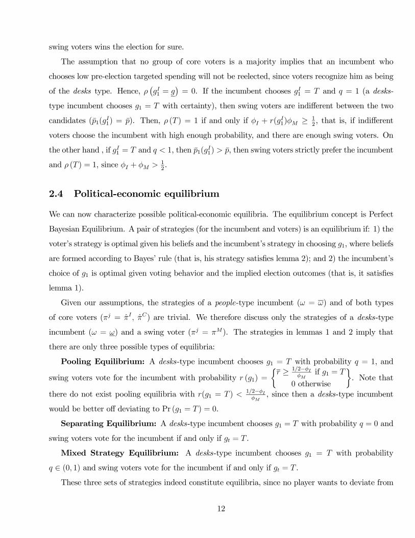
Pooling Equilibrium: A desks-type incumbent chooses g1 = T with probability q = 1, and

swing voters vote for the incumbent with probability r (g1) =

½r ≥ 1/2−φI

φMif g1 = T

0 otherwise

¾. Note that

there do not exist pooling equilibria with r(g1 = T ) < 1/2−φIφM

, since then a desks-type incumbent

would be better off deviating to Pr (g1 = T ) = 0.

Separating Equilibrium: A desks-type incumbent chooses g1 = T with probability q = 0 and

swing voters vote for the incumbent if and only if gt = T .

Mixed Strategy Equilibrium: A desks-type incumbent chooses g1 = T with probability

q ∈ (0, 1) and swing voters vote for the incumbent if and only if gt = T .

These three sets of strategies indeed constitute equilibria, since no player wants to deviate from

12

his strategy, given the other’s strategy.

Proposition 1 describes the equilibrium outcomes depending on whether a desks politician gives

higher value to re-election or to using part of the budget to provide desks rather than expenditure

favored by voters (that is, whether β(p∆Ω+ χ) is greater than or less than ∆Ω, the current utility

gain to a policy maker of ω type of choosing his own policy). As above, the Proposition focuses on

the case where swing voters shift the outcome of the election.

Proposition 1 (Political-Economic Equilibrium)

When neither type of core voter constitutes an absolute majority, there are three possible political-

economic equilibria, depending on parameter values:

Case 1) If β(p∆Ω + χ) > ∆Ω, the optimal strategy for a desks-type incumbent (ω = ω) is

Pr(g1 = T ) = 1. The optimal strategy for swing voters (πj = πM)is to vote for the incumbent with

probability r (g1) =½r ≥ 0.5−φI

φMif g1 = T

0 otherwise

¾Case 2) If β(p∆Ω+χ) = ∆Ω, the optimal strategy for the desks-type incumbent is Pr(g1 = T ) =

q ∈ [0, 1). The optimal strategy for swing voters is r (g1) =½1 if g1 = T

0 otherwise

¾Case 3) If β(p∆Ω+χ) < ∆Ω, the optimal strategy for the desks-type incumbent is Pr(g1 = T ) = 0.

The optimal strategy for swing voters is r (g1) =½1 if g1 = T

0 otherwise

¾.

Proof: Note first that all of these sets of strategies constitute equilibria, since given the voters’

strategy the incumbent’s satisfies Lemma 1, and given the incumbent’s strategy the voters’ satisfies

Lemma 2. Second, to prove that in each case only the type of equilibrium described exists, note that

a separating (pooling) equilibrium cannot be supported if β(p∆Ω + χ) > ∆Ω (< ∆Ω) because the

incumbent would deviate to gt(ω) = T (gt(ω) = g). Moreover, an equilibrium where the incumbent

plays mixed strategies can only exist if he is indifferent between the two policies, which happens iff

β(p∆Ω+ χ) = ∆Ω. ¤

Proposition 1 implies that, provided re-election is valuable enough, a political budget cycle will

exist in which: 1) expenditures targeted to voters are expected to be higher in an election than a

non—election period (the actual level will depend on which type of politician is in office); and 2)

(swing) voters will rationally vote for an incumbent who provides higher targeted expenditures even

though they know that such expenditures may be electorally motivated.

13

Specifically, the proposition shows that if re-election is valuable enough, a desks-type incumbent

will choose g1 = T with some positive probability in an election period, while in the post-election

period, he chooses g2 = g with certainty. This implies that the unconditional expectation of govern-

ment expenditure targeted to voters is higher in the pre-election period, compared to the expected

value for other periods.10 Conversely, non-targeted expenditures are expected to be lower prior to

an election than in other periods. In other words, fiscal policy exhibits cycles with the timing of

the election. These cycles take the form of a change in the composition of expenditures, which shift

towards targeted expenditures in election periods.

Of course, a political budget cycle of this form will only appear if the incentives to influence the

election are large enough. There are two parts to this requirement. The first refers to the preferences

of politicians: electoral manipulation of the budget will only arise if β(p∆Ω + χ) ≥ ∆Ω, so that

the incumbent assigns a large value to being reelected. There is, however, an additional necessary

condition, namely that swing voters (those whose votes depend on fiscal policy) can change the

outcome of the election (φI + φM ≥ 12). The existence of a political budget cycle therefore depends

on the political environment, in particular in the potential electoral benefit from convincing swing

voters of supporting the incumbent.

What is interesting about the apparently obvious condition on the need for a large fraction of

impressionable voters is that, given rational behavior of voters in the model, fiscal manipulation is less

effective to “buy” the vote of any single individual precisely in the cases where there are more swing

voters. In this simplified setting, where our assumptions imply that the probability of re-election

ρ(g1) is either 0 or 1, this is reflected in the fact that p1(T | φI+φM < 12) = 1 ≥ p1(T | φI+φM ≥ 1

2).

Note further that the assumption that ω =∞ (and the implication that a fiscal expansion in an

election year reflects mimicking by the ω politician, whom voters would not prefer if his type were

known) is a convenient modeling device, rather than essential to the existence of the political cycle.

Were ω < ∞, a cycle might take the form of signaling, in that the ω type would choose g in both

election and non-election periods, while the ω type would choose g1 just high enough to separate

himself in an election period. If this is higher than the g2 he would choose in a non-election period,

we have the same type of cycle qualitatively. This latter strategy is the one chosen by Rogoff (1990),

in a model of signaling of competence. Rogoff’s approach has been criticized (unfairly, we think)

10The unconditional expectation value of targeted expenditure is given by E(g1) = T [p+ (1− p) Pr(g1 = T | ω)] +g(1− p) Pr(g1 = g | ω) in an election period, and E(g2) = T p+ g(1− p) in non-election period.

14

in that it is the more competent candidate the one who engages in fiscal manipulation. One could

model the competence problem as one where the less competent may want to mimic the other type,

implying that the less desirable candidate is the one who engages in fiscal manipulation.

2.5 Asymmetric information about the electoral environment

So far, we have assumed φI , φM , and φC are common knowledge, in that the distribution of voter

types is known both to voters and politicians. This assumption is clearly not realistic, as the electoral

effectiveness of providing targeted spending to voters is not known with certainty, and candidates

frequently have better information about it than the public does. We now relax this assumption, and

show that the existence of asymmetric information about the political environment reinforces the

incentives faced by incumbent officials to affect election outcomes through changes in fiscal policy.

Introducing asymmetric information about political characteristics of voters will also eliminate the

unsatisfactory feature that in some of the equilibria with electorally-motivated expenditures (more

exactly in the pooling equilibrium), voters are indifferent between the challenger and the incumbent

who targets them with spending. This is of course a result of our simplifying assumptions, so we

do not take it as a prediction of the model that voters will strictly be indifferent. However, it does

open the question of how do individuals actually vote when they are “indifferent”, since one would

not expect them to simply toss a coin to define which candidate to support.

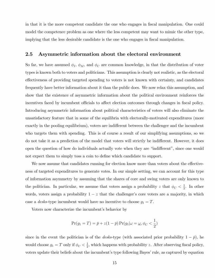
We now assume that candidates running for election know more than voters about the effective-

ness of targeted expenditures to generate votes. In our simple setting, we can account for this type

of information asymmetry by assuming that the shares of core and swing voters are only known to

the politician. In particular, we assume that voters assign a probability z that φC < 12. In other

words, voters assign a probability 1 − z that the challenger’s core voters are a majority, in which

case a desks-type incumbent would have no incentive to choose g1 = T .

Voters now characterize the incumbent’s behavior by

Pr(g1 = T ) = p+ z(1− p) Pr(g1|ω = ω, φC <1

2)

since in the event the politician is of the desks-type (with associated prior probability 1 − p), he

would choose g1 = T only if φC < 12, which happens with probability z. After observing fiscal policy,

voters update their beliefs about the incumbent’s type following Bayes’ rule, as captured by equation

15

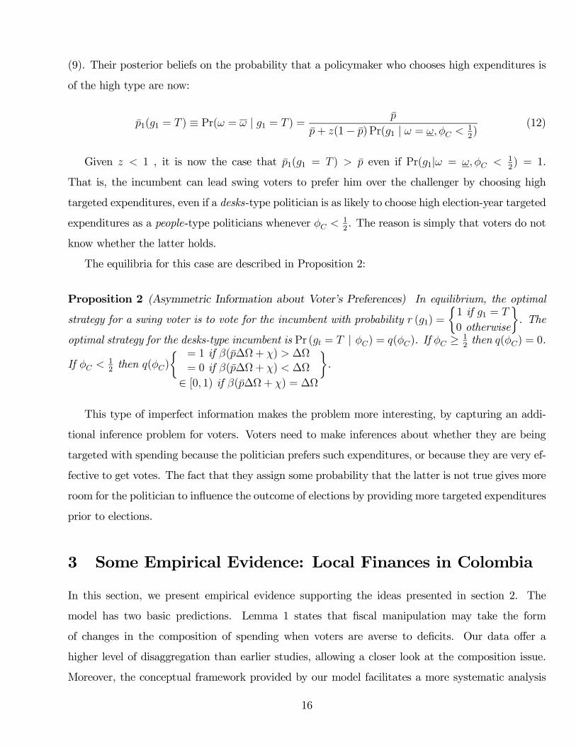
(9). Their posterior beliefs on the probability that a policymaker who chooses high expenditures is

of the high type are now:

p1(g1 = T ) ≡ Pr(ω = ω | g1 = T ) =p

p+ z(1− p) Pr(g1 | ω = ω, φC < 12)

(12)

Given z < 1 , it is now the case that p1(g1 = T ) > p even if Pr(g1|ω = ω, φC < 12) = 1.

That is, the incumbent can lead swing voters to prefer him over the challenger by choosing high

targeted expenditures, even if a desks-type politician is as likely to choose high election-year targeted

expenditures as a people-type politicians whenever φC < 12. The reason is simply that voters do not

know whether the latter holds.

The equilibria for this case are described in Proposition 2:

Proposition 2 (Asymmetric Information about Voter’s Preferences) In equilibrium, the optimal

strategy for a swing voter is to vote for the incumbent with probability r (g1) =½1 if g1 = T

0 otherwise

¾. The

optimal strategy for the desks-type incumbent is Pr (gt = T | φC) = q(φC). If φC ≥ 12then q(φC) = 0.

If φC < 12then q(φC)

½ = 1 if β(p∆Ω+ χ) > ∆Ω

= 0 if β(p∆Ω+ χ) < ∆Ω

∈ [0, 1) if β(p∆Ω+ χ) = ∆Ω

¾.

This type of imperfect information makes the problem more interesting, by capturing an addi-

tional inference problem for voters. Voters need to make inferences about whether they are being

targeted with spending because the politician prefers such expenditures, or because they are very ef-

fective to get votes. The fact that they assign some probability that the latter is not true gives more

room for the politician to influence the outcome of elections by providing more targeted expenditures

prior to elections.

3 Some Empirical Evidence: Local Finances in Colombia

In this section, we present empirical evidence supporting the ideas presented in section 2. The

model has two basic predictions. Lemma 1 states that fiscal manipulation may take the form

of changes in the composition of spending when voters are averse to deficits. Our data offer a

higher level of disaggregation than earlier studies, allowing a closer look at the composition issue.

Moreover, the conceptual framework provided by our model facilitates a more systematic analysis

16

of the different categories of spending. Lemma 2 considers the response of voters to pre-election

changes in budget composition. Hence, we present empirical evidence not only on how elections

affect budget composition, but also on how vote shares respond to these changes.

3.1 The pre-election composition of government expenditure

We concentrate first on the election-year changes in fiscal policy. The model indicates that targeted

spending should rise preceding an election, while other types of spending should contract. We

therefore try to find evidence of pre-election increases in categories of expenditure that most likely

reflect targeted spending, accompanied by contractions in other categories.

The difference between targeted and non-targeted spending is obviously hard to identify in the

data. However, opportunistic targeted expenditures, often known as pork barrel spending, are

most often associated in Colombia with infrastructure development projects: construction of roads,

schools, water plants. Projects of this type are highly visible and benefit specific (yet potentially

large) groups of voters. On the other hand, some current expenditures, such as purchases of supplies

and services, payments to other government agencies, and debt service, can be presumably cut

without visibly hurting large groups of voters. Hence, given the predictions of our model, we would

expect pre-election increases in those categories of spending that capture development projects, and

cuts in at least some categories of current spending.

Testing these hypotheses requires data on different types of government expenditures, covering

observations in both election and non-election years. We compiled a panel of data on government

accounts and electoral outcomes for all municipalities in Colombia (close to 1100 cross-sectional

units) over the period 1987 to 2000. A unique feature of our data compared to those used in previous

studies is the high level of disaggregation of expenditures, allowing us to distinguish different types

of spending. From the point of view of the study of fiscal policy in Colombia, the data are also novel

in incorporating electoral outcomes. A much more detail description of the data can be found in

Eslava (2004).

We choose this “cross-district” approach in a single country, rather than the more usual cross-

country strategy for two reasons. First, the political budget cycle effects we propose are most relevant

at the local level, where spending can be targeted most efficiently. Second, the cross sectional

variability of institutions is much harder to take into account in a multi-country setting than it is

17

for cross sectional units within the same country. Constitutional rules, national laws, electoral and

judicial systems, monetary policy, are all important determinants of the existence and strength of

political budget cycles. These characteristics vary far more across countries than in districts within

the same country, which share all of the above-mentioned institutional characteristics.11

Though the direct re-election of incumbent executive officials is banned in Colombia, electoral

manipulation of fiscal policy is regarded as a usual political practice. Political budget cycles are

thought to arise in Colombia largely due to the actions of the legislative bodies, whose members

are in fact subject of direct re-election (in the case of city councils), or at least have found ways to

circumvent formal restrictions to run for direct re-election (as in the national Congress). Moreover,

there are two reasons why an incumbent mayor who cannot run for re-election has incentives to

manipulate fiscal policy at the end of his term of office. First, an incumbent knows that his decisions

affect his party’s re-election chances (or those of the incumbent’s preferred candidate). Second,

officials usually run for election to other posts in later years, or for re-election to the same post

in the future, and their actions while in office are used by voters in future elections to assess their

preferences and competence.

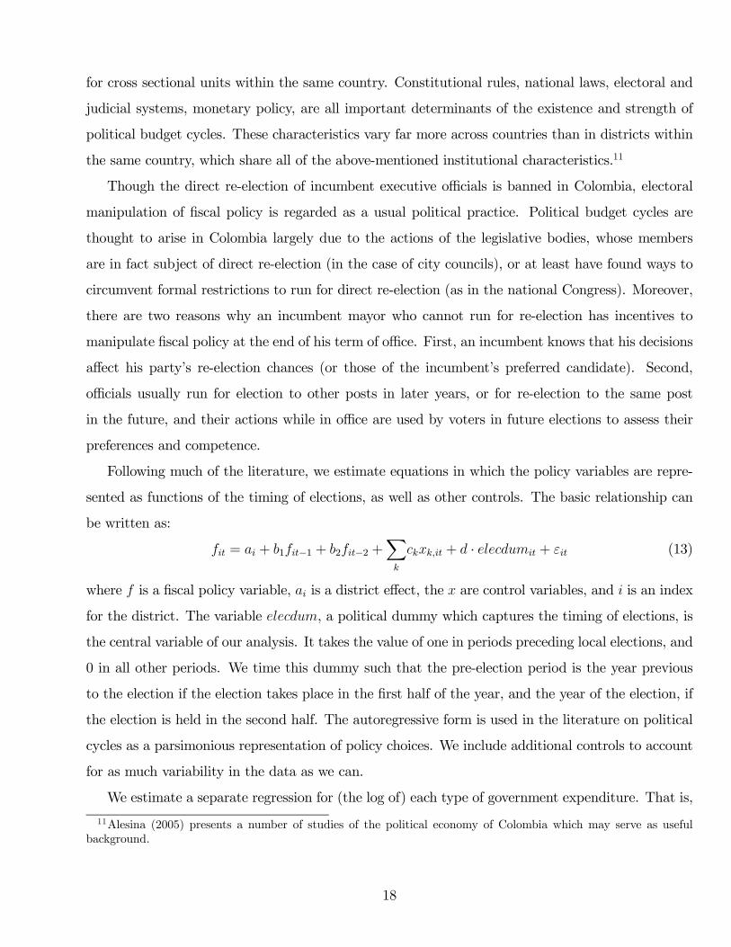
Following much of the literature, we estimate equations in which the policy variables are repre-

sented as functions of the timing of elections, as well as other controls. The basic relationship can

be written as:

fit = ai + b1fit−1 + b2fit−2 +Xk

ckxk,it + d · elecdumit + εit (13)

where f is a fiscal policy variable, ai is a district effect, the x are control variables, and i is an index

for the district. The variable elecdum, a political dummy which captures the timing of elections, is

the central variable of our analysis. It takes the value of one in periods preceding local elections, and

0 in all other periods. We time this dummy such that the pre-election period is the year previous

to the election if the election takes place in the first half of the year, and the year of the election, if

the election is held in the second half. The autoregressive form is used in the literature on political

cycles as a parsimonious representation of policy choices. We include additional controls to account

for as much variability in the data as we can.

We estimate a separate regression for (the log of) each type of government expenditure. That is,

11Alesina (2005) presents a number of studies of the political economy of Colombia which may serve as usefulbackground.

18

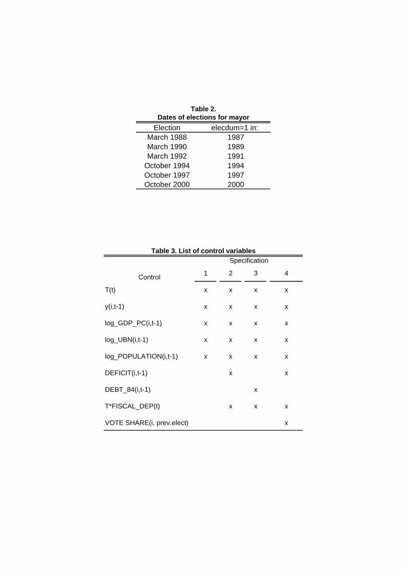
each type of government expenditure is a different f . In all regressions, we are interested in d, the

coefficient that captures the effect of elections. Of the 18 years in our sample, 6 are local election

years, when mayors, and city councils are elected. Elections occur at predetermined dates. Table 2

contains a list of elections held between 1987 and 2000.12

3.1.1 Data

We briefly present now the data we use. A more detailed description can be found in Eslava (2004).

In terms of dependent variables, as mentioned above, we want to estimate 13 for different compo-

nents of public expenditure. We use data from the Colombian Contraloría General, a public agency

with the task of monitoring public finances. Our data correspond to the figures in the financial re-

port each municipality files with the Contraloría annually. The general structure of the expenditure

accounts, as well as basic statistics, are summarized in Table 1.

We estimate (13) using each of the expenditure categories mentioned in Table 1 as dependent

variables. That is, we run a separate regression for each category of spending. Besides the categories

listed in Table 1, we also examine investment in roads, which is a subcomponent of infrastructure

investment,13 and some subcomponents of personnel payments and current transfers. As mentioned

before, we expect to find pre-election expansions in the components closely related to development

projects such as infrastructure, water, power and communications, and road construction.

For each type of expenditure, Figures 1a and 1b show mean values — in hundreds of thousands of

1998 pesos — for election and non-election years. Notice that in general current expenditure categories

have lower averages in election periods that in other periods. The opposite happens for investment

categories. While these observations suggest pre-election effects in the direction we expect, more

systematic evidence is obtained by estimating equation (13).

One should note that “Current Transfers”, as defined in the Colombian government accounts,

refer to benefits to retired and temporary employees, and transfers to other levels of government,

groups that are unlikely to be the targets of election-year spending. They do not correspond to

the kind of transfers to specific groups that are often central to electoral manipulation. As argued

12Our period of estimation begins in 1987 because mayors are elected by popular vote only since 1988. However,we have data on all variables starting in 1984. These additional observations allow us to estimate (13) in differencesand use lags of the regressors as instruments (see an explanation of estimation strategy below) without loosingobservations.13“Infrastructure” includes, besides the construction of roads, urban infrastructure and construction of market

places.

19

above, in the Colombian government accounts, election-year opportunistic spending is more likely

captured by some investment categories.

Table 3 lists the different controls we use in alternative specifications. We use different specifica-

tions, with alternative sets of controls, to analyze the robustness of our results. Our controls include

per capita GDP to account for economic activity, a time trend, and some social indicators that could

be used as inputs in fiscal policy decisions. The latter include population and a poverty indicator

known as “Unsatisfied Basic Needs”. We also use alternative financial indicators as controls, trying

to account for some constraints faced by the government. These are particularly important in later

years, when the law has required that regional governments in Colombia obtain authorization from

the central level to increase expenditure if they have been running deficits in previous years. We

use deficit, debt, and fiscal dependence indicators, which we constructed by us from the Contraloría

data. The Fiscal Dependence indicator accounts for the degree of fiscal decentralization at the na-

tional level, which grew dramatically over this period. The indicator is increasing in the share of

revenues represented by transfers from the central government (as opposed to the local government’s

own fiscal effort). We interact it with the trend variable, to differentiate the trend effects related

to the process of fiscal decentralization from any other trend effects. Finally, we include Incumbent

Advantage, measured by the percentage share of votes received by the incumbent in the last election.

We try to account in this way for the greater degrees of freedom that a popular incumbent has when

choosing fiscal policy.14

3.1.2 Estimation strategy

Given the presence of the city-specific effects, ai, we estimate (13) in differences. Since this differen-

tiation introduces endogeneity problems, estimation is done by GMM15 using fi,t−s−1 and fi,t−s−2 to

14The GDP per capita data are from DANE (the Colombian Bureau of Statistics), while population and theUnsatisfied Basic Needs indicator were provided by the University of Los Andes’ CEDE. Deficit, Debt, and FiscalDependence were constructed by us from the Contraloría data. As for Incumbent Advantage, we use electoral resultsrecorded in the National Planning Department Databases for the pre-1997 elections, while for 1997 and 2000 we useofficial results directly provided by the Registraduría Nacional. More details on the construction of all these controlscan be found in Eslava (2004).15A detailed discussion of the endogeneity problems in this estimation, as well as the virtues of the estimation

technique used can be found in Eslava (2004). It should be noted that the most widely used methodology in thisliterature is the one suggested by Arellano and Bond (1991). We do not use this approach because, with the relativelylarge numbers of periods (15) and endogenous variables (up to 5) in our estimations, the Arellano-Bond estimationcontains more than 60 instruments. GMM estimators with such a large number of overidentifying restrictions areknown to have poor finite sample properties. Our results are, however, robust to the use of Arellano-Bond techniques,although the set of instruments does not perform as well as under the methodology we use here. Results of Arellano-

20

instrument for the ∆fi,t−s = fi,t−s − fi,t−s−1, and xi,t−s−1 and xi,t−s−2 to instrument for the ∆xi,t−s.

The following sequential endogeneity constraints guarantee the validity of these instruments:

E(εitfit−s) = 0 for all t and for s ≥ 1

The electoral dummy is assumed strictly exogenous with respect to the error term, since the timing

of elections is pre-determined in Colombia. That is,

E(εitelecdumiv) = 0 for all v, t

Other controls are in general assumed to be sequentially exogenous, although some of them may

be contemporaneously correlated with the error term.16 The general assumptions are:

E(εitxit−w) = 0 for all t and for w ≥ a

where a = 0 for control variables assumed not contemporaneously correlated with the error term,

and a = 1 for the opposite case.

3.1.3 Results

Results for the political dummy d in which we are interested are presented in Table 4.17 In the table,

each of columns (1) through (4) represents a different set of controls, as detailed in Table 3. Each

row corresponds to a different regression, with the dependent variable for each regression given in

the first column. For instance, the first row reports the estimate of d when the dependent variable

is the log of current expenditure. (All dependent variables are expressed in logs.) Results in bold

letters are significant at the 5% level, in bold and italics significant at the 10% level.

Results point to an election-year change in the composition of spending in the expected direction.

We observe a decrease in some current expenditures before elections, specifically transfers to retirees,

payments to temporary workers, and payments of debt service. Concurrent with this contraction

Bond estimations of our model are presented briefly in Eslava (2004).16Incumbent advantage, the time trend, the fiscal dependence indicator (since it is an aggregate-level indicator),

and previous year’s deficit and debt are all assumed contemporaneously exogenous with respect to the error term.The rest of controls are assumed potentially correlated with the contemporaneous error term.17To facilitate reading, estimates for other coefficients are not reported. All other results are available from the

authors upon request, and some of them are reported in Eslava(2004).

21

we find an increase of spending in development projects. In particular, total investment and its sub-

categories infrastructure, power and road construction all show pre-election increases. Interestingly,

payments to permanent workers appear to increase prior to elections.18 These changes in spending

are not only statistically significant, but also large in size. For instance, current transfers fall close to

30% and interest payments close to 10%, while total investment rises about 15% before elections.19

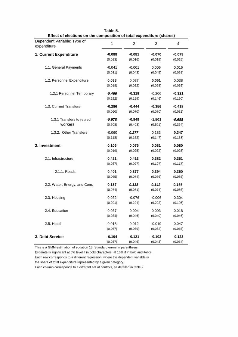
A similar message emerges if the dependent variables are the shares of total expenditure repre-

sented by each category (Table 5). While the fraction of current expenditures and interest payments

in total spending decreases before elections, the opposite occurs with investment. The reduction

of current spending is explained mainly by lower transfers to retirees and payments to temporary

workers. On the other hand, the investment category that rises before elections is infrastructure,

including road construction, and construction of power and water plants.

In summary, we find that before elections the composition of local government expenditures

changes in a systematic way. There is a shift of resources away from what we believe to be less

popular types of spending into development projects, which may represent spending clearly targeted

to voters. One is then led to ask whether such compositional changes actually change voting patterns

in favor of the incumbent. We now turn to empirical evidence on the link between the government’s

budget and election outcomes.

3.2 Voting

Our approach has two broad implications about voter response to electoral fiscal policy. First (which

is actually an assumption), voters dislike deficits. Second, and most importantly, different categories

of spending have differential effects on voting, with the incumbent deriving the most electoral benefit

from “targeted” expenditures. In this section, we address these points empirically.

18The finding of a pre-electoral expansion of personnel expenditures would be consistent with the widespread ideathat politicians in Colombia trade government jobs in exchange for political support.19Table 4 does not include the effect on total spending. The reason is that the model presented above makes no

prediction regarding total expenditure. In this approach, the effect on total spending is seen simply as the sum ofwhat happens to individual categories. It is worth mentioning, however, that by estimating (13) with f equal tothe log of total expenditure, one obtains a very small pre-electoral effect. Although in specifications 1 and 3 it isstatistically significant, it is only approximately 3%. Moreover, in specifications 2 and 4 it is not even statisticallysignificant.

22

3.2.1 Data

The relevant definition of “incumbent” for the Colombian case is the incumbent party, since officials

cannot run for direct re-election. We therefore use data on the share of votes obtained by each party

in local mayoral elections from 1992 to 2000 (four elections).20

Politics in Colombia have been traditionally dominated by two major parties, Liberal and Con-

servative. While some candidates, particularly in the 1990’s, ran under the banner of a myriad

of different parties or political movements, many of these movements can be traced back to the

traditional parties, and voters in each locality are frequently aware of those ties. In that sense,

elections are still mainly a contest between these two major parties, although there are also two

smaller left-wing parties and some truly independent political groups.

Given these political groupings, one challenge in the data is to identify which candidates are

associated with one of the major parties, in order to calculate the appropriate shares of party votes.

We use information from external sources to match the different movements with the traditional

party division between Liberals and Conservatives. Movements that were not successfully linked to

one of the main parties are considered “independents” in our analysis. We calculate the share of

votes obtained by the Liberal party, for example, as the sum of the shares obtained by all the smaller

organizations linked to the Liberal party. It is important to highlight that there is measurement error

due to the difficulty in identifying some matches (in particular, some organizations linked to one of

the parties may have been mistakenly assigned as independents). More details on the construction

of these linkages can be found in Eslava (2004).

3.2.2 The effect of fiscal policy on vote shares

Vote shares are modeled as a function of the fiscal choices of the incumbent party in the pre-election

period. Following the literature on voters as fiscal conservatives (e.g., Peltzman [1992], Brender

[2003]), we consider the effect of deficits on vote shares. We also attempt to distinguish the effects

of different spending categories, given that our theoretical results suggest that voters see targeted

expenditures differently than the rest of spending. Following the previous discussion, we treat

investment spending as targeted expenditure, and current spending as non-targeted expenditure.

20Unfortunately, for previous elections only the share of votes obtained by the winner of the election is available,so that full party shares cannot be calculated.

23

We run a regression of the following form:

votespis = α0 + α1votespis−1 + α2investis + α3currentis + α4deficitis + α5gris (14)

+ (β2investis + β3currentis + β4deficitis + β5gris) ∗ incpis−1 + visp

The time indices, s, refer to election periods, so that s is the current election and s − 1 theprevious election. votespis is the share (in percentages) of votes obtained by party p in city i in the

election at s. The fiscal variables correspond to the election year (as defined above); we include the

log of per capita investment spending (investis), the log of per capita current spending (currentis),

and the per capita government deficit (deficitit). The discrete variable incpis−1 takes a value of 1 if

the party p is in power before the election, and 0 otherwise. Average GDP growth between t−1 andt (grit) is also considered to control for other observables that may affect voters’ perceptions about

the incumbent. The direction of the results reported below is robust to changing the specification to

one that restricts the effect of fiscal policy on the votes received by the incumbent to be the negative

of its effect on the votes received by the challenger (see Eslava [2004]).

We interpret the coefficients β2, β3, β4 as reflecting the advantage (or disadvantage) the incum-

bent obtains with respect to the challenger for increasing investment, current spending or the deficit

before the election. Under the assumption that vitp captures the part of voting behavior that the

politician cannot predict, fiscal policy decisions cannot be based on those innovations, and the policy

variables included in the regression should satisfy the restriction of being orthogonal to the error

term. Assuming that there are no components of vit that affect the incumbent’s fiscal choices may

indeed be strong, but data restrictions make addressing these concerns a quite difficult task, beyond

the scope of this paper.

Results are reported in Table 6; column (1) reports estimates of (14), while column (2) reports

results of a slightly modified version that includes party/state effects.21 Robust standard errors

are reported below the point estimates. Column (3) reports results of specification (14), but the

spending variable invest is measured as a fraction of total spending (in this case, the corresponding

fraction for current spending is not included in the specification due to concerns about collinearity

of the regressors).

21A full fixed-effects version cannot be used due to restrictions of the voting shares data: for most localities wehave no more than 1 usable observation.

24

As previous studies have found for other countries (e.g. Peltzman [1992] for the U.S., Brender

[2003] for Israel, Brender and Drazen [2005] for developed countries in general), and contrary to

the implicit view in much of the empirical literature on political budget cycles, the results indicate

that Colombian voters penalize the incumbent party for running high deficits. Furthermore, high

capital expenditures (interpreted here as targeted spending) increase the share of votes obtained by

the incumbent party relative to the challenger, while current (“non-targeted”) expenditure has no

significant effect.22 From column (3), for instance, a ten percent increase in the share of spending

dedicated to investment increases the fraction of votes obtained by the incumbent party by about

1%, while a two standard deviation increase in the deficit per capita decreases the share of votes

to the incumbent party by close to 4.2%. These results are consistent with the view that voters

dislike incumbents who run high deficits, while they value specific types of expenditures. They are

also consistent with the results on electoral changes in the composition of spending discussed above

which show incumbents increasing targeted spending before the elections, while they try to avoid

concomitant increases in the overall budget.

4 Conclusions

This paper presents a view of the Political Budget Cycle in which voters may dislike fiscal deficits,

even though they value government spending on some specific types of goods. Politicians are aware

of voter preferences (which may differ from their own), and hence electoral manipulation of the

budget takes the form of a change in the composition of expenditure from less to more targeted

spending, rather than an increase in the overall size of the budget. We present a model with

perfectly rational, forward-looking voters, who use the provision of public goods to make inferences

about the incumbent’s fiscal preferences. Election-year shifts of the budget improve the incumbent’s

chances of being re-elected, since voters assign some probability that more targeted spending reflects

a the incumbent’s true preference for types of spending voters prefer, rather than purely electoral

incentives.

The predictions of our model are shown to be consistent with evidence on the composition

of public spending and the behavior of voters in Colombian municipalities. We find that, prior

22Tests of joint significance indicate that α2+β2 (the "absolute" effect of investment on the share of votes receivedby the incumbent) is positive and statistically significant, α3 + β3 is not significantly different from 0, and α4 + β4 isnegative and significant.

25

to elections, some components of spending that we believe are particularly attractive to voters

expand significantly. These components are infrastructure spending, including road construction

and construction of power and water plants. On the other hand, interest payments, transfers to

retirees, and payments to temporary workers contract in election years. We also find that voters

penalize the incumbent party for running large deficits before elections, and reward it for increasing

the amount of targeted spending observed before the election.

26

ReferencesAkhmedov, A. and Zhuravskaya, E. (2004), “Opportunistic Political Cycles: Test in a Young DemocracySetting,” Quarterly Journal of Economics 119, 1301-38.

Alesina, A., editor (2005), Institutional Reforms: The Case of Colombia, Cambridge, MA: MIT Press.Alesina, A., R. Perotti and Tavares (1998), "The Political Economy of Fiscal Adjustments," BrookingsPapers on Economic Activity 1:1998.

Brender, A. (2003), “The Effect of Fiscal Performance on Local Government Election Results in Israel:1989-1998,” Journal of Public Economics 87, 2187-2205.

Brender, A. and A. Drazen (2004), “Political Budget Cycles in New Versus Established Democracies,”NBER Working Paper 10539. (Latest version available at http://www.tau.ac.il/~drazen)

(2005), “HowDo Budget Deficits and Economic Performance Affect Reelection Prospects?,”in progress.

Dixit, A. and J. Londregan (1996), “The Determinants of Success of Special Interests in RedistributivePolitics,” Journal of Politics 58, 1132-55.

Drazen, A. and M. Eslava (2005), “Political Budget Cycles When Politicians Have Favorites,” workingpaper, University of Maryland.

Eslava, M. (2004) “Political Budget Cycles or Voters as Fiscal Conservatives? Evidence from theColombian Experience,” Mimeo, Universidad de Los Andes.

Gonzalez, M.(1999), “Political Budget Cycles and Democracy: A Multi-Country Analysis,” workingpaper, Department of Economics, Princeton University.

Gonzalez, M.(2002), “Do Changes in Democracy Affect the Political Budget Cycle? Evidence fromMexico,” Review of Development Economics 6, 204-224.

Kneebone, R. andMcKenzie, K. (2001) “Electoral and Partisan Cycles in Fiscal Policy: an Examinationof Canadian Provinces,” International Tax and Public Finance 8, 753-774.

Lindbeck, A. and J. Weibull (1987), “Balanced Budget Redistribution as the Outcome of PoliticalCompetition,” Public Choice 52, 272-97.

Peltzman, S. (1992), “Voters as Fiscal Conservatives,” Quarterly Journal of Economics 107, 327-261Persson and Tabellini (2003), The Economic Effect of Constitutions: What Do the Data Say?, Cam-bridge, MA: MIT Press.

Rogoff, K. (1990), “Equilibrium Political Budget Cycles,” American Economic Review 80, 21-36.Rogoff, K. and A. Sibert (1988), “Elections and Macroeconomic Policy Cycles,” Review of EconomicStudies 55, 1-16.

Shi, M. and J. Svensson (2002a), “Conditional Political Budget Cycles,” CEPR Discussion Paper#3352.

(2002b) “Political Business Cycles in Developed and Developing Countries,” working paper.

27

Type of ExpenditureNumber of obs.

Mean Standard deviation

Total Expenditure 12,335 56,458 611,226

1. Current Expenditure 12,334 19,856 185,433

1.1. General Payments 12,265 4,068 21,005

1.2. Personnel Exp. 12,266 9,759 82,677

1.3. Current Transfers 12,247 5,895 91,341

2. Investment 12,335 30,129 382,126

2.1. Infrastructure 5,276 3,173 8,252

2.2. Water, Energy, and Comunications 5,571 3,707 6,166

2.3. Housing 7,365 761 4,069

2.4. Education 7,469 3,615 5,523

2.5. Health 7,469 2,710 5,007

2.6. Other

3. Debt service 12,186 6,554 70,578 All measures in hundreds of pesos of 1998

Table 1. Summary statistics for different types of expenditure

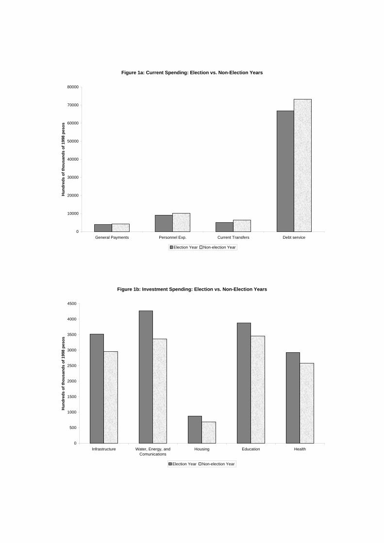
Figure 1a: Current Spending: Election vs. Non-Election Years

0

10000

20000

30000

40000

50000

60000

70000

80000

General Payments Personnel Exp. Current Transfers Debt service

Hun

dred

s of

thou

sand

s of

199

8 pe

sos

Election Year Non-election Year

Figure 1b: Investment Spending: Election vs. Non-Election Years

0

500

1000

1500

2000

2500

3000

3500

4000

4500

Infrastructure Water, Energy, andComunications

Housing Education Health

Hun

dred

s of

thou

sand

s of

199

8 pe

sos

Election Year Non-election Year

Election elecdum=1 in: March 1988 1987March 1990 1989March 1992 1991

October 1994 1994October 1997 1997October 2000 2000

Dates of elections for mayorTable 2.

Control 1 2 3 4

T(t) x x x x

y(i,t-1) x x x x

log_GDP_PC(i,t-1) x x x x

log_UBN(i,t-1) x x x x

log_POPULATION(i,t-1) x x x x

DEFICIT(i,t-1) x x

DEBT_84(i,t-1) x

T*FISCAL_DEP(t) x x x

VOTE SHARE(i, prev.elect) x

Table 3. List of control variablesSpecification

Dependent Variable: Type of expenditure 1 2 3 4

1. Current Expenditure -0.024 -0.033 -0.011 -0.041(0.024) (0.018) (0.019) (0.023)

1.1. General Payments 0.037 0.025 0.031 0.032(0.027) (0.043) (0.041) (0.051)

1.2. Personnel Expenditure 0.071 0.082 0.087 0.084(0.012) (0.020) (0.019) (0.022)

1.2.1 Personnel Temporary -0.546 -0.371 -0.303 -0.369(0.252) (0.106) (0.100) (0.109)

1.3. Current Transfers -0.222 -0.369 -0.270 -0.332(0.082) (0.101) (0.078) (0.123)

1.3.1 Transfers to retired -0.977 -0.826 -1.236 -0.659 workers (0.470) (0.437) (0.575) (0.396)

1.3.2. Other Transfers 0.043 0.324 0.247 0.398(0.125) (0.159) (0.150) (0.162)

2. Investment 0.142 0.126 0.144 0.122(0.025) (0.027) (0.028) (0.028)

2.1. Infrastructure 0.436 0.452 0.507 0.376(0.072) (0.077) (0.098) (0.083)

2.1.1. Roads 0.365 0.392 0.412 0.318(0.069) (0.076) (0.074) (0.078)

2.2. Water, Energy, and Com. 0.219 0.168 0.193 0.177(0.065) (0.072) (0.077) (0.075)

2.3. Housing 0.124 0.028 0.100 0.432(0.207) (0.232) (0.228) (0.212)

2.4. Education 0.110 0.083 0.090 0.090(0.027) (0.032) (0.032) (0.034)

2.5. Health 0.084 0.097 0.079 0.128(0.054) (0.064) (0.061) (0.070)

3. Debt Service -0.053 -0.082 -0.104 -0.090(0.031) (0.036) (0.038) (0.036)

This is a GMM estimation of equation 13. Standard errors in parenthesis.Estimate is significant at 5% level if in bold characters, at 10% if in bold and italics.Each row corresponds to a different regression, where the dependent variable is the level of expenditure in each category.Each column corresponds to a different set of controls, as detailed in table 2

Effect of elections on different types of expenditure (levels)Table 4.

Dependent Variable: Type of expenditure 1 2 3 4

1. Current Expenditure -0.088 -0.081 -0.070 -0.079(0.013) (0.016) (0.019) (0.015)

1.1. General Payments -0.041 -0.001 0.006 0.016(0.031) (0.043) (0.045) (0.051)

1.2. Personnel Expenditure 0.038 0.037 0.061 0.038(0.018) (0.032) (0.028) (0.035)

1.2.1 Personnel Temporary -0.466 -0.319 -0.206 -0.321(0.282) (0.159) (0.146) (0.160)

1.3. Current Transfers -0.286 -0.444 -0.356 -0.418(0.060) (0.070) (0.070) (0.082)

1.3.1 Transfers to retired -0.978 -0.849 -1.501 -0.688 workers (0.508) (0.403) (0.591) (0.364)

1.3.2. Other Transfers -0.060 0.277 0.183 0.347(0.118) (0.162) (0.147) (0.163)

2. Investment 0.106 0.075 0.081 0.080(0.019) (0.025) (0.022) (0.025)

2.1. Infrastructure 0.421 0.413 0.382 0.361(0.087) (0.097) (0.107) (0.117)

2.1.1. Roads 0.401 0.377 0.394 0.350(0.065) (0.074) (0.066) (0.085)

2.2. Water, Energy, and Com. 0.187 0.138 0.142 0.166(0.074) (0.081) (0.074) (0.086)

2.3. Housing 0.032 -0.076 -0.006 0.304(0.201) (0.224) (0.222) (0.195)

2.4. Education 0.037 0.004 0.003 0.018(0.034) (0.046) (0.040) (0.046)

2.5. Health 0.018 0.012 -0.019 0.047(0.067) (0.069) (0.062) (0.065)

3. Debt Service -0.104 -0.121 -0.102 -0.123(0.037) (0.046) (0.043) (0.054)

This is a GMM estimation of equation 13. Standard errors in parenthesis.Estimate is significant at 5% level if in bold characters, at 10% if in bold and italics.Each row corresponds to a different regression, where the dependent variable is the share of total expenditure represented by a given category.Each column corresponds to a different set of controls, as detailed in table 2

Effect of elections on the composition of total expenditure (shares)Table 5.

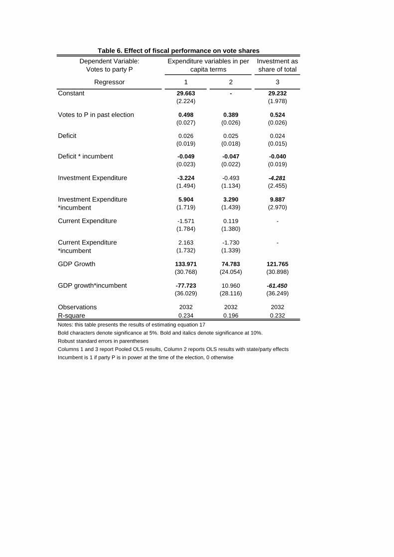
Dependent Variable: Votes to party P

Investment as share of total

Regressor 1 2 3

Constant 29.663 - 29.232(2.224) (1.978)

Votes to P in past election 0.498 0.389 0.524(0.027) (0.026) (0.026)

Deficit 0.026 0.025 0.024(0.019) (0.018) (0.015)

Deficit * incumbent -0.049 -0.047 -0.040(0.023) (0.022) (0.019)

Investment Expenditure -3.224 -0.493 -4.281(1.494) (1.134) (2.455)

Investment Expenditure 5.904 3.290 9.887*incumbent (1.719) (1.439) (2.970)

Current Expenditure -1.571 0.119 -(1.784) (1.380)

Current Expenditure 2.163 -1.730 -*incumbent (1.732) (1.339)

GDP Growth 133.971 74.783 121.765(30.768) (24.054) (30.898)

GDP growth*incumbent -77.723 10.960 -61.450(36.029) (28.116) (36.249)

Observations 2032 2032 2032R-square 0.234 0.196 0.232Notes: this table presents the results of estimating equation 17Bold characters denote significance at 5%. Bold and italics denote significance at 10%.Robust standard errors in parenthesesColumns 1 and 3 report Pooled OLS results, Column 2 reports OLS results with state/party effectsIncumbent is 1 if party P is in power at the time of the election, 0 otherwise

Expenditure variables in per capita terms

Table 6. Effect of fiscal performance on vote shares