GOME Level 1-to-2 Data Processor Version 3.0: A Major

Upgrade of the GOME/ERS-2 Total Ozone Retrieval

Algorithm

Robert Spurr(1- )1 , Diego Loyola(2), Werner Thomas(2- )2 , Wolfgang Balzer(2),

Eberhard Mikusch(3), Bernd Aberle(2), Sander Slijkhuis(2), Thomas Ruppert(3),

Michel van Roozendael(4), Jean-Christopher Lambert(4), Trisnanto Soebijanta(4-3)

(1)Harvard-Smithsonian Center for Astrophysics 60 Garden Street. Cambridge, MA 02138, USA

(2)Deutsches Zentrum für Luft- und Raumfahrt (DLR)

Institut für Methodik der Fernerkundung (IMF) PO Box 1116, D-82234 Wessling, Germany

(3)Deutsches Zentrum für Luft- und Raumfahrt (DLR)

Deutsches Fernerkundungsdatenzentrum (DFD) PO Box 1116, D-82234 Wessling, Germany

(4)Institut d'Aéronomie Spatiale de Belgique (IASB-BIRA)

3-Avenue Circulaire, B-1180 Bruxelles, Belgium

1 Now Director, RT Solutions Inc., 9 Channing Street, Cambridge, MA 02138, USA. 2 Now at Deutscher Wetterdienst (DWD), Kaiserleistr. 29, D63067 Offenbach, Germany; 3 deceased November 2003.

1

Abstract

The Global Ozone Monitoring Experiment (GOME) was launched in April 1995, and the GOME

Data Processor (GDP) retrieval algorithm has processed operational total ozone amounts since

July 1995. GDP Level 1-to-2 is based on the two-step Differential Optical Absorption

Spectroscopy (DOAS) approach, involving slant column fitting followed by Air Mass Factor

(AMF) conversions to vertical column amounts. We present a major upgrade of this algorithm to

Version 3.0. GDP 3.0 was implemented in July 2002, and the 9-year GOME data record from

July 1995 to December 2004 has been processed using this algorithm.

The key component in GDP 3.0 is an iterative approach to AMF calculation, in which

AMFs and corresponding vertical column densities are adjusted to reflect the true ozone

distribution as represented by the fitted DOAS effective slant column. A neural network-

ensemble is used to optimize the fast and accurate parameterization of AMFs. We describe

results of a recent validation exercise for the operational version of the total ozone algorithm; in

particular, seasonal and meridian errors are reduced by a factor of two. On a global basis, GDP

3.0 ozone total column results lie between –2% and +4% of ground-based values for moderate

solar zenith angles lower than 70°. A larger variability of about +5% and –8% is observed for

higher solar zenith angles up to 90°.

Copyright

OCIS codes

010.4950, 010.1120, 010.1310, 280.1120, 280.1310

2

1. Introduction

1.1 The GOME instrument

The Global Ozone Monitoring Experiment (GOME) is an across-track nadir-viewing

spectrometer on board the Second European Remote Sensing Satellite (ERS-2) platform

launched in April 1995. It has been operating successfully for over 9 years. The satellite is sun-

synchronous and polar orbiting, with a period of about 100 minutes and a local equator crossing

time of 10.30h, a semi-major axis of 7150 km, and a repeat cycle of 35 days. In normal viewing

mode, there are three forward scans followed by a back scan, with forward scan footprint size of

320x40 km for a 1.5-second detector readout integration time; the maximum swath is 960 km,

with nominal scan angle ±31° at the spacecraft. With this read-out strategy, global coverage is

achieved at the equator within three days. There is also a polar viewing mode for improved

sounding of polar latitudes during springtime.

GOME has 3584 spectral channels distributed over four serial-readout detectors; the

wavelength range is 240 to 793 nm, with a moderate spectral resolution of 0.2 to 0.4 nm. In

addition to the regular measurements of backscattered light from the Earth-atmosphere system,

GOME has a Pt-Ne-Cr lamp for on-board wavelength calibration, and the solar irradiance

spectrum is measured via a diffuser plate (this is done on a daily basis). GOME has also three

broad band (band pass > 100 nm) Polarization Measurement Devices (PMDs) measuring light in

a direction parallel to the slit. The PMDs' main purpose is to generate a polarization correction

for the level 1 spectra (calibrated and geolocated radiances). A comprehensive description of the

GOME instrument can be found in the GOME Users Manual1.

3

The spectral resolution of GOME is fine enough to resolve the trace gas absorption

signatures of chemically important atmospheric trace species. Ozone column and profile

distributions make up the main mission target2, but the instrument also retrieves total columns of

a number of minor trace species (NO2, HCHO, BrO, SO2, OClO), total water vapor content, and

some ancillary information on clouds and aerosols. The main operational Level 2 products are

the global distributions of total vertical column amounts of ozone and nitrogen dioxide. The core

operational Level 1-to-2 retrieval algorithm is based on the DOAS approach3. The GOME Data

Processor (GDP) at the German Aerospace Center (DLR)4 has been operational since August

1996 following the GOME commissioning phase, and the entire data record since July 1995 has

now been re-processed following upgrades (GDP Level 1-to-2 Versions 2.4 and 2.7 and 3.0) to

the original retrieval algorithm. The GOME near-real-time service5 was initiated in January 1997

with the installation of GDP at the Kiruna station (which receives 10 out of 14 daily ERS-2

orbits) and extended in February 2002 with additional GDP installations at the Gatineau and

Maspalomas stations. A successful application of GDP V3.0 to GOME data is presented by

Thomas et al.6.

The GDP system is implemented using FORTRAN 77 and C. It is organized in five code

layers containing specialized modules for mathematical fitting routines (layer 1), databases in

layer 2 (profile climatologies, other global databases, spectroscopic data), accessing routines to

the lower level functionalities (layer 3), and algorithm specific modules such as DOAS, AMF,

cloud retrieval (layer 4). Each major algorithm component and the operational environment have

its own independent test environment (layer 5). The system was designed to run in parallel on a

number of computers. The modularity was demonstrated when GDP 2.0 was ported from a

4

mainframe UNIX environment to become GDP 2.7 in a more cost-effective Linux cluster

environment.

1.2 GDP total ozone algorithm: earlier versions

The DOAS approach to vertical column retrieval is a two-step process involving firstly the

derivation of effective slant columns from a least-squares fitting based on the Beer-Lambert

absorption law, and secondly the conversion to vertical column densities by means of Air Mass

Factor (AMF) computations based on detailed radiative transfer modeling. The DOAS slant

column fitting method was first used over 20 years ago for slant column retrieval from ground-

based instruments. DOAS was selected for GOME total ozone retrieval in 1992, and the

algorithm was made operational in June 1996. Technical aspects of the DOAS fitting and AMF

implementation are discussed below in Sections 2 and 3 respectively. Here we give some

remarks on the history of the algorithm in order to prepare the context for the newer versions.

All GDP versions up to 3.0 have used a single contiguous fitting window from 325 nm to 335

nm covering part of the ozone Huggins bands absorption features. The initial GDP total ozone

algorithm (GDP 2.0, July 1996) used an ozone cross-section reference spectrum taken from

literature7,8, but in version 3.0, the GOME-measured flight model cross-sections have been used9.

The latter were derived from laboratory measurements made with the in-flight GOME instrument

during the calibration phase prior to launch. Versions 2.7 and earlier also assumed a single

effective temperature input to be used for the temperature dependency of the ozone cross-

sections. A more recent approach10 uses two ozone reference cross-sections to retrieve an

effective temperature in addition to the slant column, and this technique has been incorporated in

version 3.0 (section 2.2).

5

To deal with wavelength grid registration problems, it is necessary to re-sample spectra

on new wavelength grids established through shift and squeeze parameters. Shifting and

squeezing of the reference spectra (including the solar spectrum) is therefore implemented. In the

UV, GOME actually samples slightly below the Nyquist criterion, and in 1998 it was found that

this effect could be largely compensated by the introduction of an undersampling correction11. A

reference spectrum was prepared to handle this effect, and is now standard for version 3.0.

Interference from the Ring effect (inelastic rotational Raman scattering producing

“filling-in” of Fraunhofer and absorption features) has been considered from the outset. This

effect is treated as a pseudo-absorber in DOAS fitting, with the addition of one or two fitting

parameters associated with Ring reference spectra. Up to version 2.7 a single Ring spectrum

derived from pre-launch GOME zenith sky measurements; this was found to have limited

accuracy. Version 3.0 uses a theoretical Ring Fraunhofer spectrum derived from a folding of

Raman cross-sections with a high-resolution solar spectrum12. Attempts have been made to

introduce a second Ring spectrum to deal with telluric (absorption) interference effects.

AMF computations in GDP have gone through some changes. “On-the-fly” radiative

transfer (RT) computations have been generally avoided, ostensibly for performance reasons and

the need to achieve data turnover in real time. In versions up to 2.7, the single-scatter AMF was

computed from scratch, and multiple scatter correction factors were interpolated from a large

look-up table (LUT) classified according to scenario geometry and various atmospheric

parameters (time-latitude dependent trace gas profiles, aerosol loading, surface albedo and

topography. The GOMETRAN radiative transfer model13 including the so-called pseudo-

spherical approximation was used to create the multiple scatter LUTs. Surface Lambertian

albedos were derived from a 1°x1° data set that contains information about the surface type14 but

6

reduced to five surface types only (water, sand, bare soil, vegetation, snow), while the spectral

dependency is taken from Bowker et al.15 for a number of different surface types. Topography is

extracted from the ETOP05 data set provided by The National Snow and Ice Data Center

(NDISC). A substantial new determination of the AMF has been implemented in GDP 3.0; this is

one of the cornerstones of the new version, and is described in detail in Section 3.

In addition to the basic Level 1 input of calibrated geolocated earthshine measurements

(radiances), the GDP total ozone algorithm requires inputs from a pre-processing cloud property

algorithm in order to deal with partially cloudy scenes in the independent pixel approximation.

GDP ingests two cloud properties: the fractional cover that is retrieved by the Initial Cloud

Fitting Algorithm (ICFA)16 based on fitting of reflectance measurements in and around the O2-A

band at 760 nm, and the cloud-top pressure supplied from the International Satellite Cloud

Climatology Project (ISCCP) data base17.

The development of operational retrieval algorithms such as GDP is an ongoing and

iterative process requiring accurate validation of the resulting geophysical products after each

significant modification of the operational processing chain. During the commissioning phase of

the ERS-2 satellite in 1995, an intensive validation campaign18 was conducted to assess the

quality of the developmental versions of GDP, using well-controlled ground-based

measurements from SAOZ/DOAS UV-visible spectrometers, Brewer and Dobson

spectrophotometers, UV filter radiometers and ozonesondes. In addition to comparisons with

correlative data from coincident ground stations or balloon experiments, GDP ozone results were

compared on a global basis with data from the Total Ozone Mapping Spectrometer (TOMS)

instruments onboard Earth Probe and ADEOS, and with retrievals from independent DOAS

algorithms.

7

Validation results for version 2.0 (which generated the first public release of GDP data)

revealed some biases and regional discrepancies, in particular at high latitudes and high solar

zenith angles, and for situations with high or low ozone content19,20. A major validation of

version 2.4 was performed in 1998 after the accumulation of three years of data; this showed

clear improvements in both the ozone and NO2 column retrievals21. Improvements introduced in

version 2.7 were mainly confined to NO2 column retrieval; a “delta” validation of the expected

improvement was performed in 1999 on this version22. The entire data record was reprocessed

after these validations. Results from these validation programmes as well as a preliminary delta

validation of GDP V3.0 are presented in Lambert et al.23. Further comparison of GOME results

with ground-based measurements, space-based measurements and results of alternative retrieval

methods is presented e.g. in Corlett et al.24 and Bramstedt et al.25, the latter also showing first

results for GDP V3.0.

1.3 New GDP versions: scope of the paper

The present work concerns the major upgrade to GDP Level 1-to-2 version 3.0 carried out over

the 2-year period 2001-2002. Version 3.0 represents a new departure for GDP total ozone using

the DOAS approach. The DOAS algorithm (summarized in section 2.1) has been upgraded to

include most of the latest research improvements; in particular the use of two ozone reference

spectra to derive two pieces of information (effective slant column and temperature) from the fit.

These aspects are treated in Section 2.2.

The most significant change concerns the AMF implementation, and this is the heart of

the new GDP Version. It was shown26 that the AMF (and by association the vertical column

density) for ozone could be adjusted to reflect the actual ozone content as expressed through the

fitted slant column. This iterative-AMF approach has been implemented now in GDP 3.0; it is

8

described in greater detail in section 3.1. The approach requires column-classified ozone

climatology; this is summarized in section 3.2, along with the profile-column mapping that

allows the AMF iteration to be linked with vertical column density adjustment.

In version 3.0, the LIDORT scattering code27,28 is now used for simulations of

backscatter intensities required for AMF evaluations. We summarize the implementation of

LIDORT in the context of the ozone AMF calculation in section 3.3. The initial implementation

of version 3.0 used very large Look-up tables (LUTs) of pre-calculated AMFs, and employed a

number of extraction and interpolation steps to determine appropriate AMFs for a given scenario.

This time-consuming task can be replaced by a much faster AMF parameterization based on the

application of neural network techniques to calculate AMFs analytically, as suggested by

Loyola29. Section 3.4 provides a description of the AMF parameterization with neural networks.

We conclude section 3 with some remarks on the implementation and performance of GDP in

the operational environment.

Following the operational implementation of the new AMF formulations and the DOAS

improvements in GDP 3.0, the delta validation campaign was executed in 200223. A set of 2250

previously validated orbits was used (sampled over a 4-year time period). Validation tools and

ground-based data already set up for previous delta-validations were used again. These aspects

are summarized in section 4.1, which deals with the validation methodology. GDP 3.0 total

ozone retrievals were compared not only with GDP 2.7 results (section 4.2), but also with

ground-based and balloon data used in previous validation campaigns (section 4.3). Section 4.4

contains the validation summary.

9

The paper also has some concluding remarks on the transition to GDP versions beyond

3.0. The complete GOME total ozone data set from July 1995 as re-processed with GDP Version

3.0 is publicly available.

2.Upgrades to DOAS Slant Column Fitting

2.1 DOAS fitting of slant columns

In the fitting step, the forward model is reduced in essentials to the Beer-Lambert extinction law

for trace gas absorbers. This is a reasonable assumption to make for optically thin trace gas

absorption in the atmosphere, where the cross-sections are weakly dependent on pressure, and

strongly linearly dependent on temperature. In DOAS, it is standard practice to use logarithms of

the sun-normalized intensities, and then add a low-order polynomial (typically of degree 2) to

account for broadband molecular and aerosol scattering and also for reflection from the Earth’s

surface. The fitting model is then:

( ) ( 2 *2

*100 )()(

)()(ln λλαλλααλσ

λ

λ −−−−−Ω−=⎥⎦

⎤⎢⎣

⎡ΩΩ ∑

gggE

II ) . (1)

Here, Iλ is the earthshine spectrum at wavelength λ, and for GOME, 0Iλ is usually taken to be the

extraterrestrial solar spectrum. This model applies to trace gas absorption through the whole

atmosphere, where Eg(Ω) is the effective slant column density of gas g appropriate to an

atmospheric path characterized by directional variable Ω, σg(λ) is the trace gas absorption cross

section, α0, α1 and α2 are the low-order (quadratic) polynomial fitting coefficients, and λ* is a

reference wavelength for this polynomial (usually the fitting window mid-point).

10

Leaving aside issues of wavelength registration, the above expression is linear in the

fitting variables Eg(Ω) and αk. Additional reference spectra may be considered in the fitting, to

compensate for instrumental effects such as undersampling, and atmospheric effects due to

inelastic rotational Raman scattering (the Ring effect). Wavelength mismatching is often dealt

with by applying fitted shift and squeeze parameters to the wavelength grids of the reference

spectra, and also the solar spectrum. This makes the fitting iteratively non-linear (and thus much

slower), and it is desirable to use pre-established shifts and squeezes and pre-shifted reference

spectra in order to maintain linearity and reduce the possibility of numerical instability.

Over the lifetime of GOME, a number of improvements have been made to the original

DOAS algorithm following essential research by a number of groups associated with the

instrument. Many of these improvements have been incorporated in the newer GDP algorithms,

and some of these were noted in section 1.2 for earlier versions. Here, we deal first with fitting

issues and choice of reference spectra as they apply to DOAS in GDP 3.0.

2.2 Reference Spectra in GDP 3.0

Version 3.0 uses the latest release of the GOME Flight Model cross-sections (O3 and NO2), the

so-called GOME FM98 data30,9. These cross-sections are taken from cell measurements taken

with the GOME instrument prior to the April 1995 launch; measurements were taken at five

temperatures (202 K, 221 K, 241 K, 273 K and 293 K). In addition, the interfering species NO2

is also considered in the fit, with cross-sections at 241 K for this trace gas also taken from the

GOME FM98 data set. In GDP 3.0, trace gas cross-sections have been subjected to a pre-shift re-

sampling (0.012 nm towards longer wavelengths is the wavelength shift for ozone cross sections

in the customary 325-335 nm GOME DOAS window); shift and squeeze fitting for these

11

reference spectra has been disabled (this avoids occasional numerical instabilities found in the

earlier GDP versions).

Ozone cross sections in the Huggins bands are temperature dependent, and this must be

treated in the fitting. Earlier versions of GDP used a single ozone cross-section as the trace gas

reference, and the Huggins band temperature dependence was dealt with by assuming a single

effective temperature Teff corresponding to the maximum number density in the appropriate

climatological ozone profile (temperatures are selected from climatology). However, two ozone

cross-sections at different temperatures may be used in the fitting to retrieve Teff in addition to the

effective slant column10; this avoids the potentially large source of uncertainty associated with an

external choice of effective temperature. Specifically, we use the ozone cross-section at

temperature T1, and an ozone difference cross-section (between temperatures T1 and T2), and the

temperature dependence of the complete cross-section is assumed to be:

)()()()()()()()(

21

211111 TT

TTTTTT

TTTT−−

−+≈∂∂

−+=σσ

σσσσ . (2)

The dependence is linear if we assume the temperature derivative is constant. This assumption is

a good one for the limited range of stratospheric temperatures8. Taking T1 = 221 K and T2 = 241

K, so that ∆T = T1 -T2 = 20 K, we use σ(T1) and ∆σ12 = σ(T1) - σ(T2) as the reference spectra in

the fitting. The total slant column optical depth is Eσ(T), for effective slant column density E,

which is then the fitting parameter corresponding to σ(T1). If D is the fitting parameter

corresponding to the difference cross sections ∆σ12, then we can define an effective temperature

through the relation:

EDTTTTeff )( 211 −+= . (3)

12

Effective slant columns are now independent of any assumed temperature climatology. The fitted

temperature varies with latitude and season and values can be compared against climatological

data and analysis data from forecast models for diagnostic purposes (see also section 5.1).

In Figure 1, we illustrate these changes for a spring orbit. RMS has improved by a factor

of two for all cases. In the right-hand panel, fitted effective temperatures vary from 222 K to 240

K in the Northern high latitudes. These values are generally lower than ozone-maximum

temperatures selected from climatology, as used in version 2.7; the validation exercise on GDP

3.0 has proved that the use of this fitted-temperature DOAS formalism gives consistently better

total ozone column results (see section 4.2).

In subsequent studies after the GDP 3.0 algorithm was defined, ECMWF temperature

fields were averaged over atmospheric height using climatology ozone profiles as weighting

factors, and derived effective temperatures obtained. It was found that there was a positive bias

in GDP 3.0 effective temperatures (10-20 K, depending on orbit). The source of this bias is in

part due to the wavelength registration, and improved pre-shift parameters for ozone cross-

sections have gone some way to eliminating this bias. Uncertainties in weather-model

temperature fields are also a factor. However this is a complex issue that requires a more detailed

assessment that is beyond the scope of this paper.

In all GDP versions up to and including 3.0, the earthshine spectrum wavelength grid is

used as the standard; for each fitting, the sun spectrum is re-sampled on this reference grid by

application of a shift parameter to the sun spectrum wavelength. This particular wavelength

mismatch is due mainly to the solar spectrum Doppler shift (an average shift value is 0.008 nm),

and it will vary across an orbit due to changes in the instrument temperature. As in Version 2.7,

13

the static undersampling correction11 has been incorporated to deal with slit function sampling

below the Nyquist criterion.

3. Iterative AMFs and Neural Network Parameterization

3.1 Iterative AMF adjustment

The AMF definition is

( )vert

gnog IIA

τ/log

= , (4)

for which two calculations of backscatter intensity are required, one (Ig) for an atmosphere

including ozone, the other (Inog) for an atmosphere excluding ozone, and τvert is the vertical

optical depth of ozone for the whole atmosphere. All GDP versions have used this definition for

the ozone AMF, though other definitions have been used for minor trace species [see for

example Palmer et al.31. AMFs for total ozone column are calculated at 325 nm at the lower end

of the DOAS fitting window (325-335 nm). For a clear sky scenario, the final vertical column

amount is then defined as the effective slant column divided by a single AMF computed from

this chosen ozone profile. For partially cloudy GOME scenarios, the conversion from slant

column to vertical column density proceeds via the relation:

cloudclear

cloud

AAGAE

Vφφ

φ+−

+=

)1(, (5)

where E is the effective slant column, with AMFs Aclear and Acloud for clear and cloudy scenarios

respectively. In GDP, the factor φ is just the cloud fraction f. An alternative definition is φ =

fIcloud/Itotal, where Itotal = (1−f)Iclear + fIcloud. In the above equation, the cloud fraction comes from

14

the ICFA pre-processing step. The “ghost column” G is the quantity of ozone below cloud-top; it

must be computed from ozone profile climatology.

In traditional DOAS retrievals, slant column fitting and AMF calculation steps are

decoupled; for a given trace species, the AMF radiative transfer computations are based on a

priori climatological profile inputs that may have no real connection to the true profile. This is

the case with GDP versions 2.7 and earlier, where a suitable ozone profile has traditionally been

interpolated (by time and latitude) from a zonal-mean monthly climatology of profiles. If the

profile shape is a function of the total column (as it is for ozone), this approach is logically

inconsistent - in order to retrieve the total vertical column, it is necessary to know the profile first

in order to compute the correct AMF.

The shape and total content of the selected ozone profile may bear little resemblance to

the true profile, and (particularly for scenarios with high ozone content and/or high solar zenith

angles) the AMF may be significantly in error due to a poor choice of input profile. The

motivation behind the iterative AMF approach is to circumvent this uncertainty by using

information about the true profile to establish the AMF more accurately. The only relevant

profile information available to us in the DOAS context is the fitted slant column, and the

iterative AMF algorithm uses the slant column result E to make an adjustment to the AMF (and

by extension, the vertical column density) that reflects the trace gas content as expressed in the

value of E. This adjustment depends on the use of a column-classified climatology of ozone

profiles; the choice of profile is uniquely determined by a specified vertical column amount.

Such climatology was developed some years ago for the TOMS retrievals32, and this is

summarized in Section 3.2.

15

The iteration process is straightforward to describe; we treat first the clear-sky case. An

initial AMF A0 is computed given an initial choice V0 of vertical column; the required profile is

drawn from the column-classified ensemble. The initial choice V0 may be taken from the TOMS

zonal mean column climatology, or (in the GOME operational context) from a previously

retrieved result from an adjacent footprint. V0 is the first guess for the iterated vertical column

density. Given a slant column E from the DOAS fitting, an updated vertical column V1 is

calculated through the relation V1 = E / A0. From the climatology, V1 determines a new choice of

profile, which is in turn used as input to a new AMF calculation, with result A1. A new guess V2

for the vertical column follows from V2 = E / A1. This process is repeated until convergence has

been reached (the relative difference between iterations of V is less than some small number).

For the partially cloudy footprint, the iteration proceeds via:

)()(

)()()1(

)1( ncloud

nclear

ncloud

nn

fAAfAfGEV+−

+=+ , (6)

where the (n) superscript indicates the iteration number. In addition to the AMF results, the ghost

column is also updated at each step. In this way, the profile, the vertical column density and the

AMF have all been adjusted to fit the "true-situation" constraint imposed by the effect slant

column. For the great majority of scenarios, convergence for ozone columns is rapid (3 or 4

iterations for a relative change of 0.1% in the vertical column).

A simple flow diagram of the AMF and vertical column iteration is shown in .

3.2 Use of a column-classified ozone climatology

We require a way to assign a profile for a given choice of total column. GDP 3.0 uses the TOMS

Version 7 (“TV7”) column-classified ozone profile climatology32 for this task. In the TV7

16

climatology, there are 10 high- and mid-latitude profiles with total columns of 125 DU to 575

DU at intervals of 50 DU, and 6 low latitude profiles from 225 to 475 DU, also with a 50 DU

increment. There are 11 layers in total with pressure levels defined using scale heights; each

partial column is given in DU. Cross-latitude jump artifacts are avoided by mixing profiles from

adjacent zones using a distance-based weighting scheme.

To define a unique correspondence between profile and column, we proceed as follows.

If the profile is represented as a set of partial columns, then the total column is

. For two adjacent TV7 profiles and with total columns V

jU

∑=j jUV (1)

jU (2)jU (1) and V(2)

we define an intermediate profile with column amount V according to:

)1()1()2(

)2()2(

)1()2(

)1(

)( jjj UVVVVU

VVVVVU ⎟⎟

⎠

⎞⎜⎜⎝

⎛−−

+⎟⎟⎠

⎞⎜⎜⎝

⎛−

−= . (7)

This defines a linear profile-column map. This map allows us to interpolate smoothly between

profile entries in the climatology; the shape will vary continuously. We are drawing on an

ensemble of possible profiles of which the climatology is a sample. In Fig. 3, we illustrate the

application of this map for the set of 10 high-latitude TV7 profiles. The AMF and ghost column

iterations are based on this linear profile-column correspondence, and the choice of profile is

restricted to the ensemble represented by the climatology. There are some circumstances where

the climatology may be inappropriate; these are discussed below when we look at the validation.

It is worth noting here that the simplest profile-column map is a scaling

0)0()( VVUVU jj = in terms of a fixed profile with column V)0(

jU 0. This mapping is implicit in

traditional single-AMF DOAS retrieval algorithms. In this case, any profile associated with a

retrieved total column will preserve the shape of the fixed profile (all layer partial columns are

17

scaled equally). The assumption of a fixed ozone profile shape (with its typical stratospheric

bulge) may generate sizeable AMF errors in (for instance) an ozone hole scenario.

The TV7 climatology has some limitations in its classification system, particularly in the

tropics, where the fixed vertical distributions of ozone in the lowest two Umkehr layers are

unrepresentative. The newly-released TOMS Version 8 climatology has a wider column

classification and a more extensive latitudinal distribution, and variations in the Umkehr columns

in the first two layers of the TOMS atmospheres are better accounted for in the tropical profile

climatology. [The Version 8 climatology was not available at the time of the GDP 3.0

implementation].

Uncertainty in the tropospheric ozone burden is one of the main sources of error in the

AMF. Using the LIDORT model (section 3.3) to calculate AMFs, we found that changing the

burden in second-lowest layer (9 DU in the TV7 climatology) has little effect on the AMF at 325

nm (less than 0.5%). On the other hand, uncertainty in ozone in the lowest layer (set at 15 DU in

the TV7 data) is more important. For a solar zenith angle of 25º, and a surface albedo of 10%, we

find that, for a total atmospheric column of ozone of 250 DU, doubling the lowest layer burden

to 30 DU induces a decrease of 3% in the AMF, and reducing this burden to zero results in a 3%

increase. These values are representative for tropical scenarios, for which the tropospheric ozone

burden is largest.

3.3 Radiative transfer implementation

GDP Version 3.0 uses the LIDORT discrete ordinate scattering code27,28 for off-line AMF

computation. This model incorporates full multiple scattering effects in a stratified atmosphere,

with the solar beam as the driving source of scattered light. Azimuthal dependence of the

intensity is expressed in terms of the cosine of the relative azimuth between the solar and line of

18

sight directions. The phase function for scattering is expanded in terms of a Legendre polynomial

series in the cosine of the scattering angle. Integration over the multiply scattered diffuse field is

approximated by a Gauss-Legendre quadrature sum over a set of polar directions (the discrete

ordinates or streams). The resulting coupled linear differential equations of radiative transfer are

solved by standard means, and the discrete ordinate solution for the radiation field found by

application of boundary-value conditions. Finally, the radiation field at arbitrary viewing angles

and optical depth may be obtained by substitution of the discrete ordinate solution in the original

RTE and subsequent integration of the source function (this is the “post-processing” step).

Polarization is not taken into account.

LIDORT uses the so-called pseudo-spherical (P-S) approximation, in which the solar

beam attenuation is treated in a spherical shell atmosphere, but all scattering processes are still

plane parallel. This approximation is sufficiently accurate for solar zenith angles up to 90° and

for line-of-sight viewing up to 30-35° from the nadir. A number of studies have shown that

AMFs calculated with this assumption are sufficiently accurate for converting trace gas slant

columns into vertical columns (see for example Sarkissian et al.33).

LIDORT requires as input the set of layer optical thickness values, total single scatter

albedos and total phase function Legendre expansion coefficients. These optical property inputs

must be prepared from knowledge of atmospheric profile distributions of pressure and

temperature, trace gas absorbers, and aerosols, in addition to optical properties of molecules and

aerosols. Rayleigh scattering properties (cross-sections, depolarization ratios) are taken from

Bodhaine et al.35. Ozone and nitrogen dioxide cross sections are taken from the GOME FM98

database. The ground and clouds are treated as reflecting lower boundaries with Lambertian

reflection properties.

19

The TV7 climatology is specified on a fixed pressure grid. It also possesses an auxiliary

temperature data set for use with the ozone profiles (in particular for assigning the temperature

dependence of the Huggins band cross-sections), and this temperature data set has been retained

in the AMF computations for GDP 3.0. In the RT calculations, we apply a finer altitude grid with

spacing at 1 km35, and ozone profiles on the higher resolution grid are spline-interpolated from

cumulative column amounts in the TV7 data sets.

Aerosol burdens and optical properties are extracted and interpolated from the

LOWTRAN database36. Maritime and rural continental boundary layer aerosol types are taken

for footprints over sea and land surfaces respectively in the lowest 2 km of the atmosphere, while

a standard aerosol loading is used in other tropospheric and stratospheric layers. Choice of

aerosol regime is important for AMF simulations. For minor trace species such as HCHO and

NO2, AMF errors due to poor choices of boundary layer aerosols can be very substantial37. Since

most of the atmospheric ozone is in the stratosphere, we would expect ozone AMFs to be less

dependent on tropospheric aerosol burdens, but there are situations such as biomass burning

where errors may be more than 5%. For non-absorbing aerosols (single scattering albedo 0.95 or

higher), changing the aerosol extinction optical thickness in the lowest atmospheric layer

(thickness about 5.5 km) from regular values (~0.3) to high values (~2.0) has very little effect on

the AMF (less than 0.5%). The situation is different for absorbing aerosols. For a solar zenith

angle of 25º, a total ozone burden of 250 DU, and with a boundary layer aerosol optical thickness

of 1.0, we find a 4.5% decrease in the AMF when the boundary layer aerosol single scattering

albedo is reduced from 0.95 to 0.60. The latter is representative for biomass burning scenarios.

Similar figures pertain for desert dust aerosols. Errors are generally lower for higher solar zenith

angles and they increase slowly with aerosol optical thickness. A worst-case scenario with a

20

coal-burning thick sooty boundary layer aerosol (optical thickness 2.5, single scatter albedo 0.3)

and low solar zenith angle generates a difference of 7.5% compared with a default scenario with

scattering aerosols and low optical thickness.

3.4 AMF parameterization with neural networks

Earlier GDP versions used one very large AMF look-up table (LUT) covering the range of

viewing geometries and atmospheric scenarios appropriate to the global monitoring of ozone.

These algorithms required the determination of one AMF for each clear-sky and cloudy scenario,

and the LUT extraction was done by multiple interpolations through the data set. The use of

LUTs conveys a considerable performance advantage over direct “on-the-fly” RT calculations.

However, the iterative AMF approach requires repeated extraction of AMFs from LUTs, and it is

here that the use of a neural network algorithm can really enhance the performance. Before

summarizing the AMF parameterization with neural networks, we first classify the LUTs.

In GDP 3.0, there are 12 separate LUTs, classified according to three latitude bands

(tropics, mid-latitude and sub-arctic, with divisions every 30° latitude), two aerosol types

(maritime and rural planetary boundary layers, as noted above), and two viewing modes (GOME

normal, and GOME polar). For each table we have a subdivision into 6 surface albedo classes

(0.01, 0.1, 0.3, 0.5, 0.75, 0.98), 7 lower boundary height levels (0.0, 2.0, 4.0, 6.0, 8.0, 10.0, 12.0

km), and a wide range of viewing geometries, namely 14 solar zenith angles from 15° to 89.99°,

7 relative azimuths from 0° to 180° in steps of 30°, and 13 viewing zenith angles from 0° (direct

nadir view) to 60° (extreme polar view). With cloud-tops treated as highly reflecting Lambertian

boundaries, the range of albedos and lower boundary height levels will encompass any AMF

cloudy-sky radiative transfer requirements.

21

A novel approach for the AMF parameterization using neural networks is implemented in

GDP 3.0. The AMF parameterization can be seen as the old problem in approximation theory

that tries to reproduce a given function, either exactly or approximately, by evaluating a given set

of primitive functions. Neural networks can be used as universal function approximators when

the function to be approximated is specified implicitly through a representative set of input and

output examples. In our case, the AMF LUTs are the input and output examples. Each of the 12

AMF tables was divided into training, test and validation data sets. Perturbed training sets were

generated using the bagging technique29. A neural network was trained for each table and the

resulting weights stored for use in the operational processing, and AMFs are then generated

analytically from the stored neural network weights.

The 12 individual neural networks are combined with the Mixture-of-experts model38

using an overall distribution in which the mixing weights and component distributions are

dependent on the input x. The “experts” are neural networks appropriated in different regions of

the AMF input space. Expert network i maps its input x to an output yi. A special module,

referred as a gating network, identifies the expert or blend of experts whose output is most likely

to approximate the corresponding response y. The output of the gating network for an input x is a

vector g of scalars gi that weight the contributions of the various experts according to the input x.

The final output of the model is a combination of K expert outputs calculated as

∑=

=K

iii ygy

1

, (8)

where for each possible input x, the gating weights gi are greater than or equal to zero and their

sum is equal to one.

22

It should be emphasized that in this scheme, the operational processor does not contain

any AMF LUTs, or indeed any auxiliary data sets required for interpolation from such tables. We

need only the neural network weights, and knowledge of the footprint coordinates (center point),

GOME viewing mode (polar, normal) and a land/sea mask (for aerosol discrimination) is

sufficient to select and combine sets of neural network results. Differences between AMF values

calculated with the neural network ensemble and computed directly with the LIDORT radiative

transfer model are well below 1%. The errors are normally distributed with a mean of the order

of 10-3 and a standard deviation of ~10-2. Fig. 4 shows the excellent multidimensional

interpolation and extrapolation capability of the neural network.

Fig. 5 (left) shows ratios of clear-sky AMFs (GDP 3.0 to 2.7), for the springtime orbit

used in previous figures. The largest changes occur at mid and high northern latitudes, where 3.0

AMFs are consistently higher, in agreement with the normally high ozone content at this time of

year. In GDP 2.7 AMFs were too low because of inappropriate profile climatology choice. Jump

artifacts at 20°N and 30°N are present in this algorithm due to the zonal classification used in the

ozone climatology – such artifacts are absent in GDP 3.0. The corresponding vertical column

densities are shown in the right-hand panel of Fig. 5; southern mid-latitude differences are due

mainly to the improved slant column fit (effective temperature fitting).

The use of neural networks for AMF parameterization doubles the speed of the algorithm,

compared with the use of AMF look-up tables with conventional extraction and multi-

dimensional interpolation. This is notable also, because the iterative AMF scheme requires

several AMFs to be retrieved for a given footprint. This performance improvement is necessary

to establish quick turn-over for near real time GDP implementations, and it enables reprocessing

of the entire GOME data record (a little over 9 years of data as of July 2004) to be completed in

23

an efficient and timely manner. With current hardware capability the entire GOME record can be

reprocessed on a Linux-cluster of 20 CPU’s in a few days.

4. Validation of GDP 3.0 total ozone

4.1 Validation principles and methodology

Validation of operational official GDP products has been co-ordinated at the Institut

d'Aéronomie Spatiale de Belgique (BIRA-IASB) under the aegis of the European Space Agency.

Correlative studies relying on independent ground-based observations from the Network for the

Detection of Stratospheric Change (NDSC) have proved to be an efficient validation technique

for most of satellite data products, including GOME and TOMS total ozone20,22. The

complementary instrumentation involved in the NDSC (DOAS UV-visible and Fourier

Transform IR spectrometers, Dobson and Brewer spectrophotometers, millimetre wave

radiometers, lidars, and balloon-borne electrochemical ozonesondes) is well maintained and

thoroughly documented. Most of these instruments contribute to World Meteorological

Organization’s Global Atmospheric Watch (GAW) programme through participation in the

NDSC and/or the World Ozone and Ultraviolet Data Centre (WOUDC).

Comparison-based studies must deal with a variety of problems arising from the remote

sensing nature of the measurement and the geophysical nature of the observed ozone field. These

include differences in spatial and temporal resolution, differences in measurement time (mid-

morning GOME against twilight ground-based UV-visible spectrometers), geophysical

variability, inhomogeneity of atmospheric parameters along the line of sight, etc. Other problems

are related to the preparation and integration of massive amounts of correlative data acquired by

a network of ground-based instruments of different types. BIRA-IASB has developed dedicated

24

comparison and interpretation tools to address these issues. These include radiative transfer tools

for modelling the actual geolocation of the sampled air mass and retrieval tools for calculating

AMF and temperature effects. The database available for this project started well before the

GOME launch in 1995, and is upgraded regularly to reflect newly acquired data and to

accommodate latest algorithm versions.

4.2 Ground-based characterization of GDP 2.7 errors

Numerous validation studies of GDP version 2.7 have been carried out since the delta validation

with GDP version 2.4 in 1999. Theses studies have highlighted several sources of errors that

could impact the geophysical interpretation of the data. Among the most significant errors are

those that generate fictitious cycles and geographical patterns in the GOME data product. Driven

by variations in parameters to which the measurement and the retrieval are sensitive (solar

illumination, atmospheric profiles of ozone, temperature and pressure, fractional cloud cover

etc.), these artificial features are superimposed on the real geophysical variations of ozone.

Fictitious seasonal cycles and meridian structures generated by GDP 2.7 appear clearly in Fig. 6,

where GDP 2.7 total ozone is compared to ground-based network total ozone data. On a monthly

average basis, GDP 2.7 reports systematically lower values by 3% in the tropics. At higher

latitudes this annual systematic bias vanishes but a seasonal cycle appears with amplitude

increasing from ±3% at middle altitudes to ±6% at polar latitudes. Further ground-based

validation has highlighted the direct dependence of GOME/ground intercomparisons on the solar

zenith angle, the ozone column, and stratospheric temperatures. Upgrades implemented in GDP

3.0 – especially the improved calculation of AMF and the spectral derivation of the effective

temperature – were expected to reduce the amplitude of those errors.

25

4.3 Delta-validation from GDP 2.7 to 3.0

Delta validation of GDP total ozone from version 2.7 to 3.0 is based on cross-correlation studies

of GDP ozone data and on pole-to-pole comparisons with NDSC ground-based measurements. It

is clear that there is a general improvement of the total ozone data product. Fig. 7 displays the

remaining seasonal cycles and meridian structures of GDP 3.0 total ozone with respect to

ground-based data records. Although seasonal and meridian dependencies persist with this new

version of GDP, their amplitudes have decreased almost everywhere by about 30-50%. A similar

improvement is noted with the well-known dependencies on solar zenith angle and ozone

column. Fig. 8 illustrates the improvement with respect to the solar zenith angle dependence in

Northern summer: instead of the strong GDP 2.7 underestimation of ozone values by 10% and

more at large SZA, the agreement of GDP 3.0 with ground-based data ranges now between +3%

and –5% at all latitudes. Similarly, the strong 10%-15% overestimation in 2.7 of the very low

ozone columns observed during the Antarctic springtime ozone depletion has now been reduced

to the 5% level. It is important to note that the improvements vary with latitude and time: while it

is obvious that the situation has improved for Northern summer and Antarctic springtime, the

SZA dependence during Northern winter and spring has not changed significantly and still varies

from month to month. GDP improvements are also larger and consistent in the Southern than in

the Northern Hemisphere.

An end-to-end study23 of the impact of the changes on the comparison results indicates

that the improvement is mainly driven by changes in the air mass factor calculation. In particular,

the use of more appropriate ozone profile climatology reduces the amplitude of the seasonal

cycles and meridian structures. Fitted cross-sections temperatures contribute to an additional

change in the seasonal cycles of a few percent at high latitudes only. Changes in the fractional

26

cloud cover have no significant impact. The new climatology has no dramatic effect on the

calculation of the ghost column, except in polar springtime where it is reduced by up to 6% from

GDP 2.7 to GDP 3.0. In polar areas, especially during springtime, these effects can have

comparable magnitudes, sometimes leading to an improvement in the total ozone; on other

occasions there is no such improvement.

5. Concluding Remarks

GDP 3.0 is a major upgrade to the operational DOAS-AMF retrieval of total ozone from the

GOME instrument. A number of improvements have been incorporated in the DOAS slant

column fitting, but the major new departure is the use of an iterative AMF solution scheme based

on column-classified ozone climatology together with a neural network parameterization for fast

and accurate reproduction of AMF results. Validation results have shown a marked improvement

in retrieved total ozone values in several regions and seasons, with the largest improvements in

accuracy at high latitudes, northern mid-latitudes and in general for higher solar zenith angles.

The seasonal pattern is clearly reduced and results for ozone-hole conditions are also much better

in GDP 3.0 than in previous versions.

There have been a number of studies on the degradation of the GOME instrument (see for

example Tanzi et al.39), and results from this work have been included in GDP 3.0 processing.

Although there has been significant degradation particularly in the UV channel since the year

2000, we have found that the total ozone retrieval is remarkably stable, with no noticeable bias

over the 9-year GDP 3.0 processing period (1995-2004). In this regard, the use of spectral ratios

in the DOAS algorithm is an advantage, since this lowers dependence on absolute radiometric

27

calibration, and degradation effects can be partly subsumed in the polynomial closure that is a

feature of the slant column fitting.

The main retrieval problem with Version 3.0 is the lack of a correction for molecular

Ring effect (filling-in of Ozone absorption features due to inelastic scattering by air molecules).

This is responsible for a persistent solar zenith angle dependent underestimation of ozone slant

columns that has been present in all versions up to and including 3.0. A new version of GDP

(4.0) has very recently been implemented and will replace GDP 3.0 in 2005. In addition to a new

molecular Ring correction implemented in GDP 4.0, the cloud pre-processing algorithms have

been upgraded, wavelength registration has been improved, and ozone AMFs are now calculated

at 325.5 nm to further reduce bias. This algorithm was validated at the end of 2004, and

publication of this work is currently in preparation.

Acknowledgements. The authors would like to thank colleagues at DLR for help with

implementation of GDP over the period 1992 to 1999: M. Wolfmüller, C. Bilinski, S. Wahl, E.

Hegels and H. Mühle. GDP development was mainly funded by the German Ministry for

Research and Development (BMBF) through the former Deutsche Agentur für

Raumfahrtangelegenheiten (DARA). For help with the validation, we are grateful to C. Fayt, J.

Granville and P. Gerard. at BIRA-IASB. The validation campaign in 2002 was funded by

ESA/ESRIN 13554/99/I-DC/CCN-2, and by the ESA-PRODEX. The ground-based data used in

this publication was obtained as part of the Network for the Detection of Stratospheric Change

(NDSC) and is publicly available (see http://www.ndsc.ws). We would also like to thank our

colleagues A. Hahne, J. Callies, C. Zehner and M. Eisinger from the European Space Agency for

continued support over the lifetime of the mission.

28

Many scientists at a number of institutions in Europe and America have made

contributions to the GOME data processing effort. In particular, we would like to thank

colleagues from the University of Bremen (Germany), the Koninklijk Nederlands

Meteorologisch Instituut (The Netherlands), the University of Heidelberg (Germany), the

Belgian Institute for Space Aeronomy (Belgium), the Rutherford Appleton Laboratories (Great

Britain), the Harvard-Smithsonian Center for Astrophysics (USA), the Space Research

Organization of the Netherlands (SRON), the German Aerospace Center (Germany), IMGA

(Bologna, Italy) and the TOMS science and algorithm group at NASA-GSFC (USA).

References

1. GOME Global Ozone Monitoring Experiment Users Manual, ed. F. Bednarz, ESA SP-1182

(1995).

2. J. Burrows, M. Weber, M. Buchwitz, V.V. Rozanov, A. Ladstaetter-Weissenmeyer, A.

Richter, R. de Beek, R. Hoogen, K. Bramstadt, K.-U. Eichmann, M. Eisinger and D. Perner,

“The Global Ozone Monitoring Experiment (GOME): mission concept and first scientific

results”, J. Atmos. Sci, 56, 151-175 (1999b).

3. U. Platt, “Differential optical absorption spectroscopy (DOAS), in Air monitoring by

spectroscopic techniques”, ed. M. Sigrist, Chem. Anal. Ser., 127, 27-84 (1994).

4. D. Loyola, B. Aberle, W. Balzer, K. Kretschel, E. Mikusch, H. Muehle, T. Ruppert, C.

Schmid, S. Slijkhuis, R. Spurr, W. Thomas, T. Wieland and M. Wolfmueller, “Ground

Segment for ERS-2 GOME Data Processor, 3rd Symposium on Space in the Service of our

Environment”, Florence, Italy, ESA SP-414, 591-597 (1997).

5. D. Loyola, M. Bittner , B. Aberle, W. Balzer, C. Bilinski, S. Dech, R Meisner, W. Mett, and

T. Ruppert, “GOME near-real-time service”, Earth Observation Quarterly, 58, 41-43 (1998).

29

6. W. Thomas, F. Baier, T. Erbertseder, and M. Kästner, “Analysis of the Algerian severe

weather event in November 2001 and its impact on ozone and nitrogen dioxide

distributions”, TELLUS B, 55, 993-1006 (2003).

7. A. M. Bass and R. J. Paur, “The Ultraviolet Cross Sections of Ozone: I. The Measurements”,

edited by C.S. Zerefos and A. Ghazi, D. Reidel Publishing Company, In: Atmospheric

Ozone, Proceedings of the Quadrennial Ozone Symposium held in Halkidike (1984).

8. R. J. Paur and A. M. Bass, “The Ultraviolet Cross Sections of Ozone: II. Results and

Temperature Dependence”, edited by C.S. Zerefos and A. Ghazi, D. Reidel Publishing

Company, In: Atmospheric Ozone, Proceedings of the Quadrennial Ozone Symposium held

in Halkidike (1984).

9. J. Burrows, A. Richter, A. Dehn. B. Deters, S. Himmelmann, S. Voigt and J. Orphal,

“Atmospheric remote-sensing reference data from GOME: Part 2. Temperature-dependent

absorption cross-sections of O3 in the 231-794 nm range”, J. Quant. Spectrosc. Radiat.

Trans., 61, 509-517 (1999a).

10. A. Richter and J. Burrows, “Tropospheric NO2 from GOME measurements”, Adv. Space

Res., 29, 1673-1683 (2002).

11. S. Slijkhuis, A. von Bargen, W. Thomas, and K. Chance, “Calculation of Under-sampling

correction spectra for DOAS spectral fitting”, ESAMS'99 - European Symposium on

Atmospheric Measurements from Space, Noordwijk, The Netherlands, ESA WPP-161, 563-

569 (1999).

12. K. Chance and R. Spurr, “Ring effect studies: Rayleigh scattering including molecular

parameters for rotational Raman scattering, and the Fraunhofer spectrum”, Applied Optics,

36, 5224-5230 (1997).

30

13. V. Rozanov, D. Diebel, R. Spurr, and J. Burrows, “GOMETRAN : Radiative Transfer Model

for the Satellite Project GOME, the Plane-Parallel Version”, J. Geophys. Res., 102, 16683-

16695 (1997).

14. E. Matthews, “Global Vegetation and Land Use: New High-Resolution Data Bases for

Climate Studies”, J. Clim. Appl. Met., 22, 474-487 (1983).

15. D. Bowker, R. Davies, D. Myrick, K. Stacy, and W. Jones, “Spectral Reflectances of Natural

Targets for Use in Remote Sensing Studies”, NASA Reference Publication, 1139 (1985).

16. A. Kuze and K. Chance, “Analysis of Cloud-Top Height and Cloud Coverage from Satellites

Using the O2 A and B Bands”, J. Geophys. Res., 99, 14481-14491 (1994).

17. R. Schiffer and W. Rossow, “The international satellite cloud climatology project ISCCP:

The first project of the world climate research program”, Bull. Am. Meteorol. Soc., 54, 779-

784 (1983).

18. GOME Geophysical Validation Campaign, Final Results Workshop Proceedings, ESA WPP-

108 (1996).

19. J.-C. Lambert, M. Van Roozendael, M. De Maziere, P. Simon, J.-P. Pommereau, F. Goutail,

A. Sarkissian, and J. Gleason, “Investigation of pole-to-pole performances of spaceborne

atmospheric chemistry sensors with the NDSC”, J. Atmos. Sci., 56, 176-193 (1999a).

20. J.-C. Lambert, M. van Roozendael, P. Simon, J.-P. Pommereau, F. Goutail, J. Gleason, S.

Andersen, D. Arlander, N. Bui Van, H. Claude, J. de La Noe, M. de Maziere, V. Dorokhov,

P. Eriksen, A. Green, K. Tornkvist, B. Kastad Hoiskar, E. KyrØ, J. Leveau, M.-F. Merienne,

G. Milinevsky, H. Roscoe, A. Sarkissian, J. Shanklin, J. Stähelin, C. Wahlstrom-Tellefsen,

and G. Vaughan, “Combined characterization of GOME and TOMS total ozone

31

measurements from space using ground-based observations from the NDSC”, Adv. Space.

Res., 26, 1931-1940 (2000).

21. J.-C. Lambert, J. Granville, M. Van Roozendael, J.-F. Müller, J.-P. Pommereau, F. Goutail,

and A. Sarkissian, “A pseudo-global correlative study of ERS-2 GOME NO2 data with

ground-, balloon-, and space-based observations”, in Proc. European Symposium on

Atmospheric Measurements from Space (ESAMS), ESA/ESTEC, The Netherlands, 18-21

January 1999, ESA WPP-161, Vol. 1, 217-224 (1999b).

22. J.-C. Lambert, P. Peeters, A. Richter, N. Schutgens, Y. Timofeyev, T. Wagner, J. Burrows,

N. Elansky, A. Elokhov, P. Gerard, J. Granville, A. Gruzdev, D. Ionov, V. Ionov, R.

Koelemeijer, A. Ladstätter-Weißenmayer, C. Leue, D. Loyola, U. Platt, O. Postylyakov, A.

Shalamiansky, P. Simon, P. Stammes, W. Thomas, M. Van Roozendael, M. Wenig, and F.

Wittrock, “ERS-2 GOME Data Products Delta Characterisation Report 1999 – Validation

Report for GOME Data Processor Upgrade: Level-0-to-1 Version 2.0 and Level-1-to-2

Version 2.7”, Ed. by J.-C. Lambert and P. Skarlas (IASB), 104 pp., November 1999 (1999c).

23. J.-C. Lambert, G. Hansen, V. Soebijanta, W. Thomas, M. Van Roozendael, D. Balis, C. Fayt,

P. Gerard, J. Gleason, J. Granville, G. Labow, D. Loyola, J. van Geffen, R. van Oss, C.

Zehner, and C. Zerefos, “ERS-2 GOME GDP3.0 Implementation and Validation, ESA

Technical Note ERSE-DTEX-EOAD-TN-02-0006”, 138 pp., Ed. by J.-C. Lambert (IASB),

November 2002 (2002).

24. G. Corlett and P. Monks, “A Comparison of Total Column Ozone Values Derived from the

Global Ozone Monitoring Experiment (GOME), the Tiros Operational Vertical Sounder

(TOVS), and the Total Ozone Mapping Spectrometer (TOMS)”, J. Atmos. Sci., 58, 1103-

1116 (2001).

32

25. K. Bramstedt, J. Gleason, D. Loyola, W. Thomas, A. Bracher, M. Weber, and J. Burrows,

“Comparison of total ozone from the satellite instruments GOME and TOMS with

measurements from the Dobson network 1996-2000”, Atmos. Chem. Phys., 3, 1409-1419

(2003).

26. R. Spurr, “Improved climatologies and new air mass factor look-up tables for O3 and NO2

column retrievals from GOME and SCIAMACHY backscatter measurements”, ESAMS'99 -

European Symposium on Atmospheric Measurements from Space, Noordwijk, The

Netherlands, ESA WPP-161, 277-284 (1999).

27. R. Spurr, T. Kurosu, and K. Chance, “A Linearized discrete Ordinate Radiative Transfer

Model for Atmospheric Remote Sensing Retrieval”, J. Quant. Spectrosc. Radiat. Trans., 68,

689-735 (2001).

28. R. Spurr, “Simultaneous derivation of intensities and weighting functions in a general

pseudo-spherical discrete ordinate radiative transfer treatment“ J. Quant. Spectrosc. Radiat.

Trans., 75, 129-175 (2002).

29. D. Loyola, “Parameterization of AMFs using artificial neural networks”, ESAMS'99 -

European Symposium on Atmospheric Measurements from Space, 709-713, ESA WPP-161,

Noordwijk, The Netherlands (1999).

30. J. Burrows, A. Dehn, B. Deters, S. Himmelmann, A. Richter, S. Voigt, J. Orphal,

“Atmospheric Remote-Sensing Reference Data from GOME: Part 1. Temperature-dependent

Absorption cross-sections of NO2 in the 231-794nm range”, J. Quant. Spectrosc. Radiat.

Trans., 60, 1025-1031 (1998).

31. P. Palmer, D. Jacob, K. Chance, R. Martin, R. Spurr, T. Kurosu, I. Bey, R. Yantosca, A.

Fiore, and Q. Li, “Air-mass factor formulation for spectroscopic measurements from

33

satellites: Application to formaldehyde retrievals from the Global Ozone Monitoring

Experiment”, J. Geophys. Res., 106, 14539-14556 (2001).

32. C. Wellemeyer, S. Taylor, C. Seftor, R. McPeters and P. Bhartia, “A correction for total

ozone mapping spectrometer profile shape errors at high latitude”, J. Geophys. Res., 102,

9029-9038 (1997).

33. A. Sarkissian, H. Roscoe, D. Fish, M. Van Roozendael, M. Gil, H. Chen, P. Wang, J.-P.

Pommereau, and J. Lenoble, “Ozone and NO2 air-mass factors for zenith-sky spectrometers:

Intercomparison of calculations with different radiative transfer models”, Geophys. Res.

Lett., 22, 1113-1116 (1995).

34. B. Bodhaine, N. Wood, E. Dutton, and J. Slusser, “On Rayleigh optical depth calculations”,

J. Atmos. Ocean. Tech., 16, 1854-1861 (1999).

35. M. Bassford, C. McLinden, and K. Strong, “Zenith-sky observations of stratospheric gases:

the sensitivity of air mass factors of geophysical parameters and the influence of tropospheric

clouds”, J. Quant. Spectrosc. Radiat. Trans., 68, 657-677 (2001).

36. F. Kneizys, E. Shettle, L. Abreu, J. Chetwynd, G. Anderson, W. Gallery, J. Selby, and S.

Clough, “Users Guide to LOWTRAN 7, Air Force Geophysics Laboratory”, Environmental

Research Papers, No. 1010, AFGL-TR-88-0177 (1988).

37. R. Martin, D. Jacob, K. Chance, T. Kurosu, P. Palmer, and M. Evans, Global inventory of

nitrogen oxide emissions constrained by space-based observations of NO2 columns, J.

Geophys. Res., 108(D17), 4537, doi:10.1029/2003JD003453 (2003).

38. R. Jacobs, M. Jordan, S. Nowlan, and G. Hinton, “Adaptive mixtures of local experts”,

Neural Computation, 3, 79-97 (1991).

34

39. C. Tanzi, E. Hegels, I. Aben, K. Bramstedt, and A. Goede, “Performance Degradation of

GOME Polarization Monitoring”, Adv. Space Res., 23, 1393-1396 (2000).

35

FIGURE CAPTIONS

Fig. 1. (Left) Improvement from version GDP 2.7 to GDP 3.0 in the fitting RMS for ozone for a single

orbit (15621, 16 April 1998) of GOME data. (Right) Fitted effective temperatures for the same orbit.

Fig. 2. Functional diagram of the iterative solution scheme for ozone vertical column densities.

Fig. 3. (Left) TOMS high latitude ozone profiles (partial columns in [DU]). (Right) Intermediate profiles

(dotted) for total columns 10 DU intervals between the climatology values.

Fig. 4. Multidimensional interpolation and extrapolation capability of the neural network ensemble for

AMF calculations. The figure in the left panel shows the AMF as function of ozone profile and sun zenith

angle; the right panel shows AMF as function of surface height and sun zenith angle. The red surface

corresponds to the neural network results, while the green stars are the AMF values computed directly

with the LIDORT radiative transfer model.

Fig. 5. (Left) Ratios of clear sky AMFs from GDP 3.0 and 2.7 for a springtime GOME orbit. (Right)

Vertical column densities.

Fig. 6: Latitude/month cross-section of the percent relative difference between GOME GDP 2.7 total

ozone and ground-based correlative measurements ([GOME-ground]/ground) over the period 1996-1999.

Shaded areas highlight positive deviations of GOME from ground-based data.

36

Fig. 7: Latitude/month cross-section of the percent relative difference between GOME GDP 3.0 total

ozone and ground-based correlative measurements ([GOME-ground]/ground) for the same period 1996-

1999. Shaded areas highlight positive deviations of GOME from ground-based data.

Fig. 8: Solar zenith angle dependence of the mean percent relative difference between GOME GDP and

ground-based NDSC total ozone data in Northern summer. Left: GDP 2.7; right: GDP 3.0. Data are

averaged in 5°-SZA bins and in 4 latitude belts (Tropics 0°-23°N; middle latitudes 23°N-63°N; Polar

Circle 67°N±3°; high latitudes >70°N).

37

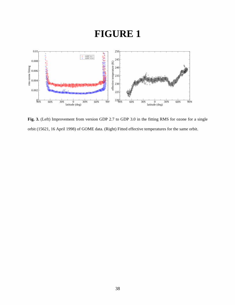
FIGURE 1

90S 60S 30S 0 30N 60N 90Nlatitude (deg)

0

0.002

0.004

0.006

0.008

0.01

rms

ozon

e fi

tting

GDP V2.7GDP V3.0

90S 60S 30S 0 30N 60N 90Nlatitude (deg)

220

225

230

235

240

245

250

effe

ctiv

e te

mpe

ratu

re (

K)

Fig. 3. (Left) Improvement from version GDP 2.7 to GDP 3.0 in the fitting RMS for ozone for a single

orbit (15621, 16 April 1998) of GOME data. (Right) Fitted effective temperatures for the same orbit.

38

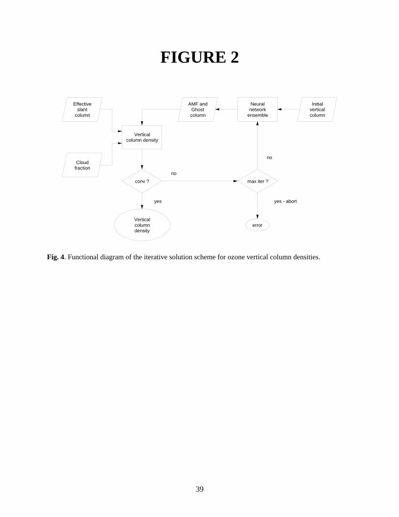
FIGURE 2

Effectiveslant

column

Cloudfraction

Verticalcolumn density

conv ?

Verticalcolumndensity

AMF andGhostcolumn

Neuralnetwork

ensemble

Initialverticalcolumn

max iter ?

error

yes yes - abort

no

no

Fig. 4. Functional diagram of the iterative solution scheme for ozone vertical column densities.

39

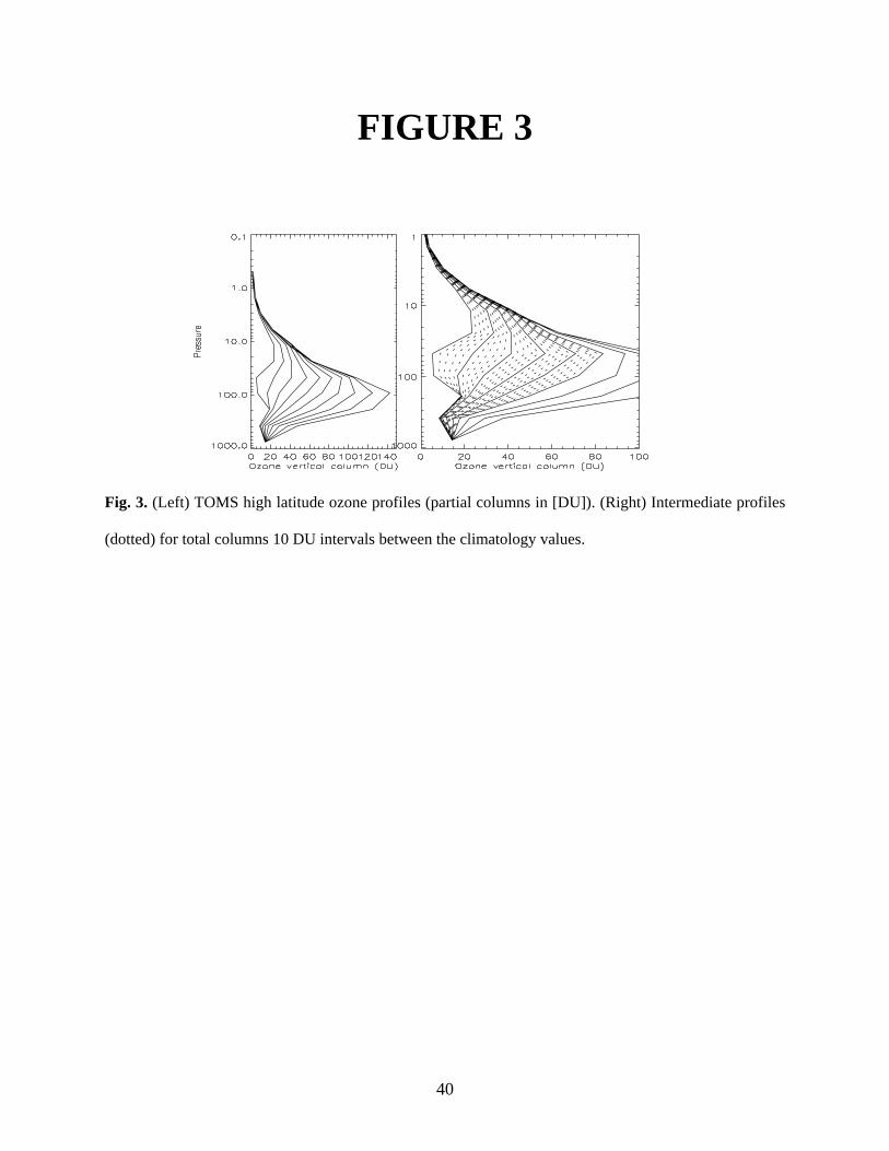
FIGURE 3

Fig. 3. (Left) TOMS high latitude ozone profiles (partial columns in [DU]). (Right) Intermediate profiles

(dotted) for total columns 10 DU intervals between the climatology values.

40

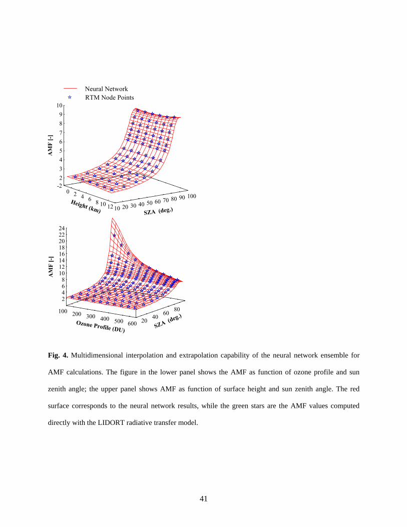
FIGURE 4

Neural NetworkRTM Node Points

-20 2 4 6

10 12Height (km) 10

2

3

4

5

6

7

8

9

10

AM

F [

-]

20 30 40 50 60 70 80 90 100

SZA (deg.)8

K

K

100 200 300 400 500 600Ozone Profile (DU)

2040

6080

SZA (deg.)

2468

1012141618202224

AM

F [

-]

Fig. 4. Multidimensional interpolation and extrapolation capability of the neural network ensemble for

AMF calculations. The figure in the lower panel shows the AMF as function of ozone profile and sun

zenith angle; the upper panel shows AMF as function of surface height and sun zenith angle. The red

surface corresponds to the neural network results, while the green stars are the AMF values computed

directly with the LIDORT radiative transfer model.

41

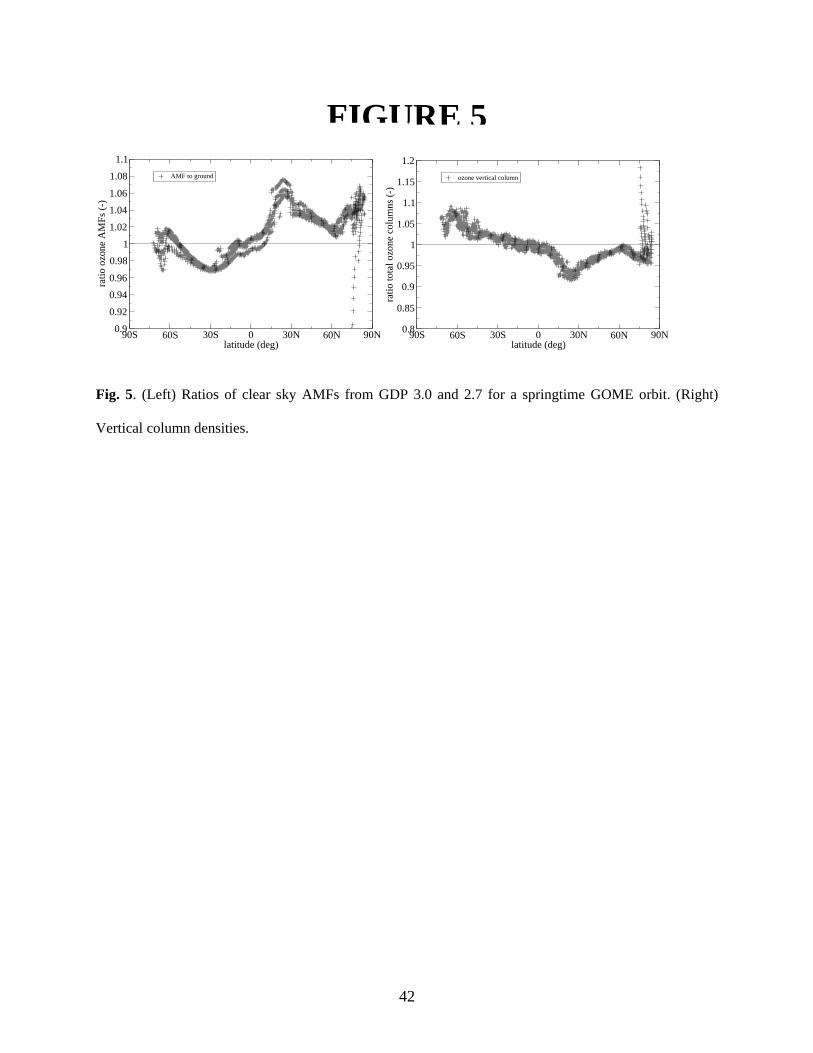
FIGURE 5

90S 60S 30S 0 30N 60N 90Nlatitude (deg)

0.9

0.92

0.94

0.96

0.98

1

1.02

1.04

1.06

1.08

1.1

ratio

ozo

ne A

MFs

(-)

AMF to ground

90S 60S 30S 0 30N 60N 90Nlatitude (deg)

0.8

0.85

0.9

0.95

1

1.05

1.1

1.15

1.2

ratio

tota

l ozo

ne c

olum

ns (

-)

ozone vertical column

Fig. 5. (Left) Ratios of clear sky AMFs from GDP 3.0 and 2.7 for a springtime GOME orbit. (Right)

Vertical column densities.

42

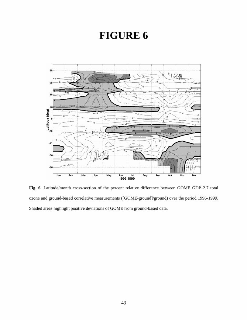
FIGURE 6

Fig. 6: Latitude/month cross-section of the percent relative difference between GOME GDP 2.7 total

ozone and ground-based correlative measurements ([GOME-ground]/ground) over the period 1996-1999.

Shaded areas highlight positive deviations of GOME from ground-based data.

43

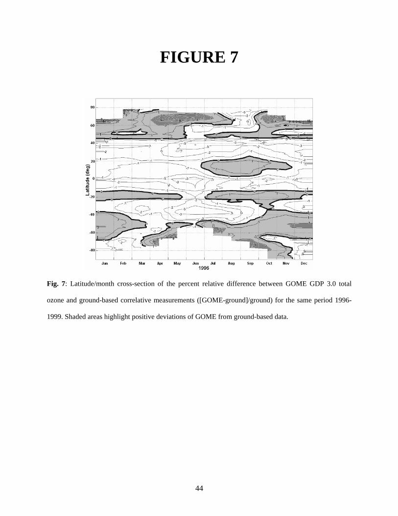
FIGURE 7

Fig. 7: Latitude/month cross-section of the percent relative difference between GOME GDP 3.0 total

ozone and ground-based correlative measurements ([GOME-ground]/ground) for the same period 1996-

1999. Shaded areas highlight positive deviations of GOME from ground-based data.

44

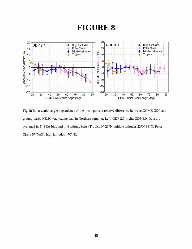
FIGURE 8

Fig. 8: Solar zenith angle dependence of the mean percent relative difference between GOME GDP and

ground-based NDSC total ozone data in Northern summer. Left: GDP 2.7; right: GDP 3.0. Data are

averaged in 5°-SZA bins and in 4 latitude belts (Tropics 0°-23°N; middle latitudes 23°N-63°N; Polar

Circle 67°N±3°; high latitudes >70°N).

45