Global Research Unit Working Paper #2021-023
35
© 2021 by Shilling & Tiwari. All rights reserved. Short sections of text, not to exceed two paragraphs, may be quoted without explicit permission provided that full credit, including © notice, is given to the source. Global Research Unit Working Paper #2021-023 On Bank Pricing of Single-family Residential Home Loans: Are Australian Households Paying Too Much? James D. Shilling, DePaul University Piyush Tiwari, University of Melbourne
-
Upload
khangminh22 -
Category
Documents
-
view
1 -
download
0
Transcript of Global Research Unit Working Paper #2021-023

© 2021 by Shilling & Tiwari. All rights reserved. Short sections of text, not to exceed two paragraphs, may be quoted without explicit permission provided that full credit, including © notice, is given to the source.
Global Research Unit Working Paper #2021-023
On Bank Pricing of Single-family Residential Home Loans: Are Australian Households Paying Too Much? James D. Shilling, DePaul University Piyush Tiwari, University of Melbourne

On Bank Pricing of Single-family Residential Home Loans: Are
Australian Households Paying Too Much?
James D. Shilling‡ and Piyush Tiwari †
Version: August 18, 2020
Abstract
This paper focuses on understanding the observed differences in interest rates on single-family residential
mortgages during September 2008 to December 2017. Exploiting the conceptual difference in risks
associated with fixed rate and variable rate mortgages for lenders, we construct a synthetic variable rate.
Synthetic variables are obtained from 3-year fixed rates by adjusting them for interest rate risks premium and
call options that are embedded in fixed rates. Estimated error correction model for the difference between
actual and synthetic mortgage rate reveals that the unbiasedness hypothesis is rejected and that the lenders in
pricing actual variable rates have attached a risk premia of 90 to 150 basis points over synthetic rates. This
requires further investigation into institutional arrangements, market structures, underwriting and lending
practices of banks as these remain unexplained.
Keywords: mortgage rate differences, swaps, swaptions, errors-in-variables
JEL Classifications: G21
‡DePaul University, 1 East Jackson Boulevard, Chicago, IL Email: [email protected].
†University of Melbourne, Melbourne, Parkville, Email: [email protected].
DePaul University University of Melbourne

1
1 Introduction
There is a feeling (not so easily testable) that Australian banks, in addition to charging excess
fees (including upfront fees, annual fees, exit fees, and partial prepayment fees) on home loan
accounts over the past several years, were also charging residential home loan borrowers high
rates of interest. Here we offer a simple way to test this hypothesis. Statistically and
economically, we construct what banks ought to have been charging residential home loan
borrowers in advance by computing a synthetic mortgage interest rate using interest rate swaps
and swaption data.1 Our goal then is to examine how much of the time-series variation in the
difference between the actual and synthetic mortgage interest rate is due to credit rationing and
differences in credit risk (e.g., debt-to-income ratios), and how much of a differential remains
after controlling for these characteristics. Because this leftover differential could be the result
of further unmeasured differences in credit rationing or credit risk, it represents an upper limit
of the difference between the actual rate and the perfect-market rate charged by Australian banks
over our sample period.
We proceed as follows. Section 2 discusses the institutional details of Australia’s mortgage
market. The Australian mortgage market relies heavily on four large banks of national character
for its funding. In classical theory, when one or a small number of banks dominates a certain
market and determines the price, an artificially high price level could well be established. At
the same time, prices may well be inflexible or “sticky” in such markets, in that they may adjust
slowly over time due to various other reasons such as the lenders’ practice not to disrupt existing
borrowers (Lowe and Rohling, 1992), financial brokers and front-line loan origination staff
(Haney Jr., 1988). The other important factor for stickiness of mortgage rates is the large
1 The model in this paper is related to the literature devoted to the study of regional differences in mortgage
financing costs and whether credit rationing in the allocation of mortgage funds exists. Much of this
literature is quite old (see, for example, Schaaf (1966) and Winger (1969)). Recently, however, Bartlett,
Morse, Stanton, and Wallace (2018) have examined the disparity in the pricing of conventional conforming
mortgages in the U.S. that are securitized by Fannie Mae and Freddie Mac. Their innovation in testing for
disparity in the pricing of conventional conforming mortgages is that they use the Fannie Mae and Freddie
Mac’s pricing grid as an identification strategy. This identification strategy is not available here, since
there is no comparable lending process in Australia.

2
transaction cost that in involved in refinancing, which makes borrowers infrequent participant
in the mortgage market (Haney Jr., 1988). Since not all prices may adjust quickly to changing
conditions, an unexpected fall in the level of interest rates may leave some banks with higher-
than-normal prices, and these higher-than-normal prices may depress loan demand and induce
banks to reduce the quantity of mortgage loans originated. In Section 3, three things are done.
First, we present a model for the determination of the price Australian banks ought to charge on
adjustable-rate home loans (the dominant mortgage form in Australia) in the light of their own
pricing of other residential home loans. These calculations are done using the assumption that
banks can enter into an interest-rate swap and swaption with a counterparty to construct an
adjustment-rate home loan from a fixed-rate home loan in order to unlock the interest rate
(which is not an overly onerous assumption). Second, we then show how the model works by
illustrating its features through numerical examples. Third, once we determine these synthetic
adjustable mortgage rates, we then compare and contrast actual adjustable mortgage rates with
our synthetic rates. A reader impatient to know whether Australian banks were also charging
residential home loan borrowers high rates of interest over the 2008-2018 period is invited to
examine these interest rate differentials. Section 4 presents estimates of a simple model of the
adjustment of actual mortgage rates to synthetic mortgage rates that is based upon the
assumption that there is a constant probability of fully adjusting in each period. A challenge in
pursuing a more generalized version of the partial adjustment model is our limited time-series
availability. Section 5 contains our conclusions.
The paper finds that actual mortgage rates on variable-rate loans in Australia generally
exceeded synthetic rates over the 2008-2017 period by between 90 and 150 basis points per
year, on average. It goes without saying that the findings are strong evidence of higher average
loan rates in less competitive/more concentrated banking markets.
2 Institutional Background
The outstanding feature of the Australian mortgage market is fewness. The market is dominated

3
by four large banks (Commonwealth Bank, Westpac, National Australia Bank, and ANZ) of
national character, and the loans they make are funded primarily through deposits with short
duration. Hence, most mortgage loans in Australia – generally between 80 and 90% of owner-
occupier loan commitments – are variable-rate loans (VRMs) that track the official cash rate,
set by the Reserve Bank of Australia (see Australian Competition and Consumer Commission,
hereafter ACCC, (2018)). But why, you may ask, are most loans VRMs? The answer, of course,
is that variable-rate instruments reduce the interest rate risk of banks by transferring this risk to
mortgage borrowers.
This, however, does not mean that fixed-rate lending (FRMs) is absent. Between 10 and
20% of owner-occupier loan commitments in Australia are FRMs. However, unlike in the U.S.,
rates are fixed generally for a period of up to 3 years, after which time the loan converts
automatically to a VRM. Of immediate relevance is the fact that most FRMs in Australia are
sold into a secondary market. The loans are then pooled together with VRMs to form a
mortgage-backed security and sold in the secondary market. The outputs of this securitization
are either purchased directly by authorized deposit-taking institutions or by superannuation
funds seeking short-term debt instruments. Hence, for these reasons mortgage rates on FRMs
in Australia are generally fixed for a limited number of years.
The majority of mortgage loans in Australia are classified in one of three ways. First, there
are basic loans with limited options. Next, there are flexible loans with facilities such as an
option to redraw (i.e., the ability to access additional payments made on top of the minimum
loan repayment schedule, including one-off lump-sum repayments, over the life of the loan),
and the option to make early repayments or convert from a variable- to a fixed-rate, or vice
versa. Then there are discounted loans, where the loan has a discounted or “honeymoon” rate
of interest for the first year of the life of the loan. Honeymoon rate loans can carry significantly
discounted initial year interest rates before reverting back to the standard variable-rate (see
ACCC (2018)). Most FRMs are basic loans (i.e., they lack add-on features), while most VRMs
are either flexible loans or honeymoon rate loans. Features such as redraw, offset and

4
progressive drawdown are generally only available on VRMs (see ACCC (2018)). Lenders in
Australia provide mortgages with much greater payment flexibility than anything available in
the US.
To ensure sound credit evaluation, home loans in Australia are underwritten entirely based
on the ability to pay back the loan. For example, most lenders set maximums for these ratios,
such as, e.g., the monthly mortgage repayment cannot exceed 25 to 35% of the borrower’s
monthly income. However, most lenders will allow a higher payment-to-income ratio for
borrowers who are well-qualified. Generally, these lending standards did not deteriorate like
they did in the US and in other countries prior to the Great Financial Crisis, nor have they since
been significantly tightened. So if payment-to-income ratios for borrowers did not deteriorate
or tightened significantly over the 2008-2018 period, and did not push the market toward riskier
loans with higher interest rates or higher points and fees, we need to look elsewhere for reasons
for (relatively) high rates of interest on residential home loans in the Australian mortgage
market.
Loan-to-value ratios (LVR) in Australia, like in the U.S. and elsewhere, exhibit some level
of variability. For example, there is evidence of low LVRs in 2008, with averages on new
applications around 62% (see Lawless (2016)). On the other hand, there is evidence of high
LVRs in 2013, with averages on new applications around 78%. Another example is low LVRs
in 2018, with averages on new applications around 73%. These results are to be expected. The
argument could be that the strongest markets, such as Sydney and Melbourne, have been the
primary drivers of lower application LVRs. As house prices in these markets have increased
greatly, first-time home buyers have retreated from these markets, causing the national average
application LVR to decrease.2
2 Of course, low LVRs could also be tied to the borrower’s creditworthiness (credit scores) over this period
(see Somasundaram (2017)). The implication is that lower creditworthiness significantly increases the
riskiness of the loan and lenders compensate by lowering the LVR. Low LVRs reduce the stress on lenders,
because when (and if) borrowers are short of cash, their property can be sold if necessary, to redeem their
loan.

5
The typical loan term in Australia is 25 years but could range from 20 to 30 years. In
practice, most mortgages are often paid off well before stated maturity, with households
choosing to make excess repayments on standard loans. It should be noted, however, that a 1-
year VRM amortized over 25 years making annual payments at the current rate is likely to have
a duration slightly less than 1 year, assuming a balloon payment on the adjustment date (see Ott
(1986)). For a 1-year VRM with facilities like an option to make early repayments and an option
to redraw, the duration could increase or decrease depending on the proportion of the mortgage
principal amortized on or before the first adjustment period. In comparison, the duration of a
FRM is likely to be substantially less than 3 years since the loan converts automatically to a
VRM in year 3 and uses the official cash rate set by the Reserve Bank of Australia as the index
rate (something which can be viewed as lowering the interest rate sensitivity in this mortgage
type).
Other things equal, when a relatively few number of firms dominate a market, there is a real
concern that these firms may be able to act in a collusive manner to maximize joint profits, with
the result being prices that may be higher than they would be in a more competitive market.
There is also the possibility that prices in this market may be inflexible or sticky and the price
changes that do occur may be orderly. Assuming given long-run production costs, such a market
may originate fewer loans, provide fewer jobs, and charge a higher price (i.e., interest rate) than
would the same industry organized competitively. The few, large, dominant firms may also
possess the means to earn excess returns as long as other firms are prevented from entering the
market.3 Such firms may have greater ability to control the market for, and the price of, its
product than would a smaller, more competitive firm.
It may be mentioned here how bank competition and overall restrictions on banking
activities vary across countries. In some countries bank activities are highly restricted and in
3 Entry costs are defined here as access to customer data. Large volumes of such information give a
competitive advantage to incumbent banks. Without this data, new entrants are unlikely to enter into this
market.

6
others they are less so. Drawing on cross-country survey data from Barth, Caprio, and Levine
(2013) (in which 180 countries from 1999 to 2011 appear), the figures indicate that Australian
banks are generally less heavily restricted than US and Chinese banks, but more heavily
restricted than UK and Hong Kong banks. A widely held view is to the effect that regulatory
restrictions to competition and monopolistic power create an environment in which a few
powerful banks stymie competition with deleterious implications for efficiency (see Demirgüç-
Kunt, Laeven, and Levine (2004) for evidence along these lines). Another theory of bank
concentration departs in important respects from this view and holds that more efficient banks
have lower costs and garner greater market share (Demsetz (1973) and Peltzman (1977)).
Particularly important according to many who hold this view is that competitive environments
tend to produce concentrated and efficient banking systems.
A variety of authors have discussed the issue of monopolistic and discriminatory pricing in
terms of increasing the risk-taking appetite of banks. Besanko and Thakor (1987) provide a
useful starting point by providing a general model where monopolistic banks prefer a risky credit
policy to a less risky credit policy. In Boyd, De Nicolo, and Smith (2004), a monopolistic
banking system has a higher probability of a banking crisis when the inflation rate is below some
threshold, while a competitive banking system is more fragile otherwise. This argument is
strengthened further in Matsuoka (2011). Matsuoka (2011) finds that banks with market power
have profits that are positively correlated with the nominal interest. Martin and Smyth (1992)
claim that monopoly lenders use discount points more intensively than do perfect competitors
and that monopoly lenders choose higher effective interest rates than do perfect competitors.
Securitization matters, but how? A pervasive view (at least in the US) is that mortgage
securitization programs gradually integrate mortgage markets into traditional capital markets
(see Hendershott and Van Order (1989) for evidence that mortgage securitization programs in
the US fully integrated the US mortgage market into traditional capital markets over the 1970s
and 1980s). Gan and Riddiough (2008) argue that as mortgage securitization programs come to
dominate the market, and as the mortgage securitizer(s) acquire vast quantities of consumer

7
credit information, they can directly address individual borrower segments, isolate them into
higher- and lower-credit-quality borrowers, and use their market power to mark the mortgage
loan rate on higher-credit-quality loans above marginal cost. The remaining lower-credit-
quality borrowers are charged a separating (risk-based) price by retail loan originators
(depository institutions), since entry is naturally deterred in this borrower segment. The key is
to charge higher-credit-quality borrowers a pooling rate, thereby deterring entry into this market
segment by obfuscating the true credit quality of particular borrowers. This two-part pricing
scheme allows monopolist lenders to profit-maximize, thereby extracting all or most consumer
surplus.
It is worth noting first that the big four Australian banks are heavily dependent on traditional
banking. More importantly, Australian banks largely eschew the lower-credit-quality
(“subprime”) mortgage market. This is in stark contrast to the mortgage market in the US, where
almost a quarter of all loans originated each year were sup-prime and the stock of sub-prime
loans had reached 8% of total US mortgage debt by 2005. By “sticking to one’s knitting” (and
pursuing a traditional “boring but safe” business model), Bell and Hindmoor (2019) argue that
Australian banks were able to avoid the Great Financial Crisis that erupted in 2007-2009. Bell
and Hindmoor’s (2009) explanation for this result is in part due to regulatory conditions (a large
policy success) and partly due to luck.
Our explanation is quite different. Evidence suggests that the large, dominant banks in
Australia were generally able to earn returns on capital that were 15% higher than business
banks and 20% higher than institutional banking over the 2008-2018 period. Further, the
evidence suggest that these returns were higher than peers, including banks in the US, Sweden,
Singapore, Hong Kong, Spain, France, the UK, and Japan (see Morgan Stanley (2018)). These
results suggest that traditional mortgage lending in Australia was anything but “boring but safe.”
These exploratory insights lay the foundation for empirically accessing whether Australian
banks were overpricing mortgage loans over this period. Under equilibrium conditions, the
8
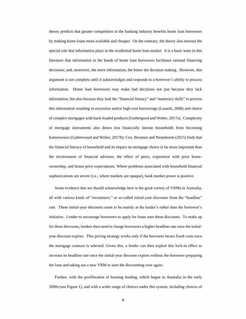
theory predicts that greater competition in the banking industry benefits home loan borrowers
by making home loans more available and cheaper. On the contrary, the theory also stresses the
special role that information plays in the residential home loan market. It is a basic tenet in this
literature that information in the hands of home loan borrowers facilitates rational financing
decisions; and, moreover, the more information, the better the decision making. However, this
argument is not complete until it acknowledges and responds to a borrower’s ability to process
information. Home loan borrowers may make bad decisions not just because they lack
information, but also because they lack the “financial literacy” and “numeracy skills” to process
this information resulting in excessive and/or high-cost borrowings (Lusardi, 2008) and choice
of complex mortgages with back-loaded products (Gethergood and Weber, 2017a). Complexity
of mortgage instruments also deters less financially literate households from becoming
homeowners (Gatherwood and Weber, 2017b). Cox, Brounen and Neuteboom (2015) finds that
the financial literacy of household and its impact on mortgage choice is far more important than
the involvement of financial advisors, the effect of peers, experience with prior home-
ownership, and house price expectations. Where problems associated with household financial
sophistications are severe (i.e., where markets are opaque), bank market power is positive.
Some evidence that we should acknowledge here is the great variety of VRMs in Australia,
all with various kinds of “sweeteners,” or so-called initial-year discounts from the “headline”
rate. These initial-year discounts seem to be mainly at the lender’s rather than the borrower’s
initiative. Lender to encourage borrowers to apply for loans uses these discounts. To make up
for these discounts, lenders then need to charge borrowers a higher headline rate once the initial-
year discount expires. This pricing strategy works only if the borrower incurs fixed costs once
the mortgage contract is selected. Given this, a lender can then exploit this lock-in effect to
increase its headline rate once the initial-year discount expires without the borrower prepaying
the loan and taking out a new VRM to start the discounting over again.
Further, with the proliferation of housing lending, which began in Australia in the early
2000s (see Figure 1), and with a wider range of choices under this system, including choices of

9
different types of VRMs with various repayment features and various headline rates, the pricing
of VRMs may have become more and more obscure (in the classical sense). As already
mentioned, the issue is, knowing which loan to take out may have become exceedingly difficult
when the options become so numerous. Critics argue that this murkiness favors lenders as a
whole at the expense of the uninformed borrower, potentially causing bouts where VRMs may
be significantly overpriced, a hypothesis ripe for testing.4 It is plausible that the preponderance
of VRMs is a consequence of the pricing strategies of lenders and the tendency of financial
advisors not to focus on risks associated with interest rate movements (Miles (2005)). One
implication, which follows in our empirical analysis, is that there could be overpricing in lending
to Australian variable-rate mortgage borrowers over the 2008-2018 period.
3 Construction of Equivalent Mortgage Rates
3.1 Basic Idea
To construct equivalent variable-rate mortgage rates for Australia, the following procedure is
used. First, we obtain monthly data on fixed-rate mortgage yields in Australia. Then direct
adjustments are made to these yield series to convert them into a variable-rate loan. These
include the impact of call risk and interest rate risk.
To make the adjustment for maturity, we use a 3-year interest rate swap. An interest rate
swap is simply an exchange of one set of cash flows (e.g., a floating-rate payment) for another
(e.g., a fixed-rate payment). We assume that the Australian homeowner pays the floating
amount of interest in the swap agreement and receives at the same intervals a fixed amount of
interest on some notional principal (i.e., the mortgage amount). The homeowner uses the fixed-
rate payments to make the payment on his or her 3-year fixed-rate mortgage. Hence, on net the
homeowner is left with a single obligation to pay a short-term variable interest rate.
4 See ACCC (2018), who found that the initial-year discounts that banks offer on headline variable rates
are highly discretionary and non-transparent. Their evidence suggests that these discounts depend on wide
variety of factors, such as perceived borrowers’ risk profile, geographic location of borrower or their
property, borrower’s value to the bank, and bank’s desire to write new business.

10
To make the adjustment for the call option in the 3-year fixed-rate mortgage, we use a 2-
year call swaption (an option to receive fixed and pay floating on a swap). Economically, a 3-
year, prepayable fixed-rate mortgage in Australia is equivalent to a variable-rate mortgage plus
an interest rate swap and a swaption. Here the swaption is an option to receive the fixed rate
specified in the swaption while paying a floating rate (“receiver” swaption). We choose year 2
because it is the middle year of the 3-year fixed-rate mortgage. If swap rates have fallen, the
homeowner would exercise the swaption and elect to receive the agreed-upon fixed rate
specified in the swaption and pay the floating rate on the swap. Simultaneously, the homeowner
would enter into a short position (pay fixed, receive floating) in a plain vanilla interest-rate swap
based on the market. The floating rates would cancel out and the homeowner would end up
receiving an interest rate spread between the agreed-upon fixed rate specified in the swaption
minus the fixed rate paid in the plain vanilla interest-rate swap based on the market. Hence, this
call option essentially allows the homeowner to effectuate an interest rate savings equal to the
difference between the fixed interest-rate on the 2-year call swaption and the fixed interest-rate
based on the market, thereby replicating the option to refinance the 3-year fixed-rate mortgage
at a lower interest rate, albeit only at time t = 2 years. Should, of course, swap rates rise over
this time period, the swaption would expire unexercised, and the homeowner would simply
continue to pay the contract rate specified in his or her 3-year fixed-rate mortgage. The price of
this option to refinance is the premium paid by the holder of the call swaption.
To make an adjustment for the flexible payment stream, such as having the option to
temporarily reduce or forgo principal payments in future periods if a financial shock or expense
shock were to occur, we use a put option on the stock market. As the stock price falls below the
strike price, the payoff from the put option starts increasing. The profit (the difference between
the stock’s market price and the option’s strike price) allows the holder to benefit from a stock
price collapse. The same gains occur on a mortgage with a flexible payment stream. As an
emergency source of funds, a flexible mortgage allows the borrower to skip or reduce principal
payments when necessary, and to borrow back any principal payments when cash is tight. This

11
option is normally of little value since financial crises or expense shocks are rare events.
However, when such events do happen, allowing borrowers the option to make their payments
anything they wish and to borrow back any principal payments can be quite expensive,
incorporating not only the perceived risk of lending in the aftermath of a financial crisis but also
the degree of risk aversion of a representative lender.
To illustrate the effect of these adjustments, let 𝑟𝑚 denote the actual interest rate on a 3-year
fixed-rate mortgage in Australia. Similarly, let 𝑖3 denote the annual fixed swap rate on a 3-year
contract and 𝑠𝑤 the price of a 2-year swaption. Let 𝑝 denote the value of a short-term (out-of-
the-money) put option, where the maturity equals one-year. Using this notation, the yield on a
synthetic variable-rate mortgage in Australia can be decomposed into four terms as follows:
𝑦 = 𝑖1 + 𝑠𝑝𝑟𝑑 − 𝑠𝑤 + 𝑝 (1)
where 𝑠𝑝𝑟𝑑 = 𝑟𝑚 − 𝑖3 is the interest rate spread on a 3-year fixed-rate mortgage in Australia.
The term 𝑖1 is the opportunity cost of the lender’s money for 1-year at time 𝑡. The term 𝑠𝑝𝑟𝑑
can be interpreted as a risk premium. This risk premium should vary, according to standard
option pricing theory, with the borrower’s option to buy back or call the mortgage at par and the
option to sell or put the hose to the lender at a price equal to value of the mortgage. The term
𝑠𝑤 is the added interest rate that a 3-year fixed-rate mortgage borrower pays for the privilege to
refinance the loan at the end of year 2. The term 𝑝 is the price the borrower pays for a flexible
payment mortgage.
To construct synthetic estimates of y, there must be estimates of 𝑟𝑚, 𝑖3, 𝑖1, 𝑠𝑤, and 𝑝. The
sources of these data are as follows. The 3-year fixed mortgage rates for Australia are actual 3-
year bank lending rates on owner-occupier housing loans as reported by the Reserve Bank of
Australia from their monthly survey of rates on bank loan rates. The interest rate swap data 𝑖3
are taken from Bloomberg. The 3-year swap rate is equal to the 3-year government bond rate
plus a swap spread. The opportunity cost of the lender’s money for 1-year is not available
throughout the time period which we considered. It was therefore necessary to use a proxy for

12
𝑖1. The proxy we chose was the 2-year government bond rate. The swaption premia, 𝑠𝑤, for
Australia are collected from Bloomberg. The put option premia, 𝑝, are calculated using Black-
Scholes. Volatilities are implied volatilities from the Australian S&P/ASX 200 VIX index,
which is similar to the CBOE VIX index based on real time data from S&P 500 options in the
US. We value the put option under the following assumptions: a) the stock price is the
Australian S&P/ASX 200 index, b) the stock index pays no dividends, c) the risk-free rate of
interest is the 3-month bank bill rate for Australia, d) the term to expiry is 1-year, e) the holder
of the option can only exercise the option on the expiry date, and f) the strike price (as a percent
of the underlying index) is set equal to 0.7. This is a reasonable way to measure the cost of put
protection over 1-year. With a 0.7-strike put, the price of this out-of-the-money option will
consist entirely of time value. This out-of-the-money put option protects only against a major
economic meltdown.5 The sample is restricted to the following time periods: June 2008 to
December 2018.
3.2 Illustrative Calculations
A simple example serves to illustrate the construction of equivalent variable mortgage rates.
Suppose the following situation exists: An Australian household is considering taking out a
prepayable mortgage on a fixed basis for 3 years. The mortgage has an amortization period of
30 years. The interest rate on this mortgage can be compared to the interest rate on an equivalent
variable-rate mortgage.
Here are the three steps that the Australian homeowner would need to undertake to construct
the interest rate on an equivalent variable-rate mortgage.
Step 1: The household enters into a 3-year swap agreement. The household agrees to pay
a short-term rate of interest, 𝑖1, to a counterparty. In return, the counterparty agrees
to pay a long-term rate (3-year fixed) of interest, 𝑖3, to the household.
5 It is important to note that setting the strike price equal to 0.7 is quite arbitrary. It would not be difficult
to pick a higher or lower strike price. A higher (lower) strike price would lead to a higher (lower) option
premium, and so raises (lowers) the synthetic variable mortgage rate.

13
Step 2: The household writes a 2-year call swaption for 𝑠𝑤. The swaption would allow
the counterparty to realize an interest rate savings equal to the difference between the
agreed-upon fixed interest-rate on the 2-year call swaption and the fixed interest-rate
based on the market, thereby replicating the option to refinance the 3-year fixed-rate
mortgage at a lower interest rate with the following proviso: The call swaption is
exercisable only at time t = 2 years. In turn, the counterparty agrees to pay a swaption
premium of 𝑠𝑤 to the household. This swaption premium allows the household to
offset the price paid for the prepayment option in the 3-year fixed mortgage.
Step 3: The household pays a premium of 𝑝 (expressed as percent of the underlying stock
price) for a put option on the stock market. The put option gives the household the
right to sell the underlying stock at the option exercise price. Hence, should the price
of stock goes down, and should the price fall below than the exercise price of the
option, the holder of the put benefits. The gross profit on the put would be the
difference between the exercise price and the market price of the stock. This profit
replicates exactly the borrow-back feature in Australian mortgages and illustrates
how Australian households heavily rely on mortgage financing as an emergency
source of revenue in response to unexpected shocks (and all of this can be done
without the need to file new loan documents or submit to another credit check when
cash is extremely tight).
In this case, the net obligation of the household would be
𝑦 = 𝑟𝑚 − (𝑖3 − 𝑖1) − 𝑠𝑤 + 𝑝
= 𝑖1 + (𝑟𝑚 − 𝑖3) − 𝑠𝑤 + 𝑝
= 𝑖1 + 𝑠𝑝𝑟𝑑 − 𝑠𝑤 + 𝑝
(2)
which shows that 𝑦 is the borrowing rate on a synthetic variable-rate mortgage. For 𝑟𝑚 =
4.15%, 𝑖1 = 1.99% (as measured by the 2-year government bond rate), 𝑖3 = 2.18% (as
measured by a 3-year swap rate, which is equal to the 3-year government bond rate plus a swap
spread), 𝑠𝑤 = 0.63%, and 𝑝 = 0.06% (which are actual values for March 2018), the value of 𝑦
is 3.39%. With an actual rate of 𝑟 = 5.20% on a variable-rate mortgage in March 2018 (as
reported by the Reserve Bank of Australia), the result for 𝑟 − 𝑦 = 1.81%.

14
3.3 Summary Measures of Cost Differences
Figure 2 shows that the relative picture for actual variable-rate borrowing costs in Australia
compared with the borrowing rate on a synthetic variable-rate mortgage. There appears to be
quite a difference in relative borrowing costs over the subsample period July 2011-March 2018,
in that the actual variable-rate mortgage interest rate is only slightly higher than the synthetic
mortgage rate without adjusting for the call swaption premium or the put premium for the
subsample period December 1998-June 2011, but contrasts sharply with the synthetic mortgage
rate without adjusting for the call swaption premium or the put premium for the subsample
period July 2011-March 2018. Overall, the actual variable-rate mortgage interest rate compared
to the synthetic mortgage rate without adjusting for the call swaption premium or the put
premium is higher over the subsample period July 2011-March 2018 by 134 basis points
compared to 71 basis points during December 2008-June 2011. The highest differential between
actual and synthetic borrowing costs over this subsample period is 218 basis points in October
2008; and the lowest is -45 basis points in January 2010.
Interestingly enough, when adjusting for the call swaption premium and the put premium,
the difference between actual and synthetic narrows over the subsample period September 2008-
March 2009, due to the large increase in the Australian S&P/ASX 200 VIX index as the
Australian S&P/ASX 200 index crashes. The difference between actual and synthetic then
increases somewhat over the subsample period April 2009-March 2018, in part due to a decline
in the put premium and partly due to an increase in the call swaption premium. Overall, the
difference between the actual variable-rate mortgage interest rate and the synthetic mortgage
rate with adjusting for the call swaption premium and the put premium for the subsample period
March 2008-March 2018 is 151 basis points. In the remainder of this paper, we examine these
differences between actual and synthetic borrowing costs to determine whether these differences
reflect our inability to fully specify all the nonlinearities and interactions in the pricing of
variable-rate mortgages (including borrower self-selection effects), as well as to measure the
swap rates and swaptions precisely, or whether these differences reflect predatory lending
15
practices which have cost consumers dearly.
4 Empirical Analysis
4.1 Tests of Over-pricing
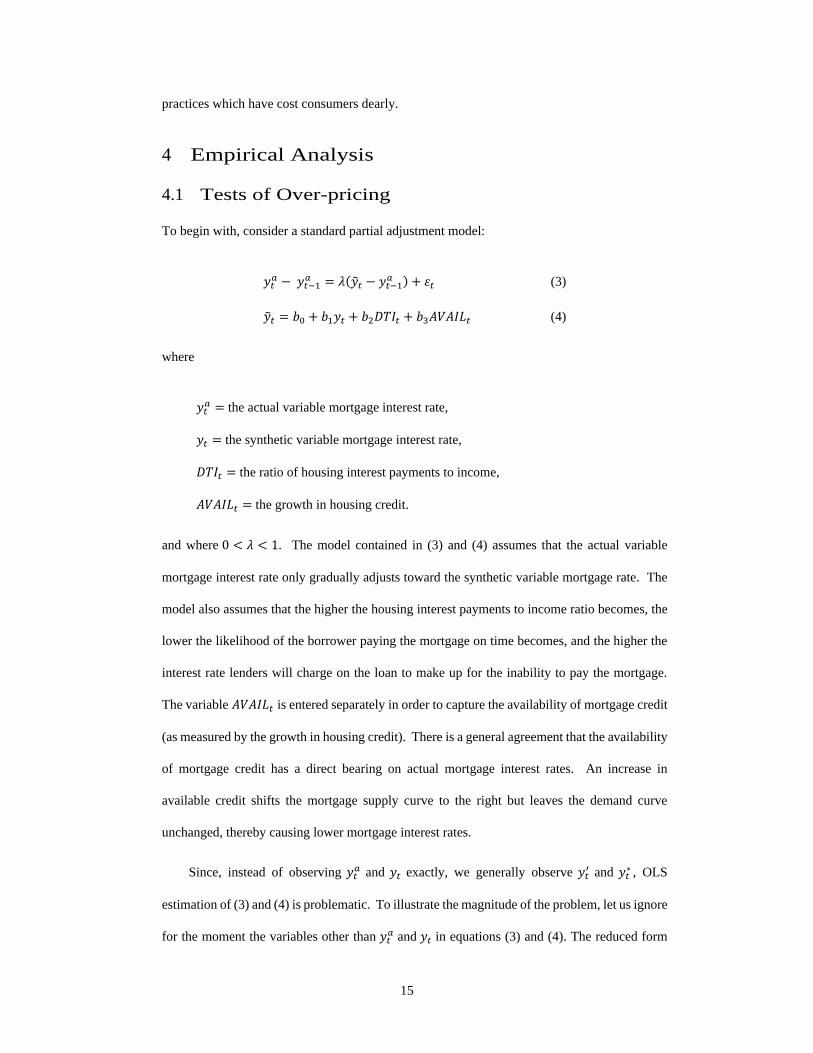
To begin with, consider a standard partial adjustment model:
𝑦𝑡𝑎 − 𝑦𝑡−1
𝑎 = 𝜆(�̃�𝑡 − 𝑦𝑡−1𝑎 ) + 𝜀𝑡 (3)
�̃�𝑡 = 𝑏0 + 𝑏1𝑦𝑡 + 𝑏2𝐷𝑇𝐼𝑡 + 𝑏3𝐴𝑉𝐴𝐼𝐿𝑡 (4)
where
𝑦𝑡𝑎 = the actual variable mortgage interest rate,
𝑦𝑡 = the synthetic variable mortgage interest rate,
𝐷𝑇𝐼𝑡 = the ratio of housing interest payments to income,
𝐴𝑉𝐴𝐼𝐿𝑡 = the growth in housing credit.
and where 0 < 𝜆 < 1. The model contained in (3) and (4) assumes that the actual variable
mortgage interest rate only gradually adjusts toward the synthetic variable mortgage rate. The
model also assumes that the higher the housing interest payments to income ratio becomes, the
lower the likelihood of the borrower paying the mortgage on time becomes, and the higher the
interest rate lenders will charge on the loan to make up for the inability to pay the mortgage.
The variable 𝐴𝑉𝐴𝐼𝐿𝑡 is entered separately in order to capture the availability of mortgage credit
(as measured by the growth in housing credit). There is a general agreement that the availability
of mortgage credit has a direct bearing on actual mortgage interest rates. An increase in
available credit shifts the mortgage supply curve to the right but leaves the demand curve
unchanged, thereby causing lower mortgage interest rates.
Since, instead of observing 𝑦𝑡𝑎 and 𝑦𝑡 exactly, we generally observe 𝑦𝑡
′ and 𝑦𝑡∗ , OLS
estimation of (3) and (4) is problematic. To illustrate the magnitude of the problem, let us ignore
for the moment the variables other than 𝑦𝑡𝑎 and 𝑦𝑡 in equations (3) and (4). The reduced form

16
solution for 𝑦𝑡𝑎 can be written as
𝑦𝑡′ = 𝛼 + 𝛽𝑦𝑡
∗ + 𝜀𝑡∗ (5)
where
𝑦𝑡′ = 𝑦𝑡
𝑎 + 𝜈𝑡 (6)
𝑦𝑡∗ = 𝑦𝑡 + 𝜉𝑡 (7)
𝜀𝑡∗ = 𝜀𝑡 + 𝜈𝑡 − 𝛽𝜉𝑡 (8)
and where 𝜀𝑡 is a disturbance term with mean zero and variance 𝜎𝜀2 in the true regression model
𝑦𝑡𝑎 = 𝛼 + 𝛽𝑦𝑡 + 𝜀𝑡 and 𝜈𝑡 and 𝜉𝑡 represent the errors in measuring the values of 𝑦𝑡
𝑎 and 𝑦𝑡 ,
respectively.6
The error terms 𝜈𝑡 and 𝜉𝑡 are assumed to be distributed
𝜈𝑡~𝑁(0, 𝜎𝜈2) (9)
𝜉𝑡~𝑁(0, 𝜎𝜉2) (10)
where 𝐸(𝜈𝑖𝜈𝑗) = 0, 𝐸(𝜉𝑖𝜉𝑗) = 0 for 𝑖 ≠ 𝑗 , and 𝐸(𝜈𝑖𝜉𝑖) = 0, 𝐸(𝜈𝑖𝜀𝑖) = 0, and 𝐸(𝜉𝑖𝜀𝑖) = 0.
Econometrically, these assumptions rule out situations in error terms that are autoregressive.
The assumptions also rule out situations in which 𝜈𝑡, 𝜉𝑡, and 𝜀𝑡 are related to each other.
One can show that the ordinary least squares (OLS) estimators of 𝛼 and 𝛽 in equation (5)
are
𝑝𝑙𝑖𝑚 �̂� = �̅�′ − 𝛽(𝜎𝜈2 (𝜎𝜈
2 + 𝜎𝜉2)⁄ )�̅�∗ (11)
𝑝𝑙𝑖𝑚 �̂� = 𝛽(𝜎𝜈2 (𝜎𝜈
2 + 𝜎𝜉2)⁄ ) (12)
From (11) and (12), it is seen that the OLS estimates of 𝛼 and 𝛽 are biased and that this bias
does not decrease with the sample size. Instead, the magnitude of the bias is determined by the
6 Equation (8) can be obtained as follows. Let 𝑦𝑡
𝑎 = 𝑦𝑡′ − 𝜈𝑡 and 𝑦𝑡 = 𝑦𝑡
∗ − 𝜉𝑡 . By substituting 𝑦𝑡𝑎 = 𝑦𝑡
′ −𝜈𝑡 and 𝑦𝑡 = 𝑦𝑡
∗ − 𝜉𝑡 into the regression equation 𝑦𝑡𝑎 = 𝛼 + 𝛽𝑦𝑡 + 𝜀𝑡 , one obtains 𝑦𝑡
′ − 𝜈𝑡 = 𝛼 + 𝛽(𝑦𝑡∗ −
𝜉𝑡) ∓ 𝜀𝑡 . Rearranging this equation, one obtains 𝑦𝑡′ = 𝛼 + 𝛽𝑦𝑡
∗ + 𝜀𝑡∗, where 𝜀𝑡
∗ = 𝜀𝑡 + 𝜈𝑡 − 𝛽𝜉𝑡 .
17
ratio of the error variance 𝜎𝜈2 to (𝜎𝜈
2 + 𝜎𝜉2).
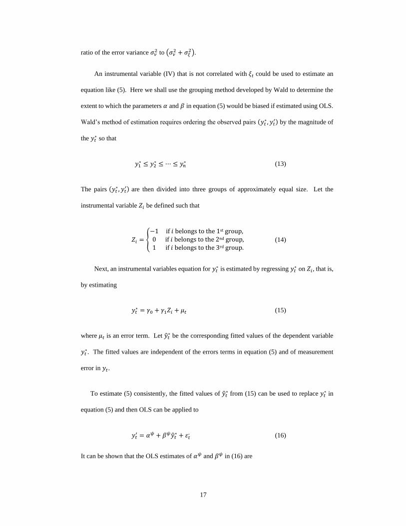
An instrumental variable (IV) that is not correlated with 𝜉𝑡 could be used to estimate an
equation like (5). Here we shall use the grouping method developed by Wald to determine the
extent to which the parameters 𝛼 and 𝛽 in equation (5) would be biased if estimated using OLS.
Wald’s method of estimation requires ordering the observed pairs (𝑦𝑡∗, 𝑦𝑡
′) by the magnitude of
the 𝑦𝑡∗ so that
𝑦1∗ ≤ 𝑦2
∗ ≤ ⋯ ≤ 𝑦𝑛∗ (13)
The pairs (𝑦𝑡∗, 𝑦𝑡
′) are then divided into three groups of approximately equal size. Let the
instrumental variable 𝑍𝑖 be defined such that
𝑍𝑖 = {
−1 if 𝑖 belongs to the 1st group,0 if 𝑖 belongs to the 2nd group,1 if 𝑖 belongs to the 3rd group.
(14)
Next, an instrumental variables equation for 𝑦𝑡∗ is estimated by regressing 𝑦𝑡
∗ on 𝑍𝑖, that is,
by estimating
𝑦𝑡∗ = 𝛾0 + 𝛾1𝑍𝑖 + 𝜇𝑡 (15)
where 𝜇𝑡 is an error term. Let �̂�𝑡∗ be the corresponding fitted values of the dependent variable
𝑦𝑡∗. The fitted values are independent of the errors terms in equation (5) and of measurement
error in 𝑦𝑡.
To estimate (5) consistently, the fitted values of �̂�𝑡∗ from (15) can be used to replace 𝑦𝑡
∗ in
equation (5) and then OLS can be applied to
𝑦𝑡′ = 𝛼𝜓 + 𝛽𝜓�̂�𝑡
∗ + 𝜀𝑡, (16)
It can be shown that the OLS estimates of 𝛼𝜓 and 𝛽𝜓 in (16) are

18
𝑝𝑙𝑖𝑚 𝛼𝜓 = �̅�′ − 𝛽𝜓�̅�∗ (17)
𝑝𝑙𝑖𝑚 𝛽𝜓 = 𝛽 +
(∑ 𝜀𝑡′(𝑍𝑡 − 1 𝑛 ∑ 𝑍𝑡
𝑛𝑡=1⁄ )𝑛
𝑡=1 ) (∑ (𝑦𝑡∗ − 1 𝑛⁄ ∑ 𝑦𝑡
∗𝑛𝑡=1 )𝑛
𝑡=1 (𝑍𝑡 − 1 𝑛⁄ ∑ 𝑍𝑡𝑛𝑡=1 ))⁄ (18)
From the condition that
𝑝𝑙𝑖𝑚 (1 𝑛⁄ ∑ 𝜀𝑡′(𝑍𝑡 − 1 𝑛 ∑ 𝑍𝑡
𝑛𝑡=1⁄ )𝑛
𝑡=1 ) = 0, (19)
It follows that the Wald parameter estimates of 𝛼𝜓 and 𝛽𝜓 in (16) are consistent estimates of 𝛼
and 𝛽.
4.2 Some Empirical Results
In this section, the results of estimating the partial adjustment model given in (3) and (4) using
OLS and Wald’s method of estimation are reported. Substituting (4) into (3) yields the reduced
form equation
𝑦𝑡′ = 𝑏0
′ + 𝑏1′ 𝑦𝑡
∗ + 𝑏2′ 𝐷𝑇𝐼𝑡 + 𝑏3
′ 𝐴𝑉𝐴𝐼𝐿𝑡 + (1 − 𝜆)𝑦𝑡−1𝑎 + 𝜀𝑡
∗ (20)
where 𝑏𝑖′ = 𝜆𝑏𝑖, 𝑦𝑡
′ = 𝑦𝑡𝑎 + 𝜈𝑡, and 𝑦𝑡
∗ = 𝑦𝑡 + 𝜉𝑡.
Our tests are based on the idea of comparing the OLS estimates of 𝑏0 and 𝑏1 with our Wald
estimates. The data on the actual mortgage interest rate on owner-occupied housing loans with
variable rates (the same data as shown in Figure 2 above) are from the Reserve Bank of
Australia. The data used to construct the synthetic variable mortgage rates on owner-occupied
housing loans are the same data described in section 3 above. We calculate two measures of the
synthetic variable mortgage rate, namely, 𝑦𝑡∗ = 𝑖𝑡 + 𝑠𝑝𝑟𝑑𝑡 − 𝑠𝑤𝑡 and 𝑦𝑡
∗ = 𝑖𝑡 + 𝑠𝑝𝑟𝑑𝑡 −
𝑠𝑤𝑡 + 𝑝𝑡. The data on the ratio of housing interest payments to income, which give a measure
of how cumbersome mortgage debt is for households, are from the Reserve Bank of Australia.
These data show a rise in housing interest payments relative to income from 6% in the fourth
19
quarter of 2002 to 11% in the second quarter of 2008 just before the Great Financial Crisis. The
ratio of housing interest payments to income then falls to a low 7.2% in the second quarter of
2009 during the Great Financial Crisis, before quickly increasing to 9.3% by the first quarter of
2011. Since then, housing interest payments as percent of income have gradually declined to
about 7-7.5%. These changes in the ratio of housing interest payments to income over the 2002-
2018 period generally follow major changes in the mortgage interest rate on variable rates loans.
Figure 3 illustrates the marked differences in the ratio of housing interest payments to income
in Australia during the 2002-2018 period.
The data on the growth in housing credit are also from the Reserve Bank of Australia. The
growth in housing credit reflects various flows during the quarter. For example, all mortgage
payments, whether scheduled or prepaid, which reduce the stock of outstanding credit, will
reduce the rate of growth in housing credit. Hence, when households choose to pay back their
mortgage faster than scheduled by making prepayments, growth in housing credit declines. An
increase in balances in offset accounts will also lower housing credit growth. Offset accounts
are an alternative form of mortgage prepayments in Australia. Offset accounts act like at-call
deposit accounts. Funds in an offset account are netted against the borrower’s outstanding
mortgage balance for the purposes of calculating interest on the loan. When offset balances
grow, meaning households are desiring to increase their rate of prepayment, a household’s net
housing debt and interest payable are reduced, which reduces credit growth. To give rise to
mortgage prepayments in Australia, redraw facilities are also used. Redraw facilities are
available on most variable rate loans in Australia. Redraw facilities allow borrowers to access
the additional repayments that they have made on their loans over and above the required
minimum repayments (usually at no fees to redraw). As such, redraw balances are not netted
against loan balances as are offset balances. Instead, loan balances and deposits are higher than
they otherwise would be if offset accounts were used. Hence, for the purpose of calculating
credit growth, redraw balances, which are larger than offset account balances but have grown at
a pace much slower than offset account balances over recent years, do not have the same

20
deleterious effect on housing credit growth as offset accounts. Housing credit growth in
Australia was quite strong in the first half of 2000s (averaging close to 17% per annum between
2002 and 2005), but weaker in the second half of the 2000s (averaging around 9% per annum
between 2006 and 2010). Housing credit growth in Australia then fell sharply, reaching a trough
at 4% per annum in the second quarter of 2012. Housing credit growth has since increased to
6% per annum on average between 2013 and 2018. The time series for the annualized growth
rate in housing credit in Australia is shown in Figure 4.
The first step is to test for unit roots in the actual mortgage rate, 𝑦𝑡𝑎, the synthetic mortgage
rate, 𝑦𝑡 (computed with and without a put premium), the ratio of housing interest payments to
income, 𝐷𝑇𝐼𝑡, and the growth in housing credit, 𝐴𝑉𝐴𝐼𝐿𝑡, over our sample period. We test for
the presence of a unit root using Augmented Dickey Fuller (ADF) tests with the null hypothesis
of a unit root. The tests are done sequentially by first testing for non-stationarity of the levels
of the series around a nonzero mean, and then repeating the tests of the levels of the series
including a time trend in addition to a nonzero mean and, finally, including a time trend but not
intercept. The ADF tests (shown in the appendix) cannot reject a unit root for any of the
variables at the 0.05 level, implying that these series are not stationary. However, a Johansen
cointegration test (results reported in the appendix) suggests that these series are first-order
integrated. The results are no different regardless of how the synthetic variable mortgage rate,
𝑦𝑡, is measured. Given these test results, we proceed to estimate a partial error correction model
since the variables are cointegrated (meaning that the same forces that shape the level of 𝑦𝑡,
𝐷𝑇𝐼𝑡, and 𝐴𝑉𝐴𝐼𝐿𝑡 also drive the value of 𝑦𝑡𝑎).
The results of estimating equation (20) are reported in Table 1. Two sets of tests are
conducted. In the first set, the synthetic variable mortgage rate is measured without using the
put premium. In the second set of tests, we reestimate the synthetic variable mortgage rate
including the put premium. The first and third columns in Table 1 report an OLS regression of
the actual mortgage rate on four variables (the synthetic mortgage rate, 𝐷𝑇𝐼, 𝐴𝑉𝐴𝐼𝐿, and the

21
actual mortgage rate lagged one period), with the synthetic mortgage rate measured with and
without using the put premium. The second and third columns in Table 1 report the Wald’s
method of estimation of the actual mortgage rate on the same four variables, again with the
synthetic mortgage rate measured with and without using the put premium. The OLS model
includes dummy variables for 2008Q3 and 2011Q3, while the Wald model includes dummy
variables for 2012Q1-2015Q4. All F-tests are able to reject the null hypothesis that there is no
relationship between 𝑦𝑡′ and 𝑦𝑡
∗ at the 0.05 level.
Empirically, we find that the standard partial adjustment model works as hypothesized. The
OLS estimates in column (1) verify the expected results that the least squares estimator of 𝑏1′ is
closer to zero than the Wald estimator of 𝑏1′ in column (2). The OLS estimator of 𝑏1
′ is 0.43
with a t-statistic of 𝑡 = 5.7. By contrast, the Wald estimator of 𝑏1′ is 1.46 and, with a t-statistic
of 𝑡 = 3.1, it is significantly different from zero at the 0.05 level. A Wald-test of the coefficient
equality yields a test statistic of 4.771, with a p-value of 0.10. Intuitively, the Wald estimate
should provide a consistent estimate in this case providing that the unobserved determinants of
𝑦𝑡 are uniformly distributed over time. The OLS estimate of 𝑏0′ is 1.04 with a t-statistic of
𝑡 =2.0. By contrast, the Wald estimator of 𝑏0′ is 0.76 and with a t-statistic of 𝑡 = 1.1. The speed
of adjustment coefficient 𝜆 suggests that the influence of a change in �̃�𝑡 − 𝑦𝑡−1𝑎 is spread out
over several quarters. The size of the adjustment coefficient is between 0.72 and 0.85. The
coefficient estimates of 𝑏2′ are between 0.26 and 0.62 and, with t-statistics between 𝑡 = 2.0 and
5.4, suggest that as housing interest payments relative to income increase, lenders charge higher
mortgage interest rates. The coefficient estimates of 𝑏3′ are between -0.56 and -0.72, with t-
statistics between 𝑡 = -1.4 and -2.3. These results are also as expected. Other things being
equal, one would expect a negative statistical relationship between the actual mortgage interest
rate on variable rate loans and the supply of credit available.
Interestingly, we find similar results when the synthetic variable mortgage rate is measured
including a put premium, but with the following exception. The Wald estimate of 𝑏1′ , 0.230, in

22
column (4) is lower than the estimate of 𝑏1′ , 0.407, from the OLS regression in column (3). A
Wald-test of coefficient equality indicates a significant difference between the two coefficients
(a Wald statistic of 5.283, with a p-value of 0.05), which confirms the lower coefficient value.
We can easily explain this finding in terms of the put premium which creates an upward bias in
estimating the synthetic variable mortgage rate in some quarters and hence a downward bias in
estimating the Wald coefficient, 𝑏1′ . The other evidence is consistent with the view that
mortgage availability has a major influence on mortgage cost and that high housing interest
payments to income present cash-flow problems that increase default risk and increase the
nominal interest rate on mortgages. The lagged dependent variable indicates a speed of
adjustment between 72 and 79 percent a quarter in these processes.
An estimate of whether Australian banks were charging residential home loan borrowers
high rates of interest for the 2008-2017 period can be determined from the results in Table 1. If
we assume the appropriate estimating equation specification of equation (4) would include an
intercept only if there were a fixed differential between the actual and synthetic mortgage
interest rate that could not be explained by differences in loan characteristics and credit
availability, then the intercept in estimating equation (20) can be interpreted as 𝑏0 = 𝑏0′ 𝜆⁄ and
the extent of the lender overpricing is 𝑏0′ 𝜆⁄ . The Wald estimates in Table 1 suggest that the
fundamental difference between the actual and synthetic mortgage interest in the Australian
mortgage market for the 2008-2017 period, holding other things constant, is between 90 and
150 basis points. The OLS estimates in Table 1 suggest that the fundamental difference between
the actual and synthetic mortgage interest in the Australian mortgage market is between 144 and
170 basis points. This evidence, therefore, suggest that Australian banks have considerable
monopsony power.
4.3 Implications for Housing Affordability
Australian’s households are among the world’s most-indebted. Total housing debt outstanding
in Australia currently exceeds $1.8 trillion Australian dollars (or about 99% of gross domestic

23
product (GDP)). When other consumer debt is included, the ratio of total household debt to
GDP for Australia in 2018 becomes 106%, which is up from about 96% in 2008. In contrast,
total household debt outstanding as a percent of GDP for the U.S. in 2018 is about 80%, which
is down from a peak of 99% in 2008.
As an example of the materiality of the above results, each extra basis point in mortgage
interest charged by lenders in Australia in excess of the synthetic mortgage rate costs Australian
mortgage holders approximately $180 million Australian dollars per year. Under these
conditions, an interest charge of about 90 to 150 basis points in excess of the synthetic mortgage
rate (from Table 1) would have cost Australian mortgage holders approximately an extra $16.2
billion Australian dollars per year. In absence of this extra interest charge, the ratio of interest
payments on housing debt to household disposable income in Australia would have been lower
relative to what it actually was (6.1% compared with an actual ratio of 7.9%, on average).
A lower interest-payments-to-household-disposable-income ratio, in turn, could have had
many effects, and some of them could have been quite significant in magnitude. First, and most
obviously, a lower interest-payments-to-household-disposable-income ratio would have
increased housing affordability. Moreover, the increased housing affordability would have
reduced the financial stress of qualifying for a mortgage loan, strengthened couple stability
(Lauster, 2008), benefitted school enrollment (Green and White (1997)), and increased home
maintenance and gardening.
The theory also predicts that a lower-interest-payment-to-disposable-income ratio would
have raised homeownership and the quantity of housing demand by owners. DiPasquale and
Glaeser (1999) show that a tilt to homeownership would have induced more households to vote
locally and to take an interest in local politics. Further, Glaeser and Shapiro (2003) argue that
a tilt to homeownership would have created positive externalities through the political process,
because homeowners favor policies that increase property values in their areas, while renters
tend to favor immediate handouts.

24
5 Summary
This paper investigated the mortgage pricing practices of lenders in Australia over the
September 2008-December 2017 period, in particular, whether the interest rates that Australian
lenders were charging on single-family residential home loans over this period were in line with
what perfect capital markets would have warranted. The results indicate that actual mortgage
rates deviated significantly from synthetic mortgage interest rates during this period. The
deviations were larger than expected from the theory. Under the law of one price, the synthetic
security should have the same price (or close thereto) as the actual security, given transaction
costs and other market imperfections. However, the results suggest otherwise. The findings
indicate that actual mortgage rates on variable-rate loans in Australia generally exceeded
synthetic rates over the 2008-2017 period by between 90 and 150 basis points per year, on
average. This finding is an important observation, because the effects of a 90 to 150 basis point
higher rate on variable-rate loans could be many (as we point out above), and some of them
could be significant in magnitude. The general approach of the methodology could be extended
to other mortgage markets where questions as to the impact of bank concentration on housing
lending rates have been raised but not decided.

25
References
Australian Competition and Consumer Commission. (2018), Residential Mortgage Price
Inquiry, Final Report. Canberra, Australian Capital Territory.
Bartlett, R., Morse, A., Stanton, R., and Wallace, N. (2018), Consumer-Lending Discrimination
in the Era of FinTech. University of California Berkeley Working Paper.
Case, K., Quigley, J., and Shiller, R. (2013), Wealth Effect Revisited, NBER Working Paper
18667, National Bureau of Economic Research, Cambridge, MA,
http://www.nber.org/papers/w18667.
Cox, R., Brounen, D. and Neuteboom, P. (2015). Financial Literacy, Risk Aversion and Choice
of Mortgage Type By Households, Journal of Real Estate Finance and Economics, 50, 74-112.
DiPasquale, D. and Glaeser, E. (1999). Incentives and Social Capital: Are Homeowners Better
Citizens? Journal of Urban Economics, Vol 45, No. 2, 354-384.
Green, R., and White, M.J. (1997). Measuring the Benefits of Homeowning: Effects on
Children, Journal of Urban Economics, 41(3), 441-461.
Gathergood, J. and Weber, J. (2017a). Financial Literacy, Present Bias And Alternative
Mortgage Products, Journal of Banking and Finance, 78, 58-83.
Gathergood, J. and Weber, J. (2017b). Financial Literacy: A Barrier to Home Ownership for the
Young? Journal of Urban Economics, 99, 62-78.
Glaeser, Edward L., and Jesse M. Shapiro. 2003. “The Benefits of the Home Mortgage Interest
Deduction.” NBER chapters in Tax Policy and the Economy, Vol. 17, edited by James M.
Poterba. Cambridge, MA: National Bureau of Economic Research: 37–82
Haney Jr., R.L. (1988). Sticky Mortgage Rates: Some Empirical Evidence, The Journal of Real
Estate Research and Finance, 3(1), 61-73.
Lauster, N.T. (2008). Better Homes and Families: Housing Markets and Young Couple Stability
in Sweden, Journal of Marriage and Family, 70(4), 891-903.
Lawless, T. (2016). Loan to Valuation ratios Level Out After Trending Lower Since 2013,
https://www.corelogic.com.au/news/loan-to-valuation-ratios-level-out-after-trending-lower-
since-2013.
Lowe, P. and Rohling, T. (1992). Loan Rate Stickiness: Theory and Evidence, Research
Discussion Paper 9206, Reserve Bank of Australia, Economics Research Department.
Lusardi, A. (2008). Financial Literacy: An Essential Tool For Informed Customer Choice?
Working Paper 14084, National Bureau of Economic Research, Cambridge, MA.

26
Miles, D. (2005). Incentives, Information and Efficiency in the UK Mortgage Market, The
Economic Journal, 115(502), C82-C98.
Morgan Stanley Research. (2018). Australia in Transition: Self-Disrupting Ideas. Retrieved
from Morgan Stanley website.
Ott, R.A. Jr. (1986), The Duration of an Adjustable Rate Mortgage and the Impact of the Index,
The Journal of Finance, 41(4), 923-933.
Schaaf, A.H. (1966), Regional Differences in Mortgage Financing Cost, Journal of Finance,
21(1), 85-94.
Somasundaram, N. (2017). Four Charts That Show Australia’s Mortgage Risk, Business Insider
Australia, https://www.businessinsider.com.au/four-charts-that-show-australias-mortgage-risk-
2017-5 (accessed 31 Aug 2019).
Winger, A. R. (1969), Regional Growth Disparities and the Mortgage Market, Journal of
Finance, 24(4), 659-662.

27
Table 1. Estimation of Partial Adjustment Model for Lending Rate on Variable-Rate Mortgages in
Australia with a Correction for Errors in Variables
(t-statistics reported in parentheses)
Synthetic Rate w/o Put
Premium
Synthetic Rate with Put
Premium OLS Wald OLS Wald
Constant 1.039 0.760 1.235 1.161
(1.956) (1.143) (2.829) (1.925)
𝑦𝑡∗ 0.430 1.462 0.407 0.230
(5.699) (3.089) (7.205) (4.389)
DTI 0.263 0.620 0.213 0.520
(1.983) (5.367) (1.985) (4.701)
AVAIL -0.762 -0.564 -0.992 -0.497
(-2.283) (-1.435) (-3.446) (-1.445)
𝑦𝑡−1′ 0.279 0.153 0.281 0.208
(3.649) (1.765) (4.395) (2.628)
Summary Statistics
R-square 0.971 0.959 0.979 0.966
F-value 185.2 158.8 320.1 195.8
Notes:
a. Dependent variable is the actual lending rate on variable-rate mortgages in Australia, quarterly, 2002-
2018.
b. See text for definition of explanatory variables. OLS equation also includes dummy variables for
2008Q3 and 2011Q3, while the Wald equation includes dummy variables for 2012QI-2015Q4.

28
Figure 1. Housing Credit, Australia Quarterly, Constant Dollars (in billions), 1990-2018
-$20
$0
$20
$40
$60
$80
$100
$0
$200
$400
$600
$800
$1,000
$1,200
$1,400
$1,600
$1,800
$2,000
Mar
-19
90
Feb
-19
91
Jan
-19
92
Dec
-19
92
No
v-1
99
3
Oct
-19
94
Sep
-19
95
Au
g-1
99
6
Jul-
19
97
Jun
-19
98
May
-19
99
Ap
r-2
00
0
Mar
-20
01
Feb
-20
02
Jan
-20
03
Dec
-20
03
No
v-2
00
4
Oct
-20
05
Sep
-20
06
Au
g-2
00
7
Jul-
20
08
Jun
-20
09
May
-20
10
Ap
r-2
01
1
Mar
-20
12
Feb
-20
13
Jan
-20
14
Dec
-20
14
No
v-2
01
5
Oct
-20
16
Sep
-20
17
Au
g-2
01
8
Ch
ange
in H
ou
sin
g C
red
it in
Co
nst
ant
Do
llars
(b
illio
ns)
Ho
usi
ng
Cre
dit
in C
on
stan
t D
olla
rs (
bill
ion
s)

29
Figure 2. Mortgage Lending Rate, Variable, Synthetic versus Actual, Australia Quarterly, 1998-2018
2
3
4
5
6
7
8
9
10
11
12
Dec
-19
98
Jul-
19
99
Feb
-20
00
Sep
-20
00
Ap
r-2
00
1
No
v-2
00
1
Jun
-20
02
Jan
-20
03
Au
g-2
00
3
Mar
-20
04
Oct
-20
04
May
-20
05
Dec
-20
05
Jul-
20
06
Feb
-20
07
Sep
-20
07
Ap
r-2
00
8
No
v-2
00
8
Jun
-20
09
Jan
-20
10
Au
g-2
01
0
Mar
-20
11
Oct
-20
11
May
-20
12
Dec
-20
12
Jul-
20
13
Feb
-20
14
Sep
-20
14
Ap
r-2
01
5
No
v-2
01
5
Jun
-20
16
Jan
-20
17
Au
g-2
01
7
Mar
-20
18
Mo
rtga
ge R
ate,
%Synthetic w/o Swaption and Put Premium Actual Synthetic Variable Rate w Swaption and Put Premium

30
Figure 3. Housing Interest Payments to Household Disposable Income Ratio, Australia, Quarterly, 2002-2018
4
5
6
7
8
9
10
11
12
Dec
-02
Jun
-03
Dec
-03
Jun
-04
Dec
-04
Jun
-05
Dec
-05
Jun
-06
Dec
-06
Jun
-07
Dec
-07
Jun
-08
Dec
-08
Jun
-09
Dec
-09
Jun
-10
Dec
-10
Jun
-11
Dec
-11
Jun
-12
Dec
-12
Jun
-13
Dec
-13
Jun
-14
Dec
-14
Jun
-15
Dec
-15
Jun
-16
Dec
-16
Jun
-17
Dec
-17
Ho
usi
ng
Inte
rest
Pay
men
ts t
o In
com
e R
atio
(i
n p
erce
nt)

31
Figure 4. Housing Credit Annual Growth Rate (includes Securitizations), Australia, Quarterly, 2002-2018
0
5
10
15
20
25
30
Mar
-03
Sep
-03
Mar
-04
Sep
-04
Mar
-05
Sep
-05
Mar
-06
Sep
-06
Mar
-07
Sep
-07
Mar
-08
Sep
-08
Mar
-09
Sep
-09
Mar
-10
Sep
-10
Mar
-11
Sep
-11
Mar
-12
Sep
-12
Mar
-13
Sep
-13
Mar
-14
Sep
-14
Mar
-15
Sep
-15
Mar
-16
Sep
-16
Mar
-17
Sep
-17
Mar
-18
Ho
usi
ng
Cre
dit
An
nu
al G
row
th R
ate
(in
per
cen
t)

32
Appendix Tables
Table A1. Augmented Dickey Fuller Unit Root Tests
Variable Test statistic Critical Value
Actual mortgage rate, 𝑦𝑡𝑎
Intercept, No trend -2.845 -2.961
Intercept, Trend -3.027 -3.544
No intercept, no trend -1.836 -1.95
Synthetic mortgage rate with put option, 𝑦𝑡
Intercept, No trend -2.381 -2.961
Intercept, Trend -3.166 -3.544
No intercept, no trend -1.989 -1.95
Growth in housing credit, 𝐴𝑉𝐴𝐼𝐿𝑡
Intercept, No trend -2.997 -2.961
Intercept, Trend -3.009 -3.544
No intercept, no trend -0.727 -1.95
Ratio of housing interest payments to income, 𝐷𝑇𝐼𝑡
Intercept, No trend -2.821 -2.961
Intercept, Trend -2.408 -3.544
No intercept, no trend -1.618 -1.95
Note: The numbers in the rows labelled intercept, no trend, intercept, trend, and no intercept, no trend are
ADF test statistics and critical values from an autoregression with, respectively, a constant, a constant plus a
time trend included, and a time trend only.

33
Table A2. Johansen Cointegration Test Results for Actual Mortgage Rate, 𝑦𝑡𝑎, Synthetic Mortgage Rate, 𝑦𝑡,
Growth in Housing Credit, 𝐴𝑉𝐴𝐼𝐿𝑡, and Ratio of Housing Interest Payments to Income, 𝐷𝑇𝐼𝑡
Rank Statistics Critical Value (5%)
Trace test
0 65.99 47.21
1 19.64 29.68
Maximum eigenvalue tests
0 46.35 27.07
1 17.32 20.97
Note: The tests are conducted through a vector error-correction mechanism with the null hypothesis of
no cointegration. For the trace test the null is at most r cointegrating vectors, with more than r vectors
under the alternative. For the maximum eigenvalue test the null is for a most r cointegrating vectors,
against the alternative of r+1 cointegrating vectors.