Global high resolution versus Limited Area Model climate change projections over Europe: quantifying...

M. Deque Æ R. G. Jones Æ M. Wild Æ F. Giorgi

J. H. Christensen Æ D. C. Hassell Æ P. L. VidaleB. Rockel Æ D. Jacob Æ E. Kjellstrom Æ M. de. Castro

F. Kucharski Æ B. van den Hurk

Global high resolution versus Limited Area Model climate changeprojections over Europe: quantifying confidence levelfrom PRUDENCE results

Received: 12 November 2004 / Accepted: 2 June 2005 / Published online: 18 August 2005� Springer-Verlag 2005

Abstract Four high resolution atmospheric general cir-culation models (GCMs) have been integrated with thestandard forcings of the PRUDENCE experiment:IPCC-SRES A2 radiative forcing and Hadley Centre seasurface temperature and sea-ice extent. The response over

Europe, calculated as the difference between the 2071–2100 and the 1961–1990means is compared with the samediagnostic obtained with nine Regional Climate Models(RCM) all driven by the Hadley Centre atmosphericGCM. The seasonal mean response for 2m temperatureand precipitation is investigated. For temperature,GCMs and RCMs behave similarly, except that GCMsexhibit a larger spread. However, during summer, thespread of the RCMs—in particular in terms of precipi-tation—is larger than that of the GCMs. This indicatesthat the European summer climate is strongly controlledby parameterized physics and/or high-resolution pro-cesses. The temperature response is larger than the sys-tematic error. The situation is different for precipitation.The model bias is twice as large as the climate response.The confidence in PRUDENCE results comes from thefact that the models have a similar response to the IPCC-SRES A2 forcing, whereas their systematic errors aremore spread. In addition, GCM precipitation response isslightly but significantly different from that of the RCMs.

1 Introduction

The primary information about possible climate changesdue to anthropogenic greenhouse gas concentration in-crease is obtained through low resolution coupled oceanatmosphere global models (IPCC 2001). High resolutionmodels, i.e. models resolving scales of 100 km or below,are used in ‘‘time-slice’’ experiments (Cubasch et al.1995), because their computation cost is little compatiblewith long equilibration runs of the coupled system. In theEC-funded HIgh REsolution Ten Year Climate Simu-lations project (HIRETYCS, Deque and Piedelievre1995; Stendel and Roeckner 1998; Stratton 1999) highresolution versions of the Centre National de RecherchesMeteorologiques (CNRM), Max Plank Institute (MPI)and Hadley Centre (HC) atmospheric general circulation

M. Deque (&)Meteo-France, Centre National de Recherches Meteorologiques,42 Avenue Coriolis, 31057 Toulouse Cedex 01, FranceE-mail: [email protected]

R. G. Jones Æ D. C. HassellMet Office, Hadley Centre for Climate Prediction and Research,FitzRoy Road, Exeter, Devon, EX1 3PB UK

M. Wild Æ P. L. VidaleInstitute for Atmospheric and Climate Science, ETH,Swiss Federal Institute of Technology,Winterthurerstrasse 190, 8057 Zurich, Switzerland

F. Giorgi Æ F. KucharskiAbdus Salam International Centre for Theoretical Physics,Trieste, Italy

J. H. ChristensenDanish Meteorological Institute,Lyngbyvej 100, 2100 Copenhagen Ø, Denmark

B. RockelGKSS Forschungszentrum Geesthacht GmbH,Institute of Coastal Research, Max Planck Strasse,21502 Geesthacht, Germany

D. JacobMax-Planck-Institut fur Meteorologie,Bundesstrasse 53, 20146 Hamburg, Germany

E. KjellstromSwedish Meteorological and Hydrological Institute,Folkborgsvagen 1, 60176 Norrkoping, Sweden

M. de CastroDept. de Ciencias Ambientales,Universidad de Castilla La Mancha,Campus Tecnologico, E-45071 Toledo, Spain

B. van den HurkKNMI, Postbus 201, 3730 AE De Bilt, Netherland

Climate Dynamics (2005) 25: 653–670DOI 10.1007/s00382-005-0052-1

models (AGCM) were compared to their respective lowresolution versions. It was shown that the large-scalefeatures have little resolution dependence, unless specifictuning of the physical parameterizations is performed.However, orographically-forced small-scale features,and, to a lesser extent, midlatitude transient activity, areimproved by resolution. This justifies, to the first order,that it is reasonable to use sea surface temperatures (SST)and sea-ice extent (SIE) calculated from atmospheric-ocean general circulation models (AOGCM) simulationsto force higher resolution versions of the AGCM. Theaim of such experiments is to refine geographically(‘‘downscale’’) the climate response under the assump-tion that the large-scale features are the same.

However, such a method has a computational cost. Inthe early 2000s, the typical resolution that is affordablefor climate simulations is T106 (120 km). Going to50 km is possible (Brankovic and Gregory 2001; Dequeand Gibelin 2002), but few computational centers havethe capacity to run ensembles of 30-year simulationswith various scenarios, unless using variable horizontalresolution (see Sect. 2). In the late 1980s, a solution wasproposed to use a Limited Area Model (LAM) forced byan AGCM at its lateral boundaries (Giorgi 1990). Thismethod, named ‘‘nesting’’, had been used for many yearsin short-range meteorological forecasting, but questionswere raised about its application to long time scales,because of possible detrimental effects of the imbalancesat the lateral boundaries. However, Denis et al. (2003)demonstrated that a Regional Climate Model (RCM)forced only by the longest waves of a high resolutionAGCM produces inside its domain the same short wavesas this AGCM (so called ‘‘big brother’’ experiment).RCMs have been widely and successfully used in the1990s for the European climate (Jones et al. 1997, 2001;Hagemann et al. 2004) as well as for other regions(Giorgi et al. 1998; Laprise et al. 2003; Whetton et al.2001; Fukutome et al. 1999). In the present study, theterm RCM signifies atmospheric LAM designed forclimate simulation. In Europe, a coordinated effort hasbeen undertaken since the mid-1990s (Machenhaueret al. 1998) to produce high quality, well documented,multi-model RCM simulations.

The EC-funded project Prediction of Regional sce-nario and Uncertainties for Defining EuropeaN Climatechange risks and Effects project (PRUDENCE, e.g. and2003, Schar et al. 2004) is a good opportunity to gofurther in the validation of RCMs versus high resolutionAGCMs in the context of a climate change experiment.Amongst the many fields archived in the PRUDENCEdatabase, we consider here 2m temperature and precip-itation. These fields offer the triple advantage of beingdirectly connected to human perception of the climate,of being comparable with reliable observations, and ofexhibiting regional-scale features that are not accessibleto coarse resolution GCMs in complex orographyregions like Europe. In Sect. 2, we present four highresolution AGCMs experiments. Their IPCC-A2 simu-lation (2071–2100) is compared to a reference simulation

(1961–1990). In order to further reduce the size of thisstudy, we concentrate on the two extreme seasons borealwinter (DJF) and summer (JJA). In Sect. 3, nine RCMsare introduced. Their responses to climate change arecompared with those of the GCMs in Sect. 4. A multi-dimensional scaling analysis is performed in Sect. 5 inorder to better compare the individual models. Conclu-sions and perspectives are given in Sect. 6.

2 Climate change in global high resolution models

2.1 The global models

Although PRUDENCE is focused on climate modelingover Europe, global models have been used in thisproject, which are necessary in regional modeling:

– to provide, in all cases, SSTs through a coupledocean–atmosphere model,

– to provide, in the case of an RCM, driving atmo-spheric boundary values. Three kind of global modelshave been used in PRUDENCE:

(1) AOGCMs. HadCM3 (Johns et al. 2001) is the cou-pled model used at the HC. Its atmospheric hori-zontal resolution is 2.5� in latitude and 3.75� inlongitude. Its resolution is too coarse to representEuropean orography forcing correctly, and its role isto provide SST to AGCMs. Two other low resolu-tion AOGCMs have been used in PRUDENCE(MPI and CNRM models), but are not part of thisstudy.

(2) Variable resolution AGCMs. Regional modeling canbe performed at a reasonable cost with AGCMs,provided the high horizontal resolution is appliedonly in a part of the globe (Deque and Piedelievre1995; Fox-Rabinovitz et al. 2001). Using aqua-pla-net experiments, Lorant and Royer (2001) haveshown that grid stretching with a reasonable reso-lution gradient does not produce numerical detri-mental effects. The high resolution model used byCNRM is ARPEGE3 (Gibelin and Deque 2003), aglobal model with spectral TL106 truncation (120-latitudes and 240-longitudes grid). Its resolution of50–70 km over Europe due to grid stretching makesit comparable with the RCMs of the PRUDENCEproject. In the present study, it will be considered asa GCM rather than as an RCM because, unlikeRCMs, this model does not have lateral boundarieswhere nesting would be applied.

(3) High resolution AGCMs. Three other AGCMs,namely HadAM3P, fvGCM and ECHAM5, withuniform horizontal resolution between 100 and150 km have been used, in order to evaluate theclimate response when the constraint by the lateralboundary forcing is removed. The global model usedin PRUDENCE to provide the common drivingdata for the RCMs is HadAM3H, developed by theHC. Its horizontal resolution is 140 km in the mid-

654 Deque et al.: Global high resolution versus Limited Area Model climate change projections over Europe

latitudes (with grid spacing of 145 latitudes by 192longitudes). The version used in this study, Had-AM3P (Jones et al. 2004a), is slightly more recentthan the version used for forcing the RCMs. Inaddition to ARPEGE3 and HadAM3P, this studyincludes fvGCM as a third global model. This modeluses a finite volume dynamical core (Lin and Rood1996) and the physical parameterizations of theNational Center for Atmospheric Research (NCAR)CCM3 (Kiehl et al. 1998), developed in the US andused at ICTP. Its horizontal resolution is 110 km inthe midlatitudes (181-latitude by 288-longitudegrid). The fourth global model is ECHAM5 devel-oped by MPI (Roeckner et al. 2003), but the simu-lations used here have been produced atEidgenossische Technische Hochschule Zurich(ETHZ). The model uses a T106 spectral truncation(160-latitude by 320-longitude grid). Its resolution is125 km over Europe, as well as in any part of theglobe. The physical parameterizations of the fourAGCMs are listed in Table 1.

The four AGCMs have been run in a control simu-lation of 30 years, driven by monthly observed SSTs ofthe period 1961–1990. The radiative forcing (greenhousegases and sulfate aerosols) is provided by observations(IPCC 2001, 10-year means). In the case of CNRM andHC, an ensemble of three simulations is available. In thecase of the NCAR model, two simulations have beenperformed. In this study we consider one ensembleaverage per model, and the four individual models willbe treated anonymously as components of a 4-membersuper-ensemble. The 4-member average will also beconsidered as the mean GCM. The systematic errors ofindividual models (AGCMs) will be analyzed in Sect. 4,when the spread of the simulations is considered; see theabove quoted literature for the strengths and weaknessesof each individual AGCM. The systematic error of themean GCM is a deceitful concept: with a good balanceof cold and warm AGCMs, one can get an artificiallygood ensemble mean. The aim of the study is to compareAGCMs against RCMs, not ECHAM5 against Had-AM3P for example.

2.2 Mean temperature response

A scenario simulation is performed with radiative forc-ing derived from the IPCC-SRES A2 emission scenariofor the period 2071–2100. SSTs are calculated by addinga delta to the SST used in the control simulation. Thisdelta is the sum of the 30-year monthly mean differenceand of the average trend between the two periods inparallel HadCM3 simulations driven by the same radi-ative forcing. We neglect therefore a possible impact onintradecadal SST variability in this scenario. Each cal-endar month is processed independently. The climateresponse, also referred to as climate change, is calculatedas a difference between 2071–2100 and 1961–1990 sea- T

able

1Summary

ofthephysicalparameterizationsoftheGCMsandRCMs

Convection

Microphysics

Radiation

Landsurface

ARPEGE

Bougeault(1985)

Ricard

andRoyer

(1993)

Morcrette(1990)

Douville

etal.(2000)

HadAM3PHadRM3H

Gregory

etal.(1997)

Smith(1990)

EdwardsandSlingo(1996)

Coxet

al.(1999)

fvGCM

MoorthiandSuarez(1992)

SudandWalker

(1999)

Kiehlet

al.(1996)

Bonan(1996)

ECHAM5

Tiedtke(1989),Nordeng(1994)

Sundqvist(1978)

Morcrette(1990)

DumenilandTodini(1992)

HIR

HAM


Sundqvist(1978)

Morcrette(1990)


CHRM

Tiedtke(1989)

Kessler

(1969),Lin

etal.(1983)

RitterandGeleyn(1992)

Dickinsonet

al.(1993)

CLM

Tiedtke(1989)

Kessler

(1969),Lin

etal.(1983)

RitterandGeleyn(1992)

REMO


Sundqvist(1978)

Morcrette(1990)


RCAO

Kain

andFritsch

(1990)

RaschandKristjansson(1998)

Savijarvi(1990)

Bringfeltet

al.(2001)

PROMES

Kain

andFritsch

(1990)

Hsieet

al.(1984)

Anthes

etal.(1987),

Stephens(1978);

Garand(1983)

Ducoudre

etal.(1993)

RegCM

Grell(1993)

Palet

al.(2000)

Kiehlet

al.(1996)

Dickinsonet

al.(1993)

RACMO

Tiedtke(1989)

White(2002)

Morcrette(1990)

Vanden

Hurk

etal.(2000)

Deque et al.: Global high resolution versus Limited Area Model climate change projections over Europe 655

sonal averages. All models have been interpolated onto acommon 0.5�·0.5� grid and are analyzed on the domain15�W–35�E and 35�N–75�N. Figures 1a, b show thewarming in winter (DJF) and summer (JJA). Thewarming gradient is West–East in winter, mainly be-cause of the eastward move of the snow-line associatedto the snow-albedo feedback. It is North–South insummer, in part because of the drying out of southernEurope (see next sub-section). One can also notice anintense summer warming of the Baltic Sea. This is atypical feature of HadCM3 scenario: as the GCMs usethe same SST, they inherit this phenomenon. Thisbehavior can be considered as erroneous or at leastexaggerated (Kjellstrom et al. 2004). This strong climatechange signal is caused by a too cold control period inthe driving low-resolution coupled simulation.

2.3 Precipitation response

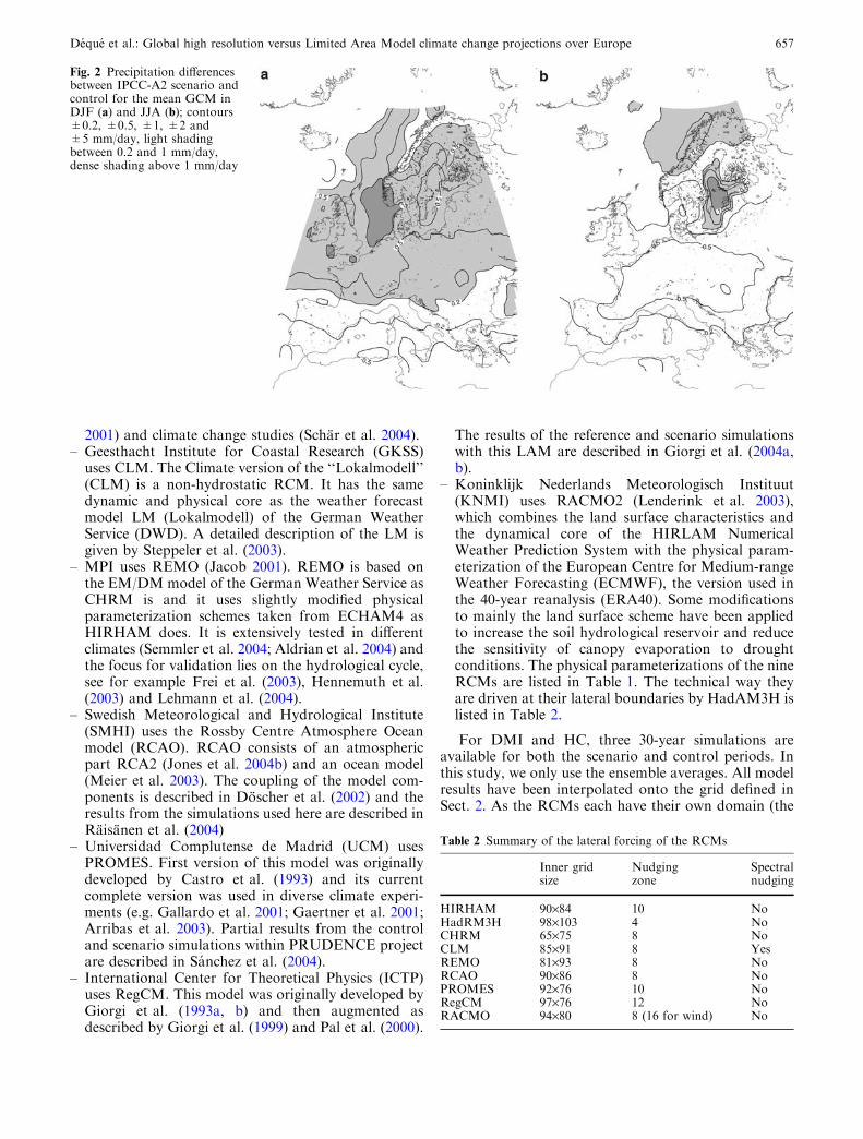
Precipitation changes are shown in Figs. 2a and b. Inwinter, precipitation decreases over the MediterraneanSea, and increases over the rest of Europe, with amaximum over the North Sea. In summer, precipitationdecreases over most of Europe, except the northernmostpart. The increase over the Baltic Sea is due to the largeSST increase mentioned above.

3 Climate change in regional climate models

The main activity within PRUDENCE has been basedon regional modeling. Contrary to GCMs, RCMs needlateral conditions to be run. In PRUDENCE, they areprovided by simulations of HadAM3H. This introducesan additional constraint, which should result in lessvariability in the response patterns amongst the RCMs

than amongst the GCMs. However, the RCMs, as wellas their driving GCM, use the same radiative forcing andthe same SST (except RCAO and RACMO which usedSSTs and sea-ice as calculated within RCAO) as theGCMs presented in Sect. 2.

Nine models have produced IPCC-A2 scenarios andcontrol experiments for the same periods as in Sect. 2

– Danish Meteorological Institute (DMI) uses HIR-HAM. HIRHAM was first developed by Christensenand van Meijgaard (1992) and later updated byChristensen et al. (1996). Further updates utilizingnew high resolution physiographical data sets of sur-face topography and land use classification have alsobeen introduced (Hagemann et al. 1999; Christensenet al. 2001a, b). Aspects of the models ability tosimulate present day and future climate are describedin Christensen et al. (1998) and Christensen andChristensen (2003, 2004).

– HC uses HadRM3H (Jones et al. 1997) which uses thesame physics as the corresponding GCM (Had-AM3H). The configuration of the model is very sim-ilar to that of HadRM3P (Jones et al. 2004a) whichwas developed, along with its parent GCM Had-AM3P, to provide realistic simulation of regionalclimate globally. The main changes related to calcu-lation of large-scale cloud and assumptions about theshape of convective anvils. Consequent changes weremade to parameters in the precipitation schemerelating to precipitation efficiency to ensure reason-able vertical cloud profiles, cloud forcing and radia-tion fields.

– ETHZ uses the CHRM. The most recent descriptionof the model is contained in Vidale et al. (2003). Themodel has heavily been tested regarding its ability torepresent the continental and Alpine-scale water cycle(e.g. Frei et al. 2003), and has been used for a widerange of process studies (Schar et al. 1999; Heck et al.

Fig. 1 2m temperaturedifferences between IPCC-A2scenario and control for themean GCM in DJF (a) and JJA(b); contour interval 1 K, lightshading between 1 and 5 K,dense shading above 5 K


2001) and climate change studies (Schar et al. 2004).– Geesthacht Institute for Coastal Research (GKSS)

uses CLM. The Climate version of the ‘‘Lokalmodell’’(CLM) is a non-hydrostatic RCM. It has the samedynamic and physical core as the weather forecastmodel LM (Lokalmodell) of the German WeatherService (DWD). A detailed description of the LM isgiven by Steppeler et al. (2003).

– MPI uses REMO (Jacob 2001). REMO is based onthe EM/DM model of the German Weather Service asCHRM is and it uses slightly modified physicalparameterization schemes taken from ECHAM4 asHIRHAM does. It is extensively tested in differentclimates (Semmler et al. 2004; Aldrian et al. 2004) andthe focus for validation lies on the hydrological cycle,see for example Frei et al. (2003), Hennemuth et al.(2003) and Lehmann et al. (2004).

– Swedish Meteorological and Hydrological Institute(SMHI) uses the Rossby Centre Atmosphere Oceanmodel (RCAO). RCAO consists of an atmosphericpart RCA2 (Jones et al. 2004b) and an ocean model(Meier et al. 2003). The coupling of the model com-ponents is described in Doscher et al. (2002) and theresults from the simulations used here are described inRaisanen et al. (2004)

– Universidad Complutense de Madrid (UCM) usesPROMES. First version of this model was originallydeveloped by Castro et al. (1993) and its currentcomplete version was used in diverse climate experi-ments (e.g. Gallardo et al. 2001; Gaertner et al. 2001;Arribas et al. 2003). Partial results from the controland scenario simulations within PRUDENCE projectare described in Sanchez et al. (2004).

– International Center for Theoretical Physics (ICTP)uses RegCM. This model was originally developed byGiorgi et al. (1993a, b) and then augmented asdescribed by Giorgi et al. (1999) and Pal et al. (2000).

The results of the reference and scenario simulationswith this LAM are described in Giorgi et al. (2004a,b).

– Koninklijk Nederlands Meteorologisch Instituut(KNMI) uses RACMO2 (Lenderink et al. 2003),which combines the land surface characteristics andthe dynamical core of the HIRLAM NumericalWeather Prediction System with the physical param-eterization of the European Centre for Medium-rangeWeather Forecasting (ECMWF), the version used inthe 40-year reanalysis (ERA40). Some modificationsto mainly the land surface scheme have been appliedto increase the soil hydrological reservoir and reducethe sensitivity of canopy evaporation to droughtconditions. The physical parameterizations of the nineRCMs are listed in Table 1. The technical way theyare driven at their lateral boundaries by HadAM3H islisted in Table 2.

For DMI and HC, three 30-year simulations areavailable for both the scenario and control periods. Inthis study, we only use the ensemble averages. All modelresults have been interpolated onto the grid defined inSect. 2. As the RCMs each have their own domain (the

Fig. 2 Precipitation differencesbetween IPCC-A2 scenario andcontrol for the mean GCM inDJF (a) and JJA (b); contours±0.2, ±0.5, ±1, ±2 and±5 mm/day, light shadingbetween 0.2 and 1 mm/day,dense shading above 1 mm/day

Table 2 Summary of the lateral forcing of the RCMs

Inner gridsize

Nudgingzone

Spectralnudging

HIRHAM 90·84 10 NoHadRM3H 98·103 4 NoCHRM 65·75 8 NoCLM 85·91 8 YesREMO 81·93 8 NoRCAO 90·86 8 NoPROMES 92·76 10 NoRegCM 97·76 12 NoRACMO 94·80 8 (16 for wind) No


lateral relaxation zone has been excluded), missing val-ues appear on this grid. The convention used in thisstudy is to present model results at each grid point (usingless RCMs at certain grid points when necessary) in thefigures. But, when numerical synthesis criteria are com-puted (e.g. root mean square difference between two 2-dhorizontal fields), we restrict these to the intersection ofall domains. We further restrict to land points, in orderto enable comparison with observed climatology. Weavoid thus the contribution of the Baltic Sea in summerand, more generally, the artificial agreement in 2mtemperature over sea due to the fact that most of themodels use the same SST. With such restrictions, thecommon domain reduces to Europe south of 65�N.

3.1 Mean temperature response

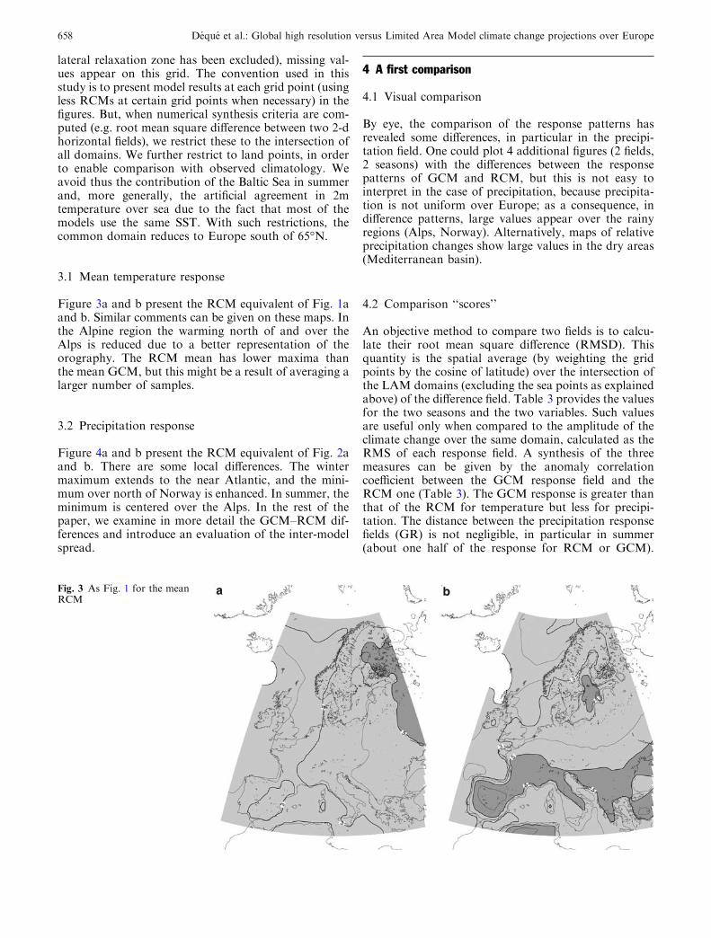
Figure 3a and b present the RCM equivalent of Fig. 1aand b. Similar comments can be given on these maps. Inthe Alpine region the warming north of and over theAlps is reduced due to a better representation of theorography. The RCM mean has lower maxima thanthe mean GCM, but this might be a result of averaging alarger number of samples.

3.2 Precipitation response

Figure 4a and b present the RCM equivalent of Fig. 2aand b. There are some local differences. The wintermaximum extends to the near Atlantic, and the mini-mum over north of Norway is enhanced. In summer, theminimum is centered over the Alps. In the rest of thepaper, we examine in more detail the GCM–RCM dif-ferences and introduce an evaluation of the inter-modelspread.

4 A first comparison

4.1 Visual comparison

By eye, the comparison of the response patterns hasrevealed some differences, in particular in the precipi-tation field. One could plot 4 additional figures (2 fields,2 seasons) with the differences between the responsepatterns of GCM and RCM, but this is not easy tointerpret in the case of precipitation, because precipita-tion is not uniform over Europe; as a consequence, indifference patterns, large values appear over the rainyregions (Alps, Norway). Alternatively, maps of relativeprecipitation changes show large values in the dry areas(Mediterranean basin).

4.2 Comparison ‘‘scores’’

An objective method to compare two fields is to calcu-late their root mean square difference (RMSD). Thisquantity is the spatial average (by weighting the gridpoints by the cosine of latitude) over the intersection ofthe LAM domains (excluding the sea points as explainedabove) of the difference field. Table 3 provides the valuesfor the two seasons and the two variables. Such valuesare useful only when compared to the amplitude of theclimate change over the same domain, calculated as theRMS of each response field. A synthesis of the threemeasures can be given by the anomaly correlationcoefficient between the GCM response field and theRCM one (Table 3). The GCM response is greater thanthat of the RCM for temperature but less for precipi-tation. The distance between the precipitation responsefields (GR) is not negligible, in particular in summer(about one half of the response for RCM or GCM).

Fig. 3 As Fig. 1 for the meanRCM


However, the correlations remain high, and one canconclude that there is a good agreement between meanGCM and mean RCM response.

4.3 Diagram

There are 8,000 grid points in the full domain of anal-ysis. With the above restrictions, only 3,188 points areused. A response field for temperature or precipitationcan be considered as a vector with 3,188 dimensions, oras a point with 3,188 coordinates if the null vector ischosen as the origin. Let us name G (resp. R) the pointcorresponding to the mean GCM (resp. RCM) response.The RMSD is simply the distance between G and R withthe metrics weighted by the fraction of area of each gridmesh. If G(x) and R(x) are the values at grid point x,and s(x) the area weight, we have:

RMSD =X

x

s(x) G(x)�R(x)ð Þ2" #1=2

ð1Þ

Introducing the origin point O, the RMS responsesare the distances OG and OR. The anomaly correlation

coefficient is the cosine of the angle (OG, OR). In theplane containing O, G and R, the values of each columnof Table 3 can thus be represented by a triangle. Thisview (Fig. 5) sums up the behavior of the mean models.

4.4 Projection of individual models

It is possible to show additional information on the samegraph by projecting each individual model onto theOGR plane. This visual approach helps to decide whe-ther the 4 GCM responses and the 9 RCM responseshave a significantly different centroid. Let X be a 2-Dhorizontal field (e.g. HadAM3P winter temperature re-sponse) with grid point values X(x). A little euclidianalgebra allows to write in our 3,188-dimensional space:

OX ¼ aOGþ bORþH; OX0 ¼ aOGþ bOR; ð2Þ

where a and b are scalars to be determined, OX, OG andOR the vectors with coordinates X(x), G(x) and R(x)respectively.H is a vector orthogonal to bothOGandOR.X¢ is the orthogonal projection ofX. With this method, allindividual GCMs and RCMs can be projected. BecauseOG and OR are not orthogonal, a and b are not suitablecoordinates in the projection plane. The choice of the axesis somewhat arbitrary and we chose to set OG along they-axis and R on the right-hand side of OG.

A visual approach is more suitable than a statisticalapproach here: a t-test assumes that the variances of thetwo populations are identical. We have good reasons tothink that this is not the case, as the RCMs undergo alateral constraint. However, the samples are too smallfor an F-test (the equality of the two variances is notrejected unless the ratio of variances is greater than 4).Figure 5 shows that as far as temperature is concerned,the two clouds of points overlap in the same regionof the diagram, far from the origin which can be

Fig. 4 As Fig. 2 for the meanRCM

Table 3 Synthetic criteria of the climate responses over Europe fortemperature (K) and precipitation (mm/day) in DJF and JJA:RMSD over Europe between the mean GCM response and themean RCM response, RMS response for the mean RCM andGCM, and correlation between the two responses

DJF T2 JJA T2 DJF Prec. JJA Prec.

RMSD (GR) 0.3 0.7 .21 .28GCM RMS (OG) 3.8 4.9 .48 .44RCM RMS (OR) 3.7 4.5 .57 .58Correlation (OG,OR) .99 .99 .93 .88

Note that correlation is dimensionless, contrary to the other rows.Geometrical equivalents (see Fig. 5) are between parentheses


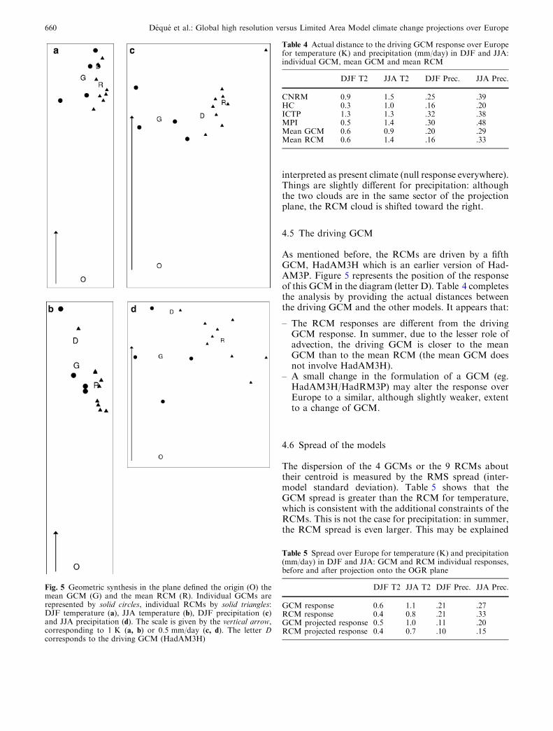
interpreted as present climate (null response everywhere).Things are slightly different for precipitation: althoughthe two clouds are in the same sector of the projectionplane, the RCM cloud is shifted toward the right.

4.5 The driving GCM

As mentioned before, the RCMs are driven by a fifthGCM, HadAM3H which is an earlier version of Had-AM3P. Figure 5 represents the position of the responseof this GCM in the diagram (letter D). Table 4 completesthe analysis by providing the actual distances betweenthe driving GCM and the other models. It appears that:

– The RCM responses are different from the drivingGCM response. In summer, due to the lesser role ofadvection, the driving GCM is closer to the meanGCM than to the mean RCM (the mean GCM doesnot involve HadAM3H).

– A small change in the formulation of a GCM (eg.HadAM3H/HadRM3P) may alter the response overEurope to a similar, although slightly weaker, extentto a change of GCM.

4.6 Spread of the models

The dispersion of the 4 GCMs or the 9 RCMs abouttheir centroid is measured by the RMS spread (inter-model standard deviation). Table 5 shows that theGCM spread is greater than the RCM for temperature,which is consistent with the additional constraints of theRCMs. This is not the case for precipitation: in summer,the RCM spread is even larger. This may be explained

Fig. 5 Geometric synthesis in the plane defined the origin (O) themean GCM (G) and the mean RCM (R). Individual GCMs arerepresented by solid circles, individual RCMs by solid triangles:DJF temperature (a), JJA temperature (b), DJF precipitation (c)and JJA precipitation (d). The scale is given by the vertical arrow,corresponding to 1 K (a, b) or 0.5 mm/day (c, d). The letter Dcorresponds to the driving GCM (HadAM3H)

Table 4 Actual distance to the driving GCM response over Europefor temperature (K) and precipitation (mm/day) in DJF and JJA:individual GCM, mean GCM and mean RCM


CNRM 0.9 1.5 .25 .39HC 0.3 1.0 .16 .20ICTP 1.3 1.3 .32 .38MPI 0.5 1.4 .30 .48Mean GCM 0.6 0.9 .20 .29Mean RCM 0.6 1.4 .16 .33

Table 5 Spread over Europe for temperature (K) and precipitation(mm/day) in DJF and JJA: GCM and RCM individual responses,before and after projection onto the OGR plane


GCM response 0.6 1.1 .21 .27RCM response 0.4 0.8 .21 .33GCM projected response 0.5 1.0 .11 .20RCM projected response 0.4 0.7 .10 .15


by the fact that the GCMs have a coarser resolutionthan the RCMs and miss some orographic forcings.After projection onto the OGM plane (Fig. 5), thespread is of course underestimated. The error is weak fortemperature, because the GCM/RCM cloud is largely1-d. For precipitation, the error is larger: the apparentsmaller spread of the RCM versus GCM in summer(0.15 versus 0.20 mm/day in Table 5) is an artifact of theprojection: the spread in a direction orthogonal to theOGR plane is not taken into account in the projection.

4.7 Limitations

Projecting onto the plane formed by two typical patterns(mean GCM and RCM responses) as in this section issimple to implement and to understand, but does notguarantee that the distances after projection are just ascaling of the actual distances. Two model responses farfrom each other can appear as neighbors after projec-tion.

The type of visualization used here is different fromthe so-called Taylor’s diagram (Taylor 2001). With thisvisualization technique two models are close to eachother on the diagram when their RMS and correlationversus a reference climatology are similar, but these twomodels may have a very different error pattern. In ourapproach we want to gather models which produce

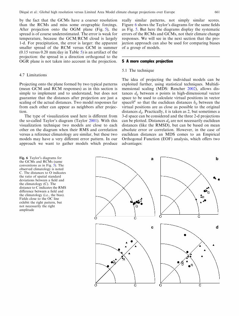
really similar patterns, not simply similar scores.Figure 6 shows the Taylor’s diagrams for the same fieldsas Fig. 5. But here the diagrams display the systematicerrors of the RCMs and GCMs, not their climate changeresponses. We will see in the next section that the pro-jection approach can also be used for comparing biasesof a group of models.

5 A more complex projection

5.1 The technique

The idea of projecting the individual models can beexploited further, using statistical techniques. Multidi-mensional scaling (MDS: Rencher 2002), allows dis-tances dij between n points in high-dimensional vectorspace to be used to calculate virtual positions in vectorspaceRk so that the euclidean distances dij between thevirtual positions are as close as possible to the originaldistances dij. Practically, k is taken as 2, but sometimes a3-d space can be considered and the three 2-d projectionscan be plotted. Distances dij are not necessarily euclideandistances (like the RMSD), but can be based on meanabsolute error or correlation. However, in the case ofeuclidean distances an MDS comes to an EmpiricalOrthogonal Function (EOF) analysis, which offers twoadvantages:

Fig. 6 Taylor¢s diagrams forthe GCMs and RCMs (sameconventions as in Fig. 5). Theobserved climatology is notedC. The distances to O indicatesthe ratio of spatial standarddeviations between a field andthe climatology (C). Thedistance to C indicates the RMSdifference between a field andthe climatology (i.e., the bias).Fields close to the OC lineexhibit the right pattern, butnot necessarily the rightamplitude


– The point representing an additional field (e.g.observed climatology) can be calculated by linearcombinations.

– The two axes of the plane can be plotted as 2-d hor-izontal fields. This method has been used in seasonalforecasting validation (Stephenson and Doblas-Reyes,2000). See Appendix for more details on the method.The outputs of this technique are:– A pair of eigenvalues (k1, k2), often expressed as a

percentage of the total variance. When the sum ofthe two percentages is 100%, the distances in theprojection plane are exactly the actual distances.This is an ideal case (n=3 or points already fittingin a plane).

– A pair of eigenvectors (i.e., fields over the Euro-pean domain) (A1, A2). They are scaled by thesquare root of the corresponding eigenvalue in thefigures of this paper in order to facilitate theinterpretation: the units are K or mm/day.

– Two series of projections (a1(i), a2(i)), i=1,n. Theycorrespond to the abscissa and ordinate of point iin the projection. They are also scaled by the squareroot of the corresponding eigenvalue. Therefore,the product of A1 by a1 (i) in the reconstruction ofthe pattern has to be scaled byðk1Þ�1=2:

5.2 All simulations

The projection technique has been applied to the 26simulations: 4 GCM controls, 4 GCM scenarios, 9 RCMcontrols and 9 RCM scenarios. The fraction of varianceexplained by the first two EOFs shows that the temper-ature projection is accurate (DJF: 90%, JJA: 92%), butthis is not the case with precipitation, in particular inwinter (DJF: 50%, JJA: 65%). We also projected theclimatology fields on the respective planes in order to getsome insight into the systematic errors. This climatologyis provided by the Climate Reseach Unit (Hulme et al.1995) and is available on the same 0.5� · 0.5� grid. Fig-ure 7 presents the projections, with blank symbols forcontrol climate (reference), solid symbols for scenariosand an asterisk for observed climatology. Figure 7a andb present an ideal situation: the lower part contains thereference runs and the climatology, the upper part theIPCC-A2 runs. The first EOF (not shown) has about tentimes more variance than the second one. Its pattern issimilar to the climate change shown in Fig. 1a and b. Thesecond EOF (not shown) represents the distributionalong the x-axis. Its pattern is less smooth than the firstEOF, but exhibits a North–South gradient with positivevalues on Scandinavia and negative ones along theMediterranean coast in both seasons. One can see inFig. 7a and b that the GCMs are located slightly on theright hand side of the RCM cloud, so that this axis can beinterpreted as an RCM–GCM contrast.

Figure 7c and d, related to precipitation, are morepuzzling. They display a mixture of all types of simula-tions from which no cluster can be isolated: the control

simulations are at the same distance to each other as tothe scenarios or as to the climatology. The cloud is toocomplex to be projected along two directions. We cansee that the individual GCMs or RCMs have very dif-ferent behaviors, and the important questions at thisstage are:

– Do GCMs and RCMs have similar systematic errors?– Despite their individual patterns, do they respond in a

similar way to the IPCC-A2 forcing?

5.3 Systematic errors

Comparing the distance between the mean GCM orRCM and the climatology is not a proper measure of theaccuracy of the models. However, averaging the indi-vidual systematic errors, also referred to as biases, andcomparing their quadratic average to the mean distancebetween a GCM and an RCM, between two differentGCMs, or between two different RCMs, gives some ideaof the ‘‘topography’’ of the reference simulations.Table 6 shows such mean distances. In order to maintainthe framework of euclidean geometry, all distances areaveraged in quadratic sense. The systematic error is farfrom negligible: about 2 K or 1 mm/day. But similarvalues are found when comparing two GCMs or oneGCM versus one RCM. The distance between twoRCMs, in the case of temperature, is smaller. If allmodels had a similar systematic error field, rows 3, 4 and5 would be smaller than the first 2. If GCMs and RCMshad a very different systematic error field, row 5 wouldbe greater than rows 3 and 4. Table 6 confirms that thereference runs of the RCMs, of the GCMs, and theobserved climatology form a cloud in which no obviouscluster appears. The only exception is that, for temper-ature, the RCM references tend to aggregate.

The distances between present climate fields (simu-lations or observation) must be compared with the meandistance between individual scenarios and the corre-sponding reference. Indeed, numerical models are acrude simplification of nature: they have and will alwayshave systematic errors. An important point is that thiserror is not too much greater than the response we ex-pect from the model. For some climate change impactinvestigations, it may even be crucial that this error isless than the response, as the first-order error cancel-ation does not work in a non-linear impact model. Amodel with an error of 0.001 K over Europe is neithercredible (one suspects some cheating) nor necessary (onedoes not need such an accuracy to estimate a possibleclimate change at the end of the century). A model withan error of 10 K is neither credible nor useful. The meanresponse of individual models can be calculated fromrows 2 and 3 of Table 3 (response of the mean model)and rows 1 and 2 of Table 5 (spread of the responses).Indeed the mean square is the sum of the variance and ofthe squared mean. The ratio of mean response overRMS systematic error for individual models is given in


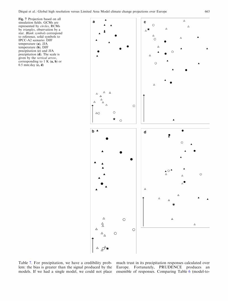
Table 7. For precipitation, we have a credibility prob-lem: the bias is greater than the signal produced by themodels. If we had a single model, we could not place

much trust in its precipitation responses calculated overEurope. Fortunately, PRUDENCE produces anensemble of responses. Comparing Table 6 (model-to-

Fig. 7 Projection based on allsimulation fields. GCMs arerepresented by circles, RCMsby triangles, observation by astar. Blank symbols correspondto reference, solid symbols toIPCC-A2 scenario: DJFtemperature (a), JJAtemperature (b), DJFprecipitation (c) and JJAprecipitation (d). The scale isgiven by the vertical arrow,corresponding to 1 K (a, b) or0.5 mm/day (c, d)


model distance in the reference runs) with Table 5(spread among the responses) increases our confidence.Indeed, a little algebra shows that the spread betweenthe systematic errors is about 0.7 times the RMS dis-tance between two models. Table 7 shows the ratio‘‘spread between responses’’ over ‘‘ spread betweensystematic errors’’. One can see this ratio is about onehalf in the case of precipitation. This shows that al-though the models behave differently in simulatingpresent climate, they offer similar ‘‘deltas’’ in response toIPCC-A2 forcing. If the spread between individual bia-ses were small, the consistency between the individualresponses would not be convincing: similar modelshaving similar biases produce similar responses. We donot claim here that we have the definite proof thatmodels are reliable, but we indicate how using a multi-model experiment increases confidence in the results.

5.4 Climate responses

To go further in the analysis of GCM/RCM differenceswithout boring the reader with columns of numbers, weapplied MDS to climate change difference fields insteadof raw fields as in Sect. 5.2. In the present approach, thereference field of a given model is subtracted from thecorresponding scenario field and to the reference field aswell. We thus projected 26 fields, of which 13 are zero. InSect. 5.2, we also projected 26 fields, giving the sameweight to present climate and to scenario. If we wereconsidering only the 13 non-zero climate change differ-ence fields in the projection, the climate response woulddisappear from the analysis, since MDS involves only

Table 6 Mean distances between individual GCM, individualRCMs and observed climatology for temperature (K) and precip-itation (mm/day)


Distance (GCM,Clim) 1.7 2.0 1.00 0.89Distance (RCM,Clim) 1.9 1.7 0.97 0.76Distance (GCM,GCM) 1.8 1.9 0.84 0.81Distance (RCM,RCM) 1.2 1.4 0.90 0.80Distance (GCM,RCM) 1.8 1.9 0.89 0.90

Table 7 Ratios calculated from Table. 3, 5 and 6


R1(GCM) 2.31 2.45 0.51 0.56R1(RCM) 1.99 2.66 0.62 0.87R2(GCM) 0.50 0.82 0.35 0.47R2(RCM) 0.50 0.77 0.33 0.58

R1 RMSD between scenario and reference over RMSD betweenreference and climatologyR2 inter-model standard deviation ofresponses over inter-model standard deviation of systematic errors

Fig. 8 Projection based on climate change difference fields. GCMsare represented by solid circles, RCMs by triangles, O is the origin(present climate): DJF temperature (a), JJA temperature (b), DJFprecipitation (c) and JJA precipitation (d). The scale is given by thevertical arrow, corresponding to 1 K (a, b) or 0.5 mm/day (c, d)


field-to-field differences. The latter approach also makessense (how do the different responses spread about themean response), but cannot be compared with earlierprojections of Figs. 5 and 7. The origin (O) correspondsto present climate for any model. The relative positionsof the responses and the present climate are displayed inFig. 8. The ‘‘topography’’ is very similar to Fig. 5,although the projection method is completely different.This projection is accurate: 99% of variance for tem-perature, 86% for winter precipitation and 81% forsummer precipitation.

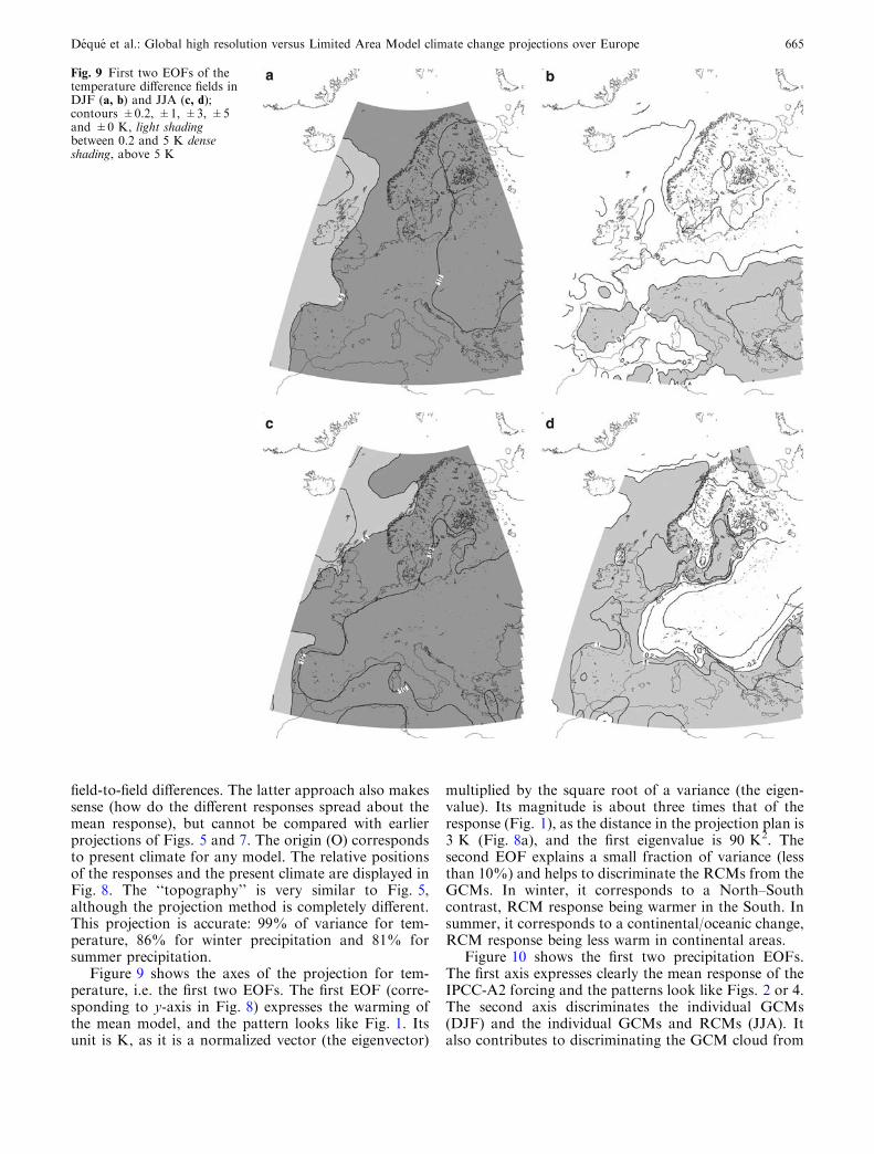
Figure 9 shows the axes of the projection for tem-perature, i.e. the first two EOFs. The first EOF (corre-sponding to y-axis in Fig. 8) expresses the warming ofthe mean model, and the pattern looks like Fig. 1. Itsunit is K, as it is a normalized vector (the eigenvector)

multiplied by the square root of a variance (the eigen-value). Its magnitude is about three times that of theresponse (Fig. 1), as the distance in the projection plan is3 K (Fig. 8a), and the first eigenvalue is 90 K2. Thesecond EOF explains a small fraction of variance (lessthan 10%) and helps to discriminate the RCMs from theGCMs. In winter, it corresponds to a North–Southcontrast, RCM response being warmer in the South. Insummer, it corresponds to a continental/oceanic change,RCM response being less warm in continental areas.

Figure 10 shows the first two precipitation EOFs.The first axis expresses clearly the mean response of theIPCC-A2 forcing and the patterns look like Figs. 2 or 4.The second axis discriminates the individual GCMs(DJF) and the individual GCMs and RCMs (JJA). Italso contributes to discriminating the GCM cloud from

Fig. 9 First two EOFs of thetemperature difference fields inDJF (a, b) and JJA (c, d);contours ±0.2, ±1, ±3, ±5and ±0 K, light shadingbetween 0.2 and 5 K denseshading, above 5 K


the RCM cloud, as the RCMs tend to have a positivecomponent along this axis and the GCMs a negativeone. In winter, negative values are found North and Eastof the domain, positive ones South and West. In sum-mer, the contrast is, as for temperature, between conti-nental and oceanic part of the domain.

6 Conclusion and perspectives

Once a scenario experiment is produced and analyzed,the big question is how much confidence can we have inthe computed responses? Contrary to other applicationsof numerical climate simulations like seasonal forecast-ing or sensitivity studies, there are no ways to evaluatewhat should be the true response. A simple methodconsists of evaluating how far the model simulates

present climate, and compare climate changes with sys-tematic errors. This method works well for temperatureresponse. The relation between radiative forcing andtemperature is rather straightforward: greenhouse gasincrease produces warming. The results shown in thispaper, in particular Figs. 7a and b, confirm with a largenumber of models of similar technological level, that wecan trust the results of the numerical models for seasonalmean temperature over Europe.

The bias-response comparison does not work forprecipitation. The RMS systematic error is about twicethe RMS climate response over Europe. However, as wehave an ensemble of models run under similar con-straints at our disposal, we can compare the spread ofthe systematic errors with the spread of the climate re-sponses. Here the ratio is inverted, i.e. the latter is halfthe former. This result gives some confidence in the

Fig. 10 As Fig. 9 forprecipitation; contours ±0.2,±1, ±2 and ±5 mm/day, lightshading between 0.2 and 1 mm/day, dense shading above 1 mm/day


precipitation responses: the models produce similarchanges (drying in the South particularly in summer,moistening in the North particularly in winter), althoughthey respond variously to the present climate forcings.

Another important result of this study is the com-parison between global models and RCMs. The differ-ences exist, but, given the confidence we have in theaccuracy of the responses, one can consider that bothrespond similarly to IPCC-A2 forcing. This is an addi-tional proof that RCMs can produce reliable results at amore attractive computation cost than high resolutionglobal models. This opens the 20 km-resolution Euro-pean-wide scenarios to investigation (Ensemble-basedPredictions of Climate Changes and their Impact, aliasENSEMBLES, a newly funded EU project).

PRUDENCE offers a very rich database for regionalclimate impacts, of which we have exploited here only asmall part. Two aspects merit priority attention:

– We have considered the responses on the mean fields,but the tails of the statistical distribution (i.e. the ex-tremes) are of great interest, in particular for precip-itation.

– All simulations (with slight exceptions) use here thesame SST as a forcing. Deque et al. (1998) showedthat a large part of the 2 m temperature changesmight come from the SST forcing, as Europe isstrongly influenced by the Atlantic air masses. ThePRUDENCE database contains runs with other SSTforcings for 3 out of the 13 simulations. Moreover, 2RCMs have been run with MPI lateral boundaryconditions, and 6 out of the 13 models have also usedIPCC-B2 forcing. It appears that for some models,two or three independent pairs of control-scenariowere available. The intra-model spread deserves someevaluation. However, the MDS technique, whose aimis to simplify interpretation, is no longer applicable, asthe plots are blurred by too much information. Vari-ance analysis techniques are more suitable to evaluatethe respective role of the various forcings, but thisis out of the scope of the present study and will beaddressed in further research.

Acknowledgements This work was supported by the EuropeanCommission Programme Energy, Environment and SustainableDevelopment under contract EVK2-2001-00156 (PRUDENCE).The French contribution was partly supported by the GICC-IMFREX contract of the Department of Environment (MEDD).The authors are grateful to Dr. O. B. Christensen (DMI) for pre-paring the database with regional scenarios.

7 Appendix

7.1 Multidimensional scaling

The aim of this method is to plot onto one (or a few)plane(s) several points which belong to a high-dimen-sional vector space, so that the distances in the projec-

tion plane are as close as possible to the actual distancesbetween the points. A simple to understand applicationof this technique is to represent the main European citieson a map on which the distance in cm between the citiesis not proportional to the actual distance in km, as in atypical road map, but to the shortest travel time by train.In the present study, it is applied to graphically syn-thesize a series of numerical model fields over Europe.

Let X(i,x) be the value of field X (e.g. 2 m temper-ature in DJF) for model i (i=1,..., n) at location x(x)representing here the latitude longitude pair). Let s(x) bethe surface of the mesh corresponding to x. The meanfield (centroid) is:

X ðxÞ ¼ 1

n

Xn

i¼1X ði; xÞ ð3Þ

and the matrix to be diagonalized is:

Vij ¼X

x

sðxÞðX ði; xÞ � X ðxÞÞðX ðj; xÞ � X ðxÞÞ ð4Þ

Let mk(i) be the kth eigenvector (with norm 1) associatedto the eigenvalue kk (the eigenvalues being sorted indecreasing order. Then the kth axis for the projection is:

AkðxÞ ¼Xn

i¼1mkðiÞðX ði; xÞ � X ðxÞÞ ð5Þ

The point representing model i isðffiffiffiffiffik1p

m1ðiÞ;ffiffiffiffiffik2p

m2ðiÞÞand the coordinates of the point representing a new fieldY(x) (k=1 or 2):

yk ¼1ffiffiffiffiffikkp

X

x

sðxÞAkðxÞðY ðxÞ � X ðxÞÞ ð6Þ

In the case of a non-euclidean distance, Eqs. 3, 4, 5, 6are no more valid since we use the array dij of the dis-tances between the models, which is no more a quadraticcombination of the array X(i,x). Equation 4 is replacedby

Vij ¼1

2

1

n

X

h

d2hj þ

1

n

X

k

d2ik � d2

ij �1

n2

X

hk

d2hk

!ð7Þ

and the eigenvectors of Vij scaled by the square root ofthe (sorted) eigenvalues provide the coordinates of therepresentative points. In this paper, we use only euclid-ean distances.

References

Aldrian E, Dumenil Gates L, Jacob D, Podzun R, Gunawan D(2004) Long term simulation of the Indonesian rainfall with theMPI Regional Model. Climate Dyn 22:795–814

Anthes RA, Hsie EY, Kuo YH (1987) Description of the PennState/NCAR Mesoscale Model Version 4 (MM4). NCARTechnical Note-282 NCAR, Boulder, CO 80307

Arribas A, Gallardo C, Gaertner MA, Castro M (2003) Sensitivityof Iberian Peninsula climate to land degradation. Climate Dyn20:477–489


Bonan GB (1996) A land surface model (LSM version 1.0) forecological, hydrological, and atmospheric studies: technicaldescription and user’s guide. NCAR technical Note NCAR/TN-417+STR. National Center for Atmospheric Research,Boulder, Colorado, pp 150

Bougeault P (1985) A simple parameterization of the large-scaleeffects of cumulus convection. Mon Wea Rev 113:2108–2121

Brankovic C, Gregory D (2001) Impact of horizontal resolution onseasonal integrations. Climate Dyn 18:123–143

Bringfelt B, Raisanen J, Gollvik S, Lindstrom G, Graham LP,Ullerstig A (2001) The land surface treatment for the RossbyCentre Regional Atmospheric Climate Model version 2 (RCA2)Reports Meteorology and Climatology, 98. Swedish Meteoro-logical and Hydrological Institute, Norrkoping, Sweden, pp 40

Castro M, Fernandez C, Gaertner MA (1993) Description of ameso-scale atmospheric numerical model. In: JI Dıaz, JL Lions(eds) Mathematics, climate and environment. Masson, Paris, pp230–253

Christensen JH, Christensen OB (2003) Climate modelling: severesummertime flooding in Europe. Nature 421:805–806

Christensen OB, Christensen JH (2004) Intensification of extremeEuropean summer precipitation in a warmer climate. Glob PlanChange 44:107–117

Christensen JH, van Meijgaard E (1992) On the construction of aregional atmospheric climate model. DMI Technical Report92–14. Available from DMI, Lyngbyvej 100, Copenhagen Ø,Denmark

Christensen JH, Christensen OB, Lopez P, van Meijgaard E, BotzetM (1996) The HIRHAM4 regional atmospheric climate model.DMI Scientific Report 96–4. Available from DMI, Lyngbyvej100, Copenhagen Ø, Denmark

Christensen OB, Christensen JH, Machenhauer B, Botzet M (1998)Very high-resolution regional climate simulations over Scandi-navia—present climate. J Climate 11:3204–3229

Christensen JH, Ra J, Iversen T, Bjorge D, Christensen OB,Rummukainen M (2001a) A synthesis of regional climatechange simulations—a Scandinavian perspective. Geophys ResLett 28(1):1003–1006

Christensen JH, Christensen OB, Schultz JP (2001b) High resolu-tion physiographic data set for HIRHAM4: an application to a50 km horizontal resolution domain covering Europe. DMITechnical Report 01–15. Available from DMI, Lyngbyvej 100,Copenhagen Ø, Denmark

Cox P, Betts R, Bunton C, Essery R, Rowntree PR, Smith J (1999)The impact of new land surface physics on the GCM simulationof climate and climate sensitivity. Climate Dyn 15:183–203

Cubasch U, Waszkewitz J, Hegerl G, Perlwitz J (1995) Regionalclimate changes as simulated in time-slice experiments. ClimChange 31:273–300

Denis B, Laprise R, Caya D (2003) Sensitivity of a regional climatemodel to the resolution of the lateral boundary conditions.Climate Dyn 20:107–126

Deque M, Gibelin AL (2002) High versus variable resolution inclimate modelling. Res Activ Atmos Ocean Model 32:704–705

Deque M, Piedelievre JP (1995) High resolution climate simulationover Europe. Climate Dyn 11:321–339

Deque M, Marquet P, Jones R (1998) Simulation of climate changeover Europe using a global variable resolution general circula-tion model. Climate Dyn 14:173–189

Dickinson RE, Henderson-Sellers A, Kennedy PJ (1993) Bio-sphere-Atmosphere Transfer Scheme (BATS) Version 1e asCoupled to the NCAR Community Climate Model, NCARTechnical Note, NCAR/TN-387+STR, 72 pp

Doscher R, Willen U, Jones C, Rutgersson A, Meier H, Hansson E,Graham M (2002) The development of the coupled regionalocean-atmosphere model RCAO. Boreal Environ Res 7:183–192

Douville H, Planton S, Royer JF, Stephenson DB, Tyteca S,Kergoat L, Lafont S, Betts RA (2000) The importance of veg-etation feedbacks in doubled-CO2 time-slice experiments.J Geophys Res 105:14841–14861

Ducoudre N, Kaval K, Perrier A (1993) SECHIBA, a new set ofparameterizations of the hydrologic exchanges at the land-

atmosphere interface within the LMD atmospheric generalcirculation model. J Climate 6:248–273

Dumenil L, Todini E (1992) A rainfall-runoff scheme for use in theHamburg climate model. In: O’Kane JP (ed) Advances in the-oretical hydrology EGS series of hydrological sciences 1. Else-vier, Amsterdam, pp 129–157

Edwards JM, Slingo A (1996) Studies with a flexible new radiationcode. I: Choosing a configuration for a large scale model. QuartJ Roy Meteor Soc 122:689–719

Fox-Rabinowitz MS, Tackacs LL, Govindajaru RC, Suarez MJ(2001) A variable resolution stretched grid GCM: regional cli-mate simulation. Mon Wea Rev 129:453–469

Frei C, Christensen JH, Deque M, Jacob D, Jones RG, Vidale PL(2003) Daily precipitation statistics in regional climate models:evaluation and intercomparison for the European Alps.J Geophys Res 108 (D3), 4124 doi:101029/2002JD002287

Fukutome S, Frei C, Luthi D, Schar C (1999) The interannualvariability as a test ground for regional climate simulations overJapan. J Meteor Soc Japan 77:649–672

Gaertner MA, Christensen OB, Prego JA, Polcher J, Gallardo C,Castro M (2001) The impact of deforestation on the hydro-logical cycle in the western Mediterranean: an ensemble studywith two regional climate models. Climate Dyn 17:857–873

Gallardo C, Arribas A, Prego JA, Gaertner MA, Castro M (2001)Multi-year simulations with a high resolution regional climatemodel over the Iberian Peninsula: current climate and 2xCO2scenario. Quart J Roy Meteor Soc 127:1659–1682

Garand L (1983) Some improvements and complements to theinfrared emissivity algorithm including a parameterization of theabsorption in the continuum region. J Atmos Sci 40:230–244

Gibelin AL, Deque M (2003) Anthropogenic climate change overthe Mediterranean region simulated by a global variable reso-lution model. Climate Dyn 20:327–339

Giorgi F (1990) Simulation of regional climate using a limited areamodel nested in a general circulation model. J Climate 3:941–963

Giorgi F, Marinucci MR, Bates GT (1993a) Development of asecond generation regional climate model (REGCM2) Part I:Boundary layer and radiative transfer processes. Mon Wea Rev121:2794–2813

Giorgi F, Marinucci MR, Bates GT, DeCanio G (1993b) Devel-opment of a second generation regional climate model (REG-CM2). Part II: Convective processes and assimilation of lateralboundary conditions. Mon Wea Rev 121:2814–2832

Giorgi F, Mearns LO, Shields C, McDaniel L (1998) Regionalnested model simulations of present day and 2·CO2 climateover the central plains of the USA. Clim Change 40:457–493

Giorgi F, Huang Y, Nishizawa K, Fu C (1999) A seasonal cyclesimulation over eastern Asia and its sensitivity to radiativetransfer and surface processes. J Geophys Res 104:6403–6423

Giorgi F, Bi X, Pal JS (2004a) Means, trends and interannualvariability in a regional climate change experiment over Europe.Part I: Present day climate (1961–1990). Climate Dyn 22:733–756

Giorgi F, Bi X, Pal JS (2004b) Means, trends and interannualvariability in a regional climate change experiment over Europe.Part II: Future climate scenarios (2071–2100). Climate Dyn22:839–858

Gregory D, Kershaw R, Inness PM (1997) Parametrization ofmomentum transport by convection. II: Tests in single columnand general circulation models. Quart J Roy Meteor Soc123:1153–1183

Grell GA (1993) Prognostic evaluation of assumptions used bycumulus parameterizations. Mon Wea Re 121:764–787

Hagemann S, Botzet M, Dumenil L, Machenhauer B (1999) Der-ivation of globalGCM boundary conditions from 1 km land usesatellite data. MPI Report 289, Max-Planck Institut fur Mete-orologie

Hagemann S, Machenhauer B, Jones RG, Christensen OB, DequeM, Jacob D, Vidale PL (2004) Evaluation of water and energybudgets in regional climate models applied over Europe. Cli-mate Dynamics, in press


Heck P, Luthi D, Wernli H, Schar C (2001) Climate impacts ofEuropean-scale anthropogenic vegetation changes: a study witha regional climate model. J Geophys Res-Atmos 106(D8):7817–7835

Hennemuth B, Rutgersson A, Bumke K, Clemens M, Omstedt A,Jacob D, Smedman AS (2003) Net precipitation over the BalticSea for one year using models and data-based methods. Tellus55A:352–367

Hsie EY, Anthes RA, Keyser D (1984) Numerical simulation offrontogenesis in a moist atmosphere. J Atmos Sci 41:2581–2594

Hulme M, Conway D, Jones PD, Jiang T, Barrow EM, Turney C(1995) Construction of a 1961–90 European climatology forclimate modelling and impacts applications. Int J Climatol15:1333–1363

IPCC (2001) Climate change. The scientific basis. Cambridge UnivPress, pp 881

Jacob D (2001) A note to the simulation of the annual and inter-annual variability of the water budget over the Baltic Seadrainage basin. Meteorol Atmos Phys 77:61–73

Johns TC, Gregory JM, Ingram WJ, Johnson CE, Jones A,Mitchell JFB, Roberts DL, Sexton DMH, Stevenson DS, TettSFB, Woodage MJ (2001) Anthropogenic climate change for1860 to 2100 simulated with the HadCM3 model under updatedemission scenarios. Hadley Centre Technical Note 22:62

Jones RG, Murphy JM, Noguer M, Keen AB (1997) Simulation ofclimate change over Europe using a nested regional climatemodel. II: Comparison of driving and regional model responsesto a doubling of carbon dioxyde. Quart J Roy Meteor Soc123:265–292

Jones RG, Noguer M, Hassell DC, Hudson D, Wilson SS, JenkinsGJ, Mitchell JFB (2004a) Generating high resolution climatechange scenarios using PRECIS. Met Office Hadley Centre,Exeter, UK, pp 35

Jones CG, Ullerstig A, Willen U, Hansson U (2004b) The RossbyCentre regional atmospheric climate model (RCA). Part I:Model climatology and performance characteristics for presentclimate over Europe. Ambio 33(4–5):199–210

Kain J, Fritsch JM (1990) A one dimensional entraining/detrainingplume models and its application to convective parameteriza-tion. J Atmos Sci 47:2784–2802

Kessler E (1969) On the distribution and continuity of water sub-stance in atmospheric circulation models. Meteor Monographs10, Americ Meteor Soc Boston, MA

Kiehl JT, Hack JJ, Bonan GB, Boville BA, Briegleb BP, William-son DL, Rasch PJ (1996) Description of the NCAR Commu-nity Climate Model (CCM3). NCAR Technical Note, NCAR/TN-420+STR, pp 152

Kiehl JT, Hack JJ, Bonan GB, Boville BA, Williamson DL, RaschPJ (1998) The National Center for Atmospheric ResearchCommunity Climate Model: CCM3. J Climate 11:1131–1149

Kjellstrom E, Doscher R, Meier HEM, Banks H (2004) Atmo-spheric response to different sea surface temperatures in theBaltic Sea: coupled versus uncoupled regional climate modelexperiments. Nordic Hydrology, submitted

Laprise R, Caya D, Frigon A, Paquin D (2003) Current and per-turbed climate as simulated by the second-generation CanadianRegional Climate Model (CRCM-II) over northwestern NorthAmerica. Climate Dynamics 21:405–421

Lehmann A, Lorenz P, Jacob D (2004) Exceptional Baltic Sea in-flow events in 2002–2003. Geophysical Research Letters2004GL020830

Lenderink G, van den Hurk B, van Meijgaard E, van Ulden A,Cuijpers H (2003) Simulation of present-day climate in RAC-MO2: first results and model developments. KNMI TechnicalReport 252:24

Lin SJ, Rood RB (1996) Multidimensional flux-form semi-Lagrangian transport schemes. Mon Wea Rev 124:2046–2070

Lin YL, Farley RD, Orville HD (1983) Bulk parameterization of thesnow field in a cloud model. J Clim ApplMeteorol 22:1065–1095

Lorant V, Royer JF (2001) Sensitivity of equatorial convection tohorizontal resolution in aqua-planet simulations with variable-resolution GCM. Mon Wea Rev 129:2730–2745

Machenhauer B, Windelband M, Botzet M, Hesselbjerg-Christensen J, Deque M, Jones RG, Ruti P, Visconti G (1998)Validation and analysis of regional present-day climate andclimate change simulations over Europe. MPI Report (Ham-burg) 275:87

Meier HEM, Doscher R, Faxen T (2003) A multiprocessor coupledice-ocean model for the Baltic Sea. Application to the salt in-flow. J Geophys Res 108,C8:3273

Moorthi S, Suarez MJ (1992) Relaxed Arakawa-Schubert: aparameterization of moist convection for general circulationmodels. Mon Wea Rev 120:978–1002

Morcrette JJ (1990) Impact of changes to the radiation transferparameterizations plus cloud optical properties in the ECMWFmodel. Mon Wea Rev 118:847–873

Nordeng TE (1994) Extended versions of the convective parame-trization scheme at ECMWF and their impact on the mean andtransient activity of the model in the tropics. ECMWF Re-search Department, Technical Memorandum No. 206, October1994, 41 pp, European Centre for Medium Range WeatherForecasts, Reading, UK

Pal JS, Small EE, Eltahir EAB (2000) Simulation of regional-scalewater and energy budgets: representation of subgrid cloud andprecipitation processes within RegCM. J Geophys Res105:29579–29594

Raisanen J, Hansson U, Ullerstig A, Doscher R, Graham LP,Jones C, Meier M, Samuelsson P, Willen U (2004) Europeanclimate in the late 21st century: regional simulations with twodriving global models and two forcing scenarios. Climate Dyn22:13–31

Rasch PJ, Kristjansson JE (1998) A comparison of the CCM3model climate using diagnosed and predicted condensateparameterizations. J Climate 11:1587–1614

Rencher AC (2002) Methods of multivariate analysis. 2nd edition.Wiley series in probability and statistics: 708

Ricard JL, Royer JF (1993) A statistical cloud scheme for use in anAGCM. Ann Geophys 11:1095–1115

Ritter B, Geleyn JF (1992) A comprehensive radiation scheme fornumerical weather prediction models with potential applica-tions in climate simulations. Mon Wea Rev 120:303–325

Roeckner E, Baeuml G, Bonaventura L, Brokopf R, Esch M,Giorgetta M, Hagemann S, Kirchner I, Kornblueh L, ManziniE, Rhodin A, Schlese U, Schulzweida U, Tompkins A (2003)The atmospheric general circulation model ECHAM5—Part 1.MPI Report 349:127

Sanchez E, Gallardo C, Gaertner M, Arribas A, Castro A (2004)Future climate extreme events in the Mediterranean simulatedby a regional climate model: a first approach. Global andPlanetary Change, in press

Savijarvi H (1990) Fast radiation parameterization schemes formesoscale and short-range forecast models. J Appl Meteor29:437–447

Schar C, Luthi D, Beyerle U, Heise E (1999) The soil-precipitationfeedback: a process study with a Regional Climate Model.J Climate 12:722–741

Schar C, Vidale PL, Luthi D, Frei C, Haberli C, Liniger MA,Appenzeller C (2004) The role of increasing temperature vari-ability in European summer heatwaves. Nature 427:332–336

Semmler T, Jacob D, Schlunzen KH, Podzun R (2004) Influence ofsea ice treatment in a regional climate model on boundary layervalues in the Fram Strait region. Month Weather Rev 132:985–999

Smith RNB (1990) A scheme for predicting layer clouds and theirwater content in a general circulation model. Quart J RMet Soc116:435–460

Statton RA (1999) A high resolution AMIP integration using theHadley Centre model HadAM2b. Climate Dyn 15:9–28

Stendel M, Roeckner E (1998) Impacts of horizontal resolution onsimulated climate statistics in ECHAM4. MPI Report 253:57

Stephens GL (1978) Radiation profiles in extended water clouds: IIParameterizaton schemes. J Atmos Sci 35:2123–2132

Stephenson DB, Doblas-Reyes FJ (2000) Statistical methods forinterpretingMonte Carlo ensemble forecasts. Tellus 52A:300–322


Steppeler J, Doms G, Schattler U, Bitzer HW, Gassmann A, Dam-rathU, Gregoric G (2003)Meso-gamma scale forecasts using thenonhydrostatic model LM. Meteorol Atm Phys 82:75–96

Sud YC, Walker GK (1999) Microphysics of clouds with the Re-laxed Arakawa-Schubert cumulus scheme (McRAS). Part I:Design and evaluation with GATE Phase III data. J Atmos Sci56:3196–3220

Sundquist H (1978) A parameterization scheme for non-convectivecondensation including precipitation including prediction ofcloud water content. Quart J R Met Soc 104:677–690

Taylor KE (2001) Summarizing multiple aspects of model perfor-mance in a single diagram. J Geophys Res 106:7183–7192

Tiedtke M (1989) A comprehensive mass flux scheme for cumulusparameterization in large-scale models. Mon Wea Rev117:1779–1800

Van den Hurk BJJM, Viterbo P, Beljaars ACM, Betts AK (2000)Offline validation of the ERA40 surface scheme. ECMWFTechMemo 295

Vidale PL, Luthi C, Frei D, Seneviratne S, Schar C (2003)Predictability and uncertainty in a regional climate model.J Geophys Res Atmos 108 (D18), 4586 doi:101029/2002JD002810

Whetton PH, Katzfey JJ, Hennessy KJ, Wu X, Mc Gregor JL,Nguyen K (2001) Developing scenarios of climate change forSoutheastern Australia: an example using regional climatemodel output. Clim Res 6:181–201

White PW (2002) Physical processes (cycle 24R4). IFS documen-tation. ECMWF, Reading


Global high resolution versus Limited Area Model climate change projections over Europe: quantifying...

Documents

Transcript of Global high resolution versus Limited Area Model climate change projections over Europe: quantifying...