g.gpr.pdf - Hong Kong Institute of Utility Specialists

Acknowledgements

The authors would like to acknowledge the financial fund under Professional Service Development

Assistance Scheme (PSDAS) of Commerce and Economic Development Bureau, The Government

of the Hong Kong Special Administration Region as well as technical support of Hong Kong

Institute of Utility Specialists (香港管綫專業學會)and Hong Kong Utility Research Centre (香港

管線管理研究中心)as well as their company members. Additionally, the support of relavant

government departments should be acknowledged for their contribution to the information related

to operation, standards, and contract requirements.

List of Company Members of HKIUS (according to alphabet):

(1) APC Surveying & Building Limited

(2) BUDA Surveying Limited

(3) B.P. (Building & Engineering) Co., Ltd

(4) EGS (Asia) Limited

(5) Freyssinet Hong Kong Ltd.

(6) INNO Pipe Engineering Limited

(7) Insituform Asia Limited

(8) Jetrod Pipeline Consultant and Engineering Ltd

(9) Patrick Yuen Underground Detection Company Limited

(10) Stanger Asia Limited

(11) Toptime Technologies Ltd.

(12) US & Associates Consulting Co.,Ltd

(13) UtilityINFO Limited

(14) U-Tech Engineering Company Ltd.

Editor in Chief Ir Dr. King Wong

Editor L.M. Cheung, C.C. Chui, C.W. Hui, W.Y. So

Consultant Prof. Mike Forde, Dr Lok Wai Lai,

Ir Dr. Wai Fan Tsang, Mr Shell Zhai

This is guideline is done in May2011.

FOREWORD

After the disastrous landslip of 1994 occurred in Kwun Lung Lau on Hong Kong Island, the

Government has paid more attention on utility maintenance with particular emphasis on leakage

detection of buried water carrying services on both slopes and roads. The Government has increased

resources and imposed additional legislation on the detection of underground utilities. As a direct

result, the utility profession has been developing rapidly, and over the last decade, the number of

―Utility Specialists‖ (管綫專業監理師 ) has grown as the Government‘s requirements for

Competent Persons to carry out the investigations has been implemented, in addition, Recognized

Professional Utility Specialist (RPUS) (管綫專業監察師) has been recognized in recent years.

However, lack of standard surveying methods, centralized monitoring systems and organized

management, have lead to unsatisfactory investigation results.

In order to address these issues, Hong Kong Institute of Utility Specialists (HKIUS) (香港管綫專

業學會), targeting the promotion of knowledge and good practice in the utility profession,

collaborated with Hong Kong Utility Research Centre (HKURC) and supported by the funding

from the Professional Services Development Assistance Scheme (PSDAS) of HKSAR, published a

series of guide books and pamphlets in 12 disciplines of the utility profession in order to set

standards for the practitioners to follow. As part of HKIUS continual effort to enhance the

professionalism of the utility profession, it is the intention of the series that the quality of the survey

can be raised and that utility related incidents can be avoided by performing high quality utility

practices. Hopefully, the resulting benefits can extend to the general public.

This issue provides good practice of using Ground Penetrating Rader (GPR)(管綫雷達探測) in

Utility Survey. It states the whole process and specification of conducting GPR from planning to

finishing stages and intended to be used by all personnel involved in the works.

_________________________

Mr, Zico Kai Yip KWOK

(郭啟業先生)

President, HKIUS (2010-11)

April, 2011

Table of Content

Table of Content................................................................................................................................... 4

1. INTRODUCTION ........................................................................................................................... 5

2. PRINCIPLE OF OPERATION ........................................................................................................ 6

2.1 Equipment ...................................................................................................................................... 6

2.2 The GPR Method: Theory of Operation ................................................................................ 7

2.3 Survey Considerations ........................................................................................................... 9

2.4 Data Processing ...................................................................................................................... 9

2.5 Principle of GPR .................................................................................................................. 10

3. NUMERICAL MODELING.......................................................................................................... 13

3.1 Effects of tank materials and contents ................................................................................. 13

3.2 Effects of fluid interfaces within tanks ................................................................................ 14

3.3 Effect of tank size ................................................................................................................ 15

3.4 Effect of antenna separation ................................................................................................. 15

3.5 Detection of tank damage .................................................................................................... 16

3.6 Effect of noise ...................................................................................................................... 16

3.7 Discussion and Conclusions................................................................................................. 17

3.8 Appendix to Section 3 .......................................................................................................... 18

4. GPR SURVEY DESIGN ............................................................................................................... 23

5. POST-ACQUISITION PROCESSING AND INTERPRETATION ............................................. 25

6. APPLICATION OF GPR............................................................................................................... 28

Reference ........................................................................................................................................... 29

Appendix A: Abbreviations ............................................................................................................... 31

1. INTRODUCTION

The first application of ground penetrating radar (GPR) survey was to determine the depth of a

glacier, reported in 1929 (Stern, 1929, 1930). Then the technology was lost until the late 1950‘s

when planes crashing into the Greenland ice cap reawakened the interest in the subject (see further

history in Clarke, 1987; Young, 1996). Since the mid-1980‘s, ground penetrating radar has become

very popular, particularly for engineering, environmental and archaeological application (Albert

and etc, 2000).

The 1929 method of radiointerferometry was independently rediscovered for the 1972 Apollo 17

mission to the moon (Simmons et al., 1972). Most ground penetrating radar systems today are short

impulse time domain systems similar to Barringer (1965) or Caldecott (1967) and used in simple

imaging mode to map subsurface events, such as the occurrence of the water table (Barringer, 1966;

Caldecott et al., 1972; Morey, 1974; Beres and Hasni, 1991), hazardous waste investigations

(Brewster and Annan, 1994), mapping sediment sequences (Smith and Hol, 1997), detection of

buried objects in conjunction with other methods (Annan et al., 1990; Stockbauer and Kalinec, 1995;

Czarnowski et al., 1994; Graf, 1989; Tong, 1993; Powers and Olhoeft, 1996), road pavement

evaluation, void detection, behind tunnel linings (Albert and etc, 2000) and detection of fractures in

limestone (M. Grasmueck et al., 2005), stratigraphy in beach sand (M. Grasmueck et al., 2006), tree

roots and building foundations (M. Grasmueck et al., 2006; A. Novo et al., 2008).

However, large scale investigations in Hong Kong have focused on properties of concrete (W.L. Lai

et al., 2009) which is applied on large aboveground infrastructure like bridge, dam and so on. This

guideline is trying to summarize the oversea nature experience and theory for reference to the

interested person in utility industry.

2. PRINCIPLE OF OPERATION

This chapter is designed as a basic introduction to some of the key concepts in the basic theory of

operation of ground-penetrating radar (GPR) and GSSI SIR System will be taken for explanation.

An understanding of the concepts discussed here will help make your understanding much more

worthwhile and enable you to save more time.

2.1 Equipment

A GPR system is made up of three main components: the control unit, antenna, and power supply

which are shown in Figure 2.1.

Figure 2.1: Complete GPR system produced by Geophysical Survey Systems, Inc. (USA)

Geophysical Survey Systems GPR equipment can be run with a variety of power supplies ranging

from small rechargeable battery packs, to vehicle batteries, and normal 110-volt current. Connectors

and adapters are available for each power source type. The unit in the photo above can run from a

small internal rechargeable battery or external power. The control unit contains electronics that

produce and regulate the pulse of radar energy that the antenna sends into the ground. It also has a

built-in computer and hard disk to record and store data for examination after fieldwork. Some

systems, such as the GSSI SIR-20, are controlled by an attached Windows laptop computer with

pre-loaded control software. This system allows data processing and interpretation without having

to download radar files to another computer.

The antenna receives the electrical pulse produced by the control unit, amplifies it, and transmits it

into the ground or other medium at a particular frequency. Antenna frequency is a major factor in

depth penetration. The higher the frequency of the antenna, the shallower into the ground it will

penetrate. A higher frequency antenna will also ‗see‘ smaller targets. Antenna choice is one of the

most important factors in survey design. Table 2.1 shows antenna frequency, approximate depth

penetration, and appropriate application.

Depth Range

(Approximate)

Primary Antenna

Choice

Secondary Antenna

Choice

Appropriate Application

0-0.5 m 1500 MHz 900 MHz Structural Concrete,

Roadways, Bridgedecks

0-1 m 900 MHz 400 MHz Concrete, Shallow soils,

Archaeology

0-3 m 400 MHz 200 MHz Shallow Geology, Utilities,

UST‘s, Archaeology

0-9 m 200 MHz 100 MHz Geology, Environmental,

Utility, Archaeology

0-30 m 100 MHz Sub-Echo 40 Geologic Profiling

Greater than 30

m

MLF (80, 40, 32,

20, 16 MHz) -

Geologic Profiling

Table 2.1: Choosing the Proper Antenna

2.2 The GPR Method: Theory of Operation

GPR works by sending a pulse of energy into a material and recording the strength and the time

required for the return of any reflected signal. A series of pulses over a single area make up what is

called a scan, or sometimes a trace. Reflections are produced whenever the energy pulse enters into

a material with different electrical conduction properties (dielectric permittivity) from the material

it left. The strength or amplitude of the reflection is determined by the contrast in the dielectric

constants of the two materials. This means that a pulse which moves from dry sand (diel of 5) to

wet sand (diel of 30) will produce a very strong, brilliantly visible reflection, while one moving

from dry sand (5) to limestone (7) will produce a very weak reflections.

While some of the energy is reflected back to the antenna, energy also keeps traveling through the

material until it either dissipates (attenuates) or the GPR control unit has closed its time window

(Figure 2.2). The rate of signal attenuation varies widely and is dependant on the dielectric

properties of the material through which the pulse is passing. Another concern is conductivity.

Materials which are highly conductive and thus attenuate (absorb) the signal rapidly. If the signal is

absorbed, then it is not allowed to penetrate deeper into a material. Water saturation dramatically

raises the dielectric (and sometimes the conductivity) of a material, so a survey area should be

carefully inspected for signs of water penetration. Radar surveys should never be conducted through

standing water, no matter how shallow. Depth penetration through a material with a high dielectric

will not be very good. Metals are considered to be a complete reflector, and do not allow any

amount of signal to pass through. Materials beneath a metal sheet, fine metal mesh, or pan decking

will not be visible. It is essential to correctly estimate the dielectric constant of a material in order to

get accurate depth calculations to features. In utility and concrete inspection work, this is commonly

done by drilling or chipping to a known object such as a piece of rebar, measuring the depth, and

calibrating that depth to the radar record. The depth accuracy of radar is extremely good if this

calibration is performed. If there is a suspicion of changing conditions in the subsurface (different

material, water infiltration), another depth calibration for that area should be done. Generally

speaking, the more depth calibrations are performed, the more accurate the depth is estimated. If

chipping or drilling is not possible, or if the survey takes place out of doors on a natural ground

surface, the dielectric must be estimated. A chart of the dielectric constants of some common

materials is included at the back of this booklet for reference.

Figure 2.2 Signal path of antenna.

Radar energy is emitted from the antenna not in a straight line, but a cone (Figure 2.3). The two-

way travel time for energy at the leading edge of the cone is longer than for energy directly beneath

the antenna. This is because that leading edge of the cone represents the hypotenuse of a right

triangle. It is a longer distance than when the antenna is directly over the target. Because it takes

longer for that energy to be received, it is recorded farther down in the profile. As the antenna is

moved over a target, the distance between them decreases until the antenna is over the target, and

increases as the antenna is moved away. It is for this reason that a single target will appear in a data

as a hyperbola, or inverted ―U.‖ The target is actually at the peak amplitude of the positive wavelet.

A mathematical function called migration may be performed during the data processing stage to

remove the tails of the hyperbola and produce a more accurate assessment of the target location.

Figure 2.3 Hyperbola creation.

A reflection wave commonly has a positive and a negative wavelet. This is why hyperbolas look

striped. If radar energy moves into air (dielectric of 1) from a higher dielectric medium like

concrete, the signal will undergo what is called a phase reversal. A normal reflection will exhibit

first a positive peak (white band) and then a negative peak (black band), while a phase-shifted

signal will show a negative (black) than positive (white) peak. If energy penetrates a thin slab and

continues into the air behind it, then a phase shift may indicate the back of the slab. Additionally,

voids and air-filled PVC, if they are large enough, may show up as phase-shifted reflections. In

some cases however, a phase shift may be falsely produced by background noise or the system‘s

internal filters. It is therefore inadvisable to consider a phase shift alone to be indicative of a void or

PVC piping.

2.3 Survey Considerations

Ground-penetrating radar, like all geophysical techniques, is the most effective when as large an

area as possible is surveyed. The reason for this is that effective interpretation depends on seeing

contrasts within the data. Furthermore, features at the edge of the survey area may not be seen as

clearly, and it is preferable to take a slightly longer time to complete the survey, then to make a

costly, potentially dangerous mistake because of an inadequate survey area. If there is to be a delay

between survey and any drilling or cutting, then some methods of relocating the survey area and

mapped features must be devised. Survey areas can be marked on the floor in permanent marker, or

the survey area‘s location in reference to some immobile object such as drill hole or a column

should be mapped.

Example:

A fiber optic cable is to be laid into a warehouse floor. The slab contains 8-inch on center rebar

mesh and live power conduits in PVC laid on top of the mesh. The trench is to be 8 inches wide and

dug to the top of the mesh. The client wants the conduit laid on top of the mesh, so accurate depth

calculation to top of mesh is essential. Multiple drill cores to mesh are permitted for depth

calibration. While it is possible to survey only the area that will be directly impacted, a much more

effective technique would be to survey an additional 12 inches to the sides of the trench. This will

help in the identification of targets at the edge of the trench. Cores should be taken down to the

mesh all along the impact area.

GPR functions by transmitting and receiving electromagnetic energy at a particular frequency.

Cellular phones, two-way radios, and pagers also transmit EM energy and will interfere with a GPR

survey. If you must have them on, it is absolutely essential to keep these devices at least 25- 30 feet

away from the antenna.

2.4 Data Processing

Many situations will require the operator only to note the location of a target so that it can be

avoided. For these clients, it may only be necessary to use a simple linescan format and mark the

approximate area on the survey surface. Other clients may require detailed subsurface maps and

depth to features. These situations will require the operator to use GSSI software to apply different

mathematical functions to the data to remove background interference, migrate hyperbolas, and

calculate accurate depth. With some GSSI systems, such as the StructureScan concrete analysis

system, this is automated. Other situations may require a greater understanding of radar processing

techniques, and the operator may wish to refer to the coming manual of ground penetrating radar

survey for detection of underground utilities.

2.5 Principle of GPR

Any GPR system includes a signal generator, transmitting and receiver antenna, and a control unit

having digital recording facilities. The impulse radar transmits electromagnetic pulses of short

duration into the ground from the transmitter antenna. Pulses radiated from the antenna are reflected

from various interfaces within the subsurface and are picked-up by the receiver antenna. Radar

reflections will be returned from any natural or man-made object that has a contrast in its dielectric

properties.

The dielectric permittivity relates polarization or electric displacement D to the applied field E

Permittivity is often expressed in terms of the permittivity of free space ε0 in terms of relative

dielectric permittivity

Figure 2.4 Sketch of the basic components of a GPR system and principle of operation.

ε0 and ε have units of coulombs/volts m or farads/m, whereas εr is dimensionless.

εr varies from its space value of 1 to a maximum of 80 for water. εr is strongly frequency dependent

in parts of the electromagnetic spectrum, and should more properly these aspects can be ignored;

we will encounter εr only at ground penetrating radar frequencies, in range 10 to 1000 MHz.

With a dielectric permittivity of 80, water dominates the permittivity of rock water mixtures

The speed of radiowaves in any medium is dependent upon the speed of light in free space (c =0.3

m/ns), the relative dielectric constant (εr) and the relative magnetic permeability (μr = 1 for non

magnetic materials). The speed of radiowaves in a material (νm) is given by

Where:

c is the speed of light in free space;

εr is the relative dielectric permittivity;

μr is the relative magnetic permittivity;

P is the loss factor, such that P = σ/ωε;

σ is the conductivity;

ω = 2πf, where f is the frequency;

ε is the permittivity =εrε0, and

ε0 is the permittivity of free space (8.852 × 10-12 F/m).

In low-loss materials, P ≈ 0 the speed of radiowaves

The success of ground penetrating radar method relies on the variability of the ground to allow the

transmission of radiowaves. Depth of penetration is a function of the radar signal attenuation consist

of electrical loses, scattering loses and spreading loses. The primarily factors control electrical

attenuation of the electrical conductivity of the subsurface and the radar frequency. An increase in

either subsurface conductivity or the radar frequency will result in greater attenuation of the radar

signal.

Some materials, such as polar ice, are virtually transparent to radiowaves. Other materials, such as

water-saturated clay and saltwater, either absorb or reflect the radiowaves to such an extent that

they are virtually opaque to radiowaves. It is the contrast in relative dielectric permittivity between

adjacent layers that gives rise to reflection of incident electromagnetic radiation. The greater the

contrast, the greater the amount of radiowave energy reflected will be. The proportion of energy

reflected, given by the reflection coefficient (R), is determined by the contrast in radiowave

velocities, and more fundamentally, by the contrast in the relative dielectric permittivity of adjacent

media.

The amplitude reflection coefficient is

Where ν1 and ν2 are the radiowave velocities in layers 1 and 2 respectively, and ν1 < ν2.

Also

Where ε1 and ε2 are the respective relative dielectric permittivities (εr) of the layers 1 and 2,

applicable for incidence at right-angles to a plane reflector assuming no other signal loses and refer

to the amplitude of a signal. In all cases the magnitude of R lies in the range +/- 1. The proportion

of energy transmitted is equal to 1-R.

GPR antennas are often identified by its approximate centre-band frequency (e.g. 50MHz, 200MHz,

etc.). In general, a high frequency antenna has a higher resolution and lower depth penetration

(higher attenuation) than low frequency antenna. The transmitter and receiver may be separate, or

the same antenna may be utilized to transmit and receive the signal. A system with a separate

transmitter and receiver is called bistatic, while a system utilizing the same antenna for transmitter

and receiver is monostatic system. High frequency antennas are shielded, so that only the down-

ward-directed signal is transmitted and received. Low frequency antennas (<200MHz) are rarely

shielded, since it is usually very difficult to absorb that wavelength signal.

3. NUMERICAL MODELING

With wide application of ground penetrating radar survey in Hong Kong, the clear interpretation for

radargram should be introduced. Under Professional Service Development Assistance Scheme

(PSDAS), the project titled as ―Professional Guide Notes and Pamphlet for utility professionals in

Hong Kong‖ will established numerical model of hyperbola in radargram with the help of ray-based

monostatic and bistatic modeling algorithms (Cai and McMechan, 1995; Zeng et al., 1995). This

technique uses ray tracing to determine propagation paths and integration along these paths to

determine traveltimes and amplitudes. The synthetic amplitudes include contributions from the

source and receiver directivities, in-plane and out-of-plane geometrical spreading, reflection and

transmission coefficients, and attenuation. The directivity used for both transmitter and receiver

antennas is that of the far-field of a dipole oriented perpendicular to the survey line (Annan et al.,

1973; Engheta et al., 1982).The reflection polarity is positive for reflection at a low-to-high velocity

contrast. Reflections that pass through a caustic (e.g., from the bottom of a tank) appear with a

phase shift of π/2.

Ray tracing is fast and efficient. The main limitation on the models is that they are 2.5-dimensions,

and the tanks and pipes are assumed to be homogeneous and of infinite length perpendicular to the

2- dimensions plane in which they are defined. The main limitations in the responses are that they

do not include off-line effects or wave phenomena such as diffractions.

As an example, Figure 3.1 shows the response of a simple tank model. The tank wall (Figure 3.1c)

has a thickness of 5 cm and a diameter of 3 m, and it is buried in silty clay soil with its top 1 m

below the earth‘s surface. It is made of PVC plastic and is empty. The dielectric permittivity and

attenuation quality factor for each element in this model are listed in Table 3.1. The corresponding

zero-offset ray paths (Figure 3.1b) are used to compute the synthetic GPR profile (Figure 3.1a).

Times and amplitudes are interpolated linearly between rays to obtain values at any desired

recording points (here equally spaced along the profile). Amplitudes are computed for the nominal

frequency of the antenna (200 MHz for this particular example); the source bandwidth is equal

approximately to the nominal frequency. Reflections from both the top and bottom of the tank are

visible. Free-surface and internal multiples are not simulated.

In this chapter, the responses of 16 different model tank configurations are presented. The model

numbers (Table 3.1) are also indicated on the corresponding synthetic radargrams in the following

figures. Through these examples, the effects on the GPR response of different tank materials will be

investigated.

3.1 Effects of tank materials and contents

Figure 3.2 contains ground penetrating radar (GPR) responses for six tanks with different

construction materials and contents. The soil is silty clay and the dominant frequency is 200 MHz.

Figure 3.2a is the radargram for three empty tanks made of fiberglass (model 1), PVC (model 2),

and metal (model 3). Because the thickness of the tank wall is relatively small compared to its

diameter, and the differences of Q (Table 3.1) of the tanks in models 1 and 2 are small, there is no

visible amplitude difference in the reflections from the two tank bottoms (D and E). The slight

difference of the amplitude of the reflection from the tops of tanks (A and B) may be concealed by

noise in real data.

The material used most commonly for the construction of tanks is metal (model 3). The reflection

from the top of the metal tank (C in Figure 3.2a) is stronger and of opposite polarity to those from

the tops of the fiberglass and PVC tanks. Neither the reflection (F) from the bottom of a metal tank

nor its contents are detectable because of the high reflectivity and high attenuation of the metal.

Figure 3.2b contains the radargrams of three tanks, all made of fiberglass, filled with either the

LNAPL benzene (model 4), the DNAPL perchloroethylene (C2Cl4) (model 5), or methanol (model

6). If the tank shape is known, it is possible to differentiate an empty fiberglass tank (model 1) from

one that is full of benzene (model 4), or one that is full of C2Cl4 (model 5), from the reflection time

differences between the top and the bottom of the tank. The relative reflection times from the

bottom of the fluid-filled tanks (G and H) are larger than that for the empty tank (D) because of the

different velocities of GPR in the different fluids. Because of the high dielectric constant and low Q

(like salt water), a full tank of methanol (model 6) has a totally different response. The polarity of

the reflection from the top (I) is reversed, and the reflection from the bottom (J) cannot be seen.

This appears very similar to the response of the metal tank, except that the amplitude of the

reflection from the top of the tank is smaller (compare with model 3).

3.2 Effects of fluid interfaces within tanks

Figure 3.3 contains the GPR responses of tanks containing two fluids, with the fluid interface in the

middle of the tank. The tanks are all made of fiberglass, buried in silty clay, and the radar frequency

is 200 MHz. Figure 3.3a shows the response of three tanks with air in the top half, and gasoline

(LNAPL), DNAPL, and methanol, respectively, in the bottom half. Although there is about a 20%

difference between the dielectric constants of the LNAPL and DNAPL (Table 3.1), the

corresponding amplitudes of the reflections (A and B) from the fluid contact within the tanks

(models 7 and 8) are visible but not likely to be distinguishable in real data. Although the

air/methanol interface (model 9) produces a much larger reflection (C) than either LNAPL or

DNAPL does, it is hard to differentiate from salt water (model 12).

Figure 3.3b shows ground penetrating radar (GPR) responses of three tanks with equal amounts of

gasoline/water (model 10), air/water (model 11), and air/salt water (model 12). The relative

amplitudes and times of the top, fluid interface, and the bottom reflections are sufficiently different

for the gasoline/water and air/water configurations that it should be possible to distinguish them.

Note particularly, the large reflection times from the tank bottom (F and G for models 10 and 11)

when a substantial portion of the tank is filled with water. The existence of a conductive (low Q)

fluid (model 12) can be determined easily by the absence of the reflection from the bottom. A

quantitative evaluation will be possible if the S/N ratio is sufficiently high.

Figure 3.4 contains the responses of three models (13, 14, and 15 in Table 2.2), at different

frequencies, to determine resolution of different fluid levels. The tanks are made of fiberglass and

are buried in silty clay. It is not possible to distinguish between the fluid levels greater than 70% (by

volume) at 100MHz (Figure 3.4a). However, if the noise is sufficiently low, this frequency can still

indicate the existence of air above the fluid by the two high amplitude spots (A) on the reflection

from the tank bottom when the fluid level is near 90% (model 15). These spots are the result of

focusing produced by differential refraction of rays that intersect the tank wall just above and just

below the fluid surface. At 200MHz (Figure 3.4b), the fluid levels up to 80% can be differentiated

(compare B and C). At levels higher than this, two high amplitude spots (E) again exist on the

reflection from the bottom. At 450 MHz (Figure 3.4c), the reflections from the fluid interfaces (F

and G) get closer to the reflection from the top as the fluid level rises, and a distinct reflection (H) is

still visible at 95% full. Comparison of the amplitudes in Figures 3.4a, 3.4b, and 3.4c shows that

attenuation affects high frequencies more than low; that is, the amplitudes of all reflections become

smaller. In Figure 4c, the reflections from the tank bottom are barely visible.

3.3 Effect of tank size

Figure 3.5 shows simulated GPR responses as a function of tank diameter. The three tanks are made

of fiberglass, filled with fresh water, and buried in silty clay with their tops at 1.0 m depth (model

16). There are two main diagnostic observations. The first is that the radius of curvature of the

reflection from both top and bottom increases as the tank diameter increases. [Migrated images

would show the tank radius directly, but are beyond the scope of this chapter]. The second is that

the reflections from the top and bottom of the tank become more separated in time as the tank

diameter increases. If the tank contents (and hence velocity) are known, the tank size could be

calculated from the zero-offset time difference at the apex of the reflections (independent of the

material in which the tank is buried).

3.4 Effect of antenna separation

Antenna separation also affects the recorded response in a systematic way. For this example, we

consider only the dipole described above. The effect of radiation patterns as a function of offset for

other types of antenna (or other dipole orientations) could be similarly simulated. Figure 3.6 shows

responses for the 3.0m diameter tank model in Figure 3.5b (model 16), as a function of antenna

offset. As offset increases, the traveltimes of both top and bottom reflections increase (because of

the increased path length), their separation in time decreases, their radius of curvature increases, and

their average amplitude decreases (because of increased geometrical spreading, and attenuation).

More importantly, when the offset is sufficiently wide that the critical refraction angle is exceeded

at the free surface, the antenna radiation, and hence the reflections, are of very small amplitude. At

1.0m offset (left side, Figure 3.6), both antennas are in the subcritical regime, and the reflection

amplitude is relatively large and a smooth function of position. At 2.0m offset (center, Figure 3.6),

rays that are reflected near the top of the tank (see A), are at postcritical angles at both antennas, so

the amplitude is small. Rays reflected farther from the top of the tank (at B), are postcritical at only

one of the two antennas and therefore give larger amplitudes. At 3.0m offset (right side, Figure 3.6),

the incidence angle at the tank top is even wider, and a critical reflection occurs at the soil-to-

fiberglass interface and produces both an amplitude increase and a π/2 phase shift in the reflection

(at C). Note also that the relative amplitude of the reflection from the tank bottom increases from

0.0 to 3.0m offset, as it is still in the precritical regime for both antennas. This reflection will

undergo the same amplitude changes seen in the reflection from the top (but not the phase shift) at

still wider offsets. Reversing the sign of the material property contrast inside and outside the tank

would generate the phase shift at the bottom, rather than the top, of the tank. A similar suite of

effects occurs for a fixed antenna separation as the depth of target decreases. The radiation pattern

is also sensitive to antenna height (Turner, 1994); a raised antenna has a narrower beam width so

the amplitude decrease associated with the critical angle occurs at a smaller offset.

3.5 Detection of tank damage

Figure 3.7 shows the effect, on GPR data, of tank damage. As the models are 2.5-dimensions, the

damage features are assumed to be of infinite extent perpendicular to the plane of the model cross-

sections. Thus ―holes‖ and ―dents‖ are really linear rather than equidimensional. Thus, some of the

response characteristics will appear different in real data than in the synthetics. For equidimensional

features, the main (in-plane) traveltimes would not change, but the amplitudes and phase would be

changed depending on their 3-D shape because of the out-of-plane contributions.

In Figure 3.7, the air-filled tank on the left (model 1) has two ―holes‖ with diameters of 25 cm, one

near the top and one near the bottom of the tank. The middle tank is the same as the first, except

that it has some gasoline in its bottom below the lower hole (the rest presumably having leaked out).

The right tank has two ―dents‖ near its top and bottom. Figure 3.7a shows the synthetic 200 MHz

responses to these anomalies. The effect of the hole near the top is hard to see, with the only visible

effect a slight shape change (A) of the otherwise perfect hyperbola. The effect of the hole near the

bottom (B) is more difficult to see. Both will be concealed by noise in real data. The slight increase

in amplitude (C) is caused by the rays reflected from the bottom passing through the upper hole, so

the attenuation and transmission loss is less than that of the rays passing through the tank wall.

The small amount of fluid left in the tank is interestingly obvious on the radargram (at D). The

effects of dents in the tank (E) are easy to detect with the appropriate frequency. The effect of the

lower dent is hard to see, because the energy reflected from the dent is spread instead of being

focused. The feature F is caused by rays reflected from the smooth tank bottom that is distorted

when passing through the upper dent.

3.6 Effect of noise

Figure 3.8 shows the effect of additive random noise on 200 MHz GPR data. The tank

configuration for this example is model 13 (Table 3.2). The lower half of the tank is full of DNAPL;

the upper half, air. For comparison, the corresponding noise-free response is shown on the left side

of Figure 3.4b. As the signal-to-noise ratio decreases, the ability to detect the reflections (F) from

the fluid interface, (B) from the tank bottom, and (T) from the tank top is successively lost.

3.7 Discussion and Conclusions

Ray-based numerical simulations of monostatic and bistatic GPR responses for several tank and

pipe configurations reveal the potential for non-invasive diagnostic evaluations. From these

preliminary results, it appears that GPR will be useful, not only for tank detection, but also for more

detailed in-situ evaluation of their condition and contents.

Simulations are also potentially useful as input to survey design as a guide to choosing an

appropriate frequency and antenna separation prior to data acquisition (although it must be

remarked that experience has shown that generally some field tests are necessary for optimization at

any specific site).

While much can be done with the simplified algorithms used above, they must be considered to be

only first-order approximations, especially if details of attenuated and dispersed amplitudes are of

interest (Powers and Olhoeft, 1996). Nevertheless, the simulations were able to reproduce the

salient features of GPR data recorded over plastic pipes filled with air, fresh water, and salt water,

and over a metal pipe as these satisfy the main assumptions in the modeling algorithm.

Of the examples above, those for which the synthetic responses are expected to be least accurate,

are those involving tank damage. The reasons are the inability to model truly 3-D features, and

because diffractions that would be generated at the corners are not simulated. 3-D modeling is an

obvious extension, and is now in development. Diffractions can be simulated by finite-difference

solutions (e.g., Xu and McMechan, 1997). Conclusions based on the responses shown above would

be strengthened by the presence of diffractions, as the latter tend to be more visible than some of the

features that we have discussed. Ideally, migration should be performed to focus and collapse

diffractions, to produce more accurately interpretable images (e.g., Fisher et al., 1992).

Some additional numerical experiments were done for which results are not shown here. For

example, provided that it is a sufficiently small fraction of a wavelength that it is below the limit of

resolution, the thickness of a non-metallic tank/pipe has a negligible effect on the response. In this

case, the response is dominated by the contrast between the surrounding soil and the contents of the

tank/pipe. Possible ambiguities occur in interpretation when different configurations give similar

responses. However, systematic simulation for the most likely configurations will allow both the

alternative explanations and the resolution of various features under various conditions to be

evaluated.

While this chapter is concentrating on tanks and pipes, the approach of generating a catalog of

responses for the situations that are most often expected should prove useful for evaluating the

potential of GPR for many other applications in engineering, archeology, sedimentology, geologic

and environmental site characterization.

3.8 Appendix to Section 3

Item Material

Relative

dielectric

permittivity

Velocity (m/ns) Conductivity

(mS/m) Q

1 Silty clay 6.0 0.12 6.6 2

2 PCV plastic 3.3 0.16 1.34 7.3

3 Fiberglass 4.8 0.14 0.66 18

4 Air 1.1 0.30 10-8

108

5 Pure water 80 0.033 0.01 4800

6 Salt water 80 0.033 5000 0.01

7 Metal 300 0.017 1010

10-8

8 Gasoline 1.94 0.22 10-7

108

9 Benzene 2.28 0.2 10-7

108

10 Methanol 32.6 0.052 34 0.9

11 DNAPL 2.3 0.19 10-7

108

Table 3.1 Material properties used in the simulations. Conductivities are at 100 MHz.

Model

no. Tank material Contents Fluid level (%)

1 Fiberglass Air 100

2 PVC Air 100

3 Metal Air 100

4 Fiberglass Benzene 100

5 Fiberglass DNAPL 100

6 Fiberglass Methanol 100

7 Fiberglass Air/Gasoline 50

8 Fiberglass Air/DNAPL 50

9 Fiberglass Air/Methanol 50

10 Fiberglass Gasoline/Pure Water 50

11 Fiberglass Air/Pure Water 50

12 Fiberglass Air/Salt Water 50



15 Fiberglass Air/Gasoline 90/95

16 Fiberglass Water 100

Table 3.2 Material properties used in the simulations. Conductivities are at 100 MHz.

Fig. 3.1 Simulation of the zero-offset GPR response at 200 MHz for a tank model.

Remarks to Figure 3.1: The model parameters are listed in Table 3.1. The synthetic profile (a) is

produced by ray tracing (b) through the model (c) to get traveltimes. Amplitudes are computed as

described in the text. A and B are reflections from the top and bottom of the tank, respectively. For

comparison with the other figures, the amplitude scale factor used for this figure is 160.

Fig. 3.2 Zero-offset GPR responses as a function of tank material (a) and contents (b).

Remarks to Figure 3.2: Numbers 1–6 refer to the corresponding numbers on the tank configurations

in Table 3.2. For comparison with the other figures, the amplitude scale factor used for this figure is

160.

Fig. 3.3 Zero-offset GPR responses of tanks containing two fluids.

Remarks to Figure 3.3: Numbers 7–12 refer to the corresponding numbers on the tank

configurations in Table 3.2. For comparison with the other figures, the amplitude scale factor used

for this figure is 100.

Fig. 3.4 Zero-offset GPR responses of tanks as a function of fluid level and frequency.

Remarks to Figure 3.4: Numbers 13–15 refer to the corresponding numbers on the tank

configurations in Table 3.3: (a) are 100 MHz; (b), 200 MHz; and (c), 450 MHz. Models 13, 14, and

15 are 70%, 80%, and 90% full, respectively, except for model 15 in panel (c), which is 95% full

(by volume). For comparison with the other figures, the amplitude scale factor used for this figure is

240.

Fig. 3.5 Effects of tank diameter.

Remarks to Figure 3.5: The tank diameters in (b) are 0.5 m (left), 1.5 m (center) and 3.0 m (right).

The synthetic responses (a) are for 200 MHz antennas. For comparison with the other figures, the

amplitude scale factor used for this figure is 60.

Fig. 3.6 Effects of antenna separation.

Remarks to Figure 3.6: From left to right, the responses are for offsets of 1.0 m, 2.0 m, and 3.0 m.

Compare with the zero-offset response of the same model in Figure 3.5. For comparison with the

other figures, the amplitude scale factors used in the left, center and right responses are 100, 120,

and 250, respectively.

Fig. 3.7 Effects of tank damage.

Remarks to Figure 3.7: From left to right, the models in (b) have two holes, two holes plus residual

fluid, and two dents. Compare the synthetic responses (a) with that of the corresponding undamaged

tank in Figure 3.1. For comparison with the other figures, the amplitude scale factor used for this

figure is 700.

4. GPR SURVEY DESIGN

Ground Penetrating Radar (GPR) is a high frequency electromagnetic sounding technique that has

been developed to investigate the shallow subsurface using the contrast of dielectric properties. The

method operates on the simple principle that electromagnetic waves, emitted from a transmitter

antenna, are reflected from buried objects and detected at another antenna, acting as receiver. GPR

data is presented in the form of time-distance plots that are analogous to conventional reflection

seismic records, and in fact the method has many similarities to seismic reflection method with a

pulse of electromagnetic energy substituting for the elastic (seismic) energy. Nevertheless, the

principles and theory of the method are based on the wave equation derived from Maxwell‘s

equations for electromagnetic wave propagation.

The procedure for recording radar sections in the field is similar to other geophysical profiling and

sounding techniques. Effective ground penetrating radar surveys involve considerable planning if

the surveys are to meet pre-defined objectives. The most important step in a ground penetrating

radar survey is to clearly define the problem. This step is not unique to radar but common to all

geophysical techniques although often overlooked in the urge to <rush off and collect data>. There

are six main parameters to define for common-offset, single-fold GPR reflection surveys:

Operating frequency – Election of the handling frequency for a radar survey is not simple. There is

a compromise between spatial portability. As a rule, it is better to trade off resolution for

penetration. Obviously, there is no use in having great resolution if the target cannot be reached. A

simple guide is to use the following formula:

Where f is the operating frequency and z is the required depth of investigation.

Estimating the time window – the way to estimate the time window (tw) required is to use the

expression

where the maximum depth and minimum velocity likely to be encountered are used. The above

expression increases the estimated time by 30% to allow for uncertainties in velocity and depth

variations. If no information is available on the electrical properties of the study area, a first

estimate will be obtained from tables in function of the porosity and moisture content of the

predominant lithology.

Sampling interval – one of the parameters utilized in designing radar data acquisition is the time

interval between points on a recorded waveform. The sampling concept should be at most half the

period of highest frequency signal in the record. Nevertheless, for good survey design, the sampling

rate should be approximately six times the centre frequency of the antenna being utilized. The

function relationship is

where f is the centre frequency in MHz and t is time in ns.

In some instances it may be possible to increase the sampling interval slightly beyond what is

quoted, but this should one be done when data volume and speed of acquisition are at a premium

over integrity of the data.

Antenna separation – Most GPR systems adopt separate antennas for transmitting and receiving

(commonly referred to as bistatic operation). The ability to vary the antenna spacing can be a

powerful aid in optimizing the system for specific types of target detection. To maximum target

coupling, antennas should be spared such that the refraction focusing peak in the transmitter and

receiver patterns point to the common depth to be investigated. Increasing the antenna separation

also increases the reflectivity of flat lying planar targets that can sometimes be advantageous.

Antenna orientation – In general, the antennas used for GPR are dipolar and radiate with a preferred

polarity. The antennas are normally oriented so that the electric field is polarized parallel to the long

axis or strike direction of the target.

Station spacing – The selection of spacing between discrete radar measurements is closely linked to

the centre operating frequency of the antennas and to the dielectric properties of the subsurface

materials involved in order to assure the ground response is not spatially aliased, the Nyquist

sampling intervals should not be exceeded.

5. POST-ACQUISITION PROCESSING AND INTERPRETATION

The degree of post-acquisition processing of GPR data is dependent on the objectives of the

investigation. Most of the post-processing techniques available for the reflection seismic method are

also useful for GPR data analysis. Nevertheless, there is a danger in making the comparison of

radargrams to seismograms that the vector nature of radar may be overlooked. So incorrect

assumptions are made about the way the radiowaves behave in geologic media. While seismic data

processing can be used effectively in most cases, the electromagnetic polarisable characteristics of

the radiowaves are analogous to seismic S-waves that to P-waves. The main post-processing and

interpretation techniques are:

Gain recovery – When radar waves propagate into the subsurface by way of transmission reflection

and refraction, its electromagnetic energy is severely attenuated not only by spatial spreading but

also by the earth‘s conductivity. Consequently, the amplitude of the signal is much smaller in the

later time. Gain recovery is designed to rescue this time dependent attenuation. These are several

mathematical gain procedures.

AGC (Automatic Gain Control) attempts to equalize all signals by applying a gain, which is

inversely proportional to the signal strength. This type of gain is most useful for defining

continuity of reflecting events.

SEC (Spreading and Exponential Compensation) is a composite of a linear and an

exponential time again.

Filtering - The main objective of filtering in GPR processing is to remove undesired noise from the

records, leaving ideally only meaningful reflections.

Trace-to-trace averaging: this processing option, as what the name implies, adds two or

more traces to produce an average trace (moving average). The primary purpose of this type

of processing is to emphasize flat lying or slowly dipping reflectors while suppressing

rapidly changing ones acting as a spatial low pass filtering.

Down-to-trace averaging: this option performs signal averaging by replacing the data at a

given point by the average over a window centered about that point. This type of averaging

acts as a low pass temporal filter by reducing random noise though averaging.

Trace-to-trace differencing: in this processing each trace is replaced by the difference

between itself and the previous trace (except for the first trace). This filter has the effect of

enhancing rapidly changing features in the profile and suppressing flat lying or constant

features. This filter is a simple high spatial filter.

Delete mean trace: this filter is used to eliminate ringing and horizontal multiples from the

radar image. When applied, this filter calculates a mean trace in time domain over a selected

area, which is then subtracted from all the traces in the image. Normally a large number of

traces must be included.

Frequency domain filtering: three kinds of filtering can be performed in the frequency

domain: low-cut, high-cut and band-pass filtering.

Modeling - GPR analysis is greatly assisted by forward modeling in which theoretical (synthetic)

radargrams are constructed for layered models in order to derive insight into physical significance

of reflection events contained in radar sections. An important use of synthetic radargrams is in

studying the effect of changes in the layering on the record. Three main modeling techniques are

available: 1D modeling, ray path modeling, F-K modeling. Where the structure and/or horizontal

velocity variation are complicated, iterative ray tracing may be used to determine a model that is

compatible with the radar observations. The usual assumption is that reflections mark the

boundaries between layers, each of which has constant velocity.

Zero offset modeling: this procedure uses a two-dimensional ray tracing approach assuming

the transmitter and receiver are coincident. Both attenuation and velocity and can be varied

in any zone. The model allows variable surface topography and incorporates the antenna

pattern. This model does not address diffraction and evanescent wave features as well as

multiple reflection.

Finite offset modeling: as in the previous case, this procedure also uses a two-dimensional

ray tracing approach but permits any transmitter/receiver separation.

F-k modeling - this procedure uses a two-dimensional Fourier approach transform single or

continuous lines of point reflectors in uniform velocity, zero attenuation background into the

equivalent time-position radar section. This model fully incorporates different events.

Migration - The purpose of migration is to transform GPR waveforms into an accurate picture of

subsurface geology. As in the reflection seismic method, GPR profiles are migrated because

subsurface reflecting points do not necessarily lie vertically beneath surface observation points. An

operational definition of computer migration is: a space and time variant filtering process which

maps observed space-time amplitude data into either time or depth with correct amplitudes at true

spatial positions.

The main reasons for migrate GPR profiles are:

Correct structural placement of dipping events;

Focus diffractions caused by point scattering centres and subsurface fault bounds;

Correct amplitudes for geometric focusing effects and spatial smearing;

Sorting out of crossing events like those produced by sharp synclines;

Improvement in resolution.

Straitigraphic interpretation - Identification of significant anomalies on GPR records is a pattern

recognition process that consists of recognizing reflection features that are characteristic of specific

geological environment are essential for interpreting the radar images. In analogy to seismic facies,

radar facies is defined as the sum of all characteristics of a reflection pattern produced by a specific

formation. Thus radar facies refers to differences in appearance of radargram and radar reflections

respond to both structural and textural features. These effects, called radar facies elements are:

Reflection amplitude;

Dominant frequency;

Reflection configuration;

Reflection continuity;

External form (geometry) of radar facies unit;

Reflection polarity;

Abundance of reflections;

Degree of penetration.

Time slices – 3D GPR data can be considered as volume and therefore can be sliced in various

ways. The data sliced horizontally provides time slices that allow the interpreter to generate

amplitude contour maps with considerable ease and accuracy. Some interactive software packages

enable to interpret effectively and efficiently 3D radar data.

6. APPLICATION OF GPR

Ground penetrating radar has been demonstrated to be a valuable tool in groundwater studies,

hazardous waste investigations, mapping sediment sequences and many other applications. The

chapter summarized three typical categories which are applied for infrastructure.

Engineering applications – In geotechnical applications, GPR can be used to detect disturbed soils

and backfills as well as to locate void and delimitations beneath concrete structures, e.g. bridge

decks, highways, and airport pavements (Benson, 1995). These objects exhibit markedly different

electrical properties compared to surrounding materials.

Conduit and pipe detection – GPR is frequently used to locate features such as buried tanks and

pipes (Zeng and McMechan, 1997), reinforcing not in concrete structures, and conduits embedded

in the ground for water, sewer, electrical cable or gas connections (Hayakawa and Kawanaka, 1998).

Locating underground pipes for efficient pipe system management and for avoiding damage during

excavation has become a relevant issue in metropolitan areas. The increasing use of trenchless

techniques for underground pipe laying has opened a new field for the applications of ground

penetrating radar. Before the drilling begins, the geological conditions and the positions of existing

utilities have to be known because otherwise they could be damaged or destroyed. Most horizontal

drilling projects in urban areas take place within a depth of 3 m, but as the available maps are not

accuracy, GPR can assist the horizontal drilling technique by predicting obstacles and avoiding

damages.

Road Inspection practice – in recent years, GPR inspection of roads has evolved as a powerful

technique offering several advantages when compared to traditional methods. In particular it is non-

destructive, the results are quasi-continuous and data can be acquired at high rates (Davis et al.,

1994). Traffic obstructions can be minimized or avoided. Important applications are the inspection

of pavement layer thickness and pavement damages, the investigation of sub-pavement structures

and locating reinforcement bars and damage in concrete structures such as bridges. The comparison

between two data sets obtained before and after rehabilitation work suggests the suitability of GPR

as a tool for quality control.

Reference

1) Albert C., Victor, P., Lluis R., 2000, Fundamentals of ground penetrating radar in

environmental and engineering applications: Annali Di Geofisica, v. 43, n. 6, p. 1091-1103.

2) Annan, A.P., Scaife, J. E., and Giamou,P., 1990, Mapping buried barrels with magnetics and

ground-penetrating radar: 60th Ann. Internat. Mtg., Soc. Expl. Geophys., Expanded

Abstracts, p. 422–423.

3) Annan, A. P., 1973, Radio interferometry depth sounding: Part 1— Theoretical discussion:

Geophysics, v. 38, p. 557–580.

A. Novo, M. Grasmueck,D. Viggiano, H. Lorenzo, 2008, 3D GPR in Archeology: What

can be gained from dense Data Acquisition and Processing?, Proc. 12th International

Conference on Ground Penetrating Radar (GPR 2008), Birmingham, UK, p. 5.

4) Barringer, A. R., 1965, Research directed to the determination of subsurface terrain

properties and ice thickness by pulsed VHF propagation methods: Air Force Cambridge

Research Laboratories contribution AF19(628)2998.

5) Barringer, A. R., 1966, The use of audio and radio frequency pulses for terrain sensing: in

Selected papers on remote sensing of the environment, reprinted by American Society of

Photogrammetry, p. 215-226.

6) Beres, M. and F. P. Haeni, 1991, application of ground penetrating radar method in

hydrogeologic studies, Ground Water, v. 29(3), p. 375-386.

7) Brewster, M. L. and A. P. Annan, 1994, ground penetrating monitoring of a controlled

DNAPL release: 200 MHz radar, Geophysics, v. 59(8), p. 1211-1221.

8) Cai, J., and McMechan, G. A., 1995, Ray-based synthesis of bistatic ground penetrating

radar profiles: Geophysics, v. 60, p. 87–89.

9) Caldecott, R., 1967, Electromagnetic Pulse Sounding for Surveying Underground Water:

Electroscience Laboratory, Ohio State University, Columbus, OH, Report 401X-1, 429p.

10) Caldecott, R., Irons Jr, D. A., Moffatt, D. L., Peters Jr, L., Puskar, R. J., Toth, J. F. and

Young,

11) Clarke, G. K. C., 1987, A short history of scientific investigations on glaciers: J. Glaciol.,

spec. issue commemorating the fiftieth anniversary of the International Glaciological

Society, p.4-24.

12) Czarnowski, J., Heinze, S., Bruhl, P., Staib, C., Robeck, M., Frank, G., and Fruhwirth, Dr.

R., 1994, Pipeline projects in Germany using GPR: Proc. 5th Internat. Conf. on GPR,

Expanded Abstracts, Univ. of Waterloo, p. 1107–1113.

13) Davis, J.L., J.R. Rossiter., D.E. Mesher and C.B. Dawley, 1994, Quantitative measurement

of pavement structures using radar, in proceedings of the 5th international conference on

Ground Penetrating Radar, Kitchener, pp. 319-334.

14) Engheta, N., Papas, C. H., and Elachi, C., 1982, Radiation patterns of interfacial dipole

antennas: Radio Sci., v. 17, p. 1557–1566.

15) Graf, F. L., 1989, Use of ground-penetrating radar to pinpoint natural gas pipeline leaks:

59th Ann. Internat. Mtg., Soc. Expl. Geophys., Expanded Abstracts, p. 226–228.

16) J. D., 1972, Electromagnetic pulse sounding for surveying underground water: Ohio State

University Electroscience Laboratory Report 401X-1, 81p.

17) M. Grasmueck, R. Weger, and H. Horstmeyer, 2005, Full-Resolution 3D GPR Imaging,

Geophysics, v. 70, p. K12-K19.

18) M. Grasmueck and D. Viggiano, 2006, 3D/4D GPR Toolbox and Data Acquisition Strategy

for High-Resolution Imaging of Field Sites,‖ in Proc. 11th International Conference on

Ground Penetrating Radar (GPR 2006), Columbus, OH , p. 6.

19) Morey, R. M., 1974, Continuous subsurface profiling by impulse radar: in Proceedings of

the Engineering Foundation Conference on Subsurface Exploration for Underground

Excavation and Heavy Construction, Henniker, NH, August 11-16, 1974, American Society

of Civil Engineers, p. 213-232.

20) Powers, H. M., and Olhoeft, G. R., 1996, Modeling the GPR response of leaking, buried

pipes: Proc. SAGEEP, Env. Eng. Geophys. Soc., Expanded Abstracts, p. 525–534.

21) Simmons, G., Strangway, D. W., Bannister, L., Baker, R., Cubley, D., La Torraca, G. and

Watts, R., 1972, The surface electrical properties experiment: in Lunar Geophysics, Z.

Kopal and D. W. Strangway, eds., Dordrecht, D. Reidel, p. 258-271.

22) Smith, D. G. and H. M. Jol, 1997, Radar structure of a Gilbert-type delta, Peyto Lake, Banff

National Park, Canada, Sediment, Geol., v. 113(3-4), p. 195-209.

23) Stern, W., 1929, Versuch einer elektrodynamischen Dickenmessung von Gletschereis: Ger.

Beitr. zur Geophysik, v. 23, p. 292-333.

24) Stern, W., 1930, Uber Grundlagen, Methodik und bisherige Ergebnisse elektrodynamischer

Dickenmessung von Gletschereis: Z. Gletscherkunde, v. 15, p. 24-42.

25) Stockbauer, F. S., and Kalinec, J. A., 1995, Real-time interpretation of EM-31 and GPR data

for expedited site investigation: Proc. SAGEEP, Env. Eng. Geophys. Soc., Expanded

Abstracts, p. 671–676.

26) Tong, L. T., 1993, Application of ground-penetrating radar to locate underground pipes:

Terr. Atm. Ocean Sci., v. 4, p. 171–178.

27) W.L. Lai, S.C. Kou, W.F. Tsang and C.S Poon, 2009, Characterization of concrete

properties from dielectric properties using ground penetrating radar, Cement and Concrete

Research 39 (2009), pp. 689-695.

28) Young, J. D., 1996, Radar history: invited plenary lecture, GPR ‘96, 6th International

Conference on Ground Penetrating Radar, Sept 30-Oct 3, Sendai, Japan, this volume.

29) Zeng, X., McMechan, G. A., Cai, J., and Chen, H. W., 1995, Comparison of ray and Fourier

methods for modeling monostatic ground penetrating radar profiles: Geophysics, v. 60, p.

1727–1734.

30) Zeng, X. and G.A McMechan, 1997, GPR characterization of buried tanks and pipes,

Geophysics, v.62(3), pp. 797-806.

31) Zeng, X., G.A. McMechan, J. Cai and H.W. Chen, 1995, Comparison of ray and Fourier

methods for modeling monostatic ground penentrating radar, Geophysics, v60, pp. 1717-

1734.

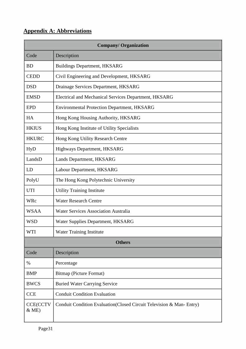
Appendix A: Abbreviations

Company/ Organization

Code Description

BD Buildings Department, HKSARG

CEDD Civil Engineering and Development, HKSARG

DSD Drainage Services Department, HKSARG

EMSD Electrical and Mechanical Services Department, HKSARG

EPD Environmental Protection Department, HKSARG

HA Hong Kong Housing Authority, HKSARG

HKIUS Hong Kong Institute of Utility Specialists

HKURC Hong Kong Utility Research Centre

HyD Highways Department, HKSARG

LandsD Lands Department, HKSARG

LD Labour Department, HKSARG

PolyU The Hong Kong Polytechnic University

UTI Utility Training Institute

WRc Water Research Centre

WSAA Water Services Association Australia

WSD Water Supplies Department, HKSARG

WTI Water Training Institute

Others

Code Description

% Percentage

BMP Bitmap (Picture Format)

BWCS Buried Water Carrying Service

CCE Conduit Condition Evaluation

CCE(CCTV

& ME)

Conduit Condition Evaluation(Closed Circuit Television & Man- Entry)

http://www.landsd.gov.hk/


CCES Conduit Condition Evaluation Specialists

CCTV Closed Circuit Television

CD Compact Disc

CL Cover Level

COP Code of practice

CP Competent Person

DN Nominal Diameter

DP Design Pressure

DVD Digital Versatile Disc

e.g. Exempli Gratia

GIS Geo-Information System

EPR Environmental Protection Requirements

etc. et cetera

GL Ground Level

H Height

HKCCEC Hong Kong Conduit Condition Evaluation Codes

HPWJ High Pressure Water Jetting

hr Hour

Hz Hertz

ICG Internal Condition Grade

ID Internal Diameter

IDMS Integrated Data Management System

IL Invert Level

ISO International Standards Organization

JPEG Joint Photographic Experts Group (Picture Format)

kHz Kilo- Hertz

kPa Kilopascal


m Meter(s)

ME Man Entry

MHICS Manhole Internal Condition Survey

mm Millimetre(s)

Mpa Megapascal

MPEG Motion Picture Experts Group (Video Format)

MS Method Statement

MSCC Manual of Sewer Condition Classification, UK

OHSAS Occupational Health and Safety Assessment Series

PPE Personal Protective Equipment

ppm Parts per million

PS Particular Specification

PSI Pound Per Square Inch

QA/ QC Quality Assurance/ Quality Control

Ref. Reference

RMSE Root Mean Square Error

RPUS Recognized Professional Utility Specialist

RTO Recognized Training Organization

SCG Service Condition Grades

SOPs Safe Operator Procedures

SPF Sun Protection Factor

SPG Structural Performance Grade

SRM Sewer Rehabilitation Manual

STP System Test Pressure

TTA Temporary Traffic Arrangement

US Utility Specialist

VHS Video High Speed


W Width

WLD Water Leakage Detection

WO Works Order

WP Work Procedure

g.gpr.pdf - Hong Kong Institute of Utility Specialists

Documents

Transcript of g.gpr.pdf - Hong Kong Institute of Utility Specialists