
Getting Started:
92
NSOFT Maxwell ® 2D Field Simulator Getting Started: A 2D Transient Linear Motion Problem February 2002
-
Upload
khangminh22 -
Category
Documents
-
view
0 -
download
0
Transcript of Getting Started:

linrmotn.book : title.fm 1 Mon Mar 11 15:50:28 2002
NSOFT
Maxwell® 2DField Simulator
Getting Started:A 2D Transient Linear Motion
Problem
February 2002

linrmotn.book : frnt.fm ii Mon Mar 11 15:50:28 2002
NoticeThe information contained in this document is subject to changewithout notice.Ansoft makes no warranty of any kind with regard to this material,including, but not limited to, the implied warranties ofmerchantability and fitness for a particular purpose. Ansoft shall notbe liable for errors contained herein or for incidental or consequentialdamages in connection with the furnishing, performance or use ofthis material.This document contains proprietary information which is protectedby copyright. All rights are reserved.
Ansoft CorporationFour Station SquareSuite 200Pittsburgh, PA 15219(412) 261 - 3200
Motif is a trademark of the Open Software Foundation.UNIX is a registered trademark of UNIX Systems Laboratories, Inc.WindowsTM and Windows NTTM are trademarks of Microsoft®
Corporation.AIXwindowsTM is a trademark of International Business MachinesCorporation.DECwindowsTM is a trademark of Digital Equipment Corporation.OpenWindowsTM is a trademark of Sun Microsystems, Inc.
© Copyright 1994-2002 Ansoft Corporation
ii

linrmotn.book : frnt.fm iii Mon Mar 11 15:50:28 2002
Printing HistoryNew editions of this manual incorporate all material updated sincethe previous edition. The manual printing date, which indicates themanual’s current edition, changes when a new edition is printed.Minor corrections and updates that are incorporated at reprint do notcause the date to change.Update packages, which may contain additional and/or replacementpages for you to merge into the manual, may be issued betweeneditions. Pages that are rearranged due to changes on a previous pageare not considered to be revised.
Edition DateSoftwareRevision
1 October 1999 7.0
2 December 2000 8.0
3 February 2002 9.0
iii
linrmotn.book : frnt.fm iv Mon Mar 11 15:50:28 2002
Welcome!This manual is a tutorial guide for setting up an electrostatic transientproblem using version 8.2 of Maxwell 2D, a software package foranalyzing electromagnetic fields in cross-sections of structures.
Installation GuideWhen installing Maxwell 2D, refer to the Ansoft PC or UNIXInstallation Guide.
User’s ReferenceFor information on all of the Maxwell Control Panel and Maxwell 2DField Simulator commands, refer to the following sources:
■ Maxwell Control Panel online documentation. The ControlPanel online help contains a detailed description of all of thecommands in the Maxwell Control Panel and in the Utilitiespanel. The Maxwell Control Panel allows you to create andopen projects, print screens, and translate files. Through theMaxwell Control Panel, you may access the Utilities panel,which allows you to either view licensing information (on theworkstation) or enter codewords (on the PC), adjust colors,open and create 2D models, open and create plots usingparametric equations, and evaluate mathematical expressions.
■ Maxwell 2D online documentation. The Maxwell 2D onlinehelp contains a detailed description of the Maxwell 2Dsoftware and the Parametric Analysis module. The ParametricAnalysis module allows you to define variables for differentparts of the model, such as geometric dimensions, materialproperties, and excitations, so that you can assign differentvalues to these variables during the solution. You then cananalyze the model’s behavior after these particular aspects ofthe model are changed.
iv

linrmotn.book : frnt.fm v Mon Mar 11 15:50:28 2002
Getting StartedIf you are using Maxwell 2D for the first time, refer to the followingguides:
■ Getting Started: An Electrostatic Problem■ Getting Started: A Magnetostatic Problem■ Getting Started: A 2D Parametric Problem
These tutorials guide you through the process of setting up andsolving simple problems in Maxwell 2D. Using them will provideyou with a good overview of how to use the software.
v

linrmotn.book : frnt.fm vi Mon Mar 11 15:50:28 2002
Using this ManualThis manual is organized in a manner that follows the sequence inwhich a problem is set up and solved as closely as possible. It isdivided into the following major sections:
For an overview of the general procedure to follow when you set up,solve, and analyze a problem, see Chapter 1, “Introduction.”
Section Title Contents
Chapter 1 Introduction Describes the purpose of Maxwell 2Dand summarizes the general procedurefor creating a model and solving aproblem.
Chapter 2 Creating theTransientProject
Describes the procedure for creating anew project directory and a Maxwell2D project.
Chapter 3 Accessing theSoftware
Describes how to open and run Max-well 2D. Also provides a brief overviewof the Maxwell 2D Executive com-mands window.
Chapter 4 Creating theModel
Describes the 2D Modeler and the pro-cedure for drawing the microstripmodel.
Chapter 5 DefiningMaterialsand Sources
Describes the procedure for assigningmaterials to the objects and definingboundary conditions and sources.
Chapter 6 Generating aSolution
Describes the procedure for enteringsolution criteria and generating a solu-tion.
Chapter 7 Analyzingthe Solution
Describes the procedure for analyzingthe results by plotting equipotentialcontours and calculating capacitance.
Index The index for the manual.
vi
linrmotn.book : frnt.fm vii Mon Mar 11 15:50:28 2002
Typeface ConventionsBold Various bold formats are used for the
following items:■ On-screen prompts and messages.■ Field names.■ Keyboard entries that must be typed
in their entirety exactly as shown.For example, the instruction “copyfile1” means to type the word copy, totype a space, and then to type file1.
■ Menu selections and buttoncommands. Menu levels are separatedby forward slashes (/).For example, the instruction “ChooseFile/Open” means to choose theOpen command under the File menu.
■ Commands that are needed to performa specific text.For example, choose OK or Cancel.
Italics Italic type is used for emphasis and for thetitles of manuals and other publications.Italic type is also used for keyboard entrieswhen a name or a variable must be typed inplace of the words in italics.For example, copy filename means to type theword copy, to type a space, and then to typethe name of a file such as file1.
Keys Keys on the computer keyboard are printed inHelvetica bold.For example, the instruction to “Press Return“means to press the Return key on the computerkeyboard.
vii

linrmotn.book : frnt.fm viii Mon Mar 11 15:50:28 2002
Accessing CommandsYou can use either the tool bar to access the most commonly used commands,or the menu bar to access many commands in Maxwell 2D modules (such asthe 2D Modeler).
➤ To access commands from the menu, do one of the following:■ Use the mouse buttons in the following ways:
■ Use the left mouse button to access, execute, and completecommands.
■ Use the right mouse button to abort commands.■ Use the keyboard in the following ways:
■ Use the Alt key to display the commands for a menu.
■ Use the hotkeys, which appear next to the names of thecommands in the menus, to access a command.
■ Use the arrow or Tab keys to move around in the menu.
☞Note: If you do not have an Alt key on your keyboard, use any one of the fol-
lowing keys instead:● The Meta key.● The Extend char key.● The Compose key.In this manual, however, it will be referred to as the Alt key.
☞Note: Throughout this manual, “choose” means to move the cursor to the
appropriate field or menu item and click any mouse button. Also,sequences of commands will be presented as Menu/Command. Forexample, “choose Model/Drawing Units” means to display the Modelmenu and then click on the Drawing Units command.
viii
linrmotn.book : linrmotnTOC.doc 1 Mon Mar 11 15:50:28 2002
Table of Contents
1. Introduction . . . . . . . . . . . . . . . . . . . . . . . . . . . . . . . . . . 1-1Sample Problem . . . . . . . . . . . . . . . . . . . . . . . . . . . . . . . . . . . . . . . . . . . . . 1-3Results to Expect . . . . . . . . . . . . . . . . . . . . . . . . . . . . . . . . . . . . . . . . . . . . 1-4
2. Creating the Transient Project . . . . . . . . . . . . . . . . . . . 2-1Access the Maxwell Control Panel . . . . . . . . . . . . . . . . . . . . . . . . . . . . . . 2-2Create a Project Directory . . . . . . . . . . . . . . . . . . . . . . . . . . . . . . . . . . . . . 2-3
Add the Project Directory . . . . . . . . . . . . . . . . . . . . . . . . . . . . . . . . . . . . 2-4Create a Project . . . . . . . . . . . . . . . . . . . . . . . . . . . . . . . . . . . . . . . . . . . . . 2-5
Access the Project Directory . . . . . . . . . . . . . . . . . . . . . . . . . . . . . . . . . . 2-5Create the New Project . . . . . . . . . . . . . . . . . . . . . . . . . . . . . . . . . . . . . . 2-5Save Project Notes . . . . . . . . . . . . . . . . . . . . . . . . . . . . . . . . . . . . . . . . . . 2-6
3. Accessing the Software . . . . . . . . . . . . . . . . . . . . . . . . 3-1Open the New Project and Run the Software . . . . . . . . . . . . . . . . . . . . . . 3-2Executive Commands Window . . . . . . . . . . . . . . . . . . . . . . . . . . . . . . . . . 3-3
Executive Commands Menu . . . . . . . . . . . . . . . . . . . . . . . . . . . . . . . . . . 3-3Display Area . . . . . . . . . . . . . . . . . . . . . . . . . . . . . . . . . . . . . . . . . . . . . . 3-3Solution Monitoring Area . . . . . . . . . . . . . . . . . . . . . . . . . . . . . . . . . . . . 3-3
Sample Problem . . . . . . . . . . . . . . . . . . . . . . . . . . . . . . . . . . . . . . . . . . . . . 3-4General Procedure . . . . . . . . . . . . . . . . . . . . . . . . . . . . . . . . . . . . . . . . . . . 3-5
4. Creating the Model . . . . . . . . . . . . . . . . . . . . . . . . . . . . 4-1Specify Solver Type . . . . . . . . . . . . . . . . . . . . . . . . . . . . . . . . . . . . . . . . . . 4-2Specify Drawing Plane . . . . . . . . . . . . . . . . . . . . . . . . . . . . . . . . . . . . . . . 4-3
Contents-1
linrmotn.book : linrmotnTOC.doc 2 Mon Mar 11 15:50:28 2002
Access the 2D Modeler . . . . . . . . . . . . . . . . . . . . . . . . . . . . . . . . . . . . . . . 4-4Layout of the 2D Modeler . . . . . . . . . . . . . . . . . . . . . . . . . . . . . . . . . . . . . 4-5
General Areas . . . . . . . . . . . . . . . . . . . . . . . . . . . . . . . . . . . . . . . . . . . . . . 4-5Project Windows . . . . . . . . . . . . . . . . . . . . . . . . . . . . . . . . . . . . . . . . . . . 4-5View Windows . . . . . . . . . . . . . . . . . . . . . . . . . . . . . . . . . . . . . . . . . . . . . 4-5
Set Up the Drawing Region . . . . . . . . . . . . . . . . . . . . . . . . . . . . . . . . . . . . 4-7Define the Drawing Size . . . . . . . . . . . . . . . . . . . . . . . . . . . . . . . . . . . . . 4-7
Create the Geometry . . . . . . . . . . . . . . . . . . . . . . . . . . . . . . . . . . . . . . . . . 4-8Keyboard Entry . . . . . . . . . . . . . . . . . . . . . . . . . . . . . . . . . . . . . . . . . . . . 4-8Draw the Band Object . . . . . . . . . . . . . . . . . . . . . . . . . . . . . . . . . . . . . . . 4-9
Create a Rectangle . . . . . . . . . . . . . . . . . . . . . . . . . . . . . . . . . . . . . . . . . . . . 4-9Define the Band’s Name and Color . . . . . . . . . . . . . . . . . . . . . . . . . . . . . . . 4-9
Draw the Magnet . . . . . . . . . . . . . . . . . . . . . . . . . . . . . . . . . . . . . . . . . . . 4-10Draw the Left Bar . . . . . . . . . . . . . . . . . . . . . . . . . . . . . . . . . . . . . . . . . . 4-11Draw the Right Bar . . . . . . . . . . . . . . . . . . . . . . . . . . . . . . . . . . . . . . . . . 4-12
Select and Copy the Left Bar . . . . . . . . . . . . . . . . . . . . . . . . . . . . . . . . . . . . 4-12Rename the Right Bar 4-13Displaying Zoomed Models . . . . . . . . . . . . . . . . . . . . . . . . . . . . . . . . . . . . . 4-13
Completed Geometry . . . . . . . . . . . . . . . . . . . . . . . . . . . . . . . . . . . . . . . . . 4-14Exit the 2D Modeler . . . . . . . . . . . . . . . . . . . . . . . . . . . . . . . . . . . . . . . . . . 4-15
5. Defining Materials and Boundaries . . . . . . . . . . . . . . . 5-1Set Up Materials . . . . . . . . . . . . . . . . . . . . . . . . . . . . . . . . . . . . . . . . . . . . 5-2
Access the Material Manager . . . . . . . . . . . . . . . . . . . . . . . . . . . . . . . . . . 5-3Material Manager Layout . . . . . . . . . . . . . . . . . . . . . . . . . . . . . . . . . . . . . 5-3
Objects . . . . . . . . . . . . . . . . . . . . . . . . . . . . . . . . . . . . . . . . . . . . . . . . . . . . . 5-3Materials . . . . . . . . . . . . . . . . . . . . . . . . . . . . . . . . . . . . . . . . . . . . . . . . . . . . 5-3Display Area . . . . . . . . . . . . . . . . . . . . . . . . . . . . . . . . . . . . . . . . . . . . . . . . . 5-4Material Properties . . . . . . . . . . . . . . . . . . . . . . . . . . . . . . . . . . . . . . . . . . . . 5-4
Assign NdFe35 to the Magnet . . . . . . . . . . . . . . . . . . . . . . . . . . . . . . . . . 5-4Assign Copper to the Flanking Bars . . . . . . . . . . . . . . . . . . . . . . . . . . . . 5-5Assign a Vacuum to the Band . . . . . . . . . . . . . . . . . . . . . . . . . . . . . . . . . 5-5Assign Materials to the Background . . . . . . . . . . . . . . . . . . . . . . . . . . . . 5-6Exit the Material Manager . . . . . . . . . . . . . . . . . . . . . . . . . . . . . . . . . . . . 5-7
Set Up Boundaries and Sources . . . . . . . . . . . . . . . . . . . . . . . . . . . . . . . . . 5-8Display the 2D Boundary/Source Manager . . . . . . . . . . . . . . . . . . . . . . . 5-92D Boundary/Source Manager Screen Layout . . . . . . . . . . . . . . . . . . . . 5-9
Boundary . . . . . . . . . . . . . . . . . . . . . . . . . . . . . . . . . . . . . . . . . . . . . . . . . . . 5-9Display Area . . . . . . . . . . . . . . . . . . . . . . . . . . . . . . . . . . . . . . . . . . . . . . . . . 5-9Boundary/Source Information . . . . . . . . . . . . . . . . . . . . . . . . . . . . . . . . . . . 5-9
Types of Boundary Conditions and Sources . . . . . . . . . . . . . . . . . . . . . . 5-10
Contents-2

linrmotn.book : linrmotnTOC.doc 3 Mon Mar 11 15:50:28 2002
Set Voltage on Copper Bars . . . . . . . . . . . . . . . . . . . . . . . . . . . . . . . . . . . 5-11Select the Copper Bars . . . . . . . . . . . . . . . . . . . . . . . . . . . . . . . . . . . . . . . . . 5-11Define a Functional Voltage . . . . . . . . . . . . . . . . . . . . . . . . . . . . . . . . . . . . 5-11Assign a Voltage 5-12Assign the Coil Value . . . . . . . . . . . . . . . . . . . . . . . . . . . . . . . . . . . . . . . . . 5-12
Balloon the Background . . . . . . . . . . . . . . . . . . . . . . . . . . . . . . . . . . . . . . 5-13Select the Background . . . . . . . . . . . . . . . . . . . . . . . . . . . . . . . . . . . . . . . . . 5-13Assign Balloon Boundary . . . . . . . . . . . . . . . . . . . . . . . . . . . . . . . . . . . . . . 5-13
Displaying, Modifying, and Deleting Boundaries and Sources . . . . . . . . 5-14Exit the Boundary Manager . . . . . . . . . . . . . . . . . . . . . . . . . . . . . . . . . . . 5-14
6. Generating a Solution . . . . . . . . . . . . . . . . . . . . . . . . . . 6-1Access the Setup Solution Menu . . . . . . . . . . . . . . . . . . . . . . . . . . . . . . . . 6-2Modify Solution Criteria . . . . . . . . . . . . . . . . . . . . . . . . . . . . . . . . . . . . . . 6-3
Manual Mesh . . . . . . . . . . . . . . . . . . . . . . . . . . . . . . . . . . . . . . . . . . . . . . 6-3Create the Mesh 6-4Exit the Meshmaker 6-5
Solver Residual . . . . . . . . . . . . . . . . . . . . . . . . . . . . . . . . . . . . . . . . . . . . 6-5Solver Choice . . . . . . . . . . . . . . . . . . . . . . . . . . . . . . . . . . . . . . . . . . . . . . 6-5Transient Analysis . . . . . . . . . . . . . . . . . . . . . . . . . . . . . . . . . . . . . . . . . . 6-6Transient Solution Criteria . . . . . . . . . . . . . . . . . . . . . . . . . . . . . . . . . . . . 6-6Exit Setup Solution . . . . . . . . . . . . . . . . . . . . . . . . . . . . . . . . . . . . . . . . . 6-6
Define the Motion Attributes . . . . . . . . . . . . . . . . . . . . . . . . . . . . . . . . . . . 6-7Define the Band Object . . . . . . . . . . . . . . . . . . . . . . . . . . . . . . . . . . . . . . 6-7Define the Moving Object . . . . . . . . . . . . . . . . . . . . . . . . . . . . . . . . . . . . 6-8Define the Stationary Objects . . . . . . . . . . . . . . . . . . . . . . . . . . . . . . . . . 6-8Define the Mechanical Transient . . . . . . . . . . . . . . . . . . . . . . . . . . . . . . . 6-8
Define the Motion Variables 6-9Define the Spring Constant . . . . . . . . . . . . . . . . . . . . . . . . . . . . . . . . . . 6-9Define the Weight . . . . . . . . . . . . . . . . . . . . . . . . . . . . . . . . . . . . . . . . . 6-9Define the Restoring Force . . . . . . . . . . . . . . . . . . . . . . . . . . . . . . . . . . 6-9Define the Damping Coefficient . . . . . . . . . . . . . . . . . . . . . . . . . . . . . . 6-9Define the Forces Factor . . . . . . . . . . . . . . . . . . . . . . . . . . . . . . . . . . . . 6-10Define the Mechanical Transient . . . . . . . . . . . . . . . . . . . . . . . . . . . . . 6-10
Exit the Motion Setup Window . . . . . . . . . . . . . . . . . . . . . . . . . . . . . . . . 6-10Generate the Solution . . . . . . . . . . . . . . . . . . . . . . . . . . . . . . . . . . . . . . . . . 6-11Monitor the Solution . . . . . . . . . . . . . . . . . . . . . . . . . . . . . . . . . . . . . . . . . 6-12Complete the Solution Process . . . . . . . . . . . . . . . . . . . . . . . . . . . . . . . . . 6-13
View Statistics . . . . . . . . . . . . . . . . . . . . . . . . . . . . . . . . . . . . . . . . . . . . . 6-13Viewing the Results . . . . . . . . . . . . . . . . . . . . . . . . . . . . . . . . . . . . . . . . . . 6-14
View the Plots . . . . . . . . . . . . . . . . . . . . . . . . . . . . . . . . . . . . . . . . . . . . . 6-14
Contents-3
linrmotn.book : linrmotnTOC.doc 4 Mon Mar 11 15:50:28 2002
7. Analyzing the Solution . . . . . . . . . . . . . . . . . . . . . . . . . 7-1Post Process the 0.1-second Time Step . . . . . . . . . . . . . . . . . . . . . . . . . . . 7-2
Access the Post Processor . . . . . . . . . . . . . . . . . . . . . . . . . . . . . . . . . . . . 7-2Post Processor Screen Layout . . . . . . . . . . . . . . . . . . . . . . . . . . . . . . . . . 7-3
General Areas . . . . . . . . . . . . . . . . . . . . . . . . . . . . . . . . . . . . . . . . . . . . . . . . 7-3Executing Commands . . . . . . . . . . . . . . . . . . . . . . . . . . . . . . . . . . . . . . . . . 7-3Project Window . . . . . . . . . . . . . . . . . . . . . . . . . . . . . . . . . . . . . . . . . . . . . . 7-3View Windows . . . . . . . . . . . . . . . . . . . . . . . . . . . . . . . . . . . . . . . . . . . . . . . 7-3
Plot the 0.1-second Magnetic Flux . . . . . . . . . . . . . . . . . . . . . . . . . . . . . 7-4Calculate the Induced Current . . . . . . . . . . . . . . . . . . . . . . . . . . . . . . . . . 7-6Calculate and Plot the 0.1-second Induced Current . . . . . . . . . . . . . . . . . 7-7
Compute J . . . . . . . . . . . . . . . . . . . . . . . . . . . . . . . . . . . . . . . . . . . . . . . . . . . 7-7Plot J 7-8
Return to the Executive Commands Window . . . . . . . . . . . . . . . . . . . . . 7-9Post Process the 0.3-second Time Step . . . . . . . . . . . . . . . . . . . . . . . . . . . 7-10
Calculate and Plot the 0.3-second Induced Current . . . . . . . . . . . . . . . . . 7-10Compute J . . . . . . . . . . . . . . . . . . . . . . . . . . . . . . . . . . . . . . . . . . . . . . . . . . . 7-10Plot J 7-11
Exit Maxwell 2D . . . . . . . . . . . . . . . . . . . . . . . . . . . . . . . . . . . . . . . . . . . . 7-12Exit the Maxwell Software . . . . . . . . . . . . . . . . . . . . . . . . . . . . . . . . . . . . 7-13
Contents-4

linrmotn.book : intro.fm 1 Mon Mar 11 15:50:28 2002
1
Introduction
The Maxwell 2D Field Simulator is an interactive software package that usesfinite element analysis (FEA) to solve two-dimensional (2D) electromagneticproblems. To analyze a problem, you specify the appropriate geometry, mate-rial properties, and excitations for a device or system of devices. The Maxwellsoftware then does the following:● Creates the required finite element mesh, either automatically or from
user-defined seeding requirements.● Iteratively calculates the desired field solution and special quantities of
interest, including force, torque, inductance, capacitance, and power loss.● Uses a transient solver to simulate the transient, large motion of the
system.● Allows you to analyze, manipulate, and display field solutions.
Introduction 1-1
linrmotn.book : intro.fm 2 Mon Mar 11 15:50:28 2002
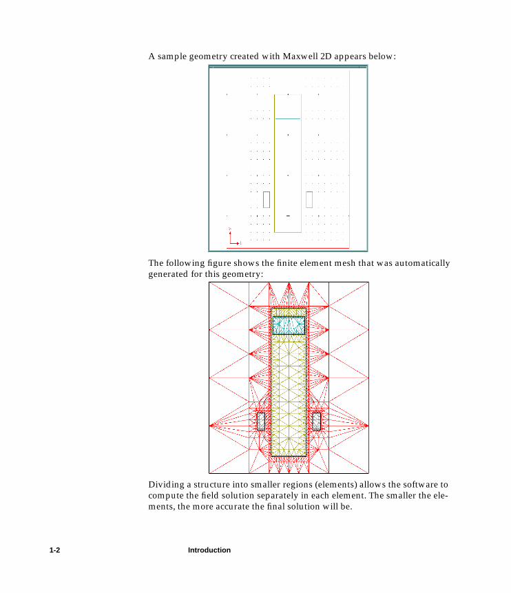
A sample geometry created with Maxwell 2D appears below:
The following figure shows the finite element mesh that was automaticallygenerated for this geometry:
Dividing a structure into smaller regions (elements) allows the software tocompute the field solution separately in each element. The smaller the ele-ments, the more accurate the final solution will be.
1-2 Introduction
linrmotn.book : intro.fm 3 Mon Mar 11 15:50:28 2002
Sample Problem
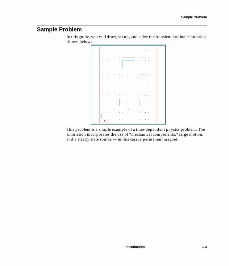
Sample ProblemIn this guide, you will draw, set up, and solve the transient motion simulationshown below:
This problem is a simple example of a time-dependent physics problem. Thesimulation incorporates the use of “mechanical components,” large motion,and a steady state source — in this case, a permanent magnet.
Introduction 1-3

linrmotn.book : intro.fm 4 Mon Mar 11 15:50:28 2002
Results to Expect
Results to ExpectAfter setting up the motion problem and generating a solution, you willobserve the following changes with respect to time:● The winding current.● The back EMF.● The flux linkage.● The position of the magnet.● The velocity of the magnet’s motion.
Time: This guide should take approximately 3 hours to work through.
1-4 Introduction
linrmotn.book : crea2d.fm 1 Mon Mar 11 15:50:28 2002
2
Creating the Transient Project
This guide assumes that Maxwell 2D has already been installed as describedin the Ansoft PC or UNIX Installation Guide.Your goals for this chapter are as follows:● Create a project directory in which to save sample problems.● Create a new project in that directory in which to save the motion
problem.
Time: This chapter should take approximately 15 minutes to work through.
Creating the Transient Project 2-1
linrmotn.book : crea2d.fm 2 Mon Mar 11 15:50:28 2002
Access the Maxwell Control Panel
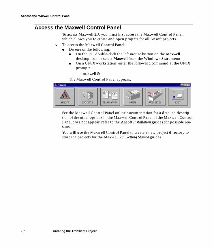
Access the Maxwell Control PanelTo access Maxwell 2D, you must first access the Maxwell Control Panel,which allows you to create and open projects for all Ansoft projects.
➤ To access the Maxwell Control Panel:● Do one of the following:
■ On the PC, double-click the left mouse button on the Maxwelldesktop icon or select Maxwell from the Windows Start menu.
■ On a UNIX workstation, enter the following command at the UNIXprompt:
maxwell &
The Maxwell Control Panel appears.
See the Maxwell Control Panel online documentation for a detailed descrip-tion of the other options in the Maxwell Control Panel. If the Maxwell ControlPanel does not appear, refer to the Ansoft Installation guides for possible rea-sons.You will use the Maxwell Control Panel to create a new project directory tostore the projects for the Maxwell 2D Getting Started guides.
2-2 Creating the Transient Project
linrmotn.book : crea2d.fm 3 Mon Mar 11 15:50:28 2002
Create a Project Directory
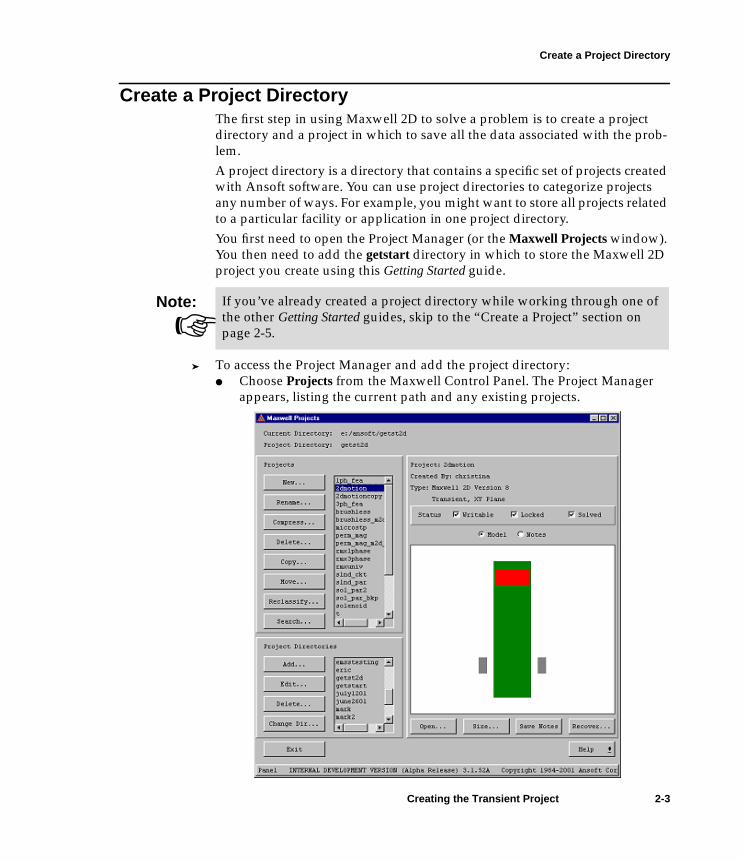
Create a Project DirectoryThe first step in using Maxwell 2D to solve a problem is to create a projectdirectory and a project in which to save all the data associated with the prob-lem.A project directory is a directory that contains a specific set of projects createdwith Ansoft software. You can use project directories to categorize projectsany number of ways. For example, you might want to store all projects relatedto a particular facility or application in one project directory.You first need to open the Project Manager (or the Maxwell Projects window).You then need to add the getstart directory in which to store the Maxwell 2Dproject you create using this Getting Started guide.
➤ To access the Project Manager and add the project directory:● Choose Projects from the Maxwell Control Panel. The Project Manager
appears, listing the current path and any existing projects.
☞Note: If you’ve already created a project directory while working through one of
the other Getting Started guides, skip to the “Create a Project” section onpage 2-5.
Creating the Transient Project 2-3
linrmotn.book : crea2d.fm 4 Mon Mar 11 15:50:28 2002
Create a Project Directory
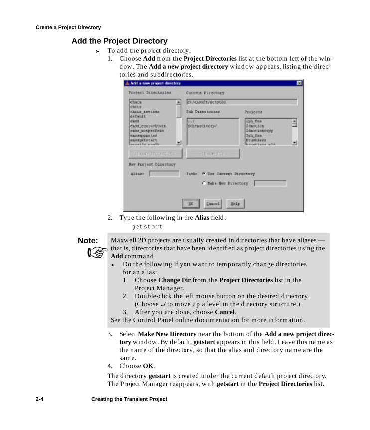
Add the Project Directory➤ To add the project directory:
1. Choose Add from the Project Directories list at the bottom left of the win-dow. The Add a new project directory window appears, listing the direc-tories and subdirectories.
2. Type the following in the Alias field:getstart
3. Select Make New Directory near the bottom of the Add a new project direc-tory window. By default, getstart appears in this field. Leave this name asthe name of the directory, so that the alias and directory name are thesame.
4. Choose OK.The directory getstart is created under the current default project directory.The Project Manager reappears, with getstart in the Project Directories list.
☞Note: Maxwell 2D projects are usually created in directories that have aliases —
that is, directories that have been identified as project directories using theAdd command.➤ Do the following if you want to temporarily change directories
for an alias:1. Choose Change Dir from the Project Directories list in the
Project Manager.2. Double-click the left mouse button on the desired directory.
(Choose ../ to move up a level in the directory structure.)3. After you are done, choose Cancel.
See the Control Panel online documentation for more information.
2-4 Creating the Transient Project
linrmotn.book : crea2d.fm 5 Mon Mar 11 15:50:28 2002
Create a Project
Create a ProjectNow you are ready to create a new project named 2dmotion in the projectdirectory getstart.
Access the Project DirectoryBefore you create the new project, access the getstart project directory.
➤ To access the project directory:● Select getstart from the Project Directories list at the bottom-left of the
window. It is now highlighted.The current directory displayed at the top of the Project Manager changes toshow the path associated with the getstart alias. Any previously created mod-els are listed in the Projects list. The Projects list is empty if you have createdno previous models in this project directory.
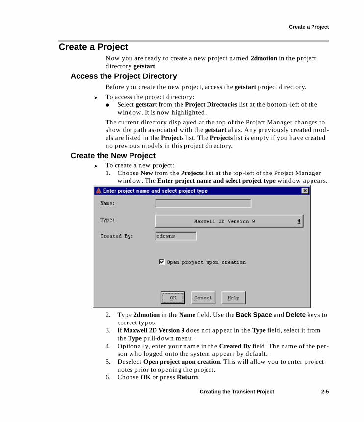
Create the New Project➤ To create a new project:
1. Choose New from the Projects list at the top-left of the Project Managerwindow. The Enter project name and select project type window appears.
2. Type 2dmotion in the Name field. Use the Back Space and Delete keys tocorrect typos.
3. If Maxwell 2D Version 9 does not appear in the Type field, select it fromthe Type pull-down menu.
4. Optionally, enter your name in the Created By field. The name of the per-son who logged onto the system appears by default.
5. Deselect Open project upon creation. This will allow you to enter projectnotes prior to opening the project.
6. Choose OK or press Return.
Creating the Transient Project 2-5

linrmotn.book : crea2d.fm 6 Mon Mar 11 15:50:28 2002
Create a Project
The information that you just entered is now displayed in the correspondingfields in the Project list. Because you created the project, Writable is selected,showing that you have access to the project.
Save Project NotesIt is a good idea to save notes about your new project so that the next timeyou use Maxwell 2D, you can view information about a project without open-ing it.
➤ To enter notes for the 2dmotion problem:1. Make certain the Notes radio button is selected (the default).2. Click the left mouse button in the area under the Notes option. This places
an I-beam cursor in the upper-left corner of the Notes area, indicating thatyou can begin typing text.
3. Enter your notes on the project, such as the following:This is the sample transient problem created usingMaxwell 2D and the 2D transient getting startedguide.
4. When you are done entering the description, choose Save Notes to savethe notes.
Now you are ready to open the new Maxwell 2D project and run Maxwell 2D.
☞Note: The Model option displays a picture of the selected model in the Notes
area. It is disabled now because you are creating a new project. After youcreate the 2dmotion problem, its geometry will appear in this area bydefault when the 2dmotion project is selected. For a detailed descriptionof the Model option, refer to the Maxwell Control Panel online documen-tation.
☞Note: Grayed out text on commands or buttons means that the command or
button is temporarily disabled.
2-6 Creating the Transient Project

linrmotn.book : run2d.fm 1 Mon Mar 11 15:50:28 2002
3
Accessing the Software
In the last chapter, you created the getstart project directory and created the2dmotion project within that directory.This chapter describes:● How to open the project you just created and run Maxwell 2D.● The Maxwell 2D Executive Commands window.● The general procedure for creating a linear motion problem in Maxwell
2D.● The sample problem and the procedures you will use to simulate its time-
varying magnetic fields.
Time: This chapter should take approximately 10 minutes to work through.
Accessing the Software 3-1
linrmotn.book : run2d.fm 2 Mon Mar 11 15:50:28 2002
Open the New Project and Run the Software
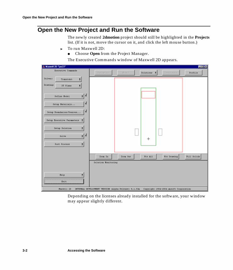
Open the New Project and Run the SoftwareThe newly created 2dmotion project should still be highlighted in the Projectslist. (If it is not, move the cursor on it, and click the left mouse button.)
➤ To run Maxwell 2D:● Choose Open from the Project Manager.The Executive Commands window of Maxwell 2D appears.
Depending on the licenses already installed for the software, your windowmay appear slightly different.
3-2 Accessing the Software
linrmotn.book : run2d.fm 3 Mon Mar 11 15:50:28 2002
Executive Commands Window
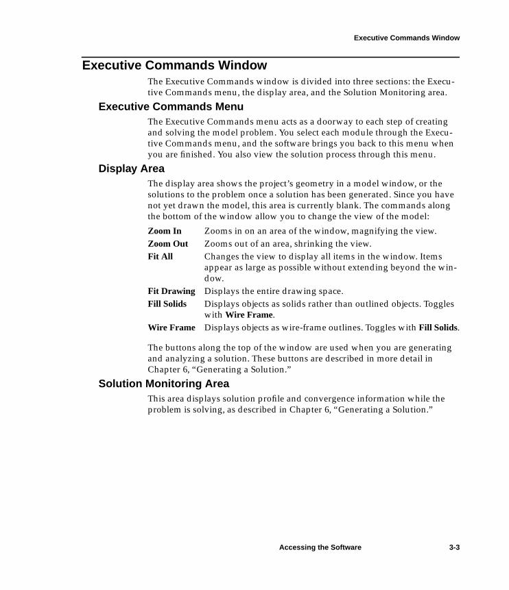
Executive Commands WindowThe Executive Commands window is divided into three sections: the Execu-tive Commands menu, the display area, and the Solution Monitoring area.
Executive Commands MenuThe Executive Commands menu acts as a doorway to each step of creatingand solving the model problem. You select each module through the Execu-tive Commands menu, and the software brings you back to this menu whenyou are finished. You also view the solution process through this menu.
Display AreaThe display area shows the project’s geometry in a model window, or thesolutions to the problem once a solution has been generated. Since you havenot yet drawn the model, this area is currently blank. The commands alongthe bottom of the window allow you to change the view of the model:
The buttons along the top of the window are used when you are generatingand analyzing a solution. These buttons are described in more detail inChapter 6, “Generating a Solution.”
Solution Monitoring AreaThis area displays solution profile and convergence information while theproblem is solving, as described in Chapter 6, “Generating a Solution.”
Zoom In Zooms in on an area of the window, magnifying the view.Zoom Out Zooms out of an area, shrinking the view.Fit All Changes the view to display all items in the window. Items
appear as large as possible without extending beyond the win-dow.
Fit Drawing Displays the entire drawing space.Fill Solids Displays objects as solids rather than outlined objects. Toggles
with Wire Frame.Wire Frame Displays objects as wire-frame outlines. Toggles with Fill Solids.
Accessing the Software 3-3
linrmotn.book : run2d.fm 4 Mon Mar 11 15:50:28 2002
Sample Problem
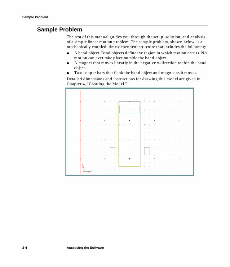
Sample ProblemThe rest of this manual guides you through the setup, solution, and analysisof a simple linear motion problem. The sample problem, shown below, is amechanically coupled, time-dependent structure that includes the following:● A band object. Band objects define the region in which motion occurs. No
motion can ever take place outside the band object.● A magnet that moves linearly in the negative x-direction within the band
object.● Two copper bars that flank the band object and magnet as it moves.Detailed dimensions and instructions for drawing this model are given inChapter 4, “Creating the Model.”
3-4 Accessing the Software
linrmotn.book : run2d.fm 5 Mon Mar 11 15:50:28 2002
General Procedure
General ProcedureThe general procedure for solving a 2D linear motion problem is as follows:1. Use the Solver command to specify which of the following electric or
magnetic field quantities to compute:■ Electrostatic■ Magnetostatic■ Eddy Current■ DC Conduction■ Thermal■ AC Conduction■ Eddy Axial■ Transient
2. Use the Drawing command to select one of the following model types:
3. Use the Define Model command to access the following options:
4. Use the Setup Materials command to assign materials to all objects in thegeometric model.
5. Use the Setup Boundaries/Sources command to define the boundaries andsources for the problem.
6. Use the Setup Solution command to access the following options:
7. Use the Solve/Nominal Problem command to solve for the appropriatefield quantities.
☞Note: Only the Ansoft packages you have purchased and installed appear in
this menu.
XY Plane Displays cartesian models as sweeping perpendicularlyto the cross-section.
RZ Plane Displays axisymmetric models as revolving around anaxis of symmetry in the cross-section.
Draw Model Allows you to access the 2D Modeler and draw theobjects that make up the geometric model.
Couple Model Allows you to couple a model for thermal analysis.Group Objects Allows you to group discrete objects that are actually one
electrical object. For instance, two terminations of a con-ductor that are drawn as separate objects in the cross-sec-tion can be grouped to represent one conductor.
Options Use this option to enter parameters that affect how thesolution is computed.
Motion Setup Use this option to define the motion parameters of thesystem.
Accessing the Software 3-5
linrmotn.book : run2d.fm 6 Mon Mar 11 15:50:28 2002
General Procedure
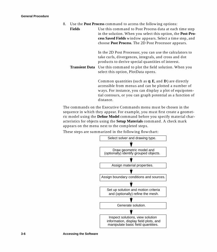
8. Use the Post Process command to access the following options:
The commands on the Executive Commands menu must be chosen in thesequence in which they appear. For example, you must first create a geomet-ric model using the Define Model command before you specify material char-acteristics for objects using the Setup Materials command. A check markappears on the menu next to the completed steps.These steps are summarized in the following flowchart:
Fields Use this command to Post Process data at each time stepin the solution. When you select this option, the Post-Pro-cess Saved Fields window appears. Select a time step, andchoose Post Process. The 2D Post Processor appears.
In the 2D Post Processor, you can use the calculators totake curls, divergences, integrals, and cross and dotproducts to derive special quantities of interest.
Transient Data Use this command to plot the field solution. When youselect this option, PlotData opens.
Common quantities (such as φ, E, and D) are directlyaccessible from menus and can be plotted a number ofways. For instance, you can display a plot of equipoten-tial contours, or you can graph potential as a function ofdistance.
Select solver and drawing type.
Draw geometric model and
Assign material properties.
Assign boundary conditions and sources.
Set up solution and motion criteria
Generate solution.
Inspect solutions, view solution
and (optionally) refine the mesh.
information, display field plots, and manipulate basic field quantities.
(optionally) identify grouped objects.
3-6 Accessing the Software

linrmotn.book : geom2d.fm 1 Mon Mar 11 15:50:28 2002
4
Creating the Model
In the last chapter, you opened the 2dmotion project, examined the ExecutiveCommands window, and reviewed the procedure for creating a 2D model.Now you are ready to use Maxwell 2D, along with its transient solver, tosolve the linear motion problem. The first step is to create the geometry forthe system being studied.This chapter shows you how to create the geometry for the motion problemthat was described in Chapter 1, “Introduction” and in Chapter 3, “Accessingthe Software.”Your goals for this chapter are as follows:● Set up the problem region.● Create the objects that make up the geometric model.● Save the geometric model to a disk file.
Time: The total time needed to complete this chapter is approximately 35 min-utes.
Creating the Model 4-1

linrmotn.book : geom2d.fm 2 Mon Mar 11 15:50:28 2002
Specify Solver Type
Specify Solver TypeThe Maxwell 2D Executive Commands window should still be on the screen.Before you start drawing your model, you need to specify which field quanti-ties to compute. By default, Electrostatic appears as the Solver type.Because you are solving a motion problem, select Transient as the Solver type.
4-2 Creating the Model

linrmotn.book : geom2d.fm 3 Mon Mar 11 15:50:28 2002
Specify Drawing Plane
Specify Drawing PlaneThe model you are drawing is actually the XY cross-section of a structure thatextends into the Z direction. This is known as a cartesian or XY plane model.By default, XY Plane appears as the Drawing plane. Because the model youwill be creating is in the XY plane, leave this type selected.Now you are ready to draw the model.
Creating the Model 4-3
linrmotn.book : geom2d.fm 4 Mon Mar 11 15:50:28 2002
Access the 2D Modeler
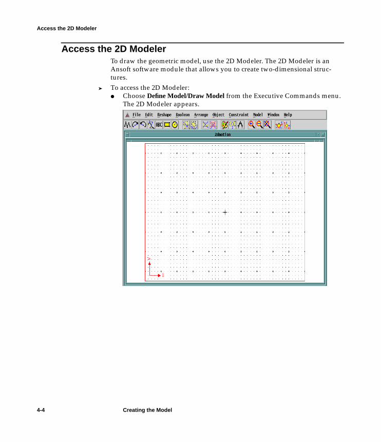
Access the 2D ModelerTo draw the geometric model, use the 2D Modeler. The 2D Modeler is anAnsoft software module that allows you to create two-dimensional struc-tures.
➤ To access the 2D Modeler:● Choose Define Model/Draw Model from the Executive Commands menu.
The 2D Modeler appears.
4-4 Creating the Model
linrmotn.book : geom2d.fm 5 Mon Mar 11 15:50:28 2002
Layout of the 2D Modeler
Layout of the 2D ModelerThe following sections provide a brief overview of the 2D Modeler.
General AreasThe 2D Modeler is divided into the following general areas:
For more information on these areas of the 2D Modeler, refer to the Maxwell2D online documentation.
Project WindowsThe outermost window in the 2D Modeler is called the project window. Aproject window contains the geometry for a specific project and displays theproject’s name in its title bar. By default, one subwindow is contained withinthe project window.
View WindowsView windows contain the drawing region in which you draw the geometricmodel. By default, this window:● Has points specified in relation to a local uv coordinate system. The U-
Menu Bar Appears at the top of the 2D Modeler window. Each item inthe menu bar has a menu of commands associated with it.
Tool Bar Appears below the menu bar in the 2D Modeler window aseither a vertical stack or a horizontal row of icons. The iconsgive you easy access to the most frequently used com-mands.
Drawing Region Appears as the grid-covered area in which you drawobjects.
Message Bar Appears at the bottom of the screen. It displays the nameand version of the software currently running, help mes-sages for commands, mouse button functions, number ofitems currently selected, and magnification level when youchange the view in a subwindow.
Status Bar Appears below the message bar. It contains fields that dis-play the coordinates of the mouse and that allow you toenter coordinates for object points. It also displays the cur-rent unit of length and the snap-to-point behavior of themouse.
☞Note: Optionally, you can open additional projects in the 2D Modeler using the
File/Open command. Opening several projects at once is useful if youwant to copy objects between geometries. See the Maxwell 2D onlinedocumentation for more details.
Creating the Model 4-5

linrmotn.book : geom2d.fm 6 Mon Mar 11 15:50:28 2002
Layout of the 2D Modeler
axis is horizontal; the V-axis is vertical; and the origin is marked by across in the middle of the window.
● Uses millimeters as the default drawing unit.● Has grid points 2 millimeters apart. The default window size is 70 mm by
100 mm.
☞Note: If a geometry is complex, you may want to open additional subwindows
so that you can alter your view of the geometry from one window to thenext. To do so, use the Windows commands that are described in theMaxwell 2D online documentation. For this linear motion geometry,however, a single view window is sufficient.
4-6 Creating the Model
linrmotn.book : geom2d.fm 7 Mon Mar 11 15:50:28 2002
Set Up the Drawing Region
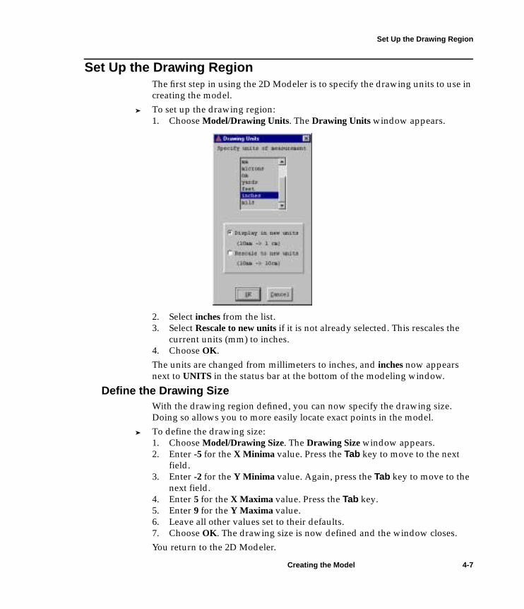
Set Up the Drawing RegionThe first step in using the 2D Modeler is to specify the drawing units to use increating the model.
➤ To set up the drawing region:1. Choose Model/Drawing Units. The Drawing Units window appears.
2. Select inches from the list.3. Select Rescale to new units if it is not already selected. This rescales the
current units (mm) to inches.4. Choose OK.The units are changed from millimeters to inches, and inches now appearsnext to UNITS in the status bar at the bottom of the modeling window.
Define the Drawing SizeWith the drawing region defined, you can now specify the drawing size.Doing so allows you to more easily locate exact points in the model.
➤ To define the drawing size:1. Choose Model/Drawing Size. The Drawing Size window appears.2. Enter -5 for the X Minima value. Press the Tab key to move to the next
field.3. Enter -2 for the Y Minima value. Again, press the Tab key to move to the
next field.4. Enter 5 for the X Maxima value. Press the Tab key.5. Enter 9 for the Y Maxima value.6. Leave all other values set to their defaults.7. Choose OK. The drawing size is now defined and the window closes.You return to the 2D Modeler.
Creating the Model 4-7

linrmotn.book : geom2d.fm 8 Mon Mar 11 15:50:28 2002
Create the Geometry
Create the GeometryNow you are ready to draw the objects that make up the geometric model. Allobjects are created using the Object commands as described in the followingsections.
Keyboard EntryWhen you specified the drawing region, you changed the drawing units frommillimeters to inches and left the default grid spacing set to two inches. In thefollowing section, several of the points you will select as you create objects liebetween grid points. You can position these points in one of two ways:● Change the grid spacing so that the object’s dimensions lie on grid points.● Use “keyboard entry” to enter the coordinates directly into the U and V
fields in the status bar.If you change grid spacing, the screen may become cluttered with too manytightly-spaced grid points and make point selection difficult. Therefore, inthis example, use the second method, keyboard entry, to enter several of thedimensions of the sample geometry.
☞Note: To change the grid spacing of the problem region, use the Window/Grid
command.
To change the size of the problem region, use the Model/Drawing Sizecommand. For more details on these commands, see the Maxwell 2Donline documentation.
4-8 Creating the Model
linrmotn.book : geom2d.fm 9 Mon Mar 11 15:50:28 2002
Create the Geometry
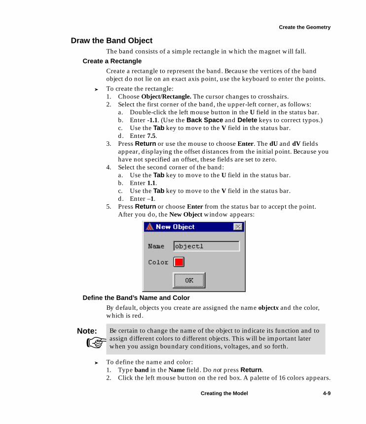
Draw the Band ObjectThe band consists of a simple rectangle in which the magnet will fall.
Create a Rectangle
Create a rectangle to represent the band. Because the vertices of the bandobject do not lie on an exact axis point, use the keyboard to enter the points.
➤ To create the rectangle:1. Choose Object/Rectangle. The cursor changes to crosshairs.2. Select the first corner of the band, the upper-left corner, as follows:
a. Double-click the left mouse button in the U field in the status bar.b. Enter -1.1. (Use the Back Space and Delete keys to correct typos.)c. Use the Tab key to move to the V field in the status bar.d. Enter 7.5.
3. Press Return or use the mouse to choose Enter. The dU and dV fieldsappear, displaying the offset distances from the initial point. Because youhave not specified an offset, these fields are set to zero.
4. Select the second corner of the band:a. Use the Tab key to move to the U field in the status bar.b. Enter 1.1.c. Use the Tab key to move to the V field in the status bar.d. Enter –1.
5. Press Return or choose Enter from the status bar to accept the point.After you do, the New Object window appears:
Define the Band’s Name and Color
By default, objects you create are assigned the name objectx and the color,which is red.
➤ To define the name and color:1. Type band in the Name field. Do not press Return.2. Click the left mouse button on the red box. A palette of 16 colors appears.
☞Note: Be certain to change the name of the object to indicate its function and to
assign different colors to different objects. This will be important laterwhen you assign boundary conditions, voltages, and so forth.
Creating the Model 4-9
linrmotn.book : geom2d.fm 10 Mon Mar 11 15:50:28 2002
Create the Geometry
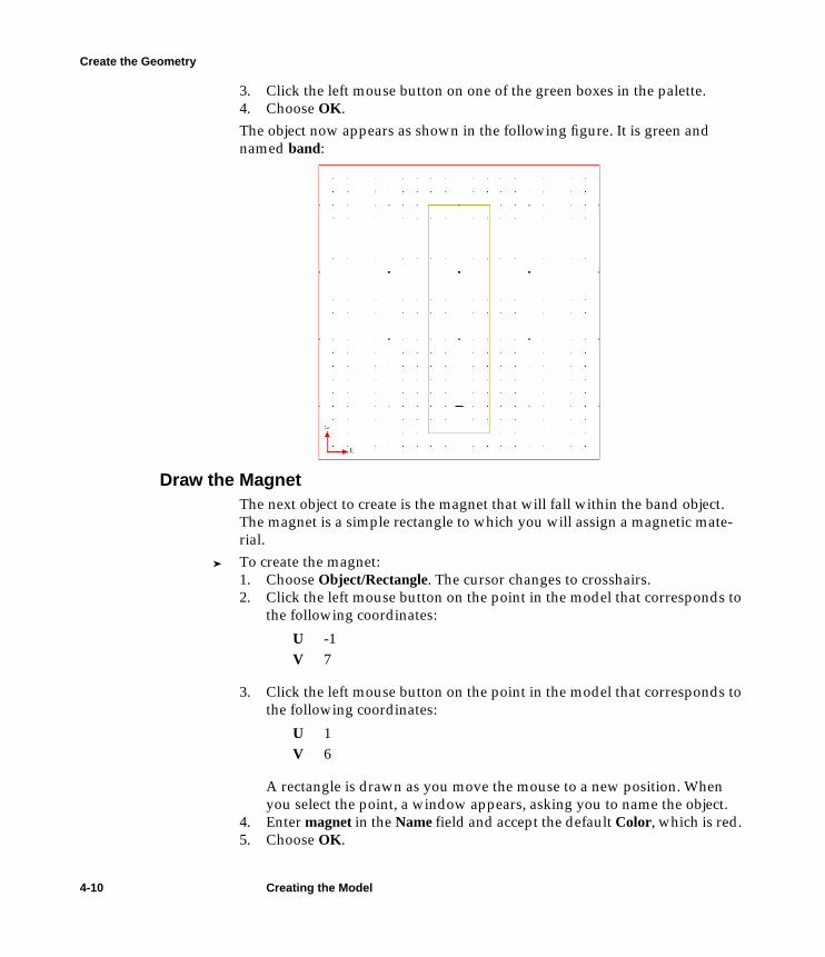
3. Click the left mouse button on one of the green boxes in the palette.4. Choose OK.The object now appears as shown in the following figure. It is green andnamed band:
Draw the MagnetThe next object to create is the magnet that will fall within the band object.The magnet is a simple rectangle to which you will assign a magnetic mate-rial.
➤ To create the magnet:1. Choose Object/Rectangle. The cursor changes to crosshairs.2. Click the left mouse button on the point in the model that corresponds to
the following coordinates:
3. Click the left mouse button on the point in the model that corresponds tothe following coordinates:
A rectangle is drawn as you move the mouse to a new position. Whenyou select the point, a window appears, asking you to name the object.
4. Enter magnet in the Name field and accept the default Color, which is red.5. Choose OK.
U -1V 7
U 1V 6
4-10 Creating the Model

linrmotn.book : geom2d.fm 11 Mon Mar 11 15:50:28 2002
Create the Geometry
Draw the Left BarNow that you have drawn the band and the magnet, draw the left bar. Theleft and right bars are used to simulate the cross-sections of copper coils. Dur-ing the solution generation, the magnet’s change in position and time causes achange in flux. The copper bars increase the flux, allowing you to more easilyobserve this effect.
➤ To create the left bar:1. Choose Object/Rectangle. The cursor changes to crosshairs.2. Click the left mouse button on the point in the model that corresponds to
the following coordinates:
3. Click the left mouse button on the point in the model that corresponds tothe following coordinates:
A rectangle is drawn as you move the mouse to a new position. Whenyou select the point, a window appears, asking you to name the object.
4. Enter left in the Name field, and change the Color to gray.5. Choose OK.
U -2V 1.5
U -1.5V .5
Creating the Model 4-11

linrmotn.book : geom2d.fm 12 Mon Mar 11 15:50:28 2002
Create the Geometry
Draw the Right BarThe left and right bars have the same dimensions; therefore, create the rightbar by copying the left one.
Select and Copy the Left Bar➤ To create the right bar:
1. Click the left mouse button on the left bar to select it as the object to becopied. A double outline appears around it, indicating that it has beenselected.
2. Choose Edit/Duplicate/Along Line. You must now select two points: firstan “anchor” point, and then a “target” point, which will be the new loca-tion for the anchor point.
3. Choose the lower-left corner of the left bar as the anchor point (-2, 0.5).After you do, two new fields appear in the status bar: dU and dV. Thesefields allow you to select the target point by specifying its offset from theanchor point rather than its u- and v-coordinates.
4. Enter 3.5 in the dU field to specify the offset between the anchor and tar-get points.
5. Press Return or use the mouse to choose Enter. The Linear Duplicateswindow appears.
6. Leave the default value of 2 in the Total Number field.7. Choose OK to accept the value and complete the command.Now both bars have been created. By default, the new object, the right bar, isselected.
☞Note: As an alternative to selecting an object by clicking on it, use the Edit/
Select commands. After an object or objects are selected, they are theobjects on which all other Edit commands operate. See the Maxwell 2Donline documentation for more details on the Edit commands.
4-12 Creating the Model

linrmotn.book : geom2d.fm 13 Mon Mar 11 15:50:28 2002
Create the Geometry
Rename the Right Bar
The 2D Modeler automatically assigns names to copied objects by appendinga number to the end of the original object’s name. For instance, the right bar isassigned the name left1 because it is the first copy of the left object. Because itis a good idea to assign meaningful names to objects, change the name of left1to right. The right bar should still be selected. If it is not, choose Edit/Select/ByName, select left1, and choose OK before continuing.
➤ To rename the right bar:1. Choose Edit/Attributes/Rename. A window that lists the names of all
selected objects appears. Because left1 is the only selected object, italready appears in the field beneath the object list.
2. Change the name to right.3. Choose Rename. The new name now appears in the object list at the top of
the window.4. Choose OK.
Since you will create other objects, it is a good idea to deselect the right bar.➤ To deselect the right bar:
● Click the left mouse button on the right bar.The bar is deselected.
Displaying Zoomed Models
Scroll bars appear on the right side and bottom of the subwindow when theentire geometric model is not displayed in the window. In these cases, youwould use the scroll bars to change your view.
➤ To change your view, do one of the following:● Click the left mouse button on the arrow buttons that appear at the top
and bottom of the scroll bar.● To scroll through the model:
1. Move the cursor to the off-colored bar, or “thumb scroll,” thatappears in the scroll bar.
2. Drag the thumb scroll up, down, left, or right in the scroll bar to theportion of the model you want to display.
For instance, to pan down a geometric model, drag the thumb scroll in thevertical scroll bar down. If the portion of the geometry in which you are inter-ested does not appear, continue to manipulate the thumb scrolls until it does.
Creating the Model 4-13
linrmotn.book : geom2d.fm 14 Mon Mar 11 15:50:28 2002
Completed Geometry
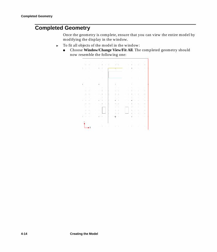
Completed GeometryOnce the geometry is complete, ensure that you can view the entire model bymodifying the display in the window.
➤ To fit all objects of the model in the window:● Choose Window/Change View/Fit All. The completed geometry should
now resemble the following one:
4-14 Creating the Model

linrmotn.book : geom2d.fm 15 Mon Mar 11 15:50:28 2002
Exit the 2D Modeler
Exit the 2D Modeler➤ To exit the 2D Modeler:
1. Choose File/Exit. A window appears, prompting you to save the defaultwindow size.
2. Choose Yes to save the window settings. A second window appears,prompting you to save the changes before exiting. Because the Maxwell2D Modeler does not automatically save changes, you must either use theFile/Save command to save the changes, or save them as you exit themodule.
3. Choose Yes. The geometry is saved to a disk file in the 2dmotion.pjtproject directory, and the Executive Commands window appears.
A checkmark appears next to Define Model, indicating that this step has beencompleted.
☞Note: Because none of the objects that you created are electrically connected at
any point in a three-dimensional rendering of the model, you do notneed to use the Define/Model/Group Objects command. For more detailson this command, refer to the Maxwell 2D online documentation.
Creating the Model 4-15

linrmotn.book : geom2d.fm 16 Mon Mar 11 15:50:28 2002
Exit the 2D Modeler
4-16 Creating the Model

linrmotn.book : setup.fm 1 Mon Mar 11 15:50:28 2002
5
Defining Materials and Boundaries
Now that you have drawn the geometry for the motion problem and returnedto the Executive Commands window, you are ready to set up the problem.Your goals for this chapter are as follows:● Assign materials to each object in the geometric model.● Define any boundary conditions, such as the behavior of the electric field
at the edge of the problem region and potentials on the surfaces of thebars.
Time: The total time needed to complete this chapter is approximately 35minutes.
Defining Materials and Boundaries 5-1

linrmotn.book : setup.fm 2 Mon Mar 11 15:50:28 2002
Set Up Materials
Set Up MaterialsTo define the material properties for the objects in the geometric model, youmust:● Assign the properties of NdFe35 to the magnet.● Assign copper to the bars.
➤ In general, to assign materials to objects:1. If necessary, add materials with the properties of the objects in your
model to the material database.2. Assign a material to each object in the geometric model:
a. Select the object(s) for which a specific material applies from theObject list.
b. Select the appropriate material from the Material list.c. Choose Assign to assign the selected material to the selected object(s).
In this sample problem, you do not need to add materials to the material data-base — all materials you need are already included in the global materialdatabase available to every project.
☞Note: You must assign a material to each object in the model.
5-2 Defining Materials and Boundaries
linrmotn.book : setup.fm 3 Mon Mar 11 15:50:28 2002
Set Up Materials
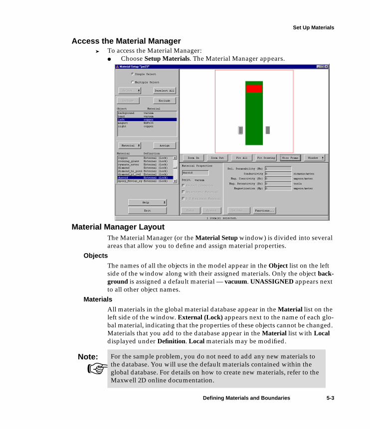
Access the Material Manager➤ To access the Material Manager:
● Choose Setup Materials. The Material Manager appears.
Material Manager LayoutThe Material Manager (or the Material Setup window) is divided into severalareas that allow you to define and assign material properties.
Objects
The names of all the objects in the model appear in the Object list on the leftside of the window along with their assigned materials. Only the object back-ground is assigned a default material — vacuum. UNASSIGNED appears nextto all other object names.
Materials
All materials in the global material database appear in the Material list on theleft side of the window. External (Lock) appears next to the name of each glo-bal material, indicating that the properties of these objects cannot be changed.Materials that you add to the database appear in the Material list with Localdisplayed under Definition. Local materials may be modified.
☞Note: For the sample problem, you do not need to add any new materials to
the database. You will use the default materials contained within theglobal database. For details on how to create new materials, refer to theMaxwell 2D online documentation.
Defining Materials and Boundaries 5-3

linrmotn.book : setup.fm 4 Mon Mar 11 15:50:28 2002
Set Up Materials
Display Area
The model is displayed so that you can choose objects by clicking on them.The following buttons appear at the bottom of the display area, allowing youto manipulate your view of the model:
■ Zoom In■ Zoom Out■ Fit All■ Fit Drawing■ Fill Solids■ Window (Measure, Grid, and Snap To Mode)
They perform the same functions as the commands with the same names thatappear on the Model and Window menus of the 2D Modeler. These menus aredescribed in more detail in the Maxwell 2D online documentation.
Material Properties
The Material Properties area that appears below the geometric model displaysthe properties of the selected material. For instance, to display the attributesof glass, choose glass from the Material list on the left side of the window.
Assign NdFe35 to the MagnetAssign a material to the magnet.
➤ To assign a material to the magnet:1. Select magnet from the Object list, or click on the magnet in the geometric
model. Capitalized material and object names are listed first.2. Select NdFe35 from the Material list. If it does not appear in the box, use
the scroll bars to scroll through the list as described in Chapter 4, “Creat-ing the Model.”
3. Choose Assign. The Assignment Coordinate System window appears,allowing you to define the alignment of the x-axis.
4. Select the Align with a given direction radio button. Since the magnetmoves perpendicular to the x-axis, you must define the direction ofmotion accordingly.
5. Enter 90 in the Angle field.6. Choose OK. The Assignment Coord. Sys. window closes.NdFe35 now appears next to magnet in the Object list.
5-4 Defining Materials and Boundaries

linrmotn.book : setup.fm 5 Mon Mar 11 15:50:28 2002
Set Up Materials
Assign Copper to the Flanking BarsNow you can assign copper to the bars that flank the band.
➤ To assign materials to the conductors:1. Choose Multiple Select from the top of the menu, if it is not already
selected.2. Do one of the following to choose left and right from the object list:
■ If you are running the software on a workstation, click the left mousebutton on each of the object names.
■ If you are running the software on a PC, do one of the following:● Hold down the Ctrl key click the left mouse button on the
object name left.● If the objects are adjacent, down the Shift key and click on
the object name right.To deselect an object, click the left mouse button on it, or for PCs, pressCtrl-click to deselect a selected object.
3. Select copper from the Material list.4. Choose Assign.The magnets have now been assigned the properties of a perfect conductor (agood approximation of which is copper). The material name copper appearsnext to left and right in the Object list.
Assign a Vacuum to the BandNow assign a vacuum to the band object.
➤ To assign a vacuum to the band:1. Select band from the Object list.
2. Select vacuum from the Material list, if it is not already selected. If it doesnot appear in the box, use the scroll bars to scroll through the list asdescribed in Chapter 4, “Creating the Model.”
3. Choose Assign.The material name vacuum now appears next to band in the Object list.
☞Note: The potentials on the surfaces of conductors are specified with the Setup
Boundaries/Sources command that is described later in this chapter.
☞Note: Capitalized material and object names are listed first.
Defining Materials and Boundaries 5-5

linrmotn.book : setup.fm 6 Mon Mar 11 15:50:28 2002
Set Up Materials
Assign Materials to the BackgroundThe background object is the only object that is assigned a material by default;by default, it is assigned to be a vacuum.In this problem, you need to include the background as part of the problemregion in which to generate the solution. When any material name appearsnext to background in the Object list, that means the background object isincluded as part of the solution region.Accept the default material of vacuum for the background.
☞Note: In some cases, such as when all objects and electromagetic fields of interest
are contained within an enclosure, including the background as part of theproblem region wastes computing resources. It also prevents you from set-ting boundary conditions defining an external electric or magnetic field forthe model.
➤ In these cases, exclude the background from the solution asfollows:1. Select background from the Object list.2. Choose the Exclude button that appears above the Object list.
This button toggles between Include and Exclude. Include is thedefault.
EXCLUDED then appears next to background in the Object list, indicatingthat it will not be included as part of the solution region.
For this example, do not exclude the background from the model. Acceptthe default material, vacuum.
5-6 Defining Materials and Boundaries

linrmotn.book : setup.fm 7 Mon Mar 11 15:50:28 2002
Set Up Materials
Exit the Material ManagerOnce materials have been assigned to each object, you may exit the MaterialManager.
➤ To exit the Material Manager:1. Choose Exit from the bottom-left of the Material Setup window. A win-
dow with the following prompt appears:Save changes before closing?
2. Choose Yes.You return to the Executive Commands window. A checkmark now appearsnext to Setup Materials, and Setup Boundaries/Sources is enabled.
☞Note: If you exit the Material Manager before excluding or assigning a mate-
rial to each object in the model, a checkmark does not appear next toSetup Materials on the Executive Commands menu, and Setup Bound-aries/Sources remains disabled.
Defining Materials and Boundaries 5-7

linrmotn.book : setup.fm 8 Mon Mar 11 15:50:28 2002
Set Up Boundaries and Sources
Set Up Boundaries and SourcesAfter setting material properties, the next step in creating the motion model isto define boundary conditions and sources.By default, the surfaces of all objects are Neumann or natural boundaries.This means that the magnetic field is defined to be perpendicular to the edgesof the problem space and continuous across all object interfaces.To finish setting up the motion problem, you need to explicitly define the fol-lowing:● The voltages on the two copper bars.● The behavior of the electric field on all surfaces exposed to the area
beyond the problem region. Since you included the background as part ofthe problem region, this exposed surface is that of the background object.
☞Note: Maxwell 2D will not solve the problem unless you specify some type of
source or magnetic field — either a current source, an external field sourceusing boundary conditions, or a permanent magnet. In this model, thecopper bars serve as sources of electric potential.
5-8 Defining Materials and Boundaries
linrmotn.book : setup.fm 9 Mon Mar 11 15:50:28 2002
Set Up Boundaries and Sources
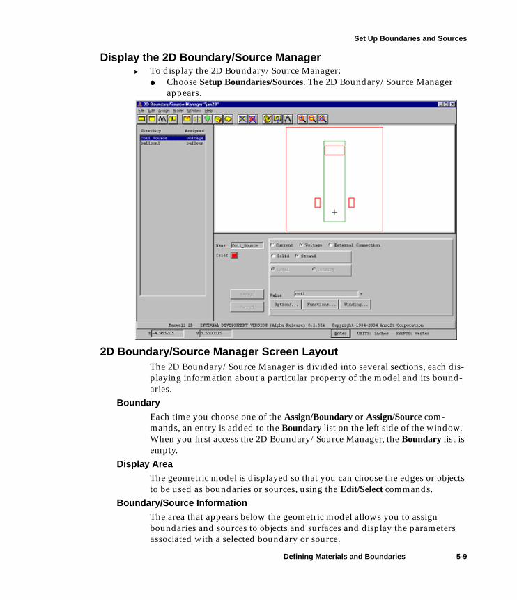
Display the 2D Boundary/Source Manager➤ To display the 2D Boundary/Source Manager:
● Choose Setup Boundaries/Sources. The 2D Boundary/Source Managerappears.
2D Boundary/Source Manager Screen LayoutThe 2D Boundary/Source Manager is divided into several sections, each dis-playing information about a particular property of the model and its bound-aries.
Boundary
Each time you choose one of the Assign/Boundary or Assign/Source com-mands, an entry is added to the Boundary list on the left side of the window.When you first access the 2D Boundary/Source Manager, the Boundary list isempty.
Display Area
The geometric model is displayed so that you can choose the edges or objectsto be used as boundaries or sources, using the Edit/Select commands.
Boundary/Source Information
The area that appears below the geometric model allows you to assignboundaries and sources to objects and surfaces and display the parametersassociated with a selected boundary or source.
Defining Materials and Boundaries 5-9

linrmotn.book : setup.fm 10 Mon Mar 11 15:50:28 2002
Set Up Boundaries and Sources
Types of Boundary Conditions and SourcesThere are two types of boundary conditions and sources you will use in thisproblem:
You will assign boundary conditions and sources to the following objects inthe geometry:
There are several ways to select objects’ surfaces, but in this sample problemyou will select each object individually. As a result, the object’s surface will beselected.
Balloon boundary Can only be applied to the outer boundary and models inwhich the structure is infinitely far away from all otherelectromagnetic sources.
Voltage sources Specifies the voltage on an object in the model. The electricscalar potential, φ, is set to a constant value, which forcesthe electric field to be perpendicular to the surface of theobjects.
Left bar This surface will be assigned a stranded voltage of 0 volts.Right bar This surface will be assigned a stranded voltage of 0 volts.Background The outer boundary of the problem region. This surface
will be ballooned to simulate a magnetically insulated sys-tem.
5-10 Defining Materials and Boundaries

linrmotn.book : setup.fm 11 Mon Mar 11 15:50:28 2002
Set Up Boundaries and Sources
Set Voltage on Copper BarsTo define the voltage on the copper bars, you must first select them. Once anobject has been selected, it can be assigned either a source or boundary condi-tion. In this case, the copper bars will receive a voltage source.
Select the Copper Bars
Select the bars to which to assign the voltage.➤ To select the bars:
1. Choose Edit/Select/Object/By Clicking. The menu bar commands are dis-abled, and the system expects you to select an item by clicking on it in themodel.
2. Click the left mouse button on the left and right bars. They are high-lighted.
3. Click the right mouse button anywhere in the display area to stop select-ing objects.
Define a Functional Voltage
The copper bars possess a functional voltage based on the motion of the mag-net. To specify the source on the bars, you must first define the functionalvalue assigned to them.
➤ To define the functional voltage:1. Choose Assign/Source/Solid. The name source1 appears in the Boundary
list, and NEW appears next to it, indicating that it has not yet beenassigned to an object or surface. New fields appear below the view win-dow.
2. Choose Options. The Property Options window appears, and you returnto the 2D Boundary Manager.
3. Select the Function radio button to define the source as a functional value.4. Choose OK. The Property Options window closes.5. Choose Functions. The Boundary/Source Symbol Table window appears.6. Enter Coil in the blank field to the left of the equals sign.7. Enter 0 in the blank field to the right of the equals sign.8. Choose Add. Coil is added to the symbol table and is assigned a base
value of 0.9. Choose Done.The Boundary/Source Symbol Table window closes, and you return to the 2DBoundary Manager.
☞Note: ➤ If the appropriate object is not highlighted, or if more objects are
highlighted, do the following:1. Exit the select mode by cancelling the command or clicking
on the right mouse button.2. Choose Edit/Deselect All. No objects are highlighted.3. Choose Edit/Select/Object/By Clicking, and select the objects.
Defining Materials and Boundaries 5-11
linrmotn.book : setup.fm 12 Mon Mar 11 15:50:28 2002
Set Up Boundaries and Sources
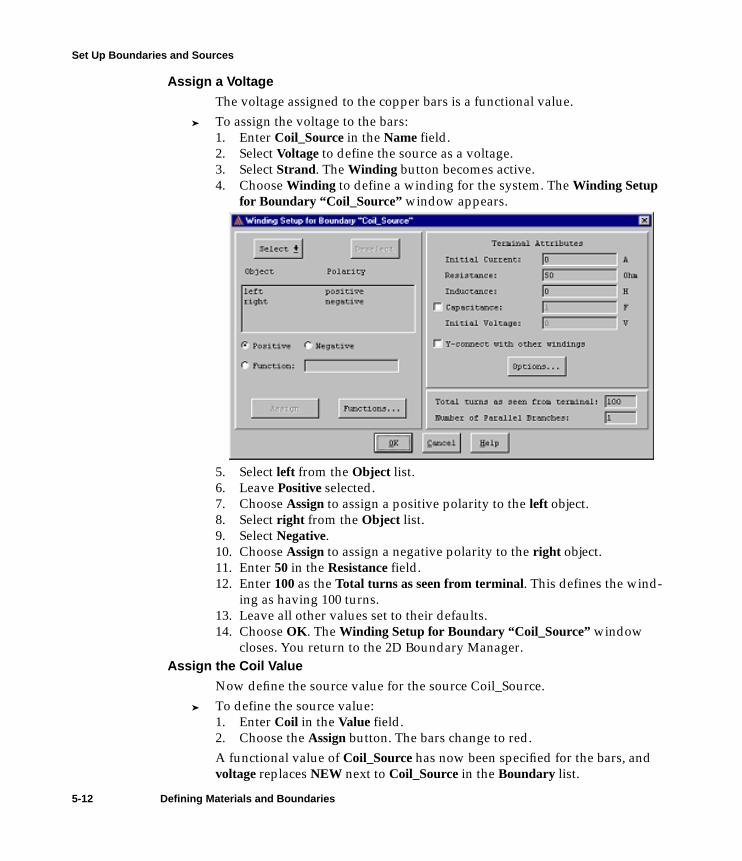
Assign a Voltage
The voltage assigned to the copper bars is a functional value.➤ To assign the voltage to the bars:
1. Enter Coil_Source in the Name field.2. Select Voltage to define the source as a voltage.3. Select Strand. The Winding button becomes active.4. Choose Winding to define a winding for the system. The Winding Setup
for Boundary “Coil_Source” window appears.
5. Select left from the Object list.6. Leave Positive selected.7. Choose Assign to assign a positive polarity to the left object.8. Select right from the Object list.9. Select Negative.10. Choose Assign to assign a negative polarity to the right object.11. Enter 50 in the Resistance field.12. Enter 100 as the Total turns as seen from terminal. This defines the wind-
ing as having 100 turns.13. Leave all other values set to their defaults.14. Choose OK. The Winding Setup for Boundary “Coil_Source” window
closes. You return to the 2D Boundary Manager.Assign the Coil Value
Now define the source value for the source Coil_Source.➤ To define the source value:
1. Enter Coil in the Value field.2. Choose the Assign button. The bars change to red.A functional value of Coil_Source has now been specified for the bars, andvoltage replaces NEW next to Coil_Source in the Boundary list.
5-12 Defining Materials and Boundaries
linrmotn.book : setup.fm 13 Mon Mar 11 15:50:28 2002
Set Up Boundaries and Sources
Balloon the BackgroundAssign a balloon boundary to the background. The balloon boundary extendsthe object it is assigned to “infinitely” far away from all other sources in alldirections.
Select the Background➤ To select the background:
1. Choose Window/Change View/Fit Drawing so that the limits of the draw-ing region are displayed.
2. Choose Edit/Select/Object/By Clicking.3. Click the left mouse button anywhere on the background so that the
boundary of the drawing region is highlighted.4. Click the right mouse button.Now you are ready to place a balloon boundary on the background.
Assign Balloon Boundary
Since the structure of the motion problem is an electrically insulated system,balloon the background.
➤ To assign the balloon boundary:1. Choose Assign/Boundary/Balloon. The balloon1 boundary appears in the
Boundary list, and the Balloon check box appears.2. Select the Balloon check box if it is not already selected.3. Choose Assign to accept the balloon boundary. The background is bal-
looned, and balloon replaces NEW next to balloon 1 in the Boundary list.
☞Note: For this sample problem, all surfaces of the background are ballooned.
Thus, you selected background to pick its entire surface before ballooningit. If you create only part of an electromagnetically symmetrical model, atleast one surface — the one representing the symmetry plane — would notbe ballooned. In this case, do not select the object’s entire surface with theEdit/Select/Object commands. Instead, use the Edit/Select/Edge command,described in the Maxwell 2D online documentation, to select the threeedges. You want to balloon these three edges separately from the edge rep-resenting the symmetry plane.
Defining Materials and Boundaries 5-13

linrmotn.book : setup.fm 14 Mon Mar 11 15:50:28 2002
Set Up Boundaries and Sources
Displaying, Modifying, and Deleting Boundaries and Sources➤ Do one of the following to display, modify, or delete boundaries and
sources:● To display boundaries and sources, simply click the left mouse button on
the boundary or source name in the Boundaries list. After you do, allparameters associated with the boundary or source are displayed at thebottom of the window.
● To modify boundaries and sources, display them, change parameters,and then choose Assign.
● To delete a boundary or source, select it from the Boundary list and thenchoose Edit/Clear.
Exit the Boundary ManagerOnce the boundaries and sources have been defined, you can exit the Bound-ary Manager.
➤ To exit the Boundary Manager:1. Choose File/Exit. A window with the following prompt appears:
Save changes to 2dmotion before closing?
2. Choose Yes.You return to the Executive Commands window. A checkmark now appearsnext to Setup Boundaries/Sources, and Setup Solution, Solve, and Post Processare now enabled.
5-14 Defining Materials and Boundaries

linrmotn.book : solve.fm 1 Mon Mar 11 15:50:28 2002
6
Generating a Solution
Now that you have created the geometry and set up the problem, you areready to specify solution parameters and generate a motion solution.Your goals for this chapter are as follows:● Modify the criteria that affect how Maxwell 2D computes the solution.● Define the motion attributes of the objects.● Setup and generate the transient solution. The transient solver calculates
magnetic fields at all time steps.● View information about how the solution converged and what
computing resources were used.
Time: The total time needed to complete this chapter is approximately 35minutes.
Generating a Solution 6-1
linrmotn.book : solve.fm 2 Mon Mar 11 15:50:28 2002
Access the Setup Solution Menu
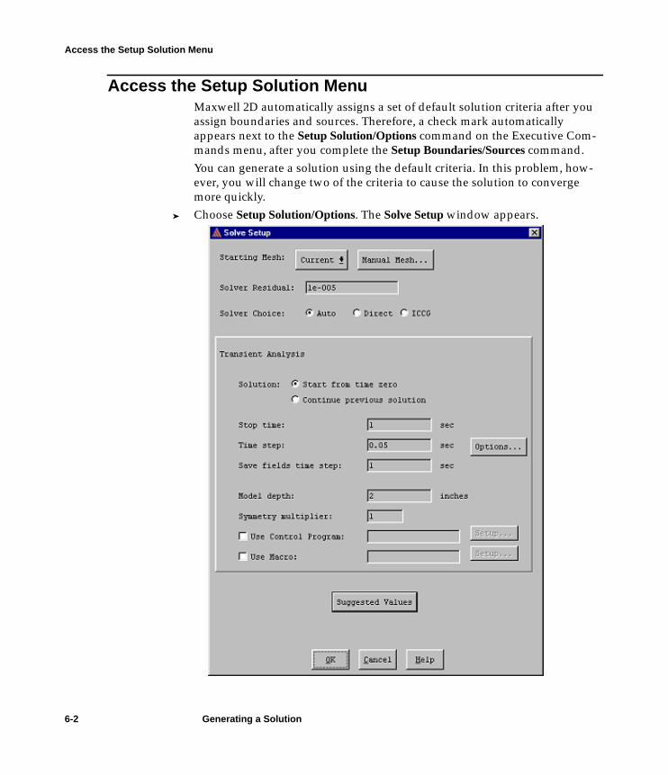
Access the Setup Solution MenuMaxwell 2D automatically assigns a set of default solution criteria after youassign boundaries and sources. Therefore, a check mark automaticallyappears next to the Setup Solution/Options command on the Executive Com-mands menu, after you complete the Setup Boundaries/Sources command.You can generate a solution using the default criteria. In this problem, how-ever, you will change two of the criteria to cause the solution to convergemore quickly.
➤ Choose Setup Solution/Options. The Solve Setup window appears.
6-2 Generating a Solution
linrmotn.book : solve.fm 3 Mon Mar 11 15:50:28 2002
Modify Solution Criteria
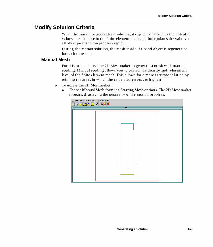
Modify Solution CriteriaWhen the simulator generates a solution, it explicitly calculates the potentialvalues at each node in the finite element mesh and interpolates the values atall other points in the problem region.During the motion solution, the mesh inside the band object is regeneratedfor each time step.
Manual MeshFor this problem, use the 2D Meshmaker to generate a mesh with manualseeding. Manual seeding allows you to control the density and refinementlevel of the finite element mesh. This allows for a more accurate solution byrefining the areas in which the calculated errors are highest.
➤ To access the 2D Meshmaker:● Choose Manual Mesh from the Starting Mesh options. The 2D Meshmaker
appears, displaying the geometry of the motion problem.
Generating a Solution 6-3
linrmotn.book : solve.fm 4 Mon Mar 11 15:50:28 2002
Modify Solution Criteria
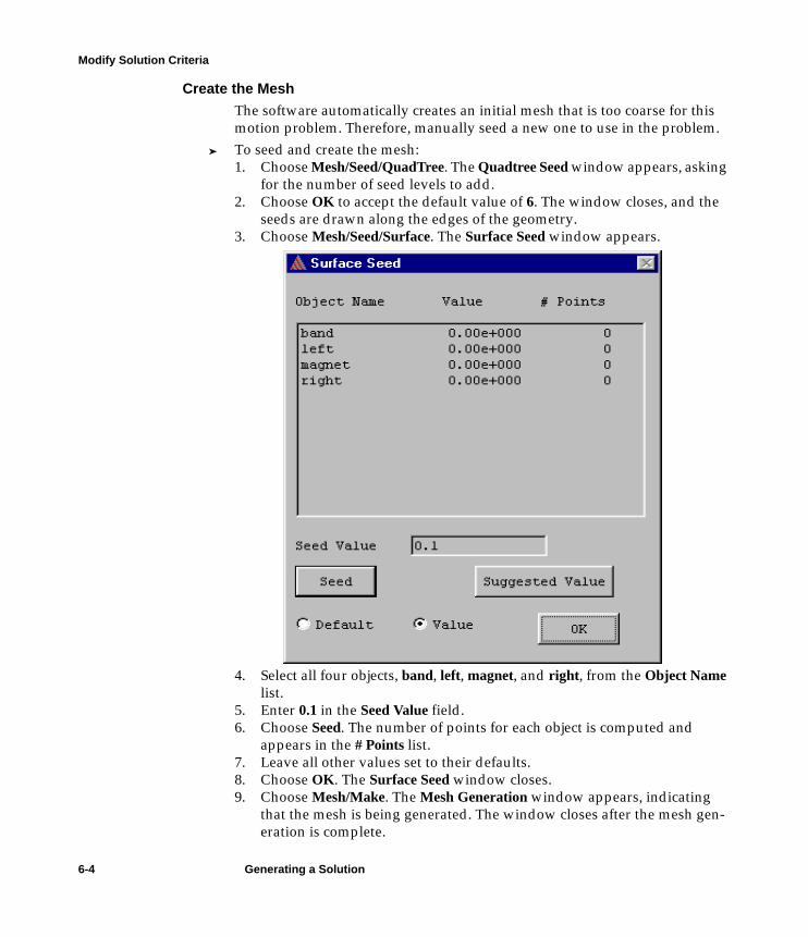
Create the Mesh
The software automatically creates an initial mesh that is too coarse for thismotion problem. Therefore, manually seed a new one to use in the problem.
➤ To seed and create the mesh:1. Choose Mesh/Seed/QuadTree. The Quadtree Seed window appears, asking
for the number of seed levels to add.2. Choose OK to accept the default value of 6. The window closes, and the
seeds are drawn along the edges of the geometry.3. Choose Mesh/Seed/Surface. The Surface Seed window appears.
4. Select all four objects, band, left, magnet, and right, from the Object Namelist.
5. Enter 0.1 in the Seed Value field.6. Choose Seed. The number of points for each object is computed and
appears in the # Points list.7. Leave all other values set to their defaults.8. Choose OK. The Surface Seed window closes.9. Choose Mesh/Make. The Mesh Generation window appears, indicating
that the mesh is being generated. The window closes after the mesh gen-eration is complete.
6-4 Generating a Solution

linrmotn.book : solve.fm 5 Mon Mar 11 15:50:28 2002
Modify Solution Criteria
Exit the Meshmaker
With the mesh complete, you can exit the 2D Meshmaker and define the solu-tion parameters.
➤ To exit the 2D Meshmaker:1. Choose File/Exit. A window appears, asking you to save the changes to
the mesh before exiting.2. Choose Yes.The mesh is saved, and you return to the Solve Setup window. The StartingMesh has changed to Current, meaning that the default initial mesh thatwould automatically be created during the solution process will be ignored infavor of the manual one you created.
Solver ResidualThe solver residual specifies how close each solution must come to satisfyingthe equations that are used to generate the solution. For this model, thedefault setting is sufficient.
➤ Leave the Solver Residual field set to the default.
Solver ChoiceYou can specify which type of matrix solver to use to solve the problem.● The ICCG solver is faster for large matrices, but on rare occasions may
fail to converge (usually on magnetostatic problems with exceptionallyhigh permeabilities and small air-gaps).
● The Direct solver will always converge but is much slower for largematrices.
● In the default Auto position, the software makes the choice. In this case,the software evaluates the matrix before attempting to solve it; if itappears to be ill-conditioned, the Direct solver is used; otherwise theICCG solver is used. If the ICCG solver fails to converge while an Autosolver is running, the software automatically reverts to the Direct solver.
➤ Leave the Solver Choice set to Auto. For this model, you want the softwareto select the solver.
☞Note: Some solution criteria are given in scientific notation shorthand. For
instance, 1e-05 is equal to 1x10⁻⁵, or 0.00001. When entering numeric val-ues, you can use either notation.
Generating a Solution 6-5

linrmotn.book : solve.fm 6 Mon Mar 11 15:50:28 2002
Modify Solution Criteria
Transient AnalysisThe Solution options in the Transient Analysis section define the time steps forthe solutions. In order to observe how the system comes to rest from its initialposition, start the simulation from time-zero.
➤ To start the simulation from time-zero:● Leave the Start from time zero option selected.
Transient Solution CriteriaSet the time steps and limits for the transient solution.
➤ To adaptively refine the mesh and solution:● Enter 0.655 as the Stop time. This instructs the solver to compute the
solutions from time-zero to 0.655 seconds.● Enter 0.005 as the Time step. This instructs the solver to compute the
solutions every 0.005 seconds during the solution process.● Enter 0.1 as the Save fields time step. This instructs the solver to save the
field solutions every 0.1 seconds.● Enter 2 as the Model depth. Because you are modeling a 2-inch bar, the
model depth must be set to 2.● Accept 1 as the Symmetry multiplier. Because you are defining the entire
model in this example, rather than a portion of a symmetric model, youneed not multiply the model to simulate the entire motion system. Theentire motion system is already represented.
Exit Setup SolutionWhen the solution criteria have been defined, you can exit the Solve Setupwindow. The solution criteria are saved automatically upon exiting.
➤ To save your changes and exit the Solve Setup window:● Choose OK, or press Return.You return to the Executive Commands window.
6-6 Generating a Solution
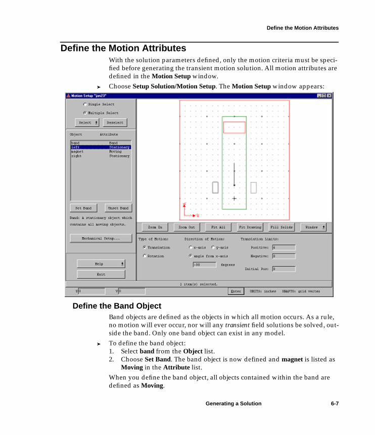
linrmotn.book : solve.fm 7 Mon Mar 11 15:50:28 2002
Define the Motion Attributes
Define the Motion AttributesWith the solution parameters defined, only the motion criteria must be speci-fied before generating the transient motion solution. All motion attributes aredefined in the Motion Setup window.
➤ Choose Setup Solution/Motion Setup. The Motion Setup window appears:
Define the Band ObjectBand objects are defined as the objects in which all motion occurs. As a rule,no motion will ever occur, nor will any transient field solutions be solved, out-side the band. Only one band object can exist in any model.
➤ To define the band object:1. Select band from the Object list.2. Choose Set Band. The band object is now defined and magnet is listed as
Moving in the Attribute list.When you define the band object, all objects contained within the band aredefined as Moving.
Generating a Solution 6-7
linrmotn.book : solve.fm 8 Mon Mar 11 15:50:28 2002
Define the Motion Attributes
Define the Moving ObjectMoving objects must reside in the band object. In this model, the magnet fallsin the band at a deviation of -90 degrees from the x-axis, causing an oscillationmotion. Because the magnet was present inside the band object at the time theband was defined, it was automatically assigned the Moving attribute.
➤ To define the motion of the magnet:1. Select magnet from the Object list.2. Select Translation as the Type of Motion.3. Select angle from x-axis as the Direction of Motion. The degrees field
becomes active.4. Enter -90 in the degrees field.5. Under Translation Limits, do the following:
■ Enter 6 in the Positive limit field.■ Enter 0 in the Negative limit field.This defines the limits of motion to be within six inches of the initial posi-tion.
6. Leave Initial Pos set to 0. This is the initial position of the magnet.
Define the Stationary ObjectsStationary objects can exist anywhere in the model, either inside or outsidethe band object. Placing a stationary object inside the band allows you to cal-culate the force and torque on the object. Placing it outside the band wouldleave it unaffected by the motion.In this example, both copper bars are stationary.Leave the left and right bars set to their defaults.
Define the Mechanical TransientNow you can define the mechanical setup of the example. Since the motion ofthe magnet involves a spring effect, you must define the motion variables asfunctions of time.
➤ To define the mechanical transient:1. Choose Mechanical Setup. The Mechanical Setup window appears.2. Choose Functions.
The Motion Setup Symbol Table appears.
6-8 Generating a Solution

linrmotn.book : solve.fm 9 Mon Mar 11 15:50:28 2002
Define the Motion Attributes
Define the Motion Variables
To simulate the spring effect of the motion, define the following variables:
Define the Spring Constant
To accurately obtain the restoring force, you must first define the spring con-stant for the motion problem.
➤ To define the spring constant:1. Enter k in the field to the left of the equals sign.2. Enter 11 in the field to the right of the equals sign.3. Choose Add. The k value is added to the table.
Define the Weight
Define the weight of the magnet. The weight is based on the magnet’s massand gravity.
➤ To define the weight:1. Enter weight in the field to the left of the equals sign.2. Enter 9.8/2.2 in the field to the right of the equals sign.3. Choose Add. The weight value is added to the table.
Define the Restoring Force➤ To define the spring-related restoring force:
1. Enter spring in the field to the left of the equals sign.2. Enter -k*(P-4) in the field to the right of the equals sign.3. Choose Add. The spring value is added to the table.
Define the Damping Coefficient
The damping value is defined as a conditional expression based on the posi-tion, P, of the magnet as it moves. You must define the damping based on thiscondition.
➤ To define the damping value:1. Enter DD in the field to the left of the equals sign.2. Enter if (((P>4)&&(P<=6)),5,0) in the field to the right of the equals sign.
This establishes a condition that if the position falls between four and sixinches, a damping value will be applied. The damping is intended todecrease the magnitude of the oscillation of position over time.
3. Choose Add. The DD value is added to the table.
k The spring constant.DD The damping coefficient.FF The force based on the weight, damping coefficient, and the
spring constant.spring The spring-related restoring force.weight The weight of the magnet.
Generating a Solution 6-9
linrmotn.book : solve.fm 10 Mon Mar 11 15:50:28 2002
Define the Motion Attributes
Define the Forces Factor
Like the damping value, the forces value is also conditional, based on theposition, weight, and spring constant.
➤ To define the forces value:1. Enter FF in the field to the left of the equals sign.2. Enter if (((P>4)&&(P<=6)),weight+spring,weight) in the field to the right of
the equals sign.3. Choose Add. The FF value is added to the table.4. Choose Done. The table closes. You return to the Mechanical Setup win-
dow.
Define the Mechanical Transient
Use the function values to define the physical parameters in the MechanicalSetup window.
➤ To define the mechanical transient:1. Select Consider Mechanical Transient if it is not already selected. Fields
appear, allowing you to define the velocity, mass, damping, and loadforce of the system.
2. Leave 0 in the Initial Velocity field.3. Enter 0.4545 for the Mass of the moving object.4. Choose Options. The Options window appears.5. Select both Damping and Load from the list. This defines both parameters
as having functional values.6. Choose OK. The Options window closes. You return to the Mechanical
Setup window.7. Enter DD in the Damping field. This is the functional value you defined
for the damping.8. Enter FF in the Load Force field. This is the functional load force value
you defined.9. Choose OK to close the Mechanical Setup window.You return to the Motion Setup window.
Exit the Motion Setup WindowWith the motion completely defined, you are ready to exit the Motion Setupwindow and solve the problem.
➤ To exit the Motion Setup window:1. Choose Exit. A window appears, prompting you to save your changes
before exiting.2. Choose Yes.The Motion Setup window closes.
6-10 Generating a Solution

linrmotn.book : solve.fm 11 Mon Mar 11 15:50:28 2002
Generate the Solution
Generate the SolutionNow that you’ve set up the solution parameters, the problem is ready to besolved. Depending upon how closely you followed the guide, the results thatyou obtain should be approximately the same as the ones given in the follow-ing sections.
➤ To execute the solution, choose Solve/Nominal Problem. The solutionprocess begins.As the problem is being solved, the following things happen:
■ The system creates the initial finite element mesh for the structure. Abar labeled Making Initial Mesh appears in the Solution Monitoringbox at the bottom of the window. It shows the system’s progress as itgenerates the mesh.
■ Buttons labeled Abort, Stop, and Refresh appear next to the progressbar and remain there throughout the entire solution process. Option-ally, you can use them to abort the solution process, temporarily stopthe solution generation, or refresh the plots in the window.If the convergence panel is displayed, choosing Refresh plots the tan-gential force of the model and lists the parameters available for plot-ting.
■ A bar labeled Setting up solution files appears.■ After the system makes the initial finite element mesh, the motion
solution process begins.
☞Note: The solutions given in this guide were computed on a SPARCstation 2
workstation. Depending on the platform and available memory, youranswers may differ slightly from those presented.
Generating a Solution 6-11

linrmotn.book : solve.fm 12 Mon Mar 11 15:50:28 2002
Monitor the Solution
Monitor the SolutionThe Solving for Transient monitoring bar appears in the Solution Monitoringarea at the bottom of the menu. This allows you to monitor the simulator’sprogress as it computes the required time steps.
6-12 Generating a Solution
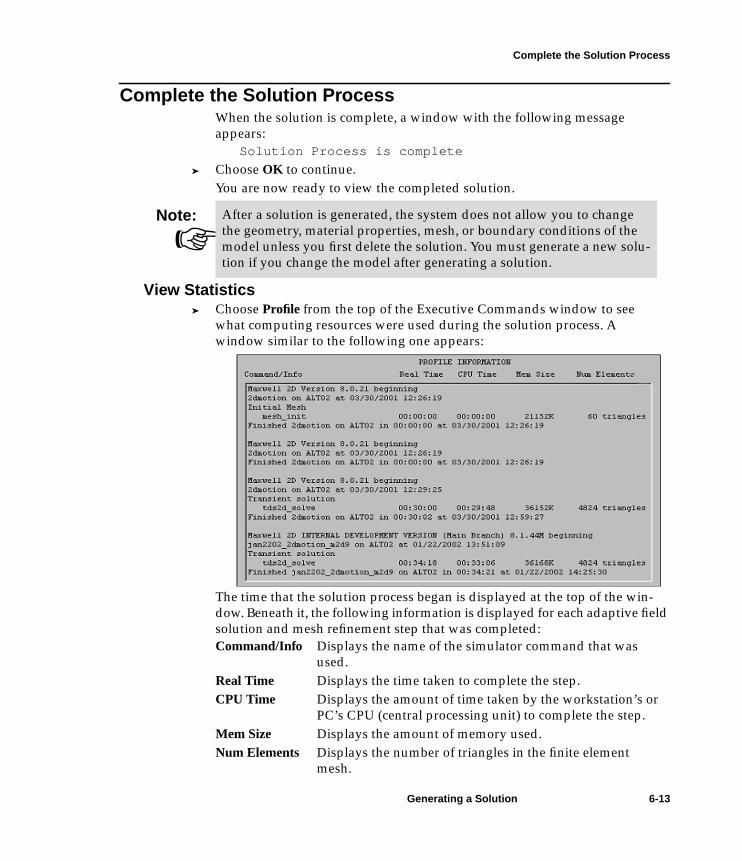
linrmotn.book : solve.fm 13 Mon Mar 11 15:50:28 2002
Complete the Solution Process
Complete the Solution ProcessWhen the solution is complete, a window with the following messageappears:
Solution Process is complete
➤ Choose OK to continue.You are now ready to view the completed solution.
View Statistics➤ Choose Profile from the top of the Executive Commands window to see
what computing resources were used during the solution process. Awindow similar to the following one appears:
The time that the solution process began is displayed at the top of the win-dow. Beneath it, the following information is displayed for each adaptive fieldsolution and mesh refinement step that was completed:
☞Note: After a solution is generated, the system does not allow you to change
the geometry, material properties, mesh, or boundary conditions of themodel unless you first delete the solution. You must generate a new solu-tion if you change the model after generating a solution.
Command/Info Displays the name of the simulator command that wasused.
Real Time Displays the time taken to complete the step.CPU Time Displays the amount of time taken by the workstation’s or
PC’s CPU (central processing unit) to complete the step.Mem Size Displays the amount of memory used.Num Elements Displays the number of triangles in the finite element
mesh.
Generating a Solution 6-13
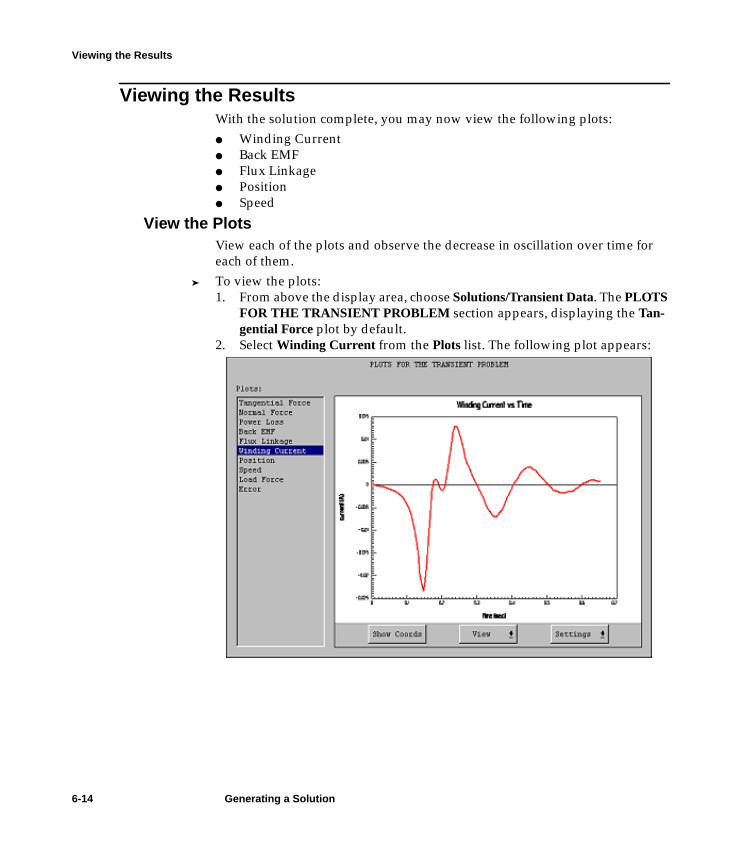
linrmotn.book : solve.fm 14 Mon Mar 11 15:50:28 2002
Viewing the Results
Viewing the ResultsWith the solution complete, you may now view the following plots:● Winding Current● Back EMF● Flux Linkage● Position● Speed
View the PlotsView each of the plots and observe the decrease in oscillation over time foreach of them.
➤ To view the plots:1. From above the display area, choose Solutions/Transient Data. The PLOTS
FOR THE TRANSIENT PROBLEM section appears, displaying the Tan-gential Force plot by default.
2. Select Winding Current from the Plots list. The following plot appears:
6-14 Generating a Solution
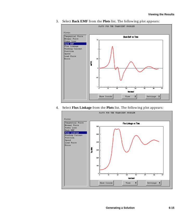
linrmotn.book : solve.fm 15 Mon Mar 11 15:50:28 2002
Viewing the Results
3. Select Back EMF from the Plots list. The following plot appears:
4. Select Flux Linkage from the Plots list. The following plot appears:
Generating a Solution 6-15
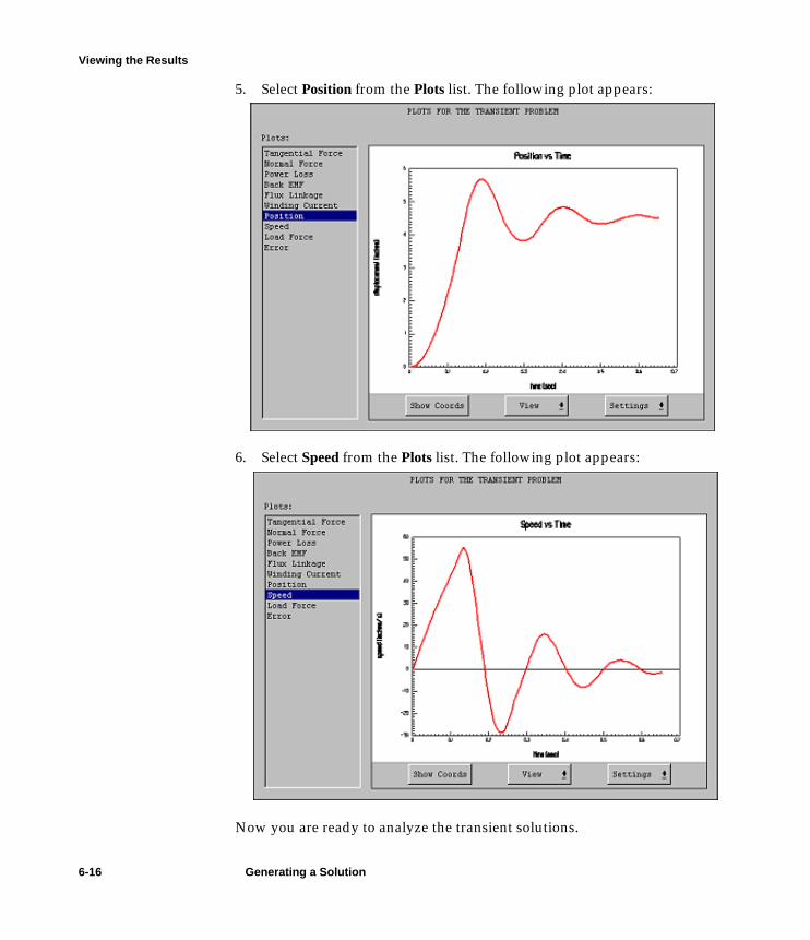
linrmotn.book : solve.fm 16 Mon Mar 11 15:50:28 2002
Viewing the Results
5. Select Position from the Plots list. The following plot appears:
6. Select Speed from the Plots list. The following plot appears:
Now you are ready to analyze the transient solutions.
6-16 Generating a Solution

linrmotn.book : anal.fm 1 Mon Mar 11 15:50:28 2002
7
Analyzing the Solution
Now that you have generated the transient solution for the motion problem,you can analyze it using the post-processing features of Maxwell 2D.Your goals for this chapter are as follows:● Plot the results of the induced current and flux density for the saved time
steps.● Use the plane calculator to derive the induced current from the current
density.
Time: The total time needed to complete this chapter is approximately 35 min-utes.
Analyzing the Solution 7-1
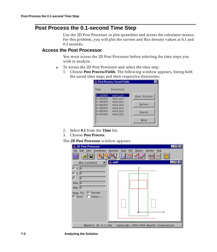
linrmotn.book : anal.fm 2 Mon Mar 11 15:50:28 2002
Post Process the 0.1-second Time Step
Post Process the 0.1-second Time StepUse the 2D Post Processor to plot quantities and access the calculator menus.For this problem, you will plot the current and flux density values at 0.1 and0.3 seconds.
Access the Post ProcessorYou must access the 2D Post Processor before selecting the time steps youwish to analyze.
➤ To access the 2D Post Processor and select the time step:1. Choose Post Process/Fields. The following window appears, listing both
the saved time steps and their respective directories:
2. Select 0.1 from the Time list.3. Choose Post Process.The 2D Post Processor window appears.
7-2 Analyzing the Solution
linrmotn.book : anal.fm 3 Mon Mar 11 15:50:28 2002
Post Process the 0.1-second Time Step
Post Processor Screen LayoutThe following sections provide a brief overview of the Post Processor in Max-well 2D. For more details, refer to the Maxwell 2D online documentation.
General Areas
The 2D Post Processor is divided into the following general areas:
Executing Commands
Use the mouse to access, execute, and abort Post Processor commands. Unlikethe other software module windows in Maxwell 2D, you cannot access com-mands via a tool bar or hotkeys.
Project Window
The outermost window in the post processor is called the project window.The project window contains the geometry for a specific project and displays2D Post Processor and the output directory name, out0, in its title bar. Bydefault, one view window is contained within the project window.
View Windows
View windows are the windows in which you display plots. Up to eight viewwindows may be displayed within the project window, allowing you to dis-play different plots of the same project in each view window.
Menu Bar Appears at the top of the Post Processor window. Gener-ally, it is set up the same way as the 2D Modeler’s menubar.
Project Window Contains the geometry and view window, allowing youto view the model and plots.
Status Area Displays the following information:● Version number of the 2D Post Processor.● The “snap-to-point” behavior of the mouse.● Maximum and minimum values of x- and y-
coordinates of displayed objects.● Coordinates of the cursor.● Current unit of length.● Mouse button functions.
☞Note: The Post Processor can only display one project window at a time.
Therefore, because each project requires a separate project window, onlyone project can be opened in the post processor at any given time.
Analyzing the Solution 7-3
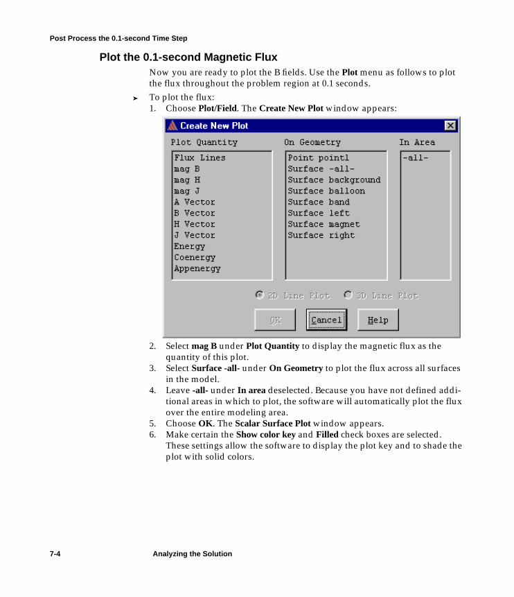
linrmotn.book : anal.fm 4 Mon Mar 11 15:50:28 2002
Post Process the 0.1-second Time Step
Plot the 0.1-second Magnetic FluxNow you are ready to plot the B fields. Use the Plot menu as follows to plotthe flux throughout the problem region at 0.1 seconds.
➤ To plot the flux:1. Choose Plot/Field. The Create New Plot window appears:
2. Select mag B under Plot Quantity to display the magnetic flux as thequantity of this plot.
3. Select Surface -all- under On Geometry to plot the flux across all surfacesin the model.
4. Leave -all- under In area deselected. Because you have not defined addi-tional areas in which to plot, the software will automatically plot the fluxover the entire modeling area.
5. Choose OK. The Scalar Surface Plot window appears.6. Make certain the Show color key and Filled check boxes are selected.
These settings allow the software to display the plot key and to shade theplot with solid colors.
7-4 Analyzing the Solution
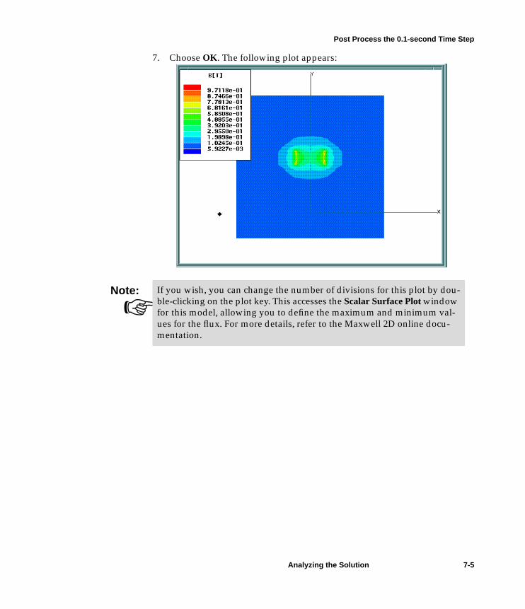
linrmotn.book : anal.fm 5 Mon Mar 11 15:50:28 2002
Post Process the 0.1-second Time Step
7. Choose OK. The following plot appears:
☞Note: If you wish, you can change the number of divisions for this plot by dou-
ble-clicking on the plot key. This accesses the Scalar Surface Plot windowfor this model, allowing you to define the maximum and minimum val-ues for the flux. For more details, refer to the Maxwell 2D online docu-mentation.
Analyzing the Solution 7-5
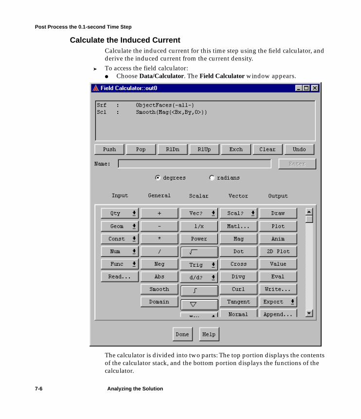
linrmotn.book : anal.fm 6 Mon Mar 11 15:50:28 2002
Post Process the 0.1-second Time Step
Calculate the Induced CurrentCalculate the induced current for this time step using the field calculator, andderive the induced current from the current density.
➤ To access the field calculator:● Choose Data/Calculator. The Field Calculator window appears.
The calculator is divided into two parts: The top portion displays the contentsof the calculator stack, and the bottom portion displays the functions of thecalculator.
7-6 Analyzing the Solution

linrmotn.book : anal.fm 7 Mon Mar 11 15:50:28 2002
Post Process the 0.1-second Time Step
The flux density appears as the field quantity in the second register. Whenyou selected mag B as the value to plot in the previous section, it was auto-matically loaded into the calculator.
Calculate and Plot the 0.1-second Induced CurrentTo plot the induced current for the 0.1-second time step, first load the currentdensity, J, into the field calculator.
Compute J
The first step in computing the induced current is to load the J vector in thetop register of the stack.
➤ To compute J:1. Choose Clear to clear the contents of the stack.2. Choose Qty/J to load J into the top register of the calculator. After J is
loaded, the top register appears as follows:Vec: <0,0,Jz>
The Vec indicates that the value is a vector quantity.3. Choose Scal?/ScalarZ. This pulls off the z-component of the current den-
sity, which is a scalar quantity.4. Choose Geom/Surface, and select left. Choose OK. This loads the surface
through which the current passes.5. Choose the integrate button.6. Choose Eval to integrate and evaluate the induced current over the left
conductor. A value of approximately -0.452 A appears for the inducedcurrent across the surface of the model. The negative sign indicates thatthe flow travels into the screen.
7. Choose Done to exit the calculator.Now you can plot the current density.
☞Note: Regardless of the drawing units used in the Maxwell 2D Modeler, the simu-
lator outputs all quantities in MKS (SI) units.
Analyzing the Solution 7-7
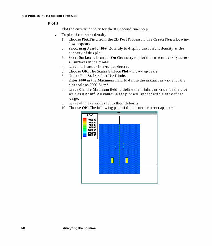
linrmotn.book : anal.fm 8 Mon Mar 11 15:50:28 2002
Post Process the 0.1-second Time Step
Plot J
Plot the current density for the 0.1-second time step.➤ To plot the current density:
1. Choose Plot/Field from the 2D Post Processor. The Create New Plot win-dow appears.
2. Select mag J under Plot Quantity to display the current density as thequantity of this plot.
3. Select Surface -all- under On Geometry to plot the current density acrossall surfaces in the model.
4. Leave -all- under In area deselected.5. Choose OK. The Scalar Surface Plot window appears.6. Under Plot Scale, select Use Limits.7. Enter 2000 in the Maximum field to define the maximum value for the
plot scale as 2000 A/m2.8. Leave 0 in the Minimum field to define the minimum value for the plot
scale as 0 A/m2. All values in the plot will appear within the definedrange.
9. Leave all other values set to their defaults.10. Choose OK. The following plot of the induced current appears:
7-8 Analyzing the Solution

linrmotn.book : anal.fm 9 Mon Mar 11 15:50:28 2002
Post Process the 0.1-second Time Step
Return to the Executive Commands WindowOnce the calculations for the 0.1-second time step are complete, you can exitthe 2D Post Processor and return to the Executive Commands window to postprocess the results for the 0.3-second time step.
➤ To return to the Executive Commands window:1. Choose File/Exit. A window appears, asking you to confirm the exit.2. Choose Yes. The 2D Post Processor window closes.You return to the Executive Commands window.
Analyzing the Solution 7-9

linrmotn.book : anal.fm 10 Mon Mar 11 15:50:28 2002
Post Process the 0.3-second Time Step
Post Process the 0.3-second Time StepNow, you will plot the current and flux values at 0.3 seconds.
➤ To access the Post Processor:1. Choose Post Process/Fields. The Post-Process Saved Fields window again
appears, listing the saved time steps and their respective directories.2. Select 0.3 from the Time list.3. Choose Post Process.4. Again, the 2D Post Processor appears, this time displaying the model for
the 0.3-second time step.Notice that the magnet has fallen significantly from its position in the 0.1-sec-ond time step.
Calculate and Plot the 0.3-second Induced CurrentAs you did for the 0.1-second time step, access the plane calculator and loadthe current density, J, into the field calculator, then derive the induced cur-rent.
Compute J➤ To compute J:
1. Choose Data/Calculator.2. Choose Clear to clear the contents of the stack.3. Choose Qty/J to load J into the top register of the calculator first. After J is
loaded, the top register appears as follows:Vec: <0,0,Jz>
The Vec indicates that the value is a vector quantity.4. Choose Scal?/ScalarZ. This pulls off the z-component of the current den-
sity, which is a scalar quantity.5. Choose Geom/Surface. The Select Surface window appears.6. Select left, choose OK. This loads the surface through which the current
passes.7. Choose the integrate button.8. Choose Eval to integrate and evaluate the induced current over the left
conductor. A value of approximately -0.047 amperes appears for theinduced current across the surface of the model.
9. Choose Done to close the calculator.Now you can plot the current density.
7-10 Analyzing the Solution
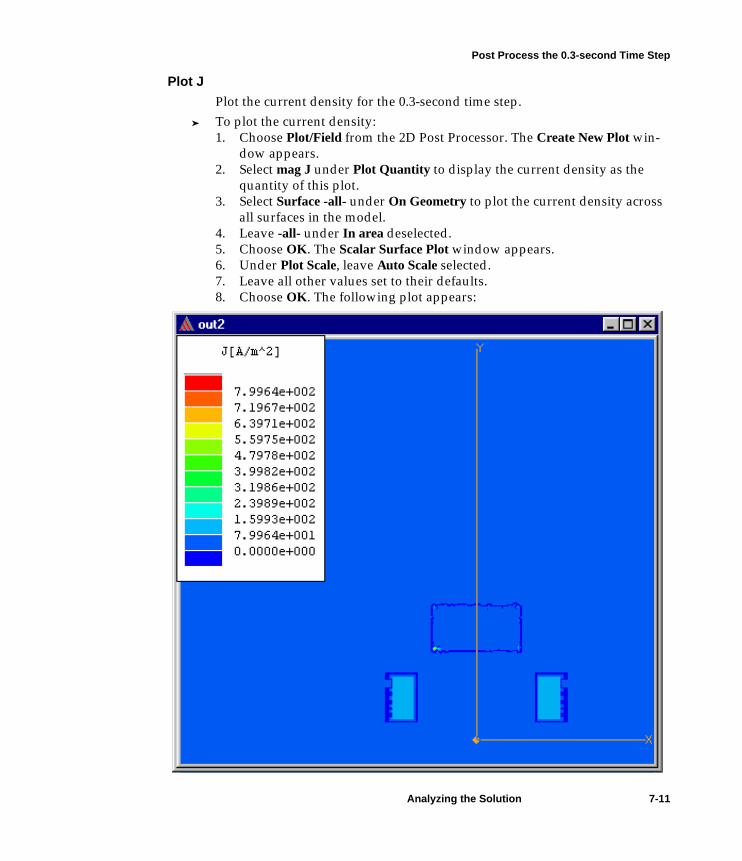
linrmotn.book : anal.fm 11 Mon Mar 11 15:50:28 2002
Post Process the 0.3-second Time Step
Plot J
Plot the current density for the 0.3-second time step.➤ To plot the current density:
1. Choose Plot/Field from the 2D Post Processor. The Create New Plot win-dow appears.
2. Select mag J under Plot Quantity to display the current density as thequantity of this plot.
3. Select Surface -all- under On Geometry to plot the current density acrossall surfaces in the model.
4. Leave -all- under In area deselected.5. Choose OK. The Scalar Surface Plot window appears.6. Under Plot Scale, leave Auto Scale selected.7. Leave all other values set to their defaults.8. Choose OK. The following plot appears:
Analyzing the Solution 7-11

linrmotn.book : anal.fm 12 Mon Mar 11 15:50:28 2002
Exit Maxwell 2D
Exit Maxwell 2DOnce you have finished with the post processing functions, you are ready toexit the software.
➤ To exit Maxwell 2D:1. Choose File/Exit from the 2D Post Processor. A window with the follow-
ing prompt appears:Exit Post Processor?
2. Choose Yes. The Executive Commands window appears.3. Choose Exit from the bottom of the Executive Commands menu. The fol-
lowing prompt appears:Exit from Maxwell 2D?
4. Choose Yes.The Executive Commands window disappears.
7-12 Analyzing the Solution

linrmotn.book : anal.fm 13 Mon Mar 11 15:50:28 2002
Exit the Maxwell Software
Exit the Maxwell SoftwareYou can exit the Project Manager when you exit the Maxwell Control Panel.
➤ To exit the Maxwell Control Panel:1. Display the Maxwell Control Panel in the foreground.2. Choose Exit. A window with the following prompt appears:
Exit Maxwell?
3. Choose Yes.Now you have exited the Project Manager and the Maxwell Control Panel.Workstation users return to the UNIX prompt, and PC users return toMicrosoft Windows.
Analyzing the Solution 7-13

linrmotn.book : anal.fm 14 Mon Mar 11 15:50:28 2002
Exit the Maxwell Software
7-14 Analyzing the Solution

linrmotn.book : linrmotnIX.doc 1 Mon Mar 11 15:50:28 2002
Index
Numerics2D Modeler
accessing 4-4exiting 4-15
2D Post Processor 7-2
Aaliases 2-4Assign/Boundary command, Balloon 5-13Assign/Source commands, Solid 5-12
Bbackground
and boundary conditions 5-8ballooning 5-13default material for 5-6excluding from solution region 5-6extending 5-13including in solution region 5-6
bars, applying voltages to 5-11boundary conditions 5-8
and symmetry 5-13changing 5-14deleting 5-14
displaying 5-9, 5-14electrically grounded system 5-13electrically insulated system 5-13for sample problem 5-10screen layout 5-9use of 5-8
Boundary Manager 5-9Boundary Manager, exiting 5-14buttons
choosing viiidisabled 2-6
CCalc commands, Plane 7-6calculators
accessing the plane 7-6complex values in registers 7-7, 7-10display of functions 7-6display of registers 7-6menu 7-6real values in registers 7-7, 7-10
Change Dir 2-4charges, and ballooned boundaries 5-13colors, changing for objects 4-9computing resources
and background 5-6viewing 6-13
Index-1
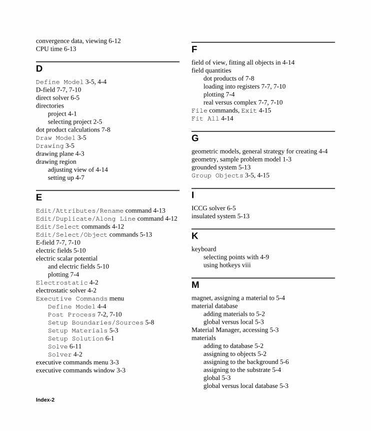
linrmotn.book : linrmotnIX.doc 2 Mon Mar 11 15:50:28 2002
convergence data, viewing 6-12CPU time 6-13
DDefine Model 3-5, 4-4D-field 7-7, 7-10direct solver 6-5directories
project 4-1selecting project 2-5
dot product calculations 7-8Draw Model 3-5Drawing 3-5drawing plane 4-3drawing region
adjusting view of 4-14setting up 4-7
EEdit/Attributes/Rename command 4-13Edit/Duplicate/Along Line command 4-12Edit/Select commands 4-12Edit/Select/Object commands 5-13E-field 7-7, 7-10electric fields 5-10electric scalar potential
and electric fields 5-10plotting 7-4
Electrostatic 4-2electrostatic solver 4-2Executive Commands menu
Define Model 4-4Post Process 7-2, 7-10Setup Boundaries/Sources 5-8Setup Materials 5-3Setup Solution 6-1Solve 6-11Solver 4-2
executive commands menu 3-3executive commands window 3-3
Ffield of view, fitting all objects in 4-14field quantities
dot products of 7-8loading into registers 7-7, 7-10plotting 7-4real versus complex 7-7, 7-10
File commands, Exit 4-15Fit All 4-14
Ggeometric models, general strategy for creating 4-4geometry, sample problem model 1-3grounded system 5-13Group Objects 3-5, 4-15
IICCG solver 6-5insulated system 5-13
Kkeyboard
selecting points with 4-9using hotkeys viii
Mmagnet, assigning a material to 5-4material database
adding materials to 5-2global versus local 5-3
Material Manager, accessing 5-3materials
adding to database 5-2assigning to objects 5-2assigning to the background 5-6assigning to the substrate 5-4global 5-3global versus local database 5-3
Index-2
linrmotn.book : linrmotnIX.doc 3 Mon Mar 11 15:50:28 2002
screen layout 5-3Maxwell 2D Field Simulator
executive commands 3-5general procedure 3-5model window 3-3
Maxwell 2D Modeler 4-4accessing menu commands viiilayout 4-5project windows 4-5subwindows 4-5tool bar viii
Maxwell Control Panelaccessing 2-2
Maxwell Control Panel commands, Projects 2-3memory size 6-13mesh
and solution accuracy 6-3default 6-3example of 1-2initial 6-11starting 6-3use of 1-2
message bar 6-12Model/Drawing Units command 4-7modeling
creating the geometry 4-8drawing microstrips 4-11using the keyboard 4-8
Nnames
changing for objects 4-9, 4-13defining object names 4-9
OObject commands, Rectangle 4-9objects
assigning materials to 5-2attributes of 4-13changing the colors of 4-9changing the names of 4-9, 4-13copying 4-12
creating 4-8, 4-9rectangles 4-9
PPlot 7-4plots
common quantities 7-4equipotential contours 7-4from calculator registers 7-6
pointsentering from the keyboard 4-9selecting with the mouse 4-9
Post Process 3-6, 7-2, 7-10post processing 7-2
plotting results 7-4post processing, screen layout 7-3
project window 7-3subwindows 7-3
post processor, screen layout 7-3Post/Plot command 7-4project alias 2-4project directory
adding 2-4creating 2-3definition of 2-3
Project Manager commandsChange Dir 2-4Projects 2-3
Project Manager optionsNew 2-5Save Notes 2-6
Projects 2-3projects
creating 2-5entering descriptions of 2-6naming 2-5project notes 2-6selecting and accessing 2-5selecting project type 2-5
RRectangle 4-9
Index-3

linrmotn.book : linrmotnIX.doc 4 Mon Mar 11 15:50:28 2002
registerscomplex values in 7-7, 7-10loading values into the plane 7-7, 7-10real values in 7-7, 7-10
residual 6-5
Ssaving geometry files 4-15scientific notation 6-6Setup Boundaries/Sources 3-5, 5-8Setup Executive Parameters 6-6Setup Materials 3-5, 5-3Setup Solution 6-1solution monitoring area 3-3solutions
analysis 7-1calculated values 6-3computing 6-11convergence 6-12CPU time 6-13criteria for computing 6-3effect of mesh 6-3generating 6-11interpolated values 6-3interrupting 6-11memory used 6-13monitoring 6-12plotting 7-4real time used 6-13satisfying equations 6-5types 6-6
Solve 3-5, 6-11Solver 3-5, 4-2solver choice 6-5solver residual 6-5solver type 4-2solvers
auto 6-5direct 6-5ICCG 6-5
sources 5-8changing 5-14deleting 5-14
displaying 5-9, 5-14for sample problem 5-10screen layout 5-9
specifying drawing planes 4-3starting mesh 6-3subwindows 7-3symmetry boundary conditions 5-13
Ttool bar viii
Uunits
changing 4-7displaying 4-7rescaling geometric models 4-7
Vvoltages
and ballooned boundaries 5-13applying to microstrips 5-11
Wwindows
project windows 7-3subwindows 7-3
Index-4