Getting Started with Abaqus/CAE - HTML
695
Getting Started with Abaqus/CAE GETTING STARTED WITH ABAQUS/CAE ABAQUS 2016
-
Upload
khangminh22 -
Category
Documents
-
view
2 -
download
0
Transcript of Getting Started with Abaqus/CAE - HTML
Getting Started with Abaqus/CAE
Abaqus ID:Printed on:
GETTING STARTED WITH ABAQUS/CAEABAQUS 2016


Getting Started with Abaqus/CAE
Abaqus ID:Printed on:

Legal NoticesAbaqus, the 3DS logo, and SIMULIA are commercial trademarks or registered trademarks of Dassault Systèmes or its subsidiaries in the United Statesand/or other countries. Use of any Dassault Systèmes or its subsidiaries trademarks is subject to their express written approval.
Abaqus and this documentation may be used or reproduced only in accordance with the terms of the software license agreement signed by the customer, or,absent such an agreement, the then current software license agreement to which the documentation relates.
This documentation and the software described in this documentation are subject to change without prior notice.
Dassault Systèmes and its subsidiaries shall not be responsible for the consequences of any errors or omissions that may appear in this documentation.
© Dassault Systèmes, 2015
Other company, product, and service names may be trademarks or service marks of their respective owners. For additional information concerningtrademarks, copyrights, and licenses, see the Legal Notices in the Abaqus 2016 Installation and Licensing Guide.
Abaqus ID:Printed on:

CONTENTS
Contents
1. Introduction
The Abaqus products 1.1
Getting started with Abaqus 1.2
Abaqus documentation 1.3
Getting help 1.4
Support 1.5
A quick review of the finite element method 1.6
Getting Started 1.7
2. Abaqus Basics
Components of an Abaqus analysis model 2.1
Introduction to Abaqus/CAE 2.2
Example: creating a model of an overhead hoist 2.3
Comparison of implicit and explicit procedures 2.4
Summary 2.5
3. Finite Elements and Rigid Bodies
Finite elements 3.1
Rigid bodies 3.2
Summary 3.3
4. Using Continuum Elements
Element formulation and integration 4.1
Selecting continuum elements 4.2
Example: connecting lug 4.3
Mesh convergence 4.4
Related Abaqus examples 4.5
Suggested reading 4.6
Summary 4.7
5. Using Shell Elements
Element geometry 5.1
Shell formulation – thick or thin 5.2
Shell material directions 5.3
Selecting shell elements 5.4
Example: skew plate 5.5
i
Abaqus ID:gsa-toc
Printed on: Sat June 20 -- 18:33:02 2015

CONTENTS
Related Abaqus examples 5.6
Suggested reading 5.7
Summary 5.8
6. Using Beam Elements
Beam cross-section geometry 6.1
Formulation and integration 6.2
Selecting beam elements 6.3
Example: cargo crane 6.4
Related Abaqus examples 6.5
Suggested reading 6.6
Summary 6.7
7. Linear Dynamics
Introduction 7.1
Damping 7.2
Element selection 7.3
Mesh design for dynamics 7.4
Example: cargo crane under dynamic loading 7.5
Effect of the number of modes 7.6
Effect of damping 7.7
Comparison with direct time integration 7.8
Other dynamic procedures 7.9
Related Abaqus examples 7.10
Suggested reading 7.11
Summary 7.12
8. Nonlinearity
Sources of nonlinearity 8.1
The solution of nonlinear problems 8.2
Including nonlinearity in an Abaqus analysis 8.3
Example: nonlinear skew plate 8.4
Related Abaqus examples 8.5
Suggested reading 8.6
Summary 8.7
9. Nonlinear Explicit Dynamics
Types of problems suited for Abaqus/Explicit 9.1
Explicit dynamic finite element methods 9.2
Automatic time incrementation and stability 9.3
Example: stress wave propagation in a bar 9.4
ii
Abaqus ID:gsa-toc
Printed on: Sat June 20 -- 18:33:02 2015

CONTENTS
Damping of dynamic oscillations 9.5
Energy balance 9.6
Summary 9.7
10. Materials
Defining materials in Abaqus 10.1
Plasticity in ductile metals 10.2
Selecting elements for elastic-plastic problems 10.3
Example: connecting lug with plasticity 10.4
Example: blast loading on a stiffened plate 10.5
Hyperelasticity 10.6
Example: axisymmetric mount 10.7
Mesh design for large distortions 10.8
Techniques for reducing volumetric locking 10.9
Related Abaqus examples 10.10
Suggested reading 10.11
Summary 10.12
11. Multiple Step Analysis
General analysis procedures 11.1
Linear perturbation analysis 11.2
Example: vibration of a piping system 11.3
Restart analysis 11.4
Example: restarting the pipe vibration analysis 11.5
Related Abaqus examples 11.6
Summary 11.7
12. Contact
Overview of contact capabilities in Abaqus 12.1
Defining surfaces 12.2
Interaction between surfaces 12.3
Defining contact in Abaqus/Standard 12.4
Modeling issues for rigid surfaces in Abaqus/Standard 12.5
Abaqus/Standard 2D example: forming a channel 12.6
General contact in Abaqus/Standard 12.7
Abaqus/Standard 3D example: shearing of a lap joint 12.8
Defining contact in Abaqus/Explicit 12.9
Modeling considerations in Abaqus/Explicit 12.10
Abaqus/Explicit example: circuit board drop test 12.11
Compatibility between Abaqus/Standard and Abaqus/Explicit 12.12
Related Abaqus examples 12.13
iii
Abaqus ID:gsa-toc
Printed on: Sat June 20 -- 18:33:02 2015

CONTENTS
Suggested reading 12.14
Summary 12.15
13. Quasi-Static Analysis with Abaqus/Explicit
Analogy for explicit dynamics 13.1
Loading rates 13.2
Mass scaling 13.3
Energy balance 13.4
Example: forming a channel in Abaqus/Explicit 13.5
Summary 13.6
A. Example Files
Overhead hoist frame A.1
Connecting lug A.2
Skew plate A.3
Cargo crane A.4
Cargo crane – dynamic loading A.5
Nonlinear skew plate A.6
Stress wave propagation in a bar A.7
Connecting lug with plasticity A.8
Blast loading on a stiffened plate A.9
Axisymmetric mount A.10
Vibration of a piping system A.11
Forming a channel A.12
Shearing of a lap joint A.13
Circuit board drop test A.14
B. Creating and Analyzing a Simple Model in Abaqus/CAE
Understanding Abaqus/CAE modules B.1
Understanding the Model Tree B.2
Creating a part B.3
Creating a material B.4
Defining and assigning section properties B.5
Assembling the model B.6
Defining your analysis steps B.7
Applying a boundary condition and a load to the model B.8
Meshing the model B.9
Creating and submitting an analysis job B.10
Viewing the results of your analysis B.11
Summary B.12
iv
Abaqus ID:gsa-toc
Printed on: Sat June 20 -- 18:33:02 2015
CONTENTS
C. Using Additional Techniques to Create and Analyze a Model in Abaqus/CAE
Overview C.1
Creating the first hinge piece C.2
Assigning section properties to the hinge part C.3
Creating and modifying a second hinge piece C.4
Creating the pin C.5
Assembling the model C.6
Defining analysis steps C.7
Creating surfaces to use in contact interactions C.8
Defining contact between regions of the model C.9
Applying boundary conditions and loads to the assembly C.10
Meshing the assembly C.11
Creating and submitting a job C.12
Viewing the results of your analysis C.13
Summary C.14
D. Viewing the Output from Your Analysis
Overview D.1
Which variables are in the output database? D.2
Reading the output database D.3
Customizing a model plot D.4
Displaying the deformed model shape D.5
Displaying and customizing a contour plot D.6
Animating a contour plot D.7
Displaying and customizing a symbol plot D.8
Displaying and customizing a material orientation plot D.9
Displaying and customizing an X–Y plot D.10
Operating on X–Y data D.11
Probing an X–Y plot D.12
Displaying results along a path D.13
Summary D.14
E. Flow through a bent tube
Overview E.1
Creating the model for the fluid flow analysis E.2
Creating a CFD analysis job for the fluid flow analysis E.3
Running and monitoring the CFD analysis E.4
Viewing the CFD analysis results E.5
Creating the fluid model for the fluid-structure interaction analysis E.6
Creating the structural model for the fluid-structure interaction analysis E.7
Creating a co-simulation job for the fluid-structure interaction analysis E.8
v
Abaqus ID:gsa-toc
Printed on: Sat June 20 -- 18:33:02 2015

CONTENTS
Running and monitoring the fluid-structure co-simulation analysis E.9
Viewing the fluid-structure co-simulation analysis results E.10
vi
Abaqus ID:gsa-toc
Printed on: Sat June 20 -- 18:33:02 2015

THE Abaqus PRODUCTS
1. Introduction
Abaqus is a suite of powerful engineering simulation programs, based on the finite element method, thatcan solve problems ranging from relatively simple linear analyses to the most challenging nonlinearsimulations. Abaqus contains an extensive library of elements that can model virtually any geometry.It has an equally extensive list of material models that can simulate the behavior of most typicalengineering materials including metals, rubber, polymers, composites, reinforced concrete, crushableand resilient foams, and geotechnical materials such as soils and rock. Designed as a general-purposesimulation tool, Abaqus can be used to study more than just structural (stress/displacement) problems.It can simulate problems in such diverse areas as heat transfer, mass diffusion, thermal management ofelectrical components (coupled thermal-electrical analyses), acoustics, soil mechanics (coupled porefluid-stress analyses), piezoelectric analysis, electromagnetic analysis, and fluid dynamics.
Abaqus offers a wide range of capabilities for simulation of linear and nonlinear applications.Problems with multiple components are modeled by associating the geometry defining each componentwith the appropriate material models and specifying component interactions. In a nonlinear analysisAbaqus automatically chooses appropriate load increments and convergence tolerances and continuallyadjusts them during the analysis to ensure that an accurate solution is obtained efficiently.
1.1 The Abaqus products
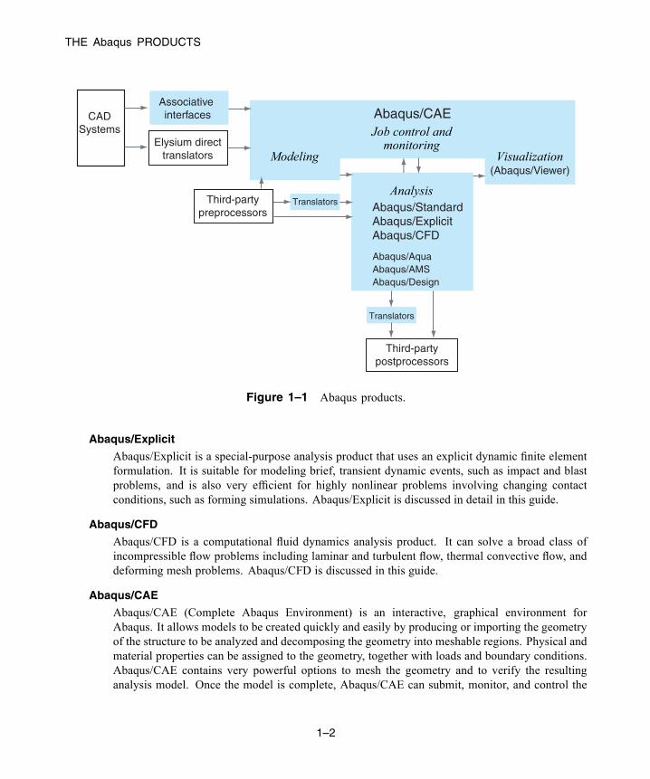
Abaqus consists of three main analysis products—Abaqus/Standard, Abaqus/Explicit, and Abaqus/CFD.Several add-on analysis options are available to further extend the capabilities of Abaqus/Standardand Abaqus/Explicit. The Abaqus/Aqua option works with Abaqus/Standard and Abaqus/Explicit.The Abaqus/Design and Abaqus/AMS options work with Abaqus/Standard. Abaqus/Foundation is anoptional subset of Abaqus/Standard. Abaqus/CAE is the complete Abaqus environment that includescapabilities for creating Abaqus models, interactively submitting and monitoring Abaqus jobs, andevaluating results. Abaqus/Viewer is a subset of Abaqus/CAE that includes just the postprocessingfunctionality. Abaqus also provides translators that convert geometry from third-party CAD systems tomodels for Abaqus/CAE, convert entities from third-party preprocessors to input for Abaqus analyses,and that convert output from Abaqus analyses to entities for third-party postprocessors. The relationshipbetween these products is shown in Figure 1–1.
Abaqus/Standard
Abaqus/Standard is a general-purpose analysis product that can solve a wide range of linear andnonlinear problems involving the static, dynamic, thermal, electrical, and electromagnetic responseof components. This product is discussed in detail in this guide. Abaqus/Standard solves a system ofequations implicitly at each solution “increment.” In contrast, Abaqus/Explicit marches a solutionforward through time in small time increments without solving a coupled system of equations ateach increment (or even forming a global stiffness matrix).
1–1
Abaqus ID:Printed on:
THE Abaqus PRODUCTS
Abaqus/StandardAbaqus/ExplicitAbaqus/CFD
(Abaqus/Viewer)
Abaqus/CAEAssociative interfacesCAD
Systems
Abaqus/AquaAbaqus/AMSAbaqus/Design
Figure 1–1 Abaqus products.
Abaqus/Explicit
Abaqus/Explicit is a special-purpose analysis product that uses an explicit dynamic finite elementformulation. It is suitable for modeling brief, transient dynamic events, such as impact and blastproblems, and is also very efficient for highly nonlinear problems involving changing contactconditions, such as forming simulations. Abaqus/Explicit is discussed in detail in this guide.
Abaqus/CFD
Abaqus/CFD is a computational fluid dynamics analysis product. It can solve a broad class ofincompressible flow problems including laminar and turbulent flow, thermal convective flow, anddeforming mesh problems. Abaqus/CFD is discussed in this guide.
Abaqus/CAE
Abaqus/CAE (Complete Abaqus Environment) is an interactive, graphical environment forAbaqus. It allows models to be created quickly and easily by producing or importing the geometryof the structure to be analyzed and decomposing the geometry into meshable regions. Physical andmaterial properties can be assigned to the geometry, together with loads and boundary conditions.Abaqus/CAE contains very powerful options to mesh the geometry and to verify the resultinganalysis model. Once the model is complete, Abaqus/CAE can submit, monitor, and control the
1–2
Abaqus ID:Printed on:
THE Abaqus PRODUCTS
analysis jobs. The Visualization module can then be used to interpret the results. Abaqus/CAEis discussed in this guide.
Abaqus/Viewer
Abaqus/Viewer is a subset of Abaqus/CAE that contains only the postprocessing capabilities of theVisualization module. The discussions of the Visualization module in this guide apply equally toAbaqus/Viewer.
Abaqus/Aqua
Abaqus/Aqua is a set of optional capabilities that can be added to Abaqus/Standard andAbaqus/Explicit. It is intended for the simulation of offshore structures, such as oil platforms.Some of the optional capabilities include the effects of wave and wind loading and buoyancy.Abaqus/Aqua is not discussed in this guide.
Abaqus/Design
Abaqus/Design is a set of optional capabilities that can be added to Abaqus/Standard to performdesign sensitivity calculations. Abaqus/Design is not discussed in this guide.
Abaqus/AMS
Abaqus/AMS is an optional capability that can be added to Abaqus/Standard. It uses the automaticmulti-level substructuring (AMS) eigensolver during a natural frequency extraction. Abaqus/AMSis not discussed in this guide.
Abaqus/Foundation
Abaqus/Foundation offers more efficient access to the linear static and dynamic analysisfunctionality in Abaqus/Standard. Abaqus/Foundation is not discussed in this guide.
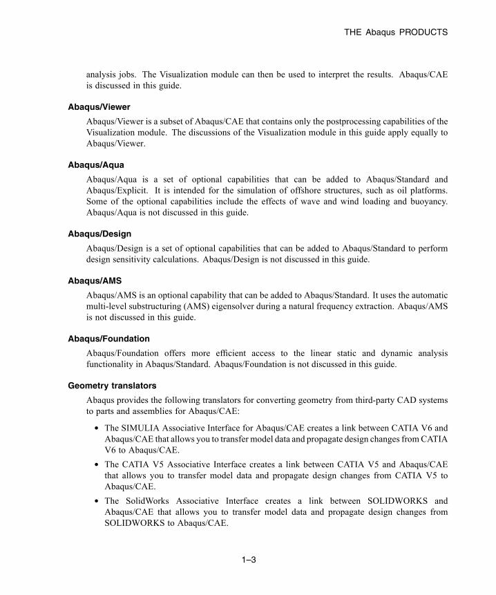
Geometry translators
Abaqus provides the following translators for converting geometry from third-party CAD systemsto parts and assemblies for Abaqus/CAE:
• The SIMULIA Associative Interface for Abaqus/CAE creates a link between CATIA V6 andAbaqus/CAE that allows you to transfer model data and propagate design changes fromCATIAV6 to Abaqus/CAE.
• The CATIA V5 Associative Interface creates a link between CATIA V5 and Abaqus/CAEthat allows you to transfer model data and propagate design changes from CATIA V5 toAbaqus/CAE.
• The SolidWorks Associative Interface creates a link between SOLIDWORKS andAbaqus/CAE that allows you to transfer model data and propagate design changes fromSOLIDWORKS to Abaqus/CAE.
1–3
Abaqus ID:Printed on:

THE Abaqus PRODUCTS
• The Pro/ENGINEER Associative Interface creates a link between Pro/ENGINEER andAbaqus/CAE that allows you to transfer model data and propagate design changes betweenPro/ENGINEER and Abaqus/CAE.
• The Geometry Translator for CATIA V4 allows you to import the geometry of CATIA V4-format parts and assemblies directly into Abaqus/CAE.
• The Geometry Translator for Parasolid allows you to import the geometry of Parasolid-formatparts and assemblies directly into Abaqus/CAE.
In addition, the Abaqus/CAE Associative Interface for NX creates a link between NX andAbaqus/CAE that allows you to transfer model data and propagate design changes between NX andAbaqus/CAE. The Abaqus/CAE Associative Interface for NX can be purchased and downloadedfrom Elysium Inc. (www.elysiuminc.com).
The geometry translators are not discussed in this guide.
Translator utilities
Abaqus provides the following translators for converting entities from third-party preprocessors toinput for Abaqus analyses or for converting output from Abaqus analyses to entities for third-partypostprocessors:
• abaqus fromansys translates an ANSYS input file to an Abaqus input file.
• abaqus fromdyna translates an LS-DYNA keyword file to an Abaqus input file.
• abaqus fromnastran translates a Nastran bulk data file to an Abaqus input file.
• abaqus frompamcrash translates a PAM-CRASH input file into an Abaqus input file.
• abaqus fromradioss translates a RADIOSS input file into an Abaqus input file.
• abaqus adams translates the results in an Abaqus SIM database file into an MSC.ADAMSmodal neutral (.mnf) file, the format required by ADAMS/Flex.
• abaqus moldflow translates finite element model information from a Moldflow analysis intoa partial Abaqus input file.
• abaqus toexcite translates data in an Abaqus substructure SIM database to an EXCITE flexiblebody interface (.exb) file.
• abaqus tonastran translates an Abaqus input file to Nastran bulk data file format.
• abaqus toOutput2 translates an Abaqus output database file to the Nastran Output2 file format.
• abaqus tosimpack translates data in an Abaqus substructure SIM database to a SIMPACKflexible body interface (.fbi) file.
• abaqus tozaero enables the exchange of aeroelastic data between Abaqus and ZAERO.
The translator utilities are not discussed in this guide.
1–4
Abaqus ID:Printed on:
GETTING STARTED WITH Abaqus
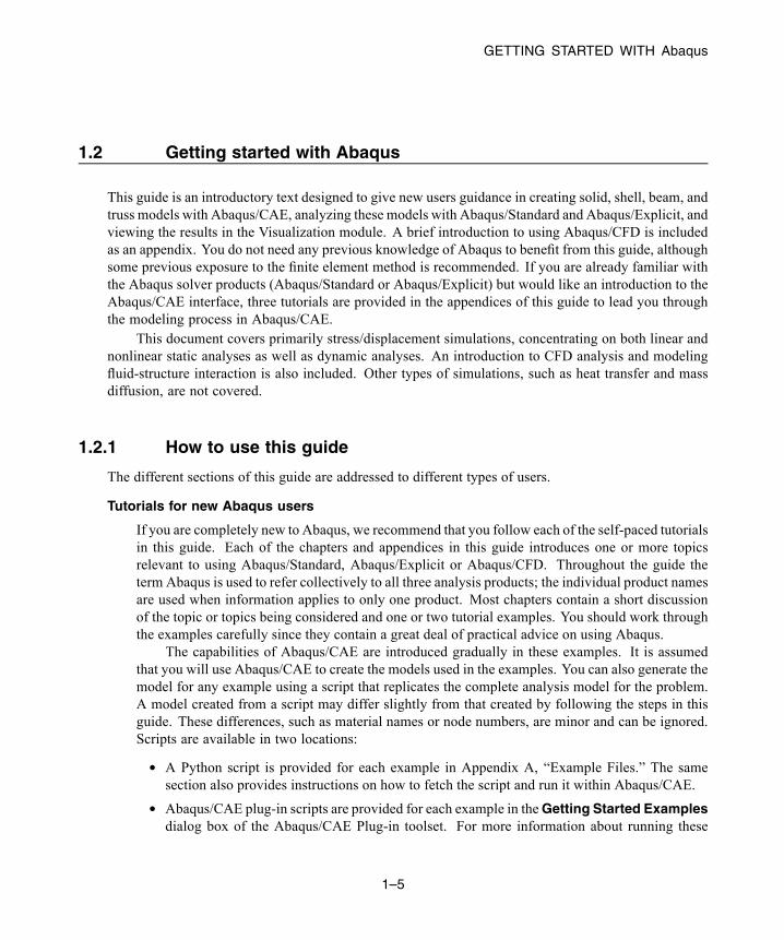
1.2 Getting started with Abaqus
This guide is an introductory text designed to give new users guidance in creating solid, shell, beam, andtruss models with Abaqus/CAE, analyzing these models with Abaqus/Standard and Abaqus/Explicit, andviewing the results in the Visualization module. A brief introduction to using Abaqus/CFD is includedas an appendix. You do not need any previous knowledge of Abaqus to benefit from this guide, althoughsome previous exposure to the finite element method is recommended. If you are already familiar withthe Abaqus solver products (Abaqus/Standard or Abaqus/Explicit) but would like an introduction to theAbaqus/CAE interface, three tutorials are provided in the appendices of this guide to lead you throughthe modeling process in Abaqus/CAE.
This document covers primarily stress/displacement simulations, concentrating on both linear andnonlinear static analyses as well as dynamic analyses. An introduction to CFD analysis and modelingfluid-structure interaction is also included. Other types of simulations, such as heat transfer and massdiffusion, are not covered.
1.2.1 How to use this guide
The different sections of this guide are addressed to different types of users.
Tutorials for new Abaqus users
If you are completely new to Abaqus, we recommend that you follow each of the self-paced tutorialsin this guide. Each of the chapters and appendices in this guide introduces one or more topicsrelevant to using Abaqus/Standard, Abaqus/Explicit or Abaqus/CFD. Throughout the guide theterm Abaqus is used to refer collectively to all three analysis products; the individual product namesare used when information applies to only one product. Most chapters contain a short discussionof the topic or topics being considered and one or two tutorial examples. You should work throughthe examples carefully since they contain a great deal of practical advice on using Abaqus.
The capabilities of Abaqus/CAE are introduced gradually in these examples. It is assumedthat you will use Abaqus/CAE to create the models used in the examples. You can also generate themodel for any example using a script that replicates the complete analysis model for the problem.A model created from a script may differ slightly from that created by following the steps in thisguide. These differences, such as material names or node numbers, are minor and can be ignored.Scripts are available in two locations:
• A Python script is provided for each example in Appendix A, “Example Files.” The samesection also provides instructions on how to fetch the script and run it within Abaqus/CAE.
• Abaqus/CAE plug-in scripts are provided for each example in theGetting Started Examplesdialog box of the Abaqus/CAE Plug-in toolset. For more information about running these
1–5
Abaqus ID:Printed on:

GETTING STARTED WITH Abaqus
scripts, see “Running the Getting Started with Abaqus examples,” Section 82.1 of theAbaqus/CAE User’s Guide, in the HTML version of this guide.
This chapter is a short introduction to Abaqus and this guide. Chapter 2, “Abaqus Basics,”which is centered around a simple example, covers the basics of using Abaqus. By the end ofChapter 2, “Abaqus Basics,” you will know the fundamentals of how to prepare a model for anAbaqus simulation, check the data, run the analysis job, and view the results.
Chapter 3, “Finite Elements and Rigid Bodies,” presents an overview of the main elementfamilies available in Abaqus. The use of continuum (solid) elements, shell elements, and beamelements is discussed in Chapter 4, “Using Continuum Elements”; Chapter 5, “Using ShellElements”; and Chapter 6, “Using Beam Elements”; respectively.
Linear dynamic analyses are discussed in Chapter 7, “Linear Dynamics.” Chapter 8,“Nonlinearity,” introduces the concept of nonlinearity in general, and geometric nonlinearity inparticular, and contains the first nonlinear Abaqus simulation. Nonlinear dynamic analyses arediscussed in Chapter 9, “Nonlinear Explicit Dynamics,” and material nonlinearity is introduced inChapter 10, “Materials.” Chapter 11, “Multiple Step Analysis,” introduces the concept of multistepsimulations, and Chapter 12, “Contact,” discusses the many issues that arise in contact analyses.Using Abaqus/Explicit to solve quasi-static problems is presented in Chapter 13, “Quasi-StaticAnalysis with Abaqus/Explicit.” The illustrative example is a sheet metal forming simulation,which requires importing between Abaqus/Explicit and Abaqus/Standard to perform the formingand springback analyses efficiently.
Abaqus/CAE tutorials for experienced Abaqus users
Four appendices are provided to introduce users familiar with the Abaqus analysis products to theAbaqus/CAE interface. In Appendix B, “Creating and Analyzing a Simple Model in Abaqus/CAE,”you create a simple model, analyze it, and then view the results. The second tutorial, Appendix C,“Using Additional Techniques to Create and Analyze a Model in Abaqus/CAE,” is more complexand illustrates how parts, sketches, datum geometry, and partitions work together and how youassemble part instances. Appendix D, “Viewing the Output from Your Analysis,” demonstrateshow you can use the Visualization module (also licensed separately as Abaqus/Viewer) to displayyour results in a variety of formats and how you can customize the display. Appendix E, “Flowthrough a bent tube,” illustrates how you can use Abaqus/CFD to model fluid flow through a benttube and use Abaqus/Standard to model structural deformation in the tube.
1.2.2 Conventions used in this guideThis guide adheres to the following conventions:
Typographical conventions
Different text styles are used in the tutorial examples to indicate specific actions or identify items.
• Input in COURIER FONT should be typed into Abaqus/CAE or your computer exactly asshown. For example,
1–6
Abaqus ID:Printed on:

GETTING STARTED WITH Abaqus
abaqus cae
would be typed on your computer to run Abaqus/CAE.
• Menu selections, tabs within dialog boxes, and labels of items on the screen in Abaqus/CAEare indicated in bold:
View→Graphics OptionsContour Plot Options
Sketcher figures
Sketches are two-dimensional profiles that form the geometry of features defining an Abaqus/CAEnative part. You use the Sketcher to create these sketches, as shown in Figure 1–2. The Sketcherdisplays major gridlines in a solid line style and the X- and Y-axes of the sketch and minor gridlinesin a dashed line style. In order to visually distinguish the part sketch from the Sketcher grid, thegridlines in most of the Sketcher figures in this guide are dashed.
H
( 25.E−03 )
50.E−03
100.E−03
1
2
3
Figure 1–2 The Sketcher.
View orientation triad
By default, Abaqus/CAE uses the alphabetical option, x-y-z, for labeling the view orientation triad.In general, this guide adopts the numerical option, 1-2-3, to permit direct correspondence withdegree of freedom and output labeling. The view orientation triad is shown in the lower left cornerof Figure 1–2.
1–7
Abaqus ID:Printed on:
GETTING STARTED WITH Abaqus
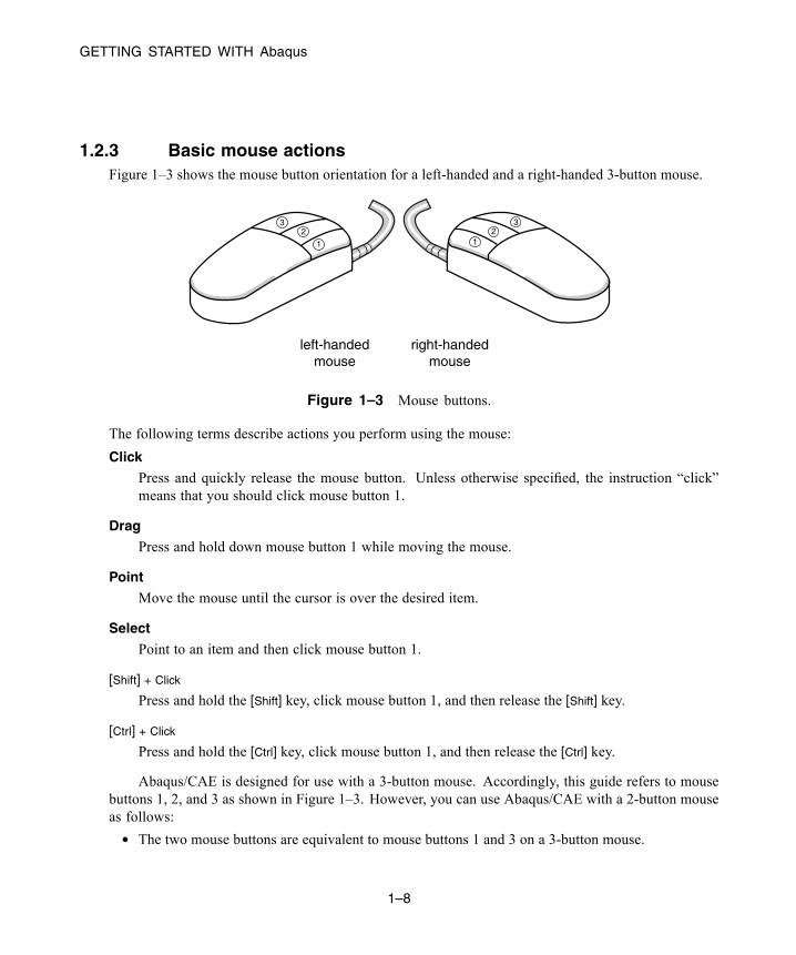
1.2.3 Basic mouse actionsFigure 1–3 shows the mouse button orientation for a left-handed and a right-handed 3-button mouse.
right-handedmouse
left-handedmouse
12
3
1
23
Figure 1–3 Mouse buttons.
The following terms describe actions you perform using the mouse:
Click
Press and quickly release the mouse button. Unless otherwise specified, the instruction “click”means that you should click mouse button 1.
Drag
Press and hold down mouse button 1 while moving the mouse.
Point
Move the mouse until the cursor is over the desired item.
Select
Point to an item and then click mouse button 1.
[Shift] + Click
Press and hold the [Shift] key, click mouse button 1, and then release the [Shift] key.
[Ctrl] + Click
Press and hold the [Ctrl] key, click mouse button 1, and then release the [Ctrl] key.
Abaqus/CAE is designed for use with a 3-button mouse. Accordingly, this guide refers to mousebuttons 1, 2, and 3 as shown in Figure 1–3. However, you can use Abaqus/CAE with a 2-button mouseas follows:
• The two mouse buttons are equivalent to mouse buttons 1 and 3 on a 3-button mouse.
1–8
Abaqus ID:Printed on:
Abaqus DOCUMENTATION
• Pressing both mouse buttons simultaneously is equivalent to pressing mouse button 2 on a 3-buttonmouse.
Tip: You are instructed to click mouse button 2 in procedures throughout this guide. Makesure that you configure mouse button 2 (or the wheel button) to act as a middle button click.
1.3 Abaqus documentation
The documentation for Abaqus is extensive and complete. The following documentation andpublications are available from SIMULIA through the Abaqus HTML documentation and in PDFformat. For more information on accessing the HTML guides, refer to the discussion of executionprocedures in the Abaqus Analysis User’s Guide. For more information on printing the guides, refer to“Printing from a PDF book,” Section 5.3 of Using Abaqus Online Documentation.
Abaqus Analysis User’s Guide
This guide contains a complete description of the elements, material models, procedures, inputspecifications, etc. It is the basic guide for Abaqus/Standard, Abaqus/Explicit, and Abaqus/CFD;and it provides both input file usage and Abaqus/CAE usage information. This guide regularlyrefers to the Abaqus Analysis User’s Guide, so you should have it available as you work throughthe examples.
Abaqus/CAE User’s Guide
This guide includes detailed descriptions of how to use Abaqus/CAE for model generation, analysis,and results evaluation and visualization. Abaqus/Viewer users should refer to the information onthe Visualization module in this guide.
Using Abaqus Online Documentation
This guide contains instructions for navigating, viewing, and searching the Abaqus HTML and PDFdocumentation. In addition, this guide explains how to use the PDF documentation to produce
a high quality printed copy and how to use the icon in all PDF books except the AbaqusScripting Reference Guide and the Abaqus GUI Toolkit Reference Guide to print a selected sectionof a book.
Other Abaqus documentation:
Abaqus Example Problems Guide
This guide contains detailed examples from which users can learn how to run simulations involvingnontrivial physics. Many of the examples are worked with several different element types, meshdensities, and other variations. Cases include large motion of an elastic-plastic pipe hitting a rigidwall; inelastic buckling collapse of a thin-walled elbow; explosive loading of an elastic, viscoplastic
1–9
Abaqus ID:Printed on:
Abaqus DOCUMENTATION
thin ring; consolidation under a footing; buckling of a composite shell with a hole; and deep drawingof a metal sheet. It is generally useful to look for relevant examples in this guide and to review themwhen embarking on a new class of problem.
When you want to use a feature that you have not used before, you should look up one or moreexamples that use that feature. Then, use the example to familiarize yourself with the correct usageof the capability. To find an example that uses a certain feature, search the online documentation oruse the abaqus findkeyword utility (see “Querying the keyword/problem database,” Section 3.2.16of the Abaqus Analysis User’s Guide, for more information).
All the input files associated with the examples are provided as part of the Abaqus installation.The abaqus fetch utility is used to extract sample Abaqus input files from the compressed archivefiles provided with the release (see “Fetching sample input files,” Section 3.2.17 of the AbaqusAnalysis User’s Guide, for more information). You can fetch any of the example files so that youcan run the simulations yourself and review the results. You can also access the input files throughthe hyperlinks in the Abaqus Example Problems Guide.
Abaqus Benchmarks Guide
This guide contains benchmark problems that provide evidence that the software can reproduce aresult from a benchmark defined by an external body or institution such as NAFEMS. The problemsare sufficient to show accuracy and convergence compared to the benchmark data. The NAFEMSbenchmark problems are included in this guide.
Abaqus Verification Guide
This guide contains test cases that provide evidence that the implementation of the numerical modelproduces the expected results for one or several well-defined options in the code. It may be usefulto run these problems when learning to use a new capability. In addition, the supplied input datafiles provide good starting points to check the behavior of elements, materials, etc.
Abaqus Theory Guide
This guide contains detailed, precise discussions of all theoretical aspects of Abaqus. It is writtento be understood by users with an engineering background.
Abaqus Keywords Reference Guide
This guide contains a complete description of all the input options that are available inAbaqus/Standard, Abaqus/Explicit, and Abaqus/CFD.
Abaqus User Subroutines Reference Guide
This guide contains a complete description of all the user subroutines available for use in Abaqusanalyses. It also discusses the utility routines that can be used when writing user subroutines.
Abaqus Glossary
This guide defines technical terms as they apply to the Abaqus Unified FEA Product Suite.
1–10
Abaqus ID:Printed on:

Abaqus DOCUMENTATION
Abaqus Release Notes
This guide contains brief descriptions of the new features available in the latest release of the Abaqusproduct line.
Abaqus Installation and Licensing Guide
This guide describes how to install Abaqus and how to configure the installation for particularcircumstances. Some of this information, of most relevance to users, is also provided in theAbaqus Analysis User’s Guide.
In addition to the documentation listed above, the following guides are available for Abaqusinterfaces and custom programming techniques not discussed in this guide:
• Abaqus Scripting User’s Guide• Abaqus Scripting Reference Guide• Abaqus GUI Toolkit User’s Guide• Abaqus GUI Toolkit Reference Guide
SIMULIA also provides documentation for all of the geometry translators described in “The Abaqusproducts,” Section 1.1.
Additional publications available from SIMULIA:
Quality Assurance Manual
This document describes the Quality Management System followed by SIMULIA. It is a controlleddocument, provided to customers who subscribe to the Quality Monitoring Service. Contact yoursupport office for more information.
Abaqus online resources
SIMULIA has a home page on the World Wide Web (www.3ds.com/simulia), containing a varietyof useful information about the Abaqus suite of programs, including:
• Frequently asked questions• Abaqus systems information and machine requirements• Benchmark timing documents• Error status reports
1–11
Abaqus ID:Printed on:

GETTING HELP
• Training course schedule• Newsletters
1.4 Getting help
You may want to read additional information about Abaqus/CAE features at various points during thetutorials. The context-sensitive help system allows you to locate relevant information quickly and easily.Context-sensitive help is available for every item in the main window and in all dialog boxes.
Note:
• On Windows platforms, the help system uses your default web browser to display the onlinedocumentation.
• On Linux platforms, the help system searches the system path for Firefox. If the help system cannotfind Firefox, an error is displayed.
The browser_type and browser_path variables can be set in the environment file to modifythis behavior. For more information, see “System customization parameters,” Section 4.1.5 of theAbaqus Installation and Licensing Guide.
To obtain context-sensitive help:
1. From the main menu bar, select Help→On Context.
Tip: You can also click the help tool to access context-sensitive help.
The cursor changes to a question mark.
2. Click any part of the main window except its frame.
A help window appears in your browser window. The help window displays information about theitem you selected.
3. Scroll to the bottom of the help window.
At the bottom of the window, a list of blue, underlined items appears. These items are links to theAbaqus/CAE User’s Guide.
4. Click any one of the items.
A book window appears in your default web browser. The window is arranged into four frames asfollows:
• The Abaqus/CAE User’s Guide appears in a text frame on the right side of the window. Theguide is turned to the item that you selected.
• An expandable table of contents is available on the lower left side of the window for easynavigation throughout the book.
1–12
Abaqus ID:Printed on:
SUPPORT
• The table of contents control tools in the upper left frame allow you to vary the level of detaildisplayed in the table of contents frame or to change the size of the frame. Click to expand
several levels in the table of contents of an online book. Click to collapse all expanded
sections in the table of contents. Click and , respectively, to widen or narrow the tableof contents frame.
• The navigation frame at the top of the book window allows you to select another book fromthe entire Abaqus documentation collection. The navigation frame also allows you to searchthe entire guide.
5. Click any item in the table of contents.
The text frame changes to reflect the item you selected.
6. Click the icon to the left of a topic heading to expand it.
The headings of the subtopics appear under the topic heading, and the sign changes to , indicatingthat the section is expanded. If appears beside a subsection, there are no further levels withinthat section to expand. To collapse an expanded section of the table of contents, click next tothe topic heading.
7. In the search panel in the navigation frame, type any word that appears in the text frame on the rightand click Search.
When the search is complete, the table of contents frame displays the number of hits next to eachtopic heading and all hits become highlighted in the text frame. Click Next Match or PreviousMatch in the navigation frame to move through the document from one hit to the next.
You can enter a single word or a phrase in the search panel, and you can use the [*] character asa wildcard. For detailed instructions on using the search capabilities of the online documentation,see Using Abaqus Online Documentation.
8. Close the web browser windows.
1.5 Support
Both technical engineering support (for problems with creating a model or performing an analysis)and systems support (for installation, licensing, and hardware-related problems) for Abaqus areoffered through a network of support offices. Regional contact information is accessible from theLocations page at www.3ds.com/simulia. Support is also available from the Support page atwww.3ds.com/simulia. When contacting your support office, please specify whether you would liketechnical support (you have encountered problems performing an Abaqus analysis) or systems support(Abaqus will not install correctly, licensing does not work correctly, or other hardware-related issueshave arisen).
1–13
Abaqus ID:Printed on:

SUPPORT
We welcome any suggestions for improvements to Abaqus software, the support program, ordocumentation. We will ensure that any enhancement requests you make are considered for futurereleases. If you wish to make a suggestion about the service or products provided by SIMULIA, refer towww.3ds.com/simulia. Complaints should be addressed by contacting your support office or by visitingthe Quality Assurance page at www.3ds.com/simulia.
1.5.1 Technical support
SIMULIA technical support engineers can assist in clarifying Abaqus features and checking errors bygiving both general information on using Abaqus and information on its application to specific analyses.If you have concerns about an analysis, we suggest that you contact us at an early stage, since it is usuallyeasier to solve problems at the beginning of a project rather than trying to correct an analysis at the end.
Please have the following information ready before calling the technical support hotline, and includeit in any written contacts:
• The release of Abaqus that are you using.
– The release numbers for Abaqus/Standard, Abaqus/Explicit, and Abaqus/CFD are given at thetop of the data (.dat) file.
– The release numbers for Abaqus/CAE and Abaqus/Viewer can be found by selectingHelp→About Abaqus from the main menu bar.
• The type of computer on which you are running Abaqus.• The symptoms of any problems, including the exact error messages, if any.• Workarounds or tests that you have already tried.
For support about a specific problem, any available Abaqus output files may be helpful in answeringquestions that the support engineer may ask you.
The support engineer will try to diagnose your problem from the model description and a descriptionof the difficulties you are having. Frequently, the support engineer will need model sketches, which canbe e-mailed, faxed, or sent in the mail. Plots of the final results or the results near the point that theanalysis terminated may also be needed to understand what may have caused the problem.
If the support engineer cannot diagnose your problem from this information, you may be asked tosupply the input data. The data can be attached to a support request in the online system. It can also besent by means of e-mail, ftp, CD, or DVD.
All support requests are tracked. This tracking enables you (as well as the support engineer) tomonitor the progress of a particular problem and to check that we are resolving support issues efficiently.You must register with the system to check on a support issue. If you contact us by means outside thesystem to discuss an existing support problem and you know the support request number, please mentionit so that we can consult the database to see what the latest action has been.
1–14
Abaqus ID:Printed on:

A QUICK REVIEW OF THE FINITE ELEMENT METHOD
1.5.2 Systems support
Abaqus systems support engineers can help you resolve issues related to the installation and running ofAbaqus, including licensing difficulties, that are not covered by technical support.
You should install Abaqus by carefully following the instructions in the Abaqus Installationand Licensing Guide. If you encounter problems with the installation or licensing, first review theinstructions in the Abaqus Installation and Licensing Guide to ensure that they have been followedcorrectly. If this method does not resolve the problems, search for known installation problems in theDassault Systèmes Knowledge Base at www.3ds.com/support/knowledge-base. If this method does notaddress your situation, please create a support request in the online system. Send whatever informationis available to define the problem: error messages from an aborted analysis or a detailed explanation ofthe problems encountered. Whenever possible, please send the output from the abaqus info=supportcommand.
1.5.3 Support for academic institutions
Under the terms of the Academic License Agreement, we do not provide support to users at academicinstitutions unless the institution has also purchased technical support. Please contact us for moreinformation.
1.6 A quick review of the finite element method
This section reviews the basics of the finite element method. The first step of any finite element simulationis to discretize the actual geometry of the structure using a collection of finite elements. Each finiteelement represents a discrete portion of the physical structure. The finite elements are joined by sharednodes. The collection of nodes and finite elements is called themesh. The number of elements per unit oflength, area, or in a mesh is referred to as the mesh density. In a stress analysis the displacements of thenodes are the fundamental variables that Abaqus calculates. Once the nodal displacements are known,the stresses and strains in each finite element can be determined easily.
1.6.1 Obtaining nodal displacements using implicit methods
A simple example of a truss, constrained at one end and loaded at the other end as shown in Figure 1–4,is used to introduce some terms and conventions used in this document.
1–15
Abaqus ID:Printed on:
A QUICK REVIEW OF THE FINITE ELEMENT METHOD
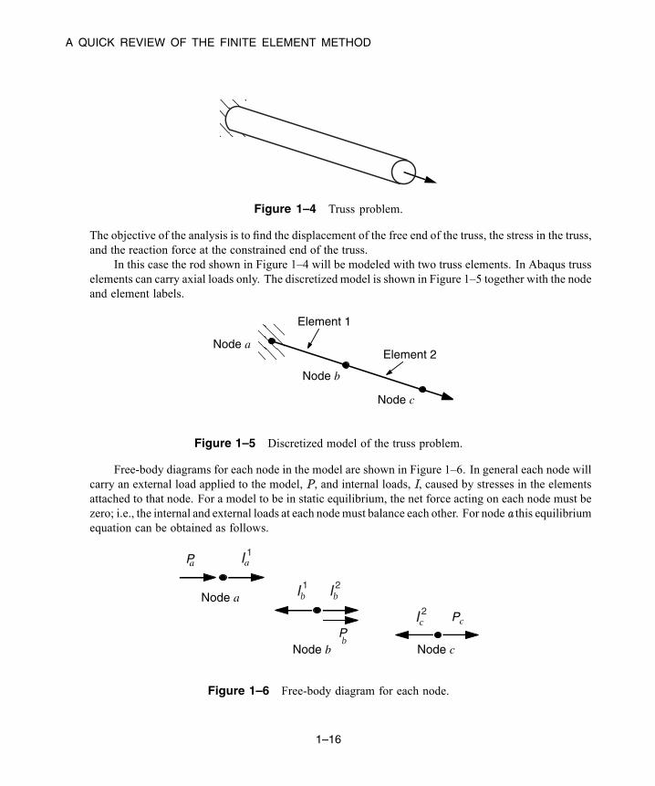
Figure 1–4 Truss problem.
The objective of the analysis is to find the displacement of the free end of the truss, the stress in the truss,and the reaction force at the constrained end of the truss.
In this case the rod shown in Figure 1–4 will be modeled with two truss elements. In Abaqus trusselements can carry axial loads only. The discretized model is shown in Figure 1–5 together with the nodeand element labels.
Node a
Node b
Node c
Element 1
Element 2
Figure 1–5 Discretized model of the truss problem.
Free-body diagrams for each node in the model are shown in Figure 1–6. In general each node willcarry an external load applied to the model, P, and internal loads, I, caused by stresses in the elementsattached to that node. For a model to be in static equilibrium, the net force acting on each node must bezero; i.e., the internal and external loads at each nodemust balance each other. For node a this equilibriumequation can be obtained as follows.
Pa
Node b
Node a
Node c
PcPb
I 1
Ib1 Ib
2
Ic2
a
Figure 1–6 Free-body diagram for each node.
1–16
Abaqus ID:Printed on:
A QUICK REVIEW OF THE FINITE ELEMENT METHOD
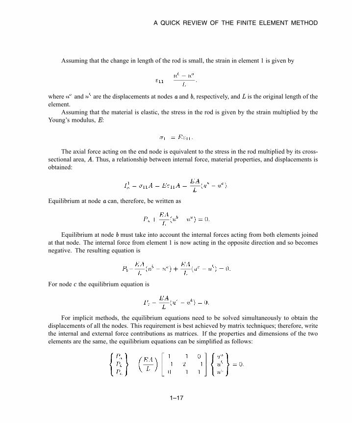
Assuming that the change in length of the rod is small, the strain in element 1 is given by
where and are the displacements at nodes a and b, respectively, and L is the original length of theelement.
Assuming that the material is elastic, the stress in the rod is given by the strain multiplied by theYoung’s modulus, E:
The axial force acting on the end node is equivalent to the stress in the rod multiplied by its cross-sectional area, A. Thus, a relationship between internal force, material properties, and displacements isobtained:
Equilibrium at node a can, therefore, be written as
Equilibrium at node b must take into account the internal forces acting from both elements joinedat that node. The internal force from element 1 is now acting in the opposite direction and so becomesnegative. The resulting equation is
For node c the equilibrium equation is
For implicit methods, the equilibrium equations need to be solved simultaneously to obtain thedisplacements of all the nodes. This requirement is best achieved by matrix techniques; therefore, writethe internal and external force contributions as matrices. If the properties and dimensions of the twoelements are the same, the equilibrium equations can be simplified as follows:
1–17
Abaqus ID:Printed on:

A QUICK REVIEW OF THE FINITE ELEMENT METHOD
In general, it may be that the element stiffnesses, the terms, are different from element toelement; therefore, write the element stiffnesses as and for the two elements in the model. We areinterested in obtaining the solution to the equilibrium equation in which the externally applied forces, P,are in equilibrium with the internally generated forces, I. When discussing this equation with referenceto convergence and nonlinearity, we write it as
For the complete two-element, three-node structure we, therefore, modify the signs and rewrite theequilibrium equation as
In an implicit method, such as that used in Abaqus/Standard, this system of equations can then be solvedto obtain values for the three unknown variables: , , and ( is specified in the problem as 0.0).Once the displacements are known, we can go back and use them to calculate the stresses in the trusselements. Implicit finite element methods require that a system of equations is solved at the end of eachsolution increment.
In contrast to implicit methods, an explicit method, such as that used in Abaqus/Explicit, does notrequire the solving of a simultaneous system of equations or the calculation of a global stiffness matrix.Instead, the solution is advanced kinematically from one increment to the next. The extension of thefinite element method to explicit dynamics is covered in the following section.
1.6.2 Stress wave propagation illustratedThis section attempts to provide some conceptual understanding of how forces propagate through amodelwhen using the explicit dynamics method. In this illustrative example we consider the propagation of astress wave along a rod modeled with three elements, as shown in Figure 1–7. We will study the state ofthe rod as we increment through time.
P1 2 3 41 2 3
l ll
Figure 1–7 Initial configuration of a rod with a concentrated load, , at the free end.
1–18
Abaqus ID:Printed on:

A QUICK REVIEW OF THE FINITE ELEMENT METHOD
In the first time increment node 1 has an acceleration, , as a result of the concentrated force, ,applied to it. The acceleration causes node 1 to have a velocity, , which, in turn, causes a strain rate,
, in element 1. The increment of strain, , in element 1 is obtained by integrating the strain ratethrough the time of increment 1. The total strain, , is the sum of the initial strain, , and the incrementin strain. In this case the initial strain is zero. Once the element strain has been calculated, the elementstress, , is obtained by applying the material constitutive model. For a linear elastic material thestress is simply the elastic modulus times the total strain. This process is shown in Figure 1–8. Nodes 2and 3 do not move in the first increment since no force is applied to them.
–
P1 2 3 41 2 3
u1P
M1------- u1⇒ u1 td∫ el1⇒
u1l
----- el1⇒ el1 t
⇒ el1
d∫
el1+ el1⇒ E el1
= = = =
= =o
Figure 1–8 Configuration at the end of increment 1 of a rodwith a concentrated load, , at the free end.
In the second increment the stresses in element 1 apply internal, element forces to the nodesassociated with element 1, as shown in Figure 1–9. These element stresses are then used to calculatedynamic equilibrium at nodes 1 and 2.
P1 2 3 41 2 3
Iel1 = el1A
u1P I el1–
M1------------------- u1⇒ u1
old u1 t
u2
d∫+
Iel1M2---------- u2⇒ u2 td∫
= =
= =
el1u2 u1–
l---------------- el1⇒ el1 t
el1⇒
d∫el1
el1⇒
+
E el1
= =
=
=
el1old
Figure 1–9 Configuration of the rod at the beginning of increment 2.
1–19
Abaqus ID:Printed on:
A QUICK REVIEW OF THE FINITE ELEMENT METHOD
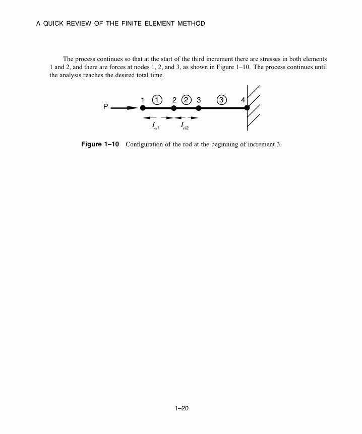
The process continues so that at the start of the third increment there are stresses in both elements1 and 2, and there are forces at nodes 1, 2, and 3, as shown in Figure 1–10. The process continues untilthe analysis reaches the desired total time.
P1 2 3 41 2 3
Iel1 I
el2
Figure 1–10 Configuration of the rod at the beginning of increment 3.
1–20
Abaqus ID:Printed on:
Abaqus BASICS
2. Abaqus Basics
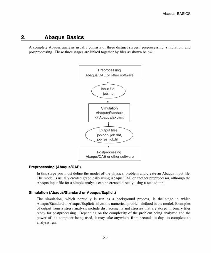
A complete Abaqus analysis usually consists of three distinct stages: preprocessing, simulation, andpostprocessing. These three stages are linked together by files as shown below:
Output files:job.odb, job.dat,job.res, job.fil
Preprocessing
Input file:job.inp
Simulation
Postprocessing
or
Abaqus/CAE or other software
Abaqus/Standard
Abaqus/CAE or other software
Abaqus/Explicit
Preprocessing (Abaqus/CAE)
In this stage you must define the model of the physical problem and create an Abaqus input file.The model is usually created graphically using Abaqus/CAE or another preprocessor, although theAbaqus input file for a simple analysis can be created directly using a text editor.
Simulation (Abaqus/Standard or Abaqus/Explicit)
The simulation, which normally is run as a background process, is the stage in whichAbaqus/Standard or Abaqus/Explicit solves the numerical problem defined in the model. Examplesof output from a stress analysis include displacements and stresses that are stored in binary filesready for postprocessing. Depending on the complexity of the problem being analyzed and thepower of the computer being used, it may take anywhere from seconds to days to complete ananalysis run.
2–1
Abaqus ID:Printed on:

COMPONENTS OF AN Abaqus ANALYSIS MODEL
Postprocessing (Abaqus/CAE)
You can evaluate the results once the simulation has been completed and the displacements,stresses, or other fundamental variables have been calculated. The evaluation is generally doneinteractively using the Visualization module of Abaqus/CAE or another postprocessor. TheVisualization module, which reads the neutral binary output database file, has a variety of optionsfor displaying the results, including color contour plots, animations, deformed shape plots, andX–Y plots.
2.1 Components of an Abaqus analysis model
An Abaqus model is composed of several different components that together describe the physicalproblem to be analyzed and the results to be obtained. At a minimum the analysis model consists ofthe following information: discretized geometry, element section properties, material data, loads andboundary conditions, analysis type, and output requests. The discussion in this chapter focuses onstructural applications. Similar concepts apply for fluid dynamics.
Discretized geometry
Finite elements and nodes define the basic geometry of the physical structure being modeled inAbaqus. Each element in the model represents a discrete portion of the physical structure, whichis, in turn, represented by many interconnected elements. Elements are connected to one anotherby shared nodes. The coordinates of the nodes and the connectivity of the elements—that is, whichnodes belong to which elements—comprise the model geometry. The collection of all the elementsand nodes in a model is called the mesh. Generally, the mesh will be only an approximation of theactual geometry of the structure.
The element type, shape, and location, as well as the overall number of elements used in themesh, affect the results obtained from a simulation. The greater the mesh density (i.e., the greaterthe number of elements in the mesh), the more accurate the results. As the mesh density increases,the analysis results converge to a unique solution, and the computer time required for the analysisincreases. The solution obtained from the numerical model is generally an approximation to thesolution of the physical problem being simulated. The extent of the approximations made in themodel’s geometry, material behavior, boundary conditions, and loading determines how well thenumerical simulation matches the physical problem.
Element section properties
Abaqus has a wide range of elements, many of which have geometry not defined completely bythe coordinates of their nodes. For example, the layers of a composite shell or the dimensions ofan I-beam section are not defined by the nodes of the element. Such additional geometric dataare defined as physical properties of the element and are necessary to define the model geometrycompletely (see Chapter 3, “Finite Elements and Rigid Bodies”).
2–2
Abaqus ID:Printed on:

COMPONENTS OF AN Abaqus ANALYSIS MODEL
Material data
Material properties for all elements must be specified. While high-quality material data are oftendifficult to obtain, particularly for the more complex material models, the validity of the Abaqusresults is limited by the accuracy and extent of the material data.
Loads and boundary conditions
Loads distort the physical structure and, thus, create stress in it. The most common forms of loadinginclude:
• point loads;• pressure loads on surfaces;• distributed tractions on surfaces;• distributed edge loads and moments on shell edges;• body forces, such as the force of gravity; and• thermal loads.Boundary conditions are used to constrain portions of the model to remain fixed (zero
displacements) or to move by a prescribed amount (nonzero displacements).In a static analysis enough boundary conditions must be used to prevent themodel frommoving
as a rigid body in any direction; otherwise, unrestrained rigid bodymotion causes the stiffnessmatrixto be singular. A solver problem will occur during the solution stage and may cause the simulationto stop prematurely. Abaqus/Standard will issue a warning message if it detects a solver problemduring a simulation. It is important that you learn to interpret such error messages. If you see a“numerical singularity” or “zero pivot” warning message during a static stress analysis, you shouldcheck whether all or part of your model lacks constraints against rigid body translations or rotations.Rigid body motions can consist of both translations and rotations of the components. The potentialrigid body motions depend on the dimensionality of the model.
Dimensionality Possible Rigid Body Motion
Three-dimensional Translation in the 1-, 2-, and 3-directions.
Rotation about the 1-, 2-, and 3-axes.
Axisymmetric Translation in the 2-direction.
Rotation about the 3-axis (axisymmetric rigid bodies only).
Plane stress Translation in the 1- and 2-directions.
Plane strain Rotation about the 3-axis.
By default, the 1-, 2-, and 3-directions are aligned with the axes of a global Cartesian coordinatesystem (discussed later).
2–3
Abaqus ID:Printed on:
INTRODUCTION TO Abaqus/CAE
In a dynamic analysis inertia forces prevent the model from undergoing infinite motioninstantaneously as long as all separate parts in the model have some mass; therefore, solverproblem warnings in a dynamic analysis usually indicate some other modeling problem, such asexcessive plasticity.
Analysis type
Abaqus can carry out many different types of simulations, but this guide only covers the two mostcommon: static and dynamic stress analyses.
In a static analysis the long-term response of the structure to the applied loads is obtained.In other cases the dynamic response of a structure to the loads may be of interest: for example,the effect of a sudden load on a component, such as occurs during an impact, or the response of abuilding in an earthquake.
Output requests
An Abaqus simulation can generate a large amount of output. To avoid using excessive disk space,you can limit the output to that required for interpreting the results.
Generally a preprocessor such as Abaqus/CAE is used to define the necessary components of themodel.
2.2 Introduction to Abaqus/CAE
Abaqus/CAE is the Complete Abaqus Environment that provides a simple, consistent interface forcreating Abaqus models, interactively submitting and monitoring Abaqus jobs, and evaluating resultsfrom Abaqus simulations. Abaqus/CAE is divided into modules, where each module defines a logicalaspect of the modeling process; for example, defining the geometry, defining material properties, andgenerating a mesh. As you move from module to module, you build up the model. When the modelis complete, Abaqus/CAE generates an input file that you submit to the Abaqus analysis product.Abaqus/Standard or Abaqus/Explicit reads the input file generated by Abaqus/CAE, performs theanalysis, sends information to Abaqus/CAE to allow you to monitor the progress of the job, andgenerates an output database. Finally, you use the Visualization module to read the output database andview the results of your analysis.
2.2.1 Starting Abaqus/CAE
To start Abaqus/CAE, you enter the command
abaqus cae
2–4
Abaqus ID:Printed on:
INTRODUCTION TO Abaqus/CAE
at your operating system prompt, where abaqus is the command used to run Abaqus. This command
may be different on your system.
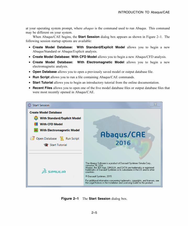
When Abaqus/CAE begins, the Start Session dialog box appears as shown in Figure 2–1. The
following session startup options are available:
• Create Model Database: With Standard/Explicit Model allows you to begin a new
Abaqus/Standard or Abaqus/Explicit analysis.
• Create Model Database: With CFD Model allows you to begin a new Abaqus/CFD analysis.
• Create Model Database: With Electromagnetic Model allows you to begin a new
electromagnetic analysis.
• Open Database allows you to open a previously saved model or output database file.
• Run Script allows you to run a file containing Abaqus/CAE commands.
• Start Tutorial allows you to begin an introductory tutorial from the online documentation.
• Recent Files allows you to open one of the five model database files or output database files that
were most recently opened in Abaqus/CAE.
Figure 2–1 The Start Session dialog box.
2–5
Abaqus ID:gsa-chp-abasics
Printed on: Mon July 13 -- 15:44:50 2015

INTRODUCTION TO Abaqus/CAE
2.2.2 Components of the main windowYou interact with Abaqus/CAE through the main window. Figure 2–2 shows the components that appearin the main window.
Title bar Menu bar Toolbars Context bar
Model Tree / Results Tree
Toolboxarea
Canvas anddrawing area
Viewport Promptarea
Message area orcommand line interface
2016
Figure 2–2 Components of the main window.
2–6
Abaqus ID:Printed on:
INTRODUCTION TO Abaqus/CAE
The components are:
Title bar
The title bar indicates the release of Abaqus/CAE you are running and the name of the current modeldatabase.
Menu bar
The menu bar contains all the available menus; the menus give access to all the functionality in theproduct. Different menus appear in the menu bar depending on which module you selected fromthe context bar. For more information, see “Components of the main menu bar,” Section 2.2.2 ofthe Abaqus/CAE User’s Guide.
Toolbars
The toolbars provide quick access to items that are also available in the menus. For moreinformation, see “Components of the toolbars,” Section 2.2.3 of the Abaqus/CAE User’s Guide.
Context bar
Abaqus/CAE is divided into a set of modules, where each module allows you to work on one aspectof your model; theModule list in the context bar allows you to move between these modules. Otheritems in the context bar are a function of the module in which you are working; for example, thecontext bar allows you to retrieve an existing part while creating the geometry of the model. Formore information, see “The context bar,” Section 2.2.4 of the Abaqus/CAE User’s Guide.
Model Tree
The Model Tree provides you with a graphical overview of your model and the objects that itcontains, such as parts, materials, steps, loads, and output requests. In addition, the Model Treeprovides a convenient, centralized tool for moving between modules and for managing objects. Ifyour model database contains more than one model, you can use the Model Tree to move betweenmodels. When you become familiar with the Model Tree, you will find that you can quicklyperform most of the actions that are found in the main menu bar, the module toolboxes, and thevarious managers. For more information, see “Working with the Model Tree and the Results Tree,”Section 3.5 of the Abaqus/CAE User’s Guide.
Results Tree
The Results Tree provides you with a graphical overview of your output databases and other session-specific data such as X–Y plots. If you have more than one output database open in your session, youcan use the Results Tree to move between output databases. When you become familiar with theResults Tree, you will find that you can quickly perform most of the actions in the Visualizationmodule that are found in the main menu bar and the toolbox. For more information, see “Anoverview of the Results Tree,” Section 3.5.2 of the Abaqus/CAE User’s Guide.
2–7
Abaqus ID:Printed on:
INTRODUCTION TO Abaqus/CAE
Toolbox area
When you enter a module, the toolbox area displays tools in the toolbox that are appropriate for thatmodule. The toolbox allows quick access to many of the module functions that are also availablefrom the menu bar. For more information, see “Understanding and using toolboxes and toolbars,”Section 3.3 of the Abaqus/CAE User’s Guide.
Canvas and drawing area
The canvas can be thought of as an infinite screen or bulletin board on which you post viewports; formore information, see Chapter 4, “Managing viewports on the canvas,” of the Abaqus/CAE User’sGuide. The drawing area is the visible portion of the canvas.
Viewport
Viewports are windows on the canvas in which Abaqus/CAE displays your model. For moreinformation, see Chapter 4, “Managing viewports on the canvas,” of the Abaqus/CAE User’sGuide.
Prompt area
The prompt area displays instructions for you to follow during a procedure; for example, it asks youto select the geometry as you create a set. For more information, see “Using the prompt area duringprocedures,” Section 3.1 of the Abaqus/CAE User’s Guide.
Message area
Abaqus/CAE prints status information and warnings in the message area. To resize the messagearea, drag the top edge; to see information that has scrolled out of the message area, use the scrollbar on the right side. The message area is displayed by default, but it uses the same space occupiedby the command line interface. If you have recently used the command line interface, you must
click the tab in the bottom left corner of the main window to activate the message area.
Note: If newmessages are added while the command line interface is active, Abaqus/CAE changesthe background color surrounding the message area icon to red. When you display the message area,the background reverts to its normal color.
Command line interface
You can use the command line interface to type Python commands and evaluate mathematicalexpressions using the Python interpreter that is built into Abaqus/CAE. The interface includesprimary (>>>) and secondary (...) prompts to indicate when you must indent commands tocomply with Python syntax.
The command line interface is hidden by default, but it uses the same space occupied by the
message area. Click the tab in the bottom left corner of the main window to switch from the
message area to the command line interface. Click the tab to return to the message area.
2–8
Abaqus ID:Printed on:
INTRODUCTION TO Abaqus/CAE
2.2.3 What is a module?
Asmentioned earlier, Abaqus/CAE is divided into functional units calledmodules. Eachmodule containsonly those tools that are relevant to a specific portion of themodeling task. For example, theMeshmodulecontains only the tools needed to create finite element meshes, while the Job module contains only thetools used to create, edit, submit, and monitor analysis jobs.
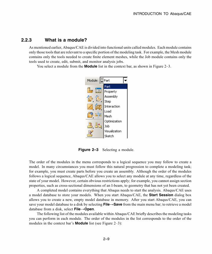
You select a module from the Module list in the context bar, as shown in Figure 2–3.
Figure 2–3 Selecting a module.
The order of the modules in the menu corresponds to a logical sequence you may follow to create amodel. In many circumstances you must follow this natural progression to complete a modeling task;for example, you must create parts before you create an assembly. Although the order of the modulesfollows a logical sequence, Abaqus/CAE allows you to select any module at any time, regardless of thestate of your model. However, certain obvious restrictions apply; for example, you cannot assign sectionproperties, such as cross-sectional dimensions of an I-beam, to geometry that has not yet been created.
A completed model contains everything that Abaqus needs to start the analysis. Abaqus/CAE usesa model database to store your models. When you start Abaqus/CAE, the Start Session dialog boxallows you to create a new, empty model database in memory. After you start Abaqus/CAE, you cansave your model database to a disk by selecting File→Save from the main menu bar; to retrieve a modeldatabase from a disk, select File→Open.
The following list of the modules available within Abaqus/CAE briefly describes the modeling tasksyou can perform in each module. The order of the modules in the list corresponds to the order of themodules in the context bar’s Module list (see Figure 2–3):
2–9
Abaqus ID:Printed on:
INTRODUCTION TO Abaqus/CAE
Part
The Part module allows you to create individual parts by sketching their geometry directly inAbaqus/CAE or by importing their geometry from other geometric modeling programs. For moreinformation, see Chapter 11, “The Part module,” of the Abaqus/CAE User’s Guide.
Property
A section definition contains information about the properties of a part or a region of a part, such asa region’s associated material definition and cross-sectional geometry. In the Property module youcreate section and material definitions and assign them to regions of parts. For more information,see Chapter 12, “The Property module,” of the Abaqus/CAE User’s Guide.
Assembly
When you create a part, it exists in its own coordinate system, independent of other parts in themodel. You use the Assembly module to create instances of your parts as well as instances ofother models and to position the instances relative to each other in a global coordinate system, thuscreating an assembly. An Abaqus model contains only one assembly. For more information, seeChapter 13, “The Assembly module,” of the Abaqus/CAE User’s Guide.
Step
You use the Step module to create and configure analysis steps and associated output requests.The step sequence provides a convenient way to capture changes in a model (such as loading andboundary condition changes); output requests can vary as necessary between steps. For moreinformation, see Chapter 14, “The Step module,” of the Abaqus/CAE User’s Guide.
Interaction
In the Interaction module you specify mechanical and thermal interactions between regions of amodel or between a region of a model and its surroundings. An example of an interaction is contactbetween two surfaces. Other interactions that may be defined include constraints, such as tie,equation, and rigid body constraints. Abaqus/CAE does not recognize mechanical contact betweenpart instances or regions of an assembly unless that contact is specified in the Interaction module;the mere physical proximity of two surfaces in an assembly is not sufficient to indicate any type ofinteraction between the surfaces. Interactions are step-dependent objects, which means that youmust specify the analysis steps in which they are active. For more information, see Chapter 15,“The Interaction module,” of the Abaqus/CAE User’s Guide.
Load
The Load module allows you to specify loads, boundary conditions, and predefined fields. Loadsand boundary conditions are step-dependent objects, whichmeans that youmust specify the analysissteps in which they are active; some predefined fields are step-dependent, while others are appliedonly at the beginning of the analysis. For more information, see Chapter 16, “The Load module,”of the Abaqus/CAE User’s Guide.
2–10
Abaqus ID:Printed on:

INTRODUCTION TO Abaqus/CAE
Mesh
The Mesh module contains tools that allow you to generate a finite element mesh on an assemblycreated within Abaqus/CAE. Various levels of automation and control are available so that you cancreate a mesh that meets the needs of your analysis. For more information, see Chapter 17, “TheMesh module,” of the Abaqus/CAE User’s Guide.
Optimization
The Optimization module allows you to create an optimization task that can be used to optimizethe topology of your model given a set of objectives and constraints. For more information, seeChapter 18, “The Optimization module,” of the Abaqus/CAE User’s Guide.
Job
Once you have finished all of the tasks involved in defining a model, you use the Job module toanalyze your model. The Job module allows you to interactively submit a job for analysis andmonitor its progress. Multiple models and runs may be submitted and monitored simultaneously.For more information, see Chapter 19, “The Job module,” of the Abaqus/CAE User’s Guide.
Visualization
The Visualization module provides graphical display of finite element models and results. It obtainsmodel and result information from the output database; you can control what information is writtento the output database by modifying output requests in the Step module. For more information, seePart V, “Viewing results,” of the Abaqus/CAE User’s Guide.
Sketch
Sketches are two-dimensional profiles that are used to help form the geometry defining anAbaqus/CAE native part. You use the Sketch module to create a sketch that defines a planar part,a beam, or a partition or to create a sketch that might be extruded, swept, or revolved to forma three-dimensional part. For more information, see Chapter 20, “The Sketch module,” of theAbaqus/CAE User’s Guide.
The contents of the main window change as you move between modules. Selecting a module fromthe Module list on the context bar causes the context bar, module toolbox, and menu bar to change toreflect the functionality of the current module.
Each module is discussed in more detail in the tutorial examples presented in this guide.
2.2.4 What is the Model Tree?
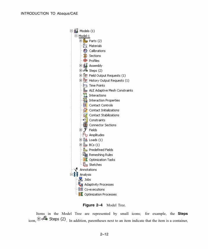
The Model Tree provides a visual description of the hierarchy of items in a model. It is located in theleft side of the main window underneath the Model tab. Figure 2–4 shows a typical Model Tree.
2–11
Abaqus ID:Printed on:
INTRODUCTION TO Abaqus/CAE
Figure 2–4 Model Tree.
Items in the Model Tree are represented by small icons; for example, the Steps
icon, . In addition, parentheses next to an item indicate that the item is a container,
2–12
Abaqus ID:Printed on:

EXAMPLE: CREATING A MODEL OF AN OVERHEAD HOIST
and the number in the parentheses indicates the number of items in the container. You can click on the“ ” and “−” signs in the Model Tree to expand and collapse a container. The right and left arrow keysperform the same operation.
The arrangement of the containers and items in the Model Tree reflects the order in which you areexpected to create your model. As noted earlier, a similar logic governs the order of modules in themodule menu—you create parts before you create the assembly, and you create steps before you createloads. This arrangement is fixed—you cannot move items in the Model Tree.
The Model Tree provides most of the functionality of the main menu bar and the module managers.For example, if you double-click on the Parts container, you can create a new part (the equivalent ofselecting Part→Create from the main menu bar).
The instructions for the examples discussed in this guide will focus on using the Model Tree toaccess the functionality of Abaqus/CAE. Menu bar actions will be considered only when necessary(e.g., when creating a finite element mesh or postprocessing results).
The Results Tree uses the same space occupied by the Model Tree. Click the Results tab in the leftside of the main window to switch from the Model Tree to the Results Tree. The Results Tree providesaccess to session-specific features (i.e., functionality available in only the Visualization module). TheResults Tree will be introduced during the course of the postprocessing exercises contained in this guide.
2.3 Example: creating a model of an overhead hoist
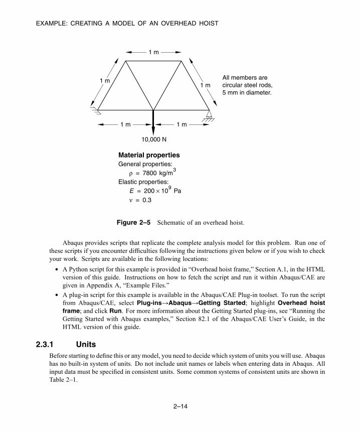
This example of an overhead hoist, shown in Figure 2–5, leads you through the Abaqus/CAE modelingprocess by using the Model Tree and showing you the basic steps used to create and analyze a simplemodel. The hoist is a simple, pin-jointed truss model that is constrained at the left end and mountedon rollers at the right end. The members can rotate freely at the joints. The frame is prevented frommoving out of plane. A simulation is first performed in Abaqus/Standard to determine the structure’sstatic deflection and the peak stress in its members when a 10 kN load is applied as shown in Figure 2–5.The simulation is performed a second time in Abaqus/Explicit under the assumption that the load isapplied suddenly to study the dynamic response of the frame.
For the overhead hoist example, you will perform the following tasks:
• Sketch the two-dimensional geometry and create a part representing the frame.• Define the material properties and section properties of the frame.• Assemble the model.• Configure the analysis procedure and output requests.• Apply loads and boundary conditions to the frame.• Mesh the frame.• Create a job and submit it for analysis.• View the results of the analysis.
2–13
Abaqus ID:Printed on:
EXAMPLE: CREATING A MODEL OF AN OVERHEAD HOIST
1 m
1 m
1 m 1 m
1 m
10,000 N
All members arecircular steel rods,5 mm in diameter.
Material propertiesGeneral properties:
Elastic properties:ρ 7800 kg/m
3=
E 200 109
Pa×=
ν 0.3=
Figure 2–5 Schematic of an overhead hoist.
Abaqus provides scripts that replicate the complete analysis model for this problem. Run one ofthese scripts if you encounter difficulties following the instructions given below or if you wish to checkyour work. Scripts are available in the following locations:
• A Python script for this example is provided in “Overhead hoist frame,” Section A.1, in the HTMLversion of this guide. Instructions on how to fetch the script and run it within Abaqus/CAE aregiven in Appendix A, “Example Files.”
• A plug-in script for this example is available in the Abaqus/CAE Plug-in toolset. To run the scriptfrom Abaqus/CAE, select Plug-ins→Abaqus→Getting Started; highlight Overhead hoistframe; and click Run. For more information about the Getting Started plug-ins, see “Running theGetting Started with Abaqus examples,” Section 82.1 of the Abaqus/CAE User’s Guide, in theHTML version of this guide.
2.3.1 UnitsBefore starting to define this or anymodel, you need to decide which system of units you will use. Abaqushas no built-in system of units. Do not include unit names or labels when entering data in Abaqus. Allinput data must be specified in consistent units. Some common systems of consistent units are shown inTable 2–1.
2–14
Abaqus ID:Printed on:
EXAMPLE: CREATING A MODEL OF AN OVERHEAD HOIST
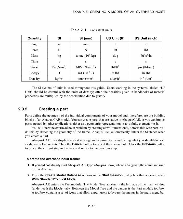
Table 2–1 Consistent units.
Quantity SI SI (mm) US Unit (ft) US Unit (inch)
Length m mm ft in
Force N N lbf lbf
Mass kg tonne (103 kg) slug lbf s2 /in
Time s s s s
Stress Pa (N/m2) MPa (N/mm2) lbf/ft2 psi (lbf/in2 )
Energy J mJ (10−3 J) ft lbf in lbf
Density kg/m3 tonne/mm3 slug/ft3 lbf s2 /in4
The SI system of units is used throughout this guide. Users working in the systems labeled “USUnit” should be careful with the units of density; often the densities given in handbooks of materialproperties are multiplied by the acceleration due to gravity.
2.3.2 Creating a part
Parts define the geometry of the individual components of your model and, therefore, are the buildingblocks of an Abaqus/CAE model. You can create parts that are native to Abaqus/CAE, or you can importparts created by other applications either as a geometric representation or as a finite element mesh.
You will start the overhead hoist problem by creating a two-dimensional, deformable wire part. Youdo this by sketching the geometry of the frame. Abaqus/CAE automatically enters the Sketcher whenyou create a part.
Abaqus/CAE often displays a short message in the prompt area indicating what you should do next,as shown in Figure 2–6. Click the Cancel button to cancel the current task. Click the Previous buttonto cancel the current step in the task and return to the previous step.
To create the overhead hoist frame:
1. If you did not already start Abaqus/CAE, type abaqus cae, where abaqus is the command usedto run Abaqus.
2. From the Create Model Database options in the Start Session dialog box that appears, selectWith Standard/Explicit Model.
Abaqus/CAE enters the Part module. The Model Tree appears in the left side of the main window(underneath the Model tab). Between the Model Tree and the canvas is the Part module toolbox.A toolbox contains a set of icons that allow expert users to bypass the menus in the main menu bar.
2–15
Abaqus ID:Printed on:

EXAMPLE: CREATING A MODEL OF AN OVERHEAD HOIST
promptprevious
cancel
Figure 2–6 Messages and instructions are displayed in the prompt area.
For many tools, as you select an item from the main menu bar or the Model Tree, the correspondingtool is highlighted in the module toolbox so you can learn its location.
3. In the Model Tree, double-click the Parts container to create a new part.
The Create Part dialog box appears. Abaqus/CAE also displays text in the prompt area near thebottom of the window to guide you through the procedure.
You use the Create Part dialog box to name the part; to choose its modeling space, type, and basefeature; and to set the approximate size. You can edit and rename a part after you create it; you canalso change its modeling space and type but not its base feature.
4. Name the part Frame. Choose a two-dimensional planar deformable body and a wire base feature.
5. In the Approximate size text field, type 4.0.
The value entered in the Approximate size text field at the bottom of the dialog box sets theapproximate size of the new part. The size that you enter is used by Abaqus/CAE to calculate thesize of the Sketcher sheet and the spacing of its grid. You should choose this value to be on theorder of the largest dimension of your finished part. Recall that Abaqus/CAE does not use specificunits, but the units must be consistent throughout the model. In this model SI units will be used.
6. Click Continue to exit the Create Part dialog box.
Abaqus/CAE automatically enters the Sketcher. The Sketcher toolbox appears in the left side ofthe main window, and the Sketcher grid appears in the viewport. The Sketcher contains a set ofbasic tools that allow you to sketch the two-dimensional profile of your part. Abaqus/CAE entersthe Sketcher whenever you create or edit a part. To finish using any tool, click mouse button 2 inthe viewport or select a new tool.
Tip: Like all tools in Abaqus/CAE, if you simply position the cursor over a tool in theSketcher toolbox for a short time, a small window appears that gives a brief descriptionof the tool. When you select a tool, a white background appears on it.
The following aspects of the Sketcher help you sketch the desired geometry:
• The Sketcher grid helps you position the cursor and align objects in the viewport.• Dashed lines indicate the X- and Y-axes of the sketch and intersect at the origin of the sketch.
2–16
Abaqus ID:Printed on:
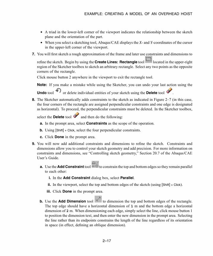
EXAMPLE: CREATING A MODEL OF AN OVERHEAD HOIST
• A triad in the lower-left corner of the viewport indicates the relationship between the sketchplane and the orientation of the part.
• When you select a sketching tool, Abaqus/CAE displays the X- and Y-coordinates of the cursorin the upper-left corner of the viewport.
7. You will first sketch a rough approximation of the frame and later use constraints and dimensions to
refine the sketch. Begin by using theCreate Lines: Rectangle tool located in the upper-rightregion of the Sketcher toolbox to sketch an arbitrary rectangle. Select any two points as the oppositecorners of the rectangle.
Click mouse button 2 anywhere in the viewport to exit the rectangle tool.
Note: If you make a mistake while using the Sketcher, you can undo your last action using the
Undo tool or delete individual entities of your sketch using the Delete tool .
8. The Sketcher automatically adds constraints to the sketch as indicated in Figure 2–7 (in this case,the four corners of the rectangle are assigned perpendicular constraints and one edge is designatedas horizontal). To proceed, the perpendicular constraints must be deleted. In the Sketcher toolbox,
select the Delete tool and then do the following:
a. In the prompt area, select Constraints as the scope of the operation.
b. Using [Shift] + Click, select the four perpendicular constraints.
c. Click Done in the prompt area.
9. You will now add additional constraints and dimensions to refine the sketch. Constraints anddimensions allow you to control your sketch geometry and add precision. For more information onconstraints and dimensions, see “Controlling sketch geometry,” Section 20.7 of the Abaqus/CAEUser’s Guide.
a. Use theAdd Constraint tool to constrain the top and bottom edges so they remain parallelto each other:
i. In the Add Constraint dialog box, select Parallel.
ii. In the viewport, select the top and bottom edges of the sketch (using [Shift] + Click).
iii. Click Done in the prompt area.
b. Use the Add Dimension tool to dimension the top and bottom edges of the rectangle.The top edge should have a horizontal dimension of 1 m and the bottom edge a horizontaldimension of 2m. When dimensioning each edge, simply select the line, click mouse button 1to position the dimension text, and then enter the new dimension in the prompt area. Selectingthe line rather than its endpoints constrains the length of the line regardless of its orientationin space (in effect, defining an oblique dimension).
2–17
Abaqus ID:Printed on:
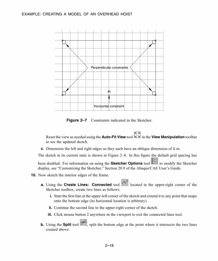
EXAMPLE: CREATING A MODEL OF AN OVERHEAD HOIST
Perpendicular constraints
Horizontal constraint
H
Figure 2–7 Constraints indicated in the Sketcher.
Reset the view as needed using theAuto-Fit View tool in the View Manipulation toolbarto see the updated sketch.
c. Dimension the left and right edges so they each have an oblique dimension of 1 m.
The sketch in its current state is shown in Figure 2–8. In this figure the default grid spacing has
been doubled. For information on using the Sketcher Options tool to modify the Sketcherdisplay, see “Customizing the Sketcher,” Section 20.9 of the Abaqus/CAE User’s Guide.
10. Now sketch the interior edges of the frame.
a. Using the Create Lines: Connected tool located in the upper-right corner of theSketcher toolbox, create two lines as follows:
i. Start the first line at the upper-left corner of the sketch and extend it to any point that snapsonto the bottom edge (its horizontal location is arbitrary).
ii. Continue the second line to the upper-right corner of the sketch.
iii. Click mouse button 2 anywhere in the viewport to exit the connected lines tool.
b. Using the Split tool , split the bottom edge at the point where it intersects the two linescreated above:
2–18
Abaqus ID:Printed on:

EXAMPLE: CREATING A MODEL OF AN OVERHEAD HOIST
H
1. 1.
2.
1.
Figure 2–8 Rough sketch of frame (with grid spacing doubled).
i. Note the small black triangles at the base of some of the toolbox icons. These trianglesindicate the presence of hidden icons that can be revealed. Click and hold the Auto-Trim
tool located on the middle-right of the Sketcher toolbox until additional icons appear.
ii. From the set of additional icons, click the Split tool .
The split tool appears in the Sketcher toolbox with a white background indicating that youselected it.
iii. Select the bottom edge as the first entity to define the split point.
iv. Select either of the two interior lines as the second entity (a red circle will appear aroundthe split point).
v. Click mouse button 2 to indicate that you have finished using the split tool.
c. Use the Add Constraint tool to constrain the two segments of the bottom edge so theyare of equal length:
i. In the Add Constraint dialog box, select Equal length.
ii. In the viewport, select the two segments of the bottom edge.
2–19
Abaqus ID:Printed on:
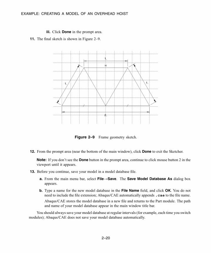
EXAMPLE: CREATING A MODEL OF AN OVERHEAD HOIST
iii. Click Done in the prompt area.
11. The final sketch is shown in Figure 2–9.
H
1.1.
2.
1.
Figure 2–9 Frame geometry sketch.
12. From the prompt area (near the bottom of the main window), click Done to exit the Sketcher.
Note: If you don’t see the Done button in the prompt area, continue to click mouse button 2 in theviewport until it appears.
13. Before you continue, save your model in a model database file.
a. From the main menu bar, select File→Save. The Save Model Database As dialog boxappears.
b. Type a name for the new model database in the File Name field, and click OK. You do notneed to include the file extension; Abaqus/CAE automatically appends .cae to the file name.
Abaqus/CAE stores the model database in a new file and returns to the Part module. The pathand name of your model database appear in the main window title bar.
You should always save your model database at regular intervals (for example, each time you switchmodules); Abaqus/CAE does not save your model database automatically.
2–20
Abaqus ID:Printed on:
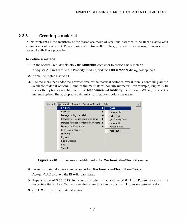
EXAMPLE: CREATING A MODEL OF AN OVERHEAD HOIST
2.3.3 Creating a materialIn this problem all the members of the frame are made of steel and assumed to be linear elastic withYoung’s modulus of 200 GPa and Poisson’s ratio of 0.3. Thus, you will create a single linear elasticmaterial with these properties.
To define a material:
1. In the Model Tree, double-click the Materials container to create a new material.
Abaqus/CAE switches to the Property module, and the Edit Material dialog box appears.
2. Name the material Steel.
3. Use the menu bar under the browser area of the material editor to reveal menus containing all theavailable material options. Some of the menu items contain submenus; for example, Figure 2–10shows the options available under the Mechanical→Elasticity menu item. When you select amaterial option, the appropriate data entry form appears below the menu.
Figure 2–10 Submenus available under the Mechanical→Elasticity menu.
4. From the material editor’s menu bar, select Mechanical→Elasticity→Elastic.
Abaqus/CAE displays the Elastic data form.
5. Type a value of 200.0E9 for Young’s modulus and a value of 0.3 for Poisson’s ratio in therespective fields. Use [Tab] or move the cursor to a new cell and click to move between cells.
6. Click OK to exit the material editor.
2–21
Abaqus ID:Printed on:
EXAMPLE: CREATING A MODEL OF AN OVERHEAD HOIST
2.3.4 Defining and assigning section propertiesYou define the properties of a part through sections. After you create a section, you can use one of thefollowing two methods to assign the section to the part in the current viewport:
• You can simply select the region from the part and assign the section to the selected region.• You can use the Set toolset to create a homogeneous set containing the region and assign the sectionto the set.
For the frame model you will create a single truss section that you will assign to the frame by selectingthe frame from the viewport. The section will refer to the material Steel that you just created as wellas define the cross-sectional area of the frame members.
Defining a truss section
A truss section definition requires only a material reference and the cross-sectional area. Rememberthat the frame members are circular bars that are 0.005 m in diameter. Thus, their cross-sectionalarea is 1.963 × 10⁻⁵ m2 .
Tip: You can use the command line interface (CLI) in Abaqus/CAE as a simplecalculator. For example, to compute the cross-sectional area of the frame members, click
the tab in the bottom left corner of the Abaqus/CAE window to activate the CLI,type pi*0.005**2/4.0 after the command prompt, and press [Enter]. The value ofthe cross-sectional area is printed in the CLI.
To define a truss section:
1. In the Model Tree, double-click the Sections container to create a section.
The Create Section dialog box appears.
2. In the Create Section dialog box:
a. Name the section FrameSection.
b. In the Category list, select Beam.
c. In the Type list, select Truss.
d. Click Continue.
The Edit Section dialog box appears.
3. In the Edit Section dialog box:
a. Accept the default selection of Steel for the Material associated with the section. Ifyou had defined other materials, you could click the arrow next to the Material text boxto see a list of available materials and to select the material of your choice.
b. In the Cross-sectional area field, enter pi*0.005**2/4.0.
2–22
Abaqus ID:Printed on:

EXAMPLE: CREATING A MODEL OF AN OVERHEAD HOIST
Tip: If a field in a dialog box is expecting a floating point number, you can enteran arithmetic expression instead. The expression is evaluated by the Pythoninterpreter that is built into Abaqus/CAE. The arithmetic expression will bereplaced by its value.
c. Click OK.
Assigning the section to the frame
The section FrameSection must be assigned to the frame.
To assign the section to the frame:
1. In the Model Tree, expand the branch for the part named Frame by clicking the “ ” symbolto expand the Parts container and then clicking the “ ” symbol to expand the Frame item.
2. Double-click Section Assignments in the list of part attributes that appears.
Abaqus/CAE displays prompts in the prompt area to guide you through the procedure.
3. Select the entire part as the region to which the section will be applied.
a. Click and hold mouse button 1 at the upper left-hand corner of the viewport.
b. Drag the mouse to create a box around the truss.
c. Release mouse button 1.
Abaqus/CAE highlights the entire frame.
4. In the prompt area, enter all as the name of the set that will be created.
This set will contain the selected regions. The advantage of creating a set is that it can be usedfor other purposes. If you prefer to not create a set, toggle off Create set in the prompt area.
5. Click mouse button 2 in the viewport or click Done in the prompt area to accept the selectedgeometry.
The Edit Section Assignment dialog box appears containing a list of existing sections.
6. Accept the default selection of FrameSection, and click OK.
Abaqus/CAE assigns the truss section to the frame, colors the entire frame aqua to indicate thatthe region has a section assignment, and closes the Edit Section Assignment dialog box.
2.3.5 Defining the assemblyEach part that you create is oriented in its own coordinate system and is independent of the other partsin the model. Although a model may contain many parts, it contains only one assembly. You define thegeometry of the assembly by creating instances of a part and then positioning the instances relativeto each other in a global coordinate system. An instance can be classified as either independent ordependent. Independent part instances are meshed individually, while the mesh of a dependent part
2–23
Abaqus ID:Printed on:

EXAMPLE: CREATING A MODEL OF AN OVERHEAD HOIST
instance is associated with the mesh of the original part. For further details, see “Working with partinstances,” Section 13.3 of the Abaqus/CAE User’s Guide. By default, part instances are dependent.
For this problem you will create a single instance of your overhead hoist. Abaqus/CAE positionsthe instance so that the origin of the sketch that defined the frame overlays the origin of the assembly’sdefault coordinate system.
To define the assembly:
1. In the Model Tree, expand the Assembly container and double-click Instances in the list thatappears.
Abaqus/CAE switches to the Assembly module, and the Create Instance dialog box appears.
2. In the dialog box, select Parts to choose parts from the current model.
3. Select Frame and click OK.
Abaqus/CAE creates an instance of the overhead hoist. In this example the single instance of theframe defines the assembly. The frame is displayed in the 1–2 plane of the global coordinate system (aright-handed, rectangular Cartesian system). A triad in the lower-left corner of the viewport indicatesthe orientation of the model with respect to the view. A second triad in the viewport indicates the originand orientation of the global coordinate system (X-, Y-, and Z-axes). The global 1-axis is the horizontalaxis of the hoist, the global 2-axis is the vertical axis, and the global 3-axis is normal to the plane of theframework. For two-dimensional problems such as this one Abaqus requires that the model lie in a planeparallel to the global 1–2 plane.
2.3.6 Configuring your analysisNow that you have created your assembly, you can configure your analysis. In this simulation we areinterested in the static response of the overhead hoist to a 10 kN load applied at the midspan, with theleft-hand end fully constrained and a roller constraint on the right-hand end (see Figure 2–5). This is asingle event, so only a single analysis step is needed for the simulation. Thus, the model will consist oftwo steps overall:
• An initial step, in which you will apply boundary conditions that constrain the ends of the frame.• An analysis step, in which you will apply a concentrated load at the midspan of the frame.
Abaqus/CAE generates the initial step automatically, but you must create the analysis step yourself. Youmay also request output for any steps in the analysis.
There are two kinds of analysis steps in Abaqus: general analysis steps, which can be used toanalyze linear or nonlinear response, and linear perturbation steps, which can be used only to analyzelinear problems. Only general analysis steps are available in Abaqus/Explicit. For this simulation youwill define a static linear perturbation step. Perturbation procedures are discussed further in Chapter 11,“Multiple Step Analysis.”
Creating an analysis step
Create a static, linear perturbation step that follows the initial step of the analysis.
2–24
Abaqus ID:Printed on:
EXAMPLE: CREATING A MODEL OF AN OVERHEAD HOIST
To create a static linear perturbation analysis step:
1. In the Model Tree, double-click the Steps container to create a step.
Abaqus/CAE switches to the Step module, and the Create Step dialog box appears. A list ofall the general procedures and a default step name of Step-1 is provided.
2. Change the step name to Apply load.
3. Select Linear perturbation as the Procedure type.
4. From the list of available linear perturbation procedures in the Create Step dialog box, selectStatic, Linear perturbation and click Continue.
The Edit Step dialog box appears with the default settings for a static linear perturbation step.
5. The Basic tab is selected by default. In the Description field, type 10 kN centralload.
6. Click the Other tab to see its contents; you can accept the default values provided for the step.
7. Click OK to create the step and to exit the Edit Step dialog box.
Requesting data output
Finite element analyses can create very large amounts of output. Abaqus allows you to control andmanage this output so that only data required to interpret the results of your simulation are produced.Four types of output are available from an Abaqus analysis:
• Results stored in a neutral binary file used by Abaqus/CAE for postprocessing. This file iscalled the Abaqus output database file and has the extension .odb.
• Printed tables of results, written to the Abaqus data (.dat) file. Output to the data file isavailable only in Abaqus/Standard.
• Restart data used to continue the analysis, written to the Abaqus restart (.res) file.• Results stored in binary files for subsequent postprocessing with third-party software, writtento the Abaqus results (.fil) file.
You will use only the first of these in the overhead hoist simulation.By default, Abaqus/CAE writes the results of the analysis to the output database (.odb) file.
When you create a step, Abaqus/CAE generates a default output request for the step. A list of thepreselected variables written by default to the output database is given in the Abaqus AnalysisUser’s Guide. You do not need to do anything to accept these defaults. You use the FieldOutput Requests Manager to request output of variables that should be written at relatively lowfrequencies to the output database from the entire model or from a large portion of the model. Youuse the History Output Requests Manager to request output of variables that should be writtento the output database at a high frequency from a small portion of the model; for example, thedisplacement of a single node.
For this example you will examine the output requests to the .odb file and accept the defaultconfiguration.
2–25
Abaqus ID:Printed on:
EXAMPLE: CREATING A MODEL OF AN OVERHEAD HOIST
To examine your output requests to the .odb file:
1. In the Model Tree, click mouse button 3 on the Field Output Requests container and selectManager from the menu that appears.
Abaqus/CAE displays the Field Output Requests Manager. This manager displays thestatus of field output requests in a table format. The left side of the table has an alphabeticallist of existing output requests. The top of the table lists the names of all the steps in the analysisin the order of execution. Each cell of the table displays the status of each output request ineach step.
You can use the Field Output Requests Manager to do the following:
• Select the variables that Abaqus will write to the output database.• Select the section points for which Abaqus will generate output data.• Select the region of the model for which Abaqus will generate output data.• Change the frequency at which Abaqus will write data to the output database.
2. Review the default output request that Abaqus/CAE generates for the Static, Linearperturbation step you created and named Apply load.
Select the cell in the table labeled Created if it is not already selected. The followinginformation related to the cell is shown in the legend at the bottom of the manager:
• The type of analysis procedure carried out in the step in that column.• The list of output request variables.• The output request status.
3. On the right side of the Field Output Requests Manager, click Edit to view more detailedinformation about the output request.
The field output editor appears. In the Output Variables region of this dialog box, there is atext box that lists all variables that will be output. If you change an output request, you canalways return to the default settings by choosing Preselected defaults above the text box.
4. Click the arrows next to each output variable category to see exactly which variables will beoutput. The boxes next to each category title allow you to see at a glance whether all variablesin that category will be output. A black check mark indicates that all variables are output,while a gray check mark indicates that only some variables will be output.
Based on the selections shown at the bottom of the dialog box, data will be generated atevery default section point in the model and will be written to the output database after everyincrement during the analysis.
5. Click Cancel to close the field output editor, since you do not wish to make any changes tothe default output requests.
6. Click Dismiss to close the Field Output Requests Manager.
2–26
Abaqus ID:Printed on:

EXAMPLE: CREATING A MODEL OF AN OVERHEAD HOIST
Note: What is the difference between the Dismiss and Cancel buttons? Dismiss buttonsappear in dialog boxes that contain data that you cannot modify. For example, the FieldOutput Requests Manager allows you to view output requests, but you must use the fieldoutput editor to modify those requests. Clicking the Dismiss button simply closes the FieldOutput Requests Manager. Conversely, Cancel buttons appear in dialog boxes that allowyou to make changes. Clicking Cancel closes the dialog box without saving your changes.
7. Review the history output requests in a similar manner by right-clicking the History OutputRequests container in the Model Tree and opening the history output editor.
2.3.7 Applying boundary conditions and loads to the model
Prescribed conditions, such as loads and boundary conditions, are step dependent, which means that youmust specify the step or steps in which they become active. Now that you have defined the steps in theanalysis, you can define prescribed conditions.
Applying boundary conditions to the frame
In structural analyses, boundary conditions are applied to those regions of the model where thedisplacements and/or rotations are known. Such regions may be constrained to remain fixed(have zero displacement and/or rotation) during the simulation or may have specified, nonzerodisplacements and/or rotations.
In this model the bottom-left portion of the frame is constrained completely and, thus, cannotmove in any direction. The bottom-right portion of the frame, however, is fixed in the verticaldirection but is free to move in the horizontal direction. The directions in which motion is possibleare called degrees of freedom (dof).
The labeling convention used for the displacement and rotational degrees of freedom in Abaqusis shown in Figure 2–11.
To apply boundary conditions to the frame:
1. In the Model Tree, double-click the BCs container.
Abaqus/CAE switches to the Load module, and the Create Boundary Condition dialog boxappears.
2. In the Create Boundary Condition dialog box:
a. Name the boundary condition Fixed.
b. From the list of steps, select Initial as the step in which the boundary condition will beactivated. All the mechanical boundary conditions specified in the Initial step musthave zero magnitudes. This condition is enforced automatically by Abaqus/CAE.
c. In the Category list, accept Mechanical as the default category selection.
2–27
Abaqus ID:Printed on:
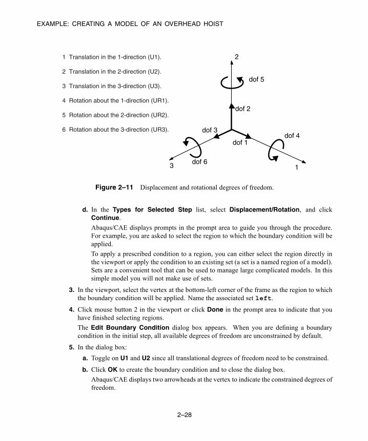
EXAMPLE: CREATING A MODEL OF AN OVERHEAD HOIST
dof 5
dof 4
dof 6
dof 1
dof 3
dof 2
2
3 1
1 Translation in the 1-direction (U1).
2 Translation in the 2-direction (U2).
3 Translation in the 3-direction (U3).
4 Rotation about the 1-direction (UR1).
5 Rotation about the 2-direction (UR2).
6 Rotation about the 3-direction (UR3).
Figure 2–11 Displacement and rotational degrees of freedom.
d. In the Types for Selected Step list, select Displacement/Rotation, and clickContinue.
Abaqus/CAE displays prompts in the prompt area to guide you through the procedure.For example, you are asked to select the region to which the boundary condition will beapplied.
To apply a prescribed condition to a region, you can either select the region directly inthe viewport or apply the condition to an existing set (a set is a named region of a model).Sets are a convenient tool that can be used to manage large complicated models. In thissimple model you will not make use of sets.
3. In the viewport, select the vertex at the bottom-left corner of the frame as the region to whichthe boundary condition will be applied. Name the associated set left.
4. Click mouse button 2 in the viewport or click Done in the prompt area to indicate that youhave finished selecting regions.
The Edit Boundary Condition dialog box appears. When you are defining a boundarycondition in the initial step, all available degrees of freedom are unconstrained by default.
5. In the dialog box:
a. Toggle on U1 and U2 since all translational degrees of freedom need to be constrained.
b. Click OK to create the boundary condition and to close the dialog box.
Abaqus/CAE displays two arrowheads at the vertex to indicate the constrained degrees offreedom.
2–28
Abaqus ID:Printed on:
EXAMPLE: CREATING A MODEL OF AN OVERHEAD HOIST
6. Repeat the above procedure to constrain degree of freedomU2 at the vertex at the bottom-rightcorner of the frame. Name this boundary condition Roller and the associated set right.
7. In the Model Tree, click mouse button 3 on the BCs container and select Manager from themenu that appears.
Abaqus/CAE displays the Boundary Condition Manager. The manager indicates that theboundary conditions are Created (activated) in the initial step and are Propagated frombase state (continue to be active) in the analysis step Apply load.
Tip: To view the title of a column in its entirety, expand its width by dragging thedividing line between the column headings.
8. Click Dismiss to close the Boundary Condition Manager.
In this example all the constraints are in the global 1- or 2-directions. In many cases constraintsare required in directions that are not aligned with the global directions. In such cases you can definea local coordinate system for boundary condition application. The skew plate example in Chapter 5,“Using Shell Elements,” demonstrates how to do this.
Applying a load to the frame
Now that you have constrained the frame, you can apply a load to the bottom of the frame. InAbaqus the term load (as in the Load module in Abaqus/CAE) generally refers to anything thatinduces a change in the response of a structure from its initial state, including:
• concentrated forces,• pressures,• nonzero boundary conditions,• body loads, and• temperature (with thermal expansion of the material defined).
Sometimes the term load is used to refer specifically to force-type quantities (as in the LoadManager of the Load module); for example, concentrated forces, pressures, and body loads butnot boundary conditions or temperature. The intended meaning of the term should be clear fromthe context of the discussion.
In this simulation a concentrated force of 10 kN is applied in the negative 2-direction to themidspan of the frame; the load is applied during the linear perturbation step you created earlier. Inreality there is no such thing as a concentrated, or point, load; the load will always be applied oversome finite area. However, if the area being loaded is small, it is an appropriate idealization to treatthe load as a concentrated load.
To apply a concentrated force to the frame:
1. In the Model Tree, click mouse button 3 on the Loads container and selectManager from themenu that appears.
2–29
Abaqus ID:Printed on:
EXAMPLE: CREATING A MODEL OF AN OVERHEAD HOIST
The Load Manager appears.
2. At the bottom of the Load Manager, click Create.
The Create Load dialog box appears.
3. In the Create Load dialog box:
a. Name the load Force.
b. From the list of steps, select Apply load as the step in which the load will be applied.
c. In the Category list, accept Mechanical as the default category selection.
d. In the Types for Selected Step list, accept the default selection ofConcentrated force.
e. Click Continue.
Abaqus/CAE displays prompts in the prompt area to guide you through the procedure. Youare asked to select a region to which the load will be applied.
As with boundary conditions, the region to which the load will be applied can be selectedeither directly in the viewport or from a list of existing sets. As before, you will select theregion directly in the viewport.
4. In the viewport, select the vertex at the bottom center of the frame as the region where the loadwill be applied. Name the associated set center.
5. Click mouse button 2 in the viewport or click Done in the prompt area to indicate that youhave finished selecting regions.
The Edit Load dialog box appears.
6. In the dialog box:
a. Enter a magnitude of -10000.0 for CF2.
b. Click OK to create the load and to close the dialog box.
Abaqus/CAE displays a downward-pointing arrow at the vertex to indicate that the loadis applied in the negative 2-direction.
7. Examine the Load Manager and note that the new load is Created (activated) in the analysisstep Apply load.
8. Click Dismiss to close the Load Manager.
2.3.8 Meshing the model
You will now generate the finite element mesh. You can choose the meshing technique that Abaqus/CAEwill use to create the mesh, the element shape, and the element type. The meshing technique for one-dimensional regions (such as the ones in this example) cannot be changed, however. Abaqus/CAE usesa number of different meshing techniques. The default meshing technique assigned to the model is
2–30
Abaqus ID:Printed on:
EXAMPLE: CREATING A MODEL OF AN OVERHEAD HOIST
indicated by the color of the model that is displayed when you enter the Mesh module; if Abaqus/CAEdisplays the model in orange, it cannot be meshed without assistance from you.
Assigning an Abaqus element type
In this section you will assign a particular Abaqus element type to the model. Although you willassign the element type now, you could also wait until after the mesh has been created.
Two-dimensional truss elements will be used to model the frame. These elements are chosenbecause truss elements, which carry only tensile and compressive axial loads, are ideal for modelingpin-jointed frameworks such as this overhead hoist.
To assign an Abaqus element type:
1. In the Model Tree, expand the Frame item underneath the Parts container if it is not alreadyexpanded. Then double-click Mesh in the list that appears.
Abaqus/CAE switches to the Mesh module. The Mesh module functionality is available onlythrough menu bar items or toolbox icons.
2. From the main menu bar, select Mesh→Element Type.
3. If you created the set named all while assigning section properties, click Sets in the right sideof the prompt area and select all from the Region Selection dialog box. Otherwise, drag themouse to create a box that selects the entire frame as the region to be assigned an element typeand click Done in the prompt area when you are finished.
The Element Type dialog box appears.
4. In the dialog box, select the following:
• Standard as the Element Library selection (the default).
• Linear as the Geometric Order (the default).
• Truss as the Family of elements.
5. In the lower portion of the dialog box, examine the element shape options. A brief descriptionof the default element selection is available at the bottom of each tabbed page.
Since the model is a two-dimensional truss, only two-dimensional truss element types areshown on the Line tabbed page. A description of the element type T2D2 appears at the bottomof the dialog box. Abaqus/CAE will now associate T2D2 elements with the elements in themesh.
6. Click OK to assign the element type and to close the dialog box.
7. In the prompt area, click Done to end the procedure.
Creating the mesh
Basic meshing is a two-stage operation: first you seed the edges of the part instance, and then youmesh the part instance. You select the number of seeds based on the desired element size or on the
2–31
Abaqus ID:Printed on:
EXAMPLE: CREATING A MODEL OF AN OVERHEAD HOIST
number of elements that you want along an edge, and Abaqus/CAE places the nodes of the mesh atthe seeds whenever possible. For this problem you will create one element on each bar of the hoist.
To seed and mesh the model:
1. From the main menu bar, select Seed→Part to seed the part instance.
Note: You can gain more control of the resulting mesh by seeding each edge of the partinstance individually, but it is not necessary for this example.
The Global Seeds dialog box appears. The dialog box displays the default element size thatAbaqus/CAE will use to seed the part instance. This default element size is based on the sizeof the part instance. A relatively large seed value will be used so that only one element will becreated per region.
2. In theGlobal Seeds dialog box, specify an approximate global element size of 1.0, and clickOK to create the seeds and to close the dialog box.
3. From the main menu bar, select Mesh→Part to mesh the part instance.
4. From the buttons in the prompt area, click Yes to confirm that you want to mesh the partinstance.
Tip: You can display the node and element numbers within the Mesh module by selectingView→Part Display Options from the main menu bar. Toggle on Show node labelsand Show element labels in theMesh tabbed page of the Part Display Options dialogbox that appears.
2.3.9 Creating an analysis jobNow that you have configured your analysis, you will create a job that is associated with your model.
To create an analysis job:
1. In the Model Tree, double-click the Jobs container to create a job.
Abaqus/CAE switches to the Job module, and the Create Job dialog box appears with a list of themodels in the model database. When you are finished defining your job, the Jobs container willdisplay a list of your jobs.
2. Name the job Frame, and click Continue.
The Edit Job dialog box appears.
3. In the Description field, type Two-dimensional overhead hoist frame.
4. Click OK to accept all other default job settings in the job editor and to close the dialog box.
2–32
Abaqus ID:Printed on:

EXAMPLE: CREATING A MODEL OF AN OVERHEAD HOIST
2.3.10 Checking the modelHaving generated the model for this simulation, you are ready to run the analysis. Unfortunately, it ispossible to have errors in the model because of incorrect or missing data. You should perform a datacheck analysis first before running the simulation.
To run a data check analysis:
1. In the Model Tree, expand the Jobs container. Click mouse button 3 on the job named Frame, andselect Data Check from the menu that appears to submit your job for a data check analysis.
2. After you submit your job, information appears next to the job name indicating the job’s status. Thestatus of the overhead hoist problem indicates one of the following conditions:
• Check Submitted while the model is being submitted for a data check.
• Check Running while Abaqus performs a data check on the model.
• Check Completed when the data check has completed successfully.
• Submitted while the job is being submitted for a full analysis.
• Running while Abaqus analyzes the model.
• Completed when the full analysis is complete, and the output has been written to the outputdatabase.
• Aborted if Abaqus/CAE finds a problem with the input file or the analysis and aborts theanalysis. In addition, Abaqus/CAE reports the problem in the message area (see Figure 2–2).
During the analysis, Abaqus/Standard sends information to Abaqus/CAE to allow you to monitorthe progress of the job. Information from the status, data, log, and message files appears in the JobMonitor dialog box. You can browse these files in the tabbed windows in the bottom half of the JobMonitor dialog box, and you can search their contents. Select the desired file tab, enter a search stringin the Text to find field, and click Next or Previous to step through the file from one hit to the next.Toggle on Match case to perform a case-sensitive search.
To monitor the status of a job:
1. In the Model Tree, click mouse button 3 on the job named Frame and select Monitor from themenu that appears to open the Job Monitor dialog box.
The Job Monitor dialog box appears.
2. The top half of the dialog box displays the information available in the status (.sta) file thatAbaqus creates for the analysis. This file contains a brief summary of the progress of an analysisand is described in “Output,” Section 4.1.1 of the Abaqus Analysis User’s Guide. The bottom halfof the dialog box allows you to view information about the analysis.
2–33
Abaqus ID:Printed on:

EXAMPLE: CREATING A MODEL OF AN OVERHEAD HOIST
• Click the Log tab to display the start and end times for the analysis that appear in the log(.log) file.
• Click the Errors and Warnings tabs to display the errors or the warnings that appear in thedata (.dat) and message (.msg) files. If a particular region of the model is causing the erroror warning, a node or element set will be created automatically that contains that region. Thename of the node or element set appears with the error or warning message, and you can viewthe set using display groups in the Visualization module.
It will not be possible to perform the analysis until the causes of any error messages arecorrected. In addition, you should always investigate the reason for any warning messagesto determine whether corrective action is needed or whether such messages can be ignoredsafely.
Abaqus limits the number of error and warning messages that appear in the job monitor (bydefault these limits are 10 error messages and 50 warning messages). If the message limitsare exceeded, information regarding the additional errors and warnings can be obtained fromthe printed output files themselves. See “Job customization parameters,” Section 4.1.4 of theAbaqus Installation and Licensing Guide, for details on changing the default message limits.
• Click the Output tab to display a record of each output data entry as it is written to the outputdatabase.
• As the analysis proceeds and Abaqus creates the data, message, and status files, Abaqus/CAEactivates the Data File,Message File, and Status File tabs and displays the contents of eachfile in the corresponding tabbed page. You can click any of these tabs to browse or search thefile for additional error and warning messages.
Note: Although Abaqus/CAE updates the contents of the Data File, Message File, andStatus File tabbed pages periodically as the analysis runs, the data might not always besynchronized with the latest data in the files.
3. Click Dismiss to close the Job Monitor dialog box.
2.3.11 Running the analysisMake any necessary corrections to your model. When the data check analysis completes with no errormessages, run the analysis itself. To do this, click mouse button 3 on the job named Frame and selectContinue from the menu that appears.
Note: Performing a data check analysis results in the creation of job files. When you submit a job foranalysis and files of the same name already exist, Abaqus/CAE displays a dialog box asking if it is OKto overwrite the job files. Click OK to continue.
You should always perform a data check analysis before running a simulation to ensure that themodel has been defined correctly and to check that there is enough disk space and memory availableto complete the analysis. However, it is possible to combine the data check and analysis phases of the
2–34
Abaqus ID:Printed on:
EXAMPLE: CREATING A MODEL OF AN OVERHEAD HOIST
simulation by clicking mouse button 3 on the job name in the Jobs container and selecting Submit fromthe menu that appears.
If a simulation is expected to take a substantial amount of time, it may be convenient to run it ina batch queue by selecting Queue as the Run Mode in the Edit Job dialog box. (The availability ofsuch a queue depends on the queue definition settings in your Abaqus environment file. If you have anyquestions, refer to “Defining analysis batch queues,” Section 4.2 of the Abaqus Installation and LicensingGuide, or ask your system administrator about defining analysis batch queues on your system.)
2.3.12 Postprocessing
Graphical postprocessing is important because of the great volume of data created during a simulation.The Visualization module of Abaqus/CAE (also licensed separately as Abaqus/Viewer) allows you toview the results graphically using a variety of methods, including deformed shape plots, contour plots,vector plots, animations, and X–Y plots. In addition, it allows you to create tabular reports of the outputdata. All of these methods are discussed in this guide. For more information on any of the postprocessingfeatures discussed in this guide, consult Part V, “Viewing results,” of the Abaqus/CAE User’s Guide.For this example you will use the Visualization module to do some basic model checks and to displaythe deformed shape of the frame.
When the job completes successfully, you are ready to view the results of the analysis with theVisualization module. In the Model Tree, click mouse button 3 on the job named Frame and selectResults from the menu that appears to enter the Visualization module. Abaqus/CAE opens the outputdatabase created by the job and displays the undeformed model shape, as shown in Figure 2–12.
You can also enter the Visualization module by selecting Visualization from the Module listlocated in the context bar. Select File→Open, select Frame.odb from the list of available outputdatabase files, and click OK.
You can choose to display the title block and state block at the bottom of the viewport; these blocksare not shown in Figure 2–12. The title block at the bottom of the viewport indicates the following:
• The description of the model (from the job description).• The name of the output database (from the name of the analysis job).• The product name (Abaqus/Standard or Abaqus/Explicit) and release used to generate the outputdatabase.
• The date the output database was last modified.The state block at the bottom of the viewport indicates the following:
• Which step is being displayed.• The increment within the step.• The step time.
The view orientation triad indicates the orientation of the model in the global coordinate system. The 3Dcompass located in the upper-right corner of the viewport allows you to manipulate the view directly.
2–35
Abaqus ID:Printed on:
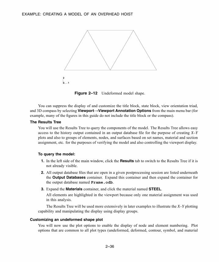
EXAMPLE: CREATING A MODEL OF AN OVERHEAD HOIST
1
2
3
Figure 2–12 Undeformed model shape.
You can suppress the display of and customize the title block, state block, view orientation triad,and 3D compass by selecting Viewport→Viewport Annotation Options from the main menu bar (forexample, many of the figures in this guide do not include the title block or the compass).
The Results Tree
You will use the Results Tree to query the components of the model. The Results Tree allows easyaccess to the history output contained in an output database file for the purpose of creating X–Yplots and also to groups of elements, nodes, and surfaces based on set names, material and sectionassignment, etc. for the purposes of verifying the model and also controlling the viewport display.
To query the model:
1. In the left side of the main window, click the Results tab to switch to the Results Tree if it isnot already visible.
2. All output database files that are open in a given postprocessing session are listed underneaththe Output Databases container. Expand this container and then expand the container forthe output database named Frame.odb.
3. Expand the Materials container, and click the material named STEEL.
All elements are highlighted in the viewport because only one material assignment was usedin this analysis.
The Results Tree will be used more extensively in later examples to illustrate the X–Y plottingcapability and manipulating the display using display groups.
Customizing an undeformed shape plot
You will now use the plot options to enable the display of node and element numbering. Plotoptions that are common to all plot types (undeformed, deformed, contour, symbol, and material
2–36
Abaqus ID:Printed on:
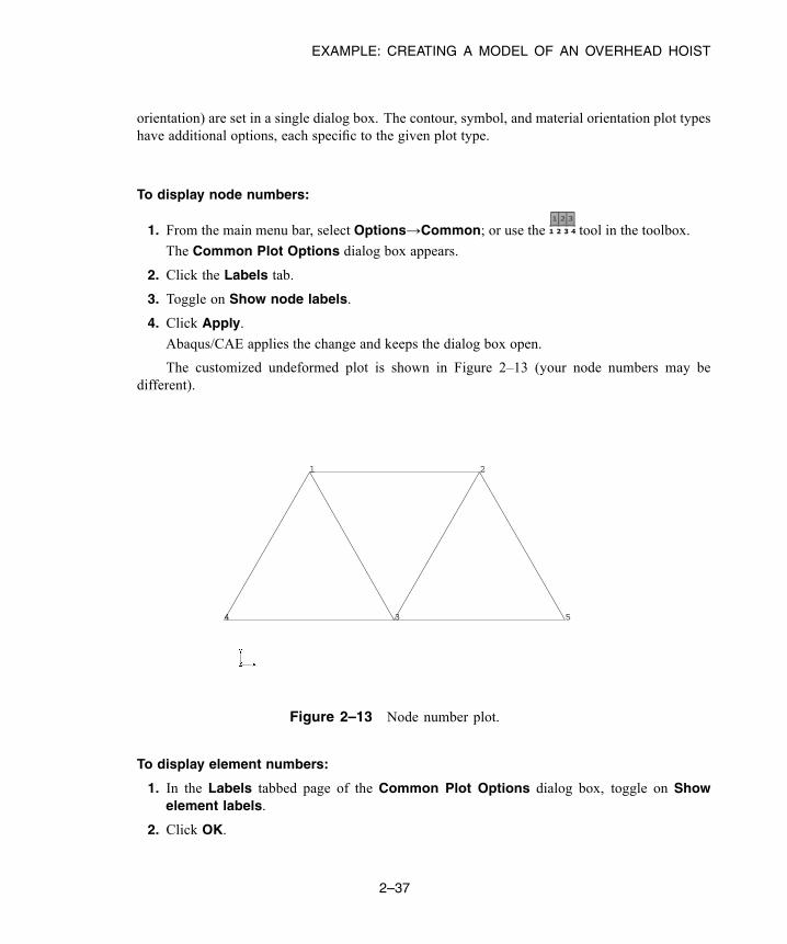
EXAMPLE: CREATING A MODEL OF AN OVERHEAD HOIST
orientation) are set in a single dialog box. The contour, symbol, and material orientation plot typeshave additional options, each specific to the given plot type.
To display node numbers:
1. From the main menu bar, select Options→Common; or use the tool in the toolbox.
The Common Plot Options dialog box appears.
2. Click the Labels tab.
3. Toggle on Show node labels.
4. Click Apply.
Abaqus/CAE applies the change and keeps the dialog box open.
The customized undeformed plot is shown in Figure 2–13 (your node numbers may bedifferent).
54 3
21
Figure 2–13 Node number plot.
To display element numbers:
1. In the Labels tabbed page of the Common Plot Options dialog box, toggle on Showelement labels.
2. Click OK.
2–37
Abaqus ID:Printed on:
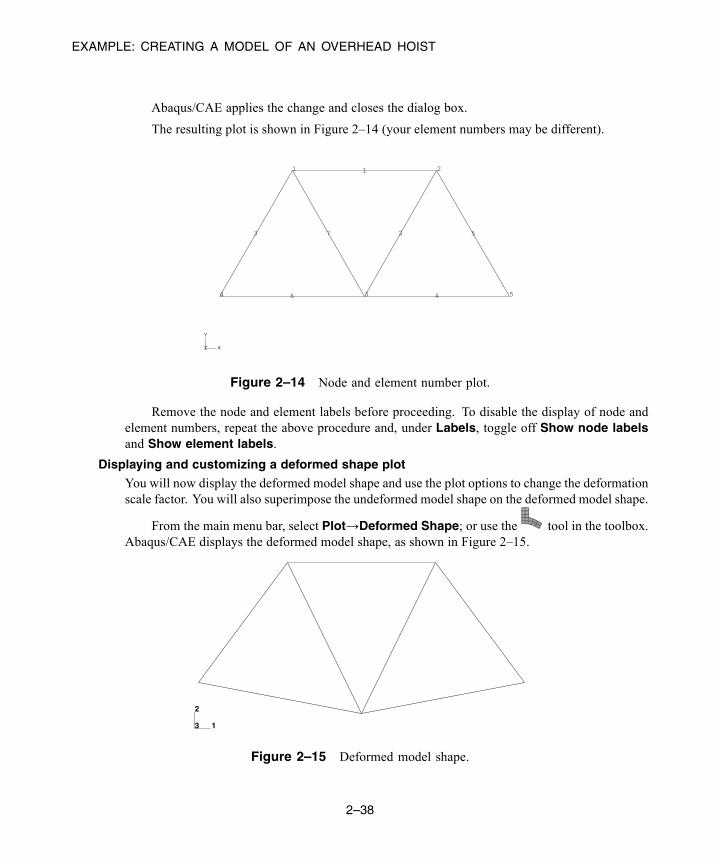
EXAMPLE: CREATING A MODEL OF AN OVERHEAD HOIST
Abaqus/CAE applies the change and closes the dialog box.
The resulting plot is shown in Figure 2–14 (your element numbers may be different).
54 3
21
7
6
5
4
3 2
1
X
Y
Z
Figure 2–14 Node and element number plot.
Remove the node and element labels before proceeding. To disable the display of node andelement numbers, repeat the above procedure and, under Labels, toggle off Show node labelsand Show element labels.
Displaying and customizing a deformed shape plot
You will now display the deformed model shape and use the plot options to change the deformationscale factor. You will also superimpose the undeformed model shape on the deformed model shape.
From the main menu bar, select Plot→Deformed Shape; or use the tool in the toolbox.Abaqus/CAE displays the deformed model shape, as shown in Figure 2–15.
1
2
3
Figure 2–15 Deformed model shape.
2–38
Abaqus ID:Printed on:

EXAMPLE: CREATING A MODEL OF AN OVERHEAD HOIST
For small-displacement analyses (the default formulation in Abaqus/Standard) thedisplacements are scaled automatically to ensure that they are clearly visible. The scale factor isdisplayed in the state block. In this case the displacements have been scaled by a factor of 42.83.
To change the deformation scale factor:
1. From the main menu bar, select Options→Common; or use the tool in the toolbox.
2. From the Common Plot Options dialog box, click the Basic tab if it is not already selected.
3. From the Deformation Scale Factor area, toggle on Uniform and enter 10.0 in the Valuefield.
4. Click Apply to redisplay the deformed shape.
The state block displays the new scale factor.
5. To return to automatic scaling of the displacements, repeat the above procedure and, in theDeformation Scale Factor field, toggle on Auto-compute.
6. Click OK to close the Common Plot Options dialog box.
To superimpose the undeformed model shape on the deformed model shape:
1. Click the Allow Multiple Plot States tool in the toolbox to allow multiple plot states
in the viewport; then click the tool or select Plot→Undeformed Shape to add theundeformed shape plot to the existing deformed plot in the viewport.
By default, Abaqus/CAE plots the deformed model shape in green and the (superimposed)undeformed model shape in a translucent white.
2. The plot options for the superimposed image are controlled separately from those of the
primary image. From the main menu bar, select Options→Superimpose; or use thetool in the toolbox to change the edge style of the superimposed (i.e., undeformed) image.
3. From the Superimpose Plot Options dialog box, click the Color & Style tab.
4. In the Color & Style tabbed page, select the dashed edge style.
5. Click OK to close the Superimpose Plot Options dialog box and to apply the change.
The plot is shown in Figure 2–16. The undeformed model shape appears with a dashed edge style.
2–39
Abaqus ID:Printed on:
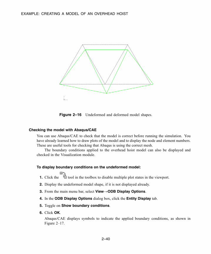
EXAMPLE: CREATING A MODEL OF AN OVERHEAD HOIST
Figure 2–16 Undeformed and deformed model shapes.
Checking the model with Abaqus/CAE
You can use Abaqus/CAE to check that the model is correct before running the simulation. Youhave already learned how to draw plots of the model and to display the node and element numbers.These are useful tools for checking that Abaqus is using the correct mesh.
The boundary conditions applied to the overhead hoist model can also be displayed andchecked in the Visualization module.
To display boundary conditions on the undeformed model:
1. Click the tool in the toolbox to disable multiple plot states in the viewport.
2. Display the undeformed model shape, if it is not displayed already.
3. From the main menu bar, select View→ODB Display Options.
4. In the ODB Display Options dialog box, click the Entity Display tab.
5. Toggle on Show boundary conditions.
6. Click OK.
Abaqus/CAE displays symbols to indicate the applied boundary conditions, as shown inFigure 2–17.
2–40
Abaqus ID:Printed on:

EXAMPLE: CREATING A MODEL OF AN OVERHEAD HOIST
1
2
3
Figure 2–17 Applied boundary conditions on the overhead hoist.
Tabular data reports
In addition to the graphical capabilities described above, Abaqus/CAE allows you to write data toa text file in a tabular format. This feature is a convenient alternative to writing tabular output tothe data (.dat) file. Output generated this way has many uses; for example, it can be used inwritten reports. In this problem you will generate a report containing the element stresses, nodaldisplacements, and reaction forces.
To generate field data reports:
1. From the main menu bar, select Report→Field Output.
2. In theVariable tabbed page of theReport Field Output dialog box, accept the default positionlabeled Integration Point. Click the triangle next to S: Stress components to expand thelist of available variables. From this list, toggle on S11.
3. In the Setup tabbed page, name the report Frame.rpt. In the Data region at the bottom ofthe page, toggle off Column totals.
4. Click Apply.
The element stresses are written to the report file.
5. In the Variable tabbed page of the Report Field Output dialog box, change the position toUnique Nodal. Toggle off S: Stress components, and select U1 and U2 from the list ofavailable U: Spatial displacement variables.
6. Click Apply.
The nodal displacements are appended to the report file.
2–41
Abaqus ID:Printed on:
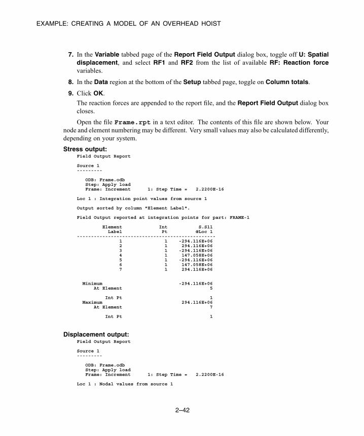
EXAMPLE: CREATING A MODEL OF AN OVERHEAD HOIST
7. In the Variable tabbed page of the Report Field Output dialog box, toggle off U: Spatialdisplacement, and select RF1 and RF2 from the list of available RF: Reaction forcevariables.
8. In the Data region at the bottom of the Setup tabbed page, toggle on Column totals.
9. Click OK.
The reaction forces are appended to the report file, and the Report Field Output dialog boxcloses.
Open the file Frame.rpt in a text editor. The contents of this file are shown below. Yournode and element numbering may be different. Very small values may also be calculated differently,depending on your system.
Stress output:Field Output Report
Source 1---------
ODB: Frame.odbStep: Apply loadFrame: Increment 1: Step Time = 2.2200E-16
Loc 1 : Integration point values from source 1
Output sorted by column "Element Label".
Field Output reported at integration points for part: FRAME-1
Element Int S.S11Label Pt @Loc 1
-------------------------------------------------1 1 -294.116E+062 1 294.116E+063 1 -294.116E+064 1 147.058E+065 1 -294.116E+066 1 147.058E+067 1 294.116E+06
Minimum -294.116E+06At Element 5
Int Pt 1Maximum 294.116E+06
At Element 7
Int Pt 1
Displacement output:Field Output Report
Source 1---------
ODB: Frame.odbStep: Apply loadFrame: Increment 1: Step Time = 2.2200E-16
Loc 1 : Nodal values from source 1
2–42
Abaqus ID:Printed on:
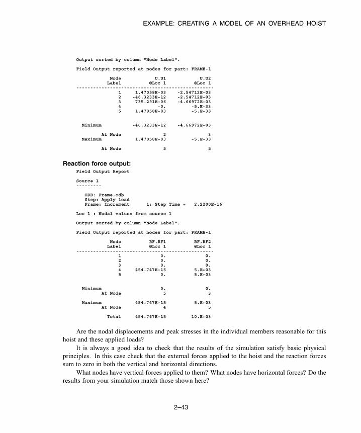
EXAMPLE: CREATING A MODEL OF AN OVERHEAD HOIST
Output sorted by column "Node Label".
Field Output reported at nodes for part: FRAME-1
Node U.U1 U.U2Label @Loc 1 @Loc 1
-------------------------------------------------1 1.47058E-03 -2.54712E-032 -46.3233E-12 -2.54712E-033 735.291E-06 -4.66972E-034 -0. -5.E-335 1.47058E-03 -5.E-33
Minimum -46.3233E-12 -4.66972E-03
At Node 2 3Maximum 1.47058E-03 -5.E-33
At Node 5 5
Reaction force output:Field Output Report
Source 1---------
ODB: Frame.odbStep: Apply loadFrame: Increment 1: Step Time = 2.2200E-16
Loc 1 : Nodal values from source 1
Output sorted by column "Node Label".
Field Output reported at nodes for part: FRAME-1
Node RF.RF1 RF.RF2Label @Loc 1 @Loc 1
-------------------------------------------------1 0. 0.2 0. 0.3 0. 0.4 454.747E-15 5.E+035 0. 5.E+03
Minimum 0. 0.At Node 5 3
Maximum 454.747E-15 5.E+03At Node 4 5
Total 454.747E-15 10.E+03
Are the nodal displacements and peak stresses in the individual members reasonable for thishoist and these applied loads?
It is always a good idea to check that the results of the simulation satisfy basic physicalprinciples. In this case check that the external forces applied to the hoist and the reaction forcessum to zero in both the vertical and horizontal directions.
What nodes have vertical forces applied to them? What nodes have horizontal forces? Do theresults from your simulation match those shown here?
2–43
Abaqus ID:Printed on:
EXAMPLE: CREATING A MODEL OF AN OVERHEAD HOIST
2.3.13 Rerunning the analysis using Abaqus/Explicit
We will rerun the same analysis in Abaqus/Explicit for comparison. This time we are interested in thedynamic response of the hoist to the same load applied suddenly at the midspan. Before continuing, clickthe Model tab in the left side of the main window to switch to the Model Tree. Click mouse button 3on Model-1 in the Model Tree and select Copy Model from the menu that appears to copy the existingmodel to a new model named Explicit. Make all subsequent changes to the Explicit model (youmay want to collapse the original model to avoid confusion). You will need to replace the static step withan explicit dynamic step, modify the output requests and the material definition, and change the elementlibrary before you can resubmit the job.
Replacing the analysis step
The step definition must change to reflect a dynamic, explicit analysis.
To replace the static step with an explicit dynamic step:
1. In theModel Tree, expand theSteps container. Click mouse button 3 on the step namedApplyload, and select Replace from the menu that appears.
2. In the Replace Step dialog box, select Dynamic, Explicit from the list of available Generalprocedures. Click Continue.
Model attributes such as boundary conditions, loads, and contact interactions are retained whenreplacing a step. Model attributes that cannot be converted will be deleted. In this simulationall necessary model attributes will be retained.
3. In the Basic tabbed page of the Edit Step dialog box, enter the step description 10 kNcentral load, suddenly applied and set the time period of the step to 0.01 s.
Modifying the output requests
Because this is a dynamic analysis in which the transient response of the frame is of interest, it ishelpful to have the displacements of the center point written as history output. Displacement historyoutput can be requested only for a preselected set. You will use the set named center, which wascreated earlier while assigning the load. If you did not create this set previously, the followinginstructions are provided for your convenience.
To create a set (if necessary):
1. In the Model Tree, expand the Assembly container and double-click the Sets item.
The Create Set dialog box appears.
2. Name the set center, accept the default selection of Geometry, and click Continue.
2–44
Abaqus ID:Printed on:

EXAMPLE: CREATING A MODEL OF AN OVERHEAD HOIST
Note: For meshed parts you can define sets that are based on either the geometry or the mesh.If you modify the mesh, you must redefine a mesh-based set. However, a geometry-based setwill update automatically. For unmeshed parts only geometry-based sets are available.
3. In the viewport, select the point at the center of the bottom edge of the truss. In the promptarea, click Done when you are finished.
To add displacements to the history output request:
1. In the Model Tree, click mouse button 3 on the History Output Requests container andselect Manager from the menu that appears.
2. In the History Output Requests Manager dialog box that appears, click Edit.
The history output editor appears.
3. Under theDomain field, select Set. Abaqus automatically provides a list of all the sets createdfor a given model. Choose the set named center.
4. Under the Frequency field, select Every n time increments and set the value of n to 1 towrite the output at every increment.
5. In the Output Variables region, toggle off the Energy output and click the arrow to the leftof the Displacement/Velocity/Acceleration category to reveal history output options fortranslations and rotations.
6. Toggle onUT, Translations to have the displacements for the selected set be written as historyoutput to the output database file.
7. Click OK to save your changes and to close the dialog box. Dismiss the History OutputRequests Manager.
Modifying the material definition
Since Abaqus/Explicit performs a dynamic analysis, a complete material definition requires thatyou specify the material density. For this problem assume the density is equal to 7800 kg/m3 .
To add density to the material definition:
1. In the Model Tree, expand the Materials container and double-click Steel.
2. In the material editor, select General→Density and type a value of 7800 for the density.
3. Click OK to close the Edit Material dialog box.
Changing the element library and submitting the job for analysis
As will be discussed in Chapter 3, “Finite Elements and Rigid Bodies,” the elements available inAbaqus/Explicit are a subset of those available in Abaqus/Standard. Thus, to ensure that you areusing a valid element type in your analysis, you must change the element library from which theelements are selected to the explicit element library. Abaqus/CAE automatically filters the available
2–45
Abaqus ID:Printed on:
EXAMPLE: CREATING A MODEL OF AN OVERHEAD HOIST
element types according to the selected element library. After changing the element library, you willcreate and run a new job for the Abaqus/Explicit analysis.
To change the element library:
1. In the Model Tree, expand the Frame item underneath the Parts container. Then double-clickMesh in the list that appears.Abaqus/CAE switches to the Mesh module.
2. From the main menu bar, select Mesh→Element Type, select the set all (or pick the entireframe in the viewport), and change the Element Library selection to Explicit.
3. Click OK to accept the new element type.
To create and run the new job:
1. In the Model Tree, double-click the Jobs container.
2. Name the new job expFrame, and select Explicit as the source model.
3. Submit the job.
2.3.14 Postprocessing the dynamic analysis resultsFor the static linear perturbation analysis done in Abaqus/Standard you examined the deformed shapeas well as stress, displacement, and reaction force output. For the Abaqus/Explicit analysis you cansimilarly examine the deformed shape and generate field data reports. Because this is a dynamic analysis,you should also examine the transient response resulting from the loading. You will do this by animatingthe time history of the deformed model shape and plotting the displacement history of the bottom centernode in the truss.
Plot the deformed shape of the model. For large-displacement analyses (the default formulation inAbaqus/Explicit) the displaced shape scale factor has a default value of 1. Change the DeformationScale Factor to 20 so that you can more easily see the deformation of the truss.
To create a time-history animation of the deformed model shape:
1. From the main menu bar, select Animate→Time History; or use the tool in the toolbox.
The time history animation begins in a continuous loop at its fastest speed. Abaqus/CAE displaysthe movie player controls in the right side of the context bar (immediately above the viewport).
2. From the main menu bar, select Options→Animation; or use the animation options tool in
the toolbox (located directly underneath the tool).
The Animation Options dialog box appears.
2–46
Abaqus ID:Printed on:

EXAMPLE: CREATING A MODEL OF AN OVERHEAD HOIST
3. Change the Mode to Play Once, and slow the animation down by moving the Frame Rate slider.
4. You can use the animation controls to start, pause, and step through the animation. From left toright of Figure 2–18, these controls perform the following functions: play/pause, first, previous,next, and last.
Firstimage
Nextimage
LaunchFrame
Selector
Play/Pause
Previousimage
Lastimage
Figure 2–18 Postprocessing animation controls.
The truss responds dynamically to the load. You can confirm this by plotting the verticaldisplacement history of the node set Center.
You can create X–Y curves from either history or field data stored in the output database (.odb)file. X–Y curves can also be read from an external file or they can be typed into the Visualization moduleinteractively. Once curves have been created, their data can be further manipulated and plotted to thescreen in graphical form. In this example you will create and plot the curve using history data.
To create an X–Y plot of the vertical displacement for a node:
1. In the Results Tree, expand the History Output container underneath the output database namedexpFrame.odb.
2. From the list of available history output, double-click Spatial displacement: U2 atNode x in NSET CENTER.
Abaqus/CAE plots the vertical displacement at the center node along the bottom of the truss, asshown in Figure 2–19.
2–47
Abaqus ID:Printed on:
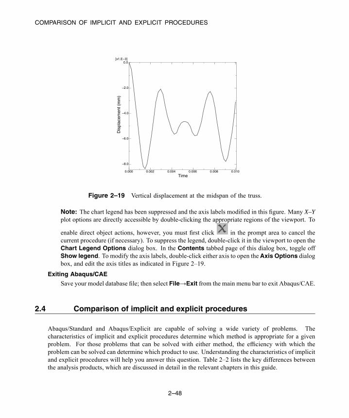
COMPARISON OF IMPLICIT AND EXPLICIT PROCEDURES
Time0.000 0.002 0.004 0.006 0.008 0.010
Dis
plac
emen
t (m
m)
−8.0
−6.0
−4.0
−2.0
0.0[x1.E−3]
Figure 2–19 Vertical displacement at the midspan of the truss.
Note: The chart legend has been suppressed and the axis labels modified in this figure. Many X–Yplot options are directly accessible by double-clicking the appropriate regions of the viewport. To
enable direct object actions, however, you must first click in the prompt area to cancel thecurrent procedure (if necessary). To suppress the legend, double-click it in the viewport to open theChart Legend Options dialog box. In the Contents tabbed page of this dialog box, toggle offShow legend. To modify the axis labels, double-click either axis to open theAxis Options dialogbox, and edit the axis titles as indicated in Figure 2–19.
Exiting Abaqus/CAE
Save your model database file; then select File→Exit from the main menu bar to exit Abaqus/CAE.
2.4 Comparison of implicit and explicit procedures
Abaqus/Standard and Abaqus/Explicit are capable of solving a wide variety of problems. Thecharacteristics of implicit and explicit procedures determine which method is appropriate for a givenproblem. For those problems that can be solved with either method, the efficiency with which theproblem can be solved can determine which product to use. Understanding the characteristics of implicitand explicit procedures will help you answer this question. Table 2–2 lists the key differences betweenthe analysis products, which are discussed in detail in the relevant chapters in this guide.
2–48
Abaqus ID:Printed on:
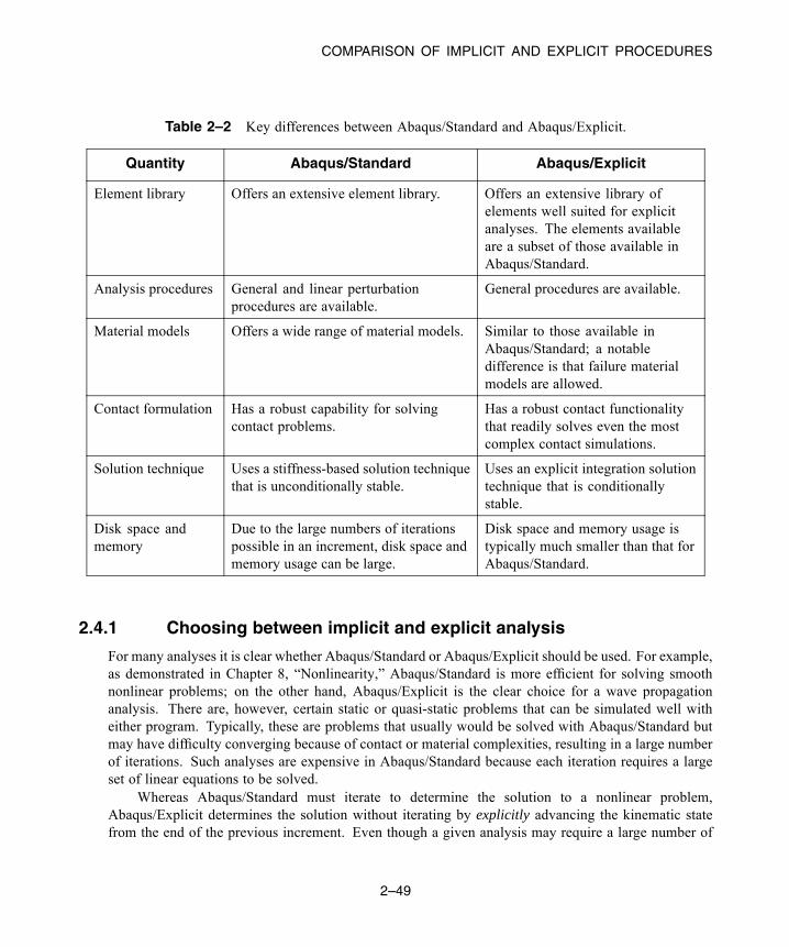
COMPARISON OF IMPLICIT AND EXPLICIT PROCEDURES
Table 2–2 Key differences between Abaqus/Standard and Abaqus/Explicit.
Quantity Abaqus/Standard Abaqus/Explicit
Element library Offers an extensive element library. Offers an extensive library ofelements well suited for explicitanalyses. The elements availableare a subset of those available inAbaqus/Standard.
Analysis procedures General and linear perturbationprocedures are available.
General procedures are available.
Material models Offers a wide range of material models. Similar to those available inAbaqus/Standard; a notabledifference is that failure materialmodels are allowed.
Contact formulation Has a robust capability for solvingcontact problems.
Has a robust contact functionalitythat readily solves even the mostcomplex contact simulations.
Solution technique Uses a stiffness-based solution techniquethat is unconditionally stable.
Uses an explicit integration solutiontechnique that is conditionallystable.
Disk space andmemory
Due to the large numbers of iterationspossible in an increment, disk space andmemory usage can be large.
Disk space and memory usage istypically much smaller than that forAbaqus/Standard.
2.4.1 Choosing between implicit and explicit analysis
For many analyses it is clear whether Abaqus/Standard or Abaqus/Explicit should be used. For example,as demonstrated in Chapter 8, “Nonlinearity,” Abaqus/Standard is more efficient for solving smoothnonlinear problems; on the other hand, Abaqus/Explicit is the clear choice for a wave propagationanalysis. There are, however, certain static or quasi-static problems that can be simulated well witheither program. Typically, these are problems that usually would be solved with Abaqus/Standard butmay have difficulty converging because of contact or material complexities, resulting in a large numberof iterations. Such analyses are expensive in Abaqus/Standard because each iteration requires a largeset of linear equations to be solved.
Whereas Abaqus/Standard must iterate to determine the solution to a nonlinear problem,Abaqus/Explicit determines the solution without iterating by explicitly advancing the kinematic statefrom the end of the previous increment. Even though a given analysis may require a large number of
2–49
Abaqus ID:Printed on:

SUMMARY
time increments using the explicit method, the analysis can be more efficient in Abaqus/Explicit if thesame analysis in Abaqus/Standard requires many iterations.
Another advantage of Abaqus/Explicit is that it requires much less disk space and memory thanAbaqus/Standard for the same simulation. For problems in which the computational cost of the twoprograms may be comparable, the substantial disk space and memory savings of Abaqus/Explicit makeit attractive.
2.4.2 Cost of mesh refinement in implicit and explicit analyses
Using the explicit method, the computational cost is proportional to the number of elements and roughlyinversely proportional to the smallest element dimension. Mesh refinement, therefore, increases thecomputational cost by increasing the number of elements and reducing the smallest element dimension.As an example, consider a three-dimensional model with uniform, square elements. If the mesh is refinedby a factor of two in all three directions, the computational cost increases by a factor of 2 × 2 × 2 as aresult of the increase in the number of elements and by a factor of 2 as a result of the decrease in thesmallest element dimension. The total computational cost of the analysis increases by a factor of 24 ,or 16, by refining the mesh. Disk space and memory requirements are proportional to the number ofelements with no dependence on element dimensions; thus, these requirements increase by a factor of 8.
Whereas predicting the cost increase with mesh refinement for the explicit method is ratherstraightforward, cost is more difficult to predict when using the implicit method. The difficulty arisesfrom the problem-dependent relationship between element connectivity and solution cost, a relationshipthat does not exist in the explicit method. Using the implicit method, experience shows that for manyproblems the computational cost is roughly proportional to the square of the number of degrees offreedom. Consider the same example of a three-dimensional model with uniform, square elements.Refining the mesh by a factor of two in all three directions increases the number of degrees of freedomby approximately 23 , causing the computational cost to increase by a factor of roughly (23 )2 , or 64.The disk space and memory requirements increase in the same manner, although the actual increase isdifficult to predict.
The explicit method shows great cost savings over the implicit method as the model size increases,as long as the mesh is relatively uniform. Figure 2–20 illustrates the comparison of cost versus modelsize using the explicit and implicit methods. For this problem the number of degrees of freedom scaleswith the number of elements.
2.5 Summary
• Abaqus/CAE can be used to create a complete Abaqus analysis model. The analysis product(Abaqus/Standard or Abaqus/Explicit) reads the input file generated by Abaqus/CAE, performsthe analysis, sends information to Abaqus/CAE to allow you to monitor the progress of the job,
2–50
Abaqus ID:Printed on:
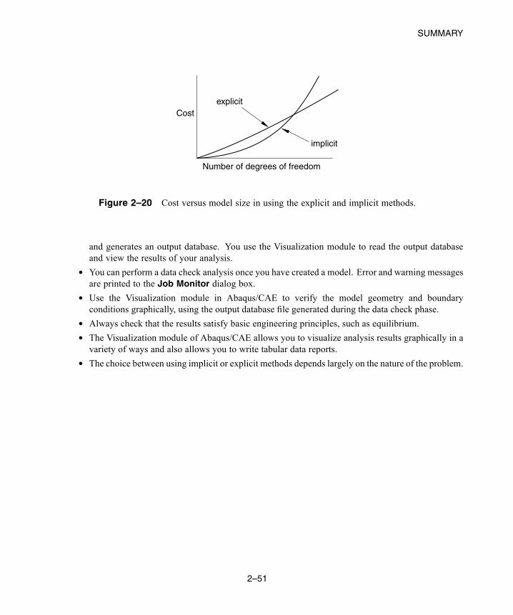
SUMMARY
Cost
Number of degrees of freedom
explicit
implicit
Figure 2–20 Cost versus model size in using the explicit and implicit methods.
and generates an output database. You use the Visualization module to read the output databaseand view the results of your analysis.
• You can perform a data check analysis once you have created a model. Error and warning messagesare printed to the Job Monitor dialog box.
• Use the Visualization module in Abaqus/CAE to verify the model geometry and boundaryconditions graphically, using the output database file generated during the data check phase.
• Always check that the results satisfy basic engineering principles, such as equilibrium.• The Visualization module of Abaqus/CAE allows you to visualize analysis results graphically in avariety of ways and also allows you to write tabular data reports.
• The choice between using implicit or explicit methods depends largely on the nature of the problem.
2–51
Abaqus ID:Printed on:

FINITE ELEMENTS
3. Finite Elements and Rigid Bodies
Finite elements and rigid bodies are the fundamental components of an Abaqus model. Finite elementsare deformable, whereas rigid bodies move through space without changing shape. While users of finiteelement analysis programs tend to have some understanding of what finite elements are, the generalconcept of rigid bodies within a finite element program may be somewhat new.
For computational efficiency Abaqus has a general rigid body capability. Any body or part of a bodycan be defined as a rigid body; most element types can be used in a rigid body definition (the exceptionsare listed in “Rigid body definition,” Section 2.4.1 of the Abaqus Analysis User’s Guide). The advantageof rigid bodies over deformable bodies is that the motion of a rigid body is described completely by nomore than six degrees of freedom at a reference node. In contrast, deformable elements have manydegrees of freedom and require expensive element calculations to determine the deformations. Whensuch deformations are negligible or not of interest, modeling a component as a rigid body producessignificant computational savings without affecting the overall results.
3.1 Finite elements
A wide range of elements is available in Abaqus. This extensive element library provides you with apowerful set of tools for solving many different problems. The elements available in Abaqus/Explicitare (with a few exceptions) a subset of those available in Abaqus/Standard. This section introduces youto the five aspects of an element that influence how it behaves.
3.1.1 Characterizing elements
Each element is characterized by the following:
• Family• Degrees of freedom (directly related to the element family)• Number of nodes• Formulation• Integration
Each element in Abaqus has a unique name, such as T2D2, S4R, or C3D8I. The element name identifieseach of the five aspects of an element. The naming convention is explained in this chapter.
Family
Figure 3–1 shows the element families most commonly used in a stress analysis. One of the majordistinctions between different element families is the geometry type that each family assumes.
3–1
Abaqus ID:Printed on:

FINITE ELEMENTS
Continuum(solid) elements
Shellelements
Beam elements
Truss elements
Membraneelements
Infiniteelements
Rigidelements
Springs and dashpots
Figure 3–1 Commonly used element families.
The element families that you will use in this guide—continuum, shell, beam, truss, and rigidelements—are discussed in detail in other chapters. The other element families are not coveredin this guide; if you are interested in using them in your models, read about them in Part VI,“Elements,” of the Abaqus Analysis User’s Guide.
The first letter or letters of an element’s name indicate to which family the element belongs.For example, the S in S4R indicates this is a shell element, while the C in C3D8I indicates this is acontinuum element.
Degrees of freedom
The degrees of freedom (dof) are the fundamental variables calculated during the analysis. Fora stress/displacement simulation the degrees of freedom are the translations at each node. Someelement families, such as the beam and shell families, have rotational degrees of freedom as well.For a heat transfer simulation the degrees of freedom are the temperatures at each node; a heattransfer analysis, therefore, requires the use of different elements than a stress analysis, since thedegrees of freedom are not the same.
The following numbering convention is used for the degrees of freedom in Abaqus:
1 Translation in direction 1
2 Translation in direction 2
3 Translation in direction 3
4 Rotation about the 1-axis
5 Rotation about the 2-axis
6 Rotation about the 3-axis
3–2
Abaqus ID:Printed on:
FINITE ELEMENTS
7 Warping in open-section beam elements
8 Acoustic pressure, pore pressure, or hydrostatic fluid pressure
9 Electric potential
10 Connector material flow (units of length)
11 Temperature (or normalized concentration in mass diffusion analysis) forcontinuum elements or temperature at the first point through the thicknessof beams and shells
12+ Temperature at other points through the thickness of beams and shells
Directions 1, 2, and 3 correspond to the global 1-, 2-, and 3-directions, respectively, unless a localcoordinate system has been defined at the nodes.
Axisymmetric elements are the exception, with the displacement and rotation degrees offreedom referred to as follows:
1 Translation in the r-direction
2 Translation in the z-direction
6 Rotation in the r–z plane
Directions r (radial) and z (axial) correspond to the global 1- and 2-directions, respectively, unlessa local coordinate system has been defined at the nodes. See Chapter 5, “Using Shell Elements,”for a discussion of defining a local coordinate system at the nodes.
In this guide our attention is restricted to structural applications. Therefore, only elementswith translational and rotational degrees of freedom are discussed. For information on other typesof elements (for example, heat transfer elements), consult the Abaqus Analysis User’s Guide.
By default, Abaqus/CAE uses the alphabetical option, x-y-z, for labeling the view orientationtriad. In general, this guide adopts the numerical option, 1-2-3, to permit direct correspondence withdegree of freedom and output labeling. For more information on labeling of axes, see “Customizingthe view triad,” Section 5.4 of the Abaqus/CAE User’s Guide.
Number of nodes—order of interpolation
Displacements, rotations, temperatures, and the other degrees of freedom mentioned in the previoussection are calculated only at the nodes of the element. At any other point in the element, thedisplacements are obtained by interpolating from the nodal displacements. Usually the interpolationorder is determined by the number of nodes used in the element, as illustrated in the examples inFigure 3–2.
• Elements that have nodes only at their corners, such as the 8-node brick shown in Figure 3–2(a),use linear interpolation in each direction and are often called linear elements or first-orderelements.
3–3
Abaqus ID:Printed on:

FINITE ELEMENTS
(a) Linear element(8-node brick, C3D8)
(b) Quadratic element(20-node brick, C3D20)
(c) Modified second-order element(10-node tetrahedron, C3D10M)
Figure 3–2 Linear brick, quadratic brick, and modified tetrahedral elements.
• Elements with midside nodes, such as the 20-node brick shown in Figure 3–2(b), use quadraticinterpolation and are often called quadratic elements or second-order elements.
• Modified triangular or tetrahedral elements with midside nodes, such as the 10-nodetetrahedron shown in Figure 3–2(c), use a modified second-order interpolation and are oftencalled modified elements or modified second-order elements.
Abaqus/Standard offers a wide selection of both linear and quadratic elements. Abaqus/Explicitoffers only linear elements, with the exception of the quadratic beam and modified tetrahedron andtriangle elements.
Typically, the number of nodes in an element is clearly identified in its name. The 8-nodebrick element, as you have seen, is called C3D8; and the 8-node general shell element is calledS8R. The beam element family uses a slightly different convention: the order of interpolation isidentified in the name. Thus, a first-order, three-dimensional beam element is called B31, whereasa second-order, three-dimensional beam element is called B32. A similar convention is used foraxisymmetric shell and membrane elements.
Formulation
An element’s formulation refers to the mathematical theory used to define the element’s behavior.In the absence of adaptive meshing all of the stress/displacement elements in Abaqus are basedon the Lagrangian or material description of behavior: the material associated with an elementremains associated with the element throughout the analysis, and material cannot flow acrosselement boundaries. In the alternative Eulerian or spatial description, elements are fixed in spaceas the material flows through them. Eulerian methods are used commonly in fluid mechanicssimulations. Abaqus/Standard uses Eulerian elements to model convective heat transfer. Adaptivemeshing combines the features of pure Lagrangian and Eulerian analyses and allows the motionof the element to be independent of the material. Eulerian elements and adaptive meshing are notdiscussed in this guide.
To accommodate different types of behavior, some element families in Abaqus includeelements with several different formulations. For example, the shell element family has threeclasses: one suitable for general-purpose shell analysis, another for thin shells, and yet another
3–4
Abaqus ID:Printed on:
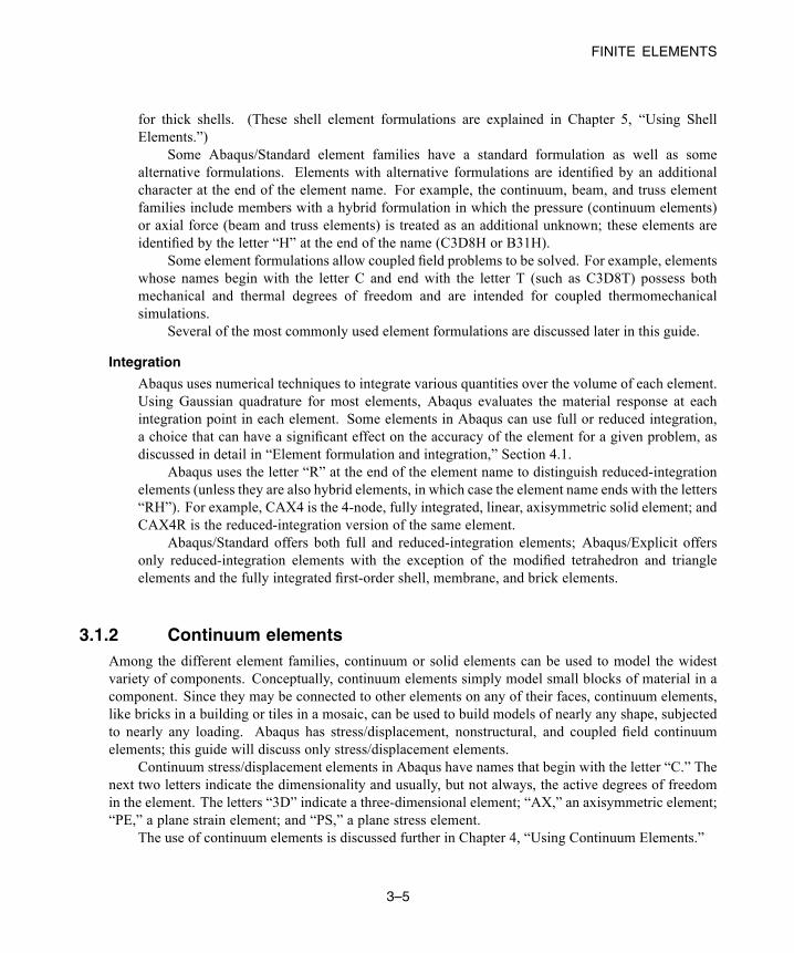
FINITE ELEMENTS
for thick shells. (These shell element formulations are explained in Chapter 5, “Using ShellElements.”)
Some Abaqus/Standard element families have a standard formulation as well as somealternative formulations. Elements with alternative formulations are identified by an additionalcharacter at the end of the element name. For example, the continuum, beam, and truss elementfamilies include members with a hybrid formulation in which the pressure (continuum elements)or axial force (beam and truss elements) is treated as an additional unknown; these elements areidentified by the letter “H” at the end of the name (C3D8H or B31H).
Some element formulations allow coupled field problems to be solved. For example, elementswhose names begin with the letter C and end with the letter T (such as C3D8T) possess bothmechanical and thermal degrees of freedom and are intended for coupled thermomechanicalsimulations.
Several of the most commonly used element formulations are discussed later in this guide.
Integration
Abaqus uses numerical techniques to integrate various quantities over the volume of each element.Using Gaussian quadrature for most elements, Abaqus evaluates the material response at eachintegration point in each element. Some elements in Abaqus can use full or reduced integration,a choice that can have a significant effect on the accuracy of the element for a given problem, asdiscussed in detail in “Element formulation and integration,” Section 4.1.
Abaqus uses the letter “R” at the end of the element name to distinguish reduced-integrationelements (unless they are also hybrid elements, in which case the element name ends with the letters“RH”). For example, CAX4 is the 4-node, fully integrated, linear, axisymmetric solid element; andCAX4R is the reduced-integration version of the same element.
Abaqus/Standard offers both full and reduced-integration elements; Abaqus/Explicit offersonly reduced-integration elements with the exception of the modified tetrahedron and triangleelements and the fully integrated first-order shell, membrane, and brick elements.
3.1.2 Continuum elementsAmong the different element families, continuum or solid elements can be used to model the widestvariety of components. Conceptually, continuum elements simply model small blocks of material in acomponent. Since they may be connected to other elements on any of their faces, continuum elements,like bricks in a building or tiles in a mosaic, can be used to build models of nearly any shape, subjectedto nearly any loading. Abaqus has stress/displacement, nonstructural, and coupled field continuumelements; this guide will discuss only stress/displacement elements.
Continuum stress/displacement elements in Abaqus have names that begin with the letter “C.” Thenext two letters indicate the dimensionality and usually, but not always, the active degrees of freedomin the element. The letters “3D” indicate a three-dimensional element; “AX,” an axisymmetric element;“PE,” a plane strain element; and “PS,” a plane stress element.
The use of continuum elements is discussed further in Chapter 4, “Using Continuum Elements.”
3–5
Abaqus ID:Printed on:

FINITE ELEMENTS
Three-dimensional continuum element library
Three-dimensional continuum elements can be hexahedra (bricks), wedges, or tetrahedra. The fullinventory of three-dimensional continuum elements and the nodal connectivity for each type can befound in “Three-dimensional solid element library,” Section 28.1.4 of the Abaqus Analysis User’sGuide.
Whenever possible, hexahedral elements or second-order tetrahedral elements should be usedin Abaqus. First-order tetrahedra (C3D4) have a simple, constant-strain formulation, and very finemeshes are required for an accurate solution.
Two-dimensional continuum element library
Abaqus has several classes of two-dimensional continuum elements that differ from each otherin their out-of-plane behavior. Two-dimensional elements can be quadrilateral or triangular.Figure 3–3 shows the three classes that are used most commonly.
Axisymmetricelement CAX4
3 (θ)
2 (z)
1 (r)
3
2
Plane strainelement CPE4
Plane stresselement CPS4
3 1
21
Figure 3–3 Plane strain, plane stress, and axisymmetric elements without twist.
Plane strain elements assume that the out-of-plane strain, , is zero; they can be used tomodel thick structures.
Plane stress elements assume that the out-of-plane stress, , is zero; they are suitable formodeling thin structures.
3–6
Abaqus ID:Printed on:

FINITE ELEMENTS
Axisymmetric elements without twist, the “CAX” class of elements, model a 360° ring; theyare suitable for analyzing structures with axisymmetric geometry subjected to axisymmetric loading.
Abaqus/Standard also provides generalized plane strain elements, axisymmetric elements withtwist, and axisymmetric elements with asymmetric deformation.
• Generalized plane strain elements include the additional generalization that the out-of-planestrain may vary linearly with position in the plane of the model. This formulation is particularlysuited for the thermal-stress analysis of thick sections.
• Axisymmetric elements with twist model an initially axisymmetric geometry that can twistabout the axis of symmetry. These elements are useful for modeling the torsion of cylindricalstructures, such as axisymmetric rubber bushings.
• Axisymmetric elements with asymmetric deformation model an initially axisymmetricgeometry that can deform asymmetrically (typically as a result of bending). They are usefulfor simulating problems such as an axisymmetric rubber mount that is subjected to shear loads.
The latter three classes of two-dimensional continuum elements are not discussed in this guide.Two-dimensional solid elements must be defined in the 1–2 plane so that the node order is
counterclockwise around the element perimeter, as shown in Figure 3–4.
Quadrilateral element Triangular element
1 2
34
1 2
3
2
1
Figure 3–4 Correct nodal connectivity for two-dimensional elements.
When using a preprocessor to generate the mesh, ensure that the element normals all point in thesame direction as the positive, global 3-axis. Failure to provide the correct element connectivitywill cause Abaqus to issue an error message stating that elements have negative area.
Degrees of freedom
All of the stress/displacement continuum elements have translational degrees of freedom at eachnode. Correspondingly, degrees of freedom 1, 2, and 3 are active in three-dimensional elements,while only degrees of freedom 1 and 2 are active in plane strain elements, plane stress elements,and axisymmetric elements without twist. To find the active degrees of freedom in the other classesof two-dimensional solid elements, see “Two-dimensional solid element library,” Section 28.1.3 ofthe Abaqus Analysis User’s Guide.
3–7
Abaqus ID:Printed on:
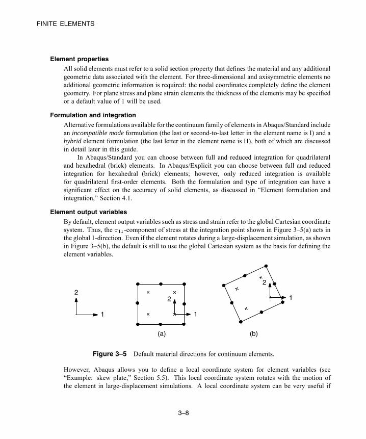
FINITE ELEMENTS
Element properties
All solid elements must refer to a solid section property that defines the material and any additionalgeometric data associated with the element. For three-dimensional and axisymmetric elements noadditional geometric information is required: the nodal coordinates completely define the elementgeometry. For plane stress and plane strain elements the thickness of the elements may be specifiedor a default value of 1 will be used.
Formulation and integration
Alternative formulations available for the continuum family of elements in Abaqus/Standard includean incompatible mode formulation (the last or second-to-last letter in the element name is I) and ahybrid element formulation (the last letter in the element name is H), both of which are discussedin detail later in this guide.
In Abaqus/Standard you can choose between full and reduced integration for quadrilateraland hexahedral (brick) elements. In Abaqus/Explicit you can choose between full and reducedintegration for hexahedral (brick) elements; however, only reduced integration is availablefor quadrilateral first-order elements. Both the formulation and type of integration can have asignificant effect on the accuracy of solid elements, as discussed in “Element formulation andintegration,” Section 4.1.
Element output variables
By default, element output variables such as stress and strain refer to the global Cartesian coordinatesystem. Thus, the -component of stress at the integration point shown in Figure 3–5(a) acts inthe global 1-direction. Even if the element rotates during a large-displacement simulation, as shownin Figure 3–5(b), the default is still to use the global Cartesian system as the basis for defining theelement variables.
2
1
2
1
2
1
(a) (b)
Figure 3–5 Default material directions for continuum elements.
However, Abaqus allows you to define a local coordinate system for element variables (see“Example: skew plate,” Section 5.5). This local coordinate system rotates with the motion ofthe element in large-displacement simulations. A local coordinate system can be very useful if
3–8
Abaqus ID:Printed on:
FINITE ELEMENTS
the object being modeled has some natural material orientation, such as the fiber directions in acomposite material.
3.1.3 Shell elements
Shell elements are used tomodel structures in which one dimension (the thickness) is significantly smallerthan the other dimensions and the stresses in the thickness direction are negligible.
Shell element names in Abaqus begin with the letter “S.” Axisymmetric shells all begin with theletters “SAX.”Abaqus/Standard also provides axisymmetric shells with asymmetric deformations, whichbegin with the letters “SAXA.” The first number in a shell element name indicates the number of nodesin the element, except for the case of axisymmetric shells, for which the first number indicates the orderof interpolation.
Two types of shell elements are available in Abaqus: conventional shell elements and continuumshell elements. Conventional shell elements discretize a reference surface by defining the element’splanar dimensions, its surface normal, and its initial curvature. Continuum shell elements, on the otherhand, resemble three-dimensional solid elements in that they discretize an entire three-dimensional bodyyet are formulated so that their kinematic and constitutive behavior is similar to conventional shellelements. In this guide only conventional shell elements are discussed. Henceforth, we will refer tothem simply as “shell elements.” Formore information on continuum shell elements, see “Shell elements:overview,” Section 29.6.1 of the Abaqus Analysis User’s Guide.
The use of shell elements is discussed in detail in Chapter 5, “Using Shell Elements.”
Shell element library
In Abaqus/Standard general three-dimensional shell elements are available with three differentformulations: general-purpose, thin-only, and thick-only. The general-purpose shells and theaxisymmetric shells with asymmetric deformation account for finite membrane strains andarbitrarily large rotations. The three-dimensional “thick” and “thin” element types provide forarbitrarily large rotations but only small strains. The general-purpose shells allow the shellthickness to change with the element deformation. All of the other shell elements assumesmall strains and no change in shell thickness, even though the element’s nodes may undergofinite rotations. Triangular and quadrilateral elements with linear and quadratic interpolationare available. Both linear and quadratic axisymmetric shell elements are available. All of thequadrilateral shell elements (except for S4) and the triangular shell element S3/S3R use reducedintegration. The S4 element and the other triangular shell elements use full integration. Table 3–1summarizes the shell elements available in Abaqus/Standard.
All the shell elements in Abaqus/Explicit are general-purpose. Finite membrane strain andsmall membrane strain formulations are available. Triangular and quadrilateral elements areavailable with linear interpolation. A linear axisymmetric shell element is also available. Table 3–2summarizes the shell elements available in Abaqus/Explicit.
3–9
Abaqus ID:Printed on:

FINITE ELEMENTS
Table 3–1 Three classes of shell elements in Abaqus/Standard.
General-Purpose Shells Thin-Only Shells Thick-Only Shells
S4, S4R, S3/S3R, SAX1, SAX2,SAX2T, SC6R, SC8R
STRI3, STRI65, S4R5,S8R5, S9R5, SAXA
S8R, S8RT
Table 3–2 Two classes of shell elements in Abaqus/Explicit.
Finite-Strain Shells Small-Strain Shells
S4, S4R, S3/S3R, SAX1 S4RS, S4RSW, S3RS
For most explicit analyses the large-strain shell elements are appropriate. If, however, theanalysis involves small membrane strains and arbitrarily large rotations, the small-strain shellelements are more computationally efficient. The S4RS and S3RS elements do not considerwarping, while the S4RSW element does.
The shell formulations available in Abaqus are discussed in detail in Chapter 5, “Using ShellElements.”
Degrees of freedom
The three-dimensional elements in Abaqus/Standard whose names end in the number “5” (e.g.,S4R5, STRI65) have 5 degrees of freedom at each node: three translations and two in-plane rotations(i.e., no rotations about the shell normal). However, all six degrees of freedom are activated at anode if required; for example, if rotational boundary conditions are applied or if the node is on afold line of the shell.
The remaining three-dimensional shell elements have six degrees of freedom at each node(three translations and three rotations).
The axisymmetric shells have three degrees of freedom associated with each node:
1 Translation in the r-direction.
2 Translation in the z-direction.
6 Rotation in the r–z plane.
Element properties
All shell elements must refer to a shell section property that defines the thickness and materialproperties associated with the element.
The stiffness of the shell cross-section can be calculated either during the analysis or once atthe beginning of the analysis.
If you choose to have the stiffness calculated during the analysis, Abaqus uses numericalintegration to calculate the behavior at selected points through the thickness of the shell. These
3–10
Abaqus ID:Printed on:

FINITE ELEMENTS
points are called section points, as shown in Figure 3–6. The associated material property definitionmay be linear or nonlinear. You can specify any odd number of section points through the shellthickness.
Figure 3–6 Section points through the thickness of a shell element.
If you choose to have the stiffness calculated once at the beginning of the analysis, you candefine the cross-section behavior to model linear or nonlinear behavior. In this case Abaqus modelsthe shell’s cross-section behavior directly in terms of section engineering quantities (area, momentsof inertia, etc.), so there is no need for Abaqus to integrate any quantities over the element cross-section. Therefore, this option is less expensive computationally. The response is calculated interms of force and moment resultants; the stresses and strains are calculated only when they arerequested for output. This approach is recommended when the response of the shell is linear elastic.
Element output variables
The element output variables for shells are defined in terms of local material directions that lie onthe surface of each shell element. In all large-displacement simulations these axes rotate with theelement’s deformation. You can also define a local material coordinate system that rotates with theelement’s deformation in a large-displacement analysis.
3.1.4 Beam elementsBeam elements are used to model components in which one dimension (the length) is significantly greaterthan the other two dimensions and only the stress in the direction along the axis of the beam is significant.
Beam element names in Abaqus begin with the letter “B.” The next character indicates thedimensionality of the element: “2” for two-dimensional beams and “3” for three-dimensional beams.The third character indicates the interpolation used: “1” for linear interpolation, “2” for quadraticinterpolation, and “3” for cubic interpolation.
The use of beam elements is discussed in Chapter 6, “Using Beam Elements.”
Beam element library
Linear, quadratic, and cubic beams are available in two and three dimensions. Cubic beams are notavailable in Abaqus/Explicit.
3–11
Abaqus ID:Printed on:

FINITE ELEMENTS
Degrees of freedom
Three-dimensional beams have six degrees of freedom at each node: three translational degreesof freedom (1–3) and three rotational degrees of freedom (4–6). “Open-section”-type beams (suchas B31OS) are available in Abaqus/Standard and have an additional degree of freedom (7) thatrepresents the warping of the beam cross-section.
Two-dimensional beams have three degrees of freedom at each node: two translational degreesof freedom (1 and 2) and one rotational degree of freedom (6) about the normal to the plane of themodel.
Element properties
All beam elements must refer to a beam section property that defines the material associated withthe element as well as the beam section profile (i.e., the element’s cross-sectional geometry); thenodal coordinates define only the length. You can define the beam section profile geometricallyby specifying the shape and dimensions of the section. Alternatively, you can define a generalizedbeam section profile by specifying the section engineering properties, such as area and moment ofinertia.
If you define the beam section profile geometrically, Abaqus calculates the cross-sectionbehavior of the beam by numerical integration over the cross-section, allowing both linear andnonlinear material behavior.
If you provide the section engineering properties (area, moments of inertia, and torsionalconstants) instead of the cross-section dimensions, there is no need for Abaqus to integrate anyquantities over the element cross-section. Therefore, this option is less expensive computationally.With this approach, the material behavior may be either linear or nonlinear. The response iscalculated in terms of the force and moment resultants; the stresses and strains are calculated onlywhen they are requested for output.
In Abaqus/Standard you can also define beams with linearly tapered cross-sections. Generalbeam sections with linear response and standard library sections are supported.
Formulation and integration
The linear beams (B21 and B31) and the quadratic beams (B22 and B32) are shear deformableand account for finite axial strains; therefore, they are suitable for modeling both slender and stoutbeams. The cubic beam elements in Abaqus/Standard (B23 and B33) do not account for shearflexibility and assume small axial strain, although large displacements and rotations of the beamsare valid. They are, therefore, suitable for modeling slender beams.
Abaqus/Standard provides variants of linear and quadratic beam elements that are suitable formodeling thin-walled, open-section beams (B31OS and B32OS). These elements model the effectsof torsion and warping in open cross-sections, such as I-beams or U-section channels. Open-sectionbeams are not covered in this guide.
Abaqus/Standard also has hybrid beam elements that are used for modeling very slendermembers, such as flexible risers on offshore oil installations, or for modeling very stiff links.Hybrid beams are not covered in this guide.
3–12
Abaqus ID:Printed on:
FINITE ELEMENTS
Element output variables
The stress components in three-dimensional, shear-deformable beam elements are the axial stress( ) and the shear stress due to torsion ( ). The shear stress acts about the section wall ina thin-walled section. Corresponding strain measures are also available. The shear-deformablebeams also provide estimates of transverse shear forces on the section. The slender (cubic) beamsin Abaqus/Standard have only the axial variables as output. Open-section beams in space also haveonly the axial variables as output, since the torsional shear stresses are negligible in this case.
All two-dimensional beams use only axial stress and strain.The axial force, bending moments, and curvatures about the local beam axes can also be
requested for output. For details of what components are available with which elements, see “Beammodeling: overview,” Section 29.3.1 of the Abaqus Analysis User’s Guide. Details of how the localbeam axes are defined are given in Chapter 6, “Using Beam Elements.”
3.1.5 Truss elementsTruss elements are rods that can carry only tensile or compressive loads. They have no resistance tobending; therefore, they are useful formodeling pin-jointed frames. Moreover, truss elements can be usedas an approximation for cables or strings (for example, in a tennis racket). Trusses are also sometimesused to represent reinforcement within other elements. The overhead hoist model in Chapter 2, “AbaqusBasics,” uses truss elements.
All truss element names begin with the letter “T.” The next two characters indicate thedimensionality of the element—“2D” for two-dimensional trusses and “3D” for three-dimensionaltrusses. The final character represents the number of nodes in the element.
Truss element library
Linear and quadratic trusses are available in two and three dimensions. Quadratic trusses are notavailable in Abaqus/Explicit.
Degrees of freedom
Truss elements have only translational degrees of freedom at each node. Three-dimensional trusselements have degrees of freedom 1, 2, and 3, while two-dimensional truss elements have degreesof freedom 1 and 2.
Element properties
All truss elements must refer to a truss section property that associates a material property definitionwith the element and specifies its cross-sectional area.
Formulation and integration
In addition to the standard formulation, a hybrid truss element formulation is available inAbaqus/Standard. It is useful for modeling very stiff links whose stiffness is much greater thanthat of the overall structure.
3–13
Abaqus ID:Printed on:
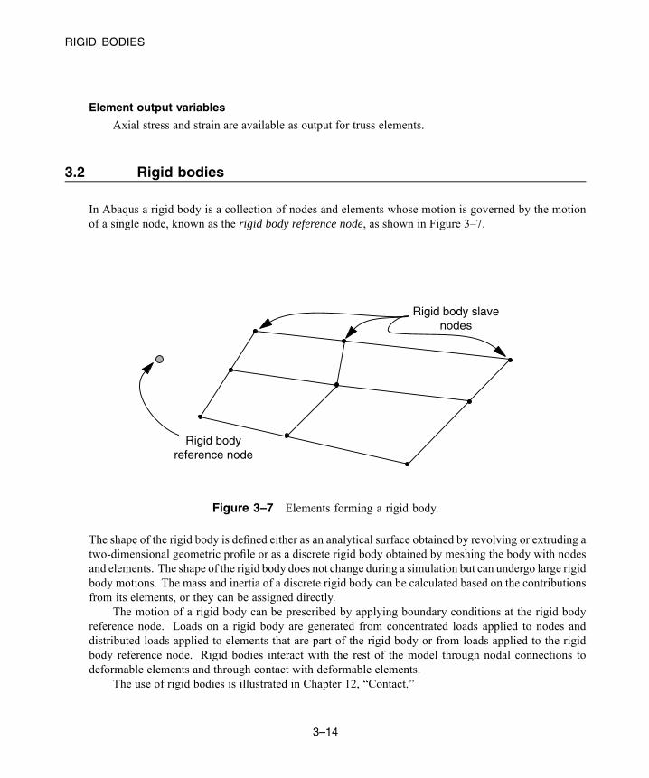
RIGID BODIES
Element output variables
Axial stress and strain are available as output for truss elements.
3.2 Rigid bodies
In Abaqus a rigid body is a collection of nodes and elements whose motion is governed by the motionof a single node, known as the rigid body reference node, as shown in Figure 3–7.
Rigid body slavenodes
Rigid bodyreference node
Figure 3–7 Elements forming a rigid body.
The shape of the rigid body is defined either as an analytical surface obtained by revolving or extruding atwo-dimensional geometric profile or as a discrete rigid body obtained by meshing the body with nodesand elements. The shape of the rigid body does not change during a simulation but can undergo large rigidbody motions. The mass and inertia of a discrete rigid body can be calculated based on the contributionsfrom its elements, or they can be assigned directly.
The motion of a rigid body can be prescribed by applying boundary conditions at the rigid bodyreference node. Loads on a rigid body are generated from concentrated loads applied to nodes anddistributed loads applied to elements that are part of the rigid body or from loads applied to the rigidbody reference node. Rigid bodies interact with the rest of the model through nodal connections todeformable elements and through contact with deformable elements.
The use of rigid bodies is illustrated in Chapter 12, “Contact.”
3–14
Abaqus ID:Printed on:

RIGID BODIES
3.2.1 Determining when to use a rigid body
Rigid bodies can be used to model very stiff components that are either fixed or undergoing large rigidbody motions. They can also be used to model constraints between deformable components, and theyprovide a convenient method of specifying certain contact interactions. When Abaqus is used forquasi-static forming analyses, rigid bodies are ideally suited for modeling tooling (such as a punch, die,drawbead, blank holder, roller, etc.) and may also be effective as a method of constraint.
It may be useful to make parts of a model rigid for verification purposes. For example, in complexmodels elements far away from the particular region of interest could be included as part of a rigidbody, resulting in faster run times at the model development stage. When you are satisfied with themodel, you can remove the rigid body definitions and incorporate an accurate deformable finite elementrepresentation throughout.
The principal advantage to representing portions of a model with rigid bodies rather than deformablefinite elements is computational efficiency. Element-level calculations are not performed for elementsthat are part of a rigid body. Although some computational effort is required to update the motion of thenodes of the rigid body and to assemble concentrated and distributed loads, the motion of the rigid bodyis determined completely by a maximum of six degrees of freedom at the rigid body reference node.
In Abaqus/Explicit rigid bodies are particularly effective for modeling relatively stiff parts ofa structure for which tracking stress waves and distributions is not important. Element stable timeincrement estimates in the stiff region can result in a very small global time increment. Since rigidbodies and elements that are part of a rigid body do not affect the global time increment, using a rigidbody instead of a deformable finite element representation in a stiff region can result in a much largerglobal time increment, without significantly affecting the overall accuracy of the solution.
Rigid bodies defined with analytical rigid surfaces in Abaqus are slightly cheaper in terms ofcomputational cost than discrete rigid bodies and may yield smoother results. In Abaqus/Explicit, forexample, contact with analytical rigid surfaces tends to be less noisy than contact with discrete rigidbodies because analytical rigid surfaces can be smooth, whereas discrete rigid bodies are inherentlyfaceted. However, the shapes that can be defined with analytical rigid surfaces are limited.
3.2.2 Components of a rigid body
The motion of a rigid body is controlled by the motion of a single node: the rigid body reference node. Arigid body reference node has both translational and rotational degrees of freedom and must be defineduniquely for every rigid body.
The position of the rigid body reference node is not important unless rotations are applied to thebody or reaction moments about a certain axis through the body are desired. In either of these situationsthe node should be placed such that it lies on the desired axis through the body.
In addition to the rigid body reference node, discrete rigid bodies consist of a collection of nodesthat are generated by assigning elements and nodes to the rigid body. These nodes, known as the rigid
3–15
Abaqus ID:Printed on:
RIGID BODIES
body slave nodes (see Figure 3–7), provide a connection to other elements. Nodes that are part of a rigidbody are one of two types:
• Pin nodes, which have only translational degrees of freedom.• Tie nodes, which have both translational and rotational degrees of freedom.The rigid body node type is determined by the type of elements on the rigid body to which the node
is attached. The node type also can be specified or modified when assigning nodes directly to a rigidbody. For pin nodes only the translational degrees of freedom are part of the rigid body, and the motionof these degrees of freedom is constrained by the motion of the rigid body reference node. For tie nodesboth the translational and rotational degrees of freedom are part of the rigid body and are constrained bythe motion of the rigid body reference node.
The nodes defining the rigid body cannot have any boundary conditions, multi-point constraints, orconstraint equations applied to them. Boundary conditions, multi-point constraints, constraint equations,and loads can be applied, however, to the rigid body reference node.
3.2.3 Rigid elements
The rigid body capability in Abaqus allows most element types to be part of a rigid body. In addition,there exists an element type specifically designated as a “rigid element.” The rules governing rigid bodies,such as how loads and boundary conditions are applied, pertain to all element types that form the rigidbody, including rigid elements.
The names of all rigid elements begin with the letter “R.” The next characters indicate thedimensionality of the element. For example, “2D” indicates that the element is planar; and “AX,” thatthe element is axisymmetric. The final character represents the number of nodes in the element.
Rigid element library
The three-dimensional quadrilateral (R3D4) and triangular (R3D3) rigid elements are used to modelthe two-dimensional surfaces of a three-dimensional rigid body. Another element—a two-node,rigid beam element (RB3D2)—is provided in Abaqus/Standard mainly to model components ofoffshore structures to which fluid drag and buoyancy loads must be applied.
Two-node, rigid elements are available for plane strain, plane stress, and axisymmetric models.A planar, two-node rigid beam element is also available in Abaqus/Standard and is used mainly tomodel offshore structures in two dimensions.
Degrees of freedom
Only the rigid body reference node has independent degrees of freedom. For three-dimensionalelements the reference node has three translational and three rotational degrees of freedom; forplanar and axisymmetric elements the reference node has degrees of freedom 1, 2, and 6 (rotationabout the 3-axis).
3–16
Abaqus ID:Printed on:

SUMMARY
The nodes attached to rigid elements have only slave degrees of freedom. The motion ofthese nodes is determined entirely by the motion of the rigid body reference node. For planarand three-dimensional rigid elements the only slave degrees of freedom are translations. The rigidbeam elements in Abaqus/Standard have the same slave degrees of freedom as the correspondingdeformable beam elements: 1–6 for the three-dimensional rigid beam and 1, 2, and 6 for the planarrigid beam.
Physical properties
All rigid elements must refer to a section property. For the planar and rigid beam elements the cross-sectional area can be defined. For the axisymmetric and three-dimensional elements the thicknesscan be defined. The default thickness is zero. These data are required only if you apply body forcesto the rigid elements or when the thickness is needed for the contact definition.
Formulation and integration
Since the rigid elements are not deformable, they do not use numerical integration points, and thereare no optional formulations.
Element output variables
There are no element output variables. The only output from rigid elements is the motion of thenodes. In addition, reaction forces and reaction moments are available at the rigid body referencenode.
3.3 Summary
• Abaqus has an extensive library of elements that can be used for a wide range of structuralapplications. Your choice of element type has important consequences regarding the accuracy andefficiency of your simulation. The elements available in Abaqus/Explicit are (in general) a subsetof those available in Abaqus/Standard.
• The degrees of freedom active at a node depend on the element types attached to the node.• The element name completely identifies the element’s family, formulation, number of nodes, andtype of integration.
• All elements must refer to a section property definition. The section property provides anyadditional data required to define the geometry of the element and also identifies the associatedmaterial property definition.
• For continuum elements Abaqus defines the element output variables, such as stress and strain, withrespect to the global Cartesian coordinate system. You can change to a local material coordinatesystem.
3–17
Abaqus ID:Printed on:

SUMMARY
• For three-dimensional shell elements Abaqus defines the element output variables with respect toa coordinate system based on the surface of the shell. You can define a local material coordinatesystem.
• For computational efficiency any part of a model can be defined as a rigid body, which has degreesof freedom only at its reference node.
• As a method of constraint in an Abaqus/Explicit analysis, rigid bodies are computationally moreefficient than multi-point constraints.
3–18
Abaqus ID:Printed on:
ELEMENT FORMULATION AND INTEGRATION
4. Using Continuum Elements
The continuum (solid) family of stress/displacement elements is the most comprehensive of theelement libraries in Abaqus. There are some differences in the solid element libraries available inAbaqus/Standard and Abaqus/Explicit.
Abaqus/Standard solid element library
The Abaqus/Standard solid element library includes first-order (linear) interpolation elementsand second-order (quadratic) interpolation elements in two or three dimensions using eitherfull or reduced integration. Triangles and quadrilaterals are available in two dimensions; andtetrahedra, triangular wedges, and hexahedra (“bricks”) are provided in three dimensions. Modifiedsecond-order triangular and tetrahedral elements are also provided.
In addition, hybrid and incompatible mode elements are available in Abaqus/Standard.
Abaqus/Explicit solid element library
The Abaqus/Explicit solid element library includes reduced-integration first-order (linear)interpolation elements in two or three dimensions. Modified second-order interpolation trianglesand tetrahedra are also available. Full integration or regular second-order elements are not availablein Abaqus/Explicit, with the exception of the fully integrated first-order hexahedral element (anincompatible mode version of this element is also available).
For detailed information on the options available for continuum elements, please see “Solid (continuum)elements,” Section 28.1.1 of the Abaqus Analysis User’s Guide.
When the permutations of all these various element options are made, the total number of solidelements available to you is large—over 20 just for three-dimensional models. The accuracy of yoursimulation will depend strongly on the type of element you use in your model. The thought of choosingwhich of these elements is best for your model may seem daunting, especially at first. However, you willcome to view this selection as a 20+ piece tool set that provides you with the ability to choose just theright tool, or element, for a particular job.
This chapter discusses the effect that different element formulations and levels of integration haveon the accuracy of a particular analysis. Some general guidelines for selecting continuum elements arealso given. These provide the foundation upon which you can build your knowledge as you gain moreexperience using Abaqus. The example at the end of this section will allow you to put this knowledge touse as you build and analyze a connecting lug.
4.1 Element formulation and integration
The influence that the order of the element (linear or quadratic), the element formulation, and the level ofintegration have on the accuracy of a structural simulation will be demonstrated by considering a staticanalysis of the cantilever beam shown in Figure 4–1.
4–1
Abaqus ID:Printed on:
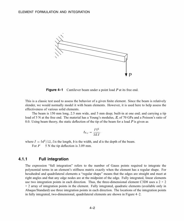
ELEMENT FORMULATION AND INTEGRATION
P
Figure 4–1 Cantilever beam under a point load P at its free end.
This is a classic test used to assess the behavior of a given finite element. Since the beam is relativelyslender, we would normally model it with beam elements. However, it is used here to help assess theeffectiveness of various solid elements.
The beam is 150 mm long, 2.5 mm wide, and 5 mm deep; built-in at one end; and carrying a tipload of 5 N at the free end. The material has a Young’s modulus, E, of 70 GPa and a Poisson’s ratio of0.0. Using beam theory, the static deflection of the tip of the beam for a load P is given as
where , l is the length, b is the width, and d is the depth of the beam.For 5 N the tip deflection is 3.09 mm.
4.1.1 Full integration
The expression “full integration” refers to the number of Gauss points required to integrate thepolynomial terms in an element’s stiffness matrix exactly when the element has a regular shape. Forhexahedral and quadrilateral elements a “regular shape” means that the edges are straight and meet atright angles and that any edge nodes are at the midpoint of the edge. Fully integrated, linear elementsuse two integration points in each direction. Thus, the three-dimensional element C3D8 uses a 2 × 2× 2 array of integration points in the element. Fully integrated, quadratic elements (available only inAbaqus/Standard) use three integration points in each direction. The locations of the integration pointsin fully integrated, two-dimensional, quadrilateral elements are shown in Figure 4–2.
4–2
Abaqus ID:Printed on:
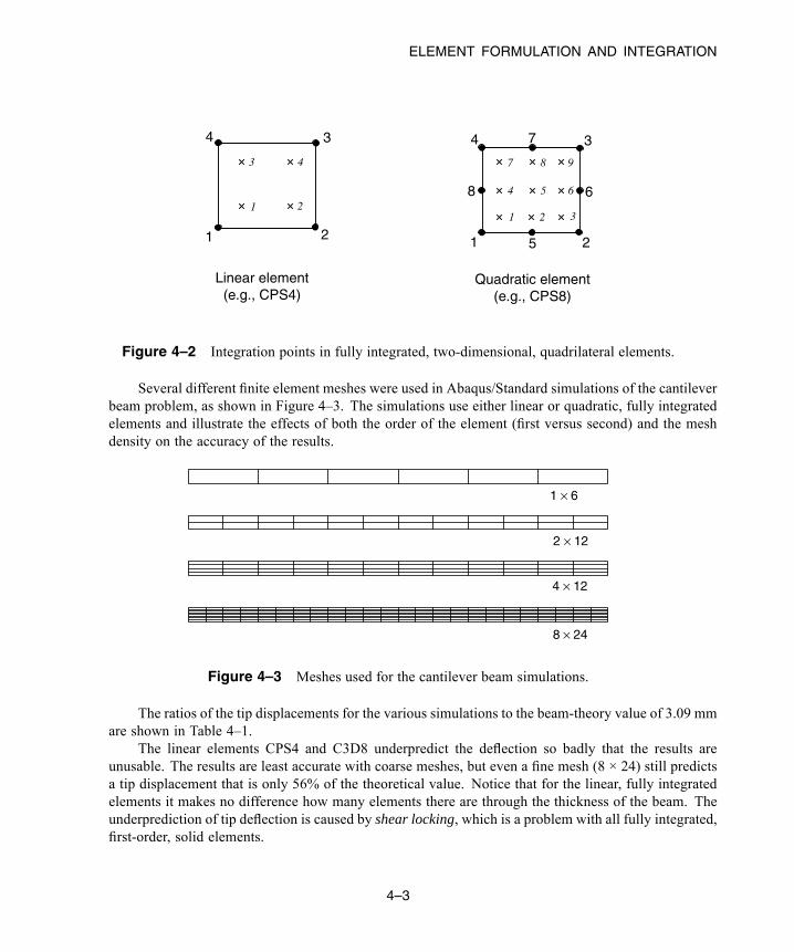
ELEMENT FORMULATION AND INTEGRATION
Quadratic element(e.g., CPS8)
Linear element(e.g., CPS4)
1 2 3
4 5 6
7 8 9
1 2
3 4
1 2
4 3
1 5 2
4
6
7
8
3
Figure 4–2 Integration points in fully integrated, two-dimensional, quadrilateral elements.
Several different finite element meshes were used in Abaqus/Standard simulations of the cantileverbeam problem, as shown in Figure 4–3. The simulations use either linear or quadratic, fully integratedelements and illustrate the effects of both the order of the element (first versus second) and the meshdensity on the accuracy of the results.
1 × 6
2 × 12
4 × 12
8 × 24
Figure 4–3 Meshes used for the cantilever beam simulations.
The ratios of the tip displacements for the various simulations to the beam-theory value of 3.09 mmare shown in Table 4–1.
The linear elements CPS4 and C3D8 underpredict the deflection so badly that the results areunusable. The results are least accurate with coarse meshes, but even a fine mesh (8 × 24) still predictsa tip displacement that is only 56% of the theoretical value. Notice that for the linear, fully integratedelements it makes no difference how many elements there are through the thickness of the beam. Theunderprediction of tip deflection is caused by shear locking, which is a problem with all fully integrated,first-order, solid elements.
4–3
Abaqus ID:Printed on:
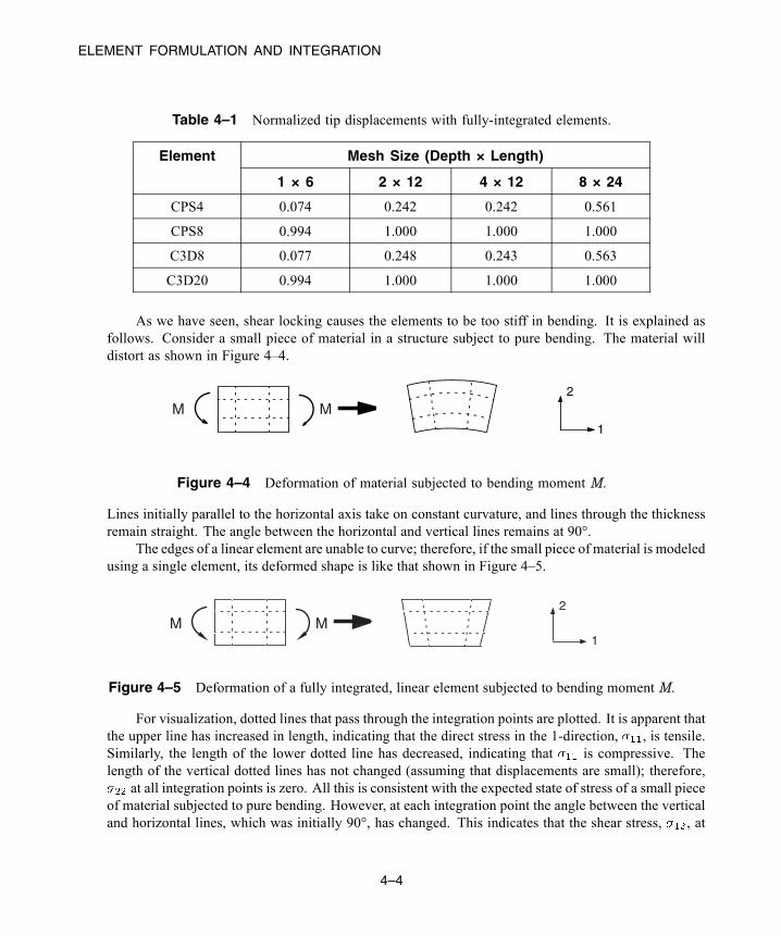
ELEMENT FORMULATION AND INTEGRATION
Table 4–1 Normalized tip displacements with fully-integrated elements.
Mesh Size (Depth × Length)Element
1 × 6 2 × 12 4 × 12 8 × 24
CPS4 0.074 0.242 0.242 0.561
CPS8 0.994 1.000 1.000 1.000
C3D8 0.077 0.248 0.243 0.563
C3D20 0.994 1.000 1.000 1.000
As we have seen, shear locking causes the elements to be too stiff in bending. It is explained asfollows. Consider a small piece of material in a structure subject to pure bending. The material willdistort as shown in Figure 4–4.
1
2
M M
Figure 4–4 Deformation of material subjected to bending moment M.
Lines initially parallel to the horizontal axis take on constant curvature, and lines through the thicknessremain straight. The angle between the horizontal and vertical lines remains at 90°.
The edges of a linear element are unable to curve; therefore, if the small piece of material is modeledusing a single element, its deformed shape is like that shown in Figure 4–5.
1
2
M M1
2
Figure 4–5 Deformation of a fully integrated, linear element subjected to bending moment M.
For visualization, dotted lines that pass through the integration points are plotted. It is apparent thatthe upper line has increased in length, indicating that the direct stress in the 1-direction, , is tensile.Similarly, the length of the lower dotted line has decreased, indicating that is compressive. Thelength of the vertical dotted lines has not changed (assuming that displacements are small); therefore,
at all integration points is zero. All this is consistent with the expected state of stress of a small pieceof material subjected to pure bending. However, at each integration point the angle between the verticaland horizontal lines, which was initially 90°, has changed. This indicates that the shear stress, , at
4–4
Abaqus ID:Printed on:
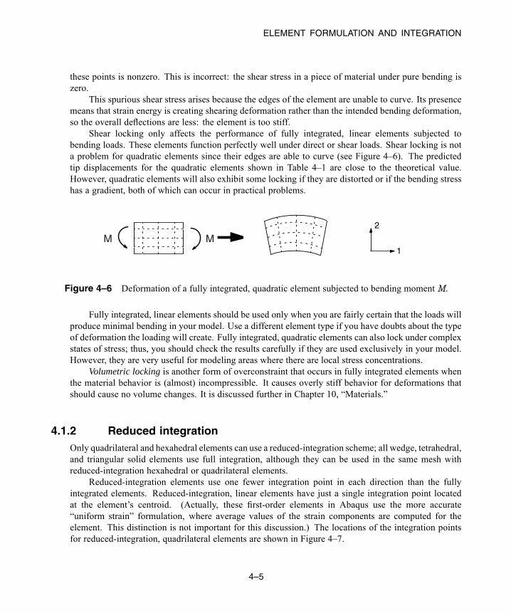
ELEMENT FORMULATION AND INTEGRATION
these points is nonzero. This is incorrect: the shear stress in a piece of material under pure bending iszero.
This spurious shear stress arises because the edges of the element are unable to curve. Its presencemeans that strain energy is creating shearing deformation rather than the intended bending deformation,so the overall deflections are less: the element is too stiff.
Shear locking only affects the performance of fully integrated, linear elements subjected tobending loads. These elements function perfectly well under direct or shear loads. Shear locking is nota problem for quadratic elements since their edges are able to curve (see Figure 4–6). The predictedtip displacements for the quadratic elements shown in Table 4–1 are close to the theoretical value.However, quadratic elements will also exhibit some locking if they are distorted or if the bending stresshas a gradient, both of which can occur in practical problems.
1
2
M M
Figure 4–6 Deformation of a fully integrated, quadratic element subjected to bending momentM.
Fully integrated, linear elements should be used only when you are fairly certain that the loads willproduce minimal bending in your model. Use a different element type if you have doubts about the typeof deformation the loading will create. Fully integrated, quadratic elements can also lock under complexstates of stress; thus, you should check the results carefully if they are used exclusively in your model.However, they are very useful for modeling areas where there are local stress concentrations.
Volumetric locking is another form of overconstraint that occurs in fully integrated elements whenthe material behavior is (almost) incompressible. It causes overly stiff behavior for deformations thatshould cause no volume changes. It is discussed further in Chapter 10, “Materials.”
4.1.2 Reduced integrationOnly quadrilateral and hexahedral elements can use a reduced-integration scheme; all wedge, tetrahedral,and triangular solid elements use full integration, although they can be used in the same mesh withreduced-integration hexahedral or quadrilateral elements.
Reduced-integration elements use one fewer integration point in each direction than the fullyintegrated elements. Reduced-integration, linear elements have just a single integration point locatedat the element’s centroid. (Actually, these first-order elements in Abaqus use the more accurate“uniform strain” formulation, where average values of the strain components are computed for theelement. This distinction is not important for this discussion.) The locations of the integration pointsfor reduced-integration, quadrilateral elements are shown in Figure 4–7.
4–5
Abaqus ID:Printed on:
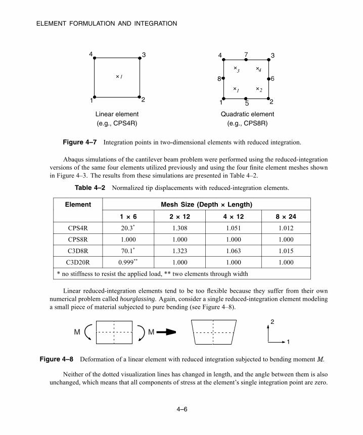
ELEMENT FORMULATION AND INTEGRATION
1 2
3 4
1
4
8
2
34
Linear element(e.g., CPS4R)
Quadratic element(e.g., CPS8R)
1
3
2
1
5
7
6
Figure 4–7 Integration points in two-dimensional elements with reduced integration.
Abaqus simulations of the cantilever beam problem were performed using the reduced-integrationversions of the same four elements utilized previously and using the four finite element meshes shownin Figure 4–3. The results from these simulations are presented in Table 4–2.
Table 4–2 Normalized tip displacements with reduced-integration elements.
Mesh Size (Depth × Length)Element
1 × 6 2 × 12 4 × 12 8 × 24
CPS4R 20.3* 1.308 1.051 1.012
CPS8R 1.000 1.000 1.000 1.000
C3D8R 70.1* 1.323 1.063 1.015
C3D20R 0.999** 1.000 1.000 1.000
* no stiffness to resist the applied load, ** two elements through width
Linear reduced-integration elements tend to be too flexible because they suffer from their ownnumerical problem called hourglassing. Again, consider a single reduced-integration element modelinga small piece of material subjected to pure bending (see Figure 4–8).
1
2
M M
Figure 4–8 Deformation of a linear element with reduced integration subjected to bending momentM.
Neither of the dotted visualization lines has changed in length, and the angle between them is alsounchanged, which means that all components of stress at the element’s single integration point are zero.
4–6
Abaqus ID:Printed on:
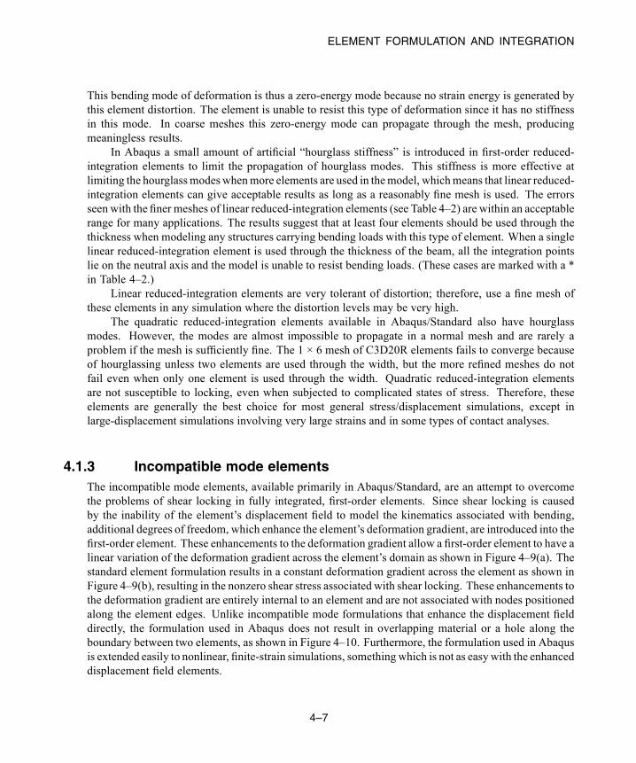
ELEMENT FORMULATION AND INTEGRATION
This bending mode of deformation is thus a zero-energy mode because no strain energy is generated bythis element distortion. The element is unable to resist this type of deformation since it has no stiffnessin this mode. In coarse meshes this zero-energy mode can propagate through the mesh, producingmeaningless results.
In Abaqus a small amount of artificial “hourglass stiffness” is introduced in first-order reduced-integration elements to limit the propagation of hourglass modes. This stiffness is more effective atlimiting the hourglassmodeswhenmore elements are used in themodel, whichmeans that linear reduced-integration elements can give acceptable results as long as a reasonably fine mesh is used. The errorsseen with the finer meshes of linear reduced-integration elements (see Table 4–2) are within an acceptablerange for many applications. The results suggest that at least four elements should be used through thethickness when modeling any structures carrying bending loads with this type of element. When a singlelinear reduced-integration element is used through the thickness of the beam, all the integration pointslie on the neutral axis and the model is unable to resist bending loads. (These cases are marked with a *in Table 4–2.)
Linear reduced-integration elements are very tolerant of distortion; therefore, use a fine mesh ofthese elements in any simulation where the distortion levels may be very high.
The quadratic reduced-integration elements available in Abaqus/Standard also have hourglassmodes. However, the modes are almost impossible to propagate in a normal mesh and are rarely aproblem if the mesh is sufficiently fine. The 1 × 6 mesh of C3D20R elements fails to converge becauseof hourglassing unless two elements are used through the width, but the more refined meshes do notfail even when only one element is used through the width. Quadratic reduced-integration elementsare not susceptible to locking, even when subjected to complicated states of stress. Therefore, theseelements are generally the best choice for most general stress/displacement simulations, except inlarge-displacement simulations involving very large strains and in some types of contact analyses.
4.1.3 Incompatible mode elementsThe incompatible mode elements, available primarily in Abaqus/Standard, are an attempt to overcomethe problems of shear locking in fully integrated, first-order elements. Since shear locking is causedby the inability of the element’s displacement field to model the kinematics associated with bending,additional degrees of freedom, which enhance the element’s deformation gradient, are introduced into thefirst-order element. These enhancements to the deformation gradient allow a first-order element to have alinear variation of the deformation gradient across the element’s domain as shown in Figure 4–9(a). Thestandard element formulation results in a constant deformation gradient across the element as shown inFigure 4–9(b), resulting in the nonzero shear stress associated with shear locking. These enhancements tothe deformation gradient are entirely internal to an element and are not associated with nodes positionedalong the element edges. Unlike incompatible mode formulations that enhance the displacement fielddirectly, the formulation used in Abaqus does not result in overlapping material or a hole along theboundary between two elements, as shown in Figure 4–10. Furthermore, the formulation used in Abaqusis extended easily to nonlinear, finite-strain simulations, something which is not as easywith the enhanceddisplacement field elements.
4–7
Abaqus ID:Printed on:
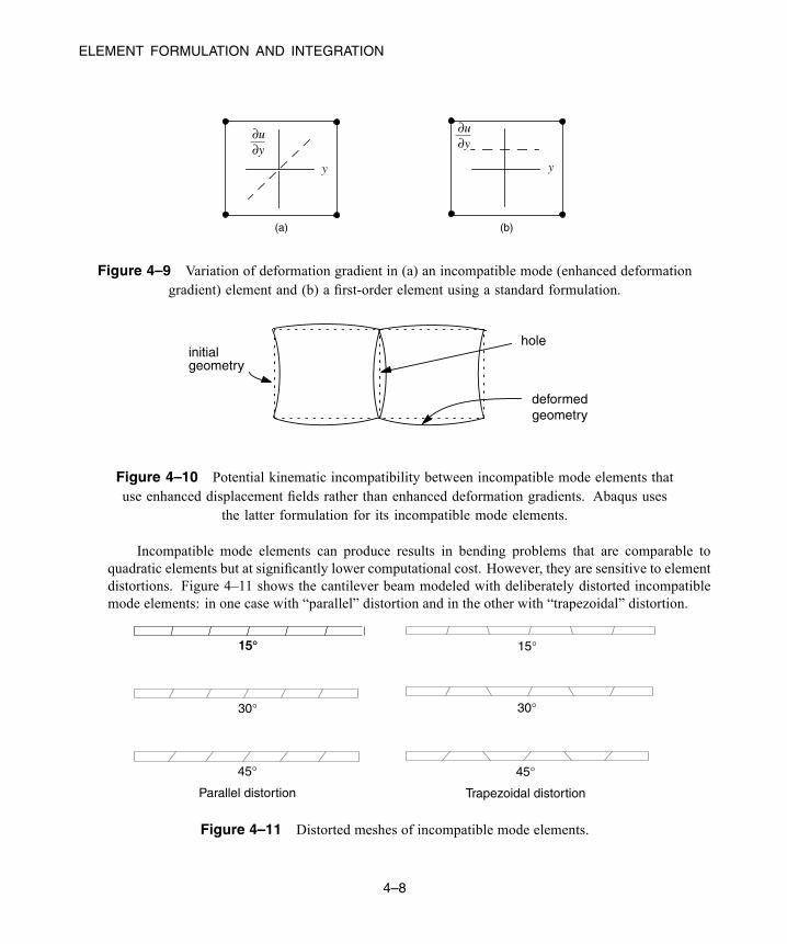
ELEMENT FORMULATION AND INTEGRATION
(a) (b)
y y
∂u∂y
∂u∂y
Figure 4–9 Variation of deformation gradient in (a) an incompatible mode (enhanced deformationgradient) element and (b) a first-order element using a standard formulation.
holeinitialgeometry
deformedgeometry
Figure 4–10 Potential kinematic incompatibility between incompatible mode elements thatuse enhanced displacement fields rather than enhanced deformation gradients. Abaqus uses
the latter formulation for its incompatible mode elements.
Incompatible mode elements can produce results in bending problems that are comparable toquadratic elements but at significantly lower computational cost. However, they are sensitive to elementdistortions. Figure 4–11 shows the cantilever beam modeled with deliberately distorted incompatiblemode elements: in one case with “parallel” distortion and in the other with “trapezoidal” distortion.
15°15° 15°
30°
45°
Parallel distortion
45°
Trapezoidal distortion
30°
Figure 4–11 Distorted meshes of incompatible mode elements.
4–8
Abaqus ID:Printed on:
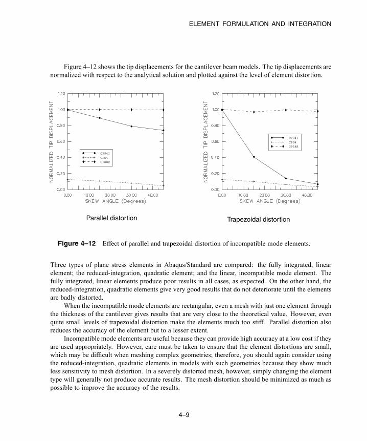
ELEMENT FORMULATION AND INTEGRATION
Figure 4–12 shows the tip displacements for the cantilever beam models. The tip displacements arenormalized with respect to the analytical solution and plotted against the level of element distortion.
Parallel distortion Trapezoidal distortion
CPS4I
CPS4
CPS8R
CPS4I
CPS4
CPS8R
Figure 4–12 Effect of parallel and trapezoidal distortion of incompatible mode elements.
Three types of plane stress elements in Abaqus/Standard are compared: the fully integrated, linearelement; the reduced-integration, quadratic element; and the linear, incompatible mode element. Thefully integrated, linear elements produce poor results in all cases, as expected. On the other hand, thereduced-integration, quadratic elements give very good results that do not deteriorate until the elementsare badly distorted.
When the incompatible mode elements are rectangular, even a mesh with just one element throughthe thickness of the cantilever gives results that are very close to the theoretical value. However, evenquite small levels of trapezoidal distortion make the elements much too stiff. Parallel distortion alsoreduces the accuracy of the element but to a lesser extent.
Incompatible mode elements are useful because they can provide high accuracy at a low cost if theyare used appropriately. However, care must be taken to ensure that the element distortions are small,which may be difficult when meshing complex geometries; therefore, you should again consider usingthe reduced-integration, quadratic elements in models with such geometries because they show muchless sensitivity to mesh distortion. In a severely distorted mesh, however, simply changing the elementtype will generally not produce accurate results. The mesh distortion should be minimized as much aspossible to improve the accuracy of the results.
4–9
Abaqus ID:Printed on:
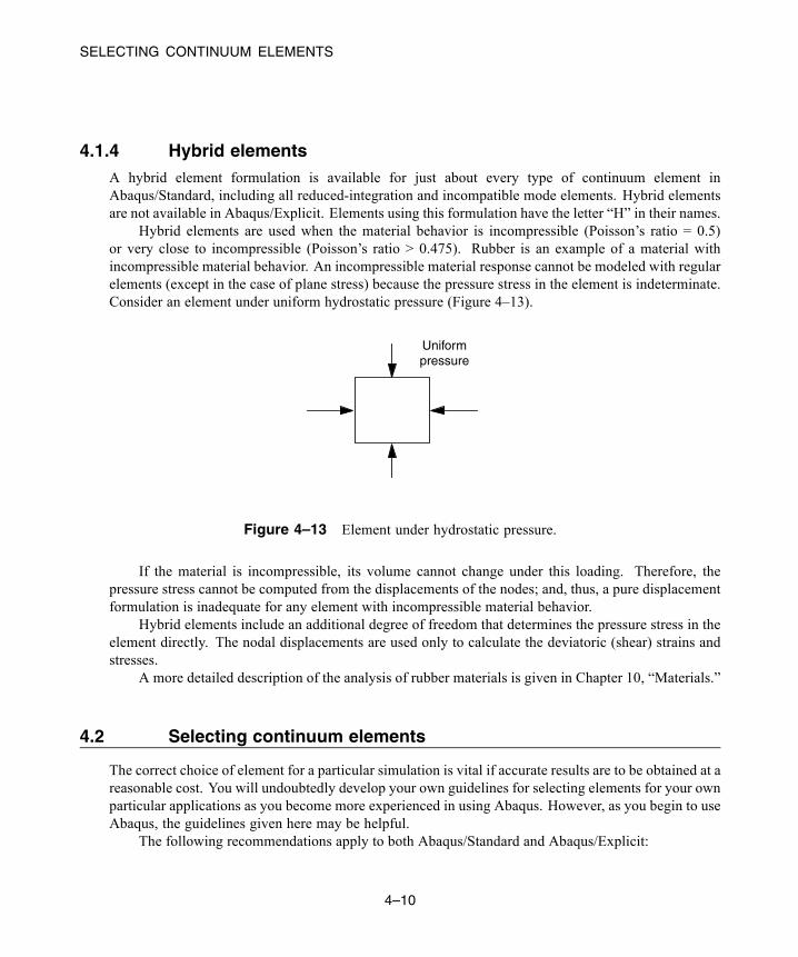
SELECTING CONTINUUM ELEMENTS
4.1.4 Hybrid elementsA hybrid element formulation is available for just about every type of continuum element inAbaqus/Standard, including all reduced-integration and incompatible mode elements. Hybrid elementsare not available in Abaqus/Explicit. Elements using this formulation have the letter “H” in their names.
Hybrid elements are used when the material behavior is incompressible (Poisson’s ratio = 0.5)or very close to incompressible (Poisson’s ratio > 0.475). Rubber is an example of a material withincompressible material behavior. An incompressible material response cannot be modeled with regularelements (except in the case of plane stress) because the pressure stress in the element is indeterminate.Consider an element under uniform hydrostatic pressure (Figure 4–13).
Uniformpressure
Figure 4–13 Element under hydrostatic pressure.
If the material is incompressible, its volume cannot change under this loading. Therefore, thepressure stress cannot be computed from the displacements of the nodes; and, thus, a pure displacementformulation is inadequate for any element with incompressible material behavior.
Hybrid elements include an additional degree of freedom that determines the pressure stress in theelement directly. The nodal displacements are used only to calculate the deviatoric (shear) strains andstresses.
A more detailed description of the analysis of rubber materials is given in Chapter 10, “Materials.”
4.2 Selecting continuum elements
The correct choice of element for a particular simulation is vital if accurate results are to be obtained at areasonable cost. You will undoubtedly develop your own guidelines for selecting elements for your ownparticular applications as you become more experienced in using Abaqus. However, as you begin to useAbaqus, the guidelines given here may be helpful.
The following recommendations apply to both Abaqus/Standard and Abaqus/Explicit:
4–10
Abaqus ID:Printed on:

EXAMPLE: CONNECTING LUG
• Minimize the mesh distortion as much as possible. Coarse meshes with distorted linear elementscan give very poor results.
• Use a fine mesh of linear, reduced-integration elements (CAX4R, CPE4R, CPS4R, C3D8R, etc.)for simulations involving very large mesh distortions (large-strain analysis).
• In three dimensions use hexahedral (brick-shaped) elements wherever possible. They give thebest results for the minimum cost. Complex geometries can be difficult to mesh completely withhexahedrons; therefore, wedge and tetrahedral elements may be necessary. The linear versions ofthese elements, C3D4 and C3D6, are poor elements (fine meshes are needed to obtain accurateresults); as a result, these elements should generally be used only when necessary to complete amesh, and, even then, they should be far from any areas where accurate results are needed.
• Some preprocessors contain free-meshing algorithms that mesh arbitrary geometries withtetrahedral elements. The quadratic tetrahedral elements in Abaqus/Standard (C3D10 orC3D10HS) are suitable for general usage; but when used with contact, they should be usedonly with the “surface-to-surface” contact discretization. An alternative to these elements isthe modified quadratic tetrahedral element (C3D10M) available in both analysis products. Thiselement is robust for large-deformation problems and contact problems using either the traditional“node-to-surface” or the “surface-to-surface” contact discretization and exhibits minimal shearand volumetric locking. With either type of element, however, the analysis will take longer torun than an equivalent mesh of hexahedral elements. You should not use a mesh containing onlylinear tetrahedral elements (C3D4): the results will be inaccurate unless you use an extremelylarge number of elements.
Abaqus/Standard users should also consider the following recommendations:
• Use quadratic, reduced-integration elements (CAX8R, CPE8R, CPS8R, C3D20R, etc.) for generalanalysis work, unless you need to model very large strains or have a simulation with complex,changing contact conditions.
• Use quadratic, fully integrated elements (CAX8, CPE8, CPS8, C3D20, etc.) locally where stressconcentrations may exist. They provide the best resolution of the stress gradients at the lowest cost.
• For contact problems use a fine mesh of linear, reduced-integration elements or incompatible modeelements (CAX4I, CPE4I, CPS4I, C3D8I, etc.). See Chapter 12, “Contact.”
4.3 Example: connecting lug
In this example you will use three-dimensional, continuum elements to model the connecting lug shownin Figure 4–14.
The lug is welded firmly to a massive structure at one end. The other end contains a hole. Whenit is in service, a bolt will be placed through the hole of the lug. You have been asked to determine thestatic deflection of the lug when a 30 kN load is applied to the bolt in the negative 2-direction. Because
4–11
Abaqus ID:Printed on:
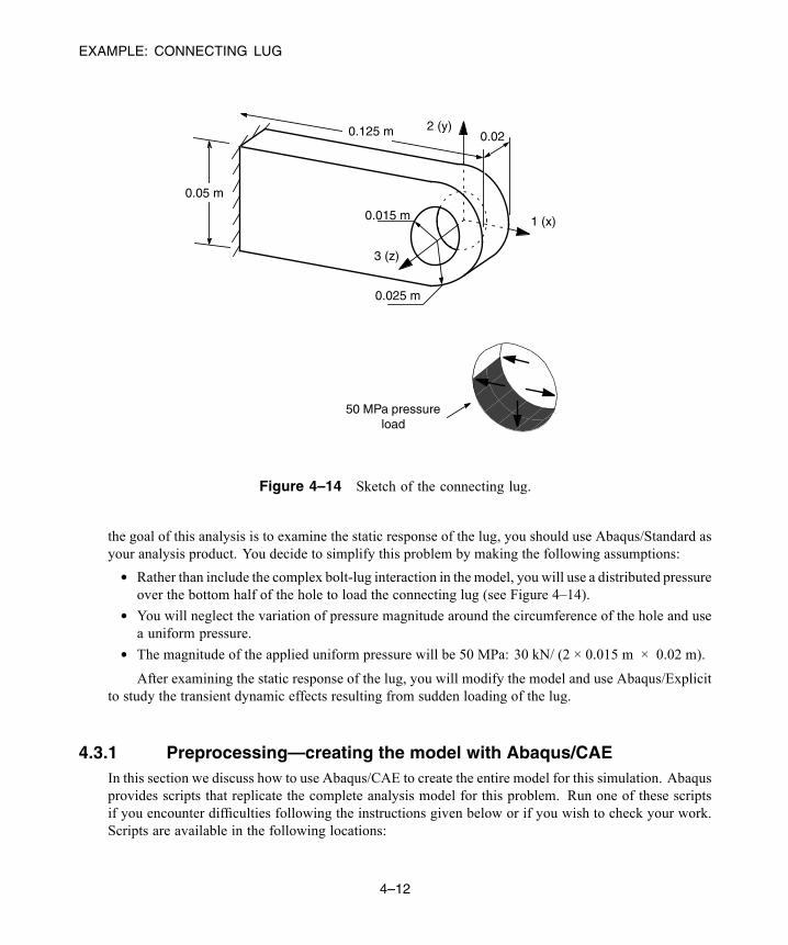
EXAMPLE: CONNECTING LUG
50 MPa pressureload
0.125 m 0.02
0.05 m
2 (y)
1 (x)
3 (z)
0.015 m
0.025 m
Figure 4–14 Sketch of the connecting lug.
the goal of this analysis is to examine the static response of the lug, you should use Abaqus/Standard asyour analysis product. You decide to simplify this problem by making the following assumptions:
• Rather than include the complex bolt-lug interaction in the model, you will use a distributed pressureover the bottom half of the hole to load the connecting lug (see Figure 4–14).
• You will neglect the variation of pressure magnitude around the circumference of the hole and usea uniform pressure.
• The magnitude of the applied uniform pressure will be 50 MPa: 30 kN/ (2 × 0.015 m × 0.02 m).
After examining the static response of the lug, you will modify the model and use Abaqus/Explicitto study the transient dynamic effects resulting from sudden loading of the lug.
4.3.1 Preprocessing—creating the model with Abaqus/CAEIn this section we discuss how to use Abaqus/CAE to create the entire model for this simulation. Abaqusprovides scripts that replicate the complete analysis model for this problem. Run one of these scriptsif you encounter difficulties following the instructions given below or if you wish to check your work.Scripts are available in the following locations:
4–12
Abaqus ID:Printed on:

EXAMPLE: CONNECTING LUG
• A Python script for this example is provided in “Connecting lug,” Section A.2, in the HTML versionof this guide. Instructions on how to fetch the script and run it within Abaqus/CAE are given inAppendix A, “Example Files.”
• A plug-in script for this example is available in the Abaqus/CAE Plug-in toolset. To run the scriptfromAbaqus/CAE, selectPlug-ins→Abaqus→Getting Started; highlightConnecting lug; andclick Run. For more information about the Getting Started plug-ins, see “Running the GettingStarted with Abaqus examples,” Section 82.1 of the Abaqus/CAE User’s Guide, in the HTMLversion of this guide.
Starting Abaqus/CAE
Start Abaqus/CAE by typing
abaqus cae
at the operating system prompt, where abaqus is the command used to run Abaqus on your system.From the Create Model Database options in the Start Session dialog box that appears, selectWith Standard/Explicit Model.
Defining the model geometry
As always, the first step in creating the model is to define its geometry. In this example you willcreate a three-dimensional, deformable body with a solid, extruded base feature. You will firstsketch the two-dimensional profile of the lug and then extrude it.
You need to decide what system of units to use in your model. The SI system of meters,seconds, and kilograms is recommended; but you can use another system if you prefer.
To create a part:
1. In the Create Part dialog box, name the part Lug and accept the default settings of a three-dimensional, deformable body and a solid, extruded base feature. In the Approximate sizetext field, type 0.250. This value is twice the largest dimension of the part. Click Continueto exit the Create Part dialog box.
2. Use the dimensions given in Figure 4–14 to sketch the profile of the lug. The following possibleapproach can be used:
a. Create an arbitrary rectangle using the Create Lines: Rectangle tool. Delete the rightvertical edge, and assign an Equal length constraint to the top and bottom edges using
the constraints tool . Use the dimensions tool to adjust the profile so that it is0.100 m long × 0.050 m wide, as shown in Figure 4–15.
Note: The figures in this section include dimensions and constraints for the purpose ofcontrolling the shape of the sketch. As seen previously, these tools are accessible fromthe Sketcher toolbox. These tools are also accessible by selecting Add→Constraint andAdd→Dimension, respectively, from the main menu bar.
4–13
Abaqus ID:Printed on:

EXAMPLE: CONNECTING LUG
H
50.E−03
100.E−03
1
2
3
Figure 4–15 Open rectangle (with grid spacing doubled).
You can edit the dimension values as you add them to the sketch, or you can edit thevalue of existing dimensions by selecting Edit→Dimension from the main menu bar or
by using the Edit Dimension Value tool.
b. Close the profile by adding a semicircular arc, as shown in Figure 4–16, using the Create
Arc: Thru 3 points tool, . Select the two vertices at the open end of the rectangleas the endpoints of the arc, starting with the top one. Select any point to the right of thesketch as a point that lies on the arc. Define Tangent constraints between the ends of thearc and the horizontal lines to refine the sketch. In Figure 4–16 the radial dimension ofthe arc is enclosed in parentheses, indicating that it is used only for reference purposes.To change any dimension to a reference value, simply edit the dimension and toggle onReference in the Edit Dimension dialog box.
c. Sketch a circle of radius 0.015 m, as shown in Figure 4–17, using the Create Circle:
Center and Perimeter tool, . Place the center of the circle to coincide approximatelywith the center of the arc created in the previous step. The perimeter point should beplaced to the right of the center point. Apply a Concentric constraint to the arc and the
circle. Use the Add Dimension tool to change the value of the radius to 0.015 m.
d. The perimeter points of the circles should be on the same horizontal plane as the circlecenter points (as in Figure 4–17). If these points do not line up correctly, dimensionthe vertical distance between the center of each circle and its perimeter point so that thedistance is 0.
4–14
Abaqus ID:Printed on:

EXAMPLE: CONNECTING LUG
H
( 25.E−03 )
50.E−03
100.E−03
1
2
3
Figure 4–16 Rounded end (with grid spacing doubled).
H
V 0.
15.E−03
( 25.E−03 )
50.E−03
100.E−03
1
2
3
Figure 4–17 Lug hole (with grid spacing doubled).
Note: When you mesh a part, Abaqus/CAE places nodes wherever vertices appear alongan edge; therefore, the location of the vertex on the circumference of the circle influencesthe final mesh. Placing it on the same horizontal plane as the center point results in ahigher quality mesh.
e. Click Done in the prompt area when you are finished sketching the profile.
4–15
Abaqus ID:Printed on:
EXAMPLE: CONNECTING LUG
The Edit Base Extrusion dialog box appears. To complete the part definition, you mustspecify the distance over which the profile will be extruded.
f. In the dialog box, enter an extrusion distance of 0.020 m and click OK.
Abaqus/CAE exits the Sketcher and displays the part.
Defining the material and section properties
The next step in creating the model involves defining and assigning material and section propertiesto the part. Each region of a deformable body must refer to a section property, which includes thematerial definition. In this model you will create a single linear elastic material with a Young’smodulus E = 200 GPa and Poisson’s ratio = 0.3.
To define material properties:
1. In the Model Tree, double-click the Materials container to create a new material definition.
2. In the material editor that appears, name the material Steel and selectMechanical→Elasticity→Elastic. Enter 200.0E9 for the Young’s Modulus and 0.3for the Poisson’s Ratio. Click OK.
To define section properties:
1. In the Model Tree, double-click the Sections container to create a new section definition.Accept the default solid, homogeneous section type; and name the section LugSection.Click Continue.
2. In the Edit Section dialog box that appears, accept Steel as the material and click OK.
To assign section properties:
1. In the Model Tree, expand the Lug item underneath the Parts container and double-clickSection Assignments in the list of part attributes that appears.
2. Select the entire part as the region to which the section will be assigned by clicking on it. Whenthe part is highlighted, click Done in the prompt area.
3. In the Edit Section Assignment dialog box that appears, accept LugSection as the sectiondefinition, and click OK.
Creating an assembly
An assembly contains all the geometry included in the finite element model. Each Abaqus/CAEmodel contains a single assembly. The assembly is initially empty, even though you have alreadycreated a part. You will create an instance of the part in the Assembly module to include it in yourmodel.
4–16
Abaqus ID:Printed on:

EXAMPLE: CONNECTING LUG
To instance a part:
1. In the Model Tree, expand theAssembly container and double-click Instances in the list thatappears to create an instance of the part.
2. In the Create Instance dialog box, select Lug from the Parts list and click OK.
The model is oriented by default so that the global 1-axis lies along the length of the lug, theglobal 2-axis is vertical, and the global 3-axis lies in the thickness direction.
Defining steps and specifying output requests
You will now define the analysis steps. Since interactions, loads, and boundary conditions can bestep dependent, analysis steps must be defined before these can be specified. For this simulationyou will define a single static, general step. In addition, you will specify output requests for youranalysis. These requests will include output to the output database (.odb) file.
To define a step:
1. In the Model Tree, double-click the Steps container to create an analysis step. In the CreateStep dialog box that appears, name the step LugLoad and accept the General proceduretype. From the list of available procedure options, accept Static, General. Click Continue.
2. In the Edit Step dialog box that appears, enter the following step description: Applyuniform pressure to the hole. Accept the default settings, and click OK.
Since you will use the Visualization module to postprocess the results, you must specify the outputdata you wish to have written to the output database file. Default history and field output requestsare selected automatically by Abaqus/CAE for each procedure type. Edit these requests so that onlythe displacements, stresses, and reaction forces are written as field data to the output database file.
To specify output requests to the .odb file:
1. In the Model Tree, click mouse button 3 on the Field Output Requests container and selectManager from the menu that appears.
2. In the Field Output Requests Manager that appears, select the cell labeled Created inthe column labeled LugLoad if it is not already selected. The information at the bottom of thedialog box indicates that preselected default field output requests have been made for this step.
3. On the right side of the dialog box, click Edit to change the field output requests. In the EditField Output Request dialog box that appears:
a. Click the arrow next to Stresses to show the list of available stress output. Accept thedefault selection of stress components and invariants.
b. Under Forces/Reactions, make the following changes:
i. Toggle off concentrated force and moment output (CF).
ii. Toggle on nodal forces due to element stresses (NFORC).
4–17
Abaqus ID:Printed on:

EXAMPLE: CONNECTING LUG
c. Toggle off Strains and Contact.
d. Accept the default Displacement/Velocity/Acceleration output.
e. Click OK, and click Dismiss to close the Field Output Requests Manager.
Note: The option Exterior only in the Edit Field Output Request dialog box can be usedto restrict field output to nodes and elements that belong to the exterior of three-dimensionalelements in a model; this option reduces the size of the output database file.
4. Delete all history output requests. In the Model Tree, click mouse button 3 on the HistoryOutput Requests container and select Manager to open the History Output RequestsManager. In the History Output Requests Manager, select the cell labeled Created inthe column labeled LugLoad if it is not already selected. At the bottom of the dialog box,click Delete and click Yes in the warning dialog box that appears. Click Dismiss to close theHistory Output Requests Manager.
Prescribing boundary conditions and applied loads
In this model the left-hand end of the connecting lug needs to be constrained in all three directions.This region is where the lug is attached to its parent structure (see Figure 4–18). In Abaqus/CAEboundary conditions are applied to geometric regions of a part rather than to the finite elementmesh itself. This association between boundary conditions and part geometry makes it very easy tovary the mesh without having to respecify the boundary conditions. The same holds true for loaddefinitions.
To prescribe boundary conditions:
1. In the Model Tree, double-click the BCs container to prescribe boundary conditions on themodel. In the Create Boundary Condition dialog box that appears, name the boundarycondition Fix left end, and select LugLoad as the step in which it will be applied(since it is a fixed condition, it can be applied either in the initial step or the analysis step;here we choose the analysis step for convenience). Accept Mechanical as the category andSymmetry/Antisymmetry/Encastre as the type. Click Continue.
2. You may need to rotate the view to facilitate your selection in the following steps. Select
View→Rotate from the main menu bar (or use the tool from the View Manipulationtoolbar) and drag the cursor over the virtual trackball in the viewport. The view rotatesinteractively; try dragging the cursor inside and outside the virtual trackball to see thedifference in behavior. Click mouse button 2 to exit the rotate view tool before proceeding.
3. Select the left end of the lug (indicated in Figure 4–18) using the cursor. Click Done inthe prompt area when the appropriate region is highlighted in the viewport, and toggle onENCASTRE in the Edit Boundary Condition dialog box that appears. Click OK to applythe boundary condition.
4–18
Abaqus ID:Printed on:
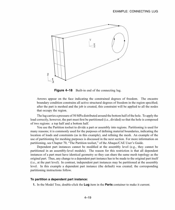
EXAMPLE: CONNECTING LUG
Y
XZ
2
31
Figure 4–18 Built-in end of the connecting lug.
Arrows appear on the face indicating the constrained degrees of freedom. The encastreboundary condition constrains all active structural degrees of freedom in the region specified;after the part is meshed and the job is created, this constraint will be applied to all the nodesthat occupy the region.
The lug carries a pressure of 50MPa distributed around the bottom half of the hole. To apply theload correctly, however, the part must first be partitioned (i.e., divided) so that the hole is composedof two regions: a top half and a bottom half.
You use the Partition toolset to divide a part or assembly into regions. Partitioning is used formany reasons; it is commonly used for the purposes of defining material boundaries, indicating thelocation of loads and constraints (as in this example), and refining the mesh. An example of theuse of partitioning for meshing purposes is discussed in the next section. For more information onpartitioning, see Chapter 70, “The Partition toolset,” of the Abaqus/CAE User’s Guide.
Dependent part instances cannot be modified at the assembly level (e.g., they cannot bepartitioned in an assembly-level module). The reason for this restriction is that all dependentinstances of a part must have identical geometry so they can share the same mesh topology as theoriginal part. Thus, any change to a dependent part instance has to be made to the original part itself(i.e., at the part level). In contrast, independent part instances may be partitioned at the assemblylevel. In this example a dependent part instance (the default) was created; the correspondingpartitioning instructions follow.
To partition a dependent part instance:
1. In the Model Tree, double-click the Lug item in the Parts container to make it current.
4–19
Abaqus ID:Printed on:
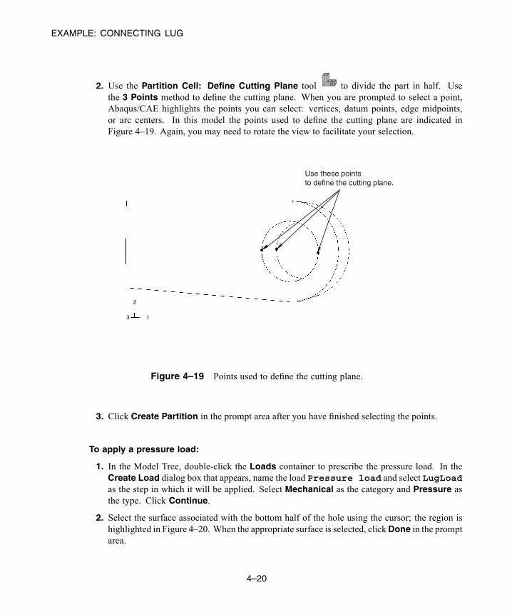
EXAMPLE: CONNECTING LUG
2. Use the Partition Cell: Define Cutting Plane tool to divide the part in half. Usethe 3 Points method to define the cutting plane. When you are prompted to select a point,Abaqus/CAE highlights the points you can select: vertices, datum points, edge midpoints,or arc centers. In this model the points used to define the cutting plane are indicated inFigure 4–19. Again, you may need to rotate the view to facilitate your selection.
1
2
3
Use these pointsto define the cutting plane.
Figure 4–19 Points used to define the cutting plane.
3. Click Create Partition in the prompt area after you have finished selecting the points.
To apply a pressure load:
1. In the Model Tree, double-click the Loads container to prescribe the pressure load. In theCreate Load dialog box that appears, name the load Pressure load and select LugLoadas the step in which it will be applied. Select Mechanical as the category and Pressure asthe type. Click Continue.
2. Select the surface associated with the bottom half of the hole using the cursor; the region ishighlighted in Figure 4–20. When the appropriate surface is selected, clickDone in the promptarea.
4–20
Abaqus ID:Printed on:
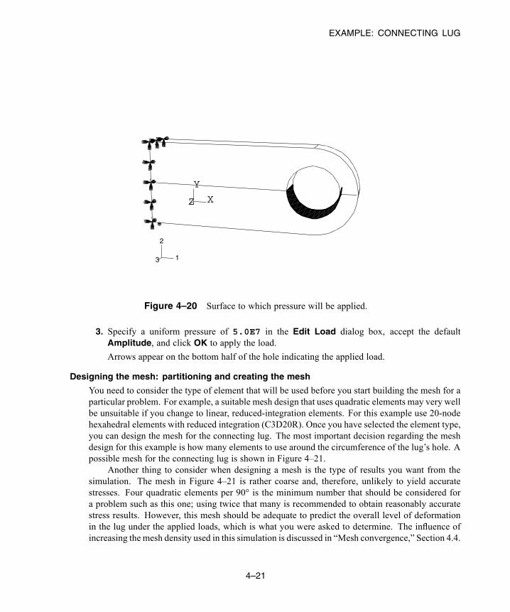
EXAMPLE: CONNECTING LUG
Z
Y
X
1
2
3
Figure 4–20 Surface to which pressure will be applied.
3. Specify a uniform pressure of 5.0E7 in the Edit Load dialog box, accept the defaultAmplitude, and click OK to apply the load.
Arrows appear on the bottom half of the hole indicating the applied load.
Designing the mesh: partitioning and creating the mesh
You need to consider the type of element that will be used before you start building the mesh for aparticular problem. For example, a suitable mesh design that uses quadratic elements may very wellbe unsuitable if you change to linear, reduced-integration elements. For this example use 20-nodehexahedral elements with reduced integration (C3D20R). Once you have selected the element type,you can design the mesh for the connecting lug. The most important decision regarding the meshdesign for this example is how many elements to use around the circumference of the lug’s hole. Apossible mesh for the connecting lug is shown in Figure 4–21.
Another thing to consider when designing a mesh is the type of results you want from thesimulation. The mesh in Figure 4–21 is rather coarse and, therefore, unlikely to yield accuratestresses. Four quadratic elements per 90° is the minimum number that should be considered fora problem such as this one; using twice that many is recommended to obtain reasonably accuratestress results. However, this mesh should be adequate to predict the overall level of deformationin the lug under the applied loads, which is what you were asked to determine. The influence ofincreasing the mesh density used in this simulation is discussed in “Mesh convergence,” Section 4.4.
4–21
Abaqus ID:Printed on:

EXAMPLE: CONNECTING LUG
1
2
3
Figure 4–21 Suggested mesh of C3D20R elements for the connecting lug model.
Abaqus/CAE offers a variety of meshing techniques to mesh models of different topologies.The different meshing techniques provide varying levels of automation and user control. Thefollowing three types of mesh generation techniques are available:
Structured meshing
Structured meshing applies preestablished mesh patterns to particular model topologies.Complex models must generally be partitioned into simpler regions to use this technique.
Swept meshing
Swept meshing extrudes an internally generated mesh along a sweep path or revolves it aroundan axis of revolution. Like structured meshing, swept meshing is limited to models withspecific topologies and geometries.
Free meshing
The free meshing technique is the most flexible meshing technique. It uses no preestablishedmesh patterns and can be applied to almost any model shape.
Bottom-up meshing
You use the bottom-up meshing technique to create a hexahedral or hex-dominated mesh ona solid region that is unmeshable or difficult to mesh using the automated top-down meshingtechniques. Bottom-up meshing is a manual process that allows you to select the method andparameters that Abaqus/CAE uses to build up a solid mesh of hexahedral elements. Bottom-upmeshing is not discussed in any of the examples in this guide.
When you enter the Mesh module, Abaqus/CAE color codes regions of the model accordingto the methods it will use to generate a mesh:
4–22
Abaqus ID:Printed on:
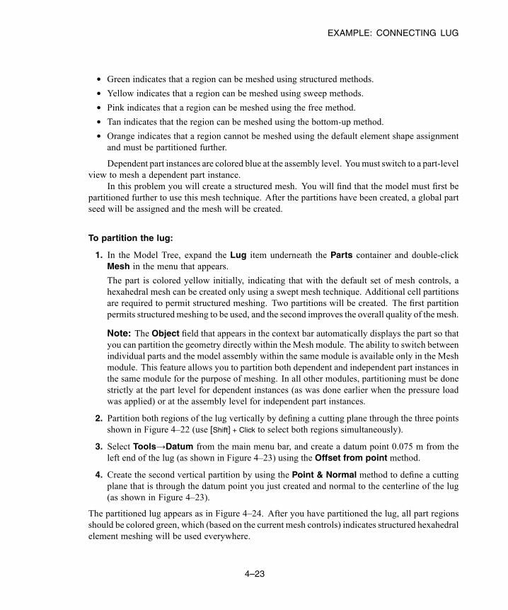
EXAMPLE: CONNECTING LUG
• Green indicates that a region can be meshed using structured methods.• Yellow indicates that a region can be meshed using sweep methods.• Pink indicates that a region can be meshed using the free method.• Tan indicates that the region can be meshed using the bottom-up method.• Orange indicates that a region cannot be meshed using the default element shape assignmentand must be partitioned further.
Dependent part instances are colored blue at the assembly level. Youmust switch to a part-levelview to mesh a dependent part instance.
In this problem you will create a structured mesh. You will find that the model must first bepartitioned further to use this mesh technique. After the partitions have been created, a global partseed will be assigned and the mesh will be created.
To partition the lug:
1. In the Model Tree, expand the Lug item underneath the Parts container and double-clickMesh in the menu that appears.
The part is colored yellow initially, indicating that with the default set of mesh controls, ahexahedral mesh can be created only using a swept mesh technique. Additional cell partitionsare required to permit structured meshing. Two partitions will be created. The first partitionpermits structured meshing to be used, and the second improves the overall quality of the mesh.
Note: The Object field that appears in the context bar automatically displays the part so thatyou can partition the geometry directly within the Mesh module. The ability to switch betweenindividual parts and the model assembly within the same module is available only in the Meshmodule. This feature allows you to partition both dependent and independent part instances inthe same module for the purpose of meshing. In all other modules, partitioning must be donestrictly at the part level for dependent instances (as was done earlier when the pressure loadwas applied) or at the assembly level for independent part instances.
2. Partition both regions of the lug vertically by defining a cutting plane through the three pointsshown in Figure 4–22 (use [Shift] + Click to select both regions simultaneously).
3. Select Tools→Datum from the main menu bar, and create a datum point 0.075 m from theleft end of the lug (as shown in Figure 4–23) using the Offset from point method.
4. Create the second vertical partition by using the Point & Normal method to define a cuttingplane that is through the datum point you just created and normal to the centerline of the lug(as shown in Figure 4–23).
The partitioned lug appears as in Figure 4–24. After you have partitioned the lug, all part regionsshould be colored green, which (based on the current mesh controls) indicates structured hexahedralelement meshing will be used everywhere.
4–23
Abaqus ID:Printed on:
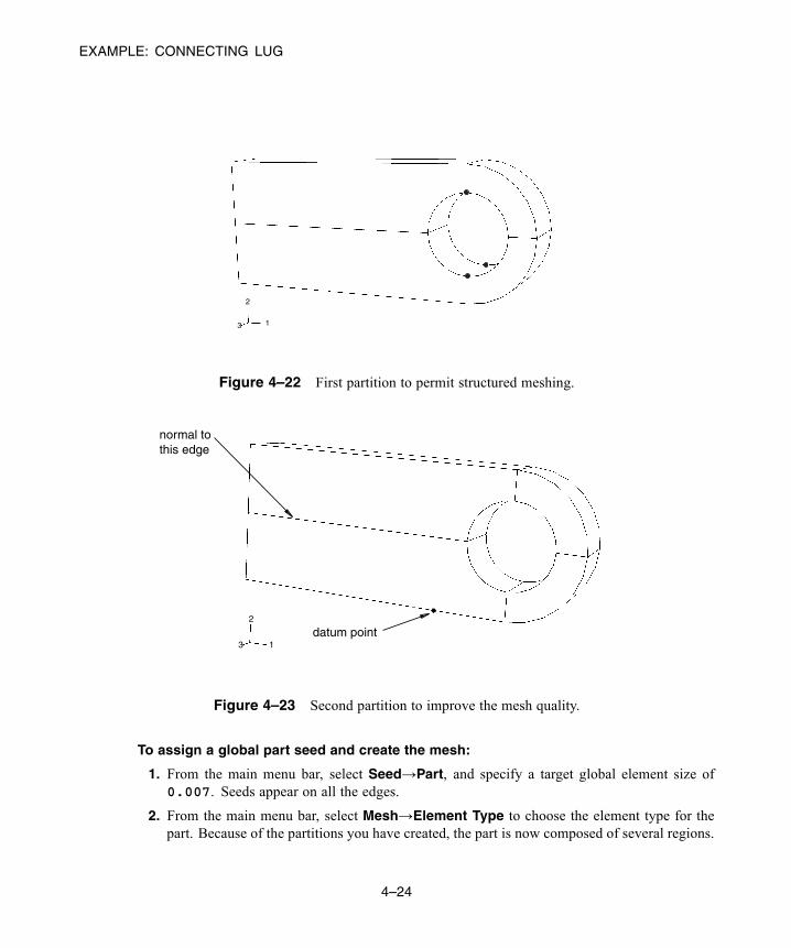
EXAMPLE: CONNECTING LUG
1
2
3
Figure 4–22 First partition to permit structured meshing.
1
2
3
normal tothis edge
datum point
Figure 4–23 Second partition to improve the mesh quality.
To assign a global part seed and create the mesh:
1. From the main menu bar, select Seed→Part, and specify a target global element size of0.007. Seeds appear on all the edges.
2. From the main menu bar, select Mesh→Element Type to choose the element type for thepart. Because of the partitions you have created, the part is now composed of several regions.
4–24
Abaqus ID:Printed on:
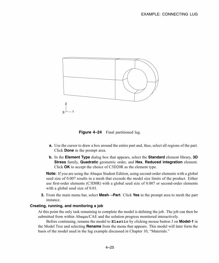
EXAMPLE: CONNECTING LUG
1
2
3
Figure 4–24 Final partitioned lug.
a. Use the cursor to draw a box around the entire part and, thus, select all regions of the part.Click Done in the prompt area.
b. In the Element Type dialog box that appears, select the Standard element library, 3DStress family, Quadratic geometric order, and Hex, Reduced integration element.Click OK to accept the choice of C3D20R as the element type.
Note: If you are using the Abaqus Student Edition, using second-order elements with a globalseed size of 0.007 results in a mesh that exceeds the model size limits of the product. Eitheruse first-order elements (C3D8R) with a global seed size of 0.007 or second-order elementswith a global seed size of 0.01.
3. From the main menu bar, select Mesh→Part. Click Yes in the prompt area to mesh the partinstance.
Creating, running, and monitoring a job
At this point the only task remaining to complete the model is defining the job. The job can then besubmitted from within Abaqus/CAE and the solution progress monitored interactively.
Before continuing, rename the model to Elastic by clicking mouse button 3 on Model-1 inthe Model Tree and selecting Rename from the menu that appears. This model will later form thebasis of the model used in the lug example discussed in Chapter 10, “Materials.”
4–25
Abaqus ID:Printed on:

EXAMPLE: CONNECTING LUG
To create a job:
1. In the Model Tree, double-click the Jobs container to create a job. Name the job Lug, andclick Continue.
2. In the Edit Job dialog box, enter the following description: Linear Elastic SteelConnecting Lug.
3. Accept the default job settings, and click OK.
Save your model in a model database file named Lug.cae.
To run the job:
1. In the Model Tree, click mouse button 3 on the job named Lug and select Submit to submityour job for analysis.
A dialog box appears to warn you that history output has not been requested for the LugLoadstep. Click Yes to continue with the job submission.
2. In the Model Tree, click mouse button 3 on the job named Lug and select Monitor from themenu that appears to open the job monitor.
At the top of the dialog box, a summary of the solution progress is included. This summaryis updated continuously as the analysis progresses. Any errors and/or warnings that areencountered during the analysis are noted in the appropriate tabbed pages. If any errors areencountered, correct the model and rerun the simulation. Be sure to investigate the cause ofany warning messages and take appropriate action; recall that some warning messages can beignored safely while others require corrective action.
3. When the job has completed, click Dismiss to close the job monitor.
4.3.2 Postprocessing—visualizing the resultsIn the Model Tree, click mouse button 3 on the job named Lug and select Results to enter theVisualization module and automatically open the output database (.odb) file created by this job.Alternatively, from the Module list located in the context bar, select Visualization to enter theVisualization module; open the .odb file by selecting File→Open from the main menu bar anddouble-clicking on the appropriate file.
Plotting the deformed shape
From the main menu bar, select Plot→Deformed Shape; or use the tool in the toolbox.Figure 4–25 displays the deformed model shape at the end of the analysis. What is the displacementmagnification level?
Changing the view
The default view is isometric. You can change the view using the options in the View menu or theview tools in the View Manipulation toolbar. You can also specify a view by entering values for
4–26
Abaqus ID:Printed on:
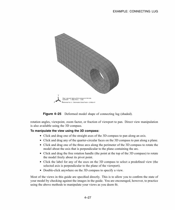
EXAMPLE: CONNECTING LUG
Step: LugLoad, Apply uniform pressure to the holeIncrement 1: Step Time = 1.000
Deformed Var: U Deformation Scale Factor: +2.962e+01X
Y
Z
Figure 4–25 Deformed model shape of connecting lug (shaded).
rotation angles, viewpoint, zoom factor, or fraction of viewport to pan. Direct view manipulationis also available using the 3D compass.
To manipulate the view using the 3D compass:
• Click and drag one of the straight axes of the 3D compass to pan along an axis.• Click and drag any of the quarter-circular faces on the 3D compass to pan along a plane.• Click and drag one of the three arcs along the perimeter of the 3D compass to rotate themodel about the axis that is perpendicular to the plane containing the arc.
• Click and drag the free rotation handle (the point at the top of the 3D compass) to rotatethe model freely about its pivot point.
• Click the label for any of the axes on the 3D compass to select a predefined view (theselected axis is perpendicular to the plane of the viewport).
• Double-click anywhere on the 3D compass to specify a view.
Most of the views in this guide are specified directly. This is to allow you to confirm the state ofyour model by checking against the images in the guide. You are encouraged, however, to practiceusing the above methods to manipulate your views as you deem fit.
4–27
Abaqus ID:Printed on:
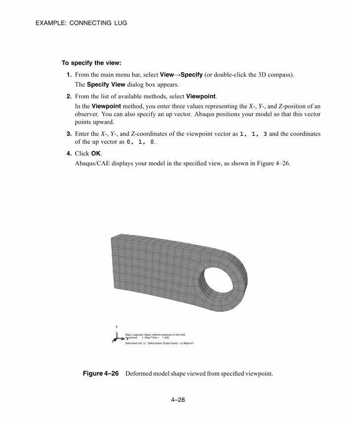
EXAMPLE: CONNECTING LUG
To specify the view:
1. From the main menu bar, select View→Specify (or double-click the 3D compass).
The Specify View dialog box appears.
2. From the list of available methods, select Viewpoint.
In the Viewpoint method, you enter three values representing the X-, Y-, and Z-position of anobserver. You can also specify an up vector. Abaqus positions your model so that this vectorpoints upward.
3. Enter the X-, Y-, and Z-coordinates of the viewpoint vector as 1, 1, 3 and the coordinatesof the up vector as 0, 1, 0.
4. Click OK.
Abaqus/CAE displays your model in the specified view, as shown in Figure 4–26.
Step: LugLoad, Apply uniform pressure to the holeIncrement 1: Step Time = 1.000
Deformed Var: U Deformation Scale Factor: +2.962e+01
X
Y
Z
Figure 4–26 Deformedmodel shape viewed from specified viewpoint.
4–28
Abaqus ID:Printed on:
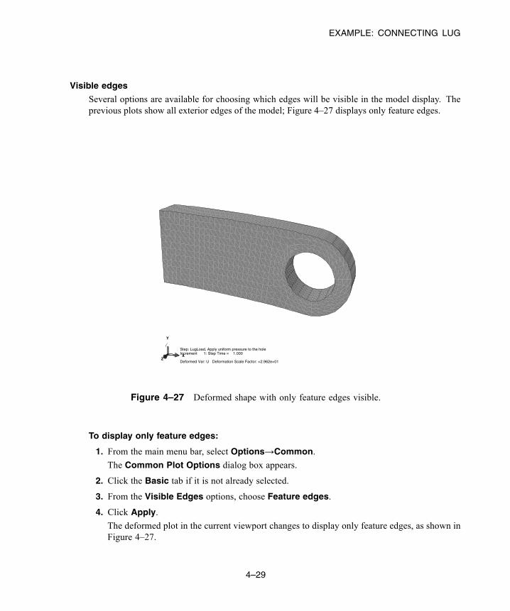
EXAMPLE: CONNECTING LUG
Visible edges
Several options are available for choosing which edges will be visible in the model display. Theprevious plots show all exterior edges of the model; Figure 4–27 displays only feature edges.
Step: LugLoad, Apply uniform pressure to the holeIncrement 1: Step Time = 1.000
Deformed Var: U Deformation Scale Factor: +2.962e+01
X
Y
Z
Figure 4–27 Deformed shape with only feature edges visible.
To display only feature edges:
1. From the main menu bar, select Options→Common.
The Common Plot Options dialog box appears.
2. Click the Basic tab if it is not already selected.
3. From the Visible Edges options, choose Feature edges.
4. Click Apply.
The deformed plot in the current viewport changes to display only feature edges, as shown inFigure 4–27.
4–29
Abaqus ID:Printed on:
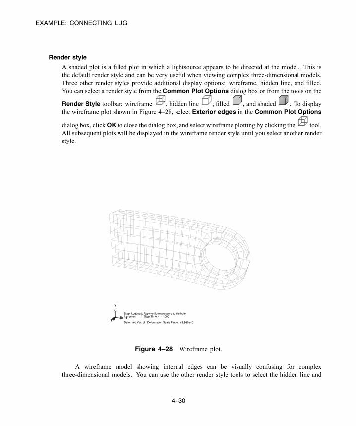
EXAMPLE: CONNECTING LUG
Render style
A shaded plot is a filled plot in which a lightsource appears to be directed at the model. This isthe default render style and can be very useful when viewing complex three-dimensional models.Three other render styles provide additional display options: wireframe, hidden line, and filled.You can select a render style from the Common Plot Options dialog box or from the tools on the
Render Style toolbar: wireframe , hidden line , filled , and shaded . To displaythe wireframe plot shown in Figure 4–28, select Exterior edges in the Common Plot Options
dialog box, clickOK to close the dialog box, and select wireframe plotting by clicking the tool.All subsequent plots will be displayed in the wireframe render style until you select another renderstyle.
Step: LugLoad, Apply uniform pressure to the holeIncrement 1: Step Time = 1.000
Deformed Var: U Deformation Scale Factor: +2.962e+01
X
Y
Z
Figure 4–28 Wireframe plot.
A wireframe model showing internal edges can be visually confusing for complexthree-dimensional models. You can use the other render style tools to select the hidden line and
4–30
Abaqus ID:Printed on:
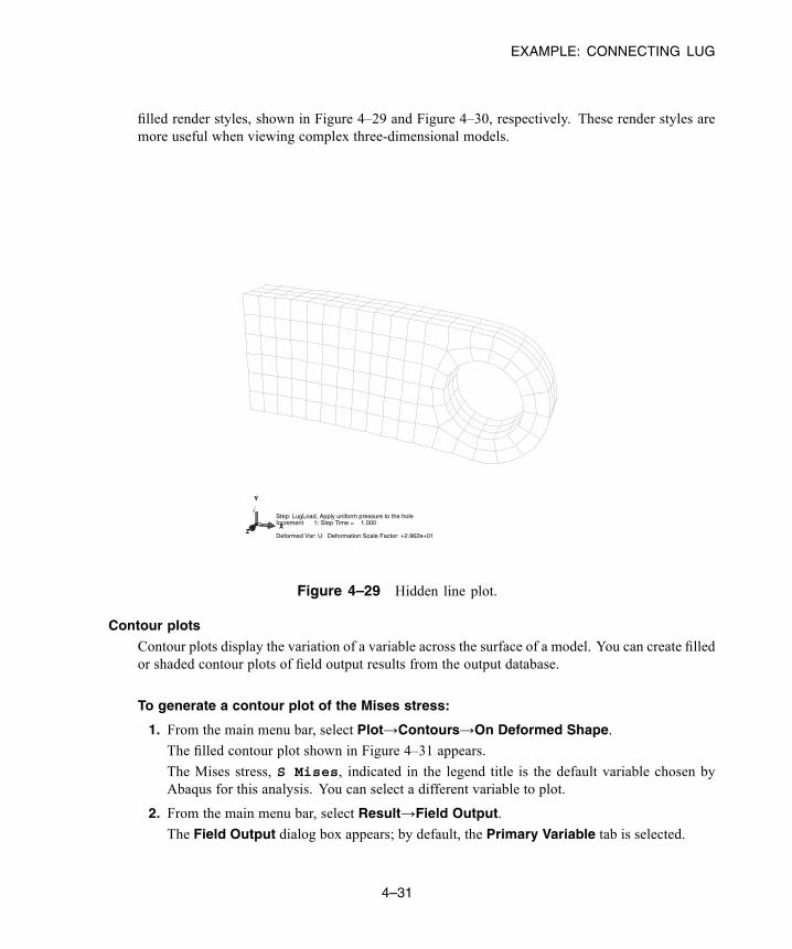
EXAMPLE: CONNECTING LUG
filled render styles, shown in Figure 4–29 and Figure 4–30, respectively. These render styles aremore useful when viewing complex three-dimensional models.
Step: LugLoad, Apply uniform pressure to the holeIncrement 1: Step Time = 1.000
Deformed Var: U Deformation Scale Factor: +2.962e+01
X
Y
Z
Figure 4–29 Hidden line plot.
Contour plots
Contour plots display the variation of a variable across the surface of a model. You can create filledor shaded contour plots of field output results from the output database.
To generate a contour plot of the Mises stress:
1. From the main menu bar, select Plot→Contours→On Deformed Shape.
The filled contour plot shown in Figure 4–31 appears.
The Mises stress, S Mises, indicated in the legend title is the default variable chosen byAbaqus for this analysis. You can select a different variable to plot.
2. From the main menu bar, select Result→Field Output.
The Field Output dialog box appears; by default, the Primary Variable tab is selected.
4–31
Abaqus ID:Printed on:

EXAMPLE: CONNECTING LUG
Step: LugLoad, Apply uniform pressure to the holeIncrement 1: Step Time = 1.000
Deformed Var: U Deformation Scale Factor: +2.962e+01
X
Y
Z
Figure 4–30 Filled element plot.
3. From the list of available output variables, select a new variable to plot.
4. Click OK.
The contour plot in the current viewport changes to reflect your selection.
Tip: You can also use the Field Output toolbar, located above the viewport, to changethe displayed field output variable. For more information, see “Using the field outputtoolbar,” Section 42.5.2 of the Abaqus/CAE User’s Guide.
Abaqus/CAE offers many options to customize contour plots. To see the available options,
click the Contour Options tool in the toolbox. By default, Abaqus/CAE automaticallycomputes the minimum and maximum values shown in your contour plots and evenly divides therange between these values into 12 intervals. You can control the minimum and maximum valuesAbaqus/CAE displays (for example, to examine variations within a fixed set of bounds), as wellas the number of intervals.
4–32
Abaqus ID:Printed on:

EXAMPLE: CONNECTING LUG
(Avg: 75%)S, Mises
+3.666e+06+3.888e+07+7.410e+07+1.093e+08+1.445e+08+1.797e+08+2.150e+08+2.502e+08+2.854e+08+3.206e+08+3.558e+08+3.910e+08+4.262e+08
Step: LugLoad, Apply uniform pressure to the holeIncrement 1: Step Time = 1.000Primary Var: S, MisesDeformed Var: U Deformation Scale Factor: +2.962e+01
X
Y
Z
Figure 4–31 Filled contour plot of Mises stress.
To generate a customized contour plot:
1. In the Basic tabbed page of the Contour Plot Options dialog box, drag the ContourIntervals slider to change the number of intervals to nine.
2. In the Limits tabbed page of the Contour Plot Options dialog box, choose Specify besideMax; then enter a maximum value of 400E+6.
3. Choose Specify beside Min; then enter a minimum value of 60E+6.
4. Click OK.
4–33
Abaqus ID:Printed on:
EXAMPLE: CONNECTING LUG
Abaqus/CAE displays your model with the specified contour option settings, as shown inFigure 4–32 (this figure shows Mises stress; your plot will show whichever output variableyou have chosen). These settings remain in effect for all subsequent contour plots until youchange them or reset them to their default values.
Displaying contour results on interior surfaces
You can cut your model such that interior surfaces are made visible. For example, you may want toexamine the stress distribution in the interior of a part. View cuts can be created for such purposes.Here, a simple planar cut is made through the lug to view the Mises stress distribution through thethickness of the part.
Note: View cuts are also available throughout the other modules of Abaqus/CAE. They areillustrated here for convenience.
To create a view cut:
1. From the main menu bar, select Tools→View Cut→Create.
2. In the dialog box that appears, accept the default name and shape. Enter 0,0,0 as the Originof the plane (i.e., a point through which the plane will pass), 1,0,1 as the Normal axis tothe plane, and 0,1,0 as Axis 2 of the plane.
3. Click OK to close the dialog box and to make the view cut.
The view appears as shown in Figure 4–33. From the main menu bar, select Tools→ViewCut→Manager to open the View Cut Manager. By default, the regions on and below the cut
are displayed (as indicated by the check marks beneath the on cut and below cutsymbols). To translate or rotate the cut, choose Translate or Rotate from the list of availablemotions and enter a value or drag the slider at the bottom of the View Cut Manager.
4. To view the full model again, toggle off Cut-4 in the View Cut Manager.
For more information on view cuts, see Chapter 80, “Cutting through a model,” of theAbaqus/CAE User’s Guide.
Maximum and minimum values
The maximum and minimum values of a variable in a model can be determined easily.
To display the minimum and maximum values of a contour variable:
1. From the main menu bar, select Viewport→Viewport Annotation Options; then click theLegend tab in the dialog box that appears.
The Legend options become available.
2. Toggle on Show min/max values.
3. Click OK.
4–34
Abaqus ID:Printed on:
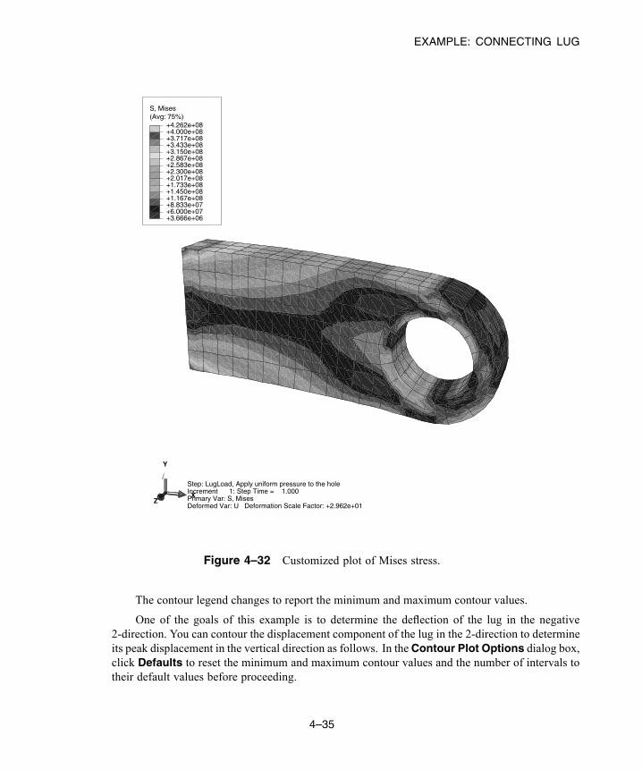
EXAMPLE: CONNECTING LUG
(Avg: 75%)S, Mises
+6.000e+07+8.833e+07+1.167e+08+1.450e+08+1.733e+08+2.017e+08+2.300e+08+2.583e+08+2.867e+08+3.150e+08+3.433e+08+3.717e+08+4.000e+08
+3.666e+06
+4.262e+08
Step: LugLoad, Apply uniform pressure to the holeIncrement 1: Step Time = 1.000Primary Var: S, MisesDeformed Var: U Deformation Scale Factor: +2.962e+01
X
Y
Z
Figure 4–32 Customized plot of Mises stress.
The contour legend changes to report the minimum and maximum contour values.
One of the goals of this example is to determine the deflection of the lug in the negative2-direction. You can contour the displacement component of the lug in the 2-direction to determineits peak displacement in the vertical direction as follows. In theContour Plot Options dialog box,click Defaults to reset the minimum and maximum contour values and the number of intervals totheir default values before proceeding.
4–35
Abaqus ID:Printed on:
EXAMPLE: CONNECTING LUG
To contour the displacement of the connecting lug in the 2-direction:
1. From the list of variable types on the left side of the Field Output toolbar, select Primary ifit is not already selected.
Tip: You can click on the left side of the Field Output toolbar to make yourselections from the Field Output dialog box instead of the toolbar. If you use thedialog box, you must click Apply or OK for Abaqus/CAE to display your selectionsin the viewport.
2. From the list of available output variables in the center of the toolbar, select output variable U.
3. From the list of available components and invariants on the right side of the Field Outputtoolbar, select U2.
What is the maximum displacement value in the negative 2-direction?
Displaying a subset of the model
By default, Abaqus/CAE displays your entire model; however, you can choose to display a subsetof your model called a display group. This subset can contain any combination of part instances,geometry (cells, faces, or edges), elements, nodes, and surfaces from the current model or outputdatabase. For the connecting lug model you will create a display group consisting of the elementsat the bottom of the hole. Since a pressure load was applied to this region, an internal set is createdby Abaqus that can be used for visualization purposes.
To display a subset of the model:
1. In the Results Tree, double-click Display Groups.
The Create Display Group dialog box opens.
2. From the Item list, select Elements. From the Method list, select Internal sets.
Once you have selected these items, the list on the right-hand side of the Create DisplayGroup dialog box shows the available selections.
3. Using this list, identify the set that contains the elements at the bottom of the hole. Toggle onHighlight items in viewport below the list so that the outlines of the elements in the selectedset are highlighted in red.
4. When the highlighted set corresponds to the group of elements at the bottom of the hole, click
Replace to replace the current model display with this element set.
Abaqus/CAE displays the specified subset of your model.
5. Click Dismiss to close the Create Display Group dialog box.
When creating an Abaqusmodel, youmaywant to determine the face labels for a solid element.For example, you may want to verify that the correct load ID was used when applying pressure loads
4–36
Abaqus ID:Printed on:

EXAMPLE: CONNECTING LUG
or when defining surfaces for contact. In such situations you can use the Visualization module todisplay the mesh after you have run a datacheck analysis that creates an output database file.
To display the face identification labels and element numbers on the undeformedmodel shape:
1. From the main menu bar, select Options→Common.
The Common Plot Options dialog box appears.
2. Set the render style to filled; all visible element edges will be displayed for convenience.
a. Toggle on Filled under Render Style.
b. Toggle on All edges under Visible Edges.
3. Click the Labels tab, and toggle on Show element labels and Show face labels.
4. Click Apply to apply the plot options.
5. From the main menu bar, select Plot→Undeformed Shape; or use the tool in thetoolbox.
Abaqus/CAE displays the element and face identification labels in the current display group.
6. Click Defaults in the Common Plot Options dialog box to restore the default plot settingsand then click OK to close the dialog box.
Displaying a free body cut
You can define a free body cut to view the resultant forces andmoments transmitted across a selectedsurface of a model. Force vectors are displayed with a single arrowhead and moment vectors witha double arrowhead.
To create a free body cut:
1. To display the entire model in the viewport, select Tools→Display Group→Plot→All fromthe main menu bar.
2. From the main menu bar, select Tools→Free Body Cut→Manager.
3. Click Create in the Free Body Cut Manager.
4. From the dialog box that appears, select 3D element faces as the Selection method andclick Continue.
5. In the Free Body Cross-Section dialog box, select Surfaces as the Item and Pick fromviewport as the Method.
6. In the prompt area, set the selection method to by angle and accept the default angle.
7. Select the surface, highlighted in Figure 4–34, to define the free body cut cross-section.
4–37
Abaqus ID:Printed on:
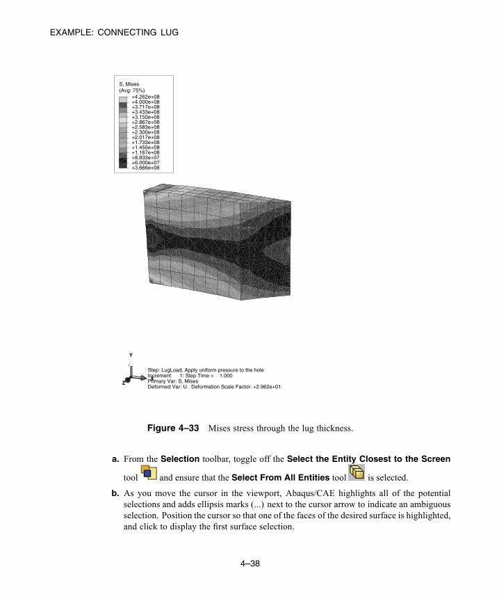
EXAMPLE: CONNECTING LUG
(Avg: 75%)S, Mises
+6.000e+07+8.833e+07+1.167e+08+1.450e+08+1.733e+08+2.017e+08+2.300e+08+2.583e+08+2.867e+08+3.150e+08+3.433e+08+3.717e+08+4.000e+08
+3.666e+06
+4.262e+08
Step: LugLoad, Apply uniform pressure to the holeIncrement 1: Step Time = 1.000Primary Var: S, MisesDeformed Var: U Deformation Scale Factor: +2.962e+01
X
Y
Z
Figure 4–33 Mises stress through the lug thickness.
a. From the Selection toolbar, toggle off the Select the Entity Closest to the Screen
tool and ensure that the Select From All Entities tool is selected.
b. As you move the cursor in the viewport, Abaqus/CAE highlights all of the potentialselections and adds ellipsis marks (...) next to the cursor arrow to indicate an ambiguousselection. Position the cursor so that one of the faces of the desired surface is highlighted,and click to display the first surface selection.
4–38
Abaqus ID:Printed on:
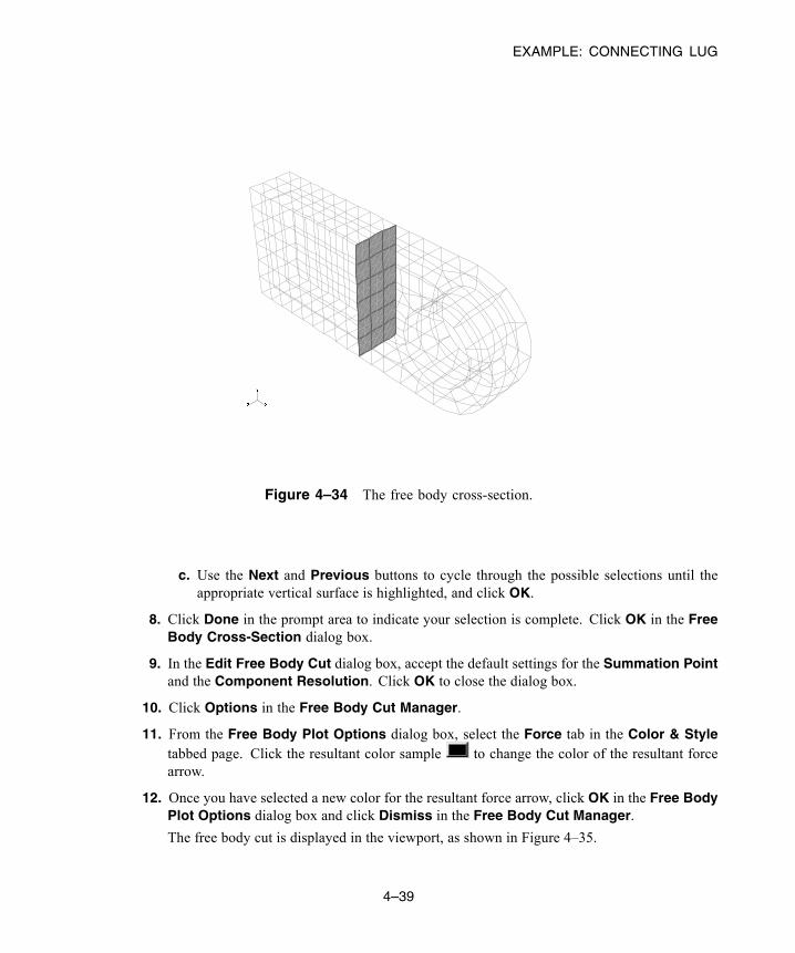
EXAMPLE: CONNECTING LUG
Figure 4–34 The free body cross-section.
c. Use the Next and Previous buttons to cycle through the possible selections until theappropriate vertical surface is highlighted, and click OK.
8. Click Done in the prompt area to indicate your selection is complete. Click OK in the FreeBody Cross-Section dialog box.
9. In the Edit Free Body Cut dialog box, accept the default settings for the Summation Pointand the Component Resolution. Click OK to close the dialog box.
10. Click Options in the Free Body Cut Manager.
11. From the Free Body Plot Options dialog box, select the Force tab in the Color & Styletabbed page. Click the resultant color sample to change the color of the resultant forcearrow.
12. Once you have selected a new color for the resultant force arrow, click OK in the Free BodyPlot Options dialog box and click Dismiss in the Free Body Cut Manager.
The free body cut is displayed in the viewport, as shown in Figure 4–35.
4–39
Abaqus ID:Printed on:

EXAMPLE: CONNECTING LUG
Figure 4–35 Free body cut displayed on the connecting lug.
Generating tabular data reports for subsets of the model
Tabular output data can be generated for selected regions of the model very easily usingAbaqus/CAE. This is achieved using display groups in conjunction with the report generationfeature. For the connecting lug problem we will generate the following tabular data reports:
• Stresses in the elements at the built-in end of the lug (to determine the maximum stress in thelug)
• Reaction forces at the built-in end of the lug (to check that the reaction forces at the constraintsbalance the applied loads)
• Vertical displacements at the bottom of the hole (to determine the deflection of the lug whenthe load is applied)
Since we did not create geometry sets corresponding to these regions, each of these reportswill be generated using display groups whose contents are selected in the viewport. Thus, begin bycreating and saving display groups for each region of interest.
To create and save a display group containing the elements at the built-in end:
1. In the Results Tree, double-click Display Groups.
2. Choose Elements from the Item list and Pick from viewport as the selection method.
3. Restore the option to select entities closest to the screen.
4–40
Abaqus ID:Printed on:

EXAMPLE: CONNECTING LUG
4. In the prompt area, set the selection method to by angle; and click the built-in face of the lug.Click Donewhen all the elements at the built-in face of the lug are highlighted in the viewport.In the Create Display Group dialog box, click Save Selection As. Save the display groupas built-in elements.
To create and save a display group containing the nodes at the built-in end:
1. In the Create Display Group dialog box, choose Nodes from the Item list and Pick fromviewport as the selection method.
2. In the prompt area, set the selection method to by angle; and click the built-in face of the lug.Click Done when all the nodes on the built-in face of the lug are highlighted in the viewport.In the Create Display Group dialog box, click Save Selection As. Save the display groupas built-in nodes.
To create and save a display group containing the nodes at the bottom of the hole:
1. In the Create Display Group dialog box, click Edit Selection to select a different group ofnodes.
2. In the prompt area, set the selection method to individually; and select the nodes at the bottomof the hole in the lug, as indicated in Figure 4–36. ClickDonewhen all the nodes on the bottomof the hole are highlighted in the viewport. In the Create Display Group dialog box, clickSave Selection As. Save the display group as nodes at hole bottom.
1
2
3
Select these nodes
Figure 4–36 Nodes in display group nodes at hole bottom.
Now generate the reports.
4–41
Abaqus ID:Printed on:

EXAMPLE: CONNECTING LUG
To generate field data reports:
1. In the Results Tree, click mouse button 3 on built-in elements underneath the DisplayGroups container. In the menu that appears, select Plot to make it the current display group.
2. From the main menu bar, select Report→Field Output.
3. In theVariable tabbed page of theReport Field Output dialog box, accept the default positionlabeled Integration Point. Click the triangle next to S: Stress components to expand thelist of available variables. From this list, selectMises and the six individual stress components:S11, S22, S33, S12, S13, and S23.
4. In the Setup tabbed page, name the report Lug.rpt. In the Data region at the bottom of thepage, toggle off Column totals.
5. Click Apply.
6. In the Results Tree, click mouse button 3 on built-in nodes underneath the Display Groupscontainer. In the menu that appears, select Plot to make it the current display group. (To seethe nodes, toggle on Show node symbols in the Common Plot Options dialog box.)
7. In the Variable tabbed page of the Report Field Output dialog box, change the position toUnique Nodal. Toggle off S: Stress components, and select RF1, RF2, and RF3 from thelist of available RF: Reaction force variables.
8. In the Data region at the bottom of the Setup tabbed page, toggle on Column totals.
9. Click Apply.
10. In the Results Tree, click mouse button 3 on nodes at hole bottom underneath the DisplayGroups container. In the menu that appears, select Plot to make it the current display group.
11. In the Variable tabbed page of the Report Field Output dialog box, toggle off RF: Reactionforce, and select U2 from the list of available U: Spatial displacement variables.
12. In the Data region at the bottom of the Setup tabbed page, toggle off Column totals.
13. Click OK.
Open the file Lug.rpt in a text editor. A portion of the table of element stresses is shownbelow. The element data are given at the element integration points. The integration point associatedwith a given element is noted under the column labeled Int Pt. The bottom of the table containsinformation on the maximum and minimum stress values in this group of elements. The resultsindicate that the maximum Mises stress at the built-in end is approximately 330 MPa. Your resultsmay differ slightly if your mesh is not identical to the one used here.Field Output Report
Source 1---------
ODB: Lug.odbStep: LugLoadFrame: Increment 1: Step Time = 1.000
4–42
Abaqus ID:Printed on:
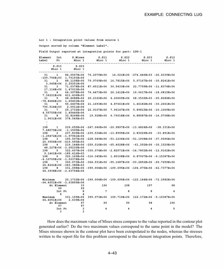
EXAMPLE: CONNECTING LUG
Loc 1 : Integration point values from source 1
Output sorted by column "Element Label".
Field Output reported at integration points for part: LUG-1
Element Int S.Mises S.S11 S.S22 S.S33 S.S12Label Pt @Loc 1 @Loc 1 @Loc 1 @Loc 1 @Loc 1------------------------------------------------------------------------------
S.S13 S.S23@Loc 1 @Loc 1
--------------------------31 1 84.0567E+06 76.2075E+06 14.021E+06 -274.446E+03 -26.4339E+06
-159.756E+03 1.70193E+0631 2 88.1108E+06 79.9769E+06 16.7815E+06 5.07167E+06 -30.8241E+063.045E+06 2.20251E+06
31 3 71.0378E+06 87.4511E+06 30.5433E+06 22.7759E+06 -11.8374E+0617.114E+06 1.47033E+0631 4 64.3978E+06 76.4473E+06 26.1412E+06 19.0617E+06 -18.6815E+06
7.36221E+06 411.436E+0331 5 48.4688E+06 20.2162E+06 4.20669E+06 68.3536E+03 -25.8284E+06
-78.8286E+03 1.65403E+0631 6 55.6407E+06 21.1693E+06 4.87661E+06 1.46182E+06 -30.2661E+06
796.514E+03 2.0911E+0631 7 25.1732E+06 22.9107E+06 7.96147E+06 5.89815E+06 -10.1069E+06
4.55755E+06 1.45446E+0631 8 32.8268E+06 19.928E+06 6.76018E+06 4.88587E+06 -16.9708E+061.9631E+06 378.549E+03..
198 1 239.655E+06 -247.046E+06 -20.9897E+06 -13.4824E+06 -38.331E+067.48079E+06 -1.1505E+06198 2 237.839E+06 -235.534E+06 -13.8995E+06 2.83029E+06 -33.891E+06
-1.25472E+06 -1.57941E+06198 3 190.507E+06 -228.049E+06 -53.1236E+06 -51.1938E+06 -37.0096E+0620.3556E+06 -419.555E+03198 4 219.144E+06 -259.016E+06 -65.4028E+06 -61.292E+06 -30.1529E+0648.227E+06 -2.60239E+06
198 5 322.607E+06 -330.074E+06 -2.82071E+06 -14.7802E+06 -12.9162E+069.1461E+06 -189.416E+03
198 6 320.169E+06 -316.345E+06 1.80108E+06 4.87007E+06 -9.15387E+06-4.10769E+06 -1.03378E+06198 7 300.073E+06 -364.931E+06 -95.1687E+06 -93.2852E+06 -69.7659E+0626.8241E+06 -343.386E+03198 8 331.098E+06 -399.004E+06 -109.695E+06 -104.075E+06 -62.7377E+0664.3938E+06 -2.63754E+06
Minimum 25.1732E+06 -399.004E+06 -109.695E+06 -122.144E+06 -72.2982E+06-64.4051E+06 -2.63899E+06
At Element 33 196 198 197 9899 99
Int Pt 8 7 8 8 44 4
Maximum 331.159E+06 399.073E+06 109.719E+06 122.172E+06 -9.15387E+0664.4051E+06 2.639E+06
At Element 97 99 99 98 19697 97
Int Pt 3 4 4 4 53 3
How does the maximum value of Mises stress compare to the value reported in the contour plotgenerated earlier? Do the two maximum values correspond to the same point in the model? TheMises stresses shown in the contour plot have been extrapolated to the nodes, whereas the stresseswritten to the report file for this problem correspond to the element integration points. Therefore,
4–43
Abaqus ID:Printed on:
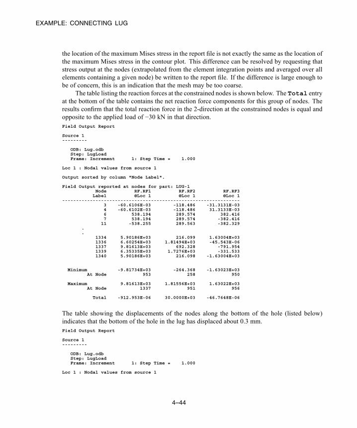
EXAMPLE: CONNECTING LUG
the location of the maximum Mises stress in the report file is not exactly the same as the location ofthe maximum Mises stress in the contour plot. This difference can be resolved by requesting thatstress output at the nodes (extrapolated from the element integration points and averaged over allelements containing a given node) be written to the report file. If the difference is large enough tobe of concern, this is an indication that the mesh may be too coarse.
The table listing the reaction forces at the constrained nodes is shown below. The Total entryat the bottom of the table contains the net reaction force components for this group of nodes. Theresults confirm that the total reaction force in the 2-direction at the constrained nodes is equal andopposite to the applied load of −30 kN in that direction.Field Output Report
Source 1---------
ODB: Lug.odbStep: LugLoadFrame: Increment 1: Step Time = 1.000
Loc 1 : Nodal values from source 1
Output sorted by column "Node Label".
Field Output reported at nodes for part: LUG-1Node RF.RF1 RF.RF2 RF.RF3
Label @Loc 1 @Loc 1 @Loc 1----------------------------------------------------------------
3 -60.6106E-03 -118.486 -31.3131E-034 -60.6102E-03 -118.486 31.3133E-036 538.194 289.574 382.4167 538.194 289.574 -382.416
11 -538.255 289.563 -382.329..
1334 5.90186E+03 216.099 1.63004E+031336 6.60254E+03 1.81494E+03 -45.543E-061337 9.81613E+03 692.328 -791.9541339 6.35335E+03 1.7276E+03 -331.5331340 5.90186E+03 216.098 -1.63004E+03
Minimum -9.81734E+03 -264.368 -1.63023E+03At Node 953 258 950
Maximum 9.81613E+03 1.81556E+03 1.63022E+03At Node 1337 951 956
Total -912.953E-06 30.0000E+03 -46.7648E-06
The table showing the displacements of the nodes along the bottom of the hole (listed below)indicates that the bottom of the hole in the lug has displaced about 0.3 mm.Field Output Report
Source 1---------
ODB: Lug.odbStep: LugLoadFrame: Increment 1: Step Time = 1.000
Loc 1 : Nodal values from source 1
4–44
Abaqus ID:Printed on:
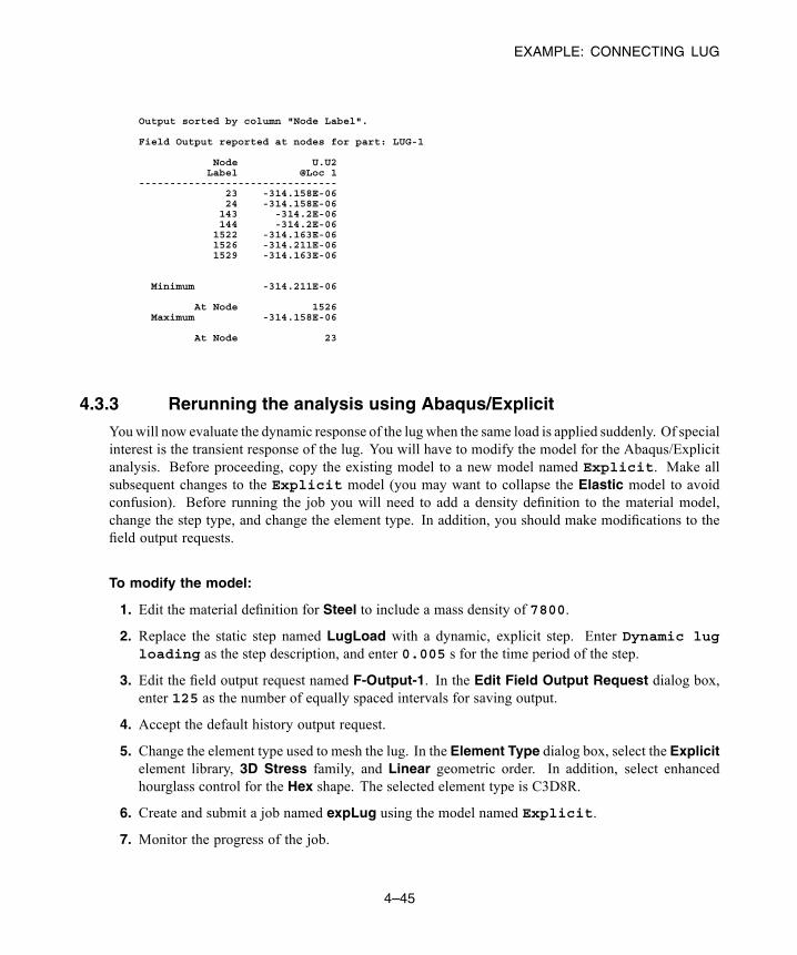
EXAMPLE: CONNECTING LUG
Output sorted by column "Node Label".
Field Output reported at nodes for part: LUG-1
Node U.U2Label @Loc 1
--------------------------------23 -314.158E-0624 -314.158E-06
143 -314.2E-06144 -314.2E-06
1522 -314.163E-061526 -314.211E-061529 -314.163E-06
Minimum -314.211E-06
At Node 1526Maximum -314.158E-06
At Node 23
4.3.3 Rerunning the analysis using Abaqus/Explicit
Youwill now evaluate the dynamic response of the lug when the same load is applied suddenly. Of specialinterest is the transient response of the lug. You will have to modify the model for the Abaqus/Explicitanalysis. Before proceeding, copy the existing model to a new model named Explicit. Make allsubsequent changes to the Explicit model (you may want to collapse the Elastic model to avoidconfusion). Before running the job you will need to add a density definition to the material model,change the step type, and change the element type. In addition, you should make modifications to thefield output requests.
To modify the model:
1. Edit the material definition for Steel to include a mass density of 7800.
2. Replace the static step named LugLoad with a dynamic, explicit step. Enter Dynamic lugloading as the step description, and enter 0.005 s for the time period of the step.
3. Edit the field output request named F-Output-1. In the Edit Field Output Request dialog box,enter 125 as the number of equally spaced intervals for saving output.
4. Accept the default history output request.
5. Change the element type used to mesh the lug. In the Element Type dialog box, select the Explicitelement library, 3D Stress family, and Linear geometric order. In addition, select enhancedhourglass control for the Hex shape. The selected element type is C3D8R.
6. Create and submit a job named expLug using the model named Explicit.
7. Monitor the progress of the job.
4–45
Abaqus ID:Printed on:
EXAMPLE: CONNECTING LUG
At the top of the expLug Monitor dialog box, a summary of the solution progress is included.This summary is updated continuously as the analysis progresses. Any errors and/or warnings thatare encountered during the analysis are noted in the appropriate tabbed pages. If any errors areencountered, correct the model and rerun the simulation. Be sure to investigate the cause of anywarning messages and take appropriate action; recall that some warning messages can be ignoredsafely while others require corrective action.
4.3.4 Postprocessing the dynamic analysis results
In the static analysis performed with Abaqus/Standard you examined the deformed shape of the lug aswell as stress and displacement output. For the Abaqus/Explicit analysis you can similarly examinethe deformed shape, stresses, and displacements in the lug. Because transient dynamic effects mayresult from a sudden loading, you should also examine the time histories for internal and kinetic energy,displacement, and Mises stress.
Open the output database (.odb) file created by this job.
Plotting the deformed shape
From the main menu bar, select Plot→Deformed Shape; or use the tool in the toolbox.Figure 4–37 displays the deformed model shape at the end of the analysis. As discussed earlier,Abaqus/Explicit assumes large deformation theory by default; thus, the deformation scale factor isautomatically set to 1. If the displacements are too small to be seen, scaling can be applied to aidthe study of the response.
To see the vibrations in the lug more clearly, change the deformation scale factor to 50. Inaddition, animate the time history of the deformed shape of the lug and decrease the frame rate ofthe time history animation.
The time history animation of the deformed shape of the lug shows that the suddenly appliedload induces vibrations in the lug. Additional insights about the behavior of the lug under this typeof loading can be gained by plotting the kinetic energy, internal energy, displacement, and stress inthe lug as a function of time. Some of the questions to consider are:
1. Is energy conserved?
2. Was large-displacement theory necessary for this analysis?
3. Are the peak stresses reasonable? Will the material yield?
X–Y plotting
X–Y plots can display the variation of a variable as a function of time. You can create X–Y plotsfrom field and history output.
4–46
Abaqus ID:Printed on:

EXAMPLE: CONNECTING LUG
Step: LugLoad, Dynamic lug loadingIncrement 6787: Step Time = 5.0000E-03
Deformed Var: U Deformation Scale Factor: +1.000e+00
1
2
3
Figure 4–37 Deformed model shape for the explicit analysis (shaded).
To create X–Y plots of the internal and kinetic energy as a function of time:
1. In the Results Tree, expand the History Output container underneath the output databasenamed expLug.odb.
2. The list of all the variables in the history portion of the output database appears; these are theonly history output variables you can plot.
From the list of available output variables, double-click ALLIE to plot the internal energy forthe whole model.
Abaqus reads the data for the curve from the output database file and plots the graph shown inFigure 4–38.
3. Repeat this procedure to plot ALLKE, the kinetic energy for the whole model (shown inFigure 4–39).
Both the internal energy and the kinetic energy show oscillations that reflect the vibrations ofthe lug. Throughout the simulation, kinetic energy is transformed into internal (strain) energyand vice-versa. Since the material is linear elastic, total energy is conserved. This can be seenby plotting ETOTAL, the total energy of the system, together with ALLIE and ALLKE. Thevalue of ETOTAL is approximately zero throughout the course of the analysis. Energy balancesin dynamic analysis are discussed further in Chapter 9, “Nonlinear Explicit Dynamics.”
4–47
Abaqus ID:Printed on:
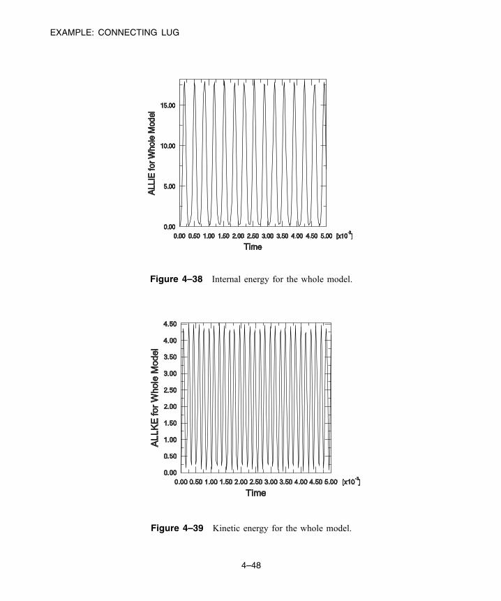
EXAMPLE: CONNECTING LUG
Figure 4–38 Internal energy for the whole model.
Figure 4–39 Kinetic energy for the whole model.
4–48
Abaqus ID:Printed on:
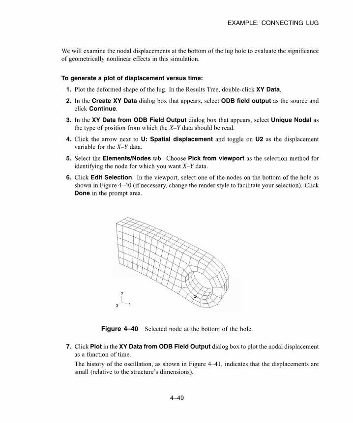
EXAMPLE: CONNECTING LUG
We will examine the nodal displacements at the bottom of the lug hole to evaluate the significanceof geometrically nonlinear effects in this simulation.
To generate a plot of displacement versus time:
1. Plot the deformed shape of the lug. In the Results Tree, double-click XY Data.
2. In the Create XY Data dialog box that appears, select ODB field output as the source andclick Continue.
3. In the XY Data from ODB Field Output dialog box that appears, select Unique Nodal asthe type of position from which the X–Y data should be read.
4. Click the arrow next to U: Spatial displacement and toggle on U2 as the displacementvariable for the X–Y data.
5. Select the Elements/Nodes tab. Choose Pick from viewport as the selection method foridentifying the node for which you want X–Y data.
6. Click Edit Selection. In the viewport, select one of the nodes on the bottom of the hole asshown in Figure 4–40 (if necessary, change the render style to facilitate your selection). ClickDone in the prompt area.
1
2
3
Figure 4–40 Selected node at the bottom of the hole.
7. Click Plot in the XY Data from ODB Field Output dialog box to plot the nodal displacementas a function of time.
The history of the oscillation, as shown in Figure 4–41, indicates that the displacements aresmall (relative to the structure’s dimensions).
4–49
Abaqus ID:Printed on:

EXAMPLE: CONNECTING LUG
Figure 4–41 Displacement of a node at the bottom of the hole.
Thus, this problem could have been solved adequately using small-deformation theory. Thiswould have reduced the computational cost of the simulation without significantly affectingthe results. Nonlinear geometric effects are discussed further in Chapter 8, “Nonlinearity.”
We are also interested in the stress history of the connecting lug. The area of the lug near the built-inend is of particular interest because the peak stresses expected to occur there may cause yielding inthe material.
To generate a plot of Mises stress versus time:
1. Plot the deformed shape of the lug again.
2. Select the Variables tab in the XY Data from ODB Field Output dialog box. Deselect U2as the variable for the X–Y data plot.
3. Change the Position field to Integration Point.
4. Click the arrow next to S: Stress components and toggle on Mises as the stress variablefor the X–Y data.
5. Select the Elements/Nodes tab. Choose Pick from viewport as the selection method foridentifying the element for which you want X–Y data.
6. Click Edit Selection. In the viewport, select one of the elements near the built-in end of thelug as shown in Figure 4–42. Click Done in the prompt area.
4–50
Abaqus ID:Printed on:
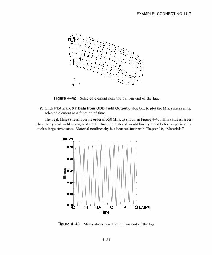
EXAMPLE: CONNECTING LUG
Figure 4–42 Selected element near the built-in end of the lug.
7. Click Plot in the XY Data from ODB Field Output dialog box to plot the Mises stress at theselected element as a function of time.
The peakMises stress is on the order of 550MPa, as shown in Figure 4–43. This value is largerthan the typical yield strength of steel. Thus, the material would have yielded before experiencingsuch a large stress state. Material nonlinearity is discussed further in Chapter 10, “Materials.”
Figure 4–43 Mises stress near the built-in end of the lug.
4–51
Abaqus ID:Printed on:
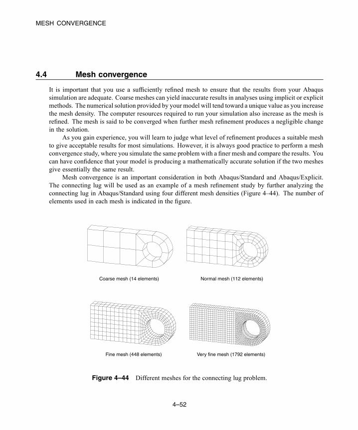
MESH CONVERGENCE
4.4 Mesh convergence
It is important that you use a sufficiently refined mesh to ensure that the results from your Abaqussimulation are adequate. Coarse meshes can yield inaccurate results in analyses using implicit or explicitmethods. The numerical solution provided by your model will tend toward a unique value as you increasethe mesh density. The computer resources required to run your simulation also increase as the mesh isrefined. The mesh is said to be converged when further mesh refinement produces a negligible changein the solution.
As you gain experience, you will learn to judge what level of refinement produces a suitable meshto give acceptable results for most simulations. However, it is always good practice to perform a meshconvergence study, where you simulate the same problem with a finer mesh and compare the results. Youcan have confidence that your model is producing a mathematically accurate solution if the two meshesgive essentially the same result.
Mesh convergence is an important consideration in both Abaqus/Standard and Abaqus/Explicit.The connecting lug will be used as an example of a mesh refinement study by further analyzing theconnecting lug in Abaqus/Standard using four different mesh densities (Figure 4–44). The number ofelements used in each mesh is indicated in the figure.
Fine mesh (448 elements) Very fine mesh (1792 elements)
Normal mesh (112 elements)Coarse mesh (14 elements)
Figure 4–44 Different meshes for the connecting lug problem.
4–52
Abaqus ID:Printed on:
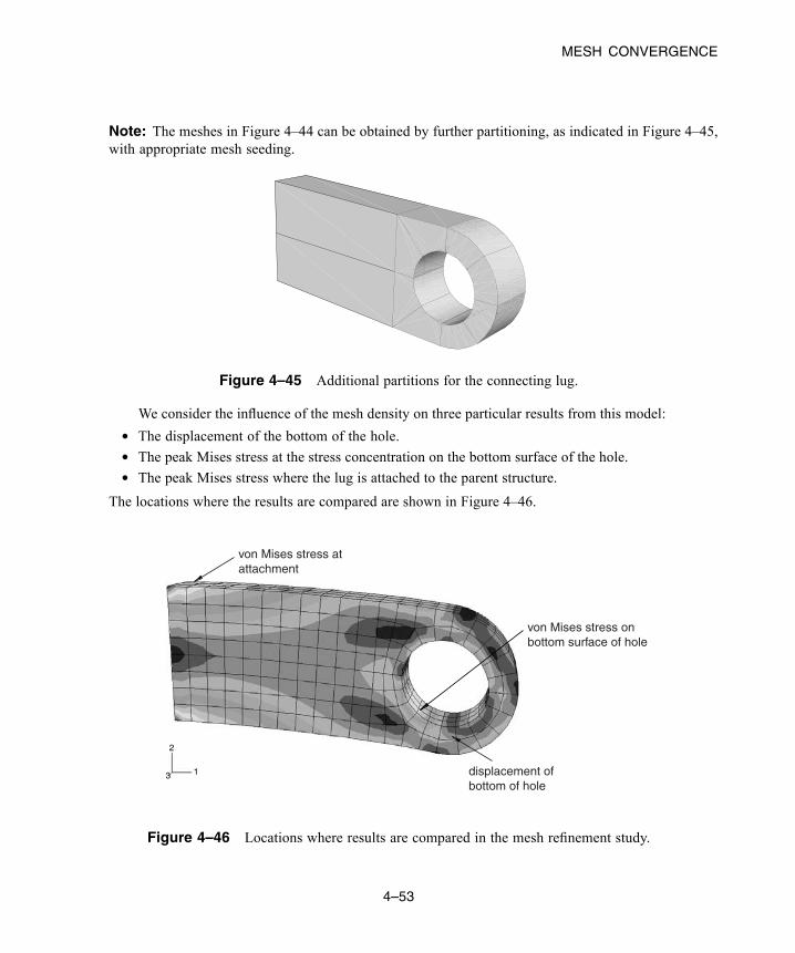
MESH CONVERGENCE
Note: The meshes in Figure 4–44 can be obtained by further partitioning, as indicated in Figure 4–45,with appropriate mesh seeding.
Figure 4–45 Additional partitions for the connecting lug.
We consider the influence of the mesh density on three particular results from this model:
• The displacement of the bottom of the hole.• The peak Mises stress at the stress concentration on the bottom surface of the hole.• The peak Mises stress where the lug is attached to the parent structure.
The locations where the results are compared are shown in Figure 4–46.
1
2
3
von Mises stress atattachment
von Mises stress onbottom surface of hole
displacement ofbottom of hole
Figure 4–46 Locations where results are compared in the mesh refinement study.
4–53
Abaqus ID:Printed on:
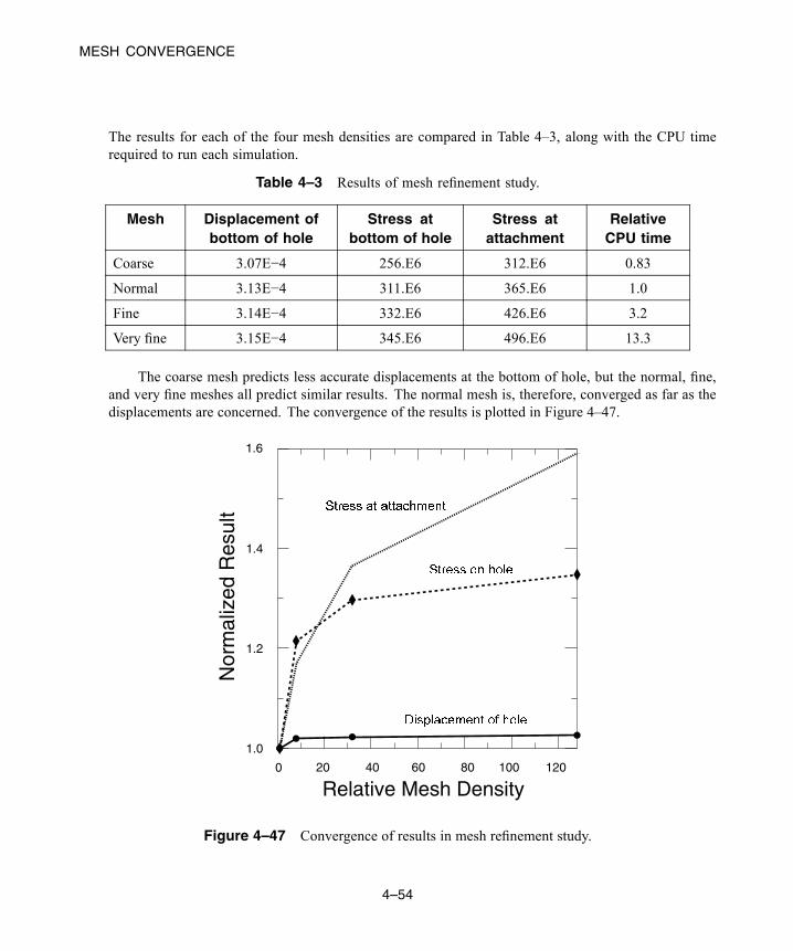
MESH CONVERGENCE
The results for each of the four mesh densities are compared in Table 4–3, along with the CPU timerequired to run each simulation.
Table 4–3 Results of mesh refinement study.
Mesh Displacement ofbottom of hole
Stress atbottom of hole
Stress atattachment
RelativeCPU time
Coarse 3.07E−4 256.E6 312.E6 0.83
Normal 3.13E−4 311.E6 365.E6 1.0
Fine 3.14E−4 332.E6 426.E6 3.2
Very fine 3.15E−4 345.E6 496.E6 13.3
The coarse mesh predicts less accurate displacements at the bottom of hole, but the normal, fine,and very fine meshes all predict similar results. The normal mesh is, therefore, converged as far as thedisplacements are concerned. The convergence of the results is plotted in Figure 4–47.
80 100 120
1.0
1.2
1.4
1.6
Relative Mesh Density
Nor
mal
ized
Res
ult
20 40 600
Figure 4–47 Convergence of results in mesh refinement study.
4–54
Abaqus ID:Printed on:

MESH CONVERGENCE
All the results are normalized with respect to the values predicted by the coarse mesh. The peakstress on the bottom of the hole converges much more slowly than the displacements because stress andstrain are calculated from the displacement gradients; thus, a much finer mesh is required to predictaccurate displacement gradients than is needed to calculate accurate displacements.
Mesh refinement significantly changes the stress calculated at the attachment of the connecting lug;it continues to increase with continued mesh refinement. A stress singularity exists at the corner of thelug where it attaches to the parent structure. Theoretically the stress is infinite at this location; therefore,increasing the mesh density will not produce a converged stress value at this location. This singularityoccurs because of the idealizations used in the finite element model. The connection between the lugand the parent structure has been modeled as a sharp corner, and the parent structure has been modeledas rigid. These idealizations lead to the stress singularity. In reality there probably will be a small filletbetween the lug and the parent structure, and the parent structure will be deformable, not rigid. If theexact stress in this location is required, the fillet between the components must be modeled accurately(see Figure 4–48) and the stiffness of the parent structure must also be considered.
Sharp cornergives a stresssingularity.
Fillet.
Finite element modelidealization.
Actual geometry ofcomponent.
Figure 4–48 Idealizing a fillet as a sharp corner.
It is common to omit small details like fillet radii from a finite element model to simplify the analysisand to keep the model size reasonable. However, the introduction of any sharp corner into a model willlead to a stress singularity at that location. This normally has a negligible effect on the overall responseof the model, but the predicted stresses close to the singularity will be inaccurate.
For complex, three-dimensional simulations the available computer resources often dictate apractical limit on the mesh density that you can use. In this case you must use the results from theanalysis carefully. Coarse meshes are often adequate to predict trends and to compare how differentconcepts behave relative to each other. However, you should use the actual magnitudes of displacementand stress calculated with a coarse mesh with caution.
It is rarely necessary to use a uniformly fine mesh throughout the structure being analyzed. Youshould use a fine mesh mainly in the areas of high stress gradients and use a coarser mesh in areas oflow stress gradients or where the magnitude of the stresses is not of interest. For example, Figure 4–49
4–55
Abaqus ID:Printed on:
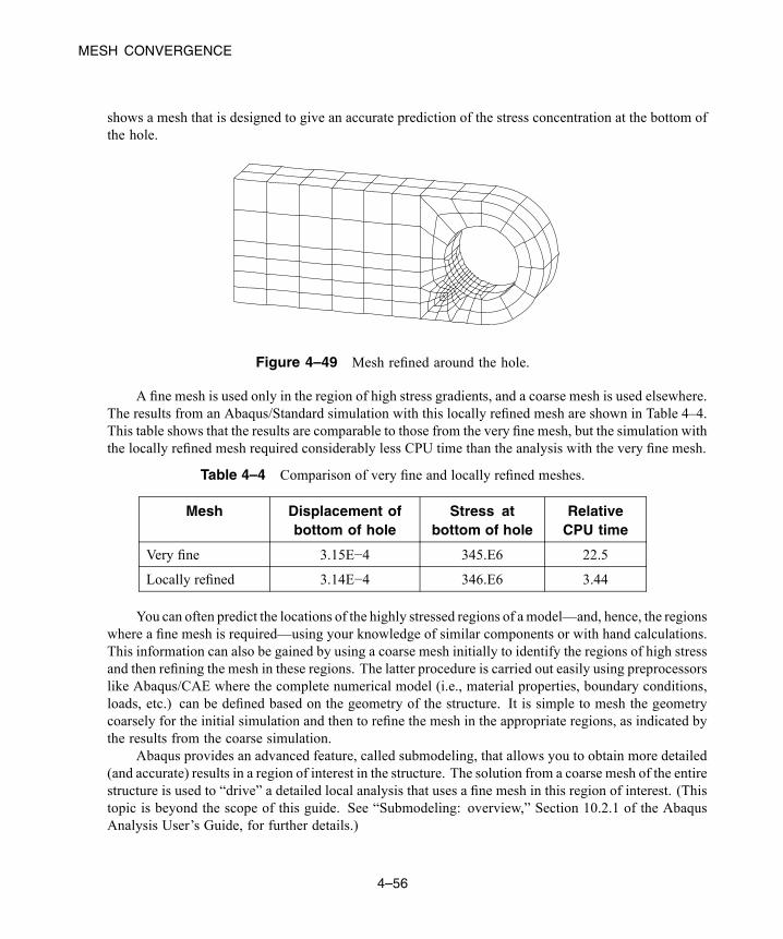
MESH CONVERGENCE
shows a mesh that is designed to give an accurate prediction of the stress concentration at the bottom ofthe hole.
Figure 4–49 Mesh refined around the hole.
A fine mesh is used only in the region of high stress gradients, and a coarse mesh is used elsewhere.The results from an Abaqus/Standard simulation with this locally refined mesh are shown in Table 4–4.This table shows that the results are comparable to those from the very fine mesh, but the simulation withthe locally refined mesh required considerably less CPU time than the analysis with the very fine mesh.
Table 4–4 Comparison of very fine and locally refined meshes.
Mesh Displacement ofbottom of hole
Stress atbottom of hole
RelativeCPU time
Very fine 3.15E−4 345.E6 22.5
Locally refined 3.14E−4 346.E6 3.44
You can often predict the locations of the highly stressed regions of amodel—and, hence, the regionswhere a fine mesh is required—using your knowledge of similar components or with hand calculations.This information can also be gained by using a coarse mesh initially to identify the regions of high stressand then refining the mesh in these regions. The latter procedure is carried out easily using preprocessorslike Abaqus/CAE where the complete numerical model (i.e., material properties, boundary conditions,loads, etc.) can be defined based on the geometry of the structure. It is simple to mesh the geometrycoarsely for the initial simulation and then to refine the mesh in the appropriate regions, as indicated bythe results from the coarse simulation.
Abaqus provides an advanced feature, called submodeling, that allows you to obtain more detailed(and accurate) results in a region of interest in the structure. The solution from a coarse mesh of the entirestructure is used to “drive” a detailed local analysis that uses a fine mesh in this region of interest. (Thistopic is beyond the scope of this guide. See “Submodeling: overview,” Section 10.2.1 of the AbaqusAnalysis User’s Guide, for further details.)
4–56
Abaqus ID:Printed on:
SUGGESTED READING
4.5 Related Abaqus examples
If you are interested in learning more about using continuum elements in Abaqus, you should examinethe following problems:
• “Geometrically nonlinear analysis of a cantilever beam,” Section 2.1.2 of the Abaqus BenchmarksGuide
• “Spherical cavity in an infinite medium,” Section 2.2.4 of the Abaqus Benchmarks Guide• “Performance of continuum and shell elements for linear analysis of bending problems,”Section 2.3.5 of the Abaqus Benchmarks Guide
4.6 Suggested reading
The volume of literature that has been written on the finite element method and the applications of finiteelement analysis is enormous. In most of the remaining chapters of this guide, a list of suggested booksand articles is provided so that you can explore the topics in more depth if you wish. While the advancedreferences will not be of interest to most users, they provide detailed theoretical information for theinterested user.
General texts on the finite element method
• NAFEMS Ltd., A Finite Element Primer, 1986.
• Becker, E. B., G. F. Carey, and J. T. Oden, Finite Elements: An Introduction, Prentice-Hall,1981.
• Carey, G. F., and J. T. Oden, Finite Elements: A Second Course, Prentice-Hall, 1983.
• Cook, R. D., D. S. Malkus, and M. E. Plesha, Concepts and Applications of Finite ElementAnalysis, John Wiley & Sons, 1989.
• Hughes, T. J. R., The Finite Element Method, Prentice-Hall, Inc., 1987.
• Zienkiewicz, O. C., and R. L. Taylor, The Finite Element Method: Volumes I, II, and III,Butterworth-Heinemann, 2000.
Performance of linear solid elements
• Prathap, G., “The Poor Bending Response of the Four-Node Plane Stress Quadrilaterals,”International Journal for Numerical Methods in Engineering, vol. 21, 825–835, 1985.
Hourglass control in solid elements
• Belytschko, T., W. K. Liu, and J. M. Kennedy, “Hourglass Control in Linear and NonlinearProblems,” Computer Methods in Applied Mechanics and Engineering, vol. 43, 251–276,1984.
4–57
Abaqus ID:Printed on:

SUMMARY
• Flanagan, D. P., and T. Belytschko, “A Uniform Strain Hexahedron and Quadrilateral withHourglass Control,” International Journal for Numerical Methods in Engineering, vol. 17,679–706, 1981.
• Puso, M. A., “A Highly Efficient Enhanced Assumed Strain Physically Stabilized HexahedralElement,” International Journal for Numerical Methods in Engineering, vol. 49, 1029–1064,2000.
Incompatible mode elements
• Simo, J. C. and M. S. Rifai, “A Class of Assumed Strain Methods and the Method ofIncompatible Modes,” International Journal for Numerical Methods in Engineering, vol. 29,1595–1638, 1990.
4.7 Summary
• The formulation and order of integration used in a continuum element can have a significant effecton the accuracy and cost of the analysis.
• First-order (linear) elements using full integration are prone to shear locking and normally shouldnot be used.
• First-order, reduced-integration elements are prone to hourglassing; sufficient mesh refinementminimizes this problem.
• When using first-order, reduced-integration elements in a simulation where bending deformationwill occur, use at least four elements through the thickness.
• Hourglassing is rarely a problem in the second-order, reduced-integration elements inAbaqus/Standard. You should consider using these elements for most general applications whenthere is no contact.
• The accuracy of the incompatible mode elements available in Abaqus/Standard is stronglyinfluenced by the amount of element distortion.
• The numerical accuracy of the results depends on the mesh that has been used. Ideally a meshrefinement study should be carried out to ensure that the mesh provides a unique solution to theproblem. However, remember that using a converged mesh does not ensure that the results from thefinite element simulation will match the actual behavior of the physical problem: that also dependson other approximations and idealizations in the model.
• In general, refine the mesh mainly in regions where you want accurate results; a finer mesh isrequired to predict accurate stresses than is needed to calculate accurate displacements.
• Advanced features such as submodeling are available in Abaqus to help you to obtain useful resultsfor complex simulations.
4–58
Abaqus ID:Printed on:
ELEMENT GEOMETRY
5. Using Shell Elements
Use shell elements to model structures in which one dimension (the thickness) is significantly smallerthan the other dimensions and in which the stresses in the thickness direction are negligible. A structure,such as a pressure vessel, whose thickness is less than 1/10 of a typical global structural dimensiongenerally can be modeled with shell elements. The following are examples of typical global dimensions:
• the distance between supports,• the distance between stiffeners or large changes in section thickness,• the radius of curvature, and• the wavelength of the highest vibration mode of interest.Abaqus shell elements assume that plane sections perpendicular to the shell midsurface remain
plane. Do not be confused into thinking that the thickness must be less than 1/10 of the elementdimensions. A highly refined mesh may contain shell elements whose thickness is greater than theirin-plane dimensions, although this is not generally recommended—continuum elements may be moresuitable in such a case.
5.1 Element geometry
Two types of shell elements are available in Abaqus: conventional shell elements and continuumshell elements. Conventional shell elements discretize a reference surface by defining the element’splanar dimensions, its surface normal, and its initial curvature. The nodes of a conventional shellelement, however, do not define the shell thickness; the thickness is defined through section properties.Continuum shell elements, on the other hand, resemble three-dimensional solid elements in that theydiscretize an entire three-dimensional body yet are formulated so that their kinematic and constitutivebehavior is similar to conventional shell elements. Continuum shell elements are more accurate incontact modeling than conventional shell elements, since they employ two-sided contact taking intoaccount changes in thickness. For thin shell applications, however, conventional shell elements providesuperior performance.
In this guide only conventional shell elements are discussed. Henceforth, we will refer to themsimply as “shell elements.” For more information on continuum shell elements, see “Shell elements:overview,” Section 29.6.1 of the Abaqus Analysis User’s Guide.
5.1.1 Shell thickness and section pointsThe shell thickness is required to describe the shell cross-section and must be specified. In addition tospecifying the shell thickness, you can choose to have the stiffness of the cross-section calculated duringthe analysis or once at the beginning of the analysis.
5–1
Abaqus ID:Printed on:
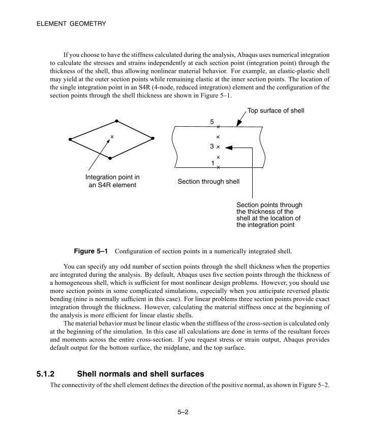
ELEMENT GEOMETRY
If you choose to have the stiffness calculated during the analysis, Abaqus uses numerical integrationto calculate the stresses and strains independently at each section point (integration point) through thethickness of the shell, thus allowing nonlinear material behavior. For example, an elastic-plastic shellmay yield at the outer section points while remaining elastic at the inner section points. The location ofthe single integration point in an S4R (4-node, reduced integration) element and the configuration of thesection points through the shell thickness are shown in Figure 5–1.
Section points throughthe thickness of theshell at the location ofthe integration point
Integration point inan S4R element Section through shell
1
3
5
Top surface of shell
Figure 5–1 Configuration of section points in a numerically integrated shell.
You can specify any odd number of section points through the shell thickness when the propertiesare integrated during the analysis. By default, Abaqus uses five section points through the thickness ofa homogeneous shell, which is sufficient for most nonlinear design problems. However, you should usemore section points in some complicated simulations, especially when you anticipate reversed plasticbending (nine is normally sufficient in this case). For linear problems three section points provide exactintegration through the thickness. However, calculating the material stiffness once at the beginning ofthe analysis is more efficient for linear elastic shells.
The material behavior must be linear elastic when the stiffness of the cross-section is calculated onlyat the beginning of the simulation. In this case all calculations are done in terms of the resultant forcesand moments across the entire cross-section. If you request stress or strain output, Abaqus providesdefault output for the bottom surface, the midplane, and the top surface.
5.1.2 Shell normals and shell surfacesThe connectivity of the shell element defines the direction of the positive normal, as shown in Figure 5–2.
5–2
Abaqus ID:Printed on:
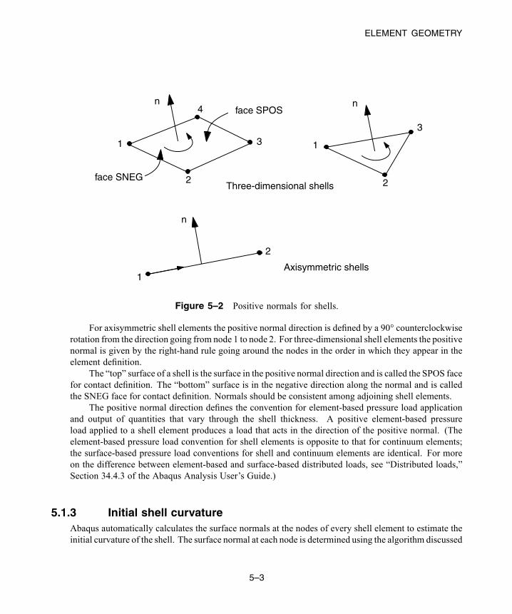
ELEMENT GEOMETRY
1
2
3
4n
1
2
3
n
n
2
1Axisymmetric shells
Three-dimensional shells
face SPOS
face SNEG
Figure 5–2 Positive normals for shells.
For axisymmetric shell elements the positive normal direction is defined by a 90° counterclockwiserotation from the direction going from node 1 to node 2. For three-dimensional shell elements the positivenormal is given by the right-hand rule going around the nodes in the order in which they appear in theelement definition.
The “top” surface of a shell is the surface in the positive normal direction and is called the SPOS facefor contact definition. The “bottom” surface is in the negative direction along the normal and is calledthe SNEG face for contact definition. Normals should be consistent among adjoining shell elements.
The positive normal direction defines the convention for element-based pressure load applicationand output of quantities that vary through the shell thickness. A positive element-based pressureload applied to a shell element produces a load that acts in the direction of the positive normal. (Theelement-based pressure load convention for shell elements is opposite to that for continuum elements;the surface-based pressure load conventions for shell and continuum elements are identical. For moreon the difference between element-based and surface-based distributed loads, see “Distributed loads,”Section 34.4.3 of the Abaqus Analysis User’s Guide.)
5.1.3 Initial shell curvatureAbaqus automatically calculates the surface normals at the nodes of every shell element to estimate theinitial curvature of the shell. The surface normal at each node is determined using the algorithm discussed
5–3
Abaqus ID:Printed on:
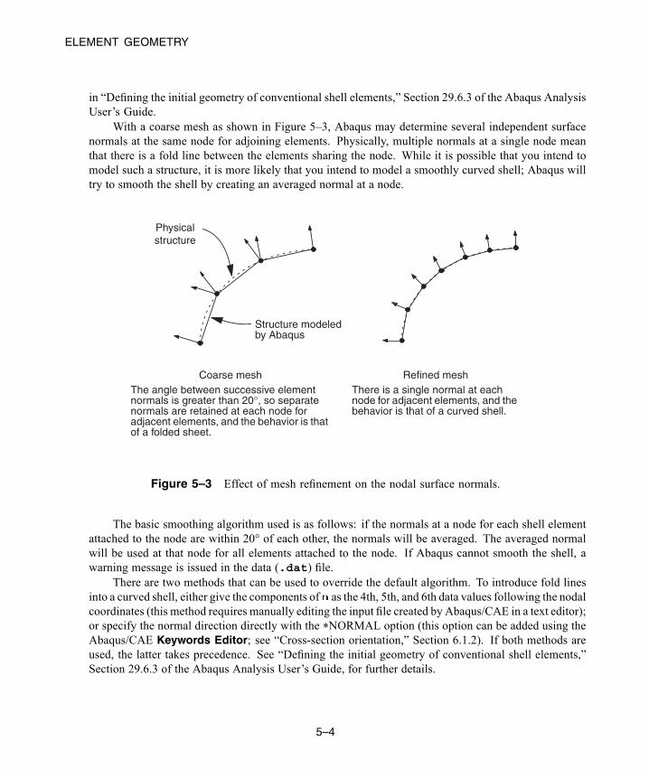
ELEMENT GEOMETRY
in “Defining the initial geometry of conventional shell elements,” Section 29.6.3 of the Abaqus AnalysisUser’s Guide.
With a coarse mesh as shown in Figure 5–3, Abaqus may determine several independent surfacenormals at the same node for adjoining elements. Physically, multiple normals at a single node meanthat there is a fold line between the elements sharing the node. While it is possible that you intend tomodel such a structure, it is more likely that you intend to model a smoothly curved shell; Abaqus willtry to smooth the shell by creating an averaged normal at a node.
Coarse meshThe angle between successive elementnormals is greater than 20°, so separatenormals are retained at each node foradjacent elements, and the behavior is thatof a folded sheet.
Refined meshThere is a single normal at eachnode for adjacent elements, and thebehavior is that of a curved shell.
Physicalstructure
Structure modeledby Abaqus
Figure 5–3 Effect of mesh refinement on the nodal surface normals.
The basic smoothing algorithm used is as follows: if the normals at a node for each shell elementattached to the node are within 20° of each other, the normals will be averaged. The averaged normalwill be used at that node for all elements attached to the node. If Abaqus cannot smooth the shell, awarning message is issued in the data (.dat) file.
There are two methods that can be used to override the default algorithm. To introduce fold linesinto a curved shell, either give the components of as the 4th, 5th, and 6th data values following the nodalcoordinates (this method requires manually editing the input file created by Abaqus/CAE in a text editor);or specify the normal direction directly with the *NORMAL option (this option can be added using theAbaqus/CAE Keywords Editor; see “Cross-section orientation,” Section 6.1.2). If both methods areused, the latter takes precedence. See “Defining the initial geometry of conventional shell elements,”Section 29.6.3 of the Abaqus Analysis User’s Guide, for further details.
5–4
Abaqus ID:Printed on:
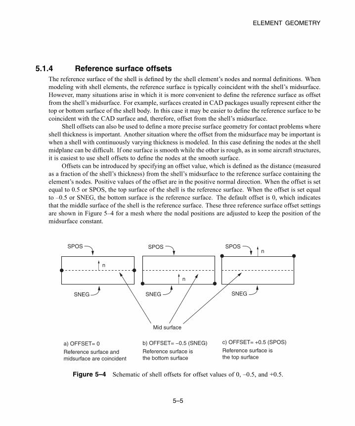
ELEMENT GEOMETRY
5.1.4 Reference surface offsetsThe reference surface of the shell is defined by the shell element’s nodes and normal definitions. Whenmodeling with shell elements, the reference surface is typically coincident with the shell’s midsurface.However, many situations arise in which it is more convenient to define the reference surface as offsetfrom the shell’s midsurface. For example, surfaces created in CAD packages usually represent either thetop or bottom surface of the shell body. In this case it may be easier to define the reference surface to becoincident with the CAD surface and, therefore, offset from the shell’s midsurface.
Shell offsets can also be used to define a more precise surface geometry for contact problems whereshell thickness is important. Another situation where the offset from the midsurface may be important iswhen a shell with continuously varying thickness is modeled. In this case defining the nodes at the shellmidplane can be difficult. If one surface is smooth while the other is rough, as in some aircraft structures,it is easiest to use shell offsets to define the nodes at the smooth surface.
Offsets can be introduced by specifying an offset value, which is defined as the distance (measuredas a fraction of the shell’s thickness) from the shell’s midsurface to the reference surface containing theelement’s nodes. Positive values of the offset are in the positive normal direction. When the offset is setequal to 0.5 or SPOS, the top surface of the shell is the reference surface. When the offset is set equalto –0.5 or SNEG, the bottom surface is the reference surface. The default offset is 0, which indicatesthat the middle surface of the shell is the reference surface. These three reference surface offset settingsare shown in Figure 5–4 for a mesh where the nodal positions are adjusted to keep the position of themidsurface constant.
a) OFFSET= 0
Reference surface and midsurface are coincident
b) OFFSET= −0.5 (SNEG)
Reference surface isthe bottom surface
c) OFFSET= +0.5 (SPOS)
Reference surface isthe top surface
SNEG
SPOS SPOS SPOS
SNEG SNEG
Mid surface
n
n
n
Figure 5–4 Schematic of shell offsets for offset values of 0, –0.5, and +0.5.
5–5
Abaqus ID:Printed on:
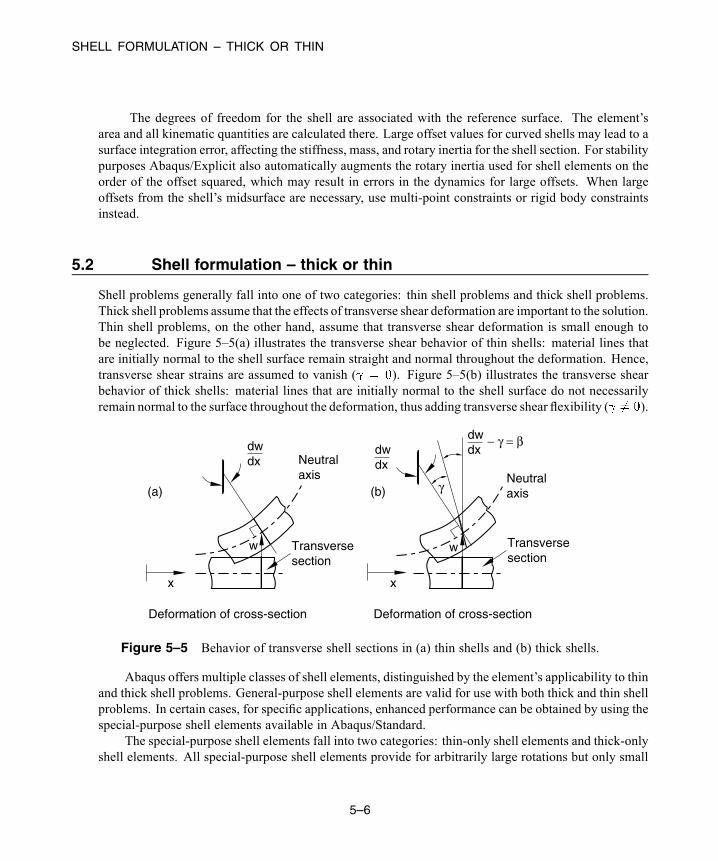
SHELL FORMULATION – THICK OR THIN
The degrees of freedom for the shell are associated with the reference surface. The element’sarea and all kinematic quantities are calculated there. Large offset values for curved shells may lead to asurface integration error, affecting the stiffness, mass, and rotary inertia for the shell section. For stabilitypurposes Abaqus/Explicit also automatically augments the rotary inertia used for shell elements on theorder of the offset squared, which may result in errors in the dynamics for large offsets. When largeoffsets from the shell’s midsurface are necessary, use multi-point constraints or rigid body constraintsinstead.
5.2 Shell formulation – thick or thin
Shell problems generally fall into one of two categories: thin shell problems and thick shell problems.Thick shell problems assume that the effects of transverse shear deformation are important to the solution.Thin shell problems, on the other hand, assume that transverse shear deformation is small enough tobe neglected. Figure 5–5(a) illustrates the transverse shear behavior of thin shells: material lines thatare initially normal to the shell surface remain straight and normal throughout the deformation. Hence,transverse shear strains are assumed to vanish ( ). Figure 5–5(b) illustrates the transverse shearbehavior of thick shells: material lines that are initially normal to the shell surface do not necessarilyremain normal to the surface throughout the deformation, thus adding transverse shear flexibility ( ).
(a) (b)
x x
Deformation of cross-section Deformation of cross-section
w wTransversesection
Transversesection
Neutral axis Neutral
axis
dwdx
dwdx
dwdx
− γ = β
γ
Figure 5–5 Behavior of transverse shell sections in (a) thin shells and (b) thick shells.
Abaqus offers multiple classes of shell elements, distinguished by the element’s applicability to thinand thick shell problems. General-purpose shell elements are valid for use with both thick and thin shellproblems. In certain cases, for specific applications, enhanced performance can be obtained by using thespecial-purpose shell elements available in Abaqus/Standard.
The special-purpose shell elements fall into two categories: thin-only shell elements and thick-onlyshell elements. All special-purpose shell elements provide for arbitrarily large rotations but only small
5–6
Abaqus ID:Printed on:
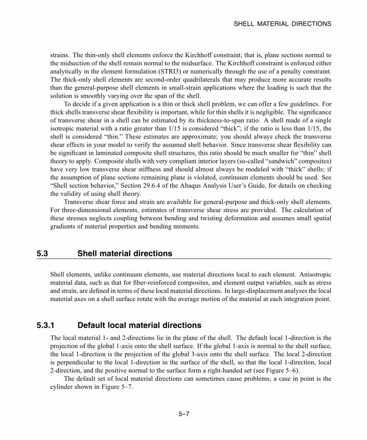
SHELL MATERIAL DIRECTIONS
strains. The thin-only shell elements enforce the Kirchhoff constraint; that is, plane sections normal tothe midsection of the shell remain normal to the midsurface. The Kirchhoff constraint is enforced eitheranalytically in the element formulation (STRI3) or numerically through the use of a penalty constraint.The thick-only shell elements are second-order quadrilaterals that may produce more accurate resultsthan the general-purpose shell elements in small-strain applications where the loading is such that thesolution is smoothly varying over the span of the shell.
To decide if a given application is a thin or thick shell problem, we can offer a few guidelines. Forthick shells transverse shear flexibility is important, while for thin shells it is negligible. The significanceof transverse shear in a shell can be estimated by its thickness-to-span ratio. A shell made of a singleisotropic material with a ratio greater than 1/15 is considered “thick”; if the ratio is less than 1/15, theshell is considered “thin.” These estimates are approximate; you should always check the transverseshear effects in your model to verify the assumed shell behavior. Since transverse shear flexibility canbe significant in laminated composite shell structures, this ratio should be much smaller for “thin” shelltheory to apply. Composite shells with very compliant interior layers (so-called “sandwich” composites)have very low transverse shear stiffness and should almost always be modeled with “thick” shells; ifthe assumption of plane sections remaining plane is violated, continuum elements should be used. See“Shell section behavior,” Section 29.6.4 of the Abaqus Analysis User’s Guide, for details on checkingthe validity of using shell theory.
Transverse shear force and strain are available for general-purpose and thick-only shell elements.For three-dimensional elements, estimates of transverse shear stress are provided. The calculation ofthese stresses neglects coupling between bending and twisting deformation and assumes small spatialgradients of material properties and bending moments.
5.3 Shell material directions
Shell elements, unlike continuum elements, use material directions local to each element. Anisotropicmaterial data, such as that for fiber-reinforced composites, and element output variables, such as stressand strain, are defined in terms of these local material directions. In large-displacement analyses the localmaterial axes on a shell surface rotate with the average motion of the material at each integration point.
5.3.1 Default local material directionsThe local material 1- and 2-directions lie in the plane of the shell. The default local 1-direction is theprojection of the global 1-axis onto the shell surface. If the global 1-axis is normal to the shell surface,the local 1-direction is the projection of the global 3-axis onto the shell surface. The local 2-directionis perpendicular to the local 1-direction in the surface of the shell, so that the local 1-direction, local2-direction, and the positive normal to the surface form a right-handed set (see Figure 5–6).
The default set of local material directions can sometimes cause problems; a case in point is thecylinder shown in Figure 5–7.
5–7
Abaqus ID:Printed on:
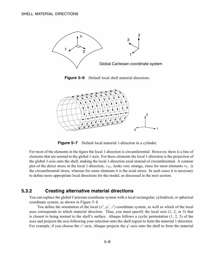
SHELL MATERIAL DIRECTIONS
32
12
1
n
Global Cartesian coordinate system
Figure 5–6 Default local shell material directions.
2
3 1
Figure 5–7 Default local material 1-direction in a cylinder.
For most of the elements in the figure the local 1-direction is circumferential. However, there is a line ofelements that are normal to the global 1-axis. For these elements the local 1-direction is the projection ofthe global 3-axis onto the shell, making the local 1-direction axial instead of circumferential. A contourplot of the direct stress in the local 1-direction, , looks very strange, since for most elements isthe circumferential stress, whereas for some elements it is the axial stress. In such cases it is necessaryto define more appropriate local directions for the model, as discussed in the next section.
5.3.2 Creating alternative material directionsYou can replace the global Cartesian coordinate system with a local rectangular, cylindrical, or sphericalcoordinate system, as shown in Figure 5–8.
You define the orientation of the local ( , , ) coordinate system, as well as which of the localaxes corresponds to which material direction. Thus, you must specify the local axis (1, 2, or 3) thatis closest to being normal to the shell’s surface. Abaqus follows a cyclic permutation (1, 2, 3) of theaxes and projects the axis following your selection onto the shell region to form the material 1-direction.For example, if you choose the -axis, Abaqus projects the -axis onto the shell to form the material
5–8
Abaqus ID:Printed on:
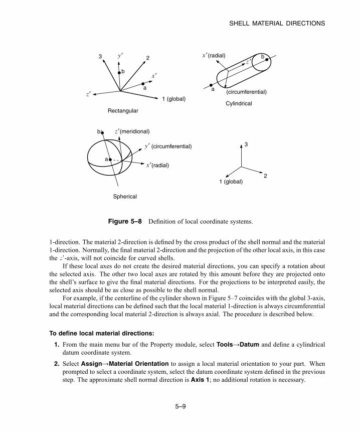
SHELL MATERIAL DIRECTIONS
1 (global)
23
b
a
Rectangular
(circumferential)a
b
Cylindrical
(meridional)
a
b
(radial)
1 (global)2
3
(radial)
(circumferential)
Spherical
z′
y ′
x ′
y ′
x ′z ′
x ′
z′
Figure 5–8 Definition of local coordinate systems.
1-direction. The material 2-direction is defined by the cross product of the shell normal and the material1-direction. Normally, the final material 2-direction and the projection of the other local axis, in this casethe -axis, will not coincide for curved shells.
If these local axes do not create the desired material directions, you can specify a rotation aboutthe selected axis. The other two local axes are rotated by this amount before they are projected ontothe shell’s surface to give the final material directions. For the projections to be interpreted easily, theselected axis should be as close as possible to the shell normal.
For example, if the centerline of the cylinder shown in Figure 5–7 coincides with the global 3-axis,local material directions can be defined such that the local material 1-direction is always circumferentialand the corresponding local material 2-direction is always axial. The procedure is described below.
To define local material directions:
1. From the main menu bar of the Property module, select Tools→Datum and define a cylindricaldatum coordinate system.
2. Select Assign→Material Orientation to assign a local material orientation to your part. Whenprompted to select a coordinate system, select the datum coordinate system defined in the previousstep. The approximate shell normal direction is Axis 1; no additional rotation is necessary.
5–9
Abaqus ID:Printed on:

EXAMPLE: SKEW PLATE
5.4 Selecting shell elements
• The linear, finite-membrane-strain, fully integrated, quadrilateral shell element (S4) can be usedwhen greater solution accuracy is desired, for problems prone to membrane- or bending-modehourglassing, or for problems where in-plane bending is expected.
• The linear, finite-membrane-strain, reduced-integration, quadrilateral shell element (S4R) is robustand is suitable for a wide range of applications.
• The linear, finite-membrane-strain, triangular shell elements (S3/S3R) can be used asgeneral-purpose elements. A refined mesh may be needed to capture bending deformationsor high strain gradients because of the constant strain approximation in the elements.
• To account for the influence of shear flexibility in laminated composite shell models, use the shellelements suitable for modeling thick shells (S4, S4R, S3/S3R, S8R); check that the assumption ofplane sections remaining plane is satisfied.
• Quadratic shell elements, either quadrilateral or triangular, are very effective for general, small-strain, thin-shell applications. These elements are not susceptible to shear or membrane locking.
• If you must use second-order elements in contact simulations, do not use the quadratic, triangularshell element (STRI65). Use the 9-node, quadrilateral shell element (S9R5) instead.
• For very large models that will experience only geometrically linear behavior, the linear, thin-shellelement (S4R5) will generally be more cost-effective than the general-purpose shell elements.
• The small membrane strain elements are effective for explicit dynamics problems involving smallmembrane strains and arbitrarily large rotations.
5.5 Example: skew plate
You have been asked to model the plate shown in Figure 5–9. It is skewed 30° to the global 1-axis, isbuilt-in at one end, and is constrained to move on rails parallel to the plate axis at the other end. Youare to determine the midspan deflection when the plate carries a uniform pressure. You are also to assesswhether a linear analysis is valid for this problem. You will perform an analysis using Abaqus/Standard.
5.5.1 Preprocessing—creating the model with Abaqus/CAEUse Abaqus/CAE to create the entire model for this simulation. Abaqus provides scripts that replicatethe complete analysis model for this problem. Run one of these scripts if you encounter difficultiesfollowing the instructions given below or if you wish to check your work. Scripts are available in thefollowing locations:
5–10
Abaqus ID:Printed on:
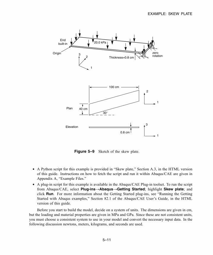
EXAMPLE: SKEW PLATE
20.0 kPaEnd
built-in
1
32
OriginThickness=0.8 cm
3
1
1
2
30°40 cm
100 cm
0.8 cm
Plan
Elevation
zerorotation
Figure 5–9 Sketch of the skew plate.
• A Python script for this example is provided in “Skew plate,” Section A.3, in the HTML versionof this guide. Instructions on how to fetch the script and run it within Abaqus/CAE are given inAppendix A, “Example Files.”
• A plug-in script for this example is available in the Abaqus/CAE Plug-in toolset. To run the scriptfrom Abaqus/CAE, select Plug-ins→Abaqus→Getting Started; highlight Skew plate; andclick Run. For more information about the Getting Started plug-ins, see “Running the GettingStarted with Abaqus examples,” Section 82.1 of the Abaqus/CAE User’s Guide, in the HTMLversion of this guide.
Before you start to build the model, decide on a system of units. The dimensions are given in cm,but the loading and material properties are given in MPa and GPa. Since these are not consistent units,you must choose a consistent system to use in your model and convert the necessary input data. In thefollowing discussion newtons, meters, kilograms, and seconds are used.
5–11
Abaqus ID:Printed on:
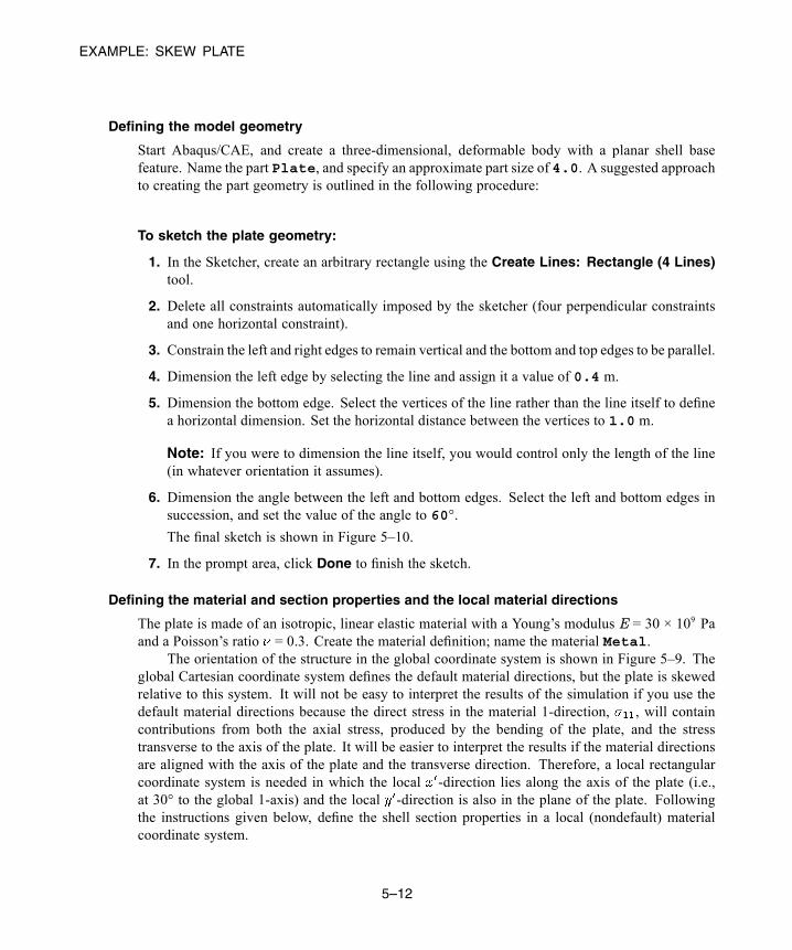
EXAMPLE: SKEW PLATE
Defining the model geometry
Start Abaqus/CAE, and create a three-dimensional, deformable body with a planar shell basefeature. Name the part Plate, and specify an approximate part size of 4.0. A suggested approachto creating the part geometry is outlined in the following procedure:
To sketch the plate geometry:
1. In the Sketcher, create an arbitrary rectangle using the Create Lines: Rectangle (4 Lines)tool.
2. Delete all constraints automatically imposed by the sketcher (four perpendicular constraintsand one horizontal constraint).
3. Constrain the left and right edges to remain vertical and the bottom and top edges to be parallel.
4. Dimension the left edge by selecting the line and assign it a value of 0.4 m.
5. Dimension the bottom edge. Select the vertices of the line rather than the line itself to definea horizontal dimension. Set the horizontal distance between the vertices to 1.0 m.
Note: If you were to dimension the line itself, you would control only the length of the line(in whatever orientation it assumes).
6. Dimension the angle between the left and bottom edges. Select the left and bottom edges insuccession, and set the value of the angle to 60°.
The final sketch is shown in Figure 5–10.
7. In the prompt area, click Done to finish the sketch.
Defining the material and section properties and the local material directions
The plate is made of an isotropic, linear elastic material with a Young’s modulus E = 30 × 109 Paand a Poisson’s ratio = 0.3. Create the material definition; name the material Metal.
The orientation of the structure in the global coordinate system is shown in Figure 5–9. Theglobal Cartesian coordinate system defines the default material directions, but the plate is skewedrelative to this system. It will not be easy to interpret the results of the simulation if you use thedefault material directions because the direct stress in the material 1-direction, , will containcontributions from both the axial stress, produced by the bending of the plate, and the stresstransverse to the axis of the plate. It will be easier to interpret the results if the material directionsare aligned with the axis of the plate and the transverse direction. Therefore, a local rectangularcoordinate system is needed in which the local -direction lies along the axis of the plate (i.e.,at 30° to the global 1-axis) and the local -direction is also in the plane of the plate. Followingthe instructions given below, define the shell section properties in a local (nondefault) materialcoordinate system.
5–12
Abaqus ID:Printed on:

EXAMPLE: SKEW PLATE
V
V
60.º
H 1.
400.E−03
1
2
3
Figure 5–10 Sketch of the plate geometry (with grid spacing doubled).
To define shell section properties and local material directions:
1. Define a homogeneous shell section named PlateSection. Specify that section integrationbe performed before the analysis since the material is linear elastic, and accept the defaultidealization option of No idealization. Assign a shell thickness of 0.8E-2 and the Metalmaterial definition to the section.
2. Define a rectangular datum coordinate system as shown in Figure 5–11 using the Create
Datum CSYS: 2 Lines tool .
3. From the main menu bar of the Property module, select Assign→Material Orientation andselect the entire part as the region to which local material directions will be applied. In theviewport, select the datum coordinate system created earlier. Select Axis 3 for the directionof the approximate shell normal. No additional rotation is needed about this axis.
Tip: To verify that the local material directions have been assigned correctly, selectTools→Query from themainmenu bar and perform a property query on thematerialorientations. Triads appear in the viewport indicating the material orientation of theregion you select.
Once the part has been meshed and elements have been created in the model, all elementvariables will be defined in this local coordinate system.
4. Assign the section definition to the plate. AcceptMiddle surface as the shell offset definition.
5–13
Abaqus ID:Printed on:
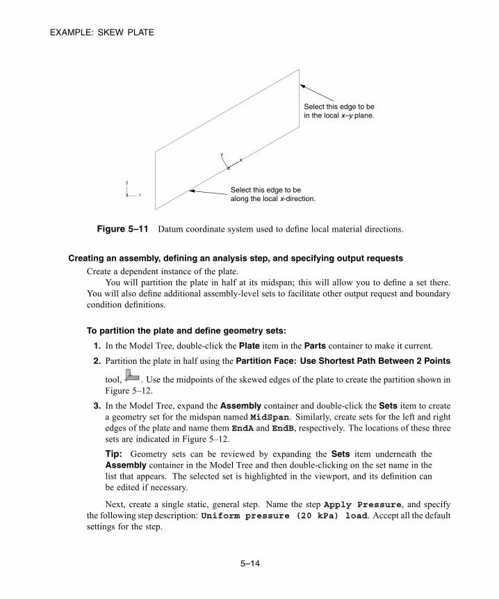
EXAMPLE: SKEW PLATE
XY
Z
XY
Z
1
2
3
Select this edge to bein the local x–y plane.
Select this edge to be along the local x-direction.
Figure 5–11 Datum coordinate system used to define local material directions.
Creating an assembly, defining an analysis step, and specifying output requests
Create a dependent instance of the plate.You will partition the plate in half at its midspan; this will allow you to define a set there.
You will also define additional assembly-level sets to facilitate other output request and boundarycondition definitions.
To partition the plate and define geometry sets:
1. In the Model Tree, double-click the Plate item in the Parts container to make it current.
2. Partition the plate in half using the Partition Face: Use Shortest Path Between 2 Points
tool, . Use the midpoints of the skewed edges of the plate to create the partition shown inFigure 5–12.
3. In the Model Tree, expand the Assembly container and double-click the Sets item to createa geometry set for the midspan named MidSpan. Similarly, create sets for the left and rightedges of the plate and name them EndA and EndB, respectively. The locations of these threesets are indicated in Figure 5–12.
Tip: Geometry sets can be reviewed by expanding the Sets item underneath theAssembly container in the Model Tree and then double-clicking on the set name in thelist that appears. The selected set is highlighted in the viewport, and its definition canbe edited if necessary.
Next, create a single static, general step. Name the step Apply Pressure, and specifythe following step description: Uniform pressure (20 kPa) load. Accept all the defaultsettings for the step.
5–14
Abaqus ID:Printed on:
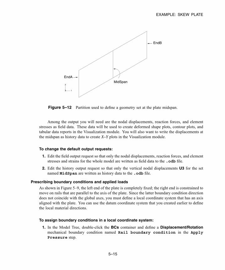
EXAMPLE: SKEW PLATE
1
2
3
EndB
MidSpanEndA
Figure 5–12 Partition used to define a geometry set at the plate midspan.
Among the output you will need are the nodal displacements, reaction forces, and elementstresses as field data. These data will be used to create deformed shape plots, contour plots, andtabular data reports in the Visualization module. You will also want to write the displacements atthe midspan as history data to create X–Y plots in the Visualization module.
To change the default output requests:
1. Edit the field output request so that only the nodal displacements, reaction forces, and elementstresses and strains for the whole model are written as field data to the .odb file.
2. Edit the history output request so that only the vertical nodal displacements U3 for the setnamed MidSpan are written as history data to the .odb file.
Prescribing boundary conditions and applied loads
As shown in Figure 5–9, the left end of the plate is completely fixed; the right end is constrained tomove on rails that are parallel to the axis of the plate. Since the latter boundary condition directiondoes not coincide with the global axes, you must define a local coordinate system that has an axisaligned with the plate. You can use the datum coordinate system that you created earlier to definethe local material directions.
To assign boundary conditions in a local coordinate system:
1. In the Model Tree, double-click the BCs container and define a Displacement/Rotationmechanical boundary condition named Rail boundary condition in the ApplyPressure step.
5–15
Abaqus ID:Printed on:
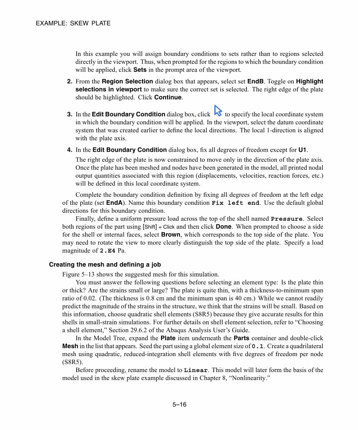
EXAMPLE: SKEW PLATE
In this example you will assign boundary conditions to sets rather than to regions selecteddirectly in the viewport. Thus, when prompted for the regions to which the boundary conditionwill be applied, click Sets in the prompt area of the viewport.
2. From the Region Selection dialog box that appears, select set EndB. Toggle on Highlightselections in viewport to make sure the correct set is selected. The right edge of the plateshould be highlighted. Click Continue.
3. In the Edit Boundary Condition dialog box, click to specify the local coordinate systemin which the boundary condition will be applied. In the viewport, select the datum coordinatesystem that was created earlier to define the local directions. The local 1-direction is alignedwith the plate axis.
4. In the Edit Boundary Condition dialog box, fix all degrees of freedom except for U1.
The right edge of the plate is now constrained to move only in the direction of the plate axis.Once the plate has been meshed and nodes have been generated in the model, all printed nodaloutput quantities associated with this region (displacements, velocities, reaction forces, etc.)will be defined in this local coordinate system.
Complete the boundary condition definition by fixing all degrees of freedom at the left edgeof the plate (set EndA). Name this boundary condition Fix left end. Use the default globaldirections for this boundary condition.
Finally, define a uniform pressure load across the top of the shell named Pressure. Selectboth regions of the part using [Shift] + Click and then click Done. When prompted to choose a sidefor the shell or internal faces, select Brown, which corresponds to the top side of the plate. Youmay need to rotate the view to more clearly distinguish the top side of the plate. Specify a loadmagnitude of 2.E4 Pa.
Creating the mesh and defining a job
Figure 5–13 shows the suggested mesh for this simulation.You must answer the following questions before selecting an element type: Is the plate thin
or thick? Are the strains small or large? The plate is quite thin, with a thickness-to-minimum spanratio of 0.02. (The thickness is 0.8 cm and the minimum span is 40 cm.) While we cannot readilypredict the magnitude of the strains in the structure, we think that the strains will be small. Based onthis information, choose quadratic shell elements (S8R5) because they give accurate results for thinshells in small-strain simulations. For further details on shell element selection, refer to “Choosinga shell element,” Section 29.6.2 of the Abaqus Analysis User’s Guide.
In the Model Tree, expand the Plate item underneath the Parts container and double-clickMesh in the list that appears. Seed the part using a global element size of0.1. Create a quadrilateralmesh using quadratic, reduced-integration shell elements with five degrees of freedom per node(S8R5).
Before proceeding, rename the model to Linear. This model will later form the basis of themodel used in the skew plate example discussed in Chapter 8, “Nonlinearity.”
5–16
Abaqus ID:Printed on:
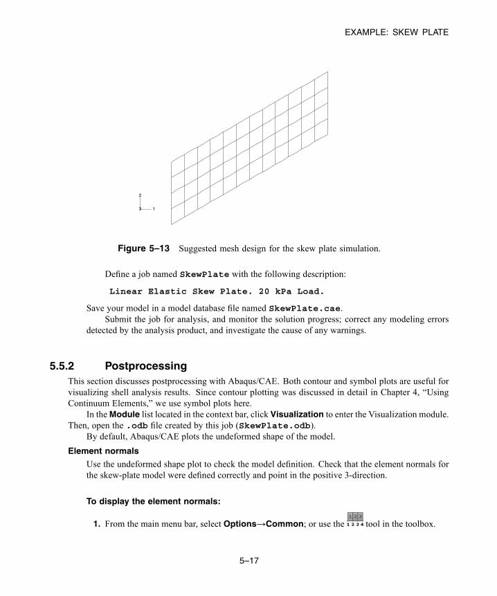
EXAMPLE: SKEW PLATE
1
2
3
Figure 5–13 Suggested mesh design for the skew plate simulation.
Define a job named SkewPlate with the following description:
Linear Elastic Skew Plate. 20 kPa Load.
Save your model in a model database file named SkewPlate.cae.Submit the job for analysis, and monitor the solution progress; correct any modeling errors
detected by the analysis product, and investigate the cause of any warnings.
5.5.2 PostprocessingThis section discusses postprocessing with Abaqus/CAE. Both contour and symbol plots are useful forvisualizing shell analysis results. Since contour plotting was discussed in detail in Chapter 4, “UsingContinuum Elements,” we use symbol plots here.
In theModule list located in the context bar, click Visualization to enter the Visualization module.Then, open the .odb file created by this job (SkewPlate.odb).
By default, Abaqus/CAE plots the undeformed shape of the model.
Element normals
Use the undeformed shape plot to check the model definition. Check that the element normals forthe skew-plate model were defined correctly and point in the positive 3-direction.
To display the element normals:
1. From the main menu bar, select Options→Common; or use the tool in the toolbox.
5–17
Abaqus ID:Printed on:
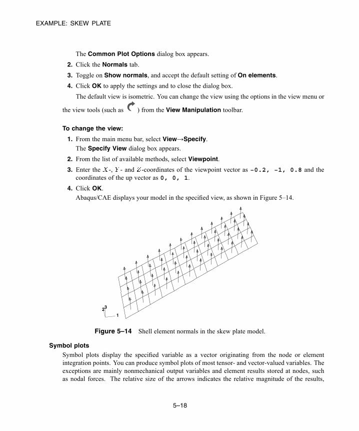
EXAMPLE: SKEW PLATE
The Common Plot Options dialog box appears.
2. Click the Normals tab.
3. Toggle on Show normals, and accept the default setting of On elements.
4. Click OK to apply the settings and to close the dialog box.
The default view is isometric. You can change the view using the options in the view menu or
the view tools (such as ) from the View Manipulation toolbar.
To change the view:
1. From the main menu bar, select View→Specify.The Specify View dialog box appears.
2. From the list of available methods, select Viewpoint.
3. Enter the -, - and -coordinates of the viewpoint vector as −0.2, −1, 0.8 and thecoordinates of the up vector as 0, 0, 1.
4. Click OK.Abaqus/CAE displays your model in the specified view, as shown in Figure 5–14.
123
Figure 5–14 Shell element normals in the skew plate model.
Symbol plots
Symbol plots display the specified variable as a vector originating from the node or elementintegration points. You can produce symbol plots of most tensor- and vector-valued variables. Theexceptions are mainly nonmechanical output variables and element results stored at nodes, suchas nodal forces. The relative size of the arrows indicates the relative magnitude of the results,
5–18
Abaqus ID:Printed on:
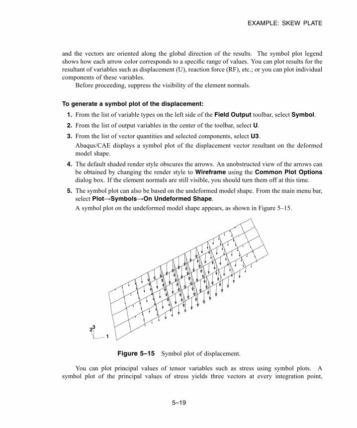
EXAMPLE: SKEW PLATE
and the vectors are oriented along the global direction of the results. The symbol plot legendshows how each arrow color corresponds to a specific range of values. You can plot results for theresultant of variables such as displacement (U), reaction force (RF), etc.; or you can plot individualcomponents of these variables.
Before proceeding, suppress the visibility of the element normals.
To generate a symbol plot of the displacement:
1. From the list of variable types on the left side of the Field Output toolbar, select Symbol.
2. From the list of output variables in the center of the toolbar, select U.
3. From the list of vector quantities and selected components, select U3.
Abaqus/CAE displays a symbol plot of the displacement vector resultant on the deformedmodel shape.
4. The default shaded render style obscures the arrows. An unobstructed view of the arrows canbe obtained by changing the render style to Wireframe using the Common Plot Optionsdialog box. If the element normals are still visible, you should turn them off at this time.
5. The symbol plot can also be based on the undeformed model shape. From the main menu bar,select Plot→Symbols→On Undeformed Shape.
A symbol plot on the undeformed model shape appears, as shown in Figure 5–15.
123
Figure 5–15 Symbol plot of displacement.
You can plot principal values of tensor variables such as stress using symbol plots. Asymbol plot of the principal values of stress yields three vectors at every integration point,
5–19
Abaqus ID:Printed on:
EXAMPLE: SKEW PLATE
each corresponding to a principal value oriented along the corresponding principal direction.Compressive values are indicated by arrows pointing toward the integration point, and tensilevalues are indicated by arrows pointing away from the integration point. You can also plotindividual principal values.
To generate a symbol plot of the principal stresses:
1. From the list of variable types on the left side of the Field Output toolbar, select Symbol.
2. From the list of output variables in the center of the toolbar, select S.
3. From the list of tensor quantities and components, select ALL_PRINCIPAL_COMPONENTSas the tensor quantity.
Abaqus/CAE displays a symbol plot of principal stresses.
4. From the main menu bar, select Options→Symbol; or use the Symbol Options tool inthe toolbox to change the arrow length.
The Symbol Plot Options dialog box appears.
5. In the Color & Style page, click the Tensor tab.
6. Drag the Size slider to select 2 as the arrow length.
7. Click OK to apply the settings and to close the dialog box.
The symbol plot shown in Figure 5–16 appears.
8. The principal stresses are displayed at section point 1 by default. To plot stresses at nondefaultsection points, select Result→Section Points from the main menu bar to open the SectionPoints dialog box.
9. Select the desired nondefault section point for plotting.
10. In a complex model, the element edges can obscure the symbol plots. To suppress the displayof the element edges, choose Feature edges in the Basic tabbed page of the Common PlotOptions dialog box.
Figure 5–17 shows a symbol plot of the principal stresses at the default section point with onlyfeature edges visible.
Material directions
Abaqus/CAE also allows you visualize the element material directions. This feature is particularlyuseful if you would like to verify that the material directions were assigned correctly in thesimulation.
To plot the material directions:
1. From the main menu bar, select Plot→Material Orientations→On Undeformed Shape; or
use the tool in the toolbox.
5–20
Abaqus ID:Printed on:
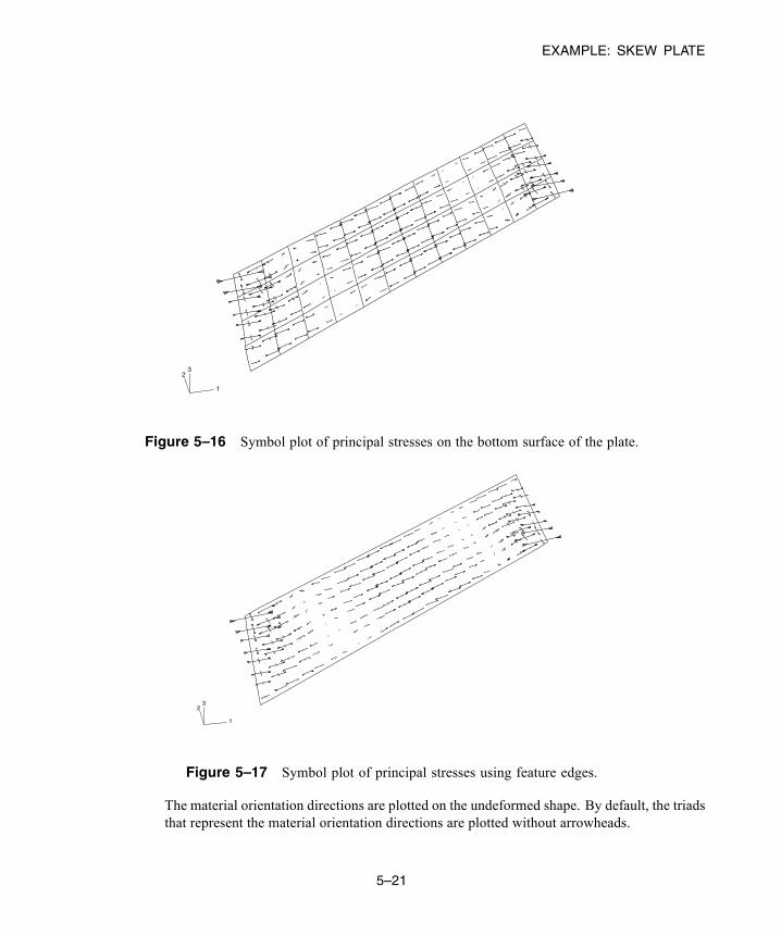
EXAMPLE: SKEW PLATE
1
23
Figure 5–16 Symbol plot of principal stresses on the bottom surface of the plate.
1
23
Figure 5–17 Symbol plot of principal stresses using feature edges.
The material orientation directions are plotted on the undeformed shape. By default, the triadsthat represent the material orientation directions are plotted without arrowheads.
5–21
Abaqus ID:Printed on:
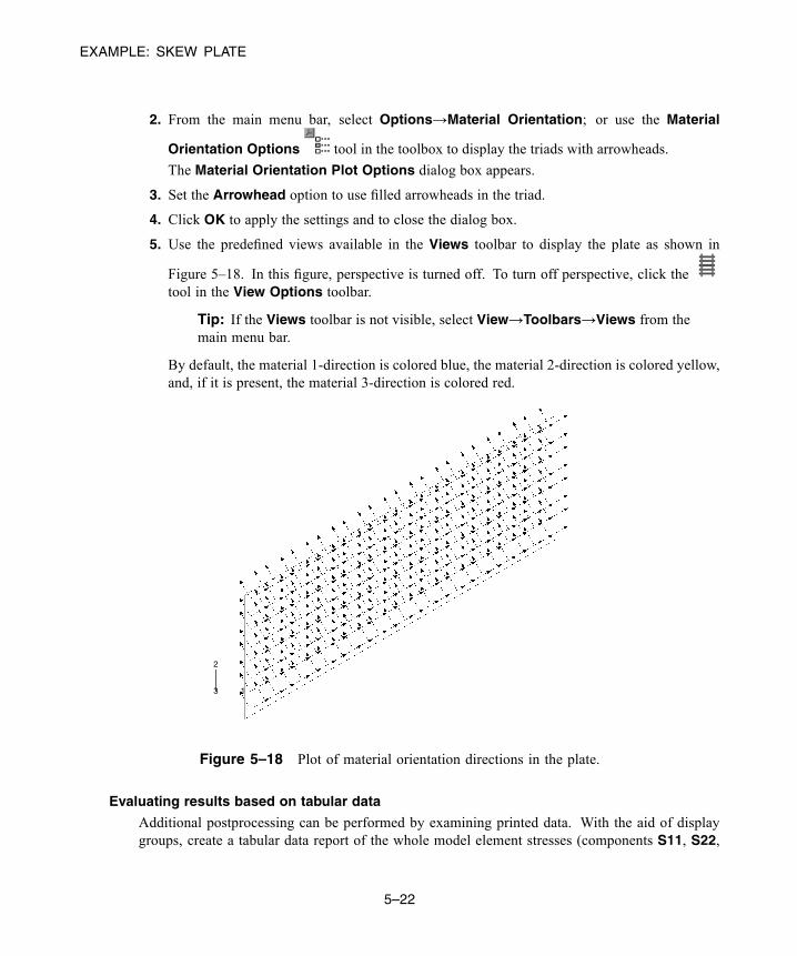
EXAMPLE: SKEW PLATE
2. From the main menu bar, select Options→Material Orientation; or use the Material
Orientation Options tool in the toolbox to display the triads with arrowheads.
The Material Orientation Plot Options dialog box appears.
3. Set the Arrowhead option to use filled arrowheads in the triad.
4. Click OK to apply the settings and to close the dialog box.
5. Use the predefined views available in the Views toolbar to display the plate as shown in
Figure 5–18. In this figure, perspective is turned off. To turn off perspective, click thetool in the View Options toolbar.
Tip: If the Views toolbar is not visible, select View→Toolbars→Views from themain menu bar.
By default, the material 1-direction is colored blue, the material 2-direction is colored yellow,and, if it is present, the material 3-direction is colored red.
1
2
3
Figure 5–18 Plot of material orientation directions in the plate.
Evaluating results based on tabular data
Additional postprocessing can be performed by examining printed data. With the aid of displaygroups, create a tabular data report of the whole model element stresses (components S11, S22,
5–22
Abaqus ID:Printed on:

EXAMPLE: SKEW PLATE
and S12), the reaction forces and moments at the supported nodes (sets EndA and EndB), and thedisplacements of the midspan nodes (set MidSpan). The stress data are shown below.
Field Output Report
Source 1---------
ODB: SkewPlate.odbStep: Apply pressureFrame: Increment 1: Step Time = 1.000
Loc 1 : Integration point values at shell general ... : SNEG, (fraction = -1.0)Loc 2 : Integration point values at shell general ... : SPOS, (fraction = 1.0)
Output sorted by column "Element Label".
Field Output reported at integration points for part: PLATE-1
Element Int S.S11 S.S11 S.S22 S.S22 S.S12 S.S12Label Pt @Loc 1 @Loc 2 @Loc 1 @Loc 2 @Loc 1 @Loc 2
-----------------------------------------------------------------------------------------------------1 1 79.7614E+06 -79.7614E+06 1.1085E+06 -1.1085E+06 -5.86291E+06 5.86291E+061 2 83.7703E+06 -83.7703E+06 7.14559E+06 -7.14559E+06 -8.00706E+06 8.00706E+061 3 66.9385E+06 -66.9385E+06 2.79241E+06 -2.79241E+06 -1.98396E+06 1.98396E+061 4 72.3479E+06 -72.3479E+06 5.05957E+06 -5.05957E+06 -7.0819E+06 7.0819E+06
.
.48 1 -142.755E+06 142.755E+06 -56.0747E+06 56.0747E+06 21.007E+06 -21.007E+0648 2 -118.848E+06 118.848E+06 -7.21449E+06 7.21449E+06 4.00065E+06 -4.00065E+0648 3 -187.19E+06 187.19E+06 -103.31E+06 103.31E+06 50.352E+06 -50.352E+0648 4 -238.323E+06 238.323E+06 -84.7331E+06 84.7331E+06 70.0676E+06 -70.0676E+06
Minimum -238.323E+06 -90.2378E+06 -103.31E+06 -10.5216E+06 -18.865E+06 -70.0676E+06At Element 48 4 24 2 12 48
Int Pt 4 4 3 2 4 4Maximum 90.2378E+06 238.323E+06 10.5216E+06 103.31E+06 70.0676E+06 18.865E+06
At Element 4 48 2 24 48 12
Int Pt 4 4 2 3 4 4
The locations Loc 1 and Loc 2 identify the section point in the element where the stress wascalculated. Loc 1 (corresponding to section point 1) lies on the SNEG surface of the shell, andLoc 2 (corresponding to section point 3) lies on the SPOS surface. Local material directions havebeen used for the element: the stresses refer to a local coordinate system.
Check that the small-strain assumption was valid for this simulation. The axial straincorresponding to the peak stress is 0.008. Because the strain is typically considered smallif it is less than 4 or 5%, a strain of 0.8% is well within the appropriate range to be modeled withS8R5 elements.
The reaction forces and moments are reported in the following table:
Field Output Report
Source 1---------
ODB: SkewPlate.odbStep: Apply pressureFrame: Increment 1: Step Time = 1.000
Loc 1 : Nodal values from source 1
Output sorted by column "Node Label".
5–23
Abaqus ID:Printed on:
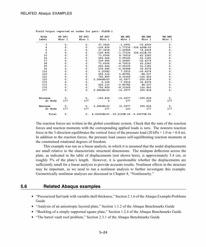
RELATED Abaqus EXAMPLES
Field Output reported at nodes for part: PLATE-1
Node RF.RF1 RF.RF2 RF.RF3 RM.RM1 RM.RM2 RM.RM3Label @Loc 1 @Loc 1 @Loc 1 @Loc 1 @Loc 1 @Loc 1
-------------------------------------------------------------------------------------3 0. 0. 37.3924 -1.5991 -76.4939 0.4 0. 0. -109.834 1.77236 -324.424E-03 0.5 0. 0. 37.3918 1.59909 76.4939 0.6 0. 0. -109.834 -1.77236 324.411E-03 0.
15 0. 0. 73.6366 8.75019 -62.2243 0.16 0. 0. 260.424 6.95105 -51.1181 0.17 0. 0. 239.685 6.56987 -35.4374 0.28 0. 0. 73.6366 -8.75019 62.2243 0.29 0. 0. 260.424 -6.95105 51.1181 0.30 0. 0. 239.685 -6.56988 35.4374 0.
116 0. 0. 6.15382 7.5915 -36.4274 0.119 0. 0. 455.132 6.80781 -88.237 0.121 0. 0. 750.805 8.31069 -126.462 0.123 0. 0. 2.2866E+03 31.0977 -205.818 0.170 0. 0. 6.154 -7.5915 36.4274 0.173 0. 0. 455.133 -6.80782 88.237 0.175 0. 0. 750.805 -8.31069 126.462 0.177 0. 0. 2.2866E+03 -31.0977 205.818 0.
Minimum 0. 0. -109.834 -31.0977 -205.818 0.At Node 177 177 6 177 123 177
Maximum 0. 0. 2.2866E+03 31.0977 205.818 0.At Node 177 177 177 123 177 177
Total 0. 0. 8.00000E+03 -39.2199E-06 -5.00679E-06 0.
The reaction forces are written in the global coordinate system. Check that the sum of the reactionforces and reaction moments with the corresponding applied loads is zero. The nonzero reactionforce in the 3-direction equilibrates the vertical force of the pressure load (20 kPa × 1.0 m × 0.4 m).In addition to the reaction forces, the pressure load causes self-equilibrating reaction moments atthe constrained rotational degrees of freedom.
This example was run as a linear analysis, in which it is assumed that the nodal displacementsare small relative to the characteristic structural dimensions. The midspan deflection across theplate, as indicated in the table of displacements (not shown here), is approximately 5.4 cm, orroughly 5% of the plate’s length. However, it is questionable whether the displacements aresufficiently small for a linear analysis to provide accurate results. Nonlinear effects in the structuremay be important, so we need to run a nonlinear analysis to further investigate this example.Geometrically nonlinear analyses are discussed in Chapter 8, “Nonlinearity.”
5.6 Related Abaqus examples
• “Pressurized fuel tank with variable shell thickness,” Section 2.1.6 of the Abaqus Example ProblemsGuide
• “Analysis of an anisotropic layered plate,” Section 1.1.2 of the Abaqus Benchmarks Guide• “Buckling of a simply supported square plate,” Section 1.2.4 of the Abaqus Benchmarks Guide• “The barrel vault roof problem,” Section 2.3.1 of the Abaqus Benchmarks Guide
5–24
Abaqus ID:Printed on:

SUMMARY
5.7 Suggested reading
The following references provide a more in-depth treatment of the theoretical and computational aspectsof shell theory.
Basic shell theory
• Timoshenko, S., Strength of Materials: Part II, Krieger Publishing Co., 1958.
• Timoshenko, S. and S. W. Krieger, Theory of Plates and Shells, McGraw-Hill, Inc., 1959.
• Ugural, A. C., Stresses in Plates and Shells, McGraw-Hill, Inc., 1981.
Basic computational shell theory
• Cook, R. D., D. S. Malkus, and M. E. Plesha, Concepts and Applications of Finite ElementAnalysis, John Wiley & Sons, 1989.
• Hughes, T. J. R., The Finite Element Method, Prentice-Hall, Inc., 1987.
Advanced shell theory
• Budiansky, B., and J. L. Sanders, “On the ‘Best’ First-Order Linear Shell Theory,” Progress inApplied Mechanics, The Prager Anniversary Volume, 129–140, 1963.
Advanced computational shell theory
• Ashwell, D. G., and R. H. Gallagher, Finite Elements for Thin Shells and Curved Members,John Wiley & Sons, 1976.
• Hughes, T. J. R., T. E. Tezduyar, “Finite Elements Based upon Mindlin Plate Theory withParticular Reference to the Four-Node Bilinear Isoparametric Element,” Journal of AppliedMechanics, 587–596, 1981.
• Simo, J. C., D. D. Fox, and M. S. Rifai, “On a Stress Resultant Geometrically Exact ShellModel. Part III: Computational Aspects of the Nonlinear Theory,” Computer Methods inApplied Mechanics and Engineering, vol. 79, 21–70, 1990.
5.8 Summary
• The cross-section behavior of shell elements can be determined using numerical integration throughthe shell thickness or using a cross-section stiffness calculated at the beginning of the analysis.
• Calculating the cross-section stiffness at the beginning of the analysis is efficient, but only linearmaterials can be considered when this is done; calculating the cross-section stiffness during theanalysis using numerical integration allows both linear and nonlinear materials to be used.
5–25
Abaqus ID:Printed on:

SUMMARY
• Numerical integration is performed at a number of section points through the shell thickness. Thesesection points are the locations at which element variables can be output. The default outermostsection points lie on the surfaces of the shell.
• The direction of a shell element’s normal determines the positive and negative surfaces of theelement. To define contact and interpret element output correctly, you must know which surface iswhich. The shell normal can be plotted in the Visualization module of Abaqus/CAE.
• Shell elements use material directions local to each element. In large-displacement analyses thelocal material axes rotate with the element. Nondefault local coordinate systems can be defined.The element variables, such as stress and strain, are output in the local directions.
• Local coordinate systems for nodes can also be defined. Concentrated loads and boundaryconditions are applied in the local coordinate system. All printed nodal output, such asdisplacements, also refer to the local system by default.
• Symbol plots can help you visualize the results from a simulation. They are especially useful forvisualizing the motion and load paths of a structure.
5–26
Abaqus ID:Printed on:
BEAM CROSS-SECTION GEOMETRY
6. Using Beam Elements
Use beam elements to model structures in which one dimension (the length) is significantly greater thanthe other two dimensions and in which the longitudinal stress is most important. Beam theory is basedon the assumption that the deformation of the structure can be determined entirely from variables thatare functions of position along the structure’s length. For beam theory to produce acceptable results,the cross-section dimensions should be less than 1/10 of the structure’s typical axial dimension. Thefollowing are examples of typical axial dimensions:
• the distance between supports,• the distance between gross changes in cross-section, and• the wavelength of the highest vibration mode of interest.Abaqus beam elements assume that plane sections perpendicular to the axis of the beam remain
plane during deformation.Do not be confused into thinking that the cross-section dimensions should be less than 1/10 of a
typical element length. A highly refined mesh may contain beam elements whose length is less thantheir cross-section dimensions, although this is not generally recommended—continuum elements maybe more suitable in such a case.
6.1 Beam cross-section geometry
You can define the beam profile in one of three ways: by choosing from the Abaqus cross-section libraryand specifying the shape and dimensions of the beam cross-section; by defining a generalized beamprofile using section engineering properties, such as area and moments of inertia; or by using a meshof special two-dimensional elements for which geometric quantities are calculated numerically, called ameshed beam cross-section.
Abaqus offers a variety of common cross-section shapes, as shown in Figure 6–1, should you decideto define the beam profile geometrically. You can also define almost any thin-walled cross-section usingthe arbitrary cross-section definition. For a detailed discussion of the beam cross-sections available inAbaqus, see “Beam cross-section library,” Section 29.3.9 of the Abaqus Analysis User’s Guide.
If you define a beam profile using one of the built-in cross-sections in the Abaqus library,Abaqus/CAE prompts you for the required cross-section dimensions, which are different for each typeof cross-section. When the beam profile is associated with a beam section property, you can specifywhether to have the section engineering properties calculated during the analysis or to have Abaqusprecompute them (at the beginning of the analysis). The former option can be used when the materialbehavior is either linear or nonlinear (for example, if the section stiffness changes due to inelasticyielding); the latter option is more efficient, however, for linear elastic material behavior.
6–1
Abaqus ID:Printed on:
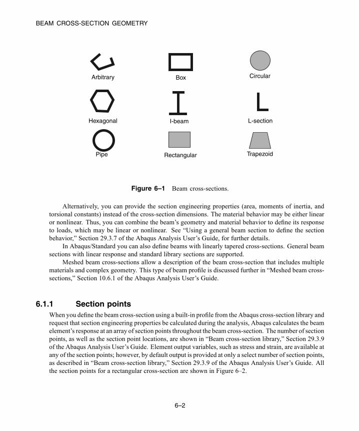
BEAM CROSS-SECTION GEOMETRY
Box Circular
Hexagonal I-beam L-section
Pipe Rectangular Trapezoid
Arbitrary
Figure 6–1 Beam cross-sections.
Alternatively, you can provide the section engineering properties (area, moments of inertia, andtorsional constants) instead of the cross-section dimensions. The material behavior may be either linearor nonlinear. Thus, you can combine the beam’s geometry and material behavior to define its responseto loads, which may be linear or nonlinear. See “Using a general beam section to define the sectionbehavior,” Section 29.3.7 of the Abaqus Analysis User’s Guide, for further details.
In Abaqus/Standard you can also define beams with linearly tapered cross-sections. General beamsections with linear response and standard library sections are supported.
Meshed beam cross-sections allow a description of the beam cross-section that includes multiplematerials and complex geometry. This type of beam profile is discussed further in “Meshed beam cross-sections,” Section 10.6.1 of the Abaqus Analysis User’s Guide.
6.1.1 Section pointsWhen you define the beam cross-section using a built-in profile from the Abaqus cross-section library andrequest that section engineering properties be calculated during the analysis, Abaqus calculates the beamelement’s response at an array of section points throughout the beam cross-section. The number of sectionpoints, as well as the section point locations, are shown in “Beam cross-section library,” Section 29.3.9of the Abaqus Analysis User’s Guide. Element output variables, such as stress and strain, are available atany of the section points; however, by default output is provided at only a select number of section points,as described in “Beam cross-section library,” Section 29.3.9 of the Abaqus Analysis User’s Guide. Allthe section points for a rectangular cross-section are shown in Figure 6–2.
6–2
Abaqus ID:Printed on:
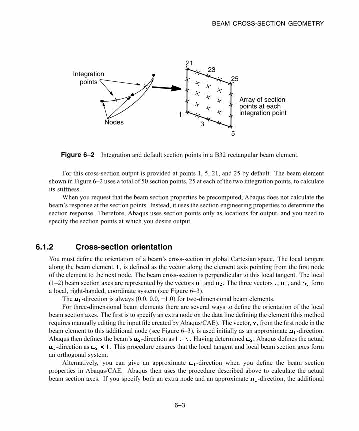
BEAM CROSS-SECTION GEOMETRY
Array of sectionpoints at eachintegration point
Integrationpoints
1
21
25
53Nodes
23
Figure 6–2 Integration and default section points in a B32 rectangular beam element.
For this cross-section output is provided at points 1, 5, 21, and 25 by default. The beam elementshown in Figure 6–2 uses a total of 50 section points, 25 at each of the two integration points, to calculateits stiffness.
When you request that the beam section properties be precomputed, Abaqus does not calculate thebeam’s response at the section points. Instead, it uses the section engineering properties to determine thesection response. Therefore, Abaqus uses section points only as locations for output, and you need tospecify the section points at which you desire output.
6.1.2 Cross-section orientationYou must define the orientation of a beam’s cross-section in global Cartesian space. The local tangentalong the beam element, , is defined as the vector along the element axis pointing from the first nodeof the element to the next node. The beam cross-section is perpendicular to this local tangent. The local(1–2) beam section axes are represented by the vectors and . The three vectors , , and forma local, right-handed, coordinate system (see Figure 6–3).
The -direction is always (0.0, 0.0, −1.0) for two-dimensional beam elements.For three-dimensional beam elements there are several ways to define the orientation of the local
beam section axes. The first is to specify an extra node on the data line defining the element (this methodrequires manually editing the input file created by Abaqus/CAE). The vector, , from the first node in thebeam element to this additional node (see Figure 6–3), is used initially as an approximate -direction.Abaqus then defines the beam’s -direction as . Having determined , Abaqus defines the actual-direction as . This procedure ensures that the local tangent and local beam section axes form
an orthogonal system.Alternatively, you can give an approximate -direction when you define the beam section
properties in Abaqus/CAE. Abaqus then uses the procedure described above to calculate the actualbeam section axes. If you specify both an extra node and an approximate -direction, the additional
6–3
Abaqus ID:Printed on:
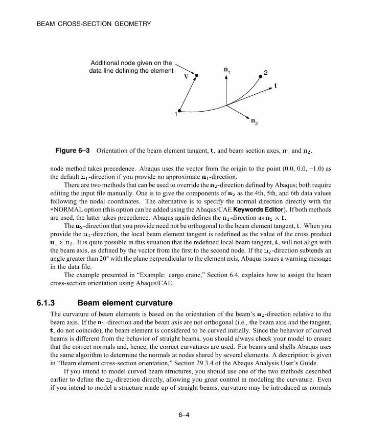
BEAM CROSS-SECTION GEOMETRY
1
2
Additional node given on thedata line defining the element n1
n2
tV
Figure 6–3 Orientation of the beam element tangent, , and beam section axes, and .
node method takes precedence. Abaqus uses the vector from the origin to the point (0.0, 0.0, −1.0) asthe default -direction if you provide no approximate -direction.
There are two methods that can be used to override the -direction defined by Abaqus; both requireediting the input file manually. One is to give the components of as the 4th, 5th, and 6th data valuesfollowing the nodal coordinates. The alternative is to specify the normal direction directly with the*NORMAL option (this option can be added using the Abaqus/CAEKeywords Editor). If bothmethodsare used, the latter takes precedence. Abaqus again defines the -direction as .
The -direction that you provide need not be orthogonal to the beam element tangent, . When youprovide the -direction, the local beam element tangent is redefined as the value of the cross product
. It is quite possible in this situation that the redefined local beam tangent, , will not align withthe beam axis, as defined by the vector from the first to the second node. If the -direction subtends anangle greater than 20° with the plane perpendicular to the element axis, Abaqus issues a warning messagein the data file.
The example presented in “Example: cargo crane,” Section 6.4, explains how to assign the beamcross-section orientation using Abaqus/CAE.
6.1.3 Beam element curvatureThe curvature of beam elements is based on the orientation of the beam’s -direction relative to thebeam axis. If the -direction and the beam axis are not orthogonal (i.e., the beam axis and the tangent,, do not coincide), the beam element is considered to be curved initially. Since the behavior of curvedbeams is different from the behavior of straight beams, you should always check your model to ensurethat the correct normals and, hence, the correct curvatures are used. For beams and shells Abaqus usesthe same algorithm to determine the normals at nodes shared by several elements. A description is givenin “Beam element cross-section orientation,” Section 29.3.4 of the Abaqus Analysis User’s Guide.
If you intend to model curved beam structures, you should use one of the two methods describedearlier to define the -direction directly, allowing you great control in modeling the curvature. Evenif you intend to model a structure made up of straight beams, curvature may be introduced as normals
6–4
Abaqus ID:Printed on:
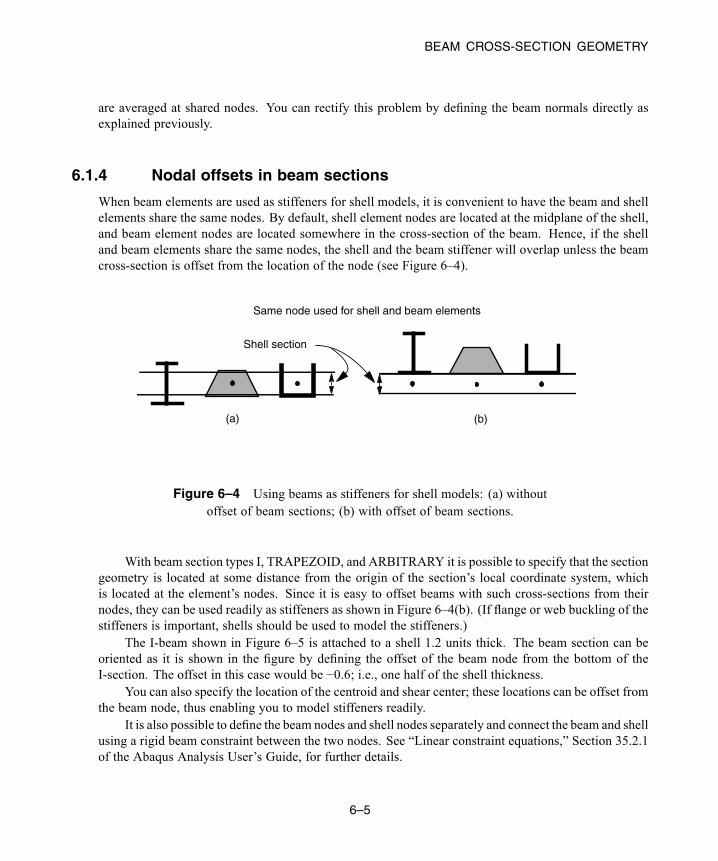
BEAM CROSS-SECTION GEOMETRY
are averaged at shared nodes. You can rectify this problem by defining the beam normals directly asexplained previously.
6.1.4 Nodal offsets in beam sections
When beam elements are used as stiffeners for shell models, it is convenient to have the beam and shellelements share the same nodes. By default, shell element nodes are located at the midplane of the shell,and beam element nodes are located somewhere in the cross-section of the beam. Hence, if the shelland beam elements share the same nodes, the shell and the beam stiffener will overlap unless the beamcross-section is offset from the location of the node (see Figure 6–4).
Same node used for shell and beam elements
Shell section
(a) (b)
Figure 6–4 Using beams as stiffeners for shell models: (a) withoutoffset of beam sections; (b) with offset of beam sections.
With beam section types I, TRAPEZOID, and ARBITRARY it is possible to specify that the sectiongeometry is located at some distance from the origin of the section’s local coordinate system, whichis located at the element’s nodes. Since it is easy to offset beams with such cross-sections from theirnodes, they can be used readily as stiffeners as shown in Figure 6–4(b). (If flange or web buckling of thestiffeners is important, shells should be used to model the stiffeners.)
The I-beam shown in Figure 6–5 is attached to a shell 1.2 units thick. The beam section can beoriented as it is shown in the figure by defining the offset of the beam node from the bottom of theI-section. The offset in this case would be −0.6; i.e., one half of the shell thickness.
You can also specify the location of the centroid and shear center; these locations can be offset fromthe beam node, thus enabling you to model stiffeners readily.
It is also possible to define the beam nodes and shell nodes separately and connect the beam and shellusing a rigid beam constraint between the two nodes. See “Linear constraint equations,” Section 35.2.1of the Abaqus Analysis User’s Guide, for further details.
6–5
Abaqus ID:Printed on:
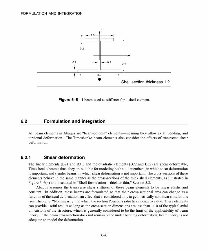
FORMULATION AND INTEGRATION
22.0
2.4
0.2
0.2 0.2
3.0
1
Shell section thickness 1.2
Figure 6–5 I-beam used as stiffener for a shell element.
6.2 Formulation and integration
All beam elements in Abaqus are “beam-column” elements—meaning they allow axial, bending, andtorsional deformation. The Timoshenko beam elements also consider the effects of transverse sheardeformation.
6.2.1 Shear deformationThe linear elements (B21 and B31) and the quadratic elements (B22 and B32) are shear deformable,Timoshenko beams; thus, they are suitable for modeling both stout members, in which shear deformationis important, and slender beams, in which shear deformation is not important. The cross-sections of theseelements behave in the same manner as the cross-sections of the thick shell elements, as illustrated inFigure 6–6(b) and discussed in “Shell formulation – thick or thin,” Section 5.2.
Abaqus assumes the transverse shear stiffness of these beam elements to be linear elastic andconstant. In addition, these beams are formulated so that their cross-sectional area can change as afunction of the axial deformation, an effect that is considered only in geometrically nonlinear simulations(see Chapter 8, “Nonlinearity”) in which the section Poisson’s ratio has a nonzero value. These elementscan provide useful results as long as the cross-section dimensions are less than 1/10 of the typical axialdimensions of the structure, which is generally considered to be the limit of the applicability of beamtheory; if the beam cross-section does not remain plane under bending deformation, beam theory is notadequate to model the deformation.
6–6
Abaqus ID:Printed on:
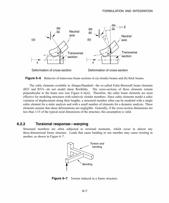
FORMULATION AND INTEGRATION
(a) (b)
x x
Deformation of cross-section Deformation of cross-section
w wTransversesection
Transversesection
Neutral axis Neutral
axis
dwdx
dwdx
dwdx
− γ = β
γ
Figure 6–6 Behavior of transverse beam sections in (a) slender beams and (b) thick beams.
The cubic elements available in Abaqus/Standard—the so-called Euler-Bernoulli beam elements(B23 and B33)—do not model shear flexibility. The cross-sections of these elements remainperpendicular to the beam axis (see Figure 6–6(a)). Therefore, the cubic beam elements are mosteffective for modeling structures with relatively slender members. Since cubic elements model a cubicvariation of displacement along their lengths, a structural member often can be modeled with a singlecubic element for a static analysis and with a small number of elements for a dynamic analysis. Theseelements assume that shear deformations are negligible. Generally, if the cross-section dimensions areless than 1/15 of the typical axial dimensions of the structure, this assumption is valid.
6.2.2 Torsional response—warpingStructural members are often subjected to torsional moments, which occur in almost anythree-dimensional frame structure. Loads that cause bending in one member may cause twisting inanother, as shown in Figure 6–7.
Torsion andbending
Bending
Figure 6–7 Torsion induced in a frame structure.
6–7
Abaqus ID:Printed on:
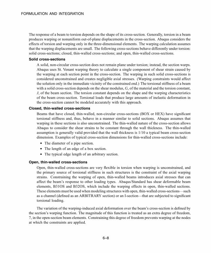
FORMULATION AND INTEGRATION
The response of a beam to torsion depends on the shape of its cross-section. Generally, torsion in a beamproduces warping or nonuniform out-of-plane displacements in the cross-section. Abaqus considers theeffects of torsion and warping only in the three-dimensional elements. The warping calculation assumesthat the warping displacements are small. The following cross-sections behave differently under torsion:solid cross-sections; closed, thin-walled cross-sections; and open, thin-walled cross-sections.
Solid cross-sections
A solid, non-circular cross-section does not remain plane under torsion; instead, the section warps.Abaqus uses St. Venant warping theory to calculate a single component of shear strain caused bythe warping at each section point in the cross-section. The warping in such solid cross-sections isconsidered unconstrained and creates negligible axial stresses. (Warping constraints would affectthe solution only in the immediate vicinity of the constrained end.) The torsional stiffness of a beamwith a solid cross-section depends on the shear modulus, G, of the material and the torsion constant,J, of the beam section. The torsion constant depends on the shape and the warping characteristicsof the beam cross-section. Torsional loads that produce large amounts of inelastic deformation inthe cross-section cannot be modeled accurately with this approach.
Closed, thin-walled cross-sections
Beams that have closed, thin-walled, non-circular cross-sections (BOX or HEX) have significanttorsional stiffness and, thus, behave in a manner similar to solid sections. Abaqus assumes thatwarping in these sections is also unconstrained. The thin-walled nature of the cross-section allowsAbaqus to consider the shear strains to be constant through the wall thickness. The thin-walledassumption is generally valid provided that the wall thickness is 1/10 a typical beam cross-sectiondimension. Examples of typical cross-section dimensions for thin-walled cross-sections include:
• The diameter of a pipe section.• The length of an edge of a box section.• The typical edge length of an arbitrary section.
Open, thin-walled cross-sections
Open, thin-walled cross-sections are very flexible in torsion when warping is unconstrained, andthe primary source of torsional stiffness in such structures is the constraint of the axial warpingstrains. Constraining the warping of open, thin-walled beams introduces axial stresses that canaffect the beam’s response to other loading types. Abaqus/Standard has shear deformable beamelements, B31OS and B32OS, which include the warping effects in open, thin-walled sections.These elementsmust be usedwhenmodeling structures with open, thin-walled cross-sections—suchas a channel (defined as an ARBITRARY section) or an I-section—that are subjected to significanttorsional loading.
The variation of the warping-induced axial deformation over the beam’s cross-section is defined bythe section’s warping function. The magnitude of this function is treated as an extra degree of freedom,7, in the open-section beam elements. Constraining this degree of freedom prevents warping at the nodesat which the constraints are applied.
6–8
Abaqus ID:Printed on:
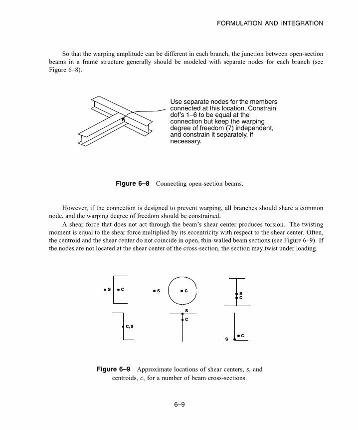
FORMULATION AND INTEGRATION
So that the warping amplitude can be different in each branch, the junction between open-sectionbeams in a frame structure generally should be modeled with separate nodes for each branch (seeFigure 6–8).
Use separate nodes for the membersconnected at this location. Constraindof’s 1–6 to be equal at theconnection but keep the warpingdegree of freedom (7) independent,and constrain it separately, ifnecessary.
Figure 6–8 Connecting open-section beams.
However, if the connection is designed to prevent warping, all branches should share a commonnode, and the warping degree of freedom should be constrained.
A shear force that does not act through the beam’s shear center produces torsion. The twistingmoment is equal to the shear force multiplied by its eccentricity with respect to the shear center. Often,the centroid and the shear center do not coincide in open, thin-walled beam sections (see Figure 6–9). Ifthe nodes are not located at the shear center of the cross-section, the section may twist under loading.
sc
cs
sc
c
s
s c
c,s
Figure 6–9 Approximate locations of shear centers, s, andcentroids, c, for a number of beam cross-sections.
6–9
Abaqus ID:Printed on:
EXAMPLE: CARGO CRANE
6.3 Selecting beam elements
• First-order, shear-deformable beam elements (B21, B31) should be used in any simulation thatincludes contact.
• If the transverse shear deformation is important, use Timoshenko (quadratic) beam elements (B22,B32).
• If the structure is either very rigid or very flexible, the hybrid beam elements (B21H, B32H, etc.)available in Abaqus/Standard should be used in geometrically nonlinear simulations.
• The Euler-Bernoulli (cubic) beams (B23, B33) available in Abaqus/Standard are very accurate forsimulations that include distributed loading, such as dynamic vibration analyses.
• Structures with open, thin-walled cross-sections should be modeled with the elements that use open-section warping theory (B31OS, B32OS) available in Abaqus/Standard.
6.4 Example: cargo crane
A light-service, cargo crane is shown in Figure 6–10. You have been asked to determine the staticdeflections of the crane when it carries a load of 10 kN. You should also identify the critical membersand joints in the structure: i.e., those with the highest stresses and loads. Because this is a static analysisyou will analyze the cargo crane using Abaqus/Standard.
The crane consists of two truss structures joined together by cross bracing. The two main membersin each truss structure are steel box beams (box cross-sections). Each truss structure is stiffened byinternal bracing, which is welded to the main members. The cross bracing connecting the two trussstructures is bolted to the truss structures. These connections can transmit little, if any, moment and,therefore, are treated as pinned joints. Both the internal bracing and cross bracing use steel box beamswith smaller cross-sections than the main members of the truss structures. The two truss structures areconnected at their ends (at point E) in such a way that allows independent movement in the 3-directionand all of the rotations, while constraining the displacements in the 1- and 2-directions to be the same.The crane is welded firmly to a massive structure at points A, B, C, and D. The dimensions of the craneare shown in Figure 6–11. In the following figures, truss A is the structure consisting of members AE,BE, and their internal bracing; and truss B consists of members CE, DE, and their internal bracing.
6–10
Abaqus ID:Printed on:
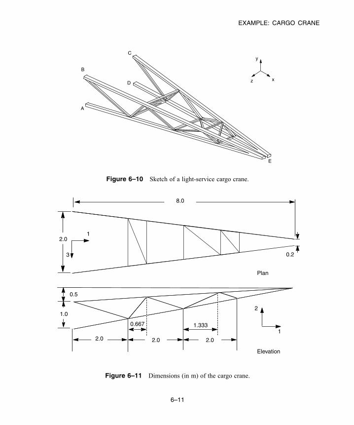
EXAMPLE: CARGO CRANE
z x
y
A
B
C
D
E
Figure 6–10 Sketch of a light-service cargo crane.
0.2
Plan
1
3
8.0
2.0
0.5
Elevation
1
21.0
2.0 2.0 2.0
1.3330.667
Figure 6–11 Dimensions (in m) of the cargo crane.
6–11
Abaqus ID:Printed on:
EXAMPLE: CARGO CRANE
The ratio of the typical cross-section dimension to global axial length in the main members of thecrane is much less than 1/15. The ratio is approximately 1/15 in the shortest member used for internalbracing. Therefore, it is valid to use beam elements to model the crane.
6.4.1 Preprocessing—creating the model with Abaqus/CAEIn this section we discuss how to use Abaqus/CAE to create the entire model for this simulation. Abaqusprovides scripts that replicate the complete analysis model for this problem. Run one of these scriptsif you encounter difficulties following the instructions given below or if you wish to check your work.Scripts are available in the following locations:
• A Python script for this example is provided in “Cargo crane,” Section A.4, in the HTML versionof this guide. Instructions of how to fetch the script and run it within Abaqus/CAE are given inAppendix A, “Example Files.”
• A plug-in script for this example is available in the Abaqus/CAE Plug-in toolset. To run the scriptfrom Abaqus/CAE, select Plug-ins→Abaqus→Getting Started, highlight Cargo crane, andclick Run. For more information about the Getting Started plug-ins, see “Running the GettingStarted with Abaqus examples,” Section 82.1 of the Abaqus/CAE User’s Guide, in the HTMLversion of this guide.
Creating the parts
The welded joints between the internal bracing and main members in the crane provide completecontinuity of the translations and rotations from one region of the model to the next. Therefore, youneed only a single geometric entity (i.e., vertex) at each welded joint in the model. A single partis used to represent the internal bracing and main members. For convenience, both truss structureswill be treated as a single part.
The bolted joints, which connect the cross bracing to the truss structures, and the connectionat the tip of the truss structures are different from the welded joint connections. Since these jointsdo not provide complete continuity for all degrees of freedom, separate vertices are needed forconnection. Thus, the cross bracing must be treated as a separate part since distinct geometricentities are required tomodel the bolted joints. Appropriate constraints between the separate verticesmust be specified.
We begin by discussing a technique to define the truss geometry. Since the two truss structuresare identical, it is sufficient to define the base feature of the part using only the geometry of a singletruss structure. The sketch of the truss geometry can be saved and then used to add the second trussstructure to the part definition.
The dimensions shown in Figure 6–11 are relative to a global Cartesian coordinate system.The base feature, however, must be sketched in a local plane. To make the sketching easier, datumfeatures will be used. A datum plane, parallel to one of the trusses (truss B in Figure 6–10, forexample), will serve as the sketch plane. The orientation of the sketch plane will be defined usinga datum axis.
6–12
Abaqus ID:Printed on:

EXAMPLE: CARGO CRANE
To define the geometry of a single truss:
1. To create a datum plane, a part must first be created. A part consisting of a single referencepoint will serve this purpose. Begin by creating a three-dimensional deformable part using thepoint base feature. Set the approximate part size to 20.0, and name the part Truss. Placethe point at the origin. This point represents point D in Figure 6–10.
2. Using the Create Datum Point: Offset From Point tool , create two datum points atdistances of (0, 1, 0) and (8, 1.5, 0.9) from the reference point. These pointsrepresent points C and E, respectively, in Figure 6–10. Reset the view using the Auto-Fit
View tool in the View Manipulation toolbar to see the full model.
3. Using the Create Datum Plane: 3 Points tool , create a datum plane to serve as thesketch plane. Select the reference point first, and then select the other two datum points in acounterclockwise fashion. Click mouse button 2 to exit the procedure.
Note: While selecting the points in this way is not required, it will make certain operationsthat follow easier. For example, by selecting the points in a counterclockwise order, the normalto the plane points out of the viewport and the sketch plane will be oriented automatically inthe 1–2 view in the Sketcher. If you select the points in a clockwise order, the plane’s normalwill point into the viewport and the sketch plane will have to be adjusted in the Sketcher.
4. Using the Create Datum Axis: Principal Axis tool , create a datum axis parallel to theY-Axis. As noted earlier, this axis will be used to position the sketch plane.
5. You are now ready to sketch the geometry. Use the Create Wire: Planar tool to enterthe Sketcher. Select the datum plane as the plane on which to sketch the wire geometry; selectthe datum axis as the axis that will appear vertical and to the left of the sketch. You may needto resize the view to select these entities.
6. Once in the Sketcher, use the Sketcher Options tool to modify the display. In the Generaltab, change the Sheet size to 20 and reduce theGrid spacing to 8. Zoom in to see the datumpoints more clearly.
Note: If the sketch plane is not oriented in the 1–2 plane, use the Views toolbar to change tothe X–Y view.
Using the Create Lines: Connected tool , sketch the lines representing the main truss,as shown in Figure 6–12. The datum points that were projected are treated as fixed points inthe sketch. Any line connected to one of these points effectively inherits a fixed constraint atthat point.
6–13
Abaqus ID:Printed on:
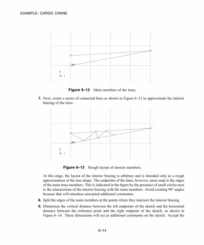
EXAMPLE: CARGO CRANE
RP
1
2
3
Figure 6–12 Main members of the truss.
7. Next, create a series of connected lines as shown in Figure 6–13 to approximate the interiorbracing of the truss.
RP
1
2
3
Figure 6–13 Rough layout of interior members.
At this stage, the layout of the interior bracing is arbitrary and is intended only as a roughapproximation of the true shape. The endpoints of the lines, however, must snap to the edgesof the main truss members. This is indicated in the figure by the presence of small circles nextto the intersections of the interior bracing with the main members. Avoid creating 90° anglesbecause that will introduce unwanted additional constraints.
8. Split the edges of the main members at the points where they intersect the interior bracing.
9. Dimension the vertical distance between the left endpoints of the sketch and the horizontaldistance between the reference point and the right endpoint of the sketch, as shown inFigure 6–14. These dimensions will act as additional constraints on the sketch. Accept the
6–14
Abaqus ID:Printed on:
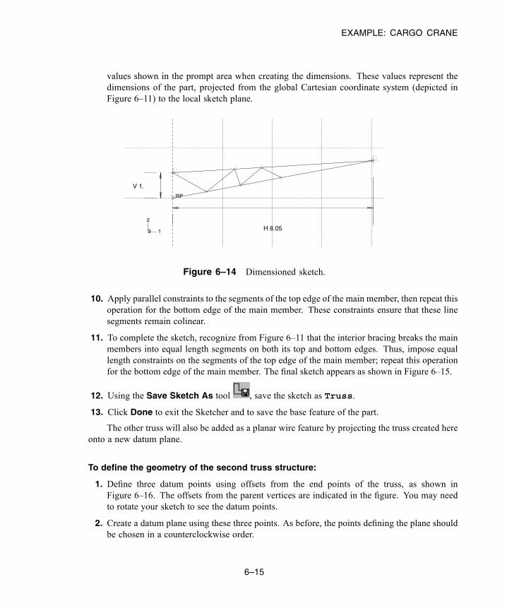
EXAMPLE: CARGO CRANE
values shown in the prompt area when creating the dimensions. These values represent thedimensions of the part, projected from the global Cartesian coordinate system (depicted inFigure 6–11) to the local sketch plane.
H 8.05
V 1.
RP
1
2
3
Figure 6–14 Dimensioned sketch.
10. Apply parallel constraints to the segments of the top edge of the main member, then repeat thisoperation for the bottom edge of the main member. These constraints ensure that these linesegments remain colinear.
11. To complete the sketch, recognize from Figure 6–11 that the interior bracing breaks the mainmembers into equal length segments on both its top and bottom edges. Thus, impose equallength constraints on the segments of the top edge of the main member; repeat this operationfor the bottom edge of the main member. The final sketch appears as shown in Figure 6–15.
12. Using the Save Sketch As tool , save the sketch as Truss.
13. Click Done to exit the Sketcher and to save the base feature of the part.
The other truss will also be added as a planar wire feature by projecting the truss created hereonto a new datum plane.
To define the geometry of the second truss structure:
1. Define three datum points using offsets from the end points of the truss, as shown inFigure 6–16. The offsets from the parent vertices are indicated in the figure. You may needto rotate your sketch to see the datum points.
2. Create a datum plane using these three points. As before, the points defining the plane shouldbe chosen in a counterclockwise order.
6–15
Abaqus ID:Printed on:
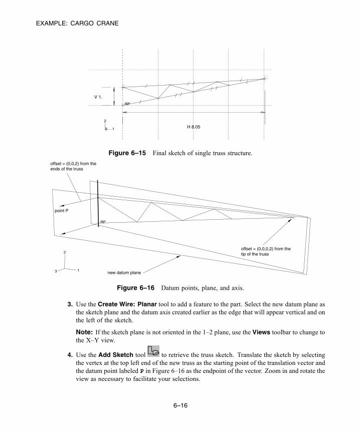
EXAMPLE: CARGO CRANE
H 8.05
V 1.
RP
1
2
3
Figure 6–15 Final sketch of single truss structure.
RP
1
2
3
offset = (0,0,2) from the ends of the truss
point P
new datum plane
offset = (0,0,0.2) from the tip of the truss
Figure 6–16 Datum points, plane, and axis.
3. Use the Create Wire: Planar tool to add a feature to the part. Select the new datum plane asthe sketch plane and the datum axis created earlier as the edge that will appear vertical and onthe left of the sketch.
Note: If the sketch plane is not oriented in the 1–2 plane, use the Views toolbar to change tothe X–Y view.
4. Use the Add Sketch tool to retrieve the truss sketch. Translate the sketch by selectingthe vertex at the top left end of the new truss as the starting point of the translation vector andthe datum point labeled P in Figure 6–16 as the endpoint of the vector. Zoom in and rotate theview as necessary to facilitate your selections.
6–16
Abaqus ID:Printed on:
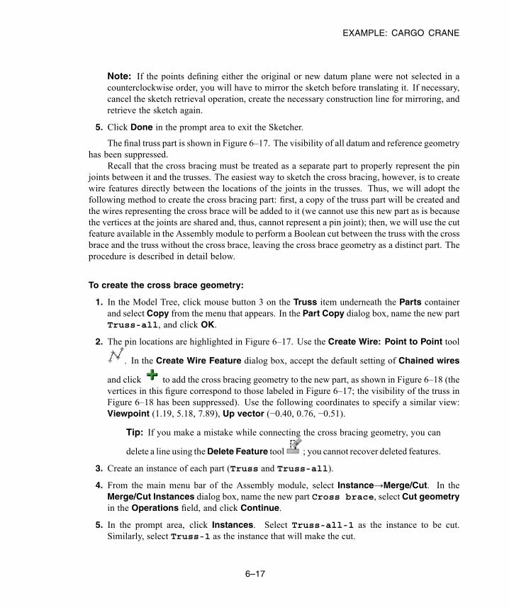
EXAMPLE: CARGO CRANE
Note: If the points defining either the original or new datum plane were not selected in acounterclockwise order, you will have to mirror the sketch before translating it. If necessary,cancel the sketch retrieval operation, create the necessary construction line for mirroring, andretrieve the sketch again.
5. Click Done in the prompt area to exit the Sketcher.
The final truss part is shown in Figure 6–17. The visibility of all datum and reference geometryhas been suppressed.
Recall that the cross bracing must be treated as a separate part to properly represent the pinjoints between it and the trusses. The easiest way to sketch the cross bracing, however, is to createwire features directly between the locations of the joints in the trusses. Thus, we will adopt thefollowing method to create the cross bracing part: first, a copy of the truss part will be created andthe wires representing the cross brace will be added to it (we cannot use this new part as is becausethe vertices at the joints are shared and, thus, cannot represent a pin joint); then, we will use the cutfeature available in the Assembly module to perform a Boolean cut between the truss with the crossbrace and the truss without the cross brace, leaving the cross brace geometry as a distinct part. Theprocedure is described in detail below.
To create the cross brace geometry:
1. In the Model Tree, click mouse button 3 on the Truss item underneath the Parts containerand select Copy from the menu that appears. In the Part Copy dialog box, name the new partTruss-all, and click OK.
2. The pin locations are highlighted in Figure 6–17. Use the Create Wire: Point to Point tool
. In the Create Wire Feature dialog box, accept the default setting of Chained wires
and click to add the cross bracing geometry to the new part, as shown in Figure 6–18 (thevertices in this figure correspond to those labeled in Figure 6–17; the visibility of the truss inFigure 6–18 has been suppressed). Use the following coordinates to specify a similar view:Viewpoint (1.19, 5.18, 7.89), Up vector (−0.40, 0.76, −0.51).
Tip: If you make a mistake while connecting the cross bracing geometry, you can
delete a line using theDelete Feature tool ; you cannot recover deleted features.
3. Create an instance of each part (Truss and Truss-all).
4. From the main menu bar of the Assembly module, select Instance→Merge/Cut. In theMerge/Cut Instances dialog box, name the new part Cross brace, select Cut geometryin the Operations field, and click Continue.
5. In the prompt area, click Instances. Select Truss-all-1 as the instance to be cut.Similarly, select Truss-1 as the instance that will make the cut.
6–17
Abaqus ID:Printed on:
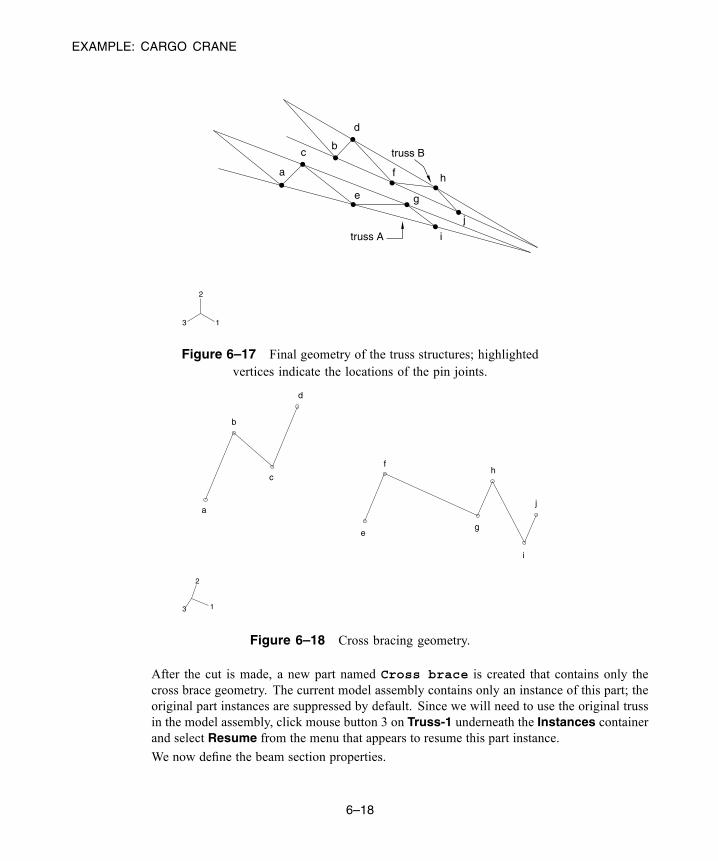
EXAMPLE: CARGO CRANE
1
2
3
truss B
truss A
d
bc
a
e
f
g
h
j
i
Figure 6–17 Final geometry of the truss structures; highlightedvertices indicate the locations of the pin joints.
1
2
3
d
b
a
c
f
e
h
g
j
i
Figure 6–18 Cross bracing geometry.
After the cut is made, a new part named Cross brace is created that contains only thecross brace geometry. The current model assembly contains only an instance of this part; theoriginal part instances are suppressed by default. Since we will need to use the original trussin the model assembly, click mouse button 3 on Truss-1 underneath the Instances containerand select Resume from the menu that appears to resume this part instance.
We now define the beam section properties.
6–18
Abaqus ID:Printed on:
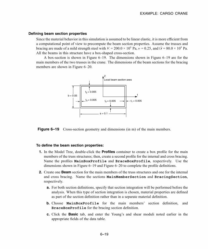
EXAMPLE: CARGO CRANE
Defining beam section properties
Since the material behavior in this simulation is assumed to be linear elastic, it is more efficient froma computational point of view to precompute the beam section properties. Assume the trusses andbracing are made of a mild strength steel with = 200.0 × 10⁹ Pa, = 0.25, and = 80.0 × 10⁹ Pa.All the beams in this structure have a box-shaped cross-section.
A box-section is shown in Figure 6–19. The dimensions shown in Figure 6–19 are for themain members of the two trusses in the crane. The dimensions of the beam sections for the bracingmembers are shown in Figure 6–20.
a = 0.1
b = 0.05
t3 = 0.005 t1 = 0.005
t2 = 0.005
t4 = 0.005
2
1
Local beam section axes
Figure 6–19 Cross-section geometry and dimensions (in m) of the main members.
To define the beam section properties:
1. In the Model Tree, double-click the Profiles container to create a box profile for the mainmembers of the truss structures; then, create a second profile for the internal and cross bracing.Name the profiles MainBoxProfile and BraceBoxProfile, respectively. Use thedimensions shown in Figure 6–19 and Figure 6–20 to complete the profile definitions.
2. Create one Beam section for the main members of the truss structures and one for the internaland cross bracing. Name the sections MainMemberSection and BracingSection,respectively.
a. For both section definitions, specify that section integration will be performed before theanalysis. When this type of section integration is chosen, material properties are definedas part of the section definition rather than in a separate material definition.
b. Choose MainBoxProfile for the main members’ section definition, andBraceBoxProfile for the bracing section definition.
c. Click the Basic tab, and enter the Young’s and shear moduli noted earlier in theappropriate fields of the data table.
6–19
Abaqus ID:Printed on:
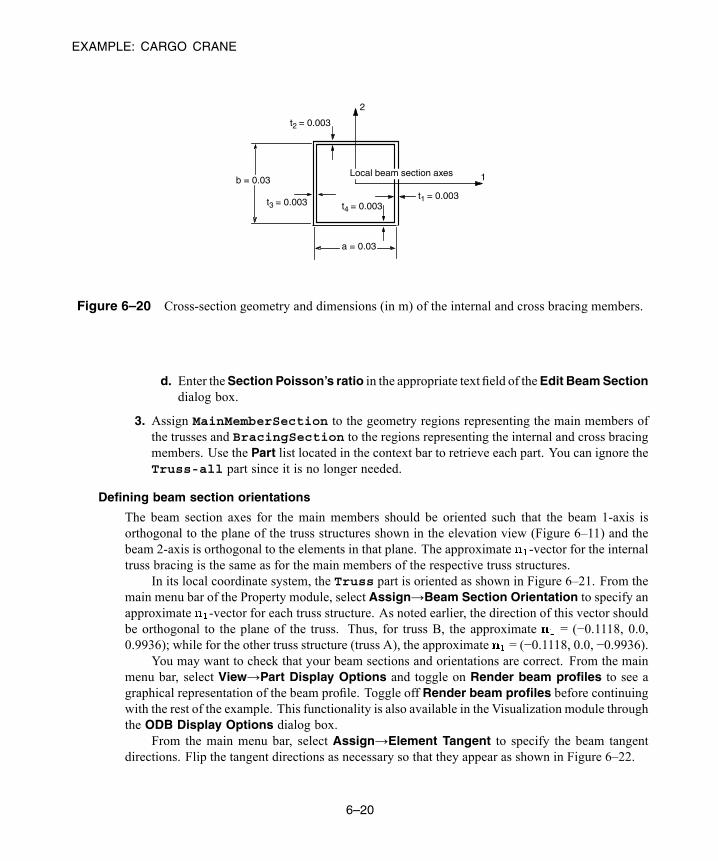
EXAMPLE: CARGO CRANE
a = 0.03
b = 0.03
t3 = 0.003t1 = 0.003
t2 = 0.003
t4 = 0.003
2
1Local beam section axes
Figure 6–20 Cross-section geometry and dimensions (in m) of the internal and cross bracing members.
d. Enter theSection Poisson’s ratio in the appropriate textfield of theEdit Beam Sectiondialog box.
3. Assign MainMemberSection to the geometry regions representing the main members ofthe trusses and BracingSection to the regions representing the internal and cross bracingmembers. Use the Part list located in the context bar to retrieve each part. You can ignore theTruss-all part since it is no longer needed.
Defining beam section orientations
The beam section axes for the main members should be oriented such that the beam 1-axis isorthogonal to the plane of the truss structures shown in the elevation view (Figure 6–11) and thebeam 2-axis is orthogonal to the elements in that plane. The approximate -vector for the internaltruss bracing is the same as for the main members of the respective truss structures.
In its local coordinate system, the Truss part is oriented as shown in Figure 6–21. From themain menu bar of the Property module, select Assign→Beam Section Orientation to specify anapproximate -vector for each truss structure. As noted earlier, the direction of this vector shouldbe orthogonal to the plane of the truss. Thus, for truss B, the approximate = (−0.1118, 0.0,0.9936); while for the other truss structure (truss A), the approximate = (−0.1118, 0.0, −0.9936).
You may want to check that your beam sections and orientations are correct. From the mainmenu bar, select View→Part Display Options and toggle on Render beam profiles to see agraphical representation of the beam profile. Toggle off Render beam profiles before continuingwith the rest of the example. This functionality is also available in the Visualization module throughthe ODB Display Options dialog box.
From the main menu bar, select Assign→Element Tangent to specify the beam tangentdirections. Flip the tangent directions as necessary so that they appear as shown in Figure 6–22.
6–20
Abaqus ID:Printed on:
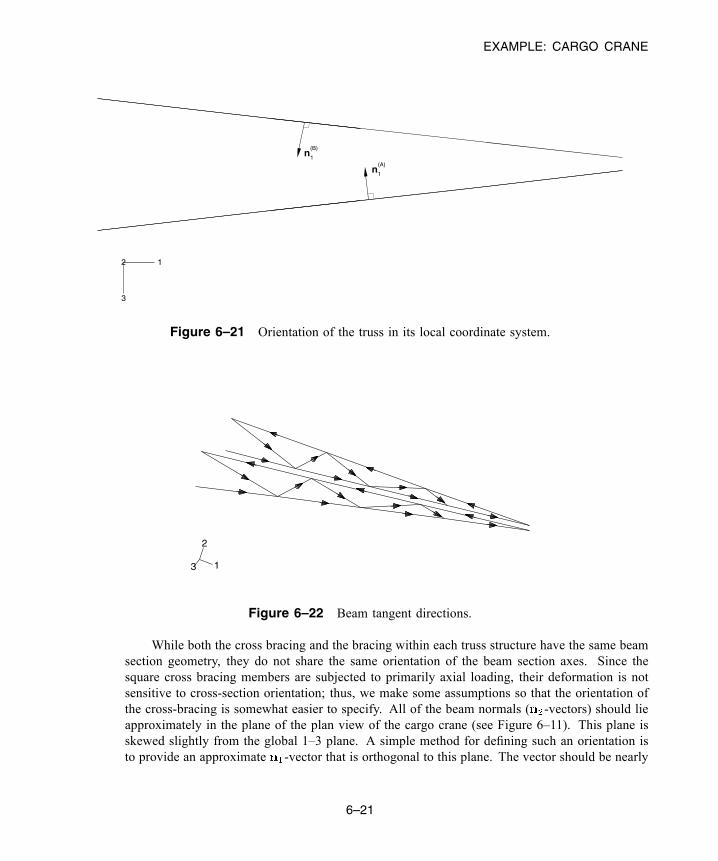
EXAMPLE: CARGO CRANE
12
3
n1
(A)
n1
(B)
Figure 6–21 Orientation of the truss in its local coordinate system.
1
2
3
Figure 6–22 Beam tangent directions.
While both the cross bracing and the bracing within each truss structure have the same beamsection geometry, they do not share the same orientation of the beam section axes. Since thesquare cross bracing members are subjected to primarily axial loading, their deformation is notsensitive to cross-section orientation; thus, we make some assumptions so that the orientation ofthe cross-bracing is somewhat easier to specify. All of the beam normals ( -vectors) should lieapproximately in the plane of the plan view of the cargo crane (see Figure 6–11). This plane isskewed slightly from the global 1–3 plane. A simple method for defining such an orientation isto provide an approximate -vector that is orthogonal to this plane. The vector should be nearly
6–21
Abaqus ID:Printed on:

EXAMPLE: CARGO CRANE
parallel to the global 2-direction. Therefore, specify = (0.0, 1.0, 0.0) for the cross bracing sothat it is aligned with the part (and as we shall see later, global) y-axis.
Beam normals
In this model you will have a modeling error if you provide data that only define the orientation ofthe approximate -vector. Unless overridden, the averaging of beam normals (see “Beam elementcurvature,” Section 6.1.3) causes Abaqus to use incorrect geometry for the cargo crane model. Tosee this, you can use the Visualization module to display the beam section axes and beam tangentvectors (see “Postprocessing,” Section 6.4.2). Without any further modification to the beam normaldirections, the normals in the crane model would appear to be correct in the Visualization module;yet, they would be, in fact, slightly incorrect.
Figure 6–23 shows the geometry of the truss structure.
1
2
3
R1R2
V1
R3R4
R5
V2
Figure 6–23 Locations where beam normals should be specified.
Referring to this figure, the correct geometry for the crane model requires three independent beamnormals at vertex V1: one each for regions R1 and R2 and a single normal for regions R3 and R4.Using the Abaqus logic for averaging normals, it becomes readily apparent that the beam normal atvertex V1 in region R2 would be averaged with the normals at this point for the adjacent regions. Inthis case the important part of the averaging logic is that normals that subtend an angle less than 20°with the reference normal are averaged with the reference normal to define a new reference normal.Assume the original reference normal at this point is the normal for regions R3 and R4. Since thenormal at vertex V1 in region R2 subtends an angle less than 20° with the original reference normal,it is averaged with the original normal to define a new reference normal at that location. On the otherhand, since the normal at vertex V1 in region R1 subtends an angle of approximately 30° with theoriginal reference normal, it will have an independent normal.
As a result of the incorrect average normal, the elements created on regions R2, R3, and R4that share the node created at vertex V1 would have an intended geometry that exhibits curvaturefrom one end of the element to the other. To prevent Abaqus from applying its averaging algorithm,specify the normal directions explicitly at positions where the subtended angle between adjacentregions will be less than 20°. In this problem you must specify the normal positions for thecorresponding regions on both sides of the crane.
6–22
Abaqus ID:Printed on:

EXAMPLE: CARGO CRANE
There is also a problem with the normals at vertex V2 at the tip of the truss structure, againbecause the angle between the two regions attached to this vertex is less than 20°. Since weare modeling straight beams, the normals are constant at both ends of each beam. This can becorrected by explicitly specifying the beam normal direction. As before, you must do this for thecorresponding regions on both sides of the crane.
Currently, the only way to specify beam normal directions in Abaqus/CAE is with theKeywords Editor. The Keywords Editor is a specialized text editor that allows you to modifythe Abaqus input file generated by Abaqus/CAE before submitting it for analysis. Thus, itallows you to add Abaqus/Standard or Abaqus/Explicit functionality when such functionality isnot supported by the current release of Abaqus/CAE. For more information on the KeywordsEditor, see “Adding unsupported keywords to your Abaqus/CAE model,” Section 9.10.1 of theAbaqus/CAE User’s Guide.
You will specify the beam normal directions later.
Creating assembly-level sets
We now focus on assembling themodel. Since the parts are already aligned with the global Cartesiancoordinate system shown in Figure 6–11, no further manipulations of the parts are necessary.
At this point, however, it is convenient to define assembly-level geometry sets that will be usedlater. In theModel Tree, expand theAssembly container and double-clickSets. Define a geometryset containing the vertices corresponding to points A through D (refer to Figure 6–10 for the exactlocations), and name the set Attach. When defining this set, be sure to select the vertices of thetruss and not reference points. You may need to use the Selection toolbar to aid in your selection.
In addition, create sets at the vertices located at the tips of the trusses (location E inFigure 6–10). Name the sets Tip-a and Tip-b, with Tip-a being the geometry set associatedwith truss A (see Figure 6–17). Finally, create a set for each region where beam normals will bespecified, referring to Figure 6–17 and Figure 6–23. For truss A, create a set named Inner-afor the region indicated by R2 and a set named Leg-a for the region indicated by R5; createcorresponding sets Inner-b and Leg-b for truss B.
Creating a step definition and specifying output
Create a single static, general step. Name the step Tip load, and enter the following stepdescription: Static tip load on crane.
Write the displacements (U) and reaction forces and moments (RF) at the nodes and the sectionforces and moments (SF) in the elements to the output database as field output for postprocessingwith Abaqus/CAE.
Defining constraint equations
Constraints between nodal degrees of freedom are specified in the Interaction module. The form ofeach equation is
where is the coefficient associated with degree of freedom .
6–23
Abaqus ID:Printed on:
EXAMPLE: CARGO CRANE
In the crane model the tips of the two trusses are connected together such that degrees offreedom 1 and 2 (the translations in the 1- and 2-directions) of each tip node are equal, while theother degrees of freedom (3–6) are independent. We need two linear constraints, one equatingdegree of freedom 1 at the two vertices and the other equating degree of freedom 2.
To create linear equations:
1. In the Model Tree, double-click the Constraints container. Name the constraintTipConstraint-1, and specify an equation constraint.
2. In the Edit Constraint dialog box, enter a coefficient of 1.0, the set name Tip-a, and degreeof freedom 1 in the first row. In the second row, enter a coefficient of -1.0, the set nameTip-b, and degree of freedom 1. Click OK.
This defines the constraint equation for degree of freedom 1.
Note: Text input is case-sensitive in Abaqus/CAE.
3. Clickmouse button 3 on the TipConstraint-1 item underneath theConstraints container, andselect Copy from the menu that appears. Copy TipConstraint-1 to TipConstraint-2.
4. Double-click TipConstraint-2 underneath the Constraints container to edit it. Change thedegree of freedom on both lines to 2.
The degrees of freedom associated with the first set defined in an equation are eliminated fromthe stiffnessmatrix. Therefore, this set should not appear in other constraint equations, and boundaryconditions should not be applied to the eliminated degrees of freedom.
Modeling the pin joint between the cross bracing and the trusses
The cross bracing, unlike the internal truss bracing, is bolted to the truss members. You can assumethat these bolted connections are unable to transmit rotations or torsion. The duplicate vertices thatwere defined at these locations are needed to define this constraint. In Abaqus such constraints canbe defined using multi-point constraints, constraint equations, or connectors. In this example thelast approach is adopted.
Connectors allow you to model a connection between any two points in a model assembly (orbetween any single point in the assembly and the ground). A large library of connectors is availablein Abaqus. See “Connector element library,” Section 31.1.4 of the Abaqus Analysis User’s Guide,for a complete list and a description of each connector type.
The JOIN connector will be used to model the bolted connection. The pinned joint createdby this connector constrains the displacements to be equal but the rotations (if they exist) remainindependent.
In Abaqus/CAE connectors are modeled using connector section assignments. You create anassembly-level wire feature to define the connector geometry and a connector section to define theconnection type. You can model connectors at all of the pin joints using one connector sectionassignment. You create the connector section assignment by selecting multiple wires and specifying
6–24
Abaqus ID:Printed on:
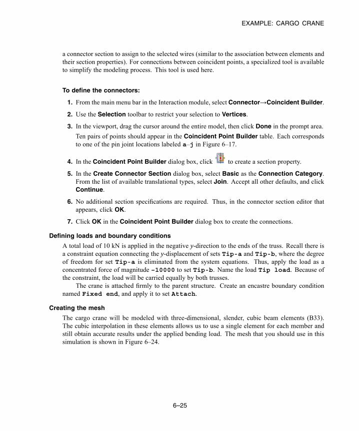
EXAMPLE: CARGO CRANE
a connector section to assign to the selected wires (similar to the association between elements andtheir section properties). For connections between coincident points, a specialized tool is availableto simplify the modeling process. This tool is used here.
To define the connectors:
1. From the main menu bar in the Interaction module, select Connector→Coincident Builder.
2. Use the Selection toolbar to restrict your selection to Vertices.
3. In the viewport, drag the cursor around the entire model, then click Done in the prompt area.
Ten pairs of points should appear in the Coincident Point Builder table. Each correspondsto one of the pin joint locations labeled a–j in Figure 6–17.
4. In the Coincident Point Builder dialog box, click to create a section property.
5. In the Create Connector Section dialog box, select Basic as the Connection Category.From the list of available translational types, select Join. Accept all other defaults, and clickContinue.
6. No additional section specifications are required. Thus, in the connector section editor thatappears, click OK.
7. Click OK in the Coincident Point Builder dialog box to create the connections.
Defining loads and boundary conditions
A total load of 10 kN is applied in the negative y-direction to the ends of the truss. Recall there isa constraint equation connecting the y-displacement of sets Tip-a and Tip-b, where the degreeof freedom for set Tip-a is eliminated from the system equations. Thus, apply the load as aconcentrated force of magnitude –10000 to set Tip-b. Name the load Tip load. Because ofthe constraint, the load will be carried equally by both trusses.
The crane is attached firmly to the parent structure. Create an encastre boundary conditionnamed Fixed end, and apply it to set Attach.
Creating the mesh
The cargo crane will be modeled with three-dimensional, slender, cubic beam elements (B33).The cubic interpolation in these elements allows us to use a single element for each member andstill obtain accurate results under the applied bending load. The mesh that you should use in thissimulation is shown in Figure 6–24.
6–25
Abaqus ID:Printed on:
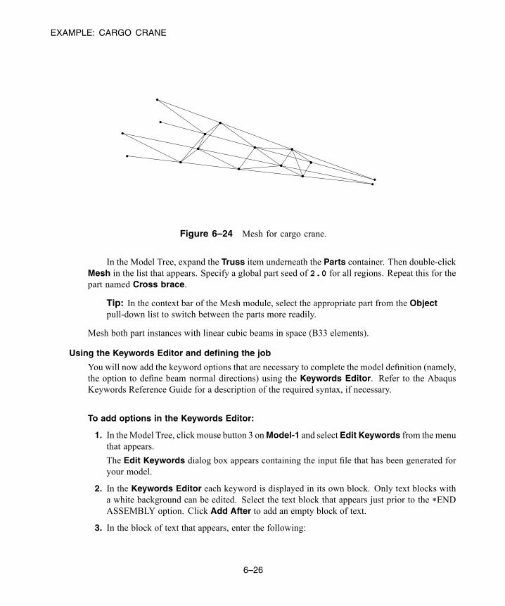
EXAMPLE: CARGO CRANE
Figure 6–24 Mesh for cargo crane.
In the Model Tree, expand the Truss item underneath the Parts container. Then double-clickMesh in the list that appears. Specify a global part seed of 2.0 for all regions. Repeat this for thepart named Cross brace.
Tip: In the context bar of the Mesh module, select the appropriate part from the Objectpull-down list to switch between the parts more readily.
Mesh both part instances with linear cubic beams in space (B33 elements).
Using the Keywords Editor and defining the job
You will now add the keyword options that are necessary to complete the model definition (namely,the option to define beam normal directions) using the Keywords Editor. Refer to the AbaqusKeywords Reference Guide for a description of the required syntax, if necessary.
To add options in the Keywords Editor:
1. In the Model Tree, click mouse button 3 onModel-1 and select Edit Keywords from the menuthat appears.
The Edit Keywords dialog box appears containing the input file that has been generated foryour model.
2. In the Keywords Editor each keyword is displayed in its own block. Only text blocks witha white background can be edited. Select the text block that appears just prior to the *ENDASSEMBLY option. Click Add After to add an empty block of text.
3. In the block of text that appears, enter the following:
6–26
Abaqus ID:Printed on:
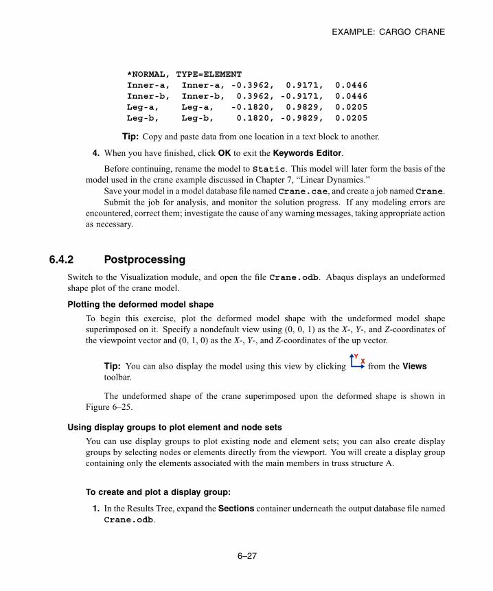
EXAMPLE: CARGO CRANE
*NORMAL, TYPE=ELEMENTInner-a, Inner-a, -0.3962, 0.9171, 0.0446Inner-b, Inner-b, 0.3962, -0.9171, 0.0446Leg-a, Leg-a, -0.1820, 0.9829, 0.0205Leg-b, Leg-b, 0.1820, -0.9829, 0.0205
Tip: Copy and paste data from one location in a text block to another.
4. When you have finished, click OK to exit the Keywords Editor.
Before continuing, rename the model to Static. This model will later form the basis of themodel used in the crane example discussed in Chapter 7, “Linear Dynamics.”
Save your model in a model database file named Crane.cae, and create a job named Crane.Submit the job for analysis, and monitor the solution progress. If any modeling errors are
encountered, correct them; investigate the cause of any warning messages, taking appropriate actionas necessary.
6.4.2 Postprocessing
Switch to the Visualization module, and open the file Crane.odb. Abaqus displays an undeformedshape plot of the crane model.
Plotting the deformed model shape
To begin this exercise, plot the deformed model shape with the undeformed model shapesuperimposed on it. Specify a nondefault view using (0, 0, 1) as the X-, Y-, and Z-coordinates ofthe viewpoint vector and (0, 1, 0) as the X-, Y-, and Z-coordinates of the up vector.
Tip: You can also display the model using this view by clicking from the Viewstoolbar.
The undeformed shape of the crane superimposed upon the deformed shape is shown inFigure 6–25.
Using display groups to plot element and node sets
You can use display groups to plot existing node and element sets; you can also create displaygroups by selecting nodes or elements directly from the viewport. You will create a display groupcontaining only the elements associated with the main members in truss structure A.
To create and plot a display group:
1. In the Results Tree, expand the Sections container underneath the output database file namedCrane.odb.
6–27
Abaqus ID:Printed on:
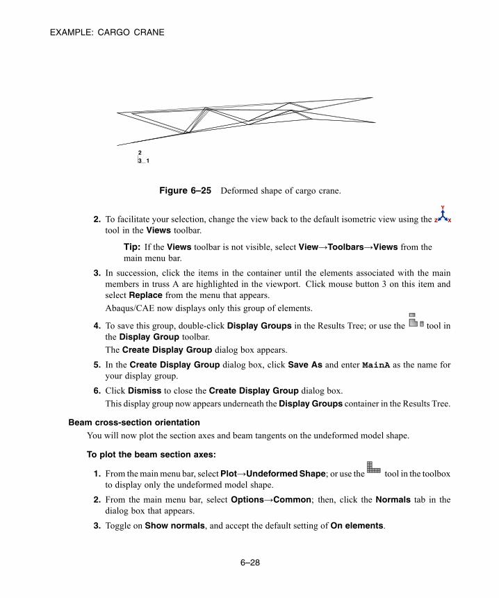
EXAMPLE: CARGO CRANE
123
Figure 6–25 Deformed shape of cargo crane.
2. To facilitate your selection, change the view back to the default isometric view using thetool in the Views toolbar.
Tip: If the Views toolbar is not visible, select View→Toolbars→Views from themain menu bar.
3. In succession, click the items in the container until the elements associated with the mainmembers in truss A are highlighted in the viewport. Click mouse button 3 on this item andselect Replace from the menu that appears.
Abaqus/CAE now displays only this group of elements.
4. To save this group, double-click Display Groups in the Results Tree; or use the tool inthe Display Group toolbar.
The Create Display Group dialog box appears.
5. In the Create Display Group dialog box, click Save As and enter MainA as the name foryour display group.
6. Click Dismiss to close the Create Display Group dialog box.
This display group now appears underneath theDisplay Groups container in the Results Tree.
Beam cross-section orientation
You will now plot the section axes and beam tangents on the undeformed model shape.
To plot the beam section axes:
1. From themain menu bar, selectPlot→Undeformed Shape; or use the tool in the toolboxto display only the undeformed model shape.
2. From the main menu bar, select Options→Common; then, click the Normals tab in thedialog box that appears.
3. Toggle on Show normals, and accept the default setting of On elements.
6–28
Abaqus ID:Printed on:
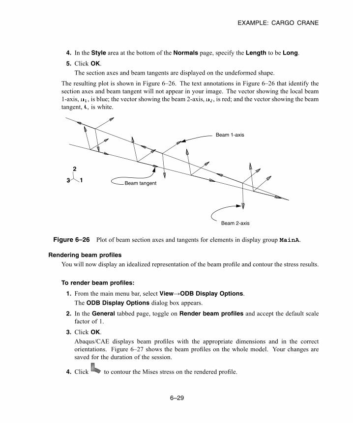
EXAMPLE: CARGO CRANE
4. In the Style area at the bottom of the Normals page, specify the Length to be Long.
5. Click OK.
The section axes and beam tangents are displayed on the undeformed shape.
The resulting plot is shown in Figure 6–26. The text annotations in Figure 6–26 that identify thesection axes and beam tangent will not appear in your image. The vector showing the local beam1-axis, , is blue; the vector showing the beam 2-axis, , is red; and the vector showing the beamtangent, , is white.
1
2
3
Beam 2-axis
Beam tangent
Beam 1-axis
Figure 6–26 Plot of beam section axes and tangents for elements in display group MainA.
Rendering beam profiles
You will now display an idealized representation of the beam profile and contour the stress results.
To render beam profiles:
1. From the main menu bar, select View→ODB Display Options.
The ODB Display Options dialog box appears.
2. In the General tabbed page, toggle on Render beam profiles and accept the default scalefactor of 1.
3. Click OK.
Abaqus/CAE displays beam profiles with the appropriate dimensions and in the correctorientations. Figure 6–27 shows the beam profiles on the whole model. Your changes aresaved for the duration of the session.
4. Click to contour the Mises stress on the rendered profile.
6–29
Abaqus ID:Printed on:
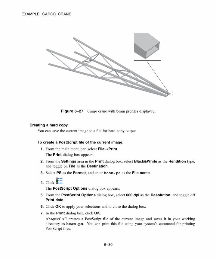
EXAMPLE: CARGO CRANE
Figure 6–27 Cargo crane with beam profiles displayed.
Creating a hard copy
You can save the current image to a file for hard-copy output.
To create a PostScript file of the current image:
1. From the main menu bar, select File→Print.
The Print dialog box appears.
2. From the Settings area in the Print dialog box, select Black&White as the Rendition type;and toggle on File as the Destination.
3. Select PS as the Format, and enter beam.ps as the File name.
4. Click .
The PostScript Options dialog box appears.
5. From the PostScript Options dialog box, select 600 dpi as the Resolution; and toggle offPrint date.
6. Click OK to apply your selections and to close the dialog box.
7. In the Print dialog box, click OK.
Abaqus/CAE creates a PostScript file of the current image and saves it in your workingdirectory as beam.ps. You can print this file using your system’s command for printingPostScript files.
6–30
Abaqus ID:Printed on:
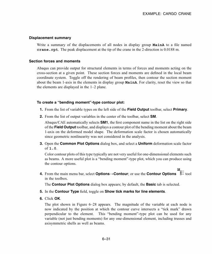
EXAMPLE: CARGO CRANE
Displacement summary
Write a summary of the displacements of all nodes in display group MainA to a file namedcrane.rpt. The peak displacement at the tip of the crane in the 2-direction is 0.0188 m.
Section forces and moments
Abaqus can provide output for structural elements in terms of forces and moments acting on thecross-section at a given point. These section forces and moments are defined in the local beamcoordinate system. Toggle off the rendering of beam profiles, then contour the section momentabout the beam 1-axis in the elements in display group MainA. For clarity, reset the view so thatthe elements are displayed in the 1–2 plane.
To create a “bending moment”-type contour plot:
1. From the list of variable types on the left side of the Field Output toolbar, select Primary.
2. From the list of output variables in the center of the toolbar, select SM.
Abaqus/CAE automatically selects SM1, the first component name in the list on the right sideof the Field Output toolbar, and displays a contour plot of the bending moment about the beam1-axis on the deformed model shape. The deformation scale factor is chosen automaticallysince geometric nonlinearity was not considered in the analysis.
3. Open the Common Plot Options dialog box, and select a Uniform deformation scale factorof 1.0.
Color contour plots of this type typically are not very useful for one-dimensional elements suchas beams. A more useful plot is a “bending moment”-type plot, which you can produce usingthe contour options.
4. From the main menu bar, select Options→Contour; or use the Contour Options toolin the toolbox.
The Contour Plot Options dialog box appears; by default, the Basic tab is selected.
5. In the Contour Type field, toggle on Show tick marks for line elements.
6. Click OK.
The plot shown in Figure 6–28 appears. The magnitude of the variable at each node isnow indicated by the position at which the contour curve intersects a “tick mark” drawnperpendicular to the element. This “bending moment”-type plot can be used for anyvariable (not just bending moments) for any one-dimensional element, including trusses andaxisymmetric shells as well as beams.
6–31
Abaqus ID:Printed on:
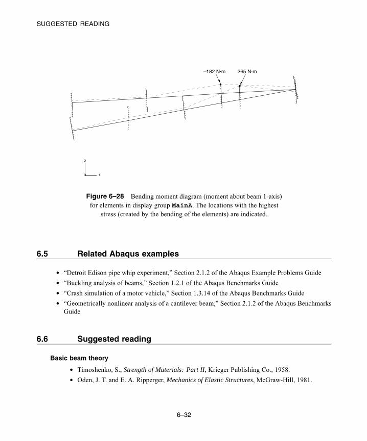
SUGGESTED READING
1
2
3
–182 N.m. 265 N.m.
Figure 6–28 Bending moment diagram (moment about beam 1-axis)for elements in display group MainA. The locations with the highest
stress (created by the bending of the elements) are indicated.
6.5 Related Abaqus examples
• “Detroit Edison pipe whip experiment,” Section 2.1.2 of the Abaqus Example Problems Guide• “Buckling analysis of beams,” Section 1.2.1 of the Abaqus Benchmarks Guide• “Crash simulation of a motor vehicle,” Section 1.3.14 of the Abaqus Benchmarks Guide• “Geometrically nonlinear analysis of a cantilever beam,” Section 2.1.2 of the Abaqus BenchmarksGuide
6.6 Suggested reading
Basic beam theory
• Timoshenko, S., Strength of Materials: Part II, Krieger Publishing Co., 1958.
• Oden, J. T. and E. A. Ripperger, Mechanics of Elastic Structures, McGraw-Hill, 1981.
6–32
Abaqus ID:Printed on:
SUMMARY
Basic computational beam theory
• Cook, R. D., D. S. Malkus, and M. E. Plesha, Concepts and Applications of Finite ElementAnalysis, John Wiley & Sons, 1989.
• Hughes, T. J. R., The Finite Element Method, Prentice-Hall Inc., 1987.
6.7 Summary
• The behavior of beam elements can be determined by numerical integration of the section or can begiven directly in terms of area, moments of inertia, and torsional constant.
• When defining beam cross-section properties numerically, you can have the section propertiescalculated once at the beginning of the analysis (linear elastic material behavior is assumed) orthroughout the analysis (linear or nonlinear material behavior is permitted).
• Abaqus includes a number of standard cross-section shapes. Other shapes, provided they are “thin-walled,” can be modeled using the ARBITRARY cross-section.
• The orientation of the cross-section must be defined either by specifying a third node or by defininga normal vector as part of the element property definition. The normals can be plotted in theVisualization module of Abaqus/CAE.
• The beam cross-section can be offset from the nodes that define the beam. This procedure is usefulin modeling stiffeners on shells.
• The linear and quadratic beams include the effects of shear deformation. The cubic beamsin Abaqus/Standard do not account for shear flexibility. The open-section beam elements inAbaqus/Standard correctly model the effects of torsion and warping (including warping constraints)in thin-walled, open sections.
• Multi-point constraints, constraint equations, and connectors can be used to connect degrees offreedom at nodes to model pinned connections, rigid links, etc.
• “Bending moment”-type plots allow the results of one-dimensional elements, such as beams, to bevisualized easily.
• Display options allow you to render beam profiles for an enhanced graphical representation of themodel.
• Hard copies of Abaqus/CAE plots can be obtained in PostScript (PS), Encapsulated PostScript(EPS), Tag Image File Format (TIFF), Portable Network Graphics (PNG), and Scalable VectorGraphics (SVG) formats.
6–33
Abaqus ID:Printed on:


INTRODUCTION
7. Linear Dynamics
A static analysis is sufficient if you are interested in the long-term response of a structure to applied loads.However, if the duration of the applied load is short (such as in an earthquake) or if the loading is dynamicin nature (such as that from rotating machinery), you must perform a dynamic analysis. This chapterdiscusses linear dynamic analysis in Abaqus/Standard; see Chapter 9, “Nonlinear Explicit Dynamics,”for a discussion of nonlinear dynamic analysis in Abaqus/Explicit.
7.1 Introduction
A dynamic simulation is one in which inertia forces are included in the dynamic equation of equilibrium:
where
M is the mass of the structure,
is the acceleration of the structure,
I are the internal forces in the structure, and
P are the applied external forces.
The expression in the equation shown above is nothing more than Newton’s second law of motion ().The inclusion of the inertial forces ( ) in the equation of equilibrium is the major difference
between static and dynamic analyses. Another difference between the two types of simulations is in thedefinition of the internal forces, I. In a static analysis the internal forces arise only from the deformationof the structure; in a dynamic analysis the internal forces contain contributions created by both the motion(i.e., damping) and the deformation of the structure.
7.1.1 Natural frequencies and mode shapes
The simplest dynamic problem is that of a mass oscillating on a spring, as shown in Figure 7–1.The internal force in the spring is given by so that its dynamic equation of motion is
7–1
Abaqus ID:Printed on:
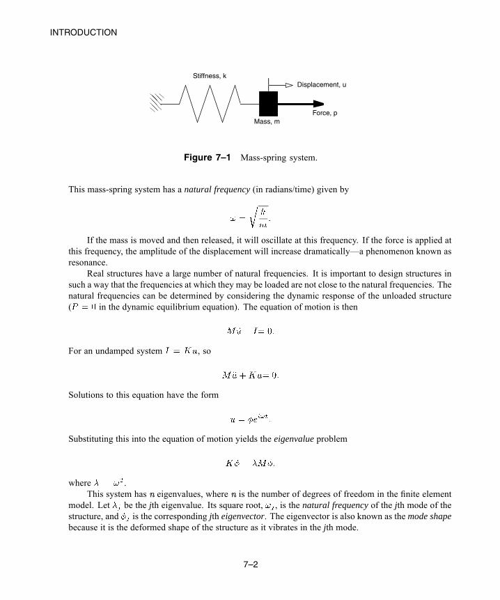
INTRODUCTION
Force, p
Displacement, uStiffness, k
Mass, m
Figure 7–1 Mass-spring system.
This mass-spring system has a natural frequency (in radians/time) given by
If the mass is moved and then released, it will oscillate at this frequency. If the force is applied atthis frequency, the amplitude of the displacement will increase dramatically—a phenomenon known asresonance.
Real structures have a large number of natural frequencies. It is important to design structures insuch a way that the frequencies at which they may be loaded are not close to the natural frequencies. Thenatural frequencies can be determined by considering the dynamic response of the unloaded structure( in the dynamic equilibrium equation). The equation of motion is then
For an undamped system , so
Solutions to this equation have the form
Substituting this into the equation of motion yields the eigenvalue problem
where .This system has n eigenvalues, where n is the number of degrees of freedom in the finite element
model. Let be the jth eigenvalue. Its square root, , is the natural frequency of the jth mode of thestructure, and is the corresponding jth eigenvector. The eigenvector is also known as the mode shapebecause it is the deformed shape of the structure as it vibrates in the jth mode.
7–2
Abaqus ID:Printed on:

INTRODUCTION
The frequency extraction procedure in Abaqus/Standard is used to determine the modes andfrequencies of the structure. This procedure is easy to use in that you need only specify the number ofmodes required or the maximum frequency of interest.
7.1.2 Modal superpositionThe natural frequencies and mode shapes of a structure can be used to characterize its dynamic responseto loads in the linear regime. The deformation of the structure can be calculated from a combination ofthe mode shapes of the structure using themodal superposition technique. Each mode shape is multipliedby a scale factor. The vector of displacements in the model, u, is defined as
where is themodal displacement and is the generalized coordinate of mode i. This technique is validonly for simulations with small displacements, linear elastic materials, and no contact conditions—inother words, linear problems.
In structural dynamic problems the response of a structure usually is dominated by a relativelysmall number of modes, making modal superposition a particularly efficient method for calculating theresponse of such systems. Consider a model containing 10,000 degrees of freedom. Direct integrationof the dynamic equations of motion would require the solution of 10,000 simultaneous equations ateach point in time. If the structural response is characterized by 100 modes, only 100 equations needto be solved every time increment. Moreover, the modal equations are uncoupled, whereas the originalequations of motion are coupled. There is an initial cost in calculating the modes and frequencies, butthe savings obtained in the calculation of the response greatly outweigh the cost.
If nonlinearities are present in the simulation, the natural frequencies may change significantlyduring the analysis, and modal superposition cannot be employed. In this case direct integration ofthe dynamic equation of equilibrium is required, which is much more expensive than modal analysis.
A problem should have the following characteristics for it to be suitable for linear transient dynamicanalysis:
• The system should be linear: linear material behavior, no contact conditions, and no nonlineargeometric effects.
• The response should be dominated by relatively few frequencies. As the frequency content of theresponse increases, such as is the case in shock and impact problems, the modal superpositiontechnique becomes less effective.
• The dominant loading frequencies should be in the range of the extracted frequencies to ensure thatthe loads can be described accurately.
• The initial accelerations generated by any suddenly applied loads should be described accuratelyby the eigenmodes.
• The system should not be heavily damped.
7–3
Abaqus ID:Printed on:
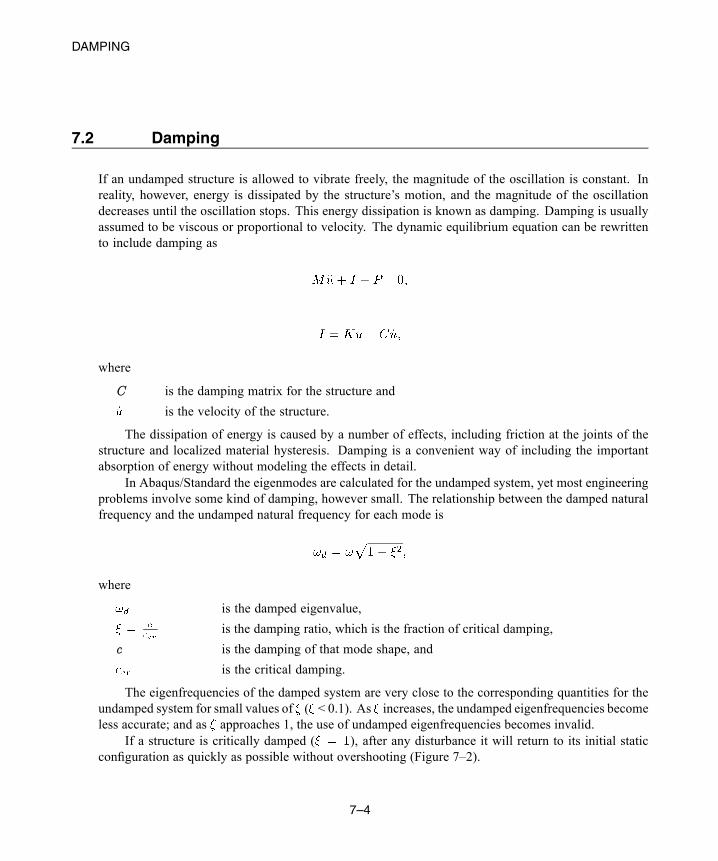
DAMPING
7.2 Damping
If an undamped structure is allowed to vibrate freely, the magnitude of the oscillation is constant. Inreality, however, energy is dissipated by the structure’s motion, and the magnitude of the oscillationdecreases until the oscillation stops. This energy dissipation is known as damping. Damping is usuallyassumed to be viscous or proportional to velocity. The dynamic equilibrium equation can be rewrittento include damping as
where
C is the damping matrix for the structure and
is the velocity of the structure.
The dissipation of energy is caused by a number of effects, including friction at the joints of thestructure and localized material hysteresis. Damping is a convenient way of including the importantabsorption of energy without modeling the effects in detail.
In Abaqus/Standard the eigenmodes are calculated for the undamped system, yet most engineeringproblems involve some kind of damping, however small. The relationship between the damped naturalfrequency and the undamped natural frequency for each mode is
where
is the damped eigenvalue,
is the damping ratio, which is the fraction of critical damping,
c is the damping of that mode shape, and
is the critical damping.
The eigenfrequencies of the damped system are very close to the corresponding quantities for theundamped system for small values of ( < 0.1). As increases, the undamped eigenfrequencies becomeless accurate; and as approaches 1, the use of undamped eigenfrequencies becomes invalid.
If a structure is critically damped ( ), after any disturbance it will return to its initial staticconfiguration as quickly as possible without overshooting (Figure 7–2).
7–4
Abaqus ID:Printed on:

DAMPING
Criticallydamped
Underdamped
Overdamped
Static Equilibrium
Figure 7–2 Damped motion patterns for various values of .
7.2.1 Definition of damping in Abaqus/StandardIn Abaqus/Standard a number of different types of damping can be defined for a transient modal analysis:direct modal damping, Rayleigh damping, and composite modal damping.
Damping is defined for modal dynamic procedures. The damping is part of the step definition, anddifferent amounts of damping can be defined for each mode.
Direct modal damping
The fraction of critical damping, , associated with each mode can be defined using direct modaldamping. Typically, values in the range of 1% to 10% of critical damping are used. Direct modaldamping allows you to define precisely the damping of each mode of the system.
Rayleigh damping
In Rayleigh damping the assumption is made that the damping matrix is a linear combination of themass and stiffness matrices,
7–5
Abaqus ID:Printed on:
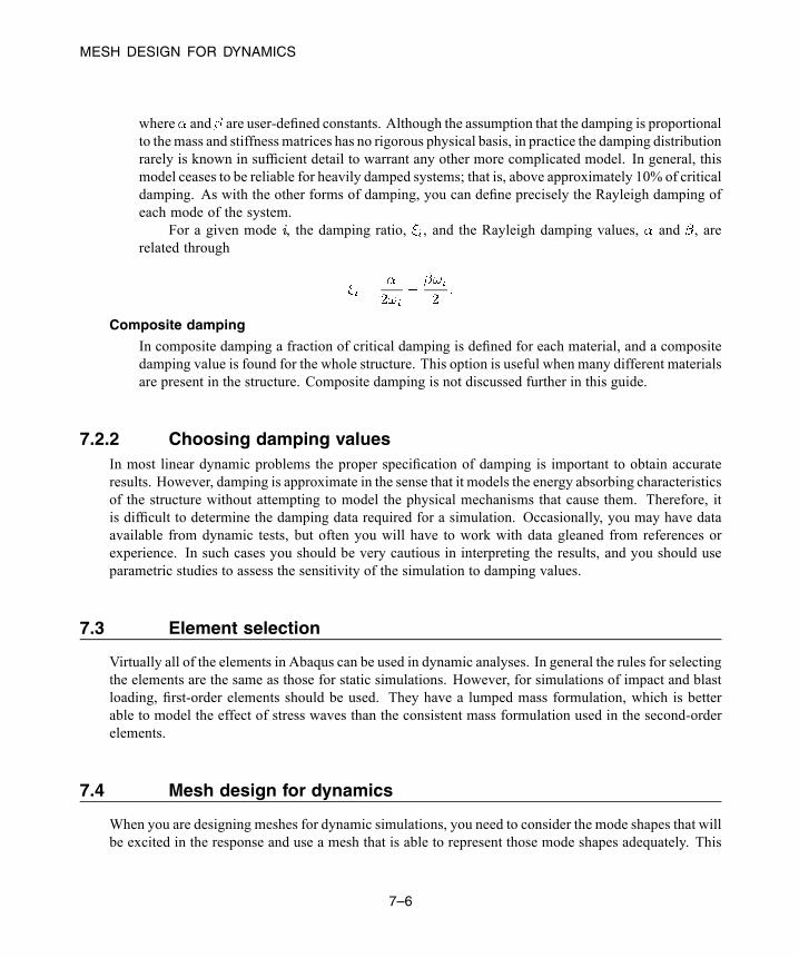
MESH DESIGN FOR DYNAMICS
where and are user-defined constants. Although the assumption that the damping is proportionalto themass and stiffness matrices has no rigorous physical basis, in practice the damping distributionrarely is known in sufficient detail to warrant any other more complicated model. In general, thismodel ceases to be reliable for heavily damped systems; that is, above approximately 10% of criticaldamping. As with the other forms of damping, you can define precisely the Rayleigh damping ofeach mode of the system.
For a given mode i, the damping ratio, , and the Rayleigh damping values, and , arerelated through
Composite damping
In composite damping a fraction of critical damping is defined for each material, and a compositedamping value is found for the whole structure. This option is useful when many different materialsare present in the structure. Composite damping is not discussed further in this guide.
7.2.2 Choosing damping valuesIn most linear dynamic problems the proper specification of damping is important to obtain accurateresults. However, damping is approximate in the sense that it models the energy absorbing characteristicsof the structure without attempting to model the physical mechanisms that cause them. Therefore, itis difficult to determine the damping data required for a simulation. Occasionally, you may have dataavailable from dynamic tests, but often you will have to work with data gleaned from references orexperience. In such cases you should be very cautious in interpreting the results, and you should useparametric studies to assess the sensitivity of the simulation to damping values.
7.3 Element selection
Virtually all of the elements in Abaqus can be used in dynamic analyses. In general the rules for selectingthe elements are the same as those for static simulations. However, for simulations of impact and blastloading, first-order elements should be used. They have a lumped mass formulation, which is betterable to model the effect of stress waves than the consistent mass formulation used in the second-orderelements.
7.4 Mesh design for dynamics
When you are designing meshes for dynamic simulations, you need to consider the mode shapes that willbe excited in the response and use a mesh that is able to represent those mode shapes adequately. This
7–6
Abaqus ID:Printed on:

MESH DESIGN FOR DYNAMICS
means that a mesh that is adequate for a static simulation may be unsuitable for calculating the dynamicresponse to loading that excites high frequency modes.
Consider, for example, the plate shown in Figure 7–3. The mesh of first-order shell elements isadequate for a static analysis of the plate under a uniform load and is also suitable for the predictionof the first mode shape. However, the mesh is clearly too coarse to be able to model the sixth modeaccurately.
(a) Mode 1: 31.1 Hz (b) Mode 6: 140 Hz
Figure 7–3 Vibration frequencies and corresponding modeshapes of the plate based on the coarse mesh.
Figure 7–4 shows the same plate modeled with a refined mesh of first-order elements. The displacedshape for the sixth mode now looks much better, and the frequency predicted for this mode is moreaccurate. If the dynamic loading on the plate is such that there is significant excitation of this mode, therefined mesh must be used; the results from the coarse mesh will not be accurate.
(a) Mode 1: 30.2 Hz (b) Mode 6: 124 Hz
Figure 7–4 Vibration frequencies and corresponding modeshapes of the plate based on the fine mesh.
7–7
Abaqus ID:Printed on:
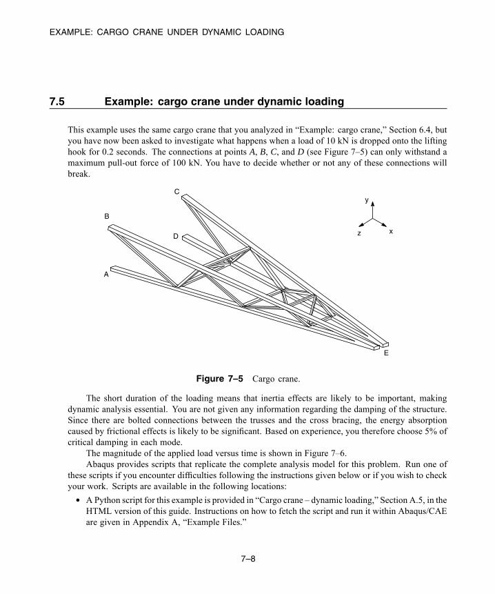
EXAMPLE: CARGO CRANE UNDER DYNAMIC LOADING
7.5 Example: cargo crane under dynamic loading
This example uses the same cargo crane that you analyzed in “Example: cargo crane,” Section 6.4, butyou have now been asked to investigate what happens when a load of 10 kN is dropped onto the liftinghook for 0.2 seconds. The connections at points A, B, C, and D (see Figure 7–5) can only withstand amaximum pull-out force of 100 kN. You have to decide whether or not any of these connections willbreak.
z x
y
A
B
C
D
E
Figure 7–5 Cargo crane.
The short duration of the loading means that inertia effects are likely to be important, makingdynamic analysis essential. You are not given any information regarding the damping of the structure.Since there are bolted connections between the trusses and the cross bracing, the energy absorptioncaused by frictional effects is likely to be significant. Based on experience, you therefore choose 5% ofcritical damping in each mode.
The magnitude of the applied load versus time is shown in Figure 7–6.Abaqus provides scripts that replicate the complete analysis model for this problem. Run one of
these scripts if you encounter difficulties following the instructions given below or if you wish to checkyour work. Scripts are available in the following locations:
• A Python script for this example is provided in “Cargo crane – dynamic loading,” Section A.5, in theHTML version of this guide. Instructions on how to fetch the script and run it within Abaqus/CAEare given in Appendix A, “Example Files.”
7–8
Abaqus ID:Printed on:
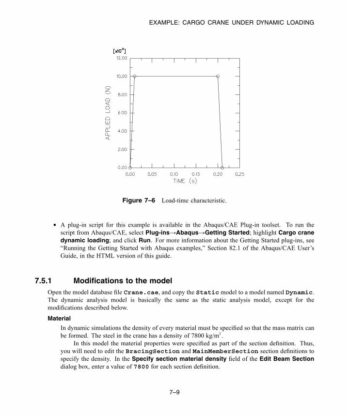
EXAMPLE: CARGO CRANE UNDER DYNAMIC LOADING
Figure 7–6 Load-time characteristic.
• A plug-in script for this example is available in the Abaqus/CAE Plug-in toolset. To run thescript from Abaqus/CAE, select Plug-ins→Abaqus→Getting Started; highlight Cargo cranedynamic loading; and click Run. For more information about the Getting Started plug-ins, see“Running the Getting Started with Abaqus examples,” Section 82.1 of the Abaqus/CAE User’sGuide, in the HTML version of this guide.
7.5.1 Modifications to the modelOpen the model database file Crane.cae, and copy the Static model to a model named Dynamic.The dynamic analysis model is basically the same as the static analysis model, except for themodifications described below.
Material
In dynamic simulations the density of every material must be specified so that the mass matrix canbe formed. The steel in the crane has a density of 7800 kg/m3 .
In this model the material properties were specified as part of the section definition. Thus,you will need to edit the BracingSection and MainMemberSection section definitions tospecify the density. In the Specify section material density field of the Edit Beam Sectiondialog box, enter a value of 7800 for each section definition.
7–9
Abaqus ID:Printed on:
EXAMPLE: CARGO CRANE UNDER DYNAMIC LOADING
Note: If material data are defined independently of the section properties, the density is includedby editing the material definition and selectingGeneral→Density in the Edit Material dialog box.
Steps
The step definitions that are used for the dynamic analysis are substantially different from thoseused in the static analysis. Therefore, the static step created previously will be replaced by two newsteps.
The first step in the dynamic analysis calculates the natural frequencies and mode shapes of thestructure. The second step then uses these data to calculate the transient modal dynamic responseof the cargo crane. In this analysis we will assume that everything is linear. If you want to modelany nonlinearities in this simulation, direct integration of the equations of motion using the implicitdynamic proceduremust be performed instead. See “Nonlinear dynamics,” Section 7.9.2, for furtherdetails.
Abaqus/Standard offers the Lanczos and the subspace iteration eigenvalue extraction methods.The Lanczos method is generally faster when a large number of eigenmodes is required for a systemwith many degrees of freedom. The subspace iteration method may be faster when only a few (lessthan 20) eigenmodes are needed.
We use the Lanczos eigensolver in this analysis and request 30 eigenvalues. Instead ofspecifying the number of modes required, it is also possible to specify the minimum and maximumfrequencies of interest so that the step will complete once Abaqus/Standard has found all of theeigenvalues inside the specified range. A shift point may also be specified so that eigenvaluesnearest the shift point will be extracted. By default, no minimum or maximum frequency or shiftis used. If the structure is not constrained against rigid body modes, the shift value should be set toa small negative value to remove numerical problems associated with rigid body motion.
To replace the static step with a frequency extraction step:
1. In the Model Tree, expand the Steps container. Then, click mouse button 3 on the step namedTip Load and select Replace from the menu that appears. In the Replace Step dialog box,select Frequency from the list of available Linear perturbation procedures.
Model attributes that cannot be converted will be deleted. In this case the concentrated loadsare deleted because they cannot be used in a frequency extraction step. However, the boundaryconditions and output requests associated with the static step are inherited by the frequencyextraction step.
2. In the Basic tabbed page of the Edit Step dialog box, enter the step description First 30modes; accept the Lanczos eigensolver option; and request 30 eigenvalues.
3. Rename the step to Extract Frequencies by clicking mouse button 3 on the name TipLoad and selecting Rename from the menu that appears.
In structural dynamic analysis the response is usually associated with the lower modes.However, enough modes should be extracted to provide a good representation of the dynamic
7–10
Abaqus ID:Printed on:

EXAMPLE: CARGO CRANE UNDER DYNAMIC LOADING
response of the structure. One way of checking that a sufficient number of eigenvalues has beenextracted is to look at the total effective mass in each degree of freedom, which indicates how muchof the mass is active in each direction of the extracted modes. The effective masses are tabulatedin the data file under the eigenvalue output. Ideally, the sum of the modal effective masses foreach mode in each direction should be at least 90% of the total mass. See “Effect of the number ofmodes,” Section 7.6, for more information.
The modal dynamics procedure will be used to perform the transient dynamic analysis. Thetransient response will be based on all the modes extracted in the first analysis step; 5% of criticaldamping should be used in all 30 modes.
To create a transient modal dynamics step:
1. In the Model Tree, double-click the Steps container to create a new step. Select Modaldynamics from the list of available Linear perturbation procedures, and name the stepTransient modal dynamics. Insert the step after the frequency extraction step definedabove.
2. In the Basic tabbed page of the Edit Step dialog box, enter the description CraneResponse to Dropped Load and specify a time period of 0.5 and a time incrementof 0.005. In dynamic analysis time is a real, physical quantity.
3. In the Damping tabbed page of the Edit Step dialog box, specify direct modal damping andenter a critical damping fraction of 0.05 for modes 1 through 30.
Output
Using the Field Output Requests Manager, modify the field output requests for the ExtractFrequencies step so that the Preselected defaults are selected. By default, Abaqus/Standardwrites the mode shapes to the output database (.odb) file so that they can be plotted using theVisualization module. The nodal displacements for each mode shape are normalized so that themaximum displacement is unity. Thus, these results, and the corresponding stresses and strains, arenot physically meaningful: they should be used only for relative comparisons.
Dynamic analyses usually require many more increments than static analyses to complete. Asa consequence, the volume of output from dynamic analyses can be very large, and you shouldcontrol the output requests to keep the output files to a reasonable size. In this example you willrequest output of the deformed shape to the output database file at the end of every fifth increment.There will be 100 increments in the step (0.5/0.005); therefore, there will be 20 frames of fieldoutput.
In addition, you will write the displacements at the loaded end of the model (for example, setTip-a) and the reaction forces at the fixed end (set Attach) as history data to the output databasefile every increment so that a higher resolution of these data will be available. In dynamic analyseswe are also concerned about the energy distribution in the model and what form the energy takes.Kinetic energy is present in the model as a result of the motion of the mass; strain energy is presentas a result of the displacement of the structure; energy is also dissipated through damping. By
7–11
Abaqus ID:Printed on:
EXAMPLE: CARGO CRANE UNDER DYNAMIC LOADING
default, whole model energies are written as history data to the .odb file for the modal dynamicprocedure. For this analysis you will restrict the energy output to the kinetic, internal, and viscousdissipation energies.
To request output for the transient modal dynamics analysis step:
1. Open the Field Output Requests Manager. Select the cell labeled Created that appearsin the column labeled Transient modal dynamics (you may need to enlarge the column tosee the complete step name).
2. Edit the field output request so that only the nodal displacements are written to the .odb fileevery 5 increments.
3. Open the History Output Requests Manager. Edit the default output request so that onlyALLIE, ALLKE, and ALLVD are written after every increment. In addition, create two newoutput requests in the step labeled Transient modal dynamics. In the first write thedisplacements (translations only) for the set Tip-a after every increment; in the second, thereaction forces (not the moments) for the set Attach after every increment.
Loads and boundary conditions
The boundary conditions are the same as for the static analysis. Since these were retained duringthe step replacement operation, no new boundary conditions need to be defined.
Apply a concentrated force to the tip of the crane. Themagnitude of this load is time dependent,as illustrated in Figure 7–6. The time dependence of the load can be defined using an amplitudecurve. The actual magnitude of the load applied at any point in time is obtained by multiplying themagnitude of the load (−10,000 N) by the value of the amplitude curve at that time.
To specify a time-dependent load:
1. Begin by defining an amplitude curve. In the Model Tree, double-click the Amplitudescontainer. Name the amplitude Bounce, and choose the type Tabular. Enter the data shownin Table 7–1 in the Edit Amplitude dialog box. Accept the default selection of Step time asthe time span, and specify 0.25 as the smoothing parameter value.
Tip: Use mouse button 3 to access the table options.
2. Now define the load. In the Model Tree, double-click the Loads container. Apply theload in the Transient modal dynamics step, name the load Dyn load, and chooseConcentrated force as the load type. Apply the load to set Tip-b. The equation constraintdefined previously between sets Tip-a and Tip-b means that the load will be carriedequally by both halves of the crane.
3. In the Edit Load dialog box, enter a value for CF2 of -1.E4, and choose Bounce for theamplitude.
In this example the structure has no initial velocities or accelerations, which is the default.However, if you wanted to define initial velocities, you could do so by selecting Predefined
7–12
Abaqus ID:Printed on:

EXAMPLE: CARGO CRANE UNDER DYNAMIC LOADING
Table 7–1 Amplitude curve data.
Time(sec)
Amplitude
0.0 0.0
0.01 1.0
0.2 1.0
0.21 0.0
Field→Create from the main menu bar and assigning initial translational velocities to selectedregions of the model in the initial step. You would also have to edit the definition of the modaldynamics step to use initial conditions.
Running the analysis
Create a job named DynCrane with the following description: 3-D model of light-service cargo crane dynamic analysis.
Save your model in a model database file, and submit the job for analysis. Monitor the solutionprogress; correct any modeling errors that are detected and investigate the cause of any warningmessages, taking action as necessary.
7.5.2 Results
The Job Monitor gives a brief summary of the automatic time incrementation used in the analysis foreach increment. The information is written as soon as the increment is completed, so that you canmonitorthe analysis as it is running. This facility is useful in large, complex problems. The information given inthe Job Monitor is the same as that given in the status file (DynCrane.sta).
Examine the Job Monitor and the printed output data file (DynCrane.dat) to evaluate theanalysis results.
Job monitor
In the Job Monitor, the first column shows the step number and the second column gives theincrement number. The sixth column shows the number of iterations Abaqus/Standard needed toobtain a converged solution in each increment. Looking at the contents of the Job Monitor, we cansee that the time increment associated with the single increment in Step 1 is very small. This stepuses no time, because time is not relevant in a frequency extraction procedure.
The output for Step 2 shows that the time increment size is constant throughout the step and thateach increment requires only one iteration. The bottom of the Job Monitor is shown in Figure 7–7.
7–13
Abaqus ID:Printed on:

EXAMPLE: CARGO CRANE UNDER DYNAMIC LOADING
Figure 7–7 Bottom portion of the Job Monitor: cargo crane dynamic analysis.
Data file
Click the Data File tab in the Job Monitor to display the data file in a tabbed page at the bottom ofthe dialog box. The primary results for Step 1 are the extracted eigenvalues, participation factors,and effective mass, as shown below.
E I G E N V A L U E O U T P U T
MODE NO EIGENVALUE FREQUENCY GENERALIZED MASS COMPOSITE MODAL DAMPING(RAD/TIME) (CYCLES/TIME)
1 1773.4 42.112 6.7023 151.92 0.00002 7016.8 83.766 13.332 30.206 0.00003 7644.1 87.431 13.915 90.400 0.00004 22999. 151.65 24.136 250.64 0.00005 24714. 157.21 25.020 275.88 0.00006 34811. 186.58 29.695 493.15 0.00007 42748. 206.76 32.906 1106.4 0.0000
7–14
Abaqus ID:Printed on:
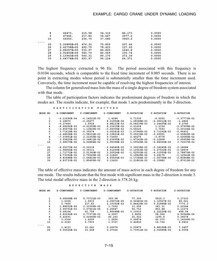
EXAMPLE: CARGO CRANE UNDER DYNAMIC LOADING
8 46473. 215.58 34.310 86.173 0.00009 47446. 217.82 34.667 2577.2 0.0000
10 56050. 236.75 37.680 3569.2 0.0000....
25 2.26885E+05 476.32 75.809 207.46 0.000026 2.42798E+05 492.75 78.423 127.02 0.000027 2.84057E+05 532.97 84.825 1240.8 0.000028 2.92450E+05 540.79 86.069 330.74 0.000029 3.13943E+05 560.31 89.176 272.39 0.000030 3.64774E+05 603.97 96.124 64.971 0.0000
The highest frequency extracted is 96 Hz. The period associated with this frequency is0.0104 seconds, which is comparable to the fixed time increment of 0.005 seconds. There is nopoint in extracting modes whose period is substantially smaller than the time increment used.Conversely, the time increment must be capable of resolving the highest frequencies of interest.
The column for generalized mass lists the mass of a single degree of freedom system associatedwith that mode.
The table of participation factors indicates the predominant degrees of freedom in which themodes act. The results indicate, for example, that mode 1 acts predominantly in the 3-direction.
P A R T I C I P A T I O N F A C T O R S
MODE NO X-COMPONENT Y-COMPONENT Z-COMPONENT X-ROTATION Y-ROTATION Z-ROTATION
1 -6.11696E-04 -6.14521E-03 1.4284 0.71335 -6.0252 -3.37773E-022 0.18470 -0.25677 8.31954E-04 1.68388E-03 -6.05012E-03 -1.68263 -0.17440 1.5515 4.88123E-03 -8.04039E-03 3.24495E-02 9.27464 -8.68256E-05 -9.61259E-03 8.23615E-02 0.21604 1.2334 -2.97905E-025 -3.80675E-03 1.13829E-03 -3.04304E-02 -0.59220 1.7593 -2.20144E-026 3.71618E-02 -0.35674 6.05241E-03 -1.67946E-02 6.71292E-03 -0.964327 -2.48508E-03 -1.58332E-03 6.19821E-02 5.09235E-02 -0.29901 -6.65849E-048 -7.03851E-02 2.31655E-02 0.72459 0.49275 -3.8778 6.69085E-029 3.59820E-02 -2.34811E-02 2.23695E-02 1.47243E-02 -0.12808 6.65955E-04
10 3.48679E-02 4.02884E-02 1.96398E-02 1.09545E-02 -6.84066E-02 3.72037E-02....
25 -8.25375E-02 -0.22218 -3.54545E-02 3.39238E-02 -2.18245E-02 -0.1868826 -1.98905E-02 -0.35111 4.61269E-02 -2.12563E-02 -1.27532E-02 -0.1893927 1.71772E-02 2.51340E-02 2.26524E-02 -1.02593E-02 -4.31559E-02 2.78870E-0228 4.73352E-02 2.79265E-02 -0.11860 5.19825E-02 0.24175 -1.12541E-0429 9.83488E-03 -3.64823E-03 4.65504E-03 -3.17284E-03 -1.56708E-02 -2.82848E-0330 4.83733E-02 1.85495E-02 0.13426 -2.21861E-02 -0.35882 -1.87612E-02
The table of effective mass indicates the amount of mass active in each degree of freedom for anyone mode. The results indicate that the first mode with significant mass in the 2-direction is mode 3.The total modal effective mass in the 2-direction is 378.26 kg.
E F F E C T I V E M A S S
MODE NO X-COMPONENT Y-COMPONENT Z-COMPONENT X-ROTATION Y-ROTATION Z-ROTATION
1 5.68458E-05 5.73721E-03 309.98 77.309 5515.3 0.173332 1.0304 1.9915 2.09072E-05 8.56481E-05 1.10567E-03 85.5213 2.7495 217.62 2.15392E-03 5.84420E-03 9.51888E-02 7776.24 1.88952E-06 2.31599E-02 1.7002 11.699 381.31 0.222445 3.99791E-03 3.57461E-04 0.25547 96.753 853.88 0.133706 0.68104 62.759 1.80648E-02 0.13910 2.22229E-02 458.587 6.83296E-03 2.77373E-03 4.2507 2.8692 98.926 4.90544E-048 0.42691 4.62440E-02 45.243 20.923 1295.8 0.385789 3.3366 1.4209 1.2896 0.55874 42.275 1.14296E-03
10 4.3393 5.7933 1.3767 0.42830 16.702 4.9402....
25 1.4133 10.241 0.26078 0.23875 9.88154E-02 7.245726 5.02526E-02 15.658 0.27026 5.73911E-02 2.06589E-02 4.5558
7–15
Abaqus ID:Printed on:
EXAMPLE: CARGO CRANE UNDER DYNAMIC LOADING
27 0.36612 0.78387 0.63672 0.13060 2.3110 0.9649928 0.74106 0.25794 4.6523 0.89371 19.329 4.18897E-0629 2.63473E-02 3.62545E-03 5.90262E-03 2.74218E-03 6.68933E-02 2.17924E-0330 0.15203 2.23557E-02 1.1711 3.19804E-02 8.3651 2.28687E-02
TOTAL 22.198 378.26 373.69 269.78 8348.4 8518.0
The total mass of the model is given earlier in the data file and is 414.34 kg.To ensure that enough modes have been used, the total effective mass in each direction should
be a large proportion of the mass of the model (say 90%). However, some of the mass of the modelis associated with nodes that are constrained. This constrained mass is approximately one-quarter ofthe mass of all the elements attached to the constrained nodes, which, in this case, is approximately28 kg. Therefore, the mass of the model that is able to move is 385 kg.
Tip: To determine the mass of the elements attached to the constrained nodes, switch to
the Mesh module, click the query tool , and select Mass properties from the listof general queries. In the prompt area, select Select mesh entities, and select the sixelements attached to the constrained nodes. The total mass is displayed in the messagearea (114 kg).
The effective mass in the x-, y-, and z-directions is 6%, 98%, and 97%, respectively, of the mass thatcan move. The total effective mass in the 2- and 3-directions is well above the 90% recommendedearlier; the total effective mass in the 1-direction is much lower. However, since the loading isapplied in the 2-direction, the response in the 1-direction is not significant.
The data file does not contain any results for the modal dynamics step, because all of the datafile output requests were suppressed.
7.5.3 PostprocessingEnter the Visualization module, and open the output database file DynCrane.odb.
Plotting mode shapes
You can visualize the deformation mode associated with a given natural frequency by plotting themode shape associated with that frequency.
To select a mode and plot the corresponding mode shape:
1. In the context bar, click the frame selector tool .
The Frame Selector dialog box appears. Drag the bottom corner of the dialog box to enlargeit so that both step names are clearly visible.
2. Drag the frame slider to select frame 1 in the Extract Frequencies step. This is the firsteigenmode.
7–16
Abaqus ID:Printed on:

EXAMPLE: CARGO CRANE UNDER DYNAMIC LOADING
3. From the main menu bar, select Plot→Deformed Shape; or use the tool in the toolbox.
Abaqus/CAE displays the deformed model shape associated with the first vibration mode, asshown in Figure 7–8.
Step: "Extract frequencies", First 30 modesMode 1: Value = 1773.5 Freq = 6.7025 (cycles/time)
Deformed Var: U Deformation Scale Factor: +8.000e-01
1
2
3
Figure 7–8 Mode 1.
4. Select the third mode (frame 3 in the Extract Frequencies step) from the Frame Selectordialog box. Afterward, close the dialog box.
Abaqus/CAE displays the third mode shape shown in Figure 7–9.
Note: A complete list of the available frames is given in the Step/Frame dialog box(Result→Step/Frame). This dialog box offers an alternative means to switching betweenframes.
Animation of results
You will animate the analysis results. First create a scale factor animation of the third eigenmode.Then create a time-history animation of the transient results.
To create a scale factor animation of an eigenmode:
1. From the main menu bar, select Animate→Scale Factor; or use the tool in the toolbox.
Abaqus/CAE displays the third mode shape and steps through different deformation scalefactors ranging from 0 to 1.
7–17
Abaqus ID:Printed on:
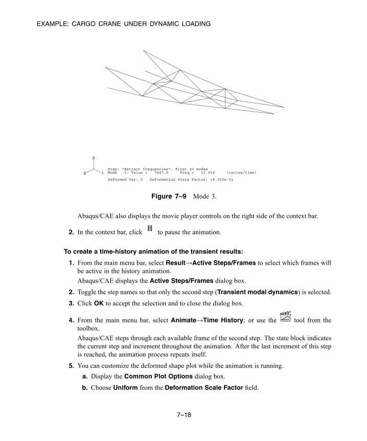
EXAMPLE: CARGO CRANE UNDER DYNAMIC LOADING
Step: "Extract frequencies", First 30 modesMode 3: Value = 7647.5 Freq = 13.918 (cycles/time)
Deformed Var: U Deformation Scale Factor: +8.000e-01
1
2
3
Figure 7–9 Mode 3.
Abaqus/CAE also displays the movie player controls on the right side of the context bar.
2. In the context bar, click to pause the animation.
To create a time-history animation of the transient results:
1. From the main menu bar, select Result→Active Steps/Frames to select which frames willbe active in the history animation.
Abaqus/CAE displays the Active Steps/Frames dialog box.
2. Toggle the step names so that only the second step (Transient modal dynamics) is selected.
3. Click OK to accept the selection and to close the dialog box.
4. From the main menu bar, select Animate→Time History; or use the tool from thetoolbox.
Abaqus/CAE steps through each available frame of the second step. The state block indicatesthe current step and increment throughout the animation. After the last increment of this stepis reached, the animation process repeats itself.
5. You can customize the deformed shape plot while the animation is running.
a. Display the Common Plot Options dialog box.
b. Choose Uniform from the Deformation Scale Factor field.
7–18
Abaqus ID:Printed on:

EXAMPLE: CARGO CRANE UNDER DYNAMIC LOADING
c. Enter 15.0 as the deformation scale factor value.
d. Click Apply to apply your change.
Abaqus/CAE now steps through the frames in the second step with a deformation scalefactor of 15.0.
e. Choose Auto-compute from the Deformation Scale Factor field.
f. Click OK to apply your change and to close the Common Plot Options dialog box.
Abaqus/CAE now steps through the frames in the second step with a default deformationscale factor of 0.8.
Determining the peak pull-out force
To find the peak pull-out force at the attachment points, create an X–Y plot of the reaction force inthe 1-direction (variable RF1) at the attached nodes. This involves plotting multiple curves at thesame time.
To plot multiple curves:
1. In the Results Tree, click mouse button 3 on History Output for the output database namedDynCrane.odb. From the menu that appears, select Filter.
2. In the filter field, enter*RF1* to restrict the history output to just the reaction force componentsin the 1-direction.
3. From the list of available history output, select the four curves (using [Ctrl] + Click) that havethe following form:
Reaction Force: RF1 PI: TRUSS-1 Node xxx in NSET ATTACH
4. Click mouse button 3, and select Plot from the menu that appears.
Abaqus/CAE displays the selected curves.
5. Click in the prompt area to cancel the current procedure.
To position the grid:
1. Double-click the plot to open the Chart Options dialog box.
2. In this dialog box, switch to the Grid Area tabbed page.
3. In the Size region of this page, select the Square option.
4. Use the slider to set the size to 75.
5. In the Position region of this page, select the Auto-align option.
6. From the available alignment options, select the last one (position the grid in the lower rightcorner of the viewport).
7. Click Dismiss.
7–19
Abaqus ID:Printed on:

EFFECT OF THE NUMBER OF MODES
To position the legend:
1. Double-click the legend to open the Chart Legend Options dialog box.
2. In this dialog box, switch to the Area tabbed page.
3. In the Position region of this page, toggle on Inset.
4. To display the minimum and maximum values in the legend, switch to the Contents tabbedpage of the dialog box. In the Numbers region of this page, toggle on Show min/max.
5. Click Dismiss.
6. Drag the legend in the viewport to reposition it.
The resulting plot (which has been customized) is shown in Figure 7–10. The curves for thetwo nodes at the top of each truss (points B and C) are almost a reflection of those for the nodes onthe bottom of each truss (points A and D).
Note: To modify the curve styles, click in the Visualization toolbox to open the CurveOptions dialog box.
At the attachment points at the top of each truss structure, the peak tensile force is around 80 kN,which is below the 100 kN capacity of the connection. Keep in mind that a negative reaction forcein the 1-direction means that the member is being pulled away from the wall. The lower attachmentsare in compression (positive reaction force) while the load is applied but oscillate between tensionand compression after the load has been removed. The peak tensile force is about 40 kN, well belowthe allowable value. To find this value, probe the X–Y plot.
To query the X–Y plot:
1. From the main menu bar, select Tools→Query.
The Query dialog box appears.
2. Click Probe values in the Visualization Module Queries field.
The Probe Values dialog box appears.
3. Select the point indicated in Figure 7–10.
The Y-coordinate of this point is –40.30 kN, which corresponds to the value of the reactionforce in the 1-direction.
7.6 Effect of the number of modes
For this simulation 30 modes were used to represent the dynamic behavior of the structure. The totalmodal effective mass for all of these modes was well over 90% of the mass of the structure that can movein the y- and z-directions, indicating that the dynamic representation is adequate.
7–20
Abaqus ID:Printed on:

EFFECT OF DAMPING
Time0.00 0.10 0.20 0.30 0.40 0.50
For
ce
−0.05
0.00
0.05
[x1.E6]
RF1 Point ARF1 Point BRF1 Point CRF1 Point D
XMIN 0.000E+00XMAX 5.000E−01YMIN −8.076E+04YMAX 7.915E+04
Peak tensile point
Probe this point
Figure 7–10 History of the reaction forces at the attached nodes.
Figure 7–11 shows the displacement in the direction of degree of freedom 2 of the node in set Tip-aversus time and illustrates the effect of using fewer modes on the quality of the results. If you look atthe table of effective mass, you will see that the first significant mode in the 2-direction is mode 3, whichaccounts for the lack of response when only two modes are used. The displacement of this node inthe direction of degree of freedom 2 for the analyses using five modes and 30 modes is similar after0.2 seconds; however, the early response differs, suggesting that there are significant modes in the rangeof 5–30 relating to the early response. When five modes are used, the total modal effective mass in the2-direction is only 57% of the moveable mass.
7.7 Effect of damping
In this simulation we used 5% of critical damping in all modes. This value was chosen from experience,based on the fact that the bolted connections between the trusses and the cross bracing might absorbsignificant energy as a result of local frictional effects. In cases such as this, where accurate data are notavailable, it is important to investigate the effect of the choices that you make.
7–21
Abaqus ID:Printed on:

COMPARISON WITH DIRECT TIME INTEGRATION
2 modes5 modes30 modes
Figure 7–11 Effect of different numbers of modes on the results.
Figure 7–12 compares the history of the reaction force at one of the top connections (point C) when1%, 5%, and 10% of critical damping are used. As expected, the oscillations at lower damping levels donot diminish as quickly as those at higher damping levels, and the peak force is higher in the models withlower damping. With damping ratios even as low as 1%, the peak pull-out force is 85 kN, which is stillless than the strength of the connection (100 kN). Therefore, the cargo crane should retain its integrityunder this drop load.
7.8 Comparison with direct time integration
Since this is a transient dynamic analysis, it is natural to consider how the results compare with thoseobtained using direct integration of the equations of motion. Direct integration can be performed witheither implicit (Abaqus/Standard) or explicit (Abaqus/Explicit) methods. Here we extend the analysis touse the explicit dynamics procedure.
A direct comparison with the results presented earlier is not possible since the B33 element typeand direct modal damping are not available in Abaqus/Explicit. Thus, in the Abaqus/Explicit analysisthe element type is changed to B31 and Rayleigh damping is used in place of direct modal damping.
Copy the Dynamic model to one named explicit. All subsequent changes should be made tothe explicit model.
7–22
Abaqus ID:Printed on:
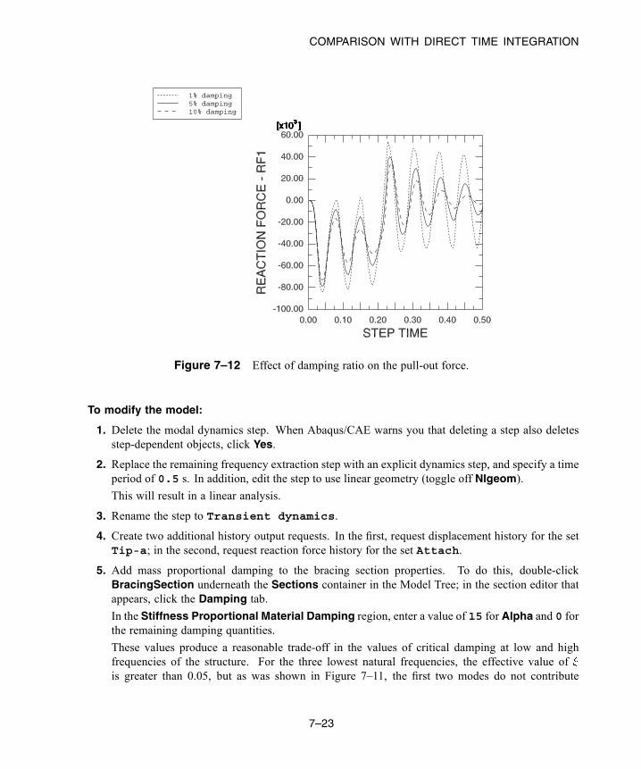
COMPARISON WITH DIRECT TIME INTEGRATION
1% damping5% damping10% damping
Figure 7–12 Effect of damping ratio on the pull-out force.
To modify the model:
1. Delete the modal dynamics step. When Abaqus/CAE warns you that deleting a step also deletesstep-dependent objects, click Yes.
2. Replace the remaining frequency extraction step with an explicit dynamics step, and specify a timeperiod of 0.5 s. In addition, edit the step to use linear geometry (toggle off Nlgeom).
This will result in a linear analysis.
3. Rename the step to Transient dynamics.
4. Create two additional history output requests. In the first, request displacement history for the setTip-a; in the second, request reaction force history for the set Attach.
5. Add mass proportional damping to the bracing section properties. To do this, double-clickBracingSection underneath the Sections container in the Model Tree; in the section editor thatappears, click the Damping tab.
In the Stiffness Proportional Material Damping region, enter a value of 15 for Alpha and 0 forthe remaining damping quantities.
These values produce a reasonable trade-off in the values of critical damping at low and highfrequencies of the structure. For the three lowest natural frequencies, the effective value ofis greater than 0.05, but as was shown in Figure 7–11, the first two modes do not contribute
7–23
Abaqus ID:Printed on:
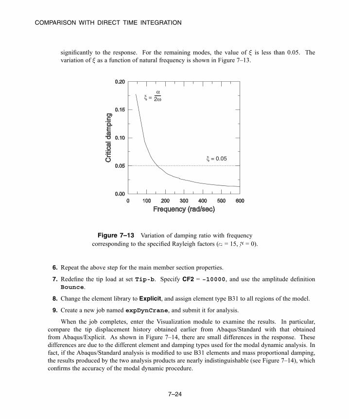
COMPARISON WITH DIRECT TIME INTEGRATION
significantly to the response. For the remaining modes, the value of is less than 0.05. Thevariation of as a function of natural frequency is shown in Figure 7–13.
ξ = 0.05
ξ = 2ωα
Figure 7–13 Variation of damping ratio with frequencycorresponding to the specified Rayleigh factors ( = 15, = 0).
6. Repeat the above step for the main member section properties.
7. Redefine the tip load at set Tip-b. Specify CF2 = −10000, and use the amplitude definitionBounce.
8. Change the element library to Explicit, and assign element type B31 to all regions of the model.
9. Create a new job named expDynCrane, and submit it for analysis.
When the job completes, enter the Visualization module to examine the results. In particular,compare the tip displacement history obtained earlier from Abaqus/Standard with that obtainedfrom Abaqus/Explicit. As shown in Figure 7–14, there are small differences in the response. Thesedifferences are due to the different element and damping types used for the modal dynamic analysis. Infact, if the Abaqus/Standard analysis is modified to use B31 elements and mass proportional damping,the results produced by the two analysis products are nearly indistinguishable (see Figure 7–14), whichconfirms the accuracy of the modal dynamic procedure.
7–24
Abaqus ID:Printed on:
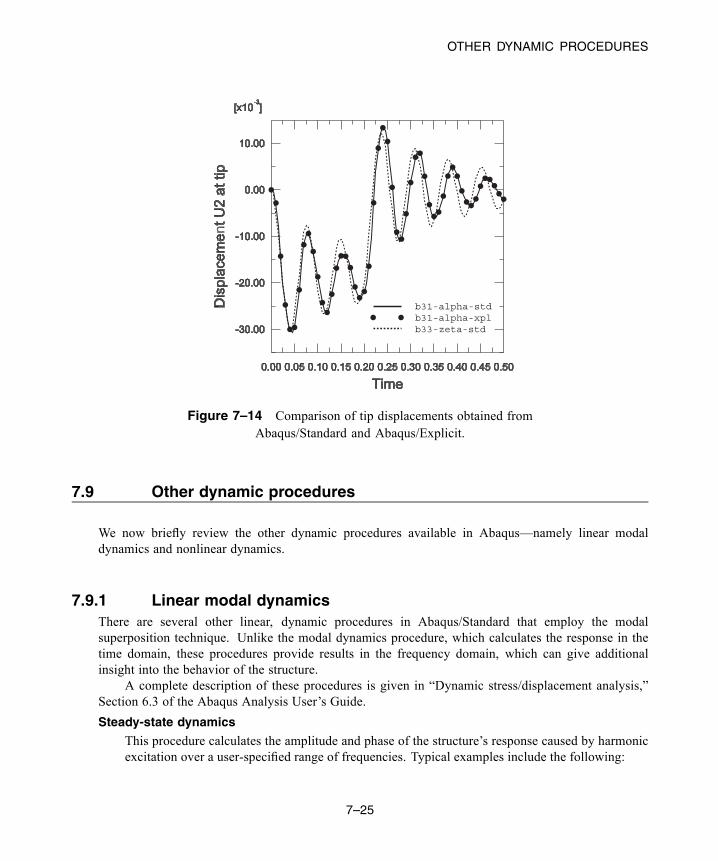
OTHER DYNAMIC PROCEDURES
b31-alpha-stdb31-alpha-xplb33-zeta-std
Figure 7–14 Comparison of tip displacements obtained fromAbaqus/Standard and Abaqus/Explicit.
7.9 Other dynamic procedures
We now briefly review the other dynamic procedures available in Abaqus—namely linear modaldynamics and nonlinear dynamics.
7.9.1 Linear modal dynamicsThere are several other linear, dynamic procedures in Abaqus/Standard that employ the modalsuperposition technique. Unlike the modal dynamics procedure, which calculates the response in thetime domain, these procedures provide results in the frequency domain, which can give additionalinsight into the behavior of the structure.
A complete description of these procedures is given in “Dynamic stress/displacement analysis,”Section 6.3 of the Abaqus Analysis User’s Guide.
Steady-state dynamics
This procedure calculates the amplitude and phase of the structure’s response caused by harmonicexcitation over a user-specified range of frequencies. Typical examples include the following:
7–25
Abaqus ID:Printed on:

OTHER DYNAMIC PROCEDURES
• The response of car engine mounts over a range of engine operating speeds.• Rotating machinery in buildings.• Components on aircraft engines.
Response spectrum
This procedure provides an estimate of the peak response (displacement, stress, etc.) when astructure is subjected to dynamic motion of its fixed points. The motion of the fixed points isknown as “base motion”; an example is a seismic event causing ground motion. Typically themethod is used when an estimate of the peak response is required for design purposes.
Random response
This procedure predicts the response of a system subjected to random continuous excitation. Theexcitation is expressed in a statistical sense using a power spectral density function. Examples ofrandom response analysis include the following:
• The response of an airplane to turbulence.• The response of a structure to noise, such as that emitted by a jet engine.
7.9.2 Nonlinear dynamics
As mentioned earlier, the modal dynamics procedure is suitable only for linear problems. Whennonlinear dynamic response is of interest, the equations of motion must be integrated directly. Thedirect-integration of the equations of motion is performed in Abaqus/Standard using an implicitdynamics procedure. When this procedure is used, the mass, damping, and stiffness matrices areassembled and the equation of dynamic equilibrium is solved at each point in time. Since theseoperations are computationally intensive, direct-integration dynamics is more expensive than the modalmethods.
Since the nonlinear dynamic procedure in Abaqus/Standard uses implicit time integration, it issuitable for nonlinear structural dynamics problems, for example, in which a sudden event initiates thedynamic response, such as an impact, or when the structural response involves large amounts of energybeing dissipated by plasticity or viscous damping. In such studies the high frequency response, which isimportant initially, is damped out rapidly by the dissipative mechanisms in the model.
An alternative for nonlinear dynamic analyses is the explicit dynamics procedure available inAbaqus/Explicit. As discussed in Chapter 2, “Abaqus Basics,” the explicit algorithm propagatesthe solution as a stress wave through the model, one element at a time. Thus, it is most suitable forapplications in which stress wave effects are important and in which the event time being simulated isshort (typically less than one second).
Another advantage associated with the explicit algorithm is that it can model discontinuousnonlinearities such as contact and failure more easily than Abaqus/Standard. Large, highlydiscontinuous problems are often more easily modeled with Abaqus/Explicit, even if the response
7–26
Abaqus ID:Printed on:
SUMMARY
is quasi-static. Explicit dynamic analyses are discussed further in Chapter 9, “Nonlinear ExplicitDynamics.”
7.10 Related Abaqus examples
• “Linear analysis of the Indian Point reactor feedwater line,” Section 2.2.2 of the Abaqus ExampleProblems Guide
• “Explosively loaded cylindrical panel,” Section 1.3.3 of the Abaqus Benchmarks Guide• “Eigenvalue analysis of a cantilever plate,” Section 1.4.6 of the Abaqus Benchmarks Guide
7.11 Suggested reading
• Clough, R. W. and J. Penzien, Dynamics of Structures, McGraw-Hill, 1975.
• NAFEMS Ltd., A Finite Element Dynamics Primer, 1993.
• Spence, P. W. and C. J. Kenchington, The Role of Damping in Finite Element Analysis, ReportR0021, NAFEMS Ltd., 1993.
7.12 Summary
• Dynamic analyses include the effect of the structure’s inertia.• The frequency extraction procedure in Abaqus/Standard extracts the natural frequencies and modeshapes of the structure.
• The mode shapes can then be used to determine the dynamic response of linear systems by modalsuperposition. This technique is efficient, but it cannot be used for nonlinear problems.
• Linear dynamic procedures are available in Abaqus/Standard to calculate the transient response totransient loading, the steady-state response to harmonic loading, the peak response to base motion,and the response to random loading.
• You should extract enough modes to obtain an accurate representation of the dynamic behavior ofthe structure. The total modal effective mass in the direction in which motion will occur should beat least 90% of the mass that can move to produce accurate results.
• You can define direct modal damping, Rayleigh damping, and composite modal damping inAbaqus/Standard. However, since the natural frequencies and mode shapes are based on theundamped structure, the structure being analyzed should be only lightly damped.
• Modal techniques are not suitable for nonlinear dynamic simulations. Direct time integrationmethods or explicit analysis must be used in these situations.
7–27
Abaqus ID:Printed on:

SUMMARY
• Time variation of loads or prescribed boundary conditions can be defined with an amplitude curve.• Mode shapes and transient results can be animated in the Visualization module of Abaqus/CAE.This provides a useful way of understanding the response of dynamic and nonlinear static analyses.
7–28
Abaqus ID:Printed on:

NONLINEARITY
8. Nonlinearity
This chapter discusses nonlinear structural analysis in Abaqus. The differences between linear andnonlinear analyses are summarized below.
Linear analysis
All the analyses discussed so far have been linear: there is a linear relationship between the appliedloads and the response of the system. For example, if a linear spring extends statically by 1 m undera load of 10 N, it will extend by 2 m when a load of 20 N is applied. This means that in a linearAbaqus/Standard analysis the flexibility of the structure need only be calculated once (by assemblingthe stiffness matrix and inverting it). The linear response of the structure to other load cases canbe found by multiplying the new vector of loads by the inverted stiffness matrix. Furthermore, thestructure’s response to various load cases can be scaled by constants and/or superimposed on oneanother to determine its response to a completely new load case, provided that the new load case isthe sum (or multiple) of previous ones. This principle of superposition of load cases assumes thatthe same boundary conditions are used for all the load cases.
Abaqus/Standard uses the principle of superposition of load cases in linear dynamicssimulations, which are discussed in Chapter 7, “Linear Dynamics.”
Nonlinear analysis
A nonlinear structural problem is one in which the structure’s stiffness changes as it deforms. Allphysical structures exhibit nonlinear behavior. Linear analysis is a convenient approximation thatis often adequate for design purposes. It is obviously inadequate for many structural simulationsincluding manufacturing processes, such as forging or stamping; crash analyses; and analyses ofrubber components, such as tires or engine mounts. A simple example is a spring with a nonlinearstiffening response (see Figure 8–1).
Linear spring.Stiffness is constant.
Nonlinear spring.Stiffness is not constant.
Force
Displacement
Force
Displacement
Figure 8–1 Linear and nonlinear spring characteristics.
8–1
Abaqus ID:Printed on:
SOURCES OF NONLINEARITY
Since the stiffness is now dependent on the displacement, the initial flexibility can no longerbe multiplied by the applied load to calculate the spring’s displacement for any load. In a nonlinearimplicit analysis the stiffness matrix of the structure has to be assembled and inverted many timesduring the course of the analysis, making it much more expensive to solve than a linear implicitanalysis. In an explicit analysis the increased cost of a nonlinear analysis is due to reductions inthe stable time increment. The stable time increment is discussed further in Chapter 9, “NonlinearExplicit Dynamics.”
Since the response of a nonlinear system is not a linear function of the magnitude of the appliedload, it is not possible to create solutions for different load cases by superposition. Each load casemust be defined and solved as a separate analysis.
8.1 Sources of nonlinearity
There are three sources of nonlinearity in structural mechanics simulations:
• Material nonlinearity.• Boundary nonlinearity.• Geometric nonlinearity.
8.1.1 Material nonlinearity
This type of nonlinearity is probably the one that you are most familiar with and is covered in more depthin Chapter 10, “Materials.” Most metals have a fairly linear stress/strain relationship at low strain values;but at higher strains the material yields, at which point the response becomes nonlinear and irreversible(see Figure 8–2).
Rubber materials can be approximated by a nonlinear, reversible (elastic) response (see Figure 8–3).Material nonlinearity may be related to factors other than strain. Strain-rate-dependent material data
and material failure are both forms of material nonlinearity. Material properties can also be a functionof temperature and other predefined fields.
8.1.2 Boundary nonlinearity
Boundary nonlinearity occurs if the boundary conditions change during the analysis. Consider thecantilever beam, shown in Figure 8–4, that deflects under an applied load until it hits a “stop.”
8–2
Abaqus ID:Printed on:

SOURCES OF NONLINEARITY
Strain
Stress
Initial yield stress
Ultimate tensile stress
MaterialFailure
Young’s modulus, ESlope is
Figure 8–2 Stress-strain curve for an elastic-plastic material under uniaxial tension.
Strain
Stress
Figure 8–3 Stress-strain curve for a rubber-type material.
Figure 8–4 Cantilever beam hitting a stop.
8–3
Abaqus ID:Printed on:
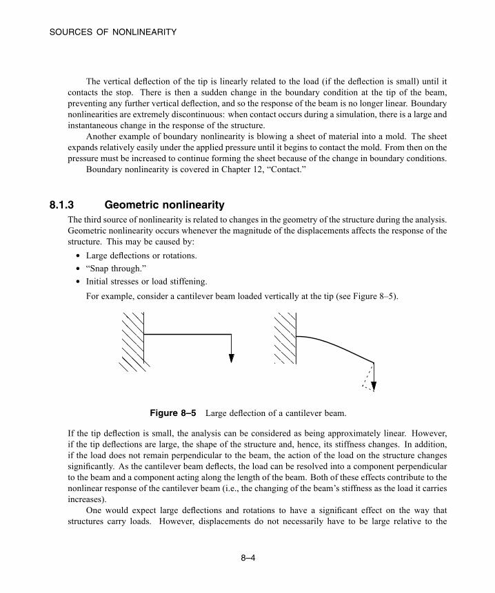
SOURCES OF NONLINEARITY
The vertical deflection of the tip is linearly related to the load (if the deflection is small) until itcontacts the stop. There is then a sudden change in the boundary condition at the tip of the beam,preventing any further vertical deflection, and so the response of the beam is no longer linear. Boundarynonlinearities are extremely discontinuous: when contact occurs during a simulation, there is a large andinstantaneous change in the response of the structure.
Another example of boundary nonlinearity is blowing a sheet of material into a mold. The sheetexpands relatively easily under the applied pressure until it begins to contact the mold. From then on thepressure must be increased to continue forming the sheet because of the change in boundary conditions.
Boundary nonlinearity is covered in Chapter 12, “Contact.”
8.1.3 Geometric nonlinearityThe third source of nonlinearity is related to changes in the geometry of the structure during the analysis.Geometric nonlinearity occurs whenever the magnitude of the displacements affects the response of thestructure. This may be caused by:
• Large deflections or rotations.• “Snap through.”• Initial stresses or load stiffening.For example, consider a cantilever beam loaded vertically at the tip (see Figure 8–5).
Figure 8–5 Large deflection of a cantilever beam.
If the tip deflection is small, the analysis can be considered as being approximately linear. However,if the tip deflections are large, the shape of the structure and, hence, its stiffness changes. In addition,if the load does not remain perpendicular to the beam, the action of the load on the structure changessignificantly. As the cantilever beam deflects, the load can be resolved into a component perpendicularto the beam and a component acting along the length of the beam. Both of these effects contribute to thenonlinear response of the cantilever beam (i.e., the changing of the beam’s stiffness as the load it carriesincreases).
One would expect large deflections and rotations to have a significant effect on the way thatstructures carry loads. However, displacements do not necessarily have to be large relative to the
8–4
Abaqus ID:Printed on:
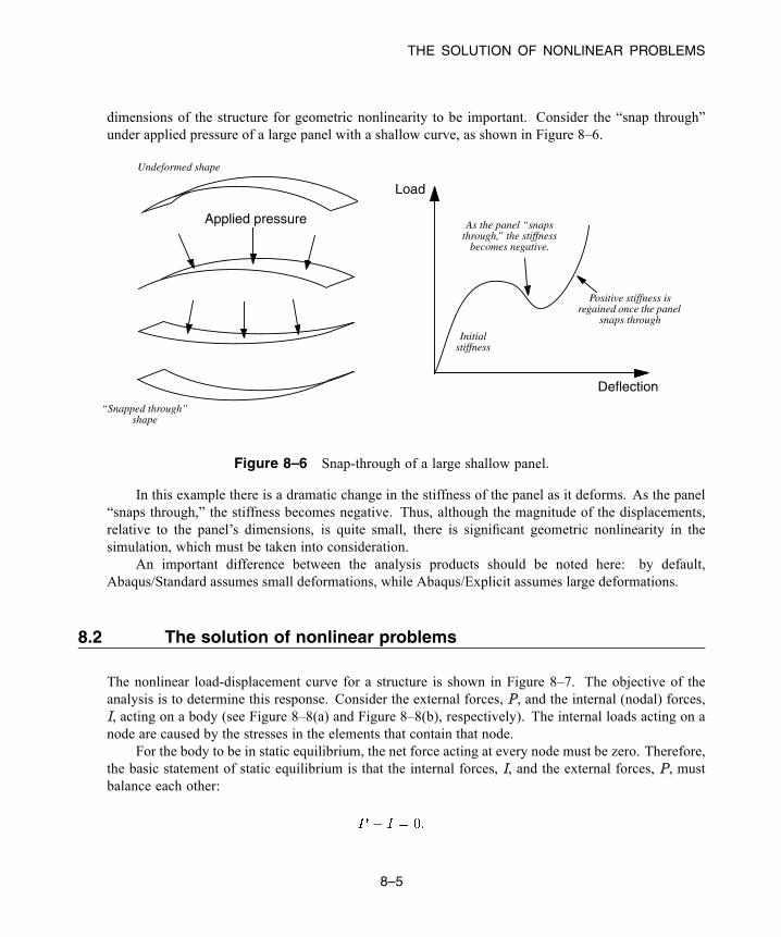
THE SOLUTION OF NONLINEAR PROBLEMS
dimensions of the structure for geometric nonlinearity to be important. Consider the “snap through”under applied pressure of a large panel with a shallow curve, as shown in Figure 8–6.
Undeformed shape
“Snapped through”shape
Initialstiffness
As the panel “snapsthrough,” the stiffness
becomes negative.
Positive stiffness isregained once the panel
snaps through
Load
Deflection
Applied pressure
Figure 8–6 Snap-through of a large shallow panel.
In this example there is a dramatic change in the stiffness of the panel as it deforms. As the panel“snaps through,” the stiffness becomes negative. Thus, although the magnitude of the displacements,relative to the panel’s dimensions, is quite small, there is significant geometric nonlinearity in thesimulation, which must be taken into consideration.
An important difference between the analysis products should be noted here: by default,Abaqus/Standard assumes small deformations, while Abaqus/Explicit assumes large deformations.
8.2 The solution of nonlinear problems
The nonlinear load-displacement curve for a structure is shown in Figure 8–7. The objective of theanalysis is to determine this response. Consider the external forces, P, and the internal (nodal) forces,I, acting on a body (see Figure 8–8(a) and Figure 8–8(b), respectively). The internal loads acting on anode are caused by the stresses in the elements that contain that node.
For the body to be in static equilibrium, the net force acting at every node must be zero. Therefore,the basic statement of static equilibrium is that the internal forces, I, and the external forces, P, mustbalance each other:
8–5
Abaqus ID:Printed on:
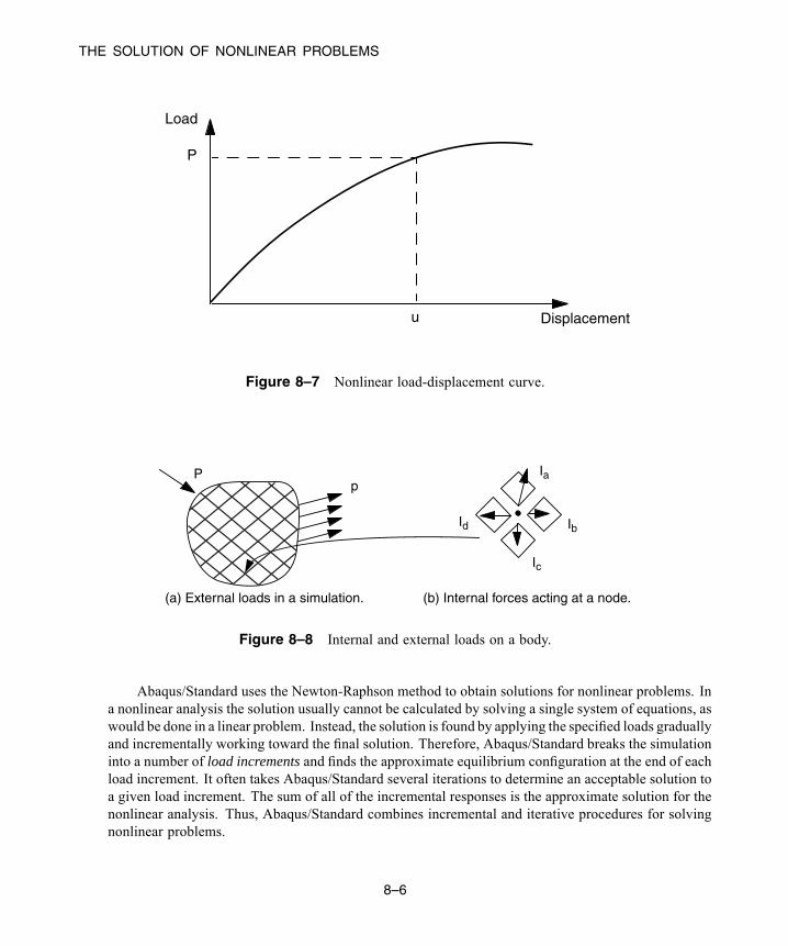
THE SOLUTION OF NONLINEAR PROBLEMS
Load
Displacement
P
u
Figure 8–7 Nonlinear load-displacement curve.
Ia
Id
Ic
Ib
Pp
(a) External loads in a simulation. (b) Internal forces acting at a node.
Figure 8–8 Internal and external loads on a body.
Abaqus/Standard uses the Newton-Raphson method to obtain solutions for nonlinear problems. Ina nonlinear analysis the solution usually cannot be calculated by solving a single system of equations, aswould be done in a linear problem. Instead, the solution is found by applying the specified loads graduallyand incrementally working toward the final solution. Therefore, Abaqus/Standard breaks the simulationinto a number of load increments and finds the approximate equilibrium configuration at the end of eachload increment. It often takes Abaqus/Standard several iterations to determine an acceptable solution toa given load increment. The sum of all of the incremental responses is the approximate solution for thenonlinear analysis. Thus, Abaqus/Standard combines incremental and iterative procedures for solvingnonlinear problems.
8–6
Abaqus ID:Printed on:

THE SOLUTION OF NONLINEAR PROBLEMS
Abaqus/Explicit determines a solution to the dynamic equilibrium equation withoutiterating by explicitly advancing the kinematic state from the end of the previous increment. Solvinga problem explicitly does not require the formation of tangent stiffness matrices. The explicit central-difference operator satisfies the dynamic equilibrium equations at the beginning of the increment, t;the accelerations calculated at time t are used to advance the velocity solution to time andthe displacement solution to time . For linear and nonlinear problems alike, explicit methodsrequire a small time increment size that depends solely on the highest natural frequency of the modeland is independent of the type and duration of loading. Simulations typically require a large number ofincrements; however, due to the fact that a global set of equations is not solved in each increment, thecost per increment of an explicit method is much smaller than that of an implicit method. The smallincrements characteristic of an explicit dynamic method make Abaqus/Explicit well suited for nonlinearanalysis.
8.2.1 Steps, increments, and iterationsThis section introduces some new vocabulary for describing the various parts of an analysis. It isimportant that you clearly understand the difference between an analysis step, a load increment, andan iteration.
• The load history for a simulation consists of one or more steps. You define the steps, which generallyconsist of an analysis procedure option, loading options, and output request options. Different loads,boundary conditions, analysis procedure options, and output requests can be used in each step. Forexample:
– Step 1: Hold a plate between rigid jaws.
– Step 2: Add loads to deform the plate.
– Step 3: Find the natural frequencies of the deformed plate.
• An increment is part of a step. In nonlinear analyses the total load applied in a step is broken intosmaller increments so that the nonlinear solution path can be followed.
In Abaqus/Standard you suggest the size of the first increment, and Abaqus/Standardautomatically chooses the size of the subsequent increments. In Abaqus/Explicit the default timeincrementation is fully automatic and does not require user intervention. Because the explicitmethod is conditionally stable, there is a stability limit for the time increment. The stable timeincrement is discussed in Chapter 9, “Nonlinear Explicit Dynamics.”
At the end of each increment the structure is in (approximate) equilibrium and results areavailable for writing to the output database, restart, data, or results files. The increments at whichyou select results to be written to the output database file are called frames.
The issues associated with time incrementation in Abaqus/Standard and Abaqus/Explicitanalyses are quite different, since time increments are generally much smaller in Abaqus/Explicit.
• An iteration is an attempt at finding an equilibrium solution in an increment when solving with animplicit method. If the model is not in equilibrium at the end of the iteration, Abaqus/Standard
8–7
Abaqus ID:Printed on:

THE SOLUTION OF NONLINEAR PROBLEMS
tries another iteration. With every iteration the solution Abaqus/Standard obtains should be closerto equilibrium; sometimes Abaqus/Standard may need many iterations to obtain an equilibriumsolution. When an equilibrium solution has been obtained, the increment is complete. Results canbe requested only at the end of an increment.
Abaqus/Explicit does not need to iterate to obtain the solution in an increment.
8.2.2 Equilibrium iterations and convergence in Abaqus/StandardThe nonlinear response of a structure to a small load increment, , is shown in Figure 8–9.Abaqus/Standard uses the structure’s initial stiffness, , which is based on its configuration at , and
to calculate a displacement correction, , for the structure. Using , the structure’s configurationis updated to .
K0
IaRa
ua
a
Ka
ΔP
u0
P
Load
Displacement
ca
Figure 8–9 First iteration in an increment.
Convergence
Abaqus/Standard forms a new stiffness, , for the structure, based on its updated configuration,. Abaqus/Standard also calculates , in this updated configuration. The difference between the
total applied load, P, and can now be calculated as:
where is the force residual for the iteration.If is zero at every degree of freedom in the model, point a in Figure 8–9 would lie on the
load-deflection curve, and the structure would be in equilibrium. In a nonlinear problem it is almostimpossible to have equal zero, so Abaqus/Standard compares it to a tolerance value. If is lessthan this force residual tolerance, Abaqus/Standard accepts the structure’s updated configuration
8–8
Abaqus ID:Printed on:
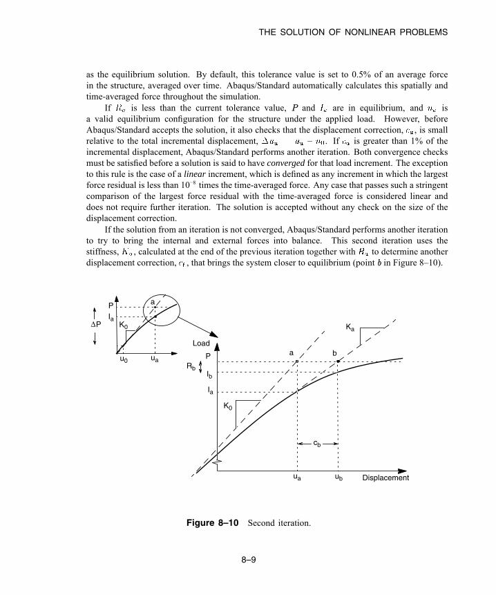
THE SOLUTION OF NONLINEAR PROBLEMS
as the equilibrium solution. By default, this tolerance value is set to 0.5% of an average forcein the structure, averaged over time. Abaqus/Standard automatically calculates this spatially andtime-averaged force throughout the simulation.
If is less than the current tolerance value, P and are in equilibrium, and isa valid equilibrium configuration for the structure under the applied load. However, beforeAbaqus/Standard accepts the solution, it also checks that the displacement correction, , is smallrelative to the total incremental displacement, . If is greater than 1% of theincremental displacement, Abaqus/Standard performs another iteration. Both convergence checksmust be satisfied before a solution is said to have converged for that load increment. The exceptionto this rule is the case of a linear increment, which is defined as any increment in which the largestforce residual is less than 10−8 times the time-averaged force. Any case that passes such a stringentcomparison of the largest force residual with the time-averaged force is considered linear anddoes not require further iteration. The solution is accepted without any check on the size of thedisplacement correction.
If the solution from an iteration is not converged, Abaqus/Standard performs another iterationto try to bring the internal and external forces into balance. This second iteration uses thestiffness, , calculated at the end of the previous iteration together with to determine anotherdisplacement correction, , that brings the system closer to equilibrium (point b in Figure 8–10).
K0
Ia
ua
a
a b
Ia
P
Ib
K0
Ka
ua ub
Rb
u0
P
ΔP
Load
Displacement
cb
Figure 8–10 Second iteration.
8–9
Abaqus ID:Printed on:
THE SOLUTION OF NONLINEAR PROBLEMS
Abaqus/Standard calculates a new force residual, , using the internal forces from thestructure’s new configuration, . Again, the largest force residual at any degree of freedom,, is compared against the force residual tolerance, and the displacement correction for the
second iteration, , is compared to the increment of displacement, . If necessary,Abaqus/Standard performs further iterations.
For each iteration in a nonlinear analysis Abaqus/Standard forms the model’s stiffness matrixand solves a system of equations. This means that each iteration is equivalent, in computational cost,to conducting a complete linear analysis. It should now be clear that the computational expense ofa nonlinear analysis in Abaqus/Standard can be many times greater than for a linear one.
It is possible with Abaqus/Standard to save results at each converged increment. Thus, theamount of output data available from a nonlinear simulation is many times that available from alinear analysis of the same geometry. Consider both of these factors and the types of nonlinearsimulations that you want to perform when planning your computer resources.
8.2.3 Automatic incrementation control in Abaqus/StandardAbaqus/Standard automatically adjusts the size of the load increments so that it solves nonlinear problemseasily and efficiently. You only need to suggest the size of the first increment in each step of yoursimulation. Thereafter, Abaqus/Standard automatically adjusts the size of the increments. If you do notprovide a suggested initial increment size, Abaqus/Standard will try to apply all of the loads defined inthe step in the first increment. In highly nonlinear problems Abaqus/Standard will have to reduce theincrement size repeatedly, resulting in wasted CPU time. Generally it is to your advantage to provide areasonable initial increment size (see “Modifications to the model,” Section 8.4.1, for an example); onlyin very mildly nonlinear problems can all of the loads in a step be applied in a single increment.
The number of iterations needed to find a converged solution for a load increment will varydepending on the degree of nonlinearity in the system. By default, if the solution appears to diverge,Abaqus/Standard abandons the increment and starts again with the increment size set to 25% ofits previous value. An attempt is then made at finding a converged solution with this smaller loadincrement. If the increment still fails to converge, Abaqus/Standard reduces the increment size again.By default, Abaqus/Standard allows a maximum of five cutbacks of increment size in an incrementbefore stopping the analysis.
In Abaqus/Standard you can also specify the maximum number of increments allowed during thestep. Abaqus/Standard terminates the analysis with an error message if it needs more increments than thislimit to complete the step. The default number of increments for a step is 100; if significant nonlinearityis present in the simulation, the analysis may require many more increments. You specify an upper limiton the number of increments that Abaqus/Standard can use, rather than the number of increments it mustuse.
In a nonlinear analysis a step takes place over a finite period of “time,” although this “time” has nophysical meaning unless inertial effects or rate-dependent behavior are present. In Abaqus/Standard youspecify the initial time increment, , and the total step time, . The ratio of the initial time
8–10
Abaqus ID:Printed on:

INCLUDING NONLINEARITY IN AN Abaqus ANALYSIS
increment to the step time specifies the proportion of load applied in the first increment. The initial loadincrement is given by
The choice of initial time increment can be critical in certain nonlinear simulations in Abaqus/Standard,but for most analyses an initial increment size that is 5% to 10% of the total step time is usually sufficient.In static simulations the total step time is usually set to 1.0 for convenience, unless, for example, rate-dependent material effects or dashpots are included in the model. With a total step time of 1.0 theproportion of load applied is always equal to the current step time; i.e., 50% of the total load is appliedwhen the step time is 0.5.
Although you must specify the initial increment size in Abaqus/Standard, Abaqus/Standardautomatically controls the size of the subsequent increments. This automatic control of the incrementsize is suitable for the majority of nonlinear simulations performed with Abaqus/Standard, althoughfurther controls on the increment size are available. Abaqus/Standard will terminate an analysis ifexcessive cutbacks caused by convergence problems reduce the increment size below the minimumvalue. The default minimum allowable time increment, , is 10−5 times the total step time. Bydefault, Abaqus/Standard has no upper limit on the increment size, , other than the total steptime. Depending on your Abaqus/Standard simulation, you may want to specify different minimumand/or maximum allowable increment sizes. For example, if you know that your simulation may havetrouble obtaining a solution if too large a load increment is applied, perhaps because the model mayundergo plastic deformation, you may want to decrease .
If the increment converges in fewer than five iterations, this indicates that the solution is beingfound fairly easily. Therefore, Abaqus/Standard automatically increases the increment size by 50% iftwo consecutive increments require fewer than five iterations to obtain a converged solution.
Details of the automatic load incrementation scheme are given in the Job Diagnostics dialog box,as shown in more detail in “Job diagnostics,” Section 8.4.2.
8.3 Including nonlinearity in an Abaqus analysis
We now discuss how to account for nonlinearity in an Abaqus analysis. The main focus is on geometricnonlinearity.
8.3.1 Geometric nonlinearityIncorporating the effects of geometric nonlinearity in an analysis requires only minor changes to anAbaqus/Standard model. You need to make sure the step definition considers geometrically nonlineareffects. This is the default setting in Abaqus/Explicit. You also need to set time incrementationparameters as discussed in “Automatic incrementation control in Abaqus/Standard,” Section 8.2.3.
8–11
Abaqus ID:Printed on:
EXAMPLE: NONLINEAR SKEW PLATE
Local directions
In a geometrically nonlinear analysis the local material directions may rotate with the deformationin each element. For shell, beam, and truss elements the local material directions always rotate withthe deformation. For solid elements the local material directions rotate with the deformation onlyif the elements refer to nondefault local material directions; otherwise, the default local materialdirections remain constant throughout the analysis.
Local directions defined at nodes remain fixed throughout the analysis; they do not rotate withthe deformation. See “Transformed coordinate systems,” Section 2.1.5 of the Abaqus AnalysisUser’s Guide, for further details.
Effect on subsequent steps
Once you include geometric nonlinearity in a step, it is considered in all subsequent steps. Ifnonlinear geometric effects are not requested in a subsequent step, Abaqus will issue a warningstating that they are being included in the step anyway.
Other geometrically nonlinear effects
The large deformations in a model are not the only important effects that are considered whengeometric nonlinearity is activated. Abaqus/Standard also includes terms in the element stiffnesscalculations that are caused by the applied loads, the so-called load stiffness. These terms improveconvergence behavior. In addition, the membrane loads in shells and the axial loads in cablesand beams contribute much of the stiffness of these structures in response to transverse loads.By including geometric nonlinearity, the membrane stiffness in response to transverse loads isconsidered as well.
8.3.2 Material nonlinearityThe addition of material nonlinearity to an Abaqus model is discussed in Chapter 10, “Materials.”
8.3.3 Boundary nonlinearityThe introduction of boundary nonlinearity is discussed in Chapter 12, “Contact.”
8.4 Example: nonlinear skew plate
This example is a continuation of the linear skew plate simulation described in Chapter 5, “Using ShellElements,” and shown in Figure 8–11. You will now reanalyze the plate in Abaqus/Standard to includethe effects of geometric nonlinearity. The results from this analysis will allow you to determine theimportance of geometrically nonlinear effects and, therefore, the validity of the linear analysis.
8–12
Abaqus ID:Printed on:

EXAMPLE: NONLINEAR SKEW PLATE
20 kPa
Endbuilt-in
1
32
zerorotation
Figure 8–11 Skew plate.
If you wish, you can follow the guidelines at the end of this example to extend the simulation toperform a dynamic analysis using Abaqus/Explicit.
Abaqus provides scripts that replicate the complete analysis model for this problem. Run one ofthese scripts if you encounter difficulties following the instructions given below or if you wish to checkyour work. Scripts are available in the following locations:
• A Python script for this example is provided in “Nonlinear skew plate,” Section A.6, in the HTMLversion of this guide. Instructions on how to fetch the script and run it within Abaqus/CAE aregiven in Appendix A, “Example Files.”
• A plug-in script for this example is available in the Abaqus/CAE Plug-in toolset. To run the scriptfrom Abaqus/CAE, select Plug-ins→Abaqus→Getting Started; highlight Nonlinear skewplate; and click Run. For more information about the Getting Started plug-ins, see “Running theGetting Started with Abaqus examples,” Section 82.1 of the Abaqus/CAE User’s Guide, in theHTML version of this guide.
8.4.1 Modifications to the modelOpen the model database file SkewPlate.cae. Copy the model named Linear to a model namedNonlinear.
For the Nonlinear skew plate model, you will include nonlinear geometric effects as well aschange the output requests.
Defining the step
In the Model Tree, double-click the Apply Pressure step underneath the Steps container to editthe step definition. In the Basic tabbed page of the Edit Step dialog box, toggle on Nlgeom toinclude geometric nonlinearity effects, and ensure the time period for the step is set to 1.0. In theIncrementation tabbed page, set the initial increment size to 0.1. The default maximum number
8–13
Abaqus ID:Printed on:
EXAMPLE: NONLINEAR SKEW PLATE
of increments is 100; Abaqus may use fewer increments than this upper limit, but it will stop theanalysis if it needs more.
You may wish to change the description of the step to reflect that it is now a nonlinear analysisstep.
Output control
In a linear analysis Abaqus solves the equilibrium equations once and calculates the results for thisone solution. A nonlinear analysis can produce much more output because results can be requestedat the end of each converged increment. If you do not select the output requests carefully, the outputfiles become very large, potentially filling the disk space on your computer.
As noted earlier, output is available in four different files:
• the output database (.odb) file, which contains data in a neutral binary format necessary topostprocess the results with Abaqus/CAE;
• the data (.dat) file, which contains printed tables of selected results (available only inAbaqus/Standard);
• the restart (.res) file, which is used to continue the analysis; and• the results (.fil) file, which is used with third-party postprocessors.Only the output database (.odb) file is discussed here. If selected carefully, data can be saved
frequently during the simulation without using excessive disk space.Open the Field Output Requests Manager. On the right side of the dialog box, click Edit to
open the field output editor. Remove the field output requests defined for the linear analysis model,and specify the default field output requests by selecting Preselected defaults under OutputVariables. This preselected set of output variables is the most commonly used set of field variablesfor a general static procedure.
To reduce the size of the output database file, write field output every second increment. Ifyou were simply interested in the final results, you could either select Last increment or set thefrequency at which output is saved equal to a large number. Results are always stored at the endof each step, regardless of the value specified; therefore, using a large value causes only the finalresults to be saved.
The history output request for the displacements of the nodes at the midspan can be keptfrom the previous analysis. You will explore these results using the X–Y plotting capability in theVisualization module.
Running and monitoring the job
Create a job for the Nonlinear model named NlSkewPlate, and give it the descriptionNonlinear Elastic Skew Plate. Remember to save your model in a new model databasefile.
Submit the job for analysis, and monitor the solution progress. If any errors are encountered,correct them; if any warning messages are issued, investigate their source and take corrective actionas necessary.
8–14
Abaqus ID:Printed on:

EXAMPLE: NONLINEAR SKEW PLATE
Figure 8–12 shows the contents of the Job Monitor for this nonlinear skew plate simulation.
Figure 8–12 Job Monitor: nonlinear skew plate analysis.
The first column shows the step number—in this case there is only one step. The second columngives the increment number. The sixth column shows the number of iterations Abaqus/Standardneeded to obtain a converged solution in each increment; for example, Abaqus/Standard neededfour iterations in increment 1. The eighth column shows the total step time completed, and theninth column shows the increment size ( ).
This example shows how Abaqus/Standard automatically controls the increment size and,therefore, the proportion of load applied in each increment. In this analysis Abaqus/Standardapplied 10% of the total load in the first increment: you specified to be 0.1 and thestep time to be 1.0. Abaqus/Standard needed four iterations to converge to a solution in thefirst increment. Abaqus/Standard only needed two iterations in the second increment, so itautomatically increased the size of the next increment by 50% to = 0.15. Abaqus/Standardalso increased in both the fourth and fifth increments. It adjusted the final increment size to bejust enough to complete the analysis; in this case the final increment size was 0.0875.
8.4.2 Job diagnosticsIn addition to allowing you to monitor the progress of your analysis job, Abaqus/CAE provides a visualdiagnostics tool to help you understand the convergence behavior of your job and debug the model if
8–15
Abaqus ID:Printed on:

EXAMPLE: NONLINEAR SKEW PLATE
necessary. Abaqus/Standard stores information in the output database for each step, increment, attempt,and iteration of an analysis. This diagnostic information is saved automatically for every job that yourun. If an analysis takes longer than expected or terminates prematurely, you can view the job diagnosticinformation in Abaqus/CAE to help determine the cause and to identify ways to correct the model.
Enter the Visualization module, and open the output database file NlSkewPlate.odb to examinethe convergence history. From the main menu bar, select Tools→Job Diagnostics to open the JobDiagnostics dialog box. Click the “ ” symbols in the Job History list to expand the list to include thesteps, increments, attempts, and iterations in the analysis job. For example, under Increment 1, selectAttempt 1, as shown in Figure 8–13.
Figure 8–13 Summary information for the first attempt of the first increment.
The Attempt information on the right side of the dialog box contains basic information such asthe increment size; the Iterations information contains the number of iterations attempted. SelectIteration 1 of this attempt to see detailed information regarding the first iteration. The information onthe Summary tabbed page tells you that convergence was not achieved in this iteration, so click theResiduals tab to understand why.
As shown in Figure 8–14, the Residuals tabbed page displays the values of the average force, ,and time average force, , in the model.
8–16
Abaqus ID:Printed on:
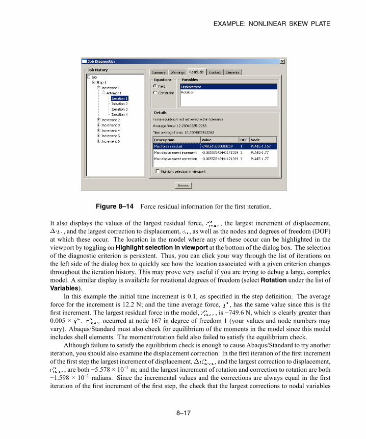
EXAMPLE: NONLINEAR SKEW PLATE
Figure 8–14 Force residual information for the first iteration.
It also displays the values of the largest residual force, , the largest increment of displacement,, and the largest correction to displacement, , as well as the nodes and degrees of freedom (DOF)
at which these occur. The location in the model where any of these occur can be highlighted in theviewport by toggling on Highlight selection in viewport at the bottom of the dialog box. The selectionof the diagnostic criterion is persistent. Thus, you can click your way through the list of iterations onthe left side of the dialog box to quickly see how the location associated with a given criterion changesthroughout the iteration history. This may prove very useful if you are trying to debug a large, complexmodel. A similar display is available for rotational degrees of freedom (select Rotation under the list ofVariables).
In this example the initial time increment is 0.1, as specified in the step definition. The averageforce for the increment is 12.2 N; and the time average force, , has the same value since this is thefirst increment. The largest residual force in the model, , is −749.6 N, which is clearly greater than0.005 × . occurred at node 167 in degree of freedom 1 (your values and node numbers mayvary). Abaqus/Standard must also check for equilibrium of the moments in the model since this modelincludes shell elements. The moment/rotation field also failed to satisfy the equilibrium check.
Although failure to satisfy the equilibrium check is enough to cause Abaqus/Standard to try anotheriteration, you should also examine the displacement correction. In the first iteration of the first incrementof the first step the largest increment of displacement, , and the largest correction to displacement,
, are both −5.578 × 10⁻³ m; and the largest increment of rotation and correction to rotation are both−1.598 × 10⁻² radians. Since the incremental values and the corrections are always equal in the firstiteration of the first increment of the first step, the check that the largest corrections to nodal variables
8–17
Abaqus ID:Printed on:
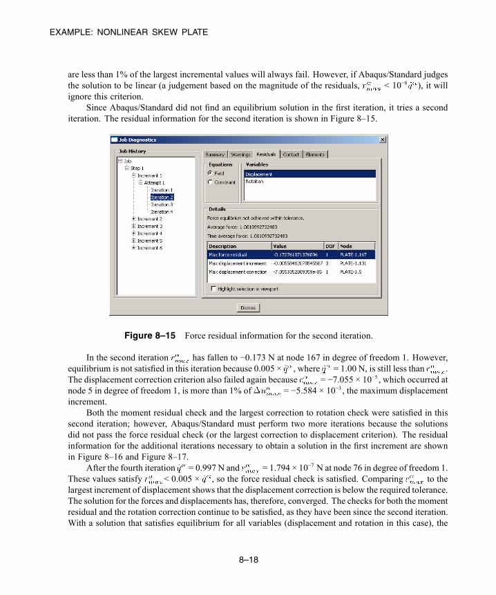
EXAMPLE: NONLINEAR SKEW PLATE
are less than 1% of the largest incremental values will always fail. However, if Abaqus/Standard judgesthe solution to be linear (a judgement based on the magnitude of the residuals, < 10−8 ), it willignore this criterion.
Since Abaqus/Standard did not find an equilibrium solution in the first iteration, it tries a seconditeration. The residual information for the second iteration is shown in Figure 8–15.
Figure 8–15 Force residual information for the second iteration.
In the second iteration has fallen to −0.173 N at node 167 in degree of freedom 1. However,equilibrium is not satisfied in this iteration because 0.005 × , where = 1.00 N, is still less than .The displacement correction criterion also failed again because = −7.055 × 10⁻⁵ , which occurred atnode 5 in degree of freedom 1, is more than 1% of = −5.584 × 10⁻³ , the maximum displacementincrement.
Both the moment residual check and the largest correction to rotation check were satisfied in thissecond iteration; however, Abaqus/Standard must perform two more iterations because the solutionsdid not pass the force residual check (or the largest correction to displacement criterion). The residualinformation for the additional iterations necessary to obtain a solution in the first increment are shownin Figure 8–16 and Figure 8–17.
After the fourth iteration = 0.997 N and = 1.794 × 10⁻⁷ N at node 76 in degree of freedom 1.These values satisfy < 0.005 × , so the force residual check is satisfied. Comparing to thelargest increment of displacement shows that the displacement correction is below the required tolerance.The solution for the forces and displacements has, therefore, converged. The checks for both the momentresidual and the rotation correction continue to be satisfied, as they have been since the second iteration.With a solution that satisfies equilibrium for all variables (displacement and rotation in this case), the
8–18
Abaqus ID:Printed on:

EXAMPLE: NONLINEAR SKEW PLATE
Figure 8–16 Force residual information for the third iteration.
Figure 8–17 Force residual information for the fourth iteration.
first load increment is complete. The attempt summary (Figure 8–13) shows the number of iterationsthat were required for this increment and the size of the increment.
8–19
Abaqus ID:Printed on:
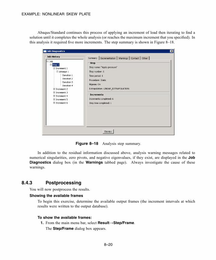
EXAMPLE: NONLINEAR SKEW PLATE
Abaqus/Standard continues this process of applying an increment of load then iterating to find asolution until it completes the whole analysis (or reaches the maximum increment that you specified). Inthis analysis it required five more increments. The step summary is shown in Figure 8–18.
Figure 8–18 Analysis step summary.
In addition to the residual information discussed above, analysis warning messages related tonumerical singularities, zero pivots, and negative eigenvalues, if they exist, are displayed in the JobDiagnostics dialog box (in the Warnings tabbed page). Always investigate the cause of thesewarnings.
8.4.3 PostprocessingYou will now postprocess the results.
Showing the available frames
To begin this exercise, determine the available output frames (the increment intervals at whichresults were written to the output database).
To show the available frames:1. From the main menu bar, select Result→Step/Frame.
The Step/Frame dialog box appears.
8–20
Abaqus ID:Printed on:
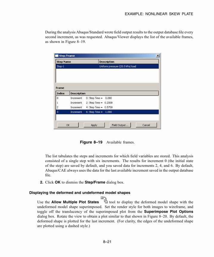
EXAMPLE: NONLINEAR SKEW PLATE
During the analysis Abaqus/Standard wrote field output results to the output database file everysecond increment, as was requested. Abaqus/Viewer displays the list of the available frames,as shown in Figure 8–19.
Figure 8–19 Available frames.
The list tabulates the steps and increments for which field variables are stored. This analysisconsisted of a single step with six increments. The results for increment 0 (the initial stateof the step) are saved by default, and you saved data for increments 2, 4, and 6. By default,Abaqus/CAE always uses the data for the last available increment saved in the output databasefile.
2. Click OK to dismiss the Step/Frame dialog box.
Displaying the deformed and undeformed model shapes
Use the Allow Multiple Plot States tool to display the deformed model shape with theundeformed model shape superimposed. Set the render style for both images to wireframe, andtoggle off the translucency of the superimposed plot from the Superimpose Plot Optionsdialog box. Rotate the view to obtain a plot similar to that shown in Figure 8–20. By default, thedeformed shape is plotted for the last increment. (For clarity, the edges of the undeformed shapeare plotted using a dashed style.)
8–21
Abaqus ID:Printed on:
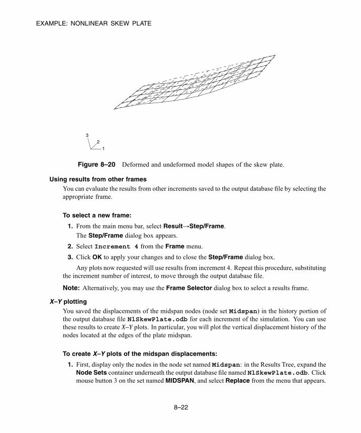
EXAMPLE: NONLINEAR SKEW PLATE
12
3
Figure 8–20 Deformed and undeformed model shapes of the skew plate.
Using results from other frames
You can evaluate the results from other increments saved to the output database file by selecting theappropriate frame.
To select a new frame:
1. From the main menu bar, select Result→Step/Frame.
The Step/Frame dialog box appears.
2. Select Increment 4 from the Frame menu.
3. Click OK to apply your changes and to close the Step/Frame dialog box.
Any plots now requested will use results from increment 4. Repeat this procedure, substitutingthe increment number of interest, to move through the output database file.
Note: Alternatively, you may use the Frame Selector dialog box to select a results frame.
X–Y plotting
You saved the displacements of the midspan nodes (node set Midspan) in the history portion ofthe output database file NlSkewPlate.odb for each increment of the simulation. You can usethese results to create X–Y plots. In particular, you will plot the vertical displacement history of thenodes located at the edges of the plate midspan.
To create X–Y plots of the midspan displacements:
1. First, display only the nodes in the node set named Midspan: in the Results Tree, expand theNode Sets container underneath the output database file named NlSkewPlate.odb. Clickmouse button 3 on the set named MIDSPAN, and select Replace from the menu that appears.
8–22
Abaqus ID:Printed on:
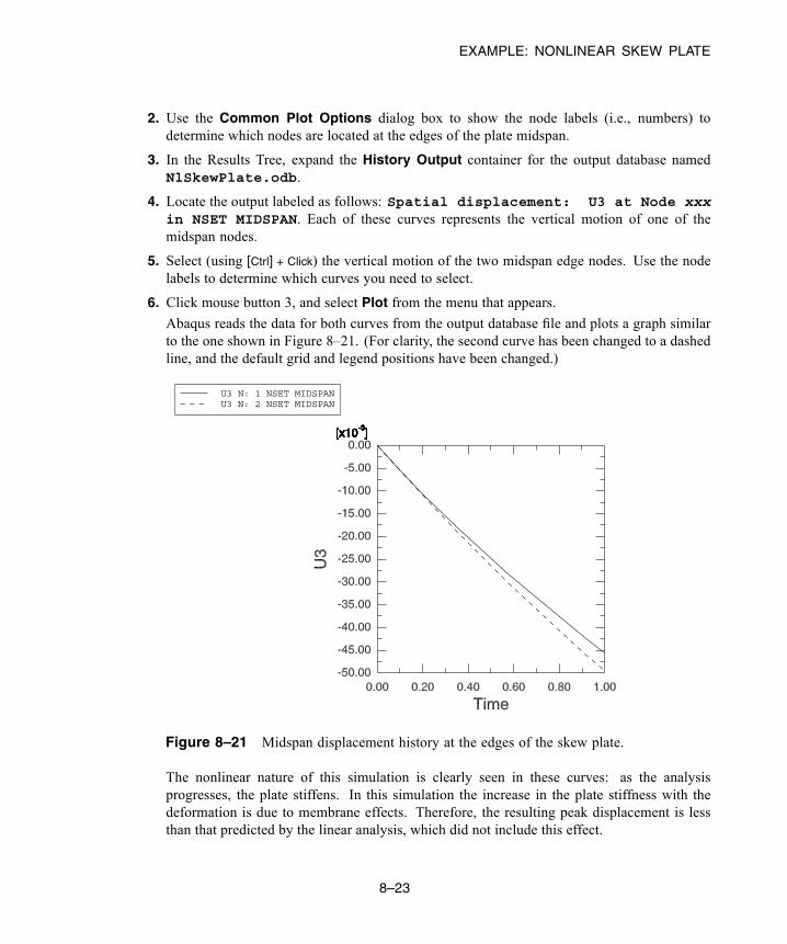
EXAMPLE: NONLINEAR SKEW PLATE
2. Use the Common Plot Options dialog box to show the node labels (i.e., numbers) todetermine which nodes are located at the edges of the plate midspan.
3. In the Results Tree, expand the History Output container for the output database namedNlSkewPlate.odb.
4. Locate the output labeled as follows: Spatial displacement: U3 at Node xxxin NSET MIDSPAN. Each of these curves represents the vertical motion of one of themidspan nodes.
5. Select (using [Ctrl] + Click) the vertical motion of the two midspan edge nodes. Use the nodelabels to determine which curves you need to select.
6. Click mouse button 3, and select Plot from the menu that appears.
Abaqus reads the data for both curves from the output database file and plots a graph similarto the one shown in Figure 8–21. (For clarity, the second curve has been changed to a dashedline, and the default grid and legend positions have been changed.)
U3 N: 1 NSET MIDSPANU3 N: 2 NSET MIDSPAN
Figure 8–21 Midspan displacement history at the edges of the skew plate.
The nonlinear nature of this simulation is clearly seen in these curves: as the analysisprogresses, the plate stiffens. In this simulation the increase in the plate stiffness with thedeformation is due to membrane effects. Therefore, the resulting peak displacement is lessthan that predicted by the linear analysis, which did not include this effect.
8–23
Abaqus ID:Printed on:
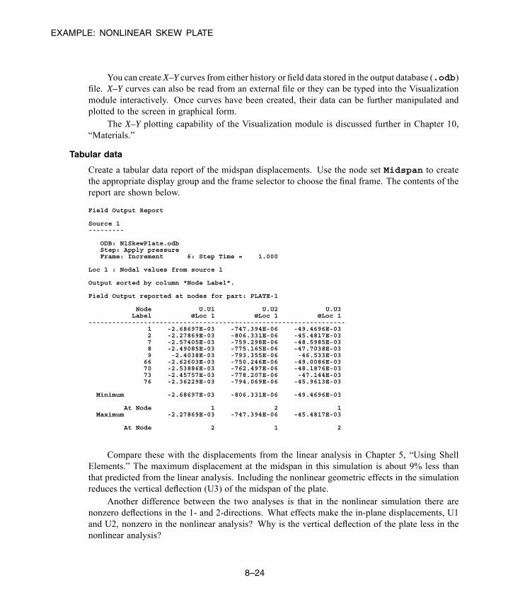
EXAMPLE: NONLINEAR SKEW PLATE
You can create X–Y curves from either history or field data stored in the output database (.odb)file. X–Y curves can also be read from an external file or they can be typed into the Visualizationmodule interactively. Once curves have been created, their data can be further manipulated andplotted to the screen in graphical form.
The X–Y plotting capability of the Visualization module is discussed further in Chapter 10,“Materials.”
Tabular data
Create a tabular data report of the midspan displacements. Use the node set Midspan to createthe appropriate display group and the frame selector to choose the final frame. The contents of thereport are shown below.
Field Output Report
Source 1---------
ODB: NlSkewPlate.odbStep: Apply pressureFrame: Increment 6: Step Time = 1.000
Loc 1 : Nodal values from source 1
Output sorted by column "Node Label".
Field Output reported at nodes for part: PLATE-1
Node U.U1 U.U2 U.U3Label @Loc 1 @Loc 1 @Loc 1
-----------------------------------------------------------------1 -2.68697E-03 -747.394E-06 -49.4696E-032 -2.27869E-03 -806.331E-06 -45.4817E-037 -2.57405E-03 -759.298E-06 -48.5985E-038 -2.49085E-03 -775.165E-06 -47.7038E-039 -2.4038E-03 -793.355E-06 -46.533E-03
66 -2.62603E-03 -750.246E-06 -49.0086E-0370 -2.53886E-03 -762.497E-06 -48.1876E-0373 -2.45757E-03 -778.207E-06 -47.144E-0376 -2.36229E-03 -794.069E-06 -45.9613E-03
Minimum -2.68697E-03 -806.331E-06 -49.4696E-03
At Node 1 2 1Maximum -2.27869E-03 -747.394E-06 -45.4817E-03
At Node 2 1 2
Compare these with the displacements from the linear analysis in Chapter 5, “Using ShellElements.” The maximum displacement at the midspan in this simulation is about 9% less thanthat predicted from the linear analysis. Including the nonlinear geometric effects in the simulationreduces the vertical deflection (U3) of the midspan of the plate.
Another difference between the two analyses is that in the nonlinear simulation there arenonzero deflections in the 1- and 2-directions. What effects make the in-plane displacements, U1and U2, nonzero in the nonlinear analysis? Why is the vertical deflection of the plate less in thenonlinear analysis?
8–24
Abaqus ID:Printed on:
SUGGESTED READING
The plate deforms into a curved shape: a geometry change that is taken into account in thenonlinear simulation. As a consequence, membrane effects cause some of the load to be carried bymembrane action rather than by bending alone. This makes the plate stiffer. In addition, the pressureloading, which is always normal to the plate’s surface, starts to have a component in the 1- and2-directions as the plate deforms. The nonlinear analysis includes the effects of this stiffening andthe changing direction of the pressure. Neither of these effects is included in the linear simulation.
The differences between the linear and nonlinear simulations are sufficiently large to indicatethat a linear simulation is not adequate for this plate under this particular loading condition.
8.4.4 Running the analysis in Abaqus/ExplicitAs an optional exercise, you can modify the model and run a dynamic analysis of the skew plate inAbaqus/Explicit. To do so, you must add a density of 7800 kg/m3 to the material definition, replace theexisting step with an explicit dynamic step, and change the element library to Explicit. After making theappropriate model changes, you can create and run a new job to examine the transient dynamic effectsin the plate under a suddenly applied load.
8.5 Related Abaqus examples
• “Elastic-plastic collapse of a thin-walled elbow under in-plane bending and internal pressure,”Section 1.1.2 of the Abaqus Example Problems Guide
• “Laminated composite shells: buckling of a cylindrical panel with a circular hole,” Section 1.2.2 ofthe Abaqus Example Problems Guide
• “Unstable static problem: reinforced plate under compressive loads,” Section 1.2.5 of the AbaqusExample Problems Guide
• “Large rotation of a one degree of freedom system,” Section 1.3.5 of the Abaqus Benchmarks Guide• “Vibration of a cable under tension,” Section 1.4.3 of the Abaqus Benchmarks Guide
8.6 Suggested reading
The following references provide additional information on nonlinear finite element methods. Theyallow the interested user to explore the topic in more depth.
General texts on nonlinear finite element analysis
• Belytschko, T., W. K. Liu, and B. Moran, Nonlinear Finite Elements for Continua andStructures, Wiley & Sons, 2000.
• Bonet, J., and R. D. Wood, Nonlinear Continuum Mechanics for Finite Element Analysis,Cambridge, 1997.
8–25
Abaqus ID:Printed on:
SUMMARY
• Cook, R. D., D. S. Malkus, and M. E. Plesha, Concepts and Applications of Finite ElementAnalysis, Wiley & Sons, 1989.
• Crisfield, M. A., Non-linear Finite Element Analysis of Solids and Structures, Volume I:Essentials, Wiley & Sons, 1991.
• Crisfield, M. A., Non-linear Finite Element Analysis of Solids and Structures, Volume II:Advanced Topics, Wiley & Sons, 1997.
• E. Hinton (editor), NAFEMS Introduction to Nonlinear Finite Element Analysis, NAFEMSLtd., 1992.
• Oden, J. T., Finite Elements of Nonlinear Continua, McGraw-Hill, 1972.
8.7 Summary
• There are three sources of nonlinearity in structural problems: material, geometric, and boundary(contact). Any combination of these may be present in an Abaqus analysis.
• Geometric nonlinearity occurs whenever the magnitude of the displacements affects the responseof the structure. It includes the effects of large displacements and rotations, snap through, and loadstiffening.
• In Abaqus/Standard nonlinear problems are solved iteratively using the Newton-Raphson method.A nonlinear problem will require many times the computer resources required by a linear problem.
• Abaqus/Explicit does not need to iterate to obtain a solution; however, the computational cost maybe affected by reductions in the stable time increment due to large changes in geometry.
• A nonlinear analysis step is split into a number of increments.– Abaqus/Standard iterates to find the approximate static equilibrium obtained at the end of eachnew load increment. Abaqus/Standard controls the load incrementation by using convergencecontrols throughout the simulation.
– Abaqus/Explicit determines a solution by advancing the kinematic state from one increment tothe next, using a smaller time increment than what is commonly used in implicit analyses. Thesize of the increment is limited by the stable time increment. By default, time incrementationis completely automated in Abaqus/Explicit.
• The Job Monitor dialog box allows the progress of an analysis to be monitored while it is running.The Job Diagnostics dialog box contains the details of the load incrementation and iterations.
• Results can be saved at the end of each increment so that the evolution of the structure’s responsecan be seen in the Visualization module. Results can also be plotted in the form of X–Y graphs.
8–26
Abaqus ID:Printed on:

TYPES OF PROBLEMS SUITED FOR Abaqus/Explicit
9. Nonlinear Explicit Dynamics
In previous chapters you explored the basics of explicit dynamics procedures; in this chapter you willexamine this topic in greater detail. The explicit dynamics procedure can be an effective tool for solvinga wide variety of nonlinear solid and structural mechanics problems. It is often complementary to animplicit solver such as Abaqus/Standard. From a user standpoint, the distinguishing characteristics ofthe explicit and implicit methods are:
• Explicit methods require a small time increment size that depends solely on the highest naturalfrequencies of the model and is independent of the type and duration of loading. Simulationsgenerally take on the order of 10,000 to 1,000,000 increments, but the computational cost perincrement is relatively small.
• Implicit methods do not place an inherent limitation on the time increment size; increment size isgenerally determined from accuracy and convergence considerations. Implicit simulations typicallytake orders of magnitude fewer increments than explicit simulations. However, since a global setof equations must be solved in each increment, the cost per increment of an implicit method is fargreater than that of an explicit method.
Knowing these characteristics of the two procedures can help you decide which methodology isappropriate for your problems.
9.1 Types of problems suited for Abaqus/Explicit
Before discussing how the explicit dynamics procedure works, it is helpful to understand what classesof problems are well-suited to Abaqus/Explicit. Throughout this guide we have incorporated pertinentexamples of the following classes of problems commonly performed in Abaqus/Explicit:
High-speed dynamic events
The explicit dynamics method was originally developed to analyze high-speed dynamic eventsthat can be extremely costly to analyze using implicit programs, such as Abaqus/Standard. Asan example of such a simulation, the effect of a short-duration blast load on a steel plate is analyzedin Chapter 10, “Materials.” Since the load is applied rapidly and is very severe, the response ofthe structure changes rapidly. Accurate tracking of stress waves through the plate is important forcapturing the dynamic response. Since stress waves are associated with the highest frequencies ofthe system, obtaining an accurate solution requires many small time increments.
Complex contact problems
Contact conditions are formulated more easily using an explicit dynamics method than using animplicit method. The result is that Abaqus/Explicit can readily analyze problems involving complexcontact interaction between many independent bodies. Abaqus/Explicit is particularly well-suitedfor analyzing the transient dynamic response of structures that are subject to impact loads and
9–1
Abaqus ID:Printed on:
EXPLICIT DYNAMIC FINITE ELEMENT METHODS
subsequently undergo complex contact interaction within the structure. An example of such aproblem is the circuit board drop test presented in Chapter 12, “Contact.” In this example a circuitboard sitting in foam packaging is dropped on the floor from a height of 1 m. The problem involvesimpact between the packaging and the floor, as well as rapidly changing contact conditions betweenthe circuit board and the packaging.
Complex postbuckling problems
Unstable postbuckling problems are solved readily in Abaqus/Explicit. In such problems thestiffness of the structure changes drastically as the loads are applied. Postbuckling response oftenincludes the effects of contact interactions.
Highly nonlinear quasi-static problems
For a variety of reasons Abaqus/Explicit is often very efficient in solving certain classes ofproblems that are essentially static. Quasi-static process simulation problems involving complexcontact such as forging, rolling, and sheet-forming generally fall within these classes. Sheetforming problems usually include very large membrane deformations, wrinkling, and complexfrictional contact conditions. Bulk forming problems are characterized by large distortions, flashformation, and contact interaction with the dies. An example of a quasi-static forming simulationis presented in Chapter 13, “Quasi-Static Analysis with Abaqus/Explicit.”
Materials with degradation and failure
Material degradation and failure often lead to severe convergence difficulties in implicit analysisprograms, but Abaqus/Explicit models such materials well. An example of material degradationis the concrete cracking model, in which tensile cracking causes the material stiffness to becomenegative. An example of material failure is the ductile failure model for metals, in which materialstiffness can degrade until it reduces to zero. At this time the failed elements are removed from themodel entirely.
Each of these types of analyses can include temperature and heat transfer effects.
9.2 Explicit dynamic finite element methods
This section contains an algorithmic description of the Abaqus/Explicit solver as well as a comparisonbetween implicit and explicit time integration and a discussion of the advantages of the explicit dynamicsmethod.
9.2.1 Explicit time integrationAbaqus/Explicit uses a central difference rule to integrate the equations of motion explicitly throughtime, using the kinematic conditions at one increment to calculate the kinematic conditions at the next
9–2
Abaqus ID:Printed on:

EXPLICIT DYNAMIC FINITE ELEMENT METHODS
increment. At the beginning of the increment the program solves for dynamic equilibrium, which statesthat the nodal massmatrix, , times the nodal accelerations, , equals the net nodal forces (the differencebetween the external applied forces, , and internal element forces, ):
The accelerations at the beginning of the current increment (time ) are calculated as
Since the explicit procedure always uses a diagonal, or lumped, mass matrix, solving for theaccelerations is trivial; there are no simultaneous equations to solve. The acceleration of any node isdetermined completely by its mass and the net force acting on it, making the nodal calculations veryinexpensive.
The accelerations are integrated through time using the central difference rule, which calculatesthe change in velocity assuming that the acceleration is constant. This change in velocity is added tothe velocity from the middle of the previous increment to determine the velocities at the middle of thecurrent increment:
The velocities are integrated through time and added to the displacements at the beginning of theincrement to determine the displacements at the end of the increment:
Thus, satisfying dynamic equilibrium at the beginning of the increment provides the accelerations.Knowing the accelerations, the velocities and displacements are advanced “explicitly” through time.The term “explicit” refers to the fact that the state at the end of the increment is based solely on thedisplacements, velocities, and accelerations at the beginning of the increment. This method integratesconstant accelerations exactly. For the method to produce accurate results, the time increments must bequite small so that the accelerations are nearly constant during an increment. Since the time incrementsmust be small, analyses typically require many thousands of increments. Fortunately, each increment isinexpensive because there are no simultaneous equations to solve. Most of the computational expenselies in the element calculations to determine the internal forces of the elements acting on the nodes. Theelement calculations include determining element strains and applying material constitutive relationships(the element stiffness) to determine element stresses and, consequently, internal forces.
Here is a summary of the explicit dynamics algorithm:
1. Nodal calculations.
a. Dynamic equilibrium.
9–3
Abaqus ID:Printed on:
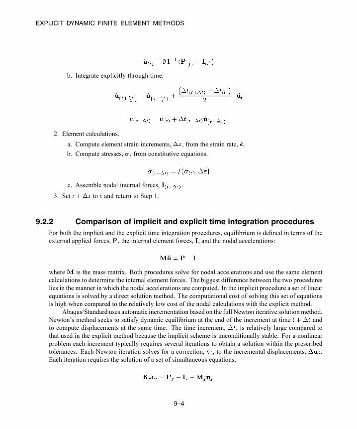
EXPLICIT DYNAMIC FINITE ELEMENT METHODS
b. Integrate explicitly through time.
2. Element calculations.
a. Compute element strain increments, , from the strain rate, .
b. Compute stresses, , from constitutive equations.
c. Assemble nodal internal forces, .
3. Set to and return to Step 1.
9.2.2 Comparison of implicit and explicit time integration proceduresFor both the implicit and the explicit time integration procedures, equilibrium is defined in terms of theexternal applied forces, , the internal element forces, , and the nodal accelerations:
where is the mass matrix. Both procedures solve for nodal accelerations and use the same elementcalculations to determine the internal element forces. The biggest difference between the two procedureslies in the manner in which the nodal accelerations are computed. In the implicit procedure a set of linearequations is solved by a direct solution method. The computational cost of solving this set of equationsis high when compared to the relatively low cost of the nodal calculations with the explicit method.
Abaqus/Standard uses automatic incrementation based on the full Newton iterative solution method.Newton’s method seeks to satisfy dynamic equilibrium at the end of the increment at time andto compute displacements at the same time. The time increment, , is relatively large compared tothat used in the explicit method because the implicit scheme is unconditionally stable. For a nonlinearproblem each increment typically requires several iterations to obtain a solution within the prescribedtolerances. Each Newton iteration solves for a correction, , to the incremental displacements, .Each iteration requires the solution of a set of simultaneous equations,
9–4
Abaqus ID:Printed on:
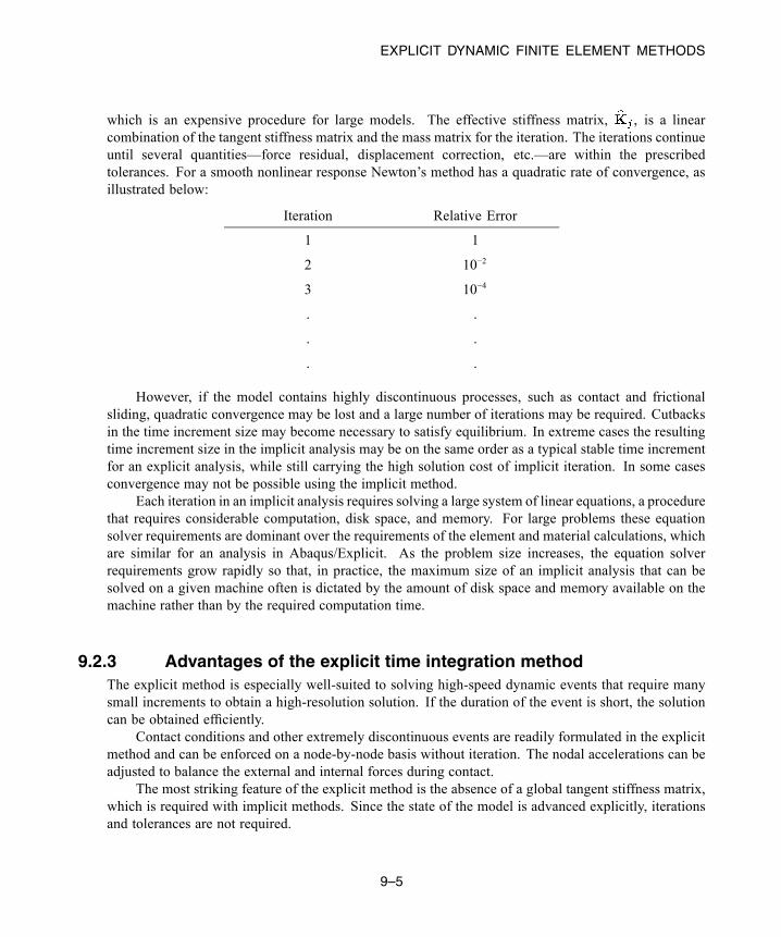
EXPLICIT DYNAMIC FINITE ELEMENT METHODS
which is an expensive procedure for large models. The effective stiffness matrix, , is a linearcombination of the tangent stiffness matrix and the mass matrix for the iteration. The iterations continueuntil several quantities—force residual, displacement correction, etc.—are within the prescribedtolerances. For a smooth nonlinear response Newton’s method has a quadratic rate of convergence, asillustrated below:
Iteration Relative Error
1 1
2 10−2
3 10−4
. .
. .
. .
However, if the model contains highly discontinuous processes, such as contact and frictionalsliding, quadratic convergence may be lost and a large number of iterations may be required. Cutbacksin the time increment size may become necessary to satisfy equilibrium. In extreme cases the resultingtime increment size in the implicit analysis may be on the same order as a typical stable time incrementfor an explicit analysis, while still carrying the high solution cost of implicit iteration. In some casesconvergence may not be possible using the implicit method.
Each iteration in an implicit analysis requires solving a large system of linear equations, a procedurethat requires considerable computation, disk space, and memory. For large problems these equationsolver requirements are dominant over the requirements of the element and material calculations, whichare similar for an analysis in Abaqus/Explicit. As the problem size increases, the equation solverrequirements grow rapidly so that, in practice, the maximum size of an implicit analysis that can besolved on a given machine often is dictated by the amount of disk space and memory available on themachine rather than by the required computation time.
9.2.3 Advantages of the explicit time integration methodThe explicit method is especially well-suited to solving high-speed dynamic events that require manysmall increments to obtain a high-resolution solution. If the duration of the event is short, the solutioncan be obtained efficiently.
Contact conditions and other extremely discontinuous events are readily formulated in the explicitmethod and can be enforced on a node-by-node basis without iteration. The nodal accelerations can beadjusted to balance the external and internal forces during contact.
The most striking feature of the explicit method is the absence of a global tangent stiffness matrix,which is required with implicit methods. Since the state of the model is advanced explicitly, iterationsand tolerances are not required.
9–5
Abaqus ID:Printed on:
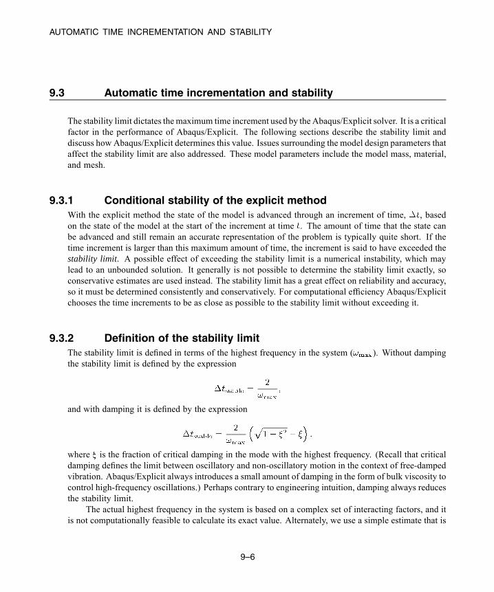
AUTOMATIC TIME INCREMENTATION AND STABILITY
9.3 Automatic time incrementation and stability
The stability limit dictates themaximum time increment used by the Abaqus/Explicit solver. It is a criticalfactor in the performance of Abaqus/Explicit. The following sections describe the stability limit anddiscuss how Abaqus/Explicit determines this value. Issues surrounding the model design parameters thataffect the stability limit are also addressed. These model parameters include the model mass, material,and mesh.
9.3.1 Conditional stability of the explicit methodWith the explicit method the state of the model is advanced through an increment of time, , basedon the state of the model at the start of the increment at time . The amount of time that the state canbe advanced and still remain an accurate representation of the problem is typically quite short. If thetime increment is larger than this maximum amount of time, the increment is said to have exceeded thestability limit. A possible effect of exceeding the stability limit is a numerical instability, which maylead to an unbounded solution. It generally is not possible to determine the stability limit exactly, soconservative estimates are used instead. The stability limit has a great effect on reliability and accuracy,so it must be determined consistently and conservatively. For computational efficiency Abaqus/Explicitchooses the time increments to be as close as possible to the stability limit without exceeding it.
9.3.2 Definition of the stability limitThe stability limit is defined in terms of the highest frequency in the system ( ). Without dampingthe stability limit is defined by the expression
and with damping it is defined by the expression
where is the fraction of critical damping in the mode with the highest frequency. (Recall that criticaldamping defines the limit between oscillatory and non-oscillatory motion in the context of free-dampedvibration. Abaqus/Explicit always introduces a small amount of damping in the form of bulk viscosity tocontrol high-frequency oscillations.) Perhaps contrary to engineering intuition, damping always reducesthe stability limit.
The actual highest frequency in the system is based on a complex set of interacting factors, and itis not computationally feasible to calculate its exact value. Alternately, we use a simple estimate that is
9–6
Abaqus ID:Printed on:
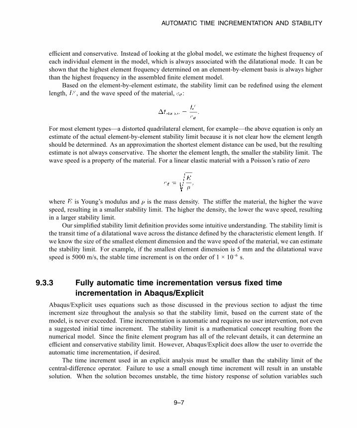
AUTOMATIC TIME INCREMENTATION AND STABILITY
efficient and conservative. Instead of looking at the global model, we estimate the highest frequency ofeach individual element in the model, which is always associated with the dilatational mode. It can beshown that the highest element frequency determined on an element-by-element basis is always higherthan the highest frequency in the assembled finite element model.
Based on the element-by-element estimate, the stability limit can be redefined using the elementlength, , and the wave speed of the material, :
For most element types—a distorted quadrilateral element, for example—the above equation is only anestimate of the actual element-by-element stability limit because it is not clear how the element lengthshould be determined. As an approximation the shortest element distance can be used, but the resultingestimate is not always conservative. The shorter the element length, the smaller the stability limit. Thewave speed is a property of the material. For a linear elastic material with a Poisson’s ratio of zero
where is Young’s modulus and is the mass density. The stiffer the material, the higher the wavespeed, resulting in a smaller stability limit. The higher the density, the lower the wave speed, resultingin a larger stability limit.
Our simplified stability limit definition provides some intuitive understanding. The stability limit isthe transit time of a dilatational wave across the distance defined by the characteristic element length. Ifwe know the size of the smallest element dimension and the wave speed of the material, we can estimatethe stability limit. For example, if the smallest element dimension is 5 mm and the dilatational wavespeed is 5000 m/s, the stable time increment is on the order of 1 × 10⁻⁶ s.
9.3.3 Fully automatic time incrementation versus fixed timeincrementation in Abaqus/Explicit
Abaqus/Explicit uses equations such as those discussed in the previous section to adjust the timeincrement size throughout the analysis so that the stability limit, based on the current state of themodel, is never exceeded. Time incrementation is automatic and requires no user intervention, not evena suggested initial time increment. The stability limit is a mathematical concept resulting from thenumerical model. Since the finite element program has all of the relevant details, it can determine anefficient and conservative stability limit. However, Abaqus/Explicit does allow the user to override theautomatic time incrementation, if desired.
The time increment used in an explicit analysis must be smaller than the stability limit of thecentral-difference operator. Failure to use a small enough time increment will result in an unstablesolution. When the solution becomes unstable, the time history response of solution variables such
9–7
Abaqus ID:Printed on:
AUTOMATIC TIME INCREMENTATION AND STABILITY
as displacements will usually oscillate with increasing amplitudes. The total energy balance will alsochange significantly. If the model contains only one material type, the initial time increment is directlyproportional to the size of the smallest element in the mesh. If the mesh contains uniform size elementsbut contains multiple material descriptions, the element with the highest wave speed will determine theinitial time increment.
In nonlinear problems—those with large deformations and/or nonlinear material response—thehighest frequency of the model will continually change, which consequently changes the stability limit.Abaqus/Explicit has two strategies for time incrementation control: fully automatic time incrementation(where the code accounts for changes in the stability limit) and fixed time incrementation.
Two types of estimates are used to determine the stability limit: element by element and global. Ananalysis always starts by using the element-by-element estimation method and may switch to the globalestimation method under certain circumstances.
The element-by-element estimate is conservative; it will give a smaller stable time incrementthan the true stability limit that is based upon the maximum frequency of the entire model. In general,constraints such as boundary conditions and kinematic contact have the effect of compressing theeigenvalue spectrum, and the element-by-element estimates do not take this into account.
The adaptive, global estimation algorithm determines the maximum frequency of the entire modelusing the current dilatational wave speed. This algorithm continuously updates the estimate for themaximum frequency. The global estimator will usually allow time increments that exceed the element-by-element values.
A fixed time incrementation scheme is also available in Abaqus/Explicit. The fixed time incrementsize is determined either by the initial element-by-element stability estimate for the step or by a timeincrement specified directly by the user. Fixed time incrementation may be useful when a more accuraterepresentation of the higher mode response of a problem is required. In this case, a time incrementsize smaller than the element-by-element estimates may be used. When fixed time incrementation isused, Abaqus/Explicit will not check that the computed response is stable during the step. The usershould ensure that a valid response has been obtained by carefully checking the energy history and otherresponse variables.
9.3.4 Mass scaling to control time incrementation
Since the mass density influences the stability limit, under some circumstances scaling the mass densitycan potentially increase the efficiency of an analysis. For example, because of the complex discretizationof many models, there are often regions containing very small or poorly shaped elements that control thestability limit. These controlling elements are often few in number and may exist in localized areas. Byincreasing the mass of only these controlling elements, the stability limit can be increased significantly,while the effect on the overall dynamic behavior of the model may be negligible.
The automatic mass scaling features in Abaqus/Explicit can keep offending elements from hinderingthe stability limit. There are two fundamental approaches used in mass scaling: defining a scaling factordirectly or defining a desired element-by-element stable time increment for the elements whose mass isto be scaled. These two approaches, described in detail in “Mass scaling,” Section 11.6.1 of the Abaqus
9–8
Abaqus ID:Printed on:
EXAMPLE: STRESS WAVE PROPAGATION IN A BAR
Analysis User’s Guide, permit additional user control over the stability limit. However, use caution whenemploying mass scaling since significantly changing the mass of the model may change the physics ofthe problem.
9.3.5 Effect of material on stability limitThe material model affects the stability limit through its effect on the dilatational wave speed. In a linearmaterial the wave speed is constant; therefore, the only changes in the stability limit during the analysisresult from changes in the smallest element dimension during the analysis. In a nonlinear material, suchas a metal with plasticity, the wave speed changes as the material yields and the stiffness of the materialchanges. Abaqus/Explicit monitors the effective wave speeds in the model throughout the analysis, andthe current material state in each element is used for stability estimates. After yielding, the stiffnessdecreases, reducing the wave speed and, consequently, increasing the stability limit.
9.3.6 Effect of mesh on stability limitSince the stability limit is roughly proportional to the shortest element dimension, it is advantageousto keep the element size as large as possible. Unfortunately, for accurate analyses a fine mesh is oftennecessary. To obtain the highest possible stability limit while using the required level of mesh refinement,the best approach is to have a mesh that is as uniform as possible. Since the stability limit is based on thesmallest element dimension in the model, even a single small or poorly shaped element can reduce thestability limit drastically. For diagnostic purposes Abaqus/Explicit provides a list in the status (.sta)file of the 10 elements in the mesh with the lowest stability limit. If the model contains some elementswhose stability limits are much lower than those of the rest of the mesh, remeshing the model moreuniformly may be worthwhile.
9.3.7 Numerical instabilityAbaqus/Explicit remains stable for most elements under most circumstances. It is possible, however,to define spring and dashpot elements such that they become unstable during the course of an analysis.Therefore, it is useful to be able to recognize a numerical instability if it occurs in your analysis. If itdoes occur, the result typically will be unbounded, nonphysical, and often characterized by oscillatorysolutions.
9.4 Example: stress wave propagation in a bar
This example demonstrates some of the fundamental ideas in explicit dynamics described earlier inChapter 2, “Abaqus Basics.” It also illustrates stability limits and the effect of mesh refinement andmaterial properties on the solution time.
The bar has the dimensions shown in Figure 9–1.
9–9
Abaqus ID:Printed on:
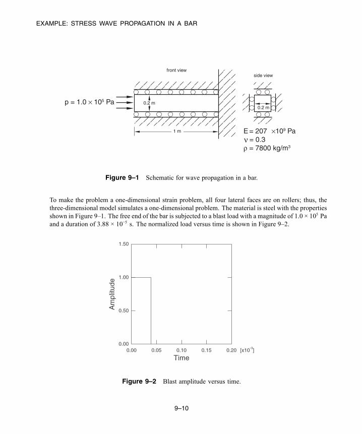
EXAMPLE: STRESS WAVE PROPAGATION IN A BAR
p = 1.0 × 10⁵ Pa
E = 207 × 109 Pa
= 7800 kg/m3
1 m
0.2 m0.2 m
side viewfront view
ν
Figure 9–1 Schematic for wave propagation in a bar.
To make the problem a one-dimensional strain problem, all four lateral faces are on rollers; thus, thethree-dimensional model simulates a one-dimensional problem. The material is steel with the propertiesshown in Figure 9–1. The free end of the bar is subjected to a blast load with a magnitude of 1.0 × 10⁵ Paand a duration of 3.88 × 10⁻⁵ s. The normalized load versus time is shown in Figure 9–2.
Figure 9–2 Blast amplitude versus time.
9–10
Abaqus ID:Printed on:
EXAMPLE: STRESS WAVE PROPAGATION IN A BAR
9.4.1 Preprocessing—creating the model with Abaqus/CAE
In this section we discuss how to use Abaqus/CAE to create the model for this simulation. Abaqusprovides scripts that replicate the complete analysis model for this problem. Run one of these scriptsif you encounter difficulties following the instructions given below or if you wish to check your work.Scripts are available in the following locations:
• A Python script for this example is provided in “Stress wave propagation in a bar,” Section A.7,in the HTML version of this guide. Instructions on how to fetch the script and run it withinAbaqus/CAE are given in Appendix A, “Example Files.”
• A plug-in script for this example is available in the Abaqus/CAE Plug-in toolset. To run thescript from Abaqus/CAE, select Plug-ins→Abaqus→Getting Started; highlight Stress wavepropagation in a bar; and click Run. For more information about the Getting Started plug-ins,see “Running the Getting Started with Abaqus examples,” Section 82.1 of the Abaqus/CAE User’sGuide, in the HTML version of this guide.
Defining the model geometry
In this example you will create a three-dimensional, deformable body with a solid, extruded basefeature. You will first sketch the two-dimensional profile of the bar and then extrude it.
To create a part:
1. Create a new part named Bar, and accept the default settings of a three-dimensional,deformable body and a solid, extruded base feature in the Create Part dialog box. Use anapproximate size of 0.5 for the model.
2. Use the dimensions given in Figure 9–3 to sketch the cross-section of the bar. The followingpossible approach can be used:
a. Create a rectangle centered about the origin using the Create Lines: Rectangle tool.
Tip: Create fixed horizontal and vertical construction lines through the originof the sketch plane, and apply appropriate geometry constraints to the sketch.
b. Dimension the sketch so that the cross-section is 0.20 m high × 0.20 m wide.
c. Click Done in the prompt area when you are finished sketching the profile.
The Edit Base Extrusion dialog box appears. To complete the part definition, you mustspecify the distance over which the profile will be extruded.
d. In the dialog box, enter an extrusion depth of 1.0 m.
3. Save your model in a model database file named Bar.cae.
9–11
Abaqus ID:Printed on:

EXAMPLE: STRESS WAVE PROPAGATION IN A BAR
Figure 9–3 Rectangular cross-section (with grid spacing doubled).
Defining the material and section properties
Create a single linear elastic material named Steel with a mass density of 7800 kg/m3, a Young’smodulus of 207E9 Pa, and a Poisson’s ratio of 0.3.
Create a solid, homogeneous section definition named BarSection with Steel as thematerial.
Assign the section definition BarSection to the entire part.
Creating an assembly
Create an instance of the bar. The model is oriented by default so that the global 3-axis lies alongthe length of the bar.
Creating geometry sets and surfaces
Create the geometry sets TOP, BOT, FRONT, BACK, FIX, and OUT as shown in Figure 9–4. (Theset OUT contains the edge shown in bold in Figure 9–4.) Create the surface named LOAD shown inFigure 9–5. These regions will be used later for the application of loads and boundary conditions,as well as for the definition of output requests.
Defining steps
Create a single dynamic, explicit step named BlastLoad. Enter Apply pressure loadpulse as the step description, and set the Time period to 2.0E-4 s. In the Edit Step dialog box,click theOther tab. To keep the stress wave as sharp as possible, set theQuadratic bulk viscosityparameter (discussed in “Bulk viscosity,” Section 9.5.1) to zero.
9–12
Abaqus ID:Printed on:
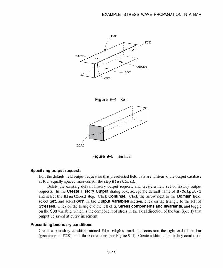
EXAMPLE: STRESS WAVE PROPAGATION IN A BAR
BOT
FRONT
BACK
TOP
FIX
OUT
Figure 9–4 Sets.
LOAD
Figure 9–5 Surface.
Specifying output requests
Edit the default field output request so that preselected field data are written to the output databaseat four equally spaced intervals for the step BlastLoad.
Delete the existing default history output request, and create a new set of history outputrequests. In the Create History Output dialog box, accept the default name of H-Output-1and select the BlastLoad step. Click Continue. Click the arrow next to the Domain field,select Set, and select OUT. In the Output Variables section, click on the triangle to the left ofStresses. Click on the triangle to the left of S, Stress components and invariants, and toggleon the S33 variable, which is the component of stress in the axial direction of the bar. Specify thatoutput be saved at every increment.
Prescribing boundary conditions
Create a boundary condition named Fix right end, and constrain the right end of the bar(geometry set FIX) in all three directions (see Figure 9–1). Create additional boundary conditions
9–13
Abaqus ID:Printed on:
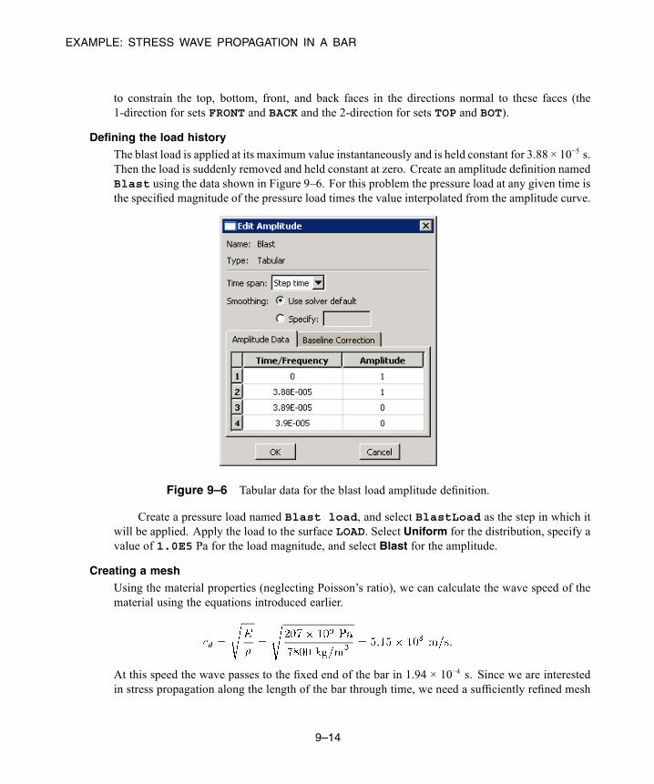
EXAMPLE: STRESS WAVE PROPAGATION IN A BAR
to constrain the top, bottom, front, and back faces in the directions normal to these faces (the1-direction for sets FRONT and BACK and the 2-direction for sets TOP and BOT).
Defining the load history
The blast load is applied at its maximum value instantaneously and is held constant for 3.88 × 10⁻⁵ s.Then the load is suddenly removed and held constant at zero. Create an amplitude definition namedBlast using the data shown in Figure 9–6. For this problem the pressure load at any given time isthe specified magnitude of the pressure load times the value interpolated from the amplitude curve.
Figure 9–6 Tabular data for the blast load amplitude definition.
Create a pressure load named Blast load, and select BlastLoad as the step in which itwill be applied. Apply the load to the surface LOAD. Select Uniform for the distribution, specify avalue of 1.0E5 Pa for the load magnitude, and select Blast for the amplitude.
Creating a mesh
Using the material properties (neglecting Poisson’s ratio), we can calculate the wave speed of thematerial using the equations introduced earlier.
At this speed the wave passes to the fixed end of the bar in 1.94 × 10⁻⁴ s. Since we are interestedin stress propagation along the length of the bar through time, we need a sufficiently refined mesh
9–14
Abaqus ID:Printed on:
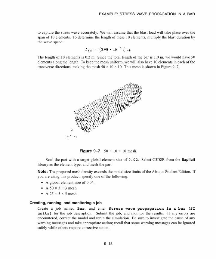
EXAMPLE: STRESS WAVE PROPAGATION IN A BAR
to capture the stress wave accurately. We will assume that the blast load will take place over thespan of 10 elements. To determine the length of these 10 elements, multiply the blast duration bythe wave speed:
The length of 10 elements is 0.2 m. Since the total length of the bar is 1.0 m, we would have 50elements along the length. To keep the mesh uniform, we will also have 10 elements in each of thetransverse directions, making the mesh 50 × 10 × 10. This mesh is shown in Figure 9–7.
1
2
3
Y
XZ
Figure 9–7 50 × 10 × 10 mesh.
Seed the part with a target global element size of 0.02. Select C3D8R from the Explicitlibrary as the element type, and mesh the part.
Note: The proposed mesh density exceeds the model size limits of the Abaqus Student Edition. Ifyou are using this product, specify one of the following:
• A global element size of 0.04.• A 50 × 3 × 3 mesh.• A 25 × 5 × 5 mesh.
Creating, running, and monitoring a job
Create a job named Bar, and enter Stress wave propagation in a bar (SIunits) for the job description. Submit the job, and monitor the results. If any errors areencountered, correct the model and rerun the simulation. Be sure to investigate the cause of anywarning messages and take appropriate action; recall that some warning messages can be ignoredsafely while others require corrective action.
9–15
Abaqus ID:Printed on:

EXAMPLE: STRESS WAVE PROPAGATION IN A BAR
The status (.sta) file
You can also look at the status file, Bar.sta, to monitor the job progress. You can browse or searchthis file by clicking the Status File tab in the Job Monitor. The status file contains informationabout moments of inertia, followed by information concerning the stability limit. The 10 elementswith the lowest stable time limits are listed in rank order.
Most critical elements:Element number Rank Time increment Increment ratio(Instance name)
----------------------------------------------------------1 1 2.237266E-06 1.000000E+00
BAR-110 2 2.237266E-06 1.000000E+00
BAR-121 3 2.237266E-06 1.000000E+00
BAR-130 4 2.237266E-06 1.000000E+00
BAR-131 5 2.237266E-06 1.000000E+00
BAR-140 6 2.237266E-06 1.000000E+00
BAR-151 7 2.237266E-06 1.000000E+00
BAR-160 8 2.237266E-06 1.000000E+00
BAR-161 9 2.237266E-06 1.000000E+00
BAR-170 10 2.237266E-06 1.000000E+00
BAR-1
The status file continues with information about the progress of the solution.
STEP 1 ORIGIN 0.0000
Total memory used for step 1 is approximately 6.8 megabytes.Global time estimation algorithm will be used.Scaling factor : 1.0000Variable mass scaling factor at zero increment: 1.0000
STEP TOTAL CPU STABLE CRITICAL KINETIC TOTALINCREMENT TIME TIME TIME INCREMENT ELEMENT ENERGY ENERGY
0 0.000E+00 0.000E+00 00:00:00 2.237E-06 70 0.000E+00 0.000E+00INSTANCE WITH CRITICAL ELEMENT: BAR-1ODB Field Frame Number 0 of 4 requested intervals at increment zero.
5 1.119E-05 1.119E-05 00:00:00 2.237E-06 70 4.504E-05 -1.963E-0610 2.237E-05 2.237E-05 00:00:00 2.237E-06 2010 9.189E-05 -2.218E-0615 3.471E-05 3.471E-05 00:00:00 2.931E-06 2090 1.434E-04 -2.361E-0619 4.640E-05 4.640E-05 00:00:00 2.910E-06 1040 1.607E-04 1.850E-0621 5.221E-05 5.221E-05 00:00:00 2.902E-06 600 1.588E-04 2.585E-06
ODB Field Frame Number 1 of 4 requested intervals at 5.176230E-0525 6.380E-05 6.380E-05 00:00:00 2.890E-06 590 1.569E-04 6.082E-0729 7.535E-05 7.535E-05 00:00:00 2.880E-06 4640 1.553E-04 -7.049E-0733 8.685E-05 8.685E-05 00:00:00 2.873E-06 4670 1.537E-04 -1.386E-06
Similar information is available in the Job Diagnostics dialog box of the Visualization module.This dialog box also allows you to plot histories of the data, as shown in Figure 9–8. To create a historyplot, select a step from the Job History, select a column in the Incrementation tab, and click Plotselected column.
9–16
Abaqus ID:Printed on:
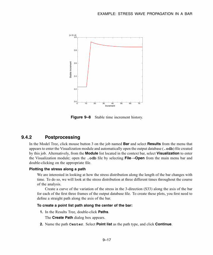
EXAMPLE: STRESS WAVE PROPAGATION IN A BAR
Increment0. 10. 20. 30. 40. 50. 60. 70.
Sta
ble
incr
emen
t
2.0
2.2
2.4
2.6
2.8
3.0[x1.E−6]
Figure 9–8 Stable time increment history.
9.4.2 PostprocessingIn the Model Tree, click mouse button 3 on the job named Bar and select Results from the menu thatappears to enter the Visualization module and automatically open the output database (.odb) file createdby this job. Alternatively, from the Module list located in the context bar, select Visualization to enterthe Visualization module; open the .odb file by selecting File→Open from the main menu bar anddouble-clicking on the appropriate file.
Plotting the stress along a path
We are interested in looking at how the stress distribution along the length of the bar changes withtime. To do so, we will look at the stress distribution at three different times throughout the courseof the analysis.
Create a curve of the variation of the stress in the 3-direction (S33) along the axis of the barfor each of the first three frames of the output database file. To create these plots, you first need todefine a straight path along the axis of the bar.
To create a point list path along the center of the bar:
1. In the Results Tree, double-click Paths.
The Create Path dialog box appears.
2. Name the path Center. Select Point list as the path type, and click Continue.
9–17
Abaqus ID:Printed on:

EXAMPLE: STRESS WAVE PROPAGATION IN A BAR
The Edit Point List Path dialog box appears.
3. In the Point Coordinates table, enter the coordinates of the centers of both ends of the bar.The input specifies a path from the first point to the second point, as defined in the globalcoordinate system of the model.
Note: If you generated the geometry and mesh using the procedure described earlier, the tableentries are 0, 0, 1 and 0, 0, 0. If you used an alternate procedure to generate the bar
geometry, you can use the tool in the Query toolbar to determine the coordinates of thecenters at each end of the bar.
4. When you have finished, click OK to close the Edit Point List Path dialog box.
To save X–Y plots of stress along the path at three different times:
1. In the Results Tree, double-click XYData.
The Create XY Data dialog box appears.
2. Choose Path as the X–Y data source, and click Continue.
The XY Data from Path dialog box appears with the path that you created visible in the listof available paths. If the undeformed model shape is currently displayed, the path you selectis highlighted in the plot.
3. Toggle on Include intersections under Point Locations.
4. Accept True distance as the selection in the X Values region of the dialog box.
5. Click Field Output in the Y Values region of the dialog box to open the Field Output dialogbox.
6. Select the S33 stress component, and click OK.
The field output variable in the XY Data from Path dialog box changes to indicate that stressdata in the 3-direction (S33) will be created.
Note: Abaqus/CAE may warn you that the field output variable will not affect the currentimage. Leave the plot state As is, and click OK to continue.
7. Click Step/Frame in the Y Values region of the XY Data from Path dialog box.
8. In the Step/Frame dialog box that appears, choose frame 1, which is the second of the fiverecorded frames. (The first frame listed, frame 0, is the base state of the model at the beginningof the step.) Click OK.
The Y Values region of the XY Data from Path dialog box changes to indicate that data fromStep 1, frame 1 will be created.
9. To save the X–Y data, click Save As.
The Save XY Data As dialog box appears.
10. Name the X–Y data S33_T1, and click OK.
9–18
Abaqus ID:Printed on:
EXAMPLE: STRESS WAVE PROPAGATION IN A BAR
S33_T1 appears in the XYData container of the Results Tree.
11. Repeat Steps 7 through 9 to create X–Y data for frames 2 and 3. Name the data sets S33_T2and S33_T3, respectively.
12. To close the XY Data from Path dialog box, click Cancel.
To plot the stress curves:
1. In the XYData container, drag the cursor to select all three X–Y data sets.
2. Click mouse button 3, and select Plot from the menu that appears.
Abaqus/CAE plots the stress in the 3-direction along the center of the bar for frames 1, 2, and3, corresponding to approximate simulation times of 5 × 10⁻⁵ s, 1 × 10⁻⁴ s, and 1.5 × 10⁻⁴ s,respectively.
3. Click in the prompt area to cancel the current procedure.
To customize the X–Y plot:
1. Double-click the Y-axis.
The Axis Options dialog box appears. The Y Axis is selected.
2. In the Tick Mode region of the Scale tabbed page, select By increment and specify that theY-axis major tick marks occur at 20E3 Pa increments.
You can also customize the axis titles.
3. Switch to the Title tabbed page.
4. Enter Stress - S33 (Pa) as the Y-axis title.
5. To edit the X-axis, select the axis label in the X Axis field of the dialog box. In the Title tabbedpage of the dialog box, enter Distance along bar (m) as the X-axis title.
6. Click Dismiss to close the Axis Options dialog box.
To customize the appearance of the curves in the X–Y plot:
1. In the Visualization toolbox, click to open the Curve Options dialog box.
2. In the Curves field, select S33_T2.
3. Choose the dotted line style for the S33_T2 curve.
The S33_T2 curve becomes dotted.
4. Repeat Steps 2 and 3 to make the S33_T3 curve dashed.
5. Dismiss the Curve Options dialog box.
9–19
Abaqus ID:Printed on:

EXAMPLE: STRESS WAVE PROPAGATION IN A BAR
The customized plot appears in Figure 9–9. (For clarity, the default grid and legend positionshave been changed.)
S33_T1S33_T2S33_T3
Figure 9–9 Stress (S33) along the bar at three different time instances.
We can see that the length of the bar affected by the stress wave is approximately 0.2 m in eachof the three curves. This distance should correspond to the distance that the blast wave travels duringits time of application, which can be checked by a simple calculation. If the length of the wave front is0.2 m and the wave speed is 5.15 × 10³ m/s, the time it takes for the wave to travel 0.2 m is 3.88 × 10⁻⁵ s.As expected, this is the duration of the blast load that we applied. The stress wave is not exactly squareas it passes along the bar. In particular, there is “ringing” or oscillation of the stress behind the suddenchanges in stress. Linear bulk viscosity, discussed later in this chapter, damps the ringing so that it doesnot affect the results adversely.
Creating a history plot
Another way to study the results is to view the time history of stress at three different points withinthe bar; for example, at distances of 0.25 m, 0.50 m, and 0.75 m from the loaded end of the bar. Todo this, we must first determine the labels of the elements located at these positions. An easy wayto accomplish this is to query the elements in a display group consisting of the elements along theedge of the bar (set OUT).
To query the element labels:
1. In the Results Tree, expand the Element Sets container underneath the output database filenamed Bar.odb. Click mouse button 3 on the set named OUT, and select Replace from themenu that appears.
9–20
Abaqus ID:Printed on:

EXAMPLE: STRESS WAVE PROPAGATION IN A BAR
2. From the main menu bar, select Tools→Query; or use the tool in the Query toolbar.
3. In the Query dialog box that appears, click Element.
4. Click on the elements shaded in Figure 9–10 (every 13th element along the bar). The elementID (label) appears in the prompt area (and also in the message area). Make note of the elementlabels for the three shaded elements.
Figure 9–10 History plot display group.
To plot the stress history:
1. In the Results Tree, click mouse button 3 on History Output and deselect Group Childrenfrom the menu that appears.
2. Select the data for the three elements you have identified (again, every 13th element). Use [Ctrl]+ Click to select multiple X–Y data sets.
3. Click mouse button 3, and select Plot from the menu that appears.
Abaqus/CAE displays an X–Y plot of the longitudinal stress in each element versus time.
4. Click in the prompt area to cancel the current procedure.
As before, you can customize the appearance of the plot.
To customize the X–Y plot:
1. Double-click the X-axis.
The Axis Options dialog box appears.
2. Switch to the Title tabbed page.
9–21
Abaqus ID:Printed on:
EXAMPLE: STRESS WAVE PROPAGATION IN A BAR
3. Specify Total time (s) as the X-axis title.
4. Click Dismiss to close the dialog box.
To customize the appearance of the curves in the X–Y plot:
1. In the Visualization toolbox, click to open the Curve Options dialog box.
2. In theCurves field, select the temporary X–Y data label that corresponds to the element closestto the free end of the bar. (Of the elements in this set, this one is affected first by the stresswave.)
3. Enter S33-0.25 as the curve legend text.
4. In the Curves field, select the temporary X–Y data label that corresponds to the element in themiddle of the bar. (This is the element affected next by the stress wave.)
5. Specify S33-0.5 as the curve legend text, and change the curve style to dotted.
6. In theCurves field, select the temporary X–Y data label that corresponds to the element closestto the fixed end of the bar. (This is the element affected last by the stress wave.)
7. Specify S33-0.75 as the curve legend text, and change the curve style to dashed.
8. Click Dismiss to close the dialog box.
The customized plot appears in Figure 9–11. (For clarity, the default grid and legend positionshave been changed.)
In the history plot we can see that stress at a given point increases as the stress wave travels throughthe point. Once the stress wave has passed completely through the point, the stress at the point oscillatesabout zero.
9.4.3 How the mesh affects the stable time increment and CPU time
In “Automatic time incrementation and stability,” Section 9.3, we discussed howmesh refinement affectsthe stability limit and the CPU time. Here wewill illustrate this effect with the wave propagation problem.We began with a reasonably refined mesh of square elements with 50 elements along the length and10 elements in each of the two transverse directions. For illustrative purposes, we will now use a coarsemesh of 25 × 5 × 5 elements and observe how refining the mesh in the various directions changes theCPU time. The four meshes are shown in Figure 9–12.
9–22
Abaqus ID:Printed on:
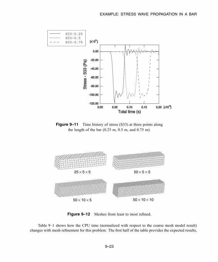
EXAMPLE: STRESS WAVE PROPAGATION IN A BAR
S33-0.25S33-0.5S33-0.75
Figure 9–11 Time history of stress (S33) at three points alongthe length of the bar (0.25 m, 0.5 m, and 0.75 m).
25 × 5 × 5 50 × 5 × 5
50 × 10 × 5 50 × 10 × 10
Figure 9–12 Meshes from least to most refined.
Table 9–1 shows how the CPU time (normalized with respect to the coarse mesh model result)changes with mesh refinement for this problem. The first half of the table provides the expected results,
9–23
Abaqus ID:Printed on:
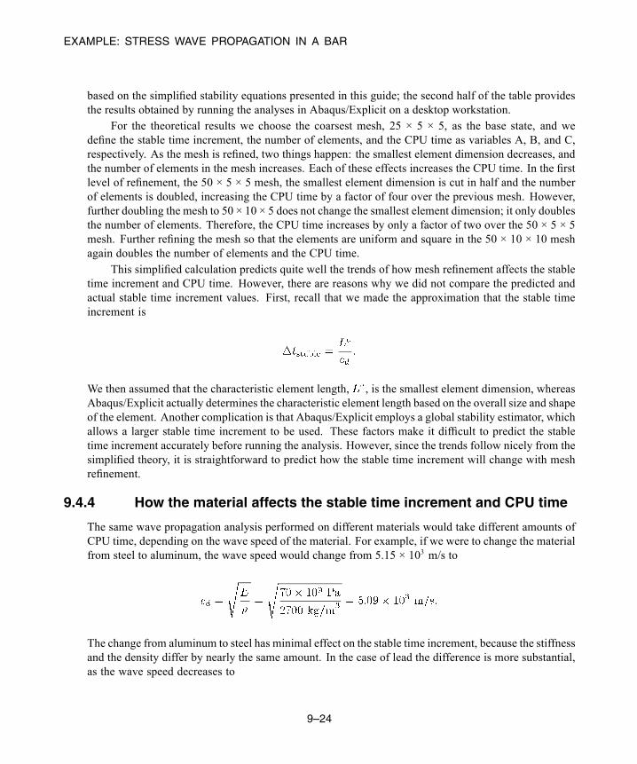
EXAMPLE: STRESS WAVE PROPAGATION IN A BAR
based on the simplified stability equations presented in this guide; the second half of the table providesthe results obtained by running the analyses in Abaqus/Explicit on a desktop workstation.
For the theoretical results we choose the coarsest mesh, 25 × 5 × 5, as the base state, and wedefine the stable time increment, the number of elements, and the CPU time as variables A, B, and C,respectively. As the mesh is refined, two things happen: the smallest element dimension decreases, andthe number of elements in the mesh increases. Each of these effects increases the CPU time. In the firstlevel of refinement, the 50 × 5 × 5 mesh, the smallest element dimension is cut in half and the numberof elements is doubled, increasing the CPU time by a factor of four over the previous mesh. However,further doubling the mesh to 50 × 10 × 5 does not change the smallest element dimension; it only doublesthe number of elements. Therefore, the CPU time increases by only a factor of two over the 50 × 5 × 5mesh. Further refining the mesh so that the elements are uniform and square in the 50 × 10 × 10 meshagain doubles the number of elements and the CPU time.
This simplified calculation predicts quite well the trends of how mesh refinement affects the stabletime increment and CPU time. However, there are reasons why we did not compare the predicted andactual stable time increment values. First, recall that we made the approximation that the stable timeincrement is
We then assumed that the characteristic element length, , is the smallest element dimension, whereasAbaqus/Explicit actually determines the characteristic element length based on the overall size and shapeof the element. Another complication is that Abaqus/Explicit employs a global stability estimator, whichallows a larger stable time increment to be used. These factors make it difficult to predict the stabletime increment accurately before running the analysis. However, since the trends follow nicely from thesimplified theory, it is straightforward to predict how the stable time increment will change with meshrefinement.
9.4.4 How the material affects the stable time increment and CPU time
The same wave propagation analysis performed on different materials would take different amounts ofCPU time, depending on the wave speed of the material. For example, if we were to change the materialfrom steel to aluminum, the wave speed would change from 5.15 × 10³ m/s to
The change from aluminum to steel has minimal effect on the stable time increment, because the stiffnessand the density differ by nearly the same amount. In the case of lead the difference is more substantial,as the wave speed decreases to
9–24
Abaqus ID:Printed on:

DAMPING OF DYNAMIC OSCILLATIONS
which is approximately one-fifth the wave speed of steel. The stable time increment for the lead barwould be five times the stable time increment of our steel bar.
9.5 Damping of dynamic oscillations
There are two reasons for adding damping to a model: to limit numerical oscillations or to add physicaldamping to the system. Abaqus/Explicit provides several methods of introducing damping into theanalysis.
9.5.1 Bulk viscosityBulk viscosity introduces damping associated with volumetric straining. Its purpose is to improve themodeling of high-speed dynamic events. Abaqus/Explicit contains linear and quadratic forms of bulkviscosity. You can modify the default bulk viscosity parameters in the step definition, although it is rarelynecessary to do so. The bulk viscosity pressure is not included in the material point stresses because itis intended as a numerical effect only. As such, it is not considered part of the material’s constitutiveresponse.
Linear bulk viscosity
By default, linear bulk viscosity is always included to damp “ringing” in the highest elementfrequency. It generates a bulk viscosity pressure that is linear in the volumetric strain rate,according to the following equation:
where is a damping coefficient, whose default value is 0.06, is the current material density,is the current dilatational wave speed, is the element characteristic length, and is the
volumetric strain rate.
Quadratic bulk viscosity
Quadratic bulk viscosity is included only in continuum elements (except for the plane stress element,CPS4R) and is applied only if the volumetric strain rate is compressive. The bulk viscosity pressureis quadratic in the strain rate, according to the following equation:
9–25
Abaqus ID:Printed on:
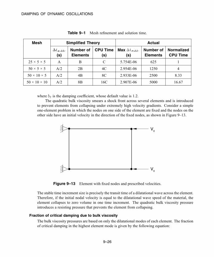
DAMPING OF DYNAMIC OSCILLATIONS
Table 9–1 Mesh refinement and solution time.
Simplified Theory ActualMesh
(s)Number ofElements
CPU Time(s)
Max(s)
Number ofElements
NormalizedCPU Time
25 × 5 × 5 A B C 5.754E-06 625 1
50 × 5 × 5 A/2 2B 4C 2.954E-06 1250 4
50 × 10 × 5 A/2 4B 8C 2.933E-06 2500 8.33
50 × 10 × 10 A/2 8B 16C 2.907E-06 5000 16.67
where is the damping coefficient, whose default value is 1.2.The quadratic bulk viscosity smears a shock front across several elements and is introduced
to prevent elements from collapsing under extremely high velocity gradients. Consider a simpleone-element problem in which the nodes on one side of the element are fixed and the nodes on theother side have an initial velocity in the direction of the fixed nodes, as shown in Figure 9–13.
V0
V0
Figure 9–13 Element with fixed nodes and prescribed velocities.
The stable time increment size is precisely the transit time of a dilatational wave across the element.Therefore, if the initial nodal velocity is equal to the dilatational wave speed of the material, theelement collapses to zero volume in one time increment. The quadratic bulk viscosity pressureintroduces a resisting pressure that prevents the element from collapsing.
Fraction of critical damping due to bulk viscosity
The bulk viscosity pressures are based on only the dilatational modes of each element. The fractionof critical damping in the highest element mode is given by the following equation:
9–26
Abaqus ID:Printed on:

DAMPING OF DYNAMIC OSCILLATIONS
where is the fraction of critical damping. The linear term alone represents 6% of critical damping,whereas the quadratic term is usually much smaller.
9.5.2 Viscous pressure
Viscous pressure loads are commonly used in structural problems and quasi-static problems to damp outthe low-frequency dynamic effects, thus allowing static equilibrium to be reached in a minimal numberof increments. These loads are applied as distributed loads defined by the following formula:
where is the pressure applied to the body; is the viscosity, given on the data line as the magnitude ofthe load; is the velocity vector of the point on the surface where the viscous pressure is being applied;and is the unit outward normal vector to the surface at the same point. For typical structural problemsit is not desirable to absorb all of the energy. Typically, is set equal to a small percentage—perhaps 1or 2 percent—of the quantity as an effective way of minimizing ongoing dynamic effects.
9.5.3 Material damping
The material model itself may provide damping in the form of plastic dissipation or viscoelasticity. Formany applications such damping may be adequate. Another option is to use Rayleigh damping. Thereare two damping factors associated with Rayleigh damping: for mass proportional damping andfor stiffness proportional damping.
Mass proportional damping
The factor defines a damping contribution proportional to the mass matrix for an element. Thedamping forces that are introduced are caused by the absolute velocities of nodes in the model. Theresulting effect can be likened to the model moving through a viscous fluid so that any motion ofany point in the model triggers damping forces. Reasonable mass proportional damping does notreduce the stability limit significantly.
Stiffness proportional damping
The factor defines damping proportional to the elastic material stiffness. A “damping stress,”, proportional to the total strain rate is introduced, using the following formula:
9–27
Abaqus ID:Printed on:
ENERGY BALANCE
where is the strain rate. For hyperelastic and hyperfoam materials is defined as the initialelastic stiffness. For all other materials is the material’s current elastic stiffness. This dampingstress is added to the stress caused by the constitutive response at the integration point when thedynamic equilibrium equations are formed, but it is not included in the stress output. Dampingcan be introduced for any nonlinear analysis and provides standard Rayleigh damping for linearanalyses. For a linear analysis stiffness proportional damping is exactly the same as defining adamping matrix equal to times the stiffness matrix. Stiffness proportional damping must beused with caution because it may significantly reduce the stability limit. To avoid a dramatic dropin the stable time increment, the stiffness proportional damping factor, , should be less than orof the same order of magnitude as the initial stable time increment without damping.
9.5.4 Discrete dashpots
Yet another option is to define individual dashpot elements. Each dashpot element provides a dampingforce proportional to the relative velocity of its two nodes. The advantage of this approach is that itenables you to apply damping only at points where you decide it is necessary. Dashpots always shouldbe used in parallel with other elements, such as springs or trusses, so that they do not cause a significantreduction in the stability limit.
9.6 Energy balance
Energy output is often an important part of an Abaqus/Explicit analysis. Comparisons between variousenergy components can be used to help evaluate whether an analysis is yielding an appropriate response.
9.6.1 Statement of energy balance
An energy balance for the entire model can be written as
where is the internal energy, is the viscous energy dissipated, is the frictional energydissipated, is the kinetic energy, is the internal heat energy, is the work done bythe externally applied loads, and , , and are the work done by contact penalties, byconstraint penalties, and by propelling added mass, respectively. is the external heat energythrough external fluxes. The sum of these energy components is , which should be constant. Inthe numerical model is only approximately constant, generally with an error of less than 1%.
9–28
Abaqus ID:Printed on:

ENERGY BALANCE
Internal energy
The internal energy is the sum of the recoverable elastic strain energy, ; the energy dissipatedthrough inelastic processes such as plasticity, ; the energy dissipated through viscoelasticity orcreep, ; the artificial strain energy, ; the energy dissipated through damage, ; theenergy dissipated through distortion control, ; and the fluid cavity energy, :
The artificial strain energy includes energy stored in hourglass resistances and transverse shear inshell and beam elements. Large values of artificial strain energy indicate that mesh refinement orother changes to the mesh are necessary.
Viscous energy
The viscous energy is the energy dissipated by damping mechanisms, including bulk viscositydamping and material damping. A fundamental variable in the global energy balance, viscousenergy is not part of the energy dissipated through viscoelasticity or inelastic processes.
External work of applied forces
The external work is integrated forward continuously, defined entirely by nodal forces (moments)and displacements (rotations). Prescribed boundary conditions also contribute to the external work.
9.6.2 Output of the energy balanceEach of the energy quantities can be requested as output and can be plotted as time histories summed overthe entire model, particular element sets, individual elements, or as energy density within each element.The variable names associated with the energy quantities summed over the entire model or element setsare as listed in Table 9–2.
Table 9–2 Whole model energy output variables.
Variable Name Energy Quantity
ALLIE Internal energy, : ALLIE = ALLSE + ALLPD + ALLCD + ALLAE +ALLDMD + ALLDC + ALLFC.
ALLKE Kinetic energy, .
ALLVD Viscous dissipated energy, .
ALLFD Frictional dissipated energy, .
ALLCD Energy dissipated by viscoelasticity, .
ALLWK Work of the external forces, .
9–29
Abaqus ID:Printed on:

ENERGY BALANCE
Variable Name Energy Quantity
ALLPW Work done by contact penalties, .
ALLCW Work done by constraint penalties, .
ALLMW Work done by propelling added mass (due to mass scaling), .
ALLSE Elastic strain energy, .
ALLPD Inelastic dissipated energy, .
ALLAE Artificial strain energy, .
ALLIHE Internal heat energy, .
ALLHF External heat energy through external fluxes, .
ALLDMD Energy dissipated by damage, .
ALLDC Energy dissipated by distortion control, .
ALLFC Fluid cavity energy (negative of work done by fluid cavities), .
ETOTAL Energy balance:.
In addition, Abaqus/Explicit can produce element-level energy output and energy density output, as listedin Table 9–3.
Table 9–3 Whole element energy output variables.
Variable Name Whole Element Energy Quantity
ELSE Elastic strain energy.
ELPD Plastic dissipated energy.
ELCD Creep dissipated energy.
ELVD Viscous dissipated energy.
ELASE Artificial energy = drill energy + hourglass energy.
EKEDEN Kinetic energy density in the element.
ESEDEN Elastic strain energy density in the element.
EPDDEN Plastic energy density dissipated in the element.
EASEDEN Artificial strain energy density in the element.
ECDDEN Creep strain energy density dissipated in the element.
9–30
Abaqus ID:Printed on:
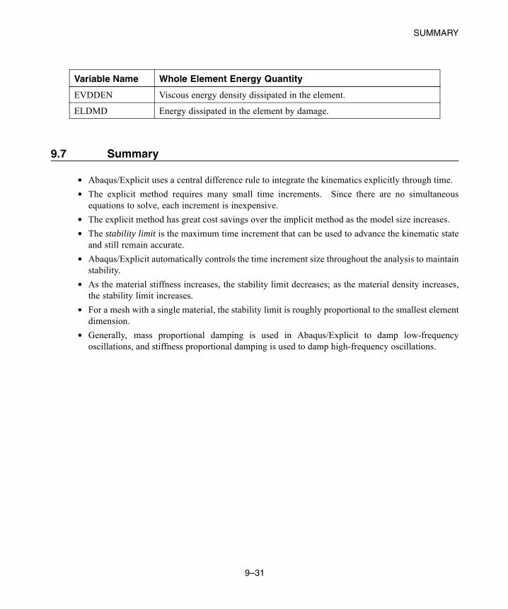
SUMMARY
Variable Name Whole Element Energy Quantity
EVDDEN Viscous energy density dissipated in the element.
ELDMD Energy dissipated in the element by damage.
9.7 Summary
• Abaqus/Explicit uses a central difference rule to integrate the kinematics explicitly through time.• The explicit method requires many small time increments. Since there are no simultaneousequations to solve, each increment is inexpensive.
• The explicit method has great cost savings over the implicit method as the model size increases.• The stability limit is the maximum time increment that can be used to advance the kinematic stateand still remain accurate.
• Abaqus/Explicit automatically controls the time increment size throughout the analysis to maintainstability.
• As the material stiffness increases, the stability limit decreases; as the material density increases,the stability limit increases.
• For a mesh with a single material, the stability limit is roughly proportional to the smallest elementdimension.
• Generally, mass proportional damping is used in Abaqus/Explicit to damp low-frequencyoscillations, and stiffness proportional damping is used to damp high-frequency oscillations.
9–31
Abaqus ID:Printed on:

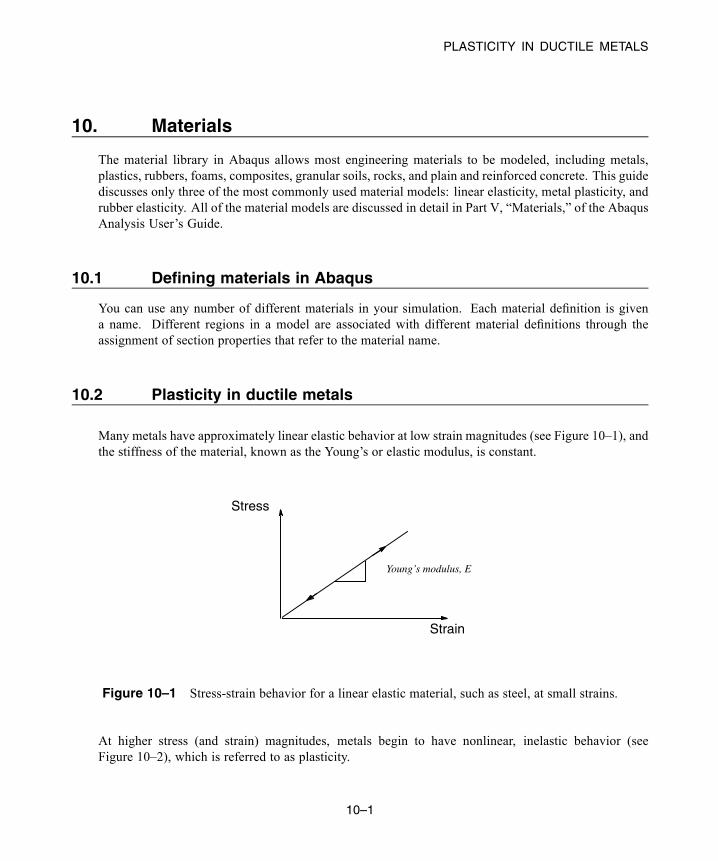
PLASTICITY IN DUCTILE METALS
10. Materials
The material library in Abaqus allows most engineering materials to be modeled, including metals,plastics, rubbers, foams, composites, granular soils, rocks, and plain and reinforced concrete. This guidediscusses only three of the most commonly used material models: linear elasticity, metal plasticity, andrubber elasticity. All of the material models are discussed in detail in Part V, “Materials,” of the AbaqusAnalysis User’s Guide.
10.1 Defining materials in Abaqus
You can use any number of different materials in your simulation. Each material definition is givena name. Different regions in a model are associated with different material definitions through theassignment of section properties that refer to the material name.
10.2 Plasticity in ductile metals
Many metals have approximately linear elastic behavior at low strain magnitudes (see Figure 10–1), andthe stiffness of the material, known as the Young’s or elastic modulus, is constant.
Strain
Stress
Young’s modulus, E
Figure 10–1 Stress-strain behavior for a linear elastic material, such as steel, at small strains.
At higher stress (and strain) magnitudes, metals begin to have nonlinear, inelastic behavior (seeFigure 10–2), which is referred to as plasticity.
10–1
Abaqus ID:Printed on:

PLASTICITY IN DUCTILE METALS
Nominal strain
Nom
inal
str
ess
Young’s modulus, E
Yield pointHardening
Ultimate strength
Necking
Failure
Unloading curveParallel to Young's modulus
1
Figure 10–2 Nominal stress-strain behavior of an elastic-plastic material in a tensile test.
10.2.1 Characteristics of plasticity in ductile metalsThe plastic behavior of a material is described by its yield point and its post-yield hardening. The shiftfrom elastic to plastic behavior occurs at a certain point, known as the elastic limit or yield point, on amaterial’s stress-strain curve (see Figure 10–2). The stress at the yield point is called the yield stress. Inmost metals the initial yield stress is 0.05 to 0.1% of the material’s elastic modulus.
The deformation of the metal prior to reaching the yield point creates only elastic strains, which arefully recovered if the applied load is removed. However, once the stress in the metal exceeds the yieldstress, permanent (inelastic) deformation begins to occur. The strains associated with this permanentdeformation are called plastic strains. Both elastic and plastic strains accumulate as the metal deformsin the post-yield region.
The stiffness of a metal typically decreases dramatically once the material yields (see Figure 10–2).A ductile metal that has yielded will recover its initial elastic stiffness when the applied load is removed(see Figure 10–2). Often the plastic deformation of the material increases its yield stress for subsequentloadings: this behavior is called work hardening.
Another important feature of metal plasticity is that the inelastic deformation is associated withnearly incompressible material behavior. Modeling this effect places some severe restrictions on thetype of elements that can be used in elastic-plastic simulations.
A metal deforming plastically under a tensile load may experience highly localized extension andthinning, called necking, as the material fails (see Figure 10–2). The engineering stress (force per unitundeformed area) in the metal is known as the nominal stress, with the conjugate nominal strain (length
10–2
Abaqus ID:Printed on:

PLASTICITY IN DUCTILE METALS
change per unit undeformed length). The nominal stress in the metal as it is necking is much lower thanthe material’s ultimate strength. This material behavior is caused by the geometry of the test specimen,the nature of the test itself, and the stress and strain measures used. For example, testing the samematerialin compression produces a stress-strain plot that does not have a necking region because the specimenis not going to thin as it deforms under compressive loads. A mathematical model describing the plasticbehavior of metals should be able to account for differences in the compressive and tensile behaviorindependent of the structure’s geometry or the nature of the applied loads. This goal can be accomplishedif the familiar definitions of nominal stress, , and nominal strain, , where the subscript 0indicates a value from the undeformed state of the material, are replaced by new measures of stress andstrain that account for the change in area during the finite deformations.
10.2.2 Stress and strain measures for finite deformations
Strains in compression and tension are the same only if considered in the limit as ; i.e.,
and
where l is the current length, is the original length, and is the true strain or logarithmic strain.The stress measure that is the conjugate to the true strain is called the true stress and is defined as
where F is the force in the material and A is the current area. A ductile metal subjected to finitedeformations will have the same stress-strain behavior in tension and compression if true stress isplotted against true strain.
10.2.3 Defining plasticity in Abaqus
When defining plasticity data in Abaqus, you must use true stress and true strain. Abaqus requires thesevalues to interpret the data correctly.
Quite often material test data are supplied using values of nominal stress and strain. In suchsituations you must use the expressions presented below to convert the plastic material data fromnominal stress-strain values to true stress-strain values.
10–3
Abaqus ID:Printed on:
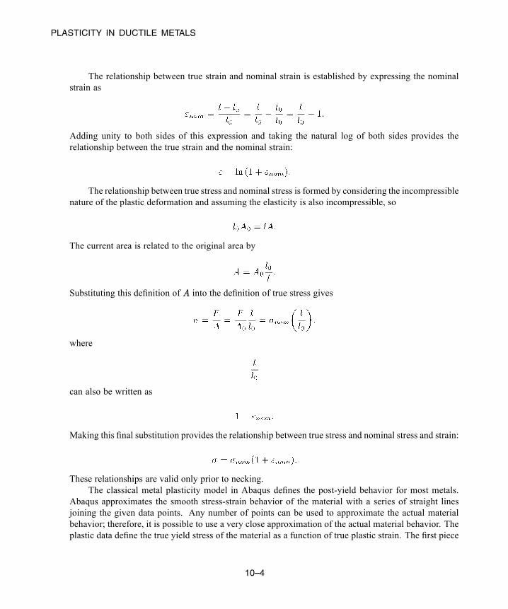
PLASTICITY IN DUCTILE METALS
The relationship between true strain and nominal strain is established by expressing the nominalstrain as
Adding unity to both sides of this expression and taking the natural log of both sides provides therelationship between the true strain and the nominal strain:
The relationship between true stress and nominal stress is formed by considering the incompressiblenature of the plastic deformation and assuming the elasticity is also incompressible, so
The current area is related to the original area by
Substituting this definition of A into the definition of true stress gives
where
can also be written as
Making this final substitution provides the relationship between true stress and nominal stress and strain:
These relationships are valid only prior to necking.The classical metal plasticity model in Abaqus defines the post-yield behavior for most metals.
Abaqus approximates the smooth stress-strain behavior of the material with a series of straight linesjoining the given data points. Any number of points can be used to approximate the actual materialbehavior; therefore, it is possible to use a very close approximation of the actual material behavior. Theplastic data define the true yield stress of the material as a function of true plastic strain. The first piece
10–4
Abaqus ID:Printed on:
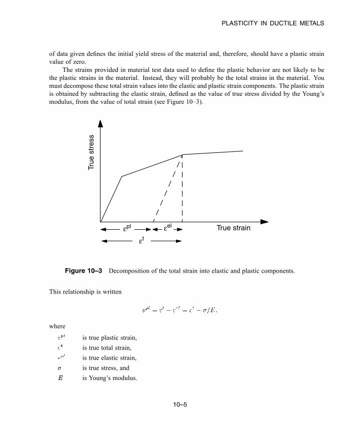
PLASTICITY IN DUCTILE METALS
of data given defines the initial yield stress of the material and, therefore, should have a plastic strainvalue of zero.
The strains provided in material test data used to define the plastic behavior are not likely to bethe plastic strains in the material. Instead, they will probably be the total strains in the material. Youmust decompose these total strain values into the elastic and plastic strain components. The plastic strainis obtained by subtracting the elastic strain, defined as the value of true stress divided by the Young’smodulus, from the value of total strain (see Figure 10–3).
εpl
εt
εel
True
str
ess
True strain
Figure 10–3 Decomposition of the total strain into elastic and plastic components.
This relationship is written
where
is true plastic strain,
is true total strain,
is true elastic strain,
is true stress, and
E is Young’s modulus.
10–5
Abaqus ID:Printed on:
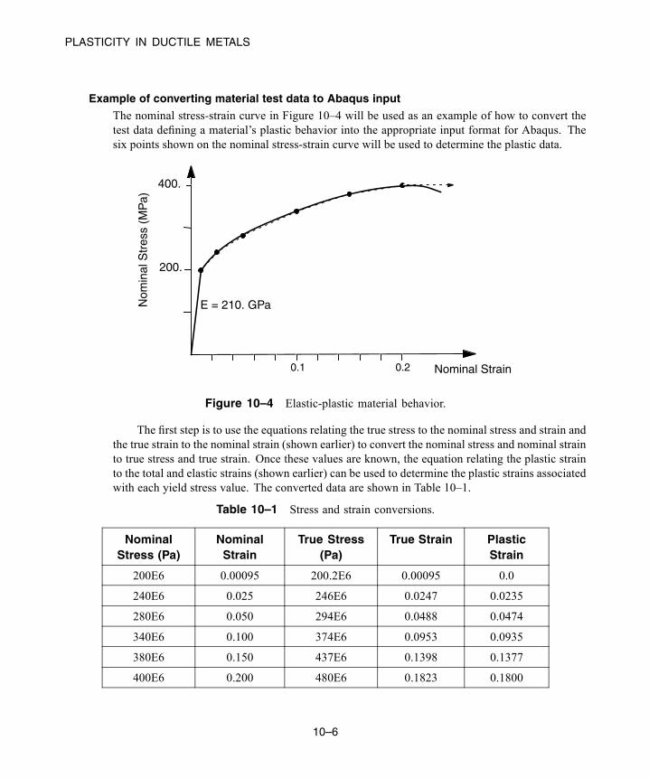
PLASTICITY IN DUCTILE METALS
Example of converting material test data to Abaqus input
The nominal stress-strain curve in Figure 10–4 will be used as an example of how to convert thetest data defining a material’s plastic behavior into the appropriate input format for Abaqus. Thesix points shown on the nominal stress-strain curve will be used to determine the plastic data.
E = 210. GPa
Nominal Strain
Nom
inal
Str
ess
(MP
a)
200.
0.1 0.2
400.
Figure 10–4 Elastic-plastic material behavior.
The first step is to use the equations relating the true stress to the nominal stress and strain andthe true strain to the nominal strain (shown earlier) to convert the nominal stress and nominal strainto true stress and true strain. Once these values are known, the equation relating the plastic strainto the total and elastic strains (shown earlier) can be used to determine the plastic strains associatedwith each yield stress value. The converted data are shown in Table 10–1.
Table 10–1 Stress and strain conversions.
NominalStress (Pa)
NominalStrain
True Stress(Pa)
True Strain PlasticStrain
200E6 0.00095 200.2E6 0.00095 0.0
240E6 0.025 246E6 0.0247 0.0235
280E6 0.050 294E6 0.0488 0.0474
340E6 0.100 374E6 0.0953 0.0935
380E6 0.150 437E6 0.1398 0.1377
400E6 0.200 480E6 0.1823 0.1800
10–6
Abaqus ID:Printed on:
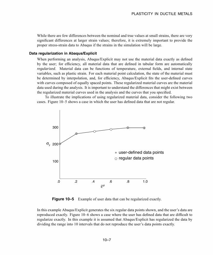
PLASTICITY IN DUCTILE METALS
While there are few differences between the nominal and true values at small strains, there are verysignificant differences at larger strain values; therefore, it is extremely important to provide theproper stress-strain data to Abaqus if the strains in the simulation will be large.
Data regularization in Abaqus/Explicit
When performing an analysis, Abaqus/Explicit may not use the material data exactly as definedby the user; for efficiency, all material data that are defined in tabular form are automaticallyregularized. Material data can be functions of temperature, external fields, and internal statevariables, such as plastic strain. For each material point calculation, the state of the material mustbe determined by interpolation, and, for efficiency, Abaqus/Explicit fits the user-defined curveswith curves composed of equally spaced points. These regularized material curves are the materialdata used during the analysis. It is important to understand the differences that might exist betweenthe regularized material curves used in the analysis and the curves that you specified.
To illustrate the implications of using regularized material data, consider the following twocases. Figure 10–5 shows a case in which the user has defined data that are not regular.
300
200
100
.0 .2 .4 .6 .8 1.0
σy
user-defined data pointsregular data points
∗
εpl
∗∗∗
∗
Figure 10–5 Example of user data that can be regularized exactly.
In this example Abaqus/Explicit generates the six regular data points shown, and the user’s data arereproduced exactly. Figure 10–6 shows a case where the user has defined data that are difficult toregularize exactly. In this example it is assumed that Abaqus/Explicit has regularized the data bydividing the range into 10 intervals that do not reproduce the user’s data points exactly.
10–7
Abaqus ID:Printed on:
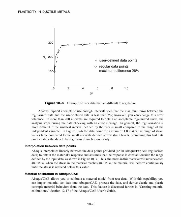
PLASTICITY IN DUCTILE METALS
300
200
100
.0 .2 .4 .6 .8 1.0
σy∗
∗
∗
∗
εpl
user-defined data points
regular data pointsmaximum difference 26%
∗
Figure 10–6 Example of user data that are difficult to regularize.
Abaqus/Explicit attempts to use enough intervals such that the maximum error between theregularized data and the user-defined data is less than 3%; however, you can change this errortolerance. If more than 200 intervals are required to obtain an acceptable regularized curve, theanalysis stops during the data checking with an error message. In general, the regularization ismore difficult if the smallest interval defined by the user is small compared to the range of theindependent variable. In Figure 10–6 the data point for a strain of 1.0 makes the range of strainvalues large compared to the small intervals defined at low strain levels. Removing this last datapoint enables the data to be regularized much more easily.
Interpolation between data points
Abaqus interpolates linearly between the data points provided (or, in Abaqus/Explicit, regularizeddata) to obtain the material’s response and assumes that the response is constant outside the rangedefined by the input data, as shown in Figure 10–7. Thus, the stress in this material will never exceed480 MPa; when the stress in the material reaches 480 MPa, the material will deform continuouslyuntil the stress is reduced below this value.
Material calibration in Abaqus/CAE
Abaqus/CAE allows you to calibrate a material model from test data. With this capability, youcan import material test data into Abaqus/CAE, process the data, and derive elastic and plasticisotropic material behaviors from the data. This feature is discussed further in “Creating materialcalibrations,” Section 12.17 of the Abaqus/CAE User’s Guide.
10–8
Abaqus ID:Printed on:

SELECTING ELEMENTS FOR ELASTIC-PLASTIC PROBLEMS
Figure 10–7 Material curve used by Abaqus.
10.3 Selecting elements for elastic-plastic problems
The incompressible nature of plastic deformation in metals places limitations on the types of elementsthat can be used for an elastic-plastic simulation. The limitations arise because modeling incompressiblematerial behavior adds kinematic constraints to an element; in this case the limitations constrain thevolume at the element’s integration points to remain constant. In certain classes of elements the additionof these incompressibility constraints makes the element overconstrained. When these elements cannotresolve all of these constraints, they suffer from volumetric locking, which causes their response to betoo stiff. Volumetric locking is indicated by a rapid variation of hydrostatic pressure stress from elementto element or integration point to integration point.
The fully integrated, second-order, solid elements available in Abaqus/Standard are very susceptibleto volumetric locking when modeling incompressible material behavior and, therefore, should not beused in elastic-plastic simulations. The fully integrated, first-order, solid elements in Abaqus/Standarddo not suffer from volumetric locking because Abaqus actually uses a constant volume strain in theseelements. Thus, they can be used safely in plasticity problems.
Reduced-integration solid elements have fewer integration points at which the incompressibilityconstraints must be satisfied. Therefore, they are not overconstrained and can be used for most elastic-plastic simulations. The second-order reduced-integration elements in Abaqus/Standard should be usedwith caution if the strains exceed 20–40% because at this magnitude they can suffer from volumetriclocking. This effect can be reduced with mesh refinement.
10–9
Abaqus ID:Printed on:
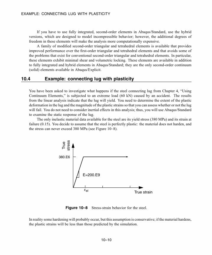
EXAMPLE: CONNECTING LUG WITH PLASTICITY
If you have to use fully integrated, second-order elements in Abaqus/Standard, use the hybridversions, which are designed to model incompressible behavior; however, the additional degrees offreedom in these elements will make the analysis more computationally expensive.
A family of modified second-order triangular and tetrahedral elements is available that providesimproved performance over the first-order triangular and tetrahedral elements and that avoids some ofthe problems that exist for conventional second-order triangular and tetrahedral elements. In particular,these elements exhibit minimal shear and volumetric locking. These elements are available in additionto fully integrated and hybrid elements in Abaqus/Standard; they are the only second-order continuum(solid) elements available in Abaqus/Explicit.
10.4 Example: connecting lug with plasticity
You have been asked to investigate what happens if the steel connecting lug from Chapter 4, “UsingContinuum Elements,” is subjected to an extreme load (60 kN) caused by an accident. The resultsfrom the linear analysis indicate that the lug will yield. You need to determine the extent of the plasticdeformation in the lug and themagnitude of the plastic strains so that you can assess whether or not the lugwill fail. You do not need to consider inertial effects in this analysis; thus, you will use Abaqus/Standardto examine the static response of the lug.
The only inelastic material data available for the steel are its yield stress (380 MPa) and its strain atfailure (0.15). You decide to assume that the steel is perfectly plastic: the material does not harden, andthe stress can never exceed 380 MPa (see Figure 10–8).
380.E6
True strain
True
stre
ss
εel
E=200.E9
Figure 10–8 Stress-strain behavior for the steel.
In reality some hardening will probably occur, but this assumption is conservative; if the material hardens,the plastic strains will be less than those predicted by the simulation.
10–10
Abaqus ID:Printed on:
EXAMPLE: CONNECTING LUG WITH PLASTICITY
Abaqus provides scripts that replicate the complete analysis model for this problem. Run one ofthese scripts if you encounter difficulties following the instructions given below or if you wish to checkyour work. Scripts are available in the following locations:
• A Python script for this example is provided in “Connecting lug with plasticity,” Section A.8, in theHTML version of this guide. Instructions on how to fetch the script and run it within Abaqus/CAEare given in Appendix A, “Example Files.”
• A plug-in script for this example is available in the Abaqus/CAE Plug-in toolset. To run the scriptfrom Abaqus/CAE, select Plug-ins→Abaqus→Getting Started; highlight Connecting lugwith plasticity; and click Run. For more information about the Getting Started plug-ins, see“Running the Getting Started with Abaqus examples,” Section 82.1 of the Abaqus/CAE User’sGuide, in the HTML version of this guide.
10.4.1 Modifications to the model
Open the model database file Lug.cae, and copy the model Elastic to a model named Plastic.
Material definition
For the Plasticmodel, you will specify the post-yield behavior of the material using the classicalmetal plasticity model in Abaqus. The initial yield stress at zero plastic strain is 380 MPa. Sinceyou are modeling the steel as perfectly plastic, no other yield stresses are required. You will performa general, nonlinear simulation because of the nonlinear material behavior in the model.
To add plasticity data to the material model:
1. In the Model Tree, expand the Materials container and double-click Steel.
2. In the material editor, select Mechanical→Plasticity→Plastic to invoke the classical metalplasticity model. Enter an initial yield stress of 380.E6 with a corresponding initial plasticstrain of 0.0.
Step definition and output requests
Edit the step definition and output requests. In the Basic tabbed page of the Edit Step dialog box,accept the total time period of 1.0 and assume that the effects of geometric nonlinearity will notbe important in this simulation. In the Incrementation tabbed page, specify an initial incrementsize that is 20% of the total step time (0.2). This simulation is a static analysis of the lug underextreme loads; you do not know in advance how many increments this simulation may require. Thedefault maximum of 100 increments, however, is reasonably large and should be sufficient for thisanalysis.
Open the Field Output Requests Manager. Edit the current output request to request thepreselected defaults at every increment.
10–11
Abaqus ID:Printed on:

EXAMPLE: CONNECTING LUG WITH PLASTICITY
Loading
The load applied in this simulation is twice what was applied in the linear elastic simulation ofthe lug (60 kN vs. 30 kN). Therefore, in the Model Tree, double-click Pressure load underneaththe Loads container, and double the magnitude of the pressure applied to the lug (i.e., change themagnitude to 10.0E7).
Job definition
In the Model Tree, create a job named PlasticLugNoHard, and enter the following jobdescription: Elastic-Plastic Steel Connecting Lug. Remember to save your modeldatabase file.
Submit the job for analysis, and monitor the solution progress. Correct any modeling errors,and investigate the source of any warning messages. This analysis should terminate prematurely;the reasons are discussed in the following section.
10.4.2 Job monitor and diagnosticsYou can monitor the progress of your analysis while it is running by looking at the Job Monitor.
Job Monitor
When Abaqus/Standard has finished the simulation, the Job Monitor will contain informationsimilar to that shown in Figure 10–9.
Figure 10–9 Job Monitor: perfectly plastic connecting lug.
10–12
Abaqus ID:Printed on:
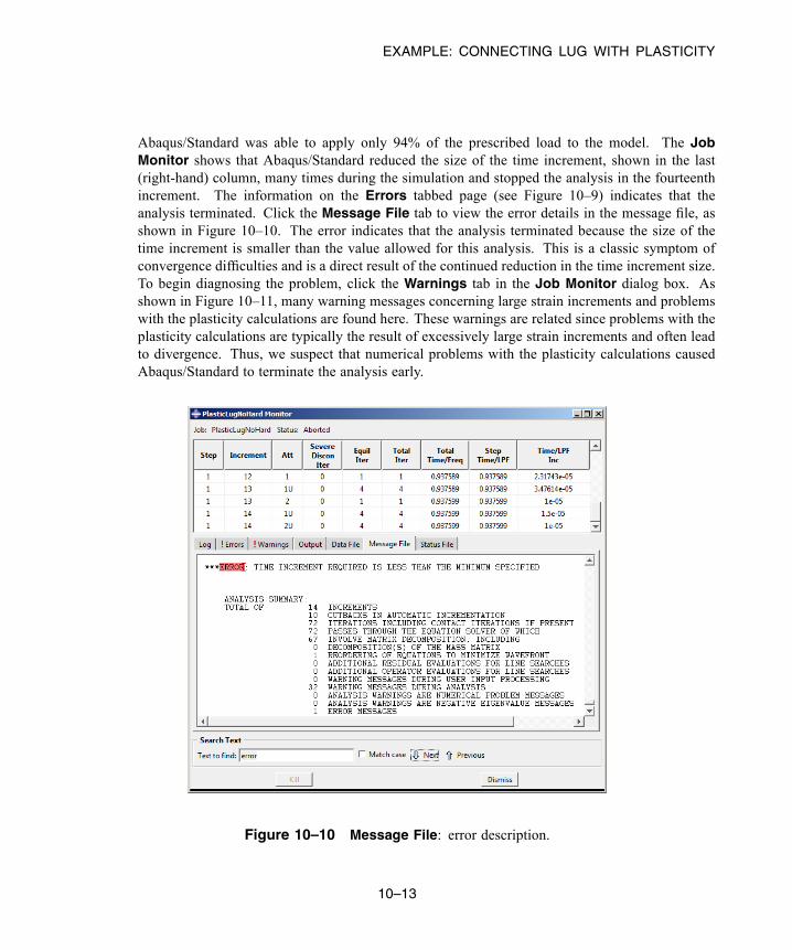
EXAMPLE: CONNECTING LUG WITH PLASTICITY
Abaqus/Standard was able to apply only 94% of the prescribed load to the model. The JobMonitor shows that Abaqus/Standard reduced the size of the time increment, shown in the last(right-hand) column, many times during the simulation and stopped the analysis in the fourteenthincrement. The information on the Errors tabbed page (see Figure 10–9) indicates that theanalysis terminated. Click the Message File tab to view the error details in the message file, asshown in Figure 10–10. The error indicates that the analysis terminated because the size of thetime increment is smaller than the value allowed for this analysis. This is a classic symptom ofconvergence difficulties and is a direct result of the continued reduction in the time increment size.To begin diagnosing the problem, click the Warnings tab in the Job Monitor dialog box. Asshown in Figure 10–11, many warning messages concerning large strain increments and problemswith the plasticity calculations are found here. These warnings are related since problems with theplasticity calculations are typically the result of excessively large strain increments and often leadto divergence. Thus, we suspect that numerical problems with the plasticity calculations causedAbaqus/Standard to terminate the analysis early.
Figure 10–10 Message File: error description.
10–13
Abaqus ID:Printed on:
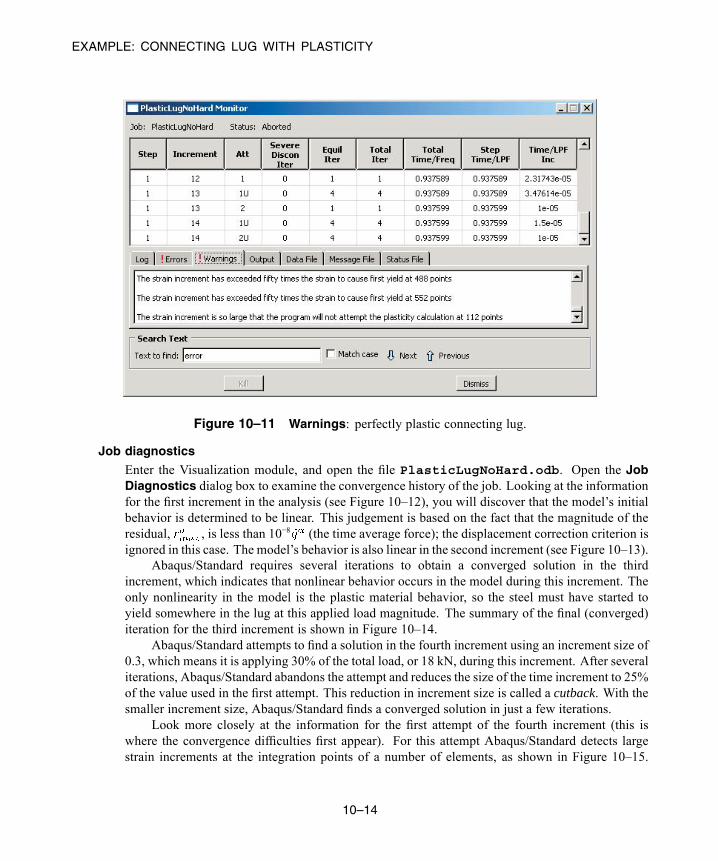
EXAMPLE: CONNECTING LUG WITH PLASTICITY
Figure 10–11 Warnings: perfectly plastic connecting lug.
Job diagnostics
Enter the Visualization module, and open the file PlasticLugNoHard.odb. Open the JobDiagnostics dialog box to examine the convergence history of the job. Looking at the informationfor the first increment in the analysis (see Figure 10–12), you will discover that the model’s initialbehavior is determined to be linear. This judgement is based on the fact that the magnitude of theresidual, , is less than 10−8 (the time average force); the displacement correction criterion isignored in this case. The model’s behavior is also linear in the second increment (see Figure 10–13).
Abaqus/Standard requires several iterations to obtain a converged solution in the thirdincrement, which indicates that nonlinear behavior occurs in the model during this increment. Theonly nonlinearity in the model is the plastic material behavior, so the steel must have started toyield somewhere in the lug at this applied load magnitude. The summary of the final (converged)iteration for the third increment is shown in Figure 10–14.
Abaqus/Standard attempts to find a solution in the fourth increment using an increment size of0.3, which means it is applying 30% of the total load, or 18 kN, during this increment. After severaliterations, Abaqus/Standard abandons the attempt and reduces the size of the time increment to 25%of the value used in the first attempt. This reduction in increment size is called a cutback. With thesmaller increment size, Abaqus/Standard finds a converged solution in just a few iterations.
Look more closely at the information for the first attempt of the fourth increment (this iswhere the convergence difficulties first appear). For this attempt Abaqus/Standard detects largestrain increments at the integration points of a number of elements, as shown in Figure 10–15.
10–14
Abaqus ID:Printed on:
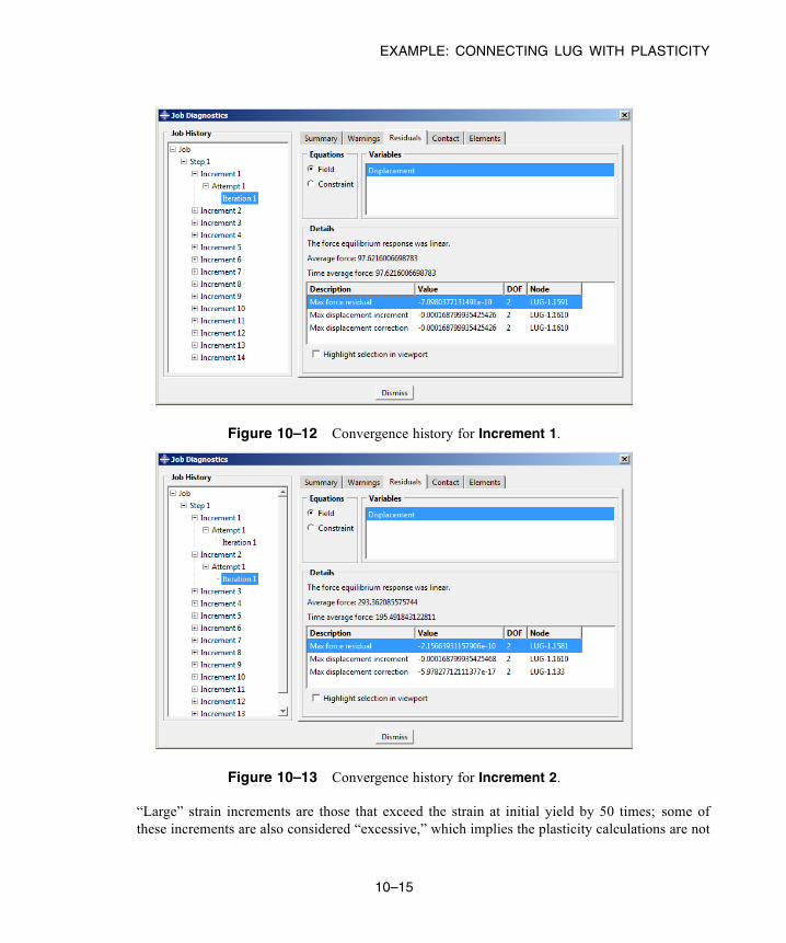
EXAMPLE: CONNECTING LUG WITH PLASTICITY
Figure 10–12 Convergence history for Increment 1.
Figure 10–13 Convergence history for Increment 2.
“Large” strain increments are those that exceed the strain at initial yield by 50 times; some ofthese increments are also considered “excessive,” which implies the plasticity calculations are not
10–15
Abaqus ID:Printed on:
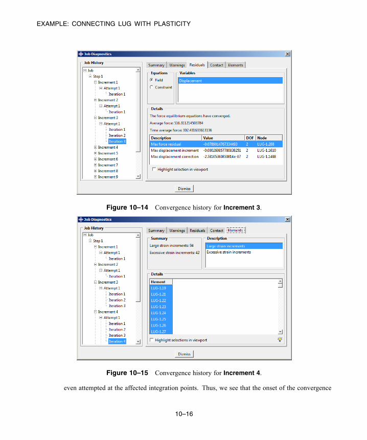
EXAMPLE: CONNECTING LUG WITH PLASTICITY
Figure 10–14 Convergence history for Increment 3.
Figure 10–15 Convergence history for Increment 4.
even attempted at the affected integration points. Thus, we see that the onset of the convergence
10–16
Abaqus ID:Printed on:
EXAMPLE: CONNECTING LUG WITH PLASTICITY
difficulties is directly related to the large strain increments and problems with the plasticitycalculations.
Abaqus/Standard encounters renewed convergence difficulties in subsequent increments untilfinally it terminates the job. In many of these increments Abaqus/Standard cuts back the timeincrement size because the strain increments are so large that the plasticity calculations are noteven performed. Thus, we conclude the overall convergence difficulties are indeed the result ofnumerical problems with the plasticity calculations.
This check on the magnitude of the total strain increment is an example of the many automaticsolution controls Abaqus/Standard uses to ensure that the solution obtained for your simulation isboth accurate and efficient. The automatic solution controls are suitable for almost all simulations.Therefore, you do not have to worry about providing parameters to control the solution algorithm:you only have to be concerned with the input data for your model.
An interesting observation is made using the Job Diagnostics dialog box: in virtually allattempts where convergence problems are encountered, the elements with large or excessive strainincrements are in the vicinity of the built-in end of the lug (where yielding begins) while the nodewith the largest displacement correction is in the vicinity of the loaded end of the lug. This impliesthat the loaded end wants to deform more than the built-in end can support. Deformed model shapeplots can help you pursue this observation further.
10.4.3 Postprocessing the results
Look at the results in the Visualization module to understand what caused the excessive plasticity.
Plotting the deformed model shape
Create a plot of the model’s deformed shape, and check that this shape is realistic.The default view is isometric. You can set the view shown in Figure 10–16 by using the options
in the View menu or the tools in the View Manipulation toolbar; in this figure perspective is alsoturned off.
The displacements and, particularly, the rotations of the lug shown in the plot are large but donot seem large enough to have caused all of the numerical problems seen in the simulation. Lookclosely at the information in the plot’s title for an explanation. The deformation scale factor used inthis plot is 0.02; i.e., the displacements are scaled to 2% of their actual values. (Your deformationscale factor may be different.)
Abaqus/CAE always scales the displacements in a geometrically linear simulation such that thedeformed shape of the model fits into the viewport. (This is in contrast to a geometrically nonlinearsimulation, where Abaqus/CAE does not scale the displacements and, instead, adjusts the view byzooming in or out to fit the deformed shape in the plot.) To plot the actual displacements, set thedeformation scale factor to 1.0. This will produce a plot of the model in which the lug has deformeduntil it is almost parallel to the vertical (global Y) axis.
The applied load of 60 kN exceeds the limit load of the lug, and the lug collapses when thematerial yields at all the integration points through its thickness. The lug then has no stiffness to
10–17
Abaqus ID:Printed on:

EXAMPLE: CONNECTING LUG WITH PLASTICITY
Step: LugLoad, Apply uniform pressure to the holeIncrement 13: Step Time = 0.9376
Deformed Var: U Deformation Scale Factor: +2.000e-02
1
2
3
Figure 10–16 Deformed model shape using results for the simulation without hardening.
resist further deformation because of the perfectly plastic post-yield behavior of the steel. This isconsistent with the pattern observed earlier concerning the locations of the large strain incrementsand maximum displacement corrections.
10.4.4 Adding hardening to the material modelThe connecting lug simulation with perfectly plastic material behavior predicts that the lug will suffercatastrophic failure caused by the collapse of the structure. We have already mentioned that the steelwould probably exhibit some hardening after it has yielded. You suspect that including hardeningbehavior would allow the lug to withstand this 60 kN load because of the additional stiffness it wouldprovide. Therefore, you decide to add some hardening to the steel’s material property definition.Assume that the yield stress increases to 580 MPa at a plastic strain of 0.35, which represents typicalhardening for this class of steel. The stress-strain curve for the modified material model is shown inFigure 10–17.
Modify your plastic material data so that it includes the hardening data. Edit the material definitionto add a second row of data to the plastic data form. Enter a yield stress of 580.E6with a correspondingplastic strain of 0.35.
10.4.5 Running the analysis with plastic hardeningCreate a job named PlasticLugHard. Submit the job for analysis, and monitor the solution progress.Correct any modeling errors, and investigate the source of any warning messages.
10–18
Abaqus ID:Printed on:
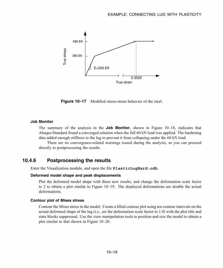
EXAMPLE: CONNECTING LUG WITH PLASTICITY
380.E6
True strain
True
str
ess
0.3529
E=200.E9
580.E6
Figure 10–17 Modified stress-strain behavior of the steel.
Job Monitor
The summary of the analysis in the Job Monitor, shown in Figure 10–18, indicates thatAbaqus/Standard found a converged solution when the full 60 kN load was applied. The hardeningdata added enough stiffness to the lug to prevent it from collapsing under the 60 kN load.
There are no convergence-related warnings issued during the analysis, so you can proceeddirectly to postprocessing the results.
10.4.6 Postprocessing the results
Enter the Visualization module, and open the file PlasticLugHard.odb.
Deformed model shape and peak displacements
Plot the deformed model shape with these new results, and change the deformation scale factorto 2 to obtain a plot similar to Figure 10–19. The displayed deformations are double the actualdeformations.
Contour plot of Mises stress
Contour the Mises stress in the model. Create a filled contour plot using ten contour intervals on theactual deformed shape of the lug (i.e., set the deformation scale factor to 1.0) with the plot title andstate blocks suppressed. Use the view manipulation tools to position and size the model to obtain aplot similar to that shown in Figure 10–20.
10–19
Abaqus ID:Printed on:
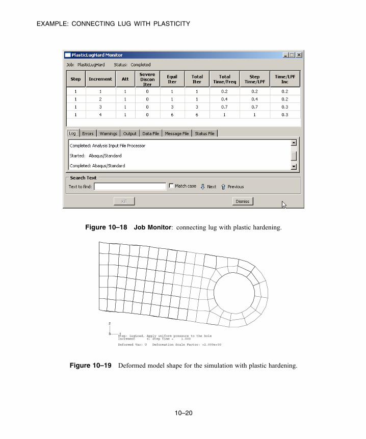
EXAMPLE: CONNECTING LUG WITH PLASTICITY
Figure 10–18 Job Monitor: connecting lug with plastic hardening.
Step: LugLoad, Apply uniform pressure to the holeIncrement 4: Step Time = 1.000
Deformed Var: U Deformation Scale Factor: +2.000e+00
1
2
3
Figure 10–19 Deformed model shape for the simulation with plastic hardening.
10–20
Abaqus ID:Printed on:
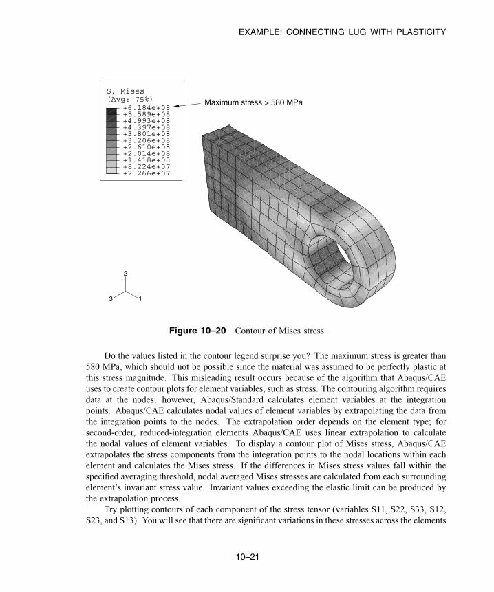
EXAMPLE: CONNECTING LUG WITH PLASTICITY
(Avg: 75%)S, Mises
+2.266e+07+8.224e+07+1.418e+08+2.014e+08+2.610e+08+3.206e+08+3.801e+08+4.397e+08+4.993e+08+5.589e+08+6.184e+08
1
2
3
Maximum stress > 580 MPa
Figure 10–20 Contour of Mises stress.
Do the values listed in the contour legend surprise you? The maximum stress is greater than580 MPa, which should not be possible since the material was assumed to be perfectly plastic atthis stress magnitude. This misleading result occurs because of the algorithm that Abaqus/CAEuses to create contour plots for element variables, such as stress. The contouring algorithm requiresdata at the nodes; however, Abaqus/Standard calculates element variables at the integrationpoints. Abaqus/CAE calculates nodal values of element variables by extrapolating the data fromthe integration points to the nodes. The extrapolation order depends on the element type; forsecond-order, reduced-integration elements Abaqus/CAE uses linear extrapolation to calculatethe nodal values of element variables. To display a contour plot of Mises stress, Abaqus/CAEextrapolates the stress components from the integration points to the nodal locations within eachelement and calculates the Mises stress. If the differences in Mises stress values fall within thespecified averaging threshold, nodal averaged Mises stresses are calculated from each surroundingelement’s invariant stress value. Invariant values exceeding the elastic limit can be produced bythe extrapolation process.
Try plotting contours of each component of the stress tensor (variables S11, S22, S33, S12,S23, and S13). You will see that there are significant variations in these stresses across the elements
10–21
Abaqus ID:Printed on:
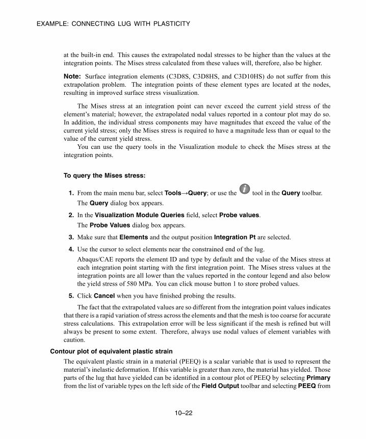
EXAMPLE: CONNECTING LUG WITH PLASTICITY
at the built-in end. This causes the extrapolated nodal stresses to be higher than the values at theintegration points. The Mises stress calculated from these values will, therefore, also be higher.
Note: Surface integration elements (C3D8S, C3D8HS, and C3D10HS) do not suffer from thisextrapolation problem. The integration points of these element types are located at the nodes,resulting in improved surface stress visualization.
The Mises stress at an integration point can never exceed the current yield stress of theelement’s material; however, the extrapolated nodal values reported in a contour plot may do so.In addition, the individual stress components may have magnitudes that exceed the value of thecurrent yield stress; only the Mises stress is required to have a magnitude less than or equal to thevalue of the current yield stress.
You can use the query tools in the Visualization module to check the Mises stress at theintegration points.
To query the Mises stress:
1. From the main menu bar, select Tools→Query; or use the tool in the Query toolbar.
The Query dialog box appears.
2. In the Visualization Module Queries field, select Probe values.
The Probe Values dialog box appears.
3. Make sure that Elements and the output position Integration Pt are selected.
4. Use the cursor to select elements near the constrained end of the lug.
Abaqus/CAE reports the element ID and type by default and the value of the Mises stress ateach integration point starting with the first integration point. The Mises stress values at theintegration points are all lower than the values reported in the contour legend and also belowthe yield stress of 580 MPa. You can click mouse button 1 to store probed values.
5. Click Cancel when you have finished probing the results.
The fact that the extrapolated values are so different from the integration point values indicatesthat there is a rapid variation of stress across the elements and that the mesh is too coarse for accuratestress calculations. This extrapolation error will be less significant if the mesh is refined but willalways be present to some extent. Therefore, always use nodal values of element variables withcaution.
Contour plot of equivalent plastic strain
The equivalent plastic strain in a material (PEEQ) is a scalar variable that is used to represent thematerial’s inelastic deformation. If this variable is greater than zero, the material has yielded. Thoseparts of the lug that have yielded can be identified in a contour plot of PEEQ by selecting Primaryfrom the list of variable types on the left side of the Field Output toolbar and selecting PEEQ from
10–22
Abaqus ID:Printed on:

EXAMPLE: CONNECTING LUG WITH PLASTICITY
the list of output variables. Any areas in the model plotted in a dark color in Abaqus/CAE still haveelastic material behavior (see Figure 10–21).
(Avg: 75%)PEEQ
+0.000e+00+9.994e-03+1.999e-02+2.998e-02+3.997e-02+4.997e-02+5.996e-02+6.996e-02+7.995e-02+8.994e-02+9.994e-02
1
2
3
Figure 10–21 Contour of equivalent plastic strain (PEEQ).
It is clear from the plot that there is gross yielding in the lug where it is attached to its parentstructure. The maximum plastic strain reported in the contour legend is about 10%. However,
this value may contain errors from the extrapolation process. Use the query tool to check theintegration point values of PEEQ in the elements with the largest plastic strains. You will find thatthe largest equivalent plastic strains in the model are about 0.087 at the integration points. Thisdoes not necessarily indicate a large extrapolation error since there are strain gradients present inthe vicinity of the peak plastic deformation.
Creating a variable-variable (stress-strain) plot
The X–Y plotting capability in Abaqus/CAE was introduced earlier in this guide. In this section youwill learn how to create X–Y plots showing the variation of one variable as a function of another.You will use the stress and strain data saved to the output database (.odb) file (in the form of fieldoutput rather than history output) to create a stress-strain plot for one of the integration points in anelement adjacent to the constrained end of the lug.
Consider the shaded element shown in Figure 10–22.
10–23
Abaqus ID:Printed on:
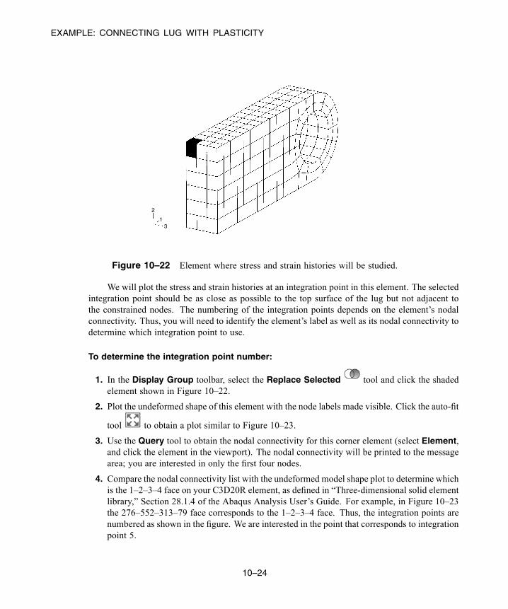
EXAMPLE: CONNECTING LUG WITH PLASTICITY
1
2
3
Figure 10–22 Element where stress and strain histories will be studied.
We will plot the stress and strain histories at an integration point in this element. The selectedintegration point should be as close as possible to the top surface of the lug but not adjacent tothe constrained nodes. The numbering of the integration points depends on the element’s nodalconnectivity. Thus, you will need to identify the element’s label as well as its nodal connectivity todetermine which integration point to use.
To determine the integration point number:
1. In the Display Group toolbar, select the Replace Selected tool and click the shadedelement shown in Figure 10–22.
2. Plot the undeformed shape of this element with the node labels made visible. Click the auto-fit
tool to obtain a plot similar to Figure 10–23.
3. Use the Query tool to obtain the nodal connectivity for this corner element (select Element,and click the element in the viewport). The nodal connectivity will be printed to the messagearea; you are interested in only the first four nodes.
4. Compare the nodal connectivity list with the undeformed model shape plot to determine whichis the 1–2–3–4 face on your C3D20R element, as defined in “Three-dimensional solid elementlibrary,” Section 28.1.4 of the Abaqus Analysis User’s Guide. For example, in Figure 10–23the 276–552–313–79 face corresponds to the 1–2–3–4 face. Thus, the integration points arenumbered as shown in the figure. We are interested in the point that corresponds to integrationpoint 5.
10–24
Abaqus ID:Printed on:
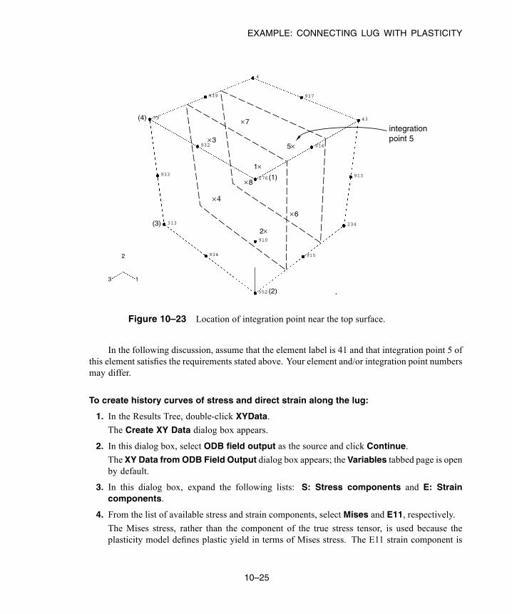
EXAMPLE: CONNECTING LUG WITH PLASTICITY
79
933
313
1
2
3
4
939
932
934
937
276
916
552
910
915
43
913
234
(4)
(3)
(2)
(1)
2
3
8
1
6
5
7integrationpoint 5
Figure 10–23 Location of integration point near the top surface.
In the following discussion, assume that the element label is 41 and that integration point 5 ofthis element satisfies the requirements stated above. Your element and/or integration point numbersmay differ.
To create history curves of stress and direct strain along the lug:
1. In the Results Tree, double-click XYData.
The Create XY Data dialog box appears.
2. In this dialog box, select ODB field output as the source and click Continue.
The XY Data from ODB Field Output dialog box appears; the Variables tabbed page is openby default.
3. In this dialog box, expand the following lists: S: Stress components and E: Straincomponents.
4. From the list of available stress and strain components, select Mises and E11, respectively.
The Mises stress, rather than the component of the true stress tensor, is used because theplasticity model defines plastic yield in terms of Mises stress. The E11 strain component is
10–25
Abaqus ID:Printed on:

EXAMPLE: CONNECTING LUG WITH PLASTICITY
used because it is the largest component of the total strain tensor at this point; using it clearlyshows the elastic, as well as the plastic, behavior of the material at this integration point.
5. Click the Elements/Nodes tab.
6. Accept Pick from viewport as the selection method, and click Edit Selection.
7. In the viewport, click on the shaded element shown in Figure 10–22; then click Done in theprompt area.
8. Click Save to save the data followed by Dismiss to close the dialog box.
Sixteen curves are created (one for each variable at each integration point), and default namesare given to the curves. The curves appear in the XYData container. Each of the curves is ahistory (variable versus time) plot. You must combine the plots for the integration point of interest,eliminating the time dependence, to produce the desired stress-strain plot.
To combine history curves to produce a stress-strain plot:
1. In the Results Tree, double-click XYData.
The Create XY Data dialog box appears.
2. Select Operate on XY data, and click Continue.
The Operate on XY Data dialog box appears. Expand the Name field to see the full name ofeach curve.
3. From the Operators listed, select combine(X,X).
combine( ) appears in the text field at the top of the dialog box.
4. In the XY Data field, select the stress and strain curves for the integration point of interest.
5. Click Add to Expression. The expression combine("E:E11 ...", "S:MISES...") appears in the text field. In this expression "E:E11 ..." will determine theX-values and "S:MISES ..." will determine the Y-values in the combined plot.
6. Save the combined data object by clicking Save As at the bottom of the dialog box.
The Save XY Data As dialog box appears. In the Name text field, type SVE11; and clickOK to close the dialog box.
7. To view the combined stress-strain plot, click Plot Expression at the bottom of the dialogbox.
8. Click Cancel to close the dialog box.
9. Click in the prompt area to cancel the current procedure.
This X–Y plot would be clearer if the limits on the X- and Y-axes were changed.
10–26
Abaqus ID:Printed on:
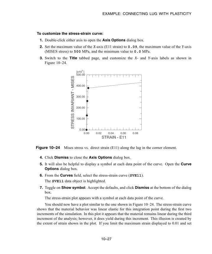
EXAMPLE: CONNECTING LUG WITH PLASTICITY
To customize the stress-strain curve:
1. Double-click either axis to open the Axis Options dialog box.
2. Set the maximum value of the X-axis (E11 strain) to 0.09, the maximum value of the Y-axis(MISES stress) to 500 MPa, and the minimum value to 0.0 MPa.
3. Switch to the Title tabbed page, and customize the X- and Y-axis labels as shown inFigure 10–24.
Figure 10–24 Mises stress vs. direct strain (E11) along the lug in the corner element.
4. Click Dismiss to close the Axis Options dialog box.
5. It will also be helpful to display a symbol at each data point of the curve. Open the CurveOptions dialog box.
6. From the Curves field, select the stress-strain curve (SVE11).
The SVE11 data object is highlighted.
7. Toggle on Show symbol. Accept the defaults, and click Dismiss at the bottom of the dialogbox.
The stress-strain plot appears with a symbol at each data point of the curve.
You should now have a plot similar to the one shown in Figure 10–24. The stress-strain curveshows that the material behavior was linear elastic for this integration point during the first twoincrements of the simulation. In this plot it appears that the material remains linear during the thirdincrement of the analysis; however, it does yield during this increment. This illusion is created bythe extent of strain shown in the plot. If you limit the maximum strain displayed to 0.01 and set
10–27
Abaqus ID:Printed on:

EXAMPLE: BLAST LOADING ON A STIFFENED PLATE
the minimum value to 0.0, the nonlinear material behavior in the third increment can be seen moreclearly (see Figure 10–25).
Figure 10–25 Mises stress vs. direct strain (E11) along thelug in the corner element. Maximum strain 0.01.
This stress-strain curve contains another apparent error. It appears that the material yields at250 MPa, which is well below the initial yield stress. However, this error is caused by the fact thatAbaqus/CAE connects the data points on the curve with straight lines. If you limit the incrementsize, the additional points on the graph will provide a better display of the material response andshow yield occurring at exactly 380 MPa.
The results from this second simulation indicate that the lug will withstand this 60 kN load ifthe steel hardens after it yields. Taken together, the results of the two simulations demonstrate thatit is very important to determine the actual post-yield hardening behavior of the steel. If the steelhas very little hardening, the lug may collapse under the 60 kN load. Whereas if it has moderatehardening, the lug will probably withstand the load although there will be extensive plastic yieldingin the lug (see Figure 10–21). However, even with plastic hardening, the factor of safety for thisloading will probably be very small.
10.5 Example: blast loading on a stiffened plate
The previous example illustrated some of the convergence difficulties that may be encountered whensolving problems involving a nonlinear material response using implicit methods. We will now focuson solving a problem involving plasticity using explicit dynamics. As will become evident shortly,convergence difficulties are not an issue in this case since iteration is not required for explicit methods.
10–28
Abaqus ID:Printed on:
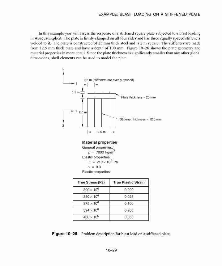
EXAMPLE: BLAST LOADING ON A STIFFENED PLATE
In this example you will assess the response of a stiffened square plate subjected to a blast loadingin Abaqus/Explicit. The plate is firmly clamped on all four sides and has three equally spaced stiffenerswelded to it. The plate is constructed of 25 mm thick steel and is 2 m square. The stiffeners are madefrom 12.5 mm thick plate and have a depth of 100 mm. Figure 10–26 shows the plate geometry andmaterial properties in more detail. Since the plate thickness is significantly smaller than any other globaldimensions, shell elements can be used to model the plate.
True Stress (Pa) True Plastic Strain
300 × 106 0.000
350 × 106 0.025
375 × 106 0.100
394 × 106 0.200
400 × 106 0.350
Material propertiesGeneral properties:
Elastic properties:
Plastic properties:
ρ 7800 kg/m3
=
E 210 109
Pa×=ν 0.3=
Plate thickness = 25 mm
Stiffener thickness = 12.5 mm
2.0 m
2.0 m
0.1 m
0.5 m (stiffeners are evenly spaced)
2
1
3
1
Figure 10–26 Problem description for blast load on a stiffened plate.
10–29
Abaqus ID:Printed on:

EXAMPLE: BLAST LOADING ON A STIFFENED PLATE
The purpose of this example is to determine the response of the plate and to see how it changes asthe sophistication of the material model increases. Initially, we analyze the behavior with the standardelastic-plastic material model. Subsequently, we study the effects of including material damping andrate-dependent material properties.
10.5.1 Preprocessing—creating the model with Abaqus/CAEUse Abaqus/CAE to create a three-dimensional model of the stiffened plate. Abaqus provides scriptsthat replicate the complete analysis model for this problem. Run one of these scripts if you encounterdifficulties following the instructions given below or if you wish to check your work. Scripts are availablein the following locations:
• A Python script for this example is provided in “Blast loading on a stiffened plate,” Section A.9,in the HTML version of this guide. Instructions on how to fetch the script and run it withinAbaqus/CAE are given in Appendix A, “Example Files.”
• A plug-in script for this example is available in the Abaqus/CAE Plug-in toolset. To run the scriptfrom Abaqus/CAE, select Plug-ins→Abaqus→Getting Started; highlight Blast loading ona stiffened plate; and click Run. For more information about the Getting Started plug-ins, see“Running the Getting Started with Abaqus examples,” Section 82.1 of the Abaqus/CAE User’sGuide, in the HTML version of this guide.
Defining the model geometry
Create a three-dimensional, deformable part with an extruded shell base feature to represent theplate. Use an approximate part size of 5.0, and name the part Plate. A suggested approach forcreating the part geometry shown in Figure 10–27 is summarized in the following procedure:
To create the stiffened plate geometry:
1. To define the plate geometry, use the Create Lines: Connected tool to sketch an arbitraryhorizontal line.
2. To define the stiffener geometry, add three vertical lines extending up from the plate. Thehorizontal position of these lines is arbitrary at this stage, but their endpoints must snap to thehorizontal line.
3. Constrain the three vertical lines so they are of equal length, and dimension one of them sothat it is 0.1 m long.
4. Split the plate at the points where it intersects the stiffeners.
5. Dimension the horizontal distance between the plate endpoints, and set the value to 2.0 m.
6. Apply equal length constraints to the four horizontal segments of the line.
The final part sketch is shown in Figure 10–27.
10–30
Abaqus ID:Printed on:
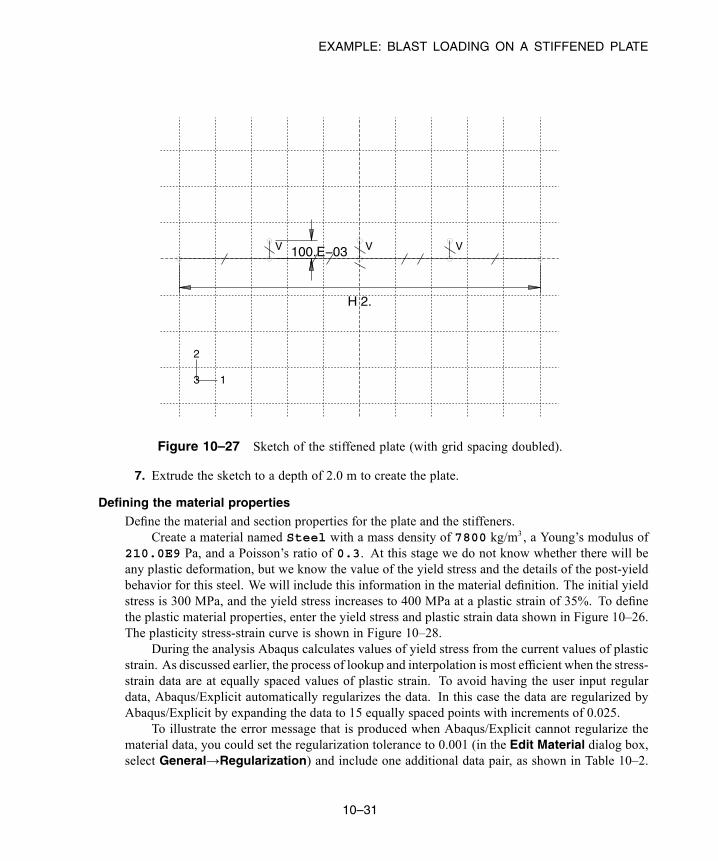
EXAMPLE: BLAST LOADING ON A STIFFENED PLATE
VVV
H 2.
100.E−03
1
2
3
Figure 10–27 Sketch of the stiffened plate (with grid spacing doubled).
7. Extrude the sketch to a depth of 2.0 m to create the plate.
Defining the material propertiesDefine the material and section properties for the plate and the stiffeners.
Create a material named Steel with a mass density of 7800 kg/m3, a Young’s modulus of210.0E9 Pa, and a Poisson’s ratio of 0.3. At this stage we do not know whether there will beany plastic deformation, but we know the value of the yield stress and the details of the post-yieldbehavior for this steel. We will include this information in the material definition. The initial yieldstress is 300 MPa, and the yield stress increases to 400 MPa at a plastic strain of 35%. To definethe plastic material properties, enter the yield stress and plastic strain data shown in Figure 10–26.The plasticity stress-strain curve is shown in Figure 10–28.
During the analysis Abaqus calculates values of yield stress from the current values of plasticstrain. As discussed earlier, the process of lookup and interpolation is most efficient when the stress-strain data are at equally spaced values of plastic strain. To avoid having the user input regulardata, Abaqus/Explicit automatically regularizes the data. In this case the data are regularized byAbaqus/Explicit by expanding the data to 15 equally spaced points with increments of 0.025.
To illustrate the error message that is produced when Abaqus/Explicit cannot regularize thematerial data, you could set the regularization tolerance to 0.001 (in the Edit Material dialog box,select General→Regularization) and include one additional data pair, as shown in Table 10–2.
10–31
Abaqus ID:Printed on:

EXAMPLE: BLAST LOADING ON A STIFFENED PLATE
Figure 10–28 Yield stress versus plastic strain.
You can add a row by clicking mouse button 3 in the table and selecting Insert Row from the menuthat appears.
Table 10–2 Modified plasticity data.
Yield Stress (Pa) Plastic Strain
300.0E6 0.000
349.0E6 0.001
350.0E6 0.025
375.0E6 0.100
394.0E6 0.200
400.0E6 0.350
The combination of the low tolerance value and the small interval in the user-defined data wouldlead to difficulty in regularizing this material definition. The following error message would bewritten to the status (.sta) file and displayed in the Job Monitor dialog box in the Job module:
***ERROR: Failed to regularize material data for materialSTEEL. Please check your input data to see if they meetboth criteria as explained in "MATERIAL DATA DEFINITION"
10–32
Abaqus ID:Printed on:
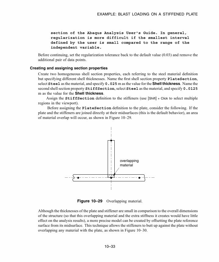
EXAMPLE: BLAST LOADING ON A STIFFENED PLATE
section of the Abaqus Analysis User's Guide. In general,regularization is more difficult if the smallest intervaldefined by the user is small compared to the range of theindependent variable.
Before continuing, set the regularization tolerance back to the default value (0.03) and remove theadditional pair of data points.
Creating and assigning section properties
Create two homogeneous shell section properties, each referring to the steel material definitionbut specifying different shell thicknesses. Name the first shell section property PlateSection,select Steel as the material, and specify 0.025m as the value for theShell thickness. Name thesecond shell section property StiffSection, select Steel as the material, and specify 0.0125m as the value for the Shell thickness.
Assign the StiffSection definition to the stiffeners (use [Shift] + Click to select multipleregions in the viewport).
Before assigning the PlateSection definition to the plate, consider the following. If theplate and the stiffeners are joined directly at their midsurfaces (this is the default behavior), an areaof material overlap will occur, as shown in Figure 10–29.
overlappingmaterial
Figure 10–29 Overlapping material.
Although the thicknesses of the plate and stiffener are small in comparison to the overall dimensionsof the structure (so that this overlapping material and the extra stiffness it creates would have littleeffect on the analysis results), a more precise model can be created by offsetting the plate referencesurface from its midsurface. This technique allows the stiffeners to butt up against the plate withoutoverlapping any material with the plate, as shown in Figure 10–30.
10–33
Abaqus ID:Printed on:

EXAMPLE: BLAST LOADING ON A STIFFENED PLATE
base plate
stiffener
plate midsurface
plate nodes lie on shell SPOS or SNEG face
stiffener nodes lieon shell midsurface
Figure 10–30 Stiffener joint in which the plate’s referencesurface is offset from its midsurface.
To determine whether to offset the plate reference surface to its positive (SPOS) or negative(SNEG) side, query the shell normals (Tools→Query) and note the color of the side of the platefacing the stiffeners (brown is the positive side; purple is the negative side). If necessary, flip theplate normals (Assign→Element Normal) so that its segments have consistent normals. Thenassign the PlateSection definition to the regions of the plate. In the Edit Section Assignmentdialog box, set the shell offset to Top surface if the brown (positive) side of the plate faces thestiffeners and Bottom surface if the purple (negative) side faces the stiffeners.
To verify the offset, selectView→Part Display Options. In thePart Display Options dialogbox that appears, toggle on Render shell thickness. If necessary, modify the offset to removeany overlap.
The model can be color-coded according to section assignment to verify that properties wereassigned correctly (select Sections from the Color Code toolbar).
Creating an assembly
Create an independent instance of the plate. Use the default rectangular coordinate system, with theplate lying in the 1–3 plane.
At this point, it is convenient to create the geometry sets that will be used to specify boundaryconditions and output requests. Create one set named Edge for the plate edges and one setnamed Center at the center of the intersection of the plate and the middle stiffener, as shown inFigure 10–31. To create the set Center, you need to first partition the edge of the original part in
half using the Partition Edge: Enter Parameter tool.
10–34
Abaqus ID:Printed on:
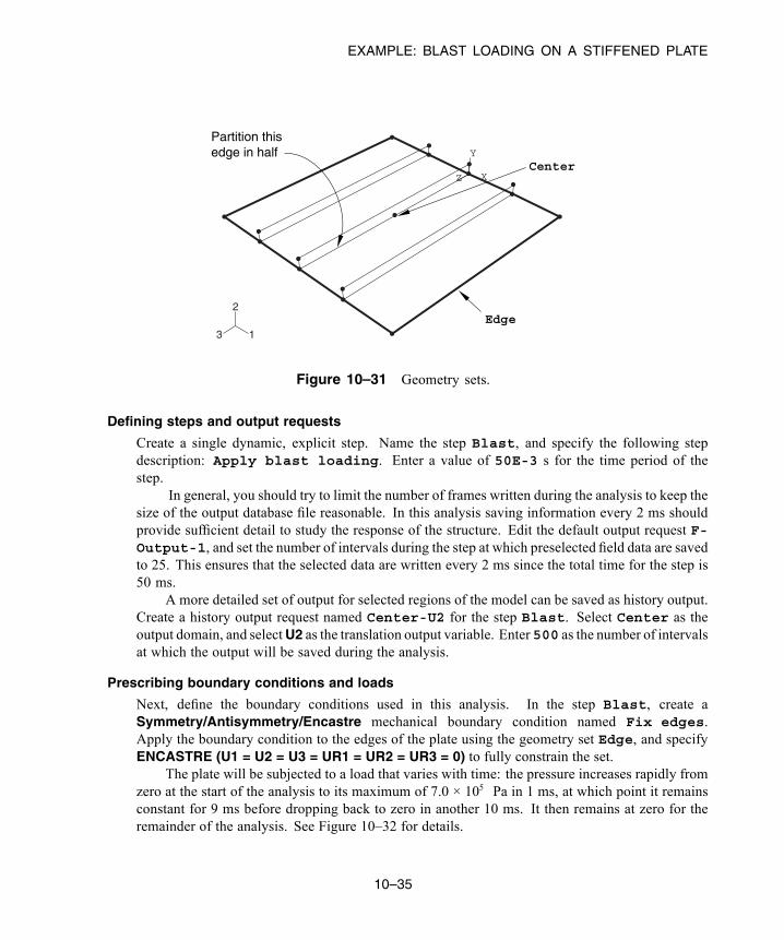
EXAMPLE: BLAST LOADING ON A STIFFENED PLATE
X
Y
Z
1
2
3
Center
Edge
Partition this edge in half
Figure 10–31 Geometry sets.
Defining steps and output requests
Create a single dynamic, explicit step. Name the step Blast, and specify the following stepdescription: Apply blast loading. Enter a value of 50E-3 s for the time period of thestep.
In general, you should try to limit the number of frames written during the analysis to keep thesize of the output database file reasonable. In this analysis saving information every 2 ms shouldprovide sufficient detail to study the response of the structure. Edit the default output request F-Output-1, and set the number of intervals during the step at which preselected field data are savedto 25. This ensures that the selected data are written every 2 ms since the total time for the step is50 ms.
A more detailed set of output for selected regions of the model can be saved as history output.Create a history output request named Center-U2 for the step Blast. Select Center as theoutput domain, and selectU2 as the translation output variable. Enter 500 as the number of intervalsat which the output will be saved during the analysis.
Prescribing boundary conditions and loads
Next, define the boundary conditions used in this analysis. In the step Blast, create aSymmetry/Antisymmetry/Encastre mechanical boundary condition named Fix edges.Apply the boundary condition to the edges of the plate using the geometry set Edge, and specifyENCASTRE (U1 = U2 = U3 = UR1 = UR2 = UR3 = 0) to fully constrain the set.
The plate will be subjected to a load that varies with time: the pressure increases rapidly fromzero at the start of the analysis to its maximum of 7.0 × 10⁵ Pa in 1 ms, at which point it remainsconstant for 9 ms before dropping back to zero in another 10 ms. It then remains at zero for theremainder of the analysis. See Figure 10–32 for details.
10–35
Abaqus ID:Printed on:
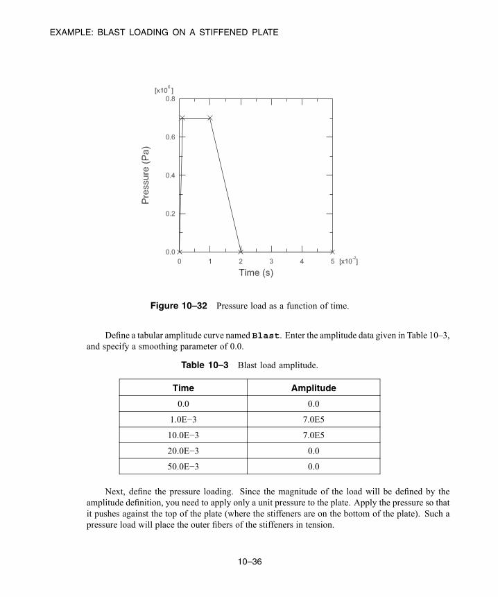
EXAMPLE: BLAST LOADING ON A STIFFENED PLATE
Figure 10–32 Pressure load as a function of time.
Define a tabular amplitude curve named Blast. Enter the amplitude data given in Table 10–3,and specify a smoothing parameter of 0.0.
Table 10–3 Blast load amplitude.
Time Amplitude
0.0 0.0
1.0E−3 7.0E5
10.0E−3 7.0E5
20.0E−3 0.0
50.0E−3 0.0
Next, define the pressure loading. Since the magnitude of the load will be defined by theamplitude definition, you need to apply only a unit pressure to the plate. Apply the pressure so thatit pushes against the top of the plate (where the stiffeners are on the bottom of the plate). Such apressure load will place the outer fibers of the stiffeners in tension.
10–36
Abaqus ID:Printed on:

EXAMPLE: BLAST LOADING ON A STIFFENED PLATE
To define the pressure loading:
1. In the Model Tree, double-click the Loads container. In the Create Load dialog box thatappears, name the load Pressure load and select Blast as the step in which it willbe applied. Select Mechanical as the load category and Pressure as the load type. ClickContinue.
2. Select all the surfaces associated with the plate. When the appropriate surfaces are selected,click Done.
Abaqus/CAE uses two different colors to indicate the two sides of the shell surface. Tocomplete the load definition, the colors must be consistent on each side of the plate.
3. If necessary, select Flip a surface in the prompt area to flip the colors for a region of the plate.Repeat this procedure until all of the faces on the top of the plate are the same color.
4. In the prompt area, select the color representing the side of the plate without the stiffeners.
5. In the Edit Load dialog box that appears, specify a uniform pressure of 1.0 Pa, and select theamplitude definition Blast. Click OK to complete the load definition.
The plate load and boundary conditions are shown in Figure 10–33.
X
Y
Z
1
2
3
Figure 10–33 Pressure load and boundary conditions.
Creating the mesh and defining a job
Seed the part instance with a global element size of 0.1. In addition, select Seed→Edges andspecify that two elements be created along the height of each stiffener (in the Local Seeds dialogbox, select By number as the method and set the number of elements to 2; toggle on the option tocreate a set containing the selected edges). Mesh the plate and stiffeners using quadrilateral shellelements (S4R) from the Explicit element library. The resulting mesh is shown in Figure 10–34.This relatively coarse mesh provides moderate accuracy while keeping the solution time to aminimum.
10–37
Abaqus ID:Printed on:

EXAMPLE: BLAST LOADING ON A STIFFENED PLATE
1
2
3
X
Y
Z
Figure 10–34 Meshed plate.
Create a job named BlastLoad. Specify the following job description: Blast load ona flat plate with stiffeners: S4R elements (20x20 mesh) Normalstiffeners (20x2).
Save your model in a model database file, and submit the job for analysis. Monitor the solutionprogress; correct any modeling errors that are detected, and investigate the cause of any warningmessages.
10.5.2 PostprocessingWhen the job completes, enter the Visualization module, and open the .odb file created by this job(BlastLoad.odb). By default, Abaqus plots the undeformed model shape with the shaded renderstyle.
Changing the view
The default view is isometric, which does not provide a particularly clear view of the plate. Toimprove the viewpoint, rotate the view using the options in the View menu or the tools in the ViewManipulation toolbar. Specify the view and select the viewpoint method for rotating the view.Enter the X-, Y-, and Z-coordinates of the viewpoint vector as 1,0.5,1 and the coordinates of theup vector as 0,1,0.
Verifying shell section assignment
You can also visualize the section assignment and the shell thickness while postprocessing theresults. For example, regions with common section assignments can be color coded to verify thatthe properties were assigned correctly (select Sections from the Color Code toolbar to color themesh according to section assignment). To render the shell thickness, select View→ODB DisplayOptions from the main menu bar. In the ODB Display Options dialog box, toggle on Render
10–38
Abaqus ID:Printed on:
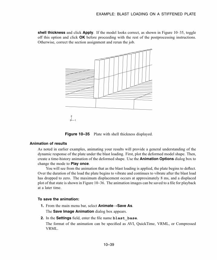
EXAMPLE: BLAST LOADING ON A STIFFENED PLATE
shell thickness and click Apply. If the model looks correct, as shown in Figure 10–35, toggleoff this option and click OK before proceeding with the rest of the postprocessing instructions.Otherwise, correct the section assignment and rerun the job.
1
2
3
Figure 10–35 Plate with shell thickness displayed.
Animation of results
As noted in earlier examples, animating your results will provide a general understanding of thedynamic response of the plate under the blast loading. First, plot the deformed model shape. Then,create a time-history animation of the deformed shape. Use the Animation Options dialog box tochange the mode to Play once.
You will see from the animation that as the blast loading is applied, the plate begins to deflect.Over the duration of the load the plate begins to vibrate and continues to vibrate after the blast loadhas dropped to zero. The maximum displacement occurs at approximately 8 ms, and a displacedplot of that state is shown in Figure 10–36. The animation images can be saved to a file for playbackat a later time.
To save the animation:
1. From the main menu bar, select Animate→Save As.
The Save Image Animation dialog box appears.
2. In the Settings field, enter the file name blast_base.
The format of the animation can be specified as AVI, QuickTime, VRML, or CompressedVRML.
10–39
Abaqus ID:Printed on:

EXAMPLE: BLAST LOADING ON A STIFFENED PLATE
Figure 10–36 Displaced shape at 8 ms.
3. Choose the QuickTime format, and click OK.The animation is saved as blast_base.mov in your current directory. Once saved, youranimation can be played external to Abaqus/CAE using industry-standard animation software.
History outputSince it is not easy to see the deformation of the plate from the deformed plot, it is desirable to viewthe deflection response of the central node in the form of a graph. The displacement of the node inthe center of the plate is of particular interest since the largest deflection occurs at this node.
Display the displacement history of the central node, as shown in Figure 10–37 (withdisplacements in millimeters).
To generate a history plot of the central node displacement:
1. In the Results Tree, double-click the history output data named Spatial displacement:U2 at the node in the center of the plate (set Center).
2. Save the current X–Y data: in the Results Tree, click mouse button 3 on the data name andselect Save As from the menu that appears. Name the data DISP.
The units of the displacements in this plot are meters. Modify the data to create a plot ofdisplacement (in millimeters) versus time by creating a new data object.
3. In the Results Tree, expand the XYData container.The DISP data are listed underneath.
4. In the Results Tree, double-click XYData; then select Operate on XY data in the Create XYData dialog box. Click Continue.
5. In the Operate on XY Data dialog box, multiply DISP by 1000 to create the plot with thedisplacement values in millimeters instead of meters. The expression at the top of the dialogbox should appear as:
"DISP" * 1000
6. Click Plot Expression to see the modified X–Y data. Save the data as U2_BASE.
10–40
Abaqus ID:Printed on:
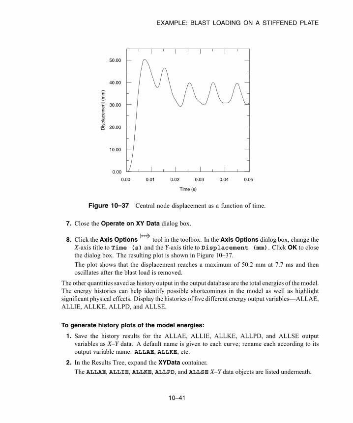
EXAMPLE: BLAST LOADING ON A STIFFENED PLATE
0.00 0.01 0.02 0.03 0.04 0.05
0.00
10.00
20.00
30.00
40.00
50.00
Time (s)
Dis
plac
emen
t (m
m)
Figure 10–37 Central node displacement as a function of time.
7. Close the Operate on XY Data dialog box.
8. Click the Axis Options tool in the toolbox. In the Axis Options dialog box, change theX-axis title to Time (s) and the Y-axis title to Displacement (mm). Click OK to closethe dialog box. The resulting plot is shown in Figure 10–37.
The plot shows that the displacement reaches a maximum of 50.2 mm at 7.7 ms and thenoscillates after the blast load is removed.
The other quantities saved as history output in the output database are the total energies of the model.The energy histories can help identify possible shortcomings in the model as well as highlightsignificant physical effects. Display the histories of five different energy output variables—ALLAE,ALLIE, ALLKE, ALLPD, and ALLSE.
To generate history plots of the model energies:
1. Save the history results for the ALLAE, ALLIE, ALLKE, ALLPD, and ALLSE outputvariables as X–Y data. A default name is given to each curve; rename each according to itsoutput variable name: ALLAE, ALLKE, etc.
2. In the Results Tree, expand the XYData container.
The ALLAE, ALLIE, ALLKE, ALLPD, and ALLSE X–Y data objects are listed underneath.
10–41
Abaqus ID:Printed on:
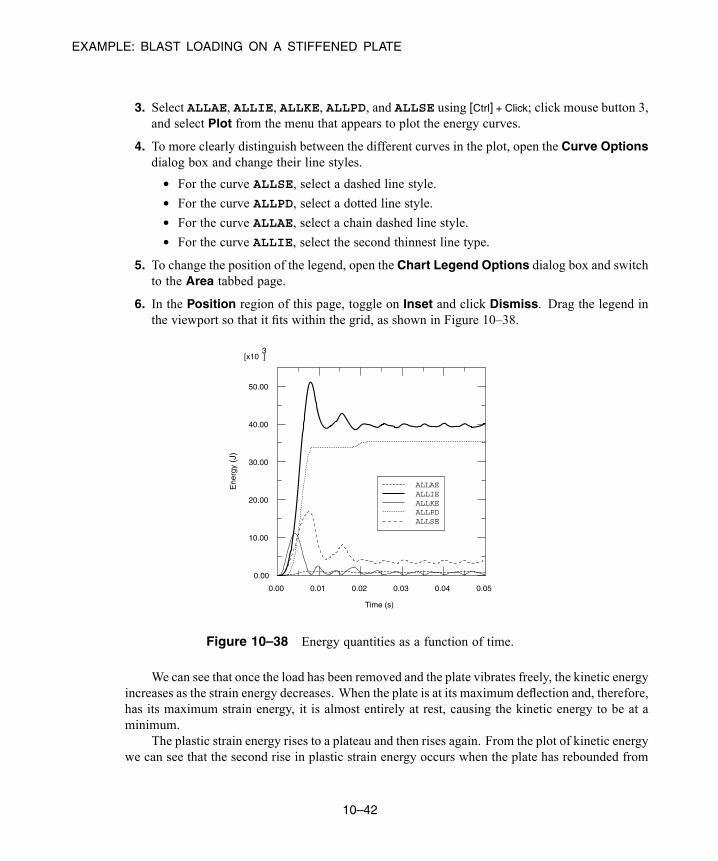
EXAMPLE: BLAST LOADING ON A STIFFENED PLATE
3. Select ALLAE, ALLIE, ALLKE, ALLPD, and ALLSE using [Ctrl] + Click; click mouse button 3,and select Plot from the menu that appears to plot the energy curves.
4. To more clearly distinguish between the different curves in the plot, open the Curve Optionsdialog box and change their line styles.
• For the curve ALLSE, select a dashed line style.• For the curve ALLPD, select a dotted line style.• For the curve ALLAE, select a chain dashed line style.• For the curve ALLIE, select the second thinnest line type.
5. To change the position of the legend, open the Chart Legend Options dialog box and switchto the Area tabbed page.
6. In the Position region of this page, toggle on Inset and click Dismiss. Drag the legend inthe viewport so that it fits within the grid, as shown in Figure 10–38.
0.00 0.01 0.02 0.03 0.04 0.05
[x10 ]3
0.00
10.00
20.00
30.00
40.00
50.00
Time (s)
ALLAEALLIEALLKEALLPDALLSE
Ene
rgy
(J)
Figure 10–38 Energy quantities as a function of time.
We can see that once the load has been removed and the plate vibrates freely, the kinetic energyincreases as the strain energy decreases. When the plate is at its maximum deflection and, therefore,has its maximum strain energy, it is almost entirely at rest, causing the kinetic energy to be at aminimum.
The plastic strain energy rises to a plateau and then rises again. From the plot of kinetic energywe can see that the second rise in plastic strain energy occurs when the plate has rebounded from
10–42
Abaqus ID:Printed on:
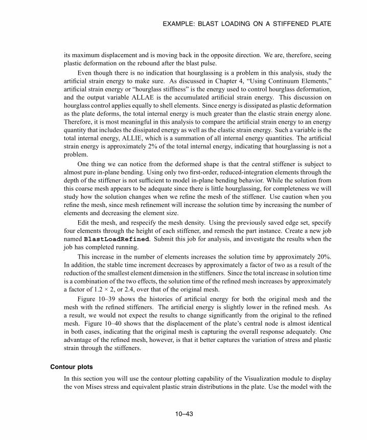
EXAMPLE: BLAST LOADING ON A STIFFENED PLATE
its maximum displacement and is moving back in the opposite direction. We are, therefore, seeingplastic deformation on the rebound after the blast pulse.
Even though there is no indication that hourglassing is a problem in this analysis, study theartificial strain energy to make sure. As discussed in Chapter 4, “Using Continuum Elements,”artificial strain energy or “hourglass stiffness” is the energy used to control hourglass deformation,and the output variable ALLAE is the accumulated artificial strain energy. This discussion onhourglass control applies equally to shell elements. Since energy is dissipated as plastic deformationas the plate deforms, the total internal energy is much greater than the elastic strain energy alone.Therefore, it is most meaningful in this analysis to compare the artificial strain energy to an energyquantity that includes the dissipated energy as well as the elastic strain energy. Such a variable is thetotal internal energy, ALLIE, which is a summation of all internal energy quantities. The artificialstrain energy is approximately 2% of the total internal energy, indicating that hourglassing is not aproblem.
One thing we can notice from the deformed shape is that the central stiffener is subject toalmost pure in-plane bending. Using only two first-order, reduced-integration elements through thedepth of the stiffener is not sufficient to model in-plane bending behavior. While the solution fromthis coarse mesh appears to be adequate since there is little hourglassing, for completeness we willstudy how the solution changes when we refine the mesh of the stiffener. Use caution when yourefine the mesh, since mesh refinement will increase the solution time by increasing the number ofelements and decreasing the element size.
Edit the mesh, and respecify the mesh density. Using the previously saved edge set, specifyfour elements through the height of each stiffener, and remesh the part instance. Create a new jobnamed BlastLoadRefined. Submit this job for analysis, and investigate the results when thejob has completed running.
This increase in the number of elements increases the solution time by approximately 20%.In addition, the stable time increment decreases by approximately a factor of two as a result of thereduction of the smallest element dimension in the stiffeners. Since the total increase in solution timeis a combination of the two effects, the solution time of the refined mesh increases by approximatelya factor of 1.2 × 2, or 2.4, over that of the original mesh.
Figure 10–39 shows the histories of artificial energy for both the original mesh and themesh with the refined stiffeners. The artificial energy is slightly lower in the refined mesh. Asa result, we would not expect the results to change significantly from the original to the refinedmesh. Figure 10–40 shows that the displacement of the plate’s central node is almost identicalin both cases, indicating that the original mesh is capturing the overall response adequately. Oneadvantage of the refined mesh, however, is that it better captures the variation of stress and plasticstrain through the stiffeners.
Contour plots
In this section you will use the contour plotting capability of the Visualization module to displaythe von Mises stress and equivalent plastic strain distributions in the plate. Use the model with the
10–43
Abaqus ID:Printed on:

EXAMPLE: BLAST LOADING ON A STIFFENED PLATE
0.00 0.01 0.02 0.03 0.04 0.05
[x10 ]3
0.00
0.20
0.40
0.60
0.80
1.00
Time (s)
OriginalRefinedA
rtifi
cial
Ene
rgy
(J)
Figure 10–39 Artificial energy in the original and refined meshes.
0.00 0.01 0.02 0.03 0.04 0.05
0.00
10.00
20.00
30.00
40.00
50.00
Time (s)
Dis
plac
emen
t (m
m)
OriginalRefined
Figure 10–40 Central node displacement history for the original and refined meshes.
refined stiffener mesh to create the plots; from the main menu bar, select File→Open and choosethe file BlastLoadRefined.odb.
10–44
Abaqus ID:Printed on:

EXAMPLE: BLAST LOADING ON A STIFFENED PLATE
To generate contour plots of the von Mises stress and equivalent plastic strain:
1. From the list of variable types on the left side of the Field Output toolbar, select Primary.
2. From the list of output variables in the center of the toolbar, select S. The stress invariants andcomponents are available in the next list to the right. Select the Mises stress invariant.
3. From the main menu bar, select Result→Section Points.
4. In the Section Points dialog box that appears, select Top and bottom as the active locationsand click OK.
5. Select Plot→Contours→On Deformed Shape, or use the tool from the toolbox.
Abaqus plots the contours of the von Mises stress on both the top and bottom faces of eachshell element. To see this more clearly, rotate the model in the viewport.
The view that you set earlier for the animation exercise should be changed so that the stressdistribution is clearer.
6. Change the view back to the default isometric view using the tool in the Views toolbar.
Tip: If the Views toolbar is not visible, select View→Toolbars→Views from themain menu bar.
Figure 10–41 shows a contour plot of the von Mises stress at the end of the analysis.
(Avg: 75%)SPOS, (fraction = 1.0)SNEG, (fraction = −1.0)S, Mises
+1.058e+07+3.632e+07+6.206e+07+8.780e+07+1.135e+08+1.393e+08+1.650e+08+1.908e+08+2.165e+08+2.422e+08+2.680e+08+2.937e+08+3.195e+08
X
Y
Z
Figure 10–41 Contour plot of von Mises stress at 50 ms.
10–45
Abaqus ID:Printed on:

EXAMPLE: BLAST LOADING ON A STIFFENED PLATE
7. Similarly, contour the equivalent plastic strain. Select Primary from the list of variable typeson the left side of the Field Output toolbar and select PEEQ from the list of output variablesnext to it.
Figure 10–42 shows a contour plot of the equivalent plastic strain at the end of the analysis.
(Avg: 75%)SPOS, (fraction = 1.0)SNEG, (fraction = -1.0)PEEQ
+0.000e+00+1.615e-03+3.231e-03+4.846e-03+6.462e-03+8.077e-03+9.692e-03+1.131e-02+1.292e-02+1.454e-02+1.615e-02+1.777e-02+1.938e-02
1
2
3
Figure 10–42 Contour plot of equivalent plastic strain at 50 ms.
10.5.3 Reviewing the analysisThe objective of this analysis is to study the deformation of the plate and the stress in various parts ofthe structure when it is subjected to a blast load. To judge the accuracy of the analysis, you will need toconsider the assumptions and approximations made and identify some of the limitations of the model.
Damping
Undamped structures continue to vibrate with constant amplitude. Over the 50ms of this simulation,the frequency of the oscillation can be seen to be approximately 100 Hz. A constant amplitudevibration is not the response that would be expected in practice since the vibrations in this typeof structure would tend to die out over time and effectively disappear after 5–10 oscillations. Theenergy loss typically occurs by a variety of mechanisms including frictional effects at the supportsand damping by the air.
Consequently, we need to consider the presence of damping in the analysis to model this energyloss. The energy dissipated by viscous effects, ALLVD, is nonzero in the analysis, indicating that
10–46
Abaqus ID:Printed on:
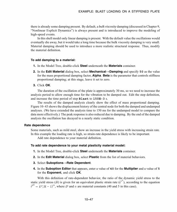
EXAMPLE: BLAST LOADING ON A STIFFENED PLATE
there is already some damping present. By default, a bulk viscosity damping (discussed in Chapter 9,“Nonlinear Explicit Dynamics”) is always present and is introduced to improve the modeling ofhigh-speed events.
In this shell model only linear damping is present. With the default value the oscillations wouldeventually die away, but it would take a long time because the bulk viscosity damping is very small.Material damping should be used to introduce a more realistic structural response. Thus, modifythe material definition.
To add damping to a material:
1. In the Model Tree, double-click Steel underneath the Materials container.
2. In the Edit Material dialog box, select Mechanical→Damping and specify 50 as the valuefor the mass proportional damping factor, Alpha. Beta is the parameter that controls stiffnessproportional damping; at this stage, leave it set to zero.
3. Click OK.
The duration of the oscillation of the plate is approximately 30 ms, so we need to increase theanalysis period to allow enough time for the vibration to be damped out. Edit the step definition,and increase the time period of step Blast to 150E-3 s.
The results of the damped analysis clearly show the effect of mass proportional damping.Figure 10–43 shows the displacement history of the central node for both the damped and undampedanalyses. (We have extended the analysis time to 150 ms for the undamped model to compare thedata more effectively.) The peak response is also reduced due to damping. By the end of the dampedanalysis the oscillation has decayed to a nearly static condition.
Rate dependence
Some materials, such as mild steel, show an increase in the yield stress with increasing strain rate.In this example the loading rate is high, so strain-rate dependence is likely to be important.
Add rate dependence to your material definition.
To add rate dependence to your metal plasticity material model:
1. In the Model Tree, double-click Steel underneath the Materials container.
2. In the Edit Material dialog box, select Plastic from the list of material behaviors.
3. Select Suboptions→Rate Dependent.
4. In the Suboption Editor that appears, enter a value of 40 for the Multiplier and a value of 5for the Exponent, and click OK.
With this definition of rate-dependent behavior, the ratio of the dynamic yield stress to thestatic yield stress ( ) is given for an equivalent plastic strain rate ( ), according to the equation
, where and are material constants (40 and 5 in this case).
10–47
Abaqus ID:Printed on:
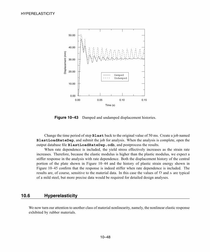
HYPERELASTICITY
0.00 0.05 0.10 0.15
0.00
10.00
20.00
30.00
40.00
50.00
Time (s)
Dis
plac
emen
t (m
m)
DampedUndamped
Figure 10–43 Damped and undamped displacement histories.
Change the time period of step Blast back to the original value of 50 ms. Create a job namedBlastLoadRateDep, and submit the job for analysis. When the analysis is complete, open theoutput database file BlastLoadRateDep.odb, and postprocess the results.
When rate dependence is included, the yield stress effectively increases as the strain rateincreases. Therefore, because the elastic modulus is higher than the plastic modulus, we expect astiffer response in the analysis with rate dependence. Both the displacement history of the centralportion of the plate shown in Figure 10–44 and the history of plastic strain energy shown inFigure 10–45 confirm that the response is indeed stiffer when rate dependence is included. Theresults are, of course, sensitive to the material data. In this case the values of and are typicalof a mild steel, but more precise data would be required for detailed design analyses.
10.6 Hyperelasticity
We now turn our attention to another class of material nonlinearity, namely, the nonlinear elastic responseexhibited by rubber materials.
10–48
Abaqus ID:Printed on:
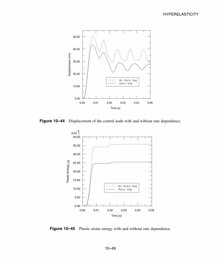
HYPERELASTICITY
0.00 0.01 0.02 0.03 0.04 0.05
0.00
10.00
20.00
30.00
40.00
50.00
Time (s)
Dis
plac
emen
t (m
m)
No Rate DepRate Dep
Figure 10–44 Displacement of the central node with and without rate dependence.
0.00 0.01 0.02 0.03 0.04 0.05
[x10 ]3
0.00
5.00
10.00
15.00
20.00
25.00
30.00
35.00
40.00
Time (s)
No Rate DepRate Dep
Pla
stic
Ene
rgy
(J)
Figure 10–45 Plastic strain energy with and without rate dependence.
10–49
Abaqus ID:Printed on:

HYPERELASTICITY
10.6.1 IntroductionThe stress-strain behavior of typical rubber materials, shown in Figure 10–46, is elastic but highlynonlinear.
Strain
Str
ess
Figure 10–46 Typical stress-strain curve for rubber.
This type of material behavior is called hyperelasticity. The deformation of hyperelastic materials, suchas rubber, remains elastic up to large strain values (often well over 100%).
Abaqus makes the following assumptions when modeling a hyperelastic material:
• The material behavior is elastic.• The material behavior is isotropic.• The simulation will include nonlinear geometric effects.
In addition, Abaqus/Standard assumes the hyperelastic material is incompressible by default.Abaqus/Explicit assumes the material is nearly incompressible (Poisson’s ratio is 0.475 by default).
Elastomeric foams are another class of highly nonlinear, elastic materials. They differ from rubbermaterials in that they have very compressible behavior when subjected to compressive loads. They aremodeled with a separate material model in Abaqus and are not discussed in detail in this guide.
10.6.2 CompressibilityMost solid rubber materials have very little compressibility compared to their shear flexibility. Thisbehavior is not a problem with plane stress, shell, or membrane elements. However, it can be a problemwhen using other elements, such as plane strain, axisymmetric, and three-dimensional solid elements.For example, in applications where the material is not highly confined, it would be quite satisfactory toassume that the material is fully incompressible: the volume of the material cannot change except for
10–50
Abaqus ID:Printed on:
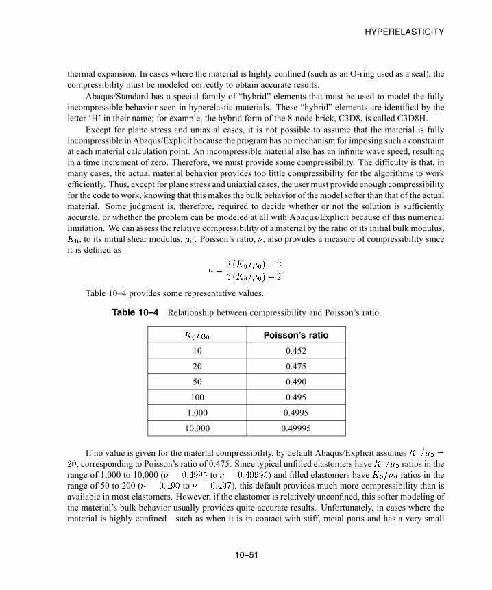
HYPERELASTICITY
thermal expansion. In cases where the material is highly confined (such as an O-ring used as a seal), thecompressibility must be modeled correctly to obtain accurate results.
Abaqus/Standard has a special family of “hybrid” elements that must be used to model the fullyincompressible behavior seen in hyperelastic materials. These “hybrid” elements are identified by theletter ‘H’ in their name; for example, the hybrid form of the 8-node brick, C3D8, is called C3D8H.
Except for plane stress and uniaxial cases, it is not possible to assume that the material is fullyincompressible in Abaqus/Explicit because the program has nomechanism for imposing such a constraintat each material calculation point. An incompressible material also has an infinite wave speed, resultingin a time increment of zero. Therefore, we must provide some compressibility. The difficulty is that, inmany cases, the actual material behavior provides too little compressibility for the algorithms to workefficiently. Thus, except for plane stress and uniaxial cases, the user must provide enough compressibilityfor the code to work, knowing that this makes the bulk behavior of the model softer than that of the actualmaterial. Some judgment is, therefore, required to decide whether or not the solution is sufficientlyaccurate, or whether the problem can be modeled at all with Abaqus/Explicit because of this numericallimitation. We can assess the relative compressibility of a material by the ratio of its initial bulk modulus,, to its initial shear modulus, . Poisson’s ratio, , also provides a measure of compressibility since
it is defined as
Table 10–4 provides some representative values.
Table 10–4 Relationship between compressibility and Poisson’s ratio.
Poisson’s ratio
10 0.452
20 0.475
50 0.490
100 0.495
1,000 0.4995
10,000 0.49995
If no value is given for the material compressibility, by default Abaqus/Explicit assumes, corresponding to Poisson’s ratio of 0.475. Since typical unfilled elastomers have ratios in the
range of 1,000 to 10,000 ( to ) and filled elastomers have ratios in therange of 50 to 200 ( to ), this default provides much more compressibility than isavailable in most elastomers. However, if the elastomer is relatively unconfined, this softer modeling ofthe material’s bulk behavior usually provides quite accurate results. Unfortunately, in cases where thematerial is highly confined—such as when it is in contact with stiff, metal parts and has a very small
10–51
Abaqus ID:Printed on:
HYPERELASTICITY
amount of free surface, especially when the loading is highly compressive—it may not be feasible toobtain accurate results with Abaqus/Explicit.
If you are defining the compressibility rather than accepting the default value in Abaqus/Explicit,an upper limit of 100 is suggested for the ratio of . Larger ratios introduce high frequency noiseinto the dynamic solution and require the use of excessively small time increments.
10.6.3 Strain energy potentialAbaqus uses a strain energy potential (U), rather than a Young’s modulus and Poisson’s ratio, to relatestresses to strains in hyperelastic materials. Several different strain energy potentials are available: apolynomial model, the Ogdenmodel, the Arruda-Boyce model, theMarlowmodel, and the van derWaalsmodel. Simpler forms of the polynomial model are also available, including the Mooney-Rivlin, neo-Hookean, reduced polynomial, and Yeoh models.
The polynomial form of the strain energy potential is one that is commonly used. Its form is
where U is the strain energy potential; is the elastic volume ratio; and are measures of thedistortion in the material; and N, , and are material parameters, which may be functions oftemperature. The parameters describe the shear behavior of the material, and the parametersintroduce compressibility. If the material is fully incompressible (a condition not allowed inAbaqus/Explicit), all the values of are set to zero and the second part of the equation shown abovecan be ignored. If the number of terms, N, is one, the initial shear modulus, , and bulk modulus, ,are given by
and
If the material is also incompressible, the equation for the strain energy density is
This expression is commonly referred to as the Mooney-Rivlin material model. If is also zero, thematerial is called neo-Hookean.
The other hyperelastic models are similar in concept and are described in “Hyperelasticity,”Section 22.5 of the Abaqus Analysis User’s Guide.
You must provide Abaqus with the relevant material parameters to use a hyperelastic material.For the polynomial form these are and . It is possible that you will be supplied with theseparameters when modeling hyperelastic materials; however, more likely you will be given test data for
10–52
Abaqus ID:Printed on:
HYPERELASTICITY
the materials that you must model. Fortunately, Abaqus can accept test data directly and calculate thematerial parameters for you (using a least squares fit).
10.6.4 Defining hyperelastic behavior using test dataA convenient way of defining a hyperelastic material is to supply Abaqus with experimental test data.Abaqus then calculates the constants using a least squares method. Abaqus can fit data for the followingexperimental tests:
• Uniaxial tension and compression• Equibiaxial tension and compression• Planar tension and compression (pure shear)• Volumetric tension and compressionThe deformation modes seen in these tests are shown in Figure 10–47. Unlike plasticity data, the
test data for hyperelastic materials must be given to Abaqus as nominal stress and nominal strain values.Volumetric compression data only need to be given if the material’s compressibility is important.
Normally in Abaqus/Standard it is not important, and the default fully incompressible behavior is used.As noted earlier, Abaqus/Explicit assumes a small amount of compressibility if no volumetric test dataare given.
Obtaining the best material model from your data
The quality of the results from a simulation using hyperelastic materials strongly depends on thematerial test data that you provide Abaqus. Typical tests are shown in Figure 10–47. There areseveral things that you can do to help Abaqus calculate the best possible material parameters.
Wherever possible, try to obtain experimental test data from more than one deformationstate—this allows Abaqus to form a more accurate and stable material model. However, someof the tests shown in Figure 10–47 produce equivalent deformation modes for incompressiblematerials. The following are equivalent tests for incompressible materials:
• Uniaxial tension↔ Equibiaxial compression
• Uniaxial compression↔ Equibiaxial tension
• Planar tension↔ Planar compression
You do not need to include data from a particular test if you already have data from another test thatmodels a particular deformation mode.
In addition, the following may improve your hyperelastic material model:
• Obtain test data for the deformation modes that are likely to occur in your simulation. Forexample, if your component is loaded in compression, make sure that your test data includecompressive, rather than tensile, loading.
10–53
Abaqus ID:Printed on:
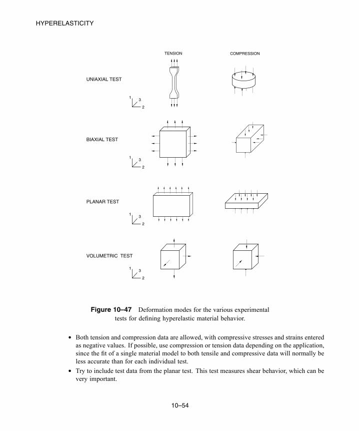
HYPERELASTICITY
13
2
TENSION COMPRESSION
UNIAXIAL TEST
BIAXIAL TEST
13
2
PLANAR TEST
13
2
VOLUMETRIC TEST
13
2
Figure 10–47 Deformation modes for the various experimentaltests for defining hyperelastic material behavior.
• Both tension and compression data are allowed, with compressive stresses and strains enteredas negative values. If possible, use compression or tension data depending on the application,since the fit of a single material model to both tensile and compressive data will normally beless accurate than for each individual test.
• Try to include test data from the planar test. This test measures shear behavior, which can bevery important.
10–54
Abaqus ID:Printed on:
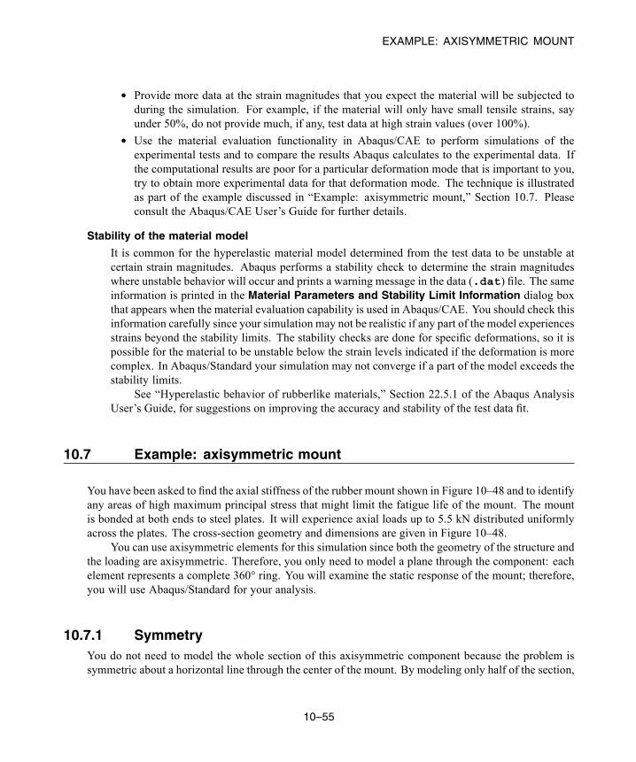
EXAMPLE: AXISYMMETRIC MOUNT
• Provide more data at the strain magnitudes that you expect the material will be subjected toduring the simulation. For example, if the material will only have small tensile strains, sayunder 50%, do not provide much, if any, test data at high strain values (over 100%).
• Use the material evaluation functionality in Abaqus/CAE to perform simulations of theexperimental tests and to compare the results Abaqus calculates to the experimental data. Ifthe computational results are poor for a particular deformation mode that is important to you,try to obtain more experimental data for that deformation mode. The technique is illustratedas part of the example discussed in “Example: axisymmetric mount,” Section 10.7. Pleaseconsult the Abaqus/CAE User’s Guide for further details.
Stability of the material model
It is common for the hyperelastic material model determined from the test data to be unstable atcertain strain magnitudes. Abaqus performs a stability check to determine the strain magnitudeswhere unstable behavior will occur and prints a warning message in the data (.dat) file. The sameinformation is printed in the Material Parameters and Stability Limit Information dialog boxthat appears when the material evaluation capability is used in Abaqus/CAE. You should check thisinformation carefully since your simulation may not be realistic if any part of the model experiencesstrains beyond the stability limits. The stability checks are done for specific deformations, so it ispossible for the material to be unstable below the strain levels indicated if the deformation is morecomplex. In Abaqus/Standard your simulation may not converge if a part of the model exceeds thestability limits.
See “Hyperelastic behavior of rubberlike materials,” Section 22.5.1 of the Abaqus AnalysisUser’s Guide, for suggestions on improving the accuracy and stability of the test data fit.
10.7 Example: axisymmetric mount
You have been asked to find the axial stiffness of the rubber mount shown in Figure 10–48 and to identifyany areas of high maximum principal stress that might limit the fatigue life of the mount. The mountis bonded at both ends to steel plates. It will experience axial loads up to 5.5 kN distributed uniformlyacross the plates. The cross-section geometry and dimensions are given in Figure 10–48.
You can use axisymmetric elements for this simulation since both the geometry of the structure andthe loading are axisymmetric. Therefore, you only need to model a plane through the component: eachelement represents a complete 360° ring. You will examine the static response of the mount; therefore,you will use Abaqus/Standard for your analysis.
10.7.1 SymmetryYou do not need to model the whole section of this axisymmetric component because the problem issymmetric about a horizontal line through the center of the mount. By modeling only half of the section,
10–55
Abaqus ID:Printed on:
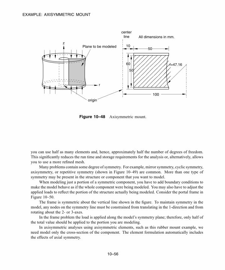
EXAMPLE: AXISYMMETRIC MOUNT
z
r
Plane to be modeled
centerline
1050
50
60
origin
r=47.16
All dimensions in mm.
100
Figure 10–48 Axisymmetric mount.
you can use half as many elements and, hence, approximately half the number of degrees of freedom.This significantly reduces the run time and storage requirements for the analysis or, alternatively, allowsyou to use a more refined mesh.
Many problems contain some degree of symmetry. For example, mirror symmetry, cyclic symmetry,axisymmetry, or repetitive symmetry (shown in Figure 10–49) are common. More than one type ofsymmetry may be present in the structure or component that you want to model.
When modeling just a portion of a symmetric component, you have to add boundary conditions tomake the model behave as if the whole component were being modeled. You may also have to adjust theapplied loads to reflect the portion of the structure actually being modeled. Consider the portal frame inFigure 10–50.
The frame is symmetric about the vertical line shown in the figure. To maintain symmetry in themodel, any nodes on the symmetry line must be constrained from translating in the 1-direction and fromrotating about the 2- or 3-axes.
In the frame problem the load is applied along the model’s symmetry plane; therefore, only half ofthe total value should be applied to the portion you are modeling.
In axisymmetric analyses using axisymmetric elements, such as this rubber mount example, weneed model only the cross-section of the component. The element formulation automatically includesthe effects of axial symmetry.
10–56
Abaqus ID:Printed on:

EXAMPLE: AXISYMMETRIC MOUNT
Mirror symmetry Axisymmetry
Cyclic symmetry
Repetitive symmetry
Figure 10–49 Various forms of symmetry.
Base built in
ENCASTREboundarycondition
Point load, P, appliedon center line
Appliedload=P/2
XSYMMboundarycondition
1
2
3
Figure 10–50 Symmetric portal frame.
10.7.2 Preprocessing—creating the model with Abaqus/CAEUse Abaqus/CAE to create the model. Abaqus provides scripts that replicate the complete analysis modelfor this problem. Run one of these scripts if you encounter difficulties following the instructions givenbelow or if you wish to check your work. Scripts are available in the following locations:
10–57
Abaqus ID:Printed on:
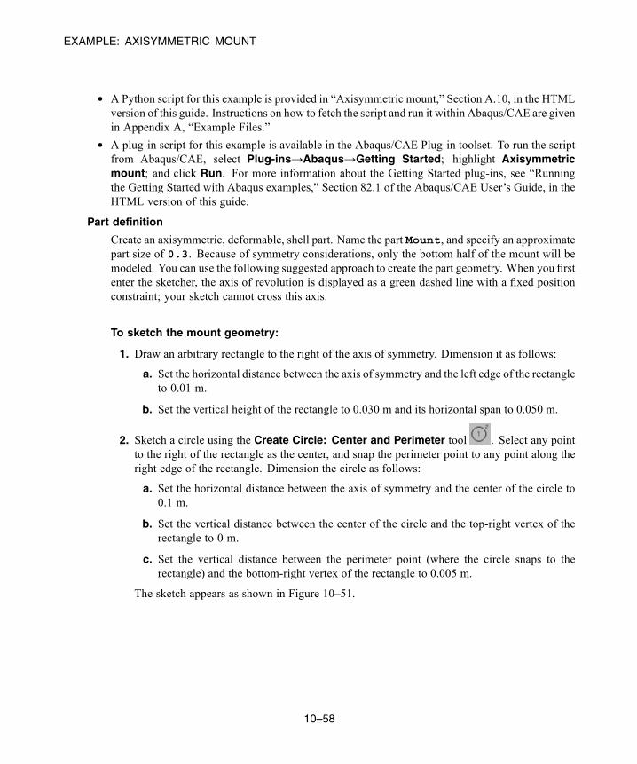
EXAMPLE: AXISYMMETRIC MOUNT
• A Python script for this example is provided in “Axisymmetric mount,” Section A.10, in the HTMLversion of this guide. Instructions on how to fetch the script and run it within Abaqus/CAE are givenin Appendix A, “Example Files.”
• A plug-in script for this example is available in the Abaqus/CAE Plug-in toolset. To run the scriptfrom Abaqus/CAE, select Plug-ins→Abaqus→Getting Started; highlight Axisymmetricmount; and click Run. For more information about the Getting Started plug-ins, see “Runningthe Getting Started with Abaqus examples,” Section 82.1 of the Abaqus/CAE User’s Guide, in theHTML version of this guide.
Part definition
Create an axisymmetric, deformable, shell part. Name the part Mount, and specify an approximatepart size of 0.3. Because of symmetry considerations, only the bottom half of the mount will bemodeled. You can use the following suggested approach to create the part geometry. When you firstenter the sketcher, the axis of revolution is displayed as a green dashed line with a fixed positionconstraint; your sketch cannot cross this axis.
To sketch the mount geometry:
1. Draw an arbitrary rectangle to the right of the axis of symmetry. Dimension it as follows:
a. Set the horizontal distance between the axis of symmetry and the left edge of the rectangleto 0.01 m.
b. Set the vertical height of the rectangle to 0.030 m and its horizontal span to 0.050 m.
2. Sketch a circle using the Create Circle: Center and Perimeter tool . Select any pointto the right of the rectangle as the center, and snap the perimeter point to any point along theright edge of the rectangle. Dimension the circle as follows:
a. Set the horizontal distance between the axis of symmetry and the center of the circle to0.1 m.
b. Set the vertical distance between the center of the circle and the top-right vertex of therectangle to 0 m.
c. Set the vertical distance between the perimeter point (where the circle snaps to therectangle) and the bottom-right vertex of the rectangle to 0.005 m.
The sketch appears as shown in Figure 10–51.
10–58
Abaqus ID:Printed on:
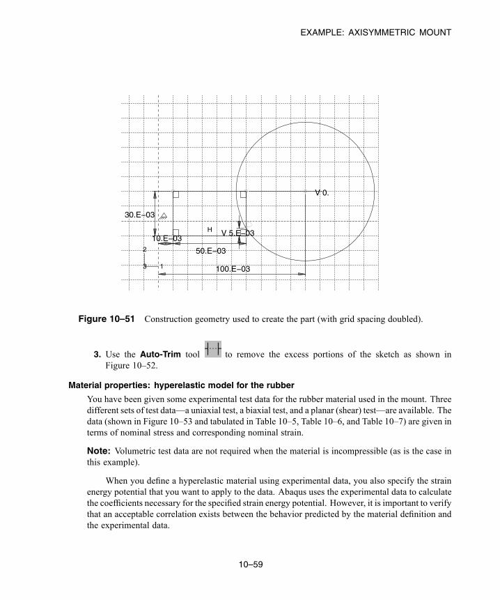
EXAMPLE: AXISYMMETRIC MOUNT
H
100.E−03
V 5.E−03
V 0.
50.E−03
30.E−03
10.E−03
1
2
3
Figure 10–51 Construction geometry used to create the part (with grid spacing doubled).
3. Use the Auto-Trim tool to remove the excess portions of the sketch as shown inFigure 10–52.
Material properties: hyperelastic model for the rubber
You have been given some experimental test data for the rubber material used in the mount. Threedifferent sets of test data—a uniaxial test, a biaxial test, and a planar (shear) test—are available. Thedata (shown in Figure 10–53 and tabulated in Table 10–5, Table 10–6, and Table 10–7) are given interms of nominal stress and corresponding nominal strain.
Note: Volumetric test data are not required when the material is incompressible (as is the case inthis example).
When you define a hyperelastic material using experimental data, you also specify the strainenergy potential that you want to apply to the data. Abaqus uses the experimental data to calculatethe coefficients necessary for the specified strain energy potential. However, it is important to verifythat an acceptable correlation exists between the behavior predicted by the material definition andthe experimental data.
10–59
Abaqus ID:Printed on:

EXAMPLE: AXISYMMETRIC MOUNT
H
( 47.E−03 )
50.E−03
30.E−03
10.E−03
1
2
3
Figure 10–52 Final part geometry (with grid spacing doubled).
UNIAXIAL
BIAXIAL
PLANAR
Nom
inal
Str
ess
(Pa)
Nominal Strain
Figure 10–53 Material test data for the rubber material.
10–60
Abaqus ID:Printed on:
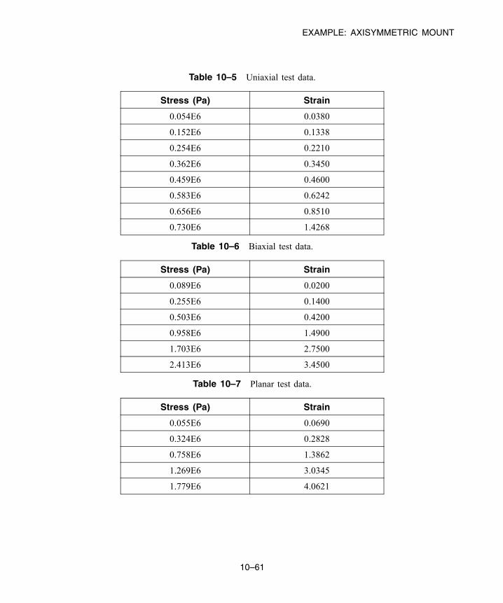
EXAMPLE: AXISYMMETRIC MOUNT
Table 10–5 Uniaxial test data.
Stress (Pa) Strain
0.054E6 0.0380
0.152E6 0.1338
0.254E6 0.2210
0.362E6 0.3450
0.459E6 0.4600
0.583E6 0.6242
0.656E6 0.8510
0.730E6 1.4268
Table 10–6 Biaxial test data.
Stress (Pa) Strain
0.089E6 0.0200
0.255E6 0.1400
0.503E6 0.4200
0.958E6 1.4900
1.703E6 2.7500
2.413E6 3.4500
Table 10–7 Planar test data.
Stress (Pa) Strain
0.055E6 0.0690
0.324E6 0.2828
0.758E6 1.3862
1.269E6 3.0345
1.779E6 4.0621
10–61
Abaqus ID:Printed on:
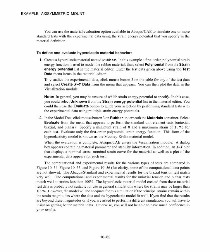
EXAMPLE: AXISYMMETRIC MOUNT
You can use the material evaluation option available in Abaqus/CAE to simulate one or morestandard tests with the experimental data using the strain energy potential that you specify in thematerial definition.
To define and evaluate hyperelastic material behavior:
1. Create a hyperelastic material named Rubber. In this example a first-order, polynomial strainenergy function is used to model the rubber material; thus, select Polynomial from the Strainenergy potential list in the material editor. Enter the test data given above using the TestData menu items in the material editor.
To visualize the experimental data, click mouse button 3 on the table for any of the test dataand select Create X–Y Data from the menu that appears. You can then plot the data in theVisualization module.
Note: In general, you may be unsure of which strain energy potential to specify. In this case,you could select Unknown from the Strain energy potential list in the material editor. Youcould then use the Evaluate option to guide your selection by performing standard tests withthe experimental data using multiple strain energy potentials.
2. In theModel Tree, clickmouse button 3 onRubber underneath theMaterials container. SelectEvaluate from the menu that appears to perform the standard unit-element tests (uniaxial,biaxial, and planar). Specify a minimum strain of 0 and a maximum strain of 1.75 foreach test. Evaluate only the first-order polynomial strain energy function. This form of thehyperelasticity model is known as the Mooney-Rivlin material model.
When the evaluation is complete, Abaqus/CAE enters the Visualization module. A dialogbox appears containing material parameter and stability information. In addition, an X–Y plotthat displays a nominal stress–nominal strain curve for the material as well as a plot of theexperimental data appears for each test.
The computational and experimental results for the various types of tests are compared inFigure 10–54, Figure 10–55, and Figure 10–56 (for clarity, some of the computational data pointsare not shown). The Abaqus/Standard and experimental results for the biaxial tension test matchvery well. The computational and experimental results for the uniaxial tension and planar testsmatch well at strains less than 100%. The hyperelastic material model created from these materialtest data is probably not suitable for use in general simulations where the strains may be larger than100%. However, the model will be adequate for this simulation if the principal strains remain withinthe strain magnitudes where the data and the hyperelastic model fit well. If you find that the resultsare beyond these magnitudes or if you are asked to perform a different simulation, you will have toinsist on getting better material data. Otherwise, you will not be able to have much confidence inyour results.
10–62
Abaqus ID:Printed on:
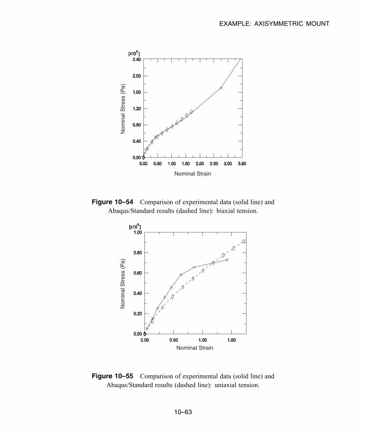
EXAMPLE: AXISYMMETRIC MOUNT
Nom
inal
Str
ess
(Pa)
Nominal Strain
Figure 10–54 Comparison of experimental data (solid line) andAbaqus/Standard results (dashed line): biaxial tension.
Nom
inal
Str
ess
(Pa)
Nominal Strain
Figure 10–55 Comparison of experimental data (solid line) andAbaqus/Standard results (dashed line): uniaxial tension.
10–63
Abaqus ID:Printed on:
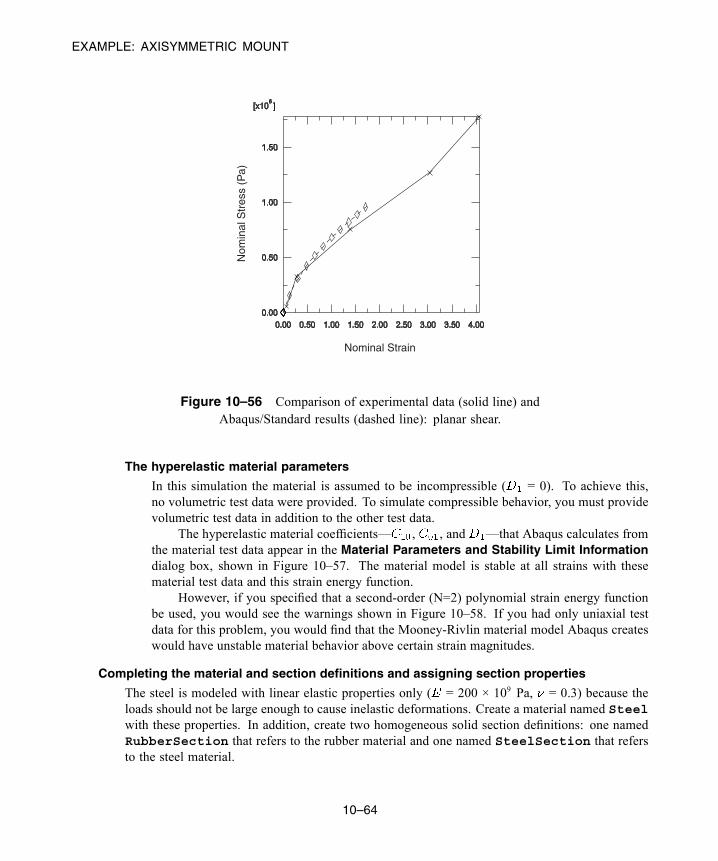
EXAMPLE: AXISYMMETRIC MOUNT
Nom
inal
Str
ess
(Pa)
Nominal Strain
Figure 10–56 Comparison of experimental data (solid line) andAbaqus/Standard results (dashed line): planar shear.
The hyperelastic material parameters
In this simulation the material is assumed to be incompressible ( = 0). To achieve this,no volumetric test data were provided. To simulate compressible behavior, you must providevolumetric test data in addition to the other test data.
The hyperelastic material coefficients— , , and —that Abaqus calculates fromthe material test data appear in the Material Parameters and Stability Limit Informationdialog box, shown in Figure 10–57. The material model is stable at all strains with thesematerial test data and this strain energy function.
However, if you specified that a second-order (N=2) polynomial strain energy functionbe used, you would see the warnings shown in Figure 10–58. If you had only uniaxial testdata for this problem, you would find that the Mooney-Rivlin material model Abaqus createswould have unstable material behavior above certain strain magnitudes.
Completing the material and section definitions and assigning section properties
The steel is modeled with linear elastic properties only ( = 200 × 109 Pa, = 0.3) because theloads should not be large enough to cause inelastic deformations. Create a material named Steelwith these properties. In addition, create two homogeneous solid section definitions: one namedRubberSection that refers to the rubber material and one named SteelSection that refersto the steel material.
10–64
Abaqus ID:Printed on:

EXAMPLE: AXISYMMETRIC MOUNT
Figure 10–57 Material parameters and stability limits for thefirst-order polynomial strain energy function.
Figure 10–58 Material parameters and stability limits for thesecond-order polynomial strain energy function.
10–65
Abaqus ID:Printed on:
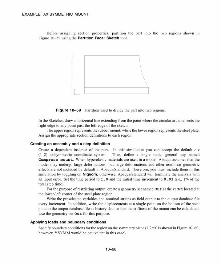
EXAMPLE: AXISYMMETRIC MOUNT
Before assigning section properties, partition the part into the two regions shown inFigure 10–59 using the Partition Face: Sketch tool.
1
2
3
Figure 10–59 Partition used to divide the part into two regions.
In the Sketcher, draw a horizontal line extending from the point where the circular arc intersects theright edge to any point past the left edge of the sketch.
The upper region represents the rubber mount, while the lower region represents the steel plate.Assign the appropriate section definitions to each region.
Creating an assembly and a step definition
Create a dependent instance of the part. In this simulation you can accept the default r–z(1–2) axisymmetric coordinate system. Then, define a single static, general step namedCompress mount. When hyperelastic materials are used in a model, Abaqus assumes that themodel may undergo large deformations; but large deformations and other nonlinear geometriceffects are not included by default in Abaqus/Standard. Therefore, you must include them in thissimulation by toggling on Nlgeom; otherwise, Abaqus/Standard will terminate the analysis withan input error. Set the time period to 1.0 and the initial time increment to 0.01 (i.e., 1% of thetotal step time).
For the purpose of restricting output, create a geometry set named Out at the vertex located atthe lower-left corner of the steel plate region.
Write the preselected variables and nominal strains as field output to the output database fileevery increment. In addition, write the displacements at a single point on the bottom of the steelplate to the output database file as history data so that the stiffness of the mount can be calculated.Use the geometry set Out for this purpose.
Applying loads and boundary conditions
Specify boundary conditions for the region on the symmetry plane (U2 = 0 is shown in Figure 10–60;however, YSYMM would be equivalent in this case).
10–66
Abaqus ID:Printed on:
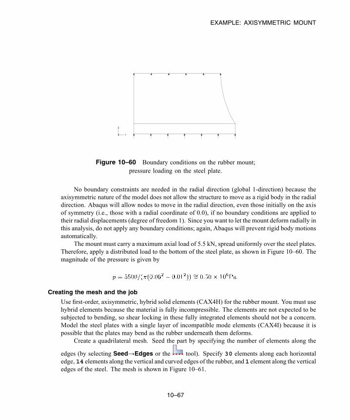
EXAMPLE: AXISYMMETRIC MOUNT
1
2
3
Figure 10–60 Boundary conditions on the rubber mount;pressure loading on the steel plate.
No boundary constraints are needed in the radial direction (global 1-direction) because theaxisymmetric nature of the model does not allow the structure to move as a rigid body in the radialdirection. Abaqus will allow nodes to move in the radial direction, even those initially on the axisof symmetry (i.e., those with a radial coordinate of 0.0), if no boundary conditions are applied totheir radial displacements (degree of freedom 1). Since you want to let the mount deform radially inthis analysis, do not apply any boundary conditions; again, Abaqus will prevent rigid body motionsautomatically.
The mount must carry a maximum axial load of 5.5 kN, spread uniformly over the steel plates.Therefore, apply a distributed load to the bottom of the steel plate, as shown in Figure 10–60. Themagnitude of the pressure is given by
Creating the mesh and the job
Use first-order, axisymmetric, hybrid solid elements (CAX4H) for the rubber mount. You must usehybrid elements because the material is fully incompressible. The elements are not expected to besubjected to bending, so shear locking in these fully integrated elements should not be a concern.Model the steel plates with a single layer of incompatible mode elements (CAX4I) because it ispossible that the plates may bend as the rubber underneath them deforms.
Create a quadrilateral mesh. Seed the part by specifying the number of elements along the
edges (by selecting Seed→Edges or the tool). Specify 30 elements along each horizontaledge, 14 elements along the vertical and curved edges of the rubber, and1 element along the verticaledges of the steel. The mesh is shown in Figure 10–61.
10–67
Abaqus ID:Printed on:
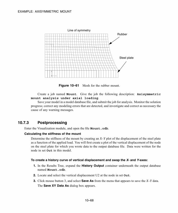
EXAMPLE: AXISYMMETRIC MOUNT
1
2
3
Line of symmetry
Steel plate
Rubber
Figure 10–61 Mesh for the rubber mount.
Create a job named Mount. Give the job the following description: Axisymmetricmount analysis under axial loading.
Save your model in a model database file, and submit the job for analysis. Monitor the solutionprogress; correct any modeling errors that are detected, and investigate and correct as necessary thecause of any warning messages.
10.7.3 PostprocessingEnter the Visualization module, and open the file Mount.odb.
Calculating the stiffness of the mount
Determine the stiffness of the mount by creating an X–Y plot of the displacement of the steel plateas a function of the applied load. You will first create a plot of the vertical displacement of the nodeon the steel plate for which you wrote data to the output database file. Data were written for thenode in set Out in this model.
To create a history curve of vertical displacement and swap the X- and Y-axes:
1. In the Results Tree, expand the History Output container underneath the output databasenamed Mount.odb.
2. Locate and select the vertical displacement U2 at the node in set Out.
3. Click mouse button 3, and select Save As from the menu that appears to save the X–Y data.
The Save XY Data As dialog box appears.
10–68
Abaqus ID:Printed on:
EXAMPLE: AXISYMMETRIC MOUNT
4. In the Save XY Data As dialog box, name the curve SWAPPED and select swap(XY) as thesave operation; click OK.
The plot of time-displacement appears in the viewport.
You now have a curve of time-displacement. What you need is a curve showingforce-displacement. This is easy to create because in this simulation the force applied to themount is directly proportional to the total time in the analysis. All you have to do to plot aforce-displacement curve is multiply the curve SWAPPED by the magnitude of the load (5.5 kN).
To multiply a curve by a constant value:
1. In the Results Tree, double-click XYData.
The Create XY Data dialog box appears.
2. Select Operate on XY data, and click Continue.
The Operate on XY Data dialog box appears.
3. In the XY Data field, double-click SWAPPED.
The expression "SWAPPED" appears in the text field at the top of the dialog box. Your cursorshould be at the end of the text field.
4. Multiply the data object in the text field by the magnitude of the applied load by entering*5500.
5. Save the multiplied data object by clicking Save As at the bottom of the dialog box.
The Save XY Data As dialog box appears.
6. In the Name text field, type FORCEDEF; and click OK to close the dialog box.
7. To view the force-displacement plot, click Plot Expression at the bottom of the Operate onXY Data dialog box.
You have now created a curve with the force-deflection characteristic of the mount (the axislabels do not reflect this since you did not change the actual variable plotted). To get the stiffness,you need to differentiate the curveFORCEDEF. You can do this by using thedifferentiate( )operator in the Operate on XY Data dialog box.
To obtain the stiffness:
1. In the Operate on XY Data dialog box, clear the current expression.
2. From the Operators listed, click differentiate(X).
differentiate( ) appears in the text field at the top of the dialog box.
3. In the XY Data field, double-click FORCEDEF.
The expression differentiate( "FORCEDEF" ) appears in the text field.
4. Save the differentiated data object by clicking Save As at the bottom of the dialog box.
The Save XY Data As dialog box appears.
10–69
Abaqus ID:Printed on:
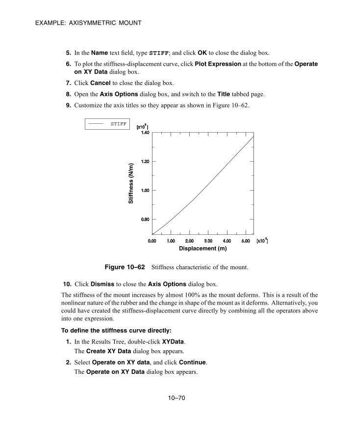
EXAMPLE: AXISYMMETRIC MOUNT
5. In the Name text field, type STIFF; and click OK to close the dialog box.
6. To plot the stiffness-displacement curve, click Plot Expression at the bottom of the Operateon XY Data dialog box.
7. Click Cancel to close the dialog box.
8. Open the Axis Options dialog box, and switch to the Title tabbed page.
9. Customize the axis titles so they appear as shown in Figure 10–62.
STIFF
Displacement (m)
Sti
ffn
ess
(N/m
)
Figure 10–62 Stiffness characteristic of the mount.
10. Click Dismiss to close the Axis Options dialog box.
The stiffness of the mount increases by almost 100% as the mount deforms. This is a result of thenonlinear nature of the rubber and the change in shape of the mount as it deforms. Alternatively, youcould have created the stiffness-displacement curve directly by combining all the operators aboveinto one expression.
To define the stiffness curve directly:
1. In the Results Tree, double-click XYData.
The Create XY Data dialog box appears.
2. Select Operate on XY data, and click Continue.
The Operate on XY Data dialog box appears.
10–70
Abaqus ID:Printed on:
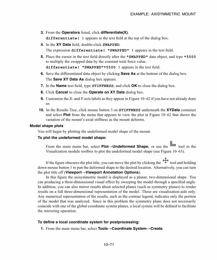
EXAMPLE: AXISYMMETRIC MOUNT
3. From the Operators listed, click differentiate(X).
differentiate( ) appears in the text field at the top of the dialog box.
4. In the XY Data field, double-click SWAPPED.
The expression differentiate( "SWAPPED" ) appears in the text field.
5. Place the cursor in the text field directly after the "SWAPPED" data object, and type *5500to multiply the swapped data by the constant total force value.
differentiate( "SWAPPED"*5500 ) appears in the text field.
6. Save the differentiated data object by clicking Save As at the bottom of the dialog box.
The Save XY Data As dialog box appears.
7. In the Name text field, type STIFFNESS; and click OK to close the dialog box.
8. Click Cancel to close the Operate on XY Data dialog box.
9. Customize the X- and Y-axis labels as they appear in Figure 10–62 if you have not already doneso.
10. In the Results Tree, click mouse button 3 on STIFFNESS underneath the XYData containerand select Plot from the menu that appears to view the plot in Figure 10–62 that shows thevariation of the mount’s axial stiffness as the mount deforms.
Model shape plots
You will begin by plotting the undeformed model shape of the mount.
To plot the undeformed model shape:
From the main menu bar, select Plot→Undeformed Shape; or use the tool in theVisualization module toolbox to plot the undeformed model shape (see Figure 10–63).
If the figure obscures the plot title, you can move the plot by clicking the tool and holdingdown mouse button 1 to pan the deformed shape to the desired location. Alternatively, you can turnthe plot title off (Viewport→Viewport Annotation Options).
In this figure the axisymmetric model is displayed as a planar, two-dimensional shape. Youcan producing a three-dimensional visual effect by sweeping the model through a specified angle.In addition, you can also mirror results about selected planes (such as symmetry planes) to renderresults on a full three-dimensional representation of the model. These are visualization aids only.Any numerical representation of the results, such as the contour legend, indicates only the portionof the model that was analyzed. Since in this problem the symmetry plane does not necessarilycoincide with one of the global coordinate system planes, a local system will be defined to facilitatethe mirroring operation.
To define a local coordinate system for postprocessing:
1. From the main menu bar, select Tools→Coordinate System→Create.
10–71
Abaqus ID:Printed on:

EXAMPLE: AXISYMMETRIC MOUNT
1
2
3
Figure 10–63 Undeformed model shape of the rubber mount.
2. In the Create Coordinate System dialog box, enter rectangular as the name and clickContinue.
3. Select the node at the top-left corner of the model as the origin, the node at the top-right corneras the point on the X-axis, and the node at the bottom-left corner as the point in the X–Y plane.
To mirror and sweep the cross-section:
1. From the main menu bar, select View→ODB Display Options.
2. In the ODB Display Options dialog box, click the Mirror/Pattern tab.
3. Select rectangular from the Mirror CSYS list.
4. Select XZ as the mirror plane.
5. Click Apply.
The mirrored image appears.
6. Click the Sweep/Extrude tab.
7. Toggle on Sweep elements and set the sweep range from 0 to 270 degrees. Set the numberof segments to 45.
8. Click OK.
The swept image appears. To more clearly distinguish between the rubber and the steel, colorcode the model based on section assignment.
You will now plot the deformed model shape of the mount. This will allow you to evaluate thequality of the deformed mesh and to assess the need for mesh refinement.
10–72
Abaqus ID:Printed on:
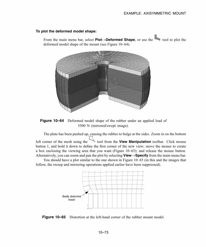
EXAMPLE: AXISYMMETRIC MOUNT
To plot the deformed model shape:
From the main menu bar, select Plot→Deformed Shape, or use the tool to plot thedeformed model shape of the mount (see Figure 10–64).
Z
Y
X
Figure 10–64 Deformed model shape of the rubber under an applied load of5500 N (mirrored/swept image).
The plate has been pushed up, causing the rubber to bulge at the sides. Zoom in on the bottom
left corner of the mesh using the tool from the View Manipulation toolbar. Click mousebutton 1, and hold it down to define the first corner of the new view; move the mouse to createa box enclosing the viewing area that you want (Figure 10–65); and release the mouse button.Alternatively, you can zoom and pan the plot by selecting View→Specify from the main menu bar.
You should have a plot similar to the one shown in Figure 10–65 (in this and the images thatfollow, the sweep and mirroring operations applied earlier have been suppressed).
Badly distortedmesh
1
2
3
Figure 10–65 Distortion at the left-hand corner of the rubber mount model.
10–73
Abaqus ID:Printed on:
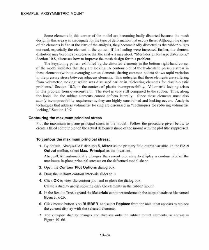
EXAMPLE: AXISYMMETRIC MOUNT
Some elements in this corner of the model are becoming badly distorted because the meshdesign in this area was inadequate for the type of deformation that occurs there. Although the shapeof the elements is fine at the start of the analysis, they become badly distorted as the rubber bulgesoutward, especially the element in the corner. If the loading were increased further, the elementdistortion may become so excessive that the analysis may abort. “Mesh design for large distortions,”Section 10.8, discusses how to improve the mesh design for this problem.
The keystoning pattern exhibited by the distorted elements in the bottom right-hand cornerof the model indicates that they are locking. A contour plot of the hydrostatic pressure stress inthese elements (without averaging across elements sharing common nodes) shows rapid variationin the pressure stress between adjacent elements. This indicates that these elements are sufferingfrom volumetric locking, which was discussed earlier in “Selecting elements for elastic-plasticproblems,” Section 10.3, in the context of plastic incompressibility. Volumetric locking arisesin this problem from overconstraint. The steel is very stiff compared to the rubber. Thus, alongthe bond line the rubber elements cannot deform laterally. Since these elements must alsosatisfy incompressibility requirements, they are highly constrained and locking occurs. Analysistechniques that address volumetric locking are discussed in “Techniques for reducing volumetriclocking,” Section 10.9.
Contouring the maximum principal stress
Plot the maximum in-plane principal stress in the model. Follow the procedure given below tocreate a filled contour plot on the actual deformed shape of the mount with the plot title suppressed.
To contour the maximum principal stress:
1. By default, Abaqus/CAE displays S, Mises as the primary field output variable. In the FieldOutput toolbar, select Max. Principal as the invariant.
Abaqus/CAE automatically changes the current plot state to display a contour plot of themaximum in-plane principal stresses on the deformed model shape.
2. Open the Contour Plot Options dialog box.
3. Drag the uniform contour intervals slider to 8.
4. Click OK to view the contour plot and to close the dialog box.
Create a display group showing only the elements in the rubber mount.
5. In the Results Tree, expand theMaterials container underneath the output database file namedMount.odb.
6. Click mouse button 3 on RUBBER, and select Replace from the menu that appears to replacethe current display with the selected elements.
7. The viewport display changes and displays only the rubber mount elements, as shown inFigure 10–66.
10–74
Abaqus ID:Printed on:
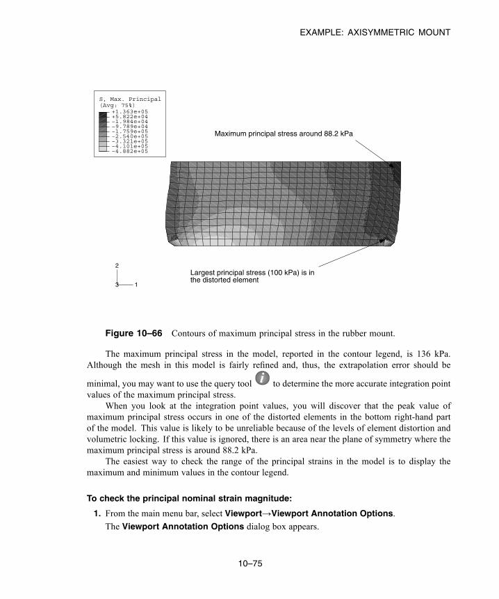
EXAMPLE: AXISYMMETRIC MOUNT
(Avg: 75%)S, Max. Principal
−4.882e+05−4.101e+05−3.321e+05−2.540e+05−1.759e+05−9.789e+04−1.984e+04+5.822e+04+1.363e+05
1
2
3
Maximum principal stress around 88.2 kPa
Largest principal stress (100 kPa) is in the distorted element
Figure 10–66 Contours of maximum principal stress in the rubber mount.
The maximum principal stress in the model, reported in the contour legend, is 136 kPa.Although the mesh in this model is fairly refined and, thus, the extrapolation error should be
minimal, you may want to use the query tool to determine the more accurate integration pointvalues of the maximum principal stress.
When you look at the integration point values, you will discover that the peak value ofmaximum principal stress occurs in one of the distorted elements in the bottom right-hand partof the model. This value is likely to be unreliable because of the levels of element distortion andvolumetric locking. If this value is ignored, there is an area near the plane of symmetry where themaximum principal stress is around 88.2 kPa.
The easiest way to check the range of the principal strains in the model is to display themaximum and minimum values in the contour legend.
To check the principal nominal strain magnitude:
1. From the main menu bar, select Viewport→Viewport Annotation Options.
The Viewport Annotation Options dialog box appears.
10–75
Abaqus ID:Printed on:

MESH DESIGN FOR LARGE DISTORTIONS
2. Click the Legend tab, and toggle on Show min/max values.
3. Click OK.
The maximum and minimum values appear at the bottom of the contour legend in the viewport.
4. In the Field Output toolbar, select Primary as the variable type if it is not already selected.
Abaqus/CAE automatically changes the current plot state to display a contour plot of themaximum in-plane principal stresses on the deformed model shape.
5. From the list of output variables, select NE.
6. From the list of invariants in the Field Output toolbar, select Max. Principal if it is notalready selected.
The contour plot changes to display values for maximum principal nominal strain. Note thevalue of the maximum principal nominal strain from the contour legend.
7. From the list of invariants, select Min. Principal.
The contour plot changes to display values for minimum principal nominal strain. Note thevalue of the minimum principal nominal strain from the contour legend.
The maximum and minimum principal nominal strain values indicate that the maximumtensile nominal strain in the model is about 100% and the maximum compressive nominal strainis about 56%. Because the nominal strains in the model remained within the range where theAbaqus hyperelasticity model has a good fit to the material data, you can be fairly confident thatthe response predicted by the mount is reasonable from a material modeling viewpoint.
10.8 Mesh design for large distortions
We know that the element distortions in the corners of the rubber mount are undesirable. The resultsin these areas are unreliable; and if the load were increased, the analysis might fail. These problemscan be corrected by using a better mesh design. The mesh shown in Figure 10–67 is an example ofan alternate mesh design that might be used to reduce element distortion in the bottom left corner ofthe rubber model. The issues surrounding the mesh distortion in the opposite corner are addressed in“Techniques for reducing volumetric locking,” Section 10.9. The elements in the bottom left-hand cornerregion are now much more distorted in the initial, undeformed configuration. However, as the analysisprogresses and the elements deform, their shape actually improves. The deformed shape plot, shown inFigure 10–68, illustrates that the amount of element distortion in this region is reduced; however, thelevel of mesh distortion in the bottom right-hand corner of the rubber model is still significant.
The contours of maximum principal stress (Figure 10–69) show that the very localized stress in thatcorner has been reduced only slightly.
Mesh design for large-distortion problems is more difficult than it is for small-displacementproblems. A mesh must be produced where the shape of the elements is reasonable throughout theanalysis, not just at the start. You must estimate how the model will deform using experience, handcalculations, or the results from a coarse finite element model.
10–76
Abaqus ID:Printed on:
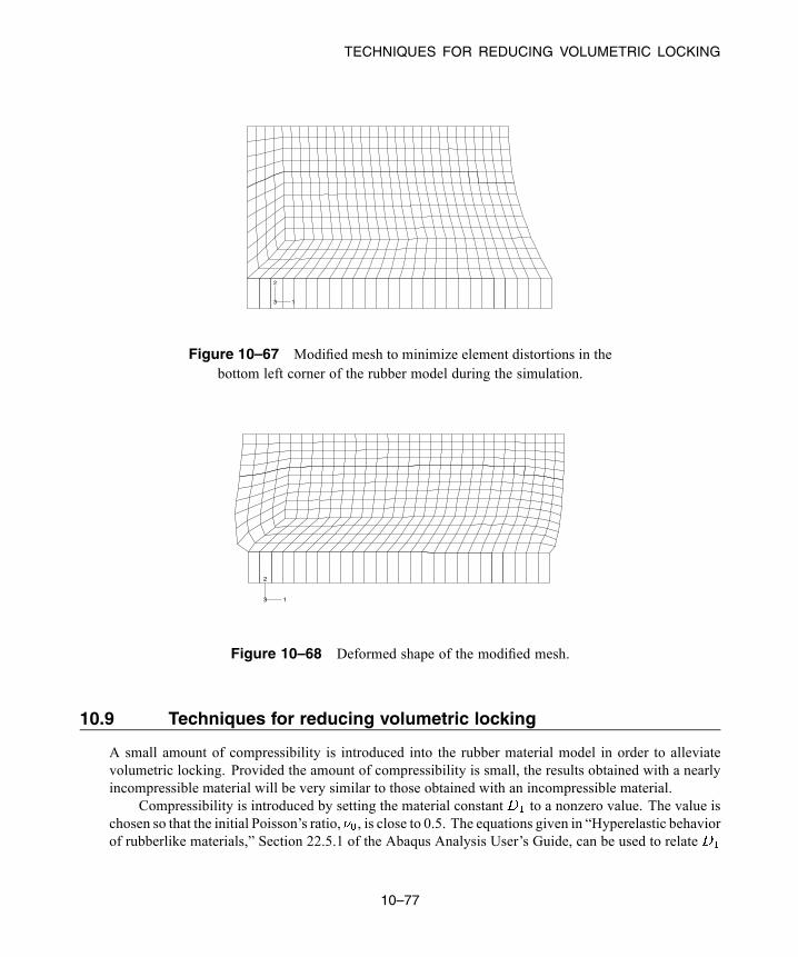
TECHNIQUES FOR REDUCING VOLUMETRIC LOCKING
1
2
3
Figure 10–67 Modified mesh to minimize element distortions in thebottom left corner of the rubber model during the simulation.
1
2
3
Figure 10–68 Deformed shape of the modified mesh.
10.9 Techniques for reducing volumetric locking
A small amount of compressibility is introduced into the rubber material model in order to alleviatevolumetric locking. Provided the amount of compressibility is small, the results obtained with a nearlyincompressible material will be very similar to those obtained with an incompressible material.
Compressibility is introduced by setting the material constant to a nonzero value. The value ischosen so that the initial Poisson’s ratio, , is close to 0.5. The equations given in “Hyperelastic behaviorof rubberlike materials,” Section 22.5.1 of the Abaqus Analysis User’s Guide, can be used to relate
10–77
Abaqus ID:Printed on:
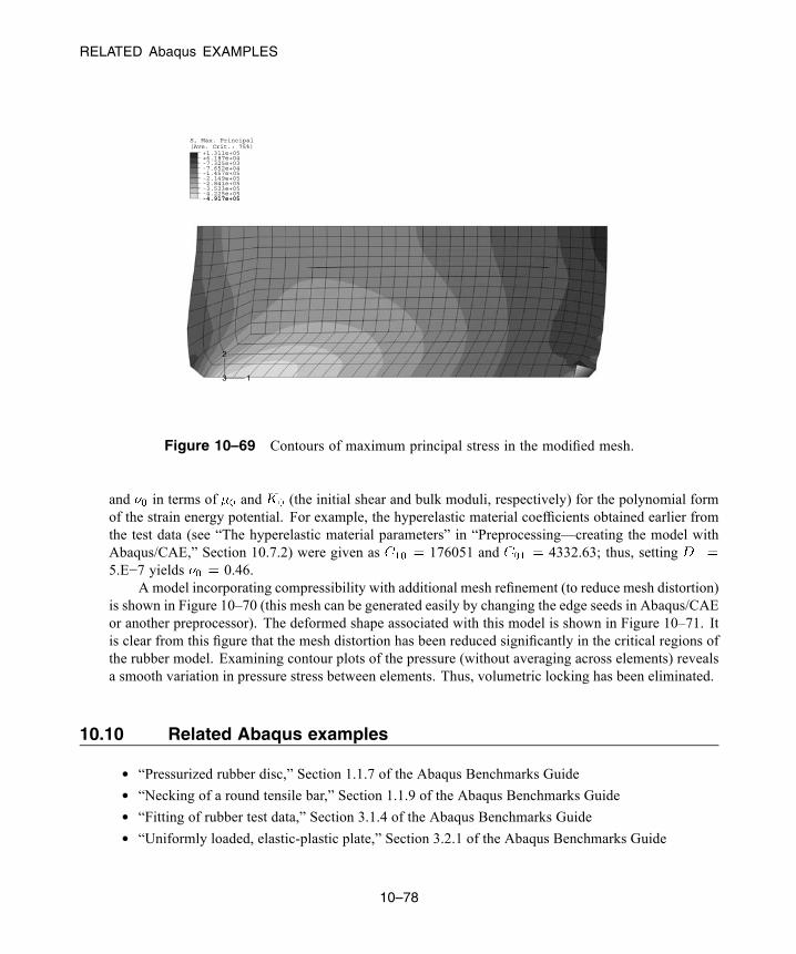
RELATED Abaqus EXAMPLES
1
2
3
-4.917e+05
(Ave. Crit.: 75%)S, Max. Principal
-4.917e+05-4.225e+05-3.533e+05-2.841e+05-2.149e+05-1.457e+05-7.652e+04-7.325e+03+6.187e+04+1.311e+05
Figure 10–69 Contours of maximum principal stress in the modified mesh.
and in terms of and (the initial shear and bulk moduli, respectively) for the polynomial formof the strain energy potential. For example, the hyperelastic material coefficients obtained earlier fromthe test data (see “The hyperelastic material parameters” in “Preprocessing—creating the model withAbaqus/CAE,” Section 10.7.2) were given as 176051 and 4332.63; thus, setting5.E−7 yields 0.46.
A model incorporating compressibility with additional mesh refinement (to reduce mesh distortion)is shown in Figure 10–70 (this mesh can be generated easily by changing the edge seeds in Abaqus/CAEor another preprocessor). The deformed shape associated with this model is shown in Figure 10–71. Itis clear from this figure that the mesh distortion has been reduced significantly in the critical regions ofthe rubber model. Examining contour plots of the pressure (without averaging across elements) revealsa smooth variation in pressure stress between elements. Thus, volumetric locking has been eliminated.
10.10 Related Abaqus examples
• “Pressurized rubber disc,” Section 1.1.7 of the Abaqus Benchmarks Guide• “Necking of a round tensile bar,” Section 1.1.9 of the Abaqus Benchmarks Guide• “Fitting of rubber test data,” Section 3.1.4 of the Abaqus Benchmarks Guide• “Uniformly loaded, elastic-plastic plate,” Section 3.2.1 of the Abaqus Benchmarks Guide
10–78
Abaqus ID:Printed on:

SUGGESTED READING
1
2
3
Figure 10–70 Modified mesh with refinement at both corners.
1
2
3
Figure 10–71 Deformed shape of the modified mesh.
10.11 Suggested reading
The following provides the interested user with additional references on material modeling.
General texts on materials
• Ashby, M. F., and D. R. H. Jones, Engineering Materials, Pergamon Press, 1980.
• Callister, W. D., Materials Science & Engineering—An Introduction, John Wiley, 1994.
• Pascoe, K. J., An Introduction to the Properties of Engineering Materials, Van Nostrand, 1978.
Plasticity
• SIMULIA, Metal Inelasticity in Abaqus.
10–79
Abaqus ID:Printed on:

SUMMARY
• Lubliner, J., Plasticity Theory, Macmillan Publishing Co., 1990.
• Calladine, C. R., Engineering Plasticity, Pergamon Press, 1969.
Rubber elasticity
• SIMULIA, Modeling Rubber and Viscoelasticity with Abaqus.
• Gent, A., Engineering with Rubber (How to Design Rubber Components), Hanser Publishers,1992.
10.12 Summary
• Abaqus contains an extensive library to model the behavior of various engineering materials. Itincludes models for metal plasticity and rubber elasticity.
• The stress-strain data for the metal plasticity model must be defined in terms of true stress and trueplastic strain. Nominal stress-strain data can be converted easily into true stress-strain data.
• The metal plasticity model in Abaqus assumes incompressible plastic behavior.• For efficiency Abaqus/Explicit regularizes user-defined material curves by fitting them with curvescomposed of equally spaced points.
• The hyperelastic material model in Abaqus/Standard allows true incompressibility. The hyperelasticmaterial model in Abaqus/Explicit does not: the default Poisson’s ratio for hyperelastic materialsin Abaqus/Explicit is 0.475. Some analyses may require increasing Poisson’s ratio to modelincompressibility more accurately.
• Polynomial, Ogden, Arruda-Boyce, Marlow, van derWaals, Mooney-Rivlin, neo-Hookean, reducedpolynomial, and Yeoh strain energy functions are available for rubber elasticity (hyperelasticity).All models allow the material coefficients to be determined directly from experimental test data.The test data must be specified as nominal stress and nominal strain values.
• The material evaluation capability in Abaqus/CAE can be used to verify the correlation betweenthe behavior predicted by the hyperelastic material models and experimental test data.
• Stability warnings may indicate that a hyperelastic material model is unsuitable for the strain rangesyou wish to analyze.
• The presence of symmetry can be used to reduce the size of a simulation since only part of thecomponent needs to be modeled. The effect of the rest of the component is represented by applyingappropriate boundary conditions.
• Mesh design for large-distortion problems is more difficult than for small-displacement problems.The elements in the mesh must not become too distorted at any stage of the analysis.
• Volumetric locking can be alleviated by permitting a small amount of compressibility. Care mustbe taken to ensure that the amount of compressibility introduced into the problem does not grosslyaffect the overall results.
10–80
Abaqus ID:Printed on:

SUMMARY
• The X–Y plotting capabilities in Abaqus/CAE allow data in curves to be manipulated to create newcurves. Two curves or a curve and a constant can be added, subtracted, multiplied, or divided.Curves can also be differentiated, integrated, and combined.
10–81
Abaqus ID:Printed on:

GENERAL ANALYSIS PROCEDURES
11. Multiple Step Analysis
The general goal of an Abaqus simulation is to predict the response of a structure to applied loads. Recallthat in a general sense the term load in Abaqus refers to anything that induces a change in the responseof a structure from its initial state; for example, nonzero boundary conditions or applied displacements,point forces, pressures, fields, etc. In some cases loads are relatively simple, such as a single set ofpoint loads on a structure. In other problems the loads applied to a structure can be very complex. Forexample, different loads may be applied to different portions of the model in a particular sequence oversome period of time, or the magnitude of the loads may vary as a function of time. The term load historyis used to refer to such complex loading of a model.
In Abaqus the user divides the complete load history of the simulation into a number of steps. Eachstep is a period of “time,” specified by the user, for which Abaqus calculates the response of the modelto a particular set of loads and boundary conditions. The user must specify the type of response, knownas the analysis procedure, during each step and may change analysis procedures from step to step. Forexample, static dead loads, perhaps gravitational loads, could be applied to a structure in one step; andthe dynamic response of the loaded structure to earthquake accelerations could be calculated in the nextstep. Both implicit and explicit analyses can contain multiple steps; however, implicit and explicit stepscannot be combined in the same analysis job. To combine a series of implicit and explicit steps, theresults transfer (or import) capability can be used. This feature is discussed in “Transferring resultsbetween Abaqus/Explicit and Abaqus/Standard,” Section 9.2.2 of the Abaqus Analysis User’s Guide,and is not discussed further here.
Abaqus divides all of its analysis procedures into two main groups: linear perturbation and general.General analysis steps can be included in an Abaqus/Standard or an Abaqus/Explicit analysis; linearperturbation steps are available only in Abaqus/Standard. Loading conditions and “time” are defineddifferently for the two cases. Furthermore, the results from each type of procedure should be interpreteddifferently.
The response of the model during a general analysis procedure, known as a general step, may beeither nonlinear or linear. In a step that uses a perturbation procedure, which is called a perturbationstep, the response can only be linear. Abaqus/Standard treats such steps as a linear perturbation about thepreloaded, predeformed state (known as the base state) created by any previous general steps; therefore,its capability for doing linear simulations is rather more general than that of a purely linear analysisprogram.
11.1 General analysis procedures
The starting point for each general step is the deformed state at the end of the last general step. Therefore,the state of the model evolves in a sequence of general steps as it responds to the loads defined in eachstep. Any initial conditions define the starting point for the first general step in the simulation.
All general analysis procedures share the same concepts for applying loads and defining “time.”
11–1
Abaqus ID:Printed on:

LINEAR PERTURBATION ANALYSIS
11.1.1 Time in general analysis stepsAbaqus has two measures of time in a simulation. The total time increases throughout all general stepsand is the accumulation of the total step time from each general step. Each step also has its own timescale (known as the step time), which begins at zero for each step. Time varying loads and boundaryconditions can be specified in terms of either time scale. The time scales for an analysis whose historyis divided into three steps, each 100 seconds long, are shown in Figure 11–1.
Totaltime
Steptime
Step 1 Step 2 Step 3
0s
0s 300s
100s0s100s100s 0s
200s100s
Figure 11–1 Step and total time for a simulation.
11.1.2 Specifying loads in general stepsIn general steps the loads must be specified as total values, not incremental values. For example, if aconcentrated load has a value of 1000 N in the first step and it is increased to 3000 N in the second generalstep, the magnitude given for the load in the two steps should be 1000 N and 3000 N, not 1000 N and2000 N.
By default, all previously defined loads are propagated to the current step. In the current step you candefine additional loads as well as modify any previously defined load (for example, change its magnitudeor deactivate it). Any previously defined load that is not specifically modified in the current step continuesto follow its associated amplitude definition, provided that the amplitude curve is defined in terms of totaltime; otherwise, the load is maintained at the magnitude it had at the end of the last general step.
11.2 Linear perturbation analysis
Linear perturbation analysis steps are available only in Abaqus/Standard.
11–2
Abaqus ID:Printed on:

LINEAR PERTURBATION ANALYSIS
The starting point for a linear perturbation step is called the base state of the model. If the first stepin a simulation is a linear perturbation step, the base state is the state of the model specified using initialconditions. Otherwise, the base state is the state of the simulation at the end of the last general step priorto the linear perturbation step. Although the response of the structure during the perturbation step is bydefinition linear, the model may have a nonlinear response in previous general steps. For models witha nonlinear response in the prior general steps, Abaqus/Standard uses the current elastic modulus as thelinear stiffness for perturbation procedures. This modulus is the initial elastic modulus for elastic-plasticmaterials and the tangent modulus for hyperelastic materials (see Figure 11–2); the moduli used forother material models are described in “General and linear perturbation procedures,” Section 6.1.3 of theAbaqus Analysis User’s Guide.
Base state
For
ce
Displacement
tangentmodulus
Figure 11–2 For hyperelastic materials the tangent modulus is used as the stiffness in linearperturbation steps that occur after general, nonlinear steps.
The loads in the perturbation step should be sufficiently small that the model’s response wouldnot deviate much from that predicted with the tangent modulus. If the simulation includes contact, thecontact state between two surfaces does not change during a perturbation step: points that were closedin the base state remain closed, and points that were open remain open.
11.2.1 Time in linear perturbation stepsIf another general step follows a perturbation step, Abaqus/Standard uses the state of the model at theend of the last general step as its starting point, not the state of the model at the end of the perturbationstep. Thus, the response from a linear perturbation step has no permanent effect on the simulation.Therefore, Abaqus/Standard does not include the step time of linear perturbation steps in the total timefor the analysis. In fact, what Abaqus/Standard actually does is to define the step time of a perturbationstep to be very small (10−36 ) so that it has no effect when it is added to the total accumulated time. Theexception to this rule is the modal dynamics procedure.
11–3
Abaqus ID:Printed on:
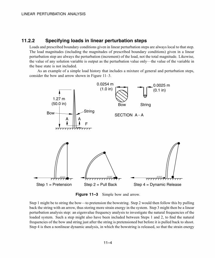
LINEAR PERTURBATION ANALYSIS
11.2.2 Specifying loads in linear perturbation stepsLoads and prescribed boundary conditions given in linear perturbation steps are always local to that step.The load magnitudes (including the magnitudes of prescribed boundary conditions) given in a linearperturbation step are always the perturbation (increment) of the load, not the total magnitude. Likewise,the value of any solution variable is output as the perturbation value only—the value of the variable inthe base state is not included.
As an example of a simple load history that includes a mixture of general and perturbation steps,consider the bow and arrow shown in Figure 11–3.
1.27 m(50.0 in)
Bow
A A
String
F
0.0254 m (1.0 in)
Bow String
SECTION A
0.0025 m(0.1 in)
Step 1 = Pretension Step 2 = Pull Back Step 4 = Dynamic Release
_ A
Figure 11–3 Simple bow and arrow.
Step 1 might be to string the bow—to pretension the bowstring. Step 2 would then follow this by pullingback the string with an arrow, thus storing more strain energy in the system. Step 3 might then be a linearperturbation analysis step: an eigenvalue frequency analysis to investigate the natural frequencies of theloaded system. Such a step might also have been included between Steps 1 and 2, to find the naturalfrequencies of the bow and string just after the string is pretensioned but before it is pulled back to shoot.Step 4 is then a nonlinear dynamic analysis, in which the bowstring is released, so that the strain energy
11–4
Abaqus ID:Printed on:
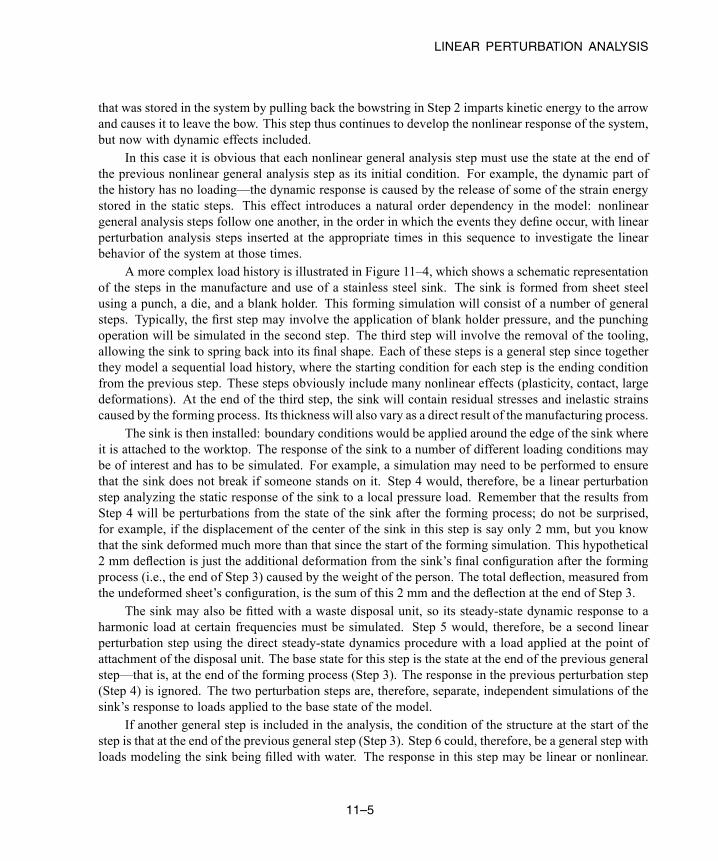
LINEAR PERTURBATION ANALYSIS
that was stored in the system by pulling back the bowstring in Step 2 imparts kinetic energy to the arrowand causes it to leave the bow. This step thus continues to develop the nonlinear response of the system,but now with dynamic effects included.
In this case it is obvious that each nonlinear general analysis step must use the state at the end ofthe previous nonlinear general analysis step as its initial condition. For example, the dynamic part ofthe history has no loading—the dynamic response is caused by the release of some of the strain energystored in the static steps. This effect introduces a natural order dependency in the model: nonlineargeneral analysis steps follow one another, in the order in which the events they define occur, with linearperturbation analysis steps inserted at the appropriate times in this sequence to investigate the linearbehavior of the system at those times.
A more complex load history is illustrated in Figure 11–4, which shows a schematic representationof the steps in the manufacture and use of a stainless steel sink. The sink is formed from sheet steelusing a punch, a die, and a blank holder. This forming simulation will consist of a number of generalsteps. Typically, the first step may involve the application of blank holder pressure, and the punchingoperation will be simulated in the second step. The third step will involve the removal of the tooling,allowing the sink to spring back into its final shape. Each of these steps is a general step since togetherthey model a sequential load history, where the starting condition for each step is the ending conditionfrom the previous step. These steps obviously include many nonlinear effects (plasticity, contact, largedeformations). At the end of the third step, the sink will contain residual stresses and inelastic strainscaused by the forming process. Its thickness will also vary as a direct result of the manufacturing process.
The sink is then installed: boundary conditions would be applied around the edge of the sink whereit is attached to the worktop. The response of the sink to a number of different loading conditions maybe of interest and has to be simulated. For example, a simulation may need to be performed to ensurethat the sink does not break if someone stands on it. Step 4 would, therefore, be a linear perturbationstep analyzing the static response of the sink to a local pressure load. Remember that the results fromStep 4 will be perturbations from the state of the sink after the forming process; do not be surprised,for example, if the displacement of the center of the sink in this step is say only 2 mm, but you knowthat the sink deformed much more than that since the start of the forming simulation. This hypothetical2 mm deflection is just the additional deformation from the sink’s final configuration after the formingprocess (i.e., the end of Step 3) caused by the weight of the person. The total deflection, measured fromthe undeformed sheet’s configuration, is the sum of this 2 mm and the deflection at the end of Step 3.
The sink may also be fitted with a waste disposal unit, so its steady-state dynamic response to aharmonic load at certain frequencies must be simulated. Step 5 would, therefore, be a second linearperturbation step using the direct steady-state dynamics procedure with a load applied at the point ofattachment of the disposal unit. The base state for this step is the state at the end of the previous generalstep—that is, at the end of the forming process (Step 3). The response in the previous perturbation step(Step 4) is ignored. The two perturbation steps are, therefore, separate, independent simulations of thesink’s response to loads applied to the base state of the model.
If another general step is included in the analysis, the condition of the structure at the start of thestep is that at the end of the previous general step (Step 3). Step 6 could, therefore, be a general step withloads modeling the sink being filled with water. The response in this step may be linear or nonlinear.
11–5
Abaqus ID:Printed on:
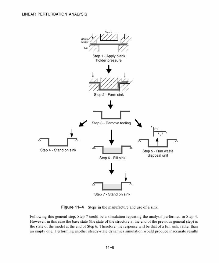
LINEAR PERTURBATION ANALYSIS
Die
Blankholder
Punch
Step 1 - Apply blankholder pressure
Step 2 - Form sink
Step 3 - Remove tooling
Step 4 - Stand on sink Step 5 - Run wastedisposal unit
F
t
Step 6 - Fill sink
Step 7 - Stand on sink
Figure 11–4 Steps in the manufacture and use of a sink.
Following this general step, Step 7 could be a simulation repeating the analysis performed in Step 4.However, in this case the base state (the state of the structure at the end of the previous general step) isthe state of the model at the end of Step 6. Therefore, the response will be that of a full sink, rather thanan empty one. Performing another steady-state dynamics simulation would produce inaccurate results
11–6
Abaqus ID:Printed on:
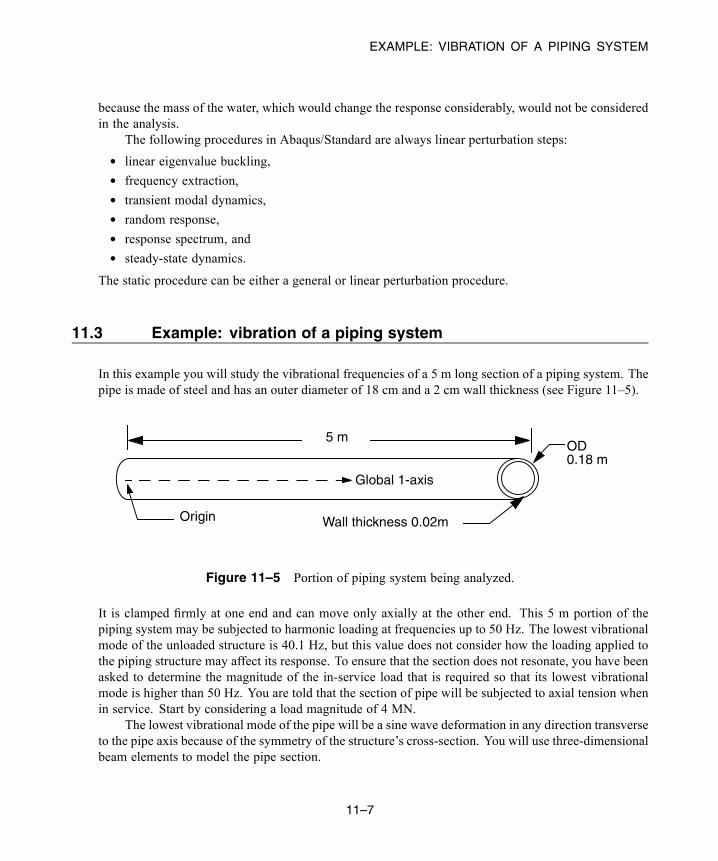
EXAMPLE: VIBRATION OF A PIPING SYSTEM
because the mass of the water, which would change the response considerably, would not be consideredin the analysis.
The following procedures in Abaqus/Standard are always linear perturbation steps:
• linear eigenvalue buckling,• frequency extraction,• transient modal dynamics,• random response,• response spectrum, and• steady-state dynamics.
The static procedure can be either a general or linear perturbation procedure.
11.3 Example: vibration of a piping system
In this example you will study the vibrational frequencies of a 5 m long section of a piping system. Thepipe is made of steel and has an outer diameter of 18 cm and a 2 cm wall thickness (see Figure 11–5).
5 mOD0.18 m
Wall thickness 0.02m
Global 1-axis
Origin
Figure 11–5 Portion of piping system being analyzed.
It is clamped firmly at one end and can move only axially at the other end. This 5 m portion of thepiping system may be subjected to harmonic loading at frequencies up to 50 Hz. The lowest vibrationalmode of the unloaded structure is 40.1 Hz, but this value does not consider how the loading applied tothe piping structure may affect its response. To ensure that the section does not resonate, you have beenasked to determine the magnitude of the in-service load that is required so that its lowest vibrationalmode is higher than 50 Hz. You are told that the section of pipe will be subjected to axial tension whenin service. Start by considering a load magnitude of 4 MN.
The lowest vibrational mode of the pipe will be a sine wave deformation in any direction transverseto the pipe axis because of the symmetry of the structure’s cross-section. You will use three-dimensionalbeam elements to model the pipe section.
11–7
Abaqus ID:Printed on:

EXAMPLE: VIBRATION OF A PIPING SYSTEM
The analysis requires a natural frequency extraction. Thus, you will use Abaqus/Standard as youranalysis product.
11.3.1 Preprocessing—creating the model with Abaqus/CAE
Create the model for this example using Abaqus/CAE. Abaqus provides scripts that replicate thecomplete analysis model for this problem. Run one of these scripts if you encounter difficultiesfollowing the instructions given below or if you wish to check your work. Scripts are available in thefollowing locations:
• A Python script for this example is provided in “Vibration of a piping system,” Section A.11, in theHTML version of this guide. Instructions on how to fetch the script and run it within Abaqus/CAEare given in Appendix A, “Example Files.”
• A plug-in script for this example is available in the Abaqus/CAE Plug-in toolset. To run thescript from Abaqus/CAE, select Plug-ins→Abaqus→Getting Started; highlight Vibration ofa piping system; and click Run. For more information about the Getting Started plug-ins, see“Running the Getting Started with Abaqus examples,” Section 82.1 of the Abaqus/CAE User’sGuide, in the HTML version of this guide.
Part geometry
Create a three-dimensional, deformable, planar wire part. (Remember to use an approximate partsize that is slightly larger than the largest dimension in your model.) Name the part Pipe, and usethe Create Lines: Connected tool to sketch a horizontal line of length 5.0 m. Dimension thesketch as needed to ensure that the length is specified precisely.
Material and section properties
The pipe is made of steel with a Young’s modulus of 200 × 109 Pa and a Poisson’s ratio of 0.3. Createa linear elastic material named Steel with these properties. You must also define the density ofthe steel material (7800 kg/m3) because eigenmodes and eigenfrequencies will be extracted in thissimulation and a mass matrix is needed for this type of procedure.
Next, create a Pipe profile. Name the profile PipeProfile, choose Thin-walled as theformulation, and specify an outer radius of 0.09 m and a wall thickness of 0.02 m for the pipe.
Create aBeam section namedPipeSection. In theEdit Beam Section dialog box, specifythat section integration will be performed during the analysis and assign material Steel and profilePipeProfile to the section definition.
Finally, assign section PipeSection to the pipe. In addition, define the beam sectionorientation with the approximate -direction as the vector (0.0, 0.0, –1.0) (the default). In thismodel the actual -vector will coincide with this approximate vector.
11–8
Abaqus ID:Printed on:
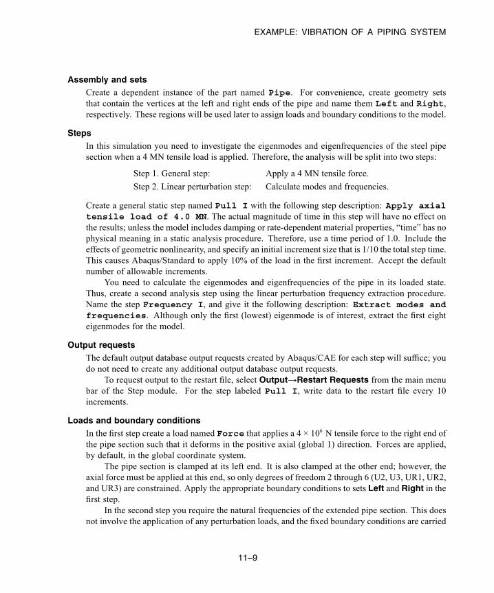
EXAMPLE: VIBRATION OF A PIPING SYSTEM
Assembly and setsCreate a dependent instance of the part named Pipe. For convenience, create geometry setsthat contain the vertices at the left and right ends of the pipe and name them Left and Right,respectively. These regions will be used later to assign loads and boundary conditions to the model.
StepsIn this simulation you need to investigate the eigenmodes and eigenfrequencies of the steel pipesection when a 4 MN tensile load is applied. Therefore, the analysis will be split into two steps:
Step 1. General step: Apply a 4 MN tensile force.
Step 2. Linear perturbation step: Calculate modes and frequencies.
Create a general static step named Pull I with the following step description: Apply axialtensile load of 4.0 MN. The actual magnitude of time in this step will have no effect onthe results; unless the model includes damping or rate-dependent material properties, “time” has nophysical meaning in a static analysis procedure. Therefore, use a time period of 1.0. Include theeffects of geometric nonlinearity, and specify an initial increment size that is 1/10 the total step time.This causes Abaqus/Standard to apply 10% of the load in the first increment. Accept the defaultnumber of allowable increments.
You need to calculate the eigenmodes and eigenfrequencies of the pipe in its loaded state.Thus, create a second analysis step using the linear perturbation frequency extraction procedure.Name the step Frequency I, and give it the following description: Extract modes andfrequencies. Although only the first (lowest) eigenmode is of interest, extract the first eighteigenmodes for the model.
Output requests
The default output database output requests created by Abaqus/CAE for each step will suffice; youdo not need to create any additional output database output requests.
To request output to the restart file, select Output→Restart Requests from the main menubar of the Step module. For the step labeled Pull I, write data to the restart file every 10increments.
Loads and boundary conditions
In the first step create a load named Force that applies a 4 × 10⁶ N tensile force to the right end ofthe pipe section such that it deforms in the positive axial (global 1) direction. Forces are applied,by default, in the global coordinate system.
The pipe section is clamped at its left end. It is also clamped at the other end; however, theaxial force must be applied at this end, so only degrees of freedom 2 through 6 (U2, U3, UR1, UR2,and UR3) are constrained. Apply the appropriate boundary conditions to sets Left and Right in thefirst step.
In the second step you require the natural frequencies of the extended pipe section. This doesnot involve the application of any perturbation loads, and the fixed boundary conditions are carried
11–9
Abaqus ID:Printed on:
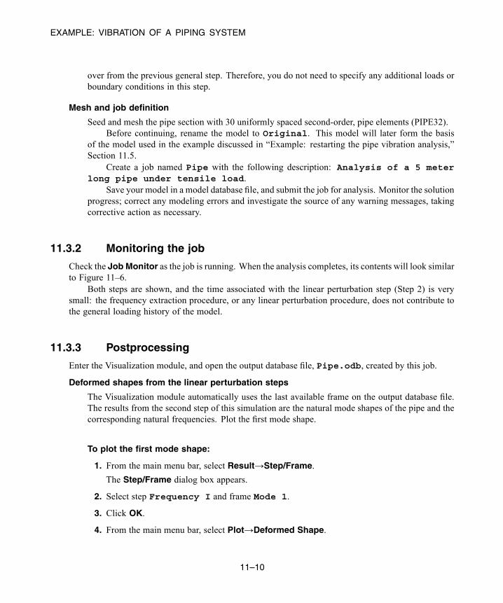
EXAMPLE: VIBRATION OF A PIPING SYSTEM
over from the previous general step. Therefore, you do not need to specify any additional loads orboundary conditions in this step.
Mesh and job definition
Seed and mesh the pipe section with 30 uniformly spaced second-order, pipe elements (PIPE32).Before continuing, rename the model to Original. This model will later form the basis
of the model used in the example discussed in “Example: restarting the pipe vibration analysis,”Section 11.5.
Create a job named Pipe with the following description: Analysis of a 5 meterlong pipe under tensile load.
Save your model in a model database file, and submit the job for analysis. Monitor the solutionprogress; correct any modeling errors and investigate the source of any warning messages, takingcorrective action as necessary.
11.3.2 Monitoring the job
Check the Job Monitor as the job is running. When the analysis completes, its contents will look similarto Figure 11–6.
Both steps are shown, and the time associated with the linear perturbation step (Step 2) is verysmall: the frequency extraction procedure, or any linear perturbation procedure, does not contribute tothe general loading history of the model.
11.3.3 Postprocessing
Enter the Visualization module, and open the output database file, Pipe.odb, created by this job.
Deformed shapes from the linear perturbation steps
The Visualization module automatically uses the last available frame on the output database file.The results from the second step of this simulation are the natural mode shapes of the pipe and thecorresponding natural frequencies. Plot the first mode shape.
To plot the first mode shape:
1. From the main menu bar, select Result→Step/Frame.
The Step/Frame dialog box appears.
2. Select step Frequency I and frame Mode 1.
3. Click OK.
4. From the main menu bar, select Plot→Deformed Shape.
11–10
Abaqus ID:Printed on:

EXAMPLE: VIBRATION OF A PIPING SYSTEM
Figure 11–6 Job Monitor: original pipe vibration analysis.
5. Click the tool in the toolbox to allow multiple plot states in the viewport; then click the
tool or selectPlot→Undeformed Shape to add the undeformed shape plot to the existingdeformed plot in the viewport.
6. Include node symbols on both plots (the superimpose options control the appearance of theundeformed shape when multiple plot states are displayed). Change the color of the nodesymbols to green and the symbol shape to a solid circle.
7. Click the auto-fit tool so that the entire plot is rescaled to fit in the viewport.
The default view is isometric. Try rotating the model to find a better view of the firsteigenmode, similar to that shown in Figure 11–7.
11–11
Abaqus ID:Printed on:
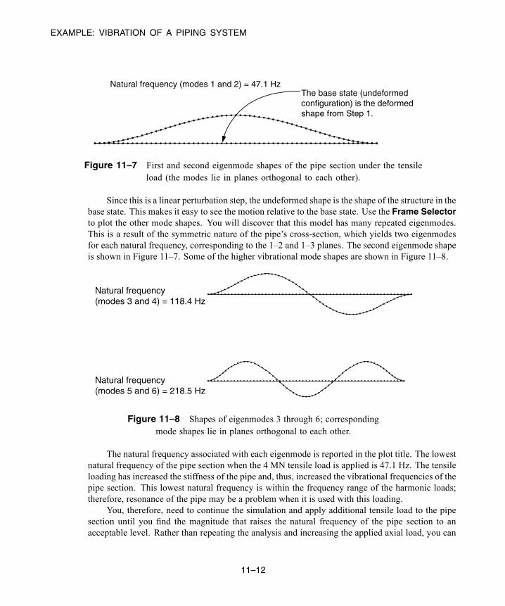
EXAMPLE: VIBRATION OF A PIPING SYSTEM
Natural frequency (modes 1 and 2) = 47.1 HzThe base state (undeformedconfiguration) is the deformedshape from Step 1.
Figure 11–7 First and second eigenmode shapes of the pipe section under the tensileload (the modes lie in planes orthogonal to each other).
Since this is a linear perturbation step, the undeformed shape is the shape of the structure in thebase state. This makes it easy to see the motion relative to the base state. Use the Frame Selectorto plot the other mode shapes. You will discover that this model has many repeated eigenmodes.This is a result of the symmetric nature of the pipe’s cross-section, which yields two eigenmodesfor each natural frequency, corresponding to the 1–2 and 1–3 planes. The second eigenmode shapeis shown in Figure 11–7. Some of the higher vibrational mode shapes are shown in Figure 11–8.
Natural frequency(modes 3 and 4) = 118.4 Hz
Natural frequency(modes 5 and 6) = 218.5 Hz
Figure 11–8 Shapes of eigenmodes 3 through 6; correspondingmode shapes lie in planes orthogonal to each other.
The natural frequency associated with each eigenmode is reported in the plot title. The lowestnatural frequency of the pipe section when the 4 MN tensile load is applied is 47.1 Hz. The tensileloading has increased the stiffness of the pipe and, thus, increased the vibrational frequencies of thepipe section. This lowest natural frequency is within the frequency range of the harmonic loads;therefore, resonance of the pipe may be a problem when it is used with this loading.
You, therefore, need to continue the simulation and apply additional tensile load to the pipesection until you find the magnitude that raises the natural frequency of the pipe section to anacceptable level. Rather than repeating the analysis and increasing the applied axial load, you can
11–12
Abaqus ID:Printed on:
RESTART ANALYSIS
use the restart capability in Abaqus to continue the load history of a prior simulation in a newanalysis.
11.4 Restart analysis
Multistep simulations need not be defined in a single job. Indeed, it is usually desirable to run a complexsimulation in stages. This allows you to examine the results and confirm that the analysis is performingas expected before continuing with the next stage. The Abaqus restart analysis capability allows asimulation to be restarted and the model’s response to additional load history to be calculated.
The restart analysis capability is discussed in detail in “Restarting an analysis,” Section 9.1.1 of theAbaqus Analysis User’s Guide.
11.4.1 The restart and state files
The Abaqus/Standard restart (.res) file and the Abaqus/Explicit state (.abq) file contain theinformation necessary to continue a previous analysis. In Abaqus/Explicit the package (.pac) fileand the selected results (.sel) file are also used for restarting an analysis and must be saved uponcompletion of the first job. In addition, both products require the output database (.odb) file. Restartfiles can become very large for large models; when restart data are requested, they are written for everyincrement or interval by default. Thus, it is important to control the frequency at which restart data arewritten. Sometimes it is useful to allow data to be overwritten on the restart file during a step. Thismeans that at the end of the analysis there is only one set of restart data for each step, corresponding tothe state of the model at the end of each step. However, if the analysis is interrupted for some reason,such as a computer malfunction, the analysis can be continued from the point where restart data werelast written.
11.4.2 Restarting an analysis
When restarting a simulation using the results of a previous analysis, you specify the particular pointin the simulation’s load history from which to restart the analysis. The model used in the restartanalysis, however, must be the same as the model used in the original analysis up to the restart location.Specifically,
• the restart analysis model must not modify or add any geometry, mesh, materials, sections,beam section profiles, material orientations, beam section orientations, interaction properties, orconstraints that are already defined in the original analysis model; and
• similarly, it must not modify any step, load, boundary condition, predefined field, or interaction ator before the restart location.
You may, however, define new sets and amplitude curves in the restart analysis model.
11–13
Abaqus ID:Printed on:
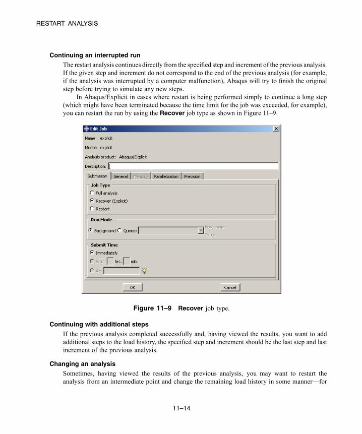
RESTART ANALYSIS
Continuing an interrupted run
The restart analysis continues directly from the specified step and increment of the previous analysis.If the given step and increment do not correspond to the end of the previous analysis (for example,if the analysis was interrupted by a computer malfunction), Abaqus will try to finish the originalstep before trying to simulate any new steps.
In Abaqus/Explicit in cases where restart is being performed simply to continue a long step(which might have been terminated because the time limit for the job was exceeded, for example),you can restart the run by using the Recover job type as shown in Figure 11–9.
Figure 11–9 Recover job type.
Continuing with additional steps
If the previous analysis completed successfully and, having viewed the results, you want to addadditional steps to the load history, the specified step and increment should be the last step and lastincrement of the previous analysis.
Changing an analysis
Sometimes, having viewed the results of the previous analysis, you may want to restart theanalysis from an intermediate point and change the remaining load history in some manner—for
11–14
Abaqus ID:Printed on:

EXAMPLE: RESTARTING THE PIPE VIBRATION ANALYSIS
example, to add more output requests, to change the loading, or to adjust the analysis controls.This can be necessary, for example, when a step has exceeded its maximum number of increments.If an analysis is restarted because the maximum number of increments has been exceeded,Abaqus/Standard thinks that the analysis is partway through a step, tries to complete the step, andpromptly exceeds the maximum number of increments again.
In such situations you should indicate that the current step should be terminated at the specifiedstep and increment. The simulation may then continue with the new steps. For example, if a stepallowed only a maximum of 20 increments, which was less than the number necessary to completethe step, a new step should be defined in which the entire step definition, including applied loads andboundary conditions, is identical to that specified in the original run with the following exceptions:
• The number of increments should be increased.• The total time of the new step should be the total time of the original step less the timecompleted in the first run. For example, if the time of the step as originally specified was 100seconds and the analysis ran out of increments at a step time of 20 seconds, the duration ofthe step in the restart analysis should be 80 seconds.
• Any amplitude definitions specified in terms of step time need to be respecified to reflect thenew time scale of the step. Amplitude definitions specified in terms of total time do not needto be changed, provided the modifications given above are used.
The magnitudes of any loads or prescribed boundary conditions remain unchanged since theyare always total values in general analysis steps.
11.5 Example: restarting the pipe vibration analysis
To demonstrate how to restart an analysis, take the pipe section example in “Example: vibration of apiping system,” Section 11.3, and restart the simulation, adding two additional steps of load history. Thefirst simulation predicted that the piping section would be vulnerable to resonance when extended axially;you must now determine how much additional axial load will increase the pipe’s lowest vibrationalfrequency to an acceptable level.
Step 3 will be a general step that increases the axial load on the pipe to 8 MN, and Step 4 willcalculate the eigenmodes and eigenfrequencies again.
11.5.1 Creating a restart analysis modelOpen the model database file Pipe.cae (if it is not already open). Copy the model named Originalto a model named Restart. The modifications to this model are discussed next.
Model attributes
To perform a restart analysis, the model’s attributes must be changed to indicate that the modelshould reuse data from a previous analysis. In the Model Tree, double-click the Restart model
11–15
Abaqus ID:Printed on:
EXAMPLE: RESTARTING THE PIPE VIBRATION ANALYSIS
underneath the Models container. In the Edit Model Attributes dialog box that appears, specifythat restart data will be read from the job Pipe and that the restart location will be the end of stepPull I.
Step definitions
You will now create two new analysis steps. The first new step is a general static step; name thestep Pull II, and insert it immediately after the step Frequency I. Give the step the followingdescription: Apply axial tensile load of 8.0 MN; and set the time period for the stepto 1.0 and the initial time increment to 0.1.
The second new step is a frequency extraction step; name the step Frequency II, and insertit immediately after the stepPull II. Give the step the following description: Extract modesand frequencies; and use the Lanczos eigensolver to extract the first 8 natural modes andfrequencies of the pipe.
Output requests
For the step Pull II, write data to the restart file every 10 increments.Accept all other default output data requests.
Load definition
Modify the load definition so that the tensile load that is applied to the pipe is doubled in the secondgeneral static step (Pull II). To do this, expand the Force item underneath the Loads containerin the Model Tree. In the list that appears, expand the States item. Double-click the step namedPull II, and change the value of the applied force to 8.0E+06 in this step.
Job definition
Create a job named PipeRestart with the following description: Restart analysis ofa 5 meter long pipe under tensile load. Set the job type to Restart if it is notalready. (If the job type is not set to Restart, Abaqus/CAE ignores the model’s restart attributes.)
Save your model in a model database file, and submit the job for analysis. Monitor the solutionprogress; correct any modeling errors and investigate the source of any warning messages, takingcorrective action as necessary.
11.5.2 Monitoring the job
Again, check the Job Monitor as the job is running. When the analysis completes, its contents will looksimilar to Figure 11–10.
11–16
Abaqus ID:Printed on:

EXAMPLE: RESTARTING THE PIPE VIBRATION ANALYSIS
Figure 11–10 Job Monitor: restart pipe vibration analysis.
This analysis starts at Step 3 since Steps 1 and 2 were completed in the previous analysis. Thereare now two output database (.odb) files associated with this simulation. Data for Steps 1 and 2 are inthe file Pipe.odb; data for Steps 3 and 4 are in the file PipeRestart.odb. When plotting results,you need to remember which results are stored in each file, and you need to ensure that Abaqus/CAE isusing the correct output database file.
11.5.3 Postprocessing the restart analysis resultsSwitch to the Visualization module, and open the output database file from the restart analysis,PipeRestart.odb.
Plotting the eigenmodes of the pipe
Plot the same six eigenmode shapes of the pipe section for this simulation as were plotted in theprevious analysis. The eigenmode shapes can be plotted using the procedures described for the
11–17
Abaqus ID:Printed on:
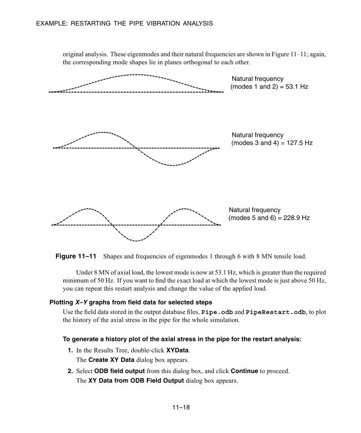
EXAMPLE: RESTARTING THE PIPE VIBRATION ANALYSIS
original analysis. These eigenmodes and their natural frequencies are shown in Figure 11–11; again,the corresponding mode shapes lie in planes orthogonal to each other.
Natural frequency(modes 1 and 2) = 53.1 Hz
Natural frequency(modes 3 and 4) = 127.5 Hz
Natural frequency(modes 5 and 6) = 228.9 Hz
Figure 11–11 Shapes and frequencies of eigenmodes 1 through 6 with 8 MN tensile load.
Under 8MN of axial load, the lowest mode is now at 53.1 Hz, which is greater than the requiredminimum of 50 Hz. If you want to find the exact load at which the lowest mode is just above 50 Hz,you can repeat this restart analysis and change the value of the applied load.
Plotting X–Y graphs from field data for selected steps
Use the field data stored in the output database files, Pipe.odb and PipeRestart.odb, to plotthe history of the axial stress in the pipe for the whole simulation.
To generate a history plot of the axial stress in the pipe for the restart analysis:
1. In the Results Tree, double-click XYData.
The Create XY Data dialog box appears.
2. Select ODB field output from this dialog box, and click Continue to proceed.
The XY Data from ODB Field Output dialog box appears.
11–18
Abaqus ID:Printed on:
EXAMPLE: RESTARTING THE PIPE VIBRATION ANALYSIS
3. In theVariables tabbed page of this dialog box, accept the default selection of IntegrationPoint for the variable position and select S11 from the list of available stress components.
4. At the bottom of the dialog box, toggle Select for the section point and click Settings tochoose a section point.
5. In the Field Report Section Point Settings dialog box that appears, select the categorybeam and choose any of the available section points for the pipe cross-section. Click OK toexit this dialog box.
6. In the Elements/Nodes tabbed page of the XY Data from ODB Field Output dialog box,select Element labels as the selectionMethod. There are 30 elements in the model, and theyare numbered consecutively from 1 to 30. Enter any element number (for example, 25) in theElement labels text field that appears on the right side of the dialog box.
7. Click Active Steps/Frames, and select Pull II as the only step from which to extractdata.
8. At the bottom of theXY Data from ODB Field Output dialog box, clickPlot to see the historyof axial stress in the element.
The plot traces the axial stress history at each integration point of the element in the restartanalysis. Since the restart is a continuation of an earlier job, it is often useful to view the resultsfrom the entire (original and restarted) analysis.
To generate a history plot of the axial stress in the pipe for the entire analysis:
1. Save the current plot by clicking Save at the bottom of the XY Data from ODB Field Outputdialog box. Two curves are saved (one for each integration point), and default names are givento the curves.
2. Rename either curve RESTART, and delete the other curve.
3. From the main menu bar, select File→Open; or use the tool in the File toolbar to openthe file Pipe.odb.
4. Following the procedure outlined above, save the plot of the axial stress history for the sameelement and integration/section point used above. Name this plot ORIGINAL.
5. In the Results Tree, expand the XYData container.
The ORIGINAL and RESTART curves are listed underneath.
6. Select both plots with [Ctrl] + Click. Click mouse button 3, and select Plot from the menu thatappears to create a plot of axial stress history in the pipe for the entire simulation.
7. To change the style of the line, open the Curve Options dialog box.
8. For the RESTART curve, select a dotted line style.
9. Click Dismiss to close the dialog box.
11–19
Abaqus ID:Printed on:
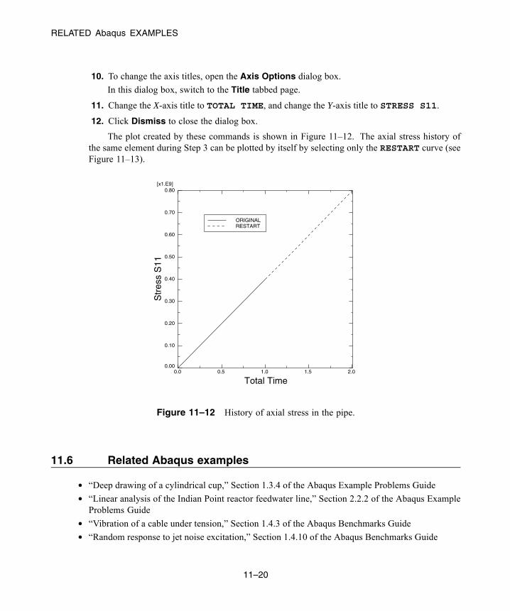
RELATED Abaqus EXAMPLES
10. To change the axis titles, open the Axis Options dialog box.
In this dialog box, switch to the Title tabbed page.
11. Change the X-axis title to TOTAL TIME, and change the Y-axis title to STRESS S11.
12. Click Dismiss to close the dialog box.
The plot created by these commands is shown in Figure 11–12. The axial stress history ofthe same element during Step 3 can be plotted by itself by selecting only the RESTART curve (seeFigure 11–13).
Total Time0.0 0.5 1.0 1.5 2.0
Str
ess
S11
0.00
0.10
0.20
0.30
0.40
0.50
0.60
0.70
0.80[x1.E9]
ORIGINALRESTART
Figure 11–12 History of axial stress in the pipe.
11.6 Related Abaqus examples
• “Deep drawing of a cylindrical cup,” Section 1.3.4 of the Abaqus Example Problems Guide• “Linear analysis of the Indian Point reactor feedwater line,” Section 2.2.2 of the Abaqus ExampleProblems Guide
• “Vibration of a cable under tension,” Section 1.4.3 of the Abaqus Benchmarks Guide• “Random response to jet noise excitation,” Section 1.4.10 of the Abaqus Benchmarks Guide
11–20
Abaqus ID:Printed on:
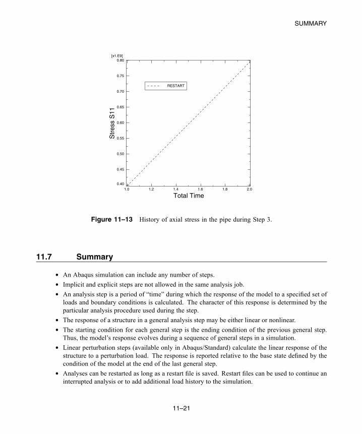
SUMMARY
Total Time1.0 1.2 1.4 1.6 1.8 2.0
Str
ess
S11
0.40
0.45
0.50
0.55
0.60
0.65
0.70
0.75
0.80[x1.E9]
RESTART
Figure 11–13 History of axial stress in the pipe during Step 3.
11.7 Summary
• An Abaqus simulation can include any number of steps.• Implicit and explicit steps are not allowed in the same analysis job.• An analysis step is a period of “time” during which the response of the model to a specified set ofloads and boundary conditions is calculated. The character of this response is determined by theparticular analysis procedure used during the step.
• The response of a structure in a general analysis step may be either linear or nonlinear.• The starting condition for each general step is the ending condition of the previous general step.Thus, the model’s response evolves during a sequence of general steps in a simulation.
• Linear perturbation steps (available only in Abaqus/Standard) calculate the linear response of thestructure to a perturbation load. The response is reported relative to the base state defined by thecondition of the model at the end of the last general step.
• Analyses can be restarted as long as a restart file is saved. Restart files can be used to continue aninterrupted analysis or to add additional load history to the simulation.
11–21
Abaqus ID:Printed on:


DEFINING SURFACES
12. Contact
Many engineering problems involve contact between two or more components. In these problems a forcenormal to the contacting surfaces acts on the two bodies when they touch each other. If there is frictionbetween the surfaces, shear forces may be created that resist the tangential motion (sliding) of the bodies.The general aim of contact simulations is to identify the areas on the surfaces that are in contact and tocalculate the contact pressures generated.
In a finite element analysis contact conditions are a special class of discontinuous constraint,allowing forces to be transmitted from one part of the model to another. The constraint is discontinuousbecause it is applied only when the two surfaces are in contact. When the two surfaces separate, noconstraint is applied. The analysis has to be able to detect when two surfaces are in contact and applythe contact constraints accordingly. Similarly, the analysis must be able to detect when two surfacesseparate and remove the contact constraints.
12.1 Overview of contact capabilities in Abaqus
Contact simulations in Abaqus/Standard can either be surface based or contact element based. Contactsimulations in Abaqus/Explicit are surface based only. In this guide, surface-based contact is discussed.
Surface-based contact can utilize either the general (“automatic”) contact algorithm or the contactpair algorithm. The general contact algorithm allows for a highly automated contact definition, wherecontact is based on an automatically generated all-inclusive surface definition. Conversely, the contactpair algorithm requires you to explicitly pair surfaces that may potentially come into contact. Bothalgorithms require specification of contact properties between surfaces (for example, friction).
The discussion of contact in this guide addresses the contact pair approach and general contact inAbaqus/Standard and general contact in Abaqus/Explicit.
12.2 Defining surfaces
Surfaces are created from the element faces of the underlying material. The discussion that followsassumes that the surfaces will be defined in Abaqus/CAE. Restrictions on the types of surfaces that canbe created in Abaqus are discussed in “Surface definition,” Section 2.3 of the Abaqus Analysis User’sGuide; please read them before beginning a contact simulation.
Surfaces on continuum elements
For two- and three-dimensional solid continuum elements you specify which regions of a part formthe contact surface by selecting the regions of a part instance in the viewport.
12–1
Abaqus ID:Printed on:
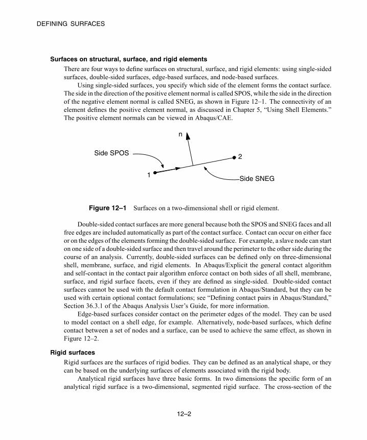
DEFINING SURFACES
Surfaces on structural, surface, and rigid elements
There are four ways to define surfaces on structural, surface, and rigid elements: using single-sidedsurfaces, double-sided surfaces, edge-based surfaces, and node-based surfaces.
Using single-sided surfaces, you specify which side of the element forms the contact surface.The side in the direction of the positive element normal is called SPOS, while the side in the directionof the negative element normal is called SNEG, as shown in Figure 12–1. The connectivity of anelement defines the positive element normal, as discussed in Chapter 5, “Using Shell Elements.”The positive element normals can be viewed in Abaqus/CAE.
n
2
1
Side SPOS
Side SNEG
Figure 12–1 Surfaces on a two-dimensional shell or rigid element.
Double-sided contact surfaces are more general because both the SPOS and SNEG faces and allfree edges are included automatically as part of the contact surface. Contact can occur on either faceor on the edges of the elements forming the double-sided surface. For example, a slave node can starton one side of a double-sided surface and then travel around the perimeter to the other side during thecourse of an analysis. Currently, double-sided surfaces can be defined only on three-dimensionalshell, membrane, surface, and rigid elements. In Abaqus/Explicit the general contact algorithmand self-contact in the contact pair algorithm enforce contact on both sides of all shell, membrane,surface, and rigid surface facets, even if they are defined as single-sided. Double-sided contactsurfaces cannot be used with the default contact formulation in Abaqus/Standard, but they can beused with certain optional contact formulations; see “Defining contact pairs in Abaqus/Standard,”Section 36.3.1 of the Abaqus Analysis User’s Guide, for more information.
Edge-based surfaces consider contact on the perimeter edges of the model. They can be usedto model contact on a shell edge, for example. Alternatively, node-based surfaces, which definecontact between a set of nodes and a surface, can be used to achieve the same effect, as shown inFigure 12–2.
Rigid surfaces
Rigid surfaces are the surfaces of rigid bodies. They can be defined as an analytical shape, or theycan be based on the underlying surfaces of elements associated with the rigid body.
Analytical rigid surfaces have three basic forms. In two dimensions the specific form of ananalytical rigid surface is a two-dimensional, segmented rigid surface. The cross-section of the
12–2
Abaqus ID:Printed on:
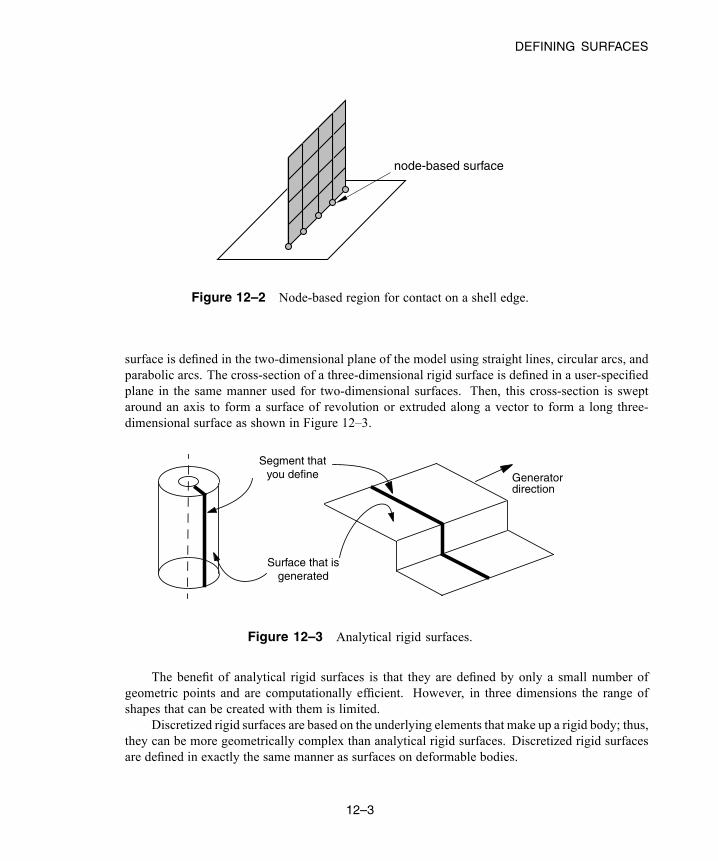
DEFINING SURFACES
node-based surface
Figure 12–2 Node-based region for contact on a shell edge.
surface is defined in the two-dimensional plane of the model using straight lines, circular arcs, andparabolic arcs. The cross-section of a three-dimensional rigid surface is defined in a user-specifiedplane in the same manner used for two-dimensional surfaces. Then, this cross-section is sweptaround an axis to form a surface of revolution or extruded along a vector to form a long three-dimensional surface as shown in Figure 12–3.
Generatordirection
Surface that isgenerated
Segment thatyou define
Figure 12–3 Analytical rigid surfaces.
The benefit of analytical rigid surfaces is that they are defined by only a small number ofgeometric points and are computationally efficient. However, in three dimensions the range ofshapes that can be created with them is limited.
Discretized rigid surfaces are based on the underlying elements that make up a rigid body; thus,they can be more geometrically complex than analytical rigid surfaces. Discretized rigid surfacesare defined in exactly the same manner as surfaces on deformable bodies.
12–3
Abaqus ID:Printed on:

INTERACTION BETWEEN SURFACES
12.3 Interaction between surfaces
The interaction between contacting surfaces consists of two components: one normal to the surfaces andone tangential to the surfaces. The tangential component consists of the relative motion (sliding) of thesurfaces and, possibly, frictional shear stresses. Each contact interaction can refer to a contact propertythat specifies a model for the interaction between the contacting surfaces. There are several contactinteraction models available in Abaqus; the default model is frictionless contact with no bonding.
12.3.1 Behavior normal to the surfacesThe distance separating two surfaces is called the clearance. The contact constraint is applied inAbaqus when the clearance between two surfaces becomes zero. There is no limit in the contactformulation on the magnitude of contact pressure that can be transmitted between the surfaces. Thesurfaces separate when the contact pressure between them becomes zero or negative, and the constraintis removed. This behavior, referred to as “hard” contact, is the default contact behavior in Abaqus andis summarized in the contact pressure-clearance relationship shown in Figure 12–4.
Contact clearance
Con
tact
pre
ssur
e
00
Figure 12–4 Contact pressure-clearance relationship for “hard” contact.
By default, “hard” contact is directly enforced when using contact pairs in Abaqus/Standard. Thedramatic change in contact pressure that occurs when a contact condition changes from “open” (apositive clearance) to “closed” (clearance equal to zero) sometimes makes it difficult to completecontact simulations in Abaqus/Standard; the same is not true for Abaqus/Explicit since iteration is notrequired for explicit methods. Alternative enforcement methods (e.g., penalty) are available for contactpairs, as discussed in “Contact constraint enforcement methods in Abaqus/Standard,” Section 38.1.2 ofthe Abaqus Analysis User’s Guide. Penalty enforcement of the contact constraints is the only optionavailable for general contact. Other sources of information include “Common difficulties associated
12–4
Abaqus ID:Printed on:
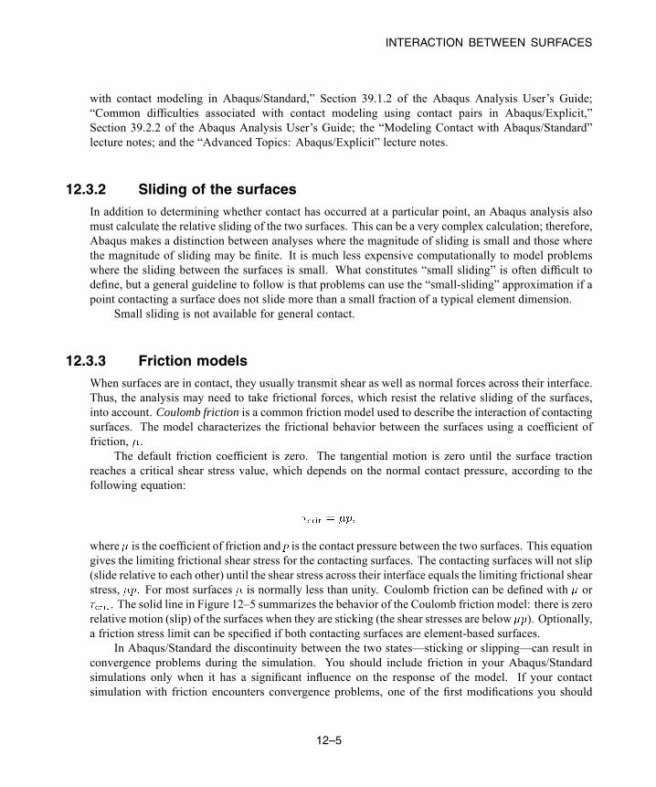
INTERACTION BETWEEN SURFACES
with contact modeling in Abaqus/Standard,” Section 39.1.2 of the Abaqus Analysis User’s Guide;“Common difficulties associated with contact modeling using contact pairs in Abaqus/Explicit,”Section 39.2.2 of the Abaqus Analysis User’s Guide; the “Modeling Contact with Abaqus/Standard”lecture notes; and the “Advanced Topics: Abaqus/Explicit” lecture notes.
12.3.2 Sliding of the surfacesIn addition to determining whether contact has occurred at a particular point, an Abaqus analysis alsomust calculate the relative sliding of the two surfaces. This can be a very complex calculation; therefore,Abaqus makes a distinction between analyses where the magnitude of sliding is small and those wherethe magnitude of sliding may be finite. It is much less expensive computationally to model problemswhere the sliding between the surfaces is small. What constitutes “small sliding” is often difficult todefine, but a general guideline to follow is that problems can use the “small-sliding” approximation if apoint contacting a surface does not slide more than a small fraction of a typical element dimension.
Small sliding is not available for general contact.
12.3.3 Friction modelsWhen surfaces are in contact, they usually transmit shear as well as normal forces across their interface.Thus, the analysis may need to take frictional forces, which resist the relative sliding of the surfaces,into account. Coulomb friction is a common friction model used to describe the interaction of contactingsurfaces. The model characterizes the frictional behavior between the surfaces using a coefficient offriction, .
The default friction coefficient is zero. The tangential motion is zero until the surface tractionreaches a critical shear stress value, which depends on the normal contact pressure, according to thefollowing equation:
where is the coefficient of friction and is the contact pressure between the two surfaces. This equationgives the limiting frictional shear stress for the contacting surfaces. The contacting surfaces will not slip(slide relative to each other) until the shear stress across their interface equals the limiting frictional shearstress, . For most surfaces is normally less than unity. Coulomb friction can be defined with or
. The solid line in Figure 12–5 summarizes the behavior of the Coulomb friction model: there is zerorelative motion (slip) of the surfaces when they are sticking (the shear stresses are below ). Optionally,a friction stress limit can be specified if both contacting surfaces are element-based surfaces.
In Abaqus/Standard the discontinuity between the two states—sticking or slipping—can result inconvergence problems during the simulation. You should include friction in your Abaqus/Standardsimulations only when it has a significant influence on the response of the model. If your contactsimulation with friction encounters convergence problems, one of the first modifications you should
12–5
Abaqus ID:Printed on:
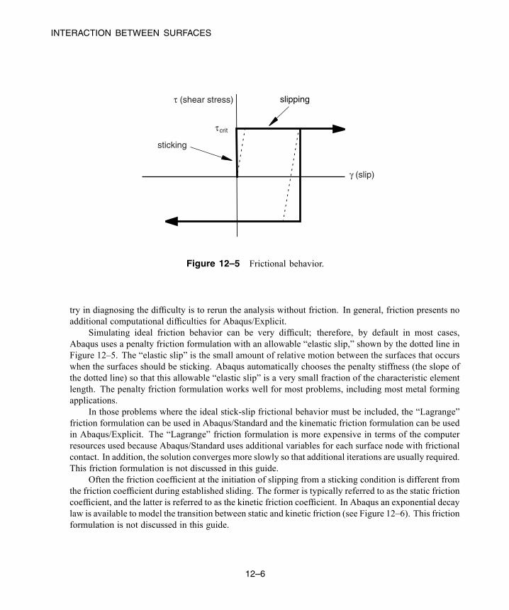
INTERACTION BETWEEN SURFACES
slippingτ (shear stress)
τ
γ (slip)
sticking
crit
Figure 12–5 Frictional behavior.
try in diagnosing the difficulty is to rerun the analysis without friction. In general, friction presents noadditional computational difficulties for Abaqus/Explicit.
Simulating ideal friction behavior can be very difficult; therefore, by default in most cases,Abaqus uses a penalty friction formulation with an allowable “elastic slip,” shown by the dotted line inFigure 12–5. The “elastic slip” is the small amount of relative motion between the surfaces that occurswhen the surfaces should be sticking. Abaqus automatically chooses the penalty stiffness (the slope ofthe dotted line) so that this allowable “elastic slip” is a very small fraction of the characteristic elementlength. The penalty friction formulation works well for most problems, including most metal formingapplications.
In those problems where the ideal stick-slip frictional behavior must be included, the “Lagrange”friction formulation can be used in Abaqus/Standard and the kinematic friction formulation can be usedin Abaqus/Explicit. The “Lagrange” friction formulation is more expensive in terms of the computerresources used because Abaqus/Standard uses additional variables for each surface node with frictionalcontact. In addition, the solution converges more slowly so that additional iterations are usually required.This friction formulation is not discussed in this guide.
Often the friction coefficient at the initiation of slipping from a sticking condition is different fromthe friction coefficient during established sliding. The former is typically referred to as the static frictioncoefficient, and the latter is referred to as the kinetic friction coefficient. In Abaqus an exponential decaylaw is available to model the transition between static and kinetic friction (see Figure 12–6). This frictionformulation is not discussed in this guide.
12–6
Abaqus ID:Printed on:
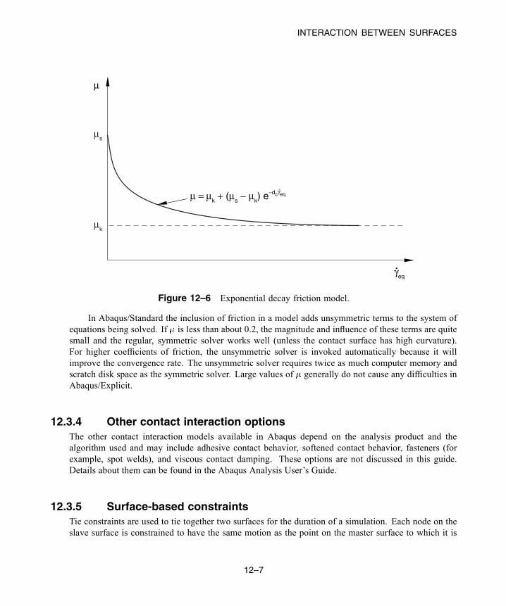
INTERACTION BETWEEN SURFACES
μk
μs
μ
γeq
μ = μk + (μs − μk) e−dcγeq
Figure 12–6 Exponential decay friction model.
In Abaqus/Standard the inclusion of friction in a model adds unsymmetric terms to the system ofequations being solved. If is less than about 0.2, the magnitude and influence of these terms are quitesmall and the regular, symmetric solver works well (unless the contact surface has high curvature).For higher coefficients of friction, the unsymmetric solver is invoked automatically because it willimprove the convergence rate. The unsymmetric solver requires twice as much computer memory andscratch disk space as the symmetric solver. Large values of generally do not cause any difficulties inAbaqus/Explicit.
12.3.4 Other contact interaction optionsThe other contact interaction models available in Abaqus depend on the analysis product and thealgorithm used and may include adhesive contact behavior, softened contact behavior, fasteners (forexample, spot welds), and viscous contact damping. These options are not discussed in this guide.Details about them can be found in the Abaqus Analysis User’s Guide.
12.3.5 Surface-based constraintsTie constraints are used to tie together two surfaces for the duration of a simulation. Each node on theslave surface is constrained to have the same motion as the point on the master surface to which it is
12–7
Abaqus ID:Printed on:

DEFINING CONTACT IN Abaqus/Standard
closest. For a structural analysis this means the translational (and, optionally, the rotational) degrees offreedom are constrained.
Abaqus uses the undeformed configuration of the model to determine which slave nodes are tied tothe master surface. By default, all slave nodes that lie within a given distance of the master surface aretied. The default distance is based on the typical element size of the master surface. This default canbe overridden in one of two ways: by specifying the distance within which slave nodes must lie fromthe master surface to be constrained or by specifying the name of a set containing the nodes that will beconstrained.
Slave nodes can also be adjusted so that they lie exactly on the master surface. If slave nodes haveto be adjusted by distances that are a large fraction of the length of the side of the element (to which theslave node is attached), the element can become severely distorted; avoid large adjustments if possible.
Tie constraints are particularly useful for rapid mesh refinement between dissimilar meshes.
12.4 Defining contact in Abaqus/Standard
The first step in defining contact pairs (and optionally general contact) in Abaqus/Standard is to definethe surfaces of the bodies that could potentially come into contact. The next step is to specify the surfacesthat interact with each other; these are the contact interactions. The final step is to define the mechanicalproperty models that govern the behavior of the surfaces when they are in contact.
The definition of surfaces is optional for general contact since an all-inclusive element-based surfaceis automatically created when general contact is used. You can use specific surface pairings to includeregions not included in the default surface, to preclude interactions between different regions of a model,or to override global contact property assignments. For example, if you want to apply a certain frictioncoefficient to all but a few surfaces in your model, you can assign the primary friction coefficient globallyand then override this property for a given pair of user-defined surfaces.
12.4.1 Contact interactions
In an Abaqus/Standard simulation possible contact is defined by assigning the surface names to a contactinteraction (contact pair approach) or by invoking an automatically-defined all-inclusive element-basedsurface as the contact domain (general contact approach). For both contact approaches, each contactinteraction must refer to a contact property, in much the same way that each element must refer to anelement property. Constitutive behavior, such as the contact pressure-clearance relationship and friction,can be included in the contact property.
When you define a contact interaction, youmust decide whether the magnitude of the relative slidingwill be small or finite. The default is the more general finite-sliding formulation. The small-slidingformulation (available only for contact pairs) is appropriate if the relative motion of the two surfacesis less than a small proportion of the characteristic length of an element face. Using the small-slidingformulation when applicable results in a more efficient analysis.
12–8
Abaqus ID:Printed on:

DEFINING CONTACT IN Abaqus/Standard
12.4.2 Slave and master surfacesBy default, contact pairs in Abaqus/Standard use a pure master-slave contact algorithm: nodes on onesurface (the slave) cannot penetrate the segments that make up the other surface (the master), as shownin Figure 12–7. The algorithm places no restrictions on the master surface; it can penetrate the slavesurface between slave nodes, as shown in Figure 12–7.
Master surface (segments)
Slave surface (nodes)
Penetration ofmaster surface
Figure 12–7 The master surface can penetrate the slave surface.
Due to the strict master-slave formulation, youmust be careful to select the slave andmaster surfacescorrectly in order to achieve the best possible contact simulation. Some simple rules to follow are:
• the slave surface should be the more finely meshed surface; and• if the mesh densities are similar, the slave surface should be the surface with the softer underlyingmaterial.
The general contact algorithm in Abaqus/Standard enforces contact in an average sense betweeninteracting surfaces; Abaqus/Standard automatically assigns master and slave roles.
12.4.3 Contact discretizationAbaqus/Standard offers two contact discretization methods: a traditional node-to-surface method anda surface-to-surface method. The node-to-surface discretization method defines contact conditionsbetween each slave node and the master surface. The surface-to-surface discretization method considersthe shape of both the master and slave surfaces when defining the contact constraints. The contactpair algorithm can use either discretization method; general contact uses only the surface-to-surfaceapproach.
12.4.4 Small and finite slidingWhen using the small-sliding formulation, Abaqus/Standard establishes the relationship between theslave nodes and the master surface at the beginning of the simulation. Abaqus/Standard determines
12–9
Abaqus ID:Printed on:
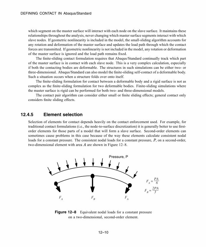
DEFINING CONTACT IN Abaqus/Standard
which segment on the master surface will interact with each node on the slave surface. It maintains theserelationships throughout the analysis, never changing which master surface segments interact with whichslave nodes. If geometric nonlinearity is included in the model, the small-sliding algorithm accounts forany rotation and deformation of the master surface and updates the load path through which the contactforces are transmitted. If geometric nonlinearity is not included in the model, any rotation or deformationof the master surface is ignored and the load path remains fixed.
The finite-sliding contact formulation requires that Abaqus/Standard continually track which partof the master surface is in contact with each slave node. This is a very complex calculation, especiallyif both the contacting bodies are deformable. The structures in such simulations can be either two- orthree-dimensional. Abaqus/Standard can also model the finite-sliding self-contact of a deformable body.Such a situation occurs when a structure folds over onto itself.
The finite-sliding formulation for contact between a deformable body and a rigid surface is not ascomplex as the finite-sliding formulation for two deformable bodies. Finite-sliding simulations wherethe master surface is rigid can be performed for both two- and three-dimensional models.
The contact pair algorithm can consider either small or finite sliding effects; general contact onlyconsiders finite sliding effects.
12.4.5 Element selection
Selection of elements for contact depends heavily on the contact enforcement used. For example, fortraditional contact formulations (i.e., the node-to-surface discretization) it is generally better to use first-order elements for those parts of a model that will form a slave surface. Second-order elements cansometimes cause problems in this case because of the way these elements calculate consistent nodalloads for a constant pressure. The consistent nodal loads for a constant pressure, P, on a second-order,two-dimensional element with area A are shown in Figure 12–8.
Pressure, P
FA
FB
FA
FB
= 2PA
3
FA
= PA
6
Figure 12–8 Equivalent nodal loads for a constant pressureon a two-dimensional, second-order element.
12–10
Abaqus ID:Printed on:
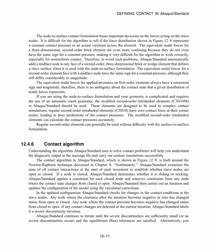
DEFINING CONTACT IN Abaqus/Standard
The node-to-surface contact formulation bases important decisions on the forces acting on the slavenodes. It is difficult for the algorithm to tell if the force distribution shown in Figure 12–8 representsa constant contact pressure or an actual variation across the element. The equivalent nodal forces fora three-dimensional, second-order brick element are even more confusing because they do not evenhave the same sign for a constant pressure, making it very difficult for the algorithm to work correctly,especially for nonuniform contact. Therefore, to avoid such problems, Abaqus/Standard automaticallyadds a midface node to any face of a second-order, three-dimensional brick or wedge element that definesa slave surface when it is used with the node-to-surface formulation. The equivalent nodal forces for asecond-order element face with a midface node have the same sign for a constant pressure, although theystill differ considerably in magnitude.
The equivalent nodal forces for applied pressures on first-order elements always have a consistentsign and magnitude; therefore, there is no ambiguity about the contact state that a given distribution ofnodal forces represents.
If you are using the node-to-surface formulation and your geometry is complicated and requiresthe use of an automatic mesh generator, the modified second-order tetrahedral elements (C3D10M)in Abaqus/Standard should be used. These elements are designed to be used in complex contactsimulations; regular second-order tetrahedral elements (C3D10) have zero contact force at their cornernodes, leading to poor predictions of the contact pressures. The modified second-order tetrahedralelements can calculate the contact pressures accurately.
Regular second-order elements can generally be used without difficulty with the surface-to-surfaceformulation.
12.4.6 Contact algorithmUnderstanding the algorithm Abaqus/Standard uses to solve contact problems will help you understandthe diagnostic output in the message file and carry out contact simulations successfully.
The contact algorithm in Abaqus/Standard, which is shown in Figure 12–9, is built around theNewton-Raphson technique discussed in Chapter 8, “Nonlinearity.” Abaqus/Standard examines thestate of all contact interactions at the start of each increment to establish whether slave nodes areopen or closed. If a node is closed, Abaqus/Standard determines whether it is sliding or sticking.Abaqus/Standard applies a constraint for each closed node and removes constraints from any nodewhere the contact state changes from closed to open. Abaqus/Standard then carries out an iteration andupdates the configuration of the model using the calculated corrections.
In the updated configuration Abaqus/Standard checks for changes in the contact conditions at theslave nodes. Any node where the clearance after the iteration becomes negative or zero has changedstatus from open to closed. Any node where the contact pressure becomes negative has changed statusfrom closed to open. If any contact changes are detected in the current iteration, Abaqus/Standard labelsit a severe discontinuity iteration.
Abaqus/Standard continues to iterate until the severe discontinuities are sufficiently small (or nosevere discontinuities occur) and the equilibrium (flux) tolerances are satisfied. Alternatively, you
12–11
Abaqus ID:Printed on:
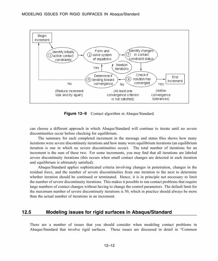
MODELING ISSUES FOR RIGID SURFACES IN Abaqus/Standard
Figure 12–9 Contact algorithm in Abaqus/Standard.
can choose a different approach in which Abaqus/Standard will continue to iterate until no severediscontinuities occur before checking for equilibrium.
The summary for each completed increment in the message and status files shows how manyiterations were severe discontinuity iterations and how many were equilibrium iterations (an equilibriumiteration is one in which no severe discontinuities occur). The total number of iterations for anincrement is the sum of these two. For some increments, you may find that all iterations are labeledsevere discontinuity iterations (this occurs when small contact changes are detected in each iterationand equilibrium is ultimately satisfied).
Abaqus/Standard applies sophisticated criteria involving changes in penetration, changes in theresidual force, and the number of severe discontinuities from one iteration to the next to determinewhether iteration should be continued or terminated. Hence, it is in principle not necessary to limitthe number of severe discontinuity iterations. This makes it possible to run contact problems that requirelarge numbers of contact changes without having to change the control parameters. The default limit forthe maximum number of severe discontinuity iterations is 50, which in practice should always be morethan the actual number of iterations in an increment.
12.5 Modeling issues for rigid surfaces in Abaqus/Standard
There are a number of issues that you should consider when modeling contact problems inAbaqus/Standard that involve rigid surfaces. These issues are discussed in detail in “Common
12–12
Abaqus ID:Printed on:
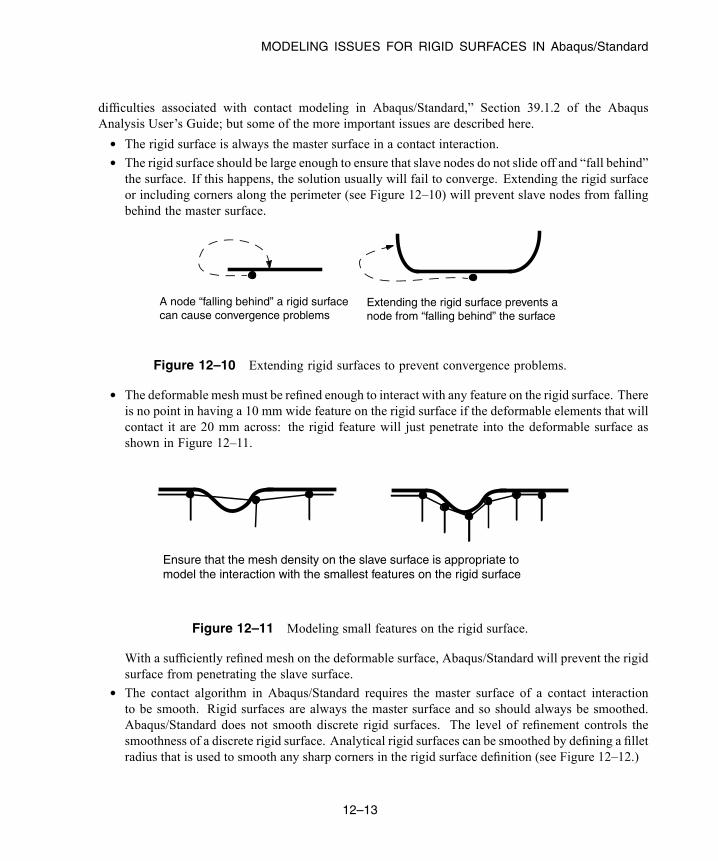
MODELING ISSUES FOR RIGID SURFACES IN Abaqus/Standard
difficulties associated with contact modeling in Abaqus/Standard,” Section 39.1.2 of the AbaqusAnalysis User’s Guide; but some of the more important issues are described here.
• The rigid surface is always the master surface in a contact interaction.• The rigid surface should be large enough to ensure that slave nodes do not slide off and “fall behind”the surface. If this happens, the solution usually will fail to converge. Extending the rigid surfaceor including corners along the perimeter (see Figure 12–10) will prevent slave nodes from fallingbehind the master surface.
A node “falling behind” a rigid surfacecan cause convergence problems
Extending the rigid surface prevents anode from “falling behind” the surface
Figure 12–10 Extending rigid surfaces to prevent convergence problems.
• The deformable mesh must be refined enough to interact with any feature on the rigid surface. Thereis no point in having a 10 mm wide feature on the rigid surface if the deformable elements that willcontact it are 20 mm across: the rigid feature will just penetrate into the deformable surface asshown in Figure 12–11.
Ensure that the mesh density on the slave surface is appropriate tomodel the interaction with the smallest features on the rigid surface
Figure 12–11 Modeling small features on the rigid surface.
With a sufficiently refined mesh on the deformable surface, Abaqus/Standard will prevent the rigidsurface from penetrating the slave surface.
• The contact algorithm in Abaqus/Standard requires the master surface of a contact interactionto be smooth. Rigid surfaces are always the master surface and so should always be smoothed.Abaqus/Standard does not smooth discrete rigid surfaces. The level of refinement controls thesmoothness of a discrete rigid surface. Analytical rigid surfaces can be smoothed by defining a filletradius that is used to smooth any sharp corners in the rigid surface definition (see Figure 12–12.)
12–13
Abaqus ID:Printed on:
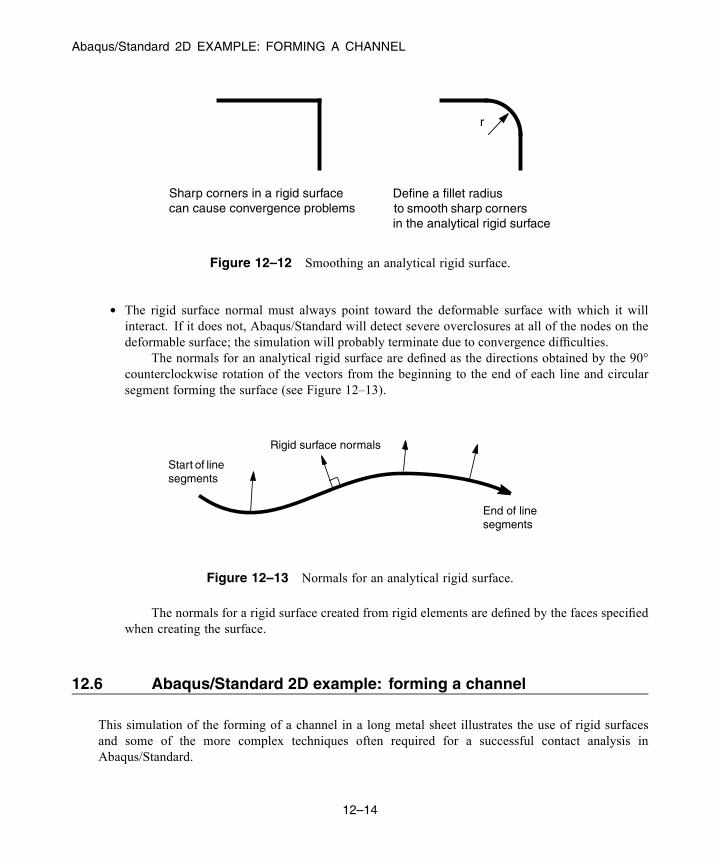
Abaqus/Standard 2D EXAMPLE: FORMING A CHANNEL
r
Sharp corners in a rigid surfacecan cause convergence problems
Define a fillet radiusto smooth sharp cornersin the analytical rigid surface
Figure 12–12 Smoothing an analytical rigid surface.
• The rigid surface normal must always point toward the deformable surface with which it willinteract. If it does not, Abaqus/Standard will detect severe overclosures at all of the nodes on thedeformable surface; the simulation will probably terminate due to convergence difficulties.
The normals for an analytical rigid surface are defined as the directions obtained by the 90°counterclockwise rotation of the vectors from the beginning to the end of each line and circularsegment forming the surface (see Figure 12–13).
Start of linesegments
Rigid surface normals
End of linesegments
Figure 12–13 Normals for an analytical rigid surface.
The normals for a rigid surface created from rigid elements are defined by the faces specifiedwhen creating the surface.
12.6 Abaqus/Standard 2D example: forming a channel
This simulation of the forming of a channel in a long metal sheet illustrates the use of rigid surfacesand some of the more complex techniques often required for a successful contact analysis inAbaqus/Standard.
12–14
Abaqus ID:Printed on:
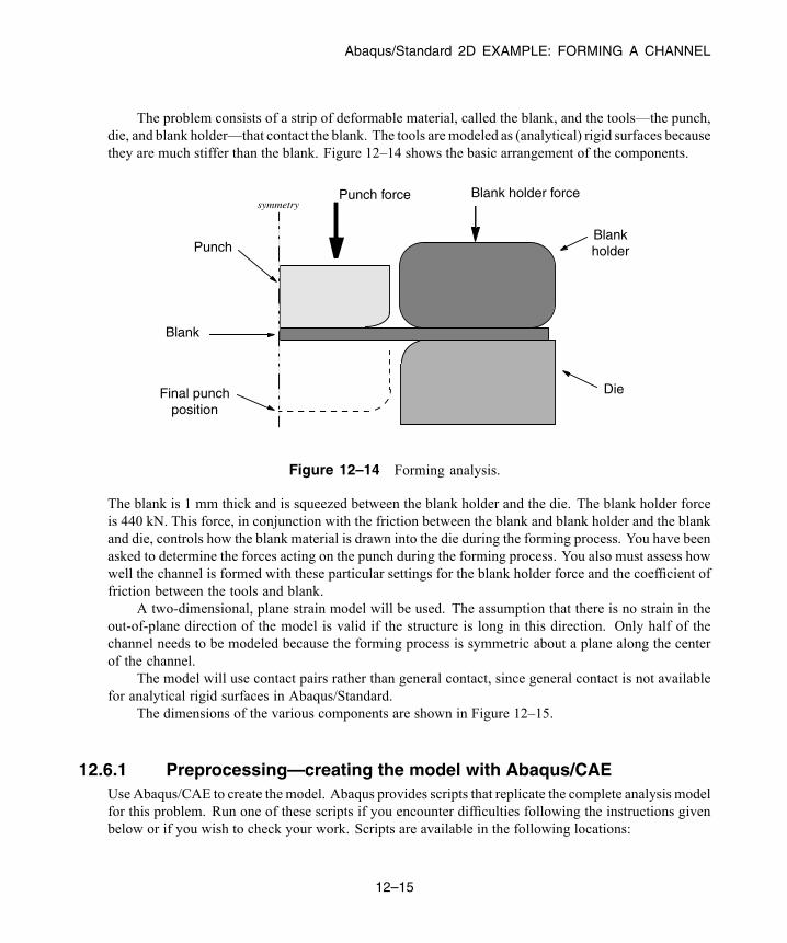
Abaqus/Standard 2D EXAMPLE: FORMING A CHANNEL
The problem consists of a strip of deformable material, called the blank, and the tools—the punch,die, and blank holder—that contact the blank. The tools are modeled as (analytical) rigid surfaces becausethey are much stiffer than the blank. Figure 12–14 shows the basic arrangement of the components.
PunchBlankholder
Die
Blank
Final punchposition
symmetryBlank holder forcePunch force
Figure 12–14 Forming analysis.
The blank is 1 mm thick and is squeezed between the blank holder and the die. The blank holder forceis 440 kN. This force, in conjunction with the friction between the blank and blank holder and the blankand die, controls how the blank material is drawn into the die during the forming process. You have beenasked to determine the forces acting on the punch during the forming process. You also must assess howwell the channel is formed with these particular settings for the blank holder force and the coefficient offriction between the tools and blank.
A two-dimensional, plane strain model will be used. The assumption that there is no strain in theout-of-plane direction of the model is valid if the structure is long in this direction. Only half of thechannel needs to be modeled because the forming process is symmetric about a plane along the centerof the channel.
The model will use contact pairs rather than general contact, since general contact is not availablefor analytical rigid surfaces in Abaqus/Standard.
The dimensions of the various components are shown in Figure 12–15.
12.6.1 Preprocessing—creating the model with Abaqus/CAEUse Abaqus/CAE to create the model. Abaqus provides scripts that replicate the complete analysis modelfor this problem. Run one of these scripts if you encounter difficulties following the instructions givenbelow or if you wish to check your work. Scripts are available in the following locations:
12–15
Abaqus ID:Printed on:
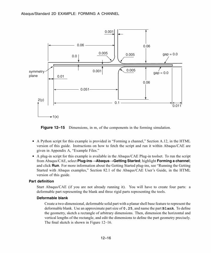
Abaqus/Standard 2D EXAMPLE: FORMING A CHANNEL
0.1
0.051
0.01
0.001
0.06
0.005
0.011
0.005
0.06
gap = 0.0
gap = 0.0
0.06
0.0050.0
0.001
symmetryplane
2(y)
1(x)
Figure 12–15 Dimensions, in m, of the components in the forming simulation.
• A Python script for this example is provided in “Forming a channel,” Section A.12, in the HTMLversion of this guide. Instructions on how to fetch the script and run it within Abaqus/CAE aregiven in Appendix A, “Example Files.”
• A plug-in script for this example is available in the Abaqus/CAE Plug-in toolset. To run the scriptfrom Abaqus/CAE, select Plug-ins→Abaqus→Getting Started; highlight Forming a channel;and click Run. For more information about the Getting Started plug-ins, see “Running the GettingStarted with Abaqus examples,” Section 82.1 of the Abaqus/CAE User’s Guide, in the HTMLversion of this guide.
Part definition
Start Abaqus/CAE (if you are not already running it). You will have to create four parts: adeformable part representing the blank and three rigid parts representing the tools.
Deformable blank
Create a two-dimensional, deformable solid part with a planar shell base feature to represent thedeformable blank. Use an approximate part size of 0.25, and name the part Blank. To definethe geometry, sketch a rectangle of arbitrary dimensions. Then, dimension the horizontal andvertical lengths of the rectangle, and edit the dimensions to define the part geometry precisely.The final sketch is shown in Figure 12–16.
12–16
Abaqus ID:Printed on:
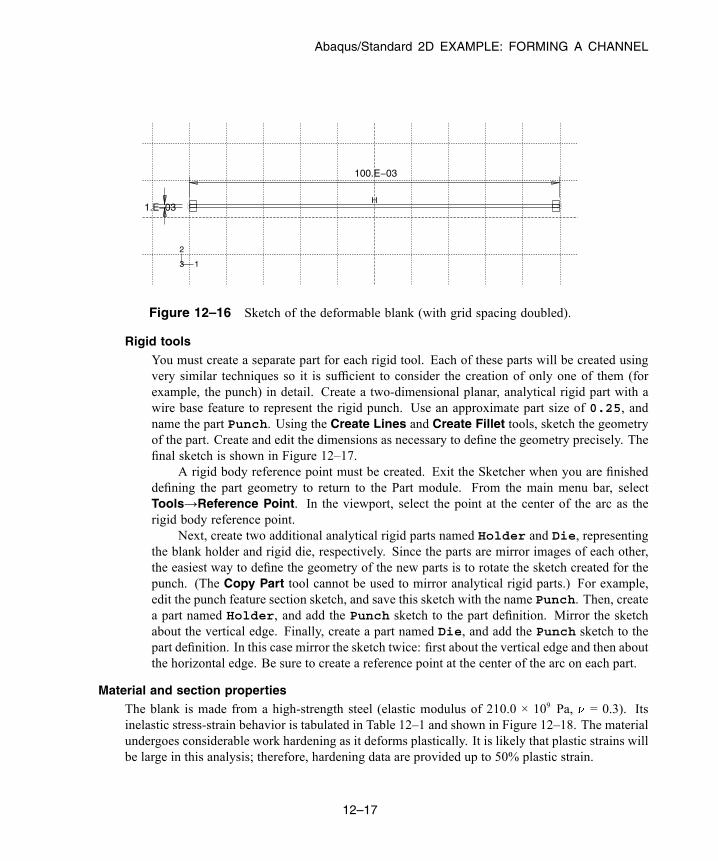
Abaqus/Standard 2D EXAMPLE: FORMING A CHANNEL
H1.E−03
100.E−03
1
2
3
Figure 12–16 Sketch of the deformable blank (with grid spacing doubled).
Rigid toolsYou must create a separate part for each rigid tool. Each of these parts will be created usingvery similar techniques so it is sufficient to consider the creation of only one of them (forexample, the punch) in detail. Create a two-dimensional planar, analytical rigid part with awire base feature to represent the rigid punch. Use an approximate part size of 0.25, andname the part Punch. Using the Create Lines and Create Fillet tools, sketch the geometryof the part. Create and edit the dimensions as necessary to define the geometry precisely. Thefinal sketch is shown in Figure 12–17.
A rigid body reference point must be created. Exit the Sketcher when you are finisheddefining the part geometry to return to the Part module. From the main menu bar, selectTools→Reference Point. In the viewport, select the point at the center of the arc as therigid body reference point.
Next, create two additional analytical rigid parts named Holder and Die, representingthe blank holder and rigid die, respectively. Since the parts are mirror images of each other,the easiest way to define the geometry of the new parts is to rotate the sketch created for thepunch. (The Copy Part tool cannot be used to mirror analytical rigid parts.) For example,edit the punch feature section sketch, and save this sketch with the name Punch. Then, createa part named Holder, and add the Punch sketch to the part definition. Mirror the sketchabout the vertical edge. Finally, create a part named Die, and add the Punch sketch to thepart definition. In this case mirror the sketch twice: first about the vertical edge and then aboutthe horizontal edge. Be sure to create a reference point at the center of the arc on each part.
Material and section propertiesThe blank is made from a high-strength steel (elastic modulus of 210.0 × 10⁹ Pa, = 0.3). Itsinelastic stress-strain behavior is tabulated in Table 12–1 and shown in Figure 12–18. The materialundergoes considerable work hardening as it deforms plastically. It is likely that plastic strains willbe large in this analysis; therefore, hardening data are provided up to 50% plastic strain.
12–17
Abaqus ID:Printed on:
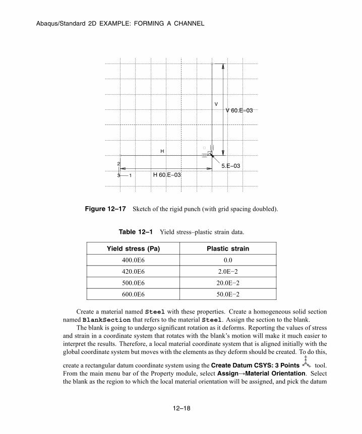
Abaqus/Standard 2D EXAMPLE: FORMING A CHANNEL
H
VV 60.E−03
H 60.E−03
5.E−03
1
2
3
Figure 12–17 Sketch of the rigid punch (with grid spacing doubled).
Table 12–1 Yield stress–plastic strain data.
Yield stress (Pa) Plastic strain
400.0E6 0.0
420.0E6 2.0E−2
500.0E6 20.0E−2
600.0E6 50.0E−2
Create a material named Steel with these properties. Create a homogeneous solid sectionnamed BlankSection that refers to the material Steel. Assign the section to the blank.
The blank is going to undergo significant rotation as it deforms. Reporting the values of stressand strain in a coordinate system that rotates with the blank’s motion will make it much easier tointerpret the results. Therefore, a local material coordinate system that is aligned initially with theglobal coordinate system but moves with the elements as they deform should be created. To do this,
create a rectangular datum coordinate system using the Create Datum CSYS: 3 Points tool.From the main menu bar of the Property module, select Assign→Material Orientation. Selectthe blank as the region to which the local material orientation will be assigned, and pick the datum
12–18
Abaqus ID:Printed on:

Abaqus/Standard 2D EXAMPLE: FORMING A CHANNEL
0.2 0.50.40.30.1
Plastic strain
Str
ess
(MP
a) 400.
300.
500.
600.
100.
200.
Figure 12–18 Yield stress vs. plastic strain.
coordinate system in the viewport as the CSYS (select Axis 3 and accept None for the additionalrotation options).
Assembling the parts
You will now create an assembly of part instances to define the analysis model. Begin by instancingthe blank. Then, instance and position the rigid tools using the techniques described below.
To instance and position the punch:
1. In the Model Tree, double-click Instances underneath the Assembly container and selectPunch as the part to instance.
Two-dimensional plane strain models must be defined in the global 1–2 plane. Therefore, donot rotate the parts after they have been instanced. You may, however, place the origin of themodel at any convenient location. The 1-direction will be normal to the symmetry plane.
2. The bottom of the punch initially rests on top of the blank, as indicated in Figure 12–15. Fromthe main menu bar, select Constraint→Edge to Edge to position the punch vertically withrespect to the blank.
3. Choose the horizontal edge of the punch as the straight edge of the movable instance and theedge on the top of the blank as the straight edge of the fixed instance.
Arrows appear on both instances. The punch will be moved so that its arrow points in the samedirection as the arrow on the blank.
4. If necessary, click Flip in the prompt area to reverse the direction of the arrow on the punch sothat both arrows point in the same direction; otherwise, the punch will be flipped. When botharrows point in the same direction, click OK.
12–19
Abaqus ID:Printed on:
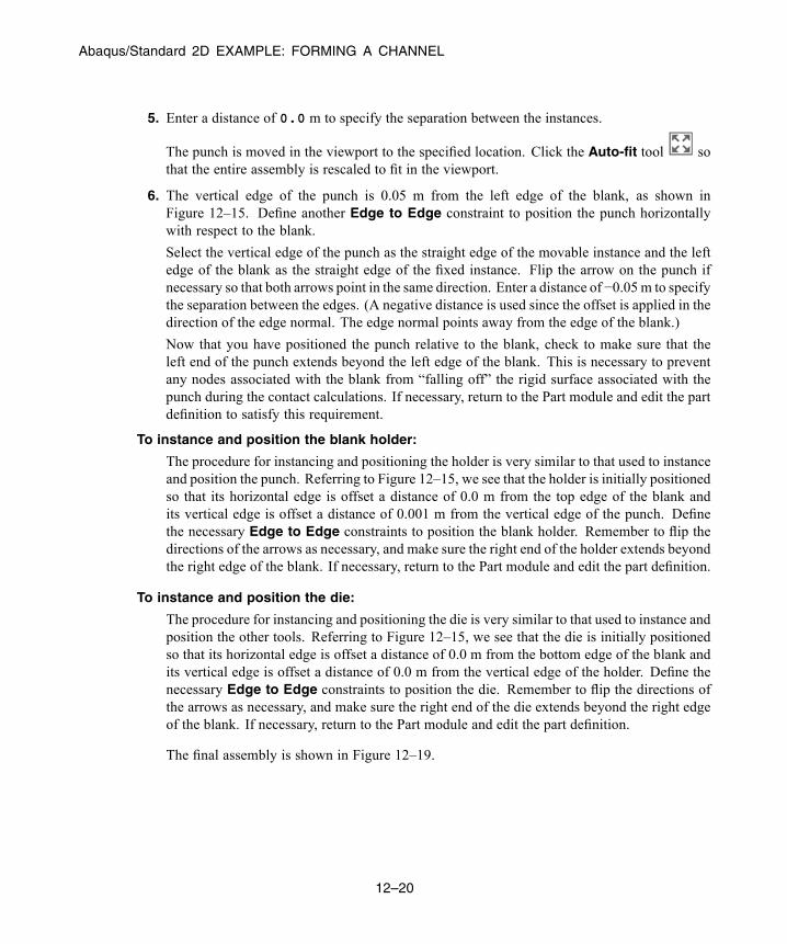
Abaqus/Standard 2D EXAMPLE: FORMING A CHANNEL
5. Enter a distance of 0.0 m to specify the separation between the instances.
The punch is moved in the viewport to the specified location. Click the Auto-fit tool sothat the entire assembly is rescaled to fit in the viewport.
6. The vertical edge of the punch is 0.05 m from the left edge of the blank, as shown inFigure 12–15. Define another Edge to Edge constraint to position the punch horizontallywith respect to the blank.
Select the vertical edge of the punch as the straight edge of the movable instance and the leftedge of the blank as the straight edge of the fixed instance. Flip the arrow on the punch ifnecessary so that both arrows point in the same direction. Enter a distance of −0.05 m to specifythe separation between the edges. (A negative distance is used since the offset is applied in thedirection of the edge normal. The edge normal points away from the edge of the blank.)
Now that you have positioned the punch relative to the blank, check to make sure that theleft end of the punch extends beyond the left edge of the blank. This is necessary to preventany nodes associated with the blank from “falling off” the rigid surface associated with thepunch during the contact calculations. If necessary, return to the Part module and edit the partdefinition to satisfy this requirement.
To instance and position the blank holder:
The procedure for instancing and positioning the holder is very similar to that used to instanceand position the punch. Referring to Figure 12–15, we see that the holder is initially positionedso that its horizontal edge is offset a distance of 0.0 m from the top edge of the blank andits vertical edge is offset a distance of 0.001 m from the vertical edge of the punch. Definethe necessary Edge to Edge constraints to position the blank holder. Remember to flip thedirections of the arrows as necessary, and make sure the right end of the holder extends beyondthe right edge of the blank. If necessary, return to the Part module and edit the part definition.
To instance and position the die:
The procedure for instancing and positioning the die is very similar to that used to instance andposition the other tools. Referring to Figure 12–15, we see that the die is initially positionedso that its horizontal edge is offset a distance of 0.0 m from the bottom edge of the blank andits vertical edge is offset a distance of 0.0 m from the vertical edge of the holder. Define thenecessary Edge to Edge constraints to position the die. Remember to flip the directions ofthe arrows as necessary, and make sure the right end of the die extends beyond the right edgeof the blank. If necessary, return to the Part module and edit the part definition.
The final assembly is shown in Figure 12–19.
12–20
Abaqus ID:Printed on:

Abaqus/Standard 2D EXAMPLE: FORMING A CHANNEL
RP RP
RP
Figure 12–19 Model assembly.
Geometry sets
At this point it is convenient to create the geometry sets that will be used to specify loads andboundary conditions and to restrict data output. Four sets should be created: one at each rigid bodyreference point, and one at the symmetry plane of the blank.
To create geometry sets:
1. Double-click the Sets item underneath the Assembly container to create the followinggeometry sets:
• RefPunch at the punch rigid body reference point.
• RefHolder at the holder rigid body reference point.
• RefDie at the die rigid body reference point.
• Center at the left vertical edge (symmetry plane) of the blank.
12–21
Abaqus ID:Printed on:
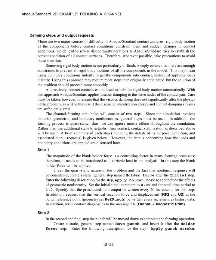
Abaqus/Standard 2D EXAMPLE: FORMING A CHANNEL
Defining steps and output requests
There are two major sources of difficulty in Abaqus/Standard contact analyses: rigid body motionof the components before contact conditions constrain them and sudden changes in contactconditions, which lead to severe discontinuity iterations as Abaqus/Standard tries to establish thecorrect condition of all contact surfaces. Therefore, wherever possible, take precautions to avoidthese situations.
Removing rigid body motion is not particularly difficult. Simply ensure that there are enoughconstraints to prevent all rigid body motions of all the components in the model. This may meanusing boundary conditions initially to get the components into contact, instead of applying loadsdirectly. Using this approach may require more steps than originally anticipated, but the solution ofthe problem should proceed more smoothly.
Alternatively, contact controls can be used to stabilize rigid body motion automatically. Withthis approach Abaqus/Standard applies viscous damping to the slave nodes of the contact pair. Caremust be taken, however, to ensure that the viscous damping does not significantly alter the physicsof the problem, as will be the case if the dissipated stabilization energy and contact damping stressesare sufficiently small.
The channel-forming simulation will consist of two steps. Since the simulation involvesmaterial, geometric, and boundary nonlinearities, general steps must be used. In addition, theforming process is quasi-static; thus, we can ignore inertia effects throughout the simulation.Rather than use additional steps to establish firm contact, contact stabilization as described abovewill be used. A brief summary of each step (including the details of its purpose, definition, andassociated output requests) is given below. However, the details concerning how the loads andboundary conditions are applied are discussed later.
Step 1
The magnitude of the blank holder force is a controlling factor in many forming processes;therefore, it needs to be introduced as a variable load in the analysis. In this step the blankholder force will be applied.
Given the quasi-static nature of the problem and the fact that nonlinear response willbe considered, create a static, general step named Holder force after the Initial step.Enter the following description for the step, Apply holder force; and include the effectsof geometric nonlinearity. Set the initial time increment to 0.05 and the total time period to1.0. Specify that the preselected field output be written every 20 increments for this step.In addition, request that the vertical reaction force and displacement (RF2 and U2) at thepunch reference point (geometry set RefPunch) be written every increment as history data.In addition, write contact diagnostics to the message file (Output→Diagnostic Print).
Step 2
In the second and final step the punch will be moved down to complete the forming operation.Create a static, general step named Move punch, and insert it after the Holder
force step. Enter the following description for the step: Apply punch stroke.
12–22
Abaqus ID:Printed on:
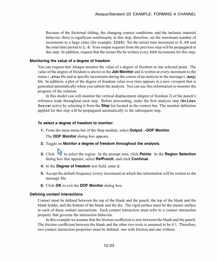
Abaqus/Standard 2D EXAMPLE: FORMING A CHANNEL
Because of the frictional sliding, the changing contact conditions, and the inelastic materialbehavior, there is significant nonlinearity in this step; therefore, set the maximum number ofincrements to a large value (for example, 1000). Set the initial time increment to 0.05 andthe total time period to 1.0. Your output requests from the previous step will be propagated tothis step. In addition, request that the restart file be written every 200 increments for this step.
Monitoring the value of a degree of freedom
You can request that Abaqus monitor the value of a degree of freedom at one selected point. Thevalue of the degree of freedom is shown in the Job Monitor and is written at every increment to thestatus (.sta) file and at specific increments during the course of an analysis to the message (.msg)file. In addition, a plot of the degree of freedom value over time appears in a new viewport that isgenerated automatically when you submit the analysis. You can use this information to monitor theprogress of the solution.
In this model you will monitor the vertical displacement (degree of freedom 2) of the punch’sreference node throughout each step. Before proceeding, make the first analysis step (Holderforce) active by selecting it from the Step list located in the context bar. The monitor definitionapplied for this step will be propagated automatically to the subsequent step.
To select a degree of freedom to monitor:
1. From the main menu bar of the Step module, select Output→DOF Monitor.
The DOF Monitor dialog box appears.
2. Toggle on Monitor a degree of freedom throughout the analysis.
3. Click to select the region. In the prompt area, click Points. In the Region Selectiondialog box that appears, select RefPunch; and click Continue.
4. In the Degree of freedom text field, enter 2.
5. Accept the default frequency (every increment) at which this information will be written to themessage file.
6. Click OK to exit the DOF Monitor dialog box.
Defining contact interactions
Contact must be defined between the top of the blank and the punch, the top of the blank and theblank holder, and the bottom of the blank and the die. The rigid surface must be the master surfacein each of these contact interactions. Each contact interaction must refer to a contact interactionproperty that governs the interaction behavior.
In this example we assume that the friction coefficient is zero between the blank and the punch.The friction coefficient between the blank and the other two tools is assumed to be 0.1. Therefore,two contact interaction properties must be defined: one with friction and one without.
12–23
Abaqus ID:Printed on:
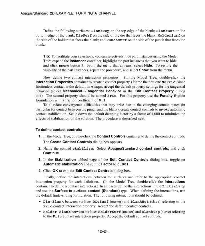
Abaqus/Standard 2D EXAMPLE: FORMING A CHANNEL
Define the following surfaces: BlankTop on the top edge of the blank; BlankBot on thebottom edge of the blank; DieSurf on the side of the die that faces the blank; HolderSurf onthe side of the holder that faces the blank; and PunchSurf on the side of the punch that faces theblank.
Tip: To facilitate your selections, you can selectively hide part instances using the ModelTree: expand the Instances container, highlight the part instances that you want to hide,and click mouse button 3. From the menu that appears, select Hide. To restore thevisibility of the part instances, repeat the procedure, and select Show from the menu.
Now define two contact interaction properties. (In the Model Tree, double-click theInteraction Properties container to create a contact property.) Name the first one NoFric; sincefrictionless contact is the default in Abaqus, accept the default property settings for the tangentialbehavior (select Mechanical→Tangential Behavior in the Edit Contact Property dialogbox). The second property should be named Fric. For this property use the Penalty frictionformulation with a friction coefficient of 0.1.
To alleviate convergence difficulties that may arise due to the changing contact states (inparticular for contact between the punch and the blank), create contact controls to invoke automaticcontact stabilization. Scale down the default damping factor by a factor of 1,000 to minimize theeffects of stabilization on the solution. The procedure is described next.
To define contact controls:
1. In theModel Tree, double-click theContact Controls container to define the contact controls.
The Create Contact Controls dialog box appears.
2. Name the control stabilize. Select Abaqus/Standard contact controls, and clickContinue.
3. In the Stabilization tabbed page of the Edit Contact Controls dialog box, toggle onAutomatic stabilization and set the Factor to 0.001.
4. Click OK to exit the Edit Contact Controls dialog box.
Finally, define the interactions between the surfaces and refer to the appropriate contactinteraction property for each definition. (In the Model Tree, double-click the Interactionscontainer to define a contact interaction.) In all cases define the interactions in the Initial stepand use the Surface-to-surface contact (Standard) type. When defining the interactions, usethe default finite-sliding formulation. The following interactions should be defined:
• Die-Blank between surfaces DieSurf (master) and BlankBot (slave) referring to theFric contact interaction property. Accept the default contact controls.
• Holder-Blank between surfaces HolderSurf (master) and BlankTop (slave) referringto the Fric contact interaction property. Accept the default contact controls.
12–24
Abaqus ID:Printed on:

Abaqus/Standard 2D EXAMPLE: FORMING A CHANNEL
• Punch-Blank between surfaces PunchSurf (master) and BlankTop (slave) referringto the NoFric contact interaction property. Using the Interaction Manager, edit thisinteraction to assign the nondefault contact controls defined earlier (stabilize) in thesecond analysis step (Move punch).
Boundary conditions and loading for Step 1
In this step contact will be established between the blank holder and the blank while the punch anddie are held fixed.
Constrain the blank holder in degrees of freedom 1 and 6, where degree of freedom 6 is therotation in the plane of the model; constrain the punch and die completely. All of the boundaryconditions for the rigid surfaces are applied to their respective rigid body reference nodes. Applysymmetric boundary constraints on the region of the blank lying on the symmetry plane (geometryset Center).
Table 12–2 summarizes the boundary conditions applied in this step.
Table 12–2 Summary of boundary conditions applied in Step 1.
BC Name Geometry Set BCs
CenterBC Center XSYMM
RefDieBC RefDie U1 = U2 = UR3 = 0.0
RefHolderBC RefHolder U1 = UR3 = 0.0
RefPunchBC RefPunch U1 = U2 = UR3 = 0.0
To apply the blank holder force, create a mechanical concentrated force namedRefHolderForce. Recall that in this simulation the required blank holder force is 440 kN.Thus, apply the load to set RefHolder, and specify a magnitude of −440.E3 for CF2.
Boundary conditions for Step 2
In this step move the punch down to complete the forming operation. Using the BoundaryCondition Manager, edit the RefPunchBC boundary condition to specify a value of −0.030 forU2, which represents the total displacement of the punch.
Before continuing, change the name of your model to Standard.
Mesh creation and job definition
You should consider the type of element you will use before you design your mesh. When choosingan element type, you must consider several aspects of your model such as the model’s geometry,the type of deformation that will be seen, the loads being applied, etc. The following points areimportant to consider in this simulation:
• The contact between surfaces. Whenever possible, first-order elements (with the exception oftetrahedral elements) should be used for contact simulations. When using tetrahedral elements,
12–25
Abaqus ID:Printed on:
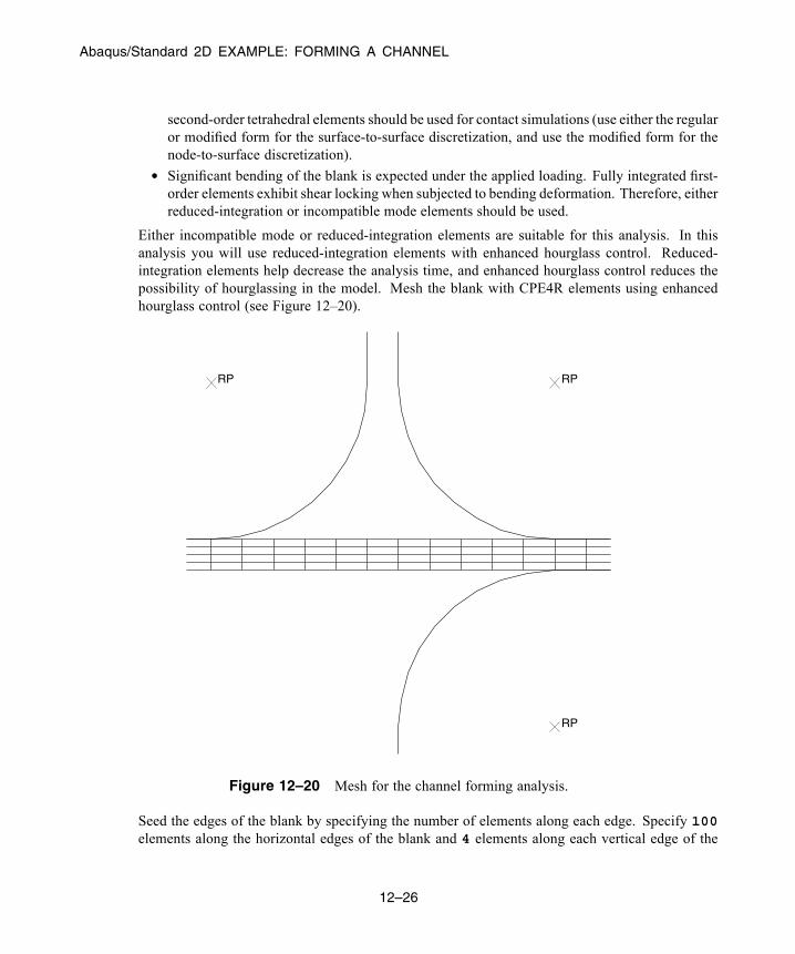
Abaqus/Standard 2D EXAMPLE: FORMING A CHANNEL
second-order tetrahedral elements should be used for contact simulations (use either the regularor modified form for the surface-to-surface discretization, and use the modified form for thenode-to-surface discretization).
• Significant bending of the blank is expected under the applied loading. Fully integrated first-order elements exhibit shear locking when subjected to bending deformation. Therefore, eitherreduced-integration or incompatible mode elements should be used.
Either incompatible mode or reduced-integration elements are suitable for this analysis. In thisanalysis you will use reduced-integration elements with enhanced hourglass control. Reduced-integration elements help decrease the analysis time, and enhanced hourglass control reduces thepossibility of hourglassing in the model. Mesh the blank with CPE4R elements using enhancedhourglass control (see Figure 12–20).
RP RP
RP
Figure 12–20 Mesh for the channel forming analysis.
Seed the edges of the blank by specifying the number of elements along each edge. Specify 100elements along the horizontal edges of the blank and 4 elements along each vertical edge of the
12–26
Abaqus ID:Printed on:
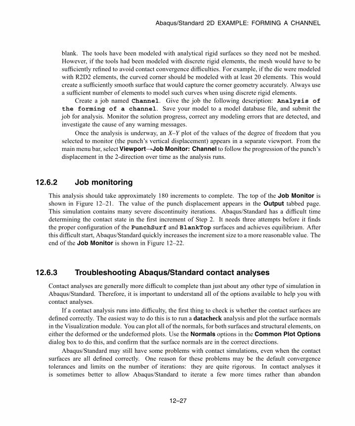
Abaqus/Standard 2D EXAMPLE: FORMING A CHANNEL
blank. The tools have been modeled with analytical rigid surfaces so they need not be meshed.However, if the tools had been modeled with discrete rigid elements, the mesh would have to besufficiently refined to avoid contact convergence difficulties. For example, if the die were modeledwith R2D2 elements, the curved corner should be modeled with at least 20 elements. This wouldcreate a sufficiently smooth surface that would capture the corner geometry accurately. Always usea sufficient number of elements to model such curves when using discrete rigid elements.
Create a job named Channel. Give the job the following description: Analysis ofthe forming of a channel. Save your model to a model database file, and submit thejob for analysis. Monitor the solution progress, correct any modeling errors that are detected, andinvestigate the cause of any warning messages.
Once the analysis is underway, an X–Y plot of the values of the degree of freedom that youselected to monitor (the punch’s vertical displacement) appears in a separate viewport. From themain menu bar, select Viewport→Job Monitor: Channel to follow the progression of the punch’sdisplacement in the 2-direction over time as the analysis runs.
12.6.2 Job monitoring
This analysis should take approximately 180 increments to complete. The top of the Job Monitor isshown in Figure 12–21. The value of the punch displacement appears in the Output tabbed page.This simulation contains many severe discontinuity iterations. Abaqus/Standard has a difficult timedetermining the contact state in the first increment of Step 2. It needs three attempts before it findsthe proper configuration of the PunchSurf and BlankTop surfaces and achieves equilibrium. Afterthis difficult start, Abaqus/Standard quickly increases the increment size to a more reasonable value. Theend of the Job Monitor is shown in Figure 12–22.
12.6.3 Troubleshooting Abaqus/Standard contact analyses
Contact analyses are generally more difficult to complete than just about any other type of simulation inAbaqus/Standard. Therefore, it is important to understand all of the options available to help you withcontact analyses.
If a contact analysis runs into difficulty, the first thing to check is whether the contact surfaces aredefined correctly. The easiest way to do this is to run a datacheck analysis and plot the surface normalsin the Visualization module. You can plot all of the normals, for both surfaces and structural elements, oneither the deformed or the undeformed plots. Use the Normals options in the Common Plot Optionsdialog box to do this, and confirm that the surface normals are in the correct directions.
Abaqus/Standard may still have some problems with contact simulations, even when the contactsurfaces are all defined correctly. One reason for these problems may be the default convergencetolerances and limits on the number of iterations: they are quite rigorous. In contact analyses itis sometimes better to allow Abaqus/Standard to iterate a few more times rather than abandon
12–27
Abaqus ID:Printed on:
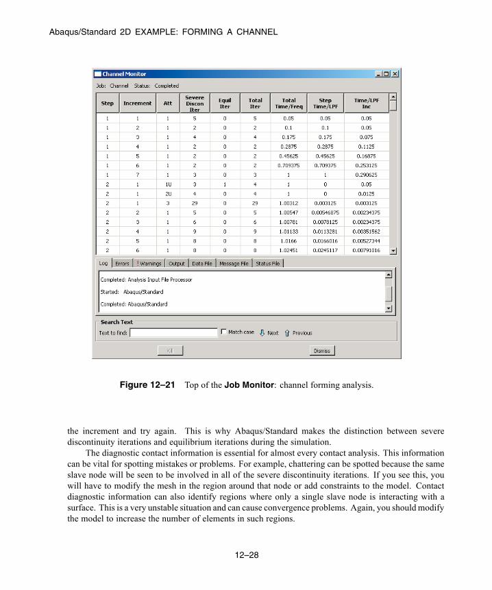
Abaqus/Standard 2D EXAMPLE: FORMING A CHANNEL
Figure 12–21 Top of the Job Monitor: channel forming analysis.
the increment and try again. This is why Abaqus/Standard makes the distinction between severediscontinuity iterations and equilibrium iterations during the simulation.
The diagnostic contact information is essential for almost every contact analysis. This informationcan be vital for spotting mistakes or problems. For example, chattering can be spotted because the sameslave node will be seen to be involved in all of the severe discontinuity iterations. If you see this, youwill have to modify the mesh in the region around that node or add constraints to the model. Contactdiagnostic information can also identify regions where only a single slave node is interacting with asurface. This is a very unstable situation and can cause convergence problems. Again, you should modifythe model to increase the number of elements in such regions.
12–28
Abaqus ID:Printed on:
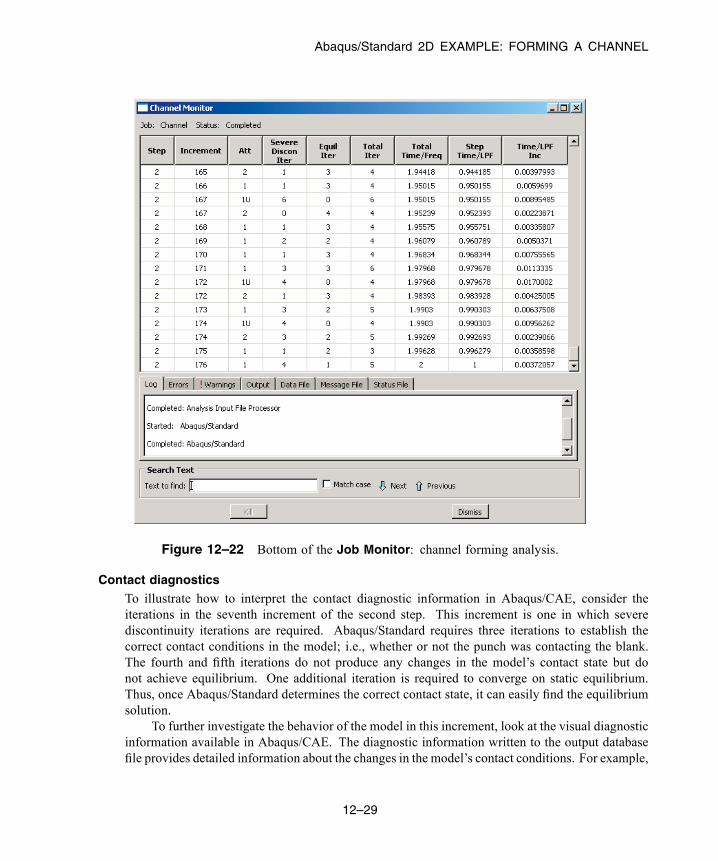
Abaqus/Standard 2D EXAMPLE: FORMING A CHANNEL
Figure 12–22 Bottom of the Job Monitor: channel forming analysis.
Contact diagnosticsTo illustrate how to interpret the contact diagnostic information in Abaqus/CAE, consider theiterations in the seventh increment of the second step. This increment is one in which severediscontinuity iterations are required. Abaqus/Standard requires three iterations to establish thecorrect contact conditions in the model; i.e., whether or not the punch was contacting the blank.The fourth and fifth iterations do not produce any changes in the model’s contact state but donot achieve equilibrium. One additional iteration is required to converge on static equilibrium.Thus, once Abaqus/Standard determines the correct contact state, it can easily find the equilibriumsolution.
To further investigate the behavior of the model in this increment, look at the visual diagnosticinformation available in Abaqus/CAE. The diagnostic information written to the output databasefile provides detailed information about the changes in the model’s contact conditions. For example,
12–29
Abaqus ID:Printed on:

Abaqus/Standard 2D EXAMPLE: FORMING A CHANNEL
the node number and location in the model of every slave node whose contact status changes in asevere discontinuity iteration, as well as the contact interaction to which it belongs, can be obtainedusing the visual diagnostics tool.
Enter the Visualization module, and open the file Channel.odb to look at the contactdiagnostics information. In the first severe discontinuity iteration of the second step (increment7, attempt 1), four nodes on the blank experience contact openings, indicating that their assumedcontact state is incompatible. This incompatibility can be seen in the Contact tabbed page ofthe Job Diagnostics dialog box (see Figure 12–23). To see where the nodes are located on themodel, toggle on Highlight selections in viewport.
Figure 12–23 Contact openings in the first severe discontinuity iteration.
Since neither the contact state nor the equilibrium checks pass in this iteration,Abaqus/Standard removes the contact constraints from these nodes and performs anotheriteration. After two additional iterations Abaqus/Standard detects no changes in the contact state.The solution in the fourth and fifth iterations do not satisfy the force residual tolerance check, soanother iteration is performed. This time, not only is the contact state converged, but the forceresidual tolerance check is satisfied and the displacement correction is acceptable relative to thelargest displacement increment, as shown in Figure 12–24. Thus, the third equilibrium iterationproduces a converged solution for this increment.
12–30
Abaqus ID:Printed on:

Abaqus/Standard 2D EXAMPLE: FORMING A CHANNEL
Figure 12–24 Converged equilibrium iteration.
12.6.4 PostprocessingIn the Visualization module, examine the deformation of the blank.
Deformed model shape and contour plots
The basic result of this simulation is the deformation of the blank and the plastic strain caused by theforming process. We can plot the deformed model shape and the plastic strain, as described below.
To plot the deformed model shape:
1. Plot the deformed model shape. You can remove the die and the punch from the display andvisualize just the blank.
2. In the Results Tree, expand the Instances container underneath the output database file namedChannel.odb.
3. From the list of available part instances, select BLANK-1. Click mouse button 3, and selectReplace from the menu that appears to replace the current display group with the selected
elements. Click , if necessary, to fit the model in the viewport.
12–31
Abaqus ID:Printed on:
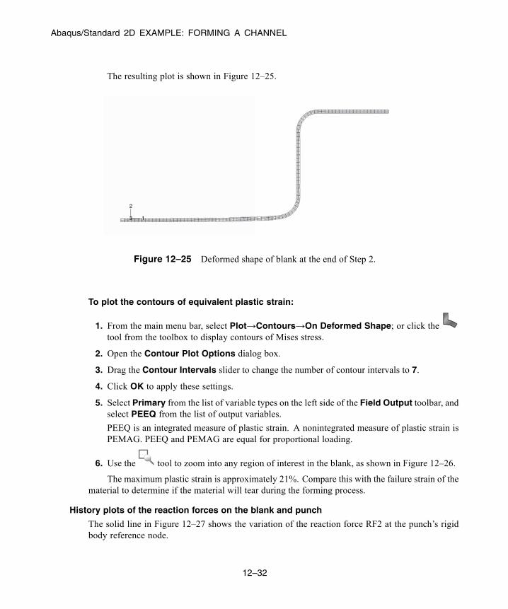
Abaqus/Standard 2D EXAMPLE: FORMING A CHANNEL
The resulting plot is shown in Figure 12–25.
1
2
3
Figure 12–25 Deformed shape of blank at the end of Step 2.
To plot the contours of equivalent plastic strain:
1. From the main menu bar, select Plot→Contours→On Deformed Shape; or click thetool from the toolbox to display contours of Mises stress.
2. Open the Contour Plot Options dialog box.
3. Drag the Contour Intervals slider to change the number of contour intervals to 7.
4. Click OK to apply these settings.
5. Select Primary from the list of variable types on the left side of the Field Output toolbar, andselect PEEQ from the list of output variables.
PEEQ is an integrated measure of plastic strain. A nonintegrated measure of plastic strain isPEMAG. PEEQ and PEMAG are equal for proportional loading.
6. Use the tool to zoom into any region of interest in the blank, as shown in Figure 12–26.
The maximum plastic strain is approximately 21%. Compare this with the failure strain of thematerial to determine if the material will tear during the forming process.
History plots of the reaction forces on the blank and punch
The solid line in Figure 12–27 shows the variation of the reaction force RF2 at the punch’s rigidbody reference node.
12–32
Abaqus ID:Printed on:
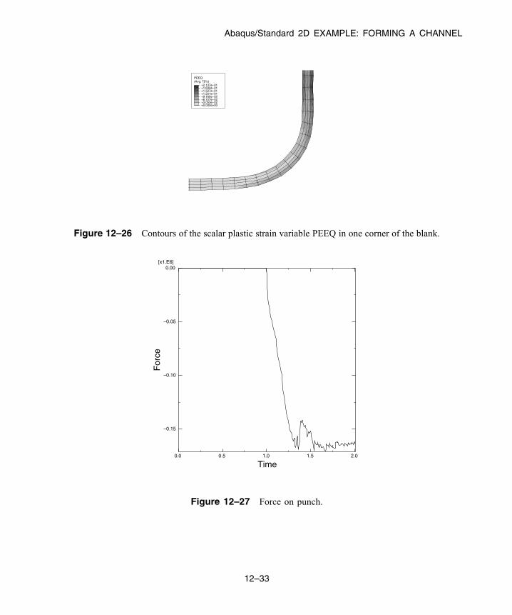
Abaqus/Standard 2D EXAMPLE: FORMING A CHANNEL
(Avg: 75%)PEEQ
+0.000e+00+3.053e−02+6.107e−02+9.160e−02+1.221e−01+1.527e−01+1.832e−01+2.137e−01
Figure 12–26 Contours of the scalar plastic strain variable PEEQ in one corner of the blank.
Time0.0 0.5 1.0 1.5 2.0
For
ce
−0.15
−0.10
−0.05
0.00[x1.E6]
Figure 12–27 Force on punch.
12–33
Abaqus ID:Printed on:

Abaqus/Standard 2D EXAMPLE: FORMING A CHANNEL
To create a history plot of the reaction force:
1. In the Results Tree, expand the History Output container. Double-click Reactionforce: RF1 PI: PUNCH–1 Node xxx in NSET REFPUNCH.
A history plot of the reaction force in the 1-direction appears.
2. Open the Axis Options dialog box to label the axes.
3. Switch to the Title tabbed page.
4. Specify Reaction Force - RF2 as the Y-axis label, and Total Time as the X-axislabel.
5. Click Dismiss to close the dialog box.
The punch force, shown in Figure 12–27, rapidly increases to about 160 kN during Step 2,which runs from a total time of 1.0 to 2.0.
History plot of the stabilization and internal energies
It is important to verify that the presence of contact stabilization does not significantly alter thephysics of the problem. One way to assess this requirement is to compare the energy dissipation dueto stabilization (ALLSD) against the internal energy of the structure (ALLIE). Ideally the amountof stabilization energy should be a small fraction of the internal energy. Figure 12–28 shows thevariation of the stabilization and internal energies. It is clear that the dissipated stabilization energyis indeed small.
Time0.0 0.5 1.0 1.5 2.0
Ene
rgy
0.0
0.5
1.0
1.5
[x1.E3]
ALLIE Whole ModelALLSD Whole Model
Figure 12–28 Stabilization and internal energies.
12–34
Abaqus ID:Printed on:

Abaqus/Standard 2D EXAMPLE: FORMING A CHANNEL
Plotting contours on surfaces
Abaqus/CAE includes a number of features designed specifically for postprocessing contactanalyses. Within the Visualization module, the Display Group feature can be used to collectsurfaces into display groups, similar to element and node sets.
To display contact surface normal vectors:
1. Plot the undeformed model shape.
2. In the Results Tree, expand theSurface Sets container. Select the surfaces namedBLANKTOPand PUNCH-1.PUNCHSURF. Click mouse button 3, and select Replace from the menu thatappears.
3. Using the Common Plot Options dialog box, turn on the display of the normal vectors (Onsurfaces) and set the length of the vector arrows to Short.
4. Use the tool, if necessary, to zoom into any region of interest, as shown in Figure 12–29.
To contour the contact pressure:
1. Plot the contours of plastic strain again.
2. From the list of variable types on the left side of the Field Output toolbar, select Primary, ifit is not already selected.
3. From the list of output variables in the center of the toolbar, select CPRESS.
4. Remove the PUNCH-1.PUNCHSURF surface from your display group.
To visualize contours of surface-based variables better in two-dimensional models, you canextrude the plane strain elements to construct the equivalent three-dimensional view. You cansweep axisymmetric elements in a similar fashion.
5. From the main menu bar, select View→ODB Display Options.
The ODB Display Options dialog box appears.
6. Select the Sweep/Extrude tab to access the Sweep/Extrude options.
7. In the Extrude region of the dialog box, toggle on Extrude elements; and set the Depth to0.05 to extrude the model for the purpose of displaying contours.
8. Click OK to apply these settings.
Rotate the model using the tool to display the model from a suitable view, such as the oneshown in Figure 12–30.
12–35
Abaqus ID:Printed on:
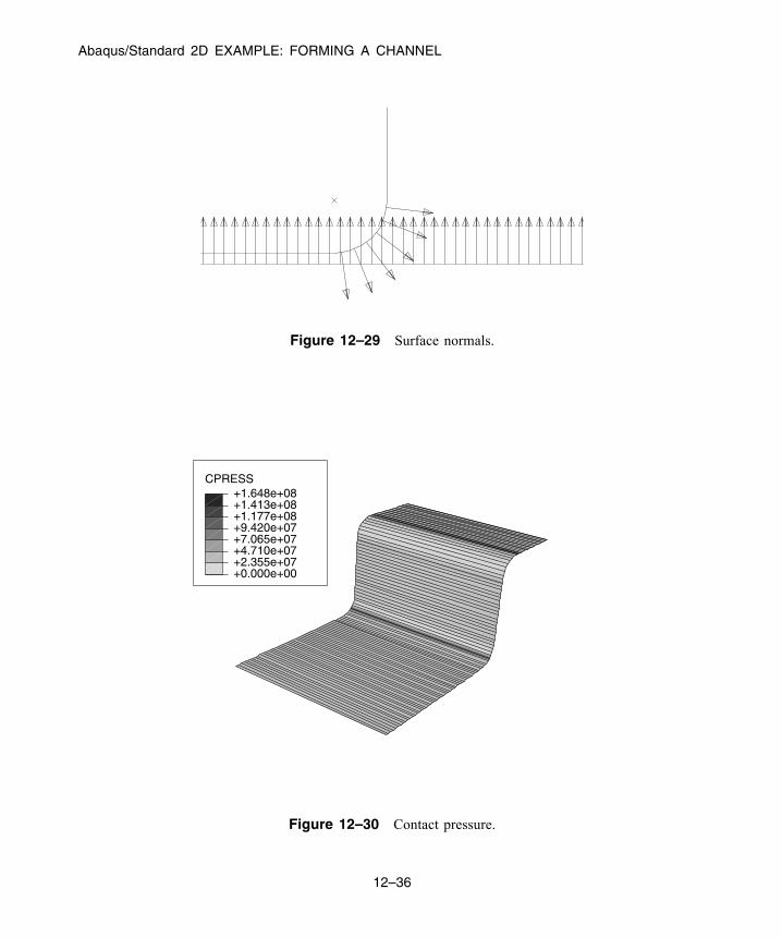
Abaqus/Standard 2D EXAMPLE: FORMING A CHANNEL
Figure 12–29 Surface normals.
CPRESS
+0.000e+00+2.355e+07+4.710e+07+7.065e+07+9.420e+07+1.177e+08+1.413e+08+1.648e+08
Figure 12–30 Contact pressure.
12–36
Abaqus ID:Printed on:
Abaqus/Standard 3D EXAMPLE: SHEARING OF A LAP JOINT
12.7 General contact in Abaqus/Standard
In the channel forming example in “Abaqus/Standard 2D example: forming a channel,” Section 12.6,contact interaction is defined using the contact pairs algorithm, which requires you to explicitly definethe surfaces that may potentially come into contact. As an alternative, you can specify contact in anAbaqus/Standard analysis by using the general contact algorithm. The contact interaction domain,contact properties, and surface attributes are specified independently for general contact, offering amore flexible way to add detail incrementally to a model. The simple interface for specifying generalcontact allows for a highly automated contact definition; however, it is also possible to define contactwith the general contact interface to mimic traditional contact pairs. Conversely, specifying self-contactof a surface spanning multiple bodies with the contact pair user interface (if the surface-to-surfaceformulation is used) mimics the highly automated approach often used for general contact.
In Abaqus/Standard, traditional pairwise specifications of contact interactions will often resultin more efficient analyses as compared to an all-inclusive self-contact approach to defining contact.Therefore, there is often a trade-off between ease of defining contact and analysis performance.Abaqus/CAE provides a contact detection tool that greatly simplifies the process of creating traditionalcontact pairs for Abaqus/Standard (see “Understanding contact and constraint detection,” Section 15.6of the Abaqus/CAE User’s Guide).
12.8 Abaqus/Standard 3D example: shearing of a lap joint
This simulation of the shearing of a lap joint illustrates the use of general contact in Abaqus/Standard.The model consists of two overlapping aluminum plates that are connected with a titanium rivet.
The left end of the bottom plate is fixed, and the force is applied to the right end of the top plate to shearthe joint. Figure 12–31 shows the basic arrangement of the components. Because of symmetry, only halfof the joint is modeled to reduce computational cost. Frictional contact is assumed.
12.8.1 Preprocessing—creating the model with Abaqus/CAE
Use Abaqus/CAE to create the model. Abaqus provides scripts that replicate the complete analysis modelfor this problem. Run one of these scripts if you encounter difficulties following the instructions givenbelow or if you wish to check your work. Scripts are available in the following locations:
• A Python script for this example is provided in “Shearing of a lap joint,” Section A.13, in the HTMLversion of this guide. Instructions on how to fetch the script and run it within Abaqus/CAE are givenin Appendix A, “Example Files.”
12–37
Abaqus ID:Printed on:
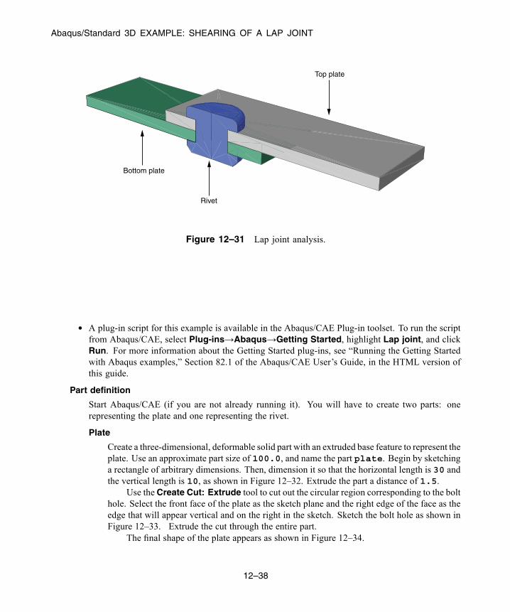
Abaqus/Standard 3D EXAMPLE: SHEARING OF A LAP JOINT
Rivet
Top plate
Bottom plate
Figure 12–31 Lap joint analysis.
• A plug-in script for this example is available in the Abaqus/CAE Plug-in toolset. To run the scriptfrom Abaqus/CAE, select Plug-ins→Abaqus→Getting Started, highlight Lap joint, and clickRun. For more information about the Getting Started plug-ins, see “Running the Getting Startedwith Abaqus examples,” Section 82.1 of the Abaqus/CAE User’s Guide, in the HTML version ofthis guide.
Part definition
Start Abaqus/CAE (if you are not already running it). You will have to create two parts: onerepresenting the plate and one representing the rivet.
Plate
Create a three-dimensional, deformable solid part with an extruded base feature to represent theplate. Use an approximate part size of 100.0, and name the part plate. Begin by sketchinga rectangle of arbitrary dimensions. Then, dimension it so that the horizontal length is 30 andthe vertical length is 10, as shown in Figure 12–32. Extrude the part a distance of 1.5.
Use the Create Cut: Extrude tool to cut out the circular region corresponding to the bolthole. Select the front face of the plate as the sketch plane and the right edge of the face as theedge that will appear vertical and on the right in the sketch. Sketch the bolt hole as shown inFigure 12–33. Extrude the cut through the entire part.
The final shape of the plate appears as shown in Figure 12–34.
12–38
Abaqus ID:Printed on:

Abaqus/Standard 3D EXAMPLE: SHEARING OF A LAP JOINT
10.
30.
H
10.
30.
H
X
Y
Z
Figure 12–32 Sketch of the plate.
H 7.5
R2.5
H 7.5
R2.5
X
Y
Z
Figure 12–33 Sketch of the bolt hole.
X
Y
Z
Figure 12–34 Final plate geometry.
12–39
Abaqus ID:Printed on:
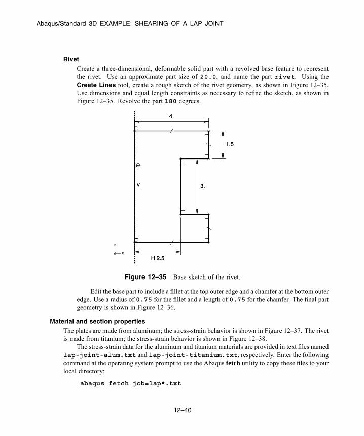
Abaqus/Standard 3D EXAMPLE: SHEARING OF A LAP JOINT
Rivet
Create a three-dimensional, deformable solid part with a revolved base feature to representthe rivet. Use an approximate part size of 20.0, and name the part rivet. Using theCreate Lines tool, create a rough sketch of the rivet geometry, as shown in Figure 12–35.Use dimensions and equal length constraints as necessary to refine the sketch, as shown inFigure 12–35. Revolve the part 180 degrees.
3.
1.5
4.
H 2.5
V 3.
1.5
4.
H 2.5
V
X
Y
Z
Figure 12–35 Base sketch of the rivet.
Edit the base part to include a fillet at the top outer edge and a chamfer at the bottom outeredge. Use a radius of 0.75 for the fillet and a length of 0.75 for the chamfer. The final partgeometry is shown in Figure 12–36.
Material and section propertiesThe plates are made from aluminum; the stress-strain behavior is shown in Figure 12–37. The rivetis made from titanium; the stress-strain behavior is shown in Figure 12–38.
The stress-strain data for the aluminum and titanium materials are provided in text files namedlap-joint-alum.txt and lap-joint-titanium.txt, respectively. Enter the followingcommand at the operating system prompt to use the Abaqus fetch utility to copy these files to yourlocal directory:
abaqus fetch job=lap*.txt
12–40
Abaqus ID:Printed on:
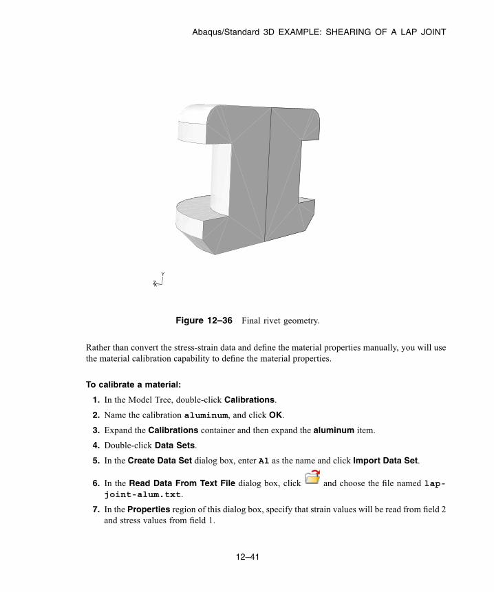
Abaqus/Standard 3D EXAMPLE: SHEARING OF A LAP JOINT
X
Y
Z
Figure 12–36 Final rivet geometry.
Rather than convert the stress-strain data and define the material properties manually, you will usethe material calibration capability to define the material properties.
To calibrate a material:
1. In the Model Tree, double-click Calibrations.
2. Name the calibration aluminum, and click OK.
3. Expand the Calibrations container and then expand the aluminum item.
4. Double-click Data Sets.
5. In the Create Data Set dialog box, enter Al as the name and click Import Data Set.
6. In the Read Data From Text File dialog box, click and choose the file named lap-joint-alum.txt.
7. In the Properties region of this dialog box, specify that strain values will be read from field 2and stress values from field 1.
12–41
Abaqus ID:Printed on:

Abaqus/Standard 3D EXAMPLE: SHEARING OF A LAP JOINT
Strain0.00 0.10 0.20 0.30 0.40 0.50 0.60
Str
ess
0.
200.
400.
600.
800. Aluminum
Figure 12–37 Aluminum stress-strain curve.
Strain0.00 0.05 0.10 0.15 0.20 0.25 0.30
Str
ess
0.0
0.4
0.8
1.2
[x1.E3]
Titanium
Figure 12–38 Titanium stress-strain curve.
12–42
Abaqus ID:Printed on:
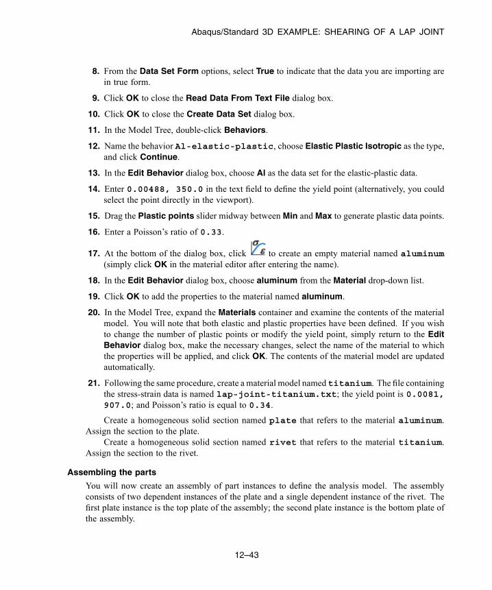
Abaqus/Standard 3D EXAMPLE: SHEARING OF A LAP JOINT
8. From the Data Set Form options, select True to indicate that the data you are importing arein true form.
9. Click OK to close the Read Data From Text File dialog box.
10. Click OK to close the Create Data Set dialog box.
11. In the Model Tree, double-click Behaviors.
12. Name the behavior Al-elastic-plastic, choose Elastic Plastic Isotropic as the type,and click Continue.
13. In the Edit Behavior dialog box, choose Al as the data set for the elastic-plastic data.
14. Enter 0.00488, 350.0 in the text field to define the yield point (alternatively, you couldselect the point directly in the viewport).
15. Drag the Plastic points slider midway between Min and Max to generate plastic data points.
16. Enter a Poisson’s ratio of 0.33.
17. At the bottom of the dialog box, click to create an empty material named aluminum(simply click OK in the material editor after entering the name).
18. In the Edit Behavior dialog box, choose aluminum from the Material drop-down list.
19. Click OK to add the properties to the material named aluminum.
20. In the Model Tree, expand the Materials container and examine the contents of the materialmodel. You will note that both elastic and plastic properties have been defined. If you wishto change the number of plastic points or modify the yield point, simply return to the EditBehavior dialog box, make the necessary changes, select the name of the material to whichthe properties will be applied, and click OK. The contents of the material model are updatedautomatically.
21. Following the same procedure, create a material model named titanium. The file containingthe stress-strain data is named lap-joint-titanium.txt; the yield point is 0.0081,907.0; and Poisson’s ratio is equal to 0.34.
Create a homogeneous solid section named plate that refers to the material aluminum.Assign the section to the plate.
Create a homogeneous solid section named rivet that refers to the material titanium.Assign the section to the rivet.
Assembling the parts
You will now create an assembly of part instances to define the analysis model. The assemblyconsists of two dependent instances of the plate and a single dependent instance of the rivet. Thefirst plate instance is the top plate of the assembly; the second plate instance is the bottom plate ofthe assembly.
12–43
Abaqus ID:Printed on:

Abaqus/Standard 3D EXAMPLE: SHEARING OF A LAP JOINT
To instance and position the plates:
1. In the Model Tree, double-click Instances underneath the Assembly container and selectplate as the part to instance.
2. Create a second instance of the plate. Toggle on the option to automatically offset the partinstances.
3. From the main menu bar, select Constraint→Face to Face. Select the back face of the plateon the right (the second instance) as the face on the movable instance. Select the back face ofthe plate on the left (the first instance) as the face on the fixed instance. If necessary, flip thearrows so that they point in opposite directions, as shown in Figure 12–39. Set the offset equalto 0.0.
X
Y
Z
Figure 12–39 Face-to-face constraint.
4. From the main menu bar, select Constraint→Parallel Edge. Select the front top edge of thesecond plate instance as the edge on the movable instance. Select the front right edge of thefirst plate instance as the edge on the fixed instance. If necessary, flip the arrows so that theypoint in the directions shown in Figure 12–40.
5. From the main menu bar, select Constraint→Coaxial. Select the cylindrical face of thesecond plate instance as the face on the movable instance. Select the cylindrical face of thefirst plate instance as the face on the fixed instance. If necessary, flip the arrows so that theypoint in the same direction, as shown in Figure 12–41.
To instance and position the rivet:
1. In the Model Tree, double-click Instances underneath the Assembly container and selectrivet as the part to instance.
2. From the main menu bar, select Constraint→Coaxial. Select the cylindrical face of the rivetbody as the face on the movable instance. Select the cylindrical face of the top plate as the face
12–44
Abaqus ID:Printed on:

Abaqus/Standard 3D EXAMPLE: SHEARING OF A LAP JOINT
X
Y
Z
Figure 12–40 Parallel edge constraint.
X
Y
Z
Figure 12–41 Plate coaxial constraint.
on the fixed instance. Flip the arrows if necessary so that they point in the directions shown inFigure 12–42.
The final assembly is shown in Figure 12–31.
12–45
Abaqus ID:Printed on:
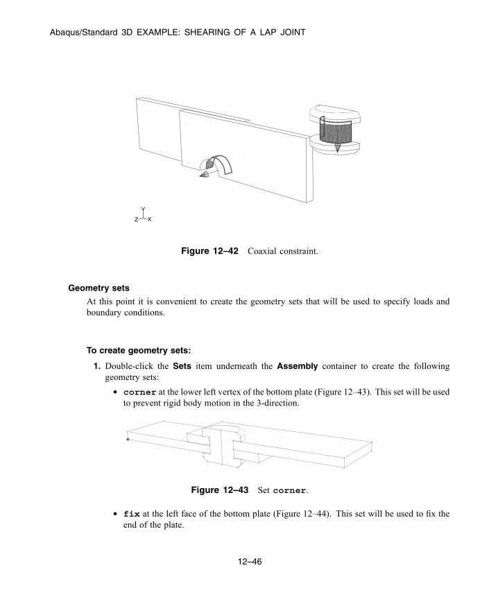
Abaqus/Standard 3D EXAMPLE: SHEARING OF A LAP JOINT
X
Y
Z
Figure 12–42 Coaxial constraint.
Geometry sets
At this point it is convenient to create the geometry sets that will be used to specify loads andboundary conditions.
To create geometry sets:
1. Double-click the Sets item underneath the Assembly container to create the followinggeometry sets:
• corner at the lower left vertex of the bottom plate (Figure 12–43). This set will be usedto prevent rigid body motion in the 3-direction.
Figure 12–43 Set corner.
• fix at the left face of the bottom plate (Figure 12–44). This set will be used to fix theend of the plate.
12–46
Abaqus ID:Printed on:

Abaqus/Standard 3D EXAMPLE: SHEARING OF A LAP JOINT
Figure 12–44 Set fix.
• pull at the right face of the top plate (Figure 12–45). This set will be used to pull theend of the plate.
Figure 12–45 Set pull.
• symm to include all faces on the symmetry plane (Figure 12–46). This set will be used toimpose symmetry conditions.
Figure 12–46 Set symm.
Defining steps and output requests
Create a single static, general step after the Initial step, and include the effects of geometricnonlinearity. Set the initial time increment to 0.05 and the total time to 1.0. Accept the defaultoutput requests.
Defining contact interactions
Contact will be used to enforce the interactions between the plates and the rivet. The frictioncoefficient between all parts is assumed to be 0.05.
This problem could use either contact pairs or the general contact algorithm. We will usegeneral contact in this problem to demonstrate the simplicity of the user interface.
12–47
Abaqus ID:Printed on:
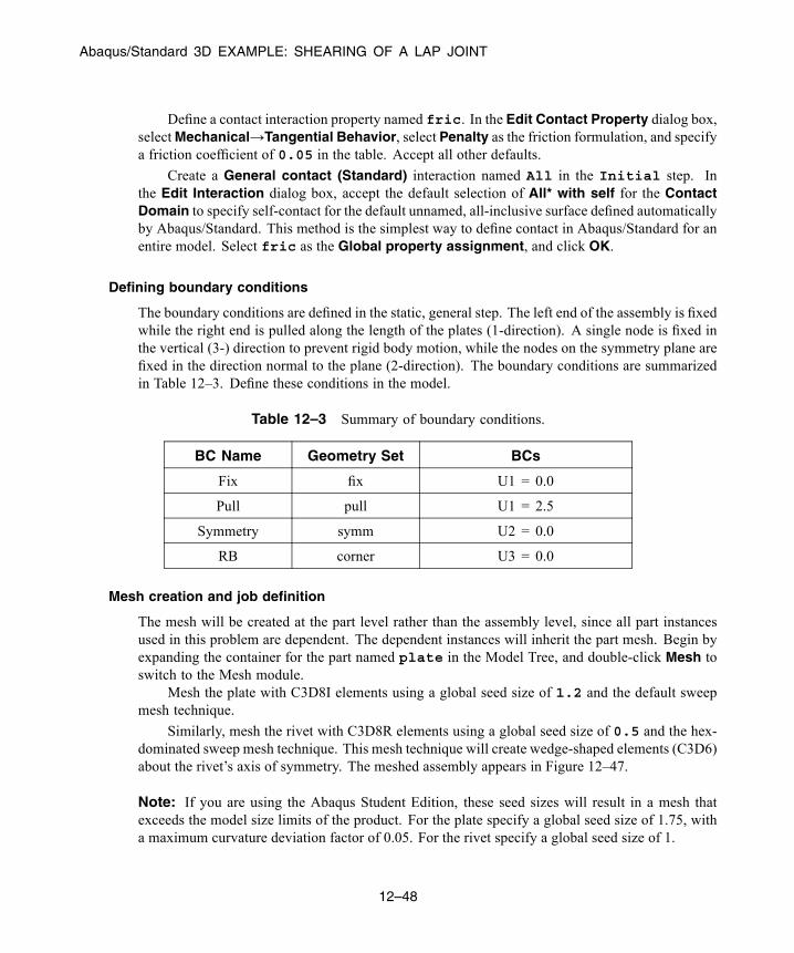
Abaqus/Standard 3D EXAMPLE: SHEARING OF A LAP JOINT
Define a contact interaction property named fric. In the Edit Contact Property dialog box,selectMechanical→Tangential Behavior, select Penalty as the friction formulation, and specifya friction coefficient of 0.05 in the table. Accept all other defaults.
Create a General contact (Standard) interaction named All in the Initial step. Inthe Edit Interaction dialog box, accept the default selection of All* with self for the ContactDomain to specify self-contact for the default unnamed, all-inclusive surface defined automaticallyby Abaqus/Standard. This method is the simplest way to define contact in Abaqus/Standard for anentire model. Select fric as the Global property assignment, and click OK.
Defining boundary conditions
The boundary conditions are defined in the static, general step. The left end of the assembly is fixedwhile the right end is pulled along the length of the plates (1-direction). A single node is fixed inthe vertical (3-) direction to prevent rigid body motion, while the nodes on the symmetry plane arefixed in the direction normal to the plane (2-direction). The boundary conditions are summarizedin Table 12–3. Define these conditions in the model.
Table 12–3 Summary of boundary conditions.
BC Name Geometry Set BCs
Fix fix U1 = 0.0
Pull pull U1 = 2.5
Symmetry symm U2 = 0.0
RB corner U3 = 0.0
Mesh creation and job definition
The mesh will be created at the part level rather than the assembly level, since all part instancesused in this problem are dependent. The dependent instances will inherit the part mesh. Begin byexpanding the container for the part named plate in the Model Tree, and double-click Mesh toswitch to the Mesh module.
Mesh the plate with C3D8I elements using a global seed size of 1.2 and the default sweepmesh technique.
Similarly, mesh the rivet with C3D8R elements using a global seed size of 0.5 and the hex-dominated sweep mesh technique. This mesh technique will create wedge-shaped elements (C3D6)about the rivet’s axis of symmetry. The meshed assembly appears in Figure 12–47.
Note: If you are using the Abaqus Student Edition, these seed sizes will result in a mesh thatexceeds the model size limits of the product. For the plate specify a global seed size of 1.75, witha maximum curvature deviation factor of 0.05. For the rivet specify a global seed size of 1.
12–48
Abaqus ID:Printed on:

Abaqus/Standard 3D EXAMPLE: SHEARING OF A LAP JOINT
X
YZ
Figure 12–47 Meshed assembly.
You are now ready to create and run the job. Create a job named lap_joint. Save yourmodel to a model database file, and submit the job for analysis. Monitor the solution progress,correct any modeling errors that are detected, and investigate the cause of any warning messages.
12.8.2 PostprocessingIn the Visualization module, examine the deformation of the assembly.
Deformed model shape and contour plots
The basic results of this simulation are the deformation of the joint and the stresses caused by theshearing process. Plot the deformed model shape and the Mises stress, as shown in Figure 12–48and Figure 12–49, respectively.
Contact pressures
You will now plot the contact pressures in the lap joint.Since it is difficult to see contact pressures when the entire model is displayed, use the Display
Groups toolbar to display only the top plate in the viewport.Create a path plot to examine the variation of the contact pressure around the bolt hole of the
top plate.
12–49
Abaqus ID:Printed on:
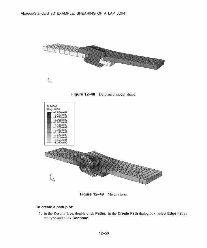
Abaqus/Standard 3D EXAMPLE: SHEARING OF A LAP JOINT
XY
Z
Figure 12–48 Deformed model shape.
(Avg: 75%)S, Mises
+8.057e+00+8.459e+01+1.611e+02+2.377e+02+3.142e+02+3.907e+02+4.672e+02+5.438e+02+6.203e+02+6.968e+02+7.734e+02+8.499e+02+9.264e+02
XY
Z
Figure 12–49 Mises stress.
To create a path plot:
1. In the Results Tree, double-click Paths. In the Create Path dialog box, select Edge list asthe type and click Continue.
12–50
Abaqus ID:Printed on:
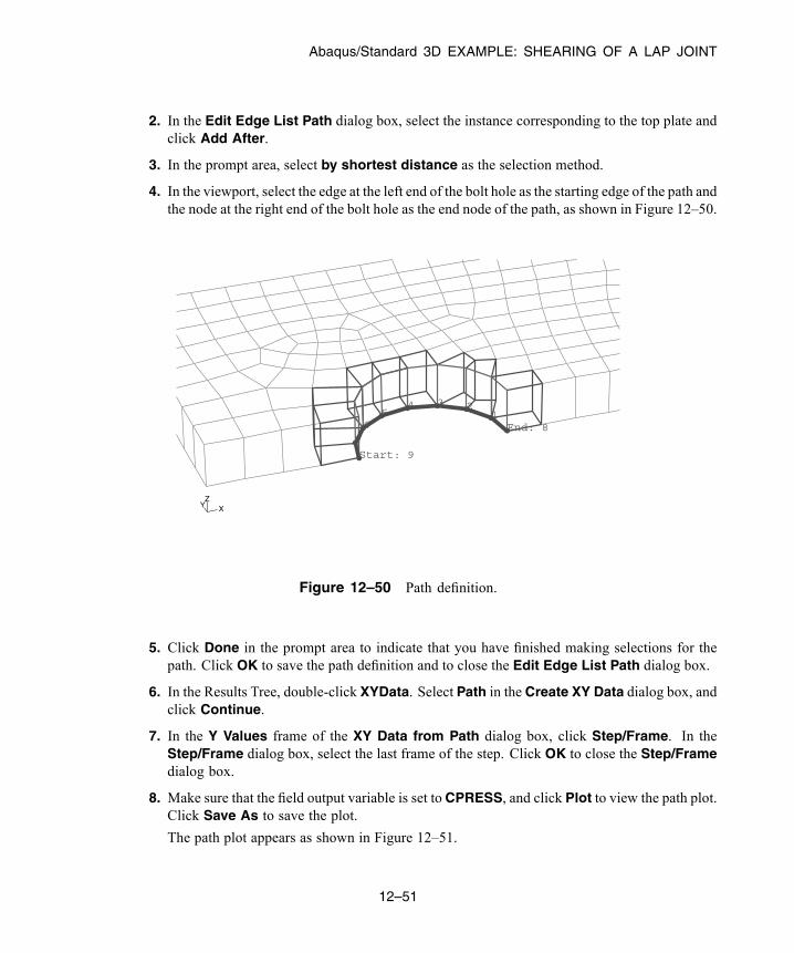
Abaqus/Standard 3D EXAMPLE: SHEARING OF A LAP JOINT
2. In the Edit Edge List Path dialog box, select the instance corresponding to the top plate andclick Add After.
3. In the prompt area, select by shortest distance as the selection method.
4. In the viewport, select the edge at the left end of the bolt hole as the starting edge of the path andthe node at the right end of the bolt hole as the end node of the path, as shown in Figure 12–50.
End: 81
2345
67
Start: 9
XYZ
Figure 12–50 Path definition.
5. Click Done in the prompt area to indicate that you have finished making selections for thepath. Click OK to save the path definition and to close the Edit Edge List Path dialog box.
6. In the Results Tree, double-click XYData. Select Path in the Create XY Data dialog box, andclick Continue.
7. In the Y Values frame of the XY Data from Path dialog box, click Step/Frame. In theStep/Frame dialog box, select the last frame of the step. Click OK to close the Step/Framedialog box.
8. Make sure that the field output variable is set to CPRESS, and click Plot to view the path plot.Click Save As to save the plot.
The path plot appears as shown in Figure 12–51.
12–51
Abaqus ID:Printed on:

DEFINING CONTACT IN Abaqus/Explicit
True distance along path0.0 2.0 4.0 6.0 8.0
Str
ess
0.
100.
200.
300.
400.
500.
600.
Figure 12–51 CPRESS distribution around the bolt hole in top plate.
12.9 Defining contact in Abaqus/Explicit
Abaqus/Explicit provides two algorithms for modeling contact interactions. The general (“automatic”)contact algorithm allows very simple definitions of contact with very few restrictions on the types ofsurfaces involved (see “Defining general contact interactions in Abaqus/Explicit,” Section 36.4.1 of theAbaqus Analysis User’s Guide). The contact pair algorithm has more restrictions on the types of surfacesinvolved and often requires more careful definition of contact; however, it allows for some interactionbehaviors that currently are not available with the general contact algorithm (see “Defining contact pairsin Abaqus/Explicit,” Section 36.5.1 of the Abaqus Analysis User’s Guide). General contact interactionstypically are defined by specifying self-contact for a default, element-based surface defined automaticallyby Abaqus/Explicit that includes all bodies in the model. To refine the contact domain, you can include orexclude specific surface pairs. Contact pair interactions are defined by specifying each of the individualsurface pairs that can interact with each other.
12–52
Abaqus ID:Printed on:
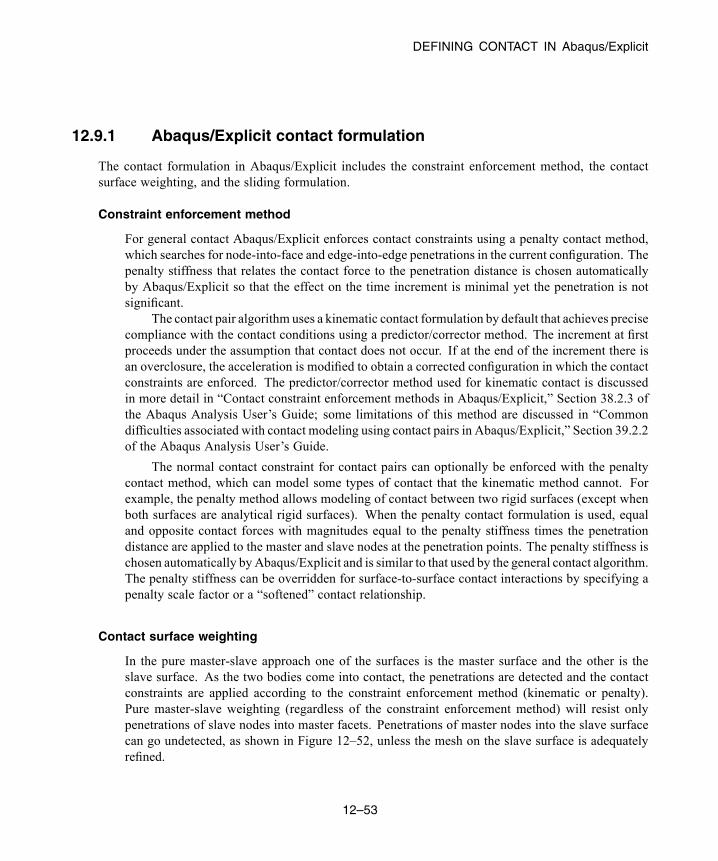
DEFINING CONTACT IN Abaqus/Explicit
12.9.1 Abaqus/Explicit contact formulation
The contact formulation in Abaqus/Explicit includes the constraint enforcement method, the contactsurface weighting, and the sliding formulation.
Constraint enforcement method
For general contact Abaqus/Explicit enforces contact constraints using a penalty contact method,which searches for node-into-face and edge-into-edge penetrations in the current configuration. Thepenalty stiffness that relates the contact force to the penetration distance is chosen automaticallyby Abaqus/Explicit so that the effect on the time increment is minimal yet the penetration is notsignificant.
The contact pair algorithm uses a kinematic contact formulation by default that achieves precisecompliance with the contact conditions using a predictor/corrector method. The increment at firstproceeds under the assumption that contact does not occur. If at the end of the increment there isan overclosure, the acceleration is modified to obtain a corrected configuration in which the contactconstraints are enforced. The predictor/corrector method used for kinematic contact is discussedin more detail in “Contact constraint enforcement methods in Abaqus/Explicit,” Section 38.2.3 ofthe Abaqus Analysis User’s Guide; some limitations of this method are discussed in “Commondifficulties associated with contact modeling using contact pairs in Abaqus/Explicit,” Section 39.2.2of the Abaqus Analysis User’s Guide.
The normal contact constraint for contact pairs can optionally be enforced with the penaltycontact method, which can model some types of contact that the kinematic method cannot. Forexample, the penalty method allows modeling of contact between two rigid surfaces (except whenboth surfaces are analytical rigid surfaces). When the penalty contact formulation is used, equaland opposite contact forces with magnitudes equal to the penalty stiffness times the penetrationdistance are applied to the master and slave nodes at the penetration points. The penalty stiffness ischosen automatically by Abaqus/Explicit and is similar to that used by the general contact algorithm.The penalty stiffness can be overridden for surface-to-surface contact interactions by specifying apenalty scale factor or a “softened” contact relationship.
Contact surface weighting
In the pure master-slave approach one of the surfaces is the master surface and the other is theslave surface. As the two bodies come into contact, the penetrations are detected and the contactconstraints are applied according to the constraint enforcement method (kinematic or penalty).Pure master-slave weighting (regardless of the constraint enforcement method) will resist onlypenetrations of slave nodes into master facets. Penetrations of master nodes into the slave surfacecan go undetected, as shown in Figure 12–52, unless the mesh on the slave surface is adequatelyrefined.
12–53
Abaqus ID:Printed on:
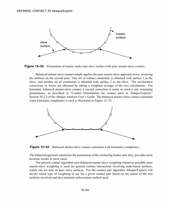
DEFINING CONTACT IN Abaqus/Explicit
slavesurface
mastersurface
Figure 12–52 Penetration of master nodes into slave surface with pure master-slave contact.
Balanced master-slave contact simply applies the pure master-slave approach twice, reversingthe surfaces on the second pass. One set of contact constraints is obtained with surface 1 as theslave, and another set of constraints is obtained with surface 2 as the slave. The accelerationcorrections or forces are obtained by taking a weighted average of the two calculations. Forkinematic balanced master-slave contact a second correction is made to resolve any remainingpenetrations, as described in “Contact formulations for contact pairs in Abaqus/Explicit,”Section 38.2.2 of the Abaqus Analysis User’s Guide. The balanced master-slave contact constraintwhen kinematic compliance is used is illustrated in Figure 12–53.
Figure 12–53 Balanced master-slave contact constraint with kinematic compliance.
The balanced approach minimizes the penetration of the contacting bodies and, thus, provides moreaccurate results in most cases.
The general contact algorithm uses balanced master-slave weighting whenever possible; puremaster-slave weighting is used for general contact interactions involving node-based surfaces,which can act only as pure slave surfaces. For the contact pair algorithm Abaqus/Explicit willdecide which type of weighting to use for a given contact pair based on the nature of the twosurfaces involved and the constraint enforcement method used.
12–54
Abaqus ID:Printed on:
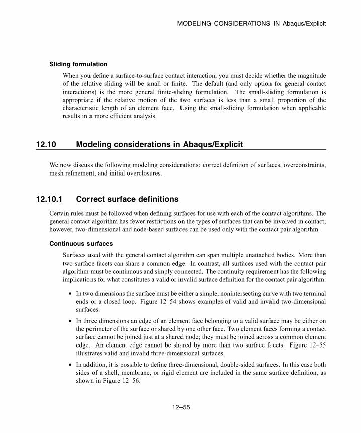
MODELING CONSIDERATIONS IN Abaqus/Explicit
Sliding formulation
When you define a surface-to-surface contact interaction, you must decide whether the magnitudeof the relative sliding will be small or finite. The default (and only option for general contactinteractions) is the more general finite-sliding formulation. The small-sliding formulation isappropriate if the relative motion of the two surfaces is less than a small proportion of thecharacteristic length of an element face. Using the small-sliding formulation when applicableresults in a more efficient analysis.
12.10 Modeling considerations in Abaqus/Explicit
We now discuss the following modeling considerations: correct definition of surfaces, overconstraints,mesh refinement, and initial overclosures.
12.10.1 Correct surface definitions
Certain rules must be followed when defining surfaces for use with each of the contact algorithms. Thegeneral contact algorithm has fewer restrictions on the types of surfaces that can be involved in contact;however, two-dimensional and node-based surfaces can be used only with the contact pair algorithm.
Continuous surfaces
Surfaces used with the general contact algorithm can span multiple unattached bodies. More thantwo surface facets can share a common edge. In contrast, all surfaces used with the contact pairalgorithm must be continuous and simply connected. The continuity requirement has the followingimplications for what constitutes a valid or invalid surface definition for the contact pair algorithm:
• In two dimensions the surface must be either a simple, nonintersecting curve with two terminalends or a closed loop. Figure 12–54 shows examples of valid and invalid two-dimensionalsurfaces.
• In three dimensions an edge of an element face belonging to a valid surface may be either onthe perimeter of the surface or shared by one other face. Two element faces forming a contactsurface cannot be joined just at a shared node; they must be joined across a common elementedge. An element edge cannot be shared by more than two surface facets. Figure 12–55illustrates valid and invalid three-dimensional surfaces.
• In addition, it is possible to define three-dimensional, double-sided surfaces. In this case bothsides of a shell, membrane, or rigid element are included in the same surface definition, asshown in Figure 12–56.
12–55
Abaqus ID:Printed on:
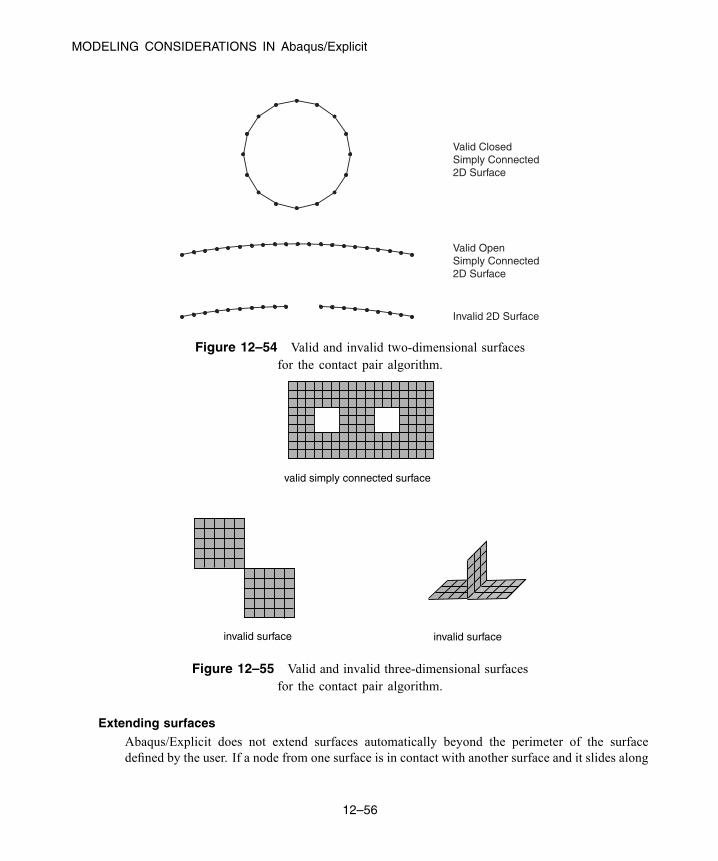
MODELING CONSIDERATIONS IN Abaqus/Explicit
Valid ClosedSimply Connected2D Surface
Valid OpenSimply Connected2D Surface
Invalid 2D Surface
Figure 12–54 Valid and invalid two-dimensional surfacesfor the contact pair algorithm.
valid simply connected surface
invalid surface invalid surface
Figure 12–55 Valid and invalid three-dimensional surfacesfor the contact pair algorithm.
Extending surfacesAbaqus/Explicit does not extend surfaces automatically beyond the perimeter of the surfacedefined by the user. If a node from one surface is in contact with another surface and it slides along
12–56
Abaqus ID:Printed on:
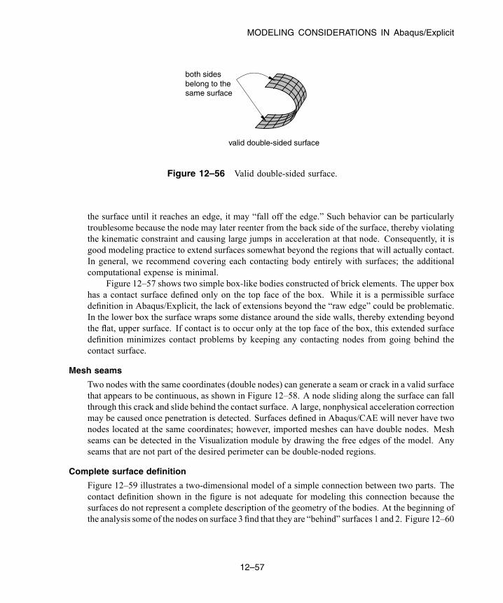
MODELING CONSIDERATIONS IN Abaqus/Explicit
valid double-sided surface
both sidesbelong to thesame surface
Figure 12–56 Valid double-sided surface.
the surface until it reaches an edge, it may “fall off the edge.” Such behavior can be particularlytroublesome because the node may later reenter from the back side of the surface, thereby violatingthe kinematic constraint and causing large jumps in acceleration at that node. Consequently, it isgood modeling practice to extend surfaces somewhat beyond the regions that will actually contact.In general, we recommend covering each contacting body entirely with surfaces; the additionalcomputational expense is minimal.
Figure 12–57 shows two simple box-like bodies constructed of brick elements. The upper boxhas a contact surface defined only on the top face of the box. While it is a permissible surfacedefinition in Abaqus/Explicit, the lack of extensions beyond the “raw edge” could be problematic.In the lower box the surface wraps some distance around the side walls, thereby extending beyondthe flat, upper surface. If contact is to occur only at the top face of the box, this extended surfacedefinition minimizes contact problems by keeping any contacting nodes from going behind thecontact surface.
Mesh seams
Two nodes with the same coordinates (double nodes) can generate a seam or crack in a valid surfacethat appears to be continuous, as shown in Figure 12–58. A node sliding along the surface can fallthrough this crack and slide behind the contact surface. A large, nonphysical acceleration correctionmay be caused once penetration is detected. Surfaces defined in Abaqus/CAE will never have twonodes located at the same coordinates; however, imported meshes can have double nodes. Meshseams can be detected in the Visualization module by drawing the free edges of the model. Anyseams that are not part of the desired perimeter can be double-noded regions.
Complete surface definition
Figure 12–59 illustrates a two-dimensional model of a simple connection between two parts. Thecontact definition shown in the figure is not adequate for modeling this connection because thesurfaces do not represent a complete description of the geometry of the bodies. At the beginning ofthe analysis some of the nodes on surface 3 find that they are “behind” surfaces 1 and 2. Figure 12–60
12–57
Abaqus ID:Printed on:

MODELING CONSIDERATIONS IN Abaqus/Explicit
Perimeter of contact surface
Perimeter of contact surface
Only top of box defined as surface
Side of box included in surface definition
Figure 12–57 Surface perimeters.
Both nodes have the samecoordinates. They are separatedto show the crack in the surface.
Figure 12–58 Example of a double-noded mesh.
12–58
Abaqus ID:Printed on:
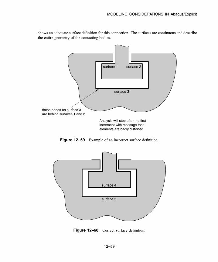
MODELING CONSIDERATIONS IN Abaqus/Explicit
shows an adequate surface definition for this connection. The surfaces are continuous and describethe entire geometry of the contacting bodies.
surface 1 surface 2
Analysis will stop after the firstincrement with message thatelements are badly distorted
surface 3
these nodes on surface 3 are behind surfaces 1 and 2
Figure 12–59 Example of an incorrect surface definition.
surface 4
surface 5
Figure 12–60 Correct surface definition.
12–59
Abaqus ID:Printed on:

MODELING CONSIDERATIONS IN Abaqus/Explicit
Highly warped surfaces
No special treatment of warped surfaces is required for the general contact algorithm. However,when a surface used with the contact pair algorithm contains highly warped facets, a more expensivetracking approach must be used than the approach required when the surface does not contain highlywarped facets. To keep the solution as efficient as possible, Abaqus monitors the warpage of thesurfaces and issues a warning if surfaces become too warped; if the normal directions of adjacentfacets differ by more than 20°, Abaqus issues a warning message. Once a surface is deemed to behighly warped, Abaqus switches from the more efficient contact search approach to a more accuratesearch approach to account for the difficulties posed by the highly warped surface.
For purposes of efficiency Abaqus does not check for highly warped surfaces every increment.Rigid surfaces are checked for high warpage only at the start of the step, since rigid surfaces donot change shape during the analysis. Deformable surfaces are checked for high warpage every 20increments by default; however, some analyses may have surfaces with rapidly increasing warpage,making the default 20 increment frequency check inadequate. The frequency of warping checkscan be changed to the desired number of increments. Some analyses in which the surface warpingis less than 20° may also require the more accurate contact search approach associated with highlywarped surfaces. The angle that defines high warpage can be redefined.
Rigid element discretization
Complex rigid surface geometries can be modeled using rigid elements. Rigid elements inAbaqus/Explicit are not smoothed; they remain faceted exactly as defined by the user. Theadvantage of unsmoothed surfaces is that the surface defined by the user is exactly the same asthe surface used by Abaqus; the disadvantage is that faceted surfaces require much higher meshrefinement to define smooth bodies accurately. In general, using a large number of rigid elementsto define a rigid surface does not increase the CPU costs significantly. However, a large number ofrigid elements does increase the memory overhead significantly.
The user must ensure that the discretization of any curved geometry on rigid bodies is adequate.If the rigid body discretization is too coarse, contacting nodes on the deformable body may “snag,”leading to erroneous results, as illustrated in Figure 12–61.
blank motion
"snagging"
sheet metalblankrigid tool
Figure 12–61 Potential effect of coarse rigid body discretization.
12–60
Abaqus ID:Printed on:

MODELING CONSIDERATIONS IN Abaqus/Explicit
A node that is snagged on a sharp corner may be trapped from further sliding along the rigid surfacefor some time. Once enough energy is released to slide beyond the sharp corner, the node willsnap dynamically before contacting the adjacent facet. Such motions cause noisy solutions. Themore refined the rigid surface, the smoother the motion of the contacting slave nodes. The generalcontact algorithm includes some numerical rounding of features that prevents snagging of nodesfrom becoming a concern for discrete rigid surfaces. In addition, penalty enforcement of the contactconstraints reduces the tendency for snagging to occur. Analytical rigid surfaces should normally beused with the contact pair algorithm for rigid bodies whose shape is an extruded profile or a surfaceof revolution.
12.10.2 Overconstraining the model
Just as multiple conflicting boundary conditions should not be defined at a given node, multi-pointconstraints and contact conditions enforced with the kinematic method generally should not be definedat the same node because they may generate conflicting kinematic constraints. Unless the constraintsare entirely orthogonal to one another, the model will be overconstrained; the resulting solution will bequite noisy, as Abaqus/Explicit tries to satisfy the conflicting constraints. Penalty contact constraintsand multi-point constraints acting on the same nodes will not generate conflicts because the penaltyconstraints are not enforced as strictly as the multi-point constraints.
12.10.3 Mesh refinement
For contact as well as all other types of analyses, the solution improves as the mesh is refined. Forcontact analyses using a pure master-slave approach, it is especially important that the slave surfaceis refined adequately so that the master surface facets do not overly penetrate the slave surface. Thebalanced master-slave approach does not require high mesh refinement on the slave surface to haveadequate contact compliance. Mesh refinement is generally most important with pure master-slavecontact between deformable and rigid bodies; in this case the deformable body is always the pure slavesurface and, thus, must be refined enough to interact with any feature on the rigid body. Figure 12–62shows an example of the penetration that can occur if the discretization of the slave surface is poorcompared to the dimensions of the features on the master surface. If the deformable surface were morerefined, the penetrations of the rigid surface would be much less severe.
Tie constraints
The tie constraint prevents surfaces initially in contact from penetrating, separating, or slidingrelative to one another. It is, therefore, an easy means of mesh refinement. Since any gaps thatexist between the two surfaces, however small, will result in nodes that are not tied to the oppositeboundary, you must adjust the nodes to ensure that the two surfaces are exactly in contact at thestart of the analysis.
12–61
Abaqus ID:Printed on:
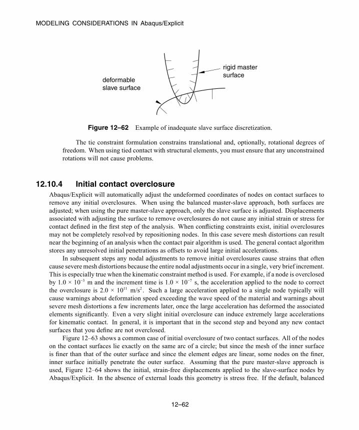
MODELING CONSIDERATIONS IN Abaqus/Explicit
deformableslave surface
rigid mastersurface
Figure 12–62 Example of inadequate slave surface discretization.
The tie constraint formulation constrains translational and, optionally, rotational degrees offreedom. When using tied contact with structural elements, you must ensure that any unconstrainedrotations will not cause problems.
12.10.4 Initial contact overclosureAbaqus/Explicit will automatically adjust the undeformed coordinates of nodes on contact surfaces toremove any initial overclosures. When using the balanced master-slave approach, both surfaces areadjusted; when using the pure master-slave approach, only the slave surface is adjusted. Displacementsassociated with adjusting the surface to remove overclosures do not cause any initial strain or stress forcontact defined in the first step of the analysis. When conflicting constraints exist, initial overclosuresmay not be completely resolved by repositioning nodes. In this case severe mesh distortions can resultnear the beginning of an analysis when the contact pair algorithm is used. The general contact algorithmstores any unresolved initial penetrations as offsets to avoid large initial accelerations.
In subsequent steps any nodal adjustments to remove initial overclosures cause strains that oftencause severemesh distortions because the entire nodal adjustments occur in a single, very brief increment.This is especially true when the kinematic constraint method is used. For example, if a node is overclosedby 1.0 × 10⁻³ m and the increment time is 1.0 × 10⁻⁷ s, the acceleration applied to the node to correctthe overclosure is 2.0 × 10¹¹ m/s2 . Such a large acceleration applied to a single node typically willcause warnings about deformation speed exceeding the wave speed of the material and warnings aboutsevere mesh distortions a few increments later, once the large acceleration has deformed the associatedelements significantly. Even a very slight initial overclosure can induce extremely large accelerationsfor kinematic contact. In general, it is important that in the second step and beyond any new contactsurfaces that you define are not overclosed.
Figure 12–63 shows a common case of initial overclosure of two contact surfaces. All of the nodeson the contact surfaces lie exactly on the same arc of a circle; but since the mesh of the inner surfaceis finer than that of the outer surface and since the element edges are linear, some nodes on the finer,inner surface initially penetrate the outer surface. Assuming that the pure master-slave approach isused, Figure 12–64 shows the initial, strain-free displacements applied to the slave-surface nodes byAbaqus/Explicit. In the absence of external loads this geometry is stress free. If the default, balanced
12–62
Abaqus ID:Printed on:
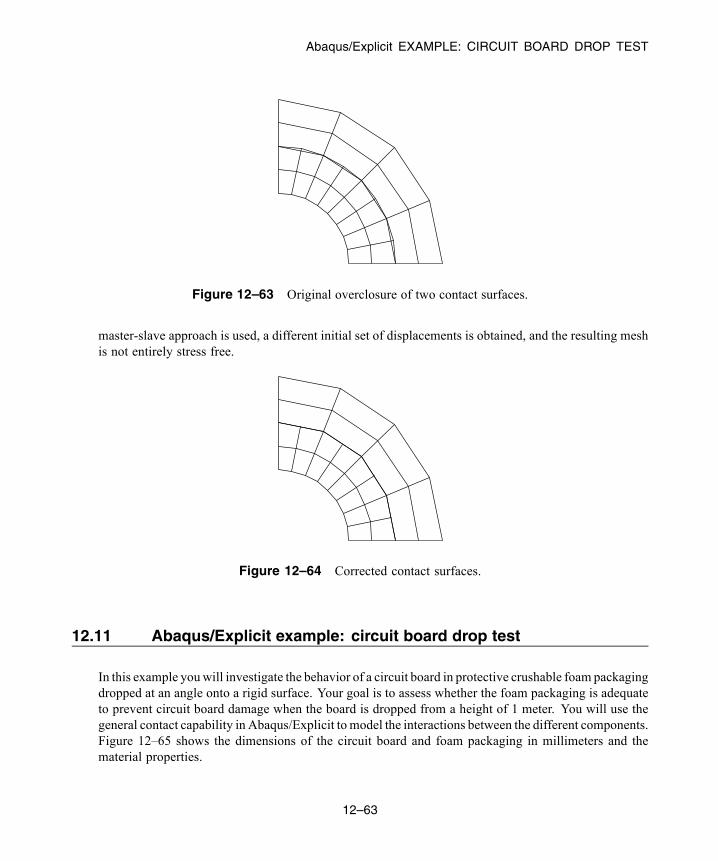
Abaqus/Explicit EXAMPLE: CIRCUIT BOARD DROP TEST
Figure 12–63 Original overclosure of two contact surfaces.
master-slave approach is used, a different initial set of displacements is obtained, and the resulting meshis not entirely stress free.
Figure 12–64 Corrected contact surfaces.
12.11 Abaqus/Explicit example: circuit board drop test
In this example youwill investigate the behavior of a circuit board in protective crushable foam packagingdropped at an angle onto a rigid surface. Your goal is to assess whether the foam packaging is adequateto prevent circuit board damage when the board is dropped from a height of 1 meter. You will use thegeneral contact capability in Abaqus/Explicit to model the interactions between the different components.Figure 12–65 shows the dimensions of the circuit board and foam packaging in millimeters and thematerial properties.
12–63
Abaqus ID:Printed on:

Abaqus/Explicit EXAMPLE: CIRCUIT BOARD DROP TEST
100
150
2
12
220
24
z
x
circuit board
foampackaging
local coordinatesystem
110
Material properties
Circuit board material (plastic):
Foam packaging material is crushable foam:
(Foam plasticity data are given in the text.)
E 45 109× Pa=
ν 0.3=
ρ 500 kg/m3
=
E 3 106× Pa=
ν 0.0=ρ 100 kg/m
3=
y
Figure 12–65 Dimensions in millimeters and material properties.
12.11.1 Preprocessing—creating the model with Abaqus/CAECreate the model for this simulation with Abaqus/CAE. Abaqus provides scripts that replicate thecomplete analysis model for this problem. Run one of these scripts if you encounter difficulties
12–64
Abaqus ID:Printed on:
Abaqus/Explicit EXAMPLE: CIRCUIT BOARD DROP TEST
following the instructions given below or if you wish to check your work. Scripts are available in thefollowing locations:
• A Python script for this example is provided in “Circuit board drop test,” Section A.14, in the HTMLversion of this guide. Instructions on how to fetch the script and run it within Abaqus/CAE are givenin Appendix A, “Example Files.”
• A plug-in script for this example is available in the Abaqus/CAE Plug-in toolset. To run the scriptfrom Abaqus/CAE, select Plug-ins→Abaqus→Getting Started; highlight Circuit board droptest; and click Run. For more information about the Getting Started plug-ins, see “Running theGetting Started with Abaqus examples,” Section 82.1 of the Abaqus/CAE User’s Guide, in theHTML version of this guide.
Defining the model geometry
You will create three parts representing the packaging, the circuit board, and the floor. The chipswill be represented using discrete point masses. You will also create a number of datum points toaid in positioning the part instances and the point masses.
To define the packaging geometry:
1. The packaging is a three-dimensional solid structure. Create a three-dimensional, deformablepart with an extruded solid base feature to represent the packaging; name the partPackaging.Use an approximate part size of 0.1, and sketch a 0.02 m × 0.024 m rectangle as the profile.Specify 0.11 m as the extrusion depth.
2. From the main menu bar, select Shape→Cut→Extrude to create the cut in the packaging inwhich the circuit board will rest.
a. Select the left end of the packaging as the plane for the extruded cut. Select a vertical lineon the packaging profile to be vertical and on the right in the sketching plane.
b. In the Sketcher, use the vertical construction line tool to create a vertical constructionline through the center of the packaging. Apply a fixed constraint to the construction line.
c. Sketch the profile of the cut shown in Figure 12–66. Use a Symmetry constraint to centerthe cut about the construction line and edit the dimensions of the cut profile so that it is0.002 m wide and extends a distance of 0.012 m into the packaging.
d. In the Edit Cut Extrusion dialog box that appears upon completion of the sketch, selectThrough All as the end condition and select the arrow direction representing a cut intothe packaging.
3. Create a datum point centered on the bottom face of the cut, as shown in Figure 12–67. Thispoint will be used to position the board relative to the packaging.
a. From the main menu bar, select Tools→Datum.
The Create Datum dialog box appears.
12–65
Abaqus ID:Printed on:

Abaqus/Explicit EXAMPLE: CIRCUIT BOARD DROP TEST
H 2.E-03
V 12.E-03
H
”|” ”|”
H 2.E-03
V 12.E-03
H
”|” ”|”
1
2
3
Figure 12–66 Profile of cut in packaging (with grid spacing doubled).
Datumpoint
Select these two points to position the datum point
Figure 12–67 Datum point at center of cut in packaging.
b. Accept the default selection of Point as the datum type and select Midway between 2points as the method.
c. Select the two points centered on the bottom face at either end of the cut to be the twopoints between which the datum point will be created.
Abaqus/CAE creates the datum point shown in Figure 12–67.
12–66
Abaqus ID:Printed on:

Abaqus/Explicit EXAMPLE: CIRCUIT BOARD DROP TEST
To define the circuit board geometry:
1. The circuit board can be modeled as a thin, flat plate with chips attached to it. Create a three-dimensional, deformable planar shell to represent the circuit board; name the part Board. Usean approximate part size of 0.5, and sketch a 0.100 m × 0.150 m rectangle for the profile.
2. Create the three datum points shown in Figure 12–68. These points will be used to positionthe chips on the board.
(0.010, 0.135)
(0.070, 0.090)
(0.080, 0.030)
Figure 12–68 Datum points used to position the chips relative to the board. Numbers in parenthesesare (x, y) coordinates in meters based on a local origin at the bottom left corner of the circuit board.
a. From the main menu bar, select Tools→Datum.
The Create Datum dialog box appears.
b. Accept the default selection of Point as the datum type, and select Offset from point asthe method.
c. Select the bottom left corner of the board as the point from which to offset, and enter thecoordinates for one of the points shown in Figure 12–68.
d. Repeat Step c to create the other two datum points.
To define the floor:
1. The surface that the circuit board will impact is effectively rigid. Create a three-dimensional,discrete rigid planar shell to represent the floor; name the part Floor. Use an approximatepart size of 0.5. The rigid surface should be large enough to keep any deformable bodies fromfalling off the edges.
12–67
Abaqus ID:Printed on:
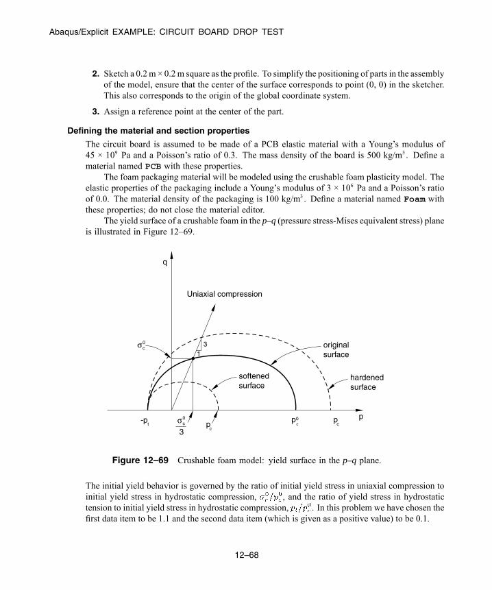
Abaqus/Explicit EXAMPLE: CIRCUIT BOARD DROP TEST
2. Sketch a 0.2m × 0.2m square as the profile. To simplify the positioning of parts in the assemblyof the model, ensure that the center of the surface corresponds to point (0, 0) in the sketcher.This also corresponds to the origin of the global coordinate system.
3. Assign a reference point at the center of the part.
Defining the material and section properties
The circuit board is assumed to be made of a PCB elastic material with a Young’s modulus of45 × 109 Pa and a Poisson’s ratio of 0.3. The mass density of the board is 500 kg/m3 . Define amaterial named PCB with these properties.
The foam packaging material will be modeled using the crushable foam plasticity model. Theelastic properties of the packaging include a Young’s modulus of 3 × 10⁶ Pa and a Poisson’s ratioof 0.0. The material density of the packaging is 100 kg/m3 . Define a material named Foam withthese properties; do not close the material editor.
The yield surface of a crushable foam in the p–q (pressure stress-Mises equivalent stress) planeis illustrated in Figure 12–69.
3
1
-p t
ppcp
c
Uniaxial compression
0pc
q
softenedsurface
originalsurface
hardened surface
0cσ
3
0cσ
Figure 12–69 Crushable foam model: yield surface in the p–q plane.
The initial yield behavior is governed by the ratio of initial yield stress in uniaxial compression toinitial yield stress in hydrostatic compression, , and the ratio of yield stress in hydrostatictension to initial yield stress in hydrostatic compression, . In this problem we have chosen thefirst data item to be 1.1 and the second data item (which is given as a positive value) to be 0.1.
12–68
Abaqus ID:Printed on:

Abaqus/Explicit EXAMPLE: CIRCUIT BOARD DROP TEST
Hardening effects are also included in the material model definition. Table 12–4 summarizesthe yield stress–plastic strain data.
Table 12–4 Yield stress–plastic strain data for the crushable foam model.
Yield stress in uniaxialcompression (Pa)
Plasticstrain
0.22000E6 0.0
0.24651E6 0.1
0.27294E6 0.2
0.29902E6 0.3
0.32455E6 0.4
0.34935E6 0.5
0.37326E6 0.6
0.39617E6 0.7
0.41801E6 0.8
0.43872E6 0.9
0.45827E6 1.0
0.49384E6 1.2
0.52484E6 1.4
0.55153E6 1.6
0.57431E6 1.8
0.59359E6 2.0
0.62936E6 2.5
0.65199E6 3.0
0.68334E6 5.0
0.68833E6 10.0
The crushable foam hardening model follows the curve shown in Figure 12–70.
12–69
Abaqus ID:Printed on:
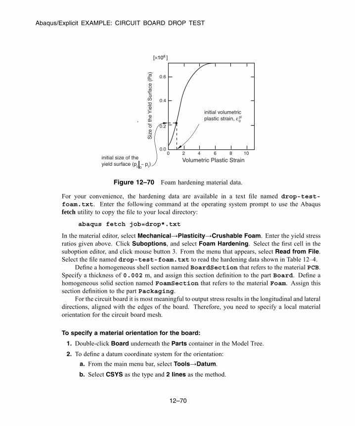
Abaqus/Explicit EXAMPLE: CIRCUIT BOARD DROP TEST
initial volumetricplastic strain, ε pl
0
0.6
0.4
0.2
0.00 2 4 6 8 10
Volumetric Plastic Strain
Siz
e of
the
Yie
ld S
urfa
ce (
Pa)
initial size of theyield surface (p p )c t0
[×10 ]6
_
Figure 12–70 Foam hardening material data.
For your convenience, the hardening data are available in a text file named drop-test-foam.txt. Enter the following command at the operating system prompt to use the Abaqusfetch utility to copy the file to your local directory:
abaqus fetch job=drop*.txt
In the material editor, select Mechanical→Plasticity→Crushable Foam. Enter the yield stressratios given above. Click Suboptions, and select Foam Hardening. Select the first cell in thesuboption editor, and click mouse button 3. From the menu that appears, select Read from File.Select the file named drop-test-foam.txt to read the hardening data shown in Table 12–4.
Define a homogeneous shell section named BoardSection that refers to the material PCB.Specify a thickness of 0.002 m, and assign this section definition to the part Board. Define ahomogeneous solid section named FoamSection that refers to the material Foam. Assign thissection definition to the part Packaging.
For the circuit board it is most meaningful to output stress results in the longitudinal and lateraldirections, aligned with the edges of the board. Therefore, you need to specify a local materialorientation for the circuit board mesh.
To specify a material orientation for the board:
1. Double-click Board underneath the Parts container in the Model Tree.
2. To define a datum coordinate system for the orientation:
a. From the main menu bar, select Tools→Datum.
b. Select CSYS as the type and 2 lines as the method.
12–70
Abaqus ID:Printed on:
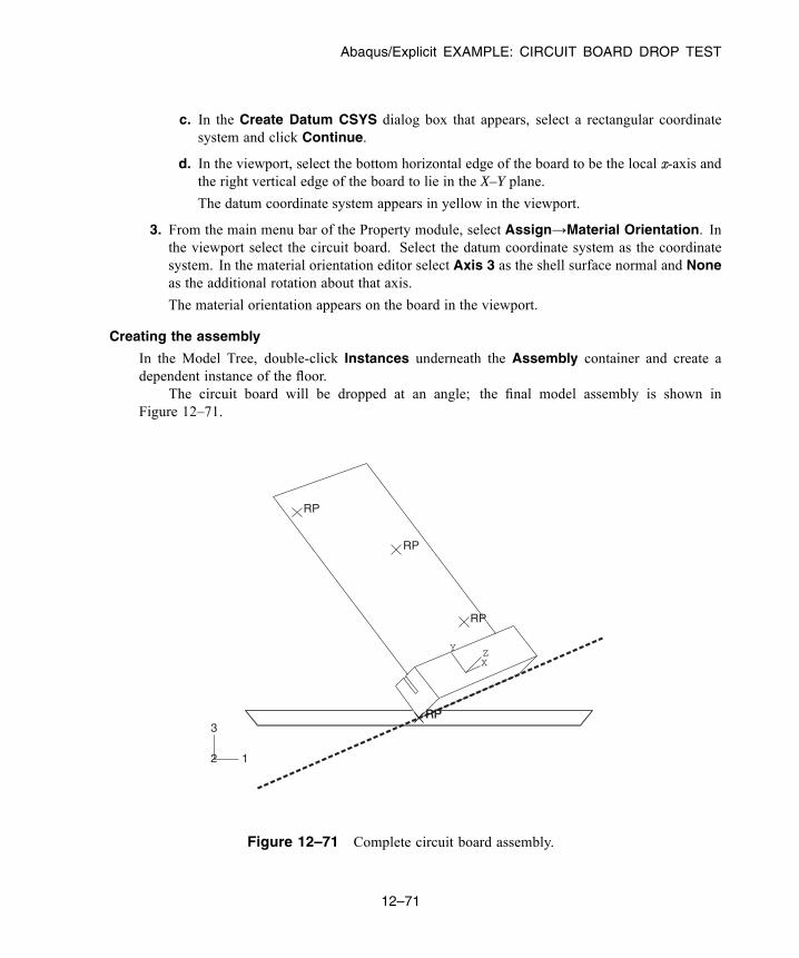
Abaqus/Explicit EXAMPLE: CIRCUIT BOARD DROP TEST
c. In the Create Datum CSYS dialog box that appears, select a rectangular coordinatesystem and click Continue.
d. In the viewport, select the bottom horizontal edge of the board to be the local x-axis andthe right vertical edge of the board to lie in the X–Y plane.
The datum coordinate system appears in yellow in the viewport.
3. From the main menu bar of the Property module, select Assign→Material Orientation. Inthe viewport select the circuit board. Select the datum coordinate system as the coordinatesystem. In the material orientation editor select Axis 3 as the shell surface normal and Noneas the additional rotation about that axis.
The material orientation appears on the board in the viewport.
Creating the assembly
In the Model Tree, double-click Instances underneath the Assembly container and create adependent instance of the floor.
The circuit board will be dropped at an angle; the final model assembly is shown inFigure 12–71.
RP RP
X
YZ
RP
RP
RP
12
3
Figure 12–71 Complete circuit board assembly.
12–71
Abaqus ID:Printed on:
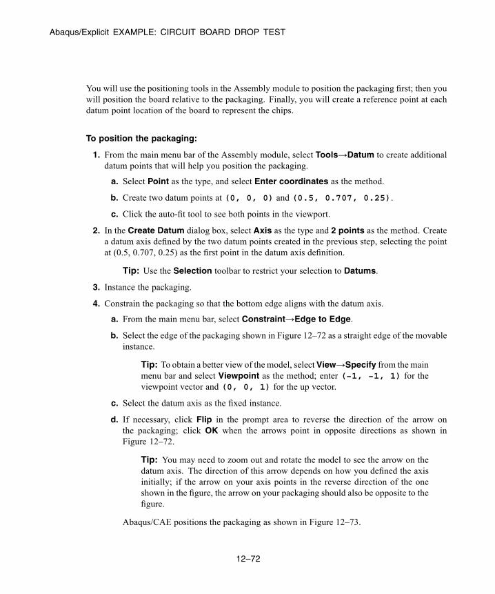
Abaqus/Explicit EXAMPLE: CIRCUIT BOARD DROP TEST
You will use the positioning tools in the Assembly module to position the packaging first; then youwill position the board relative to the packaging. Finally, you will create a reference point at eachdatum point location of the board to represent the chips.
To position the packaging:
1. From the main menu bar of the Assembly module, select Tools→Datum to create additionaldatum points that will help you position the packaging.
a. Select Point as the type, and select Enter coordinates as the method.
b. Create two datum points at (0, 0, 0) and (0.5, 0.707, 0.25).
c. Click the auto-fit tool to see both points in the viewport.
2. In the Create Datum dialog box, select Axis as the type and 2 points as the method. Createa datum axis defined by the two datum points created in the previous step, selecting the pointat (0.5, 0.707, 0.25) as the first point in the datum axis definition.
Tip: Use the Selection toolbar to restrict your selection to Datums.
3. Instance the packaging.
4. Constrain the packaging so that the bottom edge aligns with the datum axis.
a. From the main menu bar, select Constraint→Edge to Edge.
b. Select the edge of the packaging shown in Figure 12–72 as a straight edge of the movableinstance.
Tip: To obtain a better view of the model, selectView→Specify from the mainmenu bar and select Viewpoint as the method; enter (−1, −1, 1) for theviewpoint vector and (0, 0, 1) for the up vector.
c. Select the datum axis as the fixed instance.
d. If necessary, click Flip in the prompt area to reverse the direction of the arrow onthe packaging; click OK when the arrows point in opposite directions as shown inFigure 12–72.
Tip: You may need to zoom out and rotate the model to see the arrow on thedatum axis. The direction of this arrow depends on how you defined the axisinitially; if the arrow on your axis points in the reverse direction of the oneshown in the figure, the arrow on your packaging should also be opposite to thefigure.
Abaqus/CAE positions the packaging as shown in Figure 12–73.
12–72
Abaqus ID:Printed on:
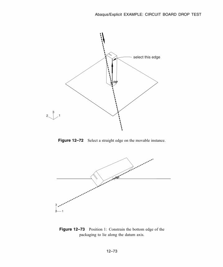
Abaqus/Explicit EXAMPLE: CIRCUIT BOARD DROP TEST
RP RP
123
select this edge
Figure 12–72 Select a straight edge on the movable instance.
RP RP
12
3
Figure 12–73 Position 1: Constrain the bottom edge of thepackaging to lie along the datum axis.
12–73
Abaqus ID:Printed on:

Abaqus/Explicit EXAMPLE: CIRCUIT BOARD DROP TEST
Note: Abaqus/CAE stores position constraints as features of the assembly; if youmake a mistake while positioning the assembly, you can delete the position constraints.Simply click mouse button 3 on the constraint you wish to delete in the list of PositionConstraints items found underneath the Assembly container in the Model Tree, andselect Delete from the menu that appears.
5. Create a third datum point at (−0.5, 0.707, −0.5), and click the auto-fit tool again.
6. In the Create Datum dialog box, select Plane as the type and Line and point as the method.Create a datum plane defined by the datum axis created earlier and the datum point created inthe previous step.
7. Constrain the packaging so that the bottom face lies on the datum plane.
a. From the main menu bar, select Constraint→Face to Face.
b. Select the face of the packaging shown in Figure 12–74 as a face of the movable instance.
RP RP
12
3
Figure 12–74 Select a face on the movable instance.
c. Select the datum plane as the fixed instance.
d. If necessary, click Flip in the prompt area; click OK when both arrows point in the samedirection.
e. Accept the default distance of 0.0 from the fixed plane.
8. Finally, constrain the packaging to contact the floor at its center.
a. From the main menu bar, select Constraint→Coincident Point.
12–74
Abaqus ID:Printed on:
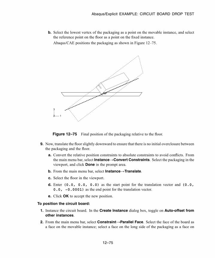
Abaqus/Explicit EXAMPLE: CIRCUIT BOARD DROP TEST
b. Select the lowest vertex of the packaging as a point on the movable instance, and selectthe reference point on the floor as a point on the fixed instance.
Abaqus/CAE positions the packaging as shown in Figure 12–75.
RP RP
12
3
Figure 12–75 Final position of the packaging relative to the floor.
9. Now, translate the floor slightly downward to ensure that there is no initial overclosure betweenthe packaging and the floor.
a. Convert the relative position constraints to absolute constraints to avoid conflicts. Fromthe main menu bar, select Instance→Convert Constraints. Select the packaging in theviewport, and click Done in the prompt area.
b. From the main menu bar, select Instance→Translate.
c. Select the floor in the viewport.
d. Enter (0.0, 0.0, 0.0) as the start point for the translation vector and (0.0,0.0, −0.0001) as the end point for the translation vector.
e. Click OK to accept the new position.
To position the circuit board:
1. Instance the circuit board. In the Create Instance dialog box, toggle on Auto-offset fromother instances.
2. From the main menu bar, select Constraint→Parallel Face. Select the face of the board asa face on the movable instance; select a face on the long side of the packaging as a face on
12–75
Abaqus ID:Printed on:

Abaqus/Explicit EXAMPLE: CIRCUIT BOARD DROP TEST
the fixed instance. If necessary, click Flip in the prompt area to ensure that the arrows on bothfaces point in the directions shown in Figure 12–76; click OK to complete the constraint.
RP RP
12
3
Figure 12–76 Parallel face constraint for the circuit board.
3. From the main menu bar, select Constraint→Parallel Edge. Select the top edge of the boardas an edge on the movable instance. Select an edge along the length of the packaging as anedge on the fixed instance. If necessary, click Flip in the prompt area to ensure that the arrowson both edges point in the same direction, as shown in Figure 12–77; click OK to complete theconstraint.
4. From the main menu bar, select Constraint→Coincident Point. Select the midpoint of thebottom of the board as a point on the movable instance. Select the datum point at the center ofthe cut in the packaging as a point on the fixed instance.
Tip: Use the Selection toolbar to restrict your selection to Datums.
Figure 12–78 shows the final position of the circuit board. The circuit board and the slot in thepackaging are the same thickness (2 mm) so there is a snug fit between the two bodies.
12–76
Abaqus ID:Printed on:

Abaqus/Explicit EXAMPLE: CIRCUIT BOARD DROP TEST
RP RP
12
3
Figure 12–77 Parallel edge constraint for the circuit board.
RP RP
X
YZ
12
3
Figure 12–78 Final position of the circuit board.
To create the chips:
Create a reference point at each of the three datum point locations on the board to representeach chip. Each of these reference points will later be assigned mass properties. To create a
12–77
Abaqus ID:Printed on:
Abaqus/Explicit EXAMPLE: CIRCUIT BOARD DROP TEST
reference point, select Tools→Reference Point from the main menu bar of the Assemblymodule.
Once you have created the reference points, the assembly is complete.
Before continuing, create the following geometry sets that you will use to specify output requestsand mass properties:
• TopChip for the reference point of the top chip
• MidChip for the reference point of the middle chip
• BotChip for the reference point of the bottom chip
• BotBoard for the bottom edge of the board
Defining the step and requesting output
Create a single dynamic, explicit step named Drop; set the time period to 0.02 s. Accept thedefault history and field output requests. In addition, request vertical displacement (U3), velocity(V3), and acceleration (A3) history output every 7 × 10⁻⁵ s for each of the three chips.
Tip: Define the history output request for the first chip; using the History OutputRequests Manager, copy the request and edit the domain to define the requests for theother chips.
Request history output every 7 × 10⁻⁵ s for the logarithmic strain components (LE11, LE22,and LE12) and the principal logarithmic strains (LEP) at the top face (section point 5) of the setBotBoard.
Defining contact
Either contact algorithm in Abaqus/Explicit could be used for this problem. However, the definitionof contact using the contact pair algorithmwould bemore cumbersome since, unlike general contact,the surfaces involved in contact pairs cannot span more than one body. We use the general contactalgorithm in this example to demonstrate the simplicity of the contact definition for more complexgeometries.
Define a contact interaction property named Fric. In the Edit Contact Property dialog box,selectMechanical→Tangential Behavior, select Penalty as the friction formulation, and specifya friction coefficient of 0.3 in the table. Accept all other defaults.
Create a General contact (Explicit) interaction named All in the Drop step. In the EditInteraction dialog box, accept the default selection of All* with self for the Contact Domainto specify self-contact for the default unnamed, all-inclusive surface defined automatically byAbaqus/Explicit. This method is the simplest way to define contact in Abaqus/Explicit for an entiremodel. Select Fric as the Global property assignment, and click OK.
Defining tie constraints
You will use tie constraints to attach the chips to the board. Begin by defining a surface namedBoard for the circuit board. Select Both sides in the prompt area to specify that the surface is
12–78
Abaqus ID:Printed on:
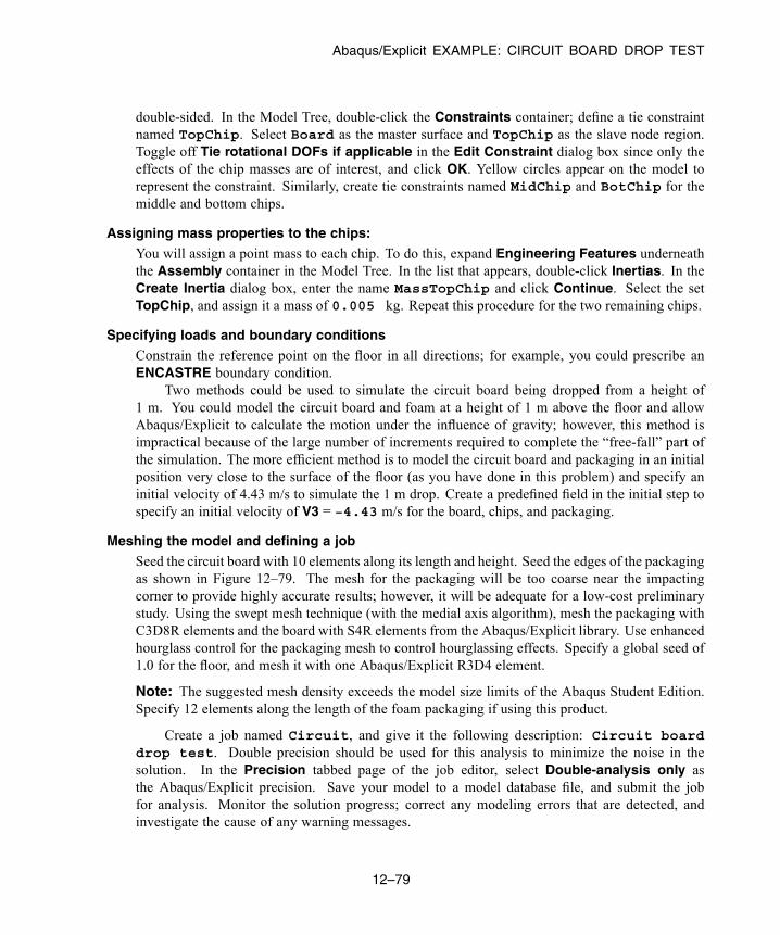
Abaqus/Explicit EXAMPLE: CIRCUIT BOARD DROP TEST
double-sided. In the Model Tree, double-click the Constraints container; define a tie constraintnamed TopChip. Select Board as the master surface and TopChip as the slave node region.Toggle off Tie rotational DOFs if applicable in the Edit Constraint dialog box since only theeffects of the chip masses are of interest, and click OK. Yellow circles appear on the model torepresent the constraint. Similarly, create tie constraints named MidChip and BotChip for themiddle and bottom chips.
Assigning mass properties to the chips:
You will assign a point mass to each chip. To do this, expand Engineering Features underneaththe Assembly container in the Model Tree. In the list that appears, double-click Inertias. In theCreate Inertia dialog box, enter the name MassTopChip and click Continue. Select the setTopChip, and assign it a mass of 0.005 kg. Repeat this procedure for the two remaining chips.
Specifying loads and boundary conditions
Constrain the reference point on the floor in all directions; for example, you could prescribe anENCASTRE boundary condition.
Two methods could be used to simulate the circuit board being dropped from a height of1 m. You could model the circuit board and foam at a height of 1 m above the floor and allowAbaqus/Explicit to calculate the motion under the influence of gravity; however, this method isimpractical because of the large number of increments required to complete the “free-fall” part ofthe simulation. The more efficient method is to model the circuit board and packaging in an initialposition very close to the surface of the floor (as you have done in this problem) and specify aninitial velocity of 4.43 m/s to simulate the 1 m drop. Create a predefined field in the initial step tospecify an initial velocity of V3 = −4.43 m/s for the board, chips, and packaging.
Meshing the model and defining a job
Seed the circuit board with 10 elements along its length and height. Seed the edges of the packagingas shown in Figure 12–79. The mesh for the packaging will be too coarse near the impactingcorner to provide highly accurate results; however, it will be adequate for a low-cost preliminarystudy. Using the swept mesh technique (with the medial axis algorithm), mesh the packaging withC3D8R elements and the board with S4R elements from the Abaqus/Explicit library. Use enhancedhourglass control for the packaging mesh to control hourglassing effects. Specify a global seed of1.0 for the floor, and mesh it with one Abaqus/Explicit R3D4 element.
Note: The suggested mesh density exceeds the model size limits of the Abaqus Student Edition.Specify 12 elements along the length of the foam packaging if using this product.
Create a job named Circuit, and give it the following description: Circuit boarddrop test. Double precision should be used for this analysis to minimize the noise in thesolution. In the Precision tabbed page of the job editor, select Double-analysis only asthe Abaqus/Explicit precision. Save your model to a model database file, and submit the jobfor analysis. Monitor the solution progress; correct any modeling errors that are detected, andinvestigate the cause of any warning messages.
12–79
Abaqus ID:Printed on:
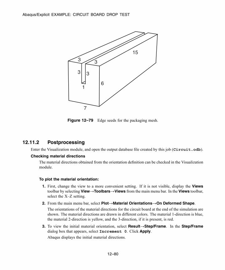
Abaqus/Explicit EXAMPLE: CIRCUIT BOARD DROP TEST
15
6
7
1
3 3
3 3
Figure 12–79 Edge seeds for the packaging mesh.
12.11.2 PostprocessingEnter the Visualization module, and open the output database file created by this job (Circuit.odb).
Checking material directions
The material directions obtained from the orientation definition can be checked in the Visualizationmodule.
To plot the material orientation:
1. First, change the view to a more convenient setting. If it is not visible, display the Viewstoolbar by selecting View→Toolbars→Views from the main menu bar. In the Views toolbar,select the X–Z setting.
2. From the main menu bar, select Plot→Material Orientations→On Deformed Shape.
The orientations of the material directions for the circuit board at the end of the simulation areshown. The material directions are drawn in different colors. The material 1-direction is blue,the material 2-direction is yellow, and the 3-direction, if it is present, is red.
3. To view the initial material orientation, select Result→Step/Frame. In the Step/Framedialog box that appears, select Increment 0. Click Apply.
Abaqus displays the initial material directions.
12–80
Abaqus ID:Printed on:

Abaqus/Explicit EXAMPLE: CIRCUIT BOARD DROP TEST
4. To restore the display to the results at the end of the analysis, select the last increment availablein the Step/Frame dialog box; and click OK.
Animation of results
You will create a time-history animation of the deformation to help you visualize the motion anddeformation of the circuit board and foam packaging during impact.
To create a time-history animation:
1. Plot the deformed model shape at the end of the analysis.
2. From the main menu bar, select Animate→Time History.
The animation of the deformed model shape begins.
3. From the main menu bar, select View→Parallel to turn off perspective.
4. In the context bar, click to pause the animation after a full cycle has been completed.
5. In the context bar, click and then select a node on the foam packaging near one of thecorners that impacts the floor. When you restart the animation the camera will move with theselected node. If you zoom in on the node, it will remain in view throughout the animation.
Note: To reset the camera to follow the global coordinate system, click in the contextbar.
While you view the deformation history of the drop test, take note of when the foam is in contactwith the floor. You should observe that the initial impact occurs over the first 4 ms of the analysis.A second impact occurs from about 8 ms to 15 ms. The deformed state of the foam and board atapproximately 4 ms after impact is shown in Figure 12–80.
Plotting model energy histories
Plot graphs of various energy variables versus time. Energy output can help you evaluate whetheran Abaqus/Explicit simulation is predicting an appropriate response.
To plot energy histories:
1. In the Results Tree, click mouse button 3 on History Output for the output database namedCircuit.odb. From the menu that appears, select Filter.
2. In the filter field, enter *ALL* to restrict the history output to just the energy output variables.
3. Select the ALLAE output variable, and save the data as Artificial Energy.
4. Select the ALLIE output variable, and save the data as Internal Energy.
5. Select the ALLKE output variable, and save the data as Kinetic Energy.
12–81
Abaqus ID:Printed on:

Abaqus/Explicit EXAMPLE: CIRCUIT BOARD DROP TEST
Figure 12–80 Deformed mesh at 4 ms.
6. Select the ALLPD output variable, and save the data as Plastic Dissipation.
7. Select the ALLSE output variable, and save the data as Strain Energy.
8. In the Results Tree, expand the XYData container.
9. Select all five curves. Click mouse button 3, and select Plot from the menu that appears toview the X–Y plot.
Next, you will customize the appearance of the plot; begin by changing the line styles of thecurves.
10. Open the Curve Options dialog box.
11. In this dialog box, apply different line styles and thicknesses to each of the curves displayedin the viewport.
Next, reposition the legend so that it appears inside the plot.
12. Double-click the legend to open the Chart Legend Options dialog box.
13. In this dialog box, switch to the Area tabbed page, and toggle on Inset.
14. In the viewport, drag the legend over the plot.
Now change the format of the X-axis labels.
15. In the viewport, double-click the X-axis to access the X Axis options in the Axis Optionsdialog box.
16. In this dialog box, switch to the Axes tabbed page, and select the Engineering label formatfor the X-axis.
12–82
Abaqus ID:Printed on:
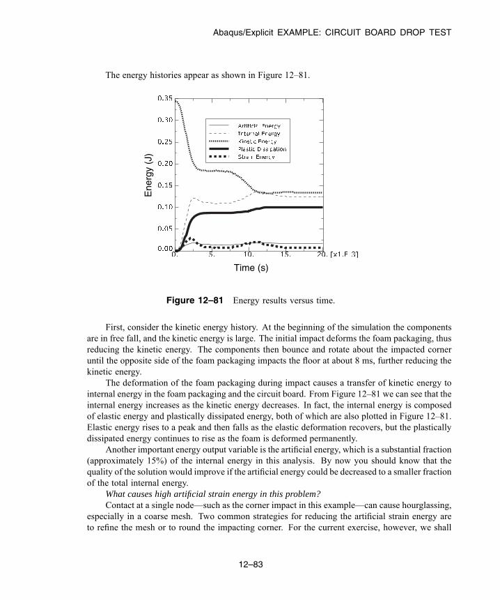
Abaqus/Explicit EXAMPLE: CIRCUIT BOARD DROP TEST
The energy histories appear as shown in Figure 12–81.
Time (s)
Ene
rgy
(J)
Figure 12–81 Energy results versus time.
First, consider the kinetic energy history. At the beginning of the simulation the componentsare in free fall, and the kinetic energy is large. The initial impact deforms the foam packaging, thusreducing the kinetic energy. The components then bounce and rotate about the impacted corneruntil the opposite side of the foam packaging impacts the floor at about 8 ms, further reducing thekinetic energy.
The deformation of the foam packaging during impact causes a transfer of kinetic energy tointernal energy in the foam packaging and the circuit board. From Figure 12–81 we can see that theinternal energy increases as the kinetic energy decreases. In fact, the internal energy is composedof elastic energy and plastically dissipated energy, both of which are also plotted in Figure 12–81.Elastic energy rises to a peak and then falls as the elastic deformation recovers, but the plasticallydissipated energy continues to rise as the foam is deformed permanently.
Another important energy output variable is the artificial energy, which is a substantial fraction(approximately 15%) of the internal energy in this analysis. By now you should know that thequality of the solution would improve if the artificial energy could be decreased to a smaller fractionof the total internal energy.
What causes high artificial strain energy in this problem?Contact at a single node—such as the corner impact in this example—can cause hourglassing,
especially in a coarse mesh. Two common strategies for reducing the artificial strain energy areto refine the mesh or to round the impacting corner. For the current exercise, however, we shall
12–83
Abaqus ID:Printed on:
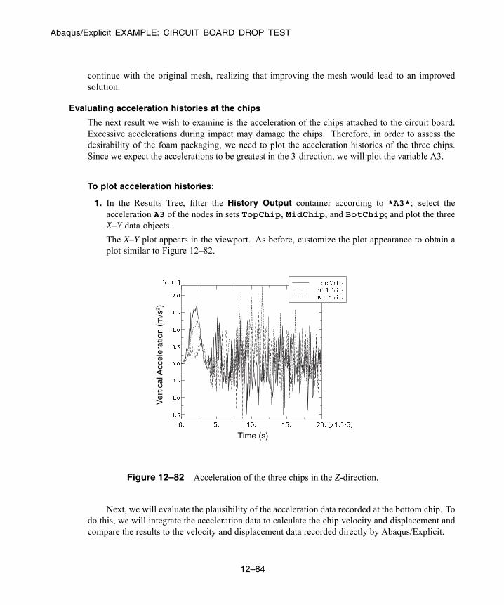
Abaqus/Explicit EXAMPLE: CIRCUIT BOARD DROP TEST
continue with the original mesh, realizing that improving the mesh would lead to an improvedsolution.
Evaluating acceleration histories at the chips
The next result we wish to examine is the acceleration of the chips attached to the circuit board.Excessive accelerations during impact may damage the chips. Therefore, in order to assess thedesirability of the foam packaging, we need to plot the acceleration histories of the three chips.Since we expect the accelerations to be greatest in the 3-direction, we will plot the variable A3.
To plot acceleration histories:
1. In the Results Tree, filter the History Output container according to *A3*; select theacceleration A3 of the nodes in sets TopChip, MidChip, and BotChip; and plot the threeX–Y data objects.
The X–Y plot appears in the viewport. As before, customize the plot appearance to obtain aplot similar to Figure 12–82.
Time (s)
Ver
tical
Acc
eler
atio
n (m
/s2 )
Figure 12–82 Acceleration of the three chips in the Z-direction.
Next, we will evaluate the plausibility of the acceleration data recorded at the bottom chip. Todo this, we will integrate the acceleration data to calculate the chip velocity and displacement andcompare the results to the velocity and displacement data recorded directly by Abaqus/Explicit.
12–84
Abaqus ID:Printed on:
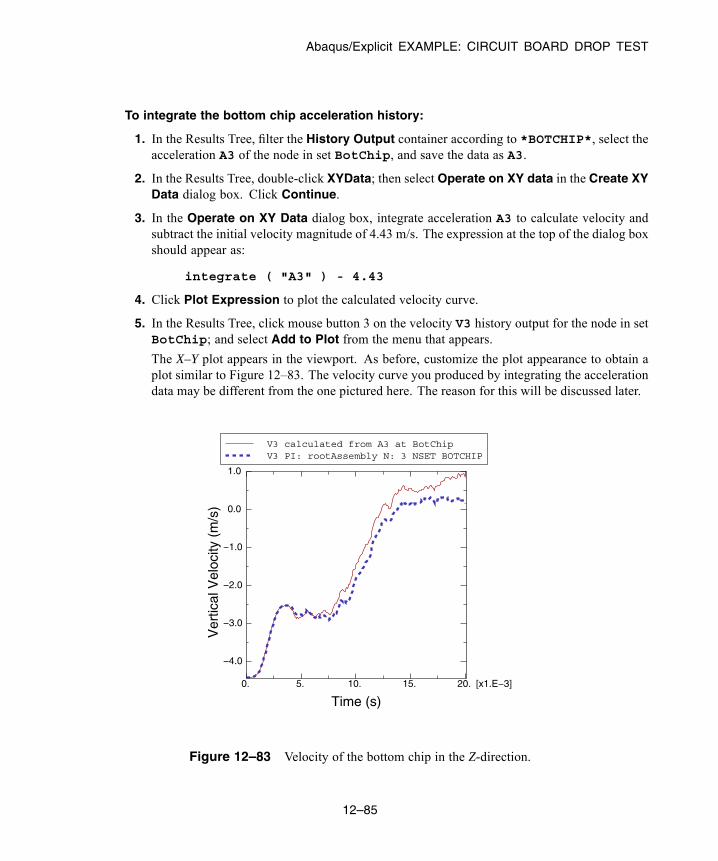
Abaqus/Explicit EXAMPLE: CIRCUIT BOARD DROP TEST
To integrate the bottom chip acceleration history:
1. In the Results Tree, filter the History Output container according to *BOTCHIP*, select theacceleration A3 of the node in set BotChip, and save the data as A3.
2. In the Results Tree, double-click XYData; then select Operate on XY data in the Create XYData dialog box. Click Continue.
3. In the Operate on XY Data dialog box, integrate acceleration A3 to calculate velocity andsubtract the initial velocity magnitude of 4.43 m/s. The expression at the top of the dialog boxshould appear as:
integrate ( "A3" ) - 4.43
4. Click Plot Expression to plot the calculated velocity curve.
5. In the Results Tree, click mouse button 3 on the velocity V3 history output for the node in setBotChip; and select Add to Plot from the menu that appears.
The X–Y plot appears in the viewport. As before, customize the plot appearance to obtain aplot similar to Figure 12–83. The velocity curve you produced by integrating the accelerationdata may be different from the one pictured here. The reason for this will be discussed later.
Time (s)0. 5. 10. 15. 20. [x1.E−3]
Ver
tical
Vel
ocity
(m
/s)
−4.0
−3.0
−2.0
−1.0
0.0
1.0
V3 calculated from A3 at BotChipV3 PI: rootAssembly N: 3 NSET BOTCHIP
Figure 12–83 Velocity of the bottom chip in the Z-direction.
12–85
Abaqus ID:Printed on:
Abaqus/Explicit EXAMPLE: CIRCUIT BOARD DROP TEST
6. In the Operate on XY Data dialog box, integrate acceleration A3 a second time to calculatechip displacement. The expression at the top of the dialog box should appear as:
integrate ( integrate ( "A3" ) - 4.43 )
7. Click Plot Expression to plot the calculated displacement curve.
Notice that the Y-value type is length. In order to plot the calculated displacement with thesame Y-axis as the displacement output recorded during the analysis, we must save the X–Ydata and change the Y-value type to displacement.
8. Click Save As to save the calculated displacement curve as U3-from-A3.
9. In the XYData container of the Results Tree, click mouse button 3 on U3-from-A3; andselect Edit from the menu that appears.
10. In the Edit XY Data dialog box, choose Displacement as the Y-value type.
11. In the Results Tree, double-click U3–from-A3 to recreate the calculated displacement plotwith the displacement Y-value type.
12. In the Results Tree, click mouse button 3 on the displacement U3 history output for the nodein set BotChip; and select Add to Plot from the menu that appears.
The X–Y plot appears in the viewport. As before, customize the plot appearance to obtain aplot similar to Figure 12–84. Again, the curve you produced by integrating the accelerationdata may be different from the one pictured here. The reason for this will be discussed later.
Why are the velocity and displacement curves calculated by integrating the acceleration datadifferent from the velocity and displacement recorded during the analysis?
In this example the acceleration data has been corrupted by a phenomenon called aliasing.Aliasing is a form of data corruption that occurs when a signal (such as the results of an Abaqusanalysis) is sampled at a series of discrete points in time, but not enough data points are saved inorder to correctly describe the signal. The aliasing phenomenon can be addressed using digital signalprocessing (DSP) methods, a fundamental principle of which is the Nyquist Sampling Theorem(also known as the Shannon Sampling Theorem). The Sampling Theorem requires that a signal besampled at a rate that is greater than twice the signal’s highest frequency. Therefore, the maximumfrequency content that can be described by a given sampling rate is half that rate (the Nyquistfrequency). Sampling (storing) a signal with large-amplitude oscillations at frequencies greaterthan the Nyquist frequency of the sample rate may produce significantly distorted results due toaliasing. In this example the chip acceleration was sampled every 0.07 ms, which is a samplingrate of 14.3 kHz (the sample rate is the inverse of the sample size). The recorded data was aliasedbecause the chip acceleration response has frequency content above 7.2 kHz (half the sample rate).
Aliasing of a sine wave
To better understand how aliasing distorts data, consider a 1 kHz sine wave sampled using varioussampling rates, as shown in Figure 12–85. According to the Sampling Theorem, this signal must
12–86
Abaqus ID:Printed on:
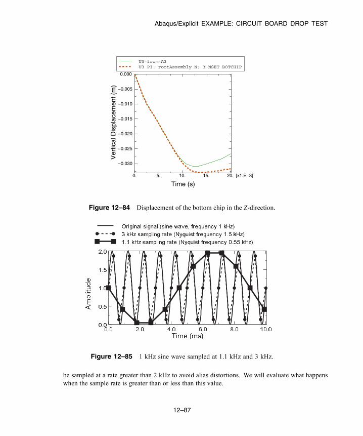
Abaqus/Explicit EXAMPLE: CIRCUIT BOARD DROP TEST
Time (s)0. 5. 10. 15. 20. [x1.E−3]
Ver
tical
Dis
plac
emen
t (m
)
−0.030
−0.025
−0.020
−0.015
−0.010
−0.005
0.000
U3−from−A3U3 PI: rootAssembly N: 3 NSET BOTCHIP
Figure 12–84 Displacement of the bottom chip in the Z-direction.
Figure 12–85 1 kHz sine wave sampled at 1.1 kHz and 3 kHz.
be sampled at a rate greater than 2 kHz to avoid alias distortions. We will evaluate what happenswhen the sample rate is greater than or less than this value.
12–87
Abaqus ID:Printed on:
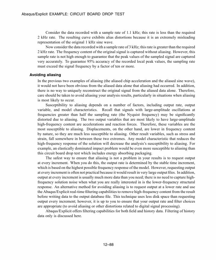
Abaqus/Explicit EXAMPLE: CIRCUIT BOARD DROP TEST
Consider the data recorded with a sample rate of 1.1 kHz; this rate is less than the required2 kHz rate. The resulting curve exhibits alias distortions because it is an extremely misleadingrepresentation of the original 1 kHz sine wave.
Now consider the data recordedwith a sample rate of 3 kHz; this rate is greater than the required2 kHz rate. The frequency content of the original signal is captured without aliasing. However, thissample rate is not high enough to guarantee that the peak values of the sampled signal are capturedvery accurately. To guarantee 95% accuracy of the recorded local peak values, the sampling ratemust exceed the signal frequency by a factor of ten or more.
Avoiding aliasing
In the previous two examples of aliasing (the aliased chip acceleration and the aliased sine wave),it would not have been obvious from the aliased data alone that aliasing had occurred. In addition,there is no way to uniquely reconstruct the original signal from the aliased data alone. Therefore,care should be taken to avoid aliasing your analysis results, particularly in situations when aliasingis most likely to occur.
Susceptibility to aliasing depends on a number of factors, including output rate, outputvariable, and model characteristics. Recall that signals with large-amplitude oscillations atfrequencies greater than half the sampling rate (the Nyquist frequency) may be significantlydistorted due to aliasing. The two output variables that are most likely to have large-amplitudehigh-frequency content are accelerations and reaction forces. Therefore, these variables are themost susceptible to aliasing. Displacements, on the other hand, are lower in frequency contentby nature, so they are much less susceptible to aliasing. Other result variables, such as stress andstrain, fall somewhere in between these two extremes. Any model characteristic that reduces thehigh-frequency response of the solution will decrease the analysis’s susceptibility to aliasing. Forexample, an elastically dominated impact problem would be even more susceptible to aliasing thanthis circuit board drop test which includes energy absorbing packaging.
The safest way to ensure that aliasing is not a problem in your results is to request outputat every increment. When you do this, the output rate is determined by the stable time increment,which is based on the highest possible frequency response of the model. However, requesting outputat every increment is often not practical because it would result in very large output files. In addition,output at every increment is usually much more data than you need; there is no need to capture high-frequency solution noise when what you are really interested in is the lower-frequency structuralresponse. An alternative method for avoiding aliasing is to request output at a lower rate and usethe Abaqus/Explicit real-time filtering capabilities to remove high-frequency content from the resultbefore writing data to the output database file. This technique uses less disk space than requestingoutput every increment; however, it is up to you to ensure that your output rate and filter choicesare appropriate (to avoid aliasing or other distortions related to digital signal processing).
Abaqus/Explicit offers filtering capabilities for both field and history data. Filtering of historydata only is discussed here.
12–88
Abaqus ID:Printed on:

Abaqus/Explicit EXAMPLE: CIRCUIT BOARD DROP TEST
12.11.3 Rerunning the analysis with output filteringIn this section you will add real-time filters to the history output requests for the circuit board droptest analysis. While Abaqus/Explicit does allow you to create user-defined output filters (Butterworth,Chebyshev Type I, and Chebyshev Type II) based on criteria that you specify, in this example we will usethe built-in antialiasing filter. The built-in antialiasing filter is designed to give you the best un-aliasedrepresentation of the results recorded at the output rate you specify on the output request. To do this,Abaqus/Explicit internally applies a low-pass, second-order, Butterworth filter with a cutoff frequencyset to one-sixth of the sampling rate. For more information, see “Overview of filtering Abaqus historyoutput” in the Dassault Systèmes Knowledge Base at www.3ds.com/support/knowledge-base. For moreinformation on defining your own real-time filters, see “Filtering output and operating on output inAbaqus/Explicit” in “Output to the output database,” Section 4.1.3 of the Abaqus Analysis User’s Guide.
Modifying the history output requests
When Abaqus writes nodal history output to the output database, it gives each data object a namethat indicates the recorded output variable, the filter used (if any), the part instance name, the nodenumber, and the node set. For this exercise you will be creating multiple output requests for thenode in set BotChip that differ only by the output sample rate, which is not a component of thehistory output name. To easily distinguish between the similar output requests, create two newsets for the bottom chip reference node. Name one of the new sets BotChip-all and the otherBotChip-largeInc.
Next, copy the history output request for the bottom chip three times. Edit the first copy toactivate the Antialiasing filter; for this request continue to record data every 7 × 10⁻⁵ s using theset BotChip. Edit the second copy to record the data at every time increment; apply this outputrequest to the set BotChip-all. Edit the third copy to record the data at every 7 × 10⁻⁴ s; applythis output request to the set BotChip-largeInc and activate the Antialiasing filter. Whenyou are finished, there will be four history output requests for the bottom chip (the original one andthe three added here).
Edit the output request for the strains in the setBotBoard in order to activate theAntialiasingfilter.
Although we will not be discussing the results here, you may wish to add the Antialiasingfilter to the history output request for the displacement, velocity, and acceleration of the node setsMidChip and TopChip.
Save your model database, and submit the job for analysis.
Evaluating the filtered acceleration of the bottom chip
When the analysis completes, test the plausibility of the acceleration history output for the bottomchip recorded every 0.07 ms using the built-in, antialiasing filter. Do this by saving and thenintegrating the filtered acceleration data (A3_ANTIALIASING for set BotChip) and comparingthe results to recorded velocity and displacement data, just as you did earlier for the unfilteredversion of these results. This time you should find that the velocity and displacement curves
12–89
Abaqus ID:Printed on:

Abaqus/Explicit EXAMPLE: CIRCUIT BOARD DROP TEST
calculated by integrating the filtered acceleration are very similar to the velocity and displacementvalues written to the output database during the analysis. You may also have noticed that thevelocity and displacement results are the same regardless of whether or not the built-in antialiasingfilter is used. This is because the highest frequency content of the nodal velocity and displacementcurves is much less than half the sampling rate. Consequently, no aliasing occurred when the datawas recorded without filtering, and when the built-in antialiasing filter was applied it had no effectbecause there was no high frequency response to remove.
Next, compare the acceleration A3 history output recorded every increment with the twoacceleration A3 history curves recorded every 0.07 ms. Plot the data recorded at every incrementfirst so that it does not obscure the other results.
To plot the acceleration histories
1. In the Results Tree, filter the History Output container according to *A3*BOTCHIP* anddouble-click the acceleration A3 history output for the node set BotChip-all.
2. Select the two acceleration A3 history output objects for the node set BotChip (one filteredwith the built-in antialiasing filter and the other with no filtering) using [Ctrl] + Click; click mousebutton 3 and select Add to Plot from the menu that appears.
The X–Y plot appears in the viewport. Zoom in to view only the first third of the results andcustomize the plot appearance to obtain a plot similar to Figure 12–86.
First consider the acceleration history recorded every increment. This curve contains a lotof data, including high-frequency solution noise which becomes so large in magnitude that itobscures the structurally-significant lower-frequency components of the acceleration. When outputis requested every increment, the output time increment is the same as the stable time increment,which (in order to ensure stability) is based on a conservative estimate of the highest possiblefrequency response of the model. Frequencies of structural significance are typically two to fourorders of magnitude less than the highest frequency of the model. In this example the stable timeincrement ranges between 8.4 × 10⁻⁴ ms to 8.8 × 10⁻⁴ ms (see the status file, Circuit.sta),which corresponds to a sample rate of about 1 MHz; this sample rate has been rounded down forthis discussion, even though it means that the value is not conservative. Recalling the SamplingTheorem, the highest frequency that can be described by a given sample rate is half that rate;therefore, the highest frequency of this model is about 500 kHz and typical structural frequenciescould be as high as 2–3 kHz (more than 2 orders of magnitude less than the highest modelfrequency). While the output recorded every increment contains a lot of undesirable solution noisein the 3 to 500 kHz range, it is guaranteed to be good (not aliased) data, which can be filtered laterwith a postprocessing operation if necessary.
Next consider the data recorded every 0.07 ms without any filtering. Recall that this is thecurve we know to be corrupted by aliasing. The curve jumps from point to point by directlyincluding whatever the raw acceleration value happens to be after each 0.07 ms interval. Thevariable nature of the high-frequency noise makes this aliased result very sensitive to otherwiseimperceptible variations in the solution (due to differences between computer platforms, for
12–90
Abaqus ID:Printed on:
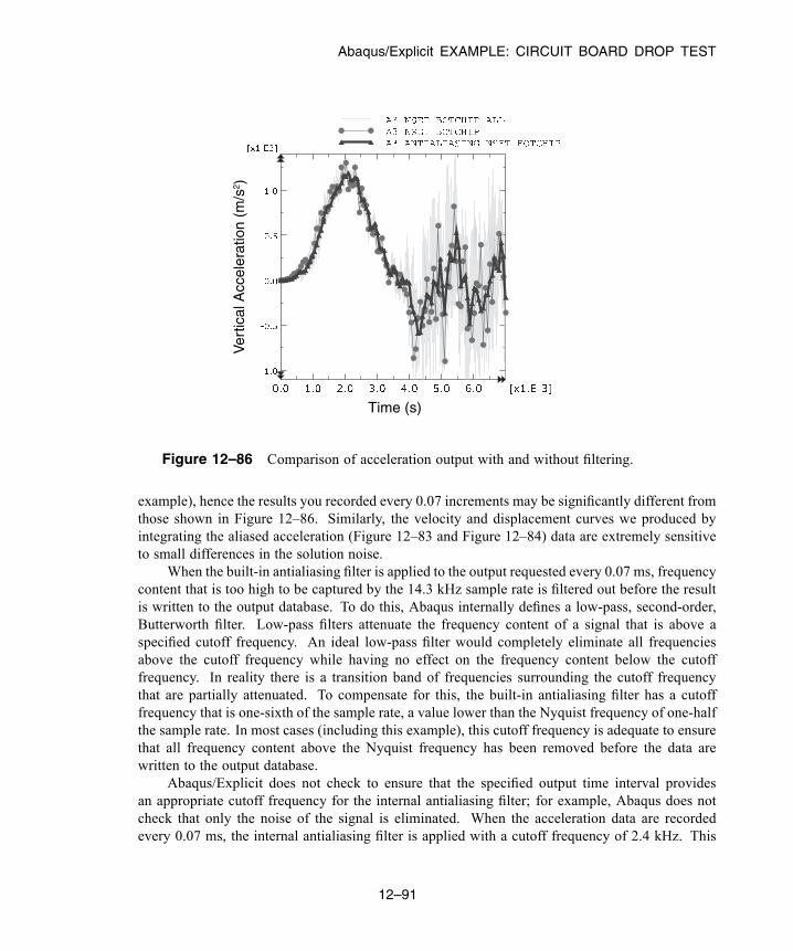
Abaqus/Explicit EXAMPLE: CIRCUIT BOARD DROP TEST
Time (s)
Ver
tical
Acc
eler
atio
n (m
/s2 )
Figure 12–86 Comparison of acceleration output with and without filtering.
example), hence the results you recorded every 0.07 increments may be significantly different fromthose shown in Figure 12–86. Similarly, the velocity and displacement curves we produced byintegrating the aliased acceleration (Figure 12–83 and Figure 12–84) data are extremely sensitiveto small differences in the solution noise.
When the built-in antialiasing filter is applied to the output requested every 0.07 ms, frequencycontent that is too high to be captured by the 14.3 kHz sample rate is filtered out before the resultis written to the output database. To do this, Abaqus internally defines a low-pass, second-order,Butterworth filter. Low-pass filters attenuate the frequency content of a signal that is above aspecified cutoff frequency. An ideal low-pass filter would completely eliminate all frequenciesabove the cutoff frequency while having no effect on the frequency content below the cutofffrequency. In reality there is a transition band of frequencies surrounding the cutoff frequencythat are partially attenuated. To compensate for this, the built-in antialiasing filter has a cutofffrequency that is one-sixth of the sample rate, a value lower than the Nyquist frequency of one-halfthe sample rate. In most cases (including this example), this cutoff frequency is adequate to ensurethat all frequency content above the Nyquist frequency has been removed before the data arewritten to the output database.
Abaqus/Explicit does not check to ensure that the specified output time interval providesan appropriate cutoff frequency for the internal antialiasing filter; for example, Abaqus does notcheck that only the noise of the signal is eliminated. When the acceleration data are recordedevery 0.07 ms, the internal antialiasing filter is applied with a cutoff frequency of 2.4 kHz. This
12–91
Abaqus ID:Printed on:
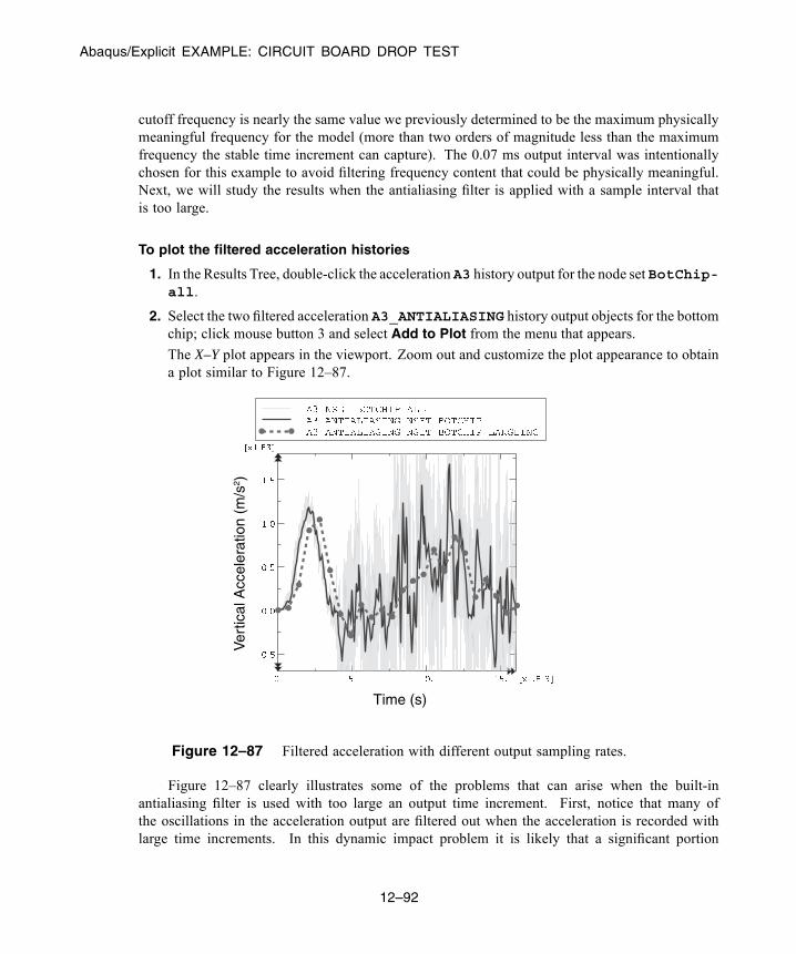
Abaqus/Explicit EXAMPLE: CIRCUIT BOARD DROP TEST
cutoff frequency is nearly the same value we previously determined to be the maximum physicallymeaningful frequency for the model (more than two orders of magnitude less than the maximumfrequency the stable time increment can capture). The 0.07 ms output interval was intentionallychosen for this example to avoid filtering frequency content that could be physically meaningful.Next, we will study the results when the antialiasing filter is applied with a sample interval thatis too large.
To plot the filtered acceleration histories
1. In the Results Tree, double-click the acceleration A3 history output for the node set BotChip-all.
2. Select the two filtered acceleration A3_ANTIALIASING history output objects for the bottomchip; click mouse button 3 and select Add to Plot from the menu that appears.
The X–Y plot appears in the viewport. Zoom out and customize the plot appearance to obtaina plot similar to Figure 12–87.
Time (s)
Ver
tical
Acc
eler
atio
n (m
/s2 )
Figure 12–87 Filtered acceleration with different output sampling rates.
Figure 12–87 clearly illustrates some of the problems that can arise when the built-inantialiasing filter is used with too large an output time increment. First, notice that many ofthe oscillations in the acceleration output are filtered out when the acceleration is recorded withlarge time increments. In this dynamic impact problem it is likely that a significant portion
12–92
Abaqus ID:Printed on:
Abaqus/Explicit EXAMPLE: CIRCUIT BOARD DROP TEST
of the removed frequency content is physically meaningful. Previously, we estimated that thefrequency of the structural response may be as large as 2–3 kHz; however, when the sampleinterval is 0.7 ms, filtering is performed with a low cutoff frequency of 0.24 kHz (sample intervalof 0.7 ms corresponds to a sample frequency of 1.43 kHz, one-sixth of which is the 0.24 kHzcutoff frequency). Even though the results recorded every 0.7 ms may not capture all physicallymeaningful frequency content, it does capture the low-frequency content of the accelerationdata without distortions due to aliasing. Keep in mind that filtering decreases the peak valueestimations, which is desirable if only solution noise is filtered, but can be misleading whenphysically meaningful solution variations have been removed.
Another issue to note is that there is a time delay in the acceleration results recorded every0.7 ms. This time delay (or phase shift) affects all real-time filters. The filter must have some inputin order to produce output; consequently the filtered result will include some time delay. Whilesome time delay is introduced for all real-time filtering, the time delay becomes more pronouncedas the filter cutoff frequency decreases; the filter must have input over a longer span of time inorder to remove lower frequency content. Increasing the filter order (an option if you have createda user-defined filter, rather than using the second-order built-in antialiasing filter) also results inan increase in the output time delay. For more information, see “Filtering output and operating onoutput in Abaqus/Explicit” in “Output to the output database,” Section 4.1.3 of the Abaqus AnalysisUser’s Guide.
Use the real-time filtering functionality with caution. In this example we would not have beenable to identify the problems with the heavily filtered data if we did not have appropriate data forcomparison. In general it is best to use a minimal amount of filtering in Abaqus/Explicit, so that theoutput database contains a rich, un-aliased, representation for the solution recorded at a reasonablenumber of time points (rather than at every increment). If additional filtering is necessary, it can bedone as a postprocessing operation in Abaqus/CAE.
Filtering acceleration history in Abaqus/CAE
In this section we will use the Visualization module in Abaqus/CAE to filter the acceleration historydata written to the output database. Filtering as a postprocessing operation in the Visualizationmodule has several advantages over the real-time filtering available in Abaqus/Explicit. In theVisualization module you can quickly filter X–Y data and plot the results. You can easily comparethe filtered results to the unfiltered results to verify that the filter produced the desired effect.Using this technique you can quickly iterate to find appropriate filter parameters. In addition, theVisualization module filters do not suffer from the time delay that is unavoidable when filtering isapplied during the analysis. Keep in mind, however, that postprocessing filters cannot compensatefor poor analysis history output; if the data has been aliased or if physically meaningful frequencieshave been removed, no postprocessing operation can recover the lost content.
To demonstrate the differences between filtering in the Visualization module and filtering inAbaqus/Explicit, we will filter the acceleration of the bottom chip in the Visualization module andcompare the results to the filtered data Abaqus/Explicit wrote to the output database.
12–93
Abaqus ID:Printed on:

Abaqus/Explicit EXAMPLE: CIRCUIT BOARD DROP TEST
To filter acceleration history:
1. In the Results Tree, select the acceleration A3 history output for the node set BotChip-all,and save the data as A3-all.
2. In the Results Tree, double-click XYData; then select Operate on XY data in the Create XYData dialog box. Click Continue.
3. In the Operate on XY Data dialog box, filter A3-all with filter options that are equivalentto those applied by the Abaqus/Explicit built-in antialiasing filter when the output incrementis 0.7 ms. Recall that the built-in antialiasing filter is a second-order Butterworth filter with acutoff frequency that is one-sixth of the output sample rate; hence, the expression at the top ofthe dialog box should appear as
butterworthFilter ( xyData="A3-all",cutoffFrequency=1/(6*0.0007) )
4. Click Plot Expression to plot the filtered acceleration curve.
5. In the Results Tree, click mouse button 3 on the filtered acceleration A3_ANTIALIASINGhistory output for node set BotChip-largeInc; and select Add to Plot from the menuthat appears. If you wish, also add the filtered acceleration history for the node set BotChip.
The X–Y plot appears in the viewport. As before, customize the plot appearance to obtain aplot similar to Figure 12–88.
In Figure 12–88 it is clear that the postprocessing filter in the Visualization module ofAbaqus/CAE does not suffer from the time delay that occurs when filtering is performed while theanalysis is running. This is because the Visualization module filters are bidirectional, which meansthat the filtering is applied first in a forward pass (which introduces some time delay) and then ina backward pass (which removes the time delay). As a consequence of the bidirectional filteringin the Visualization module, the filtering is essentially applied twice, which results in additionalattenuation of the filtered signal compared to the attenuation achieved with a single-pass filter.This is why the local peaks in the acceleration curve filtered in the Visualization module are a bitlower than those in the curve filtered by Abaqus/Explicit.
To develop a better understanding of the Visualization module filtering capabilities, return tothe Operate on XY Data dialog box and filter the acceleration data with other filter options. Forexample, try different cutoff frequencies.
Can you confirm that the cutoff frequency of 2.4 kHz associated with the built-in antialiasingfilter with a time increment size of 0.07 was appropriate? Does increasing the cutoff frequency to6 kHz, 7 kHz, or even 10 kHz produce significantly different results?
You should find that a moderate increase in the cutoff frequency does not have a significanteffect on the results, implying that we probably have not missed physically meaningful frequencycontent when we filtered with a cutoff frequency of 2.4 kHz.
Compare the results of filtering the acceleration data with Butterworth and Chebyshev Type Ifilters. The Chebyshev filter requires a ripple factor parameter (rippleFactor), which indicates how
12–94
Abaqus ID:Printed on:

Abaqus/Explicit EXAMPLE: CIRCUIT BOARD DROP TEST
Time (s)
Ver
tical
Acc
eler
atio
n (m
/s2 )
Figure 12–88 Comparison of acceleration filtered inAbaqus/Explicit and the Visualization module.
much oscillation you will allow in exchange for an improved filter response; see “Filtering outputand operating on output in Abaqus/Explicit” in “Output to the output database,” Section 4.1.3 ofthe Abaqus Analysis User’s Guide for more information. For the Chebyshev Type I filter a ripplefactor of 0.071 will result in a very flat pass band with a ripple that is only 0.5%.
You may not notice much difference between the filters when the cutoff frequency is 5 kHz, butwhat about when the cutoff frequency is 2 kHz? What happens when you increase the order of theChebyshev Type I filter?
Compare your results to those shown in Figure 12–89.
Note: The Abaqus/CAE postprocessing filters are second-order by default. To define a higher orderfilter you can use the filterOrder parameter with the butterworthFilter and the chebyshev1Filteroperators. For example, use the following expression in the Operate on XY Data dialog box tofilter A3-all with a sixth-order Chebyshev Type I filter using a cutoff frequency of 2 kHz and aripple factor of 0.017.
chebyshev1Filter ( xyData="A3-all" , cutoffFrequency=2000,rippleFactor= 0.017, filterOrder=6)
The second-order Chebyshev Type I filter with a ripple factor of 0.071 is a relatively weakfilter, so some of the frequency content above the 2 kHz cutoff frequency is not filtered out. When
12–95
Abaqus ID:Printed on:
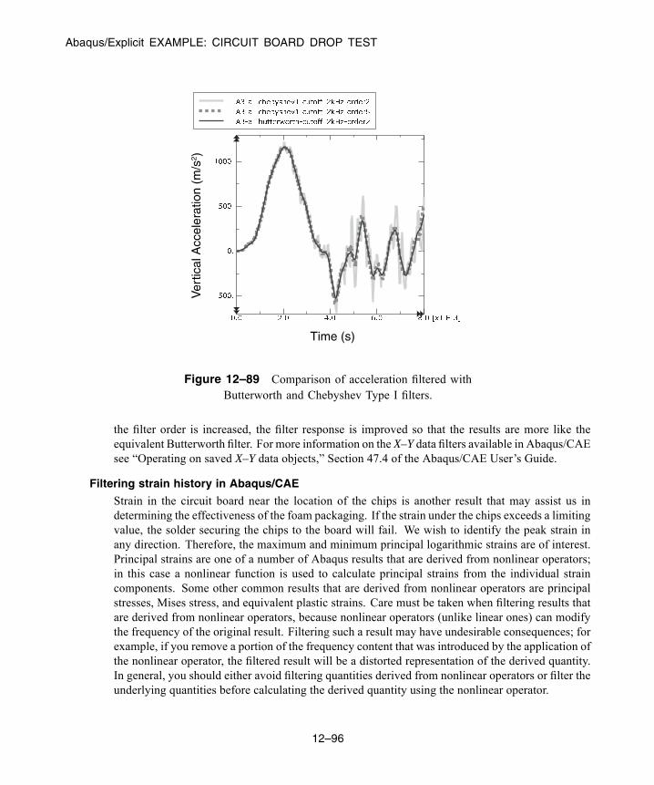
Abaqus/Explicit EXAMPLE: CIRCUIT BOARD DROP TEST
Time (s)
Ver
tical
Acc
eler
atio
n (m
/s2 )
Figure 12–89 Comparison of acceleration filtered withButterworth and Chebyshev Type I filters.
the filter order is increased, the filter response is improved so that the results are more like theequivalent Butterworth filter. For more information on the X–Y data filters available in Abaqus/CAEsee “Operating on saved X–Y data objects,” Section 47.4 of the Abaqus/CAE User’s Guide.
Filtering strain history in Abaqus/CAE
Strain in the circuit board near the location of the chips is another result that may assist us indetermining the effectiveness of the foam packaging. If the strain under the chips exceeds a limitingvalue, the solder securing the chips to the board will fail. We wish to identify the peak strain inany direction. Therefore, the maximum and minimum principal logarithmic strains are of interest.Principal strains are one of a number of Abaqus results that are derived from nonlinear operators;in this case a nonlinear function is used to calculate principal strains from the individual straincomponents. Some other common results that are derived from nonlinear operators are principalstresses, Mises stress, and equivalent plastic strains. Care must be taken when filtering results thatare derived from nonlinear operators, because nonlinear operators (unlike linear ones) can modifythe frequency of the original result. Filtering such a result may have undesirable consequences; forexample, if you remove a portion of the frequency content that was introduced by the application ofthe nonlinear operator, the filtered result will be a distorted representation of the derived quantity.In general, you should either avoid filtering quantities derived from nonlinear operators or filter theunderlying quantities before calculating the derived quantity using the nonlinear operator.
12–96
Abaqus ID:Printed on:

Abaqus/Explicit EXAMPLE: CIRCUIT BOARD DROP TEST
The strain history output for this analysis was recorded every 0.07 ms using the built-inantialiasing filter. To verify that the antialiasing filter did not distort the principal strain results, wewill calculate the principal logarithmic strains using the filtered strain components and comparethe result to the filtered principal logarithmic strains.
To calculate the principal logarithmic strains:
1. To identify the elements in set BotBoard that are closest to the bottom chip (use the ODBdisplay options to display the mass elements), plot the undeformed circuit board with elementnumbers visible.
2. In the Results Tree, filter the History Output according to *LE*Element #*, where # isthe number of one of the elements in set BotBoard that is close to the bottom chip. Selectthe logarithmic strain component LE11 on the SPOS surface of the element, and save the dataas LE11.
3. Similarly, save the LE12 and LE22 strain components for the same element as LE12 andLE22, respectively.
4. In the Results Tree, double-click XYData; then select Operate on XY data in the Create XYData dialog box. Click Continue.
5. In the Operate on XY Data dialog box, use the saved logarithmic strain components tocalculate the maximum principal logarithmic strain. The expression at the top of the dialogbox should appear as:
(("LE11"+"LE22")/2) + sqrt( power(("LE11"-"LE22")/2,2)+ power("LE12"/2,2) )
6. Click Save As to save calculated maximum principal logarithmic strain as LEP-Max.
7. Edit the expression in theOperate on XY Data dialog box to calculate the minimum principallogarithmic strain. The modified expression should appear as:
(("LE11"+"LE22")/2) - sqrt( power(("LE11"-"LE22")/2,2)+ power("LE12"/2,2) )
8. Click Save As to save calculated minimum principal logarithmic strain as LEP-Min.
In order to plot the calculated principal logarithmic strains with the same Y-axis as the strainsrecorded during the analysis, change the Y-value type to strain.
9. In the XYData container of the Results Tree, click mouse button 3 on LEP-Max; and selectEdit from the menu that appears.
10. In the Edit XY Data dialog box, choose Strain as the Y-value type.
11. Similarly, edit LEP-Min and select Strain as the Y-value type.
12. Using the Results Tree, plot LEP-Man and LEP-Min along with the principal strains recordedduring the analysis (LEP1 and LEP2) for the same element in set BotBoard.
12–97
Abaqus ID:Printed on:
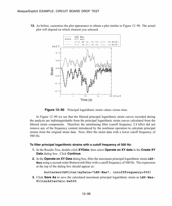
Abaqus/Explicit EXAMPLE: CIRCUIT BOARD DROP TEST
13. As before, customize the plot appearance to obtain a plot similar to Figure 12–90. The actualplot will depend on which element you selected.
Time (s)
Str
ain
Figure 12–90 Principal logarithmic strain values versus time.
In Figure 12–90 we see that the filtered principal logarithmic strain curves recorded duringthe analysis are indistinguishable from the principal logarithmic strain curves calculated from thefiltered strain components. Therefore the antialiasing filter (cutoff frequency 2.4 kHz) did notremove any of the frequency content introduced by the nonlinear operation to calculate principalstrains form the original strain data. Next, filter the strain data with a lower cutoff frequency of500 Hz.
To filter principal logarithmic strains with a cutoff frequency of 500 Hz:
1. In the Results Tree, double-click XYData; then select Operate on XY data in the Create XYData dialog box. Click Continue.
2. In theOperate on XY Data dialog box, filter the maximum principal logarithmic strain LEP-Max using a second-order Butterworth filter with a cutoff frequency of 500 Hz. The expressionat the top of the dialog box should appear as:
butterworthFilter(xyData="LEP-Max", cutoffFrequency=500)
3. Click Save As to save the calculated maximum principal logarithmic strain as LEP-Max-FilterAfterCalc-bw500.
12–98
Abaqus ID:Printed on:
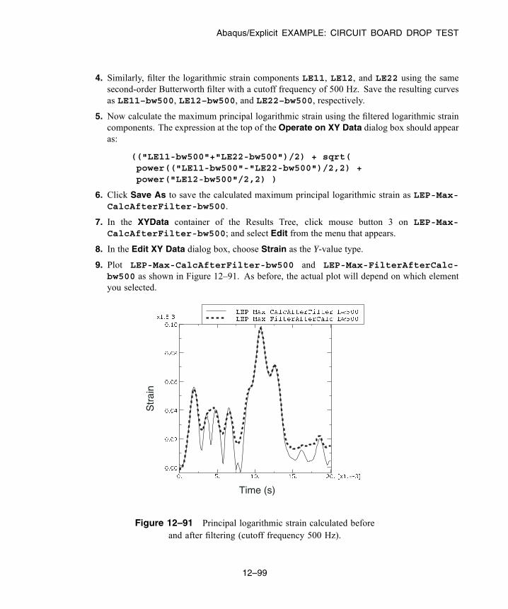
Abaqus/Explicit EXAMPLE: CIRCUIT BOARD DROP TEST
4. Similarly, filter the logarithmic strain components LE11, LE12, and LE22 using the samesecond-order Butterworth filter with a cutoff frequency of 500 Hz. Save the resulting curvesas LE11–bw500, LE12–bw500, and LE22–bw500, respectively.
5. Now calculate the maximum principal logarithmic strain using the filtered logarithmic straincomponents. The expression at the top of the Operate on XY Data dialog box should appearas:
(("LE11-bw500"+"LE22-bw500")/2) + sqrt(power(("LE11-bw500"-"LE22-bw500")/2,2) +power("LE12-bw500"/2,2) )
6. Click Save As to save the calculated maximum principal logarithmic strain as LEP-Max-CalcAfterFilter-bw500.
7. In the XYData container of the Results Tree, click mouse button 3 on LEP-Max-CalcAfterFilter-bw500; and select Edit from the menu that appears.
8. In the Edit XY Data dialog box, choose Strain as the Y-value type.
9. Plot LEP-Max-CalcAfterFilter-bw500 and LEP-Max-FilterAfterCalc-bw500 as shown in Figure 12–91. As before, the actual plot will depend on which elementyou selected.
Time (s)
Str
ain
Figure 12–91 Principal logarithmic strain calculated beforeand after filtering (cutoff frequency 500 Hz).
12–99
Abaqus ID:Printed on:

COMPATIBILITY BETWEEN Abaqus/Standard AND Abaqus/Explicit
In Figure 12–91 you can see that there is a significant difference between filtering the straindata before and after the principal strain calculation. The curve that was filtered after the principalstrain calculation is distorted because some of the frequency content introduced by applying thenonlinear principal-stress operator is higher than the 500 Hz filter cutoff frequency. In general,you should avoid directly filtering quantities that have been derived from nonlinear operators;whenever possible filter the underlying components and then apply the nonlinear operator to thefiltered components to calculate the desired derived quantity.
Strategy for recording and filtering Abaqus/Explicit history output
Recording output for every increment in Abaqus/Explicit generally produces much more data thanyou need. The real-time filtering capability allows you to request history output less frequentlywithout distorting the results due to aliasing. However, you should ensure that your output rate andfiltering choices have not removed physically meaningful frequency content nor distorted the results(for example, by introducing a large time delay or by removing frequency content introduced bynonlinear operators). Keep in mind that no amount of postprocessing filtering can recover frequencycontent filtered out during the analysis, nor can postprocessing filtering recover an original signalfrom aliased data. In addition, it may not be obvious when results have been over-filtered or aliasedif additional data are not available for comparison. A good strategy is to choose a relatively highoutput rate and use the Abaqus/Explicit filters to prevent aliasing of the history output, so that validand rich results are written to the output database. You may even wish to request output at everyincrement for a couple of critical locations. After the analysis completes, use the postprocessingtools in Abaqus/CAE to quickly and iteratively apply additional filtering as desired.
12.12 Compatibility between Abaqus/Standard and Abaqus/Explicit
There are fundamental differences in the mechanical contact algorithms in Abaqus/Standard andAbaqus/Explicit. These differences are reflected in how contact conditions are defined. The maindifferences are the following:
• For contact pairs Abaqus/Standard typically uses a pure master-slave relationship for thecontact constraints by default (see “Defining contact pairs in Abaqus/Standard,” Section 36.3.1of the Abaqus Analysis User’s Guide); the nodes of the slave surface are constrained not topenetrate into the master surface. The nodes of the master surface can, in principle, penetrateinto the slave surface. Abaqus/Explicit includes this formulation but typically uses a balancedmaster-slave weighting by default (see “Contact formulations for contact pairs in Abaqus/Explicit,”Section 38.2.2 of the Abaqus Analysis User’s Guide).
• The contact formulations in Abaqus/Standard and Abaqus/Explicit differ in many respects. Forexample, Abaqus/Standard provides a surface-to-surface formulation, while Abaqus/Explicitprovides an edge-to-edge formulation.
12–100
Abaqus ID:Printed on:
SUGGESTED READING
• The constraint enforcement methods in Abaqus/Standard and Abaqus/Explicit differ in somerespects. For example, both Abaqus/Standard and Abaqus/Explicit provide penalty constraintmethods, but the default penalty stiffnesses differ.
• Abaqus/Standard and Abaqus/Explicit both provide a small-sliding contact formulation (see“Contact formulations in Abaqus/Standard,” Section 38.1.1 of the Abaqus Analysis User’s Guide,and “Contact formulations for contact pairs in Abaqus/Explicit,” Section 38.2.2 of the AbaqusAnalysis User’s Guide). However, the small-sliding contact formulation in Abaqus/Standardtransfers the load to the master nodes according to the current position of the slave node.Abaqus/Explicit always transfers the load through the anchor point.
As a result of these differences, contact definitions specified in an Abaqus/Standard analysis cannotbe imported into an Abaqus/Explicit analysis and vice versa (see “Transferring results betweenAbaqus/Explicit and Abaqus/Standard,” Section 9.2.2 of the Abaqus Analysis User’s Guide).
12.13 Related Abaqus examples
• “Indentation of a crushable foam plate,” Section 3.2.10 of the Abaqus Benchmarks Guide• “Pressure penetration analysis of an air duct kiss seal,” Section 1.1.16 of the Abaqus ExampleProblems Guide
• “Deep drawing of a cylindrical cup,” Section 1.3.4 of the Abaqus Example Problems Guide
12.14 Suggested reading
The following references provide additional information on contact analysis with finite element methods.They allow the interested user to explore the topic in more depth.
General texts on contact analysis
• Belytschko, T., W. K. Liu, and B. Moran, Nonlinear Finite Elements for Continua andStructures, Wiley & Sons, 2000.
• Crisfield, M. A., Non-linear Finite Element Analysis of Solids and Structures, Volume II:Advanced Topics, Wiley & Sons, 1997.
• Johnson, K. L., Contact Mechanics, Cambridge, 1985.
• Oden, J. T., and G. F. Carey, Finite Elements: Special Problems in Solid Mechanics, Prentice-Hall, 1984.
General text on digital signal proccesing
• Stearns, S. D., and R. A. David, Signal Processing Algorithms in MATLAB, Prentice Hall P TR, 1996.
12–101
Abaqus ID:Printed on:
SUMMARY
12.15 Summary
• Contact analyses require a careful, logical approach. Divide the analysis into several stepsif necessary, and apply the loading slowly making sure that the contact conditions are wellestablished.
• In general, it is best to use a separate step for each part of the analysis in Abaqus/Standard even ifit is just to change boundary conditions to loads. You will almost certainly end up with more stepsthan anticipated, but the model should converge much more easily. Contact analyses are much moredifficult to complete if you try to apply all the loads in one step.
• In Abaqus/Standard achieve stable contact conditions between all components before applying theworking loads to the structure. If necessary, apply temporary boundary conditions, which may beremoved at a later stage. The final results should be unaffected, provided that the constraints produceno permanent deformation.
• Do not apply boundary conditions to nodes on contact surfaces that constrain the node in thedirection of contact in Abaqus/Standard. If there is friction, do not constrain these nodes in anydegree of freedom: zero pivot messages may result.
• Always try to use first-order elements for contact simulations in Abaqus/Standard.• Both Abaqus/Standard and Abaqus/Explicit provide two distinct algorithms for modeling contact:general contact and contact pairs.
• General contact interactions allow you to define contact between many or all regions of a model;contact pair interactions describe contact between two surfaces or between a single surface anditself.
• Surfaces used with the general contact algorithm can span multiple unattached bodies. More thantwo surface facets can share a common edge. In contrast, all surfaces used with the contact pairalgorithm must be continuous and simply connected.
• In Abaqus/Explicit single-sided surfaces on shell, membrane, or rigid elements must be defined sothat the normal directions do not “flip” as the surface is traversed.
• Abaqus/Explicit does not smooth rigid surfaces; they are faceted like the underlying elements.Coarse meshing of discrete rigid surfaces can produce noisy solutions with the contact pairalgorithm. The general contact algorithm does include some numerical rounding of features.
• Tie constraints are a useful means of mesh refinement in Abaqus.• Abaqus/Explicit adjusts the nodal coordinates without strain to remove any initial overclosures priorto the first step. If the adjustments are large with respect to the element dimensions, elements canbecome severely distorted.
• In subsequent steps any nodal adjustments to remove initial overclosures in Abaqus/Explicit inducestrains that can potentially cause severe mesh distortions.
12–102
Abaqus ID:Printed on:

SUMMARY
• When you are interested in results that are likely to contain high frequency oscillations, such asaccelerations in an impact problem, request Abaqus/Explicit history output with a relatively highoutput rate and (if the output rate is less than every increment) apply an antialiasing filter; then, usea postprocessing filter if stronger filtering is desired.
• The Abaqus Analysis User’s Guide contains more detailed discussions of contact modeling inAbaqus. “Contact interaction analysis: overview,” Section 36.1.1 of the Abaqus Analysis User’sGuide, is a good place to begin further reading on the subject.
12–103
Abaqus ID:Printed on:

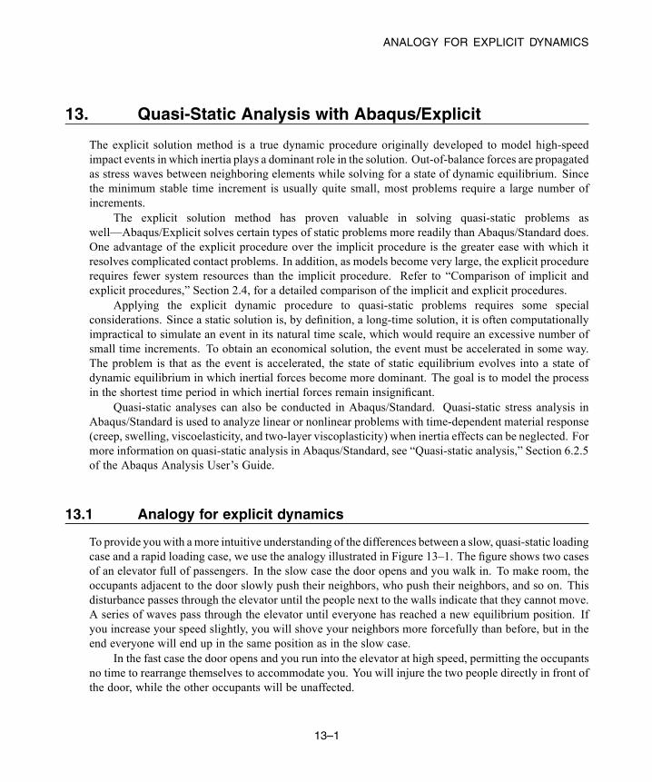
ANALOGY FOR EXPLICIT DYNAMICS
13. Quasi-Static Analysis with Abaqus/Explicit
The explicit solution method is a true dynamic procedure originally developed to model high-speedimpact events in which inertia plays a dominant role in the solution. Out-of-balance forces are propagatedas stress waves between neighboring elements while solving for a state of dynamic equilibrium. Sincethe minimum stable time increment is usually quite small, most problems require a large number ofincrements.
The explicit solution method has proven valuable in solving quasi-static problems aswell—Abaqus/Explicit solves certain types of static problems more readily than Abaqus/Standard does.One advantage of the explicit procedure over the implicit procedure is the greater ease with which itresolves complicated contact problems. In addition, as models become very large, the explicit procedurerequires fewer system resources than the implicit procedure. Refer to “Comparison of implicit andexplicit procedures,” Section 2.4, for a detailed comparison of the implicit and explicit procedures.
Applying the explicit dynamic procedure to quasi-static problems requires some specialconsiderations. Since a static solution is, by definition, a long-time solution, it is often computationallyimpractical to simulate an event in its natural time scale, which would require an excessive number ofsmall time increments. To obtain an economical solution, the event must be accelerated in some way.The problem is that as the event is accelerated, the state of static equilibrium evolves into a state ofdynamic equilibrium in which inertial forces become more dominant. The goal is to model the processin the shortest time period in which inertial forces remain insignificant.
Quasi-static analyses can also be conducted in Abaqus/Standard. Quasi-static stress analysis inAbaqus/Standard is used to analyze linear or nonlinear problems with time-dependent material response(creep, swelling, viscoelasticity, and two-layer viscoplasticity) when inertia effects can be neglected. Formore information on quasi-static analysis in Abaqus/Standard, see “Quasi-static analysis,” Section 6.2.5of the Abaqus Analysis User’s Guide.
13.1 Analogy for explicit dynamics
To provide youwith amore intuitive understanding of the differences between a slow, quasi-static loadingcase and a rapid loading case, we use the analogy illustrated in Figure 13–1. The figure shows two casesof an elevator full of passengers. In the slow case the door opens and you walk in. To make room, theoccupants adjacent to the door slowly push their neighbors, who push their neighbors, and so on. Thisdisturbance passes through the elevator until the people next to the walls indicate that they cannot move.A series of waves pass through the elevator until everyone has reached a new equilibrium position. Ifyou increase your speed slightly, you will shove your neighbors more forcefully than before, but in theend everyone will end up in the same position as in the slow case.
In the fast case the door opens and you run into the elevator at high speed, permitting the occupantsno time to rearrange themselves to accommodate you. You will injure the two people directly in front ofthe door, while the other occupants will be unaffected.
13–1
Abaqus ID:Printed on:
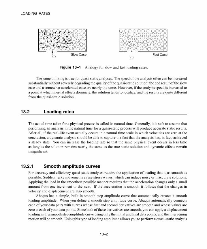
LOADING RATES
Figure 13–1 Analogy for slow and fast loading cases.
The same thinking is true for quasi-static analyses. The speed of the analysis often can be increasedsubstantially without severely degrading the quality of the quasi-static solution; the end result of the slowcase and a somewhat accelerated case are nearly the same. However, if the analysis speed is increased toa point at which inertial effects dominate, the solution tends to localize, and the results are quite differentfrom the quasi-static solution.
13.2 Loading rates
The actual time taken for a physical process is called its natural time. Generally, it is safe to assume thatperforming an analysis in the natural time for a quasi-static process will produce accurate static results.After all, if the real-life event actually occurs in a natural time scale in which velocities are zero at theconclusion, a dynamic analysis should be able to capture the fact that the analysis has, in fact, achieveda steady state. You can increase the loading rate so that the same physical event occurs in less timeas long as the solution remains nearly the same as the true static solution and dynamic effects remaininsignificant.
13.2.1 Smooth amplitude curvesFor accuracy and efficiency quasi-static analyses require the application of loading that is as smooth aspossible. Sudden, jerky movements cause stress waves, which can induce noisy or inaccurate solutions.Applying the load in the smoothest possible manner requires that the acceleration changes only a smallamount from one increment to the next. If the acceleration is smooth, it follows that the changes invelocity and displacement are also smooth.
Abaqus has a simple, built-in smooth step amplitude curve that automatically creates a smoothloading amplitude. When you define a smooth step amplitude curve, Abaqus automatically connectseach of your data pairs with curves whose first and second derivatives are smooth and whose values arezero at each of your data points. Since both of these derivatives are smooth, you can apply a displacementloading with a smooth step amplitude curve using only the initial and final data points, and the interveningmotion will be smooth. Using this type of loading amplitude allows you to perform a quasi-static analysis
13–2
Abaqus ID:Printed on:
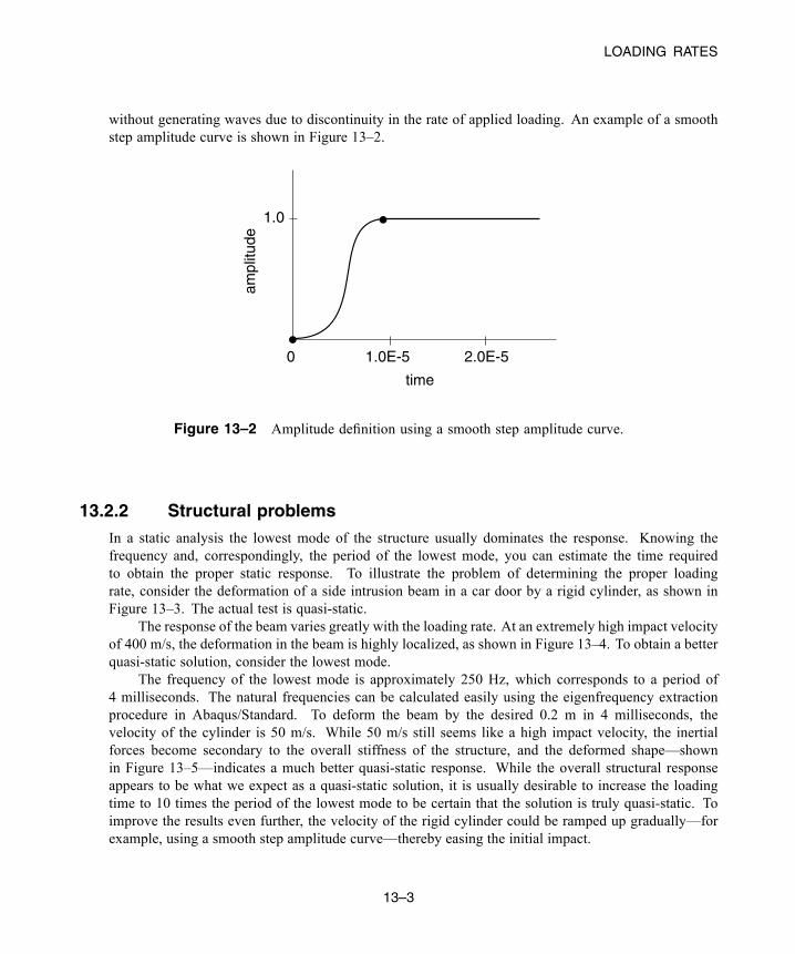
LOADING RATES
without generating waves due to discontinuity in the rate of applied loading. An example of a smoothstep amplitude curve is shown in Figure 13–2.
0
1.0
1.0E-5 2.0E-5
ampl
itude
time
Figure 13–2 Amplitude definition using a smooth step amplitude curve.
13.2.2 Structural problemsIn a static analysis the lowest mode of the structure usually dominates the response. Knowing thefrequency and, correspondingly, the period of the lowest mode, you can estimate the time requiredto obtain the proper static response. To illustrate the problem of determining the proper loadingrate, consider the deformation of a side intrusion beam in a car door by a rigid cylinder, as shown inFigure 13–3. The actual test is quasi-static.
The response of the beam varies greatly with the loading rate. At an extremely high impact velocityof 400 m/s, the deformation in the beam is highly localized, as shown in Figure 13–4. To obtain a betterquasi-static solution, consider the lowest mode.
The frequency of the lowest mode is approximately 250 Hz, which corresponds to a period of4 milliseconds. The natural frequencies can be calculated easily using the eigenfrequency extractionprocedure in Abaqus/Standard. To deform the beam by the desired 0.2 m in 4 milliseconds, thevelocity of the cylinder is 50 m/s. While 50 m/s still seems like a high impact velocity, the inertialforces become secondary to the overall stiffness of the structure, and the deformed shape—shownin Figure 13–5—indicates a much better quasi-static response. While the overall structural responseappears to be what we expect as a quasi-static solution, it is usually desirable to increase the loadingtime to 10 times the period of the lowest mode to be certain that the solution is truly quasi-static. Toimprove the results even further, the velocity of the rigid cylinder could be ramped up gradually—forexample, using a smooth step amplitude curve—thereby easing the initial impact.
13–3
Abaqus ID:Printed on:

LOADING RATES
1
2
3Rigid Cylinder
Fixed BC
Fixed BC
Circular BeamLength = 1 m
Young's Modulus = 200 GPaPoisson's Ratio = 0.3Yield Stress = 250 MPaHardening Modulus = 20 MPaDensity = 7800 Kg/m**3Shell Thickness = 3 mm
Figure 13–3 Rigid cylinder impacting beam.
1
2
3 1
2
3
Figure 13–4 Impact velocity of 400 m/s.
1
2
3 1
2
3
Figure 13–5 Impact velocity of 50 m/s.
13–4
Abaqus ID:Printed on:
LOADING RATES
13.2.3 Metal forming problemsArtificially increasing the speed of forming events is necessary to obtain an economical solution, buthow large a speedup can we impose and still obtain an acceptable static solution? If the deformationof the sheet metal blank corresponds to the deformed shape of the lowest mode, the time period of thelowest structural mode can be used as a guideline for forming speed. However, in forming processes therigid dies and punches can constrain the blank in such a way that its deformation may not relate to thestructural modes. In such cases a general recommendation is to limit punch speeds to less than 1% of thesheet metal wave speed. For typical processes the punch speed is on the order of 1 m/s, while the wavespeed of steel is approximately 5000 m/s. This recommendation, therefore, suggests a factor of 50 as anupper bound on the speedup of the punch velocity.
The suggested approach to determining an acceptable punch velocity involves running a series ofanalyses at various punch speeds in the range of 3 to 50 m/s. Perform the analyses in the order of fastestto slowest since the solution time is inversely proportional to the punch velocity. Examine the results ofthe analyses, and get a feel for how the deformed shapes, stresses, and strains vary with punch speed.Some indications of excessive punch speeds are unrealistic, localized stretching and thinning as well asthe suppression of wrinkling. If you begin with a punch speed of, for example, 50 m/s, and decreaseit from there, at some point the solutions will become similar from one punch speed to the next—anindication that the solutions are converging on a quasi-static solution. As inertial effects become lesssignificant, differences in simulation results also become less significant.
As the loading rate is increased artificially, it becomes more and more important to apply the loadsin a gradual and smooth manner. For example, the simplest way to load the punch is to impose aconstant velocity throughout the forming step. Such a loading causes a sudden impact load onto thesheet metal blank at the start of the analysis, which propagates stress waves through the blank and mayproduce undesired results. The effect of any impact load on the results becomes more pronounced as theloading rate is increased. Ramping up the punch velocity from zero using a smooth step amplitude curveminimizes these adverse effects.
Springback
Springback is often an important part of a forming analysis because the springback analysisdetermines the shape of the final, unloaded part. While Abaqus/Explicit is well-suited for formingsimulations, springback poses some special difficulties. The main problem with performingspringback simulations within Abaqus/Explicit is the amount of time required to obtain asteady-state solution. Typically, the loads must be removed very carefully, and damping mustbe introduced to make the solution time reasonable. Fortunately, the close relationship betweenAbaqus/Explicit and Abaqus/Standard allows a much more efficient approach.
Since springback involves no contact and usually includes only mild nonlinearities,Abaqus/Standard can solve springback problems much faster than Abaqus/Explicit can. Therefore,the preferred approach to springback analyses is to import the completed forming model fromAbaqus/Explicit into Abaqus/Standard.
13–5
Abaqus ID:Printed on:

MASS SCALING
13.3 Mass scaling
Mass scaling enables an analysis to be performed economically without artificially increasing the loadingrate. Mass scaling is the only option for reducing the solution time in simulations involving a rate-dependent material or rate-dependent damping, such as dashpots. In such simulations increasing theloading rate is not an option because material strain rates increase by the same factor as the loadingrate. When the properties of the model change with the strain rate, artificially increasing the loading rateartificially changes the process.
The following equations show how the stable time increment is related to the material density.As discussed in “Definition of the stability limit,” Section 9.3.2, the stability limit for the model is theminimum stable time increment of all elements. It can be expressed as
where is the characteristic element length and is the dilatational wave speed of the material. Thedilatational wave speed for a linear elastic material with Poisson’s ratio equal to zero is given by
where is the material density.
According to the above equations, artificially increasing the material density, , by a factor ofdecreases the wave speed by a factor of and increases the stable time increment by a factor of .Remember that when the global stability limit is increased, fewer increments are required to performthe same analysis, which is the goal of mass scaling. Scaling the mass, however, has exactly the sameinfluence on inertial effects as artificially increasing the loading rate. Therefore, excessive mass scaling,just like excessive loading rates, can lead to erroneous solutions. The suggested approach to determiningan acceptable mass scaling factor, then, is similar to the approach to determining an acceptable loadingrate scaling factor. The only difference to the approach is that the speedup associated with mass scalingis the square root of the mass scaling factor, whereas the speedup associated with loading rate scalingis proportional to the loading rate scaling factor. For example, a mass scaling factor of 100 correspondsexactly to a loading rate scaling factor of 10.
There are several ways to implement mass scaling in your model using either fixed or variable massscaling. The mass scaling definition can be changed from step to step, allowing great flexibility. Referto “Mass scaling,” Section 11.6.1 of the Abaqus Analysis User’s Guide, for details.
13–6
Abaqus ID:Printed on:
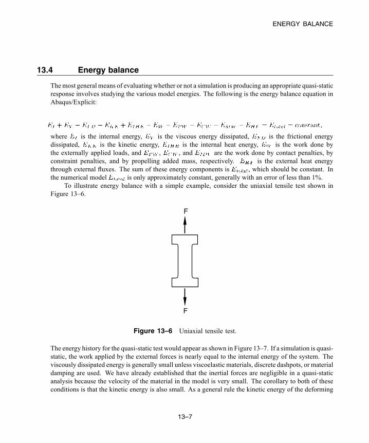
ENERGY BALANCE
13.4 Energy balance
Themost general means of evaluating whether or not a simulation is producing an appropriate quasi-staticresponse involves studying the various model energies. The following is the energy balance equation inAbaqus/Explicit:
where is the internal energy, is the viscous energy dissipated, is the frictional energydissipated, is the kinetic energy, is the internal heat energy, is the work done bythe externally applied loads, and , , and are the work done by contact penalties, byconstraint penalties, and by propelling added mass, respectively. is the external heat energythrough external fluxes. The sum of these energy components is , which should be constant. Inthe numerical model is only approximately constant, generally with an error of less than 1%.
To illustrate energy balance with a simple example, consider the uniaxial tensile test shown inFigure 13–6.
F
F
Figure 13–6 Uniaxial tensile test.
The energy history for the quasi-static test would appear as shown in Figure 13–7. If a simulation is quasi-static, the work applied by the external forces is nearly equal to the internal energy of the system. Theviscously dissipated energy is generally small unless viscoelastic materials, discrete dashpots, or materialdamping are used. We have already established that the inertial forces are negligible in a quasi-staticanalysis because the velocity of the material in the model is very small. The corollary to both of theseconditions is that the kinetic energy is also small. As a general rule the kinetic energy of the deforming
13–7
Abaqus ID:Printed on:

EXAMPLE: FORMING A CHANNEL IN Abaqus/Explicit
ener
gy
EW
EI
ETOT, EKE FD, EV
time
, E
Figure 13–7 Energy history for quasi-static tensile test.
material should not exceed a small fraction (typically 5% to 10%) of its internal energy throughout mostof the process.
When comparing the energies, remember that Abaqus/Explicit reports a global energy balance,which includes the kinetic energy of any rigid bodies with mass. Since only the deformable bodies areof interest when evaluating the results, the kinetic energy of the rigid bodies should be subtracted from
when evaluating the energy balance.For example, if you are simulating a transport problem with rolling rigid dies, the kinetic energy
of the rigid bodies may be a significant portion of the total kinetic energy of the model. In such casesyou must subtract the kinetic energy associated with rigid body motions before a meaningful comparisonwith internal energy can be made.
13.5 Example: forming a channel in Abaqus/Explicit
In this example you will solve the channel forming problem from Chapter 12, “Contact,” usingAbaqus/Explicit. You will then compare the results from the Abaqus/Standard and Abaqus/Explicitanalyses.
You will make modifications to the model created for the Abaqus/Standard analysis so that youare able to run it in Abaqus/Explicit. These modifications include adding density to the material model,changing the element library, and changing the steps. Before running the Abaqus/Explicit analysis, youwill use the frequency extraction procedure in Abaqus/Standard to determine the time period required toobtain a proper quasi-static response.
13.5.1 Preprocessing—rerunning the model with Abaqus/ExplicitUse Abaqus/CAE to modify the model for this simulation. Abaqus provides scripts that replicate thecomplete analysis model for this problem. Run one of these scripts if you encounter difficulties following
13–8
Abaqus ID:Printed on:
EXAMPLE: FORMING A CHANNEL IN Abaqus/Explicit
the instructions given below or if you wish to check your work. Scripts are available in the followinglocations:
• A Python script for this example is provided in “Forming a channel,” Section A.12, in the HTMLversion of this guide. Instructions on how to fetch the script and run it within Abaqus/CAE aregiven in Appendix A, “Example Files.”
• A plug-in script for this example is available in the Abaqus/CAE Plug-in toolset. To run the scriptfrom Abaqus/CAE, select Plug-ins→Abaqus→Getting Started; highlight Forming a channel;and click Run. For more information about the Getting Started plug-ins, see “Running the GettingStarted with Abaqus examples,” Section 82.1 of the Abaqus/CAE User’s Guide, in the HTMLversion of this guide.
Before starting, open the model database file for the channel forming example created in“Abaqus/Standard 2D example: forming a channel,” Section 12.6.
Determining an appropriate step time
“Loading rates,” Section 13.2, discusses the procedures for determining the appropriate step timefor a quasi-static process. We can determine an approximate lower bound on step time duration ifwe know the lowest natural frequency, the fundamental frequency, of the blank. One way to obtainsuch information is to run a frequency analysis in Abaqus/Standard. In this forming analysis thepunch deforms the blank into a shape similar to the lowest mode. Therefore, it is important that thetime for the forming stage is greater than or equal to the time period for the lowest mode if you wishto model structural, as opposed to localized, deformation.
To perform a natural frequency extraction:
1. Copy the existing model to a model named Frequency. Make all of the following changes tothe Frequencymodel. In the frequency extraction analysis you will replace all existing stepswith a single frequency extraction step. In addition, you will delete all of the rigid body toolsand contact interactions; they are not necessary for determining the fundamental frequency ofthe blank.
2. Add a density of 7800 to the material model Steel.
3. Delete the die, holder, and punch part instances. These rigid parts are not necessary for thefrequency analysis.
Tip: You can delete any part instance using theModel Tree by expanding Instancesunderneath the Assembly container, clicking mouse button 3 on the instance name,and selecting Delete from the menu that appears.
4. Replace the existing steps with a single frequency extraction step.
a. Delete the step Move punch.
b. In theModel Tree, click mouse button 3 on the step Holder force and selectReplacefrom the menu that appears.
13–9
Abaqus ID:Printed on:

EXAMPLE: FORMING A CHANNEL IN Abaqus/Explicit
c. In the Replace Step dialog box, select Frequency from the list of available Linearperturbation procedures. Enter the step description Frequency modes; select theLanczos eigensolver option; and request five eigenvalues. Rename the step ExtractFrequencies.
d. Suppress the DOF Monitor.
Note: Since the frequency extraction step is a linear perturbation procedure, nonlinearmaterial properties will be ignored. In this analysis the left end of the blank is constrainedin the x-direction and cannot rotate about the normal; however, it is not constrained in they-direction. Therefore, the first mode extracted will be a rigid body mode. The frequency ofthe second mode will determine the appropriate time period for the quasi-static analysis inAbaqus/Explicit.
5. Delete all contact interactions.
6. Open the Boundary Condition Manager, and examine the boundary conditions in theExtract Frequencies step. Delete all boundary conditions except the boundarycondition named CenterBC. This leaves the blank constrained with a symmetry boundarycondition applied to the left end.
7. Remesh the blank if necessary.
8. Create a job named Forming-Frequency with the following job description: Channelforming -- frequency analysis. Submit the job for analysis, and monitor thesolution progress.
9. When the analysis is complete, enter the Visualization module and open the output databasefile created by this job. From the main menu bar, select Plot→Deformed Shape; or use the
tool in the toolbox.
The deformed model shape for the first vibration mode is plotted (it is a rigid body mode).Advance the plot to the second mode of the blank. Superimpose the undeformed model shape onthe deformed model shape.
The frequency analysis shows that the blank has a fundamental frequency of 140 Hz,corresponding to a period of 0.00714 s. Figure 13–8 shows the displaced shape of the secondmode. We now know that the shortest step time for the forming analysis is 0.00714 s.
Creating the Abaqus/Explicit forming analysis
The goal of the forming process is to quasi-statically form a channel with a punch displacementof 0.03 m. In selecting loading rates for quasi-static analyses, it is recommended that you beginwith faster loading rates and decrease the loading rates as necessary to converge on a quasi-staticsolution more quickly. However, if you wish to increase the likelihood of a quasi-static resultin your first analysis attempt, you should consider step times that are a factor of 10 to 50 timesslower than that corresponding to the fundamental frequency. In this analysis you will start witha time period of 0.007 s for the forming analysis step, which is based on the frequency analysis
13–10
Abaqus ID:Printed on:
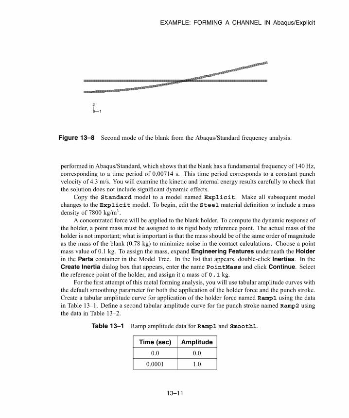
EXAMPLE: FORMING A CHANNEL IN Abaqus/Explicit
1
2
3
Figure 13–8 Second mode of the blank from the Abaqus/Standard frequency analysis.
performed in Abaqus/Standard, which shows that the blank has a fundamental frequency of 140 Hz,corresponding to a time period of 0.00714 s. This time period corresponds to a constant punchvelocity of 4.3 m/s. You will examine the kinetic and internal energy results carefully to check thatthe solution does not include significant dynamic effects.
Copy the Standard model to a model named Explicit. Make all subsequent modelchanges to the Explicit model. To begin, edit the Steel material definition to include a massdensity of 7800 kg/m3.
A concentrated force will be applied to the blank holder. To compute the dynamic response ofthe holder, a point mass must be assigned to its rigid body reference point. The actual mass of theholder is not important; what is important is that the mass should be of the same order of magnitudeas the mass of the blank (0.78 kg) to minimize noise in the contact calculations. Choose a pointmass value of 0.1 kg. To assign the mass, expand Engineering Features underneath the Holderin the Parts container in the Model Tree. In the list that appears, double-click Inertias. In theCreate Inertia dialog box that appears, enter the name PointMass and click Continue. Selectthe reference point of the holder, and assign it a mass of 0.1 kg.
For the first attempt of this metal forming analysis, you will use tabular amplitude curves withthe default smoothing parameter for both the application of the holder force and the punch stroke.Create a tabular amplitude curve for application of the holder force named Ramp1 using the datain Table 13–1. Define a second tabular amplitude curve for the punch stroke named Ramp2 usingthe data in Table 13–2.
Table 13–1 Ramp amplitude data for Ramp1 and Smooth1.
Time (sec) Amplitude
0.0 0.0
0.0001 1.0
13–11
Abaqus ID:Printed on:

EXAMPLE: FORMING A CHANNEL IN Abaqus/Explicit
Table 13–2 Ramp amplitude data for Ramp2 and Smooth2.
Time (sec) Amplitude
0.0 0.0
0.007 1.0
As with the Abaqus/Standard analysis, you will need two steps for the Abaqus/Explicitanalysis. In the first step the holder force is applied; in the second step the punch stroke is applied.Delete the step named Move punch. Replace the step named Holder force with an explicitdynamics step, and specify a time period of 0.0001 s. This time period is appropriate for theapplication of the holder force because it is long enough to avoid dynamic effects but short enoughto prevent a significant impact on the run time for the job. Enter Apply holder force as thestep description. Create a second explicit dynamics step named Move punch with a time periodof 0.007 s. Enter Apply punch stroke as the step description.
To help determine how closely the analysis approximates the quasi-static assumption, thevarious energy histories will be useful. Especially useful is comparing the kinetic energy to theinternal strain energy. The energy history is written to the output database file by default. Modifythe history output request for the punch reference node to request output at 200 evenly spacedintervals using the built-in antialiasing filter.
Open the Load Manager, and modify the concentrated force named RefHolderForce inthe step named Holder force so that the amplitude definition for this load is set to Ramp1.
Change the displacement boundary condition RefPunchBC in the Move punch step so thatU2 is set to –0.03 m in the step. Use the amplitude curve Ramp2 for this boundary condition.
Monitoring the value of a degree of freedom
In this model you will monitor the vertical displacement (degree of freedom 2) of the punch’sreference node throughout the step. Because the DOF Monitor was set to monitor the verticaldisplacement of RefPunch in the Abaqus/Standard forming analysis, you do not need to makeany changes.
Mesh creation and job definition
Change the family of the elements used to mesh the blank to Explicit, and specify enhancedhourglass control.
Create a job named Forming-1. Give the job the following description: Channelforming -- attempt 1.
Before you run the forming analysis, you may wish to know how many increments the analysiswill take and, consequently, how much computer time the analysis requires. You can use the Verify
Mesh tool to obtain an estimate of the stable time increment (the option is located in the SizeMetrics tabbed page of the Verify Mesh dialog box). Knowing the stable time increment, which
13–12
Abaqus ID:Printed on:
EXAMPLE: FORMING A CHANNEL IN Abaqus/Explicit
in this case does not change much from increment to increment, you can determine how manyincrements are required to complete the forming stage. Once the analysis begins, you can get anidea of how much CPU time is required per increment and, consequently, how much CPU time theanalysis requires.
The stable time increment for this analysis is approximately 3.5 × 10⁻⁸ s. Therefore, theforming stage requires approximately 200,000 increments for a step time of 0.007 s.
Save your model to a model database file, and submit the job for analysis. Monitor the solutionprogress; correct any modeling errors that are detected, and investigate the cause of any warningmessages.
Once the analysis is underway, an X–Y plot of the values of the degree of freedom that youselected to monitor (the punch’s vertical displacement) appears in a separate viewport. From themain menu bar, select Viewport→Job Monitor: Forming-1 to follow the progression of thepunch’s displacement in the 2-direction over time as the analysis runs.
Strategy for evaluating the results
Before looking at the results that are ultimately of interest, such as stresses and deformed shapes, weneed to determine whether or not the solution is quasi-static. One good approach is to compare thekinetic energy history to the internal energy history. In a metal forming analysis most of the internalenergy is due to plastic deformation. In this model the blank is the primary source of kinetic energy(the motion of the holder is negligible, and the punch and die have no mass associated with them).To determine whether an acceptable quasi-static solution has been obtained, the kinetic energy of theblank should be no greater than a few percent of its internal energy. For greater accuracy, especiallywhen springback stresses are of interest, the kinetic energy should be lower. This approach is veryuseful because it applies to all types of metal forming processes and does not require any intuitiveunderstanding of the stresses in the model; many forming processes may be too complex to permitan intuitive feel for the results.
While a good primary indication of the caliber of a quasi-static analysis, the ratio of kineticenergy to internal energy alone is not adequate to confirm the quality. You should also evaluate thetwo energies independently to determine whether they are reasonable. This part of the evaluationtakes on increased importance when accurate springback stress results are needed because anaccurate springback stress solution is highly dependent on accurate plasticity results. Even if thekinetic energy is fairly small, if it contains large oscillations, the model could be experiencingsignificant plasticity. Generally, we expect smooth loading to produce smooth results; if theloading is smooth but the energy results are oscillatory, the results may be inadequate. Sincean energy ratio is incapable of showing such behavior, you should also study the kinetic energyhistory itself to see whether it is smooth or noisy.
If the kinetic energy does not indicate quasi-static behavior, it can be useful to look at velocityhistories at some nodes to get an understanding of the model’s behavior in various regions. Suchvelocity histories can indicate which regions of themodel are oscillating and causing the high kineticenergies.
13–13
Abaqus ID:Printed on:
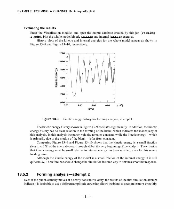
EXAMPLE: FORMING A CHANNEL IN Abaqus/Explicit
Evaluating the results
Enter the Visualization module, and open the output database created by this job (Forming-1.odb). Plot the whole model kinetic (ALLKE) and internal (ALLIE) energies.
History plots of the kinetic and internal energies for the whole model appear as shown inFigure 13–9 and Figure 13–10, respectively.
Figure 13–9 Kinetic energy history for forming analysis, attempt 1.
The kinetic energy history shown in Figure 13–9 oscillates significantly. In addition, the kineticenergy history has no clear relation to the forming of the blank, which indicates the inadequacy ofthis analysis. In this analysis the punch velocity remains constant, while the kinetic energy—whichis primarily due to the motion of the blank—is far from constant.
Comparing Figure 13–9 and Figure 13–10 shows that the kinetic energy is a small fraction(less than 1%) of the internal energy through all but the very beginning of the analysis. The criterionthat kinetic energy must be small relative to internal energy has been satisfied, even for this severeloading case.
Although the kinetic energy of the model is a small fraction of the internal energy, it is stillquite noisy. Therefore, we should change the simulation in some way to obtain a smoother response.
13.5.2 Forming analysis—attempt 2Even if the punch actually moves at a nearly constant velocity, the results of the first simulation attemptindicate it is desirable to use a different amplitude curve that allows the blank to acceleratemore smoothly.
13–14
Abaqus ID:Printed on:

EXAMPLE: FORMING A CHANNEL IN Abaqus/Explicit
Figure 13–10 Internal energy history for forming analysis, attempt 1.
When considering what type of loading amplitude to use, remember that smoothness is important in allaspects of a quasi-static analysis. The preferred approach is to move the punch as smoothly as possiblethe desired distance in the desired amount of time.
Wewill now analyze the forming stage using a smoothly applied holder force and a smoothly appliedpunch displacement; we will compare the results to those obtained earlier. Refer to “Smooth amplitudecurves,” Section 13.2.1, for an explanation of the smooth step amplitude curve.
Define a smooth step amplitude curve named Smooth1. Enter the amplitude data given inTable 13–1. Create a second smooth step amplitude curve named Smooth2 using the amplitude datagiven in Table 13–2. Modify the RefHolderForce load in the Holder force step so that itrefers to the Smooth1 amplitude. Modify the displacement boundary condition RefPunchBC in theMove punch step so that it refers to the Smooth2 amplitude. By specifying an amplitude of 0.0 atthe beginning of the step and an amplitude of 1.0 at the end of the step, Abaqus/Explicit creates anamplitude definition that is smooth in both its first and second derivatives. Therefore, using a smoothstep amplitude curve for the displacement control also assures us that the velocity and acceleration aresmooth.
Create a job named Forming-2. Give the job the following description: Channel forming-- attempt 2.
Save your model, and submit the job for analysis. Monitor the solution progress; correct anymodeling errors that are detected, and investigate the cause of any warning messages.
Evaluating the results for attempt 2
The kinetic energy history is shown in Figure 13–11. The response of the kinetic energy is clearlyrelated to the forming of the blank: the value of kinetic energy peaks in the middle of the second
13–15
Abaqus ID:Printed on:

EXAMPLE: FORMING A CHANNEL IN Abaqus/Explicit
step, corresponding to the time when the punch velocity is the greatest. Thus, the kinetic energy isappropriate and reasonable.
Figure 13–11 Kinetic energy history for forming analysis, attempt 2.
The internal energy for attempt 2, shown in Figure 13–12, shows a smooth increase from zeroup to the final value. Again, the ratio of kinetic energy to internal energy is quite small and appearsto be acceptable. Figure 13–13 compares the internal energy in the two forming attempts.
13.5.3 Discussion of the two forming attempts
Our initial criteria for evaluating the acceptability of the results was that the kinetic energy should besmall compared to the internal energy. What we found was that even for the most severe case, attempt 1,this condition seems to have been met adequately. The addition of a smooth step amplitude curve helpedreduce the oscillations in the kinetic energy, yielding a satisfactory quasi-static response.
The additional requirements—that the histories of kinetic energy and internal energy must beappropriate and reasonable—are very useful and necessary, but they also increase the subjectivity ofevaluating the results. Enforcing these requirements in general for more complex forming processesmay be difficult because these requirements demand some intuition regarding the behavior of theforming process.
13–16
Abaqus ID:Printed on:
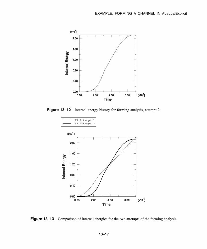
EXAMPLE: FORMING A CHANNEL IN Abaqus/Explicit
Figure 13–12 Internal energy history for forming analysis, attempt 2.
IE Attempt 1IE Attempt 2
Figure 13–13 Comparison of internal energies for the two attempts of the forming analysis.
13–17
Abaqus ID:Printed on:
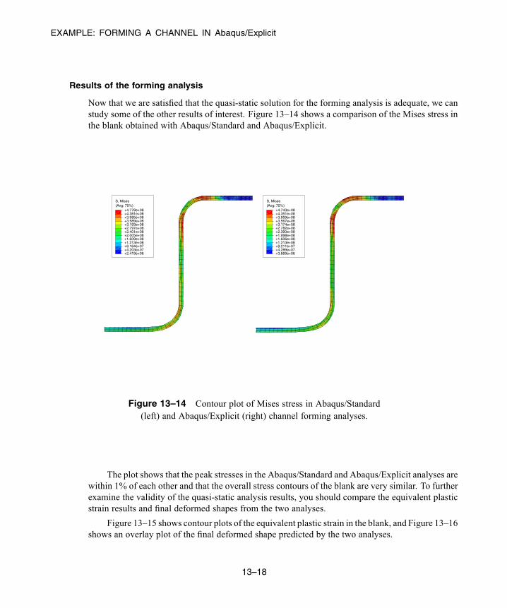
EXAMPLE: FORMING A CHANNEL IN Abaqus/Explicit
Results of the forming analysis
Now that we are satisfied that the quasi-static solution for the forming analysis is adequate, we canstudy some of the other results of interest. Figure 13–14 shows a comparison of the Mises stress inthe blank obtained with Abaqus/Standard and Abaqus/Explicit.
(Avg: 75%)S, Mises
+3.669e+06+4.289e+07+8.211e+07+1.213e+08+1.606e+08+1.998e+08+2.390e+08+2.782e+08+3.174e+08+3.567e+08+3.959e+08+4.351e+08+4.743e+08
(Avg: 75%)S, Mises
+2.419e+06+4.203e+07+8.164e+07+1.213e+08+1.609e+08+2.005e+08+2.401e+08+2.797e+08+3.193e+08+3.589e+08+3.985e+08+4.381e+08+4.778e+08
Figure 13–14 Contour plot of Mises stress in Abaqus/Standard(left) and Abaqus/Explicit (right) channel forming analyses.
The plot shows that the peak stresses in the Abaqus/Standard and Abaqus/Explicit analyses arewithin 1% of each other and that the overall stress contours of the blank are very similar. To furtherexamine the validity of the quasi-static analysis results, you should compare the equivalent plasticstrain results and final deformed shapes from the two analyses.
Figure 13–15 shows contour plots of the equivalent plastic strain in the blank, and Figure 13–16shows an overlay plot of the final deformed shape predicted by the two analyses.
13–18
Abaqus ID:Printed on:

EXAMPLE: FORMING A CHANNEL IN Abaqus/Explicit
(Avg: 75%)PEEQ
+0.000e+00+1.925e−02+3.851e−02+5.776e−02+7.701e−02+9.627e−02+1.155e−01+1.348e−01+1.540e−01+1.733e−01+1.925e−01+2.118e−01+2.310e−01
(Avg: 75%)PEEQ
+0.000e+00+2.089e−02+4.178e−02+6.268e−02+8.357e−02+1.045e−01+1.254e−01+1.462e−01+1.671e−01+1.880e−01+2.089e−01+2.298e−01+2.507e−01
Figure 13–15 Contour plot of PEEQ in Abaqus/Standard (left)and Abaqus/Explicit (right) channel forming analyses.
Figure 13–16 Final deformed shape in Abaqus/Standardand Abaqus/Explicit forming analyses.
13–19
Abaqus ID:Printed on:
EXAMPLE: FORMING A CHANNEL IN Abaqus/Explicit
The equivalent plastic strain results for the Abaqus/Standard and Abaqus/Explicit analyses arewithin 5% of each other. In addition, the final deformed shape comparison shows that the explicitquasi-static analysis results are in excellent agreement with the results from the Abaqus/Standardstatic analysis.
You should also compare the steady punch force predicted by the Abaqus/Standard andAbaqus/Explicit analyses.
To compare the punch force-displacement histories:
1. Save the punch displacement (U2) and reaction force (RF2) history data from theAbaqus/Standard analysis as U2–std and RF2–std, respectively.
2. Similarly, save punch displacement (U2) and reaction force (RF2) history data from theAbaqus/Explicit analysis as U2–xpl and RF2–xpl, respectively.
Next, you will operate on saved X–Y data to create the force-displacement curves. In the force-displacement plot we would like the downward motion of the punch to be represented as apositive value; therefore, when you create the force-displacement curves include a negativesign before the displacement history data so that motion in the negative 2-direction will bepositive.
3. In the Results Tree, double-click XYData; then select Operate on XY data in the Create XYData dialog box. Click Continue.
4. In theOperate on XY Data dialog box, combine the force and displacement history data fromthe Abaqus/Standard analysis to create a force-displacement curve. The expression at the topof the dialog box should appear as:
combine ( -"U2-std", "RF2-std" )
5. Click Save As to save the calculated displacement curve as forceDisp-std.
6. In theOperate on XY Data dialog box, combine the force and displacement history data fromthe Abaqus/Explicit analysis to create a force-displacement curve. The expression at the topof the dialog box should appear as:
combine ( -"U2-xpl", "RF2-xpl" )
7. Click Save As to save the calculated displacement curve as forceDisp-xpl.
8. Plot forceDisp-std and forceDisp-xpl in the viewport.
There is significantly more noise in the Abaqus/Explicit results compared to theAbaqus/Standard results because Abaqus/Explicit simulates a quasi-static response whileAbaqus/Standard solves for true static equilibrium. Some of the noise in the Abaqus/Explicithistory data was removed during the analysis by the built-in antialiasing filter specified onthe output request. Now, you will use an Abaqus/CAE X–Y data filter to remove more of thesolution noise from the Abaqus/Explicit force-displacement curve. The Abaqus/CAE X–Y
13–20
Abaqus ID:Printed on:

EXAMPLE: FORMING A CHANNEL IN Abaqus/Explicit
data filters should only be applied to X–Y data whose X-value is time. This avoids confusionregarding the meaning of the filter cutoff frequency and prevents problems with the dataregularization that is performed internally before the filter is applied. Consequently, youwill not filter forceDisp-xpl directly, but rather you will filter U2-xpl and RF2-xplindividually before combining them to create a new force-displacement curve. It is best toapply the same filter operations (both during the analysis and during postprocessing) to anytwo X–Y data objects that will be combined. This will ensure that any distortions due tofiltering (such as time delays) are uniformly applied to the combined data.
9. In the Operate on XY Data dialog box, filter the force history data using a Butterworth filterwith a cutoff frequency of 1100 Hz. The expression at the top of the dialog box should appearas:
butterworthFilter(xyData="RF2-xpl",cutoffFrequency=1100)
Note: Choosing an appropriate filter cutoff frequency takes engineering judgment and a goodunderstanding of the physical system being modeled. Often an iterative approach (beginningwith a relatively high cutoff frequency and then gradually reducing it) can be used to find acutoff frequency that removes solution noise withminimal distortion of the underlying physicalsolution. Knowledge of the system’s natural frequencies can also assist in the determination ofappropriate filter cutoff frequencies. For this example, we performed a frequency extractionanalysis to determine the fundamental frequency of the undeformed blank (140 Hz); however,the blank at the end of the forming step will have a fundamental frequency that is considerablyhigher. If you perform a natural frequency extraction analysis on the final model configuration,you will find that the fundamental frequency at the end of the forming step is approximately1000 Hz. Hence, a cutoff frequency that is slightly larger than this value is a good choice forthis model.
10. Click Save As to save the calculated displacement curve as RF2-xpl-bw1100.
11. Similarly, filter the displacement history data using a Butterworth filter with a cutoff frequencyof 1100 Hz. The expression at the top of the Operate on XY Data dialog box should appearas:
butterworthFilter(xyData="U2-xpl",cutoffFrequency=1100)
12. Click Save As to save the calculated displacement curve as U2-xpl-bw1100.
13. Combine the filtered Abaqus/Explicit force and displacement histories. The expression at thetop of the Operate on XY Data dialog box should appear as:
combine ( -"U2-xpl-bw1100", "RF2-xpl-bw1100" )
14. Click Save As to save the calculated displacement curve as forceDisp-xpl-bw1100.
15. Add forceDisp-xpl-bw1100 to the plot of forceDisp-std and forceDisp-xpl.Customize the plot appearance to obtain a plot similar to Figure 13–17.
13–21
Abaqus ID:Printed on:
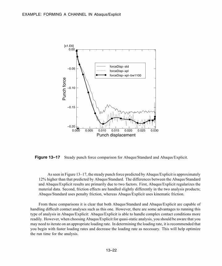
EXAMPLE: FORMING A CHANNEL IN Abaqus/Explicit
Punch displacement0.000 0.005 0.010 0.015 0.020 0.025 0.030
Pun
ch fo
rce
−0.20
−0.15
−0.10
−0.05
0.00[x1.E6]
forceDisp−stdforceDisp−xplforceDisp−xpl−bw1100
Figure 13–17 Steady punch force comparison for Abaqus/Standard and Abaqus/Explicit.
As seen in Figure 13–17, the steady punch force predicted byAbaqus/Explicit is approximately12% higher than that predicted by Abaqus/Standard. The differences between the Abaqus/Standardand Abaqus/Explicit results are primarily due to two factors. First, Abaqus/Explicit regularizes thematerial data. Second, friction effects are handled slightly differently in the two analysis products;Abaqus/Standard uses penalty friction, whereas Abaqus/Explicit uses kinematic friction.
From these comparisons it is clear that both Abaqus/Standard and Abaqus/Explicit are capable ofhandling difficult contact analyses such as this one. However, there are some advantages to running thistype of analysis in Abaqus/Explicit: Abaqus/Explicit is able to handle complex contact conditions morereadily. However, when choosing Abaqus/Explicit for quasi-static analysis, you should be aware that youmay need to iterate on an appropriate loading rate. In determining the loading rate, it is recommended thatyou begin with faster loading rates and decrease the loading rate as necessary. This will help optimizethe run time for the analysis.
13–22
Abaqus ID:Printed on:
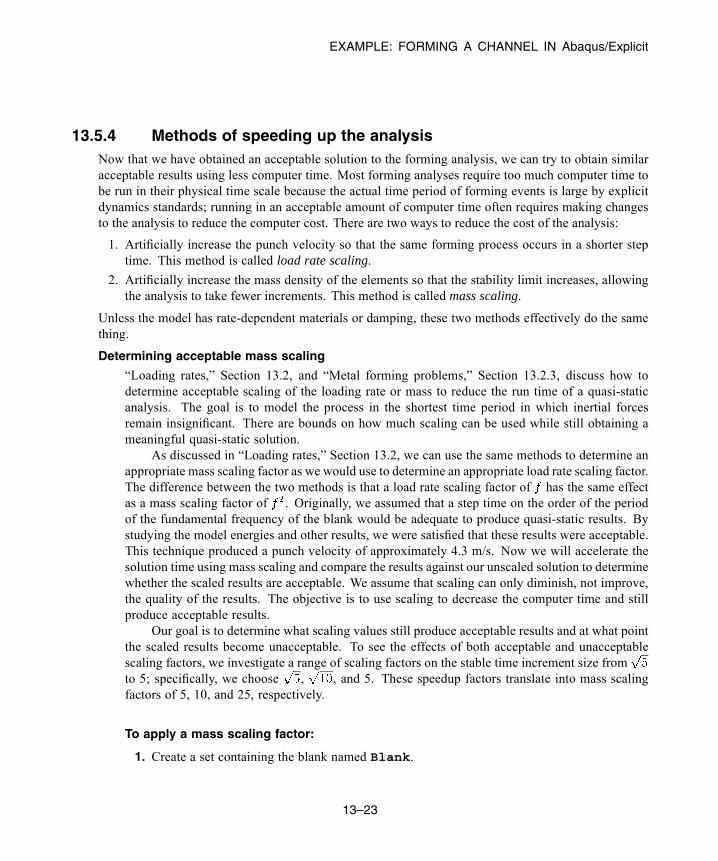
EXAMPLE: FORMING A CHANNEL IN Abaqus/Explicit
13.5.4 Methods of speeding up the analysisNow that we have obtained an acceptable solution to the forming analysis, we can try to obtain similaracceptable results using less computer time. Most forming analyses require too much computer time tobe run in their physical time scale because the actual time period of forming events is large by explicitdynamics standards; running in an acceptable amount of computer time often requires making changesto the analysis to reduce the computer cost. There are two ways to reduce the cost of the analysis:
1. Artificially increase the punch velocity so that the same forming process occurs in a shorter steptime. This method is called load rate scaling.
2. Artificially increase the mass density of the elements so that the stability limit increases, allowingthe analysis to take fewer increments. This method is called mass scaling.
Unless the model has rate-dependent materials or damping, these two methods effectively do the samething.
Determining acceptable mass scaling
“Loading rates,” Section 13.2, and “Metal forming problems,” Section 13.2.3, discuss how todetermine acceptable scaling of the loading rate or mass to reduce the run time of a quasi-staticanalysis. The goal is to model the process in the shortest time period in which inertial forcesremain insignificant. There are bounds on how much scaling can be used while still obtaining ameaningful quasi-static solution.
As discussed in “Loading rates,” Section 13.2, we can use the same methods to determine anappropriate mass scaling factor as we would use to determine an appropriate load rate scaling factor.The difference between the two methods is that a load rate scaling factor of has the same effectas a mass scaling factor of . Originally, we assumed that a step time on the order of the periodof the fundamental frequency of the blank would be adequate to produce quasi-static results. Bystudying the model energies and other results, we were satisfied that these results were acceptable.This technique produced a punch velocity of approximately 4.3 m/s. Now we will accelerate thesolution time using mass scaling and compare the results against our unscaled solution to determinewhether the scaled results are acceptable. We assume that scaling can only diminish, not improve,the quality of the results. The objective is to use scaling to decrease the computer time and stillproduce acceptable results.
Our goal is to determine what scaling values still produce acceptable results and at what pointthe scaled results become unacceptable. To see the effects of both acceptable and unacceptablescaling factors, we investigate a range of scaling factors on the stable time increment size fromto 5; specifically, we choose , , and 5. These speedup factors translate into mass scalingfactors of 5, 10, and 25, respectively.
To apply a mass scaling factor:
1. Create a set containing the blank named Blank.
13–23
Abaqus ID:Printed on:
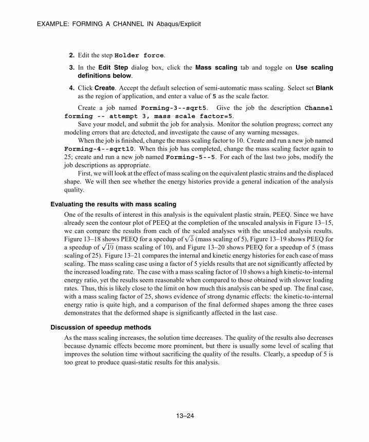
EXAMPLE: FORMING A CHANNEL IN Abaqus/Explicit
2. Edit the step Holder force.
3. In the Edit Step dialog box, click the Mass scaling tab and toggle on Use scalingdefinitions below.
4. Click Create. Accept the default selection of semi-automatic mass scaling. Select set Blankas the region of application, and enter a value of 5 as the scale factor.
Create a job named Forming-3--sqrt5. Give the job the description Channelforming -- attempt 3, mass scale factor=5.
Save your model, and submit the job for analysis. Monitor the solution progress; correct anymodeling errors that are detected, and investigate the cause of any warning messages.
When the job is finished, change the mass scaling factor to 10. Create and run a new job namedForming-4--sqrt10. When this job has completed, change the mass scaling factor again to25; create and run a new job named Forming-5--5. For each of the last two jobs, modify thejob descriptions as appropriate.
First, wewill look at the effect ofmass scaling on the equivalent plastic strains and the displacedshape. We will then see whether the energy histories provide a general indication of the analysisquality.
Evaluating the results with mass scaling
One of the results of interest in this analysis is the equivalent plastic strain, PEEQ. Since we havealready seen the contour plot of PEEQ at the completion of the unscaled analysis in Figure 13–15,we can compare the results from each of the scaled analyses with the unscaled analysis results.Figure 13–18 shows PEEQ for a speedup of (mass scaling of 5), Figure 13–19 shows PEEQ fora speedup of (mass scaling of 10), and Figure 13–20 shows PEEQ for a speedup of 5 (massscaling of 25). Figure 13–21 compares the internal and kinetic energy histories for each case of massscaling. The mass scaling case using a factor of 5 yields results that are not significantly affected bythe increased loading rate. The case with a mass scaling factor of 10 shows a high kinetic-to-internalenergy ratio, yet the results seem reasonable when compared to those obtained with slower loadingrates. Thus, this is likely close to the limit on how much this analysis can be sped up. The final case,with a mass scaling factor of 25, shows evidence of strong dynamic effects: the kinetic-to-internalenergy ratio is quite high, and a comparison of the final deformed shapes among the three casesdemonstrates that the deformed shape is significantly affected in the last case.
Discussion of speedup methods
As the mass scaling increases, the solution time decreases. The quality of the results also decreasesbecause dynamic effects become more prominent, but there is usually some level of scaling thatimproves the solution time without sacrificing the quality of the results. Clearly, a speedup of 5 istoo great to produce quasi-static results for this analysis.
13–24
Abaqus ID:Printed on:
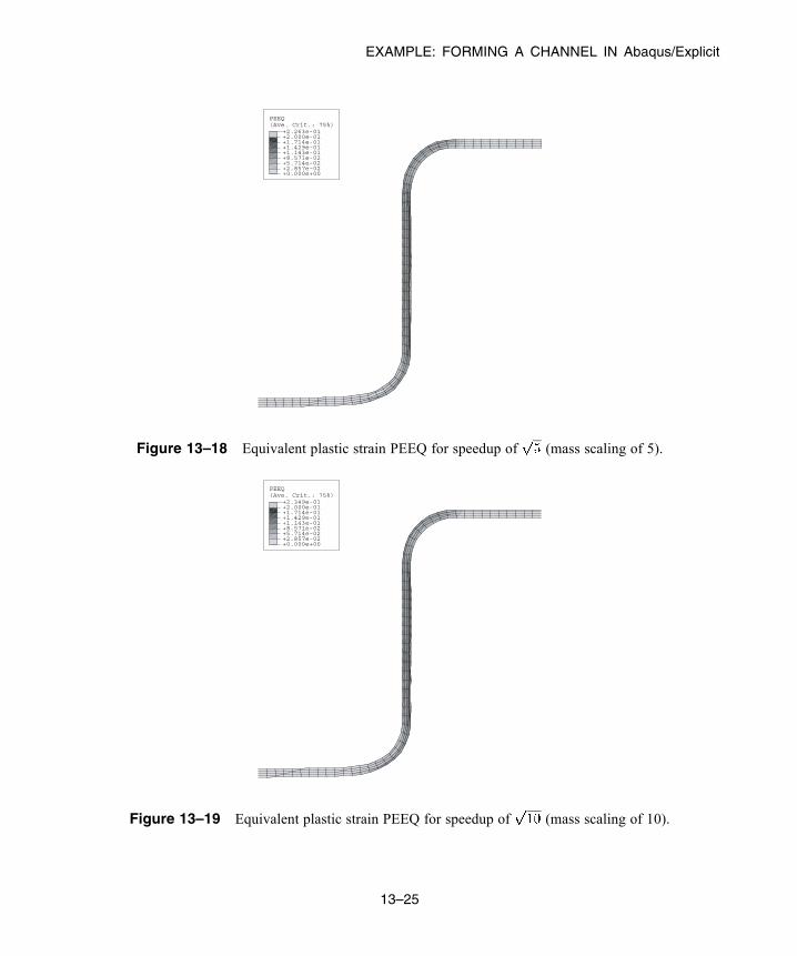
EXAMPLE: FORMING A CHANNEL IN Abaqus/Explicit
(Ave. Crit.: 75%)PEEQ
+0.000e+00+2.857e-02+5.714e-02+8.571e-02+1.143e-01+1.429e-01+1.714e-01+2.000e-01+2.263e-01
Figure 13–18 Equivalent plastic strain PEEQ for speedup of (mass scaling of 5).
(Ave. Crit.: 75%)PEEQ
+0.000e+00+2.857e-02+5.714e-02+8.571e-02+1.143e-01+1.429e-01+1.714e-01+2.000e-01+2.349e-01
Figure 13–19 Equivalent plastic strain PEEQ for speedup of (mass scaling of 10).
13–25
Abaqus ID:Printed on:
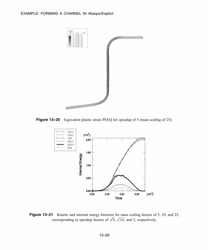
EXAMPLE: FORMING A CHANNEL IN Abaqus/Explicit
(Ave. Crit.: 75%)PEEQ
+0.000e+00+2.857e-02+5.714e-02+8.571e-02+1.143e-01+1.429e-01+1.714e-01+2.000e-01+2.109e-01
Figure 13–20 Equivalent plastic strain PEEQ for speedup of 5 (mass scaling of 25).
IE10IE25IE5KE10KE25KE5
Figure 13–21 Kinetic and internal energy histories for mass scaling factors of 5, 10, and 25,corresponding to speedup factors of , , and 5, respectively.
13–26
Abaqus ID:Printed on:
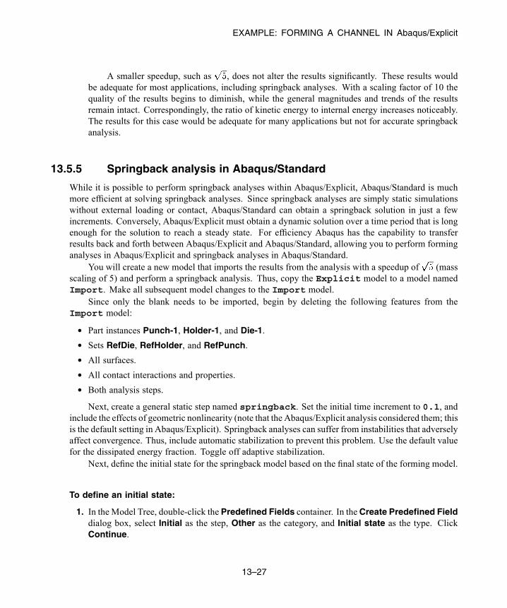
EXAMPLE: FORMING A CHANNEL IN Abaqus/Explicit
A smaller speedup, such as , does not alter the results significantly. These results wouldbe adequate for most applications, including springback analyses. With a scaling factor of 10 thequality of the results begins to diminish, while the general magnitudes and trends of the resultsremain intact. Correspondingly, the ratio of kinetic energy to internal energy increases noticeably.The results for this case would be adequate for many applications but not for accurate springbackanalysis.
13.5.5 Springback analysis in Abaqus/Standard
While it is possible to perform springback analyses within Abaqus/Explicit, Abaqus/Standard is muchmore efficient at solving springback analyses. Since springback analyses are simply static simulationswithout external loading or contact, Abaqus/Standard can obtain a springback solution in just a fewincrements. Conversely, Abaqus/Explicit must obtain a dynamic solution over a time period that is longenough for the solution to reach a steady state. For efficiency Abaqus has the capability to transferresults back and forth between Abaqus/Explicit and Abaqus/Standard, allowing you to perform forminganalyses in Abaqus/Explicit and springback analyses in Abaqus/Standard.
You will create a new model that imports the results from the analysis with a speedup of (massscaling of 5) and perform a springback analysis. Thus, copy the Explicit model to a model namedImport. Make all subsequent model changes to the Import model.
Since only the blank needs to be imported, begin by deleting the following features from theImport model:
• Part instances Punch-1, Holder-1, and Die-1.
• Sets RefDie, RefHolder, and RefPunch.
• All surfaces.• All contact interactions and properties.• Both analysis steps.Next, create a general static step named springback. Set the initial time increment to 0.1, and
include the effects of geometric nonlinearity (note that the Abaqus/Explicit analysis considered them; thisis the default setting in Abaqus/Explicit). Springback analyses can suffer from instabilities that adverselyaffect convergence. Thus, include automatic stabilization to prevent this problem. Use the default valuefor the dissipated energy fraction. Toggle off adaptive stabilization.
Next, define the initial state for the springback model based on the final state of the forming model.
To define an initial state:
1. In the Model Tree, double-click the Predefined Fields container. In theCreate Predefined Fielddialog box, select Initial as the step, Other as the category, and Initial state as the type. ClickContinue.
13–27
Abaqus ID:Printed on:

SUMMARY
2. In the viewport, select the blank as the instance to which the initial state will be assigned and clickDone in the prompt area.
3. In the Edit Predefined Field dialog box that appears, enter the job name Forming-3--sqrt5.This corresponds to the job with a speedup of . Accept all other default settings, and click OK.
This will cause the state of the model—stresses, strains, etc.—to be imported. By not updating thereference configuration, the springback displacements will be referred to the original undeformedconfiguration. This will allow for continuity in the displacements in the event additional formingstages are required.
You must redefine the boundary conditions, which are not imported. Impose the sameXSYMM-type displacement boundary conditions that were imposed in the Abaqus/Explicit model onthe set Center.
To remove rigid body motion, it is necessary to fix a single point in the blank, such as the node atthe center of the left edge, in the 2-direction (in this way you impose no unnecessary constraints). Ratherthan apply a displacement boundary condition to this point, apply a zero-velocity boundary condition to
fix this node at its position at the end of the forming stage (click the tool to display the mesh in theLoad module; create a node-based set at this node and then apply the appropriate boundary condition).This will allow the model to retain continuity in the blank location through any additional forming stagesthat may follow.
Create a new job named springback, and submit it for analysis.
Results of the springback analysis
Figure 13–22 overlays (View→Overlay Plot) the deformed shape of the blank after the formingand springback stages (the forming stage corresponds to the last frame of the Abaqus/Explicit outputdatabase file, while the springback stage corresponds to the final frame of the Abaqus/Standardoutput database file). The springback result is necessarily dependent on the accuracy of the formingstage preceding it. In fact, springback results are highly sensitive to errors in the forming stage,more sensitive than the results of the forming stage itself.
You should also plot the blank’s internal energy ALLIE and compare it with the staticstabilization energy ALLSD that is dissipated. The stabilization energy should be a small fractionof the internal energy to have confidence in the results. Figure 13–23 shows a plot of these twoenergies; the static stabilization energy is indeed small and, thus, has not significantly affected theresults.
13.6 Summary
• If a quasi-static analysis is performed in its natural time scale, the solution should be nearly thesame as a truly static solution.
• It is often necessary to use load rate scaling or mass scaling to obtain a quasi-static solution usingless CPU time.
13–28
Abaqus ID:Printed on:
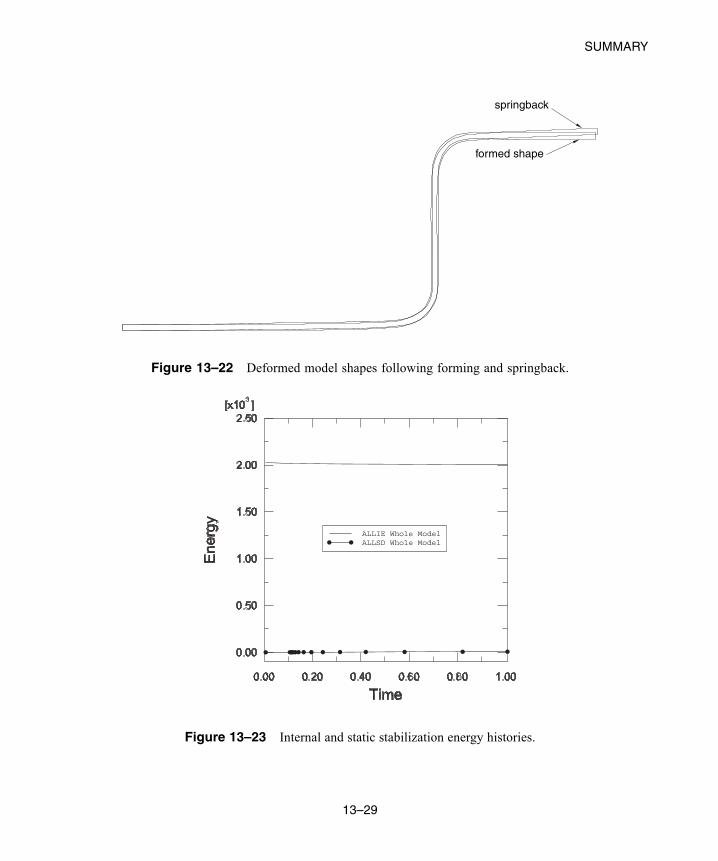
SUMMARY
springback
formed shape
Figure 13–22 Deformed model shapes following forming and springback.
ALLIE Whole ModelALLSD Whole Model
Figure 13–23 Internal and static stabilization energy histories.
13–29
Abaqus ID:Printed on:
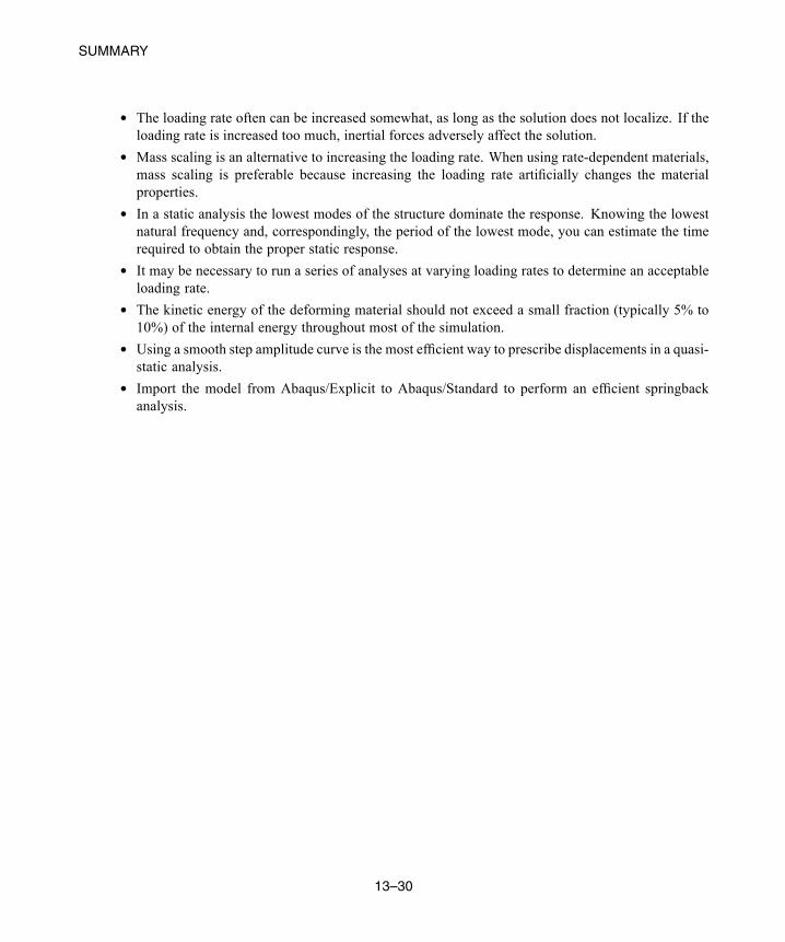
SUMMARY
• The loading rate often can be increased somewhat, as long as the solution does not localize. If theloading rate is increased too much, inertial forces adversely affect the solution.
• Mass scaling is an alternative to increasing the loading rate. When using rate-dependent materials,mass scaling is preferable because increasing the loading rate artificially changes the materialproperties.
• In a static analysis the lowest modes of the structure dominate the response. Knowing the lowestnatural frequency and, correspondingly, the period of the lowest mode, you can estimate the timerequired to obtain the proper static response.
• It may be necessary to run a series of analyses at varying loading rates to determine an acceptableloading rate.
• The kinetic energy of the deforming material should not exceed a small fraction (typically 5% to10%) of the internal energy throughout most of the simulation.
• Using a smooth step amplitude curve is the most efficient way to prescribe displacements in a quasi-static analysis.
• Import the model from Abaqus/Explicit to Abaqus/Standard to perform an efficient springbackanalysis.
13–30
Abaqus ID:Printed on:

Appendix A: EXAMPLE FILES
Appendix A: Example Files
This appendix contains a list of the Python scripts that can be used to create complete models for the examplescontained in this guide. The scripts themselves are available in the HTML version of this guide. These filesare also included with the Abaqus release; you can extract them from the compressed archive files using theabaqus fetch utility.
To fetch a script:
1. At the operating system prompt, enter the command
abaqus fetch job=file_name
where file_name includes the extension .py.
To run a script in Abaqus/CAE:
1. From the main menu bar, select File→Run Script.
The Run Script dialog box appears.
2. Choose the file from the list of available scripts, and click OK.
A.1 Overhead hoist frame
• gsi_frame_caemodel.py
A.2 Connecting lug
• gsi_lug_caemodel.py
A.3 Skew plate
• gsi_skewplate_caemodel.py
A.4 Cargo crane
• gsi_crane_caemodel.py
A.5 Cargo crane – dynamic loading
• gsi_dyncrane_caemodel.py
A–1
Abaqus ID:Printed on:

Appendix A: EXAMPLE FILES
A.6 Nonlinear skew plate
• gsi_nlskewplate_caemodel.py
A.7 Stress wave propagation in a bar
• gxi_stresswave_caemodel.py
A.8 Connecting lug with plasticity
• gsi_plasticlug_caemodel.py
A.9 Blast loading on a stiffened plate
• gxi_stiffplate_caemodel.py
A.10 Axisymmetric mount
• gsi_mount_caemodel.py
A.11 Vibration of a piping system
• gsi_pipe_caemodel.py
A.12 Forming a channel
• gsi_channel_caemodel.py• gsi_channel_caemodel_spring.py
A.13 Shearing of a lap joint
• gsi_lap_joint_caemodel.py• lap-joint-alum.txt• lap-joint-titanium.txt
A.14 Circuit board drop test
• gxi_circuit_caemodel.py• drop-test-foam.txt
A–2
Abaqus ID:Printed on:

Appendix B: Abaqus/CAE: A BASIC TUTORIAL
Appendix B: Creating and Analyzing a Simple Model inAbaqus/CAE
The following section is a basic tutorial for the experiencedAbaqus user. It leads you through the Abaqus/CAEmodeling process by visiting each of the modules and showing you the basic steps to create and analyze asimple model. To illustrate each of the steps, you will first create a model of a steel cantilever beam and loadits top surface (see Figure B–1).
20 mm
25 mm200 mm
0.5 MPa
Figure B–1 A loaded cantilever beam.
You will then analyze the beam and plot the resulting stresses and displacements. The entire tutorial takesapproximately 90 minutes to complete.
The following topics are covered:
• “Understanding Abaqus/CAE modules,” Section B.1• “Understanding the Model Tree,” Section B.2• “Creating a part,” Section B.3• “Creating a material,” Section B.4• “Defining and assigning section properties,” Section B.5• “Assembling the model,” Section B.6• “Defining your analysis steps,” Section B.7• “Applying a boundary condition and a load to the model,” Section B.8• “Meshing the model,” Section B.9• “Creating and submitting an analysis job,” Section B.10• “Viewing the results of your analysis,” Section B.11
B–1
Abaqus ID:Printed on:
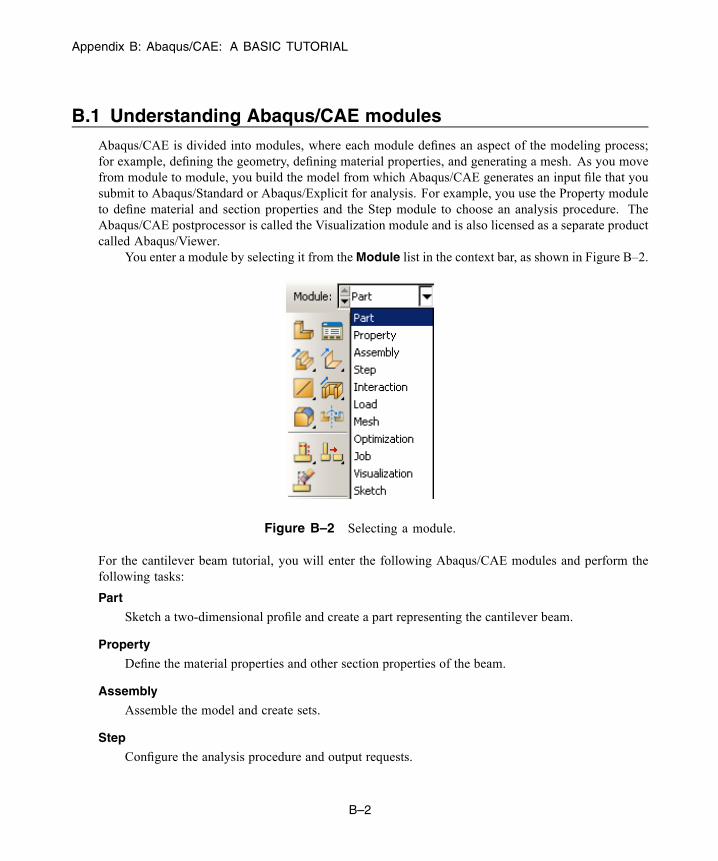
Appendix B: Abaqus/CAE: A BASIC TUTORIAL
B.1 Understanding Abaqus/CAE modulesAbaqus/CAE is divided into modules, where each module defines an aspect of the modeling process;for example, defining the geometry, defining material properties, and generating a mesh. As you movefrom module to module, you build the model from which Abaqus/CAE generates an input file that yousubmit to Abaqus/Standard or Abaqus/Explicit for analysis. For example, you use the Property moduleto define material and section properties and the Step module to choose an analysis procedure. TheAbaqus/CAE postprocessor is called the Visualization module and is also licensed as a separate productcalled Abaqus/Viewer.
You enter a module by selecting it from theModule list in the context bar, as shown in Figure B–2.
Figure B–2 Selecting a module.
For the cantilever beam tutorial, you will enter the following Abaqus/CAE modules and perform thefollowing tasks:
Part
Sketch a two-dimensional profile and create a part representing the cantilever beam.
Property
Define the material properties and other section properties of the beam.
Assembly
Assemble the model and create sets.
Step
Configure the analysis procedure and output requests.
B–2
Abaqus ID:Printed on:

Appendix B: Abaqus/CAE: A BASIC TUTORIAL
Load
Apply loads and boundary conditions to the beam.
Mesh
Mesh the beam.
Optimization
Create an optimization task (not discussed here).
Job
Create a job and submit it for analysis.
Visualization
View the results of the analysis.
Although the Module list in the context bar lists the modules in a logical sequence, you can move backand forth between modules at will. However, certain obvious restrictions apply; for example, you cannotassign section properties to geometry that has not yet been created.
A completed model contains everything that Abaqus/CAE needs to generate an input file and startthe analysis. Abaqus/CAE uses a model database to store your models. When you start Abaqus/CAE,the Start Session dialog box allows you to create a new, empty model database in memory. After youstart Abaqus/CAE, you can save your model database to a disk by selecting File→Save from the mainmenu bar; to retrieve it from a disk, select File→Open.
For a complete listing of which module generates a particular keyword, see “Abaqus keywordbrowser table,” Section A.1 of the Abaqus/CAE User’s Guide, in the HTML version of this guide.
B.2 Understanding the Model Tree
The Model Tree provides a visual description of the hierarchy of items in a model. Figure B–3 shows atypical Model Tree.
Items in the Model Tree are represented by small icons; for example, the Steps
icon, . In addition, parentheses next to an item indicate that the item is a container,and the number in the parentheses indicates the number of items in the container. You can click on the“ ” and “−” signs in the Model Tree to expand and collapse a container. The right and left arrow keysperform the same operation.
The arrangement of the containers and items in the Model Tree reflects the order in which you areexpected to create your model. As noted earlier, a similar logic governs the order of modules in themodule menu—you create parts before you create the assembly, and you create steps before you createloads. This arrangement is fixed—you cannot move items in the Model Tree.
B–3
Abaqus ID:Printed on:

Appendix B: Abaqus/CAE: A BASIC TUTORIAL
Figure B–3 Model Tree.
The Model Tree provides most of the functionality of the main menu bar and the module managers.For example, if you double-click on the Parts container, you can create a new part (the equivalent ofselecting Part→Create from the main menu bar).
B–4
Abaqus ID:Printed on:
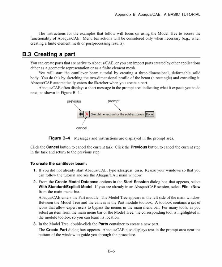
Appendix B: Abaqus/CAE: A BASIC TUTORIAL
The instructions for the examples that follow will focus on using the Model Tree to access thefunctionality of Abaqus/CAE. Menu bar actions will be considered only when necessary (e.g., whencreating a finite element mesh or postprocessing results).
B.3 Creating a partYou can create parts that are native to Abaqus/CAE, or you can import parts created by other applicationseither as a geometric representation or as a finite element mesh.
You will start the cantilever beam tutorial by creating a three-dimensional, deformable solidbody. You do this by sketching the two-dimensional profile of the beam (a rectangle) and extruding it.Abaqus/CAE automatically enters the Sketcher when you create a part.
Abaqus/CAE often displays a short message in the prompt area indicating what it expects you to donext, as shown in Figure B–4.
promptprevious
cancel
Figure B–4 Messages and instructions are displayed in the prompt area.
Click the Cancel button to cancel the current task. Click the Previous button to cancel the current stepin the task and return to the previous step.
To create the cantilever beam:
1. If you did not already start Abaqus/CAE, type abaqus cae. Resize your windows so that youcan follow the tutorial and see the Abaqus/CAE main window.
2. From the Create Model Database options in the Start Session dialog box that appears, selectWith Standard/Explicit Model. If you are already in an Abaqus/CAE session, select File→Newfrom the main menu bar.
Abaqus/CAE enters the Part module. The Model Tree appears in the left side of the main window.Between the Model Tree and the canvas is the Part module toolbox. A toolbox contains a set oficons that allow expert users to bypass the menus in the main menu bar. For many tools, as youselect an item from the main menu bar or the Model Tree, the corresponding tool is highlighted inthe module toolbox so you can learn its location.
3. In the Model Tree, double-click the Parts container to create a new part.
The Create Part dialog box appears. Abaqus/CAE also displays text in the prompt area near thebottom of the window to guide you through the procedure.
B–5
Abaqus ID:Printed on:

Appendix B: Abaqus/CAE: A BASIC TUTORIAL
You use the Create Part dialog box to name the part; to choose its modeling space, type, and basefeature; and to set the approximate size. You can edit and rename a part after you create it; you canalso change its modeling space and type but not its base feature.
4. Name the part Beam. Accept the default settings of a three-dimensional, deformable body and asolid, extruded base feature. In the Approximate size text field, type 300.
5. Click Continue to exit the Create Part dialog box.
Abaqus/CAE automatically enters the Sketcher. The Sketcher toolbox appears in the left side of themain window, and the Sketcher grid appears in the viewport. The Sketcher contains a set of basictools that allow you to sketch the two-dimensional profile of your part. Abaqus/CAE enters theSketcher whenever you create or edit a part. To finish using a Sketcher tool, click mouse button 2in the viewport or select a new tool.
Tip: Like all tools in Abaqus/CAE, if you simply position the cursor over a tool in theSketcher toolbox for a short time, a small window appears that gives a brief descriptionof the tool.
The following aspects of the Sketcher help you sketch the desired geometry:
• The Sketcher grid helps you position the cursor and align objects in the viewport.• Dashed lines indicate the X- and Y-axes of the sketch and intersect at the origin of the sketch.
• A triad in the lower-left corner of the viewport indicates the relationship between the sketchplane and the orientation of the part.
• When you select a sketching tool, Abaqus/CAE displays the X- and Y-coordinates of the cursorin the upper-left corner of the viewport.
6. To sketch the profile of the cantilever beam, you need to select the rectangle drawing tool .
The rectangle drawing tool appears in the Sketcher toolbox with a white background indicatingthat you selected it. Abaqus/CAE displays prompts in the prompt area to guide you through theprocedure.
7. In the viewport, sketch the rectangle using the following steps:
a. You will first sketch a rough approximation of the beam and then use constraints anddimensions to refine the sketch. Select any two points as the opposite corners of the rectangle.
b. Click mouse button 2 anywhere in the viewport to exit the rectangle tool.
Note: If you are a Windows user with a 2-button mouse, press both mouse buttonssimultaneously whenever you are asked to press mouse button 2.
c. The Sketcher automatically adds constraints to the sketch (in this case the four corners of therectangle are assigned perpendicular constraints and one edge is designated as horizontal).
d. Use the dimension tool to dimension the top and left edges of the rectangle. The topedge should have a horizontal dimension of 200 mm, and the left edge should have a vertical
B–6
Abaqus ID:Printed on:

Appendix B: Abaqus/CAE: A BASIC TUTORIAL
dimension of 20 mm. When dimensioning each edge, simply select the line, click mousebutton 1 to position the dimension text, and then enter the new dimension in the prompt area.
e. The final sketch is shown in Figure B–5.
H
20.
200.
Figure B–5 Sketch of the rectangle.
8. If you make a mistake while using the Sketcher, you can delete lines in your sketch, as explained inthe following procedure:
a. From the Sketcher toolbox, click the Delete tool, .
b. From the sketch, click a line to select it.
Abaqus/CAE highlights the selected line in red.
c. Click mouse button 2 in the viewport to delete the selected line.
d. Repeat steps b and c as often as necessary.
e. Click mouse button 2 in the viewport to finish using the Delete tool.
Note: You can also use the Undo tool and the Redo tool to undo and redo your previousoperations.
9. From the prompt area (near the bottom of the main window), click Done to exit the Sketcher.
Note: If you don’t see the Done button in the prompt area, continue to click mouse button 2 in theviewport until it appears.
10. Because you are creating an extruded part, Abaqus/CAE displays the Edit Base Extrusion dialogbox for you to select the depth. Optional parameters to modify the extrusion shape are also available.In the Depth field, erase the default value and type a value of 25.0. Click OK to accept this value.
Abaqus/CAE displays an isometric view of the new part, as shown in Figure B–6.
B–7
Abaqus ID:Printed on:

Appendix B: Abaqus/CAE: A BASIC TUTORIAL
1
2
3
Figure B–6 Isometric view of the beam.
To help you orient the cantilever beam during the modeling process, Abaqus/CAE displays a triadin the lower-left corner indicating the orientation of the global coordinate system.
11. Before you continue the tutorial, save your model in a model database file.
a. From the main menu bar, select File→Save. The Save Model Database As dialog boxappears.
b. Type a name for the new model database in the File Name field, and click OK. You do notneed to include the file extension; Abaqus/CAE automatically appends .cae to the file name.
Abaqus/CAE stores the model database in a new file and returns to the Part module. Thetitle bar of the Abaqus/CAE window displays the path and name of the model database. Youshould always save your model database at regular intervals (for example, each time you switchmodules).
B.4 Creating a material
For the cantilever beam tutorial you will create a single linear elastic material with Young’s modulus of209 × 103 MPa and Poisson’s ratio of 0.3.
To define a material:
1. In the Model Tree, double-click the Materials container to create a new material.
Abaqus/CAE switches to the Property module, and the Edit Material dialog box appears.
2. Name the material Steel. Use the menu bar under the browser area of the material editor to revealmenus containing all the available material options. Some of the menu items contain submenus; for
B–8
Abaqus ID:Printed on:
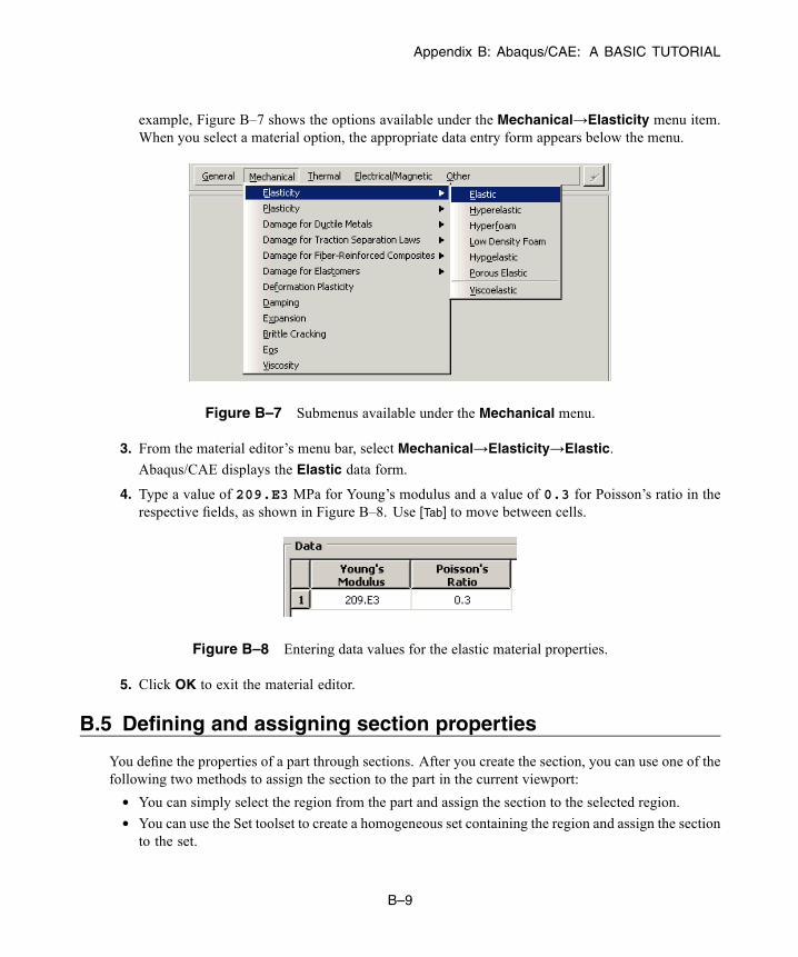
Appendix B: Abaqus/CAE: A BASIC TUTORIAL
example, Figure B–7 shows the options available under the Mechanical→Elasticity menu item.When you select a material option, the appropriate data entry form appears below the menu.
Figure B–7 Submenus available under the Mechanical menu.
3. From the material editor’s menu bar, select Mechanical→Elasticity→Elastic.
Abaqus/CAE displays the Elastic data form.
4. Type a value of 209.E3 MPa for Young’s modulus and a value of 0.3 for Poisson’s ratio in therespective fields, as shown in Figure B–8. Use [Tab] to move between cells.
Figure B–8 Entering data values for the elastic material properties.
5. Click OK to exit the material editor.
B.5 Defining and assigning section properties
You define the properties of a part through sections. After you create the section, you can use one of thefollowing two methods to assign the section to the part in the current viewport:
• You can simply select the region from the part and assign the section to the selected region.• You can use the Set toolset to create a homogeneous set containing the region and assign the sectionto the set.
B–9
Abaqus ID:Printed on:
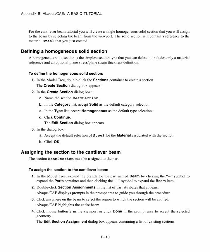
Appendix B: Abaqus/CAE: A BASIC TUTORIAL
For the cantilever beam tutorial you will create a single homogeneous solid section that you will assignto the beam by selecting the beam from the viewport. The solid section will contain a reference to thematerial Steel that you just created.
Defining a homogeneous solid sectionA homogeneous solid section is the simplest section type that you can define; it includes only a materialreference and an optional plane stress/plane strain thickness definition.
To define the homogeneous solid section:
1. In the Model Tree, double-click the Sections container to create a section.
The Create Section dialog box appears.
2. In the Create Section dialog box:
a. Name the section BeamSection.
b. In the Category list, accept Solid as the default category selection.
c. In the Type list, accept Homogeneous as the default type selection.
d. Click Continue.
The Edit Section dialog box appears.
3. In the dialog box:
a. Accept the default selection of Steel for the Material associated with the section.
b. Click OK.
Assigning the section to the cantilever beamThe section BeamSection must be assigned to the part.
To assign the section to the cantilever beam:
1. In the Model Tree, expand the branch for the part named Beam by clicking the “ ” symbol toexpand the Parts container and then clicking the “ ” symbol to expand the Beam item.
2. Double-click Section Assignments in the list of part attributes that appears.
Abaqus/CAE displays prompts in the prompt area to guide you through the procedure.
3. Click anywhere on the beam to select the region to which the section will be applied.
Abaqus/CAE highlights the entire beam.
4. Click mouse button 2 in the viewport or click Done in the prompt area to accept the selectedgeometry.
The Edit Section Assignment dialog box appears containing a list of existing sections.
B–10
Abaqus ID:Printed on:
Appendix B: Abaqus/CAE: A BASIC TUTORIAL
5. Accept the default selection of BeamSection as the section, and click OK.
Abaqus/CAE assigns the solid section to the beam, colors the entire beam aqua to indicate that theregion has a section assignment, and closes the Edit Section Assignment dialog box.
Note: When you assign a section to a region of a part, the region takes on the material propertiesassociated with the section.
B.6 Assembling the model
Each part that you create is oriented in its own coordinate system and is independent of the other partsin the model. Although a model may contain many parts, it contains only one assembly. You define thegeometry of the assembly by creating instances of a part and then positioning the instances relative toeach other in a global coordinate system. An instance may be classified as independent or dependent.Independent part instances are meshed individually while the mesh of a dependent part instance isassociated the mesh of the original part. This issue is discussed further in “Working with part instances,”Section 13.3 of the Abaqus/CAE User’s Guide.
For the cantilever beam tutorial you will create a single instance of your cantilever beam.Abaqus/CAE positions the instance so that the origin of the sketch that defined the rectangular profileof the beam overlays the origin of the assembly’s default coordinate system.
To assemble the model:
1. In the Model Tree, expand the Assembly container. Then double-click Instances in the list thatappears.
Abaqus/CAE switches to the Assembly module, and the Create Instance dialog box appears.
2. In the dialog box, select Beam and click OK.
Abaqus/CAE creates an instance of the cantilever beam and displays it using an isometricorientation. In this example the single instance of the beam defines the assembly. A second triadin the viewport indicates the origin and orientation of the global coordinate system.
3. In the View Manipulation toolbar, click the rotate view manipulation tool, .
When you move the mouse back into the viewport, a circle appears.
4. Drag the mouse in the viewport to rotate the model and examine it from all sides. You can alsopick a center of rotation by clicking Select in the prompt area; your selected center of rotation isretained for the current object and viewport. Click Use Default to return to the default (center ofviewport) rotation method.
Click mouse button 2 to exit rotate mode.
5. Several other tools (pan , magnify , zoom , and auto-fit ) are also available inthe View Manipulation toolbar to help you examine your model. Experiment with each of these
B–11
Abaqus ID:Printed on:
Appendix B: Abaqus/CAE: A BASIC TUTORIAL
tools until you are comfortable with them. Use the context-sensitive help system to obtain anyadditional information you require about these tools.
Direct view manipulation is available using the 3D compass. The compass allows you to pan orrotate your model by clicking and dragging on it. For example:
• Click and drag one of the straight axes of the 3D compass to pan along an axis.• Click and drag any of the quarter-circular faces on the 3D compass to pan along a plane.• Click and drag one of the three arcs along the perimeter of the 3D compass to rotate the modelabout the axis that is perpendicular to the plane containing the arc.
• Click and drag the free rotation handle (the point at the top of the 3D compass) to rotate themodel freely about its pivot point.
• Click the label for any of the axes on the 3D compass to select a predefined view (the selectedaxis is perpendicular to the plane of the viewport).
• Double-click anywhere on the 3D compass to specify a view.The 3D compass is discussed further in “The 3D compass,” Section 5.3 of the Abaqus/CAE User’sGuide.
B.7 Defining your analysis steps
Now that you have created your part, you can define your analysis steps. For the cantilever beam tutorialthe analysis will consist of two steps:
• An initial step, in which you will apply a boundary condition that constrains one end of the cantileverbeam.
• A general, static analysis step, in which you will apply a pressure load to the top face of the beam.Abaqus/CAE generates the initial step automatically, but you must create the analysis step yourself. Youmay also request output for any steps in the analysis.
Creating an analysis stepCreate a general, static step that follows the initial step of the analysis.
To create a general, static analysis step:
1. In the Model Tree, double-click the Steps container to create a step.
Abaqus/CAE switches to the Step module. The Create Step dialog box appears with a list of allthe general procedures and a default step name of Step-1. General procedures are those that canbe used to analyze linear or nonlinear response.
2. Name the step BeamLoad.
3. From the list of available general procedures in the Create Step dialog box, select Static, Generalif it is not already selected and click Continue.
B–12
Abaqus ID:Printed on:
Appendix B: Abaqus/CAE: A BASIC TUTORIAL
The Edit Step dialog box appears with the default settings for a general, static step.
4. The Basic tab is selected by default. In the Description field, type Load the top of thebeam.
5. Click the Incrementation tab, and accept the default time incrementation settings.
6. Click the Other tab to see its contents; you can accept the default values provided for the step.
7. Click OK to create the step and to exit the Edit Step dialog box.
Requesting data outputWhen you submit your job for analysis, Abaqus/Standard or Abaqus/Explicit writes the results of theanalysis to the output database. For each step you create, you can use the Field Output RequestsManager and the History Output Requests Manager to do the following:
• Select the region of the model for which Abaqus will generate data.• Select the variables that Abaqus will write to the output database.• Select the section points of beams or shells for which Abaqus will generate data.• Change the frequency at which Abaqus will write data to the output database.
When you create a step, Abaqus/CAE generates a default output request for the step. See “Whichvariables are in the output database?,” Section D.2, for more information on field and history output.
For the cantilever beam tutorial, you will simply examine the output requests and accept the defaultconfiguration.
To examine your output requests:
1. In the Model Tree, click mouse button 3 on the Field Output Requests container and selectManager from the menu that appears.
Abaqus/CAE displays the Field Output Requests Manager. This manager displays analphabetical list of existing output requests along the left side of the dialog box. The names of allthe steps in the analysis appear along the top of the dialog box in the order of execution. The tableformed by these two lists displays the status of each output request in each step.
2. Review the default output request that Abaqus/CAE generates for the Static, General step youcreated and named BeamLoad.
Click the cell in the table labeled Created; that cell becomes highlighted, and the followinginformation related to the cell appears in the legend at the bottom of the manager:
• The type of analysis procedure carried out in the step in that column.• The list of output request variables.• The output request status.
3. On the right side of the Field Output Requests Manager, click Edit to view more detailedinformation about the output request.
B–13
Abaqus ID:Printed on:
Appendix B: Abaqus/CAE: A BASIC TUTORIAL
The field output editor appears. In the Output Variables region of the dialog box, a text box listsall the variables that will be output. If you change an output request, you can always return to thedefault settings by clicking Preselected defaults above the text box.
4. Click the arrows next to each output variable category to see exactly which variables will be output.The check boxes next to each category title allow you to see at a glance whether all variables inthat category will be output. A black check mark on a white background indicates that all variableswill be output, while a dark gray check mark on a light gray background indicates that only somevariables will be output.
Based on the selections shown at the bottom of the dialog box, data will be generated at every defaultsection point in the model and will be written to the output database after every increment duringthe analysis.
5. Click Cancel to close the field output editor, since you do not wish to make any changes to thedefault choice.
6. Click Dismiss to close the Field Output Requests Manager.
Note: What is the difference between the Dismiss and Cancel buttons? Dismiss buttons appearin dialog boxes that contain data that you cannot modify. For example, the Field Output RequestsManager allows you to view output requests, but you must use the field output editor to modifythose requests. Clicking the Dismiss button simply closes the Field Output Requests Manager.Conversely, Cancel buttons appear in dialog boxes that allow you to make changes. ClickingCancel closes the dialog box without saving your changes.
7. Review the history output requests in a similar manner by clicking mouse button 3 on the HistoryOutput Requests container in the Model Tree and then opening the history output editor.
B.8 Applying a boundary condition and a load to the model
Prescribed conditions, such as loads and boundary conditions, are step-dependent, which means that youmust specify the step or steps in which they become active. Now that you have defined the steps in theanalysis, you can define the following prescribed conditions:
• A boundary condition that constrains one end of the cantilever beam in the X-, Y-, and Z-directions;the boundary condition is applied during the initial step.
• A load that you apply to the top face of the beam; the load is applied during the general analysisstep.
Applying a boundary condition to one end of the cantilever beamCreate a boundary condition that constrains the cantilever beam to be built-in at one end of the beam.
To apply boundary conditions to one end of the cantilever beam:
1. In the Model Tree, double-click the BCs container.
B–14
Abaqus ID:Printed on:
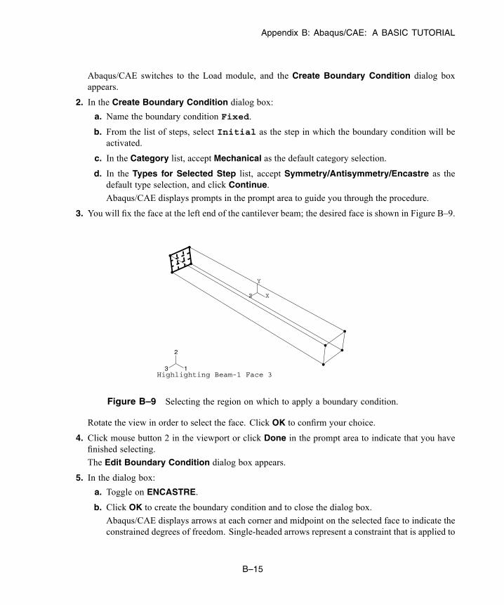
Appendix B: Abaqus/CAE: A BASIC TUTORIAL
Abaqus/CAE switches to the Load module, and the Create Boundary Condition dialog boxappears.
2. In the Create Boundary Condition dialog box:
a. Name the boundary condition Fixed.
b. From the list of steps, select Initial as the step in which the boundary condition will beactivated.
c. In the Category list, accept Mechanical as the default category selection.
d. In the Types for Selected Step list, accept Symmetry/Antisymmetry/Encastre as thedefault type selection, and click Continue.
Abaqus/CAE displays prompts in the prompt area to guide you through the procedure.
3. You will fix the face at the left end of the cantilever beam; the desired face is shown in Figure B–9.
X
Y
Z
1
2
3Highlighting Beam-1 Face 3
Figure B–9 Selecting the region on which to apply a boundary condition.
Rotate the view in order to select the face. Click OK to confirm your choice.
4. Click mouse button 2 in the viewport or click Done in the prompt area to indicate that you havefinished selecting.
The Edit Boundary Condition dialog box appears.
5. In the dialog box:
a. Toggle on ENCASTRE.
b. Click OK to create the boundary condition and to close the dialog box.
Abaqus/CAE displays arrows at each corner and midpoint on the selected face to indicate theconstrained degrees of freedom. Single-headed arrows represent a constraint that is applied to
B–15
Abaqus ID:Printed on:

Appendix B: Abaqus/CAE: A BASIC TUTORIAL
a translational degree of freedom. Double-headed arrows represent a constraint that is appliedto a rotational degree of freedom. An ENCASTRE boundary condition constrains all availabledegrees of freedom.
6. In the Model Tree, click mouse button 3 on the BCs container and select Manager from the menuthat appears.
Abaqus/CAE displays the Boundary Condition Manager. The manager indicates that theboundary condition is Created (activated) in the initial step and is Propagated (continues tobe active) in the general analysis step BeamLoad.
7. Click Dismiss to close the Boundary Condition Manager.
Applying a load to the top of the cantilever beamNow that you have fixed one end of the cantilever beam, you can apply a distributed load to the top faceof the beam. The load is applied during the general, static step you created earlier.
To apply a load to the top of the cantilever beam:
1. In the Model Tree, double-click the Loads container.
The Create Load dialog box appears.
2. In the Create Load dialog box:
a. Name the load Pressure.
b. From the list of steps, select BeamLoad as the step in which the load will be applied.
c. In the Category list, accept Mechanical as the default category selection.
d. In the Types for Selected Step list, select Pressure, and click Continue.
Abaqus/CAE displays prompts in the prompt area to guide you through the procedure.
3. In the viewport, select the top face of the beam as the surface to which the load will be applied. Thedesired face is shown by the gridded face in Figure B–10.
4. Click mouse button 2 in the viewport or click Done in the prompt area to indicate that you havefinished selecting regions.
The Edit Load dialog box appears.
5. In the dialog box:
a. Enter a magnitude of 0.5 MPa for the load.
b. Accept the default Distribution selection—Abaqus will apply the load uniformly over theface.
c. Accept the default Amplitude selection—Abaqus will ramp up the load during the step.
d. Click OK to create the load and to close the dialog box.
B–16
Abaqus ID:Printed on:
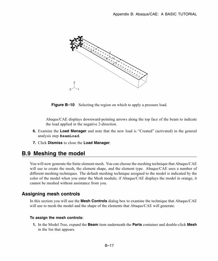
Appendix B: Abaqus/CAE: A BASIC TUTORIAL
X
Y
Z
1
2
3
Figure B–10 Selecting the region on which to apply a pressure load.
Abaqus/CAE displays downward-pointing arrows along the top face of the beam to indicatethe load applied in the negative 2-direction.
6. Examine the Load Manager and note that the new load is “Created” (activated) in the generalanalysis step BeamLoad.
7. Click Dismiss to close the Load Manager.
B.9 Meshing the model
You will now generate the finite element mesh. You can choose the meshing technique that Abaqus/CAEwill use to create the mesh, the element shape, and the element type. Abaqus/CAE uses a number ofdifferent meshing techniques. The default meshing technique assigned to the model is indicated by thecolor of the model when you enter the Mesh module; if Abaqus/CAE displays the model in orange, itcannot be meshed without assistance from you.
Assigning mesh controlsIn this section you will use the Mesh Controls dialog box to examine the technique that Abaqus/CAEwill use to mesh the model and the shape of the elements that Abaqus/CAE will generate.
To assign the mesh controls:
1. In the Model Tree, expand the Beam item underneath the Parts container and double-click Meshin the list that appears.
B–17
Abaqus ID:Printed on:
Appendix B: Abaqus/CAE: A BASIC TUTORIAL
Abaqus/CAE switches to the Mesh module. The Mesh module functionality is available onlythrough menu bar items or toolbox icons.
2. From the main menu bar, select Mesh→Controls.
TheMesh Controls dialog box appears. Abaqus/CAE colors the regions of your model to indicatewhich technique it will use to mesh that region. Abaqus/CAE will use structured meshing to meshyour cantilever beam and displays the beam in green.
3. In the dialog box, accept Hex as the default Element Shape selection.
4. Accept Structured as the default Technique selection.
5. Click OK to assign the mesh controls and to close the dialog box.
Abaqus/CAE will use the structured meshing technique to create a mesh of hexahedral-shapedelements.
Assigning an Abaqus element typeIn this section you will use the Element Type dialog box to assign a particular Abaqus element type tothe model. Although you will assign the element type now, you could also wait until after the mesh hasbeen created.
To assign an Abaqus element type:
1. From the main menu bar, select Mesh→Element Type.
The Element Type dialog box appears.
2. In the dialog box, accept the following default selections that control the elements that are availablefor selection:
• Standard is the default Element Library selection.
• Linear is the default Geometric Order.
• 3D Stress is the default Family of elements.
3. In the lower portion of the dialog box, examine the element shape options. A brief description ofthe default element selection is available at the bottom of each tabbed page.
Since the model is a three-dimensional solid, only three-dimensional solid elementtypes—hexahedral on the Hex tabbed page, triangular prism on the Wedge page, and tetrahedralon the Tet page—are shown.
4. Click the Hex tab, and choose Incompatible modes from the list of formulation options.
A description of the element type C3D8I appears at the bottom of the dialog box. Abaqus/CAE willnow associate C3D8I elements with the elements in the mesh.
5. Click OK to assign the element type and to close the dialog box.
B–18
Abaqus ID:Printed on:
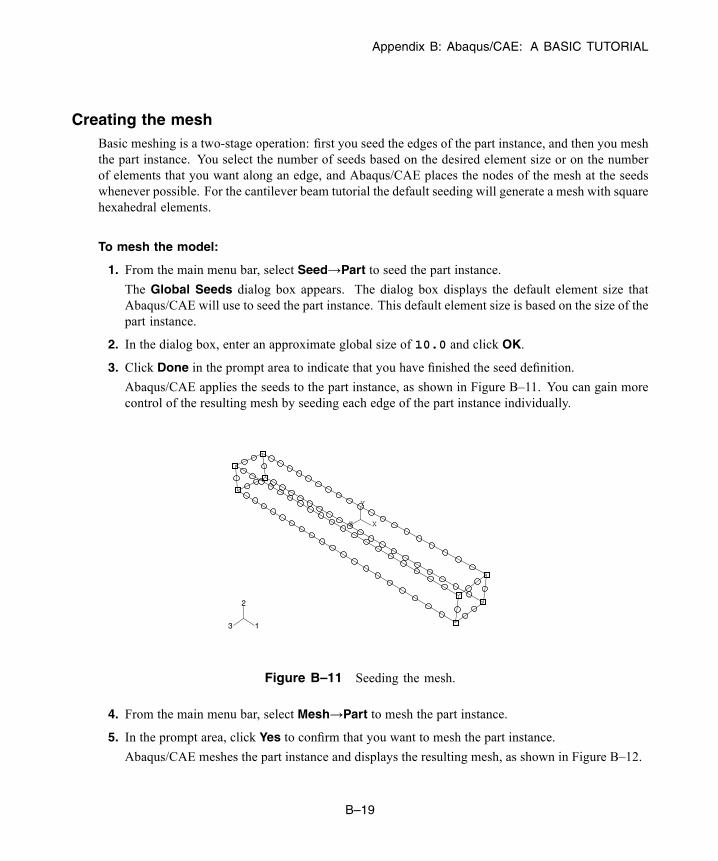
Appendix B: Abaqus/CAE: A BASIC TUTORIAL
Creating the meshBasic meshing is a two-stage operation: first you seed the edges of the part instance, and then you meshthe part instance. You select the number of seeds based on the desired element size or on the numberof elements that you want along an edge, and Abaqus/CAE places the nodes of the mesh at the seedswhenever possible. For the cantilever beam tutorial the default seeding will generate a mesh with squarehexahedral elements.
To mesh the model:
1. From the main menu bar, select Seed→Part to seed the part instance.
The Global Seeds dialog box appears. The dialog box displays the default element size thatAbaqus/CAE will use to seed the part instance. This default element size is based on the size of thepart instance.
2. In the dialog box, enter an approximate global size of 10.0 and click OK.
3. Click Done in the prompt area to indicate that you have finished the seed definition.
Abaqus/CAE applies the seeds to the part instance, as shown in Figure B–11. You can gain morecontrol of the resulting mesh by seeding each edge of the part instance individually.
X
Y
Z
1
2
3
Figure B–11 Seeding the mesh.
4. From the main menu bar, select Mesh→Part to mesh the part instance.
5. In the prompt area, click Yes to confirm that you want to mesh the part instance.
Abaqus/CAE meshes the part instance and displays the resulting mesh, as shown in Figure B–12.
B–19
Abaqus ID:Printed on:
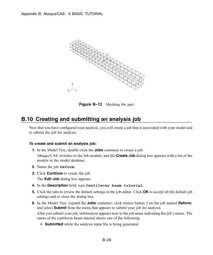
Appendix B: Abaqus/CAE: A BASIC TUTORIAL
X
Y
Z
1
2
3
Figure B–12 Meshing the part.
B.10 Creating and submitting an analysis jobNow that you have configured your analysis, you will create a job that is associated with your model andto submit the job for analysis.
To create and submit an analysis job:
1. In the Model Tree, double-click the Jobs container to create a job.
Abaqus/CAE switches to the Job module, and the Create Job dialog box appears with a list of themodels in the model database.
2. Name the job Deform.
3. Click Continue to create the job.
The Edit Job dialog box appears.
4. In the Description field, type Cantilever beam tutorial.
5. Click the tabs to review the default settings in the job editor. Click OK to accept all the default jobsettings and to close the dialog box.
6. In the Model Tree, expand the Jobs container; click mouse button 3 on the job named Deform,and select Submit from the menu that appears to submit your job for analysis.
After you submit your job, information appears next to the job name indicating the job’s status. Thestatus of the cantilever beam tutorial shows one of the following:
• Submitted while the analysis input file is being generated.
B–20
Abaqus ID:Printed on:
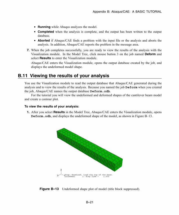
Appendix B: Abaqus/CAE: A BASIC TUTORIAL
• Running while Abaqus analyzes the model.
• Completed when the analysis is complete, and the output has been written to the outputdatabase.
• Aborted if Abaqus/CAE finds a problem with the input file or the analysis and aborts theanalysis. In addition, Abaqus/CAE reports the problem in the message area.
7. When the job completes successfully, you are ready to view the results of the analysis with theVisualization module. In the Model Tree, click mouse button 3 on the job named Deform andselect Results to enter the Visualization module.
Abaqus/CAE enters the Visualization module, opens the output database created by the job, anddisplays the undeformed model shape.
B.11 Viewing the results of your analysis
You use the Visualization module to read the output database that Abaqus/CAE generated during theanalysis and to view the results of the analysis. Because you named the job Deform when you createdthe job, Abaqus/CAE names the output database Deform.odb.
For the tutorial you will view the undeformed and deformed shapes of the cantilever beam modeland create a contour plot.
To view the results of your analysis:
1. After you select Results in the Model Tree, Abaqus/CAE enters the Visualization module, opensDeform.odb, and displays the undeformed shape of the model, as shown in Figure B–13.
Step: BeamLoad, Load the top of the beam.Increment 1: Step Time = 1.0001
2
3
Figure B–13 Undeformed shape plot of model (title block suppressed).
B–21
Abaqus ID:Printed on:
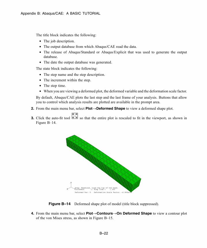
Appendix B: Abaqus/CAE: A BASIC TUTORIAL
The title block indicates the following:
• The job description.• The output database from which Abaqus/CAE read the data.• The release of Abaqus/Standard or Abaqus/Explicit that was used to generate the outputdatabase.
• The date the output database was generated.The state block indicates the following:
• The step name and the step description.• The increment within the step.• The step time.• When you are viewing a deformed plot, the deformed variable and the deformation scale factor.
By default, Abaqus/CAE plots the last step and the last frame of your analysis. Buttons that allowyou to control which analysis results are plotted are available in the prompt area.
2. From the main menu bar, select Plot→Deformed Shape to view a deformed shape plot.
3. Click the auto-fit tool so that the entire plot is rescaled to fit in the viewport, as shown inFigure B–14.
Step: BeamLoad, Load the top of the beam.Increment 1: Step Time = 1.000
Deformed Var: U Deformation Scale Factor: +2.806e+01
1
2
3
Figure B–14 Deformed shape plot of model (title block suppressed).
4. From the main menu bar, select Plot→Contours→On Deformed Shape to view a contour plotof the von Mises stress, as shown in Figure B–15.
B–22
Abaqus ID:Printed on:

Appendix B: Abaqus/CAE: A BASIC TUTORIAL
(Avg: 75%)S, Mises
+2.475e−01+1.200e+01+2.375e+01+3.551e+01+4.726e+01+5.901e+01+7.076e+01+8.252e+01+9.427e+01+1.060e+02+1.178e+02+1.295e+02+1.413e+02
Step: BeamLoad, Load the top of the beam.Increment 1: Step Time = 1.000Primary Var: S, MisesDeformed Var: U Deformation Scale Factor: +2.806e+01
1
2
3
Figure B–15 Contour plot of Mises stress (title block suppressed).
5. For a contour plot the default variable displayed depends on the analysis procedure; in this case, thedefault variable is the von Mises stress. From the main menu bar, select Result→Field Output toexamine the variables that are available for display.
Abaqus/CAE displays the Field Output dialog box; click the Primary Variable tab to choosewhich variable to display and to select the invariant or component of interest. By default, theMisesinvariant of the Stress components at integration points variable is selected.
Tip: You can also use the Field Output toolbar to change the displayed field outputvariable. For more information, see “Using the field output toolbar,” Section 42.5.2 ofthe Abaqus/CAE User’s Guide.
6. Click Cancel to close the Field Output dialog box.
You have now finished this tutorial. Appendix C, “Using Additional Techniques to Create andAnalyze a Model in Abaqus/CAE,” introduces additional techniques to create and analyze a model; forexample, you will create and assemble multiple part instances and define contact. Appendix D, “Viewingthe Output from Your Analysis,” covers the capabilities of the Visualization module in more detail.
B.12 Summary
• When you create a part, you name it and choose its type, modeling space, base feature, andapproximate size.
• Abaqus/CAE automatically enters the Sketcher when you create or edit a part. You use the Sketcherto draw the two-dimensional profiles of parts.
• Click mouse button 2 in the viewport to indicate you have finished selecting items or using a tool.
B–23
Abaqus ID:Printed on:

Appendix B: Abaqus/CAE: A BASIC TUTORIAL
• You can create a material and define its properties and create a section and define its category andtype. Since the section refers to the material, the material must be defined first.
• A model contains only one assembly. The assembly is composed of instances of parts positionedin a global coordinate system.
• Abaqus/CAE generates the initial step automatically, but you must create analysis steps. You usethe step editor to define each analysis step.
• When you create a step, Abaqus/CAE generates a default output request for the step. You usethe Field Output Requests Manager and the History Output Requests Manager to examinewhich categories of data will be output.
• You invoke the field and history output editors from the Field Output Requests Manager andthe History Output Requests Manager to select the variables that Abaqus/CAE will write tothe output database during the analysis, as well as the frequency at which they are written and theregions and section points from which they are written.
• Prescribed conditions, such as loads and boundary conditions, are step-dependent objects, whichmeans that you must specify the step or steps in which they become active.
• Managers are useful for reviewing and modifying the status of prescribed conditions in each step.• You create loads and define where the load is applied to the assembly in the Load module.• Although you can create a mesh at any point after creating the assembly, you typically do it afterconfiguring the rest of the model, since items such as loads, boundary conditions, and steps dependon the underlying geometry, not the mesh.
• You can assign the element type either before or after you create the mesh. The available elementtypes depend on the geometry of your model.
• You use seeds to define the approximate position of nodes in your final mesh. You select the numberof seeds based on the element size or on the number of elements that you want along an edge.
• You can use the Model Tree to submit jobs and to monitor the status of a job.• In the Visualization module you read the output database generated by your analysis and view theresults. You can select the variable to display from the data in the output database, and you can alsoselect the increment being displayed.
• You can display the results in several modes—undeformed, deformed, and contour. You can controlthe appearance of the display in each mode, independent of other modes.
B–24
Abaqus ID:Printed on:
Appendix C: Abaqus/CAE: AN ADVANCED TUTORIAL
Appendix C: Using Additional Techniques to Create andAnalyze a Model in Abaqus/CAE
Appendix B, “Creating and Analyzing a Simple Model in Abaqus/CAE,” explains how to create and analyzea very simple model composed of only one part. In this advanced tutorial for the experienced Abaqus useryou will create and analyze a more complex model. The model is more complex on two levels:
• It consists of three different parts rather than just one. This tutorial illustrates how you position instancesof these parts to create the assembly and how you define contact between surfaces of the assembly.
• It includes parts that you will draw using advanced sketching techniques. You will learn how sketches,datum geometry, and partitions combine to define the features that make up individual parts. You willalso learn how you can modify a part by editing a feature and how modified parts are regenerated.
As in Appendix B, “Creating and Analyzing a Simple Model in Abaqus/CAE,” you will apply sectionproperties, loads, and boundary conditions to the model; you will also mesh the model, configure the analysis,and run the analysis job. At the end of the tutorial you will view your analysis results. The entire tutorial takesapproximately three hours to complete.
This tutorial assumes that you are familiar with the techniques described in Appendix B, “Creating andAnalyzing a Simple Model in Abaqus/CAE,” including the following:
• Using the view manipulation tools to rotate and zoom an object in the viewport.• Following the prompts in the prompt area.• Using the mouse to select menu items, toolbox items, and items within the viewport.
C.1 Overview
During the tutorial you will create an assembly composed of a hinge held together by a pin. Theassembled part instances and the final mesh are illustrated in Figure C–1.
The tutorial consists of the following sections:
• “Creating the first hinge piece,” Section C.2• “Assigning section properties to the hinge part,” Section C.3• “Creating and modifying a second hinge piece,” Section C.4• “Creating the pin,” Section C.5• “Assembling the model,” Section C.6• “Defining analysis steps,” Section C.7• “Creating surfaces to use in contact interactions,” Section C.8• “Defining contact between regions of the model,” Section C.9• “Applying boundary conditions and loads to the assembly,” Section C.10• “Meshing the assembly,” Section C.11
C–1
Abaqus ID:Printed on:
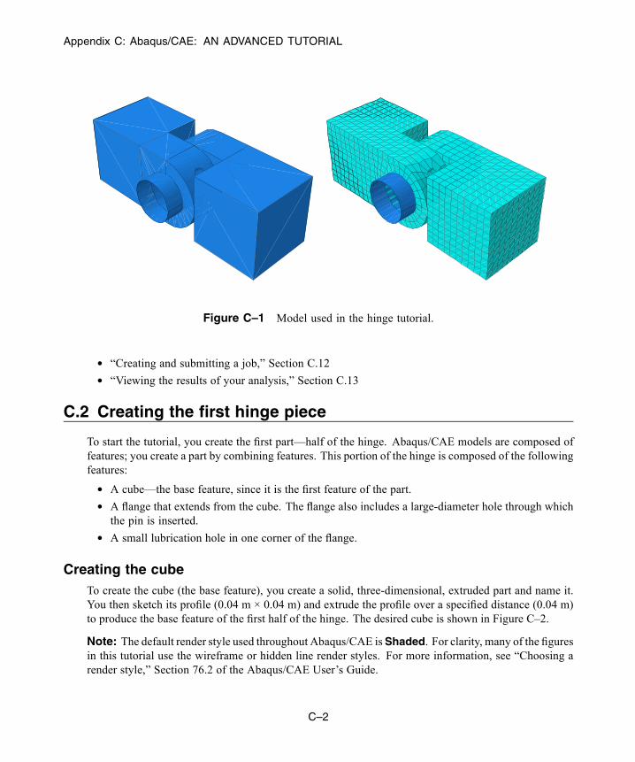
Appendix C: Abaqus/CAE: AN ADVANCED TUTORIAL
Figure C–1 Model used in the hinge tutorial.
• “Creating and submitting a job,” Section C.12• “Viewing the results of your analysis,” Section C.13
C.2 Creating the first hinge piece
To start the tutorial, you create the first part—half of the hinge. Abaqus/CAE models are composed offeatures; you create a part by combining features. This portion of the hinge is composed of the followingfeatures:
• A cube—the base feature, since it is the first feature of the part.• A flange that extends from the cube. The flange also includes a large-diameter hole through whichthe pin is inserted.
• A small lubrication hole in one corner of the flange.
Creating the cubeTo create the cube (the base feature), you create a solid, three-dimensional, extruded part and name it.You then sketch its profile (0.04 m × 0.04 m) and extrude the profile over a specified distance (0.04 m)to produce the base feature of the first half of the hinge. The desired cube is shown in Figure C–2.
Note: The default render style used throughout Abaqus/CAE is Shaded. For clarity, many of the figuresin this tutorial use the wireframe or hidden line render styles. For more information, see “Choosing arender style,” Section 76.2 of the Abaqus/CAE User’s Guide.
C–2
Abaqus ID:Printed on:
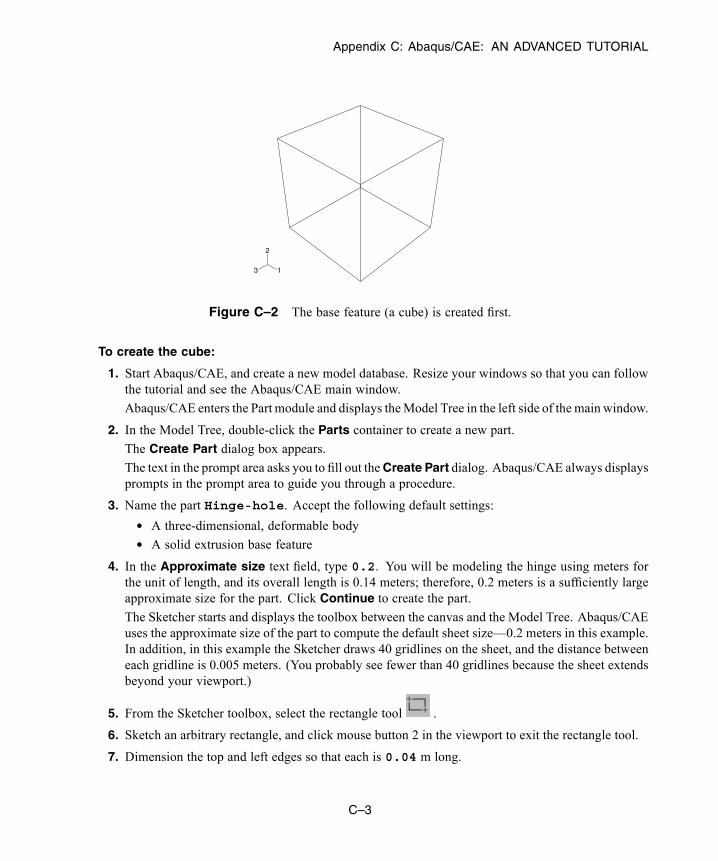
Appendix C: Abaqus/CAE: AN ADVANCED TUTORIAL
1
2
3
Figure C–2 The base feature (a cube) is created first.
To create the cube:
1. Start Abaqus/CAE, and create a new model database. Resize your windows so that you can followthe tutorial and see the Abaqus/CAE main window.
Abaqus/CAE enters the Part module and displays theModel Tree in the left side of the main window.
2. In the Model Tree, double-click the Parts container to create a new part.
The Create Part dialog box appears.
The text in the prompt area asks you to fill out theCreate Part dialog. Abaqus/CAE always displaysprompts in the prompt area to guide you through a procedure.
3. Name the part Hinge-hole. Accept the following default settings:
• A three-dimensional, deformable body• A solid extrusion base feature
4. In the Approximate size text field, type 0.2. You will be modeling the hinge using meters forthe unit of length, and its overall length is 0.14 meters; therefore, 0.2 meters is a sufficiently largeapproximate size for the part. Click Continue to create the part.
The Sketcher starts and displays the toolbox between the canvas and the Model Tree. Abaqus/CAEuses the approximate size of the part to compute the default sheet size—0.2 meters in this example.In addition, in this example the Sketcher draws 40 gridlines on the sheet, and the distance betweeneach gridline is 0.005 meters. (You probably see fewer than 40 gridlines because the sheet extendsbeyond your viewport.)
5. From the Sketcher toolbox, select the rectangle tool .
6. Sketch an arbitrary rectangle, and click mouse button 2 in the viewport to exit the rectangle tool.
7. Dimension the top and left edges so that each is 0.04 m long.
C–3
Abaqus ID:Printed on:
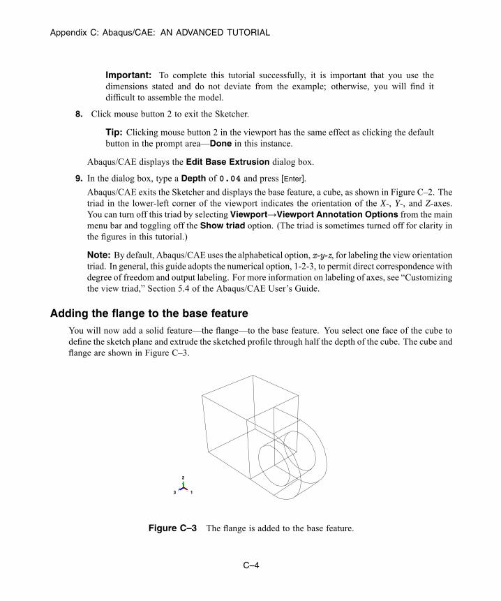
Appendix C: Abaqus/CAE: AN ADVANCED TUTORIAL
Important: To complete this tutorial successfully, it is important that you use thedimensions stated and do not deviate from the example; otherwise, you will find itdifficult to assemble the model.
8. Click mouse button 2 to exit the Sketcher.
Tip: Clicking mouse button 2 in the viewport has the same effect as clicking the defaultbutton in the prompt area—Done in this instance.
Abaqus/CAE displays the Edit Base Extrusion dialog box.
9. In the dialog box, type a Depth of 0.04 and press [Enter].
Abaqus/CAE exits the Sketcher and displays the base feature, a cube, as shown in Figure C–2. Thetriad in the lower-left corner of the viewport indicates the orientation of the X-, Y-, and Z-axes.You can turn off this triad by selecting Viewport→Viewport Annotation Options from the mainmenu bar and toggling off the Show triad option. (The triad is sometimes turned off for clarity inthe figures in this tutorial.)
Note: By default, Abaqus/CAE uses the alphabetical option, x-y-z, for labeling the view orientationtriad. In general, this guide adopts the numerical option, 1-2-3, to permit direct correspondence withdegree of freedom and output labeling. For more information on labeling of axes, see “Customizingthe view triad,” Section 5.4 of the Abaqus/CAE User’s Guide.
Adding the flange to the base featureYou will now add a solid feature—the flange—to the base feature. You select one face of the cube todefine the sketch plane and extrude the sketched profile through half the depth of the cube. The cube andflange are shown in Figure C–3.
1
2
3
Figure C–3 The flange is added to the base feature.
C–4
Abaqus ID:Printed on:
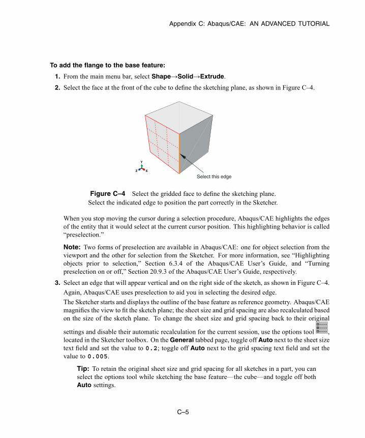
Appendix C: Abaqus/CAE: AN ADVANCED TUTORIAL
To add the flange to the base feature:
1. From the main menu bar, select Shape→Solid→Extrude.
2. Select the face at the front of the cube to define the sketching plane, as shown in Figure C–4.
X
Y
Z
Select this edge
Figure C–4 Select the gridded face to define the sketching plane.Select the indicated edge to position the part correctly in the Sketcher.
When you stop moving the cursor during a selection procedure, Abaqus/CAE highlights the edgesof the entity that it would select at the current cursor position. This highlighting behavior is called“preselection.”
Note: Two forms of preselection are available in Abaqus/CAE: one for object selection from theviewport and the other for selection from the Sketcher. For more information, see “Highlightingobjects prior to selection,” Section 6.3.4 of the Abaqus/CAE User’s Guide, and “Turningpreselection on or off,” Section 20.9.3 of the Abaqus/CAE User’s Guide, respectively.
3. Select an edge that will appear vertical and on the right side of the sketch, as shown in Figure C–4.
Again, Abaqus/CAE uses preselection to aid you in selecting the desired edge.
The Sketcher starts and displays the outline of the base feature as reference geometry. Abaqus/CAEmagnifies the view to fit the sketch plane; the sheet size and grid spacing are also recalculated basedon the size of the sketch plane. To change the sheet size and grid spacing back to their original
settings and disable their automatic recalculation for the current session, use the options tool ,located in the Sketcher toolbox. On theGeneral tabbed page, toggle off Auto next to the sheet sizetext field and set the value to 0.2; toggle off Auto next to the grid spacing text field and set thevalue to 0.005.
Tip: To retain the original sheet size and grid spacing for all sketches in a part, you canselect the options tool while sketching the base feature—the cube—and toggle off bothAuto settings.
C–5
Abaqus ID:Printed on:
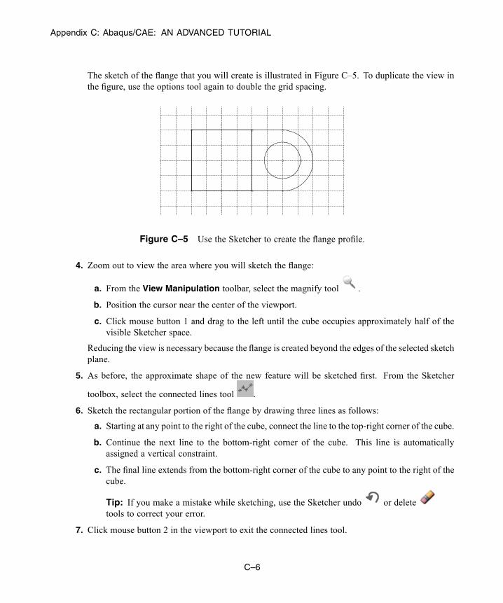
Appendix C: Abaqus/CAE: AN ADVANCED TUTORIAL
The sketch of the flange that you will create is illustrated in Figure C–5. To duplicate the view inthe figure, use the options tool again to double the grid spacing.
Figure C–5 Use the Sketcher to create the flange profile.
4. Zoom out to view the area where you will sketch the flange:
a. From the View Manipulation toolbar, select the magnify tool .
b. Position the cursor near the center of the viewport.
c. Click mouse button 1 and drag to the left until the cube occupies approximately half of thevisible Sketcher space.
Reducing the view is necessary because the flange is created beyond the edges of the selected sketchplane.
5. As before, the approximate shape of the new feature will be sketched first. From the Sketcher
toolbox, select the connected lines tool .
6. Sketch the rectangular portion of the flange by drawing three lines as follows:
a. Starting at any point to the right of the cube, connect the line to the top-right corner of the cube.
b. Continue the next line to the bottom-right corner of the cube. This line is automaticallyassigned a vertical constraint.
c. The final line extends from the bottom-right corner of the cube to any point to the right of thecube.
Tip: If you make a mistake while sketching, use the Sketcher undo or deletetools to correct your error.
7. Click mouse button 2 in the viewport to exit the connected lines tool.
C–6
Abaqus ID:Printed on:

Appendix C: Abaqus/CAE: AN ADVANCED TUTORIAL
8. Refine the sketch by defining the following constraints and dimension:
a. Use the constraints tool to constrain the top and bottom lines of the sketch so that each ishorizontal.
b. Assign an equal length constraint to these two lines (use [Shift] + Click to select both lines).
c. Dimension either line so that it is 0.02 m long.
The sketch appears as shown in Figure C–6.
20.E-03
V
H
H
20.E
V
H
H
Figure C–6 Draw the rectangular portion of the flange.
9. Close the profile by adding a semicircular arc using the 3-points circle tool .
a. Select the two vertices at the open end of the rectangle as the endpoints of the arc, starting withthe top one. Select any point to the right of the sketch as a point that lies on the arc.
b. Define tangent constraints between the ends of the arc and the horizontal lines to refine thesketch.
10. Click mouse button 2 in the viewport to exit the 3-points circle tool.
The resulting arc is shown in Figure C–7.
11. From the Sketcher toolbox, select the center-perimeter circle tool to sketch the flange hole.
a. Place the center of the circle to coincide approximately with the center of the arc createdpreviously. The perimeter point should be placed to the right of the center point. Apply aconcentric constraint between the two circular regions.
b. Use the dimension tool to change the value of the radius to 0.01 m.
C–7
Abaqus ID:Printed on:
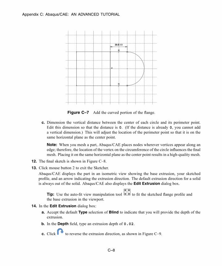
Appendix C: Abaqus/CAE: AN ADVANCED TUTORIAL
20.E-03
V
H
H
20.E
V
H
H
Figure C–7 Add the curved portion of the flange.
c. Dimension the vertical distance between the center of each circle and its perimeter point.Edit this dimension so that the distance is 0. (If the distance is already 0, you cannot adda vertical dimension.) This will adjust the location of the perimeter point so that it is on thesame horizontal plane as the center point.
Note: When you mesh a part, Abaqus/CAE places nodes wherever vertices appear along anedge; therefore, the location of the vertex on the circumference of the circle influences the finalmesh. Placing it on the same horizontal plane as the center point results in a high-quality mesh.
12. The final sketch is shown in Figure C–8.
13. Click mouse button 2 to exit the Sketcher.
Abaqus/CAE displays the part in an isometric view showing the base extrusion, your sketchedprofile, and an arrow indicating the extrusion direction. The default extrusion direction for a solidis always out of the solid. Abaqus/CAE also displays the Edit Extrusion dialog box.
Tip: Use the auto-fit view manipulation tool to fit the sketched flange profile andthe base extrusion in the viewport.
14. In the Edit Extrusion dialog box:
a. Accept the default Type selection of Blind to indicate that you will provide the depth of theextrusion.
b. In the Depth field, type an extrusion depth of 0.02.
c. Click to reverse the extrusion direction, as shown in Figure C–9.
C–8
Abaqus ID:Printed on:

Appendix C: Abaqus/CAE: AN ADVANCED TUTORIAL
20.E-03
10.E-03
V 0.V
H
H
20.E
10.E
V 0.V
H
H
Figure C–8 Final sketch.
X
Y
Z
Figure C–9 Completed flange sketch showing the extrusion direction.
d. Toggle on Keep internal boundaries. When you toggle this option on, Abaqus/CAEmaintains the face that is generated between the extruded solid feature and the existing part.As a result, the extruded flange is maintained as a second cell and is not merged with thecube. (When you mesh the model at the end of the tutorial, the internal boundary allows youto mesh the flange without having to first partition the cell and flange into separate cells.)
e. Click OK to create the solid extrusion.
C–9
Abaqus ID:Printed on:

Appendix C: Abaqus/CAE: AN ADVANCED TUTORIAL
Abaqus/CAE displays the part composed of the cube and the flange. Use the auto-fit view
manipulation tool again to resize the part to fit in the viewport.
Modifying a featureEach part is defined by a set of features, and each feature in turn is defined by a set of parameters. Forexample, the base feature (the cube) and the second feature (the flange) are both defined by a sketch andan extrusion depth. You modify a part by modifying the parameters that define its features. For the hingeexample you will change the radius of the hole in the sketch of the flange from 0.01 m to 0.012 m.
To modify a feature:
1. In the Model Tree, expand the Hinge-hole item underneath the Parts container. Then expand theFeatures container that appears.
A list showing each feature’s Name appears. In this example you have created two solid extrusionfeatures: the base feature (the cube), Solid extrude-1, and the flange, Solid extrude-2.
2. Click mouse button 3 on Solid extrude-2 (the flange) in this list.
Abaqus/CAE highlights the selected feature in the viewport.
3. From the menu that appears, select Edit.
Abaqus/CAE displays the feature editor. For an extruded solid you can change the extrusion depth,the twist or draft (if specified when the feature was created), and the profile sketch.
4. From the feature editor, click .
Abaqus/CAE displays the sketch of the second feature, and the feature editor disappears.
5. From the edit tools in the Sketcher toolbox, select the edit dimension value tool .
6. Select the radial dimension of the circle (0.010).
7. In the Edit Dimension dialog box, type a new radius of 0.012 and click OK.
Abaqus/CAE closes the dialog box and changes the radius of the circle in the sketch only.
8. Click mouse button 2 to exit the edit dimension value tool. Click mouse button 2 again to exit theSketcher.
Abaqus/CAE again displays the feature editor.
9. Click OK to regenerate the flange with the modified radius and to exit the feature editor.
The flange hole is enlarged to the new radius dimension.
Note: In some circumstances regenerating a feature causes dependent features to fail. In such acase Abaqus/CAE asks if you want to save your changes and suppress the features that failed toregenerate, or if you want to revert to the unmodified feature and lose your changes.
C–10
Abaqus ID:Printed on:
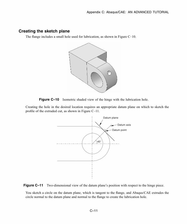
Appendix C: Abaqus/CAE: AN ADVANCED TUTORIAL
Creating the sketch planeThe flange includes a small hole used for lubrication, as shown in Figure C–10.
Figure C–10 Isometric shaded view of the hinge with the lubrication hole.
Creating the hole in the desired location requires an appropriate datum plane on which to sketch theprofile of the extruded cut, as shown in Figure C–11.
45°
Datum plane
Datum axis
Datum point
Figure C–11 Two-dimensional view of the datum plane’s position with respect to the hinge piece.
You sketch a circle on the datum plane, which is tangent to the flange, and Abaqus/CAE extrudes thecircle normal to the datum plane and normal to the flange to create the lubrication hole.
C–11
Abaqus ID:Printed on:

Appendix C: Abaqus/CAE: AN ADVANCED TUTORIAL
There are three operations involved in creating the datum plane:
• Creating a datum point on the circumference of the flange.• Creating a datum axis running between two datum points.• Creating a datum plane through the datum point on the circumference and normal to the datum axis.
To create the sketch plane:
1. From the main menu bar, select Tools→Datum.
Abaqus/CAE displays the Create Datum dialog box.
2. Create a datum point along the curved edge of the flange through which the datum plane will pass.From the Create Datum dialog box, choose the Point datum type.
3. From the list of methods, click Enter parameter.
4. Select the curved edge, as shown in Figure C–12. Note the direction of the arrow indicating anincreasing edge parameter from 0.0 to 1.0. You cannot change the direction of this arrow.
1
2
3
Select this edge
Figure C–12 Create a datum point along the curved edge of the flange.
5. In the text box in the prompt area, enter a normalized edge parameter and press [Enter]. If the arrowdirection is the same as in Figure C–12, enter 0.25 as the normalized edge parameter; if the arrowpoints in the opposite direction, enter 0.75 as the normalized edge parameter.
Abaqus/CAE creates a datum point along the selected edge.
6. Create a datum axis that will define the normal to the datum plane. From the Create Datum dialogbox, choose the Axis datum type. Click the 2 points method.
Abaqus/CAE highlights the points that can be used to create the datum axis.
C–12
Abaqus ID:Printed on:

Appendix C: Abaqus/CAE: AN ADVANCED TUTORIAL
7. Select the point at the center of the hole (created when you sketched the hole’s profile) and the datumpoint on the curved edge.
Abaqus/CAE displays a datum axis passing through the two points, as shown in Figure C–13.
1
2
3
Figure C–13 Create a datum axis defined by two datum points.
8. The final step is to create the datum plane normal to the datum axis. From theCreate Datum dialogbox, choose the Plane datum type. Click the Point and normal method.
9. Select the datum point on the curved edge as the point through which the datum plane will pass.
10. Select the datum axis as the edge that will be normal to the datum plane.
Abaqus/CAE creates the datum plane, as shown in Figure C–14.
Sketching the lubrication hole
The next operation creates the lubrication hole on the flange by extruding a circle from the datum planethat you just created. First, you need to create a datum point on the flange that indicates the center of thehole, as illustrated in Figure C–15.
C–13
Abaqus ID:Printed on:
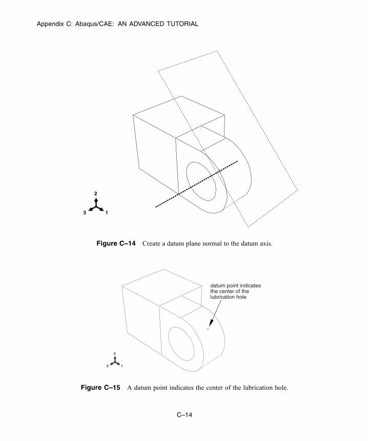
Appendix C: Abaqus/CAE: AN ADVANCED TUTORIAL
1
2
3
Figure C–14 Create a datum plane normal to the datum axis.
1
2
3
datum point indicates the center of thelubrication hole
Figure C–15 A datum point indicates the center of the lubrication hole.
C–14
Abaqus ID:Printed on:
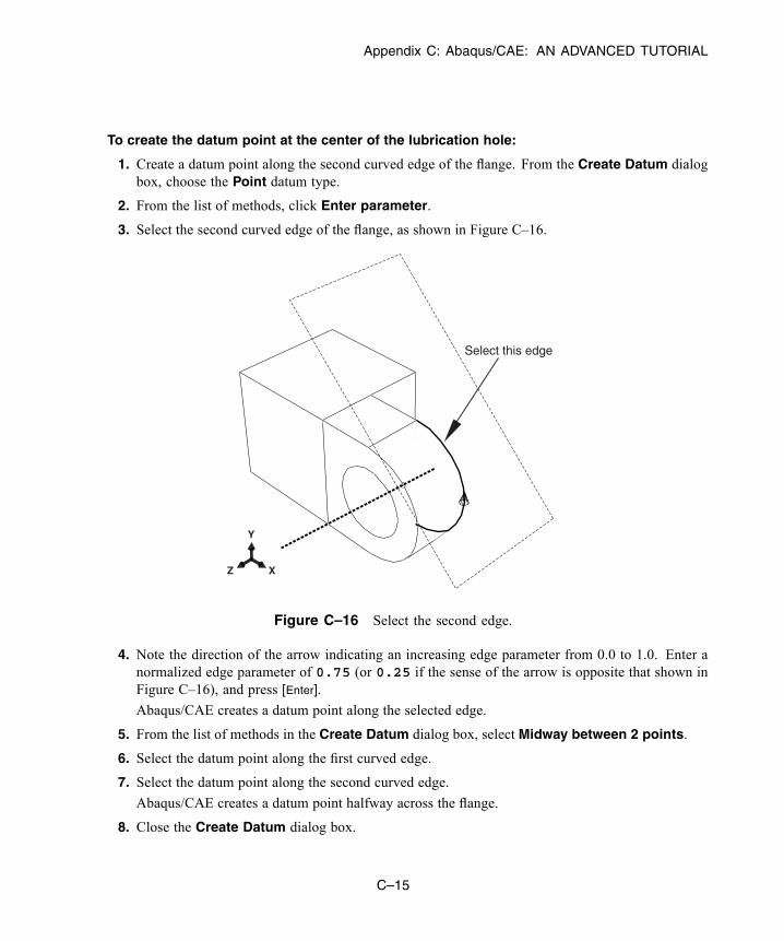
Appendix C: Abaqus/CAE: AN ADVANCED TUTORIAL
To create the datum point at the center of the lubrication hole:
1. Create a datum point along the second curved edge of the flange. From the Create Datum dialogbox, choose the Point datum type.
2. From the list of methods, click Enter parameter.
3. Select the second curved edge of the flange, as shown in Figure C–16.
X
Y
Z
Select this edge
Figure C–16 Select the second edge.
4. Note the direction of the arrow indicating an increasing edge parameter from 0.0 to 1.0. Enter anormalized edge parameter of 0.75 (or 0.25 if the sense of the arrow is opposite that shown inFigure C–16), and press [Enter].
Abaqus/CAE creates a datum point along the selected edge.
5. From the list of methods in the Create Datum dialog box, select Midway between 2 points.
6. Select the datum point along the first curved edge.
7. Select the datum point along the second curved edge.
Abaqus/CAE creates a datum point halfway across the flange.
8. Close the Create Datum dialog box.
C–15
Abaqus ID:Printed on:
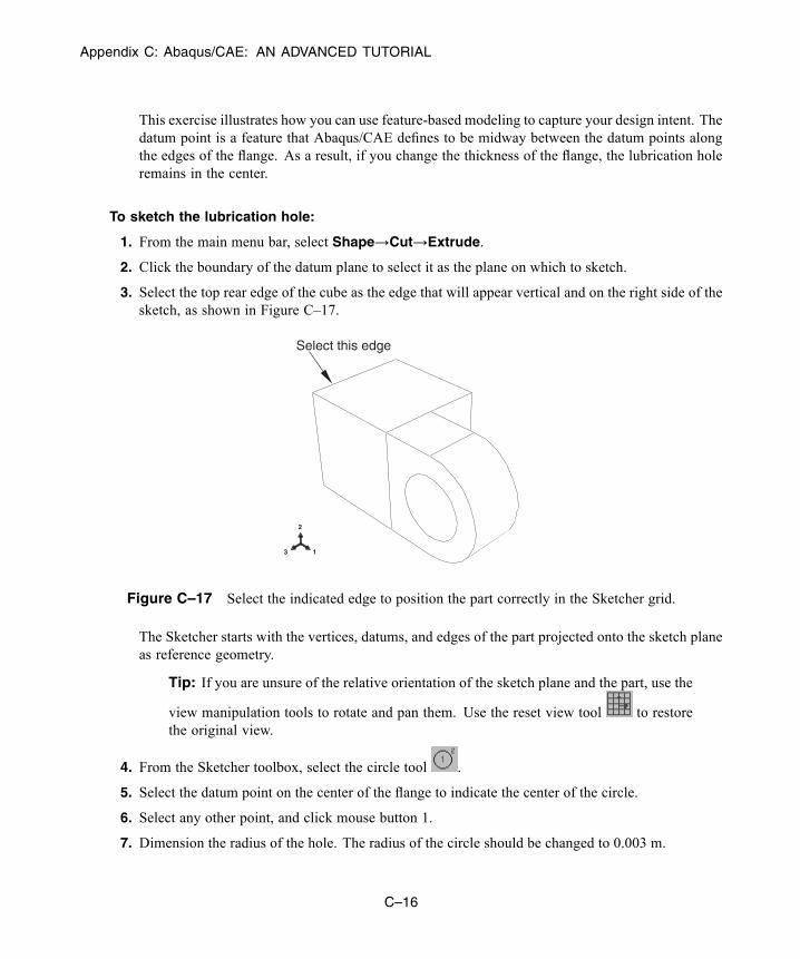
Appendix C: Abaqus/CAE: AN ADVANCED TUTORIAL
This exercise illustrates how you can use feature-based modeling to capture your design intent. Thedatum point is a feature that Abaqus/CAE defines to be midway between the datum points alongthe edges of the flange. As a result, if you change the thickness of the flange, the lubrication holeremains in the center.
To sketch the lubrication hole:
1. From the main menu bar, select Shape→Cut→Extrude.
2. Click the boundary of the datum plane to select it as the plane on which to sketch.
3. Select the top rear edge of the cube as the edge that will appear vertical and on the right side of thesketch, as shown in Figure C–17.
1
2
3
Select this edge
Figure C–17 Select the indicated edge to position the part correctly in the Sketcher grid.
The Sketcher starts with the vertices, datums, and edges of the part projected onto the sketch planeas reference geometry.
Tip: If you are unsure of the relative orientation of the sketch plane and the part, use the
view manipulation tools to rotate and pan them. Use the reset view tool to restorethe original view.
4. From the Sketcher toolbox, select the circle tool .
5. Select the datum point on the center of the flange to indicate the center of the circle.
6. Select any other point, and click mouse button 1.
7. Dimension the radius of the hole. The radius of the circle should be changed to 0.003 m.
C–16
Abaqus ID:Printed on:
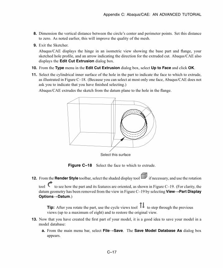
Appendix C: Abaqus/CAE: AN ADVANCED TUTORIAL
8. Dimension the vertical distance between the circle’s center and perimeter points. Set this distanceto zero. As noted earlier, this will improve the quality of the mesh.
9. Exit the Sketcher.
Abaqus/CAE displays the hinge in an isometric view showing the base part and flange, yoursketched hole profile, and an arrow indicating the direction for the extruded cut. Abaqus/CAE alsodisplays the Edit Cut Extrusion dialog box.
10. From the Type menu in the Edit Cut Extrusion dialog box, select Up to Face and click OK.
11. Select the cylindrical inner surface of the hole in the part to indicate the face to which to extrude,as illustrated in Figure C–18. (Because you can select at most only one face, Abaqus/CAE does notask you to indicate that you have finished selecting.)
Abaqus/CAE extrudes the sketch from the datum plane to the hole in the flange.
Select this surface
Figure C–18 Select the face to which to extrude.
12. From theRender Style toolbar, select the shaded display tool if necessary, and use the rotation
tool to see how the part and its features are oriented, as shown in Figure C–19. (For clarity, thedatum geometry has been removed from the view in Figure C–19 by selecting View→Part DisplayOptions→Datum.)
Tip: After you rotate the part, use the cycle views tool to step through the previousviews (up to a maximum of eight) and to restore the original view.
13. Now that you have created the first part of your model, it is a good idea to save your model in amodel database:
a. From the main menu bar, select File→Save. The Save Model Database As dialog boxappears.
C–17
Abaqus ID:Printed on:

Appendix C: Abaqus/CAE: AN ADVANCED TUTORIAL
1
2
3
Figure C–19 Isometric view of the first hinge.
b. Type a name for the new model database in the File Name field, and click OK. You do notneed to include the file extension; Abaqus/CAE appends .cae automatically to the file name.
Abaqus/CAE stores the model database in a new file and returns to the Part module. The nameof your model database appears in the main window title bar.
If you find you need to interrupt this tutorial, you can save the model database at any time and exitAbaqus/CAE. You can then start a new Abaqus/CAE session and open the saved model database byselecting Open Database from the Start Session dialog box. The model database will containany parts, materials, loads, etc. that you created, and you will be able to continue the tutorial.
C.3 Assigning section properties to the hinge part
The process of assigning section properties to a part is divided into three tasks:
• Creating a material.• Creating a section that includes a reference to the material.• Assigning the section to the part or to a region of the part.
Creating a materialYou will create a material named Steel that has a Young’s modulus of 209 GPa and a Poisson’s ratioof 0.3.
To define the material:
1. In the Model Tree, double-click the Materials container to create a new material.
The Edit Material dialog box appears.
2. Name the material Steel.
C–18
Abaqus ID:Printed on:

Appendix C: Abaqus/CAE: AN ADVANCED TUTORIAL
3. From the editor’s menu bar, select Mechanical→Elasticity→Elastic.
Abaqus/CAE displays the Elastic data form.
4. In the respective fields in the Elastic data form, type a value of 209.E9 for Young’s modulus anda value of 0.3 for Poisson’s ratio.
5. Click OK to exit the material editor.
Defining a sectionNext, you will create a section that includes a reference to the material Steel.
To define the section:
1. In the Model Tree, double-click the Sections container to create a section.
The Create Section dialog box appears.
2. In the Create Section dialog box:
a. Name the section SolidSection.
b. In the Category list, accept Solid as the default selection.
c. In the Type list, accept Homogeneous as the default selection, and click Continue.
The section editor appears.
3. In the editor, accept Steel as the material selection and click OK.
If you had defined other materials, you could click the arrow next to the Material text box to see alist of available materials and to select the material of your choice.
Assigning the sectionYou will now assign the section SolidSection to the hinge part.
To assign the section to the hinge part:
1. In the Model Tree, expand the Hinge-hole item underneath the Parts container and double-clickSection Assignments in the list that appears.
2. Drag a rectangle around the hinge piece to select the entire part.
Abaqus/CAE highlights all the regions of the part.
3. Click mouse button 2 to indicate that you have finished selecting the regions to be assigned thesection.
The Edit Section Assignment dialog box appears containing a list of existing sections.SolidSection is selected by default since there are no other sections currently defined.
4. In the Edit Section Assignment dialog box, accept the default selection of SolidSection,and click OK.
C–19
Abaqus ID:Printed on:
Appendix C: Abaqus/CAE: AN ADVANCED TUTORIAL
Abaqus/CAE assigns the section to the part and colors the entire part aqua to indicate that the regionhas a section assignment.
C.4 Creating and modifying a second hinge piece
The model contains a second hinge piece similar to the first except that the lubrication hole is not present.You will create a copy of the first hinge piece and delete the features that form the lubrication hole.
Copying the hingeFirst you will create an exact copy of the hinge piece.
To copy the hinge:
1. In the Model Tree, click mouse button 3 on Hinge-hole underneath the Parts container and selectCopy from the menu that appears.
Abaqus/CAE displays the Part Copy dialog box.
2. In the text box in the Part Copy dialog box, type Hinge-solid, and click OK.
Abaqus/CAE creates a copy of the hinge piece and names the copy Hinge-solid. The copy of thehinge piece includes the section from the original hinge piece.
Modifying the copy of the hingeNow you will create a solid hinge piece by deleting the features that form the lubrication hole.
To modify the copy of the hinge:
1. In the Model Tree, double-click Hinge-solid underneath the Parts container to make it current.
Abaqus/CAE displays the part in the current viewport. Look at the viewport title bar to see whichpart is being displayed.
2. Expand the Features container underneath Hinge-solid.
3. Click mouse button 3 on Datum pt-1 in the list of part features.
Abaqus/CAE highlights the point, as shown in Figure C–20.
4. From the menu that appears, select Delete. When you delete a selected feature, Abaqus/CAEasks whether you also want to delete any features that depend on the feature being deleted. Thefeature being deleted is called the “parent” feature, and its dependent features are called “children.”Abaqus/CAE highlights all the features that it will delete if the parent feature is deleted. From thebuttons in the prompt area, click Yes to delete the datum point and all its children.
Abaqus/CAE deletes the datum point. Because they were dependent on the datum point,Abaqus/CAE also deletes the datum axis, the datum plane, and the lubrication hole.
C–20
Abaqus ID:Printed on:
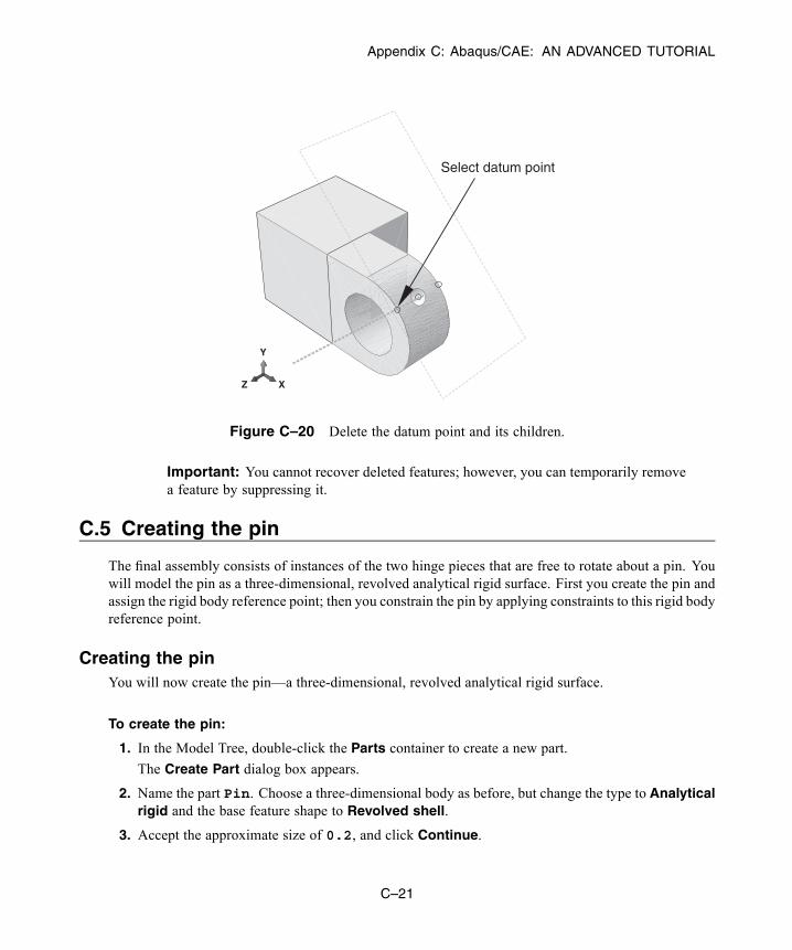
Appendix C: Abaqus/CAE: AN ADVANCED TUTORIAL
X
Y
Z
Select datum point
Figure C–20 Delete the datum point and its children.
Important: You cannot recover deleted features; however, you can temporarily removea feature by suppressing it.
C.5 Creating the pin
The final assembly consists of instances of the two hinge pieces that are free to rotate about a pin. Youwill model the pin as a three-dimensional, revolved analytical rigid surface. First you create the pin andassign the rigid body reference point; then you constrain the pin by applying constraints to this rigid bodyreference point.
Creating the pinYou will now create the pin—a three-dimensional, revolved analytical rigid surface.
To create the pin:
1. In the Model Tree, double-click the Parts container to create a new part.
The Create Part dialog box appears.
2. Name the part Pin. Choose a three-dimensional body as before, but change the type to Analyticalrigid and the base feature shape to Revolved shell.
3. Accept the approximate size of 0.2, and click Continue.
C–21
Abaqus ID:Printed on:
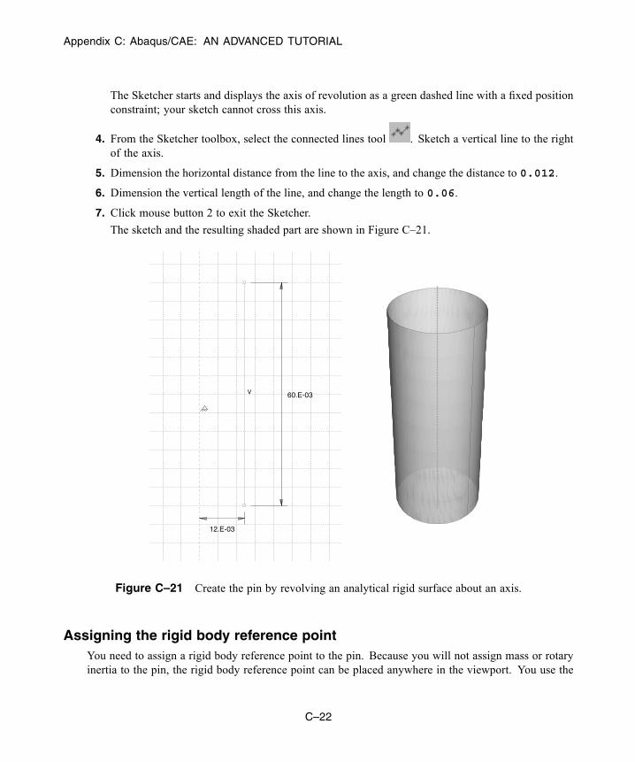
Appendix C: Abaqus/CAE: AN ADVANCED TUTORIAL
The Sketcher starts and displays the axis of revolution as a green dashed line with a fixed positionconstraint; your sketch cannot cross this axis.
4. From the Sketcher toolbox, select the connected lines tool . Sketch a vertical line to the rightof the axis.
5. Dimension the horizontal distance from the line to the axis, and change the distance to 0.012.
6. Dimension the vertical length of the line, and change the length to 0.06.
7. Click mouse button 2 to exit the Sketcher.
The sketch and the resulting shaded part are shown in Figure C–21.
V 60.E-03
12.E-03
Figure C–21 Create the pin by revolving an analytical rigid surface about an axis.
Assigning the rigid body reference pointYou need to assign a rigid body reference point to the pin. Because you will not assign mass or rotaryinertia to the pin, the rigid body reference point can be placed anywhere in the viewport. You use the
C–22
Abaqus ID:Printed on:
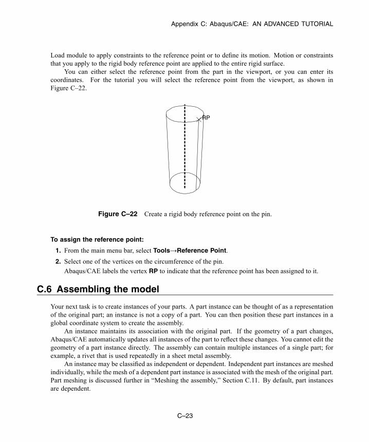
Appendix C: Abaqus/CAE: AN ADVANCED TUTORIAL
Load module to apply constraints to the reference point or to define its motion. Motion or constraintsthat you apply to the rigid body reference point are applied to the entire rigid surface.
You can either select the reference point from the part in the viewport, or you can enter itscoordinates. For the tutorial you will select the reference point from the viewport, as shown inFigure C–22.
RP
Figure C–22 Create a rigid body reference point on the pin.
To assign the reference point:
1. From the main menu bar, select Tools→Reference Point.
2. Select one of the vertices on the circumference of the pin.
Abaqus/CAE labels the vertex RP to indicate that the reference point has been assigned to it.
C.6 Assembling the model
Your next task is to create instances of your parts. A part instance can be thought of as a representationof the original part; an instance is not a copy of a part. You can then position these part instances in aglobal coordinate system to create the assembly.
An instance maintains its association with the original part. If the geometry of a part changes,Abaqus/CAE automatically updates all instances of the part to reflect these changes. You cannot edit thegeometry of a part instance directly. The assembly can contain multiple instances of a single part; forexample, a rivet that is used repeatedly in a sheet metal assembly.
An instance may be classified as independent or dependent. Independent part instances are meshedindividually, while the mesh of a dependent part instance is associated with the mesh of the original part.Part meshing is discussed further in “Meshing the assembly,” Section C.11. By default, part instancesare dependent.
C–23
Abaqus ID:Printed on:
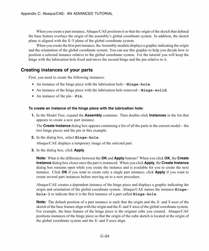
Appendix C: Abaqus/CAE: AN ADVANCED TUTORIAL
When you create a part instance, Abaqus/CAE positions it so that the origin of the sketch that definedthe base feature overlays the origin of the assembly’s global coordinate system. In addition, the sketchplane is aligned with the X–Y plane of the global coordinate system.
When you create the first part instance, the Assemblymodule displays a graphic indicating the originand the orientation of the global coordinate system. You can use this graphic to help you decide how toposition a selected instance relative to the global coordinate system. For the tutorial you will keep thehinge with the lubrication hole fixed and move the second hinge and the pin relative to it.
Creating instances of your parts
First, you need to create the following instances:
• An instance of the hinge piece with the lubrication hole—Hinge-hole.
• An instance of the hinge piece with the lubrication hole removed—Hinge-solid.
• An instance of the pin—Pin.
To create an instance of the hinge piece with the lubrication hole:
1. In the Model Tree, expand the Assembly container. Then double-click Instances in the list thatappears to create a new part instance.
The Create Instance dialog box appears containing a list of all the parts in the current model—thetwo hinge pieces and the pin in this example.
2. In the dialog box, select Hinge-hole.
Abaqus/CAE displays a temporary image of the selected part.
3. In the dialog box, click Apply.
Note: What is the difference between theOK and Apply buttons? When you clickOK, the CreateInstance dialog box closes once the part is instanced. When you clickApply, theCreate Instancedialog box remains open while you create the instance and is available for you to create the nextinstance. Click OK if you want to create only a single part instance; click Apply if you want tocreate several part instances before moving on to a new procedure.
Abaqus/CAE creates a dependent instance of the hinge piece and displays a graphic indicating theorigin and orientation of the global coordinate system. Abaqus/CAE names the instance Hinge-hole-1 to indicate that it is the first instance of a part called Hinge-hole.
Note: The default position of a part instance is such that the origin and the X- and Y-axes of thesketch of the base feature align with the origin and the X- and Y-axes of the global coordinate system.For example, the base feature of the hinge piece is the original cube you created. Abaqus/CAEpositions instances of the hinge piece so that the origin of the cube sketch is located at the origin ofthe global coordinate system and the X- and Y-axes align.
C–24
Abaqus ID:Printed on:

Appendix C: Abaqus/CAE: AN ADVANCED TUTORIAL
Creating an instance of the solid hinge piece
You will now create an instance of the solid hinge piece. To separate the solid hinge piece from theinstance of the hinge piece with the lubrication hole, you ask Abaqus/CAE to offset the new instancealong the X-axis.
To create an instance of the solid hinge piece:
1. From the Create Instance dialog box, toggle on Auto-offset from other instances.
The auto-offset function prevents new part instances from overlapping existing instances.
2. From the Create Instance dialog box, select Hinge-solid and click OK.
Abaqus/CAE closes the dialog box, creates the new dependent instance, and applies an offsetalong the X-axis that separates the two hinges, as shown in Figure C–23. (For clarity the datumgeometry has been removed from the shaded view in Figure C–23 and subsequent figures byselecting View→Assembly Display Options→Datum.)
1
2
3
Figure C–23 Create an instance of each hinge piece, and applyan offset to position them in the viewport.
C–25
Abaqus ID:Printed on:
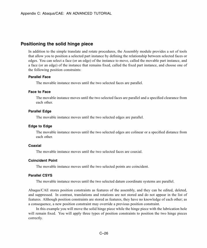
Appendix C: Abaqus/CAE: AN ADVANCED TUTORIAL
Positioning the solid hinge piece
In addition to the simple translate and rotate procedures, the Assembly module provides a set of toolsthat allow you to position a selected part instance by defining the relationship between selected faces oredges. You can select a face (or an edge) of the instance to move, called the movable part instance, anda face (or an edge) of the instance that remains fixed, called the fixed part instance, and choose one ofthe following position constraints:
Parallel Face
The movable instance moves until the two selected faces are parallel.
Face to Face
The movable instance moves until the two selected faces are parallel and a specified clearance fromeach other.
Parallel Edge
The movable instance moves until the two selected edges are parallel.
Edge to Edge
The movable instance moves until the two selected edges are colinear or a specified distance fromeach other.
Coaxial
The movable instance moves until the two selected faces are coaxial.
Coincident Point
The movable instance moves until the two selected points are coincident.
Parallel CSYS
The movable instance moves until the two selected datum coordinate systems are parallel.
Abaqus/CAE stores position constraints as features of the assembly, and they can be edited, deleted,and suppressed. In contrast, translations and rotations are not stored and do not appear in the list offeatures. Although position constraints are stored as features, they have no knowledge of each other; asa consequence, a new position constraint may override a previous position constraint.
In this example you will move the solid hinge piece while the hinge piece with the lubrication holewill remain fixed. You will apply three types of position constraints to position the two hinge piecescorrectly.
C–26
Abaqus ID:Printed on:

Appendix C: Abaqus/CAE: AN ADVANCED TUTORIAL
To position the solid hinge piece:
1. First, constrain the solid hinge piece so that the two flanges face each other. From the main menubar, select Constraint→Face to Face.
2. From the movable part instance, select the face of the solid hinge piece shown in Figure C–24.
Select this face
Figure C–24 Select a face on the movable part instance.
3. From the fixed part instance, select the face of the hinge piece with the lubrication hole shown inFigure C–25. Abaqus/CAE highlights the face on the movable part instance in red and the face onthe fixed part instance in magenta.
Select this face
Figure C–25 Select a face on the fixed instance.
C–27
Abaqus ID:Printed on:
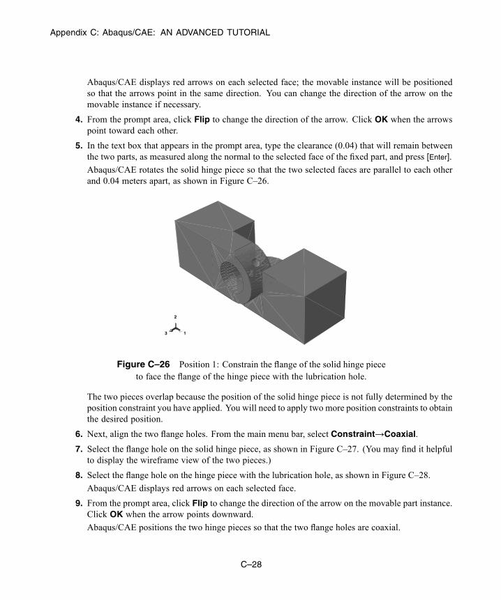
Appendix C: Abaqus/CAE: AN ADVANCED TUTORIAL
Abaqus/CAE displays red arrows on each selected face; the movable instance will be positionedso that the arrows point in the same direction. You can change the direction of the arrow on themovable instance if necessary.
4. From the prompt area, click Flip to change the direction of the arrow. Click OK when the arrowspoint toward each other.
5. In the text box that appears in the prompt area, type the clearance (0.04) that will remain betweenthe two parts, as measured along the normal to the selected face of the fixed part, and press [Enter].
Abaqus/CAE rotates the solid hinge piece so that the two selected faces are parallel to each otherand 0.04 meters apart, as shown in Figure C–26.
1
2
3
Figure C–26 Position 1: Constrain the flange of the solid hinge pieceto face the flange of the hinge piece with the lubrication hole.
The two pieces overlap because the position of the solid hinge piece is not fully determined by theposition constraint you have applied. You will need to apply two more position constraints to obtainthe desired position.
6. Next, align the two flange holes. From the main menu bar, select Constraint→Coaxial.
7. Select the flange hole on the solid hinge piece, as shown in Figure C–27. (You may find it helpfulto display the wireframe view of the two pieces.)
8. Select the flange hole on the hinge piece with the lubrication hole, as shown in Figure C–28.
Abaqus/CAE displays red arrows on each selected face.
9. From the prompt area, click Flip to change the direction of the arrow on the movable part instance.Click OK when the arrow points downward.
Abaqus/CAE positions the two hinge pieces so that the two flange holes are coaxial.
C–28
Abaqus ID:Printed on:

Appendix C: Abaqus/CAE: AN ADVANCED TUTORIAL
1
2
3Select this face
Figure C–27 Select a cylindrical face on the movable instance.
1
2
3 Select this face
Figure C–28 Select a cylindrical face on the fixed instance.
10. Use the rotate tool to look at the top view of the two pieces. Notice that the two flanges arenow overlapping, as shown in Figure C–29.
11. Finally, add a constraint to eliminate the overlap between the two flanges. From the main menu bar,select Constraint→Edge to Edge.
12. Select the straight edge on the solid hinge piece shown in Figure C–30.
C–29
Abaqus ID:Printed on:
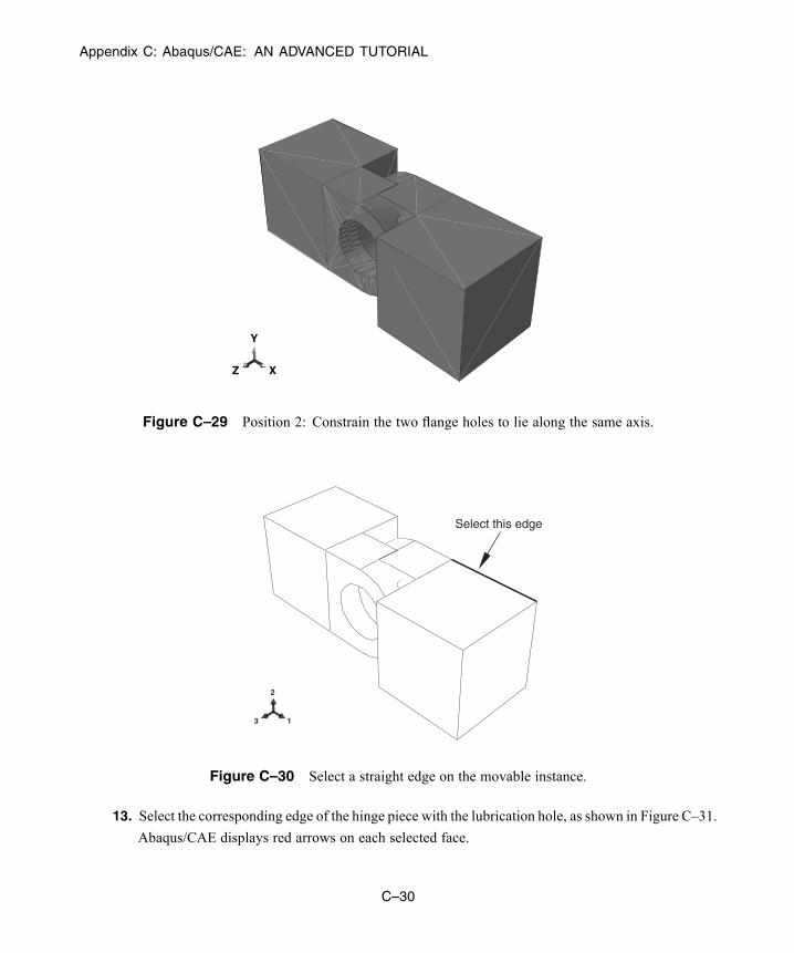
Appendix C: Abaqus/CAE: AN ADVANCED TUTORIAL
X
Y
Z
Figure C–29 Position 2: Constrain the two flange holes to lie along the same axis.
1
2
3
Select this edge
Figure C–30 Select a straight edge on the movable instance.
13. Select the corresponding edge of the hinge piece with the lubrication hole, as shown in Figure C–31.
Abaqus/CAE displays red arrows on each selected face.
C–30
Abaqus ID:Printed on:
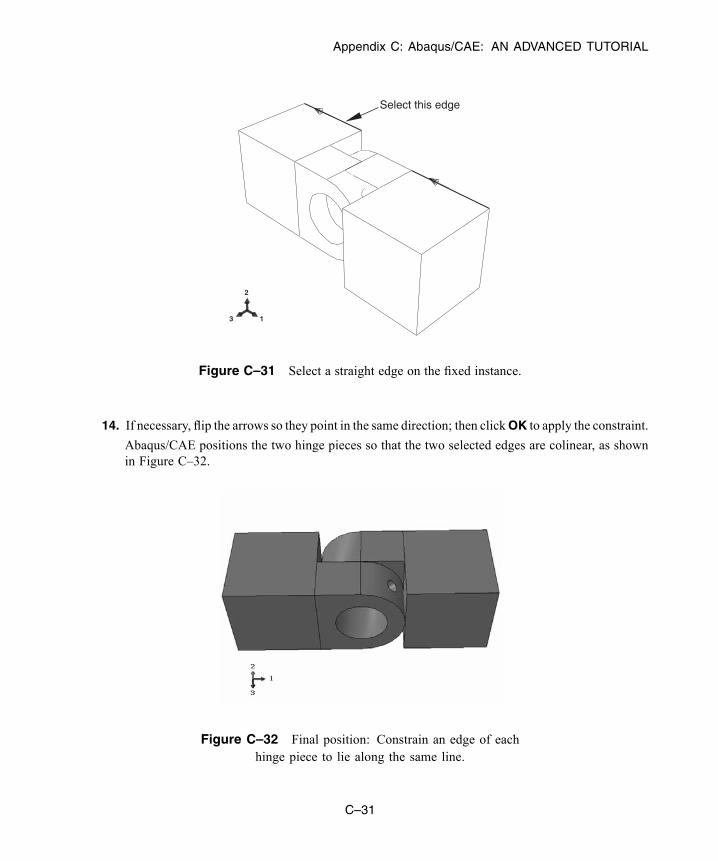
Appendix C: Abaqus/CAE: AN ADVANCED TUTORIAL
1
2
3
Select this edge
Figure C–31 Select a straight edge on the fixed instance.
14. If necessary, flip the arrows so they point in the same direction; then clickOK to apply the constraint.
Abaqus/CAE positions the two hinge pieces so that the two selected edges are colinear, as shownin Figure C–32.
Figure C–32 Final position: Constrain an edge of eachhinge piece to lie along the same line.
C–31
Abaqus ID:Printed on:

Appendix C: Abaqus/CAE: AN ADVANCED TUTORIAL
Creating and positioning an instance of the pinYou will now create an instance of the pin and position it symmetrically in the flange holes usingconstraints and translation vectors. To define the translation vector, you can select vertices from theassembly or you can enter the coordinates. You can determine the translation vector using the Querytool.
To position the pin:
1. In the Model Tree, double-click Instances underneath the Assembly container.
2. In the Create Instance dialog box, toggle off Auto-offset from other instances and create aninstance of the pin.
3. Constrain the pin to lie along the same axis as the two flange holes. Use the Constraint→Coaxialmenu as you did when you aligned the two flange holes in the previous section. (You can selecteither of the flange holes as the cylindrical surface of the fixed instance, and the direction of thearrows is not important.)
Abaqus/CAE will position the pin as shown in Figure C–33.
RP
1
2
3
Figure C–33 Align the pin to be coaxial with the two flange holes.
4. From the main menu bar, select Tools→Query.
The Query dialog box appears.
5. Select Distance from the list of General Queries.
C–32
Abaqus ID:Printed on:
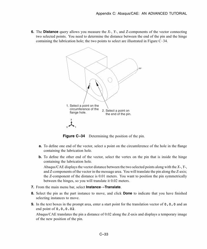
Appendix C: Abaqus/CAE: AN ADVANCED TUTORIAL
6. The Distance query allows you measure the X-, Y-, and Z-components of the vector connectingtwo selected points. You need to determine the distance between the end of the pin and the hingecontaining the lubrication hole; the two points to select are illustrated in Figure C–34.
RP
1
2
3
1. Select a point on the circumference of the flange hole.
2. Select a point on the end of the pin.
Figure C–34 Determining the position of the pin.
a. To define one end of the vector, select a point on the circumference of the hole in the flangecontaining the lubrication hole.
b. To define the other end of the vector, select the vertex on the pin that is inside the hingecontaining the lubrication hole.
Abaqus/CAE displays the vector distance between the two selected points along with the X-, Y-,and Z-components of the vector in the message area. You will translate the pin along the Z-axis;the Z-component of the distance is 0.01 meters. You want to position the pin symmetricallybetween the hinges, so you will translate it 0.02 meters.
7. From the main menu bar, select Instance→Translate.
8. Select the pin as the part instance to move, and click Done to indicate that you have finishedselecting instances to move.
9. In the text boxes in the prompt area, enter a start point for the translation vector of 0,0,0 and anend point of 0,0,0.02.
Abaqus/CAE translates the pin a distance of 0.02 along the Z-axis and displays a temporary imageof the new position of the pin.
C–33
Abaqus ID:Printed on:
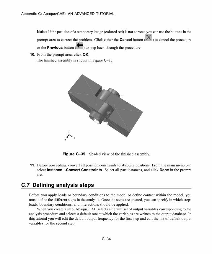
Appendix C: Abaqus/CAE: AN ADVANCED TUTORIAL
Note: If the position of a temporary image (colored red) is not correct, you can use the buttons in the
prompt area to correct the problem. Click either the Cancel button ( ) to cancel the procedure
or the Previous button ( ) to step back through the procedure.
10. From the prompt area, click OK.
The finished assembly is shown in Figure C–35.
RP
1
2
3
Figure C–35 Shaded view of the finished assembly.
11. Before proceeding, convert all position constraints to absolute positions. From the main menu bar,select Instance→Convert Constraints. Select all part instances, and click Done in the promptarea.
C.7 Defining analysis steps
Before you apply loads or boundary conditions to the model or define contact within the model, youmust define the different steps in the analysis. Once the steps are created, you can specify in which stepsloads, boundary conditions, and interactions should be applied.
When you create a step, Abaqus/CAE selects a default set of output variables corresponding to theanalysis procedure and selects a default rate at which the variables are written to the output database. Inthis tutorial you will edit the default output frequency for the first step and edit the list of default outputvariables for the second step.
C–34
Abaqus ID:Printed on:

Appendix C: Abaqus/CAE: AN ADVANCED TUTORIAL
Creating the analysis stepsThe analysis that you perform on the hinge model will consist of an initial step and two general analysissteps:
• In the initial step you apply boundary conditions to regions of the model and define contact betweenregions of the model.
• In the first general analysis step you allow contact to become established.• In the second general analysis step you modify two of the boundary conditions applied to the modeland apply a pressure load to one of the hinge pieces.
Abaqus/CAE creates the initial step by default, but you must create the two analysis steps.
To create the analysis steps:
1. In the Model Tree, double-click the Steps container to create a new step.
The Create Step dialog box appears.
2. In the Create Step dialog box:
a. Name the step Contact.
b. Accept the default procedure type (Static, General), and click Continue.
The step editor appears.
3. In the Description field, type Establish contact.
4. Click the Incrementation tab, and delete the value of 1 that appears in the Initial text field. Typea value of 0.1 for the initial increment size.
5. Click OK to create the step and to exit the editor.
The Contact step appears underneath the Steps container in the Model Tree.
6. Use the same technique to create a second general, static step named Load. Enter Apply loadin the description field and an initial increment size of 0.1.
The Load step appears underneath the Steps container in the Model Tree.
Requesting outputYou use field output requests to request output of variables that should be written at relatively lowfrequencies to the output database from the entire model or from a large portion of the model. Fieldoutput is used to generate deformed shape plots, contour plots, and animations from your analysis results.Abaqus/CAE writes every component of the variables to the output database at the selected frequency.
You use history output requests to request output of variables that should be written to the outputdatabase at a high frequency from a small portion of the model; for example, the displacement of a singlenode. History output is used to generate X–Y plots and data reports from your analysis results. When
C–35
Abaqus ID:Printed on:
Appendix C: Abaqus/CAE: AN ADVANCED TUTORIAL
you create a history output request, you must select the individual components of the variables that willbe written to the output database.
The default field output variables for the Contact and Load steps include the following:
• S (Stress components)
• PE (Plastic strain components)
• PEEQ (Equivalent plastic strain)
• PEMAG (Plastic strain magnitude)
• LE (Logarithmic strain components)
• U (Translations and rotations)
• RF (Reaction forces and moments)
• CF (Concentrated forces and moments)
• CSTRESS (Contact stresses)
• CDISP (Contact displacements)
By default, Abaqus/CAE writes the default field output variables from a static, general procedure to theoutput database after every increment of a step. In the following procedure you will change the outputfrequency during the Contact step so that data are written to the output database once—at the lastincrement of the step. In addition, you will delete the request for CDISP during the Load step, since itis not needed for postprocessing.
To edit an output request and to specify the output frequency during the Load step:
1. In the Model Tree, click mouse button 3 on the Field Output Requests container and selectManager from the menu that appears.
The Field Output Requests Manager appears. The Field Output Requests Manager isa step-dependent manager. The types of objects that appear in step-dependent managers arethose that you can create, modify, and deactivate in particular analysis steps. Step-dependentmanagers display information concerning the history of each object listed in the manager. In thisexample Abaqus/CAE named the default field output request that you created in the Contactstep F-Output-1. In addition Abaqus/CAE propagated the output request into the Load step. Formore information, see “Managing objects,” Section 3.4 of the Abaqus/CAE User’s Guide.
2. From the Field Output Requests Manager, select theF-Output-1 output request in theContactstep. From the buttons on the right side of the manager, click Edit.
The Edit Field Output Request editor appears for the Contact step.
3. Select Last increment as the output frequency to generate output only during the last incrementof the step.
4. Select Exterior only to restrict field output to nodes and elements that belong to the exterior of themodel.
5. Click OK to modify the output request.
C–36
Abaqus ID:Printed on:

Appendix C: Abaqus/CAE: AN ADVANCED TUTORIAL
6. From the Field Output Requests Manager, select the F-Output-1 output request in the Loadstep and click Edit.
The Edit Field Output Request editor appears for the Load step.
7. Set the output frequency to 1 to generate output during every increment of the step.
8. From the list of output categories, click the arrow to the left of Contact.
A list of the contact output variables available appears along with a description of each.
9. Click the check box next to CDISP to deselect this variable for output.
The check box next to Contact remains light gray with a dark gray check mark to indicate that notall variables in this category will be output. The Edit Field Output Request editor also indicatesthe following:
• Output will be generated for the whole model.• Output will be generated at default section points.• Output will include local coordinate transformations (when available).
10. Click OK to modify the output request.
In the Field Output Requests Manager the status of the output request changes to Modified forthe Load step.
11. At the bottom of the Field Output Requests Manager, click Dismiss to close the dialog box.
Selecting a degree of freedom to monitorYou can define sets that contain only selected portions of your model. Once you create a set, you canuse it to perform the following tasks:
• Assign section properties in the Property module.• Create contact pairs with contact node sets and surfaces in the Interaction module.• Define loads and boundary conditions in the Load module.• Request output to either the output database or the status file from specific regions of the model inthe Step module. Output to the status file is also reported back to the Job module in the form of acontinuously updated X–Y plot.
• Display results for specific regions of the model in the Visualization module.In this example you will define a set consisting of a single point. You will then be able to monitor theresults for one degree of freedom at that point when you submit your job for analysis later in this tutorial.
To create a set and monitor a particular degree of freedom:
1. In the Model Tree, expand the Assembly container and double-click the Sets item.
The Create Set dialog box appears.
2. Name the set Monitor, and click Continue.
3. Select the vertex of the solid hinge piece shown in Figure C–36.
C–37
Abaqus ID:Printed on:
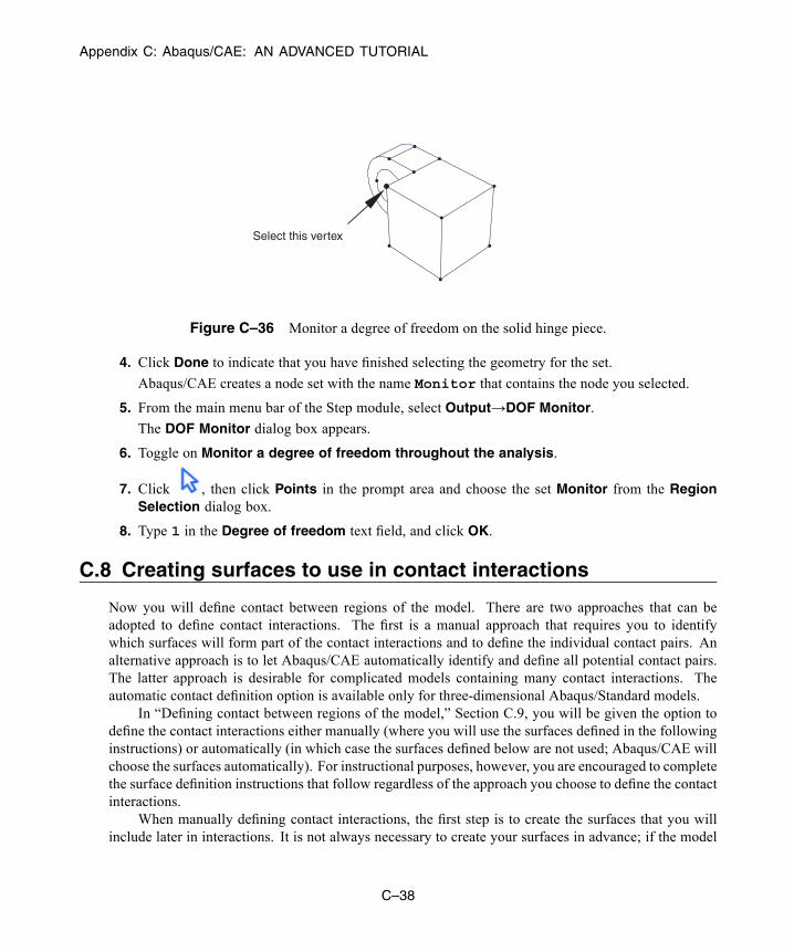
Appendix C: Abaqus/CAE: AN ADVANCED TUTORIAL
Select this vertex
Figure C–36 Monitor a degree of freedom on the solid hinge piece.
4. Click Done to indicate that you have finished selecting the geometry for the set.
Abaqus/CAE creates a node set with the name Monitor that contains the node you selected.
5. From the main menu bar of the Step module, select Output→DOF Monitor.
The DOF Monitor dialog box appears.
6. Toggle on Monitor a degree of freedom throughout the analysis.
7. Click , then click Points in the prompt area and choose the set Monitor from the RegionSelection dialog box.
8. Type 1 in the Degree of freedom text field, and click OK.
C.8 Creating surfaces to use in contact interactions
Now you will define contact between regions of the model. There are two approaches that can beadopted to define contact interactions. The first is a manual approach that requires you to identifywhich surfaces will form part of the contact interactions and to define the individual contact pairs. Analternative approach is to let Abaqus/CAE automatically identify and define all potential contact pairs.The latter approach is desirable for complicated models containing many contact interactions. Theautomatic contact definition option is available only for three-dimensional Abaqus/Standard models.
In “Defining contact between regions of the model,” Section C.9, you will be given the option todefine the contact interactions either manually (where you will use the surfaces defined in the followinginstructions) or automatically (in which case the surfaces defined below are not used; Abaqus/CAE willchoose the surfaces automatically). For instructional purposes, however, you are encouraged to completethe surface definition instructions that follow regardless of the approach you choose to define the contactinteractions.
When manually defining contact interactions, the first step is to create the surfaces that you willinclude later in interactions. It is not always necessary to create your surfaces in advance; if the model
C–38
Abaqus ID:Printed on:
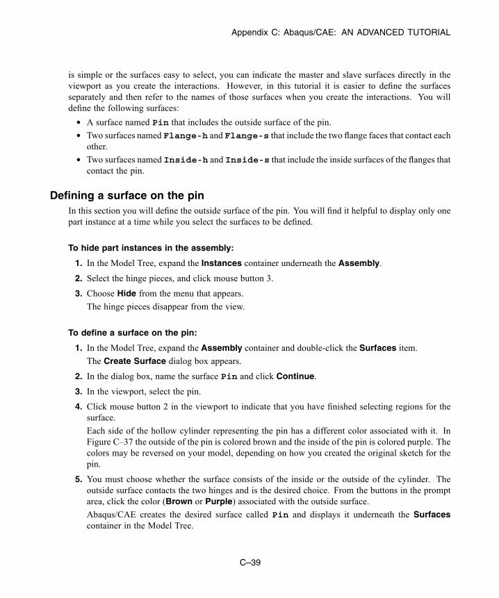
Appendix C: Abaqus/CAE: AN ADVANCED TUTORIAL
is simple or the surfaces easy to select, you can indicate the master and slave surfaces directly in theviewport as you create the interactions. However, in this tutorial it is easier to define the surfacesseparately and then refer to the names of those surfaces when you create the interactions. You willdefine the following surfaces:
• A surface named Pin that includes the outside surface of the pin.• Two surfaces named Flange-h and Flange-s that include the two flange faces that contact eachother.
• Two surfaces named Inside-h and Inside-s that include the inside surfaces of the flanges thatcontact the pin.
Defining a surface on the pinIn this section you will define the outside surface of the pin. You will find it helpful to display only onepart instance at a time while you select the surfaces to be defined.
To hide part instances in the assembly:
1. In the Model Tree, expand the Instances container underneath the Assembly.
2. Select the hinge pieces, and click mouse button 3.
3. Choose Hide from the menu that appears.
The hinge pieces disappear from the view.
To define a surface on the pin:
1. In the Model Tree, expand the Assembly container and double-click the Surfaces item.
The Create Surface dialog box appears.
2. In the dialog box, name the surface Pin and click Continue.
3. In the viewport, select the pin.
4. Click mouse button 2 in the viewport to indicate that you have finished selecting regions for thesurface.
Each side of the hollow cylinder representing the pin has a different color associated with it. InFigure C–37 the outside of the pin is colored brown and the inside of the pin is colored purple. Thecolors may be reversed on your model, depending on how you created the original sketch for thepin.
5. You must choose whether the surface consists of the inside or the outside of the cylinder. Theoutside surface contacts the two hinges and is the desired choice. From the buttons in the promptarea, click the color (Brown or Purple) associated with the outside surface.
Abaqus/CAE creates the desired surface called Pin and displays it underneath the Surfacescontainer in the Model Tree.
C–39
Abaqus ID:Printed on:
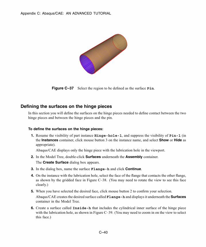
Appendix C: Abaqus/CAE: AN ADVANCED TUTORIAL
Figure C–37 Select the region to be defined as the surface Pin.
Defining the surfaces on the hinge piecesIn this section you will define the surfaces on the hinge pieces needed to define contact between the twohinge pieces and between the hinge pieces and the pin.
To define the surfaces on the hinge pieces:
1. Resume the visibility of part instance Hinge-hole-1, and suppress the visibility of Pin-1 (inthe Instances container, click mouse button 3 on the instance name, and select Show or Hide asappropriate).
Abaqus/CAE displays only the hinge piece with the lubrication hole in the viewport.
2. In the Model Tree, double-click Surfaces underneath the Assembly container.
The Create Surface dialog box appears.
3. In the dialog box, name the surface Flange-h and click Continue.
4. On the instance with the lubrication hole, select the face of the flange that contacts the other flange,as shown by the gridded face in Figure C–38. (You may need to rotate the view to see this faceclearly.)
5. When you have selected the desired face, click mouse button 2 to confirm your selection.
Abaqus/CAE creates the desired surface calledFlange-h and displays it underneath theSurfacescontainer in the Model Tree.
6. Create a surface called Inside-h that includes the cylindrical inner surface of the hinge piecewith the lubrication hole, as shown in Figure C–39. (You may need to zoom in on the view to selectthis face.)
C–40
Abaqus ID:Printed on:

Appendix C: Abaqus/CAE: AN ADVANCED TUTORIAL
1
2
3
Figure C–38 Select the region to be defined as the surface Flange-h.
Select this surface
Figure C–39 Select the region to be defined as the surface Inside-h.
7. Change the visibility settings so that only Hinge-solid-1 is visible.
8. Use similar techniques to create a surface called Flange-s that contains the corresponding faceof the solid hinge piece’s flange.
9. Finally, create a surface called Inside-s that includes the cylindrical inner surface of the solidhinge piece.
10. Return to the default visibility settings (select the three part instance names in the Instancescontainer, and click mouse button 3; from the menu that appears, select Show).
C–41
Abaqus ID:Printed on:

Appendix C: Abaqus/CAE: AN ADVANCED TUTORIAL
C.9 Defining contact between regions of the model
Interactions are objects that you create to model mechanical relationships between surfaces that are incontact or closely spaced. Mere physical proximity of two surfaces on an assembly is not enough toindicate any type of interaction between the surfaces.
You will define the following interactions:
• An interaction called HingePin-hole that defines the contact between the part instance Hinge-hole-1 and the pin.
• An interaction called HingePin-solid that defines the contact between the part instanceHinge-solid-1 and the pin.
• An interaction called Flanges that defines the contact between the two flanges.Each of these interactions requires a reference to an interaction property. Interaction properties
are collections of information that help you to define certain types of interactions. You will create amechanical interaction property that describes the tangential and normal behavior between all surfacesas frictionless. You will name this property NoFric and use it in all three of the interactions.
Creating an interaction propertyIn this procedure you will create a mechanical contact interaction property.
To create the interaction property:
1. In the Model Tree, double-click the Interaction Properties container to create a contact property.
The Create Interaction Property dialog box appears.
2. In the Create Interaction Property dialog box:
a. Name the property NoFric.
b. In the Type list, accept Contact as the default selection.
c. Click Continue.
The Edit Contact Property dialog box appears.
3. From the dialog box’s menu bar, select Mechanical→Tangential Behavior and acceptFrictionless for the friction formulation.
4. Click OK to save your settings and to close the Edit Contact Property dialog box.
Creating the interactionsIn this section you will create three mechanical surface-to-surface contact interactions. Each interactionwill refer to the interaction property that you just created. You are given the option to define the
C–42
Abaqus ID:Printed on:

Appendix C: Abaqus/CAE: AN ADVANCED TUTORIAL
interactions either automatically or manually. Please follow the instructions for one method or the other.If you choose to try both, be sure to delete or suppress any duplicate contact interactions that result.
To create the interactions automatically:
1. From the main menu bar, select Interaction→Find contact pairs.
2. In the Find Contact Pairs dialog box, click Find Contact Pairs.
Five potential contact pairs are identified.
3. In the Contact Pairs region of the dialog box:
a. Click the name of each contact pair to highlight it in the viewport. This will allow you tofamiliarize yourself with the contact interactions that have been chosen.
b. Contact pairs are defined between the rounded end of each hinge flange and the flat faceopposite it. These contact pairs are not necessary. Thus, delete them (to delete a contact pair,select it and click mouse button 3; from the menu that appears, select Delete).
c. Identify the contact pair between the hinge with the hole and the pin. Rename the interactionHingePin-hole.
d. Identify the contact pair between the solid hinge and the pin. Rename the interactionHingePin-solid.
e. Rename the remaining interaction Flanges. If necessary, switch the master and slave surfacedesignations so that the surface associated with the hinge with the hole is the master surfaceand the one associated with the solid hinge piece is the slave surface (click mouse button 3 onthe surface name; from the menu that appears, select Switch surfaces).
Tip: You can view the master and slave instance names to aid in the surfacedesignation. Click mouse button 3 anywhere on the table, and select Edit VisibleColumns. From the dialog box that appears, toggle on Master instance nameand Slave instance name.
f. Accept all default settings except for the contact discretization. Select the column headinglabeled Discretization, and click mouse button 3. From the menu that appears, select EditCells. In the dialog box that appears, select Node-to-surface, and click OK.
g. Click OK to save the interactions and to close the dialog box.
To create the interactions manually:
1. In the Model Tree, click mouse button 3 on the Interactions container and select Manager fromthe menu that appears.
The Interaction Manager appears.
2. From the lower-left corner of the Interaction Manager, click Create.
The Create Interaction dialog box appears.
C–43
Abaqus ID:Printed on:

Appendix C: Abaqus/CAE: AN ADVANCED TUTORIAL
3. In the dialog box:
a. Name the interaction HingePin-hole.
b. Select Initial from the list of steps.
c. In the Types for Selected Step list, accept the default selection of Surface-to-surfacecontact (Standard).
d. Click Continue.
The Region Selection dialog box appears containing a list of the surfaces that you defined earlier.
Note: If the Region Selection dialog box does not appear automatically, click the Surfacesbutton on the far right side of the prompt area.
4. In the Region Selection dialog box, select Pin as the master surface, and click Continue.
5. From the buttons in the prompt area, select Surface as the slave type.
6. In the Region Selection dialog box, select Inside-h as the slave surface, and click Continue.
The Edit Interaction dialog box appears.
7. In the dialog box:
a. Accept the default Sliding formulation selection of Finite sliding.
b. Change the discretization method to Node to surface.
c. Accept the default Slave Adjustment selection of No adjustment.
d. Accept NoFric as the interaction property. (If more properties were defined, you could clickthe arrow next to the Contact interaction property field to see the list of available propertiesand select the property of your choice.)
e. Click OK to save the interaction and to close the dialog box.
The interaction that you created appears in the Interaction Manager.
8. Use the same techniques explained in the previous steps to create a similar interaction calledHingePin-solid. Use Pin as the master surface, Inside-s as the slave surface, andNoFric as the interaction property.
9. Create a similar interaction called Flanges. Use Flange-h as the master surface, Flange-sas the slave surface, and NoFric as the interaction property.
10. From the Interaction Manager, click Dismiss to close the manager.
C.10 Applying boundary conditions and loads to the assembly
You will apply the following boundary conditions and load to the hinge model:
• A boundary condition called Fixed that constrains all degrees of freedom at the end of the hingepiece with the lubrication hole, as shown in Figure C–40.
C–44
Abaqus ID:Printed on:
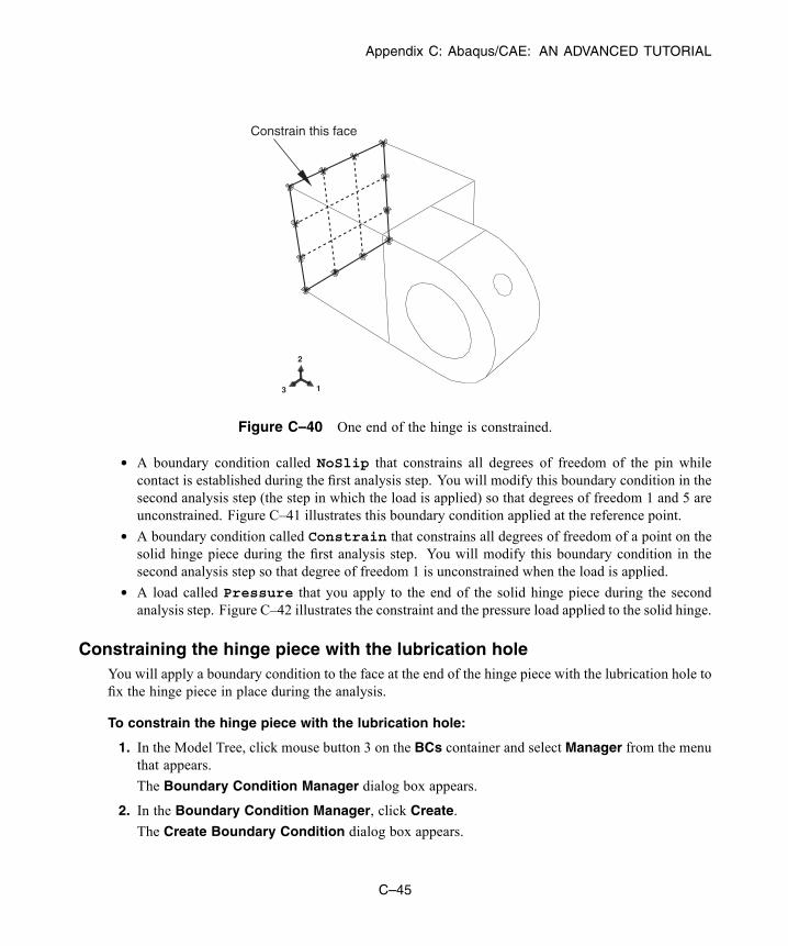
Appendix C: Abaqus/CAE: AN ADVANCED TUTORIAL
1
2
3
Constrain this face
Figure C–40 One end of the hinge is constrained.
• A boundary condition called NoSlip that constrains all degrees of freedom of the pin whilecontact is established during the first analysis step. You will modify this boundary condition in thesecond analysis step (the step in which the load is applied) so that degrees of freedom 1 and 5 areunconstrained. Figure C–41 illustrates this boundary condition applied at the reference point.
• A boundary condition called Constrain that constrains all degrees of freedom of a point on thesolid hinge piece during the first analysis step. You will modify this boundary condition in thesecond analysis step so that degree of freedom 1 is unconstrained when the load is applied.
• A load called Pressure that you apply to the end of the solid hinge piece during the secondanalysis step. Figure C–42 illustrates the constraint and the pressure load applied to the solid hinge.
Constraining the hinge piece with the lubrication holeYou will apply a boundary condition to the face at the end of the hinge piece with the lubrication hole tofix the hinge piece in place during the analysis.
To constrain the hinge piece with the lubrication hole:
1. In the Model Tree, click mouse button 3 on the BCs container and select Manager from the menuthat appears.
The Boundary Condition Manager dialog box appears.
2. In the Boundary Condition Manager, click Create.
The Create Boundary Condition dialog box appears.
C–45
Abaqus ID:Printed on:

Appendix C: Abaqus/CAE: AN ADVANCED TUTORIAL
RP
Figure C–41 The pin is constrained.
1
2
3 apply a negativepressure load to this face
Constrain this node
Figure C–42 The second hinge is constrained and loaded.
3. In the Create Boundary Condition dialog box:
a. Name the boundary condition Fixed.
b. Select Initial from the list of steps.
c. Accept Mechanical as the default Category selection.
d. Select Displacement/Rotation as the type of boundary condition for the selected step.
e. Click Continue.
The Region Selection dialog box appears.
C–46
Abaqus ID:Printed on:
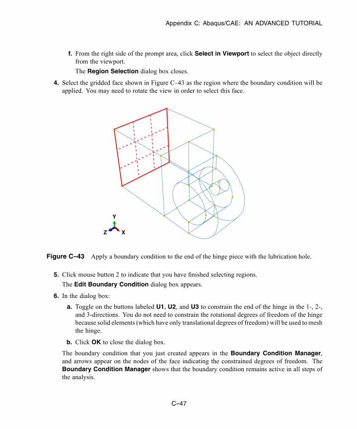
Appendix C: Abaqus/CAE: AN ADVANCED TUTORIAL
f. From the right side of the prompt area, click Select in Viewport to select the object directlyfrom the viewport.
The Region Selection dialog box closes.
4. Select the gridded face shown in Figure C–43 as the region where the boundary condition will beapplied. You may need to rotate the view in order to select this face.
X
Y
Z
Figure C–43 Apply a boundary condition to the end of the hinge piece with the lubrication hole.
5. Click mouse button 2 to indicate that you have finished selecting regions.
The Edit Boundary Condition dialog box appears.
6. In the dialog box:
a. Toggle on the buttons labeled U1, U2, and U3 to constrain the end of the hinge in the 1-, 2-,and 3-directions. You do not need to constrain the rotational degrees of freedom of the hingebecause solid elements (which have only translational degrees of freedom) will be used to meshthe hinge.
b. Click OK to close the dialog box.
The boundary condition that you just created appears in the Boundary Condition Manager,and arrows appear on the nodes of the face indicating the constrained degrees of freedom. TheBoundary Condition Manager shows that the boundary condition remains active in all steps ofthe analysis.
C–47
Abaqus ID:Printed on:
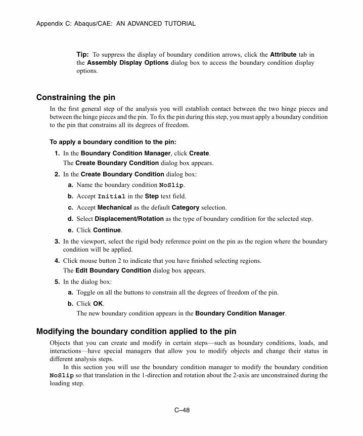
Appendix C: Abaqus/CAE: AN ADVANCED TUTORIAL
Tip: To suppress the display of boundary condition arrows, click the Attribute tab inthe Assembly Display Options dialog box to access the boundary condition displayoptions.
Constraining the pinIn the first general step of the analysis you will establish contact between the two hinge pieces andbetween the hinge pieces and the pin. To fix the pin during this step, you must apply a boundary conditionto the pin that constrains all its degrees of freedom.
To apply a boundary condition to the pin:
1. In the Boundary Condition Manager, click Create.
The Create Boundary Condition dialog box appears.
2. In the Create Boundary Condition dialog box:
a. Name the boundary condition NoSlip.
b. Accept Initial in the Step text field.
c. Accept Mechanical as the default Category selection.
d. Select Displacement/Rotation as the type of boundary condition for the selected step.
e. Click Continue.
3. In the viewport, select the rigid body reference point on the pin as the region where the boundarycondition will be applied.
4. Click mouse button 2 to indicate that you have finished selecting regions.
The Edit Boundary Condition dialog box appears.
5. In the dialog box:
a. Toggle on all the buttons to constrain all the degrees of freedom of the pin.
b. Click OK.
The new boundary condition appears in the Boundary Condition Manager.
Modifying the boundary condition applied to the pinObjects that you can create and modify in certain steps—such as boundary conditions, loads, andinteractions—have special managers that allow you to modify objects and change their status indifferent analysis steps.
In this section you will use the boundary condition manager to modify the boundary conditionNoSlip so that translation in the 1-direction and rotation about the 2-axis are unconstrained during theloading step.
C–48
Abaqus ID:Printed on:
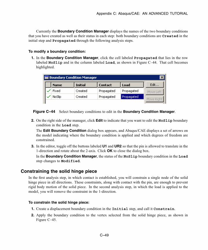
Appendix C: Abaqus/CAE: AN ADVANCED TUTORIAL
Currently the Boundary Condition Manager displays the names of the two boundary conditionsthat you have created as well as their status in each step: both boundary conditions are Created in theinitial step and Propagated through the following analysis steps.
To modify a boundary condition:
1. In the Boundary Condition Manager, click the cell labeled Propagated that lies in the rowlabeled NoSlip and in the column labeled Load, as shown in Figure C–44. That cell becomeshighlighted.
Figure C–44 Select boundary conditions to edit in the Boundary Condition Manager.
2. On the right side of the manager, click Edit to indicate that you want to edit the NoSlip boundarycondition in the Load step.
The Edit Boundary Condition dialog box appears, and Abaqus/CAE displays a set of arrows onthe model indicating where the boundary condition is applied and which degrees of freedom areconstrained.
3. In the editor, toggle off the buttons labeled U1 and UR2 so that the pin is allowed to translate in the1-direction and rotate about the 2-axis. Click OK to close the dialog box.
In the Boundary Condition Manager, the status of the NoSlip boundary condition in the Loadstep changes to Modified.
Constraining the solid hinge pieceIn the first analysis step, in which contact is established, you will constrain a single node of the solidhinge piece in all directions. These constraints, along with contact with the pin, are enough to preventrigid body motion of the solid piece. In the second analysis step, in which the load is applied to themodel, you will remove the constraint in the 1-direction.
To constrain the solid hinge piece:
1. Create a displacement boundary condition in the Initial step, and call it Constrain.
2. Apply the boundary condition to the vertex selected from the solid hinge piece, as shown inFigure C–45.
C–49
Abaqus ID:Printed on:
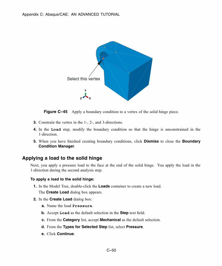
Appendix C: Abaqus/CAE: AN ADVANCED TUTORIAL
X
Y
Z
Select this vertex
Figure C–45 Apply a boundary condition to a vertex of the solid hinge piece.
3. Constrain the vertex in the 1-, 2-, and 3-directions.
4. In the Load step, modify the boundary condition so that the hinge is unconstrained in the1-direction.
5. When you have finished creating boundary conditions, click Dismiss to close the BoundaryCondition Manager.
Applying a load to the solid hingeNext, you apply a pressure load to the face at the end of the solid hinge. You apply the load in the1-direction during the second analysis step.
To apply a load to the solid hinge:
1. In the Model Tree, double-click the Loads container to create a new load.
The Create Load dialog box appears.
2. In the Create Load dialog box:
a. Name the load Pressure.
b. Accept Load as the default selection in the Step text field.
c. From the Category list, accept Mechanical as the default selection.
d. From the Types for Selected Step list, select Pressure.
e. Click Continue.
C–50
Abaqus ID:Printed on:
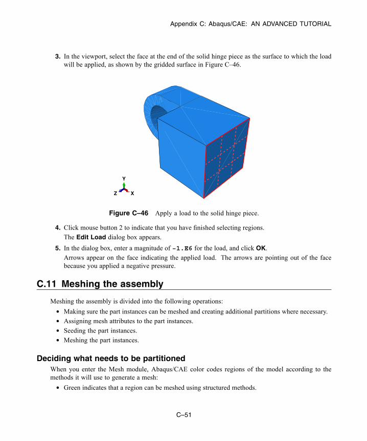
Appendix C: Abaqus/CAE: AN ADVANCED TUTORIAL
3. In the viewport, select the face at the end of the solid hinge piece as the surface to which the loadwill be applied, as shown by the gridded surface in Figure C–46.
X
Y
Z
Figure C–46 Apply a load to the solid hinge piece.
4. Click mouse button 2 to indicate that you have finished selecting regions.The Edit Load dialog box appears.
5. In the dialog box, enter a magnitude of −1.E6 for the load, and click OK.Arrows appear on the face indicating the applied load. The arrows are pointing out of the facebecause you applied a negative pressure.
C.11 Meshing the assembly
Meshing the assembly is divided into the following operations:
• Making sure the part instances can be meshed and creating additional partitions where necessary.• Assigning mesh attributes to the part instances.• Seeding the part instances.• Meshing the part instances.
Deciding what needs to be partitionedWhen you enter the Mesh module, Abaqus/CAE color codes regions of the model according to themethods it will use to generate a mesh:
• Green indicates that a region can be meshed using structured methods.
C–51
Abaqus ID:Printed on:

Appendix C: Abaqus/CAE: AN ADVANCED TUTORIAL
• Yellow indicates that a region can be meshed using sweep methods.• Orange indicates that a region cannot be meshed using the default element shape assignment(hexahedral) and must be partitioned further. (Alternatively, you can mesh any model by assigningtetrahedral elements to the model and using the free meshing technique.)
For the tutorial Abaqus/CAE indicates that the hinge with the lubrication hole needs to be partitionedto be meshed using hexahedral-shaped elements. Specifically, areas surrounding the hole in the flangemust be partitioned. The partitioned hinges are shown in Figure C–47.
1
2
3
Figure C–47 The partitioned hinges.
Use the following techniques to help you select faces and vertices during the partitioning process:
• Use a combination of the view manipulation tools, the display option tools in the View Optionstoolbar, and the tools in the Views toolbar to resize and reposition the model as necessary. (Todisplay the Views toolbar, select View→Toolbars→Views from the main menu bar.)
• Toggle off the closest object tool in the Selection toolbar to cycle through the possibleselections using the Next and Previous buttons in the prompt area.
• You will probably find the 3D compass and/or the magnification tool and the rotation toolespecially useful.
• When necessary, click the Iso tool in the Views toolbox to return the model to its original size andposition in the viewport.
• Recall that part instances are classified as dependent by default. All dependent instances of a partmust possess identical geometry (including partitions) and meshes. To satisfy this requirement, allpartitions must be created in the original part and all mesh attributes must be assigned to the original
C–52
Abaqus ID:Printed on:
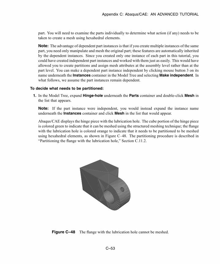
Appendix C: Abaqus/CAE: AN ADVANCED TUTORIAL
part. You will need to examine the parts individually to determine what action (if any) needs to betaken to create a mesh using hexahedral elements.
Note: The advantage of dependent part instances is that if you create multiple instances of the samepart, you need only manipulate and mesh the original part; these features are automatically inheritedby the dependent instances. Since you created only one instance of each part in this tutorial, youcould have created independent part instances and worked with them just as easily. This would haveallowed you to create partitions and assign mesh attributes at the assembly level rather than at thepart level. You can make a dependent part instance independent by clicking mouse button 3 on itsname underneath the Instances container in the Model Tree and selectingMake independent. Inwhat follows, we assume the part instances remain dependent.
To decide what needs to be partitioned:
1. In the Model Tree, expand Hinge-hole underneath the Parts container and double-click Mesh inthe list that appears.
Note: If the part instance were independent, you would instead expand the instance nameunderneath the Instances container and click Mesh in the list that would appear.
Abaqus/CAE displays the hinge piece with the lubrication hole. The cube portion of the hinge pieceis colored green to indicate that it can be meshed using the structured meshing technique; the flangewith the lubrication hole is colored orange to indicate that it needs to be partitioned to be meshedusing hexahedral elements, as shown in Figure C–48. The partitioning procedure is described in“Partitioning the flange with the lubrication hole,” Section C.11.2.
Figure C–48 The flange with the lubrication hole cannot be meshed.
C–53
Abaqus ID:Printed on:
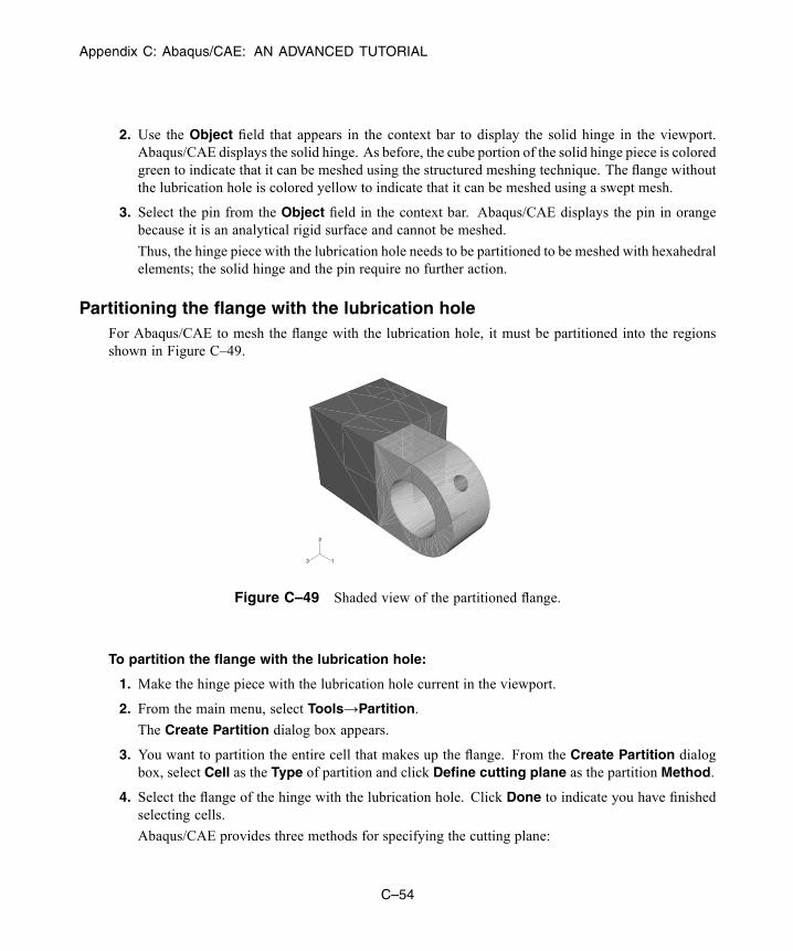
Appendix C: Abaqus/CAE: AN ADVANCED TUTORIAL
2. Use the Object field that appears in the context bar to display the solid hinge in the viewport.Abaqus/CAE displays the solid hinge. As before, the cube portion of the solid hinge piece is coloredgreen to indicate that it can be meshed using the structured meshing technique. The flange withoutthe lubrication hole is colored yellow to indicate that it can be meshed using a swept mesh.
3. Select the pin from the Object field in the context bar. Abaqus/CAE displays the pin in orangebecause it is an analytical rigid surface and cannot be meshed.
Thus, the hinge piece with the lubrication hole needs to be partitioned to be meshed with hexahedralelements; the solid hinge and the pin require no further action.
Partitioning the flange with the lubrication holeFor Abaqus/CAE to mesh the flange with the lubrication hole, it must be partitioned into the regionsshown in Figure C–49.
1
2
3
Figure C–49 Shaded view of the partitioned flange.
To partition the flange with the lubrication hole:
1. Make the hinge piece with the lubrication hole current in the viewport.
2. From the main menu, select Tools→Partition.
The Create Partition dialog box appears.
3. You want to partition the entire cell that makes up the flange. From the Create Partition dialogbox, select Cell as the Type of partition and click Define cutting plane as the partition Method.
4. Select the flange of the hinge with the lubrication hole. Click Done to indicate you have finishedselecting cells.
Abaqus/CAE provides three methods for specifying the cutting plane:
C–54
Abaqus ID:Printed on:
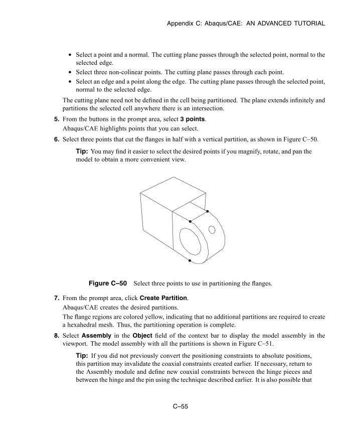
Appendix C: Abaqus/CAE: AN ADVANCED TUTORIAL
• Select a point and a normal. The cutting plane passes through the selected point, normal to theselected edge.
• Select three non-colinear points. The cutting plane passes through each point.• Select an edge and a point along the edge. The cutting plane passes through the selected point,normal to the selected edge.
The cutting plane need not be defined in the cell being partitioned. The plane extends infinitely andpartitions the selected cell anywhere there is an intersection.
5. From the buttons in the prompt area, select 3 points.
Abaqus/CAE highlights points that you can select.
6. Select three points that cut the flanges in half with a vertical partition, as shown in Figure C–50.
Tip: You may find it easier to select the desired points if you magnify, rotate, and pan themodel to obtain a more convenient view.
Figure C–50 Select three points to use in partitioning the flanges.
7. From the prompt area, click Create Partition.
Abaqus/CAE creates the desired partitions.
The flange regions are colored yellow, indicating that no additional partitions are required to createa hexahedral mesh. Thus, the partitioning operation is complete.
8. Select Assembly in the Object field of the context bar to display the model assembly in theviewport. The model assembly with all the partitions is shown in Figure C–51.
Tip: If you did not previously convert the positioning constraints to absolute positions,this partition may invalidate the coaxial constraints created earlier. If necessary, return tothe Assembly module and define new coaxial constraints between the hinge pieces andbetween the hinge and the pin using the technique described earlier. It is also possible that
C–55
Abaqus ID:Printed on:

Appendix C: Abaqus/CAE: AN ADVANCED TUTORIAL
RP
1
2
3
Figure C–51 The partitioned model.
the partition may invalidate the surfaces used for the contact interactions. Review theseand correct them as necessary.
Assigning mesh controlsIn this section you will use the Mesh Controls dialog box to examine the techniques that Abaqus/CAEwill use to mesh the parts and the shape of the elements that Abaqus/CAE will generate.
You cannot mesh an analytical rigid surface. As a result you cannot apply mesh controls to ananalytical rigid surface; neither can you seed it or assign an element type to it. Thus, you need onlyconcern yourself with the hinge pieces. Since the instances are dependent on the original part definition,you must assign mesh attributes (controls, type, and seed size) to each hinge piece individually. Forconvenience, you will begin with the hinge piece with the lubrication hole.
To assign the mesh controls:
1. Make the hinge piece with the hole current in the viewport. From the main menu bar, selectMesh→Controls.
2. Drag a square around the part to select all regions of the part, and click Done to indicate yourselection is complete.
The hinge piece appears red in the viewport to indicate that you have selected it, and Abaqus/CAEdisplays the Mesh Controls dialog box.
3. In the dialog box, accept Hex as the default Element Shape selection.
4. Select Sweep as the meshing technique that Abaqus/CAE will apply.
5. Select Medial axis as the meshing algorithm.
C–56
Abaqus ID:Printed on:
Appendix C: Abaqus/CAE: AN ADVANCED TUTORIAL
6. Click OK to assign the mesh controls and to close the dialog box.
The entire hinge will appear in yellow, indicating that it will be meshed using the swept meshingtechnique.
7. Repeat the above steps for the solid hinge piece.
Assigning the Abaqus element type
In this section you will use the Element Type dialog box to examine the element types that are assignedto each part. For convenience, you will begin with the hinge piece with the lubrication hole.
To assign an Abaqus element type:
1. Make the hinge piece with the hole current in the viewport. From the main menu bar, selectMesh→Element Type.
2. Select the hinge piece using the same technique described in the mesh controls procedure, and clickDone to indicate your selection is complete.
Abaqus/CAE displays the Element Type dialog box.
3. In the dialog box, accept Standard as the Element Library selection.
4. Accept Linear as the Geometric Order selection.
5. Accept 3D Stress as the default Family of elements.
6. Click the Hex tab, and select Reduced Integration as the formulation if it is not already selected.
A description of the default element type, C3D8R, appears at the bottom of the dialog box.Abaqus/CAE will now associate C3D8R elements with the elements in the mesh.
7. Click OK to assign the element type and to close the dialog box.
8. Click Done in the prompt area.
9. Repeat the above steps for the solid hinge piece.
Seeding the part instances
The next step of themeshing process is to seed each of the part instances. Seeds represent the approximatelocations of nodes and indicate the target density of the mesh you would like to generate. You can selectseeding based on the number of elements to generate along an edge or on the average element size, oryou can bias seed distribution toward one end of an edge. For the tutorial you will seed the parts so thatthe hinge pieces have an average element size of 0.004. For convenience, you will begin with the hingepiece with the lubrication hole.
C–57
Abaqus ID:Printed on:

Appendix C: Abaqus/CAE: AN ADVANCED TUTORIAL
To seed the parts:
1. Make the hinge piece with the hole current in the viewport. From the main menu bar, selectSeed→Part.
2. In the Global Seeds dialog box that appears, enter an approximate global element size of 0.004,and click OK.
Seeds appear on all the edges.
Note: If you are using the Abaqus Student Edition, using a global seed size of 0.004 results in amesh that exceeds the model size limits of the product. Use a global seed size of 0.008 instead.
3. Repeat the above steps for the solid hinge piece.
You are now ready to mesh the parts.
Meshing the assemblyIn this section you will mesh the parts. For convenience, you will begin with the hinge piece with thelubrication hole.
To mesh the assembly:
1. Make the hinge piece with the hole current in the viewport. From the main menu bar, selectMesh→Part.
2. Click Yes in the prompt area to create the mesh.
Abaqus/CAE meshes the part.
3. Repeat the above steps for the solid hinge piece.
The meshing operations are now complete. Display the model assembly in the viewport to see thefinal mesh, as illustrated in Figure C–52.
C.12 Creating and submitting a jobNow that you have configured your analysis, you will create a job that is associated with your model andsubmit the job for analysis.
To create and submit an analysis job:
1. In the Model Tree, double-click the Jobs container to create a job.
The Create Job dialog box appears.
2. Name the job PullHinge, and click Continue.
The job editor appears.
3. In the Description field, type Hinge tutorial.
C–58
Abaqus ID:Printed on:
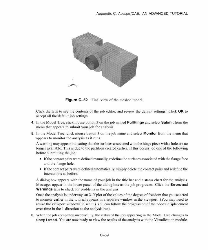
Appendix C: Abaqus/CAE: AN ADVANCED TUTORIAL
RP
1
2
3
Figure C–52 Final view of the meshed model.
Click the tabs to see the contents of the job editor, and review the default settings. Click OK toaccept all the default job settings.
4. In the Model Tree, click mouse button 3 on the job named PullHinge and select Submit from themenu that appears to submit your job for analysis.
5. In the Model Tree, click mouse button 3 on the job name and select Monitor from the menu thatappears to monitor the analysis as it runs.
A warning may appear indicating that the surfaces associated with the hinge piece with a hole are nolonger available. This is due to the partition created earlier. If this occurs, do one of the followingbefore submitting the job:
• If the contact pairs were defined manually, redefine the surfaces associated with the flange faceand the flange hole.
• If the contact pairs were defined automatically, simply delete the contact pairs and redefine theinteractions as before.
A dialog box appears with the name of your job in the title bar and a status chart for the analysis.Messages appear in the lower panel of the dialog box as the job progresses. Click the Errors andWarnings tabs to check for problems in the analysis.
Once the analysis is underway, an X–Y plot of the values of the degree of freedom that you selectedto monitor earlier in the tutorial appears in a separate window in the viewport. (You may need toresize the viewport windows to see it.) You can follow the progression of the node’s displacementover time in the 1-direction as the analysis runs.
6. When the job completes successfully, the status of the job appearing in the Model Tree changes toCompleted. You are now ready to view the results of the analysis with the Visualization module.
C–59
Abaqus ID:Printed on:

Appendix C: Abaqus/CAE: AN ADVANCED TUTORIAL
In the Model Tree, click mouse button 3 on the job name and select Results from the menu thatappears.
Abaqus/CAE enters the Visualization module, opens the output database created by the job, anddisplays the undeformed shape of the model.
Note: You can also enter the Visualization module by clicking Visualization in the Module listlocated in the context bar. However, in this case Abaqus/CAE requires you to open the outputdatabase explicitly using the File menu.
C.13 Viewing the results of your analysis
You will view the results of your analysis by drawing a contour plot of the deformed model. You willthen use display groups to display one of the hinge pieces; by displaying just a portion of the model youcan view results that are not visible when you display the whole model.
Displaying and customizing a contour plotIn this section you will display a contour plot of the model and adjust the deformation scale factor.
To display a contour plot of the model:
1. From the main menu bar, select Plot→Contours→On Deformed Shape.
Abaqus/CAE displays a contour plot of von Mises stress superimposed on the deformed shape ofthe model at the end of the last increment of the loading step, as indicated by the following text inthe state block:
Step: Load, Apply loadIncrement 6: Step Time = 1.000
By default, all surfaces with no results (in this case, the pin) are displayed in white.
The deformation is exaggerated because of the default deformation scale factor that Abaqus/CAEselects.
2. To remove the white surfaces from the display, do the following:
a. In the Results Tree, expand the Surface Sets container underneath the output database filenamed PullHinge.odb.
b. Select all the surfaces that appear in the list.
c. Click mouse button 3, and select Remove from the menu that appears.
The white surfaces disappear from the view.
3. To reduce the deformation scale factor, do the following:
a. From the main menu bar, select Options→Common.
The Common Plot Options dialog box appears.
C–60
Abaqus ID:Printed on:
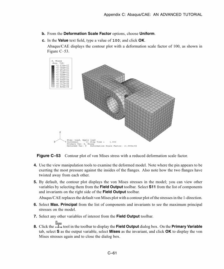
Appendix C: Abaqus/CAE: AN ADVANCED TUTORIAL
b. From the Deformation Scale Factor options, choose Uniform.
c. In the Value text field, type a value of 100; and click OK.
Abaqus/CAE displays the contour plot with a deformation scale factor of 100, as shown inFigure C–53.
(Avg: 75%)S, Mises
+2.824e+04+2.173e+06+4.317e+06+6.462e+06+8.606e+06+1.075e+07+1.290e+07+1.504e+07+1.718e+07+1.933e+07+2.147e+07+2.362e+07+2.576e+07
Step: Load, Apply loadIncrement 6: Step Time = 1.000Primary Var: S, MisesDeformed Var: U Deformation Scale Factor: +1.000e+02
1
2
3
Figure C–53 Contour plot of von Mises stress with a reduced deformation scale factor.
4. Use the view manipulation tools to examine the deformed model. Note where the pin appears to beexerting the most pressure against the insides of the flanges. Also note how the two flanges havetwisted away from each other.
5. By default, the contour plot displays the von Mises stresses in the model; you can view othervariables by selecting them from the Field Output toolbar. Select S11 from the list of componentsand invariants on the right side of the Field Output toolbar.
Abaqus/CAE replaces the default vonMises plot with a contour plot of the stresses in the 1-direction.
6. Select Max. Principal from the list of components and invariants to see the maximum principalstresses on the model.
7. Select any other variables of interest from the Field Output toolbar.
8. Click the tool in the toolbar to display the Field Output dialog box. On the Primary Variabletab, select S as the output variable, select Mises as the invariant, and click OK to display the vonMises stresses again and to close the dialog box.
C–61
Abaqus ID:Printed on:
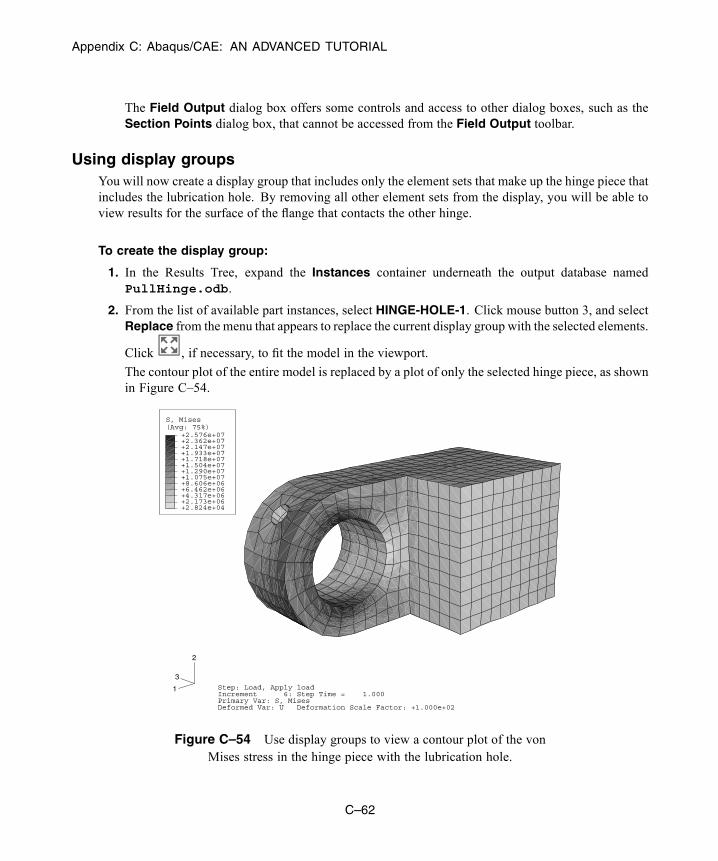
Appendix C: Abaqus/CAE: AN ADVANCED TUTORIAL
The Field Output dialog box offers some controls and access to other dialog boxes, such as theSection Points dialog box, that cannot be accessed from the Field Output toolbar.
Using display groupsYou will now create a display group that includes only the element sets that make up the hinge piece thatincludes the lubrication hole. By removing all other element sets from the display, you will be able toview results for the surface of the flange that contacts the other hinge.
To create the display group:
1. In the Results Tree, expand the Instances container underneath the output database namedPullHinge.odb.
2. From the list of available part instances, select HINGE-HOLE-1. Click mouse button 3, and selectReplace from the menu that appears to replace the current display group with the selected elements.
Click , if necessary, to fit the model in the viewport.
The contour plot of the entire model is replaced by a plot of only the selected hinge piece, as shownin Figure C–54.
(Avg: 75%)S, Mises
+2.824e+04+2.173e+06+4.317e+06+6.462e+06+8.606e+06+1.075e+07+1.290e+07+1.504e+07+1.718e+07+1.933e+07+2.147e+07+2.362e+07+2.576e+07
Step: Load, Apply loadIncrement 6: Step Time = 1.000Primary Var: S, MisesDeformed Var: U Deformation Scale Factor: +1.000e+02
1
2
3
Figure C–54 Use display groups to view a contour plot of the vonMises stress in the hinge piece with the lubrication hole.
C–62
Abaqus ID:Printed on:

Appendix C: Abaqus/CAE: AN ADVANCED TUTORIAL
3. Use the view manipulation tools to view the hinge at different angles. You can now see results forsurfaces on the hinge that were hidden by the solid hinge.
4. From the main menu bar, select Result→Field Output.
5. From the top of the Primary Variable tabbed page, toggle on List only variables with results:and choose at surface nodes from the menu.
6. From the list of variables that appears, select CPRESS, and click Apply.
Abaqus/CAE displays a contour plot of the contact pressures in the flange hole.
For more information about using the Visualization module, see the following sections:
• “Viewing the results of your analysis,” Section B.11• Appendix D, “Viewing the Output from Your Analysis”You have now completed this tutorial and learned how to:
• create and modify features;• use datum geometry to add features to a model;• use position constraints to assemble a model composed of more than one part;• define contact interactions between regions of a model;• monitor the progress of an analysis job; and• use display groups to view results for individual parts of a model.
C.14 Summary
• When you create a part, you can create a deformable part, a discrete rigid surface, or an analyticalrigid surface. You can subsequently change the type of the part.
• You can create parts by adding features to the base feature. When you add a feature, you mustselect a face on which to sketch the profile of the feature. When you delete a feature from a part,Abaqus/CAE also deletes any features that depend on the feature being deleted. These dependentfeatures are called children.
• You can edit features by modifying the sketch of the feature or a parameter associated with thefeature, such as an extrusion depth. Editing features can cause dependent features to fail duringregeneration.
• The Datum toolset allows you to create datum points, axes, and planes. Datum geometry that youcreate on a part can also be used by the Sketcher. For example, if a suitable sketch plane does notexist, you can use the Datum toolset to create one.
• Click OK in a dialog box to perform the selected operation and to close the dialog box; click Applyto leave the dialog box open while performing the selected operation. Click Cancel to close thedialog box without performing an operation.
C–63
Abaqus ID:Printed on:

Appendix C: Abaqus/CAE: AN ADVANCED TUTORIAL
• You can use the tools in the View Manipulation toolbar to change the view of the model to a moreconvenient one. Use mouse button 2 to stop any view manipulation. If you rotate or pan the sketch,use the cycle view manipulation tool to restore the original view.
• You should save the model database at regular intervals.• When you create a part instance, the default position is based on the sketch of the base feature.You can ask Abaqus/CAE to offset the new instance along the X-axis so that it does not overlapany existing instances. A graphic indicates the origin and the orientation of the global coordinatesystem in the Assembly module.
• You position part instances relative to each other in the Assembly module using a sequence ofconstraint operations.
• Part instances can be classified as either dependent or independent.• You use the step editor to control the time incrementation during the step.• You can use managers to display a list of the entities you have defined—for example, steps—andto help you perform repeated operations.
• By default, Abaqus/CAE propagates interactions or prescribed conditions defined in one step to allsubsequent steps.
• Abaqus/CAE color codes the model to indicate how a region will be meshed. Green indicates thata region can be meshed with structured methods, yellow indicates that a region can be meshed withsweep methods, and orange indicates that a region cannot be meshed.
• You use the Partition toolset to divide the model into regions that Abaqus/CAE can mesh.• When you create and name a job, Abaqus/CAE uses the same name for the input file it generates.Consequently, all files associated with the analysis (for example, the output database, the messagefile, and the status file) use the same name.
• You can view the progression of a degree of freedom over the course of an analysis that you havechosen to monitor before submitting the job.
• When you first open an output database, Abaqus/CAE displays an undeformed plot of the model.• You use display groups to display selected regions of your model. A display group can be composedof any combination of selected part instances, geometry (cells, faces, or edges), elements, nodes, orsurfaces.
C–64
Abaqus ID:Printed on:

Appendix D: Abaqus/CAE: A POSTPROCESSING TUTORIAL
Appendix D: Viewing the Output from Your Analysis
This postprocessing tutorial for the experienced Abaqus user illustrates how you can use the Visualizationmodule (also licensed separately as Abaqus/Viewer) to display the results from your analysis in graphicalform.
D.1 Overview
During the tutorial you will display the output from Case 2 of the example problem, “Indentation of anelastomeric foam specimen with a hemispherical punch,” Section 1.1.4 of the Abaqus Example ProblemsGuide. The problem studies the behavior of a heavy metal punch impacting a soft elastomeric foamblock; the resulting deformation and strain are shown in Figure D–1.
(Avg: 75%)LE, LE22
−8.279e−01−7.573e−01−6.867e−01−6.161e−01−5.455e−01−4.749e−01−4.043e−01−3.338e−01−2.632e−01−1.926e−01−1.220e−01−5.140e−02+1.919e−02
Figure D–1 Contour plot showing deformation and strain.
The problem is modeled in two dimensions and is divided into three steps:
1. The punch initially rests on the surface of the foam block and compresses the block under its ownweight. The gravity loading is ramped up over two seconds; but the analysis continues for a totalof five seconds, allowing the foam to relax fully. The analysis uses the quasi-static procedure tomodel the response of the foam block during the step.
D–1
Abaqus ID:Printed on:

Appendix D: Abaqus/CAE: A POSTPROCESSING TUTORIAL
2. The punch is forced down with an impulsive load that varies according to a half sine wave overa period of one second. The response of the foam block is modeled using the implicit dynamicprocedure.
3. The impulsive load is removed, and the punch is allowed to move freely while the foam expandsand contracts. The viscoelastic foam damps out the vibrations, and the step runs for 10 secondswhile the model returns to steady state. As with the second step, the response of the foam block ismodeled using the implicit dynamic procedure.
The tutorial consists of the following sections:
• “Which variables are in the output database?,” Section D.2• “Reading the output database,” Section D.3• “Customizing a model plot,” Section D.4• “Displaying the deformed model shape,” Section D.5• “Displaying and customizing a contour plot,” Section D.6• “Animating a contour plot,” Section D.7• “Displaying and customizing a symbol plot,” Section D.8• “Displaying and customizing a material orientation plot,” Section D.9• “Displaying and customizing an X–Y plot,” Section D.10
• “Operating on X–Y data,” Section D.11
• “Probing an X–Y plot,” Section D.12
• “Displaying results along a path,” Section D.13
D.2 Which variables are in the output database?In the first step of the elastomeric foam example, a set of options is included to control the data outputduring each step of the analysis. Abaqus/Standard writes this output to the Field Output or History Outputportion of the output database, depending on the output type.
Field Output
The Field Output portion of the output database contains variables that should be output relativelyinfrequently during the analysis; in this case, after every 10 increments and after the last incrementof a step. Typically, you select output for your entire model or a large region of your model, andAbaqus writes every component at the selected frequency. Only the selected variables are writtento the output database.
The following input file fragment shows the options that control the field output variables inthe elastomeric block example:
*OUTPUT, FIELD, FREQUENCY=10
*CONTACT OUTPUT, SLAVE=ASURF, MASTER=BSURF,VARIABLE=PRESELECT
*NODE OUTPUT
D–2
Abaqus ID:Printed on:
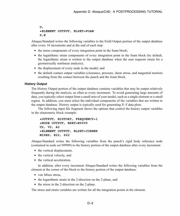
Appendix D: Abaqus/CAE: A POSTPROCESSING TUTORIAL
U,
*ELEMENT OUTPUT, ELSET=FOAMS,E
Abaqus/Standard writes the following variables to the Field Output portion of the output databaseafter every 10 increments and at the end of each step:
• the stress components of every integration point in the foam block;• the logarithmic strain components of every integration point in the foam block (by default,the logarithmic strain is written to the output database when the user requests strain for ageometrically nonlinear analysis);
• the displacement of every node in the model; and• the default contact output variables (clearance, pressure, shear stress, and tangential motion)resulting from the contact between the punch and the foam block.
History Output
The History Output portion of the output database contains variables that may be output relativelyfrequently during the analysis, as often as every increment. To avoid generating large amounts ofdata, you typically select output from a small area of your model, such as a single element or a smallregion. In addition, you must select the individual components of the variables that are written tothe output database. History output is typically used for generating X–Y data plots.
The following input file fragment shows the options that control the history output variablesin the elastomeric block example:
*OUTPUT, HISTORY, FREQUENCY=1
*NODE OUTPUT, NSET=N9999U2, V2, A2
*ELEMENT OUTPUT, ELSET=CORNERMISES, E22, S22
Abaqus/Standard writes the following variables from the punch’s rigid body reference node(contained in node set N9999) to the history portion of the output database after every increment:
• the vertical displacement,• the vertical velocity, and• the vertical acceleration.In addition, after every increment Abaqus/Standard writes the following variables from the
element at the corner of the block to the history portion of the output database:
• von Mises stress,• the logarithmic strain in the 2-direction on the 2-plane, and• the stress in the 2-direction on the 2-plane.
The stress and strain variables are written for all the integration points in the element.
D–3
Abaqus ID:Printed on:
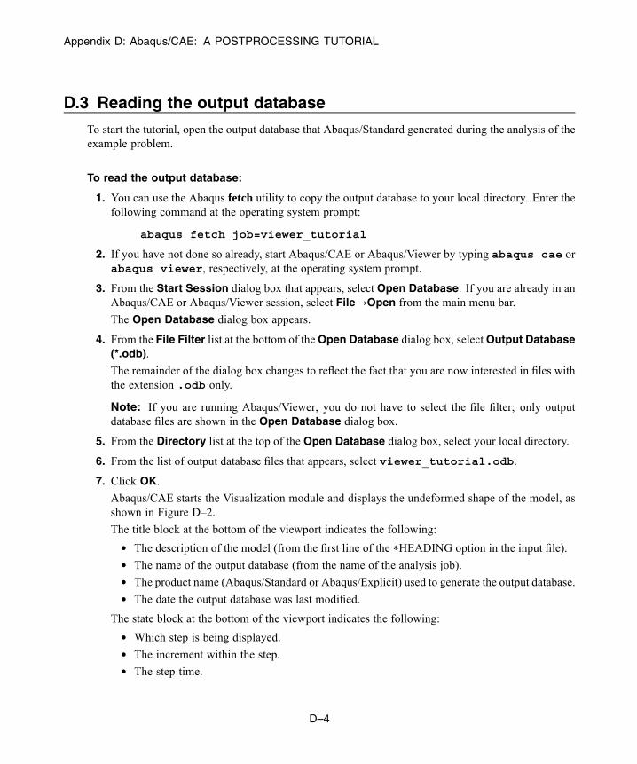
Appendix D: Abaqus/CAE: A POSTPROCESSING TUTORIAL
D.3 Reading the output database
To start the tutorial, open the output database that Abaqus/Standard generated during the analysis of theexample problem.
To read the output database:
1. You can use the Abaqus fetch utility to copy the output database to your local directory. Enter thefollowing command at the operating system prompt:
abaqus fetch job=viewer_tutorial
2. If you have not done so already, start Abaqus/CAE or Abaqus/Viewer by typing abaqus cae orabaqus viewer, respectively, at the operating system prompt.
3. From the Start Session dialog box that appears, select Open Database. If you are already in anAbaqus/CAE or Abaqus/Viewer session, select File→Open from the main menu bar.
The Open Database dialog box appears.
4. From the File Filter list at the bottom of theOpen Database dialog box, selectOutput Database(*.odb).
The remainder of the dialog box changes to reflect the fact that you are now interested in files withthe extension .odb only.
Note: If you are running Abaqus/Viewer, you do not have to select the file filter; only outputdatabase files are shown in the Open Database dialog box.
5. From the Directory list at the top of the Open Database dialog box, select your local directory.
6. From the list of output database files that appears, select viewer_tutorial.odb.
7. Click OK.
Abaqus/CAE starts the Visualization module and displays the undeformed shape of the model, asshown in Figure D–2.
The title block at the bottom of the viewport indicates the following:
• The description of the model (from the first line of the *HEADING option in the input file).• The name of the output database (from the name of the analysis job).• The product name (Abaqus/Standard or Abaqus/Explicit) used to generate the output database.• The date the output database was last modified.
The state block at the bottom of the viewport indicates the following:
• Which step is being displayed.• The increment within the step.• The step time.
D–4
Abaqus ID:Printed on:
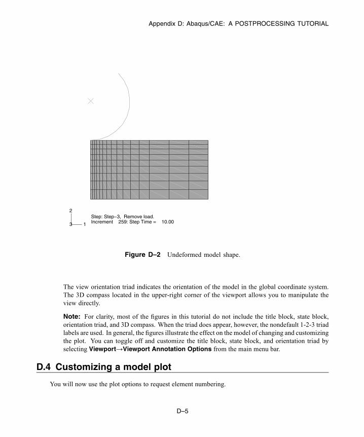
Appendix D: Abaqus/CAE: A POSTPROCESSING TUTORIAL
Step: Step−3, Remove load.Increment 259: Step Time = 10.001
2
3
Figure D–2 Undeformed model shape.
The view orientation triad indicates the orientation of the model in the global coordinate system.The 3D compass located in the upper-right corner of the viewport allows you to manipulate theview directly.
Note: For clarity, most of the figures in this tutorial do not include the title block, state block,orientation triad, and 3D compass. When the triad does appear, however, the nondefault 1-2-3 triadlabels are used. In general, the figures illustrate the effect on the model of changing and customizingthe plot. You can toggle off and customize the title block, state block, and orientation triad byselecting Viewport→Viewport Annotation Options from the main menu bar.
D.4 Customizing a model plot
You will now use the plot options to request element numbering.
D–5
Abaqus ID:Printed on:
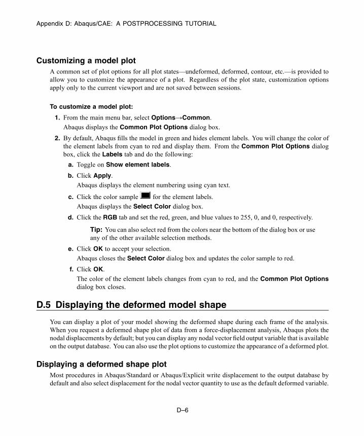
Appendix D: Abaqus/CAE: A POSTPROCESSING TUTORIAL
Customizing a model plotA common set of plot options for all plot states—undeformed, deformed, contour, etc.—is provided toallow you to customize the appearance of a plot. Regardless of the plot state, customization optionsapply only to the current viewport and are not saved between sessions.
To customize a model plot:
1. From the main menu bar, select Options→Common.
Abaqus displays the Common Plot Options dialog box.
2. By default, Abaqus fills the model in green and hides element labels. You will change the color ofthe element labels from cyan to red and display them. From the Common Plot Options dialogbox, click the Labels tab and do the following:
a. Toggle on Show element labels.
b. Click Apply.
Abaqus displays the element numbering using cyan text.
c. Click the color sample for the element labels.
Abaqus displays the Select Color dialog box.
d. Click the RGB tab and set the red, green, and blue values to 255, 0, and 0, respectively.
Tip: You can also select red from the colors near the bottom of the dialog box or useany of the other available selection methods.
e. Click OK to accept your selection.
Abaqus closes the Select Color dialog box and updates the color sample to red.
f. Click OK.
The color of the element labels changes from cyan to red, and the Common Plot Optionsdialog box closes.
D.5 Displaying the deformed model shape
You can display a plot of your model showing the deformed shape during each frame of the analysis.When you request a deformed shape plot of data from a force-displacement analysis, Abaqus plots thenodal displacements by default; but you can display any nodal vector field output variable that is availableon the output database. You can also use the plot options to customize the appearance of a deformed plot.
Displaying a deformed shape plotMost procedures in Abaqus/Standard or Abaqus/Explicit write displacement to the output database bydefault and also select displacement for the nodal vector quantity to use as the default deformed variable.
D–6
Abaqus ID:Printed on:

Appendix D: Abaqus/CAE: A POSTPROCESSING TUTORIAL
When Abaqus reads the output database, it uses the default deformed variable to determine the deformedmodel shape. In the elastomeric block example the user requested output of the displacements (U) forevery node in the model after every 10 increments, and displacement was selected as the default deformedvariable.
(Some procedures—for example, heat transfer—do not write nodal vector quantities to the outputdatabase by default and do not select a variable as the default deformed variable. Therefore, Abaquscannot display a deformed plot, since in such cases the output database does not contain any variablesthat can be used to compute a deformed shape.)
To display a deformed shape plot:
1. From the main menu bar, select Plot→Deformed Shape.
Tip: You can also plot the deformedmodel using the tool in the Visualizationmoduletoolbox.
Abaqus displays the deformed model in the same increment and step that it last displayed theundeformed model. The element labels also appear because the common plot options were usedto display them.
2. Open the Common Plot Options dialog box. Click Defaults followed by Apply to restore andapply the default options.
The state block indicates the default deformed variable being plotted (U) and the deformationscale factor (1.000e+00). Abaqus selects a default deformation scale factor of 1.0 forlarge-displacement analyses. (For small-displacement analyses Abaqus chooses the default scalefactor to fit the viewport optimally.)
3. The buttons in the context bar allow you to move between frames of the analysis. In particular, the
button on the far right of the context bar is the frame selector tool; it allows you to drag a sliderto choose the frame of interest.
You can also move directly to a selected step and increment using the following technique:
a. From the main menu bar, select Result→Step/Frame.
Abaqus displays the Step/Frame dialog box.
b. Select Step 1, Increment 0, and click Apply.
c. The Step/Frame dialog box also displays the step time associated with an increment. Use theStep/Frame dialog box to display the deformed model approximately halfway through thesecond step.
4. Use a combination of the buttons in the context bar and the Step/Frame dialog box to view thedeformed plot in different frames and in different steps.
5. Display the deformed model after the last increment of the third step (Step 3 and Step Time= 10.00), as shown in Figure D–3.
D–7
Abaqus ID:Printed on:

Appendix D: Abaqus/CAE: A POSTPROCESSING TUTORIAL
1
2
3
Figure D–3 Deformed plot of the model after the last increment of the third step.
6. Click Cancel to close the Step/Frame dialog box.
Superimposing the undeformed shape on the deformed shapeYou can plot the undeformed and deformed model shapes simultaneously.
To plot the undeformed and deformed model shapes:
1. Click the tool in the toolbox to allow multiple plot states in the viewport. Then click the
tool or select Plot→Undeformed Shape to add the undeformed shape plot to the existingdeformed plot in the viewport.
Abaqus displays the deformed plot overlaid with the undeformed plot.
2. To customize the superimposed (i.e., undeformed) plot, select Options→Superimpose from themain menu bar.
Abaqus displays the Superimpose Plot Options dialog box.
3. In the Superimpose Plot Options dialog box, select the Other tab.
4. In the Other tabbed page, select the Translucency tab. Toggle off Apply Translucency.
5. Next select the Offset tab. Select Uniform, and enter a value of 0.001 as the offset value.
6. Click OK to apply the changes and to close the Superimpose Plot Options dialog box.
Abaqus displays the customized deformed plot, as shown in Figure D–4. The undeformed modelshape is colored white and is offset slightly from the deformed model shape to prevent the colorsfrom overlapping.
D–8
Abaqus ID:Printed on:
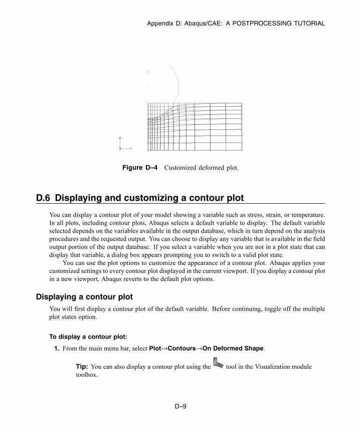
Appendix D: Abaqus/CAE: A POSTPROCESSING TUTORIAL
1
2
3
Figure D–4 Customized deformed plot.
D.6 Displaying and customizing a contour plot
You can display a contour plot of your model showing a variable such as stress, strain, or temperature.In all plots, including contour plots, Abaqus selects a default variable to display. The default variableselected depends on the variables available in the output database, which in turn depend on the analysisprocedures and the requested output. You can choose to display any variable that is available in the fieldoutput portion of the output database. If you select a variable when you are not in a plot state that candisplay that variable, a dialog box appears prompting you to switch to a valid plot state.
You can use the plot options to customize the appearance of a contour plot. Abaqus applies yourcustomized settings to every contour plot displayed in the current viewport. If you display a contour plotin a new viewport, Abaqus reverts to the default plot options.
Displaying a contour plotYou will first display a contour plot of the default variable. Before continuing, toggle off the multipleplot states option.
To display a contour plot:
1. From the main menu bar, select Plot→Contours→On Deformed Shape.
Tip: You can also display a contour plot using the tool in the Visualization moduletoolbox.
D–9
Abaqus ID:Printed on:
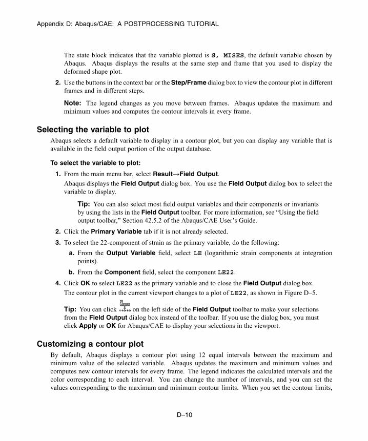
Appendix D: Abaqus/CAE: A POSTPROCESSING TUTORIAL
The state block indicates that the variable plotted is S, MISES, the default variable chosen byAbaqus. Abaqus displays the results at the same step and frame that you used to display thedeformed shape plot.
2. Use the buttons in the context bar or theStep/Frame dialog box to view the contour plot in differentframes and in different steps.
Note: The legend changes as you move between frames. Abaqus updates the maximum andminimum values and computes the contour intervals in every frame.
Selecting the variable to plotAbaqus selects a default variable to display in a contour plot, but you can display any variable that isavailable in the field output portion of the output database.
To select the variable to plot:
1. From the main menu bar, select Result→Field Output.
Abaqus displays the Field Output dialog box. You use the Field Output dialog box to select thevariable to display.
Tip: You can also select most field output variables and their components or invariantsby using the lists in the Field Output toolbar. For more information, see “Using the fieldoutput toolbar,” Section 42.5.2 of the Abaqus/CAE User’s Guide.
2. Click the Primary Variable tab if it is not already selected.
3. To select the 22-component of strain as the primary variable, do the following:
a. From the Output Variable field, select LE (logarithmic strain components at integrationpoints).
b. From the Component field, select the component LE22.
4. Click OK to select LE22 as the primary variable and to close the Field Output dialog box.
The contour plot in the current viewport changes to a plot of LE22, as shown in Figure D–5.
Tip: You can click on the left side of the Field Output toolbar to make your selectionsfrom the Field Output dialog box instead of the toolbar. If you use the dialog box, you mustclick Apply or OK for Abaqus/CAE to display your selections in the viewport.
Customizing a contour plotBy default, Abaqus displays a contour plot using 12 equal intervals between the maximum andminimum value of the selected variable. Abaqus updates the maximum and minimum values andcomputes new contour intervals for every frame. The legend indicates the calculated intervals and thecolor corresponding to each interval. You can change the number of intervals, and you can set thevalues corresponding to the maximum and minimum contour limits. When you set the contour limits,
D–10
Abaqus ID:Printed on:
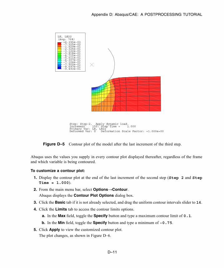
Appendix D: Abaqus/CAE: A POSTPROCESSING TUTORIAL
(Avg: 75%)LE, LE22
−9.493e−01−8.697e−01−7.900e−01−7.104e−01−6.307e−01−5.511e−01−4.715e−01−3.918e−01−3.122e−01−2.325e−01−1.529e−01−7.325e−02+6.395e−03
Step: Step−2, Apply dynamic load.Increment 155: Step Time = 1.000Primary Var: LE, LE22Deformed Var: U Deformation Scale Factor: +1.000e+00
Figure D–5 Contour plot of the model after the last increment of the third step.
Abaqus uses the values you supply in every contour plot displayed thereafter, regardless of the frameand which variable is being contoured.
To customize a contour plot:
1. Display the contour plot at the end of the last increment of the second step (Step 2 and StepTime = 1.000).
2. From the main menu bar, select Options→Contour.
Abaqus displays the Contour Plot Options dialog box.
3. Click the Basic tab if it is not already selected, and drag the uniform contour intervals slider to 16.
4. Click the Limits tab to access the contour limits options.
a. In the Max field, toggle the Specify button and type a maximum contour limit of 0.1.
b. In the Min field, toggle the Specify button and type a minimum of −0.75.
5. Click Apply to view the customized contour plot.
The plot changes, as shown in Figure D–6.
D–11
Abaqus ID:Printed on:
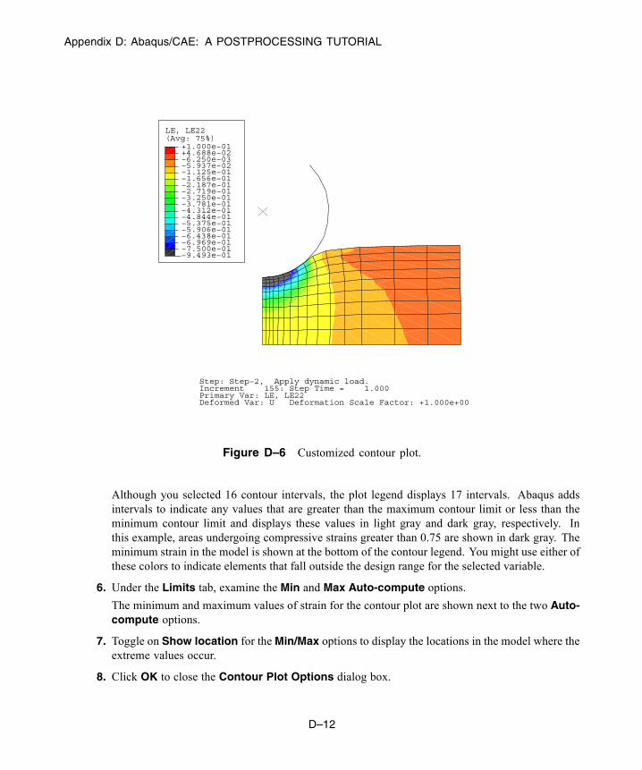
Appendix D: Abaqus/CAE: A POSTPROCESSING TUTORIAL
(Avg: 75%)LE, LE22
−7.500e−01−6.969e−01−6.438e−01−5.906e−01−5.375e−01−4.844e−01−4.312e−01−3.781e−01−3.250e−01−2.719e−01−2.187e−01−1.656e−01−1.125e−01−5.937e−02−6.250e−03+4.688e−02+1.000e−01
−9.493e−01
Step: Step−2, Apply dynamic load.Increment 155: Step Time = 1.000Primary Var: LE, LE22Deformed Var: U Deformation Scale Factor: +1.000e+00
Figure D–6 Customized contour plot.
Although you selected 16 contour intervals, the plot legend displays 17 intervals. Abaqus addsintervals to indicate any values that are greater than the maximum contour limit or less than theminimum contour limit and displays these values in light gray and dark gray, respectively. Inthis example, areas undergoing compressive strains greater than 0.75 are shown in dark gray. Theminimum strain in the model is shown at the bottom of the contour legend. You might use either ofthese colors to indicate elements that fall outside the design range for the selected variable.
6. Under the Limits tab, examine the Min and Max Auto-compute options.
The minimum and maximum values of strain for the contour plot are shown next to the two Auto-compute options.
7. Toggle on Show location for theMin/Max options to display the locations in the model where theextreme values occur.
8. Click OK to close the Contour Plot Options dialog box.
D–12
Abaqus ID:Printed on:
Appendix D: Abaqus/CAE: A POSTPROCESSING TUTORIAL
D.7 Animating a contour plot
You can animate a deformed, contour, symbol, or material orientation (time history animation only) plotusing one of the following:
Time History Animation
In a time history animation Abaqus displays each frame of each step from the output database insequence, and you can see the change in the deformation or the change in a contour or symbol plotvariable while the analysis progresses. In effect, Abaqus animates the results of the analysis. Youcan select which steps and frames to include in a time history animation.
Scale Factor Animation
Scale factor animation takes the results from a selected step and frame and simply scales themto form frames of the animation. You can select a scale factor that varies between zero and oneor between minus one and plus one. Scale factor animation is particularly useful for animatingvibration modes computed by an eigenvalue analysis.
The animation uses the plot options from the relevant mode—deformed, contour, symbol, ormaterial orientation. In addition, you can control the following:
• The speed of the animation• Whether the animation runs continuously or just once• Whether to display the animation status
For the elastomeric foam example you will display a time history animation of a contour plot. Theanimated contour plot displays the field output variable displayed in the Field Output toolbar (LE22).In addition, it uses the same options that you selected for the contour plot; for example, the contourintervals and element edge display.
To animate the contour plot:
1. From the main menu bar, select Animate→Time History.
Abaqus displays the customized contour plot at the beginning of the analysis and steps through eachframe; the state block indicates the current step and increment throughout the animation. After thelast increment of the last step, the animation restarts at the beginning of the analysis (Step 1,Increment 0, and Step Time = 0.00).
Abaqus also displays the movie player controls on the right side of the context bar:
D–13
Abaqus ID:Printed on:

Appendix D: Abaqus/CAE: A POSTPROCESSING TUTORIAL
Firstimage
Nextimage
LaunchFrame
Selector
Play/Pause
Previousimage
Lastimage
You use these controls to play, pause, and step through the animation.
2. In the context bar, click the Play/Pause button to stop the animation.
The animation stops at the current image.
3. Click the button again to continue the animation.
The animation resumes.
4. From the main menu bar, select Options→Animation to view the animation options.
Abaqus displays the Animation Options dialog box.
5. Click the Player tab if it is not already selected, and do the following:
a. Choose Swing.
b. Click OK.
Because you chose Swing, when the animation reaches the end of the analysis, it steps backwardthrough each frame instead of jumping back to the beginning of the analysis.
6. You can also customize the contour plot while the animation is running.
a. Display the Contour Plot Options dialog box.
b. Reduce the number of contour intervals to 10.
c. Click OK to apply your change and to close the Contour Plot Options dialog box.
7. When you have finished viewing the animation, click the Play/Pause button to stop the animation.
D.8 Displaying and customizing a symbol plot
Symbol plots allow you to visualize themagnitude and direction of vector and tensor variables in the formof symbols (arrows) superimposed on the model. Each symbol starts at the location in the model wherethe value was obtained; symbols representing nodal quantities appear at nodes, and symbols representingintegration point quantities appear at integration points. The length of the arrow indicates the magnitudeof the vector or tensor, and the direction of the arrow indicates its direction.
D–14
Abaqus ID:Printed on:

Appendix D: Abaqus/CAE: A POSTPROCESSING TUTORIAL
For example, in this section you will create a symbol plot of displacement. The symbol plot displaysarrows representing the magnitude and the direction of the displacement vector at each node.
Displaying a vector symbol plotUse the Field Output toolbar to specify the variable you want to plot. When you select a symbol variablefrom the toolbar, the Visualization module automatically switches the display to plot symbols on thedeformed model shape.
To create a symbol plot of nodal displacement:
1. From the list of variable types on the left side of the Field Output toolbar, select Symbol.
2. From the list of output variables in the center of the toolbar, selectU (spatial displacement at nodes).
3. From the list of vector quantities and components on the right side of the toolbar, selectRESULTANT as the vector quantity. This selection indicates that you want to plot the magnitudesof the displacement vectors.
Abaqus displays themagnitude of the displacement vector on the deformedmodel shape on a symbolplot in the current viewport, as shown in Figure D–7.
Tip: You can also display a symbol plot using the tool in the Visualization moduletoolbox or by selecting Plot→Symbols→On Deformed Shape.
1
2
3
Figure D–7 Symbol plot of displacement.
The arrows represent the total displacement at each node. The length of the arrow representsthe magnitude of the displacement, and the direction of the arrow represents the direction of the
D–15
Abaqus ID:Printed on:

Appendix D: Abaqus/CAE: A POSTPROCESSING TUTORIAL
displacement. The symbol plot legend shows how each arrow color corresponds to a specific rangeof values.
If your symbol plot is different from Figure D–7, you may have selected the incorrect outputvariable.
Customizing the symbol plotYou will now customize your symbol plot by changing the visible edges and the arrow size and color.
To customize the symbol plot:
1. From the main menu bar, select Options→Common.
The Common Plot Options dialog box appears.
2. In the Common Plot Options dialog box, click the Basic tab if it is not already selected. ChooseWireframe for the render style and Feature edges for the visible edges.
3. From the main menu bar, select Options→Symbol.
The Symbol Plot Options dialog box appears.
4. In the Color & Style tabbed page, do the following:
a. Click the Vector tab.
b. Set the color type to Uniform.
c. Click the color sample .
Abaqus/CAE displays the Select Color dialog box.
d. Click the RGB tab and set the red, green, and blue values to 0, 255 and 255, respectively.
Tip: You can also select cyan from the colors near the bottom of the dialog box oruse any of the other available selection methods.
e. Click OK to accept your selection and to close the Select Color dialog box.
f. Drag the Size slider to select 12 as the maximum length of the vector.
5. Click OK to apply your changes and to close the Symbol Plot Options dialog box.
The customized symbol plot appears, as shown in Figure D–8.
D.9 Displaying and customizing a material orientation plot
Material orientation plots allow you to visualize the material directions for each element in your model ata specified step and frame. Material orientation triads that indicate the material directions are displayedat the element integration points. Material orientation plots can be drawn on either the undeformed orthe deformed shape of the model.
D–16
Abaqus ID:Printed on:
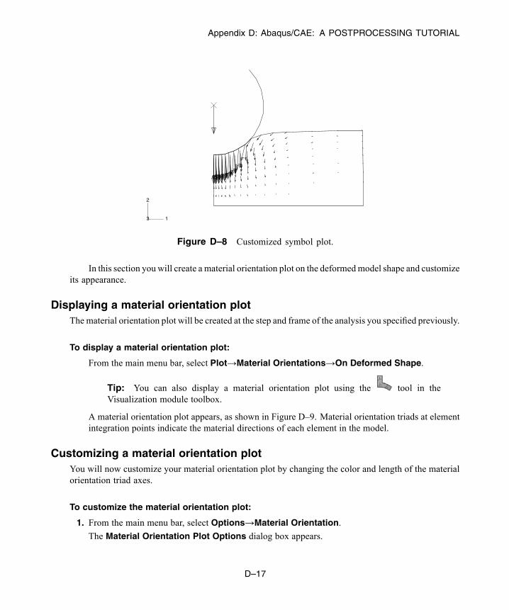
Appendix D: Abaqus/CAE: A POSTPROCESSING TUTORIAL
1
2
3
Figure D–8 Customized symbol plot.
In this section you will create a material orientation plot on the deformedmodel shape and customizeits appearance.
Displaying a material orientation plotThe material orientation plot will be created at the step and frame of the analysis you specified previously.
To display a material orientation plot:
From the main menu bar, select Plot→Material Orientations→On Deformed Shape.
Tip: You can also display a material orientation plot using the tool in theVisualization module toolbox.
A material orientation plot appears, as shown in Figure D–9. Material orientation triads at elementintegration points indicate the material directions of each element in the model.
Customizing a material orientation plotYou will now customize your material orientation plot by changing the color and length of the materialorientation triad axes.
To customize the material orientation plot:
1. From the main menu bar, select Options→Material Orientation.
The Material Orientation Plot Options dialog box appears.
D–17
Abaqus ID:Printed on:
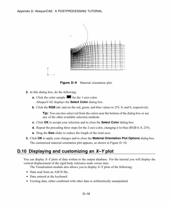
Appendix D: Abaqus/CAE: A POSTPROCESSING TUTORIAL
1
2
3
Figure D–9 Material orientation plot.
2. In this dialog box, do the following:
a. Click the color sample for the 1-axis color.
Abaqus/CAE displays the Select Color dialog box.
b. Click the RGB tab; and set the red, green, and blue values to 255, 0, and 0, respectively.
Tip: You can also select red from the colors near the bottom of the dialog box or useany of the other available selection methods.
c. Click OK to accept your selection and to close the Select Color dialog box.
d. Repeat the preceding three steps for the 2-axis color, changing it to blue (RGB 0, 0, 255).
e. Drag the Size slider to reduce the length of the triad axes.
3. Click OK to apply your changes and to close the Material Orientation Plot Options dialog box.
The customized material orientation plot appears, as shown in Figure D–10.
D.10 Displaying and customizing an X–Y plot
You can display X–Y plots of data written to the output database. For the tutorial you will display thevertical displacement of the rigid body reference node versus time.
The Visualization module also allows you to display X–Y plots of the following:
• Data read from an ASCII file.• Data entered at the keyboard.• Existing data, either combined with other data or arithmetically manipulated.
D–18
Abaqus ID:Printed on:
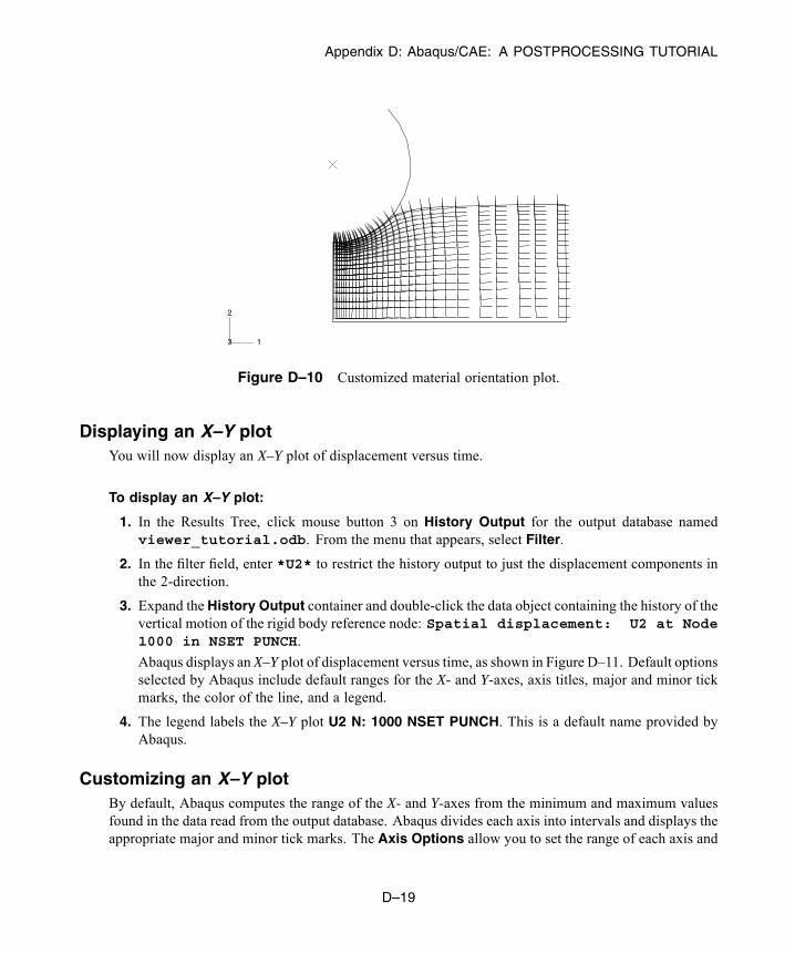
Appendix D: Abaqus/CAE: A POSTPROCESSING TUTORIAL
1
2
3
Figure D–10 Customized material orientation plot.
Displaying an X–Y plotYou will now display an X–Y plot of displacement versus time.
To display an X–Y plot:
1. In the Results Tree, click mouse button 3 on History Output for the output database namedviewer_tutorial.odb. From the menu that appears, select Filter.
2. In the filter field, enter *U2* to restrict the history output to just the displacement components inthe 2-direction.
3. Expand the History Output container and double-click the data object containing the history of thevertical motion of the rigid body reference node: Spatial displacement: U2 at Node1000 in NSET PUNCH.
Abaqus displays an X–Y plot of displacement versus time, as shown in Figure D–11. Default optionsselected by Abaqus include default ranges for the X- and Y-axes, axis titles, major and minor tickmarks, the color of the line, and a legend.
4. The legend labels the X–Y plot U2 N: 1000 NSET PUNCH. This is a default name provided byAbaqus.
Customizing an X–Y plotBy default, Abaqus computes the range of the X- and Y-axes from the minimum and maximum valuesfound in the data read from the output database. Abaqus divides each axis into intervals and displays theappropriate major and minor tick marks. The Axis Options allow you to set the range of each axis and
D–19
Abaqus ID:Printed on:

Appendix D: Abaqus/CAE: A POSTPROCESSING TUTORIAL
Figure D–11 X–Y plot of displacement versus time.
to customize the appearance of the axes; the Curve Options allow you to customize the appearance ofthe individual curves; the Chart Options and Chart Legend Options allow you to position the gridand legend, respectively. X–Y plot customization options apply only to the current viewport and are notsaved between sessions.
To customize an X–Y plot:
1. From the main menu bar, select Options→XY Options→Axis (or click in the prompt areato cancel the current procedure, if necessary, and double-click either axis in the viewport).
Abaqus displays the Axis Options dialog box.
2. Switch to the Scale tabbed page, if it is not already selected.
3. Specify that the X-axis should extend from 0 (the X-axis minimum) to 20 (the X-axis maximum)and that the Y-axis should extend from –200 (the Y-axis minimum) to 0 (the Y-axis maximum).
Tip: Select each axis in turn in the Axis Options dialog box, and then edit the scale asnoted above.
4. From the options in the Axis Options dialog box, do the following.
• In the Scale tabbed page, request that major tick marks appear on the X-axis at four-secondincrements (select By increment in the Tick Mode region of the page).
D–20
Abaqus ID:Printed on:
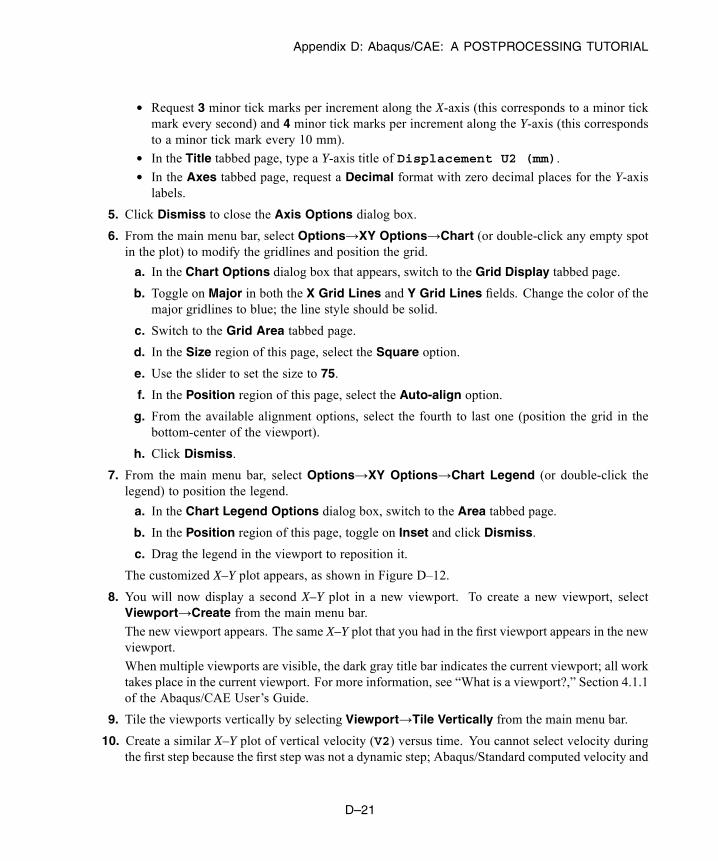
Appendix D: Abaqus/CAE: A POSTPROCESSING TUTORIAL
• Request 3 minor tick marks per increment along the X-axis (this corresponds to a minor tickmark every second) and 4 minor tick marks per increment along the Y-axis (this correspondsto a minor tick mark every 10 mm).
• In the Title tabbed page, type a Y-axis title of Displacement U2 (mm).
• In the Axes tabbed page, request a Decimal format with zero decimal places for the Y-axislabels.
5. Click Dismiss to close the Axis Options dialog box.
6. From the main menu bar, select Options→XY Options→Chart (or double-click any empty spotin the plot) to modify the gridlines and position the grid.
a. In the Chart Options dialog box that appears, switch to the Grid Display tabbed page.
b. Toggle on Major in both the X Grid Lines and Y Grid Lines fields. Change the color of themajor gridlines to blue; the line style should be solid.
c. Switch to the Grid Area tabbed page.
d. In the Size region of this page, select the Square option.
e. Use the slider to set the size to 75.
f. In the Position region of this page, select the Auto-align option.
g. From the available alignment options, select the fourth to last one (position the grid in thebottom-center of the viewport).
h. Click Dismiss.
7. From the main menu bar, select Options→XY Options→Chart Legend (or double-click thelegend) to position the legend.
a. In the Chart Legend Options dialog box, switch to the Area tabbed page.
b. In the Position region of this page, toggle on Inset and click Dismiss.
c. Drag the legend in the viewport to reposition it.
The customized X–Y plot appears, as shown in Figure D–12.
8. You will now display a second X–Y plot in a new viewport. To create a new viewport, selectViewport→Create from the main menu bar.
The new viewport appears. The same X–Y plot that you had in the first viewport appears in the newviewport.
When multiple viewports are visible, the dark gray title bar indicates the current viewport; all worktakes place in the current viewport. For more information, see “What is a viewport?,” Section 4.1.1of the Abaqus/CAE User’s Guide.
9. Tile the viewports vertically by selecting Viewport→Tile Vertically from the main menu bar.
10. Create a similar X–Y plot of vertical velocity (V2) versus time. You cannot select velocity duringthe first step because the first step was not a dynamic step; Abaqus/Standard computed velocity and
D–21
Abaqus ID:Printed on:
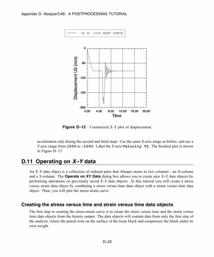
Appendix D: Abaqus/CAE: A POSTPROCESSING TUTORIAL
U2 N: 1000 NSET PUNCH
Figure D–12 Customized X–Y plot of displacement.
acceleration only during the second and third steps. Use the same X-axis range as before, and use aY-axis range from 1000 to −1000. Label the Y-axis Velocity V2. The finished plot is shownin Figure D–13.
D.11 Operating on X–Y data
An X–Y data object is a collection of ordered pairs that Abaqus stores in two columns—an X-columnand a Y-column. The Operate on XY Data dialog box allows you to create new X–Y data objects byperforming operations on previously saved X–Y data objects. In this tutorial you will create a stressversus strain data object by combining a stress versus time data object with a strain versus time dataobject. Then, you will plot the stress-strain curve.
Creating the stress versus time and strain versus time data objectsThe first step in creating the stress-strain curve is to create the stress versus time and the strain versustime data objects from the history output. The data objects will contain data from only the first step ofthe analysis, where the punch rests on the surface of the foam block and compresses the block under itsown weight.
D–22
Abaqus ID:Printed on:

Appendix D: Abaqus/CAE: A POSTPROCESSING TUTORIAL
V2 N: 1000 NSET PUNCH
Figure D–13 Customized X–Y plot of velocity.
To create the X–Y data objects:
1. In the Results Tree, double-click the XYData container.
The Create XY Data dialog box appears.
2. In this dialog box, select ODB history output if it is not already selected and click Continue.
The History Output dialog box appears.
3. In the History Output dialog box, do the following:
a. Click the Variables tab.
b. Filter the data according to *LE22*.
c. In the Output Variables field, select Logarithmic strain components: LE22at Element 1 Int Point 1 in ELSET CENT.
d. Click the Steps/Frames tab.
e. Select Step 1.
f. Click Save As.
The Save XY Data As dialog box appears.
g. Name the X–Y data Strain, and click OK.
A data object called Strain containing logarithmic strain data (LE22) from integration point 1 ofelement 1 during the first step of the analysis appears in the XYData container.
D–23
Abaqus ID:Printed on:

Appendix D: Abaqus/CAE: A POSTPROCESSING TUTORIAL
4. Use a similar technique to create a data object containing stress data (S22) from integration point 1of element 1 during the first step of the analysis. Name this data object Stress.
Tip: Filter the variable list according to *S22*.
Now you are ready to combine the two data objects to create a stress versus strain data object.
5. Dismiss the History Output dialog box.
Combining the data objectsIn this section you will create a stress versus strain data object by combining the stress versus time andstrain versus time data objects.
To combine the data objects:
1. In the Results Tree, double-click the XYData container.
2. From theCreate XY Data dialog box that appears, selectOperate on XY data and clickContinue.An Operate on XY Data dialog box appears. The dialog box contains the following lists:
• The XY Data field on the left contains a list of existing X–Y data objects.
• The Operators field on the right contains a list of all the possible operations you can performon the data objects.
3. From the Operators field, click combine(X,X).combine( ) appears in the expression text field at the top of the dialog box.
4. In the XY Data field, drag the cursor across both the Strain and the Stress data objects to selectboth and click Add to Expression near the bottom of the dialog box.The expression combine("Strain","Stress") appears in the expression text field. In thisexpression "Strain" will determine the X-values and "Stress" will determine the Y-values inthe combined plot.
5. From the buttons along the bottom of the Operate on XY Data dialog box, click Save As.
6. From the Save XY Data As dialog box that appears, enter the name Stress-Strain and clickOK.
The new data object Stress-Strain appears in the XYData container.
7. Cancel the Operate on XY Data dialog box.
Plotting and customizing the stress-strain curveYou will now use the Stress-Strain data object that you just created to plot the stress-strain curve.
To plot the stress-strain curve:
1. In the XYData container, double-click Stress-Strain.
A plot of the stress-strain curve appears in the viewport.
D–24
Abaqus ID:Printed on:
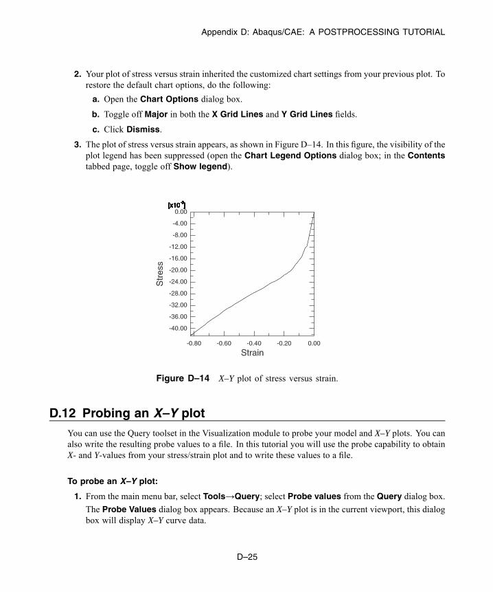
Appendix D: Abaqus/CAE: A POSTPROCESSING TUTORIAL
2. Your plot of stress versus strain inherited the customized chart settings from your previous plot. Torestore the default chart options, do the following:
a. Open the Chart Options dialog box.
b. Toggle off Major in both the X Grid Lines and Y Grid Lines fields.
c. Click Dismiss.
3. The plot of stress versus strain appears, as shown in Figure D–14. In this figure, the visibility of theplot legend has been suppressed (open the Chart Legend Options dialog box; in the Contentstabbed page, toggle off Show legend).
Figure D–14 X–Y plot of stress versus strain.
D.12 Probing an X–Y plotYou can use the Query toolset in the Visualization module to probe your model and X–Y plots. You canalso write the resulting probe values to a file. In this tutorial you will use the probe capability to obtainX- and Y-values from your stress/strain plot and to write these values to a file.
To probe an X–Y plot:
1. From the main menu bar, select Tools→Query; select Probe values from the Query dialog box.
The Probe Values dialog box appears. Because an X–Y plot is in the current viewport, this dialogbox will display X–Y curve data.
D–25
Abaqus ID:Printed on:

Appendix D: Abaqus/CAE: A POSTPROCESSING TUTORIAL
2. At the top of the dialog box, toggle on Interpolate between points. This option allows you toselect arbitrary points along the curve.
3. In the viewport, position the cursor over the X–Y curve.
When the arrow at the cursor approaches the X–Y curve, the point being probed is highlighted andinformation about it, including the corresponding X–Y coordinates, appears in the Probe Valuestable.
4. Click at various points along the curve.
The points are added to the table in the Probe Values dialog box.
5. When you have finished selecting points, click Write to File.
The Report Probe Values dialog box appears.
By default, the data in the table are written to a file called abaqus.rpt in your current directory.The options in this dialog box allow you to change the name of this file and the format of the datawritten to the file.
6. Click OK to write your data to the file.
7. From the Probe Values dialog box, click Cancel to exit probe mode.
A dialog box appears to inform you that the Selected Probe Values table contains data. ClickYes to indicate that it is OK to continue; the data in the table will be deleted.
D.13 Displaying results along a path
X–Y data can be generated for a specific path through your model. In this tutorial you will specify a nodelist path along the top of the foam block and plot the displacement magnitude along this path.
Creating a node list pathA path is a line you define by specifying a series of points through the model. In a node list path all ofthe specified points are nodal locations. You create a node list path by entering node labels or node labelranges in a table. To determine the node labels of interest, it is helpful to create a model plot with thenode labels visible.
To create a node list path:
1. Click the tool to display the undeformed model shape.
Use the Common Plot Options dialog box to display the node labels. Identify the nodes on thetop edge of the foam block.
2. In the Results Tree, double-click Paths.
The Create Path dialog box appears.
D–26
Abaqus ID:Printed on:

Appendix D: Abaqus/CAE: A POSTPROCESSING TUTORIAL
3. Name the path Displacement. Accept the default selection of Node list as the path type, andclick Continue.
The Edit Node List Path dialog box appears.
4. In the Path Definition table, select PART-1-1 in the Part Instance field, type 1:601:40 inthe Node Labels field, and press [Enter]. (This input specifies a range of nodes from 1 to 601 atincrements of 40.) Alternatively, you can pick the nodes for the node list directly from the viewportby clicking Add Before...or Add After... in the Edit Node List Path dialog box.
The selected path is highlighted in the plot in the current viewport.
5. Click OK to create the path and to close the Edit Node List Path dialog box.
Displaying results along a node list pathAbaqus obtains analysis results for each of the points on the path you have defined and generates X–Ydata pairs; the X-values are the specified points in the model, and the Y-values are the analysis results atthese points. You can generate an X–Y plot of the data pairs.
To display displacement results along a node list path:
1. In the Results Tree, double-click the XYData container.
2. In the Create XY Data dialog box that appears, select Path; and click Continue.
The XY Data from Path dialog box appears with the path that you created visible in the list ofavailable paths.
Accept the default selections in the X Values portion of the dialog box.
3. The result that will be plotted is displayed in the Y Values portion of the dialog box. If U is notindicated as the field output variable, click Field Output to change the variable.
In the Field Output dialog box:
a. Select U as the variable Name.
b. Select Magnitude from the Invariant field.
c. Click OK.
4. Click Plot to generate an X–Y plot of U along the path, as shown in Figure D–15. You may need toreset the X–Y plot options to their default settings.
You have now finished the tutorial.
D.14 Summary
• Abaqus/CAE loads the Visualization module automatically when you open an output database.• To perform many Visualization module functions, you can use either a menu item or a tool in thetoolbox.
D–27
Abaqus ID:Printed on:
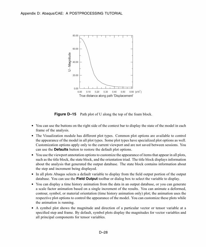
Appendix D: Abaqus/CAE: A POSTPROCESSING TUTORIAL
Figure D–15 Path plot of U along the top of the foam block.
• You can use the buttons on the right side of the context bar to display the state of the model in eachframe of the analysis.
• The Visualization module has different plot types. Common plot options are available to controlthe appearance of the model in all plot types. Some plot types have specialized plot options as well.Customization options apply only to the current viewport and are not saved between sessions. Youcan use the Defaults button to restore the default plot options.
• You use the viewport annotation options to customize the appearance of items that appear in all plots,such as the title block, the state block, and the orientation triad. The title block displays informationabout the analysis that generated the output database. The state block contains information aboutthe step and increment being displayed.
• In all plots Abaqus selects a default variable to display from the field output portion of the outputdatabase. You can use the Field Output toolbar or dialog box to select the variable to display.
• You can display a time history animation from the data in an output database, or you can generatea scale factor animation based on a single increment of the results. You can animate a deformed,contour, symbol, or material orientation (time history animation only) plot; the animation uses therespective plot options to control the appearance of the model. You can customize these plots whilethe animation is running.
• A symbol plot shows the magnitude and direction of a particular vector or tensor variable at aspecified step and frame. By default, symbol plots display the magnitudes for vector variables andall principal components for tensor variables.
D–28
Abaqus ID:Printed on:

Appendix D: Abaqus/CAE: A POSTPROCESSING TUTORIAL
• A material orientation plot shows the material directions of elements in your model at a specifiedstep and frame of your analysis. Material orientations are displayed on an element-by-element basisat the material integration points, with no averaging across elements.
• You can display an X–Y plot of any variable stored in the output database. In most cases the X-axisis assumed to be time.
• You can use theOperate on XY Data dialog box to create new X–Y data objects based on operationson existing data objects.
• You can use the Query toolset to probe a model or X–Y plot. You can write the values you obtainto a file.
D–29
Abaqus ID:Printed on:

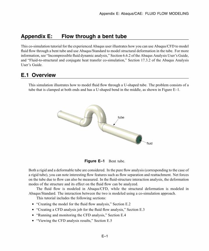
Appendix E: Abaqus/CAE: FLUID FLOW MODELING
Appendix E: Flow through a bent tube
This co-simulation tutorial for the experienced Abaqus user illustrates how you can use Abaqus/CFD to modelfluid flow through a bent tube and use Abaqus/Standard to model structural deformation in the tube. For moreinformation, see “Incompressible fluid dynamic analysis,” Section 6.6.2 of the Abaqus Analysis User’s Guide,and “Fluid-to-structural and conjugate heat transfer co-simulation,” Section 17.3.2 of the Abaqus AnalysisUser’s Guide.
E.1 Overview
This simulation illustrates how to model fluid flow through a U-shaped tube. The problem consists of atube that is clamped at both ends and has a U-shaped bend in the middle, as shown in Figure E–1.
Figure E–1 Bent tube.
Both a rigid and a deformable tube are considered. In the pure flow analysis (corresponding to the case ofa rigid tube), you can note interesting flow features such as flow separation and reattachment. Net forceson the tube due to flow can also be measured. In the fluid-structure interaction analysis, the deformationmodes of the structure and its effect on the fluid flow can be analyzed.
The fluid flow is modeled in Abaqus/CFD, while the structural deformation is modeled inAbaqus/Standard. The interaction between the two is modeled using a co-simulation approach.
This tutorial includes the following sections:
• “Creating the model for the fluid flow analysis,” Section E.2• “Creating a CFD analysis job for the fluid flow analysis,” Section E.3• “Running and monitoring the CFD analysis,” Section E.4• “Viewing the CFD analysis results,” Section E.5
E–1
Abaqus ID:Printed on:
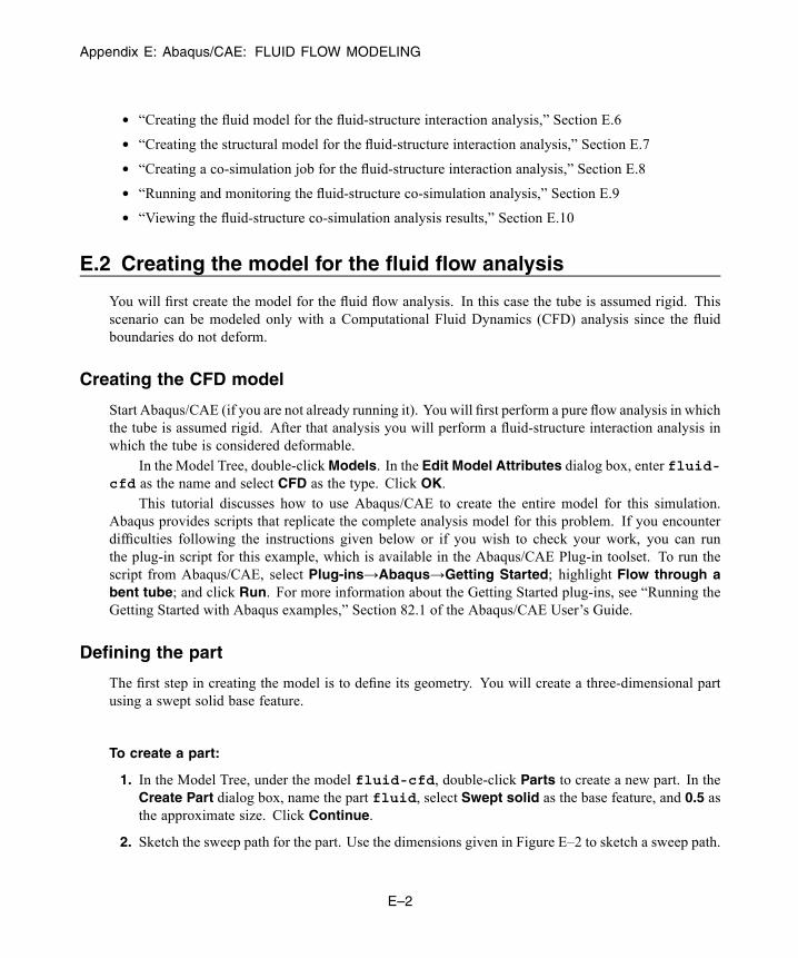
Appendix E: Abaqus/CAE: FLUID FLOW MODELING
• “Creating the fluid model for the fluid-structure interaction analysis,” Section E.6• “Creating the structural model for the fluid-structure interaction analysis,” Section E.7• “Creating a co-simulation job for the fluid-structure interaction analysis,” Section E.8• “Running and monitoring the fluid-structure co-simulation analysis,” Section E.9• “Viewing the fluid-structure co-simulation analysis results,” Section E.10
E.2 Creating the model for the fluid flow analysis
You will first create the model for the fluid flow analysis. In this case the tube is assumed rigid. Thisscenario can be modeled only with a Computational Fluid Dynamics (CFD) analysis since the fluidboundaries do not deform.
Creating the CFD model
Start Abaqus/CAE (if you are not already running it). You will first perform a pure flow analysis in whichthe tube is assumed rigid. After that analysis you will perform a fluid-structure interaction analysis inwhich the tube is considered deformable.
In the Model Tree, double-clickModels. In the Edit Model Attributes dialog box, enter fluid-cfd as the name and select CFD as the type. Click OK.
This tutorial discusses how to use Abaqus/CAE to create the entire model for this simulation.Abaqus provides scripts that replicate the complete analysis model for this problem. If you encounterdifficulties following the instructions given below or if you wish to check your work, you can runthe plug-in script for this example, which is available in the Abaqus/CAE Plug-in toolset. To run thescript from Abaqus/CAE, select Plug-ins→Abaqus→Getting Started; highlight Flow through abent tube; and click Run. For more information about the Getting Started plug-ins, see “Running theGetting Started with Abaqus examples,” Section 82.1 of the Abaqus/CAE User’s Guide.
Defining the part
The first step in creating the model is to define its geometry. You will create a three-dimensional partusing a swept solid base feature.
To create a part:
1. In the Model Tree, under the model fluid-cfd, double-click Parts to create a new part. In theCreate Part dialog box, name the part fluid, select Swept solid as the base feature, and 0.5 asthe approximate size. Click Continue.
2. Sketch the sweep path for the part. Use the dimensions given in Figure E–2 to sketch a sweep path.
E–2
Abaqus ID:Printed on:
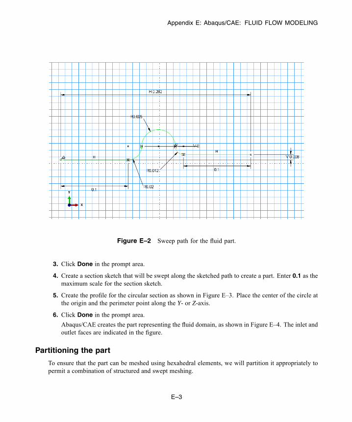
Appendix E: Abaqus/CAE: FLUID FLOW MODELING
Figure E–2 Sweep path for the fluid part.
3. Click Done in the prompt area.
4. Create a section sketch that will be swept along the sketched path to create a part. Enter 0.1 as themaximum scale for the section sketch.
5. Create the profile for the circular section as shown in Figure E–3. Place the center of the circle atthe origin and the perimeter point along the Y- or Z-axis.
6. Click Done in the prompt area.
Abaqus/CAE creates the part representing the fluid domain, as shown in Figure E–4. The inlet andoutlet faces are indicated in the figure.
Partitioning the part
To ensure that the part can be meshed using hexahedral elements, we will partition it appropriately topermit a combination of structured and swept meshing.
E–3
Abaqus ID:Printed on:

Appendix E: Abaqus/CAE: FLUID FLOW MODELING
Figure E–3 Section for the fluid part.
To partition the part:
1. In the Model Tree, expand the fluid item under the Parts container, and double-click Mesh in themenu that appears to switch to the Mesh module.
The part is initially colored orange, which means that it cannot be meshed using the defaulthexahedral element shape.
2. Use the Partition Face: Sketch tool to create a sketch of a circular section that will partitionthe inlet face. Place the center of the circle at the origin and the perimeter point along the Y- orZ-axis. The dimensions of the sketch are shown in Figure E–5.
3. Create a partition cutting midway through the entire part in the X–Y plane, as shown in Figure E–6.
a. Click the Partition Cell: Define Cutting Plane tool , and select Normal To Edge inthe prompt area to specify the cutting plane.
b. When prompted to select an edge, select the outer circular edge at the inlet.
c. When prompted to select a point on the edge, select a point on the edge on the vertical Y-axis.
d. Click Create Partition in the prompt area to complete the first partition.
E–4
Abaqus ID:Printed on:
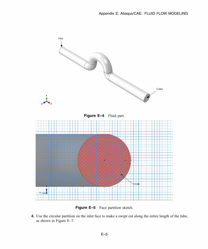
Appendix E: Abaqus/CAE: FLUID FLOW MODELING
Figure E–4 Fluid part.
Figure E–5 Face partition sketch.
4. Use the circular partition on the inlet face to make a swept cut along the entire length of the tube,as shown in Figure E–7.
E–5
Abaqus ID:Printed on:
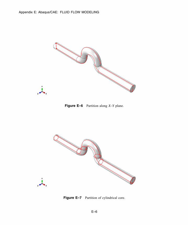
Appendix E: Abaqus/CAE: FLUID FLOW MODELING
Figure E–6 Partition along X–Y plane.
Figure E–7 Partition of cylindrical core.
E–6
Abaqus ID:Printed on:

Appendix E: Abaqus/CAE: FLUID FLOW MODELING
a. Click and hold the Partition Cell tool to reveal additional tools, and select the Partition Cell:
Extrude/Sweep Edges tool .
b. Select the entire part, and click Done in the prompt area.
c. In the prompt area, choose the by edge angle selection technique. Accept the default angleof 20.0.
d. Select the circular edge created by the face partition on the inlet face, and click Done.
e. Click Sweep Along Edge as the sweep method. Select the top edge of the straight sectioncontaining the inlet. This edge was created by the partition in the previous step.
f. Click Create Partition.
Abaqus/CAE adds a cylindrical core in the straight section of the tube. Repeat the process fourmore times to extend the cylindrical core throughout the entire length of the tube.
5. Create additional partitions along the length of the tube.
a. Click the Partition Cell: Define Cutting Plane tool .
b. Select the entire part, and click Done in the prompt area.
c. Click Point & Normal in the prompt area to specify the cutting plane.
d. When prompted to select a point, select the point on the outer circumferential edge between thestraight section containing the outlet and its adjacent curved section, as shown in Figure E–8.
e. Click Create Partition in the prompt area.
f. When prompted to select an edge, select the straight edge indicated in Figure E–8.
g. Repeat the procedure for the straight section attached to the inlet.
h. For the curved section in the center of the part, use the 3 Points method to define a cuttingplane, as indicated in Figure E–9.
6. Partition the curved sections in the center of the part using the Normal to Edgemethod. Select theouter circular edge and the point midway along the edge to define the plane. The partition is shownin Figure E–10.
Creating sets and surfacesYou will now create sets and surfaces that will be utilized to define section properties and boundaryconditions. Sets and surfaces identify the regions where analysis attributes are applied.
To define sets:
1. In the Model Tree, expand the container for the part named fluid and double-click Sets.
E–7
Abaqus ID:Printed on:

Appendix E: Abaqus/CAE: FLUID FLOW MODELING
Figure E–8 Partition using straight edge to define normal.
Figure E–9 Partition using 3 points method.
2. In the Create Set dialog box, name the set all and click Continue.
3. Select the entire geometry in the viewport, and click Done in the prompt area.
Abaqus/CAE creates a set that contains the entire part.
4. Repeat this procedure to create a set named fixed containing the faces at the inlet and outletsections of the fluid domain, as shown in Figure E–10.
E–8
Abaqus ID:Printed on:
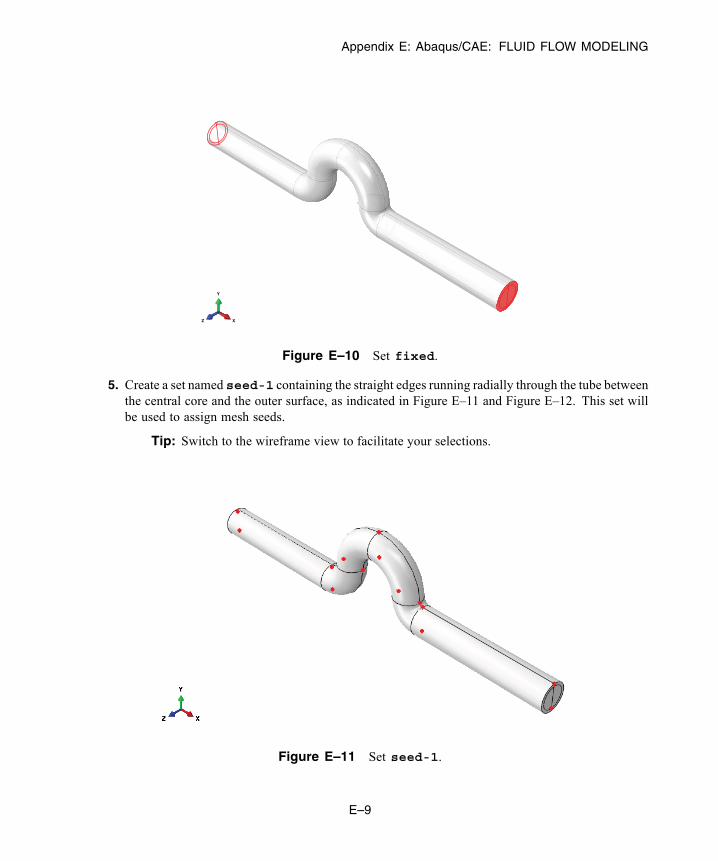
Appendix E: Abaqus/CAE: FLUID FLOW MODELING
X
Y
Z
Figure E–10 Set fixed.
5. Create a set named seed-1 containing the straight edges running radially through the tube betweenthe central core and the outer surface, as indicated in Figure E–11 and Figure E–12. This set willbe used to assign mesh seeds.
Tip: Switch to the wireframe view to facilitate your selections.
Figure E–11 Set seed-1.
E–9
Abaqus ID:Printed on:

Appendix E: Abaqus/CAE: FLUID FLOW MODELING
Figure E–12 Close-up view of set seed-1.
6. Create a set named seed-2 containing the straight edges running axially through the tube, asindicated in Figure E–13. This set will also be used to assign mesh seeds.
Figure E–13 Set seed-2.
E–10
Abaqus ID:Printed on:

Appendix E: Abaqus/CAE: FLUID FLOW MODELING
To define surfaces:
1. In the Model Tree, expand the container for the part named fluid and double-click Surfaces.
2. In the Create Surface dialog box, name the surface inlet and click Continue.
3. In the prompt area, select by angle as the selection technique. Select the faces at the inlet of thetube (Figure E–14 depicts the location of the surface).
4. Click Done in the prompt area.
5. Repeat the previous steps to create a surface named outlet at the outlet of the tube.
6. Repeat the previous steps to create a surface named wall representing the outer surface of the tube(excluding the inlet and outlet).
Figure E–14 Surface definitions for the tube.
Material and section propertiesThe next step in creating the model involves defining and assigning material and section properties tothe fluid part. Each region of the model must refer to a section property. In this model we assume thefluid is a Newtonian fluid with density 1000 kg/m3 and a viscosity of 0.001 Pa·sec (i.e., water).
E–11
Abaqus ID:Printed on:
Appendix E: Abaqus/CAE: FLUID FLOW MODELING
To define material properties:
1. In the Model Tree, double-click Materials to create a new material named fluid.
2. From the material editor, select General→Density and specify a density value of 1000 kg/m3 .
3. From the material editor, select Mechanical→Viscosity and specify a viscosity value of 0.001Pa·sec.
4. Click OK.
Abaqus/CAE creates the material definition.
To define the CFD section:
1. In theModel Tree, double-clickSections to create a new section named fluid. Accept the defaultselection of a homogeneous fluid section, and click Continue.
2. In the Edit Section dialog box, select fluid as the material and click OK.
Abaqus/CAE creates a fluid section definition.
To assign the CFD section:
1. In the Model Tree, expand the Parts container and the fluid container under it, then double-clickSection Assignments.
2. In the prompt area, clickSets. In theRegion Selection dialog box, choose all and clickContinue.
3. Click OK in the section assignment editor.
Meshing the fluid domainYou will now mesh the fluid domain.
To mesh the fluid domain:
1. In the Model Tree, expand the container for the part named fluid and double-clickMesh. Note thatthe core partition of the tube is colored yellow, while the outside cells are colored green; these colorcues mean that the core can be meshed with a sweep meshing technique, while the outside cells canbe meshed using a structured meshing technique.
2. Before meshing the part, assign mesh seeds. This seeding method creates a mesh that is finer nearthe walls of the tube and becomes coarser radially inward.
First create seeds for the outside cells.
a. Click the Seed Edges tool , and then click Sets/Surfaces in the prompt area (ifnecessary).
b. In the Region Selection dialog box, select seed-1 as the set and click Continue.
E–12
Abaqus ID:Printed on:

Appendix E: Abaqus/CAE: FLUID FLOW MODELING
c. In the Local Seeds dialog box, select By size as the method, Single as the bias type, andenter 0.0004 as the minimum size and 0.001 as the maximum size.
d. Zoom in to ensure that the seeds are concentrated near the wall. You can verify seed placementby confirming that the arrow indicating the bias direction points radially outward for each edgein the selected set.
e. If any arrow points radially inward, you can flip it by clicking Select next to Flip bias andselecting the edges where the bias direction needs to be flipped.
3. Create seeds along the length of the tube.
a. Follow the steps outlined above to create biased seeds that ensure coarser seeding at the inletand outlet and finer seeds at the sections where the straight tube sections transition to the curvedsections.
b. In the Region Selection dialog box, select seed-2 as the set and click Continue.
c. In the Local Seeds dialog box, select By size as the method, Single as the bias type, andenter 0.0035 as the minimum size and 0.01 as the maximum size.
d. Ensure that each arrow points axially inward on both the inlet as well as the outlet sides of thetube. Flip the direction of any arrow that violates this condition.
4. Set the global seed size.
a. Click the Seed Part tool . In the Global Seeds dialog box, enter 0.0025 as theapproximate global size.
b. Accept all other default values, and click OK.
Abaqus/CAE sets the global seed size for the entire part.
5. Use the medial axis algorithm for the swept mesh regions of the part.
a. Use the Display Group toolbar to display only the inner core of the tube (colored yellow).
Tip: ChooseCells as the selection method, and remove the outer regions of the part.
b. Click the Mesh Controls tool, and assign the Medial axis mesh algorithm.
c. Restore the visibility of all part regions.
6. Click the Mesh Part tool , and click Yes in the prompt area to create the part mesh.
Abaqus/CAE displays the mesh, creating approximately 9000 elements.
Assembling the partsAn assembly contains all the geometry included in the model. Each Abaqus/CAE model contains asingle assembly. The assembly is initially empty, even when you have created a part. You will create aninstance of the part in the assembly to include it in your model.
E–13
Abaqus ID:Printed on:
Appendix E: Abaqus/CAE: FLUID FLOW MODELING
To instance a part:
1. In the Model Tree, expand the Assembly container and double-click Instances in the list thatappears to create an instance of the part.
2. In the Create Instance dialog box, select fluid from the Parts list and click OK.
Defining steps and output requestsYou will now define the analysis steps. Attributes such as boundary conditions and output requests canbe step dependent, so an analysis step must be defined before these items can be specified.
To define an incompressible turbulent flow analysis step:
1. In the Model Tree, double-click Steps.
2. In the Create Step dialog box, accept Flow as the default procedure type and the default step name(Step–1). Click Continue.
3. From the Basic tabbed page of the step editor, do the following:
a. Enter Flow in a rigid hose as the description.
b. Enter 0.8 sec as the time period.
4. From the Incrementation tabbed page of the step editor, do the following:
a. Accept Automatic (Fixed CFL) as the default time incrementation type.
b. Enter 0.001 as the initial time increment.
c. Enter 2.0 as the Maximum CFL number.
5. From the Solvers tabbed page of the step editor, accept the default settings on the MomentumEquation, Pressure Equation, and Transport Equation tabbed pages.
6. From the Turbulence tabbed page of the step editor, select Spalart-Allmaras as the turbulencemodel. Abaqus/CAEwill use the Spalart-Allmaras turbulencemodel for turbulent flow calculations.
7. Click OK to close the Create Step dialog box.
To define output requests:
1. In the Model Tree, expand the Field Output Requests container. Note that a default field outputrequest named F-Output-1 was created automatically at the time the step was created.
2. Double-click F-Output-1. Note that the output is requested at 20 evenly spaced time intervals.
3. Delete the preselected output, and select the following output variables: V, PRESSURE, DIV,TURBNU, and VORTICITY.
4. Click OK to close the output request editor.
E–14
Abaqus ID:Printed on:

Appendix E: Abaqus/CAE: FLUID FLOW MODELING
Defining boundary and initial conditionsYou will now define boundary conditions and a predefined field for turbulence. We are solving a transientturbulent flow problem so specification of initial turbulence at time = 0 is required.
To define boundary conditions:
1. Define an inlet boundary condition at the inlet surface.
a. In the Model Tree, double-click BCs.
b. Name the boundary condition inlet, and select Step-1 as the step.
c. Select Fluid as the category and Fluid inlet/outlet as the type.
d. Select fluid-1.inlet as the surface to which the boundary condition will be applied (clickSurfaces in the prompt area if necessary).
e. From the Momentum tabbed page of the boundary condition editor, toggle on Specify andselect Velocity.
f. Set the X-velocity component V1 to 1. Set the Y- and Z-velocity components V2 and V3 to 0.
g. From the Turbulence tabbed page, toggle on Kinematic eddy viscosity and enter a valueof 5e–6. Abaqus/CAE sets the inlet turbulence of the flow.
h. Click OK to create the boundary condition and to close the boundary condition editor.
2. Define an outlet boundary condition at the outlet surface.
a. In the Model Tree, double-click BCs.
b. Name the boundary condition outlet, and select Step-1 as the step.
c. Select Fluid as the category and Fluid inlet/outlet as the type.
d. Select fluid-1.outlet as the surface to which the boundary condition will be applied.
e. From the Momentum tabbed page of the boundary condition editor, toggle on Specify andselect Pressure.
f. Set the pressure to 0.
g. Click OK to create the boundary condition and to close the boundary condition editor.
3. Define a no-slip/no-penetration boundary condition at the cylinder surface.
a. In the Model Tree, double-click BCs.
b. Name the boundary condition noSlip, and select Step-1 as the step.
c. Select Fluid as the category and Fluid wall condition as the type.
d. Select fluid-1.wall as the surface to which the boundary condition will be applied.
e. Select No slip as the condition.
E–15
Abaqus ID:Printed on:

Appendix E: Abaqus/CAE: FLUID FLOW MODELING
f. Click OK to close the boundary condition editor.
Abaqus/CAE creates the no-slip/no-penetration boundary condition.
To specify a predefined field for the turbulent viscosity:
1. In the Model Tree, double-click Predefined Fields.
2. Name the initial condition initial turbulence, and select Initial as the step.
3. Select Fluid as the category and Fluid turbulence as the type.
4. Set the Kinematic eddy viscosity to 5e–6.
5. Click OK to close the predefined field editor.
Abaqus/CAE creates the predefined field for turbulent viscosity.
Specifying surface output requests
Surface output quantities in fluid flow analyses are required because they provide important insight intothe adequacy and correctness of the CFD simulation. For example, measuring the inlet and outlet massflow rates can give us a good sense of the mass balance. Proper mass balance should be ensured foraccurate CFD results. In addition, a measure of the nondimensional wall distance ( ) indicates if themesh at the walls is suitable to resolve essential turbulent flow features. For more information about fluiddynamics at a wall, see “Incompressible fluid dynamic analysis,” Section 6.6.2 of the Abaqus AnalysisUser’s Guide.
You will now request surface output quantities. Since these are not supported through theAbaqus/CAE interface, they will be included using the keywords editor.
To request surface output quantities:
1. In the Model Tree, click mouse button 3 on the fluid-cfd model and select Edit Keywords fromthe menu that appears.
The keywords editor appears.
2. Scroll down, and click in the *Output, field option block.
3. Click Add After, and enter the following:
*Surface output, surface=fluid-1.wallyplus
4. Navigate to the *Output, history option block, and change the output frequency to 1.
E–16
Abaqus ID:Printed on:
Appendix E: Abaqus/CAE: FLUID FLOW MODELING
5. Click Add after, and enter the following:
*Surface output, surface=fluid-1.inletmassflow,
*Surface output, surface=fluid-1.outletmassflow,
6. Click OK to close the keywords editor.
Abaqus/CAE modifies the selected output requests.
E.3 Creating a CFD analysis job for the fluid flow analysisIn this section you will define a job for the fluid flow analysis.
To create a CFD analysis job:
1. In the Model Tree, expand the Analysis container.
2. Double-click Jobs.
3. In the Create Job dialog box, select the model fluid-cfd and name the job fluid-cfd.
Abaqus/CAE creates the new analysis job.
E.4 Running and monitoring the CFD analysisNow that the model setup is complete, you will run the CFD analysis job.
To run the job:
1. In the Model Tree, expand the Jobs container.
2. Click mouse-button 3 on the job named fluid-cfd, and select Submit from the menu that appears.
Abaqus/CAE runs the analysis job. While the job is running, you can monitor its progress; clickmouse button 3 on the job in the Model Tree, and select Monitor from the menu that appears. Note thatAbaqus/CAE updates divergence (RMS) and kinetic energy every time increment.
E.5 Viewing the CFD analysis resultsOnce the job fluid-cfd completes, perform the steps in this section to display contour plots and X–Y plotsof the output data.
To view the CFD analysis results:
1. Click mouse button 3 on the job named fluid-cfd, and select Results from the menu that appears.
The output database file fluid-cfd.odb opens in the Visualization module.
E–17
Abaqus ID:Printed on:
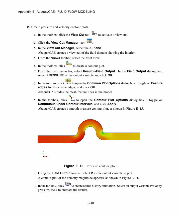
Appendix E: Abaqus/CAE: FLUID FLOW MODELING
2. Create pressure and velocity contour plots.
a. In the toolbox, click the View Cut tool to activate a view cut.
b. Click the View Cut Manager icon .
c. In the View Cut Manager, select the Z-Plane.Abaqus/CAE creates a view cut of the fluid domain showing the interior.
d. From the Views toolbar, select the front view.
e. In the toolbox, click to create a contour plot.
f. From the main menu bar, select Result→Field Output. In the Field Output dialog box,select PRESSURE as the output variable and click OK.
g. In the toolbox, click to open the Common Plot Options dialog box. Toggle on Featureedges for the visible edges, and click OK.
Abaqus/CAE hides the mesh feature lines in the model.
h. In the toolbox, click to open the Contour Plot Options dialog box. Toggle onContinuous under Contour Intervals, and click Apply.
Abaqus/CAE creates a smooth pressure contour plot, as shown in Figure E–15.
Figure E–15 Pressure contour plot.
i. Using the Field Output toolbar, select V as the output variable to plot.
A contour plot of the velocity magnitude appears, as shown in Figure E–16.
j. In the toolbox, click to create a time history animation. Select an output variable (velocity,pressure, etc.) to animate the results.
E–18
Abaqus ID:Printed on:
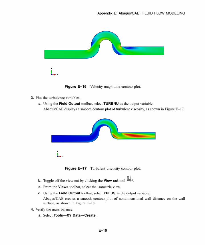
Appendix E: Abaqus/CAE: FLUID FLOW MODELING
Figure E–16 Velocity magnitude contour plot.
3. Plot the turbulence variables.
a. Using the Field Output toolbar, select TURBNU as the output variable.
Abaqus/CAE displays a smooth contour plot of turbulent viscosity, as shown in Figure E–17.
Figure E–17 Turbulent viscosity contour plot.
b. Toggle off the view cut by clicking the View cut tool .
c. From the Views toolbar, select the isometric view.
d. Using the Field Output toolbar, select YPLUS as the output variable.
Abaqus/CAE creates a smooth contour plot of nondimensional wall distance on the wallsurface, as shown in Figure E–18.
4. Verify the mass balance.
a. Select Tools→XY Data→Create.
E–19
Abaqus ID:Printed on:
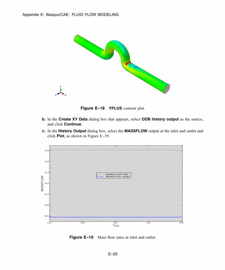
Appendix E: Abaqus/CAE: FLUID FLOW MODELING
Figure E–18 YPLUS contour plot.
b. In the Create XY Data dialog box that appears, select ODB history output as the source,and click Continue.
c. In the History Output dialog box, select the MASSFLOW output at the inlet and outlet andclick Plot, as shown in Figure E–19.
Figure E–19 Mass flow rates at inlet and outlet.
E–20
Abaqus ID:Printed on:
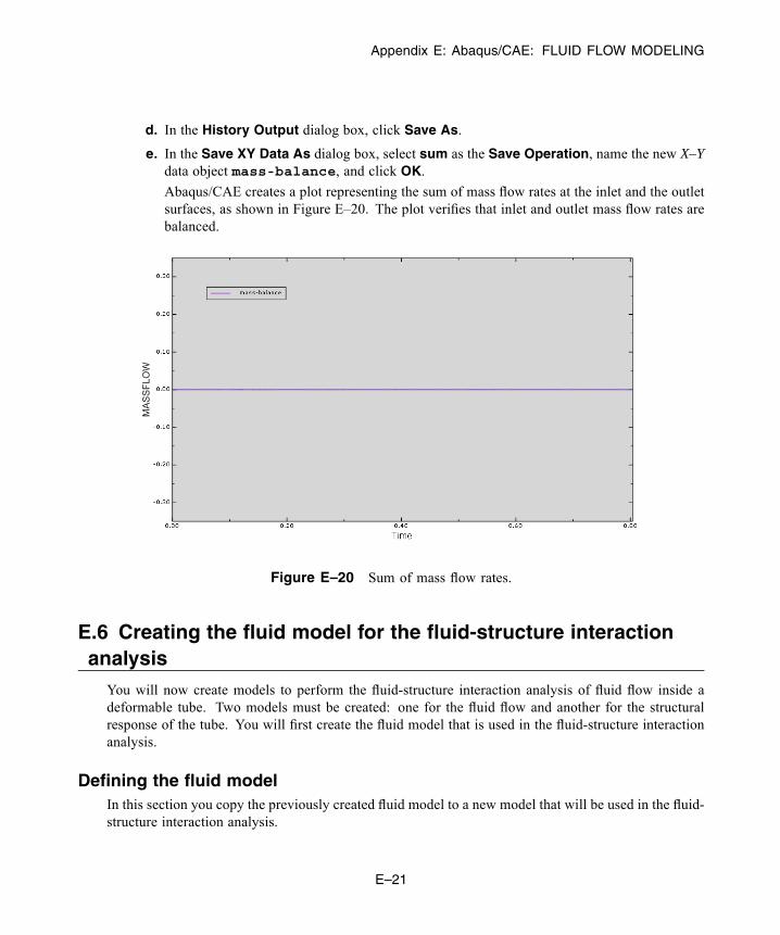
Appendix E: Abaqus/CAE: FLUID FLOW MODELING
d. In the History Output dialog box, click Save As.
e. In the Save XY Data As dialog box, select sum as the Save Operation, name the new X–Ydata object mass-balance, and click OK.
Abaqus/CAE creates a plot representing the sum of mass flow rates at the inlet and the outletsurfaces, as shown in Figure E–20. The plot verifies that inlet and outlet mass flow rates arebalanced.
Figure E–20 Sum of mass flow rates.
E.6 Creating the fluid model for the fluid-structure interactionanalysisYou will now create models to perform the fluid-structure interaction analysis of fluid flow inside adeformable tube. Two models must be created: one for the fluid flow and another for the structuralresponse of the tube. You will first create the fluid model that is used in the fluid-structure interactionanalysis.
Defining the fluid modelIn this section you copy the previously created fluid model to a new model that will be used in the fluid-structure interaction analysis.
E–21
Abaqus ID:Printed on:

Appendix E: Abaqus/CAE: FLUID FLOW MODELING
To create the fluid model:
1. In the Model Tree, click mouse button 3 on the model named fluid-cfd.
2. From the menu that appears, select Copy Model.
3. Name the new model fluid, and click OK.
Abaqus/CAE creates the fluid model. Make all subsequent changes to this model.
Modifying the analysis step and output requestsYou will now modify the total analysis time for the fluid-structure interaction analysis.
To modify the analysis step and its output requests:
1. Modify the CFD analysis step in the model named fluid.
a. In the Model Tree, expand the Steps container and double-click Step-1.
The step editor appears.
b. From the Basic tabbed page, do the following:
i. Modify the description to read Flow in a deformable hose.
ii. Set the time period of the step to 0.2 sec.
2. Modify the output requests.
a. In the Model Tree, expand the Field Output Requests container.
b. Double-click F-Output-1.
c. Select Every x units of time as the frequency, and enter 0.02 as the time interval.
d. Click OK.
Abaqus/CAE makes the specified changes to the analysis.
Modifying the boundary conditionsYou will now modify the boundary conditions. The no-slip/no-penetration wall boundary condition onthe tube wall surface is suppressed because the fluid velocities and mesh displacements are dictated bythe coupled solution. Therefore, it is not necessary to specify this boundary condition.
In addition, since the Arbitrary Lagrangian-Eulerian (ALE) method is activated to accommodatethe displacements of the tube, appropriate boundary conditions are required for the mesh deformationsolution.
To modify the boundary conditions:
1. Suppress the no-slip/no-penetration wall boundary condition on the tube wall surface.
a. In the Model Tree, expand the container for the fluid model and expand its BCs container.
E–22
Abaqus ID:Printed on:
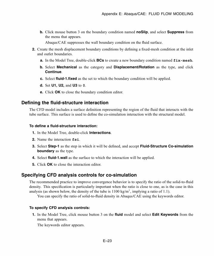
Appendix E: Abaqus/CAE: FLUID FLOW MODELING
b. Click mouse button 3 on the boundary condition named noSlip, and select Suppress fromthe menu that appears.
Abaqus/CAE suppresses the wall boundary condition on the fluid surface.
2. Create the mesh displacement boundary conditions by defining a fixed-mesh condition at the inletand outlet boundaries.
a. In the Model Tree, double-click BCs to create a new boundary condition named fix-mesh.
b. Select Mechanical as the category and Displacement/Rotation as the type, and clickContinue.
c. Select fluid-1.fixed as the set to which the boundary condition will be applied.
d. Set U1, U2, and U3 to 0.
e. Click OK to close the boundary condition editor.
Defining the fluid-structure interactionThe CFD model includes a surface definition representing the region of the fluid that interacts with thetube surface. This surface is used to define the co-simulation interaction with the structural model.
To define a fluid-structure interaction:
1. In the Model Tree, double-click Interactions.
2. Name the interaction fsi.
3. Select Step-1 as the step in which it will be defined, and accept Fluid-Structure Co-simulationboundary as the type.
4. Select fluid-1.wall as the surface to which the interaction will be applied.
5. Click OK to close the interaction editor.
Specifying CFD analysis controls for co-simulationThe recommended practice to improve convergence behavior is to specify the ratio of the solid-to-fluiddensity. This specification is particularly important when the ratio is close to one, as is the case in thisanalysis (as shown below, the density of the tube is 1100 kg/m3, implying a ratio of 1.1).
You can specify the ratio of solid-to-fluid density in Abaqus/CAE using the keywords editor.
To specify CFD analysis controls:
1. In the Model Tree, click mouse button 3 on the fluid model and select Edit Keywords from themenu that appears.
The keywords editor appears.
E–23
Abaqus ID:Printed on:
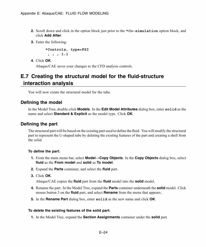
Appendix E: Abaqus/CAE: FLUID FLOW MODELING
2. Scroll down and click in the option block just prior to the *Co-simulation option block, andclick Add After.
3. Enter the following:
*Controls, type=FSI, , , 1.1
4. Click OK.
Abaqus/CAE saves your changes to the CFD analysis controls.
E.7 Creating the structural model for the fluid-structureinteraction analysis
You will now create the structural model for the tube.
Defining the modelIn the Model Tree, double-clickModels. In the Edit Model Attributes dialog box, enter solid as thename and select Standard & Explicit as the model type. Click OK.
Defining the partThe structural part will be based on the existing part used to define the fluid. Youwill modify the structuralpart to represent the U-shaped tube by deleting the existing features of the part and creating a shell fromthe solid.
To define the part:
1. From the main menu bar, select Model→Copy Objects. In the Copy Objects dialog box, selectfluid as the From model and solid as To model.
2. Expand the Parts container, and select the fluid part.
3. Click OK.
Abaqus/CAE copies the fluid part from the fluid model into the solid model.
4. Rename the part. In the Model Tree, expand the Parts container underneath the solidmodel. Clickmouse button 3 on the fluid part, and select Rename from the menu that appears.
5. In the Rename Part dialog box, enter solid as the new name and click OK.
To delete the existing features of the solid part:
1. In the Model Tree, expand the Section Assignments container under the solid part.
E–24
Abaqus ID:Printed on:

Appendix E: Abaqus/CAE: FLUID FLOW MODELING
2. Click mouse button 3 on the section fluid (which is no longer relevant), and select Delete from themenu that appears. Click Yes to confirm the operation.
3. Expand the Sets container under the solid part.
4. Select all the sets, click mouse button 3 on the selections, and select Delete from the menu thatappears. Click Yes to confirm the operation.
5. Repeat this process to delete all the surfaces and all the face and cell partitions.
To create a shell from the solid:
1. From the main menu bar in the Part module, select Tools→Geometry Edit. In the GeometryEdit dialog box, select Face as the category and Remove as the method.
2. Select the faces representing the inlet and the outlet.
3. Click Done in the prompt area.
4. Click OK when prompted to delete faces.
5. Close the Geometry Edit dialog box.
6. Click mouse button 3 on the solid part, and select Update Validity from the menu that appears.Abaqus/CAE updates the features of the part.
Defining partitions
To assign biased meshing to the part, we will first partition it.
To partition the part:
1. In the Model Tree, expand the solid item under the Parts container and double-click Mesh in themenu that appears.
2. Create a datum plane by clicking the Create Datum Plane: Offset From Principal Plane tool
.
3. Click XY Plane in the prompt area. Accept the default offset of 0.0, and press [Enter].
4. Click the Partition Face: Use Datum Plane tool to create a partition running along thelength of the tube.
5. Select all the faces of the tube in the viewport, and click Done in the prompt area.
6. Select the datum plane created in the previous step, and click Create Partition in the prompt area.
E–25
Abaqus ID:Printed on:
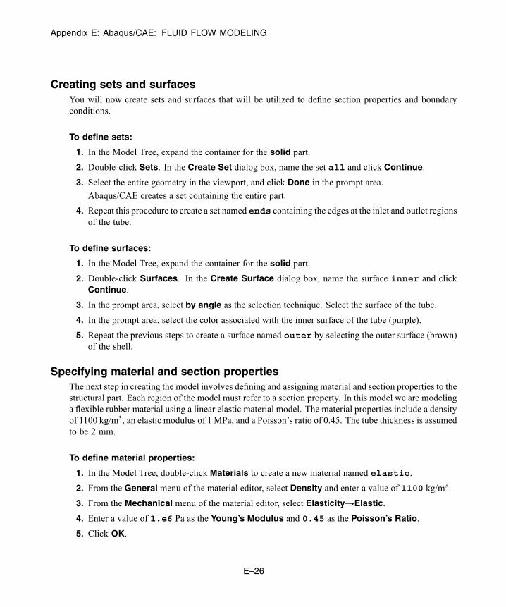
Appendix E: Abaqus/CAE: FLUID FLOW MODELING
Creating sets and surfacesYou will now create sets and surfaces that will be utilized to define section properties and boundaryconditions.
To define sets:
1. In the Model Tree, expand the container for the solid part.
2. Double-click Sets. In the Create Set dialog box, name the set all and click Continue.
3. Select the entire geometry in the viewport, and click Done in the prompt area.
Abaqus/CAE creates a set containing the entire part.
4. Repeat this procedure to create a set named ends containing the edges at the inlet and outlet regionsof the tube.
To define surfaces:
1. In the Model Tree, expand the container for the solid part.
2. Double-click Surfaces. In the Create Surface dialog box, name the surface inner and clickContinue.
3. In the prompt area, select by angle as the selection technique. Select the surface of the tube.
4. In the prompt area, select the color associated with the inner surface of the tube (purple).
5. Repeat the previous steps to create a surface named outer by selecting the outer surface (brown)of the shell.
Specifying material and section propertiesThe next step in creating the model involves defining and assigning material and section properties to thestructural part. Each region of the model must refer to a section property. In this model we are modelinga flexible rubber material using a linear elastic material model. The material properties include a densityof 1100 kg/m3, an elastic modulus of 1 MPa, and a Poisson’s ratio of 0.45. The tube thickness is assumedto be 2 mm.
To define material properties:
1. In the Model Tree, double-click Materials to create a new material named elastic.
2. From the General menu of the material editor, select Density and enter a value of 1100 kg/m3 .
3. From the Mechanical menu of the material editor, select Elasticity→Elastic.
4. Enter a value of 1.e6 Pa as the Young’s Modulus and 0.45 as the Poisson’s Ratio.
5. Click OK.
E–26
Abaqus ID:Printed on:

Appendix E: Abaqus/CAE: FLUID FLOW MODELING
To define a shell section:
1. In the Model Tree, double-click Sections to create a new section named shell.
2. Select Shell as the category and Homogeneous as the type. Click Continue.
3. In the Edit Section dialog box, enter 0.002 as the value of the constant shell thickness.
4. Select elastic as the material.
5. Click OK.
To assign the shell section:
1. In the Model Tree, expand the Parts container. Expand the container for the part named solid.
2. Double-click Section Assignments.
3. In the prompt area, clickSets. In theRegion Selection dialog box, choose all and clickContinue.
4. Click Done in the prompt area.
5. In the section assignment editor, choose the shell section created earlier and click OK.
Creating the meshYou will now create a mesh for the tube structure.
To create the mesh:
1. In the Model Tree, expand the solid item under the Parts container and double-click Mesh in themenu that appears.
Note that the entire tube is colored pink, which means that the part can be meshed with the defaultfree meshing technique.
2. Change the meshing technique to sweep.
a. From the main menu bar, select Mesh→Controls.
b. Select the entire part in the viewport to assign new controls, and click Done in the prompt area.
c. In the Mesh Controls dialog box, select Sweep as the technique and click OK.
Abaqus/CAE changes the part’s color to yellow in the current viewport.
3. Assign mesh seeds. You create biased seeds for the inlet and outlet regions of the tube. This seedingmethod creates a mesh that is coarser axially at the inlet and outlet and finer in the middle sectionsof the tube.
a. Click the Seed Edges tool , and click Select in Viewport in the prompt area (ifnecessary).
E–27
Abaqus ID:Printed on:

Appendix E: Abaqus/CAE: FLUID FLOW MODELING
b. In the viewport, select the straight edges in the inlet and outlet regions running along themidplane and click Done.
c. In the Local Seeds dialog box, select By size as the method, Single as the bias type, andenter 0.0045 as the minimum size and 0.01 as the maximum size.
d. Ensure that the seeding bias is such that seeds are concentrated away from inlet and outletregions of the tube (i.e., each arrow should point axially inward). Flip the direction of anyarrow that violates this condition.
4. Set the global seed size.
a. Click the Seed Part tool .
b. In the Global Seeds dialog box, enter 0.004 as the approximate global size.
c. Accept all the other default values, and click OK.
Abaqus/CAE sets the global seed size for the part.
5. Mesh the part.
a. Click the Mesh Part tool .
b. Click Yes in the prompt area.
Abaqus/CAE creates a mesh for the part with approximately 950 shell elements.
Create the assemblyYou will now create an instance of the part in the assembly to include it in your model.
To instance a part:
1. In the Model Tree, expand the Assembly container and double-click Instances in the list thatappears to create an instance of the part.
2. In the Create Instance dialog box, select solid from the Parts list and click OK.
Specifying steps and output requestsYou will now define the analysis step. An implicit dynamic procedure is used to model the structuralresponse of the tube.
To define an implicit dynamic analysis step:
1. In the Model Tree, double-click Steps.
2. In the Create Step dialog box, accept the default procedure type (General) and the default name(Step–1). From the list of available procedures, select Dynamic, Implicit and click Continue.
E–28
Abaqus ID:Printed on:

Appendix E: Abaqus/CAE: FLUID FLOW MODELING
3. From the Basic tabbed page of the step editor, do the following:
a. Enter deformation of the tube as the description.
b. Enter 0.2 sec as the time period.
c. Toggle on Nlgeom.
d. Select Transient fidelity as the application type.
4. From the Incrementation tabbed page of the step editor, do the following:
a. Enter 1000 as the maximum number of increments.
b. Enter 0.001 as the initial increment size.
c. Enter 2.e-6 as the minimum increment size.
d. Toggle on Suppress calculation for the Half-increment Residual.
5. Click OK to create the step.
To define output requests:
1. In the Model Tree, expand the Field Output Requests container.
2. Double-click F-Output-1.
3. Select Every x units of time as the output frequency, and enter 0.02 as the time interval.
4. Accept the default output variables, and click OK.
Defining boundary conditionsThe tube is secured at each end, so you need to define an encastre boundary condition for the set definitionthat includes the ends of the tube.
To define the boundary conditions:
1. In the Model Tree, double-click BCs underneath the solid model.
2. In the Create Boundary Condition dialog box, name the boundary condition fixed-ends andselect Initial as the step.
3. Accept Mechanical as the category, and select Symmetry/Antisymmetry/Encastre as the type.
4. Click Sets in the prompt area.
5. In the Region Selection dialog box, select the set named solid-1.ends and click Continue.
6. In the Edit Boundary Condition dialog box, select ENCASTRE and click OK.
Abaqus/CAE creates the boundary condition.
E–29
Abaqus ID:Printed on:
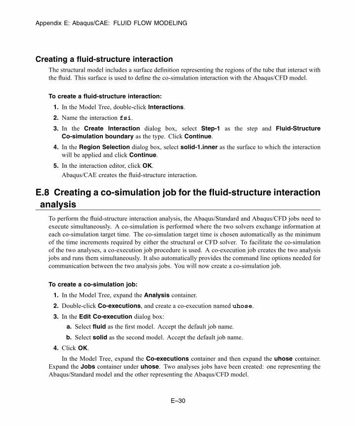
Appendix E: Abaqus/CAE: FLUID FLOW MODELING
Creating a fluid-structure interactionThe structural model includes a surface definition representing the regions of the tube that interact withthe fluid. This surface is used to define the co-simulation interaction with the Abaqus/CFD model.
To create a fluid-structure interaction:
1. In the Model Tree, double-click Interactions.
2. Name the interaction fsi.
3. In the Create Interaction dialog box, select Step-1 as the step and Fluid-StructureCo-simulation boundary as the type. Click Continue.
4. In the Region Selection dialog box, select solid-1.inner as the surface to which the interactionwill be applied and click Continue.
5. In the interaction editor, click OK.
Abaqus/CAE creates the fluid-structure interaction.
E.8 Creating a co-simulation job for the fluid-structure interactionanalysisTo perform the fluid-structure interaction analysis, the Abaqus/Standard and Abaqus/CFD jobs need toexecute simultaneously. A co-simulation is performed where the two solvers exchange information ateach co-simulation target time. The co-simulation target time is chosen automatically as the minimumof the time increments required by either the structural or CFD solver. To facilitate the co-simulationof the two analyses, a co-execution job procedure is used. A co-execution job creates the two analysisjobs and runs them simultaneously. It also automatically provides the command line options needed forcommunication between the two analysis jobs. You will now create a co-simulation job.
To create a co-simulation job:
1. In the Model Tree, expand the Analysis container.
2. Double-click Co-executions, and create a co-execution named uhose.
3. In the Edit Co-execution dialog box:
a. Select fluid as the first model. Accept the default job name.
b. Select solid as the second model. Accept the default job name.
4. Click OK.
In the Model Tree, expand the Co-executions container and then expand the uhose container.Expand the Jobs container under uhose. Two analyses jobs have been created: one representing theAbaqus/Standard model and the other representing the Abaqus/CFD model.
E–30
Abaqus ID:Printed on:

Appendix E: Abaqus/CAE: FLUID FLOW MODELING
E.9 Running and monitoring the fluid-structure co-simulationanalysis
You will now run the co-execution job from within Abaqus/CAE.
To run the co-execution job:
1. Click mouse button 3 on the co-execution job uhose.
2. From the menu that appears, select Submit.
Abaqus/CAE launches the co-execution job. Both the Abaqus/Standard and Abaqus/CFD jobs arelaunched.
While the co-execution is running, you can monitor its progress by clicking mouse button 3 onthe CFD analysis job uhose-fluid and selecting Monitor from the menu that appears. Note thatAbaqus/CAE updates divergence (RMS) and kinetic energy every time increment.
You can also monitor the progress of the Abaqus/Standard job uhose-solid.
E.10 Viewing the fluid-structure co-simulation analysis results
You can display the results of the fluid-structure co-simulation analysis.
To view fluid-structure co-simulation analysis results:
1. Click mouse button 3 on the co-execution named uhose.
2. From the menu that appears, select Results.
The output database files uhose-solid.odb and uhose-fluid.odb are openedsimultaneously in the Visualization module and are overlaid in the viewport.
3. Select View→Overlay Plot. In the Overplay Plot Layer Manager, select the layer containingthe solid material and click Plot Single.
4. Contour the displacement magnitude, as shown in Figure E–21.
E–31
Abaqus ID:Printed on:

Appendix E: Abaqus/CAE: FLUID FLOW MODELING
Figure E–21 Deformation of the tube.
E–32
Abaqus ID:Printed on:

About SIMULIADassault Systèmes SIMULIA applications, including Abaqus, Isight, Tosca, and Simulation Lifecycle Management, enable users to leverage physics-based simulation and high-performance computing to explore real-world behavior of products, nature, and life. As an integral part of Dassault Systèmes’ 3DEXPERIENCE platform, SIMULIA applications accelerate the process of making highly informed, mission-critical design and engineering decisions before committing to costly and time-consuming physical prototypes. www.3ds.com/simulia
Europe/Middle East/AfricaDassault Systèmes10, rue Marcel DassaultCS 4050178946 Vélizy-Villacoublay CedexFrance
AmericasDassault Systèmes175 Wyman StreetWaltham, Massachusetts02451-1223USA
Asia-PacificDassault Systèmes K.K.ThinkPark Tower2-1-1 Osaki, Shinagawa-ku,Tokyo 141-6020Japan
Our 3DEXPERIENCE Platform powers our brand applications, serving 12 industries, and provides a rich portfolio of industry solution experiences. Dassault Systèmes, the 3DEXPERIENCE Company, provides business and people with virtual universes to imagine sustainable innovations. Its world-leading solutions transform the way products are designed, produced, and supported. Dassault Systèmes’ collaborative solutions foster social innovation, expanding possibilities for the virtual world to improve the real world. The group brings value to over 170,000 customers of all sizes in all industries in more than 140 countries. For more information, visit www.3ds.com.
©20
15 D
assa
ult S
ystè
mes
. All
righ
ts re
serv
ed. 3
DEX
PER
IENCE
, the
Com
pass
icon
and
the
3DS
logo
, CA
TIA
, SO
LID
WO
RKS
, EN
OVI
A, D
ELM
IA, S
IMU
LIA
, GEO
VIA
, EXA
LEA
D, 3
D V
IA, B
IOVI
A, N
ETVI
BES
, and
3D
XCIT
E ar
e co
mm
erci
al tr
adem
arks
or
regi
ster
ed tr
adem
arks
of D
assa
ult S
ystè
mes
or i
ts s
ubsi
diar
ies
in th
e U
.S. a
nd/o
r oth
er c
ount
ries
. All
othe
r tra
dem
arks
are
ow
ned
by th
eir r
espe
ctiv
e ow
ners
. Use
of a
ny D
assa
ult S
ystè
mes
or i
ts s
ubsi
diar
ies
trad
emar
ks is
sub
ject
to th
eir e
xpre
ss w
ritt
en a
ppro
val.