Geometry of surfaces:from the estimation of local differential ...
137
HAL Id: tel-00102998 https://tel.archives-ouvertes.fr/tel-00102998 Submitted on 3 Oct 2006 HAL is a multi-disciplinary open access archive for the deposit and dissemination of sci- entific research documents, whether they are pub- lished or not. The documents may come from teaching and research institutions in France or abroad, or from public or private research centers. L’archive ouverte pluridisciplinaire HAL, est destinée au dépôt et à la diffusion de documents scientifiques de niveau recherche, publiés ou non, émanant des établissements d’enseignement et de recherche français ou étrangers, des laboratoires publics ou privés. Geometry of surfaces :from the estimation of local differential quantitiesto the robust extraction of global differentialfeatures Marc Pouget To cite this version: Marc Pouget. Geometry of surfaces :from the estimation of local differential quantitiesto the robust extraction of global differentialfeatures. Mathematics [math]. Université Nice Sophia Antipolis, 2005. English. tel-00102998
-
Upload
khangminh22 -
Category
Documents
-
view
4 -
download
0
Transcript of Geometry of surfaces:from the estimation of local differential ...

HAL Id: tel-00102998https://tel.archives-ouvertes.fr/tel-00102998
Submitted on 3 Oct 2006
HAL is a multi-disciplinary open accessarchive for the deposit and dissemination of sci-entific research documents, whether they are pub-lished or not. The documents may come fromteaching and research institutions in France orabroad, or from public or private research centers.
L’archive ouverte pluridisciplinaire HAL, estdestinée au dépôt et à la diffusion de documentsscientifiques de niveau recherche, publiés ou non,émanant des établissements d’enseignement et derecherche français ou étrangers, des laboratoirespublics ou privés.
Geometry of surfaces :from the estimation of localdifferential quantitiesto the robust extraction of global
differentialfeaturesMarc Pouget
To cite this version:Marc Pouget. Geometry of surfaces :from the estimation of local differential quantitiesto the robustextraction of global differentialfeatures. Mathematics [math]. Université Nice Sophia Antipolis, 2005.English. �tel-00102998�

1
UNIVERSITE DE NICE–SOPHIA ANTIPOLIS – UFR Sciences
Ecole Doctorale STIC
THÈSEpour obtenir le titre deDocteur en Sciences
de l’UNIVERSITE de Nice–Sophia AntipolisDiscipline : Mathématiques appliquées et applications desmathématiques
présentée et soutenue le 2 Décembre 2005 par
Marc POUGET
Geometry of surfaces :from the estimation of local differential quantities
to the robust extraction of global differentialfeatures
Thèse dirigée parFrédéric CAZALS et préparée à l’INRIA Sophia Antipolis, projet GEOMETRICA
Rapporteurs :
M. Jean-Marie MORVAN, Professeur (Lyon)M. Konrad POLTHIER, Directeur de recherche (Berlin)
Jury :
M. Nicholas AYACHE, Directeur de recherche INRIA, Président du juryM. Frédéric CAZALS, Chargé de recherche INRIA, Directeur de thèseM. Peter GIBLIN, Professeur (Liverpool)M. Jean-Marie MORVAN, Professeur (Lyon)M. Sylvain PETITJEAN, Chargé de recherche LORIAM. Konrad POLTHIER, Directeur de recherche (Berlin)M. Jean-Philippe THIRION, Quantificare, Membre invité

2

3
UNIVERSITE DE NICE–SOPHIA ANTIPOLIS – UFR Sciences
Ecole Doctorale STIC
THÈSEpour obtenir le titre deDocteur en Sciences
de l’UNIVERSITE de Nice–Sophia AntipolisDiscipline : Mathématiques appliquées et applications desmathématiques
présentée et soutenue le 2 Décembre 2005 par
Marc POUGET
Géométrie des surfaces :de l’estimation des quantités différentielles localesà l’extraction robuste d’éléments caractéristiques
globaux
Thèse dirigée parFrédéric CAZALS et préparée à l’INRIA Sophia Antipolis, projet GEOMETRICA
Rapporteurs :
M. Jean-Marie MORVAN, Professeur (Lyon)M. Konrad POLTHIER, Directeur de recherche (Berlin)
Jury :
M. Nicholas AYACHE, Directeur de recherche INRIA, Président du juryM. Frédéric CAZALS, Chargé de recherche INRIA, Directeur de thèseM. Peter GIBLIN, Professeur (Liverpool)M. Jean-Marie MORVAN, Professeur (Lyon)M. Sylvain PETITJEAN, Chargé de recherche LORIAM. Konrad POLTHIER, Directeur de recherche (Berlin)M. Jean-Philippe THIRION, Quantificare, Membre invité

4

Remerciements
Je tiens à remercier en premier lieu Frédéric Cazals, mon directeur de thèse, pour sa disponibilitéet sa motivation communicative. Je remercie les rapporteurs et les membres du jury d’avoiraccepté de relire avec attention ce document.
Un grand merci à tous les membres de l’équipe Géométrica pourleur accueil, leur aide etleur soutien pendant ces trois années passées à Sophia. Merci également à tout ceux avec quij’ai pu travailler en particulier dans les équipes Coprain,Galaad et Salsa.
Enfin, je remercie Nelly et ma famille qui me soutiennent et mepermettent de garder confi-ance en moi.
5

6
"– Vous savez, me dit-il, les Vikingsqui avaient sillonné les mers et décou-vert l’Amérique, c’est un mythe allé-gorique. Les vrais Vikings sont ceuxqui traversent des océans d’angoisseet découvrent des terres nouvelles.Vous êtes un Viking, Rodolphe.Il m’appelait Rodolphe parce qu’il meconnaissait déjà.– Qu’est-ce qu’il y a de vrai à décou-vrir?– Les seules réponses possibles cesont les questions, Maurice. Les vraisVikings, ce sont les questions. Lesréponses, c’est ce que les Vikings sechantent pendant la traversée pour sedonner du courage."
Pseudo, Emile Ajar.

7
À la mémoire de Laurent.
"Je ne savais pas encore quel’incompréhension va toujours plusloin que tout le savoir, plus loin quele génie, et que c’est toujours elle quia le dernier mot. Le regard de monfrère est beaucoup plus près de lavérité qu’Einstein."
Pseudo, Romain Gary.

8

Contents
1 Thesis overview 131.1 Geometry of surfaces . . . . . . . . . . . . . . . . . . . . . . . . . . . . . .. . . . . . . . . . . 13
1.1.1 Surface representations . . . . . . . . . . . . . . . . . . . . . . . .. . . . . . . . . . . . 131.1.2 Geometry and topology of surfaces : smooth versus discrete . . . . . . . . . . . . . . . . 14
1.2 Estimation geometric properties : local and global aspects . . . . . . . . . . . . . . . . . . . . . . 161.2.1 Estimation of local differential quantities . . . . . . .. . . . . . . . . . . . . . . . . . . 161.2.2 Estimation of global differential properties, the example of ridges . . . . . . . . . . . . . 171.2.3 Applications . . . . . . . . . . . . . . . . . . . . . . . . . . . . . . . . . .. . . . . . . 18
1.3 Outline and contributions . . . . . . . . . . . . . . . . . . . . . . . . .. . . . . . . . . . . . . . 191.3.1 Differential Topology and Geometry of Smooth Embedded Surfaces: Selected Topics . . . 191.3.2 Estimating Differential Quantities using Polynomial fitting of Osculating Jets . . . . . . . 191.3.3 Topology driven algorithms for ridge extraction on meshes . . . . . . . . . . . . . . . . . 201.3.4 The implicit structure of ridges of a smooth parametric surface . . . . . . . . . . . . . . 201.3.5 Topologically certified approximation of umbilics and ridges on polynomial parametric
surfaces . . . . . . . . . . . . . . . . . . . . . . . . . . . . . . . . . . . . . . . . . . .21
2 Résumé de la thèse 232.1 Géométrie des surfaces . . . . . . . . . . . . . . . . . . . . . . . . . . . .. . . . . . . . . . . . 23
2.1.1 Représentations de surfaces . . . . . . . . . . . . . . . . . . . . .. . . . . . . . . . . . 232.1.2 Géométrie et topologie des surfaces: lisse versus discret . . . . . . . . . . . . . . . . . . 24
2.2 Estimation des propriétés géométriques: aspects locaux et globaux . . . . . . . . . . . . . . . . . 262.2.1 Estimation des quantités différentielles locales . .. . . . . . . . . . . . . . . . . . . . . 282.2.2 Estimation des propriétés différentielles globales, l’exemple des ridges . . . . . . . . . . 282.2.3 Applications . . . . . . . . . . . . . . . . . . . . . . . . . . . . . . . . . .. . . . . . . 30
2.3 Plan de la thèse et contributions . . . . . . . . . . . . . . . . . . . .. . . . . . . . . . . . . . . 302.3.1 Topologie et géométrie différentielles des surfaceslisses plongées: éléments choisis . . . 302.3.2 Estimation des quantités différentielles par ajustement polynomiale des jets osculateurs . . 302.3.3 Algorithmes guidés par la topologie pour l’extraction des ridges sur un maillage . . . . . 312.3.4 La structure implicite des ridges d’une surface paramétrée . . . . . . . . . . . . . . . . . 322.3.5 Approximation topologique certifiée des ombilics et des ridges d’une surface polynomiale
paramétrée . . . . . . . . . . . . . . . . . . . . . . . . . . . . . . . . . . . . . . . . .. 322.4 Conclusion . . . . . . . . . . . . . . . . . . . . . . . . . . . . . . . . . . . . . .. . . . . . . . 32
3 Differential Topology and Geometry 373.1 Introduction . . . . . . . . . . . . . . . . . . . . . . . . . . . . . . . . . . . .. . . . . . . . . . 37
3.1.1 Motivations for a geometric and topological analysis. . . . . . . . . . . . . . . . . . . . 373.1.2 Chapter overview . . . . . . . . . . . . . . . . . . . . . . . . . . . . . . .. . . . . . . . 38
3.2 The Monge form of a surface . . . . . . . . . . . . . . . . . . . . . . . . . .. . . . . . . . . . . 383.2.1 Generic surfaces . . . . . . . . . . . . . . . . . . . . . . . . . . . . . . .. . . . . . . . 383.2.2 The Monge form of a surface . . . . . . . . . . . . . . . . . . . . . . . .. . . . . . . . . 38
3.3 Umbilics and lines of curvature, principal foliations .. . . . . . . . . . . . . . . . . . . . . . . . 403.3.1 Classification of umbilics . . . . . . . . . . . . . . . . . . . . . . .. . . . . . . . . . . . 403.3.2 Principal foliations . . . . . . . . . . . . . . . . . . . . . . . . . . .. . . . . . . . . . . 41
3.4 Contacts of the surface with spheres, Ridges . . . . . . . . . .. . . . . . . . . . . . . . . . . . . 423.4.1 Distance function and contact function . . . . . . . . . . . .. . . . . . . . . . . . . . . . 43
9

10 CONTENTS
3.4.2 Generic contacts between a sphere and a surface . . . . . .. . . . . . . . . . . . . . . . 433.4.3 Contact points away from umbilics . . . . . . . . . . . . . . . . .. . . . . . . . . . . . 443.4.4 Contact points at umbilics . . . . . . . . . . . . . . . . . . . . . . .. . . . . . . . . . . 463.4.5 Umbilic classification in the complex plane . . . . . . . . .. . . . . . . . . . . . . . . . 473.4.6 Summary of the global picture of ridges and umbilics ona generic surface . . . . . . . . . 483.4.7 Illustrations . . . . . . . . . . . . . . . . . . . . . . . . . . . . . . . . .. . . . . . . . . 49
3.5 Medial axis, skeleton, ridges . . . . . . . . . . . . . . . . . . . . . .. . . . . . . . . . . . . . . 503.5.1 Medial axis of a smooth surface . . . . . . . . . . . . . . . . . . . .. . . . . . . . . . . 503.5.2 Medial axis and ridges . . . . . . . . . . . . . . . . . . . . . . . . . . .. . . . . . . . . 51
3.6 Topological equivalence between embedded surfaces . . .. . . . . . . . . . . . . . . . . . . . . 523.6.1 Homeomorphy, isotopy, ambient isotopy . . . . . . . . . . . .. . . . . . . . . . . . . . 523.6.2 Geometric conditions for isotopy . . . . . . . . . . . . . . . . .. . . . . . . . . . . . . . 53
3.7 Conclusion . . . . . . . . . . . . . . . . . . . . . . . . . . . . . . . . . . . . . .. . . . . . . . 54
4 Estimating Differential Quantities 554.1 Introduction . . . . . . . . . . . . . . . . . . . . . . . . . . . . . . . . . . . .. . . . . . . . . . 55
4.1.1 Estimating differential quantities . . . . . . . . . . . . . .. . . . . . . . . . . . . . . . . 554.1.2 Contributions and chapter overview . . . . . . . . . . . . . . .. . . . . . . . . . . . . . 56
4.2 Geometric pre-requisites . . . . . . . . . . . . . . . . . . . . . . . . .. . . . . . . . . . . . . . 564.2.1 Curves and surfaces, height functions and jets . . . . . .. . . . . . . . . . . . . . . . . . 564.2.2 Interpolation, approximation and related variations . . . . . . . . . . . . . . . . . . . . . 584.2.3 Contributions revisited . . . . . . . . . . . . . . . . . . . . . . . .. . . . . . . . . . . . 59
4.3 Numerical pre-requisites . . . . . . . . . . . . . . . . . . . . . . . . .. . . . . . . . . . . . . . 594.3.1 Interpolation . . . . . . . . . . . . . . . . . . . . . . . . . . . . . . . . .. . . . . . . . 594.3.2 Least square approximation . . . . . . . . . . . . . . . . . . . . . .. . . . . . . . . . . 604.3.3 Numerical Issues . . . . . . . . . . . . . . . . . . . . . . . . . . . . . . .. . . . . . . . 60
4.4 Surfaces . . . . . . . . . . . . . . . . . . . . . . . . . . . . . . . . . . . . . . . .. . . . . . . . 614.4.1 Problem addressed . . . . . . . . . . . . . . . . . . . . . . . . . . . . . .. . . . . . . . 614.4.2 Polynomial fitting of the height function . . . . . . . . . . .. . . . . . . . . . . . . . . . 624.4.3 Influence of normal accuracy on higher order estimates. . . . . . . . . . . . . . . . . . . 64
4.5 Plane Curves . . . . . . . . . . . . . . . . . . . . . . . . . . . . . . . . . . . . .. . . . . . . . 654.5.1 Problem addressed . . . . . . . . . . . . . . . . . . . . . . . . . . . . . .. . . . . . . . 654.5.2 Error bounds for the interpolation . . . . . . . . . . . . . . . .. . . . . . . . . . . . . . 65
4.6 Algorithm . . . . . . . . . . . . . . . . . . . . . . . . . . . . . . . . . . . . . . .. . . . . . . . 664.6.1 CollectingN neighbors . . . . . . . . . . . . . . . . . . . . . . . . . . . . . . . . . . . . 664.6.2 Solving the fitting problem . . . . . . . . . . . . . . . . . . . . . . .. . . . . . . . . . . 664.6.3 Retrieving differential quantities . . . . . . . . . . . . . .. . . . . . . . . . . . . . . . . 67
4.7 Experimental study . . . . . . . . . . . . . . . . . . . . . . . . . . . . . . .. . . . . . . . . . . 674.7.1 Convergence estimates on a graph . . . . . . . . . . . . . . . . . .. . . . . . . . . . . . 674.7.2 Illustrations . . . . . . . . . . . . . . . . . . . . . . . . . . . . . . . . .. . . . . . . . . 68
4.8 Conclusion . . . . . . . . . . . . . . . . . . . . . . . . . . . . . . . . . . . . . .. . . . . . . . 74
5 Ridge extraction on meshes 755.1 Introduction . . . . . . . . . . . . . . . . . . . . . . . . . . . . . . . . . . . .. . . . . . . . . . 75
5.1.1 Ridges of a smooth surface . . . . . . . . . . . . . . . . . . . . . . . .. . . . . . . . . . 755.1.2 Previous work . . . . . . . . . . . . . . . . . . . . . . . . . . . . . . . . . .. . . . . . 765.1.3 Contributions and chapter overview . . . . . . . . . . . . . . .. . . . . . . . . . . . . . 77
5.2 Ridge topology and orientation issues . . . . . . . . . . . . . . .. . . . . . . . . . . . . . . . . 775.2.1 Problem addressed . . . . . . . . . . . . . . . . . . . . . . . . . . . . . .. . . . . . . . 775.2.2 Orientation and crossings . . . . . . . . . . . . . . . . . . . . . . .. . . . . . . . . . . . 785.2.3 Gaussian extremality . . . . . . . . . . . . . . . . . . . . . . . . . . .. . . . . . . . . . 785.2.4 Acute rule . . . . . . . . . . . . . . . . . . . . . . . . . . . . . . . . . . . . .. . . . . . 79
5.3 A generic algorithm . . . . . . . . . . . . . . . . . . . . . . . . . . . . . . .. . . . . . . . . . . 795.3.1 Compliant triangulations . . . . . . . . . . . . . . . . . . . . . . .. . . . . . . . . . . . 795.3.2 Generic algorithm . . . . . . . . . . . . . . . . . . . . . . . . . . . . . .. . . . . . . . 80
5.4 A Heuristic to process a triangle mesh . . . . . . . . . . . . . . . .. . . . . . . . . . . . . . . . 825.4.1 Computing the Monge coefficients using polynomial fitting . . . . . . . . . . . . . . . . 82
CONTENTS 11
5.4.2 Detection of umbilics and patches . . . . . . . . . . . . . . . . .. . . . . . . . . . . . . 825.4.3 Processing edges outside umbilic patches . . . . . . . . . .. . . . . . . . . . . . . . . . 835.4.4 Tagging ridge segments . . . . . . . . . . . . . . . . . . . . . . . . . .. . . . . . . . . 83
5.5 Filtering sharp ridges and crest lines . . . . . . . . . . . . . . .. . . . . . . . . . . . . . . . . . 845.6 Illustration . . . . . . . . . . . . . . . . . . . . . . . . . . . . . . . . . . . .. . . . . . . . . . . 855.7 Conclusion . . . . . . . . . . . . . . . . . . . . . . . . . . . . . . . . . . . . . .. . . . . . . . 87
6 The implicit structure of ridges 916.1 Introduction . . . . . . . . . . . . . . . . . . . . . . . . . . . . . . . . . . . .. . . . . . . . . . 91
6.1.1 Contributions and chapter overview . . . . . . . . . . . . . . .. . . . . . . . . . . . . . 916.1.2 Notations . . . . . . . . . . . . . . . . . . . . . . . . . . . . . . . . . . . . .. . . . . . 91
6.2 Manipulations involving the Weingarten map of the surface . . . . . . . . . . . . . . . . . . . . . 926.2.1 Principal curvatures. . . . . . . . . . . . . . . . . . . . . . . . . . .. . . . . . . . . . . 926.2.2 Principal directions. . . . . . . . . . . . . . . . . . . . . . . . . . .. . . . . . . . . . . 93
6.3 Implicitly defining ridges . . . . . . . . . . . . . . . . . . . . . . . . .. . . . . . . . . . . . . . 936.3.1 Problem . . . . . . . . . . . . . . . . . . . . . . . . . . . . . . . . . . . . . . .. . . . . 936.3.2 Method outline . . . . . . . . . . . . . . . . . . . . . . . . . . . . . . . . .. . . . . . . 946.3.3 Precisions of vocabulary . . . . . . . . . . . . . . . . . . . . . . . .. . . . . . . . . . . 946.3.4 Implicit equation of ridges . . . . . . . . . . . . . . . . . . . . . .. . . . . . . . . . . . 946.3.5 Singular points ofP . . . . . . . . . . . . . . . . . . . . . . . . . . . . . . . . . . . . . 96
6.4 Implicit system for turning points and ridge type . . . . . .. . . . . . . . . . . . . . . . . . . . . 976.4.1 Problem . . . . . . . . . . . . . . . . . . . . . . . . . . . . . . . . . . . . . . .. . . . . 976.4.2 Method outline . . . . . . . . . . . . . . . . . . . . . . . . . . . . . . . . .. . . . . . . 976.4.3 System for turning points . . . . . . . . . . . . . . . . . . . . . . . .. . . . . . . . . . . 98
6.5 Polynomial surfaces . . . . . . . . . . . . . . . . . . . . . . . . . . . . . .. . . . . . . . . . . . 996.5.1 AboutW and the vector fields . . . . . . . . . . . . . . . . . . . . . . . . . . . . . . . . 996.5.2 Degrees of expressions . . . . . . . . . . . . . . . . . . . . . . . . . .. . . . . . . . . . 1006.5.3 An example . . . . . . . . . . . . . . . . . . . . . . . . . . . . . . . . . . . . .. . . . . 100
6.6 Maple computations . . . . . . . . . . . . . . . . . . . . . . . . . . . . . . .. . . . . . . . . . . 1006.6.1 Principal directions, curvatures and derivatives . .. . . . . . . . . . . . . . . . . . . . . 1006.6.2 Ridges . . . . . . . . . . . . . . . . . . . . . . . . . . . . . . . . . . . . . . . .. . . . 1016.6.3 Turning points . . . . . . . . . . . . . . . . . . . . . . . . . . . . . . . . .. . . . . . . 103
6.7 Conclusion . . . . . . . . . . . . . . . . . . . . . . . . . . . . . . . . . . . . . .. . . . . . . . 104
7 Topology of ridges on polynomial parametric surfaces 1057.1 Introduction . . . . . . . . . . . . . . . . . . . . . . . . . . . . . . . . . . . .. . . . . . . . . . 105
7.1.1 Previous work . . . . . . . . . . . . . . . . . . . . . . . . . . . . . . . . . .. . . . . . 1057.1.2 Contributions and chapter overview . . . . . . . . . . . . . . .. . . . . . . . . . . . . . 105
7.2 Notations . . . . . . . . . . . . . . . . . . . . . . . . . . . . . . . . . . . . . . .. . . . . . . . 1067.3 The implicit structure of ridges, and study points . . . . .. . . . . . . . . . . . . . . . . . . . . 106
7.3.1 Implicit structure of the ridge curve . . . . . . . . . . . . . .. . . . . . . . . . . . . . . 1067.3.2 Study points and zero dimensional systems . . . . . . . . . .. . . . . . . . . . . . . . . 107
7.4 Note on methods for approximating implicit plane curves. . . . . . . . . . . . . . . . . . . . . . 1077.4.1 Marching cubes and relatives . . . . . . . . . . . . . . . . . . . . .. . . . . . . . . . . . 1087.4.2 Interval analysis . . . . . . . . . . . . . . . . . . . . . . . . . . . . . .. . . . . . . . . 1087.4.3 Restricted Delaunay diagrams . . . . . . . . . . . . . . . . . . . .. . . . . . . . . . . . 1087.4.4 Using Morse theory . . . . . . . . . . . . . . . . . . . . . . . . . . . . . .. . . . . . . . 108
7.5 Some Algebraic tools for our method . . . . . . . . . . . . . . . . . .. . . . . . . . . . . . . . . 1097.5.1 Zero dimensional systems . . . . . . . . . . . . . . . . . . . . . . . .. . . . . . . . . . 1097.5.2 Univariate root isolation . . . . . . . . . . . . . . . . . . . . . . .. . . . . . . . . . . . 1097.5.3 About square-free polynomials . . . . . . . . . . . . . . . . . . .. . . . . . . . . . . . . 110
7.6 On the difficulty of approximating algebraic curves . . . .. . . . . . . . . . . . . . . . . . . . . 1107.7 Certified topological approximation . . . . . . . . . . . . . . . .. . . . . . . . . . . . . . . . . 112
7.7.1 Output specification . . . . . . . . . . . . . . . . . . . . . . . . . . . .. . . . . . . . . 1127.7.2 Method outline . . . . . . . . . . . . . . . . . . . . . . . . . . . . . . . . .. . . . . . . 1137.7.3 Step 1. Isolating study points . . . . . . . . . . . . . . . . . . . .. . . . . . . . . . . . . 1147.7.4 Step 2. Regularization of the study boxes . . . . . . . . . . .. . . . . . . . . . . . . . . 115

12 CONTENTS
7.7.5 Step 3. Computing regular points in study fibers . . . . . .. . . . . . . . . . . . . . . . 1157.7.6 Step 4. Adding intermediate rational fibers . . . . . . . . .. . . . . . . . . . . . . . . . 1157.7.7 Step 5. Performing connections . . . . . . . . . . . . . . . . . . .. . . . . . . . . . . . 116
7.8 Certified plot . . . . . . . . . . . . . . . . . . . . . . . . . . . . . . . . . . . .. . . . . . . . . 1167.9 Illustrations . . . . . . . . . . . . . . . . . . . . . . . . . . . . . . . . . . .. . . . . . . . . . . 117
7.9.1 Certified topology for ridges in generic position . . . .. . . . . . . . . . . . . . . . . . . 1177.9.2 Certified plot . . . . . . . . . . . . . . . . . . . . . . . . . . . . . . . . . .. . . . . . . 118
7.10 Conclusion . . . . . . . . . . . . . . . . . . . . . . . . . . . . . . . . . . . . .. . . . . . . . . 1227.11 Appendix: Algebraic pre-requisites . . . . . . . . . . . . . . .. . . . . . . . . . . . . . . . . . . 123
7.11.1 Gröbner bases . . . . . . . . . . . . . . . . . . . . . . . . . . . . . . . . .. . . . . . . . 1237.11.2 Zero-dimensional systems . . . . . . . . . . . . . . . . . . . . . .. . . . . . . . . . . . 1247.11.3 The Rational Univariate Representation . . . . . . . . . .. . . . . . . . . . . . . . . . . 1257.11.4 From formal to numerical solutions . . . . . . . . . . . . . . .. . . . . . . . . . . . . . 1267.11.5 Signs of polynomials at the roots of a system . . . . . . . .. . . . . . . . . . . . . . . . 126
8 Conclusion 127

Chapter 1
Thesis overview
1.1 Geometry of surfaces
Our perception of the physical world around us can be captured by the surfaces of objects. We have intuitivenotions of smoothness or curvature of surfaces. In mathematics, surfaces appear as ideal objects which havebeen studied by classical smooth analysis for centuries. Surfaces are ubiquitous in applications such as scientificcomputations and simulations, computer aided design, medical imaging, visualization or computer graphics. Forinstance, in virtual reality, a scene is usually modeled with objects described by their boundary surfaces. Ingeometric computer processing, surfaces have to be described as discrete objects and many different discretizationsare used. These applications require some knowledge of the surfaces processed: their topology, as well as localand global descriptions from differential geometry.
Applied geometry, at the crossroads of mathematics and computer sciences, aims at defining concepts, methodsand algorithms for geometrical problems encountered in experimental sciences or engineering. On one hand,mathematics contribute with classical differential topology and geometry, as well as with combinatorial methodson discrete objects. On the other hand, computer science comes with discrete data structures, algorithms andcomplexity analysis.
With the constant improvements of technology, more and morecomplex shapes can be processed. Real timesimulation and visualization are a great benefit to science and industry. Acquisition systems now generate hugerough data sets that need to be structured and processed. As powerful as computer processing can be, it has itsown constraints and limitations : representations are discrete and computations are done with limited numericalprecision. Hence the mathematical objects cannot be discretized naively. Interval analysis or computer algebraare some of the new tools able to certify basic computations.At a higher level, there is a real need to developmodels of shapes rich enough to define equivalents of the smooth properties, but with the constraints of a computerprocessing. This implies a better understanding between the smooth and discrete worlds. On one way, how canone transfer informations from a smooth to a discrete object? On the other way, how can one retrieve informationof a smooth object from a discrete representation? The final aim is the conception of certified algorithms in thesense that the results come with approximation guarantees.
As surfaces are the object of our study, we first list several ways they are encoded for theoretical analysis aswell as for computer processing. Second, we introduce discrete topological and geometrical literature and discussthe relationship between the smooth and discrete worlds.
1.1.1 Surface representations
Smooth surfaces are described either explicitly by a parameterization f : R2 −→ R3 or implicitly as a level set{p∈ R3, F(p) = 0} with F : R3 −→ R. The differential quantities are computed straightforwardly in both cases,but each model has its own advantages and drawbacks. For instance, an implicit representation can model arbitrarytopology whereas a parametric surface always has the trivial topology of its domain. On the other hand, modelinga surface with multiple parametric patches offers more flexibility.
Discrete representations related to surfaces such as graphs or simplicial complexes are usual objects of com-binatorial or simplicial topology. In experimental sciences, discrete data result from measurements. For somespecific processing, a smooth object can be discretized. Hence there is a need to develop data structures to encode
13
14 CHAPTER 1. THESIS OVERVIEW
and process these discrete data. For discrete surface representation one can roughly distinguish the three followingcases.
Piecewise linear surfaces or meshes are given by a set of points and a list of facets. Such representations arewidely used in the computer graphics community. These representations are also the basic level for subdivisionsurfaces used in graphic modeling.
Point clouds acquired by scanning a real object or by sampling any other surface representation can be con-sidered as a representation of a surface. Methods have been developed to render such data, but most of the timea reconstruction is further computed. The two major categories of such algorithms are Delaunay based methodsproviding a mesh, or implicit fitting methods providing an implicit representation. Another reason to switch to analternative representation is that point clouds acquired with scanners come with noise and redundant information.
Volumetric data acquired by tomography are frequent in medical imaging. For these data, an implicit repre-sentation is computed and sometimes a mesh describing a level set is extracted with a marching cube or relatedtechnique.
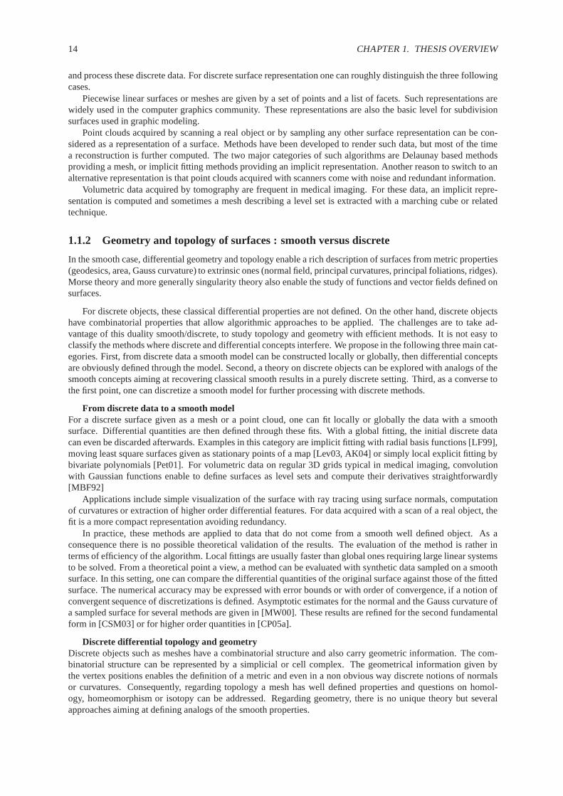
1.1.2 Geometry and topology of surfaces : smooth versus discrete
In the smooth case, differential geometry and topology enable a rich description of surfaces from metric properties(geodesics, area, Gauss curvature) to extrinsic ones (normal field, principal curvatures, principal foliations, ridges).Morse theory and more generally singularity theory also enable the study of functions and vector fields defined onsurfaces.
For discrete objects, these classical differential properties are not defined. On the other hand, discrete objectshave combinatorial properties that allow algorithmic approaches to be applied. The challenges are to take ad-vantage of this duality smooth/discrete, to study topologyand geometry with efficient methods. It is not easy toclassify the methods where discrete and differential concepts interfere. We propose in the following three main cat-egories. First, from discrete data a smooth model can be constructed locally or globally, then differential conceptsare obviously defined through the model. Second, a theory on discrete objects can be explored with analogs of thesmooth concepts aiming at recovering classical smooth results in a purely discrete setting. Third, as a converse tothe first point, one can discretize a smooth model for furtherprocessing with discrete methods.
From discrete data to a smooth modelFor a discrete surface given as a mesh or a point cloud, one canfit locally or globally the data with a smoothsurface. Differential quantities are then defined through these fits. With a global fitting, the initial discrete datacan even be discarded afterwards. Examples in this categoryare implicit fitting with radial basis functions [LF99],moving least square surfaces given as stationary points of amap [Lev03, AK04] or simply local explicit fitting bybivariate polynomials [Pet01]. For volumetric data on regular 3D grids typical in medical imaging, convolutionwith Gaussian functions enable to define surfaces as level sets and compute their derivatives straightforwardly[MBF92]
Applications include simple visualization of the surface with ray tracing using surface normals, computationof curvatures or extraction of higher order differential features. For data acquired with a scan of a real object, thefit is a more compact representation avoiding redundancy.
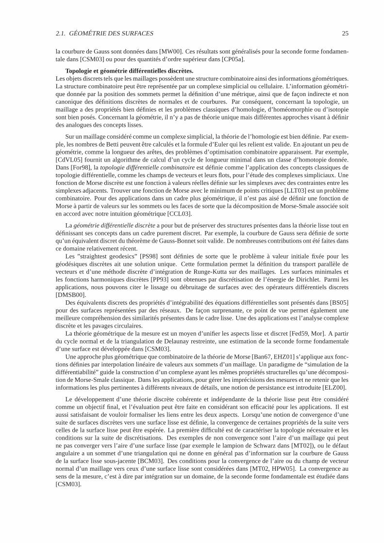
In practice, these methods are applied to data that do not come from a smooth well defined object. As aconsequence there is no possible theoretical validation ofthe results. The evaluation of the method is rather interms of efficiency of the algorithm. Local fittings are usually faster than global ones requiring large linear systemsto be solved. From a theoretical point a view, a method can be evaluated with synthetic data sampled on a smoothsurface. In this setting, one can compare the differential quantities of the original surface against those of the fittedsurface. The numerical accuracy may be expressed with errorbounds or with order of convergence, if a notion ofconvergent sequence of discretizations is defined. Asymptotic estimates for the normal and the Gauss curvature ofa sampled surface for several methods are given in [MW00]. These results are refined for the second fundamentalform in [CSM03] or for higher order quantities in [CP05a].
Discrete differential topology and geometryDiscrete objects such as meshes have a combinatorial structure and also carry geometric information. The com-binatorial structure can be represented by a simplicial or cell complex. The geometrical information given bythe vertex positions enables the definition of a metric and even in a non obvious way discrete notions of normalsor curvatures. Consequently, regarding topology a mesh haswell defined properties and questions on homol-ogy, homeomorphism or isotopy can be addressed. Regarding geometry, there is no unique theory but severalapproaches aiming at defining analogs of the smooth properties.

1.1. GEOMETRY OF SURFACES 15
On a mesh viewed as a simplicial complex, homology theory is well defined. For example, the Betti numberscan be computed and the well known Euler formula holds. Adding some geometric ingredients such as the lengthsof edges leads to combinatorial optimization problems. Forexample, in [CdVL05], an algorithm to computeshortest loops in a given homotopy class is given. In [For98], combinatorial differential topologyis defined asthe application of the standard concepts of differential topology, such as vector fields and their correspondingflows to the study of simplicial complexes. A discrete Morse function is defined as a real valued function onsimplices of any dimension with constraints between adjacent simplices. Finding a Morse function with the leastnumber of critical points [LLT03] is rather a combinatorialquestion. In more geometrical applications, it is notstraightforward to define a Morse function from given valueson vertices or on faces such that the associatedMorse-Smale decomposition respects our geometrical intuition [CCL03].
The domain ofdiscrete differential geometryaims at preserving some structure present in the smooth theorywhile defining concepts in a purely discrete setting. For example, one may define Gaussian curvature in such away that the Gauss-Bonnet theorem remains valid. Many contributions have been done in this domain.
Straightest geodesics [PS98] are defined so that there is a unique solution to the initial value problem fordiscrete geodesics. Applications are the parallel transport of vectors and discrete Runge-Kutta integration for vectorfields on meshes. Discrete minimal surfaces and harmonic functions [PP93] are obtained through the discretizationof the Dirichlet energy. Applications are smoothing or denoising of surfaces with discrete differential operators[DMSB00].
Discrete equivalents of integrability properties of differential equations are presented in [BS05] for surfacesrepresented by lattices. Surprisingly, this point of view also enables a better understanding of the similaritiespresent in the smooth setting. An application is discrete complex analysis and circle packings.
Geometric measure theory is also a way to unify the smooth anddiscrete aspects [Fed59, Mor]. Based uponthe normal cycle and restricted Delaunay triangulations, an estimate for the second fundamental form of a surfaceis developed in [CSM03].
A more geometrical than combinatorial approach of Morse theory [Ban67, EHZ01] applies to functions linearlyinterpolated from values on vertices. A “simulation of differentiability paradigm” guides the construction of acomplex with the same structural form as a smooth Morse-Smale decomposition. In applications, to deal withnoisy measurements and retain most relevant informations at different levels of details, the notion of persistence isintroduced [ELZ00].
The development of a coherent discrete theory independent of the smooth one may be the final achievementand can be evaluated by its effectiveness in applications. It may also be desirable to formalize the links betweenboth settings. When a notion of convergence of a sequence of discrete surfaces to a smooth surface is defined,one naturally expects also convergence of some properties of the sequence to the smooth surface ones. The firstproblem is to precisely characterize the required topologyand conditions on the discrete sequence. Examples ofnon-convergence are the surface area of a mesh which may not converge to that of the discretized surface (forexample thelampion de Schwarzin [MT02]), or the angular defect at a vertex of a triangulation which usuallydoes not provide any information on the Gauss curvature of the underlying smooth surface [BCM03]. Conditionsfor convergence of the surface area of a mesh and its normal vector field versus those of a smooth surface areconsidered in [MT02, HPW05]. Convergence in a measure senseof the second fundamental form of a surface isproved [CSM03].
Discretization : from a smooth model to a discrete oneFrom a smooth model it is sometimes desirable to derive a discrete representation for further processing suchas visualization (de Casteljau’s algorithm for Bezier surfaces), simulation with finite element methods (FEM) orregistration. Several properties are required for a discretization : it should be a good approximation of the smoothobject for some criterion, optimized for memory and easy to compute. The discretization conditions are guided bythe properties of the smooth model and the constraints of thepost processing.
A basic problem is to mesh a level set of a smooth function withthe guaranty that the topology is not modified.Several methods exist for a non singular surface using sampling and restricted Delaunay triangulation [BO03],Morse theory [BCSV04] or interval analysis [PV04]. In the restricted case of a polynomial surface, computeralgebra can also handle singular surfaces [MT05a]. In addition, other geometrical properties of the surface can beconsidered. In [AB99], an error bound is proved on the normalestimate to a smooth surface sampled accordingto a criterion involving the skeleton. The approximation ofthe area, the normal field and the unfolding with atriangulation is conducted in [MT02].
Finding a mesh with the minimum number of elements and minimizing a criterion such as Hausdorff distanceor Lp distance is addressed in [D’A91]. To generate a mesh for a FEM, the size and the shape of each element isoptimized according to the PDE problem to be solved [She02a].

16 CHAPTER 1. THESIS OVERVIEW
1.2 Estimation geometric properties : local and global aspects
Geometry of smooth or discrete surfaces can be described either by local properties or global ones. Local dif-ferential properties are the tangent plane (at the first order), the principal directions and curvatures (at the secondorder, see Fig. 1.3), or higher order coefficients. In the smooth case, all this information is encoded in the Taylorexpansion of the function whose graph locally defines the surface in a given coordinate system. We call ajet sucha Taylor expansion and Fig. 1.1 illustrates this local approximation. Global differential properties usually refer toloci of points having a prescribed differential property. Examples such loci are lines of curvature, parabolic lines(where the Gauss curvature vanishes Fig. 1.2), ridges (lines of extremal curvature) or the medial axis (centers ofmaximal spheres included in the complement of the surface inR3). Hence local information is required to be ableto generate global information.
In the present work, we first investigate estimation of localdifferential properties of any order. Then we studya global differential object on surfaces : the set of lines ofextremal curvature, called ridges.
Figure 1.1: The graph of jets around some vertices of a mesh are local approximation of the surface (see chap. 4).
Figure 1.2: The parabolic curves on the Apollo of Belvedere drawn by Felix Klein (from [Koe90]).
1.2.1 Estimation of local differential quantities
While local differential quantities are well defined and easy to compute on smooth surfaces, they are not welldefined for discrete surfaces. When defining a method to estimate differential quantities on a discrete surface, away to evaluate the method is to compare the results obtainedon some discretizations of a given smooth surfaceand the actual values for this smooth surface. The sensitivity of the method with respect to the properties and the

1.2. ESTIMATION GEOMETRIC PROPERTIES : LOCAL AND GLOBAL ASPECTS 17
Figure 1.3: Michelangelo’s David: principal directions associated withkmax scaled bykmin (see chap. 4).
quality of the discretizations can be analyzed. The convergence of the estimated values to the correct ones can alsobe specified for some sequence of discretizations. The development of algorithms providing such guarantees hasbeen subject to intense research [Pet01], and recent advances provide guarantees either point-wise (see chapter 4)or in the geometric measure theory sense [CSM03]. It is worthnoting that some widely used methods such as theangular defect for the Gauss curvature do not provide convergent estimations as demonstrated in [BCM03].
1.2.2 Estimation of global differential properties, the example of ridges
Estimating global differential loci needs reliable point-wise estimates, but in addition, imposes to respect (global)topological constraints. These difficulties are tangible from a practical perspective, and only few algorithms areable to report global differential patterns with some guarantee. For example, reporting the homotopy type of themedial axis has only been addressed quite recently [CL05], but problems involving homeomorphy or isotopy aremore demanding.
We focused in our work on lines ofextremalcurvature on a surface, called ridges. In terms of topologicalguarantees, we wish to report isotopic approximations. To get acquainted with extrema of curvature, first considerthe case of plane curves. Points where the curvature is extremal are called vertices, the set of centers of osculatingcircles is the focal curve and, the centers of circles tangent in two places to the curve is called the symmetry set.These objects are related : the border points of the symmetryset (centers of circles for which the two tangentpoints coincide) are the singularities of the focal curve, and the circles centered at these points touch the curve

18 CHAPTER 1. THESIS OVERVIEW
at vertices. For example, Fig. 1.4 shows the focal curve of anellipse which has four cusps corresponding to thefour vertices. For surfaces, one can define a focal surface for each principal curvature and the same propertieshold. The equivalent of vertices of a curve are lines on the surface corresponding to contact points with spherescentered on the singularities of the focal surfaces. These lines called ridges of a surface also has an alternativecharacterization : they consists of the points where one of the principal curvatures has an extremum along itscurvature line. Denotingk1 andk2 the principal curvatures —we shall always assume thatk1≥ k2, a ridge is calledblue (red) ifk1 (k2) has an extremum. Moreover, a ridge is calledelliptic if it corresponds to a maximum ofk1 or aminimum ofk2, and is calledhyperbolicotherwise. Ridges on an ellipsoid are displayed on Fig. 1.5 and 1.6. Fig.1.7, displaying a subset of the ridges on the David’s head, illustrates how these lines enhance the sharpest featuresof a model. Ridges witness extrema of principal curvatures and their definition involves derivatives of curvatures,whence third order differential quantities. Moreover, theclassification of ridges as elliptic or hyperbolic involvesfourth order differential quantities, so that the precise definition of ridges requiresC4 differentiable surfaces.
Ridges were mentioned in 1904 by A. Gullstrand, Nobel Prize for Physiology and Medicine, for his workin optics where fourth order differential quantities were necessary to explain the accommodation of the eye lens[Por01]. More recently, singularity theory allowed a precise setting to describe ridges and umbilics as specialpoints on these lines.
Figure 1.4: Focal curve (red) of an ellipse
Figure 1.5: Umbilics, ridges, and principal blue fo-liation on the ellipsoid (see chap. 3).
Figure 1.6: Schematic view of the umbilics and theridges (see chap. 3).
1.2.3 Applications
For many applications, estimating first and second order differential quantities, that is the tangent plane andcurvature-related quantities, is sufficient. In computer graphics, shading algorithms require the normal vectorfield. Gauss and mean curvatures are commonly used for surface segmentation, the mean curvature vector can beused for smoothing or denoising of surfaces. However, higher order local properties and global ones are also moreand more frequent. The lines of curvature are used for surface remeshing with quad elements [ACSD+03]. Thetopology of vector and tensor fields helps scientific visualization [DH94]. The medial axis or skeleton is used forsurface reconstruction [AB99, BC01]. The extraction of ridges is applied to the registration of medical images

1.3. OUTLINE AND CONTRIBUTIONS 19
Figure 1.7: Filtered crest lines on a 380k pts model (see chap. 5).
[MLD94, Fid97, PAT00], surface segmentation [SF04], face recognition [HGY+99] or compression of polygonalsurfaces [WB01].
1.3 Outline and contributions
This thesis addresses topics of surface geometry from localestimation to global extraction of differential charac-teristics. Discrete surfaces given by point clouds or meshes as well as smooth parametric surfaces are considered.We put the stress upon the development of algorithms providing estimations whose accuracies are analyzed. Wealso provide algorithms for the extraction of global features with guaranteed topology.
Chapter 3 is a survey of smooth surface geometry including all the notions needed in the sequel. Chapter 4addresses the estimation of local differential geometry onsampled surfaces. The following chapters are devotedto the global approximation of ridges on a generic surface. First, the case of surfaces given by a mesh is analyzedin chapter 5. Second, the implicit structure of ridges is worked out for a general parametric surface in chapter 6.Third, computer algebra methods are developed to compute the topology of ridges for a polynomial parametricsurface (chapter 7).
1.3.1 Differential Topology and Geometry of Smooth Embedded Surfaces: Selected Top-ics
Chapter 3 surveys mathematical notions and results scattered over several sources. As a prerequisite for the de-velopment of algorithms for the manipulation of surfaces, we propose a concise overview of core concepts fromdifferential geometry applied to smooth embedded surfaces. Basics of singularity theory and contact between sur-faces are introduced to enable the definition of ridges. In particular we recall the classification of umbilics and thegeometry of ridges as chapters 5 to 7 are dedicated to algorithms extracting these features. The connection betweenridges and the medial axis is analyzed. At last, topologicalnotions of homeomorphy and isotopy are discussedfor embedded surfaces. This work has been accepted for publication in the International Journal of ComputationalGeometry and Applications [CP05b].
1.3.2 Estimating Differential Quantities using Polynomial fitting of Osculating Jets
Chapter 4 addresses the point-wise estimation of differential properties of a smooth surface in 3D from a meshor a point cloud. The method consists of fitting the local representation of the manifold using a jet with eitherinterpolation or approximation. A jet is a truncated Taylorexpansion, and the incentive for using jets is that they

20 CHAPTER 1. THESIS OVERVIEW
encode all local geometric quantities —such as normal, curvatures, extrema of curvature. The main contributionof this chapter is to recast the problem of estimating differential properties into a problem of classical numericalanalysis. Since the proposed method consists of performingpolynomial fitting, connections with the questions ofinterpolation and approximation are discussed. Regardingpolynomial interpolation fitting of differential proper-ties for a surface, our results are closely related to [MW00,Lemma 4.1]. In that article, a degree two interpolationis used and analyzed. We generalize this result for arbitrary degrees, with interpolation and approximation. Ap-proximation orders of the method are proved for the estimation of any order differential quantity of the surface.In particular estimations of normal, curvatures and derivatives of curvatures are provided and will be used for thealgorithms of the next chapter on ridge extraction. More precisely, given a parameterh measuring the samplingstep, the main result is the following (see theorem 12) :
Theorem. 1 A polynomial fitting of degree n estimates any kth-order differential quantity to accuracy O(hn−k+1).In particular:
• the coefficients of the first fundamental form and the unit normal vector are estimated with accuracy O(hn),and so is the angle between the normal and the estimated normal.
• the coefficients of the second fundamental form and the shapeoperator are approximated with accuracyO(hn−1), and so are the principal curvatures and directions (as longas they are well defined, i.e. away fromumbilics).
An algorithm to process point clouds or meshes is described and the implementation for meshes confirms theexpected asymptotic convergence results. A conference version of this work has been published in the proceedingsof the Symposium on Geometric Processing 2003 and a journal version in Computer Aided Geometric Design[CP05a].
1.3.3 Topology driven algorithms for ridge extraction on meshes
Chapter 5 addresses the problem of ridge extraction for a surface given as a mesh and we make two contributions.First, for a generic smooth surface, the aim is the description of the topology of ridges from a mesh discretizing thesurface. Surprisingly, no method developed so far to reportridges from a mesh approximating a smooth surfacecomes with a careful analysis, which entails that one does not know whether the ridges are reported in a coherentfashion. We present a careful analysis of the orientation issues arising when one wishes to report the ridgesassociated to the two principal curvatures separately. Theanalysis highlights the subtle interplay between ridges,umbilics, and curvature lines. Finally, sampling conditions and a certified algorithm are given to report umbilicsand the correct topology of ridges on the mesh. The sampling conditions require a dense enough mesh such that(a) umbilics are isolated in patches, and outside these patches (b) a local orientation of the principal directionsis possible, and (c) an edge is intersected by a single ridge.As these conditions are not constructive, a heuristicalgorithm is proposed. This algorithm is implemented and uses the estimator of differential quantities provided bychapter 4. Figures 1.8 and 1.9 prove the correctness of the algorithm for a Bezier surface whose ridges topology isknown (see chapter 7 ).
Second, for a mesh which is not the approximation of a smooth surface, a filtering method allows the extractionof a subset of these lines. This subset, which has already been considered in medical imaging, can be usedfor characterization, registration and matching of surfaces. Figure 1.10 illustrates the efficiency of our filteringtechnique to capture significant features.
1.3.4 The implicit structure of ridges of a smooth parametric surface
Chapter 6 provides a theoretical contribution to the analysis of the global structure of ridges. The surface isgiven by a parameterization and ridges are sought in the parametric domain. As all previous works have to resortto local orientations of the principal directions of curvature to define ridges, they were unable to give a globaldescription of the ridge curve. Using an idea introduced in [Thi96] to turn around these orientation difficulties, anda fine analysis of the Weingarten endomorphism, we derive theimplicit equation of ridges. We also derive zerodimensional systems coding the singularities of this curve: one or three ridge umbilics and purple points (see Fig.1.11). This classification of singularities is compared to the classical one obtained with contact theory in [Por01].Finally, similar computations with the second derivativesof curvatures lead to the definition of another implicitcurve whose intersections with the ridge curve identify theso-called turning points. A turning point is a point ona ridge where the curvature extremum changes from maximum tominimum. In conclusion, we derive both theglobal structure of the ridge curve and the local classification of its singularities.

1.3. OUTLINE AND CONTRIBUTIONS 21
1
0.8
0.6
v
0.4
0
-0.15
0.2
0.4 0.2
-0.1
0.6u
0.8
-0.05
0
1
0
0.05
0.1
0.15
0.2
Figure 1.8: A (4,4) degree Bezier surface (left), its ridgesand umbilics on a triangulated model (60k points), viewfrom above (right)
Figure 1.9: Zoom view on two 3-ridge umbilics
1.3.5 Topologically certified approximation of umbilics and ridges on polynomial para-metric surfaces
Chapter 7 uses results of the previous chapter for the special case of a polynomial parametric surface. Indeed,for a polynomial parametric surface, the above mentioned equations are polynomial as well. An algorithm tocompute the topology of the ridge curve is developed. The difficulty is that even for low degree surfaces, thepolynomial defining the ridges is of rather high degree, morethan 10 times the degree of the surface. Henceclassical methods of computational algebra, based on the cylindrical algebraic decomposition [GVN02], are noteffective. The contribution is to exploit as far as possiblethe geometry of the problem to be able to produce anefficient and still certified algorithm. The method uses rational univariate representations of zero dimensionalsystems to locate the singularities in the parametric domain. One of the main advantage of this method is that itonly requires roots isolation of univariate polynomial with rational coefficients.
If the complexity of the surface prevents the computation ofthe topology of ridges, we also provide a plot atany fixed resolution of the ridge curve. Examples are provided to demonstrate the efficiency of the methods.
Results of chapters 6 and 7 have been obtained in collaboration with Jean-Charles Faugère and Fabrice Rouillierof the SALSA project, specialists of computer algebra. Thiswork has been presented at the poster session of theSymposium on Geometric Processing 2005 and at the workshop on Computational Methods for Algebraic SplineSurfaces II.

22 CHAPTER 1. THESIS OVERVIEW
Figure 1.10: Mechanical part (37k pts): (a) All crest lines,(b) crests filtered with the strength (state of the art) and(c) crests filtered with our sharpness criterion. Notice that any point on a flat or cylindrical part lies on two ridges,so that the noise observed on the top two Figs. is unavoidable. It is however easily filtered out with the sharpnesson the bottom figure.
3-ridge umbilic 1-ridge umbilic Purple point
Figure 1.11: Singularities of the ridge curve : red and blue curves distinguish extrema of the two principal curva-tures. (left and middle) There are two types of umbilics withone or three curves passing through and changingcolor at the umbilic. (right) A crossing of a blue and a red ridge is called a purple point.

Chapter 2
Résumé de la thèse
2.1 Géométrie des surfaces
La perception de notre environnement peut être décrite par les surfaces des objets qui nous entourent. Nous avonsdes notions intuitives de régularité ou de courbure d’une surface. En mathématiques, les surfaces apparaissentcomme des objets idéalisés qui sont étudiés depuis des siècles. Les surfaces sont omniprésentes dans les applica-tions telles que le calcul scientifique et la simulation, la conception assistée par ordinateur, l’imagerie médicale,la visualisation ou l’informatique graphique. Par exemple, en réalité virtuelle, une scène est souvent composée desurfaces décrivant le bord des objets. Lors du traitement dela géométrie par ordinateur, les surfaces doivent êtredécrites de manière discrète et il existe différentes discrétisations possibles. Les applications nécessitent une con-naissance des surfaces traitées: leur topologie, ainsi quedes descriptions locales et globales issues de la géométriedifférentielle.
La géométrie appliquée, à la croisée des mathématiques et del’informatique, a pour objectif la définition deconcepts, méthodes et algorithmes pour la résolution de problèmes géométriques qui se posent en sciences expéri-mentales ou en ingénierie. D’une part, les mathématiques apportent la géométrie et la topologie différentiellesclassiques, ainsi que des méthodes combinatoires sur des objets discrets. D’autre part, l’informatique apporte desstructures des données discrètes, des algorithmes ainsi que l’analyse de complexité.
Grâce aux progrès technologiques incessant, des formes de plus en plus complexes peuvent être traitées. Lasimulation et la visualisation en temps réel sont d’un grandintérêt pour la science et l’industrie. Les systèmesd’acquisition actuels génèrent des ensembles de données brutes gigantesques qui nécessitent d’être structurés etanalysés. Aussi puissant que puisse être le traitement informatique, il faut tenir compte de ses propres contraintes etlimitations: les représentations sont discrètes et les calculs sont faits avec une précision numérique limitée. Ainsi,les objets mathématiques ne peuvent être discrétisés naïvement. L’analyse par intervalles ou le calcul algébriqueformel font partie des nouveaux outils capables de certifierles opérations de base. A un niveau plus élevé, il ya un réel besoin de développer des modèles de formes suffisamment riches pour pouvoir définir des équivalentsdes propriétés lisses, mais adaptés aux contraintes du traitement informatique. Tout ceci plaide pour une meilleurecompréhension des interactions entre les mondes lisse et discret. D’une part, comment transférer de l’informationd’un objet lisse à un objet discret? D’autre part, comment analyser les propriétés d’un objet lisse à partir d’unereprésentation discrète? Le but final est la conception d’algorithmes certifiés, au sens où le résultat vient avec desgaranties d’approximation.
Puisque les surfaces sont les objets de notre étude, premièrement, nous listons différentes représentations util-isées pour une analyse théorique ainsi que pour les besoins d’un traitement informatique. Deuxièmement, nousproposons une introduction aux travaux en topologie et géométrie discrète, et discutons les relations entre lesmondes lisse et discret.
2.1.1 Représentations de surfaces
Les surfaces lisses sont décrites ou bien explicitement parune paramétrisationf : R2−→R3 ou implicitement parun ensemble de niveau{p∈ R3, F(p) = 0} avecF : R3 −→ R. Les quantités différentielles sont calculables defaçon directe dans les deux cas, mais chaque modèle possède ses avantages et inconvénients propres. Par exemple,une représentation implicite peut avoir une topologie arbitraire. D’un autre point de vue, modéliser une surfaceavec plusieurs paramétrisations offre plus de flexibilité.
23

24 CHAPTER 2. RÉSUMÉ DE LA THÈSE
Des représentations discrètes en lien avec les surfaces, telles que les graphes ou les complexes simpliciaux sontdes objets usuels en combinatoire ou topologie. En sciencesexpérimentales, les données discrètes proviennentde mesure. Pour les besoins d’un traitement particulier, unobjet lisse peut être discrétisé. Ainsi, il est néces-saire de développer des structures de données pour coder et traiter ces données discrètes. En ce qui concerne lesreprésentations discrètes de surfaces, nous pouvons grossièrement distinguer les trois cas suivants.
Les surfaces linéaires par morceaux, ou maillages, sont donnés par un ensemble de points et une liste defaces. De telles représentations sont largement utiliséesdans la communauté de l’informatique graphique. Cesreprésentations sont également à la base des surfaces de subdivisions.
Les nuages de points obtenus en scannant un objet réel ou en échantillonnant une autre représentation peuventêtre considérés comme des modèles de surfaces. Des méthodesspécifiques ont été développées pour la visualisa-tion de telles données, mais dans la plus part des cas, une reconstruction est calculée. Il existe deux grandes classesd’algorithmes de reconstruction basés sur la triangulation de Delaunay, lesquels calculent un maillage, ou baséssur une approximation implicite lesquels calculent une représentation implicite de la surface. Une autre motivationpour passer à une représentation alternative s’explique par la présence de bruit et la redondance d’informationcontenue dans les nuages de points acquis avec un scanner.
Les données volumiques acquises par tomographie sont fréquentes en imagerie médicale. Dans ce cas, unereprésentation implicite est calculée, et parfois un maillage décrivant un ensemble de niveau est extrait avec unalgorithme de “marching cube” ou une technique similaire.
2.1.2 Géométrie et topologie des surfaces: lisse versus discret
Dans le cas lisse, la géométrie et la topologie différentielles permettent une description riche des surfaces allantdes propriétés métriques (géodésiques, aires, courbure deGauss) aux propriétés extrinsèques (champs des vecteursnormaux, courbures principales, feuilletage principaux,lignes d’extrêmes de courbure). La théorie de Morse etplus généralement la théorie des singularités permettent également l’étude de fonctions ou de champs de vecteursdéfinis sur les surfaces.
Pour des objets discrets, ces propriétés différentielles discrètes ne sont pas définies. D’un autre coté, les objetsdiscrets ont des propriétés combinatoires qui permettent une approche algorithmique. L’enjeu est donc de tirerpartie de cette dualité lisse versus discret. Il n’est pas facile de classifier les méthodes où interfèrent des conceptsdiscrets et différentiels. Nous proposons une analyse en distinguant trois catégories principales. Premièrement,à partir de données discrètes, un modèle lisse peut être construit localement ou globalement, ainsi les conceptsdifférentiels sont bien définis sur le modèle et simplement transférés. Deuxièmement, une théorie sur les objetsdiscrets peut être explorée avec des analogues des conceptslisses, cherchant à retrouver des résultats de la théorielisse tout en restant purement dans le domaine discret. Troisièmement, à l’opposé du premier point, nous pouvonsdiscrétiser un modèle lisse pour le traiter ensuite avec desméthodes discrètes.
Des données discrètes à un modèle lisse.Pour une surface discrète donnée par un maillage ou un nuage de points, nous pouvons ajuster localement ouglobalement une surface lisse sur ces données. Les quantités différentielles sont alors définies par l’intermédiaire deces ajustements. Lors d’un ajustement global, les données discrètes initiales pourront même être abandonnées pourne garder que l’ajustement. Nous trouvons dans cette catégorie les représentations implicites avec des fonctionsà base radiale [LF99], les “moving least square surfaces” définies par l’ensemble des points fixes d’un fonction[Lev03, AK04] ou simplement des ajustements locaux explicites par des polynômes bivariés [Pet01]. Pour desdonnées volumiques sur des grilles régulières 3d, une convolution avec des fonctions gaussiennes permet de définirdes surfaces comme ensembles de niveau et de calculer leurs dérivées directement [MBF92].
Parmi les applications, citons la visualisation de surfaces par lancer de rayons utilisant les normales, le calculdes courbures ou l’extraction d’éléments caractéristiques différentiels d’ordre supérieur. Pour des données acquisesgrâce à un scanner à partir d’un objet réel, l’ajustement estune représentation plus compacte évitant la redondance.
En pratiques, ces méthodes sont appliquées à des données ne provenant pas d’un objet lisse bien défini. Ceciimplique qu’il n’y a donc pas de validation possible des résultats obtenus. L’évaluation de ces méthodes se faitplutôt en terme d’efficacité de l’algorithme. Les ajustements locaux sont en général plus rapides que les globauxnécessitant la résolution de systèmes linéaires de grande taille. D’un point de vue théorique, une évaluation estpossible en considérant des données artificielles échantillonnées sur une surface lisse connue. Dans ce cas, nouspouvons comparer les quantités différentielles de la surface originale avec celles que nous calculons sur son ajuste-ment. La précision numérique s’exprime alors avec des bornes d’erreurs, ou des ordres de convergence si unenotion de convergence d’une suite de discrétisation est définie. Des estimations asymptotiques de la normale et de
2.1. GÉOMÉTRIE DES SURFACES 25
la courbure de Gauss sont données dans [MW00]. Ces résultatssont généralisés pour la seconde forme fondamen-tale dans [CSM03] ou pour des quantités d’ordre supérieur dans [CP05a].
Topologie et géométrie différentielles discrètes.Les objets discrets tels que les maillages possèdent une structure combinatoire ainsi des informations géométriques.La structure combinatoire peut être représentée par un complexe simplicial ou cellulaire. L’information géométri-que donnée par la position des sommets permet la définition d’une métrique, ainsi que de façon indirecte et noncanonique des définitions discrètes de normales et de courbures. Par conséquent, concernant la topologie, unmaillage a des propriétés bien définies et les problèmes classiques d’homologie, d’homéomorphie ou d’isotopiesont bien posés. Concernant la géométrie, il n’y a pas de théorie unique mais différentes approches visant à définirdes analogues des concepts lisses.
Sur un maillage considéré comme un complexe simplicial, la théorie de l’homologie est bien définie. Par exem-ple, les nombres de Betti peuvent être calculés et la formuled’Euler qui les relient est valide. En ajoutant un peu degéométrie, comme la longueur des arêtes, des problèmes d’optimisation combinatoire apparaissent. Par exemple,[CdVL05] fournit un algorithme de calcul d’un cycle de longueur minimal dans un classe d’homotopie donnée.Dans [For98], latopologie différentielle combinatoireest définie comme l’application des concepts classiques detopologie différentielle, comme les champs de vecteurs et leurs flots, pour l’étude des complexes simpliciaux. Unefonction de Morse discrète est une fonction à valeurs réelles définie sur les simplexes avec des contraintes entre lessimplexes adjacents. Trouver une fonction de Morse avec le minimum de points critiques [LLT03] est un problèmecombinatoire. Pour des applications dans un cadre plus géométrique, il n’est pas aisé de définir une fonction deMorse à partir de valeurs sur les sommets ou les faces de sorteque la décomposition de Morse-Smale associée soiten accord avec notre intuition géométrique [CCL03].
La géométrie différentielle discrètea pour but de préserver des structures présentes dans la théorie lisse tout endéfinissant ses concepts dans un cadre purement discret. Parexemple, la courbure de Gauss sera définie de sortequ’un équivalent discret du théorème de Gauss-Bonnet soit valide. De nombreuses contributions ont été faites dansce domaine relativement récent.
Les ”straightest geodesics” [PS98] sont définies de sorte que le problème à valeur initiale fixée pour lesgéodésiques discrètes ait une solution unique. Cette formulation permet la définition du transport parallèle devecteurs et d’une méthode discrète d’intégration de Runge-Kutta sur des maillages. Les surfaces minimales etles fonctions harmoniques discrètes [PP93] sont obtenues par discrétisation de l’énergie de Dirichlet. Parmi lesapplications, nous pouvons citer le lissage ou débruitage de surfaces avec des opérateurs différentiels discrets[DMSB00].
Des équivalents discrets des propriétés d’intégrabilité des équations différentielles sont présentés dans [BS05]pour des surfaces représentées par des réseaux. De façon surprenante, ce point de vue permet également unemeilleure compréhension des similarités présentes dans lecadre lisse. Une des applications est l’analyse complexediscrète et les pavages circulaires.
La théorie géométrique de la mesure est un moyen d’unifier lesaspects lisse et discret [Fed59, Mor]. A partirdu cycle normal et de la triangulation de Delaunay restreinte, une estimation de la seconde forme fondamentaled’une surface est développée dans [CSM03].
Une approche plus géométrique que combinatoire de la théorie de Morse [Ban67, EHZ01] s’applique aux fonc-tions définies par interpolation linéaire de valeurs aux sommets d’un maillage. Un paradigme de “simulation de ladifférentiabilité” guide la construction d’un complexe ayant les mêmes propriétés structurelles qu’une décomposi-tion de Morse-Smale classique. Dans les applications, pourgérer les imprécisions des mesures et ne retenir que lesinformations les plus pertinentes à différents niveaux de détails, une notion de persistance est introduite [ELZ00].
Le développement d’une théorie discrète cohérente et indépendante de la théorie lisse peut être considérécomme un objectif final, et l’évaluation peut être faite en considérant son efficacité pour les applications. Il estaussi satisfaisant de vouloir formaliser les liens entre les deux aspects. Lorsqu’une notion de convergence d’unesuite de surfaces discrètes vers une surface lisse est définie, la convergence de certaines propriétés de la suite verscelles de la surface lisse peut être espérée. La première difficulté est de caractériser la topologie nécessaire et lesconditions sur la suite de discrétisations. Des exemples denon convergence sont l’aire d’un maillage qui peutne pas converger vers l’aire d’une surface lisse (par exemple le lampion de Schwarz dans [MT02]), ou le défautangulaire a un sommet d’une triangulation qui ne donne en général pas d’information sur la courbure de Gaussde la surface lisse sous-jacente [BCM03]. Des conditions pour la convergence de l’aire ou du champ de vecteurnormal d’un maillage vers ceux d’une surface lisse sont considérées dans [MT02, HPW05]. La convergence ausens de la mesure, c’est à dire par intégration sur un domaine, de la seconde forme fondamentale est étudiée dans[CSM03].

26 CHAPTER 2. RÉSUMÉ DE LA THÈSE
Discrétisation : d’un modèle lisse vers un modèle discret.A partir d’un modèle lisse il est souhaitable de construire une représentation discrète pour un traitement comme lavisualisation (l’algorithme de de Casteljau pour les surfaces de Bézier), la simulation avec des méthodes d’élémentsfinis ou le recalage. Plusieurs propriétés sont attendues d’une discrétisation, elle doit approcher l’objet lisse pourun critère donné, être optimisée pour la mémoire, et peu coûteuse à calculer. Les conditions de discrétisations sontguidées par les propriétés du modèle lisse et les contraintes du traitement envisagé ultérieurement.
Un problème classique est celui du maillage d’un ensemble deniveau d’une fonction lisse garantissant de ne pasmodifier la topologie. Différentes méthodes existent pour une surface non singulière utilisant l’échantillonnage etla triangulation de Delaunay restreinte [BO03], la théoriede Morse [BCSV04] ou l’analyse par intervalles [PV04].Dans le cas particulier des surfaces polynomiales, les systèmes de calcul algébrique formel permettent aussi detraiter des surfaces singulière [MT05a]. En plus de la topologie, des garanties sur la géométrie peuvent aussi êtrefournies. Dans [AB99], une borne d’erreur est donnée pour l’estimation de la normale d’une surface lisse faisantintervenir le squelette. L’approximation de l’aire, le champ des normales et du dépliage à partir d’un maillage estanalysée dans [MT02].
Construire un maillage avec le nombre minimum d’éléments etminimisant un critère comme la distancede Hausdorff ou une distanceLp est considéré dans [D’A91]. Pour générer un maillage adaptéà une méthoded’éléments finis, la taille et la forme de chaque élément sontoptimisées selon l’équation aux dérivées partielles àrésoudre [She02a].
2.2 Estimation des propriétés géométriques: aspects locaux et globaux
La géométrie des surfaces lisses ou discrètes peut être décrite par des propriétés locales ou globales. Les propriétésdifférentielles globales sont le plan tangent (au premier ordre), les courbures et directions principales (au secondordre, voir Fig. 2.3), ou des coefficients d’ordres supérieurs. Dans le cas lisse, toutes ces informations sont codéesdans le développement de Taylor de la fonction dont le graphedéfini localement la surface dans un repère donné.Nous appelonsjet ce développement de Taylor, la figure 2.1 illustre cette propriété d’approximation locale. Unepropriété différentielle globale caractérise le lieu des points ayant une propriété différentielle locale commune. Desexemples de tels lieux sont les lignes de courbure, les lignes paraboliques (où la courbure de Gauss s’annule, Fig.2.2), les “ridges” (lignes de courbure extrême) ou l’axe médian (centres des sphères maximales incluses dans lecomplémentaire de la surface dansR3). Ainsi, la connaissance de l’information locale est un prérequis pour lagénération d’informations globales.
Dans cette thèse, nous étudions, dans un premier temps, l’estimation des propriétés locales d’ordre quelconque.Puis, dans un deuxième temps, nous considérons un objet global: l’ensemble des lignes de courbure extrême ouridges.
Figure 2.1: Le graphe du jet au voisinage d’un sommet d’un maillage est une approximation locale de la surface(cf. chap. 4).

2.2. ESTIMATION DES PROPRIÉTÉS GÉOMÉTRIQUES: ASPECTS LOCAUX ET GLOBAUX 27
Figure 2.2: Les lignes paraboliques sur l’Apollon du Belvedere dessinées par Felix Klein (cf. [Koe90]).
Figure 2.3: Le David de Michel-Ange: directions principales associées à la courburekmax avec une longueurproportionnelle àkmin (cf. chap. 4).

28 CHAPTER 2. RÉSUMÉ DE LA THÈSE
2.2.1 Estimation des quantités différentielles locales
Alors que les quantités différentielles locales sont bien définies et simple à calculer sur des surfaces lisses, elles nesont pas bien définies sur des surfaces discrètes. Pour une méthode donnée d’estimation des quantités différentiellesà partir d’une surface discrète, une évaluation est possible en comparant les résultats obtenus sur des discrétisationsd’une même surface lisse avec les vraies valeurs calculées sur la surface lisse. La précision de la méthode peutêtre évaluée selon les propriétés et les qualités des discrétisations. La convergence des valeurs estimées vers lesvraies valeurs peut être analysée pour une suite de discrétisations. Le développement d’algorithmes spécifiant desgaranties d’approximation est un sujet actif de recherche [Pet01], et des travaux récents fournissent des garantiesou bien locales (cf. chap. 4) ou au sens de la théorie de la mesure [CSM03]. Il est utile de souligner que certainesméthodes communément utilisées comme le défaut angulaire pour estimer la courbure de Gauss ne donnent pasdes approximations convergentes [BCM03].
2.2.2 Estimation des propriétés différentielles globales, l’exemple des ridges
L’estimation de propriétés différentielles globales nécessite non seulement des estimations locales fiables, mais deplus impose de respecter des contraintes topologiques. Cesdifficultés sont tangibles sur le plan pratique, et raressont les algorithmes capables de calculer des lieux géométriques avec des garanties. Par exemple, le calcul du typed’homotopie de l’axe médian est un problème qui n’a été considéré que récemment [CL05], mais des problèmesconcernant l’homéomorphie ou l’isotopie sont encore plus délicats.
Nous nous concentrons dans ce travail sur les lignes de courbure extrême sur une surface. En termes degaranties topologiques, nous souhaitons obtenir des approximations isotopes. Pour se familiariser avec les extrêmesde courbure, considérons dans un premier temps le cas des courbes planes. Les points où la courbure est extrêmesont appelés les sommets, l’ensemble des centres des cercles osculateurs forment la courbe focale, et les centres descercles tangents en deux points à la courbe est appelé l’ensemble de symétrie. Ces différents objets interagissent dela façon suivante: les points du bord de l’ensemble de symétrie (c’est à dire les centres des cercles pour lesquels lesdeux points de tangence avec la courbe coïncident) sont les singularités de la courbe focale, et les cercles centrésen ces points touchent la courbe en ses sommets. Par exemple,la figure 2.4 montre la courbe focale d’une ellipsequi a quatre points de rebroussement correspondant aux quatre sommets. Dans le cas des surfaces, à chacune descourbures principales est associée une surface focale dontles propriétés sont similaires. L’équivalent des sommetsdans le cas d’une courbe sont des lignes sur la surface formées par les points de contacts avec les sphères centréessur les singularités des surfaces focales. Ces lignes, appelées ridges de la surface, ont aussi la caractérisationsuivante: elles sont l’ensemble des points pour lesquels une des courbures principales a un extrême le long dela ligne de courbure correspondante. Notonsk1 et k2 les courbures principales —avec la conventionk1 ≥ k2, unridge est qualifié de bleu (rouge) sik1 (k2) a un extrême. De plus, un ridge est appeléelliptiquesi il correspondà un maximum dek1 ou un minimum dek2, ouhyperboliquedans les autres cas. Les ridges d’un ellipsoïde sontreprésentés sur la figure 2.5 et 2.6. La figure 2.7, présentantun sous-ensemble des ridges sur la tête du David,illustre la capacité de ces lignes à souligner les parties saillantes du modèle. Les ridges révèlent les extrêmes descourbures principales et leur définition implique les dérivées des courbures, par conséquent ce sont des quantitésdifférentielles de troisième ordre. De plus, la classification des ridges en type elliptique et hyperbolique nécessitedes quantités de quatrième ordre, donc la définition précisedes ridges nécessite des surfaces de classeC4.
Les ridges sont mentionnés en 1904 par A. Gullstrand, prix Nobel de physiologie et médecine, dans ses travauxen optique où des quantités différentielles d’ordre quatreétaient indispensables pour expliquer l’accommodationdu cristallin [Por01]. Plus récemment, la théorie des singularités a permis de dégager un cadre rigoureux pourdécrire les ridges et les ombilics.

2.2. ESTIMATION DES PROPRIÉTÉS GÉOMÉTRIQUES: ASPECTS LOCAUX ET GLOBAUX 29
Figure 2.4: La courbe focale (en rouge) d’une ellipse
Figure 2.5: Ombilics, ridges, et feuilletage princi-pal bleu sur un ellipsoïde (cf. chap. 3).
Figure 2.6: Vue schématique des ombilics et desridges sur un ellipsoïde (cf. chap. 3).
Figure 2.7: Lignes de crête filtrées sur un modèle de 380k pts (cf. chap. 5).

30 CHAPTER 2. RÉSUMÉ DE LA THÈSE
2.2.3 Applications
Pour de nombreuses applications, estimer les quantités différentielles de premier et deuxième ordre, c’est à direla normale et les courbures, est suffisant. En informatique graphique, le champ des normales est utilisé pour lesalgorithmes d’éclairage. Les courbures de Gauss et moyennesont fréquentes en segmentation, le vecteur courburemoyenne est utilisé en lissage et débruitage du surfaces. Néanmoins, des quantités d’ordre supérieur, locales ouglobales apparaissent de plus en plus fréquemment. Les lignes de courbures servent pour le remaillage avec desquadrilatères [ACSD+03]. La topologie des champs de vecteurs et directions aident la visualisation scientifique[DH94]. L’axe médian ou squelette est utilisé en reconstruction de surfaces [AB99, BC01]. L’extraction des ridgess’applique au recalage d’images médicales [MLD94, Fid97, PAT00], à la segmentation [SF04], à la reconnaissancede visages [HGY+99] ou encore à la compression de surfaces polygonales [WB01].
2.3 Plan de la thèse et contributions
Cette thèse aborde des thèmes de géométrie des surfaces, de l’estimation locale à l’extraction de caractéristiquesglobales. Des surfaces données par des maillages et des nuages de points aussi bien que des surfaces lissesparamétrées sont étudiées. Nous nous concentrons sur le développement d’algorithmes générant des estimationsdont la précision est analysée. Nous proposons également des algorithmes pour l’extraction de caractéristiquesglobales avec des garanties topologiques.
Le chapitre 3 présente un panorama de la géométrie des surfaces lisses, couvrant toutes les notions nécessairesdans la suite. Le chapitre 4 aborde l’estimation de la géométrie différentielle locale à partir de surfaces échantil-lonnées. Les chapitres suivants sont consacrés à l’approximation globale des ridges d’une surface générique. Pre-mièrement, le cas d’une surface donnée par un maillage est étudié dans le chapitre 5. Deuxièmement, la structureimplicite des ridges est développée pour une surface paramétrée dans le chapitre 6. Troisièmement, des méthodesde calcul algébrique formel sont adaptées pour le calcul de la topologie des ridges d’une surface polynomialeparamétrée (chap. 7).
2.3.1 Topologie et géométrie différentielles des surfaceslisses plongées: éléments choisis
Le chapitre 3 rassemble des notions mathématiques et des résultats dispersés dans la littérature. Comme prérequisau développement d’algorithmes pour la traitement des surfaces, nous proposons un panorama succinct de conceptsde géométrie différentielle appliqués aux surfaces plongées. Une introduction à la théorie des singularités et ducontact permet la définition des ridges. En particulier, nous rappelons la classification des ombilics et la géométriedes ridges puisque les chapitres 5 à 7 sont consacrés à l’extraction de ces caractéristiques. La relation entre lesridges et l’axe médian est analysée. Enfin, les notions d’homéomorphie et d’isotopie sont discutées. Ce travail adonné lieu à une publication dans le journal “InternationalJournal of Computational Geometry and Applications”[CP05b].
2.3.2 Estimation des quantités différentielles par ajustement polynomiale des jets oscu-lateurs
Le chapitre 4 aborde l’estimation locale des propriétés différentielles d’une surface en 3D à partir d’un maillageou d’un nuage de points. La méthode consiste à ajuster le jet de la représentation locale de la variété en utilisantl’interpolation ou l’approximation. Un jet est une série deTaylor tronquée, la motivation pour utiliser les jets résidedans leur propriété de coder toutes les quantités géométriques locales —comme la normale, les courbures ou lesextrêmes de courbure. La contribution principale de ce chapitre est de replacer le problème d’estimation des pro-priétés différentielles dans le cadre de l’analyse numérique classique. Le méthode proposée utilisant l’ajustementpolynomial, les relations avec les questions d’interpolation et d’approximation sont discutées. En ce qui concernel’interpolation, nos résultats sont reliés à [MW00, Lemma 4.1]. Dans cet article, une interpolation de degré deuxest utilisée et analysée. Nous généralisons ce résultat pour un degré arbitraire, ainsi que pour l’interpolation aussibien que pour l’approximation. En particulier, des estimations des normales, des courbures et des dérivées descourbures sont données et seront utilisées dans le chapitresuivant sur l’extraction des ridges. Plus précisément,étant donné un paramètreh mesurant le pas d’échantillonnage, le résultat principal est le suivant (voir le théorème12) :
Theorem. 2 Un ajustement polynomial de degré n approche une quantité différentielle de kième-ordre avec uneprécision en O(hn−k+1). En particulier:

2.3. PLAN DE LA THÈSE ET CONTRIBUTIONS 31
• Les coefficients de la première forme fondamentale et du vecteur normal unitaire sont estimés avec uneprécision en O(hn), et il en est de même de l’angle entre la normale et la normale estimée.
• Les coefficients de la seconde forme fondamentale et de l’opérateur de Weingarten sont approchés enO(hn−1), et il en est de même des courbures et directions principales(en supposant qu’elles soient biendéfinies, c’est à dire loin des ombilics).
Un algorithme pour traiter des nuages de points ou des maillages est décrit, et l’implémentation pour le cas desmaillages confirme les résultats de convergence asymptotique attendus. Ce travail a donné lieu à une publication àla conférence “Symposium on Geometric Processing 2003” et dans le journal “Computer Aided Geometric Design”[CP05a].
2.3.3 Algorithmes guidés par la topologie pour l’extraction des ridges sur un maillage
Le chapitre 5 aborde le problème de l’extraction des ridges sur une surface donnée par un maillage, et nousapportons deux contributions. Premièrement, pour une surface lisse générique, le but est de décrire la topologiedes ridges à partir d’un maillage discrétisant la surface. De façon surprenante, aucune des méthodes développéesjusqu’à présent pour l’extraction des ridges à partir d’un maillage approchant une surface lisse ne fournit uneanalyse précise, ceci implique qu’il n’est pas possible de savoir si les ridges extraits ont une structure globalecohérente. Nous présentons une étude détaillée des problèmes d’orientation intervenant lors de l’extraction séparéedes ridges associés à chacune des courbures principales. Cette analyse révèle les relations entre ridges, ombilicset lignes de courbure. Finalement, des conditions d’échantillonnage et un algorithme certifié sont donnés pourl’extraction des ridges sur le maillage en respectant la topologie. Les conditions d’échantillonnage mettent enévidence la nécessité de disposer d’un maillage suffisamment dense pour que (a) les ombilics soient isolés dans desrégions, et pour qu’en dehors de ces régions, (b) l’orientation des direction principales soit possible localement, et(c) une arête soit intersectée par un seul ridge. Ces conditions n’étant pas constructives, un algorithme heuristiqueest aussi proposé. Cet algorithme est implémenté et utilisel’estimateur de quantités différentiables exposé auchapitre 4. Les figures 2.8 et 2.9 prouvent que l’algorithme calcule correctement la topologie des ridges pour unesurface de Bézier dont les ridges sont connus (cf. chapitre 7).
1
0.8
0.6
v
0.4
0
-0.15
0.2
0.4 0.2
-0.1
0.6u
0.8
-0.05
0
1
0
0.05
0.1
0.15
0.2
Figure 2.8: Une surface de Bézier de bi-degré (4,4) (gauche), ses ridges et ombilics sur une model triangulé (60kpoints), vue de dessus (droite)
Deuxièmement, pour un maillage qui n’est pas l’approximation d’une surface lisse, une méthode de filtragepermet l’extraction d’un sous ensemble de lignes. Ce sous ensemble, qui a déjà appliqué dans le domaine desimages médicales, peut être utilisé pour le recalage et la comparaison de surfaces. La figure 2.10 illustre l’efficacitéde notre technique de filtrage pour la mise en évidence de caractéristiques saillantes d’un model.

32 CHAPTER 2. RÉSUMÉ DE LA THÈSE
Figure 2.9: Gros plans sur deux ombilics 3-ridge de la figure 2.8
2.3.4 La structure implicite des ridges d’une surface paramétrée
Le chapitre 6 apporte une contribution théorique à l’analyse de la structure globale des ridges. La surface estdonnée par une paramétrisation et les ridges sont calculés dans le domaine paramétrique. Devant faire appel àl’orientation locale des directions principales de courbures, les approches antérieures ne pouvaient pas définirune description globale des ridges. Reprenant une idée introduite dans [Thi96] pour contourner ces difficultésd’orientation, et une analyse précise de l’endomorphisme de Weingarten, nous déduisons l’équation implicite desridges. Nous présentons également des systèmes d’équations codant les singularités de la courbe: ombilics un outrois ridges et pointspurples(cf. Fig. 2.11). Cette classification est comparée à celle obtenue grâce à la théoriedu contact dans [Por01]. Enfin, des calculs similaires avec les dérivées secondes des courbures conduisent à ladéfinition d’une autre courbe implicite, dont l’intersection avec celle des ridges permet l’identification des points“turning”. Un point “turning” est un point sur un ridge où l’extrême de courbure passe de maximum à minimum.En conclusion, nous proposons une description globale des ridges ainsi qu’une analyse locale de ses singularités.
2.3.5 Approximation topologique certifiée des ombilics et des ridges d’une surface poly-nomiale paramétrée
Le chapitre 7 exploite les résultats du chapitre précédent dans le cas particulier des surfaces polynomiales para-métrées. En effet, pour une surface polynomiale, les équations précédentes sont également polynomiales. Nousdéveloppons un algorithme pour le calcul de la topologie de la courbe des ridges. La difficulté provient de lacomplexité de cette courbe même pour des surfaces relativement simples: le degré de la courbe est plus de dixfois plus élevé que celui de la surface. Pour une telle courbe, les méthodes classiques, basées sur la décomposi-tion cylindrique algébrique [GVN02], ne sont pas assez performantes. Notre contribution est d’exploiter le pluspossible la géométrie du problème pour proposer un algorithme performant et certifié. La méthode repose sur lareprésentation univariée rationnelle des systèmes polynômiaux de dimension zéro afin de localiser les singularitésdes ridges dans le domaine paramétrique. Un des principaux avantages de la méthode provient du fait qu’elle nenécessite que l’isolation des racines de polynômes univariés à coefficientsrationnels.
Si néanmoins, la complexité de la surface ne permet pas le calcul de la topologie des ridges, nous fournissonségalement une méthode de tracé à résolution fixée. L’efficacité de ces méthodes est démontrée sur des exemples.
Les résultats des chapitres 6 et 7 ont été obtenus en collaboration avec Jean-Charles Faugère et Fabrice Rouillierdu projet SALSA, spécialistes de calcul algébrique formel.Ce travail a été présenté à la session de posters du“Symposium on Geometric Processing 2005” et au “workshop onComputational Methods for Algebraic SplineSurfaces II” dont la publication des actes est en cours.
2.4 Conclusion
Dans cette thèse, deux aspects de la géométrie des surfaces ont été abordés: l’estimation locale des propriétésdifférentielles, et le calcul global de la structure des ridges d’une surface lisse.
Concernant l’estimation des quantités différentielles, notre méthode utilise l’ajustement polynomial et s’appli-que aux maillages et aux nuages de points. Les ordres d’approximation sont les meilleurs prouvés à ce jour, et laméthode est testée avec des données échantillonnées sur dessurfaces lisses. Bien que notre méthode repose sur le

2.4. CONCLUSION 33
Figure 2.10: Pièce mécanique (37k pts): (a) toutes les lignes de crêtes, (b) lignes de crêtes filtrées par leur“strength” (état de l’art) et (c) lignes de crêtes filtrées par notre critère “sharpness”. Remarquez que les pointsdans les parties plates ou cylindriques appartiennent à deux ridges, ainsi le bruit présent sur les deux figures duhaut est inévitable. Il est néanmoins aisé d’éliminer ce bruit avec le filtrage que nous proposons (figure du bas).
cadre lisse, et donc ne définit pas de concept discret, elle permet l’estimation de quantités différentielles d’ordrearbitraire. Lorsque l’approximation est conduite avec un schéma d’approximation, nous avons expérimentalementobservé un comportement robuste face au bruit.
Une approche alternative au problème d’estimation à partirde données discrètes est proposée par la géométriedifférentielle discrète. L’idée consiste à définir des quantités différentielles directement sur l’objet lisse et dedévelopper une théorie discrète par analogie avec la théorie lisse. Le problème de convergence des quantités dis-crètes pour une suite de discrétisations peut alors être étudié. Des résultats ont été obtenus pour le champ desnormales, l’aire, les géodésiques [MT02, HPW05], les courbures de Gauss ou moyenne à l’aide d’une formulationvariationnelle [PP93], le tenseur de courbure dans le cadrede la théorie de la mesure [CSM03]. Toutes ces contri-butions s’appliquent à des maillages, et les nuages de points ne sont pas traités. Les théorèmes de convergence nesont disponibles que pour des quantités différentielles dupremier ou du second ordre.
Alors que l’intérêt pour les nuages de points s’accroît, le défi serait de comprendre dans quelle mesure lagéométrie différentielle et l’analyse statistique peuvent s’appliquer. L’irrégularité de la densité d’échantillonnage,l’anisotropie et le bruit doivent être pris en compte. Par exemple, l’influence du voisinage d’un point qu’il fautconsidérer pour faire une estimation n’est pas bien comprise [LP05]. Une analyse de l’estimation de la normaleà une surface à partir d’un nuage de points bruité est proposée dans [MN03]. Des méthodes de votes propagentl’information dans des voisinages locaux pour déterminer la pertinence de chaque information individuelle. Levote pour la normale et le tenseur de courbure permet d’identifier le bruit et le discontinuités, et donc rend possiblela traitement de surfaces lisses par morceaux [TM02].
Concernant le calcul de structures globales sur une surface, nous avons traité l’approximation topologique et

34 CHAPTER 2. RÉSUMÉ DE LA THÈSE
3-ridge umbilic 1-ridge umbilic Purple point
Figure 2.11: Singularités de la courbe des ridges: les courbes rouges et bleues différentient les extrêmes des deuxcourbures principales. (à gauche et au milieu) Il y a deux types d’ombilics traversés par une ou trois branches deridges, chacune changeant de couleur à l’ombilic. (à droite) Le croisement d’un ridge bleu et d’un ridge rouge estappelé pointpurple.
géométrique des ridges. Deux types de données ont été considérés: un maillage discrétisant une surface lisse etune surface paramétrée.
Premièrement, pour un maillage discrétisant une surface lisse, nous présentons le premier algorithme certi-fié pour l’extraction des ridges d’une surface lisse avec desgaranties sur la topologie. L’algorithme exploite lagéométrie des ridges et des ombilics d’une surface générique, et dissocie le traitement au voisinage des ombilicsdu reste de la surface. L’algorithme est générique au sens oùle calcul des quantités différentielles et l’isolationdes ombilics sont confiés à des routines qui peuvent dépendredu type de surface discrétisé par le maillage. Pourdes maillages approchants des surfaces lisses —sans pour autant avoir accès à aucune information analytique,nous fournissons des heuristiques. Pour des surfaces discrétisants des surfaces lisses dont les ridges sont connus,des exemples prouvent que notre algorithme heuristique retrouve la topologie des ridges et des ombilics. Pour desmaillages reconstruits à partir de données scannées, des exemples montrent que notre algorithme retrouve des sous-ensembles des ridges comparables aux autres méthodes de l’état de l’art (qui utilisent des ajustements globaux),tout en améliorant les temps de calculs d’au moins un ordre degrandeur et en fournissant une méthode de filtrageplus performante.
Deuxièmement, pour une surface paramétrée, nous explicitons l’équation implicite de la courbe singulièrecodant les ridges dans le domaine paramétrique. Alors que l’analyse mathématique classique des ridges étaitseulement locale, nous avons maintenant une description globale. Nous analysons ses singularités et fournissonsdes méthodes pour les identifier. Cette formulation du problème évite les difficultés d’orientation locale des di-rections principales de courbure. Elle permet donc une approche globale de l’extraction des ridges d’une surfaceparamétrée. Finalement, ces résultats sur la structure desridges sont utilisés dans le cas particulier des surfacesparamétrées polynomiales. Puisque les outils classiques de calcul algébrique formel ne permettent pas de traiternos exemples de grande complexité, nous avons tiré partie del’information géométrique fournie par l’analyse dela structure. Nous développons un algorithme spécifique basé sur les représentations univariées rationnelles dessystèmes polynômiaux de dimension zéro, et sur l’isolationdes racines de polynômes univariés à coefficients ra-tionnels. Cet algorithme est le premier à calculer une approximation topologique certifiée de ridges. Une foisla topologie obtenue, une approximation géométrique plus précise peut facilement être déduite. Nous proposonségalement un autre algorithme qui calcule un tracé certifié àrésolution fixée: les calculs sont moins coûteux, maisla topologie n’est plus garantie. Les résultats pour une surface paramétrée sont directement applicables aux sur-faces de Bézier incontournable en CAO. Il est à noter que la méthode développée pour le calcul de la topologiedes ridges peut être généralisée pour d’autres courbes algébriques, à partir du moment où le nombre de branchesréelles passant par chaque singularité peut être calculé efficacement.
En conclusion, nous donnons plusieurs algorithmes certifiés et performants pour l’extraction des ridges. Lesméthodes s’appliquent dans les cadres lisse et discret, et différents niveaux de certification sont proposés à l’utilisa-teur selon ses exigences.
L’intérêt pour l’analyse et le calcul de propriétés géométriques globales n’est pas nouveau. Par exemple, denombreuses contributions existent pour la visualisation des champs de vecteurs avec des informations topologiques[DH94, Tri02]. Néanmoins, la plupart de ces contributions se restreignent à des domaines Euclidiens et ne sontpas généralisées pour des surfaces. De plus, seulement des heuristiques sont proposées, et des algorithmes avecdes garanties topologiques font défaut.
Dans le cadre discret, les champs de vecteurs sont analysés avec une décomposition discrète de Hodge [PP03],ou avec une décomposition de Morse-Smale [EHZ01] via un paradigme desimulation de la différentiabilité. Lors

2.4. CONCLUSION 35
de l’analyse d’une propriété différentielle globale à partir d’une discrétisation, la première étape consiste à com-prendre sa stabilité et sa généricité. Une telle approche a prouvé sa réussite pour les ridges et l’axe médian. Lecalcul du type d’homotopie de l’axe médian est proposé dans [CL05] guidé par des résultats de stabilité [eRS04].Pour les surfaces, les feuilletages des directions principales de courbure sont particulièrement intéressants, ils peu-vent être utilisés pour le maillage par des quadrilatères optimisant l’approximation [ACSD+03]. Néanmoins, iln’existe pas encore de méthode pour calculer la topologie deces feuilletages.
Dans ce contexte, la collaboration entre les communautés demathématiques et d’informatiques est nécessairepour modéliser et résoudre les problèmes de géométrie appliquée.

36 CHAPTER 2. RÉSUMÉ DE LA THÈSE

Chapter 3
Differential Topology and Geometry ofSmooth Embedded Surfaces: SelectedTopics
This chapter surveys mathematical notions and results scattered over several sources. As a prerequisite for thedevelopment of algorithms for the manipulation of surfaces, we propose a concise overview of core concepts fromdifferential topology and geometry applied to smooth embedded surfaces.
The understanding of surfaces embedded inE3 requires local and global concepts, which are respectivelyevocative of differential geometry and differential topology. While the local theory has been classical for decades,global objects such as the foliations defined by the lines of curvature, or the medial axis still pose challengingmathematical problems. This duality is also tangible from apractical perspective, since algorithms manipulatingsampled smooth surfaces (meshes or point clouds) are more developed in the local than the global category.
We first recall the classification of umbilics, of curvature lines, and describe the corresponding stable foliations.Next, fundamentals of contact and singularity theory are recalled, together with the classification of points inducedby the contact of the surface with a sphere. This classification is further used to define ridges and their properties,and to recall the stratification properties of the medial axis. Finally, properties of the medial axis are used to presentsufficient conditions ensuring that two embedded surfaces are ambient isotopic.
3.1 Introduction
3.1.1 Motivations for a geometric and topological analysis
Sampled surfaces represented either by point clouds or meshes are ubiquitous in computer graphics, computeraided design, medical imaging, computational geometry, finite element methods or geology. Aside from the sit-uations where a sample surface is of self-interest —e.g. in computer graphics, sampled surfaces approximating(piecewise-)smooth surfaces are essentially found in two contexts which are surface reconstruction and surfacediscretization. In the first category, one is given a set of sample points acquired from a scanner (medical or laser)and wishes to reconstruct (by interpolation or approximation) the continuous or (piecewise-)smooth surface whichhas been sampled. In the second one, a surface is given implicitly or parametrically, and one wishes to discretize itfor visualization or calculation purposes. In any case, three types of properties are usually of interest when com-paring a (piecewise-)smooth surface and its discretization: topological and geometric properties, local differentialproperties, and global differential properties.
From a topological standpoint, one expects the surfaces to be homeomorphic or even better isotopic. Examplealgorithms with such a guarantee are [APR03, ACDL00] in the surface reconstruction area, and [BCSV04, BO03]in the surface meshing context. Apart from these algorithms, the interested reader should consult [SP03, CCS04]where sufficient conditions on isotopy can be found. It should also be pointed out that the hypothesis under whichone achieves these properties usually also yield a bound on the Hausdorff distance between the surfaces, a propertyof geometric nature.
Local differential properties are of two types, namely intrinsic and extrinsic. For extrinsic quantities, onewishes to guarantee that the tangent plane (at the first order), the principal directions and curvatures (at the sec-
37

38 CHAPTER 3. DIFFERENTIAL TOPOLOGY AND GEOMETRY
ond order), or higher order coefficients (e.g. curvature extremality coefficients) are close. The development ofalgorithms providing such guarantees has been subject to intense research [Pet01], and recent advances provideguarantees either point-wise [BCM03, CP05a] or in the geometric measure theory sense [CSM03]. Althoughextrinsic properties are usually the properties sought, some applications care for intrinsic faithfulness. These appli-cations are usually concerned with the question of flattening / parameterizing a surface, and the reader is referredto [MT02] for an example related to geology, together with the ensuing conditions.
At last, global differential properties usually refer to guarantees on loci of points having a prescribed differentialproperty. Example such loci are lines of curvature, ridges,or the medial axis. Applications involving such patternsare surface remeshing [ACSD+03], scientific visualization [DH94], feature extraction [PAT00, WB01, HGY+99],or surface reconstruction [AB99, BC01] and related topics [DZ02]. Providing such guarantees faces the difficultiesafore-mentioned. Not only point-wise estimates must be reliable, but they must also be connected correctly at thesurface level. The difficulties are tangible from a practical perspective, and only few algorithms are able to reportglobal differential patterns with some guarantee [CL05].
The lack of such algorithms is partly due to the fact that global differential patterns have an involved struc-ture described in differential topology and singularity theory sources. Easing the access to these notions is theincentive of this concise survey, which deliberately focuses on selected topics related to the geometry and topol-ogy on embedded surfaces. In selecting these topics, we had to make choices and omitted the following themes:symmetry sets [BGG85]; distance functions used in analysis[Hor94], optimization [Cla97], mathematical mor-phology [Ser82], and geometric modeling [Lie03]; bifurcations of symmetry sets and medial axis [BG86, GK02];differential geometry of skeletal structures [Dam04]; practical algorithms to extract medial axis [CL05].
Our presentation focuses on the geometric intuition ratherthan the technicalities. From a practical standpoint,we hope it will be helpful for those aiming at producing globally coherent approximations of surfaces.
3.1.2 Chapter overview
Following a natural trend, we successively examine differential geometric concepts of the second order (umbilics,lines of curvatures, foliations) and the third order (ridges, medial axis). To finish up, selected properties of themedial axis are used to specify the topological equivalencebetween embedded surfaces.
More precisely, the Monge form of a surface is recalled in section 3.2. Second order properties are presentedin section 3.3 —umbilics and lines of curvature. The classification of contact points between the surface andspheres is presented in section 3.4. This classification is used in section 3.5 to recall the stratification propertiesof the medial axis. Finally, the topological equivalence between embedded surfaces is recalled in section 3.6, andsufficient conditions involving the medial axis are also presented.
3.2 The Monge form of a surface
3.2.1 Generic surfaces
Our focus is on generic phenomena on surfaces, and the statements presented are valid for generic surfaces only.Formally if one considers the set of all smooth surfacesS in E3 as an infinite dimensional space with a well definedtopology, a property is generic if the surfaces exhibiting this property form an open dense subset. Informally thisnotion means that (i) a generic property remains valid if oneallows random perturbations, and (ii) that every surfaceis arbitrary close to another for which the property holds. Due to the infinite dimension of the space of surfaces, itis not straightforward to define a topology on this set. We will consider theCr topology (r ∈N∪{∞}) on the set ofall smooth oriented surfacesSembedded in the Euclidean spaceE3 (cf. [GS91][p.27]). A sequenceSn of surfacesconverges toS in theCr sense provided there is a sequence of real functionsfn on Ssuch thatSn = (I + fnN)(S),whereI is the identity ofE3, N is the normal vector ofSand fn tends to 0 in theCr sense. That is, for every chart(u,v) with inverse parameterizationX, fn ◦X converges to 0 together with the partial derivatives of order r, oncompact parts of the domain ofX.
3.2.2 The Monge form of a surface
We consider an oriented surfaceSembedded in the Euclidean spaceE3. We considerE3 given with an orthonormalbasis called the world coordinate system. Another orthonormal basis is calleddirect if it is the image of the worldcoordinate system by a special orthogonal tranformation. At any point of the surface which is not an umbilic,

3.2. THE MONGE FORM OF A SURFACE 39
principal directions are well defined, and the (non oriented) principal directionsd1, d2 together with the normalvectorn define two direct orthonormal frames. Ifv1 is a unit vector of directiond1 then there exists a unique unitvectorv2 so that(v1,v2,n) is direct; and the other possible frame is(−v1,−v2,n). In one of these, and as long asour study is a local differential one, the surface is assumedto be given as a Monge patch at the origin [HGY+99]—with h.o.t standing forhigher order terms:
z=12(k1x2 +k2y2)+
16(b0x3 +3b1x
2y+3b2xy2 +b3y3) (3.1)
+124
(c0x4 +4c1x3y+6c2x
2y2 +4c3xy3 +c4y4)+h.o.t (3.2)
Occasionally, we shall refer to the cubic partCM(x,y) as the Monge cubic, that is:
CM(x,y) = b0x3 +3b1x2y+3b2xy2 +b3y
3. (3.3)
If the origin is not an umbilic, the principal directiond1 (resp.d2) associated to the principal curvaturek1 (resp.k2)is thex (resp.y) axis. We shall always assume thatk1≥ k2 and we consider ’blue’ (resp. ’red’) something specialhappening withk1 (resp.k2). For example the blue focal surface is the set of centers of curvature associated to theblue curvaturek1. Note that a change of the normal surface orientation swaps the colors.
Away from umbilics, local analysis of the principal curvatures can be done for the Monge coordinate systemand along the curvature lines. The Taylor expansion of the principal curvaturek1 in the Monge coordinate systemis
k1(x,y) = k1 +b0x+b1y+(c0−3k3
1
2+
b21
k1−k2)x2 (3.4)
+(c1+2b1b2
k1−k2)xy+(
c2−k1k22
2+
b22
k1−k2)y2 +h.o.t (3.5)
The Taylor expansion ofk1 (resp. k2) along the blue (resp. red) curvature line going through theorigin andparameterized byx (resp.y) are:
k1(x) = k1 +b0x+P1
2(k1−k2)x2 +h.o.t P1 = 3b2
1 +(k1−k2)(c0−3k31). (3.6)
k2(y) = k2 +b3y+P2
2(k2−k1)y2 +h.o.t P2 = 3b2
2+(k2−k1)(c4−3k32). (3.7)
Notice also that switching from one of the two coordinate systems mentioned in introduction to the other revertsthe sign of all the odd coefficients on the Monge form of the surface.
Some notions about cubics will be useful in the sequel.
Definition. 1 A real cubic C(x,y) is a bivariate homogeneous polynomial of degree three, thatis C(x,y) = b0x3 +3b1x2y+3b2xy2 +b3y3. Its discriminant is defined byδ (C) = 4(b2
1−b0b2)(b22−b1b3)− (b0b3−b1b2)
2.
A cubic factories as a product of three polynomials of degreeone with complex coefficients, called its factorlines. In the(x,y) plane, a real factor line defines a direction along whichC vanishes. The number of real factorlines depends on the discriminant of the cubic and we have
Proposition. 1 Let C be a real cubic andδ its discriminant. Ifδ > 0 then there are 3 distinct real factors, ifδ < 0there is only one real factor.
In the particular description of surfaces as Monge patches,we have a family of Monge patches with twodegrees of freedom —the dimension of the manifold. A property requiring 1 (resp. 2) condition(s) on this familyis expected to appear on lines (resp. isolated points) of thesurface —a condition being an equation involving theMonge coefficients. A property requiring at least three conditions is not generic. As an example, ridge points(characterized by the conditionb0 = 0 orb3 = 0) appears on lines and umbilics (the two conditions are those for aquadric to have egual roots, i.e. the coefficient of thexy term vanishes and those ofx2 andy2 are equal) are isolatedpoints. A flat umbilic, requiring the additional conditionk1 = 0, is not generic.
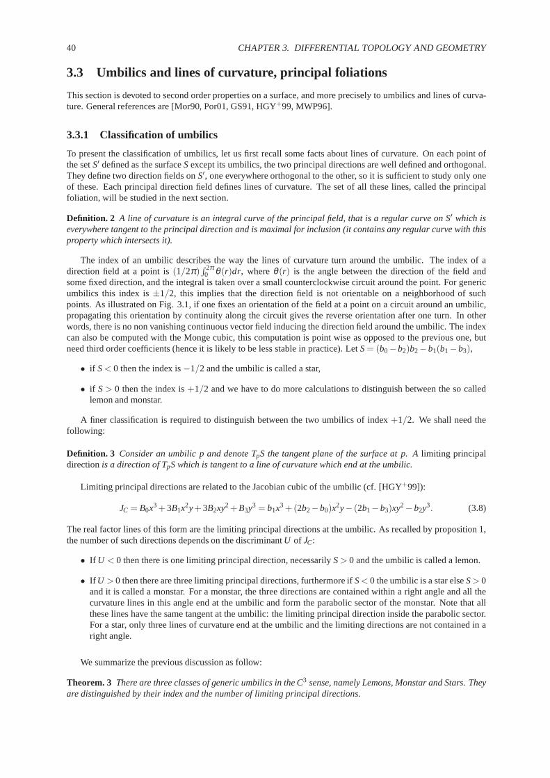
40 CHAPTER 3. DIFFERENTIAL TOPOLOGY AND GEOMETRY
3.3 Umbilics and lines of curvature, principal foliations
This section is devoted to second order properties on a surface, and more precisely to umbilics and lines of curva-ture. General references are [Mor90, Por01, GS91, HGY+99, MWP96].
3.3.1 Classification of umbilics
To present the classification of umbilics, let us first recallsome facts about lines of curvature. On each point ofthe setS′ defined as the surfaceSexcept its umbilics, the two principal directions are well defined and orthogonal.They define two direction fields onS′, one everywhere orthogonal to the other, so it is sufficient to study only oneof these. Each principal direction field defines lines of curvature. The set of all these lines, called the principalfoliation, will be studied in the next section.
Definition. 2 A line of curvature is an integral curve of the principal field, that is a regular curve on S′ which iseverywhere tangent to the principal direction and is maximal for inclusion (it contains any regular curve with thisproperty which intersects it).
The index of an umbilic describes the way the lines of curvature turn around the umbilic. The index of adirection field at a point is(1/2π)
∫ 2π0 θ (r)dr, whereθ (r) is the angle between the direction of the field and
some fixed direction, and the integral is taken over a small counterclockwise circuit around the point. For genericumbilics this index is±1/2, this implies that the direction field is not orientable on aneighborhood of suchpoints. As illustrated on Fig. 3.1, if one fixes an orientation of the field at a point on a circuit around an umbilic,propagating this orientation by continuity along the circuit gives the reverse orientation after one turn. In otherwords, there is no non vanishing continuous vector field inducing the direction field around the umbilic. The indexcan also be computed with the Monge cubic, this computation is point wise as opposed to the previous one, butneed third order coefficients (hence it is likely to be less stable in practice). LetS= (b0−b2)b2−b1(b1−b3),
• if S< 0 then the index is−1/2 and the umbilic is called a star,
• if S> 0 then the index is+1/2 and we have to do more calculations to distinguish between the so calledlemon and monstar.
A finer classification is required to distinguish between thetwo umbilics of index+1/2. We shall need thefollowing:
Definition. 3 Consider an umbilic p and denote TpS the tangent plane of the surface at p. Alimiting principaldirectionis a direction of TpS which is tangent to a line of curvature which end at the umbilic.
Limiting principal directions are related to the Jacobian cubic of the umbilic (cf. [HGY+99]):
JC = B0x3 +3B1x2y+3B2xy2 +B3y3 = b1x3 +(2b2−b0)x
2y− (2b1−b3)xy2−b2y3. (3.8)
The real factor lines of this form are the limiting principaldirections at the umbilic. As recalled by proposition 1,the number of such directions depends on the discriminantU of JC:
• If U < 0 then there is one limiting principal direction, necessarily S> 0 and the umbilic is called a lemon.
• If U > 0 then there are three limiting principal directions, furthermore ifS< 0 the umbilic is a star elseS> 0and it is called a monstar. For a monstar, the three directions are contained within a right angle and all thecurvature lines in this angle end at the umbilic and form the parabolic sector of the monstar. Note that allthese lines have the same tangent at the umbilic: the limiting principal direction inside the parabolic sector.For a star, only three lines of curvature end at the umbilic and the limiting directions are not contained in aright angle.
We summarize the previous discussion as follow:
Theorem. 3 There are three classes of generic umbilics in the C3 sense, namely Lemons, Monstar and Stars. Theyare distinguished by their index and the number of limiting principal directions.

3.3. UMBILICS AND LINES OF CURVATURE, PRINCIPAL FOLIATIONS 41
To be an umbilic requires two conditions on the Monge coefficients, this implies that the casesS= 0 orU = 0are not generic umbilics. From the same argument, a generic umbilic is a non flat point: its Gaussian curvaturedoes not vanish, and generic umbilics are isolated (cf. [Por01][p.184]).
Figure 3.1: Impossibility of a global orientation around anumbilic
Figure 3.2: Umbilics: Lemon and Monstar of index +1/2, Star of index -1/2.
3.3.2 Principal foliations
Recall that the blue (resp. red) principal foliation is the set of all blue (resp. red) curvature lines defined onS′–Sexcept its umbilics. The umbilics can be regarded as singular points for these foliations if one wishes to considerthem onS. The first element required concerns the topology of a curvature line. A line of curvatureγ is eitherhomeomorphic to:
• an open intervalI = (ω−,ω+), then it is assumed to be oriented and parameterized by this interval. Itsα(γ)(resp.ω(γ)) limit set is the collection of limit points of sequencesγ(sn), convergent inS, with sn tending toω− (resp.ω+). The limit set ofγ is the unionα(γ)∪ω(γ).
• or to a circle, then it is called a cycle. It is hyperbolic if the differential of its Poincaré return map differsfrom the identity. In other words, if one orients an hyperbolic cycle, the lines of curvature can be orientedon a neighborhood of this cycle by continuity and they are allattracted or repelled on both sides of the cycle(cf. Fig. 3.3).
Figure 3.3: A hyperbolic cycle and two non hyperbolic ones
Special lines divide the set of all curvature lines in the vicinity of an umbilic into sectors, they are separatrices.
Definition. 4 A separatrix is a line of curvature with an umbilic in its limit set and so that there exists arbitrarilyclose to that line, another line without this umbilic in its limit set.

42 CHAPTER 3. DIFFERENTIAL TOPOLOGY AND GEOMETRY
A sector defined by two consecutive separatrices is
• hyperbolic if none of the lines in the sector have the umbilicin their limit set;
• parabolic if all curvature lines in the sector have the umbilic in their α or exclusiveω limit set;
The alternative case of an elliptic sector, if all curvaturelines in the sector have the umbilic in theirα andω limitset, is not generic —cf. Nikolaev [Nik01][p.360]. Note thata separatrix is a line of curvature which ends at anumbilic, hence its tangent at this point is a limiting principal direction. But the limiting principal direction insidethe parabolic sector of a monstar is not tangent to a separatrix of this umbilic —because all lines in a neighborhoodhave the monstar in their limit set. This explains another classification of umbilics from Darboux based on thenumber of separatrices. This classification rephrases the previous one: a lemon orD1 has one separatrix, a monstaror D2 has two and a star orD3 has three.
The next result [GS91][p.27] describes stable configuration of the principal foliations for smooth compactoriented surfaces embedded inE3. A surfaceS is said to beCr principal structurally stable if for every sequenceSn converging toS in theCr sense, there is a sequence of homeomorphismsHn from Sn ontoS, which convergesto the identity ofS, such that, forn big enough,Hn is a principal equivalence fromSn ontoS. That isHn maps theumbilical set ofSn onto the umbilical set ofS, and maps the lines of the principal foliations ofSn onto those ofS.
Theorem. 4 LetΣ be the subset of smooth compact oriented surfaces which satisfies the following four conditions:
• all the umbilic points are of type Di , i = 1, . . . ,3;
• all the cycles are hyperbolic;
• the limit sets of every line of curvature are umbilics or cycles;
• all the separatrices are separatrices of a single umbilic (they cannot connect two umbilics or twice the sameone being separatrices at both ends).
ThenΣ is open and each of its elements is principal structurally stable in the C3-sense,Σ is dense in the C2-sense.
This theorem implies that stable principal foliations are described with the set of umbilics, cycles and the waythe separatrices connect these elements. The complement ofthese features on the surfaceS then decomposes oncanonical regions of two types parallel and cylindrical. Oneach region, the limit sets of all lines are the same:a cycle or aD2 umbilical point (through its parabolic sector). A region isparallel if there are separatrices in itsboundary. If the boundary consists only of cycles then the region is cylindrical.
The topology of the surfaceS constrains the number and the type of umbilics. More precisely, the sum ofindices of umbilics must be the Euler characteristicχ(S) —[Spi99b][p.223]. Moreover, the principal foliationdefines a bipartite graphG(V1,V2,E) with V1 the set of umbilics,V2 the set of cycles and parabolic sectors andEthe set of separatrices. The edges connect elements ofV1 to elements ofV2 with the following constraints.
• A Di umbilic hasi incident edges.
• Since there is no elliptic sector, a separatrix of aD2 umbilic cannot be connected to its parabolic sector.
• The graph is embedded on the surface without intersecting the separatrices.
3.4 Contacts of the surface with spheres, Ridges
To classify points of a smooth surface regarding curvature properties, we first recall fundamentals from contact andsingularity theory. Following [Por71, Por83, Mor90], we probe a point of the surface with a sphere centered alongthe normal at that point. Working out the dominant terms of the Taylor expansion of the probe function yields theclassification of points desired. General references for this section are [BG92], [Por01] or [Arn92].

3.4. CONTACTS OF THE SURFACE WITH SPHERES, RIDGES 43
3.4.1 Distance function and contact function
A standard way to classify points on a smooth surface consists of using contact theory. Consider a portion ofsurface locally parameterized in a chart(U, p(x,y)) with U ⊂R2, (x0,y0) ∈U and a sphereC of centerc. Denoting<,>, the standard inner product ofE3, the contact function at the pointp(x0,y0) ∈ S is the function defined by:
g : U ×R3 7→R, g((x,y),c) =< p(x,y)c, p(x,y)c >−< p(x0,y0)c, p(x0,y0)c > . (3.9)
This function is just the square distance from the surface tothe center of the sphere minus the square of its radiusr2 =< p(x0,y0)c, p(x0,y0)c >. The intersection points betweenSandC have coordinates(x,y, p(x,y)) satisfyingg(x,y) = 0. The philosophy of contact theory is the following. Once the center of the sphere have been chosen,the contact function is a bivariate function. Then, we wish to report the possiblenormal formsof g as a bivariatefunction.
Before illustrating this process, let us observe that if thecenter of the sphereC is not contained in the affinespace defined by the contact point and the normal at the surface S there, then the intersection betweenSandC istransverse, which does not reveal much aboutSat p. Studying the nature of the contact really starts with a centeraligned with the normal, and we shall see that the cases encountered actually yield a decomposition of the normalbundle1 of the surface.Remark. Note that if one of the principal curvatures vanishes, one can assume the center of the principal sphere isat infinity. This means that the relevant contact to be considered is that of a plane with the surface at such a point.One can find a precise description of these parabolic points in [HGY+99].
3.4.2 Generic contacts between a sphere and a surface
Before presenting the generic contacts, let us illustrate the process of finding the first normal form using the Morselemma. To ease the calculations, assume that the contact point is the origin, that the surface is given in Mongeform, and that the center of the sphere has coordinatesc(0,0, r). Then, the contact function simplifies to:
g(x,y) = x2 +y2+(z− r)2− r2 =< pc, pc>−r2. (3.10)
Using the Monge form off , one gets the following expansion:
g(x,y) = x2(1− rk1)+y2(1− rk2)−r3
CM(x,y)+h.o.t (3.11)
The expansion does not contain linear terms and the origin istherefore a critical point. Moreover, ifr 6= 1/k1 andr 6= 1/k2, the critical point is non-degenerate. By the Morse lemma, the contact function rewrites asg =±x2±y2
up to a diffeomorphism. If the coefficients of both variableshave the same sign, then the intersection betweenSandC reduces to point. Otherwise, the intersection consists of two curves.
The previous discussion is typical from singularity theory. Assumingr 6= 1/k1 andr 6= 1/k2, we worked outthenormal form of a multivariate function, thus highlighting its dominant terms. In the sequel, we shall just stateand use the classification of generic singularities of the contact function. As illustrated by Morse’s lemma, it isimportant to observe that the normal form is exact, i.e. doesnot hide any higher order term. We shall need thefollowing:
Definition. 5 Let f(x,y) be a smooth bivariate function. Function f has an Ak or Dk singularity if, up to adiffeomorphism, it can be written as:
{Ak : f =±x2±yk+1, k≥ 0,
Dk : f =±yx2±yk−1, k≥ 4.(3.12)
The singularity is further denoted A±k or D±k if the product of the coefficients of the monomials is±1.
As subsumed by this definition, anAk singularity precludes anAk+1 singularity, and similarly forDk. Animportant characteristic of these normal forms is their zero level set. Those of theAk sequence are illustrated onFig. 3.4, where the (branches of) curves are defined fromx =±y(k+1)/2. More precisely:
1The normal bundle of the surface is the three-dimensional manifold obtained by adding to each point of the surface a one-dimensionalaffine space defined by the pair (point, normal).

44 CHAPTER 3. DIFFERENTIAL TOPOLOGY AND GEOMETRY
Observation. 1 The zero level set of an A0 singularity consists of a smooth curve, and that of an A2p singularityfor p≥ 1 of one curve having a cusp at the origin. The zero level set of an A2p−1 singularity consists of twotangential curves or an isolated point depending on the product of the signs of the monomials.
For a Dk singularity, sincef = y(±x2± yk−2), the liney = 0 is always solution. For the other solutions, thediscussion is identical to theAk case.
Observation. 2 The zero level set of an D+2p (D−2p) singularity consists of one (three) curve(s). The zero level set
of an D+2p+1 or D−2p+1 singularity consists of two curves.
The classification of generic contact points is the following [Por71, Por83]:
Theorem. 5 The generic singularities of the contact function between asphere and a surface are of type A0, A1,A2, A3, A4, D4.
TheA0 contact is just the transverse intersection mentioned at the beginning of this section, and we shall notdiscuss it further. The others types of contacts —respectively Ak andDk— encode properties of the surface awayfrom umbilics and at umbilics.
f = x2�y2p+1f = x2+y2p+1
y y
xx
f = x2�y2p
y
xf = x2+y2p
y
x
A2p�1
A2p
Figure 3.4: Zero level sets of theAk : f = x2±yk+1 sin-gularities
Rb0 = 0b0 > 0b0 < 0
Figure 3.5: Variation of theb0 coefficient and turningpoint of a ridge
3.4.3 Contact points away from umbilics
We proceed with the discussion of the contacts away from umbilics.
A1 contact. [r 6= 1/k1, r 6= 1/k2] The origin is a non degenerate critical point. The local intersection reduces toone point if r is in the connected component ofR \ {1/k1,1/k2} which contains 0, or is two transverse curvesotherwise.
A2 contact. [r = 1/k1,b0 6= 0 (or r = 1/k2,b3 6= 0)] The sphere is a sphere of principal curvature, and the curva-ture is not an extremum by Eq. (3.6) sinceb0 6= 0 . Due to the presence of terms of odd degree in the normal form,the local intersection between the sphere and the surface isnot reduced to a point (cf. Fig. 3.7 and 3.8).
A3 contact. [r = 1/k1,b0 = 0,P1 6= 0 (or r = 1/k2,b3 = 0, P2 6= 0)] The sphere is a sphere of principal curvature,and the principal curvature has a local extremum sinceb0 = 0 andP1 6= 0 —or b0 = 3 andP2 6= 0. An A3 contactdefines aridge point, but not all ridge points areA3 points —see the turning points below. Distinguishing furtherbetweenA−3 andA+
3 yields the distinction between elliptic and hyperbolic ridge points2:
• Elliptic. If P1 < 0, the contact function hasA+3 singularity and its normal form isg = y2 +x4. Equivalently,
the blue curvature is maximal along its curvature line. The blue sphere of curvature has a local intersectionwith Sreduced top (cf. Fig. 3.9).
2Elliptic and hyperbolic ridge points are called sterile andfertile by Porteous. This refers to the possibility for umbilics to appear near suchridges.

3.4. CONTACTS OF THE SURFACE WITH SPHERES, RIDGES 45
• Hyperbolic. IfP1 > 0, the contact function has anA−3 singularity and its normal form isg = y2−x4. Equiv-alently, the blue curvature is minimal along its line. The local intersection of the blue sphere of curvaturewith S is two tangential curves (cf. Fig. 3.10).
Summarizing,b0 = 0,P1 6= 0 defines a blue ridge point, either elliptic or hyperbolic. Similarly, b3 = 0 definesa red ridge point, whose type is specified by the sign ofP2 defined by Eq. (3.7). A red ridge is elliptic ifk2 isminimal (P2 < 0) along its curve and hyperbolic ifk2 is maximal (P2 > 0). (Notice that in Eq. (3.7) the sign ofP2
is in accordance with the negative sign ofk2−k1.)Notice that the type, elliptic or hyperbolic, is independent of the surface orientation. However the sign ofb0
depends on the orientation of the principal directions. Thecorresponding geometric interpretation when movingalong a curvature line and crossing the ridge is recalled on Fig. 3.6.
R R
+ -
+-
-+
+-
Figure 3.6: Sign changes ofb0 along an oriented blue curvature line crossing a blue ridge :elliptic case (max ofk1, left), and hyperbolic case (min ofk1, right).
Ridge points are on smooth curves on the surface called ridgelines and can be colored according to the colorof the points. Away from umbilics, a blue ridge can cross a redridge at a ridge point colored blue and red that wecall a purple point. A crossing of ridges of the same color is not generic.
Remark. When displaying ridges, we shall adopt the following conventions:
• blue elliptic (hyperbolic) ridges are painted in blue (green),
• red elliptic (hyperbolic) ridges are painted in red (yellow).
A4 contact. [r = 1/k1,b0 = 0,P1 = 0 (or r = 1/k2,b3 = 0, P2 = 0)] The blue curvature has a inflection along itsline (k′1 = k′′1 = 0 butk′′′1 6= 0, derivatives shall be understood as along the curvature line, cf Eq. (3.6)). As anA4
singularity, the local intersection of the blue sphere of curvature withS is a curve with a cusp at the contact point.Such a point is called aridge turning point. At such a point, the ridge is tangent to the line of curvatureof thesame color, and the ridge changes from elliptic to hyperbolic —from a maximum to a minimum of the principalcurvature.
The variation of theb0 coefficient in the neighborhood of a blue ridge and a turning point of such a ridge areillustrated on Fig. 3.5. Summarizing the previous observations, we have:
Definition. 6 Let p∈ S be a non-umbilical point, then p is a blue ridge point if one of the following equivalentconditions is satisfied:
(i) the blue principal curvature has an extremum along the corresponding blue line of curvature,
(ii) b0 = 0,
(iii) the blue sphere of curvature has at least an A3 contact with S at p.
Notice again that a contact involves a sphere and the surface. The contact therefore provides information onthe surface but also on its focal surfaces —the blue/red one assuming the sphere in contact is a principal blue/redsphere of curvature. The reader is referred to [BGG85] for local models of the focal surface at such singularities.We actually have the following:

46 CHAPTER 3. DIFFERENTIAL TOPOLOGY AND GEOMETRY
Observation. 3 At a ridge point, the focal surface is not regular —the centerof the osculating sphere is locatedon a cuspidal edge of the focal surface.
Figure 3.7:A2 contact with the blue sphere Figure 3.8:A2 contact with the red sphere
Figure 3.9:A+3 contact of the blue sphere of curva-
ture at a blue elliptic ridge point (on the blue curve)
Figure 3.10:A−3 contact of the blue sphere of curva-ture at a blue Hyperbolic ridge point (on the greencurve)
3.4.4 Contact points at umbilics
Away from umbilic, thex andy coordinates of the Monge coordinate system follow the principal directions; at theumbilic there is no such canonical choice of coordinates, hence the values ofb0 andb3 are not relevant and otherinvariants must be considered.
To see which ones, consider the contact function given by Eq.(3.11). Sincer = 1/k1 = 1/k2, it is dominatedby the cubic terms. More precisely, the singularity is generically a D±4 . The number of ridges passing throughthe umbilic is the number of curves in the zero level set of thecontact function. Hence this number reads on thenormal form, and is equal to one or three as mentioned in observation 2. This fact is not intuitive and it is neitherobvious that ridges pass through umbilics. A way to explain these facts is to study the gradient field∇k1 (the sameholds for∇k2) well defined at non umbilical points. Indeed a non-umbilical blue ridge point can be seen as a pointon a blue curvature line where∇k1 is orthogonal to the curve that is< ∇k1,d1 >= 0, or equivalently the iso-curveof k1 is tangent to the curvature line. Hence one has to study orthogonality between the two fields∇k1 andd1.In section 3.3.1, it has been shown that the index of thed1 fields distinguishes stars (index -1/2) from lemons ormonstars (index +1/2). The study ofk1 and∇k1 shows that generically, one has the following:
• k1 has a minimum, then the vector field∇k1 has index 1; this also implies that the umbilic is a star and thatthere are 3 directions in which< ∇k1,d1 >= 0;
• there is a curve along whichk1 = k is constant passing through the umbilic, then∇k1 has index 0 and thereis 1 direction in which< ∇k1,d1 >= 0.
The distinction between these two cases also reads on the Monge cubicCM, its number of real factor lines is the

3.4. CONTACTS OF THE SURFACE WITH SPHERES, RIDGES 47
number of ridges, hence it depends on the sign of its discriminantD = δ (CM). One can summarize the previousdiscussion as follows [Por01, Chap 11.6, p.191]—see also Fig. 3.12:
Theorem. 6 Generic umbilics are of two types:
• Elliptic. The Monge cubic has three different real factor lines, or equivalently the contact function has aD−4 singularity. Three non-singular ridge branches cross at the umbilic. Moreover at the umbilic, k1 has aminimum and k2 a maximum. Such an umbilic is a star.
• Hyperbolic. The Monge cubic has only one real factor line, orequivalently the contact function has a D+4
singularity. Only one non-singular ridge branch passes through the umbilic. Moreover passing through theumbilic, there is one curve along which k1 (resp. k2) is constant equal to k. Such an umbilic is either alemon, a monstar or a star.
The number of ridges is given by the number of real factors lines of the Monge cubic, but these lines are notthe tangent directions to ridge lines going through the umbilic. However, these tangent directions can be computedfrom the Monge cubic cf. [HGY+99].
Definition. 7 An umbilic is called a 1-ridge (resp. 3-ridge) umbilic if there is 1 (resp. 3) non-singular ridge curvegoing through it.
Generically, the discriminantδ (CM) of CM does not vanish, so thatCM is either elliptic or hyperbolic. There-fore, a generic umbilic is either 1-ridge or 3-ridge.
The intersection between the surface and its osculating sphere at an umbilic is not reduced to a point (cf.Observation 2). This fact remains true close to the umbilic and in particular on ridges, so we have:
Observation. 4 A ridge passing through an umbilic must be hyperbolic.
It also turns out that ridges are smooth curves crossing at umbilics and changing color there —from a minimumof k1 to a maximum ofk2. Notice that a ridge may not pass through an umbilic, then it is of a single color andchanges type at each turning point if any —there is an even number of such points.
Remark. A finer distinction of elliptic umbilics concerns the ordering of ridge colors around the umbilic: it iscalled symmetrical if ridges alternate colors RBRBRB (thenT = b2
0+b23+3(b0b2+b1b3) < 0) and unsymmetrical
if the ordering is RRRBBB (T > 0). Figure 3.11 gives a schematic view of ridges at umbilics,more accurate figurescan be found in [HGY+99].
Unsymmetric elliptic umbilicHyperbolic umbilic Symmetric elliptic umbilic
Figure 3.11: Ridges at umbilic
3.4.5 Umbilic classification in the complex plane
The classification of umbilics with respect to the cubic partof the Monge form of the surface can be illustrated bya diagram in the plane (Fig. 3.12). With a change of variableswhich corresponds to a rotation in the tangent planeand notingζ = x+ iy the cubic formb0x3 + 3b1x2y+ 3b2xy2 + b3y3 becomesRe(ζ 3 + ωζ 2ζ ) for some complexnumberω . Then umbilics are parameterized byω in the complex plane. The zero sets of the four invariantsS,U,DandT give four curves partitioning the plane in sectors. Umbilics on the complement of these curves are generic.

48 CHAPTER 3. DIFFERENTIAL TOPOLOGY AND GEOMETRY
principal direction1 limiting
3 limitingprincipal directions
3 ridges1 ridge
S=0, Index
U=0, Number of principal directions
D=0, Number of ridges
T=0, Symmetry of ridges
Lemon
Monstar
Elliptic Star Unsymmetric
Ellitic Star Symmetric
Hyperbolic Star
Index −1/2
Index +1/2
Figure 3.12: Umbilic classification in the complex plane
3.4.6 Summary of the global picture of ridges and umbilics ona generic surface
To summarize, a ridge point is distinguished by its color andits type. When displaying ridge curves, we shall adoptthe following conventions:
• blue elliptic (hyperbolic) ridge curves are painted in blue(green),
• red elliptic (hyperbolic) ridges curves are painted in red (yellow).
At last, ridge curves displayed in black refer either to red or blue ridges.
Umbilic points can be considered as ridge points since they are in the closure of ridge curves. But from atopological standpoint, excluding umbilics, a ridge curveis a submanifold ofS and one can distinguish the twocases:
Definition. 8 For a closed and bounded surface, a ridge curve is calledopenif it is homeomorphic to the real line,and it is calledclosedif it is homeomorphic to a circle.
An open ridge has one or two points in its frontier which are umbilics. Hence an open ridge curve “connects”two umbilics or twice the same one.
To finish up this review, let us recall the following generic properties:
• a ridge curve contains an even number of turning points at which the ridge changes from elliptic to hyper-bolic.
• Near an umbilic, open ridge curves connected to this umbilicare hyperbolic.
• The configuration of ridges of the same color at umbilics are the following:
– either only 1 open ridge curve is connected to the umbilic which is called a 1-ridge umbilic;
– or 3 different open ridges are connected at one end to the umbilic or, 1 open ridge is connected at bothends and another open ridge is connected at one end to the umbilic (cf. Fig. 3.13). This umbilic iscalled a 3-ridge umbilic.
• Ridges of the same color do not cross.
• Two ridges of different colors may cross at a so-calledpurple point.
• The index of an umbilic is±1/2, this implies that the direction field is not orientable on aneighborhood ofsuch points.

3.4. CONTACTS OF THE SURFACE WITH SPHERES, RIDGES 49
These notions are illustrated on the famous example of the ellipsoid on Figs. 3.14 and 3.15.
������
������
������
������
����
����
������
������
����
Figure 3.13: Two cases of 3-ridge umbilics: first with 3 different ridges, second with 2 different ridges connectedto it. Points are umbilics, lines are ridges of the same color.
3.4.7 Illustrations
We illustrate the previous global structure theorems on thefamous example of an ellipsoid with three differentaxes —Fig. 3.14, an implicit blend of two ellipsoids —Fig. 3.16, and a Bezier patch —Fig. 3.17. The figuresare produced by the algorithm described in chapter 5 , while the ridges of Fig. 3.17 are certified by the algorithmpresented in chapter 7. The color conventions are: blue elliptic (hyperbolic) ridges are painted in blue (green), redelliptic (hyperbolic) ridges are painted in red (yellow). Intersections between ridges are the purple points.
On Fig. 3.14, the blue principal direction field is drawn —from which one infers that the normal is pointingoutward so that the two principal curvatures are negative. The two elliptic ridges are closed curves without turningpoint. The four Lemon umbilics are the black dots, and they are linked by four separatrices —the yellow andgreen curves. The separatrices, which are curvature lines,are also ridges in that case. More generally, any line ofsymmetry is a line of curvature and a ridge ([Por01][p.162]). Notice also that the lines of curvatures which are notseparatrices are all cycles. For each color, they are packedinto a cylinder. But this is a non stable configurationsince separatrices are umbilical connections, the cycles are not hyperbolic. The medial axis of the ellipsoid is aregion homeomorphic to a disk, and is located in the symmetryplane of the two largest axes. This region lookslike an ellipsis but is not so [Deg97]. The boundary of the medial axis projects onto the red ridge curve, andreciprocally on this example, every elliptic red ridge point corresponds to a point on the boundary of the medialaxis.
Fig.3.16 is a blend between two ellipsoids defined by the following equation:
1−exp(−0.7(x2
0.152 +y2
0.252 +z2
0.352 −1)) (3.13)
−exp(−0.7((x−0.25)2
0.12 +(y−0.1)2
0.22 +(z−0.1)2
0.32 −1)) = 0. (3.14)
This model has six umbilics of index+1/2 and two of index−1/2. Notice that this complies with the Eulercharacteristic. One can also observe purple points and turning points.
Figure 3.17 features ridges of a Bezier patch, one can observe 1 and 3-ridge umbilics. This surface is the graphof the degree 4 polynomialh(u,v) for (u,v) ∈ [0,1]2:
h(u,v) = 116u4v4−200u4v3 +108u4v2−24u4v−312u3v4 +592u3v3−360u3v2 (3.15)
+80u3v+252u2v4−504u2v3 +324u2v2−72u2v−56uv4+112uv3−72uv2+16uv. (3.16)

50 CHAPTER 3. DIFFERENTIAL TOPOLOGY AND GEOMETRY
Figure 3.14: Umbilics, ridges, and principal bluefoliation on the ellipsoid (10k points)
Figure 3.15: Schematic view of the umbilics andthe ridges.
Figure 3.16: Implicit blending of two ellipsoids(40k points)
Figure 3.17: Ridges and umbilics on a Bezier patch(60k points)
3.5 Medial axis, skeleton, ridges
3.5.1 Medial axis of a smooth surface
The medial axis has an outstanding position in many communities and has been rediscovered several times. Exam-ple relevant citation are [Erd46, Hor83] in analysis, [Tho72, Mil80] in differential geometry, [Ser82, Ser88, BA91,BA92] in mathematical morphology. Since we just aim at presenting the local and global structure of the medialaxis, we shall follow [BGG85, GK00], but the interested reader should also consult [Yom81].
Given a closed manifoldSembedded inR3, the medial axisMA(S) consists of the points of the open setR3\Shaving two or more nearest points onS. A related notion is the skeleton ofR3\S, which consists of the centers ofmaximal spheres included inR3\S —maximal for the inclusion amongst such spheres. For smoothly embeddedmanifolds, the closure of the medial axis is actually equal to the skeleton, which is why we just refer to the medialaxis in the sequel. (Interestingly, applications such as surface reconstruction, which usually assume the surface tobe reconstructed is smooth [AB99], do not distinguish between medial axis and skeleton.)
Having discussed the contact of a sphere with the surface, let us recall the classification of medial axis pointsand the correspondingstratifiedstructure. While describing ridges, we actually cared morefor the surface. Forthe medial axis, we change the perspective and care for the centers of the maximal spheres. When talking about acontact, one should therefore keep in mind that the corresponding sphere contributes its center to the medial axis.
Since we care for spheres intersecting the surface in an isolated point —otherwise the sphere is not containedin R3\S, the contact points must correspond toA+
1 andA+3 singularities —refer to Def. 5 for the definition of
theA+k types. Notice that anA+
1 singularity corresponds to a simple tangency. We shall dropthe superscript andreplace it by themultiplicity of the contact, that isAk
1 refers to a sphere havingk separateA+1 contacts. The medial
axis points actually correspond to the following five cases:

3.5. MEDIAL AXIS, SKELETON, RIDGES 51
• A41,A
31,A
21 The sphere touches the surface at four, three or two points, and has a simple tangency at each contact
point. A41 points are isolated points;A3
1 points lie on curves,A21 lie on sheets of the medial axis. Moreover,
one has the following incidences. At anA41 point, sixA2
1 sheets and fourA31 curves meet. Along anA3
1 curve,threeA2
1 sheets meet.
• A+3 The contact point is an elliptic ridge point. The corresponding medial axis points boundA2
1 sheets.
• A+3 A1 The sphere has two contact points. The center of the sphere lies at the intersection between anA3
1 curvetogether with anA+
3 curve. This is where anA21 sheet vanishes.
An example consisting of a surface with two sheets is presented on Fig. 3.18. We describe it through a planesweep from top to bottom. The top part consists of two sheets swept by two simple curves of roughly triangular andcircular section. Then the inner contour vanishes so that weare left with the outer sheet which is roughly speakinga cylinder of triangular section. Then, section of the cylinder changes from triangular to elliptic. Eventually, thecylinder splits into two legs of elliptic sections. Near thetop, the structure of the medial axis is that of a tetrahedron,with six A2
1 sheets and fourA31 curves meeting. The boundary of each sheet consists of anA3 curve. When the
section gets rounder, oneA2 sheet vanishes at anA3A1 point.
There is an intuitive way to understand the preceding results, by counting separately the numbers of degrees offreedom and the number of constraints attached to a particular medial axis point. To see how, recall that a contactinvolves one sphere and one or more points on the surface. In terms of degrees of freedom (dof), a sphere yieldsfour degrees of freedom, choosing a point on a surface is another two dof, and choosing a point on a curve drawnon a surface is one dof. In terms of constraints at the contactpoints, constraining a sphere to have anA1 contactimposes three constraints. (Indeed the tangent plane beingset to that of the surface atp, we are left with the choiceof the radius —which defines the pencil of spheres through thecontact point.) Similarly, having anA3 contactimposes four degrees of freedom since the radius of the sphere has to be one of the principal curvatures. Let usnow discuss the different cases:
• A21 Having two contacts of order one imposes 2.3 = 6 constraints. But choosing two points onS together with
the contact spheres yields 2.2+4= 8 dof. One can expectA21 points to lie on sheets.
• A31 ThreeA1 contacts define 3.3 = 9 constraints, and 3.2+4= 10 dof.A3
1 points are expected to lie on curves.
• A41 FourA1 yield 4.3= 12 constraints and 4.2+4= 12 dof. These medial axis points are expected to be isolated.
• A3 Such a point yields 4 constraints. In terms of dof, we have twodof for the choice of the contact point, andthree for the sphere with a radius equal to one of the principal radius of curvature.A3 contacts are thereforeexpected along curves.
• A3A1 The contact points respectively yield 4+ 3 constraints. On the other hand, choosing one point along acurve, another on the surface, together with the dof of the sphere yield 2+ 1+ 4 dof. Such contacts areexpected to be isolated.
3.5.2 Medial axis and ridges
Spheres centered on the boundary of the medial axis project onto elliptic ridge points of typeA+3 on the surface.
But an elliptic ridge point can fail to be the contact of a point of the boundary of the MA in two cases: (i) if thelimiting bitangent sphere crosses the surface away from theridge point or (ii) if the surface is locally inside thissphere. (This latter case happens in elliptic regions for a positive minimum ofk2 or a negative maximum ofk1). Inthe first case, the sphere is not contained inR3\S, and in the second it is not maximal for inclusion.
Fig. 3.19 illustrated case (i), the lowest point is an elliptic ridge point but its bitangent sphere has a non localintersection with the curve. Fig. 3.14 illustrates case (ii), the blue elliptic ridge is the loci of negative maximumof k1. The MA, which is an ellipsoid in the equatorial plane (spanned by the two longest principal axis of theellipsoid), only gives birth to the red ridge (negative minimum ofk2).

52 CHAPTER 3. DIFFERENTIAL TOPOLOGY AND GEOMETRY
A41
A31
A21
A3
A3A1
A31
A3
A21
A21
A3 A31
A21
A3
A3
Figure 3.18: The stratified structure of the medial axis of a smooth surface
3.6 Topological equivalence between embedded surfaces
Having discussed delicate differential notions in the previous sections, we finish up with a seemingly simplerquestion: what is the right notion of equivalence for embedded surfaces ofE3, and what are sufficient conditionsfor two surfaces two be equivalent? Interestingly, the later question can be related to properties of the medial axis.We focus on surfaces embedded inE3, orientable and without boundary, and which are either smooth —i.e. atleastC2— or piecewise linear.
3.6.1 Homeomorphy, isotopy, ambient isotopy
A well known Theorem [Mas77][Thm 5.1] states that for surfaces, the genus characterizes the topology:
Theorem. 7 Two connected compact orientable surfaces without boundary are homeomorphic iff they have thesame genus.
Nevertheless, homeomorphy is not the relevant notion for topological equivalence of embedded surfaces. Forexample, a torus and a knotted torus are homeomorphic, whilethe two surfaces are obviously not equivalent asembedded surfaces ofE3. Intuitively, two surfaces are equivalent if one can continuously deform one into theother without introducing self-intersection. The naturalnotion is that of isotopy since it is an equivalence betweenembeddings. There are two slightly different notions: isotopy and ambient isotopy.
Definition. 9 Let S and S′ be two surfaces embedded in E3.
• S and S′ are isotopic if there is a continuous map F: S× [0,1]→ E3 such that F(.,0) is the identity of S,F(S,1) = S′, and for each t∈ [0,1], F(.,t) is a homeomorphism onto its image.
• S and S′ are ambient isotopic if there is a continuous map F: E3× [0,1]→E3 such that F(.,0) is the identityof E3, F(S,1) = S′, and for each t∈ [0,1], F(.,t) is a homeomorphism of E3.
In our study of compact surfaces embedded inE3, the following theorem [Hir88][p.180] shows the equivalenceof these two definitions, so we will merely speak of isotopy.

3.6. TOPOLOGICAL EQUIVALENCE BETWEEN EMBEDDED SURFACES 53
Figure 3.19: An extrema of curvature not image of the medial axis boundary
Theorem. 8 Let S⊂M be a compact submanifold of M a manifold without boundary and F : S× [0,1]→M anisotopy of S, then F extends to a ambient isotopy of M.
Isotopy between embedded surfaces is a topological characteristic of their embeddings, hence it does notinterfere with the geometry. F. Chazal et al. [CCS04] give a purely topological condition for isotopy as well asapplications to the concepts of medial axis and local feature size. They define the notion of topological thickeningof a surface:
Definition. 10 A topological thickening of S is a set M⊂ E3 such that there exists a homeomorphismΦ : S×[0,1]→M satisfyingΦ(S×{1/2}) = S⊂M.
The boundary of a topological thickeningM of S thus is the union ofΦ(∂S× [0,1]) and two surfaces,Φ(S,0) andΦ(S,1), which will be referred to as the sides ofM. Another surfaceS′ is said to separate the sides ofM if onecannot go from one side to the other without crossingS′ or leavingM. We are then able to state their main theoremand two corollaries:
Theorem. 9 Suppose that S (resp. S′) is included in a topological thickening M′ of S′ (resp. M of S), and that S(resp. S′) separates the sides of M′ (resp. M). Then S and S′ are isotopic.
3.6.2 Geometric conditions for isotopy
Although isotopy is a topological property, sufficient conditions for isotopy can be obtained using geometric argu-ments, and in particular properties of the medial axis.
If S is smooth, fors∈ S, the local feature size ofs is defined as the Euclidean distance to the medial axis, thatis lfs(s) = d(s,MA(S)) —see [AB99]. (As observed in section 3.5, since the surface is smooth the medial axisis closed, so that the Euclidean distance is a minimum and notan infimum.) Moreover, lfs(S) is defined as thenumber infs∈Sd(s,MA(S)). Sbeing at leastC2, one has lfs(S) > 0 cf. [Fed59, Wol92]. The following is proved in[CCS04]:
Corollary. 1 Let S and S′ be compact orientable smooth surfaces without boundary.
• If each connected component of S (resp. S′) encloses exactly one connected component of MA(S′) (resp.MA(S)), then S and S′ are isotopic.
• If the Hausdorff distance H(S,S′) between the two surfaces is such that H(S,S′) < min(lfs(S), lfs(S′)), thenS and S′ are isotopic.
Roughly speaking, one proves thatS and S′ are isotopic by first finding a neighborhood ofS in E3 whichcontainsS′ and second deformingS′ to Smost of the time with the normal projection ontoS in E3.

54 CHAPTER 3. DIFFERENTIAL TOPOLOGY AND GEOMETRY
Using the global bound lfs(S) andε-neighborhoods, Sakkalis et al. [SP03] give a family of surfaces which areisotopic toS. SupposeS is smooth and oriented, forρ ∈R, So(ρ) = {s+ρns|s∈ S} is the offset surface ofS. Theyshow that for|ρ |< lfs(S) offset surfaces are smooth surfaces embedded inE3 and are isotopic toS. Moreover eachpoint of the offset has a unique nearest point onS.
With the same kind of arguments, Amenta et al. [APR03] show the isotopy between a smooth surface anda piecewise linear approximation. More precisely, Amenta at al. [ACDL00] presented an algorithm to extract apiecewise linear surfaceT from the Delaunay triangulation of aε-sample ofS. The projection fromT to its nearestpoint onS is a homeomorphism which is used to construct the isotopy. The advantage of this method is that theapproximating surface needs not to stay in aε-neighborhood globally defined.
3.7 Conclusion
We surveyed the notions of umbilics, lines of curvatures, foliations, ridges, medial axis, and topological equiva-lences for smooth embedded surfaces, with an emphasis on global structure theorems.
An important aspect which has been eluded is the dynamic case, that is the structure theorems valid if onereplace a surface by say a one-parameter family of surfaces.Of particular interest in that case are the birth anddeath phenomena. These indeed feature transitions betweenpatterns observed in the static case, and the time eventsbetween them are a measure of persistence of the objects involved. The reader is referred to [BG86, GK02, BGT96][HGY+99][chap.7] for pointers in that direction concerning ridges and MA. Note that it does not make sense tostudy a single line of curvature dynamically. One has to consider the topology of the principal foliation instead,this is usually referred to as bifurcation theory, see [Tri02].
From a practical perspective, we expect this survey to provide incentives to develop certified algorithms foranalysis and approximation of surface topology and geometry. In the following chapters, our algorithms for ridgeextraction benefit from the theoretical results of this chapter.
Acknowledgments
Abdelkrim Mebarki is acknowledged for producing the plots of Fig. 3.2 with his softwareStreamLines_2—tobe released as a CGAL package.

Chapter 4
Estimating Differential Quantities usingPolynomial fitting of Osculating Jets
This chapter addresses the point-wise estimation of differential properties of a smooth manifoldS —a curve inthe plane or a surface in 3D— assuming a point cloud sampled overS is provided. The method consists of fittingthe local representation of the manifold using a jet, and either interpolation or approximation. A jet is a truncatedTaylor expansion, and the incentive for using jets is that they encode all local geometric quantities —such asnormal, curvatures, extrema of curvature.
On the way to using jets, the question of estimating differential properties is recasted into the more generalframework of multivariate interpolation / approximation,a well-studied problem in numerical analysis. On atheoretical perspective, we prove several convergence results when the samples get denser. For curves and surfaces,these results involve asymptotic estimates with convergence rates depending upon the degree of the jet used. For theparticular case of curves, an error bound is also derived. Tothe best of our knowledge, these results are among thefirst ones providing accurate estimates for differential quantities of order three and more. On the algorithmic side,we solve the interpolation/approximation problem using Vandermonde systems. Experimental results for surfacesof R3 are reported. These experiments illustrate the asymptoticconvergence results, but also the robustness of themethods on general Computer Graphics models.
4.1 Introduction
4.1.1 Estimating differential quantities
Several applications from Computer Vision, Computer Graphics, Computer Aided Design or Computational Ge-ometry require estimating local differential quantities.Examples of such applications are surface segmentation,surface smoothing / denoising, surface reconstruction, shape design. In any case, the input consists of a point cloudor a mesh. Most of the time, estimating first and second order differential quantities, that is the tangent plane andcurvature-related quantities, is sufficient. However, some applications involving shape analysis require estimatingthird order differential quantities [HGY+99, Por01].Given these ubiquitous needs, a wealth of different estimators have been proposed in the vast literature of appliedgeometry [Pet01, GI04]. Most of these are adaptations to thediscrete setting of smooth differential geometry re-sults. For example, several definitions of normals, principal directions and curvatures over a mesh can be found in[Tau95, CW00]. Ridges of polyhedral surfaces as well as cuspidal edges of the focal sets are computed in [WB01].Geodesics and discrete versions of the Gauss-Bonnet theorem are considered in [PS98].
Out of all these contributions, few of them address the question of the accuracy of the estimates proposed orthat of their convergence when the mesh or the sample points get denser. This lack of sound theoretical analysisis however a major issue since discrete versions of smooth operators may not converge, or may converge to unex-pected values. Examples of such phenomena are the surface area of a mesh which may not converge to that of thediscretized surface [MT02], or the angular defect at a vertex of a triangulation which usually does not provide anyinformation on the Gauss curvature of the underlying smoothsurface [BCM02].
The estimation methods providing convergence guarantees are all concerned with first and second order dif-ferential quantities. In [AB99], an error bound is proved onthe normal estimate to a smooth surface sampledaccording to a criterion involving the skeleton. The surface area of a mesh and its normal vector field versus those
55

56 CHAPTER 4. ESTIMATING DIFFERENTIAL QUANTITIES
of a smooth surface are considered in [MT02]. Asymptotic estimates for the normal and the Gauss curvature of asampled surface for several methods are given in [MW00]. Based upon the normal cycle and restricted Delaunaytriangulations, an estimate for the second fundamental form of a surface is developed in [CSM03].
Another striking fact about the estimation of first and second order differential quantities is that for planecurves, these quantities are often estimated using the osculating circle, while for surfaces, using osculating pa-raboloids is ubiquitous. Why not osculating parabolas for curves and osculating ellipsoids or hyperboloids forsurfaces? Answering this question and developing estimation methods providing guarantees for third and higherorder estimates motivates the following contributions.
4.1.2 Contributions and chapter overview
The main contribution of this chapter is to recast the problem of estimating differential properties to that of fittingthe local representation of the manifold by a jet. A jet is a truncated Taylor expansion, and the incentive forusing jets is that they encode all local geometric quantities —such as normal, curvatures, extrema of curvature.Accurate estimates of the coefficients of the jet therefore translate immediately to accurate estimates of differentialquantities. Since the method proposed consists of performing a polynomial fitting, connections with the classicalquestions of interpolation and approximation deserve a careful discussion.
Interpolation is a well studied topics in numerical analysis. Most of the time however, the parameterizationdomain of interest is a subset ofRn. In particular, convergence results on the coefficients of the Lagrange inter-polation polynomial versus the Taylor expansion of a function are proved in [Coa66, CR72, QV94]. Our resultsdiffer from these in several concerns. On one hand, we are interested in interpolationandapproximation over amanifold rather than a Euclidean domain. On the other hand, the afore-mentioned papers prove error bounds whilewe establish asymptotic error estimates. It should howeverbe noticed that the dominant terms of these —as afunction of the sampling density— are the same.
Regarding polynomial fitting of differential properties for a surface, our results are closely related to [MW00,Lemma 4.1]. In that article, a degree two interpolation is used and analyzed. We generalize this result for jets orarbitrary degree, under interpolation and approximation.
To complete the description, two comments are in order. First, it should emphasized that our focus is a localinterpolation / approximation problem, that is we arenot concerned with the convergence of the Lagrange inter-polation polynomial to the height function on a whole given set. This problem requires specific conditions onthe function and the position of the points, as illustrated by the Runge divergence phenomena [LS86, Chapter 2].Therefore, our study is not to be confused with global fittingsuch as piecewise polynomial fitting encounteredin CAD. Second, our focus is on the estimation of point-wise differential quantities and not the identification ofloci of points exhibiting prescribed differential properties —examples of such loci are ridges or parabolic lines.While the former problem is local, the latter is global and therefore faces the issue of reporting loci with a globaltopological coherence.
The chapter is organized as follows. Fundamentals about jets and numerical issues are recalled in sections4.2 and 4.3. The case of surfaces and curves are examined in sections 4.4 and 4.5. Finally, the overall algorithmtogether with experimental results are presented in sections 4.6 and 4.7.
4.2 Geometric pre-requisites
4.2.1 Curves and surfaces, height functions and jets
It is well known [dC76, Spi99a] that any regular embedded smooth 1 curve or surface can be locally written as thegraph of a univariate or bivariate function with respect to any zdirection that does not belong to the tangent space.We shall call such a function aheight function. Taking an ordern Taylor expansion of the height function over acurve yields:
f (x) = JB,n(x)+O(xn+1), (4.1)
withJB,n(x) = B0 +B1x+B2x2 +B3x3 + . . .+Bnxn. (4.2)
1Regular means that the tangent space has dimension one/two for a curve/surface everywhere. Embedded forbids self-intersections. Smoothmeans as many times differentiable as we need, typicallyC3 or C4.

4.2. GEOMETRIC PRE-REQUISITES 57
Similarly for a surface:f (x,y) = JB,n(x,y)+O(||(x,y)||n+1), (4.3)
with
JB,n(x,y) =n
∑k=0
HB,k(x,y), HB,k(x,y) =k
∑j=0
Bk− j , jxk− jy j . (4.4)
Notice that in Eq. (4.3), the termO(||(x,y)||n+1) stands for the remainder in Taylor’s multivariate formula.
Borrowing to the jargon of singularity theory [BG92] , the truncated Taylor expansionJB,n(x) or JB,n(x,y) iscalled a degreen jet, orn-jet. Since the differential properties of an-jet match those of its defining curve/surfaceup to ordern, the jet is said to have an order contact with its defining curve or surface. This also accounts for thetermosculating jet—although osculating2 was initially meant for 2-jets. The degreen-jet of a curve involvesn+1terms. For a surface, since there arei + 1 monomials of degreei, then-jet involvesNn = 1+ 2+ · · ·+(n+ 1) =(n+1)(n+2)/2 terms. Notice that when thezdirection used is aligned with the normal vector to the curve/surface,one hasB1 = 0 or B1,0 = B0,1 = 0. The osculatingn-jet encloses differential properties of the curve/surface up toordern, that is any differential quantity of ordern can be computed from then-jet. In particular, the tangent spacecan be computed from the 1-jet, the curvature related information can be obtained from the 2-jet, . . . . To clarifythe presentation, we summarize as follows:
Definition. 11 For a given point on a curve or surface and n≥ 1:
• given a coordinate system, theosculatingn-jet is the Taylor expansion of the height function truncated atorder n.
• the osculating n-jet isprincipal in a given coordinate system if the linear terms vanish (i.e.the z-axis is thenormal direction of the manifold). Note that this is rather aproperty of the coordinate system which readson the jet.
• anosculating conic/quadricis a conic/quadric whose 2-jet matches that of the curve/surface (independentlyof a given coordinate system).
• an osculating conic/quadric isdegenerateif the quadratic form this conic/quadric is defined with is degen-erate (that is the form does not have full rank).
• an osculating conic/quadric isprincipalif, in the given coordinate system, its n-jet is principal.
Degenerate osculating conics/quadrics are specific curvesand surfaces since:
Theorem. 10 [Ber87, Chapter 15] There are 9 Euclidean conics and 17 Euclidean quadrics.
Observation. 5 The degenerate osculating conics to a smooth curve are parabola or lines. The degenerate oscu-lating quadrics to a smooth surface are either paraboloids (elliptic, hyperbolic), parabolic cylinders, or planes.
Degenerate osculating conics and quadrics are therefore respectively 2 out of 9 conics and 4 out of 17 quadrics.
The Monge coordinate system of a curve is defined by its tangent and normal vectors. For a surface, the Mongecoordinate system is such that thez axis is aligned with the normal and thex,y axis are aligned with the principaldirections. Note that then-jet is principal in the Monge coordinate system. The Monge form of the curve orsurface at one of its points is the local Taylor expansion of the curve/surface in the Monge coordinate system.In this particular system, the height function is called theMonge form, and lettingk1,k2 stand for the principalcurvatures, one has
f (x,y) =12(k1x2 +k2y2)+O(||(x,y)||3). (4.5)
From these observations, the question we ended paragraph 4.1.1 with can now be answered. By theorem 10 andobservation 5, using a general conic/quadric or a degenerate one to approximate a curve or a surface does not makeany difference. In both cases and up to order two, the local differential properties of the curve/surface, degenerateconic/quadric, or full rank conic/quadric are identical. All these local differential properties are enclosed is the 2-jetof the manifold. Yet, from a practical point of view, finding aconic/quadric requires more constrains than finding
2From the Latin osculare, to kiss.

58 CHAPTER 4. ESTIMATING DIFFERENTIAL QUANTITIES
a degenerate one since the latter reduces to a degree two polynomial fitting. Notice also that the normal directionto the manifold being a priori unknown, this polynomial fitting has to be performed in a coordinate system wherethe osculating jet is (in general) not principal.
As an example, consider Figure 4.1(a,b,c,d). Figure 4.1(a)features a curveC and an osculating conic3. In (b),the osculating circle is drawn, in (c), the osculating circle is replaced by the principal osculating parabola —whosesymmetry axis is the normal toC and whose curvature matches that ofC. At last, in (d) a general parabola locallyapproximatesC in a coordinate system where the jet is not principal (its symmetry axis is not aligned with thenormal toC). This last case illustrates the setting we are working within the sequel.
Figure 4.1: A curve and (a) an osculating ellipse, (b) its osculating circle (special case of osculating conic), (c) itsprincipal degenerate conic, (d) an degenerate osculating conic: a parabola.
4.2.2 Interpolation, approximation and related variations
Our methodology to retrieve differential quantities consists of fitting the osculating jet of the manifold in a givencoordinate system. The following variations need to be discussed in order to state our contributions precisely. Thecase of curves and surfaces being similar, our description focuses on surfaces. Assume we are given a set ofNpointspi(xi ,yi ,zi), i = 1, . . . ,N in the neighborhood of a given pointp on the surface processed. Pointp itself mayor may not be one of theN samples, and one can assume without loss of generality thatp is located at the originof the coordinate system used.
Interpolation versus approximation. Interpolating consists of finding a polynomial that fits exactly a set of datapoints. In our case and following Equation (4.3), letB index a coefficient of the jet of the surface, andA index acoefficient of the jet sought4 . We aim at finding a degreen polynomialJA,n such that
JA,n(xi ,yi) = f (xi ,yi) = JB,n(xi ,yi)+O(||(xi,yi)||n+1), ∀i = 1, . . . ,N. (4.6)
Approximation, on the other hand, gives up on exactness, that is the graph of the polynomial sought may notcontain the sample points. We shall focus onleast-squareapproximation, which consists of minimizing the sumof the square errors between the value of the polynomial and that of the function. The quantity to be minimized istherefore
N
∑i=1
(JA,n(xi ,yi)− f (xi ,yi))2. (4.7)
The two problems can actually be written in the same matrix form. To see why, let us write the jets in thepolynomial basis consisting of monomialsxiy j . Examples of other bases that could be used are the Bezier-Bernsteinbasis or the Newton basis. We use the monomials since this basis is convenient for the asymptotic analysis but alsothe design of effective algorithms. DenoteA theNn-vector of the coefficients of the jet sought, that is
A = (A0,0,A1,0,A0,1, . . . ,A0,n)t .
3A point worth noticing is the relative position ofC and an osculating curve: the former usually crosses the latter at the intersection point.To see why, compare the order three Taylor expansions of the of two curves.
4As a mnemonic, the reader may want to remind that indexA stands for theAnswerto the fitting problem.

4.3. NUMERICAL PRE-REQUISITES 59
DenoteZ theN-vector of the ordinates, i.e. withzi = f (xi ,yi),
Z = (z1,z2, . . . ,zN)t = (JB,n(xi ,yi)+O(||(xi,yi)||n+1))i=1,...,N.
Equations (4.6) and (4.7) yield the followingN×Nn Vandermonde matrix
M = (1,xi , yi , x2i , . . . , xiy
n−1i , yn
i )i=1,...,N. (4.8)
For the interpolation case, the number of points matches thenumber of parameters, so that matrixM is square andEq. (4.6) can be written asMA = Z. For the approximation case,M is a rectangularN×Nn matrix, and Eq. (4.7)is summarized as min||MA−Z||2.
Choosing between interpolation and approximation dependsupon the problem tackled. For noisy datasets,approximation is the method of choice. Otherwise, the alternative depends of the relative values of the numberof model parameters versus the number of available points. If the two match one-another, a natural choice isinterpolation. In any case, fitting yields a linear system, so that numerical issues arise. Facing these difficulties isthe topic of section 4.3.
Mesh or mesh-less methods. An important difference between local geometry estimationalgorithms is whetheror not they require some topological information —typically the connectivity of a mesh. Mesh-based methods areusually faster. Mesh-less techniques are more general and better suited for noisy datasets. A difficulty of the lattermethods, however, is to select the relevant points used to perform the estimates. While one can always resort toheuristics of thek-nearest-neighbors type, user defined parameters should beavoided. This issue is addressed insection 4.6.
One or two stages methods. Fitting a 2-jet provides estimates of the tangent plane and the curvature relatedinformation. These steps can be carried out sequentially orsimultaneously. Following the guideline of [SZ90],most of the methods already mentioned proceed sequentially. The provably good algorithm we propose proceedssimultaneously. Along its analysis, we also provide theoretical results on the accuracy of sequential methods.
4.2.3 Contributions revisited
Equipped with the language of jets, we can now state our contributions precisely. Consider Eqs. (4.6) and (4.7).We expectJA,n andJB,n to be equivalent in some sense. To specify this, we shall study the convergence propertiesof the coefficients ofJA,n when the pointspi converge top. More precisely, assume that the coordinates of thepi
are given bypi(xi = aih,yi = bih,zi = f (xi ,yi)). Parametersai andbi are arbitrary real numbers, whileh specifiesthat thepi uniformly tend to the origin. We actually expect
Ai j = Bi j +O(r(h)).
Functionr(h) describes the convergence rate or the precision of the fitting, and the main contribution of thischapter is to quantifyr(h) for interpolation and approximation methods. This is done applying classical results ofnumerical analysis. These results are then translated for geometric quantities such as normal and curvatures. Aswe shall see, interpolation or approximation of the same degree yield the same convergence rate. The difficultiesposed are also similar and are essentially to deal with singular matrices. This enables the design of an algorithmfor the estimation of geometric quantities together with some knowledge about the quality of these estimates.
4.3 Numerical pre-requisites
In this section, we recall the fundamentals of the fitting methods used, namely interpolation and approximation,together with the numerical issues arising from the resolutions.
4.3.1 Interpolation
The interpolation fitting is based upon the Lagrange interpolation, that is the construction of a polynomial con-strained to fit a set of data points. Although this problem is classical for the univariate case, the multivariate caseis still an active research field from both the theoretical and computational points of view. We briefly review theunivariate and multivariate basics of Lagrange interpolation.

60 CHAPTER 4. ESTIMATING DIFFERENTIAL QUANTITIES
Univariate Lagrange interpolation. Let X = {x0, . . . ,xn} be n+ 1 distinct real values, the so-callednodes.Then, for any real functionf , there is a unique polynomialP of degreen so thatP(xi) = f (xi), ∀i = 0, . . . ,n.PolynomialP is called theLagrange interpolation polynomialof f at the nodesX. For any choice of distinctnodes, this polynomial exists and is unique, and in that casethe Lagrange interpolation is said to bepoised.
Multivariate Lagrange interpolation. Consider now the following bivariate problem. LetΠn be the subspace ofbivariate polynomials of total degree equal or less thann, whose dimension isNn =
(n+2n
), and letX = {x1, . . . ,xN}
consist ofN = Nn values inR2 called nodes. (Notice thatN is exactly the number of monomials found in the jet ofEquation 4.3.) The Lagrange interpolation problem is said to be poised forX if for any function f : R2→R , thereexists a unique polynomialP in Πn so thatP(xi) = f (xi), ∀i = 1, . . . ,N. It is intuitive and well known that thisproblem is poised iff the set of nodesX is not a subset of any algebraic curve of degree at mostn, or equivalentlythe Vandermonde determinant formed by the interpolation equations does not vanish. As noticed in [SX95], theset of nodes for which the problem is not poised has measure zero, hence it is almost always poised.
However let us illustrate non-poised cases or degenerate configurations of nodes, together with almost degen-erate configurations —a more precise definition will be givenwith the conditioning in section 4.3.3. Consider thetwo quadricsq1(x,y,z) = 2x+ x2− y2− z andq2(x,y,z) = x2 + y2− z, whose intersection curveI projects in the(x,y) plane to the conicC(x,y) = 0 with C(x,y) = x−y2 (cf. Fig. 4.2). If one tries to interpolate a height functionusing points onI , uniqueness of the interpolant is not achieved since any quadric in the pencil ofq1 andq2 goesthroughI . A similar example featuring the four one-ring and one two-ring neighbors of a pointp is depicted onfigure 4.3. Notice that being able to figure out such configurations is rather a strength than a weakness of themethod since a surface is sought and, the amount of information available does not determine uniquely such asurface. A first fundamental difference between the univariate and multivariate cases is therefore the critical issueof choosing nodes so that the interpolation is poised.
In the particular case where the points lie on a regular square grid of the plane, the geometry of the configurationleads to the following remarks. On one hand, a non-poised degreen interpolation occurs if the points lies onnlines, since they define an algebraic curve of degreen. One the other hand, triangular lattices yield poised problemsfor every degree. These results and further extensions can be found in [GS00] and references therein.
Figure 4.2: Two quadrics whose intersection curveIprojects onto the parabolaC : x = y2. Interpolationpoints located onI do not uniquely define an interpo-lating height function.
p
Figure 4.3: The Kite (almost) degenerate configuration—tangent plane seen from above: the 6 points used for adegree two interpolation are (almost) located on a conic,that is two intersecting lines.
4.3.2 Least square approximation
It is well known that the minimization problem of Eq. (4.7) has a unique solution iff the matrixM is of maximumrankNn. In that case, the minimum valueρ is called theresidualof the system, that isρ = min||MA−Z||2. Theimportant issue is again the rank of the matrixM. In terms of the relative values ofN versusNn, using too manypoints certainly smoothes out geometric features, but alsomakes rank deficient matrices less likely.
4.3.3 Numerical Issues
The difficulties of solving linear and least-squares systems consist of dealing with rank-deficient matrices. We nowdiscuss these issues in more detail. Distances between matrices and matrix norms refer to the Euclidean norm.
Singular systems and condition numbers. To quantify degeneracies, we resort to a Singular Value Decompo-sition (SVD) [GvL83]. Denoteσn, . . . ,σ1 the singular values ofM sorted in decreasing order. It is well known that

4.4. SURFACES 61
the least singular value ofM is the distance fromM to rank deficient matrices. The singular values also character-izes the sensitivity of the problem, that is the way errors onthe input data induce errors on the computed solution.Notice that errors refer to the uncertainty attached to the input data and not to the rounding errors inherent to thefloating point calculations. In our case, input data are the sample points, so that errors are typically related to theacquisition system —e.g. a laser range scanner.
To quantify the previous arguments, we resort to theconditioningor condition numberof the system [GvL83,Hig96]. The conditioning is defined as a magnification factorwhich relates the afore-mentioned errors by thefollowing ruleError on solution = Error on input × conditioning. Denote
κ2(M) = ||M||2||M−1||2 = σn/σ1
the condition number of the matrixM. The conditioning of the linear problemMX = Z and the least squareproblem min||MX−Z||2 are respectively given by
{linear square system: 2κ2(M),
least square system: 2κ2(M)+ κ2(M)(κ2(M)+1)ρ||M||2||X||2 with ρ = ||MX−Z||2 the residual.
(4.9)
The following theorem provides precise error bounds:
Theorem. 11 ([Hig96] p. 133 and 392) Suppose X andX are the solutions of the problems{
linear square system: MX= Z and(M + ∆M)X = Z+ ∆Z,
least square system: min||MX−Z||2 and min||(M + ∆M)X− (Z+ ∆Z)||2,(4.10)
with ε a positive real value such that||∆M||2 ≤ ε||M||2, ||∆Z||2≤ ε||Z||2, andεκ2(M) < 1. Then one has:
||X− X||2||X||2
≤ ε1−κ2(M)ε
conditioning. (4.11)
In practice, if the conditioning is of order 10a and the relative error on the input isε ≈ 10−b — with εκ2(M) < 1,then the relative error on the solution is of order 10a−b.
Pre-conditioning the Vandermonde system. As already discussed, a convenient way to solve Eqs. (4.6) and(4.7) consists of using the basis of monomials. One ends up with the Vandermonde matrix of Eq. (4.8), that can besolved with usual methods of linear algebra. Unfortunately, Vandermonde systems are known to be ill-conditioneddue to the change of magnitude of the terms. We therefore pre-condition so as to improve the condition number.Assuming the{xi}, {yi} are of orderh, the pre-conditioning consists of performing a column scaling by dividingeach monomialxk
i yli by hk+l .
The new system isM′Y = MDY = Z with D the diagonal matrixD = (1,h,h,h2, . . . ,hn,hn), so that the solutionA of the original system isA = DY. The condition number used in the sequel is preciselyκ(M′). (Notice it has thegeometric advantage to be invariant under homothetic transformations of the input points.) Then the accuracy ofthe result can be estimated a posteriori, and almost degenerate cases hight-lighted by large conditioning.
Alternatives for the interpolation case. An alternative to the Vandermonde system consists of using the basisof Newton polynomials. Resolution of the system can be done using divided differences [Sau95], a numericallyaccurate yet instable method [Hig96].
4.4 Surfaces
4.4.1 Problem addressed
Let S be a surface andp be a point ofS. Without loss of generality, we assumep is located at the origin andwe aim at investigating differential quantities atp. Consider the height functionf given by Equation (4.3) in anycoordinate system whosez axis is not in the tangent plane. We shall interpolateS by a bivariaten-jet JA,n(x,y)whose graph is denotedQ.

62 CHAPTER 4. ESTIMATING DIFFERENTIAL QUANTITIES
The normal to a surface given by Equation (4.3) is
nS = (−B10,−B01,1)t/√
1+B210+B2
01. (4.12)
In order to characterize curvature properties, we resort tothe Weingarten mapA of the surface also called the shapeoperator, that is the tangent map of the Gauss map. (Recall that the first and second fundamental formsI , II andAsatisfyII (v,v) = I(A(v),v) for any vectorv of the tangent space.) The principal curvatures and principal directionsare the eigenvalues (eigenvectors) ofA, and the reader is referred to [dC76, Section 3.3]. If thez axis is alignedwith the normal, the linear terms of Equation (4.3) vanish, and the second fundamental form reduces to the Hessianof the height function. Further simplifications are obtained in the Monge coordinate system, whereI = Id2, theHessian is a diagonal matrix, and the principal curvatures are given by 2B20 and 2B02.
4.4.2 Polynomial fitting of the height function
We begin by an approximation result on the coefficients of theheight function. We focus on the convergence rategiven by the value of the exponent of parameterh.
Proposition. 2 Let{(xi ,yi)}i=1,...,N be a set of points ofR2 defining a poised polynomial interpolation or approx-imation problem of degree n, with xi = O(h),yi = O(h) (N = Nn for interpolation and N> Nn for approximation).Let JA,n be the degree n polynomial solution of the problem associated to the function f that is, for interpolation
JA,n(xi ,yi) = f (xi ,yi), ∀i = 1, . . . ,N;
and for approximation
JA,n = argmin{N
∑i=1
(JA,n(xi ,yi)− f (xi ,yi))2}.
Then the coefficients Bk− j , j of degree k of the Taylor expansion of f are estimated by thoseof JA,n up to accuracyO(hn−k+1):
Ak− j , j = Bk− j , j +O(hn−k+1) ∀k = 0, . . . ,n ∀ j = 0, . . . ,k.
Moreover, if the origin is one of the chosen points and interpolation is used, then A0,0 = B0,0 = 0.
Proof. [Proof of Prop. 2, interpolation case.]Let K be the convex hull of the set{(xi,yi)}i=1,...,N, dmax be thediameter ofK anddmin be the supremum of the diameter of disks inscribed inK. Also denoteDk is the differentialof orderk.
The result is a direct consequence of Theorem 2 of [CR72] or remark 3.4.2 of [QV94], which states that
sup{||Dk f (x,y)−DkJA,n(x,y)||;(x,y) ∈ K}= O(hn−k+1). (4.13)
Rephrasing it with our notations yields:
|Bk− j , j −Ak− j , j |=1
j!(k−J)!|Dk( f −JA,n)(0,0)(1,0)k− j(0,1) j |
≤ sup{|Dk( f −JA,n)(0,0)(ζ1, . . . ,ζk)|;ζi ∈ R2, ||ζi || ≤ 1}≤ ||Dk( f −JA,n)(0,0)||≤ sup{||Dk f (x,y)−DkJA,n(x,y)||;(x,y) ∈ K}.
For the particular case where the origin is one of the samples, notice that the equation involving the point(0,0)is A0,0 = f (0,0) = 0. �
As outlined by the proof, the constant hidden in the termO(hn−k+1) depends upon sup{||Dn+1 f (x,y)||;(x,y) ∈K}, and the geometry ofK. In particular, the estimates are better when the ratiodmax/dmin is small, which intu-itively means that the setK is not too “flat”.
For the approximation case, the result might be a consequence of the theorem 5 of [CR72] formulated in theSobolev setting. But in order to meet its hypothesis, one must prove that the operator of discrete least squareapproximation is continuous, which is not straightforward. Alternatively, we give the following pedestrian proof.

4.4. SURFACES 63
Proof. [Proof of Prop. 2, approximation case.]Using the notations introduced in section 4.2.2, consider the least-square system min||MA−Z||2. With the
assumption thatM is of rankNn, the approximation is equivalent to the invertible linear systemMTMA = MTZ.With the notationΣk
l = ∑Ni=1xk
i yli and the assumption||(xi ,yi)||= O(h):
MTZ =
B0,0Σ00 +B1,0Σ1
0 +B0,1Σ01 + . . . +B0,nΣ0
n +O(hn+1)B0,0Σ1
0 + . . . +B0,nΣ1n +O(hn+2)
B0,0Σ01 + . . . +O(hn+2)
......
B0,0Σ0n + . . . +O(hn+n+1)
MTM =
Σ00 Σ1
0 Σ01 . . . Σ0
nΣ1
0 Σ20 Σ1
1 . . . Σ1n
Σ01 Σ1
1 Σ02 . . . Σ0
n+1...
......
......
Σ0n Σ1
n Σ0n+1 . . . Σ0
2n
Let D be det(MTM), applying the Cramer’s rule gives:
A j ,k− j = det
Σ00 . . . B0,0Σ0
0 +B1,0Σ10 +B0,1Σ0
1 + . . .+B0,nΣ0n +O(hn+1) . . . Σ0
nΣ1
0 . . . B0,0Σ10 + . . .+B0,nΣ1
n +O(hn+2) . . . Σ1n
Σ01 . . . B0,0Σ0
1 + . . .+O(hn+2) . . . Σ0n+1
......
......
...Σ0
n . . . B0,0Σ0n + . . .+O(hn+n+1) . . . Σ0
2n
/D
Linear combinations of the columns gives:
A j ,k− j = det
Σ00 . . . B j ,k− jΣ
jk− j +O(hn+1) . . . Σ0
n
Σ10 . . . B j ,k− jΣ
j+1k− j +O(hn+2) . . . Σ1
n
Σ01 . . . B j ,k− jΣ
jk− j+1 +O(hn+2) . . . Σ0
n+1...
......
......
Σ0n . . . B j ,k− jΣ
jk− j+n +O(hn+n+1) . . . Σ0
2n
/D
The numerator of this formula splits due to the multi-linearity of the determinant, and noticing thatΣkl =
O(hk+l ) givesA j ,k− j = B j ,k− j +O(hn−k+1). �
With respect to the order of convergence, it is equivalent toperforming the fitting in any coordinate system.Nevertheless, as noted above, the error estimates are better if the convex hull of the sample points is not too flat.Consequently, it means that for the best estimates one should take a coordinate system as close as possible to theMonge system. Using the previous proposition, the order of accuracy of a differential quantity is easily related tothe degree of the interpolant and the order of this quantity.More precisely:
Theorem. 12 A polynomial fitting of degree n estimates any kth-order differential quantity to accuracy O(hn−k+1).In particular:
• the coefficients of the first fundamental form and the unit normal vector are estimated with accuracy O(hn),and so is the angle between the normal and the estimated normal.
• the coefficients of the second fundamental form and the shapeoperator are approximated with accuracyO(hn−1), and so are the principal curvatures and directions (as longas they are well defined, i.e. away fromumbilics).
Proof. It is easily checked that the formula corresponding to the geometric quantities (as long as they are welldefined) areC1 functions of the coefficients. The result follows from proposition 2 and lemma 1 below.�
Lemma. 1 Define a kth-order differential quantity —for a curve or a surface— as a C1 function F of the ofthe coefficients of the k-jet of the height function. Also assume that a degree n fitting yields a precision Aj =B j +O(hn+1− j), k = 1, . . . ,n for a curve, and Ak− j , j = Bk− j , j +O(hn−k+1), j = 0, . . . ,n, k = 0, . . . ,n for a surface.
Then, a polynomial fitting of degree n estimates a kth-order differential quantity to accuracy O(hn−k+1).

64 CHAPTER 4. ESTIMATING DIFFERENTIAL QUANTITIES
Proof. The proof is the same for curves and surfaces, and we use the notations corresponding to a curve.To begin with, we perform a substitution on the error terms inthe expression ofF :
F((Ai)i=0,...,k) = F((Bi +O(hn−i+1))i=0,...,k) = F((Bi +O(hn−k+1))i=0,...,k).
SinceF((Bi)i=0,...,k) is aC1 function, and denotingDFp the differential ofF at pointp, an order one Taylor formulayields:
F((Bi +O(hn−k+1))i=0,...,k) = F((Bi)i=0,...,k)+DF(Bi+uO(hn−k+1))i=0,...,k(O(hn−k+1), . . . ,O(hn−k+1))t , u∈]0,1[
= F((Bi)i=0,...,k)+O(hn−k+1).
�
The previous theorem generalizes [MW00, Lemma 4.1] where 2-jet interpolations only are studied. TheO(hn)bound on the normal should also be compared to the estimate ofthe normal vector using specific Voronoi centerscalled poles considered in [AB99]. The error bound proved there is equivalent to 2ε with ε the sampling densityof the surface. Letting lfs stand forlocal feature size, settingh = ε lfs and assuming lfs is bounded from above,the estimation stemming from a polynomial fitting thereforeyields more accurate results for the tangent plane, andalso provides information on higher order quantities.
4.4.3 Influence of normal accuracy on higher order estimates
Following the guideline initiated in [SZ90] several algorithms first estimate the normal to the surface and thenproceed with Hessian of the height function. We analyze the error incurred by the latter as a function of the accuracyon the former. We denoteθ the angle between the normalnS to the surface and the normalnQ estimated by the two-stages method. In order to simplify calculations, we assumethatnQ is aligned with thez-axis andnS is in the(x,z)-plane, so thatf (x,y) = B10x+ B20x2 + B11xy+ B02y2 + O(||(x,y)||3), with B10 = − tanθ . Expressed in the samecoordinate system, the interpolant —a 2-jet to simplify calculations— reads asJA,2(x,y) = A20x2 +A11xy+A02y2.
Proposition. 3 If a small errorθ is done on the estimated normal, a 2-jet interpolation givesthe Gauss curvaturewith a linear error with respect toθ :
kQ−kS= θO(h−1)+O(h)+O(θ 2).
Proof. The system of equations for the interpolation is:
A2,0x2i h+A1,1xiyi +A0,2y
2i = B1,0xi +B2,0x
2i +B1,1xiyi +B0,2y
2i +O(||(xi ,yi)||3) i = 1, . . . ,3.
Let D be the determinant:D = det(x2i , xiyi , y2
i )i=1,...,3, Cramer’s rule gives:
A2,0 = det(B1,0xi +B2,0x2i +B1,1xiyi +B0,2y
2i +O(||(xi,yi)||3), xiyi , y2
i )i=1,...,3/D
= B1,0O(h−1)+B2,0+O(h).
Similar calculations gives:A1,1 = B1,0O(h−1)+B1,1+O(h), andA0,2 = B1,0O(h−1)+B0,2 +O(h). The Gaussiancurvature ofQ is then:
kQ =4A2,0A0,2−A2
1,1
1+A21,0
= 4A2,0A0,2−A21,1
= 4(B1,0O(h−1)+B2,0+O(h))(B1,0O(h−1)+B0,2+O(h))− (B1,0O(h−1)+B1,1+O(h))2
= 4B2,0B0,2−B21,1+B1,0O(h−1)+B2
1,0O(h−2)+O(h)
= 4B2,0B0,2−B21,1+ tanθO(h−1)+ tan2 θO(h−2)+O(h).
The Gaussian curvature ofS is
kS =4B2,0B0,2−B2
1,1
(1+B21,0)
2=
4B2,0B0,2−B21,1
(1+ tan2 θ )2 = (4B2,0B0,2−B21,1)cos4 θ .

4.5. PLANE CURVES 65
Thus the error on the curvature is:
kQ−kS = (4B2,0B0,2−B21,1)cos4 θ + tanθO(h−1)+ tan2 θO(h−2)+O(h)
= θO(h−1)+O(h)+O(θ 2).
�
For a fixedh, the curvature error is a linear function of the angle between the normals. The termθO(h−1)shows that ifθ is fixed, the smallerh the worse the accuracy. Hence estimating the normal deserves specific care.
4.5 Plane Curves
All the results proved for surfaces in the previous section can also be proved for curves, and we omit them. Instead,for the interpolation case, we prove an error bound between the coefficients of the curve and those of the jet.
4.5.1 Problem addressed
Let C be a curve, and consider the height functionf following Equation (4.1) in any coordinate system whosey axis is not tangent to the curve and, whose origin is on the curve (this implies thatB0 = 0). We shall fitCby a n-jet JA,n(x). As already mentioned, there aren+ 1 unknown coefficientsAi, we assumeN data pointsPi(xi = aih,yi = f (xi)) are given, whereN = n+1 for interpolation fitting. Notice again that parameterh specifiesthe uniform convergence of these data points to the origin. The fitting equations are:
yi = f (xi) = JB,n(xi)+O(xn+1i ) = JA,n(xi).
Since curveC is given by Equation (4.1), the normal and the curvature ofC at the origin are given by
nC = (−B1,1)t/√
1+B21 , kC = 2B2/(1+B2
1)32 . (4.14)
Moreover, in the Monge coordinate system —B1 = 0, these expressions simplify tonC = (0,1)t andkC = 2B2.
4.5.2 Error bounds for the interpolation
The equivalent of Prop. 2 for curves gives the magnitude of the accuracy of the interpolation. We can actually bemore precise and provide error bounds depending upon the function interpolated and the position of the interpola-tion points.
Proposition. 4 Consider a degree n (n≥ 1) interpolation problem for a curve y= f (x). Let h be a positivenumber so that the interpolation point abscissa lie in the interval [−h,h], and c= supx∈[−h,h] | f (n+1)(x)|. Then fork = 0, ...,n:
|Ak−Bk| ≤hn−k+1c
k!(n−k+1)!.
Proof. This result is a simple application of the analysis of the Lagrange interpolation remainder which can befound in [EK66]. LetRn(x) = f (x)−JA(x), theorem 1 p.289 states that∀k = 0, . . . ,n and∀x∈ [−h,h]:
R(k)n (x) =
n−k
∏j=0
(x− ξ j)f (n+1)(η)
(n+1−k)!
with x,ξ j ,η ∈ [−h,h].Forx = 0, this leads to:
|R(k)n (0)|= |k!Ak−k!Bk| ≤
hn−k+1c(n−k+1)!
|Ak−Bk| ≤hn−k+1c
k!(n−k+1)!
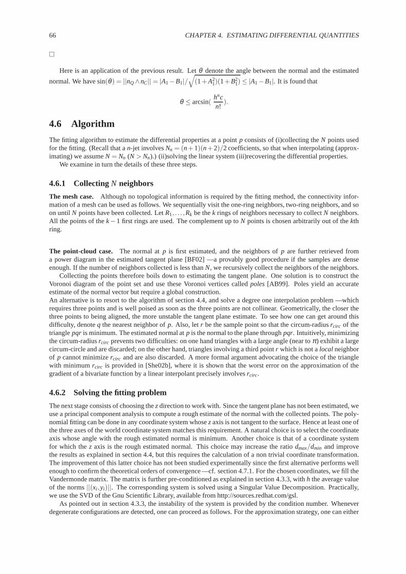
66 CHAPTER 4. ESTIMATING DIFFERENTIAL QUANTITIES
�
Here is an application of the previous result. Letθ denote the angle between the normal and the estimated
normal. We have sin(θ ) = ||nQ∧nC||= |A1−B1|/√
(1+A21)(1+B2
1)≤ |A1−B1|. It is found that
θ ≤ arcsin(hncn!
).
4.6 Algorithm
The fitting algorithm to estimate the differential properties at a pointp consists of (i)collecting theN points usedfor the fitting. (Recall that an-jet involvesNn = (n+1)(n+2)/2 coefficients, so that when interpolating (approx-imating) we assumeN = Nn (N > Nn).) (ii)solving the linear system (iii)recovering the differential properties.
We examine in turn the details of these three steps.
4.6.1 CollectingN neighbors
The mesh case. Although no topological information is required by the fitting method, the connectivity infor-mation of a mesh can be used as follows. We sequentially visitthe one-ring neighbors, two-ring neighbors, and soon until N points have been collected. LetR1, . . . ,Rk be thek rings of neighbors necessary to collectN neighbors.All the points of thek−1 first rings are used. The complement up toN points is chosen arbitrarily out of thekthring.
The point-cloud case. The normal atp is first estimated, and the neighbors ofp are further retrieved froma power diagram in the estimated tangent plane [BF02] —a provably good procedure if the samples are denseenough. If the number of neighbors collected is less thanN, we recursively collect the neighbors of the neighbors.
Collecting the points therefore boils down to estimating the tangent plane. One solution is to construct theVoronoi diagram of the point set and use these Voronoi vertices calledpoles[AB99]. Poles yield an accurateestimate of the normal vector but require a global construction.An alternative is to resort to the algorithm of section 4.4, and solve a degree one interpolation problem —whichrequires three points and is well poised as soon as the three points are not collinear. Geometrically, the closer thethree points to being aligned, the more unstable the tangentplane estimate. To see how one can get around thisdifficulty, denoteq the nearest neighbor ofp. Also, letr be the sample point so that the circum-radiusrcirc of thetrianglepqr is minimum. The estimated normal atp is the normal to the plane throughpqr. Intuitively, minimizingthe circum-radiusrcirc prevents two difficulties: on one hand triangles with a largeangle (near toπ) exhibit a largecircum-circle and are discarded; on the other hand, triangles involving a third pointr which is not alocal neighborof p cannot minimizercirc and are also discarded. A more formal argument advocating the choice of the trianglewith minimum rcirc is provided in [She02b], where it is shown that the worst error on the approximation of thegradient of a bivariate function by a linear interpolant precisely involvesrcirc.
4.6.2 Solving the fitting problem
The next stage consists of choosing thezdirection to work with. Since the tangent plane has not been estimated, weuse a principal component analysis to compute a rough estimate of the normal with the collected points. The poly-nomial fitting can be done in any coordinate system whosezaxis is not tangent to the surface. Hence at least one ofthe three axes of the world coordinate system matches this requirement. A natural choice is to select the coordinateaxis whose angle with the rough estimated normal is minimum.Another choice is that of a coordinate systemfor which thez axis is the rough estimated normal. This choice may increasethe ratiodmax/dmin and improvethe results as explained in section 4.4, but this requires the calculation of a non trivial coordinate transformation.The improvement of this latter choice has not been studied experimentally since the first alternative performs wellenough to confirm the theoretical orders of convergence —cf.section 4.7.1. For the chosen coordinates, we fill theVandermonde matrix. The matrix is further pre-conditionedas explained in section 4.3.3, withh the average valueof the norms||(xi ,yi)||. The corresponding system is solved using a Singular Value Decomposition. Practically,we use the SVD of the Gnu Scientific Library, available from http://sources.redhat.com/gsl.
As pointed out in section 4.3.3, the instability of the system is provided by the condition number. Wheneverdegenerate configurations are detected, one can proceed as follows. For the approximation strategy, one can either

4.7. EXPERIMENTAL STUDY 67
keep the same degree and increase the number of points used, or reuse the same points with a lower degree. Thesechanges are likely to provide a non singular matrixM. In the worst-case, a degree one fitting must be possiblesince then only three linearly independent points are required! For the interpolation, things are a bit more involvedsince reducing the interpolation degree requires discarding some points. Selecting the subset yielding the bestconditioning is a challenging problem [Las99, Hig96]. Notice also that for the approximation case, one can alwaysretrieve a solution from an under-constrained least-square problem by choosing, e.g., the solution vector of leastnorm.
4.6.3 Retrieving differential quantities
We have already mentioned how to compute the normal. For the second order information, we compute the Wein-garten map of the surface [dC76, Section 3.3]. Its eigenvalues (eigenvectors) provide the principal curvatures (di-rections) of the surface. For a parameterized surface givenas a height function, one ends up with the formula givenon Table 4.1. Notice that a basis of the tangent space associated to the parameterizationX(u,v) = (u,v,h(u,v))consists of the two vectorsXu = (1,0,hu)
t andXv = (0,1,hv)t . A Gram-Schmidt orthonormalization of the basis
{Xu,Xv} gives another basis{Y,Z} of the tangent space. The diagonalization of the symmetric matrix representingthe Weingarten map in the basis{Y,Z} provides the expression of the principal curvature directions with respectto the{Y,Z} orthonormal basis. Note that the sign of principal curvatures and hence the definition of minimaland maximal directions rely on the orientation of the normal. As long as our experimental study is performed onmeshes of oriented surfaces, it is straightforward to find a global and coherent orientation of the normals.
e= 1+a12
f = a2a1
g = 1+a22
l = 2a3√a1
2+1+a22
m= a4√a1
2+1+a22
n = 2a5√a1
2+1+a22
A =−(
e ff g
)−1(l mm n
)
Table 4.1: Computing the matrixA of the Weingarten map ofh(u,v) = a1u+ a2v+ a3u2 + a4uv+ a5v2 in thebasis{Xu,Xv}
4.7 Experimental study
We present results along two lines. First, we illustrate theconvergence theorems proved in section 4.4. Second,we present illustrations on standard computer graphics models.
4.7.1 Convergence estimates on a graph
Setup. We illustrate the convergence properties with the smooth height fields f (u,v) = 0.1e2u+v−v2andg(u,v) =
4u2 +2v2 defined over the parametric domain(u,v) ∈ [−0.5,0.5]2 —see Figs. 4.4 and 4.5. At selected points onthe graphs off andg, we study the angle between the normals —more precisely its sine sin(n, n), and the relativeerrors on principal curvatures. The values output by our algorithm are compared against the exact values computedanalytically with arbitrary precision under Maple, and we report both average and maximum errors over samplepoints. More precisely, the graph off or g are sampled with pointspi(xi ,yi , f (xi ,yi)) where the(xi ,yi) lies on arandomly perturbed triangulated square grid of sideh. The triangulation is randomly perturbed to avoid simpledegenerate configurations such as points lying on lines. Theperturbation for the point(u,v) of the regular grid isthe point(x,y) with x = u+ δh, y = v+ δ ′h andδ ,δ ′ random numbers in[0,0.9]. The connectivity of the graphis that of the triangulated grid. Notice also that since calculations are carried out on a surface patch parameterizedover a square grid, the direction chosen for the polynomial fitting is thez direction near the origin, and either thethex or y directions at the periphery of the domain.
The convergence properties are illustrated (i)with respect to the discretization steph of the grid —for a givenfitting degreen (ii)with respect to the fitting degreen —for a given discretization steph. We compare the conver-gence properties of the interpolation and approximation schemes, for fitting degrees ranging from one to nine. Toquantify the observations, notice that according to theorem 12, the errorδ on akth-order differential quantity is

68 CHAPTER 4. ESTIMATING DIFFERENTIAL QUANTITIES
O(hn−k+1), hence
δ ≈ c hn−k+1⇔ log(1/δ )≈ log(1/c)+ (n−k+1) log(1/h) (4.15)
⇔ log(1/δ )
log(1/h)≈ log(1/c)
log(1/h)+ (n−k+1). (4.16)
Convergence with respect to toh. To highlight the convergence properties with respect to thesize of the neigh-borhood, we consider sequences of meshes withh→ 0, more preciselyh ranges from 2−2 to 2−6. The results forf andg being alike, we focus on the exponentialf .
Curves of Figs. 4.6 to 4.11 show the average convergence behavior as the size of the neighborhood decreases.For a given degree and following equation (4.15), curves of figures 4.6 to 4.11 should be lines of slope(n−k+1).The behavior is more regular for the approximation case, andthe estimate is also better: a gain of about a digit canbe observed betweenkmax estimates of figures 4.10 and 4.11.
Convergence with respect to to the interpolation degree. For the convergence with respect to to the interpola-tion degree —withh fixed, we present results for the polynomialg (cf. Fig. 4.12 to 4.17). Conclusions are similarfor f (cf. Fig. 4.18 to 4.23), but it should however be noticed thatsince the graph ofg is more curvy than that off , a finer grid is required. (The higher the degree the more points required by the fitting ... and we compute localquantities!) To be precise, we ran experiments withh = 2−5 for f andh = 2−7 for g.
Curves of figures 4.12 and 4.13 show the convergence as a function of the degree of the fitted polynomial fora fixed neighborhood size. According to Eq. (4.16), curves ofthese figures should be lines of unit slope, witha vertical shift of one unit between normal and curvatures errors since curvature is a 2nd order quantity whereasnormal is 1st order. The gap between the average values and the maximal values is greater for interpolation thanfor approximation. The other charts provide the conditioning and the least singular value. Interpolation fitting isalways more ill-conditioned than approximation, and closer to a degenerate problem (the least singular value is thedistance of the matrix system to singular matrices). The particular case of a degree 7 approximation reveals to bebadly conditioned due to the regular connectivity of the mesh used to find the neighbors: there is only one morepoint than for the degree 7 interpolation fitting.
4.7.2 Illustrations
We depict differential informations on several models. When principal directions are displayed, blue and redrespectively correspond tokmin andkmax—that iskmin≤ kmax—, assuming the surface normal points to the outside.To display patches of osculatingn-jets, it is sufficient to select a rectangular domain in parameter space, sample itwith a grid, and plot the corresponding mesh.
Consider the mesh models of the elliptic paraboloidz= 2x2 + y2 —16k points, Fig. 4.24—, and the surfaceof revolutionz = 0.1sin(10
√(x2 + y2)) —8k points, Fig. 4.25. The arrangement of curvature lines provides
informations on umbilical points —where principal directions are not defined sincekmin = kmax. On the paraboloid, it is easy to follow curvature lines and see how they turn around an umbilic. The surface of revolution providesan example of two parabolic lines (where the principal curvature kmax vanishes), that is a curve along whichthe Gauss curvatureKGaussvanishes. This specific line splits the surface into elliptic (KGauss> 0) and hyperbolicregions (KGauss< 0). This model also illustrates a line of umbilical points where minimum and maximum principaldirections swap each over.
For a standard example from Computer Graphics, consider theMichelangelo’s David of Fig. 4.26. On thismodel of 95922 pts, the principal curvatures provide meaningful information for shape perception5. To finishup, we illustrate the robustness of the method. Figure 4.27 displays random patches on the Mechanic model, a12,500 points model reconstructed from the output of a rangescanner. In spite of the coarse sampling, patches andprincipal directions provide faithful information. In a similar vein, approximation fitting with large neighborhoodsFig. 4.28 features a noisy triangulation of a graph. In spiteof the severe level of noise, surface patchesaveragethe available information. On Fig. 4.29, a noisy triangulation of an ellipsoid, 15k points, principal directions areenough precise to recognize an umbilic.
5See also [HCV52, p197] as well as [HGY+99].

4.7. EXPERIMENTAL STUDY 69
–1
–0.5
0
0.5
1
–1
–0.5
0
0.5
1
0
0.2
0.4
0.6
0.8
Figure 4.4:f (u,v) = 0.1e2u+v−v2
–1
–0.5
0
0.5
1
–1
–0.5
0
0.5
1
0
1
2
3
4
5
6
Figure 4.5:g(u,v) = 4u2+2v2

70 CHAPTER 4. ESTIMATING DIFFERENTIAL QUANTITIES
0
5
10
15
20
25
30
1 1.5 2 2.5 3 3.5 4 4.5
log(
1/de
lta)
log(1/h)
deg 1deg 2deg 3deg 4deg 5deg 6deg 7deg 8deg 9
Figure 4.6: Exponential model: Convergence of thenormal estimate with respect toh, interpolation fitting
0
5
10
15
20
25
30
35
1 1.5 2 2.5 3 3.5 4 4.5
log(
1/de
lta)
log(1/h)
deg 1deg 2deg 3deg 4deg 5deg 6deg 7deg 8deg 9
Figure 4.7: Exponential model: Convergence of thenormal estimate with respect toh, approximation fitting
-5
0
5
10
15
20
25
1 1.5 2 2.5 3 3.5 4 4.5
log(
1/de
lta)
log(1/h)
deg 2deg 3deg 4deg 5deg 6deg 7deg 8deg 9
Figure 4.8: Exponential model: Convergence of thekmin estimate with respect toh, interpolation fitting
0
5
10
15
20
25
30
1 1.5 2 2.5 3 3.5 4 4.5
log(
1/de
lta)
log(1/h)
deg 2deg 3deg 4deg 5deg 6deg 7deg 8deg 9
Figure 4.9: Exponential model: Convergence of thekmin estimate with respect toh, approximation fitting
1e-12
1e-10
1e-08
1e-06
0.0001
0.01
1
0.01 0.1 1
delta
h
deg 2deg 3deg 4deg 5deg 6deg 7deg 8deg 9
Figure 4.10: Exponential model: Convergence of thekmax estimate with respect toh, interpolation fitting
1e-12
1e-10
1e-08
1e-06
0.0001
0.01
1
0.01 0.1 1
delta
h
deg 2deg 3deg 4deg 5deg 6deg 7deg 8deg 9
Figure 4.11: Exponential model: Convergence of thekmax estimate with respect toh, approximation fitting

4.7. EXPERIMENTAL STUDY 71
-1
-0.5
0
0.5
1
1.5
2
2.5
3
3.5
1 2 3 4 5 6 7 8 9
log(
1/de
lta)/
log(
1/h)
degree
N_avkmin_av
kmax_avN_max
kmin_maxkmax_max
Figure 4.12: Polynomial model: Convergence of nor-mal and curvature estimates with respect to the degreeof the interpolation fitting
0
0.5
1
1.5
2
2.5
3
3.5
4
1 2 3 4 5 6 7 8 9
log(
1/de
lta)/
log(
1/h)
degree
N_avkmin_av
kmax_avN_max
kmin_maxkmax_max
Figure 4.13: Polynomial model: Convergence of nor-mal and curvature estimates with respect to the degreeof the approximation fitting
1
100
10000
1e+06
1e+08
1e+10
1e+12
1e+14
1e+16
1 2 3 4 5 6 7 8 9
cond
ition
ing
degree
cn_avcn_max
Figure 4.14: Polynomial model: Conditioning with re-spect to the degree of the interpolation fitting
1
100
10000
1e+06
1e+08
1e+10
1e+12
1e+14
1 2 3 4 5 6 7 8 9
cond
ition
ing
degree
cn_avcn_max
cn_ls_avcn_ls_max
Figure 4.15: Polynomial model: Conditioning with re-spect to the degree of the approximation fitting
1e-10
1e-09
1e-08
1e-07
1e-06
1e-05
0.0001
0.001
0.01
0.1
1
1 2 3 4 5 6 7 8 9
leas
t sin
gula
r va
lue
degree
sv_avsv_min
Figure 4.16: Polynomial model: Least singular valuewith respect to the degree of the interpolation fitting
1e-07
1e-06
1e-05
0.0001
0.001
0.01
0.1
1
10
1 2 3 4 5 6 7 8 9
leas
t sin
gula
r va
lue
degree
sv_avsv_min
Figure 4.17: Polynomial model: Least singular valuewith respect to the degree of the approximation fitting

72 CHAPTER 4. ESTIMATING DIFFERENTIAL QUANTITIES
-1
0
1
2
3
4
5
6
7
8
1 2 3 4 5 6 7 8 9
log(
1/de
lta)/
log(
1/h)
degree
N_avkmin_av
kmax_avN_max
kmin_maxkmax_max
Figure 4.18: Exponential model: Convergence of nor-mal and curvature estimates with respect to the degreeof the interpolation fitting
0
1
2
3
4
5
6
7
8
9
2 3 4 5 6 7 8 9
log(
1/de
lta)/
log(
1/h)
degree
N_avkmin_av
kmax_avN_max
kmin_maxkmax_max
Figure 4.19: Exponential model: Convergence of nor-mal and curvature estimates with respect to the degreeof the approximation fitting
1
10
100
1000
10000
100000
1e+06
1e+07
1e+08
1e+09
1e+10
1 2 3 4 5 6 7 8 9
cond
ition
ing
degree
cn_avcn_max
Figure 4.20: Exponential model: Conditioning with re-spect to the degree of the interpolation fitting
10
100
1000
10000
100000
1e+06
1e+07
2 3 4 5 6 7 8 9
cond
ition
ing
degree
cn_avcn_max
cn_ls_avcn_ls_max
Figure 4.21: Exponential model: Conditioning with re-spect to the degree of the approximation fitting
1e-06
1e-05
0.0001
0.001
0.01
0.1
1
1 2 3 4 5 6 7 8 9
leas
t sin
gula
r va
lue
degree
sv_avsv_min
Figure 4.22: Exponential model: Least singular valuewith respect to the degree of the interpolation fitting
0.0001
0.001
0.01
0.1
1
2 3 4 5 6 7 8 9
leas
t sin
gula
r va
lue
degree
sv_avsv_min
Figure 4.23: Exponential model: Least singular valuewith respect to the degree of the approximation fitting

4.7. EXPERIMENTAL STUDY 73
Figure 4.24: Elliptic paraboloid Figure 4.25: Surface of revolution
Figure 4.26: Michelangelo’s David: principal directions associated withkmax scaled bykmin

74 CHAPTER 4. ESTIMATING DIFFERENTIAL QUANTITIES
Figure 4.27: Mechanic: closeup
Figure 4.28:f (u,v) = u+3v+e2u+v−v2with noise Figure 4.29: Principal directions on a noisy ellipsoid
4.8 Conclusion
Estimating differential quantities is of prime importancein many applications from Computer Vision, ComputerGraphics, Computer Aided Design or Computational Geometry. This importance accounts for the many differentdifferential estimators one can find in the vast literature of applied geometry. Unfortunately, few of these have un-dergone a precise theoretical analysis. Another striking fact is that estimates of second order differential quantitiesare always computed using degenerate conics/quadrics without even mentioning the classification of Euclideanconics/quadrics.
The main contribution of the chapter is to bridge the gap between the question of estimating differential prop-erties of arbitrary order and multivariate interpolation and approximation. In making this connection, the use ofjets —truncated Taylor expansions— is advocated. Precise asymptotic convergence rates are proved for curves andsurfaces, both for the interpolation and approximation schemes. To the best of our knowledge, these results areamong the first ones providing accurate estimates for differential quantities of order three and more. Experimentalresults for surfaces ofR3 are reported. These experiments illustrate the asymptoticconvergence results, but alsothe robustness of the methods on general Computer Graphics models.
Acknowledgments.P. Chenin is acknowledged for pointing out Ref. [EK66].

Chapter 5
Topology driven algorithms for ridgeextraction on meshes
Given a smooth surface, a ridge is a curve along which one of the principal curvatures has an extremum alongits curvature line. Ridges are curves ofextremalcurvature and therefore encode important informations used insegmentation, registration, matching and surface analysis. Surprisingly, no method developed so far to report ridgesfrom a mesh approximating a smooth surface comes with a careful analysis, which entails that one does not knowwhether the ridges are reported in a coherent fashion. To bridge this gap, we make the following contributions.
First, we present a careful analysis of the orientation issues arising when one wishes to report the ridgesassociated to the two principal curvatures separately. Theanalysis highlights the subtle interplay between ridges,umbilics, and curvature lines. Second, given a triangulation T approximating a smooth generic surfaceS, wepresent sufficient conditions onT together with a generic algorithm reporting an isotopic approximation of theridges. Third, we develop a heuristic algorithm to process amesh when no information on an underlying smoothsurface is known. Fourth, for coarse models, we provide a filtering mechanism retaining the most stable ridgesonly. Fifth, we present experimental results of the heuristic algorithm for smooth surfaces as well as coarse models.Our running times improve of at least one order of magnitude those of state-of-the-art methods.
The common point of these contributions is to exploit the topological patterns of ridges on smooth genericsurfaces recalled in chapter 3. These contributions also pave the way to the first certified algorithm for ridgeextraction on polynomial parametric surfaces, developed in the next chapters.
5.1 Introduction
5.1.1 Ridges of a smooth surface
Differential properties of surfaces embedded inR3 are a fascinating topic per se, and have long been of interestforartists and mathematicians, as illustrated by the parabolic lines drawn by Felix Klein on the Apollo of Belvedere[HCV52], and also by the developments reported in [Koe90]. Beyond these noble considerations, the recent de-velopment of laser range scanners and medical images shed light on the importance of being able to analyzediscrete datasets consisting of point clouds in 3D or medical images —grids of 3D voxels. Whenever the datasetsprocessed model piecewise smooth surfaces, a precise description of the models naturally calls for differentialproperties. In particular, applications such as shape matching [HGY+99], surface analysis [HGY+99], or registra-tion [TG95, PAT00] require the characterization of high order properties and in particular the characterization ofcurves ofextremalcurvatures, which are precisely the so-calledridges.
Chapter 3 surveys theoretical analysis of ridges, so we justrecall basic definitions below. A ridge consistsof the points where one of the principal curvatures has an extremum along its curvature line. Since each pointwhich is not an umbilic has two different principal curvatures, a point potentially belongs to two different ridges.Denotingk1 andk2 the principal curvatures —we shall always assume thatk1 ≥ k2, a ridge is called blue (red) ifk1 (k2) has an extremum. Moreover, a ridge is calledelliptic if it corresponds to a maximum ofk1 or a minimumof k2, and is calledhyperbolicotherwise. Ridges witness extrema of principal curvaturesand their definitioninvolves derivatives of curvatures, whence third order differential quantities. Moreover, the classification of ridgesas elliptic or hyperbolic involves fourth order differential quantities, so that the precise definition of ridges requires
75

76 CHAPTER 5. RIDGE EXTRACTION ON MESHES
C4 differentiable surfaces. Therefore, the calculation of ridges from a mesh approximating a smooth surface posesdifficult problems, which are of three kinds.
Numerical difficulties. It is well known that parabolic curves of a smooth surface correspond to points wherethe Gauss curvature vanishes. Similarly, ridges are witnessed by the zero crossings of the so-called extremalitycoefficients, denotedb0 (b3) for blue (red) ridges, which are the derivatives of the principal curvatures along theirrespective curvature lines. Algorithms reporting ridges need to estimateb0 andb3. Estimating these coefficientsdepends on the particular type of surface processed —implicitly defined, parameterized, discretized by a mesh—and is numerically a difficult task. Notice though, that the estimation of these quantities is independent from thecombinatorial processing of ridges.
Orientation difficulties. Since coefficientsb0 andb3 are derivatives of principal curvatures, they are third-ordercoefficients in the Monge form of the surface —the Monge form is the Taylor expansion of the surface expressedas a height function in the particular frame defined by the principal directions. But like all odd term of the Mongeform, their sign depends upon the orientation of the principal frame used. Tracking the sign change of functionswhose sign depends on the particular orientation of the frame in which they are expressed poses a problem. Inparticular, tracking a zero-crossing ofb0 or b3 along a line-segmentimposes to find a coherent orientation of theprincipal frame at the segment endpoints. Given two principal vectors at the segment endpoints, one way to findsuch an orientation consists of orienting the directions sothat they make an acute angle, whence the name ofAcuteRuleor A.R. for short. The A.R. is implicitly used in [Mor90, Mor96, TG95, OBS04], but surprisingly, none ofthese papers addresses the question of specifying conditions guaranteeing the decisions made are correct. As weshall see, such analysis highlights the interplay between foliations, ridges and umbilics. (A principal foliation isthe collection of lines of curvature associated to either principal curvature.)
Topological difficulties. The last difficulty is of topological nature and stems from the complex patterns madeon generic surfaces by ridges and umbilics. As an illustration, consider a generic closed surface of genus zero —atopological sphere. Each such surface has at least four umbilics, each being traversed by either one or three ridges.For precise relationship between ridges and umbilics, the reader is referred to [Por01] as well as to section 3.4.Reporting ridges therefore requires reporting and classifying umbilics, an issue not addressed, to the best of ourknowledge, by any paper tackling the issue of reporting ridges. This issue is illustrated in Figs. 3.14 and 3.15 forthe particular case of the ellipsoid.
Another difficulty of topological nature is the interference of red and blue ridges at the so-called purple points.Given that each point of a smooth surface (which is not an umbilic) potentially belongs to two different ridges—one for each principal curvature, ridges near purple points must be handled with care. This difficulty requiresagain an orientation procedure such as the A.R. already mentioned.
5.1.2 Previous work
To the best of our knowledge, the only algorithm taking into account the topology of ridges at umbilics is describedby Morris [Mor90, Mor96]. This method applies to parameterized surfaces and uses heuristics to orient edges andreport umbilics, so that no guarantee is provided. For algebraic surfaces, Bogaevski et al. [BLBK03] use a formalcomputation to determine the equation of a surface whose intersection with the original surface gives the ridges.For implicit surfaces, Thirion [Thi96] applies a marching line algorithm to the Gaussian extremality. However,the behavior of the algorithm near umbilics is not specified,and the Gaussian extremalityEg = b0b3 used to avoidorienting with the acute rule disconnects red and blue ridges at their intersections —5.2(c).
All other methods do not address the problem of topology, butfocus on identifying a subset of the ridgesand filtering methods. The connection between the medial axis and ridges is used by M.Hisada et al. [HBK02].(Notice though that the projection of the medial axis boundary misses all hyperbolic ridges, and may also misselliptic ones.) The connection with the focal surfaces is considered in [WB01] and [LA98]. Methods using onlythe estimation of curvatures on meshes are derived by Ohtakeet al [OB01] or Stylianou et al [SF00]. Ohtake et al.[OBS04] use implicit surface fitting of a mesh to extract ridge-valley lines. The curvature tensor and the derivativesof curvatures of a mesh vertex are defined as the analyticallycomputed values of the projection of the vertex onthe fitted surface.

5.2. RIDGE TOPOLOGY AND ORIENTATION ISSUES 77
5.1.3 Contributions and chapter overview
Following the previous discussion, given a meshT providing an approximation of a smooth compact orientedgeneric surfaceS, we aim at usingT so as to report the ridges ofS. (We implicitly assumeS andT are isotopic[ACDL00, APR03, CCS04].) We make the following contributions.
In section 5.2, we specify the topological difficulties arising when reporting ridges, and introduce the AcuteRule. In section 5.3, we definecomplianttriangulations amenable to an isotopic extraction of ridges, and develop ageneric algorithm. The algorithm is generic since two routines are assumed to compute the Monge coefficients ofthe surface at any point, and to report umbilic patches. In section 5.4, we develop a heuristic algorithm to processa mesh when no information on an underlying smooth surface isknown. In section 5.5, we develop a filteringmechanism to report the most stable ridges of a coarse mesh. Finally, experimental results are provided in section5.6.
5.2 Ridge topology and orientation issues
In this section, we introduce formally the problem addressed. Readers not familiar with ridges are referred tosection 3.4 as well as to [HGY+99]. The set of ridges is composed of simple curves either closed and free ofumbilic calledclosed ridges, or open curves connecting umbilics calledopen ridges. Hence reporting ridgesmeans reporting umbilics and these ridge curves with the correct connectivity. As our aim is to report blue and redridges separately, we focus on the setRb
S of blue ridges ofS.
5.2.1 Problem addressed
Assume we are given a triangle meshT and an homeomorphismΦ from T to S. As indicated in Fig. 5.1, weaim at reporting thepull-backof the setRb
S of ridges ofSontoT. More precisely, we aim at reporting a setRbT of
polygonal curves onT corresponding to this pull-back. Given such a polyline, each pair of consecutive points iscalled aridge segment. Let us consider onS(T) the ridge setRb
S (RbT ), together with the topology induced byR3.
Definition. 12 The set RbT is an isotopic approximation of the blue ridges of S if thepush-forwardof RbT (Φ(Rb
T))is isotopic to RbS on S, or equivalently thepull-backof Rb
S (Φ−1(RbS)) is isotopic to RbT on T .
As suggested by the previous definition, we shall use the following abuses of terminology. When saying that“an edge is crossed by a ridge” or “a triangle contains an umbilic” we shall mean “the push-forward of the edge iscrossed by a ridge” or “the push-forward of the triangle contains an umbilic”. Equivalently, this also means that“an edge is crossed by the pull-back of a ridge” or “a trianglecontains the pull-back of an umbilic”.
Before proceeding, a comment is in order. We do not consider purple points —intersection between ridges ofdifferent colors— because the topology of the blue and red sets of ridges are processed separately. The incentive forignoring purple points is that red and blue ridges are independent since functionsb0 andb3 are so. Incidently, thisassumption alleviates the constraint of reporting the correct topology of ridges around purple points, as depicted inFig. 5.2.
p
q
r2
t2
r1
t1
S
R
Figure 5.1: A ridgeR on a smooth surface, its pull-back[r1, r2] on an inscribed triangulated surface, and a straightridge segment[t1,t2] isotopic to this pull-back in the trianglepqs

78 CHAPTER 5. RIDGE EXTRACTION ON MESHES
(a) (b) (c)
Figure 5.2: (a)Two ridges of different colors (b)Blue / red ridges reported independently: the topology of eachridge is respected, but that of the union is not (c)Ridges reported simultaneously by the Gaussian extremality:ridges are disconnected at purple points. No ridge point is detected when both red and blue ridges cross the sameedge
5.2.2 Orientation and crossings
Consider a meshT approximating of a smooth compact oriented generic surfaceS as explained in the previoussection. The main issue tackled is to understand which propertiesT must have in order for one to report the ridgesof S faithfully. We first recall the following:
Observation. 6 At any point of a smooth oriented surface S which is not an umbilic, orienting the principaldirections at a vertex is equivalent to choosing a unit maximal principal vector, and there are two such orientations.(The minimal principal vector is then uniquely defined to be the unit vector so that the basis (maximal vector,minimal vector, normal) is direct.) Orienting the principal directions of an edge of a triangulation T whoseendpoints lie on S means orienting them at its two vertices, and there are four possibilities.
Consider now a simple curveC homeomorphic to the line-segment[0,1] drawn onS. If C does not containany umbilic one can define alongC two continuous unit vector fields (opposite of one another) which orient themaximum direction field alongC. Once a unit maximum vector has been chosen at one endpoint ofC, we call theorientation induced by the corresponding vector field at theother endpoint theorientation by continuity. ReplacingC by the push-forward of an edge yields the following:
Definition. 13 The orientation of the principal directions of an edge is called correct(erroneous) if it coincideswith (differs from) one of the two orientations by continuity (of its push-forward on S).
As already noticed, a blue ridge point is witnessed by the zero crossing of a bivariate functionb0. More precisely,consider a curve oriented by continuity and crossing transversally a blue ridge, then the functionb0 along the curvevanishes at the crossing point and undergoes a sign change. Since we are given a triangulationT of S, using anidea reminiscent from Marching Lines and Marching cubes, itis natural to seek the zero crossings of functionb0
along the edges ofT. But in our case however, functionb0 depends on the orientation of the principal directionsand by the above observation there are four possible orientations for the edge. Having discussed these orientationissues, we finally raise the observation used to track the blue ridge crossings with the sign ofb0:
Observation. 7 Let C be the push-forward of an edge[p,q]. Assume that the orientation of the principal directionsof the edge is correct, no ridge crossing occurs at p or q and that at a crossing point the ridge and the curve Care transverse. Then the number of blue ridge crossings on C is odd (even) iff b0(p)b0(q) < 0 (b0(p)b0(q) > 0). Ifmoreover, there is at most one blue ridge crossing on C then a ridge crosses C only once iff b0(p)b0(q) < 0.
5.2.3 Gaussian extremality
An attempt to avoid the orientation procedure has been done by J.P. Thirion [Thi96] with the introduction of theGaussian extremality. This function is defined at non-umbilical points byEg = b0b3. As bothb0 andb3 changesign if the orientation is changed, the Gaussian extremality remains independent of the orientation. A sign changeof this function along an edge means that an odd number of ridges is crossing the edge, but it does not allow toknow the color of these ridges. If one could find a mesh so that each edge crosses at most one ridge regardless thecolor, it would be possible to recover the topology of uncolored ridges correctly. Unfortunately, the existence of acrossing between red and blue ridges in a triangle implies that one of its edge is crossed by at least two ridges (cf.Fig. 5.2(c)). In conclusion, the Gaussian extremality doesnot specify the color of the ridge, and consequently isunable to preserve the topology of ridges near purple points.

5.3. A GENERIC ALGORITHM 79
5.2.4 Acute rule
Consider an edgee of the meshT. In the case of a dense meshT, and whenever the vertices ofe are close onS,one expects the maximal principal directions at the vertices of e to be nearly aligned —at least far from umbilics,which motivates the following:
Definition. 14 (Acute Rule) Orienting an edge with theacute ruleconsists of choosing maximal principal vectorsat the two vertices so that they make an acute angle in the ambient spaceR3.
Note that this rule is well defined as soon as the maximal principal directions are not at right angle. Thedeviation of the maximal principal direction along a curvature line on the surface has two components which areextrinsic (the normal curvature) and intrinsic (the geodesic curvature). The denser the mesh, the shorter the edgesof the triangulation and the smaller the extrinsic deviation. But the situation is different for the geodesic curvature.In particular, the geodesic curvature is arbitrarily largenear umbilics as illustrated on Fig. 5.4, so that the acuterule is likely to yield erroneous orientations there. For these reasons, in developing a generic algorithm, we shallprocess differently the vicinity of umbilics (the so-called umbilic patches) and the complement of these patches.
b0(p)< 0p
qb0(q)> 0
R
Figure 5.3: The A.R. gives a correct orientation.
b0(p)< 0p
q
b0(q)> 0
R
b0(q)< 0
Figure 5.4: The A.R. gives an erroneous orientationnear an umbilic —of index 1/2 here.
5.3 A generic algorithm
5.3.1 Compliant triangulations
We aim at designing an algorithm able to report an isotopic approximation of ridges as specified by definition 12.Since ridges are reported on the triangulationT, this triangulation shall fulfill some conditions. We thus definecomplianttriangulations, together with a generic algorithm in such away that for a compliant traingulation, thegeneric algorithm will report an isotopic approximation ofridges. Since blue and red ridges are handled separatelyby the same process, we focus on blue ones and unless stated differently, “ridge” refers to “blue ridge” in thesequel.
To begin with, and following a well established trend to keepthe description of the algorithm tractable withouthaving to consider degenerate situations, we shall requiregenericity conditions. Note that these hypothesis are notrestrictive in practice since they can be simulated during the processing (see the proof of theorem 13).
Hypothesis. 1 (Genericity hypothesis.)The vertices and edges of T are assumed to meet the followinggenericconditions :
S1 no ridge goes through a vertex of T .
S2 ridges intersect edges transversally.
Second, we specify conditions on the density of the triangulationT. To specify these conditions, we considerseparately regions around umbilics and their complement onthe surface. The rationale for doing so is that toprovide guarantees on ridge crossings, we need correct orientations. But the A.R. is used for orientation and asdiscussed in section 5.2.4, it is not reliable near umbilics. Therefore, we apply two different strategies to umbilicalregions inside which orientation is not certified, and to therest of the surface where a correct orientation of edgesis given.

80 CHAPTER 5. RIDGE EXTRACTION ON MESHES
Let us first discuss the case of umbilics. First, we require umbilic patches to be disjoint, which is natural sinceumbilics on generic surfaces are isolated. The orientationof edges inside patches is not certified, hence we cannotseek crossings inside a patch and have to infer the topology of ridges inside the patch from the patch boundary.This leads to the assumptions that (i) the topology inside a patch is as simple as possible (ii) one can find a correctorientation for edges on the boundary of the patch and each such boundary edge is crossed at most once by a givenridge. To substantiate these hypothesis, recall that generically, an umbilic is either a one ridge umbilic, or a threeridges umbilic (cf. section 3.4). Also recall that the threetangents to ridges connected to a three ridge umbilic aredistinct. For a small enough topological disk around an umbilic, the configurations of ridges expected are thereforethose depicted in Fig. 5.5. This formally leads to hypothesis D2.
Let us now consider the complement of the umbilic patches on the surface. Since, we are detecting ridgecrossings along edges by observation 7, we assume each edge is crossed by at most one ridge. We wish we couldassume that an edge has at most one ridge crossing witnessed by a sign change of the extremality coefficient.However, such an assumption is not realistic —if the ridge isalmost tangent to the edge (Fig. 5.6) it crosses ittwice. Hence we require instead that if one counts the numberof crossings modulo 2 on the edge then the topologyof this ridge is not modified. Finally, we require that no whole ridge is included in a triangle.
A triangulation meeting these hypothesis is called acomplianttriangulation. More formally, we define fivedensity hypothesis, namely D0 for the orientation property, D1 and D2 for umbilics, D3 and D4 for the complementof umbilic patches:
Hypothesis. 2 (Density hypothesis.)
D0 Triangulation T is such that outside umbilic patches, the A.R. correctly orients edges.
D1 Umbilic patches Ui are disjoint.
D2 A patch Ui of an umbilic ui is such that (cf. fig. 5.5)
(a) Ui does not contain a whole ridge,
(b) ridges not connected to ui do not cross the boundary of Ui ,
(c) a ridge connected to ui only once crosses exactly one edge of the boundary of Ui ,
(d) a ridge connected to ui twice crosses exactly two edges of the boundary of Ui .
D3 All edges outside and on the boundary of the patches cross at most one ridge. If an edge crosses the ridge morethan once, the topology is not modified if the number of crossing is counted modulo 2 (That is, if the numberof crossings is odd the edge is processed as it were crossing the ridge once, and if the number of crossings iseven the edge is processed as it were not crossing the ridge).
D4 A triangle of T−∪iUi does not contain a whole ridge.
������
������
������
������
������
������
Figure 5.5: The only allowed configuration ofridges near an umbilic: first figure for a 1-ridge um-bilic patch, second and third figures for a 3-ridgeumbilic patch.
���
���
���
���
����
���
���
���
���
Figure 5.6: A double crossing simplifying to nocrossing and three crossings simplifying to a singleone
5.3.2 Generic algorithm
Based upon the previous hypothesis, algorithmGenericRidges—Fig. 5.7— processes separately umbilic re-gions and their complement. The algorithm requires, as a preprocessing, (i)estimations of the differential quantitiesat vertices of the meshT and (ii)the identification of umbilic patches. The algorithm is generic in the sense that itperforms combinatorial decisions which are independent from the method of the preprocessing, but only dependon the result of this preprocessing.
Theorem. 13 For a compliant triangulation, the algorithmGenericRidges reports an isotopic approximationof ridges as specified by definition 12.
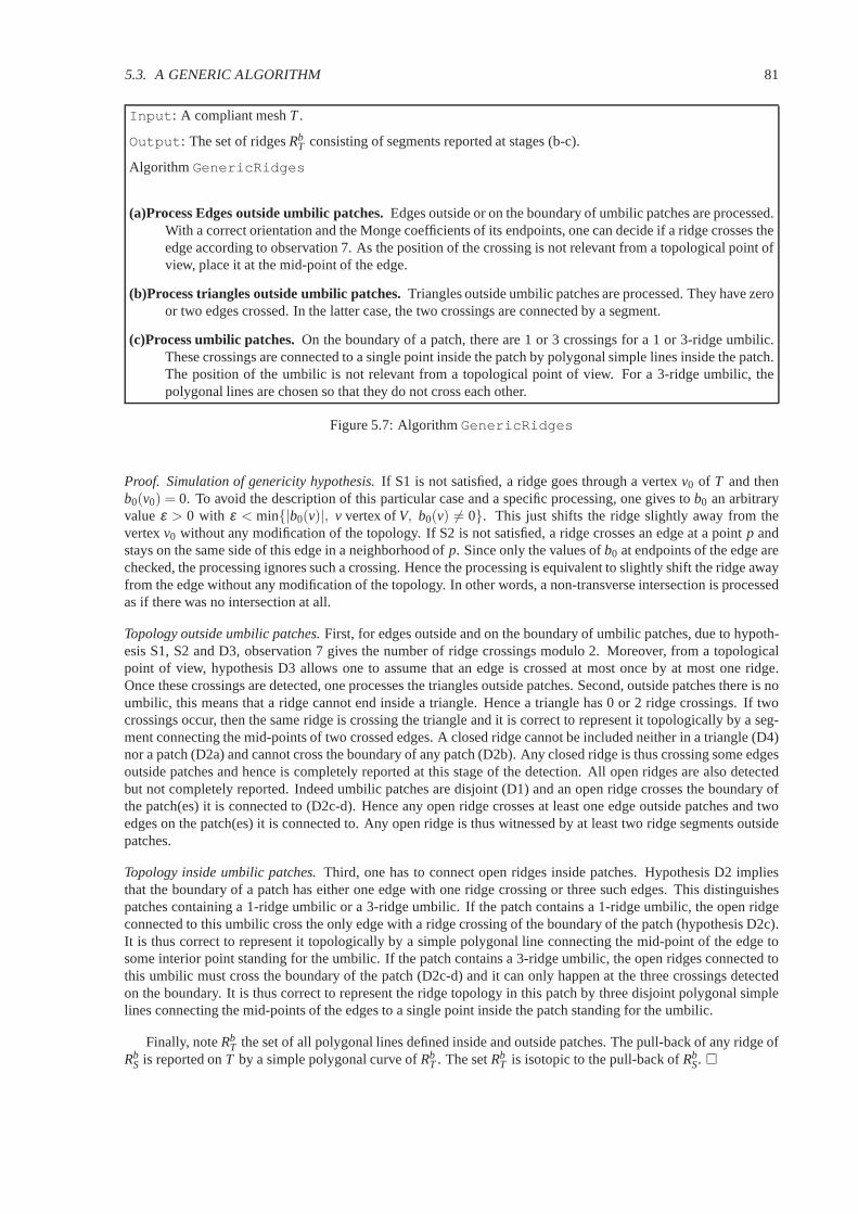
5.3. A GENERIC ALGORITHM 81
Input: A compliant meshT.
Output: The set of ridgesRbT consisting of segments reported at stages (b-c).
AlgorithmGenericRidges
(a)Process Edges outside umbilic patches.Edges outside or on the boundary of umbilic patches are processed.With a correct orientation and the Monge coefficients of its endpoints, one can decide if a ridge crosses theedge according to observation 7. As the position of the crossing is not relevant from a topological point ofview, place it at the mid-point of the edge.
(b)Process triangles outside umbilic patches.Triangles outside umbilic patches are processed. They havezeroor two edges crossed. In the latter case, the two crossings are connected by a segment.
(c)Process umbilic patches.On the boundary of a patch, there are 1 or 3 crossings for a 1 or 3-ridge umbilic.These crossings are connected to a single point inside the patch by polygonal simple lines inside the patch.The position of the umbilic is not relevant from a topological point of view. For a 3-ridge umbilic, thepolygonal lines are chosen so that they do not cross each other.
Figure 5.7: AlgorithmGenericRidges
Proof. Simulation of genericity hypothesis.If S1 is not satisfied, a ridge goes through a vertexv0 of T and thenb0(v0) = 0. To avoid the description of this particular case and a specific processing, one gives tob0 an arbitraryvalueε > 0 with ε < min{|b0(v)|, v vertex ofV, b0(v) 6= 0}. This just shifts the ridge slightly away from thevertexv0 without any modification of the topology. If S2 is not satisfied, a ridge crosses an edge at a pointp andstays on the same side of this edge in a neighborhood ofp. Since only the values ofb0 at endpoints of the edge arechecked, the processing ignores such a crossing. Hence the processing is equivalent to slightly shift the ridge awayfrom the edge without any modification of the topology. In other words, a non-transverse intersection is processedas if there was no intersection at all.
Topology outside umbilic patches.First, for edges outside and on the boundary of umbilic patches, due to hypoth-esis S1, S2 and D3, observation 7 gives the number of ridge crossings modulo 2. Moreover, from a topologicalpoint of view, hypothesis D3 allows one to assume that an edgeis crossed at most once by at most one ridge.Once these crossings are detected, one processes the triangles outside patches. Second, outside patches there is noumbilic, this means that a ridge cannot end inside a triangle. Hence a triangle has 0 or 2 ridge crossings. If twocrossings occur, then the same ridge is crossing the triangle and it is correct to represent it topologically by a seg-ment connecting the mid-points of two crossed edges. A closed ridge cannot be included neither in a triangle (D4)nor a patch (D2a) and cannot cross the boundary of any patch (D2b). Any closed ridge is thus crossing some edgesoutside patches and hence is completely reported at this stage of the detection. All open ridges are also detectedbut not completely reported. Indeed umbilic patches are disjoint (D1) and an open ridge crosses the boundary ofthe patch(es) it is connected to (D2c-d). Hence any open ridge crosses at least one edge outside patches and twoedges on the patch(es) it is connected to. Any open ridge is thus witnessed by at least two ridge segments outsidepatches.
Topology inside umbilic patches.Third, one has to connect open ridges inside patches. Hypothesis D2 impliesthat the boundary of a patch has either one edge with one ridgecrossing or three such edges. This distinguishespatches containing a 1-ridge umbilic or a 3-ridge umbilic. If the patch contains a 1-ridge umbilic, the open ridgeconnected to this umbilic cross the only edge with a ridge crossing of the boundary of the patch (hypothesis D2c).It is thus correct to represent it topologically by a simple polygonal line connecting the mid-point of the edge tosome interior point standing for the umbilic. If the patch contains a 3-ridge umbilic, the open ridges connected tothis umbilic must cross the boundary of the patch (D2c-d) andit can only happen at the three crossings detectedon the boundary. It is thus correct to represent the ridge topology in this patch by three disjoint polygonal simplelines connecting the mid-points of the edges to a single point inside the patch standing for the umbilic.
Finally, noteRbT the set of all polygonal lines defined inside and outside patches. The pull-back of any ridge of
RbS is reported onT by a simple polygonal curve ofRb
T . The setRbT is isotopic to the pull-back ofRb
S. �

82 CHAPTER 5. RIDGE EXTRACTION ON MESHES
5.4 A Heuristic to process a triangle mesh
Assume we are given a triangle meshT providing a piecewise-linear approximation ofS as an inscribed mesh—that is the vertices ofT belong toS. TriangulationT might have been reconstructed from a point cloud [AB99,ACDL00, BC00] or might be the output of a meshing algorithm such as Chew’s algorithm [Che93, BO03]. Eventhough no information on the surface underlying the mesh (ifany) is known, one can design an algorithm followingthe framework of the generic algorithm of section 5.3.2. If the mesh does comply with hypothesis Hyp. 2, then theoutput will be correct. As we shall see, the heuristic algorithm performs satisfactorily on practical examples.
Following this guideline, we instantiate the generic algorithm with two heuristic routines to compute the Mongecoefficients, and report umbilic patches. We also develop a geometric rule to tag ridges as elliptic or hyperbolic.
5.4.1 Computing the Monge coefficients using polynomial fitting
We estimate differential quantities using a local polynomial fitting described and analyzed in [CP05a]. The polyno-mial used is of degree 3 or 4 depending on the method used to identify ridge types —see section 5.4.4. Convergenceproperties and numerical degeneracies of the polynomial fitting are proved and discussed in the aforementionedarticle.
5.4.2 Detection of umbilics and patches
We want to detect patches of triangles ofT containing an umbilic. The method combines a minimization and anindex computation on the neighborhood of each triangle ofT. The size of the neighborhood is the only parameterof the algorithm. This method is a heuristic without guaranty, nevertheless it gives satisfaction in practice (cf.section 5.6).
Finding patches around triangles. Given a trianglet, we aim at defining a collection of triangles around it sothat this collection defines a topological disk on the triangulationT. To do so, the most natural way consists ofusing the successive rings of triangles aroundt. Let us define the 0-ring neighbors of a triangle as the triangle itself.Thek-th ring neighbors is defined recursively by adding to the(k−1)-th ring neighbors the triangles incident toone edge of this set. However, thek-th ring neighbors may not form a topological disk as indicated in Fig. 5.8.
To get around this difficulty and starting from the patch consisting of the trianglet, we iteratively construct apatchP by the following algorithm. Each triangle incident to one ortwo edges of the boundary ofP is placed intoa priority queue —thegradebeing the distance between the centroid of this triangle to that of t. Then, patchPis enlarged with the trianglet ′ having the least grade providedP∪ t ′ remains a topological disk. If trianglet ′ isstitched to the patch, its neighbors are inserted in the queue —if they are not already in it. The process stops assoon as the least distance is more than some threshold.
t
Figure 5.8: The third-ring triangles of the trianglet do not form a topological disk.
We aim at identifying disjoint patches of the meshT containing generic umbilics of index±1/2 (cf. section3.4). Notice that on a smooth surface, the functionk1−k2 is always positive, and vanishes at umbilics only. To usethis criterion, we define the value ofk1−k2 for a triangle as the arithmetic mean of the values at its vertices. Thedetection proceeds in three steps:
1. Compute a patch around each triangle;

5.4. A HEURISTIC TO PROCESS A TRIANGLE MESH 83
2. Select the patch of a trianglet if the functionk1− k2 has its minimum att amongst all the triangles of thepatch;
3. Compute the index of the principal directions on the contour of the patches of triangles selected in step 2.
Given a trianglet, the first step consists of aggregating the successive ringsof triangles aroundt while makingsure that any new addition retains a topological disk. This step is parameterized by a positive number defining thesize of the patch, which is defined as a multiple of the greatest grade of the one-ring triangles. The second stepis straightforward. The third step requires following the contour of each patch, orienting the maximal principaldirections with the A.R. , and computing the index by adding the angle deviations of the corresponding maximalprincipal vectors. Theoretically, the computation of the index of a direction field at a point on a manifold needsthe use of a chart [BG88, chap.7,p.260]. Here, we assume thatthe projection on the tangent plane of the studiedvertex is a chart, the index is computed for principal vectors projected on this plane. We then keep only trianglepatches with an index±1/2.
From a theoretical perspective, if the triangulated surface T is inscribed in a smooth generic closed surface,then the sum of indices of umbilics equals the Euler characteristic of the surface.
The Monge coefficients of the umbilical triangle (defined as the arithmetic mean of that of its vertices) shouldbe close to those of the umbilic it is identified to. Hence we can use them to decide further knowledge of theumbilic type. For example, the sign ofS= (b0−b2)b2−b1(b1−b3) which is a third order quantity should alsogive the index of the umbilic. It is likely to be less accuratethan our computation of step 3 which uses only secondorder quantities. Other invariants of third order decide the type 1-ridge or 3-ridge and the symmetry of ridges atthe umbilic —see [Por01] and chapter 3.
5.4.3 Processing edges outside umbilic patches
We use the acute rule as specified by definition 14 in section 5.2.4. Since umbilics are identified, the A.R. isexpected to give a correct orientation for edges outside or on the boundary of patches. A blue ridge crossingralong an edge[p,q] is detected ifb0(p)b0(q) < 0. The position ofr along the edge can be computed by linearinterpolation:
r =|b0(q)|p+ |b0(p)|q|b0(q)|+ |b0(p)| (5.1)
We associate to the pointr the differential quantities interpolated as above from theverticesp andq. For examplethe type elliptic or hyperbolic ofr is given by the sign ofP1(r) (cf. section 3.4).
Ridge points are reported along edges of the triangulation,and two consecutive points define a ridge segment.
5.4.4 Tagging ridge segments
Once a ridge segment has been reported, one may classify it aselliptic or hyperbolic. As recalled in section 3.4—see Fig. 3.6 for the geometric interpretation of ridge types, this can be done using the quantityP1 defined byEq. (3.6), which involves 4th order differential coefficients. If the signs ofP1 agree at both endpoints, the ridgesegment is tagged accordingly. If not, the ridge segment is tagged as containing a turning point. In this section,we provide a geometric tagging rule using third order differential quantities only —a procedure likely to be morestable than the one using 4th order coefficients. Notice thatridges connected to umbilics are hyperbolic, so thatour tagging rule is mainly concerned with ridges outside umbilic patches.
Consider an edge along which the sign ofb0 changes. As illustrated in Fig. 5.10, the knowledge of theprincipal directions at the edge endpoints together with the location of the ridge pointr falls short of providingenough information to state the ridge type.
In [OBS04] the following heuristic is used. The principal vectorsu1 andu2 at the endpointsv1 andv2 arechosen according to the A.R. . Notebu
0(v) the value ofb0 at the vertexv and with the principal vectoru. Theridge crossing is tagged as elliptic ifbu1
0 (v1)(u1.(v2−v1)) > 0 andbu20 (v2)(u2.(v1−v2)) > 0. This rule takes into
account the principal directions at the endpoints of the edge but not local information on the ridge itself. Thismethod implicitly assumes that orienting the principal direction with a vector making a acute angle with the edgeleads the curvature line towards the ridge. As an example, the rule fails at vertexv2 of Fig. 5.9 and vertexv1 onFig. 5.10(a). Such a situation is likely to occur when an edgeis almost parallel to the ridge.

84 CHAPTER 5. RIDGE EXTRACTION ON MESHES
Rv1
v2
b0> 0
b0< 0
Figure 5.9: Tagging a ridge point as elliptic or hyperbolic:information at edge endpoints is not sufficient.
As an alternative, we propose not to tag a ridge point but a ridge segment providing more geometric knowledge.Consider a triangle crossed by a ridge segment[r1r2]. The idea is to use the direction information given by[r1r2] todistinguish between the two types —see Fig. 5.11. The sign ofb0 for a maximal principal vector pointing towardsthe ridge segment[r1, r2] for the triangle is defined as the sign appearing at least at two vertices. If this sign ispositive then there is a maximum ofk1 and the ridge is elliptic else it is hyperbolic. Let(v1,v2,v3) be a triangle,r1 andr2 the ridge points on the edges[v1,v2] and[v1,v3]. As S is oriented, assume(v1,v2,v3) is direct. Then thesign ofb0(v1) for an orientation pointing toward the ridge segment[r1, r2] is that of:
sign(bu10 (v1))det(u1, r2− r1,n)
with u1 any of the two orientations ofd1(v1) andbu10 (v1) the value ofb0 at the vertexv1 with the orientationu1.
The sign ofb0(v2) (resp.b0(v3) for an orientation pointing toward the ridge segment[r1, r2] is that of: ‘
−sign(bu20 (v2))det(u2, r2− r1,n) (resp.−sign(bu3
0 (v3))det(u3, r2− r1,n))
with u2 (resp.u3) any of the two orientations ofd1(v2) (resp.d1(v3)).
R
b0> 0
b0< 0 R
b0> 0
b0< 0
v1
v2
v1
v2
r r
(a) (b)
Figure 5.10: An elliptic (left), and an hyperbolic(right) ridge crossing an edge of the triangulationT
Blue elliptic ridge(Max of Kmax)
Blue lines of curvature
V1
V2
V3
b0>0
b0>0
b0>0
r2
r1
Figure 5.11: Determining the type of a ridge seg-ment using third order properties
5.5 Filtering sharp ridges and crest lines
For real world applications dealing with coarse meshes, or meshes featuring degenerate regions or sharp features,one cannot expect a configuration of umbilics and ridges matching that of a smooth generic surface. For example,if the principal curvatures are constant —which is the case on a plane or a cylinder, then all points are ridge points.In this context, an appealing notion is that ofsharpridge orprominentridge. Since ridges are witnessed by zerocrossings ofb0 andb3, one can expect erroneous detections as long as these coefficients remain small. In order toselect the most prominent ridge points, we can focus on points where the variation of the curvature is fast alongthe curvature line.

5.6. ILLUSTRATION 85
Observation. 8 At a ridge point, according to the equation 3.6, the second derivative of k1 along its curvatureline satisfies k
′′1(0) = P1/(k1−k2).
Using the previous observation, one can define thesharpness of a ridgeas the integral of the absolute value ofP1/(k1−k2) along the ridge. As the second derivative of the curvature ishomogeneous to the inverse of the cubeof a length, the sharpness is homogeneous to the inverse of the square of a length. Multiplying the sharpness bythe square of the model size gives a threshold and an associated sharpness-filter which are scale independent. Itshould be noticed this filter is different from thestrength of a ridge segmentas defined in [OBS04], which is theintegral of the curvature along the line.
As an alternative to ridges, some applications focus on the so-called crest-lines [PAT00]. A crest line is anelliptic ridge which is a maximum of max(|k1|, |k2|), and one may see these lines as the visually most salientcurves on a surface. (Notice that these lines do not cross each other and avoid umbilics.) Filtering ridge pointsusing observation 8 retains more information than focusingon crest lines since hyperbolic ridges might be sharpalso.
5.6 Illustration
In this section, we illustrate the algorithm developed in section 5.4. We assume the surface is given in discretizedform as a mesh.
Smooth surfaces. The experimental setup faces two difficulties. First, finding compact genericC4 surfaces ofcomplex geometry and topology is a challenging task by itself. On one hand, subdivision surfaces do not exhibitsuch smoothness properties. On the other hand, algebraic surfaces often exhibit symmetries and or singularities.A promising class of such surfaces might be the manifold-based construction developed by Ying et al. [YZ04].We shall report experiments on these surfaces upon availability of their code. Second, given such a surface, thepatterns made by umbilics and ridges are usually unknown —the only complete descriptions we are aware of can befound in [Por01]. Consequently, we illustrate the algorithm on two surfaces whose ridges are known (the standardellipsoid, and a Bezier patch whose ridges are certified by algebraic methods (see chapter 7), and on the blendof two ellipsoids. The discretization of the Bezier patch isachieved by a regular triangular grid on the parameterspace. Implicit surfaces are meshed with the algorithm described in Boissonnat et al. [BO03].
The first test surface is the ellipsoid of Fig.3.14, where thealgorithm reports perfectly the well-known patternsof umbilics and ridges.
The second test surface, Figure 5.13, is a triangulated Bezier surface whose control points are
[0,0,0] [1/4,0,0] [2/4,0,0] [3/4,0,0] [4/4,0,0][0,1/4,0] [1/4,1/4,1] [2/4,1/4,−1] [3/4,1/4,−1] [4/4,1/4,0][0,2/4,0] [1/4,2/4,−1] [2/4,2/4,1] [3/4,2/4,1] [4/4,2/4,0][0,3/4,0] [1/4,3/4,1] [2/4,3/4,−1] [3/4,3/4,1] [4/4,3/4,0][0,4/4,0] [1/4,4/4,0] [2/4,4/4,0] [3/4,4/4,0] [4/4,4/4,0]
Alternatively, this surface can be expressed as the graph ofthe degree 4 polynomialh(u,v) for (u,v) ∈ [0,1]2:
h(u,v) =116u4v4−200u4v3 +108u4v2−24u4v−312u3v4 +592u3v3−360u3v2 +80u3v+252u2v4−504u2v3
+324u2v2−72u2v−56uv4+112uv3−72uv2+16uv.
The whole configuration of ridges and umbilics matches the correct topology computed and certified by the algo-rithm of chapter 7. Zoom views, Figure 5.14, allow one to follow ridges in the neighborhood of 3-ridge umbilics.Turning points and different ridge types can also be observed.
The third test surface is a blend between two ellipsoids displayed on Fig.5.15 and defined by the followingequation:
1−exp(−0.7(x2
0.152 +y2
0.252 +z2
0.352 −1))−exp(−0.7((x−0.25)2
0.12 +(y−0.1)2
0.22 +(z−0.1)2
0.32 −1)) = 0
The umbilic detection algorithm gives good results for a size of the patch around a vertex 2 or 3 times the size ofits 1-ring. Indeed, the greater the patch, the fewer the number of points collected with the minimization step. More

86 CHAPTER 5. RIDGE EXTRACTION ON MESHES
importantly, the boundary of large patches are not too closefrom umbilics, which as explained in section 5.2.4favors a correct orientation with the A.R. outside patches.As an example on this surface, 14 points are detectedby the minimization algorithm —using a patch size 3 times the1-ring size, while six umbilics of index+1/2 andtwo of index−1/2 are reported by the index computation. Notice that this complies with the Euler characteristic.On this model, apart from isolated ridge segments of erroneous type, the ridges reported look convincing but wecannot claim the result is correct since the configurations of ridges for this surface is unknown.
The complexity of the algorithm is linear with respect to thenumber of vertices. The whole process on a 2GHzPC takes 7 seconds for the ellipsoid, 25s for the Bezier surface and 20s for the ellipsoid blend.
1
0.8
0.6
v
0.4
0
-0.15
0.2
0.4 0.2
-0.1
0.6u
0.8
-0.05
0
1
0
0.05
0.1
0.15
0.2
Figure 5.12: Plot of the degree 4 Bezier surface
Figure 5.13: Ridges and umbilics on a triangulated model of the Bezier surface (60k points), view from above

5.7. CONCLUSION 87
Figure 5.14: Zoom view on two 3-ridge umbilics
Figure 5.15: Ridges and umbilics on the implicit blending oftwo ellipsoids (40k points)
Coarse meshes. Figure 5.16 features a coarse mesh of a mechanical part with first all crests lines, second crestlines filtered with their strength and third filtered with their sharpness. This example is especially interesting sinceit features flat and cylindrical regions. Each point on such region has constant thus critical principal curvatures andis therefore a ridge point. The whole configuration of crestsis very noisy. The strength-filtered crest lines [OBS04]avoid the planar regions but remains in cylindrical ones. The sharpness-filter discards these spurious elements incylindrical regions too, and retains only the crests appearing on salient features of the model. This example alsocalls for a comment on methods aiming at reporting ridges after having performed an interpolation / approximationof the model. Again, if the model features flat or cylindricalregions, such algorithms report many insignificantridges —that would also have to be filtered. The whole processof this mesh takes 10 seconds on a 2GHz PC.
Figure 5.17 features the David model (380k pts) processed in2 minutes. The sharpness filter is used, but thestrength filter gives similar results on this model more generic than the mechanical one. Notice that our runningtime improves the results of [OBS04] of at least one order of magnitude and that the result is quite similar even fora smaller model.
5.7 Conclusion
Given a mesh discretizing a smooth surface, this chapter presents the first algorithm for extracting an isotopicapproximation of the ridges of the smooth surface on the discretization. The algorithm exploits the patterns madeby ridges and umbilics on generic surfaces, and dissociatesthe processing near umbilics and on the rest of thesurface. The algorithm is generic since the calculation of extremality coefficients and the separation of umbilicsare deferred to routines that may depend from the type of smooth surface discretized by the mesh.

88 CHAPTER 5. RIDGE EXTRACTION ON MESHES
Figure 5.16: Mechanical part (37k pts): (a) All crest lines,(b) crests filtered with the strength and (c) crests filteredwith the sharpness. Notice that any point on a flat or cylindrical part lies on two ridges, so that the noise observedon the top two Figs. is unavoidable. It is however easily filtered out with the sharpness on the bottom figure.
For meshes approximating smooth surfaces —without access to any analytical information on the surface,we provide heuristics. We also present a geometric rule to tag ridges as elliptic or hyperbolic —which has theadvantage of using third order properties only, and a filtering procedure retaining the most stable ridges. For meshesdiscretizing smooth surface whose ridges are known, experiments show that our heuristic algorithm recovers thecorrect topology of ridges and umbilics. For meshes computed from scans by a surface reconstruction algorithm,experiments show that our algorithm recovers the ridges of state-of-the-art methods (which use global fitting),while improving running times of at least one order of magnitude and providing a more efficient filtering method.

5.7. CONCLUSION 89
Figure 5.17: Filtered crest lines on a 380k pts model

90 CHAPTER 5. RIDGE EXTRACTION ON MESHES

Chapter 6
The implicit structure of ridges of asmooth parametric surface
As seen in the previous chapter, ridge extraction algorithms need of a local orientation procedure of principaldirections. Consequently, the extraction is conducted locally and no global equation of ridges is defined.
On the way to developing certified algorithms independent from local orientation procedures, we study ridgesof a parametric surface. For this special case, we are able todescribe ridges as an implicit curve in the para-metric domain and analyze its singularities. Algorithms exploiting the structure ofP for polynomial surfaces aredeveloped in the next chapter.
6.1 Introduction
6.1.1 Contributions and chapter overview
Let Φ(u,v) be a smooth parameterized surface over a domainD ⊂ R2. Recall that we qualify blue and red theridges associated to the maximal and the minimal principal curvatures. We make the following two contributions.First, we exhibit the implicit equationP = 0 of the singular curveP encoding all ridges of the surface (blue andred), and show how to recover the colors from factors ofP. Second, we derive a zero dimensional system codingthe so-called turning points, from which elliptic and hyperbolic ridge sections of the two colors can be identified.Both contributions exploit properties of the Weingarten map of the surface and require computer algebra.
The chapter is organized as follows. Preliminary differential lemmas are proved in section 6.2. The implicitequation for ridges is derived in section 6.3. The system forturning points and the determination of ridge types arestated in section 6.4. Corollaries for polynomial parametric surfaces and an illustration of the effectiveness of themain theorem on a bidegree(4,4) Bezier surface is given in section 6.5. Symbolic computations performed withMaple are provided in section 6.6.
6.1.2 Notations
Ridges. The derivation of the implicit equationP = 0 of all ridges of a surface exploits properties of the Wein-garten map and of the Monge form of the surface. Properties ofthe Monge form, i.e. of the expression of thesurface as a height function in a coordinate frame associated to the principal directions are recalled in chapter 3.4.We just point out the main notations and some key conventions.
At any point of the surface, the maximal (minimal) principalcurvature is denotedk1 (k2), and its associateddirectiond1 (d2). Anything related to the maximal (minimal) curvature is qualified blue (red), for example we shallspeak of the blue curvature fork1 or the red direction ford2. A ridge associated withk1 is defined by the equationb0 = 0, with b0 is the directional derivative of the principal curvaturek1 along its curvature line. Similarly, ridgesassociated tok2 are defined byb3 = 0. Since we shall make precise statements about ridges, it should be recalledthat ridges through umbilics are open i.e. umbilics are excluded.
91

92 CHAPTER 6. THE IMPLICIT STRUCTURE OF RIDGES
Differential calculus. Let f (u,v) : D ⊂ R2 −→ R be a continuously differentiable function. The derivativeoff with respect to variableu denotedfu, and the gradient off is denoted denoted f = ( fu, fv). A point in D issingular if the gradientd f vanishes, else it isregular.
Misc. The inner product of two vectorsx,y is denoted< x,y>, the norm ofx is ||x||=< x,x>1/2 and the exteriorproduct isx∧y.
6.2 Manipulations involving the Weingarten map of the surface
Let Φ be the parameterization of classCk for k≥ 4. Principal directions and curvatures of the surface are expressedin terms of second order derivatives ofΦ. More precisely, the matrices of the first and second fundamental formsin the basis(Φu,Φv) of the tangent space are
I =
(e ff g
)=
(< Φu,Φu > < Φu,Φv >< Φu,Φv > < Φv,Φv >
),
II =
(l mm n
)=
(< Nn,Φuu > < Nn,Φuv >< Nn,Φuv > < Nn,Φvv >
), with N = Φu∧Φv, Nn =
N||N|| .
To compute the principal directions and curvatures, one resorts to the Weingarten map, whose matrix in the basis(Φu,Φv) is given byW = (wi j ) = I−1II . The Weingarten map is a self-adjoint operator1 of the tangent space[dC76]. The principal directionsdi and principal curvatureski are the eigenvectors and eigenvalues of the matrixW. Observing that||N||2 = detI , matrixW can also be written as follows —an expression of special interest forpolynomial surfaces:
W =1
(detI)3/2
(A BC D
). (6.1)
Recall that a parameterized surface is calledregular if the tangent map of the parameterization (the Jacobian)has rank two everywhere. Since the first fundamental form is the restriction of the inner product of the ambientspace to the tangent space, one has:
Observation. 9 If Φ is a parameterized surface which is regular, the quadratic form I is positive definite.
In the following, the surface is assumed regular, thus det(I) 6= 0.
6.2.1 Principal curvatures.
The characteristic polynomial ofW is
PW(k) = k2− tr(W)k+det(W) = k2− (w11+w22)k+w11w22−w12w21.
Its discriminant is
∆(k) = (tr(W))2−4det(W) = (w11+w22)2−4(w11w22−w12w21) = (w11−w22)
2 +4w12w21.
A simplification of this discriminant leads to the definitionof the following function, denotedp2:
p2 = (detI)3∆(k) = (A−D)2+4BC
The principal curvatureski , with the conventionk1≥ k2, are the eigenvalues ofW, that is:
k1 =A+D+
√p2
2(detI)3/2k2 =
A+D−√p2
2(detI)3/2. (6.2)
A point is called an umbilic if the principal curvatures are equal. One has:
Lemma. 2 The two following equivalent conditions characterize umbilics:
1A self-adjoint mapL over a vector spaceV with a bilinear form< .,. > is a linear map such that< Lu,v >=< u,Lv >, for all u,v ∈V.Such a map can be diagonalized in an orthonormal basis ofV.

6.3. IMPLICITLY DEFINING RIDGES 93
1. p2 = 0
2. A= D and B= C = 0.
Proof. Since det(I) 6= 0, one hasp2 = 0⇔ ∆(k) = 0, hence 1. characterizes umbilics. Condition 2. triviallyimplies1. To prove the converse, assume thatp2 = 0 i.e. the Weingarten map has a single eigenvaluek. This linear mapis self-adjoint hence diagonalizable in an orthogonal basis, and the diagonal form is a multiple of the identity. It iseasily checked that the matrix remains a multiple of the identity in any basis of the tangent space, in particular inthe basis(Φu,Φv), which implies condition 2.�
6.2.2 Principal directions.
Let us focus on the maximum principal directiond1. A vector of directiond1 is an eigenvector ofW for theeigenvaluek1. Denote:
W−k1Id =
(w11−k1 w12
w21 w22−k1
). (6.3)
At non umbilic points, the matrixW− k1Id has rank one, hence either(−w12,w11− k1) 6= (0,0) or (−w22 +k1,w21) 6= (0,0). Using the expression ofW given by Eq. 6.1, up to a normalization factor of(detI)3/2, a non zeromaximal principal vector can be chosen as either
v1 = 2(detI)3/2(−w12,w11−k1) = (−2B,A−D−√p2) or w1 = 2(detI)3/2(−w22+k1,w21) = (A−D+√
p2,2C).(6.4)
For the minimal principal directiond2 one choosesv2 = (−2B,A−D+√
p2) andw2 = (A−D−√p2,2C).
Lemma. 3 One has the following relations:v1 = (0,0)⇔ (B = 0 andA≥ D),v2 = (0,0)⇔ (B = 0 andA≤ D),w1 = (0,0)⇔ (C = 0 andA≤ D),w2 = (0,0)⇔ (C = 0 andA≥ D).
Proof. The proofs being equivalent, we focus on the first one. One has:
v1 = (0,0)⇔{
B = 0
A−D =√
(A−D)2+4BC⇔
{B = 0
A−D =√
(A−D)2⇔
{B = 0
A−D≥ 0
�
A direct consequence of lemma 3 is the following:
Observation. 10 1. The two vector fields v1 and w1 vanish simultaneously exactly at umbilics. The same holdsfor v2 and w2.
2. The equation{v1 = (0,0) or v2 = (0,0)} is equivalent to B= 0.
6.3 Implicitly defining ridges
In this section, we prove the implicit expressionP = 0 of ridges. Before diving into the technicalities, we firstoutline the method.
6.3.1 Problem
In characterizing ridges, a first difficulty comes from the fact that the sign of an extremality coefficient (b0 or b3)is not well defined. Away from umbilics, denotingd1 the principal direction associated tok1, there are two unitopposite vectorsy1 and−y1 orientingd1. That is, one can define two extremality coefficientsb0(y1) =< ▽k1,y1 >andb0(−y1) =< ▽k1,−y1 >= −b0(y1). Therefore, the sign ofb0 is not well defined. In particular, notice thattracking the zero crossings ofb0 in-between two points of the surface requires using coherent orientation of theprincipal directiond1 at these endpoints, a problem usually addressed using the acute rule (see chap. 5). Noticehowever the equationb0 = 0 is not ambiguous. A second difficulty comes from umbilics whereb0 is not definedsincek1 is not smooth —that is▽k1 is not defined.

94 CHAPTER 6. THE IMPLICIT STRUCTURE OF RIDGES
6.3.2 Method outline
Principal curvatures and directions read from the Weingarten map of the surface. At each point which is not anumbilic, one can define two vector fieldsv1 or w1 which are collinear withd1, with the additional property thatone (at least) of these two vectors is non vanishing. Letzstand for one of these non vanishing vectors. The nullityof b0 =< ▽k1,y1 > is equivalent to that of< ▽k1,z> —that is the normalization of the vector along which thedirectional derivative is computed does not matter.
Using v1 andw1, the principal maximal vectors defined in the previous section, we obtain two independentequations of blue ridges. Each has the drawback of encoding,in addition to blue ridge points, the points wherev1 (or w1) vanishes. As a consequence of observation 10, the conjunction of these two equations defines the setof blue ridges union the set of umbilics. The same holds for red ridges and the minimal principal vector fieldsv2 adw2. One has to note the symmetry between the equations for blue and red ridges in lemma 4. Eventually,combining the equation for blue ridges withv1 and the equation for red ridges withv2 gives the set of blue ridgesunion the set of red ridges union the set of zeros ofv1 = 0 or v2 = 0. This last set is alsoB = 0 (observation 10),hence dividing byB allows to eradicate these spurious points and yields the equationP= 0 of blue ridges togetherwith red ridges. One can think of this equation as an improvedversion of the Gaussian extremalityEg = b0b3
defined in [Thi96].Our strategy cumulates several advantages: (i)blue and redridges are processed at once, and the information
is encoded in a single equation (ii)orientation issues arising when one is tracking the zero crossings ofb0 or b3
disappear. The only drawback is that one looses the color of the ridge. But this color is recovered with theevaluation of the sign of factors of the expressionP.
6.3.3 Precisions of vocabulary
In the statement of the results, we shall use the following terminology. Umbilic points are points where bothprincipal curvatures are equal. A ridge point is a point which is not an umbilic, and is an extremum of a principalcurvature along its curvature line. A ridge point is furthercalled a blue (red) ridge point is a an extrema of the blue(red) curvature along its line. A ridge point may be both blueand red, in which case it is called a purple point.
6.3.4 Implicit equation of ridges
Lemma. 4 For a regular surface, there exist differentiable functions a,a′,b,b′ which are polynomials with respectto A,B,C,D anddetI, as well as their first derivatives, such that:
1. the set of blue ridges union{v1 = 0} has equation a√
p2 +b = 0,
2. the set of blue ridges union{w1 = 0} has equation a′√
p2 +b′ = 0,
3. the set of blue ridges union the set of umbilics has equation
{a√
p2 +b = 0
a′√
p2 +b′ = 0
4. the set of red ridges union{v2 = 0} has equation a√
p2−b = 0,
5. the set of red ridges union{w2 = 0} has equation a′√
p2−b′ = 0,
6. the set of red ridges union the set of umbilics has equation
{a√
p2−b= 0
a′√
p2−b′ = 0
Moreover, a,a′,b,b′ are defined by the equations:
a√
p2 +b =< Numer(dk1),v1 > a′√
p2 +b′ =< Numer(dk1),w1 > . (6.5)
Proof. The principal curvatures are not differentiable at umbilics since the denominator ofdki contains√
p2.But away from umbilics, the equation< dk1,v1 >= 0 is equivalent to< Numer(dk1),v1 >= 0. This equation isrewritten asa
√p2 +b = 0, the explicit expressions ofa andb being given in section 6.6. This equation describes
the set of blue ridge points union the set wherev1 vanishes. A similar derivation yields the second claim. Finally,the third claim follows from observation 10.
Results for red ridges are similar and the reader is referredto section 6.6 for the details.�

6.3. IMPLICITLY DEFINING RIDGES 95
Lemma. 5 1. If p2 = 0 then a= b = a′ = b′ = 0.
2. The set of purple points has equation
{a = b = a′ = b′ = 0
p2 6= 0
Proof. 1. If p2 = 0, one hasA = D andB = C = 0. Substituting these conditions in the expressions ofa,a′,b,b′
gives the result, computations are sketched in section 6.6.2. Let p be a purple point, it is a ridge point and hence not an umbilic,then p2 6= 0. The pointp is a blue
and a red ridge point, hence it satisfies all equations of lemma 4. If a 6= 0 then equations 1. and 4. imply√p2 = −b/a = b/a henceb = 0 and
√p2 = 0 which is a contradiction. Consequently,a = 0 and again equation
1. impliesb = 0. A similar argument with equation 2. and 5. givesa′ = b′ = 0.The converse is trivial: ifa = b = a′ = b′ = 0 then equations 3. and 6. imply that the point is a purple point or
an umbilic. The additional conditionp2 6= 0 excludes umbilics.�
The following definition is a technical tool to state the nexttheorem in a simple way. The meaning of thefunctionSignridge introduced here will be clear from the proof of the theorem. Essentially, this function describesall the possible sign configurations forabanda′b′ at a ridge point.
Definition. 15 The function Signridge takes the values
-1 if
{ab< 0
a′b′ ≤ 0or
{ab≤ 0
a′b′ < 0,
+1 if
{ab> 0
a′b′ ≥ 0or
{ab≥ 0
a′b′ > 0,
0 if ab= a′b′ = 0.
Theorem. 14 The set of blue ridges union the set of red ridges union the setof umbilics has equation P= 0 withP = (a2p2−b2)/B, and one also has P=−(a′2p2−b′2)/C = 2(a′b−ab′). For a point of this setP, one has:
• If p2 = 0, the point is an umbilic.
• If p2 6= 0 then:
– if Signridge =−1 then the point is a blue ridge point,
– if Signridge = +1 then the point is a red ridge point,
– if Signridge = 0 then the point is a purple point.
Proof. To form the equation ofP, following the characterization of red and blue ridges in lemma 4, and thevanishing of the vector fieldsv1 andv2 in lemma 3, we take the product of equations 1. and 3. of lemma 4. Theequivalence between the three equations ofP is proven with the help ofMaple, see section 6.6.
To qualify points onP, first observe that the casep2 = 0 has already been considered in lemma 5. Therefore,assumep2 6= 0, and first notice the following two simple facts:
• The equation(a2p2− b2)/B = 0 for P implies thata = 0⇔ b = 0⇔ ab = 0. Similarly, the equation−(a′2p2−b′2)/C = 0 for P implies thata′ = 0⇔ b′ = 0⇔ a′b′ = 0.
• If ab 6= 0 anda′b′ 6= 0, the equationab′−a′b = 0 for P impliesb/a = b′/a′, that is the signs ofabanda′b′
agree.
These two facts explain the introduction of the functionSignridge of definition 15. This function enumerates alldisjoint possible configurations of signs forab anda′b′ for a point onP. One can now study the different caseswith respect to the signs ofabanda′b′ or equivalently the values of the functionSignridge.
AssumeSignridge =−1.–First case: ab< 0. The equation(a2p2−b2)/2B = 0 implies that(a
√p2 +b)(a
√p2−b) = 0. Since
√p2 > 0,
one must havea√
p2 + b = 0 which is equation 1 of lemma 4. From the second simple fact, either a′b′ < 0 ora′b′ = 0.

96 CHAPTER 6. THE IMPLICIT STRUCTURE OF RIDGES
• For the first sub-casea′b′ < 0, equation(a′2p2−b′2)/C = 0 implies(a′√
p2 + b′)(a′√
p2−b′) = 0. Since√p2 > 0, one must havea′
√p2 +b′ = 0 which is equation 2 of lemma 4.
• For the second sub-casea′b′ = 0, one hasa′ = b′ = 0 and the equation 2 of lemma 4 is also satisfied.(Moreover, equation 5 is also satisfied which implies thatw2 = 0).
In both cases, equations 1 and 2 or equivalently equation 3 are satisfied. Since one has excluded umbilics, the pointis a blue ridge point.–Second case: ab= 0. One hasa′b′ < 0 the study is similar to the above.ab= 0 implies equation 1 anda′b′ < 0implies equation 2 of lemma 4. The point is a blue ridge point.
AssumeSignridge = 1.This case is the exact symmetric of the previous, one only hasto exchange the roles ofa,b anda′,b′.
AssumeSignridge = 0.The first simple fact impliesa = b = a′ = b′ = 0 and lemma 5 identifies a purple point.�
As shown along the proof, the conjunctions<,= and=,< in the definition ofSignridge = −1 correspond tothe blue ridge points where the vector fieldsw2 andv2 vanish. The same holds forSignridge = 1 andw1 andv1.One can also observe that the basic ingredient of the previous proof is to transform an equation with a square rootinto a system with an inequality. More formally:
Observation. 11 For x,y,z real numbers and z≥ 0, one has:
x√
z+y = 0⇐⇒{
x2z−y2 = 0
xy≤ 0(6.6)
6.3.5 Singular points ofP
Having characterized umbilics, purple points and ridges inthe domainD with implicit equations, an interestingquestion is to relate the properties of these equations to the classical differential geometric properties of thesepoints.
In particular, recall that generically (with the description of surfaces with Monge patches and contact theoryrecalled is chapter 3.4), umbilics of a surface are either 1-ridge umbilics or 3-ridge umbilics. This means that thereare either 1 or 3 non-singular ridge branches passing through an umbilic. The latter are obviously singular pointsof P since three branches of the curve are crossing at the umbilic. For the former ones, it is appealing to believethey are regular points since the tangent space to the ridge curve on the surface at such points is well defined andcan be derived from the cubic of the Monge form [HGY+99]. Unfortunately, one has:
Proposition. 5 Umbilics are singular points of multiplicity at least 3 of the function P (i.e. the gradient and theHessian of P vanish).
Proof. Following the notations of Porteous [Por01], denotePk, k = 1, . . . ,3 thekth times linear form associatedwith P, that isPk = [∂P/(∂uk−i∂vi)]i=0,...,k. Phrased differently,P1 is the gradient,P2 is the vector whose threeentries encodes the Hessian ofP, etc. To show that the multiplicity of an umbilic of coordinates(u0,v0) is at leastthree, we need to show thatP1(u0,v0) = [0, 0], P2(u0,v0) = [0, 0, 0]. We naturally do not know the coordinatesof umbilics, but lemma 2 provides the umbilical conditions.The proof consists of computing derivatives andperforming the appropriate substitutions under Maple, andis given in section 6.6.�
We can go one step further so as to relate the type of the cubicP3 —the third derivative ofP— to the numberof non-singular ridge branches at the umbilic.
Proposition. 6 The classification of an umbilic as 1-ridge or 3-ridges from P3 goes as follows:
• If P3 is elliptic, that is the discriminant of P3 is positive (δ (P3) > 0), then the umbilic is a 3-ridge umbilicand the 3 tangent lines to the ridges at the umbilic are distinct.
• If P3 is hyperbolic (δ (P3) < 0) then the umbilic is a 1-ridge umbilic.

6.4. IMPLICIT SYSTEM FOR TURNING POINTS AND RIDGE TYPE 97
Proof. Since the properties of interest here are local ones, studying ridges on the surface or in the parametricdomain is equivalent because the parameterization is a local diffeomorphism. More precisely the parameterizationΦ maps a curve passing through(u0,v0) ∈D to a curve passing through the umbilicp0 = Φ(u0,v0) on the surfaceS= Φ(D). Moreover, the invertible linear mapdΦ(u0,v0) maps the tangent to the curve inD at (u0,v0) to thetangent atp0 to its image curve in the tangent spaceTp0S.
Having observed the multiplicity of umbilics is at least three, we resort to singularity theory. From [AVGZ82,Section 11.2, p157], we know that a cubic whose discriminantis non null is equivalent up to a linear transformationto the normal formy(x2±y2). Moreover, a function having a vanishing second order Taylor expansion and its thirdderivative of this form is diffeomorphic to the same normal form. Therefore, whenever the discriminant ofP3 isnon null, up to a diffeomorphism, the umbilic is a so calledD±4 singularity ofP, whose normal form isy(x2±y2).It is then easily seen that the zero level set consists of three non-singular curves through the umbilic with distincttangents which are the factor lines of the cubic. For aD−4 singularity (δ (P3) > 0), these 3 curves are real curvesand the umbilic is a 3-ridge. For aD+
4 singularityδ (P3) < 0), only one curve is real and the umbilic is a 1-ridge.�
Note that the classifications of umbilics with the Monge cubic CM and the cubicP3 do not coincide. Indeed ifCM is elliptic, it may occur that two ridges have the same tangent. In such a case, the cubicP3 is not elliptic sinceδ (P3) = 0.
Since purple points correspond to the intersection of two ridges, one has:
Proposition. 7 Purple points are singular points of multiplicity at least 2of the function P (i.e. the gradient of Pvanish).
Proof. It follows from the equationP = 2(a′b− ab′) that dP = 2(d(a′)b+ a′d(b)− d(a)b− ad(b)). At purplepoints one hasa = a′ = b = b′ = 0 hencedP= 0. �
6.4 Implicit system for turning points and ridge type
In this section, we define a system of equations that encodes turning points. Once these turning points identified,we show how to retrieve the type (elliptic or hyperbolic) of aridge from a sign evaluation.
6.4.1 Problem
Going one step further in the description of ridges requiresdistinguishing between ridges which are maxima orminima of the principal curvatures. Following the classical terminology recalled in chapter 3.4, a blue (red) ridgechanges from a maxima to a minima at a blue (red) turning point. These turning points are witnessed by thevanishing of the second derivative of the principal curvature along its curvature line. As recalled in chapter 3.4—see [HGY+99] for the details, from the parameterization of a principal curvature along its curvature line —Eq.3.6, a turning point is witnessed by the vanishing of the coefficient P1 (P2) for blue (red) ridges. Since we areworking from a parameterization, denotingHessthe Hessian matrix of either principal curvature, we have:
Observation. 12 A blue turning point is a blue ridge point where Hess(k1)(d1,d1) = 0. Similarly, a red turningpoint is a red ridge point with Hess(k2)(d2,d2) = 0.
Generically, turning points are not purple points, howeverwe shall provide conditions identifying these cases.Even less generic is the existence of a purple point which is also a blue and a red turning point, a situation forwhich we also provide conditions.
Once turning points have been found, reporting elliptic andhyperbolic ridge sections is especially easy. Forridges through umbilics, since ridges at umbilics are hyperbolic, and the two types alternate at turning points, thetask is immediate. For ridges avoiding umbilics, one just has to test the sign ofHess(k1)(d1,d1) or Hess(k2)(d2,d2)at a ridge points, and then propagate the alternation at turning points.
6.4.2 Method outline
We focus on blue turning points since the method for red turning points is similar. As already pointed out, we donot have a global expression of the blue directiond1, but only the two blue vector fieldsv1 andw1 vanishing onsome curves going through umbilics. Consequently, we have to combine equations with these two fields to get aglobal expression of turning points. A blue ridge point is a blue turning point iffHess(k1)(d1,d1) = 0. This last

98 CHAPTER 6. THE IMPLICIT STRUCTURE OF RIDGES
equation is equivalent toNumer(Hess(k1))(v1,v1) = 0 when the vector fieldv1 does not vanish. The same holdsfor the equationNumer(Hess(k1))(w1,w1) = 0 and the solutions ofw1 = (0,0). As a consequence of observation10, the conjunction of these two equations defines the set of blue turning points.
The drawback of distinguishing the color of the turning points is that equations contain a square root. Combin-ing the equations for blue and red turning points gives an equationQ = 0 without square roots. The intersectionof the corresponding curveQ with the ridge curveP and sign evaluations allow to retrieve all turning points andtheir color.
6.4.3 System for turning points
Lemma. 6 For a regular surface, there exist differentiable functions α,α ′,β ,β ′ which are polynomials with re-spect to A,B,C,D anddetI, as well as their first and second derivatives, such that:
1. Numer(Hess(k1))(v1,v1) = α√p2 + β .
2. Numer(Hess(k1))(w1,w1) = α ′√p2 + β ′.
3. A blue ridge point is a blue turning point iff
{α√p2 + β = 0
α ′√p2 + β ′ = 0
4. Numer(Hess(k2))(v2,v2) = α√p2−β .
5. Numer(Hess(k2))(w2,w2) = α ′√p2−β ′.
6. A red ridge point is a red turning point iff
{α√p2−β = 0
α ′√p2−β ′ = 0
Proof. Calculations for points 1-2-4-5 are performed with Maple cf. section 6.6. Blue turning points are blue ridgepoints onP whereHess(k1)(d1,d1) = 0. This equation is not defined at umbilics where principal curvatures arenot differentiable. Nevertheless, including umbilics andpoints wherev1 vanishes, this equation is equivalent toNumer(Hess(k1)(v1,v1) = 0. This equation is rewritten asα√p2 + β = 0 and yields point 1. The same analysisholds forw1 and yields point 2. Point 3. is a consequence of observation 10. Results for red turning points aresimilar and the reader is referred to section 6.6 for the details. �
The following definition is a technical tool to state the nexttheorem in a simple way. As we shall see along theproof, this function describes all the possible sign configurations forαβ andα ′β ′ at a turning point.
Definition. 16 The function Signturn takes the values
-1 if
{αβ < 0
α ′β ′ ≤ 0or
{αβ ≤ 0
α ′β ′ < 0,
+1 if
{αβ > 0
α ′β ′ ≥ 0or
{αβ ≥ 0
α ′β ′ > 0,
0 if αβ = α ′β ′ = 0.
Theorem. 15 Let Q be the smooth function which is a polynomial with respect to A,B,C,D anddetI, as well astheir first and second derivatives defined by
Q = (α2p2−β 2)/B2 = (α ′2p2−β ′2)/C2 = 2(α ′β −αβ ′)/(D−A). (6.7)
The system
{P = 0
Q = 0encodes turning points in the following sense. For a point, solution of this system, one
has:
• If p2 = 0, the point is an umbilic.
• If p2 6= 0 then:
6.5. POLYNOMIAL SURFACES 99
– if Signridge =−1 and Signturn≤ 0 then the point is a blue turning point,
– if Signridge = +1 and Signturn≥ 0 then the point is a red turning point,
– if Signridge = 0 then the point is purple point and in addition
∗ if Signturn =−1 then the point is also a blue turning point,∗ if Signturn = +1 then the point is also a red turning point,∗ if Signturn = 0 then the point is also a blue and a red turning point.
Proof. Following lemma 6, we form the equation ofQ by taking the products of 1. and 4. in the lemma. Equalitiesof equation 6.7 are performed with Maple cf. section 6.6.
The casep2 = 0 has already been considered in lemma 5. Assume thatp2 6= 0, and first notice the followingtwo simple facts:
• The equation(α2p2−β 2)/B2 = 0 for Q implies thatα = 0⇔ β = 0⇔ αβ = 0. Similarly, the equation(α ′2p2−β ′2)/C2 = 0 for Q implies thatα ′ = 0⇔ β ′ = 0⇔ α ′β ′ = 0.
• If αβ 6= 0 andα ′β ′ 6= 0, the equation 2(α ′β −αβ ′)/(D−A) = 0 for Q impliesβ/α = β ′/α ′, that is thesigns ofαβ andα ′β ′ agree.
These two facts explain the introduction of the functionSignturn of definition 16. This function enumerates alldisjoint possible configurations of signs forαβ andα ′β ′ for a point onQ. The analysis of the different cases issimilar to that of the proof of theorem 14, the basic ingredient being observation 11.�
Observation. 13 Note that in the formulation of equation 6.7 there are solutions of the system (P= 0 and Q= 0)which are not turning points nor umbilics. These points are characterized by (Signridge = −1 and Signturn = +1)or (Signridge = +1 and Signturn = −1). This drawback is unavoidable since equations avoiding the term
√p2
cannot distinguish colors.
Observation. 14 The following holds:
• p2 = 0 impliesα = α ′ = β = β ′ = 0
• α = α ′ = β = β ′ = 0 are singularities of Q of multiplicity at least 2.
To test if a blue ridge segment between two turning points is amaxima or a minima requires the evaluation ofthe sign ofα√p2 + β or α ′√p2 + β ′, which cannot vanish simultaneously.
6.5 Polynomial surfaces
A fundamental class of surface used in Computer Aided Geometric Design consist of Bezier surfaces and splines.In this section, we state some elementary observations on the objects studied so far, for the particular caseof polynomial parametric surfaces. Notice that the parameterization can be general, in which caseΦ(u,v) =(x(u,v),y(u,v),z(u,v)), or can be a height functionΦ(u,v) = (u,v,z(u,v)).
6.5.1 AboutW and the vector fields
Using Eq. 6.1, we first observe that ifΦ is a polynomial then the coefficientsA,B,C andD are also polynomials—this explains the factor(detI)3/2 in the denominator ofW in equation 6.1. For example
A = (detI)3/2w11 = (detI)3/2gl− f mdetI
=√
detI(g < N/√
detI ,Φuu >− f < N/√
detI ,Φuv >)
= g < N,Φuu >− f < N,Φuv > .
Thus, in the polynomial case, the equation of ridges is algebraic. Hence the set of all ridges and umbilics isglobally described by an algebraic curve. The functionQ is also a polynomial so that turning points are describedby a polynomial system.
An interesting corollary of lemma 3 for the case of polynomial surfaces is the following:
Observation. 15 Given a principal vector v, denote Zv the zero set of v i.e. the set of points where v vanishes.For a polynomial surface, the sets Zv1,Zw1,Zv2,Zw2 are semi-algebraic sets.

100 CHAPTER 6. THE IMPLICIT STRUCTURE OF RIDGES
6.5.2 Degrees of expressions
As a corollary of Thm. 14 and 15, one can give upper bounds for the total degrees of expressions with respect tothat of the parameterization. Distinguishing the cases where Φ is a general parameterization or a height function(that isΦ(u,v) = (u,v,h(u,v))) with h(u,v) and denotingd the total degree ofΦ, table 6.1 gives the total degreesof A,B,C,D,detI ,P andQ.
Note that in the case of a height function,P is divided by its factor detI2, andQ is divided by its factor detI(cf. section 6.6).
Polynomials General parameterization Height functionA,B,C,D d1 = 5d−6 d1h = 3d−4
detI d2 = 4d−4 d2 = 4d−4P 5d1 +2d2−2 = 33d−40 5d1h−2 = 15d−22Q 10d1+4d2−4 = 66d−80 10d1h +3d2−4 = 42d−56
Figure 6.1: Total degrees of polynomials
6.5.3 An example
Theorem 14 is effective and allows one to report certified ridges of polynomial parametric surfaces without resort-ing to local orientation procedures.
Without engaging into the algebraic developments carried out in the next chapter, we just provide an illustrationof ridges for a degree four Bezier surface defined over the domainD = [0,1]× [0,1]. This surface, already studiedin the former chapter (see Fig. 5.12), can be expressed as thegraph of the total degree 8 polynomialh(u,v) for(u,v) ∈ [0,1]2:
h(u,v) =116u4v4−200u4v3 +108u4v2−24u4v−312u3v4 +592u3v3−360u3v2 +80u3v+252u2v4−504u2v3
+324u2v2−72u2v−56uv4+112uv3−72uv2+16uv.
The computation of the implicit curve has been performed using Maple 9.5 (see section 6.6). It is a bivariatepolynomialP(u,v) of total degree 84, of degree 43 inu, degree 43 inv with 1907 terms and coefficients with upto 53 digits. Figure 6.2 displays ridges on the parametric domainD , there are 17 purple points (black dots) and8 umbilics (green dots), 3 of which are 3-ridge and 5 are 1-ridge. More information on this example and otherexamples are provided in the next chapter.
6.6 Maple computations
The Maple computations are provided for convenience. The corresponding Maple worksheet is available from theauthors’ web pages.
6.6.1 Principal directions, curvatures and derivatives> v1:=[-2*B(u,v),A(u,v)-DD(u,v)-sqrt(p2(u,v))];> w1:=[A(u,v)-DD(u,v)+sqrt(p2(u,v)),2*C(u,v)];> v2:=[-2*B(u,v),A(u,v)-DD(u,v)+sqrt(p2(u,v))];> w2:=[A(u,v)-DD(u,v)-sqrt(p2(u,v)),2*C(u,v)];> k1:=(A(u,v)+DD(u,v)+sqrt(p2(u,v)))/(2*detI(u,v)^(3/2));> k2:=(A(u,v)+DD(u,v)-sqrt(p2(u,v)))/(2*detI(u,v)^(3/2));
v1 := [−2B(u,v) ,A(u,v)−DD (u,v)−√
p2(u,v)]w1 := [A(u,v)−DD (u,v)+
√p2(u,v),2C(u,v)]
v2 := [−2B(u,v) ,A(u,v)−DD (u,v)+√
p2(u,v)]w2 := [A(u,v)−DD (u,v)−
√p2(u,v),2C(u,v)]
k1 := 1/2A(u,v)+DD(u,v)+
√p2(u,v)
(detI(u,v))3/2
k2 := 1/2A(u,v)+DD(u,v)−
√p2(u,v)
(detI(u,v))3/2
First derivatives

6.6. MAPLE COMPUTATIONS 101
Figure 6.2: The certified plot ofP (1024×1024 pixels)
> k1u:=diff(k1,u);k1un:=numer(k1u):> k1v:=diff(k1,v):k1vn:=numer(k1v):> k2u:=diff(k2,u):k2un:=numer(k2u):> k2v:=diff(k2,v):k2vn:=numer(k2v):> dk1n:=[k1un, k1vn]:> dk2n:=[k2un, k2vn]:
k1u := 1/2
(∂
∂uA(u,v)+ ∂∂uDD (u,v)+1/2
∂∂ u p2(u,v)√
p2(u,v)
)(detI(u,v))−3/2−3/4
(A(u,v)+DD(u,v)+
√p2(u,v)
)∂∂ udetI(u,v)
(detI(u,v))5/2
Second derivatives
> k1uu:=diff(k1,u$2):k1uun:=numer(k1uu):> k1uv:=diff(k1,u,v):k1uvn:=numer(k1uv):> k1vv:=diff(k1,v$2):k1vvn:=numer(k1vv):> k2uu:=diff(k2,u$2):k2uun:=numer(k2uu):> k2uv:=diff(k2,u,v):k2uvn:=numer(k2uv):> k2vv:=diff(k2,v$2):k2vvn:=numer(k2vv):
6.6.2 Ridges
Blue and red equations with respect to the vector fields v1, v2, w1, w2.

102 CHAPTER 6. THE IMPLICIT STRUCTURE OF RIDGES
> subs_sqrtp2:=sqrt(p2(u,v)) = sqrtp2, p2(u,v)^(3/2)= p2(u,v)*sqrtp2;> b0v1:=subs( subs_sqrtp2, expand(linalg[dotprod](dk1n,v1, ’orthogonal’) )):> b0w1:=subs( subs_sqrtp2, expand(linalg[dotprod](dk1n,w1, ’orthogonal’) )):> b3v2:=subs( subs_sqrtp2, expand(linalg[dotprod](dk2n,v2, ’orthogonal’) )):> b3w2:=subs( subs_sqrtp2, expand(linalg[dotprod](dk2n,w2, ’orthogonal’) )):> b0v1a:=coeff(b0v1, sqrtp2, 1):b0v1b:=coeff(b0v1, sqrtp2, 0):> b0w1a:=coeff(b0w1, sqrtp2, 1):b0w1b:=coeff(b0w1, sqrtp2, 0):> b3v2a:=coeff(b3v2, sqrtp2, 1):b3v2b:=coeff(b3v2, sqrtp2, 0):> b3w2a:=coeff(b3w2, sqrtp2, 1):b3w2b:=coeff(b3w2, sqrtp2, 0):
subs_sqrtp2 :={
(p2(u,v))3/2 = p2(u,v)sqrtp2,√
p2(u,v) = sqrtp2}
Identities between b0 with (v1,w1) and b3 with (v2,w2).
> [b3v2a-b0v1a, b0v1b+b3v2b, b3w2a-b0w1a, b0w1b+b3w2b];
[0,0,0,0]
Definition of a,b,abis,bbis> subs_p2:= p2(u,v)=(A(u,v)-DD(u,v))^2+4*B(u,v)*C(u,v);> a:=expand(subs( subs_p2, b0v1a));> b:=expand(subs( subs_p2, b0v1b));> abis:=expand(subs( subs_p2, b0w1a)):> bbis:=expand(subs( subs_p2, b0w1b)):
subs_p2 :={
p2(u,v) = (A(u,v)−DD (u,v))2 +4B(u,v)C(u,v)}
a := −4B(u,v)detI(u,v)∂
∂uA(u,v)−4B(u,v)detI(u,v)
∂∂u
DD(u,v)
+6B(u,v)
(∂
∂udetI(u,v)
)A(u,v)+6B(u,v)
(∂∂u
detI(u,v)
)DD (u,v)+4detI(u,v)
(∂∂v
DD(u,v)
)A(u,v)
−4detI(u,v)
(∂∂v
DD(u,v)
)DD(u,v)−4detI(u,v)
(∂∂v
B(u,v)
)C(u,v)−4detI(u,v)B(u,v)
∂∂v
C(u,v)
+6
(∂∂v
detI(u,v)
)(DD (u,v))2−6
(∂∂v
detI(u,v)
)A(u,v)DD(u,v)+12
(∂∂v
detI(u,v)
)B(u,v)C(u,v)
b :=6B(u,v)
(∂∂u
detI(u,v)
)(DD (u,v))2 +24(B(u,v))2
(∂
∂udetI(u,v)
)C(u,v)
−8 (B(u,v))2 detI(u,v)∂
∂uC(u,v)−4detI(u,v)
(∂∂v
DD(u,v)
)(A(u,v))2
+6B(u,v)
(∂
∂udetI(u,v)
)(A(u,v))2−12
(∂∂v
detI(u,v)
)(DD(u,v))2A(u,v)
−4detI(u,v)
(∂∂v
DD(u,v)
)(DD(u,v))2 +6
(∂∂v
detI(u,v)
)DD(u,v) (A(u,v))2
−4B(u,v)detI(u,v)A(u,v)∂
∂uA(u,v)
+4B(u,v)detI(u,v)
(∂
∂uA(u,v)
)DD(u,v)+4B(u,v)detI(u,v)A(u,v)
∂∂u
DD(u,v)
−4B(u,v)detI(u,v)DD (u,v)∂
∂uDD(u,v)−8B(u,v)detI(u,v)
(∂
∂uB(u,v)
)C(u,v)
−12B(u,v)
(∂∂u
detI(u,v)
)A(u,v)DD(u,v)−8detI(u,v)
(∂∂v
A(u,v)
)B(u,v)C(u,v)
+8detI(u,v)
(∂∂v
DD(u,v)
)A(u,v)DD(u,v)−8detI(u,v)
(∂∂v
DD(u,v)
)B(u,v)C(u,v)
+4detI(u,v)A(u,v)
(∂∂v
B(u,v)
)C(u,v)+4detI(u,v)A(u,v)B(u,v)
∂∂v
C(u,v)
−4detI(u,v)DD(u,v)
(∂∂v
B(u,v)
)C(u,v)−4detI(u,v)DD(u,v)B(u,v)
∂∂v
C(u,v)
+24
(∂∂v
detI(u,v)
)DD(u,v)B(u,v)C(u,v)+6
(∂∂v
detI(u,v)
)(DD(u,v))3
Ridge equation, identies

6.6. MAPLE COMPUTATIONS 103
> curveb0b3v:=simplify( subs( subs_p2, (a^2*p2(u,v)-b^2)/B(u,v) )):> curveb0b3w:=simplify( subs( subs_p2, (abis^2*p2(u,v)-bbis^2)/(-C(u,v)) )):> curveb0b3vw:=simplify( 2*(abis*b-a*bbis) ):> [curveb0b3v-curveb0b3w,curveb0b3v-curveb0b3vw];
[0,0]
Final result: ridge has 170 terms of the form 5 times a term amongst A,B,C,DD and twice detI and derivatives> ridge:=simplify(curveb0b3vw/content(curveb0b3vw)):> [whattype(ridge),nops(ridge),op(1,ridge)];
[‘+‘,170,−36 (B(u,v))3(
∂∂udetI(u,v)
)2(C(u,v))2]
Umbilics are points on P=0 of multiplicity t least 3> list_diff:= diff(B(u, v), u)=B[u](u,v), diff(C(u, v), u)=C[u](u,v), diff(B(u, v),v)=B[v](u,v), diff(C(u, v), v)=C[v](u,v) ,diff(A(u, v), u)=A[u](u,v), diff(DD(u, v),u)=DD[u](u,v), diff(A(u, v), v)=A[v](u,v), diff(DD(u, v), v)=DD[v](u,v) :> umb_cond:=A(u,v)=DD(u,v), B(u,v)=0, C(u,v)=0 ;> ridge_sub:=subs( list_diff, courbe):> ridge_gradient:=[diff(ridge_sub, u), diff(ridge_sub, v)]:> ridge_gradient_sub:=simplify(subs( list_diff, ridge_gradient)):> ridge_gradient_umb:=simplify(subs(umb_cond, ridge_gradient_sub));> ridge_hessien:=[ diff(op(1,ridge_gradient_sub), u), diff(op(1,ridge_gradient_sub),v), diff(op(2,ridge_gradient_sub), v)]:> ridge_hessien_sub:=simplify(subs(list_diff, ridge_hessien)):> ridge_hessien_umb:=simplify(subs( umb_cond, ridge_hessien_sub));
umb_cond := {A(u,v) = DD(u,v) ,C(u,v) = 0,B(u,v) = 0}ridge_gradient_umb := [0,0]
ridge_hessien_umb := [0,0,0]
6.6.3 Turning points> subs_sqrtp2bis:=sqrt(p2(u,v)) =sqrtp2, p2(u,v)^(3/2)= p2(u,v)*sqrtp2,p2(u,v)^(5/2)=p2(u,v)^2*sqrtp2:> hessk1v1:=subs( subs_sqrtp2bis, expand(k1uun*v1[1]^2+k1uvn*v1[1]*v1[2]+k1vvn*v1[2]^2)):> hessk1w1:=subs( subs_sqrtp2bis, expand(k1uun*w1[1]^2+k1uvn*w1[1]*w1[2]+k1vvn*w1[2]^2)):> hessk2v2:=subs( subs_sqrtp2bis, expand(k2uun*v2[1]^2+k2uvn*v2[1]*v2[2]+k2vvn*v2[2]^2)):> hessk2w2:=subs( subs_sqrtp2bis, expand(k2uun*w2[1]^2+k2uvn*w2[1]*w2[2]+k2vvn*w2[2]^2)):> hessk1v1a:=coeff(hessk1v1, sqrtp2, 1):hessk1v1b:=coeff(hessk1v1, sqrtp2, 0):> hessk1w1a:=coeff(hessk1w1, sqrtp2, 1):hessk1w1b:=coeff(hessk1w1, sqrtp2, 0):> hessk2v2a:=coeff(hessk2v2, sqrtp2, 1):hessk2v2b:=coeff(hessk2v2, sqrtp2, 0):> hessk2w2a:=coeff(hessk2w2, sqrtp2, 1):hessk2w2b:=coeff(hessk2w2, sqrtp2, 0):
Identities> [hessk1v1a-hessk2v2a, hessk1v1b+hessk2v2b, hessk1w1a-hessk2w2a, hessk1w1b+hessk2w2b];
[0,0,0,0]
Definition of alpha, beta, alphabis, betabis: one has hessk1v1= a*sqrt(p2(u,v)) +b ; hessk2v2= a*sqrt(p2(u,v))-b
alpha, beta, alphabis, betabis are fct of A,B,C,DD, detI andfirst and second derivatives> alpha:=simplify( subs( subs_p2, hessk1v1a )):> alphabis:=simplify( subs( subs_p2, hessk1w1a )):> beta:=simplify( subs( subs_p2, hessk1v1b )):> betabis:=simplify( subs( subs_p2, hessk1w1b )):> [nops(alpha),nops(beta)];
[216,371]turn , turn-B and turn-C are fct of A,B,C,D,DetI and first and second derivatives> turn_B:=expand( subs( subs_p2, alpha^2*p2(u,v)-beta^2 ) /B(u,v)^2 ):> turn_C:=expand( subs( subs_p2, alphabis^2*p2(u,v)-betabis^2 ) /C(u,v)^2 ):> turn_AD:= simplify( 2*(alphabis*beta-alpha*betabis)/(-A(u, v)+DD(u, v)) ):
Equivalence of equations> [turn_B-turn_C,turn_B-turn_AD];
[0,0]
Final equation, in each term of turn, there are 10 terms amongst A,B,C,D and 4 times DetI and 4first derivatives(2*first derivative=2nd derivative)
> turn:=simplify( turn_AD/ content(turn_AD) ):> [whattype(turn), nops(turn), op(1, turn)];
[‘+‘,17302,−96 (detI(u,v))4 (A(u,v))2(
∂∂‘$‘(v,2)
B(u,v))
(C(u,v))3(
∂∂uDD (u,v)
)(∂∂vB(u,v)
)(DD(u,v))2]

104 CHAPTER 6. THE IMPLICIT STRUCTURE OF RIDGES
6.7 Conclusion
This chapter sets the implicit equationP = 0 of the singular curve encoding all ridges of a smooth parametricsurface. From a mathematical standpoint, a corollary of this result shows that ridges of polynomial surfaces arepolynomial objects. From an algorithmic perspective, thisresult paves the alley for the development of certified al-gorithms reporting ridges without resorting to local orientation procedures. For algebraic surfaces, such algorithmsare developed in the next chapter.

Chapter 7
Topologically certified approximation ofumbilics and ridges on polynomialparametric surfaces
In the context of polynomial parametric surfaces, we make two contributions for the computation of ridges. First,by instantiating to the polynomial setting the global structure theorem of ridge curves proved in the former chap-ter, we develop the first certified algorithm to produce a topological approximation of the curveP encoding allthe ridges of the surface. The algorithm exploits the singular structure ofP —umbilics and purple points, andreduces the problem to solving zero dimensional systems using Gröbner basis. Second, for cases where the zero-dimensional systems cannot be practically solved, we develop a certified plot algorithm at any fixed resolution.These contributions are respectively illustrated for Bezier surfaces of degree four and five.
7.1 Introduction
7.1.1 Previous work
Up to our knowledge, no algorithm reporting ridges in a certified fashion has been developed as of today. Mostcontributions deal with sampled surfaces known through a mesh, and a complete review of these contributions canbe found in chapter 5. In the following, we focus on contributions related to parametric surfaces.
Reporting umbilics. Umbilics of a surface are always traversed by ridges, so thatreporting ridges faithfullyrequires reporting umbilics. To do so, Morris [Mor90] minimizes the functionk1− k2, which vanishes exactly atumbilics. Meakawa et al. [MWP96] define a polynomial system whose roots are the umbilics. This system issolved with therounded interval arithmetic projected polyhedron method. This algorithm uses specific propertiesof the Bernstein basis of polynomials and interval arithmetic. The domain is recursively subdivided and a set ofboxes containing the umbilics is output, but neither existence nor uniqueness of an umbilic in a box is guaranteed.
Reporting ridges. The only method dedicated to parametric surfaces we are aware of is that of Morris [Mor90,Mor96]. The parametric domain is triangulated and zero crossings are sought on edges. Local orientation ofthe principal directions are needed but only provided with aheuristic. This enables to detect crossings assuming(i)there is at most one such crossing on an edge (ii)the orientation of the principal directions is correct. As thissimple algorithm fails near umbilics, these points are located first and crossings are found on a circle around theumbilic.
7.1.2 Contributions and chapter overview
Consider a parameterized surfaceΦ(u,v), the parameterization beingpolynomialwith rational coefficients. LetPbe the curve encoding the ridges ofΦ(u,v). We aim at studyingP on the compact box domainD = [a,b]× [c,d].We know from chapter 6 that curveP is a singular curve defined by a polynomialP with rational coefficients.Ideally, we would like to produce a topologically certified approximation ofP. Given a real algebraic curve, thestandard way to approximate it consists of resorting to the Cylindrical Algebraic Decomposition (CAD). Runningthe CAD requires computing singular points and critical points of the curve —points with a horizontal tangent.
105
106 CHAPTER 7. TOPOLOGY OF RIDGES ON POLYNOMIAL PARAMETRIC SURFACES
Theoretically, these points are defined by zero-dimensional systems. Practically, because of the high degree of thepolynomials involved, the calculations may not go through.Replacing the bottlenecks of the CAD by a resolutionmethod adapted to the singular structure ofP, we make two contributions:
1. First, we develop an algorithm producing a graphG embedded in the domainD , which is isotopic to thecurveP of ridges inD . The key points are twofold:
(a) no generic assumption is required, i.e. several critical or singular points may have the same horizontalprojection;
(b) no computation with algebraic numbers is involved.
If singular and critical points can be computed —in a reasonable amount of time, the method is effective.
2. Second, if singular or critical points cannot computed ina reasonable amount of time, we develop a certifiedplot algorithm at any fixed resolution: we subdivideD into pixels, a pixel being lit iff the curve intersects it.
The chapter is organized as follows. Notations are presented in section 7.2. The pre-requisites on ridges arerecalled in section 7.3. Section 7.4 provides a note on methods for approximating implicit plane curves. Section7.5 presents the main algebraic tools used by our algorithms, these algebraic methods are further explained inappendix 7.11. The main difficulties of CAD based algorithmsare discussed in section 7.6. Certified topologicalapproximation and the certified plot are developed in sections 7.7 and 7.8, and illustrated in section 7.9.
7.2 Notations
For a bivariate functionf (u,v), the partial derivatives are denoted with indices, for example fuuv = ∂ 3 f∂ 2u∂v
. The
quadratic form induced by the second derivatives is denotedf2(u,v) = fuuu2 + 2 fuvuv+ fvvv2. The discrimi-nant of this form is denotedδ ( f2) = f 2
uv− fuu fvv. The cubic form induced by the third derivatives in denotedf3(u,v) = fuuuu3 + 3 fuuvu2v+ 3 fuvvuv2 + fvvvv3. The discriminant of this form is denotedδ ( f3) = 4( fuuufuvv−f 2uuv)( fuuvfvvv− f 2
uvv)− ( fuuufvvv− fuuvfuvv)2.
Let f be a real bivariate polynomial andF the real algebraic curve defined byf . A point (u,v) ∈ C2 is called
• a singular point ofF if f (u,v) = 0, fu(u,v) = 0 and fv(u,v) = 0;
• a critical point ofF if f (u,v) = 0 and fu(u,v) = 0 and fv(u,v) 6= 0 (such a point has an horizontal tangent);
• a regular point ofF if f (u,v) = 0 and it is neither singular nor critical.
If the domainD of study is a subset ofR2, byfiberwe refer to a cross section of this domain at a given ordinateor abscissa.
7.3 The implicit structure of ridges, and study points
7.3.1 Implicit structure of the ridge curve
As shown in chapter 6, the ridge curveP is defined by the bivariate polynomialP(u,v). In that chapter, wealso introduce polynomialsa, b, a′ andb′, together withSignridge, p2, which are functions of the curvatures ofthe surface and their first derivatives. These functions characterize the singularities and the colors ofP in thefollowing sense
Theorem. 16 Consider a smooth parametric surface whose parameterization is denotedΦ(u,v). There existspolynomial functions P, p2 and Signridge so that the set of blue ridges union the set of red ridges unionthe set ofumbilics has equation P= 0. In addition, for a point of this setP, one has:
• If p2 = 0, the point is an umbilic.
• If p2 6= 0 then:
– if Signridge =−1 then the point is a blue ridge point,
– if Signridge = +1 then the point is a red ridge point,

7.4. NOTE ON METHODS FOR APPROXIMATING IMPLICIT PLANE CURVES 107
– if Signridge = 0 then the point is a purple point.
Following the theoretical study performed in chapter 6, theonly assumption made is that the surface admitsgeneric ridges in the sense that real singularities ofP satisfy the following conditions:
• Real singularities ofP are of multiplicity at most 3.
• Real singularities of multiplicity 2 are called purple points. They satisfy the systemSp = {a= b = a′ = b′ =0, δ (P2) > 0, p2 6= 0}. In addition, two real branches ofP are passing through a purple point.
• Real singularities of multiplicity 3 are called umbilics. They satisfy the systemSu = {p2 = 0} = {p2 =0,P= 0,Pu = 0,Pv = 0}. In addition, ifδ (P3) denote the discriminant of the cubic of the third derivatives ofP at an umbilic, one has:
– if δ (P3) > 0, then the umbilic is called a 3-ridge umbilic and three realbranches ofP are passingthrough the umbilic with three distinct tangents;
– if δ (P3) < 0, then the umbilic is called a 1-ridge umbilic and one real branch ofP is passing throughthe umbilic.
As we shall see in section 7.7, these conditions are checked during the processing of the algorithm.
7.3.2 Study points and zero dimensional systems
As recalled in introduction, the most demanding task to certify to topology of a real algebraic curve consists ofisolating its real singular and critical points. For our problem, the singular and critical points ofP have a wellknown structure which can be exploited. More precisely: we successively isolate umbilics, purple points andcritical points. As a system defining one set of these points also include as solution the points of the previoussystem, we use a localization method to simplify the calculations (see theorem 9). The points reported at eachstage are characterized as roots of a zero-dimensional system —a system with a finite number of complex solutions,together with the number of half-branches of the curve connected to each point. In addition, points on the borderof the domain of study need a special care. This setting leadsto the definition ofstudy points:
Definition. 17 Study points are points inD which are
• real singularities ofP, denoted Su∪Sp , with Su = S1R∪S3R and
– S1R = {p2 = P = Pu = Pv = 0,δ (P3) < 0} (1-ridge umbilics)
– S3R = {p2 = P = Pu = Pv = 0,δ (P3) > 0} (3-ridges umbilics)
– Sp = {a= b= a′= b′= 0, δ (P2) > 0, p2 6= 0}= {a= b= a′= b′= 0, δ (P2) > 0}\Su (purple points)
• real critical points ofP in the v-direction (i.e. points with a horizontal tangent which are not singularitiesof P) defined by the systemSc = {P = Pu = 0,Pv 6= 0} (critical points);
• intersections ofP with the left and right sides of the boxD satisfying the system
Sb = {P(a,v) = 0, v∈ [c,d]}∪{P(b,v) = 0, v∈ [c,d]}. Such a point may also be critical or singular.
7.4 Note on methods for approximating implicit plane curves
In this section, we review classical methods aiming at computing an approximationG of a plane curveP = {P=0}. Algorithms providing topological guarantees in the non-singular case use interval analysis or some additionalknowledge on the functionP. The singular case is completely handled only for algebraiccurves. Our description ofthese algorithms assumes some familiarity with the notion of local feature size[AB99], and isotopic approximation[APR03].
Let P : D ⊂ R2 −→ R be a continuously differentiable function. Assume the 0-level set ofP defines a curveP = {(u,v) ∈ R2;P(u,v) = 0} with potentially some isolated singularities. The purposeis to give a descriptionof the curveP. This description can simply be a subset ofD enclosingP or a piecewise linear graphG . Froma topological point of view, one expectsG to be isotopic toP. From a geometrical point of view, one expectsP
andG to be close for some distance.

108 CHAPTER 7. TOPOLOGY OF RIDGES ON POLYNOMIAL PARAMETRIC SURFACES
7.4.1 Marching cubes and relatives
The Marching cube algorithm discretizes the domainD with a regular square grid. An intersection between thecurveP and an edge of a cell is detected if the sign ofP changes at the vertices. The approximationG is definedfrom intersections along edges.
The main advantage of the methods is to require a mere evaluation of P. The drawbacks are that the connectionof intersection points in a grid cell can be ambiguous, and that some parts of the curve can be merged or missedsince the sign change test counts the number of intersectionpoints modulo two. If the curve has no singularity andone has a lower bound on the local feature size of the curve, these two problems can be overcome and a graphG
isotopic toP can eventually be found. It is indeed sufficient to increase the precision of the grid so as to matchthe bound onlfs. But then, one faces the question of adaptability since manygrid cells are not intersected by thecurve. Continuation methods, which consist of tracing the connected components from seed points, can overcomethis problem but they need at least one starting point on eachconnected component.
7.4.2 Interval analysis
Interval analysis consists of using inclusion functions computing lower and upper bounds on the functions manip-ulated. The simplest idea is to recursively subdivide the domainD in regions and evaluatef on these regions withan inclusion function. Regions where 0 does not belong to theinterval evaluation of the function are certified notto be intersected by the curve. One the other hand, regions where 0 belongs to the evaluation may or may not beintersected by the curve, depending on how sharp the evaluation has been done.
This method has been improved to certify the topology ofP. The idea consists of adding the requirementthat on each region intersected by the curve, the curve is thegraph of a function [Sny92, PV04]. This requirescontrolling the gradient ofP on each region with another inclusion function. On such a region, the portion ofPis approximated by polygonal lines and a graphG is constructed. The method defines a set of boxes certified toenclose all parts of the curve, and a quad-tree based recursive subdivision adapts the search to the curve.
If the curve has no singularity, the method provides a stopping criteria for the subdivision process, and certifiesthatG is isotopic toP. Moreover, some conditions may be added to the subdivision criteria to provide a bettergeometric approximation [LOF02].
Unfortunately, even in the polynomial case, calculations with inclusion functions are prohibitive for high degreepolynomials. Additionally, singular curves cannot be handled since the gradient of the function vanishes at singularpoints —the curve cannot be locally defined by a graph.
7.4.3 Restricted Delaunay diagrams
These algorithms [Che93, BO03] use properties of Delaunay and Voronoi diagram. Given samples located on thecurve, the graphG is defined as the Delaunay diagram restricted to the curve (the restricted Delaunay diagramconsists of Delaunay edges whose dual Voronoi edges intersect the curveP). If a lower bound on the local featuresize is known, these methods guarantee that upon termination, the graphG is isotopic toP, and thatG is in aε−neighborhood ofP.
The main advantage of these methods is to use a simple predicate —reporting whether a line-segment intersectsthe curve. Moreover, adaptive versions of the algorithm guarantee that locally, the sizes of simplices match thelocal feature size.
However, curves with singularities are not handled, and thelower bound onl f s is difficult (if not impossible)to compute in practice. To overcome the computation of thel f s, an alternative criteria is proposed in [CDRR04]requiring the computation of the critical points of the curve with respect to a given direction of projection.
7.4.4 Using Morse theory
If the singularities of the functionP are known and non-degenerate, classical and stratified Morse theory can beused [BCSV04]. A triangulation of the ambient space is constructed so that the 0-level set of the piecewise linearinterpolation ofP is isotopic toP. Eventually this 0-level set is meshed and a bound on the Hausdorff distancebetween the two curves is derived.

7.5. SOME ALGEBRAIC TOOLS FOR OUR METHOD 109
7.5 Some Algebraic tools for our method
In this section, we sketch the two algebraic methods ubiquitously called by our algorithms. More details areprovided in appendix 7.11.
7.5.1 Zero dimensional systems
In our algorithms, we will need to represent solutions of zero-dimensional systems depending on two or morevariables. We use the so called Rational Univariate Representation of the roots [Rou99], which can be viewed as aunivariate equivalent to the studied system.
Given a zero-dimensional systemI =< p1, . . . , ps > where thepi ∈Q[X1, . . . ,Xn], a Rational Univariate Repre-
sentation of V(I) has the following shape :ft(T) = 0,X1 =gt,X1(T)
gt,1(T) , . . . ,Xn =gt,Xn(T)
gt,1(T) , whereft ,gt,1,gt,X1, . . . ,gt,Xn ∈Q[T] (T is a new variable). It is uniquely defined w.r.t. a given polynomial t which separatesV(I) (injective onV(I)), the polynomialft being necessarily the characteristic polynomial ofmt (the multiplication operator by thepolynomialt) in Q[X1, . . . ,Xn]/I [Rou99]. The RUR defines a bijection between the roots of the systemI and thoseof ft preserving the multiplicities and the real roots :
V(I)(∩R) ≈ V( ft )(∩R)α = (α1, . . . ,αn) → t(α)
(X1(α) =gt,X1(t(α))
gt,1(t(α)) , . . . ,Xn(α) =gt,Xn(t(α))
gt,1(t(α)) ) ← t(α)
There exists several ways for computing a RUR. One can use thestrategy from [Rou99] which consists ofcomputing a Gröbner basis ofI and then to perform linear algebra operations to compute a separating element aswell as the full expression of the RUR. The Gröbner basis computation can also be replaced by the generalizednormal form from [MT05b]. There exists more or less certifiedalternatives such as the Geometrical resolution[GLS01] (it is probabilistic since the separating element is randomly chosen and its validity is not checked, onealso loses the multiplicities of the roots) or resultant based strategies such as [KOR05].
7.5.2 Univariate root isolation
This second tool is used to analyze fibers i.e. cross sectionsof D at a given ordinate or abscissa, and requiresisolating roots of univariate polynomials whose coefficients are rational numbers or intervals. The method usesthe Descartes rule and is fully explained in [RZ03]. The algorithm is based on a recursive subdivision of theinitial interval. If exact computations with rationals areperformed, the algorithm is proved to terminate —butsuch computations may be costly. However, the structure of our problem is such that certifications can be achievedusing interval arithmetic rather than an exact arithmetic.To see how, given a polynomialP= ∑n
i=0aiui with rationalcoefficients, assume we are given intervals[l i , r i ] enclosing the coefficientsai . Representing a rational number byan interval amounts to approximating the number, and we shall assume the intervals’ widths can be made arbitrarilysmall. The specifications of the algorithm [RZ03] in the caseof polynomials with intervals as coefficients are thefollowing :
• Input :
– Pε1 = ∑ni=0[l i , r i ]ui a univariate polynomial with intervals[l i , r i ] of width less thanε1 as coefficients.
Notice thatPε1 can be seen as a family of polynomials parameterized by the choice of a(n+ 1)-uple(ai)i=0...n with ai ∈ [l i , r i ];
– [a,b] an interval for the variableu;
– a precisionε2 for the interval arithmetic computations. (This is the precision used to represent theintervals’ boundaries.)
• Output :
– a listLi of intervals with rational bounds containing a unique real root ofPε1 (that is any polynomial ofthe family has a unique real root in each of these intervals);
– a list Le of interval with rational bounds where no decision was possible —i.e. the Descartes rule ofsign cannot be applied because signs of interval coefficients are not defined;
– all the elements ofLi andLe are intervals contained in]a,b[;

110 CHAPTER 7. TOPOLOGY OF RIDGES ON POLYNOMIAL PARAMETRIC SURFACES
– a real root ofPε1 in ]a,b[ is represented by an interval ofLi or Le;
According to [RZ03],Le is not empty only in one of the following situations :
• there exists a polynomial in the family of polynomialPε1 which has a multiple root in]a,b[;
• the precisionε2 of the interval arithmetic used for the computation is not sufficient;
In the present chapter, we need to solve two kinds of problems: isolating all the solutions of a polynomialwith rational coefficients; and isolating all the simple roots of a polynomial whose coefficients are intervals —ofarbitrary length, knowing intervals which separate the multiple roots from the simple ones.
In the first case, the square free part of the polynomial is computed so that it has no multiple root. Hence bothproblems become equivalent if we use interval arithmetics:we need to isolate all roots ofP on the interval[a,b]containing no multiple roots ofP. This can straightforwardly be done running the previous algorithm forPε1. Ifthe listLe is empty we are done, otherwise the algorithm is run forPε1/2 andε2/2. The termination of this processis proved in [RZ03].
7.5.3 About square-free polynomials
Many computations suppose that the considered polynomialsare square-free, replacing them, when needed, bytheir square-free part. In our algorithms, we use interpolation based algorithms (multi-modular, Hensel lifting,etc.) in the univariate case as well as in the bivariate case (default strategy in most computer algebra systems). Onekey advantage of such methods is that they detect quickly that a polynomial is square-free by solving a simplerproblem (univariate problem in the bivariate case, computation modulo a prime number in the univariate case). Inparticular, this first part of the computation can be used to test if a polynomial is square-free or not.
In the univariate case for example, if a polynomial is square-free modulo a prime number which does not divideits leading coefficient, then is is square-free.
Thus, using algorithms based on interpolation strategies,the overall cost of the computations for testing if apolynomial is square-free (or to compute its square-free part when it is not) is negligible compared to the rest.(With a standard variant using the Euclidean algorithm, onewould perform, in average,O(d2) binary operations,d being the degree of the polynomial.)
In the few cases where the computation of a square-free part is non trivial, the computing time for interpo-lation based methods is, in average, proportional to the size of the result and polynomial in the size (degree andcoefficients sizes) of the input. For example, in the univariate case, a naive variant will run Euclid’s algorithmmodulo some prime numbers (O(d2) binary operations for a polynomial of degreed) until the product of theseprime numbers exceeds the size of the coefficients in the result and finally will recover the result using the Chineseremainder theorem). Since the non trivial cases are few, these computations do not represent a blocking step in thewhole algorithms of the present chapter.
7.6 On the difficulty of approximating algebraic curves
The standard way to approximate algebraic curves is to resort to the CAD (Cylindrical Algebraic Decomposition).In this section, we recall the main steps of such strategies to approximateP and discuss the major difficulties ofalgorithms like [GVN02]. In section 7.7 we will show how to keep track of the specific implicit structure of ridges(see chap. 6) to optimize the process.
The CAD has been introduced in [Col75]. Basically, a CAD adapted to a set of multivariate polynomialsis a partition of the ambient space (Rn if the polynomials depends onn variables) into cells (connected subsetswith a trivial topology) where the signs of the considered polynomials are all constant. Such a general methodcan be adapted to compute a graph reporting the topology of 2-D or 3-D curves —see respectively [GVN02] and[GLMT04]. The following give the basic principles of the method.
Given any implicit curveP(u,v) = 0, one considerP as a univariate polynomial inu (or v) and study the valuesof v (or u) for which the number of roots ofP varies. Whenv varies, a root ofP may "go to infinity" or becomesingular. The first case corresponds to the values ofv for which the leading coefficient ofP vanishes and the secondcase to the values ofv for which the discriminant with respect tou vanishes (v-coordinates of singular points andcritical points with respect to the projection on thev-axis). Both sets of values can be expressed as the (real) rootsof a univariate polynomialc(v) which can be explicitly computed fromP. When restricted to a cylinder between

7.6. ON THE DIFFICULTY OF APPROXIMATING ALGEBRAIC CURVES 111
the fibers over two consecutive real roots ofc(v), P(u,v) = 0 has the topology of a trivial covering. Using the CADto approximate an algebraic curve requires mainly three stages.
In the following, we consider there is no (horizontal) asymptotes: no roots to the leading coefficient withrespect to the variableu. A change of coordinate is always able to transform the curvein such a configuration andanyways, as we will see later, one can easily avoid such an assumption when studying the curve in a compact box.
First stage. Produce thev-coordinates of the singular points and the critical pointswith respect to the projectionon thev-axis. Thesev-coordinates are the real rootsα1, ..,αs of the discriminant ofP w.r.t. u, denoted byCritu.
Second stage. Consists of building the fiber above eachv-coordinate of critical and singular points. This calcu-lation involves polynomials whose coefficients are algebraic numbers, so as to isolate the solutions in each fiberand at least discriminate the multiple points from the simple points. More formally, this requires solving:
• L-1a. Report the simple real roots ofP(u,αi), i = 1..s;
• L-1b. Report the multiple real roots ofP(u,αi), i = 1..sand their multiplicity;
Note that theu-coordinates of the critical and singular points are the multiple roots of the polynomialsP(u,αi).
Third stage. Finally, the connection phase consists of connecting points from fibers. This requires:
• Finding the real roots ofP(u,βi), i = 0..s, βi being any arbitrary point in]αi ,αi+1[, with the conventionα0 =−∞ andαs+1 = +∞.
• Finding the number of half branches which connect to the realroots ofP(u,αi), i = 1..s in order to connecteach real root ofP(u,βi), i = 0..s, to a real root ofP(u,αi), i = 0..sand to a real root ofP(u,αi+1), i = 0..s.
These three stages face four major difficulties.
Computing the discriminant Critu. For large polynomials, the first difficulty comes from the calculation of thediscriminant with respect tou, which may be unpractical. In section 7.7, we shall face thisdifficulty by sequentiallyreporting study points independently and thus decreasing strongly the degrees of the involved polynomials.
Isolating the roots ofP(u,αi). The second difficulty comes from the isolation of the roots ofP(u,αi), αi being areal root ofCritu and the computation of their multiplicities. Sinceαi is an algebraic number, there are three mainways to certify such a computation:
• (i) use an approximated representation of the real algebraic numbers involved such as floating point num-bers or intervals. It then becomes possible to isolate some of the simple real roots ofP(u,αi). Managingcorrectly the precision of the approximations as well as thenumerical errors during the computations, onecan hope being able to isolate all the simple real roots ofP(u,αi). However, we are not aware of any generalimplementation of this strategy.
• (ii) use an exact representation of the real algebraic numbers involved – for example an interval and apolynomial to refine it to an arbitrary precision, or Thom’s coding of the roots– and apply classical algorithmswith the induced arithmetic such as Sturm-habicht sequences and sub-resultants algorithms for computingthe roots ofP(u,αi) [BPR03] for details. For large problems, the size of the polynomials involved and thecost of exact arithmetic over real algebraic numbers prevents this solution from being practical.
• (iii) solve the zero-dimensional systemP(u,v) = 0,Critu(v) = 0. This third strategy computes directly the2D representation of the singular and critical points. On the one hand, the basic computations may be moredifficult, but in the other hand, the operations using real algebraic numbers are simple to perform (onlyevaluates polynomial at real algebraic numbers). In other words, one may increase the number of arithmeticoperations but decrease their cost.

112 CHAPTER 7. TOPOLOGY OF RIDGES ON POLYNOMIAL PARAMETRIC SURFACES
Genericity assumption. In order to avoid difficult computations in the cases where itis not possible to computethe multiplicities of the roots at the second stage of the previous algorithm or to perform computations using thestrategy (ii), most recent algorithms such as [GVN02] or [GLMT04] suppose that the curve is ingeneric positionw.r.t. the coordinate system —which means that each fiberP(u,αi) = 0 contains a unique critical or singularpoint. This implies that each polynomialP(u,αi) has one and only one multiple root. In such a situation, pointsof consecutive fibers corresponding toαi ,αi+1 are easily connected through points in an intermediate witness fiber[GVN02]. (One-to-one connections are made between regularpoints, and one is left with connections between theunique critical point of each fiberαi ,αi+1 with the remaining points of the intermediate fiber.)
The genericity hypothesis can be met through a linear changeof variables. The algorithm described in [GVN02]or [GLMT04] provides such a generic position for the curve and this eases the computation of the roots ofP(u,αi).In our case, the studied curves are usually in generic position and, anyways, it is also true that a randomly chosenlinear change of coordinates will put the curve in generic position with a probability one. But checking deter-ministically that a curve is in generic position may be more costly than all the other operations and is required ifwe pretend to implement a certified algorithm. For example, in [GVN02] such a test requires the computation ofsome principal Sturm-Habicht coefficients ofP with respect tou which is mainly as costly as using strategy (ii) forcomputing the fibers over theαi .
Moreover, one can choose not to fully certify thegeneric position(by performing a random linear change ofvariables) and thus use strategy (i) to compute the fibersP(u,αi) = 0. This is suggest by [GVN02] but the way it isdone is again not certified since they use a purely numerical function ( fsolve from MAPLE software), whichcan not make the distinction between a cluster of 3 simple roots and a triple point.
In addition, replacing a variable by a linear form in a huge bivariate polynomial may be a difficult task. Thesizes of the coefficients increases so that all the computations except perhaps those involving real algebraic numbersbecome more difficult.
All the above problems are illustrated by the example from section 7.9 :
• we were not able to perform the generic position test;
• we were not able to compute the roots of someP(u,αi) even under the generic position assumption —inwhich caseP(u,αi) has exactly one multiple root which allows to use several optimization tricks.
7.7 Certified topological approximation
In this section, we circumvent the difficulties of the CAD anddevelop a certified algorithm to compute the topologyof P.
7.7.1 Output specification
Definition. 18 Let G be a graph whose vertices are points ofD and edges are non-intersecting straight line-segments between vertices. Let the topology onG be induced by that ofD . We say thatG is a topologicalapproximation of the ridge curveP on the domainD if G is ambient isotopic toP ∩D in D .
More formally, there exists a function F: D × [0,1]−→D such that:
• F is continuous;
• ∀t ∈ [0,1], Ft = F(.,t) is an homeomorphism ofD onto itself;
• F0 = IdD and F1(P ∩D) = G .
Note that homeomorphic approximation is weaker and our algorithm using a cylindrical decomposition tech-nique actually gives isotopy. In addition, our construction allows to identify singularities ofP to a subset ofvertices ofG while controlling the error on the geometric positions. We can also color edges ofG with the colorof the ridge curve it is isotopic to. Once this topological sketch is given, one can easily compute a more accurategeometrical picture.

7.7. CERTIFIED TOPOLOGICAL APPROXIMATION 113
7.7.2 Method outline
Taking the square free part ofP, we can assumeP is square free. We can also assumeP has no part which is ahorizontal segment —parallel to theu-axis. Otherwise this means that a whole horizontal line is acomponent ofP. In other words, the content ofP with respect tou is a polynomial inv and we can study this factor separatelyand divideP by this factor. Eventually, to get the whole topology of the curve, one has to merge the components.
The algorithm
Our algorithms consists of the following five stages:
1. Isolating study points. Study point are isolated in 2D with rational univariate representations (RUR). Studypoints within a common fiber are identified.
2. Regularization of the study boxes.The boxes of study points are reduced so as to have the right numberof intersections between their border andP. This number is 6 for 3-ridge umbilic, 2 for 1-ridge umbilic,4for a purple, 2 for others. Moreover, boxes are reduced so as to have crossings on the top and bottom sidesonly. Define the number of branches coming from the top and thebottom.
3. Computing regular points in study fibers. In each fiber of a study point, theu-coordinates of intersectionpoints withP other than study points are computed.
4. Adding intermediate rational fibers. Add rational fibers between study points fibers and isolate the u-coordinates of intersection points withP.
5. Performing connections. This information is enough to perform the connections. Consider the cylinderbetween two consecutive fibers, the number of branches connected from above the lower fiber is the samethan the number of branches connected from below the higher fiber. Hence there is only one way to performconnections with non-intersecting straight segments.
Key points with respect to CAD based algorithms
Our algorithm avoids the difficulties of CAD methods, and thefollowing comments are in order.
Zero-dimensional systems versus the discriminantCritu. Instead of computing thev-coordinates of all criticaland singular points at once, as done by the CAD, study points are sequentially computed directly in 2D, togetherwith the information required to derive the graphG .
Isolating the roots of P(u,αi). The isolation of roots of polynomials whose coefficients arealgebraic numbersdoes not arise since study points are isolated in 2D in the first place. We only use the isolation of simple roots ofpolynomial whose coefficients are intervals. However, we doneed to characterize the presence of multiple studypoints in the same fibers, an information required by the connection process.
The connection phase without genericity assumption. Algorithms derived from the CAD have problems toperform the proper connection between to consecutive fibersif these fibers contain more than one critical orsingular point. We alleviate this limitation using the information on the number of half-branches connected tothe point. This number is equal to 6 for a 3-ridge umbilic, 4 for a purple point and 2 otherwise. These informationsare sufficient to build the approximationG .
Complexity-wise. The advantage of the strategy is to iteratively split the problem into simpler ones, and to solvethe sub-problems directly in 2D. The main drawback of the method may be the arithmetic asymptotic complexityupper bounds of some of the tools we use to compute and certifythe solutions of zero-dimensional systems (seesection 7.11).
Let F be a set of polynomials,mindeg(F) (resp.maxdeg(F)) the minimal (resp. maximal) degree of a polyno-mial which belongs toF . According to [Laz83], in the case of two variables, a Gröbner basis for a Degree orderinghas at mostmindeg(F)+1 polynomials of degree less than 2maxdeg(F)−1 so that modern strategies like [Fau02]will compute it in a polynomial time. In short, the algorithmis faster than inverting a matrix whose number ofcolumns is bounded by the number of possible monomials whilethe number of rows is bounded by the number of

114 CHAPTER 7. TOPOLOGY OF RIDGES ON POLYNOMIAL PARAMETRIC SURFACES
polynomials. Since all the other algorithms we use are also polynomial (RUR, isolation, etc.) in their input, thefull strategies we use are still polynomial.
We would like to point out that we need to compute, certify andprovide numerical approximations with anarbitrary precision of the real roots of huge systems. Up to our knowledge, the tools we used are, at least inpractice, the most efficient ones with such specifications.
7.7.3 Step 1. Isolating study points
The method to identify these study points is to compute a RUR of the system defining them. Details of the methodare exposed in section 7.11.
The less the number of solutions of a system, the easier the computation of the RUR. Hence, we use a local-ization method to decompose the computation of the different types of study points —see section 7.11.5. Moreprecisely, we sequentially solve the following systems:
1. The systemSu from which the setsS1R andS3R are distinguished by evaluating the sign ofδ (P3).
2. The systemSp for purple points.
3. The systemSc for critical points.
4. The systemSb for border points, that is intersections ofP with the left and right sides of the boxD . Solvingthis system together with one of the previous identifies border points which are also singular or critical.
Selecting only points belonging toD reduces to adding inequalities to the systems and is well managed bythe RUR. According to 7.11.5, solving such systems is equivalent to solving zero-dimensional systems withoutinequalities when the number of inequations remains small compared to the number of variables.
The RUR of the study points provides a way to compute a box around each study pointqi which is a productof two intervals[u1
i ;u2i ]× [v1
i ;v2i ] (see section 7.11). The intervals can be as small as desired.
The computation of the RUR of one of these systems begins withtesting if the polynomialv is separating forthe system (see 7.11 for the definition of a separating element). Note that if it is so, the solution points are ingeneric position with respect to the projection on thev-axis, that is each fiber of a point contains no other pointof this system. In any case, we compute the square-free part of the minimal or characteristic polynomial of themultiplication byv modulus the ideal generated by the system (nothing to do whenv is separating since it is thefirst polynomial of the RUR) : its roots are exactly all thev-coordinates of the solutions of the system.
Until now, we only have separate informations on the different systems. In order to identify study pointshaving the samev-coordinate, we need to cross these informations. First we compute isolation intervals for allthev-coordinates of all the study points together, denoteI this list of intervals. If two study points with the samev-coordinate are solutions of two different systems, the gcdof polynomials enable to identify them:
• Initialize the listI with all the isolation intervals of all thev-coordinates of the different systems.
• Let A andB be the square free polynomials defining thev-coordinates of two different systems, andIA, IBthe lists of isolation intervals of their roots. LetC = gcd(A,B) and IC the list of isolation intervals of itsroots. One can refine the elements ofIC until they intersect only one element ofIA and one element ofIB.Then replace these two intervals inI by the single interval which is the intersection of the threeintervals. Dothe same for every pair of systems.
• I then contains intervals defining different real numbers in one-to-one correspondence with thev-coordinatesof the study points. It remains to refine these intervals until they are all disjoint.
Second, we compare the intervals ofI and those of the 2d boxes of the study points. Let two study pointsqi andq j be represented by[u1
i ;u2i ]× [v1
i ;v2i ] and[u1
j ;u2j ]× [v1
j ;v2j ] with [v1
i ;v2i ]∩ [v1
j ;v2j ] 6= ∅. One cannot, a priori, decide
if these two points have the samev-coordinate or if a refinement of the boxes will end with disjoint v-intervals. Onthe other hand, with the listI , such a decision is straightforward. The boxes of the study points are refined untileach[v1
i ;v2i ] intersects only one interval[w1
i ;w2i ] of the list I . Then two study points intersecting the same interval
[w1i ;w2
i ] are in the same fiber.Finally, one can refine theu-coordinates of the study points with the samevcoordinate until they are represented
with disjoint intervals since, thanks to localizations, all the computed points are distinct.Checking genericity conditions of section 7.3.1.
First, real singularities shall be the union of purple and umbilical points, this reduces to compare the systemsfor singular points and for purple and umbilical points. Second, showing thatδ (P3) 6= 0 for umbilics andδ (P2) > 0for purple points reduces to sign evaluation of polynomialsat the roots of a system (see section 7.11.5).

7.7. CERTIFIED TOPOLOGICAL APPROXIMATION 115
u
v
αi
β2i,1 u1
i,1 u2i,1 β1
i,li β2i,li
u1i,mi
u2i,mi
β1i,1
n+i,j
n−
i,j
Number of branches above
Number of branches belowv1
i
v2
i
Figure 7.1: Notations for a fiber involving several critical/singular points:u1(2)i, j are used for study points,β 1(2)
i, j forsimple points.
7.7.4 Step 2. Regularization of the study boxes
At this stage, we have computed all thev-coordinatesα1, ...,αs of all the study points{qi, j , i = 1. . .s, j = 1. . .mi}by means of isolating intervals[v1
i ;v2i ], i = 1..s. We have isolatedu-coordinates of themi study points in each
fiber αi by the intervals[u1i, j ;u
2i, j ], j = 1..mi) and we know (section 7.7.3) the number of branches which should be
connected to each of them.Note that an intersection (inD) of P with a fiberv = v0 which is not a study point is a regular point ofP.
Hence, theu-coordinate of this point is a simple root of the univariate polynomialP(u,v0). The first additionalcomputation we need to do is to ensure that for each fiberP(u,αi) = 0 the isolating boxes of the study points donot contain any regular point. It is sufficient to count the number of intersection points betweenP and the borderof the isolating box to detect if the box contains or not a regular point : such a computation remains to solve 4univariate polynomials with rational coefficients and can be done efficiently using the algorithm from section 7.5.2.Precisely, if the study point is a critical point, the isolating box contains no regular point if and only if the numberof points in the computed intersection is 2 (2 for a 1-ridge, 6for a 3-ridge, 4 for a purple, 2 for a non-critical norsingular border point ). If the box contains a regular point,one use the RUR to refine the isolating box and performagain the test : after a finite number of steps, each study point will be represented by an isolating box which do notcontain any regular point.
In addition, reducing boxes if necessary, we can also assumethe intersections on the border of the isolationboxes only occur on the top or the bottom sides of the boxes (that is the sides parallel to theu-axis). This allows tocompute the number of half-branches connected to the top andto the bottom of each study point. For the specialcase of border points, one has to compute the number of branches inside the domainD only.
7.7.5 Step 3. Computing regular points in study fibers
We now compute the regular points in each fiberP(u,αi) = 0. Computing the regular points of each fiber is nowequivalent to computing the roots of the polynomialsP(u,αi) outside the intervals representing theu-coordinatesof the study points (which contain all the multiple roots ofP(u,αi)).
Denote[u1i, j ;u
2i, j ], j = 1..mi the intervals representing theu-coordinates of the study points on the fiber ofαi and
[v1i ,v
2i ]ε an interval of lengthε containing (strictly)αi and no otherα j , j 6= i. Substitutingv by [v1
i ,v2i ]ε in P(u,v)
gives a univariate polynomial with intervals as coefficients we denoteP(u, [v1i ,v
2i ]ε). We apply the algorithm 7.5.2
for the polynomialP(u, [v1i ,v
2i ]ε) and on the domain∪mi
j=1[u1i, j ;u
2i, j ]. We know that for everyvi ∈ [v1
i ,v2i ]ε the
polynomialP(u,vi) has no multiple roots on this domain. Hence the algorithm will return intervals[β 1i, j ;β 2
i, j ], j =
1. . . l i such that forε sufficiently small and∀vi ∈ [αi ]ε , each root ofP(u,vi) belonging to[a,b] \∪mij=1[u
1i, j ;u
2i, j ] is
contained in a unique[β 1i, j ;β 2
i, j ].We have isolated, along each fiber, a collection of pointssi, j , i = 1. . .s, j = 1, . . . ,mi + l i , which are either
study points or regular points ofP. Each such point is isolated in a box i.e. a product of intervals and comes withtwo integers(n+
i, j ,n−i, j) denoting the number of branches inD connected from above and from below.
7.7.6 Step 4. Adding intermediate rational fibers
Consider now an intermediate fiber, i.e. a fiber associated with v = δi i = 1. . .s− 1, with δi a rational numberin-between the intervals of isolation of two consecutive valuesαi andαi+1. If the fibersv = c or v = d are not

116 CHAPTER 7. TOPOLOGY OF RIDGES ON POLYNOMIAL PARAMETRIC SURFACES
fibers of study points, then they are added as fibersδ0 or δs.Getting the structure of such fibers amounts to solving a univariate polynomial with rational coefficients, which
is done using the algorithm described in section 7.5.2. Thus, each such fiber also comes with a collection of pointsfor which ones knows thatn+
i, j = n−i, j = 1. Again, each such point is isolated in a box.
7.7.7 Step 5. Performing connections
We thus obtain a full and certified description of the fibers: all the intersection points withP and their number ofbranches connected. We know, by construction, that the branches ofP between fibers have empty intersection.The number of branches connected from above a fiber is the samethan the number of branches connected frombelow the next fiber. Hence there is only one way to perform connections with non-intersecting straight segments.More precisely, vertices of the graph are the centers of isolation boxes, and edges are line-segments joining them.
Notice that using the intermediate fibersv = δi is compulsory if one wishes to get a graphG isotopic toP. Ifnot, whenever two branches have common starting points and endpoints, the embedding of the graphG obtainedis not valid since two arcs are identified.
The algorithm is illustrated on Fig. 7.2. In addition
• If a singular point box have widthδ , then the distance between the singular point and the vertexrepresentingit is less thanδ .
• One can compute the sign of the functionSignridge defined in 7.3.1 for each regular point of each intermediatefiber. This defines the color of the ridge branch it belongs to.Then one can assign to each edge of the graphthe color of its end point which is on an intermediate fiber.
u
v
αi+1
αi
δi
v2
i
v1
i
Figure 7.2: Performing connections
7.8 Certified plot
In this section, we develop an algorithm to provide information of P when some of the calculations required tocertify the topology do not succeed. The information we provide consists of intersections between rational fibersin the study box and the curve. These intersections are used to define the so-calledcertified plot. Notice that ifsome calculations succeed –in particular those of umbilicsand purple points, then, the isolation boxes of thesesingularities can be superimposed to the certified plot.
For simplicity, we suppose thatP is irreducible, thatP(u,v) = 0 has no isolated points, which is true under ourgenericity conditions of section 7.3.1, and that the studied domain is[0,1]× [0,1]. In addition, we denote byn′ aninteger such that there does not exists a connected component of P(u,v) = 0 which is embedded in a product ofintervals of length less than 1/n′.
Certified plot with n′ known. To specify the plot, we make the following:

7.9. ILLUSTRATIONS 117
Definition. 19 Given an integer n with n> n′, consider the n×n decomposition of the bounded domain[0,1]×[0,1] into pixels, i.e. products of intervals of length1/n: {[ i
n; i+1n ]× [ j
n; j+1n ] i = 0. . .n−1, j = 0. . .n−1}. Also
assume each pixel has a binary attribute: lit or not.This n× n decomposition is called thecertified plot ofP at resolution n if a pixel is lit if and only ifP
intersects the pixel. (Note that the intersection may occuronly on the border or even on a corner of the pixel).
The method reduces to finding intersections between the curve P and horizontal and vertical fibers definingthe pixels. The algorithm processing horizontal fibers is presented on Fig. 7.3. The same algorithm is used toprocess the vertical lines, i.e. computations are applied to polynomialsP(i/n,v).
For eachi = 0. . .n:
1. Compute the square free part ofP(u, i/n).
2. Isolate its roots with intervals of length less than 1/n. (As recalled in section 7.5.2, the algorithm terminateswith Le = /0 since the square free part has been taken.) LetLi = {I j ; j = 1. . .mi} be the set of theseintervals.
3. For eachj = 1. . .mi
(a) If I j does not intersect a fiber in the other direction, there existsk = 0. . .n−1 such thatI j ⊂ [ kn; k+1
n ].The pixels containing this segment are lit (if 0< i < n these are[ k
n; k+1n ]× [ i−1
n ; in] and [ k
n; k+1n ]×
[ in; i+1
n ], else only one of these is in the studied domain).
(b) If I j intersects the fiberu = k/n (k = 0. . .n−1) in the other direction then
• if P(k/n, i/n) 6= 0 then its sign enable to refineI j such that it does not intersect the fiber and onelights pixels as in step 3a —that is, we light the pixel to the right or the left ofu = k/n.
• if P(k/n, i/n) = 0 then one lights the pixels containing the point(k/n, i/n) (if this point is not onthe border of the domain, there are 4 such pixels).
Figure 7.3: Processing horizontal fibersP(u, i/n)
Certified plot with n′ unknown. If n′ is not known, one can choose an arbitraryn and apply the same strategy :only components which are embedded into products of intervals of length< 1/n may not be represented.
7.9 Illustrations
We illustrate our algorithms for Bezier surfaces of degree four and five respectively. In both cases, the studydomain is the domainD = [0,1]× [0,1].
7.9.1 Certified topology for ridges in generic position
Given a parameterized surface, recall that certifying the topology of ridges requires going through three stages.First, the polynomialP is computed using Maple. Second, the zero-dimensional systems defining the study pointsare solved, together with the intersections betweenP and the fibers of study points and intermediate fibers. Third,the connections between all these points are performed so asto produce the embedded graphG isotopic toP.
We illustrate this process on the Bezier surface whose control points are
[0,0,0] [1/4,0,0] [2/4,0,0] [3/4,0,0] [4/4,0,0][0,1/4,0] [1/4,1/4,1] [2/4,1/4,−1] [3/4,1/4,−1] [4/4,1/4,0][0,2/4,0] [1/4,2/4,−1] [2/4,2/4,1] [3/4,2/4,1] [4/4,2/4,0][0,3/4,0] [1/4,3/4,1] [2/4,3/4,−1] [3/4,3/4,1] [4/4,3/4,0][0,4/4,0] [1/4,4/4,0] [2/4,4/4,0] [3/4,4/4,0] [4/4,4/4,0]
Alternatively, this surface can be expressed as the graph ofthe total degree 8 polynomialh(u,v) for (u,v) ∈ [0,1]2:
h(u,v) =116u4v4−200u4v3 +108u4v2−24u4v−312u3v4 +592u3v3−360u3v2 +80u3v+252u2v4−504u2v3
+324u2v2−72u2v−56uv4+112uv3−72uv2+16uv.

118 CHAPTER 7. TOPOLOGY OF RIDGES ON POLYNOMIAL PARAMETRIC SURFACES
The computation of the implicit curve has been performed using Maple 9.5 —see the previous chapter, andrequires less than one minute. It is a bivariate polynomialP(u,v) of total degree 84, of degree 43 inu, degree 43in v with 1907 terms and coefficients with up to 53 digits.
The study pointsSu, Sp andSc were computed using the softwares FGB and RS (http://fgbrs.lip6.fr).These systems being in shape position —cf appendix 7.11.3, the RUR can be computed as shown in [Rou99].Alternatively, Gröbner basis can be computed first using [Fau99] or [Fau02]. We tested both methods and thecomputation time for the largest systemSc does not exceed 5 minutes. Table 7.1 gives the main characteristics ofthese systems.
Figure 7.4 displays the topological approximation graph ofthe ridge curve in the parametric domainD com-puted with the algorithm of section 7.7. The surface and its ridges are displayed on Fig. 7.5. To avoid occlusionproblems of lifted ridge segments by the surface, we lifted on the surface the points lit by the algorithm fromsection 7.8 rather than the ridge segments of Fig. 7.4.
There are 19 critical points (black dots), 17 purple points (pink dots) and 8 umbilics, 3 of which are 3-ridge(green) and 5 are 1-ridge (yellow). Figure 7.6 displays on the left two close-ups of the bottom left 3-ridge umbilic,and on the right a more readable sketch. One can recognize an unsymmetric umbilic, that is a 3-ridge umbilicwhere the three blue branches are followed by the three red ones round the umbilic. The other 3-ridge umbilics aresymmetric, that is branches alternate colors round the umbilic.
System # of roots∈C # of roots∈ R # of real roots∈D
Su 160 16 8Sp 749 47 17Sc 1432 44 19
Table 7.1: characteristics of zero dimensional systems
On this example, the discriminant with respect tou has degree 3594 inv and coefficients with up to 3418 digits.CAD based strategies require solving polynomials of degree43 with coefficients in a field extension defined byan irreducible polynomial of degree 1431 with coefficient of1071 digits. Up to our knowledge, none of the bestexisting software or libraries can perform such a computation in a reasonable time.
7.9.2 Certified plot
We provide a certified plot of the ridges for the degree 5 Bezier surface defined by the height function
h′(u,v) =−587u4v3−0.15u−0.5v−469.5u4v4 +1835u3v3 +353.3u5v4−213.55u5v5−1627u3v2 +407.5u3v
−1642u2v3 +1222u2v2−304u2v+0.5u2+1.8v2−1.4u3−2.5v3+465uv3−308uv2+76.5uv
+1.5u4+808u4v2−205.5u4v−401.5u3v4 +826u2v4 +1.1v4−309.75uv4−68.4u5v3−0.51u5
+0.09v5−96.9u5v2 +26.1u5v+452.75u4v5−213.3u3v5−101.9u2v5 +76.2uv5+0.05.
The ridge curve has total degree 110 and 3245 terms, it requires about 15 minutes to be computed with Maple.The system for umbilics has been computed and there are 9 solutions in the domainD . The informations to builda topological approximation cannot be obtained in reasonable time, hence we only provide a certified plot. Figure7.7 displays this certified plot and umbilics on the domainD , this 512×512 resolution plot is computed in lessthan one minute. Figure 7.8 displays the certified plot lifted on the surface.

7.9. ILLUSTRATIONS 119
Figure 7.4: Isotopic approximation of the ridge curve with 3-ridge umbilics (green), 1-ridge umbilics (yellow),purple points (pink) and critical points (black).
Figure 7.5: Plot of the degree 4 bivariate Bezier surface with ridges and umbilics

120 CHAPTER 7. TOPOLOGY OF RIDGES ON POLYNOMIAL PARAMETRIC SURFACES
(a)
(b)
(c)
Figure 7.6: Close-up on the unsymmetrical umbilic of Fig. 7.4 —bottom left umbilic: (a,b)zooms of the isotopicapproximation (c)corresponding arrangement of ridges

7.9. ILLUSTRATIONS 121
Figure 7.7: Certified plot of the degree 5 Bezier surface ridges with umbilics (circles) in the parametric domain.
Figure 7.8: Certified plot of the degree 5 Bezier surface ridges with umbilics lifted on the surface.

122 CHAPTER 7. TOPOLOGY OF RIDGES ON POLYNOMIAL PARAMETRIC SURFACES
7.10 Conclusion
This chapter develops two algorithms to investigate the ridges of parametric algebraic surfaces. The first onereports a topologically certified approximation of the ridges, and is the first one to achieve such a guarantee.For the practical cases where the resolution of the systems characterizing singular and critical points cannot beperformed, the second one computes a certified plot at any fixed resolution. These algorithms are computationallydemanding in terms of algebra. They are in a sense complementary to the heuristic ones developed in chapter 5,which are working directly on a triangulation of the surface, and provide a fast way to report non certified results.
The method developed for the computation of the topology of the ridges can be generalized for other algebraiccurves. It gives an alternative to usual algorithms based onthe CAD.
Acknowledgments.Jean-Pierre Merlet is acknowledged for fruitful discussions.

7.11. APPENDIX: ALGEBRAIC PRE-REQUISITES 123
7.11 Appendix: Algebraic pre-requisites
In this section, we summarize some basic results about Gröbner bases and their applications to solving zero-dimensional systems (systems with a finite number of complexroots). The reader may refer to [CLO92],[BPR03].
Lets denote byQ[X1, . . . ,Xn] the ring of polynomials with rational coefficients and unknownsX1, . . . ,Xn andS= {P1, . . . ,Ps} any subset ofQ[X1, . . . ,Xn]. A point x∈ Cn is a zero ofS if Pi(x) = 0 ∀i = 1. . .s. The idealI = 〈P1, . . . ,Ps〉 generated byP1, . . . ,Ps is the set of polynomials inQ[X1, . . . ,Xn] constituted by all the combinations∑R
k=1PkUk with Uk ∈ Q[X1, . . . ,Xn]. Since every element ofI vanishes at each zero ofS, we denote by V(S) =V(I) = {x∈ Cn | p(x) = 0 ∀p∈ I} (resp. VR(S) = VR(I) = V(I)
⋂Rn) the set of complex (resp. real) zeroes
of S.
7.11.1 Gröbner bases
A Gröbner basis ofI is a computable generator set ofI with good algorithmical properties (as described below)and defined with respect to a monomial ordering. In this paper, one will use the following orderings:
• lexicographic order: (Lex)
Xα11 · . . . ·Xαn
n <Lex Xβ11 · . . . ·Xβn
n ⇔∃i0≤ n ,
{αi = βi , for i = 1, . . . , i0−1,αi0 < βi0
(7.1)
• degree reverse lexicographic order (DRL):
Xα11 · . . . ·Xαn
n <DRL Xβ11 · . . . ·XβN
n ⇔ X((∑k αk),−αn,...,−α1) <Lex X((∑k βk),−βn,...,−β1) (7.2)
Lets define the mathematical object “Gröbner”:
Definition. 20 For any n-upleµ = (µ1, . . . ,µn) ∈ Nn, let denote by Xµ the monomial Xµ11 · . . . ·X
µnn . If < is
an admissible (compatible with the multiplication) monomial ordering and P= ∑ri=0aiXµ(i)
any polynomial in
Q[X1, . . . ,Xn], we define:LM(P,<) = maxi=0...r , < Xµ(i)(leading monomial of P w.r.t.<), LC(P,<) = ai with
LM(P,<) = Xµ(i)(leading coefficient of P w.r.t.<) andLT(P,<) = LC(P,<)LM(P,<) (leading term of P wrt<).
Definition. 21 A set of polynomials G is a Gröbner basis of an ideal I wrt to a monomial ordering< if for allf ∈ I there exists g∈G such that LM(g,<) divides LM( f ,<).
Given any admissible monomial ordering< one can easily extend the classical Euclidean division toreduceapolynomialp by another one or, more generally, by a set of polynomialsF , performing the reduction wrt to eachpolynomial ofF until getting an expression which can not be reduced anymore. Lets denote such a function byReduce(p,F,<) (reduction of the polynomialp wrt F). Unlike in the univariate case, the result of such a processis not canonical except ifF = G is a Gröbner basis:
Theorem. 17 Let G be a Gröbner basis of an ideal I⊂Q[X1, . . . ,Xn] for a fixed ordering<.
(i) a polynomial p∈Q[X1, . . . ,Xn] belongs to I if and only if Reduce(p,G,<) = 0,
(ii) Reduce(p,G,<) does not depend on the order of the polynomials in the list G,thus, this is a canonicalreduced expression modulo I.
Gröbner bases are computable objects. The most popular method for computing them is Buchberger’s algo-rithm ([BCL82, Buc85]). It has several variants and it is implemented in most of general computer algebra systemslike Maple or Mathematica. The computation of Gröbner basesusing Buchberger’s original strategies has to faceto two kind of problems :
• (A) arbitrary choices : the order in which are done the computations has a dramatic influence on the com-putation time; Precisely, one computeG by increasing the set of initial polynomials, adding so calledS-polynomials (spol<(p,q) = COF<(p,q)
LT(p) p− COF<(p,q)LT(q) q,COF<(p,q) = LCM(LT<(p),LT<(q)) where LCM
stands for “least common multiple”) until all the possibleS-polynomials of polynomials ofG reduce to 0moduloG (Reduce(spol<(p,q),G,<) = 0).

124 CHAPTER 7. TOPOLOGY OF RIDGES ON POLYNOMIAL PARAMETRIC SURFACES
• (B) useless computations : the original algorithm spends most of its time in computing 0 (at each step, mostof the newS-polynomials do reduce to zero in a naive algorithm).
For problem (A), J.C. Faugère proposed ([Fau99] - algorithmF4) a new generation of powerful algorithms ([Fau99])based on the intensive use of linear algebra techniques. In short, the arbitrary choices are left to computationalstrategies related to classical linear algebra problems (matrix inversions, linear systems, etc.). For problem (B),J.C. Faugère proposed ([Fau02]) a new criterion for detecting useless computations
We pay a particular attention to Gröbner bases computed for elimination orderings since they provide a wayof "simplifying" the system (an equivalent system with a structured shape). For example, a lexicographic Gröbnerbasis of a zero dimensional system (when the number of complex solutions is finite) has always the followingshape (if we suppose thatX1 < X2 . . . < Xn):
f (X1) = 0f2(X1,X2) = 0...fk2(X1,X2) = 0fk2+1(X1,X2,X3) = 0...fkn−1+1(X1, . . . ,Xn) = 0...fkn(X1, . . . ,Xn) = 0
.
(when the system is not zero dimensional some of the polynomials may be identically null). A well known propertyis that the zeros of the smallest (w.r.t.<) non null polynomial define the Zariski closure (classical closure in thecase of complex coefficients) of the projection on the coordinate’s space associated with the smallest variables.
More generally, an admissible ordering< on the monomials depending on variables[X1, . . . ,Xn] is an orderingwhich eliminatesXd+1, . . . ,Xn if Xi < Xj ∀i = 1. . .d, j = d + 1. . .n. The lexicographic ordering is a particularelimination ordering.
Definition. 22 Given two monomial orderings<U (w.r.t. the variables U1, . . . ,Ud) and <X(w.r.t. the variablesXd+1, . . . ,Xn) one can define an ordering which “eliminates“ Xd+1, . . . ,Xn by setting the so called block ordering<U,X as follows : given two monomials m and m′, m <U,X m′ if and only if m|U1=1,...,Ud=1
<X m′|U1=1,...,Ud=1or
(m|U1=1,...,Ud=1= m′|U1=1,...,Ud=1
and m|Xd+1=1,...,Xn=1<U m′|Xd+1=1,...,Xn=1
).
Two important applications of elimination theory are the “projections” and “localizations“. In the following,given any subsetV of Cd (d is an arbitrary positive integer),V is its Zariski closure, say the smallest subset ofCd
containingV which is the zero set of a system of polynomial equations.
Proposition. 8 Let G be a Gröbner basis of an ideal I⊂Q[U,X] w.r.t. any ordering< which eliminates X. ThenG
⋂Q[U ] is a Gröbner basis of I
⋂Q[U ] w.r.t. to the ordering induced by< on the variables U; Moreover, if
ΠU : Cn−→Cd denotes the canonical projection on the coordinates U, V(I ∩Q[U ]) = V(G∩Q[U ]) = ΠU(V(I)).
Proposition. 9 Let I⊂Q[X], f ∈Q[X] and T be a new indeterminate, thenV(I)\V( f ) = V((I +〈T f−1〉)⋂Q[X]).
If G′ ⊂ Q[X,T] is a Gröbner basis of I+ 〈T f − 1〉 with respect to<X,T then G′⋂
Q[X] is a Gröbner basis ofI : f ∞ := (I + 〈T f − 1〉)⋂
Q[X] w.r.t. <X. The varietyV(I)\V( f ) and the ideal I: f ∞ are usually called thelocalization of V(I) and I by f .
7.11.2 Zero-dimensional systems
Zero-dimensional systems are polynomial systems with a finite number of complex solutions. This specific caseis fundamental for many engineering applications. The following theorem shows that we can detect easily that asystem is zero dimensional or not by computing a Gröbner basis for any monomial ordering :
Theorem. 18 Let G= {g1, . . . ,gl} be a Gröbner basis for any ordering< of any system S= {P1, . . . ,Ps} ∈Q[X1, . . . ,Xn]
s. The two following properties are equivalent :
• For all index i= 1. . .n, there exists a polynomial gj ∈G and a positive integer nj such that Xn ji = LM(g j ,<);

7.11. APPENDIX: ALGEBRAIC PRE-REQUISITES 125
• The system{P1 = 0, . . . ,Ps = 0} has a finite number of solutions inCn.
If S is zero-dimensional, then, according to theorem 18, only a finite number of monomialsm∈ Q[X1, . . . ,Xn]are not reducible moduloG, meaning that Reduce(m,G,<)= m. Mathematically, a system is zero-dimensional ifand only ifQ[X1, . . . ,Xn]/I is aQ-vector space of finite dimension. This vector space can fully be characterizedwhen knowing a Gröbner basis:
Theorem. 19 Let S= {p1, . . . , ps} be a set of polynomials with pi ∈Q[X1, . . . ,Xn] ;∀i = 1. . .s, and suppose thatG is a Gröbner basis of〈S〉 with respect to any monomial ordering<. Then :
• Q[X1, . . . ,Xn]/I = {Reduce(p,G,<) , p∈Q[X1, . . . ,Xn]} is a vector space of finite dimension;
• B = {t = Xe11 · · ·Xen
n , (e1, . . . ,en)∈Nn| Reduce(t,G,<)= t}= {w1, . . . ,wD} is a basis ofQ[X1, . . . ,Xn]/Ias aQ-vector space;
• D = ♯B is exactly the number of complex zeroes of the system{P= 0, ∀P∈ S} counted with multiplicities.
Thus, when a polynomial system is known to be zero-dimensional, one can switch to linear algebra methods toget informations about its roots. Once a Gröbner basis is known, a basis ofQ[X1, . . . ,Xn]/I can easily be computed(Theorem 19) so that linear algebra methods can be applied for doing several computations.
For any polynomialq∈Q[X1, . . . ,Xn] the decompositionq =Reduce(q,G,<)=∑Di=1aiwi is unique (theorem 17)
and we denote by~q = [a1, . . . ,aD] the representation ofq in the basisB. For example, the matrix w.r.t.B of the
linear mapmq:
(Q[X1, . . . ,Xn]/I −→ Q[X1, . . . ,Xn]/I~p 7−→ −→pq
)can explicitly be computed (its columns are the
vectors−→qwi ) and one can then apply the following well-known theorem:
Theorem. 20 (Stickelberger) The eigenvalues of mq are exactly the q(α) whereα ∈VC(S).
According to Theorem 20, the i-th coordinate of allα ∈ VC(S) can be obtained frommXi eigenvalues butthe issue of finding all the coordinates of all theα ∈ VC(S) from mX1, . . . ,mXn eigenvalues is not explicit norstraightforward (see [AS98] for example) and difficult to certify.
7.11.3 The Rational Univariate Representation
The Rational Univariate Representation [Rou99] is, with the end-user point of view, the simplest way for repre-senting symbolically the roots of a zero-dimensional system without loosing information (multiplicities or realroots) since one can get all the information on the roots of the system by solving univariate polynomials.
Given a zero-dimensional systemI =< p1, . . . , ps > where thepi ∈Q[X1, . . . ,Xn], a Rational Univariate Repre-
sentation of V(I) has the following shape :ft(T) = 0,X1 =gt,X1(T)
gt,1(T) , . . . ,Xn =gt,Xn(T)
gt,1(T) , whereft ,gt,1,gt,X1, . . . ,gt,Xn ∈Q[T] (T is a new variable). It is uniquely defined w.r.t. a given polynomial t which separatesV(I) (injective onV(I)), the polynomialft being necessarily the characteristic polynomial ofmt (see above section) inQ[X1, . . . ,Xn]/I[Rou99]. The RUR defines a bijection between the roots ofI and those offt preserving the multiplicities and thereal roots :
V(I)(∩R) ≈ V( ft)(∩R)α = (α1, . . . ,αn) → t(α)
(gt,X1
(t(α))
gt,1(t(α)), . . . ,
gt,Xn(t(α))
gt,1(t(α))) ← t(α)
For computing a RUR one has to solve two problems :
• finding a separating elementt;
• given any polynomialt, compute a RUR-Candidateft ,gt,1,gt,X1, . . . ,gt,Xn such that ift is a separating poly-nomial, then the RUR-Candidate is a RUR.
According to [Rou99], a RUR-Candidate can explicitly be computed when knowing a suitable representation ofQ[X1, . . . ,Xn]/I :
• ft = ∑Di=0aiT i is the characteristic polynomial ofmt . Lets denote byft its square-free part.

126 CHAPTER 7. TOPOLOGY OF RIDGES ON POLYNOMIAL PARAMETRIC SURFACES
• for anyv∈Q[X1, . . . ,Xn], gt,v = gt,v(T) = ∑d−1i=0 Trace(mvti )Hd−i−1(T), d = deg( ft ) andH j(T) = ∑ j
i=0aiT i− j
In [Rou99], a strategy is proposed for computing a RUR for anysystem (a RUR-Candidate and a separatingelement), but there are special cases where it can be computed differently. WhenX1 is separating V(I) and whenIis a radical ideal, the system is said to be inshape position. In such cases, the shape of the lexicographic Gröbnerbasis is always the following :
f (X1) = 0X2 = f2(X1)...Xn = fn(X1)
. (7.3)
As shown in [Rou99], if the system is in shape position,gX1,1 = f ′X1and we havefX1 = f and fi(X1) =
gX1,Xi (X1)/gX1,1(X1)mod f . Thus the RUR associated withX1 and the lexicographic Gröbner basis are equivalentup to the inversion ofgX1,1 = f ′X1
modulo fX1. In the rest of the paper we call this object a RR-Form of thecorresponding lexicographic Gröbner basis. The RUR is wellknown to be much smaller than the lexicographicGröbner basis in general (this may be explained by the inversion of the denominator) and thus will be our privilegedobject. Note that it is easy to check that a system is in shape position once knowing a RUR-Candidate (and so tocheck thatX1 separates V(I)): it is necessary and sufficient thatfX1 is square-free.
We thus can multiply the strategies for computing a symbolicsolution : one can compute the RR-Form Gröbnerdirectly using [Fau99] or [Fau02] for example or by change ofordering like in [FGLM93] or a RUR using thealgorithm from [Rou99].
7.11.4 From formal to numerical solutions
Computing a RUR reduces the resolution of a zero-dimensional system to solving one polynomial in one variable
( ft ) and to evaluatingn rational fractions (gt,Xi (T)
gt,1(T) , i = 1. . .n) at its roots (note that if one simply want to compute
the number of real roots of the system there is no need to consider the rational coordinates). The next task is thusto compute all the real roots of the system (and only the real roots), providing a numerical approximation with anarbitrary precision (set by the user) of the coordinates.
The isolation of the real roots offt can be done using the algorithm proposed in [RZ03] : the output will bea list l ft of intervals with rational bounds such that for each real root α of ft , there exists a unique interval inl ftwhich containsα. The second step consists in refining each interval in order to ensure that it does not containany real root ofgt,1. Since ft and gt,1 are co-prime this computation is easy and we then can ensure that therational functions can be evaluated using interval arithmetics without any cancellation of the denominator. Thislast evaluation is performed using multi-precision arithmetics (MPFI package - [RR05]). As we will see in theexperiments, the precision needed for the computations is poor and, moreover, the rational functions defined bythe RUR are stable under numerical evaluation, even if theircoefficients are huge (rational numbers), and thus thispart of the computation is still efficient. For increasing the precision of the result, it is only necessary to decreasethe length of the intervals inl ft which can easily be done by bisection or using a certified Newton’s algorithm.Note that it is quite simple to certify the sign of the coordinates : one simply have to compute some gcds and split,when necessary the RUR.
7.11.5 Signs of polynomials at the roots of a system
Computing the sign of given multivariate polynomials{q1, . . . ,ql} at the real roots of a zero-dimensional systemmay be important for many applications and this problem is not solved by the above method. Instead of "plugging"straightforwardly the formal coordinates provided by the RUR into theqi , we better extend the RUR by computingrational functions which coincide with theqi at the roots ofI . This can theoretically simply be done by using thegeneral formula from [Rou99] :ht, j = ∑D−1
i=0 Trace(mq j t i )HD−i−1(T). One can directly compute the Trace(mq jt i )reusing the computations already done if the (classical) RUR (without additional constraints) has already beencomputed and show that as soon asl is small (at least smaller than the number of variables), it is not more costlyto compute the extended RUR than the classical one.

Chapter 8
Conclusion
In this thesis, two topics of the geometry of surfaces have been addressed: the local estimation of differentialproperties of a smooth surface from a discretization, and the computation of the global structure of ridges of asmooth surface.
Regarding the local estimations of differential quantities, our method uses local polynomial fitting and appliesto meshes and points clouds. The method is analyzed with synthetic data, and the asymptotic error estimates provedare the best known so far. Although our estimation method mimics the smooth setting, hence does not definediscrete concepts, it enables the estimation of differential quantities of any order. When the fitting is conductedwith an approximation scheme, we have experimentally observed that the method has a good behavior with noisydata.
Another approach to the estimation problem from discrete data is proposed by discrete differential geometry.The idea is to define differential quantities on the discreteobject and develop a purely discrete theory parallel to thesmooth one. Then the problem of convergence of the discrete quantities for a sequence of discretization of a smoothsurface can be addressed. Results have been obtained for thenormal field, area, geodesics [MT02, HPW05], meanand gauss curvature with a variational formulation [PP93],curvature tensor with a measure formulation [CSM03].All these contributions are based on meshes, and point clouddata are not considered. Convergence theorems areonly available for first or second order differential quantities.
As the interest for point cloud data is growing, a major issuewould be to understand how far differentialgeometry and statistical analysis can help. One has to take into account irregular sampling density, anisotropy andnoise. For example, the influence of the neighborhood of a point to be considered for the estimation is not wellunderstood [LP05]. An analysis of surface normal estimation in noisy point cloud data is proposed in [MN03].Voting techniques propagate informations in local neighborhoods to determine the reliability of each individualinformation. Normal or curvature tensor voting are well designed to identify noise and discontinuities, hence canhandle piecewise smooth objects [TM02].
Regarding the computation of global structures on surfaces, we focus on reporting the topology and a geometricapproximation of ridges. Two kinds of data have been analyzed: a mesh discretizing a smooth surface and aparametric surface.
First, for a mesh discretizing a smooth surface, we present the first certified algorithm for extracting the ridgesof the smooth surface with guaranteed topology. The algorithm exploits the patterns made by ridges and umbilicson generic surfaces, and dissociates the processing near umbilics and on the rest of the surface. The algorithm isgeneric since the calculation of local differential quantities and the separation of umbilics are deferred to routinesthat may depend from the type of smooth surface discretized by the mesh. For meshes approximating smooth sur-faces —without access to any analytical information on the surface, we provide heuristics. For meshes discretizingsmooth surfaces whose ridges are known, experiments show that our heuristic algorithm recovers the correct topol-ogy of ridges and umbilics. For meshes computed from scans bya surface reconstruction algorithm, experimentsshow that our algorithm recovers the ridges of state-of-the-art methods (which use global fitting), while improvingrunning times of at least one order of magnitude and providing a more efficient filtering method.
Second, for parametric surfaces, we derive the implicit equation of the singular curve encoding the ridges inthe parametric domain. We also analyze its singularities and provide methods to identify the different types ofridges. This formulation of the problem avoids the difficulties of the local orientation of the principal directionsof curvature. Hence it enables a global approach to ridge extraction on parametric surfaces. Finally, these resultson the structure of ridges are exploited for the special caseof polynomial parametric surfaces. As classical com-
127

128 CHAPTER 8. CONCLUSION
puter algebra tools were unable to process our large equations, we took advantage of the geometrical informationderived. We develop a specific algorithm based on rational univariate representation of zero dimensional systems,and root isolation of univariate polynomials. This strategy avoids the costly computations with algebraic num-bers. Indeed, our method only requires computations on polynomials with rational coefficients. The algorithmreports a topologically certified approximation of the ridges, and is the first one to achieve such a guarantee. Oncethe topology is computed, a more precise geometrical approximation can easily be obtained. Another algorithmcomputes a certified plot at any fixed resolution : it is less costly in terms of computations but does not providetopological guarantees. The results for parametric surfaces are directly applicable to Bezier surfaces ubiquitousin CAD. It is worth noting that the method developed for the computation of the topology of the ridges can begeneralized for other algebraic curves, provided the number of real branches going through singularities can becomputed efficiently.
In conclusion, we give several efficient and certified algorithms for the extraction of ridges. The methods applyto discrete as well as smooth data and, different levels of certification are available to satisfy the user requirements.
The interest for the analysis and the computation of global geometric properties is not new. For example, manycontributions have been done so far for the visualization ofvector fields with topological informations [DH94,Tri02]. Nevertheless, most of these contributions are addressed in Euclidean domains and not on surfaces. Inaddition, only heuristics are proposed, but algorithms providing topological guarantees or accuracy analysis aremisssing.
In a discrete setting vector fields on surfaces are analyzed with discrete Hodge decomposition [PP03], orMorse-Smale decomposition [EHZ01] via thesimulation of differentiability paradigm. When one wants to study aglobal differential property from a discretization, the first step is to analyze its stability and understand its genericpatterns. Such a method proved to be successful for the ridgeextraction as well as for the medial axis. Reportingthe homotopy type of the medial axis has been addressed in [CL05] guided by results of stability [eRS04]. Forsurfaces, the principal curvature foliations are of special interest, they may be used to quadrangulate the surfaceand optimize approximation [ACSD+03]. However, no certified methods are available to compute the topology ofsuch foliations.
Given this panorama, there is an obvious need of cooperativeresearch between mathematicians and computerscientists to set a common framework able to address and solve problems of applied geometry.

Bibliography
[AB99] Nina Amenta and Marshall Bern. Surface reconstruction by Voronoi filtering. Discrete Comput.Geom., 22(4):481–504, 1999.
[ACDL00] N. Amenta, S. Choi, T. K. Dey, and N. Leekha. A simplealgorithm for homeomorphic surfacereconstruction. InProc. 16th Annu. ACM Sympos. Comput. Geom., pages 213–222, 2000.
[ACSD+03] Pierre Alliez, David Cohen-Steiner, Olivier Devillers, Bruno Levy, and Mathieu Desbrun.Anisotropic polygonal remeshing.ACM Transactions on Graphics, 2003. SIGGRAPH ’2003 Con-ference Proceedings.
[AK04] Nina Amenta and Yong Joo Kil. Defining point-set surfaces. ACM Trans. Graph., 23(3):264–270,2004.
[APR03] N. Amenta, T. Peters, and A. Russell. Computationaltopology: ambient isotopic approximation of2-manifolds.Theoretical Computer Science, 305:3–15, 2003.
[Arn92] V.I. Arnold. Catastrophe theory (3rd Ed.). Springer, 1992.
[AS98] Auzinger and Stetter. An elimination algorithm for the computation of all zeros of a system ofmultivariate polynomial equations.Int. Series of Numerical Math., 86:11–30, 1998.
[AVGZ82] V. Arnold, A. Varchenko, and S. Goussein-Zadé.Singularités des applications différentiables –Volume I. Mir, 1982.
[BA91] Jonathan W. Brandt and V. Ralph Algazi. Computing a stable, connected skeleton from discrete data.In Proceedings of the 1991 IEEE Computer Society Conference onComputer Vision and PatternRecognition, pages 666–667, IEEE Service Center, Piscataway, NJ, USA (IEEE cat n 91CH2983-5),1991. IEEE.
[BA92] J. W. Brandt and V. R. Algazi. Continuous skeleton computation by Voronoi diagram.CVGIP: ImageUnderstanding, 55(3):329–338, 1992.
[Ban67] T. F. Banchoff. Critical points and curvature for embedded polyhedra.J. Diff. Geom., 1:245–256,1967.
[BC00] Jean-Daniel Boissonnat and Frédéric Cazals. Smoothsurface reconstruction via natural neighbourinterpolation of distance functions. InProc. 16th Annu. ACM Sympos. Comput. Geom., pages 223–232, 2000.
[BC01] J.-D. Boissonnat and F. Cazals. Natural neighbor coordinates of points on a surface.Comput. Geom.Theory Appl., 19:155–173, 2001.
[BCL82] B. Buchberger, G.-E. Collins, and R. Loos.Computer Algebra Symbolic and Algebraic Computation.Springer-Verlag, second edition edition, 1982.
[BCM02] V. Borrelli, F. Cazals, and J-M. Morvan. On the angular defect of triangulations and the pointwiseapproximation of curvatures. InCurves and Surfaces, St Malo, France, 2002. INRIA ResearchReport RR-4590.
[BCM03] V. Borrelli, F. Cazals, and J-M. Morvan. On the angular defect of triangulations and the pointwiseapproximation of curvatures.Comput. Aided Geom. Design, 20, 2003.
129

130 BIBLIOGRAPHY
[BCSV04] J.-D. Boissonnat, D. Cohen-Steiner, and G. Vegter. Meshing an implicit surface with certified topol-ogy. InACM STOC, 2004.
[Ber87] M. Berger.Geometry (vols. 1-2). Springer-Verlag, 1987.
[BF02] J.-D. Boissonnat and J. Flototto. A local coordinatesystem on a surface. InACM symposium onSolid modeling, Saarbrücken, 2002.
[BG86] J. Bruce and P. Giblin. Growth, motion and 1-parameter families of symmetry sets.Proc. R. Soc.Edinb., Sect. A, 104, 1986.
[BG88] M. Berger and B. Gostiaux.Differential geometry: Manifolds, Curves and Surfaces. Springer, 1988.
[BG92] J.W. Bruce and P.J. Giblin.Curves and singularities (2nd Ed.). Cambridge, 1992.
[BGG85] J. Bruce, P. Giblin, and C. Gibson. Symmetry sets.Proc. Roy Soc Edinburgh Sect. A, 101, 1985.
[BGT96] J. Bruce, P. Giblin, and F. Tari. Ridges, crests and sub-parabolic lines of evolving surfaces.Int. J.Computer Vision, 18(3):195–210, 1996.
[BLBK03] I. A. Bogaevski, V. Lang, A. G. Belyaev, and T. L. Kunii. Color ridges on implicit polynomialsurfaces. InGraphiCon 2003, Moscow, Russia, 2003.
[BO03] J.-D. Boissonnat and S. Oudot. Provably good surfacesampling and approximation. InSymp. onGeometry Processing, 2003.
[BPR03] S. Basu, R. Pollack, and M.-F. Roy.Algorithms in real algebraic geometry, volume 10 ofAlgorithmsand Computations in Mathematics. Springer-Verlag, 2003.
[BS05] Alexander I. Bobenko and Yuri B. Suris. Discrete differential geometry. consistency as integrability.Technical Report math.DG/0504358, Mathematics arXiv, 2005.
[Buc85] B. Buchberger.Gröbner bases : an algorithmic method in polynomial ideal theory. Recent trends inmultidimensional systems theory. Reider ed. Bose, 1985.
[CCL03] Frédéric Cazals, Frédéric Chazal, and Thomas Lewiner. Molecular shape analysis based upon themorse-smale complex and the connolly function. InProc. 19th Annu. ACM Sympos. Comput. Geom.,pages 237–246, 2003.
[CCS04] F. Chazal and D. Cohen-Steiner. A condition for isotopic approximation. InACM Symposium onSolid Modeling, 2004.
[CDRR04] Siu-Wing Cheng, Tamal K. Dey, Edgar A. Ramos, and Tathagata Ray. Sampling and meshing asurface with guaranteed topology and geometry. InSCG ’04: Proceedings of the twentieth annualsymposium on Computational geometry, pages 280–289, New York, NY, USA, 2004. ACM Press.
[CdVL05] Éric Colin de Verdière and Francis Lazarus. Optimal system of loops on an orientable surface.Discrete and Computational Geometry, 33(3):507–534, March 2005.
[Che93] L. P. Chew. Guaranteed-quality mesh generation forcurved surfaces. InProc. 9th Annu. ACMSympos. Comput. Geom., pages 274–280, 1993.
[CL05] F. Chazal and A. Lieutier. The lambda medial axis.Graphical Models, To Appear, 2005.
[Cla97] F.H. Clarke.Nonsmooth Analysis and Control Theory. Springer, 1997.
[CLO92] D. Cox, J. Little, and D. O’Shea.Ideals, varieties, and algorithms an introduction to computationalalgebraic geometry and commutative algebra. Undergraduate texts in mathematics. Springer-VerlagNew York-Berlin-Paris, 1992.
[Coa66] C. Coatmelec. Approximation et interpolation des fonctions differentielles de plusieurs variables.Ann. Sci. Ecole Norm. Sup., 83, 1966.
[Col75] G.E. Collins. Quantifier elimination for real closed fields by cylindrical algebraic decomposition.Springer Lecture Notes in Computer Science 33, 33:515–532, 1975.

BIBLIOGRAPHY 131
[CP05a] F. Cazals and M. Pouget. Estimating differential quantities using polynomial fitting of osculatingjets. Computer Aided Geometric Design, 22(2), 2005. Conference version: Symp. on GeometryProcessing 2003.
[CP05b] Frédéric Cazals and Marc Pouget. Smooth surfaces, umbilics, lines of curvatures, foliations, ridgesand the medial axis: selected topics.Int. J. of Computational Geometry and Applications, 15(5):511–536, 2005.
[CR72] P.G. Ciarlet and P.-A. Raviart. General lagrange andhermit interpolation inrn with applications tothe finite element method.Arch. Rational Mesh. Engrg., 46:177–199, 1972.
[CSM03] D. Cohen-Steiner and J.-M. Morvan. Restricted delaunay triangulations and normal cycle. InACMSymposium on Computational Geometry, 2003.
[CW00] P. Csàkàny and A.M. Wallace. Computation of local differential parameters on irregular meshes. InSpringer, editor,Mathematics of Surfaces. R. Cipolla and R. Martin Eds, 2000.
[D’A91] E. F. D’Azevedo. Optimal triangular mesh generation by coordinate transformation.SIAM J. Sci.Statist. Comput., 12(4):755–786, 1991.
[Dam04] J. Damon. On the smoothness and geometry of boundaries associated to skeletal structures ii: Ge-ometry in the blum case.Compositio Mathematica, 140(6), 2004.
[dC76] M. de Carmo.Differential Geometry of Curves and Surfaces. Prentice Hall, Englewood Cliffs, NJ,1976.
[Deg97] W. L. F. Degen. The cut locus of an ellipsoid.Geometriae Dedicata, 67(2), 1997.
[DH94] T. Delmarcelle and L. Hesselink. The topology of symmetric, second-order tensor fields. InIEEEVisualization Proceeedings, pages 104–145, 1994.
[DMSB00] M. Desbrun, M. Meyer, P. Schröder, and A. Barr. Discrete differential-geometry operators innD,2000. Preprint, The Caltech Multi-Res Modeling Group.
[DZ02] T. K. Dey and W. Zhao. Approximate medial axis as a voronoi subcomplex. InACM Sympos. SolidModeling and Applications, 2002.
[EHZ01] Herbert Edelsbrunner, John Harer, and Afra Zomorodian. Hierarchical morse complexes for piece-wise linear 2-manifolds. InACM SoCG, 2001.
[EK66] E.Isaacson and H.B. Keller.Analysis of numerical methods. John Wiley & Sons, 1966.
[ELZ00] Herbert Edelsbrunner, D. Letscher, and Alfra Zomorodian. Topological persistence and simplifica-tion. In Proc. 41st Annu. IEEE Sympos. Found. Comput. Sci., pages 454–463, 2000.
[Erd46] P. Erdös. On the hausdorff dimension of some sets in euclidean space.Bull. Am. Math. Soc., 52,1946.
[eRS04] F. Chazal et R. Soufflet. Stability and finiteness properties of medial axis and skeleton.J. of Controland Dynamical Systems, 10(2), 2004.
[Fau99] J.-C. Faugère. A new efficient algorithm for computing gröbner bases (f4). Journal of Pure andApplied Algebra, 139(1-3):61–88, June 1999.
[Fau02] Jean-Charles Faugère. A new efficient algorithm forcomputing gröbner bases without reduction tozero f5. In International Symposium on Symbolic and Algebraic Computation Symposium - ISSAC2002, Villeneuve d’Ascq, France, Jul 2002.
[Fed59] H. Federer. Curvature measures.Trans. Amer. Math. Soc., 93:418–491, 1959.
[FGLM93] J.C. Faugère, P. Gianni, D. Lazard, and T. Mora. Efficient computation of zero-dimensional gröbnerbasis by change of ordering.Journal of Symbolic Computation, 16(4):329–344, Oct. 1993.
[Fid97] Márta Fidrich. Analyse multiéchelle des invariants, Application à l’imagerie médicale volumique.Thèse de sciences, université Paris XI, Orsay, 1997.

132 BIBLIOGRAPHY
[For98] R. Forman. Morse theory for cell complexes.Advances in Mathematics, 134:90–145, 1998.
[GI04] J. Goldfeather and V. Interrante. A novel cubic-order algorithm for approximating principal directionvectors.ACM Trans. Graph., 23(1):45–63, 2004.
[GK00] P. Giblin and B. Kimia. A formal classification of 3d medial axis points and their local geometry. InComputer Vision and Pattern Recognition, Hilton Head, South Carolina, USA, 2000.
[GK02] P. Giblin and B. Kimia. Transitions of the 3d medial axis under a one-parameter family of deforma-tions. ECCV, 1, 2002.
[GLMT04] G. Gatellier, A. Labrouzy, B. Mourrain, and J.-P. Técourt. Computing the topology of 3-dimensionalalgebraic curves. InComputational Methods for Algebraic Spline Surfaces, pages 27–44. Springer-Verlag, 2004.
[GLS01] M. Giusti, G. Lecerf, and B. Salvy. A gröbner free alternative for solving polynomial systems.Journal of Complexity, 17(1):154–211, 2001.
[GS91] C. Gutierez and J Sotomayor.Lines of Curvature and Umbilical Points on Surfaces. IMPA, 1991.
[GS00] M. Gasca and T. Sauer. Polynomial interpolation in several variables.Advances in Comp. Math.,12(4), 2000.
[GvL83] G. Golub and C. van Loan.Matrix Computations. Johns Hopkins Univ. Press, Baltimore, MA, 1983.
[GVN02] L. Gonzalez-Vega and I. Necula. Efficient topology determination of implicitly defined algebraicplane curves.Computer Aided Geometric Design, 19(9), 2002.
[HBK02] M. Hisada, A. Belyaev, and T. L. Kunii. A skeleton-based approach for detection of perceptuallysalient features on polygonal surfaces. InComputer Graphics Forum, volume 21, pages 689–700,2002.
[HCV52] D. Hilbert and S. Cohn-Vossen.Geometry and the Imagination. Chelsea, 1952.
[HGY+99] P. W. Hallinan, G. Gordon, A.L. Yuille, P. Giblin, and D. Mumford. Two-and Three-DimensionalPatterns of the Face. A.K.Peters, 1999.
[Hig96] N.J. Higham.Accuracy and Stability of Numerical Algorithms. SIAM, 1996.
[Hir88] M.W. Hirsch. Differential Topology. Springer-Verlag, 1988.
[Hor83] L. Hormander.The analysis of linear partial differential operators - I. Springer, 1983.
[Hor94] L. Hormander.Notions of convexity. Birkhauser, 1994.
[HPW05] Klaus Hildebrandt, Konrad Polthier, and Max Wardetzky. On the convergence of metric and geomet-ric properties of polyhedral surfaces. Technical Report 05-24, ZIB Preprint, 2005.
[Koe90] J.J. Koenderink.Solid Shape. MIT, 1990.
[KOR05] J. Keyser, K Ouchi, and M. Rojas. The exact rational univariate representation for detecting degen-eracies. InDIMACS Series in Discrete Mathematics and Theoretical Computer Science. AMS Press,2005. To appear.
[LA98] G. Lukács and L. Andor. Computing natural division lines on free-form surfaces based on measureddata. In M. Daehlen, T. Lyche, and L. Schumaker, editors,Mathematical Methods for Curves andSurfaces II, pages 319–326. Vanderbilt University Press, 1998.
[Las99] M. Lassak. Parallelotopes of maximum volumes in a simplex. Disc. Comp. Geometry, 21, 1999.
[Laz83] D. Lazard. Gröbner bases, gaussian elimination, and resolution of systems of algebraic equations.In EUROCAL’ 83 European Computer Algebra Conference, volume 162 ofLNCS, pages 146–156.Springer, 1983.

BIBLIOGRAPHY 133
[Lev03] D. Levin. Mesh-independent surface interpolation. Geometric Modeling for Scientific Visualization,2003.
[LF99] S.K. Lodha and R. Franke. Scattered data techniques for surfaces. InDagstuhl ’97, Scientific Visual-ization, pages 181–222. IEEE Computer Society, 1999.
[Lie03] A. Lieutier. Any open bounded subset ofRn has the same homotopy type than its medial axis. InACM Solid Modeling, 2003.
[LLT03] Thomas Lewiner, Hélio Lopes, and Geovan Tavares. Optimal discrete Morse functions for 2-manifolds.Computational Geometry: Theory and Applications, 26(3):221–233, 2003.
[LOF02] H. Lopes, J.B. Oliveira, and L.H. Figueiredo. Robust adaptive polygonal approximation of implicitcurves.Computers and Graphics, 26(6), 2002.
[LP05] C. Lange and K. Polthier. Anisotropic fairing of point sets.Special Issue of CAGD, 2005.
[LS86] P. Lancaster and K. Salkauskas.Curve and surface fitting: an introduction. Academic, 1986.
[Mas77] W. S. Massey.Algebraic Topology: An Introduction, volume 56 ofGraduate Texts in Mathematics.Springer-Verlag, 1977.
[MBF92] O. Monga, S. Benayoun, and O. Faugeras. From partialderivatives of 3D volumic images to ridgelines. In IEEE Conference on Vision and Pattern Recognition (CVPR), Urbana Champaign, Juin1992.
[Mil80] D. Milman. The central function of the boundary of a domain and its differentiable properties.J.Geom., 14, 1980.
[MLD94] O. Monga, R. Lengagne, and R. Deriche. Extraction ofthe zero-crossings of the curvature derivativein volumic 3D medical images: a multi-scale approach. InProc. of IEEE Conference on ComputerVision and Pattern Recognition, pages 852–855, 1994.
[MN03] N.J. Mitra and A. Nguyen. Estimating surface normalsin noisy point cloud data. InACM SoCG, SanDiego, USA, 2003.
[Mor] J.-M. Morvan. On generalized curvatures. In preparation.
[Mor90] R. Morris. Symmetry of curves and the geometry of surfaces: two explorations with the aid ofcomputer graphics. PhD thesis, Univ. of Liverpool, 1990.
[Mor96] R. Morris. The sub-parabolic lines of a surface. In Glen Mullineux, editor,Mathematics of SurfacesVI, IMA new series 58, pages 79–102. Clarendon Press, Oxford, 1996.
[MT02] J-M. Morvan and B. Thibert. Smooth surface and triangular mesh : Comparison of the area, thenormals and the unfolding. InACM Symposium on Solid Modeling and Applications, 2002.
[MT05a] B. Mourrain and J.P. Tecourt. Computing the topology of real algebraic surfaces. InMEGA 2005,Effective Methods in Algebraic Geometry, 2005.
[MT05b] B. Mourrain and P. Trébuchet. Generalized normal forms and polynomial system solving. InPro-ceedings of the International Symposium on Symbolic and Algebraic Computation, 2005. To appear.
[MW00] D. Meek and D. Walton. On surface normal and Gaussian curvature approximations given datasampled from a smooth surface.Computer-Aided Geometric Design, 17:521–543, 2000.
[MWP96] T. Maekawa, F. Wolter, and N. Patrikalakis. Umbilics and lines of curvature for shape interrogation.Computer Aided Geometric Design, 13:133–161, 1996.
[Nik01] I. Nikolaev. Foliations on Surfaces. Springer, 2001.
[OB01] Y. Ohtake and A. Belyaev. Automatic detection of geodesic ridges and ravines on polygonal surfaces.The Journal of Three Dimensional Images, 15(1):127–132, 2001.

134 BIBLIOGRAPHY
[OBS04] Y. Ohtake, A. Belyaev, and H-P. Seidel. Ridge-valley lines on meshes via implicit surface fitting. InACM Siggraph, 2004.
[PAT00] X. Pennec, N. Ayache, and J.-P. Thirion. Landmark-based registration using features identifiedthrough differential geometry. In I. Bankman, editor,Handbook of Medical Imaging. AcademicPress, 2000.
[Pet01] S. Petitjean. A survey of methods for recovering quadrics in triangle meshes.ACM ComputingSurveys, 34(2), 2001.
[Por71] I. Porteous. The normal singularities of a submanifold. J. Diff. Geom., 5:543–564, 1971.
[Por83] I. Porteous. The normal singularities of surfaces in R3. In Proc. Symp. Pure Math. (40, Part 2), pages379–393, 1983.
[Por01] I. Porteous.Geometric Differentiation (2nd Edition). Cambridge University Press, 2001.
[PP93] U. Pinkall and K. Polthier. Computing discrete minimal surfaces and their conjugates.ExperimentalMathematics, 2(1):15–36, 1993.
[PP03] K. Polthier and E. Preuss. Identifying vector fields singularities using a discrete hodge decomposition.Visualization and Mathematics III, eds: H.C. Hege, K. Polthier, Springer Verlag, 2003.
[PS98] K. Polthier and M. Schmies. Straightest geodesics onpolyhedral surfaces. InMathematical Visual-ization, H.C. Hege, K. Polthier Editors, 1998.
[PV04] S. Plantinga and G. Vegter. Isotopic approximation of implicit c<urves and surfaces. InSymposiumon Geometric Processing, pages 251–260, 2004.
[QV94] A. Quarteroni and A. Valli.Numerical Approximation of Partial Differential Equations. Springer,1994.
[Rou99] F. Rouillier. Solving zero-dimensional systems through the rational univariate representation.Journalof Applicable Algebra in Engineering, Communication and Computing, 9(5):433–461, 1999.
[RR05] N. Revol and F. Rouillier. Motivations for an arbitrary precision interval arithmetic and the mpfilibrary. Reliable Computing, 11:1–16, 2005.
[RZ03] F. Rouillier and P. Zimmermann. Efficient isolation of polynomial real roots.Journal of Computa-tional and Applied Mathematics, 162(1):33–50, 2003.
[Sau95] T. Sauer. Computational aspects of multivariate polynomial interpolation.Advances in Comp. Math.,3(3), 1995.
[Ser82] J. Serra.Image Analysis and Mathematical Morphology. Academic Press, London, UK, 1982.
[Ser88] J. Serra, editor.Image Analysis and Mathematical Morphology, volume 2: Theoretical Advances.Academic Press, New York, 1988.
[SF00] G. Stylianou and G. Farin. Crest line extraction from3d triangulated meshes.NSF/DoE LakeTahoe Workshop on Hierarchical Approximation and Geometrical Methods for Scientific Visualiza-tion, 2000.
[SF04] Georgios Stylianou and Gerald Farin. Crest lines forsurface segmentation and flattening.IEEETransactions on Visualization and Computer Graphics, 10(5):536–544, 2004.
[She02a] J. R. Shewchuk. What is a good linear element? interpolation, conditioning, and quality measures.In Eleventh International Meshing Roundtable, pages 115–126, 2002.
[She02b] Jonathan R. Shewchuk. What is a good linear element? interpolation, conditioning, and qualitymeasures. In11th International Meshing Roundtable, Ithaca, New York, USA, 2002.
[Sny92] J. M. Snyder. Interval analysis for computer graphics. InProceedings of the 19th annual conferenceon Computer graphics and interactive techniques, pages 121–130. ACM Press, 1992.

BIBLIOGRAPHY 135
[SP03] T. Sakkalis and T. Peters. Ambient isotopic approximations for surface reconstruction and intervalsolids. InACM Symposium on Solid Modeling, 2003.
[Spi99a] M. Spivak. A comprehensie introduction to Differential Geometry (Third Ed.). Publish or Perish,1999.
[Spi99b] M. Spivak. A Comprehensive Introduction to Differential Geometry, volume 3. Publish or perish,1999.
[SX95] T. Sauer and Yuan Xu. On multivariate lagrange interpolation.Math. Comp., 64, 1995.
[SZ90] P. Sander and S. Zucker. Inferring surface trace and differential structure from 3-D images.IEEETrans. Pattern Analysis and Machine Intelligence, 12(9):833–854, 1990.
[Tau95] G. Taubin. Estimating the tensor of curvature of a surface from a polyhedral approximation. InFifthInternational Conference on Computer Vision, 1995.
[TG95] J.-P. Thirion and A. Gourdon. Computing the differential characteristics of isointensity images.Computer Vision and Image Understanding, 61(2):190–202, 1995.
[Thi96] J.-P. Thirion. The extremal mesh and the understanding of 3d surfaces.International Journal ofComputer Vision, 19(2):115–128, August 1996.
[Tho72] R. Thom. Sur le cut-locus d’une variete plongee.J. Differ. Geom., 6, 1972.
[TM02] Chi-Keung Tang and Gerard Medioni. Curvature-augmented tensor voting for shape inference fromnoisy 3d data. IEEE Transactions on Pattern Analysis and Machine Intelligence, 24(6):858–864,2002.
[Tri02] X. Tricoche. Vector and Tensor Field Topology Simplification, Tracking,and Visualization. Univer-sitat Kaiserslautern, 2002.
[WB01] K. Watanabe and A.G. Belyaev. Detection of salient curvature features on polygonal surfaces. InEurographics, 2001.
[Wol92] F. E. Wolter. Cut locus and medial axis in global shape interrogation and representation. TechnicalReport 92-2, MIT, Dept. Ocean Engg., Design Lab, Cambridge,MA 02139, USA, January 1992.
[Yom81] Y. Yomdin. On the general structure of a generic central set.Compositio Math, 43, 1981.
[YZ04] Lexing Ying and Denis Zorin. A simple manifold-basedconstruction of surfaces of arbitrary smooth-ness.ACM Trans. Graph., 23(3):271–275, 2004.

136 BIBLIOGRAPHY
SummaryThis research work relates to the geometrical aspects of mathematics and computer sciences.
It is motivated by applications such as computer aided design, medical imaging, scientific com-putations and simulations or also virtual reality and multimedia. More precisely, this thesisproposes an analysis of some local as well as global topics ofthe geometry of surfaces.
From a local point of view, the problem is the estimation of the normal, the curvatures andquantities of higher order from points sampled on a smooth surface. A method of estimation us-ing polynomial fitting is studied: the properties of convergence are established and an algorithmis proposed and implemented.
From a global point of view, we analyze the lines of extreme curvature on surfaces, calledridges. For a surface discretized by a mesh, precise sampling conditions are given, and ifthey are fulfilled, an algorithm reporting a certified topological approximation of the ridgesis developed. In the case of a parameterized surface, we showthat the ridges have a globalimplicit structure, and we characterize the singularitiesof this curve in the parametric domainwith zero-dimensional systems. For a polynomial parameterization, these equations are alsopolynomial, and specific methods of computer algebra are developed to compute the topologyof the singular curve of the ridges.
RésuméCe travail de recherche porte sur les aspects géométriques des mathématiques et de l’informa-
tique. Il est fortement motivé par des applications telles que la conception assistée par ordina-teur, l’imagerie médicale, le calcul scientifique et la simulation ou encore la réalité virtuelle etle multimédia. Plus précisément, cette thèse propose une analyse de la géométrie des surfacestant d’un point de vue local que global.
Tout d’abord, étant donnée une surface lisse connue via un échantillonnage, nous étudions leproblème de l’estimation des quantités différentielles locales: normale, courbures et quantitésd’ordre supérieur. Une méthode d’estimation utilisant un ajustement polynomial est dévelop-pée: les propriétés de convergence sont établies et un algorithme est proposé et implémenté.
D’un point de vue global, nous analysons les lignes d’extrême de courbure sur une sur-face, appelées ridges. Pour le cas d’une surface discrétisée par un maillage, des conditionsprécises d’échantillonnage sont données, et sous ces hypothèses, un algorithme produisant uneapproximation topologiquement certifiée des ridges est développé. Dans le cas d’une surfaceparamétrée, nous établissons que les ridges ont une structure implicite globale, et étudions lessingularités de la courbe associée dans le domaine de paramétrage en termes de systèmes zero-dimensionnels. Pour une paramétrisation polynomiale, ceséquations sont aussi polynomialeset des méthodes spécifiques de calcul formel sont développées pour calculer la topologie de lacourbe singulière des ridges.