Geometric Pattern Matchingin d-Dimensional Space?L. Paul Chew(1) Dorit Dor(2) Alon Efrat(2) Klara Kedem(3)(1)Department of Computer Science, Cornell University, Ithaca, NY 14853, USA(2)School of Mathematical Sciences, Tel Aviv University, Tel Aviv 69978, Israel(3)Department of Math and CS, Ben Gurion University, Beer-Sheva 84105, IsraelAbstract. We show that, using the L1 metric, the minimum Hausdor�distance under translation between two point sets of cardinality n in d-dimensional space can be computed in time O(n(4d�2)=3 log2 n) for d > 3.Thus we improve the previous time bound of O(n2d�2 log2 n) due to Chewand Kedem. For d = 3 we obtain a better result of O(n3 log2 n) time byexploiting the fact that the union of n axis-parallel unit cubes can be de-composed into O(n) disjoint axis-parallel boxes. We prove that the numberof di�erent translations that achieve the minimum Hausdor� distance in d-space is �(nb3d=2c). Furthermore, we present an algorithm which computesthe minimum Hausdor� distance under the L2 metric in d-space in timeO(nd3d=2e+1 log3 n).1 IntroductionWe consider the problem of �nding the resemblance, under translation, of two pointsets in d-dimensional space for d � 3. In many matching applications, objects are de-scribed by d parameters; thus a single object corresponds to a point in d-dimensionalspace. One would like the ability to determine whether two sets of such objects re-semble each other. A 3D example comes from molecular matching, where a moleculecan be described by its atoms, represented as points in 3-space.The tool that we suggest here for measuring resemblance is the well-researchedminimumHausdor� distance under translation. The distance function we use is theL1 metric. One advantage of using the Hausdor� distance is that it does not assumeequal cardinality of the point sets. It measures the maximal mismatch between thesets when one point set is allowed to translate in order to minimize this mismatch.Two point sets are considered to be similar if this mismatch is small. We assumethat the cardinalities of the sets are n and m = o(n) and we express our results interms of n.There have been several papers on the subject of point set resemblance using theminimumHausdor� distance under translation. Huttenlocher et al. [11, 12] �nd the? The work of the �rst and fourth authors was partly supported by AFOSR Grant AFOSR-91-0328. The �rst author was also supported by ONR Grant N00014-89-J-1946, by ARPAunder ONR contract N00014-88-K-0591, and by the Cornell Theory Center which receivesfunding from its Corporate Research Institute, NSF, New York State, ARPA, NIH, andIBM Corporation.

minimumHausdor� distance for point sets in the plane in timeO(n3 logn) under theL1, L2, or L1 metrics. For point sets in 3-dimensional space their algorithm, usingthe L2 metric, runs in time O(n5+"). The method used in [12] cannot be extendedto work under L1.Chew and Kedem [7] show that, when using the L1 metric in the plane, theminimumHausdor� distance can be computed in time O(n2 log2 n). This is a some-what surprising result, since there can be (n3) di�erent translations that achievethe (same) minimum [7, 18]. They [7] further extend their technique to compute theminimum Hausdor� distance between two point sets in d-dimensional space, usingthe L1 metric, achieving a time bound of O(n2d�2 log2 n) for a �xed dimension d.We show in this paper that, using the L1 metric, the minimum Hausdor� dis-tance between two point sets can be found in time O(n3 log2 n) for d = 3, and intime O(n(4d�2)=3 log2 n) for any �xed d > 3.To estimate the quality of the time complexity of our algorithms, it is naturalto seek the number of di�erent translations that achieve the minimum Hausdor�distance between two point sets in d-dimensional space. More precisely, the numberof connected components of feasible translations in the d-dimensional translationspace. We show that this number is �(nb3d=2c) in the worst case. Note that, as forthe planar case solved in [7], the runtime of the algorithms which we present for a�xed d � 3 is signi�cantly lower than the number of the connected components inthe d-dimensional translation space.Our algorithms can be easily extended within the same time bounds to tacklethe problem of pattern matching in the presence of spurious points, sometimes calledoutliers. In this problem we seek a small subset X � A[B of points (whose existenceis a result of noise) containing at most a pre-determined number k of points, suchthat A � X can be optimally matched, under translation, to B � X.Many optimization problems are solved parametrically by �nding an oracle for adecision problem and then using this oracle in some parametric optimization scheme.In this paper we follow this line by developing an algorithm for the Hausdor� de-cision problem (see de�nition in the next section) and then using it as an oracle inthe Frederickson and Johnson [10] optimization scheme. For the oracle in 3-space weprove that a set of n unit cubes can be decomposed into O(n) disjoint axis-parallelboxes. We then apply the orthogonal partition trees (OPTs) described by Overmarsand Yap [16] to �nd the maximal depth of disjoint axis-parallel boxes. We show thatthis su�ces to answer the Hausdor� decision problem in 3-space. For d > 3 there isa super-linear lower bound on the number of boxes obtained by disjoint decompo-sition of a union of boxes (see [4]); thus we cannot use a disjoint decomposition ofunit cubes. Instead, we build a decision-problem oracle by developing and using amodi�ed, nested version of the OPT.When using L2 as the underlying metric we show that there can be (nb3d=2c)connected componnents in the translation space, and that the complexity of thespace of feasible translations is O(nd3d=2e). We present an algorithm which com-putes the minimum Hausdor� distance under the L2 metric in d-space in timeO(nd3d=2e+1+� log3 n) for any � > 0.The paper is organized as follows: In Section 2 we de�ne the minimum Hausdor�distance problem, and describe the Hausdor� distance decision problem. In Section 3we show that the union of n axis-parallel unit cubes in 3-space can be decomposed

into O(n) disjoint axis-parallel boxes, and use the orthogonal partition trees of [16]to solve the Hausdor� distance decision problem in 3-space. For d > 3, our algorithmis more involved and hence its description is separated into two sections; Section 4contains a relaxed version of our data structures and an oracle which runs in timeO(n3d=2�1 logn). In Section 5 we modify the data structures of the relaxed versionand obtain an O(n(4d�2)=3 logn) runtime oracle. In Section 6 we show brie y how weplug the decision algorithm into the Frederickson and Johnson optimization scheme.Bounds on the number of translations that minimize the Hausdor� distance arepresented in Section 7. The algorithm for the minimum Hausdor� distance underthe L2 metric is discussed in Section 8. Open questions appear in Section 9.Since most of the spatial objects we deal with in this paper are axis-parallelcubes, axis-parallel boxes and axis-parallel cells, we will omit from now on the words`axis-parallel' and talk about cubes, boxes and cells.2 The Hausdor� Distance Decision ProblemThe well-known Hausdor� distance between two point sets A and B is de�ned asH(A;B) = max(h(A;B); h(B;A))where the one-way Hausdor� distance from A to B ish(A;B) = maxa2A minb2B �(a; b):Here, �(�; �) represents a familiar metric on points: for instance, the standard Eu-clidean metric (the L2 metric) or the L1 or L1 metrics. In this paper, unless oth-erwise noted, we use the L1 metric. In dimension d, an L1 \sphere" (i.e., a set ofpoints equidistant from a given center point) is a d-cube.The minimum Hausdor� distance between two point sets is the Hausdor� dis-tance minimized with respect to all possible translations of the point sets. Hutten-locher and Kedem [11] observe that the minimumHausdor� distance is a metric onpoint sets (and more general shapes) that is independent of translation. Intuitively,it measures the maximummismatch between two point sets after the sets have beentranslated to minimize this mismatch. For the minimumHausdor� distance the setsdo not have to have the same cardinality, although, to simplify our presentation, weassume that both point sets are of size �(n).As in [7] we approach this optimization problem by using the Hausdor� decisionproblem with parameter " > 0 as a subroutine for a search in a sorted matrix of "values. We de�ne the Hausdor� decision problem for a given " to be the questionof whether the minimum Hausdor� distance under translation is bounded by ". Wesay that the Hausdor� decision problem for sets A and B and for " is true if thereexists a translation t such that the Hausdor� distance between A and B shifted byt is less than or equal to ".We follow the approach taken in [7], solving the Hausdor� decision problemby solving a problem of the intersection of unions of cubes in the (d-dimensional)translation space. Let A and B be two sets of points as above, let " be a positivereal value, and let C" be a d-dimensional cube, with side size 2" and with the

origin at its center (the L1 \sphere" of radius "). We de�ne the set A" to beA � C", where � represents the Minkowski sum. Consider the set A" � �b where�b represents the re ection of the point b through the origin. This set is the set oftranslations that map b into A". The set of translations that map all points b 2 Binto A" is then \b2B(A" � �b); we denote this set by S(A; ";B). It can be shown[7] that the Hausdor� decision problem for point sets A and B and for " is true i�S(A; ";B)\�S(B; ";A) 6= �. We restrict our attention to the problem of determiningwhether S(A; ";B) is empty; extending our method to determining whether theintersection of this set with �S(B; ";A) is empty is reasonably straightforward.Another way to look at the Hausdor� decision problem is to assign a di�erentcolor to each b 2 B and to paint all the cubes of A" � �b for a particular b, in itsassigned color. Now we can look at A" � �b as a union of cubes of one color whichwe call a layer. We thus have n layers in n di�erent colors, one layer for each pointb 2 B. A point p 2 Rd is covered by a color i if there exists a cube in the layer ofthat color containing p (i.e., if p 2 A" ��bi). The color-depth of p is the number oflayers containing p. Our aim is thus to determine if there is a point p of color-depthn.3 The Decision Problem in 3 DimensionsOvermars and Yap [16] address the question of determining the volume of a unionof N d-boxes. Using a data structure they call an orthogonal partition tree, whichwe abbreviate as OPT, they achieve a runtime of O(Nd=2 logN ). They also observethat their data structure can be used to report other measures within the sametime bound. One problem that can be easily solved using their data structure isthe maximum coverage for a set S of N d-boxes. De�ning the coverage of a pointp 2 Rd to be the number of (closed) d-boxes that contain p, the maximum coverageis maxfcoverage(p) j p 2 Rdg.Maximum coverage is almost what we need for the Hausdor� decision problem,but instead we need the maximum color-depth. The di�erence is that maximumcoverage counts the number of di�erent boxes while we need to count the numberof di�erent colors (layers). These two concepts are the same if, for each color, allthe boxes of that color are disjoint. To achieve this, we �rst decompose each layerinto O(n) disjoint boxes; then we apply the OPT method to compute the maximumcoverage (which will now equal the maximum color-depth).Theorem1. The union of n unit cubes in R3 can be decomposed, in time O(n logn),into O(n) boxes whose interiors are disjoint.Proof: For space limitations we just outline the proof. We slice the 3-dimensionalspace by planes parallel to the z axis at z = 0; 1; 2; : : : (wlog all cubes have nonneg-ative coordinates). For each integer i, ni denotes the number of of cubes intersectedby the plane z = i, n = Pni, and E is the portion of the union of cubes thatlies within the slab bounded by z = i and z = i + 1. Since the complexity of theboundary of the union of n unit 3-cubes is linear in the number of cubes (e.g., [4]),the complexity of the boundary of E is O(ni + ni+1). To end the proof, we showthat E can be decomposed into O(ni + ni+1) boxes with disjoint interiors. 2

Applying this theorem to each of the n colors, we decompose each layer (recallthat a layer is the union of all cubes of a single color) intoO(n) disjoint boxes, gettinga total of N = O(n2) boxes, where boxes of the same color do not overlap. We cannow apply the Overmars and Yap algorithm on these boxes, getting an answer to theHausdor� decision problem in time O(n3 logn). This gives us the following theorem.Theorem2. For point sets in 3-space the Hausdor� decision problem can be an-swered in time O(n3 logn).4 Higher Dimensions: the Relaxed VersionThe decomposition method used for 3-space cannot be extended e�ciently to workfor d > 3, since as Boissonnat et al. [4] have recently shown, the complexity of theunion of n d-dimensional unit cubes is �(nbd=2c); thus a single layer (the union ofcubes for a single color) cannot be decomposed into O(n) disjoint boxes. Note thatwe cannot use the Overmars and Yap data structure and algorithm directly for theset of n2 colored cubes because of the possible overlapping of cubes of the samecolor. Our method is therefore to augment the OPT [16], adding capabilities thate�ciently handle the overlapping of same-color cubes.We describe very brie y the OPT of Overmars and Yap [16]. To use the OPTfor computing the measure of N d-boxes, Overmars and Yap [16] treat this static d-dimensional problem as a dynamic (d�1)-dimensional problem: they sweep d-spaceusing a (d�1)-dimensional hyperplane h. During this sweep, cubes enter into h(start intersecting h) and leave it afterwards. Each entering cube causes an insertionupdate to the OPT and each leaving cubes causes a deletion update. Both insertionsand deletions involve some computation concerning the required measure. Let Q =fq1; : : : ; qNg be a set of N boxes contained in (d� 1)-space. An OPT T de�ned forQ is a binary tree such that each node � is associated with a box-like (d � 1)-cellC� that contains some part of the (d�1)-space. For each node �, the cell C� is thedisjoint union of the cells associated with its children, C�left and C�right. The cellCroot is the whole (d�1)-space. We say that a cell C� is an ancestor (resp. descendent)of a cell C�0 if � is an ancestor (resp. descendent) of �0 in T . Note that this is justthe containment relation between cells. We say that a box q is a pile with respect toa cell C� if (1) C� 6� q and (2) for at least d� 2 of the axes, the projection of q onthe axes contains the projection of C�. If C� � q we say that q covers C�.The tree structure of the OPT is �xed though the data at the nodes are changedwith the insertion and deletion of cubes throughout the algorithm. Some attributesof the OPT structure and the measure algorithm are ([16]):(A1) Each cell C� stores those boxes of Q that cover C�, but don't cover the parentof C. (In this way, the OPT is an extension of the well known segment tree.)(A2) Every leaf-cell also stores all boxes partially covering it (as piles), and thereare O(pN) such boxes.(A3) Each box q partially covers O(Nd=2�1) leaf-cells (as piles with respect to thecorresponding leaf cells).(A4) The height of the tree is O(logN ).(A5) The number of nodes in the tree is O(N (d�1)=2).(A6) The measure is computed in time O(Nd=2 logN ).

As mentioned above we would like to implement these trees for N = O(n2)colored cubes (n cubes in each of the n colors), and �nd whether there is a pointcovered by n colors. Two problems arise due to the possible overlap of cubes of thesame color: (i) cubes of the same color might appear several times on a path fromthe root to a leaf, and (ii) there might be an overlap of piles or cubes of the samecolor in a leaf cell.Let us �rst explain how we handle e�ciently problem (ii). For a given leaf-cell C�denote the set of piles with respect to C� by P . We de�ne colors(P ) to be the set ofcolors of all the piles of P . At each deletion or insertion of a pile to C� (and to P ),we want to determine quickly whether there exists a point in C� covered by all colorsof colors(P ). Note that for every color i 2 colors(P ) the region in C� consisting ofpoints not covered by color i is a set of disjoint boxes Gi�. Consider an addition ofa pile of color i to C�. If the pile is contained in another pile of that color, then theaddition does not contribute anything to Gi�. Otherwise, the addition may decreasethe size of an existing box in Gi� or add one box to Gi� (because a pile is partial toan input unit cube and therefore slicing a cell into two uncovered boxes can be donein at most one axis). Thus at every instance the number of boxes in Gi� for a givencolor i is linear in the number of piles of that color at that instance.Thus determining whether there is a point in C� which is covered by all colorsof P is equivalent to determining wheteher there is a point in C� which is out ofall boxes of the sets Gi�, i 2 colors(P ). This question, in its turn, is equivalent todetermining whether the volume of the union [iGi� is equal to the volume of C�.Notice that by posing the question in this way we handle the overlapping of pilesof the same color and convert this question into a volume problem in (d � 1)-spacewhich can be answered by applying the volume algorithm in [16] on each leaf cellsepaprately, as we explain below. This means that we have to de�ne and maintainan OPT T� for each leaf cell C�. We call the OPT's constructed on leaves of T leaftrees. These trees maintain the boxes Gi� which arise in the course of the algorithm.In the next section we will describe in detail the implementation and analysis ofthis step. The intuition however is that with each insertion of a pile q of color i toa leaf-cell �, we �rst delete the set of boxes Gi� from T�, then we recompute Gi�,insert the new boxes of Gi� into T� computing the volume on the y. The operationsfor deleting a pile are symmetric.Regarding (i), we do not want to count a color twice (for the depth) when twocells along a path from the root of T to a leaf have two cubes of that color. Therefore,for each node �, we maintain the \Active" colors in this node | that is, colors thatcover this node and do not cover any of its ancestors along the path from � to theroot of T . The active colors will be the ones taken into account in the computationof the depth as we show below.We now turn to the description of the �elds of each node � in our augmentedOPT T . Notice that for some �elds we make a distinction between leaf nodes andinternal nodes.� L TOT� stores for a leaf �, all cubes covering C� (either partially or completely)but not covering its parent. If � is an internal node of T , then L TOT� storesall cubes covering C�, but not covering its parent.The �eld L TOT� is organized as a balanced search tree, sorted by colors and

lexicographicallly by cubes, so that determining whether a color i appears inL TOT� , as well as inserting a cube into or deleting a cube from L TOT�, isdone in time O(logn).� Active� stores for a leaf �, all cubes covering C� (either partially or completely),whose color does not cover completely an ancestor cell of C�. For an internalnode �, Active� stores all colors i which cover C�, and no ancestor cell of C� iscovered by color i. The �eld Active� is a balanced search tree sorted by colors.For leaf nodes the search tree is also sorted lexicographicallly by cubes, so thatdetermining whether any cube of color i appears in Active� , as well as insertingor deleting a color (or a cube, if � is a leaf) is done in time O(logn).� N Active� is a counter which always contains zero if � is a leaf. If � is an internalnode, then N Active� contains the number of di�erent colors in Active� . Thiscounter is updated whenever an element is inserted to or deleted from Active� .� Depth� is the maximal depth \achieved" by cubes stored at the Active� �elds of� and its descendent nodes. Formally, if � is a leaf, then if there is a point in C�covered by all colors in Active� then Depth� is the number of di�erent colors inActive� , otherwise Depth� = 0. If � is an internal node, then Depth� is de�nedrecursively by:Depth� = maxf Depth�left + N Active�left ; Depth�right +N Active�right gWhen a (colored) cube q is inserted into T or deleted from T , we �rst updaterecursively the relevant �elds L TOT�. This task is simple, and details are omitted.Next, we update the Depth� �elds of the leaves a�ected by q (see below). Updatingthe Active �elds of all nodes of T a�ected by q, is done in the following way: when anew cube q of color i is inserted, and we note that it completely covers a cell C� andthat no cell on the path from the root of T to � is coverd by color i, then we insertcolor i to Active� and delete all appearances of color i from the Active �elds of allnodes in the subtree rooted at � (by scanning all the nodes in the sub-tree rooted at�). When a cube q of color i is deleted from T , we �nd the nodes that have q in theirActive �eld, and for each such node � we we search the sub-tree rooted at � for itshighest nodes that contain color i in their L TOT �eld. The cubes found in L TOTare then inserted to the respective Active �elds of these nodes. Details of theseoperations are presented in procedures Insert To Active and Delete From Activein the Appendix. The Depth �elds for each internal node are updated on the y (seeAppendix) by the recursive de�nition of Depth.Recall that we �nd the depth Depth� in a leaf cell � using the method of [16] forvolume computation of the union of boxes [iGi�. This requires maintaining d � 1-dimensional OPT trees T� for each leaf �. When a pile is added (or deleted) from T�we update the nodes of T� that are a�ected by the box, and tracking the path fromthese nodes to the root of T� we thus update the volume of C�.An underlying assumption in constructing an OPT is that all the input boxeshave to be known in advance. Clearly this is not the case with the boxes Gi� sincethese boxes are constructed in the course of the algorithm. In order to construct allthe boxes Gi� in advance we �rst perform a \dummy" execution of the algorithm,in which we maintain the list of all boxes Gi� stored at each instance in each of theleaves. For the actual running of the algorithm we can assume that the boxes for thetrees T� for all leaves � are known in advance.

The correctness of the algorithm follows from the next claim:Claim 3 After the Depth �elds are updated, there is a point of depth n on thehyperplane h if and only if n = Depthroot +N ActiverootProof omitted in this version for lack of space.It follows that in order to answer the Hausdor� decision problem we only haveto compare Depthroot +N Activeroot to n after each insertion or deletion of a cube.Time and space analysisWe now bound the time required by the algorithm. Since operations on leaf-cellsconsume the larger chunk of time of our algorithm, we can a�ord, when insertingor deleteing a cube q of color i, to scan all nodes in T , and to update all theinternal nodes of T a�ected by q. There are N = n2 input cubes and O(N (d�1)=2) =O(nd�1) nodes in T (Attr. A5), therefore the total time spent on inner nodes of T isn2�O(nd�1)�O(logn) = O(nd+1 logn), where the log factor is caused by searchingthe trees associated with the �elds in each node.In bounding the leaf-cells operations, we �rst analyze the time required to insertor delete a cube q of color i to one of the leaf trees T�, and maintainingDepth� . Aswe said above, each insertion of a pile into � might create at most two new boxesin Gi� and cause the removal of at most two old such boxes. So, at insertion (ordeletion) we recompute Gi� by deleting up to two boxes from T� and inserting up totwo boxes to T�, while maintaining the volume of [iGi�.By Attribute A2, the number of cubes stored at a leaf � of T is O(pN ) = O(n),this implies that the number of boxes of Gi� for all i is O(n). Combining this factwith Theorem 4.4 of [16], we get that every leaf tree T� has O(n(d�1)=2) nodes (Attr.A5) and that the time required for one insertion or deletion of a box to T�, includingupdating the volume information at the root of T�, is only (Attr. A3)O(nd=2�1 logn): (1)Let us bound now the time required to perform all insertion and deletion op-erations on all the trees T�. We apply an amortized-type argument to get a goodbound for the total running time of the algorithm. Let q be a cube, and � a leaf ofT . We claim that during the course of the algorithm, q is inserted into Active� atmost once, and deleted at most once. This is true since q is deleted when either thesweeping hyperplane h stops intersecting it or when h intersects a new cube q0 ofthe same color that completely covers C�. In both cases q will not reappear.By Attribute A3, a cube partially covers O(nd�2) leaf-cells of T . Hence the totalnumber of leaf trees a�ected by the n2 input cubes, isn2 � O(nd�2) (2)Multiplying Equations 1 and 2 we get:Theorem4. For d > 3 we can answer the Hausdor� decision problem in timeO(n3d=2�1 logn).

Turning now to space requirements, by Theorem 4.1 of [16], the space requiredfor each of the trees T� is O(n(d�1)=2). Since in T there are O(nd�1) leaves, the totalspace required for the trees is O(n3(d�1)=2). The space requirement can be reducedto O(n2), using ideas similar to the ones in Section 5 of Overmars and Yap [16].Analysis of this claim will appear in the full version.5 Higher Dimensions: the Improved VersionIn this section we improve the relaxed algorithm,where we had two phases of OPT's.The �rst phase OPT, T , stored the decomposition of the (d�1)-space. The secondphase OPT's T� described the leaf-cells � of T . In order to distinguish between thecells in the trees of the two phases we call the cells of the second phase sub-cells.The main idea for the improved oracle is to try to decrease the number of op-erations spent on the leaf trees by decreasing the number of these trees and storingmore information in each of them. In order for the display of the improved oracleto be self-contained we �rst review brie y the decomposition of the (d�1)-space asdescribed in [16], using similar notations (for more details see [16]).Given N (d�1)-boxes Q = fq1; : : : ; qNg we wish to decompose the (d�1)-spaceinto N (d�1)=2 cells such that attributes A1{A5 from Section 4 hold. We de�ne ani-boundary of a box q to be a (d� 2)-face of q orthogonal to the i-th axis. For axis 1we split the (d�1)-space into 2pN slabs, such that each slab contains at most pN1-boundaries of the input boxes. We reapeat the process on axes j, j = 2; : : : ; d� 1.For the j-th axis we consider each slab s of level j�1 in the following way.We de�neV 1s to be the boxes that have a j0-boundary intersecting s for some j0 < j, and V 2sto be the boxes that intersect s but do not have any j0-boundary intersecting s forj0 < j; we now split the slab s by a (d� 2)- at at every j-boundary of a box in V 1sand at every pN -th j-boundary of a box in V 2s . As a result, each slab of level j � 1is split into up to 2jpN slabs of level j. This is, in essence, the cell decompositionand the OPT of Overmars and Yap, which we have used in the relaxed version.We now show how we construct our OPT T so that it will have less nodes. Thisimplies that we load more information on the leaf cells. The invariant that each leaf-cell in T is intersected just by piles is not maintained any more. We de�ne non-pilesas follows: If a box q intersects C� and is not a pile with respect to C�, nor does itcover C� completely then we call q a non-pile with respect to �. The tree T of phaseone is generated by the following procedure. Recall that we have N = n2 cubes.Cell DecompositionSplit the (d�1)-space into N1=3 = 2n2=3 slabs in the �rst axis, each of whoseinteriors contains at most 2N2=3 = n4=3 1-boundaries of boxes.Repeat for j = 2; : : : ; d � 1. De�ne V 1s and V 2s as before. For the j-th axis, weconsider a slab s of level j � 1. Split s with a (d � 2)- at at every N1=3-th j-boundary of a box in V 1s and at every N2=3-th j-boundary of a box in V 2s .Notice that in the process of Cell Decomposition , we do not put (d� 2)- ats atevery j-boundary of boxes from V 1s , but at every n2=3 of them. We denote by Fi�the set of non-pile boxes of color i in C�, for i = 1; : : : ; n.

Lemma5. In the modi�ed orthogonal partition tree generated by theCell Decomposition procedure on N = n2 boxes, each leaf-cell contains at mostO(n2=3) non-pile boxes Fi� and at most O(n4=3) pile boxes.Proof: A non-pile box F 2 Fi�, with respect to the leaf-cell C�, contains at least twoboundaries of F in C� (say b1-boundary and b2-boundary where b1 < b2). Considerlevel b2 in the Cell Decomposition and let s be the slab of level b2 � 1 that containsC�. As b1 < b2, the b1-boundary is contained in the slab s and the box F is in V 1s . Atlevel b2 we split the slab s at each n2=3-th b2-boundary of boxes from V 1s . Therefore,C� contains at most n2=3 non-pile boxes such that their largest boundary in C is b2and the number of non-pile boxes in C� does not exceed O(n2=3). 2Using the Cell Decomposition procedure we obtain the following properties:(i) The number of cells in T is O(n2(d�1)=3).(ii) Each (d�1)-box partially covers O(n2(d�2)=3) cells of T .(iii) Each leaf cell C� contains at most n4=3 boxes partially covering C�.(iv) Each leaf cell intersects at most n2=3 non-pile boxes with respect to that leaf.To verify these invariants, observe that each slab was split into 2n2=3 and, as weare dealing with (d�1)-space, the number of cells is O(n2(d�1)=3). At the moment wesplit the slabs generated for axis j�1 with respect to j-th axis, there are O(n2(j�1)=3)slabs. A box that partially covers the cell, has at least one axis in which it does notcut through the slabs. Therefore, each box cuts through at most O(n2(j�1)=3 �n2(d�1�j)=3) = O(n2(d�2)=3) cells. The last two properties follow immediately fromthe way that the slabs are split.We now modify the second-phase trees. For each leaf-cell �, we calculate as beforethe boxes Gi� consisting of points that are not covered by any pile of color i at acertain instance (ignoring the non-pile boxes). If we now construct the standardOPT for the N 0 = n4=3 boxes (Gi�), each slab at level j is split into pN 0 = n2=3slabs. As the total number of non-piles in each leaf-cell is only O(n2=3), we may alsosplit each slab at each non-pile boundary without increasing the complexity of theleaf-cells. Note that the value n2=3 was selected as the smallest number such thateach leaf-cell will contain no more than O(pn4=3 ) non-pile boxes.The following procedure describes the construction of the augmented OPT T�for a leaf-cell � of T .Sub Cell DecompositionCalculate the piles G = fGi�g and the non-piles F = fFi�g, of the leaf-cells, fori = 1; : : : ; n. Let N 0 = jGj = O(n4=3). Split the �rst axis at all pN 0 1-boundariesof boxes in G and at each 1-boundary of a non-pile box.For j = 2; : : : ; d� 1 consider the slab s generated at axis j � 1 and let V 1s be theboxes of G that have a j0-boundary in s for some j0 < j. Let V 2s be the boxes of Gthat intersect s but do not have any j0-boundary in s for j0 < j. Split s with respectto the j-th axis at each j-boundary of boxes in V 1s , at each pN 0-th j-boundary ofboxes in V 2s and at each j-boundary of a non-pile in s.Sub Cell Decomposition procedure obtains the following properties for leaf tree T�:(i) The number of sub-cells in T� is O(n2(d�1)=3).(ii) Each input box from G [ F partially covers O(n2(d�2)=3) leaf sub-cells.

(iii) Each leaf sub-cell intersects at most O(n2=3) boxes of G [ F .(vi) The boxes stored in a leaf sub-cell either totally cover this leaf sub-cellor are piles with respect to the leaf cell.The proof is as for the trees of phase 1. By the Sub Cell Decomposition procedure,each non-pile box is either disjoint from a leaf-sub-cell or completely contains it.Therefore, we may use the modi�ed OPT's T� to store N 0 = O(n4=3) disjoint boxesthat appear as piles in some leaf-sub-cells and O(n2=3) other boxes that are eitherdisjoint or contain each leaf-sub-cells.We next describe how to use no extra time but an extra logn factor of spacein order to update the Active� �eld correctly. For simplicity we �rst show how touse extra n factor of space. We store at each node two arrays: Non Active� andcolor� each of length n (the number of di�erent colors). The �eld color�(i) indicatesif there exists a box of color i which is active in a descendant of � but does notcontain C� itself. The �eld Non Active�(i) will indicate if there exists a box of colori (not containing C�) which intersects a descendant �0 of � but does not appearin Active�0 . These �elds are updated easily in constant time at each node on thepath from � to the root of T (since color�(i) = color�left (i) or color�right(i) andNon Active�(i) = Non Active�left (i) or Non Active�right(i)). In order to use onlyO(logn) (amortized) space at each node, we replace the arrays by linked lists ateach node except for the root. The lists contain only those colors for which the valueis True. This implies a logn factor of space as each box may cause a color�(i) (orNon Active�(i)) to become True on the logn nodes on the path to the root. In orderto update these lists in time O(1), we keep at each color�(i) pointers to color�left (i)and color�right(i) (the same applies for Non Active). At each update we start at theroot of T , �nding the pointers to its children and so on.Finally, the di�erence between the relaxed version and the improved version isjust the decomposition procedures. The overall complexity is now O(n2�n2(d�2)=3�n2(d�2)=3 � logn) = O(n(4d�2)=3 logn) as we sweep n2 boxes and each box updatesO(n2(d�2)=3) cells and O(n4(d�2)=3) sub-cells.6 Finding the Minimum Hausdor� DistanceNow we want to determine the minimum " for which the intersection is still non-empty. It is easy to see that the desired minimum value is achieved at some "0 forwhich two cubes touch each other. There are O(n4) such " values. We can a�ord touse a simple binary search on these values for dimension d � 4. For d = 3 this is toocostly, hence we apply here the method of Frederickson and Johnson [10] for solvingan optimization problem (see [7] for details). We getTheorem6. Given point sets A and B in d-space and using the L1 metric, theminimum Hausdor� distance between A and B under translation can be determinedin time O(n3 log2 n) if d = 3 and in time O(n(4d�2)=3 log2 n) for d > 3, wheren = maxfjAj; jBjg.

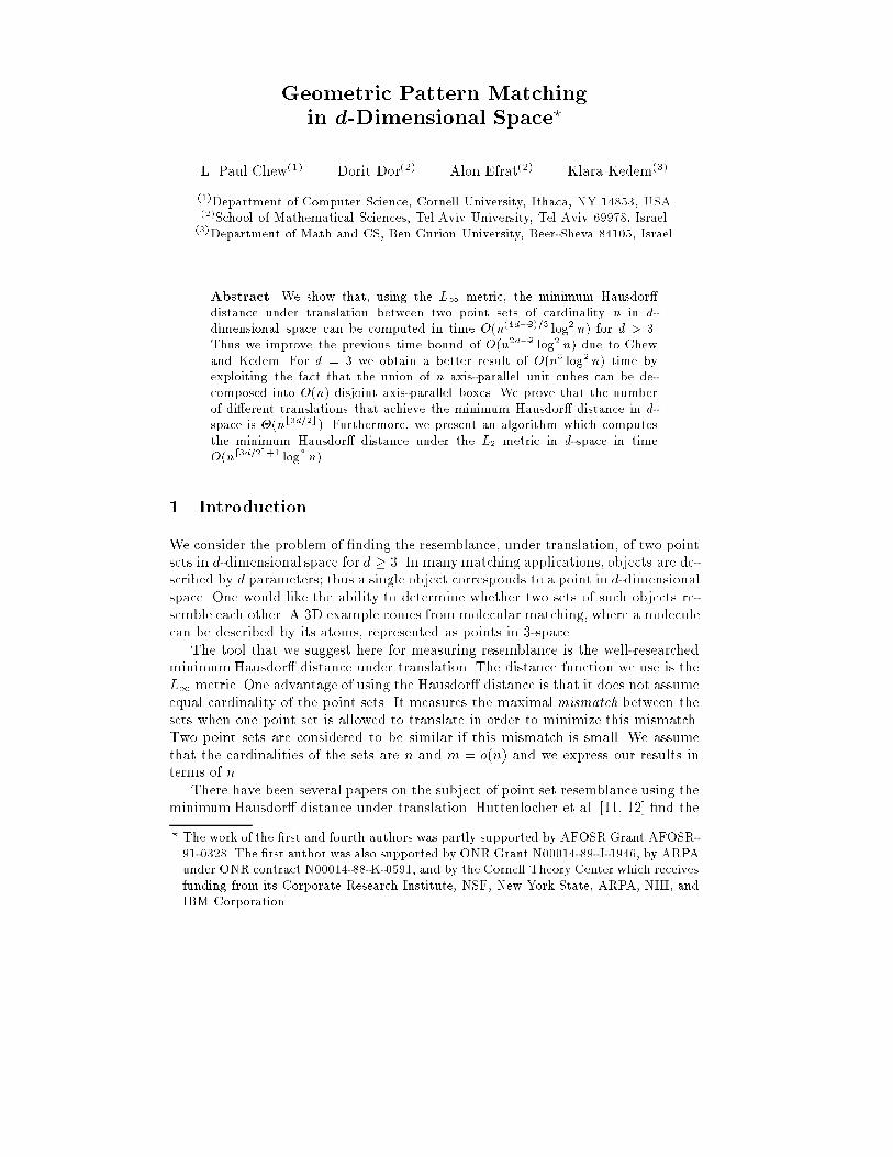
7 Combinatorial BoundsIn this section we show combinatorial results on the region (in translation space) oftranslations that minimize the Hausdor� distance between two point sets.Theorem7. Let L = fL1; : : : ;Lmg be a collection of layers in d-space where eachlayer Li is the union of n unit cubes and let T denote the intersection of the layers.Then the number of vertices of T is O(mdnbd=2c).Proof: Consider a vertex v of T . Vertex v must be the result of an interactionbetween d0 � d layers; this is because, in dimension d, no vertex can involve morethan d layers. Consider just the layers that interact to create v and call this set oflayers L0.We claim that v, a vertex of the intersection of the layers of L0, is also a vertexof the union of the layers of L0. For v not to be a vertex of the union it would haveto be hidden by a cube in some layer, say Li 2 L0. But if this were the case then, bythe way L0 was de�ned, layer Li could not possibly have interacted with the otherlayers of L0 to create v in the �rst place. Thus, each vertex of T is also a vertex ofa union of (� d) layers.The bound now follows from some simple counting. There are O(md) possiblesets of layers where the cardinality of each set is � d. Each such set of layers containsO(dn) cubes. As mentioned above, a recent result of [4] states that the union of Nunit boxes in d-space has complexityO(N bd=2c). We multiplyO(md) by O((dn)bd=2c)(and note that factors involving only d can be treated as constant and absorbed intothe big-O notation) to get the bound in the theorem. 2Note that the bound of O(mdnbd=2c) on the number of vertices of T also bounds,under general position assumption, the complexity T , and the number of connectedregions of T . For our problem m = n, thus the upper bound on the number oftranslations is O(nb3d=2c). We now turn to present a construction that shows a lowerbound on the number of translations.Theorem8. Let L be de�ned as in Theorem 7. Then the number of connected com-ponents in T = \iLi is (nb3d=2c).Proof: Our construction extends an earlier construction due to Rucklidge [18] thathe developed for the two-dimensional case. We �rst show how we can construct(n3) connected components in T for d = 2. We de�ne an i-corridor as a regionenclosed between two stairs of (2-dimensional) cubes as shown in Figure 7(a), whenthe cubes are all of the color i, and each step of the \stairs" is of size �, when � isa very small positive �xed parameter (depends on n), to be determined later. Eachi-corridor is generated by 2n cubes, and hence has n stairs.We generate n corridors, each of a di�erent color, using two batches of n=2corridors. The i-th corridor in the �rst batch is generated by a shift of i�0 of thebase corridor (in both x and y directions). The second batch, whose colors arei = n=2 + 1; : : : ; n, is generated by translating the �rst batch by �=2 in both x andy directions (see Figure 7(b)).Note that each corridor of one of the batches intersects each corridor of theother batch in (n) intersection points, yielding (n) connected regions in the

(b) (a)Fig. 1. Lower bound constructioninterior of these two corridors. Let S denote the set of (colored) cubes that de�nethese corridors. Note also that every point in the neighborhood of the corridors, butoutside all corridors in covered by all n colors in S. Hence there are (n3) connectedregions of the intersection of all cubes generated these corridors.We now show how to generate O((n3)k) connected regions in 2k-space. Let S bethe set of cubes as above. Given kn colors we denote by Sji a set of cubes whichis identical to the original set S but the colors of the cubes are (i � 1)n+ 1; : : : ; ininstead of 1; : : : ; n. In 2k-space we de�ne k sets S1; : : : ; Sk of jSj cubes each suchthat the projection of Si on the 2i � 1 and 2i axes is identical to Sji. The other2(k � 1) coordinates of the centers of the boxes in Si, are zero. The colors of thecubes in Si and Sj 6=i, are disjoint.Our claim is that the corridors de�ned by S1; : : : ; Sk introduce ((n3)k) con-nected components in the region covered all kn colors. To verify this claim, letXj1;:::;jk = (x1; x2; : : : ; x2k�1; x2k) be a 2k-dimensional point where (x2i�1; x2i) isa (two-dimensional) point in the ji-th connected regions of S and where 1 � ji �(n3). Let X 0 = Xj01;:::;j0k and X 00 = Xj001 ;:::;j00k be two di�erent points and let idenote an index such that j0i 6= j00i (this is well de�ned as X 0 and X 00 are di�erent).Let Ci = (i � 1)n + 1; : : : ; in be the set of colors in Si. Consider a line l (in the2-space) that connects the projection of X 0 and X 00 on coordinates 2i � 1 and 2i.The endpoints of l (namely the projections of X 0 and X 00) are not covered be exactlytwo colors from Ci. By de�nition of S, there is a point on l which is covered by allcolors of Ci. Hence, X 0 and X 00 could not possibly be on the same connected regionand this implies ((n3)k) regions (each corresponds to a selection of ji's). 2The bound we presented above showed that there can be O(nb3d=2c) translationst that minimize the one-way Hausdor� distance, but can be easily generalized tobound the two-way Hausdor� distance as well.Remark. The proof above generalizes with small changes to non-congruent cubes andto balls (the L2 norm). If the cubes de�neding L are not congruent then the boundwe get in Theorem 8 is larger - �(nd3d=2e). This is because for d = 1 the numberof translations is �(n2). Similarly, if each Li above is the union of d-dimensionalballs, then using the standard lifting transformation � : Rd ! Rd+1 de�ned by�((x1; : : : ; xd)) � (x1 : : : ; xd; x21 + : : : + x2d) their union can be expressed as thelower envelope of n hyperplanes in the (d + 1)-space, which by [8] has complexityO(nd(d+1)=2e). Plugging this into the above proof shows:

Theorem9. Let L = fL1; : : : ;Lmg be a collection of layers, where each layer Li isthe union of n cubes of arbitrary size. Then the complexity of \iLi is O(mdndd=2e).The same bound holds in the case that each Li is the union of n balls.8 Using the L2 NormIn this section let A and B be two sets of n points in d-space, for d � 4 and letH2(A;B) denote the Hausdor� Distance between them when L2 is the underlyingmetric. We have the following algorithmic result. (Note that [11, 12] presented analgorithm for this problem in 3-space with time O(n5+") for any " > 0.)Theorem10. Let A and B be as above. A translation t that minimizes H2(A; t+B)can be found in expected time O(nd3d=2e+1 log3 n).Proof: Due to space limitations we present only a brief sketch of the proof here.As in the L1 case, we develop an algorithm for the Hausdor� decision problem andthen combine it with the parametric search paradigm of Megiddo [15] to create analgorithm for �nding the minimum Hausdor� distance.To solve the decision problem, we show that there are just O(nd3d=2e) criticalpoints that are potential candidates for vertices of regions with color-depth n. Ourcounting method is analogous to that used in the proof of Theorem 7.Each such critical point must be tested to see if it is covered by all the colors. Todo this we use a result of [14] to build in time O(ndd=2e logO(1) n) a data structure ofsize O(ndd=2e logO(1) n) which can answer a coverage query in time O(logn). Initially,it looks as though such a data structure is needed for each color, but since the set ofspheres for one color is just a translation of the set of spheres for each other color, wereally need just one copy of this data structure. A single critical point must be testedfor every color taking time O(n logn). Thus the total time for solving the Hausdor�decision problem is O(nd3d=2e+1 logn). The extra log factors in the theorem are dueto the overhead of using parametric search to solve the corresponding optimizationproblem. 29 Open Problems� Are L1 Hausdor� decision problems inherently easier than the ones for L2? Isthere a single technique that solves both types of problems e�ciently.� Given a d-dimensional box C and n boxes G1; : : : ; Gn lying inside C, is it possibleto determine if [n1Gi = C in time o(nd=2)? Finding such a technique wouldimmediately improve the running time of our L1 algorithm.� Finally, our techniques do not take advantage of the fact that the set of cubesfor one color is really just a translation of the set of cubes for each other color.Is there some way to use this information to design a better algorithm?Acknowledgments.We would like to thank Micha Sharir for useful discussions and help in the proof of Theo-rem 7. Thanks also to Reuven Bar-Yehuda for contributing to the algorithm of Section 4.

References[1] P. K. Agarwal, B. Aronov and M. Sharir, Computing Envelopes in Four Dimen-sions with Applications, Proc. 10th Annual ACM Symposium on ComputationalGeometry 1994, 348{358.[2] P. K. Agarwal, M. Sharir and S. Toledo, Applications of Parametric Searchingin Geometric Optimization, Proc. 3rd ACM-SIAM Symposium on Discrete Algo-rithms, 1992, 72{82.[3] N. M. Amato, M. T. Goodrich and E. R. Ramos, Parallel Algorithms for Higher-Dimensional Convex Hulls, Proceedings 6 Annual ACM Symposium on Theory ofComputing 1994, 683{694.[4] J. Boissonnat, M. Sharir, B. Tagansky and M. Yvinec, Voronoi Diagrams inHigher Dimensions under Certain Polyhedral Distance Functions, Proc. 11th An-nual ACM Symposium on Computational Geometry 1995, 79{88.[5] H. Br�onnimann, B. Chazelle and J. Matou�sek, Product Range Spaces, Sensi-tive Sampling, and Derandomization, Proc. 34th Annual IEEE Symposium onthe Foundations of Computer Science 1993, 400{409.[6] B. Chazelle, H. Edelsbrunner, L. Guibas and M. Sharir, A Singly ExponentialStrati�cation Scheme for Real Semi{algebraic Varieties and Its Applications, The-oretical Computer Science 84 (1991), 77{105.[7] L.P. Chew and K. Kedem, Improvements on Geometric Pattern Matching Prob-lems, Algorithm Theory { SWAT '92, edited by O. Nurmi and E. Ukkonen, LectureNotes in Computer Science #621, Springer-Verlag, July 1992, 318{325.[8] H. Edelsbrunner, Algorithms in Combinatorial Geometry, Springer-Verlag, Hei-delberg, Germany, 1987.[9] A. Efrat and M. Sharir, A Near-linear Algorithm for the Planar Segment CenterProblem, Discrete and Computational Geometry, to appear.[10] G.N. Frederickson and D.B. Johnson, Finding kth Paths and p-Centers by Gen-erating and Searching Good Data Structures, Journal of Algorithms, 4 (1983),61{80.[11] D.P. Huttenlocher and K. Kedem, E�ciently Computing the Hausdor� Distancefor Point Sets under Translation, Proceedings of the Sixth ACM Symposium onComputational Geometry 1990, 340{349.[12] D.P. Huttenlocher, K. Kedem and M. Sharir, The Upper Envelope of VoronoiSurfaces and its Applications, Discrete and Computational Geometry, 9 (1993),267{291.[13] J. Matou�sek, Reporting Points in Halfspaces, Comput. Geom. Theory Appls. 2(1992), 169{186.[14] J. Matou�sek and O. Schwarzkopf, Linear Optimization Queries, Proc. 8th AnnualACM Symposium on Computational Geometry 1992, 16{25.[15] N. Megiddo, Applying Parallel Computation Algorithms in the Design of SerialAlgorithms, J. ACM 30 (1983), 852{865.[16] M. Overmars and C.K. Yap, New Upper Bounds in Klee's Measure Problem,SIAM Journal of Computing, 20:6 (1991), 1034{1045.[17] F.P. Preparata and M.I. Shamos, Computational Geometry, Springer-Verlag, NewYork, Berlin, Heidelberg, Tokyo, 1985.[18] W. Rucklidge, Lower Bounds for the Complexity of the Hausdor� Distance, Proc.5th Canadian Conference on Computational Geometry 1993, 145{150.[19] W. Rucklidge, Private Communication.[20] R. Seidel, Small-dimensional Linear Programming and Convex Hulls Made Easy,Discrete and Computational Geometry, 6 (1991), 423{434.

AppendixThe operations for inserting a cube q into, or deleting q from a leaf-cell C� are done by theprocedures Insert to Leaf and Delete from Leaf. They have the side e�ect of updatingthe �eld Active�. In addition, they return jcolors(Active�)j if there is a point in C� coveredby all colors of Active�, or 0 otherwise. The following procedures update the Active �eldin each node of T , and the depth �elds of the leaves of T .Insert To Active(q; �)if q is disjoint to C� then return ;if � is a leaf thendepth� Insert to Leaf(q; �);else /* � is an internal node */if q does not cover C� completely thenInsert To Active(q;�left) ; Insert To Active(q;�right)else /* q covers C� completely */if color(q) in Active� or in Active�; � an ancestor of � then returnelse /* No ancestor of � is covered by color(q) */insert color(q) into Active�for every descendant � of �if � is an internal node and color(q) 2 Active� thendelete color(q) from Active�if � is a leaf thenfor every q0 of color color(q) in Active�set Depth� Delete from Leaf(q0; �)Delete From Active(q; �)if q is disjoint to C� then return ;if q partially covers C� and � is an internal node thenDelete From Active(q;�left) ; Delete From Active(q;�righ)else if � is a leaf thenDepth� Delete from Leaf(q; �)else /* � is an internal node, covered completely by q */if no ancestor of � contains color(q) in its Active list thenrecover(color(q); �)else /*No such ancestor exists */returnRecover (color(q); �)if color(q) 2 L TOT� thenif � is an internal node thenInsert color(q) into Active�returnelse /* � is a leaf containing cubes of color(q) in L TOT� */for each box q0 of color color(q) in L TOT�Depth� Insert to Leaf(q0; �)else /* no box of color color(q) in Active� */if � is an internal node thenRecover(color(q);�left) ; Recover(color(q);�right)This article was processed using the LaTEX macro package with LLNCS style