genotype x environment interaction and stability analysis of ...

T.R.

NİĞDE ÖMER HALİSDEMİR UNIVERSITY

GRADUATE SCHOOL OF NATURAL AND APPLIED SCIENCES

DEPARTMENT OF AGRICULTURAL GENETIC ENGINEERING

GENOTYPE X ENVIRONMENT INTERACTION AND STABILITY ANALYSIS OF

POTATO BREEDING LINES

ERIC KUOPUOBE NAAWE

September 2020

NIĞ

DE

ÖM

ER

HA

LIS

DE

MIR

UN

IVE

RS

ITY

GR

AD

UA

TE

SC

HO

OL

OF

NA

TU

RA

L A

ND

PP

LIE

D S

CIE

NC

ES

M

AS

TE

R T

HE

SIS

E

. K

. N

AA

WE

, 2020

T.R.

NĠĞDE ÖMER HALĠSDEMĠR UNIVERSITY

GRADUATE SCHOOL OF NATURAL AND APPLIED SCIENCES

DEPARTMENT OF AGRICULTURAL GENETIC ENGINEERING

GENOTYPE BY ENVIRONMENT INTERACTION AND STABILITY ANALYSIS

OF POTATO BREEDING LINES

Eric Kuopuobe NAAWE

Master Thesis

Supervisor

Prof. Dr. Mehmet Emin ÇALIġKAN

September 2020

The study titled “Genotype by Environment Interaction and Stability Analysis of Potato

Breeding Lines” and presented by Eric Kuopuobe NAAWE under the supervision of Prof.

Dr. Mehmet Emin ÇALIŞKAN has been accepted as Master of Science thesis by the jury

at the Department of Agricultural Genetic Engineering of Niğde Ömer Halisdemir

University, Graduate School of Natural and Applied Sciences.

Head : Prof. Dr. Mehmet Emin ÇALIŞKAN, Niğde Ömer Halisdemir

University, Ayhan Şahenk Faculty of Agricultural Sciences and Technologies,

Department of Agricultural Genetic Engineering

Member : Assoc. Prof. Dr. Ufuk DEMİREL, Niğde Ömer Halisdemir University,

Ayhan Şahenk Faculty of Agricultural Sciences and Technologies, Department of

Agricultural Genetic Engineering

Member : Assist. Prof. Dr. Necmi BEŞER, Trakya University, Faculty of

Agriculture, Department of Genetics and Bioengineering

CONFIRMATION:

This thesis has been found appropriate at the date of 21/09/2020 by the jury mentioned

above who have been designated by Board of Directors of Graduate School of Natural

and Applied Sciences and has been confirmed with the resolution of Board of Directors

dated …./…./2020 and numbered ……………

/ /2020

Prof. Dr. Murat BARUT

DIRECTOR

iv

SUMMARY

GENOTYPE BY ENVIRONMENT INTERACTION AND STABILITY ANALYSIS

OF POTATO BREEDING LINES

NAAWE, Eric Kuopuobe

Nigde Omer Halisdemir University

Graduate School of Natural and Applied Sciences

Department of Agricultural Genetic Engineering

Supervisor :Prof. Dr. Mehmet Emin ÇALIġKAN

September 2020, 110 pages

This study was conducted in 2019 to evaluate genotype by environment interaction

(GEI) and stability analysis of twelve potato breeding lines and three standard cultivars

in three different environments in respect to yield and quality traits. Finlay and

Wilkinson's regression model, and Additive Main Effects and Multiplicative

Interactions (AMMI) analysis were used to evaluate GEI and stability of potato

genotypes. There were highly significant (p≤ 0.01) effects of genotype (G), environment

(E) and GEI on yield and quality traits of potato genotypes tested. The breeding line

MEÇ1407.17 gave the maximum yields of 967.0 g/plant, 41.77 t/ha and 41.60 t/ha

while Russet Burbank produced the lowest yields of 400.8 g/plant, 17.04 t/ha and 16.66

t/ha for total plant yield, total tuber yield and marketable tuber yield, respectively. The

breeding lines gave higher dry matter content and specific gravity than standard

cultivars. The highest dry matter content (25.6%) and specific gravity (1.106) were

obtained from the breeding line of MACAR1402.10 while Agria gave the lowest values

of 19.15% and 1.076. Sivas location was the best environment in terms of tuber yield.

The breeding lines MEÇ1407.17, MEÇ1407.05, MEÇ1407.08 and MEÇ1411.06 were

identified as candidate cultivars due to their high tuber yield and stable performances

across different environments.

Keywords: Potato, cultivar breeding, adaptation, AMMI, Finlay and Wilkinson

v

ÖZET

PATATES ISLAH HATLARININ GENOTĠP X ÇEVRE ĠNTERAKSĠYONU VE

STABĠLĠTE ANALĠZĠ

NAAWE, Eric Kuopuobe

Niğde Ömer Halisdemir Üniversitesi

Fen Bilimleri Enstitüsü

Tarımsal Genetik Mühendisliği Anabilim Dalı

DanıĢman : :Prof. Dr. Mehmet Emin ÇALIġKAN

Eylül 2020, 110 sayfa

Bu çalıĢma, oniki patates ıslah hattı ve üç standart çeĢidin verim ve kalite özellikleri

açısından üç farklı çevredeki genotip-çevre interaksiyonu (GEI) ve stabilite analizlerini

yapmak amacıyla 2019 yılında yürütülmüĢtür. Patates genotiplerinin GEI ve

stabilitelerini belirlemek için Finlay ve Wilkinson'un regresyon modeli ile Eklemeli Ana

Etkiler ve Çarpımsal Ġnteraksiyonlar (AMMI) analizi kullanılmıĢtır. Denemeye alınan

patates genotiplerinin verim ve kalite özellikleri üzerine genotip, çevre ve GEI'nun çok

önemli (p≤0.01) etkilerinin olduğu belirlenmiĢtir. MEÇ1407.17 ile sırasıyla bitki

verimi, toplam yumru verimi ve pazarlanabilir yumru verimi açısından en yüksek

değerleri verirken, aynı özellikler açısından en düĢük değerler sırasıyla ile standart

Russet BurbankçeĢidinden elde edilmiĢtir. Denemeye alınan tüm ıslah hatları standart

çeĢitlere göre daha yüksek kuru madde oranı ve özgül ağırlık değerlerine sahip

olmuĢlardır. Ortalama en yüksek kuru madde oranı (%25.6) ve özgül ağırlık (1.106)

elde edilirken, her iki özellik açısından en düĢük değerler sırasıyla %19.5 ve 1.076 ile

standart Agria çeĢidinden elde edilmiĢtir. Yumru verimi açısından Sivas lokasyonu en

iyi çevre olarak belirlenmiĢtir. Islah hatları MEÇ1407.17, MEÇ1407.05, MEÇ1407.08

ve MEÇ1411.06 tüm çevrelerdeki yumru verimi ve stabil performansları nedeniyle

ümitvar çeĢit

Anahtar Sözcükler: Patates, çeĢit ıslahı, adaptasyon, AMMI, Finlay ve Wilkinson

vi

ACKNOWLEDGMENTS

With a grateful heart, I sincerely thank and appreciate to my supervisor, Prof. Dr. Mehmet

Emin ÇALIŞKAN, for his immense and kind support, guidance, and unreserved

admonishment since my arrival in Turkey and during the period of my studies. His kind-

hearted actions radiated to all members of Potato Group toward me, which made me truly

enjoyed every moment of my stay here a memorable one and made my research an

enjoyable one.

I heartily thank and appreciate the Ayhan Şahenk Foundation for their generous financial

support during my master studies.

I deem it a pleasure to render my profound gratitude to the members of my thesis defense

committee; Assoc. Prof. Dr. Ufuk DEMİREL and Assist. Prof. Dr. Necmi BEŞER whose

immeasurable comments helped improve the scientific quality of this thesis.

I once again render my appreciation to all members of Potato Group. I greatly thank every

one of you for your individual and collective contributions, guidance and support you

offered me during the period of studies and research, I acknowledged you all.

I hail and thank my parents; Mr. Cyprano NAAWE (my father of blessed memory), my

mother Mrs. Agnes NAAWE, and my brothers; Rev Br. Aloysius POREKUU and

Emmanuel NAAWE for the love, care, moral training and discipline, sacrifice, and

support and encouragement with prayers you gave me which made me come to this stage

in life. The Abagale’s and Kandilige’s families, I thank you for taking and supporting me

as your own child during my undergraduate studies and my period of my national service.

I thank all the lecturers and staff of the Department of Agricultural Genetic Engineering

and all staff and members of the Faculty of Agricultural Sciences and Technologies for

their individual and collective support and mentorship. God richly bless you and all who

have played a role in making me complete this thesis.

vii

1TABLE OF CONTENTS

SUMMARY ............................................................................................................... IV

ÖZET ........................................................................................................................... V

ACKNOWLEDGMENTS .......................................................................................... VI

TABLE OF CONTENTS .......................................................................................... VII

LIST OF TABLES ..................................................................................................... IX

LIST OF FIGURES .................................................................................................. XIX

SYMBOLS AND ABBREVIATIONS ............................................................... XVXVI

CHAPTER I INTRODUCTION ....................................................................................1

CHAPTER II ................................................................................................................5

REVIEW OF LITERATURE ........................................................................................5

2.1. Biology Of Potato ...................................................................................................5

2.2. Taxonomic and Genetic Diversity of Potato ............................................................5

2.3 Origin and History of Potato ....................................................................................7

2.4 Potato in Turkey- Past and Present ...........................................................................8

2.5 Production Trend of Potato ......................................................................................9

2.6 Quality Traits of Potato .......................................................................................... 10

2.7 Genotype by Environment Interactions in Potato ................................................... 13

2.8 Yield Stability ........................................................................................................ 19

2.9 Model use in Genotype by Environment Interaction Analysis ................................ 19

CHAPTER III ............................................................................................................ 21

MATERIALS & METHODS ...................................................................................... 21

3.1 Plants Materials ..................................................................................................... 21

3.2 Experimental Method ............................................................................................ 21

3.2.1 Site selection and location ............................................................................ 21

3.2.2 Experimental design and setup ..................................................................... 22

3.3.Evaluated Traits ..................................................................................................... 23

3.4 Statistical Analysis................................................................................................. 25

3.5 Finlay and Wilkinson model ................................................................................ 255

3.6 AMMI Analysis ..................................................................................................... 26

CHAPTER IV ............................................................................................................. 27

PC-1

Textbox

XIII

PC-1

Textbox

PC-1

Textbox

PC-1

Textbox

Vİ

PC-1

Textbox

PC-1

Textbox

XVI

PC-1

Textbox

PC-1

Typewriter

viii

RESULTS AND DISCUSSION ................................................................................ 277

4.1 Stand Establishment (SE) ..................................................................................... 277

4.2 Number of Stems per Plant (NSP) .......................................................................... 33

4.3 Plant Height ........................................................................................................... 37

4.4 Total Plant Yield .................................................................................................... 42

4.5 Total Tuber Yield (TTY) ....................................................................................... 47

4.6 Marketable Tuber Yield ......................................................................................... 52

4.7 Number of Tuber Per Plant .................................................................................... 57

4.8 Tuber Grading ....................................................................................................... 61

4.8.1 Big Tuber (> 50mm) Yield........................................................................... 61

4.8.2 Medium Tuber (30-50 mm) Yield .............................................................. 644

4.8.3 Small Tuber (< 30mm) Yield ....................................................................... 67

4.9 Marketable Tuber Weight (MTW) ......................................................................... 69

4.10 Dry Matter Content (%) ....................................................................................... 74

4. 11 Specific Gravity (SG) .......................................................................................... 78

4.12 Principal component analysis of variables ............................................................ 84

4.13 Spearman’s Correlation analysis between the parameters ................................... 866

4.14 Potato French fries ............................................................................................... 87

4.15 Potato Chips ........................................................................................................ 88

CHAPTER V CONCLUSION ..................................................................................... 90

REFERENCES............................................................................................................ 93

CURRICULUM VITAE.......................................................................................... 1108

ix

LIST OF TABLES

Table 3.1. List of genotypes and genotypes codes, and environment names and

Codes………………………………………………………………………21

Table 3.2. Average monthly rainfall and temperature for Konya, Nigde and Sivas in

2019……………………………………………………………………….22

Table 4.1. Analysis of variance of stand establishment (SE) for 15 potato genotypes

grown in three different environments…………………………………… 28

Table 4.2. AMMI analysis of variance of stand establishment (SE) for 15 potato

genotypes grown in three different environments…………………………28

Table 4.3. Two-way table of stand establishment (SE) for 15 potato genotypes grown in

3 different environments*…………………………………………………29

Table 4.4. Stability estimation of stand establishment (SE) of potato breeding lines

grown in three different environments. …………………………………...31

Table 4.5. Analysis of variance for the number of stems per plant (NSP) of 15 potato

genotypes grown in 3 different environments. ……………………………34

Table 4.6. AMMI analysis of variance for the number of stems per plant (NSP) of 15

potato genotypes grown in three environments. ………………………….34

Table 4.7. Two-way tables of the number of stems per plant (NSP) for 15 potato

genotypes grown in three different environments…………………………35

Table 4.8. Stability estimation of number of stem per plant of potato breeding lines


Table 4.9. ANOVA of plant height for 15 genotypes grown in three different

environments. …………………………………………………………….38

Table 4.10. AMMI analysis of variance for plant height (PH) of 15 potato genotypes

grown in three environments. …………………………………………….38

Table 4.11. Two-way table of plant height (PH) for 15 potato genotypes grown in three

different environments*……………………………………………………39

Table 4.12. Stability estimation of plant height of potato breeding lines grown in three

different environments…………………………………………………….39

x

Table 4.13. ANOVA of total plant yield for 15 genotypes grown in three different

environments. ……………………………………………………………...43

Table 4.14 AMMI analysis of variance for total plant yield TPY) of 15 potato genotypes

grown in three environments. …………………………………………….43

Table 4.15. Two-way table of total plant yield (TPY) for 15 potato genotypes grown in

three different environments*.……………………………………………44

Table 4.16. Stability estimation of total plant yield of potato breeding lines grown in

three different environments……………………………………………….45

Table 4.17. ANOVA of total tuber yield (TTY) for 15 genotypes grown in three

different environments. ……………………………………………………47

Table 4.18. AMMI analysis of variance for total tuber yield (TTY) of 15 potato

genotypes grown in three environments. …………………………………48

Table 4.19. Two-way table of total tuber yield (TTY) for 15 potato genotypes grown in

three different environments*……………………………………………...49

Table 4.20. Stability estimation of total tuber yield of potato breeding lines grown in

three different environments. …………………………………………….50

Table 4.21. ANOVA of marketable tuber yield (MTY) for 15 genotypes grown in three

different environments……………………………………………………53

Table 4.22. AMMI analysis of variance for marketable tuber yield (MTY) of 15 potato

genotypes grown in three environments. ………………………………….53

Table 4.23. Two-way table of marketable tuber yield (MTY) for 15 potato genotypes


Table 4.24. Stability estimation of marketable tuber yield of potato breeding lines

grown in three different environments…………………………………….55

Table 4.25. ANOVA of number of tubers per plant for 15 genotypes grown in three


Table 4.26. AMMI analysis of variance for number of tubers per plant (NTP) of 15

potato genotypes grown in three environments……………………………58

Table 4.27. Two-way table of tubers per plant (NTP) for 15 potato genotypes grown in

three different environments*……………………………………………...59

Table 4.28. ANOVA of big tuber (> 50mm) yield (number) for 15 genotypes grown in

three different environments……………………………………………….61

Table 4.29. AMMI analysis of variance of for big tuber (> 50mm) yield (number) for 15

potato genotypes grown in three environments……………………………62

xi

Table 4.30. Two-way table of big tubers (>50mm) yield (BTN) for 15 potato genotypes

grown in three different environments*…………………………………...63

Table 4.31. Two-way table of big tubers (>50mm) yield (BTN) for 15 potato genotypes

grown in three different environments*………………………………….64

Table 4.32. ANOVA of medium tuber (30-50mm) yield for 15 genotypes grown in three


Table 4.33. AMMI analysis of variance of medium tuber (30-50mm) yield for 15 potato

genotypes grown in three environments………………………………….65

Table 4.34. Two-way table of medium tuber (30-50mm) yield for 15 potato genotypes

grown in three different environments*.………………………………….66

Table 4.35 Stability estimation of the medium size tubers of potato breeding lines


Table 4.36. ANOVA for small tubers (<30mm) for 15 genotypes grown in three


Table 4.37. AMMI analysis of variance of small tuber size (<30mm) for 15 potato

genotypes grown in three environments…………………………………...67

Table 4.38. Two-way table of small tuber (<30mm) yield for 15 potato genotypes grown

in three different environments*………………………………………….68

Table 4.39. Stability estimation of the small tuber number (STN) of potato breeding

lines grown in three different environments………………………………69

Table 4.40. ANOVA of marketable tuber weight for 15 genotypes grown in three


Table 4.41. AMMI analysis of variance of MTW for 15 potato genotypes grown in three

environments………………………………………………………………71

Table 4.42. Two-way table of marketable tuber weight (MTW) for 15 potato genotypes

grown in three different environments*.………………………………….71

Table 4.43. Stability estimation of marketable tuber weight (MTW) of potato breeding

lines grown in three different environments. …………………………….74

Table 4.44. ANOVA for dry matter content (DMC) for 15 genotypes grown in three


Table 4.45. AMMI analysis of variance of dry matter content (DMC) for 15 potato

genotypes grown in three environments………………………………….74

Table 4.46. Two-way table of dry matter content (DMC) for 15 potato genotypes grown

in three different environments*………………………………………….76

xii

Table 4.47. Stability estimation of DMC of potato breeding lines grown in three

different environments. ……………………………………………………76

Table 4.48. ANOVA of specific gravity (SG) for 15 genotypes grown in three different

environments………………………………………………………………79

Table 4.49. AMMI analysis of variance of specific gravity (SG) for 15 potato genotypes

grown in three environments………………………………………………80

Table 4.50. Two-way table of specific gravity (SG), for 15 potato genotypes grown in

three different environments*………….………………………………......81

Table 4.51. Stability estimation of specific gravity of potato breeding lines grown in

three different environments. ………….………………………………….82

Table 4.52. Spearman correlation analysis between parameters….…………………....86

Table 4.53. ANOVA of French fries for 12 genotypes grown in three different

environments………………………………………...………………..........87

Table 4.54. AMMI analysis of variance of French fries (lightness l*) for 12 potato

genotypes evaluated in three environments……….……………………….87

Table 4.55. AMMI analysis of variance of French fries (redness a*) for 12 potato

genotypes Evaluated in three environments……………………………….88

Table 4.56. AMMI analysis of variance of French fries (yellowness b*) for 12 potato

genotypes evaluated in three environments……………………………….88

Table 4.57. Calorimetry assessment of potato chips for 12 genotypes grown in three


Table 4.58. AMMI analysis of variance of potato chips lightness (l*) for 12 potato

genotypes evaluated in three environments. ………………………………89

Table 4.59. AMMI analysis of variance of potato chips redness (a*) for 12 potato

genotypes evaluated in three environments……………………………….90

Table 4.60. AMMI analysis of variance of potato chips yellowness (b*) for 12 potato

genotypes evaluated in three environments ................................................ 90

xiii

LIST OF FIGURES

Figure 3.1. Martin Lishmans’s digital potato hydrometer (PW2050) used to

measurespecific gravity and dry matter content of potato crop. ............... 24

Figure 4.1. Relationship of genotype adaptation (regression coefficient ‘bi’) and mean

stand establishment (SE) of 15 potato genotypes grown in three diverse

environments. ......................................................................................... 32

Figure 4.2. AMMI biplot analysis of interaction principal component analysis (IPCA-

1) with mean of stand establishment of potato genotype evaluated across

three different environments ................................................................... 33

Figure 4.3 Relationship of genotype adaptation (regression coefficient ‘bi’) and the

mean number of stems per plant (NSP) of 15 potato genotypes grown in

three diverse environments……………………………………………….36

Figure 4.4 Biplot analysis of interaction principal component axis (IPCA-1) with

mean of stem number per plant (NSP) of potato genotype evaluated across

three different environments…………………………………………….37


plant height (PH) of 15 potato genotypes grown in three diverse

environments .......................................................................................... 41

Figure 4.6. AMMI biplot analysis of interaction principal component analysis (IPCA-

1) with mean of plant height (PH) of potato genotype evaluated across

three different environments. .................................................................. 42


total plant yield (TPY) of 15 potato genotypes grown in three diverse

environments. ......................................................................................... 45

Figure 4.8. Biplot analysis of interaction principal component axis (IPCA-1) with

mean of total plant yield (TPY) of potato genotype evaluated across three

different environments. ........................................................................... 46


total tuber yield (TTY) of 15 potato genotypes grown in three diverse

environments. ......................................................................................... 51

xiv

Figure 4.10. AMMI biplot analysis of interaction principal component axis (IPCA-1)

with mean of total tuber yield (TTY) of potato genotype evaluated across



marketable tuber yield (MTY) of 15 potato genotypes grown in three

diverse environments. ............................................................................. 56


with mean of marketable tuber yield (MTY) of potato genotype evaluated

across three different environments ......................................................... 57


number of tubers per plant (NTP) of 15 potato genotypes grown in three

diverse environments .............................................................................. 60


with mean tubers per plant (NTP) of potato genotype evaluated across



marketable tuber weight (MTW) of 15 potato genotypes grown in three

diverse environments .............................................................................. 73


with mean marketable tuber weight (MTW) of potato genotype evaluated

across three different environments. ........................................................ 73


number of dry matter content (DMC) of 15 potato genotypes grown in

three diverse environments. ..................................................................... 77


with mean of dry matter concentration (DMC) of potato genotype

evaluated across three different environments…………………………78


specific gravity (SG) of 15 potato genotypes grown in three diverse

environments .......................................................................................... 83


with mean of specific gravity (SG) of potato genotype evaluated across

three different environments ................................................................... 83

xv

Figure 4.21. Scree plot of eigenvalues against pca with cumulative variability (%) for

GEI of the studied traits, where F1 to F12 indicates IPCA1 to IPCA12. .. 84

Figure 4.22. PCA1 and PCA2 biplot of genotype by environment interaction (GEI)

relationship of the variables in the three different environments. ............. 85

xvi

SYMBOLS AND ABBREVIATIONS

Symbols Description

AMMI Additive main effect and multiplicative interaction

BTN Big tuber number

CV Coefficient of variation

DF Degree of freedom

DMC Dry matter concentration

E Environment

FAO Food and agricultural organization

G Genotype

GEI Genotype by environment interaction

GLM Generalized linear model

IPC Interaction principal component

LSD Least significant difference

MTW Marketable tuber weight

MTY Marketable tuber yield

MTN Medium tuber number

NSP Number of stem per plant

NTP Number of tuber per plant

PH Plant height

pH power of hydrogen proton

SE Stand establishment

SG Specific gravity

STN Small tuber number

TPY Total plant yield

TTY Total tuber yield

USDA United State Department of Agriculture

% Percentage

°C Degree centigrade

1

CHAPTER I

2INTRODUCTION

The current global population growth and the glaring effects of climate change behoves

on plant breeders and agronomists to work assiduously to identify high yielding, and

stable crop varieties to meet the food security and nutritional needs of human life.

Population growth and its counterparts; industrialization and urbanization are drastically

reducing arable lands, degrading the fertile agricultural fields, diversification of agro-

zones, establishment of intra-climate modification, and make it difficult for cultivated

crops to adopt and give high and stable yield (Islam and Karim, 2020). Plant breeders

and agronomists need to keep pace with this trend of rising in population and climate

change at all costs to sustain life through the breeding of high yielding and stable crop

genotype.

Potato (Solanum tuberosum L) is a vital annual tuber crop of the Solanaceae family which

is ranked the 1st and 3rd most important tuber and food crop respectively on a global

scale per human consumption (Devaux et al. 2014), and is cultivated in over 100 countries

for its nutritional value. The global production increased from 267 million metric tonnes

to about 374.5 million metric tonnes since 1983, with approximately 19.25 million

hectares of cultivated land area. The Solanum genus is one of the 98 genera of the

Solanaceae family of which potato is the most important non-grain crop with

approximately 5000 cultivated species. Potato is rich in carotenoids, flavonoids, caffeic

acid, Vitamin A, B6, and C, carbohydrates (Ezekiel et al., 2013) and antioxidant

properties which help in digestion, heart health, blood pressure maintenance, lower risks

of stroke, brain function, and nervous system coordination. It is used in various ways such

as French fries, chips, dehydrated potatoes, freshly used products, and alcohol production.

Food security is a global issue and no country has escaped the zone of food insecurity

despite its level of development. It is defined as the access to sufficient, safe, and

nutritious food always physically, socially, and economically to meet the dietary needs

and food preferences for active and healthy living (Gibson, 2012). The diverse golden

benefits of potato, its high yield per unit area than cereals and other major crops (Miheretu

et al., 2014) including its diverse agronomic and climatic features led to its diversified

2

distribution in the temperate, subtropical and the Mediterranean zones from Peru (centre

of origin) in the South American continent. This triggered global interest and the

recommendation of the International Potato Center (CIP), the Food and Agriculture

Organization of the United Nations (FAO), and food processing industries have taken a

keen interest and acting as the major driving force behind the growth of the potato

cultivation and market (Floros et al., 2010), as food security, poverty alleviation, and

global health improvement crop (FAO, 2017). This has projected the crop average

production growth rate (CAPGR) at 1.06% during the 2019-2024 forecast period (FAO

2017) with competing production efforts among nations including Turkey in recent times

which increase potato demand and consumption.

The rise in population along with climate change has diversified agro-ecological zones in

the world which affect the biological and physiological yield performance of crops (Raza

et al., 2019) making adaptation very difficult for crops (Onyango, 2019) due to

differences in traits, resistance and /or susceptibility (Dube et al., 2016; Di Vittorio et al.,

2016; Singh and Singh, 2017). Upon climate change, previously cultivated fields behave

and present themselves as different agro-zones (FAO, 2017) and so affecting crop

adaptation to the different agro-ecological environments (Nyahunda and Tirivangasi,

2019). Anthropogenic activities including other biotic and abiotic stresses induce soil

nutrient depletion hinder the progress of potato breeders, as the energy and efforts of

potato breeders do not reflect the yield output and so mitigating against the full realization

of potato yield and production to meet market demand (Kang et al., 2004; Voss-Fels et

al., 2019).

It is worthwhile for plant breeders to keep pace with these effects through the

sustainability of agriculture (Lammerts van Bueren et al., 2018) to identify strategies to

breach the production gap and realization of the potentials of potato to feed the ever-rising

global population. Agronomist and potato breeders in their role to feed the world has

employed genotype by environment interaction and stability analysis in their breeding

programs as a mechanism to produce new potato cultivars suitable for the diverse agro-

ecological conditions, adaptation, and yield stability levels created by climate change and

to meet global consumer demand and preference (Kivuva et al., 2014; Aliche et al., 2018).

3

Genotype by environment interaction (GEI) is a multifactorial phenomenon that leads to

the differential phenotypic expression of genotypes qualitatively and quantitatively

because of different environmental parameters and nutrient accessibilities (Kivuva et al.,

2014). The extent of response of a genotype to environmental fluctuation defines the

genotype as wide or specific adaptation, and the resilience of the genotype against

environmental fluctuation defines its stability. This phenomenon is a fundamental

principle in all fields of agriculture in the identification of desired, suitable, and stable

genotypes by reducing the association between phenotypic and genotypic values and

cause a natural selection of living organisms from one environment to another. GEI has

been employed in several crop breeding studies to facilitate selection and cultivar

certification which brings about suitable crop production, adaptation (Raymundo et al.,

2018; Ngailo et al., 2019), release and provision of the right cultivar and thus the study

of GEI and stability are never out of breeding programs. Though this delay certification

processes (Dwivedi et al., 2019; Rono et al., 2016), breeders can identify superior

cultivars, and the best environments for the crop cultivation This has necessitated this

research on potato in Turkey over diverse environmental locations to identify potato

breeding lines with broad (general) and specific adaptability before registration as a new

cultivar.

The analysis of GEI and stability parameters have been made feasible by the development

of several statistical tools and models. These statistical models and tools have been

employed in several crops including potato globally either singly, jointly or in comparison

with other models and tools. These evaluate and estimate the interaction and relationship

of crop genotype and environment (Hongyu et al., 2014) through regression coefficient

bi (Finlay and Wilkinson, 1963), the sum of squared deviations from regression S2di

(Eberhart and Russell, 1966), stability variance σ2 (Shukla, 1972), coefficient of

determination and coefficient of variability (Francis and Kannenberg, 1978) and stability

parameters of α′ and λ (Tai, 1971). These models include; general linear model (GLM)

procedure of SAS software, bilinear models (AMMI and GGE), GENSTAT software

among others to perform principal component analysis, ANOVA, regression on the mean,

and factorial regression models for the establishment of adaptability and stability analysis

of GEI.

4

Having said this, the aim of this research was to investigate the adaptability and stability

levels of different potato breeding lines through the yield performance analysis of the

genotype in different environments.

5

CHAPTER II

REVIEW OF LITERATURE

2.1 Biology of Potato

Potato (Solanum tuberosum L.) belonging to the Solanaceae family (nightshade) consists

of solitary or cymose inflorescence which have bisexual flowers, hermaphroditic

syncarpous, hypogynous, and diverse floral colours. The floral whorls consist of the

pentavalent calyx, corolla, and stamens with each united and valvate aestivated, and its

gynoecium is bi-pistillate with superior ovary. Potato is a self-pollination plant and can

also exhibit cross-pollination with mostly green berry or capsulate fruits, mostly green

with the axile type of placentation containing endospermous seeds of about 150 on

average. Its leaves are simple to pinnately compound, having net venations and of an

alternate breaching pattern.

Potato cultivation takes four to nine months from sowing to harvest, due to different

genotypic makeup and origin (Maresma et al. 2019) requiring temperatures of 15 to 20˚C,

pH of 4.8 to 8.5 for optimum yield and in diverse soil types leading to differences in

maturation period. Potato is mostly cultivated on ridges to prevent tubers exposure to light

which makes the tubers green; an indication of increased glycoalkaloids and solanine

levels, which are hazardous to human health (Chowański et al., 2016). The tubers are

underground swollen stems (rhizome or stolon), with auxiliary buds (eyes) which develop

into a new shoot and scaly leaves. The crop is propagated vegetatively by planting pieces

of tubers (botanical seeds) and from the sexually formed seeds. Its tubers are

morphologically oval to round, of about 20% dry matter and 80% water composition,

with varied flesh and skin colours, and sizes due to cultivar genetic makeup, agronomic

practices, soil type, location, temperature, maturity, postharvest storage types and

conditions.

2.2 Taxonomic and Genetic Diversity of Potato

Potato (Solanum tuberosum) is a genetically diverse plant in the Solanum with both

domesticated and wild types of about 1500 to 2000 species (Burton, 1989) with two

6

groups; tuber-bearing species (Petota section) and the non-tuber bearing species

(Etuberosa). Hawkes (1990) has also sub-grouped the tuber-bearing as Potatoe and

Estolonifera whiles the non-tuber-bearing as Etuberosa and Juglandifolia 228 species,

whiles Spooner and Hijmans (2001) outlined 196 species, and Spooner (2009) reported

110 species. Spooner et al. (2007) stated that 141 infra-specific taxa of potato exist within

the cultivated potato germplasm. In 2016, Spooner et al., added the S. tuberosum as a

member of the tuber-bearing potatoes and reported that, 232 wild species. The wide

variation in the wild species in the gene pool and distribution is an indication of high

tolerance to biotic and abiotic stresses (Machida-Hirano, 2015). Wang et al. (2017)

collected and identified 288 different species of potato using SSR and AFLP techniques

which indicated a high genetic diversity with different levels of biotic and abiotic stresses

resistance and adaptabilities.

Several taxonomic classifications of potato had been given which is blamed on

interspecific hybridization, sexual and asexual reproduction, species divergence, auto- or

allopolyploidy, phenotypic plasticity, high morphological similarity among species

among others (Spooner, 2009; Machida-Hirano, 2015). Machida-Hirano (2015), stated

that cultivated potato varieties are either landraces, native varieties, or improved varieties

with variety of tuber shapes, skin, and flesh colours (CIP, 2014) and grow within

elevations of 3000–4000m above sea level.

Potato is cytologically diploid (2n = 2x = 24), triploid (2n = 3x = 36), tetraploid (2n = 4x

= 48), pentaploid (2n = 5x = 60) or hexaploid (2n=6x=72) with a basic chromosome

number of 12 (Gavrilenko, 2007). While the diploid, tetraploid, and allohexaploids are

sexually fertile, the triploid and pentaploids are sexually sterile reproduced by vegetative

propagation. About 75% of the Solanum tuberosum species are the diploids which and

self-incompatible, the tetraploid 15% and the remaining are self-compatible, express

inbreeding depression and male sterility. (Watanabe, 2015). Spooner et al. (2007)

reclassified the cultivated potatoes as S. tuberosum (the Andigenum group consisting of

diploids, triploids, and tetraploids and the Chilotanum group consisting of lowland

tetraploid Chilean landraces); S. ajanhuiri (diploid); S. juzepczukii (triploid); and S.

curtilobum (pentaploid). The S. ajanhuiri (Hawkes, 1990, Spooner et al., 2007) is believed

to have originated through natural hybridization between diploid cultivars of S.

tuberosum (Andigenum group) and S. megistacrolobum. The S. juzepczukii traces its

7

origin the diploid cultivar of S. tuberosum L. Andigenum group, and S. acaule Bitter

(Rodríguez et al. 2010) whiles the S. curtilobum is from the tetraploid forms of S.

tuberosum L. Andigenum group (S. tuberosum subsp. andigenum) and S. juzepczukii

Bukasov (Hawkes, 1990; Rodríguez et al., 2010) are tolerance and cultivated in frost

affected areas within 4000m (Spooner et al., 2010) and content high glycoalkaloids with

a bitter taste and detoxified by freeze-drying for human consumption. The triploid S.

chaucha is naturally hybridized between S. tuberosum subsp. andigena and S.

stenotomum and the S. phureja (2n = 2x = 24) are identified as the short-day plant with

low tuber dormancy whereas S. stenotomum (2n = 2x = 24) the most primitive and first

domesticated potato from the diploid wild forms which is involved in the establishment

of other cultivated species Huamán and Spooner (2002) presented a revised classification

of S. tuberosum on morphological basis to possess eight cultivar groups as Ajanhuiri,

Andigenum, Chaucha, Chilotanum, Curtilobum, Juzepczukii, Phureja, and Stenotomum

and in 2007 Spooner et al., grouped it into four.

2.3 Origin and History of Potato

Potato origin is traced to the South-American continent in Peru and Bolivia, and its

domestication started between 800 and 500 BC by the Inca indigents (Spooner et al.,

2005) and its archaeological history date back to 2500BC (Harris et al., 2014). Their

distribution started in 1532 to Spain and later to major parts of the European continent in

the 1600s. Between 1600 and 1800s, the significance of potato rose and distributed

globally to its current regions with intensified cultivation and production. Potato initially

faced acceptance challenges in Europe with great suspicion as treat to human when it was

introduced, because they contain toxic substances such as the glycoalkaloids. It was

associated with leprosy or have narcotic agents (Kim and Lee, 2019) until it was

discovered as a food crop in Ireland in Europe and the North Americas around the end of

the 17th century. This discovery and climatic, soil suitability, the high yielding and

energy content of the crop per hectare more than other food crops speedily increase the

popularity of the potato for several societal and economic reasons. Its special great

influence on the rise in the Irish population has been associated to be the turning point

and today it is a global crop cultivated in over 100 countries and within latitudes 70° N

to 50° S at an altitude of 4,000 m from sea elevation (Çalışkan et al., 2010).

8

2.4 Potato in Turkey- Past and Present

The commercialized cultivation of potato (patates as in Turkish) in Turkey started around

1872, about 72 years since its introduction into the Anatolia region of the country from

the Russian Caucasus. From its introduction with some local varieties called ruskartoe,

potato cultivation and consumption has progressively grown till date, making the country

to become the second biggest producer of potato after Iran in the whole of the Middle

East's as of 2007. Nationwide, potato (patates) is second to tomatoes (domates) as a

horticultural crop grown in about 158 000 ha of land. The Anatolian region in Turkey

being the most important cultivation zone of the country, account for almost half of the

production area with intensive cultivation being conducted in the Aegean and

Mediterranean coasts. For a decade now, Nigde; located in the central parts of Turkey,

has become the best cultivation city of potato.

Turkey is currently ranked the 14th producer of potato globally with a cultivated area of

144,706 hectors as of 2016. Potato is roughly about 170 years in Turkey as it is stated to

have existed in the country during the 1850s. There exist records of the crop production

in the Erzurum province in the Anatolia region since the 1870s (Şenol, 1971; Çalışkan et

al., 2010). Reports had it that, the potato was introduced into Turkey through the Anatolia

region from Russia and Caucasia by several immigrants during the time. This is supported

by the fact that in the Eastern Anatolia region, potato still has a Russian name “kartol”.

During this time, the production of potato realized slow growth until after the

establishment of the Turkish Republic that saw production increasing massively in the

country (Çalışkan et al., 2010). The production increase from 73 thousand tonnes in 1925

to 4.5 million tonnes in 2010; about 61 times increase after 85 years. Çaliskan et al. (2010)

attributed this rise to the 1970 national potato project and the 1980s subsidization of the

private sector potato production by the government. It is stated that, coming down from

1999 to 2009, the area and production of potato cultivation declined by 35% and 28%

respectively.

In 2014, the area cultivation of potato in Turkey was 128 thousand ha accounting for a

yield of 4.1 million tonnes (Anonymous, 2014), of which a greater percentage of the

planting seeds are imported from about 16 different countries. Over the years, the Turkish

potato industry had relied on potato cultivation seeds from outside the country to supply

9

growing materials to potato farmers, this cost the country a lot of money. In 2016, through

a research project called “Turkey’s First National Potato Seed Production” by Turkey’s

Food, Agriculture and Livestock Ministry’s Potato Research Institute, led to the

registration of two varieties of the first domestically grown potato seeds; Fatih and

Onaran2015. Ozkaynak et al. (2018) research to develop virus tolerant potato varieties in

Turkey from 2008 to 2016, release 4 early and 3 main potato varieties with high

adaptation ability, high yield, and good quality characteristics to be used in commercial

and large-scale production in the country, including other sister countries. Similarly, the

Nigde Potato Research Institute has trademarked ‘Nahita’ a national potato variety and 7

other varieties in 2018 which were to be grown in 15 different countries and domestic

breeding companies in 2019. The goal of these along with several other researches

ongoing in the country is aimed to produce domestic planting seeds potato for the country

and cut down the dependence on imported seeds and varieties into the country.

2.5 Production Trend of Potato

The high calorie properties of potato per acre than other food crops as identified by the

Americans and Europeans when introduced from the West Andes have greatly improved

food security. This, coming to the knowledge of other continents is stated to be the leading

force for the population increase in the American and European territories since the 17th

century (Nunn and Qian, 2011; Lisiecka et al., 2019). The potato has thus become the

most important root crop globally and the 4th most grown crop overall making it the third

important food crop after wheat and rice. These reasons have led to a remarkable change

in global potato production, especially in Asia some decades ago, and uprising Africa.

America and Europe were the historical potato production and consumption zones where

per capita earnings, and consumption approaches hundreds of pounds such as in Poland,

Germany and Russia with relatively lower production and consumption in Asia and

Africa (Lisiecka et al., 2019). Potato growth and production had hence increased rapidly

than any food crop in Africa and Asia since the 1960s. In 2005, for the first time, the

combined potato production of Africa, Asia, and South America exceeded that of Europe

and the United States (de Haan and Rodriguez, 2016). And today, China, India, and

Russia are by far the largest producers in the world, with a national production output of

88, 45, and 30 million tons, respectively, registered in 2013, compared with 52, 19, and

9 million tons for the 28 member countries of the European Union, the United States, and

10

the centre of crop origin, respectively. Over 3 decades (1981–2011), the total potato

cropping area in the Americas and Oceania has remained stable. However, during that

period, Africa and Asia have seen staggering growth, with 300% and 237% increases in

total area. In contract, the cropping area in Europe halved during that period.

Now, high competition exists between America, Europe, the Asian countries, and other

developing nations with China dominating global production and consumption since 2010

(FAOSTAT, 2019; Lisiecka et al., 2019). In 2019, China lead the global potato

production with 93M tonnes followed India with 51M tonnes and Ukraine with 23M

tonnes, constituting about 45% of global production, while Turkey is placed 20th with

4.55M tonnes. These surpassed the then leading potato producing countries such as

Germany, the United States, Russia, and Poland, which is expected to continue in the

coming years (FAOSTAT, 2019). Other developing countries has joint hands with China

in the potato production and now at a minimum of 70% global production of potato with

a 1% annual growth rate in the developing countries and a 1% decrease in production in

the developed countries since 2010. This trend is due to governmental actions in the

developing countries aimed at boosting food security by promoting the cultivation and

consumption of potato especially by the Chinese Academy of Agricultural Sciences in

2015 whiles there is a progressive decline in potato production by acres area and farms

in the United States of about 2.9 million from the 1950s to 2015 in acres and about 36

million in farms from 1980s to 2012 (Lisiecka et al. 2019) but an increased in yield over

the years due to improving breeding technologies ( FAO, 2017).

2.6 Quality Traits of Potato

Potato quality traits are essential in breeding programs for agronomic and industrial

purposes. The quality of a potato cultivar is dependent on yield resilience and stability,

and the consumer acceptability of the tuber seeds by other breeders, and consumer

acceptability and preference (Halterman et al., 2016; Hameed et al., 2018). The

agronomic quality of potato is linked with consumer acceptability such as yield, dry

matter content, specific gravity, beta carotene content, reducing sugars, drought-tolerant,

pest and disease resistance, tuber shape, and eyes set in the determination of good potatoes

for breeding and the consumption market (Halterman et al., 2016).

11

Potato tuber quality is an important aspects of potato production, which biologically;

consider the proteins, carbohydrates, minerals concentrations, flavour, and texture and

industrially as tuber shape, cold sweetening, starch quality, and colour of the processed

product (Carputo et al., 2005). Potato quality is also categorised as external and internal

quality traits whose preference change with market specificities of which skin colour,

tuber size and shape, and eye depth forms the external traits, whiles nutrient, culinary,

after-cooking and or processing quality, dry matter content, flavour, sugar and protein

content, starch quality, type and amount of glycoalkaloids form the internal traits. Koch

(2018) reported that consumers on a general note, prefer tubers with a firm and smooth

skin without a hollow heart, no cracks or injuries, no protuberances, no recessed eyes or

stolon attachment and tuber sizes of 150-200g either for fresh or other industrial uses.

High phytochemical absorbance frequency is a very important quality trait (Koch, 2018),

which is a good source for several minerals in the diet (Andre et al., 2007; Subramanian

et al., 2011). Dry matter content (DMC) is very important in potato in chips and French

fry processing. Tubers with high DMC have fewer reducing sugars, good greasy texture

chips, low bitter pit diseases, and give high quality French fries and chips (Koch, 2018)

with low oil absorbance, and low acrylamides production in the production process.

Breeders prefer medium tuber seed with good growth vigour devoid of diseases and pests,

produce more stems.

Cultivar, time storage method, and agronomic practices affect potato quality.

Accordingly, different potato cultivars have different quality features such as tuber yield,

DMC, stem number per plant, and respond differently to mechanical stresses during

harvesting transportation, and tuber grading. This mechanical impact leads to

physiological weakness, cracks development, and reducing the sprouting potential of the

sowed tubers. The length of storage of the tubers also affects the germination of the tubers

as longer storage time reduces the germination potential of the tubers. It is recorded that,

field practices such as irrigation, weed control, mineral especially potassium, phosphorus

and nitrogen application have a great agronomic effect on the quality traits of potato. Lack

or delayed irrigation retard growth and time to tuber initiation of potato.

Potato cultivars have diverse agronomic features physically and chemically and so bred

for specific functional and nutritional traits valuable for breeders and the consumer

12

market, thus the agronomic and breeding classification of potato varieties are based on

features of the plant and tuber characteristics (Furrer et al., 2017). It has been reported

that vegetative features of potato are based on the number of stems per the plant, plant

height, leaf shape and number, branching-pattern and types, leaf and stem texture, and

the flower colour. The potato yield or tuber features for their characterization are

dependent on tuber shape, number of buds or eyes, skin texture, skin and flesh colour.

Physiologically, breeders focus on the maturation type, distribution of pigmentation,

disease resistance (Burton, 1989; Furrer et al., 2018), and the leaf senesces period.

Several parameters have been reported to affect potato tuber quality. Koch, 2018, in a

study of the effect of potassium and magnesium nutrition on potato tuber quality and plant

development, reported that; cultivar, agronomic practices, and type and time of storage

affect tuber quality. It is also stated that tuber handling during and after harvest might

cause mechanical injuries leading to tuber cracks and change in moisture content.

Agronomic practices are a key determinant of potato tuber quality as it encompasses

mineral nutrients such as potassium (K), nitrogen (N), phosphorus (P), water supply and

biotic interactions. Potato is sensitive to drought and water stress and closes its stomata

at low soil moisture deficits which leads to decrease photosynthesis and transpiration rates

compared to other agronomic crops. Due to the shallow root zones of potato, it requires

frequent water irrigation especially in areas of low soil water holding capacities and high

evapotranspiration. Water deficiencies in potato fields cause reduced leaf area and foliage

weight, dark cast and a wilted appearance which affect the photosynthetic frequency and

the distribution of photosynthetic assimilate to the tubers leading to heat stress, tuber

malformations, physiological disorders (brown centre, hollow heart, translucent end), and

bruise susceptibility.

Nitrogen is a principal component of protein and chlorophyll and thus plays a major role

in the growth, development as well as plant yield. Sandhu et al. (2014) reported that N

and P fertilizers are the most important nutrient for potato plants which maintain higher

haulm growth, tuber bulking, and high tuber number and dry matter production. Israel et

al. (2012) show that the highest marketable yield (35 t ha−1) was recorded with the

application of 165 kg ha−1 of nitrogen and 60 kg ha−1 of phosphorus. Thus, N and P

interaction influence marketable tuber of potato with an increase by 88% (Burtukan,

2016). Firew et al. (2016) in a research to determine the effect of nitrogen and phosphorus

13

on yield and yield components of potato under irrigation condition, stated that an

application of nitrogen and phosphorus influences the yield of potato. They observed the

highest yield at a rate of 56 kg ha−1 of nitrogen and 138 kg ha−1 of phosphorus application

but beyond these yields reduces.

Similarly, Wubengeda et al. (2016) in an experiment in to determine optimal irrigation

regime and NP fertilizer rate for potato found that yield of potato increase with increasing

application of nitrogen and phosphorus up to a maximum tuber yield of 31.80 tha−1 at

244 kg ha−1 and 206 kg ha−1 of nitrogen and phosphorus application rate respectively.

Desalegn et al. (2016) studied the effects of nitrogen and phosphorus fertilizer levels on

yield and yield components of potato and recorded the highest yield by 361% over the

control treatment from the combined rate of nitrogen and phosphorus 50/135 kg ha−1.

2.7 Genotype by Environment Interactions in Potato

GEI as the differential phenotypic output due to corresponding effects of genotypic and

environmental interactions which produce an array of phenotypes that fluctuate with

varying environments. Agronomist and plant scientists are conscious of the significant

flux in yield performance among cultivated crops in their research, due to interactions of

genes with the environment over years. This made crops cultivar to fluctuate in their

performance due to GEI and so impose a challenge in identifying superior cultivars

(Badu-Apraku et al., 2012; van Eeuwijk et al. 2016; Raza et al., 2019 Kwabena et al.

2019). It is stated that understanding the interaction of genotype and environment (G×E)

is important in achieving breeding objectives, identifying ideal test conditions,

recommend the best environment for optimal cultivar adaptation, and reduce. Kang et al.

(2004) stated that GEI is an ancient, universal principle that exist in all living organisms

and categorised GEI into two broad segments as crossover and non-crossover

interactions. It is stated that the significance of GEI is lost when the ranks of genotype

over several environments do not change and thus crossover and non-crossover GEI do

not exist.

Crossover interaction is the differential phenotypic output of cultivars to diverse

environments with a change in rank order between environments which is interpreted by

intersecting lines in the graphical display (Jalata, 2011; Adu, 2012; de Leon et al., 2016).

14

Crossover interaction is very vital for crop breeders as compared with non-crossover

interaction as it gives breeders information of specific adaptation and aids to assess the

interaction degree and frequency. It is non-additive and non-separable in nature, helps in

the development of locally adapted crop cultivars with known phenotypic sensitivity to

environments (Ortiz et al. 2007; Wolfe et al. 2015; Bustos-Korts, 2017). It established

that no genotype has a superior phenotypic output in all instances in a series of selection

over environments. Crossover interaction is the major hindrance in GEI due to

uncertainties in the traits of a cultivar and so needs series of investigations in different

environments (Cooper and Delacy 1994; Crossa et al. 2015; Muthoni et al. 2015). Yan et

al. (2007) state that cultivars with high and stable yields showing little GEI interactions

are the sole desire of breeders or agronomists which will lessen and save breeders time

and resources. Non-crossover interaction is observed when the phenotypic rank of one

genotype from one environment to another never cross as interpreted graphically by

parallel lines. There may be a change in the individual yield magnitude of the genotype

but not their superiority as the rank order of genotype across environments remains

unchanged. The genotypes are genetically heterogeneous whiles test environments maybe

homogeneous or genotype being genetically homogeneous while environments are

heterogeneous (Ortiz et al. 2007; Morley et al., 2016).

Eberhart and Russell (1966) outlined stratification of heterogeneous agro-zones into small

identical sub-zones with breeding programs aimed at specific sub-regions, and the

selection of genotype with broad environmental stability as methods of developing

genotypes with low G×E interaction. Crossa et al. (2015) classified these interactions into

qualitative and quantitative forms of GEI as essential in breeding potato genotypes with

specific adaptations. These are vital steps necessary for certification of breeding line with

their agro-zones specificities (Alberts, 2004) and have being implored in the study of G×E

interaction of potato and other crops (Biru, 2017), and is vital for heritability purposes

(Caliskan et al., 2007; Kaya and Akcura, 2014; Demirel et al., 2017). High GEI leads to

low heritability and so GEI emphasizes the need to breed exceptional genotype in

different environments (Carvalho et al., 2109). Genotype by environment has been

revealed to influence all stages of crop breeding (25 – 45% positively or negatively) as

this affect the partitioning of resources and the heritability of traits (Kaya and Akcura,

2014; Tiwari et al., 2019; Li et al., 2020). Thus, multi-environment testing of potato crop

reveals hidden traits of genotypes and help in the identification of specific and broad

15

adaptation of genotypes. Affleck et al. (2007) evaluated potato genotype in different

environment and stated that, the yield performance, stability and quality traits of genotype

vary with environment. They identified Russet Burbank and Umatilla Russet as low

yielding genotypes and good for both French fry colour and total sugars quality whiles

Cal White as stable and high yielding with average stability for French fry colour.

In 2017, Gurmu et al. found highly significant differences between evaluated traits in a

study to estimate the magnitude of G x E interactions on yield stability and quality traits

of sweet potato, whiles Ngailo et al. (2019) stated that GEI analysis is key for cultivar

selection, release, and the identification of suitable production and test environments. In

a study in Northwest China, to find the genetic variations of 26 potato genotype, Bai et

al. (2014) found genotype G4 (L02277) high yielding and stable genotypes, G1

(T200882), G8 (L022718), and G2 (CK0708) as medium yielding and generally stable,

and one mega-environment with several discriminating abilities among the environments.

Changing environments affect the genotypic expression of crops resulting in

inconsistencies in the phenotypic performance as genes are suppressed or expressed

phenotypically with different environmental features because of GEI. This leads to

cultivar segregation as manifested in changes in rank order of the genotype (crossover

GEI), or alterations in genotype performance without affecting the rank order (Muthoni

et al. 2015).

Day length is an agronomic factor that has a role in plant cultivation. Plants mostly inherit

the climatic and diurnal conditions of their place of origin, giving off their best in the

optimal conditions of their agro-zone of origin. Potato originating from the temperate

climate of short-day length and cool temperature, perform best under these conditions

(Porter and Semenov, 2005). Potato tuberization is induced by short days and prevented

by long days and tuber initiation is early at low temperatures but delayed at high

temperatures. Warm nights and long days’ yield few to no tuber yield. Potato tuber

formation can therefore be controlled in a greenhouse setup where photoperiod and

temperature conditions can be altered but somewhat a challenge in field conditions

(Pourazari et al., 2018; Kim et al., 2019). Temperature affect radiation use efficiency,

photosynthesis, tuber initiation, and development of potato. High temperature affects

photosynthesis of potatoes as optimal yield occurs at approximately 24°C and decreases

drastically at 30°C, reducing stomatal conductance, facilitate leaf senescence, and divert

16

source-sink rate due to interrupted photosynthesis (Lehretz et al.,2019). This it is reported

that metabolic and vegetative growth rates of potato slowed down while tuber

development increase cooler temperatures but experience cold shock at extremely low

temperatures. Optimum vegetative and reproductive growth of potato occur within 15 and

21°C where stolon initiation, tuber growth, dry matter content, and specific gravity are at

their best deposition, and photorespiration, light interception, radiation use efficiency also

at optimum rates. Unusual growth, multiple stolon formation, and abnormal tuber shape

and development occur outside these temperatures. Potato yield is lost at high night

temperatures due to reduced harvest index and delayed tuber induction, initiation of rapid

tuber growth which leads to reduce apportioning of photosynthetic materials (Struik,

2007; Kim and Lee, 2019).

Plants are sensitive to water at all growth periods which might vary with species and

cultivar. Too much water in a potato field is inhibitory to iron uptake resulting in

unhealthy growth and yellowing of the leaves of the plants and tuber rotting occurs,

leaching of nutrients, and spread of infections. This has been reported to cause potato

yield loss to 25%. Soil moisture is important for the tuber development of potato plants

during the growth cycles. It mitigates soil temperatures and results in uniform tuber sizes,

shapes, high yield, high specific gravity, and starch content and reduce the levels of

reducing sugars. Adequate moisture is needed for stolon initiation and tuberization which

ensures the maximum number of potential tuber initiation and increases yield potential.

Sprouting, flowering, tuber initiation and maturation, and early leaf senesces occur with

an inadequate water supply, and the longer the periods of drought or low soil moisture,

the higher the reduction in potato yield. Potato growth, adaptability, yield, and quality are

particularly determined by soil and climatic parameters, agronomic practices, and genetic

makeup (Hameed et al., 2018). Soil conditions contribute to agronomic traits and harvest

traits. Aside from temperature, pH and nutrient levels of the soil affect potato growth and

yield as they maintain good and healthy plants, and thus good quality tuber yield. Potato

germination is adversely affected at soil temperature < 4°C, thus affecting the stand

establishment of the crop due to low sprouting (Placide et al., 2019). High SG and DMC

are related characters that are also temperature-dependent mostly occurring at 15 - 24°C

during the tuber growth phase (Tessema et al., 2020; Wasilewska-Nascimento et al.,

2020).

17

Potato yield and marketable tuber sizes are affected by soil pH lower soil pH yield fewer

but larger tubers because of the insufficiency of potassium (K) in the soil. K helps in

initiating many stolon’s, and it is made available at higher soil pH above 4.5. Edaphic

factors such as soil pH, Soil Organic Matter (SOM), Soil electrical conductivity (EC),

Cation exchange capacity (CEC), and sodium adsorption rate (SAR) have been enlisted

as soil quality parameters that influence GEI and crop yield (Puntel et al., 2016) as they

determine the quantity and quality of mineral nutrients available for the crop usage (El-

Ramady et al., 2018). Soil electrical conductivity (EC), an indicator of soil health,

measures the amount of salts in soil (salinity of soil) that affects crop yields, crop

suitability, plant nutrient availability, and activity of soil microorganisms which influence

key soil processes. Cation exchange capacity (CEC) influences and provide a buffer

against soil acidification. The ions associated with CEC include calcium (Ca2+),

magnesium (Mg2+), sodium (Na+), and potassium (K+) heavily affect soil nutrient

availability, soil pH, and the soil’s reaction to fertilizers and other ameliorants (Walker et

al., 2008).

Nitrogen is an integral part of chlorophyll and influences photosynthesis. Proper N in the

soil optimizes potato yield and quality (Muleta and Aga, 2019), whiles N insufficiency

reduces growth and light interception, early crop senescence, and yield (Schisler et al.,

2000; Slininger et al., 2007). Excess nitrogen results in a delay of tuber set, reduced

yields, and reduced tuber dry matter content (Muleta and Mosisa, 2019), and cause nitrate

leaching or runoff (Bach et al., 2013; Muleta and Mosisa, 2019) Generally, potato is

processed for consumption through boiling, mashing, frying, etc., before consumption.

These processes go through different mechanisms that influence the chemical and nutrient

composition to maintain or decrease the quality of the processed products (Burgos et al.,

2020). The texture and colour of potato chips and French fries is dependent on the starch

and reducing sugar content of the raw potato tubers. The pattern and nature of the

arrangement of the polysaccharides cell wall and parenchymatous cell determine the

processed food quality and contribute to the tuber fibre content (Furrer et al., 2018).

Generally, potato tubers with a small and closely packed polysaccharides cell walls and

parenchymatous cells a hard and cohesive nature which is contrarily to tubers with large

and loosely packed cells. These are important in the release of nutrients and starch

digestion in the body (Singh et al., 2013).

18

The nutritional and processing quality of potatoes and potato products are affected to a

larger extent by the starch structural characteristics and amylose-to-amylopectin ratio

among cultivars (Burgos et al., 2020; Furrer et al., 2018). Temperature, storage facilities,

and environmental conditions affect the processing and nutrient quality. A variety of

cooking methods are used in cooking potatoes including roasting, baking, and

microwaving. These techniques are reported to affect differently the endogenous nutrients

in potatoes through leaching of water-soluble nutrients, degrading of heat-volatile

nutrients, and draining of water which concentrates nutrients (Decker and Ferruzzi 2013).

The water content of boiled potato is 77%, baked potato 75%, microwaved potatoes 72%,

French fries 61%, and potato chips 2% (Decker and Ferruzzi, 2013; Robertson et al.,

2018). These differences in water content also occur in serving sizes. It is reported that

boiled and microwaved potatoes have a serving size of; 90 g, baked potato 138 g, French

fries 85 g, whiles potato chips have a serving size of 28 g (Beals, 2019).

Potassium decrease from 421 mg/100 g to 328 mg/100 g in boiled potato and other

minerals as they leach into the water whiles vitamin C degrade and decrease in thermal

fluxes from 19.7 mg/100 g in raw potatoes to 7.4 mg/100 g in boiled potatoes (Furrer,

2018; Siddique et al., 2015). Less use of water in cooking has little impact on potassium

and vitamin C concentrations, thus baking, microwave and frying has less effect on

potassium but large effects on heat-sensitive nutrients. A research on the effect of cooking

on potato phytonutrients reported that folate, CGA, and vitamin C increase, decrease, and

stay unchanged after cooking (Lisiecka et al., 2019; Furrer et al., 2018; Féart et al., 2019).

Phenolics content decreases by 50% in all cooking forms with slight differences between

boiling and microwaving whereas anthocyanins extractability rises by 15-fold in potato

(Perla et al., 2012; Lachman et al., 2013; Lisiecka et al., 2016). The quality of potatoes is

used to characterize potato on composition, cooking characteristics, and use. Based on

these, potato has been categorised into four; close (do not burst, readily break, don’t

crumble), soaty (same as waxy, but also watery and translucent), floury (often burst

spontaneously, crumble easily), and waxy (firm flesh, only breaks down by kneading).

These variations in the texture of potato are attributed to differences in dry matter content

starch type and nutritional impact (Furrer et al. 2018) due to photosynthetic distribution.

Floury potatoes have drier and mealier texture because of high amylose and starch content

(20% to 22%) whiles the waxy type has amylopectin of ranging from 16–18%.

19

2.8 Yield Stability

Crop stability is important in any crop breeding program (Cobb et al., 2019; Voss-Fels et

al., 2019) which is the consistency in yield of a crop in different environments, which

must be conducted in the development of successful new genotype (Bach et al., 2013;

Van Eeuwijk et al., 2016). Seed companies gained much interest in spatially stable crops

while plant growers are interested in temporally stable. Miheretu et al. (2014) revealed

Genotype 394640-539 as high yielding and stable across all environment. Potato

genotype stability is stated to be understood accurately, as Yan and Kang (2003)

established that, crop performance is a function of multi-factor effects determining

stability. Stability has been considered as biological stability and agronomic stability.

Biological stability refers to genotype constant yield performance across environments.

Biological stability is undesirable as agricultural sciences seek to improve and increase

crop yield with improving agronomic practices. Agronomic stability is preferred by

agricultural sciences as genotype performance is in relation to environmental inputs.

Agronomic stability has been grouped into general adaptation, and specific adaptation.

General adaptable genotypes yield well in a wide range of environments whiles in specific

adaptation agronomic stability is manifested over a limited range of environments.

2.9 Model use in GEI Analysis

Several statistical models have been developed to identify high yielding and stable

genotype of crops. Additive Main Effect and Multiplicative Interaction (AMMI) (Gauch,

1992) was developed to estimate the effect and relation between environment and

agricultural crop performance. GGE biplot analysis has also been implored to identify

mega-environments and the optimized environments for different genotype stating that

GGE combined with other statistical tools is important for testing the stability and quality

of new potato genotype (Affleck et al. 2007). GGE biplot model has been used widely in

different crops to identify high yielding and stable crops varieties in different locations in

GEI analysis (Yan and Kang, 2003; Yan and Tinker, 2006; Laurie et al., 2015). Bai et al.

(2014) stated that the use of GGE techniques is a vital tool for summarizing, examining,

and analysing potato trials for the investigation of interactions between genotype and

multi-environments. The use of GGE biplot is important which has the ability to

20

graphically display a genotype and an environment into a pattern of “which– won –

where”, identify high yielding and stable genotypes and the best environment (Yan and

Tinker, 2006; Yan et al., 2007) and provides the needed information about the genotype

degree of stability and yield output. Muthoni et al. 2015 used additive main effects and

multiplicative interaction (AMMI) analysis and genotype main effect and genotype x

environment interaction (GGE) biplot analysis to estimate the magnitude of GEI on potato

tuber yield and bacterial wilt resistance and best representative and discriminating

environments for potato testing.

The additive main effects and multiplicative interaction (AMMI) analysis (Gauch and

Zobel, 1997) that is based on the genotype main effect which is retained as additive

effects, and the multiplicative component as the GEI treatment (Gauch and Zobel, 1988)

has been adopted by researchers in several breeding studies. The genotypic main effects

approach uses analysis of variance (ANOVA) for the effects caused by genotype and

environments whereas the GEI component uses principal component analysis (PCA) for

the GEI. AMMI has been employed in several GEI analyses including potato (Ngailo et

al., 2019), sweet potato (Caliskan et al., 2007) and it successfully analysed GEI and

stability. Wassu (2017) use AMMI to study genotype x environment interaction, stability

and coheritability of tuber internal quality traits in potato cultivars which help in the

selection of Bulle, Araarsaa, Guasa, Bete, Bubu, and Belete as stable potato cultivars for

specific gravity, and Mara Charre, Chala, Bubu, Bedasa and Gera for starch content, and

as stable genotype. Hongyu et al. (2014) stated that the use of AMMI in genotype ×

environment interaction studies brings accuracy, understanding and the structuring of

interactions between genotypes, and the delineation of mega-environments and genotypes

stability.

21

3CHAPTER III

4MATERIALS & METHODS

3.1 Plants materials

Fifteen (15) potato genotypes, which were consisted of twelve (12) breeding lines

developed at the Agricultural Genetic Engineering Department, Niğde Ömer Halisdemir

University, and three (3) commercial cultivars, were used in the study. The list of

genotypes used in the study was given in Table 1. They were tested for yield and quality

performances in three different locations, Niğde, Konya, and Sivas in 2019.

Table 3. 1. List of genotypes and genotypes codes, and environment names and codes,

Genotypes

SN Code GENOTYPE Pedigrees (♀ x ♂)

1 MCR1 MACAR1402.10 White Lady x W870

2 MCR2 MACAR1402.11 White Lady x W870

3 MCR3 MACAR1406.04 01.509 x Latona

4 MCR4 MACAR1406.07 01.509 x Latona

5 MCR5 MACAR1409.09 99.463 x Kolibri

6 MEÇ1 MEÇ1402.07 Alegria x Lindita

7 MEC2 MEÇ1402.09 Alegria x Lindita

8 MEC3 MEÇ1405.06 (Alegria x Challenger) x Borwina

9 MEC4 MEÇ1407.05 (GalaxChallenger) x (Allegria)



12 MEC7 MEÇ1411.06 Ke-11 x Jelly

13 AGRA AGRIA Quarta x Semlo

14 MADA MADELEINE Leyla x KO 85-1002

15 RUBB RUSSET BURBANK Mutated Burbank (no specific parent)

Environment

SN Code Environment SN Code Environment SN Code Environment

1 NGDE Nigde 2 SVAS Sivas 3 KNYA Konya

3.2 Experimental method

3.2.1 Site selection and location

The study was conducted in three different locations: Niğde, Konya and Sivas provinces

in 2019. These were selected based on their similar crop growing seasons from April to

October. Konya lies within 37.8746° N, 32.4932° E and it is 1029m above sea level with

22

yearly average temperature, rainfall, and relative humidity of 11.3 °C and 337 mm, and

52.2, respectively. Nigde lies within 37.9698° N, 34.6766° E and is 1244m altitude with

yearly average temperature and precipitation of 10.3°C, and 338mm respectively whiles

Sivas lies between 39°45′N 37°01′E at an elevation of 1,278 m. Sivas has an annual

maximum, average and minimum temperatures of around 15.1°C, 8.9°C and 3.1°C, and

an average yearly and monthly precipitation of 427.4mm and 35.6mm respectively. The

monthly temperature and rainfall of the study site during the research period are presented

in Table 3.2

Table 3.2 Monthly mean temperature and rainfall for Konya, Nigde, and Sivas in 2019

Locations May June July August September October

Mean Temperature

(oC)

(1981-2010)

Konya 15.7 20.4 23.6 23.4 18.9 12.7

Niğde 15.3 19.7 22.9 22.7 18.2 12.4

Sivas 13.6 17.4 20.4 20.5 16.5 11.0

Mean Temperature

(oC)

(2019)

Konya 19.7 23.0 24.3 24.8 21.0 17.3

Niğde 17.6 21.3 22.2 22.6 18.2 15.1

Sivas 16.0 20.6 19.8 20.8 ? ?

Rainfall (mm)

(1981-2010)

Konya 38.6 20.5 7.8 5.6 11.3 29.7

Niğde 46.4 24.5 5.7 5.3 7.6 30.4

Sivas 58.8 34.8 10.3 5.9 16.7 41.0

Rainfall (mm) (2019)

Konya 5.4 31.8 8.2 2.0 10.2 6.4

Niğde 26.2 43.4 8.3 6.0 6.0 13.7

Sivas 18.8 48.4 18.6 6.0 ? ?

Source: Turkish State Meteorological Service

3.2.2 Experimental design and setup

The field experiment was layout in a Randomized Complete Block Design with four

replications in all three locations. Each plot was consisted of two rows of 8.1 m in length

and 0.75 m apart. The crop was planted in Konya on 05/05/2019, Niğde on 16/05/2019,

and Sivas on 20/05/2019. The seed tubers were planted using a two-row planter with 0.3

m in-row spacing and planting distance at a planting density of 54 tuber seeds per plot

(27 tubers per row). Plots were fertilized with 150 kg/ha N-P-K before planting using a

compound fertilizer (N–P–K) in the form of 15–15–15, and an additional 250 kg/ha N (as

urea) was side-dressed as three split applications during tuber initiation and bulking stages

in Sivas and Konya locations while the amount of basal and side-dressed fertilizers were

100 kg/ha N-P-K and 200 kg/ha urea in Niğde, respectively. The seed potato was treated

with a fungicide (active ingredient: 100 g/l Penflufen+18 g/l Prothioconazole) at 20

23

ml/100 kg seed rate and an insecticide (active ingredient: 350g Thiamethoxam) at 20

ml/100 kg seed rate before planting. The experimental plots were irrigated with overhead

sprinklers when needed in all locations. The pre-sowing herbicide (active ingredient: 70%

Metribuzin) was applied to soil at the rate of 750 g/ha, and the plots were maintained as

weed-free by hand weeding during growing period.

The harvesting was done on 09/10/2019 at Nigde location, on 11/10/2019 at Konya

location and on 15/10/2019 at Sivas location using a two-row harvest machine. The

harvested potato tubers were collected in bags per plot and labelled with the block and

plot number. The tubers were transported to the Laboratory of Faculty of Agricultural

Sciences and Technologies for grading, weighing, dry matter and specific gravity

analysis.

3.3. Evaluated Traits

Stand establishment (%): The number of plants in each plot was counted at the

flowering stage and the emergence rate was calculated as by dividing the plants

germinated over the number of seed tuber sowed multiplied by hundred.

Plant height (cm): The heights of ten randomly selected plants for each plot were

measured at the flowering stage using measuring tape at ±1 cm accuracy and their mean

calculated.

Number of stems per plant: The number of main stems per plant was counted on ten

randomly selected plants in each plot at the flowering stage and their mean number

computed.

Tuber size grading (%): The total number of tubers of each genotype per plot was sorted

into three grades: cull (<30 mm or damaged), the second class (30-50 mm in diameter),

and the first-class (>50 mm), and the proportion of each grade in total weight was

calculated.

Total tuber yield (t/ha): Total yield of each genotype was calculated by counting and

weighing of all tubers in each plot.

24

Marketable tuber yield (t/ha): The marketable sizes of the tubers (>30 mm) was

calculated using total yield and percentage of marketable tubers.

Number of tubers per plant: All tubers in each plot were counted and the number of

tubers per plant was calculated by dividing the total tuber number with the number of

plants per plot (stand establishment)

Mean tuber weight (g): Mean tuber weight was calculated by dividing the total tuber

weight of each plot by the number of tubers of each plot.

Dry matter content (%) and specific gravity analysis

The dry matter content and the specific gravity of the potato tubers was measured by

digital hydrometer PW2050 (Martin Lishman). Two kilograms of potato tubers were

weighed in air and then in water to obtained displaced dry weight and the specific gravity

of the tubers using Martin Lishman protocols.

Figure 3.1. Martin Lishmans’s digital potato hydrometer (PW2050) used to measure

specific gravity and dry matter content of potato crop

Chips and French Fry Quality

Two to four healthy potato tubers (plate a) were selected from each breeding line,

replication, and location, and put into a plate and labelled with the genotype name,

location, and replication code. The tubers were dry-cleaned with a wet towel and peeled

with a handheld potato peeler (plate b). One to two peeled tubers were cut into 10 mm by

10 mm by 10 cm strips using a manual French fry chipper. The strips were rinsed in tap

water, blanched for 1min at 100 ̊C, and the water drained by transferring strips into a

25

stainless-steel sieve. The blanched strips were drained and air-cooled. The other one to

two peeled tubers were also sliced using a potato chips slicer, rinsed with tap water, and

drained off the water using stainless steel sieve. The blanched French fry strips and the

sliced chips were deep-fried at 180 ̊C for 3minutes using sunflower oil.

Immediately after frying, French fries and chips were drained from the oil and placed in

a plastic tray lined with a paper towel, to drain excess oil and cooled to ambient

temperature. Ten French fries and chips each for each breeding line and location were

randomly selected and a Chroma meter CR-400 (Konica Minolta, Japan) used to measure

the colour parameters to obtain the mean Hunter L*, a*, and b* colour coordinates.

Where; L* is a measure of lightness (0 = black to 100 = white), a* is a measure of redness

and (+a* = redness; −a* = greenness), and b* is a measure of yellowness

(+b* = yellowness; −b* = blueness). The experiment was done between 23 – 26/10/2019

for Nigde location, and between 4 -7/ 11/2019 for Sivas and Konya location. The USDA

colour chart was scaled from 000 to 4.

3.4 Statistical analysis

The data for all the traits were analysed using the General Linear Model (GLM) procedure

of SAS software (SAS Institute, Cary, N.C., United States) to examine genotype,

environment, and G x E interaction effects by analysis of variance. Statistix statistical

software (version 8.1) was used to perform the mean comparison test of Duncan’s

Multiple Range Tests at a 5% level of significance where the genotype effect was

considered as fixed and the environmental effects as random. Stability parameters were

analysed using additive main effect and multiplicative interactions AMMI, and Stability-

soft online software by a joint regression analysis according to Finlay and Wilkinson

(1963). Correlation analysis was also performed to assess the interrelationships among

the various traits.

3.5 Finlay and Wilkinson model

The Finlay and Wilkinson (1963) model is given below where the environmental main

effect 𝐸𝑗 is used as a regresor.

26

Y𝑖𝑗 = 𝜇 + 𝐺𝑖 + 𝐸𝑗 + 𝐺𝐸𝑖𝑗 + 𝑒𝑖𝑗

Y𝑖𝑗 = 𝜇 + 𝐺𝑖 + 𝐸𝑗 + b𝑖𝐸𝑗 + 𝜖𝑖𝑗

Y𝑖𝑗 = 𝜇 + 𝐺𝑖 + (1 − b𝑖) 𝑗 + 𝜖𝑖𝑗

Y𝑖𝑗 = 𝜇 + 𝐺𝑖 + b𝑖 ∗𝐸𝑗 + 𝜖𝑖j

Y𝑖𝑗 = 𝜇 + 𝐺𝑖 + b𝑖 ∗𝐸𝑗 + 𝜖𝑖𝑗

Where

Yij is the ith genotype mean in the jth environment, i=1, 2,..., v; j=1,2,...,b

μ is the overall mean of the ith genotype, b𝑖 is the regression coefficient that measures the

response of the genotype of varying environments, eij is the deviation from the regression

of the ith genotype at the jth environment. Regression coefficient b𝑖 (i Yij I j) / j. Ij is the

environmental index Ij Yij i v yij ij vb I 2 j. Slope (b𝑖*) is a measure for adaptability, b𝑖

=1; average adaptability, b𝑖> 1, genotypes with higher than average adaptability, b𝑖 < 1,

genotypes with lower than average adaptability.

3.6 AMMI analysis

The genotype and environment interaction was accessed using AMMISOFT statistical

software following the protocol of Gauch and Moran, 2019. This model operates on two

analytical principles: the variance and singular value decomposition principles on one

component (principal component analysis), and the additive component for the genotype

effects (gi), environmental effects (ej), and multiplicative for the interaction effect (ge)ij

as elaborated by Gauch et al. (2011), and Gauch (2013) based on (Gauch, 1992) model:

Yijr = µ + gi + ej + br(ej ) + Xn k=1 λkαikγjk + ρij + εij (1)

Where; Yijr is the phenotypic trait of genotype i in environment j for replicate r, µ is the

grand mean, gi is the genotype main effects as deviations from µ, ej is the environment

main effects as deviations from µ, λk is the singular value for the Interaction Principal

Component (IPC) axis k, αik, and γjk are the genotypes and environment IPC scores (i.e.

the left and right singular vectors) for axis k, bi(ej ) is the effect of the replication r within

the environment j, r is the number of replications, ρij is the residual containing all

multiplicative terms not included in the model (1); n is the number of axes or principal

components (PC) retained by the model, and εijr is the experimental error.

27

CHAPTER IV

5RESULTS AND DISCUSSION

4.1 Stand Establishment (SE)

The result for the general ANOVA and combined AMMI ANOVA for SE showed highly

significant differences (P≤0.01) among the genotypes, and the GEI (P< 0.05) whiles there

was no-significant (P>0.05) differences among the environments (Table 4.1 and Table

4.2). Table 4.2 showed that the genotypes accounted for 38.84% of the treatment sum of

squares whiles GEI accounted for 56.79% of the treatment sum of squares. There was

also significant effect of the IPC1 which accounted for 76.39% of the GEI sum of squares

whilst there was no significant effect of the residual (Table 4.2). This shows the genotypic

vigour of the genotypes against environmental fluctuations and thus environment has no

influence on the stand establishment of the genotypes. The differences in the stand

establishment are attributed to genotypic effect due to differences in origin and parental

combination which led to the significant GEI with the different environmental factors.

This is reflected in the mean stand establishment among the genotypes (Table 4.3) where

there was a significant difference between the genotype with the highest SE and the

genotype with the lowest SE and the rest of the genotypes. The significant (P< 0.001)

genotypic (G) and GEI on the SE is an indication that the potato genotypes have varied

germination and survival rates in the test environments. The non-significant difference (P

> 0.05) (Table 4.1, 4.2) in SE among the locations, indicate the outstanding biological

vigour of the breeding lines against environmental impediments.

28

Table 4.1. Analysis of variance of stand establishment (SE) for 15 potato genotypes grown in

three different environments

Source DF SS MS F P-value

Genotype (G) 14 1287.56 91.9683 2.42 0.005**

Environment (E) 2 145.6 72.7984 1.91 0.151ns

G x E 28 1880.54 67.1623 1.77 0.017*

Error 135 5132.19 38.0162

Total 179 8445.89

Grand mean 93.7

CV 6.6

Table 4.2. AMMI analysis of variance of stand establishment (SE) for 15 potato genotypes

grown in three different environments

DF= degree of freedom, SS= sum of square, MS= mean square, CV= coefficient of variation, *p0.05, **

p0.01, ns p≥0.05

The significant genotypic (G), and GEI on the SE is an indication that the potato

genotypes have varied emergence and survival rates in the test environments. The large

contribution (56.79%) of the GEI to the total variation and the different genotype winners

across the environment depicted crossover type of GEI. In Table 4.3, the genotype means

across the environments, shows that MADELEINE recorded the highest SE of 97.1%,

whiles MACAR1402.11 recorded the lowest SE of 85.1% among genotypes while among

the environments, Nigde recorded the highest SE of 94.5% followed by Sivas with 93.2%

and the Konya with 93.1%. The occurrence of the crossover GEI led to the fact that

MEÇ1407.17 recorded the highest SE of 99.1% in Nigde but in Sivas, MACAR1402.10

and MACAR1406.04 recorded the highest SE of 97.3% whiles in Konya MADELEINE

recorded the highest SE of 97.7%. Also, the lowest SE in Nigde was found in

MACAR1402.10 (86.6%) whiles in Sivas and Konya the lowest SE was found in

MACAR1402.11 (72.5) and MEÇ1407.05 (87.5) respectively.

Source DF SS MS % TSS

explained

% TRT SS

explained

%GEI SS

explained

Total 179 8449 47.20 Treatment 44 3314 75.33** 43.43

Genotype (G) 14 1287 91.95** 38.84

Environment (E)

2 145 72.41 ns 4.37

G x E 28 1882 67.22* 56.79

IPC1 15 1438 95.86* (43.38) 76.39

Residual 13 444 34.18ns (13.41) 23.61 Error 135 5134 38.03 56.57

Blocks/Env 9 355 39.41ns

Pure Error 126 4780 37.93

29

In this research, the stability of the genotypes was estimated using; Finlay and Wilkinson

(1963) regression coefficient (bi), Eberhart and Russel (1966) deviation from regression

S2di, Shukla (1972) stability variance (σi2), Francis and Kannenberg (1978)

environmental coefficient of variance (CV), Kang (1988) Rank Sum and AMMI Model.

Finlay and Wilkinson (1963) proposed the regression coefficient as the stability model to

evaluate the adaptation response of genotypes under changing environments by plotting

stability parameters such as regression coefficient (bi) with the mean variables. The

regression coefficient measures the departure of actual slope (1 + B = bi) from one (1) (as

a measure of adaptability), which interpret that, genotype is said to have; average

adaptability or sensitivity to environmental influences when bi = 1, higher than average

sensitivity when bi > 1, and lower than average or less sensitive to environmental

fluctuations when bi < 1, thus measures the genotypic responsiveness to environmental

changes. The genotype could be placed among 4 quadrats depending upon its behaviour

for the measured variable in fluctuating environments (i.e., poorly adapted to a favourable

environment, well adapted to a favourable environment, poorly adapted to the

unfavourable environment, and well adapted to the unfavourable environment).

Table 4.3. Two-way table of stand establishment (SE) for 15 potato genotypes grown in 3 different environments*

GENOTYPES NIGDE SIVAS KONYA Mean

MACAR1402.10 86.6 d 97.3 ab 90.3 bcd 91.4

MACAR1402.11 91.2 abcd 72.5 e 91.6 abcd 85.1

MACAR1406.04 93.1 abcd 97.3 ab 96.8 ab 95.7

MACAR1406.07 95.4 abc 95.3 abc 93.0 abcd 94.5

MACAR1409.09 95.4 abc 95.3 abc 92.6 abcd 94.4

MEÇ1402.07 92.1 abcd 95.5 abc 91.2 abcd 92.9

MEÇ1402.09 95.0 abcd 89.8 bcd 97.2 ab 94.0

MEÇ1405.06 95.4 abc 92.0 abcd 92.6 abcd 93.3

MEÇ1407.05 94.4 abcd 97.0 ab 87.5 cd 93.0

MEÇ1407.08 94.4 abcd 95.5 abc 95.4 abc 95.1

MEÇ1407.17 99.1 a 96.5 ab 89.3 bcd 95.0

MEÇ1411.06 97.2 ab 90.0 bcd 91.2 abcd 92.8

AGRIA 97.2 ab 94.9 abcd 95.4 abc 95.8

MADELEINE 96.3 ab 97.2 ab 97.7 ab 97.1

RUSSET BURBANK 97.2 ab 92.6 abcd 94.9 abcd 94.9

Mean 94.5 93.2 93.1 93.7 *: Different letters within a row and column indicate significance at p0.05 in Duncan test

30

The variance deviation from the regression (S2di) by Eberhart and Russel (1966) was

proposed of which genotypes with an S2di = 0 are stable, while genotypes with an S2di >

0 indicate un-stability across environments. The stability variance (σi2) of genotype across

environments was also suggested by Shukla (1972) which states that genotypes with small

values are more stable. More so, the coefficient of variation (CVi) in 1978 was proposed

by Francis and Kannenberg as a stability statistics combining the CV, mean yield, and

environmental variance of genotypes with high mean yield, low CVi, low environmental

variance (EV), are considered desirable. Furthermore, Kang’s rank-sum which employs

the yield and σi2 by adding the yield and stability variance to each genotype, and the

genotypes with the lowest rank-sum depict the most desirable (Kang, 1988).

For the IPC1 mode of stability analysis by the AMMI model, the degree of adaptation of

genotype to the environment is determined by the distance of the genotype to the

IPC1.The lesser the distance away from the IPC1 axis, the lesser the G*E interaction,

which confers on the genotype a general adaptation to diverse environments. Thus, the

genotype will have a similar yield outcome over several different environments. On the

other hand, the further away of a genotype to the IPC1 axis, the high the interaction of

G*E, making the genotype to be specifically adaptive to a specific environment, thus

unstable. High yielding genotype with less G*E interaction is desired as the best genotype

to meet the breeder’s aim.

The SE stability estimates showed different ranking patterns among bi, S2d, and σ2 for

the genotypes. Genotypes MACAR1402.11, MACAR1406.07, MEÇ1405.06, AGRIA,

and MADELEINE were stable for bi (Table 4.4, Figure 4.1); MACAR1406.07,

MACAR1409.09, MEÇ1407.08, AGRIA, and MADELEINE were stable for S2d; whilst

MACAR1406.07, MACAR1409.09, MEÇ1405.06. and AGRIA were stable for σi2. For

the Francis & Kannenberg CV, MACAR1406.07, MACAR1409.09, MEÇ1405.06,

MEÇ1407.08, AGRIA, and MADALEINE have high SE and low CV and so are desirable

(Table 4.4). Whilst the AMMI model IPC1 score shows MACAR1406.07,

MACAR1409.09, MEÇ1407.08, AGRIA, and MADALEINE to be the stable genotypes.

31

Table 4.4. Stability estimation of stand establishment of potato breeding lines grown in


Genotype Mean

SE

Finlay &

Wilkinsin

Eberhart &

Russel

Shukla

Francis &

Kannenberg

Kang

Rank Sum

AMMI

Model

bi S2d σ2 CV KR IPC1

MACAR1402.10 91.37 -2.02 6.99 39.62 5.93 28 1.65

MACAR1402.11 85.12 0.51 34.07 136.65 12.85 30 -3.54 MACAR1406.04 95.69 -1.77 0.42 11.09 2.4 14 0.43

MACAR1406.07 94.56 1.01 0.13 -0.76 1.38 8 0.22

MACAR1409.09 94.4 1.21 0.2 -0.43 1.66 11 0.27

MEÇ1402.07 92.94 0.27 1.43 5.23 2.43 20 0.74

MEÇ1402.09 94.01 3.31 0.36 7.56 4.04 18 0.33

MEÇ1405.06 93.32 1.34 0.31 0.11 1.93 14 -0.34

MEÇ1407.05 92.98 2.92 3.96 19.84 5.29 24 1.18

MEÇ1407.08 95.1 -0.44 0.03 1.72 0.61 9 0.12

MEÇ1407.17 94.98 4.33 0.8 17.33 5.3 17 0.49

MEÇ1411.06 92.81 2.89 1.39 9.32 4.17 23 -0.74

AGRIA 95.83 0.89 0.15 -0.66 1.28 4 -0.24 MADALEINE 97.07 -0.64 0.00 2.46 0.73 7 0.05

R. BURBANK 94.91 1.18 1.05 2.99 2.44 13 -0.62

CV, coefficient of variation; IPC A, interaction principal component analysis axis; ASV,

Additive Main Effects and Multiplicative Interaction (AMMI) stability value

In Figure 4.1, the relationship of genotypes adaptation (regression coefficient “bi”) and

the mean stand establishment (SE) was generated which showed that, MEÇ1402.07 has

average adaptability (stability), whilst the rest of the genotypes have specific adaptability.

MEÇ1407.17, MEÇ1405.06, MEÇ1402.09, MACAR1409.09, RUSSET BURBANK,

AGRIA, and MACAR1406.07 are well adapted to favourable environments whiles

MACAR1402.11, MEÇ1411.06, and MEÇ1407.05 are poorly adopted to favourable

environment. On the other hand, MACAR1406.04, MEÇ1407.08, and MADELEINE are

well adopted to unfavourable environment whiles MACAR1402.10 is poorly adopted to

unfavourable environment. This shows that genotypes that are well adapted to

unfavourable environment are tolerant genotypes whiles MACAR1402.10 is very

sensitive to unfavourable environmental conditions.

32

Figure 4.1. Relationship of genotype adaptation (regression coefficient ‘bi’) and mean stand

establishment (SE) of 15 potato genotypes grown in three diverse environments

Also, the IPC1 scores against the mean SE biplot for the AMMI stability analysis tells the

degree of adaptability of the genotype to the environment based on the distance of the

genotype to the IPC1 axis. The lesser the distance away from the IPC1 axis, the lesser the

G*E interaction, which confers on the genotype a general adaptation to diverse

environments. Thus, the genotype will have a similar yield outcome over several different

environments. On the other hand, the further away of a genotype to the IPC1 axis, the

high the interactive G*E, making the genotype to be specifically adaptive to a specific

environment, thus unstable. High yielding genotype with less G*E interaction is desired

as the best genotype to meet the breeder’s aim. Genotype and environment close to the

IPC1 origin have less response to environmental changes, thus, have general (broad)

adaptability to a wide range of environments.

In this study, the environments were widespread for stand establishment than the

genotype with Nigde (NGDE) and Konya (KNYA) being generally less interactive while

Sivas (SVAS) was highly interactive and unstable (Figure 4.2). Except for

MACAR1402.11, which is highly interactive and unstable with the environments, almost

all the other genotypes were generally adapted and stable with generally less interaction

IPC1 scores for the SE. This reflects that there is less variation between stand

establishments of the genotypes across environments.

33

Figure 4.2. AMMI biplot analysis of interaction principal component analysis (IPCA-1) with mean of

stand establishment of potato genotype evaluated across three different environments. (Note: MCR1

=MACAR1402.10, MCR2 = MACAR1402.11, MCR3 = MACAR1406.04, MCR4 = MACAR1406.07,

MCR5 = MACAR1409.09, MEÇ1 = MEÇ1402.07, MEC2 = MEÇ1402.09, MEC3 = MEÇ1405.06,

MEC4 = MEÇ1407.05, MEC5 = MEÇ1407.08, MEC6 = MEÇ1407.17, MEC7 = MEÇ1411.06, AGRA =

AGRIA, MADA = MADELEINE, RUBB = RUSSET BURBANK; KYNA = Konya, NGDE = Nigde,

SVAS = Sivas)

4.2 Number of Stems per Plant (NSP)

There were very high significant (P≤0.001) effects of genotype, environment, and

genotype by environment interaction on the number of stems (NSP) of the potato for both

the general ANOVA and the AMMI ANOVA with a grand mean of 4.79 and CV of 9.42

(Table 4.5 and Table 4.6). The GEI accounted for 44.73% of the treatment sum of squares

more than the genotype and environment (Table 4.5). There was also a significant

difference for the IPC1 and the residual (P<0.001) and the block/environment (P<0.05).

The treatments explained 94.52% of which the genotype, environment, and genotype by

environment interaction respectively accounted for 37.9%, 17.55%, and 44.73% of the

treatment sum of squares. This shows that the potato stem number is affected by cultivar

and environmental factors due to the genotypic variability and environmental

fluctuations.

34

Table 4.5. Analysis of variance for the number of stems per plant (NSP) of 15 potato genotypes

grown in 3 different environments


Genotype 14 80.746 5.7676 28.24 0.000***

Environment 2 37.595 18.7977 92.03 0.000***

Genotype x

Environment 28 95.583 3.4137 16.71 0.000***

Error 135 27.575 0.2043

Total 179 241.5

CV 9.4 DF = degree of freedom, SS = sum of square, MS = mean square, CV = coefficient of variation, *p0.05,

** p0.01

Table 4.6. AMMI analysis of variance for the number of stems per plant (NSP) of 15 potato genotypes

grown in three environments

DF= degree of freedom, SS= sum of square, MS= mean square, TSS = total sum of squares, TRT SS =

treatment sun of squares *p0.05, *** p0.001

In Table 4.7, the highest and lowest mean NSP for genotypes occurred in MEÇ1407.08

(6.1) and MACAR1406.04 (3.9) respectively, with significant effects between the highest

and lowest stem numbers within and across environments. Across the environments,

MEÇ1402.09, MEÇ1407.08, and MACAR1409 had the highest stem number

respectively for Nigde, Sivas, and Konya whilst MACAR1406.04, and MACAR1406.07

respectively recorded the lowest stem number for Nigde and Sivas, and Konya. For the

environment mean NSP, Nigde recorded the highest mean of 5.7stems, followed by Sivas

with 4.2stems and Konya with 3.9stems. The differences in NSP ranking across the

environment were attributed to the presence of crossover type of GEI whilst within the

environment, the difference might be due to the genotypic differences among the

genotypes.


explained

% TRT SS

explained

%GEI SS

explained

Total 179 240.8 1.345

Treatment 44 213.4 4.85*** 94.52

Genotype 14 80.5 5.75*** 37.9

Environment 2 37.45 18.73*** 17.55

G x E 28 95.46 3.41*** 44.73

IPC1 15 69.73 4.65*** (32.68) 73.05

Residual 13 25.72 1.98*** (12.05) 26.95

Error 135 27.36 0.2 5.48

Blocks/Env 9 3.844 0.43*

Pure Error 126 23.52 0.19

35

Table 4.7. Two-way tables of the number of stems per plant (NSP) for 15 potato

genotypes grown in three different environments

GEN NIGDE SIVAS KONYA Mean

MACAR1402.10 3.8 mnop 3.5 opq 4.7 hijk 4.0

MACAR1402.11 3.6 opq 3.4 opq 5.8 cd 4.3

MACAR1406.04 3.4 pq 2.5 r 5.8 cd 3.9

MACAR1406.07 5.6 def 6.7 b 3.6 opq 5.3 MACAR1409.09 5.7 cde 4.5 hijkl 6.7 b 5.6

MEÇ1402.07 4.3 klmn 3.7 nopq 4.3 jklm 4.1

MEÇ1402.09 5.9 cd 3.1 qr 5.4 defg 4.8 MEÇ1405.06 4.9 fghij 4.4 ijklm 6.3 bc 5.2

MEÇ1407.05 4.7 hijk 2.6 r 4.8 ghijk 4.0

MEÇ1407.08 5.0 fghi 7.3 a 5.9 cd 6.1 MEÇ1407.17 5.8 cd 4.7 hijk 5.7 cd 5.4

MEÇ1411.06 5.9 cd 4.5 hijkl 6.3 bc 5.6

AGRIA 4.7 hijk 3.9 lmnop 4.7 hijk 4.4

MADELEINE 5.5 def 4.3 klmn 5.1 efgh 5.0 RUSSET BURBANK 4.6 hijkl 4.0 lmno 4.7 hijk 4.4

Mean 5.7 4.2 3.9

*: Different letters within a row and column indicate significance at p0.05 in Duncan test

The estimates of the NSP stability in Table 4.8 showed that except MACAR1402.11,

MACAR1406.04, MEÇ1402.09, and MEÇ1407.08 which have larger values of S2d and

thus not stable, the rest of the genotypes are stable with smaller S2d values. For the bi

estimates, MACAR1402.10, MEÇ1407.17, and MADALEINE were revealed to be

stable. The Shukla stability variance also identified MACAR1402.10, MEÇ1402.07,

MEÇ1407.17, AGRIA, and RUSSET BURBANK as stable genotypes, whilst Francis and

Kannenberg coefficient variation, and Kang’s rank sum did not identify any genotypes as

desirable and stable. The AMMI IPC1 score for the NSP in Table 4.8 shows that,

MEÇ1402.07, MEÇ1407.17, MEÇ1411.06, AGRIA, MADALEINE, RUSSET

BURBANK are stable genotypes.

In Figure 4.3, the coefficient regression (bi) biplot against the mean stem number (NSP)

showed that MEÇ1407.17 and MADELEINE are very well adapted to all environments

whiles MACAR1402.10 was poorly adapted to all environments. On the other hand,

MACAR1406.07 and MEÇ1407.08 are tolerant and well adapted to unfavourable

environments while MEÇ1405.06, MACAR140909, and MEÇ1411.06 adapted well to

favourable environment. On the contrarily, MEÇ1402.07, RUSSET BURBANK, and

AGRIA are very sensitive to environmental influences and poorly adapted to

36

unfavourable environments whereas MACAR1402.11, MACAR1406.04, MEÇ1402.09,

and MEÇ1407.05 are poorly adapted to favourable environments.

Table 4.8. Stability estimation of number of stem per plant of potato breeding lines grown in

three different environments.

Genotype Mean

NSP

Finlay &

Wilkinsin

Regression

Eberhart

& Russel

(1966)

Shukla

(1972)

Francis &

Kannenberg

Kang

Rank

Sum

AMMI

Model


MACAR1402.10 4 1.02 0.02 0.02 15.77 19 -0.01

MACAR1402.11 4.26 1.97 0.15 0.88 30.86 22 -0.39

MACAR1406.04 3.89 2.8 0.12 1.58 43.49 28 -0.71 MACAR1406.07 5.29 -2.64 0.05 4.89 28.96 20 1.41

MACAR1409.09 5.61 1.93 0.00 0.25 19.19 11 -0.36

MEÇ1402.07 4.11 0.62 0.00 0.00 9.01 15 0.15 MEÇ1402.09 4.77 2.20 0.19 1.22 30.84 20 -0.45

MEÇ1405.06 5.20 1.64 0.03 0.20 18.64 14 -0.26

MEÇ1407.05 4.04 2.10 0.05 0.58 30.88 23 -0.41 MEÇ1407.08 6.06 -1.44 0.21 2.91 19.37 15 0.92

MEÇ1407.17 5.40 1.00 0.02 0.02 11.56 8 0.00

MEÇ1411.06 5.55 1.61 0.01 0.10 16.42 9 -0.23

AGRIA 4.43 0.74 0.01 -0.02 9.82 28 0.1 MADALEINE 4.95 0.79 0.06 0.18 12.56 20 0.09

RUSSET

BURBANK 4.42 0.65 0.00 -0.01 8.38 27 0.14

CV, coefficient of variation; IPC A, interaction principal component analysis axis; ASV,

Additive Main Effects and Multiplicative Interaction (AMMI) stability value

Figure 4.3. Relationship of genotype adaptation (regression coefficient ‘bi’) and the mean

number of stems per plant (NSP) of 15 potato genotypes grown in three diverse environments

37

For the AMMI biplot analysis, MACAR1402.10, MEÇ1402.07, RUSSET BURBANK,

AGRIA, MADELEINE, MEÇ1405.06, MEÇ1407.17, MEÇ1411.06, MACAR1409.09,

MEÇ1407.05, MACAR1402.11 have general adaptability (Figure 4.4). MACAR1406.07

and MEÇ1407.08 are highly interactive with the environment and specifically adapted to

a kind of environment. An approximately equal number of genotypes have stems number

below the mean value as they are above the mean stem. Also, an approximately equal

number of genotypes are located above and below the IPC1 origin. For the environment,

Nigde (NGDE) environment is less responsive to changes and is stable for the number of

stems per plant whiles Sivas (SVAS) and Konya (KNYA) are sensitive to environmental

influences.

Figure 4.4. Biplot analysis of interaction principal component axis (IPCA-1) with mean of stem number

per plant (NSP) of potato genotype evaluated across three different environments. Note: MCR1

=MACAR1402.10, MCR2 = MACAR1402.11, MCR3 = MACAR1406.04, MCR4 = MACAR1406.07,

MCR5 = MACAR1409.09, MEÇ1 = MEÇ1402.07, MEC2 = MEÇ1402.09, MEC3 = MEÇ1405.06,

MEC4 = MEÇ1407.05, MEC5 = MEÇ1407.08, MEC6 = MEÇ1407.17, MEC7 = MEÇ1411.06, AGRA =

AGRIA, MADA = MADELEINE, RUBB= RUSSET BURBANK; KYNA = Konya, NGDE = Nigde,

SVAS = Sivas

4.3 Plant Height

The analysis of variance for plant height (PH) reveals that genotypes, environments and

the genotype by environment interaction (GEI) have highly (P≤0.001) significant effect

on the potato genotypes for the general ANOVA and the AMMI ANOVA (Table 4.9 and

Table 4.10). The grand mean of the potato plant height was 65.3 at the CV of 5.4. There

was also a significant difference for the IPC1 and the residual (P<0.001) and the

38

block/environment (P<0.05). Of the total sum of squares, 93.26% was explained by the

treatments of which the environment accounted for 76.98% of the treatment sum of

squares than the genotypes and the genotype by environment interaction. The IPC1 also

constituted 66.12% of the GEI sum of squares while the residual effect accounted for

33.88% of the GEI sum of squares.

Table 4.9. ANOVA of plant height for 15 genotypes grown in three different environments


Genotype (G) 14 5786.9 413.4 33.2 0.000***

Environment (E) 2 36638.1 18319.1 1471.26 0.000***

G x E 28 5171.2 184.7 14.83 0.000***

Error 135 1680.9 12.5

Total 179 49277.2

CV 5.4

DF= degree of freedom, SS= sum of square, MS= mean square, CV= coefficient of variation, ***

p0.001

Table 4.10 AMMI analysis of variance for plant height (PH) of 15 potato genotypes grown in

three environments


explained

% TRT SS

explained

%GEI SS

explained

Total 179 49271 275.26 Treatment 44 47591 1081.6*** 93.26

Genotype 14 5786 413.3*** 12.16

Environment 2 36634 18317*** 76.98 G x E 28 5171 184.69*** 10.87

IPC1 15 3419 227.96*** (7.18) 66.12

Residual 13 1752 134.77*** (3.68) 33.88

Error 135 1680 12.444 6.74 Blocks/Env 9 87.7 9.744*

Pure Error 126 1592 12.637


treatment sun of squares *p0.05, *** p0.001

The mean comparison in Table 4.11 shows that MEÇ1407.08 (77.2cm) and Russet

Burbank(56.5cm) respectively recorded the highest and lowest mean plant height (PH)

among the genotypes while the mean PH among the environments, Konya recorded the

highest PH of 83.9cm followed by Sivas with 63.8cm and the lowest PH was found in

Nigde with 49.2cm with statistical significance existing between the highest and lowest

PH of the genotypes within and across the environment. The highest PH; in Nigde was

found in Agria (60.5cm), while MEÇ1407.08 recorded the highest PH in Sivas of 76.2cm

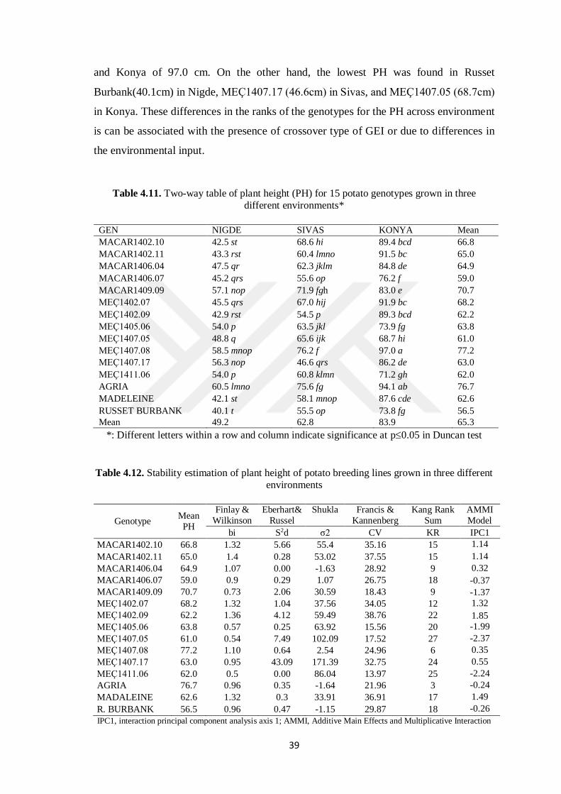
39

and Konya of 97.0 cm. On the other hand, the lowest PH was found in Russet

Burbank(40.1cm) in Nigde, MEÇ1407.17 (46.6cm) in Sivas, and MEÇ1407.05 (68.7cm)

in Konya. These differences in the ranks of the genotypes for the PH across environment

is can be associated with the presence of crossover type of GEI or due to differences in

the environmental input.

Table 4.11. Two-way table of plant height (PH) for 15 potato genotypes grown in three

different environments*


MACAR1402.10 42.5 st 68.6 hi 89.4 bcd 66.8

MACAR1402.11 43.3 rst 60.4 lmno 91.5 bc 65.0

MACAR1406.04 47.5 qr 62.3 jklm 84.8 de 64.9

MACAR1406.07 45.2 qrs 55.6 op 76.2 f 59.0

MACAR1409.09 57.1 nop 71.9 fgh 83.0 e 70.7

MEÇ1402.07 45.5 qrs 67.0 hij 91.9 bc 68.2

MEÇ1402.09 42.9 rst 54.5 p 89.3 bcd 62.2

MEÇ1405.06 54.0 p 63.5 jkl 73.9 fg 63.8

MEÇ1407.05 48.8 q 65.6 ijk 68.7 hi 61.0

MEÇ1407.08 58.5 mnop 76.2 f 97.0 a 77.2

MEÇ1407.17 56.3 nop 46.6 qrs 86.2 de 63.0

MEÇ1411.06 54.0 p 60.8 klmn 71.2 gh 62.0

AGRIA 60.5 lmno 75.6 fg 94.1 ab 76.7

MADELEINE 42.1 st 58.1 mnop 87.6 cde 62.6

RUSSET BURBANK 40.1 t 55.5 op 73.8 fg 56.5

Mean 49.2 62.8 83.9 65.3


Table 4.12. Stability estimation of plant height of potato breeding lines grown in three different

environments

Genotype Mean

PH

Finlay &

Wilkinson

Eberhart&

Russel

Shukla

Francis &

Kannenberg

Kang Rank

Sum

AMMI

Model


MACAR1402.10 66.8 1.32 5.66 55.4 35.16 15 1.14

MACAR1402.11 65.0 1.4 0.28 53.02 37.55 15 1.14

MACAR1406.04 64.9 1.07 0.00 -1.63 28.92 9 0.32

MACAR1406.07 59.0 0.9 0.29 1.07 26.75 18 -0.37

MACAR1409.09 70.7 0.73 2.06 30.59 18.43 9 -1.37

MEÇ1402.07 68.2 1.32 1.04 37.56 34.05 12 1.32

MEÇ1402.09 62.2 1.36 4.12 59.49 38.76 22 1.85

MEÇ1405.06 63.8 0.57 0.25 63.92 15.56 20 -1.99

MEÇ1407.05 61.0 0.54 7.49 102.09 17.52 27 -2.37

MEÇ1407.08 77.2 1.10 0.64 2.54 24.96 6 0.35

MEÇ1407.17 63.0 0.95 43.09 171.39 32.75 24 0.55

MEÇ1411.06 62.0 0.5 0.00 86.04 13.97 25 -2.24

AGRIA 76.7 0.96 0.35 -1.64 21.96 3 -0.24

MADALEINE 62.6 1.32 0.3 33.91 36.91 17 1.49

R. BURBANK 56.5 0.96 0.47 -1.15 29.87 18 -0.26

IPC1, interaction principal component analysis axis 1; AMMI, Additive Main Effects and Multiplicative Interaction

40

The stability estimation for the PH in Table 4.12 shows that MACAR1406.04,

MACAR1406.07, MEÇ1407.17, AGRIA, and RUSSET are stable for the Finlay and

Wilkinson regression coefficient (bi). The Eberhard BURBANK and Russel analysis

revealed that MACAR1406.04, and MEÇ1411.06, were stable genotypes for PH. For the

Shukla stability variances, MACAR1406.04, MACAR1406.07, and AGRIA were

identified to be stable of PH. There is some similarity between the Eberhard and Russel

analysis and the Shukla stability variances. However, Francis & Kannenberg failed to

identify any stable genotype for PH while Kang Rank Sum identified AGRIA as a stable

genotype in terms of PH. For the AMMI model stability estimation, genotypes with IPC1

scores less than 0.5 were considered stable. In this regards, MACAR1406.04,

MACAR1406.07, MEÇ1407.08, AGRIA, and RUSSET BURBANK were stable

genotypes for the AMMI model.

The regression analysis of the plant height (PH) (Figure 4.5) considering the relationship

of genotypes adaptation (regression coefficient “bi”) and the mean PH showed that

MEÇ1402.07, MACAR1402.10, and MEÇ1407.08 are well adaptable favourable

environment whereas MACAR1409.09 is well adapted to an unfavourable environment

which depicted specific adaptability (stability). On the other hand, MEÇ1402.09,

MACAR1402.11, and MADELEINE are poorly adapted to favourable environment

whiles MACAR1406.07, MEÇ1411.06, MEÇ1407.05, and MEÇ1405.06 are poorly

adapted to unfavourable environmental conditions. Contrarily to these, MEÇ1407.17,

RUSSET BURBANK, and MACAR1406.04 are poorly adaptable to all environments

whereas AGRIA is well adapted to all environmental conditions in terms of plant height.

This shows that genotypes that are well adapted to unfavourable environment are tolerant

genotypes whiles genotypes that are poorly adapted to unfavourable environment are

sensitive to environmental conditions.

41

Figure 4.5. Relationship of genotype adaptation (regression coefficient ‘bi’) and mean plant

height (PH) of 15 potato genotypes grown in three diverse environments

Comparatively, the AMMI biplot shows that RUSSET BURBANK, MACAR1406.07,

AGRIA, MEÇ1407.08, MACAR1406.04, MEÇ1407.17 are less influenced by

environmental input with RUBB, MACAR1406.07, MACAR1406.04, and MEÇ1407.17

having below-average stability whiles AGRIA and MEÇ1407.08 have above-average

stability. The rest of the genotypes are however having high G*E interaction and

specifically adapted to either favourable or unfavourable environments. The

environments are highly scattered across, with Konya (KNYA) and Nigde (NGDE)

highly unstable whiles Sivas (SVAS) is potentially an ideal environment for most

genotype which is closer to the mean and IPC1 origin.

42

Figure 4.6. AMMI biplot analysis of interaction principal component analysis (IPCA-1) with

mean of plant height (PH) of potato genotype evaluated across three different environments. Note: MCR1 =MACAR1402.10, MCR2 = MACAR1402.11, MCR3 = MACAR1406.04, MCR4 =

MACAR1406.07, MCR5 = MACAR1409.09, MEÇ1 = MEÇ1402.07, MEC2 = MEÇ1402.09, MEC3 =

MEÇ1405.06, MEC4 = MEÇ1407.05, MEC5 = MEÇ1407.08, MEC6 = MEÇ1407.17, MEC7 =

MEÇ1411.06, AGRA = AGRIA, MADA = MADELEINE, RUBB = RUSSET BURBANK; KYNA

= Konya, NGDE = Nigde, SVAS = Sivas

4.4. Total Plant Yield

The general ANOVA and AMMI ANOVA for the total plant yield (TPY) revealed highly

significant (p < 0.001) differences among the environments, genotypes, and the genotype

by environment interaction (Table 4.13 and Table 4.14) indicating the high effects of the

genotypes and environments on the yield of the potato breeding lines and the standard

genotypes. The CV among the genotypes and the environments were found to be 11.33

and the grand mean yield of 744.29. 75.35% of the total sum of squares was explained by

the treatment of which 28.31%, 60.70%, and 10.99% of the treatment sum of squares

were respectively accounted for by the genotypes, the environments, and the genotype by

environment interaction effects while 24.65% of the total sum of squares was attributed

to experimental errors. There was also a significant difference for the IPC1 (P<0.001)

which explained 74.55% of the GEI sum of squares and the residual (P<0.05) which

constituted 25.45% of the GEI sum of squares.

43

Table 4.13 ANOVA of total plant yield for 15 genotypes grown in three different environments

Source DF SS MS F P

Genotype (G) 14 3970464 283605 39.91 0.000***

Environment (E) 2 8750810 4375405 615.65 0.000***

G x E 28 1476318 52726 7.42 0.000***

Error 135 959436 7107

Total 179 1.52E+07

CV 11.3

DF= degree of freedom, SS= sum of square, MS= mean square, CV= coefficient of variation, *** p0.001

Table 4.5. AMMI analysis of variance for total plant yield (TPY) of 15 potato genotypes grown

in three environments


explained

% TRT SS

explained

%GEI SS

explained

Total 179 1.50E+07 84651.6

Treatment 44 1.30E+07 304587*** 75.35 Genotype 14 3793624 270973*** 28.31

Environment 2 8135012 4067506*** 60.7

G x E 28 1473184 52613.7 *** 10.99 IPC1 15 1098301 73220.1 *** (8.2) 74.55

Residual 13 374883 28837.1 * (2.8) 25.45

Error 135 1750810 12969 24.65 Blocks/Env 9 146957 16328.6 ns

Pure Error 126 1603852 12729


treatment sum of squares. GEI SS = genotype by environment interaction sum of squares, *p0.05, ***

p0.001 ns= not significant

In Table 4.15, the mean total plant yield (TPY) ranges from Russet Burbank (400.08 t/ha)

to MEÇ1407.17 (967.03 t/ha) among genotypes, while among environments; Nigde

(545.6), Sivas (1087.17), and Konya (529.47) which are significantly different among the

genotypes and environments. Crossover type of GEI was observed which led to different

genotype ranking across the environments. Yan and Tinker (2006), Atnaf et al. (2013),

Mwiiga et al. (2020), and Bhartiya et al. (2017) also states that the presence of crossover

type GEI necessitate stability analysis. The highest TPY in Nigde was found in

MEÇ1407.17 (869.2 t/ha), in Sivas, the highest TPY was found in MEÇ1407.05 (1315.2

t/ha), while in Konya, the highest TPY was found in MACAR1402.10 (885.2 t/ha)

whereas Russet Burbank recorded the lowest TPY in Nigde 226.6 t/ha, and in Sivas of

523.5t/ha while MACAR1406.04 recorded the lowest TPY in Konya of 451.7 t/ha.

Though Russet Burbank recorded the lowest TPY in both Nigde and Sivas environments,

there was a difference in the yield quantity which explained that the greater variation in

44

the TPY between genotypes is due to environmental fluctuations more than the genotypic

differences. The contribution of the total sum of squares due to the genotypes can be

attributed to the differences in the crossing parents of genotypes which brings about

different significant responses with the environments.

Table 4.6. Two-way table of total plant yield (TPY) for 15 potato genotypes grown in three



MACAR1402.10 483.1 op 996.6 de 885.2 efg 788.3

MACAR1402.11 417.8 p 799.6 ghi 692.8 ijk 636.7

MACAR1406.04 490.3 op 1199.2 ab 451.7 op 713.7

MACAR1406.07 452.2 op 1073.3 cd 546.6 lmno 690.7

MACAR1409.09 484.4 op 1220.6 ab 695 ijk 800.0

MEÇ1402.07 465.3 op 981.4 def 618.1 klmn 688.2

MEÇ1402.09 474.4 op 888.4 efg 515.4 nop 626.1

MEÇ1405.06 566.7 lmno 1261.1 ab 661.4 jkl 829.8

MEÇ1407.05 736.4 hij 1315.2 a 729.4 ijk 927.0

MEÇ1407.08 711.4 ijk 1270.3 a 660.9 jkl 880.9

MEÇ1407.17 869.2 fg 1152.2 bc 879.7 efg 967.0

MEÇ1411.06 743.3 hij 1203.7 ab 730.8 hijk 892.6

AGRIA 293.2 q 847.5 gh 472 op 537.6

MADELEINE 636.8 jklm 1011.3 d 707.3 ijk 785.2

RUSSET BURBANK 226.2 q 523.5 mnop 452.6 op 400.8

Mean 545.6 1087.2 529.47 744.3


The bi stability analysis revealed that MEÇ1402.07, MEÇ1402.09, MEÇ1411.06, and

AGRIA were stable for TPY. The Eberhart & Russel (1966) and Shukla (1972) stability

have different paterns of stability estimation that could not identify any stable genotypes.

This partially agrees with the findings of Caliskan et al. 2007 in which they found a

similar pattern of stability estimates between Eberhard & Russel (1966) and Shukla

(1972) stability models for the total tuber yield of sweet potato but both failed to identify

stable genotypes Also, the Francis & Kannenberg CV analysis recorded high CV values

and so failed to identify any desirable genotype for TPY. However, the Kang’s Rank (KR)

sum identified MEÇ1411.06 as a stable genotype due to its lower KR value (Table 4.16).

Contrarily, the AMMI stability model identified AGRIA as a stable genotype for TPY.

The differential yield traits expression of the genotypes in the varying environment is

based on three impacts; the expression of the gene in the environment, the suppressing of

the gene in the environment, or the codominance (neutrality) of the gene responsible for

the trait (Bailey-Serres et al. 2019). An environment may favour or impede the expression

45

of the phenotypic traits of interest which lead to different stability levels of the genotypes

(Kang et al. 2004).

Table 4.7. Stability estimation of total plant yield of potato breeding lines grown in three

different environments

Genotype Mean

TPY

Finlay &

Wilkinsin

Eberhard

& Russel

Shukla

Francis &

Kannenberg

Kang

Rank Sum

AMMI

Model


MACAR1402.10 788.29 0.81 7325.92 31711.2 34.27 20 -7.57

MACAR1402.11 636.75 0.62 3206.31 24335.6 30.94 24 -8.39

MACAR1406.04 713.70 1.51 3121.97 33534.4 58.97 24 11.22

MACAR1406.07 690.71 1.24 128.82 4264.72 48.46 15 4.59

MACAR1409.09 800.00 1.4 239.36 13475.4 47.4 16 5.17 MEÇ1402.07 688.24 0.98 152.24 -368.2 38.51 12 -0.53

MEÇ1402.09 626.08 0.84 196.19 1924.66 36.43 16 -0.79

MEÇ1405.06 829.74 1.39 252.03 12878.2 45.39 14 7.02

MEÇ1407.05 926.98 1.22 1477.49 8911.15 36.27 9 6.02

MEÇ1407.08 880.82 1.2 2491.52 12562.1 38.39 12 -1.72

MEÇ1407.17 967.02 0.59 216.69 14255.1 16.59 12 -4.28

MEÇ1411.06 892.61 0.97 1062.29 3330.41 30.19 7 2.24

AGRIA 537.55 1.04 308.54 370.4 52.63 16 0.02

MADALEINE 785.16 0.74 8.43 4803.52 25.35 14 -2.92

R. BURBANK 398.50 0.46 2312.14 33085.8 38.29 29 -10.06

CV, coefficient of variation; IPC1, interaction principal component analysis axis 1; AMMI,

Additive Main Effects and Multiplicative Interaction

Figure 4.7. Relationship of genotype adaptation (regression coefficient ‘bi’) and mean total

plant yield (TPY) of 15 potato genotypes grown in three diverse environments

Figure 4.7 characterized the genotypes into six levels of adaptability for the total plant

yield using the bi model. AGRIA and MEÇ1402.07 are poorly adapted to all

46

environments, whereas MEÇ1411.06 is very well adapted to all environments. On the

other hand, MEÇ1402.09 and MACAR1402.11 are poorly adapted to unfavourable

environments whiles, MACAR1406.07 and MACAR1406.04 are poorly adapted to

favourable environments. On the contrarily, genotypes; MEÇ1407.17, MACAR1402.10,

and MADELEINE are very well adapted to unfavourable environments and thus are

tolerant genotypes whiles, MEÇ1405.06, MEÇ1407.06, MEÇ1407.08 and

MACAR1409.109 are ideal genotypes and so very well adapted to favourable

environment.

In Figure 4.8 AGRIA, MEÇ1402.07, and MEÇ1402.09 though averagely low yielding,

are generally adapted to a large spectrum of environments. Among all the genotype,

Russet Burbank was the most highly adaptive to a specific environment with no

association with the other genotype. MADELEINE, MEÇ1405.06 MEC 4, MEÇ1407.08,

MEÇ1407.17, MEÇ1411.06, MACAR1409.09 were high yielding genotypes with

general adaptability. The environments were widely interactive more than the genotypes

with Sivas being the most interactive and best environment while Nigde and Konya being

very much sensitive (Figure 4.8).

Figure 4.8. Biplot analysis of interaction principal component axis (IPCA-1) with mean of total plant

yield (TPY) of potato genotype evaluated across three different environments. Note: MCR1

=MACAR1402.10, MCR2 = MACAR1402.11, MCR3 = MACAR1406.04, MCR4 = MACAR1406.07, MCR5 = MACAR1409.09, MEÇ1 = MEÇ1402.07, MEC2 = MEÇ1402.09, MEC3 = MEÇ1405.06, MEC4 = MEÇ1407.05,

MEC5 = MEÇ1407.08, MEC6 = MEÇ1407.17, MEC7 = MEÇ1411.06, AGRA = AGRIA, MADA = MADELEINE, RUBB = RUSSET BURBANK; KYNA = Konya, NGDE = Nigde, SVAS = Sivas

47

4.5 Total Tuber Yield (TTY)

The results of the total tuber yield (TTY) revealed that there were highly significant (p <

0.001) effects on the potato yield caused by the genotypes, environments, and the

genotype by environment interaction for both the standard ANOVA and AMMI ANOVA

(Table 4.17, Table 4.18) with the CV among the genotypes and the environments of 3.8

and the grand mean yield of 31.41. The IPC1 and the residual component of the GEI also

revealed a highly significant (P<0.001) effect with the IPC1 constituting 77.44% while

residual accounting for 22.56% of the GEI sum of squares. Of the total sum of squares,

the treatment explained 99.08% with 31.6%, 52.9%, and 15.3% respectively attributed to

genotype, environment, and GEI. It can be deduced that; a negligible error was observed

on the tuber yield of the potato and so is not responsible for the yield differences among

the genotypes. Greater differences in the yield can be stated to be environmentally

induced more than genetically induced and the genotypic differences is attributed to the

differences in the crossing parents of the cultivar which confers different responses with

the environments and led to the significant difference in the yield of the genotypes.

Table 4.8. ANOVA of total tuber yield (TTY) for 15 genotypes grown in three different environments


Genotype (G) 14 7986 570.43 400.27 0.000***

Environment (E) 2 13368.2 6684.09 4690.24 0.000***

G x E 28 3915.9 139.85 98.14 0.000***

Error 135 192.4 1.43

Total 179 25462.5

CV 3.8

DF= degree of freedom, SS= sum of square, MS= mean square, CV= coefficient of variation,

*** p0.001

The crossover GEI observed in the TPY also influenced the total tuber yield (TTY) of the

genotypes. The TTY of the genotypes ranges from Russet Burbank(17.033t/ha) to

MEÇ1407.17 (41.77t/ha) whiles among environment; Nigde (24.24t/ha), Sivas

(44.56t/ha), and Konya (26.45t/ha) (Table 4.19) with statistically significant yield

differences between the highest and lowest yield of the genotypes and with the rest of the

genotypes. There was a differential ranking of the genotypes across the environments.

The highest TTY across the environments was found in MEÇ1407.17 (41.01 t/ha) in

48

Nigde, MEÇ1407.05 (56.69 t/ha) in Sivas, and MACAR1402.10 (35.52 t/ha) in Konya.

On the other hand, the lowest TTY in Sivas was found in MACAR1402.11 (21.06 t/ha),

while Russet Burbank was recorded the lowest TTY of 10.47 t/ha and 19.09 t/ha

respectively in Nigde and Konya.

Table 4.18. AMMI analysis of variance for total tuber yield (TTY) of 15 potato genotypes grown in three

environments


explained

% TRT SS

explained

%GEI SS

explained

Total 179 25462.5 142.249 Treatment 44 25270.1 574.321*** 99.08

Genotype 14 7986.02 570.43*** 31.6

Environment 2 13368.2 6684.09*** 52.9 G x E 28 3915.94 139.855*** 15.5

IPC1 15 3032.54 202.169*** (12) 77.44

Residual 13 883.401 67.954*** (3.5) 22.56 Error 135 192.39 1.425 0.92

Blocks/Env 9 29.529 3.281*

Pure Error 126 162.861 1.293


treatment sum of squares. GEI SS = genotype by environment interaction sum of squares, *** p0.001

Biru (2017) reported a highly significant effect of genotype, environments, and G×E on

the yield and yield component imply that the genetic variability among genotype, and the

segregating possibility for selecting stable. Raja et al. (2018), Rymuza et al. (2015), and

Wassu, (2017) reported that the genetic difference among potato genotypes account for

the difference in marketable tuber yield, total tuber yield.

49

Table 4.19 Two-way table of total tuber yield (TTY) for 15 potato genotypes grown in three different environments*


MACAR1402.10 19.74 vwx 43.07 fg 35.52 j 32.77

MACAR1402.11 18.28 x 21.06 stuv 28.09 op 22.48

MACAR1406.04 21.55 stu 51.83 c 19.42 vwx 30.93

MACAR1406.07 20.46 tuvw 45.43 e 22.59 s 29.49

MACAR1409.09 21.99 st 51.67 c 28.36 op 34.00

MEÇ1402.07 20.40 tuvw 41.65 gh 24.97 r 29.00

MEÇ1402.09 21.93 st 37.51 i 20.39 tuvw 26.61

MEÇ1405.06 25.69 qr 51.58 c 27.16 pq 34.81

MEÇ1407.05 33.14 kl 56.69 a 28.15 op 39.33

MEÇ1407.08 31.92 lm 53.91 b 27.97 op 37.93

MEÇ1407.17 41.01 h 49.40 d 34.90 j 41.77

MEÇ1411.06 34.41 jk 48.15 d 29.44 no 37.33

AGRIA 13.55 y 35.73 j 20.01 uvw 23.10

MADELEINE 29.13 no 43.70 f 30.70 mn 34.51

RUSSET BURBANK 10.47 z 21.55 stu 19.09 wx 17.04

Mean 24.24 44.56 26.45 31.75


The AMMI IPC1 score mode of stability estimation states that the closer the IPC1 score

values are to zero, the more stable the genotypes are to their testing environments

(Purchase, 1997). In this research, the IPC1 score values of MEÇ1402.07, MEÇ1402.09,

MEÇ1411.06, and AGRIA are closer to zero and so imply that they are more in the three

test environments (Nigde, Sivas and Konya) for TTY. The Francis & Kannenberg CV

and Kang Rank Sum (KR) methods did not identify any stable genotype as a result of

their large CV and large KR. For the Shukla stability variance, MEÇ1402.07,

MEÇ1402.09, and AGRIA were identified as stable genotypes while for the Eberhard and

Russel deviation from the regression method, MACAR1406.07, MEÇ1405.06, and

MADALEINE were revealed to be stable for TTY. More so, Finlay and Wilkinson

regression coefficient (bi) revealed MACAR1402.10, MEÇ1402.07, MEÇ1402.09,

MEÇ1411.06, and AGRIA as stable genotypes for TTY (Table 4.20).

50

Table 4.9. Stability estimation of total tuber yield of potato breeding lines grown in three


Genotype Mean

TTY

Finlay &

Wilkinson

Eberhart

& Russel

Shukla

Francis &

Kannenberg

Kang Rank

Sum

AMMI

Model


MACAR1402.10 32.777 0.918 13.659 53.335 36.32 20 -1.03

MACAR1402.11 22.477 -0.067 7.161 172.576 22.495 29 -3.32

MACAR1406.04 30.933 1.695 2.49 69.386 58.605 23 2.12

MACAR1406.07 29.493 1.311 0.042 9.912 46.935 15 0.84

MACAR1409.09 34.003 1.473 0.706 28.947 45.963 16 1.02

MEÇ1402.07 29.007 1.054 0.363 -0.844 38.561 12 0.01

MEÇ1402.09 26.61 0.882 0.878 2.652 35.592 14 -0.09

MEÇ1405.06 34.813 1.375 0.175 16.141 41.763 12 1.05

MEÇ1407.05 39.323 1.392 4.685 36.028 38.768 13 1.48

MEÇ1407.08 37.933 1.284 3.325 21.115 36.845 11 1.13

MEÇ1407.17 41.77 0.592 3.974 34.722 17.428 11 -0.59

MEÇ1411.06 37.333 0.858 3.403 13.645 25.959 10 0.05

AGRIA 23.097 1.063 1.222 2.753 49.391 16 -0.08

MADALEINE 34.51 0.758 0.001 4.862 23.174 10 -0.61

R. BURBANK 17.037 0.411 4.296 59.254 34.152 28 -1.96



For the level of genotype adaptability, the Finlay and Wilkinson regression model

characterized the genotypes into four levels of adaptability for the total tuber yield (TTY)

(Figure 4.9). MACAR1406.04, MACAR1406.07, AGRIA, and MEÇ1402.07 were

identified as having poor adaptability to favourable environments while RUSSET

BURBANK, MEÇ1402.09, and MACRA1402.11 have poor adaptability to unfavourable

environments. On the other hand, MACAR1409.09, MEÇ1407.05, MEÇ1405.06, and

MEÇ1407.08 were identified as genotypes adapting favourably to favourable

environment whiles MEÇ1411.06, MEÇ1407.17, MACAR1402.10, and MADELEINE

as tolerant and very well adapted to unfavourable environments.

51

Figure 4.9. Relationship of genotype adaptation (regression coefficient ‘bi’) and mean total

tuber yield (TTY) of 15 potato genotypes grown in three diverse environments

Also, the AMMI IPC1 biplot against mean TTY group the genotypes into general stability

or specific stability, and high or low yielding genotypes. The degree of adaptability of a

genotype to the environment is determined by the distance of the genotype IPC1 scores

to the IPC1 axis. In, Figure 4.10, AGRIA, MEÇ1402.09, MEÇ1402.07, MEÇ1411.06 are

stable genotypes and broadly adapted to a wide range of environments with only

MEÇ1411.06 high yielding while MACAR1406.04 and MACAR1406.07 are low

yielding and very much interactive with favourable environmental conditions. On the

other hand, MACAR1409.09, MEÇ1405.06, MEÇ1407.08, and MEÇ1407.05 are high

yielding genotypes and highly interactive with favourable environmental conditions.

Furthermore, MACAR1402.11 and Russet Burbank are low yielding genotypes and

highly sensitive to unfavourable environmental conditions while MACAR1402.10,

MEÇ1407.17, and MADELEINE are high yielding and highly interactive to adverse

environmental fluctuations. The environments are widely interactive more than the

genotypes with Sivas being the most interactive and best environment while Nigde and

Konya being very much sensitive (Figure 4.10).

52

Figure 4.10. AMMI biplot analysis of interaction principal component axis (IPCA-1) with

mean of total tuber yield (TTY) of potato genotype evaluated across three different

environments. Note: MCR1 = MACAR1402.10, MCR2 = MACAR1402.11, MCR3 = MACAR1406.04, MCR4 = MACAR1406.07, MCR5 = MACAR1409.09, MEÇ1 = MEÇ1402.07, MEC2 = MEÇ1402.09,

MEC3 = MEÇ1405.06, MEC4 = MEÇ1407.05, MEC5 = MEÇ1407.08, MEC6 = MEÇ1407.17, MEC7 =

MEÇ1411.06, AGRA = AGRIA, MADA = MADELEINE, RUBB = RUSSET BURBANK; KYNA =

Konya, NGDE = Nigde, SVAS = Sivas

4.6 Marketable Tuber Yield

The analysis of variance for the marketable tuber yield (MTY) revealed that there were

highly significant (p < 0.001) effects of the genotypes, environments, and the genotype

by environment interaction on the potato yield for the general ANOVA and the AMMI

ANOVA (Table 4.21 and Table 4.22). The CV among the genotypes and the

environments were found to be 3.87 and the grand mean yield of 31.21. The IPC1 and the

residual component of the GEI also revealed highly significant (P<0.001) with the IPC1

constituting 77.62% while residual accounting for 22.38% of the GEI sum of squares.

The treatment explained 99.04% of the total sum of squares with 28.58%, 52.49%, and

15.52% respectively attributed to genotype, environment, and GEI. This indicates that

genotype, environment, and GEI have a great influence on the marketable tuber yield of

the potato. The greater differences in the yield can be stated to be environmentally

induced more than genetically induced. The significant differences in the genotypes are

attributed to the differences in the crossing parents of these breeding lines and their

different responses to environmental fluctuations.

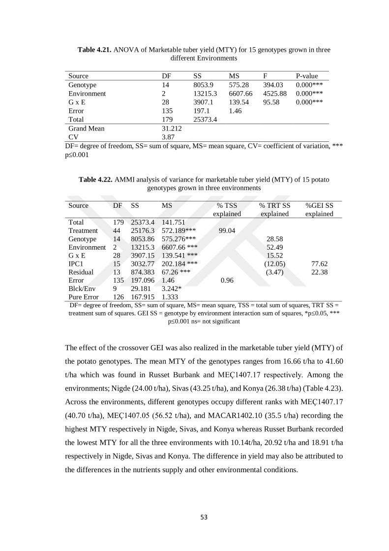
53

Table 4.21. ANOVA of Marketable tuber yield (MTY) for 15 genotypes grown in three

different Environments


Genotype 14 8053.9 575.28 394.03 0.000***

Environment 2 13215.3 6607.66 4525.88 0.000***

G x E 28 3907.1 139.54 95.58 0.000***

Error 135 197.1 1.46

Total 179 25373.4

Grand Mean 31.212

CV 3.87


p0.001

Table 4.22. AMMI analysis of variance for marketable tuber yield (MTY) of 15 potato

genotypes grown in three environments


explained

% TRT SS

explained

%GEI SS

explained

Total 179 25373.4 141.751

Treatment 44 25176.3 572.189*** 99.04

Genotype 14 8053.86 575.276*** 28.58

Environment 2 13215.3 6607.66 *** 52.49 G x E 28 3907.15 139.541 *** 15.52

IPC1 15 3032.77 202.184 *** (12.05) 77.62

Residual 13 874.383 67.26 *** (3.47) 22.38 Error 135 197.096 1.46 0.96

Blck/Env 9 29.181 3.242*

Pure Error 126 167.915 1.333 DF= degree of freedom, SS= sum of square, MS= mean square, TSS = total sum of squares, TRT SS =

treatment sum of squares. GEI SS = genotype by environment interaction sum of squares, *p0.05, ***


The effect of the crossover GEI was also realized in the marketable tuber yield (MTY) of

the potato genotypes. The mean MTY of the genotypes ranges from 16.66 t/ha to 41.60

t/ha which was found in Russet Burbank and MEÇ1407.17 respectively. Among the

environments; Nigde (24.00 t/ha), Sivas (43.25 t/ha), and Konya (26.38 t/ha) (Table 4.23).

Across the environments, different genotypes occupy different ranks with MEÇ1407.17

(40.70 t/ha), MEÇ1407.05 (56.52 t/ha), and MACAR1402.10 (35.5 t/ha) recording the

highest MTY respectively in Nigde, Sivas, and Konya whereas Russet Burbank recorded

the lowest MTY for all the three environments with 10.14t/ha, 20.92 t/ha and 18.91 t/ha

respectively in Nigde, Sivas and Konya. The difference in yield may also be attributed to

the differences in the nutrients supply and other environmental conditions.

54

Table 4.23. Two-way table of marketable tuber yield (MTY) for 15 potato genotypes grown in



MACAR1402.10 19.51 vwx 42.74 fg 35.50 j 32.58

MACAR1402.11 18.12 x 20.97 stuv 27.96 op 22.35

MACAR1406.04 21.41 stu 51.54 c 19.40 vwx 30.79

MACAR1406.07 20.22 tuvw 45.19 e 22.51 s 29.30

MACAR1409.09 21.74 st 51.50 c 28.32 op 33.85

MEÇ1402.07 20.29 tuvw 41.42 gh 24.92 r 28.88

MEÇ1402.09 21.65 st 37.24 i 20.37 tuvw 26.42

MEÇ1405.06 25.48 qr 51.21 c 27.10 pq 34.60

MEÇ1407.05 32.92 kl 56.52 a 28.11 op 39.18

MEÇ1407.08 31.60 lm 53.62 b 27.80 op 37.67

MEÇ1407.17 40.70 h 49.22 d 34.88 j 41.60

MEÇ1411.06 34.22 jk 47.96 d 29.43 no 37.20

AGRIA 13.23 y 35.41 j 19.92 uvw 22.85

MADALEIN 28.84 o 43.32 f 30.64 mn 34.26

RUSSET BURBANK 10.14 z 20.92 stuv 18.91 wx 16.66

Mean 24.00 43.25 26.38 31.21


The difference in the mean yield performance (Table; 4.16, 4.19, 4.23, and 4.27) of the

genotypes within and across environment was expected in this study as the genotypes

differed genetically from the crossing parents as reflected in the high significant

differences (p≤ 0.01) in the genotypes, environment and their interaction for the TPY,

TTY, MTY, and NTP. Effect of genotype, environment, and their interaction on NTP,

MTY, TTY (Eaton et al., 2017), and TPY can be explained by the variation in their

biological vigour of the genotypes, and probably due to the variation in favourable

environmental conditions at the study’s locations and management practices. Sivas

performed the highest MTY and it was followed by Konya and Nigde. Thus, potato

responds favourably to better environments, and hence subject to the strong influence of

genotype, environment, and genotype by environment interaction (Bai et al., 2014). It is

stated that a significant interaction of cultivar x location indicates instability of expression

of these traits in different cultivars across locations and seasons as these quality traits are

genetically controlled (Wassu, 2017). GEI has a significant impact on the potato breeding

lines assessed in these environments; Nigde, Konya, and Sivas, which confirms

Bradshaw’s (1997) study in that interactions of potato genotypes to macro-environments

and microenvironment lead to yield and traits fluctuations. This implies that the breeding

lines differ in their yield quality and stability strength, varied resistibility or susceptibility

to environmental fluctuations due to different genetic factors that explained the existence

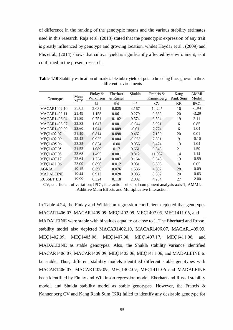
55

of difference in the ranking of the genotypic means and the various stability estimates

used in this research. Raja et al. (2018) stated that the phenotypic expression of any trait

is greatly influenced by genotype and growing location, whiles Haydar et al., (2009) and

Flis et al., (2014) shows that cultivar yield is significantly affected by environment, as it

confirmed in the present research.

Table 4.10 Stability estimation of marketable tuber yield of potato breeding lines grown in three


Genotype Mean MTY

Finlay &

Wilkinson

Eberhart

& Russel

Shukla

Francis &

Kannenberg

Kang

Rank Sum

AMMI

Model


MACAR1402.10 25.62 2.081 0.025 4.167 14.245 16 -1.04

MACAR1402.11 21.49 1.158 0.061 0.279 9.662 20 -3.29

MACAR1406.04 21.89 0.751 0.102 0.574 6.594 19 2.11

MACAR1406.07 22.83 1.047 0.001 -0.044 8.021 6 0.85

MACAR1409.09 23.60 1.044 0.009 -0.01 7.774 6 1.04

MEÇ1402.07 21.49 0.814 0.098 0.462 7.159 20 0.01

MEÇ1402.09 22.45 0.935 0.004 -0.023 7.301 9 -0.10

MEÇ1405.06 22.25 0.824 0.00 0.056 6.474 13 1.04

MEÇ1407.05 21.52 1.089 0.17 0.661 9.545 21 1.50

MEÇ1407.08 23.68 1.495 0.001 0.812 11.037 14 1.14

MEÇ1407.17 22.64 1.234 0.007 0.164 9.548 13 -0.59

MEÇ1411.06 23.00 0.896 0.012 0.031 6.863 8 0.05

AGRIA 19.15 0.396 0.076 1.536 4.507 28 -0.09

MADALEINE 19.44 0.912 0.028 0.085 8.362 20 -0.63

RUSSET BB 19.99 0.324 0.118 2.032 4.284 27 -2.00

CV, coefficient of variation; IPC1, interaction principal component analysis axis 1; AMMI, Additive Main Effects and Multiplicative Interaction

In Table 4.24, the Finlay and Wilkinson regression coefficient depicted that genotypes

MACAR1406.07, MACAR1409.09, MEÇ1402.09, MEÇ1407.05, MEÇ1411.06, and

MADALEINE were stable with bi values equal to or close to 1. The Eberhard and Russel

stability model also depicted MACAR1402.10, MACAR1406.07, MACAR1409.09,

MEÇ1402.09, MEÇ1405.06, MEÇ1407.08, MEÇ1407.17, MEÇ1411.06, and

MADALEINE as stable genotypes. Also, the Shukla stability variance identified

MACAR1406.07, MACAR1409.09, MEÇ1405.06, MEÇ1411.06, and MADALEINE to

be stable. Thus, different stability models identified different stable genotypes with

MACAR1406.07, MACAR1409.09, MEÇ1402.09, MEÇ1411.06 and MADALEINE

been identified by Finlay and Wilkinson regression model, Eberhart and Russel stability

model, and Shukla stability model as stable genotypes. However, the Francis &

Kannenberg CV and Kang Rank Sum (KR) failed to identify any desirable genotype for

56

MTY while the AMMI IPC1 score revealed MEÇ1402.07, MEÇ1402.09, MEÇ1411.06,

and AGRIA as stable genotypes for MTY.

Figure 4.11 characterized AGRIA, MEÇ1402.09, and MEÇ1402.07 as poorly adaptable

genotypes to all environmental conditions whiles MEÇ1402.10 was well adaptable to all

environments. Furthermore, MACAR1402.11, and Russet Burbank were highly sensitive

to unfavourable environmental conditions while MACAR1406.04 and MACAR1406.07

were poorly adaptable to favourable environments. On the other hand, MEÇ1407.17,

MEC1411.06, and MADELEINE were high yielding and very well adapted to

unfavourable environmental conditions whiles MACAR1409.09, MEÇ1405.06,

MEÇ1407.05, and MEÇ1407.08 were very well adaptable to favourable environmental

conditions.


marketable tuber yield (MTY) of 15 potato genotypes grown in three diverse environments

The AMMI biplot analysis of the genotype for MTY (Figure 4.12) showed that AGRIA,

MEÇ1402.09, MEÇ1402.07, and MEÇ1411.06 had general adaptation regardless of the

environmental influences which are similar to the genotype characterization in Figure

4.11. Genotype partitioned closed to each other had a positive correlation, thus the

genotypes in this biplot were generally segregated into three groups; Russet Burbank and

MACAR1402.11 forming one group, AGRIA, MEÇ1402.09, MEÇ1402.07,

57

MACAR1406.07, and MACAR1406.04 forming one group, and MACAR1402.10,

MADELEINE, MEÇ1411.06, MEÇ1407.17, MEÇ1407.08, MEÇ1407.05

MACAR1409.09, and MEÇ1405.06 also forming one group. The environments, on the

other hand, were scattered and relatively forming two groups: Nigde (NGDE) and Konya

(KNYA) on one site and Sivas (SVAS) on the other site. This similarity in the grouping

of genotype may be associated with genetic similarities between cultivars and the

similarity in the environment is predictively due to environmental inputs. Nigde (NGDE)

environment was relatively stable whiles Konya (KNYA) and Sivas (SVAS)

environments were highly unstable for marketable tuber yields for the genotype.

Figure 4.12. AMMI biplot analysis of interaction principal component axis (IPCA-1) with mean

of marketable tuber yield (MTY) of potato genotype evaluated across three different environments. Note: MCR1 =MACAR1402.10, MCR2 = MACAR1402.11, MCR3 = MACAR1406.04, MCR4 =

MACAR1406.07, MCR5 = MACAR1409.09, MEÇ1 = MEÇ1402.07, MEC2 = MEÇ1402.09, MEC3 = MEÇ1405.06, MEC4 = MEÇ1407.05, MEC5 = MEÇ1407.08, MEC6 = MEÇ1407.17, MEC7 = MEÇ1411.06,

AGRA = AGRIA, MADA = MADELEINE, RUBB = RUSSET BURBANK; KYNA = Konya, NGDE = Nigde, SVAS = Sivas

4.7. Number of Tuber Per Plant

Highly significant (p < 0.001) effect of the genotypes, environments, and the genotype

by environment interaction on the number of tubers per plant(NTP) was observed in the

ANOVA results (Table 4.25 and Table 4.26). The CV among the genotypes, and the

environments were found to be 7.76 and the grand mean yield of 6.08. The IPC1 and the


58


The treatment explained 95.23% of the total sum of squares with 39.53%, 41.47% and

19% respectively attributed to genotype, environment and GEI. This indicates that

genotype, environment, and GEI have a great influence on the tuber number per plant.

Table 4.25 ANOVA OF Number of tubers per plant for 15 genotypes grown in three different

Environments


Genotype 14 273.017 19.501 87.59 0.000***

Environment 2 287.544 143.772 645.79 0.000***

G x E 28 132.194 4.721 21.21 0.000***

Error 135 30.055 0.223

Total 179 722.81

CV 7.8


p0.001

Table 4.26 AMMI analysis of variance for number of tubers per plant (NTP) of 15 potato genotypes grown in three environments


explained % TRT SS explained

%GEI SS explained

Total 179 726.826 4.06

Treatment 44 696.411 15.828 *** 95.23

Genotype 14 275.307 19.665 *** 39.53 Environment 2 288.783 144.391 *** 41.47

G x E 28 132.322 4.726 *** 19

IPC1 15 97.921 6.528 *** (14.06) 77.44 Residual 13 34.401 2.646 *** (4.94) 22.56

Error 135 30.415 0.225 4.77

Blocks/Env 9 2.007 0.223 ns


treatment sum of squares. GEI SS = genotype by environment interaction sum of squares, *p0.05, *** p0.001 ns=

not significant

The lowest and highest mean NTP among genotypes was respectively MACAR1402.11

(4.1tubers) and MEÇ1405.06 (9.2tubers), whiles across environments, Sivas (7.9 tubers)

recorded the highest NTP followed by Konya (5.3 tubers) and Nigde (5.1 tubers),

recorded the least (Table 4.27). The highest number of tubers per plant within the

environments were recorded in MEÇ1407.17 (7.3 tubers) in Nigde, for MEÇ1405.06

(13.7 tubers) in Sivas, and for MEÇ1405.06 (8.1 tubers) in Konya while the lowest

number of tubers per plant within the environments was recorded for Russet Burbank (3.4

tubers) in Nigde, MACAR1402.11 (3.7 tubers) in Sivas, and MACAR1406.04 (3.4

59

tubers) in Konya. Greater differences in the NTP are environmentally induced more than

genetically induced and can be due to agronomic practices and nutrient input. This

confirms that agronomy, nutrients (phosphate, potassium, and calcium) and varietal

potential influenced the numbers of potato tubers produced per potato plant (Delgado et

al. 2016).

Table 4.11 Two-way table of tubers per plant (NTP) for 15 potato genotypes grown in three



MACAR1402.10 4.7 opqrs 7.7 ef 7.0 ghi 6.5

MACAR1402.11 3.8 tuvw 3.7 uvw 4.7 opqrs 4.1

MACAR1406.04 5.2 no 7.2 fgh 3.4 w 5.3

MACAR1406.07 5.4 lmn 7.7 efg 4.8 nopqr 6.0

MACAR1409.09 4.5 pqrs 7.2 fgh 4.3 rst 5.4

MEÇ1402.07 4.1 stuv 6.9 hi 4.9 nopqr 5.3

MEÇ1402.09 5.4 lmn 7.6 efg 4.7 opqrs 5.9

MEÇ1405.06 6.0 jkl 13.7 a 8.1 de 9.2

MEÇ1407.05 5.1 nopq 7.8 ef 5.1 nop 6.0

MEÇ1407.08 6.6 ij 9.9 b 5.4 lmn 7.3

MEÇ1407.17 7.3 fgh 8.9 c 6.8 hi 7.7

MEÇ1411.06 6.0 jkl 8.5 cd 6.0 jkl 6.8

AGRIA 3.5 vw 8.0de 4.3 rstu 5.2

MADELEINE 5.9 klm 6.4 ijk 5.3 mno 5.8

RUSSET BURBANK 3.4 w 7.0 ghi 4.4 qrst 4.9

Mean 5.1 7.9 5.3 6.1


The genotype characterization for NTP based on the Finlay and Wilkinson regression

analysis showed that MEÇ1402.09, MEÇ1402.07, MEÇ1407.05, MACAR1406.04,

MACAR1406.07, and MACAR1409.09 were poorly adaptable to all environmental

conditions whiles MEÇ1411.06 was well adaptable to all environmental conditions. More

so, MACAR1402.11, and MADELEINE were highly sensitive and poorly adaptable to

unfavourable environmental conditions while AGRIA and RUSSET BURBANK were

poorly adaptable to favourable environments. On the other hand, MEÇ1407.17 and

MACAR1402.10 were high yielding and very well adapted to unfavourable

environmental conditions whiles, MEÇ1405.06 and MEÇ1407.08 were very well

adaptable to favourable environmental conditions (Figure 4.13).

The AMMI biplot for the NTP (Figure 4.14) shows that, MACAR1409.09, MEÇ1402.07,

MEÇ1407.05, MACAR1406.07, MACAR1402.10, MEÇ1411.06, MEÇ1407.17 and

60

Russet Burbank were less influenced by environmental interactions due to their small

IPC1 values and so were generally stable. MEÇ1405.06 was the highest performing

genotype for tuber number per plant but also highly unstable, and thus had specific

adaptation. MACAR1402.11 gave off good tuber number in the poor environment and

had high G*E interactions. MACAR1402.10, MEÇ1407.08, MEÇ1407.17, and

MEÇ1411.06 were the suitable genotypes which were generally stable and had above-

average yield performance. Generally, the genotypes had average yield performance for

tuber number per plant and stability except for MEÇ1405.06 and MACAR1402.11 which

were unstable and segregated to the good environments and poor environments,

respectively.

Figure 4.13. Relationship of genotype adaptation (regression coefficient ‘bi’) and mean number

of tubers per plant (NTP) of 15 potato genotypes grown in three diverse environments

61


with mean tubers per plant (NTP) of potato genotype evaluated across three different

environments. Note: MCR1 =MACAR1402.10, MCR2 = MACAR1402.11, MCR3 =

MACAR1406.04, MCR4 = MACAR1406.07, MCR5 = MACAR1409.09, MEÇ1 = MEÇ1402.07, MEC2

= MEÇ1402.09, MEC3 = MEÇ1405.06, MEC4 = MEÇ1407.05, MEC5 = MEÇ1407.08, MEC6 =

MEÇ1407.17, MEC7 = MEÇ1411.06, AGRA = AGRIA, MADA = MADELEINE, RUBB = RUSSET

BURBANK; KYNA = Konya, NGDE = Nigde, SVAS = Sivas

4.8 Tuber Grading

4.8.1 Big Tuber (> 50mm) Yield

The ANOVA for the big tubers (> 50mm) yield showed that, there was highly significant

(p < 0.001) effects on the big potato tuber yield caused by the genotypes, environments,

and the genotype by environment interaction (Table 4.28; Table 4.29). The CV among

the genotypes and the environments were also found to be 1.69 and the grand mean yield

of 87.06.

Table 4.12 ANOVA of Big Tuber (> 50mm) Yield (number) for 15 genotypes grown in three

different Environments


Genotype 14 5565.8 397.56 183.14 0.000***

Environment 2 2848.4 1424.18 656.05 0.000***

G x E 28 3554.1 126.93 58.47 0.000***

Error 135 293.1 2.17

Total 179 12261.3

CV 1.69 DF= degree of freedom, SS= sum of square, MS= mean square, CV= coefficient of variation,

*** p0.001

62

Table 4.13 AMMI Analysis of variance of for big tuber (> 50mm) Yield (number) for 15 potato

genotypes grown in three environments


explained

% TRT SS

explained

%GEI SS

explained

Total 179 12264.9 68.519

Treatment 44 11971.6 272.081*** 98.29

Genotype 14 5571.99 397.999*** 46.54

Environment 2 2849.91 1424.96*** 23.81

Genotype x

Environment 28 3549.66 126.774*** 29.65

IPC1 15 3003.04 200.203*** (25.08) 84.6

Residual 13 546.62 42.048 *** (4.57) 15.4

Error 135 293.31 2.173 1.71

Blocks/Env 9 15.022 1.669ns

Pure Error 126 278.293 2.209

DF= degree of freedom, SS= sum of square, MS= mean square, TSS = total sum of squares,

TRT SS = treatment sum of squares. GEI SS = genotype by environment interaction sum of

squares, *** p0.001 ns= not significant

The IPC1 and the residual component of the GEI also revealed highly significant

(P<0.001) with the IPC1 constituting 84.6% while residual accounting for 15.4% of the

GEI sum of squares. The treatment explained 98.29% of the total sum of squares of which

46.54%, 23.81%, and 29.65%, respectively attributed to genotype, environment and GEI.

This indicates that genotype has much influence on the big tuber size than the

environment and GEI. The environmental effect may be due to temperature and nutrient

disparities among the various environments which led to different responses of the

genotypes with the environment.

Crossover interaction occurred among genotypes from one environment to another

difference in yield. MEÇ1407.05 (94.4 tubers) and MEÇ1405.06 (72.5tubers)

respectively recording the highest and lowest mean performance of the big (>50mm)

potato tubers. Across environments, Nigde (81.5 tubers) recorded the least t mean yield

for the big tuber, followed by Sivas (88.9 tubers) with the highest mean yield recorded in

Konya (90.5tubers) (Table 4.30). Also, the differences in yield may be attributed to the

differences in the nutrients supply, differences in parental origin and other environmental

conditions (Sogbohossou et al. 2019).

63

Table 4.14. Two-way table of big tubers (>50mm) yield (BTN) for 15 potato genotypes grown

in three different environments*


MACAR1402.10 74.1 v 87.9 jklmn 94.0 bcdefg 85.3

MACAR1402.11 84.6 op 96.4 a 94.4 abcde 91.8

MACAR1406.04 86.8 lmn 93.9 cdefg 94.6 abcde 91.8

MACAR1406.07 79.0 r 87.6 klmn 78.7 r 81.8

MACAR1409.09 86.0 nop 91.7 hi 95.0 abc 90.9

MEÇ1402.07 89.1 jk 89.8 ij 88.7 jkl 89.2

MEÇ1402.09 77.5 rst 86.5 mno 84.3 p 82.7

MEÇ1405.06 74.8 uv 65.9 w 76.7 stu 72.5

MEÇ1407.05 93.4 cdefgh 95.3 abc 94.7 abcd 94.4

MEÇ1407.08 81.7 q 89.3 jk 89.0 jk 86.7

MEÇ1407.17 88.5 jklm 89.1 jk 92.0 gh 89.9

MEÇ1411.06 92.6 efgh 92.2 fgh 92.2 fgh 92.3

AGRIA 75.8 tuv 92.2 fgh 92.8 defgh 86.9

MADELEINE 78.5 rs 92.9 defgh 96.0 ab 89.2

Russet Burbank 59.8 x 87.6 klmn 94.2 bcdef 80.5

Mean 81.5 88.9 90.5 87.1


For the stability estimates, Finlay and Wilkinson regression analysis revealed

MACAR1406.07, MACAR1409.09, MEÇ1402.09, MEÇ1407.05, MEÇ1411.06, and

MADALEINE as stable genotypes. Genotypes, MACAR1402.10, MACAR1406.07,

MACAR1409.09, MEÇ1402.09, MEÇ1405.06, MEÇ1407.08, MEÇ1407.17,

MEÇ1411.06, and MADALEINE were also identified to be stable by Eberhard and

Russel’s stability model, while the Shukla’s stability model identified MACAR1406.07,

MACAR1409.09, MEÇ1402.09, MEÇ1411.06, and MADALEINE as stable genotypes

(Table 4.31). There was a similar pattern of stability ranking of genotypes between the

Eberhard and Russel’s stability model and Shukla’s stability model which confirms the

results of Caliskan et al., (2007)

64

Table 4.31. Stability estimation of big tuber number of potato breeding lines grown in three


Genotype Mean

BTN

Finlay &

Wilkinson

Eberhart

& Russel

Shukla

Francis &

Kannenberg

Kang Rank

Sum

AMMI

Model


MACAR1402.10 25.623 2.081 0.025 4.167 14.245 16

MACAR1402.11 21.487 1.158 0.061 0.279 9.662 20

MACAR1406.04 21.887 0.751 0.102 0.574 6.594 19

MACAR1406.07 22.833 1.047 0.001 -0.044 8.021 6

MACAR1409.09 23.597 1.044 0.009 -0.01 7.774 6

MEÇ1402.07 21.493 0.814 0.098 0.462 7.159 20

MEÇ1402.09 22.450 0.935 0.004 -0.023 7.301 9

MEÇ1405.06 22.247 0.824 0.00 0.056 6.474 13

MEÇ1407.05 21.523 1.089 0.17 0.661 9.545 21

MEÇ1407.08 23.680 1.495 0.001 0.812 11.037 14

MEÇ1407.17 22.643 1.234 0.007 0.164 9.548 13

MEÇ1411.06 23.003 0.896 0.012 0.031 6.863 8

AGRIA 19.153 0.396 0.076 1.536 4.507 28

MADALEINE 19.437 0.912 0.028 0.085 8.362 20

Russet Burbank 19.990 0.324 0.118 2.032 4.284 27



4.8.2 Medium Tuber (30-50 mm) Yield

The ANOVA for the medium (between 30mm and 50 mm) tubers yield showed that there

was highly significant (p < 0.001) effects of genotypes, environments, and the genotype

by environment interaction on the medium tuber yield of the potato (Table 4.32; Table

4.33). The CV among the genotypes and the environments were also found to be 11.46

and the grand mean yield of 12.2 tubers.

Table 4.32. AVONA of medium tuber (30-50mm) yield for 15 genotypes grown in three



Genotype 14 5199 371.35 189.36 0.000***

Environment 2 2409.3 1204.66 614.28 0.000***

G x E 28 3331.3 118.98 60.67 0.000***

Error 135 264.7 1.96

Total 179 11204.3

CV 11.5 DF= degree of freedom, SS= sum of square, MS= mean square, CV= coefficient of variation, ***

p0.001

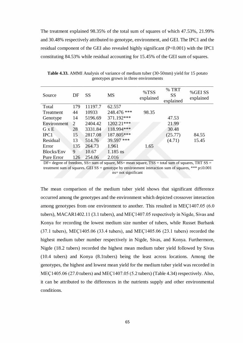
65

The treatment explained 98.35% of the total sum of squares of which 47.53%, 21.99%

and 30.48% respectively attributed to genotype, environment, and GEI. The IPC1 and the



Table 4.33. AMMI Analysis of variance of medium tuber (30-50mm) yield for 15 potato genotypes grown in three environments

Source DF SS MS %TSS

explained

% TRT

SS

explained

%GEI SS

explained

Total 179 11197.7 62.557

Treatment 44 10933 248.476 *** 98.35

Genotype 14 5196.69 371.192*** 47.53

Environment 2 2404.42 1202.21*** 21.99

G x E 28 3331.84 118.994*** 30.48

IPC1 15 2817.08 187.805*** (25.77) 84.55

Residual 13 514.76 39.597 *** (4.71) 15.45

Error 135 264.73 1.961 1.65



treatment sum of squares. GEI SS = genotype by environment interaction sum of squares, *** p0.001 ns= not significant

The mean comparison of the medium tuber yield shows that significant difference

occurred among the genotypes and the environment which depicted crossover interaction

among genotypes from one environment to another. This resulted in MEÇ1407.05 (6.0

tubers), MACAR1402.11 (3.1 tubers), and MEÇ1407.05 respectively in Nigde, Sivas and

Konya for recording the lowest medium size number of tubers, while Russet Burbank

(37.1 tubers), MEÇ1405.06 (33.4 tubers), and MEÇ1405.06 (23.1 tubers) recorded the

highest medium tuber number respectively in Nigde, Sivas, and Konya. Furthermore,

Nigde (18.2 tubers) recorded the highest mean medium tuber yield followed by Sivas

(10.4 tubers) and Konya (8.1tubers) being the least across locations. Among the

genotypes, the highest and lowest mean yield for the medium tuber yield was recorded in

MEÇ1405.06 (27.0 tubers) and MEÇ1407.05 (5.2 tubers) (Table 4.34) respectively. Also,

it can be attributed to the differences in the nutrients supply and other environmental

conditions.

66

Table 4.34. Two-way table of medium tuber (30-50mm) yield for 15 potato genotypes grown in

three different environments*


MACAR1402.10 24.7 c 11.3 jklm 6.0 qrstu 14.0

MACAR1402.11 14.5 hi 3.1 w 5.2 stuv 7.6

MACAR1406.04 12.6 ijk 5.6 rstuv 5.3 stuv 7.8

MACAR1406.07 19.8 f 11.8 jkl 20.9 ef 17.5

MACAR1409.09 12.9 ij 8.0 nop 4.8 uvw 8.5

MEÇ1402.07 10.3 lm 9.7 mn 11.1 jklm 10.4

MEÇ1402.09 21.3 def 12.8 ij 15.6 gh 16.6

MEÇ1405.06 24.5 c 33.4 b 23.1 cd 27.0

MEÇ1407.05 6.0 qrstu 5.2 stuv 4.5 uvw 5.2

MEÇ1407.08 17.3 g 10.2 lm 10.4 lm 12.6

MEÇ1407.17 10.8 klm 10.6 lm 7.9 nop 9.8

MEÇ1411.06 6.9 pqrs 7.5 opqr 7.8 nopq 7.4

AGRIA 21.8 de 6.9 pqrs 6.8 pqrst 11.9

MADELEINE 20.5 ef 6.2 pqrstu 3.8 vw 10.2

RUSSET BURBANK 37.1 a 9.4 mno 4.9 tuvw 17.1

Mean 18.2 10.4 8.1 12.2


Table 4.35 Stability estimation of the medium size tubers of potato breeding lines grown in


Genotype Mean

MTN

Finlay &

Wilkinson

Eberhard

& Russel

Shukla

Francis &

Kannenberg

Kang

Rank Sum

AMMI

Model


MACAR1402.10 25.6 2.08 0.03 4.17 14.25 16

MACAR1402.11 21.5 1.16 0.06 0.28 9.66 20

MACAR1406.04 21.9 0.75 0.10 0.57 6.59 19

MACAR1406.07 22.8 1.05 0.00 -0.04 8.02 6

MACAR1409.09 23.6 1.04 0.01 -0.01 7.77 6

MEÇ1402.07 21.5 0.81 0.10 0.46 7.16 20

MEÇ1402.09 22.5 0.94 0.00 -0.02 7.30 9

MEÇ1405.06 22.3 0.82 0.00 0.06 6.47 13

MEÇ1407.05 21.5 1.09 0.17 0.66 9.55 21

MEÇ1407.08 23.7 1.50 0.00 0.81 11.04 14

MEÇ1407.17 22.6 1.23 0.01 0.16 9.55 13

MEÇ1411.06 23.0 0.90 0.01 0.03 6.86 8

AGRIA 19.2 0.40 0.08 1.54 4.51 28

MADALEINE 19.4 0.91 0.03 0.09 8.36 20

RUSSET

BURBANK

20.0 0.32 0.12 2.03 4.28 27


67

4.8.3 Small Tuber (< 30mm) Yield

The ANOVA for the small tubers (<30mm) yield showed that, there was a highly

significant (p < 0.001) effects of genotypes, environments, and the genotype by

environment interaction on the potato tuber yield by the (Table 4.36, Table 4.37). There

was a high CV among the genotypes and the environments of 39.63 and the grand mean

yield of 0.72. The treatment explained 82.64% of the total sum of squares of which

54.66%, 29.15%, and 16.18%, respectively attributed to genotype, environment, and GEI.

The IPC1 and the residual component of the GEI also revealed highly significant

(P<0.001) with the IPC1 constituting 70.52% while residual accounting for 29.48% of

the GEI sum of squares. This indicates that genotype has much influence on the tuber

grading than environment and GEI. The environmental effect may be due to temperature

and nutrient disparities among the various environments which led to different responses

of the genotypes with the environment.

Table 4.36. ANOVA for small tubers (<30mm) for 15 genotypes grown in three different

environments


Genotype 14 43.7598 3.1257 38.33 0.000

Environment 2 23.5048 11.7524 144.14 0.000

G x E 28 12.8419 0.4586 5.62 0.000

Error 135 11.0075 0.0815

Total 179 91.1139

Grand Mean 0.7206

CV 39.63


p0.001

Table 4.15. AMMI Analysis of variance of small tuber size (<30mm) for 15 potato genotypes


Source DF SS MS %TSS

explained

% TRT SS

explained

%GEI SS

explained

Total 179 89.609 0.501

Treatment 44 78.919 1.794 *** 82.64

Genotype 14 43.139 3.081 *** 54.66

Environment 2 23.007 11.504 *** 29.15

G x E 28 12.773 0.456*** 16.18

IPC1 15 9.007 0.6 *** (11.41) 70.52

Residual 13 3.765 0.29 *** (4.77) 29.48

Error 135 10.69 0.079 17.36


Pure Error 126 10.013 0.079

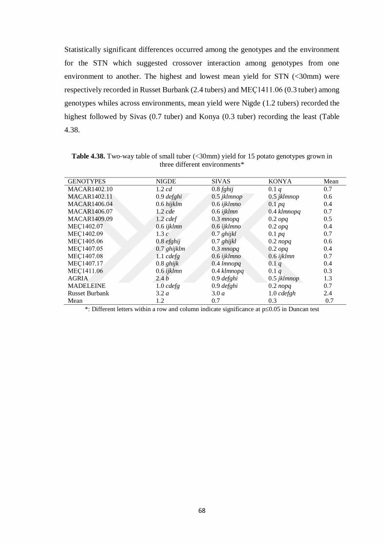
68

Statistically significant differences occurred among the genotypes and the environment

for the STN which suggested crossover interaction among genotypes from one

environment to another. The highest and lowest mean yield for STN (<30mm) were

respectively recorded in Russet Burbank (2.4 tubers) and MEÇ1411.06 (0.3 tuber) among

genotypes whiles across environments, mean yield were Nigde (1.2 tubers) recorded the

highest followed by Sivas (0.7 tuber) and Konya (0.3 tuber) recording the least (Table

4.38.

Table 4.38. Two-way table of small tuber (<30mm) yield for 15 potato genotypes grown in

three different environments*


MACAR1402.10 1.2 cd 0.8 fghij 0.1 q 0.7

MACAR1402.11 0.9 defghi 0.5 jklmnop 0.5 jklmnop 0.6

MACAR1406.04 0.6 hijklm 0.6 ijklmno 0.1 pq 0.4

MACAR1406.07 1.2 cde 0.6 ijklmn 0.4 klmnopq 0.7

MACAR1409.09 1.2 cdef 0.3 mnopq 0.2 opq 0.5

MEÇ1402.07 0.6 ijklmn 0.6 ijklmno 0.2 opq 0.4

MEÇ1402.09 1.3 c 0.7 ghijkl 0.1 pq 0.7

MEÇ1405.06 0.8 efghij 0.7 ghijkl 0.2 nopq 0.6

MEÇ1407.05 0.7 ghijklm 0.3 mnopq 0.2 opq 0.4

MEÇ1407.08 1.1 cdefg 0.6 ijklmno 0.6 ijklmn 0.7 MEÇ1407.17 0.8 ghijk 0.4 lmnopq 0.1 q 0.4

MEÇ1411.06 0.6 ijklmn 0.4 klmnopq 0.1 q 0.3

AGRIA 2.4 b 0.9 defghi 0.5 jklmnop 1.3

MADELEINE 1.0 cdefg 0.9 defghi 0.2 nopq 0.7

Russet Burbank 3.2 a 3.0 a 1.0 cdefgh 2.4

Mean 1.2 0.7 0.3 0.7


69

Table 4.39. Stability estimation of the small tuber number (STN) of potato breeding lines


Genotype Mean

STY

Finlay &

Wilkinsin

Regression

Eberhart

& Russel

(1966)

Shukla

(1972)

Francis &

Kannenberg

Kang

Rank

Sum

AMMI

Model


MACAR1402.10 25.62 2.08 0.03 4.17 14.25 16

MACAR1402.11 21.49 1.16 0.06 0.28 9.66 20

MACAR1406.04 21.89 0.75 0.10 0.57 6.59 19

MACAR1406.07 22.83 1.05 0.00 -0.04 8.02 6

MACAR1409.09 23.60 1.04 0.01 -0.01 7.77 6

MEÇ1402.07 21.49 0.81 0.10 0.46 7.16 20

MEÇ1402.09 22.45 0.94 0.00 -0.02 7.30 9

MEÇ1405.06 22.25 0.82 0.00 0.06 6.47 13

MEÇ1407.05 21.52 1.09 0.17 0.66 9.55 21

MEÇ1407.08 23.68 1.50 0.00 0.81 11.04 14

MEÇ1407.17 22.64 1.23 0.01 0.16 9.55 13

MEÇ1411.06 23.00 0.90 0.01 0.03 6.86 8

AGRIA 19.15 0.40 0.08 1.54 4.51 28

MADALEINE 19.44 0.91 0.03 0.09 8.36 20

R. BURBANK 19.99 0.32 0.12 2.03 4.28 27

CV, coefficient of variation; IPC1, interaction principal component analysis axis 1;

AMMI, Additive Main Effects and Multiplicative Interaction

MACAR1406.07, MACAR1409.09, MEÇ1402.09, MEÇ1407.05, and MADALEINE

were stable genotypes for the regression analysis while almost all the genotypes were

stable for Eberhart & Russel model (Table 4.35 and Table 4.39). Also, Shukla’s stability

model revealed MACAR1406.07, MACAR1409.09, MEÇ1402.09, MEÇ1405.06,

MEÇ1411.06, and MADALEINE as stable genotypes. Whereas Francis and Kannenberg

model and KR sum models failed to identify desirable genotypes for medium size tuber

number.

4.9. Marketable Tuber Weight (MTW)

The general ANOVA and combined AMMI ANOVA results of the MTW revealed highly

significant (p < 0.001) effects of the genotypes, environment, and their interaction on the

marketable tuber weight with a grand mean weight of 122.27kg at a CV of 3.06 among

the genotypes, and the environments of 3.06 (Table 4.40; Table 4.41). The genotypes,

environment, and the genotype by environment interaction treatment explained 94.75%

of the total sum of squares of which 50.53%, 25.46%, and 24.02% respectively accounted

70

for genotype, environment, and GEI. The IPC1 and the residual component of the GEI

also revealed highly significant (P<0.001) with the IPC1 constituting 70.8% while

residual accounting for 29.2% of the GEI sum of squares.

Table 4.40. ANOVA of marketable tuber weight for 15 genotypes grown in three different

environments


Genotype 14 81636 5831.2 415.45 0.000***

Environment 2 38730 19364.8 1379.66 0.000***

G x E 28 32452 1159 82.57 0.000***

Error 135 1895 14

Total 179 154713

Grand Mean 122.27

CV 3.06 DF= degree of freedom, SS= sum of square, MS= mean square, CV= coefficient of variation, ***

p0.001

The high significant effects observed in Table 4.40 and Table 4.41 reflect the significant

difference between genotypes across environments (Table 4.42) which shows that,

MACAR1402.11 (159.83kg) recorded the highest mean weight whiles Russet

Burbank(81.65kg) recorded the lowest with the environmental mean tuber weight of

141.54kg, 123.04kg, and 102.23kg respectively for Nigde, Sivas, and Konya. In Nigde,

the highest tuber weight was recorded in MEÇ1407.05 (145.9 kg), in Sivas,

MACAR1402.11 (222.7kg) while in Konya, MACAR1409.09 (161.1kg). On the other

hand, the lowest tuber weight in Nigde and Sivas was found in Russet Burbank of 67.7kg

and 74.5kg respectively while in Konya the lowest tuber weight was found in

MEÇ1405.06 (82.1kg). There was crossover GEI from one environment to another and

statistical significance differences occurring between the highest and lowest mean weight

of the genotypes across and within the environments which confirms Caliskan et al. 2007

finding on sweet potato.

71

Table 4.16. AMMI analysis of variance of MTW for 15 potato genotypes grown in three

environments


explained

% TRT SS

explained

%GEI SS

explained

Total 179 160149.3 894.689

Treatment 44 150978.9 3431.34 *** 94.75

Genotype 14 76288.46 5449.176*** 50.53

Environment 2 38432.21 19216.11*** 25.46

G x E 28 36258.27 1294.938*** 24.02

IPC1 15 25672.19 1711.479*** (17) 70.8

Residual 13 10586.08 814.314*** (7.01) 29.2

Error 135 9170.322 67.928 5.25

Blocks/Env 9 650.73 72.303 ns



Table 4.42. Two-way table of marketable tuber weight (MTW) for 15 potato genotypes grown

in three different environments*


MACAR1402.10 101.7 t 129.0 ghij 126.2 ijk 119.0

MACAR1402.11 109.5 pqr 222.7 a 147.3 e 159.8

MACAR1406.04 94.1 uopq 165.9 bc 132.5 gh 130.8

MACAR1406.07 83.5 wx 140.0 f 113.6 opq 112.4

MACAR1409.09 107.4 rs 169.2 b 161.1 cd 145.9

MEÇ1402.07 114.5 nop 142.7 ef 127.5 hij 128.2

MEÇ1402.09 87.9 vw 116.9 mno 110.7 pqr 105.2

MEÇ1405.06 94.9 u 92.3 uv 82.1 x 89.7

MEÇ1407.05 145.9 e 169.1 b 143.7 ef 152.9

MEÇ1407.08 108.6 qr 128.4 hij 121.4 klm 119.5

MEÇ1407.17 119.0 lmn 129.5 ghi 128.4 hij 125.6

MEÇ1411.06 124.0 jkl 142.2 ef 121.5 klm 129.2

AGRIA 84.0 wx 106.2 rst 110.9 pqr 100.4

MADELEINE 108.5 qr 158.8 d 134.1 g 133.8

Russet Burbank 67.7 z 74.5 y 102.9 st 81.7


The genotype MTW stability estimation in Table 4.43 revealed that none genotypes were

stable based on the Finlay & Wilkinsin (1963) Regression model, Eberhart & Russel

(1966) model, Shukla (1972) model, Francis & Kannenberg CV, Kang Rank Sum and

AMMI Model. Figure 4.15 categorised AGRIA, Russet Burbank, MEÇ1402.09,

MEÇ1405.06, MACAR1402.10, and MEÇ1407.08 as poorly adaptable to unfavourable

72

environmental conditions whiles MACAR1406.07 was categorised to be poorly

adaptable to favourable environmental conditions. MEÇ1402.07, MEÇ1407.05,

MEÇ1407.17, and MEÇ1411.06 on the other hand were very well adapted to

unfavourable environments whereas on the contrarily, MACAR1406.04,

MACAR1409.09 MACAR1402.11, and MADELEINE were very well adapted to

favourable environmental conditions

Table 4.43. Stability estimation of marketable tuber weight (MTW) of potato breeding lines


Genotype Mean

MTW

Finlay &

Wilkinson

Eberhart

& Russel

Shukla

Francis &

Kannenberg

Kang Rank

Sum

AMMI

Model


MACAR1402.10 118.97 0.79 6.89 22.2 12.6 13 -0.80

MACAR1402.11 159.83 3.08 75.05 1891.95 36.07 16 6.33

MACAR1406.04 130.82 2.00 1.15 352.68 27.47 17 2.80

MACAR1406.07 112.36 1.57 0.74 102.82 25.18 18 1.61

MACAR1409.09 145.89 1.78 29.78 325.4 23.02 14 1.72

MEÇ1402.07 128.23 0.78 1.14 0.22 11.05 8 -0.55

MEÇ1402.09 105.19 0.83 3.26 1.72 14.52 14 -0.63 MEÇ1405.06 89.73 -0.11 12.16 483.1 7.58 27 -2.80

MEÇ1407.05 152.87 0.60 23.51 131.58 9.23 10 -0.39

MEÇ1407.08 119.46 0.56 0.17 50.09 8.46 14 -1.26

MEÇ1407.17 125.64 0.30 1.04 162.79 4.59 18 -2.01

MEÇ1411.06 129.19 0.47 16.26 148.41 8.75 15 -1.18

AGRIA 100.36 0.66 18.28 93.81 14.3 19 -1.27

MADALEINE 133.77 1.39 1.33 40.77 18.78 8 1.14

RUSSET

BURBANK 81.65 0.28 92.08 539.96 22.86 29

-2.70

CV, coefficient of variation; IPC1, interaction principal component analysis axis 1; AMMI, Additive

Main Effects and Multiplicative Interaction

The AMMI biplot analysis of the potato tuber weight (Figure 4.16) showed that

MACAR1406.07 had a large positive IPC1 value and low weight tubers below the grand

weight of the genotypes and so was moderately susceptible to environmental conditions.

Russet Burbank, AGRIA, MACAR1402.10, MEÇ1407.08, MEÇ1402.09, and

MEÇ1405.06 produced low weighted tubers and had large negative IPC1 values, making

them susceptible and highly interactive to environmental condition and thus unstable.

MACAR1406.04, MACAR1402.11, MADELEINE, and MACAR1409.09 produce

above-average weighted tubers, with high IPC1 scores, making them unstable due to their

high interaction with the environments. On the other hand, MEÇ1402.07, MEÇ1411.06,

MEÇ1407.05, and MEÇ1407.17 had high IPC1 scores which depicted high GEI and

unstable in tuber weight in unfavourable environmental conditions.

73


marketable tuber weight (MTW) of 15 potato genotypes grown in three diverse environments

Figure 4.16. AMMI biplot analysis of interaction principal component axis (IPCA-1) with mean marketable tuber weight (MTW) of potato genotype evaluated across three different

environments. Note: MCR1 =MACAR1402.10, MCR2 = MACAR1402.11, MCR3 =

MACAR1406.04, MCR4 = MACAR1406.07, MCR5 = MACAR1409.09, MEC = MEÇ1402.07, MEC2 = MEÇ1402.09, MEC3 = MEÇ1405.06, MEC4 = MEÇ1407.05, MEC5 =

MEÇ1407.08, MEC6 = MEÇ1407.17, MEC7 = MEÇ1411.06, AGRA = AGRIA, MADA =

MADELEINE, RUBB = RUSSET BURBANK; KYNA = Konya, NGDE = Nigde, SVAS = Sivas

74

4.10 Dry Matter Content (%)

The general ANOVA and combined AMMI ANOVA revealed highly significant (p <

0.001) effects of the genotypes, environments, and the genotype by environment

interaction on the dry matter content (DMC) (Table 4.44; Table 4.45) with a grand mean

DMC of 22.1% at a CV among the genotypes, and the environments of 1.89 (Table 4.44).

A 93.96% of the total sum of squares was explained by the treatments of which genotypes,

environments, and genotype by environment constituted 51.95%, 39.4%, and 8.65% of

the total sum of squares, respectively. The high contribution of the treatment sum of

squares by genotypes and environment than the genotype by environment interaction

depicts that the variation in the DMC of the potato genotypes is largely due to genotypic

differences followed by the environments than the GEI component. The IPC1 and the



Table 4.44. ANOVA for dry matter content (DMC) for 15 genotypes grown in three different

environments


Genotype 14 483.443 34.532 199.11 0.000***

Environment 2 366.738 183.369 1057.31 0.000***

G x E 28 80.457 2.873 16.57 0.000***

Error 135 23.413 0.173

Total 179 954.052

CV 1.89 DF= degree of freedom, SS= sum of square, MS= mean square, CV= coefficient of variation, *** p 0.001

Table 4.45. AMMI Analysis of variance of dry matter content (DMC) for 15 potato genotypes



explained

% TRT SS

explained

%GEI SS

explained

Total 179 954.052 5.3299

Treatment 44 930.639 21.1511*** 93.96

Genotype 14 483.443 34.5317*** 51.95

Environment 2 366.738 183.369*** 39.41

G x E 28 80.4573 2.87347*** 8.65

IPC1 15 60.767 4.05114*** (6.53) 75.53

Residual 13 19.6902 1.51463*** (2.12) 24.47

Error 135 23.4131 0.17343 6.04

Blocks/Env 9 1.83286 0.20365 ns Pure Error 126 21.5803 0.17127



75

In Table 4.46, the mean DMC comparison revealed that the highest mean % DMC was

observed in MACAR1402.10 (25.62) whiles the lowest mean DMC was observed in

AGRIA (19.15) among the genotypes. The highest mean DMC among the environments

was observed in Sivas (23.41%) followed by Konya (22.71%) and the least observed in

Nigde (20.09%). Across environments revealed, MACAR1402.10 recorded the highest

DMC in Sivas and Konya of 28.157 and 27.273 respectively while MACAR1409.09

recorded the highest DMC in Nigde. On the other hand, AGRIA recorded the lowest

DMC for all the environments of 18.245, 19.235, and 19.972 respectively for Nigde,

Sivas, and Konya.

The differences in the dry matter content of the potato breeding lines might be due to

agro-ecological disparities. Differences in evaporative demand due to high global solar

radiation flux density, low relative humidity, and/or high wind speed cause closure of

stomata leading to reduction in photosynthesis accompanied with restriction of CO2

uptake, thus resulting in light intensities outside the required optimum for maximum dry

matter production (Stark and Love, 2003). The differences in altitude of the study areas

might also have a contributory factor in the disparities in the dry matter content as a result

of air and soil temperature differences as shown in Table 3.2 which have been ascribed

to have varietal effect on specific gravity of the potato tubers causing differences in the

dry matter concentration of the potato tubers (Pereira et al 2008).

Potato dry matter concentration is important in the food processing industry, especially

for French fries or chips. Dry matter content of >20% gives good chips quality (Kabira

and Berg, 2003; CIP 2007). Again, the Acquisition and Distribution Unit of CIP (2009)

distinctively categorized that, DMC of >23% is termed as high, DMC from 20 to 23% as

medium and DMC <20% as low according to the CIP (CIP, 2009). Wassu (2017) stated

that, the industrial use of potato is dependent on tuber dry matter concentration and starch

and that tubers with 20 to 24% dry matter concentration are ideal for French fries and

crisps processing. In the study, MACAR1402.10, MACAR1409.09, MEÇ1407.08, and

MEÇ1411.06 had high DMC (>23%); MACAR1402.11, MACAR1406.04,

MACAR1406.07, MEÇ1402.07, MEÇ1402.09, MEÇ1405.06, MEÇ1407.05, and

MEÇ1407.17 had medium DMC (20 to 23%) whilst Agria, Madeleine and Russet

Burbank had low DMC (<20%). All potato breeding lines in this study had DMC >21%

76

as compared to the check cultivars and thus making them ideal for the French fries and

chips industry.

Table 4.46. Two-way table of dry matter content (DMC) for 15 potato genotypes grown in three



MACAR1402.10 21.4 no 28.2 a 27.3 b 25.6

MACAR1402.11 19.1 v 22.6 m 22.7 lm 21.5

MACAR1406.04 20.5 qrs 23.4 hij 21.7 n 21.9

MACAR1406.07 20.7 pqr 24.2 efg 23.6 hi 22.8

MACAR1409.09 21.5 n 24.8 d 24.5 de 23.6

MEÇ1402.07 20.0 stu 23.1 ijklm 21.4 no 21.5

MEÇ1402.09 20.6 qr 23.8 fgh 22.9 jklm 22.5

MEÇ1405.06 20.6 qr 23.3 hijk 22.8 klm 22.2

MEÇ1407.05 19.6 uv 23.6 ghi 21.4 no 21.5

MEÇ1407.08 20.7 pqr 25.7 c 24.6 de 23.7

MEÇ1407.17 20.2 rst 24.4 de 23.3 hijkl 22.6

MEÇ1411.06 21.3 nop 24.4 def 23.3 hijk 23.0

AGRIA 18.2 w 19.2 v 20.0 stu 19.2

MADELEINE 17.6 x 20.4 qrst 20.4 qrst 19.4

RUSSET BURBANK 19.2 v 19.9 tu 20.9 opq 20.0


Table 4.47. Stability estimation of DMC of potato breeding lines grown in three


Genotype Mean

DMC

Finlay &

Wilkinsin

Regression

Eberhart

& Russel

(1966)

Shukla

(1972)

Francis &

Kannenberg

Kang

Rank

Sum

AMMI

Model


MACAR1402.10 25.623 2.081 0.025 4.167 14.245 16 1.33

MACAR1402.11 21.487 1.158 0.061 0.279 9.662 20 0.17 MACAR1406.04 21.887 0.751 0.102 0.574 6.594 19 -0.28

MACAR1406.07 22.833 1.047 0.001 -0.044 8.021 6 0.06

MACAR1409.09 23.597 1.044 0.009 -0.01 7.774 6 0.05

MEÇ1402.07 21.493 0.814 0.098 0.462 7.159 20 -0.2

MEÇ1402.09 22.45 0.935 0.004 -0.023 7.301 9 -0.07

MEÇ1405.06 22.247 0.824 0.000 0.056 6.474 13 -0.22

MEÇ1407.05 21.523 1.089 0.170 0.661 9.545 21 0.15

MEÇ1407.08 23.68 1.495 0.001 0.812 11.037 14 0.62

MEÇ1407.17 22.643 1.234 0.007 0.164 9.548 13 0.3

MEÇ1411.06 23.003 0.896 0.012 0.031 6.863 8 -0.12

AGRIA 19.153 0.396 0.076 1.536 4.507 28 -0.78

MADALEINE 19.437 0.912 0.028 0.085 8.362 20 -0.13

RUSSET BB 19.99 0.324 0.118 2.032 4.284 27 -0.88



77

The stability estimates in Table 4.47 revealed that MACAR1406.07, MACAR1409.09,

MEÇ1402.09, MEÇ1407.05, MEÇ1411.06, and MADALEINE were stable for based on

bi model while almost all the genotypes were stable based on S2d model. On the other

hand, except MACAR1402.10, MACAR1402.11, MACAR1406.04, AGRIA, and Russet

Burbank, the rest of the genotypes were stable based on Shukla (1972) model. The IPC1

scores also revealed that except MACAR1402.10, MEÇ1407.08, AGRIA, and Russet

Burbank, the rest of the genotypes were stable for DMC.

According to the Finlay and Wilkinson regression model, MACAR1409.09,

MACAR1406.07, and MEÇ1402.09 were well adapted to all environmental conditions,

while MEÇ1405.06, and MEÇ1411.06 were well adapted to unfavourable environmental

conditions making them tolerant to unfavourable environmental fluctuations. Also,

MACAR1402.10, MEÇ1407.08 and MEÇ1407.17 very well adapted to favourable

environmental conditions while MACAR1402.11, and MEÇ1407.05 were poorly adapted

to favourable environmental conditions. Contrarily, MACAR1406.04, MEÇ1402.07,

MADELEINE, AGRIA, and Russet Burbank were very much sensitive and are poorly

adapted to unfavourable environmental conditions.

Figure 4.17. Relationship of genotype adaptation (regression coefficient ‘bi’) and mean number of Dry Matter Content (DMC) of 15 potato genotypes grown in three diverse environments

The AMMI biplot analysis (Figure 4.18) also revealed that MACAR1406.07,

MACAR1409.09, MEÇ1402.09, MEÇ1405.06, and MEÇ1411.06 had high DMC and

78

were less influenced by environmental conditions due to their small IPC1 score making

them generally stable whilst MACAR1402.11, MACAR1406.04, MEÇ1402.07,

MEÇ1407.05, and MADELEINE had low DMC below the grand mean but generally

stable due to their small IPC1 scores. Contrarily, MACAR1402.10, MEÇ1407.08, and

MEÇ1407.17 on the other hand had very high DMC and high IPC1 scores which is an

indication of high GEI making them unstable whereas AGRIA and RUSSET BURBANK

were very susceptible to environmental condition and so highly unstable for DMC and so

have specific adaptability. The environments were grouped in to two mega environments

which are highly heterogeneous and unstable with large IPC1 values for DMC. Konya

and Sivas were positively correlated and produced high DMC whilst they were negatively

correlated with Nigde environment. Konya environment was ideal for the majority of the

genotypes in terms of DMC.

Figure 4.18. AMMI biplot analysis of interaction principal component axis (IPCA-1) with mean

of dry matter concentration (DMC) of potato genotype evaluated across three different environmentsNote: MCR1 =MACAR1402.10, MCR2 = MACAR1402.11, MCR3 = MACAR1406.04, MCR4 =

MACAR1406.07, MCR5 = MACAR1409.09, MEÇ1 = MEÇ1402.07, MEC2 = MEÇ1402.09, MEC3 = MEÇ1405.06, MEC4 = MEÇ1407.05, MEC5 = MEÇ1407.08, MEC6 = MEÇ1407.17, MEC7 = MEÇ1411.06,

AGRA = AGRIA, MADA = MADELEINE, RUBB = RUSSET BURBANK; KYNA = Konya, NGDE = Nigde,

SVAS = Sivas

4. 11 Specific Gravity (SG)

It was revealed by the ANOVA results (Table 4.48, Table 4.49) that, genotypes,

environments, and the genotype by environment interaction had a highly significant (p <

79

0.001) effects on the SG of the potato tubers with a grand mean SG of 1.089 and a CV

0.19 among the genotypes, and the environments (Table 4.48). A 93.16% of the total sum

of squares was explained by the treatments of which genotypes, environments, and

genotype by environment constituted 53.4%, 38.83%, and 9.71% of the total sum of

squares respectively. This shows that SG is genetically induced more than the

environmentally and GEI induced. The IPC1 and the residual component of the GEI also

revealed highly significant (p < 0.001) with the IPC1 constituting 50% of the GEI sum of

squares. The significant G, E, and G x E interaction effects on the DMC, SG, MTW in

the genotypes indicate that they vary in their genetic constitution (genotype main effect),

environmental fluctuations and the GEI which greatly influenced the quality traits.

Several potato scholars separately reported that, DMC (Tesfaye et al. 2013; Habtamu et

al. 2016b; Wassu, 2016) and SG are influenced by genetic varietal difference and

environmental conditions (Tessema et al. 2020). This confirms Arinaittwe et al. (2018)

reporting that GEI has a significant effect on the yield and quality traits of potato cultivars

which is reflected in the significant difference in the studied traits between genotype and

in environments.

Table 4.48 ANOVA of Specific Gravity (SG) for 15 genotypes grown in three different

environments


Genotype 14 0.01052 7.51E-04 174.61 0.000***

Environment 2 0.00831 0.00415 965.85 0.000***

G x E 28 0.00176 6.29E-05 14.63 0.000***

Error 135 0.00058 4.30E-06

Total 179 0.02117

Grand Mean 1.089

CV 0.19 DF= degree of freedom, SS= sum of square, MS= mean square, CV= coefficient of variation, *** p0.001

80

Table 4.49. AMMI Analysis of variance of specific gravity (SG) for 15 potato genotypes grown

in three environments


explained

% TRT SS

explained

%GEI SS

explained

Total 179 0.0212 0.0001

Treatment 44 0.0206 0.0005 *** 93.16 Genotype 14 0.011 0.0008 *** 53.4

Environment 2 0.008 0.0042 *** 38.83

G x E 28 0.002 0.0001 *** 9.71 IPC1 15 0.001 0.0001 *** (4.85) 50

Residual 13 0 0.0000 ***

Error 135 0.001 0.00 6.84

Blocks/Env 9 0 0.0000 ns Pure Error 126 0.001 0



It is observed in Table 4.50 that, the highest mean SG among the genotypes was found in

MACAR1402.10 (1.106) whiles the lowest SG was found in AGRIA (1.076), with Nigde

recording the least mean SG of 1.080, followed by Konya of 1.092 and Sivas recording

the highest SG of 1.095, which were significantly different from each other. It was also

observed that, all the breeding lines have higher SG than the commercial genotypes

(AGRIA, Russet Burbank, and MADELEINE). MACAR1402.10 recorded the highest

SG across the all environments making it superior over all the other genotypes in terms

of SG whereas AGRIA recorded the lowest SG in Sivas and Konya while in Nigde,

MADELEINE recorded the lowest SG. Though MACAR1402.10 was superior to all

other genotypes, there were different SG values across the environments thus indicating

crossover GEI. Potato SG is key a parameter in the food processing industry especially

for French fries or chips (Kabira and Berg, 2003; CIP, 2007; Wassu, 2017). For French

fry and potato chips, CIP (2007) set the minimum acceptable levels of potato tubers with

a specific gravity of ≥1.080, which reduces the amount of oil uptake by potato chips and

French fries during frying and enhanced texture and yield quality of finished products. In

this study, all the breeding lines have SG >1.081 gcm-3 as compared to the check cultivars

(AGRIA, Madeleine, and Russet Burbank) which have less than 1.08 gcm-3 SG and so all

the breeding lines are ideal for French fries and chips.

81

Table 4.50. Two-way table of specific gravity (SG), for 15 potato genotypes grown in three


Genotype Nigde Sivas Konya Mean

MACAR1402.10 1.087 mn 1.118 a 1.114 b 1.106

MACAR1402.11 1.075 wx 1.092 l 1.092 l 1.086

MACAR1406.04 1.082 pqrs 1.095 hijk 1.088 m 1.088

MACAR1406.07 1.083 pqr 1.099 efg 1.096 hij 1.093

MACAR1409.09 1.087 mn 1.103 d 1.100 de 1.096

MEÇ1402.07 1.079 stu 1.094 ijkl 1.086 mno 1.086

MEÇ1402.09 1.082 pqrs 1.097 fgh 1.093 jkl 1.091

MEÇ1405.06 1.082 qrs 1.095 hijk 1.092 kl 1.089

MEÇ1407.05 1.077 uvw 1.096 ghi 1.086 mno 1.086

MEÇ1407.08 1.083 opq 1.106 c 1.101 de 1.097

MEÇ1407.17 1.080 rst 1.100 def 1.095 hijk 1.092

MEÇ1411.06 1.083 pqr 1.100 def 1.096 hi 1.093

AGRIA 1.072 x 1.076 w 1.079 stu 1.076

MADELEINE 1.069 y 1.081 qrst 1.082 qrs 1.077

RUSSET BURBANK 1.076 vw 1.079 tuv 1.085 nop 1.080


In Table 4.51, MACAR1406.07, MACAR1409.09, MEÇ1402.09, MEÇ1407.05, and

MEÇ1411.06 were identified by the bi stability model to be stable. Based on the S2d and

σ2 models all the genotypes were revealed to be stable. Also, almost all the genotypes

were classified to be stable based on the IPC1 scores, but according to the Francis &

Kannenberg and Kang Rank Sum models, no genotype was identified to be stable. The

differences in the stability levels for the MTW, DMC, and SG of the genotypes can be

attributed to the difference in genotypic constitutions and environmental fluctuations

which led their different forces of interactions.

82

Table 4.51. Stability estimation of specific gravity of potato breeding lines grown in three


Genotype Mean

SG

Finlay &

Wilkinson

Eberhart

& Russel

Shukla

Francis &

Kannenberg

Kang Rank

Sum

AMMI

Model


MACAR1402.10 1.106 2.036 0.000 0.000 1.524 16 0.097

MACAR1402.11 1.086 1.167 0.000 0.000 0.903 18 0.009

MACAR1406.04 1.088 0.731 0.000 0.000 0.598 19 -0.017

MACAR1406.07 1.093 1.029 0.000 0.000 0.778 7 0.003

MACAR1409.09 1.097 1.029 0.000 0.000 0.776 2 0.001

MEÇ1402.07 1.086 0.845 0.000 0.000 0.691 9 -0.012

MEÇ1402.09 1.091 0.937 0.000 0.000 0.712 11 -0.002

MEÇ1405.06 1.09 0.823 0.000 0.000 0.625 13 -0.013

MEÇ1407.05 1.086 1.073 0.000 0.000 0.875 11 0.038

MEÇ1407.08 1.097 1.463 0.000 0.000 1.103 12 0.016

MEÇ1407.17 1.092 1.257 0.000 0.000 0.953 12 0.021

MEÇ1411.06 1.093 1.075 0.000 0.000 0.813 7 0.009

AGRIA 1.076 0.344 0.000 0.000 0.326 28 -0.062

MADALEINE 1.077 0.847 0.000 0.000 0.671 21 -0.013

R. BURBANK 1.08 0.345 0.000 0.000 0.424 27 -0.064


The bi values and mean SG biplot categorized MACAR1409.09 as well adapted to all

environmental conditions, while MACAR1406.07 is poorly adapted to all environmental

conditions. MACAR1402.10 and MEÇ1407.08 were well adapted to favourable

environmental conditions. On the contrarily, MEÇ1411.06, MEÇ1407.17, MEÇ1407.05,

and MACAR1402.11 were poorly adapted to favourable environmental conditions while

MEÇ1402.09, MEÇ1405.06, MACAR1406.04, MEÇ1402.07, MADELEINE, AGRIA,

and Russet Burbank were very much sensitive and were poorly adaptable to unfavourable

environmental conditions (Figure 4.19).

The AMMI biplot of SG (Figure 4.20) revealed that MACAR1406.07, MACAR1409.09,

MEÇ1402.09, MEÇ1405.06, and MEÇ1411.06 had high SG with less interaction with

environmental influences making them generally stable whilst MACAR1402.11,

MACAR1406.04, MEÇ1402.07, MEÇ1407.05, and MADELEINE had low SG and

generally stable. Contrarily, MACAR1402.10, MEÇ1407.08, and MEÇ1407.17 on the

other hand, had very high values of SG and high IPC1 scores indicating a high GEI

making them unstable whereas AGRIA and Russet Burbank were very susceptible to

environmental condition and so highly unstable for SG and so had specific adaptability.

The environments were highly heterogeneous with large IPC1 values and were unstable

for SG. Averagely, Konya environment was ideal for the majority of the genotypes in

83

terms of SG. Overall, 8 of the 15 genotypes had SG above grand mean and 7 (47 %)

genotypes had SG below the grand mean of 1.089. Also, 53% of the genotypes have

positive IPCA1 whilst 47% of the genotypes had negative IPCA1 values. Larger IPC1

scores and larger bi values of the genotypes indicate higher instability and specific

adaptability of the genotypes to the environment due to higher interaction (Temesgen et

al. 2015).

Figure 4.19. Relationship of genotype adaptation (regression coefficient ‘bi’) and mean specific

gravity (SG) of 15 potato genotypes grown in three diverse environments

Figure 4.20. AMMI biplot analysis of interaction principal component axis (IPCA-1) with

mean of specific gravity (SG) of potato genotype evaluated across three different environments Note: MCR1 =MACAR1402.10, MCR2 = MACAR1402.11, MCR3 = MACAR1406.04, MCR4 = MACAR1406.07,

MCR5 = MACAR1409.09, MEÇ1 = MEÇ1402.07, MEC2 = MEÇ1402.09, MEC3 = MEÇ1405.06, MEC4 = MEÇ1407.05, MEC5 = MEÇ1407.08, MEC6 = MEÇ1407.17, MEC7 = MEÇ1411.06, AGRA = AGRIA, MADA =

MADELEINE, RUBB = RUSSET BURBANK; KYNA = Konya, NGDE = Nigde, SVAS = Sivas

84

4.12. Principal component analysis of variables

To determine the number of PCA to retain, the scree plot based on the eigenvalues was

used. The PCA with an eigenvalue greater than or equal to 1 had a significant effect on

the GEI and so was retained whilst those with eigenvalue less than 1 was discarded. The

first four PCA (F1, F2, F3, and F4) had their eigenvalues greater than 1 which had a

cumulative variability of 85.63% (Figure 4.21).

Figure 4.21. Scree plot of Eigenvalues against PCA with cumulative variability (%) for GEI of

the studied traits, where F1 to F12 indicates IPCA1 to IPCA12

To avoid disturbance and complication in the analysis, the first two interaction principal

component axes (IPCA1 and IPCA2), which explained 64.72% of total GEI, were used

in the PCA analysis in constructing the biplot to evaluate the genotypes traits relationships

and adaptation to the environments (Figure 4.22). The degree of GEI was proportional to

the length of the vector of an environment from the biplot origin. Thus, the environments

with longer vectors indicated strong forces of interaction whilst the environments with

shorter vectors indicated weak forces of interaction. The PCA results of the genotypes by

environment interaction effects on the traits show that number of tubers per plant (NTP),

marketable tuber yield (MTY), total plant yield (TPY), dry matter concentration (DMC),

and specific gravity (SG) moved in the same direction and so exhibited positive

correlations. They also had longer vectored away from the PCA origin which depicted

0

20

40

60

80

100

0

1

2

3

4

5

6

7

F1 F2 F3 F4 F5 F6 F7 F8 F9 F10 F11 F12

Cu

mu

lati

ve v

aria

bil

ity

(%

)

Eig

en

va

lue

PCA

Scree plot

85

that they had very high GEI. There was almost a 100% positive correlation between DMC

and SG, and between MTY and TTY. N11, S1, S3, S4, S5, S6, S7, S8, S9, S10, S11, S12,

S13, and S14 are observed to cluster around the same quadrant of the PCA axis which

indicated that they had the same response in similar environmental conditions for NTP,

MTY, TPY, TTY, DMC, and SG. This suggested that Sivas location was the best

environment for TTY, TPY. MTY, NTP, SG, and DMC. This confirmed the Spearman’s

correlation analysis (Table 4.38).

Figure 4.22. PCA1 and PCA2 biplot of genotype by environment interaction (GEI) relationship of the variables in the three different environments

Note: N1, N2, N3, …, N15, S1, S2, S3, …, S15 and K1, K2, K3, …,K15 respectively refers to genotype

1, 2, 3, …, and 15 interactions respectively with Nigde environment, Sivas environment, and Konya

environment; N = Nigde, S = Sivas, K = Konya, 1 =MACAR1402.10, 2 = MACAR1402.11, 3 =

MACAR1406.04, 4 = MACAR1406.07, 5 = MACAR1409.09, 6 = MEÇ1402.07, 7 = MEÇ1402.09, 8=

MEÇ1405.06, 9= MEÇ1407.05, 10 = MEÇ1407.08, 11 = MEÇ1407.17, 12 = MEÇ1411.06, 13 = AGRIA,

14 = MADELEINE, 15 = RUSSET BURBANK; MTN= Medium tuber number, STN= small tuber number,

SE=stand establishment, NTP= number of tuber per plant, MTY = marketable tuber yield, TTY = total

tuber yield, TPY =total plant yield, SG=specific gravity, DMC=dry matter concentration, NSP=number of stem per plant

Genotype K1, K2, K5, K9, K10, K11, K12, K14, N12, and S2 were also clustered in the

same quadrant of PCA axis which also indicated that they correlate positively in the same

environmental conditions for MTW, PH, and BTN. The genotypes in this quadrant had

yield above-average for MTW, PH, and BTN and thus were moderately tolerant. This

N1

S1

K1N2

S2

K2

N3

S3

K3

N4

S4

K4N5

S5

K5

N6

S6

K6

N7S7

K7

N8

S8

K8

N9

S9

K9

N10

S10

K10

N11

S11

K11

N12

S12

K12

N13

S13

K13

N14

S14

K14

N15

S15

K15

SE

NSP

PH

NTP

MTW

BTN

MTN

STNTPY

TTY

MTY

DMC

SG

-8

-6

-4

-2

0

2

4

6

8

-10 -8 -6 -4 -2 0 2 4 6 8 10 12

PC

2 (

20.7

2 %

)

PC1 (44.00 %)

Biplot (axes PC1 and PC2: 64.72 %)

86

depicted that Konya environment was the best for PH, BTN, and MTW. On the contrarily,

genotypes; N14, N15, N13, N4, N8, N10, N7, N1, S15, and K8 had similar field

behaviour as they were clustered in the quadrant and were positively and strongly

correlated with SE, STN, and MTN. Nigde environment was depicted to found in this

quadrant which was moderately susceptible to unfavourable environmental conditions. It

also had high GEI. Among all the variables, only NSP had less GEI though it was very

susceptible to unfavourable environmental conditions. Genotype N3, N2, N5, N6, N9,

K3, K6, K7, K3, K4, and K13 were segregated to be susceptible to unfavourable

environmental fluctuations.

4.13 Spearman’s Correlation analysis between the parameters

Table 4.52 presents the relations between the various traits using the spearman correlation

techniques. It showed a very weak correlation between the SE, NSP, and PH and the plant

yield (TPY, TTY, MTY, BTN, MTN, STN, NTP), and quality traits (MTW, DMC, and

SG). Within and among the yield and quality traits, there exist moderate to strong

correlations which was confirmed by the PCA results (Figure 4.22). There was a high

correlation (above 70%) between NTP and the TPY, TTY, and MTY, but a weak

correlation (below 50%) with DMC and SG. Within the yield and quality traits, there exist

very high correlations above 90% between TPY, TTY, and MTY while with moderate

correlation with DMC and SG. Whiles moderate correlations occurred between MTW

and BTN, MTN, and STN.

Table 4. 17. Spearman Correlation analysis between parameters

Trait SE NSP PH NTP MTW BTN MTN STN TPY TTY MY DM SG

SE 1 0.15 -0.09 0.17 -0.37 -0.13 0.12 0.22 0.05 0.23 0.23 -0.13 -0.13 NSP 1 0.24 0.00 -0.16 -0.01 0.02 -0.14 -0.11 -0.08 -0.08 0.06 0.06 PH 1 -0.01 0.26 0.45 -0.43 -0.51 0.11 0.06 0.07 0.41 0.42 NTP 1 0.01 -0.09 0.11 -0.16 0.80 0.81 0.81 0.46 0.45 MTW 1 0.71 -0.69 -0.56 0.57 0.47 0.48 0.41 0.41

BTN 1 -1.00 -0.57 0.35 0.30 0.31 0.28 0.27 MTN 1 0.52 -0.33 -0.28 -0.29 -0.25 -0.24 STN 1 -0.43 -0.38 -0.39 -0.50 -0.50 TPY 1 0.98 0.98 0.62 0.62 TTY 1 1.00 0.57 0.56 MTY 1 0.57 0.56 DMC 1 1.00 SG 1

SE= stem establishment, PH= plant height, NTP = tuber per plant, MTW = marketable tuber weight, NSP

=stem per plant, BTN = big tuber (>50mm) Number, MTN = medium Tuber (>30mm and <50mm) number, STN = small size tuber (<30mm), TPY = total plant yield, TTY = total tuber yield, MTY =

marketable tuber yield, DMC = dry matter, SG = specific gravity

87

4.14. Potato French fries

As in Table 4.53, the ANOVA of the French fries (FF) revealed highly significant (p <

0.001) differences among the genotypes (G) and the tested environments (E) for the

lightness (L*), redness (a*) and the yellowness (b*), whiles GEI only have high

significant (P< 0.01) effects on the redness (a*) but not on the lightness (L*) and

yellowness (b*) (P > 0.05) of the FF. For the AMMI analysis, genotype had a highly

significant (P< 0.001) effect on the French Fry’s L*, a*, and b* which respectively

accounted 50.86%, 52.72%, and 58.11%. The environmental effect was also significant

(P≤ 0.01) for the L*, a*, and b* which respectively accounted 30.91%, 22.59%, and

12.67%. there was also a significant (P< 0.01) difference for IPC1 of the a* value which

contributed 64.06% of the GEI sum of squares (Table 4. 54, 4.55, 4. 56). This result

buttresses the findings of Rak et al. (2013) and Affleck et al., (2008) reporting that GEI

had a great impact on the French fry colour during processing.

Table 4.53. ANOVA of French fries for 12 genotypes grown in three different environments

Source DF Lightness (L*) Redness (a*) Yellowness (b*)

SS F>Pr SS F>Pr SS F>Pr

G 11 552.91 7.28*** 159.48 8.79*** 339.49 4.21***

E 2 335.98 24.34*** 68.36 20.72*** 74.02 5.04**

G*E 22 198.19 1.31ns 74.69 2.06** 170.67 1.06ns

Error 108 745.33 178.14 792.34

Total 143 1832.42 480.67 1376.52

GM 72.2 0.59 23.37

CV 3.64 216.36 11.59


Table 4.54. AMMI Analysis of variance of French fries (lightness L*) for 12 potato genotypes evaluated in three environments



%GEI SS explained

Total 143 1832.424 12.814 Treatment 35 1087.089 31.060*** 59.33

Genotype 11 552.911 50.265*** 50.86

Environment 2 335.986 167.993*** 30.91

G x E 22 198.192 9.009ns 18.23

IPC1 12 158.407 13.201 ns (14.57) 79.93

Residual 10 39.785 3.978 ns (3.66) 20.07

Error 108 745.335 6.901 40.67

Blocks/Env 9 55.956 6.217 ns

Pure Error 99 689.379 6.963

88

Table 4.55. AMMI Analysis of variance of French fries (redness a*) for 12 potato genotypes

evaluated in three environments


explained

% TRT SS

explained

%GEI SS

explained

Total 143 480.668 3.361

TRT 35 302.511 8.643*** 62.94

GEN 11 159.472 14.497*** 52.72

ENV 2 68.352 34.176*** 22.59

G x E 22 74.687 3.395*** 24.89

IPC1 12 47.841 3.987** (15.81) 64.06

Residual 10 26.846 2.685 (8.87) 35.94

Error 108 178.157 1.650 37.06

Blocks/Env 9 9.480 1.053ns

Pure Error 99 168.677 1.704


treatment sum of squares. GEI SS = genotype by environment interaction sum of squares, **p0.01, ***


Table 4.56. AMMI Analysis of variance of French fries (yellowness b*) for 12 potato

genotypes evaluated in three environments



%GEI SS explained

Total 143 1376.516 9.626 Treatment 35 584.178 16.691*** 42.44

Genotype 11 339.494 30.863*** 58.11

Environment 2 74.017 37.009** 12.67

G x E 22 170.667 7.758ns 29.22 IPC1 12 140.776 11.731ns 924.1) 82.49

Residual 10 29.891 2.989 ns (5.12) 17.51

Error 108 792.338 7.336 57.56 Blocks/Env 9 29.965 3.329 ns

Pure Error 99 762.373 7.701



squares, **p0.01, *** p0.001 ns= not significant

4.15 Potato Chips

The potato chips were fried and chroma-meter (Konica Minolta) measurements were

taken for ANOVA analysis. The ANOVA results showed that there was high significant

(p<0.01) effects of the environment on the potato chip but not the genotypes for the

lightness (L*) whilst there was a high significant effect (P < 0.01) for the redness (a*)

among the genotypes, but not the yellowness (b*) (p > 0.05) for the tested genotypes and

environment. There was a significant effect (P < 0.01) of GEI on the potato chips a* but

not on the L* and b* (Table 4.57). The grand mean a*, L*, b* values respectively were

89

4.41, 60.71, and 19.22 which occurred at a CV of 30.67, 4.41, and 92.69, respectively.

The AMMI ANOVA for chips L* values showed that, only the environment had a

significant (P < 0.01) effect on the chips whilst genotypes and GEI had no effect on the

chips. For the a*, there was a significant (P < 0.001 and P < 0.01) effects caused by the

genotypes and GEI but no significant effect was caused by the environment. IPC1 showed

high significance (P < 0.01) which constituted 88.93% of the GEI sum of squares. On the

contrarily, there was no significant effect of the treatments for the b* values (Table 4.58,

4.59, 60).

Table 4.57. Calorimetry assessment of potato chips for 12 genotypes grown in three different

environments

Source DF Lightness (L*) Redness (a*) Yellowness (b*)

SS F>Pr SS F>Pr SS F>Pr

Genotype (G) 11 138.7 1.54ns 102.34 5.08** 3095.3 0.89ns

Environment (E) 2 99.64 6.1** 4.777 1.3ns 632.5 1ns

G x E 22 187.98 1.05ns 92.005 2.28** 6535.5 0.94ns

Error 108 882.27 197.744 34275.2

Total 143 1308.59 396.865 44538.5 GM 60.71 4.41 19.22

CV 4.71 30.67 92.69


Table 4.58. AMMI Analysis of variance of potato chips lightness (L*) for 12 potato genotypes

evaluated in three environments


explained

% TRT SS

explained

%GEI SS

explained

Total 143 1308.596 9.151

Treatment 35 426.326 12.181 ns 32.58

Genotype (G) 11 138.703 12.609 ns 32.53

Environment (E) 2 99.644 49.822** 23.37 G x E 22 187.979 8.544 ns 44.1

IPC1 12 154.318 12.860 ns (36.2) 82.1

Residual 10 33.660 3.366 ns (7.89) 17.91

Error 108 882.271 8.169 67.42

Blocks/Env 9 90.351 10.039 ns

Pure Error 99 791.920 7.999


TRT SS = treatment sum of squares. GEI SS=genotype by environment interaction sum of

squares, **p 0.01, *** p0.001 ns = not significant

90

Table 4.59. AMMI Analysis of variance of potato chips redness (a*) for 12 potato

genotypes evaluated in three environments


explained

% TRT SS

explained

%GEI SS

explained

Total 143 396.8684 2.7753

Treatment 35 199.1224 5.68921*** 50.17

Genotype (G) 11 102.3387 9.30352*** 51.4

Environment

(E) 2 4.77732 2.38866 ns 2.4

G x E 22 92.00631 4.1821** 46.21

IPC1 12 81.81696 6.81808** (41.1) 88.93

Residual 10 10.18935 1.01893 ns 49.83 (5.12) 11.07

Error 108 197.746 1.83098

Blocks/Env 9 25.69894 2.85544 ns

Pure Error 99 172.0471 1.73785


TRT SS = treatment sum of squares. GEI SS=genotype by environment interaction sum of

squares, **p0.01, *** p0.001 ns= not significant

Table 4.60. AMMI Analysis of variance of potato chips yellowness (b*) for 12 potato genotypes evaluated in three environments


explained

% TRT SS

explained

%GEI SS

explained

Total 143 737.0348 5.15409

Treatment 35 234.5919 6.70263ns 31.83

Genotype 11 81.37793 7.39799 ns 34.69

Environment 2 21.12287 10.56143 ns 9

Genotype x

Environment 22 132.0911 6.00414 ns 56.31

IPC1 12 110.376 9.198 ns (47.1) 83.56

Residual 10 21.71514 2.17151 ns (9.26) 16.44

Error 108 502.4429 4.65225 68.17

Blocks/Env 9 39.63154 4.4035 ns

Pure Error 99 462.8114 4.67486



squares, ns= not significant

91

CHAPTER V

6CONCLUSION

The study of genotype by environment interactions in plant breeding has once again been

proven to be essential for agronomists and plant breeders. The use of stability models

such as Finlay and Wilkinson regression coefficient and the Additive main effect and

multiplicative interactions (AMMI) are vital tools in establishing the stability levels of

potato breeding lines. The study revealed that:

There were significant genotypic, environmental and GEI effects on all traits,

which shows the existence of high variabilities among the potato breeding lines

due to the different parental sources and productivity of each environment.

Crossover type of GEI was present which resulted in genotypes ranking

differently in each environment.

MEÇ1407.17, MEÇ1407.05, MEÇ1407.08 and MEÇ1411.06 were outstanding

genotypes in respect to marketable tuber yield while the standard cultivars Agria,

Russet Burbank and MACAR1402.11 were found as low yielding genotypes as

average of three locations.

Genotypes MEÇ1407.17, MEÇ1411.06, MADELEINE, MACAR1406.07,

MEÇ1402.07, MEÇ1402.09, and Agria were more stable genotypes with broad

adaptability to diverse environments.

MEÇ1405.06, MEÇ1407.05, MEÇ1407.08, MACAR1409.09, MACAR1406.04,

MACAR1402.10, MACAR1402.11 and Russet Burbank were unstable with

specific adaptation.

92

All the 12 breeding lines have DMC >20% and SG > 1.080, which are threshold

levels for potato processing industries and are ideal for chips and French fries

processing.

Sivas location was found as the most productive environment for potato yield

while the Niğde and Konya have similar performance.

Our findings revealed that, AMMI model better explained the GEI and stability

of genotypes comparing to the Finlay and Wilkinson model.

They were difference in stability model models used in terms of genotype stability

levels.

The breeding lines MEÇ1407.17, MEÇ1407.05, MEÇ1407.08 and MEÇ1411.06

were identified as promising cultivar candidates due to their high tuber yield and

stable performances across different environments

93

7REFERENCES

Adjebeng-Danquah, J., Manu-Aduening, J., Gracen, V. E., Asante, I. K. & Offei, S. K.,

“AMMI stability analysis and estimation of genetic parameters for growth and yield

components in cassava in the forest and guinea savannah ecologies of Ghana”,

International Journal of Agronomy, 1–10. 2017

Adu, G. B., “Genotype by environment interaction and grain yield stability of extra-early

maize (Zea mays L.) hybrids evaluated at three locations in Ghana”, Master thesis,

Kwame Nkrumah University of Science and Technology, 1-109, 2012

Affleck, I., Sullivan, J. A, Tarn, R. & Falk, D. E., “Genotype by environment interaction

effect on yield and quality of potatoes”, Canadian Journal of Plant Science, 88, 1099–

1107, 2008

Aliche, E. B., Oortwijn, M., Theeuwen, T. P. J. M., Bachem, C. W. B., Visser, R. G. F.

& van der Linden, C. G., “Drought response in field grown potatoes and the interactions

between canopy growth and yield”, Agricultural Water Management 206, 20–30, 2018

Arinaitwe, A. B., Mateeka, B., Deo, T. & Alex, B., “Genotype by environment interaction

(GxE) as a measure of yield stability of Dutch potato varieties in Uganda”, African

Journal of Agricultural Research 13, 890–896, 2018

Atnaf, M., Kidane, S., Abadi, S. & Fisha, Z., “GGE biplots to analyze soybean

multienvironment yield trial data in North-western Ethiopia”. Journal of. Plant

Breeding. and Crop Science. 5, 245–254, 2013

Bach, E. C., Warnock D. D., Van Horn, D. J., Weintraub, N. M., Sinsabaugh, R. L.,

Allison, S. D., German, P. G., “Measuring phenol oxidase and peroxidase activities with

pyrogallol, L-DOPA, and ABTS: Effect of assay conditions and soil type”, Soil Biology

and Biochemistry 67, 183-191, 2013

https://doi.org/10.5897/AJAR2018.13061

94

Badu-Apraku, B., Oyekunle, M., Obeng-Antwi, K., Osuman, A. S., Ado, S. G., Coulibay,

N., Yallou, C. G., Abdulai, M., Boakyewaa, G. A. & Didjeira, A., “Performance of extra-

early maize cultivars based on GGE biplot and AMMI analysis”, The Journal of

Agricultural Science, 150, 473–483, 2012

Bai, J., Zhao, F., He, J., Wang, C., Chang, H., Zhang, J. & Wang, D., “GGE biplot analysis

of genetic variations of 26 potato genotypes in semi-arid regions of Northwest China”,

New Zealand Journal of Crop and Horticultural Science, 42, 161–169, 2014.

Bailey-Serres, J., Parker, J. E., Ainsworth, E. A., Oldroyd, G. E. D. & Schroeder, J. I.,

“Genetic strategies for improving crop yields”, Nature, 575, 109–118, 2019

Baril, C. P., Denis, J.-B., Wustman, R. & van Eeuwijk, F. A., “Analysing genotype by

environment interaction in Dutch potato variety trials using factorial regression”,

Euphytica 82, 149–155, 1995

Beals, K. A., “Potatoes, Nutrition and Health”, American. Journal of Potato Research

96,102–110, 2019

Bhartiya, A., Aditya, J., Kumari, V., Kishore, N., Purwar, J. & Agrawal, A., “GGE biplot

and AMMI analysis of yield stability in multi-environment trial of soybean [Glycine max

(L.) Merrill] genotypes under rainfed condition of North-western Himalayan hills”,

Journal of Animal and Plant Sciences 27, 227–238, 2017

Biru, A., Kassahun, T., Teklehaimanot, H. & Dagnachew, L., “Genotype by environment

interactions and grain yield stability of released and advanced Desi type chickpea (Cicer

arietinum L.) genotypes in western Ethiopia”, International Journal of Biotechnology

and Molecular Biology Research 8, 30–37. 2017

Bornhofen, E., Benin, G., Storck, L., Woyann, L. G., Duarte, T., Stoco, M. G. &

Marchioro, S. V., “Statistical methods to study adaptability and stability of wheat

genotypes”, Bragantia 76, 1–10, 2017

https://doi.org/10.1017/S0021859611000761

https://doi.org/10.1038/s41586-019-1679-0

https://doi.org/10.1007/BF00027061

https://doi.org/10.5897/IJBMBR2017.0281

https://doi.org/10.1590/1678-4499.557

95

Bradshaw, J. E., “Potato-breeding strategy” Potato Biology and Biotechnology, 157–

177, 2007

Burgos, G., Zum Felde, T., Andre, C. & Kubow, S., “The potato and its contribution to

the human diet and health”, Campos H.& Ortiz O. (Eds.), The Potato Crop, 37–74, 2020

Burtukan, B., “T”EMPEffect of nitrogen and phosphorus rates on growth, yield, yield

components and quality of potato (Solanum tuberosum L.) at Dedo, South West

Ethiopia”. An MSc Thesis Presented to School of Graduate Study of Jimma University,

Ethiopia

Bustos-Korts, D., Romagosa, I., Borràs-Gelonch, G., Casas, A. M., Slafer, G. A. & van

Eeuwijk, F., “Genotype by environment interaction and adaptation”, Encyclopedia of

Sustainability Science and Technology, 1–44, 2018

Caliskan, M. E., Erturk, E., Sogut, T., Boydak, E. & Arioglu, H., “Genotype ×

environment interaction and stability analysis of sweet potato (Ipomoea batatas)

genotypes” New Zealand Journal of Crop and Horticultural Science 35, 87–99. 2007

Chowański, S., Adamski, Z., Marciniak, P., Rosiński, G., Büyükgüzel, E., Büyükgüzel,

K., Falabella, P., Scrano, L., Ventrella, E., Lelario, F. & Bufo, S., “A review of

bioinsecticidal activity of solanaceae alkaloids”, Toxins 8, 60, 2016

Cobb, J. N., Juma, R. U., Biswas, P. S., Arbelaez, J. D., Rutkoski, J., Atlin, G., Hagen,

T., Quinn, M. & Ng, E. H., “Enhancing the rate of genetic gain in public-sector plant

breeding programs: Lessons from the breeder’s equation” Theoretical and Applied

Genetics 132, 627–645, 2019

Cooper, M.& DeLacy, I.H., “Relationships among analytical methods used to study

genotypic variation and genotype-by-environment interaction in plant breeding multi-

environment experiments, Theoretical and Applied. Genetics 88, 561–572,1994

https://doi.org/10.1080/01140670709510172

https://doi.org/10.3390/toxins8030060

96

Crossa, J., Vargas, M., Cossani, C. M., Alvarado, G., Burgueño, J., Mathews, K. L. &

Reynolds, M. P., “Evaluation and interpretation of interactions”, Agronomy Journal 107,

736–747, 2015

De Haan, S. & Rodriguez, F., “Potato Origin and Production”, Advances in Potato

Chemistry and Technology, 1–32, 2016

Delgado A., Quemada M., Villalobos F.J. & Mateos L., “Fertilization with Phosphorus,

Potassium and Other Nutrients”, Principles of Agronomy for Sustainable Agriculture,

2016

Devaux, A., Kromann, P. & Ortiz, O., “Potatoes for sustainable global food security”,

Potato Research 57, 185–199, 2014

De Leon, N., Jannink, J. L., Edwards, J. W. & Kaeppler, S. M., “Introduction to a special

issue on genotype by environment interaction”, Crop Science 56, 2081–2089, 2016

Demirel, U., Çaliskan, S., Yavuz, C., Tindas, I., Polgar, Z., Vaszily, Z., Cernak, I.,

Çaliskan, M. E., “Assessment of morphophysiological traits for selection of heat-tolerant

potato genotypes”, Turkish Journal of Agriculture and Forestry 218-232, 2017

Desalegn, G., Turetschek, R., Kaul, H. P. & Wienkoop, S., “Microbial symbionts affect

Pisum sativum proteome and metabolome under Didymella pinodes infection”, Journal

of Proteomics 143, 173–187, 2016

Di Vittorio, A. V., Kyle, P. & Collins, W. D., “What are the effects of Agro-Ecological

Zones and land use region boundaries on land resource projection using the Global

Change Assessment Model”, Environmental Modelling and Software, 85, 246–265,

2016

Dube, T., Moyo, P., Ncube, M. & Nyathi, D., “The impact of climate change on agro-

ecological based livelihoods in Africa: A review”, Journal of Sustainable Development

9, 256, 2016

https://doi.org/10.1007/s11540-014-9265-1

https://doi.org/10.1016/j.envsoft.2016.08.016

97

Dwivedi, Goldman, & Ortiz, “Pursuing the potential of heirloom cultivars to improve

adaptation, nutritional, and culinary features of food crops”, Agronomy 9, 441, 2019

Eberhart, S.A. & Russell, W.A., “Stability Parameters for Comparing Varieties”, Crop

Science 6, 36-40, 1966

El-Ramady, H., Alshaal, T., Elhawat, N., Ghazi, A., Elsakhawy, T., Omara, A. E. D., El-

Nahrawy, S., Elmahrouk, M., Abdalla, N., Domokos-Szabolcsy, É. & Schnug, E., “Plant

nutrients and their roles under saline soil conditions. In M. Hasanuzzaman, M. Fujita, H.

Oku, K. Nahar, & B. Hawrylak-Nowak (Eds.), Plant Nutrients and Abiotic Stress

Tolerance, 297–324, 2018

Ezekiel, R., Singh, N., Sharma, S. & Kaur, A., “Beneficial phytochemicals in potato A

review”. Food Research, 2013

FAO, “The future of food and agriculture: Trends and challenges”, Food and Agriculture

Organization of the United Nations, 2017

FAOSTAT, “Food and Agriculture Organization of the United Nations, 2019.

Production; Crops”, http://faostat.fao.org, 2019

Finlay, K. W. & Wilkinson, G. N., “The analysis of adaptation in plant breeding

programmе”, Australian Journal of Agricultural Research 14 , 742–54, 1963

Firew, G., Nigussie, D. &, Wassu M., “Response of potato (solanum tuberosum l.) to the

application of mineral nitrogen and phosphorus under irrigation in Dire Dawa, Eastern

Ethiopia”, Journal of Natural Sciences Research 6, 2016.

Flis, B., Domański, L., Zimnoch-Guzowska, E., Polgar, Z., Pousa, S. Á. & Pawlak, A.,

“Stability analysis of agronomic traits in potato cultivars of different origin”, American

Journal of Potato Research 91, 404–413, 2014

https://doi.org/10.3390/agronomy9080441

http://faostat.fao.org/

https://doi.org/10.1007/s12230-013-9364-6

98

Floros, J.D., Newsome R., Fisher, W., Barbosa-Cánovas, G.V., Chen H., Dunne C. P.,

German J. B., Hall, R. L, Heldman D.R. & Karwe, M.V., “Feeding the world today and

tomorrow: The importance of food science and technology”. Compr. Rev. Food Sci. F.,

9: 572‒599, 2010

Francis, T. R. & Kannenberg, L. W., “Yield stability studies in short-season maize: I. A

descriptive method for grouping genotypes”,. Canadian Journal of Plant Science 58,

1029–34.,1978

Fufa, M., “AMMI analysis of tuber yield of potato genotypes grown in bale, South-

Eastern Ethiopia”, Advances in Crop Science and Technology 02, 2013

Furrer, A. N., Chegeni, M. & Ferruzzi, M. G., “Impact of potato processing on nutrients,

phytochemicals, and human health”, Critical Reviews in Food Science and Nutrition 58,

146–168, 2018

Gauch, H. G., “Model selection and validation for yield trials with interaction”,

Biometrics 44, 705–715, 1988.

Gauch H.G., “Statistical analysis of regional yield trials: AMMI analysis of

factorial designs”, Soil and Crop Science,1992:

Gauch H.G., “Statistical analysis of yield trials by AMMI and GGE”, Crop

Science 46, 1488-1500, 2006

Gauch H.G., “A Simple Protocol for AMMI Analysis of Yield Trials”, Crop

Science , 2013

Gauch, H. G. & Moran, D. R., “Ammisoft for AMMI analysis with best practices”, Soil

and Crop Science, 1-10, 2019

.

Gauch H.G., Zobel R.W., “AMMI analysis in yield trials. KANG, M. S.,Gauch, H. G.

(Ed) Genotype by environment interaction”, New York: CRC Press, 416-428, 1996

https://doi.org/10.4172/2329-8863.1000120

99

Gauch, G. H & Zobel, W. R., “Identifying Mega-Environments and Targeting

Genotypes”, Crop Science, 37, 311-326, 1997

Gavrilenko, T., “Potato cytogenetics”, Potato Biology and Biotechnology, 203–216,

2017

Gibson, M., "Food security—a commentary: What is it and why is it so complicated?”,

Foods 1, 18–27, 2012

Gurmu, F., Hussein, S. & Laing, M., “Genotype-by-environment interaction and stability

of sweetpotato genotypes for root dry matter, β-carotene, and fresh root yield”, Open

Agriculture 2, 2017

Halterman, D., Guenthner, J., Collinge, S., Butler, N. & Douches, D., “Biotech potatoes

in the 21st century: 20 years since the first biotech potato”, American Journal of Potato

Research 93, 1–20, 2016

Hameed, A., Zaidi, S. S. A., Shakir, S. & Mansoor, S., “Applications of new breeding

technologies for potato improvement”, Frontiers in Plant Science 9, 925, 2018

Hawkes, J.G., “The potato: Evolution, biodiversity and genetic resources”. Belhaven

Press London 259, 1990

Hayatgheibi, H., Fries, A., Kroon, J. & Wu, H. X., "Estimation of genetic parameters,

provenance performances, and genotype by environment interactions for growth and

stiffness in lodgepole pine (pinus contorta)”, Scandinavian Journal of Forest Research

34, 1–11, 2019

Hayward, M. D., Romagosa, I. & Bosemark, N. O., “Plant breeding: Principles and

prospects”, Chapman & Hall, 1993

Hongyu, K., García-Peña, M., Araújo, L. B. & Santos-Dias, C. T., "Statistical analysis of

yield trials by AMMI analysis of genotype × environment interaction”, Biometrical

Letters 51, 89–102, 2014

https://doi.org/10.1007/s12230-015-9485-1

https://doi.org/10.2478/bile-2014-0007

100

Huamán, Z. & Spooner, D. M., “Reclassification of landrace populations of cultivated

potatoes (Solanum section Petota)”. American Journal of Botany. 86, 947-965, 2002

.

International Potato Centre (CIP), “Catalog of potato Varieties, Acquisition and

Distribution Unit Lima, Peru”, 2009.

Islam, S. M. F., & Karim, Z., “World’s demand for food and water: The consequences of

climate change”, Hossein D. A. F. V. & Taheri, H. A. (Eds.), IntechOpen, 2020

Jalata, Z., “GGE-biplot analysis of multi-environment yield trials of barley (Hordeium

vulgare L.) genotypes in south-eastern Ethiopia highlands”, International Journal of

Plant Breeding and Genetics 5, 59–75, 2011

Kang, M.S., “A rank-sum method for selecting high-yielding, stable corn genotypes”.

Cereal Research. Communications. 16: 113-115, 1988

Kang, Y., Wang, F.-X., Liu, H. J. & Yuan, B. Z., “Potato evapotranspiration and yield

under different drip irrigation regimes. Irrigation Science 23, 133–143, 2004

Kaya, Y. & Akcura, M., "Effects of genotype and environment on grain yield and quality

traits in bread wheat (T. aestivum L.”), Food Science and Technology 34, 386–393, 2014

Khan, M. S., “Assessing genetic variation in growth and development of potato”.

Wageningen Academic Publisher, 2012.

Kim, Y.-U. & Lee, B.-W., “Differential mechanisms of potato yield loss induced by high

day and night temperatures during tuber initiation and bulking: Photosynthesis and tuber

growth” Frontiers in Plant Science 10, 300, 2019

Kivuva, B., Githiri, S., Githiri, S., Yencho, G., Yencho, G., Sibiya, J. & Sibiya, J.,

“Genotype x environment interaction for storage root yield in sweetpotato under managed

drought stress conditions”, Journal of Agricultural Science 6, 1-41. 2014

https://doi.org/10.5772/intechopen.85919

https://doi.org/10.3923/ijpbg.2011.59.75

https://doi.org/10.5539/jas.v6n10p41

101

Kwabena, O. M., Annor, B., Adjebeng- Danquah, J., Danquah, A., Danquah, E., Blay, E.

& Adu-Dapaah, H., “Genotype × environment interaction: A prerequisite for tomato

variety development”, Tatu-Nyaku, S. & Danquah, A. (Eds.), Recent Advances in

Tomato Breeding and Production”, IntechOpen, 2019

Lachman, J.; Hamouz, K.; Musilová, J.; Hejtmánková, K.; Kotíková, Z.; Pazderů, K.;

Domkářová, J.; Pivec, V. & Cimr, J., “Effect of peeling and three cooking methods on

the content of selected phytochemicals in potato tubers with various colour of flesh”,

Journal of Food Chemistry 138, 1189-1197, 2013

Lammerts van Bueren, E. T., Jones, S. S., Tamm, L., Murphy, K. M., Myers, J. R., Leifert,

C. & Messmer, M. M., “The need to breed crop varieties suitable for organic farming,

using wheat, tomato, and broccoli as examples: A review”, “NJAS Wageningen Journal

of Life Sciences 58, 193–205, 2011

Laurie, S. M., Booyse, M., Labuschagne, M. T. & Greyling, M. M., “Multienvironment

performance of new orange-fleshed sweetpotato cultivars in South Africa”, Crop Science,

55, 1585–1595, 2015

Lehretz, G. G., Sonnewald, S., Hornyik, C., Corral, J. M. & Sonnewald, U., “Post-

transcriptional regulation of flowering locus t modulates heat-dependent source-sink

development in potato”,.Current Biology, 29, 1614-1624, 2019

Lisiecka, K., Wójtowicz, A., Dziki, D., & Gawlik-Dziki, U., “The influence of Cistus

incanus L. leaves on wheat pasta quality”, Journal of Food Science and Technology, 56,

4311–4322, 2019

Li, Z., Coffey, L., Garfin, J., Miller, N. D., White, M. R., Spalding, E. P., de Leon, N.,

Kaeppler, S. M., Schnable, P. S., Springer, N. M. & Hirsch, C. N., “Genotype-by-

environment interactions affecting heterosis in maize”, PLOS ONE 13, 2018

Li, Y., Suontama, M., Burdon, R. D. & Dungey, H. S., “Genotype by environment

interactions in forest tree breeding: Review of methodology and perspectives on research

and application”, Tree Genetics and Genomes 13, 60, 2017

https://doi.org/10.5772/intechopen.76011

https://doi.org/10.1016/j.cub.2019.04.027

https://doi.org/10.1007/s11295-017-1144-x

102

Machida-Hirano R., “Diversity of potato genetic resources”, Breed Science 65, 26–40,

2015

Makino, T., Rubin, C.-J., Carneiro, M., Axelsson, E., Andersson, L. & Webster, M. T.,

“Elevated proportions of deleterious genetic variation in domestic animals and plants”,

Genome Biology and Evolution 10, 276–290, 2018

Malosetti, M., Ribaut, J. M. & van Eeuwijk, F. A., “The statistical analysis of multi-

environment data: Modeling genotype-by-environment interaction and its genetic basis”,

Frontiers in Physiology 4, 2013

Maresma, A., Ballesta, A., Santiveri, F. & Lloveras, J., “Sowing date affects maize

development and yield in irrigated Mediterranean environments”, Agriculture 9, 67,

2019

Miheretu, F., “Genotype and environment interaction and marketable tuber yield stability

of potato (Solanum tuberosum l) genotypes grown in bale highlands South-eastern

Ethiopia”, Advances in Crop Science and Technology, 02, 2013

Mohammed, W., “Genotype x environment interaction, stability and co-heritability of

tuber internal quality traits in potato (Solanum tuberosum L.) cultivars in Ethiopia”,

African Journal of Food, Agriculture, Nutrition and Development 17, 12930–12952,

2017

Molahlehi, L., Steyn, J. M. & Haverkort, A. J., “Potato crop response to genotype and

environment in a subtropical highland agro-ecology”, Potato Research 56, 237–258,

2013

Morley, V. J., Sistrom, M., Usme-Ciro, J. A., Remold, S. K. & Turner, P. E., “Evolution

in spatially mixed host environments increases divergence for evolved fitness and

intrapopulation genetic diversity in RNA viruses”, Virus Evolution, 2, 2016

Muleta, H. & Mosisa C. A., “Role of Nitrogen on Potato Production: A Review.”, Journal

of Plant Sciences 7, 36, 2019

https://doi.org/10.1093/gbe/evy004

https://doi.org/10.3389/fphys.2013.00044

https://doi.org/10.3390/agriculture9030067

https://doi.org/10.4172/2329-8863.1000121

103

Mulema, J. M. K., Olanya, O. M., Adipala, E. & Wagoire, W., “Stability of late blight

resistance in population B potato clones”, Potato Research 47, 11–24, 2004

Mustamu, Y. A., Tjintokohadi, K., Grüneberg, W. J., Karuniawan, A. & Ruswandi, D.,

“Selection of superior genotype of sweet potato in Indonesia based on stability and

adaptability”, Chilean Journal of Agricultural Research 78, 461–469, 2018

Muthoni, J., Shimelis, H. & Melis, R., “Genotype x environment interaction and stability

of potato tuber yield and bacterial wilt resistance in Kenya”, American Journal of Potato

Research 92, 367–378, 2015

Mwiinga, B., Sibiya, J., Kondwakwenda, A., Musvosvi, C. & Chigeza, G., “Genotype x

environment interaction analysis of soybean (Glycine max (l.) Merrill) grain yield across

production environments in Southern Africa”, Field Crops Research 256, 107922, 2020

Narbona, E., Ortiz, P. L. & Arista, M., “Linking self-incompatibility, dichogamy, and

flowering synchrony in two euphorbia species: Alternative mechanisms for avoiding self-

fertilization?” PLoS ONE 6, 2011

Ngailo, S., Shimelis, H., Sibiya, J., Mtunda, K. & Mashilo, J., “Genotype-by-environment

interaction of newly developed sweet potato genotypes for storage root yield, yield-

related traits, and resistance to sweet potato virus disease”. Heliyon 5, 2019

Nyahunda, L. & Tirivangasi, H. M., “Challenges faced by rural people in mitigating the

effects of climate change in the Mazungunye communal lands, Zimbabwe” Jàmbá

Journal of Disaster Risk Studies, 11, 1–9, 2019

Onyango, A. A.; Dickhoefer, U.; Rufino, M. C.; Butterbach-Bahl, K.; Goopy, J. P.,

“Temporal and spatial variability in the nutritive value of pasture vegetation and

supplement feedstuffs for domestic ruminants in Western Kenya”, Asian-Aust. Journal

of. Animal. Science. 32, 637–647, 2019

https://doi.org/10.1007/BF02731968

https://doi.org/10.4067/S0718-58392018000400461

https://doi.org/10.1007/s12230-015-9442-z

https://doi.org/10.1016/j.fcr.2020.107922

https://doi.org/10.1371/journal.pone.0020668

104

Ortiz, R., Trethowan, R., Ferrara, G. O., Iwanaga, M., Dodds, J. H., Crouch, J. H., Crossa,

J. & Braun, H. J., “High yield potential, shuttle breeding, genetic diversity, and a new

international wheat improvement strategy”, Euphytica 157, 365–384, 2007

Pereira, A. B., Nova, N. A. V., Ramos V. J. & Pereira., A. R., “Potato Potential Yield

Based on Climatic Elements and Cultivar Characteristics. Bragantia, Campinas 67, 327-

334, 2008

Perla, V., Holm, D. G. & Jayanty S.S., “Effects of cooking methods on polyphenols,

pigments and antioxidant activity in potato tubers”, Food Science and Technology 45,

161-171, 2012

Placide, R., Ndacyayisenga, T., Ntizo, S., Kirimi, S. & Nshimiyima, J. C., “Yield and

yield components of CIP advanced potato clones under Rwandan agro-ecologies”

Journal of Applied Biosciences 136, 13909–13920, 2019

Porter, J. R. & Semenov, M. A., “Crop responses to climatic variation”, Philosophical

Transactions of the Royal Society B: Biological Sciences 360, 2021–2035. 2005

Pourazari, F., Andersson, M. & Weih, M., “Altered tuber yield in genetically modified

high-amylose and oil potato lines is associated with changed whole-plant nitrogen

economy”, Frontiers in Plant Science 9, 342, 2018

Puntel, L. A., Sawyer, J. E., Barker, D. W., Dietzel, R., Poffenbarger, H., Castellano, M.

J., Moore, K. J., Thorburn, P. & Archontoulis, S. V., “Modeling long-term corn yield

response to nitrogen rate and crop rotation”, Frontiers in Plant Science 7, 1-18, 2016

Purchase, J. L., “Parametric analysis to describe genotype × environment interaction and

yield stability in winter wheat”. Unpublished PhD thesis, Department of Agronomy,

Faculty of Agriculture, University of the Orange Free State, Bloemfontein, South

Africa, 1997

https://doi.org/10.4314/jab.v136i1

https://doi.org/10.1098/rstb.2005.1752

https://doi.org/10.3389/fpls.2018.00342

105

Raza, A., Razzaq, A., Mehmood, S., Zou, X., Zhang, X., Lv, Y. & Xu, J., “Impact of

climate change on crops adaptation and strategies to tackle its outcome: A review”, Plants

8, 34, 2019

Rodriguez, A. A.; Vazquez, M.; Olivares, J.; Rivera, F.; Cruz, L. & Valencia, E.,

“Evaluation of tropical legumes: Chemical composition, in vitro degradability, and

ingestive selectivity by bovines and caprines”. J. Agric. Univ. P. R 94, 121-130, 2010

Rodrigues, P. C., Monteiro, A. & Lourenço, V. M., “A robust AMMI model for the

analysis of genotype-by-environment data”. Bioinformatics, 533. 2015

Rono, J. K., Cheruiyot, E. K., Othira, J. O., Njuguna, V. W., Macharia, J. K., Owuoche,

J., Oyier, M. & Kange, A. M., “Adaptability and stability study of selected sweet sorghum

genotypes for ethanol production under different environments using AMMI analysis and

GGE biplots”, The Scientific World Journal, 2016

Sabaghnia, N., Dehghani, H., & Sabaghpour, S. H., “Nonparametric methods for

interpreting genotype × environment interaction of lentil genotypes”, Crop Science 46,

1100–1106, 2006

SAS Institute, “The SAS System for Windows”. Cary (NC): SAS Inst., 2010

Schisler, D. A., Slininger, P. J., Kleinkopf, G., Bothast, R. J. & Ostrowski, R. C.,

“Biological control of fusarium dry rot of potato tubers under commercial storage

conditions”, American Journal of Potato Research, 77, 29–40, 2000

Şenol, S., “Erzurum Ekolojik ŞartlarıAltında Yerli ve YabancıÖnemli BazıPatates

Çeşitleri Üzerinde Araştırmalar”, Atatürk Üni. Yayınları No:83, Ziraat Fakültesi

YayınlarıNo:30, Araştırma Serisi: 10, Erzurum, 117, 1971

Shukla, G. K., “Some statistical aspects of partitioning G x E components of variability”.

Heredity 29:237–245, 1972

https://doi.org/10.3390/plants8020034

https://doi.org/10.1093/bioinformatics/btv533

https://doi.org/https:/doi.org/10.1155/2016/4060857

106

Siddique, M. N. A., Sultana, J., Huda, M. S., Abdullah, M. R. & Chowdury, M. A.,

“Potato production and management with preference to seed potato supply chain,

certification and actors involve in Bangladesh”, International Journal of Business,

Management and Social Research, 01, 01–13, 2015

Singh, R. & Singh, G. S., “Traditional agriculture: A climate-smart approach for

sustainable food production”, Energy, Ecology and Environment 2, 296–316, 2017

Slininger, P. J., Schisler, D. A., Ericsson, L. D., Brandt, T. L., Jo Frazier, M., Woodell,

L. K., Olsen, N. L. & Kleinkopf, G. E., “Biological control of post-harvest late blight of

potatoes”, Biocontrol Science and Technology,17, 647–663, 2007.

Sogbohossou, E. O. D., Kortekaas, D., Achigan-Dako, E. G., Maundu, P., Stoilova, T.,

Van Deynze, A., de Vos, R. C. H. & Schranz, M. E., “Association between vitamin

content, plant morphology and geographical origin in a worldwide collection of the

orphan crop Gynandropsis gynandra (Cleomaceae)”, Planta, 250, 933–947, 2019

Spooner, D.M. &. Hijmans, R.J., “Potato systematics and Germplasm collecting, 1989–

2000”,. American Journal of. Potato Research, 78, 237–268, 2001

Spooner, D.M.,. Núñez J, Trujillo G.,. Del Rosario Herrera M, Guzmán F. &. Ghislain

M., “Extensive simple sequence repeat genotyping of potato landraces supports a major

reevaluation of their gene pool structure and classification”,. Proc. Natl. Acad. Sci. USA

104, 19398–19403, 2007.

Spooner, D.M., “DNA barcoding will frequently fail in complicated groups: an example

in wild potatoes”, .American. Journal of. Botany.96, 1177–1189, 2009

Spooner,D.M., Gavrilenko, T., Jansky, S.H., Ovchinnikova, A., Krylova, E., Knapp S.

& Simon, R., “Ecogeography of ploidy variation in cultivated potato

(Solanum sect. Petota)”, American. Journal of. Botany 97 2049–2060, 2010.

Stark, J.C.; and Love, S.L., “Tuber Quality; Potato Production Systems”, Moscow:

University of Idaho Extension, 329-343, 2003

https://doi.org/10.1007/s40974-017-0074-7

https://jlc.jst.go.jp/DN/JALC/00327632960?type=list&lang=ja&from=J-STAGE&dispptn=1











107

Steyn, P. J., Visser, A. F., Smith, M. F., & Schoeman, J. L., “AMMI analysis of potato

cultivar yield trials”, South African Journal of Plant and Soil 10, 28–34, 1993

Taghouti, M., Gaboun, F., Nsarellah, N., Rhrib, R., El-Haila, M., Kamar, F., Abbad-

Andaloussi, & Udupa, S. M., “Genotype × environment interaction for quality traits in

durum wheat cultivators adapted to different environments”, African Journal of

Biotechnology 9, 3054-3062, 2010

Tai, G. C. C., & Young, D. A., “Genotypic stability analysis of eight potato varieties

tested in a series of ten trials”, American Potato Journal 49, 138–150, 1972

Temesgen, T., Keneni, G., Sefera, T., & Jarso, M., “Yield stability and relationships

among stability parameters in faba bean (Vicia faba L.) genotypes”, The Crop Journal

3, 258–268, 2015

Tessema, L., Mohammed, W., & Abebe, T., “Evaluation of potato (Solanum tuberosum

L.) varieties for yield and some agronomic traits”, Open Agriculture 5, 63–74, 2020

Thrall, P. H., Oakeshott, J. G., Fitt, G., Southerton, S., Burdon, J. J., Sheppard, A.,

Russell, R. J., Zalucki, M., Heino, M., & Ford Denison, R.., “Evolution in agriculture:

The application of evolutionary approaches to the management of biotic interactions in

agro-ecosystems: Evolution in agriculture”, Evolutionary Applications 4, 200–215, 2011

Tiwari, D. N., Tripathi, S. R., Tripathi, M. P., Khatri, N., & Bastola, B. R., “Genetic

variability and correlation coefficients of major traits in early maturing rice under rainfed

lowland environments of Nepal”, Advances in Agriculture 2019, 1–9, 2019

van Eeuwijk, F. A., Bustos-Korts, D. V. & Malosetti, M. “What should students in plant

breeding know about the statistical aspects of genotype × environment interactions?”,

Crop Science 56, 2119–2140, 2016

van Eeuwijk, F. A., Bustos-Korts, D., Millet, E. J., Boer, M. P., Kruijer, W., Thompson,

A., Malosetti, M., Iwata, H., Quiroz, R., Kuppe, C., Muller, O., Blazakis, K. N., Yu, K.,

Tardieu, F. & Chapman, S. C., “Modelling strategies for assessing and increasing the

https://doi.org/10.1080/02571862.1993.10634639

https://doi.org/10.1007/BF02861594

https://doi.org/10.1016/j.cj.2015.03.004

https://doi.org/10.1515/opag-2020-0006

https://doi.org/10.1111/j.1752-4571.2010.00179.x

https://doi.org/10.1155/2019/5975901

https://doi.org/10.2135/cropsci2015.06.0375

108

effectiveness of new phenotyping techniques in plant breeding”, Plant Science 282, 23–

39, 2019

Voss-Fels, K.P., Cooper, M. & Hayes, B. J., “Accelerating crop genetic gains with

genomic selection”, Theoretical and Applied Genetic 132,669–686, 2019

Walker, K. P., Theron, J. M., Moseki, B., “Performance of planted indigenous

trees, Acacia galpinii and Faidherbia albida, in semi-arid Botswana”, South. Forests 70,

205-213, 2008

Wan, X., Wu, S., Li, Z., Dong, Z., An, X., Ma, B., Tian, Y., & Li, J., “Maize genic male-

sterility genes and their applications in hybrid breeding: Progress and perspectives”

Molecular Plant 12, 321–342, 2019

Wang, L., Li, H., Zhao, C., Li, S., Kong, L., Wu, W., Kong, W., Liu, Y., Wei, Y., Zhu, J.

K. & Zhang, H., “The inhibition of protein translation mediated by AtGCN1 is essential

for cold tolerance in Arabidopsis thaliana: AtGCN1 is essential for cold tolerance”, Plant,

Cell & Environment 40, 56–68, 2017

Wasilewska-Nascimento, B., Boguszewska-Mańkowska, D., & Zarzyńska, K.,

“Challenges in the production of high-quality seed potatoes (Solanum tuberosum L.) in

the tropics and subtropics” Agronomy 10, 260, 2020

Watanabe, K., “Potato genetics, genomics, and applications” Breeding Science 65, 53–

68, 2015

Wolfe, M., Kulakow, P., Rabbi, I. Y., & Jannink, J. L., “Marker-based estimates reveal

significant non-additive effects in clonally propagated cassava (Manihot esculenta):

Implications for the prediction of total genetic value and the selection of varieties”

Genomics, 2015

Wubengeda, A., Kassu, T., Tilahun, H., Yonase, D. & Dawit, H., “Determining of optimal

irrigation regimes and Np fertilizer rate for potato (Solanum Tuberosum L.) at Kulumsa,

Arsi Zone, Ethiopia”, Academia Journal of Agricultural Research 4, 326–332, 2016

https://doi.org/10.1016/j.plantsci.2018.06.018

https://doi.org/10.1016/j.molp.2019.01.014

https://doi.org/10.3390/agronomy10020260

https://doi.org/10.1270/jsbbs.65.53

https://doi.org/10.1101/031864

109

Yan, W. & Tinker, N. A., “Biplot analysis of multi-environment trial data: Principles and

applications,” Canadian Journal of Plant Science 86, 623–645, 2006

Zhao, Q., Tong, Y., Yang, C., Yang, Y., & Zhang, M., “Identification and mapping of a

new soybean male-sterile gene”, Frontiers in Plant Science 10, 94, 2019

https://doi.org/10.3389/fpls.2019.00094

110

8

9CURRICULUM VITAE

Eric Kuopuobe NAAWE, a native of Kanguol-Piina in the Lambussie-Karni District of

the Upper West Region of Ghana was born on November 14, 1990 in Piina to Mr.

Cyprano NAAWE and Mrs. Agnes ZAATO. He attended his senior high education in

Nandom Senior High Secondary School from 2009 to 2013 where he read General

Science, and his undergraduate studies in University for Development Studies, Navrongo

Campus, from 2013-2017 where he read Applied Biology and obtained B.Sc. Applied

Biology. Eric did his one-year internship (National service) at the St John Bosco College

of Education in Navrongo where he worked as a research assistant in many departments

from 2017 to 2018. He afterwards gained admission at Niğde Ömer Halisdemir

University, Nigde, Turkey, in the Graduate School of Natural and Applied Sciences,

Department of Agricultural Genetic Engineering, for his Master studies under the Ayhan

Şahenk Scholarship Foundation.

genotype x environment interaction and stability analysis of ...

Documents

Transcript of genotype x environment interaction and stability analysis of ...