GENETIC ALGORITHMS FOR TIMETABLE GENERATION

A

THESIS

Presented to the Department of

Computer Science

African University Of Science And Technology

In Partial Fulfillment of the Requirements for the Degree of

MASTER OF SCIENCE

By

Walusungu Gonamulonga Gondwe

Abuja, Nigeria

December 2014

GENETIC ALGORITHMS FOR TIMETABLE GENERATION

By

Walusungu Gonamulonga Gondwe

A THESIS APPROVED BY THE COMPUTER SCIENCE

DEPARTMENT

RECOMMENDED: ............................................................Supervisor, Prof. Lehel Csato

............................................................Head, Computer Science Department

APPROVED: ............................................................Chief Academic Officer

............................................................Date

Abstract

Timetabling presents an NP-hard combinatorial optimization problem which requiresan efficient search algorithm. This research aims at designing a genetic algorithm fortimetabling real-world school resources to fulfil a given set of constraints and preferences.It further aims at proposing a parallel algorithm that is envisaged to speed up convergenceto an optimal solution, given its existence. The timetable problem is modeled as a con-straint satisfaction problem (CSP) and a theoretical framework is proposed, which guidesthe approach used to formulate the algorithm. The constraints are expressed mathemat-ically and a conventional algorithm is designed that evaluates solution fitness based onthese constraints. Test results based on a subset of real-world, working data indicate thatconvergence on a feasible (and optimal/Pareto) solution is possible within the search spacepresented by the given resources and constraints. The algorithm also degrades gracefullyto a workable timetable if an optimal one is not located. Further, a SIMD-based parallelalgorithm is proposed that has the potential to speed up convergence on multi-processoror distributed platforms.

ACKNOWLEDGEMENTS

I would like to thank my supervisor, Prof. Lehel Csato, for the guidance rendered duringmy research. I also would like to thank the Head of Computer Science Department atAUST, Prof. Mamadou Kaba Traore for working tirelessly to provide us with the necessarydirection during the MSc program. My gratitude also extends to all faculty and visitingprofessors for the lessons, both inside and outside the lecture room.

I am also grateful to my employer, Chancellor College of the University of Malawi, forgranting me a study passage and for all the financial support rendered during my timeas a postgraduate student. In the same light, I also thank the Directorate of TechnicalCooperation in Africa (DTCA) and the African Development Bank for the role they playedin funding my scholarship.

Last but not least, thanks to the whole AUST community for the friendships, partnerships,lessons and support.

You are all appreciated.

i

DEDICATION

To God be all the glory for seing me through. To my family, this is yet another milestonefor us. I could not have made it this far without your support. I love and appreciate you.To all my friends in Malawi, Nigeria and beyond who supported me during my studies, Iwill forever be grateful.

ii

Contents

1 Introduction 1

1.1 Research Context . . . . . . . . . . . . . . . . . . . . . . . . . . . . . . . . 11.2 Methodology . . . . . . . . . . . . . . . . . . . . . . . . . . . . . . . . . . 2

2 State of the Art 3

2.1 The Timetable Problem . . . . . . . . . . . . . . . . . . . . . . . . . . . . 32.2 Genetic Algorithm Concepts . . . . . . . . . . . . . . . . . . . . . . . . . . 32.3 Literature Review . . . . . . . . . . . . . . . . . . . . . . . . . . . . . . . . 4

3 Contribution and Analysis 8

3.1 Theoretical Framework . . . . . . . . . . . . . . . . . . . . . . . . . . . . . 83.1.1 Model Formulation . . . . . . . . . . . . . . . . . . . . . . . . . . . 83.1.2 Nature of Search Space . . . . . . . . . . . . . . . . . . . . . . . . . 93.1.3 Convergence of a GA-based Timetable Search . . . . . . . . . . . . 93.1.4 Genetic Operators . . . . . . . . . . . . . . . . . . . . . . . . . . . 11

3.2 Proposed Algorithm . . . . . . . . . . . . . . . . . . . . . . . . . . . . . . 133.2.1 Serial Algorithm Overview . . . . . . . . . . . . . . . . . . . . . . . 133.2.2 Phase 1: Group Matrix Optimization . . . . . . . . . . . . . . . . . 143.2.3 Phase 2: Group-local Timetable Optimization . . . . . . . . . . . . 173.2.4 Implementation and Results . . . . . . . . . . . . . . . . . . . . . . 213.2.5 Performance Analysis . . . . . . . . . . . . . . . . . . . . . . . . . . 253.2.6 Parallel/Distributed Algorithm . . . . . . . . . . . . . . . . . . . . 26

4 Conclusion 29

4.1 Summary . . . . . . . . . . . . . . . . . . . . . . . . . . . . . . . . . . . . 294.2 Limitations and Future Work . . . . . . . . . . . . . . . . . . . . . . . . . 30

A Algorithms and Sample Output 34

A.1 Pseudocode . . . . . . . . . . . . . . . . . . . . . . . . . . . . . . . . . . . 34A.2 Output data samples . . . . . . . . . . . . . . . . . . . . . . . . . . . . . . 38A.3 Sample output matrices . . . . . . . . . . . . . . . . . . . . . . . . . . . . 43

iii

List of Figures

3.1 Student group statistics . . . . . . . . . . . . . . . . . . . . . . . . . . . . 223.2 Student group statistics (larger data set) . . . . . . . . . . . . . . . . . . . 223.3 Trend: (α-threshold at 75th percentile) . . . . . . . . . . . . . . . . . . . . 233.4 Trend: (α-threshold at 80th percentile) . . . . . . . . . . . . . . . . . . . . 233.5 Trend: (α-threshold at 100th percentile) . . . . . . . . . . . . . . . . . . . 243.6 Trend (sample group timetable generation) . . . . . . . . . . . . . . . . . . 243.7 Trend (larger data set) . . . . . . . . . . . . . . . . . . . . . . . . . . . . . 253.8 Parallel/distributed GA Model . . . . . . . . . . . . . . . . . . . . . . . . . 27

A.1 Periodic data sample (α-threshold at 75th percentile) . . . . . . . . . . . . 38A.2 Periodic data sample (α-threshold at 80th percentile) . . . . . . . . . . . . 39A.3 Periodic data sample (α-threshold at 100th percentile) . . . . . . . . . . . . 40A.4 Group timetable data (sample group timetable generation) . . . . . . . . . 41A.5 Periodic sample (larger data set) . . . . . . . . . . . . . . . . . . . . . . . 42A.6 Group allocation matrix (α-threshold at 75th percentile) . . . . . . . . . . 43A.7 Group allocation matrix (α-threshold at 80th percentile) . . . . . . . . . . 43A.8 Group allocation matrix (α-threshold at 100th percentile) . . . . . . . . . . 44A.9 Group allocation matrix (larger data set) . . . . . . . . . . . . . . . . . . . 45A.10 Sample timetable for smaller data set (red marks indicate clashes) . . . . . 46

iv

List of Algorithms

1 Optimize Group Allocation Matrix . . . . . . . . . . . . . . . . . . . . . . 192 Group-Local Timetable Optimization . . . . . . . . . . . . . . . . . . . . . 203 Main DGA/PGA . . . . . . . . . . . . . . . . . . . . . . . . . . . . . . . . 284 Initialize Student Groups Using Group Matrix . . . . . . . . . . . . . . . . 285 Phase 1: Mutation Algorithm . . . . . . . . . . . . . . . . . . . . . . . . . 346 Phase 1: Crossover Algorithm . . . . . . . . . . . . . . . . . . . . . . . . . 357 Phase 2: Crossover Algorithm . . . . . . . . . . . . . . . . . . . . . . . . . 368 Phase 2: Mutation Algorithm . . . . . . . . . . . . . . . . . . . . . . . . . 369 Evolve Group Allocation Matrix Population . . . . . . . . . . . . . . . . . 37

v

Chapter 1

Introduction

1.1 Research Context

Timetabling is a well known NP-Hard combinatorial optimization problem that has notyet been solved in polynomial time using a deterministic algorithm. Several techniques areused to solve the timetabling problem including manual construction, search heuristics(tabu search, simulated annealing and genetic algorithms), neural networks and graphcolouring algorithms. Most timetabling problems have application specific peculiaritiesand hence, the use of domain-specific patterns together with most of the aforementionedtechniques to improve computational efficiency is not uncommon (see [9], [18]).

However, despite the considerable success of the aforementioned techniques, the timetablingproblem still remains a challenge especially when dealing with large data sets with manyconstraints. This research investigates the suitability of using genetic algorithms (GAs)to locate an optimal school timetable in a large search space. Our work is set apart fromprevious studies by the prior development of a theoretical framework as a basis for con-vergence of the proposed algorithm. In addition, our investigation targets real-time datasets governed by potentially conflicting constraints, a goal that is seldom seen in mostsimilar past research efforts. In particular, the work endeavours to achieve the followingobjectives:

1. Explore a theoretical framework for using GAs for timetable construction

2. Design and prototype a genetic algorithm to solve the timetabling problem and testit using a trial dataset

3. Propose a distributed timetabling GA based on the results of objective (2)

1

1.2 Methodology

The research sets out by modeling the timetable problem and proposing a theoreticalframework as a basis for the convergence of the proposed algorithm. Secondly, a serialalgorithm is designed and prototyped to furnish a timetable from a subset of real-worlduniversity student data with the aim of investigating the effects of various parameters onits convergence behaviour. This is followed by application of the algorithm to a biggerdata set to investigate its scalability properties. Finally, a parallel/distributed GA isproposed with the goal of exploiting current distributed/parallel architectures to enhanceperformance when applied to real-world data sets.

The rest of this paper is organised as follows: The next section (2) briefly introducescritical timetable and GA concepts with the aim of laying a foundation for understandingsubsequent discussion. The section also includes a review and analysis of literature on GA-based scheduling algorithms and heuristics. The analysis relates the proposed researchtopic to the state of the art and endeavours to situate it in the context of already existingwork. Section 3 documents and discusses the theoretical framework and the proposedgenetic algorithm and analyses the results obtained from the prototype and a test dataset. The section concludes with details of the proposed distributed genetic algorithm.Finally, Section 4 summarizes the results of the analysis, explores the limitations of thealgorithm and suggests directions for future work.

2

Chapter 2

State of the Art

2.1 The Timetable Problem

A school timetable is a combinatorial optimization problem set up as follows: Given aset of resources (lecture rooms, labs etc), and a set of student groups, along with a set ofteachers, how can these three entities be arranged in time so that given constraints aremet and optimality conditions are also satisfied. Perhaps the most complex timetables arefound in universities where the number of students and lecturers is large and enrollmentinto courses is guided by route maps. In such settings, allocation of courses and theirrespective lecturers to time slots and rooms requires that a set of potentially conflictingconstraints be satisfied.

Most literature recognize two categories of constraints; hard and soft constraints. Theformer are those that must be satisfied for the timetable to be feasible (applicable) whilethe latter may be satisfied to enhance the quality of the timetable. Examples of hardconstraints include conflicts or clashes (a lecturer cannot teach more than one course atthe same time, students can only attend one class at a time, a room cannot be allocated totwo classes at the same time) and capacity (a class must be allocated a room with enoughcapacity). Soft constraints may include administrative needs or individual/departmentalpreferences. Examples include class location and timing preferences, departmental roomallocation preferences and class spacing.

2.2 Genetic Algorithm Concepts

Genetic algorithms are a stochastic search mechanism that uses principles of natural se-lection to evolve and search for solutions to complex combinatorial problems . GAs aretypically initialized with an initial random set of potential solutions (typically called a

3

population of chromosomes) that evolve through iterative application of genetic opera-tors until a given optimal value or a maximum number of generations is observed. Themost common genetic operators include selection, crossover (recombination) and muta-tion. Selection is the mechanism of choosing parents that will produce the next popula-tion. Selected parents are allowed to crossover (mate or recombine) to produce offspring.Mutation is the introduction of minute random alterations to a chromosome to inducediversity into the population.

More advanced GAs use additional concepts such as elitism and migration that allow formore robust searching. Elitism ensures that the best chromosome is maintained betweensuccessive generations by artificially inducing it. In multi-population, distributed/parallelGAs, migration allows exchange of individuals among isolated populations in order to in-troduce new genetic material, in effect, moving the isolated searches to different regionsof the global search space. A fitness function based on the optimization objective(s) istypically used to evaluate a chromosome’s fitness value, which in turn determines thechromosome’s suitability for reproduction (crossover) and survival into the next genera-tion.

Several factors affect the efficiency, convergence time and overall performance of a GA.These include the chromosome encoding scheme, mutation rate, crossover rate, selectionmechanism and migration parameters in distributed GAs. The crossover rate or proba-bility is the likelihood that two parents will mate and produce offspring after selection. AGA’s mutation rate indicates the probability that an offspring will mutate after crossover.The selection mechanism determines how the algorithm selects parents to reproduce off-spring for the next generation and also determines the population’s selection pressure.High pressure implies that individuals with better fitness values have higher chances ofbeing selected for crossover than those with lower values. Low pressure implies uniformprobability for selection across the population. Setting the optimal pressure ensures thatthe algorithm does not converge prematurely and that it avoids local optima. Severalselection mechanisms have been proposed but the two most commonly used are fitnessproportionate methods and tournament-based methods.

For distributed GAs, additional factors that have a bearing on the algorithm’s efficiencyinclude subpopulation number and size, migration rates, topology and migration timing.

2.3 Literature Review

This section reviews several influential works in the areas of GAs and distributed/parallelGAs as applied to school timetabling and scheduling in general. The approach used aimsat critically examining each piece of literature in the context of the research objectives

4

outlined in the introduction. Particularly, the survey analyzes the extent to which GAshave been applied to real-world school timetabling problems and also developments madein terms of leveraging current hardware and software technologies to parallelize geneticalgorithms in general. It is envisaged that by the end of this survey, the research topic,approach and objectives will have been justified and situated in the context of existingrelated work.

Considerable research on scheduling/timetabling using genetic algorithms has been con-ducted, despite minimal literature documenting cases of satisfactory applications to real-world, large data sets. Corne and Ross [19] explored a successful arbitrary lecturetimetabling approach using (serial) evolutionary algorithms. Their approach was applica-ble to data sets of considerable sizes and scaling up was left to further research. Burke etal. [6] proposed a hybrid genetic algorithm for highly constrained timetabling problemsto solve a university exam timetabling problem. They proposed generation of an initialpopulation of feasible timetables using graph coloring methods and further refinementof these solutions using genetic operators. The algorithm was tested successfully on arandomly generated test problem but took considerably long to converge on real worlddata. Similar approaches can be seen in [9], [15] and [17].

Colorni et al. [9] further explore the problem of generating infeasible solutions afterapplication of genetic operators (mutation and crossover). They propose repair strategies,heuristics and filters to guide the GA and allow it to only explore promising sections ofthe search space. Using data from an Italian high school, they were able to producefeasible timetables of better quality compared to handmade ones and those produced bysimulated annealing. However, their results proved to be inferior to solutions obtainedusing tabu search and test cases were reported to take 8 hours to complete.

Another effort of comparable success was the work of Lukas et al. [18] who conducted acase study using a combination of GA and a search heuristic to solve a timetabling problemfor a university. The GA was used to salvage feasible course combinations and sequenceswhich in turn were fed into a search heuristic that allocated the course combinations totime slots. Experimental results showed a successful generation of a feasible timetablefor a representative real data set. However, the approach taken used a GA as a helpertool for generating feasible course groups rather than a dominant generator of feasibletimetables. In addition, other resources (such as rooms) were not taken into account andinclusion was left to further research.

Other works have endeavored to employ advanced genetic operators to improve the per-formance and convergence time of GA-based timetabling algorithms. Beligiannis et al.[3] proposed an adaptive GA approach to high-school timetabling in Greece. The ap-proach assigned weights to constraints to allow need-based dynamic reconfiguration. Themutation rate was incremented with each successive generation to avoid convergence on

5

local optima and elitism was used to preserve the best individuals between generations.Notably, their approach favored generation of an initial population of semi-feasible indi-viduals over the usage of repair strategies, purporting that the latter could cause the GAto be trapped in local optima, which is in contrast to the approach taken by Colorni et al.in [9]. Similarly, Sigl et al. [5] solved the timetable problem by applying improved geneticoperators with significant improvements in performance. They used binary encoding oftimetable chromosomes and used improved tournament selection with modified uniformcrossover designed to minimize constraint violation between consecutive generations. Thealgorithm was tested on both large and small data sets with noticeable improvements inboth clash minimization and convergence time.

The literature reviewed reveals that the amount work done by previous researchers toimprove genetic algorithms in general and application to the timetabling problem in par-ticular has not been matched by efforts to design GA-based approaches that can leveragecurrent distributed/parallel architectures. Most research has dwelled on designing paral-lel/distributed GA approaches with no application to substantial real world timetablingproblems. Perhaps the most notable effort to parallelize a GA specifically for timetablingpurposes is the work of Abramson and Abela [1]. Their work explored areas in a basic ge-netic algorithm that could easily be parallelized on a shared memory multiprocessor withminimal synchronization (inter-process communication) overhead. They noted that selec-tion and crossover were the two most promising areas for parallelization and distributedthe crossover operation among several worker threads. Experimental results based on 9data sets showed a maximum speedup of 9.3 on 15 processors. However, despite record-ing considerable speedup, their work only involved basic exploitation of instruction levelparallelism besides being based on an outdated multiprocessor platform.

Another research endeavor worth noting is the work of Pospichal et al. [16]. Theirresearch focused on mapping multi-population GA (using the island model as describedby the authors) for execution on a Graphics Processing Unit (GPU) through the ComputeUnified Device Architecture (CUDA) model. Standard GA benchmarking algorithms wereused to compare speedups on two types of GPUs; the GTX 285 (30 multiprocessors / 240cores) and GTX 260-SP216 (27 multiprocessors / 216 cores) against the Intel Core i792. Average speedups of seven thousand were observed without compromising the qualityof results. This promises a great potential for the timetabling problem to be efficientlysolved by employing similar techniques and technologies.

Other notable literature on parallel GAs is seen in [2], [7] and [16]. El-daily et al. [2]compared three different DGA approaches based on their ability to maintain diversityin all subpopulations post migration. The paper surveyed DGA with Diversity GuidedMigration, which migrated a special individual and replaced clones in adjacent subpopu-lations; DGA with Automated Adaptive Migration and DGA with Bi-coded Chromosomes.

6

The last two approaches replaced the worst individuals in subpopulations during migra-tion. Test results showed that DGA with Diversity Guided Migration was superior to theother two approaches in the majority of test cases. It is worth noting that the comparisoncriterion used was not based on the fundamental goals of distributed approaches such asspeedup and reduced convergence time. In addition, their work was generalized and didnot have any direct application to the timetabling/scheduling domain.

Similar work was done by Cantú-Paz [7] who conducted a survey of parallel GA-basedalgorithms and classified them into four major categories; Master-slave (global) Scheme,a single population scheme with distributed computation of fitness function on slave pro-cessors; Single Population Fine Grained Scheme involving a single population with selec-tion and crossover occurring within restricted neighborhoods; Multiple-population (multi-deme) Coarse Grained Scheme, which uses multiple populations distributed to multipleprocessors with possible migration (communication) and the Hierarchical scheme, a com-bination of the three schemes to produce a hierarchical, parallel approach.

Perhaps the scheme with the most potential for applicability is the multiple-populationscheme. The author notes that the migration rate, frequency and communication topologyin the multiple-deme scheme affects the efficiency and convergence time of the algorithmand has implications on the quality of the optimal solution. In addition, the author alsopurports that the number of demes (isolated populations) affects overall algorithm ef-ficiency and that there exist a theoretical optimum number of demes for each problemcategory over which the communication overhead of the parallel algorithm begins to over-shadow the speed up due to parallelism. Further analysis of this scalability issue led bythe same author can be seen in [8].

In addition to the main literature which has a direct bearing on the topic of research, thereare other publications that focus on specific aspects of genetic algorithms. Of some signif-icance to the topic at hand is the work of Xie and Zhang [23], which focused on adaptivetuning of selection pressure when tournament selection is used in a GA. In particular, theydistinguished purely stochastic selection mechanisms (low selection pressure) from guidedmechanisms (high selection pressure) and examined a novel adaptive selection mechanismthat adjusts the selection pressure during the course of evolution based on what theytermed as a Fitness Rank Distribution. They observed that populations undergo differentfitness distributions during evolution (uniform, reverse-quadratic, random and quadratic)and that that tournament size itself is not a sufficient factor to consider when tuningselection pressure and that more intelligence is required in the course of execution. It wasconcluded that the intelligent selection mechanism yields better results for their GA as itadapted the selection pressure to the changing fitness distribution of the population.

7

Chapter 3

Contribution and Analysis

3.1 Theoretical Framework

3.1.1 Model Formulation

The timetabling problem will be modeled as a Constraint Satisfaction Problem (CSP). Itis an NP-hard problem with no known polynomial-time algorithm and we will work underthe assumption that P 6= NP and, therefore, it may not be solved efficiently in polynomialtime using a deterministic algorithm. This, in turn implies solving using other means e.g.search heuristics. Given a timetabling problem T, then modeled as a CSP:

T = 〈X,D,Q,H, S〉

where:

• X is a set of four variables; L, C, R and P for lecturer, course, room and time slots(or periods) respectively

• D = {Dl, Dc, Dr, Dp} is a finite set of domains of all variables in X

• H is a finite set of hard constraints i.e. relations specifying the admissible or feasiblecombinations of values over sets in X

• Q ⊂ H is a set of relations that partition Dc into disjoint and collectively exhaustivesets of student groups, G, such that:

∀g ∈ G ∧ ∀a, b ∈ Dc, (a, b ∈ g ∧ a 6= b) implies a and b do not have a commonstudent and are not taught by a common lecturer

• S is a finite set of soft constraints i.e. relations specifying the preferable combinationsof values over sets in X

8

Note that this extends the classical definition of a CSP by partitioning the set of con-straints into two disjoint sets, H and S.

Given this definition, if we let V denote all possible variable combinations over theirrespective domains, given by the Cartesian product:

V =∏x∈X

x (3.1)

then we can define a feasible timetable, τ as a subset of V that at least satisfies H. Thequality of τ is determined by the extent to which it satisfies S.

3.1.2 Nature of Search Space

The cardinality of V is given by:

|V | =∏x∈X

|x| (3.2)

If we let w denote the total number of contact hours for all courses, then the number ofall possible timetables is given by the set of w-ary1 subsets of V with cardinality:

(|V |

w

)=

|V |!

w!(|V |−w)!(3.3)

This presents a large (factorial) finite search space for variable sets of moderate sizes(e.g. a typical university has more than 300 courses, 100 classrooms, 200 lecturers and 40weekly time slots).

3.1.3 Convergence of a GA-based Timetable Search

Given the complex nature of real-world constraints, it is likely that 6 ∃τ ⊂ V such that τ isan optimal solution that is complete and consistent w.r.t both H and S. A fitness functionshould be defined based on H and S to evaluate the feasibility and quality of candidatesolutions.

Ideally, in the case where no feasible solution exists, the GA should settle for the so-calledPareto solution, an optimal (and usually infeasible) allocation where further optimizationof one constraint negatively affects one or more other constraints. The following conditionsare sufficient for non-existence of a feasible solution:

1Here we assume that one time slot is equivalent to one contact hour and this can be extended, withoutloss of generality, to cover scenarios where this condition does not hold

9

Condition 1: w > |Dp|× |Dr|. i.e. the total number of contact hours (w) for all coursesis greater than the number of all possible room-time slot combinations.

Condition 2: |G| > |Dp| i.e. the number of student groups is greater than the numberof available time slots. This is can be shown by noting that given any a, b ∈ Dc and ifa ∈ gi and b ∈ gj where gi ∩ gj = ∅, then a and b cannot be allocated the same timeslot since they share either a student or lecturer. But each group g ∈ G contains at leastone course, therefore if |G| > |Dp| then the timetable needs more than |Dp| timeslots tobe feasible.

Condition 3:∑g∈G

gmax ≤ |Dp|, where gmax is the maximum number of contact hours

among the courses in each group. This can be shown by noting that the resulting timetableshould allocate at least gmax hours for each g ∈ G. This is a direct consequence of thefact that only one contact hour for a course can occupy a given time slot even in differentlocations. Thus, a course with x contact hours requires at least x separate timeslots. Wecan then conclude in a similar fashion to condition 2 that the total sum of the gmax shouldbe at most equal to |Dp|.

To increase the likelihood of convergence to a globally optimal solution in polynomialtime, the initial population should be restricted to a region that is most promising. Twotheories will constitute a framework for convergence of the proposed GA:

1. Holland’s Schema Theorem [14]

2. Markov Chain Analysis of Canonical Elitist-based GAs [22, 13, 20]

Holland [14, p. 15] defined schema as the generalization (or common pattern) of a set ofchromosomes, and their associated operators. In basic terms, he observed that certainsets of chromosomes have common patterns of alleles and if these patterns are of above-average fitness, they are most likely to be maintained and, in turn, produce above-averageoffspring. The schema theorem as generalized by Goldberg’s in [11] takes the followingform:

m(H, t+ 1) ≥ m(H, t)θ(H, t)[1− ε(H, t)] (3.4)

where m(H, t) is the number of instances of schema H at time t, θ(H, t) is the ratio ofaverage fitness of instances of schema H to the average fitness of the whole population attime t and ε(H, t) is the ‘error factor ‘that accounts for the stochastic disturbances to Hintroduced by genetic operators.

The proposed GA uses the following two strategies to ensure introduction of above-averageschemas in the timetable gene population:

10

(i) Prior knowledge of Q and the student groups that follow from partitioning (G)

(ii) Prior assignment of lectures to courses before optimization

The first strategy can be achieved by using an auxiliary partitioning algorithm or heuristic(e.g. graph coloring) prior to running the GA. The latter is easily achievable since mostschool schedules fix lecture-course assignments before generating timetables.

To further enhance the likelihood of convergence, the GA will be formulated within theframework of Markov chain analysis of GA convergence that suggests sufficient conditionsthat guarantee convergence to an optimal solution. It should be noted that GAs are a classof randomized search heuristics that possess the Markov property i.e. evolution in GAsis memoryless and stochastic. Given an initial population, θi, the probability of anotherpopulation θj being generated from θi (denoted by P(θi|θj)) depends only on the state ofθi. Markov chain analysis of the convergence behavior of canonical GAs using transitionalmatrices of conditional probabilities can be seen in [22, 13, 20]. This theory applies tocanonical GA whose transitions are triggered by genetic operators of selection, mutationand crossover. The analysis also proves that convergence is almost always guaranteedif the GA implements elitism or any variation of it i.e. if the best individual is alwaysguaranteed selection into the next generation. Our approach employs canonical geneticoperators with repair and elitist strategies.

3.1.4 Genetic Operators

The two theories that form the basis of our work are founded on canonical GA operators,namely, (uniform) selection, crossover and mutation. Further, as already seen, elitismincreases the odds of locating an optimal solution in a multi-dimensional, noisy searchspace. It is also worth noting that the generalized schema theorem as given in [11]is independent of the choice of genetic operators. This research employs the followingoperator strategies:

Selection Mechanism

Given the nature of the timetabling problem, tournament selection presents a more suit-able selection method as opposed to both fitness proportionate and rank-based mecha-nisms. Given a population of size N, tournament selection works by selecting n randomindividuals (n ≤ N) from which two parents are selected for crossover in a tournamentfashion. This is repeated until the required number of offspring for the next generationis satisfied. This technique eliminates the need for fitness scaling techniques that areused in the latter two schemes. Scaling is done to prevent premature convergence whenthere are large gaps in fitness values between individuals in the early stages of evolution

11

and to prevent stagnation when there is little variance in fitness values. In addition,tournament selection is highly amenable to parallelization which can be exploited in aparallel/distributed GA.

A critical parameter to consider when applying tournament selection to the timetablingproblem is the tournament size (n), which determines the behavior of the selection scheme.At any point during evolution, selection pressure (ps) is directly proportional to n. Ourwork will adopt the formula used by Blickle and Thiele in [4] that estimates2 the dimen-sionless value of ps by:

ps ≈√2(ln(n) − ln(

√4.14 ln(n))) (3.5)

This estimation will be utilized in this work where necessary to dynamically adjust psacross generations (by varying n) to allow more control over the search process.

Crossover and Mutation

Crossover and mutation operators will be defined with repair strategies to further guidethe search towards an optimal solution and increase the chances of polynomial-time con-vergence. Mutation and crossover rates will be modifiable between evolutions to allowadaptation of the algorithm to different ‘environments’.

Elitist Strategy

Two important factors to consider when implementing elitism are (i) elite size and (ii)replacement strategy. Elite size is the number of fittest chromosomes maintained betweenconsecutive generations. Elite replacement strategy defines how an elite chromosome (orchromosomes) from a previous generation is inserted into a new population. Two ap-proaches are commonly used; the first one replaces a random chromosome in the currentgeneration with the elite of the previous one and the second one replaces the worst chro-mosome. Our approach uses an elite size of 1 (one) and leaves the choice of replacementstrategy to the implementer to allow flexibility.

2This assumes a Gaussian (Normal) distributed population with mean 0 and standard deviation 1(G(0, 1)) but the authors purport that it can still be used as an approximation for populations that arenot normally distributed

12

3.2 Proposed Algorithm

3.2.1 Serial Algorithm Overview

The algorithm will search for a solution in two phases. The first phase allocates studentgroups to different rooms with the following objectives:

• Eliminate or optimize (minimize) student/lecturer clashes (i.e. no two or morecourses belonging to different student groups are scheduled at the same time)

• All allocations satisfy the capacity constraints i.e. all classes in the group shouldoptimally fit in the allocated room

• All required contact hours for the group are satisfied (allocated)

• Eliminate or minimize room clashes

Note that this phase assumes prior availability of student group information in addition tocourses, rooms, lecturers and time slots. Allocation of specific time slots in each room foreach group will be done in the second phase using a secondary GA to satisfy the followingobjectives:

• Allocate peer courses for each group based on the optimized group allocation matrixfrom first phase

• Optimize group timetables to satisfy departmental/administrative preferences

The algorithm searches within the boundaries of the following constraints:

Hard constraints (H)

• All required contact hours for each course are scheduled

• No clashes i.e. no student or lecturer can be in more than one class. Here classmeans a combination of course and room and time slot (period)

• Each course is allocated a room that is available at that particular time

• Each course must be scheduled in a room with sufficient capacity

• A lecturer should only be assigned the courses he/she is eligible to teach

Soft constraints (S)

• Departmental rooms should be given priority when scheduling a course. This in-cludes lab sessions, which require special rooms with appropriate equipment

13

• All courses that require multiple consecutive time slots should be scheduled appro-priately e.g. lab sessions

• Students/lecturers should be given breaks between classes (a good spread of classes)

3.2.2 Phase 1: Group Matrix Optimization

Chromosome Encoding

Let C be the set of all courses, R be the set of all rooms, P be the set of all timeslots(or periods) and G be the set of all student groups. If we let wi denote the total sum ofcontact hours for all courses in group gi ∈ G and let m = |G| and n = |R| and k = |P|

denote the cardinalities of the respective sets, then we can represent individual groupallocation chromosome as an m× n matrix of the form:

A = [aij],where aij ∈ Z ∩ [0,wi], 0 < i ≤ m, 0 < j ≤ n (3.6)

Thus aij = x indicates student group i is allocated x hours in room j. Therefore, A repre-sents possible allocations of student group contact hours to rooms3. With this encodingscheme, we can express the the hard constraints mathematically as follows:

Clashes:

Given that student groups are non-overlapping (i.e. peer courses in each group can bescheduled at the same time in different spaces) then the three requirements to ensure noclashes are:

1. Each column of A should add up to at most the total number of available timeslots for the given period (e.g. week). If the total exceeds this number then room jcontains a clash of two or more classes, i.e.

m∑i=1

aij ≤ k,∀j ∈ Z ∩ [1, n] (3.7)

2. The total number of concurrent classes in each group (each row vector) should bebound by the number of available class rooms (with enough capacity). Given ourencoding scheme, this can be mathematically expressed as:

3The matrix representation lends itself to almost effortless parallelism, a factor that will be exploitedin the design of the distributed algorithm

14

n∑j=1

aij ≤ nk, ∀i ∈ Z ∩ [1,m] (3.8)

Note that equation 3.8 should ideally be a strict equality instead of an inequalityto preserve the exact number of required weekly hours for all courses in a group.This is the approach that will be taken in our implementation in order to restrictthe search to a ‘promising’ solution space. Therefore, in the implementation, thecondition changes to:

n∑j=1

aij = wi,∀i ∈ Z ∩ [1,m] (3.9)

where wi is the total number of hours for group i

3. Assuming condition 3 for non-existence of a feasible timetable is not met (see section3.1.3), the total of the maximum allocated hours for each group should not exceedthe number of available time slots. Mathematically,

m∑i=1

max(ai) ≤ k (3.10)

where ai denotes the ith row vector of A and max(ai) is the largest entry in thevector.

The necessity of this restriction stems from the fact that any two courses fromdisjoint student groups have either at least one common student or are taught bya common lecturer and hence, they cannot be scheduled at the same time even indifferent locations. Hence the maximum number of concurrent classes that can bescheduled for each group (at different locations) is given by max(ai) and if eachgroup is allocated this number of time slots then the total sum of these maximumvalues should not exceed the total number of available time slots given by |P| = k.

Capacity

Let li denote size of the largest class in group i and cj denote the capacity of room j.Then,

∀aij, cj ≥ li (3.11)

i.e. each group should be allocated a room with adequate capacity to contain the largestclass

15

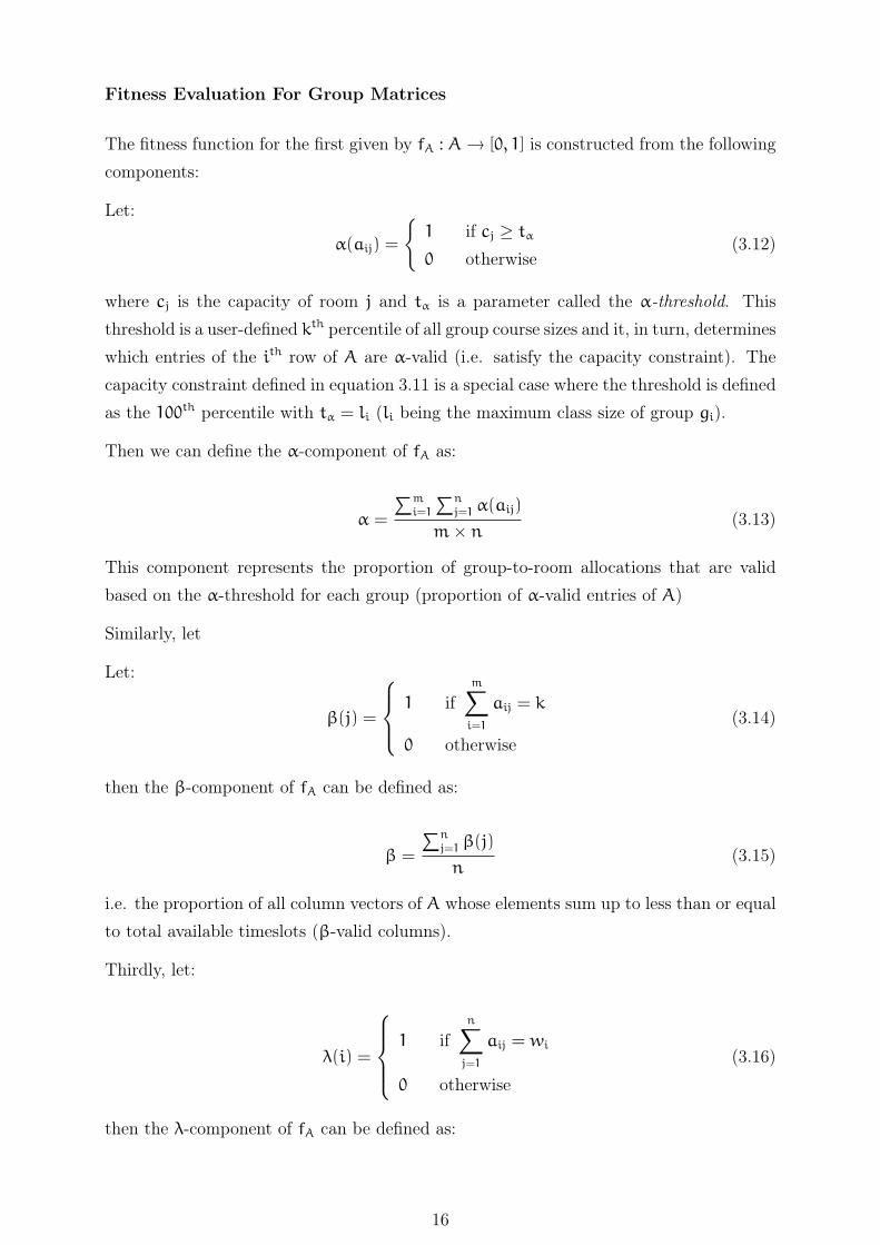
Fitness Evaluation For Group Matrices

The fitness function for the first given by fA : A→ [0, 1] is constructed from the followingcomponents:

Let:

α(aij) =

{1 if cj ≥ tα0 otherwise

(3.12)

where cj is the capacity of room j and tα is a parameter called the α-threshold. Thisthreshold is a user-defined kth percentile of all group course sizes and it, in turn, determineswhich entries of the ith row of A are α-valid (i.e. satisfy the capacity constraint). Thecapacity constraint defined in equation 3.11 is a special case where the threshold is definedas the 100th percentile with tα = li (li being the maximum class size of group gi).

Then we can define the α-component of fA as:

α =

∑mi=1

∑nj=1 α(aij)

m× n(3.13)

This component represents the proportion of group-to-room allocations that are validbased on the α-threshold for each group (proportion of α-valid entries of A)

Similarly, let

Let:

β(j) =

1 ifm∑i=1

aij = k

0 otherwise(3.14)

then the β-component of fA can be defined as:

β =

∑nj=1 β(j)

n(3.15)

i.e. the proportion of all column vectors of A whose elements sum up to less than or equalto total available timeslots (β-valid columns).

Thirdly, let:

λ(i) =

1 if

n∑j=1

aij = wi

0 otherwise

(3.16)

then the λ-component of fA can be defined as:

16

λ =

∑mi=1 λ(i)

m(3.17)

i.e. the proportion of all row vectors of A whose elements sum up to exactly the requiredgroup total contact hours (λ-valid rows)

And finally we can define the ρ-component of fA as:

ρ =

1 ifm∑i=1

max(ai) ≤ |P|

0 otherwise(3.18)

Here ρ indicates whether the total time slot allocations for the different groups is feasibleaccording to the third clash constraint i.e. the total maximum group allocations does notexceed the number of available time slots.

Therefore, fA can be defined as the weighted sum of the above components:

fA = ωαα+ωββ+ωλλ+ωρρ (3.19)

where ωα,ωβ,ωλand ωρ are the respective weights for each component.

Satisfying the above constraints in the initial phase of the GA produces a matrix contain-ing feasible allocations of required group hours to appropriate rooms. This matrix is theframework from which actual group timetables will be constructed.

3.2.3 Phase 2: Group-local Timetable Optimization

This phase deals with the actual distribution of courses for each room to optimize addi-tional (soft) constraints. This can be done (serially or in parallel) for each group using aGA or other assignment means. Our work uses a secondary GA to finalize the class-to-timeslot allocation and to optimize the individual group timetables.

Chromosome Encoding

Let Ti ⊂ T denote a random subset of time slots allocated to group gi, with:

|Ti| = hi =

{gmax if gmax > max(ai)max(ai) otherwise

(3.20)

(gmax and max(ai) are as previously defined in section 3.1.3 and 3.2.3 respectively)

Then we can represent a group timetable, Θi as an hi × n matrix of the form:

17

Θi = [ckj],where ckj ∈ gi, 0 < k ≤ hi, 0 < j ≤ n (3.21)

(n = |R| as previously defined in section 3.23)

More concisely, if we let Ri denote the set of non-zero entries in the ith row of A and letni = |Ri|, then Θi can be re-written as the dense matrix:

Θi = [ckj],where ckj ∈ gi, 0 < k ≤ hi, 0 < j ≤ ni (3.22)

Thus cij = a indicates course a is scheduled in room j during time slot k. Therefore, Θirepresents a possible final group timetable based on the group allocation matrix A. Theoverall timetable will be aggregated from the component group timetables.

Fitness Evaluation for Group Timetables

For the second phase, there are two evaluations that will contribute to the fitness functionfΘ : Θi → [0, 1] as follows:

Let θk denote the kth row of Θi. We define

µ(θk) =

{1 if ∀x, y ∈ Z ∩ (0, ni], x 6= y =⇒ θkx 6= θky0 otherwise

(3.23)

i.e. every entry in each row is unique. This prevents the GA from scheduling the samecourse during the same timeslot. Then we can define the µ component of fθ as:

µ =

∑hik=1 µ(θk)

hi(3.24)

This gives the ratio of µ-valid rows for the group timetable.

Further, let ε be defined as:

ε(ckj) =

{1 if course ckj is schedule in preferred room0 otherwise

(3.25)

Here preferred room is indicated by course requirements. If the course has no preferences,any room allocation evaluates to 1. Then the ε component of fθ can be defined as:

ε =

∑hik=1

∑nj=1 ε(ckj)

hi × ni(3.26)

Therefore,fΘ = ωµµ+ωεε (3.27)

Where, as in equation 3.19, ωµ and ωε are user defined weights.

18

Phase 1 Pseudocode

Procedure 1 Optimize Group Allocation Matrix

Input: genetic_parameters: list of key-value pairs of genetic parametersOutput: group matrix chromosome

1: procedure GroupMatrixGA(genetic_parameters)2: population ← generateInitialPopulation(parameters.pop_size)3: if empty(population) then

4: return null5: end if

6: elite ← getFittest(population)7: runs ← 08: while runs ≤ parameters.generations & elite.fitness ≤ parame-

ters.optimal_fitness do

9: population ← evolveMatrix(population, parameters)10: if parameters.elitism = True then

11: replace(population, elite, parameters.replacement_policy)12: end if

13: elite ← getFittest(population)14: runs ← runs + 115: end while

16: return elite17: end procedure

19

Phase 2 Pseudocode

Procedure 2 Group-Local Timetable Optimization

Input: group_matrix: group matrix chromosome, timeslots: list of time slot values,student_groups: set of student group partitions, parameters:list of key-value pairs ofgenetic parameters

Output: NULL

1: procedureGroupTimetableGA(group_matrix, timeslots, student_groups, parameters)2: timeslots ← randomize(timeslots)3: start_index ← 04: for all group in student_groups do

5: group.allocation_vector ← group_matrix[group.id]6: slot_count ← max(getGmax(group), getMaxCourseHours(group))7: end_index ← start_index + slot_count8: if start_index > timeslots.size then

9: assignTimeslots(group, timeslots[timeslot.size-count : timeslot.size])10: else

11: assignTimeslots(group, timeslots[start_index : end_index])12: start_index ← start_index + count13: end if

14: group_timetable = evolveTimetable(group, parameters)15: write(group_timetable)16: end for

17: return NULL18: end procedure

The evolveTimetable algorithm is the same for both phases (Procedure 1) with modifi-cations made to the mutation and crossover algorithms (see Appendix A).

20

3.2.4 Implementation and Results

A prototype of the algorithm was developed using Python 3.4 as a programming languagewith Numpy 1.91 for matrix manipulation and MySQL 5.6.12 as a database backend.The choice of language was influenced by Python’s consiseness, prototyping prowess andavailability of well supported third-party packages. The prototype was first tested4 usinga subset of real-world data obtained from the University of Malawi, Chancellor College.The data consisted 46 courses partitioned into 16 student groups to be allocated into 19rooms and a total of 45 weekly hours (9 hours per day, 5 days a week). The prototype wasthen run on a larger data set (100 courses, 41 rooms, 22 student groups and 60 weeklyhours) to test its scalability. Sample timetables were generated in both cases.

In the former case, the prototype was run to satisfy H on four different values of α-threshold; 75th, 80th and 100th percentile. As outlined in section 3.2.2, a feasible timetablewith xth percentile for α-threshold implies that x% of the classes in the group are expectedto fit in all of the group’s allocated rooms. As an example, for the 80th percentile, anallocation of hi hours of group gi in room ri indicates that at least 80% of the courses inthat group will fit in that room given that the group allocation has fitness of 1.0. Thisis to allow more flexibility in the algorithm. All runs were performed with the followinggenetic parameter values: (i) Populations size: 50, (ii) Crossover rate: 0.2, (iii) Mutationrate: 0.1, (iv) Tournament size: 10, (v) Generations: 1500, (vi) Elitism: true, (vii) Elitistreplacement policy: random. Weights for fA were assigned based on relative importanceof the components. On the other hand, fΘ only considered one component due to lackof preference information necessary to for the inclusion of ε. The fitness functions usedwere as follows:

fA = 0.3α+ 0.15β+ 0.05λ+ 0.5ρ (3.28)

fΘ = 1.0µ (3.29)

Below are the data statistics and trends obtained from the different runs:

4Testing was done on a Zinox computer, with Intel’s CORE i7 processor (2 physical cores, 4 logicalcores, 4GB RAM running Windows 7 Professional Version.

21

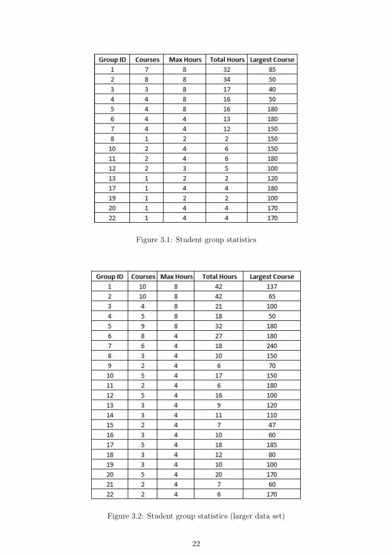
Figure 3.1: Student group statistics

Figure 3.2: Student group statistics (larger data set)

22

Figure 3.3: Trend: (α-threshold at 75th percentile)

Figure 3.4: Trend: (α-threshold at 80th percentile)

23

Figure 3.5: Trend: (α-threshold at 100th percentile)

Figure 3.6: Trend (sample group timetable generation)

24

Figure 3.7: Trend (larger data set)

3.2.5 Performance Analysis

The results for the smaller data set show that the algorithm is able to attain the maximumfitness value of 1.0 for moderate α-threshold values (e.g. 50th and 80th). The two-dimensional nature of chromosome encoding implies that the most intensive computations(e.g. crossover and mutation) are O(n2). This can be clearly seen in the mutationand crossover algorithms (see Appendix A). Holding the population size constant, thecomputational complexity of the algorithm should scale quadratically with increasinginput data (number of courses and rooms). The running time averages 4 minutes and 7minutes for the smaller and larger data sets respectively on a quad-core, hyper-threadedIntel Core i7 processor. Given the vast nature of the space, this reduced time may beattributed to the ‘pruned’ search space within which the algorithm operates.

Figures 3.3 to 3.5 show that the general trend of evolution for all trials follows an initialquadratic increase in fitness with a steep rise in the trend that coincides with a jump inρ value. The graphs also show that the search proceeds steadily without a drop in fitnessbetween generations. This general increasing trend is a direct consequence of elitism,which maintains the best chromosome between consecutive generations. However, periodicsamples of chromosome generations for all cases (see Appendix A) indicate a constantvalue of 1.0 for both β and λ components. This implies that the initial chromosomepopulations satisfies all hours−per− room allocation constraints and that all hours foreach group are fully scheduled.

25

Additionally, a closer examination of the data will reveal an inverse relationship betweenα-threshold and the probability of convergence on an optimal fitness. The higher theα-threshold value, the less likely it is to locate a feasible allocation. This is an instance ofconflicting constraints i.e. the stricter the rule on room capacity, the harder it is to finda feasible allocation with each allocated course fitting into its respective room.

An instance of this scenario can be seen in the results obtained for α-threshold value of100th percentile as shown in Figure 3.5. A number of runs were performed at this thresholdwith no significant improvement in the final optimal fitness value (approx. 0.50). A similartrend was also observed for the larger data set (Figure 3.15). This is a consequence of theinadequate time slots relative to the number of courses that require scheduling (condition3 necessary for non-existence of feasible timetable). The effect of this is seen in the outputtimetables where a number of (peer) courses register time clashes.

Finally, Figure 3.6 shows a sample trend generated by a secondary GA that is optimizinga group timetable in phase 2. It is worth noting that the trend only displays fitness valuessolely based on µ. This is due to the unavailability of departmental preference informationin the source data. This case shows a maximum fitness value of 0.875, which indicates0.115 odds of finding a time clash among peer courses within the group.

3.2.6 Parallel/Distributed Algorithm

The approach and representation chosen for the serial algorithm offer opportunities forsingle-instruction, multiple data (SIMD) parallelization that can be exploited to speedup convergence on parallel/distributed architectures. The most promising parts for par-allelization include:

1. Fitness evaluation, mutation and crossover for group allocation matrix and grouptimetables

2. Group timetable optimization

For group-local timetable optimization, each ith row of A (for group gi) will be mappedas a separate input split onto a processing node for group timetable generation. Resultswill be written to separate file for each group and merged either at runtime or manuallyafter execution. The parallelization strategy can be diagrammatically represented as inFigure 3.8 below:

26

Figure 3.8: Parallel/distributed GA Model

This parallelization scheme offers a great deal of flexibility in terms of implementationtechnology and platform. It can be implemented on a distributed computing platformor on a single node with multi-core processors depending on resource availability. It isworth noting that the level of parallelization in the proposed scheme is limited by the serialphase (phase 1) i.e. generation of the group allocation matrix. Since this phase representsapproximately 50% of the whole algorithm, by Amdahl’s law, the speedup achieved by anembarrassingly parallel implementation of phase 2 only should be at most:

limn→∞

1

0.5+ 1−0.5n

= 2 (3.30)

where n is the number of processing elements used.

However, given the nature of the chromosome encoding scheme (and the genetic oper-ator algorithms), phase 1 can also be parallelized to take advantage of multi-processingarchitectures thereby increasing the speedup beyond the predicted theoretical limit of 2.

Below is the pseudocode for the main parallel/distributed algorithm. Appendix A containspseudocode for the procedures called by the algorithm.

27

Pseudocode For Parallel/Distributed Algorithm

Procedure 3 Main DGA/PGA

1: procedure ParallelGA(constraints)2: parameters ← getParametersInput()3: group_matrix ← GroupMatrixGA(parameters)4: if group_matrix.rho_value > 0 then5: initializeGroups(group_matrix, constraints.timeslots, constraints.student_groups)6: for all group in constraints.student_groups in PARALLEL do7: group_timetable ← evolveTimetable(group)8: group_file ← group.unique_id9: write(group_timetable, group_file)10: end for11: else12: print(NoOptimalSolutionError)13: end if14: end procedure

Procedure 4 Initialize Student Groups Using Group Matrix

1: procedure initializeGroups(group_matrix, timeslots, student_groups)

2: timeslots ← randomize(timeslots)

3: start_index ← 0

4: for all group in student_groups do

5: group.allocation_vector ← group_matrix[group]

6: slot_count ← max(getGmax(group), getMaxCourseHours(group))

7: end_index ← start_index + slot_count

8: if start_index > timeslots.size then

9: assignTimeslots(group, timeslots[timeslot.size-count : timeslot.size])

10: else

11: assignTimeslots(group, timeslots[start_index : end_index])

12: start_index ← start_index + count

13: end if

14: end for

15: end procedure

28

Chapter 4

Conclusion

4.1 Summary

Timetabling presents a complicated constraint satisfaction problem that requires efficientalgorithms to solve. Genetic algorithms offer a promising mechanism due to their abilityto handle complicated search spaces. Our work proposes a theoretical framework to guideapplication of GAs to the timetabling problem. It is observed that, with this frameworkas the basis, an efficient algorithm can be designed that will converge to an optimal orPareto solution in polynomial time. The work also shows that the choice of chromosomeencoding has a great impact on algorithm performance and scalability. Our work adoptsa matrix-based encoding scheme which lends itself to almost effortless parallelization, afactor that is exploited in the proposed parallel/distributed algorithm. The scheme alsoallows for simple mathematical expression of constraints for efficient evaluation.

In addition, we note that timetabling requires balancing several parameters given thatmost real-world problems present inherently insufficient resources and conflicting con-straints and preferences. In this case, an algorithm should be able to settle for a Paretoallocation of resources i.e. an optimal equilibrium where one resource cannot be re-allocated without negatively affecting other allocations.

Finally, our work on parallel/distributed algorithm reveals that speedup can be increasedby a theoretical factor of two if only the second phase of the algorithm is parallelized.Given that this factor is too small to justify the parallelization efforts, we suggest fur-ther increasing the parallel footprint of the algorithm by implementing the basic geneticoperators on multiprocessing platforms. This approach has the potential to boost thetheoretical speedup limit by a significant factor.

29

4.2 Limitations and Future Work

The approach explored in this paper is applicable within a number of limitations. Perhapsthe most important limitation is the assumption of existence of student group informa-tion prior to generation of the group allocation matrix. In most cases, the problem ofgenerating student groups information is separated from the timetabling problem andit is usually done prior to timetable generation. However, in the absence of such priorinformation, the algorithm requires a supplementary partitioning algorithm (e.g. graphcolouring) to generate the initial input.

Another limitation is the serial nature of phase 1 of the algorithm. This arises dueto the need to have all student group information available in one ‘space’ to generatea feasible group allocation matrix. Massive parallelization of this phase would requireintricate levels of inter-process interaction and synchronization, two factors that may leadto communication overheads and reduced efficiency. However, future work may explorethis option to test different interaction and synchronization schemes and their effects onefficiency and convergence.

30

Bibliography

[1] D Abramson and J Abela. A Parallel Genetic Algorithm for Solving the SchoolTimetabling Problem. In Division of Information Technology, C.S.I.R.O, pages 1–11, 1992.

[2] Arwa Al-Edaily, Nada Al-Zaben, Sharefa Al-Ghamdi, and Aboalsamh Hati. ImprovedDistributed Genetic Algorithms Based on Their Methodology and Processes. In inProceedings of the European Computing Conference, pages 415–420, 2011.

[3] Grigorios N. Beligiannis, Charalampos N. Moschopoulos, and Spiridon D.Likothanassis. A Genetic Algorithm Approach to School Timetabling. The Jour-nal of the Operational Research Society, 60(1):23–42, 2009.

[4] Tobias Blickle and Lothar Thiele. A Comparison of Selection Schemes used in GeneticAlgorithms. Technical report, Computer Engineering and Communication NetworksLab, Swiss Federal Institute of Technology, Gloriastrasse, Zurich, Switzerland, De-cember 1995.

[5] Sigl Branimir, Marin Golub, and Vedran Mornar. Solving Timetable SchedulingProblem by Using Genetic Algorithms. In Int Conf Information Technology InterfacesIT1, pages 519–524, 2003.

[6] Edmund K. Burke, Dave G. Elliman, and Rupert F. Weare. A Hybrid GeneticAlgorithm for Highly Constrained Timetabling Problems. In Proceedings of the SixthInternational Conference on Genetic Algorithms, pages 605–610. Morgan Kaufmann,1995.

[7] Erick Cantu-Paz. A Survey of Parallel Genetic Algorithms. Calculateurs Paralleles,Reseaux et Systems Repartis, 10, 1998.

[8] Erick Cantu-Paz and David E. Goldberg. On the Scalability of Parallel GeneticAlgorithms. Journal of Evolutionary Computation, 7(4):429–449, 1999.

[9] Alberto Colorni, Marco Dorigo, and Vittorio Maniezzo. A Genetic Algorithm toSolve the Timetable Problem, 1993.

31

[10] Stephanie Forrest. Genetic Algorithms: Principles of Natural Selection Applied toComputation. Science, New Series, 261(5123):872–878, 1993.

[11] David E. Goldberg and Kalyanmoy Deb. A Comparative Analysis of SelectionSchemes Used in Genetic Algorithms. In Foundations of Genetic Algorithms, pages69–93. Morgan Kaufmann, 1991.

[12] Randy L. Haupt and Sue Ellen Haupt. Practical Genetic Algorithms. John Wiley &Sons, Hoboken, New Jersey, 2nd edition, 2004.

[13] Jun He, Feidun He, and Xin Yao. A Unified Markov Chain Approach to AnalysingRandomised Search Heuristics. Technical report, Department of Computer Science,Aberystwyth University, Aberystwyth, SY23 3DB, U.K., December 2013.

[14] John H. Holland. Adaptation in Natural And Artificial Systems. An IntroductoryAnalysis with Applications to Bilogy, Control, and Artificial Intelligence. MIT Press,5th edition, 1998.

[15] Omar Ibrahim Obaid, MohdSharifuddin Ahmad, Salama A. Mostafa, andMazin Abed Mohammed. Comparing Performance of Genetic Algorithm with Vary-ing Crossover in Solving Examination Timetabling Problem. Journal of EmergingTrends in Computing and Information Sciences, 3(10):1427–1434, 2012.

[16] Petr Pospichal, Jiri Jaros, and Josef Schwarz. Parallel Genetic Algorithm on theCUDA Architecture, EvoApplications 2010, Part I, pages 442–451. Springer-Verlag,2010.

[17] Rushil Ranghavjee and Nelishia Pillay. Use of Genetic Algorithms to Solve theSouth African School Timetabling Problem. In Second World Congress on Natureand Biologically Inspired Computing, pages 286–292, 2010.

[18] Olympia Roeva, editor. Solving Timetable Problem by Genetic Algorithm and Heuris-tic Search Case Study: Universitas Pelita Harapan Timetable, Real-World Applica-tions of Genetic Algorithms, chapter 15, pages 303–316. InTech, 2012.

[19] Peter Ross, Dave Corne, and Hsiao lan Fang. Successful Lecture Timetabling withEvolutionary Algorithms. In Proceedings of the ECAI 94 Workshop on Applicationsof Evolutionary Algorithms. Springer, 1994.

[20] Gunter Rudolph. Convergence Analysis of Canonical Genetic Algorithms. IEEETransactions on Neural Networks, 5(1):96–101, 1994.

[21] S.N. Sivanandam and S.N. Deepa. Introduction to Genetic Algorithms. Springer,Berlin Heidelberg, USA, 2008.

[22] Joe Suzuki. A Markov Chain Analysis of Genetic Algorithms: Large DeviationPrinciple Approach. Journal of Applied Probability, 47(4):967–975, 2010.

32

[23] Huayang Xie and Mengjie Zhang. Tuning Selection Pressure in Tournament Selec-tion. Technical Report ECSTR-09-10, School of Engineering and Computer Science.Victoria University of Wellington, New Zealand, 2009.

33

Appendix A

Algorithms and Sample Output

A.1 Pseudocode

Procedure 5 Phase 1: Mutation Algorithm

Input: chromosome: group matrix chromosome, mutation_rate: float value

Output: NULL

1: procedure mutateMatrix (chromosome,mutation_rate)

2: re-evalute_flag ← FALSE

3: if randomFloat(0,1) ≤ mutation_rate then

4: re-evaluate_flag ← TRUE

5: for all row in chromosome do

6: for all column in row do

7: if chromosome[row][column] 6= 0 then

8: delta ← randomInteger(0, chromosome[row][column])

9: chromosome[row][column] ← chromosome[row][column] - delta

10: repair_allele := getRandomAllele(chromosome)

11: chromosome.repair_allele ← chromosome.repair_allele + delta

12: end if

13: end for

14: end for

15: end if

16: return NULL

17: end procedure

34

Procedure 6 Phase 1: Crossover Algorithm

Input: parent1, parent2: group matrix chromosome, crossover_rate: float value

Output: NULL

1: procedure crossoverMatrix (parent1, parent2, crossover_rate)

2: if crossover_rate = 0 and parent1.size 6= parent2.size then

3: return

4: end if

5: for all row in parent1 do

6: for all column in row do

7: if parent1[row][column] != parent2[row][column] AND randomFloat(0,1) <=

crossover_rate then

8: if parent1[row][column] > parent2[row][column] then

9: diff ← parent1[row][column] - parent2[row][column]

10: parent1[row][column] ← parent2[row][column]

11: repair_allele ← getRandomElement(parent1)

12: repair_allele ← repair_allele + diff

13: else

14: diff ← parent2[row][column] - parent1[row][column]

15: parent2[row][column] ← parent1[row][column]

16: repair_allele ← getRandomAllele(parent2)

17: repair_allele ← repair_allele + diff

18: end if

19: end if

20: end for

21: end for

22: return NULL

23: end procedure

35

Procedure 7 Phase 2: Crossover Algorithm

Input: parent1, parent2: group timetable chromosome, crossover_rate: float value

Output: NULL

1: procedure crossoverTimetable(parent1, parent2, crossover_rate)

2: if crossover_rate = 0 or parent1.size 6= parent2.size then

3: return

4: end if

5: for all column in parent1 do:

6: if randomFloat(0,1) ≤ crossover_rate then

7: swap(parent1.column, parent2.column)

8: end if

9: end for

10: return NULL

11: end procedure

Procedure 8 Phase 2: Mutation Algorithm

Input: chromosome: group timetable chromosome, mutation_rate: float value

Output: NULL

1: procedure mutateTimetable(chromosome,mutation_rate)

2: re-evaluate_flag ← FALSE

3: for all column in chromosome do:

4: if randomFloat(0,1) ≤ mutation_rate then:

5: re-evaluate_flag = TRUE

6: randomize(column)

7: end if

8: end for

9: return NULL

10: end procedure

36

Procedure 9 Evolve Group Allocation Matrix Population

Input: population: list of group matrix chromosomes, parameters: list of key-value pairs of

genetic parameters

Output: list of group matrix chromosomes

1: procedure evolveMatrix (population, parameters)

2: new_population:LIST

3: while space ≥ 0 do

4: parent1 ← tournamentSelect(population, parameters.tournament_size)

5: parent2 ← tournamentSelect(population, parameters.tournament_size)

6: crossoverMatrix(parent1, parent2, parameters.crossover_rate)

7: mutateMatrix(parent1, parameters.mutation_rate)

8: mutateMatrix(parent2, parameters.mutation_rate)

9: parent1.fitness = evaluateFitness(parent1)

10: parent2.fitness = evaluateFitness(parent2)

11: new_population.append(getFittest(parent1,parent2))

12: end while

13: return new_population

14: end procedure

37

A.2 Output data samples

Figure A.1: Periodic data sample (α-threshold at 75th percentile)

38

Figure A.2: Periodic data sample (α-threshold at 80th percentile)

39

Figure A.3: Periodic data sample (α-threshold at 100th percentile)

40

Figure A.4: Group timetable data (sample group timetable generation)

41

Figure A.5: Periodic sample (larger data set)

42

A.3 Sample output matrices

Figure A.6: Group allocation matrix (α-threshold at 75th percentile)

Figure A.7: Group allocation matrix (α-threshold at 80th percentile)

43

Figure A.8: Group allocation matrix (α-threshold at 100th percentile)

44

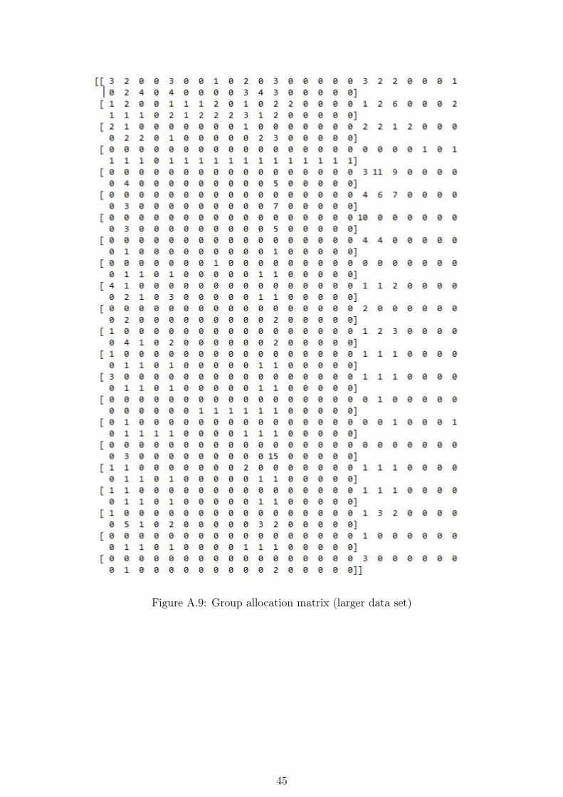
Figure A.9: Group allocation matrix (larger data set)

45

Figure A.10: Sample timetable for smaller data set (red marks indicate clashes)

46