Empirical evaluation of optimization algorithms when used in goal-oriented automated test data...

Empirical evaluation of optimization algorithmswhen used in goal-oriented automated testdata generation techniques

Man Xiao & Mohamed El-Attar & Marek Reformat &James Miller

Published online: 8 November 2006# Springer Science + Business Media, LLC 2006Editor: Mark Harman

Abstract Software testing is an essential process in software development. Softwaretesting is very costly, often consuming half the financial resources assigned to a project.The most laborious part of software testing is the generation of test-data. Currently, thisprocess is principally a manual process. Hence, the automation of test-data generation cansignificantly cut the total cost of software testing and the software development cycle ingeneral. A number of automated test-data generation approaches have already beenexplored. This paper highlights the goal-oriented approach as a promising approach todevise automated test-data generators. A range of optimization techniques can be usedwithin these goal-oriented test-data generators, and their respective characteristics, whenapplied to these situations remain relatively unexplored. Therefore, in this paper, acomparative study about the effectiveness of the most commonly used optimizationtechniques is conducted.

Keywords Empirical software engineering . Optimization techniques .

Test-data generation . Empirical results

1 Introduction

As systems grow ever more complex, the percentage of total costs consumed by verificationgrows, while defect rates increase. Defects in software systems can prevent them from

Empir Software Eng (2007) 12:183–239DOI 10.1007/s10664-006-9026-0

M. Xiao :M. El-Attar :M. Reformat : J. Miller (*)Department of Electrical and Computer Engineering, STEAM Laboratory, University of Alberta,9107-116 Street, Edmonton, AB, T6G 2V4, Canadae-mail: [email protected]

M. Xiaoe-mail: [email protected]

M. El-Attare-mail: [email protected]

M. Reformate-mail: [email protected]

performing their functionality as intended. Faulty software can be very costly, riskingpublic safety or accounting for huge financial losses. Therefore, it is essential to keep thedefect rates to a minimum, especially those associated with safety-critical or mission-criticalsystems. However, a recent study released by the National Institute of Standards andTechnology (Tassey 2002) indicate that, software bugs, or errors, are so detrimental andprevalent that they cost the U.S. economy an estimated $59.5 billion annually, or about 0.6percent of the gross domestic product. This indicates that current approaches to reducedefect rates are insufficient and inefficient, and thus new approaches need to be exploredwith great haste.

To date, there exist many methods to validate software. Common software validationmethods include code reviews and software inspections. However, software testing remainsthe most common, widely accepted and practiced method of software validation. However,the cost associated with performing software testing is very high. Studies show thatsoftware testing may account for up to 50% of the total cost of software development(Beizer 1990). This high cost is a result of software testing being a very labor-intensiveprocess. Software testing is comprised of several components. The most essentialcomponent is the generation of test-data. To date, test-data generation remains a manualprocess, where very limited automation is available. Test-data generation is perhaps themost costly sub-process within software testing. Test-data generation can roughly accountfor 40% of the total cost of software testing. Therefore, the total cost of software testing canbe significantly reduced if the process of test-data generation becomes automated. This inturn will increase software reliability, which will boost the developers’ and customers’confidence in the software system being developed.

The remainder of this paper is presented as follows: Section 2 will briefly outline currentautomated test-data generation techniques, including goal-oriented approaches which is thefocus of the paper. The description of the optimization techniques used to apply thistechnique is presented in Section 3. Section 4 outlines the experimental procedure; andSection 5 briefly describes the software under test. Section 6 presents the empirical resultsof applying these optimization techniques to automatically generate test data for five SUTprograms and provides an analytical comparison of their relative performance.

2 Automated Test-Data Generation Techniques

Several approaches to generating test-data exist. Very few of these approaches areautomated, exceptions to this include: goal-oriented, path-oriented, analysis-oriented andrandom. Due to the complexity of software programs developed in industrial settings, thesetest-data generation techniques have only been demonstrated to be effective for simpleprograms. Generally, software programs developed in industry usually exhibit commoncharacteristics: (a) they are very large in size, (b) highly complex, and (c) contain a widevariety of structural features such as arrays and pointers. The success of automated test-datagenerators with industry software has been very limited due to such characteristics,inhibiting the widespread use of automated test-data generators.

Path-oriented generators (Clarke 1976; Howden 1997; Ramamoorthy et al. 1976)operate in two main stages: (a) the structure of the SUT is analyzed to identify and select apath; then test-data is generated that will attempt to execute this path. However, if the pathis infeasible, the generator will fail to find input data required to execute that path. Randomtest-case generation (Mills et al. 1987; Thevenhod and Waeselynck 1998, Voas et al. 1991;Bird and Munoz 1982) randomly generate large sets of test-data to satisfy the test-

184 Empir Software Eng (2007) 12:183–239

requirements. This method is very simplistic and can be easily implemented. Although, itmay be sufficient for simple programs, experiences have shown that random generators canbe inefficient when used with more complex programs (Korel 1996). On the other hand,analysis-oriented generators (Change et al. 1991; Korel 1996) can efficiently generateadequate test-data. However, this is only made possible because the developers of theanalysis-oriented generators have a comprehensive understanding of the domain ofoperation. It is not reasonable to assume that such detailed knowledge is available to allmembers of the development team members, especially if the software system beingdeveloped is very large and complex or if the target domain is relatively new.

Early attempts to develop automated goal-oriented test-data generators (Korel 1990)have yielded some success. So far, goal-oriented generators were successful at producingadequate quality test-data for simple programs. All goal-oriented test-data generators aredesigned according to a paradigm. This paradigm requires the test objectives to beformulated as a series of numerical functions, which need to be minimized (or maximized).These numerical functions will be minimized (or maximized) using an optimizationtechnique. See McMinn (2004) for a complete survey of work in this area.

2.1 Goal-Oriented Generators—Which Optimization Technique is Best?

Early approaches to develop goal-oriented test-data generators faced serious problems whentrying to find the global minima. These problems are a result of the search spaces consistingof large areas with no information to guide the search algorithms. These areas do notprovide sufficient directional information to steer the search algorithms away from localminima. In addition, the success of the optimization techniques used seems to be stronglyaffected by the structure of the SUT. Therefore, a number of optimization techniques wereused in these approaches. For instance, (Michael et al. 2001), used genetic-algorithms toconstruct their tool GADGET (Genetic Algorithm Data Generation Tool). On the otherhand, the approach presented by (Tracy et al. 1998), used simulated-annealing.

As a result, it is important to evaluate and compare the effectiveness of the optimizationtechniques when used to solve the test-data generation problem. Hence, in this paper weconduct a comparative study that examines and compares the effectiveness of severalcommon non-linear optimization techniques: namely (a) Genetic Algorithms (GA), (b)Simulated Annealing (SA), (c) Genetic Simulated Annealing (GSA) and (d) SimulatedAnnealing with Advanced Adaptive Neighborhood (SA/AAN), in addition to the “RandomSearch” optimization technique which will be used as a benchmark.

3 Optimization Techniques

This section provides a brief description of the optimization techniques examined in thispaper-Genetic Algorithms (GA), Simulated Annealing (SA), Genetic Simulated Annealing(GSA), and Simulated Annealing with Advanced Adaptive Neighborhood (SA/AAN). GAand SA are considered to be the most commonly used to automatically generate data. Otheroptimization techniques such as GSA and SA/ANN are derived from these two techniques.

3.1 Genetic Algorithms (GA)

Genetic Algorithms are based on an abstract model of natural genetic evolutionary process.They were introduced by Holland in the book “Adaptation in Natural and Artificial

Empir Software Eng (2007) 12:183–239 185

Systems” in the 1970s (Holland 1975). GA are applied to different optimization problemsin the areas of science, engineering, business and medicine (Back et al. 2000). Analgorithmic overview of the GA is presented in Table 1.

In GAs, the possible solutions of the given optimization problem are represented as thebit strings called chromosomes (Schaffer 1987). The chromosomes can be represented in anumber of different ways. Traditionally, chromosomes are represented as binary strings(Holland 1975). The gray code representation, which has adjacency property, has proven tobe a better representation in some applications (Caruana and Schaffer 1988; Jones et al.1995). However, the non-binary representation has also been investigated (Janikow andMichalewicz 1991).

Evaluation of chromosomes is performed using a fitness function. The fitness functionrepresents a problem. The fitness function is discussed in detail later (see Section 4.2). Afterbeing evaluated, each individual in the population is assigned a fitness function value.

Once each chromosome in the population is evaluated, selection can occur. It is used todecide which chromosomes will be chosen to contribute to the successive generation. Thisprocess is based on the fitness function values of the individuals in the current population(Holland 1975). In the selection phase, there is a bias towards the well-fitted individuals, i.e.,the well-fitted individuals have more chances to be selected. There are a number of selectionmethods (Back and Hoffmeister 1991). The common selection methods include roulettewheel sampling selection, tournament selection, and ranking selection (Baker 1985).

Roulette wheel sampling selection selects chromosomes based on their fitness value.This selection is stochastic and proportional to the fitness function value of the individuals(Holland 1975) (Goldberg 1989). The selection possibility of each individual Psel(i) iscalculated as

Psel ið Þ ¼ f ið ÞPnk¼1

f kð Þ

where n is the size of the population, i= 1...n, and f (i) is the fitness value of each individual i.Imagine a roulette wheel, where each individual in the population corresponds to a slice, andthe size of the slice is proportional to the individual’s Psel(i). Individuals are chosen togenerate the new generation by spinning the roulette wheel.

Another selection method is tournament selection. As the name suggests, this selectionmethod is based on making n tournaments to choose n individuals. In each tournament, thechromosome with the better fitness function value in the group of k chromosomes isselected. The most widely used tournament selection method is binary tournament, i.e.,when k= 2.

Table 1 GA algorithm

Step 1 Randomly create an initial population (generate trial solutions and represent each solutionas a chromosome).

Step 2 Evaluate every individual in the population according to the fitness function that representsa problem.

Step 3 Select the best individuals based on their fitness function values.Step 4 Crossover the parents to produce offspring.Step 5 Mutate the offspring.Step 6 Evaluate the offspring according to the fitness function; if the stopping criterion is satisfied then

stop, otherwise the offspring becomes the new population; repeat Step 3.


Ranking selection was first introduced by Baker (Baker 1985) to overcome the strongbias of the roulette wheel sampling selection. In ranking selection, the population is orderedbased on the fitness function values, and each chromosome in the population is assigned arank r according to its fitness. Then selection selects the parents in the population based onthe rank rather than the actual fitness value. This selection still has a bias towards the fitterchromosomes but also allows ‘weaker’ chromosomes to have a chance to be selected. Afterthe selection is finished, the selected chromosomes undergo a modification process:crossover and mutation. Crossover is a random exchange of genetic information betweentwo parent chromosomes to produce offspring chromosomes. Singlepoint crossover is oneof the most popular types of crossover. In this kind of crossover only one crossover point isused. Once the crossover point is generated randomly in a pair of parent individuals, thesubstrings that are defined by that the crossover point are recombined together and producetwo children. Figure 1 illustrates singlepoint crossover. It can be easily observed how theencoding of the genetic information of the parents is kept in the children.

Multipoint crossover requires more than one crossover points in a pair of selected parentchromosomes, Fig. 2.

The other genetic operation-mutation is used to keep the diversity in the population andprevent GA from being trapped in a local optimum. Typically, a simple mutation is implementedby flipping one bit that is randomly selected in the string, i.e., changing it from a 1 to 0 and viceversa with a small probability. Figure 3 shows an example of a simple mutation.

As Darrell Whitley pointed out in (Whitley 1993), Genetic Algorithms are oftendescribed as a global search method that does not use gradient information. Thus, it is amore general working method than other global optimization methods.

3.2 Simulated Annealing (SA)

Simulated Annealing originates from the analogy between the annealing process of solids andthe problem of solving combinatorial optimization problems. In condensed matter physics,annealing is a process of cooling a solid to reach a minimal energy state (ground state). At initialhigh temperatures, all molecules of the solid randomly arrange themselves in a liquid state, asthe temperature descends gradually, the crystal structure becomes more ordered and reaches afrozen state when the temperature drops to zero. If the temperature drops too quickly the crystalwill not reach the thermal equilibrium at each temperature, hence, the defects will be frozen intothe crystal structure and the crystal will not reach a minimal energy state but a meta-stable state(i.e., being trapped in a local minimum energy state). Therefore, a proper initial temperature anda proper cooling schedule are important to an annealing process.

Simulated Annealing is a search technique where a single trial solution is modified atrandom. An energy represents the quality of the proposed solution. In order to find the best

parent1 parent2

1 1 0 0 1 0 0 0 0 1 1 0

crossover point

↓ ↓

crossover point child1 child2

1 1 0 0 0 1 0 1 1 1 0 0

0 1 1 0 0 1 0 1 1 1 0 0

0 1 1 0 1 0 0 0 0 1 1 0

Fig. 1 Singlepoint crossover


solution, the energy needs to be at its minimum. The smaller the energy gets, the better asolution becomes. Therefore, changes that lead to a “lower energy” are automaticallyaccepted. Meanwhile, changes that cause a “higher energy” are accepted based on aprobability given by the Boltzmann factor-acceptance rate. This probability is defined asexp(−ΔE / kT ). Where ΔE is the change in energy, k is a constant and T is theTemperature. When applying simulated annealing, the temperature T is initially set to a highvalue. This temperature is repeatedly lowered slight according to a cooling schedule. Theprobability of accepting a lesser quality solution that will lead to a “higher energy” allowsthe SA algorithm to frequently escape the local minima.

Kirkpatrick et al. (1983) suggested that a form of simulated annealing could be used tosolve complex optimization problems. In (Kirkpatrick et al. 1983), it was shown that thecurrent state of the thermodynamic system is analogous to the current solution of thecombinatorial problem, the energy equation for the thermodynamic system is analogous tothe objective function (ObjectiveFun in Table 2), and the ground state is analogous to theglobal minimum of the entire search space. In (Corana et al. 1987), a method was proposedthat adjusts the neighborhood range to keep an acceptance rate at 0.5. (Osman and Kelly1996) summarized the SA algorithm as shown in Table 2.

Though simulated annealing is a general purpose search strategy, a number of decisionsshould be made during the implementation. In (Dowsland 1993), Dowsland classified theimplementation decisions into two categories: generic decisions, which affect the searchprocess itself and problem, and specific decisions, which depend on the problem domainand representation.

The generic decisions are those that involve the parameters of the cooling schedule,which are the initial temperature, how the temperature is reduced and how manyneighborhood solutions should be examined at each temperature. Numerous theoretical

↓

0 1 0 0 0 1 0 1 0 1 0 0

0 1 0 0 0 1 0 1 0 1 1 0

Fig. 3 Mutation

parent1 parent2

1 1 0 0 1 0 0 0 0 1 1 0↓ ↓ ↓ ↓ ↓ ↓

crossoverpoints crossoverpoints

child1 child2

1 1 1 0 1 0 0 0 1 1 0 0

0 1 1 0 0 1 0 1 1 1 0 0

0 1 0 0 0 1 0 1 0 1 1 0

Fig. 2 Multipoint crossover


and practical cooling schedules have been presented in the literature. Though there is nofixed rule for setting the cooling schedule, the desirable guides for the parameters of thecooling schedule are suggested. Firstly, the initial temperature should be “high enough” toallow the reasonably free exchange of solutions around the search space. Secondly, thetemperature should be cooled slowly enough to allow the search to escape from the localoptimal solutions. Finally, the number of iterations at each temperature can be constant, orcan change as the search progresses. For example, when the temperature is low, the numberof iterations should increase to allow the search to fully examine the neighborhood space.

The specific decisions are concerned with how to represent the solution space, define theneighborhood structure and quantify the cost function. A solution’s neighborhood is definedas a set of reachable solutions. It can be very complicated and depends on different specificfeatures of the solutions. This paper addresses a software testing problem, so theneighbourhood is relatively easy to define. One more thing associated with theneighbourhood is the issue of defining the neighborhood range. In general, the range isfixed. However, Corona proposed an adaptive method of changing the range for the case ofcontinuous optimization problems (Corana et al. 1987). This method tends to adjust theneighborhood range to keep the acceptance rate at 0.5.

The cost function is used to evaluate the solution to a problem. An appropriate cost functionis essential to the implementation of the simulated annealing. It should represent the problem,provide guidelines to desirable areas of the search space and lead the search to the globaloptimum. The cost function is calculated for every solution during the whole search process, soit should be calculated efficiently, which is also important when the cost function is considered.

3.3 Genetic Simulated Annealing (GSA)

The SA and the GA are powerful optimization methods. However, both have limitations.(Koakutsu et al. 1995) discussed the characteristics of SA and GA. One of the essentialfeatures of SA is its stochastic hill climbing. SA introduces small random changes in theneighborhood so that it can exhaustively search the solution space, and this causes SA to be

Table 2 Summary of the SA algorithm

Step 1 Generate an initial random or heuristic solution S.Set an initial temperature T, and other cooling schedule parameters.

Step 2 Choose randomly S′ ∈ N (S),and compute Δ=ObjectiveFun(S′) −ObjectiveFun(S)

Step 3 If:(a) S′ is better than S (Δ< 0),or(b) S′ is worse than S but “accepted” by the randomization process at the present temperature

T, i.e., e�ΔTð Þ > q, (where 0 < θ < 1 is a random number).

ThenReplace S by S′.

ElseRetain the current solution S

Step 4 Update the temperature T depending on a set of rules, including:(a) The cooling schedule used.(b) Whether an improvement was obtained in Step 3 above.(c)Whether the neighborhood N(S ) has been completely searched.

Step 5 If a “stopping test” is successful then stop, else return to Step 2.


computationally intensive. On the other hand, the crossover operations from GA allow it tosearch for the global optimum in the large search solution space, roughly and quickly.However, it has no explicit way to facilitate small changes in the solution space. In order tocombine the good features of these two methods, a new method was proposed by(Koakutsu et al. 1995), named Genetic Simulated Annealing (GSA). GSA combines thehill-climbing features of SA and the crossover operation from GA. The process of GSA ispresented in Table 3 (Koakutsu et al. 1995).

As Table 3 shows, GSA starts with a population of size Np. There are three mainoperations in GSA: SA-based local search, GA-based crossover operation and populationupdate. SA-based local search creates the small change in the local search space andpreserves the local best-so-far solution. GA-based crossover operation creates the big jumpin the search space when the search comes to the large flat area or the system is frozen.1

GSA updates the population by replacing the worst solution. This can be conducted in twodifferent ways:

& The weakest solution in the population is replaced with the solution produced by thecrossover.

& At the end of the local SA-based search, the weakest solution is replaced with the localbest-so-far solution in the local SA-based search.

These modifications increase the optimization capabilities of SA. For example in(Koakutsu et al. 1995), GSAwas applied to the non-slicing floor-plan design problems thatare the one of the most difficult problems in layout. The results showed that GSA improvedthe average chip area by 12.4%, and the average wire length by 2.95% over SA with thesame computing resource.

3.4 Simulated Annealing with Advanced Adaptive Neighborhood (SA/AAN)

Another modification of the original Simulated Annealing algorithm is called the SimulatedAnnealing with Advanced Adaptive Neighborhood (SA/AAN). As the name suggests, themain difference between SA/AAN and SA is that the neighborhood range of SA is fixed,while the neighborhood range of SA/AAN is not.

In (Corana et al. 1987), the neighborhood range is adjusted to the level that theacceptance rate can be kept at the level of 0.5. This method uses the following equations tocontrol the neighborhood range g(p) in continuous optimization problems:

g pð Þ

1þ cp� p1

p2if p > p1

1þ cp2� p

p2

� ��1

if p < p2

1 otherwise

8>>>>>><>>>>>>:

p ¼ n=N

where c is a scaling parameter, p1 = 0.6, p2 = 0.4. The acceptance rate p can be calculatedfrom the number of acceptances n within the period N where the neighborhood range isconstant. The creation of a new candidate solution becomes very easy with the application

1 Note that a process of selection of parents in Koakutsu et al. (1995) is random, which is different from theGSA we used in experiments presented in the paper.


of Corana’s method for continuous optimization problems. Let xi be the current solution, ris a uniform random number with the interval [−1, 1] and h is the neighborhood range. Thenext candidate solution x 0i can be generated by the following.

x 0i ¼ xi þ rh

According to Corana’s method, the neighborhood range is adjusted to keep theacceptance rate of 0.5.

Mitsunori Miki (Miki et al. 2002) investigated the performance of Corana’s method andfound that when the solution is at a local optimum and the neighborhood range is smallerthan the distance of local optimum area, the magnification factor of Corana’s method is notbig enough to allow the solution to escape from the local optimum. Thus, the solution istrapped to the local optimum. Therefore, another new adaptive method, named SA/AAN,for controlling the neighborhood range in continuous optimization problems to obtain goodsolutions in shorter annealing steps has been proposed. This method introduces a parameterH0 to control the neighborhood range:

g pð ÞH0 p0ð Þ if p > p1

0:5 if p < p2

1 otherwise

8><>:

Table 3 Summary of the GSA algorithm

GSA_algorithm (Np, Na, T0, α){X={x1, ..., xNp};

xL*=the best solution among X;

xG*=xL

*; /initialize the global best-so-far/while (stop criterion is not met){T=T0; /initial temperature/

/jump/select the worst solution xi from X;select two solutions, xj, xk from X such that f(xj) ⌊ f(xk)xi=Crossover(xj, xk)/SA based local search/while not frozen or not meet stopping criterion)

{for (loop=1; loop<=Na; loop++){x′=Mutate(xi);Δf=f(x′) − f(xi);r=random()if (Δf<0 or r<exp(−Δf/T))xi=x′;if (f(xi)<f(xL

*))xL*=xi;}

T=T×α /lower temperature/}if (f(xL

*)<f(xG*))

xG*=xL

*;xi=xL

*;f(xL*)=unlimited; }return xG

*}


H0=H0×H1 Initial value of H0 = 2.0

H1 ¼2:0 if p0 > p1

0:5 if p0 < p2

1:0 otherwise

8><>:

where p= n /N (see above) and p′ = l / L, with L as the neighborhood range’s parameteradjustment interval (set to 200), while l is the number of acceptances within the period L.As with SA, SA/AAN also begins with an acceptance rate of 0.5, but it gradually drops tolower values such as 0.1. This will allow the neighborhood range to decrease gradually,which will aid the solution to escape from the local optima.

4 Generation of Test Cases

4.1 Methodology Overview

The automated test-data generators used in the experiments have been constructed in fourphases—see Table 4. In the first phase, the “Software Under Test” (SUT) is analyzed todetermine all test requirements. The test requirements are derived according to condition-decision coverage. A coverage table is then created. The coverage table is used to check-offthe conditions in the SUT that have been tested and to indicate the conditions that have notyet been tested. In the second phase, a random test case is generated. The SUT is executedfor the first time with this test case causing an initial subset of the conditions in the SUT tobe covered. The coverage percentage is recorded and the coverage table is then initialized.In the third phase, an optimization technique is applied for each test requirement that hasbeen reached until the test requirement is satisfied or a predefined stopping criterion is met.This process is repeated until all reachable test requirements are subjected to anoptimization technique.

Table 4 Automatic test-case generation process

Step 1 Preparation process• Deriving test requirements according to the condition-decision coverage;• Prepare coverage table;

Step 2 Initialization process• Random generation of a single test case;• Initial execution of the program under test with generated test case;• Monitoring the coverage status of all test requirements during the execution;• Coverage table initialization;• Store seed and relevant information;

Step 3 Reached test requirements search process (using optimization algorithms)• Seeded with the test cases that reach the current test requirement; additional test cases are generated

randomly if necessary;• Execute the target program with every test set; record the coverage, the test cases and the relevant

information; update the coverage table;• Repeat the search process for the current test requirement until the stopping criterion is met.

Step 4 Repeat step 3 until all of the reached test requirements have been subjected to the searchStep 5 Repeat step 3 for the unreachable test requirements; seeded with random test input.


The first step in the generation of test cases is the derivation of test requirements. These testrequirements are derived from condition-decision coverage of the target program. Condition-decision coverage is a testing criterion that will be discussed in detail in Section 4.2.1. Thisleads to two test requirements for each condition because each condition should take both the trueand false paths at least once. This also leads to two test requirements for each decision if thedecision is built with multiple conditions. Each test requirement is represented as thecorresponding objective (fitness) function.

The second step deals with the establishment of a coverage table. The purpose of thetable is to record the condition information of the target program, and to keep track ofwhether a test requirement is tested or not. Based on the test requirements derived from thetest adequacy criterion, the target program is instrumented with additional code for eachcondition. This allows for reporting the value of parameters in the target program. Thesevalues are used to calculate the value of the objective function during the search process.

Before the test data generation system starts, a set of test cases, called “seed test cases” aregenerated randomly in the particular input space. These test cases are used to execute theprogram under test for the first time. Typically, the first execution covers some percentage ofthe source code, which means that some test requirements are satisfied. After the firstexecution, the seed test cases and the coverage percentage are recorded and the coverage tableis initialized. The initialized coverage table provides information about test requirements thathave been reached but not satisfied.

The test data generator uses the coverage table to find out which conditions are not satisfiedyet. This information is employed to build special objective functions (Section 4.2.3). Theseobjective functions are used to “guide” the optimization process that is initiated to find testcases that satisfy the unsatisfied test requirements from the coverage table. During the search(optimization) process, the initial population is seeded with the seed test cases. Whenever anew test requirement is satisfied or reached in the search process, the coverage table is updatedand the test cases as well as the coverage percentage are recorded for future use.

For each reached but unsatisfied test requirement, the search process is repeated until thestopping criterion is met. The stopping criterion is either finding the successful test data thatsatisfy the current test requirement or reaching the maximum number of iterations by the testdata generator. The test data generator then starts another search process for the next reachabletest requirement.

After all reachable test requirements have been subjected to the search, the system stops.If there are still unreachable test requirements in the coverage table, the test data generatorinitializes the optimization process to find test cases that satisfy these unreachable testrequirements. In this process, the initial population is generated randomly.

4.2 Testing as an Optimization Problem

4.2.1 Testing Criterion

Condition-decision coverage is a test adequacy criterion that combines condition coverage anddecision coverage. To obtain the condition-decision coverage, the tester should generate a testcase that “assigns” to each conditions in a decision statement both true and false values at leastonce, and exercises the true and false outcomes of every decision. For example, consider thefollowing situation:

if ((tri = = 1) && (i + j > k)) {t = 2;


}else {

t = 1;}

The test cases should satisfy the following conditions:

& tri = = 1 takes on true and false at least once,& i + j > k takes on true and false at least once,& tri = = 1 && i + j > k take on true and false at least one time and execute the

corresponding code at least one time.

Note that the test cases that assign to each condition the values true and false, do notalways cause the whole decision to take on both true and false outcomes at least once. Forexample, let a and b be two independent inputs, consider the following code fragment:

if (a < 0 and b > 1)

A set of test cases such that each condition takes on both true and false outcomes at leastonce is as follows:

a ¼ �1; b ¼ 0

a ¼ 0; b ¼ 0

a ¼ 2; b ¼ 3

a ¼ 3; b ¼ �1:

In this case, none of four test cases exercises the true branch of the decision if a < 0 andb> 1.

Obviously, condition-decision coverage is more complicated and reliable than thestatement coverage and branch coverage. It is also less expensive than the multiplecondition coverage. These are the most important reasons for selecting condition-decisioncoverage as the test criterion in this paper.

4.2.2 Coverage Table

In order to generate test cases that exercise all conditional branches in the source code, thereis a need to generate test cases to reach those conditions first. The tester should find a wayto reach the desired code location. For example, consider the following fragment of code:

if (tri = = 0) {if ((i + j < = k)||(i + k < = j)||(j + k < = i))

tri = 4;else tri = 1;return tri;}

In order to execute the statement if ((i + j < = k)||(i + k < = j)||(j + k < = i)), the test caseneeds to satisfy the first condition if (tri = = 0). In the past, researchers used differentstrategies to find a path leading the desired code location, such as control flow analysis for aspecific path. Instead of concentrating on a specific path, an alternative approach has beenpresented in (Chang et al. 1996). This approach is also used in GADGET and the exper-


iments presented in this paper. With this approach, a coverage table is generated. The purposeof this table is to keep track of all conditional branches already covered by existing test cases.Once a conditional branch is reached, this means that one branch of this condition has beentaken, the function minimization is applied on that condition to find a test case which takesthe other branch of this condition. Consider the following code fragment:

1: if (t = = 1) printf (“triangle is scalene\n”);2: else if (t = = 2) printf (“triangle is isosceles\n”);3: else if (t = = 3) printf (“triangle is equilateral\n”);4: else if (t = = 4) printf (“this is not a triangle\n”);

Table 5 illustrates the coverage status of each condition or decision with the test case thatcover the true branch of line 3.

Table 5 shows that the existing test case has already covered the false branch of line 1,line 2 and the true branch of line 3. This test case has already reached the first threeconditions but hasn’t reached the fourth yet. According to the coverage table, the testers canapply the optimization techniques to generate the test cases, which exercise the true branchof line 1, the true branch of line 2, and the false branch of line 3. With this strategy, thetesters are able to skip the complicated control analysis to find the path to a specific codelocation.

4.2.3 Optimization Objectives

Dynamic test data generation is based on the concept of transforming of a problem offinding test cases into a problem of numerical maximization (or minimization). A functionis built as the result of this transformation. This function is then maximized (or minimized)using different optimization techniques.

The key idea of the approach is the creation of a function that guides the search for a testcase that exercises a given condition. Each branch of each condition in the target program isrepresented by a function that will be called an objective function. Therefore, the goal of thesearch process is to minimize the value of all objective functions. The objective function isused to evaluate how good the test case is. The value assigned by the function for a giventest case indicates how close the test case came to satisfying the test criterion. The objectivefunction is devised as follows.

& If the target condition is not reached, the objective function will be given a penaltywhich is a very large value;

& If the target condition is reached, but the desired branch of the target condition is notexercised, the objective function will have a value that is between 0 and the large value,representing how good the current test case is;

& If the target branch of the target condition is exercised, the value of objective function is0, which is the optimum of the objective function;

True False

Line 1 – XLine 2 – XLine 3 X –Line 4 – –

Table 5 An example of coveragetable


& If there are more than one condition which are connected with AND or OR operators inthe target decision, the + operator is used for AND operations, and the − operator isused for OR operations. Consider the following decision build using 3 conditions withAND operators:

IF cond1 AND cond2 AND cond3

in order to take the true branch of this decision, the overall objective function that combinesall conditions is:

= ¼ =1þ =2þ =3where = is the objective function value for the whole decision, and =1, =2, =3 are theobjective function values for the individual condition in this decision. On the other hand,consider the following decision which is built using OR operators:

IF cond1 OR cond2 OR cond3

in this case, to take the true branch of this decision, the objective function is:

= ¼ min =1; =2; =3ð Þwhere = is the objective function value for the whole decision, and =1, =2, =3 are theobjective function value for the single condition in this decision.

The form of the objective function depends on the conditions existing in a branch. Someexamples of conditions and their objective functions are presented in Table 6.

Where p is a significant value representing the penalty of not reaching a condition, and itis 2147483647 in the experiments presented in this paper, m is an arbitrary constant valuebetween 0 and 1, SF s a constant value to make sure that abs(i + j− k) is always smallerthan 2147483647.

Table 6 Example of objective function

Decision type Example Objective function

Equality if (I= =j) if program does reach this condition(true) =¼abs i� jð Þ=SF

else =¼pTrue/false if (tri= =1) if program does reach this condition

(true) if tri= =1 = ¼ 0else = ¼ p * m

else = ¼ pTrue/false if (i+j>=k) if program does reach this condition

(true) if i+j>=k = ¼ 0else = ¼ 1�abs iþj�kð Þ=SF

else = ¼ pTrue/false if ((tri= =1)&& (i+j>=k)) if program does reach this condition

(true) if tri≠1 =1 ¼ p * m=2 ¼ abs iþj�kð Þ=SF= ¼ =1þ=2

else if i+j>k = ¼ 0else = ¼ abs iþj�kð Þ=SF

else = ¼ p


Example: Let’s look at a fragment of a program as an example illustrating theconstruction of an objective function that will be minimized. Let the code be:

if(i = = j)... ...if (tri = = 1) && (i + j > = k)

In order to find a test case to excise both the true and false outcomes of the conditionif(i = = j), there is a need to look for a test case to reach this condition. If the program’sexecution fails to reach this code, the objective function will be given a worst value, i.e., thelarge value p. If we need to take the true branch of this condition, and the program reachesthis condition, the objective function will be given a value abs(i − j) / SF to measure howclose i and j are to each other. So, the objective function of the true outcome is:

True = ¼ p unreachedabs i� jð Þ=SF otherwise

�

For example, p= 2147483647 and SF= 3. If we need to take the false outcome of thecondition if(i = = j), the objective function will be given a low value, otherwise the objectivefunction value will be 0. So, the objective function of the false outcome is:

False = ¼0 i 6¼ j reachedp0 i ¼ j reachedp unreached

8<:

where p = 2147483647, p′=m * p. Note that in the above situation, the two branches of thecondition are also the two branches of the decision. In the following line of the code, thereare two conditions in the decision if(tri = = 1) && (i + j > = k), so we need to evaluate twoconditions separately; in addition, to evaluating the whole decision. The objective functionsare shown below:

For the condition 1: (tri = = 1),

True =1 ¼ p unreachedabs tri� 1ð Þ otherwise

�

False =1 ¼ p00 tri 6¼ 1 reached

tri ¼ 1 reachedp unreached

8<:

For the condition 2: (i + j > = k),

True =2 ¼0 iþ j � k reached

abs iþ j� kð Þ iþ j < k reachedp unreached

8<:

False =2 ¼0 iþ j < k reached

mþ abs iþ j� kð Þ iþ j � k reachedp unreached

8<:


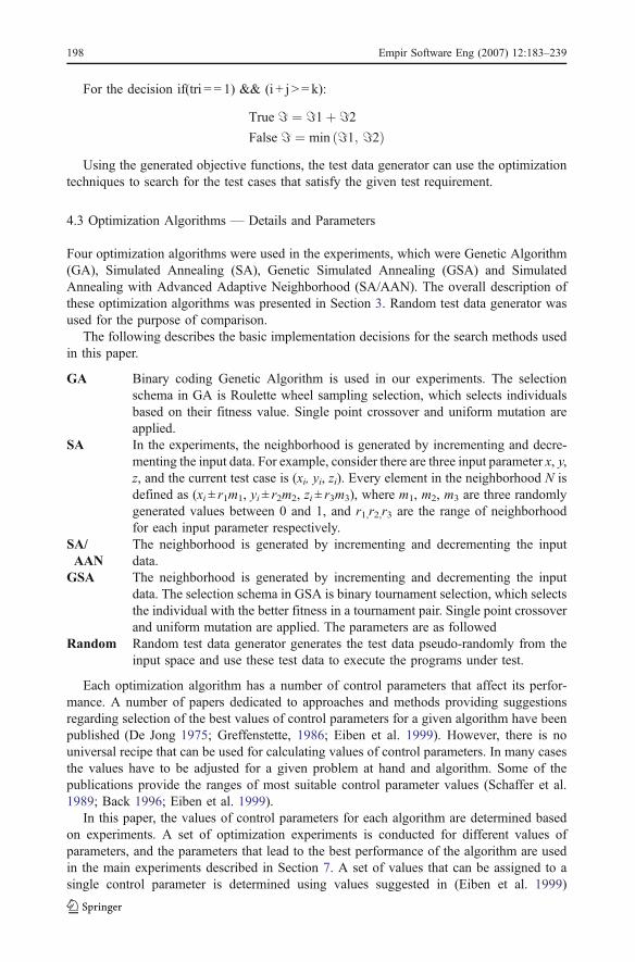
For the decision if(tri = = 1) && (i + j > = k):

True = ¼ =1þ =2False = ¼ min =1; =2ð Þ

Using the generated objective functions, the test data generator can use the optimizationtechniques to search for the test cases that satisfy the given test requirement.

4.3 Optimization Algorithms — Details and Parameters

Four optimization algorithms were used in the experiments, which were Genetic Algorithm(GA), Simulated Annealing (SA), Genetic Simulated Annealing (GSA) and SimulatedAnnealing with Advanced Adaptive Neighborhood (SA/AAN). The overall description ofthese optimization algorithms was presented in Section 3. Random test data generator wasused for the purpose of comparison.

The following describes the basic implementation decisions for the search methods usedin this paper.

GA Binary coding Genetic Algorithm is used in our experiments. The selectionschema in GA is Roulette wheel sampling selection, which selects individualsbased on their fitness value. Single point crossover and uniform mutation areapplied.

SA In the experiments, the neighborhood is generated by incrementing and decre-menting the input data. For example, consider there are three input parameter x, y,z, and the current test case is (xi, yi, zi). Every element in the neighborhood N isdefined as (xi ± r1m1, yi ± r2m2, zi ± r3m3), where m1, m2, m3 are three randomlygenerated values between 0 and 1, and r1,r2,r3 are the range of neighborhoodfor each input parameter respectively.

SA/AAN

The neighborhood is generated by incrementing and decrementing the inputdata.

GSA The neighborhood is generated by incrementing and decrementing the inputdata. The selection schema in GSA is binary tournament selection, which selectsthe individual with the better fitness in a tournament pair. Single point crossoverand uniform mutation are applied. The parameters are as followed

Random Random test data generator generates the test data pseudo-randomly from theinput space and use these test data to execute the programs under test.

Each optimization algorithm has a number of control parameters that affect its perfor-mance. A number of papers dedicated to approaches and methods providing suggestionsregarding selection of the best values of control parameters for a given algorithm have beenpublished (De Jong 1975; Greffenstette, 1986; Eiben et al. 1999). However, there is nouniversal recipe that can be used for calculating values of control parameters. In many casesthe values have to be adjusted for a given problem at hand and algorithm. Some of thepublications provide the ranges of most suitable control parameter values (Schaffer et al.1989; Back 1996; Eiben et al. 1999).

In this paper, the values of control parameters for each algorithm are determined basedon experiments. A set of optimization experiments is conducted for different values ofparameters, and the parameters that lead to the best performance of the algorithm are usedin the main experiments described in Section 7. A set of values that can be assigned to asingle control parameter is determined using values suggested in (Eiben et al. 1999)


combined with experience of the authors. In the case of GA and GSA the controlparameters that need adjustment are population size with the set of possible values {50,100, 150, 200, 500}, probability of (single point) crossover with the set {0.75, 0.8, 0.85,0.9, 0.95}, and probability of mutation with the set {0.001, 0.005, 0.01, 0.02}. For SA andSA/AAN the parameter that has to be adjusted is a neighborhood size with the set ofpossible values {10, 20, 50, 80, 100, 200}. Additionally, one important parameter that iscommon to all methods has to be set—this parameter identifies how many generations/iterations an algorithm should perform before it stops in the case when the algorithm isunsuccessful in finding a test case for a test requirement. This has to be set otherwisealgorithms would never stop. The possible values for this parameter are 20, 25, 30, 40, 60,80. All these sets are also included in Table 7 in the brackets.

The process of finding the best values of parameters is done for each algorithm and eachprogram under test (see Section 5 for details regarding programs under test). Threeoptimization experiments are conducted for each combination of the parameters’ values.The set of values that provides the best performance is selected and used for the mainexperiments. This process is repeated for each algorithm and each program. One of themain reasons of doing so is the need to ensure the best possible performance for eachalgorithm. This provides a better environment for the comparison of the algorithms basedon their performance results. Table 7 contains the best values of the parameters for GA, SA,GSA and SA/ANN. There is also an entry for RANDOM approach where a number ofrandom generations of test cases for each program are shown. As it can be seen, differentnumbers are used — they are set after all experiments have been done and they represent anaverage number of executions of a program under test performed by each algorithm.

Table 7 Parameters of algorithms used in the experiments presented in the paper

Programs parameters Hex-DecConversion

TimeShuttle

PerfectNumber

TriangleClassification

Rescue

GAPopulation size {50, 100, 150, 200, 500}* 50 200 50 100 100Crossover probability {0.75, 0.8, 0.85, 0.9, 0.95} 0.95 0.75 0.9 0.8 0.75Mutation probability {0.001, 0.005, 0.01, 0.02} 0.02 0.01 0.02 0.01 0.01Termination criterion** {20, 25, 30, 40, 60, 80} 30 20 30 20 30

SANeighborhood size {10, 20, 50, 80, 100, 200} 80 50 50 100 200Termination criterion {20, 25, 30, 40, 60, 80} 25 80 30 50 20

GSAPopulation size {50, 100, 150, 200, 500} 50 150 50 100 50Crossover probability {0.75, 0.8, 0.85, 0.9, 0.95} 0.9 0.75 0.85 0.75 0.8Mutation probability {0.001, 0.005, 0.01, 0.02} 0.01 0.005 0.02 0.005 0.02Neighborhood size {10, 20, 50, 80, 100, 200} 10 20 10 20 10Termination criterion {20, 25, 30, 40, 60, 80} 80 60 200 30 80

SA/ANNNeighborhood size {10, 20, 50, 80, 100, 200} 50 50 50 100 100Termination criterion {20, 25, 30, 40, 60, 80} 40 80 30 30 20

RANDOMNumber of random generations 10,000 30,000 10,000 30,000 40,000

*The values in brackets represent a set of possible values that can be assigned to the parameter

**The termination criterion represents a number of interactions (generations) that the algorithm performsbefore it stops in the case it does not satisfy a test requirement


5 Systems Under Test

Ideally, we would select a number of programs for the experiment, which would provide anaccurate representation of all existing computer programs. Unfortunately, this ideal state isunachievable for a number of reasons. Firstly, we don’t have anything approaching adefinition of a sampling frame for the ‘universe’ of computer programs. Hence bydefinition, any, and all, selection or sampling mechanisms must be ad hoc and open todebate. Secondly, articles that have used GA and SA techniques as implementationmechanisms for goal-oriented approaches to test case generation only report limited successwith these approaches. In addition, this limited success, was achieved on a very limited setof programs under test. This greatly limits the selection possibilities. If we were toooptimistic and choose programs “beyond the current capabilities of these approaches” thenthe study would reveal no information, as all the techniques would approach a zero percentsuccess rate. Similarly, if they were “too trivial (for the approaches)” no information wouldagain be revealed, as the techniques would all approach one hundred percent success rates.

Five C/C++ programs were tested in our experiments.2 Brief descriptions of theprograms used in the experiments are shown below:

& Hex-Dec Conversion: This program decides if an input string is a legal hexadecimalnumber. If it is, then it converts the legal hexadecimal number to a decimal number.This program has 36 test requirements to be covered.

& Time Shuttle: This program requires the user to input a destination date of the timetravel, which includes month, day and year. It returns a corresponding message to theuser. In the experiments, the input data is limited to (0,64) for the months, (0,128) forthe days and (0,16192) for the years. This program has 87 test requirements to becovered.

& Perfect Number: This program is used to decide if a number is a perfect number and if itis a prime number. This program has 37 test requirements to be covered.

& Triangle Classification: This program requires the user to input three integers as threesides of a triangle; it then determines which type of triangle it is. The output to the userhas four results, “scalene”, “isosceles”, “equilateral” and “not a triangle”. This programhas 51 test requirements to be satisfied.

& Rescue: The rescue program requires the user to input a number, and then it determinesif the input is a legal secret code. The legal secret code should be a 5-digit number andsatisfy some predefined rules. If the input is a valid secret code, the program decodesthe legal secret code and returns the corresponding secret fmessage to the user. Thisprogram has 46 test requirements to be satisfied.

All tested programs can be classified as being relatively small and of limited complexity.

6 Experimental Procedure

6.1 Experimental Setup

The comparisons between the optimization techniques’ performances were based on thenumber of SUT executions (iterations) they required to reach their optimal coverage level,

2 Source Code is available from the authors upon request.


rather than the actual computational time. This will allow for a fair comparison since theexecution of the target program itself is responsible for most of the time required togenerate test-data, especially if the programs are very large in size. In addition, in contrastto the actual computational time, this provides a uniform comparison platform regardless ofthe performance of the workstations, operation systems used or the efficiency of thecompilers, etc. For each optimization technique, the maximum number of SUT iterations itallows depends on a preset stopping criterion.

For each SUT, sets of ten complete experiments were performed with each test-datagenerator system. For a subset of the programs used, two different input spaces are used.The reason for using different input spaces is to examine the effect that the size of the inputspace has on the performance of the optimization techniques. The average coveragepercentage (ACP) is the average of the maximum coverage achieved through each set of tenexperiments that use a particular optimization technique.

6.2 Evaluation Approach

We can regard the 10 trials of each optimization approach (on each program) as a samplingfrom the performance distribution of that technique upon that system. Hence, we mightconsider comparing two techniques by using a simple statistical test (such as a t-test) andasking if a statistically significant difference exists between the two performancedistributions. We believe that this approach is fundamentally flawed for a number oftechnical reasons. First, and foremost, is that the sample size is under the direct control ofthe experimenters and the cost of increasing the sample size is next to zero. Hence, anyresearchers can generate a statistically significant result just by adding more trials. To quotefrom Miller (2004):

... Regardless of the formulation, the derived P-value is a function of:

& the difference between the measured data and the null hypothesis; and& the sample size.

For example, consider a simple test (t-test), where the question (or null hypothesis) is:“is the mean of the population under investigation equal to k.” More formally, the testis H0: μ= k and the alternative hypothesis of H1: μ< > k, where k is an arbitraryconstant. Hence, the simple test is given by:

t ¼ x� k

S�

ffiffiffiffiffiffiffiffiffiffiffin� 1

p

where x is the mean, S is the standard deviation, and n is the sample size. Hence,t can be increased (and hence the associated P-value decreased) by increasingeither x� k or

ffiffiffiffiffiffiffiffiffiffiffin� 1

p. But, as n increases then x� k and S will tend to constants—

their true values. Hence, a large value of n directly translates into a large value of t,and hence a small value of P. More formally, as n → ∞, then x � k ! constant andS → constant, t → ∞, and P → 0. Hence, it can be stated that P has a strongdependence on the sample size, and its value is almost independent of the existence,or not, of an effect when the sample size is large. ...

Hence, it is believed (that for this type of situation) that statistical testing is a pooroption, instead we have chosen to supply more qualitative rank-oriented descriptions of theperformance and supplement this with effect size estimates whenever a result of “high


interest” is encountered. This more informal approach can be regarded as highly con-servative, but as outlined above, it is believed that the technical issues facing the utilizationof standard statistical hypothesis testing approaches are too great and that any resultsproduced by this approach would be meaningless. Clearly, the calculation of effect sizespotentially still has technical issues, principally the inability to estimate an accuratestandard deviation from a restricted sample size, the assumption that the samples are takenfrom a normal distribution and reliability of the measurements—do the random componentsin the algorithm imply that the performance results cannot be considered as adhering to asingle performance distribution. While, these are all valid concerns, it is believed that thisapproach is technically “much safer” than the significance-based approach—although,clearly no definitive evidence can be provided.

Researchers have proposed a number of measures, which approximate the “true” effectsize, but under most conditions, the various formulations provide very similar results.Hence, we will report Cohen’s d, using a pooled standard deviation estimate as no truecontrol group exists, as the principle result. However, as it will be calculated from asmall sample of values available. It should therefore be regarded as only an estimate ofthe ‘true’ population value, and subject to sampling error (almost provided). Althoughusing the pooled standard deviation to calculate the effect size generally gives a betterestimate than the control group, it is still unfortunately slightly biased. In fact, it can beshown that when effect sizes are calculated from samples taken from a known population,on average the sample values are a little larger than the value for the population fromwhich they come (Hedges and Olkin 1985). Hence, we also provide a “corrected for bias”value of d as the sample size is small. Finally, this measure is only the central tendencywithin the likely set of results; hence we also provide an estimate of the true confidenceinternal to provide an extended description of the likely values (at the traditional 95%internal) for the unknown effect size. All equations are taken for Hedges and Olkin(1985). Finally, our initial post-analysis suggests that the GA-based approach is the mostlikely candidate to be considered as the “best performing” technique. Hence, to savespace within the article, we will only report effect sizes of this technique in relationshipto the other techniques. A positive effect size indicates that the GA approach provides anexample of superior performance; a negative effect size indicates that the other techniquedominates.

Finally, within the textural description of the results, we plan to utilize a Cohen’sthoughts on a universal description of effect scales (Cohen 1988). In this book, heproposes a simple translation between effect sizes and linguistic interpretations (0.2 = small;0.5 =medium; 0.8 = large), this translation does not imply a rigorous statement about aneffect, it is instead aimed at helping the reader form an interpretation of the likely impact ofeffect size in terms in its operational significance. Cohen’s descriptors stop at effect sizesequal to 0.8; we have extend this ‘scale’ to include massive at 2.0 and near perfectseparation of the populations at 4.0. While, no sound argument exists for these choices thestudy encounters several huge differences, which require translation for the reader. Clearly,caution must be exercised when considering the linguistic translations and all finaldecisions should be based upon the numerical evidence not the linguistic statements.Perhaps the easiest way to consider the implication of this translation is to note that aneffect size can be directly converted into statements about the overlap between the twosamples in terms of a comparison of percentiles. An effect size is exactly equivalent to a ‘Z-score’ of a standard Normal distribution. This clearly has much in common with McGrawand Wong’s (1992) common-language effect statistic or probability of superiority scale ofmagnitudes.


7 Experimental Results and Observations

The experimental results follow a repetitive pattern—simply, each system under test isanalyzed in turn. To allow the resultant information to be encoded in tabular form, wedefine a number of acronyms here.

ACTR Average Coverage of Test RequirementsACP Average Coverage as a PercentageE.S. Effect SizeS.E. Standard Error (associated with the effect size estimate)C.I. Confidence Internal (around the effect size)

7.1 Hex-Dec Conversion

Tables 8 and 9 show the test results of running the GA, GSA, SA, SA/AAN and randomtest-data generators with the Hex-Dec Conversion program.

Overall all optimization techniques performed very well. This can be contributed to thesimplicity of the structure of the Hex-Dec Conversion program, which contains far lesslines of code than other programs used in this work. The results indicate that the GA, SAand SA/AAN exhibit the best (identical) performances. In addition, they performed veryconsistently (no variation); it was found that in each of the ten test runs using each of theseoptimization techniques, the generators achieved the same optimal coverage percentage of97.22%. Ranked fourth is the Random generator, which also achieved a high ACP. TheGSA generator relatively had the worst performance, with an ACP below 90%. At the sametime, the results obtained with GSA generator exhibit the highest level of variation. Thedetailed analysis of all conducted experiments with GSA leads to a simple explanation. Oneof the experiments provided a very low coverage of 44.44%. It is assumed that for thatparticular experiment GSA stuck in the local optimum and was not able to move to adifferent spot in the search space. As it is discussed in Section 8, GSA exhibits a tendencyto stay in a local optimum once it finds one. GSA and the random generator, show a largeto very large effect size drop in performance when compared with the GA technique.

Further analysis of the generators’ performances revealed that all the generators failed toexecute the false branch of a particular decision in the code. This decision requires theoptimization techniques to generate a test case, which is a valid hexadecimal number that islarger than 7 digits.

Figure 4 shows the coverage plots3 of the test data generators. Generally, the GA and theSA/AAN techniques performed better than other test-data generators. The GA and the SA/AAN techniques almost achieve full coverage after 500 SUT iterations. The SA techniqueultimately achieved the same optimal coverage, as did the GA and the SA/AAN; however,it required 4,000 more SUT iterations to achieve a 90% coverage level. In contrast, toobtain a 90% coverage level, the Random generator required 7500 SUT iterations. TheGSA technique had a very similar performance to the Random technique, but towards theend of the experiment it was unable to improve beyond the 86.39% coverage level.

3 Due to the lack of space, all coverage plots presented in this paper show the performance of theoptimization techniques throughout the first 10,000 SUT iterations. It is important to note that theoptimization techniques will keep operating beyond 10,000 SUT iterations, possibly improving theircoverage level.


The most challenging test requirement in the Hex_dec program is to take the falsebranch of decision 3

if (i < = MAX)

which requires that the test case is a valid Hexadecimal number, and also the length of theinput string should be greater than 7 as the majority of the ASCII set is used. In ourexperiments, none of the test data generators can generate a test case to satisfy thiscondition. Throughout the paper, we will regularly identify the most challenging conditionfor the various programs under test. This condition is characterized simply by: the numberof opportunities to satisfy the condition normalized by the total number of possible valuesthat exist for the variables in the condition. Note, in general, the number of opportunities tosatisfy these conditions is much less than the total number of possible values.

The performance of the best two test data generators with the Hex-Dec Conversion isfurther investigated. For the GA and the SA/AAN test data generators, the maximum,minimum and average coverage achieved throughout the ten experiments performed usingeach generator, are plotted against the number of SUT iterations (see Fig. 5). It can beobserved from Fig. 5 that the GA achieved better coverage than SA/AAN in the initialstages during its poorest performances.

7.2 Time Shuttle

Tables 10 and 11 shows the test results of running the GA, GSA, SA, SA/AAN and randomtest-data generators with the Time Shuttle program.

Once again, the optimization techniques performed very well, as they all achieved anACP close to or above 90%. Generally, the decisions in Time Shuttle program were harderto satisfy than those in the Hex-Dec Conversion program. Hence, the techniques did notperform quite as well with the Time Shuttle program as they did with the Hex-DecConversion program. The GA technique ranked first, followed by SA (small to medium

Table 9 Performance results of the optimization techniques with the Hex-Dec conversion program— effectsize relative to GA

Optimization technique E.S. Bias S.E. C.I. for E.S.

E.S. E.S. Lower Upper

Random 1.00 0.96 0.47 0.03 1.88GSA 0.97 0.93 0.47 0.01 1.85

Optimizationtechnique

ACTR(36)

AverageACP

St. dev.ACP

Random 34.5 95.83 1.963GA 35 97.22 0SA 35 97.22 0GSA 31.1 86.39 15.738SA/AAN 35 97.22 0

Table 8 Performance results ofthe optimization techniques withthe Hex-Dec Conversionprogram—raw data


effect size), GSA (large to very large), Random (large to very large) and SA/AAN (large tovery large), respectively.

After analyzing the performance of the optimization techniques with the Time Shuttleprogram, it (else if(m==OCT && d<15)) was discovered once again that thetechniques found a particular condition to be the most challenging to satisfy. The generatorshad difficulties executing the true branch of that decision. In our experiments, only the GAgenerator was capable of satisfying that condition, which it did only twice.

Figure 6 shows the coverage plots of the test data generators. With the exception of theSA/AAN technique, the other techniques reached their peak coverage in less than 2000SUT iterations. The SA/AAN technique reached its peak very late in the search process. Infact, after 10,000 SUT iterations, the SA/AAN had a coverage level well below the othertechniques. To investigate further, several additional experiments were conducted. Duringthese experiments, the neighborhood size (the number of possible new solutions to choosefrom) was adjusted. Table 12 shows a comparison between the performances of the SA/AAN technique using different neighborhood sizes.

Table 12 shows that with a larger neighborhood size, the SA/AAN technique was able toultimately achieve a higher ACP. While using a smaller neighborhood size, the SA/AANtechnique was able to reach its peak coverage much quicker.

hex_dec conversion

0

10

20

30

40

50

60

70

80

90

100

0 1 2 3 4 5 6 7 8 9 10x103

number of iterations

y(Random) y(GA)y(SA) y(SA/AAN)y(GSA)

Fig. 4 Coverage plots of fivesearch methods with the Hex-DecConversion program. Note the“number of iterations” refers tothe number of complete execu-tions of the system under test

Hex_dec (GA and SA/AAN)

0102030405060708090100

0 1 2 3 4 5 6 7 8 9 10x103


y(GAmax) y(SA/AANmax)

y(GAmean) y(SA/AANmean)

y(GAmin) y(SA/AANmin)

Fig. 5 Comparison of GA andSA/AAN with the Hex-Dec con-version program


The most challenging condition in this program is decision 10

else if (m= =OCT && d< 15)

in the code listed in the Appendix. In order to take the true branch of this condition, the testcase should be (10, d, 1582), where d should be smaller than 15.4 In our experiments, onlytwo runs of GA generate test cases that satisfy this condition; one of them also satisfiesother 83 test requirements successfully and obtains a complete coverage. The other one,failed to find the test case that exercises the false branch of m==OCT, so it only satisfies83 test requirements.

As shown in Tables 10 and 11 and the coverage plot in Fig. 6, the GA and the SAtechniques have the best performances with the Time Shuttle program. For the GA and theSA test-data generators, the maximum, minimum and average coverage achievedthroughout the ten experiments performed using each generator, are plotted against thenumber of SUT iterations (Fig. 7).

It can be observed from Fig. 7 that after 10,000 SUT iterations, the performance of theGA and the SA techniques are similar. However, the range between the SAmax and theSAmin arcs are larger than the range between the GAmax and the GAmin arcs. Thisindicates that the performance of GA is more stable and consistent.

7.3 Perfect Number Program

Tables 13 and 14 shows the test results of running the GA, GSA, SA, SA/AAN and randomtest-data generators with the Perfect Number program.

The results show that the GA and the SA techniques have the best performance (only avery small to small effect size difference exists). GA achieves complete coverage in threeruns. The SA/AAN technique performs relatively poorly (very large effect size); and, theGSA and the Random techniques exhibited extremely poor performances (massive to nearperfect separation of the populations and exceeds near perfect separation of thepopulations effect sizes respectively). The most challenging condition in the PerfectNumber program requires the generators to produce a perfect number larger than 1,000.Although after ten runs, the ACP of the GA and the SA techniques are almost equivalent,the GA was capable of achieving complete coverage in three of its runs, while the SA hasfailed to achieve the same because it was not capable of producing a perfect number largerthan 1,000. Note only one perfect number exists (8,128) which is larger than 1,000 butsmaller than the maximum size of input allowed; hence this represents an extremelychallenging condition. Algorithms that favour exploitation over exploration, including SA,struggled with this condition.

4 This program uses a slightly simplified version of history, and assumes that the Gregorian Calendar startson the 15th of October 1582. Hence, this date represents day 1 for the Time Shuttle program.


ACTR(87)

AverageACP

St. dev.ACP

Random 72 85.71 0GA 78.1 92.98 4.468SA 76 91.43 3.311GSA 74 88.81 3.516SA/AAN 74.1 88.21 3.618

Table 10 Performance results ofthe optimization techniques withthe time shuttle program—rawdata


Figure 8 shows the coverage plots of the test data generators. All five optimizationtechniques were capable of getting close to their peak coverage in the early stages of thesearch process. For the GA, SA and the SA/AAN techniques, they achieved a 94%coverage level in about 1,500 SUT iterations. The SA/AAN technique showed almost noimprovement afterwards, while the GA and the SA techniques kept improving slightly.After reaching the 83% coverage level, the Random generator failed to improve, while theGSA generator improved slightly afterwards.

As shown in Tables 13 and 14 and the coverage plot in Fig. 8, the GA and the SAtechniques have the best performances with the Perfect Number program. In theexperiments, the GA and the SA techniques were also applied to the Perfect Numberprogram using a bigger input space [0,131071]. The reason for using a larger input space isto examine the effect the larger input will have on the performance of the GA and the SA.For the GA and the SA test-data generators, the maximum, minimum and average coverageachieved throughout the ten experiments performed using each generator, are plottedagainst the number of SUT iterations as shown below (see Figs. 9 and 10). Figure 9 showsthe performance of the techniques using the smaller input space [0,65535], while Fig. 10shows the performance of the techniques using the larger input space [0,131071].

The most challenging condition in the Perfect number program is decision 16

if num>1000 //16.

Tables 15 and 16 show the test results of running the GA and the SA test-data generatorswith the Perfect Number program using the larger input space [0,131071].

Tables 15 and 16 show that the ACP for the GA and the SA techniques almost remainthe same. In fact, the SA shows remarkable stability (finding 36 requirements on everyexecution) and out-performing the GA (small to medium effect size). In contrast, the GAfinds the increase in search-space increases the complexity of the problem—see Table 17.


E.S. Bias S.E. C.I. for E.S.


Random 2.30 2.20 0.57 1.09 3.31SA 0.39 0.38 0.45 −0.51 1.26GSA 1.04 0.99 0.47 0.06 1.92SA/AAN 1.17 1.12 0.48 0.18 2.07

Table 11 Performance results ofthe optimization techniques withthe time shuttle program—effectsizes

timeshuttle

0102030405060708090100

0 1 2 3 4 5 6 7 8 9 10x103

number of interations


Fig. 6 Coverage plots of fivesearch methods on Time Shuttleprogram


Figures 9 and 10 show that the SA technique requires more SUT iterations to reach itspeak coverage with the larger input space. Meanwhile, the GA technique reached its peakcoverage earlier using both input spaces. As with the Time Shuttle program, Figs. 9 and 10show that the range between the SAmax and the SAmin arcs are much larger than the rangebetween the GAmax and the GAmin arcs. This further indicates that the performance of GAis more stable and consistent.

7.4 Triangle Classification Program

Tables 18 and 19 show the test results of running the GA, GSA, SA, SA/AAN and randomtest-data generators with the Triangle Classification program using two inputs spaces. Thesmaller input space is [−65536,65535] and the larger input space is [−2147483648,214783647].

The results presented in Tables 18, 19, 20 and 21 show significant differences whencompared to the performance of the GA. No alternative algorithm has a performance, whichcan be considered “comparable”; SA/ANN has on average a massive effect size difference.The other algorithms have such large differences that the linguistic translation, suggested byCohen (1988), has no representation (but clearly far exceeds near perfect separation of thepopulations effect sizes). Even SA, which on the results from the previous evaluations has

timeshuttle (GA and SA)

20

30

40

50

60

70

80

90

100

0 1 2 3 4 5 6 7 8 9 10 11x103


y(GAmax) y(SAmax)

y(GAmean) y(SAmean)

y(GAmin) y(SAmin)

Fig. 7 Comparison of GA andSA with the Time Shuttleprogram


Average covered testrequirements (max: 87)

Average coveragepercentage (ACP) (%)

SA/AAN1(original)

77.1 88.62

Neighborhoodsize: 50

SA/AAN2 76 87.36Neighborhoodsize: 20

SA/AAN3 73 83.91Neighborhoodsize: 10

Table 12 Performance results ofthe SA/ANN optimization tech-nique using different neighbor-hood sizes, with the time shuttleprogram


demonstrated similar performance (in terms of effects sizes based upon average ACP),performs unbelievably poorly by comparison. Careful examination of the tables provideseven more insight into effectiveness of the methods. In Table 18, it is very easy to spot amediocre performance of SA generator. SA provides the lowest value of average ACP, andthe highest value of standard deviation ACP. It is an indication that the TriangleClassification program is very challenging for SA. A plausible explanation of it can bethe inability of SA to efficiently explore the search space and to cope with local optima.This is likely to be a result of the SA algorithm having no explicit mechanism to force it toconsider “distant” potential solutions from the current local position. Whereas the mutation,and to a lesser extent the crossover, operation perform this service adequately for the GAalgorithm. It is also seen in Table 18 that SA and GSA have the lowest values of averageACP as well as very low values of standard deviation ACP. A possible reason for that is away in which both these methods explore the search space. Low values of standarddeviation indicate that the methods are not able to “move” to different areas of the searchspace. They are stuck in almost the same places in the search space for every experiment.Even the application of crossover to SA, for the GSA method, did not help a lot for thisparticular program. Further, the mutation operation for the GSA algorithm differs from theGA algorithm as the mutation operation within GSA is confined to only consider mutantswithin a local neighbourhood; again not supporting the consideration of “distant” solutions.Quite a different scenario is seen for SA/AAN approach. In this case modifications of SAincreased the ability of the method to find test cases that satisfy a larger number of testrequirements.

From the result tables above, we can see none of the test data generators achieve acomplete coverage even on the small input space. GA, which performs best, still fails tocover the true branch of condition/decision if (tr > 3) and else if (t = = 3), which require that3 equal integers as input. It is interesting that in the best runs, SA/AAN only satisfies 46test requirements. After investigating the uncovered conditions, we find out this is becauseSA/AAN finds the test cases that satisfy i = = j but i + j < k. This causes that the truebranch of the decision 8 if tri = = 1 && i + j > k cannot be executed. For example, the test


ACTR(37)

AverageACP

St. dev.ACP

Random 31 83.78 0GA 36 97.30 2.205SA 35.9 97.03 0.853GSA 31.9 86.22 3.920SA/AAN 35.1 94.86 0.853

Table 13 Performance results ofthe optimization techniques withthe perfect number program—raw data

Optimization technique E.S. Bias S.E. C.I. for E.S.


Random 8.65 8.29 1.38 5.57 11.00SA 0.16 0.15 0.45 −0.72 1.03GSA 3.46 3.33 0.47 1.98 4.69SA/AAN 1.46 1.40 0.48 0.42 2.37

Table 14 Performance results ofthe optimization techniques withthe perfect number program—effect sizes


case (43615,135876,43615) cannot exercise the true branch of decision 8. This also happento decision 9

if tri = = 2 && i + k > j

and decision 10

else if tri = = 3 && j + k > i.

On the other hand, this situation does not happen to GA. Through analyzing the result,we find out that even if GA generate such a test case, it always has the ability to generateanother test case to make if tri = = 1 && i + j > k to take the true outcome. For example,we find a test case (7271,7271,22811) in one run, and we also find another test case(7271,7271,9956). This is because in our experiments, test data generators keep the testdata that can reach the condition (see Section 5), and when the test data generator start towork on satisfying this condition, the initial population is seeded with these candidate testcases. GA is population based so it has the ability to keep these good seeds, that meanskeep the good gene, in this case, it is (7271,7271,z).

On the other hand, SA/AAN starts with the single candidate seed. So this candidate seedshould be selected from the test cases which can reach the condition if tri = = 1 && i + j > k,and it has little chance to keep the good seed for the subsequent neighborhood search.

perfect number(GA and SA, input space=[0,65535])

40

50

60

70

80

90

100

0 1 2 3 4 5 6 7 8 9 10x103


y(GAmax) y(SAmax)

y(GAmean) y(SAmean)

y(GAmin) y(SAmin)

Fig. 9 Comparison of GA andSA, using the smaller input space[0,65535], with the PerfectNumber program

perfect number (input space=[0,65535])

40

50

60

70

80

90

100

0 1 2 3 4 5 6 7 8 9 10x103


y(Random) y1(GA)

y1(SA) y1(SA/AAN)

y1(GSA)

Fig. 8 Coverage plots of fivesearch methods on PerfectNumber program


For example, there are 3 candidate test cases, which are (1783,567,567),(4357,4357,10896), (1199,90234,90234). All of them can reach the condition if tri = = 1&& i + j > k, however only (4357,4357,10896) has the good gene which may cause thesubsequent test cases covered the condition if tri = = 1 && i + j > k. SA/AAN selects a seedrandomly from these three test cases, so there is only 33% chance that the valuable test case(4357,4357,10896) can be selected. Moreover, even if SA/AAN select the good seed, in thesubsequent neighborhood search, SA/AAN has little chance to keep this good gene due toits neighborhood structure design.

Figure 11 shows the performance of the optimization techniques on the TriangleClassification program using the smaller input space. The coverage plot shows that therandom generator quickly reaches its peak coverage in less than 100 SUT iterations, buthardly improves its coverage afterwards. The GSA and the SA techniques start withapproximately a 40% coverage level, which is 10% less than what the random generatorstarted with; however, with more SUT iterations, both techniques gradually and slowlyimprove their coverage, eventually exceeding the coverage level achieved by the randomgenerator. Once again the GA performed best, reaching a 90% coverage level inapproximately 2,500 SUT iterations. On the other hand, the SA/AAN technique required6,500 SUT iterations to reach an 80% coverage level, where it improved slightly afterwards.

Figure 12 shows the performance of the optimization techniques with the TriangleClassification program using the larger input space. The coverage plot shows that therandom generator performed similarly using the larger input space. Meanwhile, thecoverage level of the GSA and the SA techniques has degraded significantly, droppingbelow 50%. The performance of the GA and the SA/AAN were relatively unchanged. Theprinciple difference observed is that the GA reached its peak coverage at a significantlyslower pace when using the larger input space, requiring more than twice the SUT iterationsto reach the 90% coverage level.

perfect number(GA and SA, input space=[0,131071])

40

50

60

70

80

90

100

0 1 2 3 4 5 6 7 8 9 10x103


y(GAmax) y(SAmax)

y1(GAmean) y(SAmean)

y(GAmin) y(SAmin)

Fig. 10 Comparison of GA andSA, using the smaller input space[0,131071], with the PerfectNumber program

Table 15 Performance results of the GA and SA techniques with the perfect number program, usingdifferent input space sizes—raw sizes

Optimization technique ACTR (37) Average ACP St. dev ACP

GA 35.7 96.49 2.228SA 35.9 97.30 0


As shown in Table 17 and the coverage plots in Figs. 11 and 12, the GA and the SA/AAN techniques have the best performances with the Triangle Classification program. Forthe GA and the SA/AAN test-data generators, the maximum, minimum and averagecoverage achieved throughout the ten experiments performed using each generator, areplotted against the number of SUT iterations as shown below (see Figs. 13 and 14).Figure 13 shows the performance of the techniques using the smaller input space, whileFig. 14 shows the performance of the techniques using the larger input space.

Figures 13 and 14 show that the range between the SA/AANmax and the SA/AANminarcs are much larger than the range between the GAmax and the GAmin arcs. This furtherindicates that the performance of the GA is more stable and consistent.

7.5 Rescue Program

Tables 22, 23, 24, 25 shows the performance results of running the GA, GSA, SA, SA/AAN and random test-data generators with the Rescue program using two inputs spaces.The smaller input space is [0,524287] while the larger input space is [0,214783647].

The results presented show that the GA and the SA/AAN techniques had the bestperformances using both input spaces. The ACP of the GA and the SA/AAN techniqueswere almost equivalent using both input spaces, which indicates that the larger input spacedid not affect the performance of these two optimization techniques. However, theperformances of the SA, GSA and the Random techniques have degraded considerablywhen utilizing the larger input space. Once again, as in the case of the TriangleClassification program, SA and GSA have the lowest values of ACP. This time the ACP ofSA is extremely low and its standard deviation is zero. This means that the Rescue programis extremely difficult for SA when a large search space is used, Table 22. SA is not able toescape a local optimum. A very intriguing fact is that all SA experiments give the sameACP. This could be the result of a combination of the limited ability of SA to perform aglobal search and a very difficult fitness function for SA to optimize. It is possible that SAwould perform better with a different fitness function. This however would make thecomparison of different algorithms – the main goals of this paper – not possible. The additionof genetic operators to SA helped – the average ACP for GSA is higher – but the value is stillbelow the ACPs of GA and SA/AAN.

In the Rescue program, the most important decision is decision 1

if(!(code > 9999 && code < 100000)) // 1

Covered test requirements (37)

GA 35 36 37Small input space 1 6 3Large input space 5 3 2

Table 17 Performance results ofthe GA techniques with theperfect number program, usingdifferent input space sizes




SA −0.50 −0.48 0.45 −1.37 0.41

Table 16 Performance results ofthe GA and SA techniques withthe perfect number program,using different input spacesizes—effect sizes


If the test case cannot take the false branch of this decision, it will fail to reach the rest ofthe conditions and decisions. This is the reason why SA and random test data generator andGSA have poor performance on Rescue program.

In the Rescue program, the most challenging conditions are decision 7 to decision 13,which are deeply nested inside four if-else statements. In order to cover these conditions,the test data should satisfy four other else statements first.

Figure 15 shows the performance of the optimization techniques with the Rescueprogram using the smaller input space. All optimization techniques were capable ofperforming very well with the smaller input space, each has an average coverage close to100%, with the exception of the random technique. The coverage plot shows that alltechniques were close to their peak coverage level in less than 500 SUT iterations, with theexception of the SA technique. The SA technique required approximately 2,250 SUTiterations to reach its peak coverage level.

As shown in Fig. 16, the larger input space [0,2147483647], used for the Rescueprogram, significantly affected the performance of the GSA, SA and the Randomoptimization techniques. After 9,500 SUT iterations, the SA, GSA and Randomoptimization techniques achieved an average coverage less than 20%. Only the GSA waslater able to rebound and reach an average coverage level of 41%. Meanwhile, the largerinput space had a very minute impact on the performance of the GA and the SA/AANtechniques. The only main difference exhibited in their performance is that they requiredmany more SUT iterations to reach their respective coverage peaks.

As shown in Tables 18 and 19 and the coverage plots in Figs. 15 and 16, the GA and theSA/AAN techniques have the best performances with the Rescue program. For the GA andthe SA/AAN test-data generators, the maximum, minimum and average coverage achievedthroughout the ten experiments performed using each generator, are plotted against thenumber of iterations as shown below (see Figs. 17 and 18). Figure 17 shows the performanceof the techniques using the smaller input space, while Fig. 18 shows the performance of thetechniques using the larger input space.


Small input space

ACTR(51)

AverageACP

St. dev.ACP

Random 25 49.02 6.201GA 47.9 93.92 1.950SA 33.8 66.27 15.708GSA 41.4 81.18 4.819SA/AAN 44.3 86.86 2.933

Table 18 Performance results ofthe optimization techniques withthe triangle classification pro-gram, smaller input space[0,524287]—raw data




Random 9.77 9.36 1.55 6.33 12.39SA 2.47 2.37 0.58 1.22 3.51GSA 3.47 3.32 0.69 1.97 4.67SA/AAN 2.83 2.71 0.62 1.50 3.93

Table 19 Performance results ofthe optimization techniques withthe triangle classification pro-gram, smaller input space[0,524287]—effect sizes


When the SA/AAN and the GA generators work with the smaller input space, bothgenerators hit their peak after about 2,500 SUT iterations in all the experiments. The lowSA/AANmin arc is caused by a single run that had a very poor performance at the earlystage. In fact, the SA/AAN technique achieved full coverage in all other experiments in lessthan 1,000 SUT iterations. Therefore, the SA/AANmean arc is shown to be much closer tothe SA/AANmax rather than the SA/AANmin arc. Although both generators achieve fullcoverage after 2,500 SUT iterations, the GA technique still outperforms the SA/AANduring the first 500 SUT iterations.

When the GA and the SA/AAN generators work with the larger input space, it can beobserved that the GA generator outperforms the SA/AAN generator during the first 3,000SUT iterations. This is evident as the GAmin arc is higher than the SA/AANmax arc.However, on average, the SA/AAN technique achieves full coverage in fewer SUTiterations than required by the GA technique. The SA/AAN technique achieves completecoverage in 9 runs while the GA technique only achieves complete coverage in 5 runs.

8 Discussion of Results

This paper reports experimental results from five different C/C++ programs using dynamictest data generation. Four optimization algorithms are implemented in the test datageneration system. In our knowledge, two of them, Genetic Simulated Annealing andSimulated Annealing with Advanced Adaptive Neighborhood have not been reported in thetest data generation literature.

All four optimization algorithms used to generate test cases are search-based heuristics.A suitable introduction to the discussion about the obtained results is a short description offew important facts influencing performance of these algorithms. The critical issues are:


Large input space

ACTR(51)

AverageACP

St. dev.ACP

Random 24 47.06 0GA 47.6 93.33 1.893SA 23.8 46.67 0.826GSA 21 41.18 0SA/AAN 43.5 85.29 5.250

Table 20 Performance results ofthe optimization techniques withthe triangle classification pro-gram, large input space[0,2147483647]—raw data




Random 34.57 33.10 5.25 22.81 43.40SA 31.99 30.64 4.87 21.10 40.17GSA 39.02 37.37 5.93 25.76 48.99SA/AAN 2.04 1.95 0.54 0.89 3.02

Table 21 Performance results ofthe optimization techniques withthe triangle classification pro-gram, large input space[0,2147483647]—effect sizes


– fitness landscape—it is built of fitness measures representing a problem; the shape oflandscape has a tremendous impact on overall performance of a selection mechanismof a given method, when the landscape is a plateau all fitness (evaluation) values arealmost the same and the selection method is not working—the selection is done in arandom fashion; in the case when the landscape is more like “mountains and valleys”the fitness (evaluation) values are very different and the selection method can easily“spot” better solutions; when the landscape is flat with a number of sharp picks thenthe search method is “focusing” too much of some of the picks missing the globaloptimum;

– exploration—it is a process of searching through a space of possible solutions (called asearch space); a method should be able to perform extensive search through large areasof the search space, however, at the same time the method should not jump from onespot to another spot too frequently, especially at the later phases of optimization;

– exploitation—it is a process that is opposite to exploration, in this case the systemshould be able to refine already found solutions—in other words, the method should beable to focus on a specific location, and perform a very thorough search of theneighborhood around that location.

triangle (input space=[-2147483648,2147483647])

0102030405060708090100

0 1 2 3 4 5 6 7 8 9 10x103



Fig. 12 Coverage plots of fivesearch methods with the TriangleClassification program with inputspace [−2147483648,2147483647]

triangle (input space=[-65536,65535])

0102030405060708090100

0 1 2 3 4 5 6 7 8 9 10x103


y1(Random) y(GA)

y(SA) y(SA/AAN)

y(GSA)

Fig. 11 Coverage plots of fivesearch methods with the TriangleClassification program with inputspace [−65536,65535]


All experiments described in the paper used the same type of fitness functions. The samefitness function is used for the same program under test by each heuristic test datagenerator. This means that the “fitness landscape” factor has no influence on thecomparison process. All used methods are performing search with the same fitnesslandscape. Additionally, the control parameters of each method have been adjusted for eachprogram (for details regarding control parameters see Section 4.3). All this means is that thecomparison of the methods discussed below is related only to the ways in whichexploration and exploitation are done by each method, and therefore it is a true comparisonof the abilities of these methods to automatically generate test cases.

Generally, in the experiments for five target programs, the GA has the best overallperformance. It achieves complete condition-decision coverage on Timeshuttle, Rescue, andPerfect number program. For the Triangle and Hex_dec programs, GA achieves 93.33%and 97.22% respectively. In our experiments, the test requirements in these two programsthat GA cannot satisfy, cannot be satisfied by other optimization techniques either. As

triangle(GA and ASA, input space=[-2147483648,2147483647])

0

10

2030

40

50

60

7080

90

100

0 1 2 3 4 5 6 7 8 9 10 11x10 3





Fig. 14 Coverage plots of GA andSA/AAN with the Triangle Classi-fication program with input space[−2147483648,2147483647]

triangle (GA and SA/AAN, input space=[-65536,65535])

0

10

20

30

40

50

60

70

80

90

100

0 1 2 3 4 5 6 7 8 9 10Thousandsexecution time

cove

rag

e (%

)

y(GAmax)y(GAmean)y(GAmin)

y(SA/AANmax) y(SA/AANmean)y(SA/AANmin)

Fig. 13 Coverage plots of GAand SA/AAN with the TriangleClassification program with inputspace [−65536, 65535]


discussed in the previous sections in this chapter, GA makes good use of the coverage tableapproach that is applied in the experiments. This approach keeps track of the test cases ifthey can reach some conditions but cannot cover those conditions. These test cases willbecome candidate test cases when the test data generator starts to work on these conditions.GA has the ability to keep the good gene inherited from the ancestors and contribute to thesuccessive generation. That means GA keeps the good features of the candidates. Suchmechanism helps it find the test cases quickly. This is shown and discussed in detail inSection 6.2. However other optimization methods used in the experiments do not makegood use of the candidates. In the Hex_dec program, GA fails to satisfy one testrequirement, which is the taking the false branch of decision 3

if (i < =MAX)

which requires that the test case to find a valid 8 (or greater than 8) digit Hexadecimalnumber. In our experiments, none of the test data generators could generate a test case tosatisfy this condition.

In the experiments, GA is tuned by adjusting four parameters: the mutation probability,the crossover probability, the population size and the number of generation, Table 7. So GAis easy to implement and has a few problem specific decisions that need to be made. It is avery efficient tool for test data generation. GA is a method that possesses a goodexploration and exploitation.

On three programs under test (Rescue, triangle and Hex_dec), Simulated Annealing withAdvanced Adaptive Neighborhood has very good performance, while on other twoprograms it does not. For example, SA/AAN performs very well on the Rescue program,even better than GA on the input space [0,2147483647]. In this case, the search space ishuge [0,2147483647], while the desired test cases of rescue program only exist in a smallrange [10000,99999]. As discussed in Section 7.5”, the most important decision isdecision 1

if(!(code > 9999 && code < 100000)) // 1


Small input space

ACTR(46)

AverageACP

St. dev.ACP

Random 43 93.48 0GA 45.8 99.57 0.915SA 45 97.83 0GSA 45.9 99.78 0.686SA/AAN 46 97.83 1.025

Table 22 Performance results ofthe optimization techniques withthe rescue program, smaller inputspace [0,524287]—raw data




Random 9.36 8.97 1.49 6.05 11.88SA 2.67 2.56 0.60 1.38 3.74GSA −0.26 −0.25 0.45 −1.13 0.63SA/AAN 1.79 1.71 0.52 0.69 2.74

Table 23 Performance results ofthe optimization techniques withthe rescue program, smaller inputspace [0,524287]—effect sizes


Once the test data generator fails to find the test case, which takes the false branch of thisdecision, it will fail to reach other decisions. Although the search space is huge, SA/AANfinds such test case that exists in this small range [10000,99999] very quickly and thusfinds the test cases that satisfy other test requirements quickly. A possible explanation isthat its neighborhood range is not fixed. SA/AAN can make the big jump in the searchspace and also can make the small change in the neighborhood. The big jump in the hugesearch space helps it find the desired test cases in the small range [10000,99999] efficiently.Through examined the result, it has been found that SA/AAN is good at handling thecondition like

if a > b

In this situation, it can find the solution quickly relying on the information thatinstrumented code provides.

Compared to SA, the adaptive neighborhood helps SA/AAN search the search spaceroughly and quickly, while this also causes some limitations. In the experiments, onTimeshuttle program, SA/AAN does not perform very well. The reason is that in somecases, SA/AAN cannot adjust the step size (neighborhood range) flexibly. For example, inthe big plateaus or local optimum, the neighborhood range may decrease too fast, whichcause the neighborhood range is decreased as a value smaller than 1, thus the SA/AAN isstuck at one point. While in some other cases, the neighborhood range may increase toofast, so SA/AAN starts to search the space beyond the input space, which is fruitless.

Generally, the results in the experiments show that SA/AAN has the ability to find thesolution to satisfy some test requirements very quickly, and it works better than otheroptimization techniques in the large input space, especially for the program with simpleinput and large search space like Rescue program. From the point of view of a balancebetween exploration and exploitation, SA/AAN has some problems with exploration that isexhibited by its inability to leave the local optima, on the other hand exploitation seems itsstrong feature.


Large input space

ACTR(46)

AverageACP

St. dev.ACP

Random 7.5 16.30 8.771GA 45.6 99.13 1.121SA 3 6.52 0GSA 19 41.30 38.753SA/AAN 45.9 99.78 0.686

Table 24 Performance results ofthe optimization techniques withthe rescue program, larger inputspace [0, 214783647]—raw data




Random 13.25 12.69 2.06 8.66 16.72SA 117.2 117.1 17.71 77.3 156.9GSA 2.11 2.02 0.55 0.94 3.10SA/AAN −0.70 −0.67 0.46 −1.57 0.23

Table 25 Performance results ofthe optimization techniques withthe rescue program, larger inputspace [0, 214783647]—effectsizes


The result of experiments show that the performance of SA is consistent and predicablewhile it is very time-consuming. It performs remarkably poorly in the large search spaceproblem, which is due to its limitations. The small change in the neighborhood makes itmove slowly to the desirable search space, especially for the Rescue program. Theperformance of SA is worse than Random test data generator. This is because SA onlysearches the neighborhood of the seed test case, thus, once the seed test case is not in thesmall range [10000,99999], it needs a lot of effort to reach this desired search space. In theexperiments, SA gives up before it finds this area, thus it fails to reach other testrequirements. On the other hand, Random test data generator generate each test caserandomly, so it has better chance to reach this desired area. However, in the small searchspace, the performance of SA is stable and it is unlikely to be stuck in the local minimumlike SA/AAN since the neighborhood range in SA is fixed and will not decrease to a valuesmaller than 1, i.e., 0 in our experiments. This is shown in the results of Timeshuttle andPerfect number program. In the large search spaces the performance of SA is not very good.Such behavior can be explained by poor exploration abilities. Exploitation abilities, on theother hand, seem to be pretty good.

Generally, GSA does not perform well in our experiments, and its performance is onlyslightly better than the Random test data generator. However we have not yet tuned this

rescue ( input space=[0,2147483647])

0102030405060708090100

0 1 2 3 4 5 6 7 8 9 10x103


y(rRandom) y(GA)

y(SA) y(SA/AAN)

y(GSA)

Fig. 16 Coverage plots of fivesearch methods with the Rescueprogram with input space[0, 2147483647]

rescue (input space=[0,524287])

0

10

20

30

40

50

60

70

80

90

100

0 1 2 3 4 5 6 7 8 9 10

x10 3number of iterations

y(Random) y(GA)

y(SA) y(SA/AAN)

y(GSA)

Fig. 15 Coverage plots of fivesearch methods with the Rescueprogram with input space[0,524287]


algorithm in our experiments. This may be the reason why GSA does not perform well inthe experiments. Many parameters can be adjusted in order to improve the performance ofGSA. The issue of exploration vs. exploitation seems to be quite complex. Inherently, GSAshould have good exploration—via genetic operations of mutation and crossover, and goodexploitation—via concept of neighborhood. However, it seems that this combination is notvery effective for the test data generation problems.

Random test data generator has a good performance on the simple program with smallinput space, for example, Hex_dec program. But it has poor performance on thoseprograms with complicated control structure or large input space. The result of the Randomtest data generator resembles those reported in Michael et al. (2001).

Table 26 provides an overall viewpoint of the results from the experiments. It encodesthe performance of each approach against each test subject relative to the performance ofthe GA approach on that test subject.

As can be seen, the Table presents a consistent picture—that in the vast majority ofsituations a GA approach out-performs the other algorithms. In the few situations where theGA is out-performed, the effect size difference is “tolerable” (smaller to large differencesonly), and in terms of raw coverage numbers gives a “reasonable” result in every occasion.

rescue( SA/AAN and GA) inputs space=[0,2147483647]

0

10

20

30

40

50

60

70

80

90

100

0 1 2 3 4 5 6 7 8 9 10

x103


co

vera

ge [

%]




Fig. 18 Coverage plots of GAand SA/AAN with the Rescueprogram with input space[0,2147483647]

rescue(SA/AAN and GA) input space=[0,524287]

0

10

20

30

40

50

60

70

80

90

100

0 500 1000 1500 2000 2500 3000number of iterations




Fig. 17 Coverage plots of GAand SA/AAN with the Rescueprogram with input space[0,524287]


From an effect size viewpoint, the GAs worst performance (and the only one in the mediumto large range) is against the SA/ANN approach on the “Rescue” program using a largeinput space. For the problem, the GA has a near perfect coverage rating of 99.13%; thedifference results from SA/ANN having an almost flawless performance of 99.78%. But itis difficult to believe that the GA’s performance level would cause in significant problemsin this situation. The GA and SA/ANN approaches are the only ones that avoid at least onedisastrous result.

9 Conclusions

This paper has reported experimental results of the effectiveness of five differentoptimization techniques over five different C/C++ programs. The results show that GAhas the best overall performance. In fact, the GA technique consistently out-performs theother approaches. GA achieves complete condition-decision coverage with the Time Shuttle,Perfect Number, and Rescue programs. GA was not capable of achieving completecoverage with the other two SUT; however, no other optimization technique was able toperform better. GA has the ability to retain the good gene inherited from ancestors andcontribute it to successive generations. This helps the GA generate quality test casesquickly. The SA/AAN was not able to reach the coverage levels achieved by the GA inmany occasions. Therefore, it was considered to be second best overall. The GA and SA/AAN did generally well with both input spaces, reaching average coverage levels of 85%and above. This indicates their potential to be suitable to perform with industrial software.

The SA and the GSA techniques required a lot more effort to reach the coverage levelsachieved by the GA and SA/ANN techniques. The SA and the GSA techniques performeddramatically better with the smaller input spaces than with the larger input spaces.Generally, GSA did not perform well in the experiments, and its performance is onlyslightly better than the Random test-data generator. However, the parameters used in theGSA algorithm implemented in the experiments were not optimally tuned; this may be thereason why the GSA did not perform well. Possible improvement can be achieved byadjusting the parameters of the GSA algorithm. The Random test data generator performswell with simple program using a small input space such as the Hex-Dec Conversionprogram. But it performs poorly and inefficiently on programs with complicated structureand a large input space. This indicates that the SA, GSA and Random techniques may notbe ideal for industrial software that has very large input spaces.

In conclusion, based upon the results from this study, we would recommend thatresearchers using an optimization technique as the basis of a goal-oriented test datageneration system should use a GA based approach.

Random SA GSA SA/ANN

Hex-Dec 1.00 0 0.97 0Time Shuttle 2.20 0.38 0.99 1.12Perfect Number (small) 8.65 0.16 3.46 1.46Perfect Number (large) N/A −0.48 N/A N/ATriangle (small) 9.77 2.47 3.47 2.83Triangle (large) 34.57 31.99 39.02 2.04Rescue (small) 9.36 2.67 −0.26 1.79Rescue (large) 13.25 117.2 2.11 −0.70

Table 26 Overall performanceresults of the optimizationtechniques


Appendix

In this section we provide a skeletal outline of the programs used in this study. Theseoutlines provide all of the decision information utilized by the algorithms, but have thesequential code deleted for the sake of brevity. In addition, a brief discussion of thetranslation of the program into goal-oriented optimization criteria is presented for eachprogram.

1. Hex_dec conversion

... ...while ((c = getchar())! = ‘\n’) //1... ...if(c > = ‘0’ && c < = ‘9’||c > = ‘a’ && c<= ‘f’||c > = ‘A’ && c<= ‘F’) //2... ...else... ...if (i < =MAX) //3... ...else printf(“\nMaximum 7 digits of hex number”);... ...for (j = 0;s[j]! = ‘\n’; j+ +) //4if (s[j] > = ‘0’ && s[j] < = ‘9’) //5... ...if (s[j] > = ‘a’ && s[j] < = ‘f’) //6... ...if (s[j] > = ‘A’ && s[j] < = ‘F’) //7... ...... ...

There are 7 decisions in Hex_dec. 36 test requirements need to be satisfied to obtaincomplete condition-decision coverage. Thus, a maximum of 36 objective functions aregenerated to allow the test generators to calculate the value of objective function =(x). Forexample, consider the following fragment of code:

if(c > = ‘0’ && c<= ‘9’||c > = ‘a’ && c<= ‘f’||c > = ‘A’ && c<= ‘F’){...}

There are 6 conditions and one decision that need to be evaluated independently.According to the requirement of condition-decision coverage, 14 test requirements shouldbe satisfied. Thus, 14 objective functions are generated as below.

To ensure the decision

If(c > = ‘0’ && c<= ‘9’||c > = ‘a’ && c<= ‘f’||c > = ‘A’ && c<= ‘F’)

takes the value ”true”, the following function is built:

True : = xð Þ ¼0 090�c� 000; 0f 0�c� 0a 00; 0F 0�c� 0A0 reached

minimum =1; =2; =3ð Þ otherwise reachedp unreached

8<:


where =1 xð Þ ¼ c�090 c>090000�c c< 000

�

=2 xð Þ ¼ c�0F 0 c> 0F 00A0�c c< 0A0

�

=3 xð Þ ¼ c�0f 0 c> 0f 00a0�c c< 0a0

�


If(c > = ‘0’ && c<= ‘9’|| c > = ‘a’ && c<= ‘f’|| c > = ‘A’ && c<= ‘F’)

takes value “false”, the following function is built:

= xð Þ ¼0 unsatisfied 090� c� 000; 0f 0 � c�0a00; 0F 0 �c� 0A0ð Þ reached

=1þ =2þ=3 otherwise reachedp unreached

8<:

where =1 xð Þ ¼ c� 090 c> 090000�c c< 000

�

=2 xð Þ ¼ c�0F 0 c> 0F 00A0�c c< 0A0

�

=3 xð Þ ¼ c�0f 0 c> 0f 00a0�c c< 0a0

�

In a similar way, functions representing other 12 cases are built:

c > = ‘0’

True : = xð Þ ¼0 c � 0 reached

000 � c c � 0 reachedp unreached

8<:

False : = xð Þ ¼0 c < 0 reached

c�000 þ 1 c � 0 reachedp unreached

8<:

c < = ‘9’

True : = xð Þ ¼0 c � 090 reached

c� 090 c> 090 reachedp unreached

8<:

False : = xð Þ ¼0 c> 090 reached

090 � cþ 1 c�090 reachedp unreached

8<:


c > = ‘a’

True : = xð Þ ¼0 c� 0a0 reached

0a0�c c� 0a0 reachedp unreached

8<:

False : = xð Þ ¼0 c< 0a0 reached

c�0a0 þ 1 c�0a0 reachedp unreached

8<:

c < = ‘f’

True : = xð Þ ¼0 c� 0f 0 reached

c�0f 0 c> 0f 0 reachedp unreached

8<:

False : = xð Þ ¼0 c> 0f 0 reached

0f 0 �cþ 1 c� 0f 0 reachedp unreached

8<:

c > = ‘A’

True : = xð Þ ¼0 c� 0A0 reached

0A0�c c� 0A0 reachedp unreached

8<:

False : = xð Þ ¼0 c< 0A0 reached

c� 0A0 þ 1 c� 0A0 reachedp unreached

8<:

c < = ‘F’

True : = xð Þ ¼0 c� 0F 0 reached

c� 0F 0 c> 0F 0 reachedp unreached

8<:

False : = xð Þ ¼0 c> 0F 0 reached

0F 0 � cþ 1 c� 0F 0 reachedp unreached

8<:

2. Timeshuttle

6.2.1 Analysis of the source codeThere are 40 decisions in the Timeshuttle program, which are identified below.

int main(void)


{... ...if (validInput) //1{... ...}else{... ...}... ...}void plannedTrip(Month mToday, int dToday, int yToday, Month m, int d, int y){... ...}void randomTrip(Month mToday, int dToday, int yToday, Month m, int d, int y){... ...}bool isLeapYear(int year){... ...}int gregorianDay(Month m, int d, int y){... ...if (isValidDate(m, d, y)) //2{... ...if (y ==YEAR1) //3{... ...}else{... ...for (int i =YEAR1+ 1; i < y; i++) //4{... ...}... ...}... ...}... ...}bool isValidDate(Month m, int d, int y)


{... ...if (m < JAN || m>DEC) //5... ...else if (d > daysInMonth(m, y) || d < 1) //6... ...else if (y <YEAR1 || y >YEARMAX) //7... ...else if (y ==YEAR1) //8{if (m <OCT) //9... ...else if (m==OCT && d<15) //10... ...else... ...}else... ...}int getYearDay(Month m, int d, int y){... ...for (Month mo=JAN; mo<m; mo= static_cast<Month>(mo + 1)) //11{... ...}... ...}Weekday getWeekday(int gDay){... ...}string dayName(Weekday w){string name;switch(w){case SUN: //12name = "Sunday"; break;case MON: //13name = "Monday"; break;case TUE: //14name = "Tuesday"; break;case WED: //15name = "Wednesday"; break;case THU: //16name = "Thursday"; break;case FRI: //17


name = "Friday"; break;case SAT: //18name = "Saturday"; break;}... ...}string monthName(Month m){... ...switch(m){case JAN: //19name = "January"; break;case FEB: //20name = "February"; break;case MAR: //21name = "March"; break;case APR: //22name = "April"; break;case MAY: //23name = "May"; break;case JUN: //24name = "June"; break;case JUL: //25name = "July"; break;case AUG: //26name = "August"; break;case SEP: //27name = "September"; break;case OCT: //28name = "October"; break;case NOV: //29name = "November"; break;case DEC: //30name = "December"; break;}return name;}void getTodaysDate(Month& m, int& d, int& y){... ...}void gDay2MDY(int gDay, Month& m, int& d, int& y){... ...if (gDay<= YEAR1DAYS) //31{... ...


if (gDay<= daysInMonth(OCT, y) −14) //32... ...else{... ...}}else{... ...while (gDay > daysInYear(y)) //33{... ...}}while (gDay > daysInMonth(m, y)) //34{... ...}... ...}int daysInMonth(Month m, int y){... ...switch(m){case JAN: case MAR: case MAY: case JUL: case AUG: case OCT: case DEC: //35... ...case APR: case JUN: case SEP: case NOV: //36... ...case FEB: //37... ...}... ...}int daysInYear(int y){... ...}int randInt(int a, int b){... ...}void outputMessage(int days, Month mToday, int dToday, int yToday,Weekday w, Month m, int d, int y){... ...if (days < 0) //38


... ...else... ...if (days < 0) //39... ...else... ...}bool getInputDate(Month&m, int& d, int& y){... ...if (!valid) //40... ...}

Compared to other programs used in this paper, this program has more functions andmore complicated relationship between the input parameters and the variables that appear inthe conditions that will be evaluated. Most of the decisions do not include multipleconditions but some nested decisions exist. For example, consider the following fragment:

if (m < JAN || m>DEC) //5... ...else if (d > daysInMonth(m, y) || d < 1) //6... ...else if (y <YEAR1 || y >YEARMAX) //7... ...else if (y = =YEAR1) //8{if (m <OCT) //9... ...else if (m==OCT && d<15) //10... ...else

In order to obtain a test case to satisfy the decision if (m<OCT), the test case also needto satisfy the condition if (m< JAN || m>DEC) and (y ==YEAR1), and not satisfy(d > daysInMonth(m, y) || d < 1) and (y <YEAR1 || y >YEARMAX). Since the test datagenerators discussed in this paper does not involve any static analysis of the source code, thetest data generators only rely on the instrumented code to guide the search. The generating ofobjective function of the decision if (m <OCT) is still straightforward. To take the “true”outcome of the decision if (m<OCT), the objective function is generated as below:

= x; y; zð Þ ¼0 m < oct reached

m� oct þ 1 otherwise reachedp unreached

8<:

To take the “false” outcome of the decision if (m<OCT), the objective function is as below:

= x; y; zð Þ ¼0 m � oct reached

oct � m otherwise reachedp unreached

8<:


where oct = 10, and p is a significant value 2147483647.There are in total 84 testrequirements that require to be satisfied to obtain full condition-decision coverage in theTimeshuttle program.

3. Perfect number program

... ...if ((num % 7) = = 0) //1... ...if ((num % 11) = = 0) //2... ...if ((num % 13) = = 0) //3... ...else... ...switch(ok){case 1: //4... ...case 2: //5... ...case 3: //6... ...default:... ...}void myint::sum(){... ...if (temp == 0) //7... ...else... ...}void myint::square(){... ...}void myint::prime(){for (i = 1; i < (0.5 * num); i++) //8{if (i ! = num && num ! = 1) //9{if ((num % i) = = 0) //10... ...}else;}


if (ok > 0) //11... ...else... ...}void myint::perfect(){for (i = 2; i < (0.5 * num); i++) //12{if (num % i = = 0) //13... ...}if (perfectsum== num) //14if num>100 //15if num>1000 //16... ...else... ...}int main(){... ...}

There are 37 test requirements that should be satisfied to obtain complete condition-decision coverage of the perfect number program. The objective functions are generated inthe similar way as in the Hex_dec and Timeshuttle programs. For example, for decision 16

if num>1000 //16

True : = xð Þ ¼0 num > 1000 reached

1000� numþ 1 otherwise reachedp unreached

8<:

False : = xð Þ ¼0 num � 1000 reached

1num� 1000 otherwise reachedp unreached

8<:

Where p is 2147483647.4. Triangle classification program

int triangle (int i, int j, int k){... ...if ((i < = 0) ||( j < = 0) ||(k < = 0)) //1... ...if (i = = j) //2... ...if (i = = k) //3... ...


if (j = = k) //4... ...if (tri = = 0) //5{if ((i + j < = k)||(i + k < = j)||(j + k < = i )) //6... ...else... ...}if (tri > 3) //7... ...elseif ((tri = = 1) && (i + j > k)) //8... ...else if ((tri = = 2) && (i + k > j)) //9......else if ((tri = = 3) && (j + k > i)) //10... ...else... ...}int main(){int a,b,c,t;... ...if (t = = 1) //11{... ...}else if (t = = 2) //12{... ...}else if (t = = 3){ //13... ...}else if (t = = 4){ //14... ...}... ...}

To obtain complete condition-decision coverage, there are 51 test requirements to besatisfied. Consider the following code fragment:

else if ((tri = = 2) && (i + k > j)) //9

To ensure the condition tri = = 2 take value ”true”, the following function is built:

True =1 ¼p unreached

p� m reached tri 6¼ 20 reached tri ¼¼ 2

8<:


Execution of the instrumented code provides information about the values of tri, i, j andk allows the calculation of J(x, y, z). Where p is a significant value and it is the maximumrange of input space 2147483647 in the triangle program, m is a value between 0 and 1,which is 0.7 in our experiments.

To ensure the condition tri = = 2 take value ”false”, the following function is built:

tri = = 2

=1 ¼0 tri 6¼ 2 reached

p� m tri ¼ 2 reachedp unreached

8<:

In the similar way, functions representing all of the other 4 cases are built:

(i + k > j)

True =2 ¼0 iþ k > j reached

1þ abs iþ k � jð Þ iþ k � j reachedp unreached

8<:

False =2 ¼0 iþ k � j reached

iþ k � jð Þ iþ k > j reachedp unreached

8<:

if(tri = = 2) && (i + k > j)

True = ¼ p unreached=1þ =2 reached

�

False = ¼ p unreachedminimum =1;=2ð Þ reached

�

5. Rescue program

... ...if(!(code > 9999 && code < 100000)) //1{... ...}else{... ...... ...if (!(sum%2== 0)) //2{... ...


}else{... ...if(rescueDay < 1 || rescueDay > 7) //3{... ...}else{if(digit4 = = digit5) //4{... ...}else if(digit4 > digit5) //5{... ...}else{... ...}if((rendezvousPt ! = 2) && (rendezvousPt ! = 7) && (rendezvousPt ! = 8)) //6{... ...}else{... ...switch(rescueDay){case 1: //7... ...case 2: //8... ...case 3: //9... ...case 4: //10... ...case 5: //11... ...case 6: //12... ...case 7: //13... ...default:... ...}


// end of switchswitch(rendezvousPt){case 2: //14... ...case 7: //15... ...case 8: //16... ...default:... ...}// end of switch... ...}}}}return 0;}

There are 16 decision branches (which are identified in bold) in Rescue. According tothe definition of condition-decision coverage, the test generators need to generate the testset which satisfy will 46 test requirements to obtain a complete coverage. The program isinstrumented with additional code that reports the information needed to the test datagenerator to calculate the value of objective function J(x). For example, the first branch inRescue is

if(!(code > 9999 && code < 100000))

There are two conditions in it, code > 9999 and code < 100000. To obtain the completecondition-decision coverage, test data must make each condition take the true and falsevalue, and exercise both the true and false branches of the decision. Thus, 6 testrequirements need to be satisfied to obtain complete condition-decision coverage. These 6test requirements and their corresponding objective functions are shown below.


if(!(code > 9999 && code < 100000))

takes value ”true”, the following function is built:

True :

= xð Þ ¼0

code � 100000code � 9999

reached

minimum code� 9999; 100000� codeð Þ 9999 < code < 100000 reachedp unreached

8><>:

Where p is a significant value 2147483647.To ensure the decision

if(!(code > 9999 && code < 100000))


takes value ”false”, the following function is built:

False : = xð Þ ¼0 9999 < code < 100000

9999� codeþ 1 code � 9999code� 100000þ 1 code � 100000

p unreached

8>><>>:

In a similar way, functions representing all of the other 5 cases are built:

if(code > 9999)

True : = xð Þ ¼0 code > 9999 reached

9999� codeþ 1 code � 9999 reachedp unreached

8<:

False : = xð Þ ¼0 code � 9999 reached

code� 9999 code > 9999 reachedp unreached

8<:

if (code < 100000)

True : = xð Þ ¼0 code < 100000 reached

code� 100000þ 1 code � 100000 reachedp unreached

8<:

False : = xð Þ ¼0 code � 100000 reached

100000� code code < 100000 reachedp unreached

8<:

For the fourth branch if(digit4 = = digit5), the way to construct the objective function isslightly different from the first branch. Two test requirements must be satisfied; the ob-jective functions are shown below.

True : = xð Þ ¼0 digit4 ¼ digit5

abs digit4� digit5ð Þ þ p0 digit4 6¼ digit5p unreached

8<:

False : = xð Þ ¼p0 digit4 ¼ digit50 digit4 6¼ digit5p unreached

8<:

p and p′ are two significant values, where p′ << p. In the experiments, p= 2147483647and p= 0.7p′. In the experiment on Rescue, 46 objective functions are generated in a similarway as discussed above.


References

Back T (1996) Evolutionary algorithms in theory and practice. Oxford University Press, New YorkBack T, Hoffmeister F (1991) Extended selection mechanisms in genetic algorithms. Proc. of the Fourth Int.

Conf. on Genetic Algorithms 92–99Back T, Fogel DB, Michalewicz Z (eds) (2000) Evolutionary computations I. Institute of Physics Publishing,

BristolBaker JE (1985) Adaptive selection methods for genetic algorithms. Proc. of an International Conference on

Genetic Algorithms. Erlbaum, HillsdaleBeizer B (1990) Software testing techniques. Van Nostrand Reinhold, 2nd ednBird D, Munoz C (1982) Automatic generation of random Se•checking test cases. IBM Syst J 22(3):229–245Caruana RA, Schaffer JD (1988) Representation and hidden bias: Gray vs. binary coding for genetic algorithms.

In: Proceedings of the Fifth International Conference on Machine Learning, Morgan KaufmannChang J, Richardson D, Sankar S (1996) Structural specification-based testing with ADL. In Proceedings of

ISSTA’96 (International Symposium on Software Testing and Analysis), pp 62–70, San DiegoChange KH, Cross JH, Carlisle WH, Brown DB (1991) A framework for intelligent test data generators. J

Intell Robot Syst-Theory and ApplicationClarke LA (1976) A system to generate test data and symbolically execute programs. IEEE Trans Softw Eng

2(3):215–222Cohen J (1988) Statistical power analysis for the behavioral sciences, 2nd edn. Erlbaum, New JerseyCorana A, Marchesi M, Martini C, Ridella S (1987) Minimizing multimodal functions of continuous

variables with the “simulated annealing” algorithm. ACM Trans Math Softw 13(3):262–280De Jong, K (1975) The analysis of the behavior of a class of genetic adaptive systems, Ph.D. Dissertation,

Dept, of Computer Science, University of Michigan, Ann ArborDowsland KA (1993) Modern heuristic techniques for combinatorial problems. Chapter 2—simulated

annealing, McGraw Hill, pp 20–69Eiben AE, Hinterding R, Michalewicz Z (1999) Parameter control in evolutionary algorithms. IEEE

Transactions Computation 3(2):124–139Goldberg DE (1989) Genetic algorithms in search, optimization, and machine learning. Addison Wesley,

New YorkGreffenstette JJ (1986) Optimization of control parameters for genetic algorithms. IEEE Trans Syst Man

Cybern SMC-16 1:122–128Hedges LV, Olkin I (1985) Statistical methods for meta-analysis. Academic, Orlando, FLHolland JH (1975) Adaptation in natural and artificial systems. University of Michigan PressHowden WW (1997) Symbolic testing and the DISSECT symbolic evaluation system. IEEE Trans Softw

Eng 3(4):266–278Janikow CZ, Michalewicz Z (1991) An experimental comparison of binary and floating point representations

in genetic algorithms. In: Belew RK, Booker LB (eds) Proceedings of the Fourth InternationalConference on Genetic Algorithms, Morgan Kaufmann, pp 31–36

Jones B, Sthamer H, Eyres D (1995) The automatic generation of software test data sets using adaptivesearch techniques. Proc. of the 3rd Conference on Software Quality Management 2:435–444

Kirkpatrick S, Gelatt CD Jr, Vecchi MP (1983) Optimization by simulated annealing. Science 220(4598):671–680

Koakutsu S, Kang M, Dai WW (1995) Genetic simulated annealing and applications to non-slicing floorplandesign. (UCSC-CRL-95-52)

Korel B (1990) A dynamic approach of automated test data generation. Conference on Software Maintenance311–317

Korel B (1996) Automated test data generation for programs with procedures. In: Ziel SJ (ed) Proceedings ofthe 1996 International Symposium on Software Testing and Analysis (ISSTA), pp 209–215

McGraw KO, Wong SP (1992) A common language effect-size statistic. Psychol Bull 111:361–365McMinn P (2004) Search-based software test data generation: a survey. Softw Test Verif Reliab 14(2):105–

156Michael CC, McGraw G, Schatz MA (2001) Generating software test data by evolution. IEEE Trans Softw

Eng 27(12):1085–1110Miki M, Hiroyasu T, Ono K (2002) Simulated annealing with advanced adaptive neighborhood. In:

Computational intelligence and applications (Proceedings of the 2nd International Workshop onIntelligent Systems Design and Applications: ISDA-02, 113–118 2002

Miller J (2004) Statistical significance testing— a panacea for software technology experiments? J Syst Sofw73:183–192

Mills HD, Dyer MD, Linger RC (1987) Cleanroom software engineering. IEEE Softw 4(5):19–25


Osman AH, Kelly JP (1996) Meta-heuristics: an overview meta-heuristics: Theory & applications. 1–22Ramamoorthy CV, Ho SF, Chen WT (1976) On the generation of program test data. IEEE Trans Softw Eng 2

(4):293–300Schaffer JD (1987) Some effects of selection procedures on hyperplane sampling by genetic algorithms. In:

Davis L (ed) Genetic algorithms and simulated annealing. PitmanSchaffer JD, Caruana R, Eshelman L, Das R (1989) A study of control parameters affecting online

performance of genetic algorithms for function optimization. In: Proceedings of the 3rd InternationalConference in Genetic Algorithms, Morgan Kaufmann, San Mateo, California, pp 51–60

Tassey G (2002) The economics impact of inadequate infrastructure for software testing. National Institute ofStandards and Technology report

Thevenhod-Fosse P, Waeselynck H (1998) STATEMATE: applied to statistical software testing. Proc. of the1998 International Symposium on Software Testing and Analysis

Tracy N, Clark J, Mander K (1998) Automated program flaw finding using simulated annealing. Proc. of theInternational Symposium on Software Testing and Analysis

Voas JM, Morell L, Miller KW (1991) Predicting where faults can hide from testing. IEEE Softw 8(2):41–38Whitley D (1993) (ed) An executable model of a simple genetic algorithm. Foundations of Genetic

Algorithms (FOGA 2). Morgan Kaufmann

Man Xiao received a B.S. degree in Space Physics and Electronics Information Engineering from theUniversity of Wuhan, China; and a M.S. degree in Software Engineering, from the University of Alberta,Canada. She is now a Software Engineer at a small start-up company in Edmonton, Alberta, Canada.

Mohamed El-Attar is a Ph.D. candidate (Software Engineering) at the University of Alberta and a memberof the STEAM laboratory. His research interests include Requirements Engineering, in particular with UMLand use cases, object-oriented analysis and design, model transformation and empirical studies. Mohamedreceived a B.S. Engineering in Computer Systems from Carleton University.


Marek Reformat received his M.S. degree from the Technical University of Poznan, Poland, and his Ph.D.from the University of Manitoba, Canada. His interests are related to simulation and modeling in time-domain, and evolutionary computing and its application to optimization problems. For 3 years he worked forthe Manitoba HVDC Research Centre, Canada where he was a member of a simulation softwaredevelopment team. Currently, he is with the Department of Electrical and Computer Engineering at theUniversity of Alberta. His research interests lay in the areas of application of Computational Intelligencetechniques, such as neuro-fuzzy systems and evolutionary computing, and probabilistic and evidence theoriesto intelligent data analysis leading to translating data into knowledge. He applies these methods to conductresearch in the areas of Software Engineering, Software Quality in particular, and Knowledge Engineering.He was a member of program committees of several conferences related to computational intelligence andevolutionary computing.

James Miller received his B.S. and Ph.D. degrees in Computer Science from the University of Strathclyde,Scotland. During this period, he worked on the ESPRIT project GENEDIS on the production of a real-timestereovision system. Subsequently, he worked at the United Kingdom’s National Electronic ResearchInitiative on Pattern Recognition as a Principal Scientist, before returning to the University of Strathclyde toaccept a lectureship and subsequently a senior lectureship in Computer Science. Initially, during this period,his research interests were in computer vision, and he was a co-investigator on the ESPRIT 2 projectVIDIMUS. Since 1993, his research interests were in software and systems engineering. In 2000, he joinedthe Department of Electronic and Computer Engineering at the University of Alberta as a full professor andin 2003 became an adjunct professor at the Department of Electrical and Computer Engineering at theUniversity of Calgary. He is the principal investigator in a number of research projects that investigateverification and validation issues of software, embedded and ubiquitous computer systems. He has publishedover one hundred refereed journal and conference papers on software and systems engineering (see www.steam.ualberta.ca for details for recent directions); and currently serves on the program committee for theIEEE International Symposium on Empirical Software Engineering and Measurement; and sits on theeditorial board of the Journal of Empirical Software Engineering.


http://www.steam.ualberta.ca

http://www.steam.ualberta.ca

Empirical evaluation of optimization algorithms when used in goal-oriented automated test data...

Documents

Transcript of Empirical evaluation of optimization algorithms when used in goal-oriented automated test data...