Generation of Accurate Integral Surfaces in Time-Dependent Vector Fields
70
Generation of Accurate Integral Surfaces in Time-Dependent Vector Fields C. Garth, H. Krishnan, K. I. Joy University of California, Davis X. Tricoche Purdue University T. Bobach University of Kaiserslautern
Transcript of Generation of Accurate Integral Surfaces in Time-Dependent Vector Fields

Generation of Accurate Integral Surfaces inTime-Dependent Vector Fields
C. Garth, H. Krishnan, K. I. JoyUniversity of California, Davis
X. TricochePurdue University
T. BobachUniversity of Kaiserslautern

Overview
• Introduction: Integral Surfaces
• Approximation Algorithm
• Experiments
• Visualization using Integral Surfaces

Overview
‣ Introduction: Integral Surfaces
• Approximation Algorithm
• Experiments
• Visualization using Integral Surfaces

Introduction
Modern flow design is strongly based on CFD simulation.
Current generation flow simulations:• large (106 cells) – very large (109 cells)• time-dependent (102 – 105 time steps)• typically complex boundary conditions, flow patterns
Analysis relies heavily on Flow Visualization• exploratory / illustrative techniques are important

Integral Curves
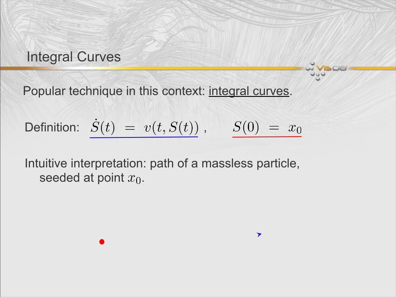
Popular technique in this context: integral curves.
Definition: ,
Intuitive interpretation: path of a massless particle, seeded at point .
Integral Curves
Popular technique in this context: integral curves.
Definition: ,
Intuitive interpretation: path of a massless particle, seeded at point .

Integral Surfaces
• Natural generalization: integral surfaces
Interpretation: surface spanned by a family of integral curves

Integral Surfaces
• Natural generalization: integral surfaces
Interpretation: surface spanned by a family of integral curves

Integral Surfaces
• Natural generalization: integral surfaces
Interpretation: surface spanned by a family of integral curves

Integral Surfaces
• Natural generalization: integral surfaces
Interpretation: surface spanned by a family of integral curves
t →
s →

Integral Surfaces
Example
seeding curve

Overview
• Introduction: Integral Surfaces
‣ Approximation Algorithm
• Experiments
• Visualization using Integral Surfaces

Algorithm Outline
Integral surface approximation is performed in two phases:
• Phase 1: Time line approximation
• Phase 2: Surface Triangulation

Algorithm Outline
Integral surface approximation is performed in two phases:
• Phase 1: Time line approximation
• Phase 2: Surface Triangulation

Integral Surfaces are also a continuum of time lines.
Approximation Algorithm: • Approximate surface by a finite set of time lines (skeleton)• Discretize time lines using a finite set of integral curves• Approximate time line ti+1 from time line ti
Phase 1: Time Line Approximation
t0t1
t2 t3t4

Phase 1: Time Line Approximation
• Step 1: Compute initial approximation, points on t1 are advected from t0
t0
t1

Phase 1: Time Line Approximation
• Step 1: Compute initial approximation, points on t1 are advected from t0
t0
t1

Phase 1: Time Line Approximation
• Step 2: Apply refinement predicate on adjacent point triplesto determine where better resolution is needed
t0
t1

Phase 1: Time Line Approximation
• Step 2: Apply refinement predicate on adjacent point triplesto determine where better resolution is needed
t0
t1

Phase 1: Time Line Approximation
• Step 2: Apply refinement predicate on adjacent point triplesto determine where better resolution is needed
t0
t1

Phase 1: Time Line Approximation
• Step 2: Apply refinement predicate on adjacent point triplesto determine where better resolution is needed
t0
t1

Phase 1: Time Line Approximation
• Step 3: Insert new points next to the insufficient points
t0
t1

Phase 1: Time Line Approximation
• Step 3: Insert new points next to the insufficient points
t0
t1

Phase 1: Time Line Approximation
• Repeat at Steps 2 and 3 until no further refinement is needed
t0
t1

Phase 1: Time Line Approximation
• Approximate sequence of timelines going from ti to ti+1
t0
t1
t2

Phase 1: Time Line Approximation
• Approximate sequence of timelines going from ti to ti+1
t0
t1
t2t3

Phase 1: Time Line Approximation
• Approximate sequence of timelines going from ti to ti+1
t0
t1
t2t3
t4

Phase 1: Time Line Approximation
• Result: Surface skeleton of integral curves + time lines
t0
t1
t2t3
t4

Refinement Predicates
Predicates: Thresholds on local curve properties such as derivative and curvature.
Discrete versions easily obtained over adjacent point triples.

Refinement Predicates
Predicates: Thresholds on local curve properties such as derivative and curvature.
Discrete versions easily obtained over adjacent point triples.
point distance
!

Refinement Predicates
Predicates: Thresholds on local curve properties such as derivative and curvature.
Discrete versions easily obtained over adjacent point triples.
point distance
!
"
inter-point angle

Refinement Predicates
Predicates: Thresholds on local curve properties such as derivative and curvature.
Discrete versions easily obtained over adjacent point triples.
point distance
!
triangle area
A
"
inter-point angle

Surface “Discontinuities”
• Integral curves can “get stuck” at critical points or boundaries(or just error out due to numerical difficulties)
• We use a discontinuity predicate to avoid over-refinementin such settings: first / second derivative over point triple
• If predicate triggers, split the timeline (removing the indicated point)
• Problem turns into two subproblems, treated with same methods as before
dx/dsd2x/ds2

Algorithm Outline
Integral surface approximation is performed in two phases:
• Phase 1: Time line approximation
• Phase 2: Surface Triangulation

• Discretize integral curves to obtain a point set on the surface
Phase 2: Surface Triangulation
t0
t1
t2t3
t4

• Discretize integral curves to obtain a point set on the surface
• Time lines are no longer needed and can be forgotten.
Phase 2: Surface Triangulation
t0
t1
t2t3
t4
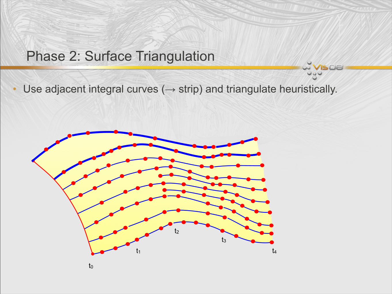
Phase 2: Surface Triangulation
• Use adjacent integral curves (→ strip) and triangulate heuristically.
t0
t1
t2t3
t4

Phase 2: Surface Triangulation
• Use adjacent integral curves (→ strip) and triangulate heuristically.• Shortest diagonal advancing front works well
t0
t1
t2t3
t4

Phase 2: Surface Triangulation
• Use adjacent integral curves (→ strip) and triangulate heuristically.• Shortest diagonal advancing front works well
t0
t1
t2t3
t4

Phase 2: Surface Triangulation
• Use adjacent integral curves (→ strip) and triangulate heuristically.• Shortest diagonal advancing front works well
t0
t1
t2t3
t4

Phase 2: Surface Triangulation
• Use adjacent integral curves (→ strip) and triangulate heuristically.• Shortest diagonal advancing front works well
t0
t1
t2t3
t4

Phase 2: Surface Triangulation
• Use adjacent integral curves (→ strip) and triangulate heuristically.• Shortest diagonal advancing front works well
t0
t1
t2t3
t4

Phase 2: Surface Triangulation
• Use adjacent integral curves (→ strip) and triangulate heuristically.• Shortest diagonal advancing front works well
t0
t1
t2t3
t4

Phase 2: Surface Triangulation
• Use adjacent integral curves (→ strip) and triangulate heuristically.• Insertions are handled by choosing the triangulation with largest sum of angles
t0
t1
t2t3
t4

Phase 2: Surface Triangulation
• Use adjacent integral curves (→ strip) and triangulate heuristically.• After an insertion point, strips are triangulated recursively
t0
t1
t2t3
t4

Phase 2: Surface Triangulation
• Use adjacent integral curves (→ strip) and triangulate heuristically.• After an insertion point, strips are triangulated recursively
t0
t1
t2t3
t4

A Note on Integral Curves
Integral Curves are advanced from ti to ti+1 using numerical integration.
Traditional adaptive integration schemes (Runge-Kutta, Runge-Kutta-Fehlberg) offer good efficiency, but deliver a polyline representation of integral curves.

A Note on Integral Curves
Integral Curves are advanced from ti to ti+1 using numerical integration.
We use a Dormand-Prince scheme (DOPRI5) that represents the integral curve in piecewise polynomial form.
This allows us to adaptively discretize the integral curves after integration by re-using the previous predicates for max. efficiency.

Overview
• Introduction: Integral Surfaces
• Approximation Algorithm
‣ Experiments
• Visualization using Integral Surfaces

Experiments
• Delta wing dataset (18e6 cells, 1000 timesteps)

Experiments
• Delta wing dataset (18e6 cells, 1000 timesteps)

Experiments
• Delta wing dataset (18e6 cells, 1000 timesteps)

Which refinement criterion?Numerical experiment
• Comprison of adaptive vs. non-adaptive high-res time lines• Distance and area critera work well, curvature does not give good results at all• Time lines are approximated correctly in the limit
1e-06
1e-05
0.0001
0.001
0.01
0.1
1e-08 1e-07 1e-06 1e-05 0.0001 0.001 0.01 0.1 1
avg.
err
or
threshold magnitude
area refinementdist. refinement
1e-05
0.0001
0.001
0.01
0.1
1e-08 1e-07 1e-06 1e-05 0.0001 0.001 0.01 0.1 1
max
. err
or
threshold magnitude
area refinementdist. refinement

Overview
• Introduction: Integral Surfaces
• Approximation Algorithm
• Experiments
‣ Visualization using Integral Surfaces

Visualization
• Integral surfaces have natural 2d-parameterization (s,t)
• Lend themselves well to texture mapping• earlier work on this by Löffelmann et al., 1997• animated textures to convey temporal flow behavior
t →
s →

Visualization
• Example: Car (stationary, 15e6 cells)

Visualization
• Example: Car (stationary, 15e6 cells)

Visualization
• Example: Car (stationary, 15e6 cells)

Visualization

Visualization
Visualization

Visualization

Visualization
• In the time-dependent case, self-intersections are possible• Explicit depiction can be helpful

Visualization

Contributions
• Novel 2-phase integral surface computation algorithm
• adaptive time-line approximation, with pluggable criteria• straightforward triangulation scheme: crack-free, high quality surfaces• efficiently applicable to time-dependent data (streaming)• near-interactive computation times facilitate dataset exploration• parallelization is feasible
• Enhanced visualization through
• highly illustrative, high-quality rendering• texture mapping• animated textures• explicit depiction of self-intersections

Differences to Previous Work
Hulquist 1992:• combined integration-triangulation (recursive-iterative) algorithm• tight coupling introduces mutual dependencies, complex algorithm• time-dependent data is not feasible
Garth et al. 2004:• based on Hultquist, uses arc-length parameterization• visualization enhancements• time-dependent data still not feasible
Our scheme• clean separation of integration / triangulation allows precise refinement
control, parallelization, time-dependent data, ...

Acknowledgements
• colleagues at IDAV, UC Davis, Univ. of Kaiserslautern
• Markus Rütten, DLR Göttingen
• DOE, contract DE-FC02-06ER-25780Scientific Discovery through Advanced Computing (SciDAC)Visualization and Analytics Center for Enabling Technologies (VACET)
• DFG IRTG 1131Visualization of Large and Unstructured Data Sets

Thank you
Questions?

Why can time lines degenerate?