Accurate and Efficient Boundary Integral Methods for Electrified Liquid Bridge Problems

SIAM J. SCI. COMPUT. c© 2005 Society for Industrial and Applied MathematicsVol. 26, No. 6, pp. 2102–2132

ACCURATE AND EFFICIENT BOUNDARY INTEGRAL METHODSFOR ELECTRIFIED LIQUID BRIDGE PROBLEMS∗

DARKO VOLKOV† , DEMETRIOS T. PAPAGEORGIOU† , AND PETER G. PETROPOULOS†

Abstract. We derive and implement boundary integral methods for axisymmetric liquid bridgeproblems in the presence of an axial electric field. The liquid bridge is bounded by solid parallelelectrodes placed perpendicular to the axis of symmetry and held at a constant potential difference.The fluid is assumed to be nonconducting and has permittivity different from that of the passivesurrounding medium. The problem reduces to the solution of two harmonic problems for the fluid andvoltage potential inside the bridge and another harmonic problem for the voltage potential outsidethe bridge. The shape of the moving interface is determined by the imposition of stress, as well askinematic and electric field boundary conditions, the former condition accounting for discontinuouselectric stresses across the interface. We propose fast and highly accurate boundary integral methodsbased on fast summations of appropriate series representations of axisymmetric Green’s functions inbounded geometries. We implement our method to calculate equilibrium shapes for electrified liquidbridges in the absence and presence of gravity. Such calculations appear in the literature using finiteelement methods, and our boundary integral approach is a fast and accurate alternative.

Key words. boundary integral method, Ewald’s method, electrified liquid bridge, capillaryinstability

AMS subject classifications. 35J65, 74S15, 76B45, 76W05

DOI. 10.1137/040604352

1. Introduction. Flows containing moving interfaces where surface tension ispresent are of fundamental importance in different applications such as mixing andemulsification, printing and spraying, imaging, heat and mass transfer, and propul-sion systems, to name a few. An important class of applications can be describedby axisymmetric flows as in liquid jets or bridges, for instance. In cylindrical ge-ometries, surface tension induces a long wave instability (this statement is a linearstability result—all wavy interfacial perturbations longer than the undisturbed jetcircumference are unstable—see Plateau (1873) and Rayleigh (1878, 1892)) that leadsto nonlinear dynamics, necking, and a topological transition. Mathematically, thisevent is a finite-time singularity of the three-dimensional axisymmetric Navier–Stokesequations in the presence of a free surface, and solution characteristics are mathe-matically and physically useful (see the reviews of Eggers (1997) and Papageorgiou(1995a, 1995b, 1996)). In fact, experiments agree with the theoretical solutions ofhighly viscous jets (see Papageorgiou (1995a)) extremely well and for times not tooclose to the singularity (see McKinley and Tripathi (2000)). Recent experiments havebeen performed to probe the fine details of the topological transition; see Rothert,Richter, and Rehberg (2001, 2003).

Full-scale simulations based on the Euler, Stokes, or Navier–Stokes equationsare necessary in the general case. There is a vast literature on this subject, and of

∗Received by the editors February 23, 2004; accepted for publication (in revised form) November 5,2004; published electronically July 26, 2005.

http://www.siam.org/journals/sisc/26-6/60435.html†Department of Mathematical Sciences and Center for Applied Mathematics and Statistics,

New Jersey Institute of Technology, University Heights, Newark, NJ 07102 ([email protected],[email protected], [email protected]). The work of the first author was supported by NationalScience Foundation grant DMS-0072228. The work of the third author was supported in part by AirForce Office of Scientific Research grant F49620-02-1-0031.

2102

ELECTRIFIED LIQUID BRIDGES 2103

particular interest to the present study are boundary integral methods. The reader isreferred to recent reviews on inviscid and Hele–Shaw flows by Hou, Lowengrub, andShelley (2001) and on Stokes flows by Pozrikidis (2001), as well as numerous referencestherein. The boundary integral methods developed herein are a first step in tacklingsingularity formation in liquid jets with either periodic boundary conditions or liquidbridges between parallel plates. In order to control the accuracy of the calculations,we choose to solve integral equations formulated over the fluid interface alone, and thisrequires the efficient calculation of series representations of the periodic or Dirichlet(Neumann) Green’s function. An alternative formulation is to distribute singularitieson the bounding plates also, the advantage being that the free-space Green’s functioncan be used; see, for example, Gaudet, McKinley, and Stone (1996) for a Stokes flowstudy of an extending liquid bridge.

There have been several theoretical and experimental studies in the area of liquidbridges and the control of their stability by imposition of an axial electric field. Inthe theoretical arena, Gonzalez et al. (1989) considered the linear stability of elec-trified dielectric liquid bridges in the absence of gravity and demonstrated that anaxial electric field can stabilize (at least in the linear regime) a bridge which wouldotherwise be unstable. They also performed experiments to confirm their findings.Residual gravity was introduced by Gonzalez and Castellanos (1993), and a similarstability analysis was carried out to determine local bifurcation diagrams near thezero gravity states. Of particular interest to the present study is that of Ramos andCastellanos (1993), who use finite element methods coupled with a Newton iterationto solve the static nonlinear problem of an electrified dielectric liquid bridge. Ourboundary integral method does not require discretization of the flow field which ex-tends radially to infinity. In a more recent linear stability study, Pelekasis, Economou,and Tsamopoulos (2001) calculate numerically stability curves from the generalizedeigenvalue problem resulting from the finite element projection of the linear equa-tions of dielectric and leaky dielectric viscous bridges, and they demonstrate clearlythe stabilization effected by the electric field.

Experiments on the dynamics of electrified liquid bridges have been carried outby Burcham and Saville (2000) in a zero gravity environment, Gonzalez et al. (1989),and Ramos, Gonzalez, and Castellanos (1994). The latter two studies were performedin a terrestrial environment with gravity effects present. The electric field was foundto stabilize the liquid bridge in the sense that equilibrium shapes could be achievedfor longer bridges beyond the Plateau limit. Gravity breaks the midplane symmetryand produces amphora-like shapes which are thinner in the vicinity of the upper plate.Our numerical results are in full agreement with all the experimental findings.

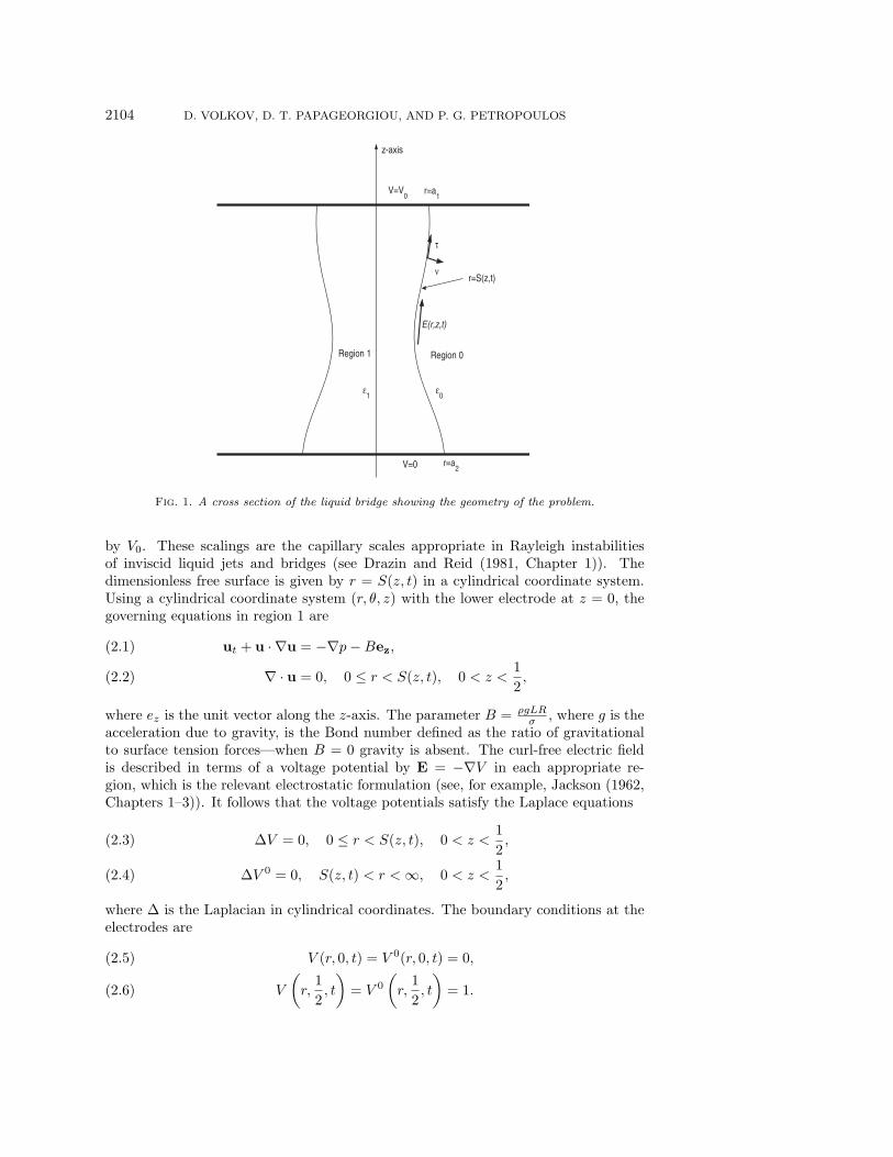
2. The governing equations. Consider an axisymmetric liquid bridge of di-mensional length L/2 held between two infinite parallel electrodes. The lower elec-trode is maintained at zero potential and the upper one at constant potential V0.In its undisturbed perfectly cylindrical state the bridge has a uniform circular crosssection of radius R. The fluid is taken to be inviscid and incompressible of density ρ.Gravity is included, and surface tension acts and has constant coefficient σ. The fluidregion (region 1) is nonconducting and has constant permittivity ε1, while the sur-rounding region (region 0) is dynamically passive, has constant permittivity ε0, andis nonconducting (e.g., air, as in the experiments; see the introduction). The problemgeometry is sketched in Figure 1.

The problem is made dimensionless by scaling lengths with L, the pressure p

by σR , fluid velocities u by ( σ

ρR )1/2, time t with (ρRL2

σ )1/2, and voltage potential V

2104 D. VOLKOV, D. T. PAPAGEORGIOU, AND P. G. PETROPOULOS

Region 0

ε0

Region 1

ε1

V=0

V=V0

r=S(z,t)

z-axis

r=a1

r=a2

τ

ν

E(r,z,t)

Fig. 1. A cross section of the liquid bridge showing the geometry of the problem.

by V0. These scalings are the capillary scales appropriate in Rayleigh instabilitiesof inviscid liquid jets and bridges (see Drazin and Reid (1981, Chapter 1)). Thedimensionless free surface is given by r = S(z, t) in a cylindrical coordinate system.Using a cylindrical coordinate system (r, θ, z) with the lower electrode at z = 0, thegoverning equations in region 1 are

ut + u · ∇u = −∇p−Bez,(2.1)

∇ · u = 0, 0 ≤ r < S(z, t), 0 < z <1

2,(2.2)

where ez is the unit vector along the z-axis. The parameter B = ρgLRσ , where g is the

acceleration due to gravity, is the Bond number defined as the ratio of gravitationalto surface tension forces—when B = 0 gravity is absent. The curl-free electric fieldis described in terms of a voltage potential by E = −∇V in each appropriate re-gion, which is the relevant electrostatic formulation (see, for example, Jackson (1962,Chapters 1–3)). It follows that the voltage potentials satisfy the Laplace equations

ΔV = 0, 0 ≤ r < S(z, t), 0 < z <1

2,(2.3)

ΔV 0 = 0, S(z, t) < r < ∞, 0 < z <1

2,(2.4)

where Δ is the Laplacian in cylindrical coordinates. The boundary conditions at theelectrodes are

V (r, 0, t) = V 0(r, 0, t) = 0,(2.5)

V

(r,

1

2, t

)= V 0

(r,

1

2, t

)= 1.(2.6)


In addition, the electric field far from the liquid bridge is uniform, that is,

limr→∞

V 0 = 2z.(2.7)

The flow is irrotational, and hence we can write u = ∇Φ, with Φ(r, z, t) to bedetermined. The continuity equation (2.2) implies that Φ is a harmonic function,

ΔΦ = 0, 0 ≤ r < S(z, t), 0 < z <1

2,(2.8)

with no penetration boundary conditions at the plates

Φz(r, 0, t) = 0, 0 ≤ r ≤ a1,(2.9)

Φz

(r,

1

2, t

)= 0, 0 ≤ r ≤ a2,(2.10)

where a1 and a2 are the dimensionless radial locations of the fixed contact rings theliquid bridge makes with the lower and upper electrodes, respectively, and are takento be different. If Φ is known, the momentum equations (2.1) determine the pressureat any point in the fluid.

On the moving interface r = S(z, t) the electric potential satisfies a continuitycondition,

[V ]01 = 0,(2.11)

and a no flux condition (i.e., continuity of the normal component of the displacementfield εE), which in dimensionless form is given by[ε

ε 0∇V · ν

]0

1= 0,(2.12)

where variables inside and outside the free surface take subscripts or superscripts1 and 0, respectively, and ν is the exterior unit normal vector to S. For the fluiddynamics we write the boundary conditions at the interface in terms of the stresstensor Tij whose dimensional form is

Tij = −pδi,j + ε

(EiEj −

1

2|E|2δi,j

),(2.13)

where Ei is the ith component of the electric field E in an orthonormal basis. In thepresence of surface tension the dimensional normal stress balance reads

[ν · T · ν]01 = σ

(1

R1+

1

R2

),(2.14)

where the notation [·]01 signifies that we subtract values of the quantity in squarebrackets in region 1 from corresponding values in region 0, e.g., V 0 − V ; the quantity( 1R1

+ 1R2

) is the sum of the principal radii of curvature on S. The Bernoulli boundarycondition on r = S(z, t) is derived by integration of Euler’s equations (2.1) and elim-ination of the pressure jump across the interface given by the normal stress condition(2.13). Performing the calculation and making the equation dimensionless using thescalings introduced earlier yields

DΦ

Dt− 1

2|∇Φ|2 +

(1

R1+

1

R2

)+ Eb

[1

2

ε

ε0(E2

τ − E2ν)

]0

1

+ Bz = 0,(2.15)


where DDt = ∂

∂t + ∇Φ · ∇ is the material derivative, τ is the unit tangent vectorto S, and Eτ , Eν are the tangential and normal components of the electric field. The

parameter Eb =ε0V

20 R

σL is an electric Weber number measuring the ratio of electrical tocapillary stresses (see Tilley, Petropoulos, and Papageorgiou (2001) and Papageorgiouand Vanden-Broeck (2004)). Finally, we have the kinematic condition,

D

Dt(r − S) = 0.(2.16)

In the remainder of the paper we denote the ratio of permittivities by

εp =ε1

ε0.(2.17)

In this paper we consider the construction of equilibrium shapes (if they exist)for different physical parameters in order to assess the ability of the electric fieldto stabilize capillary instability and prevent collapse. We do not consider the relateddynamic problem where the fluid potential Φ must also be calculated. At equilibrium,the pressure p1 can be written as p1 = −ρgz + const., where the first term is thehydrostatic part. The normal stress condition (2.14) provides an expression for thejump p1−p0 at the interface (see Landau and Lifshitz (1987, Chapter 6)). Eliminatingthis jump using the above decomposition for p1 and nondimensionalizing yields thefollowing electrically modified Young–Laplace equation,(

1

R1+

1

R2

)+ Eb

[1

2

ε

ε0(E2

τ − E2ν)

]0

1

+ Bz − α = 0,(2.18)

where the constant pressure jump term α must be found as part of the solution inorder to satisfy mass conservation.

For future reference we recall the expression of the sum of the principal radii ofcurvature for axisymmetric surfaces,(

1

R1+

1

R2

)=

1

S(1 + S′2)12

− S′′

(1 + S′2)32

,(2.19)

where primes denote z-derivatives. The solution of this problem constitutes a non-linear problem which must be addressed numerically. We emphasize that equilibriumstates may not exist for arbitrary fixed values of bridge radii a1 and a2 at the elec-trodes; see boundary condition (2.10); in the case of a perfectly cylindrical bridge,S(z, t) = a1 = a2, it is well known that if a1 < 1

2π and no electric field acts, the bridgeis unstable and undergoes a topological transition to ultimately form two drops, oneattached to the lower electrode and the other to the upper electrode.

3. The electric field problem. In order to determine the equilibrium positionsor the dynamic evolution of the liquid bridge, we need to be able to compute veryaccurately and efficiently the electric potential V for a given shape S. The quantitiesof interest in our problem are the tangential and the normal derivatives of V on S.

3.1. Formulation of the integral equation for ∂V∂ν

|1. Let G(x, y, z, x0, y0, z0)

be the Green’s function defined in the region 0 ≤ z ≤ 12 , 0 ≤ z0 ≤ 1

2 satisfying

Δx,y,zG = −δx0,y0,z0 ,

G(x, y, 0, x0, y0, z0) = 0,


G

(x, y,

1

2, x0, y0, z0

)= 0,

limr→∞

(G− 1

2πlog

1

r

)= 0.

Using this Dirichlet Green’s function and (2.3) and applying Green’s theorem, weobtain, for points (x0, y0, z0) in region 1,

(V − 2z0) = −∫S

∂G

∂νx,y,z(V − 2z)ds(x, y, z) +

∫S

G∂(V − 2z)

∂νx,y,z|1ds(x, y, z).(3.1)

For points in region 0, using the asymptotic behavior of G at infinity given above andthe fact that (V − 2z) approaches 0 at infinity, we obtain

(V − 2z0) =

∫S

∂G

∂νx,y,z(V − 2z)ds(x, y, z) −

∫S

G∂(V − 2z)

∂νx,y,z|0ds(x, y, z).(3.2)

Next, we take the limit of the normal derivative of (3.1) and add it to the limit as(x0, y0, z0) approaches S of the normal derivative of (3.2); using standard propertiesof single and double layer potentials, we obtain the integral equation for ∂V

∂ν |1

1

2(1 + εp)

∂V

∂ν|1 − (1 − εp)

∫S

∂G

∂νx0,y0,z0

∂V

∂ν|1(x, y, z)ds(x, y, z) = 2ν · ez.(3.3)

After solving (3.3), we can find the potential V using the following formula, which isobtained by taking the limit of (3.1) as (x0, y0, z0) approaches S and adding it to thecorresponding limit of (3.2):

V = 2z0 + (1 − εp)

∫S

G∂V

∂ν|1(x, y, z)ds(x, y, z).(3.4)

The domain of integration for (3.3) can be greatly simplified by taking advantageof axisymmetry. We can integrate separately in the variable θ, the polar angle incylindrical coordinates, since ∂V

∂ν |1(x, y, z) is independent of θ; this yields

1

2(1 + εp)

∂V

∂ν|1 − (1 − εp)

∫S

(∫ 2π

0

∂G

∂νx0,y0,z0

dθ

)∂V

∂ν|1(r, z)ds(r, z) = 2ν · ez.(3.5)

The above equation is an integral equation along the curve defined by the cross sectionof S by any plane containing the z-axis. In order to simplify notation, we also denoteby S that curve in the r, z coordinates. The integral equation (3.5) now involves anew Green’s function

H(r, z, r0, z0) =

∫ 2π

0

Gdθ(3.6)

or, more precisely, the normal derivative of H. Integral equation (3.5) thus becomes

1

2(1 + εp)

∂V

∂ν|1 − (1 − εp)

∫S

∂H

∂νr0,z0

∂V

∂ν|1(r, z)ds(r, z) = 2ν · ez.(3.7)

We describe next the procedure to obtain G used in (3.6).


3.2. Ewald’s method for evaluating the Green’s function G. Ewald’smethod refers to the technique for rapidly convergent summations of series repre-sentations of Green’s functions, first uncovered by Ewald in his original paper (seeEwald (1921)). It has been applied in different areas of mathematical physics, as,for example, in the dynamic theory of crystal lattices (see Born and Huang (1954)).Linton (1998, 1999) has shown how Ewald’s method can be successfully applied inelectromagnetic applications.

In our case, the Green’s function G will be obtained from the periodic Green’sfunction P (x, y, z, x0, y0, z0) that satisfies

Δx,y,zP =

n=∞∑n=−∞

−δx0,y0,z0+n,

P (x, y, z + 1, x0, y0, z0) = P (x, y, z, x0, y0, z0),

limr→∞

(P − 1

2πlog

1

r

)= 0.

The most straightforward way of expressing the Green’s function P is throughthe formal series

P (x, y, z, x0, y0, z0) =

n=∞∑n=−∞

G0(x− x0, y − y0, z − z0 − n),(3.8)

where G0 is the free-space Green’s function defined by

G0(x, y, z, x0, y0, z0) =1

4π|(x− x0, y − y0, z − z0)|.(3.9)

A natural idea for studying the integral equation (3.5) is to decompose H as H =H0 + (H −H0). The singular part of H is the integrated free-space Green’s functionand has been well documented. The (H − H0) part is smooth. This decompositionenables us to maintain accuracy in a consistent manner. Starting from the free-spaceGreen’s function it is well known that integration in the angle θ yields

H0(r, z, r0, z0) =1

π

1√(r + r0)2 + (z − z0)2

K(m),(3.10)

where m = 4rr0(r+r0)2+(z−z0)2

, and K is the complete elliptic integral function defined

by

K(m) =

∫ π2

0

dθ

(1 −m sin2 θ)12

.(3.11)

From standard properties of elliptic functions (see Abramowitz and Stegun (1992), forexample) we know that K(m) ∼ −1

2 log(1−m) as m approaches 1. We now describeour approach for the evaluation of the complete elliptic function K appearing in theevaluation of H0. It is well known that the elliptic function K(m) can be written as

K(m) = K1(m) + log(1 −m)K2(m),

for 0 ≤ m < 1, where K1 and K2 are two smooth functions which can be efficientlyapproximated by polynomials for 0 ≤ m < 1. More precisely, we will use the approx-imation

K(m) � PK1(m) + log(1 −m)PK2(m),


where PK1 and PK2 are two polynomials. Abramowitz and Stegun (1992) providetwo polynomials of degree 4 for PK1 and PK2, respectively, yielding a single pre-cision approximation (8-digit accuracy). We were able to obtain a double precisionapproximation (16-digit accuracy) by solving a minimization problem in quadrupleprecision (32-digit accuracy). However, we had to set the degree of PK1 and PK2to be 8.

The derivative of K can be expressed in terms of the complete elliptic integralfunction E:

K ′(m) =1

2m

(E(m)

1 −m−K(m)

),

where E(m) =

∫ π2

0

(1 −m sin2 θ)12 dθ.

The singularity in E(m) can be factored out as follows:

E(m) = E1(m) + log(1 −m)E2(m),

where E1 and E2 are smooth. E(m) is in turn approximated by polynomials:

E(m) � PE1(m) + log(1 −m)PE2(m).

Here, too, we obtained a double precision approximation by solving a minimizationproblem in quadruple precision. We had to set the degree of PE1 and PE2 to be 8.

3.2.1. Evaluation of the periodic Green’s function. The formal sum (3.8)is not convergent and as such cannot be used in the construction of G. If insteadwe sum the x-, y-, or z-derivative of each term, we obtain a sum that converges veryslowly. The series appearing in the following calculation are formal, although takingone derivative in any of the variables will make them locally uniformly convergent.To ease notation, P will temporarily designate P (x, y, z, 0, 0, 0).

The basis of Ewald’s method is to rewrite expression (3.8) in terms of the followingintegral representation:

P =1

4π

n=∞∑n=−∞

2√π

∫ ∞

0

e−((z−n)2+x2+y2)ρ2

dρ

=1

4π

{n=∞∑n=−∞

2√π

∫ 1

0

e−((z−n)2+x2+y2)ρ2

dρ +

n=∞∑n=−∞

2√π

∫ ∞

1

e−((z−n)2+x2+y2)ρ2

dρ

}.

The last series in the above expression is rapidly convergent. Indeed, for 0 ≤ z ≤ 1and |n| ≥ 2,

2√π

∫ ∞

1

e−((z−n)2+x2+y2)ρ2

dρ ≤ Ce−(1−|n|)2 ,

for some constant C, independent of x, y, z, and n. Note that it is crucial that thelower bound be different from 0 in the above integral for the estimate to hold. A similarestimate for the same integrand does not hold when integrating on the interval [0, 1].

Thus we apply a transformation to the series∑n=∞

n=−∞2√π

∫ 1

0e−((z−n)2+x2+y2)ρ2

dρ.

Denoting

h(x, y, z) =n=∞∑n=−∞

e−((z−n)2+x2+y2)ρ2

(3.12)


and noting that h is a periodic function in z of period 1, we can calculate its Fouriercoefficient h(l),

h(l) =

∫ 1

0

n=∞∑n=−∞

e−((z−n)2+x2+y2)ρ2−2iπlzdz

=

∫ ∞

−∞e−(z2+x2+y2)ρ2−2iπlzdz

= e− l2π2

ρ2 −(x2+y2)ρ2√π

ρ.

Hence

h(x, y, z) =n=∞∑n=−∞

e−n2π2

ρ2 −(x2+y2)ρ2+2iπnz√π

ρ.(3.13)

Finally, substituting (3.13) into (3.12) we find that

P =1

4π

{n=∞∑n=−∞

2√π

∫ 1

0

e−n2π2


ρdρ

+

n=∞∑n=−∞

2√π

∫ ∞

1

e−((z−n)2+x2+y2)ρ2

dρ

}.(3.14)

Note that in this new expression for P , for n = 0, the term∫ 1

0

e−n2π2


ρdρ,

in the first series, is less than Ce−n2π2

, for some constant C, independent of x, y, z,and n. The first integral in the series expression (3.14) is not convergent for n = 0.However, that difficulty disappears when one derivative is taken with respect to anyof the variables; alternatively we can add an integrating term which is compatiblewith all the derivatives and with the behavior of P as r tends to infinity. We alsonotice that the first sum in (3.14) can be changed into a sum of cosines. Finally, weobtain the expression (reintroducing the sources at (x0, y0, z0))

P (x, y, z, x0, y0, z0) =1

2π

n=∞∑n=1

{∫ 1

0

2 cos(2πn(z − z0))e−n2π2

ρ2 −((x−x0)2+(y−y0)

2)ρ2 dρ

ρ

}

+1

2π

∫ 1

0

e−((x−x0)2+(y−y0)

2)ρ2 − 1

ρdρ

+1

2π

n=∞∑n=−∞

1√π

∫ ∞

1

e−(z−z0−n)2ρ2

e−((x−x0)2+(y−y0)

2)ρ2

dρ.(3.15)

Next, we briefly demonstrate the stated asymptotic behavior of (3.15) as r approachesinfinity. It is clear that the series terms in the first and the last terms of (3.15) alltend uniformly to zero as r approaches infinity. We then take the r-derivative of thesecond term to obtain

1

2π

∫ 1

0

−ρ(2r − 2r0 cos(θ − θ0))e−(r2+r2

0−2rr0 cos(θ−θ0))ρ2

dρ,(3.16)

which can be integrated exactly. From there we see that the principal part of (3.15)as r grows large is − 1

2πr , as expected.


3.2.2. The axisymmetric form of the periodic Green’s function. Theexpression (3.15) for the 1-periodic Green’s function can be specialized further to anexpression which is useful for the axisymmetric problems of interest here. This isachieved by integrating P in the angle θ between 0 and 2π, which yields the followingnovel expression for the axisymmetric Green’s function Q, say,

Q(r, z, r0, z0) =

n=∞∑n=1

{∫ 1

0


ρ2 −(r−r0)2ρ2

I0(2rr0ρ2)e−2rr0ρ

2 dρ

ρ

}

+

∫ 1

0

e−(r−r0)2ρ2


2 − 1

ρdρ

+n=∞∑n=−∞

{1√π

∫ ∞

1

e−(z−z0−n)2ρ2

e−(r−r0)2ρ2


2

dρ

}.(3.17)

This formula is new as far as we know. I0 denoted the modified Bessel function of thefirst kind. Note that I0(s)e

−s is a bounded function of s > 0 and is sometimes referredto as the rescaled modified Bessel function of the first kind. Derivatives of H can beobtained by differentiating each term in the series from expression (3.17). For fastercomputations, it is worth keeping in mind that Q satisfies the following identities:

Q(r, z, r0, z0) = Q(r, z − z0, r0, 0),

Q(r, z, r0, 0) = Q(r,−z, r0, 0),

Q(r, z, r0, z0) = Q(r0, z, r, z0).

Finally, we obtained the following formula for Q −H0 (H0 is the free-space Green’sfunction; see (3.10)), valid for points where (r, z) = (r0, z0), in the range 0 ≤ z ≤ 1

2 .Since

H0(r, z, r0, z0) =1

4π

∫ 2π

0

dθ√(z − z0)2 + r2 + r2

0 − 2rr0 cos θ

=1

4π

∫ 2π

0

∫ ∞

0

2√πe−((z−z0)

2+r2+r20−2rr0 cos θ)ρ2

dρ dθ

=1√π

∫ ∞

0

e−((z−z0)2+(r−r0)

2)ρ2


2

dρ,

we infer, upon subtraction, that

(Q−H0)(r, z, r, z) =

n=∞∑n=1

∫ 1

0

2e−n2π2

ρ2 I0(2r2ρ2)e−2r2ρ2 dρ

ρ

+

∫ 1

0

I0(2r2ρ2)e−2r2ρ2 − 1

ρdρ− 1√

π

∫ 1

0

I0(2r2ρ2)e−2r2ρ2

dρ

+

n=∞∑n=−∞, n �=0

1√π

∫ ∞

1

e−n2ρ2

I0(2r2ρ2)e−2r2ρ2

dρ.(3.18)

Formula (3.18) is particularly interesting since each of the functions Q and H0 issingular at points where (r, z) = (r0, z0), but the difference can be calculated explicitlyas given above.


3.2.3. Final calculation of the Green’s function G. The function Q is the1-periodic axisymmetric Green’s function which would be pertinent to axially periodicflows such as infinitely long liquid jets, for example. The liquid bridge problem,however, is of finite extent a Dirichlet axisymmetric Green’s function (we called this G)and is appropriate. It is simple to obtain G from Q by using periodicity, and thefollowing formula is obtained:

G(r, z, r0, z0) = Q(r, z − z0, r0, 0) −Q(r,−z − z0, r0, 0).(3.19)

Note that Q(r,−z − z0, r0, 0) is not singular if z = z0 and 0 ≤ z, z0 ≤ 12 are simul-

taneously satisfied. As indicated earlier, we chose to have the function H0 bear thesingularity. In effect, we used the following decomposition:

G(r, z, r0, z0) = H0(r, z, r0, z0) + (Q−H0)(r, z, r0, z0) −Q(r,−z − z0, r0, 0).(3.20)

4. Algorithm and numerical tests of the Green’s function calculation.In this section we undertake numerical tests for the evaluation of H0 and Q and theirderivatives. All other functions relevant to our problem can then be obtained in astraightforward way as explained above.

4.1. Evaluating the axisymmetric and periodic Green’s function Q. Inthis section we describe our algorithm for evaluating Q with a 10-digit accuracythroughout. (It is understood that more nodes should be used if higher accuracyis desired and fewer nodes if faster speed is desired, sacrificing some of the accuracy.)Analogous algorithms for evaluating ∂Q

∂r and ∂Q∂z were also constructed, but we omit

their detailed description since the steps are completely equivalent.We first estimate the general terms in the infinite series expression (3.17) for Q

by ∣∣∣∣∫ 1

0


ρ2 −(r−r0)2ρ2


2 dρ

ρ

∣∣∣∣ ≤ Ce−n2π2

,∣∣∣∣∫ ∞

1

e−(z−z0−n)2ρ2

e−(r−r0)2ρ2


2

dρ

∣∣∣∣ ≤ Ce−(|n|− 12 )2 ,

where C is a constant independent of r, z, r0, and z0, provided that 0 ≤ z, z0 ≤ 12 .

This explains why it is sufficient to truncate the first series in (3.17) at n = 2 andto run a summation for the second series between n = −5 and n = 5, since C isreasonably small and our accuracy goal of 10 digits is met; see the results below.

We now explain the numerical procedure for evaluating the integrals involved inthe series (3.17) while maintaining the set 10-digit accuracy. For the integrals∫ 1

0


ρ2 −(r−r0)2ρ2


2 dρ

ρ,

∫ 1

0

e−(r−r0)2ρ2


2 − 1

ρdρ,

we make a linear change of variables to transform the range of integration onto [−1, 1]and apply a 64-point Legendre quadrature. Nodes and weights can be computed bya service routine from NETLIB, for example.

The integrals involved in the last term in (3.17) require slightly more care. Sincethese integrals depend on z and z0 only through z − z0, we temporarily set z0 = 0 to


ease notation. Set L = (z − n)2 + (r − r0)2. Substitutions lead to the identity∫ ∞

1

e−(z−n)2ρ2

e−(r−r0)2ρ2


2

dρ

=e−L

2√L

∫ ∞

0

e−sI0

(2rr0

( s

L+ 1

))e−2rr0(

sL+1)(s + L)−

12 ds.(4.1)

The integral (4.1) is denoted by IL. If L ≥ 1, a Laguerre quadrature in s is appliedto the integral in (4.1). We picked a 64-point scheme, but only the first 24 nodesneeded to be considered. For small L, the values of the integrand become more andmore important for an accurate numerical value of IL. We first present an algorithmbased on splitting the interval of integration for IL. If .1 ≤ L < 1, the domain ofintegration for IL is split into two parts, the first part being [0, 1] and the second [1,∞).After a linear change of variables, we applied Legendre and Laguerre quadratures tothe two parts, respectively. For .01 ≤ L < .1, we split the domain of integrationfor IL into three parts, the first part being [0, 10L], the second [10L, 1], and the third[1,∞). Applying a linear change of variables, the two intervals [10L, 1] and [1,∞) aretransformed into [−1, 1] and [0,∞), respectively. Legendre and Laguerre quadraturesare then applied. The same idea is iterated to each case where 10−(p+1) ≤ L < 10−p,where p is a positive integer. As p grows, it is crucial to use more and more pointsnear 0 for maximum accuracy. Note that a small value for L can at most occur for asingle value of n in the series (3.17). In addition, we did not need to use values for Lsmaller than 10−4 for the problem considered here.

Alternatively, if z − z0 is smaller than, say, .25, we may use the decompositionQ = (Q−H0) + H0, where the formula for (Q−H0) is

(Q−H0)(r, z, r0, z0)

=

n=∞∑n=1

{∫ 1

0


ρ2 −(r−r0)2ρ2


2 dρ

ρ

}

+

∫ 1

0

e−(r−r0)2ρ2


2 − 1

ρdρ

− 1√π

∫ 1

0

e−((z−z0)2+(r−r0)

2)ρ2


2

dρ

+

n=∞∑n=−∞, n �=0

{1√π

∫ ∞

1

e−(z−z0−n)2ρ2

e−(r−r0)2ρ2


2

dρ

}.

That way, all the integrals IL can be evaluated in a single step by Laguerre quadrature.This is the approach that we choose to follow throughout the rest of the paper.

Derivatives of Q are obtained by differentiating analytically the formula for Q.Subsequently, numerical evaluations of derivatives of Q are performed analogously tonumerical evaluations of Q.

4.2. Algorithm verification.

4.2.1. Comparison with the obvious approach. In this section we evaluatethe accuracy of our summation method by considering a specific numerical example.We pick the following numerical values,

r = .24, z = .11, r0 = .25, z0 = 0,

and we seek to evaluate ∂Q∂z (r, z, r0, z0).


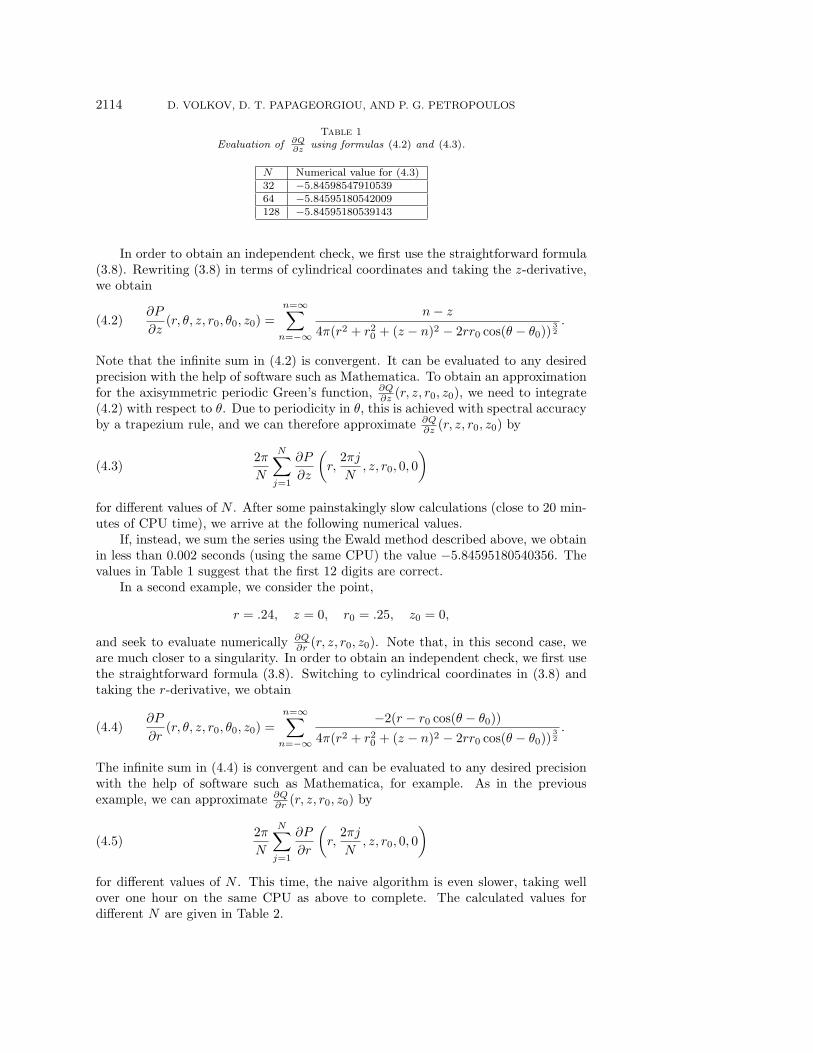
Table 1

Evaluation of ∂Q∂z

using formulas (4.2) and (4.3).

N Numerical value for (4.3)32 −5.8459854791053964 −5.84595180542009128 −5.84595180539143

In order to obtain an independent check, we first use the straightforward formula(3.8). Rewriting (3.8) in terms of cylindrical coordinates and taking the z-derivative,we obtain

∂P

∂z(r, θ, z, r0, θ0, z0) =

n=∞∑n=−∞

n− z

4π(r2 + r20 + (z − n)2 − 2rr0 cos(θ − θ0))

32

.(4.2)

Note that the infinite sum in (4.2) is convergent. It can be evaluated to any desiredprecision with the help of software such as Mathematica. To obtain an approximationfor the axisymmetric periodic Green’s function, ∂Q

∂z (r, z, r0, z0), we need to integrate(4.2) with respect to θ. Due to periodicity in θ, this is achieved with spectral accuracyby a trapezium rule, and we can therefore approximate ∂Q

∂z (r, z, r0, z0) by

2π

N

N∑j=1

∂P

∂z

(r,

2πj

N, z, r0, 0, 0

)(4.3)

for different values of N . After some painstakingly slow calculations (close to 20 min-utes of CPU time), we arrive at the following numerical values.

If, instead, we sum the series using the Ewald method described above, we obtainin less than 0.002 seconds (using the same CPU) the value −5.84595180540356. Thevalues in Table 1 suggest that the first 12 digits are correct.

In a second example, we consider the point,

r = .24, z = 0, r0 = .25, z0 = 0,

and seek to evaluate numerically ∂Q∂r (r, z, r0, z0). Note that, in this second case, we

are much closer to a singularity. In order to obtain an independent check, we first usethe straightforward formula (3.8). Switching to cylindrical coordinates in (3.8) andtaking the r-derivative, we obtain

∂P

∂r(r, θ, z, r0, θ0, z0) =

n=∞∑n=−∞

−2(r − r0 cos(θ − θ0))

4π(r2 + r20 + (z − n)2 − 2rr0 cos(θ − θ0))

32

.(4.4)

The infinite sum in (4.4) is convergent and can be evaluated to any desired precisionwith the help of software such as Mathematica, for example. As in the previousexample, we can approximate ∂Q

∂r (r, z, r0, z0) by

2π

N

N∑j=1

∂P

∂r

(r,

2πj

N, z, r0, 0, 0

)(4.5)

for different values of N . This time, the naive algorithm is even slower, taking wellover one hour on the same CPU as above to complete. The calculated values fordifferent N are given in Table 2.


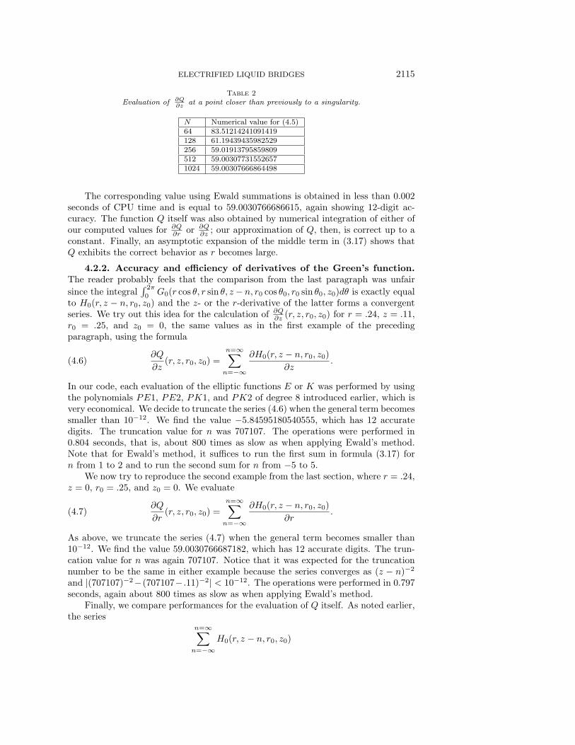
Table 2

Evaluation of ∂Q∂z

at a point closer than previously to a singularity.

N Numerical value for (4.5)64 83.51214241091419128 61.19439435982529256 59.01913795859809512 59.003077315526571024 59.00307666864498

The corresponding value using Ewald summations is obtained in less than 0.002seconds of CPU time and is equal to 59.0030766686615, again showing 12-digit ac-curacy. The function Q itself was also obtained by numerical integration of either ofour computed values for ∂Q

∂r or ∂Q∂z ; our approximation of Q, then, is correct up to a

constant. Finally, an asymptotic expansion of the middle term in (3.17) shows thatQ exhibits the correct behavior as r becomes large.

4.2.2. Accuracy and efficiency of derivatives of the Green’s function.The reader probably feels that the comparison from the last paragraph was unfair

since the integral∫ 2π

0G0(r cos θ, r sin θ, z− n, r0 cos θ0, r0 sin θ0, z0)dθ is exactly equal

to H0(r, z − n, r0, z0) and the z- or the r-derivative of the latter forms a convergentseries. We try out this idea for the calculation of ∂Q

∂z (r, z, r0, z0) for r = .24, z = .11,r0 = .25, and z0 = 0, the same values as in the first example of the precedingparagraph, using the formula

∂Q

∂z(r, z, r0, z0) =

n=∞∑n=−∞

∂H0(r, z − n, r0, z0)

∂z.(4.6)

In our code, each evaluation of the elliptic functions E or K was performed by usingthe polynomials PE1, PE2, PK1, and PK2 of degree 8 introduced earlier, which isvery economical. We decide to truncate the series (4.6) when the general term becomessmaller than 10−12. We find the value −5.84595180540555, which has 12 accuratedigits. The truncation value for n was 707107. The operations were performed in0.804 seconds, that is, about 800 times as slow as when applying Ewald’s method.Note that for Ewald’s method, it suffices to run the first sum in formula (3.17) forn from 1 to 2 and to run the second sum for n from −5 to 5.

We now try to reproduce the second example from the last section, where r = .24,z = 0, r0 = .25, and z0 = 0. We evaluate

∂Q

∂r(r, z, r0, z0) =

n=∞∑n=−∞

∂H0(r, z − n, r0, z0)

∂r.(4.7)

As above, we truncate the series (4.7) when the general term becomes smaller than10−12. We find the value 59.0030766687182, which has 12 accurate digits. The trun-cation value for n was again 707107. Notice that it was expected for the truncationnumber to be the same in either example because the series converges as (z − n)−2

and |(707107)−2−(707107− .11)−2| < 10−12. The operations were performed in 0.797seconds, again about 800 times as slow as when applying Ewald’s method.

Finally, we compare performances for the evaluation of Q itself. As noted earlier,the series

n=∞∑n=−∞

H0(r, z − n, r0, z0)


is not convergent. Instead, the series,

n=∞∑n=−∞

H0(r, z − n, r0, z0) −1 − δ0,n

2|n| ,(4.8)

is convergent and yields Q(r, z, r0, z0) to within an unknown constant, which is suffi-cient for our problem. To test this formula on a numerical example, we evaluate

Q(.24, .1, .25, 0) −Q(.3, .1, .25, 0),

using Ewald’s method and, for comparison, the series (4.8) truncated when thegeneral term becomes smaller than 10−10. In the case of Ewald’s method we ob-tain 0.215472859717063 in less than .001 seconds. Using the series (4.8) we obtain0.215472859719637 in 0.323 seconds for a truncation value of 223608. The two nu-merical values agree over the first 11 decimals.

Remark. Whereas algorithms for evaluating sums such as (4.6), (4.7), and (4.8)are straightforward to design, algorithms for the evaluation of the series (3.17) arenontrivial, since the terms are integrals to which quadrature rules are applied. Itis quite possible that a finer analysis for the evaluation of these integrals will yielda more efficient algorithm than ours, which suggests further advantages for Ewald’smethod regarding speed and accuracy.

5. Numerical solution of the integral equation for the normal compo-nent of the electric field. We recall that the function H − H0 is smooth for all0 < z, z0 < 1

2 and r, r0 > 0, and, as shown in the preceding section, we possess a fastand accurate technique to evaluate it, even at those points where (r, z) = (r0, z0).Consequently, we rewrite (3.7) as

1

2(1 + εp)

∂V

∂ν|1 − (1 − εp)

∫S

∂H0

∂νr0,z0

∂V

∂ν|1(r, z)ds(r, z)

− (1 − εp)

∫S

∂(H −H0)

∂νr0,z0

∂V

∂ν|1(r, z)ds(r, z) = 2ν · ez.(5.1)

We choose the following parametrization for S,

z = z(t), r = r(t), 0 ≤ t ≤ 1,

such that z(0) = 0, z(1) = 12 , and rewrite (5.1) using this, to obtain

1

2(1 + εp)

∂V

∂ν|1(r(t), z(t))

− (1 − εp)

∫ 1

0

∂H0

∂νr0,z0(r(v), z(v), r(t), z(t))

∂V

∂ν|1(r(v), z(v))r(v)

√r′(v)2 + z′(v)2dv

− (1 − εp)

∫ 1

0

∂(H −H0)

∂νr0,z0(r(v), z(v), r(t), z(t))

∂V

∂ν|1(r(v), z(v))r(v)

√r′(v)2 + z′(v)2dv

= 2ν(r(t), z(t)) · ez.(5.2)

According to the properties of the elliptic function K(m), the first integral in (5.2)can be expressed as ∫ 1

0

log |t− v|F1(t, v)dv +

∫ 1

0

F2(t, v)dv(5.3)


for some functions F1 and F2. More precisely, setting

m =4r(t)r(v)

[r(t) + r(v)]2 + [z(t) − z(v)]2,

we obtain

∂H0

∂νr0,z0(r(v), z(v), r(t), z(t)) =

1

2πr(t)((r(t) + r(v))2 + (z(t) − z(v))2)12 (r′(t)2 + z′(t)2)

12

×[(E(m) −K(m))z′(t) + 2r(t)K(m)

(r(t) − r(v))z′(t) − (z(t) − z(v))r′(t)

(r(t) − r(v))2 + (z(t) − z(v))2

]

Note that F1(t, v) and F2(t, v) can be evaluated with the aid of the polynomials PK1,PK2, PE1, and PE2, introduced in the preceding section. The second integral in(5.2) can be expressed as ∫ 1

0

F3(t, v)dv,(5.4)

and F3(t, v) is evaluated with the aid of the polynomials PK1, PK2, PE1, and PE2and the rapidly converging series for H and H−H0 introduced previously. We choosethe collocation points tj = j

n for 1 ≤ j ≤ n− 1. The following quadrature rules werefound for each of the two types of integrals appearing in (5.3) and (5.4):∫ 1

0

log |tj − v|F (tj , v)dv =

l=n−1∑l=1

q1(j, l, n)F (tj , tl) + O

(log n

n4

),(5.5)

∫ 1

0

F (tj , v)dv =

l=n−1∑l=1

q2(l, n)F (tj , tl) + O

(1

n4

).(5.6)

The coefficients q1(j, l, n) and q2(l, n) were obtained by substituting an appropriatepolynomial Pr,n(v) interpolating F (tj , v) for v over [ rn ,

r+1n ] followed by the following

approximations: ∫ 1

0

log |tj − v|F (tj , v)dv �n−2∑r=1

∫ r+1n

rn

log |tj − v|Pr,n(v)dv

+

∫ 1n

0

log |tj − v|P1,n(v)dv +

∫ 1

n−1n

log |tj − v|Pn−2,n(v)dv,(5.7)

∫ 1

0

F (tj , v)dv �n−2∑r=1

∫ r+1n

rn

Pr,n(v)dv +

∫ 1n

0

P1,n(v)dv +

∫ 1

n−1n

Pn−2,n(v)dv.(5.8)

We proceed to obtain a system of linear equations in the unknowns ∂V∂ν |1(r(tj), z(tj))

for 1 ≤ j ≤ n − 1. The following section is aimed at proving that this systemof linear equations is well posed and yields an approximation to the true value of∂V∂ν |1(r(tj), z(tj)) with the error O( logn

n4 ).

5.1. Convergence of the numerical scheme. It is possible to prove that ifthe integral equation (5.2) is numerically approximated as described above, then thenumerical scheme converges to the unique solution of the continuous problem. Wecarried out our proof using elementary potential theory and the general theory oflinear integral equations, referring to Kress (1999). The detailed proof appears in theappendix.


0 10 20 30 40 500

0.05

0.1

0.15

0.2

0.25

0.3

0.35

0.4

0.45

0.5

j

z

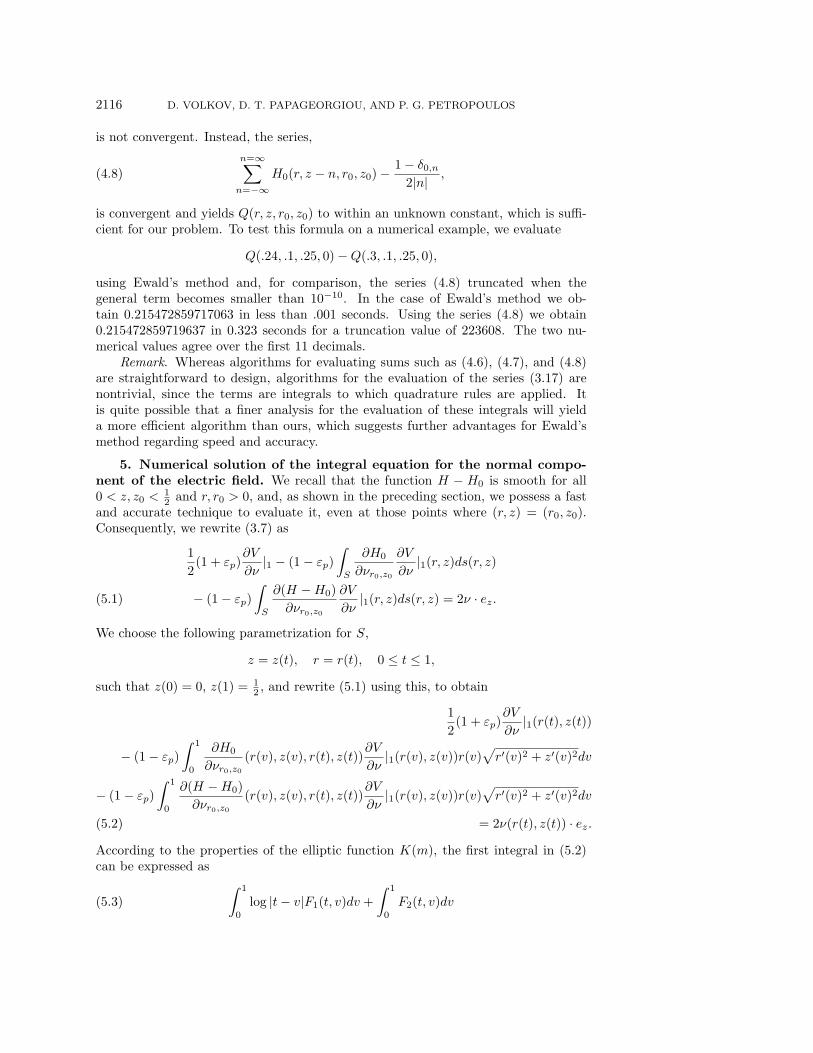
Fig. 2. The distribution of quadrature points on the z-axis for n = 50.

5.2. Parametrization of the interface S. In practice, the Green’s function His derived from the periodic Green’s function Q through the identity

H(r, z, r0, z0) = Q(r, z − z0, r0, 0) −Q(r, z − z0 − 1, r0, 0).(5.9)

If z0 is close to 0 or 12 , then as (r, z) approaches (r0, z0), the term Q(r, z−z0−1, r0, 0)

is close to being singular. An efficient numerical code must take into account thatpoints closer to the plates are problematic. A standard method is to cluster pointsnear the plates. To do so, we chose the following point distribution for the z variable.Set

g(s) =s

1.7 − e−s2.

Then pick

z

(j

n

)=

g( 2jn − 1) − g(−1)

2(g(1) − g(−1))

for 0 ≤ j ≤ n. In Figure 2 we plot z against j for n = 50.In order to solve the integral equation (5.2) and the associated Bernoulli equation

(see section 5), we need to possess accurate values for the components of the unittangent vector and the curvature at the quadrature knots. The shape of the interfaceis unknown and must be determined as part of the solution. In order to obtain accurateapproximations of important geometric quantities, approximate the surface S by anequation giving r as a polynomial function of z. The degree of the polynomial isfixed, and the coefficients of the polynomials are constrained. A least squares methodis applied to obtain the polynomial equation at each time or iteration step. Whenwe ran tests without the smoothing effects of the least squares method, errors in the


calculation of the curvature accumulated exponentially. The errors first appearednear the walls, because the marker points there are not allowed to move, whereastheir immediate neighbors are free to move. These errors then propagated to the restof the curve, giving it over time a ragged aspect and eventually leading to numericaloverflow. We anticipate that our constrained polynomial approach is a reasonableone since we expect to find very smooth shapes at equilibrium. In addition, oncea polynomial equation for the curve S is set, it is straightforward to calculate thecomponents of the unit tangent vector and curvature.

5.3. Calculation of the potential at the interface S. As mentioned earlier,the values of V on S are calculated from ∂V

∂ν |1 through the formula (3.4). In practice,we use again the decomposition H = H0 + (H −H0); that is, we write

V = 2z0 + (1 − εp)

∫S

H0∂V

∂ν|1(r, z)ds(r, z)

+ (1 − εp)

∫S

(H −H0)∂V

∂ν|1(r, z)ds(r, z).

We recall the expression for H0 given by (3.10) and again apply the quadrature rules(5.5) and (5.6) described above. Finally, we determine ∂V

∂τ from V through a fourth-order numerical differentiation scheme compatible with the accuracy of the quadra-tures q1 and q2 defined in (5.5) and (5.6). This yields the tangential derivative of Valong S, which is an important quantity in our numerical solutions.

5.4. Numerical tests on a model problem. Before proceeding to numericalsolutions of the electrified liquid bridge equilibria, we undertake the numerical so-lution of the integral equation (5.2) for a test problem with known exact solution.This provides us with a crucial test of the efficiency and accuracy of the algorithmsdeveloped here and provides a benchmark for more complex problems.

The function

f(r, z) = I0(2πpr) sin(2πpz)(5.10)

is harmonic and equal to 0 on the two plates z = 0 and z = 12 for any positive

integer p. We picked the following contour for S,

r = .2 − .025 sin

(1.8

(z − 1

2

)2π

)−(z − 1

2

),

for 0 ≤ z ≤ 12 .

We start from the data ∂f∂ν |S to solve the interior Neumann problem within S.

The exact solution to this problem is f |S . In order to use an integral equation verysimilar to (5.2), we want to solve for an unknown density μ such that

f =

∫S

Hμds(r, z).(5.11)

We take the interior limit of the normal derivative of the above identity to obtain theintegral equation for μ,

1

2μ +

∫S

∂H

∂νr0,z0μ(r, z)ds(r, z) =

∂f

∂ν.(5.12)


Table 3

Relative error in solving the model problem (5.11)–(5.12).

p n1 16 1.287729936141243E-003 1.714755977106271E-0031 60 7.762965695679299E-006 1.186067134489967E-0041 100 6.242540303816384E-006 5.431369796707948E-0052 16 6.310690919176223E-003 3.311169996169350E-0032 60 3.429196669294850E-005 2.448969102186786E-0042 100 2.683594220378686E-005 1.129425510500699E-0045 16 0.229937851009152 6.384322807134564E-0025 60 3.224724948116380E-004 8.378366516111891E-0045 100 1.260027832920140E-004 3.961639420588690E-004

Table 4

Relative error for the tangential derivative in problem (5.11)–(5.12).

p n1 16 1.581671458412389E-002 5.837237070761748E-0031 60 1.083613264814597E-004 2.295652299395658E-0031 100 3.236637872189426E-005 1.985969562593125E-0032 16 2.904969291019818E-002 1.199488810790314E-0022 60 3.502947054305484E-004 4.160789204244608E-0032 100 5.753436032240671E-005 3.567525695685254E-0035 16 0.360893813029678 0.1082921680688755 60 4.193195791752120E-003 8.116018733827291E-0035 100 5.265448522853693E-004 6.785711322636750E-003

After solving (5.12) for μ, we calculate f at the quadrature nodes based on formula(5.11). Finally, we measure the relative error. In Table 3, we indicate in the thirdcolumn the maximum of the relative error for 0.05 < z < 0.45. In the fourth column,we indicate the maximum of the relative error for 0 < z < 0.05 or for 0.45 < z < 0.5.The first two columns contain the values of p and n, where p appears in the definitionof f and measure spatial frequency, and n is the number of quadrature nodes.

In Table 4 we repeat the simulations, this time measuring the relative error inthe tangential derivative of f .

6. Physical examples: Equilibrium shapes of electrified liquid bridges.In previous sections we described how the electrified liquid bridge problem can besolved numerically using boundary integral methods. In this section we concentrateon the specific physical problem of using such methods to obtain equilibrium shapes(if they exist) for different physical parameters.

In the numerical experiments we describe below, we choose to fix the contactpoints between the fluid and the electrodes (i.e., the values of a1 and a2 are fixed)and α and to search for equilibrium solutions satisfying the boundary condition (2.18)by incorporating a motion by curvature along the normal-type algorithm describedbelow. We note that this procedure does not preserve volume, and a value of the finalvolume is obtained at equilibrium. Different values of α will yield different volumes.An iteration on α and the addition of a volume constraint can be used if desired,as was done in the finite element calculations of Ramos and Castellanos (1993). Wedescribe such results based on our methods in a later section.

The algorithm for finding equilibrium shapes is as follows:

1. Prescribe the physical parameters Eb, εp, B, and α and pick the values ofa1 and a2 which define the fixed wetted area on the lower and upper plate,


respectively.2. Prescribe an initial shape S0 defined on a discrete set of mesh or marker

points. Each of the two points of S0 on the upper and lower plate are notallowed to move.

3. Solve for Eτ and Eν using the boundary integral methods described in pre-ceding sections.

4. Calculate the quantity

(1

R1+

1

R2

)+ Eb

[1

2

ε

ε0(E2

τ − E2ν)

]0

1

+ Bz − α = 0(6.1)

at each of the marker points.5. Move marker points along the interior normal. They are moved for a distance

proportional to the quantity (6.1).6. The new position for the marker points provides a new shape S. Apply a least

squares method to derive an equation for the new shape by approximating ras a polynomial P7 of degree 7 in z. The coefficients of P7 are constrained bybounds. In addition, this polynomial meets the requirement that its graphpasses through the top and bottom points.

7. With a new smooth shape computed, the iteration procedure is repeated bygoing back to step 3 of the algorithm.

Remark. The middle term in (6.1) can be simplified by writing

Eb

[1

2

ε

ε0(E2

τ − E2ν)

]0

1

=Eb

2(1 − εp)(E

2τ + εpE

2ν,1).(6.2)

This quantity is positive if ε0 > ε1 and negative if ε0 < ε1; the latter case is morerepresentative of physical situations where the outside surrounding phase is air or agas. Thus the stabilizing effect of electric fields in such situations is readily apparent.

The iteration is stopped when either of the following occurs:

- Denote by Sr the shape obtained at step r of the iteration. If the distancebetween Sr and Sp is smaller than a certain set tolerance for all r0 ≤ r,p ≤ r0 + 100, then we assume that we have found an equilibrium position,Sr0 . We also check whether we can reduce the quantity (6.1) below a certaintolerance level.

- The shape tends to collapse into two parts. There is a topological transition.In that case, the surface tension caused the shape to collapse, and the electricstress was not strong enough to counteract that effect. The ultimate shapeof the fluid at equilibrium has more than one connected component.

- The shape tends to expand radially to infinity. In that case, the electricstress is dominant and cannot be counteracted by surface tension forces andthe pressure term α. The simulation suggests that in such cases, there is noequilibrium shape, for that value of α, that extends from wall to wall andthat passes through the given top and bottom points.

6.1. The minimal energy solution. We present a first set of numerical resultscorresponding to the pressure α = 0. These results are of a rather theoretical nature,because they are hard to obtain physically. However, they provide several test exam-ples: in the absence of electric fields, it is possible to find shapes at equilibrium bymeans of independent and straightforward methods.


0 0.1 0.2 0.3 0.4 0.5 0.6 0.70

0.05

0.1

0.15

0.2

0.25

0.3

0.35

0.4

0.45

0.5

r

z

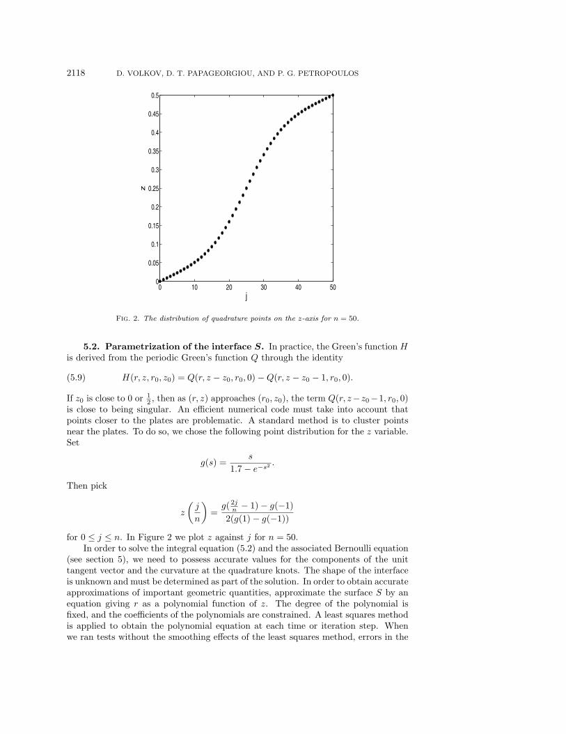
Fig. 3. Minimal energy equilibrium shapes in the absence of an electric field. The initial curveis the straight line segment, the curve in the middle is found after 50 iterations, and the final curveis found after 200 iterations.

6.1.1. The case where the electric effects are absent. Euler was the firstto study this case. In the absence of gravity, B = 0, either there exists a piece ofcatenary with equation

r = C cosh

(z −D

C

), C > 0,(6.3)

passing through the two fixed points at the top and bottom, and in that case theequilibrium shape is given by that piece of catenary, or coefficients C and D allowingthe catenary to pass through the two fixed points do not exist, in which case thereis no connected equilibrium shape. Note that the second case corresponds to thephysical situation where the top and bottom points are “too close” to the z-axis, andthe liquid bridge collapses. Note also that the coefficients C and D have to be soughtnumerically.

In a first example, we fixed the bottom point at (0.4, 0) and the top point at(0.5, 0.5). The initial shape is the line segment joining these two points, which is thedashed-dotted line in Figure 3. The dashed curve is the boundary of the approximateshape after 50 iterations. The solid curve is the piece of catenary connecting the twopoints. Past 200 iterations, it is not possible to tell the difference, by looking at a plotwith the same resolution, between the piece of catenary and the computed shape. Itwas checked that the discrete L2 norm of the difference in the r-coordinates betweenthe marker points and points on the exact equilibrium shape curve with the samez-coordinate was less than 10−4.

In a second example, we fixed the bottom point at (0.3, 0) and the top point at(0.4, 0.5). The initial shape is the line segment joining these two points, which is thedashed-dotted curve in Figure 4. No connected equilibrium exists in this case, and


0 0.1 0.2 0.3 0.4 0.50

0.05

0.1

0.15

0.2

0.25

0.3

0.35

0.4

0.45

0.5

r

z

initial shape

final shape

Fig. 4. A collapsing bridge through motion by curvature in the absence of an electric field. Noconnected minimal energy equilibrium shape is possible.

no real C and D can be found such that the curve defined by (6.3) passes through(0.3, 0) and (0.4, 0.5). After some 520 iterations, the updated shape intersects thez-axis, indicating that the search for connected equilibrium shapes has failed.

6.1.2. The cylindrical equilibrium shape. If S is a vertical line segment, theelectric potential V can be found in closed form and is V = 2z. If the fixed top andbottom points lie on the same vertical line, for any value of ε0, ε1 such that ε0 < ε1,there is a choice of Eb making the cylinder passing through the two fixed points anequilibrium shape with α = 0. This value is

Eb =1

2a0(εp − 1),(6.4)

where a0 is the radius of the cylinder. In addition, if these cylinders are wide enough,they are stable equilibrium shapes. To test our search for equilibrium positions, wepick the values,

εp = 2, Eb = 1, a0 = .5,(6.5)

and we start with the initial shape,

r = .5 + .05 sin(4πz).

The equilibrium shape is the cylinder r = .5 for the parameters (6.5). In Figure 5,we plot the initial shape, which is the most curved one, and also the shapes after 30,60, 90, and 110 iterations using our algorithm. The contours converge to a segmentline. The last plotted contour after 110 iterations is indistinguishable from a verticalline segment. Any additional iteration did not alter the segment line, although thecoefficients of P7 did not converge.


0.3 0.4 0.5 0.6 0.7 0.80

0.05

0.1

0.15

0.2

0.25

0.3

0.35

0.4

0.45

0.5

r

zinitial shape final shape

Fig. 5. Equilibrium shape calculation in the presence of an electric field; εp = 2, Eb = 1. Theinitial shape is the most curved one, and it gradually evolves into the cylinder of radius 0.5.

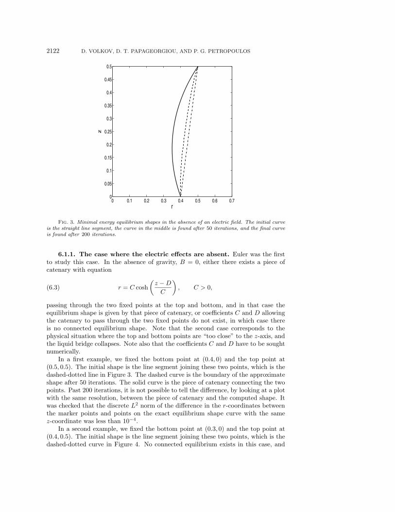
6.1.3. More interesting cases. In this section we obtain new zero pressureequilibrium shapes in regimes where there is a balance between electric and capillarystresses. In a first example, we fix the top and bottom points with the values a1 = .3,a2 = .2. The initial shape is the line segment connecting these two points. Withoutthe aid of an electric field, the corresponding liquid bridge would collapse due tocapillary forces. We now pick

εp = 2, Eb = 1.44.

After 130 iterations, changes in iterated shapes are minimal, but it appears that thereis still a slight oscillation about the equilibrium position. This oscillation can beeliminated, to graphical precision, by choosing a smaller constant of proportionalityin step 3 of our algorithm. The computed equilibrium position is depicted in Figure 6.

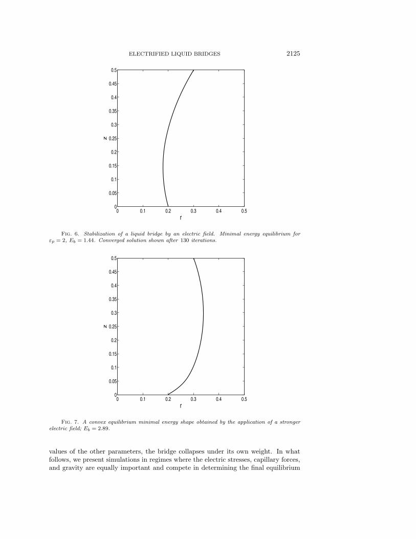
Results from another numerical simulation show that a value of Eb = 1.21 isnot strong enough in this case to prevent capillary collapse. As the value of Eb isincreased, however, we find convex equilibrium shapes. For example, with the values

εp = 2, Eb = 2.89

and the same initial shape as in the preceding case, the computed shape convergesafter about 500 iterations. We plot it in Figure 7.

For values of Eb = 3.61 or higher, no zero pressure equilibrium could be reached.The electric stress was just too strong to be compensated by capillary forces. Wenote that in practice no such physical phenomenon arises due to the adjustment ofthe pressure jump across the interface which is proportional to α.

6.1.4. Adding the effect of gravity. If the Bond number B is small, theeffects of gravity are negligible to leading order. If B grows too large, for fixed


0 0.1 0.2 0.3 0.4 0.50

0.05

0.1

0.15

0.2

0.25

0.3

0.35

0.4

0.45

0.5

r

z

Fig. 6. Stabilization of a liquid bridge by an electric field. Minimal energy equilibrium forεp = 2, Eb = 1.44. Converged solution shown after 130 iterations.

0 0.1 0.2 0.3 0.4 0.50

0.05

0.1

0.15

0.2

0.25

0.3

0.35

0.4

0.45

0.5

r

z

Fig. 7. A convex equilibrium minimal energy shape obtained by the application of a strongerelectric field; Eb = 2.89.

values of the other parameters, the bridge collapses under its own weight. In whatfollows, we present simulations in regimes where the electric stresses, capillary forces,and gravity are equally important and compete in determining the final equilibrium


0.4 0.5 0.6 0.7 0.8 0.90

0.05

0.1

0.15

0.2

0.25

0.3

0.35

0.4

0.45

0.5

r

z

Eb=0, B=0

Eb=0, B=7

Eb=0.36, B=7

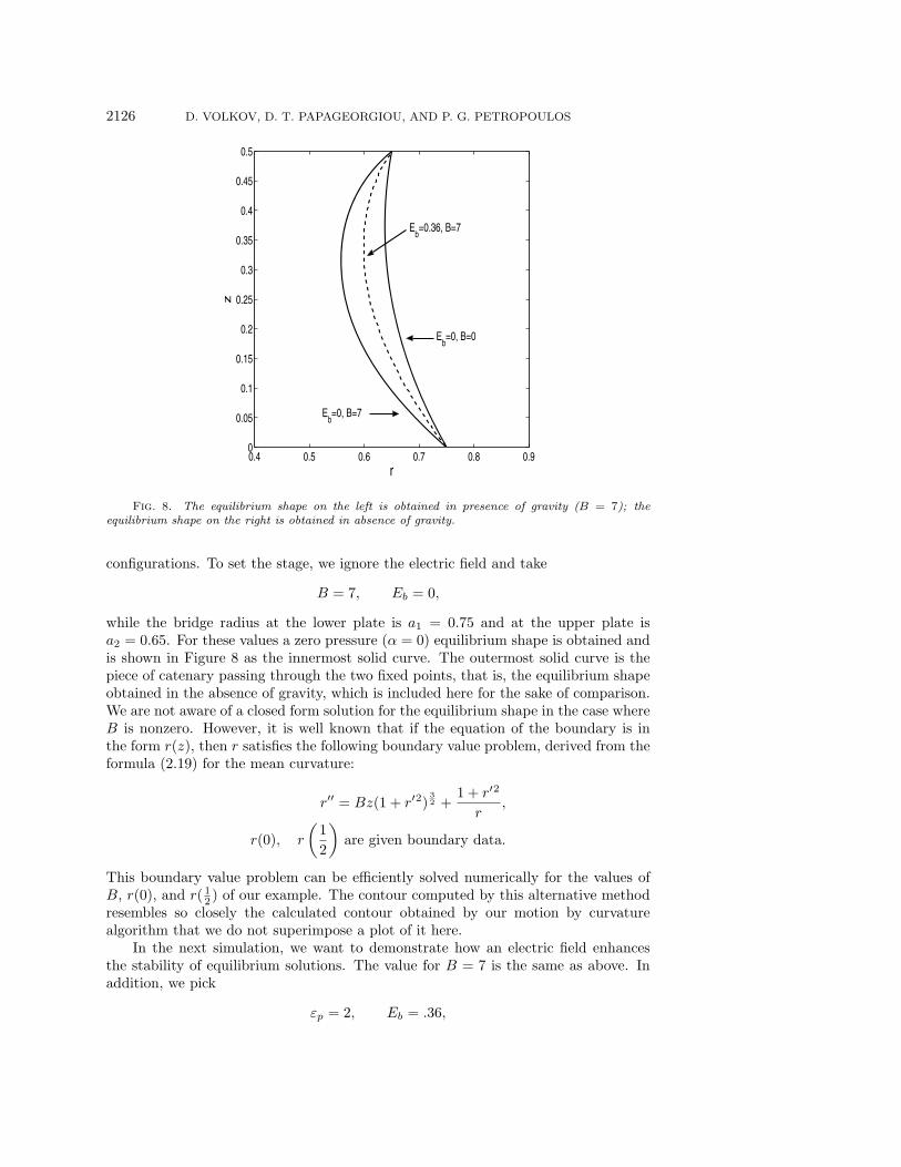
Fig. 8. The equilibrium shape on the left is obtained in presence of gravity (B = 7); theequilibrium shape on the right is obtained in absence of gravity.

configurations. To set the stage, we ignore the electric field and take

B = 7, Eb = 0,

while the bridge radius at the lower plate is a1 = 0.75 and at the upper plate isa2 = 0.65. For these values a zero pressure (α = 0) equilibrium shape is obtained andis shown in Figure 8 as the innermost solid curve. The outermost solid curve is thepiece of catenary passing through the two fixed points, that is, the equilibrium shapeobtained in the absence of gravity, which is included here for the sake of comparison.We are not aware of a closed form solution for the equilibrium shape in the case whereB is nonzero. However, it is well known that if the equation of the boundary is inthe form r(z), then r satisfies the following boundary value problem, derived from theformula (2.19) for the mean curvature:

r′′ = Bz(1 + r′2)32 +

1 + r′2

r,

r(0), r

(1

2

)are given boundary data.

This boundary value problem can be efficiently solved numerically for the values ofB, r(0), and r( 1

2 ) of our example. The contour computed by this alternative methodresembles so closely the calculated contour obtained by our motion by curvaturealgorithm that we do not superimpose a plot of it here.

In the next simulation, we want to demonstrate how an electric field enhancesthe stability of equilibrium solutions. The value for B = 7 is the same as above. Inaddition, we pick

εp = 2, Eb = .36,


and we plot also in Figure 8 the resulting equilibrium shape: it appears as the dashedline. The electric field acts to reduce the curvature of the equilibrium shape, andhence acts in a stabilizing manner.

6.2. Volume preserving equilibrium shapes. In this section, we computeequilibrium shapes satisfying two constraints: (i) the points on the top and bottomplates are imposed and fixed, and (ii) volume is conserved. As discussed earlier, thefinal pressure difference α is then an unknown, and it has to be calculated as partof the solution. The final volume obtained by application of our search algorithmfor a fixed α is an increasing function of α: this is because of the motion along thenormal vector. For finding volume preserving equilibrium shapes and correspondingpressures at equilibrium, we make two initial guesses for α, and then iterate on α usingthe secant method, to find the value α∗ that will preserve a given initial volume.

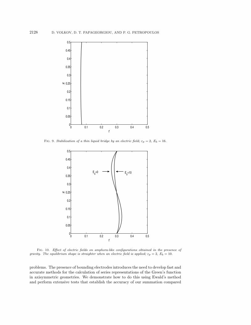
In the first experiment, we fix the points on the top and bottom plates to be atr = .07 and take B = 0. We seek equilibrium shapes that preserve the initial volumegiven by the equation

r = .07(1 − .1 sin(2πz))(6.6)

and which is equal to 6.75538 · 10−3, correct to 6 decimals. This initial configurationlies below the Plateau limit where no stable equilibrium exists for Eb = 0. Thenumerical search for equilibrium fails, as predicted by the theory. We now introducethe effects of an electric field using the values εp = 2, Eb = 16. Note that the valuechosen for Eb is a value that yields an equilibrium position for a cylinder passingthrough the closest point to the z-axis on the curve of (6.6), that is, a cylinder ofradius 0.063. The search for an equilibrium shape and final pressure was successful,and the computed value for α∗ is −17.1732731713385. We conclude that equilibriumis reached after some 300 iterations, because no change in shape is observed if thealgorithm is continued for another 50 iterations. The shape at equilibrium is plottedin Figure 9.

The computed equilibrium shape has the desired volume, up to 6 decimals. Thevisual difference in shape between the final curve in the algorithm and the curve (6.6)is slight.

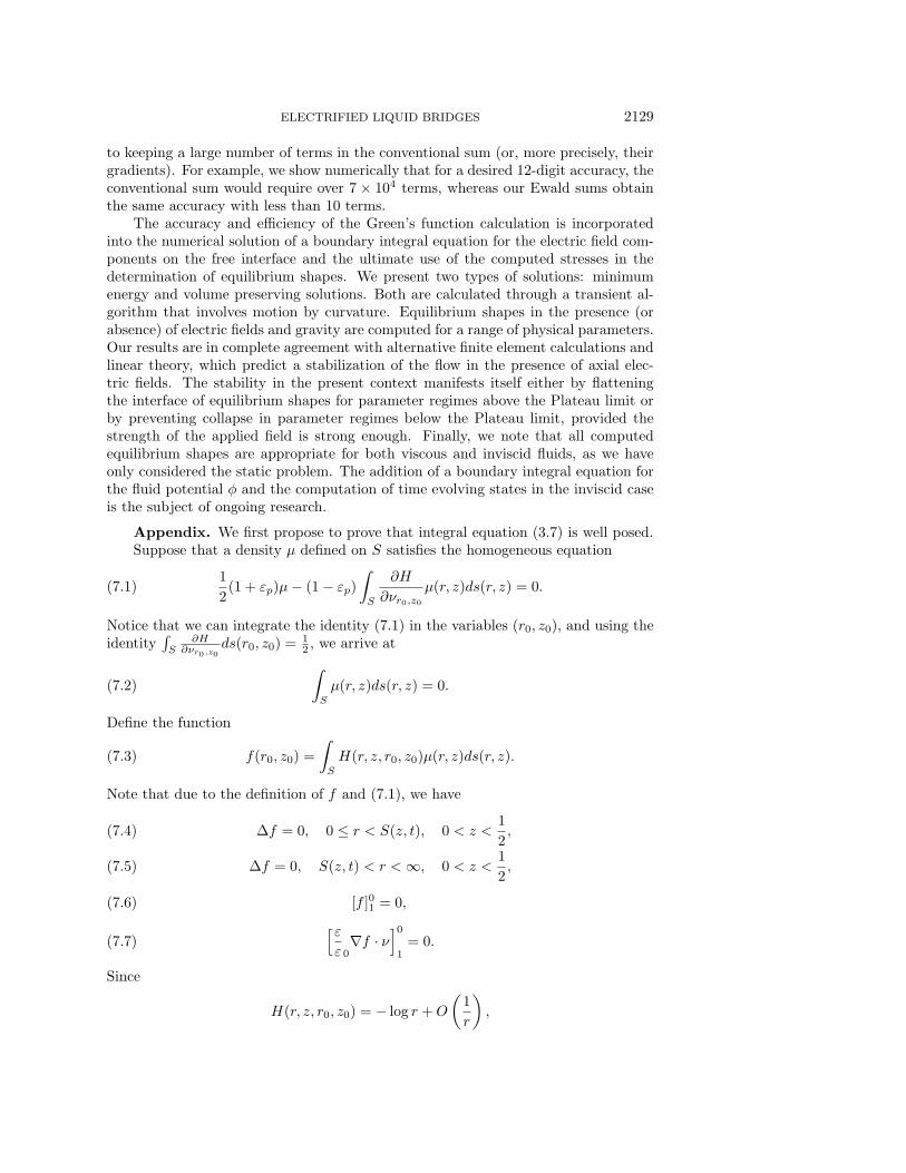
In a second simulation, we fix the points on the top and bottom plates to be atr = .3. We seek to preserve the volume occupied by the corresponding cylinder, thatis, approximately, 0.1413716. This time we are well above the Plateau limit allowedfor gravity to be present with the Bond number B = 30. In a first run, we compute anequilibrium shape in the absence of electric forces and obtain the familiar amphora-like shape; the final pressure value is α∗ = 10.7302756813844. We then apply anelectric field using the values εp = 2, Eb = 10. The final shape at equilibrium ismuch flatter in this case, and the configuration is closer to an undisturbed cylinderdue to the stabilizing effects of the electric field. Equilibrium shapes in each caseare plotted in Figure 10. The final computed value for α∗ is −9.2584080738938.This calculation verifies that the electric field acts to offset the destabilizing effectsof gravity through stabilizing electric stresses at the interface. This is in agreementwith results from experiments (see Gonzalez et al. (1989) and Ramos, Gonzalez, andCastellanos (1994)), as well as linear stability studies of the governing equations (seePelekasis, Economou, and Tsamopoulos (2001)).

7. Conclusions. We have introduced and implemented efficient and highly ac-curate boundary integral methods which can be used to solve electrified liquid bridge


0 0.1 0.2 0.3 0.4 0.50

0.05

0.1

0.15

0.2

0.25

0.3

0.35

0.4

0.45

0.5

r

z

Fig. 9. Stabilization of a thin liquid bridge by an electric field; εp = 2, Eb = 16.

0 0.1 0.2 0.3 0.4 0.50

0.05

0.1

0.15

0.2

0.25

0.3

0.35

0.4

0.45

0.5

r

z

Eb=10 E

b=0

Fig. 10. Effect of electric fields on amphora-like configurations obtained in the presence ofgravity. The equilibrium shape is straighter when an electric field is applied; εp = 2, Eb = 10.

problems. The presence of bounding electrodes introduces the need to develop fast andaccurate methods for the calculation of series representations of the Green’s functionin axisymmetric geometries. We demonstrate how to do this using Ewald’s methodand perform extensive tests that establish the accuracy of our summation compared


to keeping a large number of terms in the conventional sum (or, more precisely, theirgradients). For example, we show numerically that for a desired 12-digit accuracy, theconventional sum would require over 7 × 104 terms, whereas our Ewald sums obtainthe same accuracy with less than 10 terms.

The accuracy and efficiency of the Green’s function calculation is incorporatedinto the numerical solution of a boundary integral equation for the electric field com-ponents on the free interface and the ultimate use of the computed stresses in thedetermination of equilibrium shapes. We present two types of solutions: minimumenergy and volume preserving solutions. Both are calculated through a transient al-gorithm that involves motion by curvature. Equilibrium shapes in the presence (orabsence) of electric fields and gravity are computed for a range of physical parameters.Our results are in complete agreement with alternative finite element calculations andlinear theory, which predict a stabilization of the flow in the presence of axial elec-tric fields. The stability in the present context manifests itself either by flatteningthe interface of equilibrium shapes for parameter regimes above the Plateau limit orby preventing collapse in parameter regimes below the Plateau limit, provided thestrength of the applied field is strong enough. Finally, we note that all computedequilibrium shapes are appropriate for both viscous and inviscid fluids, as we haveonly considered the static problem. The addition of a boundary integral equation forthe fluid potential φ and the computation of time evolving states in the inviscid caseis the subject of ongoing research.

Appendix. We first propose to prove that integral equation (3.7) is well posed.Suppose that a density μ defined on S satisfies the homogeneous equation

1

2(1 + εp)μ− (1 − εp)

∫S

∂H

∂νr0,z0μ(r, z)ds(r, z) = 0.(7.1)

Notice that we can integrate the identity (7.1) in the variables (r0, z0), and using theidentity

∫S

∂H∂νr0,z0

ds(r0, z0) = 12 , we arrive at

∫S

μ(r, z)ds(r, z) = 0.(7.2)

Define the function

f(r0, z0) =

∫S

H(r, z, r0, z0)μ(r, z)ds(r, z).(7.3)

Note that due to the definition of f and (7.1), we have

Δf = 0, 0 ≤ r < S(z, t), 0 < z <1

2,(7.4)

Δf = 0, S(z, t) < r < ∞, 0 < z <1

2,(7.5)

[f ]01 = 0,(7.6)

[εε 0

∇f · ν]0

1= 0.(7.7)

Since

H(r, z, r0, z0) = − log r + O

(1

r

),


as r grows large, recalling (7.2), we infer that

f(r0, z0) = O

(1

r0

),

as r0 grows large. Similarly,

∂H(r, z, r0, z0)

∂r= −1

r+ o

(1

r

)

and

∂f(r0, z0)

∂r0= o

(1

r0

).

In view of (7.4)–(7.7), applying Green’s theorem to f ∂f∂z in a rectangle in the r-z plane

such that two opposite sides lie on the planes z = 0 and z = 1/2 and the other twosides tend to infinity, we derive

εp

∫R1

|∇f |2 +

∫R0

|∇f |2 = 0,(7.8)

where R1 is the region inside S, and R0 is the corresponding exterior region. Sinceεp = 0, ∇f has to be zero in R0 and in R1. Now, using the usual jump condition forthe derivatives of single layer potentials, we infer that μ = 0.

We have thus proved uniqueness for the linear integral equation of the secondkind (3.7). Note that, up to a constant, the left-hand side of this equation appearsin the classical form “identity plus compact.” According to Theorem 10.9 in Kress(1999), we just need to verify that our sequence of operators that approximate theintegral operators involved in the left-hand side of (3.7) is pointwise convergent andcollectively compact. Our approximated operators are obtained by applying converg-ing numerical quadratures. As explained in Theorem 12.8 in Kress (1999), collectivecompactness is guaranteed when integrating against continuous kernels. More carehas to be taken for the integration kernel exhibiting a logarithmic singularity. Weseek to verify the necessary condition 12.14 in Kress (1999). That condition ensurescollective compactness for a sequence of approximating operators derived by quadra-ture, converging to a weakly singular integral operator. In our case, we found the

quadrature coefficients β(n)k (t) for the integral,

∫ 1

0

log |t− v|g(v)dv �n−1∑k=1

β(n)k (t)g

(k

n

).(7.9)

With these notations, Kress’s necessary condition 12.14 can be expressed as

limu→t

supn

n−1∑k=1

|β(n)k (t) − β

(n)k (u)| = 0.(7.10)

We chose to derive the β(n)k (t) as follows:

• For 2 ≤ k ≤ n − 3, g was approximated on [ kn ,k+1n ] by the mean of the

quadratic polynomial interpolating g at k−1n , k

n ,k+1n and the quadratic poly-

nomial interpolating g at kn ,

k+1n , k+2

n .


• g was approximated on [0, 2n ] by the quadratic polynomial interpolating g at

1n ,

2n ,

3n .

• g was approximated on [n−2n , 1] by the quadratic polynomial interpolating g

at n−3n , n−2

n , n−1n .

It follows that our quadrature rule is convergent and the β(n)k satisfy the estimate

|β(n)k (t) − β

(n)k (u)| ≤ M

∫ k+2n

k−2n

∣∣log |t− v| − log |t− u|∣∣dv,(7.11)

where the constant M is independent of k, n, t, and u. Thus to ensure (7.10), we justneed to verify that

limu→t

∫ 1

0

∣∣log |t− v| − log |u− v|∣∣dv = 0,(7.12)

which is elementary.

REFERENCES

M. Abramowitz and I. Stegun, eds. (1992), Handbook of Mathematical Functions with Formulas,Graphs, and Mathematical Tables, Dover, New York.

M. Born and K. Huang (1954), Dynamical Theory of Crystal Lattices, Oxford University Press,Oxford, UK.

C. L. Burcham and D. A. Saville (2000), The electrohydrodynamic stability of a liquid bridge: Mi-crogravity experiments on a bridge suspended in a dielectric gas, J. Fluid Mech., 405, pp. 37–56.

P. G. Drazin and W. H. Reid (1981), Hydrodynamic Stability, Cambridge University Press, Cam-bridge, UK.

P. P. Ewald (1921), Die Berechnung optischer und elektrostatischen Gitterpotentiale, Ann. Phys.,64, pp. 253–268.

J. Eggers (1997), Nonlinear dynamics and breakup of free-surface flows, Rev. Modern Phys., 3,pp. 865–929.

S. Gaudet, G. H. McKinley, and H. A. Stone (1996), Extensional deformation of liquid bridges,Phys. Fluids A, 8, pp. 2568–2579.

H. Gonzalez and A. Castellanos (1993), The effect of residual gravity on the stability of liquidcolumns subjected to electric fields, J. Fluid Mech., 249, pp. 185–206.

H. Gonzalez, F. M. J. McCluskey, A. Castellanos, and A. Barrero (1989), Stabilization of di-electric liquid bridges by electric fields in the absence of gravity, J. Fluid Mech., 206, pp. 545–561.

T. Y. Hou, J. S. Lowengrub, and M. J. Shelley (2001), Boundary integral methods for multi-component fluids and multiphase materials, J. Comput. Phys., 169, pp. 302–362.

J. D. Jackson (1962), Classical Electrodynamics, Wiley, New York.R. Kress (1999), Linear Integral Equations, 2nd ed., Appl. Math. Sci. 82, Springer-Verlag, New

York.L. D. Landau and E. M. Lifshitz (1987), Fluid Mechanics. Course of Theoretical Physics, Vol-

ume 6, 2nd ed., Butterworth Heinemann, Burlington, MA.C. M. Linton (1998), The Green’s function for the two-dimensional Helmholtz equation in periodic

domains, J. Engrg. Math., 33, pp. 377–402.C. M. Linton (1999), Rapidly convergent representations for Green’s functions for Laplace’s equa-

tion, R. Soc. Lond. Proc. Ser. A Math. Phys. Eng. Sci., 455, pp. 1767–1797.G. H. McKinley and A. Tripathi (2000), How to extract the Newtonian viscosity from capillary

breakup measurements in a filament rheometer, J. Rheol., 44, pp. 653–670.D. T. Papageorgiou (1995a), On the breakup of viscous liquid threads, Phys. Fluids, 7, pp. 1529–

1544.D. T. Papageorgiou (1995b), Analytical description of the breakup of liquid jets, J. Fluid Mech.,

301, pp. 109–132.D. T. Papageorgiou (1996), Description of jet breakup, in Advances in Multi-fluid Flows, Y. Y. Re-

nardy, A. C. Coward, D. T. Papageorgiou, and S.-M. Sun, eds., SIAM, Philadelphia, pp. 171–198.D. T. Papageorgiou and M. Vanden-Broeck (2004), Large amplitude capillary waves in electrified

fluid sheets, J. Fluid Mech., 508, pp. 71–88.


N. A. Pelekasis, K. Economou, and J. A. Tsamopoulos (2001), Linear oscillations and stabilityof a liquid bridge in an axial electric field, Phys. Fluids, 13, pp. 3564–3581.

J. Plateau (1873), Statique Experimentale et Theoretique des Liquides Soumis aux Seules ForcesMoleculaires, Gauthier-Villars, Paris.

C. Pozrikidis (2001), Interfacial dynamics for Stokes flow, J. Comput. Phys., 169, pp. 250–301.A. Ramos and A. Castellanos (1993), Bifurcation diagrams of axisymmetric liquid bridges of

arbitrary volume in electric and gravitational axial fields, J. Fluid Mech., 249, pp. 207–225.A. Ramos, H. Gonzalez, and A. Castellanos (1994), Experiments on dielectric liquid bridges

subjected to axial electric fields, Phys. Fluids, 6, pp. 3206–3208.L. Rayleigh (1878), On the instability of jets, Proc. London Math. Soc., 10, pp. 4–13.L. Rayleigh (1892), On the stability of a cylinder of viscous liquid under capillary force, Phil. Mag.,

34, p. 145.A. Rothert, R. Richter, and I. Rehberg (2001), Transition from symmetric to asymmetric scaling

function before drop pinch-off, Phys. Rev. Lett., 87, 084501.A. Rothert, R. Richter, and I. Rehberg (2003), Formation of a drop: Viscosity dependence of

three flow regimes, New J. Phys., 5, article 59.B. S. Tilley, P. G. Petropoulos, and D. T. Papageorgiou (2001), Dynamics and rupture of

planar electrified liquid sheets, Phys. Fluids, 13, pp. 3547–3563.

Accurate and Efficient Boundary Integral Methods for Electrified Liquid Bridge Problems

Documents

Transcript of Accurate and Efficient Boundary Integral Methods for Electrified Liquid Bridge Problems