Generating Self-excited Oscillations for

Underactuated Mechanical Systems

via Two-Relay Controller

(Draft copy)

Luis T. Aguilar∗, Igor Boiko†, Leonid Fridman,‡ and Rafael Iriarte‡

Abstract

A tool for the design of a periodic motion in an underactuated mechanical system viagenerating a self-excited oscillation of a desired amplitude and frequency by means of the vari-able structure control is proposed. Firstly, an approximate approach based on the describingfunction method is given, which requires that the mechanical plant should be a linear low-passfilter - the hypothesis that usually holds when the oscillations are relatively fast. The methodbased on the Locus of a Perturbed Relay Systems (LPRS) provides an exact model of theoscillations when the plant is linear. Finally, the Poincare maps design provides the value ofthe controller parameters ensuring the locally orbitally stable periodic motions for an arbitrarymechanical plant. The proposed approach is shown by the controller design and experimentson the Furuta pendulum.

Keywords: Variable structure systems, underactuated systems, periodic solution, frequencydomain methods.

1 Introduction

1.1 Overview

In this paper, we consider the control of one of the simplest types of a functional motion: generation

of a periodic motion in underactuated mechanical systems which could be of non-minimum-phase.

Current representative works on periodic motions in an orbital stabilization of underactuated

∗L.T. Aguilar is with Instituto Politecnico Nacional, Centro de Investigacion y Desarrollo de Tecnologıa Digital,PMB 88, PO BOX 439016 San Ysidro CA USA 92143-9016; (e-mail: luis.aguilar@ieee.org) (Corresponding author).†I. Boiko is with University of Calgary, 2500 University Dr. N.W., Calgary, Alberta, Canada (e-mail:

i.boiko@ieee.org).‡L. Fridman and R. Iriarte are with Universidad Nacional Autonoma de Mexico (UNAM), Engineering Fac-

ulty, Department of Control, C.P. 04510, Mexico City (e-mails: lfridman@servidor.unam.mx, ririarte@dctrl.fi-b.unam.mx).

1

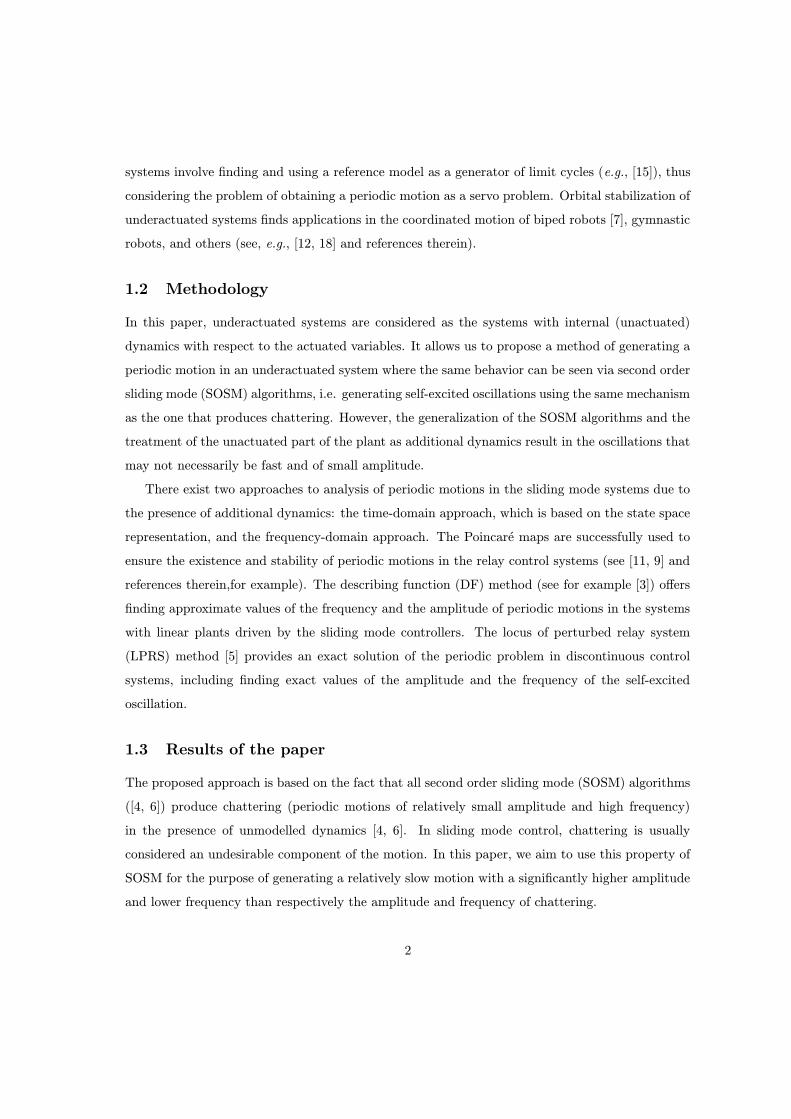
systems involve finding and using a reference model as a generator of limit cycles (e.g., [15]), thus

considering the problem of obtaining a periodic motion as a servo problem. Orbital stabilization of

underactuated systems finds applications in the coordinated motion of biped robots [7], gymnastic

robots, and others (see, e.g., [12, 18] and references therein).

1.2 Methodology

In this paper, underactuated systems are considered as the systems with internal (unactuated)

dynamics with respect to the actuated variables. It allows us to propose a method of generating a

periodic motion in an underactuated system where the same behavior can be seen via second order

sliding mode (SOSM) algorithms, i.e. generating self-excited oscillations using the same mechanism

as the one that produces chattering. However, the generalization of the SOSM algorithms and the

treatment of the unactuated part of the plant as additional dynamics result in the oscillations that

may not necessarily be fast and of small amplitude.

There exist two approaches to analysis of periodic motions in the sliding mode systems due to

the presence of additional dynamics: the time-domain approach, which is based on the state space

representation, and the frequency-domain approach. The Poincare maps are successfully used to

ensure the existence and stability of periodic motions in the relay control systems (see [11, 9] and

references therein,for example). The describing function (DF) method (see for example [3]) offers

finding approximate values of the frequency and the amplitude of periodic motions in the systems

with linear plants driven by the sliding mode controllers. The locus of perturbed relay system

(LPRS) method [5] provides an exact solution of the periodic problem in discontinuous control

systems, including finding exact values of the amplitude and the frequency of the self-excited

oscillation.

1.3 Results of the paper

The proposed approach is based on the fact that all second order sliding mode (SOSM) algorithms

([4, 6]) produce chattering (periodic motions of relatively small amplitude and high frequency)

in the presence of unmodelled dynamics [4, 6]. In sliding mode control, chattering is usually

considered an undesirable component of the motion. In this paper, we aim to use this property of

SOSM for the purpose of generating a relatively slow motion with a significantly higher amplitude

and lower frequency than respectively the amplitude and frequency of chattering.

2

The twisting algorithm [13] originally created as a SOSM controller -to ensure the finite-time

convergence - is generalized, so that it can generate self-excited oscillations in the closed loop

system containing an underactuated plant. The required frequencies and amplitudes of periodic

motions are produced without tracking of precomputed trajectories. It allows for generating a

wider (than the original twisting algorithm with additional dynamics) range of frequencies and

encompassing a variety of plant dynamics.

A systematic approach is proposed to find the values of the controller parameters allowing one

to obtain the desired frequencies and the output amplitude, which includes:

• An approximate approach based on the describing function method that requires for the

plant to be a low-pass filter;

• a design methodology based on the locus of a perturbed relay systems (LPRS) that gives

exact values of controller parameters for the linear plants;

• an algorithm that uses Poincare maps and provides the values of the controller parame-

ters ensuring the existence of the locally orbitally stable periodic motions for an arbitrary

mechanical plant.

The theoretical results are validated experimentally via the tests on the laboratory Furuta

pendulum. The periodic motion is generated around the upright position (which gives the non-

minimum phase system case).

1.4 Organization of the paper

This paper is structured as follows: Section 2 introduces the problem statement. In Section 3,

the idea of the two-relay controller is explained via the frequency domain methods. In Section 4

are computed the approximate values of controller parameters via the describing function method

and stability of the periodic solution will be provided. In Section 5 is provided the LPRS method

to compute the exact values of the controller parameters. In Section 6, the Poincare method will

be used as a design tool. An example is provided in Section 7 in order to illustrate the design

methodologies given in Section 4, 5, and 6. In Section 8, the design methodology is validated via

periodic motion design for the experimental Furuta pendulum. Section 9 provides final conclusions.

3

2 Problem statement

Let the underactuated mechanical system, which is a plant in the system where a periodic motion

is supposed to occur, be given by the Lagrange equation:

M(q)q +H(q, q) = B1u (1)

where q ∈ IRm is the vector of joint positions; u ∈ IR is the vector of applied joint torques

where m < n; B1 = [0(m−1), 1]T is the input that maps the torque input to the joint coordinates

space; M(q) ∈ IRm×m is the symmetric positive-definite inertia matrix; and H(q, q) ∈ IRm is the

vector that contains the Coriolis, centrifugal, gravity, and friction torques. The following two-relay

controller is proposed for the purpose of exciting a periodic motion:

u = −c1sign(y)− c2sign(y), (2)

where c1 and c2 are parameters designed such that the scalar output of the system (the position

of a selected link of the plant)

y = h(q) (3)

has a steady periodic motion with the desired frequency and amplitude.

Let us assume that the two-relay controller has two independent parameters c1 ∈ C1 ⊂ IR and

c2 ∈ C2 ⊂ IR, so that the changes to those parameters result in the respective changes of the

frequency Ω ∈ W ⊂ IR and the amplitude A1 ∈ A ⊂ IR of the self-excited oscillations. Then we

can note that there exists two mappings F1 : C1 × C2 7→ W and F2 : C1 × C2 7→ A, which can be

rewritten as F : C1 × C2 7→ W × A ⊂ IR2. Assume that mapping F is unique. Then there exists

an inverse mapping G : W × A 7→ C1 × C2. The objective is, therefore, (a) to obtain mapping

G using a frequency-domain method for deriving the model of the periodic process in the system,

(b) to prove the uniqueness of mappings F and G for the selected controller, and (c) to find the

ranges of variation of Ω and A1 that can be achieved by varying parameters c1 and c2.

The analysis and design objectives are formulated as follows: Find the parameter values c1

and c2 in (2) such that the system (1) has a periodic motion with the desired frequency Ω and

4

-1.4 -1.2 -1 -0.8 -0.6 -0.4 -0.2 0

x 10-3

0

1

2

3

4

5

6

7

8x 10

-4

Re W(jω)

Im W

(jω)

x

θ

u

lmg

M

Figure 1: The cart-pendulum system and its corresponding Nyquist plot of transfer function fromthe angle of the pendulum to the input of the actuator.

desired amplitude of the output signal A1. Therefore, the main objective of this research is to find

mapping G to be able to tune c1 and c2 values.

3 The idea of the method

The idea of the method is to provide the mapping from a set of desired frequencies W ⊂ IR

and amplitudes A ⊂ IR into a set of gain values C ⊂ IR2, that is G : W × A 7→ C. To achieve

the objective, let us start with the design via the describing function method which is a useful

frequency-domain tool for time-invariant linear plants to predict the existence or absence of limit

cycles and estimate the frequency and amplitude when it exists. In the scenario introduced in [4],

the DF method was used for analysis of chattering for the closed-loop system with the twisting

algorithm where the inverse of this mapping was derived.

5

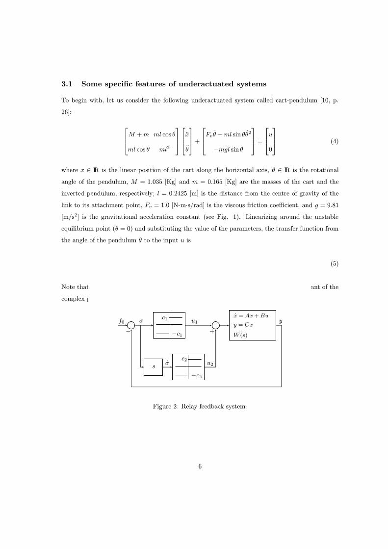
3.1 Some specific features of underactuated systems

To begin with, let us consider the following underactuated system called cart-pendulum [10, p.

26]:

M +m ml cos θ

ml cos θ ml2

x

θ

+

Fv θ −ml sin θθ2

−mgl sin θ

=

u

0

(4)

where x ∈ IR is the linear position of the cart along the horizontal axis, θ ∈ IR is the rotational

angle of the pendulum, M = 1.035 [Kg] and m = 0.165 [Kg] are the masses of the cart and the

inverted pendulum, respectively; l = 0.2425 [m] is the distance from the centre of gravity of the

link to its attachment point, Fv = 1.0 [N-m∙s/rad] is the viscous friction coefficient, and g = 9.81

[m/s2] is the gravitational acceleration constant (see Fig. 1). Linearizing around the unstable

equilibrium point (θ = 0) and substituting the value of the parameters, the transfer function from

the angle of the pendulum θ to the input u is

W (s) =Θ(s)

U(s)=

1

0.1s+ 1∙

1

0.25 (s2 + s− 2887). (5)

Note that the Nyquist plot of the above transfer function is located in the second quadrant of the

complex plane.

W (s)

s

f0c1

c2

y

u2

u1x = Ax+Bu

σ

−c2

−c1

σ

y = Cx+−

Figure 2: Relay feedback system.

6

4 Describing function of the two-relay controller

Let firstly, the linearized plant be given by:

x = Ax+Bu

y = Cx

, x ∈ IRn, y ∈ IR, n = 2m (6)

which can be represented in the transfer function form as follows:

W (s) = C(sI −A)−1B.

Let us assume that matrix A has no eigenvalues at the imaginary axis and the relative degree of

(6) is greater than 1.

The Describing Function (DF), N , of the variable structure controller (2) is the first harmonic

of the periodic control signal divided by the amplitude of y(t) [3]:

N =ω

πA1

∫ 2π/ω

0

u(t) sinωtdt+ jω

πA1

∫ 2π/ω

0

u(t) cosωtdt (7)

where A1 is the amplitude of the input to the nonlinearity (of y(t) in our case) and ω is the

frequency of y(t). However, the algorithm (2) can be analyzed as the parallel connection of two

ideal relay where the input to the first relay is the output variable and the input to the second

relay is the derivative of the output variable (see Fig. 1). For the first relay the DF is:

N1 =4c1πA1,

and for the second relay it is [3]:

N2 =4c2πA2,

where A2 is the amplitude of dy/dt. Also, take into account the relationship between y and dy/dt

in the Laplace domain, which gives the relationship between the amplitudes A1 and A2: A2 = A1Ω,

where Ω is the frequency of the oscillation. Using the notation of the algorithm (2) we can rewrite

7

this equation as follows:

N = N1 + sN2 =4c1πA1

+ jΩ4c2πA2

=4

πA1(c1 + jc2), (8)

where s = jΩ. Let us note that the DF of the algorithm (2) depends on the amplitude value only.

This suggests the technique of finding the parameters of the limit cycle - via the solution of the

harmonic balance equation [3]:

W (jΩ)N(a) = −1, (9)

where a is the generic amplitude of the oscillation at the input to the nonlinearity, and W (jω) is

the complex frequency response characteristic (Nyquist plot) of the plant. Using the notation of

the algorithm (2) and replacing the generic amplitude with the amplitude of the oscillation of the

input to the first relay this equation can be rewritten as follows:

W (jΩ) = −1

N(A1), (10)

where the function at the right-hand side is given by:

−1

N(A1)= πA1

−c1 + jc24(c21 + c

22).

Equation (9) is equivalent to the condition of the complex frequency response characteristic of the

open-loop system intersecting the real axis in the point (−1, j0). The graphical illustration of the

technique of solving (9) is given in Fig. 2. The function −1/N is a straight line the slope of which

depends on c2/c1 ratio. The point of intersection of this function and of the Nyquist plot W (jω)

provides the solution of the periodic problem.

4.1 Tuning the parameters of the controller

Here, we summarize the steps to tune c1 and c2:

a) Identify the quadrant in the Nyquist plot where the desired frequency Ω is located, which

8

ReW

ImW

ψ

W (jω)

− 1N

Q1Q2

Q3 Q4

Figure 3: Example of a Nyquist plot of the open-loop system W (jω) with two-relay controller.

falls into one of the following categories (sets):

Q1 = {ω ∈ IR : Re{W (jω)} > 0, Im{W (jω)} ≥ 0}

Q2 = {ω ∈ IR : Re{W (jω)} ≤ 0, Im{W (jω)} ≥ 0}

Q3 = {ω ∈ IR : Re{W (jω)} ≤ 0, Im{W (jω)} < 0}

Q4 = {ω ∈ IR : Re{W (jω)} > 0, Im{W (jω)} < 0}.

b) The frequency of the oscillations depends only on the c2/c1 ratio, and it is possible to obtain

the desired frequency Ω by tuning the ξ = c2/c1 ratio:

ξ =c2

c1= −Im{W (jΩ)}Re{W (jΩ)}

. (11)

Since the amplitude of the oscillations is given by

A1 =4

π|W (jΩ)|

√c21 + c

22, (12)

9

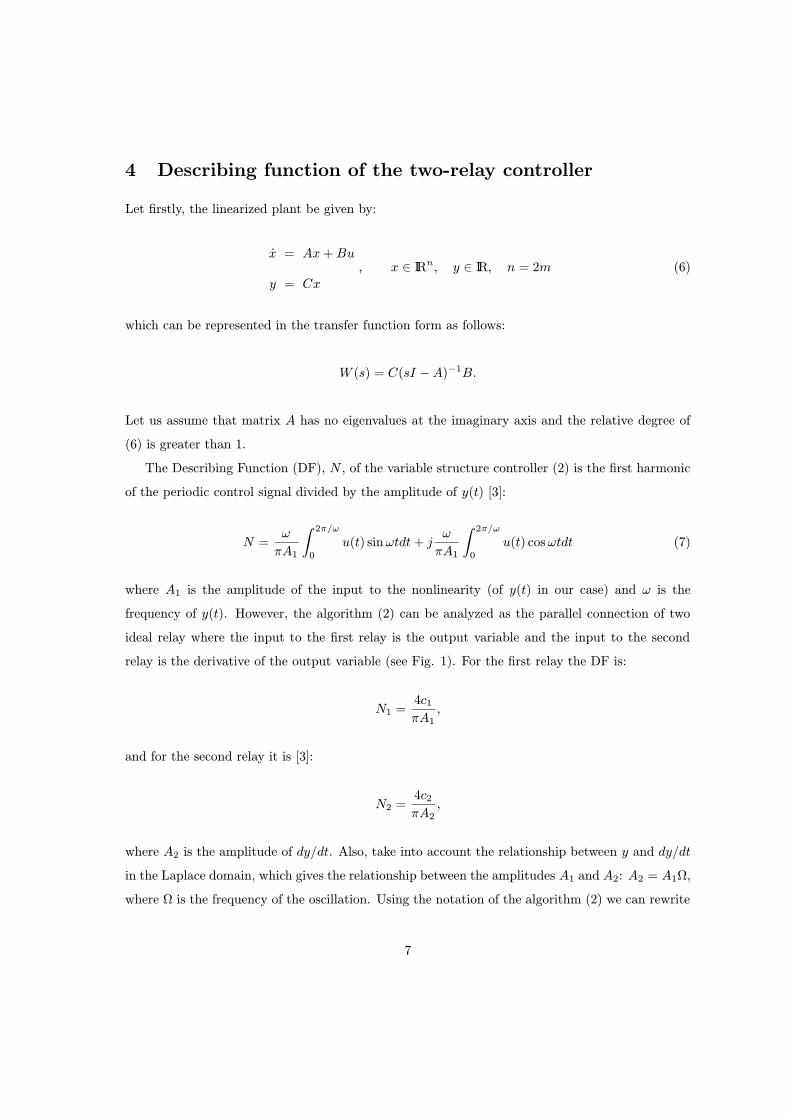
then the c1 and c2 values can be computed as follows

c1 =

π4 ∙

A1|W (jΩ)| ∙

(√1 + ξ2

)−1if Ω ∈ Q2 ∪Q3

−π4 ∙A1

|W (jΩ)| ∙(√1 + ξ2

)−1elsewhere

(13)

c2 = ξ ∙ c1. (14)

4.2 Stability of periodic solutions

We shall consider that the harmonic balance condition still holds for small perturbations of the

amplitude and the frequency with respect of the periodic motion. In this case the oscillation can

be described as a damped one. If the damping parameter will be negative at a positive increment

of the amplitude and positive at a negative increment of the amplitude then the perturbation will

vanish, and the limit cycle will be asymptotically stable.

Theorem 1 Suppose that for the values of the c1 and c2 given by (13) and (14) there exists a

corresponding periodic solution to the system (2), (6). If

Red argW

d lnω

∣∣∣∣ω=Ω

≤ −c1c2

c21 + c22

< 0 (15)

then the above-mentioned periodic solutions to the system (2), (6) is orbitally asymptotically stable.

Proof. The proof of this Theorem is given in [1]

5 Locus of a Perturbed Relay System design (LPRS)

The LPRS proposed in [5] provides an exact solution of the periodic problem in a relay feedback

system having a plant (6) and the control given by the hysteretic relay. The LPRS is defined as

a characteristic of the response of a linear part to an unequally spaced pulse control of variable

frequency in a closed-loop system [5]. This method requires a computational effort but will provide

an exact solution. The LPRS can be computed as follows:

J(ω) =

∞∑

k=1

(−1)k+1Re{W (kω)}+ j∞∑

k=1

1

2k − 1Im {W [(2k − 1)ω]} . (16)

10

J(ω)

πb4c

12Kn

ω = Ω

Im

Re

Figure 4: LPRS and oscillation analysis.

The frequency of the periodic motion for the algorithm (2) can be found from the following equation

[5] (see Fig. 6):

ImJ(Ω) = 0.

In effect, we are going to consider the plant being nonlinear, with the second relay transposed to

the feedback in this equivalent plant. Introduce the following function, which will be instrumental

in finding a response of the nonlinear plant to the periodic square-wave pulse control.

L(ω, θ) =

∞∑

k=1

1

2k − 1(sin[(2k − 1)2πθ]Re{W [(2k − 1)ω]}

+cos[(2k − 1)2πθ]Im{W [(2k − 1)ω]}). (17)

The function L(ω, θ) denotes a linear plant output (with a coefficient) at the instant t = θT (with

T being the period: T = 2π/ω) if a periodic square-wave pulse signal of unity amplitude is applied

to the plant:

L(ω, θ) =πy(t)

4c

∣∣∣∣t=2πθ/ω

11

with θ ∈ [−0.5, 0.5] and ω ∈ [0,∞], where t = 0 corresponds to the control switch from −1 to +1.

With L(ω, θ) available, we obtain the following expression for Im{J(ω)} of the equivalent plant:

Im{J(ω)} = L(Ω, 0) +c2

c1L(Ω, θ). (18)

The value of the time shift θ between the switching of the first and second relay can be found from

the following equation

y(θ) = 0.

As a result, the set of equations for finding the frequency Ω and the time shift θ is as follows:

c1L(Ω, 0) + c2L(Ω, θ) = 0

c1L1(Ω,−θ) + c2L1(Ω, 0) = 0.(19)

The amplitude of the oscillations can be found as follows. The output of the system is:

y(t) =4

π

∞∑

i=1

{c1 sin[(2k − 1)Ω + ϕL((2k − 1)Ω)]

+c2 sin[(2k − 1)Ωt+ ϕL((2k − 1)Ω) + (2k − 1)2πθ]}AL((2k − 1)Ω) (20)

where ϕL(ω) = argW (ω), which is a response of the plant to the two square pulse-wave signals

shifted with respect to each other by the angle 2πθ. Therefore, the amplitude is

A1 = maxt∈[0;2π/ω]

y(t). (21)

Yet, instead of the true amplitude we can use the amplitude of the fundamental frequency compo-

nent (first harmonic) as a relatively precise estimate. In this case, we can represent the input as

the sum of two rotating vectors having amplitudes 4c1/π and 4c2/π, with the angle between the

vectors 2πθ. Therefore, the amplitude of the control signal (first harmonic) is

Au =4

π

√c21 + c

22 + 2c1c2 cos(2πθ), (22)

12

0 200 400 600 800 1000 12000

1000

2000

3000

4000

5000

6000

7000

8000

9000

10000

c1

c 2=ξ

c1

Ω1

Ω2

Ω3

Ω4

Ω5

a2

a4

a6

a8

a10

Figure 5: Plot of c1 vs c2 for arbitrary frequencies Ω1 < Ω < Ω5 and amplitudes a1 < A1 < a10.

and the amplitude of the output (first harmonic) is

A1 =4

π

√c21 + c

22 + 2c1c2 cos(2πθ)AL(Ω), (23)

where AL(ω) = |W (jω)|. Expressions (19), (23) if considered as equations for Ω and A1 provide

one with mapping F . This mapping is depicted in Figure 5 as curves of equal values of Ω and A1 in

the coordinates (c1, c2). From (19) one can see that the frequency of the oscillations depends only

on the ratio c2/c1 = ξ. Therefore, Ω is invariant with respect to c2/c1: Ω(λc1, λc2) = Ω(c1, c2).

It also follows from (23) that there is the following invariance for the amplitude: A1(λc1, λc2) =

λA1(c1, c2). Therefore, Ω and A1 can be manipulated independently in accordance with mapping

G considered below.

Mapping G (inverse of F ) can be derived from (19), (23) if c1, c2 and θ are considered unknown

parameters in those equations. For any given Ω, from equation (19) the ratio c2/c1 = ξ can be

found (as well as θ). Therefore, we can find first ξ = c2/c1 = h(Ω), where h(Ω) is an implicit

function that corresponds to (19). After that c1 and c2 can be computed as per the following

13

formulas:

c1 =π

4

A1

AL(Ω)

1√1 + 2ξ cos(2πθ) + ξ2

(24)

c2 =π

4

A1

AL(Ω)

ξ√1 + 2ξ cos(2πθ) + ξ2

. (25)

6 Poincare design

Poincare map is a recognized tool for analysis of the existence of limit cycles for nonlinear systems.

Therefore, this tool is appropriate to satisfy the goal defined in Section 2. To begin with, let us

consider that the actuated degrees of freedom are represented by the elements of η = (η1, η2) ∈ IR2

and the unactuated degrees of freedom are represented by the elements of ν = (ν1, ν2) ∈ IR2m−2.

Let us define the output y = η1. The Lagrange equation (1) can be represented in the state-space

form by:

η1

η2

ν1

ν2

=

η2

Δ−1m {M22(η1, ν1)[u−N1(η, ν)] +M12(η1, ν1)N2(η, ν)}

ν2

Δ−1m {−M12(η1, ν1)[u−N1(η, ν)]−M11(η1, ν1)N2(η, ν)}

=

η2

f1(η, ν, u)

ν2

f2(η, ν, u)

(26)

where u is given in (2), and Δm =M11(η1, ν1)M22(η1, ν1)−M12(η1, ν1)M12(η1, ν1).

To construct the Poincare map, one has to choose a surface of section S in the extended state

space IR× IR2m−2 and consider the points of successive intersections of a given trajectory with this

14

S1

S2

S3

S4R1

R2

R3

R4

η1

η2

ν1

(η01 , 0, ν0)

(0, η+2 (T+sw, η

01 , ν0), ν

+1 (T

+sw, η

01 , ν0))

(η+1 (Tp, η01 , ν0), 0, ν

+1 (Tp, η

01 , ν0))

(0, η2(Tp, η01 , ν0), ν

+1 (Tp, η

01 , ν0))

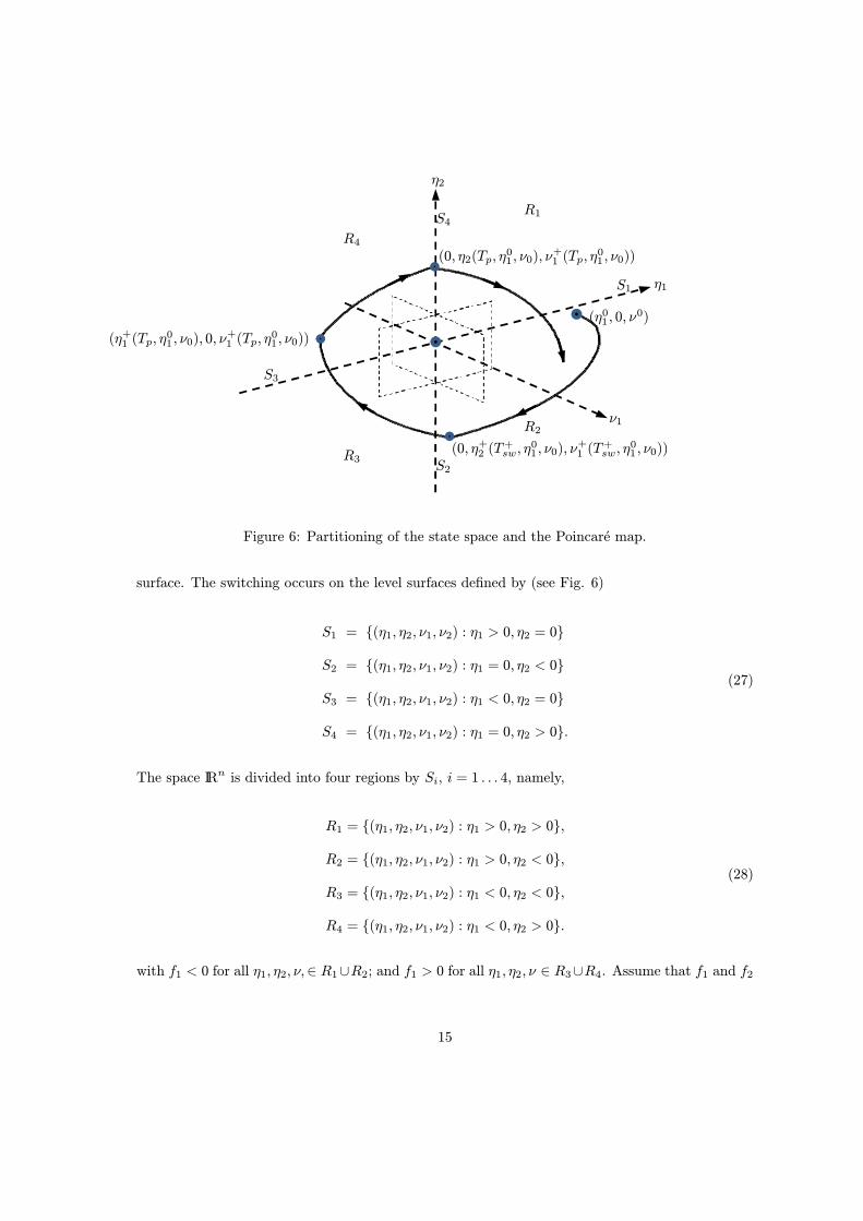
Figure 6: Partitioning of the state space and the Poincare map.

surface. The switching occurs on the level surfaces defined by (see Fig. 6)

S1 = {(η1, η2, ν1, ν2) : η1 > 0, η2 = 0}

S2 = {(η1, η2, ν1, ν2) : η1 = 0, η2 < 0}

S3 = {(η1, η2, ν1, ν2) : η1 < 0, η2 = 0}

S4 = {(η1, η2, ν1, ν2) : η1 = 0, η2 > 0}.

(27)

The space IRn is divided into four regions by Si, i = 1 . . . 4, namely,

R1 = {(η1, η2, ν1, ν2) : η1 > 0, η2 > 0},

R2 = {(η1, η2, ν1, ν2) : η1 > 0, η2 < 0},

R3 = {(η1, η2, ν1, ν2) : η1 < 0, η2 < 0},

R4 = {(η1, η2, ν1, ν2) : η1 < 0, η2 > 0}.

(28)

with f1 < 0 for all η1, η2, ν,∈ R1∪R2; and f1 > 0 for all η1, η2, ν ∈ R3∪R4. Assume that f1 and f2

15

are differentiable in the domain Ri, i = 1, . . . , 4. Moreover, suppose that the values of the functions

of fk, k = 1, 2 in the domains Ri could be smoothly extended till their closures Ri. Considering

(η1, η2), let us derive the Poincare map from the domain ϕ1(∙) = (η1, 0), where η1 > 0, into the

domain ϕ2(∙) = (0, η2), where η2 < 0 (see region R2 in Fig. 6). Let η01 > 0 and denote as

η+1 (t, η01 , ν

0, c1, c2), η+2 (t, η

01 , ν

0, c1, c2)

ν+1 (t, η01 , ν

0, c1, c2), ν+2 (t, η

01 , ν

0, c1, c2)

(29)

the solution of the system (26) with the initial conditions

η+1 (0, η01 , ν

0, c1, c2) = η01 , η

+2 (0, η

01 , ν

0, c1, c2) = 0, ν+(0, η,1ν

0, c1, c2) = ν0. (30)

Let Tsw(η, ν, c1, c2) be the smallest positive root of the equation

η+1 (Tsw, η01 , ν

0, c1, c2) = 0 (31)

and such thatdη+1dt(Tsw, η

01 , ν

0, c1, c2) = η+2 (Tsw, η

01 , ν

0, c1, c2) < 0, i.e., the functions

Tsw(η01 , ν

0, c1, c2), η+1 (Tsw, η

01 , ν

0, c1, c2), η+2 (Tsw, η

01 , ν

0, c1, c2), ν+(Tsw, η

01 , ν

0, c1, c2),

smoothly depends on their arguments.

Now, let us derive the Poincare map from the sets ϕ2(∙) = (0, η2, ν01), where η2 < 0, into the

sets ϕ3(∙) = (η1, 0, ν01) where η1 < 0 (see region R3 in Fig. 6). To this end, denote as

η+1p(t, η01 , ν

0, c1, c2), η+2p(t, η

01 , ν

0, c1, c2), ν+p (t, η

01 , ν

0, c1, c2), (32)

the solution of the system (26) with the initial conditions

η+1p(T+sw(η

01 , ν

0, c1, c2), η0, ν0, c1, c2) = 0,

η+2p(T+sw(η

01 , ν

0, c1, c2), η0, ν0, c1, c2) = η

+2 (T

+sw(η

01 , ν

0, c1, c2), η01 , ν

0, c1, c2),

ν+p (T+sw(η

01 , ν

0, c1, c2), η0, ν0, c1, c2) = ν

+1 (T

+sw(η

01 , ν

0, c1, c2), η01 , ν

0, c1, c2),

(33)

16

Let T+p (η, ν, c1, c2) be the smallest root satisfying the restrictions T+p > T

+sw > 0 of the equation

η+2p(T+p , η

01 , ν

0, c1, c2) = 0 (34)

and such thatdη+2dt(T+p ) = f1(T

+p , η1, η2, ν, c1, c2) < 0, i.e., the functions

Tp(η01 , ν

0, c1, c2), η+1 (Tp, η01 , ν

0, c1, c2), η+2 (Tp, η

01 , ν

0, c1, c2),

ν+1 (Tp, η01 , ν

0, c1, c2), ν+2 (Tp, η

01 , ν

0, c1, c2)

smoothly depends on their arguments. Therefore, we have designed the map

Ξ+(η01 , ν0, c1, c2) =

η+1 (T

+p (η

01 , ν

0, c1, c2), η01 , ν

0, c1, c2)

ν+(T+p (η01 , ν

0, c1, c2), η01 , ν

0, c1, c2)

(35)

The map Ξ−(η01 , ν0, c1, c2) of the domain ϕ3(∙) = (η1, 0, ν0), η1 < 0 starting at the point Ξ+(η01 , ν

0, c1, c2)

into the domain ϕ1(∙) = (η1, 0), η1 > 0 together with the time constant T+p < T−sw < T

−p can be

defined by the similar procedure.

So the desired periodic solution corresponds to the fixed point of the Poincare map

η?1

ν?

− Ξ−(T−p , η

?1 , ν

?, c1, c2) = 0 (36)

Finally, to complete the design of periodic solution with desired period T−p = 2π/Ω and amplitude

η?1 = A1 it is required to solve the set of algebraic equations with respect to c1, c2, and ν0:

A1

ν?

− Ξ−(2π/Ω, A1, ν?, c1, c2) = 0,

η−2p(2π/Ω, A1, ν?, c1, c2) = 0,

(37)

where c1 and c2, are unknown parameters.

Theorem 2 Suppose that for the given value of amplitude A1 and value of frequency Ω there exist

17

c1 and c2 such the Poincare map Ξ(η01 , ν

0, c1, c2) has a fixed point [η?1 , ν

?] such that T−p = 2π/Ω,

η?1 = A1,

∥∥∥∥∥∂Ξ−(η1, ν, c1, c2)

∂(η1, ν)

∣∣∣∣(A1,ν?)

∥∥∥∥∥< 1 (38)

holds. Then, the system (26) has an orbitally asymptotically stable limit cycle with a desired period

2π/Ω and amplitude A1.

7 Illustrative example

Let us consider the transfer function

W (s) =1

(Js+ 1)(s2 + Fvs− a2), J > 0 (39)

and its corresponding linear state-space representation

dη1dt= η2

dη2dt= ν

dνdt= J−1

[a2η1 − (Fv − Ja2)η2 − (1 + JFv)ν + u

]

(40)

where J = 4/3, Fv = 1/4, a = 1/√8, and

u = −c1sign(η1)− c2sign(η2), (41)

is the two-relay controller which forces the output y = η1 to have a periodic motion. In the

example, we set Ω = 1 [rad/s] and A1 = 0.7.

18

-1 -0.5 0 0.5 1 -1

0

1

-1

-0.5

0

0.5

1

η2

η1

η 3

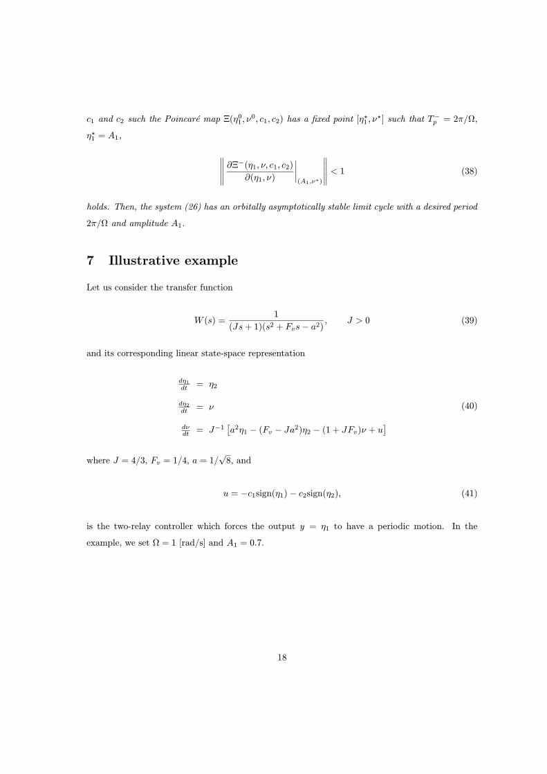
Figure 7: Evolution of the states η, ν of the closed-loop system.

7.1 Describing function and LPRS

First, we compute the value of c1 and c2 through DF by using the set of equations:

c1 =

π4 ∙

A1|W (jΩ)| ∙

(√1 + ξ2

)−1if Ω ∈ Q2 ∪Q3

−π4 ∙A1

|W (jΩ)| ∙(√1 + ξ2

)−1elsewhere

c2 = ξ ∙ c1.

where ξ = c2/c1, obtaining c1 = 0.8018 and c2 = 0.78.

To check if the periodic solution is stable find the derivative of the phase characteristic of the

plant with respect to the frequency

d argW

d lnω

∣∣∣∣ω=Ω

= −d arctan(Jω)

d lnω

∣∣∣∣ω=Ω

+d arctan( Fvω

ω2+a2 )

d lnω

∣∣∣∣∣ω=Ω

= −JΩ

J2Ω2 + 1+

FvΩ(a2 − Ω2)

F 2vΩ2 + (a2 +Ω2)2

.

(42)

The stability condition (??) for the system becomes:

−JΩ

J2Ω2 + 1+

FvΩ(a2 − Ω2)

F 2vΩ2 + (a2 +Ω2)2

≤ −ξ

ξ2 + 1. (43)

19

Notice that the left-hand side of (43) is −0.6447 and the right-hand side is −0.4998. Therefore,

the system is orbitally asymptotically stable.

Now, let us compute the exact values of c1 and c2 through LPRS by using the following formulas:

c1 =π

4

A1

AL(Ω)

1√1 + 2ξ cos(2πθ) + ξ2

, c2 =π

4

A1

AL(Ω)

ξ√1 + 2ξ cos(2πθ) + ξ2

,

obtaining c1 = 0.7017 and c2 = 0.6015.

7.2 Poincare map design

Let us begin with the mapping from ϕ1 into the domain ϕ2 (region R2) where the system (40)

takes the form:

dη1

dt= η2,

dη2

dt= ν,

dν

dt=3

32η1 −

1

16η2 − ν −

3

4c1 +

3

4c2. (44)

The solution of (44) on the time interval [0, Tsw] subject to the initial condition:

η+1 (η01 , ν

0, c1, c2) = η01 > 0, η

+2 (η

01 , ν

0, c1, c2) = 0, ν+(η01 , ν

0, c1, c2) = ν01

results in

η+1 = 8c1 − 8c2︸ ︷︷ ︸γ1

+

(

8c2 − 8c1 + η01 −16

3ν01

)

︸ ︷︷ ︸γ2(η01 ,ν

0,c1,c2)

e−t/2 +

(

4c2 − 4c1 +1

2η01 +

4

3ν01

)

︸ ︷︷ ︸γ3(η01 ,ν

0,c1,c2)

et/4 (45)

+

(

4c1 − 4c2 −1

2η01 + 4ν

01

)

︸ ︷︷ ︸γ4(η01 ,ν

0,c1,c2)

e−3t/4 (46)

η+2 = −1

2γ2(η

01 , ν

0, c1, c2)e−t/2 +

1

4γ3(η

01 , ν

0, c1, c2)et/4 −

3

4γ4(η

01 , ν

0, c1, c2)e−3t/4 (47)

ν+ =1

4γ2(η

01 , ν

0, c1, c2)e−t/2 +

1

16γ3(η

01 , ν

0, c1, c2)et/4 +

9

16γ4(η

01 , ν

0, c1, c2)e−3t/4, (48)

20

where

Tsw(η01 , ν

0, c1, c2) = 4 ln z, z = et/4 (49)

is obtained as the smallest positive root of

η+1 (Tsw, η01 , ν

0, c1, c2) = γ3z4 + γ1z

3 + γ2z + γ4 = 0, (50)

where γ1 = γ1(η01 , ν

0, c1, c2), γ2 = γ2(η01 , ν

0, c1, c2), and γ3 = γ3(η01 , ν

0, c1, c2). Let us proceed with

the mapping from ϕ2 into the domain ϕ3 (region R3) where the system (40) takes the form:

dη1

dt= η2,

dη2

dt= ν,

dν

dt=3

32η1 −

1

16η2 − ν +

3

4c1 +

3

4c2. (51)

The solution of (51) on the time interval [Tsw, Tp] subject to the initial condition:

η+1sw = η+1p(Tsw, η

01 , c1, c2) = 0,

η+2sw = η+2p(Tsw, η

01 , c1, c2) = −

1

2γ2e

−Tsw/2 +1

4γ3e

Tsw/4 −3

4γ4e

−3Tsw/4

results in

η+1p = −8c1 − 8c2 + 8

(

c1 + c2 −1

3η+2sw

)

︸ ︷︷ ︸γ1p(η01 ,ν

0,c1,c2)

e−(t−Tsw)/2 − 4

(

c1 + c2 −1

4η+2sw

)

︸ ︷︷ ︸γ2p(η01 ,ν

0,c1,c2)

e−3(t−Tsw)/4

+4

(

c1 + c2 +5

12η+2sw

)

︸ ︷︷ ︸γ3p(η01 ,ν

0,c1,c2)

e(t−Tsw)/4 (52)

η+2p = −4γ1pe−(t−Tsw)/2 + 3γ2pe

−3(t−Tsw)/4 + γ3pe(t−Tsw)/4 (53)

η+3p = 2γ1pe−(t−Tsw)/2 −

9

4γ2pe

−3(t−Tsw)/4 +1

4γ3pe

(t−Tsw)/4 (54)

21

where γ1p = γ1p(η01 , ν

0, c1, c2), γ2p = γ2p(η01 , ν

0, c1, c2), γ3p = γ3p(η01 , ν

0, c1, c2), and

Tp(η01 , ν

0, c1, c2) = 4 ln zp + Tsw, zp = e(t−Tsw)/4 (55)

results from the the smallest positive root of

η+2p(Tp, η01 , ν

0, c1, c2) = γ3pz4p − 4γ1pzp + 3γ2p = 0. (56)

Then, the Poincare map is

Ξ+1 (Tp(η01 , ν

0, c1, c2), η01 , ν

0, c1, c2) =

γ1 + γ2e

−Tp/2 + γ3eTp/4 + γ4e

−3Tp/4

14γ2e

−Tp/2 + 116γ3e

Tp/4 + 916γ4e

−3Tp/4

(57)

and the fixed point that is the solution of

−

η01

ν0

= Ξ+1 (Tp(η01 , ν

0, c1, c2), η0, ν0, c1, c2)

which results in

(η01)?= −

γ1 + [8c2 − 8c1 − 163 ν01 ]e−Tp/2 + [4c2 − 4c1 + 43ν

01 ]eTp/4 + [4c1 − 4c2 + 4ν01 ]e

−3Tp/4

1 + e−ΔT/2 + 12eΔT/4 − 12e

−3ΔT/4

(ν01)?=

14

[8c2 − 8c1 + η01

]e−Tp/2 + 1

16

[4c2 − 4c1 + 12η

01

]eTp/4 + 9

16

[4c1 − 4c2 + 12η

01

]e−3Tp/4

43e−Tp/2 − 1

12eTp/4 − 94e

−3Tp/4.

To complete the design it remains to provide the set of equations to find c1 and c2 in terms of the

known parameters Tp and η01 . Toward this end, we obtain from above equations that c1 and c2 are

solution of the following set of equations

c2 − c1 =1

4∙−[1 + e−Tp/2 + 12e

Tp/4 − 14e−3Tp/4](η01)

? − γ1 + ( 163 e−Tp/2 − 43e

Tp/4 − 4e−3Tp/4)ν012e−Tp/2 + eTp/4 − e−3Tp/4

(58)

c2 + c1 =

[43e−Tp/2 − 1

12eTp/4 − 94e

−3Tp/4](ν0)? −

[14e−Tp/2 + 1

32eTp/4 + 9

32e−3Tp/4

]η01

2e−Tp/2 + 14eTp/4 − 94e

−3Tp/4. (59)

22

Finally, for a given frequency T1+T2 = 2π/Ω and amplitude η01 = A1 we need to check the stability,

i.e.,

∥∥∥∥∥∂Ξ+1 ((η

01)?, (ν0)?, c1, c2)

∂(η01 , ν0)

∣∣∣∣(η01)

?,(ν0)?

∥∥∥∥∥=

∥∥∥∥∥∥∥∥∥∥

∂Ξ+11((η01)?,(ν0)?,c1,c2)

∂η01

∣∣∣(η01)

?,(ν0)?

∂Ξ+11((η01)?,(ν0)?,c1,c2)∂ν0

∣∣∣(η01)

?,(ν0)?

∂Ξ+21((η01)?,(ν0)?,c1,c2)

∂η01

∣∣∣(η01)

?,(ν0)?

∂Ξ+21((η01)?,(ν0)?,c1,c2)∂ν0

∣∣∣(η01)

?,(ν0)?

∥∥∥∥∥∥∥∥∥∥

< 1, (60)

where

∂Ξ+11(η01 , ν

0, c1, c2)

∂η01= −

[

−1

2γ2e

−Tp/2 +1

4γ3e

Tp/4 −3

4γ4e

−3Tp/4

]∂Tp

∂η01

+e−Tp/2 +1

2eTp/4 −

1

2e−3Tp/4 ' −0.4416 (61)

∂Ξ+11(η01 , ν

0, c1, c2)

∂ν0= −

[

−1

2γ2e

−Tp/2 +1

4γ3e

Tp/4 −3

4γ4e

−3Tp/4

]∂Tp

∂ν0

−16

3e−Tp/2 +

3

4eTp/4 + 4e−3Tp/4 ' 0.1745 (62)

∂Ξ+21(η01 , ν

0, c1, c2)

∂η01= −

[

−1

8γ2e

−Tp/2 +1

64γ3e

Tp/4 −27

64γ4e

−3Tp/4

]∂Tp

∂η01

+1

4e−Tp/2 +

1

16eTp/4 +

9

16e−3Tp/4 ' 0.2088 (63)

∂Ξ+21(η01 , ν

0, c1, c2)

∂ν0= −

[

−1

8γ2e

−Tp/2 +1

64γ3e

Tp/4 −27

64γ4e

−3Tp/4

]∂Tp

∂ν0

−4

3e−Tp/2 +

1

12eTp/4 +

9

4e−3Tp/4 ' 0.1042, (64)

23

0 20 40 60 80 100-0.8

-0.6

-0.4

-0.2

0

0.2

0.4

0.6

0.8

Time [s]

x1 [r

ad]

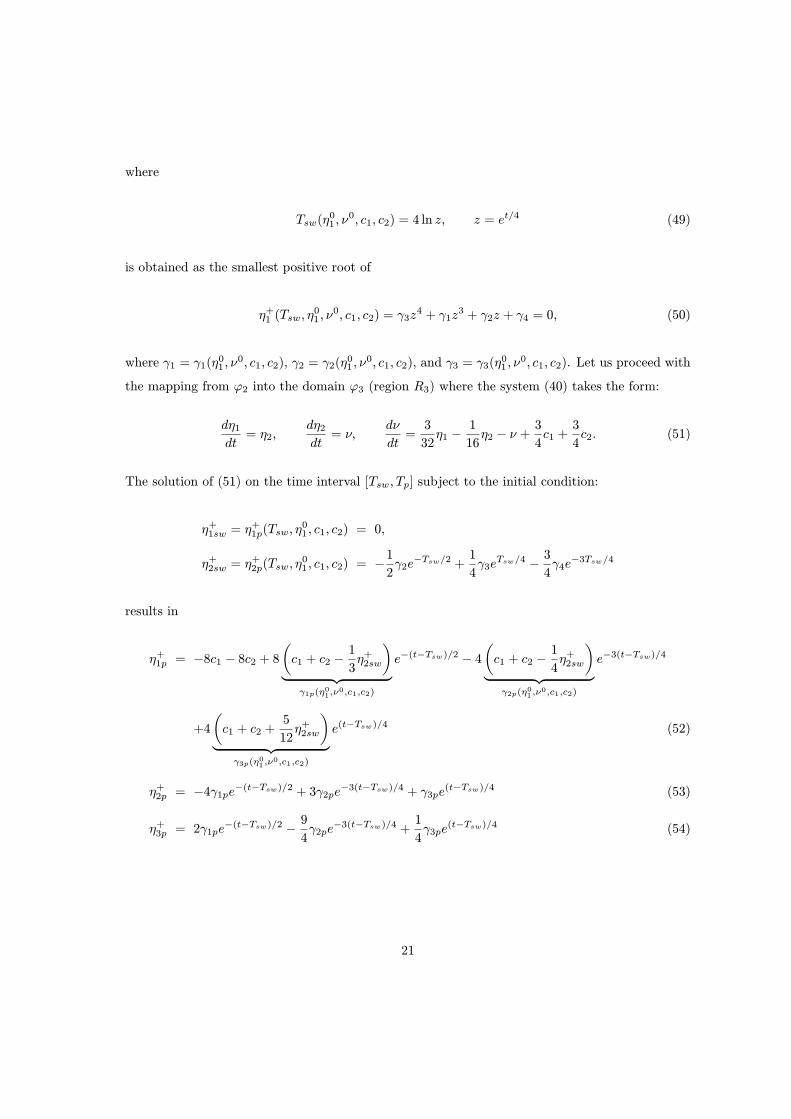
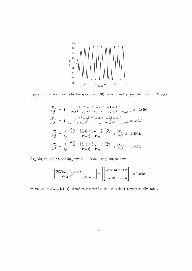
Figure 8: Simulation results for the system (2), (40) under c1 and c2 computed from LPRS algo-rithm.

∂Tsw

∂η01= 4 ∙

12z−4 − z−3 + 12z

−1 + 1− 12z3

−4γ3z3 − 3γ1z2 − γ2 + γ3 − 2γ2z−3 − 3γ4z−4' −0.6399,

∂Tsw

∂ν0= 4 ∙

4z−4 − 163 z−3 − 4z−1 + 203 −

43z3

4γ3z3 + 3γ1z2 + γ2 − γ3 + 2γ2z−3 + 3γ4z−4' 1.4989,

∂Tp

∂η01=4

zp∙

∂η+2p∂η01−[512z

4p +

43zp −

34

] ∂η+2sw∂η01

4γ3pz3p − 4γ1p+∂Tsw

∂η01' −2.4002,

∂Tp

∂ν0=4

zp∙∂η+2p∂ν0−[512z

4p +

43zp −

34

] ∂η+2sw∂ν0

4γ3pz3p − 4γ1p+∂Tsw

∂ν0' −1.0468,

∂η+2p/∂η01 ' −9.8782, and ∂η

+2p/∂ν

0 ' −1.5876. Using (60), we have

∥∥∥∥∥∂Ξ+1 (η

01 , ν

0, c1, c2)

∂(η01 , ν0)

∣∣∣∣(η01)

?,(ν0)?

∥∥∥∥∥=

∥∥∥∥∥∥∥

−0.4416 0.1745

0.2088 0.1042

∥∥∥∥∥∥∥' 0.5030

where ‖A‖ =√λmax{ATA}; therefore, it is verified that the orbit is asymptotically stable.

24

r

Lp

hq2

q1

x

z

y

Figure 9: The experimental Furuta pendulum system.

8 Experimental study: The Furuta pendulum

8.1 Experimental setup

In this section, we present experimental results using the laboratory Furuta pendulum, produced

by Quanser Consulting Inc., depicted in Figure 8. It consists of a 24-Volt DC motor that is coupled

with an encoder and is mounted vertically in the metal chamber. The L-shaped arm, or hub, is

connected to the motor shaft and pivots between ±180 degrees. At the end, a suspended pendulum

is attached. The pendulum angle is measured by the encoder. As described in Fig. 8, the arm

rotates about z axis and its angle is denoted by q1 while the pendulum attached to the arm rotates

about its pivot and its angle is called q2. The experimental setup includes a PC equipped with an

NI-M series data acquisition card connected to the Educational Laboratory Virtual Instrumentation

Suite (NI-ELVIS) workstation from National Instrument. The controller was implemented using

Labview programming language allowing debugging, virtual oscilloscope, automation functions,

and data storage during the experiments. The sampling frequency for control implementation has

been set to 400 Hz. Appendix A gives the dynamic model of the Furuta pendulum.

8.2 Experimental results

Experiments were carried out to achieve the orbital stabilization of the unactuated link (the pen-

dulum) y = q2 around the equilibrium point q? = (π, 0). The equation of motion of the Furuta

pendulum (1) is linearized around q? ∈ IR2 and by virtue of the instability of the linearized open-

loop system, a state-feedback controller uf = −Kx and x = (q − q?, q)T ∈ IR4, is designed such

25

10-2

10-1

100

101

102

-100

-50

0

50

mag

nitu

de [d

B]

Bode diagram

10-2

10-1

100

101

102

-200

-100

0

100

200

Frequency [rad/s]

phas

e [d

eg]

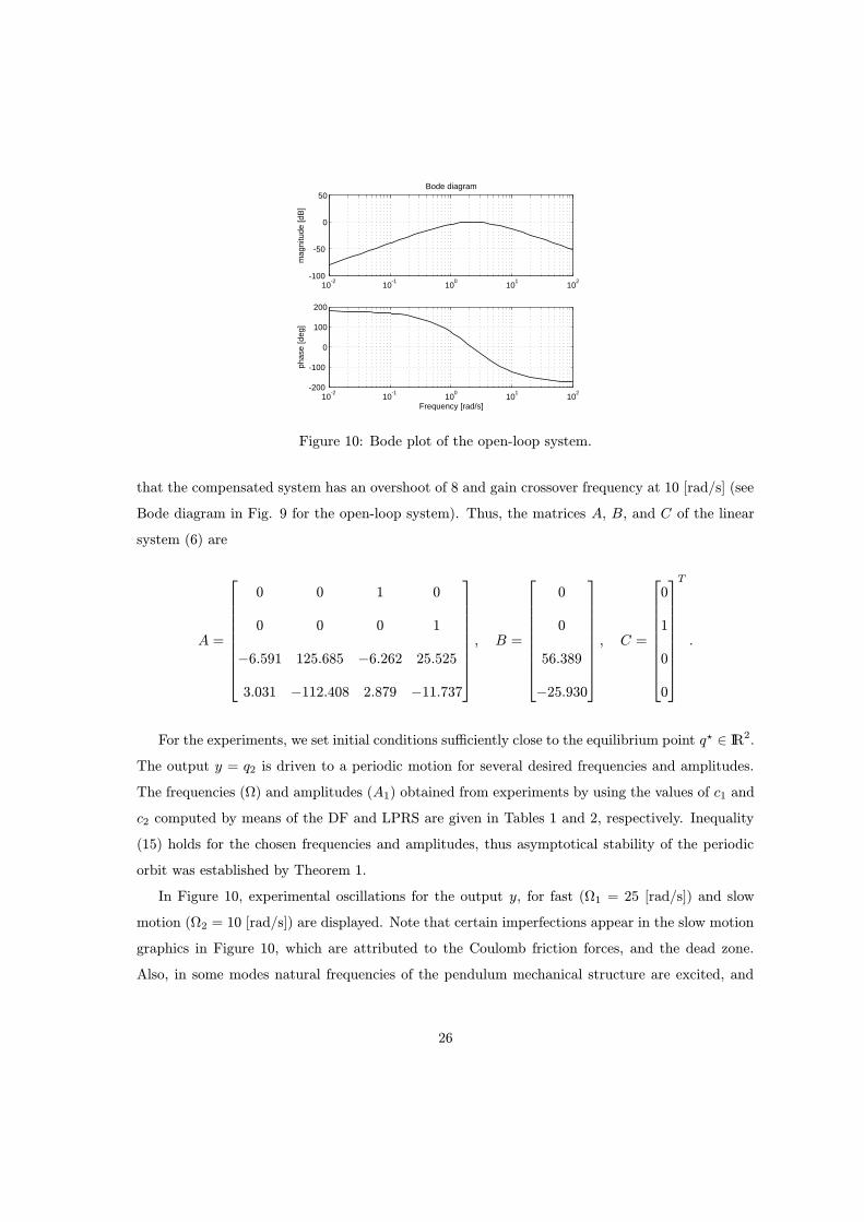
Figure 10: Bode plot of the open-loop system.

that the compensated system has an overshoot of 8 and gain crossover frequency at 10 [rad/s] (see

Bode diagram in Fig. 9 for the open-loop system). Thus, the matrices A, B, and C of the linear

system (6) are

A =

0 0 1 0

0 0 0 1

−6.591 125.685 −6.262 25.525

3.031 −112.408 2.879 −11.737

, B =

0

0

56.389

−25.930

, C =

0

1

0

0

T

.

For the experiments, we set initial conditions sufficiently close to the equilibrium point q? ∈ IR2.

The output y = q2 is driven to a periodic motion for several desired frequencies and amplitudes.

The frequencies (Ω) and amplitudes (A1) obtained from experiments by using the values of c1 and

c2 computed by means of the DF and LPRS are given in Tables 1 and 2, respectively. Inequality

(15) holds for the chosen frequencies and amplitudes, thus asymptotical stability of the periodic

orbit was established by Theorem 1.

In Figure 10, experimental oscillations for the output y, for fast (Ω1 = 25 [rad/s]) and slow

motion (Ω2 = 10 [rad/s]) are displayed. Note that certain imperfections appear in the slow motion

graphics in Figure 10, which are attributed to the Coulomb friction forces, and the dead zone.

Also, in some modes natural frequencies of the pendulum mechanical structure are excited, and

26

6 6.5 7 7.5 8-0.5

0

0.5

q1 [r

ad]

6 6.5 7 7.5 8

3

3.1

3.2

3.3

Time [s]

y=q2

[rad

]

6 6.5 7 7.5 8-0.5

0

0.5

1

q1 [r

ad]

6 6.5 7 7.5 83

3.1

3.2

3.3

Time [s]

y=q2

[rad

]

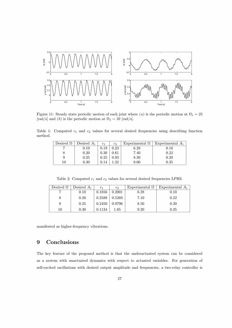
Figure 11: Steady state periodic motion of each joint where (a) is the periodic motion at Ω1 = 25[rad/s] and (b) is the periodic motion at Ω2 = 10 [rad/s].

Table 1: Computed c1 and c2 values for several desired frequencies using describing functionmethod.

Desired Ω Desired A1 c1 c2 Experimental Ω Experimental A17 0.10 0.19 0.23 6.28 0.108 0.20 0.30 0.61 7.40 0.229 0.25 0.25 0.93 8.30 0.2010 0.30 0.14 1.32 9.00 0.35

Table 2: Computed c1 and c2 values for several desired frequencies LPRS.

Desired Ω Desired A1 c1 c2 Experimental Ω Experimental A17 0.10 0.1856 0.2001 6.28 0.10

8 0.20 0.2589 0.5269 7.10 0.22

9 0.25 0.2450 0.9796 8.50 0.20

10 0.30 0.1134 1.65 9.20 0.35

manifested as higher-frequency vibrations.

9 Conclusions

The key feature of the proposed method is that the underactuated system can be considered

as a system with unactuated dynamics with respect to actuated variables. For generation of

self-excited oscillations with desired output amplitude and frequencies, a two-relay controller is

27

proposed. The systematic approach for two-relay controller parameter adjustment is proposed.

The DF method provides approximate values of controller parameters for the plants with the low-

pass filter properties. The LPRS gives exact values of the controller parameters for the linear

plants. The Poincare maps provides the values of the controller parameters ensuring the existence

of the locally orbitally stable periodic motions for an arbitrary mechanical plant. The effectiveness

of the proposed design procedures is supported by experiments carried out on the Furuta pendulum

from Quanser.

A Dynamic model of Furuta pendulum

The equation motion of Furuta pendulum, described by (1), was specified by applying the Euler-

Lagrange formulation [8] where

M(q) =

M11(q) M12(q)

M12(q) M22(q)

, H(q, q) =

H1(q, q)

H2(q, q)

with

M11(q) = Jeq +Mpr2 cos2(q1),

M12(q) = −1

2Mprlp cos(q1) cos(q2),

M22(q) = Jp +Mpl2p,

H1(q, q) = −2Mpr2 cos(q1) sin(q1)q

21 +1

4Mprlp cos(q1) sin(q2)q

22

H2(q, q) =1

2Mprlp sin(q1) cos(q2)q

21 +Mpglp sin(q2)

where Mp = 0.027 [Kg] is mass of the pendulum, lp = 0.153 [m] is the length of pendulum

center of mass from pivot, Lp = 0.191 [m] is the total length of pendulum, r = 0.0826 [m] is

the length of arm pivot to pendulum pivot, g = 9.810 [m/s2] is the gravitational acceleration

constant, Jp = 1.23 × 10−4 [Kg-m2] is the pendulum moment of inertia about its pivot axis, and

Jeq = 1.10× 10−4 [Kg-m2] is the equivalent moment of inertia about motor shaft pivot axis.

28

References

[1] L. Aguilar, I. Boiko, L. Fridman and R Iriarte, “Generating self-excited oscillations via two-

relay controller,” To appear in IEEE Transactions on Automatic Control, vol. 54, no. 1, 2009.

[2] L. Aguilar, I. Boiko, L. Fridman and R. Iriarte, “Periodic motion of underactuated mechanical

systems self-generated by variable structure controllers: design and experiments,” in 2007

European Control Conference, July 2–5, pp. 3796–3801, Kos, Greece, 2007.

[3] D.P. Atherton, Nonlinear control engineering–Describing Function Analysis and Design.

Workingham, U.K.: Van Nostrand, 1975.

[4] I. Boiko, L. Fridman and M.I. Castellanos, “Analysis of second-order sliding-mode algorithms

in the frequency domain,” IEEE Trans. Automat. Contr., vol. 49, no. 6, pp. 946–950, June

2004.

[5] I. Boiko, “Oscillations and transfer properties of relay servo systems – the locus of a perturbed

relay system approach,” Automatica, vol. 41, no. 4, pp. 677–683, Apr. 2005.

[6] I. Boiko, L. Fridman, A. Pisano and E. Usai, “Analysis of chattering in systems with second-

order sliding modes,” IEEE Trans. Automat. Contr., vol. 52, no. 11, pp. 2085–2102, Nov.

2007.

[7] C. Chevallereau, G. Abba, Y. Aoustin, F. Plestan, C. Canudas-de-Wit and J.W. Grizzle,

“RABBIT: A testbed for advanced control theory,” IEEE Control Systems Magazine, vol. 23,

no. 5, pp. 57–79, Oct. 2003.

[8] J. Craig, Introduction to robotics: Mechanics and Control. Massachusetts, MA: Addison-

Wesley Publishing, 1989.

[9] M. Di Bernardo, K.H Johansson, F. Vasca, “Self-oscillations and sliding in relay feedback

systems: Symmetry and bifurcations,” Int. J. of Bifurcation and Chaos, vol. 11, pp. 1121–

1140, April 2001.

[10] I. Fantoni and R. Lozano, Nonlinear control for underactuated mechanical systems. London:

Springer, 2001.

29

[11] L.Fridman, “An averaging approach to chattering,” IEEE Trans. Automat. Contr., vol. 46,

no. 8, pp. 1260–1265, 2001.

[12] J.W. Grizzle, C.H. Moog and C. Chevallereau, “Nonlinear control of mechanical systems with

an unactuated cyclic variable,” IEEE Trans. Autom. Control, vol. 50, no. 5, pp. 559–576, May

2005.

[13] A. Levant, “Sliding order and sliding accuracy in sliding mode control,” Int. J. of Control,

vol. 58, pp.1247–1263, 1993.

[14] J.M. Loeb, “Advances in nonlinear servo theory”, in R. Oldenburger (ed.), Frequency Re-

sponse, The Macmillan Company, New York, pp.260–268, 1956.

[15] Y. Orlov, S. Riachy, T. Floquet, and J.-P. Richard, “Stabilization of the cart-pendulum sys-

tem via quasi-homogeneous switched control,” Proc. of the 2006 Int. Workshop on Variable

Structure Systems, Alghero, Italy, June 5-7, pp. 139–142, 2006.

[16] S. Riachy, Y. Orlov, T. Floquet, R. Santiesteban and J.P. Richard, “Second-order sliding

mode control of underactuated mechanical systems I: Local stabilization with application to

an inverted pendulum,” Int. J. of Robust and Nonlinear Control, vol. 18, nos. 4-5, pp. 529–543,

2008.

[17] S. Sastry, Nonlinear systems: Analysis, stability and control. London: Springer, 1999

[18] A.S. Shiriaev, L.B. Freidovich, A. Robertsson and A. Sandberg, “Virtual-holonomic-

constraints-based design stable oscillations of Furuta pendulum: theory and experiments,”

IEEE Trans. Robot., vol. 23, no. 4, pp. 827–832, 2007.

[19] V.I.Utkin, Sliding modes in control and optimization, Berlin: Springer Verlag, 1992.

30