Generalized theory for the dynamic analysis of thin shells with 1

application to circular cylindrical geometries 2

by 3

Raydin Salahifar a , Magdi Mohareb b 4 a Baha’i Institute for Higher Education, Tehran, Iran, Tel.: +989125472292, Raydin.Salahifar@bihe.org, 5

RaydinSalahifar@yahoo.com (Corresponding author) 6 b Department of Civil Engineering, University of Ottawa, Ottawa, ON, Canada K1N 6N5, 7

MMohareb@uottawa.ca 8

9

Abstract 10

A generalized theory is formulated for the analysis of thin shells of general curvatures based 11

on the variational form of the Hamiltonian functional in conjunction with tensor calculus. 12

Simplifying approximations and subtle inconsistencies made at the early stages of common 13

classical formulations are avoided herein, and hence, the present treatment leads to field 14

equations and boundary conditions that are accurate and consistent. The theory is then 15

specialized to circular cylindrical shells. The well -known field equations of Flugge and 16

Donnell-Mushtari-Vlasov (DMV) theories are recovered as consistent approximations from 17

the present theory. Closed form solutions are then developed for the present and past 18

cylindrical shell theories by Flugge, Timoshenko, and DMV. A comparative study is 19

conducted to assess and quantify the effects of approximations made in classical theories on 20

the predicted displacements and stresses. 21

Keywords 22

Thin shell theory, shells with general curvature, cylindrical shells, Hamilton principle, steady 23

state response, Tensor-based formulation 24

25

This article is to be cited as 26 Salahifar R, Mohareb M, (2019) Generalized theory for the dynamic analysis of thin shells with application to circular 27 cylindrical geometries, Thin-Walled Structures, 139: 347-36. 28

The copy-edited version of this article is available at: https://doi.org/10.1016/j.tws.2018.11.021. 29

2

1. Introduction 30

Thin shells are commonly encountered in structural applications, onshore and offshore 31

pipelines, and mechanical equipment, where they are commonly subjected to a variety of 32

static, quasi-static or dynamic loading. Under such conditions, shells may undergo a complex 33

deformational behaviour. The literature reveals the presence of several seemingly conflicting 34

stress-deformation theories for thin-shells. The selection for a proper shell theory in a given 35

application requires (a) an in-depth understanding of the underlying assumptions, and (b) a 36

critical assessment of various assumptions on the predictive ability of the theory. Within this 37

context, the present study contributes to both objectives by developing a theory for thin shells 38

of general geometries while keeping the assumptions and simplifications made to a minimum. 39

The formulation is then specialized to circular cylindrical shells. By applying various 40

approximations to the resulting formulation, other well-established cylindrical thin-walled 41

shell theories are recovered as special cases. 42

1.1 Literature Review 43

Classical linear shell theories involve the work of Timoshenko [1], Novozhilov [2], Koiter [3], 44

Flugge [4] (and [5]), Saada [6], DMV [7] and Niordson [7]. Non-linear shell theories include 45

the work of Leonard [8], Sanders [9], Koiter [10] , [11] and Budiansky [12]. The 46

comprehensive monograph by Leissa [13] provides a detailed report on the wide range of shell 47

theories available. Libai and Bert [14] developed mixed variational principles for the elastic 48

small-strains and large-rotation analysis of shells based on the Kirchhoff-Love hypothesis. 49

Muneeb et al. [15] developed a higher order theory for the dynamic response of isotropic 50

thermo-elastic analysis of cylindrical shells. Kolesnikov [16] formulated a refined theory for 51

the vibration of multilayer orthotropic cylindrical shells through a series expansion of the 52

radial displacement field in terms of the shell thickness. Through asymptotic expansion of the 53

general equilibrium equations for a general state of stress in three-dimensional bodies, 54

Niordson [17] formulated a two-dimensional shell theory for circular cylindrical shells. 55

Ugrimov [18] presented a layerwise generalized theory for the elasto-dynamic analysis of 56

multilayer plates by expanding the displacement components of each layer as power series of 57

the transverse coordinate. Ciarlet and Gratie [19] developed an approach to minimize the 58

quadratic problem arising in Koiter's linear shell theory. Using the Cosserat surface model, 59

Birsan [20] presented a theory for porous elastic shells by employing the Nunziato-Cowin 60

3

theory of elastic materials with voids, to characterize the porosity within the shell. Altenbach 61

et al. [21] developed a linear shell theory that accounts for transverse shear and surface 62

stresses. Weicker et al. ([22] and [23]) developed a closed form solution for the static analysis 63

of thin-walled pipes [22], and a finite element formulation [23]. Salahifar and Mohareb [24] 64

formulated a closed form solution for circular cylindrical shells under harmonic forces. 65

Amabili and Reddy [25] derived a consistent higher-order shear deformable theory for doubly 66

curved shells of general geometries based on non-linear strain-displacement expressions. 67

Their solution accounts for geometric imperfections. Paimushin [26] developed a large 68

displacement shell theory based on the classical Kirchhoff-Love assumption. The solution 69

accounts for deformations in the transverse direction by introducing additional displacement 70

fields. Salahifar and Mohareb [27] formulated a finite element for the analysis of circular 71

cylindrical thin shells under harmonic forces based on shape functions that satisfy the 72

governing field equations. Favata and Podio-Guidugli [28] developed a theory of linearly 73

elastic orthotropic shells with potential application to the continuous modeling of carbon 74

nanotubes. Sansour et al. [29] developed a computationally efficiently strain gradient 75

formulation that captures the scale effects of shell-like structures when one of the dimensions 76

is very small relative to the other two dimensions. Xuea et al. [30] extended the Karman-77

Donnell theory for shallow cylindrical shells to account for large deformations. Based on an 78

expansion of the axisymmetric equations of elasticity, Zozulya [31] developed a high-order 79

theory for functionally graded axisymmetric cylindrical shells using Legendre polynomial 80

series. Carrera et al. [32] (and [33]) developed a unified hierarchical formulation for 81

multilayered composite structures, which enables the implementation of multiple plate/shell 82

theories and finite elements based on a few fundamental nuclei. Cattabiani et al. [34] 83

developed a variational shell theory that approximates the solution for the vibration problem 84

as a sum of shape functions that identically satisfy the equilibrium equations while satisfying 85

the weak form of the boundary conditions. Chowdhurya et al. [35] developed a state-based 86

peridynamic formulation for the linear elastic analysis of shells that captures discontinuities 87

by expressing the equations of motion in integro-differential form as opposed to partial 88

differential equations. Zveryayev [36] developed an itertative shell solution, in which the 89

three-dimensional equations of the elasticity in curvilinear coordinates were reduced using the 90

Saint-Venant semi-inverse method. Awrejcewicz et al. [37] presented a mathematical model 91

for nonlinear analysis of micro-shells that accounts for temperature-deformation coupling. 92

Using Hamilton’s principle, Wangab et al. [38] developed a first-order shear deformable shell 93

4

theory for the free and transient vibration analysis of composite laminated cylindrical shells 94

by partitioning the radial displacement field into bending and shear components. Okhovat and 95

Bostrom [39] derived a hierarchy of shell equations in the form of power series in terms of the 96

shell thickness for the dynamic analysis of orthotropic cylindrical shells. Qingshan et al. [40] 97

developed a first-order shear deformable shell theory for the free and transient vibration 98

analysis of laminated open cylindrical shells with general boundary conditions. 99

1.2 Common Assumptions 100

In general, the theory of thin shells involves two aspects: a) developing the governing field 101

equations and the boundary conditions and b) providing solutions to the field equations for 102

problems with specific geometries, boundary conditions, and loading. Most thin-shell 103

formulations are based on the following assumptions: 104

1. Conservation of normals: All points lying on a normal to the middle surface before 105

deformation remain on the normal to the deformed middle surface. This implies a linear 106

distribution of the in-plane displacements across the thickness of the shell and zero shear 107

strains in the planes normal to the mid-surface. 108

2. A surface at a distance z from the middle surface before deformation will remain at the 109

same distance from the middle surface after deformation, and 110

3. Displacements are small compared to the radii of curvature of the middle surface. This 111

signifies that the curvatures of the shell mid-surface after deformation are considered 112

nearly equal to the curvatures before deformation. 113

1.3 Differences among Shell Theories 114

A survey of the literature reveals the presence of multiple cylindrical thin-shell theories. The 115

differences between these shell theories are attributed to the following aspects: 116

1. The adoption of different strain-displacement relationships: In some theories (e.g., 117

Timoshenko[1] and Flugge [3]) the strain-displacement relationships are obtained based on 118

geometric inspection of an infinitesimal portion of the shell undergoing deformation. In 119

other theories (e.g., Novozhilov [2], Saada [6] and Niordson [7]), a vector or tensor analysis 120

approach is adopted. 121

5

2. The use of different methodologies in formulating the governing equations: In most theories 122

(e.g., Timoshenko [1], Flugge [4], Saada [6] and Niordson [7]), equilibrium equations are 123

obtained based on the force equilibrium of an infinitesimal shell element, while others (e.g., 124

Novozhilov [2]) adopt a variational approach. 125

3. The enforcement of additional simplifications: Most researchers have applied various 126

simplifications at different stages of the formulation, which had implications on the final 127

form of the governing field equations and the boundary conditions. For example, 128

Novozhilov [2] has neglected some of the terms in the expression of total potential energy 129

compared to the other terms. 130

4. Inconsistencies in enforcing simplifications: Most theories (Timoshenko [1], Saada [6], 131

Niordson [7], etc.) involved slight inconsistencies in their simplifications. For example, the 132

effect of the shell thickness in the strain expression is neglected in some terms, but kept in 133

other terms within the same formulation. These types of inconsistencies, in most cases, 134

arose from separating the membrane strains from the bending strains. 135

Given the above discrepancies, it is difficult to judge which theories provide superior results 136

and which are most suited for a given engineering problem. While, in some cases, there could 137

be some qualitative notion on which theory could be judged to provide reliable predictions of 138

the response, a systematic quantitative comparative assessment is missing. For a given 139

problem, it becomes difficult to judge how much error is attributed to treating a given problem 140

as a thin shell and how much is attributed to the approximations and treatments specific to the 141

adopted theory. In order to elucidate the problem, the present treatment focuses on developing 142

a generalized thin shell theory in which the strain-displacement relationships are thoroughly 143

formulated based on tensor calculus in conjunction with assumptions that are well accepted 144

within the framework of all thin-shell theories, while avoiding inconsistencies. 145

2. Generalized Thin Shell Theory Formulation 146

2.1 Geometric preliminaries 147

In general, a thin shell can be considered as a group of parallel curved surfaces in the 148

immediate vicinity of the middle surface. Point 0P on a surface can be defined by two 149

curvilinear coordinates of a two dimensional subspace ( R ) of the general three-dimensional 150

6

space ( iR ). As a notation convention, all Latin indices take the values 1, 2, 3, while Greek 151

indices take the values 1 and 2. This implies that, in a curvilinear coordinate system ix , the 152

geometry of any of those surfaces can be defined by two curvilinear coordinates x within 153

the middle surface and an additional coordinate 3x normal to the middle surface (Figure 1). 154

In a Cartesian coordinate system i with iI as a covariant unit vector, position vector 155

1 1

i iP P it t R I at time t for a point 1P within the shell (Figure 1), can be defined as 156

the vector sum of position vector 0 0

i iP P it t r I of its projection 0P on the middle 157

surface and vector 0 1P P

, i.e., 158

1 0 0 10 1 ,i i i i

P P P Pt t P P t t

R r (1) 159

In Eq. 1, expressing the Cartesian coordinates i for points 0P and 1P (i. e. 0

iP t and

1

iP t160

) in terms of curvilinear coordinates ix enables expressing the position vectors for points 0P 161

and 1P as 00,P

i i jP it x t r I and 11

,Pi i jP it x t R I , respectively. Thus, 162

Cartesian coordinates i appearing in Eq. 1 can be expressed in terms of curvilinear 163

coordinates ix yielding 164

1 0 0 10 1, , , , ,P P P Pi j i j i j i jx t x t P P x t x t

R r (2) 165

or 166

01

33, ,PP

i j ix t x t x R r a (3) 167

in which unit vector 31 2 1 2 a a a a a is normal to the plane defined by base vectors 168

x a r . Equation 3 provides the transformation of a shell surface from curvilinear 169

coordinate system ix into Cartesian coordinate system i . It can be re-written as 170

1 2 3 1 2 33, , , , ,x x x t x x t x R r a (4) 171

172

7

173 Figure 1 - Shell Geometry 174

In a similar manner, bases ii x g R pertain to a general surface within the shell volume. 175

It can be shown that base vectors g on a surface parallel to the mid-surface are related to the 176

base vectors of the middle surface a through g a . Here, 3x b

is the shifter 177

tensor, is the Kronecker delta tensor and b

is the mixed curvature tensor for the middle 178

surface, which is related to the Christoffel symbol through 3b . Christoffel symbols 179

of the second kind are defined as , , , 2k klij li j lj i ij lg g g g and, as a matter of 180

convention, all symbols with a bar denote quantities pertaining to the middle surface, unless 181

mentioned otherwise. 182

In general, the contravariant counterparts of the covariant base vectors are g a and183

3 3g a , in which and the covariant and contravariant base vectors are related 184

through i ij j g g . The covariant and contravariant metric tensors for surfaces parallel to the 185

middle surface are respectively expressed as 186

,g a g a g g g g (5a-b) 187

8

where a and a are the covariant and contravariant metric tensors of the middle surface, 188

respectively, and defined as 189

,a a a a a a (6a-b) 190

The second fundamental tensor of the surface (curvature tensor) is defined as 3,b a a . 191

The Jacobian g at a generic point within the shell, given by det ijg g , represents a 192

differential element of volume. 193

2.2 Strains in Thin Shells 194

Using the Lagrangian approach, the strain tensor is defined in terms of the metric tensor 195

through ˆ 2ij ij ijg g . One can show [41] that the strain-displacement relationship is 196

defined by 12 | | | |k

ij i j j i i k jU U U U in which, the notationi denotes the covariant 197

derivative of the argument vector with respect to 1, 2,3i . Under the small deformation 198

assumption, the nonlinear terms | |ki k jU U are negligible compared to the linear terms. Also, 199

for thin shells, the strains can be resolved into in-plane components and out-of-plane 200

components 3 3 and 33 , and the displacement strain relations can be approximated by: 201

1 1 13 3 3 3 33 3 3 3 32 2 2| | , | | , | |U U U U U U (7a-c) 202

According to Assumption 2 in Section 1.2 , the strain normal to the mid-surface vanishes, i.e. 203

133 3 3 3 32 | | 0U U . Also, according to Assumption 1 in Section 1.2 , the transverse 204

shear strains acting on the planes perpendicular to the mid-surface are negligible for thin shells 205

leading to the simplification 3 3 0 . 206

2.3 Displacements of a Point within the Shell 207

In general, displacement vector U of a point A offset from the middle surface can be defined 208

as 209

1 2 3 1 2 3, , , , , ,i ii iU x x x t U x x x t U g g (8) 210

9

where iU and iU are, respectively, the covariant and contravariant components of the 211

displacement vector in the ix coordinate system. Displacement vector U is related to position 212

vector R in the undeformed configuration (Figure 2) and position vector R in the deformed 213

configuration through ˆ U R R . Vectors R and R at point A are related to vectors r and 214

r at the corresponding point B on the mid-surface and unit vectors normal to the mid-surface 215

3a and 3a as 216

3 3 33 3 3 3

ˆ ˆ ˆ ˆ ˆx x x U R R r a r a r r a a (9) 217

Noting that the difference ˆ u r r is the displacement vector at point B and 3a , 3a are the 218

unit vectors normal to the mid-surface at point B before and after deformation, the difference 219

3 3ˆ θ a a characterizes the angle of rotation of the middle surface and thus Eq. 9 can be re-220

written as 221

1 2 3 1 2, , , ,x x t x x x t U u θ (10) 222

Assumption 1 in Section 1.2 , regarding the normality to the mid-surface, implies zero shear 223

strains on the planes perpendicular to the mid-surface, i.e. 3 3 3 3| | 2 0U U . 224

It can be used [41] to relate the displacement U of arbitrary point A , located at a distance 225

3 0x from the shell mid-surface within the shell, to those of its projection on the middle 226

surface, point B ( iiuu a ), through 227

3 33 3, 3 3; ,U U U u x u U u

U g g (11) 228

Figure 2 shows points A and B , and their corresponding displacements U and u , 229

respectively. The geometric interpretations for U g and 3

3U g are schematically shown in 230

Figure 3, in which point A undergoes displacements U parallel to the shell mid-surface and 231

a displacement 3U normal to the mid-surface. Similarly, the contravariant components of the 232

displacement are related to those of point B on the middle surface through 233

3 3 3 33 3, 3, ,U U U U g u x u g U u u

U g g (12a-c) 234

10

235 Figure 2- Deformed and Un-deformed Configurations of a Thin Shell 236

237

238

239 Figure 3 - Displacement of a generic point within the shell 240

A

A

3

2

hx

3

2

hx

3

2

hx

3

2

hx

3 0x

3 0x

U g

33U g U

11

2.4 Stress-Strain Relationship 241

For elastic materials, stress tensor ij ( , 1,2,3i j ) for a point at a distance 3x from the middle 242

surface ( 32 2h x h ) is related to the corresponding strain tensor lm ( , 1,2,3l m ) 243

through ij ijlmlmE (e.g., Flugge [5]), in which ijlmE is the fourth order constitutive elastic 244

tensor. For thin shells, where the stresses perpendicular to the middle surface are negligible, 245

the number of non-zero stress components reduces from nine to four and the stress-strain 246

relationships reduce to 247

, , , , 1,2E (13) 248

Under linear elastic isotropy, the constitutive tensor can be shown [41] to take the form 249

2

2 1 1

EE g g g g g g

(14) 250

in which E is the Modulus of elasticity and is Poisson’s ratio. 251

2.5 Hamilton Principle for Thin Shells of General Geometries 252

According to Hamilton’s principle, the variation of the mechanical energy is given by 253

2 2 2

1 1 1

( ) 0t t t

t t t

dt T V dt W dt (15) 254

in which all time integrations are performed over an arbitrary period starting from time 1t to 255

time 2t and T , V and W are the kinetic energy, internal strain energy and external work 256

in the system, respectively, and are given by 257

, ,i ijkl ii kl ij i

V V V

T U U dV V E dV W F U dV (16a-c) 258

in which integrations are over the volume V and symbols iF denote the contravariant 259

components of the applied forces. From Eq. 16a-c, by substituting into Eq. 15, integrating by 260

parts the kinetic energy terms with respect to time, and using the relation 261

3| ||U U U b (in which, symbol || denotes the covariant derivative components of the 262

12

preceding argument with respect to x , i.e. ,||U U U ) in the internal strain energy 263

integral term and integrating by parts with respect to x yields [41] 264

22 2

1 11

132 0

13, 32

132

132

|| || 2

|| || 2 2 ||

|| || || 2

|| || 2

tt ti i

i it V t Vt

x

A

V

dt U U dV U U dVdt

E U U U b U dA

E U U U b U b

E U U U b U dV

E U U U b

3

0

V

ii

V

b U dV

F U dV dt

(17) 265

Equation 17 is the variational form of the mechanical energy for a thin shell with general 266

curvature. The theory can be specialized to shells with specific geometries. In this context, the 267

present paper aims at specializing Eq. 17 to circular cylindrical shells. Readers interested in 268

the application of the theory to other shell geometries are referred to [41], where it has been 269

specialized to toroidal shells. 270

3. Special Case: Circular Cylindrical Thin Shells (CCTS) 271

3.1 Geometric properties 272

Position vector r for a general point lying on the middle surface of a circular cylinder is 273

expressed in terms of unit vectors iI

in the Cartesian coordinate system i (Figure 4). In terms 274

of the curvilinear coordinates system ix , it takes the form 275

1 2 1 2 21 2 3, , sin cosx x t x R x R R x R r I I I

(18) 276

13

277 Figure 4 - Cartesian and Curvilinear Coordinates 278

From this point, symbols , ,x s z will be used instead of 1 2 3, ,x x x for clarity. The non-zero 279

components of the covariant and contravariant base vectors for a surface parallel to the mid-280

surface lying within the shell can be shown [41] to be 281

1 1 2 2 3 311 1 2 2 3 3

, 1 ,

, 1 ,

z R

z R

g j g j g j

g j g j g j

(19) 282

where ij

and ij

are the covariant and contravariant unit vectors associated with base vectors 283

ig and ig , respectively. The non-zero covariant and contravariant components of the metric 284

tensor are 285

2 211 33 2211 33 221 , 1 , 1g g g g g z R g z R

(20) 286

Also, the non-zero covariant and mixed components of the curvature tensor for a general 287

surface within the shell that is parallel to the middle surface are 22 1b z R R and288

22 1 1b R z R , respectively. Finally, the volume of an infinitesimal volumetric element 289

is 1dV z R dzdsdx . 290

14

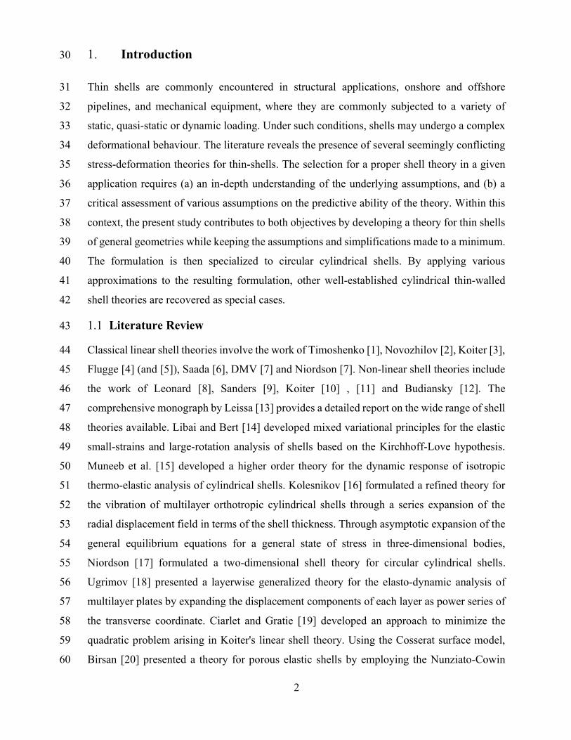
3.2 Displacements in terms of mid-surface displacements 291

Considering the geometric properties obtained in Section 3.1 , the covariant and contravariant 292

displacement components are expressed as 293

21 ,1 2 ,2 3

11 2 3,1 ,2

, 1 1 ,

, 1 ,

U u zw U z R v z z R w U w

U u zw U v z z R w U w

(21a-f) 294

where symbols , ,u v w have been used instead of 1 2 3, ,u u u for clarity. It is noted that the 295

covariant and contravariant components of the displacements become identical at the middle 296

surface 0z , i.e., 0 0iiU z U z . 297

3.3 Strain-displacement relations 298

By specializing the strain displacement relations in Eq. 7a, to cylindrical shells (e.g., [41]) one 299

obtains 300

1, 3, 3 , 3, 32 u z u u b u z u u b

(22) 301

Prescribing the shifter tensor and the curvature tensor of the middle surface b , introduced 302

in Sec. 2.1 , for CCTSs and substituting into Eq. 22 yields the corresponding covariant strain 303

tensor. The physical components of the strain tensor, denoted subsequently by a tilda, can be 304

expressed as 305

11 ,1 ,11

,2222 ,2

,212 21 ,1 ,12

1 1

1 11 1

2 1 1

u zwzww

vR z R z R

uz R v z w

z R z R

(23a-c) 306

3.4 Components of Constitutive Tensor 307

Given the components of the metric tensors (Eqs.20), by substituting into the elastic 308

constitutive tensor in Eq.14, one recovers the following expressions for non-zero components 309

of the constitutive tensor 310

15

1111 2222 1122 22112 4 22 2

1212 1221 2112 212122

, , ,1 1 1 1 1

1

2 1 1

E E EE E E E

z R z R

EE E E E

z R

311

(24a-d) 312

3.5 Hamilton Principle for CCTS 313

From Eqs. 21 and 24, by substituting into the variation of the Hamilton’s principle in Eq. 17, 314

integrating with respect to z , grouping like-terms and integrating by parts with respect to x 315

and s yields [41] 316

2 2

1 1

1 1 1 11 ,1 2 ,2 3 4 ,112

2 2 21 ,2 2 ,1 3 ,12

3 3 3 3 3 3 3 31 ,11 2 ,22 3 ,12 4 ,111 5 ,122 6 7 ,1 8

4 4 4 41 ,1 2 ,2 3 ,11 4 ,22 ,1

0

11 ,11 22

1

1

t t

t t s

xw

L

Ehdt Hu Hv Hw Hw u

Hu Hv Hw v

Hu Hu Hv Hw Hw Hu Hw Hf w

Hu Hv Hw Hw w ds

EhGu

1 1 1 1 1,22 3 ,12 4 ,1 5 ,111 6 ,122

1 1 17 8 ,1 9

2 2 2 2 2 2 2 2 21 ,12 2 ,11 3 ,22 4 ,2 5 ,112 ,222 6 7 ,2 8

3 3 3 3 3 3 3 31 ,1 2 ,2 3 ,11 4 ,22 5 ,111 6 ,122 7

A

xu

sva

a

Gu Gv Gw Gw Gw

Gu Gw Gf u

Gu Gv Gv Gw Gw Gw Gv Gw Gf v

Gu Gv Gw Gw Gw Gu Gu Gv

3,112 ,222

3 3 3 3 3 3 3 38 ,1111 9 ,1122 10 ,2222 11 12 ,11 13 ,22 14 ,1 15 ,2

3 3 316 ,1 17 ,2 18 0

b

xw sw zw

Gw

Gw Gw Gw Gw Gw Gw Gu Gv

Gf Gf Gf w dsdx dt

(25) 317

where coefficients 11G - 3

18G and 11H - 4

4 H , depend on the parameter 318

/ ln 2 / 2h R R h h R h R (26) 319

and are defined in Appendix A. The terms , , , ,xu xw sv sw zwf f f f f arising in Eq. 25 are related 320

to the physical force components per unit volume , ,x s zp p p and are provided in Appendix 321

B. 322

16

3.6 Discussion 323

The field equations and corresponding boundary conditions for a CCTS can be obtained from 324

Eq. 25 through integration by parts. The details and relevant equations are provided in 325

Appendix B, where the boundary conditions are given by Eq. B.2 and the field equations are 326

given by Eq. B.3. These are entirely consistent with the assumptions postulated in Section 1.2 327

. In order to recover simpler approximate forms of the field equations and cast the present 328

formulation in a format comparable to other CCTS theories, the logarithmic function (Eq. 26329

) appearing in Eq. 25 is replaced by a truncated Taylor series expansion 330

2 41 12 80h R h R h R (27) 331

By omitting all time dependent terms, retaining the traction terms xuf , svf , zwf , omitting 332

the terms xwf , swf and using the series approximation in Eq. 27 up to the second term, one 333

recovers the field equations in Flugge’s theory [4] as a special case of the present formulation. 334

A simpler version of the present theory can also be obtained by adopting the approximation335

1 1z R , in the strain displacement expressions (Eqs. 23a-c), the base vector expressions, 336

and the Jacobian. The resulting field equations are found to coincide with those of the DMV 337

theory [7]. Finally, as 11 z R , the present theory, the Flugge theory and the DMV are 338

found to converge to the same field equations. 339

In contrast to other thin-shell theories known to the authors, the present formulation treats the 340

applied loads as body forces, and thus, is able to capture the spatial variations of the loads 341

along all three dimensions. Mid-surface tractions, line loads, and point loads can all be treated 342

as body forces by using the Dirac delta and Heaviside functions. 343

3.7 Comparison 344

Table 1 compares the strain expressions adopted in the past theories to those of the present 345

study. All theories are in agreement regarding the expression 11 ,1 ,11u zw for the 346

longitudinal strain. The Jacobian determinant is taken as unity in all theories except the present 347

and Flugge’s theories, in which the Jacobian is 21 z R . Table 1 provides a comparison of 348

the circumferencial and shear strains 22 and 12 as given in various theories. Strain 349

17

expressions based on Flugge’s theory are observed to become in exact agreement with those 350

of the present theory when the approximation 21 12h R h R is adopted. The 351

Novozhilov strain expressions can be obtained from the strains of the present theory by 352

applying the approximations 21 12h R h R and 11 / 1 /z R z R

, while the 353

DMV strain expressions can be recovered from the strains of the present theory by applying 354

the approximations 21 12h R h R and 1 / 1z R . In contrast, strain expressions 355

in the theories of Timoshenko [1], Saada [6], Morley-Koiter [7] and Niordson [7] include 356

additional terms that do not arise in the present tensor-based approach. Such terms stem from 357

additional approximations that have been introduced in these theories, but avoided in the 358

present tensorial treatment. 359

Table 1– Comparing strain-displacement expressions in various thin shell theories 360

Theory Strain Expressions

22 12

Flugge’s theory [4] & Present Theory with approximation

21 12h R h R

,2 ,221 R

v w z wR z R z

,2 ,1 ,121 22

R R z R zu v z w

R z R R z

Novozhilov [2] & Present Theory with approximations

21 12h R h R

and 11 / 1 /z R z R

,2 ,221 R z

v w zwR R

,2 ,1 ,12

12

2R z R z

u v zwR R

Saada [6] ,2 ,22

1R zv w zw

R R

,2 ,1 ,12

12

2R z

u v zwR

Timoshenko [1] ,2 ,22

1R zv w zw

R R

,2 ,1 ,12

1 22

2R z

u v zwR

Morley-Koiter [7] & Niordson [7] ,2 ,22

2 1R z R zv w zw

R R R

,2 ,1 ,12

1 22

2R z

u v zwR

DMV [7] & Present Theory with approximations 1h R and

1 / 1z R

,2 ,221

v w zwR

,2 ,1 ,121

22

u v zw

The presence of such differences at the strain expression stage, combined with other 361

simplifications and approximations, leads to differences in their corresponding field equations 362

18

and boundary conditions. In order to conduct a comparative study, irrespective of the CCTS 363

theory adopted, the equilibrium conditions can be cast into the following generic form 364

2

,11 1.1 ,22 ,12 ,1 1.2 ,111 1.3 ,122

2 2

1.4 ,1

1 1 1

2 2 12 2

10

12xu

hu u v w w w

R R

hu w f

E R

365 2 2

,12 2.1 ,11 2.2 ,22 ,2 2.3 ,112 2.4 ,222

2 2

2.5 2.6 ,2

1 1 1

2 2 12 12

10

6sv

h hu v v w w w

R R R

h fv wE R

366

2

,1 ,2 3.1 3.2 ,11 3.3 ,22 3.4 ,111 3.5 ,1222

2 2

3.6 ,112 3.7 ,222 ,1111 3.8 ,1122 3.9 ,2222

2 22

3.10 ,11 ,22 3.11 ,1 ,2

2,1

1 1 1

12 2

12 12

1 212 12

1 xw

hu v w w w u u

R R RR

h hv w w w w

R

h hE w w w u v

R

Eh f

,2 0sw zwf f

367

where coefficients .i j are theory-dependent and are defined in Table 2. As observed, the 368

adoption of various assumptions/approximations in various theories, has led to the elimination 369

of terms in some cases (e.g., 21.2 ,11112h R w , 2

3.4 ,11112h R u and 370

3.5 ,1221 2 u for Timoshenko, Novozhilov and Saada), and to the emergence of 371

additional terms in other cases (e.g., 2.4 ,222w , 3.2 ,11w and 3.7 ,222w for Timoshenko, 372

Novozhilov and Saada), when compared to the present treatment. Such 373

approximations/simplifications have only affected the magnitude of coefficients of other terms 374

in some cases. 375

376

Table 2 - Comparison of field equation coefficients .i j for various CCTS theories 377

F.E.s Present Theory Flugge [4] Timoshenko [1], Novozhilov [2],

Saada [6],

Morley-Koiter [7], Niordson [7], DMV

[7]

1 .1 2 21 12h R 1 1

1.2 1

1

0 0

19

1.3 1R

2 12h R

0 0

1.4 1 - 0 0

2 .1 2 21 4h R 2 21 4h R 2 21 3h R

[Take (2 2

1 12h R ) for Timoshenko] 1

2.2 1 1 2 21 12h R 1

2.3 3 2

3 2

1 [Take ( 2 ) for Novozhilov]

0

2.4 0 0 1 0

2.5 2 21 12h R

2 21 12h R

- 1

2.6 1 1 - 0

3 .1 2 21 12h R 1 2 21 12h R

[Take unity for DMV]

3.2 0 0 0 2 21 6h R

[Vanishes for DMV]

3.3 2 1

2 26h R

0 2 26h R

[Vanishes for DMV]

3.4 1 1 0 0

3.5 1R

2 12h R

0 0

3.6 23 23 2

[Take unity for Saada] 0

3.7 0 0 2 12h R

0

3.8

2

2

243

21 1

h

R

2 6h 2 6h 2 6h

3.9 2 1R 2 12h 2 12h 2 12h

3.10 1 - - 1

3.11 1 - - 0

3.12 1 - - 1

Similarly, the boundary terms have been cast into the following generic form. 378

2

,1 ,2 1.1 ,1112

hu v w w u

R R

379

2

,2 2.1 ,1 ,124

h vu v wR

380

20

2 2 2 2

3.1 ,11 3.2 ,22 3.3 ,12 ,111 3.4 ,1221

12 2 12 12 12

h h h h wu u v w wR R

381

2 2 2 2

4.1 ,1 4.2 ,2 ,11 ,22 ,112 12 12 12

h h h hu v w w w

R R

382

Table 3 provides coefficients .i j for the present theory and those of Flugge, Timoshenko 383

and DMV. 384

385

Table 3 - Comparison of field equation coefficients .i j for various CCTS theories 386

B.C.s Present Theory Flugge Timoshenko DMV

1 .1 1 1 0 0

2.1 2 21 4h R 2 21 4h R 2 3 0

3 .1 1 1 0 0

3.2 1R 2 12h R 0 0

3.3 3 2 3 2 1 0

3.4 2 23 2 11 6R h 2 1 2

4.1 1 1 0 0

4.2 1 1 1 0

387

3.8 Steady State Analysis under Harmonic Forces 388

Consider a CCTS under general harmonic force per unit volume 389

, , , , , , , , , , , , , , , , , , , Rex s z x s z i tp x s z t p x s z t p x s z t p x s z p x s z p x s z e , 390

with an exciting frequency . It is possible to express the force functions using double Fourier 391

series with N circumferential modes and K longitudinal modes yielding: 392

21

2 / /

2 2

0 0

Re ,

, ,

, ,

, ,

x xnkN K

s s ikx L ins R i tnk

n N k Kz znk

x xnk

s R x Ls s ikx L ins Rnk s xz znk

p p zp p e e ezp p z

p p x s zzp p x s z e e dxdszp p x s zz

(28a-b) 393

in which, each applied force component is expressed in terms of its Fourier series expansion 394

in x and s . From Eq. 28, by substituting into Equations B.1a-e and integrating over the 395

thickness, one obtains 396

2 / /

2

Re ,

1

1

1

xuxunk

svsvN K nk

ikx L ins Rzwzw i tnk

xwxw n N k Knk

swswnk

xxunknk

sv snk nk

zw znk nk

xwnk

swnk

ff

ff

e eff e

ff

ff

p z Rf z

f p z Rz

f p z Rz

f

f

2

2 1

1

hz

hz x

nk

znk

dz

p z z Rz

p z z Rz

(29a-b) 397

For a given load, constants xuf , svf , zwf , xwf and swf are determined and a procedure 398

similar to that reported in [24] is then used to provide a closed form solution for each of the 399

theories developed. The corresponding steady state displacements are expressed in the 400

following form. 401

22

8

2 / /

1

8

2 / /

1

8

2 /

1

, , ,

, , ,

, , ,

nj

nj

nj

KNm x ikx Li t ins R i t

nj nj nk

j k Kn NKN

m x ikx Li t ins R i tnj nj nk

j k Kn N

Km x ikx Li t

nj nj nk

j k K

A A e R eu x s t u x s e e e

A B e S ev x s t v x s e e e

A C e T ew x s t w x s e

/

N

ins R i t

n N

e e

(30a-c) 402

Symbols njm are the eigenvalues and each set of symbols njA , njB , njC form the 403

corresponding eigenvectors of the characteristic equation of the system related to mode n . 404

Symbols nkR , nkS , nkT and njA are unknown integration constants to be determined from 405

boundary conditions (e.g., [24]). 406

3.9 Examples 407

In the following examples, the above solution technique is adopted to express the applied 408

forces and displacement fields in the circumferential direction s and lomgitudinal direction x409

. Examining the terms in Eqs. B.2 and B.3, as well as the entries in Table 2 and Table 3 reveals 410

that the theories of Timoshenko, Novozhilov and Saada have largely similar governing 411

equations and boundary conditions. Thus, the theory of Timoshenko has been chosen as a 412

representative of this group. Similarly, the DMV theory has been taken as a representative of 413

the Morley-Koiter, Niordson and DMV group of theories given their similarity. In all 414

examples, results based on Abaqus models are provided for comparison. Four types of 415

elements have been used in Abaqus models depending on the problem. 416

S4R: A four-noded general-purpose (thin or thick) shell element, with reduced integration 417

and hourglass control. 418

S8R: An eight-noded doubly curved thick shell element with reduced integration 419

C3D8R: An eight-noded linearly interpolated brick element with reduced integration and 420

hourglass control, and 421

C3D20R: A twenty-node quadratically interpolated brick element with reduced integration. 422

In all examples, steel is assumed to have a density of 37850kg m , a modulus of elasticity 423

of 200GPa and a Poisson's ratio of 0.3 . 424

23

3.9.1 Example 1 - Pipe under Self-Weight 425

A 4 m long fixed-free horizontal pipe with a radius 200R mm and a thickness 6h mm is 426

subjected to its self-weight. The response is obtained based on the present theory, the Flugge, 427

Timoshenko, DMV theories, and the Abaqus shell model. In the Abaqus model, by refining 428

the mesh from 64 200 to 128 400 S4R elements, the changes in the predicted 429

displacements were within 0.9%, suggesting that convergence has been achieved. The static 430

solution sought in the present problem is recovered by setting to zero the exciting frequency431

. Figure 5 provides a comparison of the longitudinal and radial displacements at the top 432

generator of the pipe mid-surface. Nearly perfect agreement is observed among all solutions 433

except for the DMV, which exhibits a significantly stiffer response as indicated by the lower 434

displacements observed. A comparison of the predictions of the present and DMV theories 435

shows a 53% difference (for a thickness 6h mm ). When the pipe thickness is reduced to436

3h mm , the difference between both solutions reduces to 22% , drops further to 6.5% for 437

1.5h mm , and becomes only 3% for 1h mm . The fact that the DMV theory adopts the 438

approximation 11 z R , while the other theories do not enforce such an approximation, 439

limits the usability of the DMV theory for very thin shells. 440

441 Figure 5–Comparison of longitudinal and radial displacements at the top generator 442

3.9.2 Example 2 - Fixed pipe under harmonic pressure 443

Example 1 in [24] is revisited: A pipe with span length 5L m , radius 25R mm , thickness 444

5h mm is fixed at both ends and is subjected to wind load traction 445

2, , 100cos coszt x s t s R t kN m , where 200 rad s , simulating a vortex shedding 446

24

phenomenon. Casting the applied traction in form of body forces applicable to the present 447

formulation yields 3, , 2z zp t x s t Dirac z h N m . In addition to the present theory, 448

solutions are to be provided under the Flugge, Timoshenko, and DMV theories as well as 449

Abaqus FEA for comparisons. In the Abaqus model, by refining the mesh from 64 200 to 450

128 400 S4R elements, the change in the predicted displacements was less than 0.05%, 451

suggesting that convergence has been achieved by 64 200 mesh. 452

453

Figure 6 - Cross-sectional distribution of the wind load. 454

The maximum longitudinal and radial displacements at midsurface ( 0z ) take place at the 455

generators passing through points A ( 0s ) and C ( 4s ) and the maximum 456

circumferential midsurface displacement occurs at the generators passing through points B (457

8s ) and D ( 3 8s ), as shown in Figure 6. Table 4 gives the maximum displacements 458

and their respective locations as provided by the present theory and percentage differences 459

based on other solutions mentioned above. For the present problem, the predictions of the 460

present theory are indistinguishable from those of the Flugge and Timoshenko theories, while 461

the DMV solution slightly underpredicts the displacement by about 2.7%. The Abaqus 462

solution, also, is found to slightly underpredicting the displacement by less than 1%. 463

464

25

Table 4 - Comparing the displacement components at the location of their maximum 465

Present theory Difference from the present theory (%)

Flugge Timoshenko DMV Abaqus

( 64 200 S4R)

A Cu u at 0.21x L

A Cu u at 0.79x L 0.4410 mm 0.00 -0.01 2.73 0.91

B Dv v at 0.5x L 3.753 mm 0.00 -0.01 2.72 0.92

A Cw w at 0.5x L 3.725 mm 0.00 -0.01 2.72 0.92 466

The distribution of longitudinal stresses xx and transverse stresses ss for the generator 467

passing through point A (Figure 6) are depicted in Figure 7 and Figure 8. Flugge’s theory 468

predictions nearly coincide with those of the present solution, and the Timoshenko theory 469

predictions are in rather close agreement. The predictions of the DMV theory are 1-3% below 470

those based on the other theories. Although, in the present example, all four theories predict 471

stresses in rather close agreement, this will not always be the case. For instance, if all degrees 472

of freedom at end x L are released (turning the beam into a cantilever), the stresses predicted 473

by the DMV are found to depart from those predicted by the Timoshenko, Flugge and present 474

theories. Figure 9 depicts the longitudinal stress xx along a generator passing through point 475

A (in Figure 6) under only 20% of the magnitude of , ,zt x s t (to keep the maximum stresses 476

within the elastic range of the structural steel properties). The figure shows that the DMV 477

prediction significantly departs from those of the other theories. 478

26

479 Figure 7 - Longitudinal stress ( xx ) along a generator passing through point A 480

481

482 Figure 8 - Transverse stress ( ss ) along a generator passing through point A 483

27

484 Figure 9 - Longitudinal stress ( xx ) along a generator passing through point A for cantilever 485

486

The amplitudes of the radial displacements at Point A as predicted by the present solution are 487

compared to those predicted by the Abaqus shell model for wide range of angular frequencies 488

(Figure 10). In Abaqus, by refining the mesh from 80 255 to 160 510 S4R elements, the 489

change in the predicted displacements was less than 0.9% for frequencies ranging from 0 to 200 490

rad s , suggesting that convergence has been achieved. The radial displacement amplitudes (as 491

identified on the scale of the left vertical axis) based on both solutions are nearly in perfect 492

agreement and are barely distinguishable within the scale of the figure. The loci of the peak 493

amplitudes, indicative of the natural frequencies, are also in excellent agreement with Abaqus 494

predictions. Also shown on the figure is the percentage difference of the radial displacement at 495

point A between both solutions, as identified on the scale of the right vertical axis. Except near 496

the natural frequencies where both solutions approach infinity, or where the amplitude 497

approaches zero, the amplitude difference is within 3%. The comparison indicates that the present 498

theory predicts lower natural frequencies for most of the frequency range and higher amplitudes 499

compared to Abaqus. 500

28

501

Figure 10 – Radial amplitude versus exciting frequency 502 503

3.9.3 Example 3 - Pipe under a Point Load 504

The fixed pipe in Example 2 is set free at end x L and is subject to an inclined point load 505

1,1, 1 kN (Figure 11) along the x , s and z directions, acting at point506

0 , , 0.7 ,0,0P x s z L . 507

x

s

z

1 kN

1 kN

1 kN0P

508 Figure 11 – Location, magnitude and direction of the point load components 509

The point loads can be expressed as body forces 510

, , 0.7 1,1,1x s zp p p Dirac x L Dirac s Dirac z kN and expanded as double Fourier 511

series in the x and z directions. To investigate the convergence of the solution, the number of 512

Fourier modes taken is varied ( 7, 10, 15, 20, 25N K ). Five Abaqus S4R shell models, 513

with uniform meshes, were conducted for comparison (16 50 , 32 100 , 64 200 , 128 400 514

and 320 640 ). The four coarse meshes are uniform while the most refined mesh ( 320 640515

29

) is identical to the 128 400 mesh, with a refined rectangular patch of elements in the 516

neighborhood of the point load. The patch extends longitudinally from 0.6x L to 0.8x L 517

and from 2s R to 2s R in the circumferential direction and consists of 256 320 518

elements (instead of 64 80 elements in the 128 400 elements model), and is intended to 519

capture localized deformations around the point load. In Abaqus, a mesh study indicated that 520

convergence was achieved for 128 400 S4R mesh. A finer 320 640 mesh resulted only in 521

a maximum difference of 0.23% in the displacements predicted. 522

The longitudinal, circumferential, and radial displacements at the generator at which the point 523

load is applied ( 0s z ) are respectively depicted in Figure 12 to Figure 14. As the number 524

of Fourier terms increases in the present solution, and as the number of elements increase in 525

the Abaqus solution, both models are observed to approach one another, albeit in the limit, 526

both converged solutions do not exactly coincide. The rather minor differences observed arise 527

from the fact that an exact representation of the point load requires an infinite number of modes 528

( N & K ), which is unachievable as the number of modes taken has to be 529

truncated. To confirm this hypothesis, an additional Abaqus solution is conducted (denoted as 530

A. 128 640 7N K ). The applied point loads (originally modelled as nodal forces in the 531

shell model) were replaced by applied tractions that follow the exact distribution based on the 532

first seven Fourier modes, in a manner consistent with the load characterization in the present 533

solution (denoted as P. T. 7N K ). As expected, both solutions (P. T. 7N K ), and 534

(A. 128 640 7N K ) predict nearly identical displacements. 535

Locally, the Abaqus shell solution exhibits minor displacement fluctuations within the vicinity 536

of the applied point load while the present solution predicts smoother displacement profiles. 537

Two additional Abaqus models were developed based on the S8R shell element and the 538

C3D20R brick element (both elements using quadratic interpolations as opposed to linear 539

interpolation in the S4R element). For the C3D20R, two layers of elements were taken across 540

the pipe thickness. Both models (not shown on Figure 12 to Figure 14 for clarity) were found 541

to exhibit less fluctuation within the vicinity of the point load than the S4R model, i.e., their 542

response is found closer to that of the present model. 543

30

544 Figure 12 – Comparison of longitudinal displacements at top generator 545

546

547 Figure 13 – Comparison of circumferential displacements at top generator 548

549

31

550

551 Figure 14 – Comparison of radial displacement at top generator 552

To investigate the effect of span on the results, three spans are considered; 0.5L m , 553

2.5L m and 5L m . The displacement components of the top generator ( 0s z ) versus 554

the normalized longitudinal coordinate /x L are provided in Figure 15 to Figure 17. The 555

number of modes taken is 25N K , which is beyond the number of modes required for 556

convergence. Abaqus S4R meshes were based 240 elements in the circumferencial direction 557

and 400 elements in longitudinal directions (a 240 400 mesh) for span 0.5L m , a 558

128 200 mesh for span 2.5L m , and a 128 640 mesh for span 5L m ). 559

As a general observation, all predictions are in very good agreement with the exception of the 560

DMV theory. In addition, the difference between the responses predicted by the DMV solution 561

and those of the other solutions tend to grow with the pipe span. In all cases, the DMV solution 562

underestimates the dispacements compared to other solutions. 563

The maximum difference between the present solution results and those based on Abaqus are 564

negligible. In general, the present theory predicts a slightly more flexible response compared 565

to that of the Abaqus model with fine meshes. Irrespective of the span, the present theory’s 566

32

predictions are in excellent agreement with Flugge's predictions, while the predictions of the 567

Timoshenko's theory tend to deviate slightly from those of the two theories for shorter spans. 568

569 Figure 15 - Longitudinal displacement at the top generator 570

571 Figure 16 - Circumferential displacement at the top generator 572

33

573

574 Figure 17 - Radial displacement at the top generator 575

To investigate the effect of thickness on various theories, the problem defined in the current 576

example ( 5L m and 250R mm , with the same point load) is solved again while varying 577

the thickness to 5.0, 12.5, 25.0h mm , which correspond to radius to thickness values of578

/ 50, 20, 10R h , respectively). The problems are solved using two types of Abaqus models: 579

one is based on 128 400 S4R Shell elements and the other is based on 4 128 400 C3D8R 580

Brick elements. 581

As shown in Figure 18 to Figure 20, predictions of the present theory, Flugge, and Timoshenko 582

are in near perfect agreement, while Abaqus solutions provide an indistinguishable stiffer 583

response. As the DMV results were far from the comparable range, they were not included in 584

the plots. For the thicker pipe, the Timoshenko theory shows a negligibly more flexible 585

response. In the proximity of the point load application, the finite element solutions exhibit 586

localized oscillations, particularly for the brick element solution, which contrasts with the 587

smoothness of the shell responses. 588

34

589 Figure 18 - Longitudinal displacement on the top generator for various theories and different Abaqus 590

elements 591

592

35

593 Figure 19 - Circumferential displacement on the top generator for various theories and different Abaqus 594

elements 595

596

597 Figure 20 - Radial displacement on the top generator for various theories and different Abaqus elements 598

36

3.9.4 Example 4 – Comparisons against experimental results and 599 analytical predictions 600

The natural frequencies based on the present theory are compared to the experimental results 601

reported in [42]. The specimens tested were made of steel ( 200E GPa , 37760kg m , 602

0.29 ) with span 0.664L m , radius 175R mm , thickness 1.02h mm . Figure 21 603

depicts excellent agreement between the predictions of the present theory and the experimental 604

results. Symbol n denotes the circumferential wave number and symbol denotes the 605

longitudinal half-wave number and satisfies the relation m i L . The present theory tends 606

to predict slightly higher natural frequencies for higher circumferential modes. In all cases, 607

the maximum difference between the present theory predictions and experimental results is 608

1.5%. 609

610 Figure 21 – Comparing natural frequencies 611

Additional comparisons are made against the analytical predictions in [43] which reported the 612

natural frequencies for a simply supported pipe made of rubber ( 0.45E GPa , 0.45 , 613

31452kg m ), span 0.2L m , radius 100R mm , and thickness 2h mm . Table 5 shows 614

that, for 1,...,8 and 1,...,10n , the present theory is found to yield natural frequencies 615

of up to 1.36% lower than the values reported in [43]. 616

37

Table 5 – Comparing natural frequencies based on the present theory with analytical results 617

1 2 3 4 5 6 7 8

n

1 Present theory

523.6 782.2 849.8 889.8 938.8 1011.8 1117.4 1260.3 Ref. [43] 524.1 783.7 852.8 894.8 946.2 1021.9 1130.4 1276.5 Diff. % -0.09 -0.19 -0.35 -0.55 -0.78 -0.99 -1.15 -1.27

2 Present theory

303.4 607.2 752.4 834.8 907.6 995.5 1111.2 1261.0 Ref. [43] 303.9 609.1 755.8 840.1 915.3 1005.8 1124.3 1277.3 Diff. % -0.17 -0.32 -0.44 -0.64 -0.84 -1.02 -1.17 -1.28

3 Present theory

188.1 456.1 641.2 763.7 865.6 973.9 1104.1 1264.0 Ref. [43] 188.6 458.4 645.2 769.7 873.8 984.6 1117.4 1280.5 Diff. % -0.28 -0.50 -0.63 -0.78 -0.94 -1.08 -1.19 -1.28

4 Present theory

149.5 355.8 546.7 695.7 823.9 953.6 1100.0 1272.0 Ref. [43] 150.0 358.2 551.4 702.5 832.9 964.9 1113.8 1288.8 Diff. % -0.33 -0.66 -0.85 -0.97 -1.08 -1.17 -1.24 -1.30

5 Present theory

167.3 309.9 485.4 645.6 792.9 941.4 1103.4 1287.6 Ref. [43] 167.6 312.1 490.2 653.0 802.7 953.4 1117.9 1305.0 Diff. % -0.21 -0.69 -0.99 -1.13 -1.22 -1.26 -1.29 -1.33

6 Present theory

218.4 314.5 463.9 622.9 780.9 943.2 1118.5 1313.7 Ref. [43] 218.7 316.2 468.4 630.4 791.0 955.8 1133.6 1331.7 Diff. % -0.13 -0.53 -0.96 -1.18 -1.28 -1.32 -1.33 -1.35

7 Present theory

288.7 358.4 481.9 631.7 792.5 963.3 1148.3 1352.5 Ref. [43] 289.0 359.7 485.7 638.7 802.6 976.2 1163.9 1371.1 Diff. % -0.11 -0.36 -0.79 -1.10 -1.26 -1.32 -1.34 -1.36

8 Present theory

372.9 429.2 533.1 670.9 829.4 1003.7 1194.8 1405.6 Ref. [43] 373.3 430.4 536.3 677.2 839.0 1016.5 1210.7 1424.7 Diff. % -0.11 -0.27 -0.60 -0.93 -1.15 -1.26 -1.31 -1.34

9 Present theory

469.4 519.1 610.0 736.9 890.3 1064.7 1258.9 1474.0 Ref. [43] 470.0 520.2 612.8 742.5 899.3 1077.2 1274.8 1493.5 Diff. % -0.13 -0.22 -0.45 -0.76 -1.00 -1.16 -1.25 -1.31

10 Present theory

577.6 623.9 706.9 825.2 972.9 1145.4 1340.5 1557.9 Ref. [43] 578.5 625.2 709.6 830.3 981.4 1157.6 1356.4 1577.8 Diff. % -0.16 -0.21 -0.38 -0.62 -0.86 -1.05 -1.18 -1.26

4. Summary and Conclusions 618

A variational expression is developed for the dynamic analysis of thin shells of general 619

geometries based on tensor calculus in conjunction with the Hamilton variational principle. 620

The solution is based on a minimal number of assumptions at the outset of the formulation 621

while avoiding non-essential approximations advocated in past theories. The variational 622

expression is then specialized to CCTS and used to formulate the governing equilibrium 623

equations and boundary conditions. The governing equations thus obtained are free from non-624

essential approximations and can potentially serve as a benchmark to assess the accuracy of 625

38

past circular cylindrical thin shell theories. The field equations derived are then compared to 626

those of Flugge, Timoshenko, Novozhilov, Morley-Koiter, Niordson, Saada and DMV. A 627

number of problems were numerically investigated using the present theory and comparisons 628

were made with the Flugge, Timoshenko, and DMV theories. 629

The main conclusions of the study are: 630

(1) The governing field equations of the Flugge and DMV theories were recovered as special 631

cases from the present theory by applying consistent approximations relating to the radius-to-632

thickness ratio to the governing equations derived herein. 633

(2) Compared to the present treatment, the theories of Timoshenko, Novozhilov, Morley-634

Koiter, Niordson, and Saada were found to involve inconsistent approximations. In some 635

cases, such inconsistencies lead to over-simplifications in the field equations, while in others, 636

they lead to the emergence of additional/unnecessary terms. 637

(3) The inconsistent simplifications made in the above theories do not necessarily correspond 638

to a significant reduction in their predictive power. Specifically, the inconsistencies involved 639

in Timoshenko’s theory are of a small order and do not significantly influence its predictive 640

ability. For DMV, while the approximations made are of a consistent order, the order of 641

approximation implied happens to be too coarse to capture the response of pipes with moderate 642

thicknesses. 643

(4) Numerical predictions of the 3D and shell FEA solutions are in excellent agreement with 644

those of the present theory for a wide range of pipe dimensions ( 2 20L R and645

10 50R h ). 646

(5) The numerical predictions of the Flugge theory are found to be consistently in excellent 647

agreement with those of the present theory and Abaqus finite element solutions, and is thus 648

advocated as a more simplified CCTS theory, but yet as an accurate alternative to the present 649

theory. 650

(6) In contrast, DMV exhibits an overly stiff behaviour compared to the present and other 651

theories. In addition, it grossly overestimates the stresses in some cases. The theory is suitable 652

only for very thin pipes. 653

39

Acknowledgement 654

The authors would like to express their deepest gratitude to the Baha´i Institute for Higher 655

Education (BIHE), Tehran, Iran for its encouragement and support to the first author. Also, 656

research funding from the Natural Science and Engineering Research Council of Canada 657

(NSERC) to the second author is gratefully acknowledged. 658

40

5. List of Symbols 659

ia Covariant base vectors of the middle surface

ija First fundamental tensor defined on the middle surface of a thin shell

a Determinant of the first fundamental tensor ija

b Curvature tensor of the surfaces parallel and adjacent to the middle surface

b Second fundamental tensor or curvature tensor defined on the middle surface of a thin shell

ia Contravariant base vectors of the middle surface ija First fundamental tensor of the second kind defined on the middle surface

of a thin shell

ig Covariant base vectors of any surface parallel and adjacent to the middle surface

ijg First fundamental tensor defined within the shell g Determinant of the first fundamental tensor ijg

ig Contravariant base vectors of any surface parallel and adjacent to the middle surface

ijg First fundamental tensor of the second kind defined within the shell

, ,x y zp p p Physical components of the Contravariant body force components iF as a

function of , , ,x s z t

, ,x y zp p p Physical components of the Contravariant body force components iF as a

function only of , ,x s z .

,R r Position vector of a point within the shell and on the middle surface, respectively, before deformation.

ˆ ˆ,R r Position vector of a point within the shell and on the middle surface, respectively, after deformation.

,U u Displacement of a point within the shell and on the middle surface, respectively.

, iiU U Covariant and contravariant components of the displacement of a point on

a surface parallel and adjacent to the middle surface along axis ix , respectively.

iu Covariant components of the displacement of a point on the middle surface along axis ix

, ,u v w Components of the displacement of a point on the middle surface along axes 1x , 2x and 3x , respectively

i Coordinate system/Coordinates of the system ix Coordinate system/Coordinates of the system , ,x s z Coordinates of the system, equivalent to 1x , 2x and 3x , respectively

, ,... All Greek superscripts or subscripts range from 1 to 2

, ,...ii All Italic superscripts or subscripts range from 1 to 3

660

41

,i ii j

Covariant unit vectors along axis ix in middle surface and adjacent surfaces, respectively

,i ii j

Contravariant unit vectors along axis ix in middle surface and adjacent surfaces, respectively

kij Christoffel symbols in terms of ig and ijg

kij Christoffel symbols in terms of ia and ija (defined for the middle surface)

Inner product Cross product | Covariant derivative || Covariant derivative in two dimensional spaces

T Kinetic energy

V Potential energy V Volume

W External work Mechanical energy of the system

ij Components of the strain tensor on the middle surface

ij Components of the strain tensor on surfaces adjacent to the middle surface

In-plane components of the strain tensor

Physical components of ij Stress tensor In-plane components of the stress tensor ij

Longitudinal half-wave number ijlmE Generalized Hooke’s Law

E In-plane components of the generalized Hooke’s Law ijlmE

,... i Partial derivative with respect to ix Kronecker delta function Mixed shifter tensor connecting the covariant base vectors of an arbitrary

point within the shell to corresponding base vectors of the middle surface. Inverse of mixed shifter tensor

Density of the mass E Modulus of elasticity Poisson’s ratio t time

661 662

42

6. References 663

[1] S. Timoshenko, Theory of Plates and Shells. McGraw-Hill Book Company, New York, 664

1959. 665

[2] V.V. Novozhilov, Thin Shell Theory. P. Noordhoff Ltd. –Groningen-The Netherlands, 666

1964. 667

[3] W. T. Koiter, On the mathematical foundation of shell theory, Actes. Congres intern. 668

Math. 3 (1970) 123-130. 669

[4] W. Flugge, Stresses in Shells. Springer-Verlag, New York Heidelberg Berlin, 1973. 670

[5] W. Flugge, Tensor Analysis and Continuum Mechanics, Springer-Verlag, New York 671

Heidelberg Berlin, 1972. 672

[6] A. S. Saada, Elasticity: Theory and Applications, Pergamon Press Inc., New York, 1974. 673

[7] F. I. Niordson, Shell Theory. North-Holland Series In Applied Mathematics and 674

Mechanics, 1985. 675

[8] R. W. Leonard, Nonlinear First Approximation Thin Shell and Membrane Theory. Ph. D. 676

Dissertation, Virginia Polytechnic Institute, Blacksburg, Virginia, 1961. 677

[9] J. L. Sanders Jr., Nonlinear Theories for Thin Shells, Q. J. Appl. Math. 21 (1) (1963) 21-678

36. 679

[10] W. T. Koiter, On the Nonlinear Theory of Thin Elastic Shells. Proceedings of the 680

Koninklijke Nederlandse Akademie van Wetenschappen, Series B, 69 (1966) 1-54. 681

[11] W. T. Koiter, General Equations of Elastic Stability for Thin Shells. Proceedings-682

Symposium on the Theory of Shells, University of Houston, (1967), 187-227. 683

[12] B. Budiansky, Notes on Nonlinear Shell Theory, J. Appl. Mech. 35 (2) (1968) 393-401. 684

[13] A.W. Leissa, Vibration of Shells, Acoust. Soc. Am., 1993. 685

[14] A. Libai, C. W. Bert, A mixed variational principle and its application to the nonlinear 686

bending problem of orthotropic tubes-I. Development of general theory and reduction to 687

cylindrical shells, Int. J. Solids Struct. 31 (7) (1994) 1003-1018. 688

[15] A. -H. Muneeb, G. A. Birlik, Y. Mengi, A higher order dynamic theory for isotropic 689

thermoelastic cylindrical shells: Part 1: Theory, J. Sound Vib. 179 (5) (1995) 817-826. 690

[16] S. V. Kolesnikov, A refined theory of the vibrations of a cylindrical shell based on an 691

expansion in series of the normal displacement, J. Appl. Math. Mech. 60 (1) (1996) 113-692

119. 693

43

[17] F. I. Niordson, An asymptotic theory for circular cylindrical shells, Int. J. Solids Struct. 694

37 (13) (2000) 1817-1839. 695

[18] S. V. Ugrimov, Generalized theory of multilayer plates, Int. J. Solids Struct. 39 (4) (2002) 696

819-839. 697

[19] P. G. Ciarlet, L. Gratie, Another approach to linear shell theory and a new proof of Korn’s 698

inequality on a surface, Mathematical Problems in Mechanics, C. R. Acad. Sci. Paris, Ser. 699

I 340 (2005). 700

[20] M. Birsan, On the theory of elastic shells made from a material with voids, Int. J. Solids 701

Struct. 43 (2006) 3106-3123. 702

[21] H. Altenbach, V. A. Eremeyev, N. F. Morozov, Linear theory of shells taking into account 703

surface stresses. Dokl. Phys. 54 (12) (2009) 531-535. 704

[22] K. Weicker, R. Salahifar, M. Mohareb, Shell analysis of thin-walled pipes. Part I - Field 705

equations and solution, Int. J. Press. Vessels Pip. 87 (7) (2010) 402-413. 706

[23] K. Weicker, R. Salahifar, M. Mohareb, Shell analysis of thin-walled pipes. Part II - Finite 707

element formulation, Int. J. Press. Vessels Pip. 87 (7) (2010) 414-423. 708

[24] R. Salahifar, M. Mohareb, Analysis of circular cylindrical shells under harmonic forces, 709

Thin Walled Struct. 48 (7) (2010) 528-539. 710

[25] M. Amabili, J. N. Reddy, A new non-linear higher-order shear deformation theory for 711

large-amplitude vibrations of laminated doubly curved shells, Int. J. Non Linear Mech. 712

45 (4) (2010) 409-418. 713

[26] V. N. Paimushin, A theory of thin shells with finite displacements and deformations based 714

on a modified Kirchhoff-Love model, J. Appl. Math. Mech. 75 (5) (2011) 568-579. 715

[27] R. Salahifar, M. Mohareb, Finite element for cylindrical thin shells under harmonic 716

forces, Finite Elem. Anal. Des. 52 (2012) 83-92. 717

[28] A. Favata, P. Podio-Guidugli, A new CNT-oriented shell theory, Eur. J. Mech. A. Solids 718

35 (2012) 75-96. 719

[29] C. Sansour, S. Skatulla, M. Hjiaj, A shell theory with scale effects and higher order 720

gradients, Int. J. Solids Struct. 50 (2013) 2271-2280. 721

[30] J. Xuea, D. Yuana, F. Hanb, R. Liua, An extension of Karman–Donnell's theory for non-722

shallow, long cylindrical shells undergoing large deflection, Eur. J. Mech. A. Solids 37 723

(2013) 329-335. 724

[31] V. V. Zozulya, A high-order theory for functionally graded axially symmetric cylindrical 725

shells, Arch. Appl. Mech. 83 (3) (2013) 331-343. 726

44

[32] E Carrera, S. Brischetto, P. Nali, Plates and shells for smart structures: classical and 727

advanced theories for modeling and analysis. John Wiley & Sons, 2011. 728

[33] E. Carrera, M. Cinefra, M. Petrolo, E. Zappino, Finite element analysis of structures 729

through unified formulation. John Wiley & Sons, 2014. 730

[34] A. Cattabiani, H. Riou, A. Barbarulo, P. Ladevèze, B. Troclet, The Variational Theory of 731

Complex Rays applied to the shallow shell theory, Comput. Struct. 158 (2015) 98-107. 732

[35] S. R. Chowdhurya, P. Roya, D. Roya, J. N. Reddy, A peridynamic theory for linear elastic 733

shells, Int. J. Solids Struct. 84 (2016) 110-132. 734

[36] Ye. M. Zveryayev, A consistent theory of thin elastic shells, J. Appl. Math. Mech. 80 735

(2016) 409-420. 736

[37] J. Awrejcewicz, V. A. Krysko, A. A. Sopenko, M. V. Zhigalov, A. V. Kirichenko, A. V. 737

Kryskoc, Mathematical modelling of physically/geometrically non-linear micro-shells 738

with account of coupling of temperature and deformation fields, Chaos, Solitons Fractals 739

104 (2017) 635-654. 740

[38] Q. Wangab, D. Shaoc, B. Qind, A simple first-order shear deformation shell theory for 741

vibration analysis of composite laminated open cylindrical shells with general boundary 742

conditions, Compos. Struct. 184 (15) (2018) 211-232. 743

[39] R. Okhovat, A. Bostrom, Dynamic equations for an orthotropic cylindrical shell, Compos. 744

Struct. 184 (2018) 1197-1203. 745

[40] Q. Wang, D. Shao, B. Qin, A simple first-order shear deformation shell theory for 746

vibration analysis of composite laminated open cylindrical shells with general boundary 747

conditions, Compos. Struct. 184 (2018) 211-232. 748

[41] R. Salahifar, Analysis of Pipeline Systems under Harmonic Forces, Ph. D. Thesis, 749

Department of Civil Engineering, University of Ottawa, Ontario, Canada, 2011. 750

[42] M. Amabili, G. Dalpiaz, Breathing vibrations of a horizontal circular cylindrical tank 751

shell, partially filled with liquid, J. Vib. Acoust. 117 (1995) 187-191. 752

[43] I. Senjanović, I. Ćatipović, N. Alujević, N. Vladimir, D. Čakmak, A finite strip for the 753

vibration analysis of rotating circular cylindrical shells, Thin Walled Struct. 122 (2018) 754

158-172. 755

45

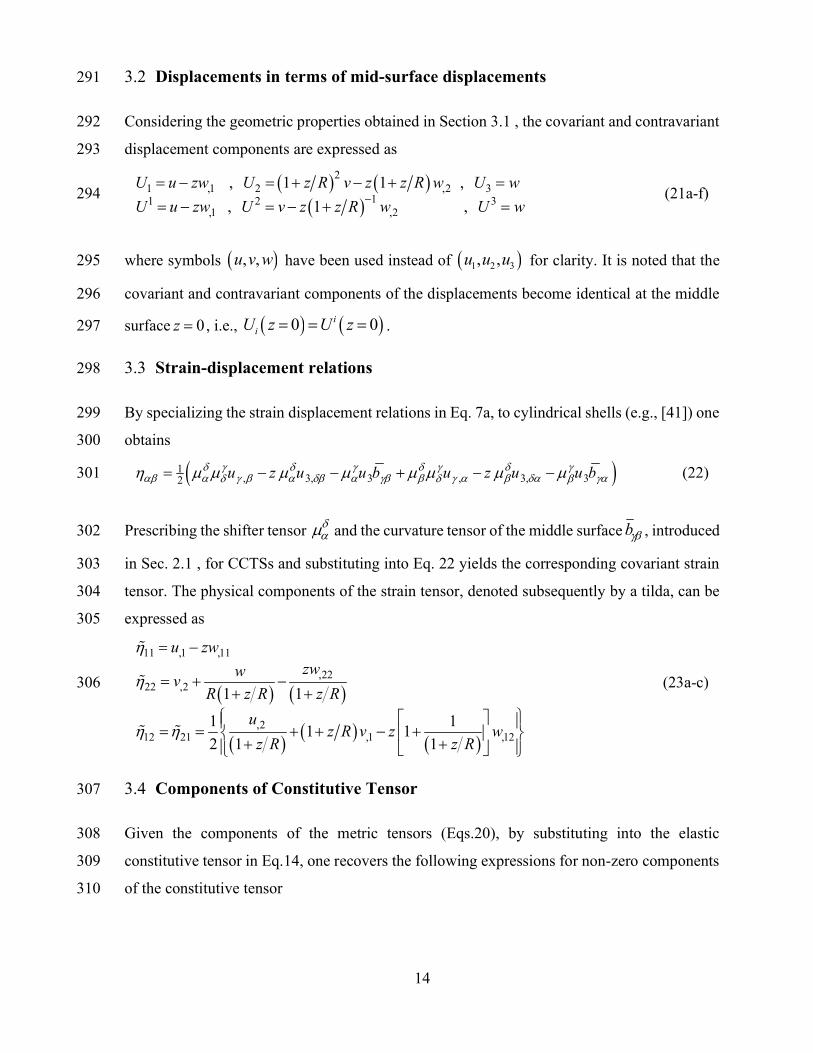
Appendix A- Coefficients appearing in Hamilton functional for CCTS 756

1 1 1 1 21 2 3 4

2 2 2 2 2 21 2 3

3 2 3 3 21 2 3

3 2 3 2 24 5

3 2 2 3 2 26 7

3 28

4 2 4 21 2

1 , , , 12

1 2 , 1 1 4 2 , 1 8

12 , 1 1 2 , 3 24

12 , 3 24 1 1 2

1 12 , 1 12

1

12 , 12

H H H R H h R

H H h R H h R

H h R H R H h R

H h H h R

H h R E H h E

H Eh

H h R H h

4 23

4 24

1 1 11 2 3

1 1 24 5

1 1 26 7

1 2 2 1 28 9

2 2 2 2 21 2 3

2 2 2 24 5

2 2 2 2 2 2 26 7

, 12

12

1 , 1 2 , 1 2

, 12

1 1 2 , 1 ,

1 12 , 1

1 2 , 1 1 4 2 , 1

1 , 3 24 , 0

1 1 12 , 1

a

R H h

H h

G G G

G R G h R

G R G E

G h RE G Eh

G G h R G

G R G h R G

G h R E G h

2 28

3 3 3 21 2 3

3 3 24 5

3 3 2 36 7

3 2 3 2 28 9

3 2 3 210 11

3 2 2 3 2 212 13

3 2 214 15

6 ,

1

, 1 ,

2 1 , 12

1 1 2 , 3 24 , 0

12 , 3 24 1 1 2

1 , 1

1 12 , 1 12

1 12 ,

b

RE

G Eh

G R G R G R

G G h R

G R G h R G

G h G h R

G R G E

G h E G h E

G h RE

3 2 2

3 2 3 216 17

3 218

1 6

1 , 1

1

G h RE

G Eh G Eh

G Eh

757

where / ln 2 / 2h R R h h R h R 758

46

Appendix B - Force terms, Boundary Conditions and Field Equations 759

760

The terms , , , ,xu xw sv sw zwf f f f f are related to the physical force components , ,x s zp p p per 761

unit volume (of the contravariant external force components iF , respectively) through the 762

integrals 763

2

2

2

1

1

1

1

1

xxu

sv sh

zw zh

xw x

sw s

p z Rf

f p z R

dzf p z R

f p z z R

f p z z R

(B.1a-e) 764

In Eq. 25, since 1t and 2t are arbitrary times and the variations u , v , w and ,1w are 765

arbitrary within the domain ( 0 x L and 0 2s R ) , the first and second integrals have 766

to vanish independently. The former integral yields eight boundary conditions, 767

1 1 1 11 ,1 2 ,2 3 4 ,11

0

2 2 21 ,2 2 ,1 3 ,12

0

3 3 3 3 3 3 3 31 ,11 2 ,22 3 ,12 4 ,111 5 ,122 6 7 ,1 8

0

4 4 4 41 ,1 2 ,2 3 ,11 4 ,22 ,1

0

0

0

0

0

L

L

Lxw

L

Hu Hv Hw Hw u

Hu Hv Hw v

Hu Hu Hv Hw Hw Hu Hw Hf w

Hu Hv Hw Hw w

(B.2) 768

in which either the bracketed expressions vanish, yielding the natural boundary conditions, or 769

their respective coefficient does, yielding the essential boundary conditions, and the second 770

integral of Eq. 25 yields the following three equilibrium equations. 771

1 1 1 1 1 1 1 1 11 ,11 2 ,22 3 ,12 4 ,1 5 ,111 6 ,122 7 8 ,1 9

2 2 2 2 2 2 2 2 21 ,12 2 ,11 3 ,22 4 ,2 5 ,112 ,222 6 7 ,2 8

3 3 3 3 3 3 31 ,1 2 ,2 3 ,11 4 ,22 5 ,111 6 ,122 7

0

0

xu

sva

a

Gu Gu Gv Gw Gw Gw Gu Gw Gf

Gu Gv Gv Gw Gw Gw Gv Gw Gf

Gu Gv Gw Gw Gw Gu Gu

3 3,112 ,222

3 3 3 3 3 3 3 38 ,1111 9 ,1122 10 ,2222 11 12 ,11 13 ,22 14 ,1 15 ,2

3 3 316 ,1 17 ,2 18 0

b

xw sw zw

Gv Gw

Gw Gw Gw Gw Gw Gw Gu Gv

Gf Gf Gf

(B.3) 772